Embed Size (px)
Citation preview
8/9/2019 Mortenson, Michael E. - Mathematics for computer graphics applications.pdf
http://slidepdf.com/reader/full/mortenson-michael-e-mathematics-for-computer-graphics-applicationspdf 1/367
1l
8/9/2019 Mortenson, Michael E. - Mathematics for computer graphics applications.pdf
http://slidepdf.com/reader/full/mortenson-michael-e-mathematics-for-computer-graphics-applicationspdf 2/367
k, nlkiI I,,
-I-
PU IIU
FION
S OND E D I T I O N
f
TOA
SO0
M.I.
NATION
8/9/2019 Mortenson, Michael E. - Mathematics for computer graphics applications.pdf
http://slidepdf.com/reader/full/mortenson-michael-e-mathematics-for-computer-graphics-applicationspdf 3/367
Library of Congress
Cataloging-in-Publication
Data
Mortenson,
Michael E.,
Mathematics for
computer
graphics
applications:
an
introduction
to the
mathematics and
geometry of
CAD/CAM,
geometric
modeling,
scientific visualization,
and
other CG applications/Michael
Mortenson.-2nd ed.
p. cm.
Rev. ed.
of
Computer graphics. c1989.
ISBN 0-8311-3111-X
1. Computer graphics-Mathematics. I. Mortenson,
Michael
E.,
Computer
graphics. II.
Title.
T385.M668 1999
006.6'01'51-dc2l
99-10096
CIP
The first edition
was
published under the
title
Computer Graphics: An Introduction
To the
Mathematics
and
Geometry
Industrial
Press,
Inc.
200
Madison Avenue
New
York,
NY 10016-4078
Second
Edition,
1999
Sponsoring
Editor:
John Carleo
Project Editor:
Sheryl A. Levart
Interior
Text
and
Cover
Designer:
Janet
Romano
Copyright
© 1999 by
Industrial
Press
Inc.,
New
York. Printed in the United
States
of
America. All rights reserved. This book, or
any
parts
thereof,
may
not be
reproduced,
stored
in a
retrieval system, or
transmitted in
any
form without the
permission
of
the
publisher.
Printed in the
United
States of
America
109876543

8/9/2019 Mortenson, Michael E. - Mathematics for computer graphics applications.pdf
http://slidepdf.com/reader/full/mortenson-michael-e-mathematics-for-computer-graphics-applicationspdf 4/367
To
JAM
8/9/2019 Mortenson, Michael E. - Mathematics for computer graphics applications.pdf
http://slidepdf.com/reader/full/mortenson-michael-e-mathematics-for-computer-graphics-applicationspdf 5/367
PREFACE
Computer
graphics is
more than
an isolated discipline at
an intersection
of computer
science,
mathematics, and engineering.
It
is the very visible leading
edge
of
a
revolution
in
how
we use com puters
and
automation
to
enhance
our
lives.
It
has
changed
forever
the
worlds of engineering and science, medicine, and
the
media, too. The wonderful special
effects that entertain and inform us at the movies, on TV, or while surfing cyberspace
are possible
only
through powerful computer graphics
applications.
From the
creatures
of
Jurassic
Park, and the imaginary worlds
of
Myst
and
Star
Wars, to the
dance of virtual
molecules on a chemist's
computer
display screen,
these effects applied
in the arts,
entertainment,
and science are possible,
in
turn, only because
an equally wonderful
world
of mathematics
is
at work behind the scenes. Some of the mathematics
is
traditional, but
with a new
job
to do,
and some
is brand
new.
Mathematicsfor
Computer
Graphics
Applications
introduces
the
mathematics
that
is the
foundation
of many of today's
most
advanced computer graphics
applications.
These include computer-aided design and manufacturing, geometric modeling, scien-
tific
visualization, robotics, computer
vision, virtual reality, ... and,
oh yes, special ef-
fects in cinematography. It is a
textbook
for
the
college student
majoring
in computer
science, engineering, or
applied
mathematics
and
science, whose special interests are in
computer graphics, CAD/CAM
systems, geometric modeling, visualization, or
related
subjects. Some exposure to elementary calculus and a familiarity with introductory lin-
ear
algebra as usually
presented
in standard college algebra courses
is
helpful but not
strictly necessary.
(Careful
attention
to
the ma terial
of
Chapter 5, which discusses limit
and continuity, may preempt the calculus prerequisite.) The textbook
is
also
useful for
on-the-job
training of employees whose skills
can be p rofitably expanded
into
this
area,
and
as
a tutorial for
independent
study.
The
professional working
in
these
fields
will
find it to be a
comprehensive
reference.
This second
edition includes thoroughly
updated
subject
matter,
some major
organizational changes,
and several new
topics: chapters on symmetry, limit
and
con-
tinuity,
constructive solid
geometry, and the Bezier
curve
have been
added. Many new
figures and exercises
are also presented.
This
new edition brings to the
fore
the basic
mathematical tools
of
computer
graphics, including
vectors,
matrices, and
transforma-
tions.
The
text
then
uses these
tools to
present
the
geometry,
from the elementary
building
blocks of points, lines, and
planes, to
complex three-dimensional constructions and
the
Bezier
curve.
Here is an outline
of what
you will find in each chapter.
iv
8/9/2019 Mortenson, Michael E. - Mathematics for computer graphics applications.pdf
http://slidepdf.com/reader/full/mortenson-michael-e-mathematics-for-computer-graphics-applicationspdf 6/367
Preface V
Chapter 1
Vectors There are
several ways to teach and to learn about
vectors.
Today most of these methods
are within
the
context
of some other
area
of
study.
While
this approach usually works, it too often
unnecessarily
delays
a
student's experience
with
vectors
until
more specialized courses are
taken. Experience
shows, however,
that
students are capable of
learning
both
the
abstract and the practical natures
of
vectors
much earlier.
Vectors, it
turns
out, have
a
strong intuitive appeal because
of
their innate
geometric
character.
This chapter
builds upon
this intuition.
Chapter2 Matrix
Methods As
soon
as a student
learns
how to solve
simultaneous
linear
equations, he
or
she
is also
ready to learn simple matrix
algebra. The
usefulness
of
the matrix formulation
is
immediately
obvious,
and
allows the
student
to
see that
there
are
ways to
solve
even very
large sets of equations. There
is ample material
here
for both student
and teacher to
apply
to the
understanding of
concepts in later chapters.
Subjects
covered
include
definitions,
matrix
equivalence,
matrix
arithmetic,
partitioning,
determinants,
inversion, and
eigenvectors.
Chapter 3 Transformationsexplores geometric
transformations
and
their
invari-
ant properties. It
introduces
systems of
equations
that
produce
linear
transformations
and
develops the
algebra and geometry of translations, rotations,
reflection, and scaling.
Vectors and matrix algebra
are put to
good use here, in ways that clearly demonstrate
their
effectiveness.
The mathematics of transformations
is
indispensable to animation
and special effects, as well as many areas of physics
and
engineering.
Chapter
4 Symmetry and Groups
This
chapter uses geometry
and intuition to
define symmetry
and
then
introduces easy-to-understand
but
powerful
analytic methods
to further
explore
this
subject.
It
defines
a
group and
the
more
specialized
symmetry group.
The
so-called
crystallographic estriction
shows how symmetry depends on the
nature
of
space
itself. This
chapter concludes
with
a
look
at the rotational symm etry of polyhedra.
Chapter
5 Limit
and
Continuity
Limit processes are at work
in compu ter graphics
applications to ensure the display of smooth, continuous-looking curves and surfaces.
Continuity
is
now an
important
consideration
in the
construction
and rendering of
shapes
for CAD/CAM and similar applications. These call
forth
the
most
fundamental
and
elementary concepts of the calculus, because the
big
difference
between
calculus
and
the
subjects that
precede
it
is
that calculus
uses limiting processes
and requires a
definition of
continuity. The
ancient
Greek
method
of
exhaustion
differs
from integral
calculus
mainly
because the former lacks the concept of the limit of a function. This chapter takes a
look at some o ld and some new
ways
to
learn
about limit and continuity, including
the
method of exhaustion, sequences and series, functions, limit theorems, continuity and
continuous functions.
Chapter 6 Topology
What
makes
a sphere
different from
a torus? Why
are
left
and
right not
reliable
directions on a Mobius strip?
This
chapter answers questions
like
these. It shows that
topology
is
the
study of
continuity
and
connectivity
and how these
characteristics are
preserved
when geometric figures are deformed. Although histori-
cally a
relative newcomer,
topology
is
an
important
part
of
many
disciplines,
including
geometric modeling and mathematical
physics.
In fact,
for
the
latter,
the Mobius strip
and
its analog in a higher dimension, the
Klein
bottle,
both appear in
superstring theory
as aspects of
Feynman
diagrams representing
the
interactions of
elementary
particles.
8/9/2019 Mortenson, Michael E. - Mathematics for computer graphics applications.pdf
http://slidepdf.com/reader/full/mortenson-michael-e-mathematics-for-computer-graphics-applicationspdf 7/367
vi
Preface
Topological
equivalence,
topology
of a
closed
path,
piecewise
flat surfaces, closed
curved
surfaces,
orientation,
and
curvature are among
the many topics
covered here.
Chapter
7
Halfspaces
Halfspaces
are
always fun to
play
with
because
we
can
combine
very
simple
halfspaces to create complex
shapes
that
are
otherwise
extremely
difficult,
if not
impossible,
to
represent mathematically.
This
chapter explores both
two-
and three-dimensional
halfspaces.
It first
reviews elementary
set
theory
and
how to
interpret
it
geometrically in Venn
diagrams
and
then explains
the
Boolean
operators
union,
intersectionand difference
and how
to use
them to create
more
complex
shapes.
Chapter
8 Points,
Chapter9
Lines, and Chapter
10 Planes
define
and
discuss these
three simple
geometric
objects
and show how
they
are the basic
building
blocks
for
other
geometric
objects.
Arrays of points,
absolute and
relative
points, line
intersections, and
the relationship
between
a
point
and
a plane
are some
of the
topics
explored.
Chapter 11
Polygons Polygons
and polyhedra
were
among the first
forms
stud-
ied
in geometry.
Their
regularity
and symmetry
made them the center
of
attention
of
mathematicians,
philosophers,
artists,
architects,
and
scientists
for thousands
of years.
Polygons are still important
today.
For
example,
their
use
in computer graphics
is
widespread,
because
it is easy to subdivide
and approximate
the
surfaces of solids
with
planes bounded by them.
Topics covered here
include definitions
of the
various types of
polygons,
their geometric
properties,
convex hulls,
construction
of the
regular
polygons,
and symmetry.
Chapter 12
PolyhedraThis
chapter defines convex,
concave,
and
stellar polyhe-
dra,
with
particular attention
to the
five regular
polyhedra,
or
Platonic solids.
It defines
Euler's Formula
and
shows
how
to
use
it
to
prove
that
only
five
regular polyhedra
are
possible in
a space of
three dimensions.
Other topics
include
definitions of
the various
families
of polyhedra,
nets, the convex
hull of
a
polyhedron, the connectivity
matrix,
halfspace representations
of polyhedra,
model
data structures,
and
maps.
Chapter
13
Constructive
Solid Geometry
Traditional
geometry,
plane and
solid-
or
analytic-does
not tell
us how to create
even
the simplest shapes
we
see
all around us.
Constructive
solid geometry
is
a
way to describe
these shapes
as combinations
of
even
simpler
shapes. The
chapter revisits
and applies some
elementary
set
theory,
halfspaces,
and Boolean
algebra. Binary
trees are
introduced, and many
of their more
interesting
properties
are explored.
Chapter 14 Curves explores
the
mathematical
definition
of a curve
as
a set
of
parametric
equations,
a form that
is
eminently
computationally
useful to
CAD/CAM,
geometric
modeling,
and
other computer graphic
applications.
Parametric
equations
are the
basis
for B&zier,
NURBS, and
Hermite curves. Both
plane and space curves
are
introduced, followed by
discussions
of
the tangent vector,
blending
functions, conic
curves,
reparameterization,
and
continuity.
Chapter
15
The
Bezier Curve This
curve is
not only
an important part
of almost
every computer-graphics
illustration
program, it
is a
standard
tool of
animation
tech-
niques. The
chapter
begins
by describing
a
surprisingly
simple geometric
construction
of
a
Bezier curve,
followed
by
a
derivation
of
its
algebraic
definition, basis
functions,
control
points, and how to join
two curves end-to-end to form
a single, more complex
curve.
8/9/2019 Mortenson, Michael E. - Mathematics for computer graphics applications.pdf
http://slidepdf.com/reader/full/mortenson-michael-e-mathematics-for-computer-graphics-applicationspdf 8/367
Preface vii
Chapter 16 Surfaces develops the
parametric equations
of surfaces, a natural
extension of the mathematics of curves discussed in
Chapter
14. Topics include the
surface patch,
plane
and cylindrical surfaces, the bicubic surface, the Bezier surface, and
the
surface
normal.
Chapter 17 Computer
Graphics
Display Geometry
introduces some of
the
basic
geometry
and
mathematics of computer
graphics,
including display coordinate
systems,
windows, line and polygon clipping,
polyhedra
edge
visibility,
and silhouettes.
Chapter 18 Display
and
Scene Transformationsdiscusses orthographic and per-
spective transformations,
and
explores some
scene transformations:
orbit,
pan, and
aim.
Chapters
17
and 18
draw
heavily
on concepts
introduced
earlier in the
text
and lay the
foundation
for
more advanced studies
in
computer graphics
applications.
Most chapters include
many exercises, with answers to selected exercises
pro-
vided
following
the last
chapter.
A
separate
Solutions
Manual,
which presents hints and
solutions
for
all
the
exercises,
is
available
for instructors. Here
is a suggestion
that was
offered in the first
edition
and must be
repeated
here: Read all of
the
exercises (even those
not
assigned).
They are
a
great help
to the
reader who chooses
to
use this textbook
as
a
tutorial, and for the student in the
classroom
setting who is serious about mastering all
the concepts.
An
annotated bibliography
is
also included. Use it
to find
more advanced
coverage
of these subjects or
to browse
works
both
contemporary and classic that
put
these
same subjects into a broader context,
both mathematical and cultural.
Mathematics
for
Computer
Graphics
Applications is
a textbook with
a purpose,
and
that
is
to
provide a strong
and
comprehensive
base for later
more advanced studies
that the student will encounter in
math, computer
science, physics, and engineering,
including
specialized
subjects such as algebraic
and
computational
geometry, geometric
modeling, and
CAD/CAM.
At the same time, the material is developed enough
to be
immediately
put to work by the novice or experienced professional. Because the text-
book's content is relevant to
contemporary development
and
use
of
computer
graphics
applications, and because it introduces each subject
from
an elementary standpoint,
Mathematics for
Computer
Graphics Applications
is
suitable for
industry or
government
on-the-job training programs aimed at increasing the skills and versatility of employees
who
are
working
in
related but less mathematically
demanding areas.
It
can
be used as a
primary
textbook,
as
a
supplementary
teaching
resource, as
a
tutorial
for
the
individual
who
wants to
master this material on his or
her
own, or as
a
professional
reference.
The
creation
of
this
second
edition
was
made
possible
by
the generous help
and
cooperation of many people.
First,
thanks
to
all the
readers
of the
first
edition
who
took
the
time to
suggest improvem ents and corrections. Thanks to the
necessarily
anonymous
reviewers whose
insightful
comments
also
contributed
to this
new edition. Thanks to
John
Carleo, Sheryl Levart,
and Janet
Romano of
Industrial
Press, Inc. whose
many
editorial
and
artistic talents
transformed
my manuscript-on-a-disk
into an attractive
book.
Finally, thanks
to
my
wife Janet, who read
and reread the many
drafts
of this
edition,
and who was
a
relentless
advocate
for
simplicity
and
clarity.
8/9/2019 Mortenson, Michael E. - Mathematics for computer graphics applications.pdf
http://slidepdf.com/reader/full/mortenson-michael-e-mathematics-for-computer-graphics-applicationspdf 9/367
TABLE
OF
CONTENTS
1. Vectors .......
..........................
................. 1
1.1
Introduction .............................................
1
1.2
Hypernumbers ........................................... 2
1.3 Geometric
Interpretation
.................................. 4
1.4
Vector
Properties ........................................ 8
1.5 Scalar Multiplication .................................... 10
1.6
Vector
Addition ........................................ 10
1.7 Scalar and
Vector Products
................................ 11
1.8 Elements
of Vector Geometry
..............................
14
1.9
Linear Vector
Spaces
.................................... 19
1.10 Linear Independence and
Dependence
.......................
20
1.11
Basis Vectors
and
Coordinate
Systems
........................
21
1.12 A Short
History
........................................ 22
2. Matrix
Methods ..........................................
28
2.1 Definition
of a
Matrix
................................... 28
2.2 Special
Matrices ....................................... 29
2.3
Matrix Equivalence ..................................... 31
2.4 Matrix Arithmetic ...................................... 31
2.5
Partitioning a
Matrix .................................... 34
2.6
Determinants .........................................
36
2.7
Matrix
Inversion .......................................
37
2.8
Scalar and
Vector Products ..................................
39
2.9
Eigenvalues
and
Eigenvectors .................................
39
2.10 Similarity
Transformation ................................. 41
2.11
Symm etric Transformations .................................. 42
2.12 Diagonalization of a Matrix ................................. 42
3.
Transformations
........................................... 47
3.1
The
Geometries
of
Transformations .......................... 47
3.2 Linear Transformations .................................. 52
3.3 Translation .......................................... 54
ix
8/9/2019 Mortenson, Michael E. - Mathematics for computer graphics applications.pdf
http://slidepdf.com/reader/full/mortenson-michael-e-mathematics-for-computer-graphics-applicationspdf 10/367
x Table of Contents
3.4
Rotations in the Plane ...................................
56
3.5 Rotations in Space ...................................... 60
3.6 Reflection ...........................................
64
3.7
Homogeneous Coordinates
................................
69
4.
Symmetry and
Groups ...................................... 73
4.1
Introduction
..........................................
73
4.2
Groups .............................................
77
4.3
Symmetry Groups ...................................... 78
4.4
Ornamental
Groups
.....................................
80
4.5 The
Crystallographic
Restriction
............................
83
4.6 Plane
Lattices .......................................... 84
4.7
Tilings
...............................................
85
4.8
Polyhedral Symmetry ...................................
86
5. Limit and Continuity .................................... 90
5.1 The Greek
Method of Exhaustion ........................... 90
5.2 Sequences and Series
....................................
93
5.3
Functions ............................................
98
5.4
Limit
of a Function ..................................... 103
5.5
Limit
Theorems ......................................
107
5.6
Limit
and
the
Definite
Integral
.............................
111
5.7
Tangent
to a Curve .....................................
114
5.8
Rate of Change ...................................... 115
5.9 Intervals ...........................................
119
5.10 Continuity
.......................................... 121
5.11 Continuous Functions ................................... 122
6.
Topology ................................................
129
6.1 Topological Equivalence.. ................................
129
6.2
Topology
of a
Closed Path
................................
132
6.3 Piecewise Flat Surfaces .................................. 137
6.4
Closed Curved Surfaces ................................. 141
6.5 Euler
Operators ......................................
142
6.6 Orientation ..........................................
144
6.7 Curvature
..........................................
147
6.8 Intersections ......................................... 149
7.
Halfspaces
.......................... ..................
152
7.1
Definition
............................ ............. 152
7.2 Set Theory ........................................... 153
7.3 Functions Revisited ....................................
154
8/9/2019 Mortenson, Michael E. - Mathematics for computer graphics applications.pdf
http://slidepdf.com/reader/full/mortenson-michael-e-mathematics-for-computer-graphics-applicationspdf 11/367
Table
of
Contents xi
7.4 Halfspaces in the Plane .................................. 156
7.5 Halfspaces in Three
Dimensions ...........................
159
7.6 Combining Halfspaces ..................................
160
8. Points ................................................. 165
8.1 Definition ........................................... 165
8.2 Arrays
of
Points ....................................... 167
8.3 Absolute
and
Relative Points .............................. 168
8.4 Displaying Points ..................................... 169
8.5
Translating and Rotating Points .................................. 170
9.
Lines
...................................................
174
9.1 Lines
in
the
Plane ...................................... 174
9.2 Lines in Space ........................................ 177
9.3 Computing Points
on a Line
...............................
180
9.4
Point and
Line
Relationships ..............................
181
9.5
Intersection
of Lines
.................................... 183
9.6 Translating and Rotating Lines ..................................
184
10. Planes
.................................................. 187
10.1
Algebraic
Definition
...................................
187
10.2
Normal Form ........................................
189
10.3 Plane Defined
by
Three Points ..................................
190
10.4 Vector Equation
of a
Plane ..................................
190
10.5 Point and Plane Relationships .............................
191
10.6 Plane Intersections .................................... 192
11. Polygons
...............................................
195
11.1 Definitions
........................................ 195
11.2
Properties
..........................................
197
11.3
The
Convex
Hull of a Polygon .............................
200
11.4
Construction of
Regular Polygons ......................... 201
11.5 Symmetry of Polygons Revisited .................................. 201
11.6
Containment ........................................
202
12. Polyhedra ...............................................
205
12.1
Definitions ........................................
205
12.2
The
Regular
Polyhedra
.................................. 207
12.3
Semiregular
Polyhedra ..................................
209
12.4
Dual Polyhedra
......................................
211
12.5 Star Polyhedra
....................................... 212
8/9/2019 Mortenson, Michael E. - Mathematics for computer graphics applications.pdf
http://slidepdf.com/reader/full/mortenson-michael-e-mathematics-for-computer-graphics-applicationspdf 12/367
xii
Table
of Contents
12.6
Nets
..............................................
213
12.7 The
Convex
Hull
of
a Polyhedron
.........................
214
12.8
Euler's
Formula for Simple
Polyhedra ......................
214
12.9
Euler's
Formula
for
Nonsimple Polyhedra
...........................
217
12.10
Five and
Only Five Regular
Polyhedra: The
Proof
.............. 218
12.11
The Connectivity
Matrix
......................................
219
12.12
Halfspace Representation
of Polyhedra
...............................
221
12.13
Model Data S tructure
......................................
223
12.14 Maps of
Polyhedra ......................................
223
13. Constructive
Solid Geometry
................................
226
13.1
Set Theory Revisited
......................................
226
13.2
Boolean
Algebra
......................................
227
13.3
Halfspaces
Revisited .....................................
229
13.4 Binary
Trees
.........................................
230
13.5 Solids
.............................................
233
13.6 Boolean
Operators ......................................
235
13.7 Boolean
Models
......................................
240
14. Curves
.................................................
244
14.1
Parametric
Equations of
a Curve ....................................
244
14.2
Plane
Curves ........................................
245
14.3
Space
Curves ........................................
249
14.4
The Tangent
Vector
....................................
252
14.5
Blending
Functions ......................................
256
14.6
Approximating
a
Conic
Curve ......................................
258
14.7
Reparameterization
....................................
259
14.8 Continuity and
Composite
Curves ...................................
260
15.
The Bezier Curve
.........................................
264
15.1
A
Geometric
Construction ......................................
264
15.2
An Algebraic
Definition ................................
267
15.3 Control Points
.......................................
270
15.4
Degree Elevation
......................................
272
15.5 Truncation
..........................................
273
15.6
Composite
BLzier
Curves ......................................
275
16.
Surfaces ...............................................
277
16.1
Planes .............................................
277
16.2
Cylindrical
Surfaces
...................................
278
16.3
The
Bicubic Surface ...................................
279
8/9/2019 Mortenson, Michael E. - Mathematics for computer graphics applications.pdf
http://slidepdf.com/reader/full/mortenson-michael-e-mathematics-for-computer-graphics-applicationspdf 13/367
Table
of
Contents xiii
16.4 The
B6zier
Surface .................................... 283
16.5 Surface
Normal ......................................
284
17.
Computer Graphics
Display
Geometry
........................
286
17.1 Coordinate Systems ...................................
286
17.2 Window and Viewport .................................. 293
17.3 Line
Clipping ....................................... 296
17.4
Polygon Clipping .....................................
299
17.5 Displaying Geometric
Elements
..................................
299
17.6 Visibility
........................................... 308
18.
Display
and
Scene
Transformations
...........................
313
18.1
Orthographic
Projection
..................................
314
18.2
Perspective
Projection
..................................
318
18.3
Orbit .............................................
321
18.4
Pan ............................................. 323
18.5 Aim
..............................................
324
Bibliography ...............................................
326
Answers
to
Selected
Exercises
..................................
329
Index
..................................................... 349
8/9/2019 Mortenson, Michael E. - Mathematics for computer graphics applications.pdf
http://slidepdf.com/reader/full/mortenson-michael-e-mathematics-for-computer-graphics-applicationspdf 14/367
(Ai
PM
VECTORS
Perhaps the single most
important
mathematical
device
used
in
computer
graphics
and
many
engineering
and
physics applications
is
the
vector.
A
vector
is
a
geometric
object
of a sort, because, as we will soon
see,
it fits our
notion
of a displacement or motion.
(We can
think
of
displacement as a change
in
position. If we move a book
from
a shelf
to
a table, we
have
displaced it a specific
distance
and direction.) Vector
methods
offer a
distinct advantage
over
traditional
analytic geometry by
minimizing our computational
dependence
on a specific coordinate system until the later stages
of
solving a problem.
Vectors
are
direct descendants of complex numbers
and
are generalizations
of
hyper-
complex numbers.
Interpreting these numbers
as
directed line
segments
makes
it easier
for us to understand their properties
and to apply them to practical problems.
Length
and
direction
are
the most important vector properties. Scalar multipli-
cation
of
a
vector (that
is,
multiplication
by
a
constant),
vector
addition,
and
scalar
and
vector products
of
two vectors reveal more geometric subtleties. Representing straight
lines and
planes
using
vector equations
adds
to
our understanding
of
these elements and
gives
us powerful
tools for solving many
geometry
problems.
Linear
vector
spaces
and
basis
vectors
provide
rigor and a
deeper insight into
the subject of vectors. The history
of
vectors
and vector geometry tells
us
much about
how
mathematics develops,
as well
as
how gifted mathematicians established a new discipline.
1.1
Introduction
In the 19th century, mathematicians developed a new mathematical
object-
a new kind of number. They were
motivated
in part by
an
important
observation in
physics: Physicists had long known that while some phenomena
can
be described
by a
single number-the
temperature
of
a beaker
of
water
(60C),
the mass
of
a sample
of iron
(1
7
.5g),
or
the
length of
a rod
(31.736
cm)-other
phenomena require
something more.
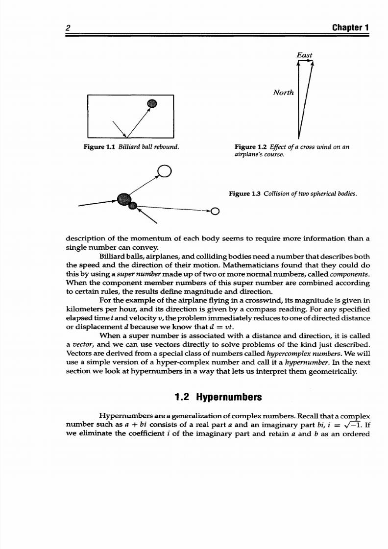
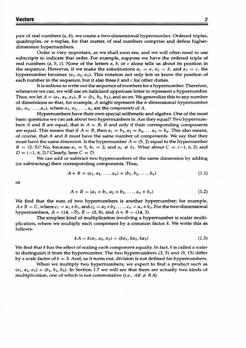
A ball strikes the side rail of a billiard table at a certain
speed
and angle (Fig-
ure
1.1);
we cannot describe its
rebound
by a single
number. A
pilot steers north with
an air
speed
of
800
kph
in
a
cross
wind
of
120
kph
from
the
west
(Figure
1.2);
we
cannot
describe
the airplane's true motion relative
to
the ground by a
single
number. Two spher-
ical bodies collide;
if
we
know the momentum
(mass x velocity) of each body before
impact, then we
can
determine their
speed and direction after impact (Figure 1.3).
The
1
8/9/2019 Mortenson, Michael E. - Mathematics for computer graphics applications.pdf
http://slidepdf.com/reader/full/mortenson-michael-e-mathematics-for-computer-graphics-applicationspdf 15/367
2
Chapter
1
East
North
V
Figure
1.1
Billiard ball rebound.
Figure 1.2 Effect of
a
cross wind on an
airplane's
course.
Figure
1.3 Collision
of two
spherical
bodies.
description
of
the
momentum
of
each body
seems to require
more information
than
a
single
number
can convey.
Billiard balls, airplanes,
and colliding
bodies
need
a
number that
describes
both
the
speed
and
the
direction of
their
motion. Mathematicians
found that
they could
do
this
by using a super
number
made
up
of two or
more normal numbers,
called
components.
When
the
component member numbers
of
this
super number are
combined according
to certain
rules,
the results define magnitude and direction.
For
the example of
the airplane
flying
in a crosswind,
its
magnitude
is given
in
kilometers
per hour,
and its
direction is
given
by a
compass reading.
For
any specified
elapsed
time t and velocity v,
the problem
immediately
reduces
to one
of
directed distance
or
displacement
d
because
we know
that
d
=
vt.
When
a super number
is
associated with a distance
and direction,
it
is called
a vector, and we can
use
vectors
directly to solve
problems of
the kind just
described.
Vectors are
derived
from
a special class
of numbers called hypercomplex
numbers.
We will
use
a simple
version
of
a hyper-complex
number and
call it a hypernumber.
In the next
section
we look at hypernumbers
in a way that lets
us
interpret them
geometrically.
1.2
Hypernumbers
Hypernumbers
are
a
generalization
of
complex
numbers.
Recall
that
a
complex
number
such
as a + bi consists
of
a
real
part
a and an imaginary part bi,
i =VT. If
we eliminate
the
coefficient
i
of
the imaginary part and
retain a
and
b as
an ordered
8/9/2019 Mortenson, Michael E. - Mathematics for computer graphics applications.pdf
http://slidepdf.com/reader/full/mortenson-michael-e-mathematics-for-computer-graphics-applicationspdf 16/367
Vectors
3
pair of
real
numbers
(a,
b), we
create
a two-dimensional hypernumber. Ordered triples,
quadruples, or n-tuples,
for that matter,
of
real
numbers comprise
and define higher-
dimension hypernumbers.
Order
is
very important,
as
we
shall
soon
see,
and
we
will
often need to use
subscripts
to
indicate that order.
For example,
suppose we
have
the ordered
triple
of
real
numbers
(a, b, c). None
of
the
letters
a, b, or
c
alone tells us
about
its position
in
the
sequence. However,
if we make the
substitutions a, =
a, a
2
=
b,
and a
3
= c, the
hypernumber becomes (a,,
a
2
, a
3
).
This notation not only lets
us
know the position of
each
number
in
the
sequence,
but
it also
frees
b
and c
for
other duties.
It
is tedious
to write out the
sequence
of numbers for a hypernumber. Therefore,
whenever we can, we will use an italicized uppercase letter to represent a hypernumber.
Thus, we let A = (a,,a
2
, a
3
),
B
= (b
1
, b
2
, b
3
), and so on. We generalize this to
any number
of
dimensions
so
that,
for example, A
might
represent the n-dimensional
hypernumber
(al, a
2
, .
..
, an),
where
a,, a
2
, .. .,
an are
the
components
of A.
Hypernumbers
have their
own
special arithmetic and
algebra.
One
of the most
basic questions we
can ask
about two hypernumbers
is: Are
they equal? Two hypernum-
bers A and
B
are
equal,
that is A =
B,
if and
only if their
corresponding components
are equal.
This
means that if A
=
B, then a
1
= bi, a
2
= b
2
, ...
an
=
bn. This also
means,
of course, that A and B must have the same number of
components.
We say that they
must
have
the same dimension.
Is the hypernumber
A =
(5, 2)
equal
to
the
hypernumber
B = (2, 5)? No, because
a,
= 5, b, = 2, and a
1
0
bl. What about
C
=
(-1,
6,2) and
D = (-1, 6, 2)? Clearly, here C = D.
We
can
add
or subtract
two hypernumbers
of
the
same
dimension
by adding
(or subtracting)
their
corresponding components. Thus,
A+
B
= (a,, a
2
,...,
an)
+
(bi, b
2
,...,bn)
(1.1)
or
A+ B
=
(a, + bi,
a
2
+ b
2
,..., an + bn)
(1.2)
We find that the sum
of
two hypernumbers is another hypernumber; for example,
A+
B
=
C,wherec
1
=
a
1
+bl,andc
2
= a
2
+b
2
, . . ., cn =
an+bn. For
the
two-dimensional
hypernumbers, A
= (14, -5), B = (0,
8), and
A + B =
(14, 3).
The simplest kind of multiplication involving a hypernumber is scalar multi-
plication,
where we multiply each component by a
common
factor k. We write this as
follows:
kA = k(al,
a2,
a
3
) = (kaj, ka
2
, ka
3
)
(1.3)
We find
that
k
has
the effect
of
scaling
each
component
equally. In
fact,
k is
called
a scalar
to distinguish it from the hypernumber.
The
two hypernumbers
(3,
5)
and
(9, 15)
differ
by a scale factor
of
k = 3. And, as
it
turns
out,
division is not
defined for
hypermumbers.
When we multiply
two
hypernumbers, we expect
to find
a
product
such as
(a
1
, a
2
, a
3
)
x (b,,
b
2
, b
3
). In
Section 1.7 we will see
that
there are actually two kinds of
multiplication, one
of which is not commutative
(i.e., AB :A B A).
8/9/2019 Mortenson, Michael E. - Mathematics for computer graphics applications.pdf
http://slidepdf.com/reader/full/mortenson-michael-e-mathematics-for-computer-graphics-applicationspdf 17/367
4
Chapter 1
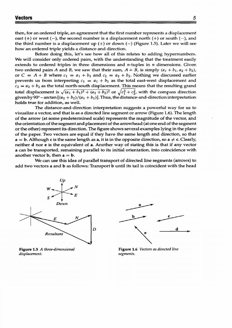
1.3 Geometric
Interpretation
To see the full power
of
hypernumbers,
we must
give
them
a geometric inter-
pretation.
Distance
and
direction
are
certainly
important
geometric
properties,
and
we
will
now
see how
to
derive them
from hypernumbers.
Imagine that
an ordered
pair
of numbers,
a
hypernumber,
is
really just a set
of
instructions
for
moving about
on
a
flat
two-dimensional
surface.
For
the moment,
let's
agree that
the first number of
the
pair
represents
a displacement (how
we are to
move)
east
if
plus
(+), or west
if minus
(-),
and that
the
second number
represents
a
displacement
north (+)
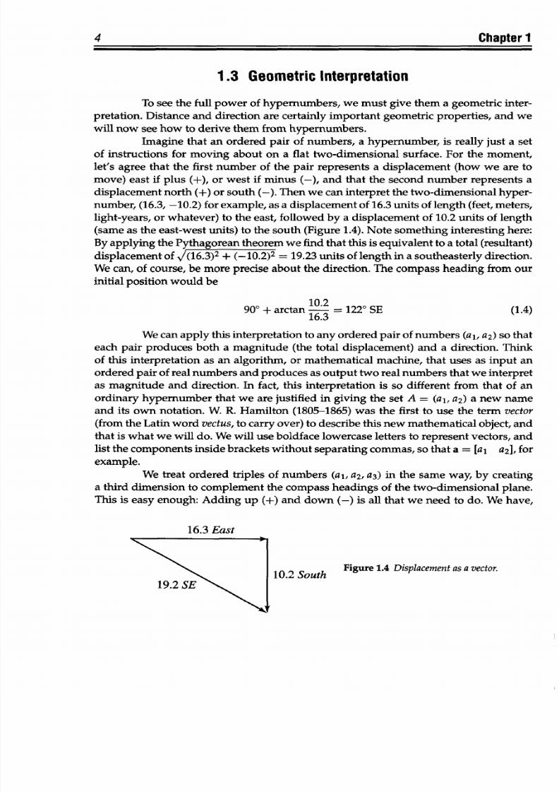
or south (-). Then
we can interpret the
two-dimensional hyper-
number, (16.3, -10.2)
for
example,
as a displacement of 16.3
units
of
length (feet,
meters,
light-years,
or whatever) to
the
east, followed
by a displacement of
10.2 units of
length
(same as
the east-west units) to the south (Figure 1.4).
Note something
interesting
here:
By applying the Pythagorean
theorem we
find that
this
is
equivalent to a total
(resultant)
displacement of (16.3)2
+ (-10.2)2 = 19.23 units of
length
in
a
southeasterly
direction.
We can, of
course, be more precise
about the direction.
The
compass heading from
our
initial position
would
be
90° + arctan
1220 SE (1.4)
16.3
We can apply
this interpretation to
any ordered
pair of
numbers (a,,
a
2
)
so
that
each pair
produces
both a magnitude
(the total displacement)
and a direction.
Think
of
this
interpretation
as
an
algorithm,
or
mathematical
machine,
that
uses
as
input
an
ordered
pair
of
real
numbers
and
produces
as
output
two real numbers that
we
interpret
as
magnitude
and direction. In
fact,
this
interpretation
is
so
different from that of
an
ordinary hypernumber
that
we
are
justified
in
giving the set A =
(a,, a
2
) a new
name
and its
own notation.
W.
R.
Hamilton (1805-1865)
was the first
to
use the
term
vector
(from
the
Latin word vectus, to carry over)
to
describe this
new mathematical
object,
and
that
is
what we will do.
We will
use
boldface lowercase
letters
to represent
vectors, and
list
the components inside
brackets
without
separating commas, so that
a =
[a
1
a
2
], for
example.
We
treat ordered
triples
of
numbers
(a,,
a
2
, a
3
) in
the
same
way,
by
creating
a
third
dimension to
complement the compass
headings
of the
two-dimensional
plane.
This
is easy
enough: Adding
up
(+)
and down
(-)
is all
that we
need
to
do.
We
have,
16.3 East
Figure 1.4 Displacement
as
a vector.
10.2 South
8/9/2019 Mortenson, Michael E. - Mathematics for computer graphics applications.pdf
http://slidepdf.com/reader/full/mortenson-michael-e-mathematics-for-computer-graphics-applicationspdf 18/367
8/9/2019 Mortenson, Michael E. - Mathematics for computer graphics applications.pdf
http://slidepdf.com/reader/full/mortenson-michael-e-mathematics-for-computer-graphics-applicationspdf 19/367
6
Chapter
1
a
b
c = a+b
-
ab b
c=ba
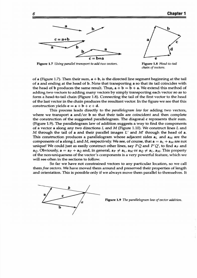
Figure
1.7 Using parallel transport
o
add
two vectors.
Figure
1.8 Head-to-tail
chain
of
vectors.
of a
(Figure 1.7). Then their
sum, a +
b, is the directed
line segment
beginning at
the
tail
of
a
and
ending
at
the
head
of b.
Note
that
transporting
a so
that
its tail
coincides
with
the
head of b
produces
the same
result. Thus, a +
b
= b + a.
We extend this
method
of
adding
two
vectors to adding
many
vectors
by simply
transporting each vector
so as
to
form a head-to-tail chain (Figure 1.8). Connecting the tail of the first vector to the head
of the last
vector in
the
chain
produces the resultant vector. In the figure we see that this
construction yields e = a
+
b
+
c
+
d.
This process leads directly to the
parallelogram aw
for adding
two vectors,
where
we
transport a
and/or b
so that their tails
are
coincident and
then complete
the construction of the suggested parallelogram.
The
diagonal
c
represents their sum.
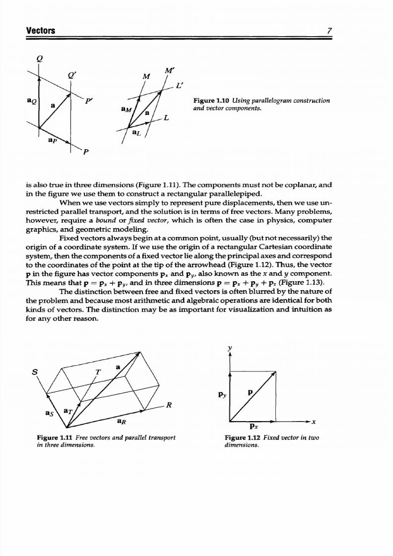
(Figure 1.9). The parallelogram law of addition suggests a
way
to find the components
of
a
vector a along any two directions
L
and
M
(Figure 1.10). We
construct
lines L and
M
through the
tail
of
a
and their
parallel
images L' and M' through
the
head of a.
This
construction
produces a parallelogram whose
adjacent sides aL and aM are
the
components
of
a along L and M, respectively. We see, of course, that a = aL + aM are
not
unique We could just
as
easily construct other lines, say P Q
and
P'Q', o find
ap and
aQ. Obviously, a
=
ap
+
aQ and, in general, ap 0 aL, aM or aQ = L, aM. This property
of
the non-uniqueness
of the vector's components
is a
very powerful feature, which
we
will
see often in the sections to follow.
So far we have
not
constrained
vectors
to any particular
location, so
we call
themrfree
vectors.
We
have
moved them
around and
preserved
their
properties
of
length
and
orientation. This is
possible only
if we always
move
them
parallel to
themselves. It
Figure
1.9
The
parallelogram aw
of
vector
addition.
8/9/2019 Mortenson, Michael E. - Mathematics for computer graphics applications.pdf
http://slidepdf.com/reader/full/mortenson-michael-e-mathematics-for-computer-graphics-applicationspdf 20/367
Vectors
7
Q
L'
Figure
1.10
Using
parallelogram onstruction
and
vector
components.
is
also true
in
three
dimensions (Figure
1.11). The components
must not be coplanar, and
in the figure we use them to construct a rectangular parallelepiped.
When
we use
vectors
simply
to represent
pure
displacements, then
we
use
un-
restricted parallel
transport, and
the solution
is
in
terms
of free vectors.
Many
problems,
however,
require
a bound or fixed vector, which is often the case in
physics,
computer
graphics,
and geometric
modeling.
Fixed vectors always
begin at a common point,
usually
(but not necessarily)
the
origin
of a coordinate
system. If we use the
origin
of a
rectangular
Cartesian
coordinate
system,
then the components of
a fixed vector
lie
along the
principal axes
and
correspond
to
the
coordinates of
the
point
at the tip of the arrowhead (Figure
1.12).
Thus, the vector
p in the figure has vector components px
and py,
also
known
as the
x and y
component.
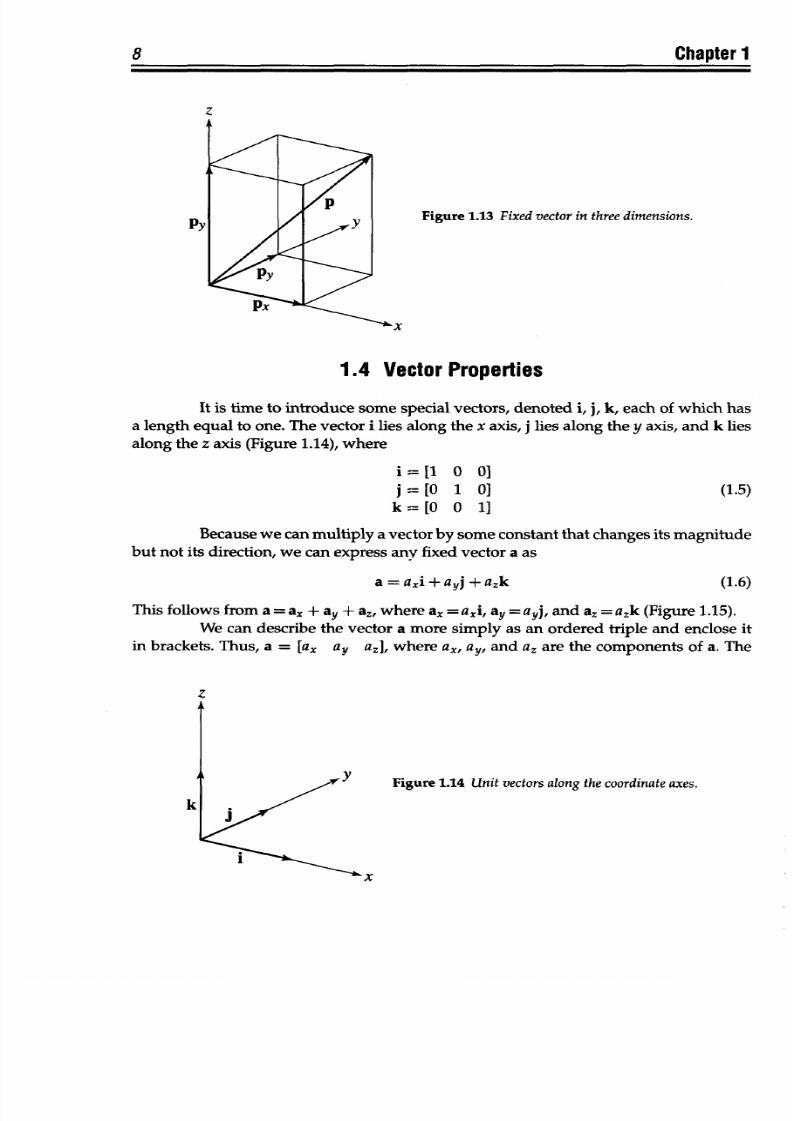
This means that
p = Px + py,
and
in three dimensions p = px
+ py +
pz
(Figure
1.13).
The
distinction
between free
and
fixed vectors is often
blurred by
the
nature of
the
problem
and
because most arithmetic and algebraic
operations
are identical for both
kinds of vectors. The
distinction
may
be
as
important
for
visualization
and
intuition
as
for
any
other reason.
C
Py
R
Figure
1.11
Free vectors
and
parallel
transport
in
three dimensions.
x
Px
Figure
1.12
Fixed
vector in two
dimensions.
V
8/9/2019 Mortenson, Michael E. - Mathematics for computer graphics applications.pdf
http://slidepdf.com/reader/full/mortenson-michael-e-mathematics-for-computer-graphics-applicationspdf 21/367
Chapter 1
z
Figure
1.13 Fixed
vector
in
three
dimensions.
1.4 Vector Properties
It is
time to
introduce some
special
vectors,
denoted
i, j, k, each of which
has
a length equal to one. The
vector i
lies
along the
x axis, j
lies
along the
y
axis,
and k lies
along the z axis (Figure
1.14), where
i
= 1 0 0]
j=
[O
1 0]
k=[O
0
1]
(1.5)
Because we
can
multiply a vector by some constant that changes its magnitude
but not its
direction, we
can express
any fixed
vector a
as
a =
axi
+
ayj
+ azk (1.6)
This follows
from a = ax + ay +
az,
where
a, = aji,
ay
=
ayj, and a,
= azk
(Figure 1.15).
We can describe
the vector a more
simply
as
an ordered
triple and enclose it
in brackets. Thus, a
=
[ax
ay
az], where
ax,
ay, and az are
the components of a. The
z
f
jay
i
x
Figure 1.14
Unit vectors along
the
coordinateaxes.
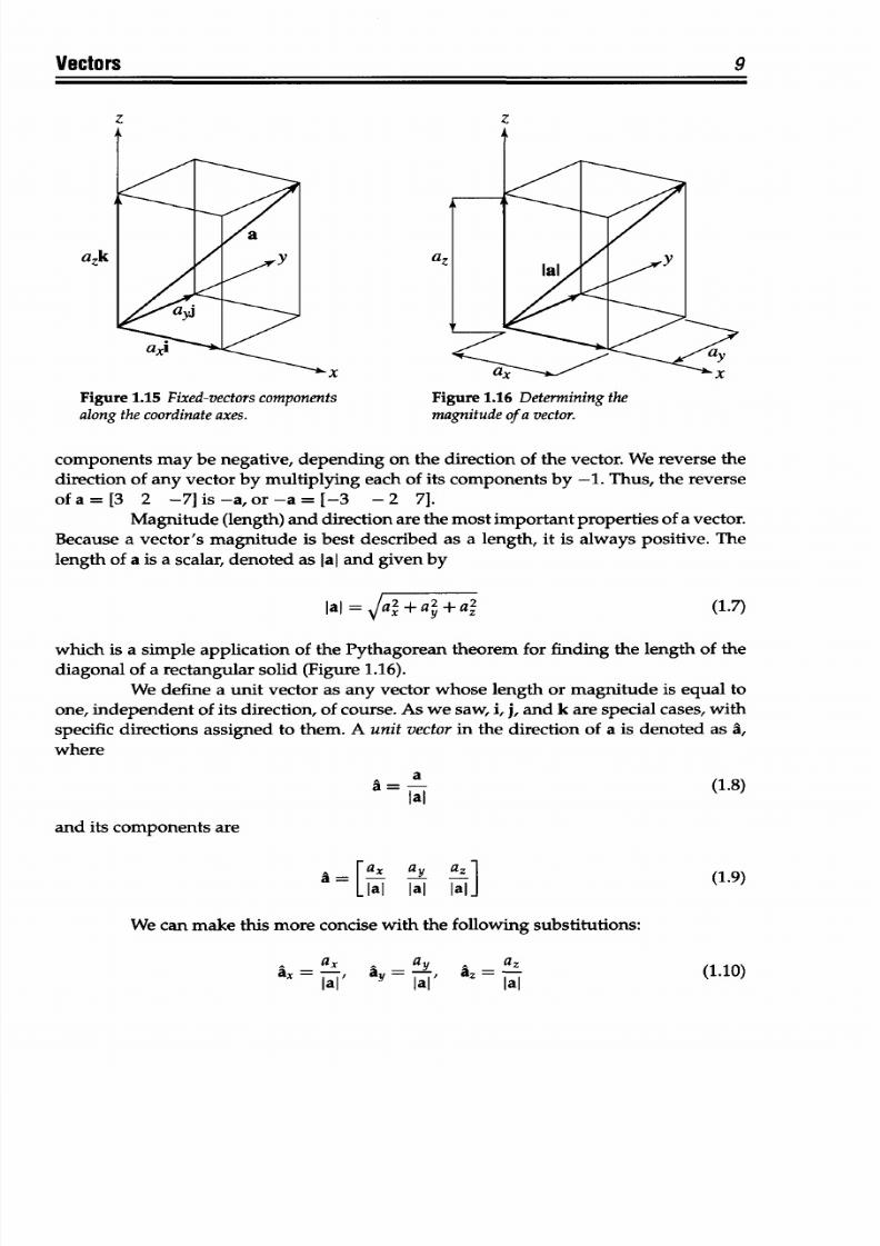
8
k
8/9/2019 Mortenson, Michael E. - Mathematics for computer graphics applications.pdf
http://slidepdf.com/reader/full/mortenson-michael-e-mathematics-for-computer-graphics-applicationspdf 22/367
azk
z
/
x
,---'*x
Figure
1.15 Fixed-vectors
components
along the coordinateaxes.
z
lal
/
,-"y
/=Uy
ax
- - X
Figure 1.16 Determining
the
magnitude
of a vector.
components may be negative,
depending
on the direction
of the
vector.
We reverse the
direction
of any vector
by multiplying each
of its
components
by -1. Thus,
the reverse
of a = [3 2
-7]
is-a,
or-a = [-3 -2 7].
Magnitude
(length) and direction
are
the
most important
properties
of
a
vector.
Because
a
vector's magnitude is best
described
as
a
length, it is always
positive. The
length
of a is a scalar,
denoted
as
laI
and given by
jai
= FaX2+
ay2+
a2
(1.7)
which is a
simple application
of the
Pythagorean theorem
for
finding the
length of
the
diagonal of
a
rectangular
solid
(Figure
1.16).
We define a
unit
vector as any vector whose length
or
magnitude is
equal
to
one, independent of
its direction, of course. As
we
saw, i, j,
and
k
are special cases, with
specific directions
assigned to
them. A
unit vector in the
direction of a
is
denoted as
&,
where
(1.8)
a=
l
and
its components
are
[a=L
(1.9)
y
Jai
We
can make this
more
concise with
the
following substitutions:
ax= ,
ay=-,
az=l
lax- AY la,
Vectors
9
(1.10)
I
I4
,
I
e,
-- ,I
,,a, -
axi
al
fA I
8/9/2019 Mortenson, Michael E. - Mathematics for computer graphics applications.pdf
http://slidepdf.com/reader/full/mortenson-michael-e-mathematics-for-computer-graphics-applicationspdf 23/367
10
Chapter
1
so
that
a=[ax
Ay
Ad
(1.11)
Note
that
if a,
P,
and
y
are the
angles
between a
and the
x, y, and z axes,
respectively,
then
ax= = cos a,
ay ==
yI= cos#,
jai
AZ=
- =
cos y
jai
(1.12)
This
means that ax,
iy,
and Az
are also
the
direction cosines
of a.
1.5
Scalar Multiplication
Multiplying any
vector
a
by
a
scalar
k
produces
a
vector
ka
or,
in component
form,
ka = [kax
kay kaz]
(1.13)
If
k is positive, then
a and ka are in the same direction.
If
k is negative, then
a
and ka are
in opposite directions. The magnitude
(length) of ka
is
Ikal =
jk2a2
+
k
2
a2 +
k
2
a2
(1.14)
so that
Ikal =
kial
(1.15)
We can
see
that scalar
multiplication is
well
named, because it changes
the scale
of
the vector. Here are the possible
effects
of a scalar
multiplier k:
k
> 1 Increases
length
k =
1 No change
0 <
k
<
1 Decreases length
k =
0 Null vector (O ength,
direction undefined)
-1 < k
< 0 Decreases length and
reverses
direction
k = -1
Reverses direction
only
k < -1 Reverses direction
and increases length
1.6 Vector
Addition
Vector addition
(or subtraction) in
terms
of components
is
perhaps the simplest
of
all vector operations (except for
multiplication of
a vector
by
a scalar). Given
a =
[a.
ay a,] and b
=
[bx by b.], then
a+b=[a,+bx ay+by
az+bj(
(1.16)
8/9/2019 Mortenson, Michael E. - Mathematics for computer graphics applications.pdf
http://slidepdf.com/reader/full/mortenson-michael-e-mathematics-for-computer-graphics-applicationspdf 24/367
Vectors
Y
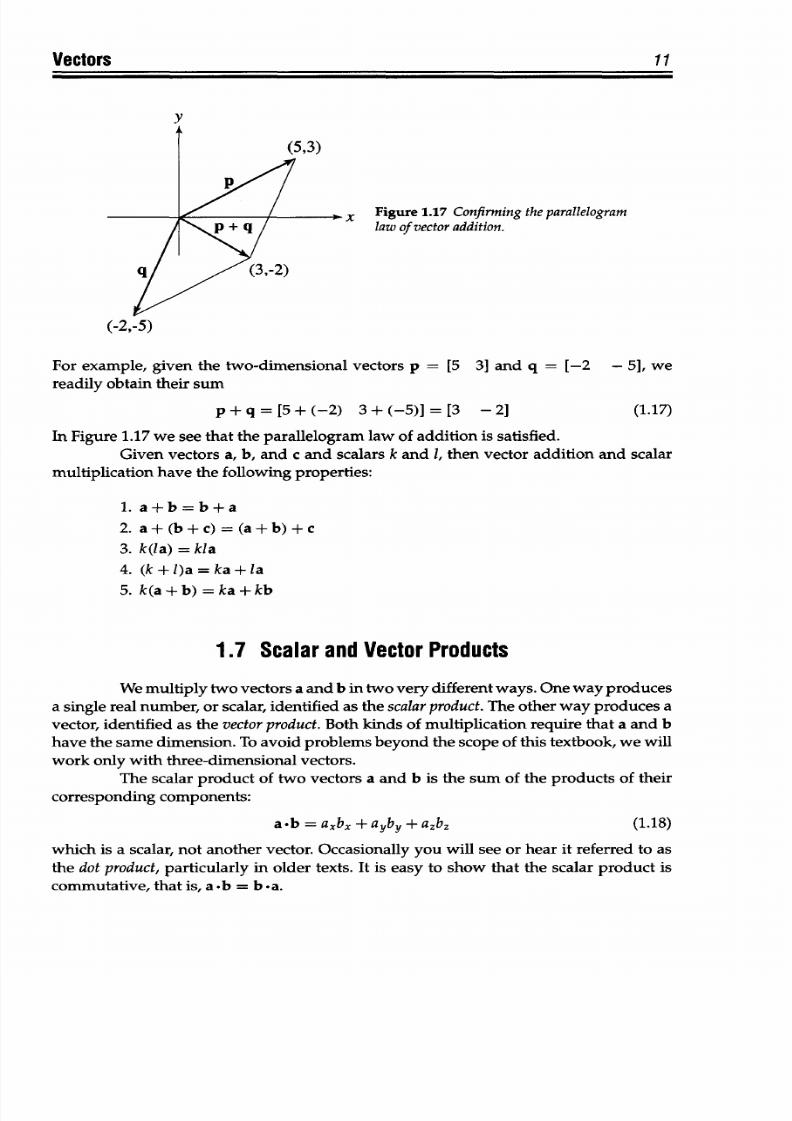
X Figure
1.17 Confirming
the
parallelogram
law
of vector addition.
For
example,
given the two-dimensional
vectors p = [5
3]
and
q
= [-2 - 5], we
readily
obtain their sum
p+q=[5+(-2) 3+(-5)]=[3
-2]
(1.17)
In
Figure 1.17 we
see
that
the
parallelogram
law
of addition
is
satisfied.
Given vectors
a,
b, and c and scalars k and 1, hen vector addition and scalar
multiplication have
the following properties:
1.
a+b=b+a
2. a+
(b+c) =
(a+b)
+c
3. k(la)
=
kla
4. (k+l)a=ka+la
5. k(a+b)=ka+kb
1.7 Scalar
and Vector Products
We multiply two vectors a
and
b in
two very
different ways. One way produces
a
single
real number,
or scalar,
identified as
the
scalar product. The
other
way
produces a
vector, identified
as
the vector product. Both kinds
of
multiplication
require
that a and b
have
the same dimension. To
avoid
problems beyond
the
scope of this textbook,
we
will
work
only
with
three-dimensional
vectors.
The scalar product of
two
vectors a
and
b
is the
sum of the
products
of their
corresponding components:
a
-b
=
a~b.
+
ayby
+
azbz
(1.18)
which
is
a
scalar,
not
another
vector.
Occasionally
you
will
see
or
hear
it
referred
to
as
the
dot
product, particularly
in older texts.
It
is easy to
show
that
the
scalar product is
commutative,
that is, a
-b
= b
*a.
11
8/9/2019 Mortenson, Michael E. - Mathematics for computer graphics applications.pdf
http://slidepdf.com/reader/full/mortenson-michael-e-mathematics-for-computer-graphics-applicationspdf 25/367
8/9/2019 Mortenson, Michael E. - Mathematics for computer graphics applications.pdf
http://slidepdf.com/reader/full/mortenson-michael-e-mathematics-for-computer-graphics-applicationspdf 26/367
Vectors
13
a
*cand
b
c:
a.c
= a,(ayb, - azby) -
ay(axbz -
azbx)
+ az(axby -
aybx)
=
axaybz
-
axazby
-
axayb, + ayazbx + axazby
- ayazbx (1.25)
=0
Because a
.c
=
0,
we
know
that a and c are perpendicular.
We
can also
show
that b *c = 0.
If two
vectors a and
b
are parallel, then a
x
b =
0. To
prove
this,
we
let
b
= ka;
this guarantees
that a and b
are
parallel. Then we compute
a
x
ka:
a
x
ka
=
[(kayaz -
kazay)
- (kaxaz - kazax) (kaxay - kaya,)]
(1.26)
This reduces
to
axka=[O
0
0] (1.27)
and
[0 0
01 is
the so-called null vector, or
0.
Obviously,
this
means that
a
x
a
=
O,
because we have put
no
restrictions on k.
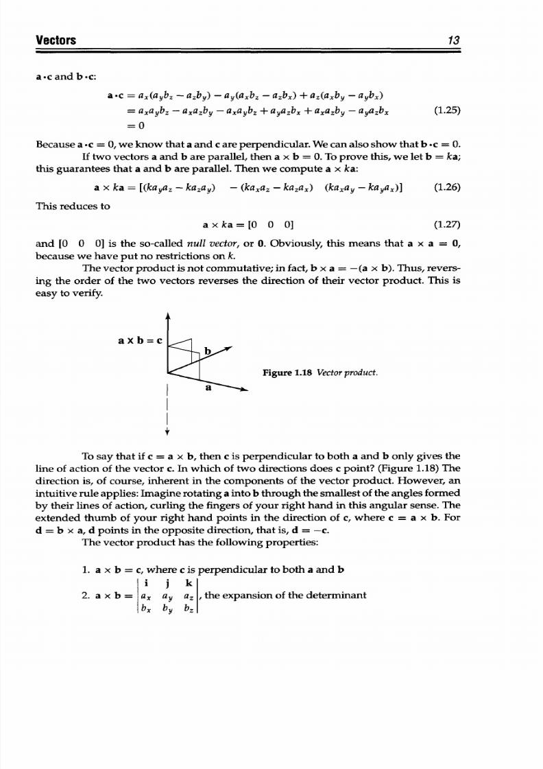
The
vector
product is
not commutative; in fact, b x a =-(a x b).
Thus, revers-
ing
the
order
of
the
two vectors reverses
the direction
of
their vector
product. This
is
easy to
verify.
axb
=c
Figure 1.18 Vector product.
To
say that
if
c = a
x
b, then c is perpendicular to
both
a
and
b only
gives
the
line of action of the vector c.
In
which
of
two directions does c point?
(Figure
1.18) The
direction is, of course,
inherent
in
the
components of the vector
product.
However, an
intuitive rule
applies: Imagine
rotating
a
into
b through the smallest of the angles formed
by
their
lines
of
action,
curling the fingers of
your
right hand in
this
angular
sense. The
extended thumb of your right hand points in the direction of c,
where
c
= a x
b. For
d
=
b x
a, d points in the
opposite
direction, that is, d = -c.
The
vector
product has the
following
properties:
1.
a
x
b
=
c, where c
is perpendicular
to
both
a
and b
i j
k
2.
a
x b =
a, ay
a. , the expansion
of the determinant
b, by b,
8/9/2019 Mortenson, Michael E. - Mathematics for computer graphics applications.pdf
http://slidepdf.com/reader/full/mortenson-michael-e-mathematics-for-computer-graphics-applicationspdf 27/367
14 Chapter 1
3.
ax
b
= lal Ib fi sin
,
where fi
is the unit vector
perpendicular to the
plane
of
a
and
b
and
0 is the
angle
between
them
4. a x b = -b x a
5.
a
x
(b
+ c)
=
a
x
b
+
a
x
c
6. (ka) x
b
= a x (kb) = k(a > b)
7. i x j =
k,
j x k
=
i, k x i
=j
8. If
a is
parallel
to
b,
then
a x b = 0
9. a
x a = 0
1.8
Elements of Vector
Geometry
We
can
use
vector
equations
to describe
many
geometric
objects,
from
points,
lines,
and
curves to
very
complex surfaces. We do
this by
writing a vector
equation
in
terms
of
one or more variables. We will
be
exploring only straight lines and planes
here.
Lines
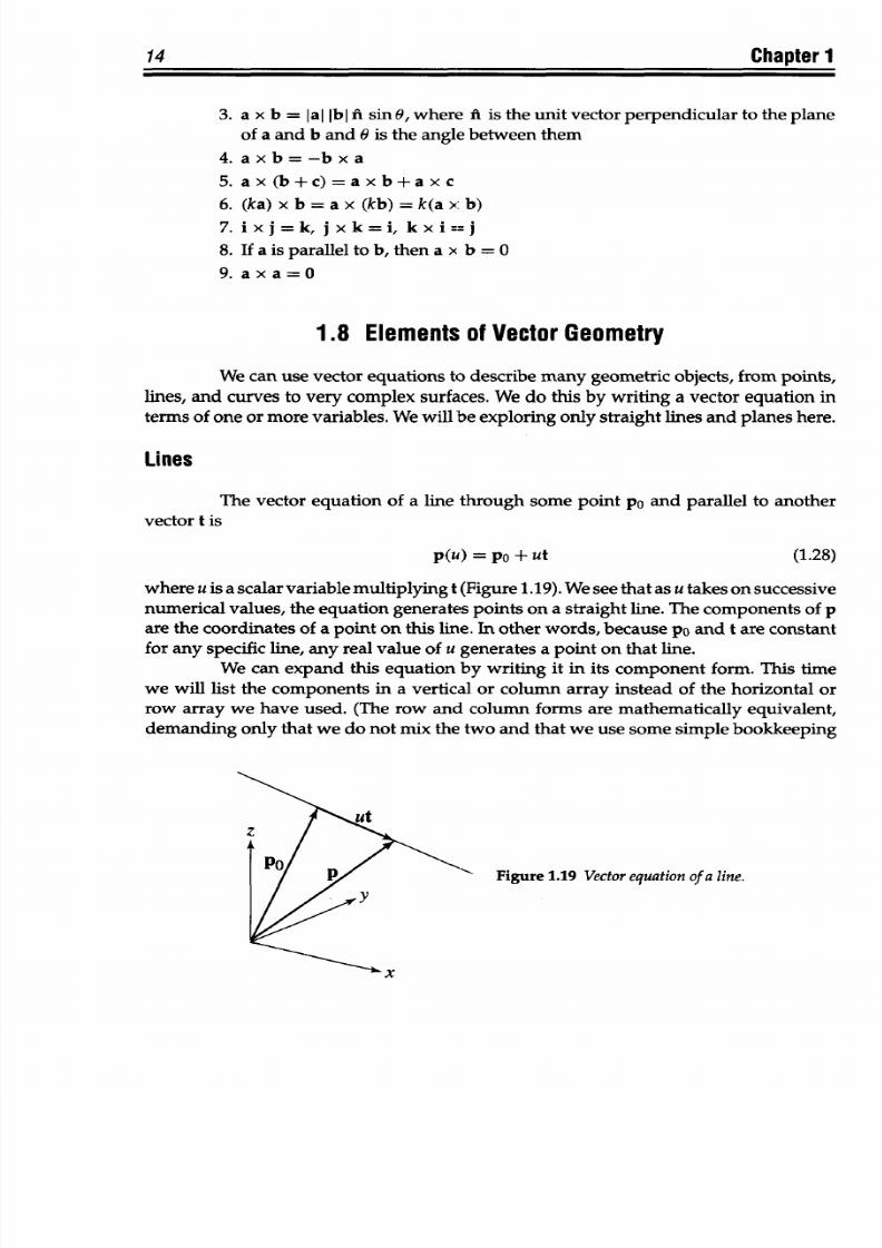
The vector equation of a line
through
some
point
po and parallel to another
vector
t is
p(u) =
po
+
ut
(1.28)
where
u
is
a scalar variable multiplying
t
(Figure
1.19).
We see that
as
u takes on
successive
numerical values, the equation generates
points
on a straight line.
The
components
of
p
are the
coordinates of
a point on this
line.
In other
words,
because
po and
t
are constant
for
any
specific line, any real
value
of
u generates a point
on
that line.
We
can
expand
this equation by writing it
in its
component
form. This
time
we will
list the components in
a vertical
or column array instead
of
the horizontal
or
row
array we
have used. (The row and column forms are mathematically
equivalent,
demanding
only that we
do
not mix
the
two
and that
we use some simple bookkeeping
Figure
1.19
Vector
equation of
a line.
8/9/2019 Mortenson, Michael E. - Mathematics for computer graphics applications.pdf
http://slidepdf.com/reader/full/mortenson-michael-e-mathematics-for-computer-graphics-applicationspdf 28/367
Vectors
ii-1 n
u=O
u=
5
U=1
u=2.0
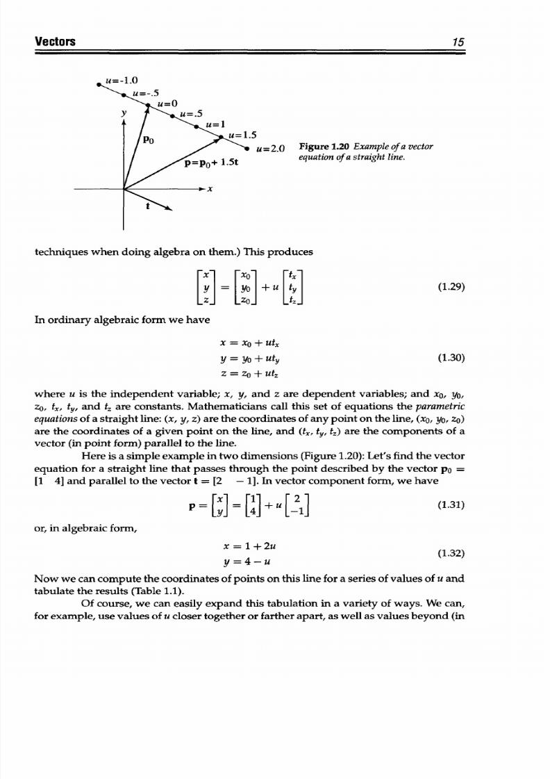
Figure
1.20
Example
of
a vector
equation of a straight line.
techniques
when
doing
algebra
on them.)
This
produces
L]
+
(1.29)
In
ordinary
algebraic
form
we have
X = Xb
+
utX
Y
=yo
+
uty
(1.30)
z =
zo
+ Utz
where
u
is the
independent variable;
x,
y,
and
z
are
dependent
variables; and x
0
,
yo ,
zo,
tx,
ty,
and t4
are constants. Mathematicians call
this set of
equations the
parametric
equationsof a straight
line:
(x, y, z) are
the coordinates
of
any
point on the line, (xo,
yo,
zo)
are the coordinates of a given point on the line, and (tx, ty, t,) are
the
components of a
vector (in point form) parallel to the line.
Here
is
a simple
example in
two
dimensions
(Figure 1.20): Let's
find
the
vector
equation
for
a
straight
line
that
passes
through
the
point
described
by
the vector
po
=
[1 4] and parallel
to
the vector t = [2
-1].
In vector component
form,
we have
[x]
[]
+ u[2]
(1.31)
or,
in algebraic form,
x =
1 +
2u (1.32)
y
=4-u
Now
we
can
compute
the
coordinates
of points
on
this line for a
series
of values of u and
tabulate the results (Table 1.1).
Of course, we can easily expand
this
tabulation in
a
variety
of ways. We can,
for example, use values
of
u
closer
together
or
farther apart,
as well as values
beyond
(in
15
8/9/2019 Mortenson, Michael E. - Mathematics for computer graphics applications.pdf
http://slidepdf.com/reader/full/mortenson-michael-e-mathematics-for-computer-graphics-applicationspdf 29/367
16
Chapter 1
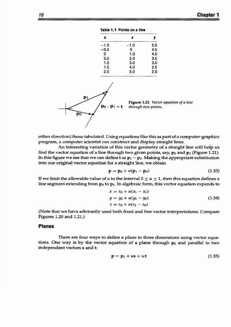
Table 1.1
Points on a line
U X
y
-1.0
-1.0
5.0
-0.5
0 4.5
0
1.0
4.0
0.5 2.0
3.5
1.0
3.0
3.0
1.5
4.0 2.5
2.0 5.0 2.0
Figure
1.21
Vector equation
of a line
I = t
through two points.
either direction)
those tabulated.
Using
equations
like
this as part
of
a computer-graphics
program, a computer scientist can
construct and display straight lines.
An
interesting
variation
of this
vector geometry
of
a
straight
line will
help
us
find
the
vector
equation
of a line through
two
given
points,
say,
po and p1
(Figure
1.21).
In
this figure we see that
we can define
t
as pi - po.
Making the appropriate
substitution
into
our original vector equation
for a straight
line,
we
obtain
p =
P0 + u(p
1
-
P0)
(1.33)
If we limit the
allowable value of u
to
the interval 0 < u < 1,
then
this equation
defines
a
line segment
extending from po to pi. In algebraic
form,
this
vector
equation expands to
x
=
Ab +
u(X
1
- Xo)
y
=yo +
u(yi
-yO)
(1.34)
z = zo + u(z
1
- Zo)
(Note that we
have arbitrarily
used
both fixed
and free vector
interpretations.
Compare
Figures 1.20 and
1.21.)
Planes
There are
four ways to define
a
plane
in
three
dimensions
using
vector
equa-
tions.
One way is
by
the
vector equation
of a plane
through
po and parallel to
two
independent
vectors
s and
t:
p
= Po+
us+
wt
(1.35)
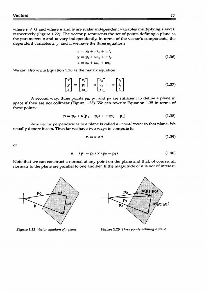
8/9/2019 Mortenson, Michael E. - Mathematics for computer graphics applications.pdf
http://slidepdf.com/reader/full/mortenson-michael-e-mathematics-for-computer-graphics-applicationspdf 30/367
Vectors
17
where
s
#
kt and
where u
and w are scalar independent variables multiplying
s
and t,
respectively (Figure 1.22). The vector
p represents the set
of points defining
a plane as
the parameters u and w vary independently. In terms of the
vector's
components, the
dependent
variables
x, y,
and
z,
we have
the three
equations
X = X0 +USx +
Wtx
y = yo +USy
+Wty
(1.36)
z =
Zo
+
Usz
+Wtz
We can also
write
Equation
1.36
as
the matrix equation
Y
=
Y O +
u
sy
+w ty(1.37)
-z
-ZO
z tz
A second way:
three
points
pO, pi, and P2 are sufficient to define a plane
in
space if they are not collinear
(Figure 1.23). We can
rewrite Equation
1.35
in
terms
of
these points:
p
= pO + u(p1 - PO)
+
w(p2 - p1) (1.38)
Any
vector perpendicular
to a plane is called a
normal vector
to
that
plane.
We
usually
denote it as
n.
Thus
far
we
have two
ways
to compute
it:
n=sxt
(1.39)
or
n
=
(pi - po) x (p2 - pi)
(1.40)
Note that
we
can
construct a
normal at any
point
on
the plane
and that, of course, all
normals to the plane
are
parallel to
one
another.
If
the
magnitude of n is not of interest,
IJ
P2
Figure 1.23
Three
points defining a plane.
pi)
Figure
1.22
Vector equation of
a plane.
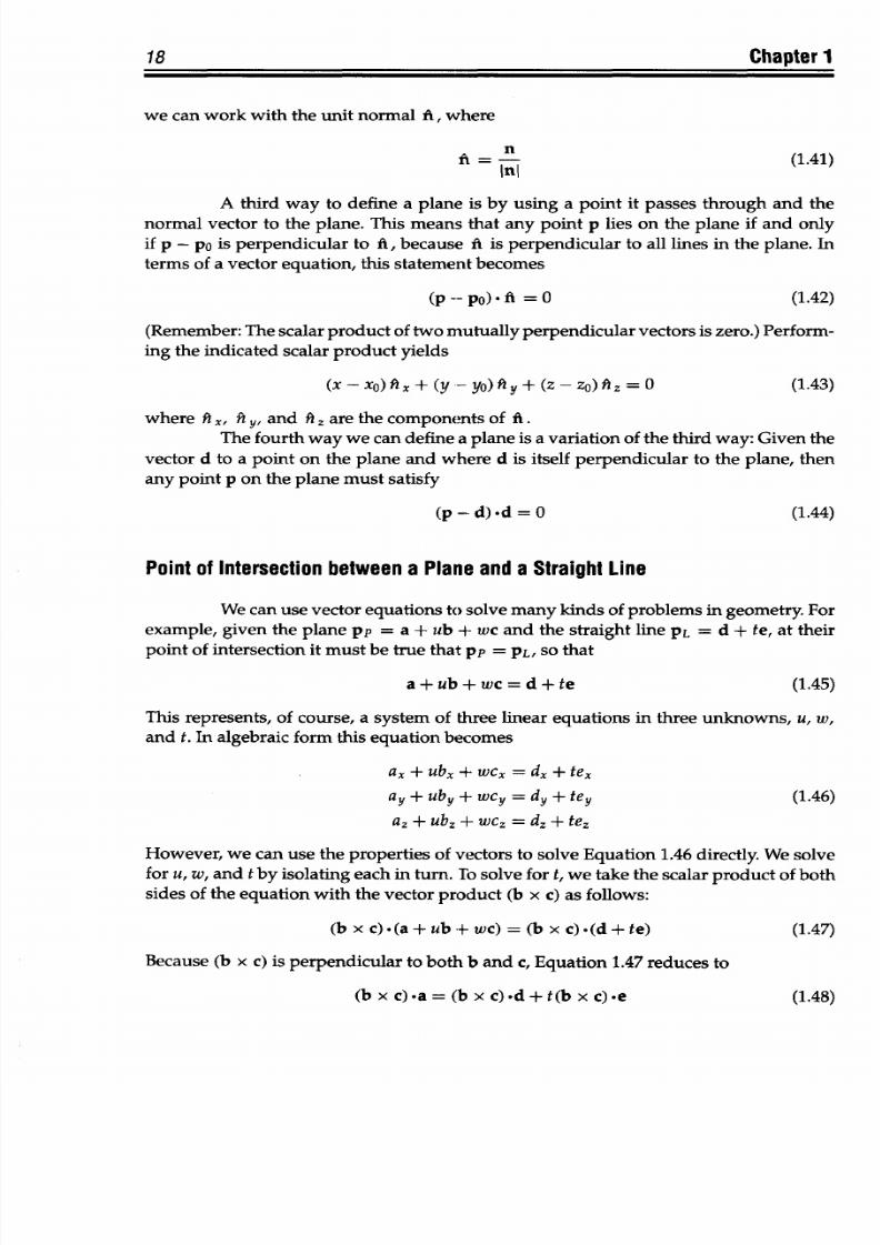
8/9/2019 Mortenson, Michael E. - Mathematics for computer graphics applications.pdf
http://slidepdf.com/reader/full/mortenson-michael-e-mathematics-for-computer-graphics-applicationspdf 31/367
18
Chapter
1
we can work
with
the
unit
normal
ft,
where
ft
An
(1.41)
Inj
A
third
way
to define
a plane
is
by
using
a point it
passes
through
and the
normal vector to the
plane.
This
means that
any
point
p
lies
on the
plane
if
and only
if p
-
po
is perpendicular
to
ft, because ft
is
perpendicular
to all
lines
in
the
plane. In
terms
of a
vector equation,
this
statement becomes
(p
-po) .
ft = 0
(1.42)
(Remember: The
scalar product
of two mutually
perpendicular
vectors
is zero.) Perform-
ing
the indicated
scalar product
yields
(X-Xo)ftx
+
(Y
-
yo)Piy+
(z-Zo)
fz =O (1.43)
where
A}
, fl
y, and
ft z
are
the components
of
ft.
The
fourth way we can
define a
plane is a variation of
the third way: Given
the
vector
d to
a point on the
plane
and
where
d is itself
perpendicular
to
the
plane, then
any
point
p on the
plane must satisfy
(p
-d) -d = 0
(1.44)
Point
of
Intersection
between
a
Plane
and
a
Straight
Line
We
can
use vector equations to
solve
many kinds of
problems in geometry.
For
example,
given the
plane pp
=
a
+
ub
+
wc
and
the straight line PL
= d
+
te,
at their
point
of intersection
it must be true
that pp
=
PL,
SO
that
a+ub+wc = d+te
(1.45)
This
represents,
of course,
a system of three
linear
equations
in three unknowns,
u, w,
and
t. In
algebraic form
this
equation becomes
ax
+ ubx +
wcx =
dx +
tex
ay
+
uby
+ wcY
=
dy
+ tey
(1.46)
az + ubz +
wcz
= dz
+
tez
However,
we can
use
the
properties of vectors
to solve
Equation
1.46
directly. We
solve
for u, w,
and
t by isolating each
in turn. To
solve
for t, we take
the
scalar
product of
both
sides
of
the
equation with the vector
product (b
x c) as follows:
(b x
c)-(a
+ ub
+ wc) = (b x
c)
.(d
+ te)
(1.47)
Because
(b
x
c)
is perpendicular to
both b and
c,Equation 1.47
reduces to
(b xc) a=(bxc).d+t(bxc).e
(1.48)
8/9/2019 Mortenson, Michael E. - Mathematics for computer graphics applications.pdf
http://slidepdf.com/reader/full/mortenson-michael-e-mathematics-for-computer-graphics-applicationspdf 32/367
Vectors
19
Solving Equation 1.48 for t yields
t = (b
x
c).a-
(b x c).d
(1.49)
(b x c) .e
We
continue in the
same way to solve for u and w:
(c x
e)
d-(c x e).a (1.50)
(c
x
e) .b
(b x e) .d - (b
x
e)a
(1.51)
(b x
e).c
1.9
Linear
Vector
Spaces
If we algebraically
treat
vectors
as if
they
originated at a common
point, then
we
work in a
linear
vector
space. Not only
do
all
vectors have
a common origin, but any
vector combines with
any
other
vector
according to
the
parallelogram
law of
addition.
Vectors
must
be
subjected
to the
following
two
operations to
qualify
as members of
a
linear vector space:
1.
Addition
of any two vectors must produce a
third
vector, identified as their
sum:
a
+
b
=
c.
2.
Multiplication
of
a
vector
a
by
a
scalar
k
must
produce another
vector
ka as
the
product.
The set of all
vectors
is closedwith respect
to
these two operations, which means
that
both the sum of
two
vectors
and the
product of
a vector and
a
scalar
are themselves
vectors. These two operations
have
the following properties, some of
which
we
have
seen
before:
1. Commutativity:
a
+ b = b + a
2. Associativity:
(a +
b)
+
c = a
+
(b
+ c)
3. Identity element: a
+ 0 = a
4. Inverse:
a - a = 0
5. Identity under scalar multiplication: ka =
a, when
k = 1
6. c(da)
=
(cd)a
7. (c + d)a = ca + da
8. k(a+b)
=ka+kb
A set of vectors that can be subjected to the two operations with these eight
properties
forms
a
linear
vector
space. The
other
vector
operations
we
have
discussed,
such
as
the
scalar and vector
products,
are
not pertinent
to this definition of a linear vector
space. This brings
us
back
to
hypernumbers. It is easy
to
show that the set
of
all
vectors
of
the
form r
= [r, r
2
...
rn], where ri,
r
2
, ... ,
rn
are
real numbers,
constitutes
a linear
vector
space.
8/9/2019 Mortenson, Michael E. - Mathematics for computer graphics applications.pdf
http://slidepdf.com/reader/full/mortenson-michael-e-mathematics-for-computer-graphics-applicationspdf 33/367
20
Chapter 1
The
set
of all
linear combinations
of
a given
set
of vectors (none of which is
a
scalar
multiple of any other in
the set) forms
a vector
space. For example, if
we
let
xl, x2, ... , xn
be any
n vectors, then aix
1
+ a
2
x
2
+ *.. anxn (where a,,
a
2
,
. . ., an are
scalars) is a
linear combination
of
the vectors xi, x
2
, .
. ., x". But that is
not
all
we
can do.
If we let
s = aixi
+ a
2
x
2
+ + anXn
(1.52)
t
=
bjxj
+
b
2
x
2
+ * +
bnXn
so
that the
vectors
s and t
are
linear combinations
of
the
vectors xl, x2,
. . ., x , then
s + t = (a,
+
bl)xl
+
(a
2
+
b
2
)x
2
+ *+ (an + bn)xn
(1.53)
We also
have
ks
=
(kai)xi
+
(ka
2
)x
2
+
+
(kan)xn
(1.54)
which is also a
linear
combination of xl,
X2, . . .,
xn.
Mathematicians
point
out
that the
space of all linear combinations
of a given set
of
vectors is the space generated by that
set.
Given
a single vector
x,
the space generated by
all scalar
multiples
of
x
is
a
straight line collinear with
x
(for x
0
0). Given
two
vectors
s and t, where t
is not
a
scalar
multiple of
s,
then
the space generated by
their
linear
combinations is
the
plane
containing
s
and t.
For
example,
if
we let r = as + bt, then from the
parallelogram law
of addition
we know that
vectors
r,
s, and t
are
coplanar. Of
course, we could continue
this
process, generating spaces
of three and more dimensions simply
by
increasing
the
number
of
vectors in
the
generating
set.
To
do
this,
we
must
impose
certain
conditions,
as in the previous example where we did not allow s
and
t to be
scalar
multiples of each
other. This leads
us
to
the
concepts of
linear independence and dependence.
1.10 Linear
Independence and Dependence
Vectors xl, x
2
, . . ., x, are linearlydependent if and only if there are real numbers
a,, a
2
,
. . .,
an not
all
equal
to zero,
such that
aixi
+ a2x2 +
+
anxn
=
0
(1.55)
If this
equation is
true
only
if a,,
a
2
,
... ,an are
all
zero, then x
1
, x
2
, ... , xn
are
linearly
independent.
If x
1
, X2,
. . .,
xn
are
linearly dependent,
then
we can express
any
one of
them as
a linear
combination
of
the others. On
the other
hand, if
one
of
the vectors xi, x
2
, . . ., xn
is a linear combination of
the others, then the vectors are linearly dependent.
Another
way of saying this is
that vectors x
1
,
x
2
, . . ., xn
are
linearly
dependent
if and
only if one
of
them belongs to the space generated
by
the
remaining n - 1
vectors.
We can
now define
the dimension of
a linear
space as
equal
to
the maximum number
of linearly
independent
vectors
that
it
can contain.
This fact
underlies
our
study
of basis
vectors.
We
observe that any
two
vectors are dependent
if and only if
they
are parallel
(or collinear);
three
vectors are dependent if and only if
they
are coplanar;
four
vectors
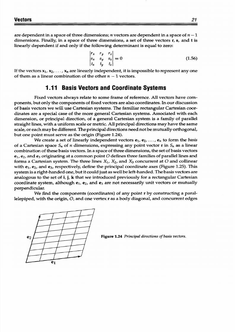
8/9/2019 Mortenson, Michael E. - Mathematics for computer graphics applications.pdf
http://slidepdf.com/reader/full/mortenson-michael-e-mathematics-for-computer-graphics-applicationspdf 34/367
Vectors
21
are
dependent
in a space of three
dimensions;
n vectors
are
dependent
in a space of
n -1
dimensions. Finally, in a space
of three dimensions, a set of
three
vectors r, s,
and t
is
linearly
dependent if
and
only if the
following
determinant is equal to zero:
r,
ry rz
S. sy s, =
0
(1.56)
tx
ty tz
If
the
vectors
xl,
x
2
, . . .,
xn
are linearly
independent, it is impossible
to represent any
one
of
them
as
a linear combination
of
the
other n
- 1
vectors.
1.11
Basis Vectors and Coordinate Systems
Fixed
vectors always relate to some
frame of
reference.
All vectors have
com-
ponents,
but
only the com ponents
of fixed vectors
are
also coordinates.
In
our
discussion
of
basis
vectors we will use Cartesian systems. The
familiar
rectangular Cartesian coor-
dinates are a
special
case
of
the
more general
Cartesian systems. Associated
with each
dimension,
or principal
direction, of
a general
Cartesian system
is a family of
parallel
straight lines,
with
a uniform
scale or
metric. All
principal directions may have
the
same
scale,
or each may be different. The principal directions
need not be
mutually
orthogonal,
but one
point
must
serve as
the origin (Figure
1.24).
We
create
a set
of
linearly independent vectors
el,
e
2
, . . ., en to form the basis
of a Cartesian space S,, of n dimensions, expressing any point vector r in
S"
as a linear
combination of these basis
vectors.
In
a
space of three
dimensions,
the
set of
basis
vectors
el,
e
2
, and e
3
originating
at
a
common point
0 defines three families of parallel lines
and
forms a Cartesian system. The three lines
X
1
, X
2
,
and X
3
concurrent at 0
and
collinear
with el,
e
2
, and e
3
,
respectively, define
the
principal coordinate axes (Figure
1.25).
This
system is a
right-handed
one, but
it
could just
as
well be left-handed. The basis vectors are
analogous
to the
set
of i, j, k
that
we
introduced previously for a
rectangular Cartesian
coordinate system,
although
el,
e
2
, and e
3
are not necessarily
unit
vectors
or
mutually
perpendicular.
We find the components (coordinates) of any
point
r by constructing a paral-
lelepiped,
with
the
origin,
0,
and
one vertex
r
as
a
body
diagonal,
and
concurrent edges
Figure 1.24 Principaldirectionsof basis vectors.
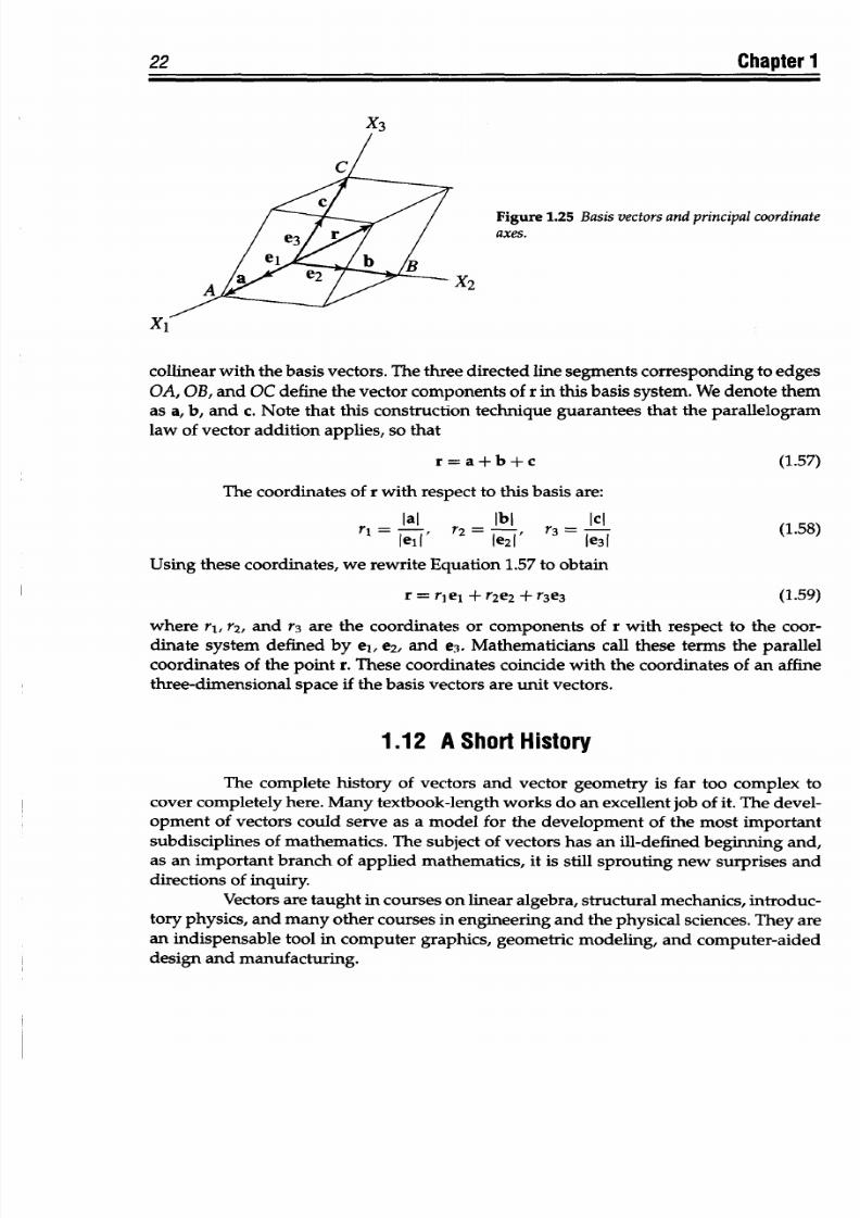
8/9/2019 Mortenson, Michael E. - Mathematics for computer graphics applications.pdf
http://slidepdf.com/reader/full/mortenson-michael-e-mathematics-for-computer-graphics-applicationspdf 35/367
22
Chapter 1
X
3
Figure
1.25 Basis vectors
and
principal
coordinate
axes.
X
2
x
1
collinear
with
the basis
vectors. The
three
directed line
segments corresponding to edges
OA, OB, and
OC define
the
vector
components
of r
in
this
basis
system. We
denote
them
as
a,
b,
and
c. Note
that
this construction
technique
guarantees that
the parallelogram
law of
vector
addition
applies, so
that
r
=
a + b
+
c
(1.57)
The
coordinates
of
r
with
respect
to this
basis are:
Jal
I2I
Ic
ri l I, =
leI, r3 = le3l
(1.58)
Using
these
coordinates,
we rewrite
Equation 1.57 to obtain
r
=
riel
+
r2e
2
+ r
3
e
3
(1.59)
where r
1
,
r
2
, and
r3
are
the
coordinates
or
components of r with
respect
to
the coor-
dinate
system defined by
el, e2,
and
e
3
.
Mathematicians
call
these
terms
the
parallel
coordinates
of
the point
r. These
coordinates
coincide
with the
coordinates
of an
affine
three-dimensional
space if the basis vectors
are unit
vectors.
1.12
AShortHistory
The
complete
history
of vectors
and
vector
geometry
is far too
complex
to
cover completely
here.
Many textbook-length
works do an excellent
job of
it.
The
devel-
opment of vectors
could
serve
as a model
for the development
of the
most
important
subdisciplines of mathematics.
The subject of
vectors
has
an
ill-defined
beginning
and,
as
an important
branch
of applied
mathematics,
it is
still
sprouting new
surprises
and
directions
of inquiry.
Vectors
are taught in courses
on
linear algebra,
structural mechanics, introduc-
tory
physics,
and
many
other
courses in
engineering
and
the
physical
sciences.
They are
an indispensable
tool in computer graphics,
geometric
modeling,
and
computer-aided
design
and
manufacturing.
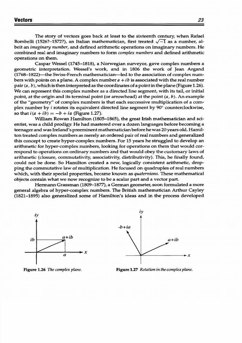
8/9/2019 Mortenson, Michael E. - Mathematics for computer graphics applications.pdf
http://slidepdf.com/reader/full/mortenson-michael-e-mathematics-for-computer-graphics-applicationspdf 36/367
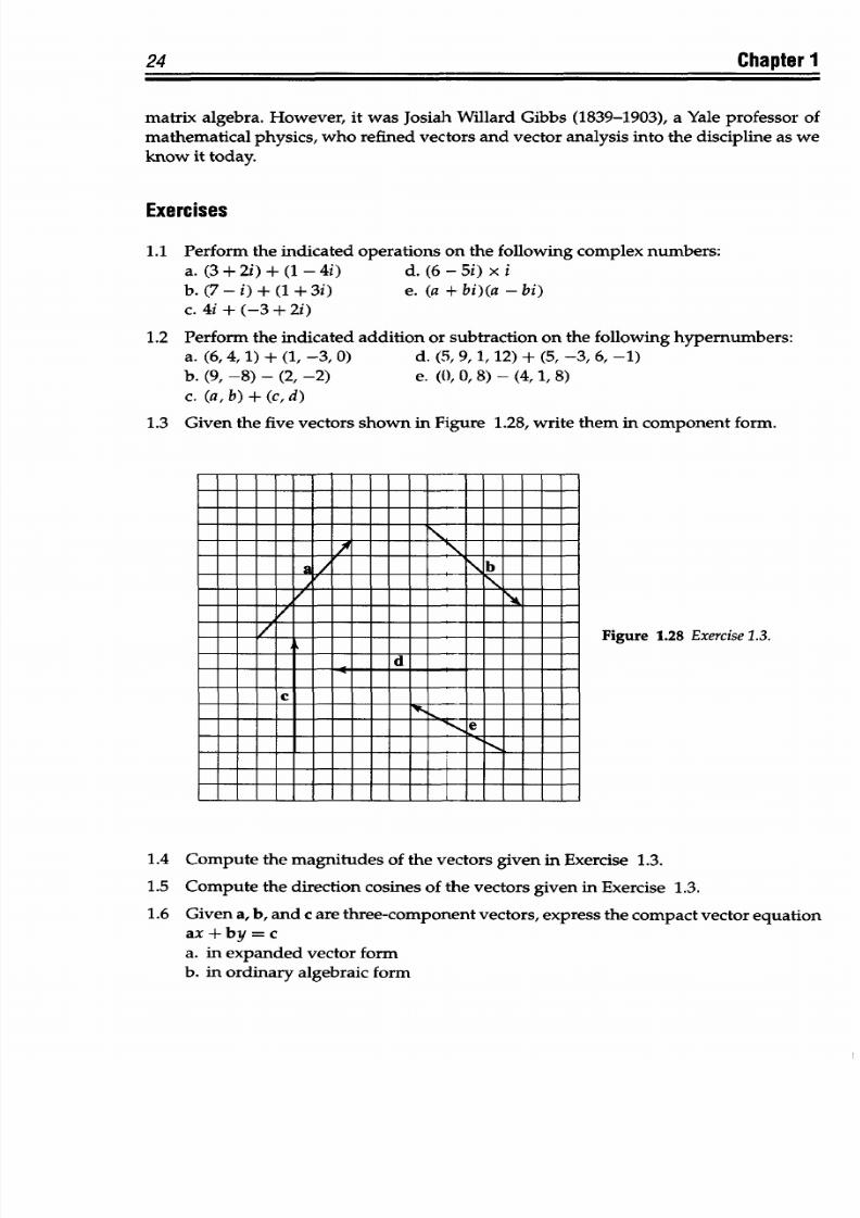
8/9/2019 Mortenson, Michael E. - Mathematics for computer graphics applications.pdf
http://slidepdf.com/reader/full/mortenson-michael-e-mathematics-for-computer-graphics-applicationspdf 37/367
24
Chapter
1
matrix
algebra. However,
it was
Josiah Willard Gibbs
(1839-1903),
a
Yale professor
of
mathematical
physics, who refined vectors
and vector analysis
into the discipline
as
we
know
it today.
Exercises
1.1
Perform
the indicated operations on
the following complex
numbers:
a.(3+2i)+(1-4i)
d.(6-5i)xi
b. (7
- i) + (1+
3i)
e.
(a
+
bi)(a - bi)
c. 4i + (-3 + 2i)
1.2
Perform the
indicated
addition
or subtraction
on
the
following
hypernumbers:
a.
(6,4,1) +
(1,
-3, 0) d. (5, 9,1,12)
+ (5, -3, 6,-1)
b. (9,
-8)
-
(2,
-2) e.
(0,0, 8)
- (4,1, 8)
c.
(a,b)+(c,d)
1.3
Given
the five vectors shown in Figure 1.28,
write
them
in component
form.
1I I
A I>
L d
I
Figure
1.28 Exercise 1.3.
Compute the magnitudes of
the
vectors
given in Exercise 1.3.
Compute the
direction
cosines
of the
vectors given
in Exercise 1.3.
Given
a,
b, and
c
are
three-component
vectors,
express the compact vector
equation
ax
+
by =
c
a. in expanded
vector form
b.
in
ordinary
algebraic
form
1.4
1.5
1.6
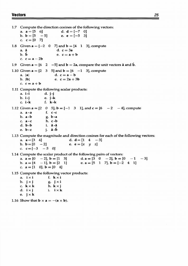
8/9/2019 Mortenson, Michael E. - Mathematics for computer graphics applications.pdf
http://slidepdf.com/reader/full/mortenson-michael-e-mathematics-for-computer-graphics-applicationspdf 38/367
Vectors
1.7 Compute the direction
cosines
of the following
vectors:
a. a=[5 6]
d.
d=[-7
0]
b. b=[5 -5] e.
e=[-5 3]
c.
c=[O
7]
1.8 Given
a =
[-2 0 7]
and b
= [4
1 3], compute
a. a
d. c=3a
b. b
e.
c=a+b
c.
c=a-2b
1.9
Given
a
=[6
2
-5]
and b
=
2a, compare the
unit vectors
a and
6.
1.10 Givena =[2 3
5]
andb
= [6
-1 3],compute
a. lal
d.
c=a-b
b.
IbI
e.
c=2a+3b
c. c=a+b
1.11
Compute the following scalar
products:
a. i-i
d.
j-j
b.
i-j e. j.k
c. i-k
f.
k.k
1.12
Given
a
=
[2
0 5], b = [-1 3 1], and c =[6
-
2
-
4], compute
a. a-a f.
c-c
b. a-b
g.
b-a
c.
a-c
h.
c-b
d. b.b
i. a-a
e. b-c
j.
a.6
1.13
Compute
the magnitude and direction
cosines
for each
of
the
following
vectors:
a.
a= [3 4]
d. d=[1
4
-3]
b. b=[O -2]
e. e = [x y
z]
c. c=[-3 -5 0]
1.14
Compute the
scalar product of
the
following
pairs of
vectors:
a.
a=[O
-2],b=[1
3]
d.a=[3
0
-2],b=[O
-1
-3]
b. a=[4 -1],b=[2
1]
e.a=[5 1
7],b=[-2
4 1]
c.
a=[1 0],b=[O 4]
1.15
Compute the following vector
products:
a. ixi f. kxi
b.
jxj
g.
jx i
c.
kxk h. kxj
d.
ixj i.
ixk
e. jxk
1.16
Show
that b
x
a
=
-(a
x
b) .
25
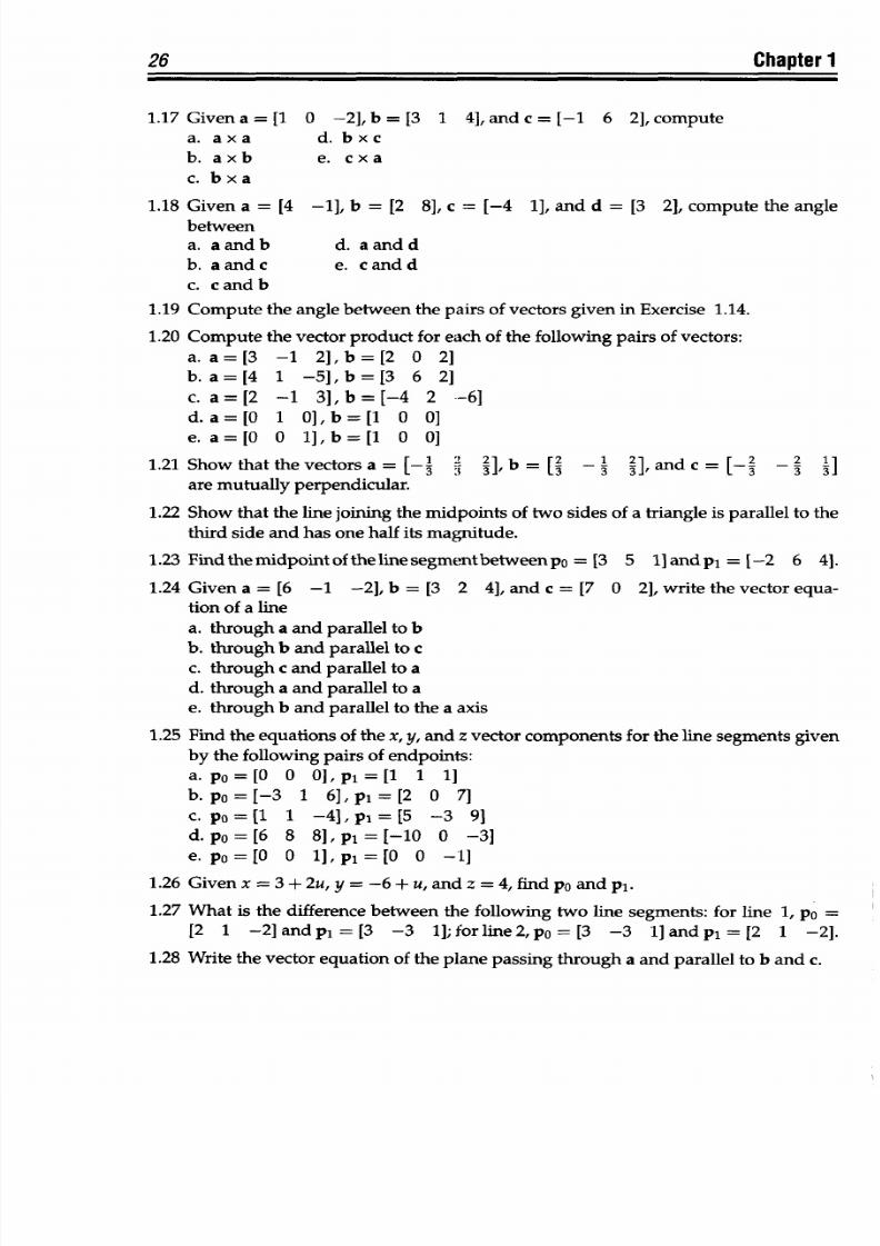
8/9/2019 Mortenson, Michael E. - Mathematics for computer graphics applications.pdf
http://slidepdf.com/reader/full/mortenson-michael-e-mathematics-for-computer-graphics-applicationspdf 39/367
26
Chapter
1
1.17 Given
a = [1 0 -2],
b
=
[3
1
4],
and
c = [-1 6
2],
compute
a.
axa d. bxc
b. axb e. cxa
c. bxa
1.18 Given a
= [4 -1], b = [2
8], c = [-4 1], and
d
=
[3
2], compute
the angle
between
a.
aandb
d.
aandd
b. aandc e. candd
c. candb
1.19 Compute
the
angle
between the pairs
of
vectors given
in Exercise
1.14.
1.20
Compute
the
vector product for
each of
the
following
pairs
of
vectors:
a. a=[3
-1
2],b=[2
0 2]
b.
a=
[4
1
-5],
b =[3
6
2]
c.
a=[2 -1
3],b=[-4
2 -6]
d.a=[0 1 0],b=[1 0
0]
e.
a=[0 0 1],b=[1 0
0]
1.21 Show
that the
vectors a = [-_
2 2 ],
b = [2
-
3
],and c
=
[-2
-
2
]
are
mutually perpendicular.
1.22
Show that the
line joining the midpoints
of two
sides of
a triangle is
parallel
to the
third
side and
has one half
its
magnitude.
1.23
Findthemidpointofthelinesegmentbetweenpo
=
[3
5
1]andpl
=
[-2
6 4].
1.24 Given a
= [6 -1
-2],
b = [3
2
4],
and c = [7
0
2],
write the vector equa-
tion
of
a line
a.
through a and parallel to
b
b. through
b
and parallel
to
c
c.
through c and parallel
to a
d.
through
a and
parallel to a
e. through
b
and parallel to
the a axis
1.25
Find the
equations
of
the x, y, and
z
vector
components for the line
segments
given
by
the
following
pairs
of endpoints:
a. po=[0
0 OI,pi=[1 1 1]
b. po = [-
3
1
61,
pi
= [2
0 7]
c.
po =
[1 1 -
4
],
pi
= 15
-3
91
d.po=[6 8
8
],pi=[-10 0
-3]
e. po = [O 0
1], pi = [O 0 -1]
1.26
Given x = 3
+
2u,
y = -6 + u, and z
= 4, find
po
and
pi.
1.27 What
is
the
difference
between
the following
two line segments:
for line 1,
po
=
[2
1
-2]andpl
=
[3
-3
1];forline2,pO
=
[3
-3
1]andpl
=
[2
1
-2].
1.28
Write the vector
equation
of
the
plane passing through a and
parallel to b and
c.
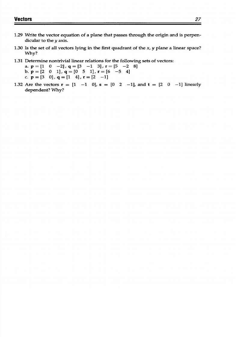
8/9/2019 Mortenson, Michael E. - Mathematics for computer graphics applications.pdf
http://slidepdf.com/reader/full/mortenson-michael-e-mathematics-for-computer-graphics-applicationspdf 40/367
Vectors
27
1.29
Write
the
vector equation of
a
plane that
passes
through the origin and is perpen-
dicular
to
the y
axis.
1.30 Is
the
set of all vectors
lying
in
the
first quadrant of the x, y
plane
a linear space?
Why?
1.31
Determine nontrivial
linear
relations for
the
following sets of
vectors:
a.
p =[1 0 -2],
q =
[3 -1
3],
r = [5 -2 8]
b.p=[2
0
1],q=[0 5
1],r=[6
-5
4]
c. p=[3 0],q=[1
4],r=[2 -1]
1.32 Are
the
vectors
r
= [1 -1 0],
s
= [0
2
-1], and t
= [2 0 -1] linearly
dependent? Why?
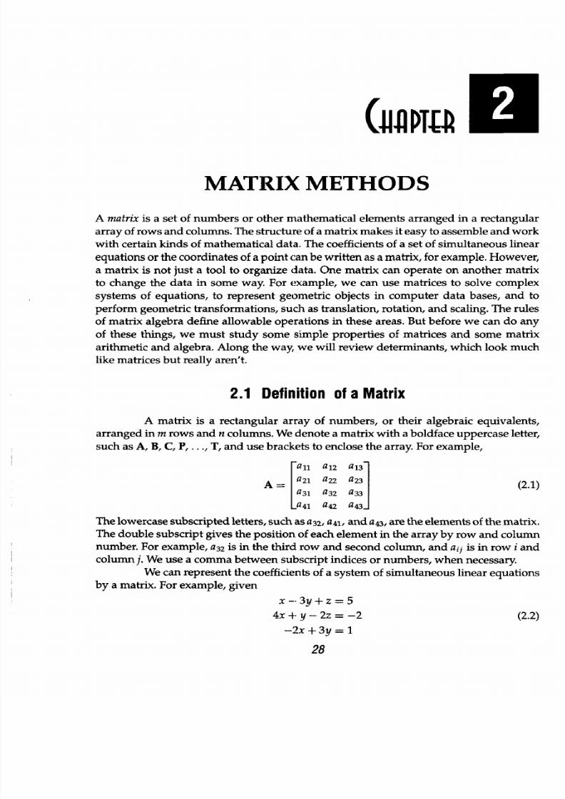
8/9/2019 Mortenson, Michael E. - Mathematics for computer graphics applications.pdf
http://slidepdf.com/reader/full/mortenson-michael-e-mathematics-for-computer-graphics-applicationspdf 41/367
(AUT
MATRIX
METHODS
A matrix
is a set
of
numbers or other
mathematical
elements arranged in a rectangular
array of rows
and columns. The
structure
of
a
matrix
makes it easy to assemble
and
work
with
certain
kinds
of
mathematical data.
The
coefficients
of
a set
of
simultaneous
linear
equations
or the coordinates
of
a
point can
be
written
as a m atrix, for
example.
However,
a
matrix
is
not just
a
tool
to
organize data. One
matrix can operate on
another matrix
to
change the data
in some way. For
example,
we
can
use matrices
to
solve complex
systems
of equations,
to
represent
geometric objects
in computer data bases,
and
to
perform geometric transformations,
such
as
translation,
rotation, and
scaling.
The rules
of matrix
algebra
define allowable
operations in
these
areas. But before
we can do an y
of these things,
we
must study some
simple
properties
of matrices
and some matrix
arithmetic and algebra.
Along the
way,
we will
review
determinants, which
look
much
like
matrices
but
really
aren't.
2.1 Definition
of a Matrix
A
matrix
is
a
rectangular
array of numbers, or
their algebraic equivalents,
arranged
in
m
rows and
n
columns.
We
denote
a matrix
with a boldface uppercase letter,
such as A, B, C,
P. . . .,
T,
and use brackets to
enclose
the array. For
example,
[all
a
12
a
13
A=
a
21
a22
a
23
(2.1)
a
31
a
3 2
a33
La41 a
42
a
43
j
The
lowercase subscripted letters, such as
a
32
, a
4
l,
and
a43,
are
the elements of
the matrix.
The double subscript gives the position
of each element
in
the array by
row and column
number.
For example,
a
32
is in the
third
row and
second
column,
and aij is in row
i and
column j.
We
use
a
comma between
subscript indices or numbers,
when necessary.
We
can represent the coefficients
of
a
system
of
simultaneous
linear equations
by
a matrix. For
example, given
x
--
3y
+
z =
5
4x + y - 2z = -2
(2.2)
-2x +
3y =
1
28
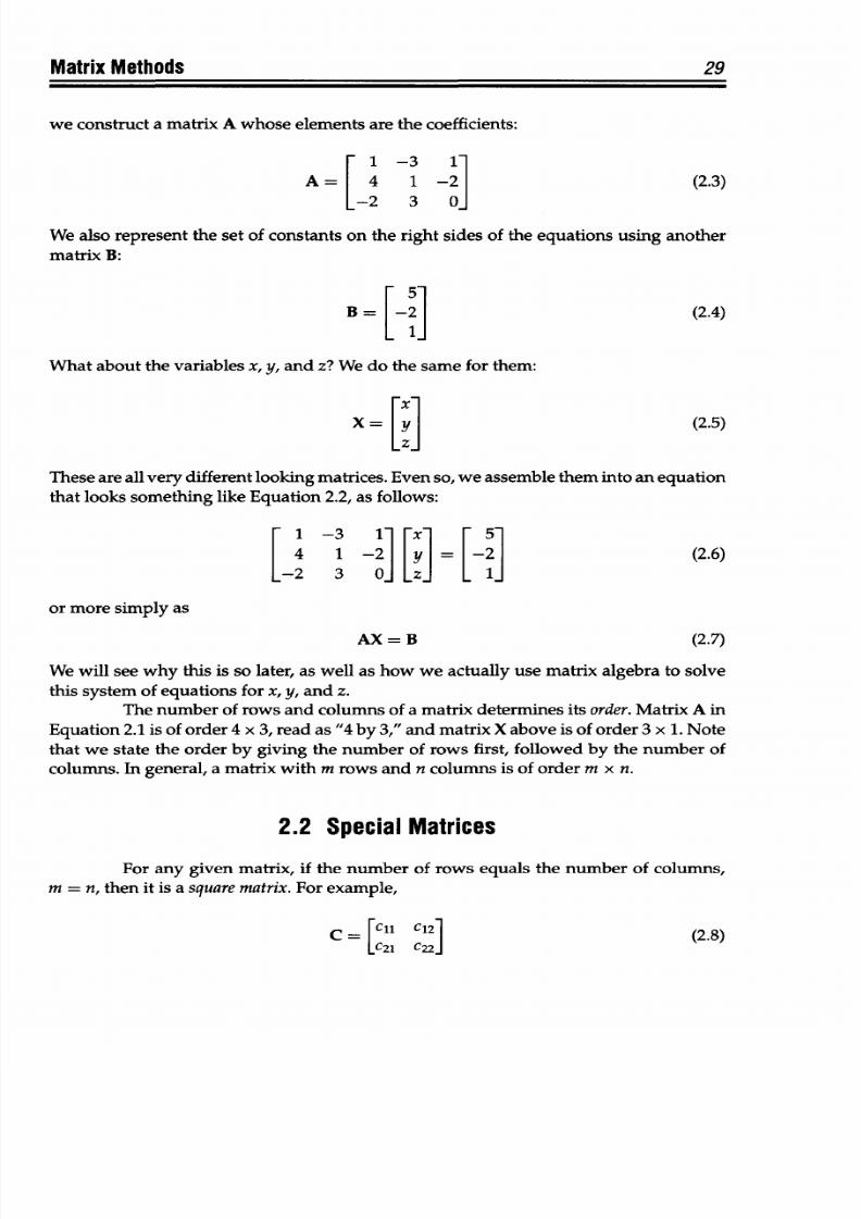
8/9/2019 Mortenson, Michael E. - Mathematics for computer graphics applications.pdf
http://slidepdf.com/reader/full/mortenson-michael-e-mathematics-for-computer-graphics-applicationspdf 42/367
Matrix Methods 29
we construct
a
matrix
A
whose
elements are
the
coefficients:
1
-3
1-
A
=
4
1
-2
(2.3)
-2 3 0-
We also represent
the set
of
constants on the
right sides of
the
equations
using
another
matrix
B:
5~
B =
-2
(2.4)
1
What about the
variables
x,
y,
and
z? We
do
the
same
for them:
x
X = Y
(2.5)
FZ-
These
are
all very different looking matrices. Even so, we assemble them into an equation
that looks
something
like
Equation
2.2, as follows:
1-2
2
y[l
[-l]
(2.6)
or
more
simply as
AX=B (2.7)
We will
see why
this
is so
later,
as well as how
we
actually
use matrix
algebra
to
solve
this system of equations
for x,
y, and
z.
The number of rows and columns of a
matrix
determines its order. Matrix
A in
Equation
2.1
is of
order
4
x
3,
read
as "4
by
3,"
and matrix
X
above
is
of
order
3
x
1.Note
that
we state the order
by
giving the
number of
rows first,
followed by
the
number of
columns. In general, a matrix
with
m rows
and n
columns
is
of order m
x
n.
2.2
Special
Matrices
For any given matrix,
if
the
number
of rows equals the
number
of columns,
m
=
n, then
it
is
a
square
matrix.
For example,
C = [C
11
Cl
2
] (2.8)
C21 C2 2
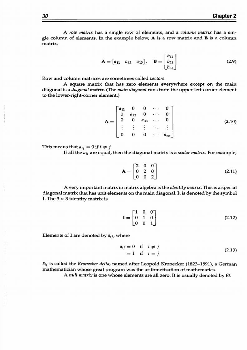
8/9/2019 Mortenson, Michael E. - Mathematics for computer graphics applications.pdf
http://slidepdf.com/reader/full/mortenson-michael-e-mathematics-for-computer-graphics-applicationspdf 43/367
30
Chapter
2
A row matrix
has a
single
row
of elements,
and
a
column matrix has
a
sin-
gle column
of
elements.
In the
example
below, A
is a
row matrix and B is a
column
matrix.
A=
[all a
2
a
1
3
],
B=
b
2
l
(2.9)
b
31
Row
and
column
matrices
are sometimes called
vectors.
A
square
matrix
that has zero elements
everywhere
except on
the
main
diagonal
is
a
diagonal
matrix. (The main diagonal
runs
from the
upper-left-corner
element
to the
lower-right-corner
element.)
all
0
... 0
0
a22
0 ...
0
A=
0 0 a33 ...
0 (2.10)
(210
LO 0 0
...
ann]
This
means
that
aij
=
O
if i
1j.
If
all the
aii are
equal, then the diagonal
matrix
is a scalar
matrix.
For
example,
20
O-
A=
0 2
0
(2.11)
0 0
2_
A
very
important
matrix
in matrix algebra
is
the identity
matrix.
This
is a special
diagonal matrix
that
has unit elements
on the main diagonal.
It
is
denoted
by
the
symbol
I.
The 3 x 3 identity
matrix
is
I
1 0
(2.12)
Elements of
I are
denoted
by Sip
where
=ij=0 if
i
j (2.13)
=1 if
i=j
¾ij
is
called
the
Kronecker delta,
named
after
Leopold
Kronecker
(1823-1891), a
German
mathematician
whose
great
program
was
the
arithmetization of
mathematics.
A null ma trix
is one
whose elements
are
all zero.
It is
usually denoted by
0.
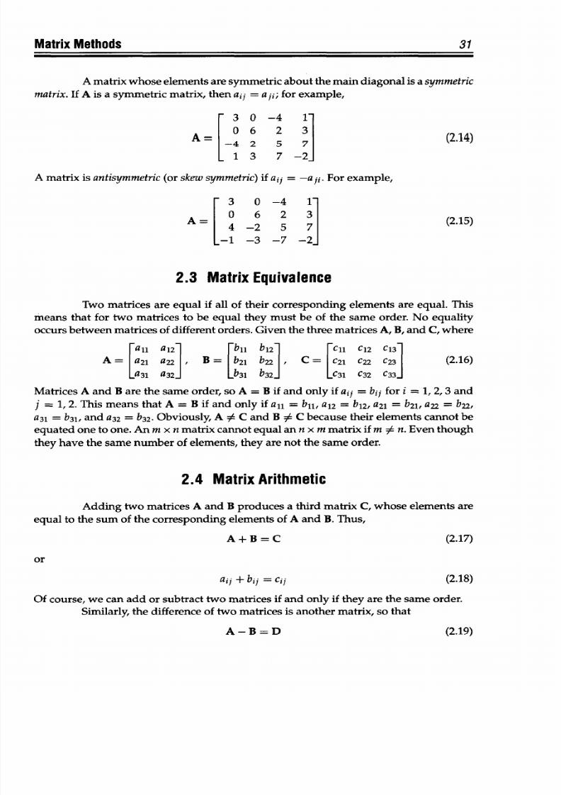
8/9/2019 Mortenson, Michael E. - Mathematics for computer graphics applications.pdf
http://slidepdf.com/reader/full/mortenson-michael-e-mathematics-for-computer-graphics-applicationspdf 44/367
Matrix
Methods
31
A matrix whose elements are symmetric about the main diagonal is a symmetric
matrix.
If A is
a symmetric matrix, then aij
= a ji; for example,
-
3 0
-4
1-
A =
0
6
2 3
(2.14)
1 3
7
-2-
A
matrix
is
antisymmetric (or
skew
symmetric) if aij
=
-a
ji. For example,
-
3 0
-4 1-
A
(2.15)
A=
4 -2 5
7 (.5
--
1
-3
-
7 -2-
2.3
Matrix Equivalence
Two matrices are equal if all
of
their
corresponding
elements
are equal. This
means
that for
two matrices to be equal they must be of the same
order.
No equality
occurs
between
matrices of different orders. Given
the
three m atrices A, B,and
C, where
[
11
a 12 bil b
12
c11 C
1
2 C13]
A=
a
21
a
2
2 ,
B=
b
21
b2
2
, C
21
C22
C
23
I
(2.16)
a31 a
32
b
31
b
32
c
31
C
2
C
33
J
Matrices
A and B
are
the same order,
so
A = B
if
and only
if
aij = bij
for i
= 1, 2,3 and
j =
1,
2. This means that A = B
if
and only
if
all =
bil, a
12
= b
12
,
a
21
= b
21
, a22 = b22i
a
31
=
b
31
, and
a
32
=
b
32
.
Obviously,
A 0
C
and
B
0
C because their elements cannot
be
equated one
to
one.
An
m
x n
matrix cannot equal an
n
x
m matrix
if
m
:A
n. Even
though
they have the
same number
of
elements, they are not the same order.
2.4
Matrix
Arithmetic
Adding two matrices A and B produces
a third
matrix C, whose elements
are
equal to the sum
of
the
corresponding
elements
of
A and B. Thus,
A+B =C
(2.17)
or
aij + bij
= cij
(2.18)
Of
course, we can
add
or
subtract two
matrices
if
and
only
if
they
are
the
same
order.
Similarly, the
difference of
two matrices is another matrix,
so
that
A-B= D
(2.19)
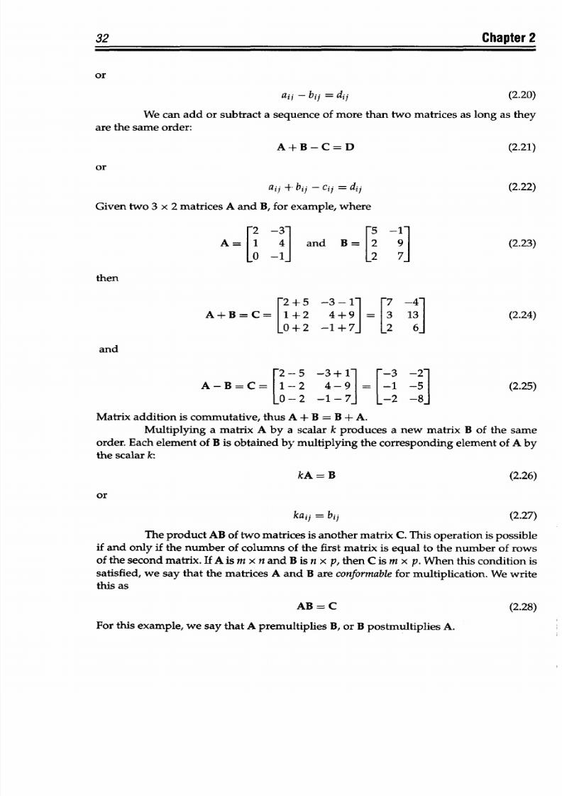
8/9/2019 Mortenson, Michael E. - Mathematics for computer graphics applications.pdf
http://slidepdf.com/reader/full/mortenson-michael-e-mathematics-for-computer-graphics-applicationspdf 45/367
32
Chapter
2
or
aij
-
bij
= dij
(2.20)
We
can
add
or
subtract
a
sequence
of
more
than
two
matrices
as
long
as
they
are the same order:
A
+B-C=D
(2.21)
or
aij + bij
-
cij
=
dij (2.22)
Given
two 3 x 2
matrices A and B,for example,
where
A=
[1
4]
and B=
[
9]
(2.23)
then
-2+ 5 -3-1-
F
-4
A+EB=C=
1+2 4 +
9
= 13
(2.24)
10+2
-1+7
2 6
and
r2 -- 5 -3
+ 1-
~-3
-2-
A-B=C=
1--2 49 =
[-1
-5 (2.25)
0
-- 2 -1
-
7 -2
-8-
Matrix addition
is
commutative,
thus A + B = B + A.
Multiplying a matrix
A by a scalar k produces
a
new
matrix B
of
the same
order.
Each element of B is
obtained by
multiplying
the corresponding
element
of A by
the scalar k:
kA=B
(2.26)
or
kaij
= bij (2.27)
The
product AB
of
two
matrices
is another matrix
C.
This
operation is possible
if
and only
if
the number
of
columns
of
the
first
matrix
is
equal to the number of
rows
of the
second matrix. If A
is m
x
n and B is
n
x
p, then
C is m
x
p. When
this
condition
is
satisfied,
we say that the matrices
A and B are conformable for
multiplication.
We
write
this as
AB = C (2.28)
For
this example,
we say
that
A premultiplies B,
or B postmultiplies A.
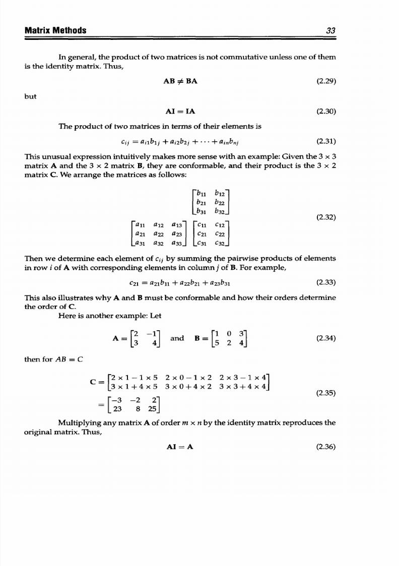
8/9/2019 Mortenson, Michael E. - Mathematics for computer graphics applications.pdf
http://slidepdf.com/reader/full/mortenson-michael-e-mathematics-for-computer-graphics-applicationspdf 46/367
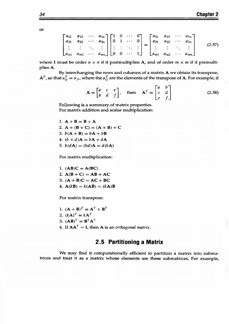
8/9/2019 Mortenson, Michael E. - Mathematics for computer graphics applications.pdf
http://slidepdf.com/reader/full/mortenson-michael-e-mathematics-for-computer-graphics-applicationspdf 47/367
34 Chapter
2
or
Caln
an2
aln- ...-
aa l an
a2l a2
2
... a2,I
0
= 0 a
1 1
a22 ... a2n
aml am
amnL
.
1
am,
am2 amn]
where
I
must be order n
x
n if it
postmultiplies
A,
and
of order
m
x m
if it
premulti-
plies
A.
By interchanging
the
rows and columns of
a matrix
A
we
obtain
its transpose,
A so that
a T
=
a i, where the
aT are the elements
of
the transpose
of
A. For
example, if
A=
]bf then AT =[c d (2.38)
Following
is
a summary
of
matrix p roperties.
For matrix
addition and scalar
multiplication:
1.
A+B=B+A
2.
A+(B+C)=(A+B)+C
3.
b(A+B)=bA+bB
4.
(b
+d)A
= bA+dA
5.
b(dA)
=
(bd)A
=
d(bA)
For matrix
multiplication:
1. (AB)C
= A(BC)
2. A(B
+
C)
=
AB
+
AC
3. (A + B)C = AC +
BC
4.
A(kB) = k(AB) =
(kA)B
For matrix
transpose:
1. (A+B)T=AT+BT
2.
(kA)T
= kAT
3. (AB)T =
BTAT
4. If AAT = I, then A is an
orthogonal
matrix.
2.5
Partitioning
a
Matrix
We
may find
it
computationally
efficient
to partition
a matrix into subma-
trices and treat
it
as
a
matrix whose
elements
are
these submatrices.
For
example,
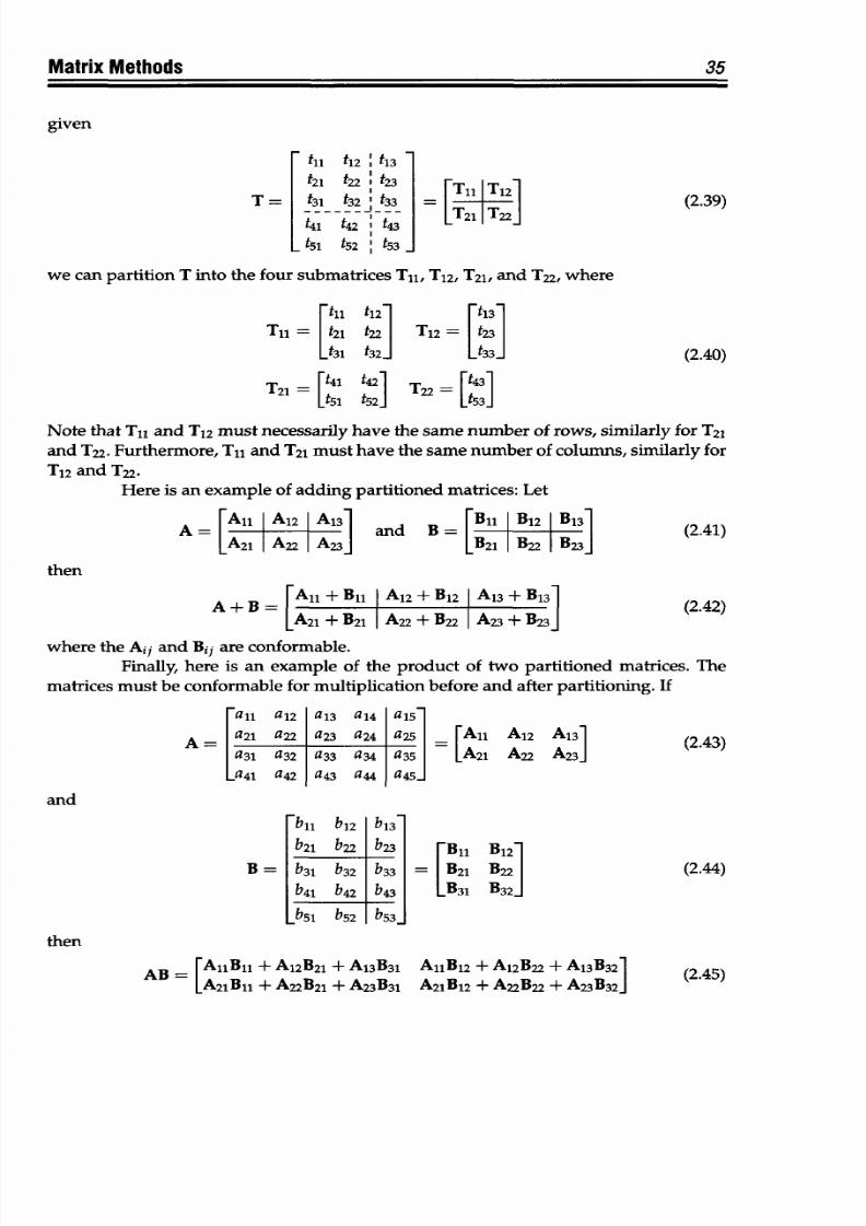
8/9/2019 Mortenson, Michael E. - Mathematics for computer graphics applications.pdf
http://slidepdf.com/reader/full/mortenson-michael-e-mathematics-for-computer-graphics-applicationspdf 48/367
Matrix Methods
35
given
tll t42 tl3
T
= t3 t32 t3
TI
T
12
(2.39)
------ [-T
2 1
IT22
t
5
l t
52
It53
we can partition T into
the four subm atrices
T
1
1,
T
12
, T
21
,
and T22, where
-tll t12
tl3
Til =
t
2
l
t22
T
1 2
=
t
2 3
t
3
l
t
32
J
Lt
33
i
(2.40)
T
= 41 42]
T = [t43]
Note
that
T
11
and
T
12
must
necessarily
have the same
number of rows, similarly
for T
21
and T22.
Furthermore, Tll and T
21
must
have the
same
number of columns, similarly for
T
12
and T22.
Here
is an
example of adding partitioned
matrices:
Let
A
=
[All
A
12
Al
3
l and
B
= [Bil B
12
B
13
1 (2.41)
[A
2 1
A22
A
2
]
LB21 B2
B23(
then
A + B
[All
+
Bl|
A
1
2
+ B
12
A
13
+ B
13
1
(2.42)
[A
2 1
+ B
2 1
A22 +
B22
A
2
3 +B
2 3
where
the Aij and Bij
are conformable.
Finally,
here
is
an
example of
the
product
of
two
partitioned
matrices. The
matrices must be conformable for
multiplication
before and after
partitioning.
If
[all
a
12
a
13
a
14
a
1
5
A
=
a
2
a22
a
23
a
24
a
25
=
All
A
12
A
13
(2143)
a
3
l a
3 2
a
3 3
a34 a
3 5
[A
2 1
A22 A
2 3
]
-a
4
l a42 a
4 3
a44 a
4 5
]
and
bil b
12
b
13
1
b
2
l b22 b
2
3
-Bl
B
12
B = b3l b32 b
3
3
= B
21
B22
(2.44)
b
4
l b42 b43
B
31
B
32
]
bsl
b
52
b
53
-
then
AB [AlBll
+ A
12
B
21
+ A
13
B
3 1
AlB
1
2
+
A1
2
B22 + A
13
B
3 2
1
(2145)
AA
2
Bll
+ A22B
21
+ A
23
B
31
A
21
B
12
+
A2B2 + A
2 3
B
32
J
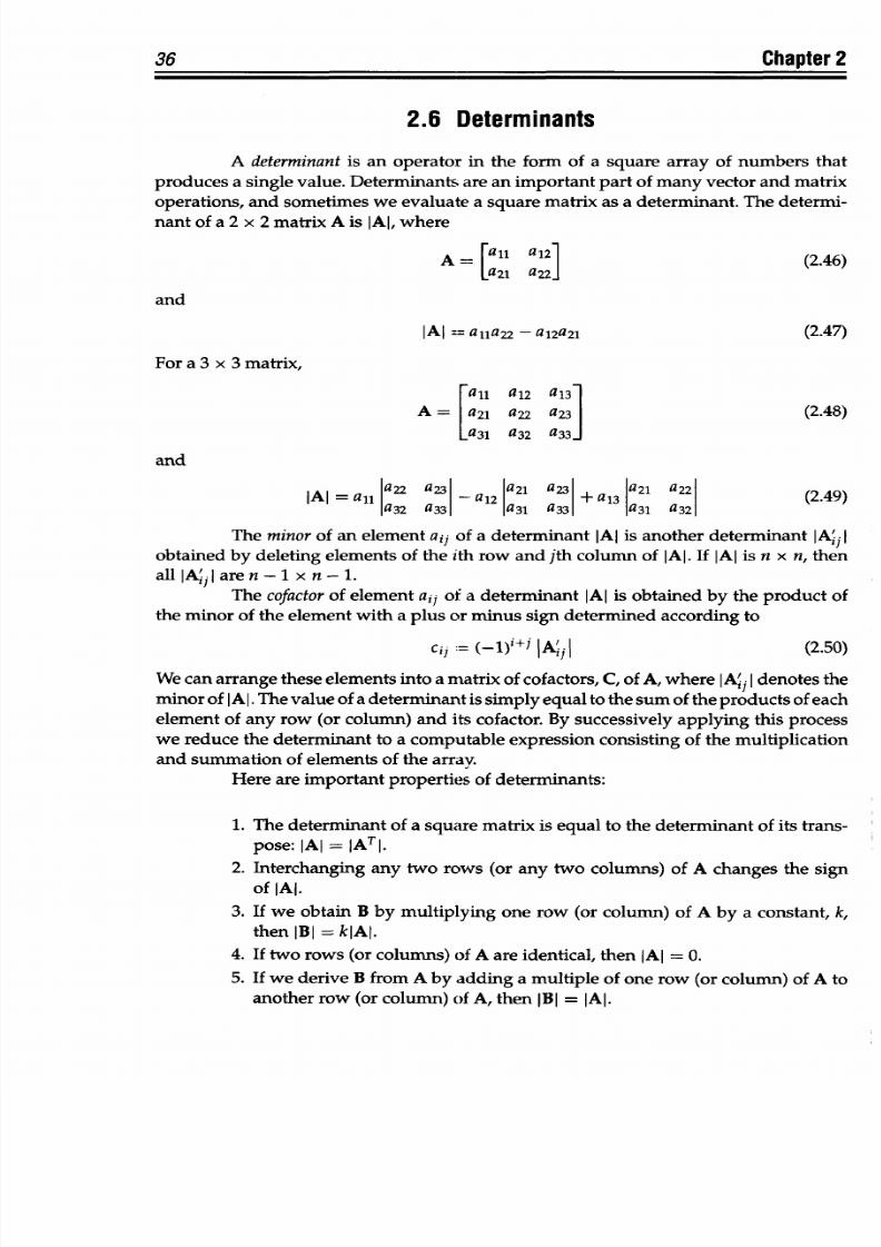
8/9/2019 Mortenson, Michael E. - Mathematics for computer graphics applications.pdf
http://slidepdf.com/reader/full/mortenson-michael-e-mathematics-for-computer-graphics-applicationspdf 49/367
36 Chapter 2
2.6 Determinants
A
determinant is an operator in
the
form of
a
square
array of numbers that
produces
a
single
value.
Determinants
are
an
important
part
of
many
vector
and
matrix
operations, and
sometimes we evaluate
a
square matrix as a
determinant. The determi-
nant of a
2 x
2 matrix
A is
JAI,
where
A= [all a1
2
]
(2.46)
and
JAI
=
a
1
a22 -
al
2
a
2
l
(2.47)
For a 3 x 3 matrix,
Fall a
12
a
13
A =
a
21
a22 a
23
(2.48)
a31 a
3 2
a
3 3
and
JAl =
all
a22
a2 -
a
12
|a2j
a23 +
a
1
3 ja2l a221 (2.49)
a
3
2
a
3 3
a
3
l a
3
3
a
31
a
3 2
The
minor
of an element aij of a
determinant
JAI is
another
determinant
IA'
1
I
obtained
by
deleting elements
of
the ith
row and
jth
column
of
IAl.
If
IAI
is
n
x
n,
then
all
IAJ
Iare n-1 x
n-1.
The
cofactor of
element
aij of
a
determinant
JAI
is
obtained
by
the product of
the minor of
the
element with
a
plus or minus
sign determined according
to
cij:=
(-l)i~j
IA~AI
(2.50)
We can
arrange
these elements
into
a matrix of cofactors,
C,
of
A,
where IA j Idenotes
the
minor
of IAl
. The
value
of
a
determinant
is simply
equal to
the sum of the products of each
element of
any row
(or
column)
and
its
cofactor. By successively applying
this process
we reduce
the determinant to
a computable expression
consisting
of
the multiplication
and summation of elements of
the array.
Here
are
important
properties of determinants:
1. The determinant
of
a square matrix is equal to the determinant of
its
trans-
pose: JAI = IATI.
2. Interchanging
any two rows
(or any two
columns)
of
A changes the sign
of JAI.
3.
If
we obtain B by
multiplying one
row
(or
column) of A by
a
constant,
k,
then
IBI
=
kiAl.
4.
If two rows
(or
columns)
of A
are identical,
then IAI
=
0.
5.
If we
derive
B from
A by adding
a multiple
of one row (or
column) of A
to
another row (or
column)
of A, then
IB =
IAl.
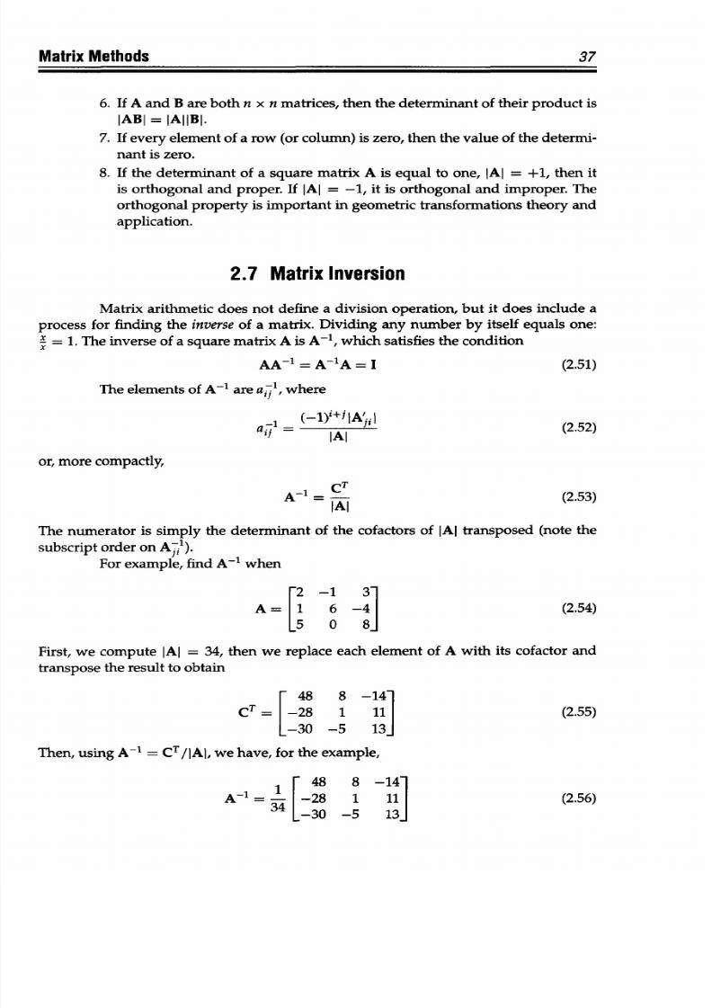
8/9/2019 Mortenson, Michael E. - Mathematics for computer graphics applications.pdf
http://slidepdf.com/reader/full/mortenson-michael-e-mathematics-for-computer-graphics-applicationspdf 50/367
Matrix
Methods
37
6. If A
and B are both n
x
n matrices, then
the
determinant of their product
is
IABI = JAIBI.
7. If every
element of a row (or column)
is
zero, then the value of the determi-
nant
is zero.
8. If the determinant of
a
square matrix A
is
equal to one,
JAI = +1, then it
is
orthogonal
and proper. If JAI = -1, it is
orthogonal
and improper.
The
orthogonal property is important in geometric transformations
theory and
application.
2.7 Matrix Inversion
Matrix arithmetic does not define
a division
operation, but it does include a
process for finding the
inverse
of
a
matrix. Dividing
any
number by itself equals
one:
x = 1. The inverse of
a
square matrix A is
A-', which satisfies
the
condition
AA-
=
A- A
=
I
(2.51)
The
elements of A-l are a
-
,
where
-1
(-1)i+i
iA
1
(2.52)
or, more
compactly,
CT
A-1
-
C
(2.53)
JA l
The
numerator is
simply the
determinant
of the cofactors of
JAI
transposed (note
the
subscript
order on Aj7.).
For example, find A-' when
r2-1 3-
A=[1
6
_4
(2.54)
50 8_
First, we compute JAI = 34,
then
we replace each element of A with its cofactor and
transpose the result to obtain
[48 8
-141
CT= -28 1
11 (2.55)
-30 -5 13 -
Then,
using A-
=
CT/IAl,
we have, for the example,
-
48
8 -14-
A- = -28 1
11
(2.56)
34
-30
-5
131
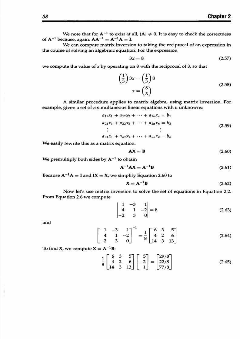
8/9/2019 Mortenson, Michael E. - Mathematics for computer graphics applications.pdf
http://slidepdf.com/reader/full/mortenson-michael-e-mathematics-for-computer-graphics-applicationspdf 51/367
38
Chapter 2
We note
that
for
A-'
to exist
at
all,
JAl 0. It is easy to
check
the correctness
of A-' because,
again. AA-' = A- A = I.
We
can compare
matrix inversion to
taking the
reciprocal of an expression
in
the
course
of
solving
an
algebraic
equation.
For
the
expression
3x =
8
(2.57)
we compute
the value of x
by
operating on 8
with the reciprocal of
3, so
that
() 3x = (3)8 (2.58)
A
similar
procedure applies
to
matrix
algebra,
using matrix
inversion.
For
example,
given a set of n simultaneous
linear equations
with
n unknowns:
alix
1
+
a
12
x
2
+
. . +
alnXn
=
bi
a
2
1
x1 +
a2:x
2
+ .
+ a2nxn
=
b2
(2.59)
anIx
1
+
anf2X2
+ +
annxn
=
bn
We
easily
rewrite this as a
matrix
equation:
AX
=B
(2.60)
We premultiply
both
sides
by A-'
to obtain
A--AX = A-1B (2.61)
Because A-1A
=
I
and IX
=
X,
we simplify
Equation 2.60 to
X=
A-1B
(2.62)
Now let's use matrix
inversion to
solve
the
set of equations in Equation 2.2.
From Equation
2.6
we compute
1 -3 1
4
1 -2
= 8
(2.63)
-2 3
0
and
r1 -3
1- -l1 -6
3
5l
4 1 -
4
2 6
(2.64)
L-2
3
0
8 14 3 132
To find X, we
compute
X =A B
1
26
5
[1]
[2 .86
-
4
2
6
_2
= 28
(2.65)
8 -14
3
13 1 -78-
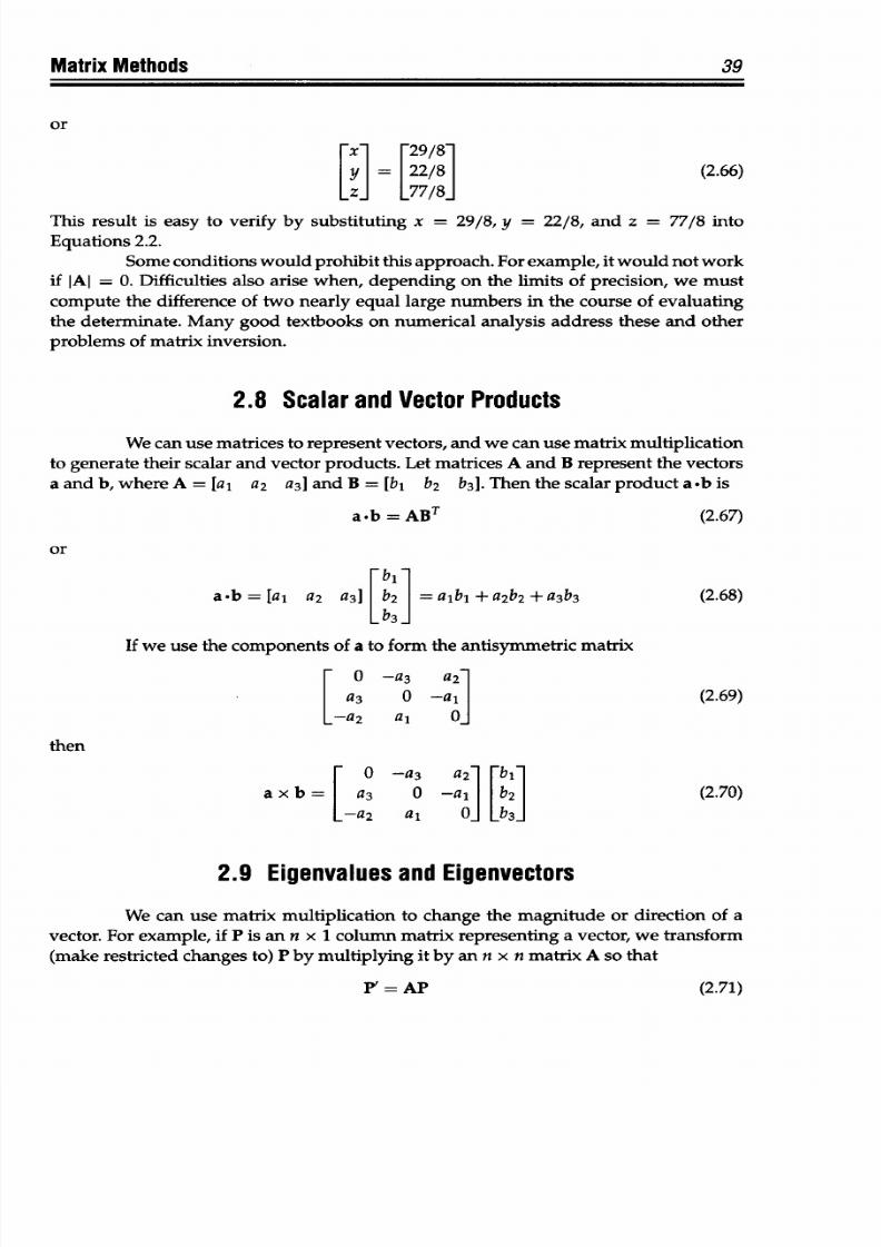
8/9/2019 Mortenson, Michael E. - Mathematics for computer graphics applications.pdf
http://slidepdf.com/reader/full/mortenson-michael-e-mathematics-for-computer-graphics-applicationspdf 52/367
Matrix Methods
39
or
Y = 8 (2.66)
-Z-
778_
This
result is easy to verify by substituting x = 29/8, y
= 22/8, and z = 77/8
into
Equations 2.2.
Some
conditions
would prohibit
this
approach. For
example, it
would
not
work
if JAI
=
0. Difficulties also arise when,
depending
on
the limits of precision, we
must
compute the difference
of
two
nearly
equal
large numbers
in the course of evaluating
the determinate. Many good textbooks on numerical analysis address these and other
problems
of
matrix
inversion.
2.8 Scalar and Vector Products
We can use matrices to represent vectors,
and
we can use matrix m ultiplication
to generate their scalar and vector products. Let matrices A and B represent
the
vectors
a
and
b,
where
A
= [al
a
2
a
3
]
and
B
= [b
b
2
b
3
]. Then the scalar
product a.b
is
a.b =
ABT
(2.67)
or
[bil
a.b=[al
a
2
a
3
] [b
2
= alb
+
a
2
b
2
+a
3
b
3
(2.68)
b3
If we use
the
components
of a
to form the
antisymmetric matrix
[0 -a
3
a
2
-
a3 0 -a]
(2.69)
--
a2
a, °-
then
F 0 -a
3
a
2
lb1l
a x b = a
3
0 -a,
2
(2.70)
-a2 a, ° b
3
]
2.9
Eigenvalues and Elgenvectors
We can use matrix multiplication to change the
magnitude
or direction
of
a
vector.
For example,
if
P
is
an
n
x
1 column matrix representing
a vector,
we transform
(make restricted changes
to)
P by multiplying it by an n x n matrix A
so
that
P'
= AP (2.71)
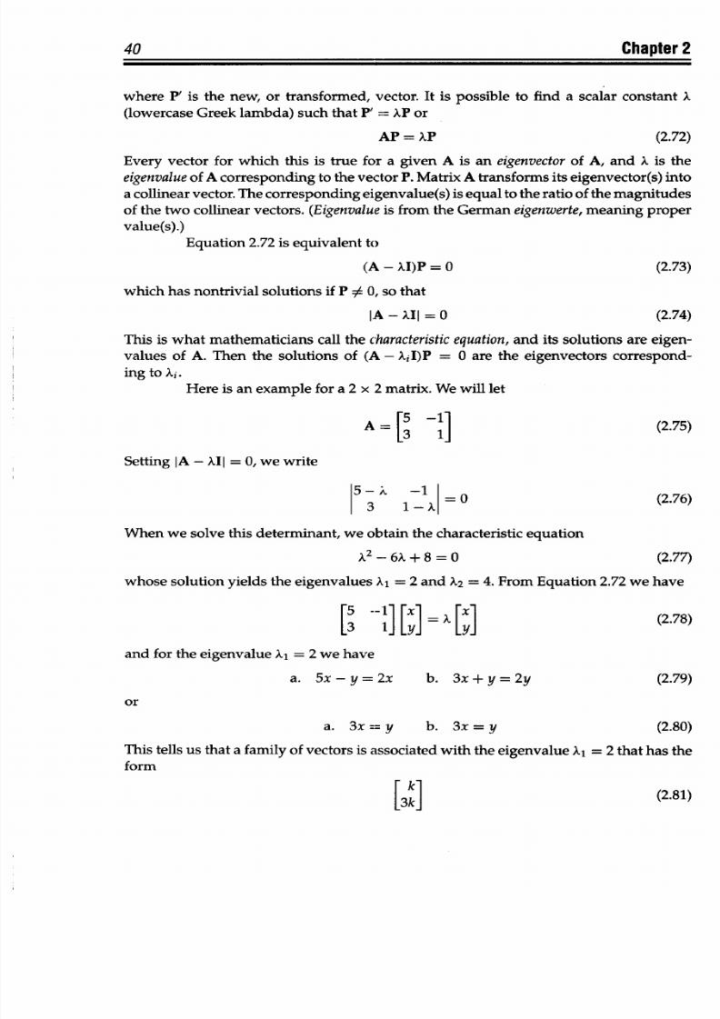
8/9/2019 Mortenson, Michael E. - Mathematics for computer graphics applications.pdf
http://slidepdf.com/reader/full/mortenson-michael-e-mathematics-for-computer-graphics-applicationspdf 53/367
8/9/2019 Mortenson, Michael E. - Mathematics for computer graphics applications.pdf
http://slidepdf.com/reader/full/mortenson-michael-e-mathematics-for-computer-graphics-applicationspdf 54/367
Matrix Methods 41
where
k :A 0. In other
words, any
vector
whose y component
is exactly three times as
great as its
x component
is an
eigenvector of A. For the
other
eigenvalue, A
2
= 4,
we
have
a.
5x-y=4x
b.
3x+y=4y
(2.82)
or
a. x=y
b.
x=y (2.83)
So that A
2
has
eigenvectors of
the
form
[k] (2.84)
In this
example,
any vector
whose
x
and
y components
are equal is an eigenvector of A.
For the general case of
a
2
x
2
matrix, if
A =[a b] (2.85)
then we compute the eigenvalues
from
a
- X
b i
(2.86)
or
X
2
_ (a +
d)x
+ (ad - bc)
=0
(2.87)
There are,
of
course, two roots to
Equation
2.87,
two
eigenvalues.
These may
be
real
and distinct,
equal or
complex.
Using the
eigenvalues
we can compute
values of
the corresponding
eigenvectors. By
doing
this
we
find two possible
forms for the ratio
of the vector components, depending on the value
of A;
thus,
Px b
d-A
-= - or -
-
(2.88)
Py
a Xi
c
where i
=
1, 2.
We
can
generalize this
process to
apply
to
n
x
n matrices,
but
this
is
beyond the scope of this book.
2.10 Similarity Transformation
If a matrix A is premultiplied and postmultiplied
by
another
matrix
and
its
inverse, respectively,
then the resulting matrix B is
a similarity transformationof A;
thus,
B =
TAT-
1
(2.89)
and A and B are similar matrices. Similar matrices have equal
determinants,
the same
characteristic equation, and
the
same eigenvalues,
although
not
necessarily
the same
eigenvectors. Similarity
transformations
preserve eigenvalues.
8/9/2019 Mortenson, Michael E. - Mathematics for computer graphics applications.pdf
http://slidepdf.com/reader/full/mortenson-michael-e-mathematics-for-computer-graphics-applicationspdf 55/367
42
Chapter 2
If A is similar to a
diagonal matrix D then
Al0
.. 0
0
X2 ...
°
D
= .
. .
(2.90)
where X
1
,
A2.
. ., Xn are
the
eigenvalues of A. However,
for this
to
be
true, there must
be
a
nonsingular
matrix
S
such
that SAS-' = D. Obviously,
the elements on the
main
diagonal of
a
diagonal
matrix D
are
its eigenvalues. Therefore,
the eigenvalues
of D are
the
eigenvalues of A. Finally,
if
the
eigenvalues of
A are distinct,
then
it
is
similar
to a
diagonal
matrix.
2.11
Symmetric
Transformations
As
we
have already
seen, by definition
a
real symmetric matrix satisfies
the
condition
aij = a
ji,
or
AT
=
A.
If A and
B are
symmetric
so that
[ABIT
=
BTAT =
BA ,
then
the
product
of two symmetric
matrices is symmetric
if
and only if
the two
matrices
commute.
The eigenvalues
of a real symmetric
matrix
are real.
If
A
is a
real
symmetric
matrix, then
there
is
an orthogonal
matrix
R(RRT)
=
IR such that R-'AR is a
diagonal
matrix.
Furthermore,
if
A
is a
real
symmetric m atrix,
then
the
eigenvectors
of
A associated
with
the distinct
eigenvalues
are mutually
orthogonal vectors.
2.12 Diagonalization of
a Matrix
As we
have
seen previously,
we associate
an
eigenvector
Pi
with each eigen-
value
Xi,
which we write
as
APi
=
XiPi (2.91)
Now
we can
readily
construct
a square
matrix
E of
order
n whose
columns are
the
eigenvectors
Pi of A,
and we
rewrite Equation 2.91:
AE =
EA (2.92)
where A
is a
diagonal
matrix
whose
elements
are
the
eigenvalues of A:
=1 0
(2. 93
O X2 ... °
A
=
. ..
.(2.93)
: : .. :n
8/9/2019 Mortenson, Michael E. - Mathematics for computer graphics applications.pdf
http://slidepdf.com/reader/full/mortenson-michael-e-mathematics-for-computer-graphics-applicationspdf 56/367
Matrix Methods
43
If
the eigenvalues
in
Equation
2.93
are distinct, then the
matrix
E
is nonsingular,
and
we
can premultiply
both sides of the
equation by E-l to yield
E- AE
= A
(2.94)
We see that
by
using
the matrix of
eigenvectors
and its inverse we can
transform any
matrix
A
with distinct eigenvalues
into
a
diagonal
matrix
whose elements are
the eigen-
values
of A. Mathematicians call
this process the diagonalization
of the matrix A.
Exercises
2.1 GivenA=
5
and
B =[
find
a. A+B
b.
A-B
~7 4 4
- 5~
2.2 GivenA=
9 1 3 and B 1 find
02
5
-
9-
a. a
23
b. al2
c. a
3
l
d. b
1
l
e.
b32
f. What
is
the order of
A?
g. What is
the order of
B?
h.
Which
matrix,
if
any, is a
square matrix?
i.
List
the elements, in
order,
on
the
main
diagonal of A.
j.
Change a
12
, a
13
, and a
23
so that A is
a
symmetric matrix.
2.3 Find the values
of the following Sj:
a. 83,2
d. 87,10
b. 81,4
e. ii
c. 83,3
~54 9-
2.4 GivenA= 1
0
-67 1
a.
Change
a
1
2
,
a
1
3
,
and
a
23
so
that
A
becomes
antisymmetric.
b. What other changes, if any, are
necessary?
2.5 Write
out the 2 x
2
null matrix.
8/9/2019 Mortenson, Michael E. - Mathematics for computer graphics applications.pdf
http://slidepdf.com/reader/full/mortenson-michael-e-mathematics-for-computer-graphics-applicationspdf 57/367
44
2.6
GivenA
=
1 0]
1
B
[4]
andC [1 -2 4 6], find
a. a
23
b. a
3
2
c.
b3
d.
C
14
e. What is the
order of A?
f. What
is
the order of B?
g.
What is the
order
of C?
h. Which
is
the
column matrix?
i. Which
is the
row
matrix?
j. Which
is the
identity
matrix?
2.7
Given A
= [3 7
-2], find -A.
2.8 Given
A = [
a. A+2A
b. B + B
c. 2A+B
5
2]=
6
1 3
4andC=1
-1
4 ,B=0
9
2]
anC5
8
31,in
d.A-B+C
e.
A-2B-C
2.9 Given
A =
[3 0] find
1.5A.
2.10 Find IT.
2 e
3 8[-
6 7]
2.11
Given
A
=
-
1
4
7 and
B
=
10
9
find
AB.
0 1
1
2 _3-
2.12 Given
A = [2
and
B= [6]
find
AB.
2.13 Given A =
[4 1 7],
find AT.
2.14
Given A=
1
0]
and
B=
[5
find
[6
7 2 4]
a. (AT)T
c. AT +
BT
b.(A+B)T d.
BT+AT
2x
ay
2.15 Find the product [t2
t 1]
bx by I
cx
CY
Chapter 2
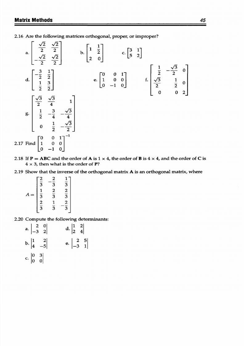
8/9/2019 Mortenson, Michael E. - Mathematics for computer graphics applications.pdf
http://slidepdf.com/reader/full/mortenson-michael-e-mathematics-for-computer-graphics-applicationspdf 58/367
Matrix
Methods
2.16
Are the following
matrices
orthogonal, proper,
or improper?
a.
[4
2]
2b.
2
[5 2]
[ 3 1
d.
2
2
1 3
L 2 2J
g.
1
2
4
1
3
2
4
1
0
2-
0 1 - -2
e.
1 0
0 f1 X
1
0
La
-1 0
2
2
L0
0 2j
-O
0 1-
-1
2.17
Find 1 0 0
0 -1
0
2.18 If P
=
ABC and
the order
of A is 1 x 4, the order of
B is 4
x 4,
and
the order
of C
is
4 x 3, then what
is the order
of
P?
2.19 Show
that
the
inverse
of
the
orthogonal matrix
A is an orthogonal
matrix, where
1
2
2
3
2
1
l1
2
3
3
2.20
Compute
the
following
determinants:
a.
3
°I
d.
1
2
1 2 254
b.
1 _ e.
3
1_
b4 -5
3
03
45
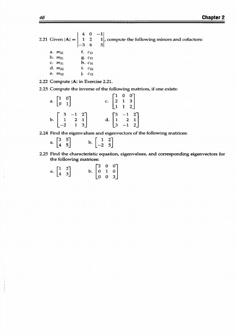
8/9/2019 Mortenson, Michael E. - Mathematics for computer graphics applications.pdf
http://slidepdf.com/reader/full/mortenson-michael-e-mathematics-for-computer-graphics-applicationspdf 59/367
46
Chapter 2
4
0
-1
2.21
Given Al =
1 2 1 , compute
the following
minors and cofactors:
-3
6
5
a.
m
11
f.
c
11
b.
M
2
1
g.
C2
1
C.
M
3
1
h.
c
31
d.
m22
i. c
22
e. M
12
j. c
12
2.22
Compute JAI
in
Exercise
2.21.
2.23
Compute
the inverse
of the following
matrices,
if
one
exists:
a.
[1
1]
C.
° °]
3
-1
2-
-3-1
2-
b.
1
2 1
d.
1 2 1
_2
1
3
3 -1 2-
2.24
Find
the eigenvalues
and
eigenvectors
of
the following matrices:
a. [3
5]
b [
1
2]
2.25
Find
the
characteristic
equation,
eigenvalues,
and
corresponding
eigenvectors
for
the following
matrices:
[1
2][
0
O-
.[4
31
b. 010
L0
3_
8/9/2019 Mortenson, Michael E. - Mathematics for computer graphics applications.pdf
http://slidepdf.com/reader/full/mortenson-michael-e-mathematics-for-computer-graphics-applicationspdf 60/367
(AuKA
TRANSFORMATIONS
The geometers of antiquity
took two
different paths
toward
understanding
the shapes
of
objects
and
the
figures
they
drew
to
represent
them. One
path
led them to
study
prop-
erties that they
could
measure,
such
as angles, distance,
area,
and volume.
The
other
led them to
study logical
relationships among
shapes,
such
as
equivalence,
similarity,
and constructability. Both paths
led
them
to the conclusion
that certain
geometric prop-
erties of an object do not
change
when the object
is translated or
rotated,
expanded
or
twisted.
Geometers discovered
that
different
kinds
of changes,
transformations,
left dif-
ferent properties unchanged, or invariant,
and
this led them
to
identify different kinds
of
geometry.
This
chapter explores
geometric transformations
and their
invariant properties.
It introduces systems
of
equations that produce linear transformations
and
develops the
algebra and geometry of translations, rotations,
reflection,
and
scaling,
including how
to combine them. Vectors
and
matrices
are put
to good use
here,
in ways
that clearly
demonstrate
their
effectiveness.
3.1
The Geometries of Transformations
Here
we will
discover what geometric properties are preserved
when
we im-
pose transformations on
figures. Each
transformation
changes
some
properties and
leaves others
unchanged;
for example, angles may
be
preserved but not distance.
Congruentgeometry applies only to figures of identical size and shape. We
can
translate and
rotate
a figure
without
changing
its congruent
properties.
Conformal ge-
ometry
applies to similar
figures,
those whose
size
is
different
but whose corresponding
angles
are equal.
Euclidean geometry studies the properties
of both
congruent and
sim-
ilar
figures.
Affine
geometry allows
transformations
where distances
only
are preserved
be-
tween points
on the
same or parallel
lines,
and angles are not preserved at all. Parallelism
is
an
important
invariant
of
this
geometry.
Projective geometry
allows transformations where parallel lines are
not
pre-
served, but straight
lines remain
straight. A projective
transformation transforms circles,
ellipses,
hyperbolas,
and
parabolas into
one another.
47
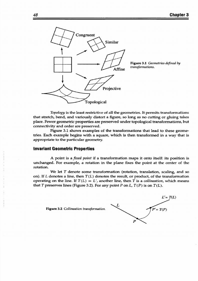
8/9/2019 Mortenson, Michael E. - Mathematics for computer graphics applications.pdf
http://slidepdf.com/reader/full/mortenson-michael-e-mathematics-for-computer-graphics-applicationspdf 61/367
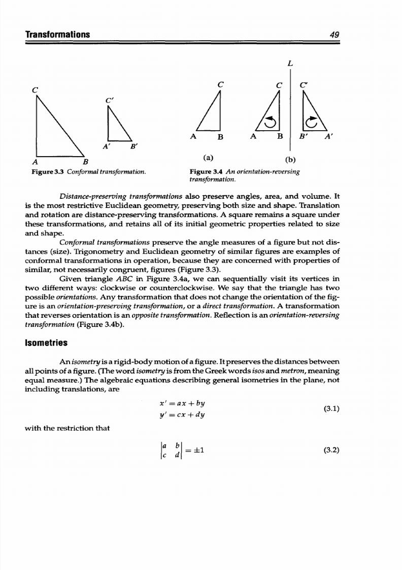
8/9/2019 Mortenson, Michael E. - Mathematics for computer graphics applications.pdf
http://slidepdf.com/reader/full/mortenson-michael-e-mathematics-for-computer-graphics-applicationspdf 62/367
Transformations
L
C
C
C
A
A
CAAB
A
B
A B
\
A'B'
49
C'
B' A'
A
B
ka)
(b)
Figure
3.3
Conformal
transformation.
Figure
3.4
An
orientation-reversing
transformation.
Distance-preserving
transformationsalso
preserve
angles,
area, and volume.
It
is the most restrictive
Euclidean
geometry, preserving
both
size
and
shape. Translation
and
rotation
are distance-preserving
transformations.
A square
remains a square under
these
transformations,
and retains all
of
its
initial geometric properties
related
to size
and
shape.
Conformal
transformations preserve the angle
measures
of a figure
but
not dis-
tances (size).
Trigonometry
and
Euclidean
geometry
of
similar
figures
are examples
of
conformal
transformations
in operation, because
they are
concerned with properties of
similar, not
necessarily congruent,
figures (Figure 3.3).
Given triangle
ABC
in Figure 3.4a,
we
can
sequentially
visit
its vertices
in
two
different
ways:
clockwise
or counterclockwise.
We say
that
the
triangle has
two
possible
orientations.
Any
transformation
that does not change the orientation
of the
fig-
ure is an
orientation-preserving
ransformation,
or a direct
transformation.
A
transformation
that reverses
orientation is
an
opposite
transformation.
Reflection
is
an
orientation-reversing
transformation
Figure
3.4b).
Isometries
An
isometry is a rigid-body
motion of
a figure. It
preserves
the
distances
between
all
points
of
a
figure. (The
word isometry
is from
the
Greek
words isos
and
metron,
meaning
equal
measure.)
The
algebraic
equations describing
general isometrics in the
plane, not
including
translations,
are
x'=
ax
+
by
(3.1)
y'=cx+dy
with
the restriction
that
ac d
(3.2)
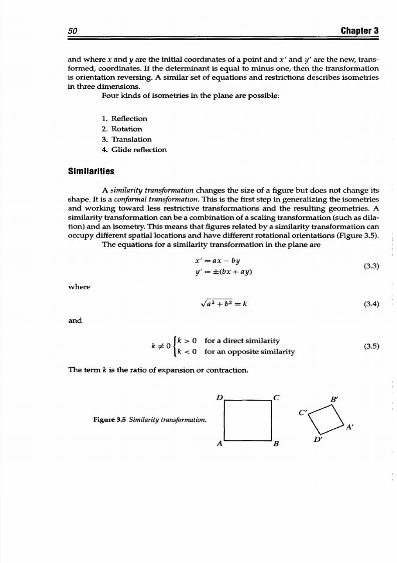
8/9/2019 Mortenson, Michael E. - Mathematics for computer graphics applications.pdf
http://slidepdf.com/reader/full/mortenson-michael-e-mathematics-for-computer-graphics-applicationspdf 63/367
50
Chapter 3
and where x
and
y are
the initial coordinates
of
a
point and x' and y'
are
the
new, trans-
formed, coordinates.
If the
determinant
is
equal
to
minus one,
then the transformation
is
orientation reversing.
A similar
set of
equations
and
restrictions describes isometrics
in three dimensions.
Four kinds of
isometrics in the
plane
are possible:
1.
Reflection
2.
Rotation
3. Translation
4.
Glide
reflection
Similarities
A similarity
ransformation
changes the
size of a figure
but does
not
change its
shape.
It is a conformal transformation.
This
is
the first
step in generalizing
the
isometrics
and working
toward
less
restrictive
transformations
and
the resulting
geometries.
A
similarity transformation
can be
a
combination
of a
scaling
transformation
(such
as
dila-
tion)
and an isometry.
This
means
that figures
related
by a similarity
transformation can
occupy different
spatial
locations and
have different
rotational orientations
(Figure
3.5).
The equations
for
a
similarity
transformation in
the
plane are
x'= ax -
by
y'=
(bx
+
ay)
where
.Va
2
+
b
2
= k
(3.4)
and
J
k
>
0
for
a
direct similarity
k
7#
0 k < 0
for an opposite
similarity
The
term
k is the
ratio
of expansion or contraction.
D
C B'
C
'
Figure 3.5 Similarity
transformation.
A'
A
B
D'
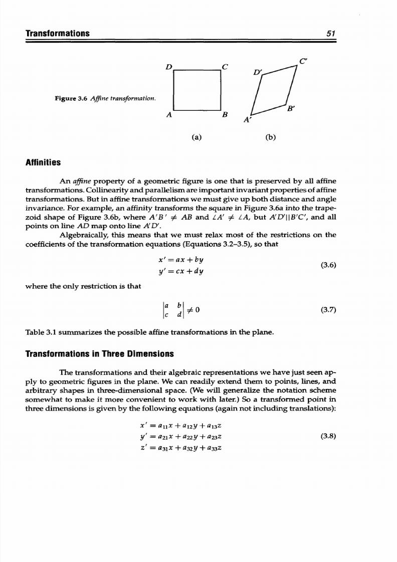
8/9/2019 Mortenson, Michael E. - Mathematics for computer graphics applications.pdf
http://slidepdf.com/reader/full/mortenson-michael-e-mathematics-for-computer-graphics-applicationspdf 64/367
Transformations 51
C,
D
C
Figure
3.6
Affine
transformation.
-A
(a) (b)
Affinities
An affine property
of
a geometric figure is one that
is
preserved by all affine
transformations. Collinearity and parallelism
are
important
invariant properties
of
affine
transformations.
But in affine transformations
we must give up both distance and
angle
invariance. For
example,
an
affinity transforms the square
in Figure 3.6a into
the trape-
zoid shape
of
Figure
3.6b, where
A'B' AB and ZA' 0 ZA, but A'D'IIB'C', and all
points
on line
AD map onto
line A'D'.
Algebraically, this means that
we must
relax
most
of the restrictions
on
the
coefficients
of
the transformation equations
(Equations
3.2-3.5),
so
that
x'=
ax +
by
(3.6)
y'=cx+dy
where the only
restriction
is that
C
d|A
0
(3.7)
Table 3.1
summarizes
the
possible
affine
transformations
in
the
plane.
Transformations
in
Three
Dimensions
The
transformations
and
their
algebraic
representations
we have just
seen ap-
ply
to geometric
figures
in the plane. We
can
readily extend them
to
points,
lines,
and
arbitrary
shapes in three-dimensional space. (We will generalize the notation
scheme
somewhat
to make it more convenient
to work with later.)
So
a
transformed
point in
three
dimensions is given
by
the
following equations (again not
including
translations):
x'
=
alix+ a
12
y + a
1
3
Z
y'
= a
2
lx + a22y + a23z
(3.8)
z' =
a
3 1
x
+ a32y + a33z
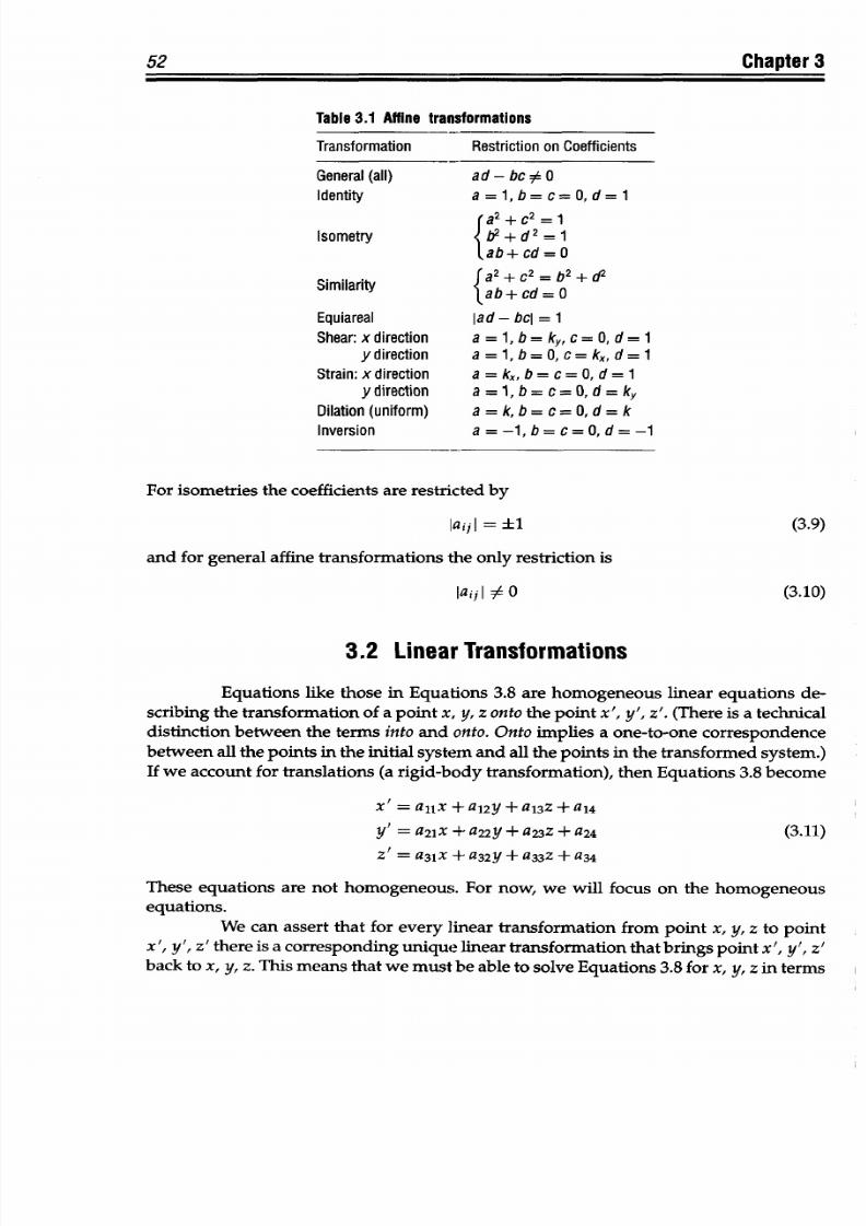
8/9/2019 Mortenson, Michael E. - Mathematics for computer graphics applications.pdf
http://slidepdf.com/reader/full/mortenson-michael-e-mathematics-for-computer-graphics-applicationspdf 65/367
52
Chapter
3
Table
3.1
Affine transformations
Transformation
Restriction
on
Coefficients
General
(all) ad
-
bc
$
0
Identity
a
=
1,b
=
c
=0,
d = 1
a
2
+C
2
=1
Isometry
b
2
+ d
2
= 1
ab + cd =
0
S aa
+
C
2
b
2
+
d
2
Similarity
ab+
cd= 0
Equiareal
lad - bcl =
1
Shear: x
direction a = 1,b= ky,
c= 0, d= 1
ydirection a=1,b=0,c=k,,d=1
Strain:
xdirection
a
=
kx,
b=
c=
0, d=
1
ydirection
a=1,b=c=0,d=ky
Dilation
(uniform) a
= k,
b = c
= 0,d
= k
Inversion a = -1, b=
c=
0,d = -1
For
isometrics the coefficients are restricted by
laii
= ±1 (3.9)
and
for
general
affine
transformations
the only restriction
is
laij I
#
0
(3.10)
3.2
Linear
Transformations
Equations
like those
in Equations 3.8
are
homogeneous
linear
equations
de-
scribing the
transformation of a
point
x, y, z onto
the
point
x',
y',
z'.
(There
is
a technical
distinction
between
the
terms
into
and
onto.
Onto implies
a
one-to-one
correspondence
between
all
the points
in
the initial system and
all the points in the
transformed system.)
If we account for
translations (a rigid-body
transformation), then
Equations
3.8 become
x' = alix +
al2y
+
a
13
z + a
14
yl
= a
2 1
x
+ a22y + a
2 3
z + a
24
(3.11)
z'
=
a
31
x
+
a32y
+
a
33
Z + a34
These
equations
are not
homogeneous.
For
now,
we
will focus
on
the
homogeneous
equations.
We
can
assert
that
for
every linear
transformation
from
point
x,
y,
z
to
point
x',
y', z'
there
is a
corresponding unique linear
transformation that
brings
point x', y',
z'
back
to x,
y,
z. This
means
that we
must
be
able
to
solve
Equations 3.8 for x, y,
z in terms
8/9/2019 Mortenson, Michael E. - Mathematics for computer graphics applications.pdf
http://slidepdf.com/reader/full/mortenson-michael-e-mathematics-for-computer-graphics-applicationspdf 66/367
Transformations 53
of x', y', z';
that
is,
x = aflx'
+ a1
2
y'
+
a/
3
Z'
y
=
alx'
+
a22y'
+
a2
3
z
(3.12)
z = a3lx'
+ a
3 2
y + a33Z
For
this set
of
equations to have a unique solution, the determinant
of
the coefficients
must not equal
zero:
all
at
2
at
3
a2l a' a23 :
O
(3.13)
a3
1
a3
2
a
33
In the
plane, Equations 3.12
become
x
= al
1
x' +
al
2 Y
(3.14)
y=a;
1
x'+aly (314
y= a21
+
22Y
Affine Transformation of
a
Line
The equation of a line in the plane is
Ax+By+C=O (3.15)
Let's
see
how
an
affine
transformation
affects the form
of
this equation, and therefore
the line
itself.
Substituting from Equations
3.14
we
find that
A(a' x' +
aj
2
y') +
B
(alx'
+
a'
2
y')
+ C = 0
(3.16)
or
(Aa'
1
+ Ba
1
,)
x'
+
(Aa1
2
+
Ba'
)
y'
+ C =
0
(3.17)
To
simplify
things somewhat, we
make the
following substitutions:
A' = (Aa'
1
+ Ba
1
j)
B' = (Aa'
2
+ Ba')
(3.18)
C'
=
C
Then
Equation
3.17
becomes
A'x'
+
B'y'
+
C'
=
0
(3.19)
This has the
same form
as Equation 3.15, and we
conclude
that straight lines transform
into straight lines under affine
transformations.
8/9/2019 Mortenson, Michael E. - Mathematics for computer graphics applications.pdf
http://slidepdf.com/reader/full/mortenson-michael-e-mathematics-for-computer-graphics-applicationspdf 67/367
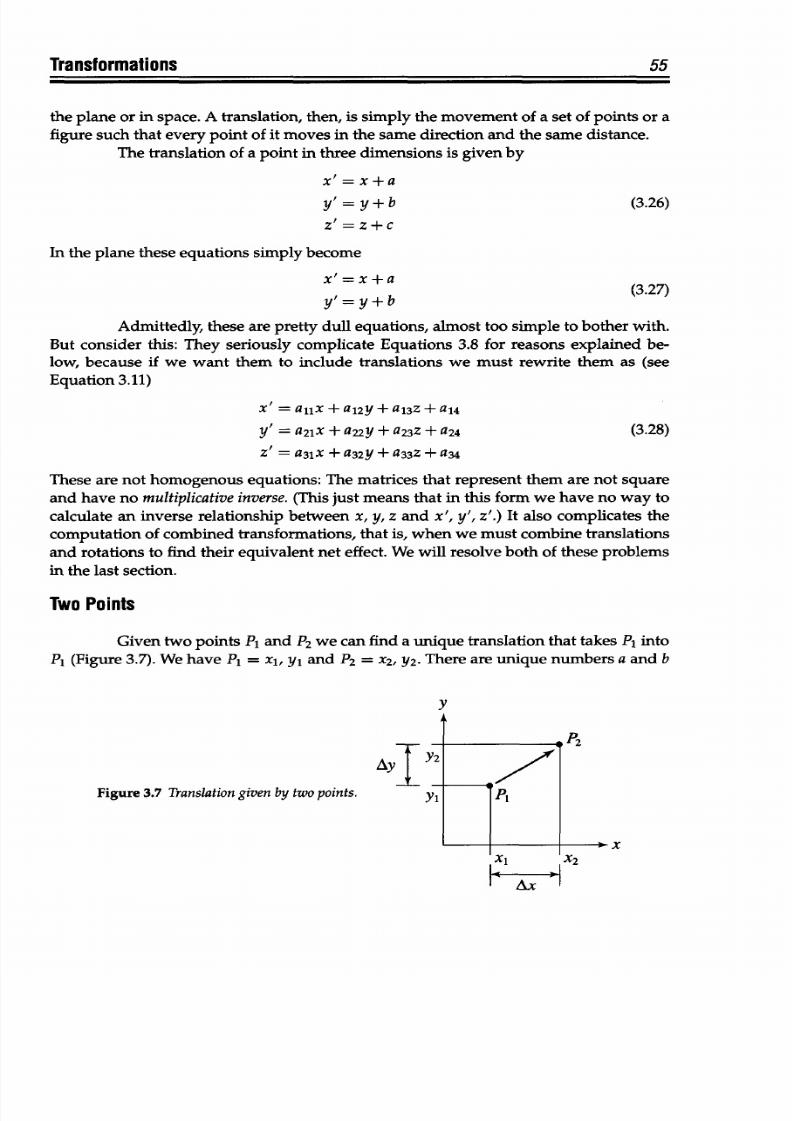
8/9/2019 Mortenson, Michael E. - Mathematics for computer graphics applications.pdf
http://slidepdf.com/reader/full/mortenson-michael-e-mathematics-for-computer-graphics-applicationspdf 68/367
Transformations
55
the plane
or
in space. A
translation, then, is simply the movement
of
a
set of
points
or a
figure such that
every
point of it moves in the same
direction
and the
same
distance.
The translation of a point
in three
dimensions
is given by
x' =
x
+ a
(3.26)
= y+b
Z' =
Z+ c
In
the plane
these
equations
simply become
x'=
x
+ a
y' = y + b
Adm ittedly, these
are pretty dull
equations,
almost too simple to
bother
with.
But consider
this:
They
seriously
complicate
Equations
3.8 for reasons
explained be-
low,
because if we
want
them
to include
translations
we
must
rewrite
them
as (see
Equation 3.11)
x' = alix
+ a12y + a
13
z +
a
14
y' = a
21
x + a22y + a
2 3
z + a
24
(3.28)
z = a
3 1
X
+
a32y + a
3 3
Z + a34
These
are not
homogenous
equations: The matrices that
represent them
are
not square
and
have no multiplicative inverse. (This just means
that
in
this form
we have no way to
calculate
an
inverse relationship between x, y, z and x', y', z'.) It also complicates the
computation
of
combined transformations,
that
is, when we must
combine
translations
and
rotations to
find
their equivalent
net effect. We will resolve
both
of these problems
in the
last
section.
Two Points
Given two points Pi and P
2
we can find a unique
translation
that takes
PI
into
PI
(Figure 3.7). We
have
Pi = xi, yi and P
2
= x
2
,
Y2.
There
are unique numbers a and b
y
Figure 3.7
Translation
given by two
points.
AYIE ½
y1-
' 2
1
x
IAx
1
(3.27)
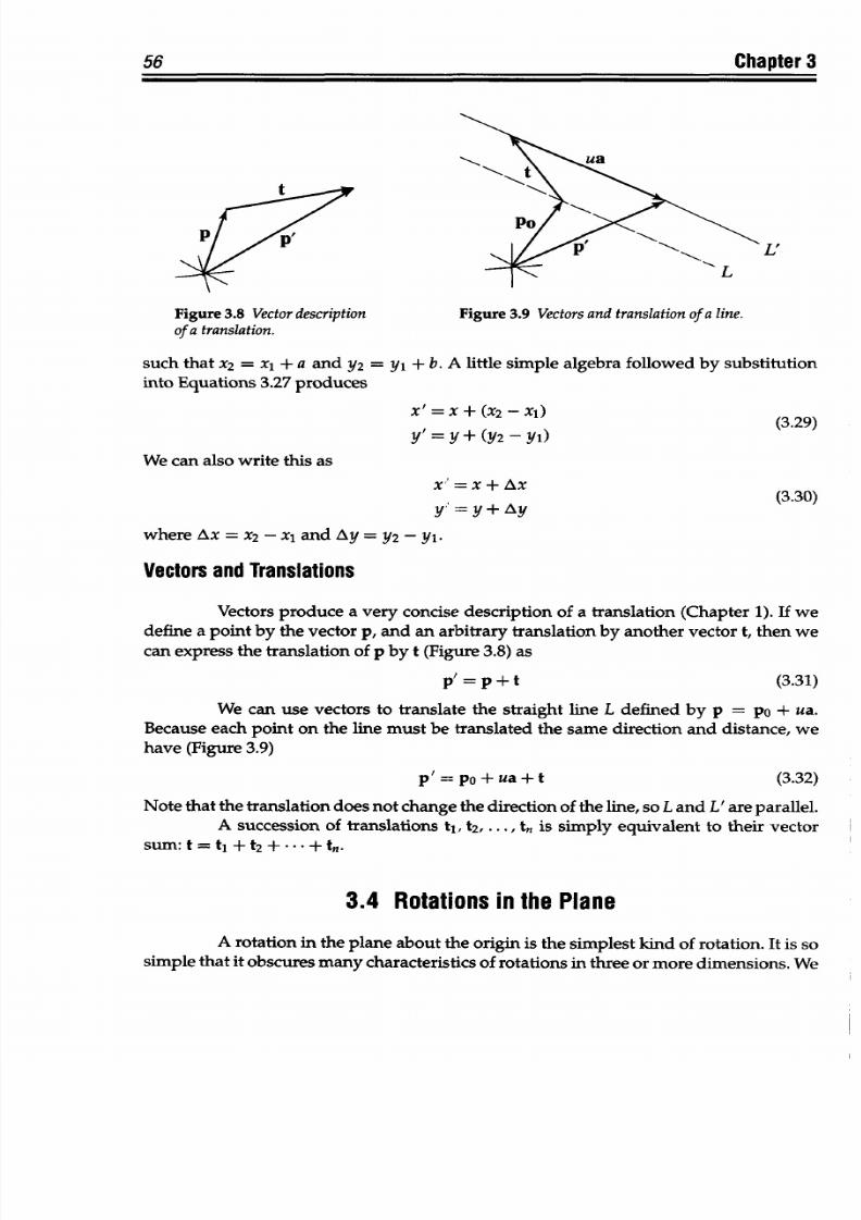
8/9/2019 Mortenson, Michael E. - Mathematics for computer graphics applications.pdf
http://slidepdf.com/reader/full/mortenson-michael-e-mathematics-for-computer-graphics-applicationspdf 69/367
56
Chapter
3
L'
Figure 3.8
Vector description
Figure 3.9
Vectors and translation
of a
line.
of
a translation.
such
that
x
2
=
xl
+
a
and
Y2
=
yi
+
b.
A
little
simple algebra followed
by
substitution
into Equations
3.27 produces
x'=x+(x2-xl)
(3.29)
y'
=y+(y2-yl )
(.9
We can
also
write
this
as
x' =
x
+
Ax
y=y+
Ay
(3.30)
where
Ax
=
x
2
- xl
and
Ay =
Y2 -
yl-
Vectors
and
Translations
Vectors
produce a
very
concise
description of a
translation (Chapter
1). If
we
define a point
by the vector
p,
and
an
arbitrary
translation
by
another vector t,
then
we
can express
the translation of p by
t
(Figure 3.8) as
p
1
= p
+ t
(3.31)
We
can
use
vectors
to
translate the straight line
L defined
by p =
pa + ua.
Because
each
point on
the
line
must
be translated the
same
direction
and
distance,
we
have
(Figure
3.9)
p'
=
po
+
ua
+ t
(3.32)
Note
that the translation
does
not change
the direction of the line,
so
L
and L'
are parallel.
A
succession
of
translations
tj, t
2
,
. .
.,
t,
is simply equivalent
to their vector
sum:
t=
t+t
2
+ *+ tn .
3.4
Rotations
in he
Plane
A
rotation in the
plane about
the origin
is the simplest
kind
of
rotation.
It
is
so
simple that it
obscures
many
characteristics
of
rotations in
three or
more
dimensions.
We
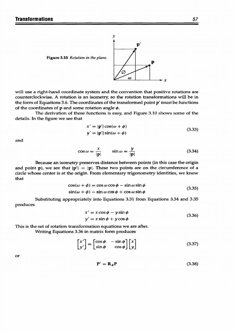
8/9/2019 Mortenson, Michael E. - Mathematics for computer graphics applications.pdf
http://slidepdf.com/reader/full/mortenson-michael-e-mathematics-for-computer-graphics-applicationspdf 70/367
Transformations
y
Figure
3.10
Rotation in the plane.
will use a
right-hand coordinate
system and
the convention that positive rotations are
counterclockwise. A
rotation is
an
isometry,
so
the
rotation transformations will be in
the
form of Equations
3.6. The
coordinates
of
the transformed
point p' must be functions
of
the coordinates
of
p and some
rotation
angle
4.
The
derivation
of
these
functions is easy, and Figure
3.10
shows some
of
the
details. In
the
figure we see that
X
= IP I cos(w +
O)
(3.33)
y' =
Ip I
sin(w
+4)
and
cosw
=
sinMg=
- (3.34)
IPI IPI
Because
an
isometry preserves distance between
points
(in
this case
the origin
and point p), we see that
Ip'I
= Ip.
These
two points are on
the
circumference
of a
circle
whose
center is at
the
origin.
From elementary
trigonometry
identities, we know
that
cos(co +
4 =
cos a
cos4'
-
sin
w
sin 0
sin(co +4' = sin w
cos
+ cos
co sin (
Substituting appropriately
into Equations
3.31
from
Equations
3.34
and
3.35
produces
x'
= x cos- y
sin
(3.36)
y'=
xsino
+
ycos4
This
is the set of
rotation transformation equations
we are after.
Writing Equations
3.36 in matrix
form produces
x'
= cos
-sin
1
(3.37)
LY'] [sin
cosin
4YX
or
57
P'
p
P
0
P' =
RoP
(3.38)
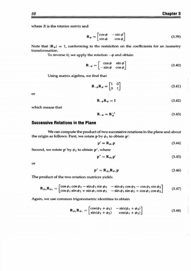
8/9/2019 Mortenson, Michael E. - Mathematics for computer graphics applications.pdf
http://slidepdf.com/reader/full/mortenson-michael-e-mathematics-for-computer-graphics-applicationspdf 71/367
58 Chapter 3
where
R is the rotation
matrix
and
RX = [sing
Csitn
(3.39)
Note that IR,,I
=
1, conforming
to
the
restriction on the coefficients
for
an isometry
transformation.
To
reverse it, we apply the
rotation
-0
and
obtain
R.
F cos
0
sin
34
- sin
0 cos
(
Using matrix algebra,
we find that
R-R [O
1
(3.41)
or
R-OR= I
(3.42)
which means
that
R =
R-1
(3.43)
Successive Rotations
in
he
Plane
We
can
compute
the product of two successive
rotations in the plane and
about
the origin
as
follows: First, we rotate
p by
Xl
to obtain
p':
p =
RO
1
p
(3.44)
Second,
we rotate p' by 02 to
obtain p", where
p = Ro,
2
p' (3.45)
or
p = RO
2
RO
1
p
(3.46)
The product of the two rotation
matrices yields
R.R.
-=
cos
1
cos0
2
-sinolsin0
2
-sin~jcos02-cos~lsinO
2
3
Xcos
1
sinO
2
+ sin
1
costO
2
-sin
1
lsinO
2
+
COS0
1
COS@021
Again,
we
use
common
trigonometric
identities
to obtain
RO2RO
= FCoS(01
+
02)
-sin(01 +
02)1
(3.48)
[Sin(Il
+
02)
Cos(0
1
+ @2)]
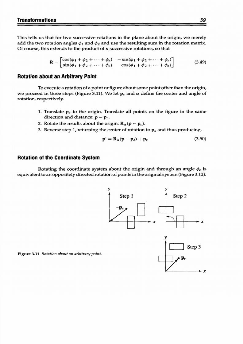
8/9/2019 Mortenson, Michael E. - Mathematics for computer graphics applications.pdf
http://slidepdf.com/reader/full/mortenson-michael-e-mathematics-for-computer-graphics-applicationspdf 72/367
Transformations
59
This tells
us that
for
two
successive
rotations in the plane about the origin, we merely
add
the two rotation angles 01 and
02
and use the resulting
sum
in the rotation
matrix.
Of course, this
extends to the
product
of
n successive
rotations,
so that
(3.49)
= [Cs0(01l+0
2
+***+n)
-Sin(01++
2
+* + 0n)]
LSin(0l +
02 +
'
+
0.b)
COS(¢01 +
0b2
+ - -' +
Oin)]
Rotation about
an Arbitrary Point
To execute
a rotation of a
point or figure about some point
other
than
the
origin,
we
proceed in three
steps
(Figure 3.11). We let Pc and a define the center and angle
of
rotation,
respectively.
1. Translate Pc to
the
origin.
Translate
all
points on the
figure
in the same
direction and distance: p
-
Pc
2.
Rotate the results
about
the
origin: Ra (p - p,)
3.
Reverse
step
1,
returning
the center of rotation
to
Pc and thus producing.
p'
=
Ra(p-pc)
+
pc
(3.50)
Rotation
of the
Coordinate
System
Rotating
the
coordinate
system
about
the origin
and through
an
angle he is
equivalent to an oppositely directed rotation
of
points in the original
system
(Figure 3.12).
y
Step
2
x
y
Figure
3.11 Rotation about
an
arbitrarypoint.
x
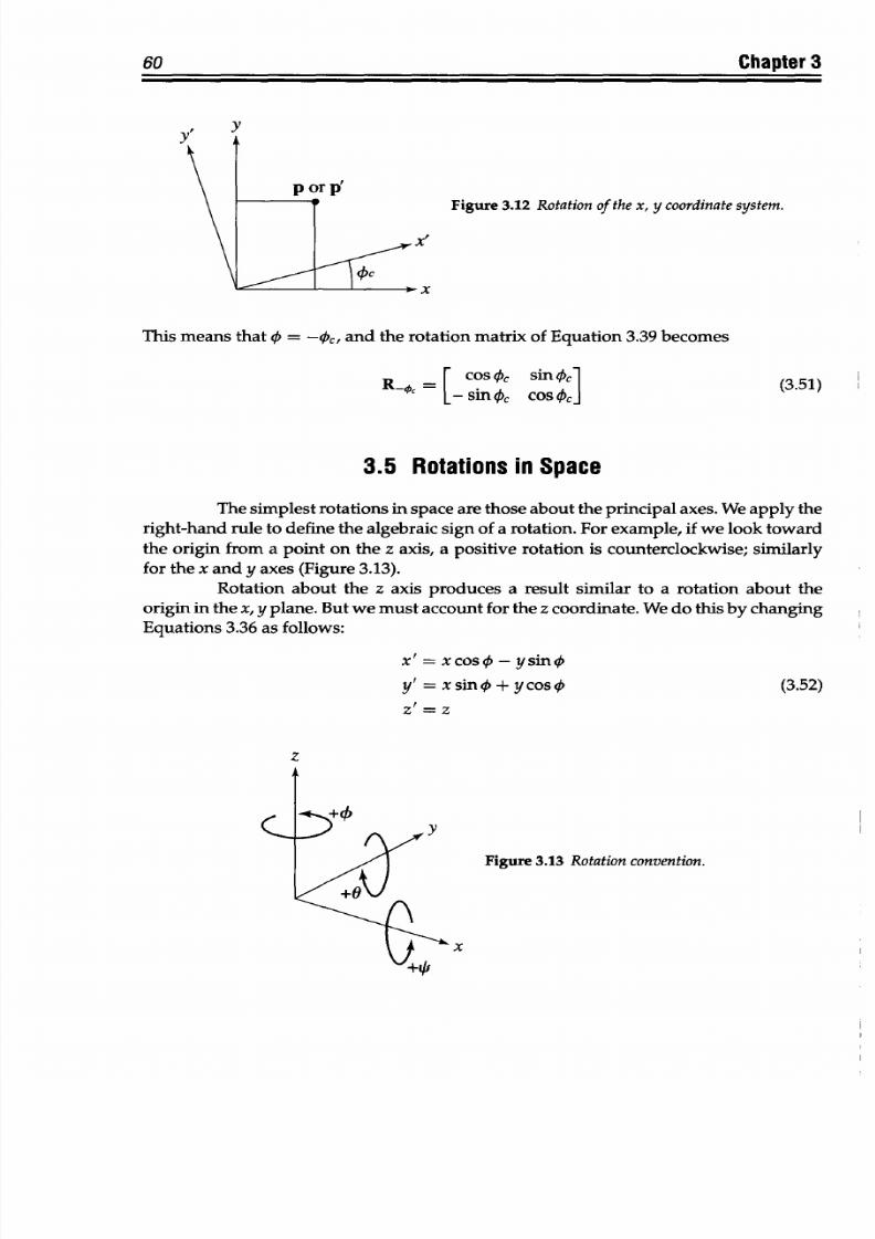
8/9/2019 Mortenson, Michael E. - Mathematics for computer graphics applications.pdf
http://slidepdf.com/reader/full/mortenson-michael-e-mathematics-for-computer-graphics-applicationspdf 73/367
60
Chapter
3
Av
Figure
3.12 Rotation
of the
x,
y coordinate
system.
x
This means that 0
=
-(Pc, and the rotation matrix
of Equation 3.39
becomes
R. = cosmic
singOc
L-sinoc
cos(i
I
(3.51)
3.5
Rotations inSpace
The
simplest rotations
in space
are those
about
the
principal axes.
We
apply the
right-hand rule
to
define
the algebraic sign
of
a
rotation.
For example, if
we look
toward
the
origin from
a point
on the
z
axis,
a
positive
rotation
is
counterclockwise;
similarly
for the x and y axes
(Figure 3.13).
Rotation about the z axis produces a result
similar
to
a rotation about the
origin in the
x,
y plane. But we
must
account for
the z
coordinate.
We
do
this by
changing
Equations
3.36 as follows:
x'
=
xcost -
ysino
y' =
x
sing +ycoso
zf
= Z
(3.52)
z
Y
Figure
3.13 Rotation convention.
x
60 Chapter
3
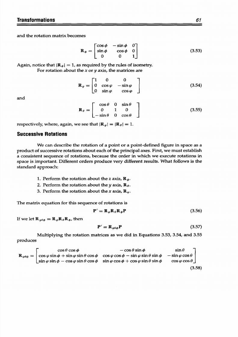
8/9/2019 Mortenson, Michael E. - Mathematics for computer graphics applications.pdf
http://slidepdf.com/reader/full/mortenson-michael-e-mathematics-for-computer-graphics-applicationspdf 74/367
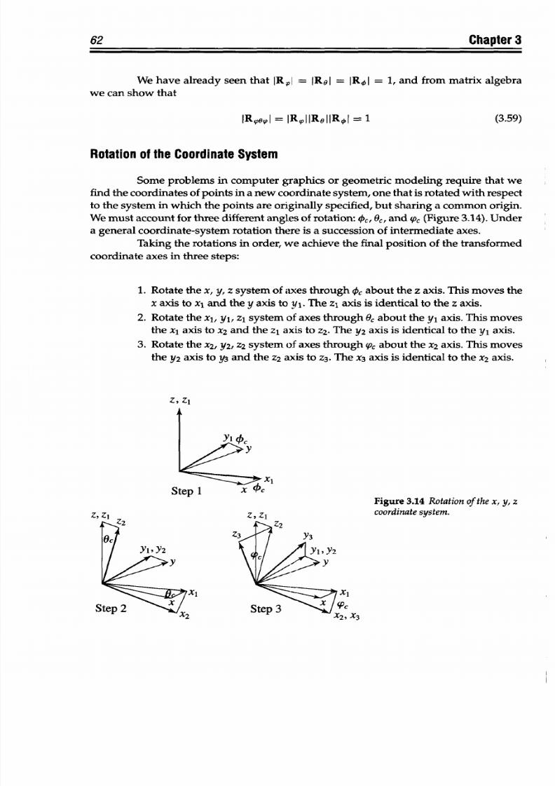
8/9/2019 Mortenson, Michael E. - Mathematics for computer graphics applications.pdf
http://slidepdf.com/reader/full/mortenson-michael-e-mathematics-for-computer-graphics-applicationspdf 75/367
62
Chapter 3
We
have already seen that IR,, =
IRCH
= IR I
=
1, and from matrix
algebra
we can show
that
IROegj
=
IRpjIRoIIRI
=
1
(3.59)
Rotation of
the
Coordinate System
Some
problems in comp uter
graphics
or geometric
modeling require that we
find the coordinates of points
in a new coordinate system, one
that
is rotated
with
respect
to
the
system
in which
the
points
are originally specified,
but
sharing
a
common
origin.
We must
account
for
three different
angles
of
rotation: Tic,
60,
and
(c
(Figure 3.14).
Under
a
general
coordinate-system rotation there is a succession of intermediate
axes.
Taking the rotations
in order, we
achieve
the
final
position of the transformed
coordinate axes in three steps:
1.
Rotate the x,
y,
z
system
of
axes through
he about
the
z
axis. This moves
the
x axis
to
xl
and
the y axis
to
yl. The
z
1
axis
is
identical
to the
z axis.
2. Rotate
the xl, yl, z
1
system
of
axes through O
about
the
yi axis.
This
moves
the
x
1
axis to x
2
and the z
1
axis to
z
2
. The y2 axis is identical to the
yj axis.
3.
Rotate
the
x
2
, y2, Z
2
system
of
axes
through
v,
about the x
2
axis. This moves
the
Y2
axis
to
y3
and the
z
2
axis
to
Z
3
.
The
X3
axis is
identical to
the x
2
axis.
z, zi
Figure
3.14
Rotation
of the x, y, z
RA
_-nS01S-
...
Z, Zi
Lu(JFLSLLULtC fbyt (.
'2, -3
:
-
rY
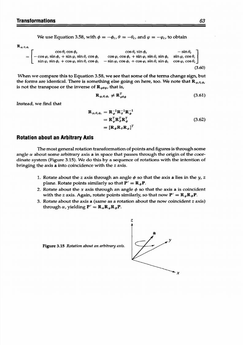
8/9/2019 Mortenson, Michael E. - Mathematics for computer graphics applications.pdf
http://slidepdf.com/reader/full/mortenson-michael-e-mathematics-for-computer-graphics-applicationspdf 76/367
Transformations
63
We use
Equation
3.58,
with
0 =
-d, 0
= -0&,and up = -sac, to
obtain
cos
6cos
cos
0,
sinm
-sin6
1
=
-cos s
in
+ sin c
sin6
cos 0,
cos , cos
+
sinq sin6 sinm sinq
cos
c
sin ,o sinC + cos
(p
sin6 cos 0,
-sino
cos
+
cos (c sinO sink cos
1P
cos
0,
(3.60)
When we
compare
this to Equation
3.58, we
see that
some
of the terms
change
sign, but
the forms
are identical. There
is something else going on
here,
too.
We
note
that
Rpto
is
not
the transpose or the inverse of
Rwe0, that
is,
RpaecO,
0
ROUX(3.61)
Instead, we find
that
R.poO
R- R- R-1
=
R
TRTR
T
(3.62)
=
[RoR
6
Rw4T
Rotation about an
Arbitrary
Axis
The most general rotation transformation of
points
and figures is
through
some
angle
a
about
some
arbitrary
axis
a
in space
that
passes
through
the origin
of
the
coor-
dinate system (Figure 3.15). We do this by a sequence of rotations with the intention of
bringing the axis a into coincidence with the z axis.
1. Rotate about the z axis through an angle 0
so
that the axis a lies in the y, z
plane. Rotate points similarly so that
P' = R
OP.
2. Rotate about the
x axis
through
an
angle X
so
that the
axis
a
is coincident
with the
z
axis. Again, rotate
points
similarly, so that now P'
=
RVROP.
3.
Rotate
about the
axis
a
(same
as a rotation about the
now coincident
z axis)
through
a,
yielding P
=
RaRROP.
z
Figure 3.15
Rotation about an arbitrary
axis.
x
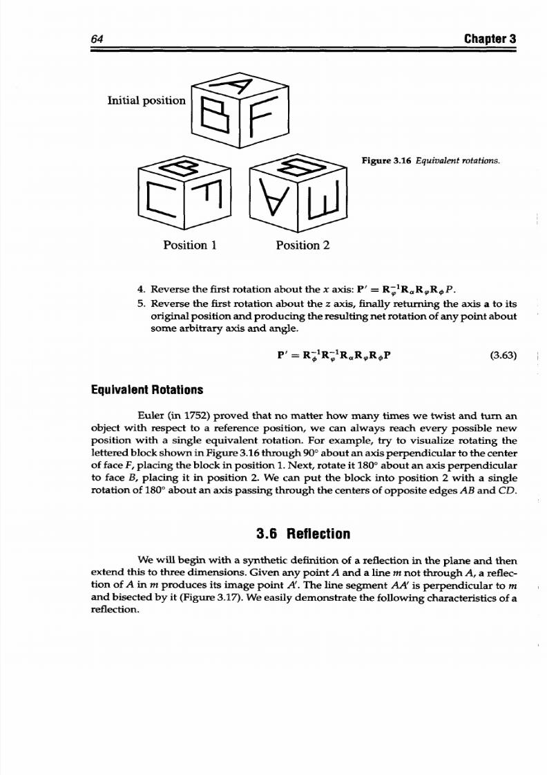
8/9/2019 Mortenson, Michael E. - Mathematics for computer graphics applications.pdf
http://slidepdf.com/reader/full/mortenson-michael-e-mathematics-for-computer-graphics-applicationspdf 77/367
Chapter
3
Initial
position
Figure 3.16
Equivalent
rotations.
Position 1
Position
2
4. Reverse
the first rotation about
the
x
axis: P'
=
Rp Rl ,
R ,RP.
5. Reverse
the
first
rotation
about
the
z axis,
finally returning
the axis
a
to
its
original
position and producing
the resulting net rotation
of any
point about
some
arbitrary axis and
angle.
PF = R R- RaR,pRRP
(3.63)
Equivalent Rotations
Euler
(in 1752) proved
that no
matter how many
times we
twist and turn
an
object with
respect
to a reference
position, we can
always
reach
every possible
new
position
with a single
equivalent
rotation. For
example, try
to visualize
rotating the
lettered block
shown
in Figure
3.16
through
900 about an
axis
perpendicular
to the
center
of face F,
placing the
block in
position 1.
Next,
rotate it
1800
about an
axis
perpendicular
to face
B, placing it
in position
2. We can put
the
block
into position
2 with a single
rotation of
1800 about
an axis passing through
the
centers
of
opposite
edges
AB
and
CD .
3.6
Reflection
We
will
begin
with
a synthetic definition
of
a
reflection
in the
plane
and then
extend
this
to
three dimensions. Given
any point A
and
a line m not through A,
a reflec-
tion
of
A
in
m
produces
its image
point
A'.
The
line
segment
AA'
is
perpendicular
to
m
and bisected
by it (Figure
3.17).
We easily demonstrate
the following characteristics
of a
reflection.
64
__*4
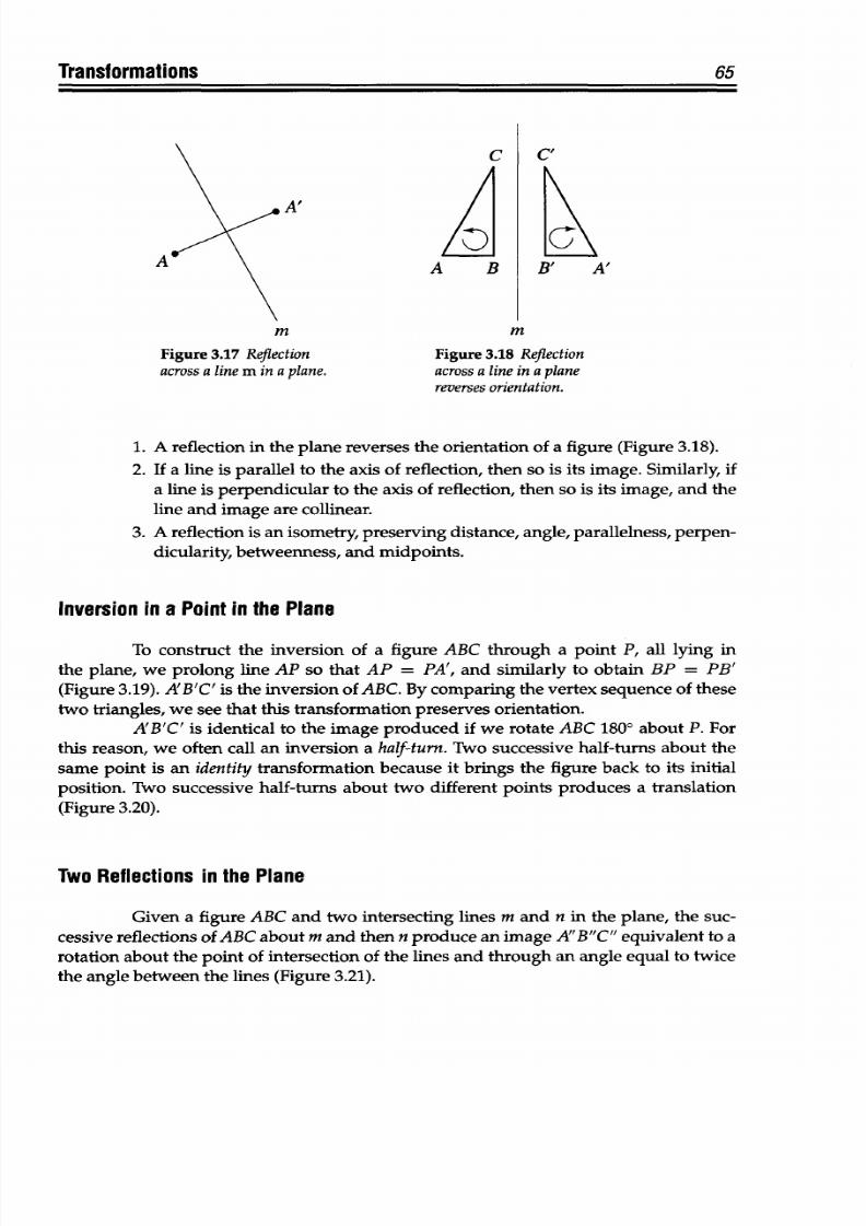
8/9/2019 Mortenson, Michael E. - Mathematics for computer graphics applications.pdf
http://slidepdf.com/reader/full/mortenson-michael-e-mathematics-for-computer-graphics-applicationspdf 78/367
Transformations
A
65
C
A'
A
A B
C'
B'
A'
m
m
Figure 3.17 Reflection
Figure 3.18
Reflection
across
a
line
m
in a plane. across a line in a plane
reverses orientation.
1. A
reflection
in the plane
reverses
the orientation
of a figure (Figure 3.18).
2. If a line
is
parallel
to
the axis
of reflection,
then
so is
its
image.
Similarly,
if
a line
is
perpendicular to
the
axis of reflection,
then so is
its image,
and the
line and
image
are
collinear.
3.
A reflection
is
an
isometry,
preserving
distance, angle, parallelness, perpen-
dicularity,
betweenness,
and midpoints.
Inversion
in a
Point
in the Plane
To
construct the
inversion
of
a figure ABC through
a point P, all lying in
the
plane,
we
prolong
line
AP
so
that AP
=
PA', and similarly
to
obtain
BP
=
PB'
(Figure 3.19). A'B'C' is the inversion of ABC. By comparing
the
vertex sequence of these
two
triangles, we see that this
transformation
preserves
orientation.
A'B'C'
is identical
to
the image produced
if
we
rotate ABC 180°
about P. For
this reason, we often call
an
inversion a
half-turn.
Two
successive
half-turns
about
the
same point
is an
identity
transformation because it brings the
figure
back
to its initial
position. Two
successive
half-turns
about two
different
points produces
a
translation
(Figure 3.20).
Two Reflections in the
Plane
Given
a
figure
ABC
and two
intersecting
lines
m
and
n
in
the
plane, the
suc-
cessive
reflections
of
ABC
about m
and then n produce an image
A"B"C"
equivalent to a
rotation about the
point of
intersection
of
the
lines
and
through
an
angle equal to twice
the angle between the lines
(Figure
3.21).
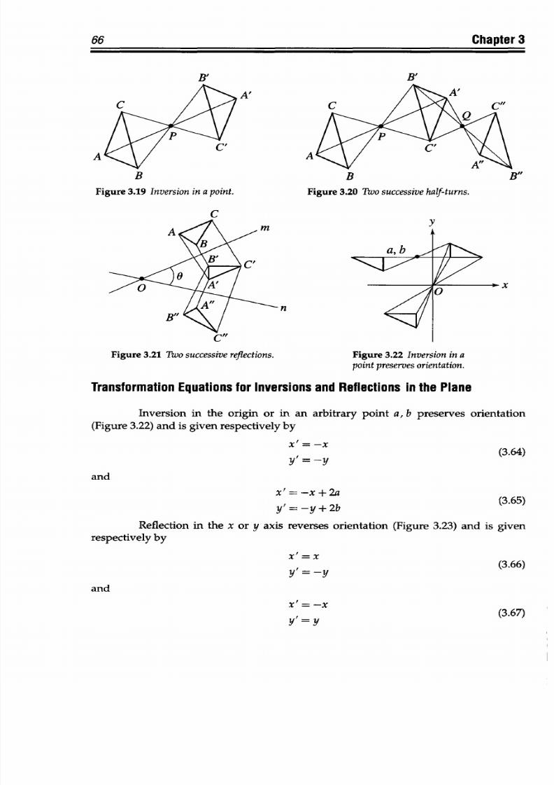
8/9/2019 Mortenson, Michael E. - Mathematics for computer graphics applications.pdf
http://slidepdf.com/reader/full/mortenson-michael-e-mathematics-for-computer-graphics-applicationspdf 79/367
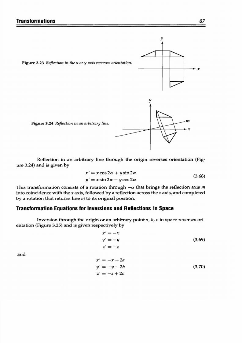
8/9/2019 Mortenson, Michael E. - Mathematics for computer graphics applications.pdf
http://slidepdf.com/reader/full/mortenson-michael-e-mathematics-for-computer-graphics-applicationspdf 80/367
Transformations
67
Figure
3.23
Reflection
in
the
x or y axis
reverses
orientation.
x
y
Figure 3.24
Reflection
in
an arbitrary ine.
m
IV1
Reflection
in an arbitrary line through
the origin reverses orientation
(Fig-
ure 3.24) and is given by
x'
= xcos2a
+ ysin2a
(3.68)
y'= xsin2a
-
ycos2a
This transformation consists
of
a rotation through -a
that
brings the
reflection
axis m
into coincidence with
the
x
axis,
followed by a reflection across
the
x
axis, and completed
by a
rotation
that returns
line
m to its
original position.
Transformation
Equations
for
Inversions
and
Reflections
in
Space
Inversion through the
origin
or
an arbitrary point
a,
b,
c in
space reverses ori-
entation (Figure 3.25)
and is
given respectively by
X' = -x
(3.69)
, =
-y
Z'
=
-z
and
x'
=
-x+2a
y' = -y+2b
z' = -z+2c
(3.70)
67
j
Transformations
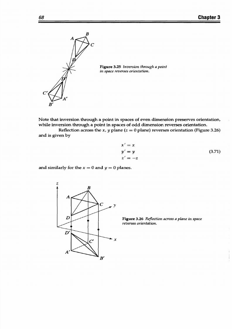
8/9/2019 Mortenson, Michael E. - Mathematics for computer graphics applications.pdf
http://slidepdf.com/reader/full/mortenson-michael-e-mathematics-for-computer-graphics-applicationspdf 81/367
8/9/2019 Mortenson, Michael E. - Mathematics for computer graphics applications.pdf
http://slidepdf.com/reader/full/mortenson-michael-e-mathematics-for-computer-graphics-applicationspdf 82/367
8/9/2019 Mortenson, Michael E. - Mathematics for computer graphics applications.pdf
http://slidepdf.com/reader/full/mortenson-michael-e-mathematics-for-computer-graphics-applicationspdf 83/367
70 Chapter
3
We make
all
transformations
of
homogeneous points
by
means
of
a 4
x
4
transformation
matrix.
To
use
this technique, we
must represent
curves
or
surfaces
by
their
control point matrices. We add the fourth or homogeneous coordinate
h to each
control point.
We
make the
required transformations
and then
convert the
resulting
ho-
mogeneous
coordinates into ordinary
three-dimensional coordinates by means of Equa-
tion
3.76.
Now
let us
investigate
some of
the
possible transformations, expressing them
as
Pi' =
ThPh
(3.77)
We
translate
points using
the
following matrix product:
-1
0 0
tx
[x'
yI Z'
1= 0 10 1t[x
y z 1] (3.78)
O0 0 0 1-
where tx, ty, t, are components
of
the vector t that
describes
the transformation p'
=
p +
t.
The
matrix
product
yields
[xI
y'
IZ' 1]=1'x+tx y+ty z+t'
1]
(3.79)
from
which we readily compute the ordinary transformed
coordinates
x'=x+tx, Y'=y+ty, z'=z+tz
(3.80)
To rotate a point around
a
principal axis
we use
one
of
the
three
following matrix
products.
For
rotation around the z
axis:
-cos
0
-
sin 0 0 0]
[x'
y Z' 1]
=
sin0 Cos 0 o [x
y
z
1] (3.81)
- °
0 1-
For
rotation
around the y
axis:
F
cos
0 sinfi 01
[x'
yf' z' 1
() 1
0 0
[x y
z
1] (3.82)
() 0 0 1i
For
rotation
around the
x axis:
-1
0 0 o-
[x
y
z'
1]
= 0
csiy -s y 0
[x
y z
1]
(3.83)
O
0 0
1
8/9/2019 Mortenson, Michael E. - Mathematics for computer graphics applications.pdf
http://slidepdf.com/reader/full/mortenson-michael-e-mathematics-for-computer-graphics-applicationspdf 84/367
Transformations
71
The
differential scaling
equation
is
[Sx 0 0 01
[x'
y'
z'
=
0 y
0
0 [x
y z
1]
(3.84)
00
s 1
And
finally for projections we have
-1
0
0 I-
[x'/
y Z' 1]=
0
0 1
0
[x
y
z
1] (3.85)
[ [x
p
q
r
1
which
we
use
in
Chapter
18.
Thus, by what only amounts to
temporarily
adding
an
extra coordinate to
the
P
and
P' matrices and adjusting
R
and
T
accordingly,
we
can
write an
arbitrary
sequence
of transformations
as a
single equivalent matrix product.
Let's see how
this works in two
dimensions, for
rotation and translation
in
the
x,
y
plane. If we must first translate a point by T and then rotate the
result
by R,
we
write
this
as
P'
=
RTP
(3.86)
where
Fcos 0
-sin 0
tx
cos
G-ty
sin
0
RT = sin 0
cos
0 tx sin 0 + ycos
0 (3.87)
0 0 1
Or, reversing the order and
translating the
point
before
rotating
it,
we
write
P'
=
TRP
(3.88)
where
cos 0 - sin
0
tx
TR = sin6 cos6
ty (3.89)
This
also
shows us that
TR#
RT
(3.90)
A
very
simple
and
obvious
extension of these ideas applies
to
rotations
and
translations in
space.
8/9/2019 Mortenson, Michael E. - Mathematics for computer graphics applications.pdf
http://slidepdf.com/reader/full/mortenson-michael-e-mathematics-for-computer-graphics-applicationspdf 85/367
72
Chapter
3
Exercises
3.1
Describe
the following
linear transformations:
a.
x'=x,y'=ay
b.
x'
= ax,
y'
= by
c.
x' = ax, y' = ay
d. x'
=
(x-y)/, y'
=
(x
+ y)v2
3.2
How
far
is a point
moved under the translation given by
Equation
3.26?
3.3
Show that the product of
the following
two
reflection
matrices is
a
rotation:
[1
0] and
[1 0]
3.4
Reflections
in
space are
summarized
by
the
following
matrix.
Write
out
all
the
possible combinations as individual
matrices, and give
their corresponding
linear
equations,
describing what each does.
-i1 0 O-
Rf= 0 +1 0
3.5 Describe
the
product of
reflection
of a point in two mutually
perpendicular lines
in
the plane.
3.6
Describe
the
product
of reflection of a
point
in
three
mutually perpendicular
planes.
3.7 Show that the
product of sequential reflections
in
two parallel
lines,
xl = a and
Xm =
b, of a point Po
is
the
equivalent of a
single translation. Find the
translation.
3.8 Show
that, in
the
plane,
translating two points pi
and
P2, each
by
t,
preserves
the
distance between them.
3.9
Compare R
0
,o
and
Roo
to
show that different
orders
of rotation
produce different
results.
3.10
Show that
the
translation
of a point P to P"
produced by two
successive
half-turns
about
different
points
A
and
B
is
equal
to
twice
the directed distance
from
A
to
B.
Draw
a sketch
to
support your answer.
3.11
Derive
Equation 3.65.
3.12
Derive
Equation
3.68.
8/9/2019 Mortenson, Michael E. - Mathematics for computer graphics applications.pdf
http://slidepdf.com/reader/full/mortenson-michael-e-mathematics-for-computer-graphics-applicationspdf 86/367
(iu
pTa
SYMMETRY
AND GROUPS
Symmetry
brings to
mind
decorative patterns, tilings,
and
repetitive mirror-images. As a
subject o f study,
it
was
once
thought
to
be unrelated
to serious
mathematics
and
scientific
thinking.
Not until
the
19th century did
mathematicians
discover a close
relationship
between
analytical
geometry
and
symmetry. Then
they invented group
theory
to
study
the symmetry of mathematical
objects.
Aside from the obvious application of symmetry to the decorative arts and
engineered constructions, the
understanding
of symmetry
is
now central to mathemat-
ical
physics and the
study
of elementary particles
and cosmology.
In the equations of
quantum
mechanics
and
general
relativity,
the presence or absence of certain algebraic
symmetries profoundly affects how
we
interpret
them.
The
highly intuitive geometric
nature of the
elementary
principles of symmetry and groups makes this subject easy to
teach
and learn.
This
chapter takes an
analytical
approach to
symmetry. It defines a group
and
the more specialized symmetry group, including cyclic, dihedral, and
finite
symmetry
groups.
The
symmetry
of
ornamental groups
(frieze
groups and wallpapergroups) reveals
a surprising quantitative aspect to these aesthetic
forms. The crystallographic
estriction
shows
how
symmetry
depends
on the
nature of space itself. This is also true of
plane
lattices
and
tilings. The
chapter
concludes with a look
at
the rotational symmetry
of
polyhedra.
4.1
Introduction
When we
say that a
figure is
symmetric, we
mean
that
certain
motions or
rear-
rangements of its
parts
leave it unchanged as
a
whole. A figure is symmetric
if
it is congru-
ent
to itself in
more than
one way.
For
example, if
we
rotate
a
square 900
about its center,
we
see
no difference between the original figure and its rotated image. They
coincide
exactly.
So
we can call this motion a symmetry transformation.
Reflections,
rotations, and
inversions,
subject
to certain conditions,
can
produce symmetry
transformations.
Any
ro-
tation
of a circle about its
center,
or any reflection about a diameter, is
a
symmetry of
a
circle.
We begin
with
an
investigation
of
the
six symmetries of an
equilateral triangle
(Figure 4.1). We will
look
for
its symmetries
by
finding
different ways of
transforming
73
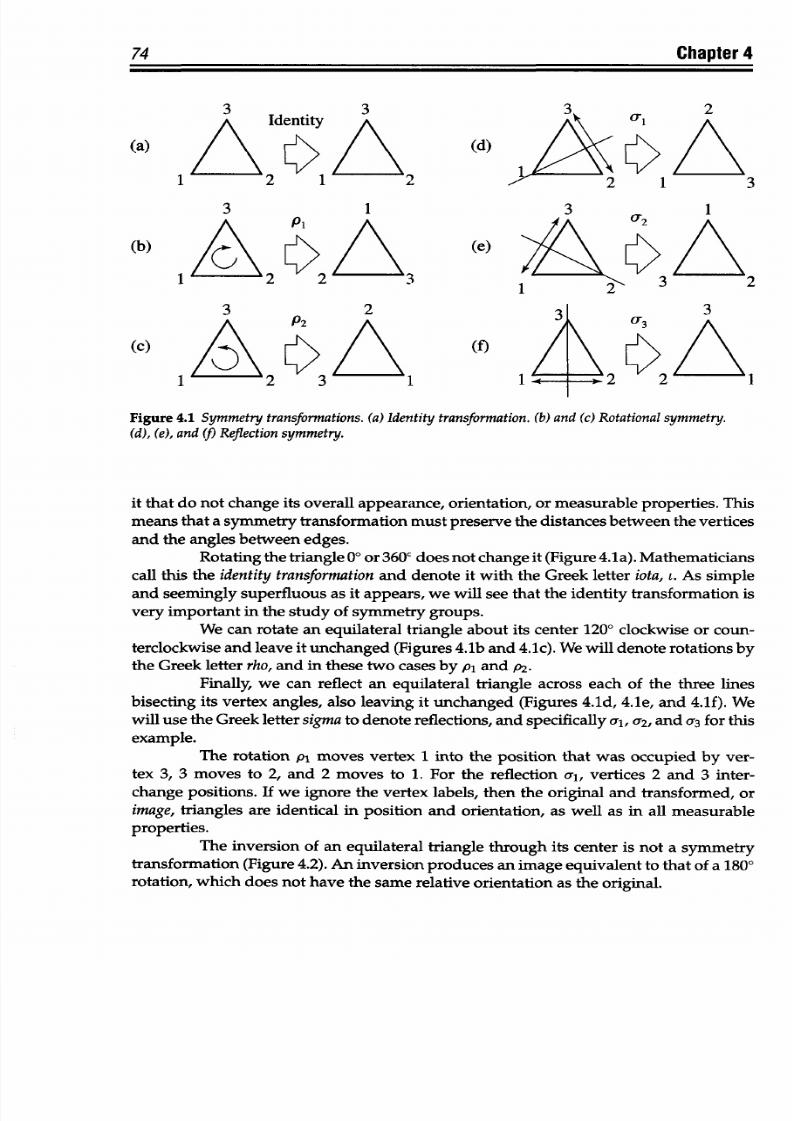
8/9/2019 Mortenson, Michael E. - Mathematics for computer graphics applications.pdf
http://slidepdf.com/reader/full/mortenson-michael-e-mathematics-for-computer-graphics-applicationspdf 87/367
74
Chapter
4
3
(a)
1
A
3
1 /C
2
(b)
3
(c)
A
1
2
entity
1 2
1
P
ŽA
2
P
2
3
(d)
1
3
(e)
1
2
(f)
1
2
1
3
A
3
/\1
Figure
4.1
Symmetry transformations.
(a) Identity transformation.
(b)
and
(c)
Rotational
symmetry.
(d), (e), and
(1)Reflection
symmetry.
it
that
do not
change its overall
appearance, orientation, or measurable properties.
This
means that a symmetry
transformation must
preserve the distances
between the
vertices
and
the angles
between edges.
Rotating the
triangle 00 or 360c does
not
change
it
(Figure
4.1a). Mathematicians
call
this
the
identity
transformation
and
denote
it with the
Greek letter iota, t.
As
simple
and seemingly
superfluous as it
appears,
we
will see that
the
identity
transformation
is
very
important
in the study of
symmetry groups.
We
can rotate an
equilateral triangle about
its
center 120°
clockwise
or
coun-
terclockwise
and leave it
unchanged (Figures
4.1b
and
4.1c).
We will denote
rotations
by
the Greek letter rho, and in
these
two
cases
by p, and
p2.
Finally,
we
can reflect an
equilateral triangle across each of
the three lines
bisecting its vertex
angles, also leaving it
unchanged (Figures 4.1d,
4.1e,
and
4.1f). We
will use the Greek
letter
sigma
to denote
reflections,
and
specifically
a,,
a
2
,
and a-3 for this
example.
The rotation p1
moves
vertex 1
into
the position
that was
occupied by
ver-
tex 3,
3 moves to 2, and
2 moves to
1. For
the reflection al, vertices
2 and 3
inter-
change
positions. If we ignore the
vertex
labels,
then the original and
transformed, or
image, triangles
are
identical in position and
orientation, as well as
in
all
measurable
properties.
The
inversion
of
an
equilateral triangle
through
its
center
is
not
a
symmetry
transformation (Figure 4.2).
An
inversion produces an image equivalent to
that of a 1800
rotation,
which
does
not
have
the same relative
orientation
as the
original.
74
Chapter 4
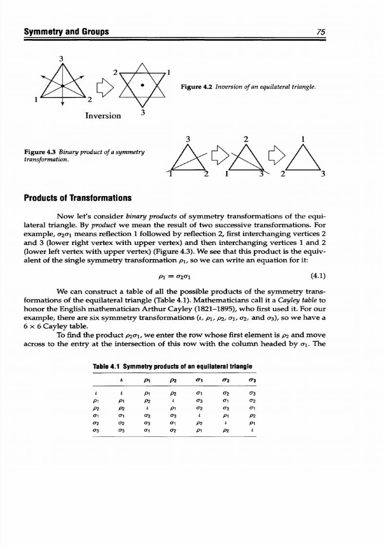
8/9/2019 Mortenson, Michael E. - Mathematics for computer graphics applications.pdf
http://slidepdf.com/reader/full/mortenson-michael-e-mathematics-for-computer-graphics-applicationspdf 88/367
Symmetry and
Groups
3
Figure
4.2 Inversion of
an
equilateral triangle.
1
Inversion 3
Figure 4.3 Binary product of
a
symmetry
transformation.
3
2
1 3 2
Products of Transformations
Now let's consider
binary
products of
symmetry
transformations
of
the
equi-
lateral
triangle. By
product
we
mean
the
result
of
two
successive
transformations. For
example,
a2a, means
reflection
1 followed by
reflection 2, first
interchanging
vertices
2
and 3 (lower
right vertex
with upper
vertex)
and
then
interchanging vertices
1 and 2
(lower left vertex with upper
vertex)
(Figure
4.3). We
see
that this product is the
equiv-
alent of the
single
symmetry transformation
pl, so
we
can
write an equation for
it:
P1 =
`2rl
(4.1)
We
can
construct a table
of
all
the possible
products
of
the symmetry trans-
formations
of
the equilateral triangle
(Table
4.1). Mathematicians call it a Cayley table to
honor the Eng lish mathematician Arthur
Cayley
(1821-1895), who first
used
it.
For
our
example,
there
are
six symmetry transformations
(i,
pl,
P2,
cr,, a2,
and o3), so we
have a
6
x
6
Cayley
table.
To
find
the
product p2al, we
enter
the
row
whose first element
is P2 and move
across to
the entry at the intersection of this row with the column headed by
a1. The
Table
4.1 Symmetry
products of
an equilateral triangle
t
P1
P2 0.1 02 0a3
1 P1
P2
01
a2 U3
Pi P1
P2
L 03
aUl 2
P2 P2
L
Pi
a2
U3
a1
01
01 U2 73 I P1 P2
q
2
a2 a3
at
P2
I
Pi
a3
03
a1
a2 P1 P2
L
75
A/
3
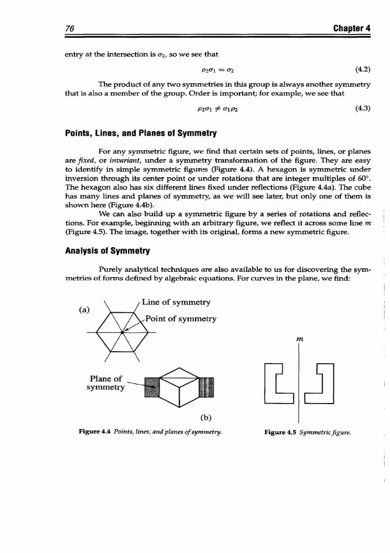
8/9/2019 Mortenson, Michael E. - Mathematics for computer graphics applications.pdf
http://slidepdf.com/reader/full/mortenson-michael-e-mathematics-for-computer-graphics-applicationspdf 89/367
76 Chapter 4
entry
at the intersection is a
2
,
so
we
see that
p
2
al =
a2 (4.2)
The
product
of
any two
symmetries
in
this
group
is
always
another symmetry
that is
also
a
member of
the
group.
Order
is
important;
for example, we see
that
P2(1 :A Orlp2
(4.3)
Points,
Lines,
and Planes
of Symmetry
For
any symmetric
figure, we
find
that
certain
sets
of
points, lines, or
planes
are
fixed, or invariant, under
a symmetry
transformation of
the
figure.
They are easy
to identify
in
simple symmetric
figures
(Figure
4.4). A
hexagon
is
symmetric
under
inversion
through its center point
or under
rotations
that
are integer
multiples of 600.
The
hexagon also
has six different
lines
fixed
under reflections (Figure
4.4a). The cube
has many
lines
and planes of symm etry, as
we
will
see later, but only
one of
them
is
shown here
(Figure
4.4b).
We can also build
up
a
symmetric
figure by a series of
rotations
and
reflec-
tions.
For example,
beginning with an
arbitrary
figure,
we reflect
it
across
some
line
m
(Figure 4.5). The image,
together with
its
original, forms a new symmetric
figure.
Analysis
of Symmetry
Purely analytical techniques are also available to
us
for discovering the sym-
metries
of
forms defined by algebraic equations. For curves in the plane,
we
find:
Line of symmetry
Point of symmetry
nm
>51<_
Plane
of
symmetry
(b)
Figure 4.4
Points,
lines,
and
planes
of
symmetry.
Figure 4.5
Symmetricfigure.
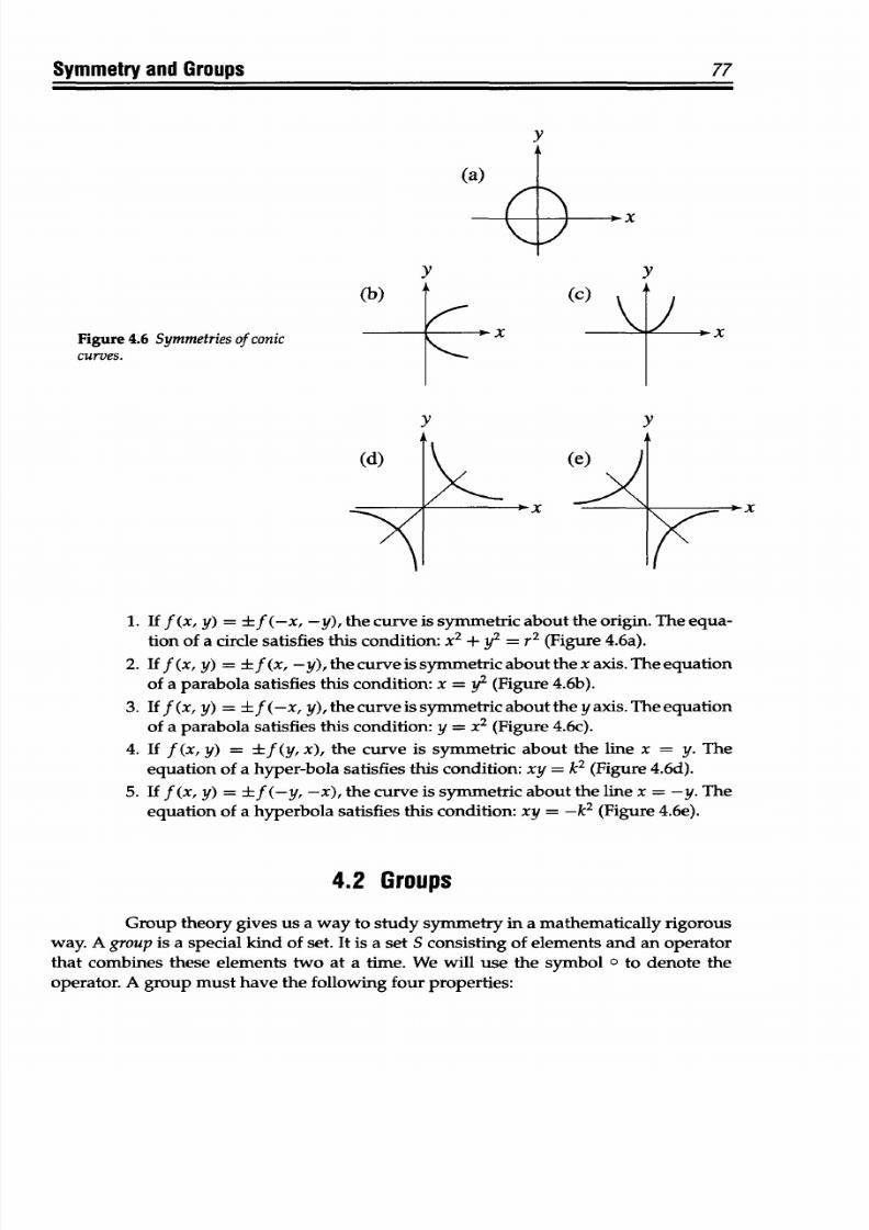
8/9/2019 Mortenson, Michael E. - Mathematics for computer graphics applications.pdf
http://slidepdf.com/reader/full/mortenson-michael-e-mathematics-for-computer-graphics-applicationspdf 90/367
Symmetry and Groups
y
(a)
y
x
y
x
igure
4.6 Symmetries
of conic
curves.
(d)
Y Y
X
1. If
f
(x, y) =
± f
-x,
-y), the curve is symmetric about the origin. The equa-
tion
of a
circle
satisfies
this condition: x
2
+ y
2
= r
2
(Figure
4.6a).
2. If f(x, y)
=
±f(x,
-y), the
curve
is
symmetric about
the
x axis. The equation
of a
parabola
satisfies
this
condition: x =
y
2
(Figure
4.6b).
3.
If
f
(x,
y)
= ±f
-x, y), the curve
is
symmetric about the
y
axis.
The
equation
of a parabola satisfies this condition: y =
x
2
(Figure 4.6c).
4. If
f
(x, y)
= if (y, x), the
curve is
symmetric about the line
x
=
y. The
equation of
a
hyper-bola
satisfies this condition: xy = k
2
(Figure
4.6d).
5.
If f
(x,
y)
= ± f
-y, -x),
the curve is symmetric
about
the
line
x = -y.
The
equation of
a
hyperbola
satisfies
this
condition: xy
= -k
2
(Figure 4.6e).
4.2 Groups
Group theory
gives
us
a
way
to
study
symmetry in
a
mathematically
rigorous
way.
A group
is
a special kind of
set. It is a set
S consisting
of
elements
and an
operator
that
combines these elements
two at a time. We
will use the symbol 0
to
denote the
operator.
A group must have the following
four
properties:
77
(
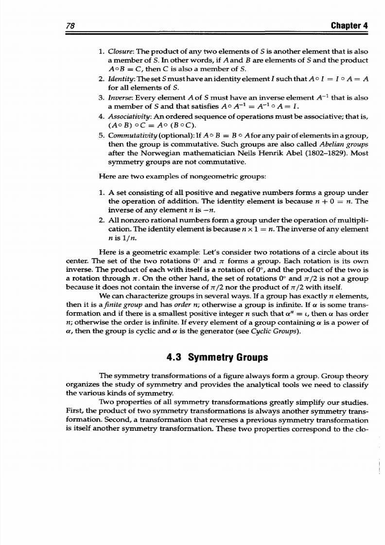
8/9/2019 Mortenson, Michael E. - Mathematics for computer graphics applications.pdf
http://slidepdf.com/reader/full/mortenson-michael-e-mathematics-for-computer-graphics-applicationspdf 91/367
78
Chapter 4
1. Closure:
The product
of any two elements
of S
is
another
element
that is also
a
member
of S. In other words, if
A
and
B are elements
of
Sand
the
product
AoB
=
C, then C
is also
a member of
S.
2.
Identity: The
set
S
must
have
an
identity
element
I
such
that
A
0
I
=
I
o
A
=
A
for all elements of S.
3. Inverse: Every
element A of Smust
have an inverse element
A-'
that
is also
a member of
S
and
that satisfies A o A-`
= A-'
o
A
= I.
4. Associativity: An
ordered
sequence
of operations must
be associative; that
is,
(AO B)
oC = Ac (Bo C).
5. Commutativity (optional):
If A o B = B
c Afor any
pair of
elements in
a group,
then
the group
is commutative. Such groups
are
also
called
Abelian groups
after the Norwegian
mathematician Neils Henrik Abel
(1802-1829).
Most
symmetry groups
are
not
commutative.
Here are two examples of nongeometric
groups:
1. A
set
consisting of all
positive
and
negative numbers forms
a group under
the
operation of
addition. The identity
element is
because
n
+ 0 = n. The
inverse of any
element n is -n.
2. All nonzero
rational numbers form a group
under the operation
of
multipli-
cation.
The identity element
is because n x 1
= n. The
inverse of
any element
n is 1/n.
Here is a
geometric
example:
Let's consider two
rotations of a circle about
its
center. The
set
of the two rotations 0°
and
or
forms a
group.
Each
rotation
is
its own
inverse.
The
product
of
each with
itself is
a rotation of
00,
and the product of the
two
is
a rotation
through
or. On
the other hand,
the set
of
rotations
00
and
7r/2
is
not a
group
because it
does
not
contain the inverse of
7r/2 nor
the
product of 7r/2 with itself.
We
can characterize
groups in several ways. If a group
has exactly n elements,
then it
is
a finite
group
and
has
order
n; otherwise
a
group
is
infinite. If
a
is
some trans-
formation
and
if there is a smallest
positive integer n
such that an
=
(, then
a has order
n; otherwise the order
is
infinite.
If every
element
of
a group
containing
a
is a
power
of
a, then
the group is cyclic and
a is the generator (see
Cyclic Groups).
4.3 Symmetry
Groups
The symmetry transformations of
a
figure always
form
a group.
Group
theory
organizes the
study of
symmetry
and provides
the
analytical tools
we need to classify
the various kinds of
symmetry.
Two properties of all
symmetry
transformations
greatly
simplify our studies.
First,
the
product
of two
symmetry transformations
is
always
another symmetry trans-
formation.
Second,
a transformation that reverses a
previous symmetry
transformation
is
itself another
symmetry transformation. These
two properties correspond
to
the clo-
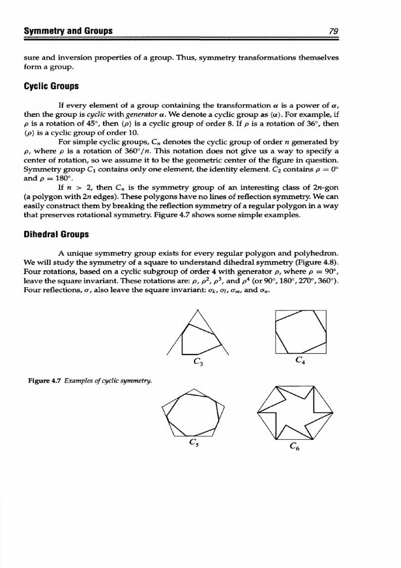
8/9/2019 Mortenson, Michael E. - Mathematics for computer graphics applications.pdf
http://slidepdf.com/reader/full/mortenson-michael-e-mathematics-for-computer-graphics-applicationspdf 92/367
Symmetry and Groups
79
sure and inversion properties
of
a group. Thus, symmetry transformations
themselves
form a group.
Cyclic
Groups
If
every element
of
a
group
containing
the
transformation
a is a power of a,
then
the group is cyclic
with generator
a.
We
denote
a
cyclic group
as (a).
For example,
if
p is a
rotation
of 450,
then
(p)
is
a cyclic
group
of
order
8.
If
p
is
a rotation of 360,
then
(p) is a cyclic group of order 10.
For
simple cyclic groups,
Cn
denotes the
cyclic group of order n
generated
by
p,
where
p is
a rotation
of
360'/n.
This
notation does
not
give us a way
to
specify a
center of rotation, so
we assume
it to be the geometric center of
the
figure in question.
Symmetry group
C
1
contains
only one
element,
the
identity
element.
C
2
contains
p
=
00
and
p = 180°.
If
n > 2, then Cn is
the
symmetry group of an
interesting
class
of 2n-gon
(a
polygon
with
2n
edges). These polygons have no lines of reflection symmetry. We
can
easily
construct
them by
breaking
the reflection symmetry of a regular polygon
in
a way
that
preserves rotational
symmetry.
Figure
4.7 shows
some
simple
examples.
Dihedral
Groups
A
unique symmetry group
exists for
every
regular polygon and polyhedron.
We
will
study
the symmetry
of
a square to
understand
dihedral symmetry
(Figure
4.8).
Four rotations, based on a cyclic subgroup
of
order 4
with
generator
p,
where
p = 900,
leave
the square invariant. These rotations
are:
p,
p2,
p
3
, and p
4
(or 900, 180°, 270°, 3600).
Four
reflections, a, also leave
the square invariant:
ak, al,
am, and an.
C3 C
4
Figure
4.7
Examples of
cyclic
symmetry.
C
6
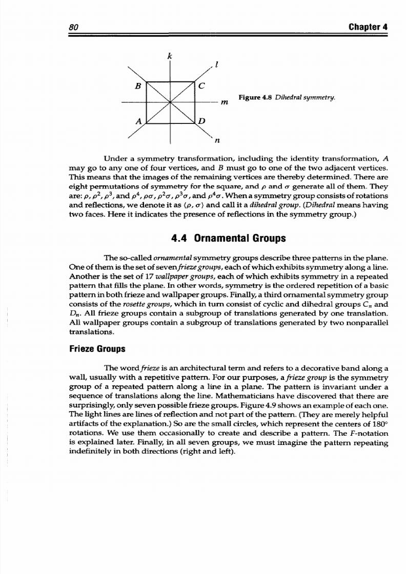
8/9/2019 Mortenson, Michael E. - Mathematics for computer graphics applications.pdf
http://slidepdf.com/reader/full/mortenson-michael-e-mathematics-for-computer-graphics-applicationspdf 93/367
80 Chapter 4
k
m
Figure 4.8
Dihedralsymmetry.
Under a
symmetry
transformation, including the
identity
transformation,
A
may
go to
any one
of
four
vertices,
and B must go to one
of
the two adjacent
vertices.
This
means
that
the images of the remaining
vertices are
thereby determined.
There are
eight
permutations
of symmetry
for
the square,
and
p and a generate all
of them.
They
are: p,
p
2
. p
3
, and p
4
, par, p
2
a,
p
3
a,
and
p4a
.
When
a
symmetry
group consists
of rotations
and reflections,
we denote
it
as (p, a)
and
call
it
a dihedral
group. (Dihedral
means
having
two faces. Here it indicates the presence of
reflections
in the symmetry group.)
4.4
Ornamental
Groups
The so-called
ornamental
symmetry groups
describe
three
patterns in
the
plane.
One
of
them is the
set of sevenfirieze groups,each of
which exhibits symmetry
along a line.
Another
is the
set
of
17
wallpapergroups,
each
of
which exhibits symmetry
in a
repeated
pattern that fills the plane. In other words, symmetry is the ordered repetition of a basic
pattern
in
both frieze and wallpaper
groups.
Finally, a third
ornamental symmetry group
consists of
the
rosette
groups,
which
in
turn
consist of
cyclic
and dihedral groups Cn and
Dn.
All
frieze groups contain
a
subgroup of translations
generated
by one translation.
All wallpaper
groups
contain
a
subgroup of
translations generated by two nonparallel
translations.
Frieze Groups
The wordfrieze is
an
architectural term and
refers to a
decorative
band along
a
wall, usually with
a repetitive
pattern. For our purposes, afrieze group is
the
symmetry
group of
a
repeated pattern along a line in
a
plane. The
pattern
is invariant under a
sequence of
translations along
the
line. Mathematicians have
discovered
that
there are
surprisingly,
only seven possible frieze
groups. Figure 4.9
shows
an example of
each one.
The
light lines
are lines of reflection
and not part of
the pattern.
(They
are merely
helpful
artifacts of
the
explanation.)
So
are
the small circles, which represent
the centers of
1800
rotations.
We
use them
occasionally to
create
and
describe
a
pattern.
The
F-notation
is
explained
later. Finally,
in
all
seven
groups, we
must
imagine the
pattern
repeating
indefinitely
in
both
directions
(right and left).
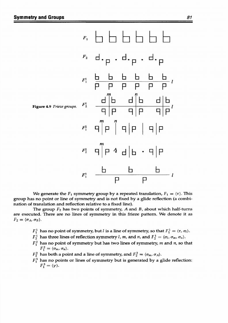
8/9/2019 Mortenson, Michael E. - Mathematics for computer graphics applications.pdf
http://slidepdf.com/reader/full/mortenson-michael-e-mathematics-for-computer-graphics-applicationspdf 94/367
Symmetry and Groups
81
F2 C .
.
Fb
b
Lb
b
P
P
P P
P
P
m n
Fb
d
b
L
b
Figure
4.9
Frieze
groups.
2
- P
9
P 9
-
m n
FQ,
9 |p
|~
9|q p
m
F
F
F' - P
P
We
generate
the
F,
symmetry group
by
a
repeated
translation,
F
1 =
(r).
This
group has no point
or
line
of symmetry and
is not
fixed
by
a
glide reflection (a
combi-
nation of
translation and reflection relative
to a
fixed
line).
The
group
F
2
has
two
points of symmetry,
A
and
B, about
which
half-turns
are executed.
There
are no lines
of symmetry in
this
frieze
pattern.
We denote
it
as
F
2
=
(a,,
UB)-
F1 has
no point
of
symmetry,
but
I
is a line
of
symmetry, so that
F 1 = (r, al).
F2
has three lines of reflection
symmetry 1,m, and n, and Fl
=
(al, am,
an).
F
2
has
no point
of
symmetry
but
has
two
lines of symmetry,
m
and
n,
so
that
F = (am,
Un).
F
2 has
both
a point
and
a
line
of
symmetry,
and
F= Um,
aA)-
F3 has no points or lines of symmetry
but
is
generated by a
glide reflection:
F3 =(y).
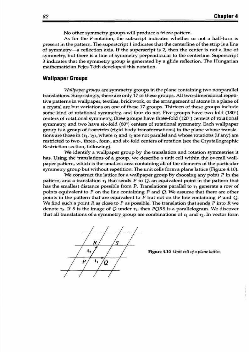
8/9/2019 Mortenson, Michael E. - Mathematics for computer graphics applications.pdf
http://slidepdf.com/reader/full/mortenson-michael-e-mathematics-for-computer-graphics-applicationspdf 95/367
82
Chapter 4
No
other symmetry groups
will
produce a frieze pattern.
As for the F-notation, the
subscript
indicates whether or not a
half-turn
is
present
in
the
pattern.
The superscript 1 indicates that the centerline of the
strip
is
a
line
of symmetry-a
reflection axis.
If
the superscript is 2,
then
the center
is
not
a
line
of
symmetry,
but there is
a
line of symmetry perpendicular to the centerline. Superscript
3 indicates that the symmetry group is
generated by a glide reflection. The Hungarian
mathematician
Fejes-T6th
developed this notation.
Wallpaper Groups
Wallpapergroupsare
symmetry groups
in
the plane
containing
two nonparallel
translations.
Surprisingly,
there
are
only 17
of
these groups. All two-dimensional repeti-
tive
patterns
in
wallpaper, textiles,
brickwork,
or
the arrangement
of atoms in a
plane of
a
crystal are
but
variations
on one
of
these
17
groups. Thirteen
of
these
groups
include
some
kind of rotational
symmetry, and
four do
not.
Five
groups have two-fold
(1800)
centers
of rotational
symmetry,
three groups have
three-fold (1200) centers of
rotational
symmetry,
and two have
six-fold (600) centers
of
rotational symmetry.
Each wallpaper
group is a group of
isometrics
(rigid-body transformations) in the plane whose transla-
tions
are
those in
rT,
T
2
),
where Ti and
T2 are
not parallel
and whose
rotations (if
any) are
restricted
to two-, three-,
four-,
and six-fold centers
of rotation (see
the Crystallographic
Restriction section, following).
We identify
a
wallpaper
group
by the
translation and rotation
symmetries it
has.
Using the
translations
of
a
group,
we
describe
a
unit
cell
within
the
overall
wall-
paper pattern,
which
is the smallest area containing all of the elements of the
particular
symmetry
group but without repetition. The unit cells form
a plane
lattice (Figure
4.10).
We construct the lattice for
a
wallpaper group by choosing any
point
P
in
the
pattern,
and
a
translation
rz that sends P
to
Q, an equivalent
point in the
pattern
that
has the smallest distance possible
from
P. Translations parallel to
ri
generate
a
row
of
points equivalent
to P on
the
line
containing P and Q.
We assume that there are other
points
in
the pattern
that
are equivalent
to
P but
not
on the
line
containing P
and
Q.
We
find
such
a
point R
as
close to
P as
possible. The
translation that sends
P into
R
we
denote r
2
. If S is the
image
of Q
under T2,
then
PQRS
is a parallelogram.
We discover
that all
translations
of a
symmetry group
are combinations
of Ti and
r2. In vector
form
Figure 4.10 Unit cell of a plane lattice.
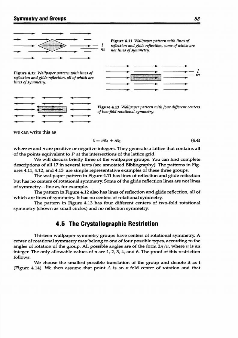
8/9/2019 Mortenson, Michael E. - Mathematics for computer graphics applications.pdf
http://slidepdf.com/reader/full/mortenson-michael-e-mathematics-for-computer-graphics-applicationspdf 96/367
Symmetry and Groups
a -----
- ,-
A
,
-
<
-
- --
.- -
1
m
Figure 4.11 Wallpaperpattern with
lines
of
reflection
and
glide
reflection,
some of which are
not
lines
of
symmetry.
Figure 4.12
Wallpaperpattern with
lines
of
reflection
and
glide
reflection,
all
of
which are
lines
of
symmetry.
- 0 ------- * -------- 0
Figure 4.13 Wallpaperpattern with
four
different centers
of
two-fold
rotational ymmetry.
we can write this as
where m and
n are positive
or
negative
integers. They
generate
a lattice
that
contains
all
of
the
points
equivalent
to P at
the
intersections
of
the
lattice grid.
We will discuss
briefly three of the wallpaper groups.
You
can find complete
descriptions
of
all
17
in
several texts (see annotated Bibliography).
The patterns in Fig-
ures
4.11,
4.12, and 4.13
are simple representative
examples of these three
groups.
The wallpaper
pattern
in
Figure 4.11 has lines
of reflection and
glide reflection
but
has
no centers of rotational
symmetry. Some of the glide reflection lines
are not lines
of symmetry-line
m, for
example.
The pattern in Figure
4.12 also has lines of reflection
and
glide
reflection,
all of
which
are lines of symmetry.
It
has
no centers of
rotational symmetry.
The
pattern
in
Figure
4.13
has
four different
centers of
two-fold rotational
symmetry (shown
as
small circles) and
no reflection symmetry.
4.5 The
Crystallographic
Restriction
Thirteen wallpaper
symmetry groups
have centers of
rotational symmetry.
A
center of rotational symmetry may belong
to one of four possible types, according
to the
angles
of rotation of the
group. All possible
angles
are
of the form
27r/n, where
n
is
an
integer. The
only allowable
values
of n are
1,
2,
3,
4,
and
6.
The
proof
of
this
restriction
follows.
We choose
the smallest
possible
translation
of the group
and
denote
it
as
t
(Figure
4.14).
We
then
assume that
point
A
is an n-fold
center of rotation
and
that
83
-.* --------- -
0 0 0 0
t = mt, + nt2
(4.4)
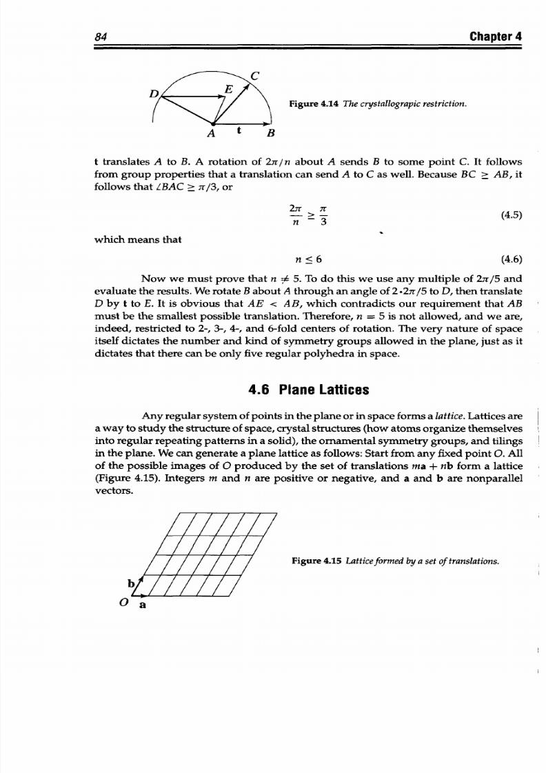
8/9/2019 Mortenson, Michael E. - Mathematics for computer graphics applications.pdf
http://slidepdf.com/reader/full/mortenson-michael-e-mathematics-for-computer-graphics-applicationspdf 97/367
84
Chapter 4
Figure 4.14
The
crystallograpic estriction.
t translates
A to
B.
A
rotation of 27r/ n about
A
sends B
to
some
point C. It
follows
from group
properties
that a
translation
can
send
A to C as well. Because BC >
AB,
it
follows
that
ZBAC
> Jr/3,
or
2:r
or
.2r
-
3(4.5)
n ~3
which means
that
n
<
6
(4.6)
Now we must prove
that
n
$
5.
To do
this we use
any
multiple of 2r/5 and
evaluate the results. We rotate
B about A
through
an
angle of 2.27r/5 to
D,
then
translate
D
by
t to E.
It
is
obvious that AE < AB, which contradicts
our
requirement
that AB
must be the smallest possible
translation. Therefore, n = 5
is not allowed, and we are,
indeed, restricted
to 2-, 3-, 4-, and 6-fold centers
of rotation. The
very
nature
of space
itself dictates the number and kind
of
symmetry groups
allowed
in the
plane, just as it
dictates that there can be only five regular polyhedra in
space.
4.6 Plane Lattices
Any regular system
of
points in the plane
or
in space forms a lattice.
Lattices
are
a
way
to
study
the
structure
of space,
crystal structures (how
atoms organize themselves
into
regular repeating
patterns
in
a solid), the
ornamental symmetry groups,
and tilings
in
the plane. We
can
generate a plane lattice as follows:
Start
from any
fixed point 0.
All
of
the
possible images
of
0
produced by
the
set
of
translations
ma
+
nb form
a
lattice
(Figure 4.15).
Integers
m
and
n are
positive or negative,
and a
and
b are
nonparallel
vectors.
Figure
4.15 Lattice
formed
by
a set of
translations.
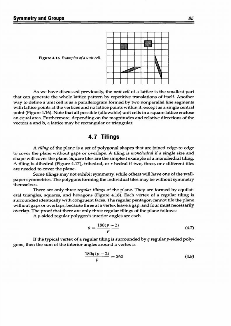
8/9/2019 Mortenson, Michael E. - Mathematics for computer graphics applications.pdf
http://slidepdf.com/reader/full/mortenson-michael-e-mathematics-for-computer-graphics-applicationspdf 98/367
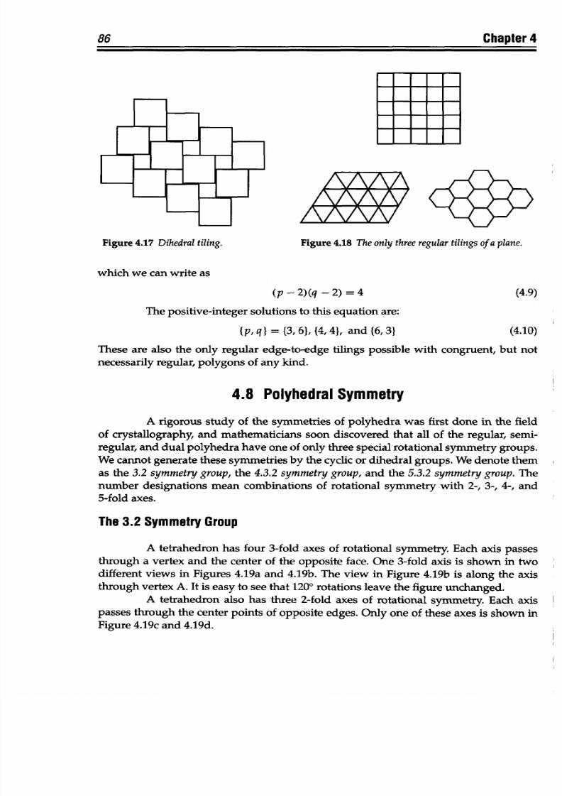
8/9/2019 Mortenson, Michael E. - Mathematics for computer graphics applications.pdf
http://slidepdf.com/reader/full/mortenson-michael-e-mathematics-for-computer-graphics-applicationspdf 99/367
86
Chapter
4
Figure
4.17
Dihedraltiling.
Figure
4.18
The
only
three
regular
tilings of
a
plane.
which we
can
write
as
(p -- 2)(q-2)
=
4
(4.9)
The
positive-integer
solutions to
this equation
are:
{p,
qI =
3, 61,
{4, 4}, and {6, 3}
(4.10)
These
are
also
the only
regular
edge-to-edge
tilings possible with congruent,
but not
necessarily
regular,
polygons
of
any kind.
4.8 Polyhedral Symmetry
A rigorous study
of the
symmetries of polyhedra
was
first
done in
the field
of crystallography,
and
mathematicians
soon discovered that
all of the
regular, semi-
regular,
and dual
polyhedra
have
one
of only three
special rotational
symmetry
groups.
We cannot
generate
these symm etries
by the cyclic
or
dihedral
groups. We
denote
them
as the
3.2
symmetry group,
the
4.3.2
symmetry
group,
and the
5.3.2
symmetry
group.
The
number
designations mean
combinations of
rotational
symmetry
with
2-, 3-, 4-,
and
5-fold axes.
The 3.2
Symmetry Group
A tetrahedron has
four 3-fold axes
of
rotational symmetry.
Each
axis
passes
through a vertex
and the
center
of
the opposite face.
One 3-fold axis is
shown in
tw o
different
views
in
Figures 4.19a
and
4.19b. The
view in
Figure 4.19b
is along the axis
through
vertex
A.
It
is easy
to
see that 1200
rotations
leave
the
figure
unchanged.
A
tetrahedron
also
has three
2-fold axes of
rotational
symmetry. Each
axis
passes through
the center
points
of opposite
edges.
Only one of
these
axes
is
shown in
Figure 4.19c
and 4.19d.
/'17VVA
AAAA/
AAAA/
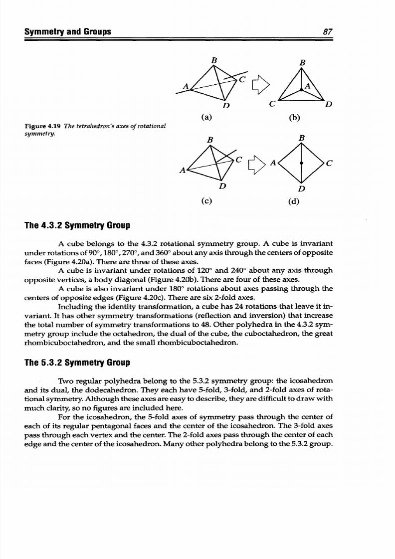
8/9/2019 Mortenson, Michael E. - Mathematics for computer graphics applications.pdf
http://slidepdf.com/reader/full/mortenson-michael-e-mathematics-for-computer-graphics-applicationspdf 100/367
87
ymmetry and
Groups
B
R
D C
(a)
(b)
Figure 4.19 The
tetrahedron's
axes of rotational
symmetry.
(c) (d)
The 4.3.2 Symmetry Group
A cube belongs
to the 4.3.2
rotational
symmetry
group.
A
cube is invariant
under
rotations
of
90, 180°,2700,
and
3600
about any
axis
through
the centers
of
opposite
faces (Figure 4.20a).
There
are three
of
these
axes.
A cube
is
invariant
under
rotations
of
1200
and
2400 about
any
axis through
opposite vertices, a body diagonal
(Figure 4.20b). There
are four
of
these axes.
A cube
is
also
invariant
under 1800 rotations
about axes
passing
through the
centers
of
opposite edges (Figure 4.20c). There are six 2-fold axes.
Including the
identity
transformation, a cube has 24 rotations that leave
it
in-
variant.
It has
other symmetry
transformations
(reflection
and inversion)
that
increase
the total number
of
symmetry transformations to 48. Other polyhedra in the 4.3.2 sym-
metry group
include the octahedron, the
dual
of
the
cube,
the cuboctahedron, the
great
rhombicuboctahedron,
and
the
small rhombicuboctahedron.
The
5.3.2
Symmetry Group
Two regular polyhedra belong to the 5.3.2 symmetry group: the icosahedron
and
its
dual,
the dodecahedron. They each
have
5-fold, 3-fold,
and
2-fold axes of rota-
tional
symmetry. Although
these axes are easy to describe, they are difficult to draw with
much clarity,
so
no figures are included
here.
For
the icosahedron,
the 5-fold
axes of
symmetry pass
through the center of
each of its regular pentagonal
faces
and
the center
of
the icosahedron.
The
3-fold axes
pass through
each vertex and the center.
The 2-fold axes
pass through
the center
of each
edge and the center
of
the icosahedron. Many other polyhedra belong to the 5.3.2 group.
0
D
D
0
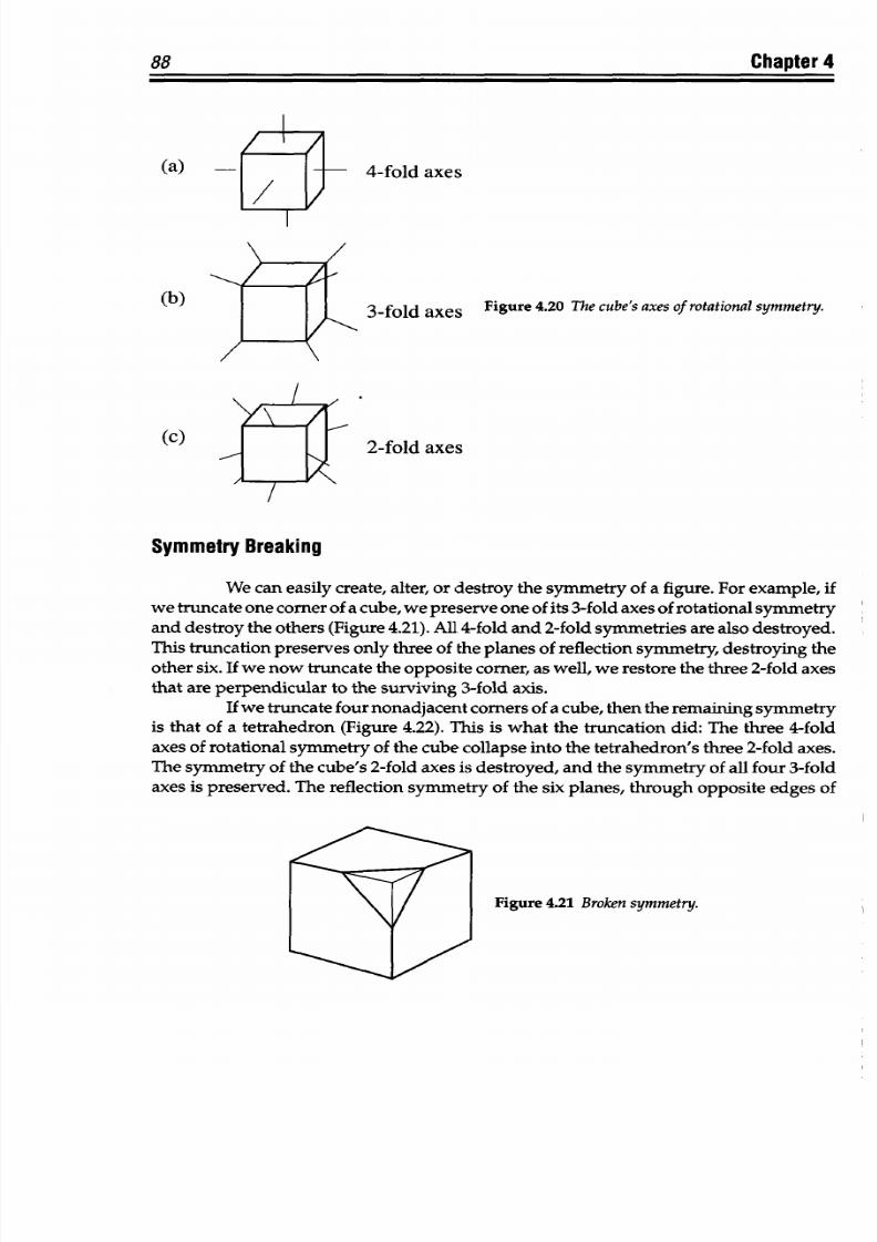
8/9/2019 Mortenson, Michael E. - Mathematics for computer graphics applications.pdf
http://slidepdf.com/reader/full/mortenson-michael-e-mathematics-for-computer-graphics-applicationspdf 101/367
88
(a)
Chapter 4
4-fold axes
(b)
cat
3-fold
axes
Figure
4.20
The cube's axes of
rotationalsymmetry.
2-fold axes
Symmetry
Breaking
We
can
easily create,
alter,
or
destroy the symmetry
of a
figure. For example,
if
we truncate
one
corner of
a
cube,
wepreserve
one
of
its 3-fold axes of
rotational symmetry
and
destroy the others (Figure
4.21). All
4-fold
and 2-fold
symmetries
are also
destroyed.
This
truncation
preserves
only
three of
the planes of
reflection
symmetry, destroying
the
other six. If we
now truncate the opposite
corner, as well, we
restore
the
three
2-fold axes
that
are
perpendicular
to the surviving 3-fold axis.
If we
truncate
four nonadjacent
corners
of
a cube,
then the remaining
symmetry
is
that
of a
tetrahedron
(Figure 4.22).
This
is
what
the
truncation
did:
The
three 4-fold
axes of
rotational symmetry
of
the
cube collapse
into
the
tetrahedron's
three
2-fold axes.
The symmetry
of the cube's 2-fold
axes is destroyed, and
the symm etry of
all four 3-fold
axes
is
preserved.
The
reflection symmetry
of the
six planes, through opposite edges
of
Figure 4.21
Broken
symmetry.
k-1
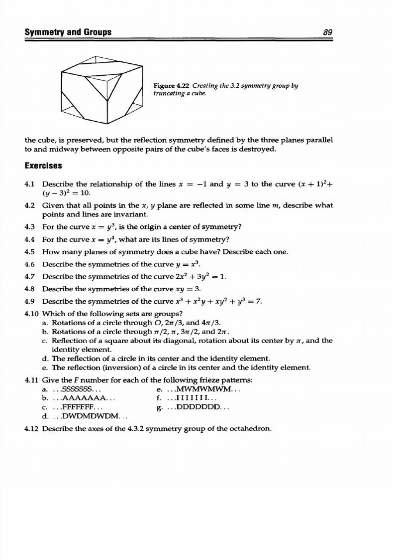
8/9/2019 Mortenson, Michael E. - Mathematics for computer graphics applications.pdf
http://slidepdf.com/reader/full/mortenson-michael-e-mathematics-for-computer-graphics-applicationspdf 102/367
89
ymmetry
and
Groups
Figure
4.22
Creating
he 3.2
symmetry group
by
truncatinga
cube.
the
cube,
is
preserved,
but the
reflection symmetry defined by
the
three
planes
parallel
to
and
midway
between opposite
pairs
of the cube's
faces
is
destroyed.
Exercises
4.1 Describe
the relationship of
the
lines
x
=
-1
and
y
= 3 to the curve (x
+
1)2+
(y -
3)2 =
10.
4.2 Given that
all
points
in the
x,
y
plane are
reflected
in
some
line
m, describe what
points and
lines are invariant.
4.3
For
the curve x =
y3,
is the origin a center
of
symmetry?
4.4
For
the curve
x
= y
4
, what
are
its lines
of symmetry?
4.5
How
many
planes
of
symmetry
does
a
cube have?
Describe
each
one.
4.6 Describe the symmetries
of
the curve y =
x
3
.
4.7 Describe
the
symmetries of
the curve
2x
2
+
3y
2
=
1.
4.8
Describe
the symm etries
of
the
curve
xy
=
3.
4.9 Describe the symmetries of the curve
x
3
+ x
2
y + xy
2
+ y
3
=
7.
4.10
Which of the following sets are
groups?
a.
Rotations
of
a circle through 0, 27r/3, and 47r/3.
b.
Rotations of
a circle
through 7r/2, 7r,
37r/2, and
27r.
c.
Reflection of a square
about
its
diagonal, rotation about
its
center by
7r,
and
the
identity
element.
d.
The reflection of
a circle in
its
center
and
the identity
element.
e. The reflection (inversion) of a
circle
in its center and the
identity
element.
4.11 Give
the
F number for each of
the following
frieze
patterns:
a. ... SSSSSSS...
e....4W
4WIWM...
b. ...AAAAAAA... f. ... IIIIIII...
c.
...
FFFFFFF... g.
...
DDDDDDD...
d.
... DWDMDWDM...
4.12
Describe the axes
of
the
4.3.2 symmetry
group of
the
octahedron.
8/9/2019 Mortenson, Michael E. - Mathematics for computer graphics applications.pdf
http://slidepdf.com/reader/full/mortenson-michael-e-mathematics-for-computer-graphics-applicationspdf 103/367
(X;
pTa
LIMIT AND CONTINUITY
Soon after geometrybecame a
separatebranch
of mathematics,
geometersbegan
to
study
problems
they
could best solve
by
processes
that they
imagined
could
be continued
in-
definitely. These
were problems
related to
vanishingly
small distances,
and
problems
related to sets containing infinitely many
elements. For
example, a circle begins
to
co-
incide with the
limiting figure
of
a regular polygon
inscribed
in it
as
we increase
the
number of
sides,
giving
rise to the
concept
of a
nonending
process. Or, we can succes-
sively halve the distance
between
two
points
AB
on
a
straight
line segment
to
produce
lengths 1/2, 1/4,
1/8, ... , 1/2"
that of
the
initial
length, again
setting
off a nonending
process
and introducing vanishingly small distances. Furthermore, the set of
points
on
a line segment is an infinite set. All of
these
processes are related to the continuity of line
segments and to the concept
of limit.
These, in
turn, provide
the
basis
for the calculus.
Limit
and
continuity
processes are
at
work
in computer graphics applications
to ensure the
display
of smooth, continuous-looking curves and surfaces. They are an
important
consideration
in
the construction
and
rendering
of
shapes
for computer-aided
design and manufacturing, scientific visualization, and similar
applications.
This
chapter
explains
limit
and
continuity. It begins with the Greek
method
of
exhaustion, which appeals strongly to our
intuition
and
sets the stage for a more rigorous
discussion of the limit process to come. The section on sequences
and
series extends this
appeal to
numbers
and algebra.
The
chapter
then
reviews
the definition of a
function
and follows this
with
discussions of the
limit of
a
function,
limit
theorems and rules,
and
limit
and
the definite integral. The next two topics again appeal to
our
intuition,
but with strong support from the more quantitative
and
analytical side of mathematics:
these are the
tangent
to a curve, and rate of change.
A
discussion of intervals supports
the concluding two sections
on continuity
and
continuous
functions.
Although this
chapter reviews much of
the
material usually introduced
in first-
year
calculus, its
purpose
is to highlight and
re-emphasize these
concepts,
because
they
occur over
and
over again in more
advanced
studies.
5.1
The
Greek Method of Exhaustion
Behind the innocent
word
"limit" is a subtle process, simple to describe, but
awesome in its
implications. It is the cornerstone of
the
calculus. The story of the
90
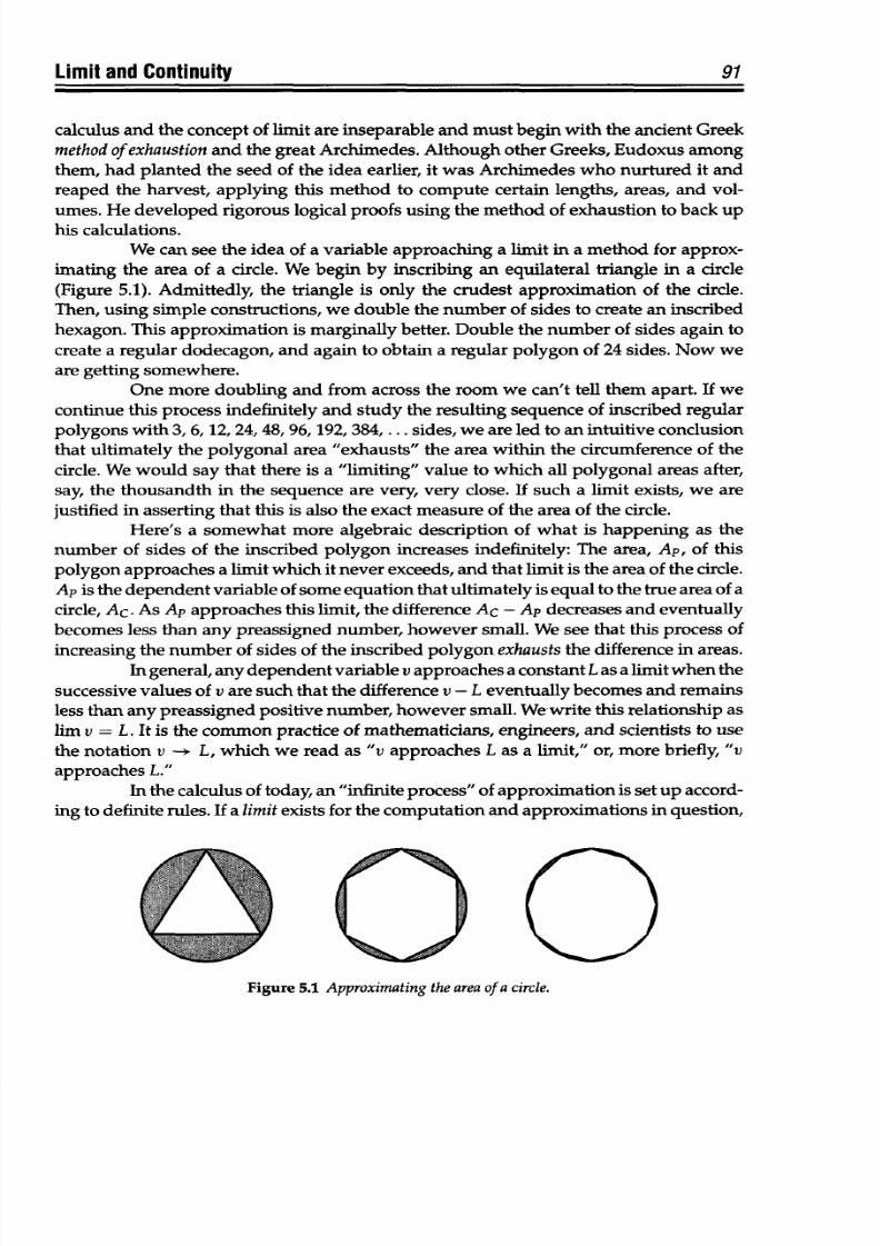
8/9/2019 Mortenson, Michael E. - Mathematics for computer graphics applications.pdf
http://slidepdf.com/reader/full/mortenson-michael-e-mathematics-for-computer-graphics-applicationspdf 104/367
Limit and Continuity
91
calculus
and the
concept
of limit are inseparable and
must
begin with the ancient
Greek
method ofexhaustion and the
great
Archimedes.
Although other
Greeks,
Eudoxus
among
them, had planted
the
seed
of
the idea earlier, it was Archimedes who nurtured it and
reaped the harvest, applying
this
method
to
compute
certain
lengths,
areas,
and
vol-
umes.
He
developed
rigorous logical proofs using
the method
of exhaustion
to back
up
his calculations.
We
can
see
the
idea
of
a variable
approaching
a limit
in
a
method
for
approx-
imating the area
of
a circle.
We begin by inscribing an equilateral triangle
in a circle
(Figure
5.1). Admittedly,
the triangle
is only
the
crudest
approximation
of
the
circle.
Then, using
simple constructions, we
double
the number of sides to
create
an
inscribed
hexagon. This
approximation is marginally better. Double the
number of
sides again to
create a
regular
dodecagon, and again to
obtain
a regular
polygon
of 24 sides. Now
we
are
getting somewhere.
One more doubling and
from across
the room we
can't
tell them apart. If we
continue this process indefinitely and study the
resulting
sequence
of
inscribed regular
polygons
with
3, 6, 12, 24,
48,
96, 192,
384, ... sides,
we
are led to an
intuitive
conclusion
that
ultimately the
polygonal
area
"exhausts" the
area within the
circumference
of the
circle.
We
would say that there is a "limiting"
value
to
which
all
polygonal
areas after,
say, the thousandth
in
the sequence are very, very close. If
such
a
limit
exists, we are
justified in asserting
that
this is also the
exact
measure of the
area
of the circle.
Here's
a
somewhat
more
algebraic
description
of what
is happening as the
number of
sides
of
the inscribed polygon
increases indefinitely: The area, Ap, of this
polygon
approaches a limit
which
it
never
exceeds, and that limit is the area of
the
circle.
Ap is the dependent
variable
of some
equation
that
ultimately
is
equal
to
the
true area of
a
circle, Ac. As Ap approaches
this limit,
the difference
Ac
-
Ap
decreases and
eventually
becomes less
than
any
preassigned
number, however small. We see that
this
process of
increasing the
number of
sides of the inscribed polygon
exhausts
the
difference in areas.
In general,
any
dependent variable v approaches a constant Las a limit when
the
successive values of
v
are such
that the
difference
v -
L eventually becomes and remains
less
than any preassigned positive
number,
however
small.
We write
this relationship as
lim v = L. It is the common practice of mathematicians, engineers, and scientists to use
the
notation v
-*
L,
which
we read
as
"v
approaches
L
as
a
limit,"
or,
more
briefly,
"v
approaches
L."
In
the
calculus of today,
an
"infinite process" of
approximation
is set up accord-
ing
to
definite rules. If a limit
exists for
the computation and approximations in question,
Figure
5.1
Approximating
the area
of
a
circle.
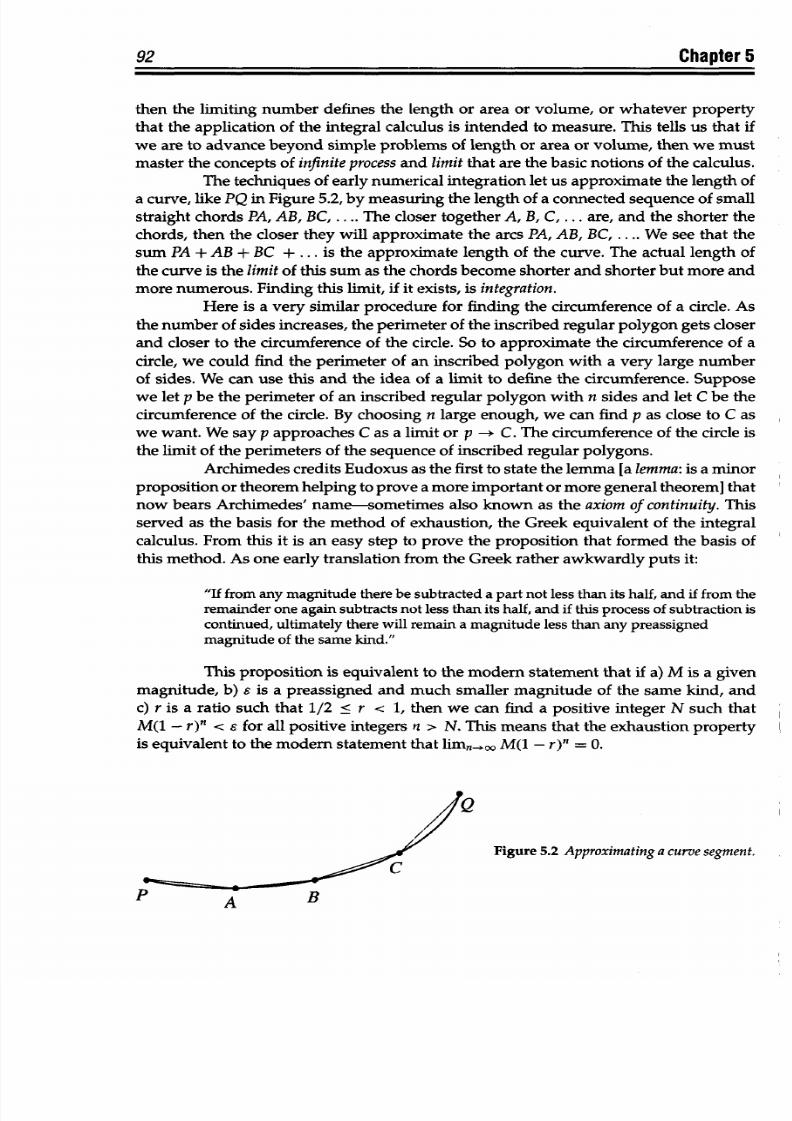
8/9/2019 Mortenson, Michael E. - Mathematics for computer graphics applications.pdf
http://slidepdf.com/reader/full/mortenson-michael-e-mathematics-for-computer-graphics-applicationspdf 105/367
92
Chapter
5
then
the
limiting
number defines the length or
area
or volume, or
whatever
property
that the app lication
of the
integral calculus is intended
to
measure. This tells
us
that if
we
are to advance beyond simple problems of length or area
or
volume,
then
we
must
master the
concepts
of
infinite
process
and
limit
that
are
the
basic
notions
of
the
calculus.
The
techniques of early numerical integration let us approximate the length of
a
curve,
like
PQ
in
Figure 5.2, by measuring the
length of
a connected sequence of
small
straight chords PA,
AB,
BC, .... The
closer
together A, B, C, ... are, and the shorter the
chords, then
the closer they
will approximate the arcs PA,
AB,
BC, ..
We see
that
the
sum PA + AB +
BC + . . . is the approximate length
of
the
curve.
The actual length of
the
curve is
the
limit
of this sum as the
chords
become shorter and
shorter
but
more and
more numerous. Finding this limit, if it
exists,
is integration.
Here
is
a very similar procedure for finding the circumference
of
a circle.
As
the number of
sides
increases, the
perimeter
of
the inscribed
regular polygon gets closer
and
closer
to
the
circumference
of
the
circle.
So
to approximate the
circumference of
a
circle,
we could find the perimeter of
an inscribed polygon with a very large number
of sides. We
can use this and the idea
of a limit
to define
the
circumference. Suppose
we let p
be
the perimeter of an
inscribed
regular
polygon
with
n
sides and
let
C be
the
circumference
of
the circle.
By
choosing
n
large enough, we
can find
p as close
to C
as
we want.
We say p
approaches
C as a
limit
or
p
-+ C.
The
circumference of
the
circle is
the limit
of
the perimeters
of
the sequence of inscribed regular polygons.
Archimedes credits Eudoxus as the first
to state the lemma [a lemma: is a minor
proposition or
theorem helping to prove a
more
important
or more
general theorem]
that
now
bears Archimedes'
name-sometimes
also
known
as
the
axiom
of
continuity.
This
served as the
basis
for the
method
of
exhaustion,
the Greek equivalent of the integral
calculus.
From
this it is
an
easy step
to
prove
the
proposition that formed the basis of
this method.
As
one early
translation
from the
Greek
rather awkwardly puts it:
"If
from
any
magnitude
there be
subtracted a part not
less than
its
half, and if
from the
remainder one again subtracts
not less
than its
half,
and if this
process of
subtraction
is
continued, ultimately there
will
remain a
magnitude less than
any preassigned
magnitude of
the same kind."
This
proposition
is
equivalent to
the modern statement
that
if
a)
M
is
a
given
magnitude, b)
e
is a preassigned and much smaller magnitude of the same kind, and
c) r
is a
ratio such
that
1/2 < r <
1,
then we
can
find
a
positive integer N such that
M(1
r)"
<
s for all positive integers n > N. This means that
the
exhaustion property
is equivalent to
the modern statement
that lim,,,
x
M(1
- r)" = 0.
Figure
5.2
Approximating a
curve
segment.
r
A H
8/9/2019 Mortenson, Michael E. - Mathematics for computer graphics applications.pdf
http://slidepdf.com/reader/full/mortenson-michael-e-mathematics-for-computer-graphics-applicationspdf 106/367
Limit and Continuity
93
5.2 Sequences
and Series
The
method of
exhaustion and its variations shows
us how
to add
smaller
and
smaller bits of area or length
so
that the accumulated total approaches some limiting
area
or
length. Certain sets
of real numbers may also approach some limiting value.
We
begin with
some definitions.
A sequence
is
a succession
of
terms in a particular order and is formed according
to some fixed rule. For example:
and1, X,
2
X
3
X
1,4,9,16,25,... and
1
(5.1)
The
first, of course,
is the sequence of
squares
of the natural numbers,
and
the
second
follows from a somewhat
more complicated formula, soon
explained.
A
series
is
the sum of the terms of a sequence.
From the
above
sequences
we
construct the
following
series:
x
2
X
3
1+4+9+16+
- and 1-x+--T2-+*
(5.2)
2 3
When the number of terms
is
fixed and countable, the sequence or series is
finite. An infinite
sequence has infinitely many
terms,
as
many terms,
in
fact,
as
there
are natural numbers.
In
these sequences, we are usually interested in what happens in
the long run.
We
want
to find
out what happens
to
the
nth
term
when
n
becomes
very
large. For
example, in the sequence 1,
1/2,1/3,1/4,1/5,
.. . , 1/n, the terms get smaller
and
smaller,
getting
closer
and
closer to
0.
This infinite sequence approaches zero as the
limiting value. We indicate this by writing
lim
-= (5.3)
n-iox
n
again, where
"him"
stands for limit and
"n
-* oo" stands for n approaches infinity or, in
other
words
n increases beyond
any bound.
The general,
or
nth,
term
is
an expression which
describes
how
to
construct the
individual terms. In the first
example
above, the general,
or nth,
term is
n
2
. Here we
construct the first term by setting
n =
1,
the second term by setting
n = 2, and
so on.
In
the second
example,
the nth term,
except
for n =
1, s
--
(5.4)
To indicate that a
sequence
or series continues
indefinitely,
we
use
the ellipsis,
a
set
of three dots,
as
in
1,
49 n
2
(5.5)
Here
is a
geometric
series
of
n terms:
Sn
=a
+ar +ar2
+ .*
+arn-
(5.6)
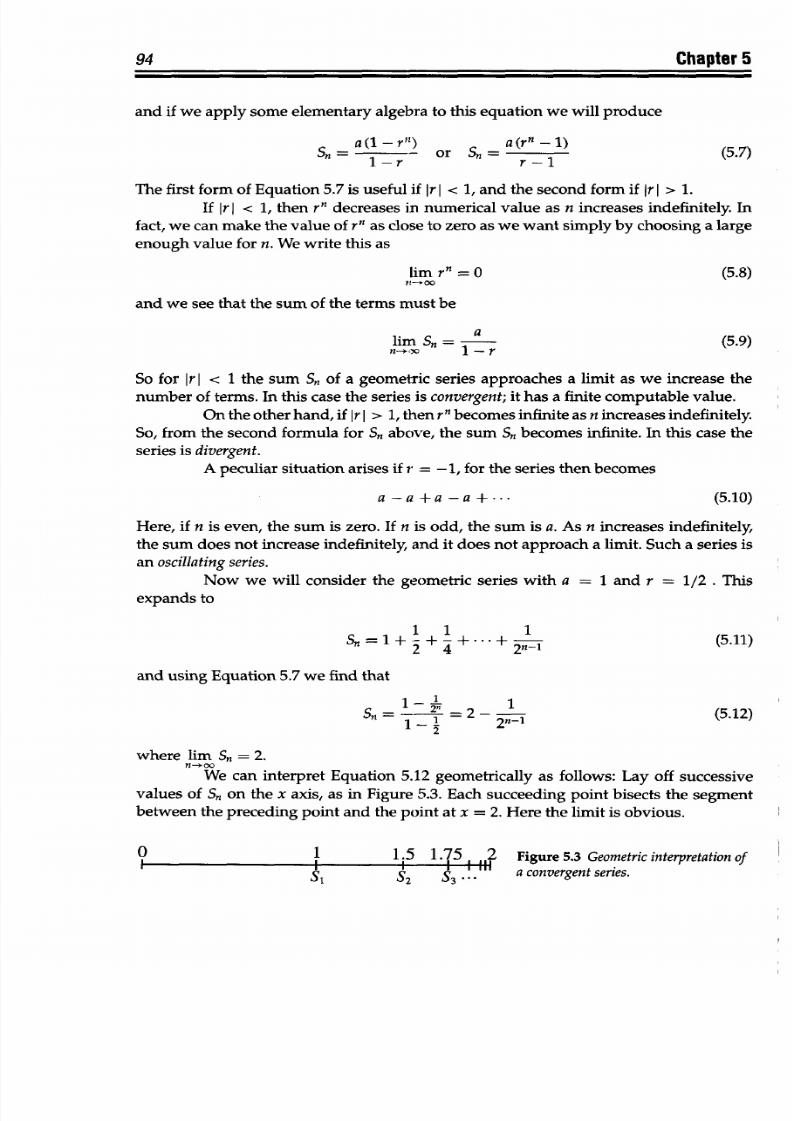
8/9/2019 Mortenson, Michael E. - Mathematics for computer graphics applications.pdf
http://slidepdf.com/reader/full/mortenson-michael-e-mathematics-for-computer-graphics-applicationspdf 107/367
8/9/2019 Mortenson, Michael E. - Mathematics for computer graphics applications.pdf
http://slidepdf.com/reader/full/mortenson-michael-e-mathematics-for-computer-graphics-applicationspdf 108/367
Limit and
Continuity
95
The
limit
of
a
sequence is
a
special type, because a sequence
is
afunctionwhose
domain
is the set
of
natural
numbers, {1, 2, 3, . . ., n), ordered
according
to size.
The range,
that is
the set
of
function
values, listed in the corresponding order,
is
{al, a2, a
3
, . . . an),
the ordered
set,
which
is
a
sequence.
Notice that subscripts
will play
a
bookkeeping role
for
us, to help us keep track
of similar terms and their order. At the very
least,
they serve as simple identification
tags.
Using numbers
for
subscripts
usually,
but not
necessarily, indicates an ordering of some
sort: We may read t
1
as "the
first
time" and t
2
as "the second time"
of
some sequence of
events.
Furthermore, mathematicians
usually
reserve the
lowercase
Roman italic letters
i, j, k, m,
and
n
for
subscripts on
a
general
or intermediate term of an
expression or
sequence
of
similar terms.
We can use the behavior of sequences
and series
to help
us to
define limits
more
carefully. Here are
four
different
sequences,
where
we
let
n
-*
oo:
1.
an =
(n - 1)/(n + 1):
For sufficiently large
n we
ignore
the l's and see that
an 1.
2.
an = lan- + 2:
No
matter
what value
of a,
we
start
with, we
will always
find that an -- 4.
3. an = the chance
of
living to the age
of
n years: Since the fountain of youth is
as
yet undiscovered,
we
can sadly
but safely
assume that an
-+ 0.
4. an
=
the
proportion
of zeros among
the
first n digits of 7: Since
the
digits of
7r
do not form
a
repeating sequence, we can expect
that
an -+ 0.10.
Let
us see
what
is required of
a sequence
of positive
numbers
for it to approach
zero. In
other words,
what
do
we mean when we
write an
-* 0? Clearly, the numbers
{a,,
a
2
, a
3
,
. . . an) must somehow become smaller. In
fact,
for any small
number
we
can
specify the
ans
must eventually go
below
that number and stay below it.
We test
for
convergence to
zero by choosing
some
small number-let's try 10-6
(that's one millionth
or 1/1,000,000).
Then for some n, the a, must be less
than
that
number
and
stay below
it.
Before
that
point
in
the sequence, a, may oscillate above and
below
our arbitrary
threshold
limit
of
10-6,
but eventually all
terms must go
below this
limit. Later
in the
sequence,
maybe much
later, all
terms
must
be
less
than,
say,
10-12.
Obviously,
we can continue this process indefinitely.
It
does not
matter how
many terms
must pass in a sequence
before
values
of
all succeeding terms fall below
and
remain
below these ever decreasing and arbitrary threshold values. Because the sequence does
eventually meet this
test,
we conclude that the sequence does indeed converge to
zero,
or
approach zero as a
limit.
The sequence 10-3, 10-2, 10-6, 1i-0, lo -
9
,
10-8, ... converges to zero.
Even
though the values oscillate up and down, at some point
all
the succeeding
numbers
eventually stay below
any
arbitrarily
small number.
However, we
see that the sequence 10-4,
10-6,
10-4, 10-8, 10-4, 10-1o, ...
does
not
converge to
zero, because
the values do not remain
less than 10-4.
Mathematicians, engineers, and scientists
often
use
the Greek lower case letter
E (epsilon) to represent an
arbitrarily
small
positive
number, and
we will do
the same.
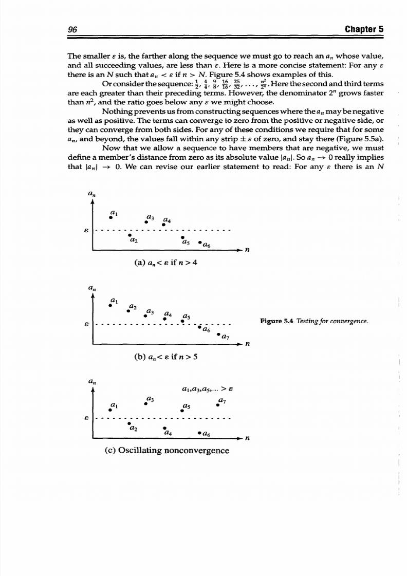
8/9/2019 Mortenson, Michael E. - Mathematics for computer graphics applications.pdf
http://slidepdf.com/reader/full/mortenson-michael-e-mathematics-for-computer-graphics-applicationspdf 109/367
Chapter 5
The smaller
e is, the
farther
along the sequence we must
go to
reach an a,
whose
value,
and
all
succeeding
values, are less
than
e. Here is
a
more concise statement: For any e
there is an N such that
an <
e
if
n
> N. Figure
5.4
shows examples of this.
Or consider
the sequence:
1
4
9
16 25'.
,,
n2.
Here
the
second
and
third
terms
2'
4
8'
16
32 **
2'
are
each greater
than
their
preceding terms. However,
the
denominator
2"
grows
faster
than n
2
, and the ratio goes below any s we
might
choose.
Nothing prevents
us from constructing sequences
where
the
a, maybe negative
as well as
positive. The terms can converge
to
zero
from the
positive
or negative
side, or
they can
converge from
both
sides. For any of these conditions we require
that
for some
an, and beyond, the
values
fall
within
any strip ± e of zero, and
stay
there (Figure 5.5a).
Now
that we
allow a sequence to have
members that
are negative, we must
define a
member's
distance from zero as
its
absolute value
IanI.
So a, -+ 0 really implies
that
lad -* 0.
We
can
revise
our earlier statement to read:
For any
e there
is an N
a
a
£
al
a3 a
4
0
a
2
a
5
*a6
(a) an<
s
if
n
>4
a
1
In
,' a,
* a
2
0
a3 a4 a
5
0
. .. .. . . . . . . .... . .. .. . .
6a
6
I Oa
7
n
n
Figure 5.4 Testingfor convergence.
(b) a,,<
s
if n>
5
a
3
0
a
2
a
5
a
4
96
a,
0
£
a
7
*a
6
ni
(c) Oscillating nonconvergence
aj,a3,a5,-..
>
e'
. . . . . . . . . . . . . . . . . . . . . . . .
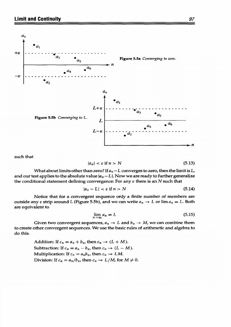
8/9/2019 Mortenson, Michael E. - Mathematics for computer graphics applications.pdf
http://slidepdf.com/reader/full/mortenson-michael-e-mathematics-for-computer-graphics-applicationspdf 110/367
Limit
and Continuity
+6
-£
*a,
.......... ...... . . . .o - - - - - - - - - - - - - - -
a
3
9
a
5
Figure 5.5a
Converging to
zero.
,a
6
0
a
2
Figure 5.5b Converging to
L.
L
IaQI <
Eifn
>
N
What
about limits
other than zero? If an L converges to zero, then the limit
is
L,
and
our
test
applies to
the absolute
value la, - L 1.
Now we
are ready to further
generalize
the
conditional
statement
defining
convergence: For
any £ there
is
an
N such that
lan-L I
<eifn>N
(5.14)
Notice
that
for
a
convergent
sequence
only
a
finite
number
of members
are
outside
any e
strip
around
L (Figure 5.5b), and we can write an -+ L or
liman
= L.
Both
are equivalent
to
lim
an = L
n-xoo
(5.15)
Given two
convergent
sequences, an
--
L and bn -+ M, we can combine them
to create other
convergent
sequences. We use the
basic
rules of
arithmetic
and algebra to
do
this.
Addition: If
cn
= an + bn,
then
cn
- (L + M).
Subtraction:
If
cn
=
an-
bn,
then cn
-+ (L -
M).
Multiplication: If cn =
anbn, then cn - LM.
Division:
If cn =
an/bn, then
Cn -+ L/M, for
M
:
0.
97
such that
(5.13)
. . . . . . . . . . . . . . . . . . . . . . . . .
L+s
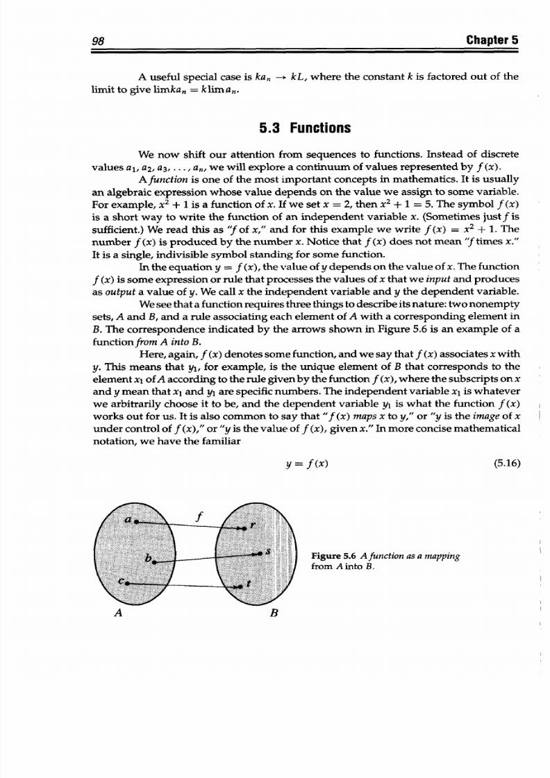
8/9/2019 Mortenson, Michael E. - Mathematics for computer graphics applications.pdf
http://slidepdf.com/reader/full/mortenson-michael-e-mathematics-for-computer-graphics-applicationspdf 111/367
98
Chapter
5
A useful special case
is kan -+
kL,
where
the
constant
k
is
factored out of the
limit
to
give
limkan
= klima,.
5.3 Functions
We now shift our attention from sequences
to
functions. Instead of discrete
values a,, a
2
, a
3
,
. . ., a,,
we will
explore
a
continuum
of values represented by f
(x).
A
function
is one of the
most
important
concepts
in mathem atics. It is usually
an
algebraic expression
whose value
depends on
the
value we assign
to
some
variable.
For example, x
2
+ 1 is
a
function
of x.
If
we set x = 2, then x
2
+ 1 = 5. The
symbol f (x)
is
a short
way
to
write the
function
of an
independent variable
x. (Sometimes
just
f is
sufficient.)
We read this as
f of
x,"
and for this
example we
write f
(x) =
x
2
+ 1. The
number
f (x) is
produced by
the
number
x.
Notice
that
f (x) does
not
mean f times x."
It
is a
single, indivisible symbol standing for some function.
In the equation
y =
f
(x),
the value of
y
depends on the value of x.
The function
f (x) is
some expression or
rule that
processes
the
values
of x
that we input and produces
as output a
value
of
y. We
call x the
independent variable
and y the
dependent
variable.
We see
that
a
function requires
three
things to
describe its
nature: two nonempty
sets, A and
B, and
a rule associating
each element of A
with
a corresponding
element in
B. The
correspondence
indicated by
the arrows shown in Figure
5.6
is
an example of a
function
from
A
into B.
Here,
again,
f
(x)
denotes some function,
and
we say
that
f
(x)
associates
x
with
y. This means that
yi,
for example, is
the unique element of B
that corresponds
to the
element xl ofA according to the rule given by the function f (x), where the subscripts on x
and y mean
that
xi
and
yi
are
specific numbers. The
independent variable xl is whatever
we arbitrarily
choose it
to
be,
and
the dependent variable
yi
is
what
the function
f (x)
works out for
us. It
is
also common
to
say that "f
(x) maps x to y," or "y
is
the
image
of
x
under control of f (x)," or "y is the
value of f (x), given
x."
In more concise
mathematical
notation, we
have the familiar
=
f
(x) (5.16)
f
Figure
5.6 A function
as
a
mapping
from
A
into
B.
A
B
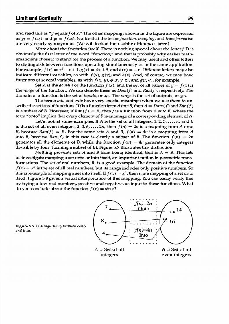
8/9/2019 Mortenson, Michael E. - Mathematics for computer graphics applications.pdf
http://slidepdf.com/reader/full/mortenson-michael-e-mathematics-for-computer-graphics-applicationspdf 112/367
Limit and
Continuity
99
and read this as "y equalsf of
x."
The other mappings shown in the figure
are
expressed
as y2
= f
(x
2
),
and y3 =
f
(x
3
).
Notice that the termsfunction,
mapping, and transformation
are
very nearly
synonymous. (We
will look at their
subtle
differences later.)
More
about
theft
notation
itself:
There
is
nothing
special
about the
letter It
is
obviously the first
letter of
the word
"function," and
that
is probably
why
earlier math-
ematicians chose it
to
stand
for
the
process
of a function. We
may
use it and
other
letters
to distinguish between functions operating simultaneously or in the same application.
For
example,
f
(x)
=
x2-X +
1,g(x)
= 4x +
3,
and h(x) = -x. Different letters
may
also
indicate different variables, as with f
(x), g(y),
and h(z). And, of course, we may have
functions of several variables, as with f
(x, y),
qi (x, y, z), and g(r, 9), for example.
Set A is the
domain
of the
function f (x), and
the set of
all
values of y
= f (x) is
the range of
the
function. We can denote
these
as Dom(f) and Ran(f),
respectively.
The
domain of
a
function is the
set
of inputs, or xis. The range
is the
set
of
outputs,
or yis.
The terms into
and
onto have very special meanings when we use them to de-
scribe the actions of functions.
Iffis
a
function
fromA intoB,then A
=
Dom(f )
and
Ran(f )
is a
subset of
B. However,
if
Ran(f)
= B, thenf is a
function
from
A onto B, where
the
term "onto" implies that every element of B is an image of
a
corresponding element of A.
Let's look at
some examples.
If A is the set of all integers, 1,
2,
3, ..., n,
and
B
is the set
of all even integers, 2, 4, 6,
. . .,
2n, then f (n) = 2n
is a
mapping from A onto
B,
because
Ran(f)
=
B.
For the same sets A
and
B, f (n)
=
4n is a
mapping
from A
into
B,
because Ran(f) in this
case
is
clearly
a
subset
of B. The
function f(n) =
2n
generates all the elements of B, while the function f (n) =
4n
generates only integers
divisible by four (forming
a
subset
of
B).
Figure
5.7
illustrates this
distinction.
Nothing prevents
sets
A
and
B from being
identical, that is
A = B.
This lets
us investigate mapping a
set onto
or into
itself, an
important
notion
in
geometric trans-
formations. The set of real numbers, R, is a
good
example. The domain of the
function
f
(x)
=
x
2
is the
set of all real numbers,
but its range includes
only
positive
numbers. So
it is an example of mapping
a set
into itself. If f (x) = x
3
,
then it
is a
mapping
of a
set
onto
itself. Figure 5.8 gives
a
visual interpretation
of
this mapping. You can easily verify this
by
trying
a
few
real numbers, positive and negative, as input to
these
functions.
What
do
you
conclude
about
the function f
(x)
= sin x?
Figure
5.7
Distinguishing
between onto
and
into.
A = Set
of all B
= Set
of
all
integers even integers
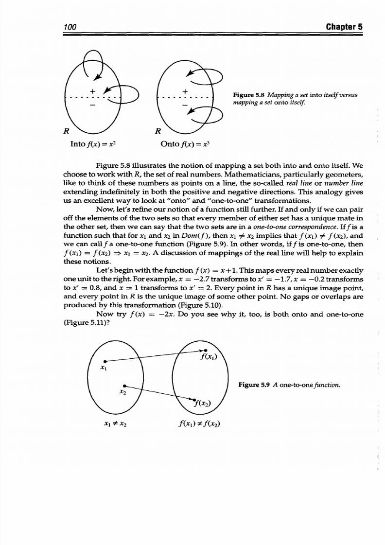
8/9/2019 Mortenson, Michael E. - Mathematics for computer graphics applications.pdf
http://slidepdf.com/reader/full/mortenson-michael-e-mathematics-for-computer-graphics-applicationspdf 113/367
100
Chapter
5
Figure 5.8
Mapping
a set
into
itself
versus
mapping a set onto
itself.
Into f(x) =
X2
Onto flx)
=X3
Figure
5.8
illustrates the notion
of
mapping
a
set
both
into and onto
itself.
We
choose
to
work with
R, the set
of
real numbers. Mathematicians, particularly
geometers,
like to think
of these
numbers
as
points
on a line,
the
so-called
real line or number line
extending indefinitely
in both the positive and
negative
directions. This
analogy
gives
us an
excellent way
to look
at "onto" and
"one-to-one"
transformations.
Now,
let's refine our notion
of a function
still further.
If
and
only if
we can
pair
off
the
elements of
the two sets so
that every member of
either
set has
a unique
mate
in
the other set, then we can
say
that
the
two sets
are in
a one-to-one correspondence.
Iff is a
function such that for
xl and x
2
in
Dom(f
),
then
xl
:A x
2
implies
that
f (xI) : f (x
2
),
and
we
can call
f
a
one-to-one
function
(Figure
5.9).
In other words,
if
f
is one-to-one,
then
f (xi)
=
f
(x
2
)
X*xi = x
2
. A
discussion
of
mappings of
the
real
line will help to explain
these
notions.
Let's begin
with
the function f
(x)
= x + 1.This maps
every
real
number exactly
one unit
to the
right. For
example, x = -2.7
transforms
to
x' = -1.7,
x
=
-0.2 transforms
to
x'
=
0.8, and
x
= 1 transforms
to
x'
= 2. Every point
in
R
has
a
unique
image point,
and
every
point in
R
is the unique image of some
other point.
No
gaps
or overlaps are
produced by this
transformation (Figure
5.10).
Now try
f
(x)
=
-2x.
Do
you
see
why it, too, is both
onto and one-to-one
(Figure 5.11)?
Figure
5.9
A
one-to-one unction.
xf(x) •f(x
2
)
A
Xl
#X2
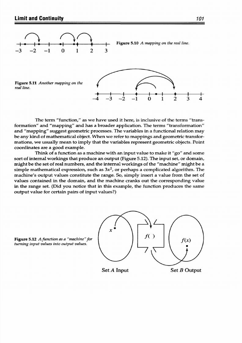
8/9/2019 Mortenson, Michael E. - Mathematics for computer graphics applications.pdf
http://slidepdf.com/reader/full/mortenson-michael-e-mathematics-for-computer-graphics-applicationspdf 114/367
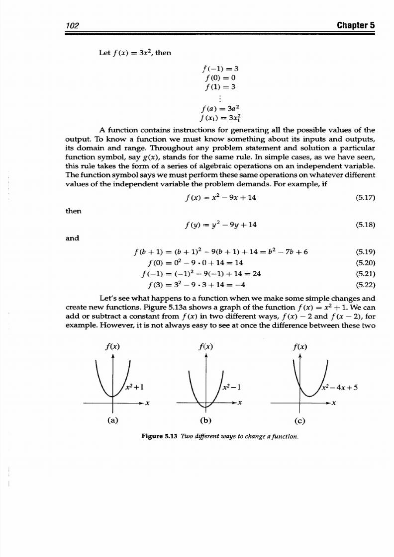
8/9/2019 Mortenson, Michael E. - Mathematics for computer graphics applications.pdf
http://slidepdf.com/reader/full/mortenson-michael-e-mathematics-for-computer-graphics-applicationspdf 115/367
102
Chapter 5
Let f
(x)
= 3x
2
, then
f (-1) = 3
f
(0)=O
f
(1) =
3
f
(a) =3a
2
f
(xi) = 3x
A
function
contains instructions
for
generating
all the
possible
values
of the
output.
To
know
a function
we must
know
something about
its inputs
and outputs,
its
domain and
range. Throughout any problem
statement and
solution
a particular
function symbol, say
g(x),
stands for
the
same
rule. In simple
cases, as
we
have seen,
this
rule takes the form
of a
series
of
algebraic
operations on an
independent
variable.
The
function symbol says we must perform these same operations on whatever different
values of the
independent
variable
the problem demands.
For
example, if
f(x)
x2
-
9x +
14
(5.17)
then
f(y) y2 - 9y + 14 (5.18)
and
f
(b
+
1)
=
(b
+
1)
2
-
9(b
+
1)
+
14 =
b
2
-
7b
+
6 (5.19)
f
(O)
= O 2
9
*0
+
14
=
14
(5.20)
f(-l) =
(_1)2
- 9(-1) + 14
= 24
(5.21)
f
(3)
= 32 _
9 *3
+ 14 = -4
(5.22)
Let's
see
what
happens
to
a
function
when
we make some simple changes and
create new functions. Figure
5.13a shows
a graph
of the function
f
(x)
=
x
2
+
1.
We
can
add or
subtract a constant
from
f
(x) in
two
different
ways,
f
(x)
-
2 and
f
(x
-
2),
for
example.
However, it is not
always easy
to
see
at once the difference
between
these two
f(x)
fix)
f(x)
x
2
x
-1
;11 y x
-4x+5
).x
(a)
(b)
(c)
Figure 5.13 Two d fterent ways to change afunction.
I
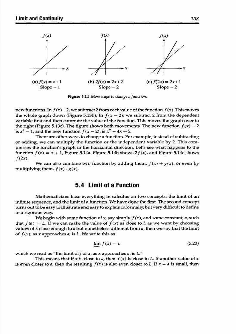
8/9/2019 Mortenson, Michael E. - Mathematics for computer graphics applications.pdf
http://slidepdf.com/reader/full/mortenson-michael-e-mathematics-for-computer-graphics-applicationspdf 116/367
Limit and
Continuity
103
f(x)
f(x) f(x)
x
(a)f(x) =x+1 (b) 2f(x) = 2x+2 (c)f(2x) =
2x+I
Slope = 1 Slope =
2
Slope = 2
Figure 5.14 More
ways
to change function.
new
functions.
In f
(x)
- 2, we subtract 2 from each value of the function f (x).
This
moves
the
whole graph
down
(Figure
5.13b).
In
f (x
-
2), we subtract 2 from the
dependent
variable first and then
compute the value
of
the
function. This
moves
the
graph over to
the right (Figure
5.13c).
The
figure
shows both
movements.
The
new
function f (x) - 2
isx -1, and
the new
function f
(x-2), is
x
2
-
4x
+ 5.
There are
other
ways to change
a
function. For example,
instead
of
subtracting
or
adding,
we
can
multiply
the function
or
the
independent variable
by
2.
This com-
presses the
function's graph in the horizontal
direction. Let's
see
what happens to
the
function
f(x)
=
x
+ 1,
Figure
5.14a.
Figure
5.14b
shows
2f(x),
and
Figure
5.14c
shows
f (2x).
We
can also
combine
two function by adding them,
f
(x)
+ g(x), or
even
by
multiplying
them, f (x) *g(x).
5.4
Limit
of
a Function
Mathematicians base
everything in
calculus on two concepts: the
limit
of
an
infinite
sequence,
and the
limit of
a function.
We
have done the
first.
The
second
concept
turns out to be easy to illustrate and easy to explain informally, but very difficult to define
in a
rigorous
way.
We begin
with some
function of
x, say simply
f
(x), and some constant, a, such
that
f
(a)
= L.
If
we
can
make
the
value of f (x) as close
to
L as we
want by choosing
values of x close
enough
to a
but nonetheless different from a,
then
we
say
that
the
limit
of
f (x),
as
x approaches a, is L. We write this as
lim f(x) = L
(5.23)
which
we
read
as
"the
limit
off
of
x,
as
x
approaches
a,
is
L."
This
means
that if
x is close to a, then f (x) is close
to
L.
If
another value
of x
is even
closer
to a,
then
the resulting f (x) is
also
even
closer
to
L. If x - a
is small,
then
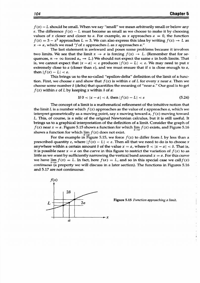
8/9/2019 Mortenson, Michael E. - Mathematics for computer graphics applications.pdf
http://slidepdf.com/reader/full/mortenson-michael-e-mathematics-for-computer-graphics-applicationspdf 117/367
104
Chapter
5
f
(x) - L
should
be small. When we say "small"
we mean arbitrarily small or
below
any
£. The difference f
(x)
- L
must become as small as we choose to make
it
by
choosing
values
of x closer
and
closer to a. For example, as x
approaches a
=
0, the
function
f
(x) =
3
- x
3
approaches
L = 3. We can also
express
this
idea by
writing
f
(x)
-) L
as
x
--
*
a, which we read "fof x approaches L as
x
approaches
a."
The last statement is awkward
and poses
some problems because it
involves
two limits. We see
that the
limit x -* a is forcing
f
(x) -+ L. (Remember that
for se-
quences,
n -+ oo
forced
an -+
L.)
We should not expect the same e in both limits. That
is,
we cannot expect that
Ix- a I < s produces If
(x) -
L I < e. We may need to put x
extremely
close to
a
(closer
than 6),
and
we must ensure that
if
x
is close
enough
to
a,
then
If(x) - LI <e.
This
brings
us
to the
so-called
"epsilon-delta" definition of the limit of a func-
tion. First, we choose
e
and
show
that
f (x) is
within
e
of
L
for every x
near
a. Then
we
choose
some
number
a
(delta)
that
quantifies the
meaning
of
"near
a."
Our
goal
is
to
get
f
(x) within E
of L
by
keeping x
within
5
of a:
If 0
<
Ix-a I<',
then
If(x)-LI
< e (5.24)
The concept of a
limit is
a
mathematical
refinement of the intuitive
notion that
the limit L
is a
number
which
f
(x)
approaches as the value of
x
approaches
a, which
we
interpret
geometrically as
a
moving point, say x moving
toward
a, f (x) moving
toward
L. This, of
course,
is a relic of the original Newtonian
calculus,
but it is
still useful.
It
brings
us
to a graphical interpretation
of the definition
of a
limit.
Consider the
graph
of
f
(x)
near
x
= a.
Figure
5.15
shows
a
function for which lim
f
(x) exists,
and
Figure
5.16
x-+a
shows
a
function for
which
lim
f (x)
does not
exist.
For
the
example
in Figure
5.15, we
force
f (x) to differ from L
by
less
than
a
prescribed
quantity
e, where If (x) - LI <
e.
Then all that we need to do is to choose x
anywhere within
a certain
amount of the
value x =
a,
where 0 < Ix
-
a I
<
S. That is,
it
is possible
near
x
= a
on
the curve in
this
figure to restrict the
variation
of f (x)
to as
little as we wvant
by
sufficiently narrowing the vertical
band around x = a.
For this curve
we have lim f(x) = L.
In fact,
here f
(a) =
L,
and so
in this
special case
we callf (x)
continuous
(a
property
we will discuss in a later
section).
The functions in Figures 5.16
and
5.17
are
not
continuous.
Figure
5.15 Functionapproaching
a
limit.
a
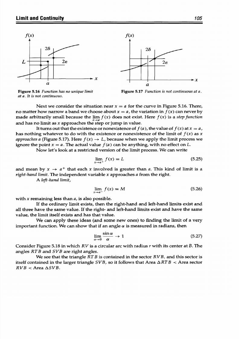
8/9/2019 Mortenson, Michael E. - Mathematics for computer graphics applications.pdf
http://slidepdf.com/reader/full/mortenson-michael-e-mathematics-for-computer-graphics-applicationspdf 118/367
Limit and
Continuity
105
f(X)
f(X)
2s
1
J
L-
LO
le_
2e
A-1x
a a
Figure
5.16 Function
has no
unique
limit Figure
5.17 Function
is not
continuous
at a.
at
a.
It is
not continuous.
Next we consider the
situation
near
x = a for the curve in
Figure
5.16. There,
no matter how narrow
a band
we
choose
about x = a, the variation in f (x)
can
never by
made arbitrarily small because the
lim
f
(x)
does not
exist.
Here f
(x)
is a
step
function
and
has
no limit
as
x approaches the step or jump
in
value.
It turns out that the existence
or
nonexistence of
f
(a), the value
of f
(x) at x = a,
has nothing whatever to do with
the
existence
or
nonexistence of the limit of f (x) as
x
approaches a
(Figure 5.17). Here f (x) -) L, because when we apply the limit process we
ignore the
point
x = a.
The
actual value f
(a) can
be anything, with no effect on L.
Now let's
look
at
a
restricted
version of the
limit
process. We can write
lim f (x)
=
L (5.25)
and mean by x
-*
a+
that
each
x involved is greater than a. This kind of limit is a
right-handlimit. The independent
variable
x
approaches
a from
the
right.
A left-hand
limit,
lim f
(x)
= M (5.26)
x
ya-
with
x
remaining less
than a,
is
also
possible.
If
the
ordinary
limit
exists,
then
the right-hand
and
left-hand limits
exist
and
all
three have the same value. If the right- and left-hand limits exist and have the same
value, the limit
itself exists and
has
that value.
We can apply
these
ideas (and some new
ones) to
finding the
limit
of a very
important function. We
can
show that
if
an angle a is measured in radians, then
lim sin a- 1
(5.27)
to~o
a
Consider
Figure 5.18 in
which
RV
is a circular arc
with
radius
r
with its center at B. The
angles
RTB
and SVB are right
angles.
We
see
that
the triangle RT
B
is
contained
in
the
sector
RVB,
and
this sector
is
itself contained in the larger triangle
S VB, so
it follows that
Area ART
B < Area
sector
RVB
<
Area ASVB.
I
-
:
1
4
11 Q
I--'
40
1-11
I
1% Q
I
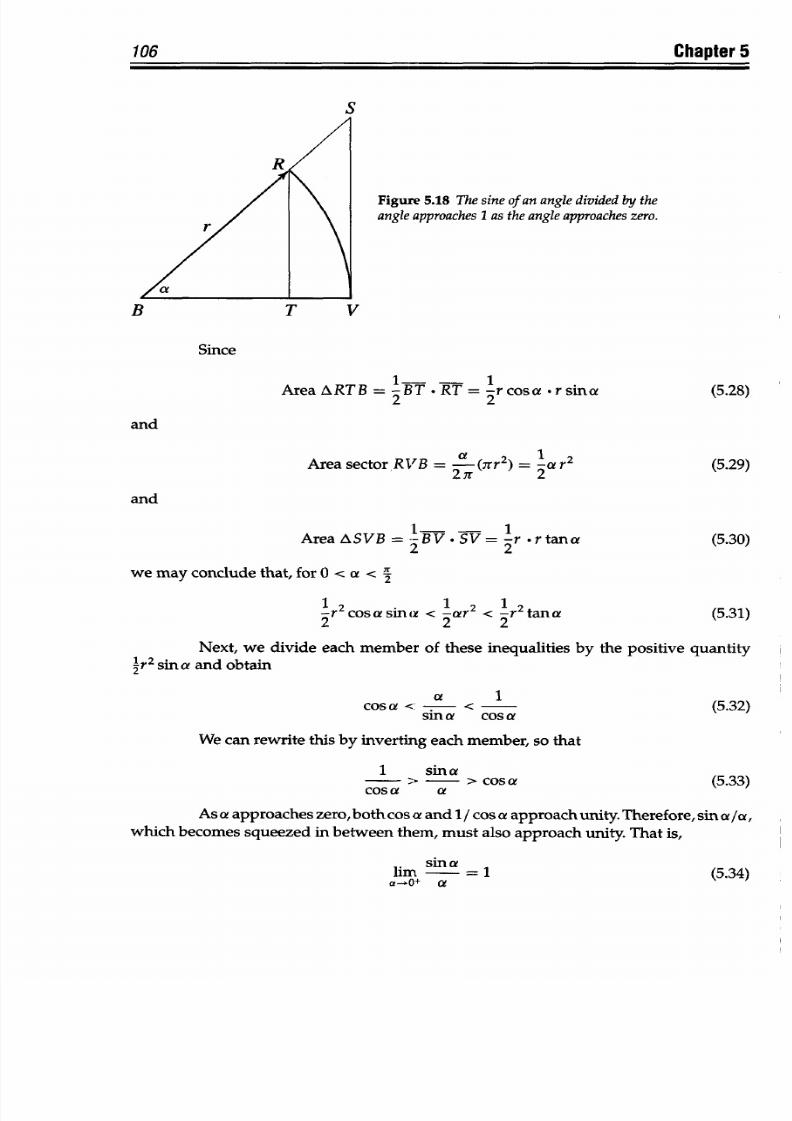
8/9/2019 Mortenson, Michael E. - Mathematics for computer graphics applications.pdf
http://slidepdf.com/reader/full/mortenson-michael-e-mathematics-for-computer-graphics-applicationspdf 119/367
106
Chapter
5
Figure
5.18 The
sine of
an
angle divided
by
the
angle
approaches
1as
the
angle approaches zero.
B
T
V
Since
1--
- 1T
cso
ic
Area ARTB
=
2 BT
. RT =
-2rcosa .rsina
(5.28)
and
Area sector
RVB
=
-(7rr2) =
-ar
2
(5.29)
2 ir
2
and
Area
ASVB = 2-BV
.
SV
= -r
. r
tana
(5.30)
2
2
we may
conclude
that,
for
0
<
a
<
'r
2
1 r2cosasina
< 1car2 < 1r2 tana
(5.31)
Next,
we divide
each member of
these inequalities
by
the positive
quantity
ir
sin
a
and
obtain
a
1
cosa
<
a co
(5.32)
sina
Cos aI
We
can
rewrite
this by
inverting
each member,
so
that
1 sina
cs
- >
cos a
(5.33)
Cos
a a1
As
a
approaches
zero, both
cos a
and
1/ cos
a approach
unity. Therefore,
sin
a/a,
which becomes
squeezed
in between
them, must
also
approach unity.
That
is,
sinl at
lim
= 1
(5.34)
a-O e
8/9/2019 Mortenson, Michael E. - Mathematics for computer graphics applications.pdf
http://slidepdf.com/reader/full/mortenson-michael-e-mathematics-for-computer-graphics-applicationspdf 120/367
Limit and
Continuity
107
This is
also
true
for
the left-hand
limit, because
sina
sin(-a) (535)
a0
(-a)
Notice that direct
substitution
of
a = 0 in the expression sin a/a produces the
unacceptable result 0/0. And this completes our proof of the assertion of Equation
5.27).
A
careful application
of
this method
lets
us compute a variety of other impor-
tant limits. For example,
we
can determine lim sn3o. Since
sin
30 sin
30
Ad= 3 * 3
(5.36)
0 30
we simply take a = 3
0
in Equation
5.26 to produce
sin 30 sin 30
Iim3
* = 3lim
-3 (5.37)
o--o
30
9eo
30
If you are tempted to think that
Equation
5.27 justifies us in
assigning a value
to
the nonsense
symbol
sin
0/0, you should
note that the value
suggested by this equation
would
be
in conflict
with
Equation
5.37.
5.5 Limit Theorems
How
does the limit process apply
to
the
algebraic
combination of two or
more
functions?
Sometimes
the problems we must confront involve the
sum
or
product
of two
or more functions, or
the quotient of
two functions. We
will
need the following three
theorems
on
limits:
Theorem
1:
The limit of the
sum
of two (or
more)
functions is equal to the sum
of their
limits:
lim[f (x) +g(x)]
= lim f(x)
+ limg(x)
(5.38)
Theorem
2: The limit of
the
product
of two
(or more) functions
is equal to
the
product of their limits:
lim[f(X)
Xg(X)]
[=
mf(x)]
X [limg(x)]
(5.39)
Theorem
3: The limit
of the quotient of two
functions is
equal to the quotient of
their limits,
provided
the limit of the denominator is
not
zero:
()_limng
(x)
liMg( ) =
_ai if limf(x)
0
(5.40)
x-a f X)
lim (x) x-a
8/9/2019 Mortenson, Michael E. - Mathematics for computer graphics applications.pdf
http://slidepdf.com/reader/full/mortenson-michael-e-mathematics-for-computer-graphics-applicationspdf 121/367
108
Chapter
5
These
theorems
assume
that
the
limits of
the two functions
exist. However,
even though
it may
be
true
that neither function
separately approaches
a limit,
the sum,
product, or
quotient may do
so.
The exceptional
case
of
Theorem
3,
in
which the denominator
approaches
zero, requires
further
investigation.
Thus, given
any quotient
g(x)/f (x) in which
f (x)
approaches
zero, there are
two
possibilities:
g(x)
does
not
approach zero
or g(x) also
approaches
zero.
In the
first case, we
can make
the value of the
quotient g(x)/f (x)
greater
than
any
preassigned
value
by
making f (x )
sufficiently
small, so that
the
quotient will
not
approach
a
limit.
In the second
case,
where
the
numerator
and
the denominator both
approach
zero,
Theorem 3
does
not
apply,
because the
ratio of the
limit is
the
meaningless
expression 0/0.
However,
the limit of the ratio
g(x)/f
(x)
may exist.
Here are
some
examples:
Example
(a): Evaluate
lim(x
3
+ 2x). By Theorem 2 we
have
x-~3
lim(x
3
)
= lim(X
x
x
x x) =
3
x
3
x
3 = 27
(5.41)
x~3
x-3
and
by Theorem
1:
lim(x
3
+ 2x) =
lim(x
3
)
+
lim(2x) = 27 +
6 = 33
(5.42)
Example
(b):
Evaluate lim
-
2X
-2
+
6*
By
Theorems
1 and
2
we
have
x-*)2 x 2
lim(x
3
- 2x
2
-
3x + 6)
=
8
-
8
- 6
+ 6 =
0
(5.43)
x-*2
an d
lim(x - 2)
= 0
(5.44)
X+2
This gives
us
the
exceptional
case
2
under
Theorem 3,
but for all values
of x except
x
=
2
we have
x
3
-
2x
2
-
3x
+
6
(x
-
2)(x
2
-3)
2
.=
x -3 (5.45)
x -2
x- 2
so that
li
x
3
-2x
2
-3x
+6 li(
2
-3) =1
(5.46)
x2 x - 2
Here
is yet
another way
to look
at the
limit
theorems
of
functions and their
application:
Suppose
that the
functions
of f (x),
g(x),
and
h (x)
each have the
following
limits,
mlim
h(x) = C
(5.47)
im f (x)
=
A
xa
limg(x) = B
X--)a
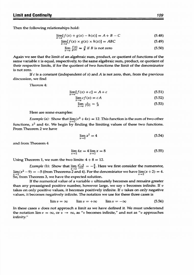
8/9/2019 Mortenson, Michael E. - Mathematics for computer graphics applications.pdf
http://slidepdf.com/reader/full/mortenson-michael-e-mathematics-for-computer-graphics-applicationspdf 122/367
Limit and
Continuity 109
Then the following relationships hold:
lim[f(x)
+g(x) - h(x)] = A+ B -
C (5.48)
lim[f(x)
x g(x)
x
h(x)]
=
ABC
(5.49)
lim f A
if
B is not zero
(5.50)
Again we see that the
limit
of
an algebraic
sum, product, or
quotient
of functions of the
same variable x is equal, respectively, to the same algebraic sum, product, or quotient of
their respective limits, if for the quotient of two functions the limit of the denominator
is not
zero.
If
c is
a
constant (independent of x) and A is not zero, then, from the previous
discussion, we
find
Theorem
4:
lim[f
(x)
+
c] =A
+
c (5.51)
lim cf (x) =cA
(5.52)
lim
-i-
x-+a x)
A
(5.53)
Here
are some examples:
Example (a): Show that lim(x
2
+
4x)
= 12. This function is the sum of two other
functions,
x
2
and
4x.
We
begin
by
finding the limiting values
of
these
two
functions.
From Theorem 2 we have
lim x
2
=
4
(5.54)
and from Theorem 4
lim4x
=
4limx = 8 (5.55)
x-2
x2
Using Theorem 1,
we sum the two
limits:
4
+
8
=
12.
Example
(b):
Show
that
lim
x
2
9
=
.
Here we
first
consider the
numerator,
lim(x
2
-9)
=
-5 (from Theorems2 and 4). For the
denominatorwehavelim(x+2)
= 4.
So,
from Theorem 3,
we
have the
expected solution.
If
the numerical value of a variable v ultimately becomes and remains greater
than
any preassigned
positive
number, however
large,
we say v becomes infinite. If v
takes
on
only positive values,
it
becomes
positively
infinite. If
v takes
on
only negative
values, it becomes negatively infinite. The notation we use for these three
cases
is
limv = oo lim v = +oo limv
=
-oo (5.56)
In these
cases
v
does
not
approach
a
limit
as
we have defined
it.
We
must understand
the
notation
him v
= oo,
or v -> oo,
as
"v
becomes
infinite,"
and
not as
"v
approaches
infinity."
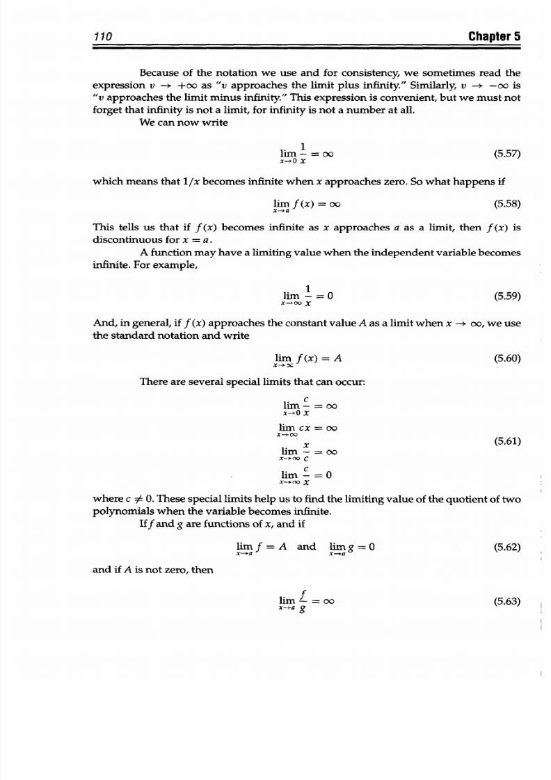
8/9/2019 Mortenson, Michael E. - Mathematics for computer graphics applications.pdf
http://slidepdf.com/reader/full/mortenson-michael-e-mathematics-for-computer-graphics-applicationspdf 123/367
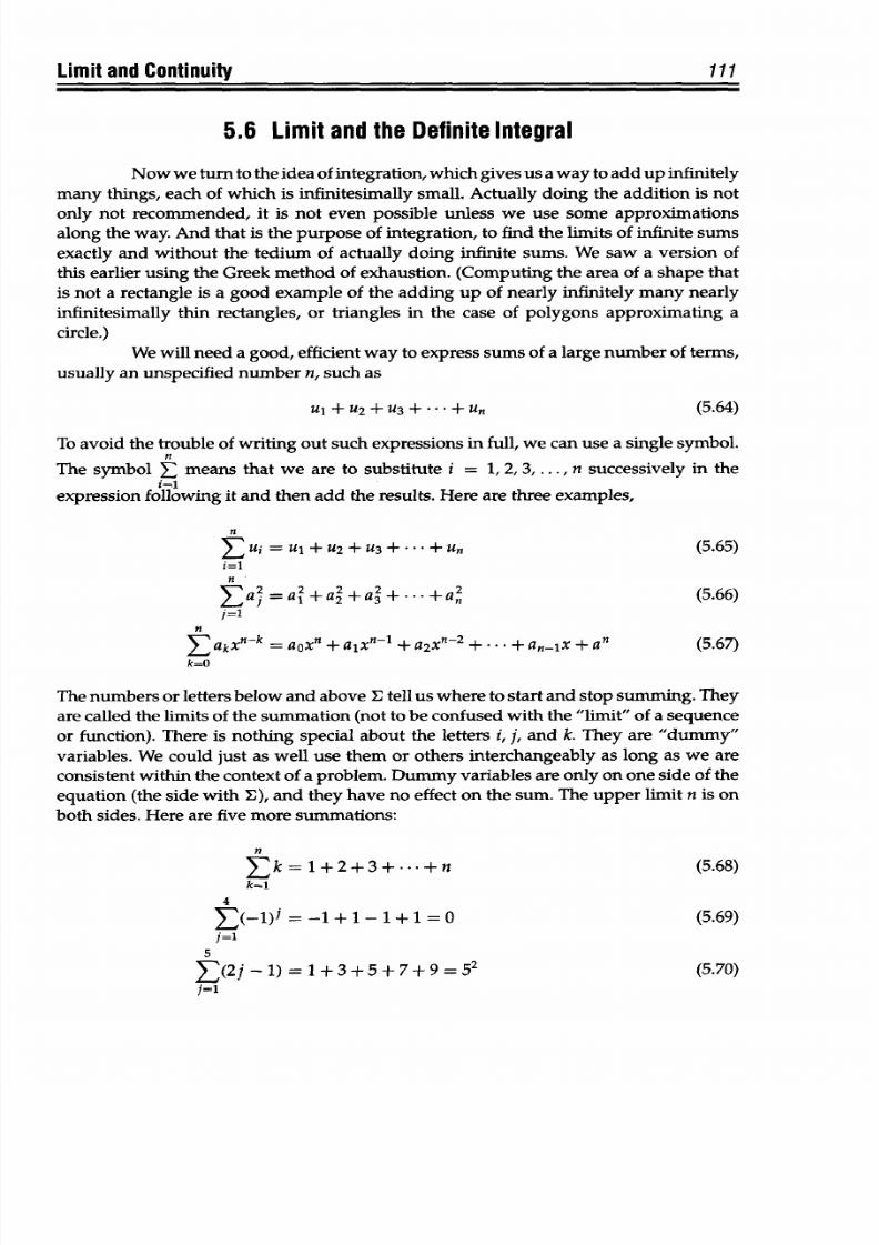
8/9/2019 Mortenson, Michael E. - Mathematics for computer graphics applications.pdf
http://slidepdf.com/reader/full/mortenson-michael-e-mathematics-for-computer-graphics-applicationspdf 124/367
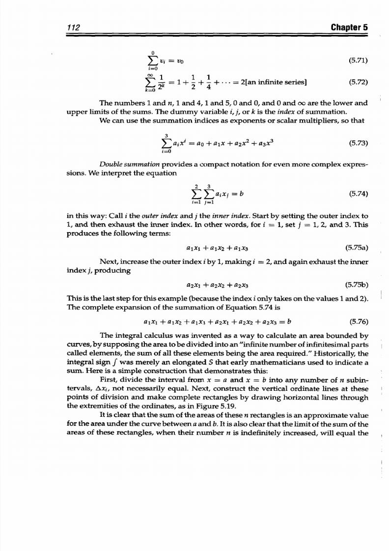
8/9/2019 Mortenson, Michael E. - Mathematics for computer graphics applications.pdf
http://slidepdf.com/reader/full/mortenson-michael-e-mathematics-for-computer-graphics-applicationspdf 125/367
112
Chapter 5
0
E = vo
(5.71)
i=O
=
1
+ - + - +
*.
=
2[an infinite
series]
(5.72)
Fk
2 4
The
numbers
1 and
n,
1 and 4,1
and 5,
0 and 0, and
0 and oo are
the lower
and
upper limits of
the sums.
The
dummy
variable
i, j, or
k
is
the index of
summation.
We can use
the summation
indices
as exponents
or scalar
multipliers,
so that
3
2
3(5)
Eaix
=ao+a
l
x+a
2
x
+a
3
x
(5.73)
i=o
Double
summation
provides
a
compact
notation
for
even more
complex expres-
sions. We interpret
the equation
2 3
E
Eaixj =
b
(5.74)
i=l j=l
in this way:
Call i the outer
index
and j
the
inner index. Start
by
setting the
outer index to
1, and then
exhaust
the
inner index.
In
other words, for
i = 1, set
j
=
1,2,
and
3. This
produces the
following
terms:
aixi
+ alx2 +
ajx
3
(5.75a)
Next, increase
the outer index
i by 1,
making i
=
2,
and
again
exhaust the inner
index
j, producing
a
2
x
1
+ a
2
x
2
+ a
2
x
3
(5.75b)
This
is the
last
step for
this example (because
the
index
i
only takes
on
the
values 1and 2).
The
complete expansion
of the
summation
of Equation
5.74
is
alx
1
+
alx
2
+
alX3
+
a
2
xI
+
a
2
X
2
+
a
2
X
3
= b
(5.76)
The
integral
calculus
was invented
as
a
way
to
calculate
an
area
bounded
by
curves, by supposing
the area to
be divided
into
an "infinite
number
of infinitesimal
parts
called elements,
the
sum
of
all these
elements being
the
area
required."
Historically,
the
integral sign f
was merely an
elongated
S
that
early mathematicians
used to indicate
a
sum. Here
is
a
simple construction
that demonstrates this:
First, divide the
interval
from
x =
a
and x =
b
into
any
number
of n subin-
tervals,
Axi, not necessarily
equal. Next,
construct the vertical
ordinate lines
at these
points of division
and make complete
rectangles
by drawing
horizontal
lines
through
the
extremities
of
the ordinates,
as in
Figure
5.19.
It is clear
that
the sum
of
the
areas
of
these
n
rectangles is
an approximate value
for
the
area under
the curve
between
a
and b.It
is also clear that the
limit
of the sum of
the
areas
of these rectangles,
when their
number n is
indefinitely
increased,
will equal
the
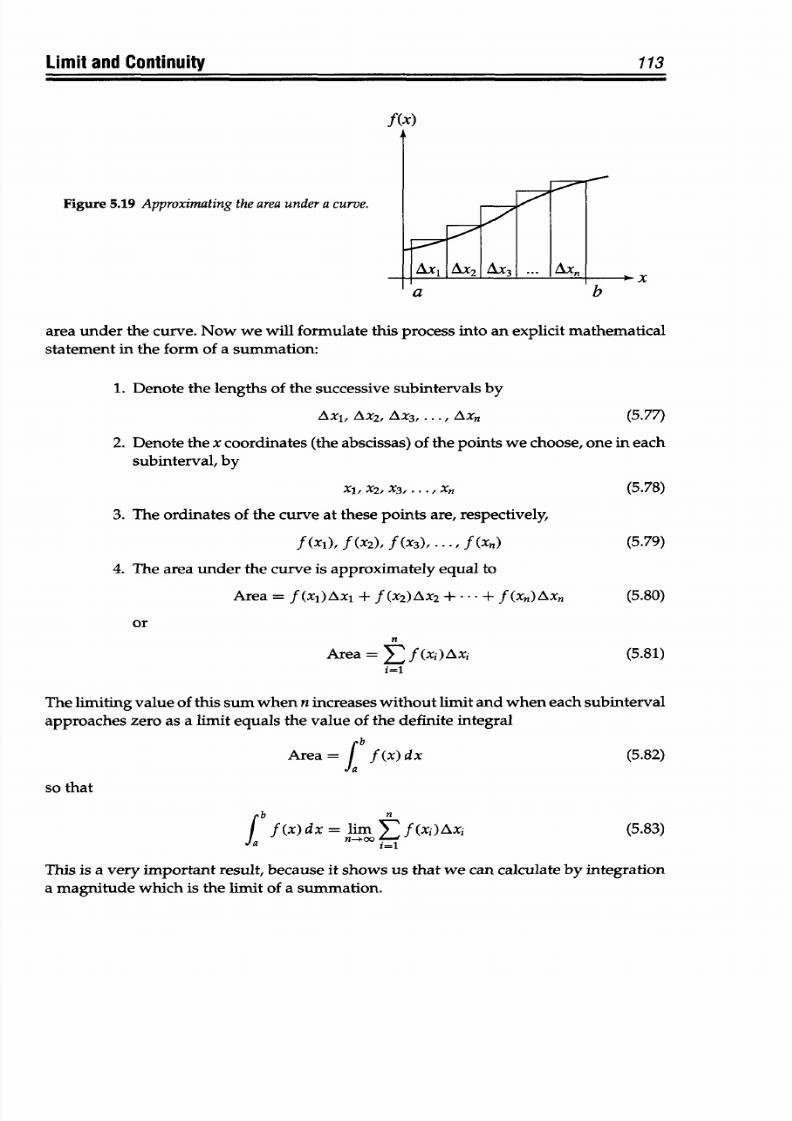
8/9/2019 Mortenson, Michael E. - Mathematics for computer graphics applications.pdf
http://slidepdf.com/reader/full/mortenson-michael-e-mathematics-for-computer-graphics-applicationspdf 126/367
Limit and
Continuity
f(X)
Figure 5.19 Approximating the area under a curve.
a
D
area
under
the
curve.
Now we
will formulate this
process
into
an
explicit
mathematical
statement in
the
form of
a summation:
1.
Denote the lengths
of
the
successive
subintervals
by
AX
1
,
AX
2
,
AX
3
, ...
,
AXn
(5.77)
2. Denote the x coordinates (the
abscissas) of
the
points
we choose,
one in
each
subinterval,
by
XI, X2, X3, . . .,
Xn
3.
The
ordinates
of
the curve at these points
are, respectively,
f
(X1),
f (X2), f (X3),
* **,
f (Xn)
4. The area under the curve is approximately equal to
Area = f(xi)Axi +
f(x
2
)Ax
2
+*-* + f(xn)Axn
or
n
Area = E f
(xi)Axi
i=-
The
limiting value
of
this sum when
n
increases
without limit and
when each
subinterval
approaches zero
as
a
limit equals
the value of the
definite integral
A
Area =
fJ f (X)
dx
(5.82)
so that
mb n
f
(X)
dx
=
Jim
E f (xi)AXi
(5.83)
This
is
a
very
important result, because it shows
us
that
we
can calculate by
integration
a
magnitude
which is the limit of
a
summation.
113
(5.78)
(5.79)
(5.80)
(5.81)
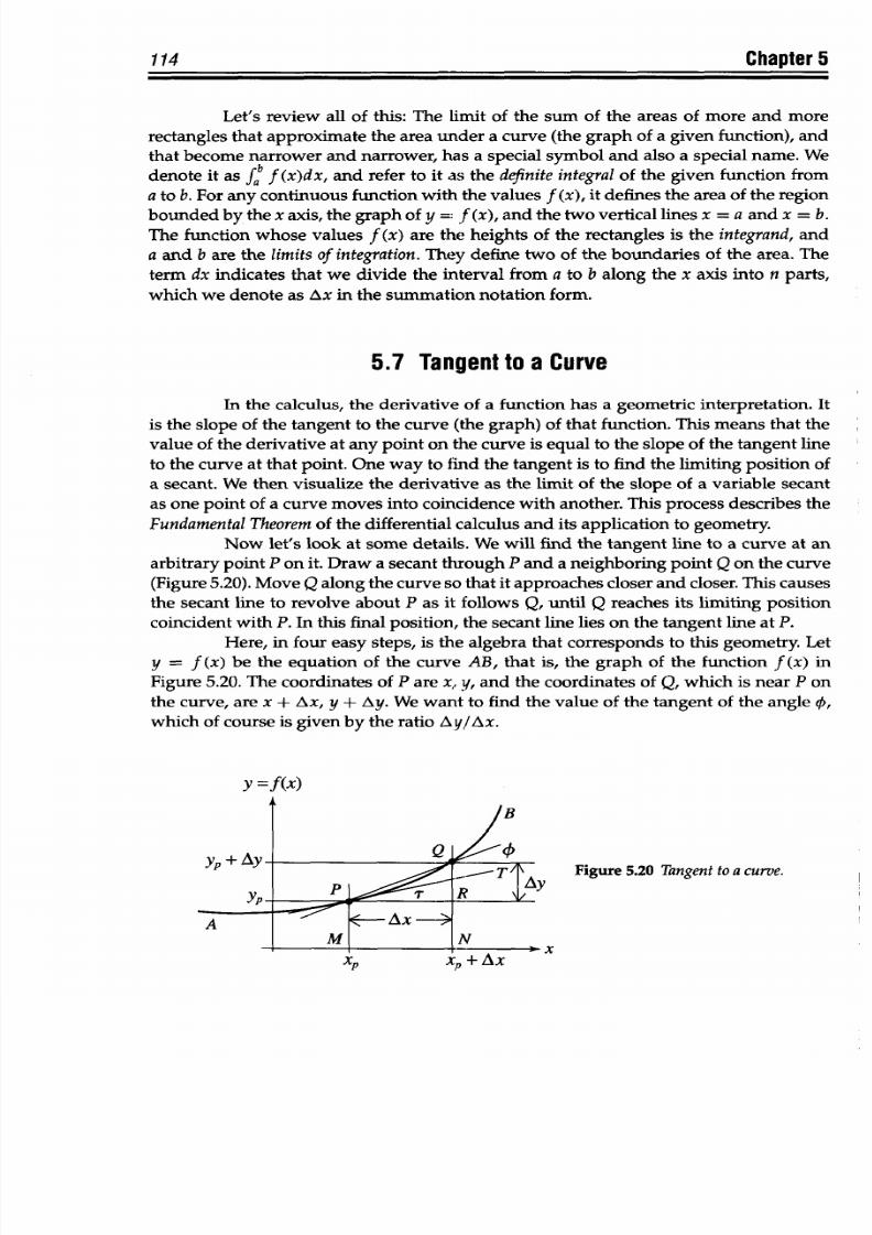
8/9/2019 Mortenson, Michael E. - Mathematics for computer graphics applications.pdf
http://slidepdf.com/reader/full/mortenson-michael-e-mathematics-for-computer-graphics-applicationspdf 127/367
8/9/2019 Mortenson, Michael E. - Mathematics for computer graphics applications.pdf
http://slidepdf.com/reader/full/mortenson-michael-e-mathematics-for-computer-graphics-applicationspdf 128/367
Limit and
Continuity
115
1. Evaluate
this function
at
x
+
Ax, which yields y
+
Ay
(represented geomet-
rically
by
NQ).
y +
Ay
=
f
(x
+
Ax)
=
NQ
(5.84)
2. To find
Ay
compute NQ
-
NR = RQ, or
y
+
Ay
= f (x +
Ax)
=
NQ
-y
= -f
(x) =
MP = NR
(5.85)
Ay = f(x
+
Ax)-f(x)
=
RQ
3. The ratio Ay/Ax is simply
Ay f (x + Ax)-f
(x)
RQ RQ
Ax Ax
MN
PR
=
tanZRPQ
= tans (5.86)
=
slope
of
the secant
line
PQ
Now we have the ratio of the increments Ay
and
Ax, which equals the slope
of
the
secant line drawn
through
the
points P and Q on
the
graph of
the
function.
The
geometry
of the fourth
and
final
step
is
as
follows: We
have
fixed
the value
of x, so P
is
a
fixed point
on the graph.
We
allow Ax to
vary
and approach zero
as a limit.
The point Q moves
along the
curve and
approaches
P as
a limiting
position.
The
secant
line
drawn through
P
and
Q
then rotates
about P
and
approaches
the
tangent
line
at P
as
its
limiting position. In
the figure we
see that X is
the varying
angle of
the moving secant
line PQ, and r
is
the
angle of
the
tangent line PT.
Then
it must
be true that
lim
. T.
4.
Assuming
that tan 0
is a continuous
function,
we have
the fourth and final
step:
- = lim. tang0 = tan r
dyx Ax- (5.87)
= slope
of
the tangent
line
at P
We
see
that as Ax
approaches
zero, Q
approaches
P along the curve, so that
the
slope
of
the
secant
approaches as
its
limit the
slope of
the
curve at
P.
This
limit is equal
to
the derivative
of
y
with respect
to
x. This
means
that
the derivative
of a
function
is
identi-
cal
to the slope of the graph. And this means
that
if, n the formula for dy/dx, we substitute
some value of x, the number we obtain
is
the slope of the curve at the
point
whose abscissa
is
the given value of x. It is at
this
point
that the full story of the differential
calculus begins.
5.8
Rate
of
Change
The
idea
of rate of change occurs all
the
time in our everyday
experience.
We
are
all
familiar with expressions
such
as miles per hour,
miles
per gallon, pressure per
8/9/2019 Mortenson, Michael E. - Mathematics for computer graphics applications.pdf
http://slidepdf.com/reader/full/mortenson-michael-e-mathematics-for-computer-graphics-applicationspdf 129/367
116
Chapter 5
square inch,
price
per pound,
and so on. They
all represent
rates
of change. An
analogous
idea in mathematics is
that of
the
rate
of change of a
function.
Given
some function y
=
f
(x),
we
can
change
x by
some
Ax. This, of
course,
causes
a
change
in
the
dependent
variable
y,
say
Ay.
If Ay is
proportional to
Ax,
then
the function
changes
uniformly,
or at a uniform rate. This means that
the change in y,
corresponding to a given
change in x,
is
constant,
independent
of the actual value of
x.
The rate is the change in the function
divided
by
the change in the argument:
- Y= m (5.88)
Ax
where
m
is
a constant. The graph of
this function
is a straight line
whose
slope is m:
y = mx +
k
(5.89)
When
a
function
does
not vary
uniformly, the
ratio
Ay/Ax
is
merely the average
rate
of change over the interval Ax. If we let Ax approach zero,
this
ratio
approaches
a
definite
limiting
value, or
the instantaneous rateof change:
dy
lim
Ay
(5.90)
dx Ax-*O AX
which
is
the rate
of change of y with respect to
x.
We
need
nothing
more
than our
ordinary everyday experience to
understand
this
idea. We
can do a thought experiment to illustrate it. Suppose
that
we set up tw o
posts beside
a
highway
and
measure
the
distance
between
them.
A
car
drives
past
them.
If Ax is the
distance
between the
posts
and
if At is
the
time it
takes the
car to pass
from
one post
to
the other, then for a car
traveling at a constant
speed, that
speed is simply
Ax/At.
However,
if
the speed
varies, then this
ratio
is
the
average speed.
If we
wish to
know the
car's
speed at a particular
instant,
say
when it
is passing the
first
post, common
sense suggests
what
we place the posts close together.
This decreases
the time interval,
At,
so
that
there is less time
for
the speed
to
change very much,
and
the average speed
will nearly equal the instantaneous speed.
In practice,
we cannot
use this procedure beyond a certain point, but it is clear
that our
intuitive idea
of
instantaneous speed
is expressed exactly by Ax/At, the limit
of Ax/At as At
approaches
zero. We can now
assert
that the
derivative
of a
function
is
identical to its rate
of change.
Now we
realize
that the three quantities derivative, slope,
and rate of change
are all
equivalent.
The
geometry shows
us
that
when
the
slope of a
curve
(Figure 5.21) is
positive
(as
on
the curve segment AB),
the
ordinate y is increasing as x increases;
when
the
slope
is
negative (as
on the
curve
segment BC),
the ordinate is decreasing.
This
simply
tells us
that
a function increases or decreases according to whether its rate
of
change is positive
or
negative.
Calculus solves
the
following kinds
of problems dealing
with
motion:
1. If the speed of an
object is
not constant but
always
changing, how do we
compute the distance it travels?
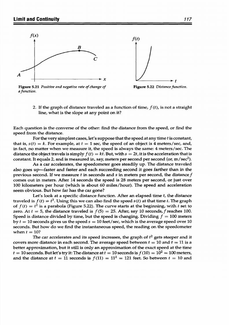
8/9/2019 Mortenson, Michael E. - Mathematics for computer graphics applications.pdf
http://slidepdf.com/reader/full/mortenson-michael-e-mathematics-for-computer-graphics-applicationspdf 130/367
Limit and Continuity 117
f(x)
A
B
C
' X
IJ l)
f
Figure
5.21 Positive and
negative rate of
change
of
Figure 5.22 Distancefunction.
function.
2.
If the graph
of distance
traveled
as
a function
of
time, f (t), s not a straight
line,
what
is the
slope at
any
point
on it?
Each question is the converse
of
the other: find the distance from the speed, or find the
speed from the
distance.
For
the
very simplest
cases, let's suppose
that the speed
at
any time t is constant,
that
is, s(t) = k.
For
example, at t = 1 sec, the speed of an object is 4 meters/sec, and,
in fact,
no
matter
when
we measure it, the speed
is always
the
same: 4
meters/sec.
The
distance the object travels is simply
f
(t)
= kt. But,
with s =
2t,
it is
the
acceleration
that
is
constant.
It equals 2,
and
is
measured in, say, meters per
second per second
(or,
m/sec
2
).
As a car accelerates, the speedom eter goes steadily up.
The
distance traveled
also goes up-faster and
faster
and each
succeeding
second
it
goes farther than in the
previous
second.
If
we measure t in seconds and s in meters
per
second, the distance f
comes
out in meters.
After
14 seconds the
speed
is 28
meters
per
second, or just
over
100 kilometers per hour (which is
about
60 miles/hour).
The
speed and acceleration
seem obvious.
But how far has the car
gone?
Let's
look at
a
specific
distance
function. After
an
elapsed time
t,
the
distance
traveled is f
(t)
=
t
2
. Using this we can also find the speed s (t) at
that
time
t.
The graph
of
f(t)
= t
2
is a parabola
(Figure 5.22). The curve
starts
at
the beginning,
with
t set
to
zero.
At
t =
5, the
distance traveled is
f (5)
= 25. After,
say
10 seconds,
f
reaches 100.
Speed is
distance
divided
by
time,
but
the speed
is
changing. Dividing f = 100 meters
by t =
10
seconds gives us the speed s = 10
feet/sec,
which is the average speed over
10
seconds. But
how
do we find the instantaneous speed, the reading
on
the speedometer
when t = 10?
The
car accelerates
and its speed
increases,
the graph of t
2
gets steeper
and
it
covers
more distance
in each second.
The average
speed between t =
10 and
t
=
11 is a
better
approximation,
but
it still is only an approximation of the exact speed
at
the time
t = 10 seconds. But let's
try
it: The distance at t = 10 seconds is
f
(10) = 102 = 100 meters,
and
the
distance at t =
11
seconds is
f
(11)
= 112
=
121 feet.
So between
t
= 10
and
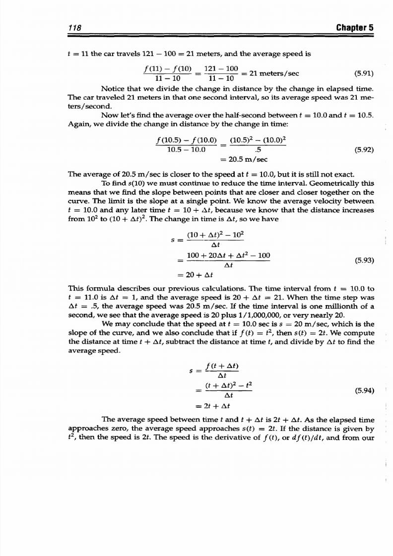
8/9/2019 Mortenson, Michael E. - Mathematics for computer graphics applications.pdf
http://slidepdf.com/reader/full/mortenson-michael-e-mathematics-for-computer-graphics-applicationspdf 131/367
118
Chapter
5
t = 11 the car
travels
121
-
100
=
21
meters, and the
average
speed
is
f(11)
- f(10) 121 -
=
21
meters/sec
(5.91)
1-10-
-
11
-
lo mtr/sc(.1
Notice
that we
divide the change
in distance by
the
change
in
elapsed time.
The car
traveled
21 meters in
that
one
second interval,
so its average
speed
was 21
me-
ters/second.
Now let's
find the average
over
the half-second
between t
= 10.0
and
t = 10.5.
Again,
we divide the
change
in distance by
the change
in
time:
f
(10.5)
- f (10.0) (10.5)2
-
(10.0)2
10.5 - 10.0
.5
(5.92)
=
20.5
m/sec
The
average of
20.5 m/sec
is closer
to the speed at t = 10.0,
but it
is still
not exact.
To find
s(10) we
must
continue to reduce
the time interval.
Geometrically
this
means that
we find the slope
between
points that
are closer and
closer
together on the
curve. The
limit
is the slope at a single
point. We know the
average velocity
between
t = 10.0 and
any later
time t = 10
+
At,
because
we know that
the distance increases
from
102
to
(10
+
At)
2
. The
change
in time is
At, so we have
(10 +
At)
2
-
102
s =
At
100 +
2OAt
+ At
2
-
100
At
(5.93)
At
=20+
At
This
formula describes our
previous
calculations.
The time
interval from t
= 10.0 to
t
= 11.0
is
At
= 1, and
the average
speed
is 20 +
At
= 21. When
the time step
was
At = .5,
the
average speed
was 20.5
m/sec. If the
time interval
is one millionth of
a
second,
we
see
that the average
speed
is
20
plus 1/1,000,000,
or very
nearly
20.
We may conclude
that
the
speed at
t = 10.0 sec
is s = 20 m/sec,
which is
the
slope
of
the
curve,
and
we
also
conclude
that
if
f
(t)
=
t
2
,
then
s
(t)
=
2t.
We
compute
the distance
at time t
+ At, subtract
the distance
at
time
t, and
divide
by
At
to find
the
average
speed.
- f(t + At)
At
(t
+ At)
2
-
t
2
(5.94)
At
=
2t + At
The average
speed between
time t
and
t
+
At is 2t
+
At. As
the elapsed
time
approaches zero,
the average
speed
approaches
s(t) =
2t.
If
the distance
is given
by
t
2
, then
the speed
is 2t.
The
speed
is
the derivative of
f (t),
or df
(t)/dt, and
from
our
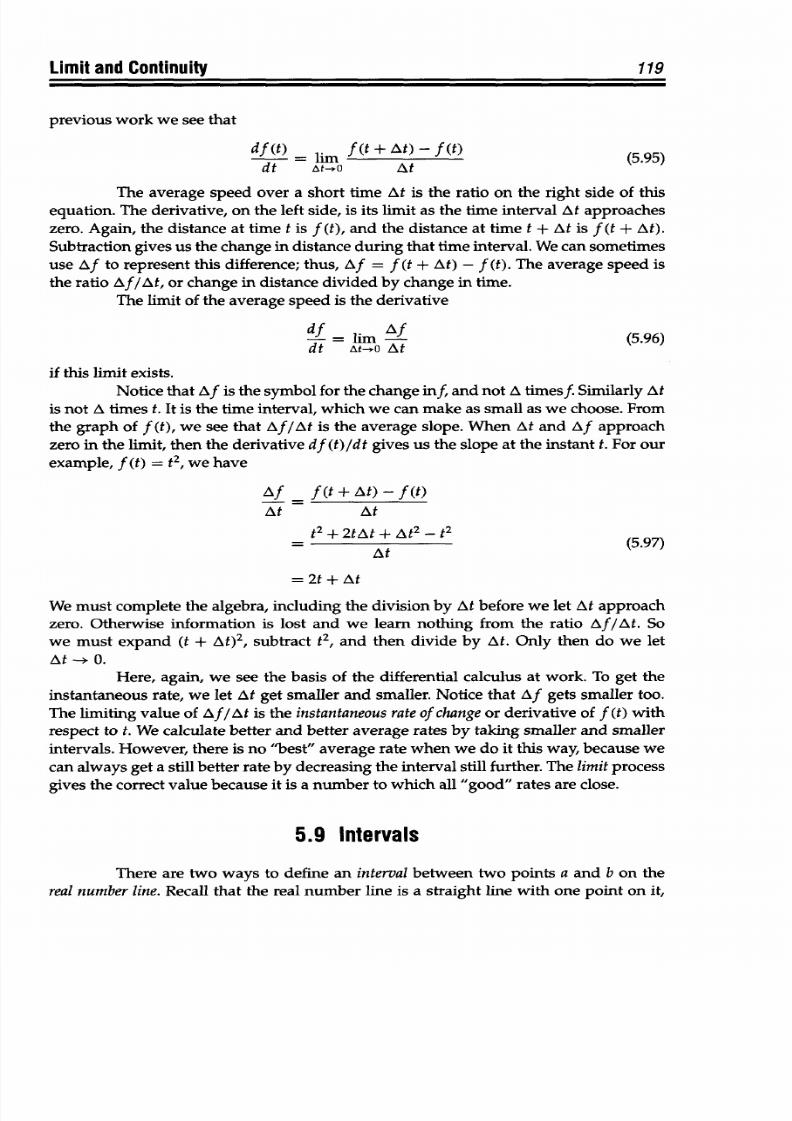
8/9/2019 Mortenson, Michael E. - Mathematics for computer graphics applications.pdf
http://slidepdf.com/reader/full/mortenson-michael-e-mathematics-for-computer-graphics-applicationspdf 132/367
Limit and Continuity 119
previous
work
we see
that
df
(t)
= im f
(t
+
At)
- f (t) (595)
dt
At-0o
At
The average speed over
a short
time At is the ratio on the right side of this
equation. The derivative,
on
the left
side,
is its limit as the time interval At approaches
zero. Again, the distance at time t is f (t), and the distance at time t +
At
is f (t + At).
Subtraction gives
us the
change
in
distance during that time interval.
We can
sometimes
use Af to represent this difference;
thus, Af
= f (t
+ At)
-f (t). The average
speed is
the ratio Af/At, or change in distance divided
by
change in
time.
The
limit
of
the average speed is the derivative
df=
lim
Af
(5.96)
dt At-O At
if this limit
exists.
Notice that Af is the symbol for the change inf, and not A timesf. Similarly At
is not A times
t.
It is the time interval, which we
can
make as small as we choose. From
the
graph
of
f
(t),
we
see that Af/At is the average slope.
When
At and Af
approach
zero in the limit, then the derivative df (t)/dt gives us the slope
at
the instant t. For our
example, f (t) = t
2
, we have
Af
f
(t
+
At)
- f
(t)
At
At
t
2
+ 2tAt
+
A t
2
- t
2
(5.97)
At
= 2t +
At
We must
complete
the algebra, including the division by
At
before we let At approach
zero. Otherwise information
is
lost and we learn nothing
from
the ratio Af/At. So
we
must expand (t + At)
2
, subtract t
2
, and then divide
by
At. Only
then
do we let
At
-- 0.
Here,
again,
we
see
the
basis of the
differential
calculus
at
work.
To
get the
instantaneous
rate,
we let At get smaller and smaller.
Notice that
Af
gets
smaller too.
The limiting value of Af/At is the
instantaneous rate
of change or derivative of f (t) with
respect to t. We
calculate
better and better average rates
by
taking smaller
and
smaller
intervals. However,
there
is no "best" average rate when we
do
it this way,
because
we
can always
get a
still better
rate
by decreasing
the interval
still further. The
limit process
gives
the
correct
value
because it
is a
number to
which all "good" rates
are
close.
5.9
Intervals
There are two ways to define an
interval
between two points a and b on the
real number
line.
Recall that the real number line is
a
straight line with one point on
it,
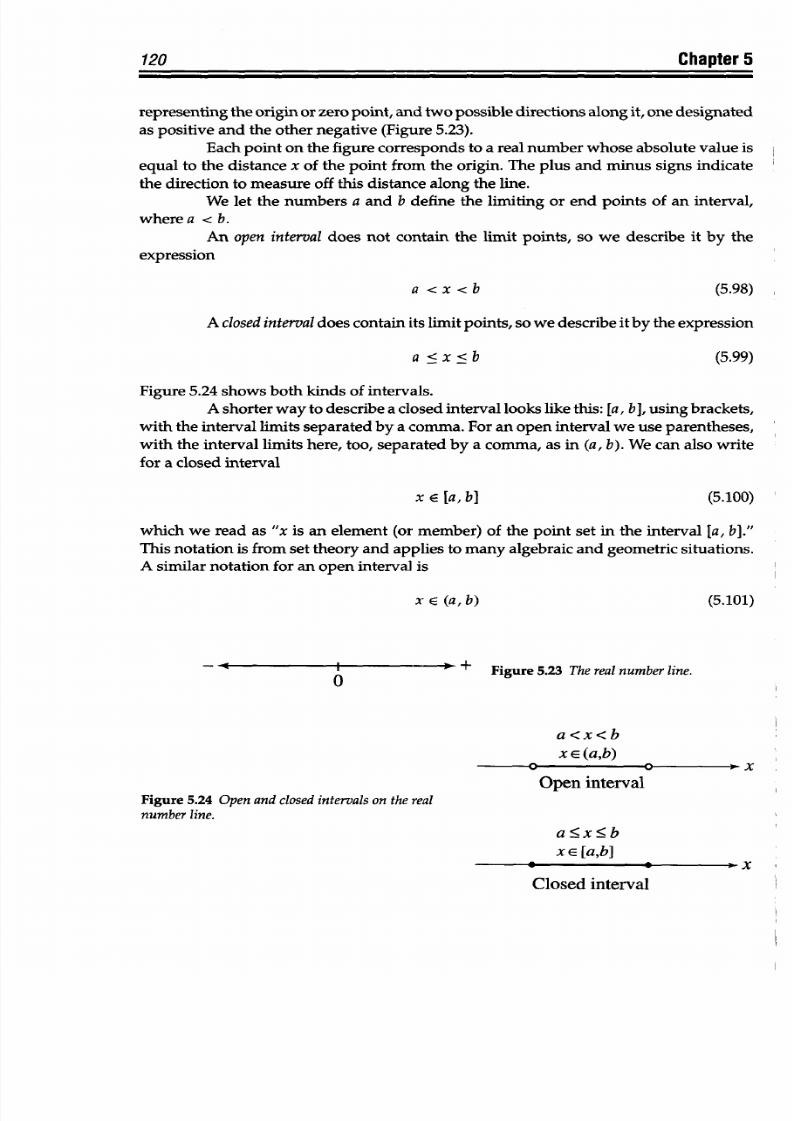
8/9/2019 Mortenson, Michael E. - Mathematics for computer graphics applications.pdf
http://slidepdf.com/reader/full/mortenson-michael-e-mathematics-for-computer-graphics-applicationspdf 133/367
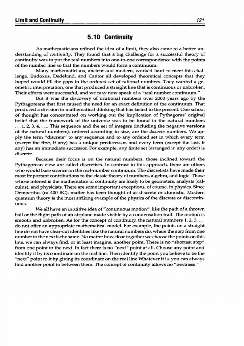
8/9/2019 Mortenson, Michael E. - Mathematics for computer graphics applications.pdf
http://slidepdf.com/reader/full/mortenson-michael-e-mathematics-for-computer-graphics-applicationspdf 134/367
Limit and Continuity
121
5.10 Continuity
As mathematicians
refined
the idea
of
a
limit,
they
also came
to a better un-
derstanding of
continuity. They found
that
a big challenge for a
successful
theory of
continuity
was
to
put
the real
numbers into one-to-one correspondence with the points
of the
number line so that
the
numbers would form
a continuum.
Many mathematicians, ancient and modem, worked
hard
to meet this chal-
lenge. Eudoxus,
Dedekind,
and Cantor
all developed
theoretical concepts
that
they
hoped would fill the gaps in the ordered set
of rational numbers. They wanted a ge-
ometric interpretation, one that produced a straight
line
that is continuous or unbroken.
Their efforts
were
successful,
and we
may now
speak of a
"real number
continuum."
But it
was the
discovery of
irrational numbers
over 2000 years
ago
by the
Pythagoreans
that
first
caused
the need
for
an
exact
definition
of
the
continuum.
That
produced
a division in mathematical thinking
that has
lasted
to
the
present.
One
school
of
thought has
concentrated
on working
out the
implication of Pythagoras'
original
belief
that
the framework
of
the universe
was to be found
in
the
natural
numbers
... 1,2, 3,
4,
.... This
sequence
and
the set of
integers (including the
negative versions
of
the
natural
numbers), ordered
according
to
size,
are
the discrete
numbers. We
ap-
ply
the term
"discrete"
to any
sequence and
to
any
ordered set in which
every term
(except
the first, if
any)
has a
unique
predecessor,
and every term (except
the
last, if
any) has
an
immediate successor.
For example,
any
finite
set (arranged in any order)
is
discrete.
Because
their focus is on the
natural
numbers, those inclined toward
the
Pythagorean view
are
called
discretists.
In contrast to this approach, there
are
others
who would
base science on
the
real-number continuum.
The discretists have made their
most
important contributions to
the
classic theory of numbers, algebra,
and
logic.
Those
whose
interest
is
the mathematics of continuity are
likely to
be
geometers, analysts (cal-
culus), and
physicists.
There are some important
exceptions,
of course,
in physics. Since
Democritus (ca 400 BC), matter has been
thought
of
as
discrete
or
atomistic.
Modem
quantum theory is the most
striking
example of
the
physics of the discrete or discontin-
uous.
We
all
have an intuitive
idea
of
"continuous motion",
like
the
path
of
a
thrown
ball or
the
flight path of an airplane made visible by
a condensation
trail.
The
motion
is
smooth and
unbroken.
As for the concept of continuity, the natural
numbers
1, 2, 3, ...
do
not offer an appropriate
mathematical
model. For example,
the
points
on a
straight
line
do
not
have clear-cut identities like the
natural
numbers do, where the step from one
number to
the next
is
the
same.
No
matter how
close together we
choose
the
points
on this
line, we
can always find, or at
least imagine, another
point. There
is no "shortest
step"
from one
point
to
the
next. In fact
there
is no
"next"
point
at all. Choose any point and
identify it
by its coordinate on
the
real
line.
Then
identify
the point you believe
to be the
"next"
point
to
it by
giving
its coordinate on
the
real
line
Whatever
it
is,
you
can
always
find another
point
in between them. The concept
of
continuity allows no neatnesss."
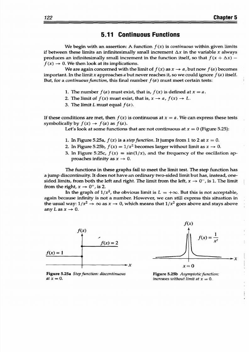
8/9/2019 Mortenson, Michael E. - Mathematics for computer graphics applications.pdf
http://slidepdf.com/reader/full/mortenson-michael-e-mathematics-for-computer-graphics-applicationspdf 135/367
122
Chapter 5
5.11 Continuous
Functions
We
begin
with an assertion:
A function f (x)
is
continuous
within
given
limits
if
between
these limits an infinitesimally small increment
Ax
in
the
variable
x
always
produces an
infinitesimally small increment
in
the function
itself,
so that f (x
+
Ax)
-
f
(x) --* 0.
We
then look
at its implications.
We
are
again concerned with the limit of f (x) as x - a, but
now
f (a) becomes
important.
In the
limit x
approaches
a
but
never reaches it,
so
we
could ignore f (a) itself.
But, for
a continuous unction, this final number
f
(a) must meet certain tests:
1. The number f
(a)
must exist, that
is, f (x)
is defined
at
x
=
a.
2. The
limit
of
f (x)
must
exist,
that is, x -+
a, f
(x)
L.
3.
The
limit
L
must
equal
f
(a).
If these
conditions are met, then f
(x) is continuous at
x = a. We can
express these tests
symbolically
by
f (x)
- f (a) as f (a).
Let's look at some functions
that
are
not
continuous at x
=
0 (Figure
5.25):
1.
In
Figure
5.25a,
f (x) is a
stepfunction. It
jumps from 1
to 2
at x
=
0.
2. In
Figure 5.25b, f (x)
=
1/X
2
becomes larger without
limit as x 0.
3.
In Figure
5.25c,
f (x)
=
sin(1/x), and the frequency of the
oscillation ap-
proaches infinity
as
x
0.
The functions in these graphs fail to meet
the
limit
test.
The
step
function has
a
jump
discontinuity. It does not have an
ordinary
two-sided limit but has, instead, one-
sided
limits, from
both the
left and right. The limit
from the
left,
x
-+ 0, is
1.The limit
from the right, x --
*
0+,
is
2.
In the
graph
of 1/x
2
, the obvious limit is L = +oo. But this is not acceptable,
again because infinity
is
not
a
number.
However,
we can still
express
this
situation
in
the usual way: 1 x
2
-*oo as x - 0, which means that
1l/x
goes above and stays above
any L as
x
-O
0.
f(X)
f(X) A
f(x) = 1
f(x)
=2
1
l (x) = -
1. X
X=O
Figure
5.25b
Asymptoticfunction:
increases
without limit
at x
=
0.
Figure
5.25a Stepfunction: discontinuous
at x =
0.
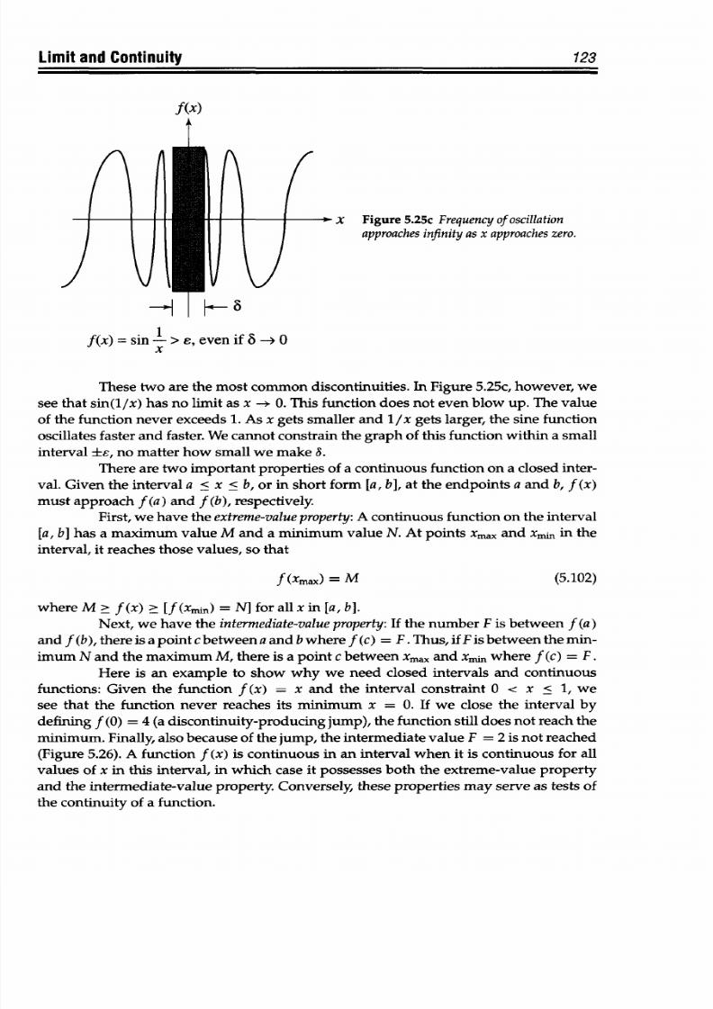
8/9/2019 Mortenson, Michael E. - Mathematics for computer graphics applications.pdf
http://slidepdf.com/reader/full/mortenson-michael-e-mathematics-for-computer-graphics-applicationspdf 136/367
Limit and
Continuity
f(X)
t
x Figure 5.25c Frequency of oscillation
approaches infinity as x approaches zero.
__ I
e_
°
f(x)
= sin
l
> e, even if 6 - 0
These two
are
the most
common discontinuities.
In Figure
5.25c,
however,
we
see
that sin(l/x) has
no limit as x
-* 0.
This function does not even blow up. The value
of the function never
exceeds
1.
As
x gets smaller and 1/x
gets
larger, the
sine
function
oscillates
faster and
faster.
We cannot constrain the graph of this function within a small
interval
±E,
no
matter how
small
we
make
8.
There are
two important properties of a
continuous function
on a closed inter-
val.
Given
the
interval
a
<
x < b, or
in
short form
[a, b],
at the
endpoints a
and
b, f
(x)
must approach f (a)
and
f (b),
respectively.
First, we have
the
extreme-value property:A continuous
function
on
the interval
[a,
b] has a maximum
value
M and a
minimum value
N. At points xmax and xnm
in the
interval, it
reaches
those values,
so that
f (Xmax) =
M (5.102)
where
M
>
f
(x)
>
[f
(xmil)
=
N]
for all
x
in
[a, b].
Next,
we
have
the intermediate-value
property:
If the number
F is
between
f (a)
and
f
(b), there
is a point c
between
a
and
b where
f
(c) = F. Thus, if
F isbetween the min-
imum N and the maximum
M, there is
a point
c between
xmax and
xmn where
f (c)
=
F.
Here
is an example
to
show why
we need
closed intervals
and continuous
functions:
Given
the
function
f
(x) = x and the interval constraint
0
< x < 1, we
see that the function never
reaches its
minimum
x
= 0.
If we close the interval
by
defining
f
(0) = 4 (a discontinuity-producing
jump), the function
still
does
not
reach
the
minimum. Finally,
also
because
of
the jump, the intermediate value F = 2 is not reached
(Figure
5.26).
A
function
f
(x)
is
continuous
in
an interval
when
it is continuous
for all
values
of x in
this
interval,
in which case it possesses both
the
extreme-value
property
and
the intermediate-value property. Conversely, these
properties may serve as tests of
the continuity
of a function.
123
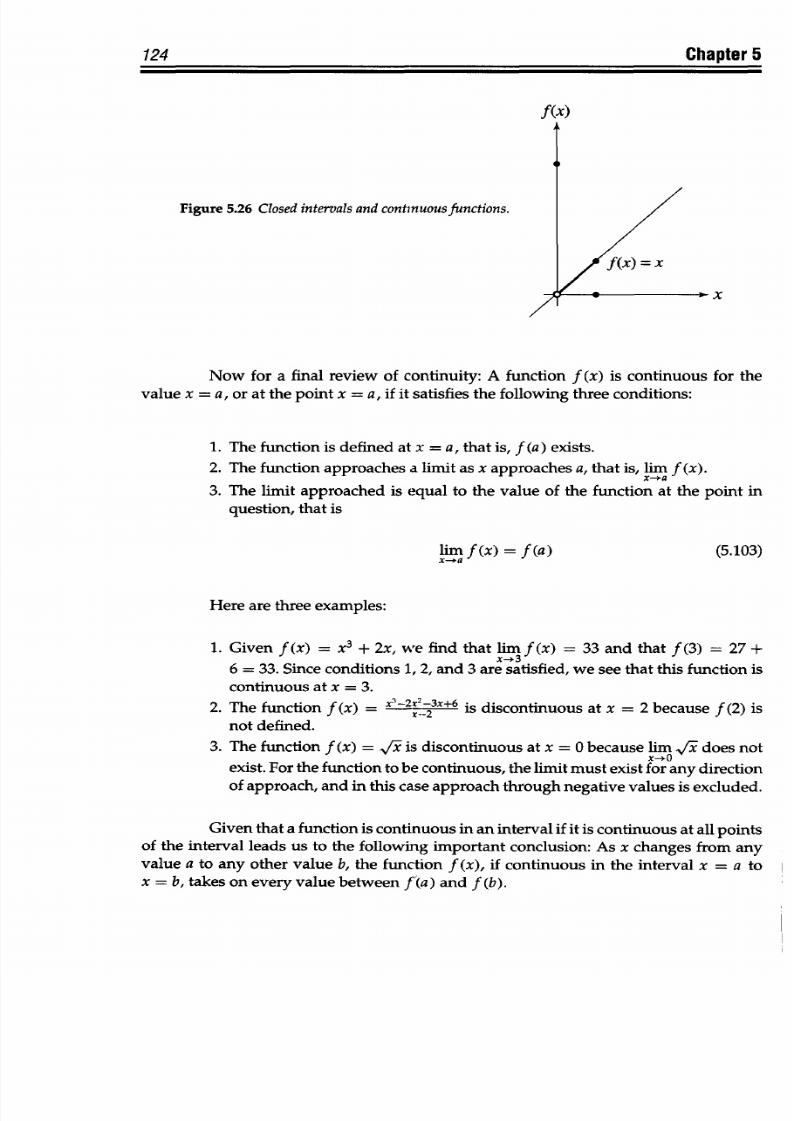
8/9/2019 Mortenson, Michael E. - Mathematics for computer graphics applications.pdf
http://slidepdf.com/reader/full/mortenson-michael-e-mathematics-for-computer-graphics-applicationspdf 137/367
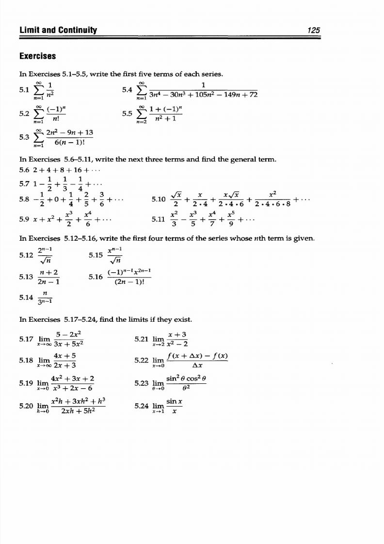
8/9/2019 Mortenson, Michael E. - Mathematics for computer graphics applications.pdf
http://slidepdf.com/reader/full/mortenson-michael-e-mathematics-for-computer-graphics-applicationspdf 138/367
Exercises
In Exercises 5.1-5.5, write
the
first five terms of
each series.
00
1
5-4
E 3n
4
- 30n
3
+ 105n
2
- 149n + 72
5.2
n
)+ 5.5
2
( 1)
n!1 n-2
£
2n
2
- 9n + 13
Yn- 6(n-1)
In Exercises
5.6-5.11, write
the next three terms and
find the
general term.
5.6
2+4+8+16+ ...
5.7 1 - 1 + 1 - 1 +
1 12
3
5.9
x-
+ 02
2 + x + .. .
58 2 4
5
6
5.9 x+x
2
x
3
x
4
.
2
6
2
2
.*4 2
. 4 .
6
2 *4. 6.8
2 3 4 5
5.11 - - - + - + -
+ -.
In Exercises 5.12-5.16,
write the first four
terms of the series whose nth term
is given.
5.15
-
(-W)n-lx2n-1
(2n -
1)
In Exercises 5.17-5.24, find
the limits if
they
exist.
5.17 lim 5-2X
2
3x
+
5x
2
5.18 lim 4x+5
x-*oo2x+3
5.19 lim
4x
2
+3x+2
x- O
x
3
+2x-6
5.20 hirnx
2
h +
3xh
2
+h
3
h->O
2xh+5h
2
5.21
lim x+3
x-2
2 - 2
5.22 lim
f
(x + Ax)
-
f
(x)
x
yo Ax
5.23
lim
sin2
H os2 H
@OO
02
5.24
lim
-
x-*1 X
Limit and
Continuity
5.1
00
T
2
n=l
125
2n-1
5.12 -
5.13 n+2
2n - 1
3n-i
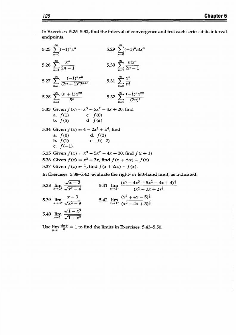
8/9/2019 Mortenson, Michael E. - Mathematics for computer graphics applications.pdf
http://slidepdf.com/reader/full/mortenson-michael-e-mathematics-for-computer-graphics-applicationspdf 139/367
126
Chapter
5
In
Exercises
5.25-5.32,
find
the interval
of convergence
and
test
each
series
at its interval
endpoints.
00
x
5.25
(-1)nx
5.29
(-l)'n Xn
n=O
n= O
5.26 E 2 1
5.30 E2 n -
5.27
£0-____5__31
Oc
5 (2n +
l)23n+l
5.31
E
5.28 00
(n
+
1)x
2
n 5.32
DC( 1n~
nT
55
E
(2n)!
5.33 Given
f (x)
=
x
3
- 5X
2
- 4x
+
20,
find
a.
f(1)
c. f(0)
b.
f(5)
d.
f(a)
5.34 Given
f(x)
=
4 - 2x
2
+ X
4
,
find
a. f(0)
d. f(2)
b.
f(1)
e.
f(-2)
c.
f(-1)
5.35 Given
f(x)
= x
3
- 5X
2
-
4x + 20, find
f(t
+ 1)
5.36
Given f(x) =
x
3
+
3x,
find f(x
+
Ax) - f(x)
5.37
Given
f(x)
=
1,
find f(x
+ Ax)
-
f(x).
In
Exercises
5.38-5.42,
evaluate
the right-
or
left-hand
limit,
as
indicated.
5.38
lirn
5.41
lim
(x4-
4x3
+ 5X2
-
4x
+4)
4
x-+2+
(x
2
-
3x+2)2
5.39
lim
x-3 5.42
lirn
(X2+
4x
-
5)2
x-+3+
x21+
(X
2
-
4x
+
3)3
5.40 lim
x-*
1-
Use
lim
snO =
1 to
find
the
limits
in Exercises
5.43-5.50.
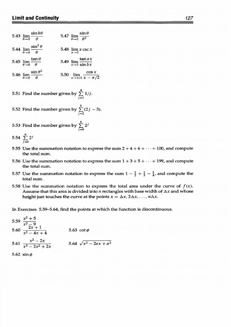
8/9/2019 Mortenson, Michael E. - Mathematics for computer graphics applications.pdf
http://slidepdf.com/reader/full/mortenson-michael-e-mathematics-for-computer-graphics-applicationspdf 140/367
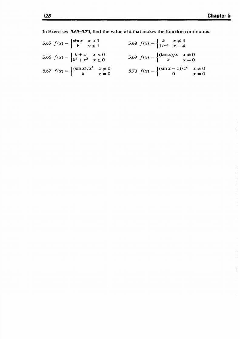
8/9/2019 Mortenson, Michael E. - Mathematics for computer graphics applications.pdf
http://slidepdf.com/reader/full/mortenson-michael-e-mathematics-for-computer-graphics-applicationspdf 141/367
128
Chapter
5
In
Exercises
5.65-5.70,
find
the value
of
k
that
makes
the function
continuous.
5.65
f
(X)
=I k
x <
1
5.68
f(x)
= Il/X3
X-4
5.66
f(x)
=
[k
+ xk x
0
5.69
f (x)=
((tanx)/x
x :O
.7(x)
k2X2
x
>O
k x
0
5 6
JfX
-x ((sin
X)/X
2
X
A 0
5{0f
x =(sin
-x)/Ixk
x
:A0
56
1
k-
x=0
5.0fx
o
X=O
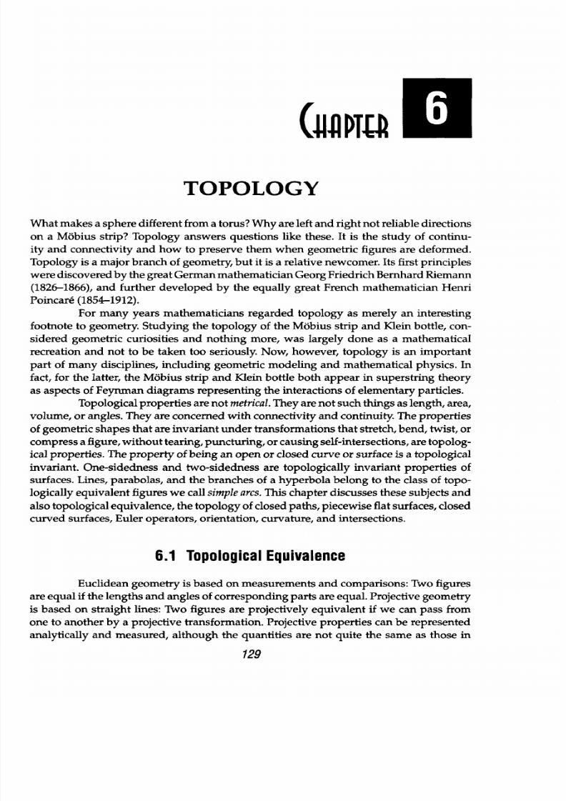
8/9/2019 Mortenson, Michael E. - Mathematics for computer graphics applications.pdf
http://slidepdf.com/reader/full/mortenson-michael-e-mathematics-for-computer-graphics-applicationspdf 142/367
(uj
pTa
TOPOLOGY
What
makes
a sphere
different from
a
torus?
Why are
left and right
not reliable
directions
on
a
Mobius strip?
Topology
answers questions
like
these. It
is
the
study
of
continu-
ity and connectivity and how to preserve them when geometric figures are
deformed.
Topology
is a
major
branch
of geometry,
but
it is
a
relative newcomer. Its first principles
were
discovered by
the great German mathematician Georg
Friedrich Bernhard
Riemann
(1826-1866),
and
further developed
by
the
equally great
French mathematician Henri
Poincar6 (1854-1912).
For
many
years
mathematicians
regarded
topology
as merely an
interesting
footnote to geometry. Studying
the topology of the
Mobius strip
and
Klein bottle, con-
sidered geometric curiosities and nothing more, was largely done as a mathematical
recreation
and
not
to be taken too seriously.
Now,
however, topology is an
important
part
of
many
disciplines,
including
geometric
modeling
and
mathematical
physics.
In
fact,
for the latter, the Mobius strip
and
Klein bottle
both
appear
in
superstring
theory
as
aspects
of Feynman
diagrams representing
the
interactions
of elementary particles.
Topological properties
are
not metrical.They are not
such
things
as length,
area,
volume,
or
angles. They are concerned with connectivity
and
continuity. The properties
of geometric shapes
that
are
invariant
under
transformations
that stretch,
bend,
twist, or
compress a figure, without tearing,
puncturing,
or causing self-intersections, are topolog-
ical
properties.
The property
of
being
an open
or
closed curve or
surface
is a
topological
invariant. One-sidedness
and
two-sidedness
are topologically invariant properties of
surfaces. Lines,
parabolas,
and
the branches
of
a
hyperbola belong
to the
class of
topo-
logically equivalent
figures
we call
simple
arcs.
This chapter discusses these
subjects
and
also topological equivalence, the topology of closed paths, piecewise flat surfaces, closed
curved
surfaces,
Euler
operators, orientation,
curvature,
and intersections.
6.1
Topological Equivalence
Euclidean geometry is
based
on m easurements
and
comparisons: Two figures
are equal if the lengths
and
angles of corresponding parts are equal. Projective geometry
is based
on straight lines:
Two
figures are projectively
equivalent if
we
can pass from
one
to another
by
a projective transformation.
Projective
properties can be represented
analytically
and
measured,
although
the quantities are
not
quite the same as those in
129
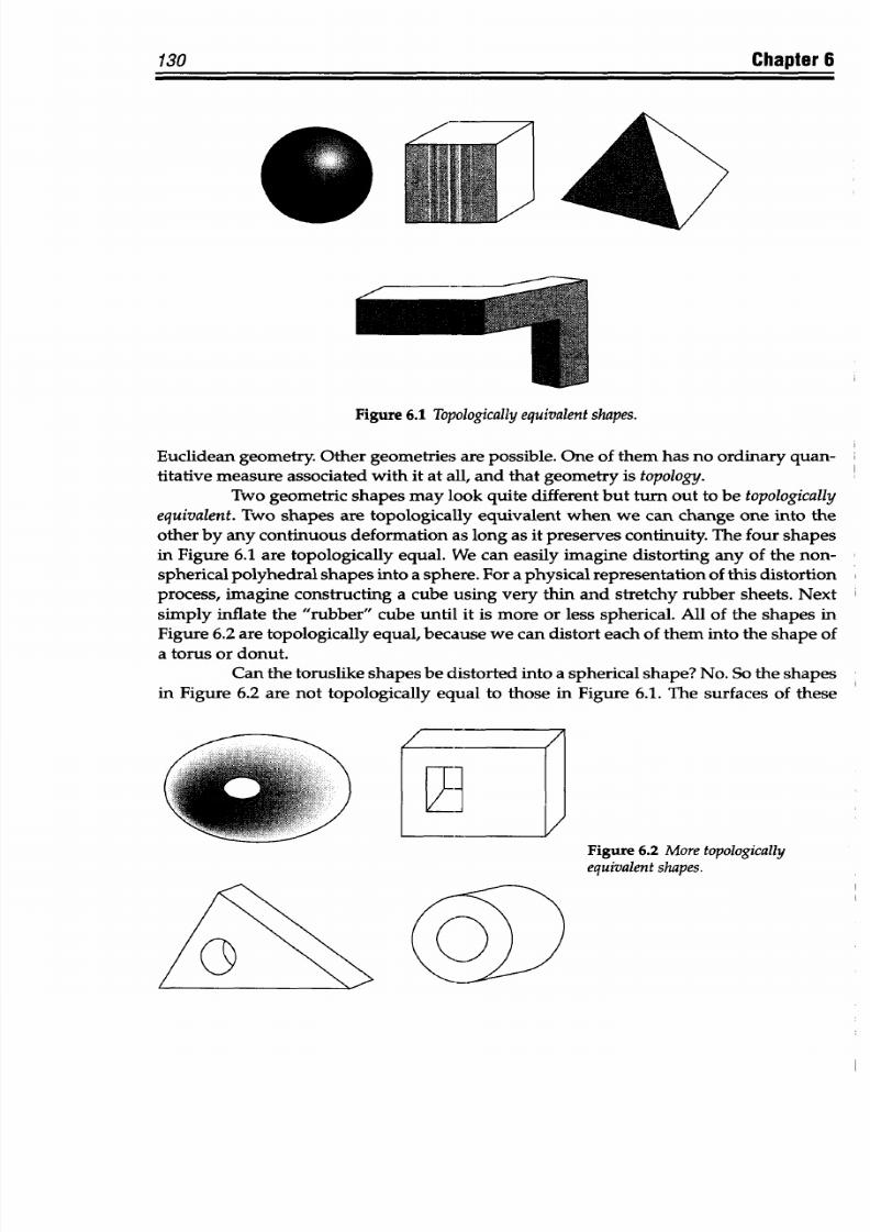
8/9/2019 Mortenson, Michael E. - Mathematics for computer graphics applications.pdf
http://slidepdf.com/reader/full/mortenson-michael-e-mathematics-for-computer-graphics-applicationspdf 143/367
130 Chapter
6
Figure
6.1 Topologically equivalent shapes.
Euclidean geometry. Other geometries
are
possible. One of them
has
no
ordinary quan-
titative measure
associated with it at
all,
and that
geometry
is
topology.
Two geometric shapes
may
look quite
different
but turn out to be topologically
equivalent. Two
shapes are topologically equivalent when we can
change one into
the
other
by any
continuous deformation as long as it preserves continuity. The four shapes
in Figure
6.1
are topologically equal.
We
can
easily imagine
distorting
any
of
the
non-
spherical polyhedral
shapes into a sphere. For a
physical
representation of this distortion
process, imagine constructing
a
cube
using
very
thin
and
stretchy rubber sheets. Next
simply inflate the
"rubber"
cube
until
it is
more
or
less
spherical. All of the shapes in
Figure
6.2 are
topologically equal, because we can distort
each
of them into
the
shape of
a
torus
or donut.
Can
the toruslike shapes
be distorted
into a
spherical
shape? No.
So
the shapes
in Figure 6.2 are not
topologically
equal
to
those
in
Figure
6.1.
The surfaces of
these
1zigure o.z More topologically
equivalent
shapes.
VI
I
___Y
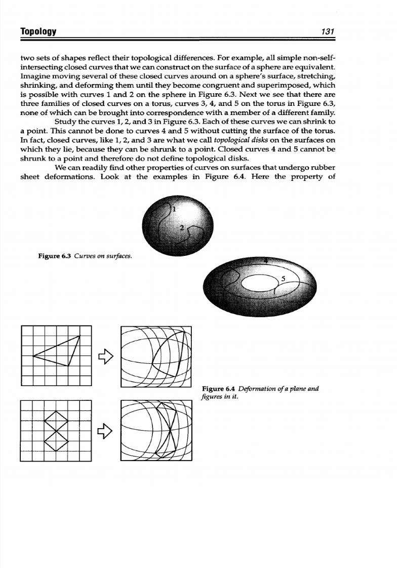
8/9/2019 Mortenson, Michael E. - Mathematics for computer graphics applications.pdf
http://slidepdf.com/reader/full/mortenson-michael-e-mathematics-for-computer-graphics-applicationspdf 144/367
two
sets of
shapes
reflect
their
topological differences. For example, all
simple
non-self-
intersecting closed curves that
we can construct on the surface
of
a sphere
are equivalent.
Imagine moving
several of these closed curves
around
on a sphere's surface, stretching,
shrinking, and deforming them
until
they
become
congruent and superimposed,
which
is
possible
with
curves 1 and 2 on the sphere in Figure
6.3.
Next we
see that
there are
three families of closed curves
on a
torus, curves 3, 4, and 5 on the torus
in
Figure 6.3,
none
of
which
can be brought
into
correspondence with a
member
of a different
family.
Study the curves 1,
2,
and
3
in Figure
6.3.
Each of these curves we
can
shrink to
a point. This cannot be done to curves 4
and 5
without cutting the surface of the torus.
In fact,
closed
curves,
like
1,
2, and
3
are
what we call
topological
disks on the
surfaces
on
which they lie, because they can be
shrunk
to a point. Closed curves 4 and 5 cannot be
shrunk to
a
point and
therefore
do
not define topological disks.
We
can
readily find other properties
of
curves
on
surfaces
that
undergo
rubber
sheet deformations.
Look
at
the
examples
in
Figure 6.4.
Here the
property
of
Figure
6.3
Curves
on surfaces.
I
Figure 6.4 Deformation of a plane and
figures
in
it.
131opology
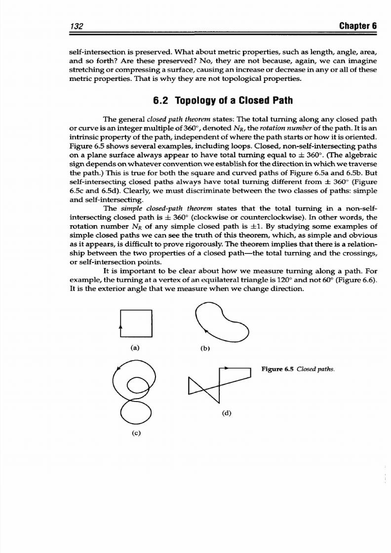
8/9/2019 Mortenson, Michael E. - Mathematics for computer graphics applications.pdf
http://slidepdf.com/reader/full/mortenson-michael-e-mathematics-for-computer-graphics-applicationspdf 145/367
132
Chapter
6
self-intersection is preserved. What
about
metric properties, such as length,
angle, area,
and
so
forth? Are
these preserved? No, they
are not
because, again, we can imagine
stretching
or
compressing
a surface, causing an increase or decrease
in
any or all
of
these
metric
properties.
That
is
why
they
are
not topological
properties.
6.2
Topology of a
Closed
Path
The
general closed path theorem
states:
The total turning
along
any
closed
path
or curve is an integer multiple
of
3600, denoted
NR,
the
rotationnumber
of
the path. It is
an
intrinsic property of the path,
independent
of where
the
path starts
or
how it is oriented.
Figure 6.5
shows
several examples, including loops. Closed, non-self-intersecting paths
on a
plane
surface always appear to
have
total
turning equal
to ±
3600. (The algebraic
sign
depends on
whatever convention we establish
for
the d irection in which w e traverse
the path.)
This
is
true for both the square and
curved
paths of Figure 6.5a and 6.5b. But
self-intersecting
closed paths
always have total
turning different
from
±
3600 (Figure
6.5c
and
6.5d). Clearly, we must discriminate between the two classes of paths: simple
and self-intersecting.
The simple closed-path theorem states that
the
total
turning
in
a non-self-
intersecting
closed path is ± 3600 (clockwise or counterclockwise). In
other
words,
the
rotation number NR of any
simple
closed path is ±1. By
studying
some examples of
simple
closed paths
we
can see
the truth
of
this theorem,
which, as
simple
and
obvious
as
it appears, is
difficult
to prove
rigorously. The
theorem implies
that
there
is a
relation-
ship between the two properties
of a closed
path-the total
turning and
the
crossings,
or
self-intersection
points.
It is important to be clear about how
we
measure
turning
along a
path. For
example, the
turning
at a vertex of an
equilateral triangle
is 120° and
not
600 (Figure 6.6).
It is
the
exterior angle that
we m easure
when
we change direction.
D
(a) (b)
Figure 6.5 Closedpaths.
(d)
(c)
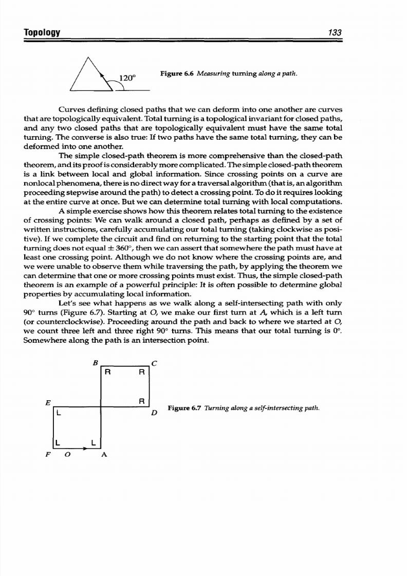
8/9/2019 Mortenson, Michael E. - Mathematics for computer graphics applications.pdf
http://slidepdf.com/reader/full/mortenson-michael-e-mathematics-for-computer-graphics-applicationspdf 146/367
133
opology
Figure 6.6 Measuring
turning
along a path.
Curves defining closed paths
that we
can deform into one
another
are curves
that
are
topologically equivalent. Total
turning
is a topological invariant for closed paths,
and
any
two
closed
paths that are topologically
equivalent
must
have the
same total
turning.
The
converse is
also
true: If two paths have the same total turning, they
can
be
deformed
into
one
another.
The simple closed-path theorem
is
more comprehensive than the closed-path
theorem, and its proof is considerably
more
complicated.
The simple
closed-path
theorem
is
a
link
between
local
and
global
information.
Since
crossing
points on
a
curve
are
nonlocal phenomena, there
is no
direct
way for
a
traversal
algorithm
(that
is, an algorithm
proceeding stepwise around the
path) to
detect a crossing point.
To
do it requires look ing
at the entire
curve
at once.
But
we can determine total turning
with local
computations.
A simple exercise shows how
this
theorem relates
total
turning to the existence
of crossing points: We
can
walk around a closed
path,
perhaps as defined by a set of
written
instructions, carefully accumulating
our
total turning
(taking clockwise
as
posi-
tive). If we complete
the
circuit
and find on returning to
the
starting point that
the
total
turning
does
not
equal ± 360°,
then
we can
assert
that somewhere
the
path
must
have at
least one crossing
point.
Although w e
do
not
know
where
the
crossing
points
are,
and
we were
unable
to observe
them
while
traversing the path,
by applying
the
theorem
we
can
determine that one
or
more
crossing
points must exist.
Thus,
the simple closed-path
theorem is
an
example
of
a
powerful
principle: It
is
often possible to determine global
properties
by accumulating local
information.
Let's see what happens as we
walk
along a self-intersecting path with only
900 turns
(Figure 6.7).
Starting at 0, we make
our first turn
at
A,
which
is a
left
turn
(or counterclockwise).
Proceeding
around
the path
and
back
to
where we started at
0,
we count three
left and
three
right 900
turns.
This means that our
total turning
is 00.
Somewhere
along the path is an intersection point.
E
Figure
6.7 Turningalong a self-intersectingpath.
F 0
A
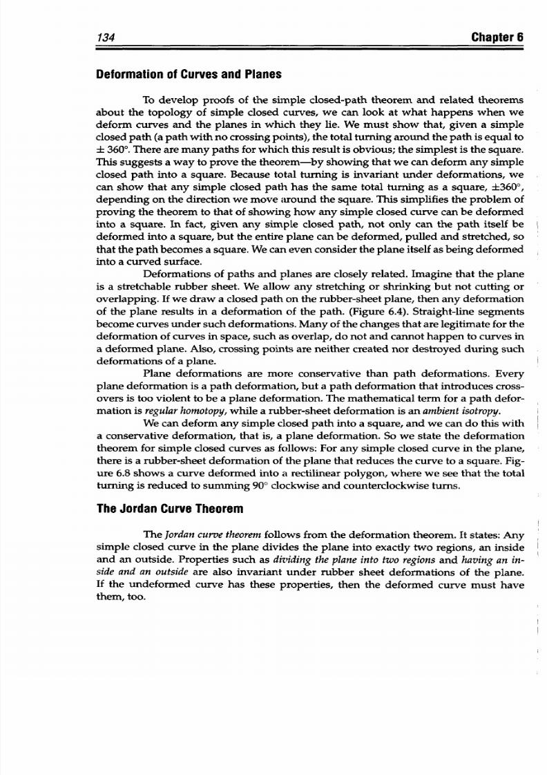
8/9/2019 Mortenson, Michael E. - Mathematics for computer graphics applications.pdf
http://slidepdf.com/reader/full/mortenson-michael-e-mathematics-for-computer-graphics-applicationspdf 147/367
134
Chapter
6
Deformation of
Curves and
Planes
To develop
proofs
of
the simple closed-path theorem and related theorems
about
the topology
of
simple
closed curves,
we
can
look
at
what happens when
we
deform
curves and
the planes
in
which
they lie. We
must
show that, given
a simple
closed
path (a
path
with
no crossing points),
the
total turning
around
the
path
is equal
to
± 360°.
There
are many
paths
for which this result is obvious; the simplest
is the square.
This
suggests
a way to
prove the
theorem-by showing that we
can deform any simple
closed
path
into a square. Because total
turning
is
invariant
under
deformations, we
can
show
that any
simple closed path has
the
same
total
turning as
a square, ±3600,
depending on the direction we move around the square. This simplifies the problem of
proving the theorem to that
of
showing how any simple closed curve can be deformed
into
a square. In fact, given any simple closed
path, not
only
can
the
path itself
be
deformed into
a
square,
but
the entire plane
can
be deformed,
pulled
and
stretched,
so
that the path becomes a square. We can
even
consider the plane itself as being deformed
into a curved
surface.
Deformations
of paths
and
planes are closely related.
Imagine
that the
plane
is
a stretchable rubber sheet.
We
allow any stretching or shrinking but
not
cutting or
overlapping. If we draw a closed path on
the
rubber-sheet plane,
then any
deformation
of
the plane results
in a deformation
of the path. (Figure 6.4).
Straight-line
segments
become curves
under
such deformations. Many of the changes that are legitimate for the
deformation of
curves
in space,
such
as
overlap, do
not
and cannot
happen
to curves in
a
deformed plane.
Also,
crossing
points
are
neither created
nor
destroyed
during
such
deformations of a
plane.
Plane deformations are more conservative than
path
deformations. Every
plane
deformation is a path
deformation,
but a path deformation that introduces cross-
overs is too violent
to
be a plane deformation.
The
mathematical term for a
path defor-
mation is
regularhomotopy, while a rubber-sheet deformation is
an
ambient isotropy.
We
can deform any
simple closed path
into
a square,
and we can do this with
a
conservative
deformation,
that
is, a
plane deformation.
So we state
the
deformation
theorem for simple closed
curves
as follows: For any
simple
closed
curve in
the
plane,
there is a rubber-sheet deformation
of
the plane that reduces the curve to a
square.
Fig-
ure 6.8 shows
a curve
deformed into
a rectilinear
polygon,
where
we see that
the
total
turning
is
reduced to summing
900 clockwise and
counterclockwise turns.
The Jordan
Curve
Theorem
The
Jordan
curve
theorem follows from the deformation theorem. It
states:
Any
simple
closed
curve
in
the plane
divides
the plane
into
exactly
two
regions, an inside
and an outside. Properties
such as dividing the
plane
into two regions
and having
an
in-
side
and an outside are also
invariant
under
rubber
sheet
deformations of
the plane.
If
the
undeformed
curve has these properties,
then
the deformed curve
must
have
them, too.
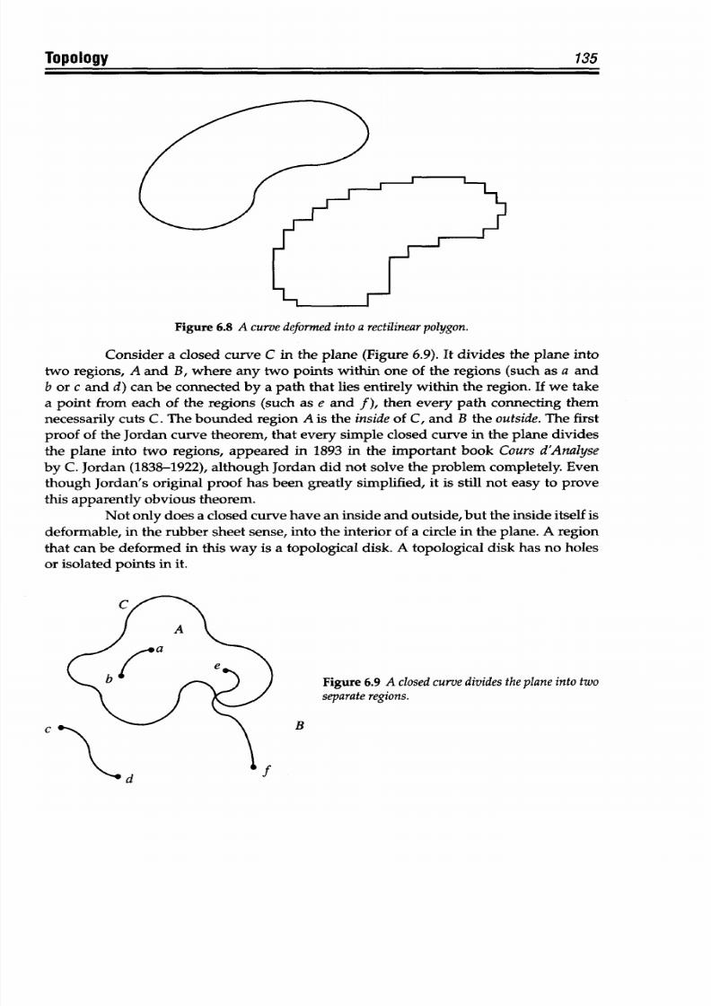
8/9/2019 Mortenson, Michael E. - Mathematics for computer graphics applications.pdf
http://slidepdf.com/reader/full/mortenson-michael-e-mathematics-for-computer-graphics-applicationspdf 148/367
Topology 135
Figure
6.8
A curve deformed into a rectilinear
olygon.
Consider
a closed curve
C
in
the
plane (Figure
6.9). It divides the
plane into
two
regions, A
and B, where any two points within one of
the regions
(such as a an d
b
or
c and d)
can
be connected
by
a
path that
lies
entirely within
the
region.
If we
take
a point
from each of
the
regions (such as e
and
f), then
every
path connecting
them
necessarily cuts C. The bounded region A is the inside of
C, and B
the
outside.
The
first
proof of the Jordan
curve
theorem, that every simple
closed
curve
in the
plane divides
the plane into
two regions,
appeared
in
1893
in
the
important
book
Cours d'Analyse
by
C. Jordan (1838-1922),
although
Jordan did not solve the problem completely.
Even
though Jordan's original
proof
has been greatly
simplified,
it is still not easy to prove
this apparently obvious
theorem.
Not only
does a
closed curve
have an inside and outside,
but the
inside
itself
is
deformable,
in the rubber
sheet sense,
into the interior
of
a circle in the
plane.
A region
that
can
be
deformed in this
way
is a topological disk. A
topological
disk has no holes
or isolated
points
in it.
Figure 6.9
A closed
curve divides the plane
into two
separate
regions.
B
.
J
' d
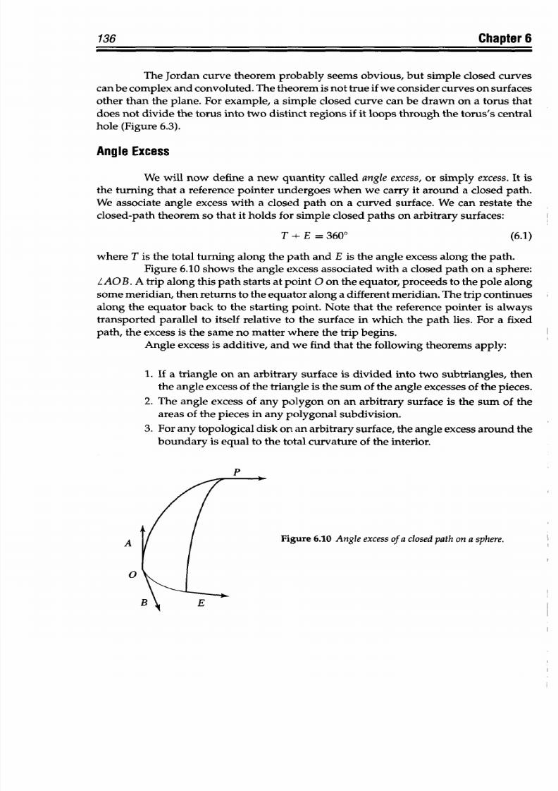
8/9/2019 Mortenson, Michael E. - Mathematics for computer graphics applications.pdf
http://slidepdf.com/reader/full/mortenson-michael-e-mathematics-for-computer-graphics-applicationspdf 149/367
136
Chapter 6
The
Jordan
curve
theorem probably seems
obvious,
but
simple
closed
curves
can be
complex and
convoluted.
The theorem is
not
true if we consider
curves
on surfaces
other than the plane.
For
example, a simple
closed curve
can
be
drawn on
a torus that
does
not
divide the
torus
into
two
distinct regions
if
it loops
through
the
torus's
central
hole
(Figure 6.3).
Angle
Excess
We will
now define a
new quantity
called angle
excess, or simply excess.
It is
the
turning
that
a reference pointer
undergoes when we carry it
around
a
closed
path.
We associate
angle
excess
with
a closed path on a curved surface. We can restate
the
closed-path theorem so
that
it
holds for
simple
closed paths on
arbitrary
surfaces:
T
-
E
=
360°
(6.1)
where T
is
the
total turning along
the path
and
E is the
angle
excess along the path.
Figure 6.10 shows
the angle excess associated
with
a closed
path on a sphere:
LAO B. A
trip
along this path starts at point 0 on the equator, proceeds to
the
pole along
some
meridian,
then returns
to
the equator
along
a
different
meridian. The trip
continues
along the equator back to the starting point.
Note that
the
reference
pointer
is always
transported
parallel to itself
relative
to the surface in which the
path
lies.
For
a fixed
path,
the excess is the same
no
matter where the trip begins.
Angle
excess
is additive,
and
we find that the following theorems apply:
1. If a triangle on an
arbitrary surface
is divided into two
subtriangles, then
the angle excess of the triangle is the
sum
of the angle excesses of the pieces.
2. The
angle
excess
of any polygon
on an arbitrary surface is
the
sum
of
the
areas of the pieces in any polygonal
subdivision.
3.
For any topological
disk on
an arbitrary surface, the angle
excess around
the
boundary is
equal
to
the total curvature of
the interior.
P
Figure 6.10 Angle excess
of
a
closed path on a sphere.
A
0
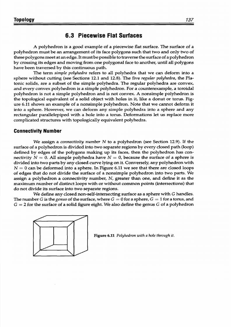
8/9/2019 Mortenson, Michael E. - Mathematics for computer graphics applications.pdf
http://slidepdf.com/reader/full/mortenson-michael-e-mathematics-for-computer-graphics-applicationspdf 150/367
Topology
137
6.3 Piecewise Flat Surfaces
A
polyhedron
is a
good
example
of a piecewise
flat surface.
The
surface of a
polyhedron must be
an arrangement of its face polygons such
that
two and only two of
these
polygons
meet
at
an
edge. It
mustbe
possible to traverse the surface of
a
polyhedron
by crossing its edges
and
moving from one polygonal face to another, until all polygons
have been traversed
by
this continuous path.
The
term simple polyhedra refers
to all polyhedra that
we
can deform into a
sphere
without cutting (see Sections 12.1 and
12.8). The
five
regular
polyhedra,
the
Pla-
tonic solids, are a subset of the simple polyhedra. The regular
polyhedra
are convex,
and every
convex
polyhedron
is a simple
polyhedron.
For
a
counterexample,
a
toroidal
polyhedron is
not a
simple
polyhedron and
is not convex.
A nonsimple
polyhedron
is
the
topological
equivalent
of
a
solid
object
with
holes in
it, like
a
donut
or torus.
Fig-
ure
6.11 shows
an example of a nonsimple polyhedron. Note
that
we cannot deform it
into a sphere. However, we can deform any simple
polyhedra
into a sphere
and
any
rectangular parallelepiped
with
a hole into a
torus. Deformations let us replace more
complicated structures
with
topologically
equivalent polyhedra.
Connectivity Number
We
assign
a connectivity
number
N to a polyhedron (see Section 12.9). If the
surface
of
a
polyhedron
is
divided
into
two separate
regions
by
every closed
path
(loop)
defined by
edges
of
the polygons
making up its faces, then
the polyhedron
has con-
nectivity N
=
0. All simple
polyhedra
have N = 0, because the
surface
of
a sphere
is
divided
into
two
parts by
any closed
curve
lying on it.
Conversely,
any
polyhedron with
N = 0 can be deformed
into
a sphere.
In
Figure 6.11 we see
that there are closed loops
of edges that do not
divide
the surface of a nonsimple
polyhedron
into two parts. We
assign a
polyhedron
a connectivity number,
N,
greater than one, and
define it
as the
maximum
number of
distinct loops with
or without common points
(intersections)
that
do
not
divide its surface
into
two separate regions.
We define any
closed non-self-intersecting surface as a sphere with G handles.
The
number G
is the genus of
the surface, where
G = 0for
a sphere,
G = 1
for a
torus,
and
G
=
2
for the surface of a
solid
figure
eight.
We
also
define
the genus
G
of
a polyhedron
Figure 6.11 Polyhedron with a hole through
it.
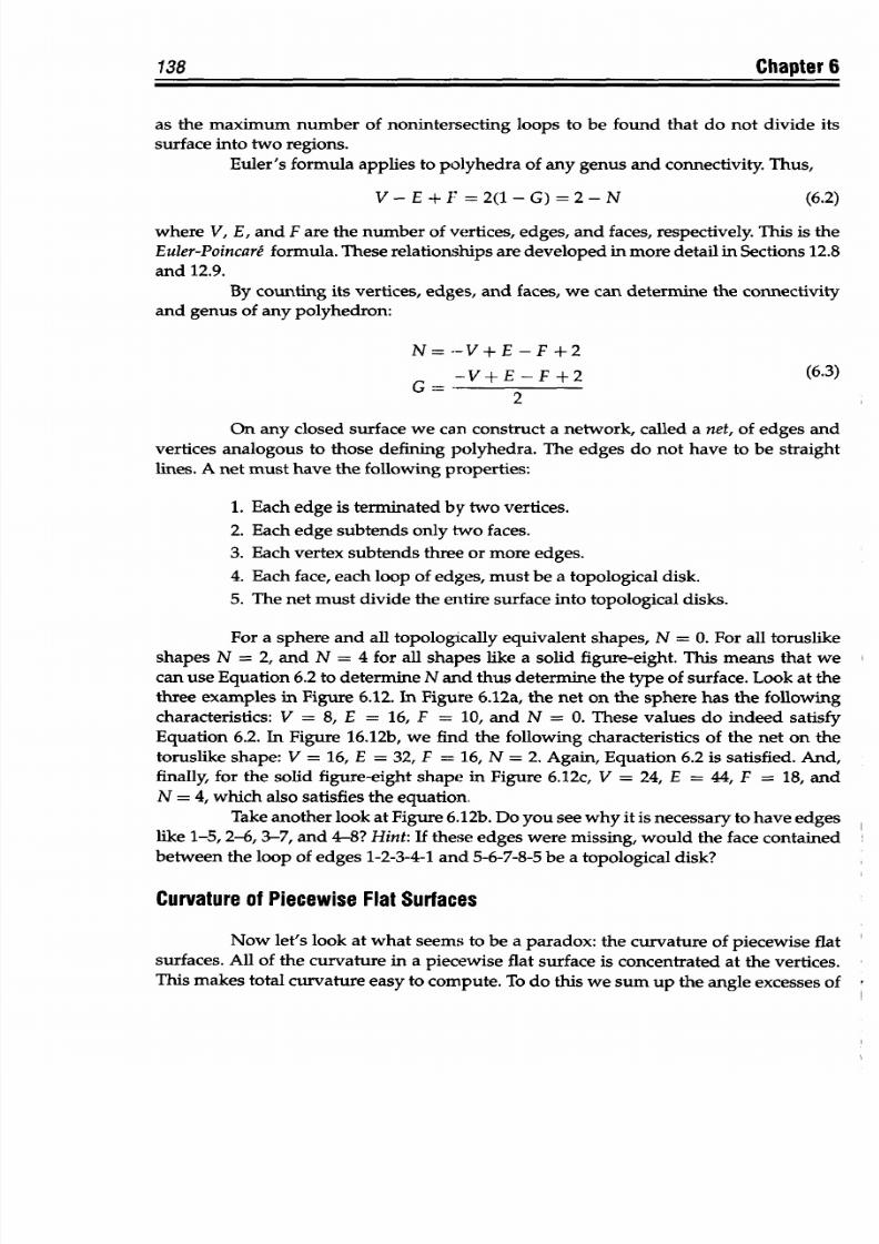
8/9/2019 Mortenson, Michael E. - Mathematics for computer graphics applications.pdf
http://slidepdf.com/reader/full/mortenson-michael-e-mathematics-for-computer-graphics-applicationspdf 151/367
138
Chapter
6
as the maximum number
of nonintersecting
loops to be
found
that
do not divide its
surface
into two
regions.
Euler's
formula applies to polyhedra of
any genus and connectivity. Thus,
V-E
+ F = 2(1-G)
=
2-N
(6.2)
where V, E, and
F are
the
number
of vertices, edges,
and faces, respectively. This
is
the
Euler-Poincare ormula. These
relationships are
developed in more
detail in Sections
12.8
and 12.9.
By counting its
vertices, edges,
and
faces,
we can determine
the
connectivity
and genus of
any polyhedron:
N= --V+E-F +2
-V+
E-F
+2
(6.3)
2
On
any
closed
surface we
can construct a network, called
a
net,
of
edges and
vertices
analogous
to
those
defining
polyhedra. The
edges
do not
have to be straight
lines.
A
net must
have
the following
properties:
1. Each edge is terminated by
two
vertices.
2.
Each edge subtends
only
two
faces.
3.
Each vertex
subtends
three or more
edges.
4. Each face, each loop
of edges,
must be a topological disk.
5.
The
net
must divide
the
entire surface
into topological disks.
For
a sphere and
all
topologically
equivalent shapes, N = 0.
For
all
toruslike
shapes N = 2, and N = 4 for
all
shapes
like
a
solid figure-eight.
This
means
that
we
can
use
Equation
6.2 to determine
N
and thus determine
the
type
of surface. Look
at the
three examples in
Figure
6.12.
In Figure 6.12a, the net
on
the
sphere
has the following
characteristics:
V
=
8, E
= 16, F = 10,
and
N
=
0. These values do
indeed
satisfy
Equation 6.2. In Figure
16.12b, we find the following
characteristics of
the
net on
the
toruslike
shape:
V = 16,
E
=
32, F
= 16,
N
=
2. Again, Equation
6.2
is satisfied.
And,
finally, for the solid
figure-eight shape
in
Figure
6.12c, V = 24,
E
=
44, F = 18,
and
N
=
4, which
also
satisfies
the
equation.
Take
another look at
Figure
6.12b. Do
you
see why it
is necessary
to have
edges
like
1-5, 2-6, 3-7,
and 4-8?
Hint: If
these edges were missing,
would the
face contained
between
the loop
of edges
1-2-3-4-1
and 5-6-7-8-5
be
a
topological
disk?
Curvature of Piecewise
Flat Surfaces
Now let's
look
at
what
seems
to
be
a
paradox:
the
curvature
of
piecewise
flat
surfaces.
All of the curvature
in
a
piecewise
flat surface
is
concentrated at the vertices.
This makes
total curvature
easy to compute. To
do this
we sum up the
angle excesses
of
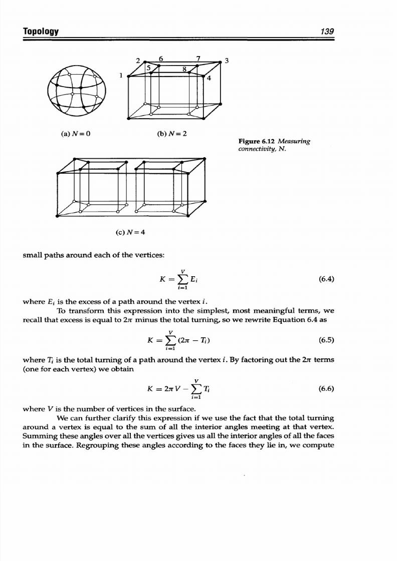
8/9/2019 Mortenson, Michael E. - Mathematics for computer graphics applications.pdf
http://slidepdf.com/reader/full/mortenson-michael-e-mathematics-for-computer-graphics-applicationspdf 152/367
Topology
3
1
(b)
N = 2
139
Figure 6.12
Measuring
connectivity, N.
7/
(c)N=4
small
paths
around
each of
the
vertices:
V
K
YEi
i=1
(6.4)
where
E
1
is
the
excess of
a
path around the vertex i.
To
transform
this expression
into the
simplest,
most
meaningful terms, we
recall that excess
is
equal to 27r minus the
total
turning, so
we rewrite
Equation 6.4 as
V
K =
E
(2r-T7)
i=1
(6.5)
where T7
s
the total
turning
of
a
path around the vertex i. By
factoring out
the 27r terms
(one for each vertex) we obtain
V
K
=27rV-ETi
i=1
(6.6)
where
V
is the
number of vertices in
the surface.
We can further clarify this expression if
we
use
the
fact that
the total
turning
around
a
vertex
is
equal to the sum of all
the
interior angles meeting at that vertex.
Summing these angles over
all the
vertices gives
us
all the interior angles of
all
the faces
in the surface.
Regrouping these angles
according to
the faces they lie
in, we
compute
(a)N=O
-
Z
w
r-
-
-
-
-.
I
f
X
; ,
g
I
4
Q
8/9/2019 Mortenson, Michael E. - Mathematics for computer graphics applications.pdf
http://slidepdf.com/reader/full/mortenson-michael-e-mathematics-for-computer-graphics-applicationspdf 153/367
140
Chapter 6
total curvature as
F
K = 27rV-E i
(6.7)
i=1
where
fi is the sum of
the interior angles
of the
face i.
This
is a surprising result, because it shows that
we
computed the second
term
without knowing how the edges are joined together. If we know all the
individual
faces
of
a piecewise
flat surface
and
we
know
V,
we
can
compute
total
curvature.
For piecewise square surfaces, the
formula
is even simpler, because
the sum
of
interior angles
of
any face
is 27r. Therefore,
K
= 2rV
- 2irF or K
=
27r(V -
F).
This
equation
for total
curvature
does not depend on
angles at
all
And
we can
do even
better.
Curiously enough, we can compute the total curvature
of
any closed piecewise
flat
surface
without
knowing any
angles. All
we need
to
know
is
the
number
of
faces,
vertices,
and
edges. For
a closed
piecewise
flat
surface
with V vertices,
E
edges,
and
F
faces, the total curvature is
K
=
2ir(V-E +
F)
(6.8)
To
prove
Equation
6.8,
we
must
show
that
we can
express the summation term
of
Equation 13 independently
of
the
values
of
the
angles. We
do
not know
much
in
general about the sum
of
the interior angles of
a
face, but we do know a
closely
related
quantity: the sum of
the exterior
angles. The boundary of each
face
is a
simple
closed
path,
so
we know that
the
sum
of
the exterior angles
is
27r.
To
relate
the
exterior angles
to
the interior
angles,
we
note
that
each exterior
angle
pairs
off
with
an interior
angle to
sum to
1800,
and there
are as
many of these pairs as there are edges to a
face.
Therefore,
fi
= sum
of
(ir
- exterior angles)
= 7r
x
ei (sum of
exterior
angles of the face) (6.9)
=
7r x ei - 27r
where
ei
is the
number of
edges
of
the face
i. Summing
this
quantity over all
the faces
yields
F F
,
fi
=
Eei
-27rF
(6.10)
i=l
i=1
Now
we simplify
the
summation on
ei,
keeping in mind that in a closed surface
each
edge is shared by
precisely
two faces, and that summing
the
number of
edges in a
face over
all
the separate faces counts
each
edge exactly twice. This
means that
F
Eei
= 2E (6.11)
I=1
Combining
Equation
6.10 with
6.11
yields
F
If = 27r (E -F) (6.12)
1=1
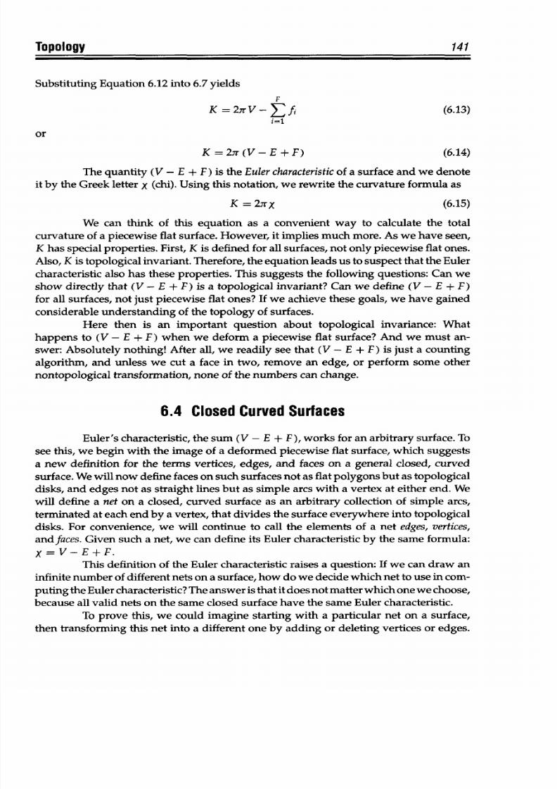
8/9/2019 Mortenson, Michael E. - Mathematics for computer graphics applications.pdf
http://slidepdf.com/reader/full/mortenson-michael-e-mathematics-for-computer-graphics-applicationspdf 154/367
Topology
141
Substituting Equation 6.12 into 6.7 yields
F
K = 27r V- fi
(6.13)
or
K = 27r (V-E +
F)
(6.14)
The
quantity
(V -
E
+
F) is
the Euler characteristicof a surface
and
we denote
it by the Greek letter X (chi).
Using this notation, w e rewrite the curvature
formula as
K = 27nx (6.15)
We can
think of this
equation
as
a convenient way to
calculate
the total
curvature
of
a piecewise
flat surface.
However,
it implies
much
more.
As
we have
seen,
K
has
special
properties.
First, K
is
defined for all surfaces,
not only
piecewise
flat ones.
Also,
K
is topological invariant.
Therefore,
the equation leads us to suspect that the
Euler
characteristic also has
these properties.
This suggests
the
following questions:
Can
we
show directly
that
(V - E
+ F) is a topological invariant? Can
we define
(V -
E +
F)
for all surfaces, not just piecewise flat ones?
If
we achieve
these
goals, we have gained
considerable
understanding of
the topology of
surfaces.
Here then
is
an important question
about topological invariance: What
happens to (V -
E
+ F) when we deform a piecewise flat surface?
And
we must an-
swer:
Absolutely nothing After all, we readily see
that
(V - E + F)
is
just a counting
algorithm,
and
unless
we
cut a
face
in
two, remove
an edge,
or
perform
some
other
nontopological transformation, none of the numbers
can
change.
6.4
Closed Curved Surfaces
Euler's characteristic, the sum (V - E +
F),
works for an
arbitrary
surface. To
see
this, we
begin with
the image
of
a
deformed
piecewise
flat
surface, which suggests
a new definition for the terms
vertices,
edges, and faces on a general
closed,
curved
surface.
We
will
now
define
faces
on
such
surfaces
not
as flat
polygons
but
as
topological
disks, and edges
not as
straight lines
but as
simple arcs
with
a vertex at either end. We
will
define
a
net on a closed, curved surface
as
an arbitrary collection of simple
arcs,
terminated at
each
end by a vertex, that
divides
the surface everywhere
into
topological
disks. For convenience, we will continue to
call the elements
of a net edges, vertices,
and aces. Given such
a net, we can define its Euler
characteristic
by
the same
formula:
x = V-E + F.
This definition
of
the Euler characteristic raises a question: If we can
draw
an
infinite number of different
nets on a surface,
how
do
we
decide
which
net
to
use
in com-
puting
the
Euler
characteristic? The
answer
is
that
it does
not
matter
which
one
we
choose,
because
all
valid nets on the same closed surface have the same Euler
characteristic.
To prove this, we could imagine starting with a particular
net
on a surface,
then
transforming
this
net
into
a
different one
by adding or deleting vertices or
edges.
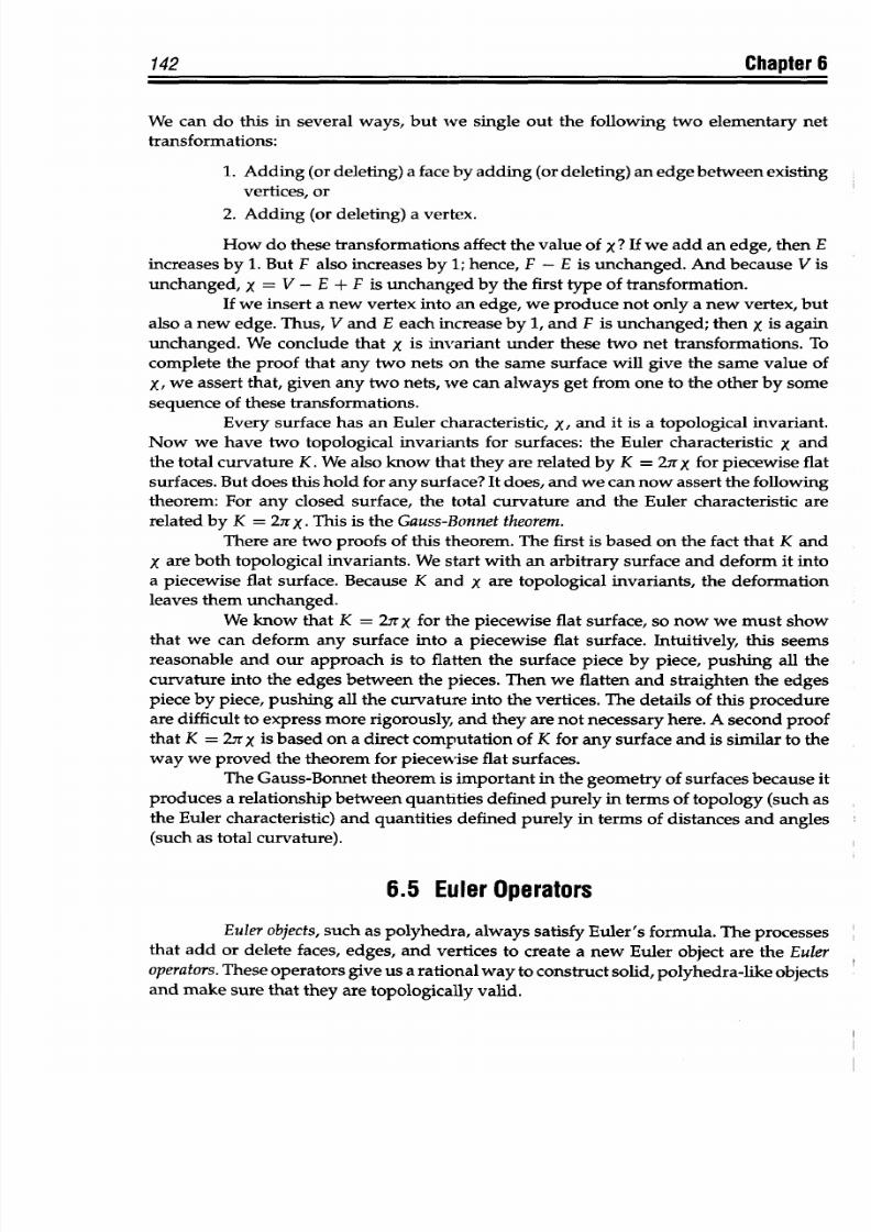
8/9/2019 Mortenson, Michael E. - Mathematics for computer graphics applications.pdf
http://slidepdf.com/reader/full/mortenson-michael-e-mathematics-for-computer-graphics-applicationspdf 155/367
142
Chapter 6
We can do this in several
ways, but we single out the following two elementary ne t
transformations:
1.
Adding
(or deleting) a
face
by adding
(or deleting)
an edge between
existing
vertices,
or
2.
Adding (or
deleting) a
vertex.
How do
these
transformations
affect the value of
X?
If
we
add
an
edge, then
E
increases
by
1.
But F also
increases by 1; hence,
F - E is unchanged.
And
because V is
unchanged,
X
= V
-
E + F
is unchanged by the first type of transformation.
If we insert a
new vertex into an edge,
we
produce
not
only
a
new
vertex, but
also a
new
edge.
Thus,
V
and
E
each increase by
1,
and F is unchanged; then
X is
again
unchanged.
We conclude
that
X
is invariant under
these two net transformations.
To
complete
the
proof that any
two nets on the same surface
will give the same value
of
X, we assert that,
given any
two
nets,
we can always get
from one
to
the
other
by some
sequence of these
transformations.
Every surface has
an Euler characteristic, x, and it is
a
topological invariant.
Now
we
have two
topological
invariants
for surfaces:
the
Euler
characteristic
X and
the total curvature
K. We also
know
that
they
are
related
by
K
=
27r
x for
piecewise flat
surfaces.
But does this
hold
for any
surface? It does,
and
we
can
now
assert the following
theorem: For
any closed
surface,
the
total
curvature
and the
Euler characteristic
are
related by K
=
2
7r X. This is the Gauss-Bonnet theorem.
There
are two
proofs of
this theorem. The first is based
on the fact
that K
and
x
are
both
topological
invariants.
We
start with
an
arbitrary
surface
and
deform it into
a piecewise
flat surface.
Because
K
and x are topological
invariants, the deformation
leaves them
unchanged.
We
know
that
K
=
27r X for the piecewise flat
surface,
so
now we
must
show
that
we
can
deform any surface into
a piecewise
flat
surface.
Intuitively, this seems
reasonable
and
our
approach
is
to flatten the surface
piece by piece,
pushing
all the
curvature
into the edges between
the pieces. Then we flatten
and straighten the
edges
piece by piece, pushing
all
the curvature
into the vertices. The
details of this procedure
are
difficult
to
express
more rigorously,
and they are
not
necessary here. A second
proof
that
K
=
27r
X
is
based
on
a
direct
computation
of
K
for
any
surface
and
is
similar
to
the
way
we
proved the theorem
for piecewise
flat
surfaces.
The Gauss-Bonnet
theorem is
important
in
the geometry
of surfaces
because
it
produces a relationship
between
quantities
defined
purely
in terms of topology
(such as
the
Euler
characteristic)
and quantities defined
purely
in terms
of distances and
angles
(such
as total curvature).
6.5
Euler Operators
Euler
objects,
such
as
polyhedra, always
satisfy
Euler's
formula.
The
processes
that
add or delete
faces, edges,
and
vertices to create
a new Euler object
are the
Euler
operators.
These operators
give us a rational way
to construct solid,
polyhedra-like
objects
and
make
sure that
they
are
topologically valid.
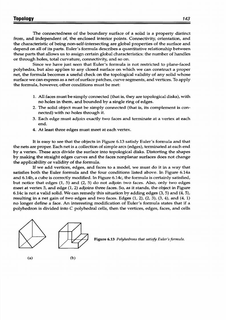
8/9/2019 Mortenson, Michael E. - Mathematics for computer graphics applications.pdf
http://slidepdf.com/reader/full/mortenson-michael-e-mathematics-for-computer-graphics-applicationspdf 156/367
Topology
143
The
connectedness
of
the boundary
surface
of a solid is a property distinct
from,
and
independent of, the enclosed
interior
points.
Connectivity, orientation, and
the characteristic
of
being non-self-intersecting
are global properties of the
surface
and
depend
on
all of
its
parts.
Euler's
formula
describes
a
quantitative
relationship between
these parts that allows us
to assign certain global
characteristics:
the
number of
handles
or through holes, total curvature,
connectivity,
and so on.
Since
we
have
just seen
that
Euler's
formula
is not
restricted to
plane-faced
polyhedra, but
also
applies
to
any
closed surface
on
which
we can
construct
a
proper
net, the formula becomes a
useful
check
on the topological
validity
of
any solid whose
surface
we
can express as
a net of surface patches,
curve
segments, and
vertices.
To
apply
the
formula,
however,
other
conditions must
be
met:
1.
All faces
must
be
simply
connected (that
is,
they
are
topological
disks),
with
no holes in them, and
bounded
by a single ring
of
edges.
2. The solid object must
be simply connected
(that
is,
its complement is con-
nected) with
no
holes
through
it.
3. Each edge must adjoin
exactly
two faces and
terminate at
a vertex at each
end.
4. At least three edges must
meet
at each vertex.
It
is
easy to see
that the
objects in Figure 6.13 satisfy Euler's formula
and that
the
nets are proper. Each net
is
a collection of simple arcs (edges),
terminated
at
each
end
by a vertex.
These arcs
divide the surface into topological
disks.
Distorting the shapes
by
making the straight edges curves and
the
faces
nonplanar surfaces does not change
the
applicability
or validity of
the
formula.
If
we add vertices,
edges,
and
faces
to
a model, we
must
do it
in
a way that
satisfies both
the
Euler
formula and the four
conditions listed
above. In Figure
6.14a
and
6.14b, a cube is
correctly
modified. In Figure 6.14c, the formula is certainly satisfied,
but notice that edges (1,
5)
and
(2,
5) do not
adjoin
two faces.
Also,
only two edges
meet at vertex 5, and edge (1,
2)
adjoins three
faces. So,
as
it
stands,
the object in Figure
6.14c
is
not
a
valid
solid.
We
can
remedy
this
situation
by adding
edges
(3, 5)
and
(4, 5),
resulting
in
a net
gain of
two edges and
two faces. Edges (1,2),
(2,
3), (3, 4),
and
(4,
1)
no longer
define a face. An interesting modification
of
Euler's
formula states that
if a
polyhedron
is
divided into C polyhedral
cells,
then the vertices, edges,
faces,
and cells
Figure
6.13
Polyhedrons
that
satisfy
Euler'sformula.
(a)
(b)
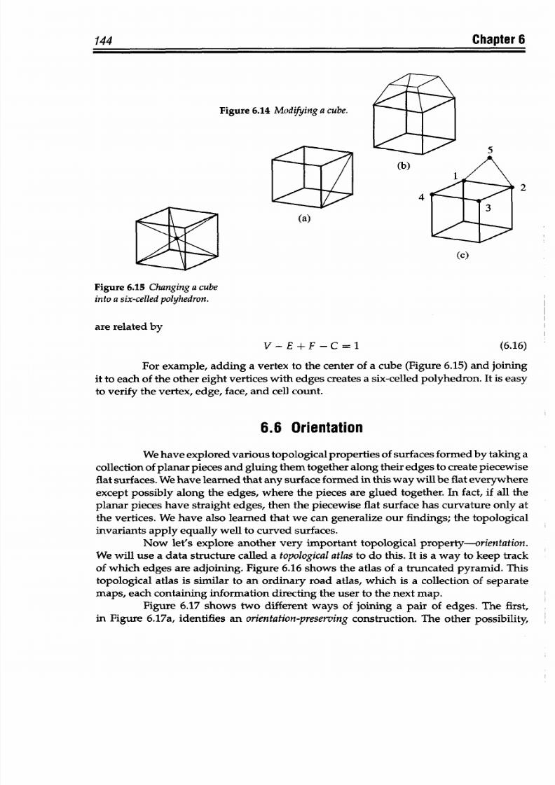
8/9/2019 Mortenson, Michael E. - Mathematics for computer graphics applications.pdf
http://slidepdf.com/reader/full/mortenson-michael-e-mathematics-for-computer-graphics-applicationspdf 157/367
144
Figure 6.14 Modifying
a
cube.
(b)
4
Chapter 6
2
(a)
(c)
Figure 6.15 Changinga cube
into
a
six-celled polyhedron.
are
related
by
V - E + F-C = 1
(6.16)
For example,
adding
a
vertex
to the center
of
a
cube
(Figure
6.15)
and joining
it to
each
of the
other eight vertices
with
edges
creates
a six-celled polyhedron. It is easy
to verify the vertex, edge, face, and cell
count.
6.6
Orientation
We have
explored various topological
properties
of surfaces
formed
by
taking
a
collection of
planar
pieces and gluing them together
along
their
edges
to create piecewise
flat surfaces.
We
have learned that
any
surface formed in this way will
be
flat
everywhere
except possibly along the edges, where the
pieces are
glued together. In
fact,
if all the
planar pieces
have straight edges, then the piecewise flat surface has curvature only at
the
vertices.
We have
also
learned
that
we can generalize
our
findings; the topological
invariants apply equally well to curved
surfaces.
Now let's explore another very important topological property-orientation.
We will use a
data
structure
called
a topologicalatlas to do this.
It is
a
way to keep track
of
which
edges
are
adjoining. Figure
6.16
shows
the atlas
of
a truncated pyramid. This
topological
atlas is
similar
to an
ordinary
road atlas, which is a
collection
of separate
maps,
each
containing information directing the user
to
the next
map.
Figure 6.17
shows two
different
ways of
joining
a pair of
edges. The
first,
in
Figure
6.17a, identifies
an
orientation-preservingconstruction.
The other
possibility,
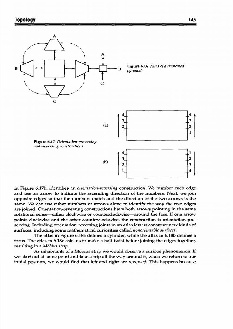
8/9/2019 Mortenson, Michael E. - Mathematics for computer graphics applications.pdf
http://slidepdf.com/reader/full/mortenson-michael-e-mathematics-for-computer-graphics-applicationspdf 158/367
Topology
145
A
Figure 6.16
Atlas of
a truncated
B pyramid.
C
B
Figure
6.17
Orientation-preserving
and
-reversing constructions.
4-
3-
2-
(a)
(b)
4-
3-
2-
I I
t I
-4
-3
-2
-1
-1
3
-4
in
Figure 6.17b, identifies
an
orientation-reversing onstruction. We
number
each
edge
and
use
an
arrow
to
indicate
the
ascending
direction of the
numbers.
Next, we
join
opposite edges
so
that
the
numbers
match
and
the direction
of
the two arrows
is
the
same.
We can use either numbers
or
arrows alone to identify the way the two edges
are joined.
Orientation-reversing
constructions have
both arrows pointing
in
the same
rotational
sense either
clockwise or counterclockwise-around the
face.
If
one
arrow
points
clockwise
and
the other counterclockwise, the
construction is
orientation pre-
serving. Including
orientation-reversing
joints
in
an
atlas lets
us construct new kinds of
surfaces, including some mathematical curiosities called nonorientable
urfaces.
The atlas in Figure
6.18a
defines a cylinder, while the atlas
in
6.18b defines
a
torus. The atlas in 6.18c
asks
us to
make
a half
twist
before
joining the edges
together,
resulting
in
a
Mdbius
strip.
As inhabitants
of
a Mobius strip we would
observe
a curious phenomenon. If
we
start out at some point
and
take
a
trip
all
the
way around it, when
we return
to
our
initial
position, we would find
that left
and
right
are
reversed. This happens because
I
145
opology
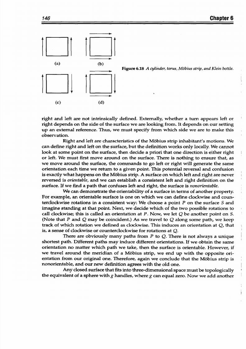
8/9/2019 Mortenson, Michael E. - Mathematics for computer graphics applications.pdf
http://slidepdf.com/reader/full/mortenson-michael-e-mathematics-for-computer-graphics-applicationspdf 159/367
146
Chapter
6
(a) (b)
Figure 6.18
A cylinder,
torus,
Mobius strip, and
Klein bottle.
(c)
(d)
right
and
left
are not
intrinsically
defined.
Externally,
whether
a
turn
appears
left
or
right depends
on the side
of
the
surface we are looking
from. It
depends
on
our setting
up an external
reference.
Thus,
we
must specify from
which
side
we
are
to
make
this
observation.
Right and
left
are characteristics
of
the Mobius strip
inhabitant's motions.
We
can define
right
and
left
on
the
surface, but the definition
works only locally.
We
cannot
look
at some point
on
the surface,
then decide a
priori
that
one direction is either right
or
left.
We
must
first
move
around
on
the
surface. There is
nothing
to
ensure that,
as
we
move
around
the
surface,
the
commands to go
left or right will generate
the same
orientation
each
time w e
return
to a
given point. This potential reversal and confusion
is
exactly
what
happens
on the
Mobius
strip. A
surface on which left and right
are never
reversed
is
orientable,
and
we can establish
a consistent left
and right definition on the
surface. If
we
find
a
path that confuses left and
right, the
surface
is
nonorientable.
We can demonstrate the orientability
of a surface in
terms
of
another
property.
For example,
an orientable surface
is one on
which
we can
define clockwise and
coun-
terclockwise rotations
in a consistent way: We
choose a point
P
on the
surface S and
imagine
standing
at
that
point.
Next,
we
decide
which
of
the
two
possible rotations
to
call clockwise;
this is called an
orientation
at
P. Now, we
let Q
be
another point
on S.
(Note that
P
and
Q may
be coincident.)
As we travel to Q along
some
path,
we keep
track
of
which
rotation we defined
as
clockwise.
This
induces
an
orientation
at Q, that
is, a sense of clockwise
or counterclockwise for
rotations
at
Q.
There are obviously
many paths
from P to
Q. There is not
always a
unique
shortest path. Different
paths may induce
different orientations.
If we obtain the
same
orientation
no
matter
which
path we take, then
the surface is orientable.
However, if
we
travel
around
the
meridian of a Mobius
strip,
we end
up with
the
opposite
ori-
entation
from
our original
one.
Therefore,
again
we
conclude that
the Mobius
strip is
nonorientable,
and
our new
definition
agrees
with
the
old
one.
Any closed surface that
fits
into
three-dimensional space must
be topologically
the
equivalent
of a sphere
with
g
handles, where
g can equal
zero.
Now
we add
another
8/9/2019 Mortenson, Michael E. - Mathematics for computer graphics applications.pdf
http://slidepdf.com/reader/full/mortenson-michael-e-mathematics-for-computer-graphics-applicationspdf 160/367
condition,
namely, that
the surface
must
be orientable. A sphere
is orientable, and it
is
not hard
to show
that adding
a handle cannot change that.
The Mobius strip does
fit
into
three-dimensional
space, but
it
is not closed.
To
transform the
Mobius
strip
into
a closed surface,
we make an orientation-preserving
construction of the top
and
bottom edges on the atlas exactly as we
did
when we pro-
duced a torus from a cylinder
(Figure
6.18d). The
resulting
surface is
a Klein
bottle,
and, like
the Mobius
strip, it
is nonorientable.
Producing the Klein bottle
involves
pushing the sur-
face
through itself-a
rather drastic operation, but the best we can do
in
three dimensions.
The Klein bottle will not fit
into
a three-dimensional space without self-intersections.
6.7 Curvature
We can
show
that the
total
curvature for
a sphere is
47r
and
that the angle
excess
is
proportional to the area,
or
E
= kA.
Thus, for any polygon on a sphere
of
radius r,
E
=
k,
where k
=
I
/r
2
(if is
measured
in radians).
For
a simple closed
path
on the
surface
of a
sphere, total
turning
in radians is expressed
as T
=
2ir
-
A/r
2
,
where A is the area
enclosed by the path
and
r
is
the radius of
the
sphere.
In general, for an arbitrary
surface,
k
is
a measurement taken at any point on
the
surface.
The
value of k at a point is
the
excess per unit area of a
small
patch of surface
containing
the point. We call k
the
curvature
density of the surface
at
a point.
We
use
the
term density
because
k is "something per unit area," and
we
use the
term curvature
density
rather
than
excess
density because,
although
k
is
measured using
excess,
it
tells
us
how
curved the surface
is
at the point. To approximate a small patch
of
an arbitrary surface
by a
small
patch
of
some surface
we
know very well,
we observe that
within a
small
enough
area,
almost any surface will appear planar.
We can
make an even better
approximation by
using a small
piece
of a
sphere.
We will
choose
the
approximating
sphere to have the same excess
per unit
area
as
a small
piece of
the arbitrary surface. Therefore,
if k does
not
change radically
in
the small piece,
then all
of
the geometry there-angles, total
turning,
and
so on-is very close to the
geometry on a
sphere
whose
radius is
determined by k =
1/r
2
.
The
smaller
the radius
of the approxim ating sphere (that
is,
the greater the curvature density), the more curved
is
the surface.
A
football, for example,
is
not very curved
in
the middle;
k is
small there.
But
at
the
pointed ends, the football is
curved
as much as a sphere
of small radius. From
the middle to the pointed ends,
k
gradually
increases.
Curvature
density
is
a local
quantity
that is measured in the
vicinity
of a point
on an arbitrary
surface.
A global version of curvature density is
called total curvature. We
start with a
region
of an arbitrary surface
and divide
it
into
polygonal pieces. For each
polygon we compute the excess and sum the excesses
for
all the
pieces. The
result is the
total curvature K
of
the
region. Of
course, for this definition to make
sense,
we
must
be
sure that if
we subdivide
a
region into polygons
in
two different ways, the
sum of the
excess
of
the pieces
is
the
same
in both cases.
If
the
initial
region is
itself a
polygon,
the
additivity
theorem
implies
that K
is
precisely equal to the excess around the
boundary
of the polygon.
Therefore, K
is a
147
opology
8/9/2019 Mortenson, Michael E. - Mathematics for computer graphics applications.pdf
http://slidepdf.com/reader/full/mortenson-michael-e-mathematics-for-computer-graphics-applicationspdf 161/367
148
Chapter
6
kind of excess
over the region, and it
is
true
for
any region on
the
surface, not just for
polygons.
Handles
on
Spheres
To compute
K
for a region that has no boundary at all, the sphere, we
divide
the
region into
two
pieces,
for
example,
the
northern
and
southern
hemispheres. Each
of these is bounded
by
the equator, which
we
know
has
excess 27r.
This means
that
47r is
the total curvature of
a
sphere. Observe that
the
curvature
density k
of
a sphere depends
on
the
radius,
but the
total curvature K is the same for
all
spheres.
It
turns
out that the total
curvature
K is a topological
invariant
for closed
surfaces. For surfaces
with
a
boundary, the total
curvature is
unchanged
by
deformations
that do not affect the vicinity
of the
boundary
of the
surface.
Any
torus
has
zero
total
curvature.
We
are
not
asserting
that
a
torus
is
flat like
a cylinder
or
a
plane, which would
imply
that
the
curvature
density is
zero everywhere.
We are
merely
asserting
that
any
torus
has
just
as much negative curvature as positive
curvature.
We
now
know the total curvature of two
kinds
of closed surfaces, the sphere
and
the
torus. A
sphere
is not topologically the same as a torus,
yet
they are related.
The
torus
can
be
described as a sphere
with
a handle
attached.
The process of
"handle
attaching," though not
a deformation, is a
practical
way of making new closed surfaces
from
old ones because it
is
easy to keep track
of
how
total curvature
changes in
the
process.
Let's
explore
this
process
a
little more.
We
start
with
a
sphere
and
flatten
out two
regions
on it. From each region
we cut out a flat disk and attach a handle in
the
holes
left by the
disks. The handle is
topologically
a
cylinder,
but
the edges
of
the
cylinder
must
be flared out to blend with
the
flat
regions
around
the disks. The result is
topologically a torus.
In
other words,
Sphere
-
2Disks + Handle = Torus (6.17)
Next,
we
compute
the
total curvature
on each
side
of the
equation. The sphere
has
K = 4zr.
The
disks were
flat and
thus
have K =
0.
The
torus, as we
just
asserted, also
has
K
=
0.
Then, for
the
equation
to be
balanced,
the
handle
must
have
a
total curvature
of -47r.
By
flattening, cutting,
and
gluing, we can
attach a
handle to
any
surface. We
now
know the curvature in the handle, and
we see
that it always
decreases the total
curvature
by
47r. We
find that
the
total
curvature
of
a two-holed
torus
is
the
same as
that of a torus
with
a
handle
attached
or
a sphere with two
handles attached.
This
is
expressed
as
K (2 hole
torus) = 47r
- 4r -4nr =-47r (6.18)
In general, for a surface that
is
topologically
the
same
as a sphere
withg handles
attached, the total curvature
is
K
(sphere + g handles) = 47r (1
- g)
(6.19)
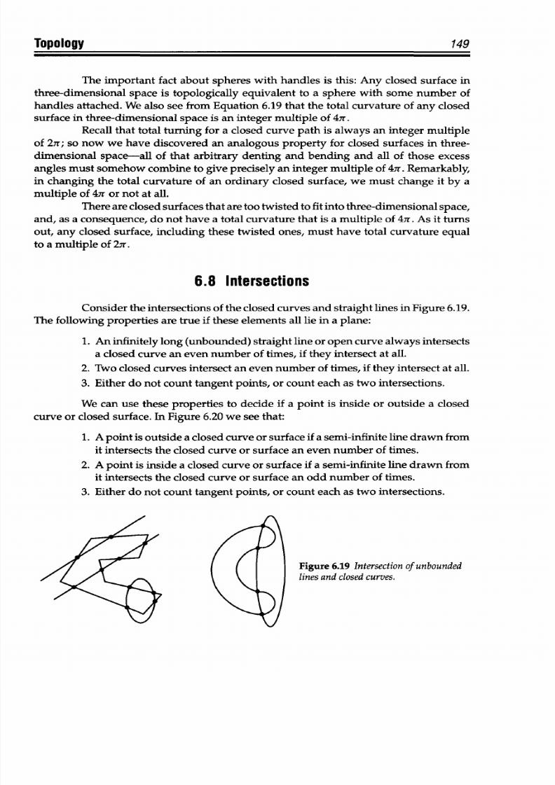
8/9/2019 Mortenson, Michael E. - Mathematics for computer graphics applications.pdf
http://slidepdf.com/reader/full/mortenson-michael-e-mathematics-for-computer-graphics-applicationspdf 162/367
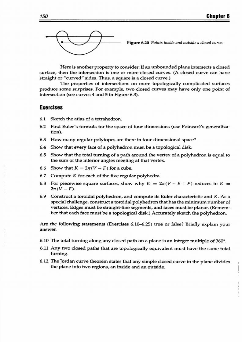
8/9/2019 Mortenson, Michael E. - Mathematics for computer graphics applications.pdf
http://slidepdf.com/reader/full/mortenson-michael-e-mathematics-for-computer-graphics-applicationspdf 163/367
8/9/2019 Mortenson, Michael E. - Mathematics for computer graphics applications.pdf
http://slidepdf.com/reader/full/mortenson-michael-e-mathematics-for-computer-graphics-applicationspdf 164/367
Topology
151
6.13 Every simple closed curve on the surface of a torus divides the surface into two
separate
regions.
6.14 On a closed path on a
curved
surface,
the angle excess plus the total turning equals
3600.
6.15 For
any
topological
disk
on
an
arbitrary
surface,
the
angle excess around
the
bound-
ary
is
equal
to
the total curvature
of
the
interior.
6.16 A torus has
zero
total curvature.
6.17 A two-holed torus
has
a total
curvature
equal to 47r.
6.18 Angle excess
is
always zero around a closed path
on
a plane surface.
6.19 Simple
polyhedra
can
be continuously
deformed into a sphere.
6.20
Euler's
formula
for
simple
polyhedra
relates
total curvature
to
V, E, and
F.
6.21
All
the
curvature
in a closed, piecewise flat surface is concentrated at
the
vertices.
6.22
The
quantity
V
- E + F - 2 is
called
the
Euler characteristic
of a polyhedron.
6.23
Every
face
of a
polyhedron must be
a
topological
disk.
6.24 A
net
on
a
general surface is
a collection of
simple
arcs
that divide the
surface
everywhere
into topological
disks.
6.25
The
surface of a sphere has a unique net.
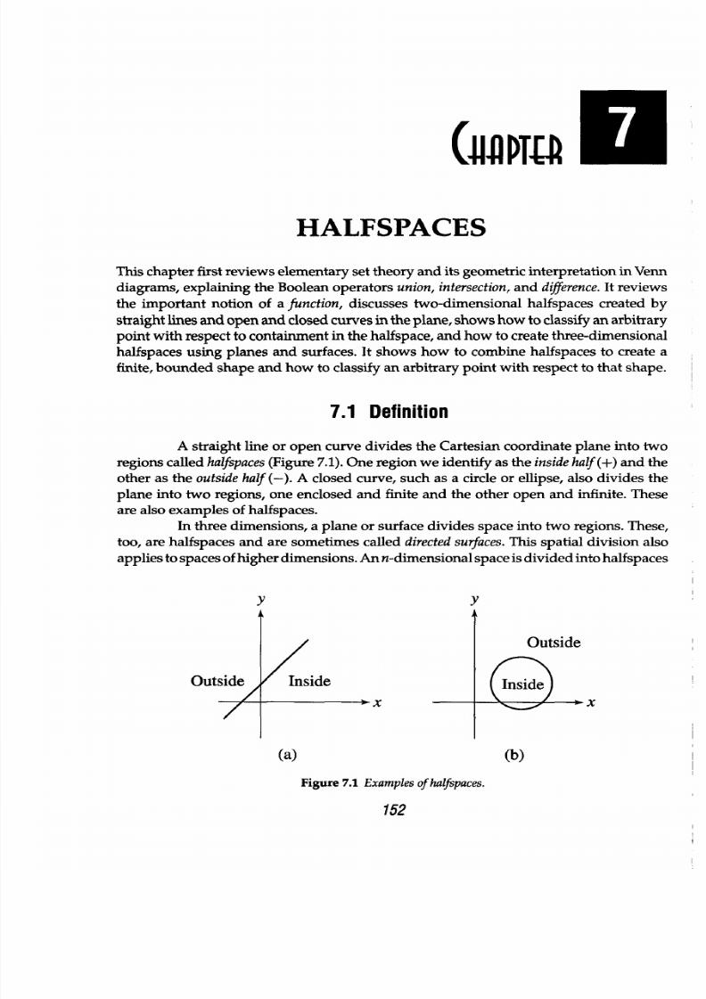
8/9/2019 Mortenson, Michael E. - Mathematics for computer graphics applications.pdf
http://slidepdf.com/reader/full/mortenson-michael-e-mathematics-for-computer-graphics-applicationspdf 165/367
(XX
PM
HALFSPACES
This chapter first reviews elementary set theory and its geometric
interpretation
in Venn
diagrams, explaining
the Boolean operators
union,
intersection, and difference. It reviews
the
important
notion
of
a
function,
discusses
two-dimensional
halfspaces created by
straight
lines and
open
and
closed curves in
the
plane,
shows how to
classify
an
arbitrary
point with respect
to containment in
the
halfspace, and how to create
three-dimensional
halfspaces using planes and surfaces. It shows how to combine halfspaces to create a
finite, bounded shape and how to classify
an
arbitrary
point
with respect to that shape.
7.1 Definition
A
straight
line or
open
curve
divides the Cartesian
coordinate
plane
into
two
regions called
halfspaces (Figure
7.1). One region we identify
as the
insidehalf (+)and
the
other
as
the
outside
half (-). A closed
curve,
such as a
circle or
ellipse, also divides
the
plane into two
regions, one
enclosed and
finite
and the other open and
infinite. These
are also examples of halfspaces.
In
three
dimensions, a
plane or surface
divides
space into
two
regions. These,
too,
are
halfspaces
and
are sometimes called directed
surfaces.
This spatial division
also
applies
to spaces of
higher dimensions. A n n-dimensional space
is divided
into
halfspaces
Y Y
Out
x
(a)
(b)
Figure
7.1
Examples of halfspaces.
152
8/9/2019 Mortenson, Michael E. - Mathematics for computer graphics applications.pdf
http://slidepdf.com/reader/full/mortenson-michael-e-mathematics-for-computer-graphics-applicationspdf 166/367
Halfspaces
153
by
a hypersurface of n
-
1 dimensions. We can combine two
or more
simple halfspaces
using
Boolean operators to create more complex
shapes
and to establish or limit
the
visibility of objects in a computer-graphics display. The mathematics
and
geometry of
halfspaces makes it easy to
do
window
and
clipping operations
and
to solve
many
containment problems in computer
graphics.
7.2
Set Theory
Set theory is the
primary
source
of the algebra
and
operations
that
govern
combining halfspaces to form complex shapes.
A set is a well-defined collection of objects
that
are,
in
turn, elements or
members
of
the
set.
Examples of
a set are: all
natural
numbers,
all even numbers,
all
white
crows,
all diamonds
in a deck
of cards,
or the
first
ten
prime
numbers.
In geometry, the point is a basic element, and in geometric modeling, computer
graphics,
and
similar applications we
may examine
and
operate on the set
of
points along
a curve, the set
of points
inside a circle, or the set of
points
on the surface
of
some object,
and so on.
A
set that contains
all
of
the
elements of all
of
the
sets
in a particular problem
is called the universal set.
It
is
symbolized by
E.
In
geometry, E is often taken
to
mean
all
the
points
in a two- or three-dimensional space. We use uppercase italic letters to denote
a
particular
set. The complement of a set A with respect to a universal set E is the set of
all elements of E that
are not
elements of A.
The
complement
of
A is
written
cA. The
null
set,
denoted
as 0,
is a
set
having
no
elements
at
all.
It is also
known
as
the
empty
set.
A
set A is a subset
of
another set B if and
only
if
every
member
of
A is
also
a member
of
B.
The symbol
c denotes the relationship between
set
and subset. A c B
says
that A
is a subset
of
B. For example, if B is
the
set
of all
natural numbers and A
is
the set of
all
even numbers,
then
A
c
B. A is a proper
subset
of B if every member of A
is
contained in B
and
if B has at least one element not in A. Every set is a subset
of
itself,
but
not
a
proper
subset. We form
new sets
by combining the elements of
two
or more
existing sets.
The
mathematics
that
describes this process is
called
Boolean algebra.
George
Boole (1815-1864), one
of
England's
most original mathematicians,
invented an
algebra for
the
study
of logic.
He
did
this
by
separating
the symbols
of
mathematical operations
from
the objects upon
which
they
operate.
He studied
these
operators
as independent
mathematical objects and
asked
two
important
questions: Can
these
operations
be
combined?
Are there
algebra-like rules
for
doing
this? The results
of
his investigations are
formalized as
Boolean
algebra, where sets are treated as algebraic
quantities
by
the operations
of
union, intersection,
and
difference.
The union operator
U
combines two
sets
A and
B
to form
a third set
C
whose
members are
all of
the
members of A
plus
all of the
members
of
B. This is
expressed
as
C=AUB
(7.1)
For
example,
if
A
consists of
four members
a,
b, c,
and
d
and
if
B
consists of
three members c,
d,
and e, then if
AU B
= C, we find
that
C consists of
the
five members
a, b, c,
d,
and e.
8/9/2019 Mortenson, Michael E. - Mathematics for computer graphics applications.pdf
http://slidepdf.com/reader/full/mortenson-michael-e-mathematics-for-computer-graphics-applicationspdf 167/367
154
Chapter
7
Another operator,
the intersection
operator
n,
combines
two sets A
and
B to
form a third
set
C whose
members
are only
those common
to
both
A and
B.
This
is
expressed
as
C
=
A
nB
(7.2)
Using the example of sets
A
and
B, we find that if
C = A
n
B,
then
the members
of C
are c and
d.
The
difference operator,
-,
combines
two
sets A
and B
to
form a third set
C
whose members
are only those
of the first
set that
are
not
also members
of
the second.
This is
expressed
as
C =
A-B
(7.3)
Here,
we find
that
if C = A - B,
then the members
of
C are a
and b.
The
union and
intersection
operators
are commutative:
A u B =
B uA
(7.4)
and
A•nB
=
BnA
(7.5)
But the difference
operator
is not commutative:
A --
B $ B-A (7.6)
This is
demonstrated
in
the example, where
we find A
-
B = {a,
b and
B - A = {e}.
The curly
brackets
{I are
commonly
used in
set
theory to enclose
members
of
a
set. They are part of
what
is called
the set-buildernotation.
Set operations obey
the
rules of
Boolean algebra. They govern
the
ways
we can
combine
sets and determine
the
results
we
should
expect. The
properties
of
this
algebra
are summarized in
Table 7.1.
Venn diagrams,
named
after the logician John
Venn (1834-1883),
give us a
visual, geometric
interpretation
of
set theory
and the
Boolean
operations. In many ap-
plications of geometry today,
sets consist
of points, where
the universal
set
is
often the
set of
points defining a Euclidean space
of one, two, or three dimensions.
Venn
diagrams
suggest ways
to operate
on
subsets
of
those
points
that
define geometric
shapes and
classify these points
as being inside,
outside,
or
on the
boundary of
the
shape.
Figure
7.2
shows
four different
Venn
diagrams.
The outermost rectangle
of
each
diagram encloses
the
universal
set. The smaller inner rectangles
are sets within
the
universal
set: sets
A,
B,
and
C. In each diagram,
the
outcome of the
indicated operation
is
shown
as
a shaded region.
7.3 Functions
Revisited
Function notation
is used
to
develop
the mathematics
of halfspaces. Recall
that a
function
is
a
mathematical
expression-not
an
equation,
although
a function
may appear
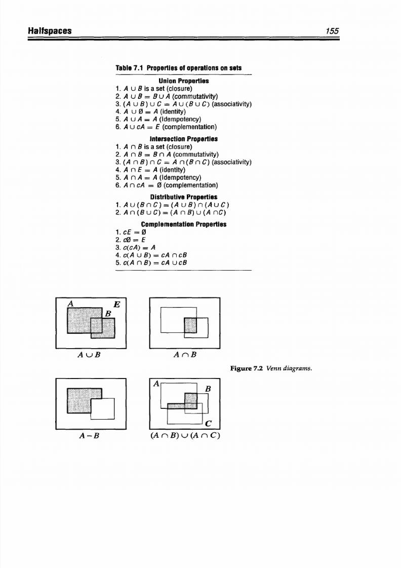
8/9/2019 Mortenson, Michael E. - Mathematics for computer graphics applications.pdf
http://slidepdf.com/reader/full/mortenson-michael-e-mathematics-for-computer-graphics-applicationspdf 168/367
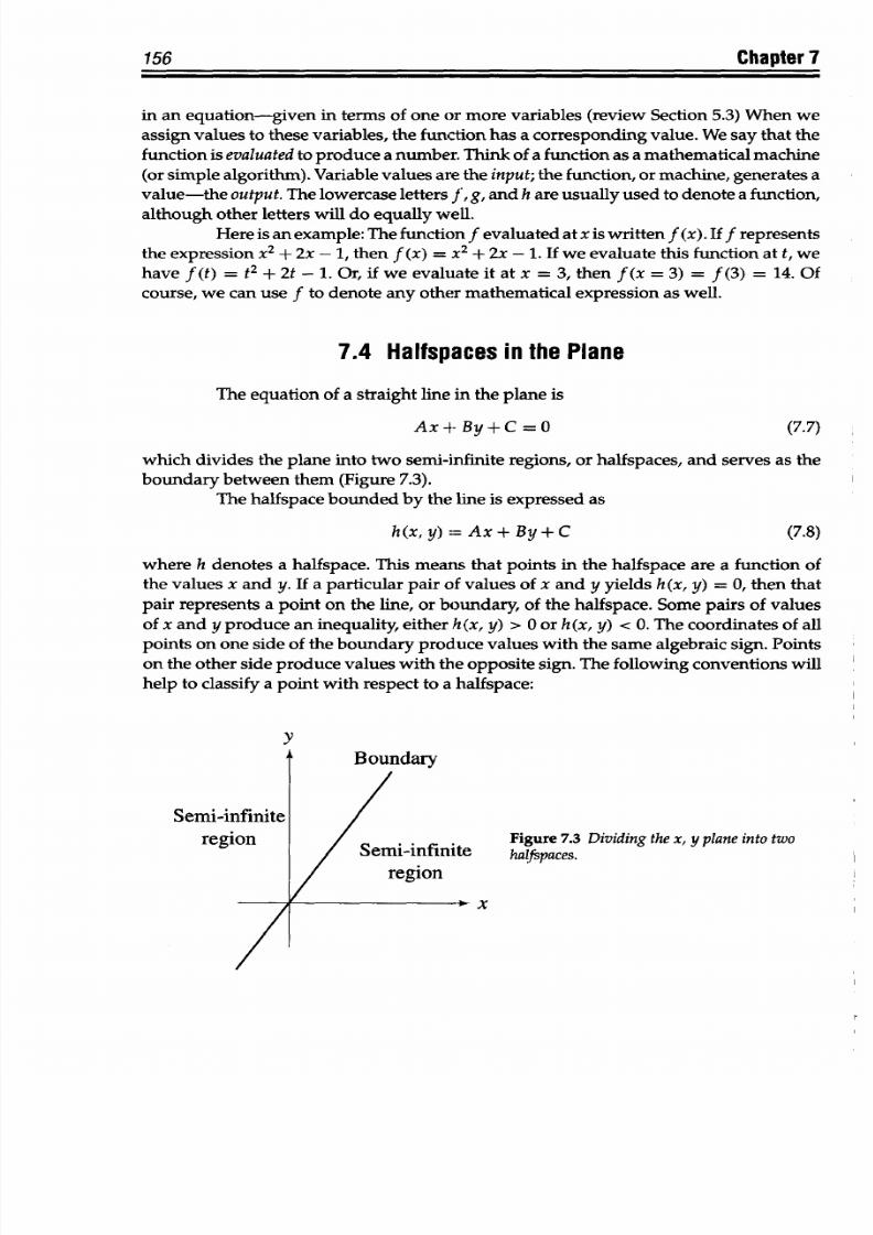
8/9/2019 Mortenson, Michael E. - Mathematics for computer graphics applications.pdf
http://slidepdf.com/reader/full/mortenson-michael-e-mathematics-for-computer-graphics-applicationspdf 169/367
156
Chapter
7
in
an equation-given in terms
of one or more variables (review
Section
5.3) When we
assign values to these variables, the function has
a
corresponding value. We say
that
the
function
is
evaluated
to produce a number. Think of a
function
as a
mathematical
machine
(or simple algorithm).
Variable values are the input;
the function,
or machine,
generates
a
value-the output. The lowercase letters
J,
g,
and
h
are usually used to denote a function,
although
other letters will do equally well.
Here
is
an
example: The function f
evaluated
at
x is
written
f (x).
If f
represents
the expression
x
2
+
2x -
1,
then
f (x) = X
2
+
2x -
1.If we evaluate this function at
t, we
have f (t) = t
2
+
2t
- 1. Or, if
we evaluate
it at x
=
3, then f (x
= 3)
=
f (3)
= 14. Of
course, we can
use f
to denote
any other
mathematical
expression
as
well.
7.4 Halfspaces
in
he Plane
The
equation
of a
straight
line in
the
plane is
Ax+ By+C
=
0 (7.7)
which divides the plane into two semi-infinite regions, or halfspaces,
and
serves as the
boundary between them (Figure 7.3).
The halfspace
bounded
by the line is
expressed
as
h(x,y)=Ax+By+C (7.8)
where
h
denotes
a
halfspace. This
means
that
points
in the
halfspace are
a
function of
the values
x
and y. If a particular
pair
of values of x
and
y
yields
h(x, y)
= 0, then
that
pair represents
a
point on the
line, or boundary, of the
halfspace. Some
pairs of
values
of x
and
y produce an inequality, either h(x,
y)
> 0 or h(x,
y)
< 0.
The
coordinates of all
points on
one side
of the
boundary
produce
values
with the
same
algebraic
sign.
Points
on
the other
side
produce values with the
opposite sign.
The following conventions will
help
to classify
a
point
with
respect to a halfspace:
y
Figure
7.3 Dividing he
x,
y
plane into
two
halfspaces.
region
x
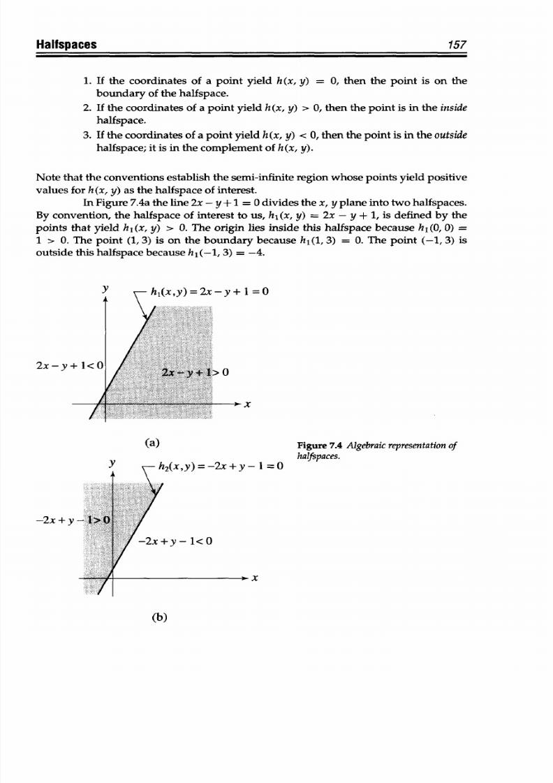
8/9/2019 Mortenson, Michael E. - Mathematics for computer graphics applications.pdf
http://slidepdf.com/reader/full/mortenson-michael-e-mathematics-for-computer-graphics-applicationspdf 170/367
Hallspaces
157
1.
If
the
coordinates
of
a point yield h(x,
y)
=
0, then the
point is
on
the
boundary
of the
halfspace.
2. If the
coordinates
of a point
yield
h(x, y) >
0, then
the point is in the inside
halfspace.
3.
If the
coordinates
of a
point yield h
(x, y) <
0, then
the
point
is
in
the
outside
halfspace;
it
is in the complement of h(x, y).
Note that the
conventions
establish
the
semi-infinite region
whose points
yield
positive
values for h (x, y)
as
the halfspace of interest.
In
Figure 7.4a the line 2x - y + 1
=
0divides the x, y plane into two halfspaces.
By convention,
the halfspace of interest to us, h
1
(x, y)
= 2x - y + 1, is
defined by the
points that yield hI(x, y) > 0. The origin lies inside this halfspace because hI (0, 0)
=
1 > 0.
The
point
(1,3)
is on
the
boundary because
h
1
(1,
3) =
0. The
point
(-1,
3)
is
outside this
halfspace because
h
1
(-1, 3)
= -4.
Y 7-h,(xv)=2x-y+1=0
2x - y
+ 1
I0
-*. x
(a)
V h
2
(x,y)=-2x+y- 1
=0
Figure
7.4
Algebraic representationof
halfspaces.
-2x
+ y
*y-
1<0
(b)
y
L . I I I I
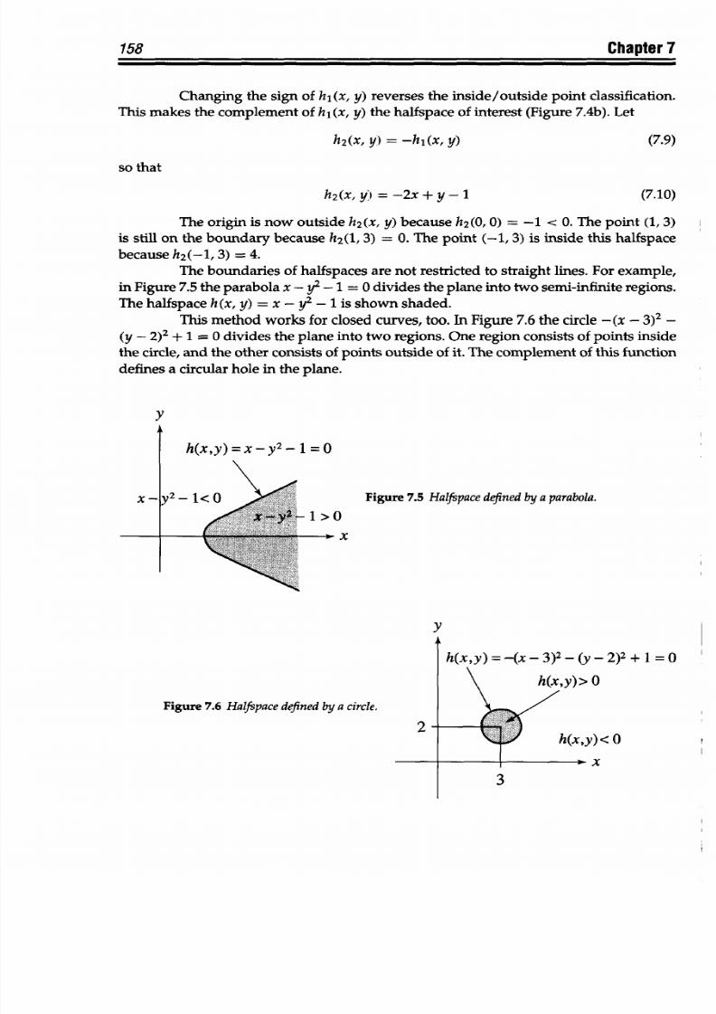
8/9/2019 Mortenson, Michael E. - Mathematics for computer graphics applications.pdf
http://slidepdf.com/reader/full/mortenson-michael-e-mathematics-for-computer-graphics-applicationspdf 171/367
Chapter 7
Changing the
sign
of hi
(x,
y)
reverses the
inside/outside point
classification.
This makes
the complement
of
hi (x, y)
the halfspace of interest
(Figure
7.4b). Let
so
that
h
2
(x, y) =
-hi(x, y)
h
2
(x,y) =-2x+y-1
(7.9)
(7.10)
The
origin is now
outside
h
2
(x, y) because
h
2
(0, 0) = -1 <
0.
The point
(1,3)
is still
on
the
boundary
because h
2
(1, 3)
= 0.
The point
(-1, 3)
is inside this halfspace
because h
2
(-l, 3)
= 4.
The boundaries
of
halfspaces
are
not restricted
to
straight
lines.
For
example,
in
Figure
7.5
the parabola x
- y2 - 1 = 0
divides
the plane
into two semi-infinite
regions.
The
halfspace
h(x,
y)
=
x
-
y2
-
1 is
shown shaded.
This method works
for
closed curves, too.
In
Figure 7.6 the
circle
-
(x
- 3)2 -
(y - 2)2 + 1
=
0
divides
the
plane
into two regions.
One region consists
of points
inside
the circle, and the other consists of
points
outside of it. The
complement
of this
function
defines a
circular
hole in the plane.
y
h(x,y)=x-y
2
- 1
=0
y
2
- I Figure 7.5 Halfspacedefined by a parabola.
1>0
-
X
y
Figure 7.6 Halfspace
defined
by a circle.
2
2)2 + 1 =0
0
x
3
58
x -
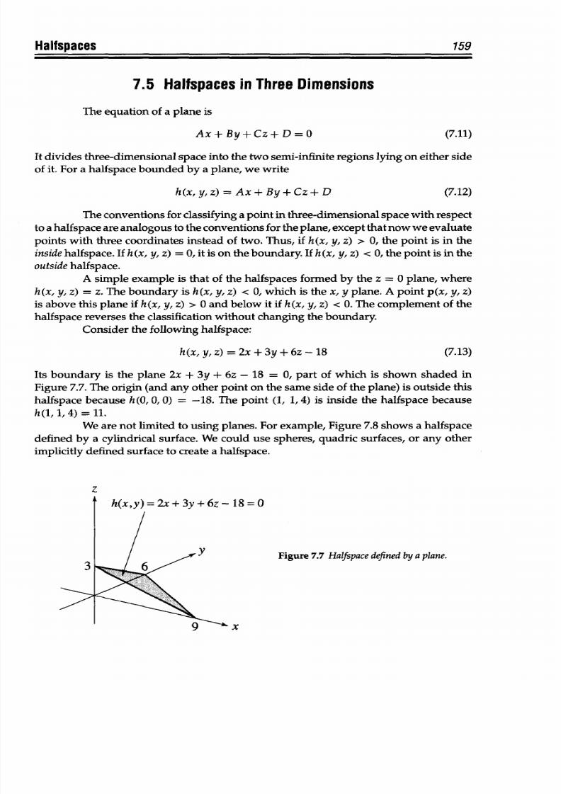
8/9/2019 Mortenson, Michael E. - Mathematics for computer graphics applications.pdf
http://slidepdf.com/reader/full/mortenson-michael-e-mathematics-for-computer-graphics-applicationspdf 172/367
159
7.5 Halfspaces
inThree
Dimensions
The equation of a plane is
Ax + By + Cz + D =O (7.11)
It divides
three-dimensional
space
into
the
two semi-infinite
regions
lying
on
either
side
of it.
For
a
halfspace bounded by
a
plane,
we
write
h(x, y, z) = Ax + By + Cz + D (7.12)
The
conventions for classifying a
point
in three-dimensional space
with respect
to
a
halfspace
are analogous
to
the
conventions
for the
plane,
except
thatnow
we evaluate
points
with
three
coordinates
instead
of
two. Thus,
if
h(x,
y,
z)
>
0,
the
point
is
in
the
inside halfspace. If h (x, y, z) = 0,
it is on
the boundary. If h (x, y, z)
<
0,
the
point is in
the
outside halfspace.
A simple
example is that of
the halfspaces formed by the
z = 0 plane, where
h(x, y,
z) = z.
The boundary
is h(x,
y, z) < 0,
which
is
the
x, y plane.
A point
p(x,
y,
z)
is above this plane if h (x,
y,
z) > 0 and below it if
h
(x, y,
z)
< 0.
The
complement of the
halfspace
reverses the
classification
without changing the boundary.
Consider the following halfspace:
h(x,
y,
z)
=
2x + 3y +
6z
- 18 (7.13)
Its
boundary
is the
plane 2x
+ 3y +
6z - 18 =
0,
part of
which
is
shown shaded in
Figure
7.7. The
origin (and any other
point
on the
same
side of the
plane)
is outside this
halfspace
because h(0, 0, 0) =
-18.
The point (1, 1,4) is inside the
halfspace
because
h(1, 1,
4)
= 11 .
We are not limited to
using
planes. For example, Figure 7.8 shows
a
halfspace
defined
by
a
cylindrical
surface. We
could use
spheres, quadric
surfaces, or any other
implicitly
defined surface
to create a
halfspace.
z
3
18=0
Figure
7.7 Halfspace
defined by a
plane.
x
Halfspaces
,
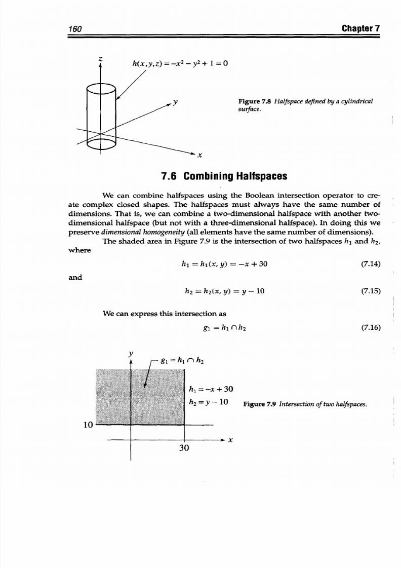
8/9/2019 Mortenson, Michael E. - Mathematics for computer graphics applications.pdf
http://slidepdf.com/reader/full/mortenson-michael-e-mathematics-for-computer-graphics-applicationspdf 173/367
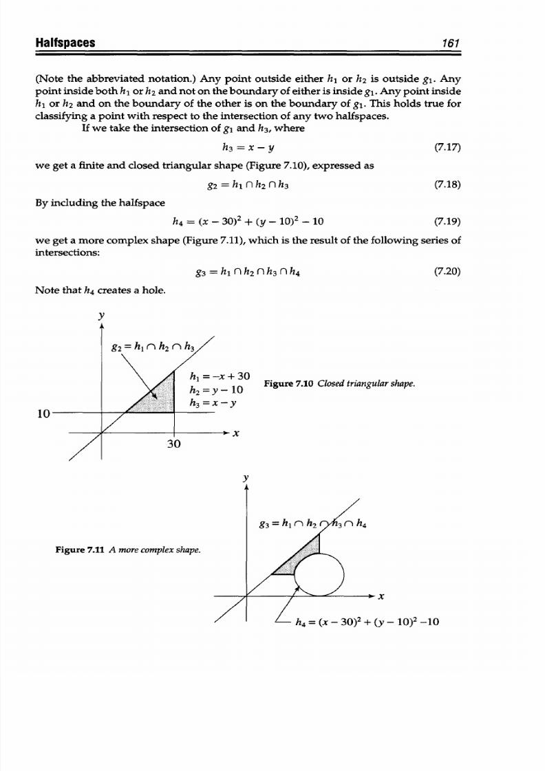
8/9/2019 Mortenson, Michael E. - Mathematics for computer graphics applications.pdf
http://slidepdf.com/reader/full/mortenson-michael-e-mathematics-for-computer-graphics-applicationspdf 174/367
Halfspaces
161
(Note the
abbreviated
notation.) Any point
outside either h,
or h
2
is
outside
gi.
Any
point inside both h,
or h
2
and
not
on
the
boundary of
either is
inside gi.
Any
point inside
h,
or h
2
and on the
boundary
of the other
is
on the
boundary
of gi.
This
holds true for
classifying
a
point with
respect
to
the intersection
of
any
two
halfspaces.
If we take the intersection of gi and h
3
, where
h
3
- X
- y
we get a finite
and
closed
triangular
shape (Figure 7.10),
expressed as
g2
=h
lnh
2
nh
3
By
including the halfspace
h4 = (x -
30)2
+
(y - 10)2 -
10
(7.17)
(7.18)
(7.19)
we get a
more
complex shape (Figure 7.11), which
is
the result of the
following
series of
intersections:
g3 =h lnh
2
nh
3
nh
4
(7.20)
Note
that
h
4
creates a
hole.
y
0
Figure 7.10 Closed triangular hape.
Figure
7.11 A more
complex shape.
r)h
4
x
{v- 1 f1
2
-1
A
-4 -
k-
-- , . %,j .- j -
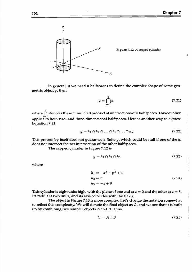
8/9/2019 Mortenson, Michael E. - Mathematics for computer graphics applications.pdf
http://slidepdf.com/reader/full/mortenson-michael-e-mathematics-for-computer-graphics-applicationspdf 175/367
162
Chapter
7
z
V
Figure 7.12 A
capped
cylinder.
x
In general,
if we need n
halfspaces
to
define the complex shape of
some
geo-
metric
object
g, then
n
g=
fhi
i=1
(7.21)
where n denotes the accumulated product of
intersections
of n halfspaces.
This equation
j=1
applies to
both
two- and three-dimensional
halfspaces.
Here is another way to
express
Equation
7.21:
(7.22)
This process by
itself does
not
guarantee a
finite
g, which could be
null
if one of the hi
does
not intersect the net
intersection of
the
other halfspaces.
The capped cylinder
in
Figure 7.12 is
where
g
=hi
nh
2
nh
3
h,
=
-x
2
- y
2
+4
h2
= z
h
3
= -z +
8
(7.23)
(7.24)
This cylinder is eight
units
high,
with the plane
of
one
end at z
= 0
and
the other
at z = 8.
Its radius is two un its,
and
its
axis
coincides
with the z
axis.
The object in Figure
7.13
is
more
complex. Let's
change the
notation somewhat
to
reflect
this
complexity.
We
will
denote the
final object as
C,
and
we
see
that
it
is
built
up
by combining
two
simpler objects
A
and B.Thus,
C=AUB
(7.25)
g
= h,
nh2n
... nhi n...
nhn
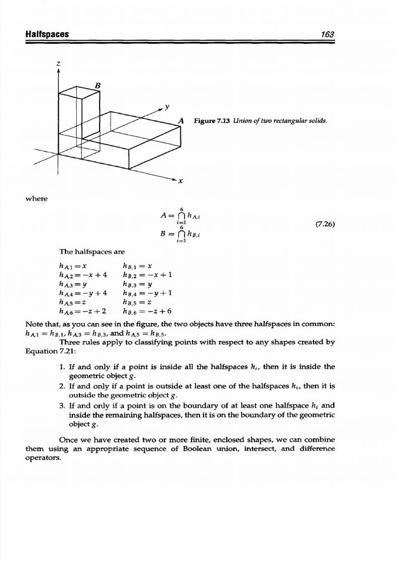
8/9/2019 Mortenson, Michael E. - Mathematics for computer graphics applications.pdf
http://slidepdf.com/reader/full/mortenson-michael-e-mathematics-for-computer-graphics-applicationspdf 176/367
8/9/2019 Mortenson, Michael E. - Mathematics for computer graphics applications.pdf
http://slidepdf.com/reader/full/mortenson-michael-e-mathematics-for-computer-graphics-applicationspdf 177/367
164 Chapter
7
Exercises
7.1
If the universal
set
E
consists
of
the integers 1 through
24,
a set A in E consists
of
the even
integers,
and
B
in
E
consists
of
multiples
of
3,
list
the members
of
a.
AUB
c.
A-B
b.
AnB d. B-A
7.2 Find
the complement of
Au
B
(see
Exercise
7.1).
7.3
Find
the complement of A -
B
(see
Exercise
7.1).
7.4
Using Venn diagrams,
demonstrate
that
for
A
c
B it
is necessary and sufficient
that
AU
B = B
or An B = A.
7.5
Show
that
A-(A-B) =
A n B.
7.6
Classify
the
following
points
in the
plane
with
respect to
hi =
y
- 2:
a. (0,
0)
f. (-1,
-2)
b.
(4,
-2)
g.
(-4,
1)
c. (4,
4)
h.
(-3,1)
d.
(2,3)
i. (-1,4)
e. (2, 2)
j. (3, 5)
7.7
Classify
the
points
given
in
Exercise
7.6
with respect
to h
2
=
-x
+
3.
7.8
Classify
the points
given in
Exercise 7. 6
with
respect
to h
3
=
x
- y +
2.
7.9
Classify
the
points
given
in
Exercise
7.6
with
respect
to
hlnh
2
nh
3
.
Use
the
halfspaces
given
in Exercises
7.6-7.8.
7.10
Classify
the points
given
in Exercise 7.6 with respect
to h
4
Uhh
, where
h
4
=
-(x-4)
2
-(y-3)
2
+16andh
5
=
-x
2
-y
2
+9.
7.11
Classify
the
points
given
in
Exercise
7.6
with respect
to h
5
- h
4
. (The
minus
sign
is
the Boolean
difference
operator.)
7.12
Which
of
the
points
given in Exercise 7.6 are outside
h
6
=
x
2
+
y
2
- 9?
7.13 Write
the equation
defining
the
halfspace
whose boundary
is
the parabola y
= x2+1,
so
that
the origin
is
outside.
7.14
Write
the
equations
defining the halfspaces
whose combined
Boolean intersection
produces
a
unit cube
centered
at the origin.
7.15 Sketch
the plane figure
produced by
the
combined
Boolean intersections
of the
following
halfspaces:
hj(x, y)
= -x+2
h
2
(x,y) =x+2
h
3
(x,y)
=
-y+6
h
4
(x,
y)
= Y
h5(x,
y) = -x - y + 5
h
6
(x,y) =x-y+5
Is
this the most
efficient combination
of
halfspaces for
this shape?
Why?
8/9/2019 Mortenson, Michael E. - Mathematics for computer graphics applications.pdf
http://slidepdf.com/reader/full/mortenson-michael-e-mathematics-for-computer-graphics-applicationspdf 178/367
(A
Kpa
POINTS
A
point
is the simplest of the elementary geometric objects: points, lines,
and
planes. In
fact
we cannot
define
a
point
in terms
of
anything
simpler
except as
a
set of numbers.
Points are the basic
building
blocks for all other geometric
objects, and elementary ge-
ometry demonstrates how
many figures
are
defined as
a
locus
of points
with
certain con-
straining
characteristics. For
example,
in a plane,
a
circle
is the
locus
of
points equidistant
from a given point, and a
straight line is
the
locus
of
points equidistant
from two given
points. In three-dimensional space,
a plane
is
the
locus of
points equidistant
from two
given
points. We can also
define more
complex curves,
surfaces, and solids
this
way, by
usingequations to define the locus of points. This is a powerful way of describing geomet-
ric objects, because
it
allows us to analyze and quantify
their properties and relationships.
Most
importantly
to
today's
technology,
points
are indispensable
when we create
com-
puter
graphic displays and
geometric models.
This
chapter
discusses
the
definition of
a
point
as a
set
of real numbers,
point
relationships,
arrays
of points, absolute and
relative
points,
displaying
points,
pixels and
point
resolution,
and
translating
and
rotating points.
8.1 Definition
A
point
suggests the
idea
of
place
or location.
We define
a point
by
a set
of on e
or more real
numbers, its coordinates.
The coordinates of
a
point not only
locate
it in a
coordinate system, but also with respect to other points in the system.
A set of n real numbers define a
point
in n-dimensional space
P =
(X1,
2, . .
., Xn)
(8.1)
where x
1
,
x2,
. . ., xn
are
the coordinates of
p and
n is
the number
of
dimensions
of the
coordinate system. A boldface, lowercase letter p will denote
a
point. This is consistent
with the vector notation of Chapter 1.In fact,
under
certain conditions there is a one-to-
one
correspondence between the coordinates of a
point
and
the components
of its vector
representation.
In geometric modeling and computer graphics, most work is in two- or three-
dimensional space, so
we will not
usually see
Equation
8.1 in this
generalized
form.
Note, though,
that
each coordinate has an identifying number, shown as an attached
subscript. This is usually not necessary if the
geometry
is
in two
or three
dimensions,
165
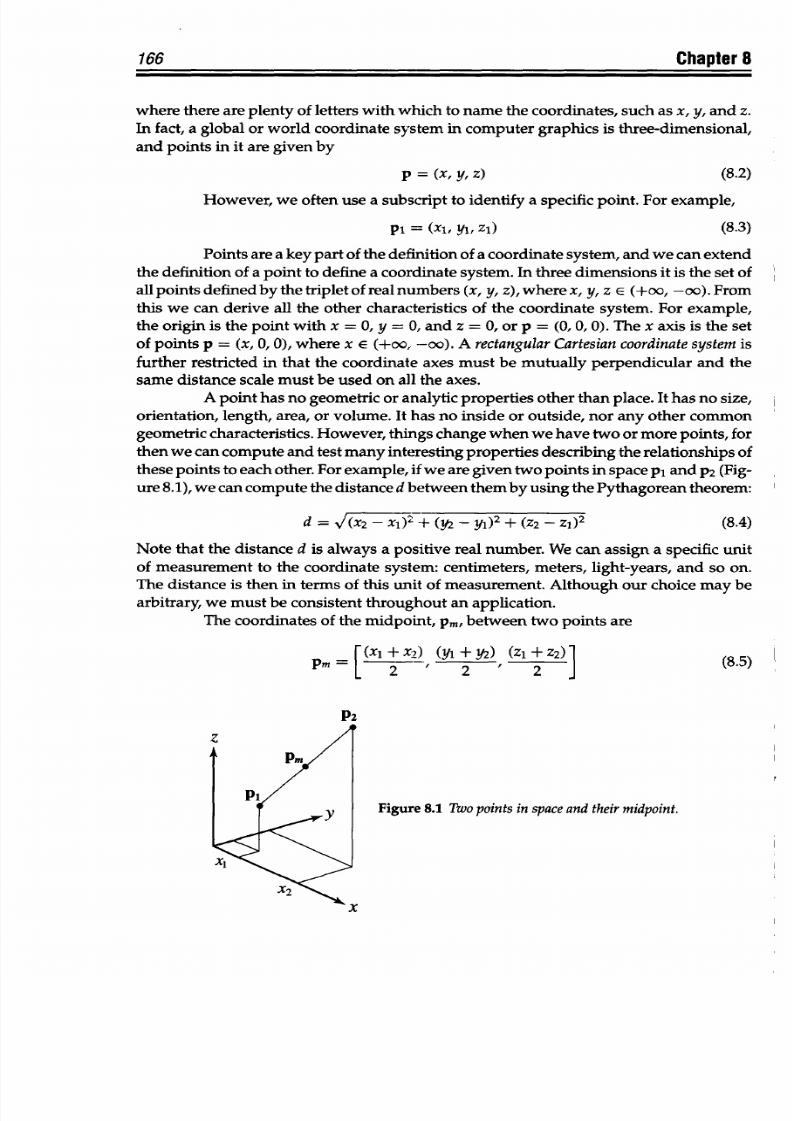
8/9/2019 Mortenson, Michael E. - Mathematics for computer graphics applications.pdf
http://slidepdf.com/reader/full/mortenson-michael-e-mathematics-for-computer-graphics-applicationspdf 179/367
166
Chapter 8
where there are
plenty
of
letters
with
which to
name
the
coordinates,
such
as
x,
y,
and z.
In
fact,
a
global
or
world
coordinate system
in computer graphics
is
three-dimensional,
and points
in it are given by
p =
(x,
y,
Z)
(8.2)
However, we
often
use
a subscript
to
identify
a specific
point. For
example,
pi =
(xi,
yi, zi) (8.3)
Points are a key part
of
the
definition of
a
coordinate
system, and we can extend
the
definition of a
point
to
define
a
coordinate
system. In three
dimensions
it
is
the set of
all
points
defined
by
the
triplet
of real numbers
(x, y, z),
where
x, y, z
E (+co, -cc). From
this
we
can
derive all
the other
characteristics of the coordinate
system. For example,
the origin is the
point
with
x
=
0,
y
= 0,
and
z
=
0,
or p
=
(0, 0, 0). The x axis
is the set
of
points
p
=
(x,
0, 0),
where
x
E
(+o,
-00).
A
rectangular
Cartesian
coordinatesystem
is
further
restricted in
that
the coordinate
axes must be
mutually
perpendicular and
the
same distance
scale
must be used on
all
the axes.
A point
has no
geometric
or analytic properties
other
than place. It
has no
size,
orientation,
length, area, or volume.
It has no inside or outside, nor
any other common
geometric
characteristics. However,
things change
when
we
have two or more
points, for
then
we
can compute
and test
many
interesting
properties describing the relationships
of
these points
to each
other.
For example,
if we are given two points
in space pi and P2 (Fig-
ure 8.1),
we
can compute
the distance d between
them
by using
the
Pythagorean
theorem:
d
= /(x2
- xl) + (y2
-
y)
2
+
(Z2 -
Z1)
2
(8.4)
Note
that the distance
d is always a positive
real number. We can assign
a
specific
unit
of
measurement
to the coordinate system:
centimeters,
meters, light-years, and
so on.
The distance
is
then
in
terms
of
this
unit of measurement.
Although
our
choice
may be
arbitrary, we must
be consistent throughout
an application.
The coordinates
of
the
midpoint,
pm, between
two
points
are
[
(Xi
+
X2)
(y1
+
yZ)
(Z
1
+
Z2)
(8.5)
P2
Figure
8.1 Twlo points in
space
and their midpoint.
A.
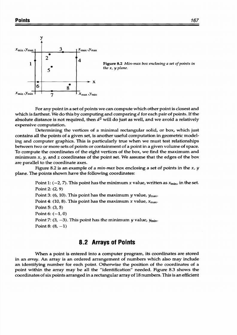
8/9/2019 Mortenson, Michael E. - Mathematics for computer graphics applications.pdf
http://slidepdf.com/reader/full/mortenson-michael-e-mathematics-for-computer-graphics-applicationspdf 180/367
Points
167
V
Xnin'Ymax
X-in CVmin
6
0
2 1
5
L
Xmax
Ymax
Figure 8.2
Min-max
box enclosing
a
set of points
in
the x,
y
plane.
7-*-
X
Xr. .vYi..
For any
point
in
a
set of
points
we can compute which other
point
is closest
and
which
is
farthest. We do
this
by
computing
and comparing
d for
each pair
of points.
If
the
absolute distance is not required, then d
2
will do just as well, and we avoid
a
relatively
expensive
computation.
Determining
the
vertices
of a minimal
rectangular solid,
or
box,
which
just
contains all the
points
of a given set, is another useful computation in geometric model-
ing
and computer graphics.
This is particularly true when
we
must
test
relationships
between two or more sets of points or containment of
a
point in
a given volume of space.
To
compute the
coordinates
of
the eight
vertices of
the
box,
we find the
maximum and
minimum
x, y,
and
z coordinates of
the point set.
We
assume
that
the edges of the box
are parallel to the
coordinate
axes.
Figure
8.2
is an example of a min-max box enclosing a
set
of points in
the x,
y
plane. The points
shown
have the following coordinates:
Point
1: (-2, 7).
This
point
has the
minimum x value, written as xmin,
in the set.
Point
2: (2, 9)
Point
3:
(6,
10).
This
point
has
the
maximum y
value,
ymax-
Point
4:
(10,
8).
This
point
has the maximum
x
value,
xnax.
Point
5:
(3, 5)
Point 6:
(-1, 0)
Point 7: (3,-3). This
point
has the
minimum
y value, ymni.
Point 8: (8,
-1)
8.2
Arrays of Points
When
a
point
is
entered
into
a
computer program,
its coordinates
are
stored
in an array. An array
is an ordered arrangement
of numbers
which
also
may
include
an
identifying
number
for
each
point. Otherwise the position
of the coordinates of a
point
within the array
may
be all the "identification" needed. Figure 8.3 shows the
coordinates
of six points arranged in
a
rectangular array
of 18 numbers. This
is an
efficient
I
I
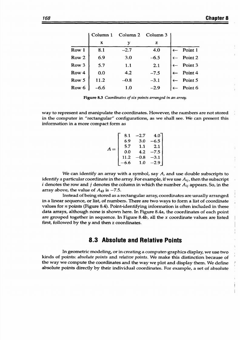
8/9/2019 Mortenson, Michael E. - Mathematics for computer graphics applications.pdf
http://slidepdf.com/reader/full/mortenson-michael-e-mathematics-for-computer-graphics-applicationspdf 181/367
168
Chapter
8
Row
I
Row 2
Row
3
Row 4
Row S
Row 6
Column
1 Column
2 Column
3
x y
z
8.1
-2.7
4.0
6.9
3.0 -6.5
5.7
1.1
2.1
0.0
4.2
-7.5
11.2
--0.8 -3.1
-6.6
1.0
-2.9
.-
v
Point
1
<-
Point 2
e-
Point
3
v-
Point 4
v- Point
5
v- Point 6
Figure
8.3 Coordinates
of
six points arranged
n
an
array.
way
to represent
and manipulate
the coordinates.
However, the numbers
are
not stored
in
the computer
in "rectangular"
configurations,
as we
shall see. We can present
this
information
in
a
more compact form
as
8.1
-2.7
4.0
6.9
3.0 -6.5
5.7
1.1
2.1
0.0
4.2
-7.5
11.2 -0.8
-3.1
-6.6
1.0 -2.9
We
can
identify
an array with
a
symbol,
say
A, and
use double subscripts
to
identify
a particular coordinate
in the
array.
For
example, if we use Aij, then
the subscript
i
denotes the
row and
j denotes
the column
in which
the
number
Aij
appears.
So, in the
array
above,
the
value
of A
43
is
-7.5.
Instead of
being stored as
a
rectangular
array, coordinates
are usually
arranged
in
a
linear
sequence, or list, of
numbers. There
are two ways
to form
a list of coordinate
values
for
n
points
(Figure
8.4).
Point-identifying
information
is
often
included
in
these
data
arrays, although
none
is
shown
here.
In Figure 8.4a,
the coordinates
of each
point
are grouped
together
in sequence.
In Figure
8.4b, all the
x coordinate values are
listed
first, followed by
the
y
and
then z coordinates.
8.3
Absolute
and
Relative
Points
In geometric
modeling,
or
in
creating a computer-graphics
display,
we
use
two
kinds
of
points:
absolute points
and
relative
points.
We
make
this distinction
because
of
the
way
we
compute the coordinates
and the
way
we plot and display
them. We
define
absolute points
directly
by
their
individual
coordinates. For
example, a set
of absolute
A=
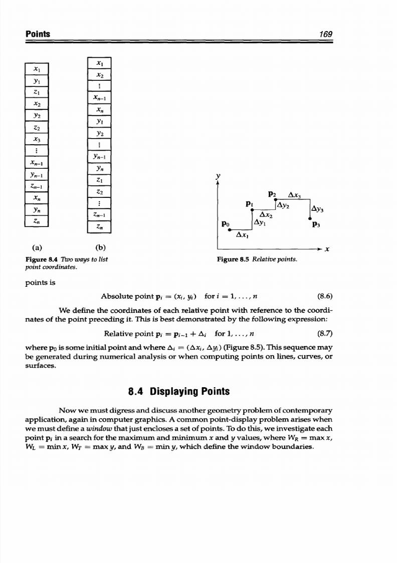
8/9/2019 Mortenson, Michael E. - Mathematics for computer graphics applications.pdf
http://slidepdf.com/reader/full/mortenson-michael-e-mathematics-for-computer-graphics-applicationspdf 182/367
Points
169
xI
Y1
Z
1
X
2
Y2
Z2
X
3
Xn-I
Yn-1
Zn-I
Xn
Yn
Zn
(a)
(h)
Figure
8.4 Two ways
to
list
Figure 8.5
Relative points.
point coordinates.
points
is
Absolute
point
pi
=
(xi, yi)
for
i
=
1,..., n (8.6)
We define
the coordinates of
each
relative
point with
reference to
the
coordi-
nates of the
point
preceding it. This is
best demonstrated
by the
following
expression:
Relative
point
pi= pi
+ Ai
for
1, . . ., n
(8.7)
where
po is
some initial
point
and
where Ai =
(Axi, Ayi) (Figure
8.5).
This
sequence may
be generated
during
numerical
analysis or when
computing
points on lines, curves,
or
surfaces.
8.4
Displaying Points
Now
we must digress and
discuss another geometry problem
of contemporary
application, again in computer
graphics. A
common
point-display
problem
arises
when
we
must
define a
window
that just
encloses
a
set
of
points.
To
do
this, we investigate
each
point
pi
in a
search for the maximum
and
minimum
x and y values, where
WR = max
x,
WL = min x, WT = max y, and WB = min y,
which
define the window
boundaries.
xl
X2
Xn-1
Xn
Y1
~Yn-l
-Y
Z2
Z-I
Zn-
P2
Ax
3
PtAy,
Ay
Po
AY
P3
AxI
I
Y
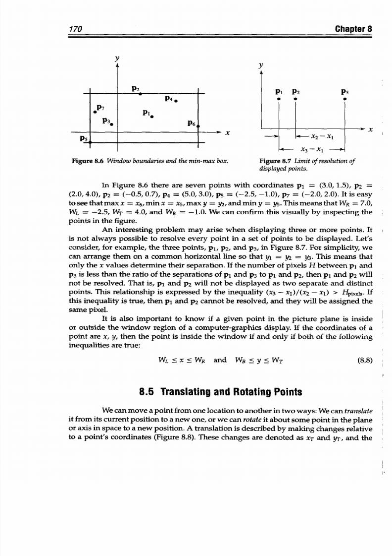
8/9/2019 Mortenson, Michael E. - Mathematics for computer graphics applications.pdf
http://slidepdf.com/reader/full/mortenson-michael-e-mathematics-for-computer-graphics-applicationspdf 183/367
170
Chapter
8
y
1no
F2
P4.
Pie
P6,
Y
- X
-X
Pi
P2
P3
*
0
a
X
2
-XXI
X
3
-XI
- X
Figure
8.6
Window
boundaries and
the
min-max
box.
Figure
8.7 Limit of resolution of
displayed points.
In Figure
8.6
there are seven
points
with
coordinates
p1
= (3.0,1.5),
P2 =
(2.0,4.0),
P2
= (-0.5, 0.7),
p4
=
(5.0,
3.0), p5
=
(-2.5, -1.0),
P7 = (-2.0,
2.0).
It
is easy
to
see
that max x
= x
6
,
min x
= X5, max y
=
y2, and
min y
= y5. This means that
W R
= 7.0,
WL
=-2.5, WT
= 4.0,
and
WB
= -1.0.
We can confirm
this visually by inspecting
the
points
in the figure.
An
interesting problem may
arise
when displaying
three or more
points. It
is
not
always possible
to resolve
every
point
in
a set
of
points to be
displayed.
Let's
consider,
for example,
the three
points, pI, P2,
and
p3, in Figure
8.7.
For simplicity,
we
can arrange
them on a
common
horizontal line
so that
yi
=
Y2
=
Y3.
This
means
that
only the
x values
determine
their separation.
If the number
of
pixels
H
between pi and
P3
is less than
the ratio of
the separations
of
pi and
P3 to pi and P2, then
pi
and
P2 will
not
be
resolved.
That
is,
pi
and P2 will not
be displayed
as
two
separate
and
distinct
points.
This
relationship
is expressed by
the inequality (x
3
- xl)/(x
2
- X
1
) >
Hpiels. If
this
inequality is true, then pi and
P2
cannot be
resolved,
and
they will be assigned the
same
pixel.
It is also
important
to
know
if
a
given
point
in
the
picture plane
is inside
or outside
the
window
region of a
computer-graphics
display.
If the coordinates
of
a
point
are
x, y,
then
the
point
is
inside
the
window
if
and
only
if
both
of
the
following
inequalities are
true:
WL<X<WR
and
WB'Y<WT
(8.8)
8.5
Translating
and
Rotating
Points
We
can
move a point
from one
location to
another
in two ways:
We can translate
it
from
its
current position
to
a
new
one,
or
we
can rotate
t
about
some
point
in
the
plane
or
axis
in
space to
a
new position.
A translation is
described by
making changes
relative
to a point's
coordinates
(Figure 8.8).
These
changes
are
denoted
as XT
and
YT, and
the
P7
0
P3.
P5
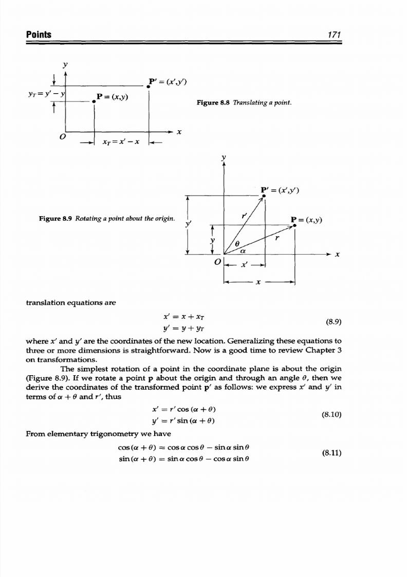
8/9/2019 Mortenson, Michael E. - Mathematics for computer graphics applications.pdf
http://slidepdf.com/reader/full/mortenson-michael-e-mathematics-for-computer-graphics-applicationspdf 184/367
Points
y
P'
= (x',y')
__
P = (xy)
o HI
XT=X -X
Figure 8.9 Rotating
a
point about the origin.
Figure 8.8
Translating
a point.
x
P =
(x',y')
(x,y)
x
translation
equations
are
XX=
X + X T
Y = Y+YT
(8.9)
where x' and
y'
are the coordinates of the new location. Generalizing these equations to
three or more dimensions
is
straightforward.
Now
is
a
good time to review
Chapter 3
on transformations.
The simplest rotation of a
point
in the coordinate plane is about the origin
(Figure 8.9). If
we rotate
a
point p about
the
origin
and
through
an
angle 0,
then we
derive
the
coordinates of
the transformed
point
p'
as
follows:
we express x' and y' in
terms of
a +
9
and
r', thus
x' = r'cos
(a +
0) (8.10)
y' = r'sin (a + 0)
From elementary
trigonometry
we
have
cos(a
+
9)
= cosa cos9 - sina
sine
sin(a
+ 0)
=
sinacos
-cosa
sin9
171
YT=Y Y-Y
F-
(8.11)
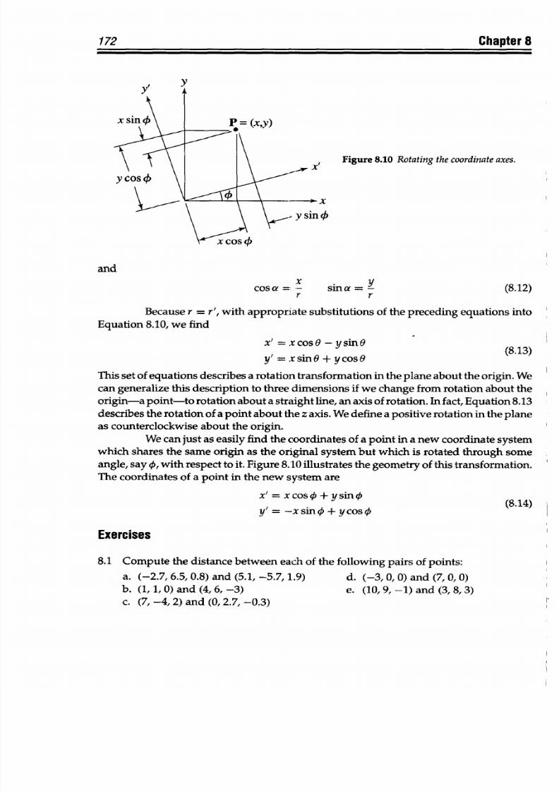
8/9/2019 Mortenson, Michael E. - Mathematics for computer graphics applications.pdf
http://slidepdf.com/reader/full/mortenson-michael-e-mathematics-for-computer-graphics-applicationspdf 185/367
172
Chapter 8
and
x y
cosa
= - sina =
-
(8.12)
r r
Because r = r', with appropriate
substitutions of the preceding
equations into
Equation 8.10, we
find
x' =.xcosO
- ysin8
y'
=.
xsinO
+
ycosO
This set of equations describes
a rotation transformation
in the
plane
about the origin.
We
can generalize
this description
to
three
dimensions if
we
change from
rotation
about
the
origin-a point-to
rotation about
a
straight
line, an
axis
of rotation.
In
fact,
Equation 8.13
describes
the rotation of a
point
about the z axis.
We
define
a
positive
rotation in
the plane
as counterclockwise about the origin.
We can just as
easily find the coordinates
of a point
in
a
new
coordinate
system
which shares the
same
origin as
the original system
but
which is rotated
through
some
angle,
say X,
with
respect
to
it.
Figure 8.10 illustrates
the
geometry of
this transformation.
The
coordinates
of
a
point
in the
new
system
are
x'
=
x
cos
4 +
y
sin(
y'=
-xsino
+
ycos
(
Exercises
8.1
Compute the distance
between each of
the
following
pairs of points:
a.
(-2.7,
6.5, 0.8)
and (5.1,
-5.7,1.9)
d. (-3,
0, 0) and
(7, 0,
0)
b. (1, 1, 0) and
(4,6,
-3)
e. (10,
9,
-1)
and (3, 8,3)
c. (7,
-4,
2)
and
(0, 2.7, -0.3)
I Figure 8.10
Rotating
the
coordinate axes.
-x
nX
8/9/2019 Mortenson, Michael E. - Mathematics for computer graphics applications.pdf
http://slidepdf.com/reader/full/mortenson-michael-e-mathematics-for-computer-graphics-applicationspdf 186/367
Points
173
8.2 Compute
the
coordinates of
the
points
in
Exercise
8.1 relative to
a coordinate system
centered at
(3, 1, 0) in the
original
system and parallel
to
it.
8.3
Compute the distance
between
each
of the
points
found
for Exercise
8.2.
8.4
Show
that the
distance between
any pair
of
points
is
independent of
the
coordinate
system
chosen.
8.5 Compute the midpoint
between
the
pairs
of points in Exercise 8.1.
8.6
Given
an arbitrary set of points, find the
coordinates
of the vertices of a rectangular
box that just encloses it.
8.7 Find
the
coordinates of
the eight
vertices of
a rectangular
box that just
encloses the
ten
points
given in
Exercise
8.1.
8.8
Given
that
Ai
is a
constant
for
all pi,
that
is,
Ai
=
(Axi,
Ayi)
=
(Ax, Ay),
find
P4
in
terms
of po
and
Ai.
8.9 Find the
set
of
Ais for the
vertex
points of a
square
whose
sides are
three
units
long
and with po = (1,0). Assume
that
the
sides of
the square are parallel to the x, y
coordinate axes,
and
proceed counterclockwise.
8.10
Repeat Exercise
8.9
for a square whose
sides
are four
units
long
and with
po =
(-2,
-2).
8.11
Repeat Exercise 8.10 for po =
(1,
-4).
8.12
Given
WR
=
14,
WL
=
-2,
WT
=
8,
and
WB
=
-4,
determine which
of
the
following
points
are inside this computer-graphics
display
window:
a.
p, = (15,4) d.
p4
= (-2, 8)
b. P2 =
(3,
10)
e.
P5
=
(10, 10)
c.
p3=(1
4
,
2
)
8.13
Find the
coordinates of
the
corners
of the
window defined in
Exercise
8.12.
8.14
State a mathematical test to determine if a point is contained in a rectangular volume
in
space, whose sides are parallel to the principal planes.
8.15
Derive
the
equations
that
describe
the
resultant
transformation
of a
point
that
is
first
translated
by XT,
yT
and then
rotated by 0.
8.16 Derive the equations that
describe the
resultant transformations of
a
point
that is
first rotated
by
0
and
then translated
by
XT,
YT.
8.17 Compare
and
comment on the results of
Exercises
8.15
and
8.16.
8/9/2019 Mortenson, Michael E. - Mathematics for computer graphics applications.pdf
http://slidepdf.com/reader/full/mortenson-michael-e-mathematics-for-computer-graphics-applicationspdf 187/367
(Al
Ka
LINES
A
straight
line is the next simplest geometric object after
a
point. All physical exam-
ples of a straight line are finite line segments
with
well-defined
endpoints
and length.
However, the mathematical or geometric
line
may
be
unbounded
or
infinite,
or it
may
be a
semi-infinite half-line
or
ray.
This chapter reviews the mathematical description of
lines in two and
three dimensions,
including
linear
parametric equations. It describes
how
to compute
points on
a line, geometric
relationships
between points
and lines, line
intersections, and translating and rotating
lines.
9.1 Lines in he Plane
The
slope-interceptform s algebraically
the simplest
way
to describe
a
straight
line
that
lies in the
x,
y
plane
(Figure 9.1). If we know the slope m of a
line
and where it
intersects the y axis, at y
=
b,
then
we write the equation of the
line
as
y=mx+b
(9.1)
The slope m is the ratio of the change in y to the change in x between any two
points
on
the line. If the coordinates of these
two
points are xl,
yi
and x
2
, y2, then the
slope of
the
line that passes through them is
x
-
(9.2)
The point-slopeform is a
variation of
the
slope intercept form
(Figure 9.2). If
we
know the slope m and
a
point
xi, yi
through
which
the line passes,
then
y - y
1
=
m(x -
x) (9.3)
If
we
use the
point
xl
=
0,
y, =
b,
then
Equation
9.3
simplifies to Equation
9.1.
The two-pointform
derives from the proposition that any
two distinct points in
the plane
define
a line
that passes through both of
them (Figure
9.3).
Thus,
given two
174

8/9/2019 Mortenson, Michael E. - Mathematics for computer graphics applications.pdf
http://slidepdf.com/reader/full/mortenson-michael-e-mathematics-for-computer-graphics-applicationspdf 188/367
V
y=b
/
y
/
x
/
Figure 9.1 Slope-interceptform.
y
m
/ X,,
yI
Figure 9.2 Point-slopeform.
V
X
2
,
Y2
zx
1
, YI
/a
Figure 9.3
Two-pointform.
bZ
Figure
9.4 Interceptform.
points x
1
,
yi
and x
2
,
y2,
we substitute Equation 9.2
into
Equation
9.3
for
m, and
rearrange
the
terms to
obtain
Y-Y1
= y-yi
X-X1 X2-X1
(9.4)
Using Equation 9.4
for
the
two points
(x1, yi) = (a, 0)
and (x2,
y2) = (0, b),
produces
x+Y-=
1
a b
(9.5)
This is the
intercept
orm, aptly named, since
it
defines a line by its points of intersection
with
the
coordinate
axes (Figure 9.4).
Equations
9.1
and
9.3 are
explicit
equations, where
x is the independent variable
and y is the dependent
variable.
That is,
we choose
arbitrary
values for x and
compute
the corresponding
values of
y. The value of
y
depends
on the
value
of
x. Equations 9.4
and 9.5 are
implicit equations,
where we
can choose
either x
or
y to
be
the
independent
Lines
175
-
b
-
>
Y
-
8/9/2019 Mortenson, Michael E. - Mathematics for computer graphics applications.pdf
http://slidepdf.com/reader/full/mortenson-michael-e-mathematics-for-computer-graphics-applicationspdf 189/367
176
Chapter 9
variable.
However, we can
express x and y separately in
terms
of
a third
variable,
say
u.
Using this approach we need two
equations to define a
line in
the plane.
They are
x
= au+ b
(9.6)
y
=
cu
+ d
These are parametric
equations,and u
is the parametricvariable
. Ordinarily, we
treat
u
as the
independent
variable and x and
y as
dependent variables.
The parametric equations of
a line in the plane work like
this:
Let's
say
we want
to define
a
line
that
passes
through
xi, yi and x
2
, y2 and that u
=
0 at the first point,
u
=
1
at
the second
point.
This is enough
information to write
two
sets of
two simultaneous
equations to determine
the constant coefficients
a,
b,
c, and d. In
this case, for
u =
0
in
Equations 9.6, we have
x
=
b b
=
x 9.7)
yj
=d d
=
and for u = 1
a
+ b =
X2
9.8)
c +d =
y
2
We find
b and
d directly,
from Equations
9.7, and substitute appropriately
into
Equations 9.8 to find
a
and
c. Thus
x2
=a
+xi
a =x
2
-xl (9.9)
or
.
y2=c+Yl
C=y2-yl
Now
we know a,
b,
c, and d
for
the
line
passing
through
the two given points,
and
we
rewrite
Equations 9.6 to obtain the parametric
equations of this
line:
X
= (X2-
Xl)U
+ X1
(9.10)
x
= (x
2
-
YO)U
+
x
1
ye=(y2-yl)u+yl
910
To find a set of points
on
this line,
we substitute
a set
of
u
values
into Equa-
tions
9.10.
Each u
value
determines a coordinate
pair of x, y
values. This
way
of
defining
straight lines is often used
in computer
graphics and geometric
modeling, because it
allows
a
sequence
of
points on
the
line to be
computed and
plotted
on
a
display
screen.
These are linearparametric
quations . We
use
higher-order parametric equations to define
curves
and surfaces.
Of
course, the
extension to
three dimensions is
obvious.
Because
parametric
equations allow us
to separate
the
dependent
x and y
coordinate
values
of points along
a
line, the
method
readily lends itself
to
vector
geometry
(see Chapter 1).
We
can
express
the angle 0 between two
lines in
the
plane
as a
function
of
their
two
respective slopes,
ml
and m
2
(Figure 9.5):
1t+
ml
m
2
(9.11)
The
derivation of
Equation
9.11
is
a simple exercise
in
algebra and
trigonometry.
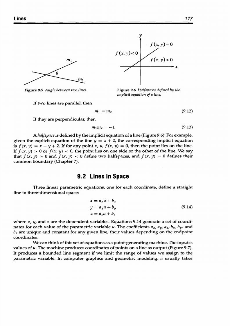
8/9/2019 Mortenson, Michael E. - Mathematics for computer graphics applications.pdf
http://slidepdf.com/reader/full/mortenson-michael-e-mathematics-for-computer-graphics-applicationspdf 190/367
Lines
Ml
0M
177
Figure
9.5 Angle between
two lines.
Figure 9.6 Halfspaces defined
by the
implicit equation of
a
line.
If
two
lines are parallel,
then
ml
= M2
(9.12)
If they are perpendicular,
then
mlm
2
=-1
(9.13)
A halfspaceis
defined
by
the implicit equation of a line (Figure 9.6). For example,
given the explicit
equation of the
line y
= x
+
2,
the
corresponding implicit
equation
is
f
(x,
y)
=
x
-
y
+
2.
If for
any
point
x,
y, f
(x,
y)
=
0,
then
the
point
lies
on the
line.
If
f (x, y) > 0
or
f (x, y) < 0,
the point
lies on
one
side or the other
of
the
line. We
say
that
f (x, y)
> 0 and
f (x, y) <
0
define two halfspaces,
and
f
(x,
y) =
0
defines their
common
boundary (Chapter 7).
9.2
Lines
in
Space
Three linear
parametric
equations, one for each
coordinate,
define
a straight
line in three-dimensional space:
x
=
axu
+
bx
y
= aYu +
by
(9.14)
z = azu + bz
where x,
y, and
z are the
dependent variables. Equations 9.14
generate a set
of
coordi-
nates
for each value of
the
parametric variable u. The coefficients
a.,
ay, a.,
bx, by,
and
b, are
unique
and
constant for
any
given line,
their
values
depending on the endpoint
coordinates.
We can
think
of
this set
of
equations as a point-generating
machine. The
input is
values
of
u. The
machine produces coordinates
of
points
on
a
line
as
output
(Figure 9.7).
It
produces
a bounded line
segment
if
we limit
the range of
values
we assign
to the
parametric
variable.
In
computer
graphics and
geometric
modeling,
u
usually
takes
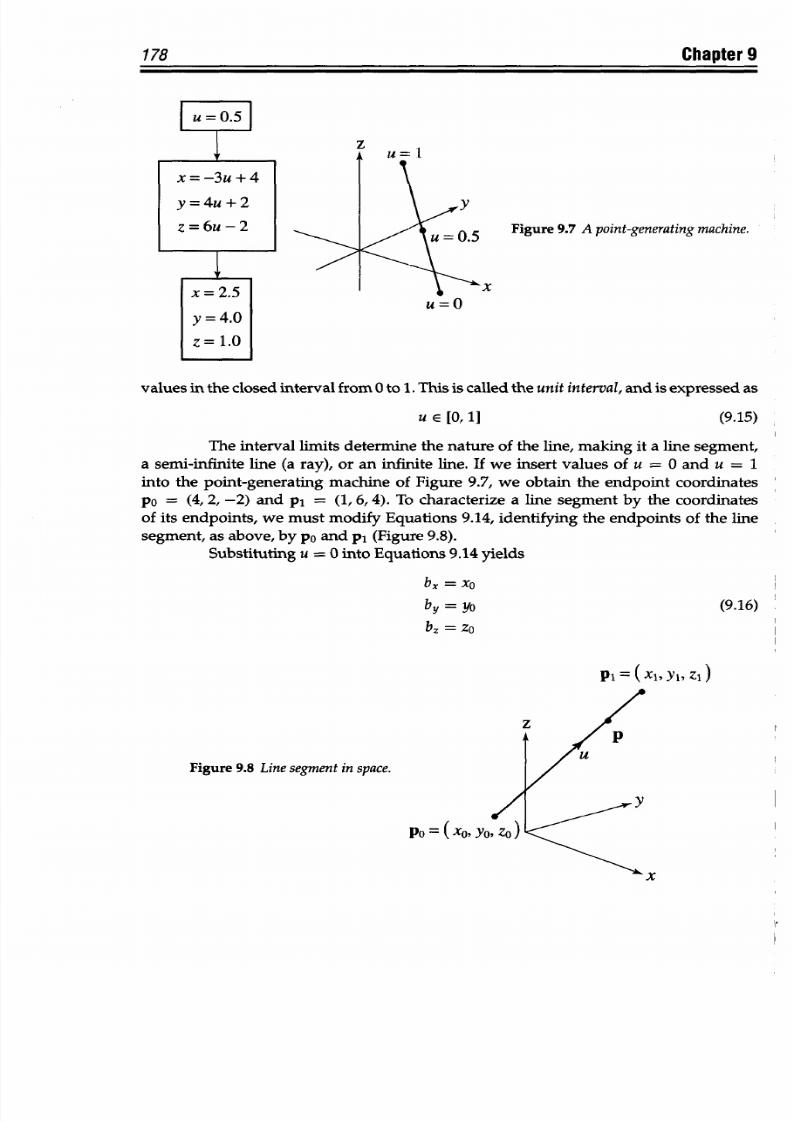
8/9/2019 Mortenson, Michael E. - Mathematics for computer graphics applications.pdf
http://slidepdf.com/reader/full/mortenson-michael-e-mathematics-for-computer-graphics-applicationspdf 191/367
178
Chapter
9
z
Figure 9.7 A point-generatingmachine.
u=O
values in
the
closed interval
from 0 to 1.
This
is called
the unit
interval,
and
is expressed as
U E [0, 11
(9.15)
The
interval limits determine the
nature
of the line, making it a
line
segment,
a
semi-infinite line
(a
ray), or
an
infinite
line. If we insert values
of u
= 0 and
u
= 1
into
the point-generating
machine
of
Figure 9.7, we
obtain the endpoint coordinates
po
=
(4, 2, -2)
and
p1
=
(1, 6,4).
To
characterize a line
segment by the
coordinates
of
its endpoints, we
must
modify
Equations
9.14,
identifying the
endpoints
of the line
segment,
as above, by po and
pl (Figure
9.8).
Substituting u = 0 into
Equations 9.14
yields
bX =
xo
(9.16)
y
=
Yo
bz
= zo
Pi
=
(
x
1
Y
Zi
Figure 9.8 Line segment
in
space.
Po
= (x
0
, YO
A
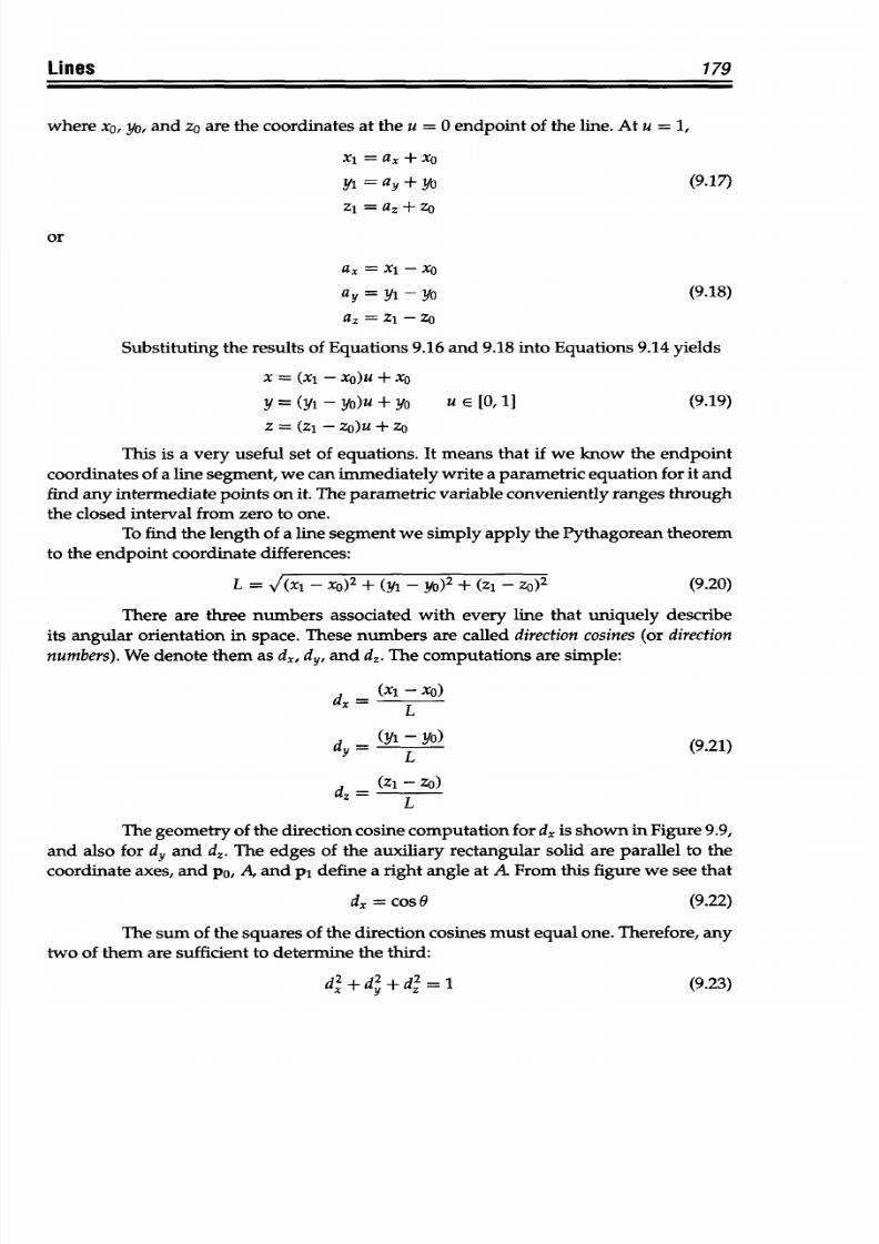
8/9/2019 Mortenson, Michael E. - Mathematics for computer graphics applications.pdf
http://slidepdf.com/reader/full/mortenson-michael-e-mathematics-for-computer-graphics-applicationspdf 192/367
Lines
179
where xo, yo, and zo are the coordinates
at
the u = 0
endpoint
of the line.
At
u = 1,
X
=ax+ xo
yi
=ay+yo
(9.17)
z
=
az
+
zo
or
ax
= Xi
-
xo
ay =
yi
- Yo
(9.18)
az =z1 -zo
Substituting the results of Equations 9.16
and
9.18 into Equations
9.14 yields
x
=(xi
- xo)u
+
xo
y =
(yi - yo)u +yo U E
[0,
1] (9.19)
Z
= (Z
1
-
Zo)u +
Zo
This is a very useful set of
equations.
It means
that
if we know the
endpoint
coordinates of a line segment, we can immediately
write
a parametric equation for it
and
find
any
intermediate points
on
it. The parametric variable conveniently ranges
through
the closed
interval from
zero
to
one.
To
find
the length of a line segment w e simply
apply
the Pythagorean theorem
to the
endpoint
coordinate differences:
L =
I(xl
-
Xo)
2
+ (yi
-
yo)
2
+ (Z
1
-
Zo )
2
(9.20)
There
are
three numbers associated with every line that
uniquely describe
its angular orientation
in space. These numbers are
called
direction cosines (or direction
numbers).
We denote them as
dx,
dy, and
d,.The
computations
are simple:
(x
1
- xo)
L
dy
= (Yi - Yo) (9.21)
L
(z
1
-
Z
o
)
L
The geometry
of the direction cosine
computation for dx is shown in Figure
9.9,
and
also
for
dy
and d,.
The
edges of the
auxiliary
rectangular solid
are
parallel to the
coordinate axes,
and
po, A, and Pi define a
right
angle at A From this
figure
we
see
that
dx = cos
0
(9.22)
The
sum
of
the squares
of
the direction
cosines
must
equal
one. Therefore,
any
two of them are
sufficient to
determine
the third:
d2 +d
2+ d2
= 1
x y Z
(9.23)
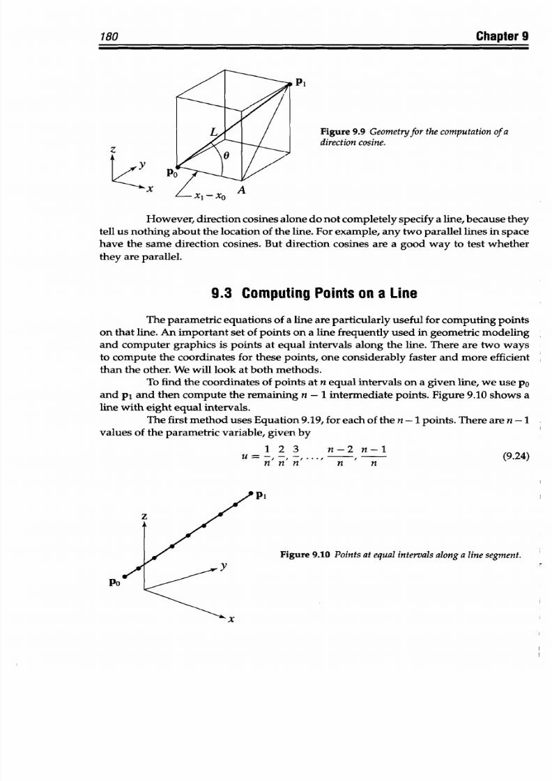
8/9/2019 Mortenson, Michael E. - Mathematics for computer graphics applications.pdf
http://slidepdf.com/reader/full/mortenson-michael-e-mathematics-for-computer-graphics-applicationspdf 193/367
180 Chapter
9
z
tx
P
1
Figure 9.9 Geometryfor
the
computation
of
a
direction cosine.
However,
direction cosines
alone
do not completely specify
a line,
because
they
tell
us
nothing
about the
location
of
the
line.
For example,
any two parallel
lines
in
space
have the
same direction
cosines.
But direction
cosines are a good
way
to test whether
they
are
parallel.
9.3
Computing
Points on
a
Line
The
parametric equations of a
line
are particularly useful for
computing points
on
that
line. An important set of
points
on a
line
frequently
used
in geometric modeling
and computer graphics is points at equal intervals along the line.
There are
two ways
to
compute the
coordinates
for
these
points,
one
considerably
faster
and
more efficient
than
the other. We will
look
at both methods.
To find
the
coordinates
of
points at
n equal intervals on a given line, we use po
and pi and
then
compute the remaining
n - 1
intermediate points. Figure 9.10 shows
a
line with
eight equal intervals.
The first method
uses Equation
9.19, for each of the n
-1 points.
There are n -1
values
of the parametric variable,
given
by
1
23
n-2 n-1
=-,-,- 2,... n 2 .n.. (9.24)
n
n
n n n
Figure
9.10 Pointsat
equal
intervals alonga line
segment.
Po
-A
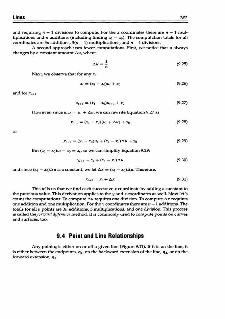
8/9/2019 Mortenson, Michael E. - Mathematics for computer graphics applications.pdf
http://slidepdf.com/reader/full/mortenson-michael-e-mathematics-for-computer-graphics-applicationspdf 194/367
Lines
181
and requiring n - 1
divisions to
compute. For the
x
coordinates there are n - 1 mul-
tiplications and n additions (including
finding
xl - xo). The computation totals for
all
coordinates
are 3n additions, 3(n - 1)
multiplications,
and n - 1 divisions.
A
second
approach uses
fewer
computations.
First,
we
notice
that
u
always
changes by a
constant
amount Au, where
Au = -
(9.25)
n
Next,
we
observe that for any xi
xi = (xi -
xO)ui + x
0
(9.26)
and
for
xi+l
xi+1 = (xi - xo)ui+i + x
0
(9.27)
However, since uj+
1
= ui + Au, we can rewrite
Equation
9.27
as
xi+1
=
(xi
- xo)(ui + Au) +
xo
(9.28)
or
Xi+1 =
(x1 - X)Ui + (x1 - xo)Au
+ xO
(9.29)
But (xi - xo)ui + xo = xi, so we can simplify Equation 9.29:
xi+, = xi + (xi
-
xO)Au
(9.30)
and since
(xl
- xo)Au is a constant, we let Ax = (xl - xo)Au. Therefore,
xi+
1
=
xi
+
Ax
(9.31)
This tells us that we find each successive
x
coordinate by adding
a
constant to
the previous
value.
This
derivation applies
to
the
y
and
z
coordinates
as well.
Now let's
count the
computations:
To
compute Au requires o ne division. To compute
Ax requires
one
addition and
one
multiplication.
For the x coordinates there
are
n
-1 additions.
The
totals
for
all
n points
are
3n additions, 3 multiplications, and one division.
This
process
is called
theforwarddifference method.
It
is commonly
used to
compute
points
on
curves
and
surfaces,
too.
9.4
Point
and Line Relationships
Any point q is either on
or
off a given line (Figure
9.11).
If
it
is on
the
line, it
is
either between the endpoints, qi, on the backward
extension
of the line,
q2, or on the
forward extension,
q3.
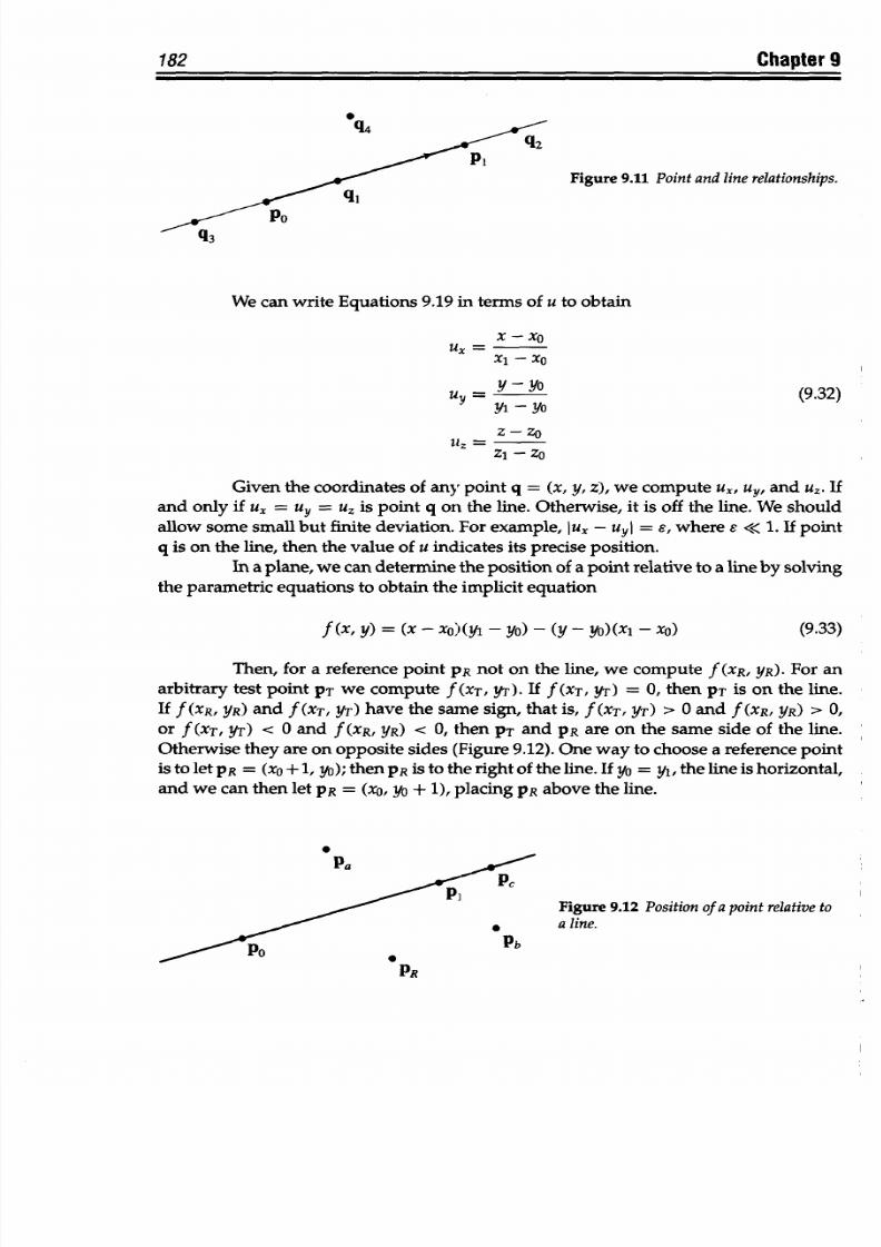
8/9/2019 Mortenson, Michael E. - Mathematics for computer graphics applications.pdf
http://slidepdf.com/reader/full/mortenson-michael-e-mathematics-for-computer-graphics-applicationspdf 195/367
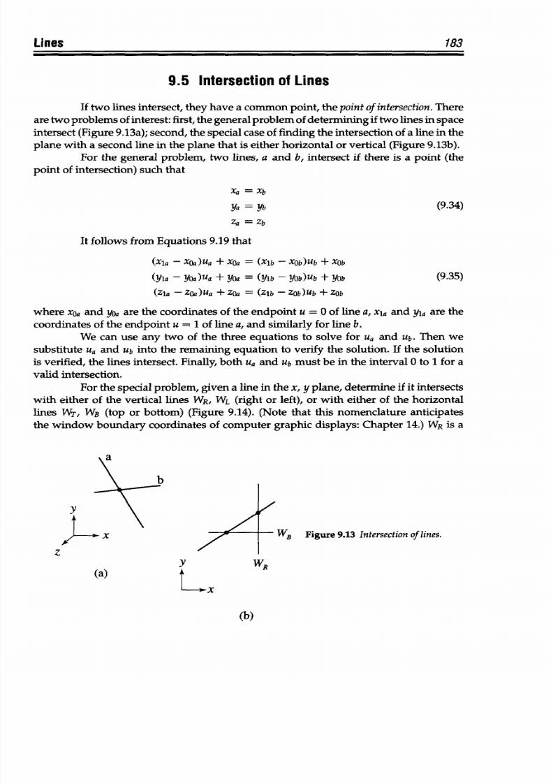
8/9/2019 Mortenson, Michael E. - Mathematics for computer graphics applications.pdf
http://slidepdf.com/reader/full/mortenson-michael-e-mathematics-for-computer-graphics-applicationspdf 196/367
Lines
183
9.5 Intersection
of
Lines
If two lines intersect,
they have
a
common
point,
the point of
intersection. There
are
two problems
of interest: first,
the general problem
of
determining
if
two
lines
in
space
intersect (Figure
9.13a);
second, the special case of finding the
intersection
of a
line in
the
plane
with a second line in the plane
that
is either horizontal or vertical (Figure 9.13b).
For the general problem, two lines, a and b, intersect if there is
a point (the
point of intersection) such that
Xa = Xb
Ya
= Yb
(9.34)
Za = Zb
It
follows
from Equations 9.19 that
(Xla - XOa)Ua + XOa = (Xlb
-
XOb)Ub + XOb
(Yla
- YOa)Ua +
yOa
= (ylb - yob)ub + YOb (9.35)
(Zia
- ZOa)Ua +
ZOa
= (Zlb - ZOb)Ub +
ZOb
where
xOa
and
yoa are
the
coordinates of
the
endpoint u = 0 of
line a, xla and y3a
are the
coordinates of the endpoint
u
= 1 of line
a,
and similarly for line
b.
We can
use any two of
the three
equations
to solve for
Ua
and
Ub.
Then we
substitute
ua
and Ub
into
the
remaining equation
to
verify
the
solution. If the
solution
is verified,
the lines
intersect.
Finally,
both
ua and Ub
must
be
in the
interval
0
to
1 for a
valid
intersection.
For
the
special
problem,
given a
line
in
the x, y plane,
determine if it intersects
with
either
of
the
vertical lines
WR,
WL (right or left), or with
either
of
the horizontal
lines
WT,
WB (top or
bottom)
(Figure 9.14). (Note that
this
nomenclature anticipates
the window boundary coordinates of computer graphic
displays:
Chapter 14.) WR is a
Y
1f
ax
-z
WB Figure 9.13 Intersection
of lines.
Y WR
(a)
ax
(b)
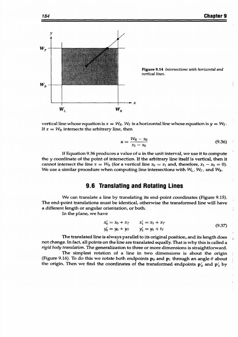
8/9/2019 Mortenson, Michael E. - Mathematics for computer graphics applications.pdf
http://slidepdf.com/reader/full/mortenson-michael-e-mathematics-for-computer-graphics-applicationspdf 197/367
184
Chapter
9
WT
WB
WL
WR
vertical
line whose
equation is x =
WR.
WT
is
a
horizontal
line whose
equation
is y = WT.
If
x = WR intersects
the
arbitrary line,
then
WR
- XO
(9.36)
Xi
-
X
If
Equation
9.36
produces
a
value
of
u
in the
unit
interval,
we use
it
to compute
the
y coordinate
of the point
of
intersection.
If
the
arbitrary
line
itself
is
vertical,
then it
cannot
intersect
the line
x
=
WR (for a vertical
line xO
= xl
and,
therefore,
xi
- xO =
0).
We use a similar
procedure when
computing
line
intersections
with WL,
WT, and WB.
9.6
Translating
and Rotating
Lines
We can
translate
a
line by
translating
its
end-point
coordinates
(Figure
9.15).
The
end-point translations
must
be
identical,
otherwise
the transformed
line
will have
a
different
length
or angular
orientation,
or both.
In the
plane, we have
Xo =
X O
+ XF X,
= X,
+ XT
(9.37)
O= YO + YT
Y = Y1
+ tT
The translated line
is always
parallel
to
its
original
position, and its length
does
not
change.
In fact,
all
points
on the
line are translated
equally.
That is
why
this
is
called a
rigid
body translation.
The
generalization
to three or
more dimensions
is
straightforward.
The
simplest rotation
of
a
line
in
two dimensions
is
about
the
origin
(Figure 9.16).
To
do this we
rotate both endpoints
po and
pi through
an angle
0 about
the
origin.
Then
we
find
the
coordinates of
the transformed
endpoints
p'
and pl by
Figure
9.14
Intersections
with
horizontal
and
vertical
lines.
x
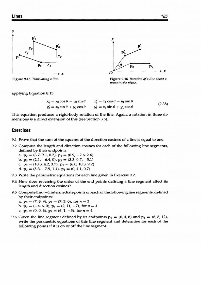
8/9/2019 Mortenson, Michael E. - Mathematics for computer graphics applications.pdf
http://slidepdf.com/reader/full/mortenson-michael-e-mathematics-for-computer-graphics-applicationspdf 198/367
Lines
185
y
y
T
x
Figure 9.15
Translating
a line. Figure 9.16 Rotation of a
line
abouta
point in
the plane.
applying Equation
8.13:
xO =
xo
cos
&-yo
sin
0 x1 = xi
cos6 -yj sin(
yO =
xo
sin6
+ yo cosO yj = x
1
sinO + y
1
cos (
This equation produces a rigid-body rotation of the line. Again,
a
rotation in
three
di-
mensions is
a
direct extension
of
this (see Section
3.5).
Exercises
9.1
Prove that the
sum
of
the
squares of
the direction cosines of a line is equal to
one.
9.2 Compute the length and direction cosines for each
of
the following line segments,
defined by their
endpoints:
a.
po =
(3.7, 9.1, 0.2), p1
=
(0.9,
-2.6,
2.6)
b. po = (2.1,
-6.4,
0), p1 = (3.3, 0.7, -5.1)
c. po =
(10.3,
4.2,
3.7),
pi = (6.0, 10.3,
9.2)
d. Po = (5.3,
-7.9, 1.4),
p1 = (0, 4.1,
0.7)
9.3 Write the parametric equations
for each line
given
in
Exercise
9.2.
9.4
How
does
reversing the order of the end
points
defining
a line segment
affect
its
length and direction
cosines?
9.5
Compute the
n-1
intermediate points on each
of
the following line segments, defined
by their
endpoints:
a. po = (7, 3, 9),
pi
= (7, 3, 0),
for
n = 3
b.
po
=
(-4, 6,
0),
pi
= (2,
11, -7), for n = 4
c. po = (0, 0, 6), pi = (6,1, -5), for n = 4
9.6
Given
the
line
segment
defined by its endpoints po
= (6,
4,
8) and
pi
= (8,
8,
12),
write
the
parametric equations of
this
line
segment
and determine for each of the
following
points
if
it
is on or off the
line
segment.
PO
XT
- x
8/9/2019 Mortenson, Michael E. - Mathematics for computer graphics applications.pdf
http://slidepdf.com/reader/full/mortenson-michael-e-mathematics-for-computer-graphics-applicationspdf 199/367
186
Chapter
9
a. qi = (4,0,8) d. q
4
=:(10,4,2)
b.
q2
=
(12,
-8, 20) e.
q5
(10,
12,16)
c. q3 = (7,6, 10)
9.7
Write
the parametric equations
for
each of the
line
segments whose
endpoints
are
given, and find
the
point of
intersection (ifany)
between each
pair of
line
segments.
a. Line 1: po = (2, 4, 6),
p' = (4, 6, -4)
Line 2: po =
(0,
0, 1), p1 = (6, 8, -6)
b.
Line
1:
po
=
(2,4,
6),
p1
= (4, 6, -4)
Line 2: po = (4, 3, 5),
pi =
(2.5,
4.5, 3.5)
c. Line 1:
po
= (2,
4,
6),
p'
=
(4,
6, --4)
Line 2:
po
=
(3,
5, 1), p' = (0, 2, 16)
d.
Line 1: po = (10,
8,
0),
p'
= (-1, --
1,
0)
Line
2: po
=
(13,
2, 0),
pi
=
(4,
7,
0)
e.
Line 1:
po
= (5, 0,
0),
pi = (2, 0, 0)
Line 2:
po
= (8,
0, 0),
pi = (10, 0, 0)
8/9/2019 Mortenson, Michael E. - Mathematics for computer graphics applications.pdf
http://slidepdf.com/reader/full/mortenson-michael-e-mathematics-for-computer-graphics-applicationspdf 200/367
~U
PT
PLANES
The
mathematics
and
geometry
of planes pervades computer
graphics, geometric
model-
ing, computer-aided design
and
manufacturing, scientific visualization,
and many more
applications.
This chapter
looks at
various ways to
define them,
including
the normal
form
and
the three-point form, the relationship between
a
point
and plane, and plane
intersections.
10.1 Algebraic Definition
Euclidean geometry
defines
a
plane in space
as the locus of
points
equidis-
tant from two fixed points. The resulting plane is the
perpendicular
bisector
of
the
line
joining the
two
points.
We
call
this definition
a demonstrative
or
constructive definition.
Computer-graphics and geometric-modeling applications require a more quantitative
definition, because these
planes may be
bounded by
polygons to
form the polyhedral
facets representing the surface of some modeled
object
or the plane of projection of some
view of an object, and so
on.
The
classic
algebraic definition of
a plane is the
first
step
toward
quantification.
The implicit
Cartesian
equation
of a plane is
Ax + By+
Cz + D =
0 (10.1)
This
is
a
linear
equation
in
x, y,
and
z.
By
assigning numerical values for
each
of the
constant
coefficients
A, B, C,
and D,
we define a specific plane in space. It is
an
arbitrary
plane
because,
depending
on the values of the coefficients,
we
can give
it
any orientation.
Figure
10.1 shows
only
that part
of a plane that
is in the
positive x, y, and
z
octant.
The three
bounding lines are the intersections of the
arbitrary
plane with
the principal
planes.
If
the coordinates of any point satisfy E quation 10.1, then the point lies on the
plane. We can arbitrarily specify any two coordinates x and y and determine the third
coordinate
z
by solving this equation.
We
obtain
a
more
restricted
version
of
this general
equation
by
setting
one
of
the coefficients
equal
to zero. If we
set
C equal to zero, for example, we obtain
Ax + By + D = 0 (10.2)
187
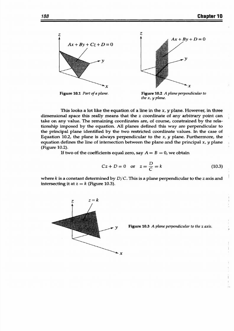
8/9/2019 Mortenson, Michael E. - Mathematics for computer graphics applications.pdf
http://slidepdf.com/reader/full/mortenson-michael-e-mathematics-for-computer-graphics-applicationspdf 201/367
Chapter 10
z
Ax+
By+ Cz+D=0
B-
Y
x
Figure 10.1 Partof
a
plane.
. A t
RM.D.
n-A
tIA 1 L y -r L -vU
Y
X
Figure 10.2 A
plane perpendicular
o
the x, y
plane.
This looks
a
lot like the equation of
a
line in the x, y plane.
However,
in
three
dimensional space this really means
that
the z coordinate of any arbitrary
point
can
take
on
any value. The remaining coordinates
are, of course,
constrained
by
the rela-
tionship imposed
by the equation.
All planes
defined this way
are
perpendicular to
the principal
plane identified by
the
two restricted coordinate values. In the
case of
Equation 10.2, the
plane is always perpendicular
to the x, y plane.
Furthermore,
the
equation defines the
line
of intersection between the plane and
the
principal
x,
y plane
(Figure 10.2).
If
two of
the coefficients
equal
zero,
say
A =
B
=
0, we
obtain
Cz+D=O or
z=
-=k
C
(10.3)
where
k
is a constant determined by
D,'C.
This
is
a
plane perpendicular
to
the z
axis
and
intersecting it at z = k
(Figure
10.3).
z z=k
t /
Y
Figure 10.3
A
plane perpendicular
o the
z axis.
x
188
i
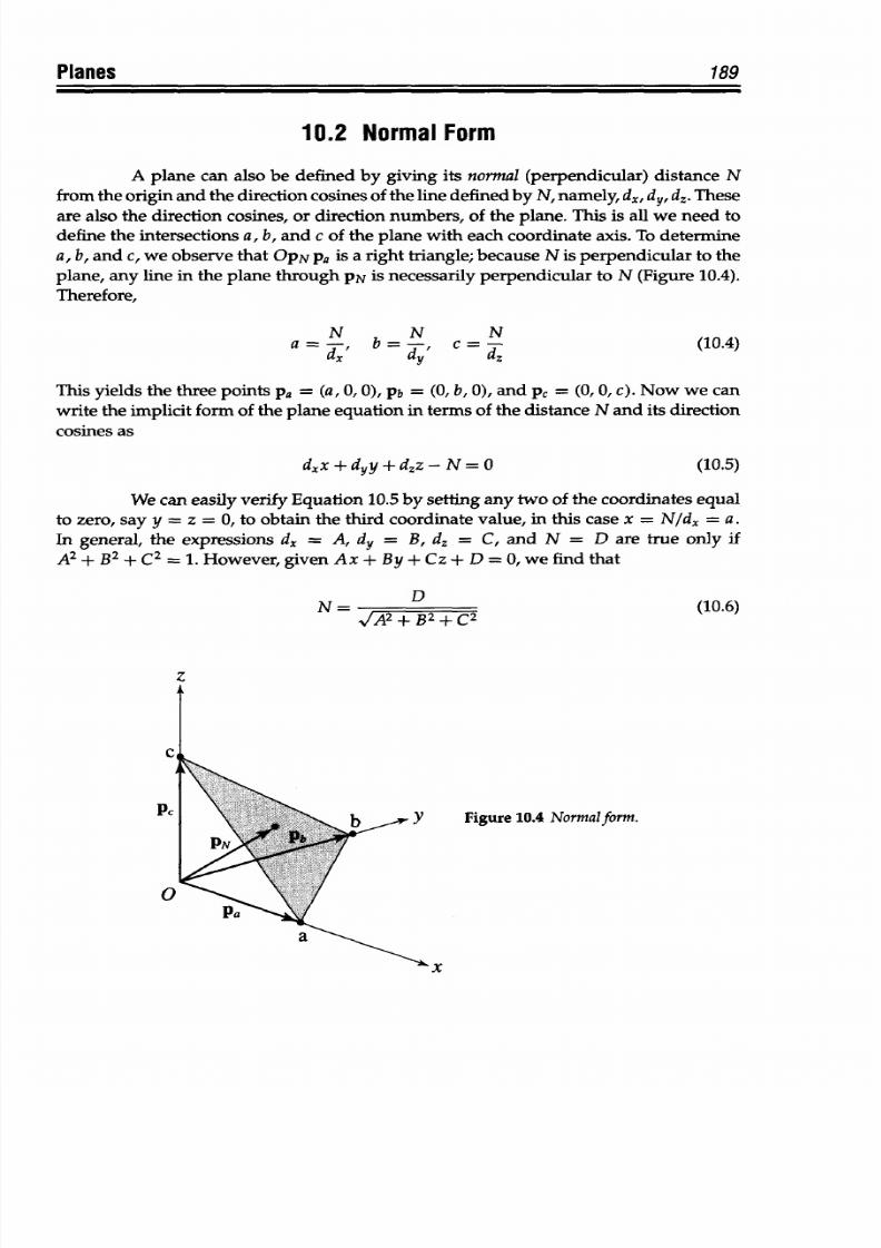
8/9/2019 Mortenson, Michael E. - Mathematics for computer graphics applications.pdf
http://slidepdf.com/reader/full/mortenson-michael-e-mathematics-for-computer-graphics-applicationspdf 202/367
Planes 189
10.2
Normal Form
A
plane
can also be defined by giving its
normal (perpendicular)
distance N
from the origin
and
the
direction cosines of the line defined by
N,
namely,
dx,
dy, d.. These
are
also the
direction cosines, or direction numbers,
of the plane.
This
is all we
need
to
define the intersections
a,
b, and
c of the plane
with
each
coordinate axis. To determine
a,
b, and c, we observe
that OPN pa
is a
right
triangle;
because N is perpendicular
to the
plane, any line in the plane
through
PN is necessarily perpendicular to N (Figure 10.4).
Therefore,
N N N
a =- b = d-
(10.4)
This yields
the
three points pa = (a, 0, 0), Pb = (0, b, 0), and
pc
= (0, 0,
c). Now we
can
write the
implicit form of
the plane equation
in
terms
of the distance N and
its direction
cosines
as
d~x+ dyy + dz
-N
= 0
(10.5)
We can easily verify Equation 10.5
by
setting
any two of the coordinates equal
to zero, say
y
= z = 0, to obtain the
third
coordinate value, in this case
x
= N/dx = a.
In
general, the expressions dx
=
A,
dy
=
B.
dz
= C, and N =
D
are
true
only if
A
2
+ B
2
+ C
2
=
1.
However, given
Ax
+
By
+
Cz
+ D
= 0,
we find
that
VA
2
+ B
2
+
C2
(10.6)
z
I
P.
Y Figure
10.4 Normal orm.
a
x
8/9/2019 Mortenson, Michael E. - Mathematics for computer graphics applications.pdf
http://slidepdf.com/reader/full/mortenson-michael-e-mathematics-for-computer-graphics-applicationspdf 203/367
190
Chapter 10
an d
A
V
B2+C2
B
(10.7)
,rA+
B
C2
C
VAB2+C2
Finally, if two
planes have
the
same direction
cosines, then they are
parallel.
10.3
Plane Defined by Three Points
Another
way
to
define
a
plane
is
by
specifying
three noncollinear
points
in
space. We demonstrate
this as follows: We
assume that the
coordinates of these
three
points
are p,
=
(xI, y1,
z
1
), P2
=
(x
2
, y2, z
2
), and p3 =
(X, y3, z
3
). Then we let
A'
=
A/D,
B'= B/D,
and
C'=
C/D.
The implicit
equation
of
a plane becomes
A'x +
B'y
+ C'z
+
1
=
0
(10.8)
Using
this
equation and the coordinates of the
three points, we can write
A'x, + B'yi +C'zi
+1 =
0
A'x
2
+
By
2
+
C'z
2
+
1 = 0
(10.9)
A'x
3
+
B'y
3
+ C'z
3
+ 1 = 0
Now we have three
equations in three
unknowns:
A', B',
and
C',
which
we can readily
solve. Two
points
are not sufficient to determine
A', B', and C', and
a
fourth
point
would
not necessarily
fall
on
the
plane.
If the three
points are the
points
of
intersection of the plane with
the coordinate
axes pa =
(a,
0,
0), Pb
= (0,
b, 0),
and p, =
(0,0,
c),
then the plane equation
is
x
y
z
- + b + - = 1
(10.10)
10.4 Vector
Equation
of
aPlane
There are at least
four
ways
to define a
plane
using vectors.
We
will
discuss one
of
them. Others are
thoroughly discussed
in Section 1.8. The normal
form of the
vector
equation
is
easy to express
using vectors.
All we must do
is express the perpendicular
distance
from the origin
to the
plane in question
as a vector,
n. From this
the
other
properties follow.
For
example,
since the
components
of
a
unit
vector are also
its
direction
cosines,
we
have
(10.11)
x =
d,
hy
= dyl
h
= d,
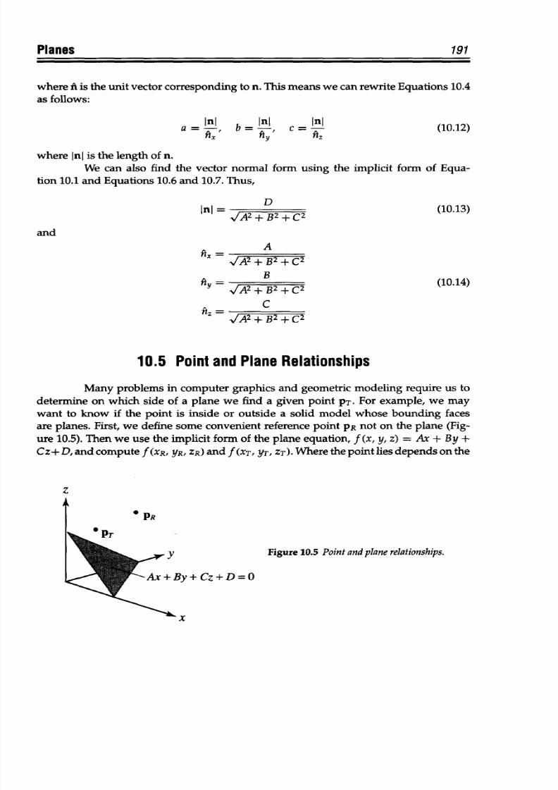
8/9/2019 Mortenson, Michael E. - Mathematics for computer graphics applications.pdf
http://slidepdf.com/reader/full/mortenson-michael-e-mathematics-for-computer-graphics-applicationspdf 204/367
Planes
191
where
fi
is
the
unit vector
corresponding
to n.
This means
we can rewrite
Equations
10.4
as
follows:
a=
IA
b- C
IA
(10.12)
where
Inms
the length
of n.
We can also find the vector
normal
form
using the implicit
form of
Equa-
tion
10.1
and Equations 10.6
and 10.7.
Thus,
Inj
D
(10.13)
m-
2
+ B
2
+
c2
and
=
A
n, vA~2+
B2
~+ 2
A
2
+ B
2
+C
2
(10.14)
C
= A
2
+ B
2
+ C
2
10.5
Point
and
Plane
Relationships
Many problems in computer
graphics
and
geometric modeling
require us to
determine
on which
side of a plane
we find a
given
point
PT.
For example,
we
may
want
to know
if the
point is inside
or outside a
solid
model
whose
bounding faces
are planes.
First, we define some
convenient
reference
point PR
not
on the
plane (Fig-
ure 10.5).
Then we
use
the implicit
form of the
plane
equation, f(x,
y, z) = Ax +
By +
Cz+ D, and
compute
f(xR,
YR, ZR)
and
f(xT, YT, ZT). Where
the point lies
depends
on the
z
PR
*
V y
Figure 10.5
Pointand
plane
relationships.
-Ax+By+Cz+D=0
x
I
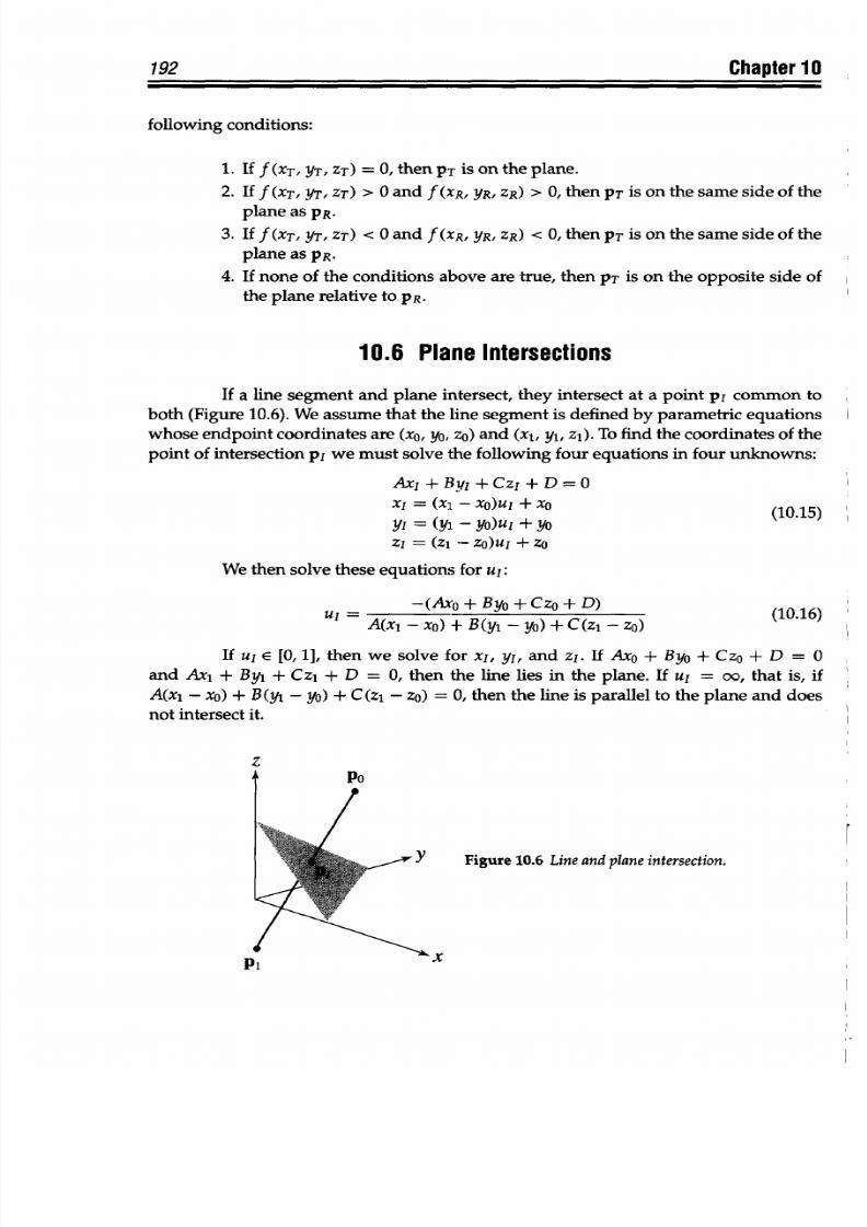
8/9/2019 Mortenson, Michael E. - Mathematics for computer graphics applications.pdf
http://slidepdf.com/reader/full/mortenson-michael-e-mathematics-for-computer-graphics-applicationspdf 205/367
192
Chapter
10
following conditions:
1.
If f (XT, YT, ZT)
= 0,
then
PT
is on
the plane.
2. If
f (XT, YT,
ZT) > 0 and f (XR,
YR,
ZR) > 0,
then
PT is on
the
same
side of
the
plane
as
PR.
3. If f (XT, YT, ZT) <
0
and f (XR, YR, ZR) < O, then PT is on the same side of the
plane as PR.
4. If none of the conditions above are true, then
PT
is on the opposite side
of
the
plane
relative
to PR.
10.6 Plane
Intersections
If a
line segment
and plane
intersect,
they intersect
at
a
point pi common
to
both
(Figure
10.6).
We
assume that
the line segment
is
defined by
parametric
equations
whose endpoint coordinates are (xO, yo zo)
and
(xl, yl,
zj).
To
find the
coordinates
of
the
point
of intersection
p1
we
must solve the following four
equations in four unknowns:
Ax,
+By,+Cz
1
+D=O
xi = (xi -
xo)ui
+ x
0
(10.15)
y,
=
(yi
-
yO)ui
+ YO
Zi
=
(Zi
-
Zo)u
+ Zo
We then solve
these equations
for
ul:
I
-(AxO+Byo+Czo+D)
A(x
1
- xo + B(y
1
- yo) + C(z
1
-zo) (10.16)
If Ul
E
[0, 1], then we
solve for xl,
yl, and zi. If AxO + ByO + CzO + D = 0
and
Ax, + By, +
Cz
1
+ D = 0,
then the line
lies in the
plane.
If
u
1
= oo, that is, if
A(x
1
-
xo)
+ B(y
1
- yo) +
C(z
1
- zo)
=
0, then the
line is parallel to the plane and does
not intersect
it.
z
/Po
Y
Figure 10.6 Line and
plane intersection.
/
U'
X
I
4
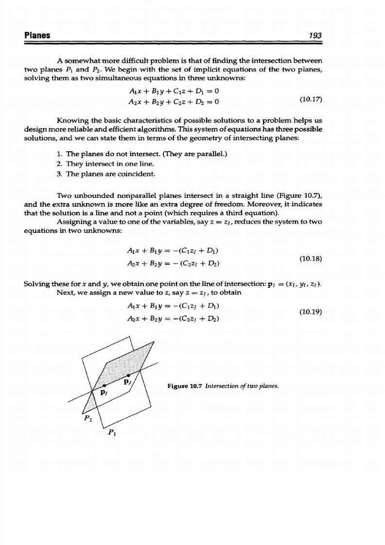
8/9/2019 Mortenson, Michael E. - Mathematics for computer graphics applications.pdf
http://slidepdf.com/reader/full/mortenson-michael-e-mathematics-for-computer-graphics-applicationspdf 206/367
Planes
193
A somewhat more
difficult
problem is that of finding the intersection between
two planes
P
1
and P
2
.
We begin with
the
set of implicit equations of
the two
planes,
solving
them
as two simultaneous equations
in
three unknowns:
Aix+ Bly+Clz+
Di
= 0
A
2
x +
B
2
y +
C
2
z +
D
=
°
(10.17)
Knowing
the basic characteristics of
possible
solutions to
a problem helps us
design more reliable and efficient algorithms.
This system of equations has three possible
solutions,
and
we can state
them
in
terms
of the geometry
of
intersecting planes:
1. The planes do
not
intersect. (They are parallel.)
2.
They
intersect
in
one line.
3.
The planes
are coincident.
Two
unbounded
nonparallel planes intersect in a straight
line
(Figure
10.7),
and the extra
unknown
is more like an extra degree of freedom. Moreover, it indicates
that the
solution is
a line and not a point (which requires a third equation).
Assigning
a
value to
one of
the
variables, say z =
z
1
,
reduces
the
system to
two
equations
in
two unknowns:
Aix
+
Bly
= -(CIz
1
+ DI)
A
2
x
+ B
2
y = -
(C
2
zI
+
02)
(10.18)
Solving these for
x
and y, we
obtain
one point
on
the line of intersection: pj = (xl, yI, z
1
).
Next,
we assign a new value to
z, say
z
=
z
1
, to obtain
Aix
+
Bly
=
-(Cizj
+
Di) (10.19)
A
2
x +
B
2
y
= -(C
2
ZJ +
D2 )
Figure
10.7 Intersectionof two planes.
PI
8/9/2019 Mortenson, Michael E. - Mathematics for computer graphics applications.pdf
http://slidepdf.com/reader/full/mortenson-michael-e-mathematics-for-computer-graphics-applicationspdf 207/367
8/9/2019 Mortenson, Michael E. - Mathematics for computer graphics applications.pdf
http://slidepdf.com/reader/full/mortenson-michael-e-mathematics-for-computer-graphics-applicationspdf 208/367
ApTa
POLYGONS
Polygons
and
polyhedra were among the
first
forms
studied in
geometry.
Their regular-
ity,
symmetry,
and
orderly lawfulness
made
them the
center of
attention
of
mathemati-
cians,
philosophers, artists,
architects,
and scientists for thousands of
years.
They are
surprisingly simple arrangements of points,
lines,
and planes. This
simplicity,
however,
harbors
subtleties of symmetry
and
order
that
deepen
our understanding
of
the physical
universe, the atoms
of
which we
are
made,
and
the space-time
in
which we
live.
Polygons are still important
today.
For example,
their use in computer graphics
is as
common
as points
and
lines,
because
it
is
easy to subdivide and approximate the
surfaces
of
solids with planes bounded by
polygons. Computer-graphics applications
project,
fill, and shade
these
polygonal facets to create realistic
images
of solids.
The
study
of polygons leads to insights into elementary geometry, algebraic geometry,
and
number
theory.
This chapter
discusses
two-dimensional
polygons whose sides are all straight
lines
lying
in the same plane. Three-dimensional
polyhedra whose
faces are planar
and
whose edges are straight lines are the
subjects of
the next
chapter.
Polygons
and
polyhe-
dra also exist in higher-dimension spaces and may have curved edges and faces. Topics
covered here include definitions
of
the
various
types of polygons, their geometric prop-
erties, convex hulls, construction of
regular
polygons, symmetry, and
containment.
11.1
Definitions
A somewhat formal
but effective definition goes
like this:
A
polygon is
a many-
sided two-dimensional figure bounded by a closed
circuit
of straight-line segments join-
ing successive
pairs
of points. The line segments are edges and
the points
are vertices.
An edge is a
bounded
straight-line
segment-a finite
length
of
an otherwise
unbounded
straight line.
A
polygon, then,
encloses a
finite, two-dimensional
area,
bounded by edges
and vertices. If the
vertices
all lie
in the same plane, then
the
polygon
is a plane polygon;
otherwise it
is a
skew
polygon. It
is possible
to construct
polygons
whose edges
are curve
segments on curved surfaces. We will study only
plane
polygons here.
The examples
of
polygons
in Figures 11.1a-11.ld are three-, four-,
five-,
and
six-sided
polygons, respectively. There is no
limit
to the
number of
edges
a
polygon can
have. And there
is
an infinite number
of each
type; that is, there
is
an infinite number
195
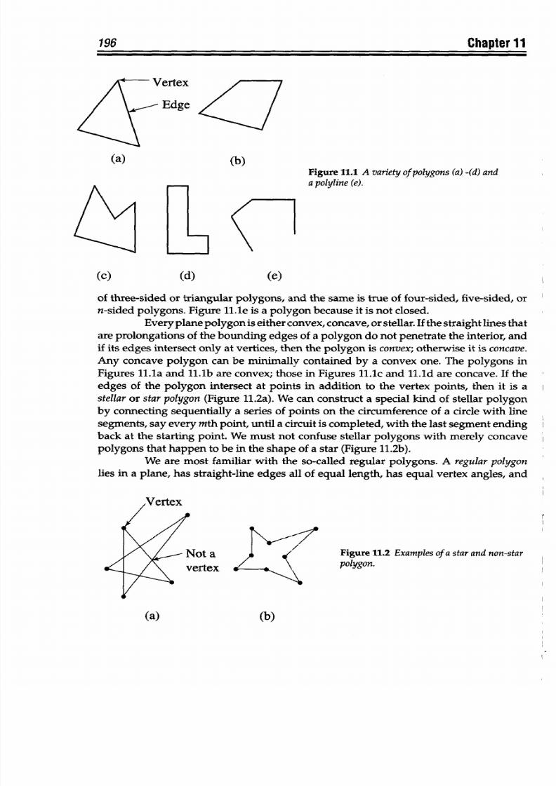
8/9/2019 Mortenson, Michael E. - Mathematics for computer graphics applications.pdf
http://slidepdf.com/reader/full/mortenson-michael-e-mathematics-for-computer-graphics-applicationspdf 209/367
196
Chapter
11
(a)
(b)
Figure
11.1
A variety
of polygons (a)
-(d)
and
K
a polyline e .
(c)
(d)
(e)
of three-sided
or
triangular polygons,
and the
same
is
true of
four-sided,
five-sided, or
n-sided polygons.
Figure l1.le
is a
polygon
because it is not
closed.
Every
plane
polygon
is either convex,
concave, or
stellar. If the straight
lines that
are prolongations
of
the
bounding
edges
of a polygon
do
not
penetrate
the
interior, and
if
its edges intersect
only at
vertices,
then
the
polygon is convex;
otherwise
it
is concave.
Any
concave
polygon
can be
minimally contained
by
a
convex one. The
polygons
in
Figures l1.la
and
l1.lb
are convex;
those in
Figures 1l.lc
and
ll.ld
are
concave.
If
the
edges
of the
polygon
intersect
at points
in
addition
to
the
vertex
points,
then it
is
a
stellaror star
polygon
(Figure
11.2a).
We can
construct
a
special
kind of stellar
polygon
by
connecting
sequentially
a series
of points on the
circumference
of a
circle
with
line
segments,
say
every mth point, until
a circuit is
completed,
with
the
last segment
ending
back
at
the
starting point.
We
must
not
confuse
stellar
polygons with merely
concave
polygons
that
happen
to
be in
the shape of a
star (Figure 11.2b).
We
are most
familiar
with the
so-called regular polygons.
A
regular
polygon
lies
in
a
plane,
has straight-line edges
all of
equal
length, has equal vertex angles,
an d
lot a
ertex
Figure 11.2
Examples of
a star
and
non-star
polygon.
(b)
a)
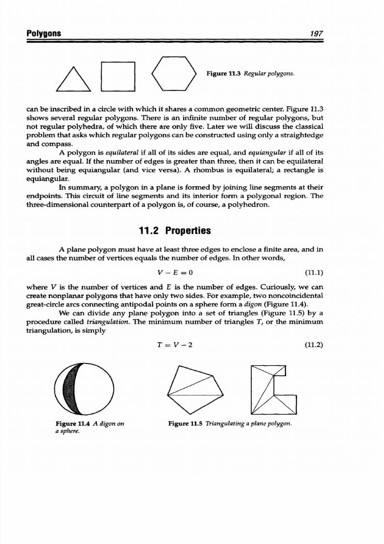
8/9/2019 Mortenson, Michael E. - Mathematics for computer graphics applications.pdf
http://slidepdf.com/reader/full/mortenson-michael-e-mathematics-for-computer-graphics-applicationspdf 210/367
Polygons
197
Figure 11.3
Regular
polygons.
can be inscribed in a circle with which it shares a common geometric center. Figure
11.3
shows several regular polygons. There
is
an infinite number of regular polygons, but
not regular
polyhedra, of which there are
only
five. Later
we will
discuss
the
classical
problem that
asks
which
regular
polygons can be
constructed using
only
a
straightedge
and
compass.
A polygon
is
equilateral f all of its sides
are
equal, and equiangular
f
all of its
angles
are equal. If
the
number
of edges
is
greater
than
three,
then
it
can
be equ ilateral
without
being
equiangular
(and vice versa). A rhombus is
equilateral;
a
rectangle is
equiangular.
In
summary,
a polygon in a plane
is formed by joining
line
segments at their
endpoints. This circuit of line segments and its interior form a polygonal region.
The
three-dimensional counterpart of a polygon is, of course, a polyhedron.
11.2 Properties
A
plane
polygon
must
have
at
least three edges to
enclose a finite area,
and
in
all
cases
the number of vertices equals the number
of
edges. In other words,
V-E=O (11.1)
where V
is the
number of
vertices and E is the
number
of edges. Curiously,
we
can
create nonplanar polygons that have only two
sides.
For example, two noncoincidental
great-circle arcs connecting antipodal
points on
a sphere
form a digon
(Figure
11.4).
We
can divide any
plane polygon into a set of
triangles (Figure 11.5)
by
a
procedure called
triangulation.The minimum number of triangles T, or
the
minimum
triangulation,
is
simply
T =
V-2
(11.2)
Figure 11.4
A digon on
a
sphere.
Figure
11.5
Triangulatinga plane polygon.
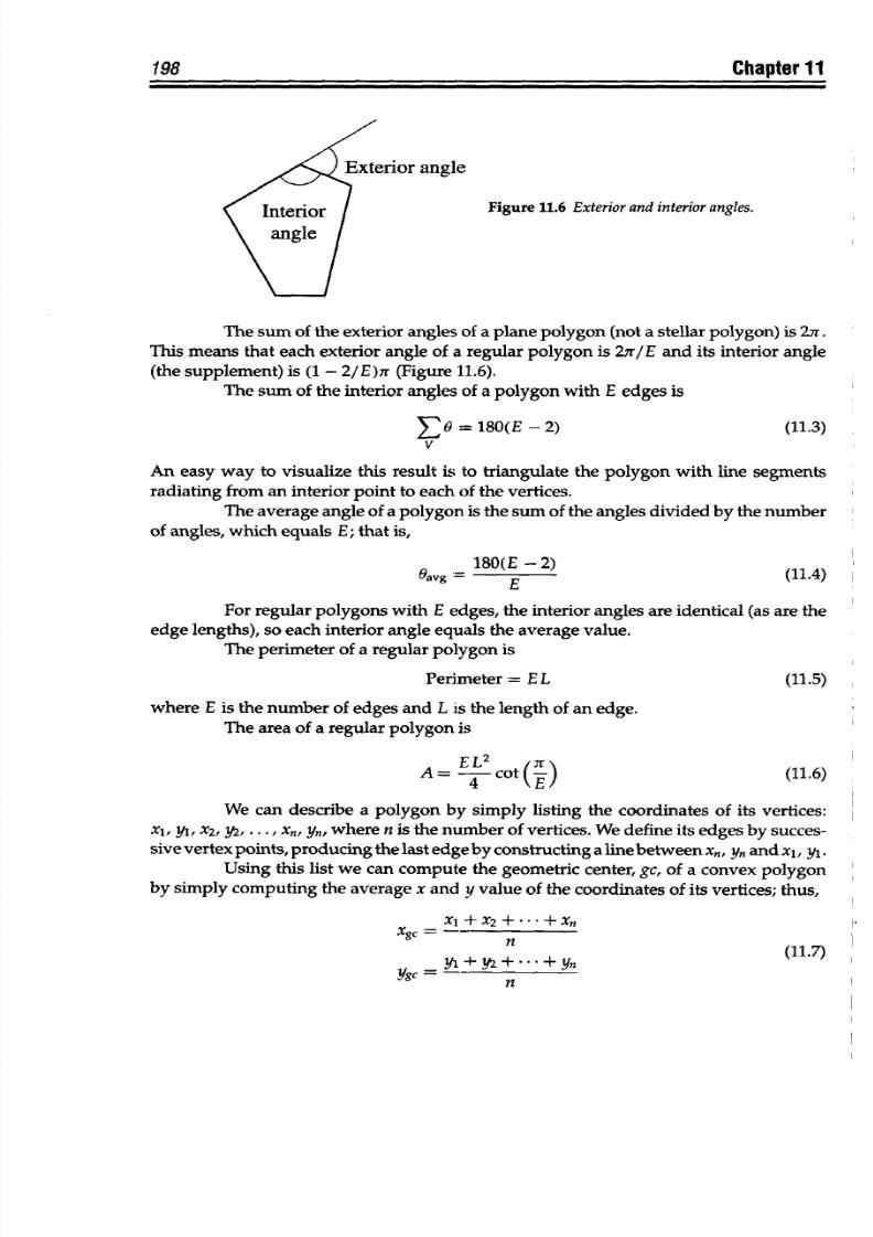
8/9/2019 Mortenson, Michael E. - Mathematics for computer graphics applications.pdf
http://slidepdf.com/reader/full/mortenson-michael-e-mathematics-for-computer-graphics-applicationspdf 211/367
198
Chapter
11
Figure
11.6 Exterior
and interior
angles.
The sum
of
the exterior angles of
a
plane polygon (not a stellar polygon) is 27r.
This
means
that
each
exterior
angle of a regular
polygon
is
27r/E
and its interior angle
(the supplement)
is
(1
-
2/E)ir
(Figure
11.6).
The sum
of
the interior
angles
of a polygon with
E edges is
E 0
= 180(E
-2) (11.3)
V
An easy way to visualize this result
is to triangulate the
polygon with
line segments
radiating from
an interior point
to each of
the
vertices.
The average angle of a polygon is the sum of
the angles divided
by
the
number
of angles,
which equals E; that
is,
Oavg
-=
180(E
-
2)
(11.4)
E
For
regular
polygons
with
E edges, the
interior angles
are
identical (as
are the
edge lengths), so each
interior angle equals the
average value.
The perimeter
of
a regular
polygon
is
Perimeter
=
EL
(11.5)
where E
is
the number of edges
and L is
the
length of an
edge.
The
area
of a
regular
polygon
is
A
=
L cot('E)
(11.6)
We can describe a
polygon by simply
listing the coordinates of
its vertices:
xi,
yi,
x
2
,
A,
.
.
.,
xn,
yn, where
n is
the number
of vertices. We
define its edges
by succes-
sive vertex points, producing the last edge by
constructing a line between Xn, yn and xl, yl .
Using this
list
we
can
compute
the geometric center, gc,
of a
convex
polygon
by simply computing the average x and y value of the coordinates of its
vertices; thus,
XI
+X2
+
*+Xn
Xgc
-
n
(117)
_g Y 2 + *2 Yn
/gC-
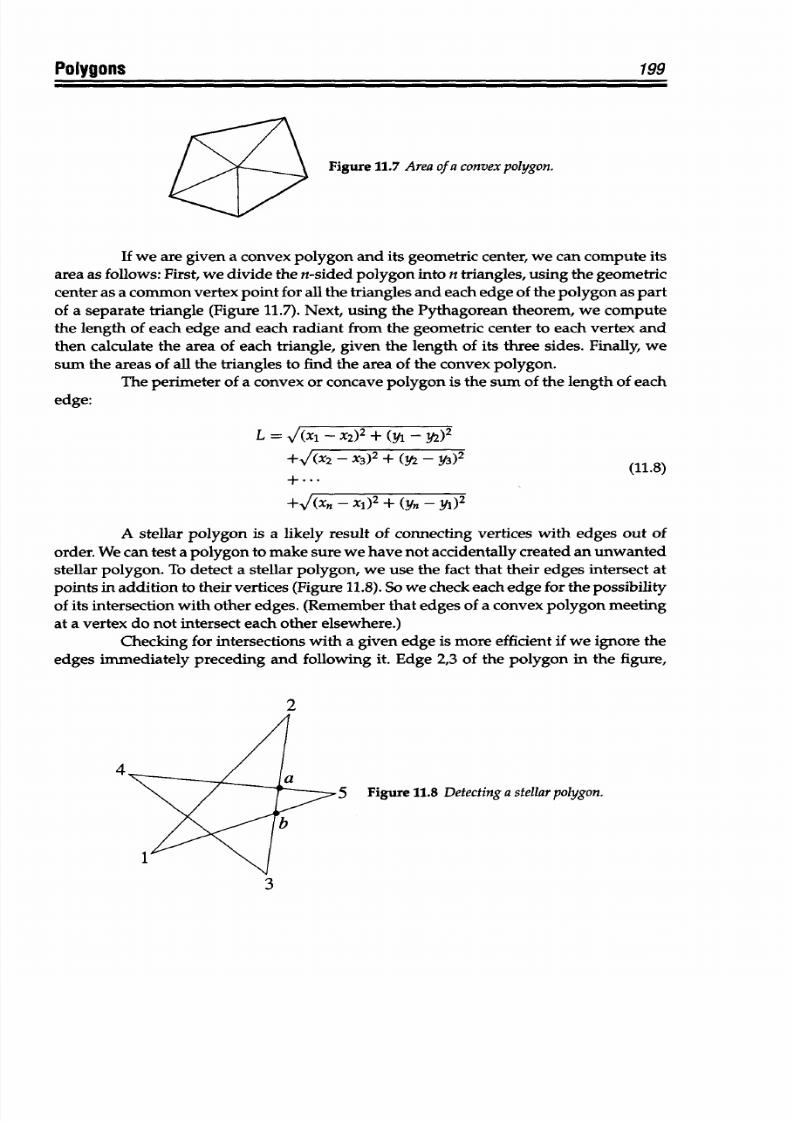
8/9/2019 Mortenson, Michael E. - Mathematics for computer graphics applications.pdf
http://slidepdf.com/reader/full/mortenson-michael-e-mathematics-for-computer-graphics-applicationspdf 212/367
Polygons 199
Figure
11.7 Area
of
a
convex polygon.
If we
are given
a convex
polygon
and
its
geometric
center, we can
compute
its
area as follows:
First, we
divide the
n-sided polygon
into
n triangles,
using
the
geometric
center as a common
vertex point for
all
the triangles and
each edge of the polygon
as
part
of a separate triangle (Figure 11.7).
Next,
using
the Pythagorean theorem,
we compute
the length of each edge and
each
radiant from the geometric center
to each vertex
and
then
calculate the
area of each
triangle,
given
the length
of its three
sides. Finally, we
sum the areas of all the triangles
to find the area of the convex polygon.
The
perimeter
of
a convex
or
concave
polygon
is
the sum
of
the length of each
edge:
L = I(xl-x2)
2
+ (yl-y2)
2
+
-X
3
)
2
+
(Y2-
y3)
2
(11.8)
+,[(~X-,X
1
)
2
+
(yn
-)
A stellar
polygon is
a
likely result of connecting
vertices
with
edges out
of
order.
We can test a polygon to
make sure we
have not accidentally
created
an unwanted
stellar polygon. To detect a stellar polygon,
we use the
fact
that their edges intersect
at
points in
addition
to
their
vertices
(Figure
11.8).
So we
check
each edge for
the possibility
of its intersection with
other edges. (Remember that edges
of a convex polygon meeting
at
a
vertex
do not
intersect
each other
elsewhere.)
Checking
for intersections
with a
given edge
is more efficient if we ignore
the
edges immediately
preceding and following
it. Edge
2,3
of the polygon
in the figure,
2
4
Figure 11.8 Detecting
a stellar
polygon.
lb
3
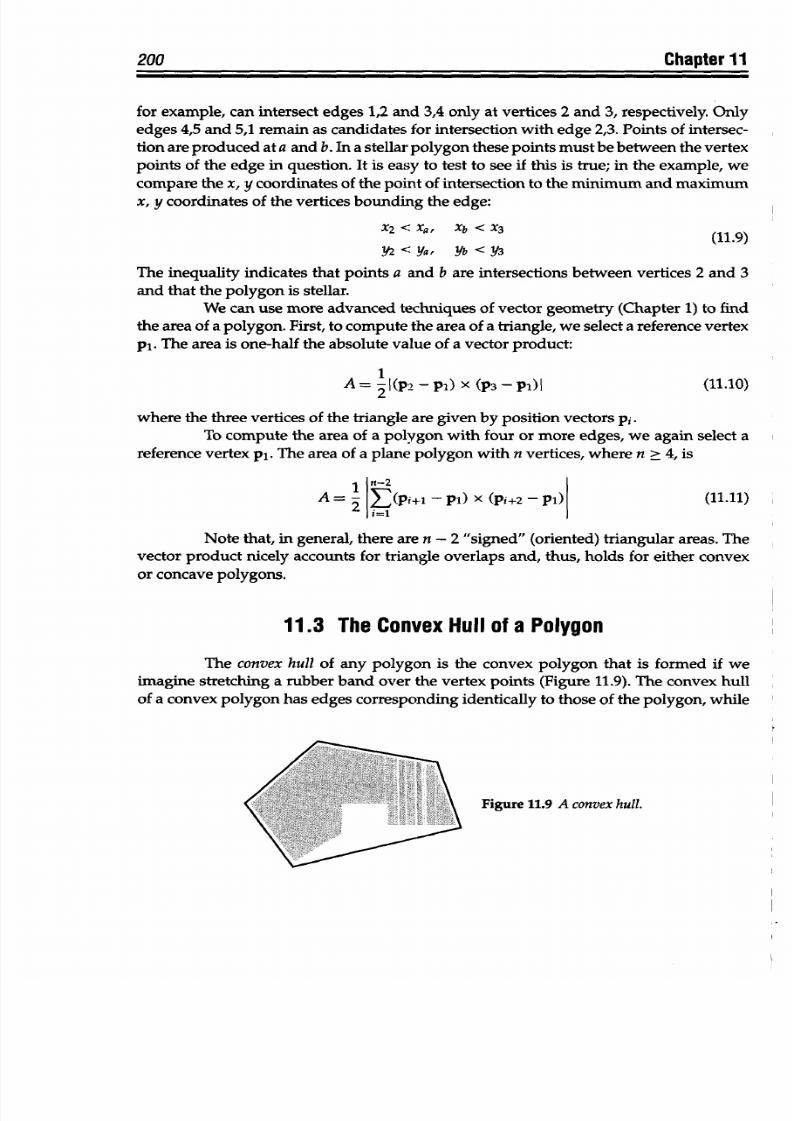
8/9/2019 Mortenson, Michael E. - Mathematics for computer graphics applications.pdf
http://slidepdf.com/reader/full/mortenson-michael-e-mathematics-for-computer-graphics-applicationspdf 213/367
8/9/2019 Mortenson, Michael E. - Mathematics for computer graphics applications.pdf
http://slidepdf.com/reader/full/mortenson-michael-e-mathematics-for-computer-graphics-applicationspdf 214/367
Polygons
201
the
convex hull
of
a
concave
polygon always has
fewer
edges
than the polygon, some
edges of
which are not collinear,
and
it
encloses a
larger
area.
We
also
associate a
con-
vex hull with
any arbitrary
set of
points
in the
plane.
Polyhedra and
sets of
points
in
space
have
three-dimensional
convex
hulls, analogous
to
the two-dimensional
case.
In
fact,
the convex
hull of the points
defining
a Bezier
curve
or surface closely ap-
proximates
the curve or
surface,
and it is useful in analyzing
and
modifying
its
shape.
11.4
Construction of Regular
Polygons
Recall that regular
polygons have
equal
edges and
interior angles. Their ver-
tices
lie
on
a
circle,
and another
circle is
tangent
to each of
the
edges. This
means
that
constructing a regular polygon
with n vertices and n edges is
equivalent
to dividing
the circumference
of a
circle into n equal parts. If we
can
do this division, then we
can
construct
the corresponding regular
polygon.
C.
F.Gauss (1777-1855)
showed
thatwe
can
construct
a regular
convex
polygon
of n
sides
with a
compass and straight
edge
if and
only if
1.
n = 2k, where
k is
any
integer,
or
2. n = 2k
* (2r
+ 1)
*
25 + 1) .
(2' + 1) .. ,where (2' + 1), (25
+ 1), (2' + 1), .. .
are different
Fermat
prime
numbers.
Gauss's
theorem says that we can
construct polygons
of 3, 4, 5, 6,
8,
10,
12, 15,
16, 17,
20, 24,. .. sides, but not those with 7, 9, 11, 13,
14,
18,
19,
21, 22, 23, 25,...
sides.
We cannot construct exactly a
regular
convex seven-sided
polygon
(heptagon),
so
it is
impossible
to
divide the
circumference of a
circle into seven
equal parts.
Perhaps
this is
why
the heptagon
is rarely
used in architecture.
11.5
Symmetry
of
Polygons
Revisited
Regular polygons have
three kinds
of symmetry:
reflection, rotation, and in-
version
(Chapter
4). A regular
polygon
with n
edges has
n
rotational
and n reflection
symmetry
transformations. If n is an
even
number, then it has an inversion symmetry
transformation.
An equilateral triangle
has
six
symmetry
transformations, consisting of three
rotations
(120°,
2400, 3600) and three reflections. The lines
of
symmetry
for
reflection
are
shown
in Figure 11.10. Note that inversion of
an
equilateral
triangle produces a
differ-
ent
figure. A
square
has
nine
symmetry
transformations:
one
inversion, four rotations
(90', 180°, 270°, 360°),
and
four
reflections (Figure
11.11). Of course, nonregular polygons
can also have
symmetry
transformations.
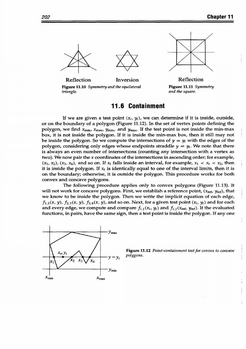
8/9/2019 Mortenson, Michael E. - Mathematics for computer graphics applications.pdf
http://slidepdf.com/reader/full/mortenson-michael-e-mathematics-for-computer-graphics-applicationspdf 215/367
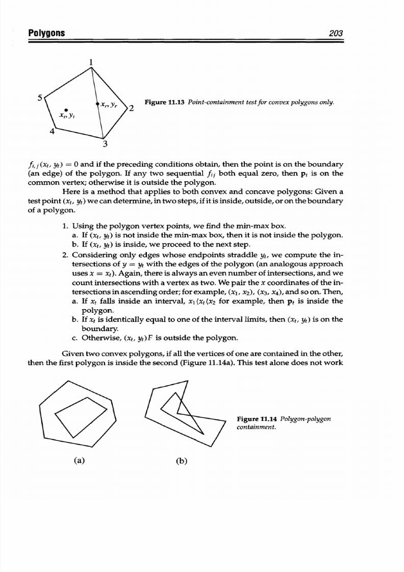
8/9/2019 Mortenson, Michael E. - Mathematics for computer graphics applications.pdf
http://slidepdf.com/reader/full/mortenson-michael-e-mathematics-for-computer-graphics-applicationspdf 216/367
Polygons 203
1
5
2
Figure 11.13 Point-containment
estfor
convex polygons
only.
fi, j (xt, yt) =
0
and
if
the preceding conditions obtain, then the point
is on the boundary
(an edge) of
the polygon.
If
any two sequential
fij
both
equal
zero,
then
pt
is
on
the
common vertex; otherwise it
is
outside the polygon.
Here
is
a
method
that
applies
to both convex and
concave polygons:
Given a
test point
(xt, yt)
we can determine, in two steps, if it is inside, outside , or on the
boundary
of a polygon.
1. Using the
polygon
vertex
points,
we
find the
min-max box.
a.
If
(xt, yt)
is
not inside the
min-max
box,
then
it is not inside the
polygon.
b.
If
(xt, yt)
is inside,
we proceed to the next step.
2.
Considering only edges whose
endpoints straddle
yt,
we
compute
the
in-
tersections
of
y
=
yt with
the edges of the polygon
(an
analogous approach
uses
x = xt).
Again, there
is
always an even
number of intersections, and
we
count
intersections
with a
vertex
as two.
We
pair the x
coordinates
of the in-
tersections in ascending order; for example, (x
1
,
x
2
),
(X3, x
4
),
and so
on.
Then,
a.
If xt
falls inside
an interval,
xi (xt
(x
2
for example,
then pt
is inside the
polygon.
b. If
xt is identically
equal
to
one of the interval limits,
then (xt,
yt) is on the
boundary.
c. Otherwise, (xt, yt)F is
outside
the polygon.
Given two
convex
polygons, if all the vertices of one are contained in the other,
then
the first
polygon
is inside the second (Figure 11.14a). This test alone does not
work
Figure
11.14
Polygon-polygon
containment.
(a)
(b)
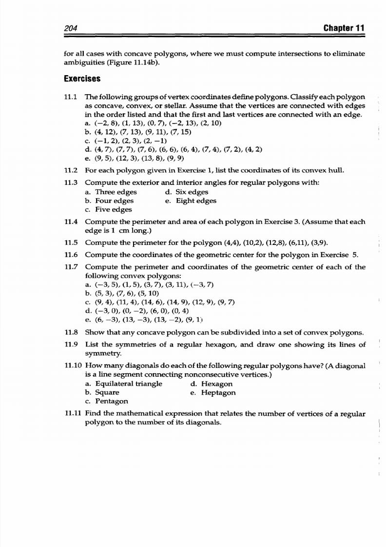
8/9/2019 Mortenson, Michael E. - Mathematics for computer graphics applications.pdf
http://slidepdf.com/reader/full/mortenson-michael-e-mathematics-for-computer-graphics-applicationspdf 217/367
8/9/2019 Mortenson, Michael E. - Mathematics for computer graphics applications.pdf
http://slidepdf.com/reader/full/mortenson-michael-e-mathematics-for-computer-graphics-applicationspdf 218/367
(IU
K Ta
POLYHEDRA
Polyhedra,
in
their infinite
variety, have been objects of study
for more
than 2500 years.
In
ancient
Greece,
contemplation of the
regular polyhedra
and
a
few semiregular deriva-
tive shapes led
to
the
establishment
of
the classical world's most
famous
school,
Plato's
Academy.
We find polyhedral forms expressed
concretely in
the civil and monumen-
tal architecture
of
antiquity. Their usefulness to us, and our interest in them, continues
undiminished
today. We
now use polyhedra in the mathematics
of
geometric modeling
to represent
more
complex shapes. We use assemblies of
them,
like building blocks, to
create computer
graphics displays.
Alone
and
in Boolean
combinations, their properties
are
relatively
easy to
compute. And,
what
is
most
amazing,
all
possible
polyhedra are
defined
by only
the three
simplest of
geometric elements-points, lines,
and planes.
Regular
and semiregular polyhedra are
the most
interesting. Many
are
found
in
nature, as
well
as
in
art
and
architecture. Economy
of
structure and
aesthetically-
pleasing
symmetries
characterize
these shapes,
and help
account for their prevalence
in nature and in man's constructions. Salt crystals are cubic polyhedra. Certain
copper
compounds
are
octahedral. Buckminster Fuller's
geodesic
dome, in its simplest form, is
an icosahedron w hose faces
are
subdivided
into equilateral triangles.
This chapter
defines
convex, concave, and
stellar
polyhedra, with particular
attention to the five regular polyhedra,
or
Platonic solids, and
the
13
semiregular, or
Archimedean,
polyhedra and their
duals. Using
Euler's
formula,
we
will
prove that
only
five regular polyhedra are possible in a space
of
three dimensions. Other topics include
nets, the
convex
hull
of
a
polyhedron,
geometric
properties, the connectivity matrix,
halfspace
representations
of
polyhedra,
model data
structure,
and
so-called "maps".
12.1 Definitions
A polyhedron is a
multifaceted three-dimensional solid
bounded
by a
finite,
connected set of plane polygons such that every edge
of
each polygon belongs also to
just
one
other
polygon.
The
polygonal faces
form
a closed surface,
dividing space
into
two regions, the interior
of
the polyhedron and the exterior. A cube
(or
hexahedron)
is
a
familiar
example of a polyhedron. The number
of faces
determines the
name of a
regular polyhedron. For
a more
complex polyhedron,
the
name may also
indicate
the
presence of differently shaped faces and special features, such
as
a truncated or snub
205
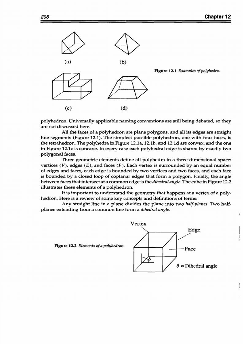
8/9/2019 Mortenson, Michael E. - Mathematics for computer graphics applications.pdf
http://slidepdf.com/reader/full/mortenson-michael-e-mathematics-for-computer-graphics-applicationspdf 219/367
206
Chapter 12
(a)
(b)
Figure
12.1
Examples
of polyhedra.
(c)
(d)
polyhedron.
Universally
applicable
naming conventions
are
still
being debated, so
they
are not
discussed
here.
All
the faces
of
a polyhedron are
plane polygons,
and
all
its
edges are
straight
line segments (Figure 12.1). The
simplest possible polyhedron, one with
four faces, is
the
tetrahedron. The
polyhedra in Figure
12.1a, 12.1b, and
12.1d
are
convex,
and the one
in Figure
12.1c
is
concave. In every
case
each
polyhedral edge
is
shared
by
exactly
two
polygonal
faces.
Three
geometric
elements
define
all polyhedra in
a three-dimensional
space:
vertices
(V),
edges (E), and faces (F). Each
vertex
is surrounded
by
an equal
number
of edges
and faces,
each
edge
is
bounded
by
two
vertices
and
two
faces,
and
each
face
is bounded by a closed loop
of coplanar edges
that form a
polygon.
Finally,
the
angle
between faces
that intersect at a common
edge is the dihedral
angle.The cube
in
Figure
12.2
illustrates
these elements
of
a polyhedron.
It
is important
to understand the geometry
that happens at a vertex
of
a poly-
hedron. Here is a review
of
some
key
concepts
and
definitions
of
terms:
Any
straight line in
a
plane divides the
plane into two half-planes. Two
half-
planes extending from a common line
form
a dihedralangle.
Vertex
dge
Figure
12.2 Elements
of a polyhedron.
iedral angle
.X~
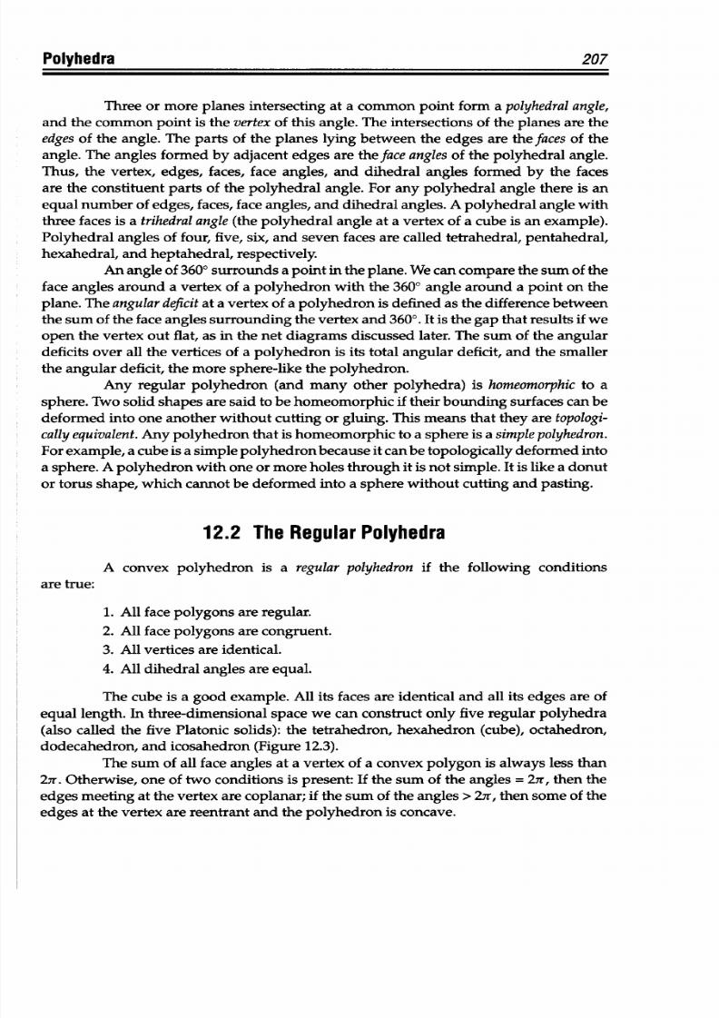
8/9/2019 Mortenson, Michael E. - Mathematics for computer graphics applications.pdf
http://slidepdf.com/reader/full/mortenson-michael-e-mathematics-for-computer-graphics-applicationspdf 220/367
Polyhedra
207
Three
or more planes intersecting at a common point form a polyhedral angle,
and
the common
point
is the
vertex of
this angle.
The intersections of
the planes
are
the
edges of the angle. The parts of
the planes
lying
between
the edges are the
faces
of the
angle.
The
angles
formed
by
adjacent
edges
are
the
face
angles
of
the polyhedral
angle.
Thus, the
vertex,
edges, faces, face angles, and
dihedral
angles formed by the
faces
are
the
constituent
parts of
the
polyhedral angle. For any polyhedral angle there is an
equal
number of
edges,
faces, face angles,
and
dihedral
angles. A
polyhedral
angle
with
three
faces is
a
trihedralangle (the polyhedral angle
at
a vertex of a cube is an example).
Polyhedral
angles of four, five,
six,
and seven
faces
are
called
tetrahedral,
pentahedral,
hexahedral, and heptahedral, respectively.
An angle of 3600 surrounds a point in
the
plane.
We
can compare the
sum of
the
face
angles
around a vertex of a
polyhedron
with the 3600 angle around a point on the
plane.
The
angular
deficit
at
a
vertex
of a
polyhedron
is
defined
as
the
difference
between
the
sum
of the face
angles
surrounding the vertex and
3600.
It is the gap that results
if
we
open
the
vertex out flat, as in the net diagrams
discussed later.
The sum
of the angular
deficits over all the
vertices
of a polyhedron is its
total
angular
deficit,
and the smaller
the angular deficit, the more sphere-like the polyhedron.
Any regular
polyhedron (and many
other polyhedra)
is homeomorphic
to
a
sphere. Two solid shapes are
said
to be
homeomorphic
if their
bounding
surfaces can be
deformed into
one
another
without
cutting
or gluing. This
means
that
they
are topologi-
cally equivalent.
Any polyhedron that is homeomorphic to a sphere
is
a
simple polyhedron.
For
example, a
cube
is
a
simple
polyhedron because it
can
be
topologically deformed into
a sphere. A
polyhedron with one
or more holes through it is not simple. It is like a donut
or torus
shape,
which cannot
be
deformed
into a
sphere
without cutting
and
pasting.
12.2 The
Regular Polyhedra
A convex
polyhedron is a
regular polyhedron
if
the
following conditions
are true:
1.
All
face
polygons
are regular.
2. All face
polygons are congruent.
3. All vertices are identical.
4. All dihedral angles are equal.
The cube is
a good
example. All its faces are identical and all its
edges
are of
equal
length. In
three-dimensional space we
can
construct
only
five
regular
polyhedra
(also
called
the five
Platonic
solids): the tetrahedron, hexahedron (cube), octahedron,
dodecahedron,
and
icosahedron
(Figure 12.3).
The
sum
of
all face
angles at
a
vertex
of
a
convex
polygon
is
always
less
than
27r. Otherwise,
one
of two conditions is
present:
If the
sum
of the
angles
=
27r,
then the
edges
meeting
at
the
vertex are coplanar; if
the
sum of
the
angles > 27r, then some of the
edges at the vertex
are reentrant
and the
polyhedron
is
concave.
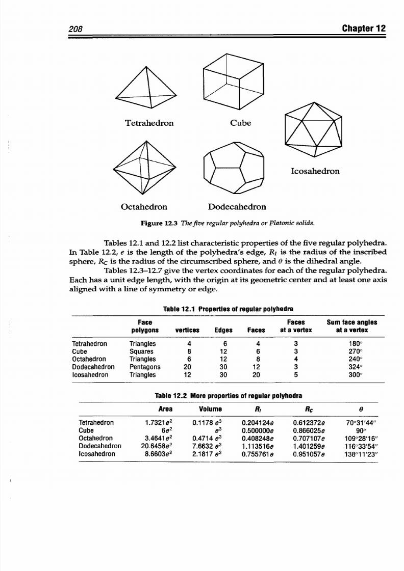
8/9/2019 Mortenson, Michael E. - Mathematics for computer graphics applications.pdf
http://slidepdf.com/reader/full/mortenson-michael-e-mathematics-for-computer-graphics-applicationspdf 221/367
Tetrahedron
Octahedron
Cube
Dodecahedron
Icosahedron
Figure 12.3
The five regular
polyhedra or
Platonic solids.
Tables
12.1
and 12.2 list
characteristic properties
of the five
regular polyhedra.
In Table 12.2, e is the length
of
the
polyhedra's
edge,
RI is
the
radius of
the inscribed
sphere,
Rc
is the
radius of
the circumscribed sphere,
and
0
is
the
dihedral angle.
Tables 12.3-12.7
give
the vertex coordinates for each
of
the regular polyhedra.
Each
has a
unit
edge length, with the origin at its geometric
center
and
at
least one
axis
aligned with a
line
of symmetry or edge.
Table 12.1
Properties
of
regular polyhedra
Face
Faces
Sum face
angles
polygons vertices Edges Faces at a
vertex at
a vertex
Tetrahedron
Triangles
4
6
4 3 1800
Cube Squares
8
12 6 3 2700
Octahedron
Triangles
6
12
8
4 2400
Dodecahedron Pentagons
20 30
12 3 3240
Icosahedron Triangles 12
30
20
5
3000
Table 12.2 More
properties
of regular
polyhedra
Area Volume RI Rc 0
Tetrahedron
Cube
Octahedron
Dodecahedron
Icosahedron
1.7321e
2
6e
2
3.4641
e
2
20.6458e
2
8.6603e
2
0.1178
e
3
0.4714 e
3
7.6632
e3
2.1817 e
3
0.2041 24e
0.500000e
0.408248e
1.113516e
0.755761
e
0.61 2372e
0.866025e
0.7071 07e
1.401
259e
0.951 057e
70031 '44"
900
1
9028'1
6
116°33'54"
13801 '23"
208
Chapter 12
- .
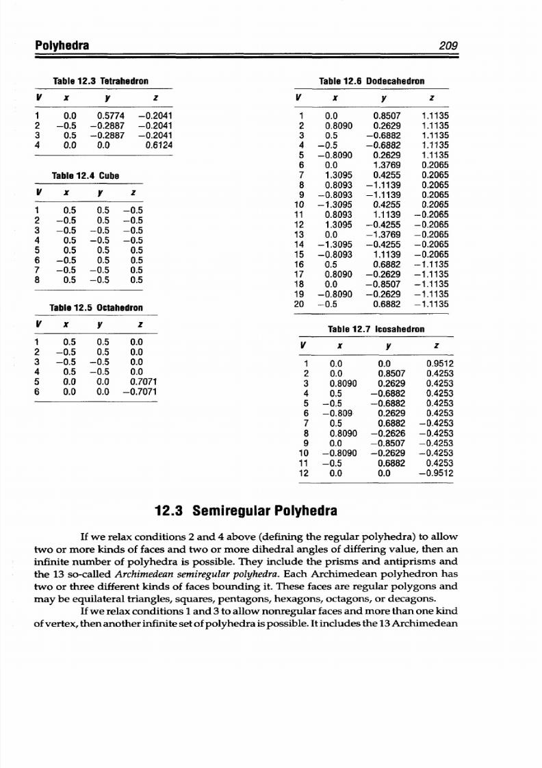
8/9/2019 Mortenson, Michael E. - Mathematics for computer graphics applications.pdf
http://slidepdf.com/reader/full/mortenson-michael-e-mathematics-for-computer-graphics-applicationspdf 222/367
Polyhedra
Table
12.3 Tetrahedron
V
x y z
1
0.0
0.5774
-0.2041
2 -0.5 -0.2887 -0.2041
3 0.5 -0.2887 -0.2041
4 0.0 0.0 0.6124
Table 12.4
Cube
V
x Y
z
1
0.5 0.5 -0.5
2
-0.5
0.5
-0.5
3
-0.5
-0.5 -0.5
4 0.5
-0.5 -0.5
5 0.5 0.5 0.5
6
-0.5 0.5 0.5
7
-0.5
-0.5
0.5
8
0.5
-0.5 0.5
Table 12.5 Octahedron
V x
Y z
1
0.5 0.5 0.0
2 -0.5
0.5
0.0
3
-0.5
-0.5 0.0
4 0.5 -0.5 0.0
5
0.0 0.0
0.7071
6
0.0
0.0 -0.7071
209
Table 12.6 Dodecahedron
V x
y z
1
0.0
0.8507
1.1135
2 0.8090 0.2629 1.1135
3 0.5 -0.6882 1.1135
4
-0.5
-0.6882
1.1135
5 -0.8090 0.2629
1.1135
6 0.0
1.3769 0.2065
7
1.3095 0.4255
0.2065
8
0.8093
-1.1139 0.2065
9 -0.8093 -1.1139 0.2065
10
-1.3095 0.4255
0.2065
11
0.8093
1.1139
-0.2065
12 1.3095 -0.4255 -0.2065
13
0.0
-1.3769 -0.2065
14 -1.3095
-0.4255
-0.2065
15
-0.8093
1.1139
-0.2065
16 0.5
0.6882 -1.1135
17 0.8090 -0.2629 -1.1135
18
0.0
-0.8507 -1.1135
19
-0.8090 -0.2629 -1.1135
20
-0.5
0.6882
-1.1135
Table 12.7 lcosahedron
V x
y
z
1
0.0
0.0
0.9512
2
0.0
0.8507
0.4253
3
0.8090
0.2629 0.4253
4
0.5
-0.6882
0.4253
5
-0.5
-0.6882
0.4253
6 -0.809 0.2629 0.4253
7
0.5 0.6882 -0.4253
8 0.8090
-0.2626 -0.4253
9
0.0 -0.8507 -0.4253
10
-0.8090 -0.2629
-0.4253
11
-0.5
0.6882 0.4253
12
0.0 0.0
-0.9512
12.3
Semiregular
Polyhedra
If we
relax
conditions 2
and
4 above
(defining
the regular polyhedra) to allow
two or
more kinds
of
faces and two
or more dihedral angles
of differing value, then
an
infinite number
of
polyhedra is possible. They include the prisms and antiprisms and
the
13
so-called
Archimedean
semiregular
polyhedra.
Each
Archimedean
polyhedron
has
two or three different kinds of faces
bounding
it.
These
faces are
regular
polygons and
may be equilateral triangles, squares, pentagons, hexagons,
octagons,
or
decagons.
If we relax conditions 1 and
3
to allow nonregular faces
and more
than one
kind
of vertex, then another infinite set
of
polyhedra is possible.
It
includes the
13
Archimedean
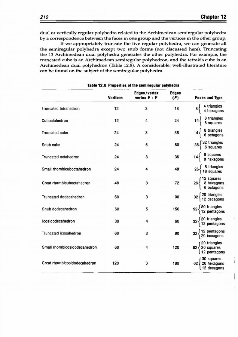
8/9/2019 Mortenson, Michael E. - Mathematics for computer graphics applications.pdf
http://slidepdf.com/reader/full/mortenson-michael-e-mathematics-for-computer-graphics-applicationspdf 223/367
210
Chapter
12
dual
or vertically regular polyhedra related
to
the Archimedean semiregular polyhedra
by a
correspondence between the faces in
one
group and the
vertices
in the other
group.
If we
appropriately truncate
the five
regular polyhedra, we
can
generate all
the semiregular
polyhedra
except
two snub
forms (not discussed
here).
Truncating
the 13 Archimedean dual
polyhedra generates the other polyhedra.
For example, the
truncated cube is an Archimedean semiregular
polyhedron,
and the
tetrakis
cube is an
Archimedean
dual
polyhedron (Table
12.8).
A
considerable,
well-illustrated literature
can be
found
on
the subject of the semiregular
polyhedra.
Table 12.8 Properties of the
semiregular
polyhedra
Edges/vertex
Vertices vertex
E:
V
Edges
(F)
Faces and Type
Truncated tetrahedron
Cuboctahedron
Truncated
cube
Snub
cube
Truncated
octahedron
Small rhombicuboctahedron
Great rhombicuboctahedron
Truncated dodecahedron
Snub
dodecahedron
Icosidodecahedron
Truncated
icosahedron
Small rhombicosidodecahedron
Great rhombicosidodecahedron
12
12
24
24
24
24
48
60
60
30
60
60
120
3
4
3
5
3
4
3
3
5
4
3
4
3
18 8I 4 triangles
1 4
hexagons
24 14{ 8 triangles
6
squares
36 14f 8 triangles
3 6
octagons
60 38 { 32 triangles
36 14
f 6 squares
8 hexagons
48 26f
triangles
\18 squares
(12
squares
72 264 8 hexagons
16 octagons
90 32 f 20 triangles
912 decagons
150
92 {80
triangles
12
pentagons
60 32{20
triangles
90 32
f
12 pentagons
20
hexagons
(20 triangles
120 62 30 squares
12
pentagons
(30
squares
180 62 20 hexagons
112 decagons
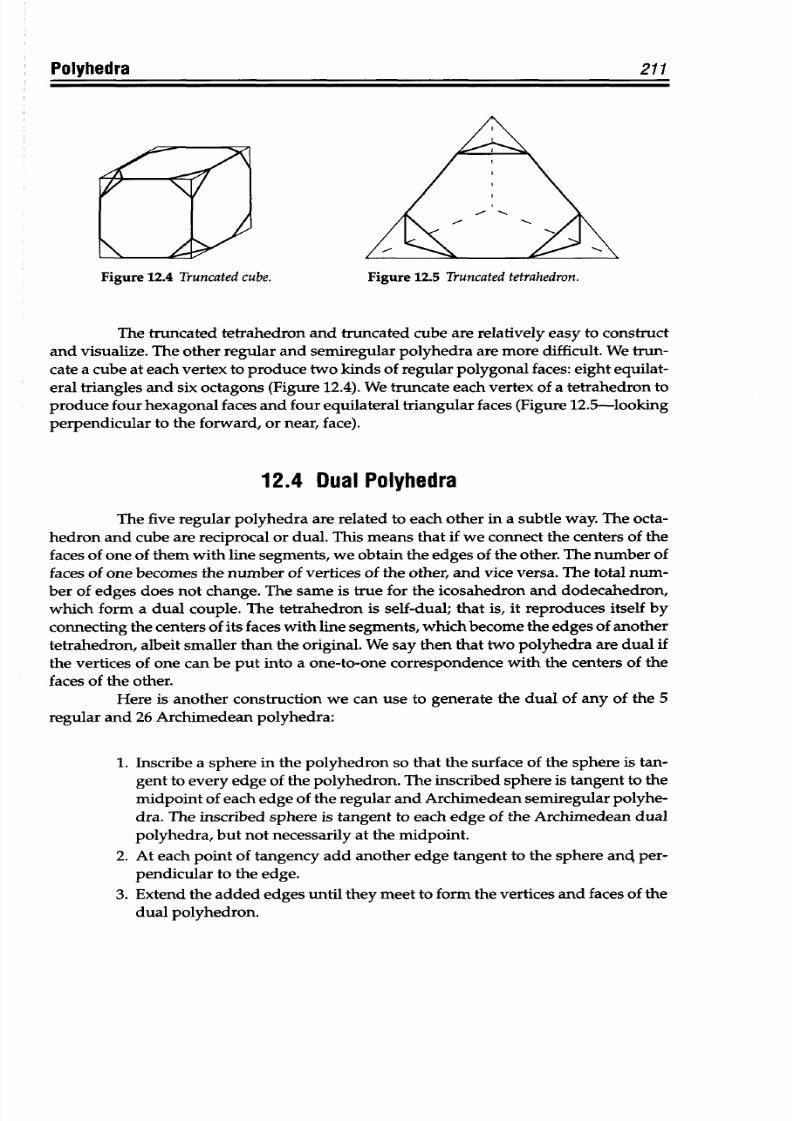
8/9/2019 Mortenson, Michael E. - Mathematics for computer graphics applications.pdf
http://slidepdf.com/reader/full/mortenson-michael-e-mathematics-for-computer-graphics-applicationspdf 224/367
211
Figure 12.4 Truncatedcube.
Figure
12.5 Truncated tetrahedron.
The
truncated tetrahedron
and
truncated
cube are
relatively easy
to
construct
and visualize.
The
other
regular
and semiregular
polyhedra are
more
difficult. We
trun-
cate
a cube at
each
vertex
to produce
two kinds
of
regular polygonal faces: eight equilat-
eral triangles and six octagons (Figure
12.4).
We truncate
each
vertex
of a tetrahedron to
produce four hexagonal
faces and four equilateral triangular
faces
(Figure 12.5-looking
perpendicular to the forward,
or
near, face).
12.4
Dual Polyhedra
The
five regular polyhedra
are
related
to each other in
a subtle
way.
The octa-
hedron and cube are reciprocal or
dual. This
means that if we connect the
centers
of
the
faces
of
one
of
them with line
segments,
we obtain
the edges
of the other.
The
number
of
faces
of one
becomes the
number
of
vertices of the
other,
and
vice
versa.
The total
num-
ber of edges does not
change. The
same
is
true
for the icosahedron and dodecahedron,
which
form a
dual couple. The
tetrahedron
is
self-dual;
that
is, it reproduces
itself by
connecting the centers
of
its faces with line segments, which become the edges
of another
tetrahedron,
albeit smaller
than the original. We say then that two
polyhedra
are dual if
the
vertices of
one
can be
put into
a
one-to-one
correspondence
with
the centers
of
the
faces of
the
other.
Here is
another
construction we
can
use
to
generate the dual of
any of the
5
regular and 26 Archimedean polyhedra:
1. Inscribe a sphere in the polyhedron
so that
the
surface
of the sphere is
tan-
gent to
every
edge
of
the polyhedron. The
inscribed
sphere
is tangent
to the
midpoint of each edge of the regular
and Archimedean semiregular polyhe-
dra.
The
inscribed
sphere
is
tangent to
each edge
of
the A rchimedean
dual
polyhedra,
but
not
necessarily
at
the midpoint.
2.
At
each point of tangency add
another
edge tangent
to
the
sphere anct
per-
pendicular
to
the
edge.
3. Extend
the added
edges until they
meet to form the vertices and faces
of
the
dual
polyhedron.
Polyhedra
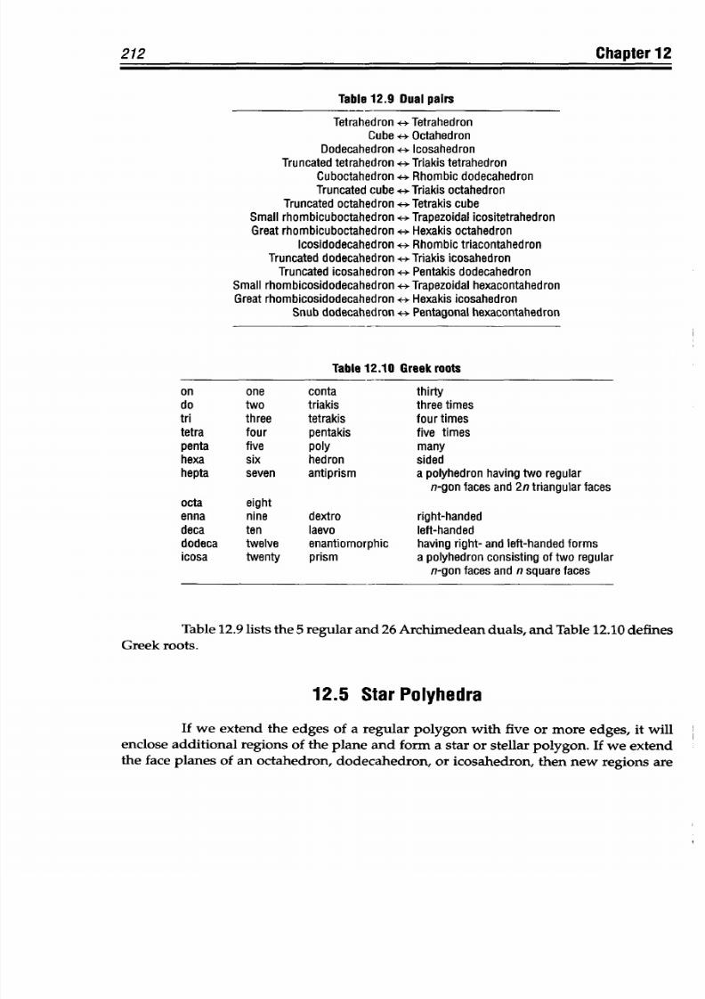
8/9/2019 Mortenson, Michael E. - Mathematics for computer graphics applications.pdf
http://slidepdf.com/reader/full/mortenson-michael-e-mathematics-for-computer-graphics-applicationspdf 225/367
212
Chapter
12
Table
12.9 Dual
pairs
Tetrahedron
* Tetrahedron
Cube
+*
Octahedron
Dodecahedron
+
Icosahedron
Truncated tetrahedron + Triakis tetrahedron
Cuboctahedron
e
Rhombic
dodecahedron
Truncated cube -
Triakis
octahedron
Truncated
octahedron
Tetrakis
cube
Small
rhombicuboctahedron
Trapezoidal
icositetrahedron
Great rhombicuboctahedron
e
Hexakis octahedron
Icosidodecahedron
4
Rhombic triacontahedron
Truncated dodecahedron Triakis icosahedron
Truncated
icosahedron
e
Pentakis
dodecahedron
Small
rhombicosidodecahedron Trapezoidal hexacontahedron
Great
rhombicosidodecahedron
*
Hexakis
icosahedron
Snub
dodecahedron
4*
Pentagonal
hexacontahedron
Table
12.10
Greek roots
on
one conta
thirty
do
two triakis three
times
tri three
tetrakis
four
times
tetra four pentakis
five
times
penta
five poly
many
hexa
six hedron sided
hepta
seven antiprism
apolyhedron
having
two
regular
n-gon faces
and 2n
triangular faces
octa eight
enna nine
dextro right-handed
deca ten
laevo left-handed
dodeca twelve
enantiomorphic having
right- and
left-handed
forms
icosa twenty
prism apolyhedron
consisting of two regular
n-gon faces and nsquare faces
Table
12.9 lists
the 5 regular
and 26 Archimedean
duals,
and
Table 12.10 defines
Greek roots.
12.5
Star Polyhedra
If
we
extend the edges
of a
regular polygon
with five
or more edges,
it will
enclose
additional regions of
the plane
and
form a
star or stellar polygon. If
we extend
the face planes
of an octahedron, dodecahedron,
or icosahedron, then
new regions
are
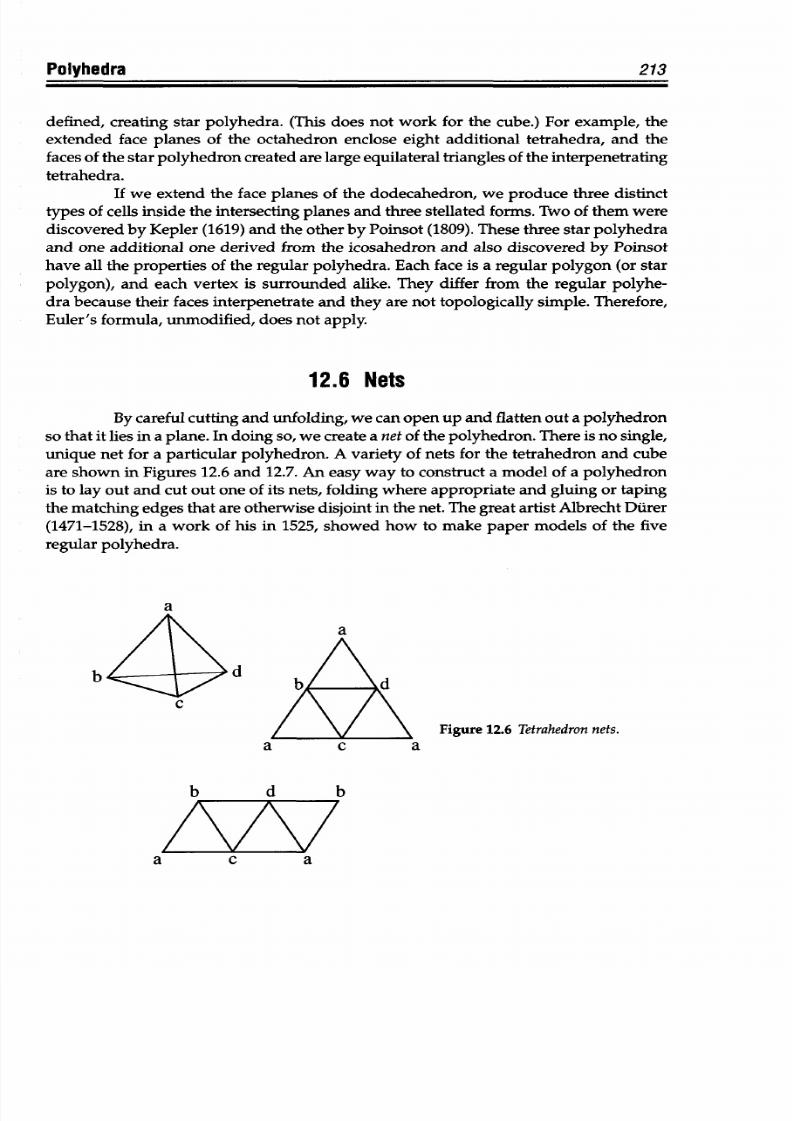
8/9/2019 Mortenson, Michael E. - Mathematics for computer graphics applications.pdf
http://slidepdf.com/reader/full/mortenson-michael-e-mathematics-for-computer-graphics-applicationspdf 226/367
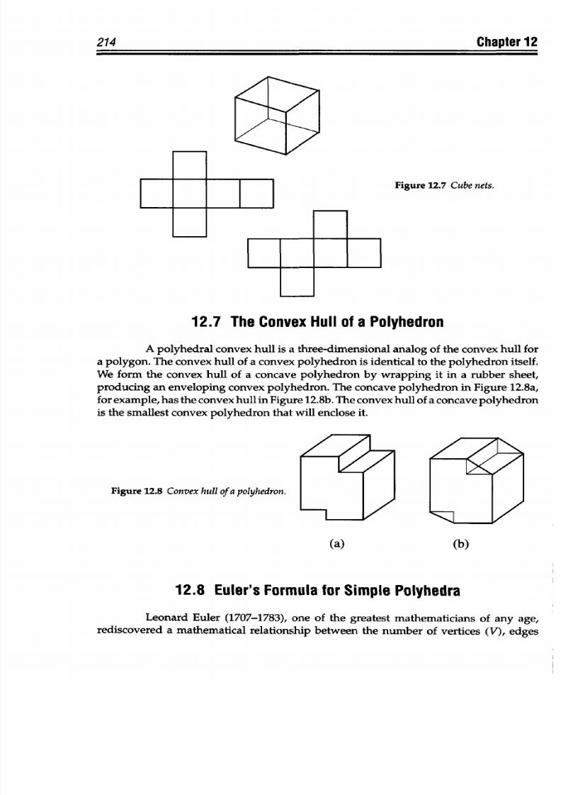
8/9/2019 Mortenson, Michael E. - Mathematics for computer graphics applications.pdf
http://slidepdf.com/reader/full/mortenson-michael-e-mathematics-for-computer-graphics-applicationspdf 227/367
214
Chapter
12
EL
Figure
12.7 Cube nets.
12.7
The
Convex Hull of a
Polyhedron
A polyhedral
convex hull
is a
three-dimensional
analog
of
the convex
hull
for
a
polygon.
The convex
hull
of
a
convex
polyhedron
is
identical to
the
polyhedron
itself.
We
form the convex hull
of a concave
polyhedron
by
wrapping
it in a
rubber sheet,
producing
an
enveloping convex
polyhedron. The concave
polyhedron
in
Figure
12.8a,
for
example,
has
the
convex hull
in
Figure
12.8b.
The
convex
hull of
a
concave polyhedron
is
the
smallest
convex polyhedron
that
will enclose it.
Figure 12.8 Convex
hull of a polyhedron.
(a)
(b)
12.8
Euler's
Formula
for Simple
Polyhedra
Leonard
Euler
(1707-1783), one
of
the
greatest
mathematicians of
any
age,
rediscovered
a
mathematical
relationship
between
the
number of
vertices (V),
edges
K
214 Chapter 12
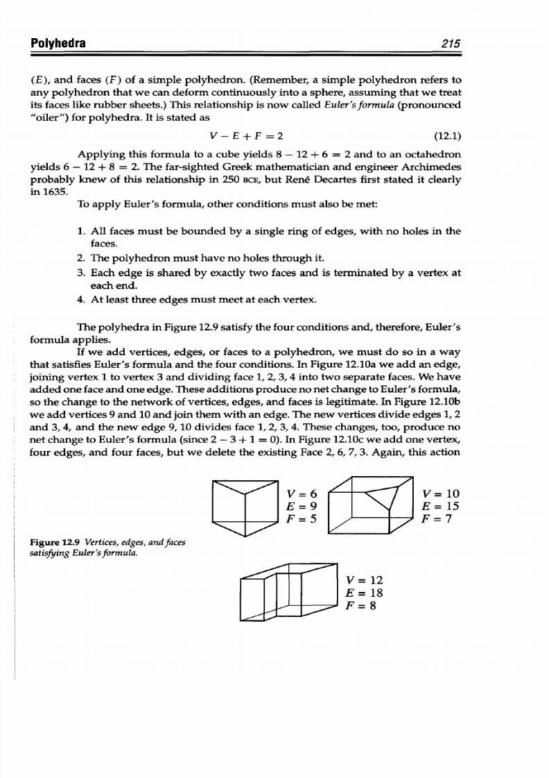
8/9/2019 Mortenson, Michael E. - Mathematics for computer graphics applications.pdf
http://slidepdf.com/reader/full/mortenson-michael-e-mathematics-for-computer-graphics-applicationspdf 228/367
Polyhedra 215
(E),
and faces (F) of
a
simple
polyhedron.
(Remember, a simple polyhedron refers to
any polyhedron that we
can
deform continuously into a sphere, assuming that we treat
its
faces like rubber sheets.) This relationship is now called
Euler'sformula
(pronounced
"oiler")
for
polyhedra.
It is
stated
as
V-E +F =2 (12.1)
Applying this
formula
to
a
cube yields 8 -
12
+ 6 = 2 and to an octahedron
yields 6 - 12 +
8
= 2.
The
far-sighted Greek mathematician and engineer
Archimedes
probably knew of this relationship in
250
BCE, but Ren6 Decartes first stated it
clearly
in
1635.
To apply Euler's
formula, other conditions must also be met:
1.
All faces
must
be
bounded
by
a
single
ring
of
edges,
with
no
holes
in the
faces.
2.
The
polyhedron must
have no holes through
it.
3.
Each
edge is shared by exactly two faces and
is
terminated
by
a
vertex at
each end.
4. At least
three edges must
meet at each vertex.
The
polyhedra
in
Figure 12.9
satisfy
the
four conditions and,
therefore,
Euler's
formula applies.
If
we
add
vertices,
edges, or
faces
to
a
polyhedron,
we
must
do
so
in
a
way
that satisfies
Euler's formula and
the
four
conditions. In
Figure
12.10a we
add
an
edge,
joining vertex
1
to vertex 3 and dividing
face 1,
2, 3, 4 into
two
separate
faces. We have
added one face and one edge. These additions produce
no net
change
to Euler's
formula,
so the change to the network of vertices, edges, and faces is legitimate. In Figure 12.10b
we
add
vertices 9 and 10
and
join them with an edge. The new vertices divide edges 1, 2
and 3,
4,
and the new edge 9, 10 divides face 1, 2, 3,4. These
changes, too,
produce
no
net change to
Euler's
formula (since 2
-
3
+ 1
= 0). In Figure 12.10c
we add
one vertex,
four
edges, and
four
faces, but
we
delete the
existing
Face
2, 6,
7,
3. Again, this
action
V=
10
E=
15
F = 7
Figure
12.9 Vertices,
edges, andfaces
satisfying Euler'sformula.
V=
12
E= 18
F=
8
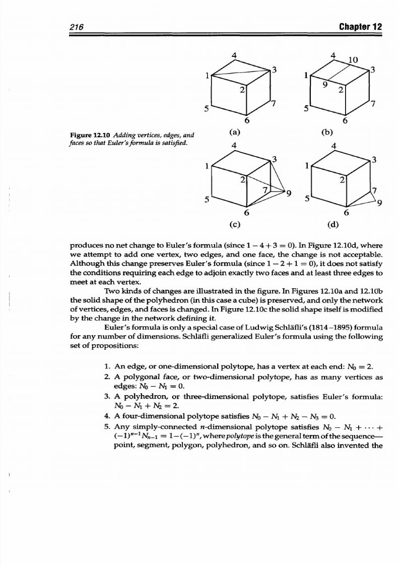
8/9/2019 Mortenson, Michael E. - Mathematics for computer graphics applications.pdf
http://slidepdf.com/reader/full/mortenson-michael-e-mathematics-for-computer-graphics-applicationspdf 229/367
216
Chapter
12
A
A
Figure 12.10
Adding
vertices, edges,
and
(a)
(b)
faces so that Euler'slormula
s
satisped.
1
5
1
5
(c)
(d)
produces no net change
to Euler's formula
(since 1 - 4 + 3 =
0).
In
Figure 12.10d, where
we
attempt
to
add
one
vertex,
two
edges,
and
one
face,
the change
is
not
acceptable.
Although this change preserves Euler's
formula (since
1 -2 + 1
= 0),
it does
not
satisfy
the conditions
requiring
each
edge to
adjoin exactly two faces
and at least three edges
to
meet at
each vertex.
Two
kinds
of changes are
illustrated in the
figure. In Figures
12.10a and 12.10b
the solid
shape
of
the polyhedron
(in
this
case
a
cube)
is preserved,
and only the network
of vertices,
edges,
and faces
is changed. In
Figure 12.10c
the solid shape
itself
is
modified
by
the
change
in
the network defining it.
Euler's
formula
is only a special
case of
Ludwig Schiafli's
(1814-1895) formula
for any number of
dimensions.
Schlafli
generalized
Euler's
formula
using
the following
set
of
propositions:
1. An edge, or one-dimensional
polytope, has a
vertex at
each end:
No
= 2.
2. A polygonal
face, or two-dimensional
polytope,
has
as many
vertices as
edges:
No -
N
1
=
0.
3. A
polyhedron, or three-dimensional
polytope, satisfies
Euler's formula:
No-N
1
+
N
2
= 2.
4.
A four-dimensional
polytope satisfies
No
- N
1
+ N
2
-
N
3
= 0.
5.
Any
simply-connected n-dimensional
polytope
satisfies
No
-
N
1
+
-
+
(-l)n-1Nn
1
= 1-
(-
1
)n, where
polytope is
the general
term of the
sequence-
point,
segment, polygon,
polyhedron,
and so on. Schldfli also
invented the
I
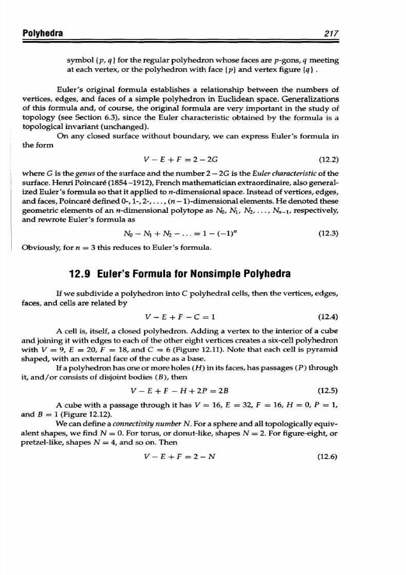
8/9/2019 Mortenson, Michael E. - Mathematics for computer graphics applications.pdf
http://slidepdf.com/reader/full/mortenson-michael-e-mathematics-for-computer-graphics-applicationspdf 230/367
Polyhedra
217
symbol {p, q ) for the regular
polyhedron
whose faces are p-gons,
q
meeting
at
each vertex, or the
polyhedron
with
face I
p1
and
vertex figure {q
.
Euler's original
formula
establishes
a relationship between
the
numbers
of
vertices,
edges, and faces
of
a
simple
polyhedron in
Euclidean space. Generalizations
of
this formula
and,
of
course,
the
original formula are very important
in
the study
of
topology (see Section 6.3), since the Euler characteristic obtained
by
the formula is
a
topological
invariant
(unchanged).
On any closed surface without boundary, we can express
Euler's
formula in
the
form
V-E
+ F
= 2-2G (12.2)
where
G
is
the
genus
of
the
surface
and
the
number
2
-
2G
is
the
Euler characteristicof
the
surface. Henri
Poincare
(1854
-1912), French mathematician
extraordinaire, also general-
ized
Euler's
formula so
that
it
applied
to n-dimensional
space. Instead of vertices, edges,
and faces,
Poincar6
defined 0-, 1-, 2-, ... , (n -
l)-dimensional
elements.
He denoted these
geometric
elements of an n-dimensional
polytope
as
No,
Ni, N
2
,
...
, Nn-
1
, respectively,
and rewrote
Euler's
formula as
No-_Nl +N2
* _-(-l)n
(12.3)
Obviously,
for n = 3 this reduces to
Euler's formula.
12.9 Euler s Formula
for
Nonsimple
Polyhedra
If we subdivide a polyhedron
into
C polyhedral cells, then
the vertices,
edges,
faces,
and
cells are
related by
V-E+F-C=1 (12.4)
A
cell is, itself, a
closed
polyhedron. Adding a
vertex
to the interior
of
a cube
and joining
it with
edges to each of the other eight vertices
creates
a six-cell polyhedron
with V =
9, E
= 20, F =
18,
and C
=
6
(Figure 12.11). Note
that each cell is
pyramid
shaped,
with
an
external face of
the cube
as
a
base.
If
a polyhedron has one
or more
holes
(H)
in its
faces,
has passages
(P) through
it, and/or consists
of
disjoint bodies
(B),
then
V-E + F-H+ 2P = 2B (12.5)
A
cube
with
a
passage through it has V = 16,
E
= 32, F = 16, H = 0,
P
=
1,
and
B =
1
(Figure 12.12).
We can define
a
connectivity number
N. For a sphere and all topologically equiv-
alent
shapes,
we
find
N
=
0.
For
torus, or
donut-like,
shapes
N
=
2.
For
figure-eight,
or
pretzel-like, shapes
N
=
4,
and
so
on.
Then
V-E+F
=2-N
(12.6)
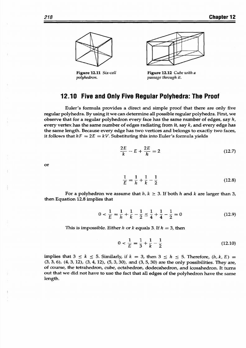
8/9/2019 Mortenson, Michael E. - Mathematics for computer graphics applications.pdf
http://slidepdf.com/reader/full/mortenson-michael-e-mathematics-for-computer-graphics-applicationspdf 231/367
Figure 12.11
Six-cell
polyhedron.
Figure
12.12 Cube with a
passage
through
it.
12.10
Five
and
Only Five
Regular Polyhedra: The
Proof
Euler's
formula provides
a
direct and
simple proof that
there
are only
five
regular polyhedra.
By
using
it
we
can
determine all possible regular
polyhedra.
First,
we
observe that
for
a
regular polyhedron
every
face
has
the same number
of edges,
say
h,
every vertex has the same
number
of
edges radiating
from
it,
say k, and
every edge has
the same
length.
Because every
edge has
two vertices
and
belongs
to
exactly
two
faces,
it follows
that hF
=
2E
= kV.
Substituting this into Euler's
formula yields
or
2E E 2E
k
h
1 1 1
1
E h
k
(12.7)
(12.8)
For
a
polyhedron we
assume that h, k >
3. If both h and k are
larger than 3,
then Equation
12.8 implies
that
1 1 1 1 1 1 1
0 < = 0- ----
< -+
- - -
-0
E h
224 4 2
(12.9)
This is impossible.
Either h
or k equals 3.
If
h
= 3,
then
0 < 1 = 1 + 1
- 1
(12.10)
E
3
k
2
implies that
3 <
k < 5.
Similarly,
if k = 3,
then 3 <
h < 5. Therefore,
(h, k, E) =
(3,
3,
6), (4,
3,
12), (3,
4,
12),
(5,
3,
30),
and
(3,
5,
30)
are
the only
possibilities.
They
are,
of course, the
tetrahedron, cube,
octahedron,
dodecahedron,
and
icosahedron. It
turns
out that
we did not have to
use the fact that
all
edges
of
the
polyhedron have
the same
length.
218 Chapter 12
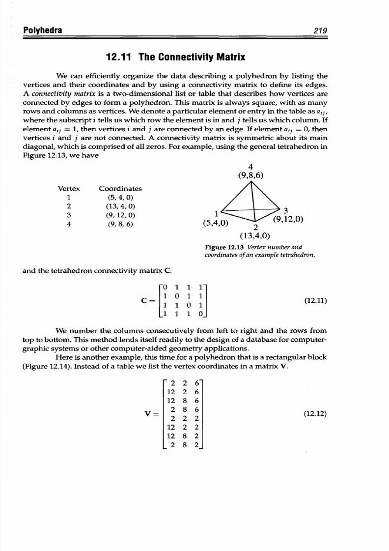
8/9/2019 Mortenson, Michael E. - Mathematics for computer graphics applications.pdf
http://slidepdf.com/reader/full/mortenson-michael-e-mathematics-for-computer-graphics-applicationspdf 232/367
Polyhedra 219
12.11 The Connectivity Matrix
We can
efficiently
organize the data
describing a polyhedron by listing the
vertices
and their
coordinates
and by using
a
connectivity matrix to define
its edges.
A
connectivity
matrix
is a
two-dimensional
list or table
that describes
how vertices
are
connected by edges
to
form
a
polyhedron. This matrix is always square, with
as
many
rows
and
columns as vertices. We denote
a
particular element or entry in the table as aij,
where
the subscript
i tells
us which row
the
element is in
and
j
tells
us which
column. If
element aij = 1, hen vertices i and j are connected
by
an
edge. If element
aij
= 0, then
vertices i and
j
are not
connected. A connectivity matrix
is
symmetric
about
its
main
diagonal, which is comprised of all
zeros.
For example, using the general tetrahedron
in
Figure 12.13,
we have
4
Vertex
Coordinates
1 (5,4,0)
2
(13,4, 0)
3
(9,12,
0)
1
A -n - 11 IC A
3
,12,O)
2
(13,4,0)
Figure
12.13 Vertex
number
and
coordinates
of
an example tetrahedron.
and the tetrahedron connectivity matrix C:
-O
1
1 l-
C= 1 1
(12.11)
1 1 10
We
number
the
columns consecutively
from
left to
right
and
the rows
from
top
to
bottom.
This
method lends
itself readily
to the
design of
a
database for
computer-
graphic systems or other
computer-aided
geometry applications.
Here is another example, this time for a polyhedron that is a rectangular
block
(Figure 12.14).
Instead of
a table we list the
vertex coordinates in a matrix
V.
2
2 6
12 2
6
12
8
6
2
8
6
2
2
2
12
2
2
12 8
2
2
8
2
(12.12)
=
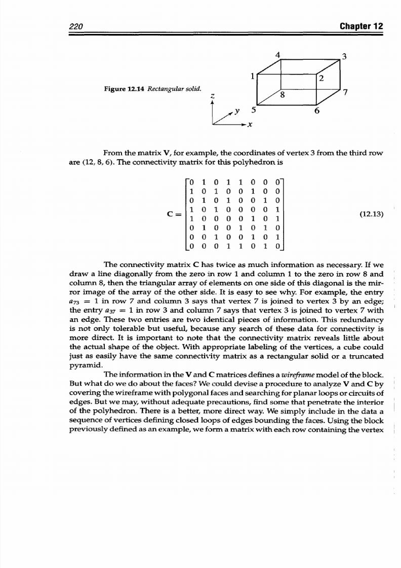
8/9/2019 Mortenson, Michael E. - Mathematics for computer graphics applications.pdf
http://slidepdf.com/reader/full/mortenson-michael-e-mathematics-for-computer-graphics-applicationspdf 233/367
220 Chapter 12
4
a
Figure 12.14
Rectangularsolid.
Y
7
L•2X
From
the matrix
V,
for
example,
the coordinates
of
vertex
3 from
the third
row
are (12, 8, 6). The
connectivity matrix
for
this
polyhedron
is
0 1 0 1 1
0 0
0
1
0
1
0
0
1 0 0
0 1 0 1 0 0 1
0
1
0
1 0 0 0 0 1
1
0
0 0 0 1
0 1
0 1
0 0
1 0 1
0
0 0 1 0 0 1 0 1
0 0 0
1
1
0
1
0
(12.13)
The
connectivity matrix C has twice as
much
information as necessary. If we
draw a line
diagonally
from the zero
in
row 1 and column 1 to
the
zero in
row
8 and
column
8,
then the triangular
array
of elements on one side
of
this
diagonal is the
mir-
ror image
of
the array
of
the other
side.
It
is easy to see
why.
For example,
the entry
a
73
=
1
in
row
7 and column 3 says
that
vertex 7 is
joined
to
vertex
3 by an edge;
the
entry a
37
= 1 in
row
3 and column 7
says that vertex
3
is joined
to vertex 7 with
an edge.
These
two entries
are
two identical pieces
of
information.
This redundancy
is
not
only
tolerable
but useful, because any
search of
these data
for
connectivity is
more direct.
It
is important to note that the connectivity
matrix
reveals little
about
the actual shape
of
the object.
With appropriate
labeling
of
the vertices, a
cube
could
just as easily
have
the
same connectivity matrix
as a rectangular
solid or
a
truncated
pyramid.
The information
in
the
V
and C
matrices defines a
wireframe
model
of
the
block.
But what
do we do about
the faces? We could
devise a procedure
to analyze V
and C by
covering the wireframe with
polygonal faces and searching for planar
loops or circuits of
edges. But
we may,
without
adequate precautions,
find
some
that penetrate
the interior
of the
polyhedron. There
is
a better,
more direct
way. We
simply
include
in
the
data a
sequence
of vertices defining
closed loops of
edges bounding
the faces. Using the block
previously
defined
as
an
example,
we form
a
matrix
with
each
row containing the vertex
C
=
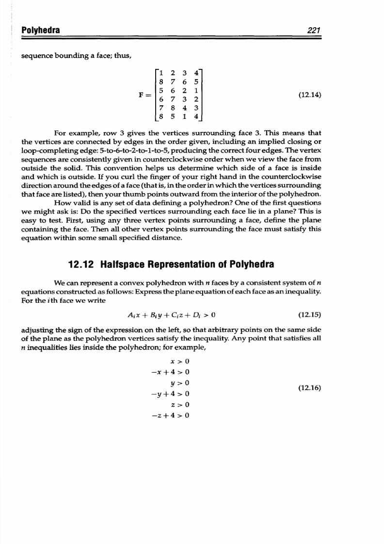
8/9/2019 Mortenson, Michael E. - Mathematics for computer graphics applications.pdf
http://slidepdf.com/reader/full/mortenson-michael-e-mathematics-for-computer-graphics-applicationspdf 234/367
Polyhedra
221
sequence
bounding
a face; thus,
1 2
3 4
8 7 6
5
F [
6 2
(12.14)
F
16 7
3
21
1.4
7 8
4 3
85
1 4
For example,
row
3
gives the vertices surrounding
face
3.
This
means
that
the
vertices
are
connected
by edges
in the order given, including an implied
closing
or
loop-completing edge: 5-to-6-to-2-to-1-to-5, producing
the correct four
edges. The
vertex
sequences
are
consistently
given in counterclockwise order
when
we view the
face from
outside
the
solid.
This
convention
helps us determine
which side
of
a face
is
inside
and which is
outside. If
you
curl
the finger
of
your right hand in the counterclockwise
direction around
the
edges
of
a face
(that is, in the order
in which the vertices
surrounding
that
face
are listed), then your thumb
points
outward
from the interior
of the polyhedron.
How
valid
is
any set
of
data defining
a polyhedron? One
of
the
first questions
we might
ask is: Do
the
specified vertices surrounding each
face
lie
in a
plane?
This is
easy
to test. First,
using
any
three vertex
points
surrounding a face, define
the plane
containing
the face. Then
all
other vertex points
surrounding the
face
must satisfy
this
equation
within some
small specified distance.
12.12 Halfspace Representation
of
Polyhedra
We
can represent a convex
polyhedron
with n
faces
by a
consistent
system
of n
equations
constructed
as follows: Express
the plane equ ation of
each
face
as an
inequality.
For
the ith face we write
Aix + Biy + Ciz
+ Di >
0
(12.15)
adjusting the sign
of
the expression on the
left, so
that
arbitrary
points
on the
same
side
of the plane
as
the
polyhedron
vertices satisfy the inequality. Any point that satisfies
all
n inequalities lies inside the polyhedron;
for
example,
x
> O
-x +
4 >
0
-y
(12.16)
-y
+4 > 0
z >
0
-z +4 >
0
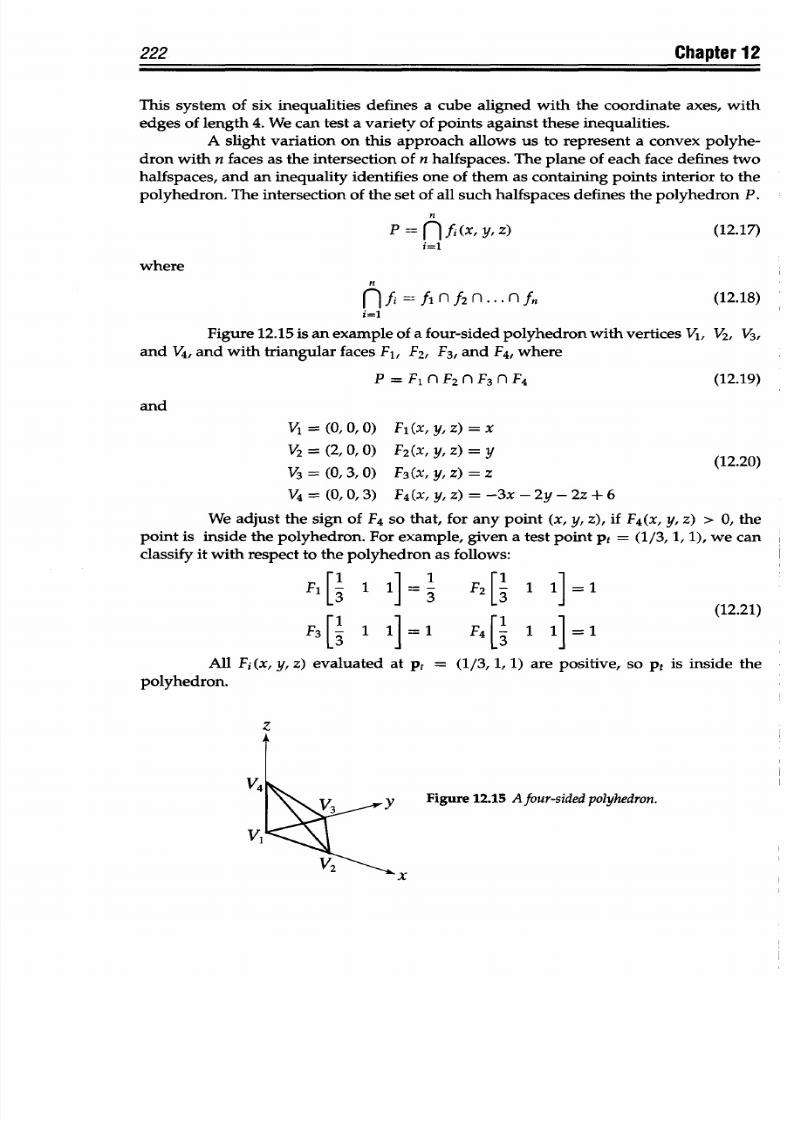
8/9/2019 Mortenson, Michael E. - Mathematics for computer graphics applications.pdf
http://slidepdf.com/reader/full/mortenson-michael-e-mathematics-for-computer-graphics-applicationspdf 235/367
222
Chapter
12
This
system
of
six inequalities defines a
cube
aligned with the coordinate axes, with
edges
of
length
4.
We can
test a variety
of points
against these
inequalities.
A slight
variation
on
this approach
allows us to
represent
a convex polyhe-
dron with
n faces
as
the intersection of n halfspaces.
The
plane of
each
face
defines
two
halfspaces, and an inequality identifies one
of
them as containing points interior
to
the
polyhedron.
The
intersection
of
the
set
of
all
such
halfspaces
defines
the polyhedron
P.
n
P=nfi(x,yz)
(12.17)
i=1
where
n
n
i=fi,
nf
2
n
... n
fn (12.18)
i=l
Figure
12.15
is
an
example
of a
four-sided
polyhedron
with
vertices
V
1
, V
2
, V
3
,
and V
4
,
and
with
triangular faces F
1
, F
2
, F
3
, and
F
4
,
where
P=F
1
nF
2
nF
3
nF
4
(12.19)
and
V,
= (O.O. 0)
F.i(x,
y,
z) = x
V
2
= (2,
0,
0)
F
2
(x,
y,
z) = y(12.20)
V
3
= (0,
3,
O)
F
3
(x,
y,z) =
z
V
4
=
(0,O , 3)
F
4
(x, y, z)=-3x-2y-2z
+ 6
We adjust
the sign
of
F
4
so that,
for any point (x,
y, z), if F
4
(x, y, z) >
0,
the
point
is
inside
the
polyhedron.
For
example,
given a test point
pt
= (1/3, 1,
1),
we can
classify
it with
respect
to the polyhedron
as follows:
1 ]=3
F
2
[3
1 1]=1
(12.21)
F3 1 1]1 F
4
[ 1
1
1
All
Fi
(x, y,
z)
evaluated at
pt
=
(1/3,
1, 1)
are
positive,
so pt
is inside
the
polyhedron.
Figure
12.15
A
four-sided
polyhedron.
-x
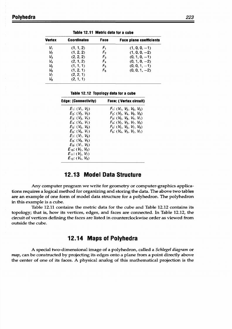
8/9/2019 Mortenson, Michael E. - Mathematics for computer graphics applications.pdf
http://slidepdf.com/reader/full/mortenson-michael-e-mathematics-for-computer-graphics-applicationspdf 236/367
223
olyhedra
Table 12.11 Metric data
for
a
cube
Vertex Coordinates
Face
Face
plane coefficients
V,
(1,1,2)
F
1
(1,0,0,-1)
V2
(1, 2, 2) F
2
(1,0, ,2)
13 (2,2,2)
F
3
(0,1,0,-1)
14 (2,1,2)
F
4
(0,1,0,-2)
15 (1,1,1) F
5
(0,0,1,-1)
V6 (1, 2,1) F
6
(°' 0,1,
-2)
V7 (2,2,1)
V8
(2,1,1)
Table
12.12 Topology data
for
a cube
Edge:
(Connectivity)
Face:
(Vertex
circuit)
E
1
:
(V1,
V
2
)
F
1
: (V
1
,
V2,
V6,
/s)
E
2
: (V
2
,
V3)
F
2
: (V
3
, V4,
V8,
V
9
)
E
3
:
(13,
14
F
3
: (
Vs,
V8,
V4, Vl
E
4
: (1V4,
)
F
4
:
(1/2, V3,
V7, VO)
E
5
:
Vs, 16)
F
5
:
Vs,
V6,
V7, V
8
)
E
6
: (V6, V
7
)
F
6
:
(V4,
V3,
V2,
V
1
)
E
7
: (1V7,
1)
E
8
:V8,
V5)
E
9
:
Vi,
Vs)
E
0
:
(1V2,
6)
E
1
: (V3,
V7)
E12: (V4,
V8)
12.13
Model
Data
Structure
Any
computer
program
we write
for
geometry or computer-graphics
applica-
tions requires a
logical
method
for
organizing and
storing the data. The
above two tables
are
an
example
of
one
form
of
model
data
structure
for
a
polyhedron.
The
polyhedron
in this example is a
cube.
Table 12.11 contains the metric
data
for
the cube and Table 12.12
contains its
topology;
that
is, how its
vertices,
edges, and faces are
connected. In Table 12.12,
the
circuit of
vertices defining
the
faces
are
listed in
counterclockwise
order as viewed
from
outside
the
cube.
12.14
Maps of
Polyhedra
A special
two-dimensional
image of
a
polyhedron, called a Schlegel diagram
or
map, can be
constructed by projecting
its edges onto
a plane from a point directly
above
the
center of
one of
its faces.
A physical
analog
of
this
mathematical
projection
is the

8/9/2019 Mortenson, Michael E. - Mathematics for computer graphics applications.pdf
http://slidepdf.com/reader/full/mortenson-michael-e-mathematics-for-computer-graphics-applicationspdf 237/367
224
Chapter
12
Figure
12.16 Schlegel
diagramof
a
cube.
shadow
of
a polyhedron's
edges
cast on
a
plane
by
a
point of
light also
located above
the center
of
one of the
polyhedron's
faces.
The
image constructed
in this
way
is
an
exaggerated perspective
view. One of
the
faces of
the
polyhedron, the
one closest
to and
centered on
the point of projection, frames
all
the
others, and
we must include
this
face
when
counting faces.
Although the
polyhedron's
congruent faces
do not
map as
such
on
the plane,
the
Schlegel
diagram
does enable
us
to
see
a realistic
two-dimensional representation
of
a three-dimensional object
that preserves such important
characteristics
of
the original
as
its
connectivity
of
edges
and
vertices
and
some
of its symmetry. Figure
12.16 is a
Schlegel
diagram of a cube.
Exercises
12.1 Why
is
a triangle necessarily a
plane figure, while
a four-sided
polygon
in three-
dimensional
space
need not
be?
12.2
How many
different
planes
in
three-dimensional
space
are
determined by
a. Four points
b.
Five points
c. n points
12.3
If the
center of
each of
the six faces of a
cube is joined by a line
segment to the
center
of
each
of
its
adjacent faces,
what kind
of
polyhedron is formed?
Sketch
the
resulting
polyhedron,
and demonstrate that
any
two
of
its edges are equal.
12.4
Same
as
Exercise 3, except
begin
with a
tetrahedron.
12.5
Same as Exercise
3,
except
begin
with
an
octahedron.
12.6
A
quartz crystal
has
the
form of a
hexagonal prism
with
a pyramid
on one of
its
bases. Show that Euler's
formula holds.
12.7 Verify that the five
regular
polyhedra satisfy Euler's
formula.
12.8
Show that a seven-edged
polyhedron
is
impossible.
12.9
Compute
the sum of
the
angles between adjacent
edges at a vertex of each
of the
regular polyhedra.
12.10
Compute the sum of the angles
between adjacent edges
at vertex
10
of the poly-
hedron shown in
Figure
12.17.
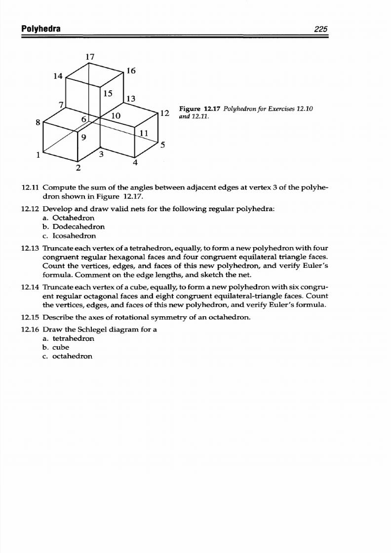
8/9/2019 Mortenson, Michael E. - Mathematics for computer graphics applications.pdf
http://slidepdf.com/reader/full/mortenson-michael-e-mathematics-for-computer-graphics-applicationspdf 238/367
Polyhedra 225
17
8
1
Figure 12.17 PolyhedronforExercises
12.10
12 and
12.11.
5
2
12.11
Compute
the
sum of
the
angles between adjacent edges at vertex
3
of the polyhe-
dron shown in Figure 12.17.
12.12 Develop and
draw
valid nets
for
the following regular polyhedra:
a.
Octahedron
b. Dodecahedron
c. Icosahedron
12.13
Truncate
each vertex
of
a
tetrahedron,
equally,
to form
a
new polyhedron
with
four
congruent regular hexagonal faces
and
four congruent equilateral triangle faces.
Count
the
vertices, edges,
and
faces of this new polyhedron,
and
verify Euler's
formula.
Comment on
the edge lengths,
and
sketch
the
net.
12.14 Truncate each
vertex
of
a
cube, equally,
to form a new polyhedron with six congru-
ent regular octagonal faces and eight congruent equilateral-triangle faces. Count
the vertices, edges, and faces of this new polyhedron, and verify Euler's formula.
12.15 Describe the
axes
of
rotational
symmetry of an octahedron.
12.16
Draw the
Schlegel
diagram
for
a
a.
tetrahedron
b. cube
c.
octahedron
8/9/2019 Mortenson, Michael E. - Mathematics for computer graphics applications.pdf
http://slidepdf.com/reader/full/mortenson-michael-e-mathematics-for-computer-graphics-applicationspdf 239/367
(AU
Ka
CONSTRUCTIVE
SOLID GEOMETRY
Traditional
geometry, plane
and solid--or even analytic-does
not tell us how
to create
even
the most simple shapes
we
see all
around us
in
both
the
natural
world
and the
made one.
The
methods of constructive solid geometry
(CSG) gives us a way
to
describe
complicated
solid shapes as
combinations of
simpler
solid shapes.
This makes
it an im-
portant tool for
computer
graphics
and geometric
modeling.
CSG uses Boolean operators
to construct a procedural
model of a complex solid.
This model, or rather
the data describ-
ing
the
model,
is
stored in the mathematical
form of a binary
tree, where
the
leaf
nodes
are
simple shapes, or primitives,
sized and
positioned in space, and each branch
node
is
a
Boolean
operator: union,
difference,
or
intersection.
This
chapter discusses
set theory, Boolean
algebra, halfspaces,
binary trees,
solids, the
special operators called regularized
Boolean
operators,
set- membership classifi-
cation, the Boolean
model
and how
to
construct
it using
those
operators, p rimitives,
and
boundary
evaluation.
13.1
Set
Theory Revisited
Recall that a
set is
a
collection
of
objects, called elements
or members of
the
set
(see
Section 7.2).
Examples of
a
set
may
be
mathematical, as
in
the
set of all even
numbers;
geometric,
as in the
set
of
points
on a line segment; logical,
as in all nonempty
sets; or
almost
any
specifiable collection
of things, as
in
all
white crows.
A set containing all
of
the
elements of all of the sets in
a particular
problem
is the universal
set, E. In geometry, E
often indicates all of the
points in a two- or three-
dimensional
space.
The complement of
a
set
A, written cA,
with
respect
to
the universal
set E, is
the
set of all
of the elements in E
that
are not
elements of
A.
The
null
set, or
empty set,
0, is
the set having
no elements
at all.
A set
A is a subset of
another
set B
if and only if every
member of A
is
also
a
member
of
B.
The symbol c denotes
the
relationship
between a
set and a
subset. A
c
B
says
that
A
is
a subset
of
B.
For
example,
if A is the set of all
numbers between 1 and 10,
inclusive,
whose
names
have
three
letters, and if B is
the
set
of all numbers between
1
and
10,
then
A
is a
subset
of
B,
A
c
C.
A
is a proper subset
of
B
if
every element
of A
is
contained
in
B
and if B
has at least one element
not in
A, which is true of the example
just given. Every
set is
a subset
of
itself,
but
not
a
proper
subset.
226
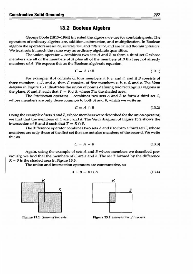
8/9/2019 Mortenson, Michael E. - Mathematics for computer graphics applications.pdf
http://slidepdf.com/reader/full/mortenson-michael-e-mathematics-for-computer-graphics-applicationspdf 240/367
Constructive Solid Geometry
227
13.2 Boolean Algebra
George Boole (1815-1864)
invented the
algebra we use for combining sets. The
operators
of
ordinary
algebra
are,
addition,
subtraction,
and
multiplication. In
Boolean
algebra the
operators
are union,
intersection,
and difference, and are
called
Booleanoperators.
We
treat
sets
in
much the same way as ordinary
algebraic
quantities.
The
union operator U
combines
two sets A and B to
form
a third set C whose
members are all of
the
members of
A
plus all of the memb ers of B
that
are not
already
members
of
A. We express this
as
the Boolean algebraic equation
C = A
U B
(13.1)
For example,
if A consists
of
four members
a,
b, c,
and
d, and
if
B consists of
three
members
c,
d,
and
e,
then
C
consists
of five
members
a,
b,
c,
d,
and
e.
The
Venn
diagram n Figure 13.1 illustrates
the
union of points defining
two rectangular regions in
the plane,
R
and S,
such
that T = R U
5, where
T is
the
shaded area.
The intersection
operator n
combines two sets
A
and
B
to
form
a third
set
C,
whose members are only those common to both A and
B, which
we write as
C = A
n
B (13.2)
Using the example of sets
A
and
B,
whose
mem bers were described for the union operator,
we
find that
the
members
of
C are c and
d. The
Venn
diagram of Figure 13.2 shows the
intersection
of
R
and S such
that
T
=
R
n
S.
The difference
operator
combines
two
sets
A and
B to
form
a third set C,
whose
members are
only
those
of
the first
set
that are not
also
members of the second. We write
this as
C
= A-B
(13.3)
Again,
using
the example
of sets
A and
Bwhose members we
described
pre-
viously,
we find that the members
of
C are
a
and b.
The
set
T formed
by the difference
R - S
is the shaded area in
Figure 13.3.
The
union and
intersection
operators
are
commutative,
so
A U
B
=
B UA (13.4)
R
R
Figure
13.2 Intersection
of
two
sets.
at
Figure 13.1 Union of two sets.
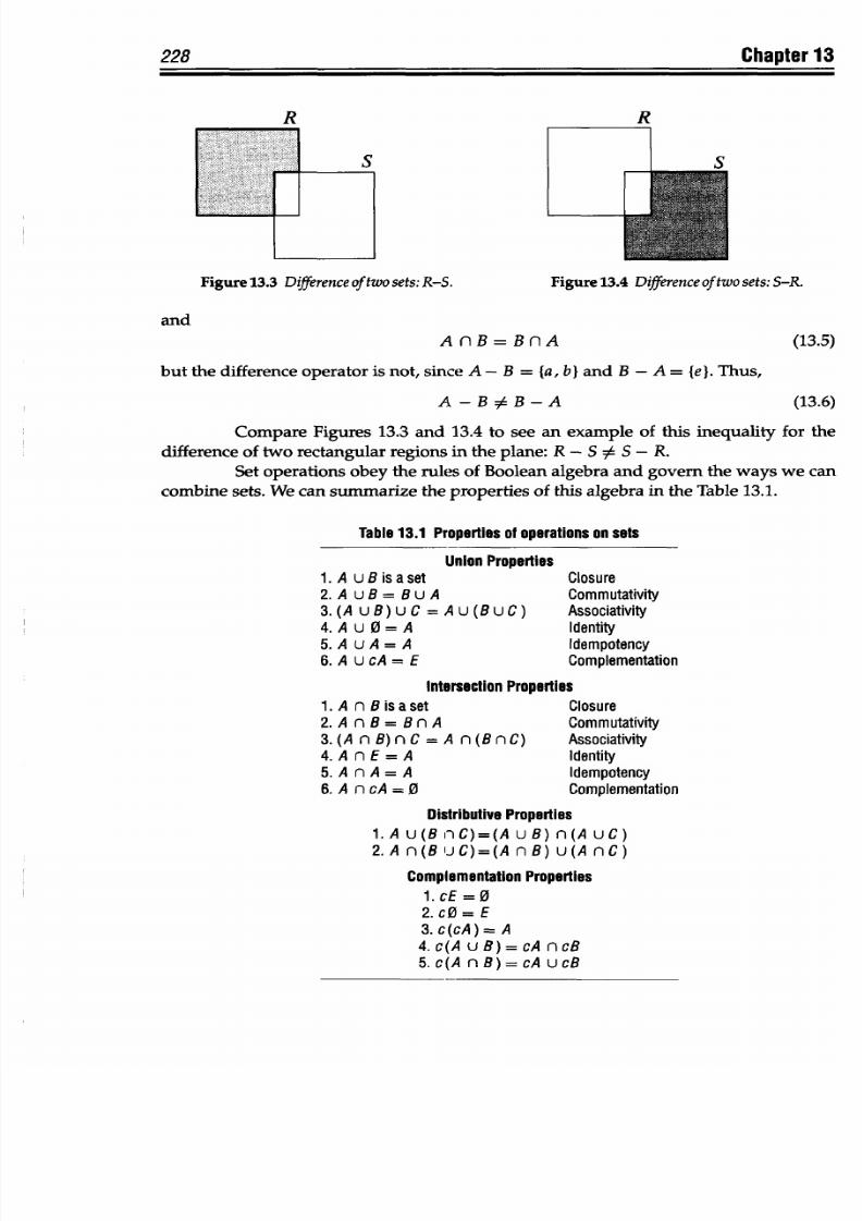
8/9/2019 Mortenson, Michael E. - Mathematics for computer graphics applications.pdf
http://slidepdf.com/reader/full/mortenson-michael-e-mathematics-for-computer-graphics-applicationspdf 241/367
R
Figure 13.3 Differenceoftwo sets:
R-S. Figure 13.4 Difference
oftwo
sets:
S-R.
A
n
B
=
B
n A
but
the
difference
operator
is
not,
since
A
-
B
=
la,
b}
and
B
-
A
=
{e}.
Thus,
A-B # B-A
(13.5)
(13.6)
Compare
Figures 13.3 and 13.4 to see
an example of this inequality
for the
difference
of
two
rectangular
regions in the plane:
R
-
S
:
S
-
R.
Set operations obey the rules
of
Boolean algebra and govern the ways we can
combine sets. We can
summarize
the prope rties of
this
algebra
in the Table
13.1.
Table 13.1 Properties of operations on sets
1.
A
u B
s
a et
2. A uB=
BuA
3.(A uB)uC =
4. A
u
0 = A
5. A
uA
= A
6. A ucA = E
Union Properties
Au BuC)
Closure
Commutativity
Associativity
Identity
Idempotency
Complementation
Intersection Properties
1.A
nBisaset
2. A n B =
B
n A
3.(A
nB)nC=A
n BnC)
4.
A n E
=
A
5.
A n A= A
6. A
n
cA =0
Closure
Commutativity
Associativity
Identity
Idempotency
Complementation
Distributive
Properties
1.A u(B inC)=(A uB) n(A
uC)
2.A n(B uC)=(A
nB)
u(A nC)
Complementation Properties
1.cE = 0
2.
cO
=
E
3.c cA)= A
4.c(A
uB)=cA
lncB
5.c(A n
B)
=
cA
u
cB
228
Chapter 13
and
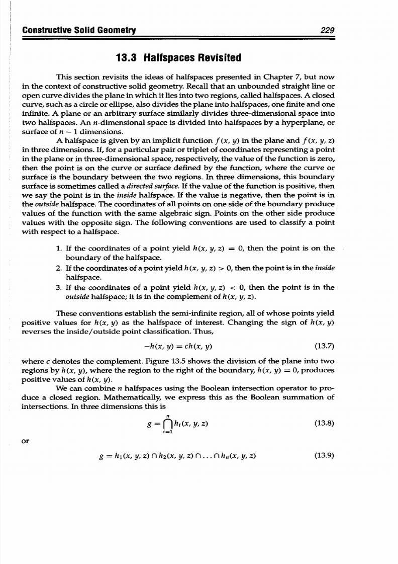
8/9/2019 Mortenson, Michael E. - Mathematics for computer graphics applications.pdf
http://slidepdf.com/reader/full/mortenson-michael-e-mathematics-for-computer-graphics-applicationspdf 242/367
Constructive Solid Geometry
229
13.3 Halfspaces
Revisited
This
section revisits
the ideas
of
halfspaces
presented
in
Chapter 7, but
now
in
the
context of
constructive
solid
geometry. Recall
that
an
unbounded
straight
line
or
open curve divides
the
plane in which it
lies
into
two
regions, called halfspaces. A
closed
curve, such as a circle or
ellipse, also
divides the plane into
halfspaces, one finite and
one
infinite.
A plane or an arbitrary
surface
similarly divides three-dimensional space into
two
halfspaces.
An n-dimensional
space
is
divided
into halfspaces
by
a hyperplane, or
surface of n -
1 dimensions.
A
halfspace is given
by an implicit
function f (x,
y)
in
the
plane
and
f
(x, y, z)
in three
dimensions. If, for
a
particular pair
or
triplet of
coordinates representing
a point
in the plane
or in
three-dimensional
space, respectively, the value
of the function
is zero,
then the
point
is
on
the curve or
surface
defined
by
the
function,
where the curve
or
surface is
the boundary between the two
regions.
In three dimensions, this
boundary
surface
is
sometimes called a directed surface. If
the
value of
the
function is positive, then
we say the
point is
in the
inside
halfspace. If the value is negative,
then
the point is
in
the outside halfspace. The coordinates of all points on
one side
of the boundary produce
values
of
the function
with the same algebraic
sign.
Points on
the other
side
produce
values
with
the opposite
sign. The following conventions are used
to
classify a point
with respect
to a
halfspace.
1.
If the
coordinates of
a
point yield h(x, y, z) = 0, then
the
point is on
the
boundary of
the
halfspace.
2. If the coordinates of a
point
yield
h
(x,
y, z)
> 0,
then
the
point
is
in
the inside
halfspace.
3. If
the
coordinates of
a
point yield
h(x, y,
z) < 0, then the
point
is
in
the
outside
halfspace; it is
in the
complement
of h
(x,
y,
z).
These conventions establish
the
semi-infinite region,
all
of whose points yield
positive
values
for
h (x,
y)
as the halfspace of
interest.
Changing
the
sign
of
h (x,
y)
reverses
the
inside/outside
point classification.
Thus,
-h(x,
y)
= ch(x,
y)
(13.7)
where c denotes the complement. Figure 13.5
shows the division
of
the
plane
into two
regions by h (x, y),
where the region
to
the
right of the
boundary,
h (x, y)
=
0,
produces
positive values
of h (x,
y).
We
can
combine n halfspaces
using
the
Boolean
intersection operator to pro-
duce a
closed region. Mathematically,
we
express this as
the
Boolean summation of
intersections. In three dimensions this
is
n
g
hi(x
Y,
)
(13.8)
i.=l
(13.9)
=
hi
(x,
y,
z) n
h2(X, y,
z) n
...
n
h,
(x,
y,
z)
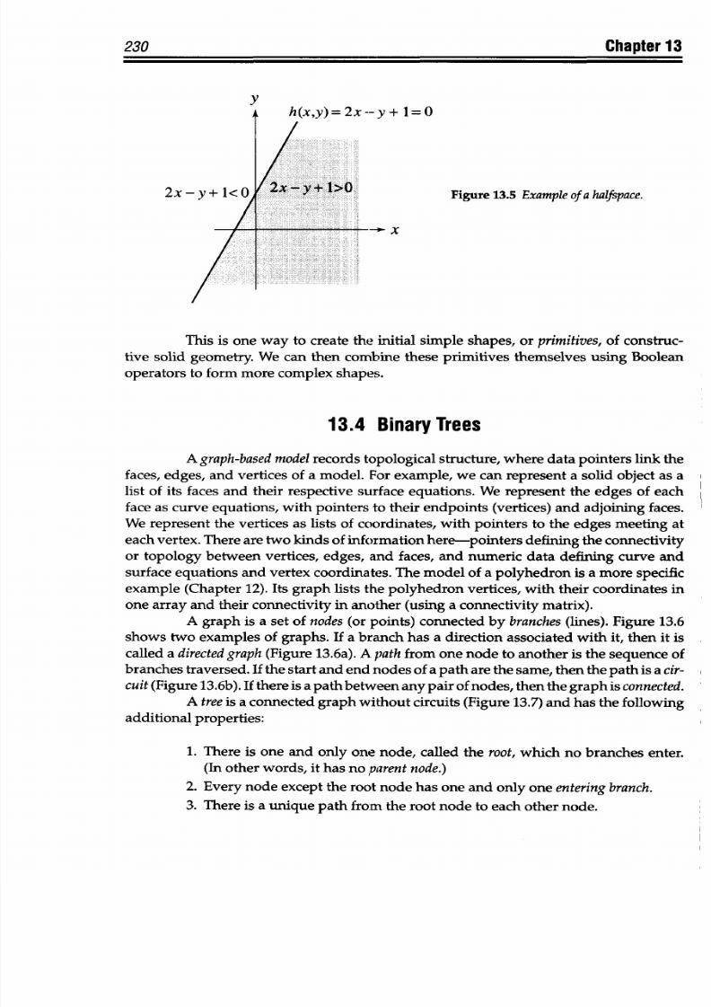
8/9/2019 Mortenson, Michael E. - Mathematics for computer graphics applications.pdf
http://slidepdf.com/reader/full/mortenson-michael-e-mathematics-for-computer-graphics-applicationspdf 243/367
Chapter
13
y
2x-y+ 1<0
h(xy)=2x-y+ 1=0
2x;
Y
+
1>0t
Figure
13.5 Example
of a halfspace.
Witft~taiACR-b. X00:A0E
/
This
is one way to
create
the initial
simple shapes,
or
primitives,
of
construc-
tive
solid
geometry.
We
can
then combine
these
primitives
themselves
using Boolean
operators to
form more
complex
shapes.
13.4 Binary
Trees
A
graph-basedmodel
records
topological structure,
where
data
pointers
link
the
faces,
edges, and
vertices of
a
model.
For example,
we can
represent a solid
object
as a
list of
its
faces and their
respective surface
equations. We
represent
the
edges
of each
face as curve
equations, with
pointers
to their endpoints
(vertices) and
adjoining
faces.
We
represent the vertices
as lists of coordinates,
with
pointers
to the edges
meeting at
each
vertex. There
are two kinds
of information here-pointers
defining
the
connectivity
or
topology between
vertices, edges,
and
faces, and numeric
data
defining curve
and
surface
equations and vertex coordinates.
The model
of a polyhedron is
a
more
specific
example
(Chapter
12). Its graph lists
the polyhedron
vertices, with
their coordinates in
one
array and
their connectivity
in another
(using
a
connectivity
matrix).
A
graph
is a set
of nodes
(or points)
connected by branches
(lines). Figure
13.6
shows two
examples of
graphs. If
a
branch
has
a direction
associated
with
it, then
it
is
called
a
directed
graph (Figure
13.6a).
A path
from one node to
another
is
the sequence
of
branches traversed.
If the
start
and end
nodes
of
a path are the
same, then
the
path is
a cir-
cuit (Figure
13.6b).
If
there
is
a
pathbetween
any
pair
of
nodes, then the graph
is connected.
A
tree
is
a connected
graph
without circuits
(Figure 13.7)
and
has the following
additional
properties:
1.
There
is
one
and
only one
node,
called
the
root,
which
no
branches
enter.
(In
other
words,
it has
no
parent
node.)
2. Every
node
except
the root
node
has one
and only
one
entering branch.
3. There
is a unique
path from
the
root
node
to
each
other node.
230
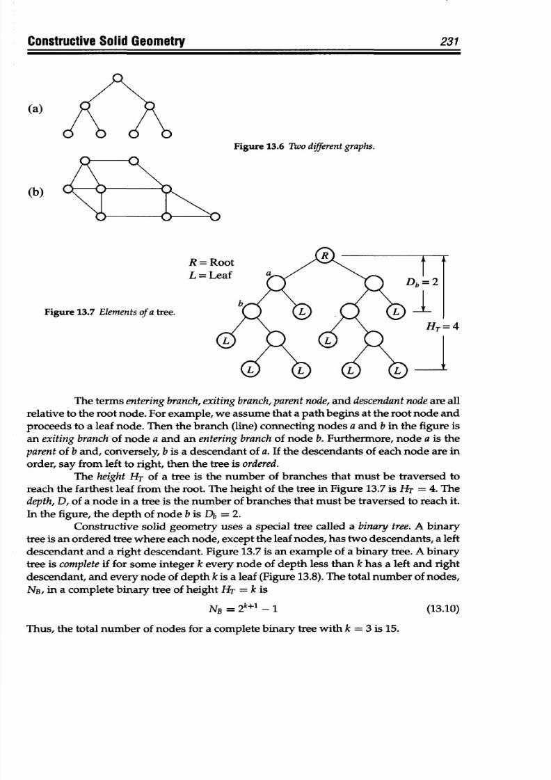
8/9/2019 Mortenson, Michael E. - Mathematics for computer graphics applications.pdf
http://slidepdf.com/reader/full/mortenson-michael-e-mathematics-for-computer-graphics-applicationspdf 244/367
Constructive Solid
Geometry
Figure
13.6 Two different graphs.
R=F
L=L
Figure 13.7
Elements of
a
tree.
4
The terms entering branch, exiting
branch,
parentnode, and
descendant
node are all
relative to the root
node. For example, we assume
that
a path begins
at
the root node and
proceeds
to
a
leaf node. Then the branch (line) connecting nodes a and
b
in
the
figure is
an exiting branch of node a and an
entering
branch of node
b. Furthermore,
node a is
the
parent
of
b
and,
conversely, b is
a descendant
of a. If the descendants of each
node
are
in
order,
say
from
left
to
right,
then
the tree
is
ordered.
The height
HT
of
a tree
is
the
number of
branches that
must
be traversed to
reach the farthest leaf from the
root.
The
height of the tree in Figure 13.7
is
HT
= 4.
The
depth,
D,
of a node in
a
tree is the number of
branches
that
must
be traversed
to
reach it.
In the
figure,
the depth of
node
b is
Db
= 2.
Constructive
solid
geometry uses
a special
tree
called
a binary
tree. A
binary
tree
is
an
ordered tree where
each node,
except
the
leaf
nodes, has
two descendants, a left
descendant
and
a
right descendant. Figure
13.7 is
an
example
of a
binary
tree. A binary
tree
is
complete if for some integer k every
node
of
depth less
than k has a
left and
right
descendant,
and
every node
of depth
k is a
leaf
(Figure 13.8).
The
total
number of nodes,
NB,
in
a
complete
binary
tree
of
height
HT
=
k is
NB
=
2
k+1
-
1
(13.10)
Thus, the total number of nodes for
a
complete binary tree with k = 3 is 15.
231
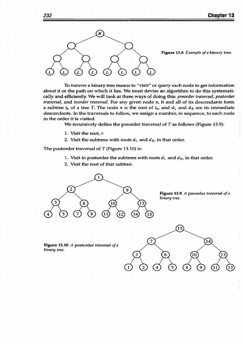
8/9/2019 Mortenson, Michael E. - Mathematics for computer graphics applications.pdf
http://slidepdf.com/reader/full/mortenson-michael-e-mathematics-for-computer-graphics-applicationspdf 245/367
232
Chapter
13
Figure
13.8
Example
of
a
binary
tree.
To
traversea
binary
tree
means
to
"visit" or query each
node
to
get information
about it or the path on
which it lies. We must
devise an algorithm to
do
this
systemati-
cally
and
efficiently.
We
will look at
three ways of doing
this:
preorder
raversal,
postorder
traversal,
and
inordertraversal.
For
any
given
node
n,
it
and
all
of
its
descendants
form
a
subtree
t,
of
a
tree T. The node
n is
the
root of ta, and
dL
and
dR are its immediate
descendants. In
the traversals to follow,
we assign
a number,
in sequence,
to each node
in
the
order it is visited.
We recursively
define
the preorder
traversal
of
T
as
follows (Figure 13.9):
1. Visit the root, r.
2.
Visit
the subtrees
with
roots
dL
and
dR, in that
order.
The postorder
traversal
of T (Figure 13.10) is:
1. Visit in postorder
the subtrees
with roots dL
and
dR,
in that order.
2. Visit the root of that
subtree.
Figure
13.9 A
preorder traversalof
a
binary tree.
Figure
13.10 A postorder traversal
of a
binary
tree.
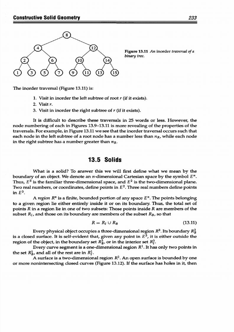
8/9/2019 Mortenson, Michael E. - Mathematics for computer graphics applications.pdf
http://slidepdf.com/reader/full/mortenson-michael-e-mathematics-for-computer-graphics-applicationspdf 246/367
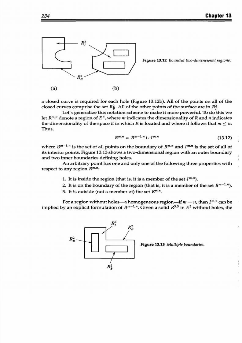
8/9/2019 Mortenson, Michael E. - Mathematics for computer graphics applications.pdf
http://slidepdf.com/reader/full/mortenson-michael-e-mathematics-for-computer-graphics-applicationspdf 247/367
234
Chapter
13
2-
Figure 13.12
Bounded
two-dimensional
regions.
R
2
(a) (b)
a
closed
curve
is
required
for each hole (Figure
13.12b).
All
of
the points on
all
of
the
closed curves
comprise the set RB. All of
the other
points of
the surface are in
R,.
Let's generalize this notation scheme to
make
it more
powerful.
To
do
this we
let R
m
'"
denote
a region of En,
where
m indicates the
dimensionality of
R and n indicates
the
dimensionality of the
space E
in which
R
is located
and
where
it
follows that m
<
n.
Thus,
Rm
n= Bm-ln U
Imn
(13.12)
where
B,-l"n
is
the set of all points on
the
boundary
of
R,'n
and
Imn is
the set
of all
of
its
interior points.
Figure
13.13
shows a two-dimensional
region
with
an
outer boundary
and
two inner
boundaries
defining
holes.
An arbitrary
point
has
one and
only
one of the
following three
properties
with
respect
to any region
Rmn:
1. It is inside the region (that
is,
it is a member of the set It n).
2. It
is
on the
boundary of
the
region
(that
is,
it
is
a
member of
the
set Bmt-ln).
3. It is
outside (not a member
of)
the set
R
m
'n.
For a region
without holes-a
homogeneous
region-if m =
n,
then
Im n can
be
implied
by
an
explicit
formulation
of
B,-ln.
Given
a
solid
R
3
'
3
in
E
3
without
holes,
the
R2
2
Figure
13.13 Multiple
boundaries.
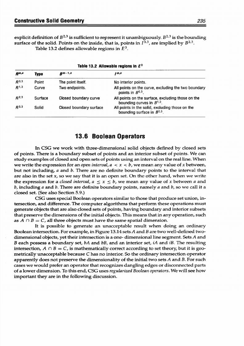
8/9/2019 Mortenson, Michael E. - Mathematics for computer graphics applications.pdf
http://slidepdf.com/reader/full/mortenson-michael-e-mathematics-for-computer-graphics-applicationspdf 248/367
Constructive Solid
Geometry
235
explicit definition of B
2
'
3
is sufficient to represent it unambiguously. B
2
'
3
is the
bounding
surface of
the
solid. Points
on
the inside, that is, points in J3,3,
are
implied
by B
2
'
3
.
Table 13.2 defines allowable regions in
E
3
.
Table 13.2 Allowable
regions
inE
3
RMflA Type Sm-1,0
/mJ
R
0
3
Point
The
point itself.
No
interior points.
R
1
,
3
Curve Two endpoints.
All
points
on
the curve, excluding
the two boundary
points in
B03.
R
2
,
3
Surface Closed
boundary curve
All
points on the
surface,
excluding those
on
the
bounding
curves
in
B1,3.
R
3
,
3
Solid Closed
boundary surface
All
points in he solid, excluding those
on
the
bounding
surface inB2,3.
13.6
Boolean Operators
In
CSG
we
work
with
three-dimensional
solid objects defined by closed sets
of
points.
There
is a
boundary
subset
of
points and an interior subset
of
points.
We
can
study examples of closed and open sets of points using an
interval on the
real line.
When
we write the
expression for
an open
interval,
a
<
x < b,
we m ean any
value
of
x between,
but
not including,
a
and b.
There are
no
definite
boundary points
to
the interval that
are also
in the set
x,
so we say that it is an open set. On the other
hand,
when we write
the expression
for
a closed interval, a
< x < b,
we mean any value of x between a and
b, including a and
b.
There
are
definite boundary points, namely a and
b,
so we call it a
closed set. (See also
Section
5.9.)
CSG uses
special Boolean
operators
similar
to those
that
produce set union,
in-
tersection, and
difference. The
computer algorithms
that perform these operations must
generate
objects
that
are also closed sets of
points, having
boundary
and
interior
subsets
that
preserve the dimensions of the initial objects.
This
means
that
in any operation, such
as A n B = C, all
three
objects
must have
the same spatial
dimension.
It is possible to generate an unacceptable
result when
doing
an ordinary
Boolean
intersection. For
example, in Figure
13.14 sets A and
B
are two well-defined
two-
dimensional
objects,
yet
their intersection
is a
one-
dimensional
line
segment. Sets
A and
B each
possess
a
boundary set,
bA
and bB, and
an interior
set, iA and
iB.
The
resulting
intersection,
A n B
= C,
is mathematically
correct according to set
theory,
but
it is
geo-
metrically unacceptable because
C
has no interior.
So
the ordinary intersection operator
apparently
does
not
preserve the dimensionality
of
the
initial
two
sets
A
and
B.
For
such
cases
we
would
prefer an operator
that recognizes
dangling edges or disconnected parts
of a lower dimension.
To
this end,
CSG
uses
regularizedBoolean operators.
We will
see
how
important they are in the
following discussion.
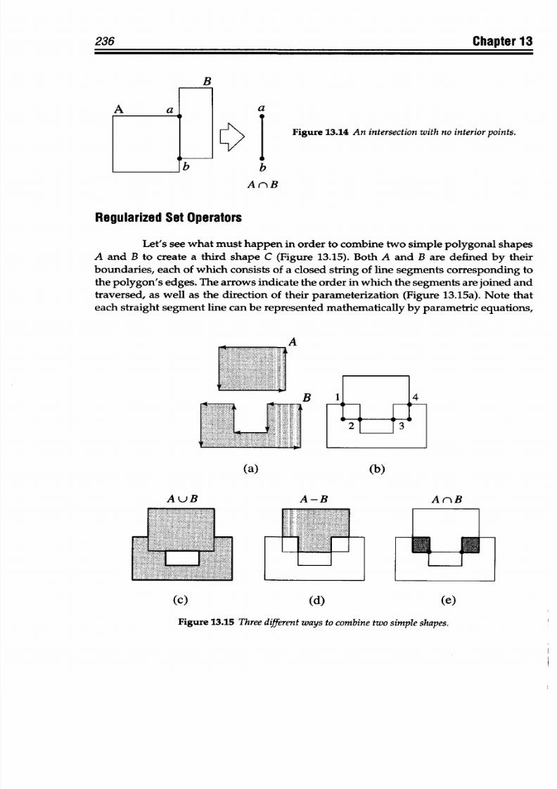
8/9/2019 Mortenson, Michael E. - Mathematics for computer graphics applications.pdf
http://slidepdf.com/reader/full/mortenson-michael-e-mathematics-for-computer-graphics-applicationspdf 249/367
Chapter
13
B
a
b
ArnB
Figure
13.14 An
intersection
with no interior
points.
Regularized
Set
Operators
Let's
see what
must happen
in
order
to combine
two
simple polygonal
shapes
A and
B to
create
a third
shape C (Figure
13.15). Both
A
and
B are
defined
by
their
boundaries,
each
of
which
consists of a closed
string
of
line
segments corresponding
to
the polygon's
edges.
The arrows
indicate
the
order
in
which the
segments
are
joined
and
traversed,
as well
as the direction of
their
parameterization (Figure
13.15a).
Note that
each
straight
segment line can
be
represented
mathematically
by
parametric
equations,
A
(a)
AuB
-I
P
(b)
A-B
A nrB
(c)
(d)
(e)
Figure
13.15 Three
different ways to
combine two simple
shapes.
236
I
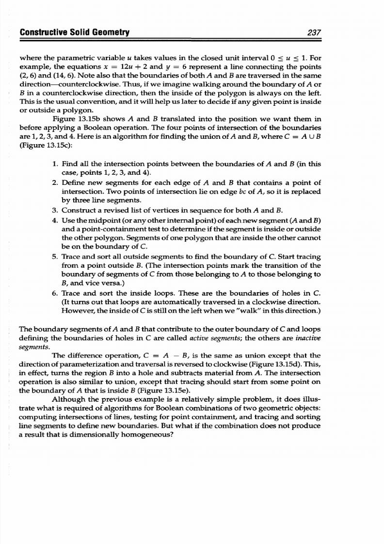
8/9/2019 Mortenson, Michael E. - Mathematics for computer graphics applications.pdf
http://slidepdf.com/reader/full/mortenson-michael-e-mathematics-for-computer-graphics-applicationspdf 250/367
Constructive Solid
Geometry
237
where the parametric variable u takes values in the closed
unit
interval
0
< u
< 1.
For
example,
the equations
x = 12u + 2
and
y = 6
represent
a line connecting the points
(2, 6)
and
(14, 6). Note also
that
the boundaries of both A and B
are
traversed
in
the same
direction-counterclockwise.
Thus,
if
we
imagine
walking
around
the
boundary
of A
or
B in
a
counterclockwise direction, then the inside of the polygon is always on
the left.
This
is the usual convention,
and
it will help
us
later to decide
if
any given
point
is inside
or outside a polygon.
Figure 13.15b
shows
A and B translated into the position we want them in
before applying
a
Boolean
operation. The
four
points of intersection of
the
boundaries
are 1, 2,3, and
4.
Here
is
an
algorithm for finding the
union
of
A and B,
where
C =
A
U
B
(Figure
13.15c):
1.
Find
all
the
intersection
points between the boundaries of
A
and
B
(in
this
case, points 1, 2,
3,
and
4).
2. Define
new segments
for each
edge of
A and B that
contains
a point
of
intersection.
Two points of intersection lie
on
edge bc of A, so it is replaced
by
three
line segments.
3. Construct a revised list of
vertices
in sequence
for both
A and B.
4.
Use the
midpoint (or
any other internal point) of each
new
segment
(A and
B)
and
a point-containment test to determine if the segment
is
inside or outside
the
other polygon. Segments of
one
polygon
that
are inside
the
other cannot
be on the
boundary
of
C.
5. Trace
and
sort all outside segments to
find
the
boundary
of
C.
Start tracing
from
a
point
outside B. (The intersection points mark the transition of the
boundary of
segments
of C from
those belonging
to
A
to
those belonging
to
B, and
vice
versa.)
6. Trace and sort
the inside
loops. These are the
boundaries
of holes
in
C.
(It turns out that loops are
automatically
traversed in
a
clockwise direction.
However, the inside
of C is still on
the
left when
we "walk" in this direction.)
The
boundary
segments
of
A
and
B
that
contribute to the
outer boundary
of
C
and
loops
defining the boundaries of holes in
C
are called
active
segments; the others are
inactive
segments.
The difference
operation,
C =
A - B, is the same
as
union except that the
direction of parameterization
and
traversal
is
reversed to
clockwise (Figure 13.15d). This,
in effect, turns the region
B
into
a
hole and
subtracts material
from
A.
The intersection
operation
is also similar to
union,
except that tracing should start from some point on
the
boundary of
A
that is
inside B
(Figure 13.15e).
Although the previous example is a relatively simple problem, it does
illus-
trate
what
is
required
of
algorithms
for
Boolean
combinations of
two
geometric
objects:
computing intersections of
lines,
testing for
point
containment, and
tracing
and
sorting
line
segments
to define new boundaries. But what if
the
combination does not produce
a
result
that is
dimensionally homogeneous?
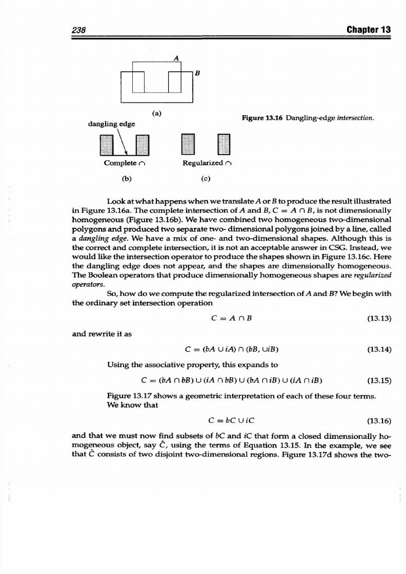
8/9/2019 Mortenson, Michael E. - Mathematics for computer graphics applications.pdf
http://slidepdf.com/reader/full/mortenson-michael-e-mathematics-for-computer-graphics-applicationspdf 251/367
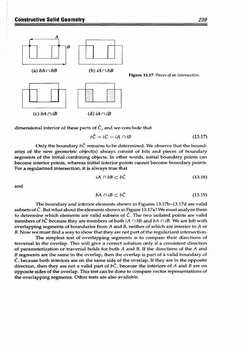
8/9/2019 Mortenson, Michael E. - Mathematics for computer graphics applications.pdf
http://slidepdf.com/reader/full/mortenson-michael-e-mathematics-for-computer-graphics-applicationspdf 252/367
Constructive
Solid
Geometry
239
jB
(a) bA
n
bB (b) iA
n
bB
Figure 13.17 Pieces of
an intersection.
(c)
bA
n
iB (d)
iA
r
iB
dimensional interior
of
these
parts
of
C, and we conclude that
iC
= iC = iA n iB
(13.17)
Only the boundary
bC
remains
to
be determined. We observe that the bound-
aries of the new
geometric object(s) always
consist of bits
and
pieces of boundary
segments
of
the initial combining
objects. In
other
words,
initial
boundary
points
can
become
interior points,
whereas
initial
interior
points cannot
become
boundary
points.
For a regularized intersection,
it
is
always
true that
iA
n
bB c
bC
(13.18)
and
bA niB c bC
(13.19)
The
boundary and interior elements shown
in
Figures 13.17b-13.17d
are
valid
subsets
of
C.
But
what
about
the
elements
shown
in Figure
13.17a? We
must
analyze them
to
determine which
elements are
valid
subsets of C. The two isolated
points are
valid
members
of bt
because they
are
members
of
both iA
n
bB and
bA n
iB.
We
are left with
overlapping
segments of
boundaries
from A
and
B,
neither of
which
are
interior
to A
or
B.
Now
we must find
a
way
to show
that
they
are not
part
of
the
regularized
intersection.
The
simplest test of overlapping segments
is to compare their directions of
traversal
in
the
overlap. This
will
give a correct
solution only if
a
consistent
direction
of
parameterization or traversal holds
for
both
A
and B. If the
directions of
the
A
and
B segments are the same
in
the overlap, then the overlap is part of
a
valid
boundary of
C,
because
both
interiors
are
on the sam e side
of
the overlap.
If
they
are
in
the
opposite
direction,
then
they
are not
a
valid
part of
b(C,
because
the interiors of
A
and
B
are
on
opposite sides
of
the
overlap.
This
test can be done
to
compare vector representations of
the
overlapping
segments. Other tests
are
also available.
8/9/2019 Mortenson, Michael E. - Mathematics for computer graphics applications.pdf
http://slidepdf.com/reader/full/mortenson-michael-e-mathematics-for-computer-graphics-applicationspdf 253/367
240
Chapter
13
We express
the
process
for finding
the regularized intersection of two bounded
sets
as
C =
bt
Uit
(13.20)
and
expand
this to
C = Validb(bA n bB)
U
(iA
n
bB)
U
(bA
n iB) U
(iA
n iB) (13.21)
We can separate this last
expression
into interior and
exterior
parts
as
follows:
bC =
Validb(bA
n bB) U (iA
n
bB)
U
(bA
n
iB) (13.22)
and
iC = iA n
iB
(13.23)
Nothing
in
Equations 13.22
and
13.23
indicates dimensionality,
because they
are equally
applicable to one-, two-, three-,
or
n-dimensional
objects. Similar procedures
apply to
the
union and
difference
operators.
Set-Membership
Classification
One
of
the
geometric
tools
we
can
use to
regularize
sets produced by a Boolean
combination of
other
sets
is to
determine
whether
a given
point is inside,
outside, or
on
the boundary
of
a set.
Any regularized set A has
three
important
subsets
associated with
it:
the set
of
all
of
its
interior points,
denoted
iA,
the
set
of
all
points on
its boundary,
denoted
bA, and all points
outside of it,
denoted
cA.
Determining which set
a
given point
belongs
to is
called set-membership classification.
Set-membership
classification helps us solve
several
important
problems
in
geometric
modeling and
computer
graphics.
Here
are
four
of
them:
1.
The
point-inclusion
problem:
Given some arbitrary
geometric solid and
some
point,
is
the
point inside, outside, or
on the boundary
of
the
solid?
2.
The
clipping
problem: Given a polygon and a
line segment, what parts of
the
line
are
inside,
outside,
or on
the
boundary
of
the
polygon?
3.
The
polygon-intersection problem:
Given two polygons
A
and
B,
what, if
any,
is
the
intersection
polygon A n B?
4. The solid-interferenceproblem:
Given two solids A
and
B, do
they interfere
(that is,
intersect unintentionally)?
13.7 Boolean
Models
A
Boolean
model
is
a complex
solid
formed by the Boolean
combination of
two
or
more
simpler
solids.
If
A
and
B
are
regularized
geometric solids,
that
is,
solids
that
are
dimensionally homogeneous,
and
if
C
=
A
< OP
>
B, where <
OP
>
is any
regularized
Boolean
operator
(union,
difference,
or
intersection),
then A < OP
> B
is
a
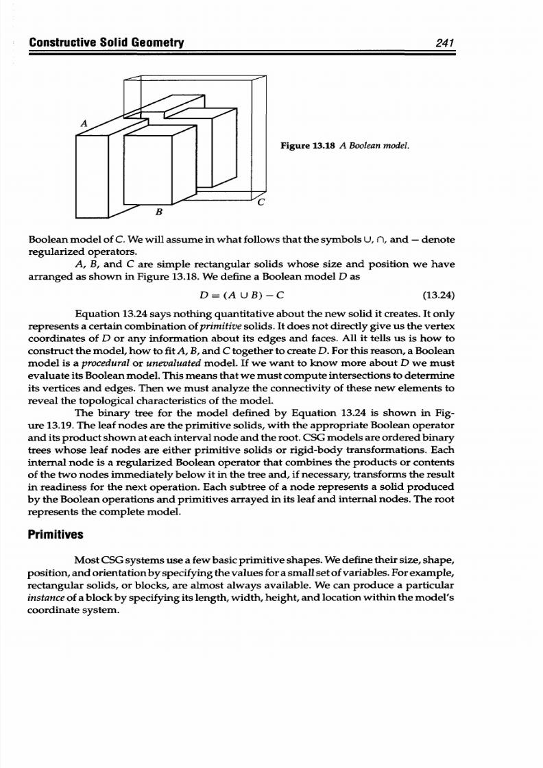
8/9/2019 Mortenson, Michael E. - Mathematics for computer graphics applications.pdf
http://slidepdf.com/reader/full/mortenson-michael-e-mathematics-for-computer-graphics-applicationspdf 254/367
Constructive
Solid Geometry
Figure 13.18 A
Boolean
model.
Boolean
model of C. We will
assume
in
what
follows
that
the symbols U, n,
and
- denote
regularized operators.
A, B,
and
C are
simple rectangular solids whose
size and position
we have
arranged as shown
in Figure
13.18. We define a Boolean
model D as
D = (A UB)-C (13.24)
Equation
13.24
says nothing quantitative about the new solid
it creates.
It only
represents a certain
combination
of primitivesolids.
It
does
not
directly give us the vertex
coordinates
of
D
or any information about its
edges
and faces. All
it
tells
us
is how to
construct
the
model, how
to
fit A,
B,
and
C
together
to create D. For this reason, a Boolean
model is
a proceduralor unevaluated
model.
If
we
want to
know
more
about D we
must
evaluate its
Boolean
model.
This means that
we
must
compute
intersections
to determine
its
vertices
and
edges.
Then
we
must
analyze the
connectivity
of
these new elements
to
reveal the
topological characteristics of
the
model.
The binary tree
for
the model defined
by
Equation
13.24
is shown
in Fig-
ure
13.19.
The leaf nodes are
the
primitive solids,
with
the appropriate
Boolean
operator
and its
product
shown at each
interval
node and the
root.
CSG
models
are ordered binary
trees
whose
leaf nodes are either primitive
solids or rigid-body
transformations.
Each
internal node
is a
regularized
Boolean
operator
that
combines
the products
or contents
of the two nodes immediately below it in the
tree
and, if
necessary,
transforms the result
in readiness
for
the next operation.
Each
subtree of a
node
represents a solid produced
by
the
Boolean
operations and primitives
arrayed
in its leaf
and
internal nodes. The root
represents
the
complete model.
Primitives
Most
CSG systems
use
a few basic
primitive shapes.
We
define their
size,
shape,
position,
and
orientation
by
specifying
the
values for
a
small
set of
variables.
For example,
rectangular
solids, or blocks, are almost always available. We can
produce
a
particular
instanceof
a
block by
specifying its
length, width,
height,
and
location
within
the model's
coordinate
system.
241
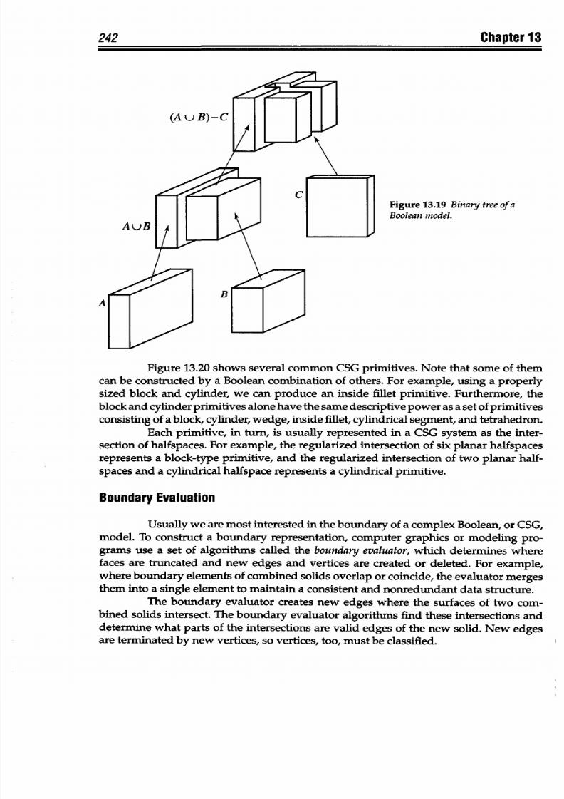
8/9/2019 Mortenson, Michael E. - Mathematics for computer graphics applications.pdf
http://slidepdf.com/reader/full/mortenson-michael-e-mathematics-for-computer-graphics-applicationspdf 255/367
242 Chapter
13
Figure
13.19
Binary tree
ofa
Boolean
model.
Figure
13.20
shows several
common CSG primitives.
Note
that some
of
them
can be constructed by
a Boolean
combination of
others. For
example, using a
properly
sized
block
and
cylinder,
we
can
produce
an inside fillet
primitive.
Furthermore, the
block and
cylinder primitives
alone have
the same descriptive power
as a
set
of primitives
consisting
of
a
block,
cylinder,
wedge,
inside
fillet, cylindrical
segment,
and
tetrahedron.
Each
primitive,
in
turn,
is
usually
represented
in a
CSG system
as
the inter-
section of halfspaces.
For
example,
the
regularized
intersection
of six planar
halfspaces
represents
a
block-type
primitive,
and
the
regularized
intersection of two
planar
half-
spaces
and a
cylindrical halfspace
represents
a cylindrical
primitive.
Boundary
Evaluation
Usually
we
are
most
interested
in the
boundary
of
a complex Boolean,
or
CSG,
model.
To
construct a boundary
representation, computer
graphics
or modeling
pro-
grams
use a set of
algorithms
called the boundary evaluator,
which
determines
where
faces
are truncated and
new
edges
and
vertices are
created
or
deleted.
For example,
where
boundary
elements
of
combined solids
overlap
or coincide,
the evaluator merges
them
into a
single
element
to
maintain
a consistent
and nonredundant data
structure.
The
boundary
evaluator
creates
new edges where the
surfaces of
two
com-
bined
solids intersect.
The
boundary
evaluator algorithms
find these
intersections
and
determine
what
parts
of
the intersections are
valid
edges
of
the
new solid.
New
edges
are
terminated
by
new
vertices,
so vertices,
too, must
be classified.
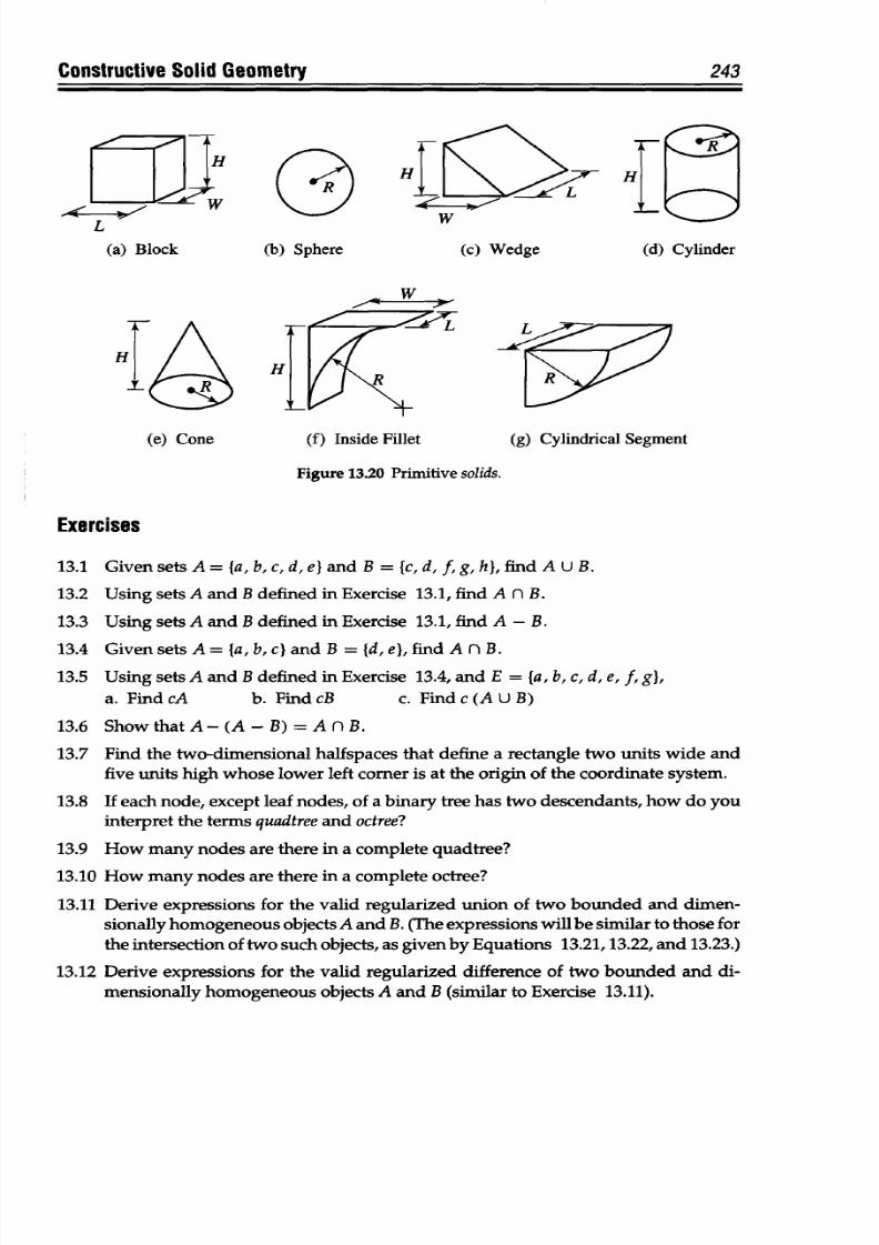
8/9/2019 Mortenson, Michael E. - Mathematics for computer graphics applications.pdf
http://slidepdf.com/reader/full/mortenson-michael-e-mathematics-for-computer-graphics-applicationspdf 256/367
Constructive Solid
Geometry
243
H H
L W
(a)
Block (b) Sphere (c)
Wedge
(d)
Cylinder
(e) Cone (f) Inside Fillet (g) Cylindrical Segment
Figure
13.20 Primitive solids.
Exercises
13.1
GivensetsA=
{a,b,c,d,e}and
B
=
{c,d,f,g,hl,findAUB.
13.2
Using
sets A and B defined in
Exercise
13.1, find A n
B.
13.3
Using
sets A and B defined in
Exercise
13.1, find A - B.
13.4
Given sets A ={a, b, c} and B ={d,
e},
find
A n
B.
13.5
Using
sets
A and
B
defined
in
Exercise
13.4,
and E
=
{a, b,
c,
d,
e,
f,
g},
a. Find cA
b.
Find
cB
c. Find c (A
U B)
13.6
Show that A-(A-B) =
A n B.
13.7
Find the two-dimensional
halfspaces
that
define
a
rectangle
two
units wide
and
five units high whose lower left corner is at the origin
of the
coordinate system.
13.8
If
each
node,
except leaf nodes, of a
binary
tree has two descendan ts,
how
do you
interpret
the terms
quadtree
and octree?
13.9
How
many
nodes
are
there
in a complete quadtree?
13.10 How
many
nodes
are
there
in a complete octree?
13.11 Derive expressions for the
valid
regularized
union
of two bounded and
dimen-
sionally homogeneous objects A and B.
(The
expressions will be similar to those for
the
intersection
of
two such
objects, as
given
by
Equations
13.21,13.22,
and
13.23.)
13.12 Derive expressions for the valid regularized difference of two bounded
and
di-
mensionally hom ogeneous
objects A and B
(similar
to
Exercise
13.11).
8/9/2019 Mortenson, Michael E. - Mathematics for computer graphics applications.pdf
http://slidepdf.com/reader/full/mortenson-michael-e-mathematics-for-computer-graphics-applicationspdf 257/367
(lA
pla
CURVES
We
all
have
a strong intuitive
sense
of
what
a
curve
is. Although
we
never see a curve
floating
around
free of
any
object,
we
can readily
identify the curved edges and
silhou-
ettes
of objects
and
easily
imagine the
curve
that
describes
the
path
of a
moving
object.
This
chapter explores the mathematical definition of a
curve in
a form
that is
very useful
to
geometric modeling and
other
computer
graphics applications: that
definition con-
sists of
a set
of parametricequations.
The mathematics
of
parametric equations
is the
basis
for Bezier,
NURBS,
and
Hermite
curves. The
curves discussed in
this
chapter may
be
placed in the Hermite
family
of
curves.
Bezier curves
are
the
subject of
the next chapter,
and
NURBS
are best left for more advanced texts
on
geometric modeling. Both plane
curves
and
space curves are introduced here, followed by
discussions
of the tangent
vec-
tor,
blending functions, conic curves,
reparameterization,
and
continuity
and composite
curves.
14.1
Parametric Equations of a Curve
A
parametric
curve is one
whose defining equations are
given
in terms
of a
single, common, independent variable called the parametric variable. We
have already
encountered parametric variables in earlier
discussions
of vectors, lines, and planes.
Imagine
a
curve in three-dimensional
space. Each point on the
curve
has a
unique
set of coordinates: a
specific
x value, y value,
and
z value. Each coordinate is
controlled
by
a
separate parametric equation, whose
general form looks
like
x = x(u),
y
= y(u), z
=
z(u) (14.1)
where
x(u) stands for some
as yet unspecified
function in which u is the independent
variable;
for
example, x(u)
= au
2
+
bu
+
c, and
similarly for y(u) and z(u). It
is
important
to understand that
each
of these
is an independent
expression. This
will become
clear
as
we
discuss
specific
examples
later.
The
dependent variables are
the
x,
y,
and
z
coordinates
themselves,
because
their
values
depend
on the
value of
the parametric
variable
u. Engineers and
program-
mers
who
do
geometric
modeling
usually
prefer
these
kinds
of
expressions because
the
coordinates
x,
y, and z are independent of
each
other, and
each is
defined
by its
own
parametric
equation.
244
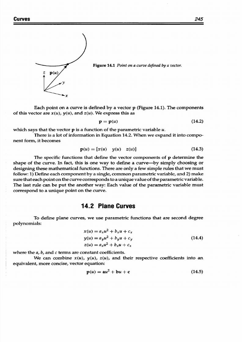
8/9/2019 Mortenson, Michael E. - Mathematics for computer graphics applications.pdf
http://slidepdf.com/reader/full/mortenson-michael-e-mathematics-for-computer-graphics-applicationspdf 258/367
245
urves
Figure 14.1 Point on a curve
defined
by a
vector.
Each point on a curve is defined by a vector p (Figure 14.1). The
components
of
this
vector are
x(u), y(u),
and
z(u).
We
express this
as
p = p(u) (14.2)
which
says
that the
vector
p is a function of the parametric variable u.
There is a lot of
information
in
Equation
14.2.
When
we expand it into
compo-
nent
form, it becomes
p(u) = [x(u) y(u)
zu)]
(14.3)
The
specific functions that define
the
vector
components
of p
determine the
shape
of
the
curve.
In
fact,
this is
one way
to
define a curve-by
simply choosing
or
designing
these
mathematical
functions. There are only
a
few
simple rules
that
we
must
follow:
1)
Define
each component
by a single, common
parametric
variable,
and
2)
make
sure
that
each
point
on the curve corresponds to a unique value of the parametric variable.
The last
rule can be
put
the another
way: Each
value of the parametric variable
must
correspond
to a
unique point on
the
curve.
14.2
Plane
Curves
To
define plane curves, we use parametric functions that are second degree
polynomials:
x(u) =
axu
2
+
bxu
+
cx
y(u)
= ayu
2
+ byu +
cY
(14.4)
z(u)
= azu
2
+ bzu + cz
where the a,
b, and c
terms
are
constant coefficients.
We
can
combine x(u), y(u),
z(u),
and their
respective
coefficients
into an
equivalent, more
concise,
vector equation:
p(u) = au2
+ bu
+ c
(14.5)
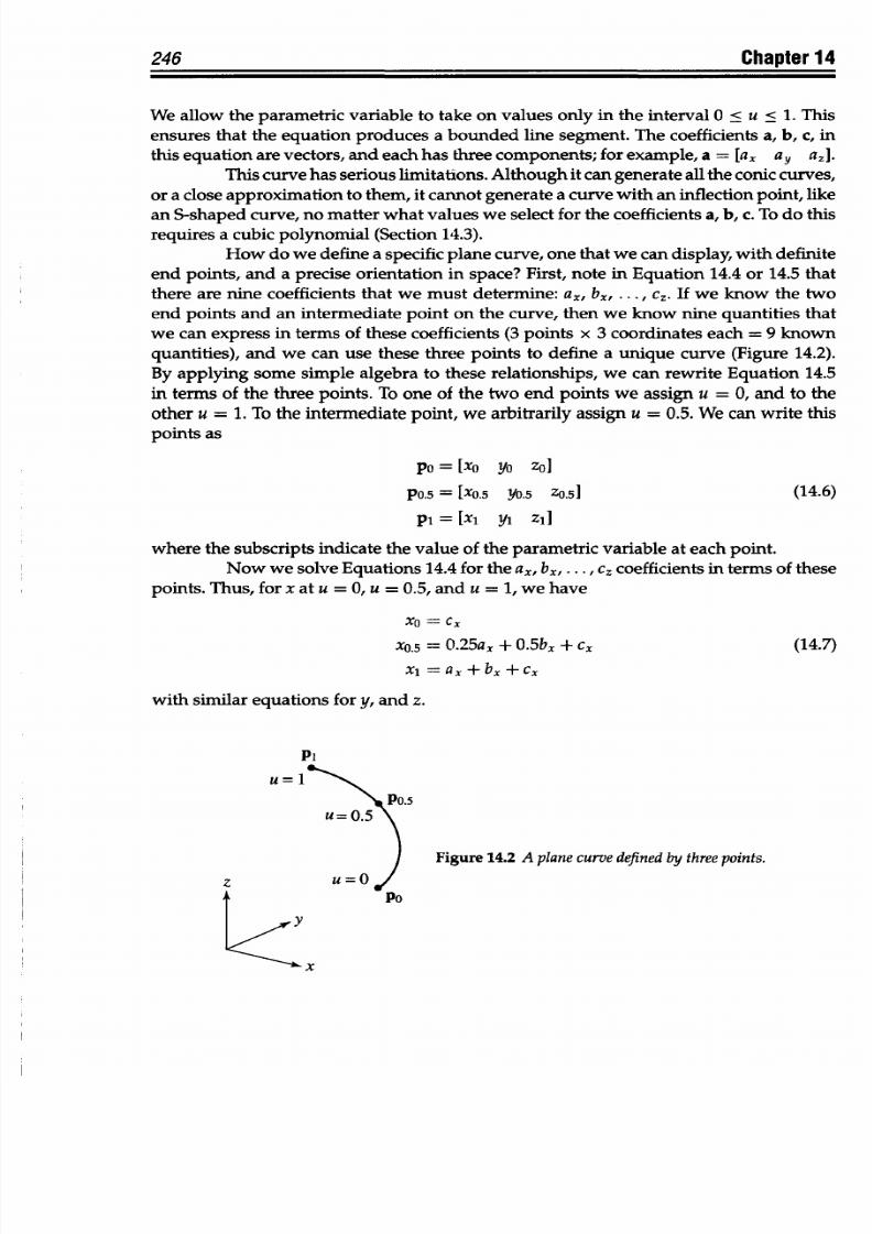
8/9/2019 Mortenson, Michael E. - Mathematics for computer graphics applications.pdf
http://slidepdf.com/reader/full/mortenson-michael-e-mathematics-for-computer-graphics-applicationspdf 259/367
246
Chapter 14
We allow
the parametric
variable to take on
values
only
in the interval
0
<
u <
1.
This
ensures that the
equation produces
a bounded line segment. The coefficients a, b, c, in
this
equation
are vectors, and each
has
three components; for example, a = [ax
ay
aj].
This curve
has
serious limitations. Although it can generate all
the
conic curves,
or
a
close
approximation to
them, it cannot generate a curve with an
inflection
point, like
an
S-shaped
curve,
no matter what values we select for the coefficients a,
b,
c.
To
do this
requires
a
cubic
polynomial (Section 14.3).
How do we define
a
specific plane
curve,
one that we
can
display, with definite
end points, and a
precise
orientation in
space?
First, note in Equation
14.4
or
14.5
that
there are nine coefficients
that we
must
determine:
ax, b,,
... , c.. If
we know
the
two
end points and an intermediate
point
on the curve, then
we
know nine quantities that
we
can express
in terms of these coefficients (3 points x
3
coordinates
each
=
9
known
quantities), and we can use these three points to define a unique curve (Figure 14.2).
By
applying
some simple
algebra
to
these relationships,
we
can
rewrite Equation
14.5
in terms of the three points.
To
one
of
the two end points we assign u
=
0, and to the
other
u =
1.
To
the intermediate point, we arbitrarily assign u
= 0.5.
We
can
write this
points as
Po
= [xO Yo zol
PO.5 =
[X
0
.
5
YO.5 ZO.5] (14.6)
Pi
=
[X
1
yi
Z
1
]
where
the
subscripts
indicate
the value
of
the parametric
variable at
each
point.
Now
we
solve
Equations
14.4 for
the
ax, bx, ..
. , cz
coefficients
in
terms of these
points. Thus,
for
x at u
=
0, u
=
0.5,
and
u
=
1,
we
have
xo = Cx
xO.5
= 0.25ax +
0.5bx
+ cx
(14.7)
x
1
=ax+bx+cx
with
similar equations
for
y, and
z.
Pi
u
= 1
PO.5
u=05
Figure 14.2 A
plane curve
defined
by
three points.
z u=O
Po
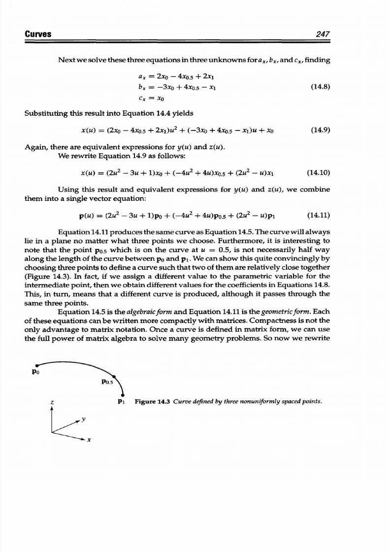
8/9/2019 Mortenson, Michael E. - Mathematics for computer graphics applications.pdf
http://slidepdf.com/reader/full/mortenson-michael-e-mathematics-for-computer-graphics-applicationspdf 260/367
Curves
247
Next we solve these three equations in three unknowns for ax, bx, and c,, finding
a. =
2xO
- 4xO.
5
+ 2x,
bx
=
-3xo +
4
xO.5- x (14.8)
Cx
=xo
Substituting this
result
into
Equation
14.4
yields
x(u)
= (2xo - 4xo
5
+ 2x,)u
2
+
(-3xo
+
4Xo.5
- x)u +
x
0
(14.9)
Again,
there
are
equivalent expressions
for
y(u) and
z(u).
We
rewrite
Equation
14.9
as follows:
x(u)
=
(2u
2
-
3u + 1)xo + (-4U
2
+ 4u)xo
5
+
(2u
2
- u)x
1
(14.10)
Using this
result
and
equivalent
expressions for y(u) and z(u),
we
combine
them
into
a single
vector equation:
p(u)
=
(2u
2
-
3u +
1)po
+ (-4U
2
+ 4u)po.
5
+ (2u
2
-
u)pl
(14.11)
Equation
14.11
produces the same curve
as
Equation
14.5.
The
curve will always
lie
in
a
plane
no matter what three points we choose. Furthermore, it is interesting to
note
that
the
point
Po.5
which
is
on the
curve at
u =
0.5,
is
not
necessarily
half
way
along
the length
of the
curve between
p0
and
pl. We can
show
this
quite convincingly
by
choosing three points to define a curve such
that
two
of them are relatively close together
(Figure 14.3).
In fact,
if
we assign
a
different value to the parametric variable
for
the
intermediate point,
then
we
obtain
different
values for the coefficients in Equations 14.8.
This,
in
turn, means that a different curve
is
produced, although it passes through the
same
three
points.
Equation 14.5 is the algebraicformand
Equation
14.11 is
the
geometricform.
Each
of
these
equations
can
be
written more compactly with matrices. Compactness is not the
only
advantage
to
matrix
notation.
Once a
curve
is
defined in matrix
form,
we
can
use
the
full power
of matrix algebra
to solve
many geometry problems.
So now
we rewrite
Po
P0.5
z
Pi Figure
14.3
Curve defined by threenonuniformly
spacedpoints.
y
x
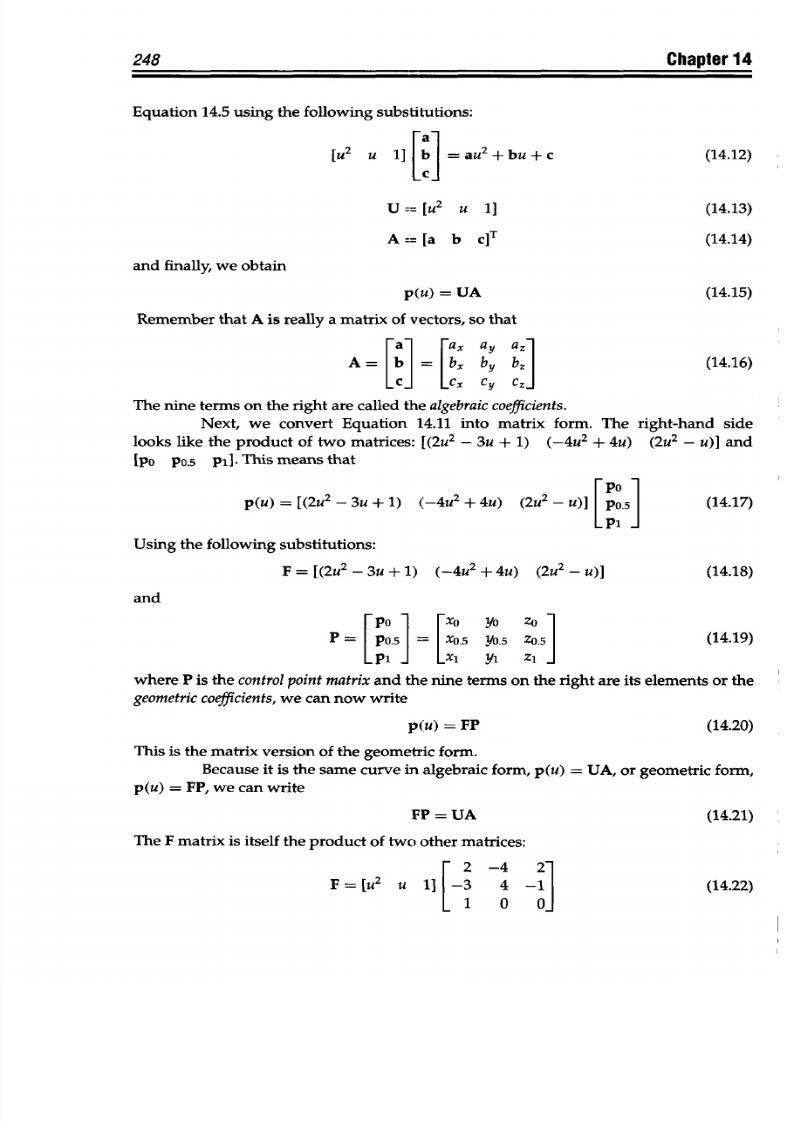
8/9/2019 Mortenson, Michael E. - Mathematics for computer graphics applications.pdf
http://slidepdf.com/reader/full/mortenson-michael-e-mathematics-for-computer-graphics-applicationspdf 261/367
248
Chapter 14
Equation 14.5
using the following
substitutions:
[u
2
u
1]
au +bu+c
(14.12)
c
U =
[U
2
u 1]
(14.13)
A= [a
b c]T
(14.14)
and
finally,
we obtain
p(u)
= UA
(14.15)
Remember that
A
is
really
a
matrix
of vectors,
so that
[a]
Fax ay
azl
A
=b
= bx by
bj
(14.16)
c
cX
cy cz
The nine
terms
on
the
right
are called
the algebraic
coefficients.
Next, we
convert Equation
14.11
into matrix form.
The
right-hand side
looks like
the
product
of
two
matrices: [(2u
2
-
3u
+ 1)
(-4U
2
+ 4u) (2u
2
-
u)]
and
[PO PO.5 pi.
This means
that
p(u)
=
[(2u
2
- 3u +
1)
(-4u
2
+ 4u)
(2u
2
-
U)]
[P0.5]
(14.17)
Using
the
following
substitutions:
F
= [(2u
2
- 3u +
1) (-4U
2
+ 4u) (2u
2
-
U)]
(14.18)
and
PO
xO
yo
Zo
P
PO.5
X0.5
YO.5 Z0.5
(14.19)
-P- Xi
Yi Zi
where
P is
the
control
point matrix
and the
nine terms on
the
right
are its
elements or the
geometric
coefficients,
we can now write
p(u) =
FP (14.20)
This
is the
matrix
version of the
geometric form.
Because it is the same
curve in algebraic form,
p(u)
= UA,
or geometric form,
p(u)
= FP, we can write
FP = UA (14.21)
The
F
matrix
is
itself
the
product
of
two
other
matrices:
2 -4 2
F
=
[U2
U
1] -3 4 -1
(14.22)
1 0
0
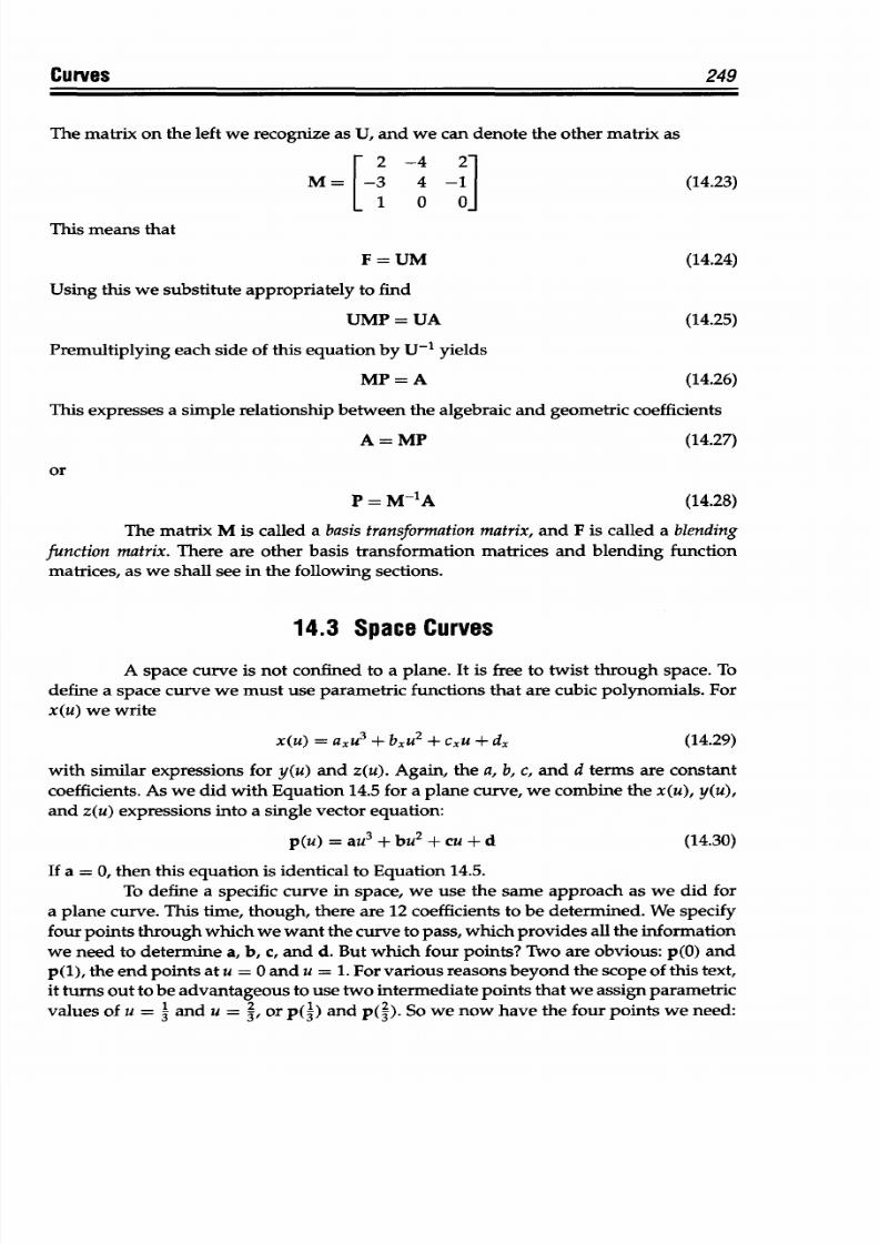
8/9/2019 Mortenson, Michael E. - Mathematics for computer graphics applications.pdf
http://slidepdf.com/reader/full/mortenson-michael-e-mathematics-for-computer-graphics-applicationspdf 262/367
Curves 249
The
matrix on the
left
we
recognize
as
U,
and we
can
denote the other matrix as
2 -4 2-
M=
-3
4
-1
(14.23)
1
0
0-
This means
that
F = UM
(14.24)
Using this we substitute appropriately to
find
UMP = UA (14.25)
Premultiplying
each side
of
this equation
by U-1 yields
MP
= A (14.26)
This
expresses a simple relationship between the algebraic and geometric coefficients
A=MP (14.27)
or
P
= M-1A (14.28)
The
matrix M
is called
a basis transformationmatrix, and F is
called
a
blending
function matrix. There are other basis transformation
matrices and blending function
matrices, as
we shall
see
in the
following sections.
14.3 Space Curves
A space
curve is
not confined
to
a
plane.
It
is free
to
twist
through space. To
define a space
curve we must use parametric
functions that are cubic
polynomials.
For
x(u) we write
x(u)
=
axu
3
+
bxu
2
+
cxu
+
dx
(14.29)
with similar expressions for
y(u) and
z(u). Again, the a, b, c, and d terms
are
constant
coefficients.
As
we did
with
Equation
14.5
for a
plane
curve, we combine the x(u), y(u),
and z(u) expressions into a single vector equation:
p(u)
= au
3
+ bu
2
+ cu +
d
(14.30)
If a
=
0, then this equation
is identical
to
Equation
14.5.
To define a specific
curve in
space,
we
use
the same approach
as we did
for
a plane curve. This time, though, there are 12 coefficients to be determined. We
specify
four
points
through
which we
want
the
curve to
pass,
which provides
all
the
information
we
need
to
determine a,
b,
c, and d.
But
which
four
points? Two
are obvious: p(O)
and
p(l), the
end points at
u = 0
and
u =
1.
For
various reasons beyond
the scope of
this
text,
it turns out to be
advantageous
to
use
two
intermediate
points that we assign
parametric
values
of
u
=
3 and
u =
2, or
p(b)
and p(2). So we
now
have the
four points
we
need:
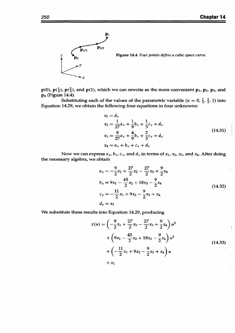
8/9/2019 Mortenson, Michael E. - Mathematics for computer graphics applications.pdf
http://slidepdf.com/reader/full/mortenson-michael-e-mathematics-for-computer-graphics-applicationspdf 263/367
250
Chapter
14
Pi
z
Po
Figure
14.4
Fourpoints
define
a cubic
space
curve.
y
x
p(O), p(3), p(-),
and p(l), which
we
can
rewrite as the more
convenient
pi, P2,
p3, and
P4
(Figure
14.4).
Substituting
each of
the values
of
the
parametric
variable
(u
=
O,
1) into
Equation 14.29,
we obtain
the
following
four equations in four unknowns:
xi
=d,
1 1
1
X2 =
7ax
+
-bx
+
-cx
+
dx
27
9 3
8 4 2
(14.31)
x3=
T~x+
-bx +
-cx +
dx
9
3
x4=
ax
+ bx +
cx
+ dx
Now we can express ax,
bx, cr, and
dx in terms of x
1
, x
2
, x
3
, and x
4
.
After
doing
the
necessary
algebra,
we
obtain
9
27 27 9
ax
=
--
xi
+
-x
2
-2X
3
+
-X
4
22
2
2
45
9
bx
= 9x
1
- -x
2
+ 18x3 -- X4
2
2 (14.32)
CX = xI
+ 9X
2
- -X3 + X4
2 2
We substitute
these
results into Equation
14.29, producing
x(u) = +
X
2-
X3 + 2X4 U
+
(9xi
- -X
2
+ 18X
3
--
X4
U2
2 xl (14.33)
+
-X
+
9X
2
-
X
3
+X
4
) u
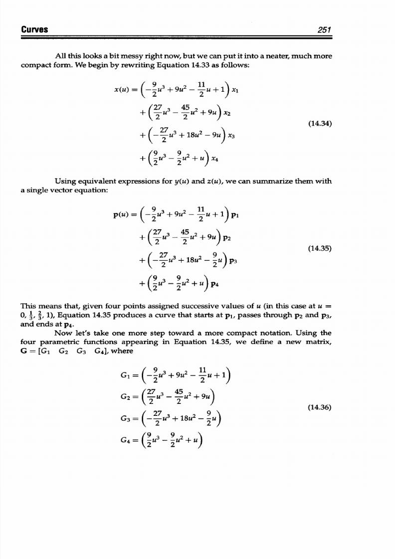
8/9/2019 Mortenson, Michael E. - Mathematics for computer graphics applications.pdf
http://slidepdf.com/reader/full/mortenson-michael-e-mathematics-for-computer-graphics-applicationspdf 264/367
Curves
251
All
this
looks
a
bit
messy
right now, but
we
can put it
into a
neater, much more
compact form.
We begin
by
rewriting Equation 14.33
as follows:
x(u)= ( -9U3+9U
u+1) x1
+ 27U3 _
45U2
+ 9u) X2
(u
+(14.34)
+(-2 u+18U2 -9U)
X3
+
(u3
-
+u2 X4
Using equivalent expressions for y(u) and z(u), we can summarize them with
a
single vector equation:
p(u)= (9u3 + 9u2 u+1 Pi
+ (27U3 _ 45U2 +
9U)
P2
27
9)
(14.35)
+ -2u3+ 18U2
-- U P3
+18
2
~
+
9(-U3
_u2 +
u P4
This means that, given four points assigned
successive
values of u
(in
this
case at
u
0, 1, 3, 1), Equation 14.35 produces a curve that starts at
pl,
passes through
P2
and p3,
and
ends at p4.
Now
let's
take
one
more
step
toward
a
more compact notation.
Using
the
four parametric
functions
appearing in Equation 14.35, we define
a
new
matrix,
G
= [G
G
2
G
3
G
4
1,
where
G
1
=
(_
9u3+9U2
- 2
1)
G
2
=
(27U3 45U29u) (14.36)
G
3
=
(-2u3
+
18u
2
-U
G
4
=
(9u3
_9u2+u)
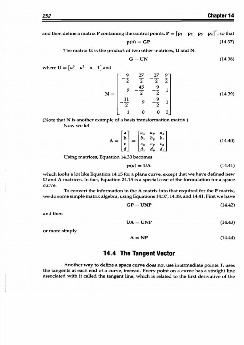
8/9/2019 Mortenson, Michael E. - Mathematics for computer graphics applications.pdf
http://slidepdf.com/reader/full/mortenson-michael-e-mathematics-for-computer-graphics-applicationspdf 265/367
252
Chapter 14
and
then define a
matrix
P containing
the control points, P =
[Pt
P2 P3 P4]T, SO
that
p(u) = GP
(14.37)
The
matrix
G
is
the
product
of
two other
matrices,
U
and
N:
G=UN
(14.38)
whereU=
[U
3
U
2
U
1]
and
N=
-
9 27
27 9'
-.-
-2 -- 2 -2
9
-4 -- 1
2
2
11 9
- -
9
-- 12 2
1 0 0 0
(14.39)
(Note
that N is another example of a basis
transformation matrix.)
Now we let
Fal
Fax
ay
az]
A= b = b
y
y bz(14.40)
c cx cy Cz
Ld Ld
dy
d,
Using
matrices,
Equation
14.30
becomes
p(u)
= UA
(14.41)
which looks a lot like Equation 14.15
for
a
plane
curve,
except
that
we
have defined new
U and A matrices. In fact,
Equation
24.15
is a special case
of
the
formulation for a space
curve.
To convert
the information in
the
A
matrix
into that required
for the P matrix,
we
do some simple matrix algebra,
using
Equations 14.37,14.38,
and 14.41. First
we
have
GP
=
UNP
(14.42)
and then
UA
= UNP
(14.43)
or more
simply
A=NP
(14.44)
14.4
The Tangent
Vector
Another way to define a
space curve
does
not
use intermediate points. It
uses
the tangents at
each end of a curve, instead. Every
point
on a
curve
has
a
straight
line
associated
with it called the tangent
line,
which
is
related
to the first derivative of
the
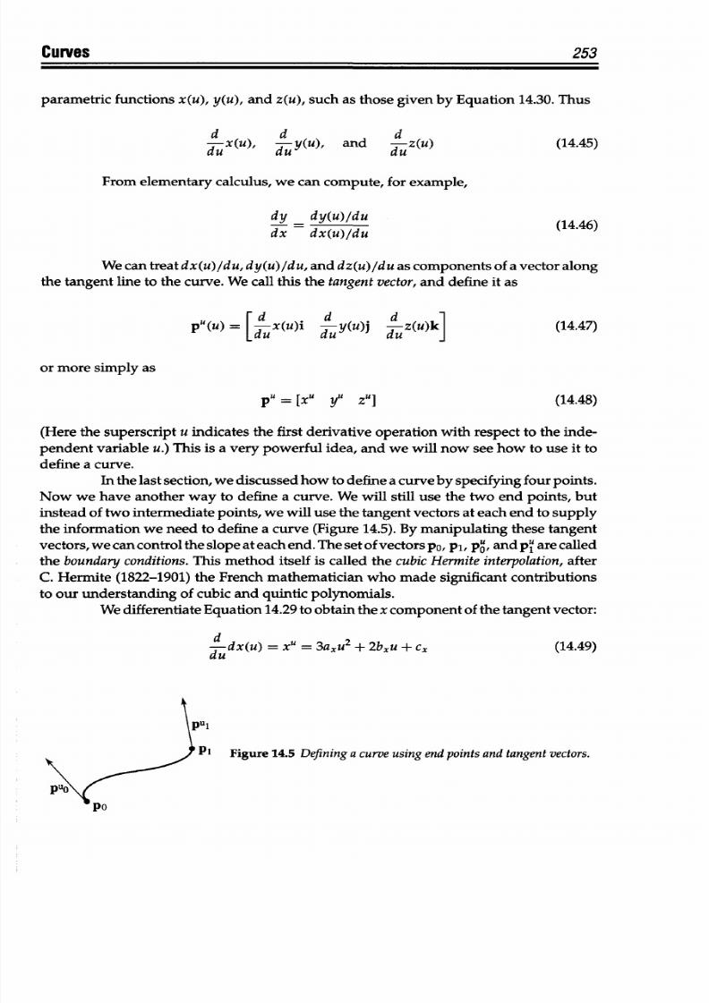
8/9/2019 Mortenson, Michael E. - Mathematics for computer graphics applications.pdf
http://slidepdf.com/reader/full/mortenson-michael-e-mathematics-for-computer-graphics-applicationspdf 266/367
Curves
253
parametric functions x(u), y(u), and
z(u),
such as those given
by
Equation 14.30. Thus
d x(u), d y(u), and
d
z(u) (14.45)
From elementary
calculus,
we can compute, for example,
dy _ dy(u)/du
(14.46)
dx dx(u)/du
We can
treat dx(u)/du,
dy(u)/du, and dz(u)/du
as
components of a vector
along
the tangent line to the curve. We call
this
the tangent vector, and define it as
pu()
=
-X(U)i -y(u)j -z(u)k] (14.47)
or more simply as
pU
=
[xu yU
z']
(14.48)
(Here
the superscript u
indicates the first derivative operation
with
respect to the inde-
pendent
variable
u.)
This
is a
very powerful idea, and we
will
now
see
how
to use
it
to
define a curve.
In
the last
section,
we discussed
how to define
a
curve
by specifying
four points.
Now
we have another
way to define
a
curve. We will still
use the two
end
points,
but
instead of two
intermediate points,
we will use the tangent vectors
at each
end
to
supply
the information we
need
to
define
a curve
(Figure 14.5). By
manipulating these tangent
vectors, we can
control the
slope at each end. The set of
vectors
po, pl,
pu,
and pu
are
called
the boundary
conditions. This
method
itself is called the cubic
Hermite interpolation,after
C. Hermite (1822-1901) the
French
mathematician
who
made significant contributions
to
our understanding of
cubic
and
quintic polynomials.
We differentiate
Equation
14.29 to obtain
the x component
of the tangent
vector:
d dx(u)
=
xu
= 3axu
2
+
2bxu
+ cx
(14.49)
du
Figure
14.5
Defining
a
curve
using
end
points and
tangent
vectors.
8/9/2019 Mortenson, Michael E. - Mathematics for computer graphics applications.pdf
http://slidepdf.com/reader/full/mortenson-michael-e-mathematics-for-computer-graphics-applicationspdf 267/367
254
Chapter 14
Evaluating Equations 14.29 and 14.49 at u =
0
u =
1,yields
xo
=
d.
xl =
ax
+ bx + cx + dx
(14.50)
xOU
c'
xl =3ax +2bx +cx
Using these four equations
in four unknowns, we
solve
for
ax, bx, cx,
and dx
in
terms
of
the boundary
conditions
ax = 2(xo - xi + xOu x
bx=
3
(-x( + xi)
- 2xOu - xi
(14.51)
dx = xo
Substituting the result into
Equation 14.29, yields
x(u)
= (2xo
-
2x
1
+ xOu
+ xl) u
3
+ (-3xo +
3x
1
- 2xO-l
)
u
2
+
XOu +
x
0
(14.52)
Rearranging
terms w e can rewrite this as
x(u)
=
(2u
3
-
3u
2
+
1)xo
+
(-2u
3
+ 3u
2
)xl (14.53)
+
(u3
-2U2 +
U XO U
+ (u3
-
U2)xlu
Because y(u)
and
z(u)
have
equivalent forms,
we can include
them by
rewriting
Equation
14.53
in vector
form:
p(u)
= (2u
3
-
3U
2
+
1)po
+
(-2u
3
+ 3u
2
)pl
(14.54)
+
(u
3
-
2u
+ u)p, + (u
3
- U2)pu
To
express
Equation
14.54
in matrix notation,
we first
define
a
blending function
matrix F
=
[F
1
F
2
F
3
F
4
1,
where
F
1
= 2u
3
-
3u
2
+ 1
F
2
= -2u
3
+
3U
2
(14.55)
F
3
=u
3
-2u
2
+ u
F
4
= u3-u2
These matrix elements are
the polynomial
coefficients
of
the vectors in Equation 14.54,
which we rewrite
as
p(u)
= Fjpo + F
2
pj + F
3
pu +
F
4
pu
(14.56)
If
we assemble the vectors
representing
the boundary
conditions into a
matrix
B,
B
= [po
P o
(14.57)
then
p(u)
=
FB
(14.58)
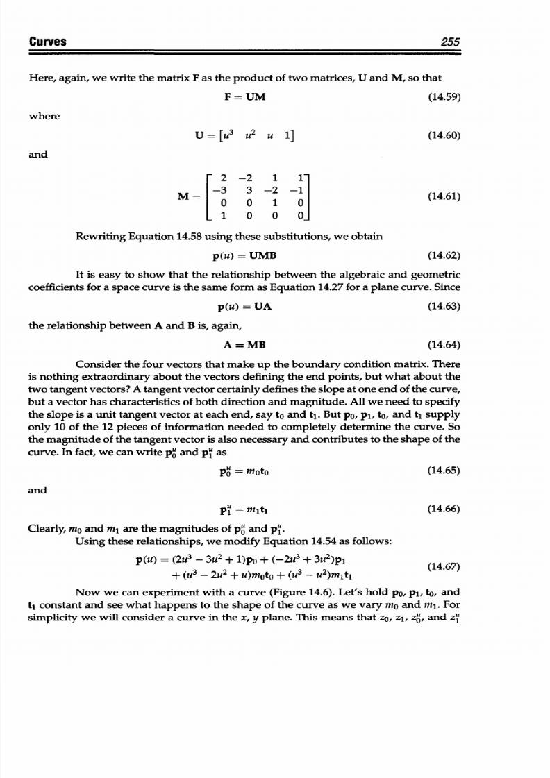
8/9/2019 Mortenson, Michael E. - Mathematics for computer graphics applications.pdf
http://slidepdf.com/reader/full/mortenson-michael-e-mathematics-for-computer-graphics-applicationspdf 268/367
Curves 255
Here, again,
we write the matrix
F
as
the
product of
two
matrices, U and M, so that
F=UM
(14.59)
where
U = [U
3
U
U 1]
(14.60)
and
2 -2 1 1-
M =-3
3 -2
-1
(14.61)
1 0
0 0-
Rewriting
Equation
14.58
using
these
substitutions, we
obtain
p(u) =
UMB (14.62)
It is easy
to show
that
the relationship between the
algebraic and
geometric
coefficients for
a
space curve is
the same form
as
Equation
14.27
for a
plane curve. Since
p(u) =
UA (14.63)
the relationship between
A and B is, again,
A
= MB
(14.64)
Consider the four vectors that make up the boundary condition
matrix.
There
is
nothing extraordinary about
the
vectors defining
the
end points, but what about the
two tangent
vectors?
A tangent
vector
certainly defines
the slope
at one end of
the curve,
but
a
vector has
characteristics of both direction and
magnitude.
All we need
to
specify
the
slope
is a
unit tangent
vector
at each
end, say
to
and
tl.
But po, pi, to, and ti supply
only
10
of the
12
pieces of information needed to completely determine the curve.
So
the
magnitude
of the tangent vector is also necessary and contributes to the shape of the
curve.
In fact, we can write pO and
p'
as
pu=
moto
(14.65)
and
pu= mltl
(14.66)
Clearly, mO and
ml
are
the
magnitudes of
pu
and pu.
Using these relationships,
we
modify
Equation
14.54 as follows:
p(u)
= (2U
3
- 3U
2
+
l)po +
(-2U
3
+
3U
2
)pl
+ (U
3
-
2u
2
+
U)Moto
+ (U
3
-
u
2
)mltl
(14.67)
Now we can experiment
with
a curve
(Figure
14.6). Let's hold
po,
pi,
to,
and
tj constant and
see
what happens to the shape of the curve as we vary mo and ml. For
simplicity
we
will consider
a
curve
in the
x, y plane. This
means
that zo, zl,
z0 ,
and
zlu
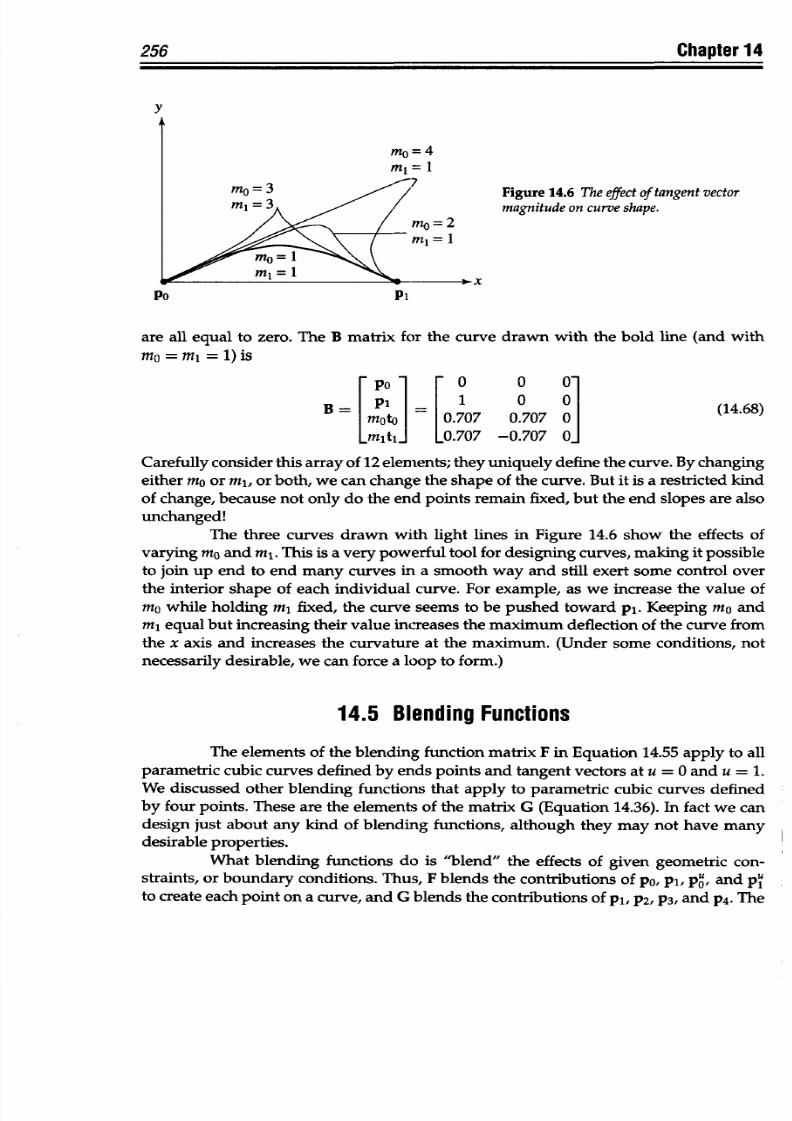
8/9/2019 Mortenson, Michael E. - Mathematics for computer graphics applications.pdf
http://slidepdf.com/reader/full/mortenson-michael-e-mathematics-for-computer-graphics-applicationspdf 269/367
256
Chapter
14
y
Figure 14.6 The
effect of tangentvector
magnitude on curve
shape.
x
Po
Pi
are all
equal
to
zero.
The
B
matrix
for
the
curve
drawn
with
the
bold
line (and
with
M =
=l
1) is
Po
O
0
0
0
B
0.707
0.707 0
(14.68)
moto
0.707 -0.707
0
Carefully
consider this array
of
12 elements;
they
uniquely
define
the
curve. By
changing
either
mO
or
ml,
or both,
we
can
change the shape
of the curve.
But
it is
a restricted kind
of
change, because
not
only
do
the end
points
remain
fixed,
but
the
end
slopes
are also
unchanged
The
three
curves
drawn
with
light lines
in
Figure 14.6 show the effects of
varying mO and
ml.
This is
a very powerful
tool
for
designing curves, making
it possible
to
join
up end
to
end many
curves in a
smooth
way and
still exert some control
over
the interior shape
of
each individual curve. For
example,
as we increase
the value
of
mo
while holding
ml fixed, the curve
seems to
be pushed toward pi. Keeping
mo and
ml
equal
but increasing
their value
increases
the maximum deflection
of the curve from
the
x
axis
and increases
the
curvature
at the maximum.
(Under some conditions, not
necessarily
desirable, we can force
a
loop to form.)
14.5 Blending Functions
The elements of
the blending
function matrix F in
Equation
14.55 apply
to
all
parametric
cubic curves
defined by ends
points and tangent
vectors
at
u = 0 and
u = 1.
We
discussed other
blending functions that apply
to parametric cubic curves
defined
by
four points. These are
the elements
of the matrix G (Equation
14.36). In fact
we
can
design just about
any kind
of
blending
functions, although
they
may
not
have
many
desirable
properties.
What
blending
functions
do
is
"blend" the
effects
of
given
geometric
con-
straints,
or boundary
conditions. Thus, F blends
the con tributions of po, pi,
pu, and
pu
to create each point
on
a curve,
and
G
blends
the
contributions
of
p1, P2, p3, and
P4. The
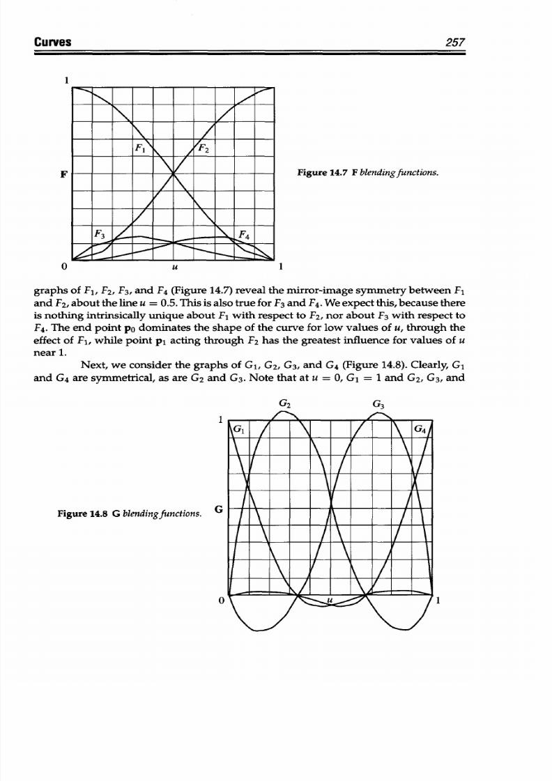
8/9/2019 Mortenson, Michael E. - Mathematics for computer graphics applications.pdf
http://slidepdf.com/reader/full/mortenson-michael-e-mathematics-for-computer-graphics-applicationspdf 270/367
Curves
1
F
0
U
Figure
14.7
F blending unctions.
1
graphs
of F
1
, F
2
, F
3
,
and F
4
(Figure 14.7)
reveal the mirror-image
symmetry between F
1
and F
2
, about the line
u
= 0.5.
This
is
also
true for
F
3
and F
4
. We expect this, because there
is
nothing intrinsically unique about F
1
with
respect to F
2
, nor about F
3
with respect to
F
4
. The
end
point po dominates the shape of the
curve
for low values of
u, through the
effect
of F
1
,
while point pi
acting
through F
2
has
the
greatest
influence for
values
of
u
near 1.
Next,
we consider the graphs of G
1
, G
2
, G
3
,
and
G
4
(Figure 14.8).
Clearly, G
1
and
G
4
are symmetrical,
as
are G
2
and G
3
. Note
that
at
u
=
0,
G
1
=
1 and G
2
, G
3
, and
1
Figure 14.8 G blending unctions. G
UG 1/
I/ I
t
G4
I \
IA
257
0 1
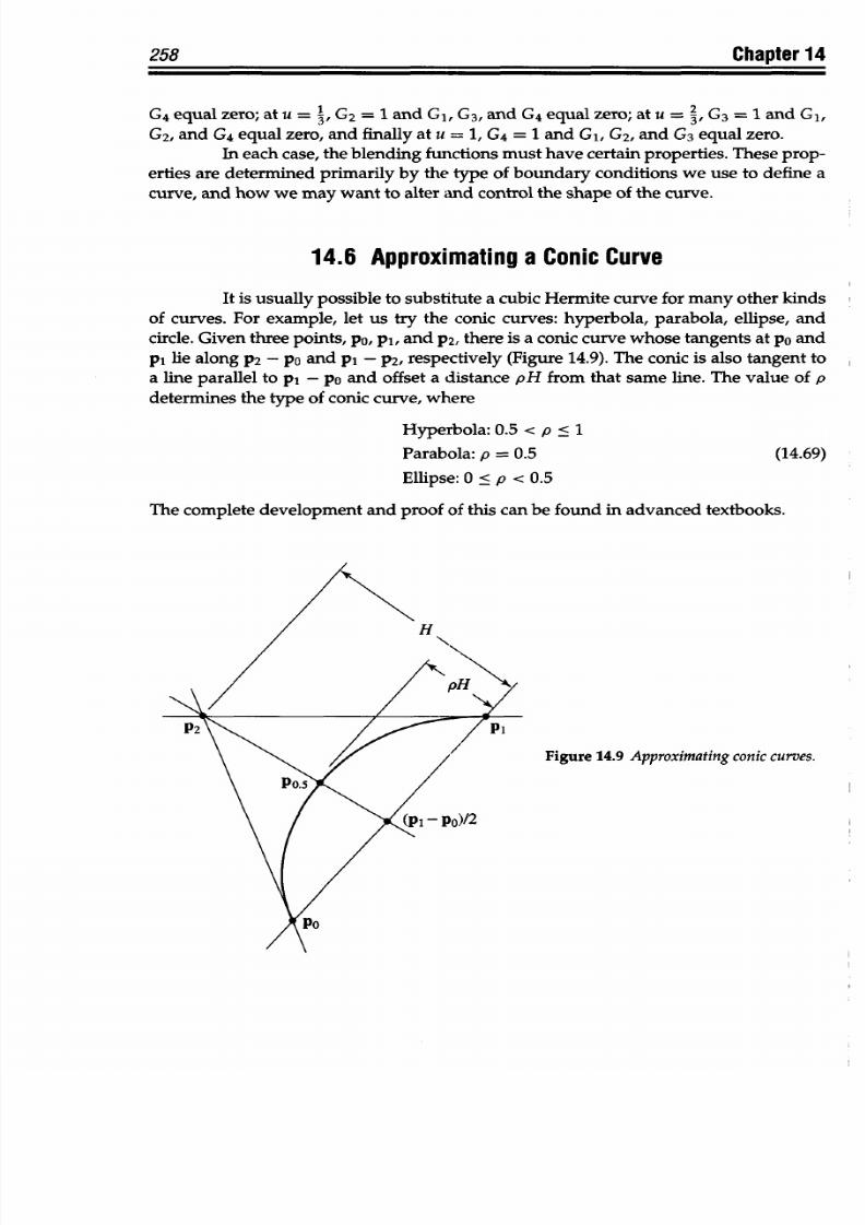
8/9/2019 Mortenson, Michael E. - Mathematics for computer graphics applications.pdf
http://slidepdf.com/reader/full/mortenson-michael-e-mathematics-for-computer-graphics-applicationspdf 271/367
258
Chapter
14
G
4
equal zero;
at
u
=
3,
G
2
=
1 and
G
1
, G
3
, and
G
4
equal zero; at u
= Z,
G
3
=
1 and G
1
,
G
2
, and G
4
equal
zero,
and finally
at u
= 1, G
4
=
1 and G
1
, G
2
, and G
3
equal zero.
In each
case,
the blending functions must have certain properties. These prop-
erties are determined primarily by the type
of boundary
conditions we use to define a
curve, and how
we
may want to alter and control the shape of the curve.
14.6 Approximating
aConic
Curve
It
is
usually possible to substitute a
cubic
Hermite curve for many other kinds
of curves. For example, let
us
try the conic curves: hyperbola, parabola, ellipse,
and
circle. Given three
points,
po,
p1, and P2,
there
is
a conic curve whose tangents at
po
and
pi
lie along P2 -
po and pi
-
P2,
respectively
(Figure
14.9). The
conic is
also
tangent to
a
line parallel
to pi
-
po and offset a
distance pH
from that
same
line. The value of
p
determines the
type
of conic
curve,
where
Hyperbola: 0.5 <
p <
1
Parabola: p
=
0.5
(14.69)
Ellipse: 0
< p < 0.5
The
complete development and proof of this can be found in advanced
textbooks.
Figure
14.9
Approximating conic curves.
po)/2
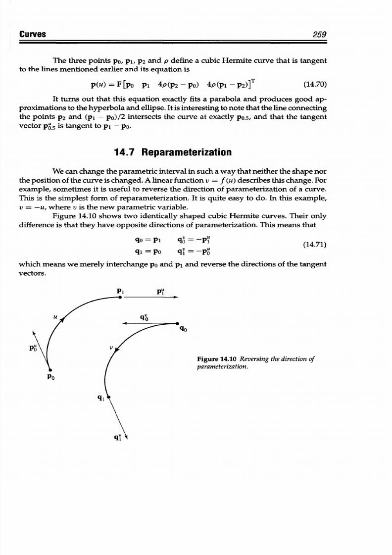
8/9/2019 Mortenson, Michael E. - Mathematics for computer graphics applications.pdf
http://slidepdf.com/reader/full/mortenson-michael-e-mathematics-for-computer-graphics-applicationspdf 272/367
Curves
259
The
three points po, p ,
2 and
p
define
a
cubic
Hermite curve that
is
tangent
to
the
lines
mentioned earlier and
its
equation
is
p(u)
=
F
[po
pi
4p(p2
-po)
4
p(pi
-P
2
)]T
(14.70)
It
turns
out
that this
equation exactly fits
a parabola and produces
good
ap-
proximations to the
hyperbola and
ellipse. It
is
interesting to note that the line connecting
the
points P2 and (pi -
po)/
2
intersects the curve
at
exactly
po.5, and that
the tangent
vector p
0
u is
tangent
to pi -
Po.
14.7 Reparameterization
We
can change the
parametric interval
in such a way
that neither the
shape nor
the
position of
the
curve
is
changed. A linear
function
v =
f (u)
describes
this change. For
example,
sometimes
it
is useful
to
reverse
the
direction
of
parameterization
of a
curve.
This
is
the
simplest
form
of reparameterization.
It
is quite
easy to
do. In
this example,
v = -u,
where
v
is the
new
parametric
variable.
Figure 14.10 shows
two identically shaped
cubic
Hermite
curves. Their only
difference
is
that
they have opposite
directions of parameterization. This means that
qo =pi qV
= -p
0=0
q
= -Pi (14.71)
q,
= po
qv
=
-p
o
which
means we merely interchange po and pi and reverse the directions of the tangent
vectors.
qo
Figure
14.10
Reversing
the
direction
of
parameterization.
Po
q
1
IPU
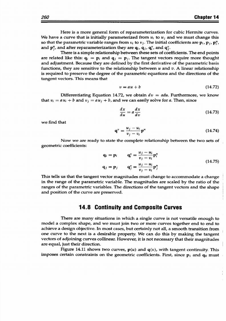
8/9/2019 Mortenson, Michael E. - Mathematics for computer graphics applications.pdf
http://slidepdf.com/reader/full/mortenson-michael-e-mathematics-for-computer-graphics-applicationspdf 273/367
260
Chapter
14
Here is a
more general
form of
reparameterization for
cubic
Hermite
curves.
We
have
a curve that
is initially parameterized
from
ui
to ui and
we
must
change
this
so that
the parametric variable
ranges from vi to vp.
The initial
coefficients are
pi, pp
pit,
and
p7,
and
after
reparameterization they
are
qi,
qp,
qv,
and
q7.
There is a
simple relationship
between these sets of
coefficients.
The
end points
are
related
like
this: qi = pi and
qj =
pp.
The tangent
vectors require
more
thought
and
adjustment.
Because
they are defined by
the first derivative
of the parametric
basis
functions,
they
are
sensitive
to
the relationship
between
u
and
v. A
linear
relationship
is
required to preserve
the
degree of
the parametric equations and
the directions of the
tangent
vectors. This
means that
v=au+b
(14.72)
Differentiating
Equation
14.72,
we obtain
dv
=
adu.
Furthermore, we know
that
vi = a
ui + b and
vy
= a
uj
+ b, and we
can easily solve for
a. Then, since
dx
dx
d=
ad
(14.73)
we find
that
qV
= Uj -
Ui pU
(14.74)
Vj -
Vi
Now
we are ready
to
state
the
complete
relationship
between
the
two
sets of
geometric
coefficients:
qi
=pi qY
=lU,
Pi
Vj
-
Vi(14.75)
qj =pj
q7 =
uj-u
p1
This
tells
us
that
the
tangent vector magnitudes
must change
to accommodate
a
change
in the range of the
parametric
variable.
The
magnitudes are
scaled by
the ratio of
the
ranges
of
the parametric
variables.
The directions
of the tangent vectors
and the shape
and
position
of
the
curve
are
preserved.
14.8
Continuity and Composite Curves
There are many
situations in
which a single curve
is not versatile
enough to
model a complex
shape,
and we
must
join two
or
more curves
together
end
to end to
achieve
a design
objective.
In most
cases,
but certainly
not
all, a
smooth transition from
one curve to the
next
is
a desirable
property.
We can
do
this by making the
tangent
vectors
of
adjoining
curves
collinear.
However,
it
is
not
necessary
that
their magnitudes
are
equal, just their direction.
Figure 14.11
shows
two
curves, p(u) and q(v),
with
tangent
continuity. This
imposes certain
constraints
on the geometric
coefficients. First,
since
p1
and
qo must
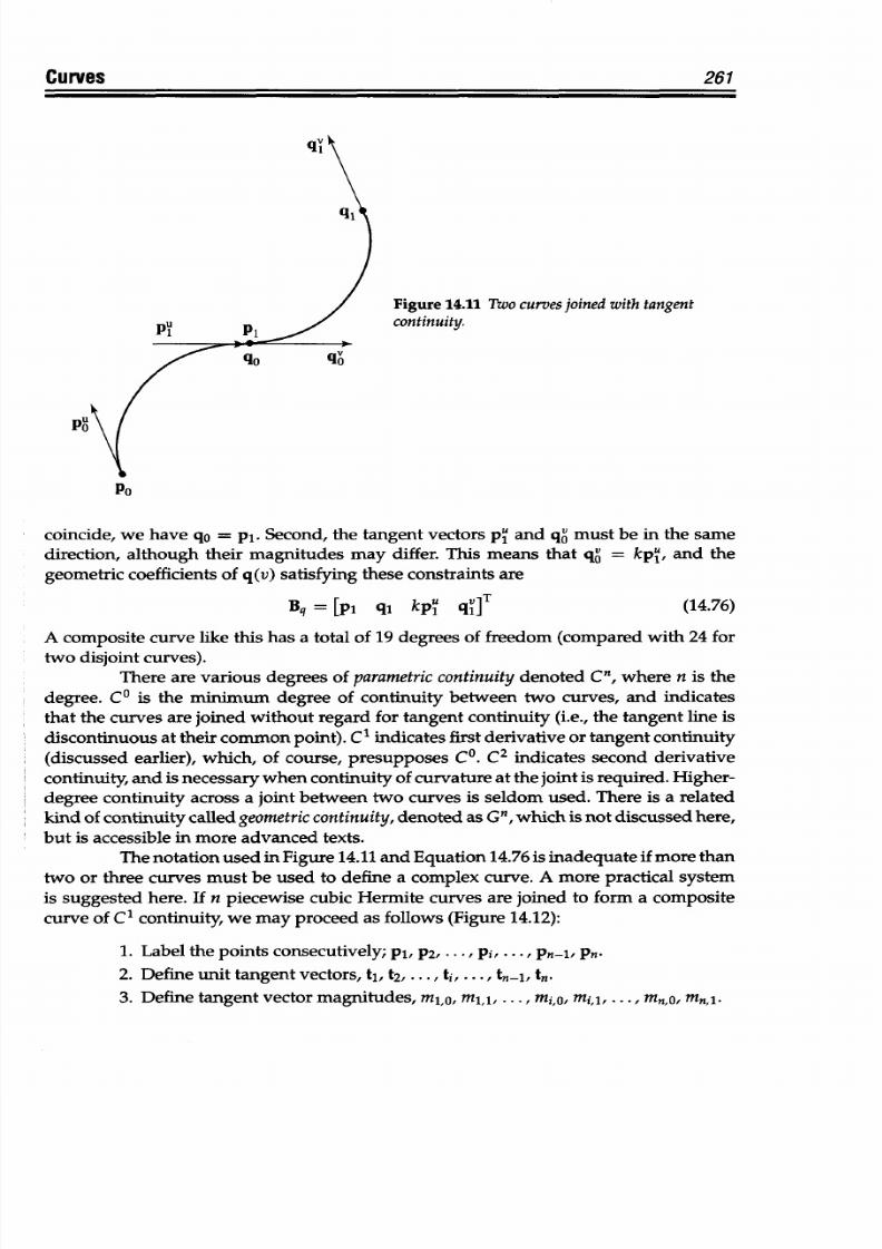
8/9/2019 Mortenson, Michael E. - Mathematics for computer graphics applications.pdf
http://slidepdf.com/reader/full/mortenson-michael-e-mathematics-for-computer-graphics-applicationspdf 274/367
261
urves
Figure
14.11 Two curves
joined with
tangent
continuity.
Po
coincide, we have qo = pi. Second, the
tangent
vectors pu
and
qv
must be
in
the
same
direction,
although
their magnitudes may
differ. This means that qv = kpu,
and the
geometric coefficients
of q(v)
satisfying these
constraints
are
Bq
= [pi
qi
kpu q ]T
(14.76)
A
composite curve
like
this has a total
of
19 degrees
of
freedom (compared with 24 for
two
disjoint
curves).
There are
various
degrees
of
parametric
continuity denoted
Cn,
where
n is the
degree.
CO is
the
minimum
degree
of
continuity between two curves,
and
indicates
that
the
curves are
joined without
regard
for tangent
continuity
(i.e.,
the tangent
line is
discontinuous
at
their
common point). C1 indicates first derivative or tangent
continuity
(discussed
earlier),
which,
of course, presupposes
Co. C
2
indicates
second derivative
continuity, and
is
necessary when
continuity
of
curvature
at the joint is required. Higher-
degree
continuity
across
a joint
between
two curves
is seldom
used.
There
is a related
kind of
continuity
called
geometric
continuity, denoted as
Gn,
which is not
discussed
here,
but is
accessible in
more advanced
texts.
The
notation
used in Figure 14.11
and
Equation 14.76
is inadequate if more
than
two or three curves must
be
used
to
define a complex
curve.
A more practical system
is
suggested
here.
If
n piecewise cubic
Hermite curves
are joined to
form
a
composite
curve
of
C1 continuity, we may proceed
as
follows
(Figure 14.12):
1.
Label
the
points
consecutively; pi,
p2,
.
.
-, pi, ** *, Pn-1, Pn-
2.
Define
unit
tangent
vectors,
tI,
t
2
,
. . ., ti, .. *, tn-it
tn -
3.
Define
tangent vector magnitudes, mio, mi,i,
...
,
Inmi,,
mijl, . . .,
m
o, mn.
PU
0
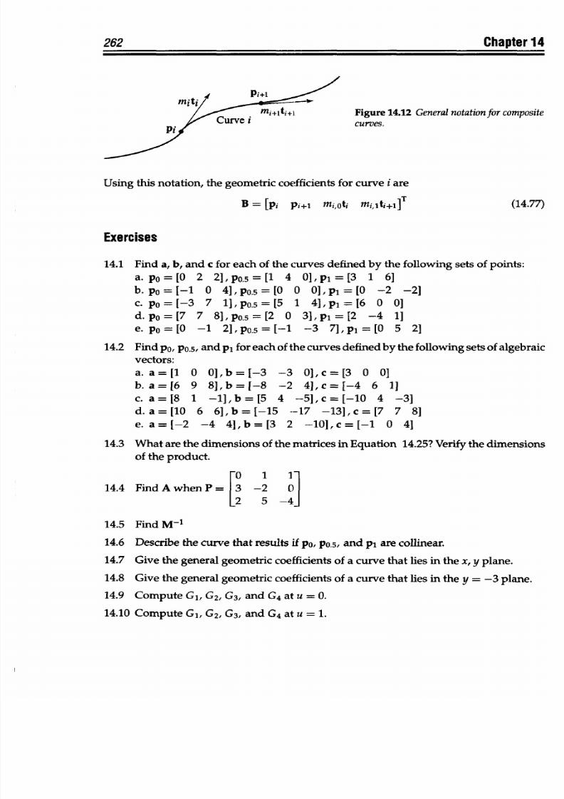
8/9/2019 Mortenson, Michael E. - Mathematics for computer graphics applications.pdf
http://slidepdf.com/reader/full/mortenson-michael-e-mathematics-for-computer-graphics-applicationspdf 275/367
262 Chapter
14
Figure
14.12 General
notationfor
composite
curves.
Using this notation,
the
geometric
coefficients
for curve
i are
B
=
[pi Pi+1
miOt
i
Milti+J]
(14.77)
Exercises
14.1
Find
a,
b, and c for each of the
curves defined by the
following sets
of
points:
a. po=[O 2
2
1,po.5=[l 4 01,p'=[3
1 6]
b. po =
[-
1
0 4], po.5 = [0 0 °],
pi
=
[0
-2 -2]
c.
po
=
[-
3
7
i],po.5
=
[5 1
4],pi = [6
0
0]
d.
po
=
[
7
7
8
], PO.5
=
[
2
0
3], pi =
[2 -4
1]
e. pO [O
-1
2
1,
PO.5
=
[-1
-3
7], pi
=
[0 5 2]
14.2 Find po,
po.5, and pi for each
of the
curves defined
by the
following
sets of algebraic
vectors:
a.
a=[1 0 0],b=[-3
-3 O],c=[3 0
0]
b.
a=[6 9 8],b=[-8
-2 4],c=[-4
6 1]
c. a= [8 1
-1],
b
=[5
4
-5], c
=[-10
4 -3]
d.
a
=[10
6 6],b =[-15
--17
-13], c =
[7
7
8]
e.
a=
[-2 -4 4],b=
[3
2 -1O1,c=
[-1
0
4]
14.3
What are
the
dimensions of
the m atrices in Equation 14.25?
Verify
the
dimensions
of the product.
-O 1 1-
14.4
Find
A whenP=
-2
0
25 -4
14.5
Find
M-1
14.6
Describe the
curve that results if po,
po.5, and pi are
collinear.
14.7
Give
the
general
geometric
coefficients of
a curve that
lies in the
x, y plane.
14.8 Give
the general
geometric
coefficients
of
a curve
that
lies
in
the
y =
-3 plane.
14.9
Compute G
1
, G
2
, G
3
,
and
G
4
at
u
= 0.
14.10
Compute
G
1
, G
2
,
G
3
,
and
G
4
at
u =
1.
8/9/2019 Mortenson, Michael E. - Mathematics for computer graphics applications.pdf
http://slidepdf.com/reader/full/mortenson-michael-e-mathematics-for-computer-graphics-applicationspdf 276/367
8/9/2019 Mortenson, Michael E. - Mathematics for computer graphics applications.pdf
http://slidepdf.com/reader/full/mortenson-michael-e-mathematics-for-computer-graphics-applicationspdf 277/367
(AU M
THE BEZIER
CURVE
The
Bezier curve is an
important
part
of
almost every computer-graphics illustration
program
and computer-aided design
system
in use
today. It
is
used
in
many
ways,
from
designing
the curves
and
surfaces
of
automobiles
to
defining
the shape
of
letters
in
type
fonts.
And because it
is numerically the most stable
of
all
the
polynomial-based
curves
used
in
these applications, the Bezier curve
is the
ideal
standard for
representing
the
more
complex piecewise
polynomial
curves.
In the early 1960s,
Peter
Bezier (pronounced bay-zee-aye)
began
looking for
a
better way to define curves and surfaces, one that would be
useful
to a
design
engineer.
He
was
familiar
with
the work
of
Ferguson and
Coons
and their
parametric
cubic
curves
and bicubic surfaces. However,
these did not
offer
an intuitive
way to
alter and
control
shape.
The results of
B&zier's
research led
to the curves
and surfaces that
bear
his
name
and
became
part
of
the
UNISURF
system.
The
French
automobile manufacturer,
Renault,
used
UNISURF
to
design the sculptured
surfaces of
many
of
its products.
This
chapter
begins
by describing a surprisingly simple geometric
construction
of a Bezier curve, followed by a derivation
of its
algebraic
definition,
basis functions,
control
points, degree
elevation, and
truncation.
It
concludes
by
showing
how
to
join
two
curves end-to-end to form a single composite
curve.
15.1
AGeometric Construction
We
can
draw
a
B&zier
curve using
a
simple recursive geometric
construction.
Let's begin
by constructing a
second-degree curve
(Figure
15.1).
We select
three
points
A, B, C,
so
that line
AB
is
tangent to the curve at
A,
and line BC is tangent at C. The curve
begins at
A
and ends at C.
For
any ratio
ui,
where 0
< ui c 1,we construct
points
D and
E so
that
AL)
B
E
AB BC
i (15.1)
On
DE
we
construct
F so that DF
DE
=
ui. Point F
is
on the
curve.
Repeating this
process for
other values
of
ui,
we
produce
a
series of
points
on
a B&zier
curve.
Note that
we must be consistent in the order in which
we
sub-divide
AB
and BC. For
example,
AD/AB
:A EC/BC.
264
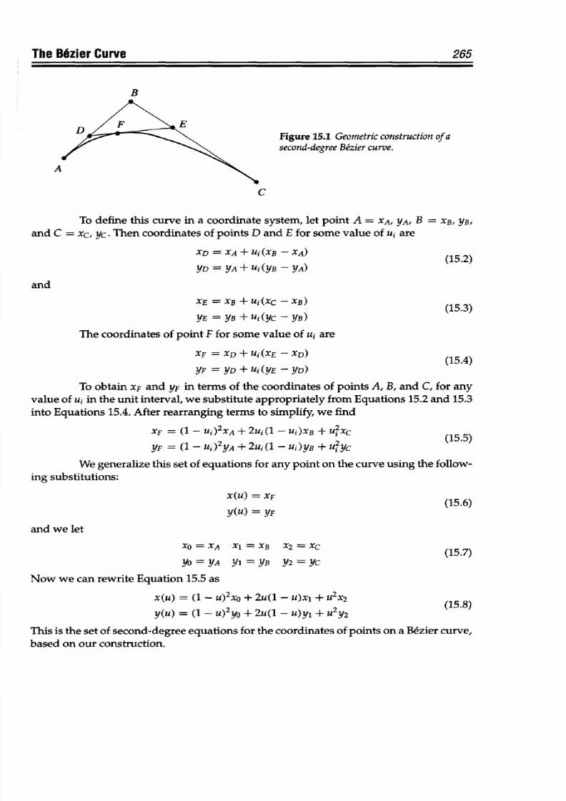
8/9/2019 Mortenson, Michael E. - Mathematics for computer graphics applications.pdf
http://slidepdf.com/reader/full/mortenson-michael-e-mathematics-for-computer-graphics-applicationspdf 278/367
The Bezier Curve 265
B
Figure 15.1
Geometric
construction
of
a
second-degree BMzier curve.
A
C
To define this
curve
in a
coordinate
system, let
point
A
= XA,
yA, B = XB, YB,
and C
= xc,
yc.
Then coordinates
of
points D
and
E for
some
value
of ui
are
XD
=
XA
+
Ui(XB
-
XA)
(15.2)
YD
= YA
+
Ui(YB -YA)
and
XE
=
XB
+ Ui(Xc - XB)
YE = YB +Ui
(YCY-IYB)
The coordinates of
point
F for some value of ui are
XF
= XD
+ Ui (XE - XD)
(15.4)
YF
= YD + Ui(YE - YD)
To
obtain
XF and yF in terms of the co ordinates of
points
A, B,
and
C, for
any
value of ui in the
unit interval,
we
substitute
appropriately from
Equations
15.2 and
15.3
into Equations 15.4.
After rearranging terms to simplify, we
find
XF
= (1
-
U)
2
XA
+
2ui(1 -
Ui)XB
+ U>XC (15.5)
yF = (1 -U)
2
yA +
2
Ui(l -Ui)yB + 2iyc
We generalize
this
set
of equations
for any point on
the
curve
using the follow-
ing
substitutions:
X(U)
= XF
(56
Y(U) = YF
and we let
XO
=
XA X1
=
XB X2
=
XC
(15.7)
YO = YA Y1 = YB Y2 = YC
Now we
can
rewrite Equation
15.5
as
x(u) = (1
-
u)
2
xO
+
2u(1 -
u)x
1
+ u
2
x
2
y(u)
=
(1
-
u)
2
yo + 2u(1
- u)yl + u
2
y
2
(15.8)
This is the set of second-degree equations for the coordinates of
points
on a B&zier curve,
based
on
our construction.
-. -, .
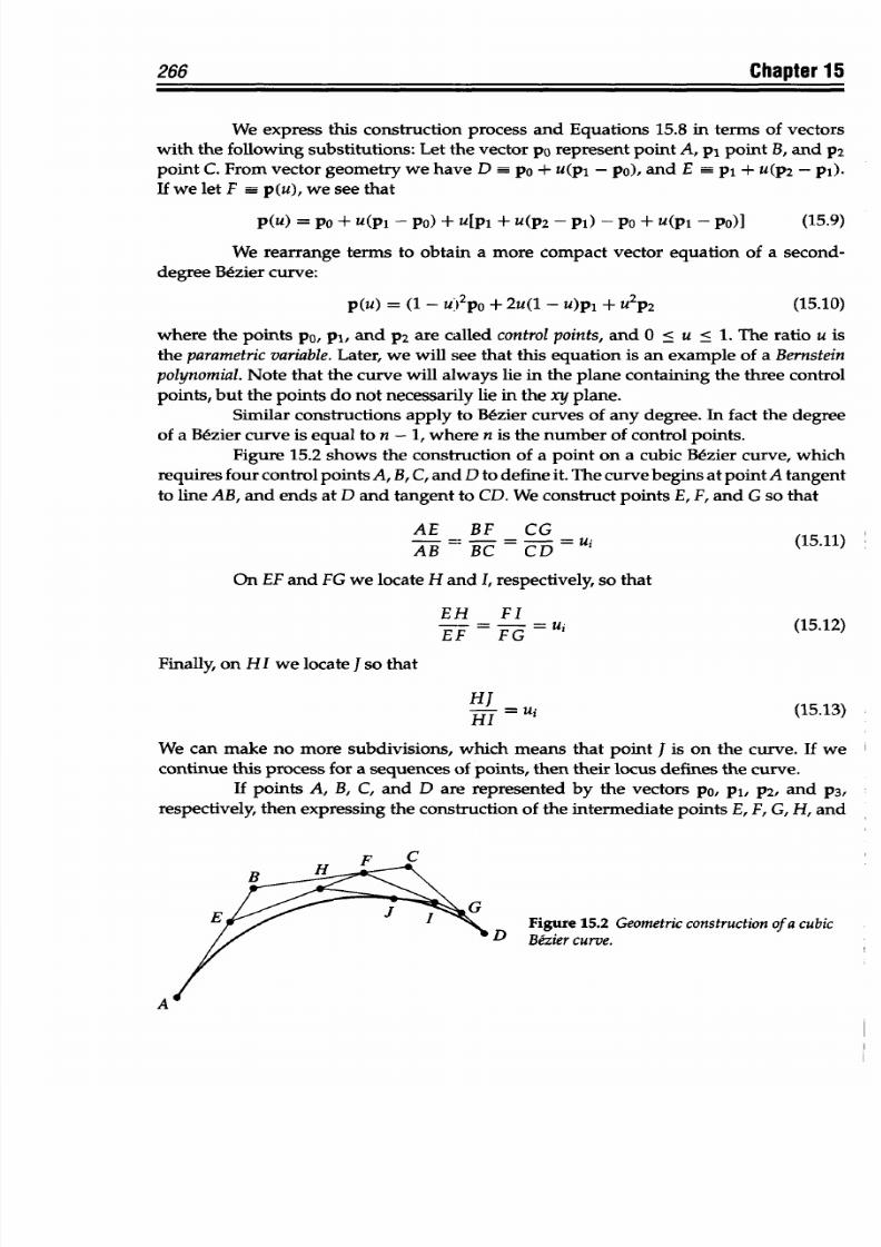
8/9/2019 Mortenson, Michael E. - Mathematics for computer graphics applications.pdf
http://slidepdf.com/reader/full/mortenson-michael-e-mathematics-for-computer-graphics-applicationspdf 279/367
266
Chapter 15
We
express
this
construction
process
and Equations 15.8
in terms
of
vectors
with the following
substitutions: Let
the vector P0 represent point
A, pi
point
B,and
p2
point C.From vector
geometry we
have
D -
pO
+
u(p
1
- PO), and E
p' +
u(p
2
-
pi).
If
we
let F -p(u),
we
see
that
p(u)
=
pO
+ u(p
1
- P0) + ulp1 + u(p2 - p1)
- pO + u(p1 - PO)]
(15.9)
We rearrange terms
to
obtain
a
more compact vector
equation of
a
second-
degree Bezier curve:
p(u) (1 - u
2
pO
+
2u(1
-
u)pl + u
2
p2
(15.10)
where
the
points
Po, pl, and p2
are called control points,
and
0 <
u <
1.
The
ratio u is
the
parametricvariable.
Later,
we
will see that
this
equation
is
an
example of a Bernstein
polynomial.
Note
that
the curve
will always
lie
in
the
plane
containing the three
control
points,
but the
points
do not necessarily lie
in
the
xy
plane.
Similar
constructions
apply
to Bezier curves
of any degree. In fact the degree
of a
Bezier
curve is
equal to n - 1,
where
n
is the number of control
points.
Figure 15.2
shows the construction of a
point
on
a cubic B&zier curve, which
requires
four control
points A, B,
C,
and
D to define it. The curve
begins
at
point A
tangent
to line AB,
and
ends at
D
and
tangent
to
CD.
We
construct points
E, F, and G so
that
AE
BF
CG
AB BC =CD
=
u(15.11)
On EF and FG we locate
H
and
I, respectively,
so
that
EH _F l
E=
=
Ui
(15.12)
Finally, on HI we
locate
I so that
HI
= Ui
(15.13)
HI
We
can make
no more subdivisions, which means
that point
I is
on the
curve. If
we
continue
this
process
for
a
sequences
of
points, then
their
locus defines
the curve.
If
points A, B, C, and D
are
represented
by
the
vectors
po,
pi, p2,
and
P3,
respectively,
then
expressing
the
construction of
the intermediate points E, F, G, H, and
Figure 15.2 Geometric
constructionofa cubic
D
BMzier
curve.
A
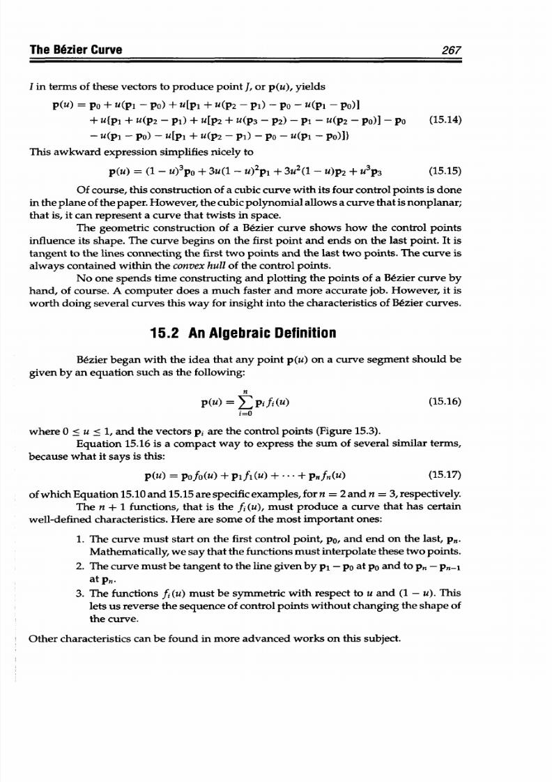
8/9/2019 Mortenson, Michael E. - Mathematics for computer graphics applications.pdf
http://slidepdf.com/reader/full/mortenson-michael-e-mathematics-for-computer-graphics-applicationspdf 280/367
The Bdzier
Curve
267
I
in
terms
of
these vectors
to
produce point J, or p(u), yields
p(U)
= pO
+ U(pl -o) + U[pl +
U(p2 -
pl)
- pO - U(pl
- Po)
+
U{p1
+
U(p2
-
p)
+U[p2 + U(p
3
-
p2)
-pi
- U(p2
-o)]-pO (15.14)
-U(p
1
-Po) -U[p
1
+ U(p2-pl)
-pO-U(p -pO)])
This awkward expression simplifies nicely to
p(u) = (1 -
u)
3
po
+
3u(1
-
U)
2
p, +
3U
2
(1 -
U)p2 + U
3
p3 (15.15)
Of course, this construction
of
a cubic curve with its
four
control points is done
in the plane
of
the paper. However, the
cubic
polynomial
allows a curve that
is
nonplanar;
that is, it
can
represent
a
curve
that
twists in
space.
The
geometric construction of a Bezier curve shows how the control points
influence its shape. The
curve begins on the
first point
and ends
on
the last point. It
is
tangent to the lines connecting
the first
two
points and
the last
two points. The
curve is
always contained within the convex hull
of
the control points.
No one spends time constructing and plotting the points
of
a Bezier curve by
hand, of course. A
computer
does a
much faster and more
accurate job. However,
it
is
worth doing several curves this way for
insight into
the characteristics of Bezier curves.
15.2
An Algebraic
Definition
Bezier
began
with the idea that
any
point
p(u)
on a
curve
segment
should be
given by an equation such
as
the
following:
n
p(u) = Epi i(u)
(15.16)
i=o
where
0 < u < 1, and the vectors pi are the control points
(Figure 15.3).
Equation 15.16
is
a compact way to express
the
sum
of
several similar terms,
because
what it says
is
this:
p(u) = pofo(u)
+ pifi(u) +
*
+ pnfn(u) (15.17)
of
which Equation
15.10
and
15.15
are specific
examples, forn = 2
and
n = 3, respectively.
The
n + 1 functions, that is the fi (u), must produce a curve that
has
certain
well-defined characteristics. Here are some of the most
important ones:
1. The curve must
start
on the first control
point,
Po, and end on the
last,
pn-
Mathematically, we say that the functions must interpolate these two points.
2.
The
curve must be tangent
to
the
line
given
by pi
-
p0 at p0 and
to
Pn
-
Pn-1
at Pn.
3. The
functions fi (u) must
be
symmetric with respect
to u and
(1 - u).
This
lets
us
reverse the
sequence of
control points
without
changing the shape
of
the
curve.
Other
characteristics can
be found in
more
advanced works
on this subject.
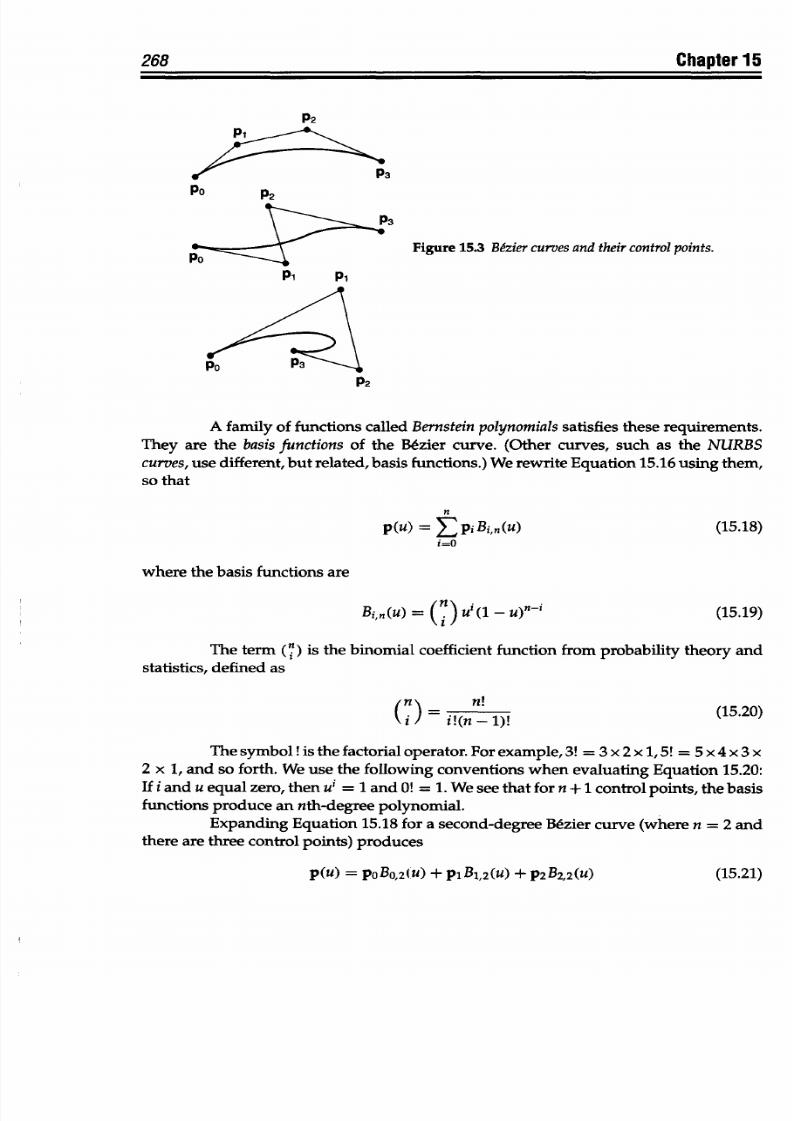
8/9/2019 Mortenson, Michael E. - Mathematics for computer graphics applications.pdf
http://slidepdf.com/reader/full/mortenson-michael-e-mathematics-for-computer-graphics-applicationspdf 281/367
268
Chapter
15
P2
Ply
t
PS
Po P
2
> -
P3
Figure 15.3
BMzier curves
and
their
control
points.
Pi Pi
P
2
A
family
of functions
called Bernstein
polynomials satisfies
these requirements.
They are the
basis
functions
of
the
Bdzier
curve.
(Other
curves,
such as the
NURBS
curves,
use different,
but
related, basis functions.)
We
rewrite
Equation
15.16 using
them,
so
that
n
p(u) = EpiBi,n(u)
(15.18)
i=O
where
the basis
functions
are
Bi,n U)
=(ia
)
-H
1ur-i
(15.19)
The
term (i) is the
binomial
coefficient
function
from
probability
theory
and
statistics,
defined
as
(nf
n!
(15.20)
(i
) = (n-1)
The
symbol
is
the
factorial
operator.
For
example, 3! = 3
x 2
x
1,5!
=
5
x 4
x 3
x
2
x
1,
and
so
forth.
We
use the following conventions
when
evaluating
Equation 15.20:
If i and u
equal zero,
then
ui
=
1 and 0!
=
1.
We
see that
for n + 1
control points,
the basis
functions produce
an nth-degree
polynomial.
Expanding
Equation 15.18
for a second-degree Bezier
curve
(where
n = 2
and
there
are
three control points)
produces
p(u) =
poBo,
2
(u)
+
piB
1
,
2
(U)
+p
2
B
2
,
2
(u)
(15.21)
8/9/2019 Mortenson, Michael E. - Mathematics for computer graphics applications.pdf
http://slidepdf.com/reader/full/mortenson-michael-e-mathematics-for-computer-graphics-applicationspdf 282/367
The Bezier Curve
269
From
Equation
15.20 we find
Bo,
2
(u) =
(1
-
u)
2
(15.22)
B1,
2
(u)
=
2u(1
-
u) (15.23)
B
2
,
2
(u) = U2
(15.24)
These
are
the
basis functions for
a
second-degree Bezier curve. Substituting them into
Equation
15.21 and
rearranging
terms,
we
find
p(u) = (1
-
u)
2
po
+
2u(1 -
u)pl
+ u
2
p2
(15.25)
This is
the
same expression
we
found
from
the geometric construction,
Equation
15.10.
The variable
u is now
called
the
parametricvariable.
Now,
let's expand Equation
15.18
for
a cubic Bezier
curve,
where
n
=
3:
p(u) =
poBo,
3
(u) + pi B1,
3
(u)
+ p
2
B
2
,
3
(u) + p
3
B
3
,
3
(u) (15.26)
and
from Equation 15.20 we find
Bo,
3
(u) =
(1
-_u)
3
(15.27)
BL
3
(u)
=
3u(1 -U)2 (15.28)
B
2
,
3
(u)
= 3u
2
(1
-
u) (15.29)
B
3
,
3
(u)
=
U3
(15.30)
Substituting these
into Equation
15.26 and rearranging terms produces
p(u)
=
(1
-
u)
3
po + 3u(1
-
u)
2
p, + 3u
2
(1
-
u)p2 + u
3
p3 (15.31)
B&zier curve
equations
are
well suited
for expression in
matrix
form.
We
can
expand the
cubic
parametric
functions and
rewrite Equation
15.31
as
(1-3u + 3U2
-
u
3
)
T
u)
u -
6u
2
+ 3u
3
)
P(
p(u)
(3U2
-
3U3)
P2
(15.32)
U P3
or
as
-[1 3
-3 1- Po
p(u)=[u3
u2
u 1]
3
-6 3 0
p2
(15.33)
1
0 0 0-
P3_
If we
let
U = [u
3
u
2
u 1] (15.34)
P =
[pO Pl P2
p3]
(15.35)
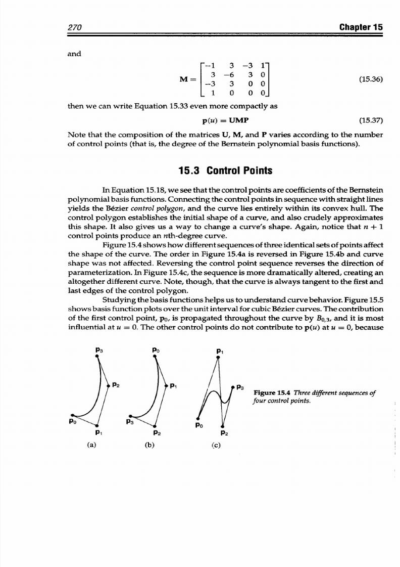
8/9/2019 Mortenson, Michael E. - Mathematics for computer graphics applications.pdf
http://slidepdf.com/reader/full/mortenson-michael-e-mathematics-for-computer-graphics-applicationspdf 283/367
270
Chapter
15
and
--_ 3
-3
1-
M
3 -6 3
0
(15.36)
I
0
0
0-
then
we
can write
Equation 15.33 even
more compactly
as
p(u) = UMP
(15.37)
Note that the
composition of
the
matrices
U,
M,
and P varies according
to the number
of control
points (that
is,
the degree of the Bernstein
polynomial
basis functions).
15.3
Control
Points
In
Equation
15.18,
we see that the control
points are
coefficients of
the
Bernstein
polynomial
basis
functions.
Connecting
the
control
points
in sequence with straight lines
yields
the
Bezier control
polygon,
and
the
curve
lies entirely within its
convex hull. The
control polygon
establishes the initial
shape
of a
curve,
and also
crudely
approximates
this
shape. It also
gives us a way to change
a curve's shape. Again,
notice that n + 1
control
points
produce
an nth-degree
curve.
Figure
15.4
shows
how different sequences of three
identical sets of
points
affect
the shape
of
the
curve. The
order
in Figure
15.4a
is
reversed
in Figure
15.4b
and
curve
shape was not
affected.
Reversing the control
point sequence reverses
the direction
of
parameterization. In
Figure
15.4c,
the sequence is more
dramatically altered, creating an
altogether different
curve. Note,
though,
that
the curve
is always
tangent
to
the
first
and
last
edges of the control polygon.
Studying the basis
functions
helps
us to
understand
curve
behavior.
Figure
15.5
shows
basis
function
plots over the
unit
interval
for cubic B&zier
curves. The contribution
of
the
first
control
point,
po,
is
propagated
throughout
the curve
by
BO,
3
, and it
is
most
influential at u
=
0.The other control points do not
contribute to p(u)
at u =
0,
because
Pi
P2
P3
I3
Figure
15.4 Three
different
sequences
of
four control points.
Pi
(a) (b)
P2
(c)
P2
I
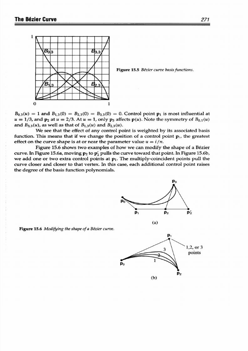
8/9/2019 Mortenson, Michael E. - Mathematics for computer graphics applications.pdf
http://slidepdf.com/reader/full/mortenson-michael-e-mathematics-for-computer-graphics-applicationspdf 284/367
The Bezier Curve
1
271
0
Figure 15.5 Bezier curve basis
functions.
1
BO ,
3
(u) = 1
and
B
1
,
3
(0)
= B
2
,
3
(0) = B
3
,
3
(0) = 0. Control point pi is most influential
at
u
= 1/3,
and P2
at
u
= 2/3.
At
u = 1, only
p3
affects
p(u). Note the symmetry
of
Bo,, (u)
and B
3
,
3
(u), as well as that of B
1
,
3
(u) and B
2
,
3
(u).
We see
that
the
effect
of any
control point
is weighted
by its associated basis
function. This
means
that if
we
change
the position
of
a
control point pi,
the
greatest
effect on the curve shape is at or near the parameter value u
=
i/n.
Figure 15.6
shows two
examples of how
we
can
modify
the shape of a
Bezier
curve.
In
Figure
15.6a, moving p
2
to P
2
pulls
the curve toward
that
point. In Figure 15.6b,
we
add
one
or
two
extra control
points
at
pi.
The
multiply-coincident points
pull
the
curve closer and closer to that vertex.
In
this case,
each
additional
control point raises
the degree of
the
basis
function
polynomials.
P
1
P2 P2
(a)
Figure 15.6
Modifying
the shape of
a
Bezier curve.
1,2,
or 3
points
P2
(b)
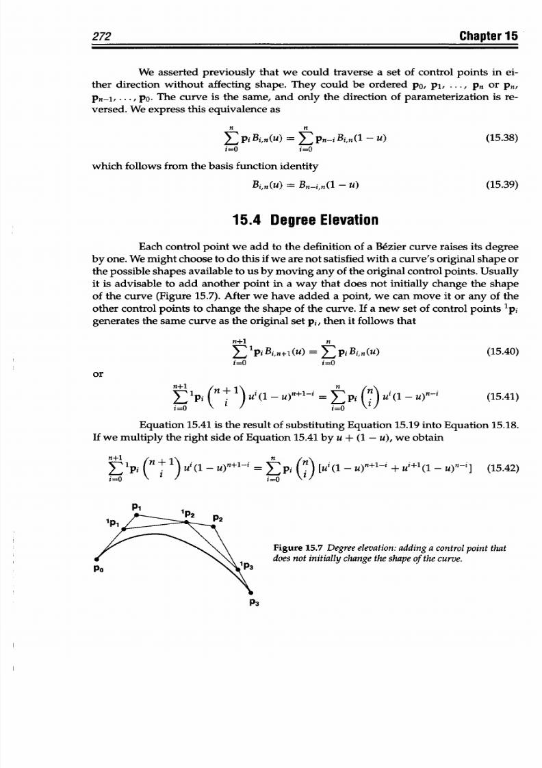
8/9/2019 Mortenson, Michael E. - Mathematics for computer graphics applications.pdf
http://slidepdf.com/reader/full/mortenson-michael-e-mathematics-for-computer-graphics-applicationspdf 285/367
272
Chapter 15
We asserted previously
that
we could traverse
a
set
of
control points
in
ei-
ther direction
without
affecting shape. They could be
ordered po, pl,
... , Pn
or
pn,
Pn-l, .. . ,
po. The
curve
is
the same, and
only the
direction of parameterization
is re-
versed.
We
express
this
equivalence as
n n
E pi Bi~n,()
=
Epn-i Bin(1 - u) (15.38)
i=O i=O
which
follows
from the basis function identity
Bin(U) = Bn-i~n(l -
U) (15.39)
15.4
Degree
Elevation
Each
control
point
we
add to
the definition of
a
Bezier curve raises its degree
by
one.
We
might
choose
to do this if we are not satisfied
with a
curve's original shape or
the
possible
shapes available to us
by
moving any
of the original control
points. Usually
it
is
advisable
to
add another point
in a
way that
does
not initially change
the shape
of
the curve (Figure 15.7). After
we have
added a
point,
we can
move
it
or any
of
the
other
control points
to change the shape of the
curve.
If
a new set
of
control
points
'pi
generates the same curve
as
the original set pi,
then
it
follows
that
n+1 n
E
p=
EjpiBzn(u)
(15.40)
i=O
i=O
or
E lpi
(n + u(1 -
u)n+
1
-
Epi
(n)
ui(1
-
U)n (15.41)
Equation 15.41 is the result of substituting
Equation
15.19 into Equation 15.18.
If we multiply the right
side
of
Equation
15.41 by u
+
(1 - u), we obtain
E pi
u
(1 - u)n+l i = EPi
[l i
(1
- U)n+1 )n (15.42)
i=O
=
Figure 15.7 Degree elevation:adding a control
point that
does not initially
change
the shape of the curve.
P
3
l
I
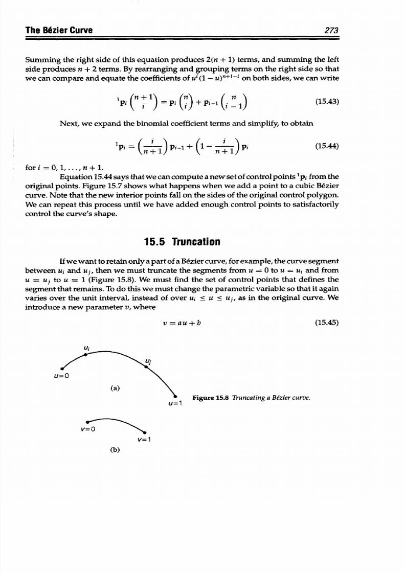
8/9/2019 Mortenson, Michael E. - Mathematics for computer graphics applications.pdf
http://slidepdf.com/reader/full/mortenson-michael-e-mathematics-for-computer-graphics-applicationspdf 286/367
The Bdzier Curve
273
Summing the right side of this equation produces 2(n + 1) terms, and summing the left
side produces n + 2 terms. By rearranging
and
grouping terms on the right side so
that
we can compare
and
equate the coefficients
of ui (1 -
u)f+
1
-i on both
sides, we can
write
p i ) +p (i -
1
) (15.43)
Next, we
expand
the binomial
coefficient terms and simplify,
to obtain
1
Pi =
(+)1p+ (
n+1)
(15.44)
for i= 1, .. ,n+ 1.
Equation
15.44
says that
we
can compute a new set of control points 'pi
from
the
original points. Figure
15.7 shows what
happens when
we
add a point
to
a
cubic
Bezier
curve. Note that the
new
interior points
fall
on
the
sides
of the original
control
polygon.
We can
repeat
this process
until
we
have
added
enough control points to satisfactorily
control the curve's shape.
15.5
Truncation
If
we
want
to
retain only
a
part
of
a
Bezier curve,
for
example,
the curve segment
between ui
and up,
hen we must
truncate the
segments from u = 0 to
u
= ui and from
u
=
uj
to u
= 1 (Figure
15.8). We must
find the
set
of
control
points
that defines the
segment that remains. To do this we must change the parametric variable
so
that it again
varies over
the
unit
interval, instead of
over ui
< u < u,, as in the original
curve. We
introduce
a
new
parameter v, where
v=au+b
(15.45)
Li
tbnFialr
aE Tnmn-nh
ua
n cPurn--
U=
1 4
- -
If
- - -
v=0
v=1
(b)
8/9/2019 Mortenson, Michael E. - Mathematics for computer graphics applications.pdf
http://slidepdf.com/reader/full/mortenson-michael-e-mathematics-for-computer-graphics-applicationspdf 287/367
274
Chapter 15
This
transformation applies
to
parametric
polynomial
equations of any
degree. The
linear
relationship
between u
and
v
(Equation 15.45)
preserves
the degree of
the polynomial.
If v
=
Oat
u =
-ui,
and
v =
1 at u = uj, then
u
=
(uj
ui)v
+
ui
(15.46)
or
u
= Auiv +u
where
Aui
= Uj
-i
(15.48)
The
general
transformation equation for
the parametric variable
(not derived
here)
is
n
n
n-k
=
k(n k)ul (AUi V)
(15.49)
This
equation looks
more formidable than
it
is. From
it
we
extract
a transformation matrix
T such
that
[un un-I
...
U
1]
= [vn
fl-1 .-
v 1]T
or
U=VT
(15.50)
(15.51)
Here
is an example: Given
the three
control points
that define
a
second-
degree
Bezier curve, we
can find three
new control
points that
define the
segment of
the curve
from
ui to uj
in
terms
of
a new parameter
v, which
spans the unit
interval,
0 < v < 1.
The
control
points
that define
the original curve
are
(in
matrix
form)
P
=
p[
and
the
control
points
that
define
the
truncated
segment
are
PI
o
(15.52)
(15.53)
So for
a second-degree B6zier
curve,
we have (similar to the
matrix
Equation
15.37
for
a
cubic curve)
p(U) =
UMP
(15.54)
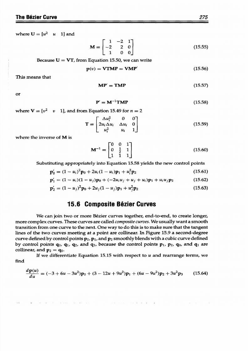
8/9/2019 Mortenson, Michael E. - Mathematics for computer graphics applications.pdf
http://slidepdf.com/reader/full/mortenson-michael-e-mathematics-for-computer-graphics-applicationspdf 288/367
The
BMzier
Curve
275
where U
= [u
2
u
1] and
1
-2
1-
M= -2
2
0 (15.55)
-1
0
0
Because
U
=
VT,
from Equation 15.50, we can write
p(v)
=
VTMP
=
VMP'
(15.56)
This
means
that
MP
=
TMP (15.57)
or
P' = M-1TMP
(15.58)
where V
=
[v
2
v 1], and from Equation 15.49 for n
=
2
[
Au? 0
0
T 2ui Aui Aui
0
(15.59)
U Ui 1
where
the inverse of
M is
O0
1
M-1= ° 1 ]
(15.60)
Substituting
appropriately into Equation 15.58 yields
the
new control points
p'
=
(1 - ui)
2
po + 2ui (1 -
ui)p1
+
up
2
(15.61)
p'=
(1 - ui)(1 - u)po
+ (-2uiuj + uj + ui)pl
+ uiuj
p
2
(15.62)
p
2
= (1 - + 2uj(1 -
uj)pI
+
ujp2
(15.63)
15.6 Composite
Bezier
Curves
We can
join two
or more Bezier curves together, end-to-end,
to
create longer,
more complex
curves.
These curves
are
called composite curves. We
usually want
a
smooth
transition from
one
curve to
the next.
One way to
do this
is to make
sure that
the tangent
lines
of
the
two curves
meeting
at
a
point are collinear. In Figure 15.9
a
second-degree
curve defined by control points
po,
pi, and
p2 smoothly
blends with a cubic curve defined
by
control
points qo,
qi, q2,
and
q3,
because the control points p1,
P2, qo,
and qi
are
collinear, and P2
= qo.
If
we differentiate Equation 15.15
with respect
to u
and
rearrange
terms, we
find
dp(u) = (-3 +
6u
- 3U
2
)po
+ (3- 12u + 9u
2
)pl + (6u -
9u
2
)p2 + 3u
2
p3
(15.64)
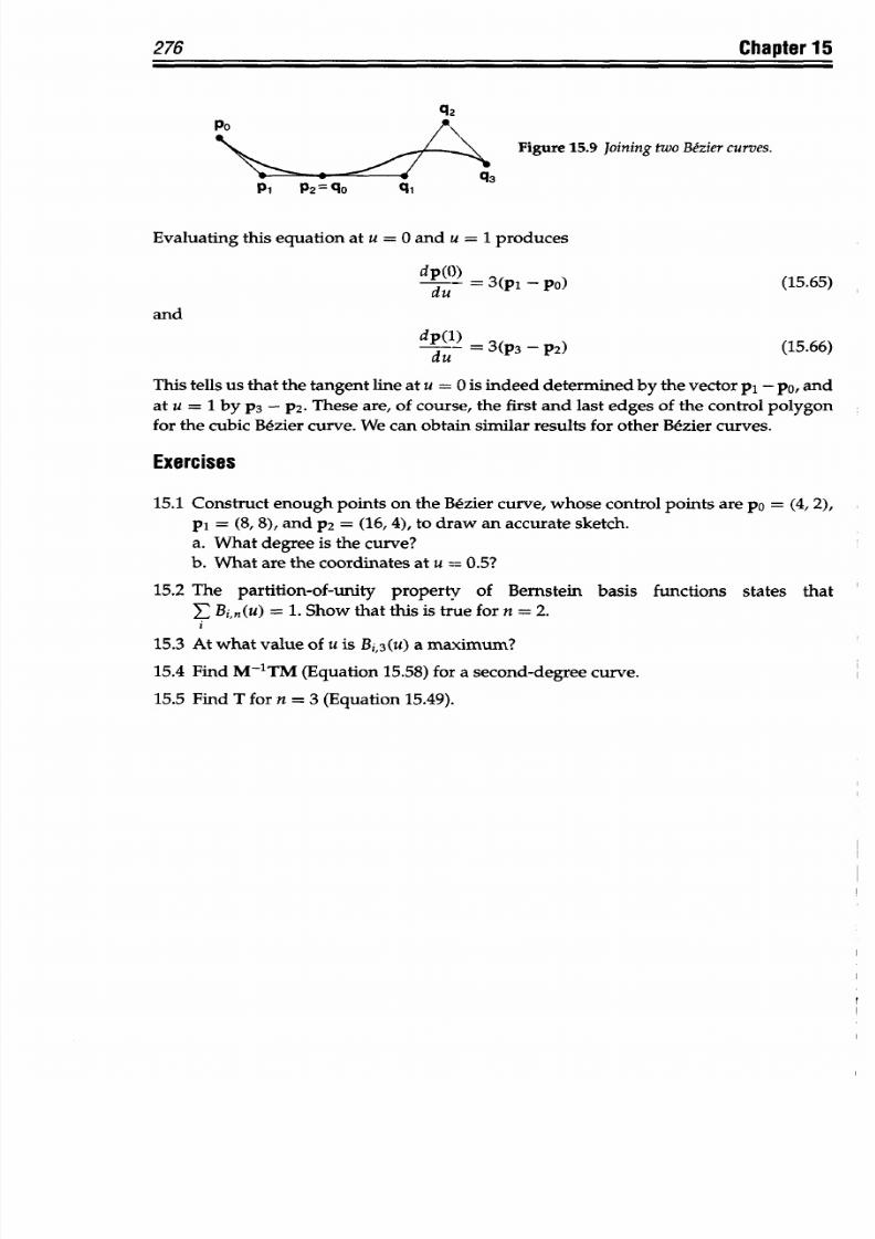
8/9/2019 Mortenson, Michael E. - Mathematics for computer graphics applications.pdf
http://slidepdf.com/reader/full/mortenson-michael-e-mathematics-for-computer-graphics-applicationspdf 289/367
276
Chapter 15
q
2
Po
Figure
15.9 Joining
two Bezier curves.
q
3
PI
P2=
qO
qt
Evaluating
this equation
at u =0 and u =1 produces
dp(u) 3(p-
-
po)
(15.65)
and
dp(l)
3(P -
P2)
(15.66)
This tells us
that the tangent
line at
u = 0
is indeed determined by the
vector
pl
-
po, and
at
u
= 1 by p3
-
P2. These
are,
of
course, the first
and
last edges
of
the
control
polygon
for the
cubic Bezier curve.
We
can
obtain
similar
results for
other
Bezier
curves.
Exercises
15.1
Construct
enough
points on
the B&zier curve, whose control
points are po =
(4,
2),
pi =
(8,
8), and p2
= (16, 4), to
draw
an
accurate
sketch.
a. What degree
is the
curve?
b. What
are
the
coordinates at
u
0.5?
15.2
The partition-of-unity property
of Bernstein
basis functions
states that
E B,(u)
= 1.
Show that this
is true for n = 2.
15.3
At
what
value of u
is Bi,
3
(u)a maximum?
15.4 Find
M-
1
TM
(Equation 15.58) for a second-degree curve.
15.5 Find T for n
=
3 (Equation 15.49).
8/9/2019 Mortenson, Michael E. - Mathematics for computer graphics applications.pdf
http://slidepdf.com/reader/full/mortenson-michael-e-mathematics-for-computer-graphics-applicationspdf 290/367
(Au
Ta
SURFACES
Just as with
curves,
we all have an intuitive
sense
of what
a
surface
is.
A
surface
is
perhaps a little
less abstract
a concept than a curve,
if only because we
can ac-
tually touch
the
surfaces of the ordinary
objects
that
fill
our environment.
It is
light
reflected
off an
object's surfaces that
makes it visible. It didn't take long
for math-
ematicians and
computer
graphics applications developers to realize
that
to create a
convincing
display
of an object they
had
to thoroughly understand the
mathematics of
surfaces.
The
parametric
functions that describe a surface
are somewhat
different from
those used for curves.
Two
independent parametric
variables
are
required
for
surfaces,
so the equations' general form looks
like
x
=
x(u, w),
y
= y(u, w), z = z(u, w) (16.1)
Both parametric variables
are
usually
limited to
the
unit interval
0
<
u, w < 1,
which
is
often expressed as u,
w
e [0, 1].
This
defines the
simplest
element of a surface,
called
a
surface patch, or
just
patch.
We
model very
complex
surfaces
by
joining together
several patches.
16.1
Planes
The simplest
patch
is a plane. The following equations define a plane patch in
the x, y plane:
x
=
(c - a)u + a
y = (d -
b)w
+ b
(16.2)
z = O
where
U,
w
E
[0,
1] and
a,
b, c,
and
d
are
constant
coefficients.
Figure
16.1
illustrates
this
patch,
which
has some rather easy-to-identify characteristics.
Its
four corner points
277
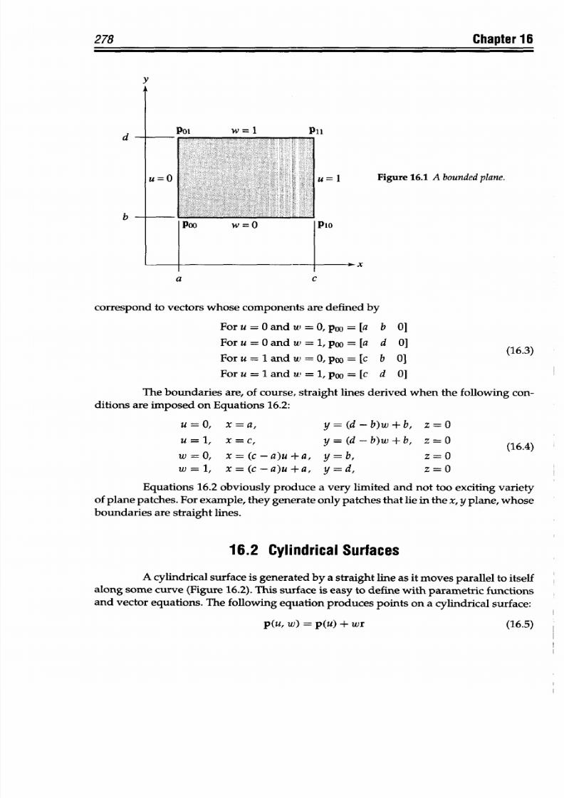
8/9/2019 Mortenson, Michael E. - Mathematics for computer graphics applications.pdf
http://slidepdf.com/reader/full/mortenson-michael-e-mathematics-for-computer-graphics-applicationspdf 291/367
Chapter 16
Figure
16.1
A bounded
plane.
a
c
correspond to
vectors whose
components
are defined by
Foru=Oanduw=Opoo=[a
b
01
Foru=Oandu=1,poO=[a
d
Foru=landw=O,poO=[c
b
Foru=landw=l,poo=[c
d
0]
01
0]
(16.3)
The boundaries
are,
of
course, straight
lines
derived
when the following
con-
ditions
are
imposed
on
Equations
16.2:
u=O, x=a,
u=1,
x=c,
w=O. x=(c
w=1,
x=(c
-a)u+a, y=b,
-a)u+a,
y=d,
Equations
16.2 obviously
produce
a very limited and not
too exciting
variety
of plane patches.
For
example,
they generate
only patches that
lie
in the
x,
y
plane,
whose
boundaries are straight
lines.
16.2
Cylindrical Surfaces
A cylindrical
surface is
generated by
a
straight
line
as it
moves
parallel to itself
along
some
curve (Figure
16.2).
This
surface
is easy to define
with
parametric
functions
and
vector
equations.
The
following
equation produces
points
on
a cylindrical surface:
p(u, w) =
p(u) +
wr
278
d
b
y=(d-b)w+b,
z=O
y=(d-b)w+b,
z=O
z
=
0
z=0
(16.4)
(16.5)
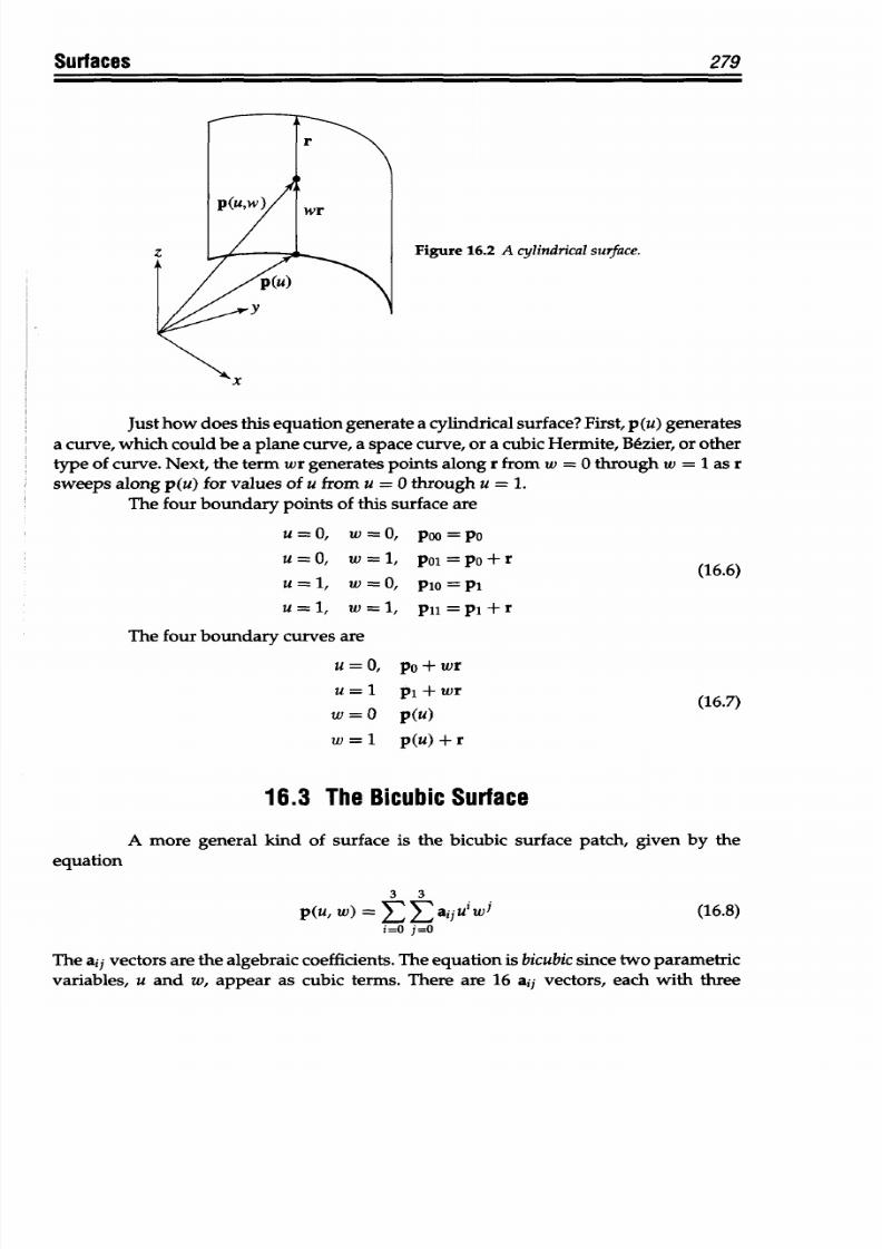
8/9/2019 Mortenson, Michael E. - Mathematics for computer graphics applications.pdf
http://slidepdf.com/reader/full/mortenson-michael-e-mathematics-for-computer-graphics-applicationspdf 292/367
Surfaces
279
A
Just how
does this equation generate a
cylindrical surface?
First, p(u) generates
a
curve, which could be
a plane
curve,
a
space curve,
or a
cubic Hermite,
Bezier, or other
type
of curve. Next,
the term
wr generates points along r from w = 0 through
w
=
1
as
r
sweeps along p(u) for values of u from u = 0
through
u =
1.
The four boundary
points
of this surface are
u=O,
w=O,
poo=pO
u=O,
w=1, pol=po+r
(16.6)
u=l, w=O,
P1o=Pi
u=1, w=l, pu1=pi+r
The
four
boundary curves are
u=O, po+wr
u=1
pi+wr
(16.7)
w = 0 p(u)
w=l
p(u)+r
16.3 The Bicubic Surface
A more
general
kind of
surface is the bicubic surface
patch,
given
by
the
equation
3 3
p(u, w)= aijuiwj
(16.8)
i=o j=o
The
ai
1
vectors are the algebraic coefficients.
The
equation is bicubic
since
two parametric
variables, u and w,
appear
as cubic terms. There are
16
aij vectors, each with three
Figure
16.2 A
cylindrical surface.
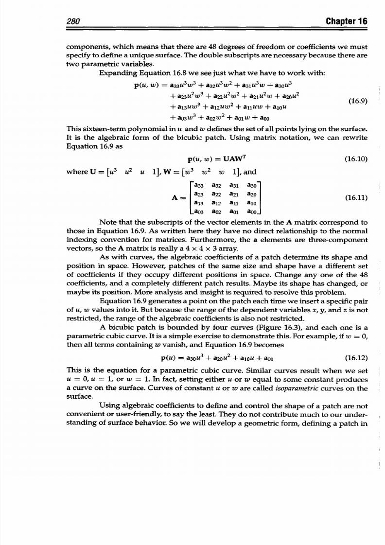
8/9/2019 Mortenson, Michael E. - Mathematics for computer graphics applications.pdf
http://slidepdf.com/reader/full/mortenson-michael-e-mathematics-for-computer-graphics-applicationspdf 293/367
280
Chapter
16
components,
which
means
that there are
48
degrees
of
freedom
or coefficients
we
must
specify
to
define
a
unique surface.
The
double subscripts are
necessary because
there are
two
parametric
variables.
Expanding
Equation
16.8
we see just what
we
have to work
with:
p(u,
w) =
a33u
3
w
3
+
a
32
u
3
w
2
+ a31u
3
w + a3ou
3
+
a2
3
u
2
W3
+
a22u
2
w
2
+
a2lu
2
w
+
a2 u
2
(16.9)
+ a13uw3
+
a12uw
2
+
alluw
+
alou
+ aO3W + ao
2
WI
+ aoiw
+ aoo
This
sixteen-term
polynomial in u and w defines the set of
all points lying
on
the surface.
It is
the
algebraic
form
of
the bicubic patch.
Using matrix
notation,
we
can rewrite
Equation 16.9 as
p(u,
w)= UAWT
(16.10)
whereU
=
[u
3
u
2
u
1],W= [W
3
W
2
W 1],and
[a,
3
a32 a
3
l
a
3
O
A=
a23 a22
a
2
l
a
20
(16.11)
a
13
a12 all
alo
LaO3 ao2
aoi a~oo
Note
that
the subscripts
of
the vector
elements in the
A matrix correspond
to
those in Equation
16.9.
As
written
here
they
have
no
direct relationship to
the normal
indexing convention
for matrices. Furthermore,
the a elements
are three-component
vectors,
so
the
A
matrix
is
really a
4
x
4 x
3
array.
As
with curves,
the algebraic coefficients of
a patch determine
its
shape and
position in
space. However,
patches of
the
same size
and
shape
have
a different
set
of coefficients
if they occupy different
positions in
space.
Change any
one of
the 48
coefficients, and
a completely different patch
results.
Maybe
its shape
has
changed, or
maybe
its position.
More analysis
and
insight is required to resolve
this problem.
Equation
16.9
generates
a point
on the patch
each
time we insert
a
specific
pair
of u,
w
values
into
it. But because
the
range
of the dependent
variables x, y, and z is
not
restricted,
the range of the algebraic
coefficients
is also
not restricted.
A bicubic
patch
is
bounded by four
curves
(Figure
16.3),
and
each one
is
a
parametric cubic curve.
It is a
simple
exercise
to demonstrate this. For example,
if w
=
0,
then all
terms
containing
w
vanish,
and Equation 16.9 becomes
p(u)
= a
3
Ou + a20u2
+
alou
+ aoo
(16.12)
This
is
the
equation for a
parametric cubic curve.
Similar
curves result
when
we
set
u = 0,u =
1, or w = 1.
In fact, setting either
u
or w
equal to
some
constant produces
a curve on the
surface. Curves of
constant u or
w
are called isoparametric
curves
on the
surface.
Using
algebraic
coefficients
to define
and control
the shape
of
a
patch
are
not
convenient
or user-friendly,
to say
the least. They do not
contribute
much
to our
under-
standing of
surface behavior.
So we will
develop
a geometric
form, defining a
patch in

8/9/2019 Mortenson, Michael E. - Mathematics for computer graphics applications.pdf
http://slidepdf.com/reader/full/mortenson-michael-e-mathematics-for-computer-graphics-applicationspdf 294/367
281
urfaces
P11
= 1 Figure 16.3 Some
elementsofa bicubic patch.
U=O Pol
terms
of its boundary
geometry. This
geometry is
given at
the
comer points.
First,
of
course,
there are the
four
corner
points
themselves.
Then
there are the
tangent
vectors
associated
with
the
boundary
curves. Finally, we introduce
a twist
vector
at each
cor-
ner, which control the
rate of change of the
tangent vectors of the interior
isoparametric
curves. We denote
these
twist
vectors as
puO2O,
o l ,
pl , and
pluw. They are defined as
=W a
2
(
W) ,vlaeauOnw=
POO=
aP ua)
,evaluated
at
u =O and
w =
1
UW
a
2
p u,
W)(1.3
Po~l = PU-a'
),evaluated
at
u =
0
and w
= 1
(16.13)
pW= P(U' ),
evaluated
at
u
= 1 and w =
0
UW
2
p(u, W)
p
=
auaw
,evaluated at u = 1
and
w = 1
The
calculus
operation
called for in Equation 16.13 is called
partial
differentiation,
and is not very
different from ordinary
differentiation.
In
this case,
we take
the derivative
of a function with
two
independent variables,
treating each independent
variable, in
turn,
as a constant
while
differentiating
with respect
to the other.
Let
us
see
how
this
works
for pOuO.
First,
we
compute
ap(u,
w)/aw,
treating
u as a
constant in Equation 16.9.
This
yields
ap(u, w)
= 3a33u3w2
+
2a
3
2u
3
w
+ a
31
u
3
aw
+ 3a23u
2
w
2
+
2a22u
2
w
+ a
2
lu
2
(16.14)
+ 3a
13
uw
2
+ 2al2uw
+ allu
+ 3a
0
3w
2
+ 2aO2W
+
aOl
P
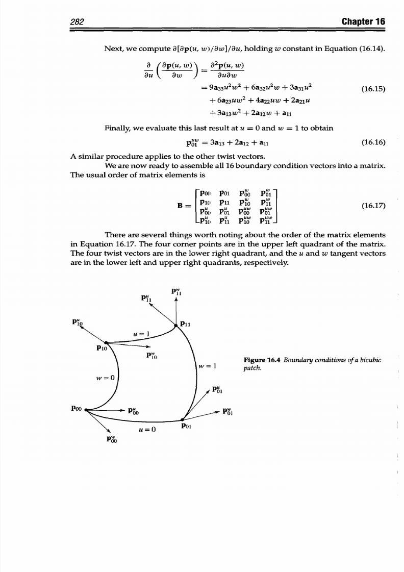
8/9/2019 Mortenson, Michael E. - Mathematics for computer graphics applications.pdf
http://slidepdf.com/reader/full/mortenson-michael-e-mathematics-for-computer-graphics-applicationspdf 295/367
282 Chapter 16
Next, we compute
8[ap(u,
w '/aw]/au, holding w constant in Equation (16.14).
a (ap(u, w) _ a
2
p(u, W)
au V
aw
a- vw
=
9a
33u
2
w
2
+
6a
3 2
u
2
w
+
3a
3
ju
2
(16.15)
+
6a
23
uw
2
+ 4a22uw + 2a
2
lu
+
3a13w
2
+ 2al2w +
all
Finally, we evaluate this last result at
u = 0 and w = 1 o obtain
pul = 3a13 +
2a1
2
+
all
(16.16)
A
similar procedure
applies
to
the other
twist
vectors.
We are now ready
to
assemble all 16
boundary
condition vectors into a matrix.
The
usual
order
of
matrix
elements
is
poo Pol
Poo
Po1
R-
lC
1
1
l0
P1i (16.17)
PoO Pol
POO
Pol
-PW I P1 P1 Pil{
There
are
several
things
worth noting
about the order of the matrix
elements
in Equation 16.17. The four corner
points
are
in
the upper left quadrant of the matrix.
The four
twist
vectors are in the lower
right quadrant,
and
the
u
and w tangent
vectors
are in
the
lower left and
upper right
quadrants,
respectively.
P`II
Figure
16.4 Boundary conditions of a bicubic
patch.
pOW
p
0
8/9/2019 Mortenson, Michael E. - Mathematics for computer graphics applications.pdf
http://slidepdf.com/reader/full/mortenson-michael-e-mathematics-for-computer-graphics-applicationspdf 296/367
Surfaces 283
There
is
even more information in this
order.
The elements comprising the
first
row
are
the
geometric
coefficients of
the
boundary
curve corresponding
to
u =
0.
The elements
in
the
second
row
are the geometric
coefficients of
the boundary curve
corresponding to
u = 1. The first and second columns contain, in order, the
geomet-
ric coefficients
for the boundary curves corresponding to w = 0 and w = 1.
Rows
3
and
4,
and
columns
3 and 4,
define
auxiliary
curves,
which describe how the interior
isoparametric curve tangent
vectors
vary.
The complete matrix equation for
a
bicubic Hermite patch in terms
of
these
geometric
coefficients
is
p(u,
w)
= UMBMTWT (16.18)
where
M
is the same as that given for cubic Hermite curves in Equation 14.61.
The
relationship between the algebraic
and
geometric
coefficients is
A = MBMT
(16.19)
and
B
=
M-lA(MT)-l
(16.20)
There are other ways to define a bicubic
surface.
For example,
a
grid
of
16
points is sufficient. These
are
usually
the four
corner
points, two intermediate
points on
each
boundary
curve,
and four
interior
points.
16.4 The Bezier
Surface
A
Bezier
surface requires
a
grid
of
controlpoints for its definition (Figure 16.5).
These
control points define a characteristic
polyhedron, analogous to
the characteristic
polygon of
the
Bezier
curve. Evaluating the following parametric function
at a set of
P24
P44
Figure
16.5
Bicubic Bezier surface.
Pi
P41
11
It
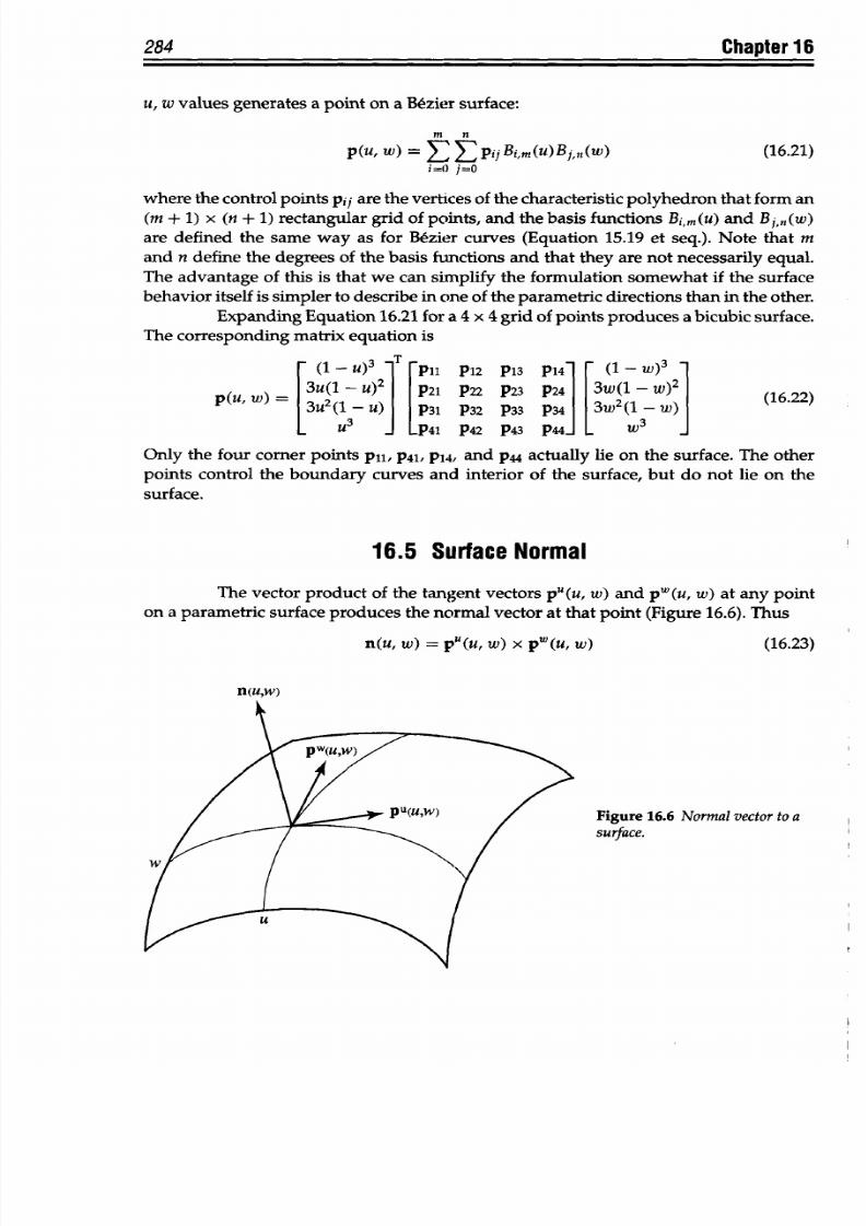
8/9/2019 Mortenson, Michael E. - Mathematics for computer graphics applications.pdf
http://slidepdf.com/reader/full/mortenson-michael-e-mathematics-for-computer-graphics-applicationspdf 297/367
284
Chapter
16
u, w values
generates
a point on a Bzier
surface:
m n
p(u, w)
= E
EpiIBim(u)Bjn(W)
(16.21)
i=O
j=O
where the
control points
pij
are the
vertices of the characteristic
polyhedron that form
an
(m
+ 1) x
(n
+ 1)
rectangular grid
of points, and the
basis functions
Bi,m(u) and Bj,n(w)
are
defined
the same
way as
for
Bezier
curves (Equation 15.19 et
seq.).
Note that
m
and n
define
the degrees
of the basis
functions and that they are
not
necessarily
equal.
The advantage of this
is that we can simplify
the
formulation somewhat
if the surface
behavior
itself
is
simpler to describe
in one of the parametric
directions
than
in the
other.
Expanding Equation 16.21
for
a 4 x
4
grid
of
points produces
a bicubic surface.
The corresponding
matrix
equation
is
-
(1- U)3
-FP1
P12
P13 P14
-
W)
3
-
(u ) = 3u(1 -
U)
P21
P22 P23
p24
3w(1 - w)2
16.22
3U2(1
-
U) P31 P32
P33 P34 3W2(l - W)
- U3
-p41
p42 p43
p44-
- W3
-
Only the four
corner points P11,
P41,
P14,
and
p44
actually
lie
on the
surface. The other
points control
the boundary curves
and interior of the
surface, but
do not
lie
on the
surface.
16.5
Surface Normal
The vector
product
of the tangent vectors
pu
(u,
w)
and
pW
(u,
w)
at any point
on a parametric surface
produces the normal
vector
at that point
(Figure 16.6).
Thus
n(u, w) =
pu(u,
w)
x pw(u, w)
(16.23)
n(u,w)
Figure 16.6 Normal
vector
to a
surface.
8/9/2019 Mortenson, Michael E. - Mathematics for computer graphics applications.pdf
http://slidepdf.com/reader/full/mortenson-michael-e-mathematics-for-computer-graphics-applicationspdf 298/367
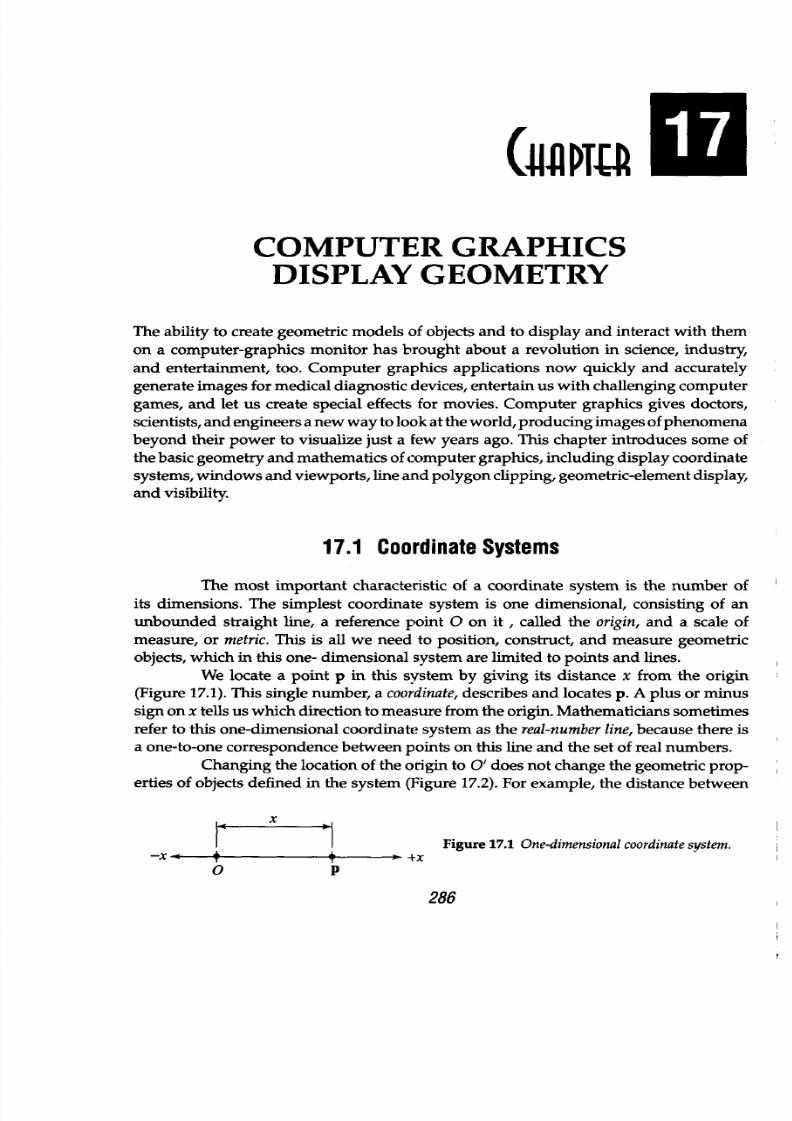
8/9/2019 Mortenson, Michael E. - Mathematics for computer graphics applications.pdf
http://slidepdf.com/reader/full/mortenson-michael-e-mathematics-for-computer-graphics-applicationspdf 299/367
UA
KTa
COMPUTER
GRAPHICS
DISPLAY
GEOMETRY
The ability to create geometric models of
objects and
to
display
and interact with
them
on a computer-graphics
monitor
has brought
about a revolution in science,
industry,
and
entertainment, too.
Computer
graphics applications now quickly and accurately
generate images for medical diagnostic devices,
entertain
us
with
challenging computer
games, and let us create special
effects for
movies. Computer graphics gives doctors,
scientists,
and
engineers
a new
way to
look
at the
world,
producing
images of phenomena
beyond
their
power to visualize just a
few
years
ago.
This
chapter introduces
some of
the basic
geometry and mathematics
of
computer graphics, including display coordinate
systems, windows and
viewports,
line and
polygon
clipping, geom etric-element display,
and
visibility.
17.1 Coordinate Systems
The
most
important characteristic
of a coordinate
system is
the number
of
its
dimensions. The
simplest
coordinate
system
is
one dimensional,
consisting of
an
unbounded
straight
line, a reference point 0
on
it, called
the
origin, and a
scale of
measure,
or metric. This is
all we
need
to position,
construct, and measure
geometric
objects,
which
in
this one- dimensional system are limited to points and
lines.
We
locate a
point
p
in this system
by
giving
its
distance
x
from
the
origin
(Figure 17.1). This single number, a coordinate, describes
and locates p. A plus or minus
sign
on
x
tells
us
which
direction to
measure
from the origin. Mathematicians sometimes
refer to this one-dimensional coordinate system
as the
real-number
line, because
there
is
a one-to-one
correspondence
between
points
on this line and the set of real
numbers.
Changing
the
location of the
origin
to O' does
not change the geometric
prop-
erties of
objects
defined in the
system (Figure
17.2). For example,
the distance
between
x
Figure
17.1
One-dimensionalcoordinate system.
x 4
4
AX
0 P
286
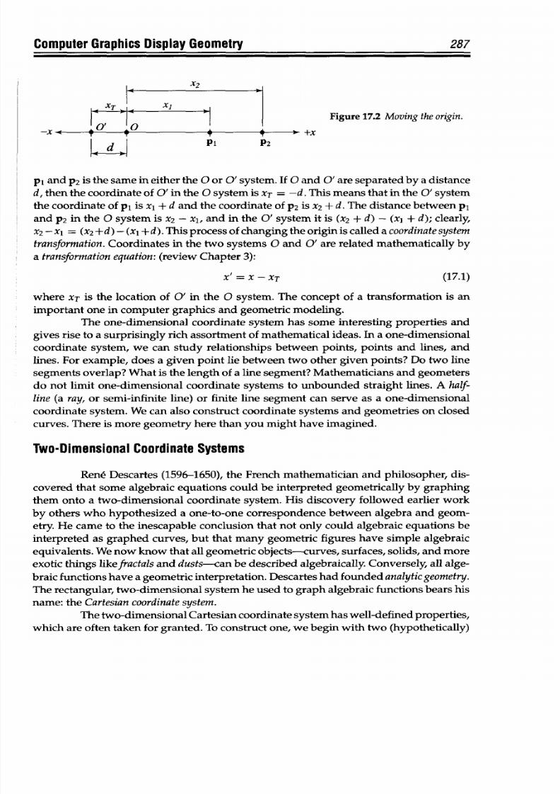
8/9/2019 Mortenson, Michael E. - Mathematics for computer graphics applications.pdf
http://slidepdf.com/reader/full/mortenson-michael-e-mathematics-for-computer-graphics-applicationspdf 300/367
Computer
Graphics Display
Geometry
287
XT
Xj
x
Figure
17.2
Moving
the
origin.
Pi
P2
pi
and
P2
is the same
in either the 0 or O' system. If
0
and
O' are
separated
by
a
distance
d,
then the
coordinate of O' in
the 0 system
is XT =
-d.
This means
that in the O'
system
the
coordinate of
pi
is
xl +
d
and the
coordinate
of
P2 is x
2
+
d. The distance
between
p,
and P2 in
the 0 system is x2 - xi, and in the O' system
it
is (x
2
+ d) - (xl + d); clearly,
x2-xl =
(x
2
+d)-(xl +d). Thisprocess
of
changing the
originis
called
a
coordinate ystem
transformation. Coordinates in the two systems
0
and
O'
are related mathematically by
a
transformationequation: (review Chapter
3):
X
=X-XT
(17.1)
where XT is the location
of O' in the
0 system. The concept
of a transformation
is
an
important one
in comp uter
graphics
and geometric
modeling.
The
one-dimensional coordinate system has some interesting
properties and
gives rise to a
surprisingly
rich assortment
of
mathematical ideas. In a one-dimensional
coordinate system, we can study
relationships
between points,
points
and
lines, and
lines.
For example, does
a
given
point
lie
between
two
other
given
points?
Do
two
line
segments overlap? What is the
length of
a line segment? Mathematicians
and
geometers
do
not
limit one-dimensional coordinate systems to unbounded straight lines. A half-
line (a ray, or semi-infinite line) or finite line segment can serve as a one-dimensional
coordinate
system. We
can also
construct
coordinate systems and geometries on
closed
curves.
There
is
more
geometry
here
than you might have
imagined.
Two-Dimensional Coordinate Systems
Ren6
Descartes
(1596-1650),
the
French
mathematician
and
philosopher,
dis-
covered that some
algebraic equations could be interpreted
geometrically by graphing
them onto a two-dimensional
coordinate system.
His discovery
followed earlier work
by
others
who hypothesized a one-to-one
correspondence
between
algebra and geom-
etry. He came to the inescapable conclusion
that not
only could algebraic equations be
interpreted as
graphed
curves, but
that
many
geometric figures
have
simple algebraic
equivalents.
We
now know that
all
geometric
objects-curves, surfaces, solids,
and
more
exotic things likefractals
and
dusts-can
be described algebraically.
Conversely,
all alge-
braic
functions have
a geometric interpretation. Descartes had founded
analyticgeometry.
The rectangular, two-dimensional system he used to graph algebraic
functions
bears his
name:
the
Cartesian coordinate ystem.
The two-dimensional
Cartesian coordinate system has well-defined properties,
which are
often taken
for granted.
To
construct one, we begin
with
two (hypothetically)
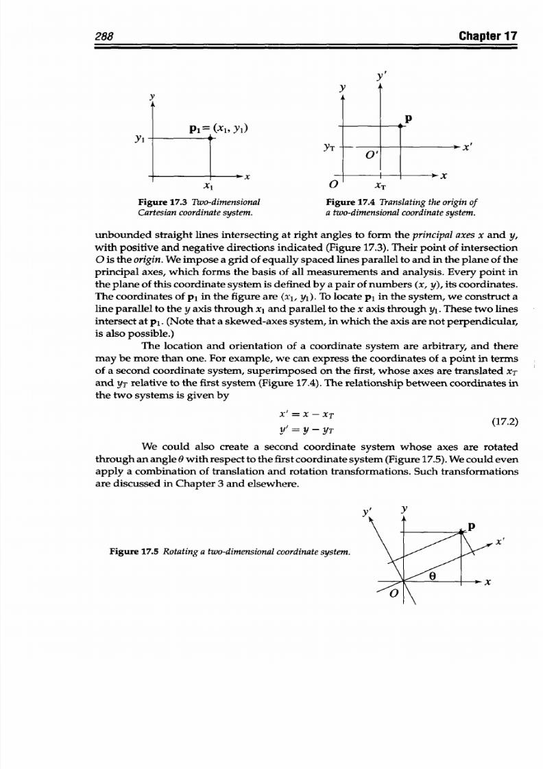
8/9/2019 Mortenson, Michael E. - Mathematics for computer graphics applications.pdf
http://slidepdf.com/reader/full/mortenson-michael-e-mathematics-for-computer-graphics-applicationspdf 301/367
288
Chapter 17
Y'
y
yl
,)
YT
-
-x
o'
p
Xl
(JXT
Figure
17.3
Two-dimensional
Figure 17.4 Translating he
origin of
Cartesian
coordinate system.
a two-dimensional
coordinate
system.
unbounded
straight
lines intersecting
at
right
angles
to
form
the
principal
axes
x
and
y,
with positive and
negative directions indicated
(Figure
17.3). Their
point of intersection
0
is
the
origin.We
impose
a
grid
of
equally spaced lines parallel to
and in
the plane of the
principal axes, which
forms the basis of all measurements
and
analysis.
Every
point
in
the plane
of
this
coordinate
system is
defined by
a pair of
numbers
(x,
y),
its coordinates.
The coordinates of
p, in the
figure are
(xl,
yi). To
locate
p, in the
system,
we construct
a
line parallel
to the y axis through
xi and parallel
to the
x
axis
through
yi.
These
two lines
intersect
at pl. (Note that
a skewed-axes system, in
which the axis are not
perpendicular,
is
also
possible.)
The location
and
orientation
of
a
coordinate
system
are arbitrary,
and
there
may be more
than
one.
For example,
we
can express
the coordinates of
a point in terms
of
a
second
coordinate system,
superimposed
on
the
first,
whose axes
are
translated
XT
and
YT
relative
to the first
system
(Figure 17.4).
The
relationship between coordinates
in
the two
systems
is given
by
X' = X
-
XT
=
- yr(17.2)
Y' =
Y
-YT
We
could also create a second
coordinate system
whose axes
are
rotated
through
an angle
0
with
respect to the first coordinate
system
(Figure
17.5).
We
could even
apply
a combination
of
translation
and rotation transformations.
Such transformations
are
discussed
in Chapter 3 and
elsewhere.
Y
Figure
17.5
Rotating a two-dimensionalcoordinate
system.
x
i
i
0
X
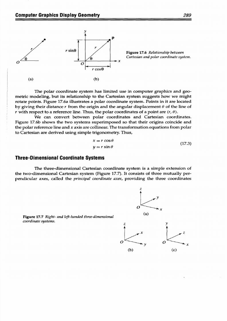
8/9/2019 Mortenson, Michael E. - Mathematics for computer graphics applications.pdf
http://slidepdf.com/reader/full/mortenson-michael-e-mathematics-for-computer-graphics-applicationspdf 302/367
Computer Graphics Display Geometry
. x
r cosO
Figure 17.6 Relationship between
Cartesianand polar
coordinate system.
(b)
The
polar
coordinate system has limited use in computer graphics
and
geo-
metric modeling,
but
its relationship to the Cartesian system suggests
how
we
might
rotate
points.
Figure
17.6a
illustrates
a polar coordinate
system.
Points
in it
are
located
by
giving their distance r from the origin
and
the angular displacement 0 of the line
of
r
with respect
to a reference line.
Thus,
the
polar coordinates
of a
point are (r,
0).
We can convert
between polar
coordinates and Cartesian
coordinates.
Figure
17.6b
shows the two systems superimposed
so
that their origins coincide and
the polar reference
line
and x axis
are collinear. The
transformation
equations from
polar
to Cartesian are derived using simple trigonometry. Thus,
x = r cos 9
(17.3)
y
=
r sin
1
Three-Dimensional
Coordinate Systems
The
three-dimensional Cartesian
coordinate
system
is a
simple
extension of
the
two-dimensional
Cartesian system (Figure 17.7).
It
consists of three mutually
per-
pendicular axes, called the principal
coordinate axes,
providing the
three
coordinates
z
0 <~
(a)
z
x
0
Omy
(b)
y
z
0
x
(c)
Y
289
0
r sinO
0
(a)
Figure 17.7 Right-
and
left-handed three-dimensional
coordinate
systems.
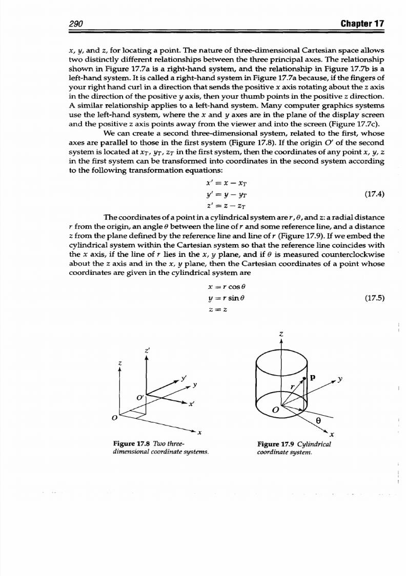
8/9/2019 Mortenson, Michael E. - Mathematics for computer graphics applications.pdf
http://slidepdf.com/reader/full/mortenson-michael-e-mathematics-for-computer-graphics-applicationspdf 303/367
290
Chapter 17
x, y,
and z, for locating a point.
The nature
of
three-dimensional
Cartesian space
allows
two distinctly different
relationships between
the three principal
axes. The
relationship
shown
in
Figure
17.7a is
a
right-hand
system,
and
the relationship
in Figure 17.7b is
a
left-hand
system.
It is
called
a
right-hand system
in
Figure 17.7a
because, if
the
fingers
of
your
right
hand
curl
in
a
direction
that
sends the positive
x
axis
rotating about
the
z
axis
in the direction of the positive
y axis, then your thumb
points in the
positive z direction.
A similar relationship applies
to
a
left-hand system. Many
computer graphics systems
use the
left-hand system, where
the x
and
y axes are in
the plane of the display
screen
and the positive
z axis points away from
the
viewer and
into
the
screen (Figure
17.7c).
We
can
create
a second three-dimensional system,
related to the first,
whose
axes are
parallel to those in the
first
system
(Figure 17.8).
If the
origin
O' of the second
system
is
located at
XT,
YT,
ZT in
the first system, then
the coordinates of any point
x, y, z
in the first system
can be transformed into
coordinates in the
second system according
to the following
transformation
equations:
X' = X -XT
Y =
Y-YT
(17.4)
2'= Z-ZT
The coordinates
of a
point
in a cylindrical system are r,
0,
and
z: a radial distance
r
from the
origin, an
angle
0
between
the
line of r
and some reference
line,
and
a
distance
z
from
the
plane
defined by
the reference
line
and line of r (Figure
17.9). If we embed the
cylindrical system within the Cartesian
system
so
that the
reference line
coincides with
the
x axis,
if the line of r lies
in the x,
y
plane, and
if
0 is
measured
counterclockwise
about
the
z
axis
and
in the
x,
y
plane,
then the
Cartesian coordinates
of
a
point
whose
coordinates
are given in the cylindrical system
are
x r cos 9
y =
r
sinG (17.5)
Z = Z
zI
0
Figure
17.8
Two
three-
dimensional
coordinate systems.
Figure
17.9 Cylindrical
coordinate
system.
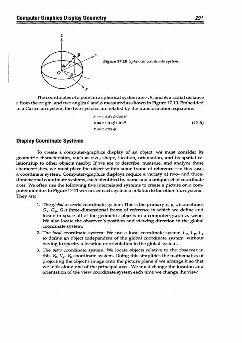
8/9/2019 Mortenson, Michael E. - Mathematics for computer graphics applications.pdf
http://slidepdf.com/reader/full/mortenson-michael-e-mathematics-for-computer-graphics-applicationspdf 304/367
Computer Graphics
Display
Geometry
z
Y
Figure
17.10
Sphericalcoordinatesystem.
The coordinates of a
point in
a spherical
system are r, 0,
and
0: a radial distance
r
from
the
origin,
and
two angles
0
and
0
measured
as
shown in
Figure
17.10.
Embedded
in
a Cartesian system, the two systems
are
related
by the transformation equations
x
=
r
sin
0 cos 0
y = r sin 0 sin
a
(17.6)
z =r cos
0
Display
Coordinate Systems
To create a computer-graphics
display
of an object,
we
must consider its
geometric characteristics, such
as size, shape, location, orientation,
and
its spatial
re-
lationship
to other
objects nearby.
If we are to describe, measure, and analyze
these
characteristics, we
must
place the
object
within some frame
of reference-in
this
case,
a coordinate
system.
Computer-graphics
displays require a variety of two- and three-
dimensional
coordinate systems, each
identified by
name and a unique set of coordinate
axes.
We often
use the
following
five interrelated
systems
to
create
a
picture
on a
com-
puter monitor. In Figure 17.11 we
can
see
each
system
in
relation
to
the other four systems.
They
are:
1. The global or
world
coordinate
system:
This
is
the
primary
x,
y,
z
(sometimes
Gx,
GY1 G,) three-dimensional frame of reference in which we define and
locate
in
space all of the geometric
objects
in
a
computer-graphics scene.
We also locate
the
observer's
position
and viewing direction in
the
global
coordinate
system.
2. The
local coordinate system: We use a
local
coordinate
system
Lx,
Ly, L,
to define an object
independent
of the
global
coordinate system,
without
having
to specify a
location
or
orientation
in
the
global system.
3. The
view coordinate
system:
We
locate objects
relative to the
observer in
this Vx, Vy, V, coordinate system. Doing this simplifies the mathematics of
projecting the
object's
image onto the
picture plane
if
we
arrange it
so that
we look along one of the principal axes. We
must change
the
location
and
orientation of
the view coordinate system each time
we
change the view.
291
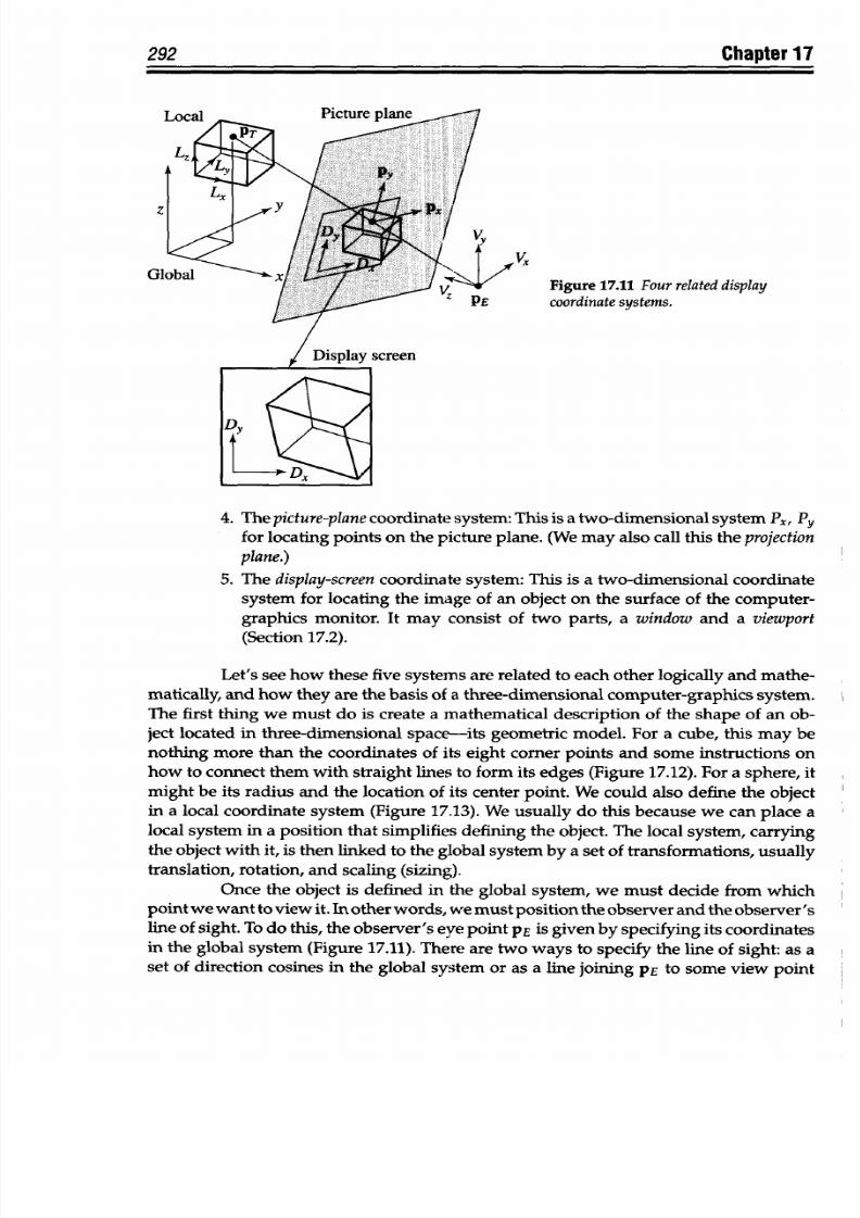
8/9/2019 Mortenson, Michael E. - Mathematics for computer graphics applications.pdf
http://slidepdf.com/reader/full/mortenson-michael-e-mathematics-for-computer-graphics-applicationspdf 305/367
292
Chapter
17
Picture plane
Figure
17.11 Fourrelated
display
coordinate
ystems.
4.
The picture-plane
coordinate
system: This
is a two-dimensional
system
Px, Py
for locating points on
the
picture plane. (We
may
also call
this
the projection
plane.)
5.
The display-screen
coordinate
system:
This is
a
two-dimensional
coordinate
system
for locating
the image of
an
object
on
the
surface
of
the
computer-
graphics monitor.
It may
consist of
two parts,
a
window and
a viewport
(Section 17.2).
Let's
see how these
five systems
are related to each
other
logically
and mathe-
matically, and
how they are
the
basis of
a three-dimensional
computer-graphics
system.
The first
thing we
must
do
is
create
a
mathematical
description
of
the shape of
an ob-
ject
located
in
three-dimensional
space-its
geometric
model.
For
a
cube,
this may be
nothing
more than the
coordinates
of its eight
corner points
and some
instructions
on
how to
connect them
with straight
lines
to form
its
edges
(Figure 17.12).
For
a
sphere,
it
might
be
its radius
and the
location of
its
center point.
We could
also define
the
object
in
a
local coordinate
system
(Figure
17.13).
We
usually
do this because
we can
place
a
local
system
in a position
that
simplifies
defining
the object.
The local system, carrying
the object with it,
is then linked to
the global
system by a set
of transformations,
usually
translation,
rotation,
and
scaling
(sizing).
Once the
object is
defined
in the global
system,
we must decide
from which
point
we want
to view it.
In
other
words,
we
must
position
the
observer and
the observer's
line
of sight.
To
do
this,
the
observer's
eye
point
PE
is
given
by
specifying
its coordinates
in
the
global
system
(Figure 17.11).
There
are
two
ways to
specify
the
line of sight:
as a
set of direction
cosines in
the
global
system
or
as
a line joining
PE to some
view point
2
G.
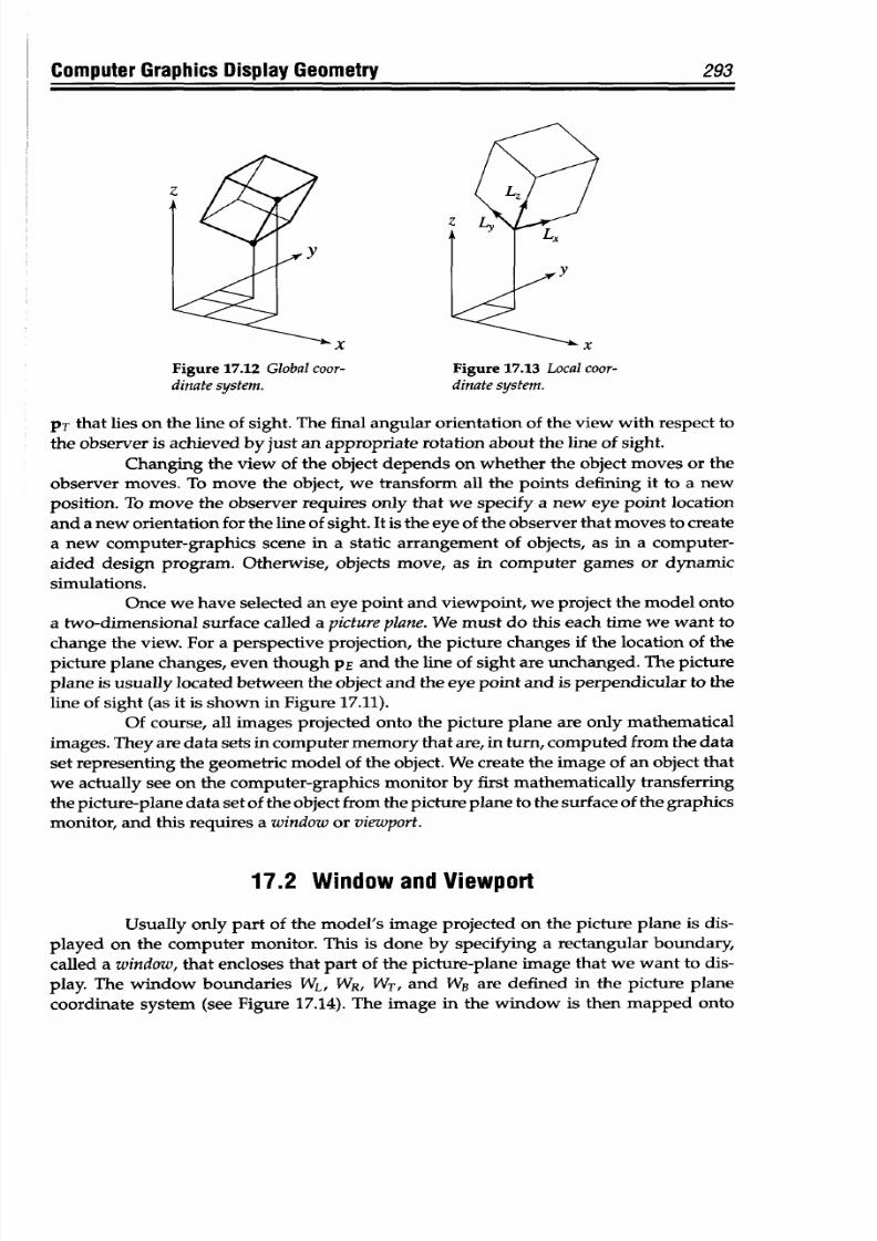
8/9/2019 Mortenson, Michael E. - Mathematics for computer graphics applications.pdf
http://slidepdf.com/reader/full/mortenson-michael-e-mathematics-for-computer-graphics-applicationspdf 306/367
Computer
Graphics Display
Geometry
293
Figure
17.12
Global
coor-
Figure
17.13 Local coor-
dinate system.
dinate system.
PT
that lies
on
the line
of
sight.
The final angular
orientation
of
the
view
with
respect
to
the observer
is
achieved
by just
an
appropriate
rotation
about
the line of sight.
Changing the
view of
the object
depends on whether
the object
moves or
the
observer
moves. To move
the
object,
we transform
all the
points
defining
it to a new
position. To move
the
observer
requires only that we specify a new eye
point location
and a new
orientation
for the line
of
sight.
It is the eye
of the
observer
that moves
to
create
a new computer-graphics
scene in a
static arrangement
of
objects, as in
a computer-
aided design program.
Otherwise,
objects
move,
as
in
computer
games or
dynamic
simulations.
Once
we have selected
an eye point and viewpoint,
we project
the model onto
a two-dimensional
surface
called
a
picture
plane.
We
must do
this each
time we want
to
change the view.
For a perspective
projection,
the picture
changes if
the
location of
the
picture plane changes,
even
though
PE
and
the line
of
sight are unchanged.
The picture
plane is
usually located between the object
and
the eye point
and
is
perpendicular
to the
line
of sight
(as
it
is
shown
in Figure 17.11).
Of
course, all
images projected onto
the picture plane
are only
mathematical
images. They are
data
sets
in
computer memory
that
are,
in
turn, computed
from
the
data
set
representing the geometric model
of
the object. We create the image
of
an object
that
we
actually
see on the computer-graphics
monitor
by
first
mathematically transferring
the p icture-plane data set
of the object from the
picture
plane
to the surface
of the graphics
monitor, and
this
requires a
window
or viewport.
17.2
Window and Viewport
Usually
only part
of
the
model's image projected
on the picture plane
is dis-
played
on the computer monitor.
This is done
by
specifying
a rectangular
boundary,
called a window,
that encloses that part
of the p icture-plane
image that we want to
dis-
play. The
window
boundaries
WL,
WR,
WT,
and WB are defined
in the picture plane
coordinate system (see Figure 17.14).
The image in the window is then mapped onto
I
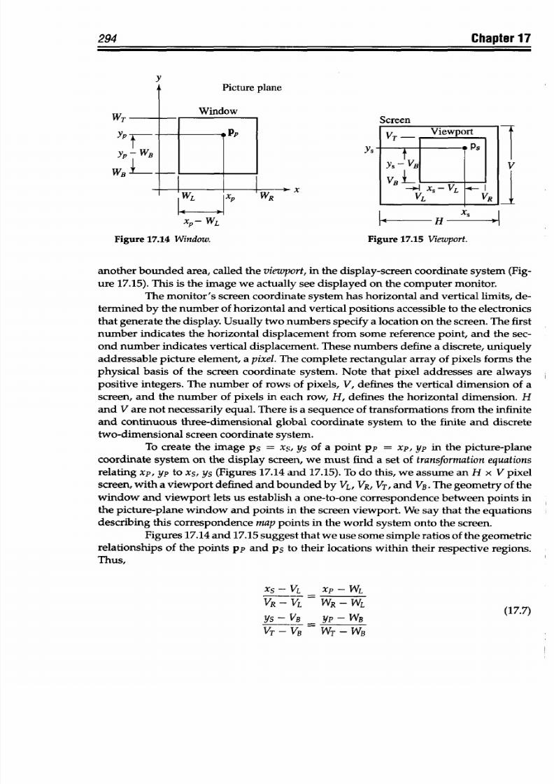
8/9/2019 Mortenson, Michael E. - Mathematics for computer graphics applications.pdf
http://slidepdf.com/reader/full/mortenson-michael-e-mathematics-for-computer-graphics-applicationspdf 307/367
294
Chapter
17
WT
Yp
WB
Screen
VT -
Viewport
YS-VB
V
x
VBL~-). X
- VL -* I
VL VR
I
x,
I
XP- WL
I
- H
- 1
Figure
17.14 Window.
Figure
17.15 Viewport.
another
bounded area,
called the
viewport, in
the display-screen
coordinate
system
(Fig-
ure
17.15).
This
is the
image
we
actually see
displayed on
the
computer
monitor.
The
monitor's screen
coordinate
system
has horizontal and vertical limits,
de-
termined
by the number of horizontal and
vertical
positions
accessible
to
the
electronics
that
generate the
display.
Usually
two numbers specify
a location o n the screen. The first
number
indicates the horizontal displacement
from some reference point,
and the sec-
ond number
indicates vertical displacement. These
numbers
define a discrete, uniquely
addressable picture
element, a
pixel.
The
complete rectangular array
of
pixels
forms
the
physical
basis of
the screen
coordinate system. Note
that
pixel
addresses are
always
positive
integers.
The
number
of
rows
of
pixels, V,
defines the vertical dimension of
a
screen,
and
the
number of
pixels
in
each row,
H,
defines
the horizontal
dimension. H
and V are not necessarily
equal.
There
is
a sequence of
transformations
from the infinite
and continuous
three-dimensional global
coordinate
system to
the finite and discrete
two-dimensional
screen
coordinate system.
To create the image ps =
xs,
ys
of a point pp = xp, yp in the
picture-plane
coordinate
system on the display screen,
we must find
a
set
of
transformation
equations
relating
xp,
yp
to
x
5
,
ys
(Figures
17.14
and
17.15).
To
do
this,
we
assume an
H x
V
pixel
screen, with
a viewport
defined
and bounded
by
VL, VR, VT,
and
VB.
The
geometry
of
the
window and viewport
lets us establish a
one-to-one correspondence
between points in
the
picture-plane window
and
points
in
the screen viewport.
We say that the
equations
describing
this
correspondence
map points
in the world
system
onto
the
screen.
Figures 17.14
and
17.15
suggest
that
we use
some simple ratios of
the geometric
relationships of
the points pp
and ps
to
their locations
within their
respective regions.
Thus,
XS-
VL
XP
-
WL
VR-VL
WR-WL
(17.7)
YS-
VB - YP-WB
VT-VB WT-WB
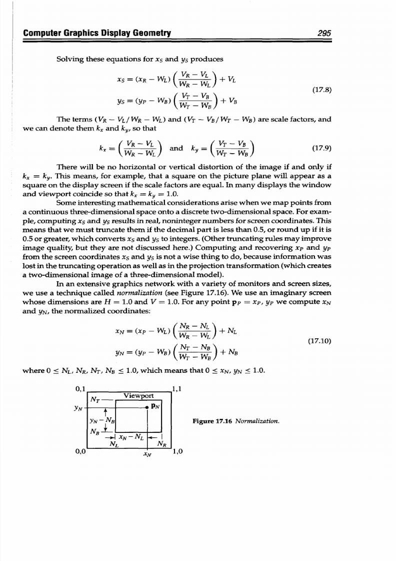
8/9/2019 Mortenson, Michael E. - Mathematics for computer graphics applications.pdf
http://slidepdf.com/reader/full/mortenson-michael-e-mathematics-for-computer-graphics-applicationspdf 308/367
Computer Graphics
Display
Geometry 295
Solving
these equations
for xs and
ys produces
XS
= (XR-WL) VR
- ) +
VL
WR-
WL)
(17.8)
YS =
(YP
-
WB)
(
- W ) +
VB
The
terms
(VR -
VL/WR
- WL)
and
(VT -
VB/WT
-
WB) are scale factors,
and
we can denote
them
kx and ky, so that
kx
=
VR
VL )
and k
= V -
VB
(17.9)
'\WR
-WL /
WT-WB/
There will be
no horizontal
or vertical
distortion
of
the
image
if
and
only
if
kx = ky. This means,
for example, that a square on the picture
plane
will
appear
as
a
square on
the
display
screen
if the
scale factors are equal. In
many
displays
the
window
and viewport coincide
so that kx = ky =
1.0.
Some
interesting mathematical considerations arise when we
map
points
from
a continuous three-dimensional space onto
a
discrete two-dimensional space. For exam-
ple, computing
Xs
and
ys
results
in
real,
noninteger
numbers for
screen
coordinates. This
means that
we
must truncate them if
the
decimal part
is less
than
0.5,
or round
up if it is
0.5 or
greater, which
converts xs
and ys to integers. (Other truncating rules may improve
image quality,
but
they
are
not
discussed here.)
Computing
and recovering xp
and
yp
from the screen coordinates xs and ys is
not
a wise
thing
to do, because information was
lost in the truncating operation as well as
in
the projection transformation (which creates
a two-dimensional
image
of a three-dimensional model).
In an extensive
graphics
network with
a
variety
of
monitors and
screen
sizes,
we use a technique
called normalization
(see Figure
17.16). We use
an imaginary screen
whose d imensions are
H
= 1.0
and V
= 1.0. For
any
point pp
=
xp, yp we compute XN
and
YN, the normalized
coordinates:
XN = XP - WL) NR -
NL
+
NL
(WR
-
WL
/(17.10)
YN
= (YP-WB) B) + NB
where 0 < NL,
NR,
NT,
NB
< 1.0, which means that 0 < XN,
YN
<
1.0.
Figure
17.16
Normalization.
,0
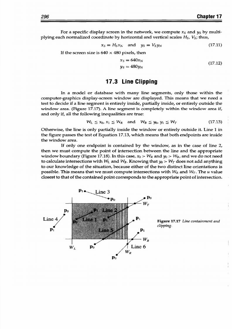
8/9/2019 Mortenson, Michael E. - Mathematics for computer graphics applications.pdf
http://slidepdf.com/reader/full/mortenson-michael-e-mathematics-for-computer-graphics-applicationspdf 309/367
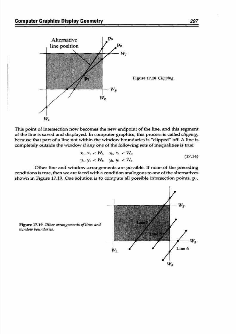
8/9/2019 Mortenson, Michael E. - Mathematics for computer graphics applications.pdf
http://slidepdf.com/reader/full/mortenson-michael-e-mathematics-for-computer-graphics-applicationspdf 310/367
Computer
Graphics Display
Geometry
Alternative
line
position
I Po
I
Po
+-
WT
Figure 17.18 Clipping.
- WB
OR
WL
This point
of intersection
now becomes
the
new endpoint
of
the line,
and
this segment
of
the
line is
saved
and
displayed.
In computer graphics, this process is called clipping,
because
that part of
a
line not within
the
window boundaries is
"clipped"
off. A line
is
completely outside the
window
if any one of the following
sets
of inequalities is
true:
297
XO, X1 <
WL XO,Xl < WR
YO,
Y1
< WB YO, Y1 <
WT
(17.14)
Other line and
window
arrangements are
possible.
If none of the preceding
conditions
is
true,
then
we
are faced with a
condition analogous
to one of the
alternatives
shown in Figure
17.19. One
solution is to compute
all
possible intersection points, p1,
Figure 17.19 Otherarrangementsof lines and
window boundaries.
WB
WR
I
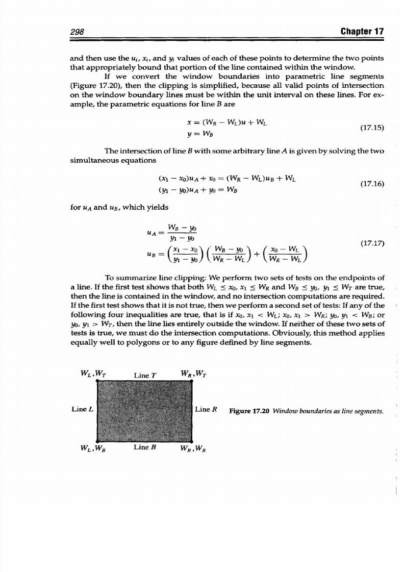
8/9/2019 Mortenson, Michael E. - Mathematics for computer graphics applications.pdf
http://slidepdf.com/reader/full/mortenson-michael-e-mathematics-for-computer-graphics-applicationspdf 311/367
298
Chapter 17
and
then use the ui,
xi,
and
yz
values of each of these
points
to determine the
two points
that appropriately
bound
that
portion
of the line
contained within
the window.
If
we convert the
window boundaries into
parametric
line
segments
(Figure
17.20),
then
the clipping
is
simplified, because
all
valid
points
of
intersection
on the
window boundary
lines
must be within the unit
interval on
these
lines.
For
ex-
ample, the
parametric equations
for
line B
are
X
=
(W - WL)U + WL
(17.15)
Y =
WB
The intersection of line
B
with some
arbitrary line
A
is given by solving the
two
simultaneous equations
(X
1
-
XO)UA + X0) = (WR -
WL)UB
+ WL
(17.16)
(y -
YO)UA +
YO
= WB
for UA and
UB, which yields
WB
-YO
UA -
y1
A (17.17)
UB
(X1-
X0
('WB
-YO
A
R WLA
U
YB
(x
\
WR)
WLY
XOVW
)-
L( .
To summarize line clipping: We perform two sets of tests on the endpoints of
a
line.
If
the first test
shows that both WL
< x,
x
1
<
WR and WB
< yo,
yi
<
WT are true,
then
the line is contained
in the
window,
and
no intersection
computations
are required.
If
the first
test
shows that
it is not true, then
we
perform a second
set of
tests: If any of the
following
four
inequalities
are
true,
that
is
if
x0, x
1
<
WL;
xo,
x
1
>
WR;
yo,
yi
< WB;
or
yo,
yj
>
WT,
then
the line lies entirely outside the
window. If
neither of
these two sets
of
tests
is true,
we
must
do
the intersection
computations.
Obviously, this
method
applies
equally well to
polygons
or to
any
figure defined
by
line
segments.
WLWT Tine
T
WRWT
Line L
Line R Figure 17.20
Window
boundaries
as
line
segments.
WL, WB Line B
WR, WB
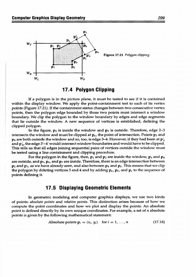
8/9/2019 Mortenson, Michael E. - Mathematics for computer graphics applications.pdf
http://slidepdf.com/reader/full/mortenson-michael-e-mathematics-for-computer-graphics-applicationspdf 312/367
Computer
Graphics Display
Geometry
WT
WB
Figure
17.21 Polygon clipping.
WL
WR
17.4
Polygon
Clipping
If a polygon is
in the picture
plane, it
must be tested to
see
if it
is
contained
within
the
display window.
We apply
the point-containment test
to
each of its
vertex
points (Figure
17.21).
If the
containment status changes
between two consecutive
vertex
points, then
the polygon edge
bounded by those two points
must
intersect
a window
boundary.
We clip
the
polygon to
the
window boundary by edges
and
edge segments
that
lie
outside
the window. A new sequence
of
vertices is established,
defining the
clipped polygon.
In the
figure, P2 is
inside
the window
and
p3
is
outside.
Therefore, edge
2-3
intersects
the window and
must
be clipped at
pa, the point
of
intersection.
Points
p3
and
P4 are both outside
the
window
and so,
too,
is
edge
3-4. However, if
they had been at p
3
and
p , the edge 3'-4' would
intersect
window
boundaries
and
would have to
be
clipped.
This tells us
that
all edges joining sequential pairs of vertices outside the window must
be
tested using
a line containment and
clipping
procedure.
For
the
polygon
in the figure, then, pl
and
P2 are
inside the window, p3 and
P4
are outside,
and
p5,
p6,
and p7
are inside.
Therefore, there is an
edge intersection between
p2
and
p3,
as
we have already
seen,
and
also
between
P4
and
p5.
This
means
that
we
clip
the polygon by
deleting vertices
3
and 4 and
by adding Pa,
Pb,
and
Pc
to the
sequence
of
points defining it.
17.5 Displaying Geometric
Elements
In geometric modeling and
computer graphics displays,
we use two
kinds
of
points:
absolute points and relative points. This distinction arises because
of
how
we
compute the point
coordinates
and
how we
plot
and
display the
points.
An
absolute
point is defined
directly by its own unique coordinates.
For
example,
a set
of
n absolute
points is given
by the
following m athematical statement:
Absolute
points pi
=
(xi, yi) for
i
=
1,..., n
299
(17.18)
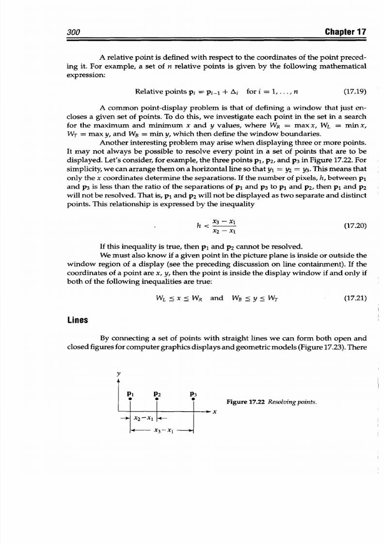
8/9/2019 Mortenson, Michael E. - Mathematics for computer graphics applications.pdf
http://slidepdf.com/reader/full/mortenson-michael-e-mathematics-for-computer-graphics-applicationspdf 313/367
300
Chapter 17
A relative
point
is defined
with respect
to the
coordinates of
the
point preced-
ing
it. For
example,
a
set of n relative points
is
given by the following
mathematical
expression:
Relative
points pi - pi-,
+ Ai for i
= 1, ... ,
n (17.19)
A common point-display problem is
that of defining
a
window that just
en-
closes
a given set of points. To do
this, we investigate each point
in the set in a
search
for
the maximum and
minimum
x
and
y values,
where WR
=
max x, WL
=
minx,
WT = max
y,
and
WB
= min
y,
which then define the window boundaries.
Another interesting problem may arise when displaying three
or more
points.
It may
not
always be possible to resolve every point in
a
set of
points
that are to be
displayed. Let's consider, for example,
the
three points pl, P2, and p3
in
Figure 17.22. For
simplicity, we can arrange them on a horizontal
line so
that yi
=
y2
=
y3. This
means that
only the
x coordinates determine the separations.
If the
number
of
pixels,
h, between
pi
and
p3
is less than
the ratio
of
the separations of p, and
P3 to p, and p2, then
p1
and
P2
will not be
resolved. That is, p, and p2
will
not
be
displayed as two separate
and distinct
points. This relationship is expressed by the inequality
<X3 -
XI
(17.20)
X XI
If
this inequality
is
true, then
p,
and
P2
cannot
be resolved.
We
must also know if
a given
point
in the
picture
plane is inside or
outside
the
window region
of a display
(see the
preceding discussion
on
line
containment). If
the
coordinates
of a
point are x,
y, then the
point
is inside the display
window
if
and
only if
both
of the following inequalities are true:
WL'X<WR
and
WB<y<WT (17.21)
Lines
By
connecting
a
set of
points
with straight
lines
we can form both
open
and
closed figures for
computer
graphics
displays
and
geometric
models
(Figure 17.23). There
y
Figure
17.22
Resolving points.
x
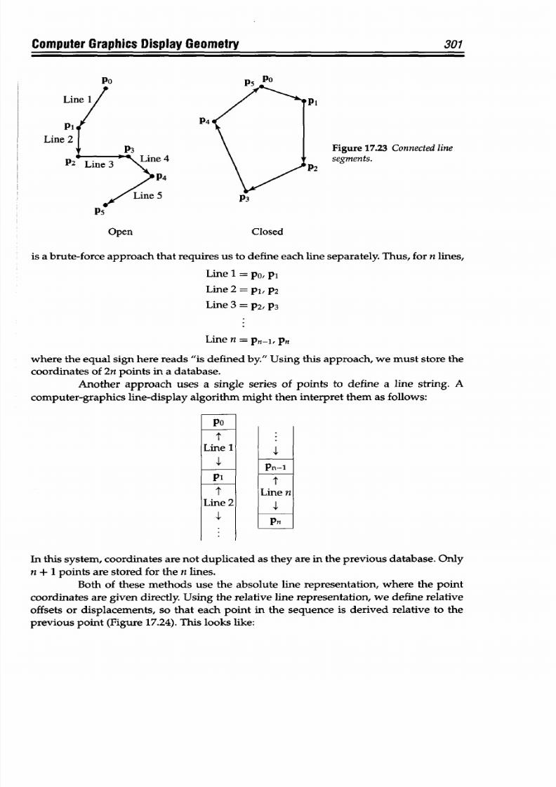
8/9/2019 Mortenson, Michael E. - Mathematics for computer graphics applications.pdf
http://slidepdf.com/reader/full/mortenson-michael-e-mathematics-for-computer-graphics-applicationspdf 314/367
Computer
Graphics
Display
Geometry
301
Po
Pi
P4
P3
4
14
Figure 17.23
Connected line
segments.
P2
P3
P5
Open Closed
is
a
brute-force approach that requires us to define each line separately. Thus, for n lines,
Line 1 = po,
p1
Line 2
=pI,p
2
Line 3 = P2, P3
Line n =
Pn-1,
Pn
where the equal
sign here
reads
"is
defined
by."
Using this
approach,
we
must
store the
coordinates of
2n
points in
a
database.
Another approach uses a single series of points to define a line string. A
computer-graphics line-display algorithm might
then
interpret them as follows:
Po
Line
1
Pi
Line
2
I-
Pn-1
Line n
Pn
In
this
system,
coordinates are not duplicated as
they are in
the
previous database.
Only
n
+ 1 points
are
stored
for
the n lines.
Both of these methods use the absolute
line
representation, where the
point
coordinates
are
given
directly.
Using
the
relative line
representation, we
define relative
offsets
or
displacements,
so that each point
in
the
sequence
is
derived relative to
the
previous
point
(Figure 17.24).
This looks
like:
Line
1
301
omputer Graphics Display Geometry
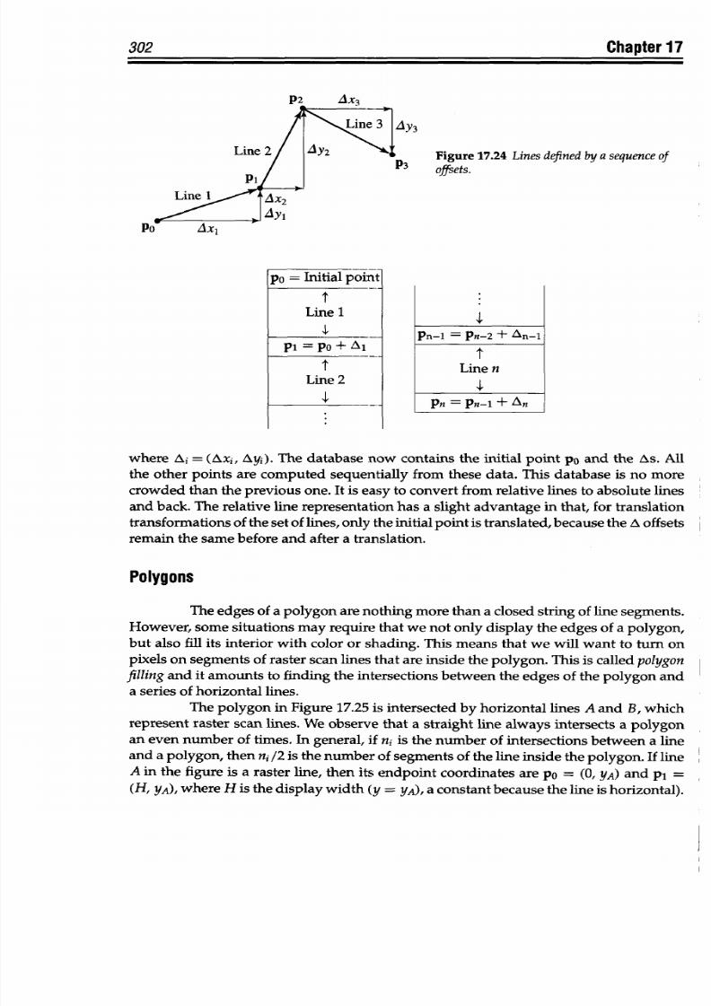
8/9/2019 Mortenson, Michael E. - Mathematics for computer graphics applications.pdf
http://slidepdf.com/reader/full/mortenson-michael-e-mathematics-for-computer-graphics-applicationspdf 315/367
Chapter 17
AY
3
LP
Figure
17.24
Lines defined by
a sequence
of
P offsets.
po
= Initial point
-1-
Line
1
pi = Po+ Al
Line
2
Pn-l =
Pn-2 +
An-l
t
Line n
Pn = Pn-1
+
An
where
Ai
=
(Axi,
Ayi).
The
database now
contains
the initial
point
pu and
the
As.
All
the other points
are computed
sequentially
from these data.
This
database
is
no more
crowded
than
the
previous
one.
It is easy to convert
from relative
lines
to absolute
lines
and
back.
The relative
line representation has
a slight
advantage in that,
for translation
transformations
of the set
of
lines,
only the
initial
point is
translated,
because the
A
offsets
remain
the same
before and
after a
translation.
Polygons
The
edges
of a
polygon
are
nothing
more
than
a closed
string
of line segments.
However,
some situations may
require
that
we
not only
display
the
edges
of a polygon,
but also fill
its interior
with color or
shading. This
means
that
we
will
want to turn
on
pixels on
segments
of raster
scan
lines
that
are inside
the
polygon.
This
is called
polygon
filling and
it
amounts to finding
the intersections
between the edges
of the
polygon
and
a series of
horizontal lines.
The
polygon
in Figure 17.25
is
intersected
by
horizontal
lines
A
and
B, which
represent
raster scan
lines. We
observe that
a
straight
line always
intersects
a polygon
an even
number
of times. In
general, if
ni is the number
of
intersections
between
a line
and
a
polygon,
then
ni
/2
is
the
number
of
segments
of
the
line
inside
the polygon.
If
line
A
in
the
figure is
a
raster
line, then its endpoint
coordinates
are
po
=
(0, yA)
and
p,
=
(H,
YA), where H
is the
display
width
(y
= YA), a constant
because the
line
ishorizontal).
302
P2
Line
1
PC
'AX2
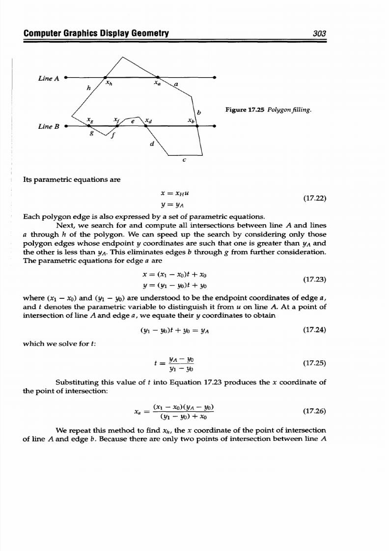
8/9/2019 Mortenson, Michael E. - Mathematics for computer graphics applications.pdf
http://slidepdf.com/reader/full/mortenson-michael-e-mathematics-for-computer-graphics-applicationspdf 316/367
Computer
Graphics Display Geometry
Line A
Line
B
Figure
17.25
Polygonfilling.
gd \
d\
C
Its
parametric equations are
X =
XHU
Y = YA
(17.22)
Each polygon edge is
also
expressed by
a
set of parametric equations.
Next, we search
for
and
compute all
intersections
between line A
and
lines
a through h of the
polygon.
We
can
speed up the search
by considering
only those
polygon
edges
whose
endpoint y coordinates are
such
that
one is greater
than
YA and
the
other is less
than
YA.
This eliminates edges
b
through g from
further
consideration.
The
parametric equations for edge a
are
x
= (x
1
-
xo)t
+ xo (17.23)
Y= (yi - yO)t + yO
where
(xl
- xo) and (yi - yo)
are
understood
to
be the endpoint coordinates of edge a,
and t
denotes
the parametric variable to distinguish it
from
u
on line
A. At
a
point of
intersection of
line A
and
edge a, we equate their y
coordinates
to
obtain
303
which we solve
for t:
(Y1
-YO)t
+
YO
=
YA
t- YA-YO
yi
- yO
Substituting
this
value of t into
Equation
17.23 produces the
x
coordinate
of
the
point of
intersection:
(X
1
- XO)(yA -
yO)
(y -yO) + Xo
(17.26)
We repeat this
method
to find xh,
the
x coordinate of
the
point
of
intersection
of
line A
and edge b. Because there
are only
two points
of intersection
between line A
(17.24)
(17.25)
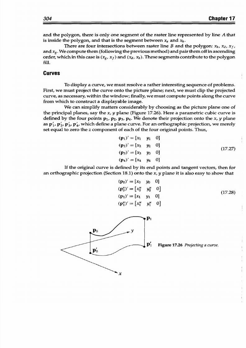
8/9/2019 Mortenson, Michael E. - Mathematics for computer graphics applications.pdf
http://slidepdf.com/reader/full/mortenson-michael-e-mathematics-for-computer-graphics-applicationspdf 317/367
304 Chapter
17
and
the polygon, there is only one segment of
the
raster line represented by line
A
that
is inside
the polygon,
and
that
is
the segment
between
xa and
xh.
There
are four
intersections
between
raster
line B
and the polygon: Xb, Xd, xf,
and
xg.
We
compute
them
(following
the previous method)
and
pair
them
off
in
ascending
order,
which in this case is (xg, xf
)
and
(xd, Xb).
These
segments contribute to
the
polygon
fill.
Curves
To
display
a curve, we must resolve a
rather
interesting sequence of problems.
First, we must project the curve onto the picture plane; next, we must clip the projected
curve, as
necessary, within
the window;
finally,
we
must
compute points
along
the
curve
from which to construct a displayable image.
We can simplify matters considerably by choosing as the picture
plane
one
of
the p rincipal planes, say
the
x, y
plane
(Figure 17.26). Here
a
parametric cubic curve
is
defined
by
the four
points
P1, P2, P3, P4. We denote their projection onto the x, y plane
as
p 1,
p , p ,
p ,
which define
a
plane
curve.
For
an
orthographic
projection,
we merely
set equal
to
zero the
z
component of each of
the four
original
points.
Thus,
(p2), = [x
2
Y
01
(P2)'= [X2 Y3 0]
(17.27)
(P3)'
= [X3
Y3
0]
(P4)=[X
4
Y4
0]
If
the original curve is defined by its
end
points
and
tangent
vectors,
then for
an orthographic projection (Section 18.1) onto the x, y plane it is also easy to show that
(Po),= LXo yo 0]
(Po) =
[xW
you
0]
(17.28)
(pi)' =
[xi y,
01
(p)
=
N[xU yA 0]
l Figure 17.26 Projecting
a
curve.
x
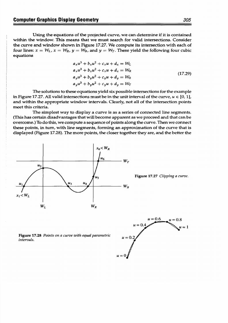
8/9/2019 Mortenson, Michael E. - Mathematics for computer graphics applications.pdf
http://slidepdf.com/reader/full/mortenson-michael-e-mathematics-for-computer-graphics-applicationspdf 318/367
Computer Graphics
Display
Geometry
305
Using the equations
of
the projected curve, we
can
determine if it is contained
within the window. This means that
we must
search
for valid
intersections. Consider
the curve and window shown in Figure 17.27.
We
compute its intersection
with
each of
four
lines: x = WL, x
=
WR,
y =
WB, and y = WT. These yield the following
four
cubic
equations
axu
3
+ bxu
2
+ cxu +
dx
=
WL
axu
3
+
bxu
2
+ c~u + dx
=
WR (17.29)
aY u
3
+ byu
2
+ cYu + dy
=
WB
ayu
3
+
byu
2
+
cYu
+
dY
=
WT
The solutions
to
these equations yield six
possible intersections
for
the example
in
Figure
17.27.
All
valid intersections
must
be
in
the
unit
interval
of
the
curve,
u
E
[0, 1],
and
within the
appropriate
window intervals. Clearly, not all of the intersection
points
meet this
criteria.
The simplest way to display a curve is as a series of connected line segments.
(This has certain disadvantages that will become apparent
as
we proceed
and
that can
be
overcome.) To do this, we compute a sequence of
points along
the
curve.
Then we
connect
these
points, in
turn, with line
segments,
forming
an ap proximation
of the curve that is
displayed
(Figure
17.28). The
more
points, the closer together they are, and the better
the
WT
Figure
17.27
Clippinga curve.
WB
WL
WR
Figure 17.28 Points on a curve with equal parametric
intervals.
u=0.6 u=0.8
u=O.4
u= l
u=0.2
u=0
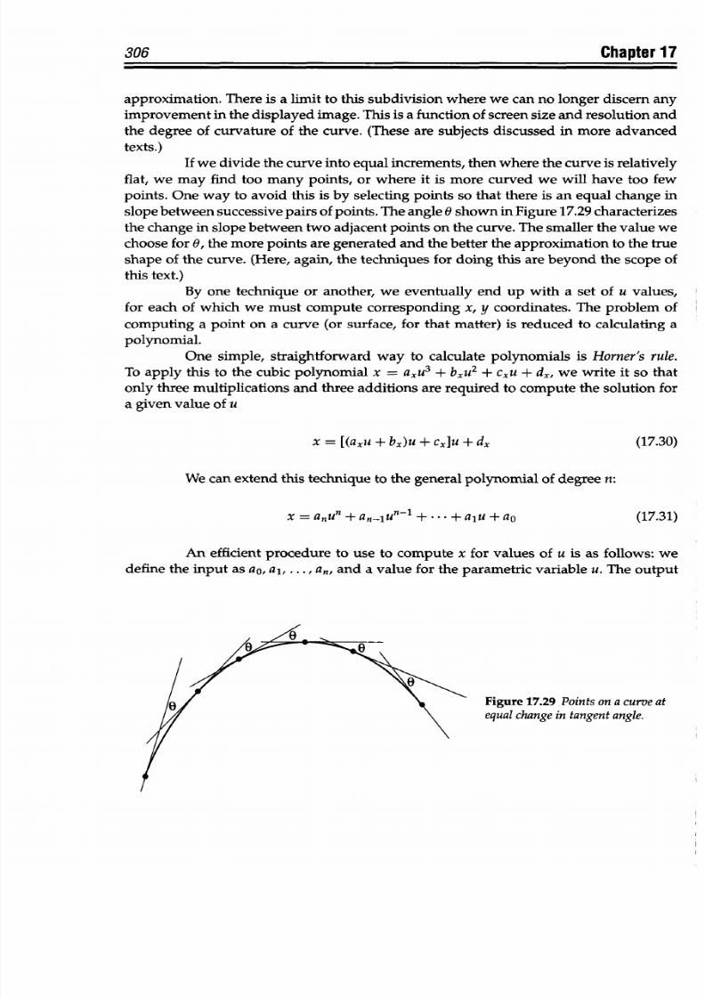
8/9/2019 Mortenson, Michael E. - Mathematics for computer graphics applications.pdf
http://slidepdf.com/reader/full/mortenson-michael-e-mathematics-for-computer-graphics-applicationspdf 319/367
306
Chapter
17
approximation.
There
is
a
limit
to
this subdivision where we
can
no longer discern any
improvement in
the
displayed
image. This is
a
function of screen size
and resolution and
the degree of
curvature
of the
curve. (These
are subjects discussed in more advanced
texts.)
If we
divide
the
curve into
equal
increments, then where the curve is
relatively
flat, we
may
find too many points, or
where
it
is
more
curved
we will
have
too
few
points.
One way
to
avoid this is by selecting points
so
that there
is
an equal
change
in
slope
between
successive pairs of points.
The
angle & hown in Figure
17.29
characterizes
the change in slope
between
two adjacent points
on the
curve. The
smaller the value we
choose for 0,
the
more
points are generated and
the better the approximation
to the true
shape
of the
curve. (Here,
again,
the
techniques
for
doing this
are
beyond the
scope of
this text.)
By one technique or
another,
we eventually end up with a set
of
u values,
for each of which we
must compute corresponding
x, y
coordinates.
The
problem of
computing a point
on
a
curve
(or
surface,
for
that
matter)
is
reduced
to
calculating
a
polynomial.
One simple,
straightforward
way
to calculate polynomials is Horner's
rule.
To
apply this
to
the
cubic
polynomial
x =
axu
3
+
bxu
2
+ cxu + dx, we write
it
so that
only three multiplications and three additions
are
required to compute the solution for
a given
value
of u
x = [(axu + bx)u + cJu + dx
(17.30)
We can
extend
this technique
to
the general
polynomial
of degree n:
x
=
anun +
an
1
Un
1
+. +±aluao
(17.31)
An
efficient
procedure to use to compute
x for
values
of
u is as follows:
we
define the
input as
ao,
al, . . .,
an,
and a value for the
parametric
variable u. The
output
Figure
17.29 Pointson a curve at
equal change in tangent angle.
8/9/2019 Mortenson, Michael E. - Mathematics for computer graphics applications.pdf
http://slidepdf.com/reader/full/mortenson-michael-e-mathematics-for-computer-graphics-applicationspdf 320/367
Computer Graphics
Display
Geometry
307
is,
of course, x. We generalize
Homer's rule
so
that
Forn=1: x(u)=alu+ao
For
n
=
2:
x(u)
=
(a
2
u
+
ai)u
+
ao
For n = 3: x(u) = [(a
3
u
+
a
2
)U +
al]u+aO (17.32)
For n = 4:
x(u)
=
{[(a
4
+
a
3
)U
+
a
2
]U
+
a,}u
+
ao
and so on.
For
any
n, we develop what
is
called a
straight-line
program of
2n
steps to
evaluate a general nth-degree polynom ial. Clearly, n
multiplications
and n additions are
necessary. Combining Homer's rule
with
a straight-line program yields,
for
n
=
1,
n =
2,
and n
= 3:
Forn=1 t<-alu
x
<- t + ao
Forn=2
t <-a
2
u
t <-t+aa
t <- tu
x
- t +
ao (17.33)
Forn =3 t -a
3
u
t <- t
+ a
2
t
<-
t
+
tu
t <-t+a,
t
<- tu
x *- t + ao
This process is
easily extended to higher-degree polynomials.
Surfaces
Many
of
the problems
of
displaying
a
surface are
the
same
as
those
for
a
curve.
To
produce
a simple wireframe image of
a
surface,
we
project, clip,
and
plot a
set of
representative curves lying
on the
surface. At
the very minimum, this
might
be
the four
bounding
curves at u =
0,
u =
1,
w =
0, and w
= 1.
As shown
in
Figure
17.30a, this
is barely adequate. Including some intermediate curves, as in
Figure 17.30,
produces a
more meaningful image of interior
surface
behavior.
The most realistic display of
a
surface requires that we introduce
color,
shading,
and other lighting effects. This is called
rendering.
To
do
this we
need
the normal at enough
points on
the
surface to
adequately adjust
each of
its display pixels.
The relationship of
the surface
normal
to the line
of
sight,
the
incident light, and surface texture
determine
the quality
and quantity of
light emitted
by
the
surface
back to the
viewer's eye,
which
in turn determines what
we must
do
to
each
pixel. These techniques are
thoroughly
discussed
in
more
advanced
textbooks.
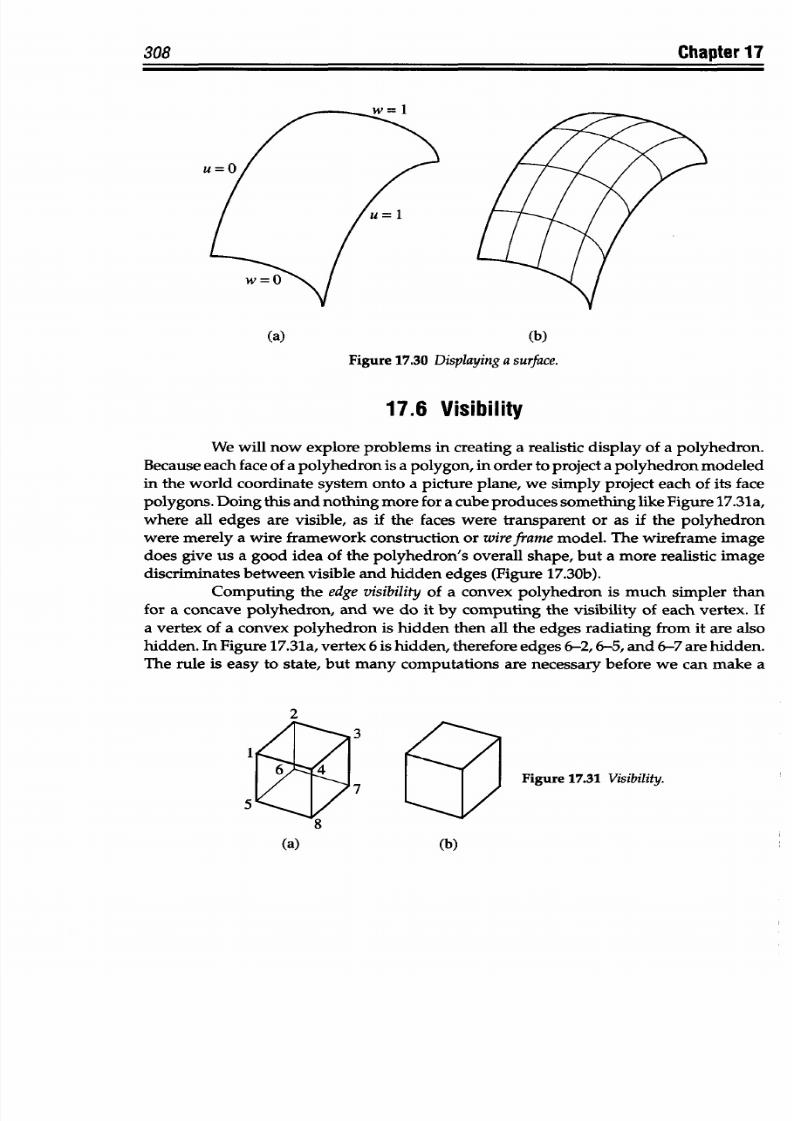
8/9/2019 Mortenson, Michael E. - Mathematics for computer graphics applications.pdf
http://slidepdf.com/reader/full/mortenson-michael-e-mathematics-for-computer-graphics-applicationspdf 321/367
308
Chapter
17
(a)
(b)
Figure 17.30
Displaying
a surface.
17.6
Visibility
We
will
now
explore problems in
creating
a realistic
display
of a polyhedron.
Because each
face
of
a polyhedron is a polygon, in order to project a polyhedron
modeled
in the
world
coordinate system onto a picture plane, we simply project
each of its
face
polygons.
Doing
this
and
nothing
more
for
a
cube
produces something
like
Figure
17.31 a,
where
all edges are
visible,
as
if
the
faces were transparent
or as
if
the polyhedron
were
merely
a
wire framework construction
or wire
frame
model.
The wireframe
image
does
give us a good idea of
the
polyhedron's overall
shape, but
a
more
realistic
image
discriminates
between
visible and hidden edges
(Figure
17.30b).
Computing the edge
visibility of
a convex polyhedron is much simpler than
for a concave
polyhedron, and
we do it by
computing the visibility
of
each
vertex. If
a vertex
of
a
convex
polyhedron
is
hidden then
all
the edges radiating from
it
are also
hidden. In
Figure 17.31a,
vertex
6
is hidden, therefore edges 6-2,6-5, and 6-7 are hidden.
The rule
is
easy
to state,
but many computations are
necessary
before
we
can make
a
2
1
5
Figure 17.31
Visibility.
(b)a)
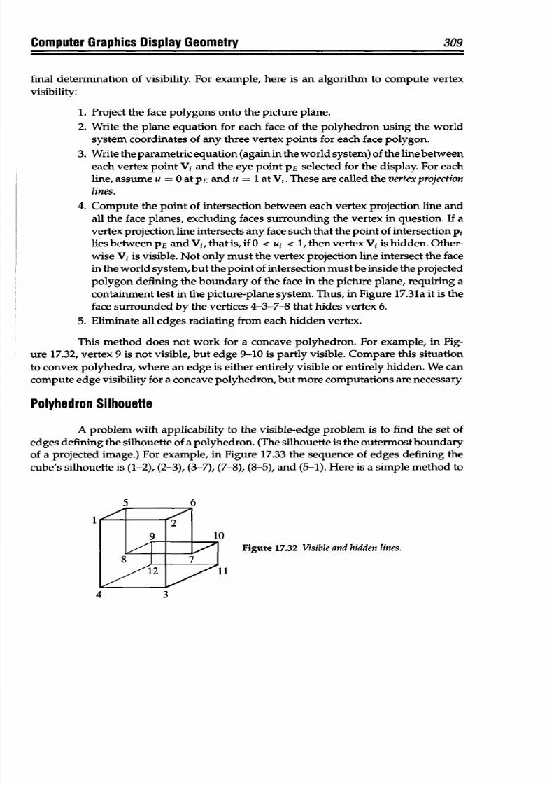
8/9/2019 Mortenson, Michael E. - Mathematics for computer graphics applications.pdf
http://slidepdf.com/reader/full/mortenson-michael-e-mathematics-for-computer-graphics-applicationspdf 322/367
Computer Graphics Display Geometry
309
final
determination of
visibility. For example,
here
is
an
algorithm to compute
vertex
visibility:
1. Project the face polygons
onto the picture plane.
2. Write the plane equation for each face
of
the polyhedron using the world
system coordinates of
any
three vertex
points
for
each
face polygon.
3. Write the parametric equation (again in the
world
system) of the
line
between
each
vertex
point
Vi and
the eye point
PE selected for the
display. For
each
line, assume u =
0
at PE
and
u =
1 at
Vi. These are called
the
vertex
projection
lines.
4.
Compute the
point of
intersection between each vertex
projection
line
and
all
the
face
planes, excluding
faces
surrounding
the vertex
in
question.
If
a
vertex
projection line
intersects any
face
such
that
the
point
of
intersection
pi
lies between PE
and
Vi, that is, if
0
< ui <
1,
then vertex
Vi is
hidden. Other-
wise Vi is
visible. Not
only
must the vertex projection line intersect the
face
in
the world
system,
but the point of
intersection
must be inside
the
projected
polygon
defining the
boundary of
the face
in
the
picture
plane,
requiring
a
containment test in the picture-plane system. Thus, in Figure 17.31a it is the
face
surrounded by
the vertices 4-3-7--
that
hides vertex 6.
5.
Eliminate all
edges radiating from
each hidden
vertex.
This
method does
not
work for
a
concave
polyhedron. For
example, in Fig-
ure
17.32,
vertex
9
is
not
visible,
but
edge
9-10
is
partly
visible.
Compare this situation
to convex polyhedra, where an edge is either
entirely
visible
or entirely
hidden. We can
compute edge visibility for a
concave
polyhedron,
but more com putations
are necessary.
Polyhedron
Silhouette
A problem with applicability to the visible-edge problem is to find the set of
edges
defining the silhouette
of
a polyhedron.
(The
silhouette
is the outermost
boundary
of
a projected image.)
For
example, in Figure 17.33 the sequence of edges defining the
cube's
silhouette
is (1-2), (2-3), (3-7),
(7-8),
(8-5),
and
(5-1). Here is a simple
method
to
0
Figure 17.32
Visible
and hidden
lines.
11
4
3
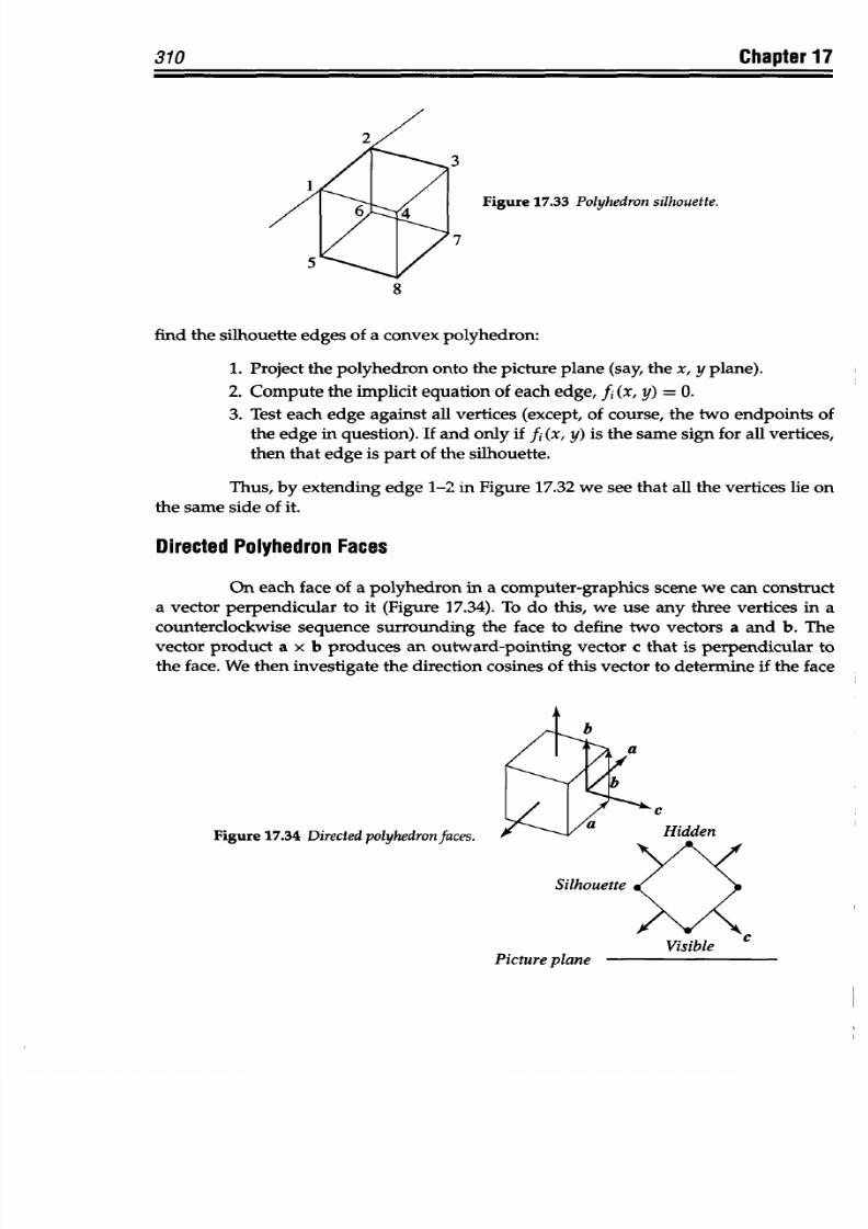
8/9/2019 Mortenson, Michael E. - Mathematics for computer graphics applications.pdf
http://slidepdf.com/reader/full/mortenson-michael-e-mathematics-for-computer-graphics-applicationspdf 323/367
310
Chapter
17
Figure
17.33 Polyhedron
silhouette.
8
find the
silhouette edges
of
a convex polyhedron:
1.
Project
the
polyhedron
onto the picture
plane
(say,
the
x,
y
plane).
2. Compute the implicit equation of each edge, fi (x, y) = 0.
3.
Test
each edge against all vertices (except,
of
course, the two
endpoints
of
the
edge
in
question). If and
only
if f, (x, y) is the
same
sign
for
all vertices,
then that edge
is
part of
the silhouette.
Thus, by extending edge 1-2 in Figure
17.32
we see
that all
the vertices lie on
the same side
of
it.
Directed Polyhedron
Faces
On
each
face of a polyhedron in a computer-graphics scene we can
construct
a
vector
perpendicular
to it (Figure
17.34). To do
this,
we
use
any
three
vertices
in a
counterclockwise sequence surrounding the face to define two vectors a and b. The
vector
product
a x
b produces
an
outward-pointing vector
c
that is
perpendicular to
the face. We then investigate the direction
cosines of
this vector to determine if the
face
Figure 17.34 Directed
polyhedronfaces.
Silhouette
Visible
Picture
plane
I
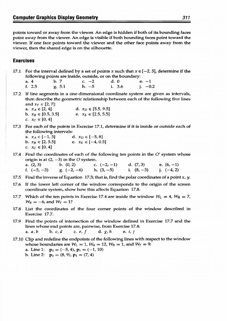
8/9/2019 Mortenson, Michael E. - Mathematics for computer graphics applications.pdf
http://slidepdf.com/reader/full/mortenson-michael-e-mathematics-for-computer-graphics-applicationspdf 324/367
Computer
Graphics
Display
Geometry
311
points toward
or away from
the
viewer. An edge
is
hidden if both of
its bounding faces
point away from the viewer. An edge
is
visible
if
both bounding faces point toward
the
viewer. If
one face points
toward the viewer
and the other face points away
from the
viewer,
then
the
shared
edge
is
on the silhouette.
Exercises
17.1 For
the
interval
defined
by
a
set
of points
x such
that
x E [-2,
51, determine
if
the
following points are inside, outside, or
on
the
boundary:
a.
4
b.
7 c. -2
d.
0
e.
-1
f.
2.5 g. 5.1
h. -5 i.
3.6
j.
-0.2
17.2
If line segments in
a
one-dimensional coordinate system
are
given
as
intervals,
then describe the
geometric
relationship between each
of
the following
five lines
and
XT
E [2,
7]:
a. XA
E
[2,4] d. XD E [55.,
9
.5]
b. XB E [0.5,3.5] e.
XE
E [2.5,5.5]
c. Xc E [0,4]
17.3 For each
of the
points in
Exercise
17.1,
determine
if
it is
inside
or outside
each
of
the following intervals:
a. XA E [-1, 3] d. XD E
[-5,8]
b.
XB
E [2, 5.5] e.
XE E
[-4, 0.5]
c.
Xc E
[, 4]
17.4 Find the coordinates of
each
of the following ten points in the O' system whose
origin is at (2, -3) in the 0
system.
a. (2,
3) b.
(0,
2)
c. (-2, -1)
d.
(7,
3)
e. (6, -1)
f. (-5, -3) g. (-2, -6) h.
(3,
-5) i. (8, -3) j. (-4, 2)
17.5
Find the
inverse of Equation
17.3;
that is, find the polar coordinates of a
point
x,
y.
17.6 If the lower
left
corner of the
window
corresponds to the origin
of
the
screen
coordinate
system,
show
how
this affects Equation
17.8.
17.7 Which
of the ten
points in
Exercise
17.4
are inside the
window WL = 4,
WR =
7,
WB = -6, and WT = 1?
17.8 List the
coordinates of
the
four corner
points of
the
window
described in
Exercise
17.7.
17.9 Find
the
points
of
intersection of the window defined in Exercise 17.7 and
the
lines whose end points
are,
pairwise, from Exercise 17.4:
a. a,b b. cd c. e,f d. g,h e.
i,j
17.10
Clip and redefine the endpoints of the following
lines
with respect to the window
whose boundaries
are WL =
1,
WR = 12, WB =
1, and
WT =
9:
a.
Line
1:
po = (-5, 4),
pl
=
(-1,
10)
b.
Line2:
pO
= (8,9),pj = (7,4)
8/9/2019 Mortenson, Michael E. - Mathematics for computer graphics applications.pdf
http://slidepdf.com/reader/full/mortenson-michael-e-mathematics-for-computer-graphics-applicationspdf 325/367
312
Chapter
17
c.
Line
3:
Po
= (12, -1), p1 = (12,
3)
d.
Line 4: Po = (4, 10),
pi (0, 2)
e. Line
5: po = (
3
,
-1),
pi= (6,
2
)
f.
Line 6:
Po
= (4, 3), p'
=
(6, -1)
g. Line
7:
Po
= (2, 0),
p1 =
(2,
12)
h. Line
8: Po = (7, 10),
pi
=
(11,
-2)
i. Line
9:
po = (11, 7), pi = (15,
7)
j.
Line
10:
Po =
(15,
-2),
pi = (12,
-5)
17.11 Clip
and redefine
as
necessary
the endpoints
of the following line
segments
with
respect to a
window
whose boundaries are WL = 2,
WR
=
14,
WT =
10,
and
WB
= -2. Describe each
line's relationship
to this
window.
a.
Po = (-5,
4), p'
= (1,
13) f.
Po
=
(4, 3), pi = (8, -4)
b. Po
= (
7
,
4
), pi =
(5, 9)
g.
Po
= (
2
,1),
p1 = (2,12)
c. Po
= (12,
6), pi = (12,
0) h.
Po = (12,
-6),
pi =
(6,13)
d. Po = (5,12), pi = (-3,
-4)
i. Po = (11,
7),
pi =
(15,
7)
e. Po
=
(2,
-2), pi
=
(6, 2)
j.
Po
=
(13,
-5),
pi =
(18, 4)
17.12 Use
the
following
sequence
of point coordinates
to construct each of
the three
line data
formats
discussed
in this
chapter: po =
(1,
3), pi = (4, 5), P2 = (4, 8),
p3
= (9, 5),
p4
= (5,
1),
p5
= (7,
-3).
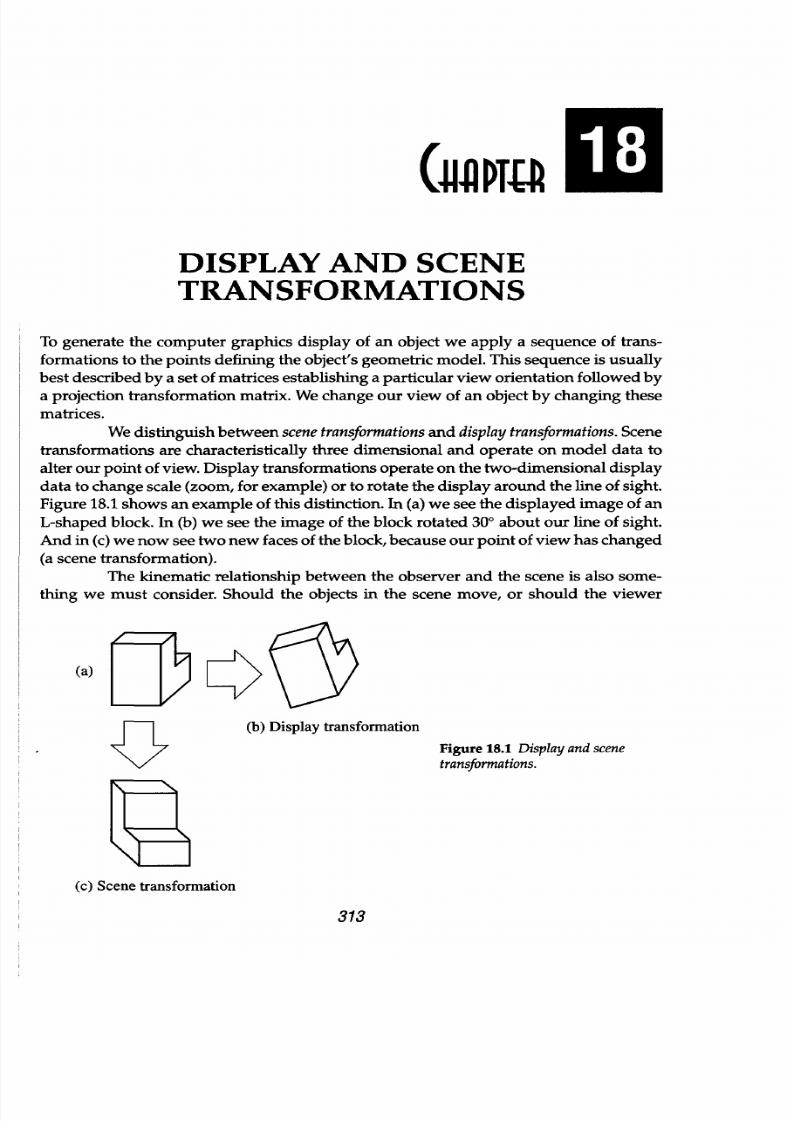
8/9/2019 Mortenson, Michael E. - Mathematics for computer graphics applications.pdf
http://slidepdf.com/reader/full/mortenson-michael-e-mathematics-for-computer-graphics-applicationspdf 326/367
DISPLAY
AND SCENE
TRANSFORMATIONS
To
generate
the computer
graphics
display
of
an
object
we
apply
a
sequence
of
trans-
formations
to
the
points defining
the
object's geometric model. This sequence is usually
best
described by
a set
of matrices
establishing a
particular view
orientation
followed
by
a
projection
transformation
matrix. We change our view of
an
object by
changing these
matrices.
We
distinguish
between
scene transformationsand display transformations.Scene
transformations
are characteristically
three dimensional
and
operate
on
model
data to
alter
our point
of view. Display transformations operate on the two-dimensional display
data to change scale (zoom, for example) or to
rotate
the display around the line of sight.
Figure
18.1
shows
an example
of
this
distinction.
In
(a)
we
see
the displayed image
of
an
L-shaped
block.
In (b)
we
see
the image of the block rotated 300 about our line of sight.
And
in
(c)
we
now see two new faces of the block, because our point of
view has changed
(a scene transformation).
The kinematic relationship between the observer
and
the
scene
is
also
some-
thing we must
consider.
Should
the
objects in the
scene
move, or should
the
viewer
(a)
>
(b) Display transformation
X 7 Figure
18.1 Displayand
scene
transformations.
(c) Scene
transformation
313
ApTa
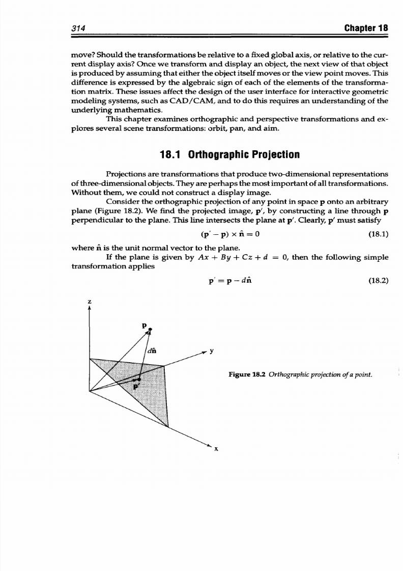
8/9/2019 Mortenson, Michael E. - Mathematics for computer graphics applications.pdf
http://slidepdf.com/reader/full/mortenson-michael-e-mathematics-for-computer-graphics-applicationspdf 327/367
314
Chapter 18
move? Should the transformations be
relative
to a
fixed global axis,
or
relative
to the cur-
rent display
axis? Once we transform
and
display
an object, the
next view of
that object
is produced by
assuming
that
either the object itself moves or the view
point moves. This
difference
is
expressed
by the
algebraic
sign
of
each
of
the
elements
of
the transforma-
tion
matrix. These
issues
affect
the design of the user
interface for
interactive
geometric
modeling systems,
such
as CAD/CAM, and
to
do this requires an
understanding
of the
underlying mathematics.
This
chapter examines orthographic
and
perspective transformations
and
ex-
plores several scene transformations:
orbit,
pan, and aim.
18.1 Orthographic Projection
Projections are
transformations
that
produce two-dimensional representations
of
three-dimensional objects. They
are
perhaps
the
most
important of
all transformations.
Without them, we could not construct
a
display
image.
Consider
the
orthographic projection of any
point
in space
p
onto an arbitrary
plane
(Figure 18.2).
We find the
projected image, p', by
constructing a
line through p
perpendicular to the plane. This line intersects the plane
at
p'. Clearly,
p'
must
satisfy
(p' -p) x f=O (18.1)
where
fi
is the
unit normal
vector
to
the
plane.
If
the plane
is
given by
Ax
+
By
+
Cz
+
d
=
0,
then the
following
simple
transformation applies
p' =
p
- dn (18.2)
z
y
Figure 18.2
Orthographic rojection
of
a
point.
x
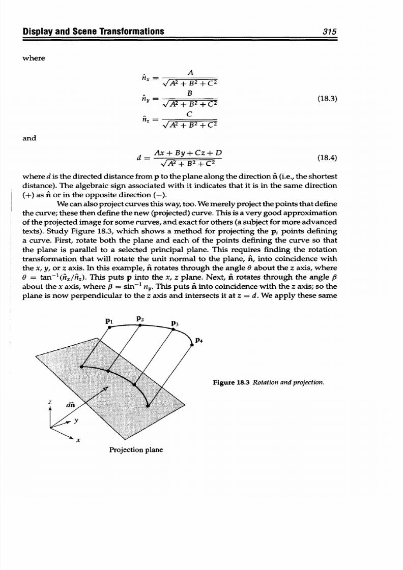
8/9/2019 Mortenson, Michael E. - Mathematics for computer graphics applications.pdf
http://slidepdf.com/reader/full/mortenson-michael-e-mathematics-for-computer-graphics-applicationspdf 328/367
Display and Scene
Transformations 315
where
A
n, =
/A
2
+ B
2
+c
2
B
y A
2
+ B
2
+ C
2
(18.3)
C
nz = /A2+B2+C2
and
d = Ax+By+Cz+ D (18.4)
1/A
2
+ B
2
+C
2
(1
where
d
is
the
directed distance
from p
to the plane along
the
direction
fl
(i.e., the
shortest
distance).
The algebraic
sign associated with it indicates
that
it is in the same
direction
(+) as Aor in the
opposite direction (-).
We can also
project curves this way, too. We merely project the points
that
define
the
curve;
these then
define the new (projected) curve. This
is
a
very good
approximation
of the
projected
image for some curves,
and exact
for others (a
subject
for more advanced
texts).
Study
Figure 18.3, which shows
a method
for projecting
the
pi
points defining
a
curve. First,
rotate both the plane and
each
of the points defining the curve so that
the plane is parallel to a selected principal plane. This requires finding the rotation
transformation
that
will
rotate
the
unit
normal
to
the
plane,
fi,
into
coincidence
with
the
x,
y, or z
axis.
In this example, ft rotates through the angle
0
about the
z
axis, where
9
= tan-<(hx/nh). This puts p into
the
x, z plane. Next, ii
rotates
through the angle
P
about
the x
axis,
where P = sin-' ny,. This puts
fl
into coincidence with
the
z
axis;
so
the
plane is now
perpendicular to the z axis and
intersects
it
at
z
=
d. We
apply
these
same
n_
P4
Figure
18.3 Rotation
and projection.
Projection
plane
- . . . - - . ..
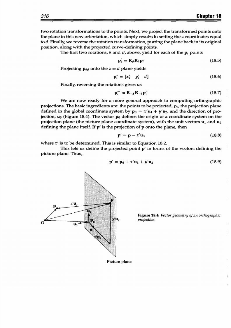
8/9/2019 Mortenson, Michael E. - Mathematics for computer graphics applications.pdf
http://slidepdf.com/reader/full/mortenson-michael-e-mathematics-for-computer-graphics-applicationspdf 329/367
Chapter
18
two rotation
transformations to the points.
Next, we project the
transformed points onto
the
plane in
this new orientation,
which simply results in setting the z coordinates
equal
to d. Finally, we
reverse the rotation transformation, putting
the plane
back in its original
position, along
with
the
projected
curve-defining points.
The first
two rotations,
6 and
fl,
above, yield
for each of the
pi
points
pi= RpRopi
Projecting
pop onto the z =
d plane
yields
p'=[xj
yi d]
Finally, reversing the rotations
gives
us
p'
=
R
OR
opj'
(18.5)
(18.6)
(18.7)
We are
now
ready for a
more
general
approach
to computing orthographic
projections. The
basic ingredients
are:
the points
to be projected, pi, the projection
plane
defined in the global coordinate
system by
po
=
x'u
1
+
y'u2,
and the
direction
of
pro-
jection,
U3
(Figure 18.4). The
vector
po defines
the origin of a
coordinate system on the
projection
plane (the picture
plane coordinate system), with
the unit vectors ul and
u2
defining
the plane itself.
If
p' is
the
projection of p
onto
the
plane, then
p
= p -Z
U3
(18.8)
where
z' is to be determined.
This is similar
to Equation
18.2.
This
lets
us
define
the projected
point
p'
in
terms
of
the
vectors
defining
the
picture plane. Thus,
p' = PO
+ X'U1 + y'U
2
(18.9)
Figure
18.4 Vectorgeometry of an orthographic
-2 projection.
Picture
plane
316
I
P
U3 4
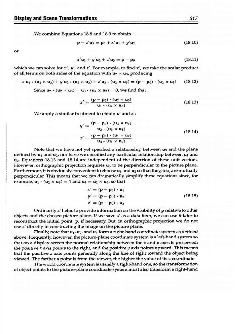
8/9/2019 Mortenson, Michael E. - Mathematics for computer graphics applications.pdf
http://slidepdf.com/reader/full/mortenson-michael-e-mathematics-for-computer-graphics-applicationspdf 330/367
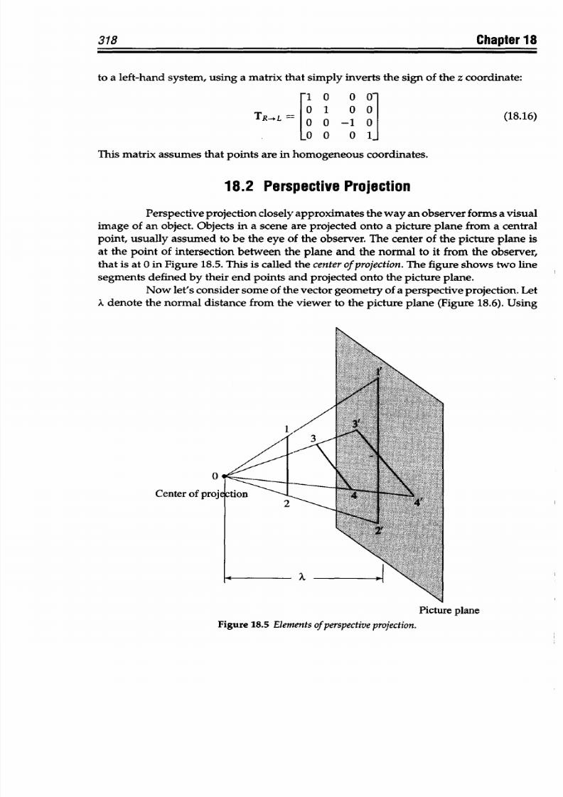
8/9/2019 Mortenson, Michael E. - Mathematics for computer graphics applications.pdf
http://slidepdf.com/reader/full/mortenson-michael-e-mathematics-for-computer-graphics-applicationspdf 331/367
318 Chapter
18
to a left-hand
system,
using a matrix that
simply inverts the
sign
of
the
z coordinate:
-1
0
0
O-
TRL =
0
1
0
(18.16)
O0 0 0 1-
This
matrix assumes
that
points
are in homogeneous
coordinates.
18.2 Perspective Projection
Perspective projection closely
approximates the
way
an observer
forms a visual
image of
an
object.
Objects in a scene are
projected
onto
a
picture
plane
from
a central
point,
usually assumed
to
be the
eye of
the
observer. The
center of
the picture
plane
is
at
the
point of
intersection
between the
plane and
the normal
to it
from
the
observer,
that is at
0
in Figure 18.5.
This is called
the
center
ofprojection. The figure
shows
two
line
segments defined
by
their end
points
and
projected onto
the picture plane.
Now
let's
consider
some
of
the vector
geometry of
a
perspective projection.
Let
Xdenote
the normal
distance from
the viewer to
the picture plane (Figure 18.6).
Using
Center of
Picture
plane
Figure
18.5
Elements
of
perspective
projection.
8/9/2019 Mortenson, Michael E. - Mathematics for computer graphics applications.pdf
http://slidepdf.com/reader/full/mortenson-michael-e-mathematics-for-computer-graphics-applicationspdf 332/367
Display
and
Scene Transformations
P
Figure
18.6
Geometry
of
a perspective
projection.
x
PE
some
simple vector
geometry,
we see that p'
= PE +k(p-PE).
We
find that k = X/(z+AX),
and
the
components
of
p'
are
Ax
z+A
Y,
=
Xy
z+A
(18.17)
z' =
0
Here,
homogeneous
coordinates
again
prove
to be
very
useful. Consider the
following transformation:
1 00
0-
,
0 1 0 0
0100
01
o0
0
r
1a
If p = [x y z 1],then
p' = [x
y
0
(rz
+ 1)]
or,
in
ordinary
Cartesian coordinates
Ptr=
x Y 0
I z+1
rz+1
I
319
x
(18.18)
(18.19)
(18.20)
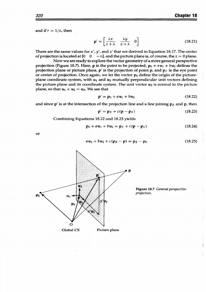
8/9/2019 Mortenson, Michael E. - Mathematics for computer graphics applications.pdf
http://slidepdf.com/reader/full/mortenson-michael-e-mathematics-for-computer-graphics-applicationspdf 333/367
320 Chapter 18
and if r = 1/A, then
p,= I.X
A Y 0] (18.21)
LZ
+
z
+ X
These are the same values for x', y', and z'
that
we derived in Equation
18.17. The
center
of projection
is located
at
[0 0 - A], and
the picture plane
is,
of
course, the z = 0
plane.
Now we are
ready to explore the
vector geometry of
a
more general perspective
projection (Figure
18.7).
Here,
p
is the
point
to be projected, pa + aul + bu
2
defines the
projection plane or picture plane,
p'
is
the
projection
of point p,
and PE
is the
eye
point
or
center of projection. Once
again, we
let
the vector
PO define the origin
of the picture-
plane coordinate system, with ul and U 2 mutually perpendicular
unit
vectors defining
the
picture plane and
its
coordinate
system.
The
unit vector U3 is
normal to the picture
plane,
so
that
u
1
X U
2
=
U
3
.
We
see
that
p' = pa +
au,
+ bu
2
(18.22)
and since
p'
is at
the
intersection of
the projection
line and a
line
joining PE
and p, then
P = PE
+ C(P PE) (18.23)
Combining Equations
18.22
and 18.23 yields
PO + aul
+
bU
2
=
PE +
C(P-PE) (18.24)
or
au, +
bu
2
+ c(pE
-
p) = PE -
PO (18.25)
p
Figure
18.7 General
perspective
projection.
Picture
plane
pi
Global
CS
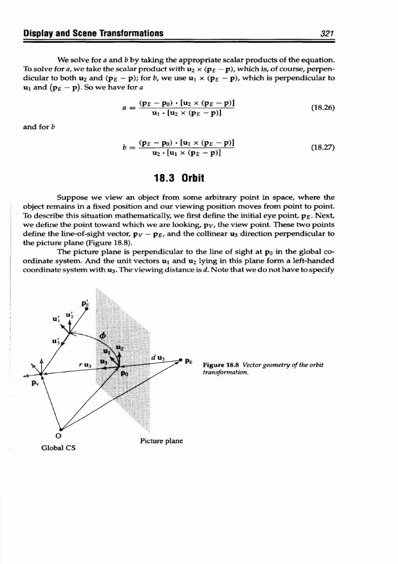
8/9/2019 Mortenson, Michael E. - Mathematics for computer graphics applications.pdf
http://slidepdf.com/reader/full/mortenson-michael-e-mathematics-for-computer-graphics-applicationspdf 334/367
Display
and Scene Transformations
321
We
solve for a and b by
taking
the
appropriate
scalar
products
of
the equation.
To solve for a, we take the scalar product with U2 X (PE -
p),
which is, of course, perpen-
dicular
to
both
u2
and (PE - p); for b, we use
ul
x (PE - p), which is perpendicular to
ul
and
(PE
- p).
So
we have
for
a
a
=
(PE -
PO)
* [U
2
X (PE -P)]
(18.26)
U1 * U2 X PE
-P)]
and for b
b = (PE - PO) *
[U
X
(PE
-P)] (18.27)
U2 * U1 X (PE -P)]
18.3
Orbit
Suppose we
view
an object from some
arbitrary
point in
space,
where
the
object remains in a
fixed
position
and
our viewing position moves
from
point to point.
To describe this situation mathematically,
we
first define the initial eye point, PE.
Next,
we
define
the
point toward
which we
are looking, pv, the view point. These
two
points
define
the
line-of-sight
vector, pv -
PE, and
the collinear
U3
direction perpendicular to
the
picture
plane (Figure
18.8).
The
picture plane
is
perpendicular
to
the
line
of
sight at
po
in
the
global
co-
ordinate
system.
And the
unit vectors
ul and u
2
lying in this plane form a left-handed
coordinate system with U
3
.
The
viewing distance
is d.
Note
that
we do not have to
specify
PE Figure
18.8
Vector geometry of
the
orbit
transformation.
0
Global CS
Picture
plane
8/9/2019 Mortenson, Michael E. - Mathematics for computer graphics applications.pdf
http://slidepdf.com/reader/full/mortenson-michael-e-mathematics-for-computer-graphics-applicationspdf 335/367
322 Chapter
18
po,
because
we
can calculate
it from
the other known
vectors
as
PO
= PE + du
3
(18.28)
Here the distance
d
is
positive,
although the
coordinates
of
PE
in
the
picture plane
coordinate
system
are (0,
0, -d).
So, first we
specify
PE,
pv,
and d.
Transformations
to produce
the
initial view
we
might
arrange as follows:
Con-
struct
ul, u
2
, and U
3
at
the origin
of
the global
coordinate
system aligned with
the positive
x, y,
and z axes.
Then
translate
them
to pv
using
Tv,
where
-I
O O
-Xv-
TV
= ° 1 0
-yv(18.29)
O0
0
0
1
Next,
we
convert
to a left-hand
coordinate system
using
TRWL, Equation 18.16.
Then
we compute
the angles of
rotation that will
align
U3
with
pv - PE, and
apply
the required
rotation
transformations,
say K&
and Rp. Usually,
only
two
rotations
are
necessary.
We
translate
this system
to
pi
using
To =
° 1
0 0
(18.30)
-°
0
0
1-
where
r
=
Ipv - pol.
The
perspective projection
transformation becomes
-1 0 0
0-
Tp
= 0
/0d
(18.31)
O0
0
l/d
1-
Finally,
we
can combine
all
of
these
transformations
into
a
single
expression
giving
the transformation of points
in the global
system
into the p icture plane:
p1
=
TVTR-LR.RpToTpp
(18.32)
As PE
orbits around point
pv,
we invoke
orbit
scene
transformations
to
gener-
ate new images.
The line of
sight
is
always toward
pv,
although both d
and r may
vary.
For
example, if
PE orbits to
the right relative
to the
picture-plane
coordinate
system,
then
the eye
point,
PE,
must
rotate about pv, say, through
an
angle
P
in
the
plane
defined
by
ul and
U
3
.
This
orbital
motion can
be described
several ways,
each leading
to
another
set
of
transformation matrices
appropriate
for
the new view.
The eye point
may rotate around
an
axis
in the
direction of
u
2
and through
pv
to produce P ES a
new
eye
point, repeating all
the
steps
outlined above using
p E to create
the new
view.
The
orbiting
type
of eye point
movement can, of
course,
include
orbiting
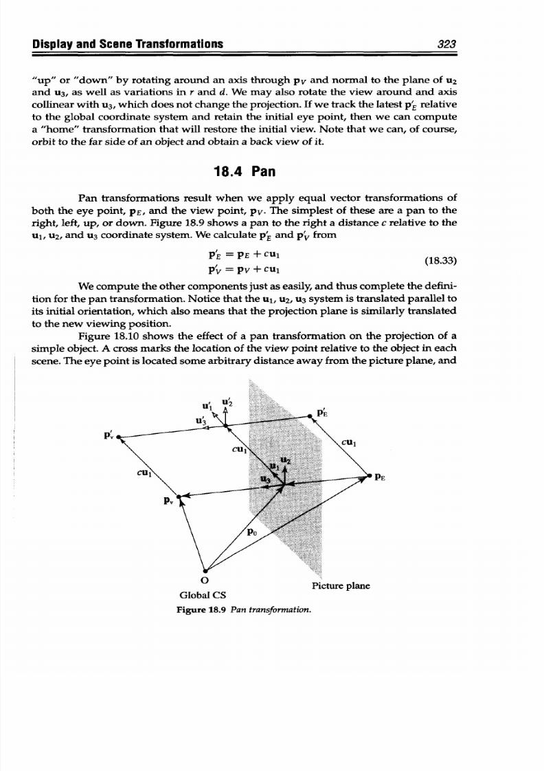
8/9/2019 Mortenson, Michael E. - Mathematics for computer graphics applications.pdf
http://slidepdf.com/reader/full/mortenson-michael-e-mathematics-for-computer-graphics-applicationspdf 336/367
Display
and
Scene Transformations 323
"up" or
"down" by rotating around an axis through
pv and
normal
to the
plane
of u2
and U
3
,
as
well
as
variations in r and
d.
We may
also
rotate
the view
around
and
axis
collinear
with
U
3
,
which does
not
change the
projection.
If we track the
latest
p E relative
to
the
global
coordinate system
and
retain the
initial
eye
point,
then
we
can
compute
a "home"
transformation that will
restore the initial
view.
Note that we can, of course,
orbit to the
far side
of
an object and
obtain
a
back
view of
it.
18.4
Pan
Pan
transformations result when
we
apply
equal vector
transformations of
both
the eye point, PE,
and
the
view
point,
pv.
The
simplest of
these
are a pan to the
right, left, up, or
down. Figure 18.9 shows a pan to the right a distance
c relative to the
u
1
,
U2,
and
U3
coordinate
system.
We
calculate
P E
and
P'v
from
PE = PE +
CU
1
(18.33)
Pv
=
Pv + cul
We compute the other com ponents just
as
easily,
and thus complete the
defini-
tion
for the pan transformation.
Notice
that the u1, U2,
U3 system is
translated
parallel to
its
initial orientation,
which also means that the
projection plane is
similarly
translated
to
the new
viewing position.
Figure
18.10 shows
the effect of
a pan transformation on
the projection of a
simple
object. A cross
marks the
location
of
the view
point
relative to
the
object
in
each
scene. The eye point
is
located
some
arbitrary
distance
away from the
picture
plane, and
Pv
*PE
v Picture
plane
Global
CS
Figure
18.9
Pan transformation.
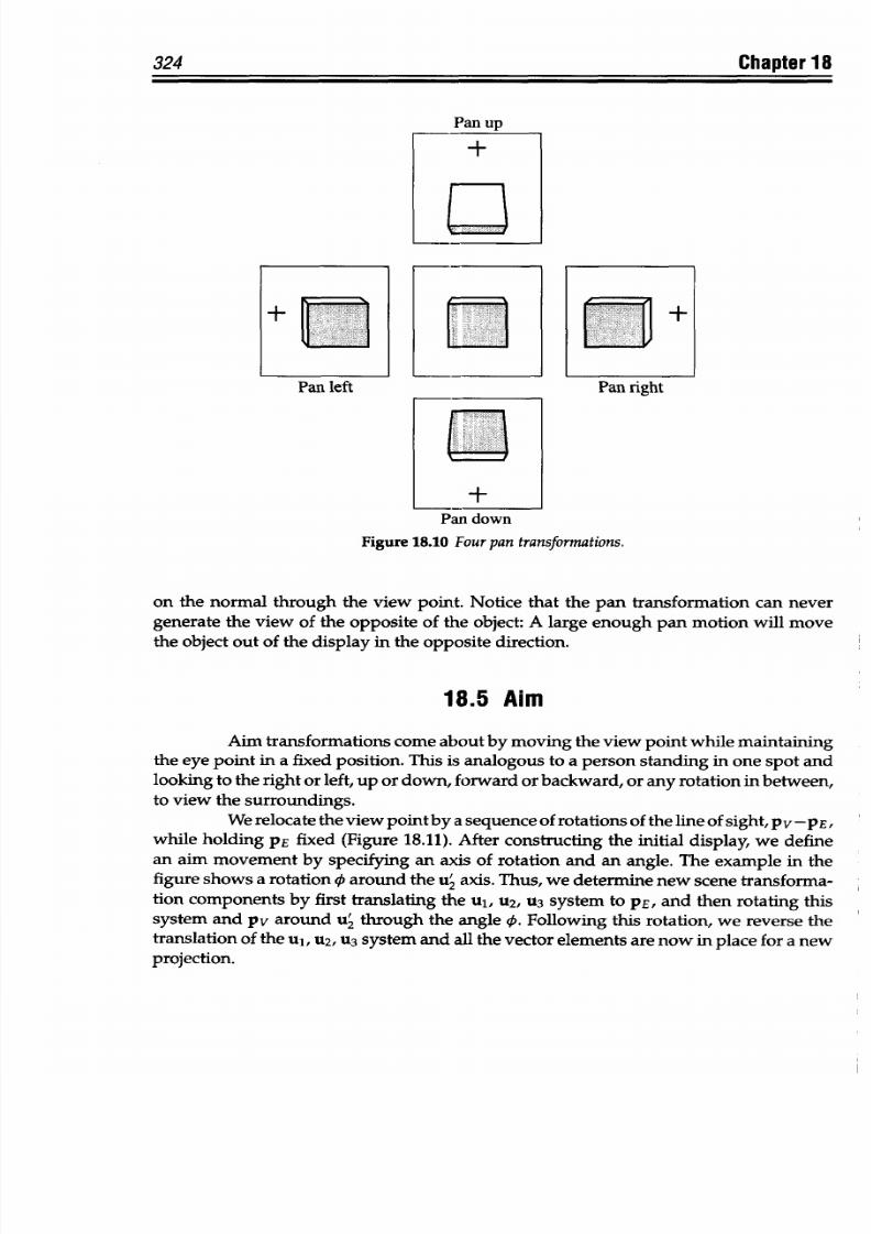
8/9/2019 Mortenson, Michael E. - Mathematics for computer graphics applications.pdf
http://slidepdf.com/reader/full/mortenson-michael-e-mathematics-for-computer-graphics-applicationspdf 337/367
324
Chapter 18
Pan left
Pan
nght
Pan down
Figure
18.10 Fourpan transformations.
on the
normal
through the view
point. Notice that
the pan
transformation
can never
generate
the
view
of
the
opposite
of the
object:
A
large
enough pan motion
will move
the
object
out
of the display
in the
opposite
direction.
18.5 Aim
Aim
transformations
come
about by
moving
the
view
point
while maintaining
the eye
point in a fixed position.
This
is
analogous to
a person
standing
in
one
spot and
looking to
the
right or
left, up
or
down,
forward
or backward,
or any rotation in
between,
to
view
the surroundings.
We
relocate the
view
point
by
a
sequence of
rotations of
the line of sight,
Pv -PE,
while
holding
PE
fixed
(Figure
18.11). After
constructing
the initial display,
we define
an
aim movement by
specifying an
axis
of rotation
and
an
angle. The
example
in the
figure
shows
a rotation
0
around
the
u2 axis.
Thus,
we
determine
new scene
transforma-
tion components
by
first
translating the
u
1
,
u
2
,
U3 system to PE,
and
then rotating
this
system
and pv
around
u'
through
the
angle
0.
Following
this
rotation,
we reverse
the
translation
of the ul, u2,
u
3
system
and all the vector
elements
are now in place
for
a
new
projection.
Tow
-
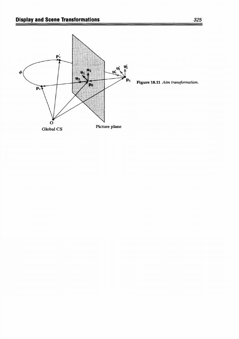
8/9/2019 Mortenson, Michael E. - Mathematics for computer graphics applications.pdf
http://slidepdf.com/reader/full/mortenson-michael-e-mathematics-for-computer-graphics-applicationspdf 338/367
Display and Scene
Transformations
0
Global CS
325
Figure
18.11 Aim
transformation.
Picture plane
8/9/2019 Mortenson, Michael E. - Mathematics for computer graphics applications.pdf
http://slidepdf.com/reader/full/mortenson-michael-e-mathematics-for-computer-graphics-applicationspdf 339/367
BIBLIOGRAPHY
Akivis, M. A.,
and
V. V.Goldberg.
An
Introduction to
Linear
Algebra and Tensors. New York: Dover,
1972.
This
is a translation
of an outstanding
Russian
textbook. It is a more rigorous
intro-
duction
than
usual
for this subject, because
it
leads directly into tensors.
Bachmann,
F.,
H. Gehnke, K.
Fladt,
and W.
SUss,
eds. Fundamentals of
Mathematics,
Volume III
Analysis. Cambridge: The MIT Press, 1988.
Bell, E. T. Men of
Mathematics.
New
York: Simon
and
Schuster, 1965. This
classic
is more
than a
book
about
math. It also reveals the human side of this wonderful and ancient
science
through a series
of
unique
biographies.
Bell writes with wit, irony and sharp good
sense.
As history and
Bell show
us, most
great
mathematicians
lived strange
lives
as soldiers,
theologians,
lawyers, diplomats, charlatans, mystics, drunkards, professors, and business-
men.
Bell
writes in
a
language
and
style easily
accessible
to
students
and
teachers
in
the
secondary level and up. Here be sure to read
about
William Rowan Ham ilton, the discoverer
of vectors, in the
chapter aptly
titled "An Irish
Tragedy."
Also, trace
the history of func-
tions, limit,
and continuity through
2500
years of
mathematical thinking and
rethinking
about
these
concepts in Bell's classic work.
Berlinski,
David.
A
Tour
of
the
Calculus. New
York; Vintage Books,
1995.
Berlinski
offers a
fresh
view of real
numbers,
functions, and limits. This
is
really literature with equations added.
Bennett, M.
K.,
Affine and Projective Geometry,
Wiley-Interscience, 1995. This is a textbook
for ad -
vanced undergraduate math students. It combines three different approaches
to
affine and
projective
geometry-algebraic, synthetic, and lattice
theoretic.
Bezier,
P.
The
MathematicalBasis
of
the UNISURF
CAD
System.
London:
Butterworths,
1986.
Bum,
R.
P.
Deductive TransformationGeometry.
Cambridge University
Press,
1975.
Campbell, H. G.
An
Introduction to Matrices, Vectors,
and
Linear Programming.New York: Prentice
Hall, 1977.
Coxeter,
H.
S. M. Regular
Polytopes.
New York: Dover, 1973. This is a another classic. Coxeter defines
a
polytope as
a
geometric figure bounded by lines,
planes,
and for
the case of
dimensions
higher
than three, hyperplanes.
The
text begins with the
fundamental
concepts of plane
and solid geometry
and
then moves
on
to multi-dimensions. The
coverage
of polygons
here is brief but crucial for a rigorous base from which to move
on to
constructions
in
higher
dimensions.
Cromwell, Peter
R.
Polyhedra. Cambridge University Press, 1997. This text is a
thought-provoking
balance
of the
historical
development of the mathematics of polyhedra and a modem rig-
orous treatment of the
subject.
Crowe, MichaelJ.
A H istoryofVectorAnalysis. NewYork:
Dover,
1985. This is one of the first in-depth
studies
of the
development
of vectorial systems. Crowe traces
the
rise of the vector concept
from
the discovery of complex
numbers
through the systems
of
hypercomplex numbers
created
by Hamilton
and Grassmann to the final acceptance in
the
early 20th century of the
modem
system of
vector analysis.
Cullen, C.
G.
Matrices and Linear Transformations.
2d ed., Dover,
1990.
de Casteljau,
P. Shape, Math-
ematics and
CAD. London: Kegan
Page,
1986.
Dodge, C. W.
Euclidean
Geometry and
Transformations.
Reading: Addison-Wesley, 1972.
Farin,
G.
Curvesand
Surfaces
orComputer-Aided Geometric
Design.New
York:
Academic
Press,
1993.
Faux, I. D., and
M.
J. Pratt. Computational Geometryfor
Design
and Manufacturing.Chichester:
Ellis
Horwood
Ltd.,
1981.
Foley, J.D., A.
Van
Dam,
and S.
K.
Feiner. Fundamentals
ofInteractive Computer Graphics.New York:
Addison-Wesley,
1993.
326
8/9/2019 Mortenson, Michael E. - Mathematics for computer graphics applications.pdf
http://slidepdf.com/reader/full/mortenson-michael-e-mathematics-for-computer-graphics-applicationspdf 340/367
Bibliography
327
Gans, D. Transformationsand Geometries.
New
York:
Appleton-Century-Crofts, 1969.
Ghyka, M. The
Geometry
of Art and Life. New York: Dover, 1977. This
is
the
republication
of a (now)
fifty-year old essay
which
looks
at geometry
from a
very
broad
perspective.
Golub, Gene H., and Charles
F.
Van
Loan.
Matrix
Computations.Johns Hopkins U. Press,
1996. Cov-
ers computational aspects
of
matrices, applicable to numerical analysis and linear
algebra.
GrUnbaum,
B.,
and G. C. Shephard. Tilings and Patterns.New York: W. H. Freeman,
1987. This is
the first authoritative,
comprehensive,
and
systematic treatment of
the geometry
of
filings.
It
focuses
on the classification and enumeration of
filings,
providing
detailed surveys of
coloring problems, tilings by polygons, and tilings by topologically unusual tiles.
Hoffman, Banesh. About Vectors. New York: Dover, 1975.
This delightful,
short
and unconventional
book
is must reading for anyone with
the
slightest interest
in vectors.
Hoffmann
presents
a
provocative discussion about defining
a vector,
and an easy
introduction
to
tensors.
Holden,
A. Shapes, Space,
and
Symmetry.
Dover,
1991. Although
the title
is
appropriate, the text is
really
about
polyhedra and how
shape, space,
and symmetry are
revealed in them.
Hsu,
H.
Applied Vector
Analysis.
New York: Harcourt, Brace,
Jovanovich,
1991.
Infeld, Leopold.
Whom the Gods
Love:
The
Story
of
Evariste
Galois.
The
National
Council
of Teachers,
1978. Evariste
Galois
(1811-1831)
discovered the
principles of group theory
while
still a
teenager. Although
he was
killed
in
a duel
when he
was
just
twenty
years old,
the value
of his contribution to mathematics
exceeds
that
of most more fortunate
and
longer-lived
mathematicians. The title is part of a
Greek aphorism
attributed
to
Menander (342-292 BCE),
whose
complete statement is "Whom the
gods
love dies
young."
Leopold Infeld, himself
a
mathematical physicist of no small reputation, has written a sensitive and fascinating story
of Galois' tragic life as a mathematician and rebel
during the
revolution
of 1830
in
France.
This
biographical
work is inspiring
reading for
both
students and
teachers of all
ages.
Kappraff, J. Connections: The Geometric Bridge between Art
and
Science. New York:
McGraw-Hill,
1991. Kappraff
writes
about the
hidden harmony in
the
works
of
man and nature.
He
shows how
both
natural and
artificial
designs
are all
governed
by
geometrical laws,
from
the
great
pyramid of
Cheops
to
patterns
of plant growth. The role of symmetry
is
apparent
throughout
this
work.
It is
written in
a language
accessible
to students
and teachers.
Kelly, P.J., and E.
G.
Strauss. Elements
of
Analytic
Geometry and
Linear
Transformations.New
York:
Scott-Foresman,
1970.
Klein,
F.
Elementary Mathematics rom an Advanced Standpoint. New
York:
Macmillan,
1939. Felix
Klein (1849-1925)
defined geometry to be "the study
of
those properties
that are
invariant
when the
elements
(points)
of
a
given
set
are
subjected
to
the transformations
of
a given
transformation
group." His great
work
unified geometry and revealed
a hierarchy of
ge-
ometries, where each geometry is characterized by a particular
group
of transformations
producing
a set of invariant
properties.
This very readable and still timely textbook is
the
result
of
much
of
his
work
in this
area.
Kramer,
Edna E. The
Nature
and Growth of Modern Mathematics.
Princeton
University Press,
1982.
The National Council of
Teachers of
Mathematics
rightly
identifies
this
fascinating
book
as one
to
be
read and to
browse,
to use
for reference
and
for
review
of
various aspects
of mathematics. For vectors and vector
geometry read
her
chapters
titled "Algebra from
Hypatia to Hamilton" and "Twentieth-Century
Vistas-Algebra."
Liebeck, P. Vectors
and Matrices. New York: Pergamon
Press, 1972.
Mortenson,
M.
E.
Geometric Modeling.
2d
ed. New
York:
John Wiley & Sons, Inc.,
1997.
Including
the
most
recent
developments, this
text presents a
comprehensive
discussion of the core
concepts of this subject. It describes and compares all
the important mathematical
methods
for modeling curves, surfaces,
and solids,
and shows
how
to transform and assemble
these
elements
into
complex models.
Mortenson, M. E. Geometric
Transformations.
New York: Industrial Press, 1995. Written specifically
for engineers and
mathematicians
working
in
computer graphics, geometric
modeling,
8/9/2019 Mortenson, Michael E. - Mathematics for computer graphics applications.pdf
http://slidepdf.com/reader/full/mortenson-michael-e-mathematics-for-computer-graphics-applicationspdf 341/367
328
Bibliography
CAD/CAM,
virtual reality, computational geom etry, robotics, kinematics,
or
scientific vi-
sualization,
this
text
explores and develops
the
theory
and application of transformations
and gives the reader a
full
understanding
of
transformation theory, the role of invariants, the
uses
of
various notation systems, and the relationships between transformations.
Vectors
are
introduced early
and
used
throughout
this
work.
Munkres, J. R. Topology; A
First
Course. Prentice Hall, 1974.
Newman, W M.,
and R. F.
Sproull.
Principles of
Interactive C omputer
Graphics.
2d ed. New York:
McGraw-Hill, 1979.
Olver, P.J.
Equivalence,
Invariants,
and Symmetry. Cambridge University Press, 1995.
Here
is
a unique
rmix of methods used
to
study problems
of
equivalence and symmetry which
are
present
in a variety of
mathematical fields and physical
applications.
Pedoe, D. Geometry
and
the VisualArts. New
York: Dover, 1983.
This is a
thought-provoking
look
at the importance of geometry in
the development
of
aesthetics.
Pedoe
traces
the effects
of
geometry on artistic achievement and discusses its fundamental importance to artists,
scientists,
architects,
philosophers and others.
Pettofrezzo,
A.
J.
Matrices and
Transformations.
New
York:
Dover,
1966.
Reinreich,
G. GeometricalVectors. University
of
Chicago
Press,
1998.
Reinreich
presents
a
discussion
of
vectors that appeals
to one's
intuition
and is
highly
geometrical yet
leads quite naturally
into the study of tensors.
Rose, John S.
A
Course on Group Theory. New
York: Dover, 1994.
Rosen, Joe. Symmetry
Discovered. New
York:
Dover,
1998. This
is a very accessible
introduction to
symmetry, successfully
simplifying
complex concepts.
Schey,
Harry
M. Div. Grad, Curl, and All
That: An
Informal Text
on
Vector Calculus. 3d ed., W
W.
Norton, 1997. This book introduces the basics of vector calculus, with an emphasis on
intuitive
and geometrical understanding
of
the
concepts.
Schneider, H. G. P.Barker,
Matrices
and Linear
Algebra.
New York: Dover,
1989.
Scott,
W. R.
Group
Theory.
New
York:
Dover,
1987.
Stevens,
P.S. Patterns
in Nature. New
York: Little,
Brown and
Co.,
1974. Stevens gives the reader
an impressive synthesis of art
and science,
exploring the universal patterns in
which nature
expresses itself.
Stewart,
I.,
and M.
Golubitsky.
Fearful Symmetry. Cambridge: Blackwell, 1992. This book offers
a
very
original point of view of symmetry and symmetry breaking.
It
is full of thought-
provoking
illustrations and
photos. It
will make you
take another
look
at nature,
a deeper
look.
Strang, Gilbert. Calculus.
Wellesley:
Wellesley-Cambridge Press, 1991. This
is
a thorough
and
rig-
orous textbook with
a
clear and lively presentation
of
basic classroom calculus. It
is
one of
those rare works that
is
meant
to
be
actually
read and not just
as a cookbook of
mathematical
recipes.
Weyl,
H. Symmetry. Princeton University
Press,
1980. This is
a
reissue
of Weyl's
classic work
first
published in
1952.
Herman Weyl
was a distinguished professor
of
mathematics
at
The
Institute
of
Advanced Study in
Princeton.
Wrede,
Robert O. Introduction to Vector
and
TensorAnalysis. New
York:
Dover,
1972. This is
perhaps
the most advanced work
on this list. Wrede is aiming at the advanced
undergraduate
student and
beyond to
graduate and
professional readers. He stresses
the
relationships
between algebra
and geometry, and demonstrates that
vector
and tensor
analysis provides
a
kind of bridge
between elementary aspects of linear algebra, geometry,
and analysis.
Yale,
Paul
B.Geometry
and Symmetry.
New York: Dover, 1988.
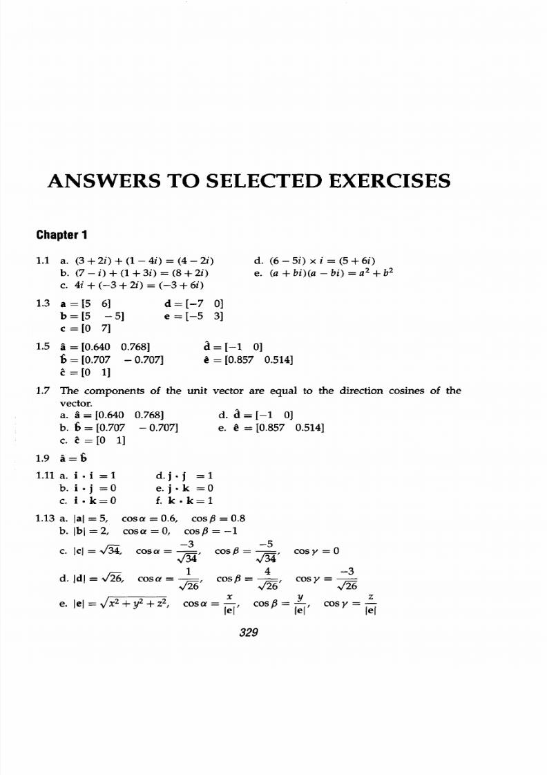
8/9/2019 Mortenson, Michael E. - Mathematics for computer graphics applications.pdf
http://slidepdf.com/reader/full/mortenson-michael-e-mathematics-for-computer-graphics-applicationspdf 342/367
ANSWERS
TO SELECTED
EXERCISES
Chapter
1
1.1 a. 3
i) +
1 4i) = (4
- 2i )
b. 7-i)+ 1+3i)= 8+2i)
c.
i
+ -3+ i
= -3+
i
1.3
a=[5
61
b=[5 -5]
c
=
[0
7]
1.5
a
=
[0.640 0.768]
b = [0.707 - 0.707]
c =[O 1]
d= [-7 0]
e = [-5 3]
a=[-l
0]
] = [0.857 0.514]
1.7 The
components of
the
unit vector
are
equal
to the direction
cosines of the
vector.
a.
= [0.640
b.
b
= [0.707
c. c
=[O
1]
1.9 a=b
1.11 a. i.i = 1
b. i.j =0
C. i *k=0
0.768]
-
0.7071
d.
d=[-1 01
e.
6
=
[0.857
0.514]
d.j.j
=1
e.j.k
=0
f.
k-k=l
a =
5, cos a =
0.6,
cos
f
= 0.8
b, =
2,
cos
a
= O.
cos = -1
c.
IcI = 3,
d.
IdI
= ,
-3
cosa
= ,3,
1
cos a
=
1/2=6
e.
ej
= Vx
2
+y
2
+z
2
, cosa =
-5
cosfi
=
.. 34
cosy
= 0
cos = -, cosy = -3
x y
z
=-je,
cosfi=-jj, OSY j
329
d. 6-5i xi= 5+6i
e.
a bi) a-bi) = a
2
b
2
1.13
a.
b.
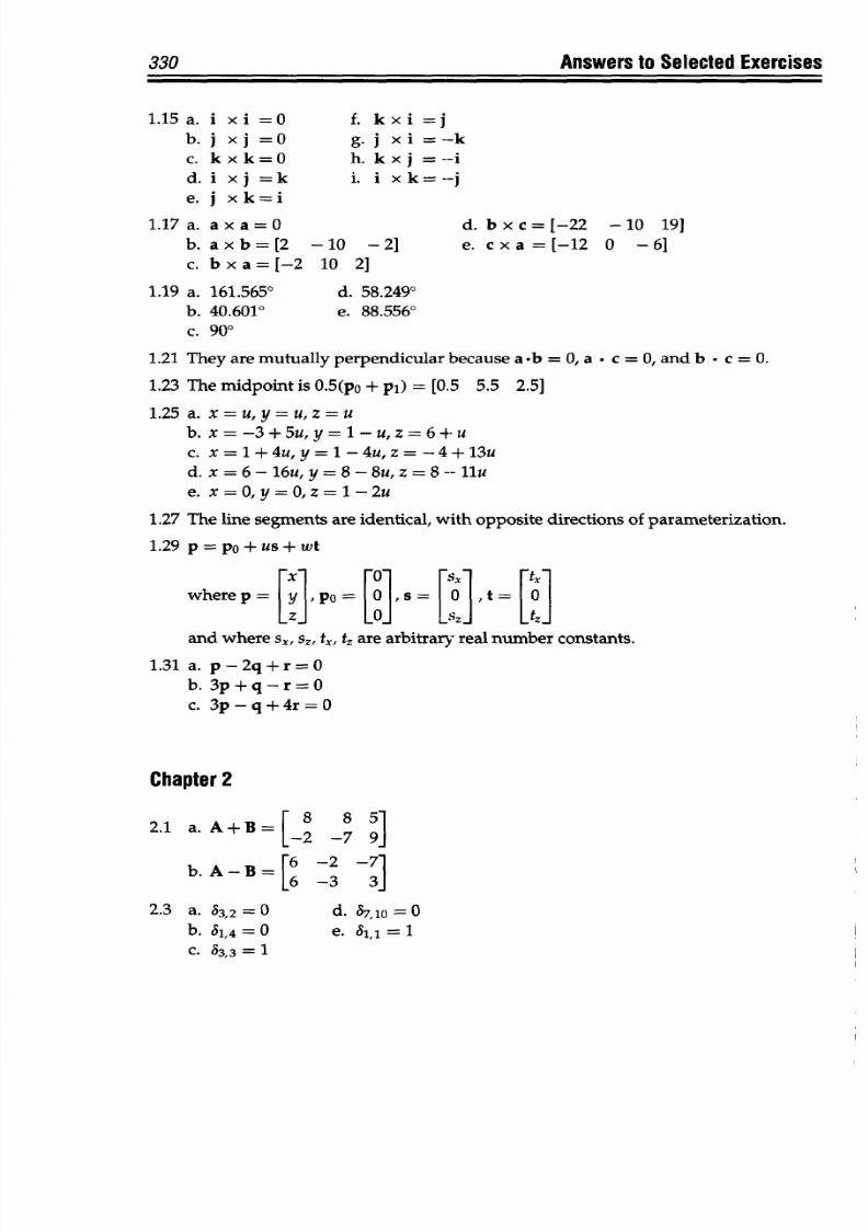
8/9/2019 Mortenson, Michael E. - Mathematics for computer graphics applications.pdf
http://slidepdf.com/reader/full/mortenson-michael-e-mathematics-for-computer-graphics-applicationspdf 343/367
330
Answers to
Selected Exercises
1.15a. i
xi
=0
f. kxi =j
b.
j
xj =0 g.
j
xi
=-k
c. k x k=0
h. k
x
j =--i
d. i
xj =k
i.
i
xk=--j
e. j xk=i
1.17a.
axa=0
d.
bxc=[-22
-10
19]
b.
axb=[2 -10
-21 e. cxa=[-12
0 -61
c.
bxa=[-2 10
2]
1.19 a.
161.565°
d. 58.2490
b.
40.6010
e. 88.556°
c.
900
1.21
They are mutually perpendicular
because
a-b
= 0, a * c = 0, and
b
c = 0.
1.23 The
midpoint
is
0.
5
(po + pi)
=
[0.5 5.5 2.5]
1.25 a. x=u,y=u,z=u
b.
x=-3+5u,y=1-u,z=64-u
c.
x=1+4u,y=1-4u,z=-4+13u
d. x=6-16u,y=8-8u,z=8--11u
e. x=O,y=Oz=1-2u
1.27
The line segments
are identical, with
opposite
directions
of
parameterization.
1.29
p=po+us+wt
where
p=[Y],PO
[]S=[]t
=
and where
sx,
sz, tx,
tz
are
arbitrary
real number constants.
1.31
a. p-2q+r=0
b. 3p+q-r=0
c. 3p-q+4r=0
Chapter 2
2.1
a. A+
B
82
[-2 _7 9]
b. A-B=[
6
2
7
[6
-3 3]
2.3 a. 83,2=0 d. 87,10=0
b.
81,4=0
e.
8
i i=1
C. 33,3
= 1
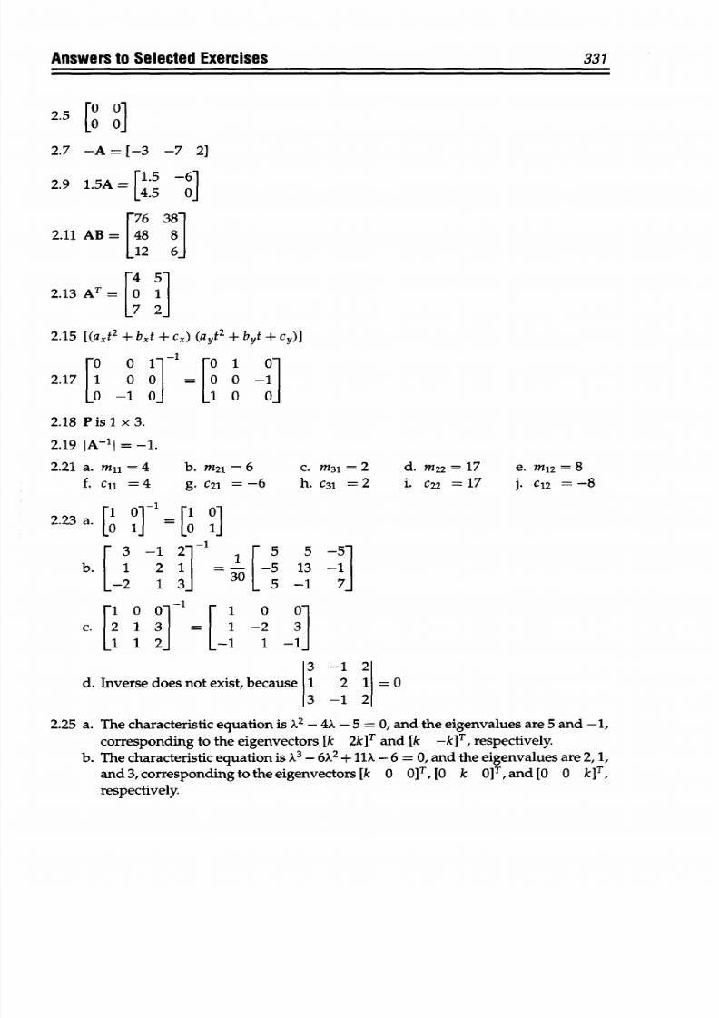
8/9/2019 Mortenson, Michael E. - Mathematics for computer graphics applications.pdf
http://slidepdf.com/reader/full/mortenson-michael-e-mathematics-for-computer-graphics-applicationspdf 344/367
Answers to Selected Exercises
331
2.5 [O
O]
2.7 -A = [-3 -7
2]
2.91.A
[1.5
61
[4.5 0]
2.11
AB
=
[ 8
8
126-
45-
2.13
AT = [ 1
72_
2.15 [(a
t
2
+
b~t +
c,)
(ayt
2
+ byt
+
cY)]
OO FO 1 01
2.17
1 0 0
=0 0
-1
-1 -
1 0
0]
2.18 Pis1
x3.
2.19 IA-I =
-1.
2.21 a.
ml,=4 b.
m
2
1
=6
c. m
3
1
=2 d. m22=17
e.
m
1
2
=8
f. cll
=4 g C21 = -6 h. c
31
= 2 i. c22
=
17 j. C1
= -8
2 231 ° [1
0]
.23 a.[0 =
[O]
3 -1 2--
1 5
5
-5~
b. -2 1 3-5
13
-1
_2
0
3O0- -1
7 0
O
c. 21
3
= 1 -2
3
11 2
-1
1 -1
3 -1 2
d.
Inverse does not exist, because 1 2 1 = 0
3
-1 2
2.25
a.
The characteristic
equation
is X
2
-
4X
-5 = 0, and
the
eigenvalues
are
5 and -1,
corresponding to
the
eigenvectors [k 2k]T and [k -k]T, respectively.
b. The characteristic equation
is
1
3
- 6X
+
11k
-
6 = 0, and
the eigenvalues
are 2,
1,
and
3,
corresponding
to
the
eigenvectors
[k
0
o]T,
[O
k
o]T
and
[O
0
kIT,
respectively.
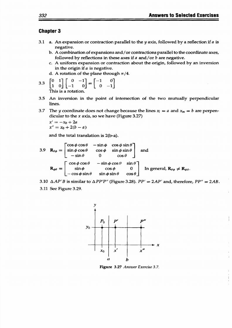
8/9/2019 Mortenson, Michael E. - Mathematics for computer graphics applications.pdf
http://slidepdf.com/reader/full/mortenson-michael-e-mathematics-for-computer-graphics-applicationspdf 345/367
332
Answers
to
Selected
Exercises
Chapter 3
3.1 a.
An expansion or contraction
parallel to the y axis, followed by
a reflection
if
a
is
negative.
b.
A combination of expansions
and/or
contractions parallel to the coord inate
axes,
followed
by
reflections
in these axes if a and/or b
are
negative.
c.
A uniform
expansion
or
contraction
about
the origin,
followed
by an
inversion
in the origin if a
is negative.
d. A rotation of
the plane through 7r/4.
3.3
[0
11 [
] =
[-1
0]
This is a rotation.
3.5
An inversion in
the
point
of
intersection of the
two
mutually
perpendicular
lines.
3.7
The y coordinate does not
change
because
the lines xl =
a
and
Xm
=
b are perpen-
dicular to the
x axis, so we
have
(Figure
3.27)
x'= -xo
+
2a
x"xO
+ 2(b -
a)
and
the
total translation
is 2(b-a).
oscos 0 -sin
0 cos 0
sin 1
3.9
Rs00 =
sin
X
cos
0
cos
0
sin
0
sin
0
and
-sinG 0 cosO
cos 4 cos 0
-sin
0cos 0
sin
G
LOO =
sin X cos
0
0
In general,
Rep # Roo.
-cos
sin
a
sin 0
sin 0
cos 0
3.10
AAP'B
is
similar
to APP'P (Figure 3.28).
PP'= AP'
and,
therefore, PP
2AB.
3.11 See
Figure 3.29.
y
Yo -
PO
Yn
PI
x
U
D
hlx
b
Figure 3.27 Answer Exercise
3.7.
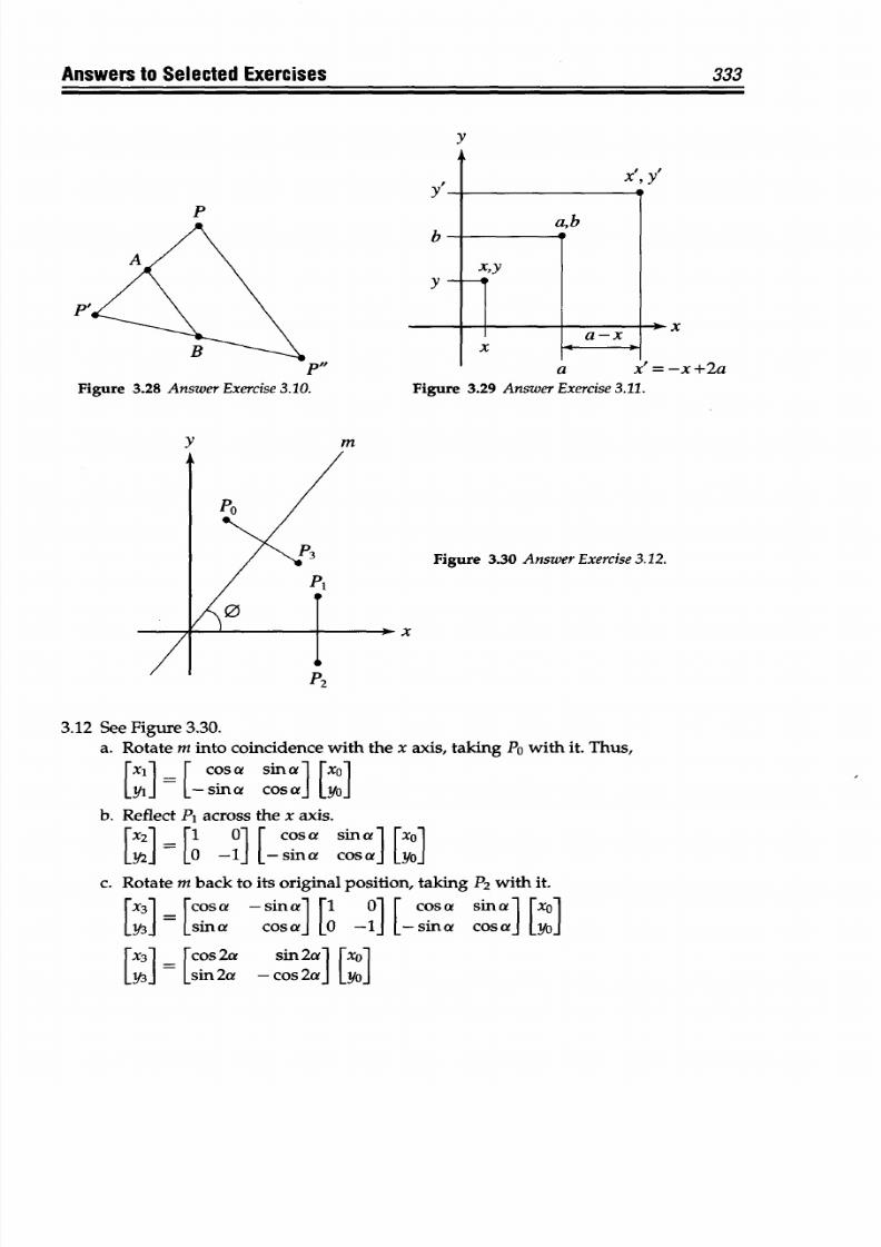
8/9/2019 Mortenson, Michael E. - Mathematics for computer graphics applications.pdf
http://slidepdf.com/reader/full/mortenson-michael-e-mathematics-for-computer-graphics-applicationspdf 346/367
Answers to Selected
Exercises
P
A
B
Figure
3.28
Answer Exercise
3.10.
y
XIyI
a,b
Xiy
X
a-x - -,
a
x
=-x--+za
Figure 3.29 Answer Exercise 3.11.
m
Figure
3.30
Answer
Exercise
3.12.
X
r2
3.12
See Figure 3.30.
a.
Rotate
m
into
coincidence
with
the
x
axis,
taking
Po with
it.
Thus,
x]
=r[
Cos
a
sinaI
rxo]
[Yxi
L-sina
cosaJ
LYOJ
b.
Reflect
P
1
across
the x axis.
LX2] =l
01Eosa sina lxol
LY1
L°
-J
L-sina cosa]
[YOJ
c.
Rotate m back
to its original position, taking
P
2
with it.
[x
3
1 = [cos a
-sin
aI
[1 01 [
cos
a
sina [xol
Ly31 -sina
cosaj[L -1]
[-sina cosa]
[tyo
[x3=
[cos2a
sin2al [xol
[Y3=
Lsin
2a
-cos
2aJ
LyoJ
333
y
k
-
x
.
1
.
.
n
8/9/2019 Mortenson, Michael E. - Mathematics for computer graphics applications.pdf
http://slidepdf.com/reader/full/mortenson-michael-e-mathematics-for-computer-graphics-applicationspdf 347/367
334
Answers to
Selected
Exercises
Chapter 4
4.1 The curve is a circle whose center is
(-1,
3).
The lines
pass through
the center
and
are, therefore,
lines
of
symmetry,
4.3 Yes.
4.5
A
cube
has nine planes of symmetry: three planes parallel to and
midway between
opposite
faces,
six planes
containing
opposite
parallel edges.
4.7 It is symmetric
about the origin
and both
axes,
but
not
the lines x
=
y and x
=
-y.
4.9
It
is symmetric
about
the
line
x
= y.
4.12
A
4-fold axis
passes through each
vertex and the
center of
the octahedron. A
3-fold
axis passes
through
the
center of each
face
and the
center
of the octahedron.
A 2-fold
axis
passes
through
the
center
of
each edge
and
the center
of
the
octahedron.
Chapter
5
5.1
1_
5.1 E 2=1
+ - + 9-+ 6 +
25 +
2n
2
- 9n +13 _ 1 1
1 1
5.3 1 =1 + 2-+ + l + +
E
6(n-1)!
-
2
3
4
8
5.
01 + (_l)n 2
0 2+ +2
_
n
2
+1
=
-5
17
+
37
+
5.7
1
-1+1
1+ 1- 1 +1 + (
1)
2 3
4567 n
5.9
x +x
2
+ X3+
+4
+5
+1-2 +-2-3
+1-.2-3.4
+12.3.4.5
X7
nxn
+1*2-3-4 .5 6+
+n
X
2
X
3
X
4
X
5
x
6
X
7
X8 (-X)n+l
3 5
7 9 11
13
15
2n+1
5133+34+5
6+- + + 2
3
5
7
2n- 1
5.15 1 +
x+ x
-X3 -
5.17
lim
5-2x
2
2
xGu
T3x
+5X
2
5
8/9/2019 Mortenson, Michael E. - Mathematics for computer graphics applications.pdf
http://slidepdf.com/reader/full/mortenson-michael-e-mathematics-for-computer-graphics-applicationspdf 348/367
Answers
to
Selected
Exercises
335
Proof: lim
-2x
2
li x2
x-+oo
3x
+ 5x
2
x*oo
3
+
5
x
5.19 lim
4x2
+ 3x +
2 1
x0 x
3
+ 2x-6
3
5.21 lim x3 =-
x-2X
2
-2
- 2
5.23 lim
sin
2
0 CO S
2
0 1
9-0
02
5.25
For
E
(-l)'
x'
the interval
of
convergence
is
-1
< x <
1.
n=0
00 (-l1
n xn
5.27
For
E
(1)
n
the
interval
of convergence
is -3
<
x <3
n=0 (2n +123n1+1
oo
5.29 For
E
(-l)n
n xn convergence
is at x
=
0.
n=0
5.31
5 - converges
for
all
values
of
x.
n=0
n
5.33
Given
f(x)
=
x
3
-
5X
2
-
4x
+
20,
then
a. f(l)
= 12
c.
f(0) =20
b. f(5) =
0
d. f(a) =a
3
-
5a
2
- 4a +
20
5.35 f t
+
1) = t
3
- 2t
2
-
llt
+ 12
5.37
f(x +
Ax)
- f(x)
=
A-xxAZ
5.39
lim
=
0
x~3+
IX2
(X4
-4X3 +
5x2 -
4x
+
4)
14_
45
5.41
lrm
1
=
xo2+
(
-X233X
2)2
sin kO
5.43 hrnk
6-40 0
tan 0
5.45
limr
= 1
0-~0
0
sn
0
5.47 lim si
has
no limit.
eo 02
549
li
tanax
a
x-o
sinbx
b
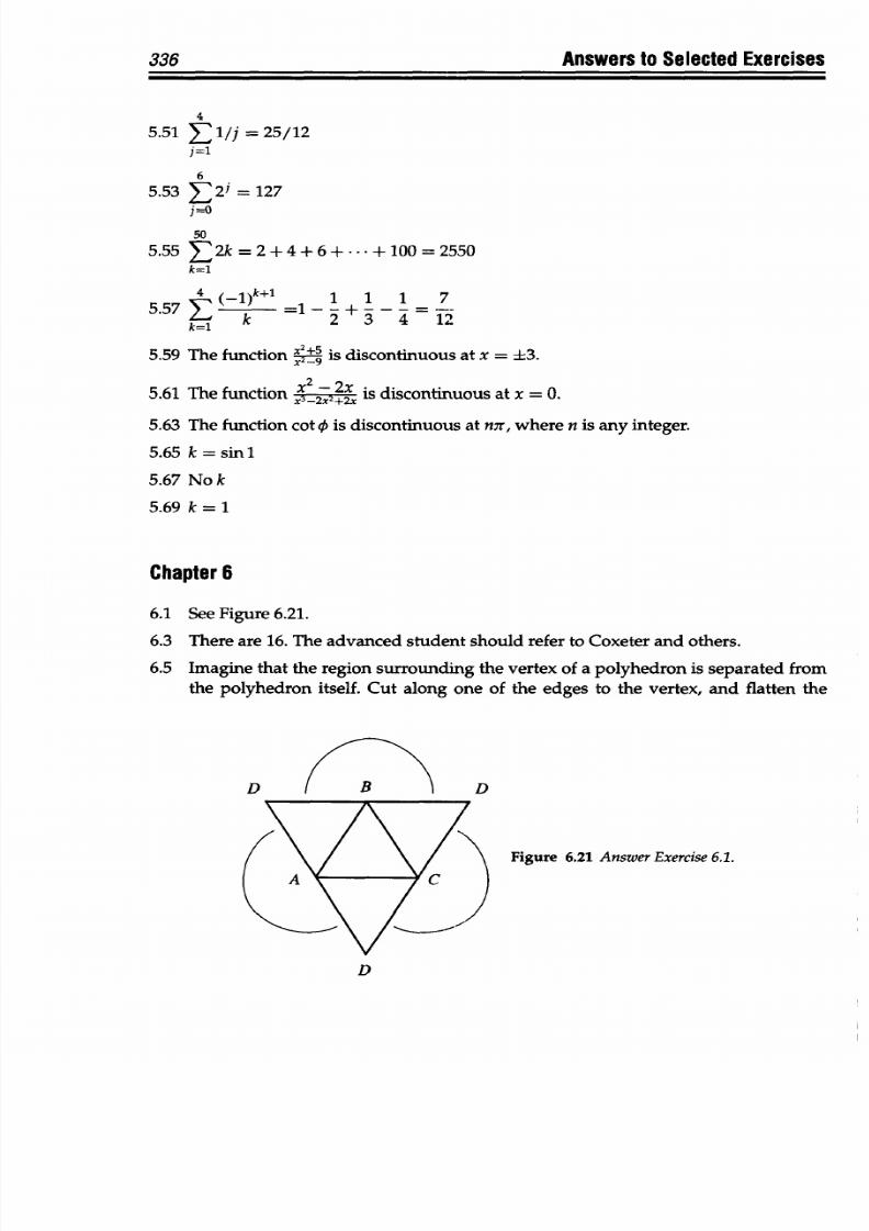
8/9/2019 Mortenson, Michael E. - Mathematics for computer graphics applications.pdf
http://slidepdf.com/reader/full/mortenson-michael-e-mathematics-for-computer-graphics-applicationspdf 349/367
Answers
to Selected Exercises
4
5.51
11/j=25/12
j=1
6
5.53
E2
= 127
j=o
50
5.55
2k =2+4+6+--
+100=2550
k=1
5.57
E (k
=1 -
2-+ -3 =4
5.59
The
function
25is discontinuous
at x
= ±3.
5.61
The function
-2x
is discontinuous at
x = 0.
5.63
The function
cot
0
is
discontinuous at
nor, where n
is
any
integer.
5.65 k =
sinl
5.67
No k
5.69
k
=
1
Chapter
6
6.1 See Figure 6.21.
6.3
There
are
16. The advanced student
should
refer
to Coxeter and
others.
6.5 Imagine
that
the region surrounding
the vertex of
a
polyhedron
is
separated
from
the polyhedron
itself.
Cut
along one
of the
edges to the vertex, and
flatten
the
D
B
D
Figure
6.21
Answer
Exercise 6.1.
D
336
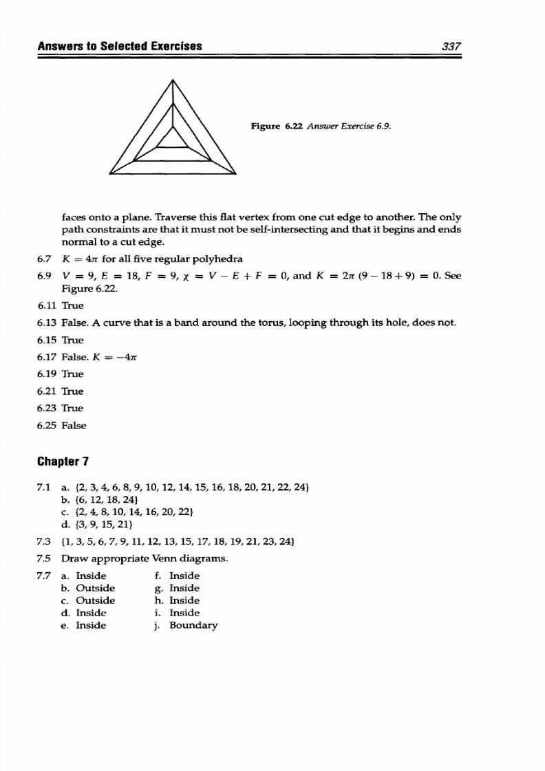
8/9/2019 Mortenson, Michael E. - Mathematics for computer graphics applications.pdf
http://slidepdf.com/reader/full/mortenson-michael-e-mathematics-for-computer-graphics-applicationspdf 350/367
Answers to Selected Exercises
337
Figure 6.22 Answer Exercise
6.9.
faces
onto a
plane. Traverse
this
flat
vertex from
one
cut edge to
another. The
only
path
constraints
are
that
it
must not
be
self-intersecting
and that
it
begins and ends
normal to
a cut
edge.
6.7
K = 4-r for all
five regular
polyhedra
6.9
V
=
9,
E
=
18, F = 9,
X
=
V-E
+
F
=
O,
and K
= 27r(9-18+9)
=
0. See
Figure 6.22.
6.11 True
6.13
False. A curve that is a band around the torus, looping
through
its hole, does
not.
6.15
True
6.17 False.
K
= -47r
6.19
True
6.21
True
6.23
True
6.25 False
Chapter
7
7.1
a. {2,
3,4, 6,
8, 9, 10, 12, 14, 15, 16,
18,
20,
21,
22,
24)
b. {6,
12,
18, 24)
c. {2, 4, 8, 10, 14, 16, 20, 22)
d. {3,9,15,21}
7.3 {1, 3,
5, 6,
7,9, 11,
12, 13, 15, 17, 18, 19, 21,
23,
24)
7.5
Draw
appropriate
Venn diagrams.
7.7 a. Inside f. Inside
b. Outside g. Inside
c. Outside
h.
Inside
d. Inside i. Inside
e. Inside j. Boundary
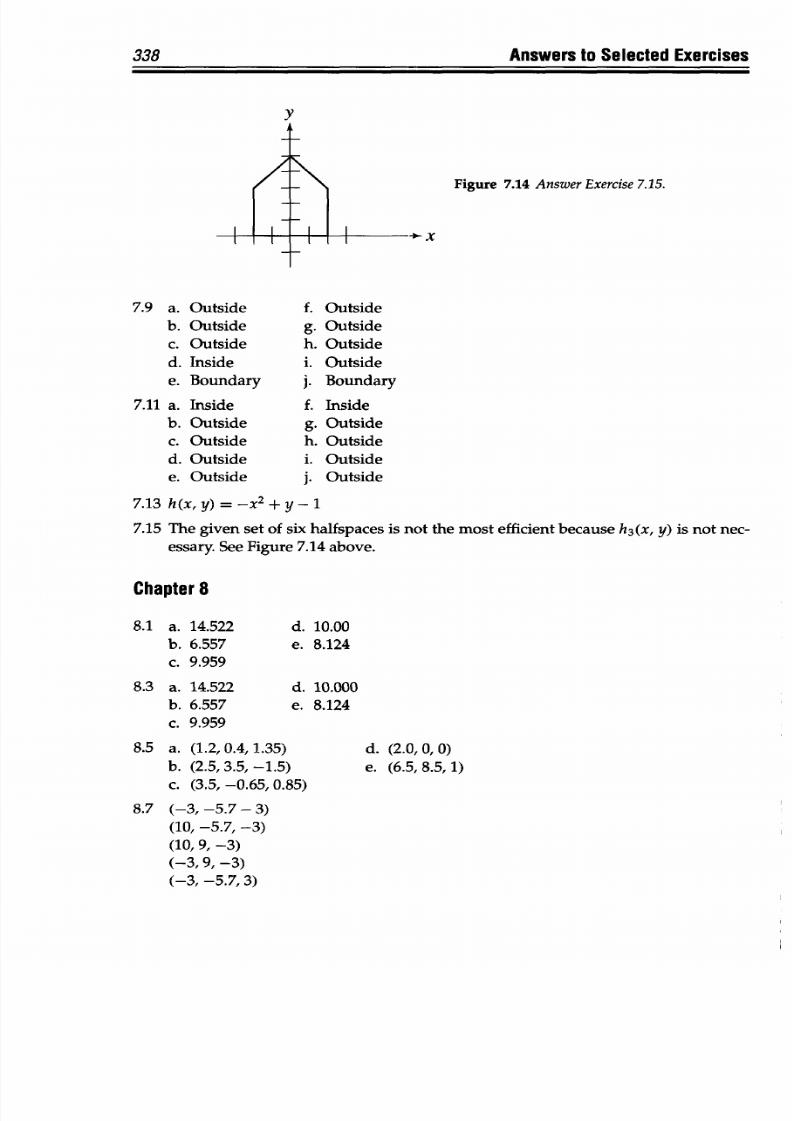
8/9/2019 Mortenson, Michael E. - Mathematics for computer graphics applications.pdf
http://slidepdf.com/reader/full/mortenson-michael-e-mathematics-for-computer-graphics-applicationspdf 351/367
Answers to Selected
Exercises
Figure 7.14
Answer
Exercise 7.15.
I I I
7.9 a. Outside f.
Outside
b. Outside
g. Outside
c. Outside
h.
Outside
d. Inside
i. Outside
e.
Boundary
j. Boundary
7.11
a.
Inside
f. Inside
b. Outside
g.
Outside
c.
Outside
h.
Outside
d.
Outside
i. Outside
e. Outside
j.
Outside
7.13
h(x,y)
=
-x
2
+y-1
7.15
The given
set
of six
halfspaces
is not the
most
efficient because h
3
(x, y) is not nec-
essary.
See Figure 7.14
above.
Chapter 8
8.1
a. 14.522
b.
6.557
c.
9.959
8.3 a. 14.522
b. 6.557
c. 9.959
d. 10.00
e.
8.124
d. 10.000
e.
8.124
8.5
a. (1.2, 0.4, 1.35)
b. (2.5, 3.5,
-1.5)
c. (3.5, -0.65,0.85)
8.7
(-3,
-5.7
- 3)
(10,
-5.7,
-3)
(10,
9,
-3)
(-3,9, -3)
(-3,
-5.7, 3)
d. (2.0,
0, 0)
e. (6.5, 8.5, 1)
338
y
I I I
or
.. ,
8/9/2019 Mortenson, Michael E. - Mathematics for computer graphics applications.pdf
http://slidepdf.com/reader/full/mortenson-michael-e-mathematics-for-computer-graphics-applicationspdf 352/367
Answers
to
Selected
Exercises
339
(10, -5.7, 3)
(10,9,3)
(-3,9,3)
8.9
A
1
=
(Ax
1
= 3, Ayi
=
0)
A
2
= (AX2
=
O,
Ay2 = 3)
A
3
=
(AX
3
=
-3,
Ay
3
=
0)
8.11 Al
= (Ax
1
=
4, Ayi
=
0)
A
2
= (AX2
= 0,
Ay
2
= 4)
A
3
= (Ax
3
= -4, Ay3
=
0)
8.13 (-2, -4), (14, -4),
(14, 8), (-2, 8)
8.15
X' =
(X+XT)
COS
O
-
(y+yT)
sin
6
Y'
=
(X+XT)
s in6+(y+yT)cos
6
8.17
The
order
in which
two or more
transformations are performed
is
important.
Trans-
lating and
then rotating
a point does not,
in general,
produce the
same result
as
rotating
and
then
translating
the
point.
Chapter 9
9.1
From
Equations
9.23, we
can
write
d2+ d2
+
d2=
(X
1
- Xo)
2
+ (yi
-
yo)
2
+
(Zl -
ZO)2
but (x
1
- xo)
2
+ (yi -
yo)
2
+ (Zl -
zO)
2
=
L2,
therefore,
d2 +
d2
+ d2
=
1.
9.3
a.
x =
-2.8u + 3.7, y
= -11.7u +
9.1, z = 2.4u +
0.2
b.
x
=
1.2u +
2.1,
y = 7.1u
-
6.4,
z =
-5.lu
c.
x = -4.3u
+
10.3,
y =6.1u +
4.2, z
=5.5u +
3.7
d.
x =-5.3u
+
5.3,
y =12u +-7.9,
z
=-.7u +
1.4
9.5 a.
b.
c.
(7,
3, 6),
(7,
3, 3)
(-2.5,
7.25,
-1.75),
(-1,
8.5,
-3.5),
(0.5, 9.75,
-5.25)
(1.5,
0.25, 3.25),
(3,
0.5,
0.5), (4.5, 0.75,
-2.25)
9x =I2u+2
9.7
a. Linel1:
y
=2u
+4
z
=
-10u +6
Ix
= 6u
Line: y
=
8u
z= -7u
+
1
The two lines do
not intersect.
I =2u+2
x =
-1.5u+4
b.
Line 1: =
2u +
4 Line
2: y
= 1.5u
+
3
The two lines
do not intersect.
z= -10u+6
z
=
-1.5u+5
x
=2u+2
x
= -3u
+
3
c.
Line 1: y =
2u +
4 Line 2: y = -3u
+
5 The two lines
overlap.
z
= -10u+6
z=
15u+1
8/9/2019 Mortenson, Michael E. - Mathematics for computer graphics applications.pdf
http://slidepdf.com/reader/full/mortenson-michael-e-mathematics-for-computer-graphics-applicationspdf 353/367
Answers to
Selected
Exercises
I= -11U
+
10 x = -9u + 13
d. Line
1: =-9u
+
8
Line
2: y
=
5u
+ 2
=
z
=0
e =
-3u+5
e. Line
: =
0
z= 0
Intersecting
at
u,
=
0.287
and
u
2
=
0.683
Ix
=
2u
+ 8
Line
2: y =
0
z
=
Both
segments
lie on the
x axis. They
do
not
overlap.
Chapter
10
10.1
Hint:
Solve
the
following
four simultaneous
equations:
Ax+By+Cz+D=0
Aa+D=0
Bb+D=O
Cc+D=O
10.2
a. Same side as
the
reference
point
b. On the plane
c. Same
side
10.3
a. Same side
b. On the
plane
c.
On the plane
10.4 a.
u = +0.333
b.
u
= -1.000
c.
u
=
0.666
d.
Opposite
side
e. Opposite
side
d. Opposite
side
e.
Opposite
side
d. The
line
lies
in the plane.
e. u =
0.5
Chapter
11
11.1
a. Stellar
b. Concave
c.
Convex
d. Concave
e.
Convex
11.2
a.
(-2,
8), (-2,
13),
(1,
13), (2,
10)
b.
(4, 12),
(7, 15),
(9, 11 )
c. (-1, 2),
(2, 3), (2,-1).
A convex polygon
is identical
to its
convex
hull.
d.
(4,
7),
(7,
7), (7, 2), (4,
2)
e.
(9,5), (12, 3),
(13, 8),
(9,
9)
11.3
a. 1200, 60°
b.
90°, 90°
c.
720, 108°
11.5
11.6
d. 60°, 120°
e. 450, 1350
Perimeter
=
29.358 cm
XCG
=
6.6, YCG = 6.8
340
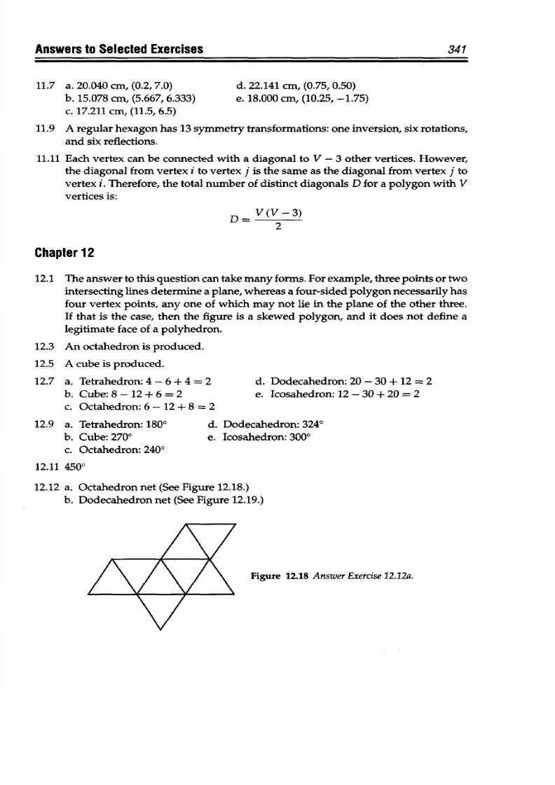
8/9/2019 Mortenson, Michael E. - Mathematics for computer graphics applications.pdf
http://slidepdf.com/reader/full/mortenson-michael-e-mathematics-for-computer-graphics-applicationspdf 354/367
Answers
to
Selected
Exercises
11.7 a. 20.040 cm, (0.2, 7.0)
b. 15.078 cm, (5.667, 6.333)
c.
17.211
cm,
(11.5,
6.5)
d. 22.141 cm, (0.75, 0.50)
e. 18.000
cm,
(10.25, -1.75)
11.9
A
regular
hexagon has 13 symmetry transformations: one inversion, six rotations,
and
six reflections.
11.11
Each vertex
can be connected with
a diagonal to
V - 3
other
vertices.
However,
the diagonal from vertex i to vertex
j
is the same as the diagonal from vertex
j
to
vertex i. Therefore, the total
number
of
distinct diagonals D for a
polygon
with
V
vertices
is:
D= V(V -3)
2
Chapter
12
12.1 The answer to
this
question can take
many
forms.
For example,
three
points
or
tw o
intersecting
lines determine
a plane,
whereas
a four-sided
polygon necessarily
has
four vertex points, any one
of
which
may not
lie
in the
plane
of
the other
three.
If
that
is the case, then the
figure
is a skewed polygon, and
it
does not define a
legitimate
face of a polyhedron.
12.3 An octahedron is produced.
12.5 A cube is produced.
12.7 a. Tetrahedron:
4
- 6 + 4 = 2
b. Cube:
8 -
12+6
=2
c.
Octahedron:
6-12 +
8 =
2
12.9
a.
Tetrahedron:
180° d.
b. Cube: 2700 e.
c.
Octahedron: 2400
d.
Dodecahedron: 20 - 30 +
12
= 2
e. Icosahedron: 12
-30 + 20
=
2
Dodecahedron:
3240
Icosahedron:
300O
12.11
4500
12.12
a.
Octahedron
net
(See Figure 12.18.)
b. Dodecahedron
net
(See Figure 12.19.)
Figure
12.18 Answer
Exercise 12.12a.
341
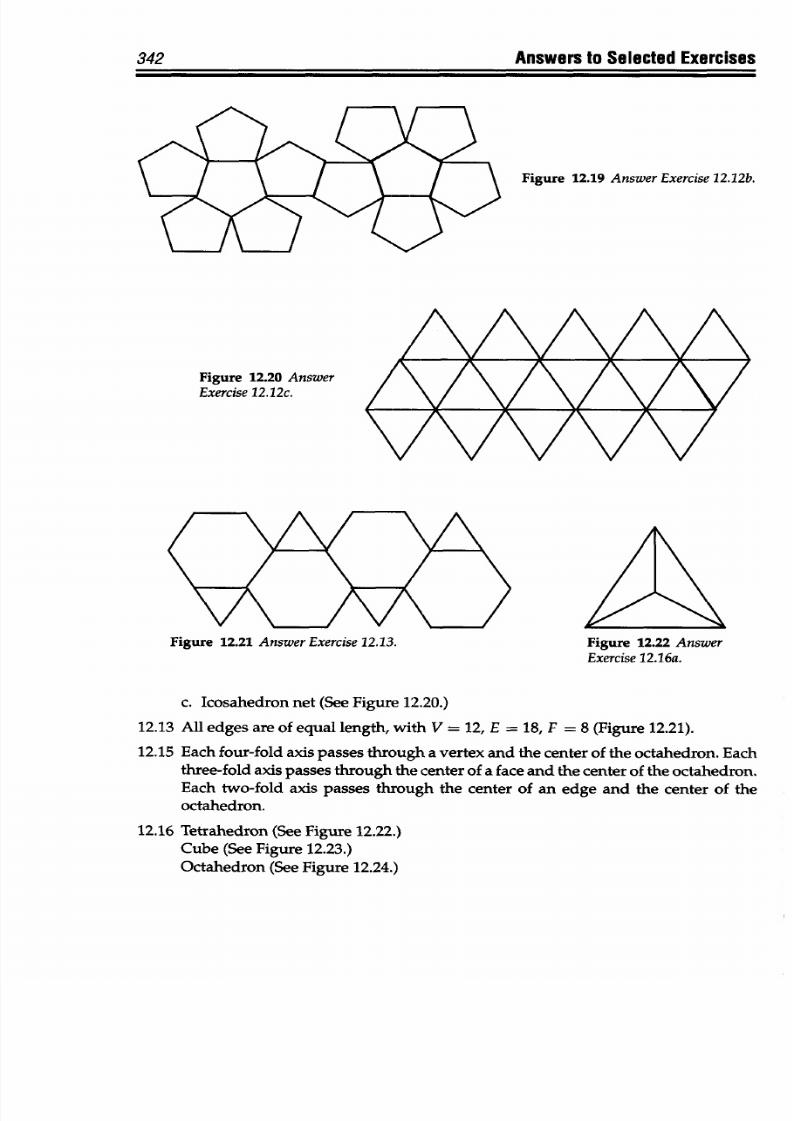
8/9/2019 Mortenson, Michael E. - Mathematics for computer graphics applications.pdf
http://slidepdf.com/reader/full/mortenson-michael-e-mathematics-for-computer-graphics-applicationspdf 355/367
Answers to
Selected Exercises
Figure 12.19
Answer Exercise 12.12b.
Figure
12.20 Answer
Exercise
12.12c.
Figure 12.21
Answer Exercise
12.13.
Figure 12.22 Answer
Exercise 12.16a.
c.
Icosahedron
net (See
Figure 12.20.)
12.13
All
edges
are of equal
length,
with V
= 12,
E
=
18,
F
= 8 (Figure 12.21).
12.15
Each
four-fold axis passes
through
a vertex
and
the center
of the
octahedron.
Each
three-fold axis
passes
through
the center of
a face
and
the
center of the octahedron.
Each two-fold
axis
passes
through
the center of
an
edge
and
the
center
of
the
octahedron.
12.16
Tetrahedron
(See Figure
12.22.)
Cube
(See
Figure
12.23.)
Octahedron
(See Figure 12.24.)
342
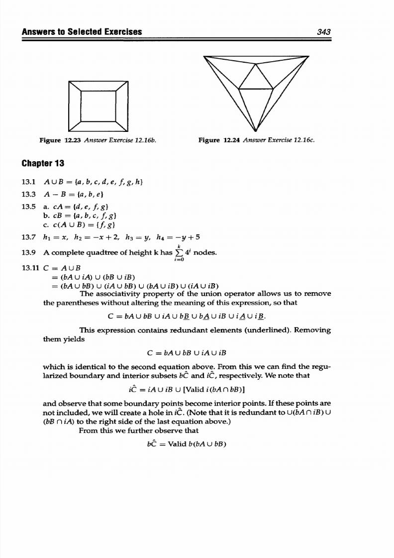
8/9/2019 Mortenson, Michael E. - Mathematics for computer graphics applications.pdf
http://slidepdf.com/reader/full/mortenson-michael-e-mathematics-for-computer-graphics-applicationspdf 356/367
Answers
to
Selected
Exercises
343
Figure
12.23 Answer
Exercise 12.16b. Figure 12.24 Answer Exercise
12.16c.
Chapter
13
13.1 AUB={a,b,c,d,e,f,g,h)
13.3
A
- B =
la,
b, e}
13.5 a. cA={d,e,f,gl
b. cB =
{a,
b, c,
f,gl
c.
c(AUB)={f,g}
13.7 h,
=
x,
h
2
=-x+2, h
3
=
y,
h
4
=-y+5
k
13.9
A
complete
quadtree
of
height
k has E
4i
nodes.
i=O
13.11 C
=
AUB
= (bA U iA) U
(bB
U iB)
= (bA
U bB)
U
(iA U bB)
U (bA U
iB)
U (iA U iB)
The
associativity property
of the union operator allows us to
remove
the parentheses without
altering
the meaning of
this
expression, so that
C =
bAU bB U
iAU
bB
U bAU iB U iAU
iB.
This
expression contains
redundant
elements (underlined).
Removing
them yields
C =
bA U
bB
U iA U
iB
which
is identical to
the second
equation above. From this
we
can find the regu-
larized
boundary and interior
subsets
bC and iC, respectively. We
note
that
iC = iA U
iB
U
[Valid
i(bA n bB)]
and observe
that some boundary points
become interior points. If
these points
are
not included,
we will create
a hole in
iC. (Note
that it is
redundant
to
U(bA n
iB) U
(bB
n
iA) to the right
side
of
the
last equation
above.)
From this
we further
observe that
bC =
Valid b(bA U
bB)
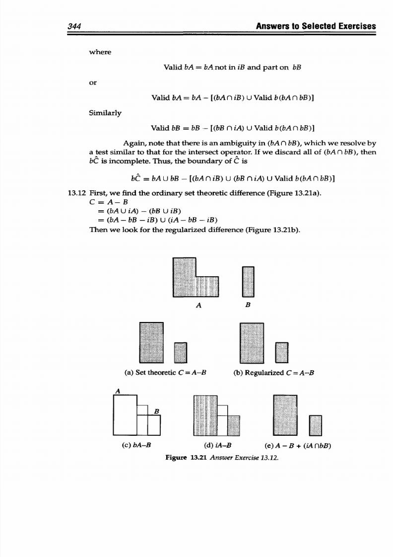
8/9/2019 Mortenson, Michael E. - Mathematics for computer graphics applications.pdf
http://slidepdf.com/reader/full/mortenson-michael-e-mathematics-for-computer-graphics-applicationspdf 357/367
344
Answers
to Selected
Exercises
where
Valid
bA
=
bA
not
in
iB
and
part on
bB
Valid bA = bA - [(bA
n
iB) UValid
b(bA
n bB)]
Valid bB
=
bB
-[(bB
n iA)
Valid
b(bA
n bB)]
Again,
note
that there is an
ambiguity in (bA n
bB),
which
we
resolve
by
a
test
similar to
that for the intersect operator. If
we discard all of
(bA n
bB),
then
bC
is
incomplete. Thus,
the boundary of C is
bC = bA
U bB
-
[(bA n
iB)
U
(bB
fl iA)
U Valid
b(bAfn bB)]
13.12 First, we
find
the ordinary
set theoretic difference
(Figure 13.21a).
C=A-B
= (bA U
A)
- (bB U B)
= (bA
-
bB
- iB) U (iA - bB - iB)
Then
we
look
for the
regularized
difference (Figure 13.21b).
t<t; \
.M@
. .
ORa;
O 9.,@
8..s^.
-
A B
LM
(a)
Set theoretic C
= A-B
(c)
bA-B
(d)
iA-B
l.li
,'
O.
(b)
Regularized C
= A-B
a
(e)
A
- B + (iA
nbB)
Figure 13.21 Answer
Exercise
13.12.
or
Similarly
344
Answers to Selected Exercises
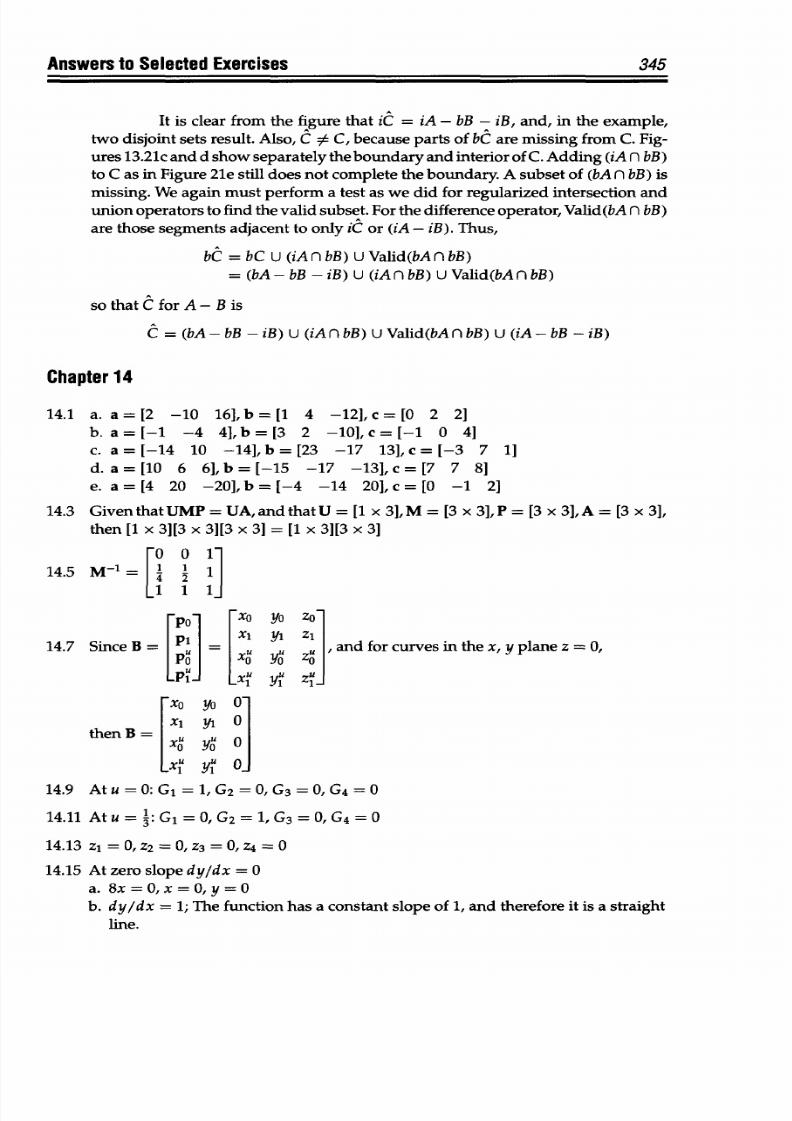
8/9/2019 Mortenson, Michael E. - Mathematics for computer graphics applications.pdf
http://slidepdf.com/reader/full/mortenson-michael-e-mathematics-for-computer-graphics-applicationspdf 358/367
Answers to
Selected
Exercises
345
It
is
clear
from the
figure that iC = iA -
bB - iB, and,
in
the
example,
two
disjoint sets result. Also, C = C, because parts of
bC
are missing
from C.
Fig-
ures
13.21c and d
show
separately the boundary and interior
of
C.
Adding (iA
n
bB)
to
C
as in Figure
21e
still
does
not
complete
the
boundary.
A
subset
of (bA
n
bB)
is
missing. We
again
must
perform
a
test as we did
for
regularized intersection and
union
operators to
find the
valid
subset.
For
the
difference
operator, Valid(bA n bB)
are those segments adjacent to only
iC
or
(iA
- iB). Thus,
bC = bC U (iA n bB) U Valid(bA
n
bB)
=
(bA-bB
-iB) U (iA n bB) U Valid(bA n
bB)
so that C for A -
B
is
C
=
(bA-bB
-iB)
U
(iA
n
bB) U
Valid(bA
n
bB)
U
(iA-bB
-iB)
Chapter
14
14.1 a.
a
= [2
-10
16],b
=[1 4 -12],c
=[O 2
2]
b. a =
[-1
-4
4],b =[3 2 -10], c =[-1 0
4]
c. a = [-14
10
-14], b = [23
-17
13], c = [-3 7 1]
d. a
= [10 6
6],b
= [-15
-17
-13],c
=
[7 7
8]
e. a =
[4
20 -20], b
=
[-4
-14 20],
c
=
[0
-1
2]
14.3
GiventhatUMP = UAandthatU = [1
x
3],M
=
[3
x
3],P
= [3
x
3],A
= [3 x 3],
then [1
x
3][3 x 3][3 x 3] = [1
x
3][3 x 3]
O
0
1
14.5 M-1 = 1
Po0
Xo yo
Zo
14.7 SinceB=
ps
X Yo
Z, and for
curves
in
the
x,
y
plane
z 0,
Fxo yo
01
X i
-Xi A01
then
B
= X
Iy
xOi yO 0O
14.9
Atu =0:G
1
=
1,G
2
=0,G
3
=0 G
4
=0
14.11 Atu= 1:G= 0,G
2
=1,G
3
=0,G
4
=0
14.13
z
1
=
0,
z
2
=
0,
z
3
=
0,
z
4
=
0
14.15 At zero slope dy/dx =
0
a. 8x=O,x=O,y=0
b. dy/dx
=
1; The function
has
a constant slope of 1, and therefore
it is
a straight
line.
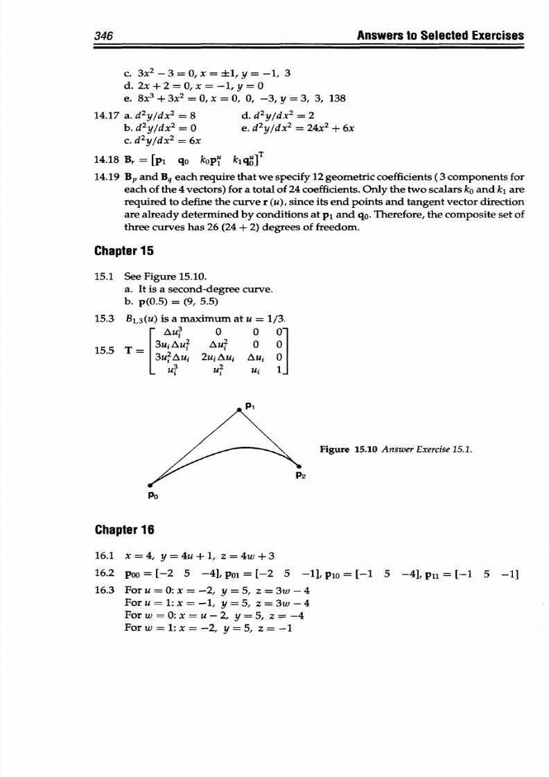
8/9/2019 Mortenson, Michael E. - Mathematics for computer graphics applications.pdf
http://slidepdf.com/reader/full/mortenson-michael-e-mathematics-for-computer-graphics-applicationspdf 359/367
346
Answers
to Selected Exercises
c.
3x
2
-3=0,x=±1,y=-1,
3
d. 2x+2=0,x=-l,y=O
e.
8x
3
+3x
2
=0,
x=0, 0, -3,y=3,
3, 138
14.17
a.
d
2
y/dx
2
=
8
d.
d
2
y/dx
2
=
2
b.
d
2
y/dx
2
=
0 e.
d
2
y/dx
2
= 24 X
2
+
6x
c.
d
2
y/dx
2
=
6x
14.18
B,
= [pi
qo
kopu
kiqu ]
14.19
BP and
Bq each require
that we specify
12 geometric
coefficients (3
components
for
each of
the 4
vectors)
for
a
total
of 24
coefficients.
Only
the two
scalars
ko
and
k,
are
required to define
the
curve
r
(u),
since
its
end
points and tangent
vector
direction
are
already determined
by conditions
at pi
and
qo. Therefore,
the
composite set
of
three curves
has
26
(24
+
2) degrees of freedom.
Chapter 15
15.1 See Figure
15.10.
a.
It
is
a
second-degree curve.
b. p(O.5) = (9,
5.5)
15.3
B1,
3
(u) is a maximum
at
u
= 1/3.
F Au?
0
0 0
15.5
T= I3u
Au
2 AuI
0
01
3u2Aui 2uiAui
Auj 0
o
U?3
Ui
1-
Figure
15.10 Answer
Exercise 15.1.
2
po
Chapter 16
16.1
x=4,
y=4u+1, z=4w+3
16.2 Poo
= [-2 5
-4],
poi = [-2 5
-11, plo = [-1
5 -4],
pi
= [-1 5
-11
16.3
Foru=O:x=-2,
y=5,
z=3w-4
Foru=1:x=-1,
y=5, z=3w-4
Forw=O:x=u-2,
y=5,
z=-4
Forw=1:x=-2,
y=5,
z=-1
8/9/2019 Mortenson, Michael E. - Mathematics for computer graphics applications.pdf
http://slidepdf.com/reader/full/mortenson-michael-e-mathematics-for-computer-graphics-applicationspdf 360/367
Answers
to Selected
Exercises
16.4
poo =
aoo
p0l = aO
+ ao
2
+ ao
+
aoo
plo
= a
30
+
a20
+
alo
+
aoo
pll = a33 + a
3
2 + a
3
l
+ a
30
+
a2
3
+ a22 +
a21 + a2o
+a,3 + al2 + all + ala + aO3 + aO2 +
aOl
+
aoo
16.5 From Equation 16.9 we
have
(-)
p(u) = 3(a33u
2
w
3
+
a
3 2
u
2
w
2
+
a3lu
2
w +
a
3
0
u
2
)
du + 2(a23uw3 + a22uw +
a
21
uW + a
2
aU)
+ a
13
w3 + a
1
2W2
+
ajiw
+
ala
so
that:
Poo =
ala
pol
= a13
+
a12
+
all
+ a
10
Plo = 3a
30
+
2a2
0
+
alo
pll = 3 (a33 + a32
+ a
3
l
+ a
30
) + 2 (a
23
+ a22
+ a2l + a2o) + a1
3
+
a12
+ all + al
0
For the
four tangent vectors
in
the w
direction,
we have
d p(u, w)=
3a
3 3
u
3
w
2
+ 2a
32
u
3
w +
a
3
iU
3
+3a23u
2
w
2
+
2a22u
2
W
+ a
2
lu
2
+ 3a
1 3
uw
2
+
2al2UW +
allu
+
3aO3W
2
+
2aO
2
w
+ aoi
so
that
pw
a~oi
Pol=
3ao3
+
2aO2
+ aOl
p
=
a
3
l
+ a
2
l
+ all + ao
1
P
=
3
(a33
+ a23
+
a13
+
a03)
+
2(a
32
+ a22
+ a
1
2
+
aO2)
+ a
3
l
+
a21
+ all + aol
Chapter
17
17.1 a. Inside
f.
Inside
b.
Outside
g. Outside
c.
Boundary
h. Outside
17.2
a.
XA
inside
XT b. XB
overlaps
XT
d. XD
overlaps
XT
e.
XE
inside XT
17.3 a.
d,
f, j
inside; a, b,
c,
e, g, h, i
outside
b.
a,
f, g, i inside; b, c, d,
e,
h,
j
outside
c.
f,
i
inside; a,
b,
c,
d,
e, g,
h,
j
outside
d.
All inside
e.
c,
d, e, j
inside;
a,
b,
f,
g,
h,
i
outside
17.5 r =
X
2
+y
2
, 0
= arctan
(-)
17.7 c,e,g,
andh
d. Inside e. Inside
i. Inside j. Inside
c.
xC
outside
XT
347
8/9/2019 Mortenson, Michael E. - Mathematics for computer graphics applications.pdf
http://slidepdf.com/reader/full/mortenson-michael-e-mathematics-for-computer-graphics-applicationspdf 361/367
348 Answers to Selected Exercises
17.9
a.
Line (a, b) lies outside
the
window.
b.
Line
(c, d) intersects
WT
at (2.5, 1).
c.
Line
(e, f)
intersects WL at
(-4,
-2.818).
d.
Line
(g,
h) lies inside the window.
e. Line (i, j)
intersects
WT
at (-
1.6, 1)
and WR at
(7, -2.583).
17.11
a.
Outside window
b.
Inside
window
c. Inside
window
d. Intersects WT
and
WL, Clipped
to p0 =
(4, 10)
and
p,
=
(2, 6)
e.
Inside
window
f. Intersects
WB
g. Partially coincident with WL
h.
Intersects
WB
and
WT
i.
Intersects
WR
j. Outside
window
8/9/2019 Mortenson, Michael E. - Mathematics for computer graphics applications.pdf
http://slidepdf.com/reader/full/mortenson-michael-e-mathematics-for-computer-graphics-applicationspdf 362/367
INKX
Absolute
points,
168,299
Affine geometry,
47,51
Angle between
lines, 176
Angle between two vectors,
12
Angle
excess,
136, 147
Antisymmetric
matrix, 39
Archimedes,
90, 215
Arcs, simple,
129
Argand, J., (1768-1822) 23
Arrays, 28, 167-168
Associativity, 78
Atlas, topological, 144
Basis
functions,
268, 271
Basis vectors,
21
B&zier curve:
algebraic definition, 267
basis functionss,
268,
271
basis function identity, 272
Bernstein polynomial,
266,
268, 270
binomial coefficient,
268
blending
functions,
267-269
composite
curves,
260,
275
construction,
geometric,
264
control points, 252, 266,
270
control polygon, 270
convex
hull, 200, 214,267
cubic, 249,269
degree, 266
degree elevation, 272
modify shape, 271
parametric variable, 244,
266,
269
parametric variable,
transformation,
274
partition-of-unity
property, 276
truncation, 273
B&zier, P., 264
Bezier
surface,
283
Bicubic
surface,
279, 283
Binary product, 75
Binary trees:
branches,
230
circuit,
230
complete, 231
connected
graph,
230
connectivity,
143, 230
depth, 231
descendant,
231,
232
directed graph, 230
entering branch,
231
exiting
branch,
231
graph-based
model,
230
height, 231
inorder traversal, 232
node, 230
node
numbering, 233
number of
nodes,
231
parent node,
231
path, 230
postorder traversal,
232
preorder
traversal, 232
root node,
subtrees,
232
topological structure, 230
traverse, 232
tree, 230
Blending
functionss, 256, 258,
267-269
Bombelli, R.,
(1526?-1572?), 23
Boolean
models, 226
Boolean
operators, 227
Boole, G. (1815-1864), 153, 227
Boundary, 233-234
Boundary conditions, 253, 254,
256,258
Boundary evaluation, 242
Branches,
230
Breaking
symmetry, 88
Cayley, A., (1821-1895), 23
Cayley table, 75
Cells, 217
Characteristic equation, 40
Characteristic polyhedron,
283
Circle, 258
Circuit,
230
Clipping,
296-299
Closed
interval,
120
Closed
path theorem,
132
Closure, 78
Cofactor,
36
Collineation, 48
Column matrix, 30
Commutativity, 78
Complement,
153
Complex number(s), 1, 2
Components of
a
hypernumber,
3
Composite
curve(s),
260, 275
Computer graphics:
aim, 324
clipping, 296-299
coordinate
systems,
291
directed
faces,
310
displaying geometric
elements, 299,
304
display transformations,
313
Homer's rule,
306
lines,
300
normalization, 295
orbit,
321
orthographic projection,
314
pan, 323
perspective
projection,
318
pixel, 294
polygon clipping, 299
polygon filling, 302
scene
transformations,
313
silhouette,
309
surfaces,
307
window, 169, 293
wireframe model, 220,
308
viewport,
293
visibility,
308
Concave polygon,
195
Conformable matrices, 32
Conformal
geometry,
47
Conformal transformations, 49
Congruent
geometry,
47
Conic, affine transformation
of, 54
Conic curve,
approximating,
258
Connected graph, 230
Connectivity, 143,
230
Connectivity matrix, 219
Connectivity
number, 137, 217
Construction of regular
polygons,
201
Constructive
solid geometry:
binary
trees,
226, 230
block, 242
boolean models,
240
boolean operators, 226, 235
boundary,
233, 234
boundary evaluation,
242
circuit, 230
connectivity,
230
cylindrical segment, 242
dangling edge, 238
definition,
226
difference operator, 227
dimensional homogeneity,
238
directed
surface,
229, 230
349
8/9/2019 Mortenson, Michael E. - Mathematics for computer graphics applications.pdf
http://slidepdf.com/reader/full/mortenson-michael-e-mathematics-for-computer-graphics-applicationspdf 363/367
350
Constructive
(continued)
fillet, 242
graph-based
model,
230
halfspaces,
229
inside,
outside, 227,
234
interior, 233
interior
set,
235
intersection
operator, 227
interval, closed, 235
interval,
open, 235
octree, 243
path,
230
point
classification,
227
point containment, 237
primitives, 226, 230, 241
quadtree, 243
region, 233
regularized
Boolean
operators,
235,
236,
238,
239
set-membership
classification, 240
set
theory,
226
solids, 233
tetrahedron,
242
topological structure, 230
tree,
230
union
operator, 22 7
union, algorithm for
finding,
237
Venn diagram, 227
wedge, 242
Containment,
202
Continuity,
121,260
Continuous functions, 122
Control points, 252, 266,
270
Convex hull, 200, 214, 267
Convex polygon,
195
Coordinate system(s):
basis vectors, 21
artesian, rectangular,
21,
287
cylindrical,
290
display, 292
global, 291
homogeneous coordinates,
69
local,
291
normalization, 295
origin, 286, 288
picture plane, 292, 293
polar,
289
principle
axes,
288, 289
real-number
line,
286
spherical, 291
transformation, 287
view,
291, 293
viewport,
293
window,
293
Cube,
205,
207,
211, 213, 222,
224
Crystallographic restriction,
83
Curvature,
138-141,
147-149
Curve(s):
algebraic
coefficients, 248,
249
algebraic
definition,
247
basis
transformation
matrix, 249,
252
Bezier curve,
264
blending functionss,
256,
258,
267-269
blending
function matrix,
249, 256
boundary
condition
matrix,
254
boundary
conditions,
253,
254,
256,
258
circle, 258
composite curves, 260, 275
conic
curve,
approximating,
246, 258
continuity,
260
control
point(s),
252, 266,
270
control
point
matrix,
248
cubic polynomial,
249, 269
degree elevation, 272
designing,
256
direction
of
parameterization,
259
ellipse,
258
geometric
coefficients,
248,
249
geometric
construction of ,
26 4
geometric continuity, 261
geometric definition,
247
Hermite interpolation,
cubic, 253
hyperbola,
258
matrix form,
247
modifying,
271
parabola, 258
parametric continuity,
261
parametric
equations
of ,
24 4
parametric variable,
176,
244,
266,
269
plane curves, 245
reparameterization,
259
space curves, 249
tangent
vector,
252
Index
Dangling edge, 238
Deformation
of curves and
planes, 134
Degree elevation,
272
Determinant(s),
36
Descartes, Rene
(1596-1650),
287
Diagonal
matrix,
30,42
Difference
operator,
154
Dihedral angle,
206
Dimensional
homogeneity,
160
Directed
surface,
152
Direction
cosines,
10,
179, 189
Direction
numbers, 179
Disk,
topological,
131, 135
Distance-preserving
transformations,
49
Dodecahedron,
207
Domain, 99
Dot product,
11
Dual polyhedra,
211
Dfirer,
A. (1471-1528), 213
Eigenvalues, 39-41
Eigenvectors, 39-41
Ellipse,
258, 259
Empty
set, 153
Equivalence,
topological,
129
Euler characteristic,
142, 217
Euler,
L.
(1707-1783),
214
Euler operators,
142
Euler's
formula,
205, 214, 217
Euler-Poincard formula, 138
Exhaustion,
Greek
method of ,
90
Fixed
vector,
7
Football curvature, 147
Forward
difference
method,
181
Free
vectors, 6
Frieze
group,
80
Function(s):
characteristics
of, three
important, 98
continuous, 122
correspondence,
one-to-one,
100
definitions,
154
domain, 99
evaluation, 156
image,
98
into, 99
limit,
103
mapping,
98, 100
notation,
154-156
number
line,
100
onto,
99
8/9/2019 Mortenson, Michael E. - Mathematics for computer graphics applications.pdf
http://slidepdf.com/reader/full/mortenson-michael-e-mathematics-for-computer-graphics-applicationspdf 364/367
Index
range, 99
real
line,
100
step, 122
transformation,
99
Gauss-Bonnet theorem, 142
Gauss, C.
F.,
201
Genus, 137, 217
Geometric
center,
198
Gibbs, J.
W.,
(1839-1903),
24
Grassman,
H.,
(1809-1877),
23
Greek
method of
exhaustion,
91
Greek
roots
(prefixes,
suffixes),
212
Group(s):
associativity, 78
closure, 78
commutativity, 78
cyclic,
79
dihedral,
79
frieze group, 80
generator, 79
identity, 78
inverse, 78
isometrics,
82
ornamental group, 80
rosette, 80
symmetry, 78
wallpaper
group,
80,
82
Halfspace(s):
Boolean
algebra, rules of,
227
Boolean operators, 227
combining,
160-163
complement, 153, 226
definition,
152, 177
difference operator,
152-154, 227
dimensional
homogeneity,
160
directed surfaces, 152
empty
set,
153, 226
functions and,
152, 154
inside,
outside, 152,
156-158
intersection operator,
152-154, 160, 227
in
the
plane,
156
in
three
dimensions,
null
set, 153, 226
set-builder notation,
154
set theory and, 153
union operator, 152,
153,
227
universal set, 153, 226
Venn diagram, 152,227
Hamilton, W. R. (1805-1865),
4,12,23
Handles on spheres, 137, 148
Hermite,
C.
(1822-1901),
253
Hermite patch, 283
Holes, 207 1
Homogeneous equations, 55,
69
Homogeneous coordinates, 69
Homer's rule, 305
Hyperbola, 258, 259
Hypercomplex number(s), 2
Hypemumber(s):
addition and subtraction
of, 3, 4
components
of, 3
definition, 2
geometric interpretation
of,
4
multiplying
two, 3
scalar multiplication of, 3
Icosahedron,
207, 218
Identity,
78
Identity
matrix,
30
Identity transformation, 74
Inside, outside, 227, 234
Intersection operator,
160
Intersection(s), 183-193
Intervals,
119-120
Invariance (invariant), 47-50,
142
Inverse,
78
Inversion, 65-69,
74
Inversion, matrix, 37
Isoparametric curves, 280
Jordan,
C.
(1838-1922), 135
Jordan
curve theorem, 134
Klein
bottle, 147
Kronecker delta, 30
Kronecker, L., (1823-1891),
30
Lattices, 84
Limit:
circle, approximating area
of, 91
continuity, 121, 260
continuity, axiom of, 92
continuous functions, 104,
122
convergence, test for, 95
convergent series, 94
divergent series,
94
domain, 95
double
summation,
112
351
exhaustion, Greek method
of,
90
extreme-value
property,
123
function,
95,
98,
103
Fundamental Theorem, 114
geometric series, 93, 94
index of
summation, 112
infinite
process,
91
integral, definite, 111
intermediate-value
property, 123
intervals, 119, 120
oscillating
series, 94
range,
95
rate of change, 115-116
real
number
line,
119
right (left)-hand limit, 105
sequence, 93
series, 93
step function, 105,
122
summation, 111
tangent to a curve, 11 4
theorems, 107
Linear independence and
dependence,
20
Linear parametric equations,
176
Linear
transformations,
52
Linear vector
spaces, 19
Line(s):
affine transformations of,
53
angle
between two,
176
direction cosines, 179
direction
numbers,
179
explicit
equation,
175
forward
difference
method,
181
implicit
equation, 175, 177
in
the plane,
174
in space, 177
intercept
form, 175
intersection
of,
183
linear parametric
equations,
176
parametric equations of,
15, 176
point and line
relationships, 181
points on,
computing,
180
point-slope form,
174
rotating,
184
slope-intercept
form,
174
translating,
184
two-point
form,
174
unit interval, 177
vector equation
of, 14
8/9/2019 Mortenson, Michael E. - Mathematics for computer graphics applications.pdf
http://slidepdf.com/reader/full/mortenson-michael-e-mathematics-for-computer-graphics-applicationspdf 365/367
352
Index
Main
diagonal,
30
Maps,
223
Matrix
(matrices):
addition,
31
antisymmetric,
39
arithmetic,
31
characteristic
equation,
40
column,
30
conformable,
32
connectivity,
219
definition
of, 28
determinants
and,
36
diagonal,
30,42
diagonalization
of, 42
eigenvalues,
39,42
eigenvectors,
39, 42
equivalence,
31
identity,
30
inversion,
37
inverse,
37
Kronecker delta,
30
main diagonal,
30
multiplying
by a
scalar, 32
null, 30
order, 29
orthogonal,
34
partitioning,
34
product
of
two, 33
row,
30
scalar,
30
scalar
product
and,
39
similarity
transformation,
41
special matrices,
29
square,
29
symmetric, 31, 42
vector
product
and, 39
vectors, as, 30, 39
Min-max
box,
167,
202
Minor
of
a determinant,
36
Mobius
strip, 145-147
Multiplication,
scalar,
10
Net(s), 138,
141, 213
Net
transformations,
142
Node, 230
Normal form, plane,
189
Normal vector,
17
Null
matrix,
30
Null
set,
153
Null vector,
13
Octahedron,
207, 211
Octree,
243
One-to-one
correspondence,
100
Open interval,
120
Orbit, 321
Orientation,
49,
144
Origin,
286,
288
Ornamental
group,
80
Orthogonal
matrix,
34
Orthographic
projection,
314
Parabola,
258
Parallelogram
law, 6,
22
Parallel
transport,
5
Parametric
continuity, 261
Parametric
equations,
15, 176,
244
Parametric
variable,
176,
244,
266,
269
Partitioning
a matrix,
34
Perspective
projection,
318
Piecewise
flat
surfaces,
137
Pixel,
294
Plane(s):
defined
by three points,
19(
definition,
algebraic,
187
direction
cosines, 189
intersections,
192-194
normal
form
of, 189
parallel,
190
point
and
plane
relationship,
191
vector equation
of, 16, 190
vector
normal
form,
191
Poincar6,
H. (1854-1912),
129,
217
Point(s):
absolute,
168,
299
arrays,
167
classification,
227
computing
on
a line, 180
containment,
202,237
definition,
165
displaying, 169
distance
between two,
166
forward
difference
method, 181
line, computing
points
on,
180
min-max
box enclosing
a
set
of, 167
n-dimensional
space,
in,
165
relative, 168,
299
resolving
displayed,
170
window
enclosing
a set
of,
169
Polygon(s):
area,
198,
200
clipping,
299
concave, 195
construction
of regular,
201
containment,
202
convex, 195
convex
hull of,
200
definition,
195
digon,
197
edge,
195
equiangular,
197
equilateral,
197
exterior
angles, 198
filling,
302
Gauss's
theorem,
201
geometric
center, 198-199
inside,
outside,
202
interior
angles,
198
intersections,
edge, 199,
203
perimeter,
198-199
plane,
195
properties,
197
rectangle,
197
regular,
196
rhombus,
197
skew,
195
square,
201
star,
196
stellar, 196, 199
symmetry,
201
triangle,
equilateral,
201
triangle,
area
of,
200
triangulation,
197
vertex,
195
Polyhedra:
angle,
polyhedral,
207
angle
deficit, 207
angle
excess,
136, 147
antiprisms,
209
Archimedean
dual,
209
Archimedean
semiregular
polyhedra,
209
cells, 217
connectivity
number,
217
connectivity matrix,
219
constructing
model,
213
convex
hull,
214
cube,
205,
207,
211,
213,
218, 222,
224
definition,
205
dihedral angle,
206
dodecahedron,
207, 212,
218
dual,
211
edge,
206
Euler
characteristic,
217
Euler's
formula,
205, 214,
217
face,
206,
310
face
angle,
207
genus,
217
8/9/2019 Mortenson, Michael E. - Mathematics for computer graphics applications.pdf
http://slidepdf.com/reader/full/mortenson-michael-e-mathematics-for-computer-graphics-applicationspdf 366/367
Index
353
Greek roots
(prefixes,
suffixes), 212
halfspace representation
of,
221
holes,
207
icosahedron, 207, 212, 218
inside, outside, 221
maps
of, 223
model
data structure,
223
model data validity,
221
nets,
138,
141,
213
nonsimple,
217
octahedron,
207, 211, 212,
218
polyhedral angle, 207
polytope, 216
prisms,
209
properties of regular, 208
-209
regular, 137, 207, 218
Schldfli's formula,
216
Schlegal
diagram,
223
semiregular, 209
simple, 207
sphere,
homeomorphic
to,
207
star, 212
tetrahedron, 206, 207, 211,
213,
219,220
torus,
217
trihedral
angle,
207
truncated cube,
211
truncated tetrahedron,
211
truncating,
210
vertex, vertices, 206
Polyline, 196
Polytope, 216
Primitives, 226,241
Projective geometry,
47
Quadtrees, 243
Quaternions,
23
Range, 99
Real
number
line,
119, 286
Reflection,
65-68
Regularized
Boolean
operators,
Regular polygon, 196, 218
Relative
points, 168,
299
Reparameterization, 259, 274
Resolving points, 170
Rigid
body
motion,
54
Riemann,
G.
F. B.
(1826-1866),
129
Rotation, 56-64
Rotation number,
132
Row matrix, 30
Scalar matrix,
30
Scalar
product,
11,
39
Scaling, differential, 71
Schldfli, L. (1814-1895), 216
Semiregular
polyhedra,
209
Sequences, 93
Series, 93
Set-builder
notation,
154
Set-membership classification,
240
Set
theory:
Boolean algebra,
154
complement, 153
difference operator, 154
elements, 226
empty set, 226
intersection operator,
154
introduction, 226
members, 226
null set,
226
set-builder notation,
154
subset, proper, 226
union, 154
universal set, 226
Venn diagrams, 154
Silhouette, 309
Similarity,
50
Similarity transformation,
41
Simple
polyhedra,
137, 207
Solids, 233
Sphere, 137, 138, 148, 207
Square, 201
Square matrix, 29
Star polygon, 196
Star polyhedra,
212
Summation,
112
Surface(s):
algebraic
coefficients, 280
auxiliary curves,
283
Bezier, 283
bicubic,
279,
283
boundary
condition
matrix, 282
boundary curves, 278, 280
characteristic polyhedron,
283
closed
curved, 141
control points, 283
comer points,
281
cylindrical,
278
Hermite
patch,
283
isoparametric curves,
280
matrix equation
for, 283
normal, 284
patch,
277
planes,
277
twist
vectors,
281
Symmetric matrix, 31
Symmetry:
analysis of, 76
binary
products,
75
breaking, 88
Cayley
table,
75
crystallographic
restriction,
73, 83
definition,
73
5.3.2 symmetry group,
87
4.3.2 symmetry group, 87
frieze
group, 73,
80
group(s), 73,
77-80
group theory,
73
identity transformation, 74
inversion,
74
isometrics, 82
lattices,
plane,
84
ornamental groups, 73,
80
points,
lines, and
planes
of,
76
polygonal, 201
polyhedral,
86
products of
transformations, 75
rosette
group,
80
3.2 symmetry group, 86
tilings,
85
transformation, 73
triangle, equilateral,
201
unit
cell,
85
wallpaper group, 73, 80, 82
Symmetric
transformations,
42
Tangent to a curve, 114
Tangent vector(s), 252
Tetrahedron,
206, 211, 218, 219
Tilings, 85
Topological
atlas,
144
Topology:
angle
excess, 136, 147
arcs,
simple,
129
atlas, topological,
144
closed
path, 132, 136
closed path, simple,
132
connectivity, 137, 143
connectivity number, 137
curvature, 138,
141,
147
curvature
density, 147
curvature, total, 140, 143,
147, 149
definition, 48, 129
deformation
of curves
and
planes, 134
disk,
topological,
131, 135
equivalence, topological,
129, 138, 146,
207
Euler
characteristic, 141,
142
8/9/2019 Mortenson, Michael E. - Mathematics for computer graphics applications.pdf
http://slidepdf.com/reader/full/mortenson-michael-e-mathematics-for-computer-graphics-applicationspdf 367/367
354
Euler objects, 142
Euler operators,
142
Euler-Poincare formula,
138
excess density, 147
faces,
adding
and
deleting,
142
football
curvature
distribution, 147
Gauss-Bonnet
theorem,
142
genus, 137
global characteristics,
143
handles, 137, 143,
148
holes, 143
handles on spheres,
137,
148
inside,
outside,
134
intersections, 149
invariant, topological, 129,
142, 148
Jordan
curve theorem,
134
Klein
bottle, 147
M6bius strip, 145, 147
net, 138
net
transformations,
142
nonorientable
surface, 145
orientation,
143,
144
orientation-preserving, 144
orientation-reversing,
145
path,
two
classes of, 132
piecewise
flat surfaces,
137, 138,
144
polyhedra, simple, 137
properties,
topological,
129
rotation number,
132
sphere, 138, 147,
148
surfaces, closed curved,
141
torus, 137, 138,
14,
2078
turning,
136
turning,
total,
136
validity, topological,
143
vertex, adding or deleting,
142
Torus,
137, 138, 148, 207,
217
Transformations:
affine geometry,
47
affine
properties,
51
affinities, 51
aim, 324
collineation, 48
congruent
geometry,
47
conformal geometry, 47
conic, affine
transformation of, 54
coordinate system, 287
direct, 49
display,
313
distance-preserving, 49
fixed point, 48
geometries of, 47
homogeneous coordinates,
69
homogeneous equations,
55, 69
into
and onto, 52
invariance,
47,
48
inversion, 65-68
isometries, 49
linear,
52
line, affine transformation
of, 53
matrix form, 54
multiplicative inverse, 55
opposite,
49
orbit,
321
orientation-preserving, 49
orientation-reversing, 49
orthographic projection,
314
pan,
323
perspective
projection,
318
projective geometry, 47
reflection,
64-68
rigid-body motions, 54
rotation about an arbitrary
axis, 63
rotation about an
arbitrary
point,
59
rotation in the plane, 56
rotation in space, 60,
70
rotation matrix, 58
rotation of
the coordinate
system,
59, 62
rotations, equivalent,
64
rotations,
successive,
58,
61
scaling, differential, 71
scene, 313
similarities,
47,
50
topology,
48
translation, 54, 70
Translation, 54, 70
Tree, 230
Triangle,
equilateral, 201
Triangulation,
197
Index
Union operator,
153
Unit
interval,
178
Unit vector,
8
Universal
set, 153, 226
Vector(s):
addition, 10
angle
between two vectors,
12
area of
a polygon,
198,
200
basis vectors,
21
directed line
segment, 5
direction, 8
direction
cosines, 10
dot product, 11
equality,
5
fixed vector,
7
free vectors,
6
geometric interpretation, 4
geometry,
14-19
history, 4,
22-24
hypemumbers,
2-4
introduction to, 1
length (or magnitude) of, 8
linear
independence and
dependence, 20
linear vector
spaces, 19
lines, 14
magnitude, 8
normal vector, 17
null vector, 13
parallel transport,
5
parallelogram law of
addition,
6,
22
plane, vector
equation of,
16
properties,
8
scalar,
multiplication,
10
scalar product, 11
special
vectors, i,
j, k, 8
unit
vector,
8
vector
product,
11,
12, 39
visualizing,
5
Venn diagram,
227
Venn,
J. (1834-1883), 152, 227
Viewport,
293
Visibility, 308
Wallpaper groups,
82
Wessel, C., (1745-1818), 23
Window, 169,
293