Chapter 5

Motion Planning

by Lydia E. Kavraki and Steven M. LaValle

A fundamental robotics task is to plan collision-freemotions for complex bodies from a start to a goal po-sition among a collection of static obstacles. Althoughrelative simple, this geometric path planning problemis provably computationally hard [84]. Extensions ofthis formulation take into account additional constraintsthat are inherited from mechanical and sensor limita-tions of real robots such as uncertainties, feedback anddifferential constraints, which further complicate the de-velopment of automated planners. Modern algorithmshave been fairly successful in addressing hard instancesof the basic geometric problem and a lot of effort is de-voted to extend their capabilities to more challenginginstances. These algorithms have had widespread suc-cess in applications beyond robotics, such as computeranimation, virtual prototyping, and computational biol-ogy. There are many available surveys [36, 70, 91] andbooks [23, 57, 60] that cover modern motion planningtechniques and applications.

This chapter first provides a formulation of the ge-ometric path planning problem in Section 5.1 andthen introduces sampling-based planning in Section 5.2.Sampling-based planners are general techniques applica-ble to a wide set of problems and have been successful indealing with hard planning instances. For specific, oftensimpler planning instances, alternative approaches existand are presented in Section 5.3. These approaches pro-vide theoretical guarantees and for simple planning in-stances they outperform sampling-based planners. Sec-tion 5.4 considers problems that involve differential con-straints, while Section 5.5 overviews several other ex-tensions of the basic problem formulation and proposedsolutions. Finally, Section 5.7 addresses some importantand more advanced topics related to motion planning.

5.1 Motion Planning Concepts

This section provides a description of the fundamentalmotion planning problem or else the geometric path plan-ning problem. Extensions of this basic formulation tomore complicated instances will be discussed later in thechapter and they will be revisited throughout this book.

5.1.1 Configuration Space

In path planning, a complete description of the geometryof a robot A and of a workspace W is provided. Theworkspace W = R

N , in which N = 2 or N = 3, is astatic environment populated with obstacles. The goalis to find a collision-free path for A to move from aninitial position and orientation to a goal position andorientation.

To achieve that, a complete specification of the loca-tion of every point on the robot geometry, or a configu-ration q, must be provided. The configuration space, orC-space (q ∈ C), is the space of all possible configura-tions. The C-space represents the set of all transforma-tions that can be applied to a robot given its kinematicsas described in Chapter 1 (Kinematics). It was recog-nized early on in motion planning research [104, 71] thatthe C-space is a useful way to abstract planning prob-lems in a unified way. The advantage of this abstractionis that a robot with a complex geometric shape is mappedto a single point in the C-space. The number of degreesof freedom of a robot system is the dimension of the C-space, or the minimum number of parameters needed tospecify a configuration.

Let the closed set O ⊂ W represent the (workspace)obstacle region, which is usually expressed as a collec-tion of polyhedra, 3D triangles, or piecewise-algebraic

1

2 CHAPTER 5. MOTION PLANNING BY LYDIA E. KAVRAKI AND STEVEN M. LAVALLE

Figure 5.1: A robot translating in the plane: (a) a tri-angular robot moves in a workspace with a single rect-angular obstacle. (b) The C-space obstacle.

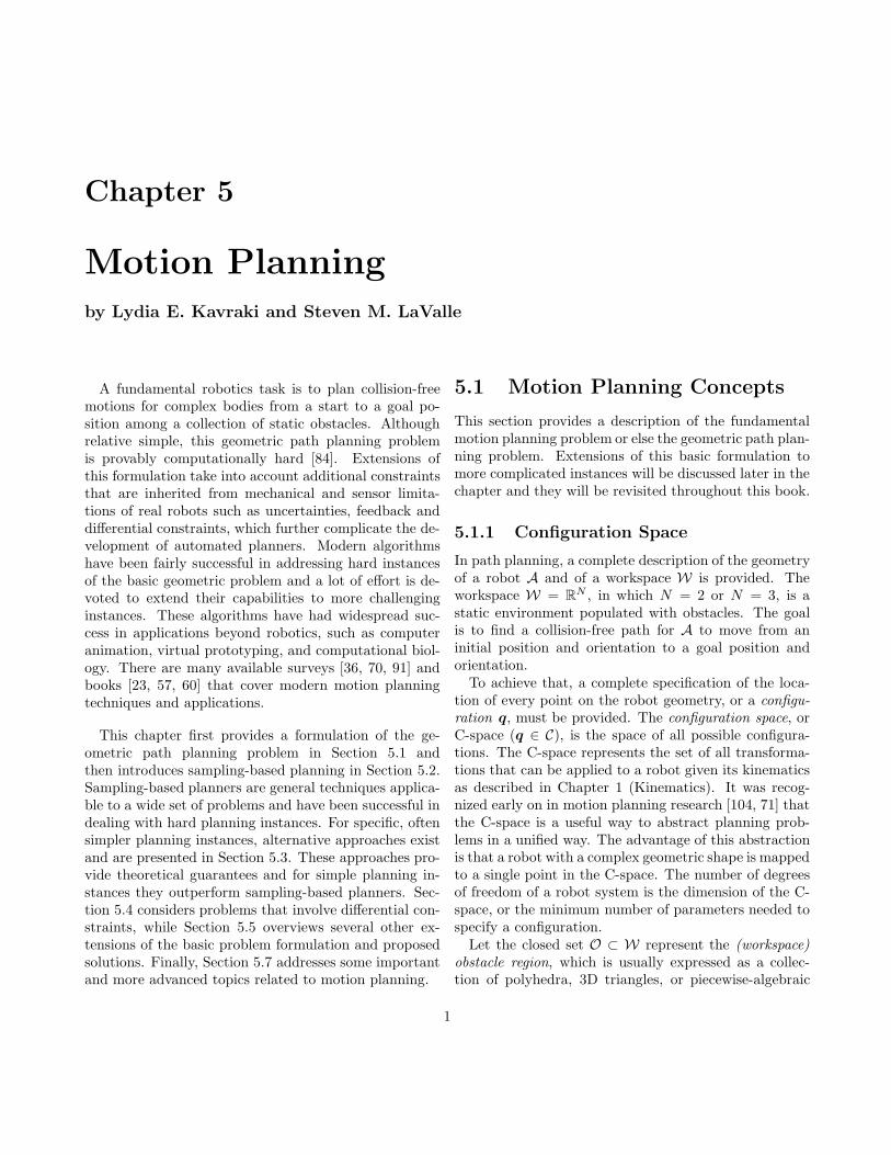
Figure 5.2: A two-joint planar arm: (a) links are pinnedand there are no joint limits. (b) The C-space.

surfaces. Let the closed set A(q) ⊂ W denote the setof points occupied by the robot when at configurationq ∈ C; this set is usually modeled using the same primi-tives as used for O. The C-space obstacle region, Cobs, isdefined as

Cobs = {q ∈ C | A(q) ∩ O 6= ∅}. (5.1)

Since O and A(q) are closed sets in W , the obstacleregion is a closed set in C. The set of configurations thatavoid collision is Cfree = C \ Cobs, and is called the freespace.

Simple examples of C-spaces

Translating Planar Rigid Bodies: The robot’sconfiguration can be specified by a reference point (x, y)on the planar rigid body relative to some fixed coordi-nate frame. Therefore the C-space is equivalent to R

2.Figure 5.1 gives an example of a C-space for a triangularrobot and a single polygonal obstacle. The obstaclein the C-space can be traced by sliding the robotaround the workspace obstacle to find the constraintson all q ∈ C. Motion planning for the robot is nowequivalent to motion planning for a point in the C-space.

Planar Arms: Figure 5.2 gives an example of a two-joint planar arm. The bases of both links are pinned, so

that they can only rotate around the joints and there areno joint limits. For this arm, specifying the rotationalparameters θ1 and θ2 provides the configuration. Eachjoint angle θi corresponds to a point on the unit circleS

1 and the C-space is S1×S

1 = T 2, the two-dimensionaltorus as Figure 5.2 shows. For a higher number of linkswithout joint limits, the C-space can be similarly definedas:

C = S1 × S

1 × · · · × S1. (5.2)

If a joint has limits, then each corresponding S1 is often

replaced with R, even though it is a finite interval. Ifthe base of the planar arm is mobile and not pinned,then the additional translation parameters must also beconsidered in the arm’s configuration:

C = R2 × S

1 × S1 × · · · × S

1 (5.3)

Additional examples of C-spaces are provided in Sec-tion 5.6.1, where topological properties of configurationspaces are discussed.

5.1.2 Geometric Path Planning Problem

The basic motion planning problem, also known as thePiano Mover’s problem [84], is defined as follows.Given:

1. A workspace W , where either W = R2 or W = R

3.

2. An obstacle region O ⊂ W .

3. A robot defined in W . Either a rigid body A or acollection of m links: A1,A2, . . . ,Am.

4. The configuration space C (Cobs and Cfree are thendefined).

5. An initial configuration qI ∈ Cfree.

6. A goal configuration qG ∈ Cfree. The initial andgoal configuration are often called a query (qI , qG).

Compute a (continuous) path, τ : [0, 1] → Cfree, suchthat τ(0) = qI and τ(1) = qG.

5.1.3 Complexity of Motion Planning

The main complications in motion planning are that it isnot easy to directly compute Cobs and Cfree and the di-mensionality of the C-space is often quite high. In termsof computational complexity, the Piano Mover’s problemwas studied early on and it was shown to be PSPACE-hardby Reif [84]. A series of polynomial time algorithms forproblems with fixed dimension suggested an exponentialdependence on the problem dimensionality [92, 93]. A

5.2. SAMPLING-BASED PLANNING 3

single exponential algorithm in the C-space dimension-ality was proposed by Canny and showed that the prob-lem is PSPACE-complete [19]. Although impractical, thealgorithm serves as an upper bound on the general ver-sion of the basic motion planning problem. It appliescomputational algebraic geometry techniques for model-ing the C-space in order to construct a roadmap, a 1Dsubspace that captures the connectivity of Cfree. Ad-ditional details about such techniques can be found inSection 5.6.3.

The complexity of the problem motivated work in pathplanning research. One direction was to study subclassesof the general problem for which polynomial time algo-rithms exist [37]. Even some simpler, special cases ofmotion planning, however, are at least as challenging.For example, the case of a finite number of translating,axis-aligned rectangles in R

2 is PSPACE-hard as well [42].Some extensions of motion planning are even harder. Forexample, a certain form of planning under uncertainty in3D polyhedral environment is NEXPTIME-hard [18]. Thehardest problems in NEXPTIME are believed to requiredoubly-exponential time to solve.

A different direction was the development of alterna-tive planning paradigms that were practical under real-istic assumptions. Many combinatorial approaches canefficiently construct 1D roadmaps for specific 2D or 3Dproblems. Potential field-based approaches define vec-tor fields which can be followed by a robot towards thegoal. Both approaches, however, do not scale well inthe general case. They will be described in Section 5.3.An alternative paradigm, sampling-based planning, is ageneral approach that has been shown to be succesful inpractise with many challenging problems. It avoids theexact geometric modeling of the C-space but it cannotprovide the guarantees of a complete algorithm. Com-plete and exact algorithms are able to detect that no pathcan be found. Instead sampling-based planning offers alower level of completeness guarantee. This paradigm isdescribed in the following section.

5.2 Sampling-based Planning

Sampling-based planners are described first because theyare the method of choice for a very general class of prob-lems. The following section will describe other planners,some of which were developed before the sampling-basedframework. The key idea in sampling-based planning isto exploit advances in collision detection algorithms thatcompute whether a single configuration is collision-free.

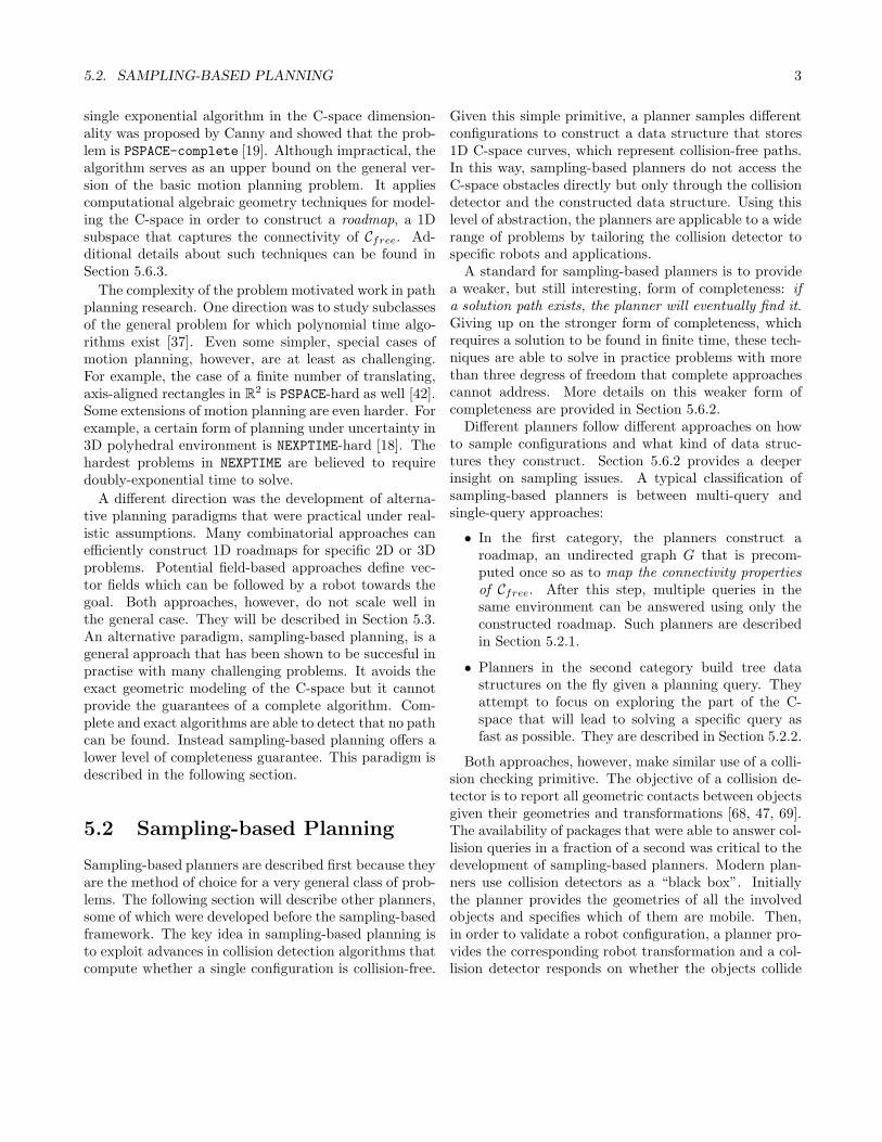
Given this simple primitive, a planner samples differentconfigurations to construct a data structure that stores1D C-space curves, which represent collision-free paths.In this way, sampling-based planners do not access theC-space obstacles directly but only through the collisiondetector and the constructed data structure. Using thislevel of abstraction, the planners are applicable to a widerange of problems by tailoring the collision detector tospecific robots and applications.

A standard for sampling-based planners is to providea weaker, but still interesting, form of completeness: ifa solution path exists, the planner will eventually find it.Giving up on the stronger form of completeness, whichrequires a solution to be found in finite time, these tech-niques are able to solve in practice problems with morethan three degress of freedom that complete approachescannot address. More details on this weaker form ofcompleteness are provided in Section 5.6.2.

Different planners follow different approaches on howto sample configurations and what kind of data struc-tures they construct. Section 5.6.2 provides a deeperinsight on sampling issues. A typical classification ofsampling-based planners is between multi-query andsingle-query approaches:

• In the first category, the planners construct aroadmap, an undirected graph G that is precom-puted once so as to map the connectivity propertiesof Cfree. After this step, multiple queries in thesame environment can be answered using only theconstructed roadmap. Such planners are describedin Section 5.2.1.

• Planners in the second category build tree datastructures on the fly given a planning query. Theyattempt to focus on exploring the part of the C-space that will lead to solving a specific query asfast as possible. They are described in Section 5.2.2.

Both approaches, however, make similar use of a colli-sion checking primitive. The objective of a collision de-tector is to report all geometric contacts between objectsgiven their geometries and transformations [68, 47, 69].The availability of packages that were able to answer col-lision queries in a fraction of a second was critical to thedevelopment of sampling-based planners. Modern plan-ners use collision detectors as a “black box”. Initiallythe planner provides the geometries of all the involvedobjects and specifies which of them are mobile. Then,in order to validate a robot configuration, a planner pro-vides the corresponding robot transformation and a col-lision detector responds on whether the objects collide

4 CHAPTER 5. MOTION PLANNING BY LYDIA E. KAVRAKI AND STEVEN M. LAVALLE

or not. Many packages represent the geometric modelshierarchically, avoid computing all-pairwise interactionsand conduct a binary search to evaluate collisions. Ex-cept from configurations, a planner must also validateentire paths. Some collision detectors return distance-from-collision information, which can be used to inferthat entire neighborhoods in C are valid. It is often moreexpensive, however, to extract this information; insteadpaths are usually validated point-by-point using a smallstepping size either incrementally or by employing bi-nary search. Some collision detectors are incremental bydesign, which means that they can be faster by reusinginformation from a previous query [68].

5.2.1 Multi-Query Planners:

Mapping the Connectivity of Cfree

Planners that aim to answer multiple queries for a cer-tain static environment use a preprocessing phase duringwhich they attempt to map the connectivity propertiesof Cfree onto a roadmap. This roadmap has the form ofa graph G, with vertices as configurations and edges aspaths. A union of 1D curves is a roadmap G if it satisfiesthe following properties:

1. Accessibility: From any q ∈ Cfree, it is simple andefficient to compute a path τ : [0, 1] → Cfree suchthat τ(0) = q and τ(1) = s, in which s may be anypoint in S(G). S(G) is the swath of G, the union ofall configurations reached by all edges and vertices.This means that it is always possible to connect aplanning query pair, qI and qG to some sI and sG,respectively, in S(G).

2. Connectivity Preserving: The second conditionrequires that if there exists a path τ : [0, 1]→ Cfree

such that τ(0) = qG and τ(1) = qG, then there alsoexists a path τ ′ : [0, 1]→ S(G), such that τ ′(0) = sI

and τ ′(1) = sG. Thus, solutions are not missedbecause G fails to capture the connectivity of Cfree.

The Probabilistic Roadmap Method (PRM) approach[50] attempts to approximate such a roadmap G in acomputationally efficient way. The preprocessing phaseof PRM, which can be extended to sampling-basedroadmaps in general, follows these steps:

1. Initialization: Let G(V, E) represent an undi-rected graph, which initially is empty. Vertices of Gwill correspond to collision-free configurations, andedges to collision-free paths that connect vertices.

α(i)

Cobs

Cobs

Figure 5.3: The sampling-based roadmap is constructedincrementally by attempting to connect each new sam-ple, α(i), to nearby vertices in the roadmap.

2. Configuration Sampling: A configuration α(i) issampled from Cfree and added to the vertex set V .α(·) is an infinite, dense sample sequence and α(i)is the i-th point in that sequence.

3. Neighborhood Computation: Usually, a metricis defined in the C-space, ρ : C × C → R. Verticesq already in V are then selected as part of α(i)’sneighborhood if they have small distance accordingto ρ.

4. Edge Consideration: For those vertices q, whichdo not belong in the same connected component of Gwith α(i), the algorithm attempts to connect themwith an edge.

5. Local Planning Method: Given α(i) and q ∈Cfree a module is used that attempts to constructa path τs : [0, 1] → Cfree such that τ(0) = α(i)and τ(1) = q. Using collision detection, τs must bechecked to ensure that it does not cause a collision.

6. Edge Insertion: Insert τs into E, as an edge fromα(i) to q.

7. Termination: The algorithm is typically termi-nated when a predefined number of collision-freevertices N has been added in the roadmap.

The algorithm is incremental in nature. Computationcan be repeated by starting from an already existinggraph. A general sampling-based roadmap is summa-rized in Algorithm 1.

An illustration of the algorithm’s behavior is depictedin Figure 5.3. To solve a query, qI and qG are connectedto the roadmap, and graph search is performed.

5.2. SAMPLING-BASED PLANNING 5

Algorithm 1 SAMPLING-BASED ROADMAP

N: number of nodes to include in the roadmap————————————————————————G.init(); i← 0;while i < N do

if α(i) ∈ Cfree thenG.add vertex(α(i)); i← i + 1;for q ∈ neighborhood(α(i),G) do

if connect(α(i), q)) thenG.add edge(α(i), q);

endifend for

end ifend while

For the original PRM [50], the configuration α(i) wasproduced using random sampling. For the connectionstep betweem q and α(i), the algorithm used straight linepaths in the C-space. In some cases a connection was notattempted if q and α(i) were in the same connected com-ponent. There have been many subsequent works thattry to improve the roadmap quality while using fewersamples. Methods for concentrating samples at or nearthe boundary of Cfree are presented in [2, 13]. Methodsthat move samples as far from the boundary as possibleappear in [40, 67]. Deterministic sampling techniques,including grids, appear in [61]. A method of pruning ver-tices based on mutual visibility appears in [98] that leadsto a dramatic reduction in the number of roadmap ver-tices. Theoretical analysis of sampling-based roadmapsappears in [6, 61, 55] and is briefly discussed in Section5.6.2. An experimental comparison of sampling-basedroadmap variants appears in [33]. One difficulty in theseroadmap approaches is identifying narrow passages. Oneproposal is to use bridge test for identifying these [43].For other PRM-based works, see [12, 16, 46, 66, 77]. Ex-tended discussion of the topic can be found in [23, 60].

5.2.2 Single-Query Planners:

Incremental Search

Single-query planning methods focus on a single initial-goal configuration pair. They probe and search the con-tinuous C-space by extending tree data structures initial-ized at these known configurations and eventually con-necting them. Most single-query methods conform to thefollowing template:

1. Initialization: Let G(V, E) represent an undi-rected search graph, for which the vertex set, V ,

qn

q0

Cobs

qs

α(i)

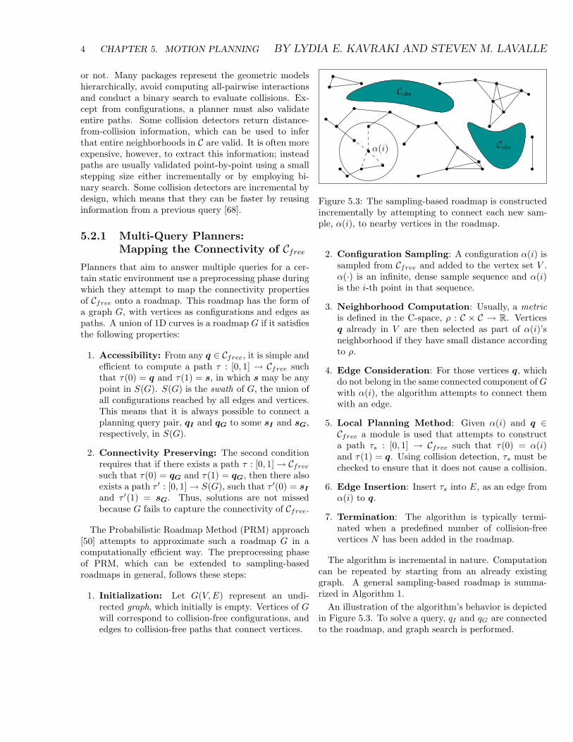
Figure 5.4: If there is an obstacle, the edge travels up tothe obstacle boundary, as far as allowed by the collisiondetection algorithm.

contains a vertex for one (usually qI) or more con-figurations in Cfree, and the edge set, E, is empty.Vertices of G are collision-free configurations, andedges are collision-free paths that connect vertices.

2. Vertex Selection Method: Choose a vertexqcur ∈ V for expansion.

3. Local Planning Method: For some qnew ∈ Cfree,which may correspond to an existing vertex in Vbut on a different tree or a sampled configuration,attempt to construct a path τs : [0, 1]→ Cfree suchthat τ(0) = qcur and τ(1) = qnew. Using collisiondetection, τs must be checked to ensure that it doesnot cause a collision. If this step fails to produce acollision-free path segment, then go to Step 2.

4. Insert an Edge in the Graph: Insert τs into E,as an edge from qcur to qnew. If qnew is not alreadyin V , then it is inserted.

5. Check for a Solution: Determine whether G en-codes a solution path.

6. Return to Step 2: Iterate unless a solution hasbeen found or some termination condition is satis-fied, in which case the algorithm reports failure.

During execution, G may be organized into one ormore trees. This leads to: 1) unidirectional methods,which involves a single tree, usually rooted at qI [64], 2)bidirectional methods, which involves two trees, typicallyrooted at qI and qG [64], and 3) multidirectional meth-ods, which may have more than two trees [10, 101]. Themotivation for using more than one tree is that a singletree may become trapped trying to find an exit througha narrow opening. Traveling in the opposite direction,however, may be easier. As more trees are considered itbecomes more complicated to determine which connec-tions should be made between trees.

6 CHAPTER 5. MOTION PLANNING BY LYDIA E. KAVRAKI AND STEVEN M. LAVALLE

Rapidly-Exploring Dense Trees

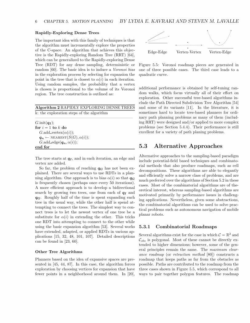
The important idea with this family of techniques is thatthe algorithm must incrementally explore the propertiesof the C-space. An algorithm that achieves this objec-tive is the Rapidly-exploring Random Tree (RRT) [64],which can be generalized to the Rapidly-exploring DenseTree (RDT) for any dense sampling, deterministic orrandom [60]. The basic idea is to induce a Voronoi biasin the exploration process by selecting for expansion thepoint in the tree that is closest to α(i) in each iteration.Using random samples, the probability that a vertexis chosen is proportional to the volume of its Voronoiregion. The tree construction is outlined as:

Algorithm 2 RAPIDLY EXPLORING DENSE TREES

k: the exploration steps of the algorithm————————————————————————G.init(qI );for i = 1 to k do

G.add vertex(α(i));qn ← nearest(S(G), α(i));G.add edge(qn, α(i));

end for

The tree starts at qI , and in each iteration, an edge andvertex are added.

So far, the problem of reaching qG has not been ex-plained. There are several ways to use RDTs in a plan-ning algorithm. One approach is to bias α(i) so that qG

is frequently chosen (perhaps once every 50 iterations).A more efficient approach is to develop a bidirectionalsearch by growing two trees, one from each of qI andqG. Roughly half of the time is spent expanding eachtree in the usual way, while the other half is spend at-tempting to connect the trees. The simplest way to con-nect trees is to let the newest vertex of one tree be asubstitute for α(i) in extending the other. This tricksone RDT into attempting to connect to the other whileusing the basic expansion algorithm [53]. Several workshave extended, adapted, or applied RDTs in various ap-plications [15, 32, 48, 101, 107]. Detailed descriptionscan be found in [23, 60].

Other Tree Algorithms

Planners based on the idea of expansive spaces are pre-sented in [45, 44, 87]. In this case, the algorithm forcesexploration by choosing vertices for expansion that havefewer points in a neighborhood around them. In [20],

Edge-Edge Vertex-Vertex Vertex-Edge

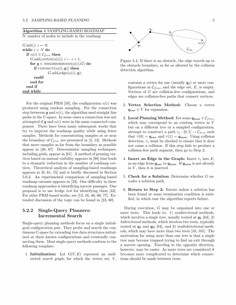
Figure 5.5: Voronoi roadmap pieces are generated inone of three possible cases. The third case leads to aquadratic curve.

additional performance is obtained by self-tuning ran-dom walks, which focus virtually all of their effort onexploration. Other successful tree-based algorithms in-clude the Path Directed Subdivision Tree Algorithm [54]and some of its variants [11]. In the literature, it issometimes hard to locate tree-based planners for ordi-nary path planning problems as many of them (includ-ing RRT) were designed and/or applied to more complexproblems (see Section 5.4.4). Their performance is stillexcellent for a variety of path planing problems.

5.3 Alternative Approaches

Alternative approaches to the sampling-based paradigminclude potential-field based techniques and combinato-rial methods that also produce roadmaps, such as celldecompositions. These algorithms are able to elegantlyand efficiently solve a narrow class of problems, and aremuch preferred over the algorithms of Section 5.2 in thesecases. Most of the combinatorial algorithms are of the-oretical interest, whereas sampling-based algorithms aremotivated primarily by performance issues in challeng-ing applications. Nevertheless, given some abstractions,the combinatorial algorithms can be used to solve prac-tical problems such as autonomous navigation of mobileplanar robots.

5.3.1 Combinatorial Roadmaps

Several algorithms exist for the case in which C = R2 and

Cobs is polygonal. Most of these cannot be directly ex-tended to higher dimensions; however, some of the gen-eral principles remain the same. The maximum clear-ance roadmap (or retraction method [80]) constructs aroadmap that keeps paths as far from the obstacles aspossible. Paths are contributed to the roadmap from thethree cases shown in Figure 5.5, which correspond to allways to pair together polygon features. The roadmap

5.3. ALTERNATIVE APPROACHES 7

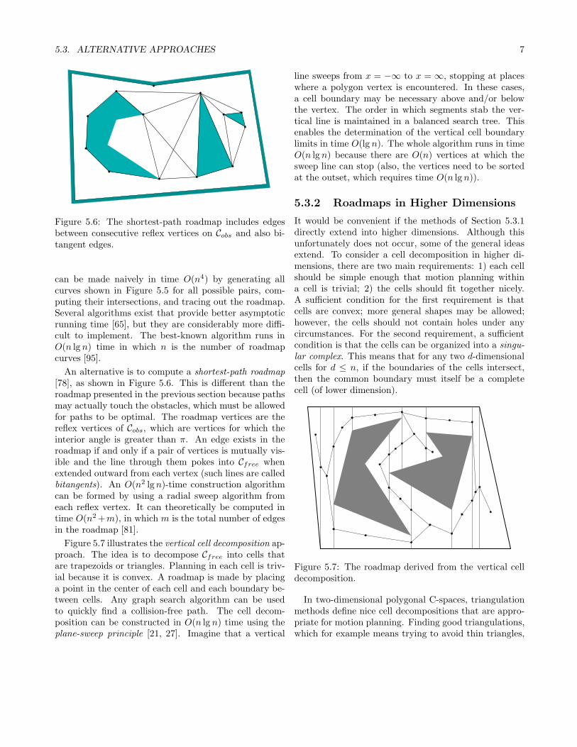
Figure 5.6: The shortest-path roadmap includes edgesbetween consecutive reflex vertices on Cobs and also bi-tangent edges.

can be made naively in time O(n4) by generating allcurves shown in Figure 5.5 for all possible pairs, com-puting their intersections, and tracing out the roadmap.Several algorithms exist that provide better asymptoticrunning time [65], but they are considerably more diffi-cult to implement. The best-known algorithm runs inO(n lg n) time in which n is the number of roadmapcurves [95].

An alternative is to compute a shortest-path roadmap[78], as shown in Figure 5.6. This is different than theroadmap presented in the previous section because pathsmay actually touch the obstacles, which must be allowedfor paths to be optimal. The roadmap vertices are thereflex vertices of Cobs, which are vertices for which theinterior angle is greater than π. An edge exists in theroadmap if and only if a pair of vertices is mutually vis-ible and the line through them pokes into Cfree whenextended outward from each vertex (such lines are calledbitangents). An O(n2 lg n)-time construction algorithmcan be formed by using a radial sweep algorithm fromeach reflex vertex. It can theoretically be computed intime O(n2 +m), in which m is the total number of edgesin the roadmap [81].

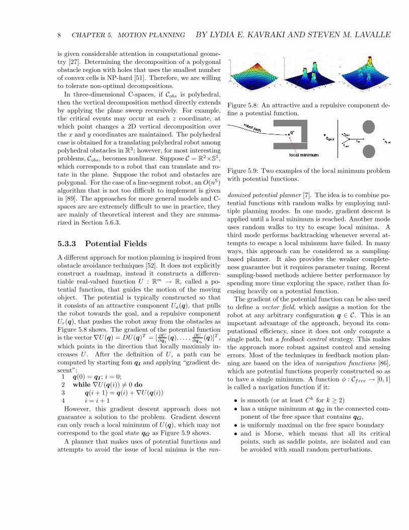
Figure 5.7 illustrates the vertical cell decomposition ap-proach. The idea is to decompose Cfree into cells thatare trapezoids or triangles. Planning in each cell is triv-ial because it is convex. A roadmap is made by placinga point in the center of each cell and each boundary be-tween cells. Any graph search algorithm can be usedto quickly find a collision-free path. The cell decom-position can be constructed in O(n lg n) time using theplane-sweep principle [21, 27]. Imagine that a vertical

line sweeps from x = −∞ to x = ∞, stopping at placeswhere a polygon vertex is encountered. In these cases,a cell boundary may be necessary above and/or belowthe vertex. The order in which segments stab the ver-tical line is maintained in a balanced search tree. Thisenables the determination of the vertical cell boundarylimits in time O(lg n). The whole algorithm runs in timeO(n lg n) because there are O(n) vertices at which thesweep line can stop (also, the vertices need to be sortedat the outset, which requires time O(n lg n)).

5.3.2 Roadmaps in Higher Dimensions

It would be convenient if the methods of Section 5.3.1directly extend into higher dimensions. Although thisunfortunately does not occur, some of the general ideasextend. To consider a cell decomposition in higher di-mensions, there are two main requirements: 1) each cellshould be simple enough that motion planning withina cell is trivial; 2) the cells should fit together nicely.A sufficient condition for the first requirement is thatcells are convex; more general shapes may be allowed;however, the cells should not contain holes under anycircumstances. For the second requirement, a sufficientcondition is that the cells can be organized into a singu-lar complex. This means that for any two d-dimensionalcells for d ≤ n, if the boundaries of the cells intersect,then the common boundary must itself be a completecell (of lower dimension).

Figure 5.7: The roadmap derived from the vertical celldecomposition.

In two-dimensional polygonal C-spaces, triangulationmethods define nice cell decompositions that are appro-priate for motion planning. Finding good triangulations,which for example means trying to avoid thin triangles,

8 CHAPTER 5. MOTION PLANNING BY LYDIA E. KAVRAKI AND STEVEN M. LAVALLE

is given considerable attention in computational geome-try [27]. Determining the decomposition of a polygonalobstacle region with holes that uses the smallest numberof convex cells is NP-hard [51]. Therefore, we are willingto tolerate non-optimal decompositions.

In three-dimensional C-spaces, if Cobs is polyhedral,then the vertical decomposition method directly extendsby applying the plane sweep recursively. For example,the critical events may occur at each z coordinate, atwhich point changes a 2D vertical decomposition overthe x and y coordinates are maintained. The polyhedralcase is obtained for a translating polyhedral robot amongpolyhedral obstacles in R

3; however, for most interestingproblems, Cobs, becomes nonlinear. Suppose C = R

2×S1,

which corresponds to a robot that can translate and ro-tate in the plane. Suppose the robot and obstacles arepolygonal. For the case of a line-segment robot, an O(n5)algorithm that is not too difficult to implement is givenin [89]. The approaches for more general models and C-spaces are are extremely difficult to use in practice, theyare mainly of theoretical interest and they are summa-rized in Section 5.6.3.

5.3.3 Potential Fields

A different approach for motion planning is inspired fromobstacle avoidance techniques [52]. It does not explicitlyconstruct a roadmap, instead it constructs a differen-tiable real-valued function U : R

m → R, called a po-tential function, that guides the motion of the movingobject. The potential is typically constructed so thatit consists of an attractive component Ua(q), that pullsthe robot towards the goal, and a repulsive componentUr(q), that pushes the robot away from the obstacles asFigure 5.8 shows. The gradient of the potential functionis the vector∇U(q) = DU(q)T = [ ∂U

∂q1

(q), . . . , ∂U∂q

m

(q)]T ,

which points in the direction that locally maximaly in-creases U . After the definition of U , a path can becomputed by starting fom qI and applying “gradient de-scent”:1 q(0) = qI ; i = 0;2 while ∇U(q(i)) 6= 0 do3 q(i + 1) = q(i) +∇U(q(i))4 i = i + 1However, this gradient descent approach does not

guarantee a solution to the problem. Gradient descentcan only reach a local minimum of U(q), which may notcorrespond to the goal state qG as Figure 5.9 shows.

A planner that makes uses of potential functions andattempts to avoid the issue of local minima is the ran-

Figure 5.8: An attractive and a repulsive component de-fine a potential function.

Figure 5.9: Two examples of the local minimum problemwith potential functions.

domized potential planner [7]. The idea is to combine po-tential functions with random walks by employing mul-tiple planning modes. In one mode, gradient descent isapplied until a local minimum is reached. Another modeuses random walks to try to escape local minima. Athird mode performs backtracking whenever several at-tempts to escape a local minimum have failed. In manyways, this approach can be considered as a sampling-based planner. It also provides the weaker complete-ness guarantee but it requires parameter tuning. Recentsampling-based methods achieve better performance byspending more time exploring the space, rather than fo-cusing heavily on a potential function.

The gradient of the potential function can be also usedto define a vector field, which assigns a motion for therobot at any arbitrary configuration q ∈ C. This is animportant advantage of the approach, beyond its com-putational efficiency, since it does not only compute asingle path, but a feedback control strategy. This makesthe approach more robust against control and sensingerrors. Most of the techniques in feedback motion plan-ning are based on the idea of navigation functions [86],which are potential functions properly constructed so asto have a single minimum. A function φ : Cfree → [0, 1]is called a navigation function if it:

• is smooth (or at least Ck for k ≥ 2)

• has a unique minimum at qG in the connected com-ponent of the free space that contains qG,

• is uniformly maximal on the free space boundary

• and is Morse, which means that all its criticalpoints, such as saddle points, are isolated and canbe avoided with small random perturbations.

5.4. DIFFERENTIAL CONSTRAINTS 9

Figure 5.10: Examples of sphere and star spaces.

Navigation functions can be constructed for sphereboundary spaces centered at qI that contain only spher-ical obstacles as Figure 5.10 shows. Then they can beextended to a large family of C-spaces that are diffeo-morphic to sphere-spaces, such as star-shaped spaces asin Figure 5.10. A more elaborate description of strate-gies for feedback motion planning will be presented inchapters 35, 36 and 37.

Putting the issue of local minima aside, another majorchallenge for such potential function based approaches isconstructing and representing the C-space in the firstplace. This issue makes the applications of these tech-niques too complicated for high-dimensional problems.

5.4 Differential Constraints

Robot motions must usually conform to both global andlocal constraints. Global constraints on C have been con-sidered in the form of obstacles and possibly joint lim-its. Local constraints are modeled with differential equa-tions, and are therefore called differential constraints.These limit the velocities, and possibly accelerations,at every point due to kinematic considerations, such aswheels in contact, and dynamical considerations, such asthe conservation of angular momentum.

5.4.1 Concepts and Terminology

Let q denote a velocity vector. Differential constraintson C can be expressed either implicitly in the formgi(q, q) = 0 or parametrically in the form x = f(q, u).The implicit form is more general but often more diffi-cult to understand and utilize. In the parametric form, avector-valued equation indicates the velocity that is ob-tained for a given q and u, in which u is an input, chosenfrom some input space, U . Let T denote an interval oftime, starting at t = 0.

To model dynamics, the concepts are extended intoa phase space, X , of the C-space. Usually each pointx ∈ X represents both a configuration and velocity,

qq = 0

q < 0

q > 0

q Xric

Xric

Xric

Xobs

Xric

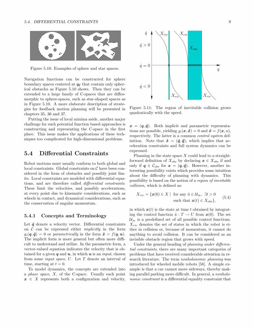
Figure 5.11: The region of inevitable collision growsquadratically with the speed.

x = (q, q). Both implicit and parametric representa-tions are possible, yielding gi(x, x) = 0 and x = f(x, u),respectively. The latter is a common control system def-inition. Note that x = (q, q), which implies that ac-celeration constraints and full system dynamics can beexpressed.

Planning in the state space X could lead to a straight-forward definition of Xobs by declaring x ∈ Xobs if andonly if q ∈ Cobs for x = (q, q). However, another in-teresting possibility exists which provides some intuitionabout the difficulty of planning with dynamics. Thispossibility is based on the notion of a region of inevitablecollision, which is defined as:

Xric = {x(0) ∈ X | for any u ∈ U∞, ∃t > 0

such that x(t) ∈ Xobs},(5.4)

in which x(t) is the state at time t obtained by integrat-ing the control function u : T → U from x(0). The setU∞ is a predefined set of all possible control functions.Xric denotes the set of states in which the robot is ei-ther in collision or, because of momentum, it cannot doanything to avoid collision. It can be considered as aninvisible obstacle region that grows with speed.

Under the general heading of planning under differen-tial constraints, there are many important categories ofproblems that have received considerable attention in re-search literature. The term nonholonomic planning wasintroduced for wheeled mobile robots [58]. A simple ex-ample is that a car cannot move sideways, thereby mak-ing parallel parking more difficult. In general, a nonholo-nomic constraint is a differential equality constraint that

10 CHAPTER 5. MOTION PLANNING BY LYDIA E. KAVRAKI AND STEVEN M. LAVALLE

Two stages Four stages

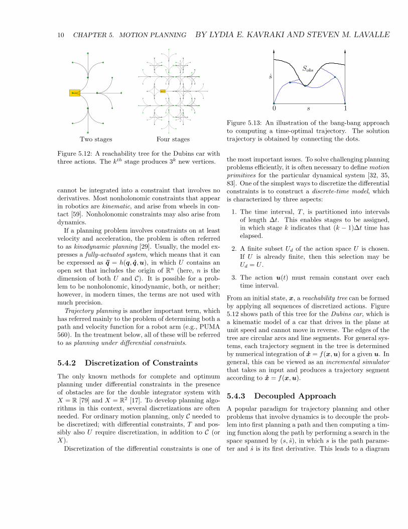
Figure 5.12: A reachability tree for the Dubins car withthree actions. The kth stage produces 3k new vertices.

cannot be integrated into a constraint that involves noderivatives. Most nonholonomic constraints that appearin robotics are kinematic, and arise from wheels in con-tact [59]. Nonholonomic constraints may also arise fromdynamics.

If a planning problem involves constraints on at leastvelocity and acceleration, the problem is often referredto as kinodynamic planning [29]. Usually, the model ex-presses a fully-actuated system, which means that it canbe expressed as q = h(q, q, u), in which U contains anopen set that includes the origin of R

n (here, n is thedimension of both U and C). It is possible for a prob-lem to be nonholonomic, kinodynamic, both, or neither;however, in modern times, the terms are not used withmuch precision.

Trajectory planning is another important term, whichhas referred mainly to the problem of determining both apath and velocity function for a robot arm (e.g., PUMA560). In the treatment below, all of these will be referredto as planning under differential constraints.

5.4.2 Discretization of Constraints

The only known methods for complete and optimumplanning under differential constraints in the presenceof obstacles are for the double integrator system withX = R [79] and X = R

2 [17]. To develop planning algo-rithms in this context, several discretizations are oftenneeded. For ordinary motion planning, only C needed tobe discretized; with differential constraints, T and pos-sibly also U require discretization, in addition to C (orX).

Discretization of the differential constraints is one of

s

s

0 1

Sobs

Figure 5.13: An illustration of the bang-bang approachto computing a time-optimal trajectory. The solutiontrajectory is obtained by connecting the dots.

the most important issues. To solve challenging planningproblems efficiently, it is often necessary to define motionprimitives for the particular dynamical system [32, 35,83]. One of the simplest ways to discretize the differentialconstraints is to construct a discrete-time model, whichis characterized by three aspects:

1. The time interval, T , is partitioned into intervalsof length ∆t. This enables stages to be assigned,in which stage k indicates that (k − 1)∆t time haselapsed.

2. A finite subset Ud of the action space U is chosen.If U is already finite, then this selection may beUd = U .

3. The action u(t) must remain constant over eachtime interval.

From an initial state, x, a reachability tree can be formedby applying all sequences of discretized actions. Figure5.12 shows path of this tree for the Dubins car, which isa kinematic model of a car that drives in the plane atunit speed and cannot move in reverse. The edges of thetree are circular arcs and line segments. For general sys-tems, each trajectory segment in the tree is determinedby numerical integration of x = f(x, u) for a given u. Ingeneral, this can be viewed as an incremental simulatorthat takes an input and produces a trajectory segmentaccording to x = f(x, u).

5.4.3 Decoupled Approach

A popular paradigm for trajectory planning and otherproblems that involve dynamics is to decouple the prob-lem into first planning a path and then computing a tim-ing function along the path by performing a search in thespace spanned by (s, s), in which s is the path parame-ter and s is its first derivative. This leads to a diagram

5.4. DIFFERENTIAL CONSTRAINTS 11

such as the one shown in Figure 5.13, in which the upperregion Sobs must be avoided because the correspondingmotion of the mechanical system violates the differentialconstraints. Most methods are based on early work in[41, 96], and determine a bang-bang control, which meansthat they switch between accelerating and deceleratingat full speed. This applies to determining time-optimaltrajectories (optimal once constrained to the path). Dy-namic programming can be used for more general prob-lems [97].

For some problems and nonholonomic systems,steeringmethods have been developed to efficiently solve the two-point boundary value problem [59, 88]. This means thatfor any pair of states, a trajectory that ignores obstaclesbut satisfies the differential constraints can be obtained.Moreover, for some systems, the complete set of optimaltrajectories has been characterized [5, 100]. These con-trol based approaches enable straightforward adaptationof the sampling-based roadmap approach [103, 94]. Onedecoupled approach is to first plan a path that ignoresdifferential constraints, and then incrementally trans-form it into one that obeys the constraints [31, 59].

5.4.4 Kinodynamic Planning

Due to the great difficulty of planning under differentialconstraints, many succesful planning algorithms that ad-dress kinodynamic problems directly in the phase spaceX are sampling-based.

Sampling-based planning algorithms proceed by ex-ploring one or more reachability trees. Many parallelscan be drawn with searching on a grid; however, reach-ability trees are more complicated because they do notnecessarily involve a regular lattice structure. The ver-tex set of reachability trees is dense in most cases. It istherefore not clear how to exhaustively search a boundedregion at a fixed resolution. It is also difficult to designapproaches that behave like a multiresolution grid, inwhich refinements can be made arbitrarily to ensure res-olution completeness.

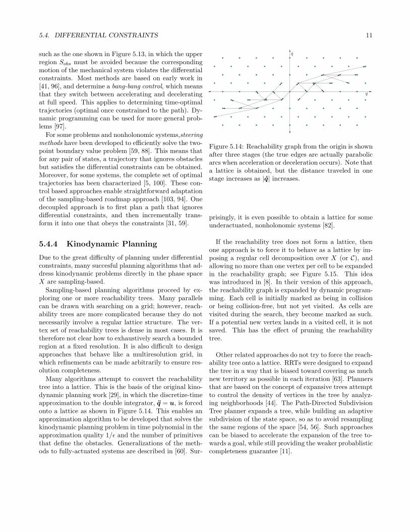
Many algorithms attempt to convert the reachabilitytree into a lattice. This is the basis of the original kino-dynamic planning work [29], in which the discretize-timeapproximation to the double integrator, q = u, is forcedonto a lattice as shown in Figure 5.14. This enables anapproximation algorithm to be developed that solves thekinodynamic planning problem in time polynomial in theapproximation quality 1/ǫ and the number of primitivesthat define the obstacles. Generalizations of the meth-ods to fully-actuated systems are described in [60]. Sur-

q

q

Figure 5.14: Reachability graph from the origin is shownafter three stages (the true edges are actually parabolicarcs when acceleration or deceleration occurs). Note thata lattice is obtained, but the distance traveled in onestage increases as |q| increases.

prisingly, it is even possible to obtain a lattice for someunderactuated, nonholonomic systems [82].

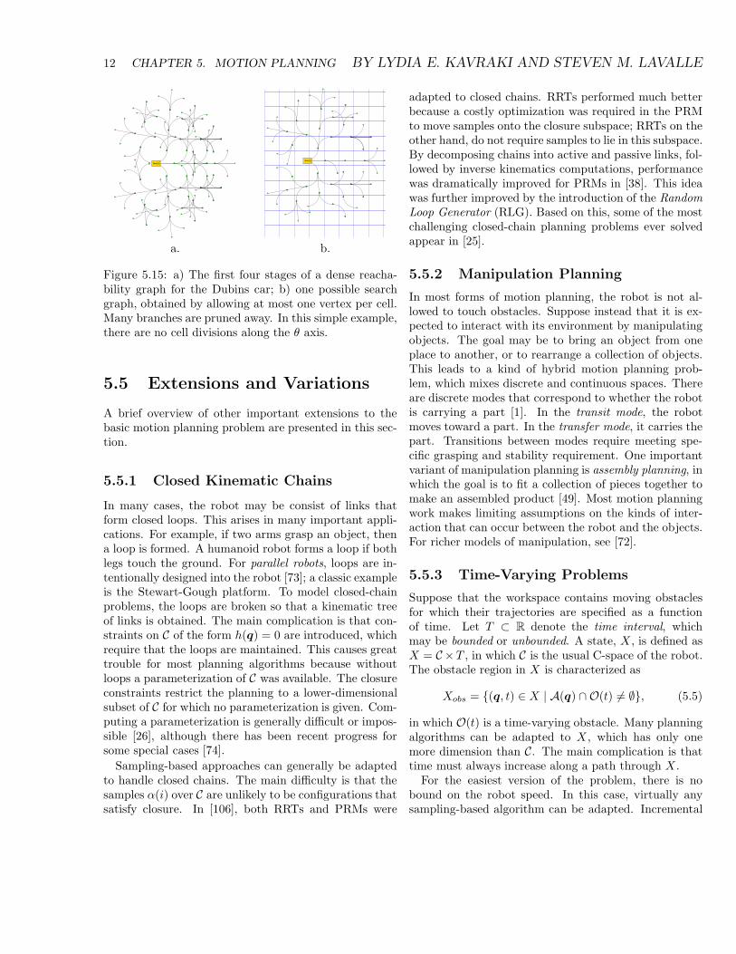
If the reachability tree does not form a lattice, thenone approach is to force it to behave as a lattice by im-posing a regular cell decomposition over X (or C), andallowing no more than one vertex per cell to be expandedin the reachability graph; see Figure 5.15. This ideawas introduced in [8]. In their version of this approach,the reachability graph is expanded by dynamic program-ming. Each cell is initially marked as being in collisionor being collision-free, but not yet visited. As cells arevisited during the search, they become marked as such.If a potential new vertex lands in a visited cell, it is notsaved. This has the effect of pruning the reachabilitytree.

Other related approaches do not try to force the reach-ability tree onto a lattice. RRTs were designed to expandthe tree in a way that is biased toward covering as muchnew territory as possible in each iteration [63]. Plannersthat are based on the concept of expansive trees attemptto control the density of vertices in the tree by analyz-ing neighborhoods [44]. The Path-Directed SubdivisionTree planner expands a tree, while building an adaptivesubdivision of the state space, so as to avoid resamplingthe same regions of the space [54, 56]. Such approachescan be biased to accelerate the expansion of the tree to-wards a goal, while still providing the weaker probablisticcompleteness guarantee [11].

12 CHAPTER 5. MOTION PLANNING BY LYDIA E. KAVRAKI AND STEVEN M. LAVALLE

a. b.

Figure 5.15: a) The first four stages of a dense reacha-bility graph for the Dubins car; b) one possible searchgraph, obtained by allowing at most one vertex per cell.Many branches are pruned away. In this simple example,there are no cell divisions along the θ axis.

5.5 Extensions and Variations

A brief overview of other important extensions to thebasic motion planning problem are presented in this sec-tion.

5.5.1 Closed Kinematic Chains

In many cases, the robot may be consist of links thatform closed loops. This arises in many important appli-cations. For example, if two arms grasp an object, thena loop is formed. A humanoid robot forms a loop if bothlegs touch the ground. For parallel robots, loops are in-tentionally designed into the robot [73]; a classic exampleis the Stewart-Gough platform. To model closed-chainproblems, the loops are broken so that a kinematic treeof links is obtained. The main complication is that con-straints on C of the form h(q) = 0 are introduced, whichrequire that the loops are maintained. This causes greattrouble for most planning algorithms because withoutloops a parameterization of C was available. The closureconstraints restrict the planning to a lower-dimensionalsubset of C for which no parameterization is given. Com-puting a parameterization is generally difficult or impos-sible [26], although there has been recent progress forsome special cases [74].

Sampling-based approaches can generally be adaptedto handle closed chains. The main difficulty is that thesamples α(i) over C are unlikely to be configurations thatsatisfy closure. In [106], both RRTs and PRMs were

adapted to closed chains. RRTs performed much betterbecause a costly optimization was required in the PRMto move samples onto the closure subspace; RRTs on theother hand, do not require samples to lie in this subspace.By decomposing chains into active and passive links, fol-lowed by inverse kinematics computations, performancewas dramatically improved for PRMs in [38]. This ideawas further improved by the introduction of the RandomLoop Generator (RLG). Based on this, some of the mostchallenging closed-chain planning problems ever solvedappear in [25].

5.5.2 Manipulation Planning

In most forms of motion planning, the robot is not al-lowed to touch obstacles. Suppose instead that it is ex-pected to interact with its environment by manipulatingobjects. The goal may be to bring an object from oneplace to another, or to rearrange a collection of objects.This leads to a kind of hybrid motion planning prob-lem, which mixes discrete and continuous spaces. Thereare discrete modes that correspond to whether the robotis carrying a part [1]. In the transit mode, the robotmoves toward a part. In the transfer mode, it carries thepart. Transitions between modes require meeting spe-cific grasping and stability requirement. One importantvariant of manipulation planning is assembly planning, inwhich the goal is to fit a collection of pieces together tomake an assembled product [49]. Most motion planningwork makes limiting assumptions on the kinds of inter-action that can occur between the robot and the objects.For richer models of manipulation, see [72].

5.5.3 Time-Varying Problems

Suppose that the workspace contains moving obstaclesfor which their trajectories are specified as a functionof time. Let T ⊂ R denote the time interval, whichmay be bounded or unbounded. A state, X , is defined asX = C ×T , in which C is the usual C-space of the robot.The obstacle region in X is characterized as

Xobs = {(q, t) ∈ X | A(q) ∩ O(t) 6= ∅}, (5.5)

in which O(t) is a time-varying obstacle. Many planningalgorithms can be adapted to X , which has only onemore dimension than C. The main complication is thattime must always increase along a path through X .

For the easiest version of the problem, there is nobound on the robot speed. In this case, virtually anysampling-based algorithm can be adapted. Incremental

5.5. EXTENSIONS AND VARIATIONS 13

Cfree(t1) Cfree(t2) Cfree(t3)

t3t2t1

xt

yt

qG

t

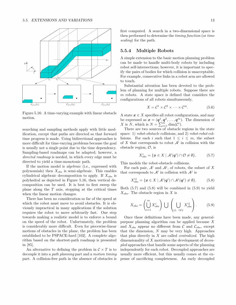
Figure 5.16: A time-varying example with linear obstaclemotion.

searching and sampling methods apply with little mod-ification, except that paths are directed so that forwardtime progress is made. Using bidirectional approaches ismore difficult for time-varying problems because the goalis usually not a single point due to the time dependency.Sampling-based roadmaps can be adapted; however, adirected roadmap is needed, in which every edge must bedirected to yield a time-monotonic path.

If the motion model is algebraic (i.e., expressed withpolynomials) then Xobs is semi-algebraic. This enablescylindrical algebraic decomposition to apply. If Xobs ispolyhedral as depicted in Figure 5.16, then vertical de-composition can be used. It is best to first sweep theplane along the T axis, stopping at the critical timeswhen the linear motion changes.

There has been no consideration so far of the speed atwhich the robot must move to avoid obstacles. It is ob-viously impractical in many applications if the solutionrequires the robot to move arbitrarily fast. One steptowards making a realistic model is to enforce a boundon the speed of the robot. Unfortunately, the problemis considerably more difficult. Even for piecewise-linearmotions of obstacles in the plane, the problem has beenestablished to be PSPACE-hard [102]. A complete algo-rithm based on the shortest-path roadmap is presentedin [85].

An alternative to defining the problem in C × T is todecouple it into a path planning part and a motion timingpart. A collision-free path in the absence of obstacles is

first computed. A search in a two-dimensional space isthen performed to determine the timing function (or timescaling) for the path.

5.5.4 Multiple Robots

A simple extension to the basic motion planning problemcan be made to handle multi-body robots by includingrobot self-intersections; however, it is important to spec-ify the pairs of bodies for which collision is unacceptable.For example, consecutive links in a robot arm are allowedto touch.

Substantial attention has been devoted to the prob-lem of planning for multiple robots. Suppose there arem robots. A state space is defined that considers theconfigurations of all robots simultaneously,

X = C1 × C2 × · · · × Cm. (5.6)

A state x ∈ X specifies all robot configurations, and maybe expressed as x = (q1, q2, . . . , qm). The dimension ofX is N , which is N =

∑mi=1 dim(Ci).

There are two sources of obstacle regions in the statespace: 1) robot-obstacle collisions, and 2) robot-robot col-lisions. For each i such that 1 ≤ i ≤ m, the subsetof X that corresponds to robot Ai in collision with theobstacle region, O, is

X iobs = {x ∈ X | Ai(qi) ∩ O 6= ∅}. (5.7)

This models the robot-obstacle collisions.For each pair, Ai and Aj , of robots, the subset of X

that corresponds to Ai in collision with Aj is

X ijobs = {x ∈ X | Ai(qi) ∩Aj(qj) 6= ∅}. (5.8)

Both (5.7) and (5.8) will be combined in (5.9) to yieldXobs. The obstacle region in X is

Xobs =

(

m⋃

i=1

X iobs

)

⋃

⋃

ij, i6=j

X ijobs

. (5.9)

Once these definitions have been made, any general-purpose planning algorithm can be applied because Xand Xobs appear no different from C and Cobs, exceptthat the dimension, N may be very high. Approachesthat plan directly in X are called centralized. The highdimensionality of X motivates the development of decou-pled approaches that handle some aspects of the planningindependently for each robot. Decoupled approaches areusually more efficient, but this usually comes at the ex-pense of sacrificing completeness. An early decoupled

14 CHAPTER 5. MOTION PLANNING BY LYDIA E. KAVRAKI AND STEVEN M. LAVALLE

s1

s2

s3

s1

s2

s1

s3

s2

s3

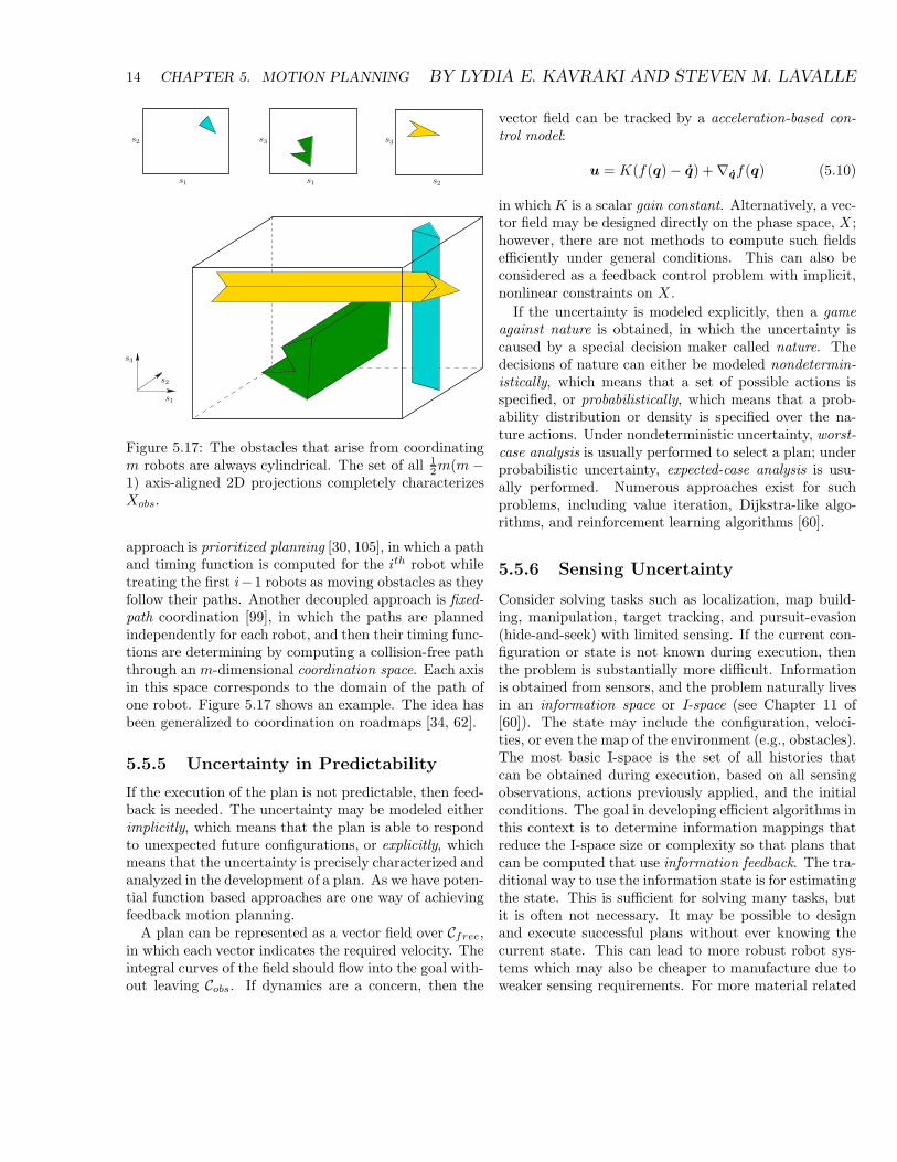
Figure 5.17: The obstacles that arise from coordinatingm robots are always cylindrical. The set of all 1

2m(m−1) axis-aligned 2D projections completely characterizesXobs.

approach is prioritized planning [30, 105], in which a pathand timing function is computed for the ith robot whiletreating the first i−1 robots as moving obstacles as theyfollow their paths. Another decoupled approach is fixed-path coordination [99], in which the paths are plannedindependently for each robot, and then their timing func-tions are determining by computing a collision-free paththrough an m-dimensional coordination space. Each axisin this space corresponds to the domain of the path ofone robot. Figure 5.17 shows an example. The idea hasbeen generalized to coordination on roadmaps [34, 62].

5.5.5 Uncertainty in Predictability

If the execution of the plan is not predictable, then feed-back is needed. The uncertainty may be modeled eitherimplicitly, which means that the plan is able to respondto unexpected future configurations, or explicitly, whichmeans that the uncertainty is precisely characterized andanalyzed in the development of a plan. As we have poten-tial function based approaches are one way of achievingfeedback motion planning.

A plan can be represented as a vector field over Cfree,in which each vector indicates the required velocity. Theintegral curves of the field should flow into the goal with-out leaving Cobs. If dynamics are a concern, then the

vector field can be tracked by a acceleration-based con-trol model:

u = K(f(q)− q) +∇qf(q) (5.10)

in which K is a scalar gain constant. Alternatively, a vec-tor field may be designed directly on the phase space, X ;however, there are not methods to compute such fieldsefficiently under general conditions. This can also beconsidered as a feedback control problem with implicit,nonlinear constraints on X .

If the uncertainty is modeled explicitly, then a gameagainst nature is obtained, in which the uncertainty iscaused by a special decision maker called nature. Thedecisions of nature can either be modeled nondetermin-istically, which means that a set of possible actions isspecified, or probabilistically, which means that a prob-ability distribution or density is specified over the na-ture actions. Under nondeterministic uncertainty, worst-case analysis is usually performed to select a plan; underprobabilistic uncertainty, expected-case analysis is usu-ally performed. Numerous approaches exist for suchproblems, including value iteration, Dijkstra-like algo-rithms, and reinforcement learning algorithms [60].

5.5.6 Sensing Uncertainty

Consider solving tasks such as localization, map build-ing, manipulation, target tracking, and pursuit-evasion(hide-and-seek) with limited sensing. If the current con-figuration or state is not known during execution, thenthe problem is substantially more difficult. Informationis obtained from sensors, and the problem naturally livesin an information space or I-space (see Chapter 11 of[60]). The state may include the configuration, veloci-ties, or even the map of the environment (e.g., obstacles).The most basic I-space is the set of all histories thatcan be obtained during execution, based on all sensingobservations, actions previously applied, and the initialconditions. The goal in developing efficient algorithms inthis context is to determine information mappings thatreduce the I-space size or complexity so that plans thatcan be computed that use information feedback. The tra-ditional way to use the information state is for estimatingthe state. This is sufficient for solving many tasks, butit is often not necessary. It may be possible to designand execute successful plans without ever knowing thecurrent state. This can lead to more robust robot sys-tems which may also be cheaper to manufacture due toweaker sensing requirements. For more material related

5.6. ADVANCED ISSUES 15

to this topic, see the chapter included in Section C ofthis book.

5.6 Advanced Issues

We cover here a series of more advanced issues, suchas topics from topology and sampling theory, and howthey influence the performance of motion planners. Thelast section is devoted to computational algebraic geom-etry techniques that achieve completeness in the generalcase. Rather than being a practical alternative, thesetechniques serve as an upper bound on the best asymp-totic running time that could be obtained.

5.6.1 Topology of Configuration Spaces

Manifolds

One reason that the topology of a C-space is important,is because it effects its representation. Another reason isthat if a path-planning algorithm can solve problems ina topological space, then that algorithm may carry overto topologically equivalent spaces.

The following definitions are important in order to de-scribe the topology of C-space. A map φ : S → T iscalled a homeomorphism if φ is a bijection and both φand φ−1 are continuous. When such a map exists, Sand T are said to be homeomorphic. A set S is a n-dimensional manifold if it is locally homeomorphic toR

n, meaning that each point in S possesses a neighbor-hood that is homeomorphic to an open set in R

n. Formore details, see [14, 39].

In the vast majority of motion planning problems,the configuration space is a manifold. An example ofa C-space that is not manifold is the closed unit square:[0, 1]×[0, 1] ⊂ R

2, which is a manifold with boundary ob-tained by pasting the one-dimensional boundary on thetwo-dimensional open set (0, 1)×(0, 1). When a C−spaceis a manifold, then we can represent it with just n pa-rameter, in which n is the dimension of the configurationspace. Although an n-dimensional manifold can be rep-resented using as few as n parameters, due to constraintsit might be easier to use a representation that has highernumber of parameters, e.g. the unit circle S

1 can be rep-resented as S

1 = {(x, y)|x2 + y2 = 1} by embedding S1

in R2. Similarly T 2 can be embedded in R

3.

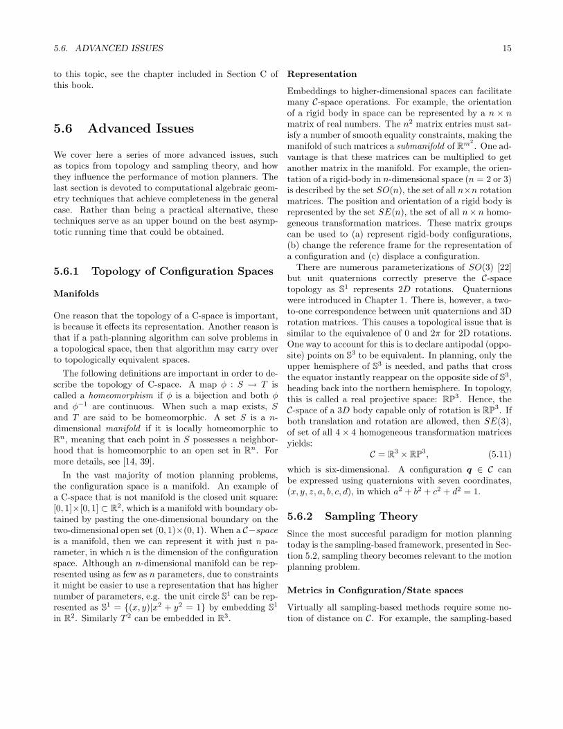
Representation

Embeddings to higher-dimensional spaces can facilitatemany C-space operations. For example, the orientationof a rigid body in space can be represented by a n × nmatrix of real numbers. The n2 matrix entries must sat-isfy a number of smooth equality constraints, making themanifold of such matrices a submanifold of R

m2

. One ad-vantage is that these matrices can be multiplied to getanother matrix in the manifold. For example, the orien-tation of a rigid-body in n-dimensional space (n = 2 or 3)is described by the set SO(n), the set of all n×n rotationmatrices. The position and orientation of a rigid body isrepresented by the set SE(n), the set of all n× n homo-geneous transformation matrices. These matrix groupscan be used to (a) represent rigid-body configurations,(b) change the reference frame for the representation ofa configuration and (c) displace a configuration.

There are numerous parameterizations of SO(3) [22]but unit quaternions correctly preserve the C-spacetopology as S

1 represents 2D rotations. Quaternionswere introduced in Chapter 1. There is, however, a two-to-one correspondence between unit quaternions and 3Drotation matrices. This causes a topological issue that issimilar to the equivalence of 0 and 2π for 2D rotations.One way to account for this is to declare antipodal (oppo-site) points on S

3 to be equivalent. In planning, only theupper hemisphere of S

3 is needed, and paths that crossthe equator instantly reappear on the opposite side of S

3,heading back into the northern hemisphere. In topology,this is called a real projective space: RP

3. Hence, theC-space of a 3D body capable only of rotation is RP

3. Ifboth translation and rotation are allowed, then SE(3),of set of all 4 × 4 homogeneous transformation matricesyields:

C = R3 × RP

3, (5.11)

which is six-dimensional. A configuration q ∈ C canbe expressed using quaternions with seven coordinates,(x, y, z, a, b, c, d), in which a2 + b2 + c2 + d2 = 1.

5.6.2 Sampling Theory

Since the most succesful paradigm for motion planningtoday is the sampling-based framework, presented in Sec-tion 5.2, sampling theory becomes relevant to the motionplanning problem.

Metrics in Configuration/State spaces

Virtually all sampling-based methods require some no-tion of distance on C. For example, the sampling-based

16 CHAPTER 5. MOTION PLANNING BY LYDIA E. KAVRAKI AND STEVEN M. LAVALLE

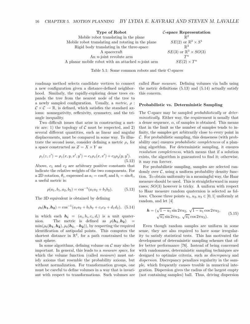
Type of Robot C-space RepresentationMobile robot translating in the plane R

2

Mobile robot translating and rotating in the plane SE(2) or R2 × S1

Rigid body translating in the three-space R3

A spacecraft SE(3) or R3 × SO(3)

An n-joint revolute arm T n

A planar mobile robot with an attached n-joint arm SE(2)× T n

Table 5.1: Some common robots and their C-spaces

roadmap method selects candidate vertices to connecta new configuration given a distance-defined neighbor-hood. Similarly, the rapidly-exploring dense trees ex-pands the tree from the nearest node of the tree toa newly sampled configuration. Usually, a metric, ρ :C × C → R, is defined, which satisfies the standard ax-ioms: nonnegativity, reflexivity, symmetry, and the tri-angle inequality.

Two difficult issues that arise in constructing a met-ric are: 1) the topology of C must be respected, and 2)several different quantities, such as linear and angulardisplacements, must be compared in some way. To illus-trate the second issue, consider defining a metric ρz fora space constructed as Z = X × Y as

ρz(z, z′) = ρz(x, y, x′, y′) = c1ρx(x, x′) + c2ρy(y, y′).(5.12)

Above, c1 and c2 are arbitrary positive constants thatindicate the relative weights of the two components. Fora 2D rotation, θi, expressed as ai = cos θi and bi = sin θi,a useful metric is:

ρ(a1, b1, a2, b2) = cos−1(a1a2 + b1b2). (5.13)

The 3D equivalent is obtained by defining

ρ0(h1, h2) = cos−1(a1a2 + b1b2 + c1c2 + d1d2), (5.14)

in which each hi = (ai, bi, ci, di) is a unit quater-nion. The metric is defined as ρ(h1, h2) =min(ρ0(h1, h2), ρ0(h1,−h2)), by respecting the requiredidentification of antipodal points. This computes theshortest distance in R

4, for a path constrained to theunit sphere.

In some algorithms, defining volume on C may also beimportant. In general, this leads to a measure space, forwhich the volume function (called measure) must sat-isfy axioms that resemble the probability axioms, butwithout normalization. For transformation groups, onemust be careful to define volumes in a way that is invari-ant with respect to transformations. Such volumes are

called Haar measure. Defining volumes via balls usingthe metric definitions (5.13) and (5.14) actually satisfythis concern.

Probabilistic vs. Deterministic Sampling

The C-space may be sampled probabilistically or deter-ministically. Either way, the requirement is usually thata dense sequence, α, of samples is obtained. This meansthat in the limit as the number of samples tends to in-finity, the samples get arbitrarily close to every point inC. For probabilistic sampling, this denseness (with prob-ability one) ensures probabilistic completeness of a plan-ning algorithm. For deterministic sampling, it ensuresresolution completeness, which means that if a solutionexists, the algorithm is guaranteed to find it; otherwise,it may run forever.

For probabilistic sampling, samples are selected ran-domly over C, using a uniform probability density func-tion. To obtain uniformity in a meaningful way, the Haarmeasure should be used. This is straightforward in manycases; SO(3) however is tricky. A uniform with respectto Haar measure random quaternion is selected as fol-lows. Choose three points u1, u2, u3 ∈ [0, 1] uniformly atrandom, and let [4]

h = (√

1− u1 sin 2πu2,√

1− u1 cos 2πu2,√u1 sin 2πu3,

√u1 cos 2πu3).

(5.15)

Even though random samples are uniform in somesense, they are also required to have some irregular-ity to satisfy statistical tests. This has motivated thedevelopment of deterministic sampling schemes that of-fer better performance [76]. Instead of being concernedwith randomness, deterministic sampling techniques aredesigned to optimize criteria, such as discrepancy anddispersion. Discrepancy penalizes regularity in the sam-ple, which frequently causes trouble in numerical inte-gration. Dispersion gives the radius of the largest empty(not containing samples) ball. Thus, driving dispersion

5.6. ADVANCED ISSUES 17

down quickly means that the whole space is exploredquickly. Deterministic samples may be irregular neigh-borhood structure (appearing much like random sam-ples), or regular neighborhood structure, which meansthat points are arranged along a grid or lattice. Formore details in the context of motion planning, see [60].

5.6.3 Computational Algebraic Geome-

try Techniques

Sampling-based algorithms which provide good practicalperformance at the expense of achieving only a weakerform of completeness. On the other hand, complete al-gorithms, which are the focus of this section, are able todeduce that there is no solution to a planning problem.

Complete algorithms are able to solve virtually anymotion planning problem as long as Cobs is representedby patches of algebraic surfaces. Formally, the modelmust be semi-algebraic, which means that it is formedfrom unions and intersections of roots of multivariatepolynomials in q, and for computability, the polynomialsmust have rational coefficients (otherwise roots may nothave finite representations). The set of all roots to poly-nomials with rational coefficients is called real algebraicnumbers and has many nice computational properties.See [9, 19, 75, 90] for more information on the exact rep-resentation and calculation with real algebraic numbers.For a gentle introduction to algebraic geometry, see [26].

To use techniques based on algebraic geometry, thefirst step is to convert the models into the required poly-nomials. Suppose the models the robot, A, and obsta-cles, O, are semi-algebraic (this includes polyhedral mod-els). For any number of attached 2D or 3D bodies, thekinematic transformations can be expressed using poly-nomials. Since polynomial transformations of polyno-mials yield polynomials, the transformed robot model ispolynomial. The algebraic surfaces that comprise Cobs

are computed by carefully considering all contact types,which characterize all ways to pair a robot feature (faces,edges, vertices) with an obstacle feature [28, 57, 60, 71].This step already produces too many model primitivesto be useful in most applications.

Once the semi-algebraic representation has been ob-tained, powerful techniques from algebraic geometry canbe exploited. One of the most widely-known algorithms,cylindrical algebraic decomposition [3, 9, 24], provides theinformation needed to solve the motion planning prob-lem. It was originally designed to determine whetherTarski sentences, which involve quantifiers and polyno-mials, are satisfiable, and to find an equivalent expres-

sion that does not involve quantifiers. The decomposi-tion produces a finite set of cells over which the signs ofthe polynomials remain fixed. This enables a systematicapproach to satisfiability and quantifier elimination. Itwas recognized by Schwartz and Sharir [90] that it alsosolves motion planning.

3

5

6

7

9

10

11

12

1 13

14

15

16

17

18

19

20

21

22

23

24

25

26

27

28

29

328

33

342

35

30

364

37

31

R

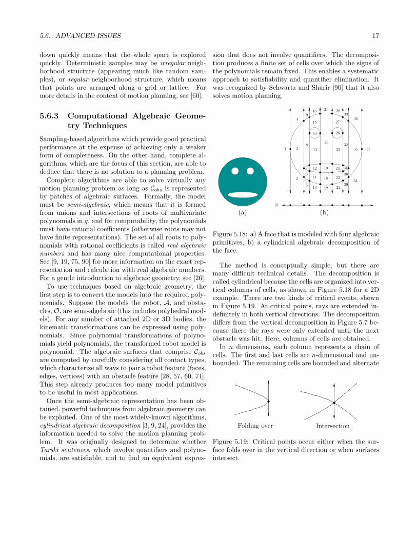
(a) (b)

Figure 5.18: a) A face that is modeled with four algebraicprimitives, b) a cylindrical algebraic decomposition ofthe face.

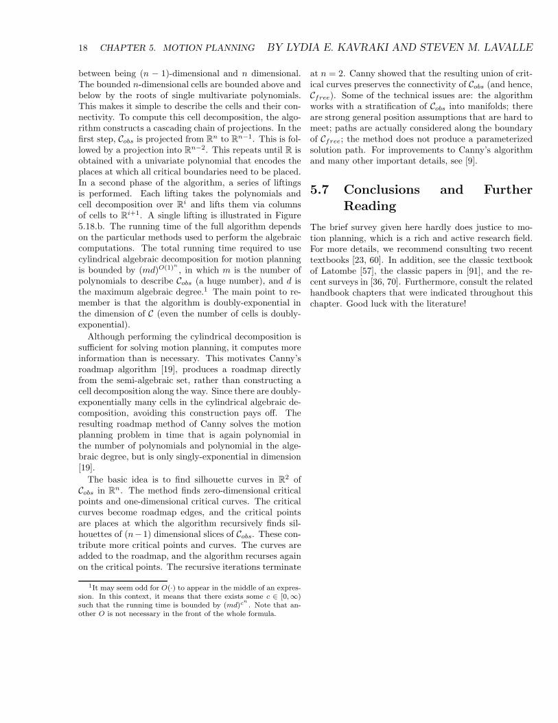
The method is conceptually simple, but there aremany difficult technical details. The decomposition iscalled cylindrical because the cells are organized into ver-tical columns of cells, as shown in Figure 5.18 for a 2Dexample. There are two kinds of critical events, shownin Figure 5.19. At critical points, rays are extended in-definitely in both vertical directions. The decompositiondiffers from the vertical decomposition in Figure 5.7 be-cause there the rays were only extended until the nextobstacle was hit. Here, columns of cells are obtained.

In n dimensions, each column represents a chain ofcells. The first and last cells are n-dimensional and un-bounded. The remaining cells are bounded and alternate

Folding over Intersection

Figure 5.19: Critical points occur either when the sur-face folds over in the vertical direction or when surfacesintersect.

18 CHAPTER 5. MOTION PLANNING BY LYDIA E. KAVRAKI AND STEVEN M. LAVALLE

between being (n − 1)-dimensional and n dimensional.The bounded n-dimensional cells are bounded above andbelow by the roots of single multivariate polynomials.This makes it simple to describe the cells and their con-nectivity. To compute this cell decomposition, the algo-rithm constructs a cascading chain of projections. In thefirst step, Cobs is projected from R

n to Rn−1. This is fol-

lowed by a projection into Rn−2. This repeats until R is

obtained with a univariate polynomial that encodes theplaces at which all critical boundaries need to be placed.In a second phase of the algorithm, a series of liftingsis performed. Each lifting takes the polynomials andcell decomposition over R

i and lifts them via columnsof cells to R

i+1. A single lifting is illustrated in Figure5.18.b. The running time of the full algorithm dependson the particular methods used to perform the algebraiccomputations. The total running time required to usecylindrical algebraic decomposition for motion planningis bounded by (md)O(1)n

, in which m is the number ofpolynomials to describe Cobs (a huge number), and d isthe maximum algebraic degree.1 The main point to re-member is that the algorithm is doubly-exponential inthe dimension of C (even the number of cells is doubly-exponential).

Although performing the cylindrical decomposition issufficient for solving motion planning, it computes moreinformation than is necessary. This motivates Canny’sroadmap algorithm [19], produces a roadmap directlyfrom the semi-algebraic set, rather than constructing acell decomposition along the way. Since there are doubly-exponentially many cells in the cylindrical algebraic de-composition, avoiding this construction pays off. Theresulting roadmap method of Canny solves the motionplanning problem in time that is again polynomial inthe number of polynomials and polynomial in the alge-braic degree, but is only singly-exponential in dimension[19].

The basic idea is to find silhouette curves in R2 of

Cobs in Rn. The method finds zero-dimensional critical

points and one-dimensional critical curves. The criticalcurves become roadmap edges, and the critical pointsare places at which the algorithm recursively finds sil-houettes of (n−1) dimensional slices of Cobs. These con-tribute more critical points and curves. The curves areadded to the roadmap, and the algorithm recurses againon the critical points. The recursive iterations terminate

1It may seem odd for O(·) to appear in the middle of an expres-sion. In this context, it means that there exists some c ∈ [0,∞)such that the running time is bounded by (md)c

n

. Note that an-other O is not necessary in the front of the whole formula.

at n = 2. Canny showed that the resulting union of crit-ical curves preserves the connectivity of Cobs (and hence,Cfree). Some of the technical issues are: the algorithmworks with a stratification of Cobs into manifolds; thereare strong general position assumptions that are hard tomeet; paths are actually considered along the boundaryof Cfree; the method does not produce a parameterizedsolution path. For improvements to Canny’s algorithmand many other important details, see [9].

5.7 Conclusions and Further

Reading

The brief survey given here hardly does justice to mo-tion planning, which is a rich and active research field.For more details, we recommend consulting two recenttextbooks [23, 60]. In addition, see the classic textbookof Latombe [57], the classic papers in [91], and the re-cent surveys in [36, 70]. Furthermore, consult the relatedhandbook chapters that were indicated throughout thischapter. Good luck with the literature!

Bibliography

[1] R. Alami, J.-P. Laumond, and T. Simeon. Two ma-nipulation planning algorithms. In J.-P. Laumondand M. Overmars, editors, Algorithms for RoboticMotion and Manipulation. A.K. Peters, Wellesley,MA, 1997.

[2] N. M. Amato, O. B. Bayazit, L. K. Dale, C. Jones,and D. Vallejo. OBPRM: An obstacle-based PRMfor 3D workspaces. In Proceedings Workshop onAlgorithmic Foundations of Robotics, pages 155–168, 1998.

[3] D. S. Arnon. Geometric reasoning with logic andalgebra. Artificial Intelligence Journal, 37(1-3):37–60, 1988.

[4] J. Arvo. Fast random rotation matrices. InD. Kirk, editor, Graphics Gems III, pages 117–120.Academic, New York, 1992.

[5] D. J. Balkcom and M. T. Mason. Time optimal tra-jectories for bounded velocity differential drive ve-hicles. International Journal of Robotics Research,21(3):199–217, 2002.

[6] J. Barraquand, L. Kavraki, J.-C. Latombe, T.-Y.Li, R. Motwani, and P. Raghavan. A random sam-pling scheme for robot path planning. In G. Gi-ralt and G. Hirzinger, editors, Proceedings Inter-national Symposium on Robotics Research, pages249–264. Springer-Verlag, New York, 1996.

[7] J. Barraquand and J.-C. Latombe. Robot mo-tion planning: A distributed representation ap-proach. International Journal of Robotics Re-search, 10(6):628–649, December 1991.

[8] J. Barraquand and J.-C. Latombe. Nonholonomicmultibody mobile robots: Controllability and mo-tion planning in the presence of obstacles. Algo-rithmica, 10:121–155, 1993.

[9] S. Basu, R. Pollack, and M.-F. Roy. Algorithms inReal Algebraic Geometry. Springer-Verlag, Berlin,2003.

[10] K. E. Bekris, B. Y. Chen, A. Ladd, E. Plaku,and L. E. Kavraki. Multiple query probabilisticroadmap planning using single query primitives. InProceedings IEEE/RSJ International Conferenceon Intelligent Robots and Systems, 2003.

[11] K. E. Bekris and L. E. Kavraki. Greedy but safereplanning under differential constraints. In ICRA,Rome, Italy, 2007.

[12] R. Bohlin and L. Kavraki. Path planning usingLazy PRM. In Proceedings IEEE InternationalConference on Robotics & Automation, 2000.

[13] V. Boor, M. H. Overmars, and A. F. van der Stap-pen. The Gaussian sampling strategy for proba-bilistic roadmap planners. In Proceedings IEEEInternational Conference on Robotics & Automa-tion, pages 1018–1023, 1999.

[14] W. M. Boothby. An Introduction to DifferentiableManifolds and Riemannian Geometry. Revised 2ndEd. Academic, New York, 2003.

[15] J. Bruce and M. Veloso. Real-time randomizedpath planning for robot navigation. In ProceedingsIEEE/RSJ International Conference on IntelligentRobots and Systems, 2002.

[16] B. Burns and O. Brock. Sampling-based motionplanning using predictive models. In ProceedingsIEEE International Conference on Robotics & Au-tomation, 2005.

[17] J. Canny, A. Rege, and J. Reif. An exact algorithmfor kinodynamic planning in the plane. Discreteand Computational Geometry, 6:461–484, 1991.

[18] J. Canny and J. Reif. New lower bound techniquesfor robot motion planning problems. In Proceed-ings IEEE Symposium on Foundations of Com-puter Science, pages 49–60, 1987.

[19] J. F. Canny. The Complexity of Robot MotionPlanning. MIT Press, Cambridge, MA, 1988.

19

20 BIBLIOGRAPHY

[20] S. Carpin and G. Pillonetto. Robot motion plan-ning using adaptive random walks. In ProceedingsIEEE International Conference on Robotics & Au-tomation, pages 3809–3814, 2003.

[21] B. Chazelle. Approximation and decompositionof shapes. In J. T. Schwartz and C. K. Yap,editors, Algorithmic and Geometric Aspects ofRobotics, pages 145–185. Lawrence Erlbaum As-sociates, Hillsdale, NJ, 1987.

[22] G. S. Chirikjian and A. B. Kyatkin. EngineeringApplications of Noncommutative Harmonic Anal-ysis. CRC Press, Boca Raton, FL, 2001.

[23] H. Choset, K. M. Lynch, S. Hutchinson, G. Kan-tor, W. Burgard, L. E. Kavraki, and S. Thrun.Principles of Robot Motion: Theory, Algorithms,and Implementations. MIT Press, Cambridge, MA,2005.

[24] G. E. Collins. Quantifier elimination by cylindricalalgebraic decomposition–twenty years of progress.In B. F. Caviness and J. R. Johnson, editors, Quan-tifier Elimination and Cylindrical Algebraic De-composition, pages 8–23. Springer-Verlag, Berlin,1998.

[25] J. Cortes. Motion Planning Algorithms for Gen-eral Closed-Chain Mechanisms. PhD thesis, Insti-tut National Polytechnique de Toulouse, Toulouse,France, 2003.

[26] D. Cox, J. Little, and D. O’Shea. Ideals, Varieties,and Algorithms. Springer-Verlag, Berlin, 1992.

[27] M. de Berg, M. van Kreveld, M. Overmars, andO. Schwarzkopf. Computational Geometry: Algo-rithms and Applications, 2nd Ed. Springer-Verlag,Berlin, 2000.

[28] B. R. Donald. A search algorithm for motion plan-ning with six degrees of freedom. Artificial Intelli-gence Journal, 31:295–353, 1987.

[29] B. R. Donald, P. G. Xavier, J. Canny, and J. Reif.Kinodynamic planning. Journal of the ACM,40:1048–66, November 1993.

[30] M. A. Erdmann and T. Lozano-Perez. On multiplemoving objects. Algorithmica, 2:477–521, 1987.

[31] P. Ferbach. A method of progressive constraintsfor nonholonomic motion planning. In Proceedings

IEEE International Conference on Robotics & Au-tomation, pages 2949–2955, 1996.

[32] E. Frazzoli, M. A. Dahleh, and E. Feron. Real-time motion planning for agile autonomous ve-hicles. AIAA Journal of Guidance and Control,25(1):116–129, 2002.

[33] R. Geraerts and M. Overmars. Sampling tech-niques for probabilistic roadmap planners. In Pro-ceedings International Conference on IntelligentAutonomous Systems, 2004.

[34] R. Ghrist, J. M. O’Kane, and S. M. LaValle. Paretooptimal coordination on roadmaps. In ProceedingsWorkshop on Algorithmic Foundations of Robotics,pages 185–200, 2004.

[35] J. Go, T. Vu, and J. J. Kuffner. Autonomousbehaviors for interactive vehicle animations. InProceedings SIGGRAPH Symposium on ComputerAnimation, 2004.

[36] H. H. Gonzalez-Banos, D. Hsu, and J. C.Latombe. Automous Mobile Robots: Sensing, Con-trol, Decision-Making and Applications, chapterMotion Planning: Recent Developments. CRCPress, 2006.

[37] D. Halperin and M. Sharir. A near-quadratic al-gorithm for planning the motion of a polygon ina polygonal environment. Discrete and Computa-tional Geometry, 16:121–134, 1996.

[38] L. Han and N. M. Amato. A kinematics-basedprobabilistic roadmap method for closed chainsystems. In B. R. Donald, K. M. Lynch, andD. Rus, editors, Algorithmic and ComputationalRobotics: New Directions, pages 233–246. A.K. Pe-ters, Wellesley, MA, 2001.

[39] A. Hatcher. Algebraic Topology. Cambridge Uni-versity Press, Cambridge, U.K., 2002.

[40] C. Holleman and L. E. Kavraki. A framework forusing the workspace medial axis in PRM planners.In Proceedings IEEE International Conference onRobotics & Automation, pages 1408–1413, 2000.

[41] J. Hollerbach. Dynamic scaling of manipulator tra-jectories. Technical report, MIT A.I. Lab Memo700, 1983.

BIBLIOGRAPHY 21

[42] J. E. Hopcroft, J. T. Schwartz, and M. Sharir.On the complexity of motion planning for multi-ple independent objects: PSPACE-hardness of the“warehouseman’s problem”. International Journalof Robotics Research, 3(4):76–88, 1984.

[43] D. Hsu, T. Jiang, J. Reif, and Z. Sun. The bridgetest for sampling narrow passages with probabilis-tic roadmap planners. In Proceedings IEEE In-ternational Conference on Robotics & Automation,2003.

[44] D. Hsu, R. Kindel, J-C. Latombe, and S. Rock.Randomized kinodynamic motion planning withmoving obstacles. In B. R. Donald, K. M. Lynch,and D. Rus, editors, Algorithmic and Compu-tational Robotics: New Directions. A.K. Peters,Wellesley, MA, 2001.

[45] D. Hsu, J.-C. Latombe, and R. Motwani. Pathplanning in expansive configuration spaces. Inter-national Journal Computational Geometry & Ap-plications, 4:495–512, 1999.

[46] P. Isto. Constructing probabilistic roadmaps withpowerful local planning and path optimization. InProceedings IEEE/RSJ International Conferenceon Intelligent Robots and Systems, pages 2323–2328, 2002.

[47] P. Jimenez, F. Thomas, and C. Torras. Collisiondetection algorithms for motion planning. In J.-P. Laumond, editor, Robot Motion Planning andControl, pages 1–53. Springer-Verlag, Berlin, 1998.

[48] M. Kallmann and M. Mataric. Motion planningusing dynamic roadmaps. In Proceedings IEEE In-ternational Conference on Robotics & Automation,2004.

[49] L. E. Kavraki and M. Kolountzakis. Partition-ing a planar assembly into two connected partsis NP-complete. Information Processing Letters,55(3):159–165, 1995.

[50] L. E. Kavraki, P. Svestka, J.-C. Latombe, andM. H. Overmars. Probabilistic roadmaps for pathplanning in high-dimensional configuration spaces.IEEE Transactions on Robotics & Automation,12(4):566–580, June 1996.

[51] J. M. Keil. Polygon decomposition. In J. R. Sackand J. Urrutia, editors, Handbook on Computa-tional Geometry. Elsevier, New York, 2000.

[52] O. Khatib. Real-time obstacle avoidance for ma-nipulators and mobile robots. International Jour-nal of Robotics Research, 5(1):90–98, 1986.

[53] J. J. Kuffner and S. M. LaValle. An efficient ap-proach to path planning using balanced bidirec-tional RRT search. Technical Report CMU-RI-TR-05-34, Robotics Institute, Carnegie Mellon Univer-sity, Pittsburgh, PA, August 2005.

[54] A. Ladd and L. E. Kavraki. Fast exploration forrobots with dynamics. In Proceedings Workshopon Algorithmic Foundations of Robotics, Zeist, TheNetherlands, July 2004.

[55] A. Ladd and L. E. Kavraki. Measure the-oretic analysis of probabilistic path planning.IEEE Transactions on Robotics & Automation,20(2):229–242, 2004.

[56] A. M. Ladd and L. E. Kavraki. Motion planning inthe presence of drift, underactuation and discretesystem changes. In Robotics: Science and SystemsI, pages 233–241, Boston, MA, June 2005. MITPress.

[57] J.-C. Latombe. Robot Motion Planning. Kluwer,Boston, MA, 1991.

[58] J.-P. Laumond. Trajectories for mobile robots withkinematic and environment constraints. In Pro-ceedings International Conference on IntelligentAutonomous Systems, pages 346–354, 1986.

[59] J.-P. Laumond, S. Sekhavat, and F. Lami-raux. Guidelines in nonholonomic motion plan-ning for mobile robots. In J.-P. Laumond, editor,Robot Motion Planning and Control, pages 1–53.Springer-Verlag, Berlin, 1998.

[60] S. M. LaValle. Planning Algorithms. CambridgeUniversity Press, Cambridge, U.K., 2006. Alsoavailable at http://planning.cs.uiuc.edu/.

[61] S. M. LaValle, M. S. Branicky, and S. R. Lin-demann. On the relationship between classicalgrid search and probabilistic roadmaps. Interna-tional Journal of Robotics Research, 23(7/8):673–692, July/August 2004.

[62] S. M. LaValle and S. A. Hutchinson. Optimal mo-tion planning for multiple robots having indepen-dent goals. IEEE Trans. on Robotics and Automa-tion, 14(6):912–925, December 1998.

22 BIBLIOGRAPHY

[63] S. M. LaValle and J. J. Kuffner. Randomized kin-odynamic planning. In Proceedings IEEE Inter-national Conference on Robotics and Automation,pages 473–479, 1999.

[64] S. M. LaValle and J. J. Kuffner. Rapidly-exploringrandom trees: Progress and prospects. In B. R.Donald, K. M. Lynch, and D. Rus, editors, Algo-rithmic and Computational Robotics: New Direc-tions, pages 293–308. A K Peters, Wellesley, MA,2001.

[65] D. Leven and M. Sharir. Planning a purelytranslational motion for a convex object in two-dimensional space using generalized Voronoi di-agrams. Discrete and Computational Geometry,2:9–31, 1987.

[66] P. Leven and S. A. Hutchinson. Using manipu-lability to bias sampling during the constructionof probabilistic roadmaps. IEEE Transactions onRobotics & Automation, 19(6):1020–1026, Decem-ber 2003.

[67] J.-M. Lien, S. L. Thomas, and N. M. Amato.A general framework for sampling on the medialaxis of the free space. In Proceedings IEEE In-ternational Conference on Robotics & Automation,2003.

[68] M. C. Lin and J. F. Canny. Efficient algorithmsfor incremental distance computation. In Proceed-ings IEEE International Conference on Robotics &Automation, 1991.

[69] M. C. Lin and D. Manocha. Collision and proxim-ity queries. In J. E. Goodman and J. O’Rourke,editors, Handbook of Discrete and ComputationalGeometry, 2nd Ed., pages 787–807. Chapman andHall/CRC Press, New York, 2004.

[70] S. R. Lindemann and S. M. LaValle. Current issuesin sampling-based motion planning. In P. Darioand R. Chatila, editors, Robotics Research: TheEleventh International Symposium, pages 36–54.Springer-Verlag, Berlin, 2005.

[71] T. Lozano-Perez. Spatial planning: A configura-tion space approach. IEEE Transactions on Com-puting, C-32(2):108–120, 1983.

[72] M. T. Mason. Mechanics of Robotic Manipulation.MIT Press, Cambridge, MA, 2001.

[73] J.-P. Merlet. Parallel Robots. Kluwer, Boston, MA,2000.

[74] R. J. Milgram and J. C. Trinkle. The geometry ofconfiguration spaces for closed chains in two andthree dimensions. Homology, Homotopy, and Ap-plications, 6(1):237–267, 2004.

[75] B. Mishra. Computational real algebraic geome-try. In J. E. Goodman and J. O’Rourke, editors,Handbook of Discrete and Computational Geome-try, pages 537–556. CRC Press, New York, 1997.

[76] H. Niederreiter. Random Number Generation andQuasi-Monte-Carlo Methods. Society for Industrialand Applied Mathematics, Philadelphia, 1992.

[77] D. Nieuwenhuisen and M. H. Overmars. Useful cy-cles in probabilistic roadmap graphs. In Proceed-ings IEEE International Conference on Robotics &Automation, pages 446–452, 2004.

[78] N. J. Nilsson. A mobile automaton: An applicationof artificial intelligence techniques. In 1st Interna-tional Conference on Artificial Intelligence, pages509–520, 1969.

[79] C. O’Dunlaing. Motion planning with inertial con-straints. Algorithmica, 2(4):431–475, 1987.

[80] C. O’Dunlaing and C. K. Yap. A retraction methodfor planning the motion of a disc. Journal of Algo-rithms, 6:104–111, 1982.

[81] J. O’Rourke. Visibility. In J. E. Goodman andJ. O’Rourke, editors, Handbook of Discrete andComputational Geometry, 2nd Ed., pages 643–663.Chapman and Hall/CRC Press, New York, 2004.

[82] S. Pancanti, L. Pallottino, D. Salvadorini, andA. Bicchi. Motion planning through symbols andlattices. In Proceedings IEEE International Con-ference on Robotics & Automation, pages 3914–3919, 2004.

[83] M. Pivtoraiko and A. Kelly. Generating near min-imal spanning control sets for constrained motionplanning in discrete state spaces. In ProceedingsIEEE/RSJ International Conference on IntelligentRobots and Systems, 2005.

[84] J. H. Reif. Complexity of the mover’s problem andgeneralizations. In Proceedings IEEE Symposiumon Foundations of Computer Science, pages 421–427, 1979.

BIBLIOGRAPHY 23

[85] J. H. Reif and M. Sharir. Motion planning in thepresence of moving obstacles. Journal of the ACM,41:764–790, 1994.

[86] E. Rimon and D. E. Koditschek. Exact robot navi-gation using artificial potential fields. IEEE Trans-actions on Robotics & Automation, 8(5):501–518,October 1992.

[87] G. Sanchez and J.-C. Latombe. A single-querybi-directional probabilistic roadmap planner withlazy collision checking. In Proceedings Interna-tional Symposium on Robotics Research, 2001.

[88] S. Sastry. Nonlinear Systems: Analysis, Stability,and Control. Springer-Verlag, Berlin, 1999.

[89] J. T. Schwartz and M. Sharir. On the PianoMovers’ Problem: I. The case of a two-dimensionalrigid polygonal body moving amidst polygonal bar-riers. Communications on Pure and Applied Math-ematics, 36:345–398, 1983.

[90] J. T. Schwartz and M. Sharir. On the PianoMovers’ Problem: II. General techniques for com-puting topological properties of algebraic mani-folds. Communications on Pure and Applied Math-ematics, 36:345–398, 1983.

[91] J. T. Schwartz and M. Sharir. A survey of motionplanning and related geometric algorithms. Artifi-cial Intelligence Journal, 37:157 – 169, 1988.

[92] Jacob T. Schwartz and Micha Sharir. On the pianomovers’ problem: I. the case of a two-dimensionalrigid polygonal body moving admidst polygonalbarriers. 36:345–398, 1983.

[93] Jacob T. Schwartz and Micha Sharir. On the pianomovers’ problem: V. the case of a rod moving inthree-dimensional space amidst polyhedral obsta-cles. 37:815–848, 1984.

[94] S. Sekhavat, P. Svestka, J.-P. Laumond, and M. H.Overmars. Multilevel path planning for nonholo-nomic robots using semiholonomic subsystems. In-ternational Journal of Robotics Research, 17:840–857, 1998.

[95] M. Sharir. Algorithmic motion planning. In J. E.Goodman and J. O’Rourke, editors, Handbook ofDiscrete and Computational Geometry, 2nd Ed.,pages 1037–1064. Chapman and Hall/CRC Press,New York, 2004.

[96] K. G. Shin and N. D. McKay. Minimum-time con-trol of robot manipulators with geometric pathconstraints. IEEE Transactions on AutomaticControl, 30(6):531–541, 1985.

[97] K. G. Shin and N. D. McKay. A dynamic program-ming approach to trajectory planning of roboticmanipulators. IEEE Transactions on AutomaticControl, 31(6):491–500, 1986.

[98] T. Simeon, J.-P. Laumond, and C. Nissoux. Vis-ibility based probabilistic roadmaps for motionplanning. Advanced Robotics, 14(6), 2000.

[99] T. Simeon, S. Leroy, and J.-P. Laumond. Pathcoordination for multiple mobile robots: A reso-lution complete algorithm. IEEE Transactions onRobotics & Automation, 18(1), February 2002.

[100] P. Soueres and J.-D. Boissonnat. Optimal trajecto-ries for nonholonomic mobile robots. In J.-P. Lau-mond, editor, Robot Motion Planning and Control,pages 93–169. Springer-Verlag, Berlin, 1998.

[101] M. Strandberg. Augmenting RRT-planners withlocal trees. In Proceedings IEEE InternationalConference on Robotics & Automation, pages3258–3262, 2004.

[102] K. Sutner and W. Maass. Motion planningamong time dependent obstacles. Acta Informat-ica, 26:93–122, 1988.

[103] P. Svestka and M. H. Overmars. Coordinated mo-tion planning for multiple car-like robots usingprobabilistic roadmaps. In Proceedings IEEE In-ternational Conference on Robotics & Automation,pages 1631–1636, 1995.

[104] S. Udupa. Collision Detection and Avoidance inComputer Controlled Manipulators. PhD thesis,Dept. of Electrical Engineering, California Insti-tute of Technology, 1977.

[105] J. van den Berg and M. Overmars. Prioritized mo-tion planning for multiple robots. In ProceedingsIEEE/RSJ International Conference on IntelligentRobots and Systems, pages 2217–2222, 2005.

[106] J. Yakey, S. M. LaValle, and L. E. Kavraki. Ran-domized path planning for linkages with closedkinematic chains. IEEE Transactions on Roboticsand Automation, 17(6):951–958, December 2001.

24 BIBLIOGRAPHY

[107] A. Yershova, L. Jaillet, T. Simeon, and S. M.LaValle. Dynamic-domain RRTs: Efficient ex-ploration by controlling the sampling domain.In Proceedings IEEE International Conference onRobotics and Automation, 2005.