Embed Size (px)
DESCRIPTION
p
Citation preview
i ii
PLANNING ALGORITHMS
Steven M. LaValle
University of Illinois
Copyright 1999-2003
Contents
Preface ix
0.1 What is meant by “Planning Algorithms”? . . . . . . . . . . . . . ix
0.2 Who is the Intended Audience? . . . . . . . . . . . . . . . . . . . x
0.3 Suggested Use . . . . . . . . . . . . . . . . . . . . . . . . . . . . . x
0.4 Acknowledgments . . . . . . . . . . . . . . . . . . . . . . . . . . . x
0.5 Help! . . . . . . . . . . . . . . . . . . . . . . . . . . . . . . . . . . xi
I Introductory Material 1
1 Introduction 3
1.1 Planning to Plan . . . . . . . . . . . . . . . . . . . . . . . . . . . 3
1.2 Illustrative Problems . . . . . . . . . . . . . . . . . . . . . . . . . 5
1.3 Perspective . . . . . . . . . . . . . . . . . . . . . . . . . . . . . . 5
1.4 Mathematical and Algorithmic Preliminaries . . . . . . . . . . . . 8
2 Discrete Planning 9
2.1 Introduction . . . . . . . . . . . . . . . . . . . . . . . . . . . . . . 9
2.2 Three Representations of Discrete Planning . . . . . . . . . . . . 10
2.2.1 STRIPS-Like Representation . . . . . . . . . . . . . . . . . 10
2.2.2 State Space Representation . . . . . . . . . . . . . . . . . 12
2.2.3 Graph Representation . . . . . . . . . . . . . . . . . . . . 14
2.3 Search Algorithms . . . . . . . . . . . . . . . . . . . . . . . . . . 14
2.3.1 General Forward Search . . . . . . . . . . . . . . . . . . . 15
2.3.2 Particular Forward Search Methods . . . . . . . . . . . . . 17
2.3.3 Other General Search Schemes . . . . . . . . . . . . . . . . 20
2.4 Optimal Planning . . . . . . . . . . . . . . . . . . . . . . . . . . . 21
2.4.1 State space formulation . . . . . . . . . . . . . . . . . . . . 22
2.4.2 Backwards dynamic programming . . . . . . . . . . . . . . 23
2.4.3 Forward dynamic programming . . . . . . . . . . . . . . . 24
2.4.4 A simple example . . . . . . . . . . . . . . . . . . . . . . . 25
2.5 Other Approaches . . . . . . . . . . . . . . . . . . . . . . . . . . . 27
iii
iv CONTENTS
II Motion Planning 29
3 Geometric Representations and Transformations 333.1 Geometric Modeling . . . . . . . . . . . . . . . . . . . . . . . . . 33
3.1.1 Polygonal and Polyhedral Models . . . . . . . . . . . . . . 343.1.2 Semi-Algebraic Models . . . . . . . . . . . . . . . . . . . . 383.1.3 Other Models . . . . . . . . . . . . . . . . . . . . . . . . . 40
3.2 Rigid Body Transformations . . . . . . . . . . . . . . . . . . . . . 423.2.1 2D Transformations . . . . . . . . . . . . . . . . . . . . . . 423.2.2 3D Transformations . . . . . . . . . . . . . . . . . . . . . . 45
3.3 Transformations of Kinematic Chains of Bodies . . . . . . . . . . 473.3.1 A Kinematic Chain in R2 . . . . . . . . . . . . . . . . . . 473.3.2 A Kinematic Chain in R3 . . . . . . . . . . . . . . . . . . 50
3.4 Transforming Other Models . . . . . . . . . . . . . . . . . . . . . 55
4 The Configuration Space 594.1 Basic Topological Concepts . . . . . . . . . . . . . . . . . . . . . 59
4.1.1 Topological Spaces . . . . . . . . . . . . . . . . . . . . . . 594.1.2 Constructing Manifolds . . . . . . . . . . . . . . . . . . . . 614.1.3 Paths in Topological Spaces . . . . . . . . . . . . . . . . . 64
4.2 Defining the Configuration Space . . . . . . . . . . . . . . . . . . 654.3 Configuration Space Obstacles . . . . . . . . . . . . . . . . . . . . 704.4 Kinematic Closure and Varieties . . . . . . . . . . . . . . . . . . . 794.5 More Topological Concepts . . . . . . . . . . . . . . . . . . . . . . 80
5 Combinatorial Motion Planning 835.1 Introduction . . . . . . . . . . . . . . . . . . . . . . . . . . . . . . 835.2 Algorithms for a Point Robot . . . . . . . . . . . . . . . . . . . . 84
5.2.1 Vertical Cell Decomposition . . . . . . . . . . . . . . . . . 845.2.2 Retraction: Maximal Clearance Paths . . . . . . . . . . . . 885.2.3 Bitangent Graph: Shortest Paths . . . . . . . . . . . . . . 89
5.3 Moving a Ladder . . . . . . . . . . . . . . . . . . . . . . . . . . . 905.4 Theory of Semi-Algebraic Sets . . . . . . . . . . . . . . . . . . . . 905.5 Cylindrical Algebraic Decomposition . . . . . . . . . . . . . . . . 905.6 Complexity of Motion Planning . . . . . . . . . . . . . . . . . . . 905.7 Other Combinatorial Methods . . . . . . . . . . . . . . . . . . . . 92
6 Sampling-Based Motion Planning 936.1 Collision Detection . . . . . . . . . . . . . . . . . . . . . . . . . . 94
6.1.1 Basic Concepts . . . . . . . . . . . . . . . . . . . . . . . . 946.1.2 Hierarchical Methods . . . . . . . . . . . . . . . . . . . . . 956.1.3 Incremental Methods . . . . . . . . . . . . . . . . . . . . . 97
6.2 Metric Spaces . . . . . . . . . . . . . . . . . . . . . . . . . . . . . 996.3 An Incremental Search Framework . . . . . . . . . . . . . . . . . 101
CONTENTS v
6.4 Classical Grid-Based Search . . . . . . . . . . . . . . . . . . . . . 1056.4.1 Dynamic programming . . . . . . . . . . . . . . . . . . . . 1066.4.2 Other grid-based search algorithms . . . . . . . . . . . . . 107
6.5 Randomized Potential Field . . . . . . . . . . . . . . . . . . . . . 1086.6 Rapidly-Exploring Random Trees . . . . . . . . . . . . . . . . . . 108
6.6.1 Designing Path Planners . . . . . . . . . . . . . . . . . . . 1106.7 Sampling-Based Roadmaps for Multiple Queries . . . . . . . . . . 1146.8 Sampling-Based Roadmap Variants . . . . . . . . . . . . . . . . . 1176.9 Deterministic Sampling Theory . . . . . . . . . . . . . . . . . . . 118
6.9.1 Sampling Criteria . . . . . . . . . . . . . . . . . . . . . . . 1186.9.2 Finite Point Sets and Infinite Sequences . . . . . . . . . . 1196.9.3 Low-Discrepancy Sampling . . . . . . . . . . . . . . . . . . 1206.9.4 Low-Dispersion Sampling . . . . . . . . . . . . . . . . . . . 122
7 Extensions of Basic Motion Planning 1257.1 Time-Varying Problems . . . . . . . . . . . . . . . . . . . . . . . 1257.2 Multiple-Robot Coordination . . . . . . . . . . . . . . . . . . . . 1277.3 Manipulation Planning . . . . . . . . . . . . . . . . . . . . . . . . 1287.4 Assembly Planning . . . . . . . . . . . . . . . . . . . . . . . . . . 129
8 Feedback Motion Strategies 1318.1 Basic Concepts . . . . . . . . . . . . . . . . . . . . . . . . . . . . 1318.2 Potential Functions and Navigation Functions . . . . . . . . . . . 1318.3 Dynamic Programming . . . . . . . . . . . . . . . . . . . . . . . . 1328.4 Harmonic Functions . . . . . . . . . . . . . . . . . . . . . . . . . 1328.5 Sampling-Based Neighborhood Graph . . . . . . . . . . . . . . . . 132
8.5.1 Problem Formulation . . . . . . . . . . . . . . . . . . . . . 1328.5.2 Sampling-Based Neighborhood Graph . . . . . . . . . . . . 1338.5.3 SNG Construction Algorithm . . . . . . . . . . . . . . . . 1358.5.4 Radius selection . . . . . . . . . . . . . . . . . . . . . . . . 1368.5.5 A Bayesian termination condition . . . . . . . . . . . . . . 1378.5.6 Some Computed Examples . . . . . . . . . . . . . . . . . . 137
III Decision-Theoretic Planning 139
9 Basic Decision Theory 1419.1 Basic Definitions . . . . . . . . . . . . . . . . . . . . . . . . . . . 1419.2 A Game Against Nature . . . . . . . . . . . . . . . . . . . . . . . 143
9.2.1 Having a single observation . . . . . . . . . . . . . . . . . 1459.3 Applications of Optimal Decision Making . . . . . . . . . . . . . . 146
9.3.1 Classification . . . . . . . . . . . . . . . . . . . . . . . . . 1469.3.2 Parameter Estimation . . . . . . . . . . . . . . . . . . . . 147
9.4 Utility Theory . . . . . . . . . . . . . . . . . . . . . . . . . . . . . 148
vi CONTENTS
9.4.1 Choosing a Good Reward . . . . . . . . . . . . . . . . . . 1489.4.2 Axioms of Rationality . . . . . . . . . . . . . . . . . . . . 149
9.5 Criticisms of Decision Theory . . . . . . . . . . . . . . . . . . . . 1509.5.1 Nondeterministic decision making . . . . . . . . . . . . . . 1509.5.2 Bayesian decision making . . . . . . . . . . . . . . . . . . 151
9.6 Multiobjective Optimality . . . . . . . . . . . . . . . . . . . . . . 1529.6.1 Scalarizing L . . . . . . . . . . . . . . . . . . . . . . . . . 153
10 Sequential Decision Theory: Perfect State Information 15510.1 Basic Definitions . . . . . . . . . . . . . . . . . . . . . . . . . . . 155
10.1.1 Non-Deterministic Forward Projection . . . . . . . . . . . 15510.1.2 Probabilistic Forward Projection . . . . . . . . . . . . . . 15610.1.3 Strategies . . . . . . . . . . . . . . . . . . . . . . . . . . . 156
10.2 Dynamic Programming over Discrete Spaces . . . . . . . . . . . . 15710.3 Infinite Horizon Problems . . . . . . . . . . . . . . . . . . . . . . 159
10.3.1 Average Loss-Per-Stage . . . . . . . . . . . . . . . . . . . . 16010.3.2 Discounted Loss . . . . . . . . . . . . . . . . . . . . . . . . 16010.3.3 Optimization in the Discounted Loss Model . . . . . . . . 16010.3.4 Forward Dynamic Programming . . . . . . . . . . . . . . . 16110.3.5 Backwards Dynamic Programming . . . . . . . . . . . . . 16110.3.6 Policy Iteration . . . . . . . . . . . . . . . . . . . . . . . . 163
10.4 Dynamic Programming over Continuous Spaces . . . . . . . . . . 16410.4.1 Reformulating Motion Planning . . . . . . . . . . . . . . . 16410.4.2 The Algorithm . . . . . . . . . . . . . . . . . . . . . . . . 167
10.5 Reinforcement Learning . . . . . . . . . . . . . . . . . . . . . . . 17210.5.1 Stochastic Iterative Algorithms . . . . . . . . . . . . . . . 17310.5.2 Finding an Optimal Strategy: Q-learning . . . . . . . . . . 173
11 Sequential Decision Theory: Imperfect State Information 17511.1 Information Spaces . . . . . . . . . . . . . . . . . . . . . . . . . . 175
11.1.1 Manipulating the Information Space . . . . . . . . . . . . 17611.2 Preimages and Forward Projections . . . . . . . . . . . . . . . . . 17911.3 Dynamic Programming on Information Spaces . . . . . . . . . . . 17911.4 Kalman Filtering . . . . . . . . . . . . . . . . . . . . . . . . . . . 17911.5 Localization . . . . . . . . . . . . . . . . . . . . . . . . . . . . . . 17911.6 Sensorless Manipulation . . . . . . . . . . . . . . . . . . . . . . . 17911.7 Other Searches on Information Spaces . . . . . . . . . . . . . . . 179
12 Sensor-Based Planning 18112.1 Bug Algorithms . . . . . . . . . . . . . . . . . . . . . . . . . . . . 18112.2 Map Building . . . . . . . . . . . . . . . . . . . . . . . . . . . . . 18312.3 Coverage Planning . . . . . . . . . . . . . . . . . . . . . . . . . . 18312.4 Maintaining Visibility . . . . . . . . . . . . . . . . . . . . . . . . . 18312.5 Visibility-Based Pursuit-Evasion . . . . . . . . . . . . . . . . . . . 183
CONTENTS vii
13 Game Theory 18713.1 Overview . . . . . . . . . . . . . . . . . . . . . . . . . . . . . . . . 18713.2 Single-Stage Two-Player Zero Sum Games . . . . . . . . . . . . . 188
13.2.1 Regret . . . . . . . . . . . . . . . . . . . . . . . . . . . . . 19013.2.2 Saddle Points . . . . . . . . . . . . . . . . . . . . . . . . . 19113.2.3 Mixed Strategies . . . . . . . . . . . . . . . . . . . . . . . 19213.2.4 Computation of Equilibria . . . . . . . . . . . . . . . . . . 193
13.3 Nonzero Sum Games . . . . . . . . . . . . . . . . . . . . . . . . . 19513.3.1 Nash Equilibria . . . . . . . . . . . . . . . . . . . . . . . . 19613.3.2 Admissibility . . . . . . . . . . . . . . . . . . . . . . . . . 19713.3.3 The Prisoner’s Dilemma . . . . . . . . . . . . . . . . . . . 19813.3.4 Nash Equilibrium for mixed strategies . . . . . . . . . . . 198
13.4 Sequential Games . . . . . . . . . . . . . . . . . . . . . . . . . . . 19913.5 Dynamic Programming over Sequential Games . . . . . . . . . . . 20013.6 Algorithms for Special Games . . . . . . . . . . . . . . . . . . . . 200
IV Continuous-Time Planning 201
14 Differential Models 20314.1 Motivation . . . . . . . . . . . . . . . . . . . . . . . . . . . . . . . 20314.2 Representing Differential Constraints . . . . . . . . . . . . . . . . 20314.3 Kinematics for Wheeled Systems . . . . . . . . . . . . . . . . . . 206
14.3.1 A Simple Car . . . . . . . . . . . . . . . . . . . . . . . . . 20714.3.2 A Continuous-Steering Car . . . . . . . . . . . . . . . . . . 20814.3.3 A Car Pulling Trailers . . . . . . . . . . . . . . . . . . . . 20914.3.4 A Differential Drive . . . . . . . . . . . . . . . . . . . . . . 209
14.4 Rigid-Body Dynamics . . . . . . . . . . . . . . . . . . . . . . . . 21014.5 Multiple-Body Dynamics . . . . . . . . . . . . . . . . . . . . . . . 21214.6 More Examples . . . . . . . . . . . . . . . . . . . . . . . . . . . . 212
15 Nonholonomic System Theory 21315.1 Vector Fields and Distributions . . . . . . . . . . . . . . . . . . . 21315.2 The Lie Bracket . . . . . . . . . . . . . . . . . . . . . . . . . . . . 21515.3 Integrability and Controllability . . . . . . . . . . . . . . . . . . . 21615.4 More Differential Geometry . . . . . . . . . . . . . . . . . . . . . 220
16 Planning Under Differential Constraints 22116.1 Functional-Based Dynamic Programming . . . . . . . . . . . . . . 22116.2 Tree-Based Dynamic Programming . . . . . . . . . . . . . . . . . 22116.3 Geodesic Curve Families . . . . . . . . . . . . . . . . . . . . . . . 22216.4 Steering Methods . . . . . . . . . . . . . . . . . . . . . . . . . . . 22316.5 RRT-Based Methods . . . . . . . . . . . . . . . . . . . . . . . . . 22316.6 Other Methods . . . . . . . . . . . . . . . . . . . . . . . . . . . . 224
viii CONTENTS
Preface
0.1 What is meant by “Planning Algorithms”?
Due to many exciting developments in the fields of robotics, artificial intelligence,and control theory, three topics that were once quite distinct are presently on acollision course. In robotics, motion planning was originally concerned with prob-lems such as how to move a piano from one room to another in a house withouthitting anything. The field has grown, however, to include complications such asuncertainties, multiple bodies, and dynamics. In artificial intelligence, planningoriginally meant a search for a sequence of logical operators or actions that trans-form an initial world state into a desired goal state. Presently, planning extendsbeyond this to include many decision-theoretic ideas such as Markov decisionprocesses, imperfect state information, and game-theoretic equilibria. Althoughcontrol theory has traditionally been concerned with issues such as stability, feed-back, and optimality, there has been a growing interest in designing algorithmsthat find feasible open-loop trajectories for nonlinear systems. In some of thiswork, the term motion planning has been applied, with a different interpretationof its use in robotics. Thus, even though each originally considered different prob-lems, the fields of robotics, artificial intelligence, and control theory have expandedtheir scope to share an interesting common ground.
In this text, I use the term planning in a broad sense that encompasses thiscommon ground. This does not, however, imply that the term is meant covereverything important in the fields of robotics, artificial intelligence, and controltheory. The presentation is focused primarily on algorithm issues relating to plan-ning. Within robotics, the focus is on designing algorithms that generate usefulmotions by processing complicated geometric models. Within artificial intelli-gence, the focus is on designing systems that use decision-theoretic models com-pute appropriate actions. Within control theory, the focus of the presentationis on algorithms that numerically compute feasible trajectories or even optimalfeedback control laws. This means that analytical techniques, which account forthe majority of control theory literature, are not addressed here.
The phrase “planning and control” is often used to identify complementary is-sues in developing a system. Planning is often considered as a higher-level processthan control. In this text, we make no such distinctions. Ignoring old connotationsthat come with the terms, “planning” or “control” could be used interchangeably.
ix
x PREFACE
Both can refer to some kind of decision making in this text, with no associatednotion of “high” or “low” level. A hierarchical planning (or control!) strategycould be developed in any case.
0.2 Who is the Intended Audience?
The text is written primarily for computer science and engineering students atthe advanced undergraduate or beginning graduate level. It is also intended asan introduction to recent techniques for researchers and developers in roboticsand artificial intelligence. It is expected that the presentation here would beof interest to those working in other areas such as computational biology (drugdesign, protein folding), virtual prototyping, and computer graphics.
I have attempted to make the book as self-contained and readable as possible.Advanced mathematical concepts (beyond concepts typically learned by under-graduates in computer science and engineering) are introduced and explained.For readers with deeper mathematical interests, directions for further study aregiven at the end of some chapters.
0.3 Suggested Use
The ideas should flow naturally from chapter to chapter, but at the same time,the text has been designed to make it easy to skip chapters.
If you are only interested in robot motion planning, it is only necessary toread Chapters 3-8, possibly with the inclusion of search algorithm material fromChapter 2. Chapters 3 and 4 provide the foundations needed to understand basicrobot motion planning. Chapters 5 and 6 present algorithmic techniques to solvethis problem. Chapters 7 and 8 consider extensions of the basic problem. Chapter12 is covers sensor-based extension of motion planning, for those interested.
If you are additionally interested in nonholonomic planning and other problemsthat involve differential constraints, then it is safe to jump ahead to Chapters 14-16, after completing Chapters 3-6.
If you are mainly interested in decision-theoretic planning, then you can readChapter 2, and jump straight to Chapters 9-11. The extension to multiple decisionmakers is covered in Chapter 13. The material in these later chapters does notdepend much on Chapters 3 and 4, which lay the foundations of robot motionplanning. Thus, if you are not interested in this case, it may be easily skipped.
0.4 Acknowledgments
I am very grateful to many students and colleagues who have given me extensivefeedback and advice in developing this text. I am also thankful for the support-ive environments provided both by Iowa State University and the University of
0.5. HELP! xi
Illinois. In both universities, I have been able to develop courses for which thematerial presented here has been developed and refined.
0.5 Help!
Since the text appears on the web, it is easy for me to incoprorate feedbackfrom readers. This will be very helpful as I complete this project. If you findmistakes, have requests for coverage of topics, find some explanations difficultto follow, have suggested exercises, etc., please let me know by sending mail [email protected]. Note that this book is current a work in progress. Please bepatient as I update parts over the coming year or two.
xii PREFACE

Part I
Introductory Material
1
Chapter 1
Introduction
1.1 Planning to Plan
Planning is a term that means different things to different groups of people. Afundamental need in robotics is to have algorithms that can automatically tellrobots how to move when they are given high-level commands. The terms motionplanning and trajectory planning are often used for these kinds of problems. Aclassical version of motion planning is sometimes referred to as the Piano Mover’sProblem. Imagine giving a precise 3D CAD model of a house and a piano as inputto an algorithm. The algorithm must determine how to move the piano from oneroom to another in the house without hitting anything. Most of us have encoun-tered similar problems when moving a sofa or mattress up a set of stairs. Robotmotion planning usually ignores dynamics and other differential constraints, andfocuses primarily on the translations and rotations required to move the piano.Recent work, however, does consider other aspects, such as uncertainties, differ-ential constraints, modeling uncertainties, and optimality. Trajectory planningusually refers to the problem of taking the solution from a robot motion planningalgorithm and determining how to move along the solution in a way that respectsthe mechanical limitations of the robot.
Control theory has historically been concerned with designing inputs to sys-tems described by differential equations. These could include mechanical systemssuch as cars or aircraft, electrical systems such as noise filters, or even systemsarising in areas as diverse as chemistry, economics, and sociology. Classically,control theory has developed feedback policies, which enable an adaptive responseduring execution, and has focused on stability, which ensures that the dynamicsdo not cause the system to become wildly out of control. A large emphasis is alsoplaced on optimizing criteria to minimize resource consumption, such as energyor time. In recent control theory literature, motion planning sometimes refers tothe construction of inputs to a nonlinear dynamical system that drives it from aninitial state to a specified goal state. For example, imagine trying to operate aremote-controlled hovercraft that glides over the surface of a frozen pond. Sup-
3
4 S. M. LaValle: Planning Algorithms
pose we would like the hovercraft to leave its current resting location and come torest at another specified location. Can an algorithm be designed that computesthe desired inputs, even in an ideal simulator that neglects uncertainties that arisefrom model inaccuracies? It is possible to add other considerations, such as uncer-tainties, feedback, and optimality, but the problem is already challenging enoughwithout these.
In artificial intelligence, the term AI planning takes on a more discrete flavor.Instead of moving a piano through a continuous space, as in the robot motionplanning problem, the task might be to solve a puzzle, such as the Rubik’s cube ora sliding tile puzzle. Although such problems could be modeled with continuousspaces, it seems natural to define a finite set of actions that can be applied toa discrete set of states, and to construct a solution by giving the appropriatesequence of actions. Historically, planning has been considered different fromproblem solving; however, the distinction seems to have faded away in recentyears. In this book, we do not attempt to make a distinction between the two.Also, substantial effort has been devoted to representation language issues inplanning. Although some of this will be covered, it is mainly outside of ourfocus. Many decision-theoretic ideas have recently been incorporated into the AIplanning problem, to model uncertainties, adversarial scenarios, and optimization.These issues are important, and are considered here in detail.
Given the broad range of problems to which the term planning has been ap-plied in the artificial intelligence, control theory, and robotics communities, onemight wonder whether it has a specific meaning. Otherwise, just about anythingcould be considered as an instance of planning. Some common elements for plan-ning problems will be discussed shortly, but first we consider planning as a branchof algorithms. Hence, this book is entitled Planning Algorithms. The primaryfocus is on algorithmic and computational issues of planning problems that havearisen in several disciplines. On the other hand, this does not mean that planningalgorithms refers to an existing community of researchers within the general algo-rithms community. This book will not be limited to combinatorics and asymptoticcomplexity analysis, which is the main focus in pure algorithms. The focus hereincludes numerous modeling considerations and concepts that are not necessarilyalgorithmic, but aid in solving or analyzing planning problems.
The obvious goal of virtually any planning algorithm is to produce a plan.Natural questions are: What is a plan? How is a plan represented? What is itsupposed to achieve? How will its quality be evaluated? Who or what is going touse it? Regarding the user of the plan, it obviously depends on the application.In most applications, an algorithm will execute the plan; however, sometimes theuser may be a human. Imagine, for example, that the planning algorithm providesyou with an investment strategy. A generic term that will used frequently hereto refer to the user is decision maker. In robotics, the decision maker is simplyreferred to as a robot. In artificial intelligence and related areas, it has becomepopular in recent years to use the term agent, possibly with adjectives to make
1.2. ILLUSTRATIVE PROBLEMS 5
intelligent agent or software agent. Control theory usually refers to the decisionmaker as a system or plant. The plan in this context is sometimes referred to asa policy or control law. In a game-theoretic context, it might make sense to referto decision makers as players. Regardless of the terminology used in a particulardiscipline, this book is concerned with planning algorithms that find a strategy forone or more decision makers. Therefore, it is important to remember that termslike “robot”, “agent”, and “system” are interchangeable.
Section 1.2 presents several motivating planning problems, and Section ??gives an overview of planning concepts that will appear throughout the book.
1.2 Illustrative Problems
This is only written for motion planning–need other examples from discrete plan-ning, game theory, etc.
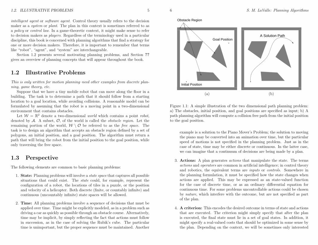
Suppose that we have a tiny mobile robot that can move along the floor in abuilding. The task is to determine a path that it should follow from a startinglocation to a goal location, while avoiding collisions. A reasonable model can beformulated by assuming that the robot is a moving point in a two-dimensionalenvironment that contains obstacles.
Let W = R2 denote a two-dimensional world which contains a point robot,denoted by A. A subset, O, of the world is called the obstacle region. Let theremaining portion of the world, W \ O be referred to as the free space. Thetask is to design an algorithm that accepts an obstacle region defined by a set ofpolygons, an initial position, and a goal position. The algorithm must return apath that will bring the robot from the initial position to the goal position, whileonly traversing the free space.
1.3 Perspective
The following elements are common to basic planning problems:
1. State: Planning problems will involve a state space that captures all possiblesituations that could exist. The state could, for example, represent theconfiguration of a robot, the locations of tiles in a puzzle, or the positionand velocity of a helicopter. Both discrete (finite, or countably infinite) andcontinuous (uncountably infinite) state spaces will be allowed.
2. Time: All planning problems involve a sequence of decisions that must beapplied over time. Time might be explicitly modeled, as in a problem such asdriving a car as quickly as possible through an obstacle course. Alternatively,time may be implicit, by simply reflecting the fact that actions must followin succession, as in the case of solving the Rubik’s cube. The particulartime is unimportant, but the proper sequence must be maintained. Another
6 S. M. LaValle: Planning Algorithms
Goal Position
Obstacle Region
Initial Position
A Solution Path
(a) (b)
Figure 1.1: A simple illustration of the two dimensional path planning problem:a) The obstacles, initial position, and goal positions are specified as input; b) Apath planning algorithm will compute a collision free path from the initial positionto the goal position.
example is a solution to the Piano Mover’s Problem; the solution to movingthe piano may be converted into an animation over time, but the particularspeed of motions is not specified in the planning problem. Just as in thecase of state, time may be either discrete or continuous. In the latter case,we can imagine that a continuum of decisions are being made by a plan.
3. Actions: A plan generates actions that manipulate the state. The termsactions and operators are common in artificial intelligence; in control theoryand robotics, the equivalent terms are inputs or controls. Somewhere inthe planning formulation, it must be specified how the state changes whenactions are applied. This may be expressed as an state-valued functionfor the case of discrete time, or as an ordinary differential equation forcontinuous time. For some problems uncontrollable actions could be chosenby nature, which interfere with the outcome, but are not specified as partof the plan.
4. A criterion: This encodes the desired outcome in terms of state and actionsthat are executed. The criterion might simply specify that after the planis executed, the final state must lie in a set of goal states. In addition, itmight specify a real-valued costs that should be optimized in some sense bythe plan. Depending on the context, we will be sometimes only interested
1.3. PERSPECTIVE 7
3 54
2
1
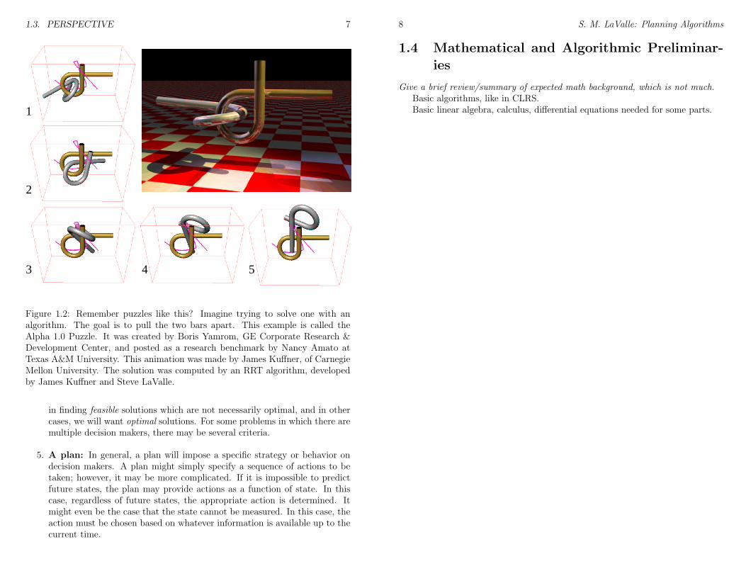
Figure 1.2: Remember puzzles like this? Imagine trying to solve one with analgorithm. The goal is to pull the two bars apart. This example is called theAlpha 1.0 Puzzle. It was created by Boris Yamrom, GE Corporate Research &Development Center, and posted as a research benchmark by Nancy Amato atTexas A&M University. This animation was made by James Kuffner, of CarnegieMellon University. The solution was computed by an RRT algorithm, developedby James Kuffner and Steve LaValle.
in finding feasible solutions which are not necessarily optimal, and in othercases, we will want optimal solutions. For some problems in which there aremultiple decision makers, there may be several criteria.
5. A plan: In general, a plan will impose a specific strategy or behavior ondecision makers. A plan might simply specify a sequence of actions to betaken; however, it may be more complicated. If it is impossible to predictfuture states, the plan may provide actions as a function of state. In thiscase, regardless of future states, the appropriate action is determined. Itmight even be the case that the state cannot be measured. In this case, theaction must be chosen based on whatever information is available up to thecurrent time.
8 S. M. LaValle: Planning Algorithms
1.4 Mathematical and Algorithmic Preliminar-
ies
Give a brief review/summary of expected math background, which is not much.Basic algorithms, like in CLRS.Basic linear algebra, calculus, differential equations needed for some parts.
Chapter 2
Discrete Planning
This covers discrete, classical AI planning, which models no uncertaintiesSome parts of the current contents come from my class notes of CS497 Spring
2003, which were originally scribed by Rishi Talreja.
2.1 Introduction
The chapter provides introductory concepts that serve as an entry point intoother parts of the book. The planning problems considered here are the simplestto describe because the state space will be finite in most cases. When it is notfinite, it will at least be countably infinite (i.e., every state can be enumeratedwith a distinct integer). Therefore, no geometric models or differential equationswill be needed to characterize the discrete planning problems.
The most important parts of this chapter are the representations of planningproblems (Section ), and the basic search algorithms, which will be useful through-out the book as more complicated forms of planning are considered (Section 2.3).Section 2.4 takes a close look at optimal discrete planning, and various forms ofdynamic programming that can be applied. It is useful to understand these alter-native forms in the context of discrete planning because in more-general settings,only one particular form may apply. In the present setting, all of the variants canbe explained, to help you understand how they are related. Section 2.5 presentsseveral planning algorithms that were developed particularly for discrete planning.
Although this chapter addresses a form of planning, it may also be consideredproblem solving. Throughout the history of artificial intelligence research, thedistinction between problem solving and planning has been rather elusive. For ex-ample, in a current leading textbook [1], two of the eight major parts are termed“Problem-solving” and “Planning”. The problem solving part begins by stating,“Problem solving agents decide what to do by finding sequences of actions thatlead to desirable states.” ([1], p. 59). The planning part begins with, “The task ofcoming up with a sequence of actions that will achieve a goal is called planning.”([1], p. 375). The STRIPS system is considered one of the first planning algo-
9
10 S. M. LaValle: Planning Algorithms
rithms and representations [?], and its name means STanford Research InstituteProblem Solver. Perhaps the term “planning” carries connotations of future time,where as “problem solving” sounds somewhat more general. A problem solvingtask might be to take evidence from a crime scene and piece together the actionstaken by suspects. It might seem odd to call this a “plan” because it occurred inthe past.
Given that there are no clear distinctions between problem solving and plan-ning, we will simply refer to both as planning. This also helps to keep with thetheme of the book. Note, however, that some of the concepts apply to a broaderset of problems that what is often meant by planning.
2.2 Three Representations of Discrete Planning
In this section, we formulate discrete planning three different ways. Althoughthis might seem tedious, there are good reasons to give redundant formulations.Section 2.2.1 introduces STRIPS-like representations, which have been used inthe earliest formulations of planning, and for certain kinds of problems, they offercompact representations. One problem with these representations is that they aredifficult to generalize to problems that involve concerns such as uncertainty orcontinuous variables. This motivates the introduction of the state space represen-tation in Section 2.2.2. It will be easy to extend and adapt this representation tothe problems covered throughout this book. Since many forms of planning reduceto a kind of search, it will be sometimes convenient to refer to a graph representa-tion of planning, which is the subject of Section 2.2.3. In this way, some forms ofplanning may be understood as running a search algorithm on a large, unexploredgraph.
2.2.1 STRIPS-Like Representation
STRIPS and its variants are the most common representations of planning prob-lems in artificial intelligence. The STRIPS language is a very simple logic basedonly on (ground) literals and predicates. Let I denote a finite set of instances(often referred to as propositional literals), which serve as the basic objects in theworld. For example, I, might include the names of automobile parts in a planningproblem that involves assembling a car. For example,
I = Radiator, RadiatorHose, Alternator, SparkP lug.
Let P denote a finite set of predicates, which are binary valued functions ofone or more instances. In other words, each p ∈ P , may be considered as p :I×I×· · ·×I → False, True. An example might be a predicate called Attached,which indicates which automobile parts are attached. Example values could beAttached(RadiatorHose,Radiator) = true andAttached(SparkP lug,Radiator) =
2.2. THREE REPRESENTATIONS OF DISCRETE PLANNING 11
false). In some applications, it might make sense to restrict the domain of eachp to “relevant” instances; however, this will not be considered here.
As far as planning is concerned, the state of the world is completely determinedonce the predicates are fully specified. Every possible question regarding theinstances will have an answer of true or false. If each predicate was a functionof exactly k instances, then there would be |P | |I|k possible questions. Typically,the number of arguments will vary over the predicates. Each question is referredto as a (first-order) literal. If the literal is true, it is called positive; otherwise, itis called negative.
The state of the world can be specified by giving the complete set of positiveliterals. All other literals are assumed to be negative. The initial state is specifiedin this way. The goal is expressed as a set of positive and negative literals. Thetask of a planning is to transform the world into any state that satisfies all of thegoal literals. Any literals not mentioned the goal are permitted to be either trueor false.
To solve a planning problem, we need to transform the world from one stateto another. This is achieved by a set, O, of operators. In addition to its name,each operator has two components:
1. The precondition, which lists positive and negative literals that must besatisfied for the operator to be applicable. To avoid tedious specifications ofpreconditions for every instance, variables are allowed to appear in predicatearguments. For example, Attached(x,Radiator) indicates that anythingmay be attached to the radiator for the operator to apply. Without usingthe variable x, we would be required to define an operator for every instance.
2. The effect, which specifies precisely how the world is changed. Some literalsmay be made positive, and others may be made negative. This is specifiedas a list of positive and negative literals. Any literals not mentioned in theoperator effect are unaffected by the operator. Variables may also be usedhere.
Consider the following example, based on contemporary politics. Suppose thatGeorge W. Bush’s team of experts is using STRIPS planning to determine someway to avoid hostile threats. Suppose that the instances are country names,
I = Canada, France, Iraq, Thailand, China, Zaire, ....
The predicates are
P = HasWMD,Friendly, Angry,
each of which is assumed to be a function from I to false, true.The world must be manipulated through operators. Suppose there are only
two:O = Attack,Befriend.
12 S. M. LaValle: Planning Algorithms
The Attack operator could be defined as
Op(NAME : Attack(i),
PRECONDITION : HasWMD(i) ∧ ¬Friendly(i),
EFFECT : ¬HasWMD(i) ∧ Angry(i))
Above, logic notation has been used: ∧means logical conjunction (AND); ¬meanslogical negation (NOT). The precondition states that the operator can be appliedwhen a country has weapons of mass destruction and is not friendly. Under thesame condition, another operator that could be applied is
Op(NAME : Befriend(i),
PRECONDITION : HasWMD(i) ∧ ¬Friendly(i),
EFFECT : Friendly(i))
Initially, the values for all predicates are fully specified. The goal could requirespecific countries to be without weapons of mass destruction, and others to befriendly. One kind of goal that seems reasonable is to have every country, i, tobe either Friendly(i) or ¬HasWMD(i). Unfortunately, such disjunctive goalsare not allowed in the original STRIPS representation. It is possible, however, toextend the representation to allow this.
Once all of the components have been specified, the planning task can bestated. Find a sequence of operators that can be applied in succession from theinitial state, and that cause the world to be transformed into a goal state.
The STRIPS representation is very nice for representing planning problems ina descriptive way that corresponds closely to the application. Also, the operatordefinitions enable problems that have enormous complexity to be expressed com-pactly in many cases. One problem with these representations, however, is thatthey are difficult to extend to more general settings.
2.2.2 State Space Representation
Consider representing the discrete planning problem in terms of states and statetransitions. We first give a list of formal definitions, and then describe how toconvert a planning problem represented with STRIPS operators in to a state spacerepresentation.
1. Let X be a nonempty, finite set which is called the state space. Let x ∈ Xdenote a specific state.
2. Let xI denote the initial state.
2.2. THREE REPRESENTATIONS OF DISCRETE PLANNING 13
3. Let XG ⊂ X denote a set of goal states.
4. For each x ∈ X, let U(x) denote a nonempty, finite set of actions. LetU = ∪x∈XU(x) denote the set of all possible actions.
5. Define a partial function, f : X × U → X, called the state transition equa-tion. This is used to produce new states, x′ = f(x, u), given some statex ∈ X and action u ∈ U(x). The reason f is a partial function is becausesome actions are not applicable in some states.
Now consider converting a planning problem represented with STRIPS into thestate space representation. The set of questions from Section ?? may be encodedas a sequence of bits, referred to as a binary string, by imposing an linear orderingto the instances, I, and the predicates, P . The state of the world is then specifiedin order,. Using the example from Section 2.2.1, this might appear like:
(HasWMD(Russia),¬HasWMC(Jamaica), . . . , F riendly(Canada), . . .).
Using the binary string, each element can be “0” to denote false, or “1” to denotetrue. The resulting state would be x = 110 · · · 1 · · · .
The initial state xI is given by specifying a string, and XG is the set of allstrings that are consistent with the goal positive and negative goal literals. Youcan alternatively imagine a string that has a “0” for each negative literal, a “1”for each positive literal, and a “δ” for all others, in which the δ means “don’tcare.”
The next step is to convert the operators. For each state, x ∈ X, the set U(x)will represent the set of operators who preconditions are satisfied by the statex. The effect of the operator is encoded by the state transition equation. If thestate is given, it is straightforward to determine which bits to flip in the string,resulting in x′.
There are both advantages and disadvantages to the the state space represen-tation. First, consider disadvantages. One obvious drawback with the state spacerepresentation described here is the useful descriptive information that appearedin the STRIPS model has been dropped. Also, note that using the STRIPS modelit might be possible to succinctly describe a planning problem that would be ex-tremely tedious to specify using the state space representation. Many problemsto which the STRIPS model is applied have huge state spaces, which are muchtoo large to fit into any electronic storage. Therefore, it is not feasible to performthe entire conversion as described above.
Next, consider advantages. First of all, the representation does not need tobe explicitly constructed by an algorithm. It is more useful as a precise way toformulate and analyze planning problems. In algorithms, any one of a number ofrepresentations may be preferable depending on the context. However, regardlessof the representation chosen in implementation, an underlying state space can be
14 S. M. LaValle: Planning Algorithms
defined. It is implicitly determined once the planning problem is defined, eventhough there is not an explicit representation of it.
The most significant advantage of the state space representation is that is gen-eralizes nicely to many other planning problems. It is very difficult to incorporateelements such as probabilistic uncertainty, continuous instance spaces, and game-theoretic notions into the STRIPS model. On the other hand, it is very naturalto incorporate these notions using the state space representation. In fact, mostof the literature on these more complicated problems, which have been studied inartificial intelligence, robotics, and control theory, all involve state space repre-sentations. Therefore, the state space representation will be prevalent throughoutthis book. However, one should remember that in a particular implementation,an alternative representation, such as STRIPS, might be preferable (if it can bedirectly used).
2.2.3 Graph Representation
Once the state space representation has been given, it is not difficult to see anunderlying graph structure in which the states are vertices, and the actions aredirected edges that connect states. Let G = (V,E) be a directed graph. Define thevertex set to be the set of all possible states, V = X. The edge set is somewhattricky to define. From every vertex, a set of outgoing edges is defined in whichthere is one edge for each u ∈ U(x). The set, E, of all edges, represents the unionof all of these edges. Note that E is generally larger than the set U because thesame action may apply at many states, and each time it generates a new edge inE.
The graph representation will seem most natural at the algorithm level, espe-cially for planning problems that reduce to a kind of search. Just as in the caseof the state space representation, the graph representation does not have to beexplicitly constructed in advance. In viewing planning as a kind of search, we canimagine that an enormous graph is implicitly defined once the STRIPS model isgiven for a particular problem. The planning problem reduces to exploring thisgraph in the hopes of finding a goal state. This is the topic of Section 2.3.
2.3 Search Algorithms
We already know that the discrete planning problem may be interpreted as asearch in a graph. In most applications, the graph is enormous, but not explicitlyencoded at the outset. Instead, the graph is gradually revealed, step by step,through the use of a search algorithm. Graph searching is a basic part of algo-rithms [17]. The presentation in this section can be considered as graph searchalgorithms tailored to planning problems.
2.3. SEARCH ALGORITHMS 15
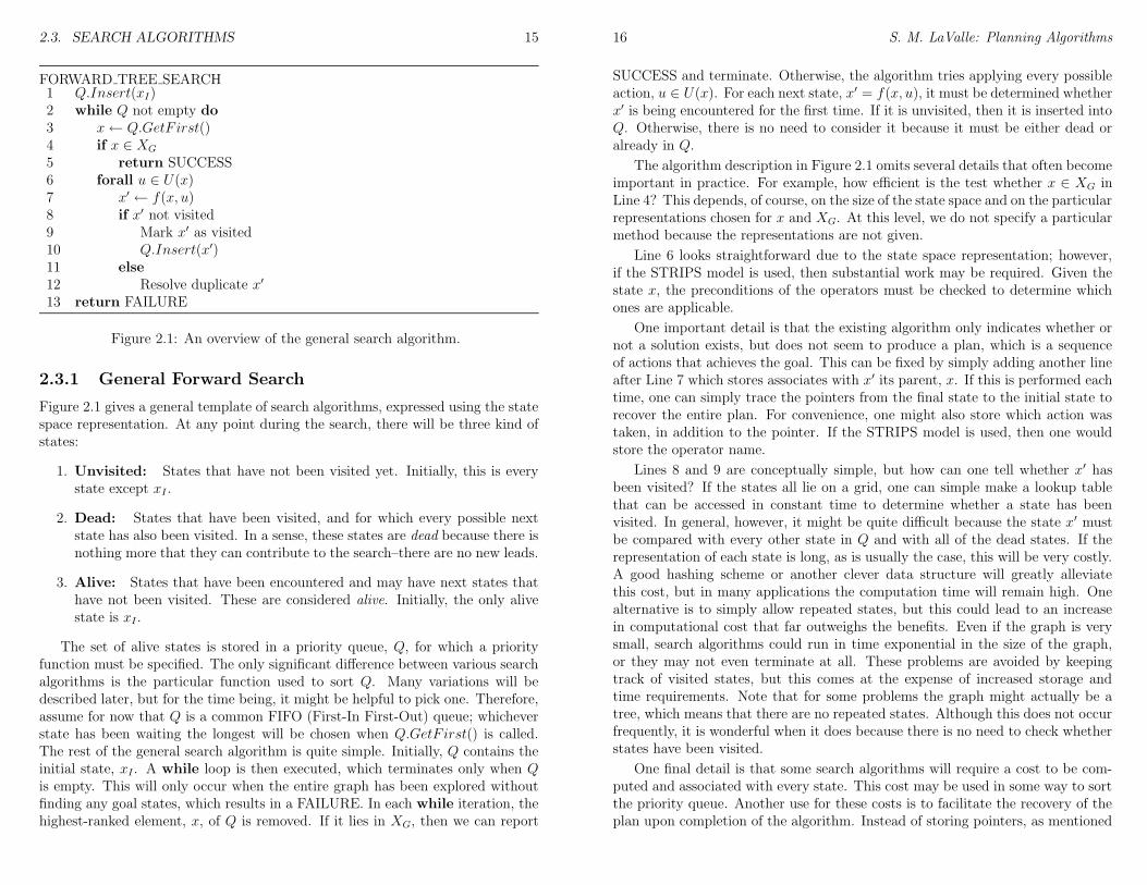
FORWARD TREE SEARCH1 Q.Insert(xI)2 while Q not empty do3 x← Q.GetF irst()4 if x ∈ XG
5 return SUCCESS6 forall u ∈ U(x)7 x′ ← f(x, u)8 if x′ not visited9 Mark x′ as visited10 Q.Insert(x′)11 else12 Resolve duplicate x′
13 return FAILURE
Figure 2.1: An overview of the general search algorithm.
2.3.1 General Forward Search
Figure 2.1 gives a general template of search algorithms, expressed using the statespace representation. At any point during the search, there will be three kind ofstates:
1. Unvisited: States that have not been visited yet. Initially, this is everystate except xI .
2. Dead: States that have been visited, and for which every possible nextstate has also been visited. In a sense, these states are dead because there isnothing more that they can contribute to the search–there are no new leads.
3. Alive: States that have been encountered and may have next states thathave not been visited. These are considered alive. Initially, the only alivestate is xI .
The set of alive states is stored in a priority queue, Q, for which a priorityfunction must be specified. The only significant difference between various searchalgorithms is the particular function used to sort Q. Many variations will bedescribed later, but for the time being, it might be helpful to pick one. Therefore,assume for now that Q is a common FIFO (First-In First-Out) queue; whicheverstate has been waiting the longest will be chosen when Q.GetF irst() is called.The rest of the general search algorithm is quite simple. Initially, Q contains theinitial state, xI . A while loop is then executed, which terminates only when Qis empty. This will only occur when the entire graph has been explored withoutfinding any goal states, which results in a FAILURE. In each while iteration, thehighest-ranked element, x, of Q is removed. If it lies in XG, then we can report
16 S. M. LaValle: Planning Algorithms
SUCCESS and terminate. Otherwise, the algorithm tries applying every possibleaction, u ∈ U(x). For each next state, x′ = f(x, u), it must be determined whetherx′ is being encountered for the first time. If it is unvisited, then it is inserted intoQ. Otherwise, there is no need to consider it because it must be either dead oralready in Q.
The algorithm description in Figure 2.1 omits several details that often becomeimportant in practice. For example, how efficient is the test whether x ∈ XG inLine 4? This depends, of course, on the size of the state space and on the particularrepresentations chosen for x and XG. At this level, we do not specify a particularmethod because the representations are not given.
Line 6 looks straightforward due to the state space representation; however,if the STRIPS model is used, then substantial work may be required. Given thestate x, the preconditions of the operators must be checked to determine whichones are applicable.
One important detail is that the existing algorithm only indicates whether ornot a solution exists, but does not seem to produce a plan, which is a sequenceof actions that achieves the goal. This can be fixed by simply adding another lineafter Line 7 which stores associates with x′ its parent, x. If this is performed eachtime, one can simply trace the pointers from the final state to the initial state torecover the entire plan. For convenience, one might also store which action wastaken, in addition to the pointer. If the STRIPS model is used, then one wouldstore the operator name.
Lines 8 and 9 are conceptually simple, but how can one tell whether x′ hasbeen visited? If the states all lie on a grid, one can simple make a lookup tablethat can be accessed in constant time to determine whether a state has beenvisited. In general, however, it might be quite difficult because the state x′ mustbe compared with every other state in Q and with all of the dead states. If therepresentation of each state is long, as is usually the case, this will be very costly.A good hashing scheme or another clever data structure will greatly alleviatethis cost, but in many applications the computation time will remain high. Onealternative is to simply allow repeated states, but this could lead to an increasein computational cost that far outweighs the benefits. Even if the graph is verysmall, search algorithms could run in time exponential in the size of the graph,or they may not even terminate at all. These problems are avoided by keepingtrack of visited states, but this comes at the expense of increased storage andtime requirements. Note that for some problems the graph might actually be atree, which means that there are no repeated states. Although this does not occurfrequently, it is wonderful when it does because there is no need to check whetherstates have been visited.
One final detail is that some search algorithms will require a cost to be com-puted and associated with every state. This cost may be used in some way to sortthe priority queue. Another use for these costs is to facilitate the recovery of theplan upon completion of the algorithm. Instead of storing pointers, as mentioned
2.3. SEARCH ALGORITHMS 17
previously, the optimal cost to to return to the initial state could be stored witheach state. This cost alone is sufficient to determine the action sequence thatleads to any state visited state. Solution paths can be constructed in the sameway by using the computed costs after running Dijkstra’s algorithm.
2.3.2 Particular Forward Search Methods
We now discuss several single-tree search algorithms, each of which is a special caseof the algorithm in Figure 2.1, obtained by defining a different sorting functionfor Q. Most of these are just classical graph search algorithms; see [17]. Sincethe graph is finite, all of the methods below are complete: if a solution exists, thealgorithm will find it; otherwise, it will terminate in finite time and report failure.The completeness is based on the assumption that the algorithm keeps track ofvisited states. Without this information some of the algorithms below may runforever by cycling through the same states.
Breadth First
The method given in Section 2.3.1 specifiesQ as a FIFO queue, which selects statesusing the first-come, first-serve principle. This causes the search frontier to growuniformly, and is therefore referred to as breadth-first search. All plans that havek steps are exhausted before plans with k + 1 steps are investigated. Therefore,breadth first guarantees that the first solution found will use the smallest numberof steps. Upon detection that a state has been revisited, there is no work to do inLine 12. Given its systematic exploration, breadth first search is complete withoutkeeping track of visited states (although the running time increases dramatically).
The running time breadth first search is O(|V | + |E|), in which |V | and |E|are the numbers of vertices and edges, respectively, in the graph representationof the planning problem. This assumes that all operations, such as determiningwhether a state has been visited, are performed in constant time. In practice,these operations will typically require more time, and must be counting as partof the algorithm complexity. The running time be expressed in terms of the otherrepresentations. Recall that |V | = |X| is the number of states. If the sameactions, U , are available from every state, then |E| = |U ||X|. If action sets U(x1)and U(x2) are pairwise disjoint for any x1, x2 ∈ X, then |E| = |U |. In terms ofSTRIPS, the case of the same actions available from any state would mean thatall operators can be applied from any state, resulting in |E| = |O||X|. In the caseof pairwise disjoint actions, each operator applies only in a single state, resultingin |E| = |O||X|. Recall that |X| can be expressed in terms of the number ofinstances and predicates, if all predicates have the same number, k, of arguments.The result is |X| = |I||P |k.
18 S. M. LaValle: Planning Algorithms
Depth First
By making Q a stack (Last-In, First-Out), aggressive exploration is the graphoccurs, as opposed to the uniform expansion of breadth first search. The resultingvariant is called depth first search because the search dives quickly into the graph.The preference is toward investigating longer plans very early. Although thisaggressive behavior might seem desirable, note that the particular choice of longerplans is arbitrary. Actions are applied in the forall loop in whatever order theyhappen to be defined. Once again, if a state is revisited, there is no work to do inLine 12. The running time of this algorithm is also O(|V |+ |E|).
Dynamic Programming (Dijkstra)
Up to this point, there has been no reason to prefer any action or operator overany other in the search. Section 2.4 will formalize optimal discrete planning, andwill present several algorithms that find optimal plans. Before going into that,we present an optimal planning here as a variant of forward search. The resultis the well-known Dijkstra’s algorithm for finding single-source shortest paths ina graph []. Suppose that every edge, e ∈ E, in the graph representation of adiscrete planning problem, has an associated positive cost l(e), which is the costto apply the action or operator. The cost l(e) could be written using the statespace representation as l(x, u), indicating that it costs l(x, u) to apply action ufrom state x. The total cost of a plan is just the sum of the edge costs over thepath from the initial state to a goal state.
The priority queue, Q, will be sorted according to a function, L∗ : X → [0,∞],called the optimal cost-to-come or just cost-to-come if it is clearly optimal fromthe context. For each state, x, the value L∗(x) will represent the optimal cost toreach x from the initial state, xI . This optimal cost is obtained by summing edgecosts, l(e), over all possible paths from xI to x, and using the path produces theleast cumulative cost.
The cost-to-come is computed incrementally during the execution of the searchalgorithm in Figure 2.1. Initially, L∗(xI) = 0. Each time the state x′ is generated,a cost is computed as: L(x′) = L∗(x) + l(e), in which e is the edge from x to x′
(equivalently, we may write L(x′) = L∗(x) + l(x, u)). Here, L(x′) represents bestcost-to-come that is known so far, but we do not write L∗ because it is not yetknown whether x′ was reached optimally. Because of this, some work is requiredin Line 12. If x′ already exists in Q, then it is possible that the newly-discoveredpath to x′ is more efficient. If so, then the cost-to-come value L(x′) must beupdated for x′, and Q must be updated accordingly.
When does L(x) finally become L∗(x) for some state x? Once x is removedfrom Q using Q.GetF irst(), the state becomes dead, and it is known that there isno better way to reach it. This can be argued by induction. For the initial state,L∗(xI) is known, and this serves as the base case. Now assume that all deadstates have their optimal cost-to-come correctly determined. This means that
2.3. SEARCH ALGORITHMS 19
their cost-to-come values can no longer change. For the first element, x, of Q, thevalue must be optimal because any path that has lower total cost would have totravel through another state in Q, but these states already have higher cost. Allpaths that pass only through dead states were already considered in producingL(x). Once all edges leaving x are explored, then x can be declared as dead, andthe induction continues. This is not enough detail to constitute a proof; muchmore detailed arguments appear in [17]. The running time is O(|V | lg |V |+|E|), inwhich |V | and |E| are the numbers of edges and vertices, respectively, in the graphrepresentation of the discrete planning problem. This assumes that the priorityqueue is implemented with a Fibonacci heap, and that all other operations, suchas determining whether a state has been visited, are performed in constant time.If other data structures are used to implement the priority queue, then differentrunning times will be obtained.
A∗
The A∗ search algorithm is a variant of dynamic programming that tries to reducethe total number of states explored by incorporating a heuristic estimate of thecost to get the goal from a given state. Let LI(x) denote the cost-to-come from xIto x, and let LG(x) denote the cost-to-go from x to some state in XG. AlthoughL∗I(x) can be computed incrementally by dynamic programming, there is no wayto know the true optimal cost-to-go. However, in many applications it is possibleto construct a reasonable underestimate of this cost. For example, if you aretrying to get from one point to another in a labyrinth, the line-of-sight distanceserves as a reasonable underestimate of the distance you must travel through thecorridors of the labyrinth. Of course, zero could also serve as an underestimate,but that will not provide any helpful information to the algorithm. The aim is tocompute an estimate that is as close as possible to the optimal cost-to-go, and isalso guaranteed to be no greater. Let LG(x) denote such an estimate.
The A∗ search algorithm works in exactly the same way as the previous dy-namic programming algorithm. The only difference is the function used to sort Q.In the A∗ algorithm, the sum LI(x
′) + LG(x′) is used, implying that the priority
queue is sorted by estimates of the optimal cost from xI to XG. If LG(x) is anunderestimate of the true optimal cost-to-go for all x ∈ X, the A∗ algorithm isguaranteed to find optimal plans [?, ?]. As LG becomes closer to LG, fewer nodestend to be explored in comparison with dynamic programming. This would al-ways seem advantageous, but in some problems it is not possible to find a goodheuristic. Note that when LG(x) = 0 for all x ∈ X, then A∗ degenerates to theprevious dynamic programming algorithm.
Best First
For best first search, the priority queue is sorted according to LG, which is anestimate of the optimal cost-to-go. The solutions obtained in this way are not
20 S. M. LaValle: Planning Algorithms
necessarily optimal; therefore, it does not matter whether or not the estimateexceeds the true optimal cost-to-go. Although optimal solutions are not found,in many cases, far fewer nodes are explored, which results in much faster runningtimes. There is no guarantee, however, that this will happen. The worst-case per-formance of best first search is worst than that of A∗ and dynamic programming.One must be careful when applying it in practice. In a sense, the approach is themost greedy of the algorithms so far because it prefers states that “look good”very early in the search. If these are truly the best states, then great performancebenefits are obtained. If they are not, then the price must be paid for beinggreedy!
Need to make a 2D local minimum example for this algorithm, and maybe acouple of others. The spiral death trap is good for this one.
Iterative Deepening
Depth limited and IDA∗ can fit here.
2.3.3 Other General Search Schemes
This section covers two other general templates for search algorithms. The firstone is simply a “backwards” version of the tree search algorithm in Figure 2.1.The second one is a bidirectional approach that grows two search trees, one fromthe initial state, and one from a goal state.
Backwards Tree Search
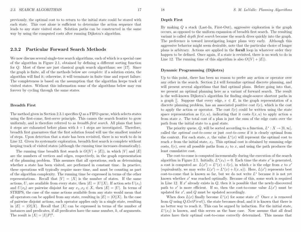
Suppose that there is a single goal state, xG. For many planning problems, it mightbe the case that the branching factor is large when starting from xI . It this cases,it might be more efficient to start the search at a goal state and work backwardsuntil the initial state is encountered. A general template for this approach is givenin Figure 2.2. To apply this idea, the particular planning problem must allow usto define an inverse of the state transition equation. In the forward search case,an action u ∈ U is applied at a state x ∈ X, to obtain a new state, x′ = f(x, u).To enable backwards search, we must be able to determine a set of state/actionpairs that bring the world into some state x in one step. For a given state x, letU−1(x) denote the set of actions that could be applied from other states to arriveat x. In other words, if u ∈ U−1(x), then there exists some x′ ∈ X and u ∈ U(x′)such that x = f(x′, u). The state x′ is given by the expression φ(x, u) in Line 7,which is determined by inverting f , the state transition equation. If it possible toperform such an inversion, then there is a perfect symmetry with respect to theforward search of Section 2.3.1. Any of the search algorithm variants from Section2.3.2 could be adapted to the template in Figure 2.2.
2.4. OPTIMAL PLANNING 21
BACKWARDS TREE SEARCH1 Q.Insert(xG)2 while Q not empty do3 x← Q.GetF irst()4 if x = xI5 return SUCCESS6 forall u ∈ U−1(x)7 x′ ← φ(x, u)8 if x′ not visited9 Mark x′ as visited10 Q.Insert(x′)11 else12 Resolve duplicate x′
13 return FAILURE
Figure 2.2: An overview of the general search algorithm.
Bidirectional Search
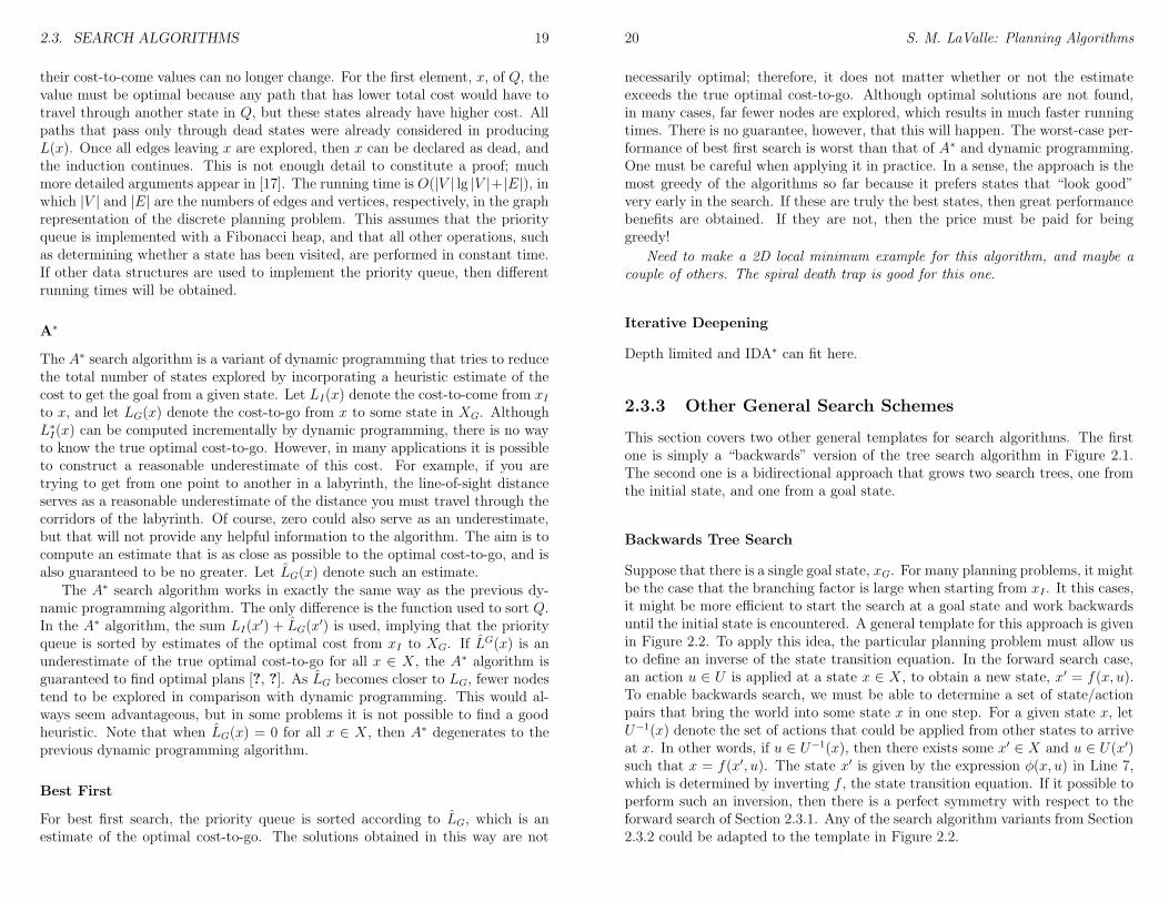
Now that forward and backwards search have been covered, it reasonable idea isto conduct a bidirectional search [58]. The general search template given in Figure2.3 can be considered as a combination of the two in Figures 2.1 and 2.2. One treeis grown from the initial state, and the other is grown from the goal state. Thesearch terminates with success when the two trees meet. Failure occurs if bothpriority queues have been exhausted. For many problems bidirectional search candramatically reduce the amount of exploration required to solve the problem. Thedynamic programming and A∗ variants of bidirectional search will lead to optimalsolutions. For best-first and other variants, it may be challenging to ensure thatthe two trees meet quickly. They might come very close to each other, and thenfail fail to connect. Additional heuristics may help in some settings to help guidethe trees into each other.
2.4 Optimal Planning
This section extends the state space representation to allow optimal planningproblems to be defined. Rather than being satisfied with any sequence of actionsthat leads to the goal set, we would like a solution that optimizes some criterion,such as time, distance, or energy consumed. Three important extensions will bemade: 1) a stage index will be added for convenience to indicate the presentplan step; 2) a cost functional will be introduced, which serves as a kind of taximeter to determine how much cost will accumulate; 3) a termination action, whichintuitively indicates when it is time to turn the meter off and stop the plan.
22 S. M. LaValle: Planning Algorithms
BIDIRECTIONAL SEARCH1 QI .Insert(xI)2 QG.Insert(xG)3 while QI not empty or QG not empty do4 if QI not empty5 x← QI .GetF irst()6 if x ∈ xG or x ∈ QG
7 return SUCCESS8 forall u ∈ U(x)9 x′ ← f(x, u)10 if x′ not visited11 Mark x′ as visited12 QI .Insert(x
′)13 else14 Resolve duplicate x′
15 if QG not empty16 x← QG.GetF irst()17 if x = xI or x ∈ QI
18 return SUCCESS19 forall u ∈ U−1(x)20 x′ ← φ(x, u)21 if x′ not visited22 Mark x′ as visited23 QG.Insert(x
′)24 else25 Resolve duplicate x′
26 return FAILURE
Figure 2.3: An overview of the general search algorithm.
2.4.1 State space formulation
By adding these new components to the state space representation from Section2.2.2, we obtain the following formulation of optimal discrete planning:
1. Let the state space, X, be a nonempty, finite set of states.
2. Let U(x) denote a nonempty, finite set of actions that can be applied froma state x ∈ X. Assume U(x) is specified for all x ∈ X.
3. Let k ∈ 1, . . . , K+1 denote the stage. It is assumed that K is larger thanthe number of stages required for the longest optimal path between any pairof states in X.
4. Let F denote the index of the final stage. If K is finite, then F = K + 1.
2.4. OPTIMAL PLANNING 23
5. Let f denote a state transition equation, which yields xk+1 = f(xk, uk) forany xk ∈ X and uk ∈ U(xk).
6. Let xI denote the initial state, and let xG denote the goal state. Alterna-tively, we may consider a set of goal states, XG, or there may be no explicitgoal.
7. Let L denote an additive loss functional, which is applied to the sequence,u1, . . . , uK , of applied actions, and achieved states, x1, . . . , xF :
L =K∑
k=1
l(xk, uk) + lF (xF ). (2.1)
The final term, lF (xF ) is usually defined as lF (xF ) = 0 if xF ∈ XG, andlF (xF ) =∞ otherwise.
8. Each U(x) contains a special termination action, uT . If uT is applied to xk,then the action is repeatedly applied until stage K, and the state remainsin xk until the final stage. Furthermore, no loss accumulates: l(xk, uT ) = 0for any k and xk.
9. The task is to find a sequence of actions, u1, . . . , uK that minimizes L.
To correspond to STRIPS planning, the following cost functions can be used:l(x, u) = 0, lF (xF ) = 0 if xF ∈ XG and lF (xF ) = 1, otherwise. To obtain optimal-step planning, let l(x, u) = 1, lF (xF ) = 0 if xF ∈ XG and lF (xF ) =∞, otherwise.
2.4.2 Backwards dynamic programming
Since it involves less notation, we first consider the case of backwards dynamic pro-gramming. In this case, dynamic programming becomes a recursive formulationof the optimal cost-to-go to the goal.
Suppose that the final-stage loss is defined as lF (xF ) = 0 if xF = xG, andlF (xF ) =∞ otherwise. The final-stage optimal cost-to-go is:
L∗F,F (xF ) = lF (xF ). (2.2)
This makes intuitive sense: since there are no stages in which an action can beapplied, we immediately receive the penalty for not being in the goal.
For an intermediate stage, k ∈ 2, . . . , K the following represents the optimalcost-to-go:
L∗k,F (xk) = minuk,...,uK
K∑
i=k
l(xi, ui) + lF (xF )
(2.3)
In the minimization above, it is assumed that ui ∈ U(xi) for every i ∈ k, . . . ,K.Equation (2.3) expresses the lowest possible loss that can be received by starting
24 S. M. LaValle: Planning Algorithms
from xk and applying actions over K − k + 1 stages. The termination action canbe applied at any stage, but a loss, lF (xF ) must be paid at the final stage. Thus,if you are not already in the goal, you are forced to move; otherwise, infinite losswill be obtained.
The final step in backwards dynamic programming is the arrival at the initialstage. The cost-to-go in this case is
L∗1,F (x1) = minu1,...,uK
lI(x1) +K∑
i=1
l(xi, ui) + lF (xF )
, (2.4)
in which lI(x1) denotes an initial loss. For most applications of backwards dynamicprogramming, we can safely make lI(x1) = 0 for all x1 ∈ X. In forward dynamicprogramming, lI becomes more important, and lF becomes unimportant.
The dynamic programming equation expresses L∗k,F in terms of L∗k+1,F :
L∗k,F (xk) = minuk∈U(xk)
L∗k+1,F (xk+1) + l(xk, uk)
. (2.5)
Note that xk+1 is given by the state transition equation: xk+1 = f(xk, uk).
2.4.3 Forward dynamic programming
Dynamic programming in this case involves the recursive formulation of the cost-to-come from an initial state. Notice that the concepts here are the symmetricequivalent of backwards dynamic programming concepts.
Suppose that the initial loss is defined as lI(x1) = 0 if x1 = xI , and lI(x1) =∞otherwise. This will ensure that only paths that start at xI are considered (in thebackwards case, lF ensures that only paths which end at xG are considered).
The initial optimal cost-to-come is:
L∗1,1(x1) = lI(x1). (2.6)
For an intermediate stage, k ∈ 2, . . . , K the following represents the optimalcost-to-come:
L∗1,k(xk) = minu1,...,uk−1
lI(x1) +k−1∑
i=1
l(xi, ui)
. (2.7)
Note that the sum refers to a sequence of states, x1, . . . , xk, which are the result ofapplying the action sequence u1, . . . , uk−1. As in (2.3) it is assumed that ui ∈ U(xi)for every i ∈ 1, . . . , k − 1. The resulting xk, obtained after applying uk−1 mustbe the same xk that is named in the argument on the right side of (2.7). It mightappear odd that x1 appears inside the min above; however, this is not a problem.The state x1 can be completely determined once u1, . . . , uk−1 and xk are given.
The final step in forward dynamic programming is the arrival at the final stage.The cost-to-come in this case is
L∗1,F (xF ) = minu1,...,uK
lI(x1) +K∑
i=1
l(xi, ui) + lF (xF )
. (2.8)
2.4. OPTIMAL PLANNING 25
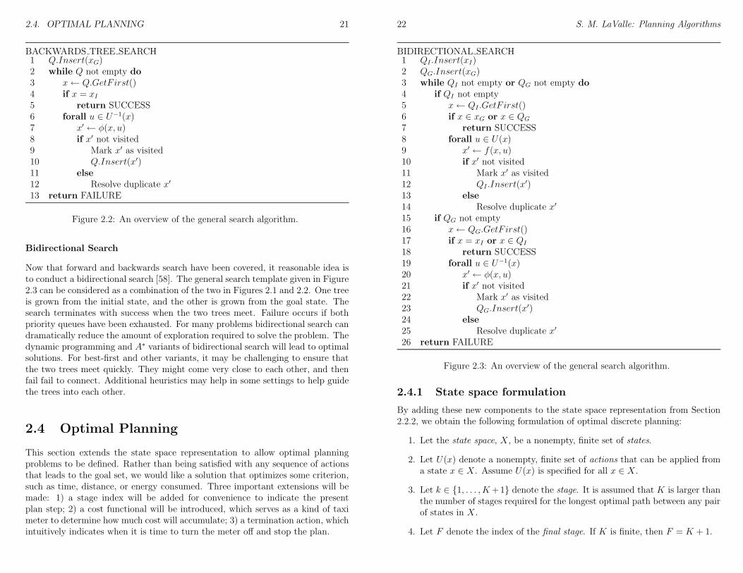
1 2 3 4 52
11
111
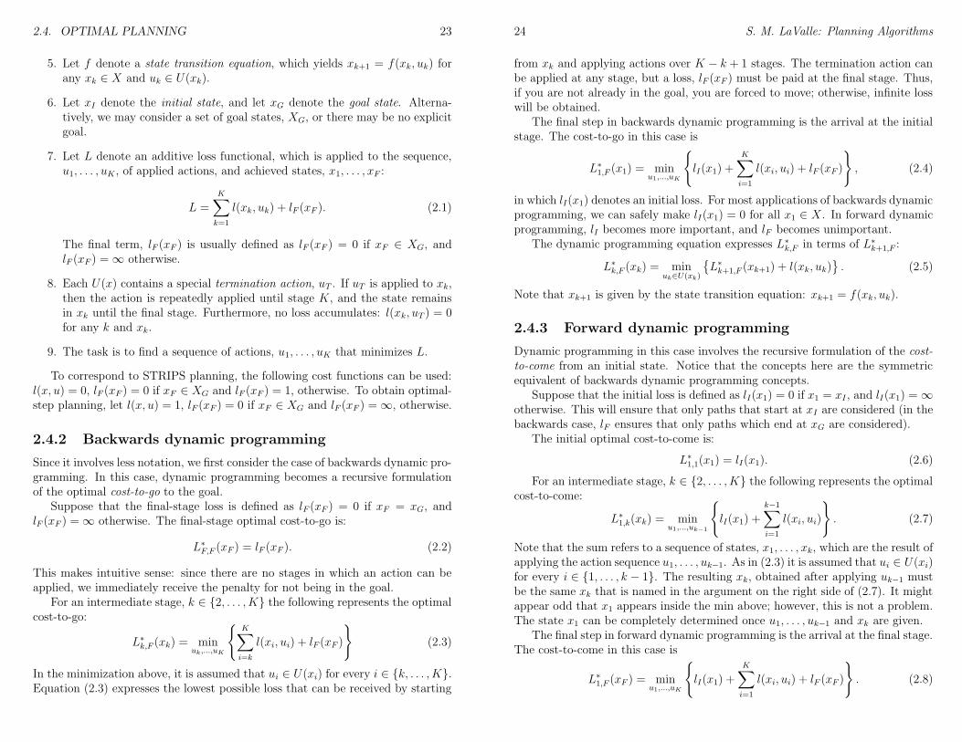
42
Figure 2.4: A five-state example is shown. Each vertex represents a state, and eachedge represents an input that can be applied to the state transition equation tochange the state. The weights on the edges represent l(xk, uk) (xk is the originatingvertex of the edge).
This equation looks the same as (2.4), but x1 is replaced with xF on the right.This means that all paths ending at xF are considered here, whereas all pathsstarting at x1 were considered in the backwards case.
To express the dynamic programming recurrence, one further issue remains.Suppose that L∗F,k−1 is known by induction, and we want to compute L∗1,k(xk) fora particular xk. This means that we must start at some state xk−1 and arrivein state xk by applying some action. Which actions are possible? In terms ofthe graph representation, this means that we need to consider all in-edges for thenode xk. For the case of backward dynamic programming, we used the out-edges,which are simply given by applying each uk ∈ U(xk) in f(xk, uk) to obtain eachxk+1. This effectively tries all out-edges of xk.
To try all in-edges, we can formulate a backwards state transition equation,which can always be derived from the (forward) state transition equation. Letxk−1 = φ(xk, ωk) denote the backwards state transition equation. The ωk canbe considered as a kind of backwards action that when applied to xk, moves usbackwards to state xk. Let Ω(xk) denote the set of all backwards actions availablefrom state xk. Each element, ωk, of Ω(xk) corresponds exactly to an in-edge to xkin the graph representation. Furthermore, ωk corresponds to an input, uk−1 thatgot applied to xk−1 to reach state xk. Thus, we have simply derived a “backwards”version of the state transition equation, xk+1 = f(xk, uk).
Using the backwards state transition equation, the dynamic programmingequation is:
L∗1,k(xk) = minωk∈Ω(xk)
L∗1,k−1(xk−1) + l(xk−1, uk−1)
, (2.9)
in which xk−1 = φ(xk, ωk) and uk−1 is the input to which ωk corresponds.
2.4.4 A simple example
Consider the example shown in Figure 2.4, in which X = 1, 2, 3, 4, 5. Supposethat xI = 2 and xG = 5.
26 S. M. LaValle: Planning Algorithms
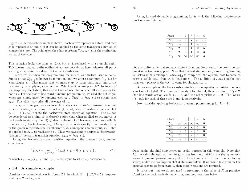
Using forward dynamic programming for K = 4, the following cost-to-comefunctions are obtained:
State 1 2 3 4 5
L∗1,1 ∞ 0 ∞ ∞ ∞L∗1,2 ∞ 0 1 4 ∞L∗1,3 2 0 1 2 5
L∗1,4 2 0 1 2 3
L∗1,5 ∞ ∞ ∞ ∞ 3
For any finite value that remains content from one iteration to the next, the ter-mination action was applied. Note that the last step of the dynamic programmingis useless in this example. Once L∗1,4 is computed, the optimal cost-to-come toevery possible state from xI is determined. The addition of lF (xF ) in the laststage only preserves the cost-to-come for the goal state.
As an example of the backwards state transition equation, consider the con-struction of L∗1,3(4). There are two in-edges for state 4; thus, the size of Ω3 is 2.One backwards action yields x2 = 3, and the other yields x2 = 2. The losses,l(x2, u2), for each of these are 1 and 4, respectively.
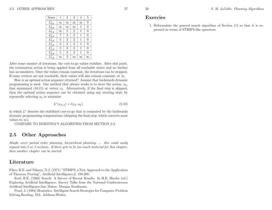
Next consider applying backwards dynamic programming for K = 4:
State 1 2 3 4 5
L∗5,5 ∞ ∞ ∞ ∞ 0
L∗4,5 ∞ ∞ ∞ 1 0
L∗3,5 ∞ 5 2 1 0
L∗2,5 7 3 2 1 0
L∗1,5 ∞ 3 ∞ ∞ ∞
Once again, the final step serves no useful purpose in this example. Note thatL∗2,5 contains the optimal cost to go to xG from any initial state (by symmetry,forward dynamic programming yielded the optimal cost to come from xI to anystate), under the assumption that 3 steps are taken. If we would like to know theoptimal cost to go from state 1, then more iterations are required.
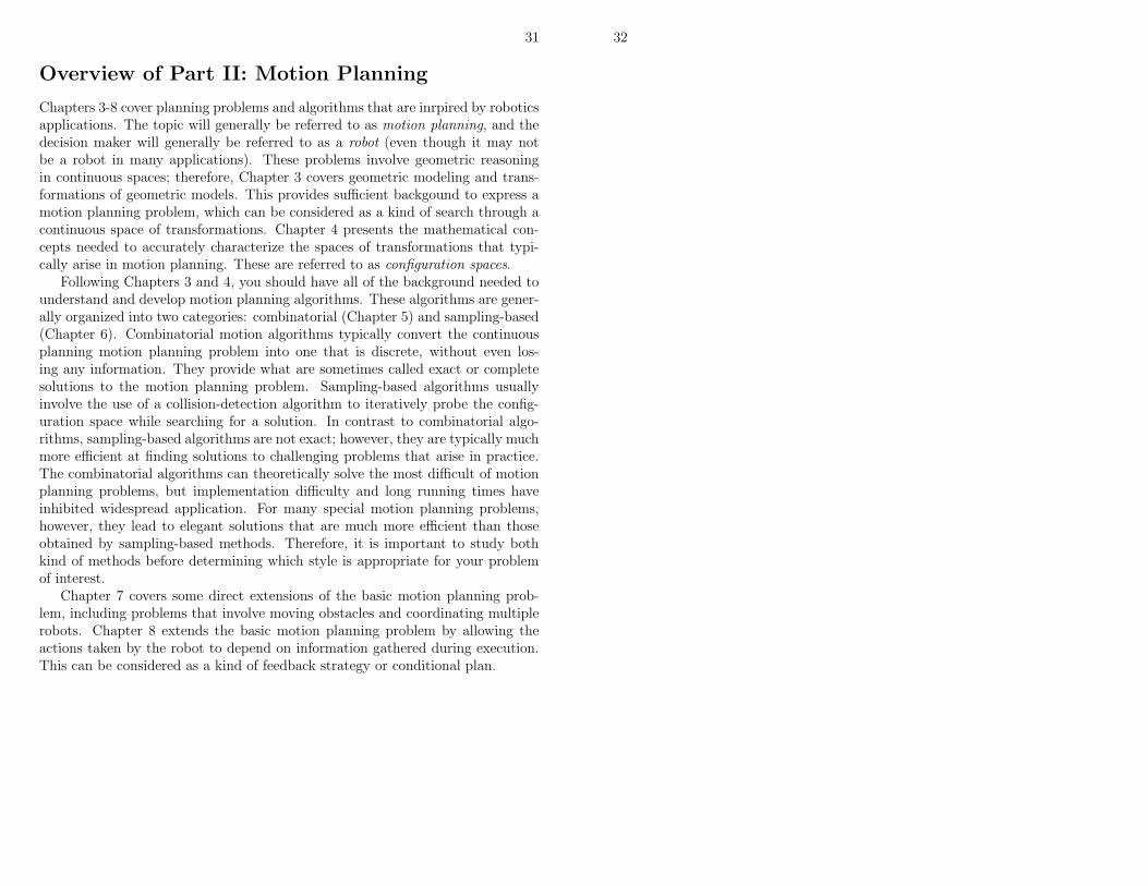
It turns out that we do not need to precompute the value of K in practice.Consider the backwards dynamic programming iterations below:
2.5. OTHER APPROACHES 27
State 1 2 3 4 5
L∗9,9 ∞ ∞ ∞ ∞ 0
L∗8,9 ∞ ∞ ∞ 1 0
L∗7,9 ∞ 5 2 1 0
L∗6,9 7 3 2 1 0
L∗5,9 5 3 2 1 0
L∗4,9 5 3 2 1 0
L∗3,9 5 3 2 1 0
L∗2,9 5 3 2 1 0
L∗1,9 ∞ 3 ∞ ∞ ∞
After some number of iterations, the cost-to-go values stabilize. After this point,the termination action is being applied from all reachable states and no furtherloss accumulates. Once the values remain constant, the iterations can be stopped.If some vertices are not reachable, their values will also remain constant, at ∞.
How is an optimal action sequence returned? Assume that backwards dynamicprogramming is used. One method that always works is to store the action, uk,that minimized (10.15) at vertex xk. Alternatively, if the final step is skipped,then the optimal action sequence can be obtained using any starting state byrepeatedly selecting uk to minimize
L∗(xk+1) + l(xk, uk), (2.10)
in which L∗ denotes the stabilized cost-to-go that is computed by the backwardsdynamic programming computations (skipping the final step, which converts mostvalues to ∞).
COMPARE TO DIJKSTRA’S ALGORITHM FROM SECTION 2.3.
2.5 Other Approaches
Maybe cover partial order planning, hierarchical planning, ... this could easilyexpand into 2 or 3 sections. If there gets to be too much material for this chapter,then another chapter can be started.
Literature
Fikes, R.E. and Nilsson, N.J. (1971) ”STRIPS: a New Approach to the Applicationof Theorem Proving”, Artificial Intelligence,2, 189-208.
Korf, R.E. (1988) Search: A Survey of Recent Results. In H.E. Shrobe (ed.)Exploring Artificial Intelligence: Survey Talks from the National ConferencesonArtificial Intelligence,San Mateo: Morgan Kaufmann.
Pearl, J. (1984) Heuristics: Intelligent Search Strategies for Computer ProblemSolving,Reading, MA: Addison-Wesley.
28 S. M. LaValle: Planning Algorithms
Exercies
1. Reformulate the general search algorithm of Section 2.3 so that it is ex-pressed in terms of STRIPS-like operators.

Part II
Motion Planning
29
31
Overview of Part II: Motion Planning
Chapters 3-8 cover planning problems and algorithms that are inrpired by roboticsapplications. The topic will generally be referred to as motion planning, and thedecision maker will generally be referred to as a robot (even though it may notbe a robot in many applications). These problems involve geometric reasoningin continuous spaces; therefore, Chapter 3 covers geometric modeling and trans-formations of geometric models. This provides sufficient backgound to express amotion planning problem, which can be considered as a kind of search through acontinuous space of transformations. Chapter 4 presents the mathematical con-cepts needed to accurately characterize the spaces of transformations that typi-cally arise in motion planning. These are referred to as configuration spaces.
Following Chapters 3 and 4, you should have all of the background needed tounderstand and develop motion planning algorithms. These algorithms are gener-ally organized into two categories: combinatorial (Chapter 5) and sampling-based(Chapter 6). Combinatorial motion algorithms typically convert the continuousplanning motion planning problem into one that is discrete, without even los-ing any information. They provide what are sometimes called exact or completesolutions to the motion planning problem. Sampling-based algorithms usuallyinvolve the use of a collision-detection algorithm to iteratively probe the config-uration space while searching for a solution. In contrast to combinatorial algo-rithms, sampling-based algorithms are not exact; however, they are typically muchmore efficient at finding solutions to challenging problems that arise in practice.The combinatorial algorithms can theoretically solve the most difficult of motionplanning problems, but implementation difficulty and long running times haveinhibited widespread application. For many special motion planning problems,however, they lead to elegant solutions that are much more efficient than thoseobtained by sampling-based methods. Therefore, it is important to study bothkind of methods before determining which style is appropriate for your problemof interest.
Chapter 7 covers some direct extensions of the basic motion planning prob-lem, including problems that involve moving obstacles and coordinating multiplerobots. Chapter 8 extends the basic motion planning problem by allowing theactions taken by the robot to depend on information gathered during execution.This can be considered as a kind of feedback strategy or conditional plan.
32
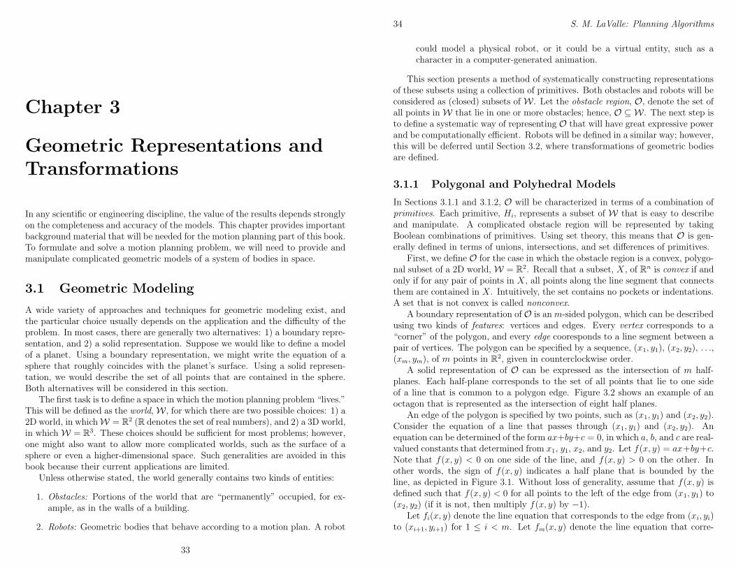
Chapter 3
Geometric Representations andTransformations
In any scientific or engineering discipline, the value of the results depends stronglyon the completeness and accuracy of the models. This chapter provides importantbackground material that will be needed for the motion planning part of this book.To formulate and solve a motion planning problem, we will need to provide andmanipulate complicated geometric models of a system of bodies in space.
3.1 Geometric Modeling
A wide variety of approaches and techniques for geometric modeling exist, andthe particular choice usually depends on the application and the difficulty of theproblem. In most cases, there are generally two alternatives: 1) a boundary repre-sentation, and 2) a solid representation. Suppose we would like to define a modelof a planet. Using a boundary representation, we might write the equation of asphere that roughly coincides with the planet’s surface. Using a solid represen-tation, we would describe the set of all points that are contained in the sphere.Both alternatives will be considered in this section.
The first task is to define a space in which the motion planning problem “lives.”This will be defined as the world,W , for which there are two possible choices: 1) a2D world, in whichW = R2 (R denotes the set of real numbers), and 2) a 3D world,in which W = R3. These choices should be sufficient for most problems; however,one might also want to allow more complicated worlds, such as the surface of asphere or even a higher-dimensional space. Such generalities are avoided in thisbook because their current applications are limited.
Unless otherwise stated, the world generally contains two kinds of entities:
1. Obstacles: Portions of the world that are “permanently” occupied, for ex-ample, as in the walls of a building.
2. Robots: Geometric bodies that behave according to a motion plan. A robot
33
34 S. M. LaValle: Planning Algorithms
could model a physical robot, or it could be a virtual entity, such as acharacter in a computer-generated animation.
This section presents a method of systematically constructing representationsof these subsets using a collection of primitives. Both obstacles and robots will beconsidered as (closed) subsets of W . Let the obstacle region, O, denote the set ofall points inW that lie in one or more obstacles; hence, O ⊆ W . The next step isto define a systematic way of representing O that will have great expressive powerand be computationally efficient. Robots will be defined in a similar way; however,this will be deferred until Section 3.2, where transformations of geometric bodiesare defined.
3.1.1 Polygonal and Polyhedral Models
In Sections 3.1.1 and 3.1.2, O will be characterized in terms of a combination ofprimitives. Each primitive, Hi, represents a subset of W that is easy to describeand manipulate. A complicated obstacle region will be represented by takingBoolean combinations of primitives. Using set theory, this means that O is gen-erally defined in terms of unions, intersections, and set differences of primitives.
First, we define O for the case in which the obstacle region is a convex, polygo-nal subset of a 2D world, W = R2. Recall that a subset, X, of Rn is convex if andonly if for any pair of points in X, all points along the line segment that connectsthem are contained in X. Intuitively, the set contains no pockets or indentations.A set that is not convex is called nonconvex.
A boundary representation of O is anm-sided polygon, which can be describedusing two kinds of features: vertices and edges. Every vertex corresponds to a“corner” of the polygon, and every edge cooresponds to a line segment between apair of vertices. The polygon can be specified by a sequence, (x1, y1), (x2, y2), . . .,(xm, ym), of m points in R2, given in counterclockwise order.
A solid representation of O can be expressed as the intersection of m half-planes. Each half-plane corresponds to the set of all points that lie to one sideof a line that is common to a polygon edge. Figure 3.2 shows an example of anoctagon that is represented as the intersection of eight half planes.
An edge of the polygon is specified by two points, such as (x1, y1) and (x2, y2).Consider the equation of a line that passes through (x1, y1) and (x2, y2). Anequation can be determined of the form ax+by+c = 0, in which a, b, and c are real-valued constants that determined from x1, y1, x2, and y2. Let f(x, y) = ax+by+c.Note that f(x, y) < 0 on one side of the line, and f(x, y) > 0 on the other. Inother words, the sign of f(x, y) indicates a half plane that is bounded by theline, as depicted in Figure 3.1. Without loss of generality, assume that f(x, y) isdefined such that f(x, y) < 0 for all points to the left of the edge from (x1, y1) to(x2, y2) (if it is not, then multiply f(x, y) by −1).
Let fi(x, y) denote the line equation that corresponds to the edge from (xi, yi)to (xi+1, yi+1) for 1 ≤ i < m. Let fm(x, y) denote the line equation that corre-
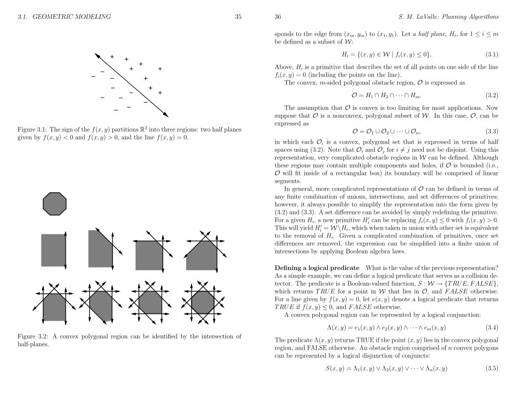
3.1. GEOMETRIC MODELING 35
++
++
++
+
+
−
−
−
−
−−
−−
−−
Figure 3.1: The sign of the f(x, y) partitions R2 into three regions: two half planesgiven by f(x, y) < 0 and f(x, y) > 0, and the line f(x, y) = 0.
Figure 3.2: A convex polygonal region can be identified by the intersection ofhalf-planes.
36 S. M. LaValle: Planning Algorithms
sponds to the edge from (xm, ym) to (x1, y1). Let a half plane, Hi, for 1 ≤ i ≤ mbe defined as a subset of W :
Hi = (x, y) ∈ W | fi(x, y) ≤ 0. (3.1)
Above, Hi is a primitive that describes the set of all points on one side of the linefi(x, y) = 0 (including the points on the line).
The convex, m-sided polygonal obstacle region, O is expressed as
O = H1 ∩H2 ∩ · · · ∩Hm. (3.2)
The assumption that O is convex is too limiting for most applications. Nowsuppose that O is a nonconvex, polygonal subset of W . In this case, O, can beexpressed as
O = O1 ∪ O2 ∪ · · · ∪ On, (3.3)
in which each Oi is a convex, polygonal set that is expressed in terms of halfspaces using (3.2). Note that Oi and Oj for i 6= j need not be disjoint. Using thisrepresentation, very complicated obstacle regions in W can be defined. Althoughthese regions may contain multiple components and holes, if O is bounded (i.e.,O will fit inside of a rectangular box) its boundary will be comprised of linearsegments.
In general, more complicated representations of O can be defined in terms ofany finite combination of unions, intersections, and set differences of primitives;however, it always possible to simplify the representation into the form given by(3.2) and (3.3). A set difference can be avoided by simply redefining the primitive.For a given Hi, a new primitive H ′
i can be replacing fi(x, y) ≤ 0 with fi(x, y) > 0.This will yieldH ′
i =W\Hi, which when taken in union with other set is equivalentto the removal of Hi. Given a complicated combination of primitives, once setdifferences are removed, the expression can be simplified into a finite union ofintersections by applying Boolean algebra laws.
Defining a logical predicate What is the value of the previous representation?As a simple example, we can define a logical predicate that serves as a collision de-tector. The predicate is a Boolean-valued function, S :W → TRUE,FALSE,which returns TRUE for a point in W that lies in O, and FALSE otherwise.For a line given by f(x, y) = 0, let e(x, y) denote a logical predicate that returnsTRUE if f(x, y) ≤ 0, and FALSE otherwise.
A convex polygonal region can be represented by a logical conjunction:
Λ(x, y) = e1(x, y) ∧ e2(x, y) ∧ · · · ∧ em(x, y) (3.4)
The predicate Λ(x, y) returns TRUE if the point (x, y) lies in the convex polygonalregion, and FALSE otherwise. An obstacle region comprised of n convex polygonscan be represented by a logical disjunction of conjuncts:
S(x, y) = Λ1(x, y) ∨ Λ2(x, y) ∨ · · · ∨ Λn(x, y) (3.5)
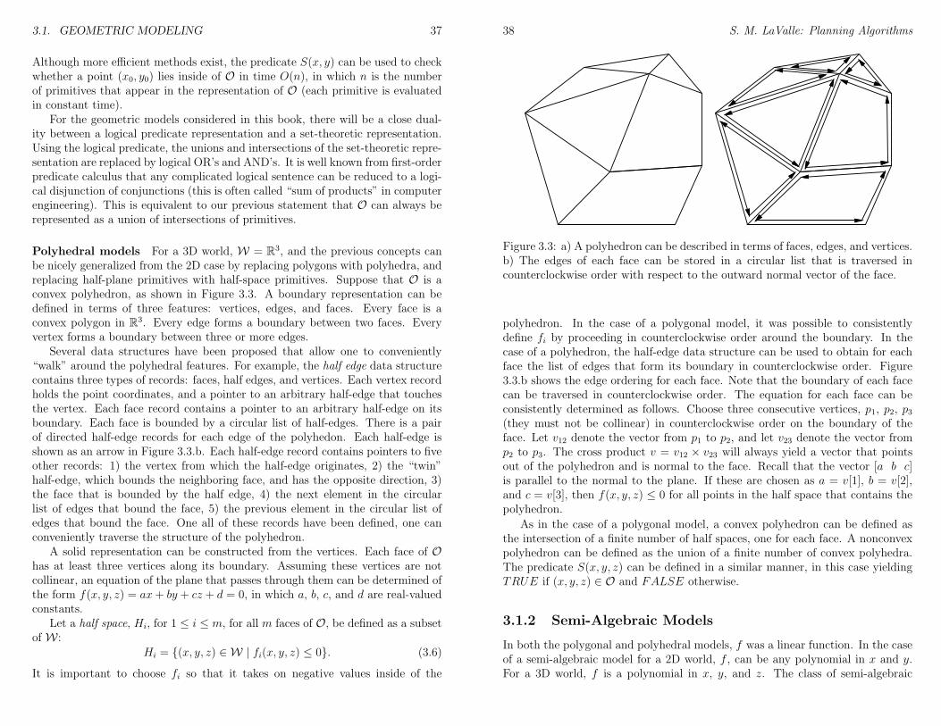
3.1. GEOMETRIC MODELING 37
Although more efficient methods exist, the predicate S(x, y) can be used to checkwhether a point (x0, y0) lies inside of O in time O(n), in which n is the numberof primitives that appear in the representation of O (each primitive is evaluatedin constant time).
For the geometric models considered in this book, there will be a close dual-ity between a logical predicate representation and a set-theoretic representation.Using the logical predicate, the unions and intersections of the set-theoretic repre-sentation are replaced by logical OR’s and AND’s. It is well known from first-orderpredicate calculus that any complicated logical sentence can be reduced to a logi-cal disjunction of conjunctions (this is often called “sum of products” in computerengineering). This is equivalent to our previous statement that O can always berepresented as a union of intersections of primitives.
Polyhedral models For a 3D world, W = R3, and the previous concepts canbe nicely generalized from the 2D case by replacing polygons with polyhedra, andreplacing half-plane primitives with half-space primitives. Suppose that O is aconvex polyhedron, as shown in Figure 3.3. A boundary representation can bedefined in terms of three features: vertices, edges, and faces. Every face is aconvex polygon in R3. Every edge forms a boundary between two faces. Everyvertex forms a boundary between three or more edges.
Several data structures have been proposed that allow one to conveniently“walk” around the polyhedral features. For example, the half edge data structurecontains three types of records: faces, half edges, and vertices. Each vertex recordholds the point coordinates, and a pointer to an arbitrary half-edge that touchesthe vertex. Each face record contains a pointer to an arbitrary half-edge on itsboundary. Each face is bounded by a circular list of half-edges. There is a pairof directed half-edge records for each edge of the polyhedon. Each half-edge isshown as an arrow in Figure 3.3.b. Each half-edge record contains pointers to fiveother records: 1) the vertex from which the half-edge originates, 2) the “twin”half-edge, which bounds the neighboring face, and has the opposite direction, 3)the face that is bounded by the half edge, 4) the next element in the circularlist of edges that bound the face, 5) the previous element in the circular list ofedges that bound the face. One all of these records have been defined, one canconveniently traverse the structure of the polyhedron.
A solid representation can be constructed from the vertices. Each face of Ohas at least three vertices along its boundary. Assuming these vertices are notcollinear, an equation of the plane that passes through them can be determined ofthe form f(x, y, z) = ax+ by + cz + d = 0, in which a, b, c, and d are real-valuedconstants.
Let a half space, Hi, for 1 ≤ i ≤ m, for all m faces of O, be defined as a subsetof W :
Hi = (x, y, z) ∈ W | fi(x, y, z) ≤ 0. (3.6)
It is important to choose fi so that it takes on negative values inside of the
38 S. M. LaValle: Planning Algorithms
Figure 3.3: a) A polyhedron can be described in terms of faces, edges, and vertices.b) The edges of each face can be stored in a circular list that is traversed incounterclockwise order with respect to the outward normal vector of the face.
polyhedron. In the case of a polygonal model, it was possible to consistentlydefine fi by proceeding in counterclockwise order around the boundary. In thecase of a polyhedron, the half-edge data structure can be used to obtain for eachface the list of edges that form its boundary in counterclockwise order. Figure3.3.b shows the edge ordering for each face. Note that the boundary of each facecan be traversed in counterclockwise order. The equation for each face can beconsistently determined as follows. Choose three consecutive vertices, p1, p2, p3(they must not be collinear) in counterclockwise order on the boundary of theface. Let v12 denote the vector from p1 to p2, and let v23 denote the vector fromp2 to p3. The cross product v = v12 × v23 will always yield a vector that pointsout of the polyhedron and is normal to the face. Recall that the vector [a b c]is parallel to the normal to the plane. If these are chosen as a = v[1], b = v[2],and c = v[3], then f(x, y, z) ≤ 0 for all points in the half space that contains thepolyhedron.
As in the case of a polygonal model, a convex polyhedron can be defined asthe intersection of a finite number of half spaces, one for each face. A nonconvexpolyhedron can be defined as the union of a finite number of convex polyhedra.The predicate S(x, y, z) can be defined in a similar manner, in this case yieldingTRUE if (x, y, z) ∈ O and FALSE otherwise.
3.1.2 Semi-Algebraic Models
In both the polygonal and polyhedral models, f was a linear function. In the caseof a semi-algebraic model for a 2D world, f , can be any polynomial in x and y.For a 3D world, f is a polynomial in x, y, and z. The class of semi-algebraic
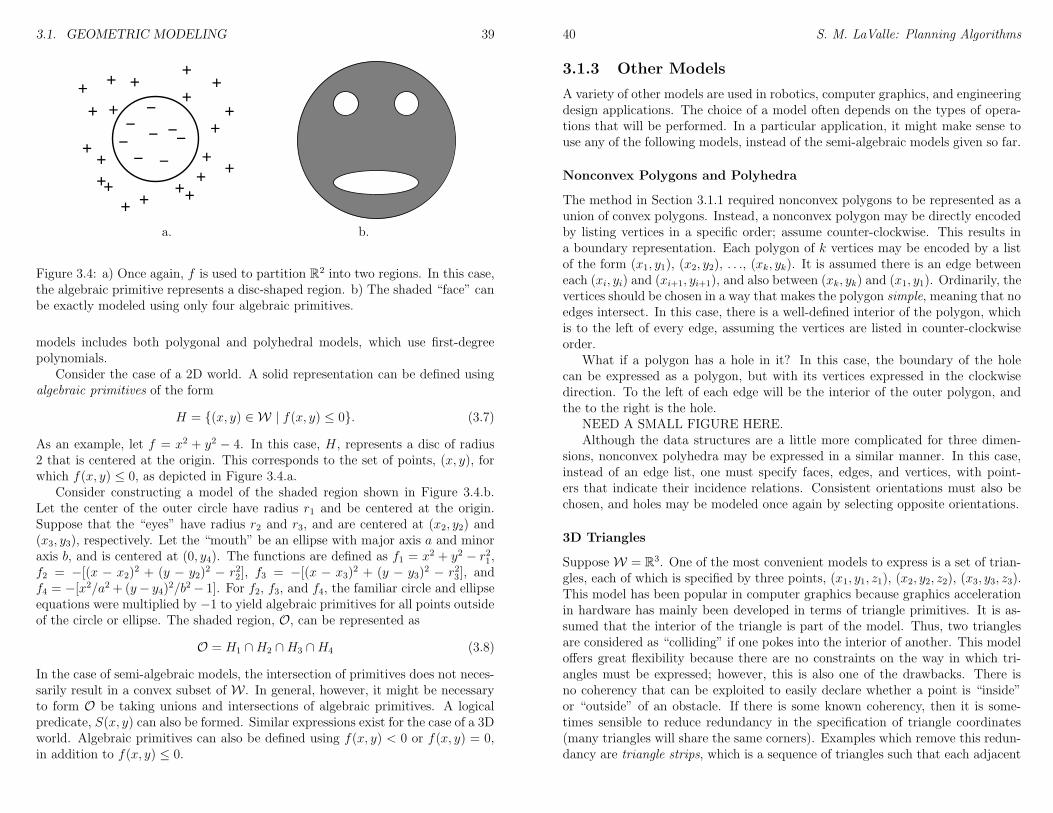
3.1. GEOMETRIC MODELING 39
++
++
++
++−
−
−−
−−
−−
++
+++
++
++++
++
a. b.
Figure 3.4: a) Once again, f is used to partition R2 into two regions. In this case,the algebraic primitive represents a disc-shaped region. b) The shaded “face” canbe exactly modeled using only four algebraic primitives.
models includes both polygonal and polyhedral models, which use first-degreepolynomials.
Consider the case of a 2D world. A solid representation can be defined usingalgebraic primitives of the form
H = (x, y) ∈ W | f(x, y) ≤ 0. (3.7)
As an example, let f = x2 + y2 − 4. In this case, H, represents a disc of radius2 that is centered at the origin. This corresponds to the set of points, (x, y), forwhich f(x, y) ≤ 0, as depicted in Figure 3.4.a.
Consider constructing a model of the shaded region shown in Figure 3.4.b.Let the center of the outer circle have radius r1 and be centered at the origin.Suppose that the “eyes” have radius r2 and r3, and are centered at (x2, y2) and(x3, y3), respectively. Let the “mouth” be an ellipse with major axis a and minoraxis b, and is centered at (0, y4). The functions are defined as f1 = x2 + y2 − r21,f2 = −[(x − x2)
2 + (y − y2)2 − r22], f3 = −[(x − x3)
2 + (y − y3)2 − r23], and
f4 = −[x2/a2+ (y− y4)
2/b2− 1]. For f2, f3, and f4, the familiar circle and ellipseequations were multiplied by −1 to yield algebraic primitives for all points outsideof the circle or ellipse. The shaded region, O, can be represented as
O = H1 ∩H2 ∩H3 ∩H4 (3.8)
In the case of semi-algebraic models, the intersection of primitives does not neces-sarily result in a convex subset of W . In general, however, it might be necessaryto form O be taking unions and intersections of algebraic primitives. A logicalpredicate, S(x, y) can also be formed. Similar expressions exist for the case of a 3Dworld. Algebraic primitives can also be defined using f(x, y) < 0 or f(x, y) = 0,in addition to f(x, y) ≤ 0.
40 S. M. LaValle: Planning Algorithms
3.1.3 Other Models
A variety of other models are used in robotics, computer graphics, and engineeringdesign applications. The choice of a model often depends on the types of opera-tions that will be performed. In a particular application, it might make sense touse any of the following models, instead of the semi-algebraic models given so far.
Nonconvex Polygons and Polyhedra
The method in Section 3.1.1 required nonconvex polygons to be represented as aunion of convex polygons. Instead, a nonconvex polygon may be directly encodedby listing vertices in a specific order; assume counter-clockwise. This results ina boundary representation. Each polygon of k vertices may be encoded by a listof the form (x1, y1), (x2, y2), . . ., (xk, yk). It is assumed there is an edge betweeneach (xi, yi) and (xi+1, yi+1), and also between (xk, yk) and (x1, y1). Ordinarily, thevertices should be chosen in a way that makes the polygon simple, meaning that noedges intersect. In this case, there is a well-defined interior of the polygon, whichis to the left of every edge, assuming the vertices are listed in counter-clockwiseorder.
What if a polygon has a hole in it? In this case, the boundary of the holecan be expressed as a polygon, but with its vertices expressed in the clockwisedirection. To the left of each edge will be the interior of the outer polygon, andthe to the right is the hole.
NEED A SMALL FIGURE HERE.Although the data structures are a little more complicated for three dimen-
sions, nonconvex polyhedra may be expressed in a similar manner. In this case,instead of an edge list, one must specify faces, edges, and vertices, with point-ers that indicate their incidence relations. Consistent orientations must also bechosen, and holes may be modeled once again by selecting opposite orientations.
3D Triangles
Suppose W = R3. One of the most convenient models to express is a set of trian-gles, each of which is specified by three points, (x1, y1, z1), (x2, y2, z2), (x3, y3, z3).This model has been popular in computer graphics because graphics accelerationin hardware has mainly been developed in terms of triangle primitives. It is as-sumed that the interior of the triangle is part of the model. Thus, two trianglesare considered as “colliding” if one pokes into the interior of another. This modeloffers great flexibility because there are no constraints on the way in which tri-angles must be expressed; however, this is also one of the drawbacks. There isno coherency that can be exploited to easily declare whether a point is “inside”or “outside” of an obstacle. If there is some known coherency, then it is some-times sensible to reduce redundancy in the specification of triangle coordinates(many triangles will share the same corners). Examples which remove this redun-dancy are triangle strips, which is a sequence of triangles such that each adjacent
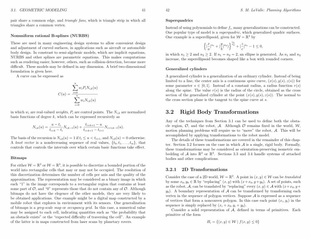
3.1. GEOMETRIC MODELING 41
pair share a common edge, and triangle fans, which is triangle strip in which alltriangles share a common vertex.
Nonuniform rational B-splines (NURBS)
These are used in many engineering design systems to allow convenient designand adjustment of curved surfaces, in applications such as aircraft or automobilebody design. In constrast to semi-algebraic models, which are implicit equations,NURBS and other splines are parametric equations. This makes computationssuch as rendering easier; however, others, such as collision-detection, become moredifficult. These models may be defined in any dimension. A brief two-dimensionalformulation is given here.
A curve can be expressed as
C(u) =
n∑
i=0
wiPiNi,k(u)
n∑
i=0
wiNi,k(u)
in which wi are real-valued weights, Pi are control points. The Ni,k are normalizedbasis functions of degree k, which can be expressed recursively as
Ni,k(u) =u− titi+k − ti
Ni,k−1(u) +ti+k+1 − u
ti+k+1 − ti+1Ni+1,k−1(u).
The basis of the recursion isNi,0(u) = 1 if ti ≤ u < ti+1, andNi,0(u) = 0 otherwise.A knot vector is a nondecreasing sequence of real values, t0, t1, . . . , tm, thatcontrols that controls the intervals over which certain basic functions take effect.
Bitmaps
For eitherW = R2 orW = R3, it is possible to discretize a bounded portion of theworld into rectangular cells that may or may not be occupied. The resolution ofthis discretization determines the number of cells per axis and the quality of theapproximation. The representation may be considered as a binary image in whicheach “1” in the image corresponds to a rectangular region that contains at leastsome part of O, and “0” represents those that do not contain any of O. Althoughbitmaps do not have the elegence of the other models, they are very likely tobe obtained applications. One example might be a digital map constructed by amobile robot that explores in environment with its sensors. One generalizationof bitmaps is a grey-scale map or occupancy grid. In this case, a numerical valuemay be assigned to each cell, indicating quantities such as “the probability thatan obstacle exists” or the “expected difficulty of traversing the cell”. An exampleof the latter is in maps constructed from laser scans by planetary rovers.
42 S. M. LaValle: Planning Algorithms
Superquadrics
Instead of using polynomials to define fi, many generalizations can be constructed.One popular type of model is a superquadric, which generalized quadric surfaces.One example is a superellipsoid, given for W = R3 by
|x
a|n1 + |
y
b|n2)
n1n2 + |
z
c|n1 − 1 ≤ 0,
in which n1 ≥ 2 and n2 ≥ 2. If n1 = n2 = 2, an ellipse is generated. As n1 and n2increase, the superellipsoid becomes shaped like a box with rounded corners.
Generalized cylinders
A generalized cylinder is a generalization of an ordinary cylinder. Instead of beinglimited to a line, the center axis is a continuous spine curve, (x(s), y(s), z(s)) forsome parameter s ∈ [0, 1]. Instead of a constant radius, a radius function r(s)along the spine. The value r(s) is the radius of the circle, obtained as the crosssection of the generalized cylinder at the point (x(s), y(s), z(s)). The normal tothe cross section plane is the tangent to the spine curve at s.
3.2 Rigid Body Transformations
Any of the techniques from Section 3.1 can be used to define both the obsta-cle region, O, and the robot, A. Although O remains fixed in the world, W ,motion planning problems will require us to “move” the robot, A. This will beaccomplished by applying transformations to the robot model.
The details of these transformations are covered in the remainder of this chap-ter. Section 3.2 focuses on the case in which A is a single, rigid body. Formally,these transformations may be considered as orientation-preserving isometric em-bedding of A into R2 or R3. Sections 3.3 and 3.4 handle systems of attachedbodies and other complications.
3.2.1 2D Transformations
Consider the case of a 2D world,W = R2. A point in (x, y) ∈ W can be translatedby some x0, y0 ∈ R by “replacing” (x, y) with (x+x0, y+y0). A set of points, suchas the robot, A, can be translated by “replacing” every (x, y) ∈ A with (x+x0, y+y0). A boundary representation of A can be transformed by transforming eachvertex in the sequence of polygon vertices. Suppose A is expressed as a sequenceof vertices that form a nonconvex polygon. In this case each point (xi, yi) in thesequence is simply replaced by (xi + x0, yi + y0).
Consider a solid representation of A, defined in terms of primitives. Eachprimitive of the form
Hi = (x, y) ∈ W | f(x, y) ≤ 0
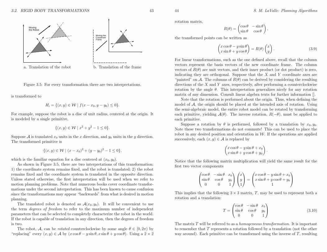
3.2. RIGID BODY TRANSFORMATIONS 43
Movingthe Robot
Moving theCoordinateFrame
a. Translation of the robot b. Translation of the frame
Figure 3.5: For every transformation there are two interpretations.
is transformed to
Hi = (x, y) ∈ W | f(x− x0, y − y0) ≤ 0.
For example, suppose the robot is a disc of unit radius, centered at the origin. Itis modeled by a single primitive,
(x, y) ∈ W | x2 + y2 − 1 ≤ 0.
Suppose A is translated x0 units in the x direction, and y0 units in the y direction.The transformed primitive is
(x, y) ∈ W | (x− x0)2 + (y − y0)
2 − 1 ≤ 0,
which is the familiar equation for a disc centered at (x0, y0).As shown in Figure 3.5, there are two interpretations of this transformation:
1) the coordinate system remains fixed, and the robot is translated; 2) the robotremains fixed and the coordinate system is translated in the opposite direction.Unless stated otherwise, the first interpretation will be used when we refer tomotion planning problems. Note that numerous books cover coordinate transfor-mations under the second interpretation. This has been known to cause confusionsince the transformations may appear “backwards” from what is desired in motionplanning.
The translated robot is denoted as A(x0, y0). It will be convenient to usethe term degrees of freedom to refer to the maximum number of independentparameters that can be selected to completely characterize the robot in the world.If the robot is capable of translation in any direction, then the degrees of freedomis two.
The robot, A, can be rotated counterclockwise by some angle θ ∈ [0, 2π) by“replacing” every (x, y) ∈ A by (x cos θ − y sin θ, x sin θ + y cos θ). Using a 2 × 2
44 S. M. LaValle: Planning Algorithms
rotation matrix,
R(θ) =
(
cos θ − sin θsin θ cos θ
)
,
the transformed points can be written as(
x cos θ − y sin θx sin θ + y cos θ
)
= R(θ)
(
xy
)
. (3.9)
For linear transformations, such as the one defined above, recall that the columnvectors represent the basis vectors of the new coordinate frame. The columnvectors of R(θ) are unit vectors, and their inner product (or dot product) is zero,indicating they are orthogonal. Suppose that the X and Y coordinate axes are“painted” on A. The columns of R(θ) can be derived by considering the resultingdirections of the X and Y axes, respectively, after performing a counterclockwiserotation by the angle θ. This interpretation generalizes nicely for any rotationmatrix of any dimension. Consult linear algebra texts for further information [].
Note that the rotation is performed about the origin. Thus, when defining themodel of A, the origin should be placed at the intended axis of rotation. Usingthe semi-algebraic model, the entire robot model can be rotated by transformingeach primitive, yielding A(θ). The inverse rotation, R(−θ), must be applied toeach primitive.
Suppose a rotation by θ is performed, followed by a translation by x0, y0.Note these two transformations do not commute! This can be used to place therobot in any desired position and orientation in W . If the operations are appliedsuccessively, each (x, y) ∈ A is replaced by
(
x cos θ − y sin θ + x0x sin θ + y cos θ + y0
)
.
Notice that the following matrix multiplication will yield the same result for thefirst two vector components
cos θ − sin θ x0sin θ cos θ y00 0 1
xy1
=
x cos θ − y sin θ + x0x sin θ + y cos θ + y0
1
This implies that the following 3× 3 matrix, T , may be used to represent both arotation and a translation:
T =
cos θ − sin θ x0sin θ cos θ y00 0 1
(3.10)
The matrix T will be referred to as a homogeneous transformation. It is importantto remember that T represents a rotation followed by a translation (not the otherway around). Each primitive can be transformed using the inverse of T , resulting
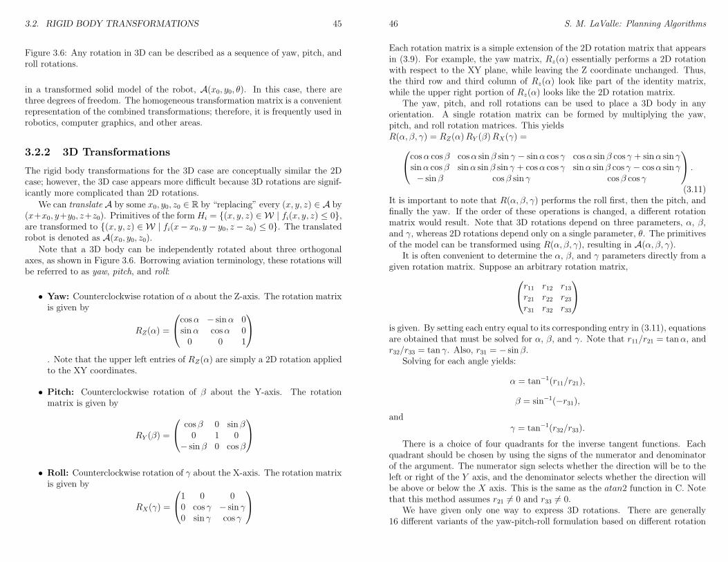
3.2. RIGID BODY TRANSFORMATIONS 45
Figure 3.6: Any rotation in 3D can be described as a sequence of yaw, pitch, androll rotations.
in a transformed solid model of the robot, A(x0, y0, θ). In this case, there arethree degrees of freedom. The homogeneous transformation matrix is a convenientrepresentation of the combined transformations; therefore, it is frequently used inrobotics, computer graphics, and other areas.
3.2.2 3D Transformations
The rigid body transformations for the 3D case are conceptually similar the 2Dcase; however, the 3D case appears more difficult because 3D rotations are signif-icantly more complicated than 2D rotations.
We can translate A by some x0, y0, z0 ∈ R by “replacing” every (x, y, z) ∈ A by(x+x0, y+y0, z+z0). Primitives of the form Hi = (x, y, z) ∈ W | fi(x, y, z) ≤ 0,are transformed to (x, y, z) ∈ W | fi(x− x0, y − y0, z − z0) ≤ 0. The translatedrobot is denoted as A(x0, y0, z0).
Note that a 3D body can be independently rotated about three orthogonalaxes, as shown in Figure 3.6. Borrowing aviation terminology, these rotations willbe referred to as yaw, pitch, and roll:
• Yaw: Counterclockwise rotation of α about the Z-axis. The rotation matrixis given by
RZ(α) =
cosα − sinα 0sinα cosα 00 0 1
. Note that the upper left entries of RZ(α) are simply a 2D rotation appliedto the XY coordinates.
• Pitch: Counterclockwise rotation of β about the Y-axis. The rotationmatrix is given by
RY (β) =
cos β 0 sin β0 1 0
− sin β 0 cos β
• Roll: Counterclockwise rotation of γ about the X-axis. The rotation matrixis given by
RX(γ) =
1 0 00 cos γ − sin γ0 sin γ cos γ
46 S. M. LaValle: Planning Algorithms
Each rotation matrix is a simple extension of the 2D rotation matrix that appearsin (3.9). For example, the yaw matrix, Rz(α) essentially performs a 2D rotationwith respect to the XY plane, while leaving the Z coordinate unchanged. Thus,the third row and third column of Rz(α) look like part of the identity matrix,while the upper right portion of Rz(α) looks like the 2D rotation matrix.
The yaw, pitch, and roll rotations can be used to place a 3D body in anyorientation. A single rotation matrix can be formed by multiplying the yaw,pitch, and roll rotation matrices. This yieldsR(α, β, γ) = RZ(α)RY (β)RX(γ) =
cosα cos β cosα sin β sin γ − sinα cos γ cosα sin β cos γ + sinα sin γsinα cos β sinα sin β sin γ + cosα cos γ sinα sin β cos γ − cosα sin γ− sin β cos β sin γ cos β cos γ
.
(3.11)It is important to note that R(α, β, γ) performs the roll first, then the pitch, andfinally the yaw. If the order of these operations is changed, a different rotationmatrix would result. Note that 3D rotations depend on three parameters, α, β,and γ, whereas 2D rotations depend only on a single parameter, θ. The primitivesof the model can be transformed using R(α, β, γ), resulting in A(α, β, γ).
It is often convenient to determine the α, β, and γ parameters directly from agiven rotation matrix. Suppose an arbitrary rotation matrix,
r11 r12 r13r21 r22 r23r31 r32 r33
is given. By setting each entry equal to its corresponding entry in (3.11), equationsare obtained that must be solved for α, β, and γ. Note that r11/r21 = tanα, andr32/r33 = tan γ. Also, r31 = − sin β.
Solving for each angle yields:
α = tan−1(r11/r21),
β = sin−1(−r31),
andγ = tan−1(r32/r33).
There is a choice of four quadrants for the inverse tangent functions. Eachquadrant should be chosen by using the signs of the numerator and denominatorof the argument. The numerator sign selects whether the direction will be to theleft or right of the Y axis, and the denominator selects whether the direction willbe above or below the X axis. This is the same as the atan2 function in C. Notethat this method assumes r21 6= 0 and r33 6= 0.
We have given only one way to express 3D rotations. There are generally16 different variants of the yaw-pitch-roll formulation based on different rotation
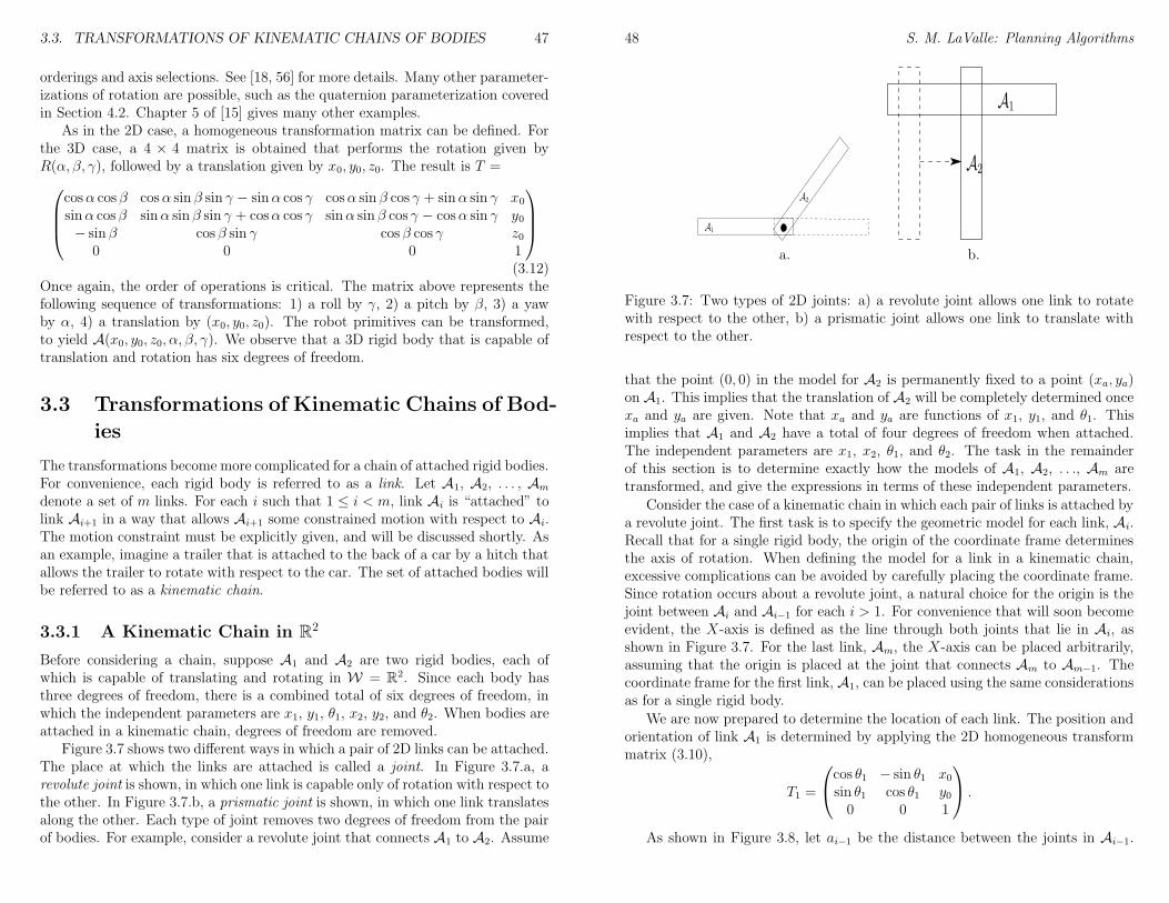
3.3. TRANSFORMATIONS OF KINEMATIC CHAINS OF BODIES 47
orderings and axis selections. See [18, 56] for more details. Many other parameter-izations of rotation are possible, such as the quaternion parameterization coveredin Section 4.2. Chapter 5 of [15] gives many other examples.
As in the 2D case, a homogeneous transformation matrix can be defined. Forthe 3D case, a 4 × 4 matrix is obtained that performs the rotation given byR(α, β, γ), followed by a translation given by x0, y0, z0. The result is T =
cosα cos β cosα sin β sin γ − sinα cos γ cosα sin β cos γ + sinα sin γ x0sinα cos β sinα sin β sin γ + cosα cos γ sinα sin β cos γ − cosα sin γ y0− sin β cos β sin γ cos β cos γ z0
0 0 0 1
(3.12)Once again, the order of operations is critical. The matrix above represents thefollowing sequence of transformations: 1) a roll by γ, 2) a pitch by β, 3) a yawby α, 4) a translation by (x0, y0, z0). The robot primitives can be transformed,to yield A(x0, y0, z0, α, β, γ). We observe that a 3D rigid body that is capable oftranslation and rotation has six degrees of freedom.
3.3 Transformations of Kinematic Chains of Bod-
ies
The transformations become more complicated for a chain of attached rigid bodies.For convenience, each rigid body is referred to as a link. Let A1, A2, . . . , Am
denote a set of m links. For each i such that 1 ≤ i < m, link Ai is “attached” tolink Ai+1 in a way that allows Ai+1 some constrained motion with respect to Ai.The motion constraint must be explicitly given, and will be discussed shortly. Asan example, imagine a trailer that is attached to the back of a car by a hitch thatallows the trailer to rotate with respect to the car. The set of attached bodies willbe referred to as a kinematic chain.
3.3.1 A Kinematic Chain in R2
Before considering a chain, suppose A1 and A2 are two rigid bodies, each ofwhich is capable of translating and rotating in W = R2. Since each body hasthree degrees of freedom, there is a combined total of six degrees of freedom, inwhich the independent parameters are x1, y1, θ1, x2, y2, and θ2. When bodies areattached in a kinematic chain, degrees of freedom are removed.
Figure 3.7 shows two different ways in which a pair of 2D links can be attached.The place at which the links are attached is called a joint. In Figure 3.7.a, arevolute joint is shown, in which one link is capable only of rotation with respect tothe other. In Figure 3.7.b, a prismatic joint is shown, in which one link translatesalong the other. Each type of joint removes two degrees of freedom from the pairof bodies. For example, consider a revolute joint that connects A1 to A2. Assume
48 S. M. LaValle: Planning Algorithms
A1
A2
A1
A2
a. b.
Figure 3.7: Two types of 2D joints: a) a revolute joint allows one link to rotatewith respect to the other, b) a prismatic joint allows one link to translate withrespect to the other.
that the point (0, 0) in the model for A2 is permanently fixed to a point (xa, ya)on A1. This implies that the translation of A2 will be completely determined oncexa and ya are given. Note that xa and ya are functions of x1, y1, and θ1. Thisimplies that A1 and A2 have a total of four degrees of freedom when attached.The independent parameters are x1, x2, θ1, and θ2. The task in the remainderof this section is to determine exactly how the models of A1, A2, . . ., Am aretransformed, and give the expressions in terms of these independent parameters.
Consider the case of a kinematic chain in which each pair of links is attached bya revolute joint. The first task is to specify the geometric model for each link, Ai.Recall that for a single rigid body, the origin of the coordinate frame determinesthe axis of rotation. When defining the model for a link in a kinematic chain,excessive complications can be avoided by carefully placing the coordinate frame.Since rotation occurs about a revolute joint, a natural choice for the origin is thejoint between Ai and Ai−1 for each i > 1. For convenience that will soon becomeevident, the X-axis is defined as the line through both joints that lie in Ai, asshown in Figure 3.7. For the last link, Am, the X-axis can be placed arbitrarily,assuming that the origin is placed at the joint that connects Am to Am−1. Thecoordinate frame for the first link, A1, can be placed using the same considerationsas for a single rigid body.
We are now prepared to determine the location of each link. The position andorientation of link A1 is determined by applying the 2D homogeneous transformmatrix (3.10),
T1 =
cos θ1 − sin θ1 x0sin θ1 cos θ1 y00 0 1
.
As shown in Figure 3.8, let ai−1 be the distance between the joints in Ai−1.
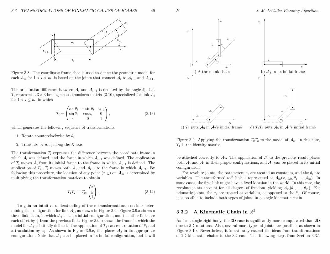
3.3. TRANSFORMATIONS OF KINEMATIC CHAINS OF BODIES 49
A i
Y
X
ai
A i+1
A i−1
θi+1
Figure 3.8: The coordinate frame that is used to define the geometric model foreach Ai, for 1 < i < m, is based on the joints that connect Ai to Ai−1 and Ai+1.
The orientation difference between Ai and Ai−1 is denoted by the angle θi. LetTi represent a 3× 3 homogeneous transform matrix (3.10), specialized for link Ai
for 1 < i ≤ m, in which
Ti =
cos θi − sin θi ai−1sin θi cos θi 00 0 1
, (3.13)
which generates the following sequence of transformations:
1. Rotate counterclockwise by θi
2. Translate by ai−1 along the X-axis
The transformation Ti expresses the difference between the coordinate frame inwhich Ai was defined, and the frame in which Ai−1 was defined. The applicationof Ti moves Ai from its initial frame to the frame in which Ai−1 is defined. Theapplication of Ti−1Ti moves both Ai and Ai−1 to the frame in which Ai−2. Byfollowing this procedure, the location of any point (x, y) on Am is determined bymultiplying the transformation matrices to obtain
T1T2 · · ·Tm
xy1
. (3.14)
To gain an intuitive understanding of these transformations, consider deter-mining the configuration for link A3, as shown in Figure 3.9. Figure 3.9.a shows athree-link chain, in which A1 is at its initial configuration, and the other links areeach offset by π
2from the previous link. Figure 3.9.b shows the frame in which the
model for A3 is initially defined. The application of T3 causes a rotation of θ3 anda translation by a2. As shown in Figure 3.9.c, this places A3 in its appropriateconfiguration. Note that A2 can be placed in its initial configuration, and it will
50 S. M. LaValle: Planning Algorithms
X1
X2
X3
θ3
θ2A1
A3
Y1
A2A3
Y3
X3
a) A three-link chain b) A3 in its initial frame
X2
A2
Y2
A3
X1
A1
A3
Y1
A2
c) T3 puts A3 in A2’s initial frame d) T2T3 puts A3 in A1’s initial frame
Figure 3.9: Applying the transformation T2T3 to the model of A3. In this case,T1 is the identity matrix.
be attached correctly to A3. The application of T2 to the previous result placesboth A3 and A2 in their proper configurations, and A1 can be placed in its initialconfiguration.
For revolute joints, the parameters ai are treated as constants, and the θi arevariables. The transformed mth link is represented as Am(x0, y0, θ1, . . . , θm). Insome cases, the first link might have a fixed location in the world. In this case, therevolute joints account for all degrees of freedom, yielding Am(θ1, . . . , θm). Forprismatic joints, the ai are treated as variables, as opposed to the θi. Of course,it is possible to include both types of joints in a single kinematic chain.
3.3.2 A Kinematic Chain in R3
As for a single rigid body, the 3D case is significantly more complicated than 2Ddue to 3D rotations. Also, several more types of joints are possible, as shown inFigure 3.10. Nevertheless, it is naturally extend the ideas from transformationsof 2D kinematic chains to the 3D case. The following steps from Section 3.3.1
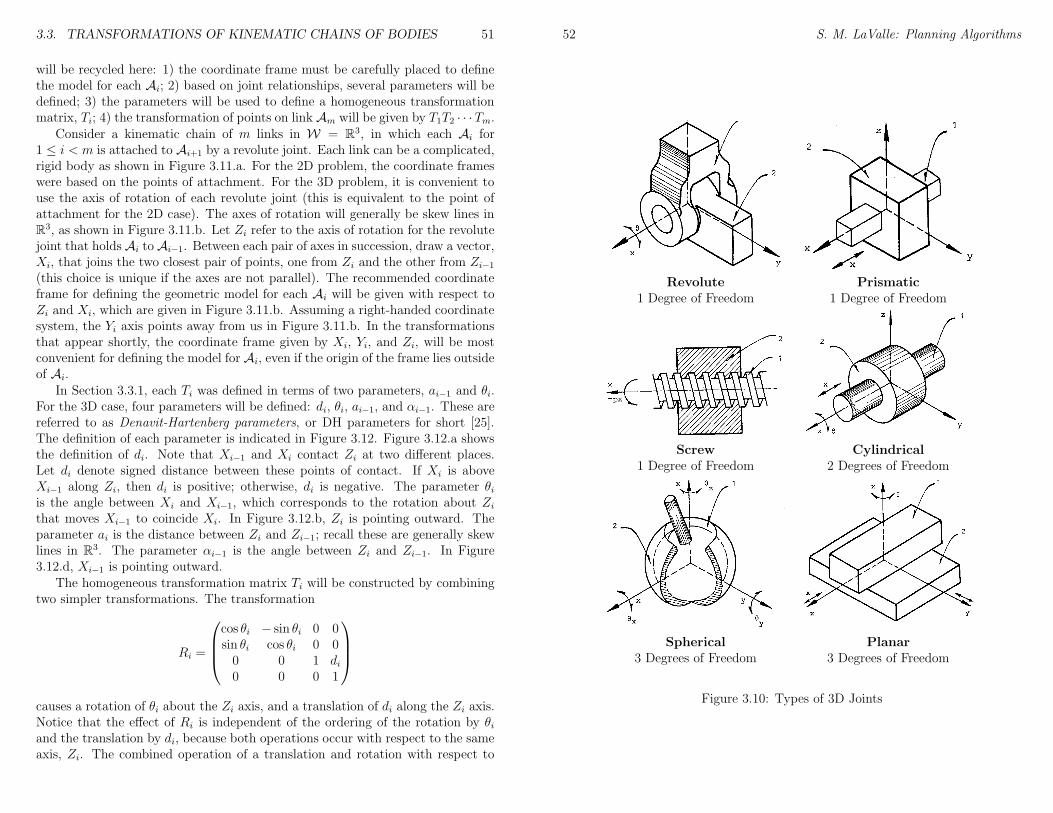
3.3. TRANSFORMATIONS OF KINEMATIC CHAINS OF BODIES 51
will be recycled here: 1) the coordinate frame must be carefully placed to definethe model for each Ai; 2) based on joint relationships, several parameters will bedefined; 3) the parameters will be used to define a homogeneous transformationmatrix, Ti; 4) the transformation of points on link Am will be given by T1T2 · · ·Tm.
Consider a kinematic chain of m links in W = R3, in which each Ai for1 ≤ i < m is attached to Ai+1 by a revolute joint. Each link can be a complicated,rigid body as shown in Figure 3.11.a. For the 2D problem, the coordinate frameswere based on the points of attachment. For the 3D problem, it is convenient touse the axis of rotation of each revolute joint (this is equivalent to the point ofattachment for the 2D case). The axes of rotation will generally be skew lines inR3, as shown in Figure 3.11.b. Let Zi refer to the axis of rotation for the revolutejoint that holds Ai to Ai−1. Between each pair of axes in succession, draw a vector,Xi, that joins the two closest pair of points, one from Zi and the other from Zi−1(this choice is unique if the axes are not parallel). The recommended coordinateframe for defining the geometric model for each Ai will be given with respect toZi and Xi, which are given in Figure 3.11.b. Assuming a right-handed coordinatesystem, the Yi axis points away from us in Figure 3.11.b. In the transformationsthat appear shortly, the coordinate frame given by Xi, Yi, and Zi, will be mostconvenient for defining the model for Ai, even if the origin of the frame lies outsideof Ai.
In Section 3.3.1, each Ti was defined in terms of two parameters, ai−1 and θi.For the 3D case, four parameters will be defined: di, θi, ai−1, and αi−1. These arereferred to as Denavit-Hartenberg parameters, or DH parameters for short [25].The definition of each parameter is indicated in Figure 3.12. Figure 3.12.a showsthe definition of di. Note that Xi−1 and Xi contact Zi at two different places.Let di denote signed distance between these points of contact. If Xi is aboveXi−1 along Zi, then di is positive; otherwise, di is negative. The parameter θiis the angle between Xi and Xi−1, which corresponds to the rotation about Zi
that moves Xi−1 to coincide Xi. In Figure 3.12.b, Zi is pointing outward. Theparameter ai is the distance between Zi and Zi−1; recall these are generally skewlines in R3. The parameter αi−1 is the angle between Zi and Zi−1. In Figure3.12.d, Xi−1 is pointing outward.
The homogeneous transformation matrix Ti will be constructed by combiningtwo simpler transformations. The transformation
Ri =
cos θi − sin θi 0 0sin θi cos θi 0 00 0 1 di0 0 0 1
causes a rotation of θi about the Zi axis, and a translation of di along the Zi axis.Notice that the effect of Ri is independent of the ordering of the rotation by θiand the translation by di, because both operations occur with respect to the sameaxis, Zi. The combined operation of a translation and rotation with respect to
52 S. M. LaValle: Planning Algorithms
Revolute Prismatic1 Degree of Freedom 1 Degree of Freedom
Screw Cylindrical1 Degree of Freedom 2 Degrees of Freedom
Spherical Planar3 Degrees of Freedom 3 Degrees of Freedom
Figure 3.10: Types of 3D Joints
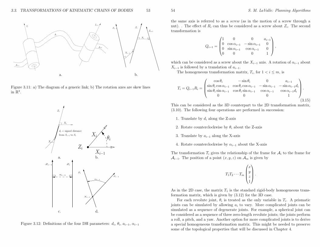
3.3. TRANSFORMATIONS OF KINEMATIC CHAINS OF BODIES 53
Ai
Ai−1
Ai+1
Zi+1Zi
Zi−1 Zi
Zi+1
Xi
Xi−1
a. b.
Figure 3.11: a) The diagram of a generic link; b) The rotation axes are skew linesin R3.
Zi
Xi
Xi−1
di = signed distance
from Si−1 to Si Xi
Xi−1
θi
Zi
a. b.
ZiZi−1
ai−1
αi−1
Zi
Zi−1
Xi−1
c. d.
Figure 3.12: Definitions of the four DH parameters: di, θi, ai−1, αi−1
54 S. M. LaValle: Planning Algorithms
the same axis is referred to as a screw (as in the motion of a screw through anut). . The effect of Ri can thus be considered as a screw about Zi. The secondtransformation is
Qi−1 =
1 0 0 ai−10 cosαi−1 − sinαi−1 00 sinαi−1 cosαi−1 00 0 0 1
,
which can be considered as a screw about the Xi−1 axis. A rotation of αi−1 aboutXi−1 is followed by a translation of ai−1.
The homogeneous transformation matrix, Ti, for 1 < i ≤ m, is
Ti = Qi−1Ri =
cos θi − sin θi 0 ai−1sin θi cosαi−1 cos θi cosαi−1 − sinαi−1 − sinαi−1disin θi sinαi−1 cos θi sinαi−1 cosαi−1 cosαi−1di
0 0 0 1
.
(3.15)This can be considered as the 3D counterpart to the 2D transformation matrix,(3.10). The following four operations are performed in succession:
1. Translate by di along the Z-axis
2. Rotate counterclockwise by θi about the Z-axis
3. Translate by ai−1 along the X-axis
4. Rotate counterclockwise by αi−1 about the X-axis
The transformation Ti gives the relationship of the frame for Ai to the frame forAi−1. The position of a point (x, y, z) on Am is given by
T1T2 · · ·Tm
xyz1
.
As in the 2D case, the matrix T1 is the standard rigid-body homogeneous trans-formation matrix, which is given by (3.12) for the 3D case.
For each revolute joint, θi is treated as the only variable in Ti. A prismaticjoints can be simulated by allowing ai to vary. More complicated joints can besimulated as a sequence of degenerate joints. For example, a spherical joint canbe considered as a sequence of three zero-length revolute joints; the joints performa roll, a pitch, and a yaw. Another option for more complicated joints is to derivea special homogeneous transformation matrix. This might be needed to preservesome of the topological properties that will be discussed in Chapter 4.
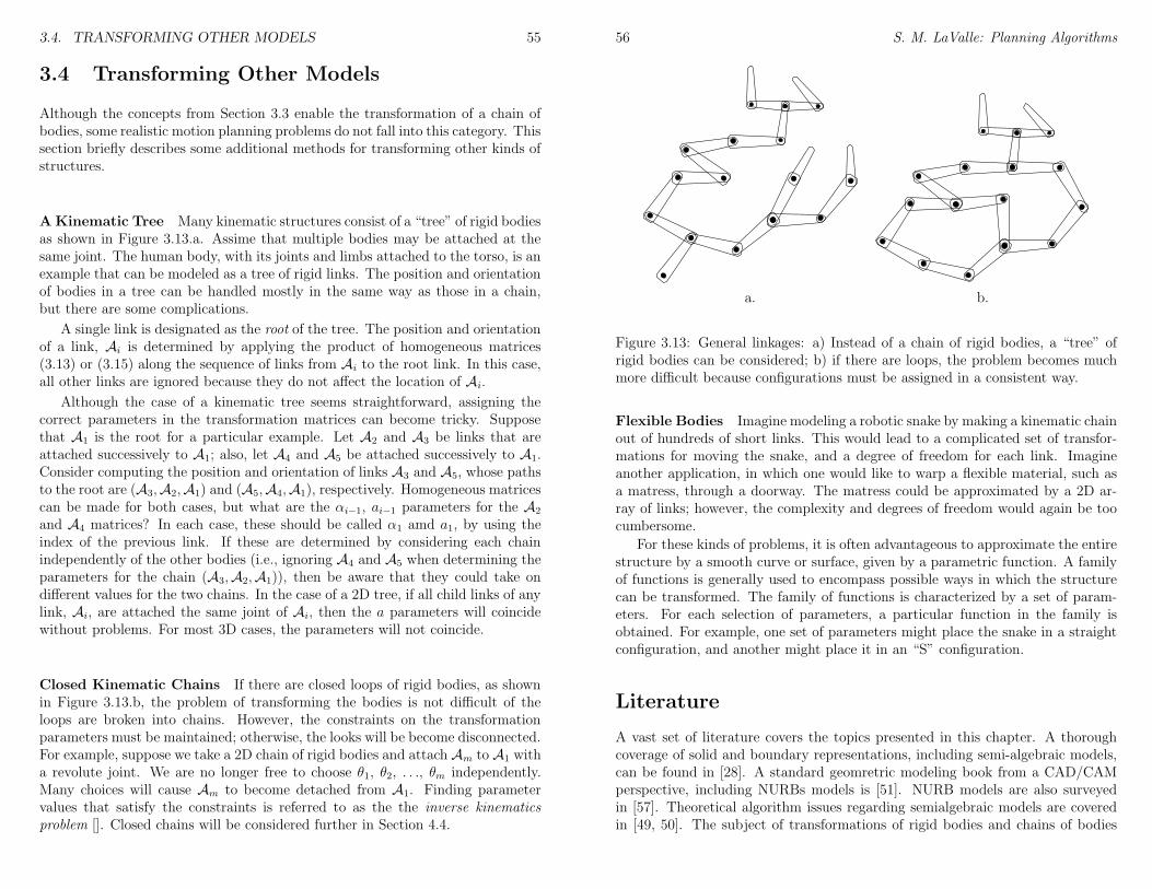
3.4. TRANSFORMING OTHER MODELS 55
3.4 Transforming Other Models
Although the concepts from Section 3.3 enable the transformation of a chain ofbodies, some realistic motion planning problems do not fall into this category. Thissection briefly describes some additional methods for transforming other kinds ofstructures.
AKinematic Tree Many kinematic structures consist of a “tree” of rigid bodiesas shown in Figure 3.13.a. Assime that multiple bodies may be attached at thesame joint. The human body, with its joints and limbs attached to the torso, is anexample that can be modeled as a tree of rigid links. The position and orientationof bodies in a tree can be handled mostly in the same way as those in a chain,but there are some complications.
A single link is designated as the root of the tree. The position and orientationof a link, Ai is determined by applying the product of homogeneous matrices(3.13) or (3.15) along the sequence of links from Ai to the root link. In this case,all other links are ignored because they do not affect the location of Ai.
Although the case of a kinematic tree seems straightforward, assigning thecorrect parameters in the transformation matrices can become tricky. Supposethat A1 is the root for a particular example. Let A2 and A3 be links that areattached successively to A1; also, let A4 and A5 be attached successively to A1.Consider computing the position and orientation of links A3 and A5, whose pathsto the root are (A3,A2,A1) and (A5,A4,A1), respectively. Homogeneous matricescan be made for both cases, but what are the αi−1, ai−1 parameters for the A2and A4 matrices? In each case, these should be called α1 amd a1, by using theindex of the previous link. If these are determined by considering each chainindependently of the other bodies (i.e., ignoring A4 and A5 when determining theparameters for the chain (A3,A2,A1)), then be aware that they could take ondifferent values for the two chains. In the case of a 2D tree, if all child links of anylink, Ai, are attached the same joint of Ai, then the a parameters will coincidewithout problems. For most 3D cases, the parameters will not coincide.
Closed Kinematic Chains If there are closed loops of rigid bodies, as shownin Figure 3.13.b, the problem of transforming the bodies is not difficult of theloops are broken into chains. However, the constraints on the transformationparameters must be maintained; otherwise, the looks will be become disconnected.For example, suppose we take a 2D chain of rigid bodies and attach Am to A1 witha revolute joint. We are no longer free to choose θ1, θ2, . . ., θm independently.Many choices will cause Am to become detached from A1. Finding parametervalues that satisfy the constraints is referred to as the the inverse kinematicsproblem []. Closed chains will be considered further in Section 4.4.
56 S. M. LaValle: Planning Algorithms
a. b.
Figure 3.13: General linkages: a) Instead of a chain of rigid bodies, a “tree” ofrigid bodies can be considered; b) if there are loops, the problem becomes muchmore difficult because configurations must be assigned in a consistent way.
Flexible Bodies Imagine modeling a robotic snake by making a kinematic chainout of hundreds of short links. This would lead to a complicated set of transfor-mations for moving the snake, and a degree of freedom for each link. Imagineanother application, in which one would like to warp a flexible material, such asa matress, through a doorway. The matress could be approximated by a 2D ar-ray of links; however, the complexity and degrees of freedom would again be toocumbersome.
For these kinds of problems, it is often advantageous to approximate the entirestructure by a smooth curve or surface, given by a parametric function. A familyof functions is generally used to encompass possible ways in which the structurecan be transformed. The family of functions is characterized by a set of param-eters. For each selection of parameters, a particular function in the family isobtained. For example, one set of parameters might place the snake in a straightconfiguration, and another might place it in an “S” configuration.
Literature
A vast set of literature covers the topics presented in this chapter. A thoroughcoverage of solid and boundary representations, including semi-algebraic models,can be found in [28]. A standard geomretric modeling book from a CAD/CAMperspective, including NURBs models is [51]. NURB models are also surveyedin [57]. Theoretical algorithm issues regarding semialgebraic models are coveredin [49, 50]. The subject of transformations of rigid bodies and chains of bodies
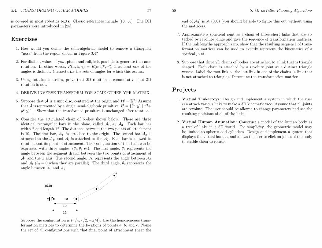
3.4. TRANSFORMING OTHER MODELS 57
is covered in most robotics texts. Classic references include [18, 56]. The DHparameters were introduced in [25].
Exercises
1. How would you define the semi-algebraic model to remove a triangular“nose” from the region shown in Figure 3.4?
2. For distinct values of yaw, pitch, and roll, is it possible to generate the samerotation. In other words, R(α, β, γ) = R(α′, β′, γ′), if at least one of theangles is distinct. Characterize the sets of angles for which this occurs.
3. Using rotation matrices, prove that 2D rotation is commutative, but 3Drotation is not.
4. DERIVE INVERSE TRANSFORM FOR SOME OTHER YPR MATRIX.
5. Suppose that A is a unit disc, centered at the origin and W = R2. AssumethatA is represented by a single, semi-algebraic primitive, H = (x, y) | x2+y2 ≤ 1. Show that the transformed primitive is unchanged after rotation.
6. Consider the articulated chain of bodies shown below. There are threeidentical rectangular bars in the plane, called A1,A2,A3. Each bar haswidth 2 and length 12. The distance between the two points of attachmentis 10. The first bar, A1, is attached to the origin. The second bar A2 isattached to the A1, and A3 is attached to the A2. Each bar is allowed torotate about its point of attachment. The configuration of the chain can beexpressed with three angles, (θ1, θ2, θ3). The first angle, θ1 represents theangle between the segment drawn between the two points of attachment ofA1 and the x axis. The second angle, θ2, represents the angle between A2and A1 (θ2 = 0 when they are parallel). The third angle, θ3 represents theangle between A3 and A2.
(0,0)
2
10
a
b
c
12
Suppose the configuration is (π/4, π/2,−π/4). Use the homogeneous trans-formation matrices to determine the locations of points a, b, and c. Namethe set of all configurations such that final point of attachment (near the
58 S. M. LaValle: Planning Algorithms
end of A3) is at (0, 0) (you should be able to figure this out without usingthe matrices).
7. Approximate a spherical joint as a chain of three short links that are at-tached by revolute joints and give the sequence of transformation matrices.If the link lengths approach zero, show that the resulting sequence of trans-formation matrices can be used to exactly represent the kinematics of asperical joint.
8. Suppose that three 2D chains of bodies are attached to a link that is triangleshaped. Each chain is attached by a revolute joint at a distinct trianglevertex. Label the root link as the last link in one of the chains (a link thatis not attached to triangle). Determine the transformation matrices.
Projects
1. Virtual Tinkertoys: Design and implement a system in which the usercan attach various links to make a 3D kinematic tree. Assume that all jointsare revolute. The user should be allowed to change parameters and see theresulting positions of all of the links.
2. Virtual Human Animation: Construct a model of the human body asa tree of links in a 3D world. For simplicity, the geometric model maybe limited to spheres and cylinders. Design and implement a system thatdisplays the virtual human, and allows the user to click on joints of the bodyto enable them to rotate.
Chapter 4
The Configuration Space
The concepts of Chapter 3 enable the construction and transformation geometricmodels, which can be used to formulate path planning problems in the world, W .For the development and analysis of algorithms, however, it will be convenientto view the path planning as a search in the space of possible transformationsthat can be applied to the robot, A. This space of transformations is termedthe configuration space, which represents a powerful representation that unifies abroad class of path planning problems in a single mathematical framework. Thisfacilitates the development of path planning techniques that can be applied oradapted to a wide variety of robots and models.
Section 4.1 introduces some preliminary mathematical concepts from topology.Section 4.2 defines the configuration space for a given robot and its set of pos-sible transformations. Section 4.2 characterizes the portion of the configurationspace in which the robot is in collision with an obstacle. Section 6.1 presents anoverview of the collision detection problem. Section 4.4 represents configurationspace concepts for the complicated case in which closed kinematic chains exist.
4.1 Basic Topological Concepts
4.1.1 Topological Spaces
A set X is called a topological space if there is a collection of subsets of X calledopen sets such that the following axioms hold:
1. The union of any number of open sets is an open set.
2. The intersection of a finite number of open set is an open set.
3. Both X and ∅ are open sets.
Examples of topological spaces:
59
60 S. M. LaValle: Planning Algorithms
• X = RIn this case, the open sets are defined in the familiar way; a topologicalspace is simply a generalization of the open set concept for R. Examples ofopen sets are open intervals, such as (0, 2) or (1, 3) (i.e., the endpoints arenot included). By using the axioms, sets such as (1, 2) and (0, 3) must beopen sets. Other examples include a set of intervals, such as (0, 1) ∪ (5, 6),and intervals that extend toward infinity, such as (0,∞).
• X = Rn
Consider the case of n = 2. An example of an open set is (x, y) | x2+ y2 <1, the interior of the unit circle.
• X = cat, dog, tree, house. A topological space can be defined for any set,as long as the declared open sets obey the axioms. For this case, supposethat cat and dog are open sets. Then, car, dog must also be an openset. Closed sets and boundary points can be easily derived for this topologyonce the open sets are defined.
• We could even define a trivial topological space for any set X by simplydeclaring that X and ∅ are the only open sets (verify that all of the axiomsare satisfied).
Closed sets For a given topological space, a collection of closed sets can beinferred. A subset C of a topological space X is a closed set if and only if X \ Cis an open set.
Examples of closed sets for the case of X = R are closed intervals, such as[0, 1], and countable collections of points, such as −1, 3, 7. Verify that thesesatisfy the definition.
Here is a question to ponder: are all subsets of X either closed or open?Although it appears that open sets and closed sets are opposites in some sense,the answer to the question is NO. The interval [0, 2π) is neither open nor closedif X = R (the interval [2π,∞) is closed and (−∞, 0) is open). Note that X and∅ are both open and closed!
Boundary and Closure Let U be any subset of a topological space X. A pointx ∈ X is a boundary point of U if neither U nor X \ U contains an open subsetthat contains x.
Consider an example for which X = R. If U = (0, 1), then 0 and 1 areboundary points of U . If U = [0, 1], 0 and 1 are still boundary points of U . LetX = R2. Any point (x, y) such that x2 + y2 = 1 is a boundary point of the set(x, y) | x2 + y2 < 1.
The set of all boundary points of U is called the boundary of U , denoted by∂U . The closure of U is the union of U with its boundary, ∂U . Note that the
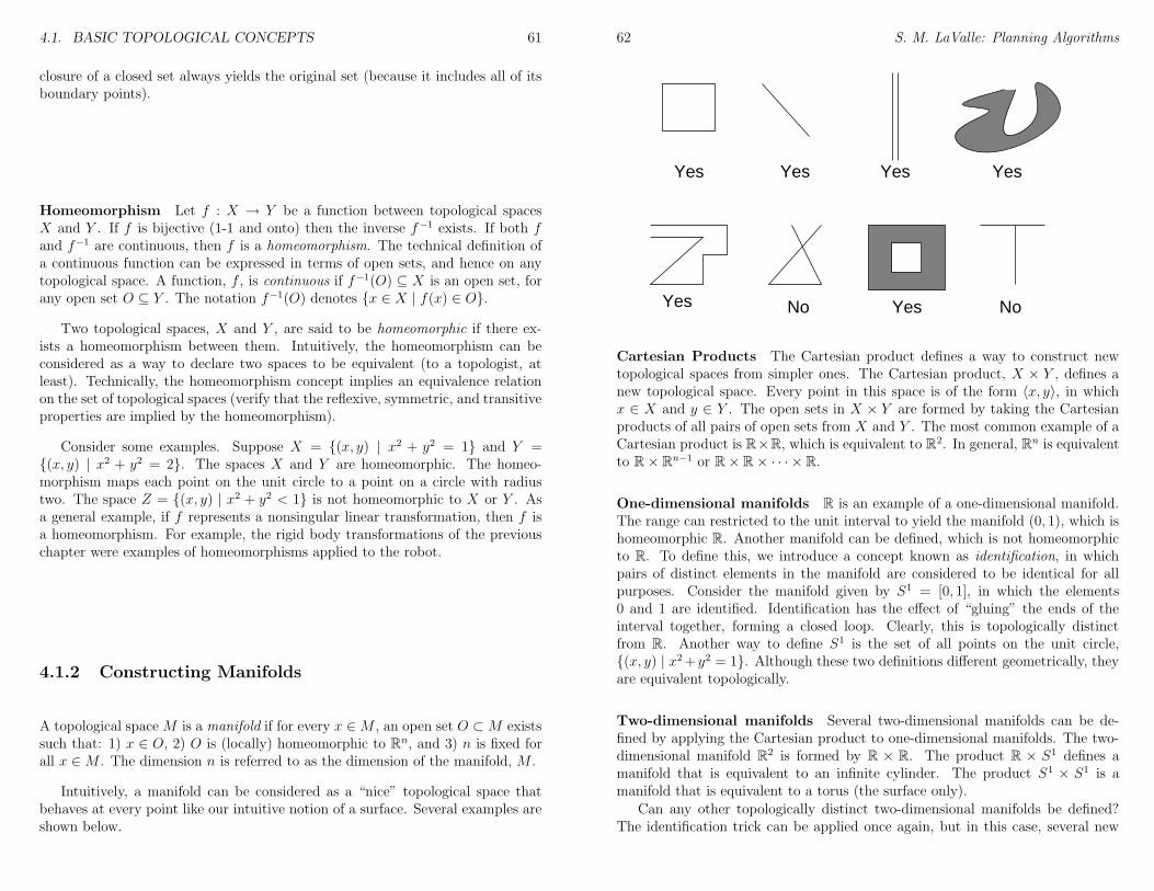
4.1. BASIC TOPOLOGICAL CONCEPTS 61
closure of a closed set always yields the original set (because it includes all of itsboundary points).
Homeomorphism Let f : X → Y be a function between topological spacesX and Y . If f is bijective (1-1 and onto) then the inverse f−1 exists. If both fand f−1 are continuous, then f is a homeomorphism. The technical definition ofa continuous function can be expressed in terms of open sets, and hence on anytopological space. A function, f , is continuous if f−1(O) ⊆ X is an open set, forany open set O ⊆ Y . The notation f−1(O) denotes x ∈ X | f(x) ∈ O.
Two topological spaces, X and Y , are said to be homeomorphic if there ex-ists a homeomorphism between them. Intuitively, the homeomorphism can beconsidered as a way to declare two spaces to be equivalent (to a topologist, atleast). Technically, the homeomorphism concept implies an equivalence relationon the set of topological spaces (verify that the reflexive, symmetric, and transitiveproperties are implied by the homeomorphism).
Consider some examples. Suppose X = (x, y) | x2 + y2 = 1 and Y =(x, y) | x2 + y2 = 2. The spaces X and Y are homeomorphic. The homeo-morphism maps each point on the unit circle to a point on a circle with radiustwo. The space Z = (x, y) | x2 + y2 < 1 is not homeomorphic to X or Y . Asa general example, if f represents a nonsingular linear transformation, then f isa homeomorphism. For example, the rigid body transformations of the previouschapter were examples of homeomorphisms applied to the robot.
4.1.2 Constructing Manifolds
A topological space M is a manifold if for every x ∈M , an open set O ⊂M existssuch that: 1) x ∈ O, 2) O is (locally) homeomorphic to Rn, and 3) n is fixed forall x ∈M . The dimension n is referred to as the dimension of the manifold, M .
Intuitively, a manifold can be considered as a “nice” topological space thatbehaves at every point like our intuitive notion of a surface. Several examples areshown below.
62 S. M. LaValle: Planning Algorithms
Yes
NoYes
Yes Yes
Yes No
Yes
Cartesian Products The Cartesian product defines a way to construct newtopological spaces from simpler ones. The Cartesian product, X × Y , defines anew topological space. Every point in this space is of the form 〈x, y〉, in whichx ∈ X and y ∈ Y . The open sets in X × Y are formed by taking the Cartesianproducts of all pairs of open sets from X and Y . The most common example of aCartesian product is R×R, which is equivalent to R2. In general, Rn is equivalentto R× Rn−1 or R× R× · · · × R.
One-dimensional manifolds R is an example of a one-dimensional manifold.The range can restricted to the unit interval to yield the manifold (0, 1), which ishomeomorphic R. Another manifold can be defined, which is not homeomorphicto R. To define this, we introduce a concept known as identification, in whichpairs of distinct elements in the manifold are considered to be identical for allpurposes. Consider the manifold given by S1 = [0, 1], in which the elements0 and 1 are identified. Identification has the effect of “gluing” the ends of theinterval together, forming a closed loop. Clearly, this is topologically distinctfrom R. Another way to define S1 is the set of all points on the unit circle,(x, y) | x2+y2 = 1. Although these two definitions different geometrically, theyare equivalent topologically.
Two-dimensional manifolds Several two-dimensional manifolds can be de-fined by applying the Cartesian product to one-dimensional manifolds. The two-dimensional manifold R2 is formed by R × R. The product R × S1 defines amanifold that is equivalent to an infinite cylinder. The product S1 × S1 is amanifold that is equivalent to a torus (the surface only).
Can any other topologically distinct two-dimensional manifolds be defined?The identification trick can be applied once again, but in this case, several new
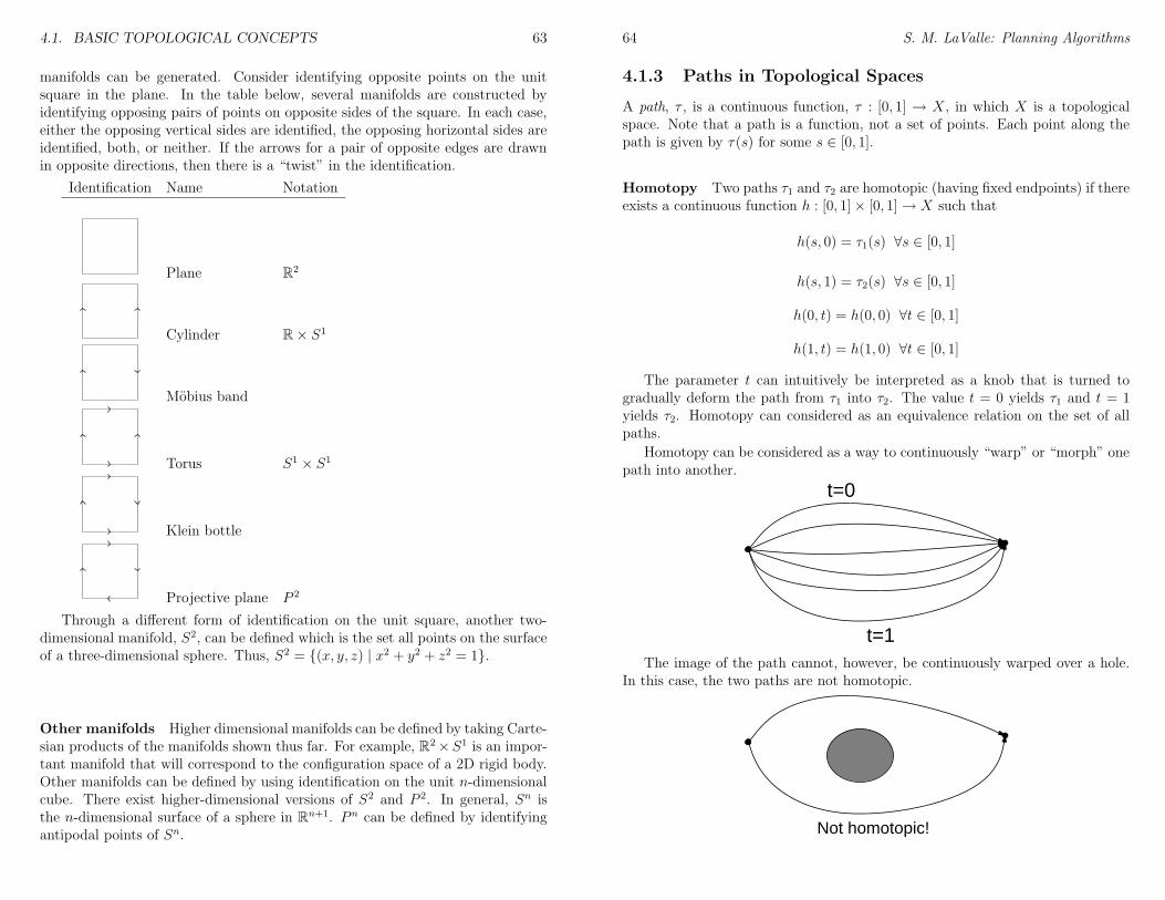
4.1. BASIC TOPOLOGICAL CONCEPTS 63
manifolds can be generated. Consider identifying opposite points on the unitsquare in the plane. In the table below, several manifolds are constructed byidentifying opposing pairs of points on opposite sides of the square. In each case,either the opposing vertical sides are identified, the opposing horizontal sides areidentified, both, or neither. If the arrows for a pair of opposite edges are drawnin opposite directions, then there is a “twist” in the identification.
Identification Name Notation
Plane R2
Cylinder R× S1
Mobius band
Torus S1 × S1
Klein bottle
Projective plane P 2
Through a different form of identification on the unit square, another two-dimensional manifold, S2, can be defined which is the set all points on the surfaceof a three-dimensional sphere. Thus, S2 = (x, y, z) | x2 + y2 + z2 = 1.
Other manifolds Higher dimensional manifolds can be defined by taking Carte-sian products of the manifolds shown thus far. For example, R2×S1 is an impor-tant manifold that will correspond to the configuration space of a 2D rigid body.Other manifolds can be defined by using identification on the unit n-dimensionalcube. There exist higher-dimensional versions of S2 and P 2. In general, Sn isthe n-dimensional surface of a sphere in Rn+1. P n can be defined by identifyingantipodal points of Sn.
64 S. M. LaValle: Planning Algorithms
4.1.3 Paths in Topological Spaces
A path, τ , is a continuous function, τ : [0, 1] → X, in which X is a topologicalspace. Note that a path is a function, not a set of points. Each point along thepath is given by τ(s) for some s ∈ [0, 1].
Homotopy Two paths τ1 and τ2 are homotopic (having fixed endpoints) if thereexists a continuous function h : [0, 1]× [0, 1]→ X such that
h(s, 0) = τ1(s) ∀s ∈ [0, 1]
h(s, 1) = τ2(s) ∀s ∈ [0, 1]
h(0, t) = h(0, 0) ∀t ∈ [0, 1]
h(1, t) = h(1, 0) ∀t ∈ [0, 1]
The parameter t can intuitively be interpreted as a knob that is turned togradually deform the path from τ1 into τ2. The value t = 0 yields τ1 and t = 1yields τ2. Homotopy can considered as an equivalence relation on the set of allpaths.
Homotopy can be considered as a way to continuously “warp” or “morph” onepath into another.
t=0
t=1The image of the path cannot, however, be continuously warped over a hole.
In this case, the two paths are not homotopic.
Not homotopic!
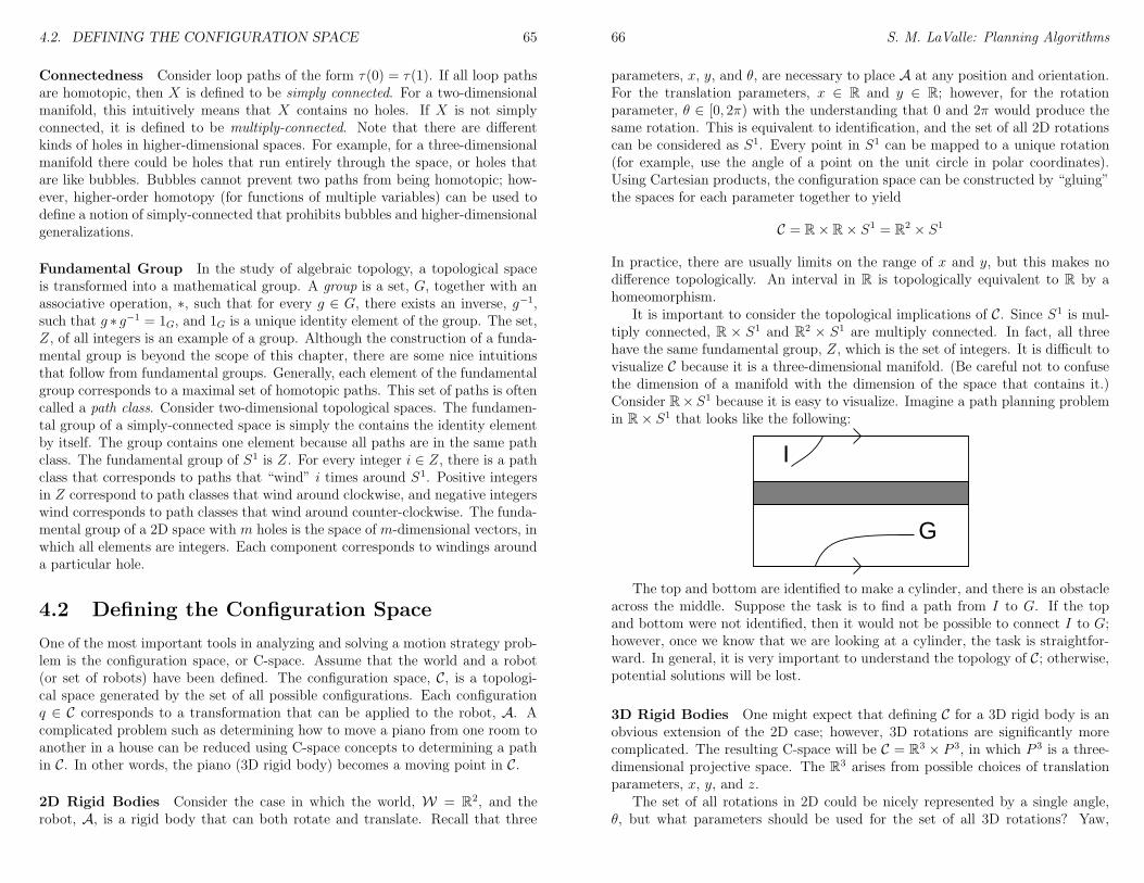
4.2. DEFINING THE CONFIGURATION SPACE 65
Connectedness Consider loop paths of the form τ(0) = τ(1). If all loop pathsare homotopic, then X is defined to be simply connected. For a two-dimensionalmanifold, this intuitively means that X contains no holes. If X is not simplyconnected, it is defined to be multiply-connected. Note that there are differentkinds of holes in higher-dimensional spaces. For example, for a three-dimensionalmanifold there could be holes that run entirely through the space, or holes thatare like bubbles. Bubbles cannot prevent two paths from being homotopic; how-ever, higher-order homotopy (for functions of multiple variables) can be used todefine a notion of simply-connected that prohibits bubbles and higher-dimensionalgeneralizations.
Fundamental Group In the study of algebraic topology, a topological spaceis transformed into a mathematical group. A group is a set, G, together with anassociative operation, ∗, such that for every g ∈ G, there exists an inverse, g−1,such that g ∗ g−1 = 1G, and 1G is a unique identity element of the group. The set,Z, of all integers is an example of a group. Although the construction of a funda-mental group is beyond the scope of this chapter, there are some nice intuitionsthat follow from fundamental groups. Generally, each element of the fundamentalgroup corresponds to a maximal set of homotopic paths. This set of paths is oftencalled a path class. Consider two-dimensional topological spaces. The fundamen-tal group of a simply-connected space is simply the contains the identity elementby itself. The group contains one element because all paths are in the same pathclass. The fundamental group of S1 is Z. For every integer i ∈ Z, there is a pathclass that corresponds to paths that “wind” i times around S1. Positive integersin Z correspond to path classes that wind around clockwise, and negative integerswind corresponds to path classes that wind around counter-clockwise. The funda-mental group of a 2D space with m holes is the space of m-dimensional vectors, inwhich all elements are integers. Each component corresponds to windings arounda particular hole.
4.2 Defining the Configuration Space
One of the most important tools in analyzing and solving a motion strategy prob-lem is the configuration space, or C-space. Assume that the world and a robot(or set of robots) have been defined. The configuration space, C, is a topologi-cal space generated by the set of all possible configurations. Each configurationq ∈ C corresponds to a transformation that can be applied to the robot, A. Acomplicated problem such as determining how to move a piano from one room toanother in a house can be reduced using C-space concepts to determining a pathin C. In other words, the piano (3D rigid body) becomes a moving point in C.
2D Rigid Bodies Consider the case in which the world, W = R2, and therobot, A, is a rigid body that can both rotate and translate. Recall that three
66 S. M. LaValle: Planning Algorithms
parameters, x, y, and θ, are necessary to place A at any position and orientation.For the translation parameters, x ∈ R and y ∈ R; however, for the rotationparameter, θ ∈ [0, 2π) with the understanding that 0 and 2π would produce thesame rotation. This is equivalent to identification, and the set of all 2D rotationscan be considered as S1. Every point in S1 can be mapped to a unique rotation(for example, use the angle of a point on the unit circle in polar coordinates).Using Cartesian products, the configuration space can be constructed by “gluing”the spaces for each parameter together to yield
C = R× R× S1 = R2 × S1
In practice, there are usually limits on the range of x and y, but this makes nodifference topologically. An interval in R is topologically equivalent to R by ahomeomorphism.
It is important to consider the topological implications of C. Since S1 is mul-tiply connected, R × S1 and R2 × S1 are multiply connected. In fact, all threehave the same fundamental group, Z, which is the set of integers. It is difficult tovisualize C because it is a three-dimensional manifold. (Be careful not to confusethe dimension of a manifold with the dimension of the space that contains it.)Consider R×S1 because it is easy to visualize. Imagine a path planning problemin R× S1 that looks like the following:
I
G
The top and bottom are identified to make a cylinder, and there is an obstacleacross the middle. Suppose the task is to find a path from I to G. If the topand bottom were not identified, then it would not be possible to connect I to G;however, once we know that we are looking at a cylinder, the task is straightfor-ward. In general, it is very important to understand the topology of C; otherwise,potential solutions will be lost.
3D Rigid Bodies One might expect that defining C for a 3D rigid body is anobvious extension of the 2D case; however, 3D rotations are significantly morecomplicated. The resulting C-space will be C = R3 × P 3, in which P 3 is a three-dimensional projective space. The R3 arises from possible choices of translationparameters, x, y, and z.
The set of all rotations in 2D could be nicely represented by a single angle,θ, but what parameters should be used for the set of all 3D rotations? Yaw,
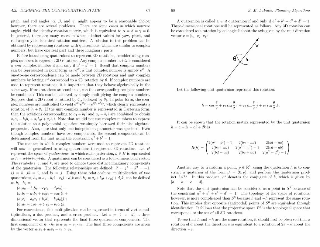
4.2. DEFINING THE CONFIGURATION SPACE 67
pitch, and roll angles, α, β, and γ, might appear to be a reasonable choice;however, there are several problems. There are some cases in which nonzeroangles yield the identity rotation matrix, which is equivalent to α = β = γ = 0.In general, there are many cases in which distinct values for yaw, pitch, androll angles yield identical rotation matrices. A solution to this problem can beobtained by representing rotations with quaternions, which are similar to complexnumbers, but have one real part and three imaginary parts.
Before introducing quaternions to represent 3D rotations, consider using com-plex numbers to represent 2D rotations. Any complex number, a+bi is considereda unit complex number if and only if a2 + b2 = 1. Recall that complex numberscan be represented in polar form as reiθ; a unit complex number is simply eiθ. Aone-to-one correspondence can be made between 2D rotations and unit complexnumbers by letting eiθ correspond to a 2D rotation by θ. If complex numbers areused to represent rotations, it is important that they behave algebraically in thesame way. If two rotations are combined, can the corresponding complex numbersbe combined? This can be achieved by simply multiplying the complex numbers.Suppose that a 2D robot is rotated by θ1, followed by θ2. In polar form, the com-plex numbers are multiplied to yield eiθ1eiθ2 = ei(θ1+θ2), which clearly represents arotation of θ1 + θ2. If the unit complex number is represented in Cartesian form,then the rotations corresponding to a1 + b1i and a2 + b2i are combined to obtaina1a2− b1b2+ a1b2i+ a2b1i. Note that we did not use complex numbers to expressthe solution to a polynomial equation; we simply borrowed their nice algebraicproperties. Also, note that only one independent parameter was specified. Eventhough complex numbers have two components, the second component can bedetermined from the first using the constraint a2 + b2 = 1.
The manner in which complex numbers were used to represent 2D rotationswill now be generalized to using quaternions to represent 3D rotations. Let Hrepresent the space of quaternions, in which each quaternion, h ∈ H is representedas h = a+bi+cj+dk. A quaternion can be considered as a four-dimensional vector.The symbols i, j, and k, are used to denote three distinct imaginary componentsof the quaternion. The following relationships are defined: i2 = j2 = k2 = −1,ij = k, jk = i, and ki = j. Using these relationships, multiplication of twoquaternions, h1 = a1+ b1i+ c1j+d1k and h2 = a2+ b2i+ c2j+d2k, can be definedas h1 · h2 =
(a1a2 − b1b2 − c1c2 − d1d2) +
(a1b2 + a2b1 + c1d2 − c2d1)i +
(a1c2 + a2c1 + b2d1 − b1d2)j +
(a1d2 + a2d1 + b1c2 − b2c1)k.
For convenience, this multiplication can be expressed in terms of vector mul-tiplications, a dot product, and a cross product. Let v = [b c d], a threedimensional vector that represents the final three quaternion components. Thefirst component of h1 · h2 is a1a2 − v1 · v2. The final three components are givenby the vector a1v2 + a2v1 − v1 × v2.
68 S. M. LaValle: Planning Algorithms
A quaternion is called a unit quaternion if and only if a2 + b2 + c2 + d2 = 1.Three-dimensional rotations will be represented as follows. Any 3D rotation canbe considered as a rotation by an angle θ about the axis given by the unit directionvector v = [v1 v2 v3]:
θ
v
Let the following unit quaternion represent this rotation:
h = cosθ
2+ v1 sin
θ
2i+ v2 sin
θ
2j + v3 sin
θ
2k.
It can be shown that the rotation matrix represented by the unit quaternionh = a+ bi+ cj + dk is
R(h) =
2(a2 + b2)− 1 2(bc− ad) 2(bd− ac)2(bc+ ad) 2(a2 + c2)− 1 2(cd− ab)2(bd− ac) 2(bc+ ad) 2(a2 + d2)− 1
Another way to transform a point, p ∈ R3, using the quaternion h is to con-struct a quaterion of the form p′ = (0, p), and perform the quaternion prod-uct hp′h∗. In this product, h∗ denotes the conjugate of h, which is given by[a − b − c − d].
Note that the unit quaternion can be considered as a point in S3 because ofthe constraint a2 + b2 + c2 + d2 = 1. The topology of the space of rotations,however, is more complicated than S3 because h and −h represent the same rota-tion. This implies that opposite (antipodal) points of S3 are equivalent throughidentification. It follows that the projective space P 3 is the topological space thatcorresponds to the set of all 3D rotations.
To see that h and −h are the same rotation, it should first be observed that arotation of θ about the direction v is equivalent to a rotation of 2π− θ about thedirection −v:
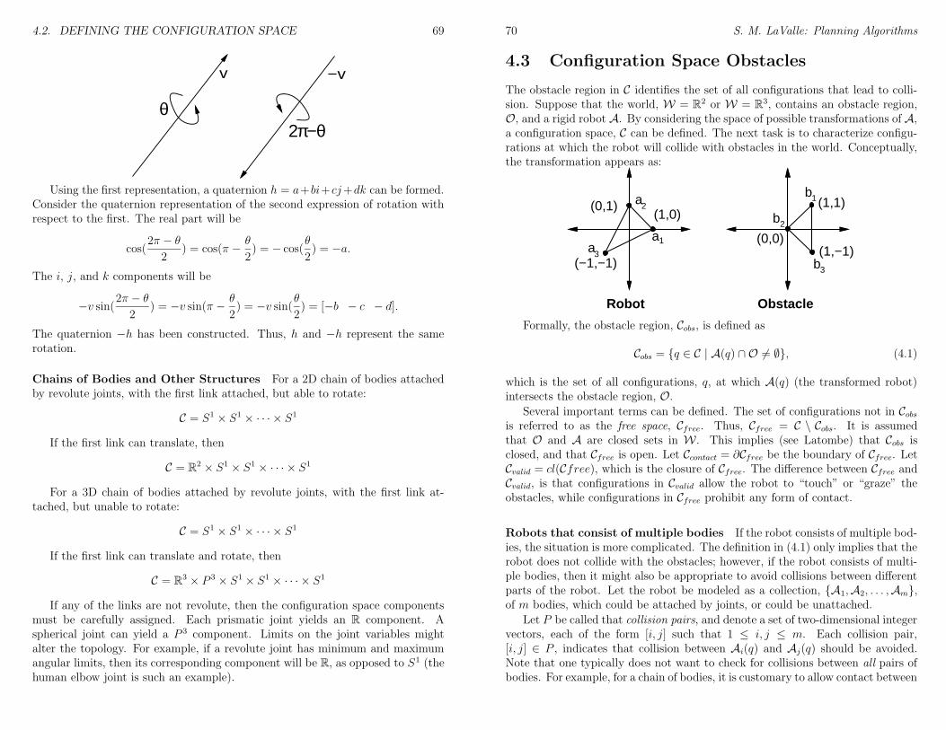
4.2. DEFINING THE CONFIGURATION SPACE 69
θ
v
2π−θ
−v
Using the first representation, a quaternion h = a+bi+cj+dk can be formed.Consider the quaternion representation of the second expression of rotation withrespect to the first. The real part will be
cos(2π − θ
2) = cos(π −
θ
2) = − cos(
θ
2) = −a.
The i, j, and k components will be
−v sin(2π − θ
2) = −v sin(π −
θ
2) = −v sin(
θ
2) = [−b − c − d].
The quaternion −h has been constructed. Thus, h and −h represent the samerotation.
Chains of Bodies and Other Structures For a 2D chain of bodies attachedby revolute joints, with the first link attached, but able to rotate:
C = S1 × S1 × · · · × S1
If the first link can translate, then
C = R2 × S1 × S1 × · · · × S1
For a 3D chain of bodies attached by revolute joints, with the first link at-tached, but unable to rotate:
C = S1 × S1 × · · · × S1
If the first link can translate and rotate, then
C = R3 × P 3 × S1 × S1 × · · · × S1
If any of the links are not revolute, then the configuration space componentsmust be carefully assigned. Each prismatic joint yields an R component. Aspherical joint can yield a P 3 component. Limits on the joint variables mightalter the topology. For example, if a revolute joint has minimum and maximumangular limits, then its corresponding component will be R, as opposed to S1 (thehuman elbow joint is such an example).
70 S. M. LaValle: Planning Algorithms
4.3 Configuration Space Obstacles
The obstacle region in C identifies the set of all configurations that lead to colli-sion. Suppose that the world, W = R2 or W = R3, contains an obstacle region,O, and a rigid robot A. By considering the space of possible transformations of A,a configuration space, C can be defined. The next task is to characterize configu-rations at which the robot will collide with obstacles in the world. Conceptually,the transformation appears as:
(1,0)(0,1)
(−1,−1)
(1,1)
a1
2a
3ab3
b2
b1
Robot Obstacle
(1,−1)(0,0)
Formally, the obstacle region, Cobs, is defined as
Cobs = q ∈ C | A(q) ∩ O 6= ∅, (4.1)
which is the set of all configurations, q, at which A(q) (the transformed robot)intersects the obstacle region, O.
Several important terms can be defined. The set of configurations not in Cobsis referred to as the free space, Cfree. Thus, Cfree = C \ Cobs. It is assumedthat O and A are closed sets in W . This implies (see Latombe) that Cobs isclosed, and that Cfree is open. Let Ccontact = ∂Cfree be the boundary of Cfree. LetCvalid = cl(Cfree), which is the closure of Cfree. The difference between Cfree andCvalid, is that configurations in Cvalid allow the robot to “touch” or “graze” theobstacles, while configurations in Cfree prohibit any form of contact.
Robots that consist of multiple bodies If the robot consists of multiple bod-ies, the situation is more complicated. The definition in (4.1) only implies that therobot does not collide with the obstacles; however, if the robot consists of multi-ple bodies, then it might also be appropriate to avoid collisions between differentparts of the robot. Let the robot be modeled as a collection, A1,A2, . . . ,Am,of m bodies, which could be attached by joints, or could be unattached.
Let P be called that collision pairs, and denote a set of two-dimensional integervectors, each of the form [i, j] such that 1 ≤ i, j ≤ m. Each collision pair,[i, j] ∈ P , indicates that collision between Ai(q) and Aj(q) should be avoided.Note that one typically does not want to check for collisions between all pairs ofbodies. For example, for a chain of bodies, it is customary to allow contact between
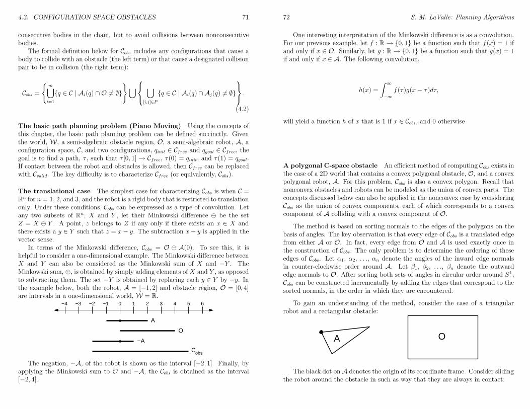
4.3. CONFIGURATION SPACE OBSTACLES 71
consecutive bodies in the chain, but to avoid collisions between nonconsecutivebodies.
The formal definition below for Cobs includes any configurations that cause abody to collide with an obstacle (the left term) or that cause a designated collisionpair to be in collision (the right term):
Cobs =
m⋃
i=1
q ∈ C | Ai(q) ∩ O 6= ∅
⋃
⋃
[i,j]∈Pq ∈ C | Ai(q) ∩ Aj(q) 6= ∅
.
(4.2)
The basic path planning problem (Piano Moving) Using the concepts ofthis chapter, the basic path planning problem can be defined succinctly. Giventhe world, W , a semi-algebraic obstacle region, O, a semi-algebraic robot, A, aconfiguration space, C, and two configurations, qinit ∈ Cfree and qgoal ∈ Cfree, thegoal is to find a path, τ , such that τ [0, 1] → Cfree, τ(0) = qinit, and τ(1) = qgoal.If contact between the robot and obstacles is allowed, then Cfree can be replacedwith Cvalid. The key difficulty is to characterize Cfree (or equivalently, Cobs).
The translational case The simplest case for characterizing Cobs is when C =Rn for n = 1, 2, and 3, and the robot is a rigid body that is restricted to translationonly. Under these conditions, Cobs can be expressed as a type of convolution. Letany two subsets of Rn, X and Y , let their Minkowski difference ª be the setZ = X ª Y . A point, z belongs to Z if any only if there exists an x ∈ X andthere exists a y ∈ Y such that z = x− y. The subtraction x− y is applied in thevector sense.
In terms of the Minkowski difference, Cobs = O ª A(0). To see this, it ishelpful to consider a one-dimensional example. The Minkowski difference betweenX and Y can also be considered as the Minkowski sum of X and −Y . TheMinkowski sum, ⊕, is obtained by simply adding elements of X and Y , as opposedto subtracting them. The set −Y is obtained by replacing each y ∈ Y by −y. Inthe example below, both the robot, A = [−1, 2] and obstacle region, O = [0, 4]are intervals in a one-dimensional world, W = R.
−4 −3 −2 −1 0 1 2 3 4 5 6
A
O
−A
Cobs
The negation, −A, of the robot is shown as the interval [−2, 1]. Finally, byapplying the Minkowski sum to O and −A, the Cobs is obtained as the interval[−2, 4].
72 S. M. LaValle: Planning Algorithms
One interesting interpretation of the Minkowski difference is as a convolution.For our previous example, let f : R → 0, 1 be a function such that f(x) = 1 ifand only if x ∈ O. Similarly, let g : R→ 0, 1 be a function such that g(x) = 1if and only if x ∈ A. The following convolution,
h(x) =
∫ ∞
−∞f(τ)g(x− τ)dτ,
will yield a function h of x that is 1 if x ∈ Cobs, and 0 otherwise.
A polygonal C-space obstacle An efficient method of computing Cobs exists inthe case of a 2D world that contains a convex polygonal obstacle, O, and a convexpolygonal robot, A. For this problem, Cobs is also a convex polygon. Recall thatnonconvex obstacles and robots can be modeled as the union of convex parts. Theconcepts discussed below can also be applied in the nonconvex case by consideringCobs as the union of convex components, each of which corresponds to a convexcomponent of A colliding with a convex component of O.
The method is based on sorting normals to the edges of the polygons on thebasis of angles. The key observation is that every edge of Cobs is a translated edgefrom either A or O. In fact, every edge from O and A is used exactly once inthe construction of Cobs. The only problem is to determine the ordering of theseedges of Cobs. Let α1, α2, . . ., αn denote the angles of the inward edge normalsin counter-clockwise order around A. Let β1, β2, . . ., βn denote the outwardedge normals to O. After sorting both sets of angles in circular order around S1,Cobs can be constructed incrementally by adding the edges that correspond to thesorted normals, in the order in which they are encountered.
To gain an understanding of the method, consider the case of a triangularrobot and a rectangular obstacle:
A O
The black dot on A denotes the origin of its coordinate frame. Consider slidingthe robot around the obstacle in such as way that they are always in contact:
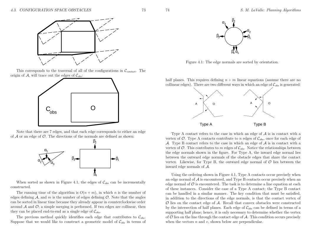
4.3. CONFIGURATION SPACE OBSTACLES 73
This corresponds to the traversal of all of the configurations in Ccontact. Theorigin of A, will trace out the edges of Cobs:
Cobs
O
Note that there are 7 edges, and that each edge corresponds to either an edgeof A or an edge of O. The directions of the normals are defined as shown:
α1
α2β3
β4
β1
β2
α3
When sorted as shown in Figure 4.1, the edges of Cobs can be incrementallyconstructed.
The running time of the algorithm is O(n +m), in which n is the number ofedges defining A, and m is the number of edges defining O. Note that the anglescan be sorted in linear time because they already appear in counterclockwise orderaround A and O; a simple merging is performed. If two edges are collinear, thenthey can be placed end-to-end as a single edge of Cobs.
The previous method quickly identifies each edge that contributes to Cobs.Suppose that we would like to construct a geometric model of Cobs in terms of
74 S. M. LaValle: Planning Algorithms
α1
α2β3
β4
β1
β2α3
Figure 4.1: The edge normals are sorted by orientation.
half planes. This requires defining n +m linear equations (assume there are nocollinear edges). There are two different ways in which an edge of Cobs is generated:
A O A O
Type A Type B
Type A contact refers to the case in which an edge of A is in contact with avertex of O. Type A contacts contribute to n edges of Cobs, once for each edge ofA. Type B contact refers to the case in which an edge of A is in contact with avertex of O. This contributes to m edges of Cobs. Notice the relationships betweenthe edge normals shown in the figure. For Type A, the inward edge normal liesbetween the outward edge normals of the obstacle edges that share the contactvertex. Likewise, for Type B, the outward edge normal of O lies between theinward edge normals of A.
Using the ordering shown in Figure 4.1, Type A contacts occur precisely whenan edge normal of A is encountered, and Type B contacts occur precisely when anedge normal of O is encountered. The task is to determine a line equation at eachof these instances. Consider the case of a Type A contact; the Type B contactcan be handled in a similar manner. The key condition that must be satisfied,in addition to the directions of the edge normals, is that the contact vertex ofO lies on the contact edge of A. Recall that convex obstacles were constructedby the intersection of half planes. Each edge of Cobs can be defined in terms of asupporting half plane; hence, it is only necessary to determine whether the vertexof O lies on the line through the contact edge of A. This condition occurs preciselywhen the vectors n and v, shown below are perpendicular.

4.3. CONFIGURATION SPACE OBSTACLES 75
A Ov
n
p
This occurs precisely when their inner product (dot product) is zero, n · v = 0.Note that n does not depend on the configuration of A (because rotation is notallowed). The vector v, however, depends on the translation, q = (x0, y0) of thepoint p. Therefore, it is more appropriate to write the condition as n·v(x0, y0) = 0.The transformation equations are linear for translation; hence, n · v = 0 is theequation of a line in C. For example, if the coordinates of p are (1, 2) whenA is at the origin, then the expression for p at configuration (x0, y0) is simply(1 + x0, 2+ y0). Clearly, the resulting inner product n · v = 0 is a linear equation.Let f(x0, y0) = n · v. Let H = (x0, y0) ∈ C | f(x0, y0) ≤ 0. Observe thatconfigurations not in H lie in Cfree. The half plane H is used to define one edgeof Cobs. The obstacle region Cobs can be completely characterized by intersectingthe resulting half planes for each of the Type A and Type B contacts. This yieldsa convex polygon in C that has n+m sides, as expected.
A polyhedral C-space obstacle Most of the previous ideas generalize nicelyfor the case of a polyhedral robot that is capable of translation only in a 3Dworld that contains polyhedral obstacles. If A and O are convex polyhedra, theresulting Cobs is a convex polyhedron.
There are three different kinds of contacts that lead to half spaces:
• Type A: A face of A and a vertex of O
• Type B: A vertex of A and a face of O
• Type C: An edge of A and an edge of O
Each half space defines a face of the polyhedron. The resulting polyhedron canbe constructed in O(n +m+ k) time, in which n is the number of faces of A, mis the numfer of faces of O, and k is the number of faces of Cobs, which is at mostnm.
A semi-algebraic C-space obstacle Unfortunately, the cases in which Cobs ispolygonal or polyhedral are quite limited. Most problems yield far more compli-cated C-space obstacles. With a few tricks, however, Cobs can almost always beexpressed using algebraic models. This will hold true for any of the robots and
76 S. M. LaValle: Planning Algorithms
transformations presented in Chapter 2. It might not be true for other kinds oftransformations, such as parameters that warp a flexible material.
Consider the case of a convex polygonal robot and a convex polygonal obstaclein a 2D world. The robot is allowed to rotate and translate; thus, C = R2 × S1
and q = (x0, y0, θ). The task is to define a set of algebraic primitives that canbe combined to define Cobs. Once again, it is important to distinguish betweenType A and Type B contacts. We will describe how to construct the algebraicprimitives for the Type A contacts; Type B can be handled in a similar manner.Confider the following figure for a Type A contact:
v2
A Ov
n
p
v1
For the translation-only case, we were able to determine all of the Type A con-ditions by sorting the edge normals. With rotation, the ordering of edge normalsdepends on θ. This implies that the applicability of a Type A contact depends onθ. Recall the constraint that the inward normal of A must lie between the outwardnormals of the edges of O that contain the vertex of contact. This constraint canbe expressed in terms of inner products using the vectors v1 and v2. The state-ment regarding the directions of the normals can equivalently be formulated asthe statement that the angle between n and v1, and between n and v2, must eachbe less than π
2. Using inner products, this implies that n ·v1 ≥ 0 and n ·v2 ≥ 0. As
in the translation case, the condition n ·v = 0 is required for contact. Note that ndepends on q. A given configuration, q, lies in Cfree if n(q) · v1 ≥ 0, n(q) · v2 ≥ 0,and n(q) · v > 0. Note that for any q ∈ C, if n(q) · v1 ≥ 0, n(q) · v2 ≥ 0, andn(q) ·v(q) > 0, then q ∈ Cfree. Let Hf denote the set of configurations that satisfythese conditions. These conditions can be used to determine whether a point isin Cfree; however, it is not a complete characterization of Cfree because all otherType A and Type B contacts could possibly imply that other points are in Cfree.Thus, Hf is s strict subset, Hf ⊂ Cfree. This implies that the complement, C \Hf ,is a superset of Cobs, i.e., Cobs ⊂ C \Hf . Let HA = C \Hf . The following primitivescan be used to define HA:
H1 = q ∈ C | n(q) · v1 < 0
H2 = q ∈ C | n(q) · v2 < 0
H3 = q ∈ C | n(q) · v(q) ≤ 0
The set of configurations in HA = H1 ∪H2 ∪H3 possibly lie in Cobs, although
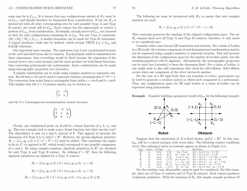
4.3. CONFIGURATION SPACE OBSTACLES 77
some may lie in Cfree. It is known that any configurations outside of HA must bein Cfree, and should therefore be eliminated from consideration. If the set HA isintersected with all other corresponding sets for each possible Type A and TypeB contact, the result will be Cobs. Each contact has the opportunity to remove aportion of Cfree from consideration. Eventually, enough pieces of Cfree are removedso that the only configurations remaining lie in Cobs. For any Type A constraint,(H1 ∪H2) \H3 ⊆ Cfree. A similar statement can be made for Type B constraints.A logical predicate could also be defined, which returns TRUE if q ∈ Cobs andFALSE otherwise.
One important issue remains. The expression n(q) is not a polynomial becauseof the cos θ and sin θ terms due to rotation. If polynomals could be substituted forthese expressions, then everything would be fixed because the expression of thenormal vector (not a unit normal) and the inner product are both linear functions,thus converting polynomials into polynomials. Such a substitution can be madeusing stereographic projection (see Latombe).
A simpler substitution can be made using complex numbers to represent rota-tion. Recall that a+bi can be used to represent rotation, assuming that a2+b2 = 1.The conversion from polar form to rectangular form yields a = cos θ and b = sin θ.This implies that the 2× 2 rotation matrix can be written as
(
a −bb a
)
and the 3× 3 homogeneous transformation matrix becomes
a −b x0b a y00 0 1
.
Clearly, any transformed point on A will be a linear function of a, b, x0, andy0. This was a simple trick to make a nice, lienar function, but what was the cost?The dependency is now on a and b, instead of θ. This appears to increase thedimension of C from 3 to 4, and C = R4. However, the special algabraic primitiveHs = (x0, y0, a, b) ∈ C | a
2 + b2 = 1 must be added. This constrains the anglesto lie in S1, as opposed to R2, which would correspond to any possible assignmentof a and b. By using complex numbers, algebraic primitives in R4 are obtainedfor each Type A and Type B contact. By defining C = R4, then the followingalgebraic primitives are defined for a Type A contact:
H1 = (x0, y0, a, b) ∈ C | n(x0, y0, a, b) · v1 < 0
H2 = (x0, y0, a, b) ∈ C | n(x0, y0, a, b) · v2 < 0
H3 = (x0, y0, a, b) ∈ C | n(x0, y0, a, b) · v(x0, y0, a, b) ≤ 0
78 S. M. LaValle: Planning Algorithms
The following set must be intersected with HA to ensure that unit complexnumbers are used:
Hs = (x0, y0, a, b) ∈ C | a2 + b2 − 1 = 0
This constraint preserves the topology of the original configuration space. The setHs remains fixed over all Type A and Type B contacts; therefore, it only needsto be considered once.
Consider other cases beyond 2D translation and rotation. For a chain of bodiesin a 2D world, the rotation component of each homogeneous transformation matrixcan be expressed using complex numbers to represent rotation. This will increasethe dimension of the configuration space by the number of revolute joints, but theresulting primitives will be algebraic. Alternatively, the stereographic projectioncan be used (see Latombe) to keep the dimension fixed. For a chain of bodies, itone might want to also add expressions that check for self-collision. Self-collisionoccurs when one component of the robot intersects another.
For the case of a 3D rigid body that can translate or rotate, quaternions canbe used to generate a rotation matrix in which each component is a polynomial.Thus, any configuration space for 3D rigid bodies or a chain of bodies can beexpressed using polynomials.
Example Consider building a geometric model of Cobs for the following example:
(1,0)(0,1)
(−1,−1)
(1,1)(−1,1)
(−1,−1)a1
2a
3a
4bb3
b2 b1
Robot Obstacle
(1,−1)
Suppose that the orientation of A is fixed shown, and C = R2. In this case,Cobs will be a convex polygon with seven sides. The following contact conditionsoccur (the ordering is given as normals appear as shown in Figure 4.1).
Type Vertex O Edge n v Half PlaneB a3 b4-b1 [1, 0] [x0 − 2, y0] HB = q ∈ C | x0 − 2 ≤ 0B a3 b1-b2 [0, 1] [x0 − 2, y0 − 2] HB = q ∈ C | y0 − 2 ≤ 0A b2 a3-a1 [1,-2] [−x0, 2− y0] HA = q ∈ C | − x0 + 2y0 − 4 ≤ 0B a1 b2-b3 [−1, 0] [2 + x0, y0 − 1] HB = q ∈ C | − x0 − 2 ≤ 0A b3 a1-a2 [1, 1] [−1− x0,−y0] HA = q ∈ C | − x0 − y0 − 1 ≤ 0B a2 b3-b4 [0,−1] [x0 + 1, y0 + 2] HB = q ∈ C | − y0 − 2 ≤ 0A b4 a2-a3 [−2, 1] [2− x0,−y0] HA = q ∈ C | 2x0 − y0 − 4 ≤ 0
For the rotation case, all possible contacts must be considered. For this exam-ple, there are 12 Type A contacts and 12 Type B contacts. Each contact produces3 algebraic primitives. With the inclusion of Hs, this simple example produces 73
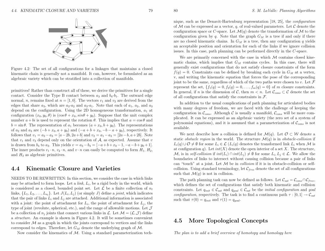
4.4. KINEMATIC CLOSURE AND VARIETIES 79
Figure 4.2: The set of all configurations for a linkages that maintains a closedkinematic chain is generally not a manifold. It can, however, be formulated as analgebraic variety which can be stratified into a collection of manifolds.
primitives! Rather than construct all of these, we derive the primitives for a singlecontact. Consider the Type B contact between a3 and b4-b1. The outward edgenormal, n, remains fixed at n = [1, 0]. The vectors v1 and v2 are derived from theedges that share a3, which are a3-a2 and a3-a1. Note that each of a1, a2, and a3depend on the configuration. Using the 2D homogeneous transformation, a1 atconfiguration (x0, y0, θ) is (cos θ + x0, sinθ + y0). Suppose that the unit complexnumber a+ bi is used to represent the rotation θ. This implies that a = cos θ andb = sin θ. The representation of a1 becomes (a+ x0, b+ y0). The representationsof a2 and a3 are (−b+ x0, a+ y0) and (−a+ b+ x0,−b− a+ y0), respectively. Itfollows that v1 = a2−a3 = [a−2b, 2a+ b] and v2 = a1−a3 = [2a− b, a+2b]. Notethat v1 and v2 depend only on the orientation of A, as expected. Assume that vis drawn from b4 to a3. This yields v = a3− b4 = [−a+ b+x0−1,−a− b+y0+1].The inner products v1 ·n, v2 ·n, and v ·n can easily be computed to form H1, H2,and H3 as algebraic primitives.
4.4 Kinematic Closure and Varieties
NEEDS TO BE REWRITTEN: In this section, we consider the case in which linksmay be attached to form loops. Let a link, Li, be a rigid body in the world, whichis considered as a closed, bounded point set. Let L be a finite collection of nllinks, L1, L2, . . . , Lnl
. Let J(Li, Lj) (or simply J) define a joint, which indicatesthat the pair of links Li and Lj are attached. Additional information is associatedwith a joint: the point of attachment for Li, the point of attachment for Lj, thetype of joint (revolute, spherical, etc.), and the range of allowable motions. Let Jbe a collection of nj joints that connect various links in L. LetM = (L,J ) definea structure. An example is shown in Figure 4.2. It will be sometimes convenientto considerM as a graph in which the joints correspond to vertices and the linkscorrespond to edges. Therefore, let GM denote the underlying graph ofM.
Now consider the kinematics ofM. Using a standard parameterization tech-
80 S. M. LaValle: Planning Algorithms
nique, such as the Denavit-Hartenburg representation [18, 25], the configurationofM can be expressed as a vector, q, of real-valued parameters. Let C denote theconfiguration space or C-space. LetM(q) denote the transformation ofM to theconfiguration given by q. Note that the graph GM is a tree if and only if thereare no closed kinematic chains. In GM is a tree, then any configuration q yieldsan acceptable position and orientation for each of the links if we ignore collisionissues. In this case, path planning can be performed directly in the C-space.
We are primarily concerned with the case in which M contains closed kine-matic chains, which implies that GM contains cycles. In this case, there willgenerally exist configurations that do not satisfy closure constraints of the formf(q) = 0. Constraints can be defined by breaking each cycle in GM at a vertex,v, and writing the kinematic equation that forces the pose of the correspondingjoint to be the same, regardless of which of the two paths were chosen to v. Let Frepresent the set, f1(q) = 0, f2(q) = 0, . . . , fm(q) = 0 of m closure constraints.In general, if n is the dimension of C, then m < n. Let Ccons ⊂ C denote the setof all configurations that satisfy the constraints in F .
In addition to the usual complications of path planning for articulated bodieswith many degrees of freedom, we are faced with the challenge of keeping theconfiguration in Ccons. Although C is usually a manifold, Ccons will be more com-plicated. It can be expressed as an algebraic variety (the zero set of a system ofpolynomial equations), and it is assumed that a parameterization of Ccons is notavailable.
We next describe how a collision is defined for M(q). Let O ⊂ W denote astatic obstacle region in the world. The structureM(q) is in obstacle-collision ifLi(q)∪O 6= ∅ for some Li ∈ L (Li(q) denotes the transformed link Li whenM isat configuration q). Let int(X) denote the open interior of a set X. The structure,M, is in self-collision if int(Li) ∩ int(Lj) 6= ∅ for some Li, Lj ∈ L. We allow theboundaries of links to intersect without causing collision because a pair of linkscan “touch” at a joint. LetM be in collision if it is in obstacle-collision or self-collision. Using standard terminology, let Cfree denote the set of all configurationssuch thatM(q) is not in collision.
The path planning task can now be defined as follows. Let Csat = Ccons∩Cfree,which defines the set of configurations that satisfy both kinematic and collisionconstraints. Let qinit ∈ Csat and qgoal ∈ Csat be the initial configuration and goalconfiguration, respectively. The task is to find a continuous path τ : [0, 1]→ Csatsuch that τ(0) = qinit and τ(1) = qgoal.
4.5 More Topological Concepts
The plan is to add a brief overview of homotopy and homology here
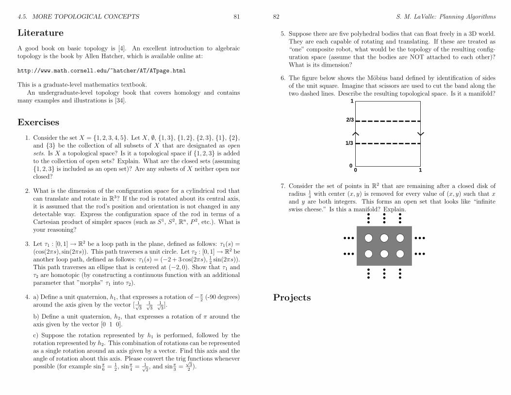
4.5. MORE TOPOLOGICAL CONCEPTS 81
Literature
A good book on basic topology is [4]. An excellent introduction to algebraictopology is the book by Allen Hatcher, which is available online at:
http://www.math.cornell.edu/~hatcher/AT/ATpage.html
This is a graduate-level mathematics textbook.An undergraduate-level topology book that covers homology and contains
many examples and illustrations is [34].
Exercises
1. Consider the set X = 1, 2, 3, 4, 5. Let X, ∅, 1, 3, 1, 2, 2, 3, 1, 2,and 3 be the collection of all subsets of X that are designated as opensets. Is X a topological space? Is it a topological space if 1, 2, 3 is addedto the collection of open sets? Explain. What are the closed sets (assuming1, 2, 3 is included as an open set)? Are any subsets of X neither open norclosed?
2. What is the dimension of the configuration space for a cylindrical rod thatcan translate and rotate in R3? If the rod is rotated about its central axis,it is assumed that the rod’s position and orientation is not changed in anydetectable way. Express the configuration space of the rod in terms of aCartesian product of simpler spaces (such as S1, S2, Rn, P 2, etc.). What isyour reasoning?
3. Let τ1 : [0, 1]→ R2 be a loop path in the plane, defined as follows: τ1(s) =(cos(2πs), sin(2πs)). This path traverses a unit circle. Let τ2 : [0, 1]→ R2 beanother loop path, defined as follows: τ1(s) = (−2 + 3 cos(2πs), 1
2sin(2πs)).
This path traverses an ellipse that is centered at (−2, 0). Show that τ1 andτ2 are homotopic (by constructing a continuous function with an additionalparameter that ”morphs” τ1 into τ2).
4. a) Define a unit quaternion, h1, that expresses a rotation of −π2(-90 degrees)
around the axis given by the vector [ 1√3
1√3
1√3].
b) Define a unit quaternion, h2, that expresses a rotation of π around theaxis given by the vector [0 1 0].
c) Suppose the rotation represented by h1 is performed, followed by therotation represented by h2. This combination of rotations can be representedas a single rotation around an axis given by a vector. Find this axis and theangle of rotation about this axis. Please convert the trig functions wheneverpossible (for example sinπ
6= 1
2, sinπ
4= 1√
2, and sinπ
3=
√32).
82 S. M. LaValle: Planning Algorithms
5. Suppose there are five polyhedral bodies that can float freely in a 3D world.They are each capable of rotating and translating. If these are treated as“one” composite robot, what would be the topology of the resulting config-uration space (assume that the bodies are NOT attached to each other)?What is its dimension?
6. The figure below shows the Mobius band defined by identification of sidesof the unit square. Imagine that scissors are used to cut the band along thetwo dashed lines. Describe the resulting topological space. Is it a manifold?
0 10
1/3
2/3
1
7. Consider the set of points in R2 that are remaining after a closed disk ofradius 1
4with center (x, y) is removed for every value of (x, y) such that x
and y are both integers. This forms an open set that looks like “infiniteswiss cheese.” Is this a manifold? Explain.
Projects
Chapter 5
Combinatorial Motion Planning
This chapter could expand into two...
5.1 Introduction
Combinatorial approaches to motion planning find paths through the continuousconfiguration space without resorting to approximations. Because of this property,they are alternatively referred to as exact algorithms. This is in contrast to thesampling-based motion planning algorithms which are covered in Chapter ??.
All of the algorithms presented in this chapter have one important property:they are complete, which means that for any problem instance (over the space ofproblems for which the algorithm is designed), the algorithm will either find asolution, or will correctly report that no solution exists.
When studying combinatorial motion planning algorithms, it is important tocarefully consider the definition of the input. What is the representation usedfor the robot and obstacles? What set of transformations may be applied to therobot? What is the dimension of the world? Are the robot and obstacles convex?Are they piecewise linear? The specification of possible inputs defines a class ofproblem instances on which the algorithm will operate. If this class of problemshas certain convenient properties (e.g., low dimensionality, convex models), thena combinatorial algorithm may provide an elegant, practical solution. If the classof problems is too broad, then a requirement of both completeness and practi-cal solutions seems unreasonable. Many general formulations of general motionplanning problems are PSPACE-hard (implying NP-hard); therefore, such a hopeappears unattainable. Nevertheless, there exist general, complete motion planningalgorithms.
Based on these observations, there are generally two good reasons to studycombinatorial approaches to motion planning:
1. In many applications, one may only be interested in a special class of plan-ning problems. For example, the world might be two-dimensional, and therobot might only be capable of translation. For many special classes, elegant
83
84 S. M. LaValle: Planning Algorithms
and efficient algorithms can be developed. These algorithm are complete, dono depend on approximation, and can offer much better performance thanincomplete methods, such as those in Chapter 6.
2. It is both interesting and satisfying to know that there are complete algo-rithms for an extremely broad class of motion planning problems. Thus,even if the class of interest does not have some special limiting assumptions,there still exist general-purpose tools and algorithms that can solve it.
It will be helpful to formalize this “extremely broad” class of motion planningproblems. To acheive this, we reiterate concepts from Chapter 4. Let W denotethe world, which will either be W = R2 or W = R3. A semi-algebraic obstacleregion, O ⊂ W is defined. The robot model, A, is also semi-algebraic, and iscomposed of one or more rigid bodies that move in W . The number of degrees offreedom of A is finite, but may be arbitrarily large. This results in a configurationspace, C, which is a manifold whose dimension is finite, but may be artrarilylarge. Let Cfree be the set of collision-free configurations, as defined in Section 4.3.Given an initial configuration, qinit and a goal configuration, qgoal, the algorithmmust compute a continuous path, τ : [0, 1] → Cfree such that τ(0) = qinit andτ(1) = qgoal.
5.2 Algorithms for a Point Robot
This section presents several beautiful solutions to the problem of moving a pointrobot in a planar world. This problem is much simpler than path planning ina general configuration space; therefore, many elegant solutions exist that nicelyillustrate the principles of combinatorial motion planning.
Throughout the section, we consider the following simple model.
Model 1 The robot, A is a single point. It makes no sense to rotate a point robot;therefore, we only consider the set of possible translations. This means that boththe world and configuration space are identical: W = C = R2. Let the obstacleregion, O, be polygonal.
Note that the obstacle regions, O and Cobs are identical, which avoids the compli-cated constructions from Section ??. This means that to describe the algorithms,there is no need to refer to the configuration space.
5.2.1 Vertical Cell Decomposition
A cell decomposition technique will be presented here. The general idea is todivide the free space into a set of simple cells. Planning inside of each cell isstraightforward, and the task is to find a sequence of cells with the followingproperties: 1) The first cell contains the initial position. 2) The final cell contains
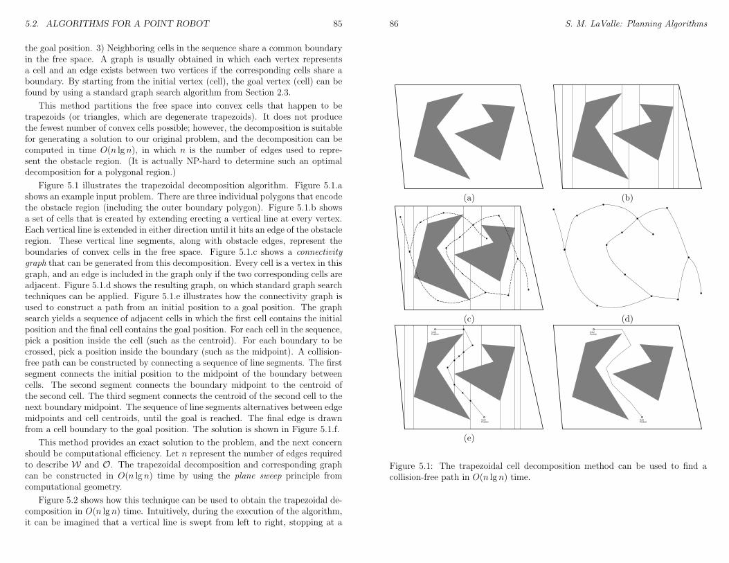
5.2. ALGORITHMS FOR A POINT ROBOT 85
the goal position. 3) Neighboring cells in the sequence share a common boundaryin the free space. A graph is usually obtained in which each vertex representsa cell and an edge exists between two vertices if the corresponding cells share aboundary. By starting from the initial vertex (cell), the goal vertex (cell) can befound by using a standard graph search algorithm from Section 2.3.
This method partitions the free space into convex cells that happen to betrapezoids (or triangles, which are degenerate trapezoids). It does not producethe fewest number of convex cells possible; however, the decomposition is suitablefor generating a solution to our original problem, and the decomposition can becomputed in time O(n lg n), in which n is the number of edges used to repre-sent the obstacle region. (It is actually NP-hard to determine such an optimaldecomposition for a polygonal region.)
Figure 5.1 illustrates the trapezoidal decomposition algorithm. Figure 5.1.ashows an example input problem. There are three individual polygons that encodethe obstacle region (including the outer boundary polygon). Figure 5.1.b showsa set of cells that is created by extending erecting a vertical line at every vertex.Each vertical line is extended in either direction until it hits an edge of the obstacleregion. These vertical line segments, along with obstacle edges, represent theboundaries of convex cells in the free space. Figure 5.1.c shows a connectivitygraph that can be generated from this decomposition. Every cell is a vertex in thisgraph, and an edge is included in the graph only if the two corresponding cells areadjacent. Figure 5.1.d shows the resulting graph, on which standard graph searchtechniques can be applied. Figure 5.1.e illustrates how the connectivity graph isused to construct a path from an initial position to a goal position. The graphsearch yields a sequence of adjacent cells in which the first cell contains the initialposition and the final cell contains the goal position. For each cell in the sequence,pick a position inside the cell (such as the centroid). For each boundary to becrossed, pick a position inside the boundary (such as the midpoint). A collision-free path can be constructed by connecting a sequence of line segments. The firstsegment connects the initial position to the midpoint of the boundary betweencells. The second segment connects the boundary midpoint to the centroid ofthe second cell. The third segment connects the centroid of the second cell to thenext boundary midpoint. The sequence of line segments alternatives between edgemidpoints and cell centroids, until the goal is reached. The final edge is drawnfrom a cell boundary to the goal position. The solution is shown in Figure 5.1.f.
This method provides an exact solution to the problem, and the next concernshould be computational efficiency. Let n represent the number of edges requiredto describe W and O. The trapezoidal decomposition and corresponding graphcan be constructed in O(n lg n) time by using the plane sweep principle fromcomputational geometry.
Figure 5.2 shows how this technique can be used to obtain the trapezoidal de-composition in O(n lg n) time. Intuitively, during the execution of the algorithm,it can be imagined that a vertical line is swept from left to right, stopping at a
86 S. M. LaValle: Planning Algorithms
(a) (b)
(c) (d)InitialPosition
GoalPosition
InitialPosition
GoalPosition
(e)
Figure 5.1: The trapezoidal cell decomposition method can be used to find acollision-free path in O(n lg n) time.
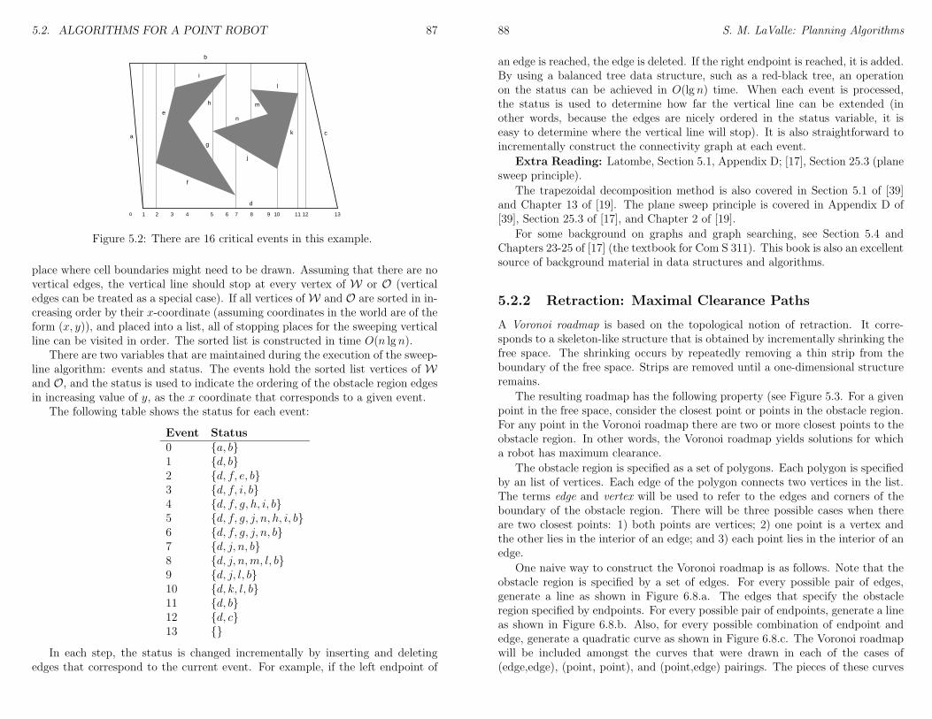
5.2. ALGORITHMS FOR A POINT ROBOT 87
1 2 3 4 5 6 7 8 9 10 11 12 13
a
b
c
d
e
f
g
h
i
j
k
l
m
n
0
Figure 5.2: There are 16 critical events in this example.
place where cell boundaries might need to be drawn. Assuming that there are novertical edges, the vertical line should stop at every vertex of W or O (verticaledges can be treated as a special case). If all vertices ofW and O are sorted in in-creasing order by their x-coordinate (assuming coordinates in the world are of theform (x, y)), and placed into a list, all of stopping places for the sweeping verticalline can be visited in order. The sorted list is constructed in time O(n lg n).
There are two variables that are maintained during the execution of the sweep-line algorithm: events and status. The events hold the sorted list vertices of Wand O, and the status is used to indicate the ordering of the obstacle region edgesin increasing value of y, as the x coordinate that corresponds to a given event.
The following table shows the status for each event:
Event Status0 a, b1 d, b2 d, f, e, b3 d, f, i, b4 d, f, g, h, i, b5 d, f, g, j, n, h, i, b6 d, f, g, j, n, b7 d, j, n, b8 d, j, n,m, l, b9 d, j, l, b10 d, k, l, b11 d, b12 d, c13
In each step, the status is changed incrementally by inserting and deletingedges that correspond to the current event. For example, if the left endpoint of
88 S. M. LaValle: Planning Algorithms
an edge is reached, the edge is deleted. If the right endpoint is reached, it is added.By using a balanced tree data structure, such as a red-black tree, an operationon the status can be achieved in O(lg n) time. When each event is processed,the status is used to determine how far the vertical line can be extended (inother words, because the edges are nicely ordered in the status variable, it iseasy to determine where the vertical line will stop). It is also straightforward toincrementally construct the connectivity graph at each event.
Extra Reading: Latombe, Section 5.1, Appendix D; [17], Section 25.3 (planesweep principle).
The trapezoidal decomposition method is also covered in Section 5.1 of [39]and Chapter 13 of [19]. The plane sweep principle is covered in Appendix D of[39], Section 25.3 of [17], and Chapter 2 of [19].
For some background on graphs and graph searching, see Section 5.4 andChapters 23-25 of [17] (the textbook for Com S 311). This book is also an excellentsource of background material in data structures and algorithms.
5.2.2 Retraction: Maximal Clearance Paths
A Voronoi roadmap is based on the topological notion of retraction. It corre-sponds to a skeleton-like structure that is obtained by incrementally shrinking thefree space. The shrinking occurs by repeatedly removing a thin strip from theboundary of the free space. Strips are removed until a one-dimensional structureremains.
The resulting roadmap has the following property (see Figure 5.3. For a givenpoint in the free space, consider the closest point or points in the obstacle region.For any point in the Voronoi roadmap there are two or more closest points to theobstacle region. In other words, the Voronoi roadmap yields solutions for whicha robot has maximum clearance.
The obstacle region is specified as a set of polygons. Each polygon is specifiedby an list of vertices. Each edge of the polygon connects two vertices in the list.The terms edge and vertex will be used to refer to the edges and corners of theboundary of the obstacle region. There will be three possible cases when thereare two closest points: 1) both points are vertices; 2) one point is a vertex andthe other lies in the interior of an edge; and 3) each point lies in the interior of anedge.
One naive way to construct the Voronoi roadmap is as follows. Note that theobstacle region is specified by a set of edges. For every possible pair of edges,generate a line as shown in Figure 6.8.a. The edges that specify the obstacleregion specified by endpoints. For every possible pair of endpoints, generate a lineas shown in Figure 6.8.b. Also, for every possible combination of endpoint andedge, generate a quadratic curve as shown in Figure 6.8.c. The Voronoi roadmapwill be included amongst the curves that were drawn in each of the cases of(edge,edge), (point, point), and (point,edge) pairings. The pieces of these curves
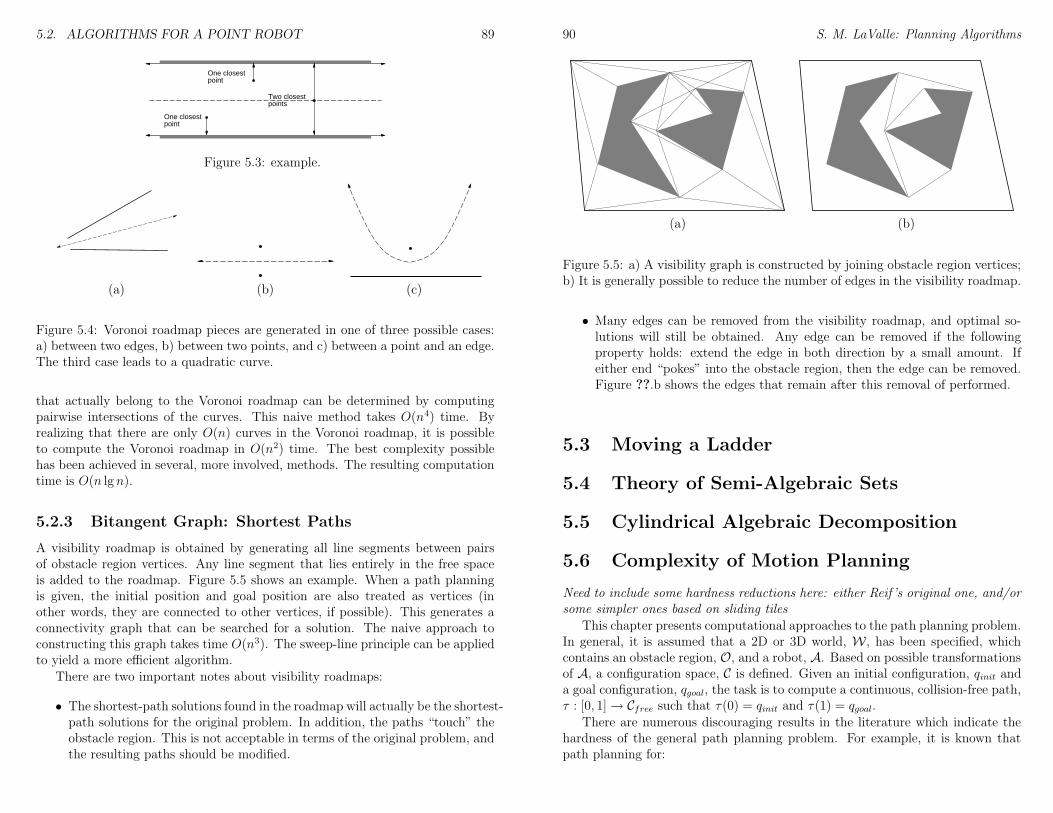
5.2. ALGORITHMS FOR A POINT ROBOT 89
One closestpoint
Two closestpoints
One closestpoint
Figure 5.3: example.
(a) (b) (c)
Figure 5.4: Voronoi roadmap pieces are generated in one of three possible cases:a) between two edges, b) between two points, and c) between a point and an edge.The third case leads to a quadratic curve.
that actually belong to the Voronoi roadmap can be determined by computingpairwise intersections of the curves. This naive method takes O(n4) time. Byrealizing that there are only O(n) curves in the Voronoi roadmap, it is possibleto compute the Voronoi roadmap in O(n2) time. The best complexity possiblehas been achieved in several, more involved, methods. The resulting computationtime is O(n lg n).
5.2.3 Bitangent Graph: Shortest Paths
A visibility roadmap is obtained by generating all line segments between pairsof obstacle region vertices. Any line segment that lies entirely in the free spaceis added to the roadmap. Figure 5.5 shows an example. When a path planningis given, the initial position and goal position are also treated as vertices (inother words, they are connected to other vertices, if possible). This generates aconnectivity graph that can be searched for a solution. The naive approach toconstructing this graph takes time O(n3). The sweep-line principle can be appliedto yield a more efficient algorithm.
There are two important notes about visibility roadmaps:
• The shortest-path solutions found in the roadmap will actually be the shortest-path solutions for the original problem. In addition, the paths “touch” theobstacle region. This is not acceptable in terms of the original problem, andthe resulting paths should be modified.
90 S. M. LaValle: Planning Algorithms
(a) (b)
Figure 5.5: a) A visibility graph is constructed by joining obstacle region vertices;b) It is generally possible to reduce the number of edges in the visibility roadmap.
• Many edges can be removed from the visibility roadmap, and optimal so-lutions will still be obtained. Any edge can be removed if the followingproperty holds: extend the edge in both direction by a small amount. Ifeither end “pokes” into the obstacle region, then the edge can be removed.Figure ??.b shows the edges that remain after this removal of performed.
5.3 Moving a Ladder
5.4 Theory of Semi-Algebraic Sets
5.5 Cylindrical Algebraic Decomposition
5.6 Complexity of Motion Planning
Need to include some hardness reductions here: either Reif ’s original one, and/orsome simpler ones based on sliding tiles
This chapter presents computational approaches to the path planning problem.In general, it is assumed that a 2D or 3D world, W , has been specified, whichcontains an obstacle region, O, and a robot, A. Based on possible transformationsof A, a configuration space, C is defined. Given an initial configuration, qinit anda goal configuration, qgoal, the task is to compute a continuous, collision-free path,τ : [0, 1]→ Cfree such that τ(0) = qinit and τ(1) = qgoal.
There are numerous discouraging results in the literature which indicate thehardness of the general path planning problem. For example, it is known thatpath planning for:
5.6. COMPLEXITY OF MOTION PLANNING 91
• n polyhedral bodies that comprise a robot in a 3D world that contains afixed number of polyhedral obstacles is PSPACE-hard.
• n rectangles with up, down, left, and right translation only is PSPACE-complete.
• a fixed robot among nmoving obstacles with known trajectories is PSPACE-hard.
• a point robot with uncertainties in sensing and control in a 3D world isNEXPTIME-hard.
These and many other results general indicate that it is highly unlikely or impos-sible that many general path planning problems will ever be solved by an efficient,polynomial-time algorithm.
These hardness results can be considered as lower bounds on the difficulty ofthe problem. These bounds indicate the complexity of the problem, as opposed toa particular algorithm. Even though it is believed that an efficient solution to thegeneral path planning problem will never be found, it was important to developa complete algorithm that actually solves the problem. This was first achieved in1983 by Schwartz and Sharir in their application of cylindrical algebraic decom-position techniques to develop a cell decomposition algorithm that applies to anyCobs that can be represented algebraically [66]. Unfortunately, the time complex-ity of this algorithm was doubly-exponential in d, in which n is the dimensionof the configuration space. In 1987, Canny proposed a general path planningalgorithm that is the most efficient known to date, with a time complexity thatis singly-exponential in d [14]. Recently, the complexity of cylindrical albegraicdecomposition has been improved [8], which leads to singly-exponential time forthe method of Schwartz and Sharir.
Although these complete approaches to path planning are very elegant, theirrunning times would be too much for most practical path planning problems.This has led many researchers to develop efficient planning algorithm for morespecific classes of problems, or to tolerate incomplete algorithms. Incompletealgorithms are not guaranteed yield a solution, if a solution exists; however, anyanswer returned is guaranteed to be correct. In some applications this behavior isunacceptable, but in a wide variety of contexts, incompleteness can be tolerated.In this case becomes particularly important to minimize the likelihood that thealgorithm will fail, and in general to improve its computational performance asmuch as possible. Often times a very efficient algorithm can be developed if weare willing to pay a small price of occasionally missing the solution.
92 S. M. LaValle: Planning Algorithms
5.7 Other Combinatorial Methods
Literature
Caviness, B. F. and Johnson, J. R. (Eds.). Quantifier Elimination and CylindricalAlgebraic Decomposition. New York: Springer-Verlag, 1998.
Collins, G. E. ”Quantifier Elimination for Real Closed Fields by CylindricalAlgebraic Decomposition.” In Proc. 2nd GI Conf. Automata Theory and FormalLanguages. New York: Springer-Verlag, pp. 134-183, 1975.
Collins, G. E. ”Quantifier Elimination by Cylindrical Algebraic Decomposition–Twenty Years of Progress.” In Quantifier Elimination and Cylindrical AlgebraicDecomposition (Ed. B. F. Caviness and J. R. Johnson). New York: Springer-Verlag, pp. 8-23, 1998.
Collins, G. E. and Hong, H. ”Partial Cylindrical Algebraic Decomposition forQuantifier Elimination.” J. Symb. Comput. 12, 299-328, 1991.
Davenport, J. H. ”Computer Algebra for Cylindrical Algebraic Decomposi-tion.” Report TRITA-NA-8511, NADA, KTH, Stockholm, Sept. 1985.
Davenport, J. and Heintz, J. ”Real Quantifier Elimination if Doubly Exponen-tial.” J. Symb. Comput. 5, 29-35, 1988.
Dolzmann, A. and Sturm, T. ”Simplification of Quantifier-Free Formulae overOrdered Fields.” J. Symb. Comput. 24, 209-231, 1997.
Dolzmann, A. andWeispfenning, V. ”Local Quantifier Elimination.” http://www.fmi.uni-passau.de/ dolzmann/refs/MIP-0003.ps.Z.
Heintz, J.; Roy, R.-F.; and Solerno, P. ”Complexit du principe de Tarski-Seidenberg.” C. R. Acad. Sci. Paris Sr. I Math. 309, 825-830, 1989.
Loos, R. and Weispfenning, V. ”Applying Lattice Quantifier Elimination.”Comput. J. 36, 450-461, 1993.
Strzebonski, A. ”Solving Algebraic Inequalities.” Mathematica J. 7, 525-541,2000.
Weispfenning, V. ”The Complexity of Linear Problems in Fields.” J. Symb.Comput. 5, 3-27, 1988.
Exercises
1. Propose a complete motion planning algorithm for Model 1 based on de-composing Cobs into triangles. What is the running time of your algorithm?
2. Extend the bitangent graph algorithm to work for obstacle boundaries thatare either pieces of circular arcs or line segments.
Chapter 6
Sampling-Based Motion Planning
This chapter might expand into two at some point...
Ariadne was the daughter of King Minos of Crete. Minos had Daedalus
build a Labyrinth, a house of winding passages, to house the bull-man,
the Minotaur, the beast that his wife Pasiphae bore after having
intercourse with a bull. (Minos had refused to sacrifice a bull to
Poseidon, as the king promised, so the god took revenge by causing his
wife to desire the bull--but that’s another story.) Minos required
tribute from Athens in the form of young men and women to be
sacrificed to the Minotaur.
Theseus, an Athenian, volunteered to accompany one of these groups of
victims to deliver his country from the tribute to Minos. Ariadne fell
in love with Theseus and gave him a thread which he let unwind through
the Labyrinth so that he was able to kill the Minotaur and find his
way back out again.
Ovid says that Daedalus built a house in which he confused the usual
passages and deceived the eye with a conflicting maze of various
wandering paths (in errorem variarum ambage viarum) (Metamorphoses
8.161):
"so Daedalus made the innumerable paths of deception [innumeras errore
vias], and he was barely able to return to the entrance: so deceptive
was the house [tanta est fallacia tecti]" (8.166-68).
Source: http://www.georgetown.edu/labyrinth/info_labyrinth/ariadne.html
Although the combinatorial approaches to path planning are very elegant, theirrunning times would be too much for most practical path planning problems.This has led many researchers to develop efficient planning algorithm for more
93
94 S. M. LaValle: Planning Algorithms
specific classes of problems, or to tolerate incomplete algorithms. Incompletealgorithms are not guaranteed yield a solution, if a solution exists; however, anyanswer returned is guaranteed to be correct. In some applications this behavior isunacceptable, but in a wide variety of contexts, incompleteness can be tolerated.In this case becomes particularly important to minimize the likelihood that thealgorithm will fail, and in general to improve its computational performance asmuch as possible. Often times a very efficient algorithm can be developed if weare willing to pay a small price of occasionally missing the solution.
6.1 Collision Detection
The combinatorial approaches to motion planning construct a representation ofthe obstacle region, Cobs, in C-space. To enable sampling-based approaches, wewill instead build a logical predicate that serves as a probe to test whether a con-figuration lies in Cobs. This is referred to as collision detection, and it is expectedin general that collision detection is much more efficient than constructing a com-plete representation of Cobs. The tradeoff is that a motion strategy algorithm hasbetter information with a complete characterization of Cobs.
A variety of collision detection algorithms exist, ranging from theoretical algo-rithms that have excellent computational complexity to heuristic, practical algo-rithms whose performance is tailored to a particular application. The techniquesfrom Section ?? can, of course, be used to develop a collision detection algorithmby defining a logical predicate using the geometric model of Cobs. For the case ofa 2D world, with a convex robot and obstacle, this leads to an O(n + m) timecollision detection algorithm.
6.1.1 Basic Concepts
Collision detection may be viewed abtractly as the construction of a logical pred-icate (boolean-valued function), c : C → true, false which yields c(q) = true ifand only if q ∈ Cobs. A collision detector may be viewed as a kind of probe thatcan indicate whether or not some q ∈ C is in collision.
In the boolean-valued function there is no notion of how far robot is fromhitting obstacles. For many path planning algorithms, this additional informationis quite useful. A distance function serves this purpose, and is defined as d : C →[0,∞), in which the real-value in the range of f indicates the distance in the world,W , between the closest pair of points over all pairs from A(q) and O. In general,for two closed, bounded subsets, E,F , of Rn, the (Hausdorff) distance is definedas
ρ(E,F ) = mine∈E
minf∈F‖e− f‖,
in which ‖E − F‖ denotes the Euclidean distance between two points in Rn.Clearly, if E ∩ F 6= ∅, then ρ(E,F ) = 0.
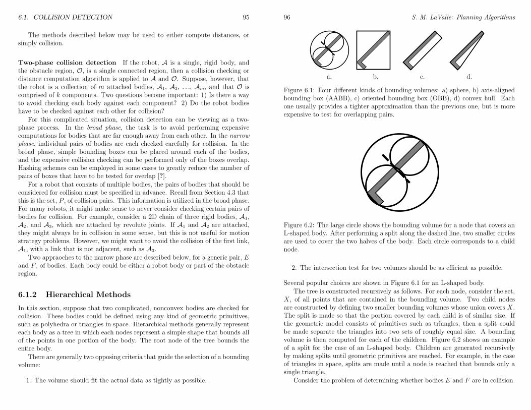
6.1. COLLISION DETECTION 95
The methods described below may be used to either compute distances, orsimply collision.
Two-phase collision detection If the robot, A is a single, rigid body, andthe obstacle region, O, is a single connected region, then a collision checking ordistance computation algorithm is applied to A and O. Suppose, however, thatthe robot is a collection of m attached bodies, A1, A2, . . ., Am, and that O iscomprised of k components. Two questions become important: 1) Is there a wayto avoid checking each body against each component? 2) Do the robot bodieshave to be checked against each other for collision?
For this complicated situation, collision detection can be viewing as a two-phase process. In the broad phase, the task is to avoid performing expensivecomputations for bodies that are far enough away from each other. In the narrowphase, individual pairs of bodies are each checked carefully for collision. In thebroad phase, simple bounding boxes can be placed around each of the bodies,and the expensive collision checking can be performed only of the boxes overlap.Hashing schemes can be employed in some cases to greatly reduce the number ofpairs of boxes that have to be tested for overlap [?].
For a robot that consists of multiple bodies, the pairs of bodies that should beconsidered for collision must be specified in advance. Recall from Section 4.3 thatthis is the set, P , of collision pairs. This information is utilized in the broad phase.For many robots, it might make sense to never consider checking certain pairs ofbodies for collision. For example, consider a 2D chain of three rigid bodies, A1,A2, and A3, which are attached by revolute joints. If A1 and A2 are attached,they might always be in collision in some sense, but this is not useful for motionstrategy problems. However, we might want to avoid the collision of the first link,A1, with a link that is not adjacent, such as A3.
Two appraoches to the narrow phase are described below, for a generic pair, Eand F , of bodies. Each body could be either a robot body or part of the obstacleregion.
6.1.2 Hierarchical Methods
In this section, suppose that two complicated, nonconvex bodies are checked forcollision. These bodies could be defined using any kind of geometric primitives,such as polyhedra or triangles in space. Hierarchical methods generally representeach body as a tree in which each nodes represent a simple shape that bounds allof the points in one portion of the body. The root node of the tree bounds theentire body.
There are generally two opposing criteria that guide the selection of a boundingvolume:
1. The volume should fit the actual data as tightly as possible.
96 S. M. LaValle: Planning Algorithms
a. b. c. d.
Figure 6.1: Four different kinds of bounding volumes: a) sphere, b) axis-alignedbounding box (AABB), c) oriented bounding box (OBB), d) convex hull. Eachone usually provides a tighter approximation than the previous one, but is moreexpensive to test for overlapping pairs.
Figure 6.2: The large circle shows the bounding volume for a node that covers anL-shaped body. After performing a split along the dashed line, two smaller circlesare used to cover the two halves of the body. Each circle corresponds to a childnode.
2. The intersection test for two volumes should be as efficient as possible.
Several popular choices are shown in Figure 6.1 for an L-shaped body.
The tree is constructed recursively as follows. For each node, consider the set,X, of all points that are contained in the bounding volume. Two child nodesare constructed by defining two smaller bounding volumes whose union covers X.The split is made so that the portion covered by each child is of similar size. Ifthe geometric model consists of primitives such as triangles, then a split couldbe made separate the triangles into two sets of roughly equal size. A boundingvolume is then computed for each of the children. Figure 6.2 shows an exampleof a split for the case of an L-shaped body. Children are generated recursivelyby making splits until geometric primitives are reached. For example, in the caseof triangles in space, splits are made until a node is reached that bounds only asingle triangle.
Consider the problem of determining whether bodies E and F are in collision.
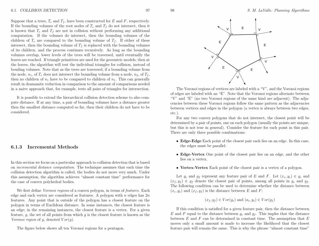
6.1. COLLISION DETECTION 97
Suppose that a trees, Te and Tf , have been constructed for E and F , respectively.If the bounding volumes of the root nodes of Te and Tf do not intersect, then itis known that Te and Tf are not in collision without performing any additionalcomputation. If the volumes do intersect, then the bounding volumes of thechildren of Te are compared to the bounding volume of Tf . If either of theseintersect, then the bounding volume of Tf is replaced with the bounding volumesof its children, and the process continues recursively. As long as the boundingvolumes overlap, lower levels of the trees will be traversed, until eventually theleaves are reached. If triangle primitives are used for the geoemtric models, then atthe leaves, the algorithm will test the individual triangles for collision, instead ofbouding volumes. Note that as the trees are traversed, if a bounding volume fromthe node, n1, of Te does not intersect the bounding volume from a node, n2, of Tf ,then no children of n1 have to be compared to children of n1. This can generallyresult in dramamtic reduction in comparison to the amount of comparisons neededin a naive approach that, for example, tests all pairs of triangles for intersection.
It is possible to extend the hierarchical collision detection scheme to also com-pute distance. If at any time, a pair of bounding volumes have a distance greaterthen the smallest distance computed so far, then their children do not have to beconsidered.
6.1.3 Incremental Methods
In this section we focus on a particular approach to collision detection that is basedon incremental distance computation. The technique assumes that each time thecollision detection algorithm is called, the bodies do not move very much. Underthis assumption, the algorithm achieves “almost constant time” performance forthe case of convex polyhedral bodies.
We first define Voronoi regions of a convex polygon, in terms of features. Eachedge and each vertex are considered as features. A polygon with n edges has 2nfeatures. Any point that is outside of the polygon has a closest feature on thepolygon in terms of Euclidean distance. In some instances, the closest feature isan edge; in the remaining instances, the closest feature is a vertex. For a givenfeature, g, the set of all points from which g is the closest feature is known as theVoronoi region of g, denoted V or(g).
The figure below shows all ten Voronoi regions for a pentagon.
98 S. M. LaValle: Planning Algorithms
VV
V
V
V
EE
EE
E
The Voronoi regions of vertices are labeled with a “V”, and the Voronoi regionsof edges are labeled with an “E”. Note that the Voronoi regions alternate between“V” and “E” (no two Voronoi regions of the same kind are adjacent). The adja-cencies between these Voronoi regions follow the same pattern as the adjacenciesbetween vertices and edges in the polygon (a vertex is always between two edges,etc.).
For any two convex polygons that do not intersect, the closest point will bedetermined by a pair of points, one on each polygon (usually the points are unique,but this is not true in general). Consider the feature for each point in this pair.There are only three possible combinations:
• Edge-Edge Each point of the closest pair each lies on an edge. In this case,the edges must be parallel.
• Edge-Vertex One point of the closest pair lies on an edge, and the otherlies on a vertex.
• Vertex-Vertex Each point of the closest pair is a vertex of a polygon.
Let ge and gf represent any feature pair of E and F . Let (xe, ye) ∈ ge and(xf , yf ) ∈ gf denote the closest pair of points, among all points in ge and gf .The following condition can be used to determine whether the distance between(xe, ye) and (xf , yf ) is the distance between E and F :
(xf , yf ) ∈ V or(ge) and (ae, ye) ∈ V or(gf )
If this condition is satisfied for a given feature pair, then the distance betweenE and F equal to the distance between ge and gf . This imples that the distancebetween E and F can be determined in constant time. The assumption that Emoves only a small amount is made to increase the likelihood that the closestfeature pair will remain the same. This is why the phrase “almost constant time”
6.2. METRIC SPACES 99
is used to describe the performance of the algorithm. Of course, it is possiblethat the closest feature pair will change. In this case, neighboring features can betested using the condition above, until the new closest pair of features is found.
The same ideas can be applied for the case in which the bodies are convexpolyhedra. The primary difference is that three kinds of features are considered:faces, edges, and vertices. The cases become more complicated, but the idea isthe same. Once again, the condition regarding mutual Voronoi regions holds, andthe algorithm has nearly constant time performance.
6.2 Metric Spaces
Distance is a fundamental notion in many path planning problems and approaches.It is generally useful to evaluate the distance from the robot to the goal, or tocompare any two configurations. We are already quite familiar with Euclideandistance in the world, but how is distance measured in a general topological space,such as C?
A metric space, (X, ρ), is a topological space, X, equipped with a function,ρ : X ×X → R such that for any x1, x2, x3 ∈ X:
1. ρ(x1, x2) ≥ 0 (non-negativity)
2. ρ(x1, x2) = 0 if and only if x1 = x2 (reflexivity)
3. ρ(x1, x2) = ρ(x2, x1) (symmetry)
4. ρ(x1, x2) + ρ(x2, x3) ≥ ρ(x1, x3) (triangle inequality) .
The function ρ defines distances between points in the metric space, and eachof the four conditions on ρ agrees with our intuitions about distance. The finalcondition implies that ρ is optimal in the sense that the distance from x1 to x3 willalways be less than or equal to the total distance obtained by traveling throughan intermediate point x2, on the way from x1 to x3.
Example 1 (Euclidean space) Suppose X = R2, and let a point in R2 be denotedby (x, y). The Euclidean (or L2) metric is defined as
ρ(x1, y1, x2, y2) =√
(x1 − x2)2 + (y1 − y2)2
Other metric spaces can be defined for R2.
Example 2 (Manhattan distance) The Manhattan (or L1) metric is defined overR2 as
ρ(x1, y1, x2, y2) = |x1 − x2|+ |y1 − y2|
Example 3 (L∞ distance) The L∞ metric is defined over R2 as
ρ(x1, y1, x2, y2) = max(|x1 − x2|, |y1 − y2|)
100 S. M. LaValle: Planning Algorithms
Example 4 (Distance in S1 using θ) In the case of X = S1, the metric becomesslightly more complicated due to the topology of S1. If S1 is represented by θ ∈[0, 2π), then the metric may be defined as
ρ(θ1, θ2) = min(|θ1 − θ2|, 2π − |θ1 − θ2|)
Example 5 (Distance in S1 using complex numbers) If S1 is represented by unitcomplex numbers, a+ bi, then a metric may be defined as
ρ(a1, b1, a2, b2) =√
(a1 − a2)2 + (b1 − b2)2
A metric can be defined for a space such as C = R2 × S1 by combining themetrics from R2 and S1. Suppose that two metric spaces, (X, ρx), and (Y, ρy),are defined. A metric space, (Z, ρz), can be constructed for the Cartesian productZ = X × Y by defining the metric ρz as
ρz(z1, z2) = ρ(x1, y1, x2, y2) = c1ρx(x1, x2) + c2ρy(y1, y2),
in which c1 > 0 and c2 > 0 are any positive, real constants. Other combinationslead to a metric for Z, such as
ρz(z1, z2) =√
c1ρ2x(x1, x2) + c2ρ2y(y1, y2).
In either of these cases, two positive constants must be chosen. It is importantto understand that many choices are possible, and there is no natural notion of a“correct” choice. A metric defined on C = R2 × S1 must compare both distancein the plane and an angular quantity. For example, even if c1 = c2 = 1, the rangefor S1 is [0, 2π) using radians, but [0, 360) using degrees. If the same constantc2 is used in either case, two very different metrics will be obtained. The unitsthat one are applied to R2 and S1 are completely incompatible. In terms of pathplanning, this implies that no natural metric exists for configuration spaces.
A final metric will be given, which is perhaps the most appropriate for pathplanning problems; however, it is also the most complicated to evaluate. For anytwo configurations q1, q2 ∈ C, for any configuration space, C, the distance is
Example 6 (Robot displacement metric) ρ(q1, q2) = maxa∈A ‖a(q1)− a(q2)‖,
in which a(qi) is the position of the point a in the world, when the robot, A is atconfiguration qi. Intuitively, the robot displacement metric yields the maximumamount in the world that any part of the robot is displaced from configuration q1to q2.
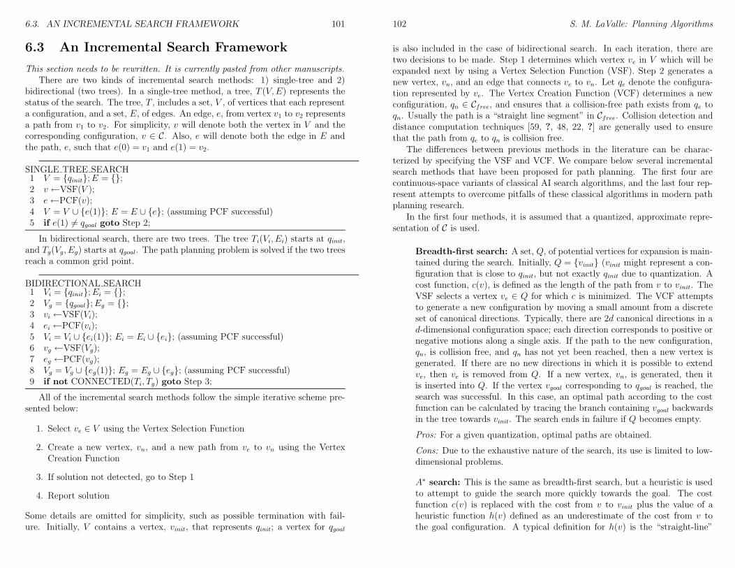
6.3. AN INCREMENTAL SEARCH FRAMEWORK 101
6.3 An Incremental Search Framework
This section needs to be rewritten. It is currently pasted from other manuscripts.There are two kinds of incremental search methods: 1) single-tree and 2)
bidirectional (two trees). In a single-tree method, a tree, T (V,E) represents thestatus of the search. The tree, T , includes a set, V , of vertices that each representa configuration, and a set, E, of edges. An edge, e, from vertex v1 to v2 representsa path from v1 to v2. For simplicity, v will denote both the vertex in V and thecorresponding configuration, v ∈ C. Also, e will denote both the edge in E andthe path, e, such that e(0) = v1 and e(1) = v2.
SINGLE TREE SEARCH1 V = qinit;E = ;2 v ←VSF(V );3 e←PCF(v);4 V = V ∪ e(1); E = E ∪ e; (assuming PCF successful)5 if e(1) 6= qgoal goto Step 2;
In bidirectional search, there are two trees. The tree Ti(Vi, Ei) starts at qinit,and Tg(Vg, Eg) starts at qgoal. The path planning problem is solved if the two treesreach a common grid point.
BIDIRECTIONAL SEARCH1 Vi = qinit;Ei = ;2 Vg = qgoal;Eg = ;3 vi ←VSF(Vi);4 ei ←PCF(vi);5 Vi = Vi ∪ ei(1); Ei = Ei ∪ ei; (assuming PCF successful)6 vg ←VSF(Vg);7 eg ←PCF(vg);8 Vg = Vg ∪ eg(1); Eg = Eg ∪ eg; (assuming PCF successful)9 if not CONNECTED(Ti, Tg) goto Step 3;
All of the incremental search methods follow the simple iterative scheme pre-sented below:
1. Select ve ∈ V using the Vertex Selection Function
2. Create a new vertex, vn, and a new path from ve to vn using the VertexCreation Function
3. If solution not detected, go to Step 1
4. Report solution
Some details are omitted for simplicity, such as possible termination with fail-ure. Initially, V contains a vertex, vinit, that represents qinit; a vertex for qgoal
102 S. M. LaValle: Planning Algorithms
is also included in the case of bidirectional search. In each iteration, there aretwo decisions to be made. Step 1 determines which vertex ve in V which will beexpanded next by using a Vertex Selection Function (VSF). Step 2 generates anew vertex, vn, and an edge that connects ve to vn. Let qe denote the configura-tion represented by ve. The Vertex Creation Function (VCF) determines a newconfiguration, qn ∈ Cfree, and ensures that a collision-free path exists from qe toqn. Usually the path is a “straight line segment” in Cfree. Collision detection anddistance computation techniques [59, ?, 48, 22, ?] are generally used to ensurethat the path from qe to qn is collision free.
The differences between previous methods in the literature can be charac-terized by specifying the VSF and VCF. We compare below several incrementalsearch methods that have been proposed for path planning. The first four arecontinuous-space variants of classical AI search algorithms, and the last four rep-resent attempts to overcome pitfalls of these classical algorithms in modern pathplanning research.
In the first four methods, it is assumed that a quantized, approximate repre-sentation of C is used.
Breadth-first search: A set, Q, of potential vertices for expansion is main-tained during the search. Initially, Q = vinit (vinit might represent a con-figuration that is close to qinit, but not exactly qinit due to quantization. Acost function, c(v), is defined as the length of the path from v to vinit. TheVSF selects a vertex ve ∈ Q for which c is minimized. The VCF attemptsto generate a new configuration by moving a small amount from a discreteset of canonical directions. Typically, there are 2d canonical directions in ad-dimensional configuration space; each direction corresponds to positive ornegative motions along a single axis. If the path to the new configuration,qn, is collision free, and qn has not yet been reached, then a new vertex isgenerated. If there are no new directions in which it is possible to extendve, then ve is removed from Q. If a new vertex, vn, is generated, then itis inserted into Q. If the vertex vgoal corresponding to qgoal is reached, thesearch was successful. In this case, an optimal path according to the costfunction can be calculated by tracing the branch containing vgoal backwardsin the tree towards vinit. The search ends in failure if Q becomes empty.
Pros: For a given quantization, optimal paths are obtained.
Cons: Due to the exhaustive nature of the search, its use is limited to low-dimensional problems.
A∗ search: This is the same as breadth-first search, but a heuristic is usedto attempt to guide the search more quickly towards the goal. The costfunction c(v) is replaced with the cost from v to vinit plus the value of aheuristic function h(v) defined as an underestimate of the cost from v tothe goal configuration. A typical definition for h(v) is the “straight-line”
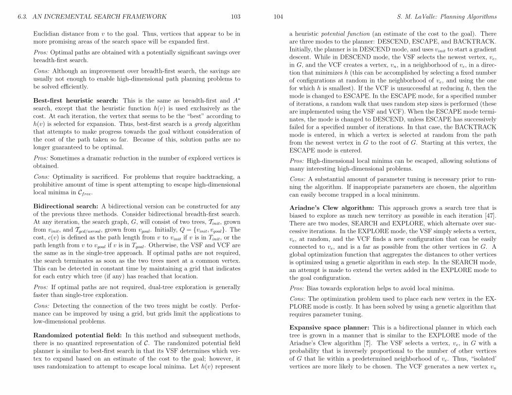
6.3. AN INCREMENTAL SEARCH FRAMEWORK 103
Euclidian distance from v to the goal. Thus, vertices that appear to be inmore promising areas of the search space will be expanded first.
Pros: Optimal paths are obtained with a potentially significant savings overbreadth-first search.
Cons: Although an improvement over breadth-first search, the savings areusually not enough to enable high-dimensional path planning problems tobe solved efficiently.
Best-first heuristic search: This is the same as breadth-first and A∗
search, except that the heuristic function h(v) is used exclusively as thecost. At each iteration, the vertex that seems to be the “best” according toh(v) is selected for expansion. Thus, best-first search is a greedy algorithmthat attempts to make progress towards the goal without consideration ofthe cost of the path taken so far. Because of this, solution paths are nolonger guaranteed to be optimal.
Pros: Sometimes a dramatic reduction in the number of explored vertices isobtained.
Cons: Optimality is sacrificed. For problems that require backtracking, aprohibitive amount of time is spent attempting to escape high-dimensionallocal minima in Cfree.
Bidirectional search: A bidirectional version can be constructed for anyof the previous three methods. Consider bidirectional breadth-first search.At any iteration, the search graph, G, will consist of two trees, Tinit, grownfrom vinit, and Tgcd/usroal, grown from vgoal. Initially, Q = vinit, vgoal. Thecost, c(v) is defined as the path length from v to vinit if v is in Tinit, or thepath length from v to vgoal if v is in Tgoal. Otherwise, the VSF and VCF arethe same as in the single-tree approach. If optimal paths are not required,the search terminates as soon as the two trees meet at a common vertex.This can be detected in constant time by maintaining a grid that indicatesfor each entry which tree (if any) has reached that location.
Pros: If optimal paths are not required, dual-tree exploration is generallyfaster than single-tree exploration.
Cons: Detecting the connection of the two trees might be costly. Perfor-mance can be improved by using a grid, but grids limit the applications tolow-dimensional problems.
Randomized potential field: In this method and subsequent methods,there is no quantized representation of C. The randomized potential fieldplanner is similar to best-first search in that its VSF determines which ver-tex to expand based on an estimate of the cost to the goal; however, ituses randomization to attempt to escape local minima. Let h(v) represent
104 S. M. LaValle: Planning Algorithms
a heuristic potential function (an estimate of the cost to the goal). Thereare three modes to the planner: DESCEND, ESCAPE, and BACKTRACK.Initially, the planner is in DESCEND mode, and uses vinit to start a gradientdescent. While in DESCEND mode, the VSF selects the newest vertex, ve,in G, and the VCF creates a vertex, vn, in a neighborhood of ve, in a direc-tion that minimizes h (this can be accomplished by selecting a fixed numberof configurations at random in the neighborhood of ve, and using the onefor which h is smallest). If the VCF is unsuccessful at reducing h, then themode is changed to ESCAPE. In the ESCAPE mode, for a specified numberof iterations, a random walk that uses random step sizes is performed (theseare implemented using the VSF and VCF). When the ESCAPE mode termi-nates, the mode is changed to DESCEND, unless ESCAPE has successivelyfailed for a specified number of iterations. In that case, the BACKTRACKmode is entered, in which a vertex is selected at random from the pathfrom the newest vertex in G to the root of G. Starting at this vertex, theESCAPE mode is entered.
Pros: High-dimensional local minima can be escaped, allowing solutions ofmany interesting high-dimensional problems.
Cons: A substantial amount of parameter tuning is necessary prior to run-ning the algorithm. If inappropriate parameters are chosen, the algorithmcan easily become trapped in a local minimum.
Ariadne’s Clew algorithm: This approach grows a search tree that isbiased to explore as much new territory as possible in each iteration [47].There are two modes, SEARCH and EXPLORE, which alternate over suc-cessive iterations. In the EXPLORE mode, the VSF simply selects a vertex,ve, at random, and the VCF finds a new configuration that can be easilyconnected to ve, and is a far as possible from the other vertices in G. Aglobal optimization function that aggregates the distances to other verticesis optimized using a genetic algorithm in each step. In the SEARCH mode,an attempt is made to extend the vertex added in the EXPLORE mode tothe goal configuration.
Pros: Bias towards exploration helps to avoid local minima.
Cons: The optimization problem used to place each new vertex in the EX-PLORE mode is costly. It has been solved by using a genetic algorithm thatrequires parameter tuning.
Expansive space planner: This is a bidirectional planner in which eachtree is grown in a manner that is similar to the EXPLORE mode of theAriadne’s Clew algorithm [?]. The VSF selects a vertex, ve, in G with aprobability that is inversely proportional to the number of other verticesof G that lie within a predetermined neighborhood of ve. Thus, “isolated’vertices are more likely to be chosen. The VCF generates a new vertex vn
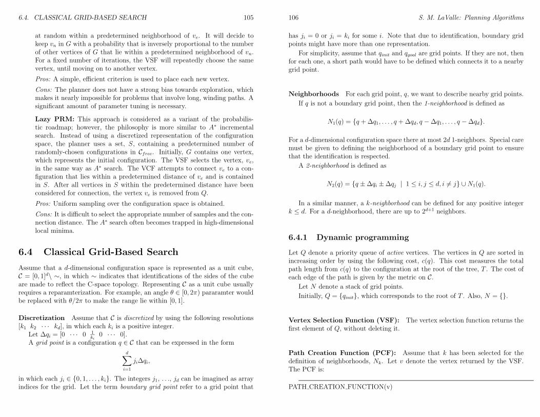
6.4. CLASSICAL GRID-BASED SEARCH 105
at random within a predetermined neighborhood of ve. It will decide tokeep vn in G with a probability that is inversely proportional to the numberof other vertices of G that lie within a predetermined neighborhood of vn.For a fixed number of iterations, the VSF will repeatedly choose the samevertex, until moving on to another vertex.
Pros: A simple, efficient criterion is used to place each new vertex.
Cons: The planner does not have a strong bias towards exploration, whichmakes it nearly impossible for problems that involve long, winding paths. Asignificant amount of parameter tuning is necessary.
Lazy PRM: This approach is considered as a variant of the probabilis-tic roadmap; however, the philosophy is more similar to A∗ incrementalsearch. Instead of using a discretized representation of the configurationspace, the planner uses a set, S, containing a predetermined number ofrandomly-chosen configurations in Cfree. Initially, G contains one vertex,which represents the initial configuration. The VSF selects the vertex, ve,in the same way as A∗ search. The VCF attempts to connect ve to a con-figuration that lies within a predetermined distance of ve and is containedin S. After all vertices in S within the predetermined distance have beenconsidered for connection, the vertex ve is removed from Q.
Pros: Uniform sampling over the configuration space is obtained.
Cons: It is difficult to select the appropriate number of samples and the con-nection distance. The A∗ search often becomes trapped in high-dimensionallocal minima.
6.4 Classical Grid-Based Search
Assume that a d-dimensional configuration space is represented as a unit cube,C = [0, 1]d\ ∼, in which ∼ indicates that identifications of the sides of the cubeare made to reflect the C-space topology. Representing C as a unit cube usuallyrequires a reparamterization. For example, an angle θ ∈ [0, 2π) pararamter wouldbe replaced with θ/2π to make the range lie within [0, 1].
Discretization Assume that C is discretized by using the following resolutions[k1 k2 · · · kd], in which each ki is a positive integer.
Let ∆qi = [0 · · · 0 1ki
0 · · · 0].A grid point is a configuration q ∈ C that can be expressed in the form
d∑
i=1
ji∆qi,
in which each ji ∈ 0, 1, . . . , ki. The integers j1, . . ., jd can be imagined as arrayindices for the grid. Let the term boundary grid point refer to a grid point that
106 S. M. LaValle: Planning Algorithms
has ji = 0 or ji = ki for some i. Note that due to identification, boundary gridpoints might have more than one representation.
For simplicity, assume that qinit and qgoal are grid points. If they are not, thenfor each one, a short path would have to be defined which connects it to a nearbygrid point.
Neighborhoods For each grid point, q, we want to describe nearby grid points.
If q is not a boundary grid point, then the 1-neighborhood is defined as
N1(q) = q +∆q1, . . . , q +∆qd, q −∆q1, . . . , q −∆qd.
For a d-dimensional configuration space there at most 2d 1-neighbors. Special caremust be given to defining the neighborhood of a boundary grid point to ensurethat the identification is respected.
A 2-neighborhood is defined as
N2(q) = q ±∆qi ±∆qj | 1 ≤ i, j ≤ d, i 6= j ∪N1(q).
In a similar manner, a k-neighborhood can be defined for any positive integerk ≤ d. For a d-neighborhood, there are up to 2d+1 neighbors.
6.4.1 Dynamic programming
Let Q denote a priority queue of active vertices. The vertices in Q are sorted inincreasing order by using the following cost, c(q). This cost measures the totalpath length from c(q) to the configuration at the root of the tree, T . The cost ofeach edge of the path is given by the metric on C.
Let N denote a stack of grid points.
Initially, Q = qinit, which corresponds to the root of T . Also, N = .
Vertex Selection Function (VSF): The vertex selection function returns thefirst element of Q, without deleting it.
Path Creation Function (PCF): Assume that k has been selected for thedefinition of neighborhoods, Nk. Let v denote the vertex returned by the VSF.The PCF is:
PATH CREATION FUNCTION(v)
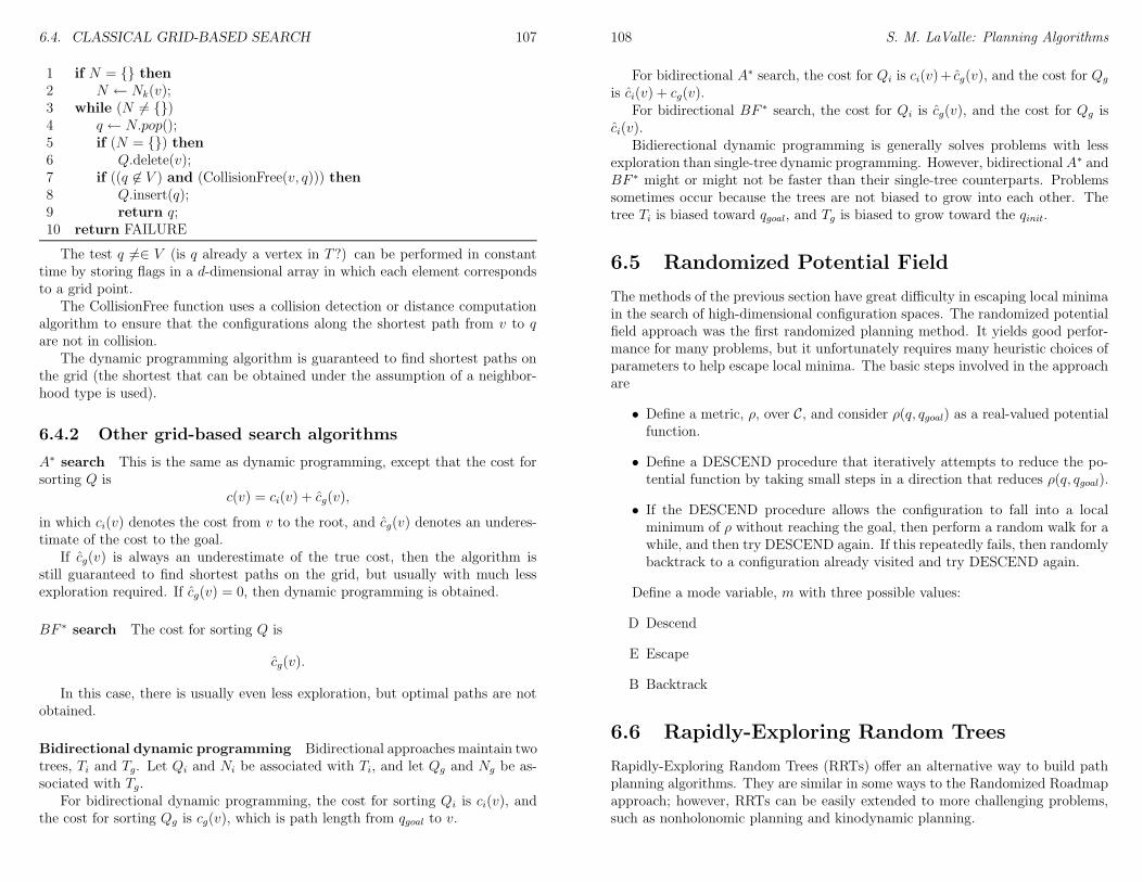
6.4. CLASSICAL GRID-BASED SEARCH 107
1 if N = then2 N ← Nk(v);3 while (N 6= )4 q ← N.pop();5 if (N = ) then6 Q.delete(v);7 if ((q 6∈ V ) and (CollisionFree(v, q))) then8 Q.insert(q);9 return q;10 return FAILURE
The test q 6=∈ V (is q already a vertex in T?) can be performed in constanttime by storing flags in a d-dimensional array in which each element correspondsto a grid point.
The CollisionFree function uses a collision detection or distance computationalgorithm to ensure that the configurations along the shortest path from v to qare not in collision.
The dynamic programming algorithm is guaranteed to find shortest paths onthe grid (the shortest that can be obtained under the assumption of a neighbor-hood type is used).
6.4.2 Other grid-based search algorithms
A∗ search This is the same as dynamic programming, except that the cost forsorting Q is
c(v) = ci(v) + cg(v),
in which ci(v) denotes the cost from v to the root, and cg(v) denotes an underes-timate of the cost to the goal.
If cg(v) is always an underestimate of the true cost, then the algorithm isstill guaranteed to find shortest paths on the grid, but usually with much lessexploration required. If cg(v) = 0, then dynamic programming is obtained.
BF ∗ search The cost for sorting Q is
cg(v).
In this case, there is usually even less exploration, but optimal paths are notobtained.
Bidirectional dynamic programming Bidirectional approaches maintain twotrees, Ti and Tg. Let Qi and Ni be associated with Ti, and let Qg and Ng be as-sociated with Tg.
For bidirectional dynamic programming, the cost for sorting Qi is ci(v), andthe cost for sorting Qg is cg(v), which is path length from qgoal to v.
108 S. M. LaValle: Planning Algorithms
For bidirectional A∗ search, the cost for Qi is ci(v)+ cg(v), and the cost for Qg
is ci(v) + cg(v).For bidirectional BF ∗ search, the cost for Qi is cg(v), and the cost for Qg is
ci(v).Bidierectional dynamic programming is generally solves problems with less
exploration than single-tree dynamic programming. However, bidirectionalA∗ andBF ∗ might or might not be faster than their single-tree counterparts. Problemssometimes occur because the trees are not biased to grow into each other. Thetree Ti is biased toward qgoal, and Tg is biased to grow toward the qinit.
6.5 Randomized Potential Field
The methods of the previous section have great difficulty in escaping local minimain the search of high-dimensional configuration spaces. The randomized potentialfield approach was the first randomized planning method. It yields good perfor-mance for many problems, but it unfortunately requires many heuristic choices ofparameters to help escape local minima. The basic steps involved in the approachare
• Define a metric, ρ, over C, and consider ρ(q, qgoal) as a real-valued potentialfunction.
• Define a DESCEND procedure that iteratively attempts to reduce the po-tential function by taking small steps in a direction that reduces ρ(q, qgoal).
• If the DESCEND procedure allows the configuration to fall into a localminimum of ρ without reaching the goal, then perform a random walk for awhile, and then try DESCEND again. If this repeatedly fails, then randomlybacktrack to a configuration already visited and try DESCEND again.
Define a mode variable, m with three possible values:
D Descend
E Escape
B Backtrack
6.6 Rapidly-Exploring Random Trees
Rapidly-Exploring Random Trees (RRTs) offer an alternative way to build pathplanning algorithms. They are similar in some ways to the Randomized Roadmapapproach; however, RRTs can be easily extended to more challenging problems,such as nonholonomic planning and kinodynamic planning.
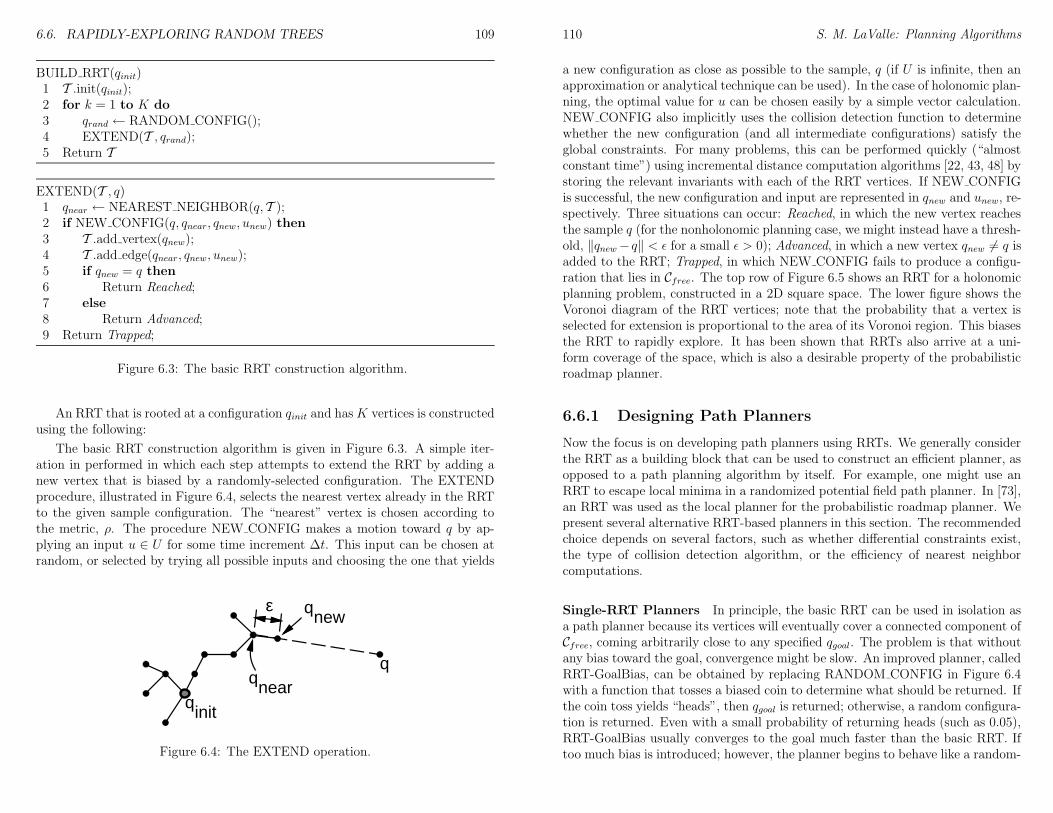
6.6. RAPIDLY-EXPLORING RANDOM TREES 109
BUILD RRT(qinit)1 T .init(qinit);2 for k = 1 to K do3 qrand ← RANDOM CONFIG();4 EXTEND(T , qrand);5 Return T
EXTEND(T , q)1 qnear ← NEAREST NEIGHBOR(q, T );2 if NEW CONFIG(q, qnear, qnew, unew) then3 T .add vertex(qnew);4 T .add edge(qnear, qnew, unew);5 if qnew = q then6 Return Reached;7 else8 Return Advanced;9 Return Trapped;
Figure 6.3: The basic RRT construction algorithm.
An RRT that is rooted at a configuration qinit and hasK vertices is constructedusing the following:
The basic RRT construction algorithm is given in Figure 6.3. A simple iter-ation in performed in which each step attempts to extend the RRT by adding anew vertex that is biased by a randomly-selected configuration. The EXTENDprocedure, illustrated in Figure 6.4, selects the nearest vertex already in the RRTto the given sample configuration. The “nearest” vertex is chosen according tothe metric, ρ. The procedure NEW CONFIG makes a motion toward q by ap-plying an input u ∈ U for some time increment ∆t. This input can be chosen atrandom, or selected by trying all possible inputs and choosing the one that yields
init
near
newε
q
q
q
q
Figure 6.4: The EXTEND operation.
110 S. M. LaValle: Planning Algorithms
a new configuration as close as possible to the sample, q (if U is infinite, then anapproximation or analytical technique can be used). In the case of holonomic plan-ning, the optimal value for u can be chosen easily by a simple vector calculation.NEW CONFIG also implicitly uses the collision detection function to determinewhether the new configuration (and all intermediate configurations) satisfy theglobal constraints. For many problems, this can be performed quickly (“almostconstant time”) using incremental distance computation algorithms [22, 43, 48] bystoring the relevant invariants with each of the RRT vertices. If NEW CONFIGis successful, the new configuration and input are represented in qnew and unew, re-spectively. Three situations can occur: Reached, in which the new vertex reachesthe sample q (for the nonholonomic planning case, we might instead have a thresh-old, ‖qnew− q‖ < ε for a small ε > 0); Advanced, in which a new vertex qnew 6= q isadded to the RRT; Trapped, in which NEW CONFIG fails to produce a configu-ration that lies in Cfree. The top row of Figure 6.5 shows an RRT for a holonomicplanning problem, constructed in a 2D square space. The lower figure shows theVoronoi diagram of the RRT vertices; note that the probability that a vertex isselected for extension is proportional to the area of its Voronoi region. This biasesthe RRT to rapidly explore. It has been shown that RRTs also arrive at a uni-form coverage of the space, which is also a desirable property of the probabilisticroadmap planner.
6.6.1 Designing Path Planners
Now the focus is on developing path planners using RRTs. We generally considerthe RRT as a building block that can be used to construct an efficient planner, asopposed to a path planning algorithm by itself. For example, one might use anRRT to escape local minima in a randomized potential field path planner. In [73],an RRT was used as the local planner for the probabilistic roadmap planner. Wepresent several alternative RRT-based planners in this section. The recommendedchoice depends on several factors, such as whether differential constraints exist,the type of collision detection algorithm, or the efficiency of nearest neighborcomputations.
Single-RRT Planners In principle, the basic RRT can be used in isolation asa path planner because its vertices will eventually cover a connected component ofCfree, coming arbitrarily close to any specified qgoal. The problem is that withoutany bias toward the goal, convergence might be slow. An improved planner, calledRRT-GoalBias, can be obtained by replacing RANDOM CONFIG in Figure 6.4with a function that tosses a biased coin to determine what should be returned. Ifthe coin toss yields “heads”, then qgoal is returned; otherwise, a random configura-tion is returned. Even with a small probability of returning heads (such as 0.05),RRT-GoalBias usually converges to the goal much faster than the basic RRT. Iftoo much bias is introduced; however, the planner begins to behave like a random-
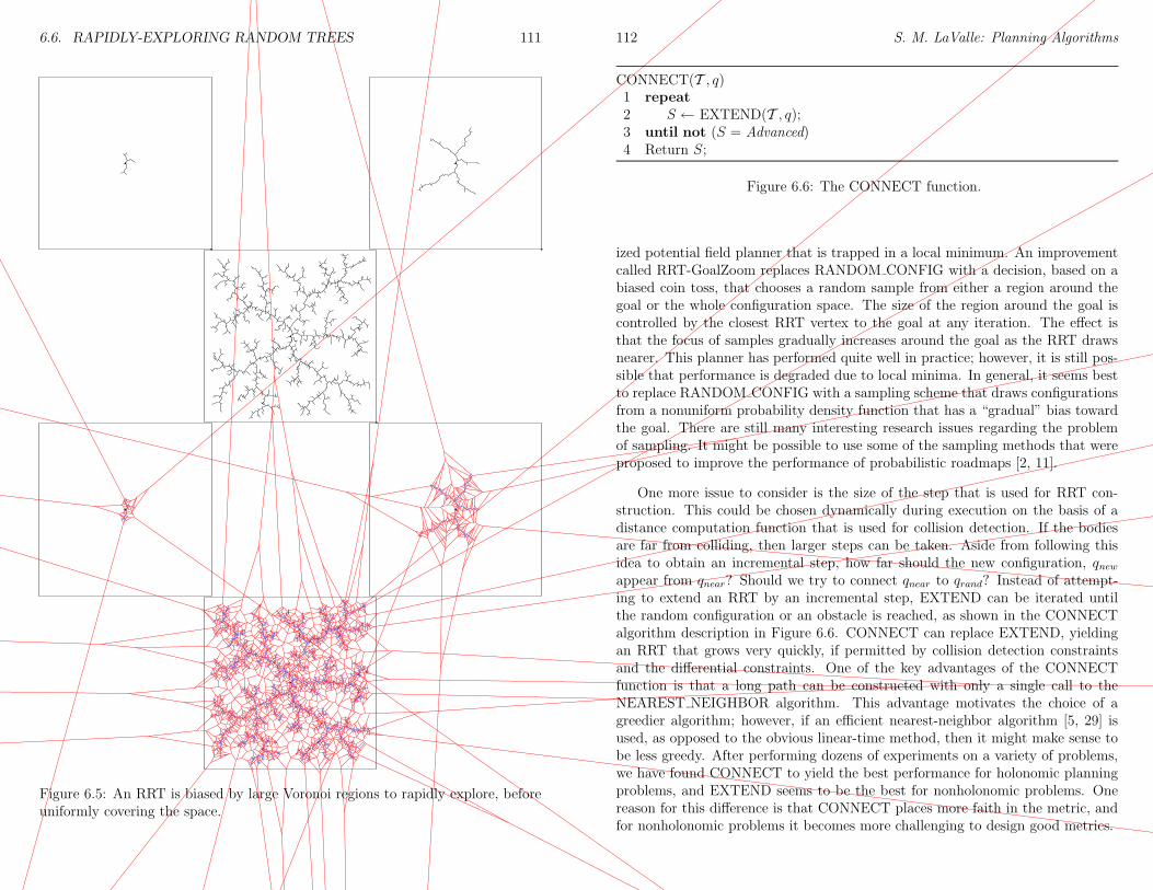
6.6. RAPIDLY-EXPLORING RANDOM TREES 111
Figure 6.5: An RRT is biased by large Voronoi regions to rapidly explore, beforeuniformly covering the space.
112 S. M. LaValle: Planning Algorithms
CONNECT(T , q)1 repeat2 S ← EXTEND(T , q);3 until not (S = Advanced)4 Return S;
Figure 6.6: The CONNECT function.
ized potential field planner that is trapped in a local minimum. An improvementcalled RRT-GoalZoom replaces RANDOM CONFIG with a decision, based on abiased coin toss, that chooses a random sample from either a region around thegoal or the whole configuration space. The size of the region around the goal iscontrolled by the closest RRT vertex to the goal at any iteration. The effect isthat the focus of samples gradually increases around the goal as the RRT drawsnearer. This planner has performed quite well in practice; however, it is still pos-sible that performance is degraded due to local minima. In general, it seems bestto replace RANDOM CONFIG with a sampling scheme that draws configurationsfrom a nonuniform probability density function that has a “gradual” bias towardthe goal. There are still many interesting research issues regarding the problemof sampling. It might be possible to use some of the sampling methods that wereproposed to improve the performance of probabilistic roadmaps [2, 11].
One more issue to consider is the size of the step that is used for RRT con-struction. This could be chosen dynamically during execution on the basis of adistance computation function that is used for collision detection. If the bodiesare far from colliding, then larger steps can be taken. Aside from following thisidea to obtain an incremental step, how far should the new configuration, qnewappear from qnear? Should we try to connect qnear to qrand? Instead of attempt-ing to extend an RRT by an incremental step, EXTEND can be iterated untilthe random configuration or an obstacle is reached, as shown in the CONNECTalgorithm description in Figure 6.6. CONNECT can replace EXTEND, yieldingan RRT that grows very quickly, if permitted by collision detection constraintsand the differential constraints. One of the key advantages of the CONNECTfunction is that a long path can be constructed with only a single call to theNEAREST NEIGHBOR algorithm. This advantage motivates the choice of agreedier algorithm; however, if an efficient nearest-neighbor algorithm [5, 29] isused, as opposed to the obvious linear-time method, then it might make sense tobe less greedy. After performing dozens of experiments on a variety of problems,we have found CONNECT to yield the best performance for holonomic planningproblems, and EXTEND seems to be the best for nonholonomic problems. Onereason for this difference is that CONNECT places more faith in the metric, andfor nonholonomic problems it becomes more challenging to design good metrics.
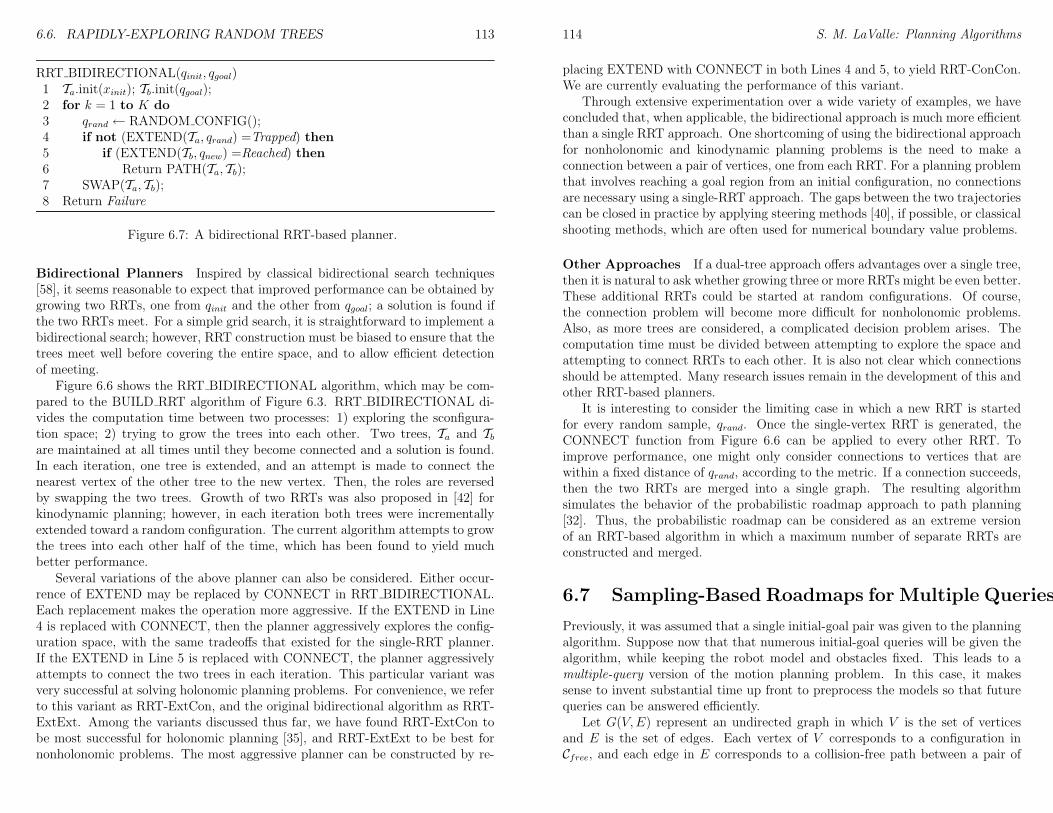
6.6. RAPIDLY-EXPLORING RANDOM TREES 113
RRT BIDIRECTIONAL(qinit, qgoal)1 Ta.init(xinit); Tb.init(qgoal);2 for k = 1 to K do3 qrand ← RANDOM CONFIG();4 if not (EXTEND(Ta, qrand) =Trapped) then5 if (EXTEND(Tb, qnew) =Reached) then6 Return PATH(Ta, Tb);7 SWAP(Ta, Tb);8 Return Failure
Figure 6.7: A bidirectional RRT-based planner.
Bidirectional Planners Inspired by classical bidirectional search techniques[58], it seems reasonable to expect that improved performance can be obtained bygrowing two RRTs, one from qinit and the other from qgoal; a solution is found ifthe two RRTs meet. For a simple grid search, it is straightforward to implement abidirectional search; however, RRT construction must be biased to ensure that thetrees meet well before covering the entire space, and to allow efficient detectionof meeting.
Figure 6.6 shows the RRT BIDIRECTIONAL algorithm, which may be com-pared to the BUILD RRT algorithm of Figure 6.3. RRT BIDIRECTIONAL di-vides the computation time between two processes: 1) exploring the sconfigura-tion space; 2) trying to grow the trees into each other. Two trees, Ta and Tbare maintained at all times until they become connected and a solution is found.In each iteration, one tree is extended, and an attempt is made to connect thenearest vertex of the other tree to the new vertex. Then, the roles are reversedby swapping the two trees. Growth of two RRTs was also proposed in [42] forkinodynamic planning; however, in each iteration both trees were incrementallyextended toward a random configuration. The current algorithm attempts to growthe trees into each other half of the time, which has been found to yield muchbetter performance.
Several variations of the above planner can also be considered. Either occur-rence of EXTEND may be replaced by CONNECT in RRT BIDIRECTIONAL.Each replacement makes the operation more aggressive. If the EXTEND in Line4 is replaced with CONNECT, then the planner aggressively explores the config-uration space, with the same tradeoffs that existed for the single-RRT planner.If the EXTEND in Line 5 is replaced with CONNECT, the planner aggressivelyattempts to connect the two trees in each iteration. This particular variant wasvery successful at solving holonomic planning problems. For convenience, we referto this variant as RRT-ExtCon, and the original bidirectional algorithm as RRT-ExtExt. Among the variants discussed thus far, we have found RRT-ExtCon tobe most successful for holonomic planning [35], and RRT-ExtExt to be best fornonholonomic problems. The most aggressive planner can be constructed by re-
114 S. M. LaValle: Planning Algorithms
placing EXTEND with CONNECT in both Lines 4 and 5, to yield RRT-ConCon.We are currently evaluating the performance of this variant.
Through extensive experimentation over a wide variety of examples, we haveconcluded that, when applicable, the bidirectional approach is much more efficientthan a single RRT approach. One shortcoming of using the bidirectional approachfor nonholonomic and kinodynamic planning problems is the need to make aconnection between a pair of vertices, one from each RRT. For a planning problemthat involves reaching a goal region from an initial configuration, no connectionsare necessary using a single-RRT approach. The gaps between the two trajectoriescan be closed in practice by applying steering methods [40], if possible, or classicalshooting methods, which are often used for numerical boundary value problems.
Other Approaches If a dual-tree approach offers advantages over a single tree,then it is natural to ask whether growing three or more RRTs might be even better.These additional RRTs could be started at random configurations. Of course,the connection problem will become more difficult for nonholonomic problems.Also, as more trees are considered, a complicated decision problem arises. Thecomputation time must be divided between attempting to explore the space andattempting to connect RRTs to each other. It is also not clear which connectionsshould be attempted. Many research issues remain in the development of this andother RRT-based planners.
It is interesting to consider the limiting case in which a new RRT is startedfor every random sample, qrand. Once the single-vertex RRT is generated, theCONNECT function from Figure 6.6 can be applied to every other RRT. Toimprove performance, one might only consider connections to vertices that arewithin a fixed distance of qrand, according to the metric. If a connection succeeds,then the two RRTs are merged into a single graph. The resulting algorithmsimulates the behavior of the probabilistic roadmap approach to path planning[32]. Thus, the probabilistic roadmap can be considered as an extreme versionof an RRT-based algorithm in which a maximum number of separate RRTs areconstructed and merged.
6.7 Sampling-Based Roadmaps for Multiple Queries
Previously, it was assumed that a single initial-goal pair was given to the planningalgorithm. Suppose now that that numerous initial-goal queries will be given thealgorithm, while keeping the robot model and obstacles fixed. This leads to amultiple-query version of the motion planning problem. In this case, it makessense to invent substantial time up front to preprocess the models so that futurequeries can be answered efficiently.
Let G(V,E) represent an undirected graph in which V is the set of verticesand E is the set of edges. Each vertex of V corresponds to a configuration inCfree, and each edge in E corresponds to a collision-free path between a pair of
6.7. SAMPLING-BASED ROADMAPS FOR MULTIPLE QUERIES 115
configurations in Cfree. The graph G is constructed in a preprocessing phase. Ina query phase, G is used to solve a particular path planning question for a givenqinit and qgoal.
The following algorithm builds a graph, G, in Cfree:
BUILD ROADMAP(A,O)1 G.init();2 for i = 1 to M3 q ←RAND FREE CONF(q);4 G.add vertex(q);5 for each v ∈ NBHD(q,G)6 if ((not G.same component(q, v)) and CONNECT(q, v)) then7 G.add edge(q, v);8 Return G;
The graph resulting graph will have M vertices. Each of the major compo-nents in described in more detail below. Sometimes it is preferable to replace thecondition (not G.same component(q, v)) with G.vertex degree(q) < K, for somefixed K (e.g., K = 15). The same component condition checks whether q and vare in the same connected component of G. If they are, then it is generally notnecessary to attempt to connect q to v. However, it might be too costly to evalu-ate this condition each time, and one might prefer shorter paths. In this case, itwould be appropriate to increase the density of edges in G. A limit K can be seton the maximum allowable degree for any vertex in G.
A random configuration in Cfree is simply found by picking a configuration atrandom, and using a collision detection algorithm to test whether the configurationlies in Cobs or Cfree. If it lies in Cobs, then a new random configurations are chosen,until one lies in Cfree. The running time of this algorithm will obviously beaffected by the amount of freedom the robot has to move in the world. If mostconfigurations are in collision, this algorithm will spend more time trying to finda free configuration. The algorithm is outlined below.
RAND FREE CONF()1 repeat2 q ←RAND CONF();3 until q ∈ Cfree;4 Return q;
The following algorithm returns an ordered list of vertices in G(V,E), whosecorresponding configurations are within a distance ε of q. The distance threshold,ε, and the metric ρ(q, v) are selected in advance.NBHD(q,G)
116 S. M. LaValle: Planning Algorithms
1 Q.init();2 for each v ∈ V3 if ρ(q, v) < ε then4 Q.insert();5 Return q;
Is it assumed that Q is a priority queue, with elements sorted in increasing orderaccording to ρ(q, v). This ordering will cause the roadmap building algorithm toattempt connections to closer vertices first, before proceeding to more difficultconnections.
The CONNECT(q, v) algorithm is considered conceptually as a local planner.The simplest form of a local planner is one that simply connects q to v by a“straight line” in Cfree. This line is defined by performing interpolation betweenq and v. If this line intersects Cobs, then an edge cannot be made in G to con-nect q and v. One way to ensure that the entire line lies in Cfree is to performcollision detection incrementally along the line from q to v. In each step, therobot is moved a small amount, and the configuration is checked for collision. Anincremental collision detection algorithm would be suitable for this phase of thealgorithm. Alternatively, it may be preferable to precompute a bitmap for fastcollision detection. If the steps are made small enough so that no point on A isdisplaced by more than some δ1 > 0, then one can guarantee that a collision notoccur in any intermediate configurations if the robot is at least δ2 away from theobstacles in the world. The robot displacement metric can be used to determineδ1, and the incremental collision detection algorithm can be used to determine δ2.
In the query phase, an initial configuration, qinit, and a goal configuration,qgoal, are given. To perform path planning, the first step is to pretend as if qinitand qgoal were chosen randomly for connection to G. The NBHD and CONNECTalgorithms can be used to attempt connection. If these succeed in connectingqinit and qgoal to other vertices in G, a graph search is performed for a path thatconnects the vertex qinit to the vertex qgoal. The path in the graph correspondsdirectly to a path in Cfree, which is a solution to the query. Unfortunately, if thismethod fails, it cannot be determined conclusively whether a solution exists. Oneapproach could be to add more random vertices to G, and then try again to solvethe path planning problem.
In general, the best one can assure is that the probabilistic roadmap planningalgorithm in probabilistically complete. This is a fairly weak statement, whichsimply implies that the probability of finding a solution (if one exists) convergesto one, while the running time approaches infinity. This seems to guarantee thata solution will be found, but this guarantee could only be made “after” runningthe algorithm forever. Thus, the algorithm cannot conclude that a solution doesnot exist after a finite period of time.
It is very challenging to analyze the performance of randomized path planningalgorithms. Among these algorithms, the strongest analysis thus far exists forthe randomized roadmap approach. The concept is based on the notion of ε-

6.8. SAMPLING-BASED ROADMAP VARIANTS 117
goodness. Consider cases in which the CONNECT algorithm will be unlikely tomake a connection, even though a connection exists. The following examples areextremely difficult (especially the right one) because of the narrow corridor thatlinks two portions of Cfree.
These are examples in a 2D configurations, and in higher dimensions, theproblem can become even more difficult. Many planning problems involve movinga robot through an area with tight clearance. This will generally cause narrowchannels to form in Cfree, which leads to a challenging planning problem for therandomized roadmap algorithm.
Let S(q) denote the set of all configurations that can be connected to q usingthe CONNECT algorithm. Intuitively, this can be considered as the set of allconfigurations that can be “seen” using line-of-sight visibility. The ε-goodness isdefined in terms of the following parameter,
ε = minq∈Cfree
µ(S(q))
µ(Cfree),
in which µ represents the volume (or more technically, the measure). Intuitively,ε represents the small fraction of Cfree that is visible from any point. In terms ofε and M (the number of vertices in G), a theorem has been established recentlythat yields the probability that a solution will be found. The main difficultiesare that the ε-goodness concept is very conservative (it uses worst-case analysisover all configurations), and ε-goodness is defined in terms of the structure ofCfree, which cannot be computed efficiently. The result is interesting for gaininga better understanding of the algorithm, but the theorem is very difficult to usein a particular application to determine whether the algorithm will perform well.
6.8 Sampling-Based Roadmap Variants
The following variants should be covered:
• Node enhancement
• Visibility PRM
118 S. M. LaValle: Planning Algorithms
• Obstacle-based PRM
• Medial axis PRM
6.9 Deterministic Sampling Theory
This section gives an overview of deterministic sampling concepts and techniques.
6.9.1 Sampling Criteria
Motivated by applications in numerical integration and optimization, the mostcommon criteria are discrepancy and dispersion. Each of these measures theamount of uniformity in a collection of points. This is different from statisticaltests that might be applied to points generated by a pseudo-random numbergenerator. The criteria are designed to match the problem to which the pointsare applied, as opposed to simulation of “randomness.”
Let X = [0, 1]d ⊂ Rd define a space over which to generate points. LetP = p0, . . . , pN−1 denote a finite set of N points in X. Let R be a collection ofsubsets of X that is called a range space. With respect to a particular point set,P , and range space, R, the discrepancy [76] is defined as
D(P,R) = supR∈R
∣
∣
∣
∣
|P ∩R|
N− µ(R)
∣
∣
∣
∣
(6.1)
in which | · | applied to a finite set denotes its cardinality, and µ is Lebesguemeasure. Each term in the supremum considers how well P can be used to estimatethe volume of R. For example, if µ(R) is 1/5, then we would hope that about1/5 of the points in P fall into R. The discrepancy measures the largest volumeestimation error that can be obtained over all sets in R.
In most cases, R is chosen as the set of all axis-aligned rectangular subsets. Inthis case, the range space will be denoted as Raar. This is motivated primarily byapplications to numerical integration. In this case, the Koksma-Hlawka inequalityexpresses the convergence rate in terms of a constant for bounded variation (in thesense of Hardy-Krause) of the integrand, and the bounded variation is expressedin terms of rectangular partitions [53].
For applications to optimization, the notion of dispersion was developed:
δ(P, ρ) = supx∈X
minp∈P
ρ(x, p), (6.2)
in which ρ denotes any metric. Cases in which ρ is the Euclidean metric or `∞ willbe referred to as Euclidean dispersion and `∞ dispersion, respectively. Dispersioncan be considered as the radius of the largest ball that does not contain an elementof P . This represents a natural choice for many optimization problems because theerror can be related directly to a Lipschitz constant for the function. For example,
6.9. DETERMINISTIC SAMPLING THEORY 119
in one dimension, the maximum error is proportional to the longest interval thatdoes not contain a sample point.
Since a large empty ball contains substantial measure, there is a close rela-tionship between discrepancy, which is measure-based, and dispersion, which ismetric-based. For example, for any P ,
δ(P, `∞) ≤ D(P,Raar)1/d,
which means low-discrepancy implies low-dispersion. Note that the converse isnot true. An axis-aligned grid yields high discrepancy because of alignments withthe boundaries of sets in Raar, but the dispersion is very low.
6.9.2 Finite Point Sets and Infinite Sequences
There are two important sampling families: 1) finite point sets, and 2) infinitesequences. We will use the term point set to refer to the first form, and sequenceto refer to the second. For a point set, the number, N , is specified in advance,and a set of N points is chosen that optimizes discrepancy or dispersion. As forany set, there is no notion of ordering in a point set; however, for a sequence, theordering of points becomes crucial.
Each of the two forms of sampling is suited for a different kind of algorithm. Agrid is the most common example of a point set. Samples drawn using a pseudo-random number generator are a typical example of a sequence. If the appropriateN is known in advance, then a point set should be used. If the algorithm cannotdetermine N in advance, but is able to incrementally add more and more points,then a sequence is usually more appropriate. The availability of a sequence frompseudo-random number generators represents a major part of the past appealof using randomization in motion planning; however, many other sequences areavailable.
Analysis of discrepancy or dispersion in the quasi-Monte Carlo literature isusually asymptotic [53]. The vast majority of sample construction algorithmsare so simple and efficient that complexity analysis of the algorithm itself is notperformed. The definition of asymptotic analysis for a sample sequence is straight-forward; however, a point set must be converted into a sequence to perform theanalysis. In this case, asymptotic analysis is actually performed over a sequenceof point sets. Let PN denote a point set in the sequence. For asymptotic analysisof point sets, PN+1 does not have to contain any of the points from PN . For se-quences, strict containment must always occur; each iteration adds a single pointto the previous ones. Therefore, point sets often appear better than sequencesin theory, but they might pose difficulties in practice because they may requirethe specification of N . A low-discrepancy sequence or point set is one that yieldsthe best-possible asymptotic discrepancy, which is O(N−1 logdN) for infinite se-quences and O(N−1 logd−1N) for finite point sets, under the common range spaceRaar. Note that the second bound is better, for reasons mentioned in the previous
120 S. M. LaValle: Planning Algorithms
paragraph. A low-dispersion sequence or point set is one that obtains the lowest-possible asymptotic dispersion. For any `p metric, both sequences and point setscan achieve O(N−1/d). The remainder of this section provides an overview oflow-discrepancy and low-dispersion sampling.
In the bounds above, N , is the variable considered in the asymptotic analysis(i.e., the limit is taken with respect to N). Therefore, the dimension, d, is treatedas a constant. Thus, if there is a multiplicative factor which is a function of d,say b(d), then it is not shown in an expression such as O(N−1/d). However, it isimportant to understand that for many well-known cases, b(d), and ultimately thedispersion or discrepancy, may increase dramatically with respect to dimension.Therefore, a substantial amount of recent research has been conducted to improvesample quality as the dimension increases. These issues will become important inour theoretical analysis, presented in Section ??.
6.9.3 Low-Discrepancy Sampling
Due to the fundamental importance of numerical integration, and the intricatelink between discrepancy and integration error, most of the quasi-Monte Carloliterature has led to low-discrepancy sequences and point sets. Although motionplanning is quite different from integration, it is worth evaluating these carefully-constructed and well-analyzed samples. Their potential use in motion planning isno less reasonable than using pseudo-random sequences, which were also designedwith a different intention in mind.
Low-discrepancy sampling methods can be divided into three categories: 1)Halton/Hammersley sampling, 2) (t,s)-sequences and (t,m,s)-nets, and 3) lattices.The first category represents one of the earliest methods, based on the originalideas of van der Corput [74], who defined a low-discrepancy sequence of pointsin [0, 1]. Consider a binary representation of points in [0, 1]. A one-dimensional“grid” can be made with resolution 8, then samples are taken at: 0.000, 0.001,0.010, 0.011, 0.100, etc. The problem with using such points in this order is thatthey scan from left to right, as opposed to moving around in a manner similar tothat of pseudo-random sequences. The van der Corput sequence simply takes thebinary counting above and reverses the order of the bits. During the original scan,the least significant bit alternates in every step, but this only yields a small changein value. By reversing bit order, the change is maximized, causing the coverage tobe nearly uniform at every point in the sequence. After bit reversal, the sequenceis: 0.000, 0.100, 0.010, 0.110, 0.001, 0.101, 0.011, 0.111. An infinite sequence isconstructed by using reversed-bit representations of higher binary numbers. Thenext eight samples are obtained by reversing binary representations of 8 through15.
The Halton sequence is a d dimensional generalization that uses van der Cor-put sequences of d different bases, one for each coordinate [23]. First, choose drelatively prime integers p1, p2, . . . , pd (usually the first d primes, p1 = 2, p2 = 3,
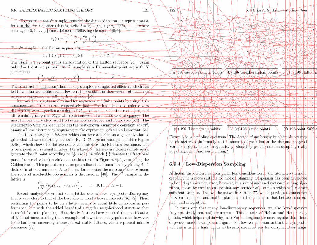
6.9. DETERMINISTIC SAMPLING THEORY 121
. . . ). To construct the ith sample, consider the digits of the base p representationfor i in the reverse order (that is, write i = a0 + pa1 + p2a2 + p3a3 + . . ., whereeach aj ∈ 0, 1, . . . , p) and define the following element of [0, 1]:
rp(i) =a0p
+a1p2
+a2p3
+a3p4
+ · · · .
The ith sample in the Halton sequence is
(rp1(i), rp2(i), . . . , rpd(i)), i = 0, 1, 2, . . . .
The Hammersley point set is an adaptation of the Halton sequence [24]. Usingonly d − 1 distinct primes, the ith sample in a Hammersley point set with Nelements is
(
i
N, rp1(i), . . . , rpd−1
(i)
)
, i = 0, 1, . . . , N − 1.
The construction of Halton/Hammersley samples is simple and efficient, which hasled to widespread application. However, the constant in their asymptotic analysisincreases superexponentially with dimension [53].
Improved constants are obtained for sequences and finite points by using (t,s)-sequences, and (t,m,s)-nets, respectively [53]. The key idea is to enforce zerodiscrepancy over a particular subset of Raar known as canonical rectangles, andall remaining ranges in Raar will contribute small amounts to discrepancy. Themost famous and widely-used (t,s)-sequences are Sobol’ and Faure (see [53]). TheNiederreiter-Xing (t,s)-sequence has the best-known asymptotic constant, (a/d)d,among all low-discrepancy sequences; in the expression, a is a small constant [54].
The third category is lattices, which can be considered as a generalization ofgrids that allows nonorthogonal axes [46, 67, 75]. As an example, consider Figure6.8(e), which shows 196 lattice points generated by the following technique. Letα be a positive irrational number. For a fixed N (lattices are closed sample sets),generate the ith point according to ( i
N, iα), in which · denotes the fractional
part of the real value (modulo-one arithmetic). In Figure 6.8(e), α =√5+12
, theGolden Ratio. This procedure can be generalized to d dimensions by picking d−1distinct irrational numbers. A technique for choosing the αk parameters by usingthe roots of irreducible polynomials is discussed in [46]. The ith sample in thelattice is
(
i
N, iα1, . . . , iαd−1
)
, i = 0, 1, . . . , N − 1.
Recent analysis shows that some lattice sets achieve asymptotic discrepancythat is very close to that of the best-known non-lattice sample sets [26, 72]. Thus,restricting the points to lie on a lattice seems to entail little or no loss in per-formance, but with the added benefit of a regular neighborhood structure thatis useful for path planning. Historically, lattices have required the specificationof N in advance, making them examples of low-discrepancy point sets; however,there has been increasing interest in extensible lattices, which represent infinitesequences [27].
122 S. M. LaValle: Planning Algorithms
(a) 196 pseudo-random points (b) 196 pseudo-random points (c) 196 Halton points
(d) 196 Hammersley points (e) 196 lattice points (f) 196-point Sukharev grid
Figure 6.8: A sampling spectrum. The degree of uniformity in a sample set maybe characterized informally as the amount of variation in the size and shape ofVoronoi regions. Is the irregularity produced by pseudo-random sampling reallyadvantageous in motion planning?
6.9.4 Low-Dispersion Sampling
Although dispersion has been given less consideration in the literature than dis-crepancy, it is more suitable for motion planning. Dispersion has been developedto bound optimization error; however, in a sampling-based motion planning algo-rithm, it can be used to ensure that any corridor of a certain width will containsufficient samples. This will be shown in Section ??, which provides a connectionbetween dispersion and motion planning that is similar to that between discrep-ancy and integration.
It turns out that many low-discrepancy sequences are also low-dispersion(asymptotically optimal) sequences. This is true of Halton and Hammersleypoints, which helps explain why their Voronoi regions are more regular than thoseof pseudo-random samples in Figure 6.8. However, the constant in the asymptoticanalysis is usually high, which is the price one must pay for worrying about align-
6.9. DETERMINISTIC SAMPLING THEORY 123
ments with elements ofR. Since dispersion is not concerned with such alignments,one can do much better.
While grids are a terrible choice for minimizing discrepancy over Raar, it turnsout that some grids represent the best that can be done for dispersion. ConsiderFigure 6.8 once again. The Euclidean dispersions for the sample sets are: (a)0.1166, (b) 0.1327, (c) 0.0912, (d) 0.0714, (e) 0.0664, and (f) 0.0505. As theamount of regularity in the samples increases, the dispersion decreases.
Determining the optimal sequence or point set (given d and N) in terms ofEuclidean dispersion is closely related to the notoriously challenging problem ofsphere packing [16]. Fortunately, the situation is much simpler for `∞ disper-sion. Even though this metric might seem less natural than the Euclidean met-ric, a sequence that has optimal asymptotic `∞ dispersion will also have optimalasymptotic Euclidean dispersion. Thus, there is at least some insensitivity to themetric. Note, however, that the implied constant in the asymptotic analysis willvary with the use of a different metric. For the case of a Euclidean metric, it isextremely challenging to find a collection of samples that optimizes the impliedconstant [16]; however, for the `∞ metric, the problem is much more manageable,as shown by Sukharev.
The Sukharev sampling criterion [69] is a lower bound which states that forany point set P ,
δ(P ) ≥1
2bN1d c. (6.3)
Thus, to keep dispersion fixed, the number of samples required grows exponentiallyin dimension. For a grid, this means holding the points per axis fixed; however,this bounds applies to any sequence! It turns out that for a fixed N , if N
1d is
an integer, k, then the Sukharev grid yields the best possible dispersion, whichis precisely 1
2N−1/d. This was shown for N = 196 and d = 2 in Figure 6.8(f).
The grid is constructed by partitioning [0, 1]d into N cubes of width 1/k so thata tiling of k× k× · · · × k is obtained, and a sample is placed at the center of eachcube.
The Sukharev grid represents a point set. Nongrid, low-dispersion infinitesequences exist that have 1
ln 4as the constant in the asymptotic convergence rate
[53]. Also, extensible versions of these grids have been developed, which yield aninfinite sequence [45].
Literature
Hierarchical collision detection is covered in [?, 44, ?]. The incremental collisiondetection ideas are borrowed from the Lin-Canny algorithm [43] and V-Clip [48].
124 S. M. LaValle: Planning Algorithms
Chapter 7
Extensions of Basic MotionPlanning
7.1 Time-Varying Problems
This section addresses a time-varying version of path planning. Although therobot is allowed to move, it has been assumed so far that the obstacle region, O,and the goal configuration, qgoal are stationary for all time. It is now assumedthat these entities may vary over time, although their motions are predictable.The case in which unpredictable motions occur is covered in Chapter 8.
Let T denote an interval of time, which is given by T = [0, tf ] for some finaltime tf > 0, or T = [0,∞).
Let qgoal(t) denote the goal configuration at time t ∈ T . The initial configura-tion may be denoted as qinit(0).
Let O(t) denote the obstacle region at time t ∈ T . The model can definedusing time-varying primitives. The obstacle region in the configuration space nowvaries with time, and is therefore written as Cobs(t). This can be defined as
Cobs(t) = q ∈ C | A(q) ∩ O(t) 6= ∅
A time varying obstacle region appears significantly more complicated thana stationary obstacle region; however, it is possible to define a new space thatremoves the explicit dependency on the parameter, t.
Let a topological space, X be called the state space, defined as X = C × T . Astate, x ∈ X, represents both a configuration and a time. Thus, x may be writtenas (q, t). An obstacle region can be described as a subset of X, given by
Xobs = x ∈ X | A(q) ∩ O(t) 6= ∅.
If the primitives are expressed algebraically in terms of t, then it is possible toconstruct a semi-algebraic representation of Xobs. A given state, x = (q, t), canbe tested for inclusion in Xobs by running a collision detection algorithm for the
125
126 S. M. LaValle: Planning Algorithms
configuration q and the obstacle region at time t. The collision-free subset of thestate space can be written as Xfree = X \Xobs.
For a time-varying path planning problem the following components are de-fined:
1. A 2D or 3D world
2. A robot A
3. A configuration space C (the set of all transformations for A)
4. A time interval, T
5. The obstacle region O(t) for all t ∈ T
6. The initial state xinit
7. The goal region Xgoal
It is assumed that xinit is of the form xinit = (qinit, 0). A stationary goal configu-ration, qgoal, can be specified as
Xgoal = (q, t) ∈ X | q = qgoal.
The task is to compute a continuous path, τ : [0, t]→ Xfree such that τ(0) = xinitand τ(t) ∈ Xgoal.
Since Xobs and Cobs are conceptually similar, it is natural to ask whether stan-dard path planning algorithms can be adapted easily to the time-varying case.There is one important distinction: a path in X must be monotonically increas-ing with respect to time.
Randomized path planning methods can generally be adapted by defining anappropriate metric. Suppose that (C, ρ) is a metric space. A suitable metric, ρx,can be define over X as
ρx(x, x′) =
0 If q = q′
∞ If q 6= q′ and t′ ≤ tρ(q, q′) Otherwise
As an example, to extend the randomized roadmap approach, the metric abovewould be used to select nearest neighbors to attempt possible connection. Theresulting roadmap would be a directed graph in which edge progress through thestate space by increasing time.
There has been no consideration so far of the speed at which the robot mustmove to avoid obstacles. It is obviously impractical in many applications if thesolution requires the robot to move arbitrarily fast. One simple approach is toenforce a bound on the speed of the robot. For example, a constraint such as‖dq/dt‖ ≤ c for some constant c can be enforced.
7.2. MULTIPLE-ROBOT COORDINATION 127
7.2 Multiple-Robot Coordination
Suppose that M robots, A1, A2, . . ., AM , operate in a common world, W . Eachrobot, Ai, has its associated configuration space, C i, and its initial and goal con-figurations, qiinit and qigoal.
A state space can be defined that considers the configurations of all of therobots simultaneously,
X = C1 × C2 × · · · × CM .
A state x ∈ X specifies all robot configurations, and may be expressed as x =(q1, q2, . . . , qM).
There are two kinds of obstacle regions in the state space: 1) robot-obstaclecollisions, and 2) robot-robot collisions. For each i from 1 to M , the subset of Xthat corresponds to robot Ai in collision with the obstacle region is defined as
X iobs = x ∈ X | A
i(qi) ∩ O 6= ∅.
For each pair, Ai and Aj, of robots, the subset of X that corresponds to Ai
in collision with Aj is given by
X ijobs = x ∈ X | A
i(qi) ∩ Aj(qj) 6= ∅.
Finally, the obstacle region in X is given by
Xobs =
(
M⋃
i=1
X iobs
)
⋃
(
⋃
ij, i6=jX ijobs
)
.
The task is to compute a continuous path, τ : [0, 1] → Xfree such thatτ(0) = xinit and τ(1) ∈ xgoal, in which xinit = (q1init, q
2init, . . . , q
Minit) and xgoal =
(q1goal, q2goal, . . . , q
Minit).
It is straightforward to adapt general path planning methods from the standardconfiguration space, C, to the state space X. One drawback of this approachis that the dimension of X can be high. For example, of there are 7 robotswhich each have 6 degrees of freedom, then the dimension of X is 42. A semi-algebraic representation of Xobs can be constructed, and complete path planningtechniques can be applied; however, they are unlikely to be efficient. Randomizedpath planning methods offer a reasonable alternative is one is willing to sacrificecompleteness.
Another option is to take a decoupled approach to the coordination of multi-ple robots. Rather then considering all interactions simultaneously, a decoupledapproach plans for some robots independently, and then considers interactions.
Prioritized planning One decoupled approach, called prioritized planning,proceeds as follows:
• Compute a path and motion for A1.
128 S. M. LaValle: Planning Algorithms
• Treat A1 as a moving obstacle, and compute a path for A2.
• Treat A1 and A2 as moving obstacles, and compute a path for A3.
• vdots
• Treat A1, . . . ,AM−1 as moving obstacles, and compute a path for AM .
Even if the path planning method used for each robot is complete, the prioritizedplanning method is not complete because the motions generated in the earlier stepsmight prevent later robots from reaching their goals. One can try to improve thelikelihood of success by trying different orderings, but there is still no guaranteeof success.
Fixed-path coordination Another decoupled approach, called fixed path coor-dination, plans all paths independently, and then attempts to schedule the motionsof the robots along their paths to avoid collisions.
Suppose M = 2. A collision-free path, τi : [0, 1]→ Cifree is computed for each
robot, Ai for i = 1, 2. Define a state space X = [0, 1] × [0, 1]. Each state x ∈ Xis of the form (s1, s2) in which si represents a configuration τi(si) of A
i. In otherwords, each si places A
i at a configuration given by its path τi. The task is tofind a collision-free path in X from (0, 0) to (1, 1). A state x ∈ X is in collision ifA1(τ1(s1)) ∩ A
2(τ2(s2)) 6= ∅.
7.3 Manipulation Planning
In all of the problems considered thus far, one primary objective has been toavoid collisions. In the case of manipulation planning, contacts between bodiesare allowed. A manipulation task usually involves using the robot to move anobject or part.
Let P denote a part, which is modeled in terms of geometric primitives, as de-scribed in Section 3.1. It is assumed that P is allowed to undergo transformations,and will therefore have its own configuration space Cp.
The robot, A, will be referred to as a manipulator because it is allowed tointeract with the part. Let Cm denote the configuration space of the manipulator.It will be convenient for manipulation planning to define a state space as X =Cm×Cp, in which each state x ∈ X is of the form x = (qm, qp). As usual, states inwhich the manipulator is in collision with the obstacle region should be avoided,leading to
Xmobs = (q
m, qp) ∈ X | A(qm) ∩ O.
States in which the part is in collision with the obstacle region should also beavoided; however, it is usually necessary to allow contact between the part andobstacle region. Imagine, for example, placing a vase on a table; the vase and tableare required to touch. These “touching” configurations can be defined as Cpcontact =
7.4. ASSEMBLY PLANNING 129
∂Cpfree (the boundary of Cfree). The complete set of permitted configurations forthe part is then given by Cpvalid = C
pfree∪C
pcontact. The set of forbidden configurations
for the part is Cpobs = Cp \ Cpvalid. This results in another obstacle region in thestate space, given by
Xpobs = (q
m, qp) ∈ X | qp ∈ Cpobs
The sets Xmobs and Xp
obs consider collisions with the obstacle region, and theremaining task is to consider interactions between the manipulator and the part.The manipulator might be allowed to push or carry the part. In general, theinteractions could become quite complicated and even unpredictable. The obstacleregion, Xobs can be formed in terms of Xm
obs, Xpobs, and the set of states in which
the manipulator and part are in an illegal configuration.Since the general manipulation planning problem is quite complicated, a re-
stricted version will be defined. Assume that the manipulator carries the partonly if the part is grasped in a specified way. When it is being carried, the partcan be considered as part of the manipulator. When the part is lying in its initialconfiguration, qpinit, it can be considered as part of the obstacle region in the world.
Assume that the manipulation problem can be solved by picking up the partonce and delivering it to its destination, qpgoal. In this case, any solution path canbe considered as the concatenation of two paths:
• Transit Path: The manipulator moves from its initial configuration, qminit,to any configuration that enables the part to be grasped.
• Transfer Path: The manipulator carries the part to its desired goal con-figuration.
A state space, X = Cm×G, can be defined for the restricted problem in whichG = 0, 1. States in which g = 0 for g ∈ G indicate the transit mode, in whichthe part is in its initial configuration, and is treated as an obstacle. States inwhich g = 1 indicate the transfer mode, in which the part is being carried, and istreated as part of the manipulator. The manipulation planning task can now beformulated as computing a path, τ : [0, 1]→ Xfree, in which
• τ(0) is the initial state xinit
• τ(1) is a state of the form (qm, qpgoal).
• Xfree is the set of allowable states.
A variety of path planning algorithms can be adapted to solve this problem.For example, the randomized roadmap or rapidly-exploring random trees can beeasily adapted.
7.4 Assembly Planning
130 S. M. LaValle: Planning Algorithms
Chapter 8
Feedback Motion Strategies
Up to now, it has been assumed that the robot motions are completely predictable.In many applications, this assumption is too strong. A collision-free path mightbe insufficient as a representation of a motion strategy. This chapter addresses theproblem of computing a motion strategy that uses feedback. During execution,the action taken by the robot will depend only on the measured configuration orstate.
8.1 Basic Concepts
If a path is insufficient, what form should a motion strategy take? Suppose that aworld with a robot and obstacles is defined. This leads to the definition of config-uration space, C, and its collision-free subset Cfree. Suppose the goal configurationis qgoal. We might also consider a goal region Cgoal.
One possible representation of a feedback motion strategy is a velocity field,~V over C. At any q ∈ C, a velocity vector ~V (q) is given, which indicates thehow the configuration should change. A successful motion strategy is one inwhich the velocity field, when integrated from any initial configuration, lead to aconfiguration in Cgoal.
For nonholonomic problems, a feedback motion strategy can take the form ofa function C → U , in which U is the set of inputs, applied in the state transitionequation, x = f(x, u). However, nonholonomic feedback motion strategies willnot be considered in this chapter.
8.2 Potential Functions and Navigation Func-
tions
One convenient way to generate a velocity field is through the gradient of a scalar-valued function. Let E : C → R denote a real-valued, differentiable potentialfunction. Using E, a feedback motion strategy can be defined as ~V = −∇E, in
131
132 S. M. LaValle: Planning Algorithms
which ∇ denotes the gradient. If designed appropriately, the potential functioncan be viewed as a kind of “ski slope” that guides the robot to a specified goal.
As a simple example, suppose C = R2, and that there are no obstacles.Let (x, y) denote a configuration. Suppose that the goal qgoal = (0, 0). Aquadratic function E(x, y) = x2 + y2 serves as a good potential function toguide the configuration to the goal. The feedback motion strategy is definedas ~V = −∇E = [−2x − 2y].
If the goal is at any (x0, y0), then a potential function that guides the config-uration to the goal is E(x, y) = (x− x0)
2 + (y − y0)2.
Suppose the configuration space contains point obstacles. The previous func-tion E can be considered as an attractive potential because the configuration isattracted to the goal. One can also construct a repulsive potential that repels theconfiguration from the obstacles to avoid collision. If Ea denotes the attractivecomponent, and Er denotes the repulsive potential, then a potential function ofthe form E = Ea + Er can be defined to combine both effects. The robot shouldbe guided to the goal while avoiding obstacles. The problem is that there is noway in general to insure that the potential function will not contain multiple localminima. The configuration could become trapped at a local minimum that is notin the goal region.
Rimon and Koditschek [64] presented a method for designing potential func-tions that contain only one minimum, which is precisely at the goal. These specialpotential functions are called navigation functions. Unfortunately, the techniqueapplies only applies when Cfree is of a special form. In general, there are no knownways to efficiently compute a potential function that contains only one local min-imum which is at the goal. This is not surprising given the difficulty of the basicpath planning problem.
8.3 Dynamic Programming
8.4 Harmonic Functions
8.5 Sampling-Based Neighborhood Graph
Sampling-based techniques can be used to compute a navigation function (a po-tential function with one local minimum, which is at the goal) over most of Cfree.One method presented here is called the Sampling-Based Neighborhood Graph(SNG).
8.5.1 Problem Formulation
Assume that a robot moves in a bounded 2D or 3D world, W ⊂ RN , such thatN = 2 or N = 3. An n-dimensional configuration vector, q, captures position,
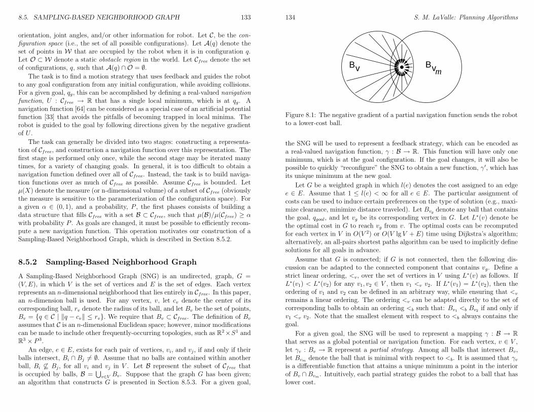
8.5. SAMPLING-BASED NEIGHBORHOOD GRAPH 133
orientation, joint angles, and/or other information for robot. Let C, be the con-figuration space (i.e., the set of all possible configurations). Let A(q) denote theset of points in W that are occupied by the robot when it is in configuration q.Let O ⊂ W denote a static obstacle region in the world. Let Cfree denote the setof configurations, q, such that A(q) ∩ O = ∅.
The task is to find a motion strategy that uses feedback and guides the robotto any goal configuration from any initial configuration, while avoiding collisions.For a given goal, qg, this can be accomplished by defining a real-valued navigationfunction, U : Cfree → R that has a single local minimum, which is at qg. Anavigation function [64] can be considered as a special case of an artificial potentialfunction [33] that avoids the pitfalls of becoming trapped in local minima. Therobot is guided to the goal by following directions given by the negative gradientof U .
The task can generally be divided into two stages: constructing a representa-tion of Cfree, and construction a navigation function over this representation. Thefirst stage is performed only once, while the second stage may be iterated manytimes, for a variety of changing goals. In general, it is too difficult to obtain anavigation function defined over all of Cfree. Instead, the task is to build naviga-tion functions over as much of Cfree as possible. Assume Cfree is bounded. Letµ(X) denote the measure (or n-dimensional volume) of a subset of Cfree (obviouslythe measure is sensitive to the parameterization of the configuration space). Fora given α ∈ (0, 1), and a probability, P , the first phases consists of building adata structure that fills Cfree with a set B ⊂ Cfree, such that µ(B)/µ(Cfree) ≥ αwith probability P . As goals are changed, it must be possible to efficiently recom-pute a new navigation function. This operation motivates our construction of aSampling-Based Neighborhood Graph, which is described in Section 8.5.2.
8.5.2 Sampling-Based Neighborhood Graph
A Sampling-Based Neighborhood Graph (SNG) is an undirected, graph, G =(V,E), in which V is the set of vertices and E is the set of edges. Each vertexrepresents an n-dimensional neighborhood that lies entirely in Cfree. In this paper,an n-dimension ball is used. For any vertex, v, let cv denote the center of itscorresponding ball, rv denote the radius of its ball, and let Bv be the set of points,Bv = q ∈ C | ‖q − cv‖ ≤ rv. We require that Bv ⊂ Cfree. The definition of Bv
assumes that C is an n-dimensional Euclidean space; however, minor modificationscan be made to include other frequently-occurring topologies, such as R2×S1 andR3 × P 3.
An edge, e ∈ E, exists for each pair of vertices, vi, and vj, if and only if theirballs intersect, Bi ∩ Bj 6= ∅. Assume that no balls are contained within anotherball, Bi 6⊆ Bj, for all vi and vj in V . Let B represent the subset of Cfree thatis occupied by balls, B =
⋃
v∈V Bv. Suppose that the graph G has been given;an algorithm that constructs G is presented in Section 8.5.3. For a given goal,
134 S. M. LaValle: Planning Algorithms
Bv mBv
Figure 8.1: The negative gradient of a partial navigation function sends the robotto a lower-cost ball.
the SNG will be used to represent a feedback strategy, which can be encoded asa real-valued navigation function, γ : B → R. This function will have only oneminimum, which is at the goal configuration. If the goal changes, it will also bepossible to quickly “reconfigure” the SNG to obtain a new function, γ ′, which hasits unique minimum at the new goal.
Let G be a weighted graph in which l(e) denotes the cost assigned to an edgee ∈ E. Assume that 1 ≤ l(e) < ∞ for all e ∈ E. The particular assignment ofcosts can be used to induce certain preferences on the type of solution (e.g., maxi-mize clearance, minimize distance traveled). Let Bvg
denote any ball that containsthe goal, qgoal, and let vg be its corresponding vertex in G. Let L∗(v) denote bethe optimal cost in G to reach vg from v. The optimal costs can be recomputedfor each vertex in V in O(V 2) or O(V lg V + E) time using Dijkstra’s algorithm;alternatively, an all-pairs shortest paths algorithm can be used to implicitly definesolutions for all goals in advance.
Assume that G is connected; if G is not connected, then the following dis-cussion can be adapted to the connected component that contains vg. Define astrict linear ordering, <v, over the set of vertices in V using L∗(v) as follows. IfL∗(v1) < L∗(v2) for any v1, v2 ∈ V , then v1 <v v2. If L∗(v1) = L∗(v2), then theordering of v1 and v2 can be defined in an arbitrary way, while ensuring that <v
remains a linear ordering. The ordering <v can be adapted directly to the set ofcorresponding balls to obtain an ordering <b such that: Bv1 <b Bv2 if and only ifv1 <v v2. Note that the smallest element with respect to <b always contains thegoal.
For a given goal, the SNG will be used to represent a mapping γ : B → Rthat serves as a global potential or navigation function. For each vertex, v ∈ V ,let γv : Bv → R represent a partial strategy. Among all balls that intersect Bv,let Bvm
denote the ball that is minimal with respect to <b. It is assumed that γvis a differentiable function that attains a unique minimum a point in the interiorof Bv ∩Bvm
. Intuitively, each partial strategy guides the robot to a ball that haslower cost.
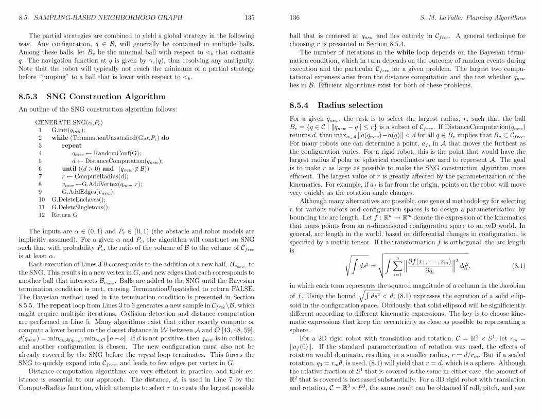
8.5. SAMPLING-BASED NEIGHBORHOOD GRAPH 135
The partial strategies are combined to yield a global strategy in the followingway. Any configuration, q ∈ B, will generally be contained in multiple balls.Among these balls, let Bv be the minimal ball with respect to <b that containsq. The navigation function at q is given by γv(q), thus resolving any ambiguity.Note that the robot will typically not reach the minimum of a partial strategybefore “jumping” to a ball that is lower with respect to <b.
8.5.3 SNG Construction Algorithm
An outline of the SNG construction algorithm follows:
GENERATE SNG(α,Pc)1 G.init(qinit);2 while (TerminationUnsatisfied(G,α,Pc) do
3 repeat
4 qnew ← RandomConf(G);5 d← DistanceComputation(qnew);6 until ((d > 0) and (qnew 6∈ B))7 r ← ComputeRadius(d);8 vnew ←G.AddVertex(qnew, r);9 G.AddEdges(vnew);10 G.DeleteEnclaves();11 G.DeleteSingletons();12 Return G
The inputs are α ∈ (0, 1) and Pc ∈ (0, 1) (the obstacle and robot models areimplicitly assumed). For a given α and Pc, the algorithm will construct an SNGsuch that with probability Pc, the ratio of the volume of B to the volume of Cfreeis at least α.
Each execution of Lines 3-9 corresponds to the addition of a new ball, Bvnew, to
the SNG. This results in a new vertex inG, and new edges that each corresponds toanother ball that intersects Bvnew
. Balls are added to the SNG until the Bayesiantermination condition is met, causing TerminationUnsatisfied to return FALSE.The Bayesian method used in the termination condition is presented in Section8.5.5. The repeat loop from Lines 3 to 6 generates a new sample in Cfree\B, whichmight require multiple iterations. Collision detection and distance computationare performed in Line 5. Many algorithms exist that either exactly compute orcompute a lower bound on the closest distance inW between A and O [43, 48, 59],d(qnew) = mina∈A(qnew)mino∈O ‖a−o‖. If d is not positive, then qnew is in collision,and another configuration is chosen. The new configuration must also not bealready covered by the SNG before the repeat loop terminates. This forces theSNG to quickly expand into Cfree, and leads to few edges per vertex in G.
Distance computation algorithms are very efficient in practice, and their ex-istence is essential to our approach. The distance, d, is used in Line 7 by theComputeRadius function, which attempts to select r to create the largest possible
136 S. M. LaValle: Planning Algorithms
ball that is centered at qnew and lies entirely in Cfree. A general technique forchoosing r is presented in Section 8.5.4.
The number of iterations in the while loop depends on the Bayesian termi-nation condition, which in turn depends on the outcome of random events duringexecution and the particular Cfree for a given problem. The largest two compu-tational expenses arise from the distance computation and the test whether qnewlies in B. Efficient algorithms exist for both of these problems.
8.5.4 Radius selection
For a given qnew, the task is to select the largest radius, r, such that the ballBv = q ∈ C | ‖qnew − q‖ ≤ r is a subset of Cfree. If DistanceComputation(qnew)returns d, then maxa∈A ‖a(qnew)−a(q)‖ < d for all q ∈ Bv implies that Bv ⊂ Cfree.For many robots one can determine a point, af , in A that moves the furthest asthe configuration varies. For a rigid robot, this is the point that would have thelargest radius if polar or spherical coordinates are used to represent A. The goalis to make r as large as possible to make the SNG construction algorithm moreefficient. The largest value of r is greatly affected by the parameterization of thekinematics. For example, if af is far from the origin, points on the robot will movevery quickly as the rotation angle changes.
Although many alternatives are possible, one general methodology for selectingr for various robots and configuration spaces is to design a parameterization bybounding the arc length. Let f : Rn → Rm denote the expression of the kinematicsthat maps points from an n-dimensional configuration space to an mD world. Ingeneral, arc length in the world, based on differential changes in configuration, isspecified by a metric tensor. If the transformation f is orthogonal, the arc lengthis
√
∫
ds2 =
√
√
√
√
∫ n∑
i=1
∥
∥
∥
∂f(x1, . . . , xm)
∂qi
∥
∥
∥
2
dq2i , (8.1)
in which each term represents the squared magnitude of a column in the Jacobian
of f . Using the bound√
∫
ds2 < d, (8.1) expresses the equation of a solid ellip-
soid in the configuration space. Obviously, that solid ellipsoid will be significientlydifferent according to different kinematic expressions. The key is to choose kine-matic expressions that keep the eccentricity as close as possible to representing asphere.
For a 2D rigid robot with translation and rotation, C = R2 × S1, let rm =‖af (0)‖. If the standard parameterization of rotation was used, the effects ofrotation would dominate, resulting in a smaller radius, r = d/rm. But if a scaledrotation, q3 = rmθ, is used, (8.1) will yield that r = d, which is a sphere. Althoughthe relative fraction of S1 that is covered is the same in either case, the amount ofR2 that is covered is increased substantially. For a 3D rigid robot with translationand rotation, C = R3×P 3, the same result can be obtained if roll, pitch, and yaw
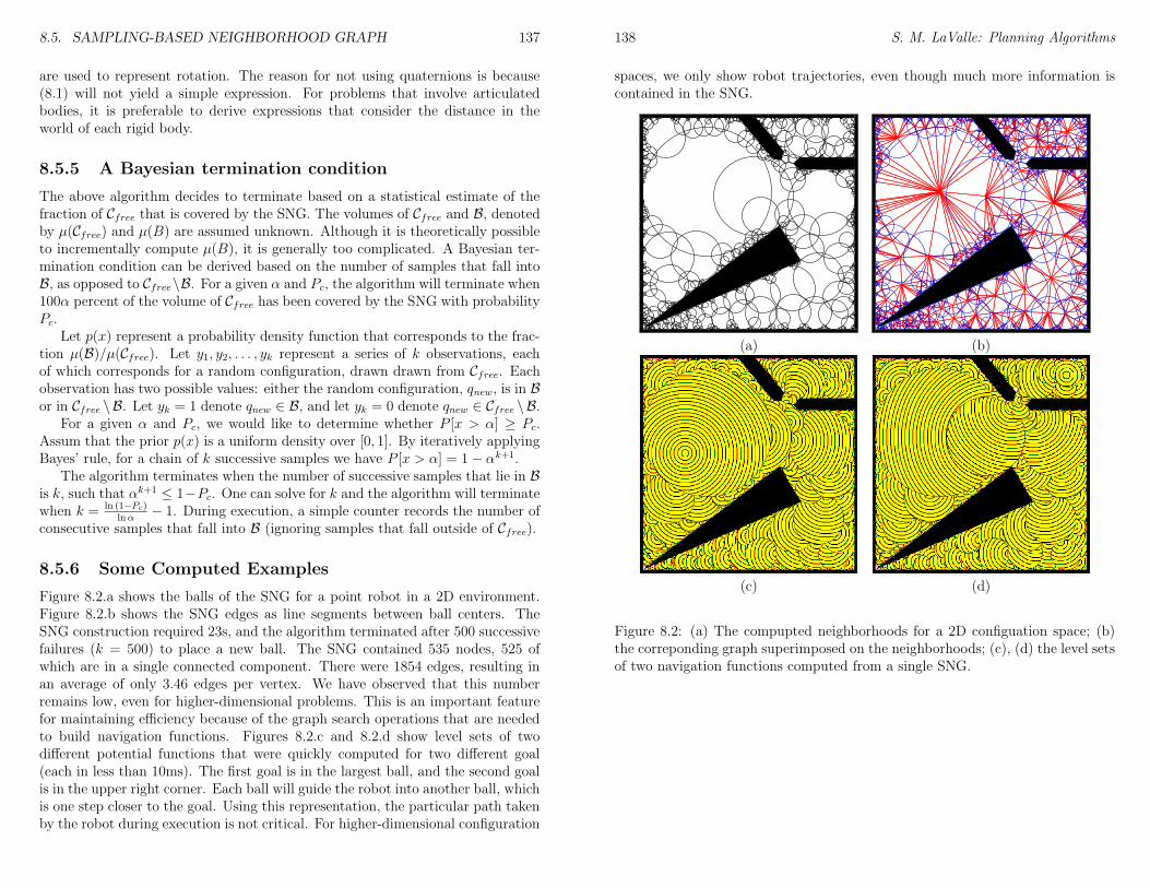
8.5. SAMPLING-BASED NEIGHBORHOOD GRAPH 137
are used to represent rotation. The reason for not using quaternions is because(8.1) will not yield a simple expression. For problems that involve articulatedbodies, it is preferable to derive expressions that consider the distance in theworld of each rigid body.
8.5.5 A Bayesian termination condition
The above algorithm decides to terminate based on a statistical estimate of thefraction of Cfree that is covered by the SNG. The volumes of Cfree and B, denotedby µ(Cfree) and µ(B) are assumed unknown. Although it is theoretically possibleto incrementally compute µ(B), it is generally too complicated. A Bayesian ter-mination condition can be derived based on the number of samples that fall intoB, as opposed to Cfree\B. For a given α and Pc, the algorithm will terminate when100α percent of the volume of Cfree has been covered by the SNG with probabilityPc.
Let p(x) represent a probability density function that corresponds to the frac-tion µ(B)/µ(Cfree). Let y1, y2, . . . , yk represent a series of k observations, eachof which corresponds for a random configuration, drawn drawn from Cfree. Eachobservation has two possible values: either the random configuration, qnew, is in Bor in Cfree \B. Let yk = 1 denote qnew ∈ B, and let yk = 0 denote qnew ∈ Cfree \B.
For a given α and Pc, we would like to determine whether P [x > α] ≥ Pc.Assum that the prior p(x) is a uniform density over [0, 1]. By iteratively applyingBayes’ rule, for a chain of k successive samples we have P [x > α] = 1− αk+1.
The algorithm terminates when the number of successive samples that lie in Bis k, such that αk+1 ≤ 1−Pc. One can solve for k and the algorithm will terminatewhen k = ln (1−Pc)
lnα− 1. During execution, a simple counter records the number of
consecutive samples that fall into B (ignoring samples that fall outside of Cfree).
8.5.6 Some Computed Examples
Figure 8.2.a shows the balls of the SNG for a point robot in a 2D environment.Figure 8.2.b shows the SNG edges as line segments between ball centers. TheSNG construction required 23s, and the algorithm terminated after 500 successivefailures (k = 500) to place a new ball. The SNG contained 535 nodes, 525 ofwhich are in a single connected component. There were 1854 edges, resulting inan average of only 3.46 edges per vertex. We have observed that this numberremains low, even for higher-dimensional problems. This is an important featurefor maintaining efficiency because of the graph search operations that are neededto build navigation functions. Figures 8.2.c and 8.2.d show level sets of twodifferent potential functions that were quickly computed for two different goal(each in less than 10ms). The first goal is in the largest ball, and the second goalis in the upper right corner. Each ball will guide the robot into another ball, whichis one step closer to the goal. Using this representation, the particular path takenby the robot during execution is not critical. For higher-dimensional configuration
138 S. M. LaValle: Planning Algorithms
spaces, we only show robot trajectories, even though much more information iscontained in the SNG.
(a) (b)
(c) (d)
Figure 8.2: (a) The compupted neighborhoods for a 2D configuation space; (b)the correponding graph superimposed on the neighborhoods; (c), (d) the level setsof two navigation functions computed from a single SNG.

Part III
Decision-Theoretic Planning
139
Chapter 9
Basic Decision Theory
These are class notes from CS497 Spring 2003, parts of which were scribed bySteve Lindemann, Shai Sachs.
9.1 Basic Definitions
To introduce some of the basic concepts in single-stage decision making, considerthe following scenario:
Scenario 0 1. Let U be a set of possible choices: u1, u2, . . . , un.
2. Let L : U → R be a loss function or cost function.
3. Select a u ∈ U that minimizes L(U).
In this scenario, we see that the set U consists of all choices that we can make; theseare also called actions or inputs. The loss function L represents the cost associatedwith each possible choice; another approach is to define a reward function R whichrepresents the gain or benefit of each choice. These approaches are equivalent,since on can simply take R(u) = −L(u).
A method used to make a decision is called a strategy. In this scenario, ourstrategy was deterministic; that is, given some set U and function L, our choice iscompletely determined. Alternatively, we could have taken a randomized strategy,in which our decision also depended on the outcome of some random events.In this strategy, we define a function p : U → R such that the probability ofselecting a particular choice u is p(u); denote p(ui) = pi. The ordinary rulesgoverning probability spaces apply (e.g.,
∑ni=1 pi = 1, pi ≥ 0 ∀i). Randomized
and deterministic strategies are also called mixed and pure, respectively. Forpurposes of notation, we will use u∗ to refer to a randomized strategy and U torefer to the set of all randomized strategies.
Example 7 Let the input set U = a, b. Then one can choose a randomizedstrategy u∗ in the following way:
141
142 S. M. LaValle: Planning Algorithms
1. Flip a fair H/T coin.
2. If the result is H, choose a; if T, choose b.
Since the coin is fair, this corresponds to choosing p(a) = 0.5, p(b) = 0.5.
Consider the following scenario:
Scenario 1 1. U = u1, u2, . . . , un
2. L : U → R
3. Select u∗ ∈ U that minimizes E[L] =∑n
i=1 L(ui)pi.
E[L] reflects the average loss if the game were to be played many times. Now,Scenarios 0 and 1 are identical, with the exception that one uses a deterministicstrategy, and one uses a randomized strategy. Which is better? To help answerthis, we give the following example:
Example 8 Let U = 1, 2, 3, and L(1) = 2, L(2) = 3, L(3) = 5 (we may writethis in vector notation as L = [2 3 5]). Following the deterministic strategy fromScenario 0, we choose u = 1. What if we use the strategy from Scenario 1? Byinspection we can see that we need p = [1 0 0]; thus, the randomized strategyresults in the same choice as the deterministic one.
We have seen in the above example that a randomized strategies and determin-istic ones can produce identical results. However, what if for some input set U andloss function L, we have L(ui) = L(uj)? Then, there can be randomized strategieswhich act differently than deterministic ones. However, if one only considers theminimum loss attained, they are not better because both types of strategies willselect actions resulting in minimum loss. Thus, in this case we find that Scenario1 is useless! However, randomized strategies are very useful in general, as shownin the following example.
Example 9 (Matching Pennies) Consider a game in which two players simul-taneously choose H or T. If the outcome is HH or TT (the players choose thesame), then Player 1 pays Player 2 $1; if the outcome is HT or TH, then Player2 pays Player 1 $1. What happens if Player 1 uses a deterministic strategy? IfPlayer 2 can determine what that strategy is, then he can choose his strategy sothat he always wins the game. However, if Player 1 chooses a randomized strategy,he can at least expect to break even (what randomized strategy guarantees this?).
So far, we have examined scenarios in which there were only a finite number ofpossible choices. Many problems, however, have a continuum of choices, as doesthe following:
Scenario 2 1. U ⊆ Rd (usually, U is closed and bounded)
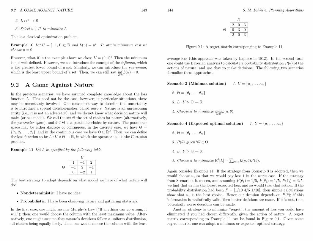
9.2. A GAME AGAINST NATURE 143
2. L : U → R
3. Select u ∈ U to minimize L
This is a classical optimization problem.
Example 10 Let U = [−1, 1] ⊂ R and L(u) = u2. To attain minimum cost wechoose u = 0.
However, what if in the example above we chose U = (0, 1)? Then the minimumis not well-defined. However, we can introduce the concept of the infimum, whichis the greatest lower bound of a set. Similarly, we can introduce the supremum,which is the least upper bound of a set. Then, we can still say inf
u∈UL(u) = 0.
9.2 A Game Against Nature
In the previous scenarios, we have assumed complete knowledge about the lossfunction L. This need not be the case, however; in particular situations, theremay be uncertainty involved. One convenient way to describe this uncertaintyis to introduce a special decision-maker, called nature. Nature is an unreasoningentity (i.e., it is not an adversary), and we do not know what decision nature willmake (or has made). We call the set Θ the set of choices for nature (alternatively,the parameter space), and θ ∈ Θ is a particular choice by nature. The parameterspace may be either discrete or continuous; in the discrete case, we have Θ =θ1, θ2, . . . , θn, and in the continuous case we have Θ ⊆ Rd. Then, we can definethe loss function to be L : U ×Θ→ R, in which the operator ·× · is the Cartesianproduct.
Example 11 Let L be specified by the following table:
U
Θ1 −1 2−1 2 −10 −2 1
The best strategy to adopt depends on what model we have of what nature willdo:
• Nondeterministic: I have no idea.
• Probabilistic: I have been observing nature and gathering statistics.
In the first case, one might assume Murphy’s Law (“If anything can go wrong, itwill”); then, one would choose the column with the least maximum value. Alter-natively, one might assume that nature’s decisions follow a uniform distribution,all choices being equally likely. Then one would choose the column with the least
144 S. M. LaValle: Planning Algorithms
U
Θ2 0 30 3 02 0 3
Figure 9.1: A regret matrix corresponging to Example 11.
average loss (this approach was taken by Laplace in 1812). In the second case,one could use Bayesian analysis to calculate a probability distribution P (θ) of theactions of nature, and use that to make decisions. The following two scenariosformalize these approaches.
Scenario 3 (Minimax solution) 1. U = u1, . . . , un
2. Θ = θ1, . . . , θm
3. L : U ×Θ→ R
4. Choose u to minimize maxθ∈Θ
L(u, θ).
Scenario 4 (Expected optimal solution) 1. U = u1, . . . , un
2. Θ = θ1, . . . , θm
3. P (θ) given ∀θ ∈ Θ
4. L : U ×Θ→ R
5. Choose u to minimize Eθ[L] =∑
θ∈Θ L(u, θ)P (θ).
Again consider Example 11. If the strategy from Scenario 3 is adopted, then wewould choose u1 so that we would pay loss 1 in the worst case. If the strategyfrom Scenario 4 is chosen, and assuming P (θ1) = 1/5, P (θ2) = 1/5, P (θ3) = 3/5,we find that u2 has the lowest expected loss, and so would take that action. If theprobability distribution had been P = [1/10 4/5 1/10], then simple calculationsshow that u1 is the best choice. Hence our decision depends on P (θ); if thisinformation is statistically valid, then better decisions are made. If it is not, thenpotentially worse decisions can be made.
Another strategy is to minimize “regret”, the amount of loss you could haveeliminated if you had chosen differently, given the action of nature. A regretmatrix corresponding to Example 11 can be found in Figure 9.1. Given someregret matrix, one can adopt a minimax or expected optimal strategy.
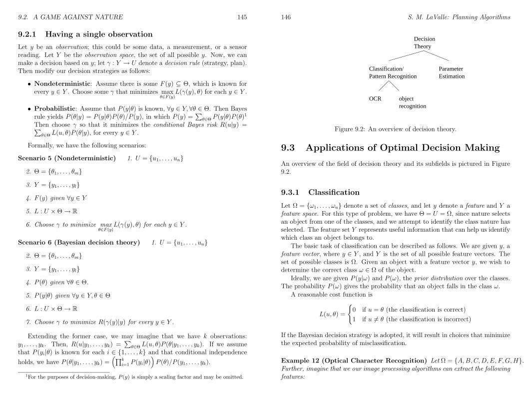
9.2. A GAME AGAINST NATURE 145
9.2.1 Having a single observation
Let y be an observation; this could be some data, a measurement, or a sensorreading. Let Y be the observation space, the set of all possible y. Now, we canmake a decision based on y; let γ : Y → U denote a decision rule (strategy, plan).Then modify our decision strategies as follows:
• Nondeterministic: Assume there is some F (y) ⊆ Θ, which is known forevery y ∈ Y . Choose some γ that minimizes max
θ∈F (y)L(γ(y), θ) for each y ∈ Y .
• Probabilistic: Assume that P (y|θ) is known, ∀y ∈ Y,∀θ ∈ Θ. Then Bayesrule yields P (θ|y) = P (y|θ)P (θ)/P (y), in which P (y) =
∑
θ∈Θ P (y|θ)P (θ)1
Then choose γ so that it minimizes the conditional Bayes risk R(u|y) =∑
θ∈Θ L(u, θ)P (θ|y), for every y ∈ Y .
Formally, we have the following scenarios:
Scenario 5 (Nondeterministic) 1. U = u1, . . . , un
2. Θ = θ1, . . . , θm
3. Y = y1, . . . , yl
4. F (y) given ∀y ∈ Y
5. L : U ×Θ→ R
6. Choose γ to minimize maxθ∈F (y)
L(γ(y), θ) for each y ∈ Y .
Scenario 6 (Bayesian decision theory) 1. U = u1, . . . , un
2. Θ = θ1, . . . , θm
3. Y = y1, . . . , yl
4. P (θ) given ∀θ ∈ Θ.
5. P (y|θ) given ∀y ∈ Y, θ ∈ Θ
6. L : U ×Θ→ R
7. Choose γ to minimize R(γ(y)|y) for every y ∈ Y .
Extending the former case, we may imagine that we have k observations:y1, . . . , yk. Then, R(u|y1, . . . , yk) =
∑
θ∈Θ L(u, θ)P (θ|y1, . . . , yk). If we assumethat P (yi|θ) is known for each i ∈ 1, . . . , k and that conditional independence
holds, we have P (θ|y1, . . . , yk) =(
∏ki=1 P (yi|θ)
)
P (θ)/P (y1, . . . , yk).
1For the purposes of decision-making, P (y) is simply a scaling factor and may be omitted.
146 S. M. LaValle: Planning Algorithms
DecisionTheory
Classification/Pattern Recognition
ParameterEstimation
OCR objectrecognition
Figure 9.2: An overview of decision theory.
9.3 Applications of Optimal Decision Making
An overview of the field of decision theory and its subfields is pictured in Figure9.2.
9.3.1 Classification
Let Ω = ω1, . . . , ωn denote a set of classes, and let y denote a feature and Y afeature space. For this type of problem, we have Θ = U = Ω, since nature selectsan object from one of the classes, and we attempt to identify the class nature hasselected. The feature set Y represents useful information that can help us identifywhich class an object belongs to.
The basic task of classification can be described as follows. We are given y, afeature vector, where y ∈ Y , and Y is the set of all possible feature vectors. Theset of possible classes is Ω. Given an object with a feature vector y, we wish todetermine the correct class ω ∈ Ω of the object.
Ideally, we are given P (y|ω) and P (ω), the prior distribution over the classes.The probability P (ω) gives the probability that an object falls in the class ω.
A reasonable cost function is
L(u, θ) =
0 if u = θ (the classification is correct)
1 if u 6= θ (the classification is incorrect)
If the Bayesian decision strategy is adopted, it will result in choices that minimizethe expected probability of misclassification.
Example 12 (Optical Character Recognition) Let Ω = A,B,C,D,E, F,G,H.Further, imagine that we our image processing algorithms can extract the followingfeatures:

9.3. APPLICATIONS OF OPTIMAL DECISION MAKING 147
Shape 0 A E F H1 B C D G
Ends 0 B D12 A C G3 F E4 H
Holes 0 C E F G H1 A D2 B
Assuming that the image processing algorithms never err, we can use a minimaxstrategy to make our decision. Are there any letters which the features do notdistinguish? If so, what enhancements might we make to our image processingalgorithms to distinguish them? If we assume that that the image processing al-gorithms sometimes make mistakes, then we can use a Bayesian strategy. Afterrunning the algorithms thousands of times and gathering statistics, we can learnthe necessary conditional probabilities and use them to make the decision with thehighest expectation of success.
9.3.2 Parameter Estimation
One subfield of Decision Theory is parameter estimation. The goal is to estimatethe value of some parameter, given some observation of the parameter. We con-sider the parameter to be some fixed constant, and denote the set of all possibleparameters (the parameter space) as X.
Using our notation from decision theory, we have Θ = X. The parameter weare trying to estimate is nature’s choice.
Since the goal is the guess the correct value of the parameter, the set of actionsU is also equal to X; that is, the human player’s action is to choose some validvalue of the parameter as her guess. Therefore, we have X = Θ = U .
Further, we have an observation about the parameter, y; we denote the set ofall possible observations by Y . Clearly, X ⊆ Y .
Suppose we have X = [0, 1] ⊆ R, p(y|x) = 1√2πσ2
exp(
−(x−y)22σ2
)
, and p(x) = 1.
We interpret these probability density functions as follows: p(y|x) tells us thatthere is some Gaussian noise in the observation (that is, our observations of theparameters, over many trials, will be concentrated around the true parameter in aGaussian distribution); further, p(x) tells us that each parameter is equally likely.
Finally, we choose a loss function which measures the estimation error (thatis, the difference between our estimate and the true parameter). We use L(u, x) =(u− x)2.
We wish to choose the input u which minimizes our risk; we therefore chooseu which minimizes
148 S. M. LaValle: Planning Algorithms
R(u) =
∫
x
L(u, x)p(y|x)p(x)dx (9.1)
Note that when Equation 9.1 is multiplied by 1p(y)
, by Bayes’ rule we have
R(u) =
∫
x
L(u, x)p(y|x)p(x)1
p(y)dx =
∫
x
L(u, x)p(x|y)dx
Then the expression for R(u) becomes exactly analogous to the discrete form ofthe risk function from our previous lecture. Since p(y) is constant over X, we mayremove it from the integral without affecting the correct choice of u. ThereforeR(u) in Equation 9.1 is not exactly the risk function, but it is closely related.
9.4 Utility Theory
Utility theory asks: Where does the loss function L come from? In other words,how useful is one loss compared against another?
In utility theory we replace “loss” with “reward”; the human wants to maxi-mize reward. Note that this convention can easily be inverted to return the theusual “loss” convention in decision theory.
9.4.1 Choosing a Good Reward
Let u1 be some fairly unpleasant task (such as writing scribe notes), and u2 bethe act of doing nothing. We consider the problem of choosing a good rewardfunction using the following examples.
1. Let R(u1) = 1000, and R(u2) = 0. For a poor graduate student, it maybe worthwhile to write scribe notes for $ 1000, so the student will probablydo u1 in this scenario. One difficulty in this scenario is that we haven’tconsidered the possible cost to the human of each action.
2. Let R(u1) = 10001000, and R(u2) = 10000000. Although the relative rewardis the same, the action chosen is probably different! This is so because thevalue (or utility) of money decreases as we have more of it.
3. Let R(u1) = 10000 and R(u2) = 25, 000 with probability 12, and 0 with
probability 12. In this scenario some conservative students may choose u1,
to guarantee a reward; while more adventurous gamblers may choose u2, asthe expected gain is greater.
4. Let R(u1) = 100, and R(u2) = 250 with probability 12, and 0 otherwise;
allow the student to choose an action (and collect the corresponding reward)100 times. The expected reward for each action remains the same, but we
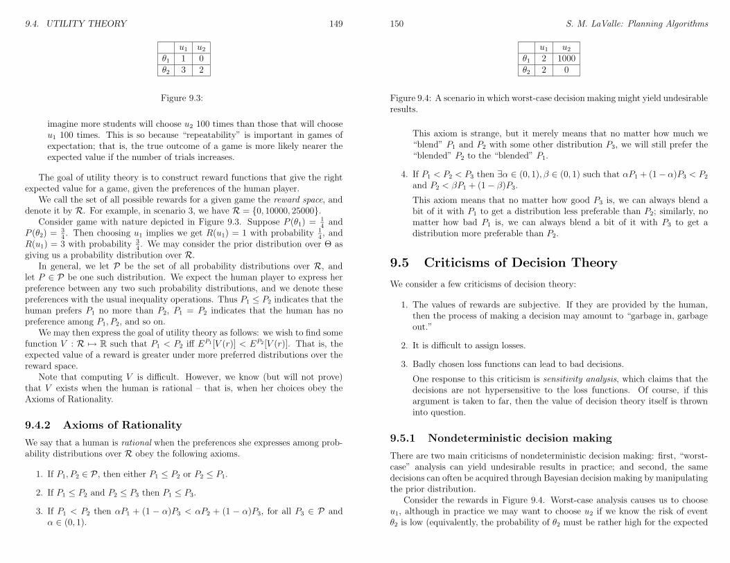
9.4. UTILITY THEORY 149
u1 u2θ1 1 0θ2 3 2
Figure 9.3:
imagine more students will choose u2 100 times than those that will chooseu1 100 times. This is so because “repeatability” is important in games ofexpectation; that is, the true outcome of a game is more likely nearer theexpected value if the number of trials increases.
The goal of utility theory is to construct reward functions that give the rightexpected value for a game, given the preferences of the human player.
We call the set of all possible rewards for a given game the reward space, anddenote it by R. For example, in scenario 3, we have R = 0, 10000, 25000.
Consider game with nature depicted in Figure 9.3. Suppose P (θ1) = 14and
P (θ2) =34. Then choosing u1 implies we get R(u1) = 1 with probability 1
4, and
R(u1) = 3 with probability 34. We may consider the prior distribution over Θ as
giving us a probability distribution over R.In general, we let P be the set of all probability distributions over R, and
let P ∈ P be one such distribution. We expect the human player to express herpreference between any two such probability distributions, and we denote thesepreferences with the usual inequality operations. Thus P1 ≤ P2 indicates that thehuman prefers P1 no more than P2, P1 = P2 indicates that the human has nopreference among P1, P2, and so on.
We may then express the goal of utility theory as follows: we wish to find somefunction V : R 7→ R such that P1 < P2 iff EP1 [V (r)] < EP2 [V (r)]. That is, theexpected value of a reward is greater under more preferred distributions over thereward space.
Note that computing V is difficult. However, we know (but will not prove)that V exists when the human is rational – that is, when her choices obey theAxioms of Rationality.
9.4.2 Axioms of Rationality
We say that a human is rational when the preferences she expresses among prob-ability distributions over R obey the following axioms.
1. If P1, P2 ∈ P , then either P1 ≤ P2 or P2 ≤ P1.
2. If P1 ≤ P2 and P2 ≤ P3 then P1 ≤ P3.
3. If P1 < P2 then αP1 + (1 − α)P3 < αP2 + (1 − α)P3, for all P3 ∈ P andα ∈ (0, 1).
150 S. M. LaValle: Planning Algorithms
u1 u2θ1 2 1000θ2 2 0
Figure 9.4: A scenario in which worst-case decision making might yield undesirableresults.
This axiom is strange, but it merely means that no matter how much we“blend” P1 and P2 with some other distribution P3, we will still prefer the“blended” P2 to the “blended” P1.
4. If P1 < P2 < P3 then ∃α ∈ (0, 1), β ∈ (0, 1) such that αP1 + (1− α)P3 < P2and P2 < βP1 + (1− β)P3.
This axiom means that no matter how good P3 is, we can always blend abit of it with P1 to get a distribution less preferable than P2; similarly, nomatter how bad P1 is, we can always blend a bit of it with P3 to get adistribution more preferable than P2.
9.5 Criticisms of Decision Theory
We consider a few criticisms of decision theory:
1. The values of rewards are subjective. If they are provided by the human,then the process of making a decision may amount to “garbage in, garbageout.”
2. It is difficult to assign losses.
3. Badly chosen loss functions can lead to bad decisions.
One response to this criticism is sensitivity analysis, which claims that thedecisions are not hypersensitive to the loss functions. Of course, if thisargument is taken to far, then the value of decision theory itself is throwninto question.
9.5.1 Nondeterministic decision making
There are two main criticisms of nondeterministic decision making: first, “worst-case” analysis can yield undesirable results in practice; and second, the samedecisions can often be acquired through Bayesian decision making by manipulatingthe prior distribution.
Consider the rewards in Figure 9.4. Worst-case analysis causes us to chooseu1, although in practice we may want to choose u2 if we know the risk of eventθ2 is low (equivalently, the probability of θ2 must be rather high for the expected
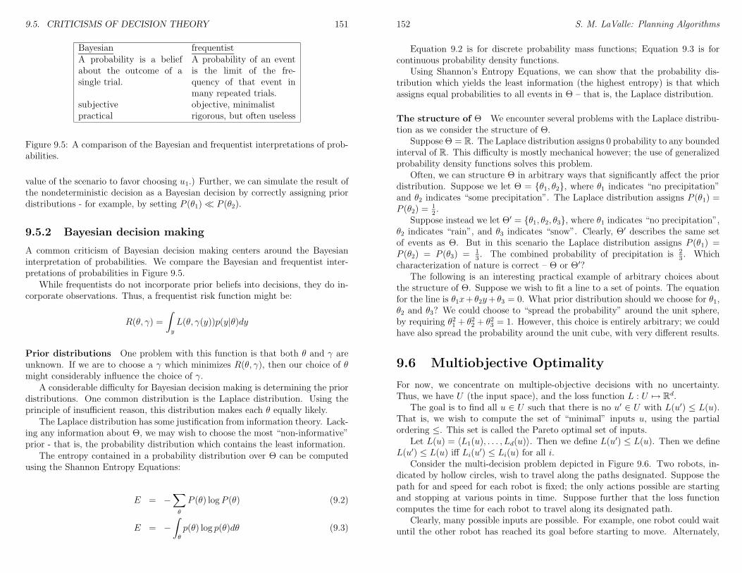
9.5. CRITICISMS OF DECISION THEORY 151
Bayesian frequentistA probability is a beliefabout the outcome of asingle trial.
A probability of an eventis the limit of the fre-quency of that event inmany repeated trials.
subjective objective, minimalistpractical rigorous, but often useless
Figure 9.5: A comparison of the Bayesian and frequentist interpretations of prob-abilities.
value of the scenario to favor choosing u1.) Further, we can simulate the result ofthe nondeterministic decision as a Bayesian decision by correctly assigning priordistributions - for example, by setting P (θ1)¿ P (θ2).
9.5.2 Bayesian decision making
A common criticism of Bayesian decision making centers around the Bayesianinterpretation of probabilities. We compare the Bayesian and frequentist inter-pretations of probabilities in Figure 9.5.
While frequentists do not incorporate prior beliefs into decisions, they do in-corporate observations. Thus, a frequentist risk function might be:
R(θ, γ) =
∫
y
L(θ, γ(y))p(y|θ)dy
Prior distributions One problem with this function is that both θ and γ areunknown. If we are to choose a γ which minimizes R(θ, γ), then our choice of θmight considerably influence the choice of γ.
A considerable difficulty for Bayesian decision making is determining the priordistributions. One common distribution is the Laplace distribution. Using theprinciple of insufficient reason, this distribution makes each θ equally likely.
The Laplace distribution has some justification from information theory. Lack-ing any information about Θ, we may wish to choose the most “non-informative”prior - that is, the probability distribution which contains the least information.
The entropy contained in a probability distribution over Θ can be computedusing the Shannon Entropy Equations:
E = −∑
θ
P (θ) logP (θ) (9.2)
E = −
∫
θ
p(θ) log p(θ)dθ (9.3)
152 S. M. LaValle: Planning Algorithms
Equation 9.2 is for discrete probability mass functions; Equation 9.3 is forcontinuous probability density functions.
Using Shannon’s Entropy Equations, we can show that the probability dis-tribution which yields the least information (the highest entropy) is that whichassigns equal probabilities to all events in Θ – that is, the Laplace distribution.
The structure of Θ We encounter several problems with the Laplace distribu-tion as we consider the structure of Θ.
Suppose Θ = R. The Laplace distribution assigns 0 probability to any boundedinterval of R. This difficulty is mostly mechanical however; the use of generalizedprobability density functions solves this problem.
Often, we can structure Θ in arbitrary ways that significantly affect the priordistribution. Suppose we let Θ = θ1, θ2, where θ1 indicates “no precipitation”and θ2 indicates “some precipitation”. The Laplace distribution assigns P (θ1) =P (θ2) =
12.
Suppose instead we let Θ′ = θ1, θ2, θ3, where θ1 indicates “no precipitation”,θ2 indicates “rain”, and θ3 indicates “snow”. Clearly, Θ′ describes the same setof events as Θ. But in this scenario the Laplace distribution assigns P (θ1) =P (θ2) = P (θ3) = 1
3. The combined probability of precipitation is 2
3. Which
characterization of nature is correct – Θ or Θ′?The following is an interesting practical example of arbitrary choices about
the structure of Θ. Suppose we wish to fit a line to a set of points. The equationfor the line is θ1x+ θ2y+ θ3 = 0. What prior distribution should we choose for θ1,θ2 and θ3? We could choose to “spread the probability” around the unit sphere,by requiring θ21 + θ22 + θ23 = 1. However, this choice is entirely arbitrary; we couldhave also spread the probability around the unit cube, with very different results.
9.6 Multiobjective Optimality
For now, we concentrate on multiple-objective decisions with no uncertainty.Thus, we have U (the input space), and the loss function L : U 7→ Rd.
The goal is to find all u ∈ U such that there is no u′ ∈ U with L(u′) ≤ L(u).That is, we wish to compute the set of “minimal” inputs u, using the partialordering ≤. This set is called the Pareto optimal set of inputs.
Let L(u) = 〈L1(u), . . . , Ld(u)〉. Then we define L(u′) ≤ L(u). Then we defineL(u′) ≤ L(u) iff Li(u
′) ≤ Li(u) for all i.Consider the multi-decision problem depicted in Figure 9.6. Two robots, in-
dicated by hollow circles, wish to travel along the paths designated. Suppose thepath for and speed for each robot is fixed; the only actions possible are startingand stopping at various points in time. Suppose further that the loss functioncomputes the time for each robot to travel along its designated path.
Clearly, many possible inputs are possible. For example, one robot could waituntil the other robot has reached its goal before starting to move. Alternately,
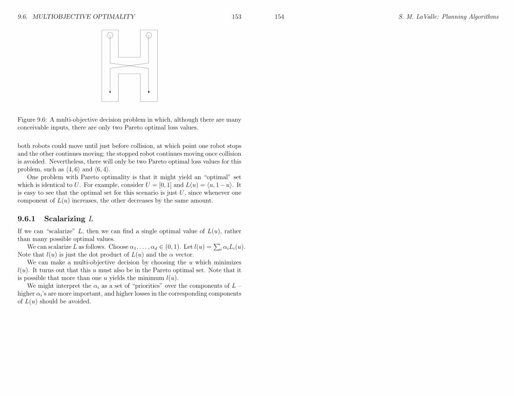
9.6. MULTIOBJECTIVE OPTIMALITY 153
Figure 9.6: A multi-objective decision problem in which, although there are manyconceivable inputs, there are only two Pareto optimal loss values.
both robots could move until just before collision, at which point one robot stopsand the other continues moving; the stopped robot continues moving once collisionis avoided. Nevertheless, there will only be two Pareto optimal loss values for thisproblem, such as 〈4, 6〉 and 〈6, 4〉.
One problem with Pareto optimality is that it might yield an “optimal” setwhich is identical to U . For example, consider U = [0, 1] and L(u) = 〈u, 1−u〉. Itis easy to see that the optimal set for this scenario is just U , since whenever onecomponent of L(u) increases, the other decreases by the same amount.
9.6.1 Scalarizing L
If we can “scalarize” L, then we can find a single optimal value of L(u), ratherthan many possible optimal values.
We can scalarize L as follows. Choose α1, . . . , αd ∈ (0, 1). Let l(u) =∑
i αiLi(u).Note that l(u) is just the dot product of L(u) and the α vector.
We can make a multi-objective decision by choosing the u which minimizesl(u). It turns out that this u must also be in the Pareto optimal set. Note that itis possible that more than one u yields the minimum l(u).
We might interpret the αi as a set of “priorities” over the components of L –higher αi’s are more important, and higher losses in the corresponding componentsof L(u) should be avoided.
154 S. M. LaValle: Planning Algorithms
Chapter 10
Sequential Decision Theory:Perfect State Information
These are class notes from CS497 Spring 2003, parts of which were scribed byXiaolei Li, Warren Shen, Sherwin Tam.
10.1 Basic Definitions
Notation
U(xk) the set of decision maker actions from the state xkuk ∈ U(xk)
Θ(xk) the set of actions nature can perform in state xkθk ∈ Θ(xk)
θk ∈ Θ(xk, uk) like above, except that nature responds to decision maker
The state transition equation: xk+1 = f(xk, uk, θk)
The cost functional: L =∑K
i=1 l(xi, ui, θi) + lF (xF )
Use termination actions as before. Also, assume the current state is alwaysknown.
10.1.1 Non-Deterministic Forward Projection
If nature is non-deterministic, what will our next state be given our current stateand our action that we apply?
Let θk be whatever action nature does after we apply uk in state xk, andF (xk, uk) be the set of states that we can be in after uk and θk is applied whenwe were in state xk. So, we have θk ∈ Θ(xk, uk) and F (xk, uk) ⊆ X, where X isthe set of all states.
155
156 S. M. LaValle: Planning Algorithms
In the non-deterministic case, we have
f(xk, uk) = xk+1 | ∃θk ∈ Θ(xk, uk) such that xk+1 = f(xk, uk, θk)
This is a 1-stage forward projection, where we project all possible states onestep forward. Here is a 2-stage forward projection:
F (F (xk, uk), uk+1)
This can be further expanded to any number of stages.
10.1.2 Probabilistic Forward Projection
In the probabilistic case, assume we have a probability distribution over the pos-sible actions nature can do given our action uk in state xk. Thus, the probabilitythat nature performs action θk could be written as
P (θk | x1 · · · xk, u1, · · · uk, θ1 · · · θk−1)
which is the probability given everything that has happened in the past.This is too big - so our solution is to arbitrarily knock out stuff until we’re
happy. To make it not so arbitrary, we’ll go by the Markovian assumption andsay that the probability depends only on local values. So, now we have
P (θk | xk)
Now, given this probability as well as the fact that we’re in state xk and applyaction uk, we want to get the probability that we’ll get to state xk+1. We cansimply combine the state transition function, xk+1 = f(xk, uk, θk), and P (θk, | xk)to get P (xk+1 | xk, uk). This is a 1-state probabiltic forward projection.
A 2-stage probabilistic forward projection is the probability that we’ll get toa state xk+2 from xk. This probability is P (xk+2 | xk, uk, uk+1). In order to getthis to a form we know, we can marginalize variables and get
P (xk+2 | xk, uk, uk+1) =∑
xk+1
P (xk+2 | xk+1, uk+1)P (xk+1 | xk, uk)
10.1.3 Strategies
A strategy γ : x → u is a plan that tells the decision maker what action totake given a state (uk = γ(xk)). Remember that our c ost functional is L =li(xi) +
∑ki=1 l(xi, ui, θi) + lf(xf ). How should we choose our strategy?
In the non-deterministic case, we can think of our strategy problem as a table,where each row specifies a state we could be in right now, and each column specifiesstates we could go to if we applied γ(xi). Wherever there is a 1, that means thatthe state is reachable from our current state.
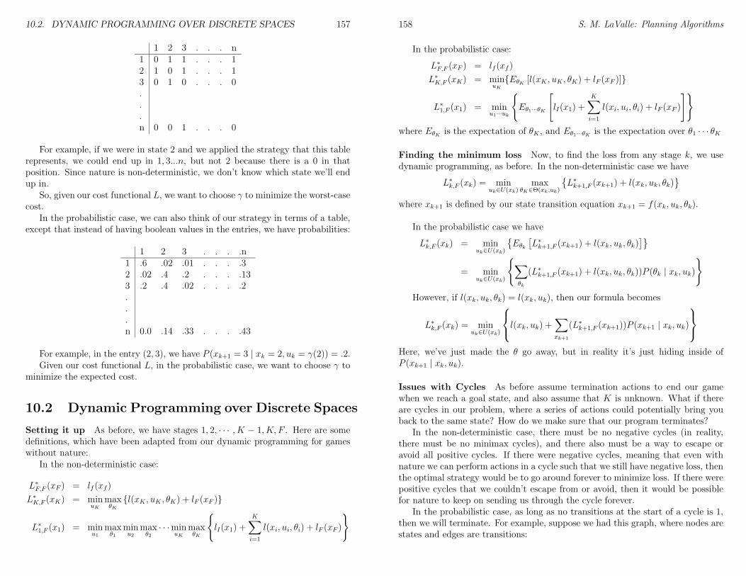
10.2. DYNAMIC PROGRAMMING OVER DISCRETE SPACES 157
1 2 3 . . . n1 0 1 1 . . . 12 1 0 1 . . . 13 0 1 0 . . . 0...n 0 0 1 . . . 0
For example, if we were in state 2 and we applied the strategy that this tablerepresents, we could end up in 1, 3...n, but not 2 because there is a 0 in thatposition. Since nature is non-deterministic, we don’t know which state we’ll endup in.
So, given our cost functional L, we want to choose γ to minimize the worst-casecost.
In the probabilistic case, we can also think of our strategy in terms of a table,except that instead of having boolean values in the entries, we have probabilities:
1 2 3 . . . .n1 .6 .02 .01 . . . .32 .02 .4 .2 . . . .133 .2 .4 .02 . . . .2...n 0.0 .14 .33 . . . .43
For example, in the entry (2, 3), we have P (xk+1 = 3 | xk = 2, uk = γ(2)) = .2.Given our cost functional L, in the probabilistic case, we want to choose γ to
minimize the expected cost.
10.2 Dynamic Programming over Discrete Spaces
Setting it up As before, we have stages 1, 2, · · · , K − 1, K, F . Here are somedefinitions, which have been adapted from our dynamic programming for gameswithout nature:
In the non-deterministic case:
L∗F,F (xF ) = lf (xf )
L∗K,F (xK) = minuK
maxθK
l(xK , uK , θK) + lF (xF )
L∗1,F (x1) = minu1
maxθ1
minu2
maxθ2· · ·min
uK
maxθK
lI(x1) +K∑
i=1
l(xi, ui, θi) + lF (xF )
158 S. M. LaValle: Planning Algorithms
In the probabilistic case:
L∗F,F (xF ) = lf (xf )
L∗K,F (xK) = minuK
EθK[l(xK , uK , θK) + lF (xF )]
L∗1,F (x1) = minu1···uk
Eθ1···θK
[
lI(x1) +K∑
i=1
l(xi, ui, θi) + lF (xF )
]
where EθKis the expectation of θK , and Eθ1···θK
is the expectation over θ1 · · · θK
Finding the minimum loss Now, to find the loss from any stage k, we usedynamic programming, as before. In the non-deterministic case we have
L∗k,F (xk) = minuk∈U(xk)
maxθK∈Θ(xk,uk)
L∗k+1,F (xk+1) + l(xk, uk, θk)
where xk+1 is defined by our state transition equation xk+1 = f(xk, uk, θk).
In the probabilistic case we have
L∗k,F (xk) = minuk∈U(xk)
Eθk
[
L∗k+1,F (xk+1) + l(xk, uk, θk)]
= minuk∈U(xk)
∑
θk
(L∗k+1,F (xk+1) + l(xk, uk, θk))P (θk | xk, uk)
However, if l(xk, uk, θk) = l(xk, uk), then our formula becomes
L∗k,F (xk) = minuk∈U(xk)
l(xk, uk) +∑
xk+1
(L∗k+1,F (xk+1))P (xk+1 | xk, uk)
Here, we’ve just made the θ go away, but in reality it’s just hiding inside ofP (xk+1 | xk, uk).
Issues with Cycles As before assume termination actions to end our gamewhen we reach a goal state, and also assume that K is unknown. What if thereare cycles in our problem, where a series of actions could potentially bring youback to the same state? How do we make sure that our program terminates?
In the non-deterministic case, there must be no negative cycles (in reality,there must be no minimax cycles), and there also must be a way to escape oravoid all positive cycles. If there were negative cycles, meaning that even withnature we can perform actions in a cycle such that we still have negative loss, thenthe optimal strategy would be to go around forever to minimize loss. If there werepositive cycles that we couldn’t escape from or avoid, then it would be possiblefor nature to keep on sending us through the cycle forever.
In the probabilistic case, as long as no transitions at the start of a cycle is 1,then we will terminate. For example, suppose we had this graph, where nodes arestates and edges are transitions:
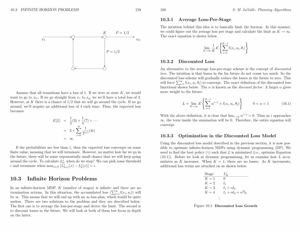
10.3. INFINITE HORIZON PROBLEMS 159
- i - i -
?i¾i
6xI xG
K
P = 1/2
P = 1/2
Assume that all transitions have a loss of 1. If we were at state K, we wouldwant to go to xG. If we go straight from x1 to xg, we we’ll have a total loss of 3.However, at K there is a chance of 1/2 that we will go around the cycle. If we goaround, we’ll acquire an additional loss of 4 each time. Thus, the expected lossbecomes
E[L] =1
2(3) +
1
4(7) + · · ·
= 3 +∞∑
i=0
1
2i+1(4i)
< ∞
If the probabilities are less than 1, then the expected loss converges on somefinite value, meaning that we will terminate. However, no matter how far we go inthe future, there will be some exponentially small chance that we will keep goingaround the cycle. To calculate L∗k, when do we stop? We can pick some thresholdε and terminate when maxx∈X
∣
∣L∗k+1(x)− L∗k(x)∣
∣ < ε.
10.3 Infinite Horizon Problems
In an infinite-horizon MDP, K (number of stages) is infinite and there are notermination actions. In this situation, the accumulated loss (
∑∞i=1 l(xi, ui)) will
be∞. This means that we will end up with an∞-loss plan, which would be quiteuseless. There are two solutions to the problem and they are described below.The first one is to average the loss-per-stage and derive the limit. The second isto discount losses in the future. We will look at both of them but focus in depthon the latter.
160 S. M. LaValle: Planning Algorithms
10.3.1 Average Loss-Per-Stage
The intuition behind this idea is to basically limit the horizon. In this manner,we could figure out the average loss per stage and calculate the limit as K →∞.The exact equation is shown below.
limK→∞
1
KE
K−1∑
i=1
l(xi, ui, θi)
10.3.2 Discounted Loss
An alternative to the average loss-per-stage scheme is the concept of discountedloss. The intuition is that losses in the far future do not count too much. So thediscounted loss scheme will gradually reduce the losses in the future to zero. Thiswill force
∑∞i=1 l(xi, ui, θi) to converge. The exact definition of the discounted loss
functional shown below. The α is known as the discount factor. A larger α givesmore weight to the future.
L = limK→∞
E
K−1∑
i=1
αi−1 × l(xi, ui, θi)
0 < α < 1 (10.1)
With the above definition, it is clear that limi→∞ αi−1 = 0. Thus as i approaches∞, the term inside the summation will be 0. Therefore, the entire equation willconverge.
10.3.3 Optimization in the Discounted Loss Model
Using the discounted loss model described in the previous section, it is now pos-sible to optimize infinite-horizon MDPs using dynamic programming (DP). Weneed to find the best policy (γ) such that L is minimized (i.e., optimize Equation(10.1)). Before we look at dynamic programming, let us examine how L accu-mulates as K increases. When K = 1, there are no losses. As K increments,additional loss terms are attached on as shown below.
Stage L∗KK = 1 0K = 2 l1K = 3 l1 + αl2K = 4 l1 + αl2 + α2l3
...
Figure 10.1: Discounted Loss Growth
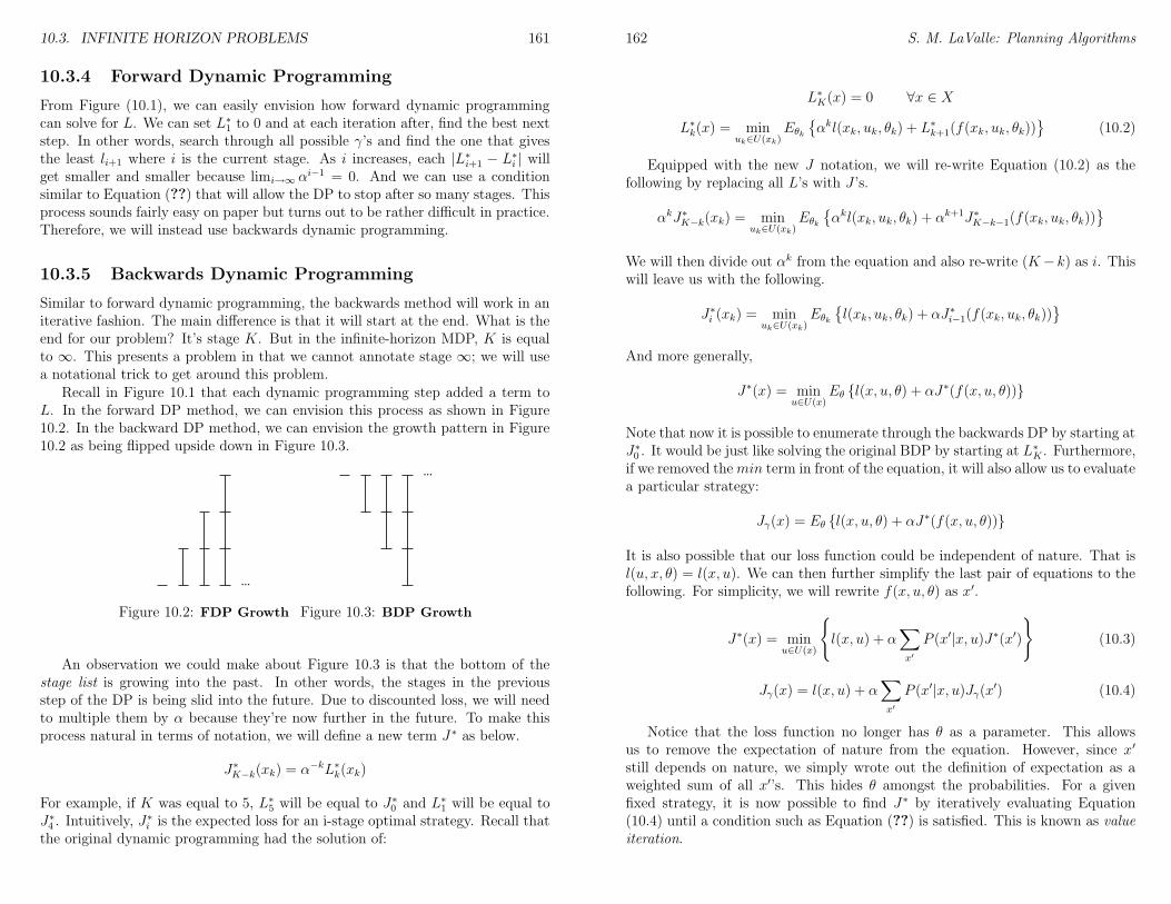
10.3. INFINITE HORIZON PROBLEMS 161
10.3.4 Forward Dynamic Programming
From Figure (10.1), we can easily envision how forward dynamic programmingcan solve for L. We can set L∗1 to 0 and at each iteration after, find the best nextstep. In other words, search through all possible γ’s and find the one that givesthe least li+1 where i is the current stage. As i increases, each |L∗i+1 − L∗i | willget smaller and smaller because limi→∞ αi−1 = 0. And we can use a conditionsimilar to Equation (??) that will allow the DP to stop after so many stages. Thisprocess sounds fairly easy on paper but turns out to be rather difficult in practice.Therefore, we will instead use backwards dynamic programming.
10.3.5 Backwards Dynamic Programming
Similar to forward dynamic programming, the backwards method will work in aniterative fashion. The main difference is that it will start at the end. What is theend for our problem? It’s stage K. But in the infinite-horizon MDP, K is equalto ∞. This presents a problem in that we cannot annotate stage ∞; we will usea notational trick to get around this problem.
Recall in Figure 10.1 that each dynamic programming step added a term toL. In the forward DP method, we can envision this process as shown in Figure10.2. In the backward DP method, we can envision the growth pattern in Figure10.2 as being flipped upside down in Figure 10.3.
...
Figure 10.2: FDP Growth
...
Figure 10.3: BDP Growth
An observation we could make about Figure 10.3 is that the bottom of thestage list is growing into the past. In other words, the stages in the previousstep of the DP is being slid into the future. Due to discounted loss, we will needto multiple them by α because they’re now further in the future. To make thisprocess natural in terms of notation, we will define a new term J ∗ as below.
J∗K−k(xk) = α−kL∗k(xk)
For example, if K was equal to 5, L∗5 will be equal to J∗0 and L∗1 will be equal toJ∗4 . Intuitively, J
∗i is the expected loss for an i-stage optimal strategy. Recall that
the original dynamic programming had the solution of:
162 S. M. LaValle: Planning Algorithms
L∗K(x) = 0 ∀x ∈ X
L∗k(x) = minuk∈U(xk)
Eθk
αkl(xk, uk, θk) + L∗k+1(f(xk, uk, θk))
(10.2)
Equipped with the new J notation, we will re-write Equation (10.2) as thefollowing by replacing all L’s with J ’s.
αkJ∗K−k(xk) = minuk∈U(xk)
Eθk
αkl(xk, uk, θk) + αk+1J∗K−k−1(f(xk, uk, θk))
We will then divide out αk from the equation and also re-write (K− k) as i. Thiswill leave us with the following.
J∗i (xk) = minuk∈U(xk)
Eθk
l(xk, uk, θk) + αJ∗i−1(f(xk, uk, θk))
And more generally,
J∗(x) = minu∈U(x)
Eθ l(x, u, θ) + αJ∗(f(x, u, θ))
Note that now it is possible to enumerate through the backwards DP by starting atJ∗0 . It would be just like solving the original BDP by starting at L∗K . Furthermore,if we removed themin term in front of the equation, it will also allow us to evaluatea particular strategy:
Jγ(x) = Eθ l(x, u, θ) + αJ∗(f(x, u, θ))
It is also possible that our loss function could be independent of nature. That isl(u, x, θ) = l(x, u). We can then further simplify the last pair of equations to thefollowing. For simplicity, we will rewrite f(x, u, θ) as x′.
J∗(x) = minu∈U(x)
l(x, u) + α∑
x′
P (x′|x, u)J∗(x′)
(10.3)
Jγ(x) = l(x, u) + α∑
x′
P (x′|x, u)Jγ(x′) (10.4)
Notice that the loss function no longer has θ as a parameter. This allowsus to remove the expectation of nature from the equation. However, since x′
still depends on nature, we simply wrote out the definition of expectation as aweighted sum of all x′’s. This hides θ amongst the probabilities. For a givenfixed strategy, it is now possible to find J ∗ by iteratively evaluating Equation(10.4) until a condition such as Equation (??) is satisfied. This is known as valueiteration.
10.3. INFINITE HORIZON PROBLEMS 163
10.3.6 Policy Iteration
The method of finding an optimal strategy, γ∗, using Equation (10.3) is known aspolicy iteration. The process can be summarized below.
1. Guess a strategy γ.
2. Evaluate γ using Equation (10.4).
3. Use Equation (10.3) to find an improved γ ′.
4. Go back to Step 2 and repeat until no improvements occur in Step 3.
Example We shall illustrate the above algorithm through a simple example.Suppose we have X = 1, 2 and U = a, b. Let Figures 10.4 and 10.5 be theprobabilities of actions a and b. In addition, let the discount factor α equal 9
10.
1
1
2
2
1/4
3/4
1/4
3/4
Figure 10.4: Action a
1
1
2
2
1/4
3/4
1/4
3/4
Figure 10.5: Action b
Assuming that l(x, u, θ) = l(x, u), we have the following loss values.
l(1, a) = 2 l(1, b) = 12
l(2, a) = 1 l(2, b) = 3
Now, let us follow the algorithm described earlier. Step 1 is to choose aninitial γ. We will randomly choose one that is γ(1) = a and γ(2) = b. In otherwords, choose action a when in state 1 and choose action b when in state 2.
Step 2 is to evaluate γ using Equation (10.4). This results in the followingpair of equations. With them, we see that there are two unknowns with twoequations and thus can be easily solved.
Jγ(1) = l(1, a) +9
10
(
3
4Jγ(1) +
1
4Jγ(2)
)
Jγ(2) = l(2, b) +9
10
(
1
4Jγ(1) +
3
4Jγ(2)
)
Jγ(1) = 24.12 Jγ(2) = 25.96
164 S. M. LaValle: Planning Algorithms
Step 3 is to minimize Jγ . With the answers above, we can now evaluateEquation (10.3) by putting them in place of J ∗(x′). This will let us find a new γwhich we can repeat in Step 2 (which will turn out to be γ(1) = b and γ(2) = a).This process is relatively simple and is guaranteed to find a global minimum.However, when the number of states are large and the number of actions arelarge, the system of equations can become impossible to solve practically.
10.4 Dynamic Programming over Continuous Spaces
I wrote this in 1997 for CS326a at Stanford. It needs to be better integrated in tothe current context. It should also be enhanced to allow nature to be added.
This section describes how the dynamic programming principle can be usedto compute optimal motion plans. Optimality is expressed with respect to adesired criterion, and the method can only provide a solution that is optimal fora specified resolution. The method generally applies to a variety of holonomicand nonholonomic problems, and can be adapted to many other problems thatinvolve complications such as stochastic uncertainty in prediction. The primarydrawback of the approach is that the computation time and space are exponentialin the dimension of the C-space. This limits its applicability to three or four-dimensional problems (however, for many problems it is the only known methodto obtain optimal solutions). Although there are connections between dynamicprogramming in this context and in graph search, its use in these notes appliesto continuous spaces. The dynamic programming formulation presented here ismore similar to what appears in optimal control literature [3, 12, 38].
10.4.1 Reformulating Motion Planning
Recall that the goal of the basic motion planning problem is to compute a pathτ : [0, 1]→ Cfree such that τ(0) = qinit and τ(1) = qgoal, when such a path exists.In the case of nonholonomic systems, velocity constraints must additionally besatisfied.
We are next going to add some new concepts to the standard motion planningformulation. First, it will be helpful to define time, both for motion planningproblems that vary over time and to help in the upcoming concepts. Since timeis irrelevant for basic motion planning, it can be considered in this case as anauxiliary variable that only assists in the formulation. Suppose that there is someinitial time, t = 0, at which the robot is at qinit. Suppose also that there is somefinal time, Tf (one would like to at least have the robot at the goal before t = Tf ).
Recall that q represents the velocity of the robot in the configuration space.Suppose that C is an m-dimensional configuration space, and that u is a continu-ous, vector-valued function that depends on time: u : [0, Tf ]→ Rm. If we select u,and let q(t) = u(t), then a trajectory has been specified for the robot: q(0) = qinit
10.4. DYNAMIC PROGRAMMING OVER CONTINUOUS SPACES 165
and for 0 < t ≤ Tf , we can obtain
q(t) = q(0) +
∫ t
0
q(t′) dt′ = q(0) +
∫ t
0
u(t′) dt′. (10.5)
The function u can be considered as a control input, because it allows us to movethe robot by specifying its velocity. As will be seen shortly, the case of q(t) = u(t)corresponds to a holonomic planning problem. Suppose that we can choose anycontrol input such that for all t it is either normalized, ‖u(t)‖ = 1, or u(t) = 0.This implies that we can locally move the robot in any allowable direction from itstangent space. For nonholonomic problems, one will only be allowed to move therobot through a function of the form q = f(q(t), u(t)). For example, as describedin [39], p. 432, the equations for the nonholonomic car robot can be expressed asx = v cos(θ), y = v sin(θ), and θ = v
Ltan(φ). Using the notation in these notes,
(x, y, θ) becomes (q1, q2, q3), and (v, φ) becomes (u1, u2). The function f can beconsidered as a kind of interface between the user and the robot. Commands arespecified through u(t), but the resulting velocities in the configuration space gettransformed using f (which in general prevents the user from directly controllingvelocities).
Incorporating optimality If we want to consider optimality, then it will behelpful to define a function that assigns a cost to a given trajectory that is executedby the robot. One can also make this cost depend on the control function. Forexample, if the control is an accelerator of a car, then one might want to penalizerapid accelerations which use more fuel. A loss functional is defined that evaluatesany configuration trajectory and control function:
L =
∫ Tf
0
l(q(t), u(t))dt+Q(q(Tf )). (10.6)
The integrand l(q(t), u(t)) represents an instantaneous cost, which when inte-grated can be imagined as the total amount of energy that is expended. The termQ(q(Tf )) is a final cost that can be used to induce a preference over trajectoriesthat terminate in a goal region of the configuration space.
The loss functional can reduced to a binary function when encoding a basicpath planning problem that does not involve optimality. The loss functional canbe simplified to L = Q(q(Tf )). We take Q(q(Tf )) = 0 if q(Tf ) = qgoal, andQ(q(Tf )) = 1 otherwise. This partitions the space of controls functions into twoclasses: control functions that cause the basic motion planning problem to besolved receive zero loss; otherwise, unit loss is received.
The previous formulation considered all control inputs that achieve the goalto be equivalent. As another example, the following measures the path length forcontrol inputs that lead to the goal:
L =
∫ Tf
0
‖q(t)‖dt if q(Tf ) = qgoal
∞ otherwise. (10.7)
166 S. M. LaValle: Planning Algorithms
The term∫ Tf
0‖q(t)‖dt measures path length, and recall that q(t) = u(t) for all t.
There is a small technicality about considering optimal collision-free paths.For example, the visibility-graph method produces optimal solutions, but thesepaths must graze the obstacles. Any path that maps into Cfree can be replaced bya shorter path that still maps into Cfree, but might come closer to obstacles. Theproblem exists because Cfree is an open set, and can be fixed by allowing the pathto map into Cvalid (which is the closure of Cfree. If one still must use Cfree, thenthe optimal path that maps into Cvalid will represent an infinum (a lower boundthat can’t quite be reached) over paths that only map into Cfree.
A discrete-time representation The motion planning problem can alterna-tively be characterized in discrete time. For the systems that we will consider,discrete-time representations can provide arbitrarily close approximations to thecontinuous case, and facilitate the development of the dynamic programming al-gorithm.
With the discretization of time, [0, Tf ] is partitioned into stages, denoted byk ∈ 1, . . . , K + 1. Stage k refers to time (k − 1)∆t. The final stage is given byK = bTf/∆tc. Let qk represent the configuration at stage k. At each stage k, anaction uk can be chosen from an action space U . Because
dq
dt= lim
∆t→0
q(t+∆t)− q(t)
∆t, (10.8)
the equation q(t) = u(t) can be approximated as
qk+1 = qk +∆t uk, (10.9)
in which qk = q(t), qk+1 = q(t + ∆t), and uk = u(t). As an example of howthis representation approximates the basic motion planning problem, consider thefollowing example. Suppose Cfree ⊆ R2. It is assumed that ‖uk‖ = 1 and, hence,the space of possible actions can be sufficiently characterized by the parameterφk ∈ [0, 2π). The discrete-time transition equation becomes
qk+1 = qk +∆t
[
cos(φk)sin(φk)
]
. (10.10)
At each stage, the direction of motion is controlled by selecting φk. Any K-segment polygonal curve of length K∆t can be obtained as a possible trajectoryof the system. If an action is included that causes no motion, shorter polygonalcurves can also be obtained.
In general, a variety of holonomic and nonholonomic problems can also be ap-proximated in discrete time. The equation q = f(q(t), u(t)) can be approximatedby a transition equation of the form qk+1 = fk(qk, uk).
A discrete-time representation of the loss functional can also be defined:
L(q1, . . . , qK+1, u1, . . . , uK) =K∑
k=1
lk(qk, uk) + lK+1(qK+1), (10.11)
10.4. DYNAMIC PROGRAMMING OVER CONTINUOUS SPACES 167
in which lk and lK+1 serve the same purpose as l and Q in the continuous-timeloss functional.
The basic motion planning problem can be represented in discrete time byletting lk = 0 for all k ∈ 1, . . . , K, and defining the final term as lK+1(qK+1) = 0if qk = qgoal, and lK+1(qK+1) = 1 otherwise. This gives equal preference to alltrajectories that reach the goal. To approximate the problem of planning anoptimal-length path, lk = 1 for all k ∈ 1, . . . , K. The final term is then definedas lK+1(qK+1) = 0 if qk = qgoal, and lK+1(qK+1) =∞ otherwise.
10.4.2 The Algorithm
This section presents algorithm issues that result from computing approximateoptimal motion strategies. Variations of this algorithm, which apply to a vari-ety of motion planning problems are discussed in detail in [41]. The quality ofthis approximation depends on the resolution of the representation chosen for theconfiguration space and action space. The efforts are restricted to obtaining ap-proximate solutions for three primary reasons: 1) known lower-bound hardnessresults for basic motion planning and a variety of extensions; 2) exact methodsoften depend strongly on specialized analysis for a specific problem class; and 3)the set of related optimal-control and dynamic-game problems for which analyti-cal solutions are available is quite restrictive. The computational hardness resultshave curbed many efforts to find efficient, complete algorithms to general motionplanning problems. In [61] the basic motion planning problem was shown to bePSPACE-hard for polyhedral robots with n links. In [13] is was shown that com-puting minimum-distance paths in a 3-D workspace is NP-hard. It was also shownthat the compliant motion control problem with sensing uncertainty is nondeter-ministic exponential time hard. In [62] it was shown that planning the motion ofa disk in a 3-D environment with rotating obstacles is PSPACE-hard. In [63], a3-D pursuit-evasion problem is shown to be exponential time hard, even thoughthere is perfect sensing information. Such results have turned motion planningefforts toward approximate techniques. For example, a polynomial-time algorithmis given in [55] for computing epsilon approximations of minimum-distance pathsin a 3-D environment. Also, randomized techniques are used to compute solu-tions for high degree-of-freedom problems that are unapproachable by completemethods [2, 7, 30, 71].
The second motivation for considering approximate solutions is to avoid spe-cialized analysis of particular cases, with the intent of allowing the algorithms tobe adaptable to other problem classes. Of course, in many cases there is greatvalue in obtaining an exact solutions to a specialized class of problems. The ap-proach described in this paper can be considered as a general way to approximatesolutions that might be sufficient for a particular application, or the approachmight at least provide some understanding of the solutions.
The final motivation for considering approximate solutions is that the class of
168 S. M. LaValle: Planning Algorithms
related optimal-control and dynamic-game problems that can be solved directlyis fairly restrictive. In both control theory and dynamic game theory, the classicset of problems that can be solved are those with a linear transition equation andquadratic loss functional [3, 6, 12].
The algorithm description is organized into three parts. First, the generalprinciple of optimality is described, which greatly reduces the amount of effortthat is required to compute optimal strategies. The next part describes how cost-to-go functions are computed as an intermediate representation of the optimalstrategy. The third part describes how the cost-to-go is used as a navigationfunction to execute the represented strategy (i.e., selecting optimal actions duringon-line execution). Following this, basic complexity assessments are given.
Exploiting the principle of optimality Because the decision making ex-pressed in qk+1 = fk(qk, uk) is iterative, the dynamic programming principle cangenerally be employed to avoid brute-force enumeration of alternative strategies,and it forms the basis of our algorithm. Although there are obvious connectionsto dynamic programming in graph search, it is important to note the distinctionsbetween Dijkstra’s algorithm and the usage of the dynamic programming princi-ple in these notes. In optimal control theory, the dynamic programming principleis represented as a differential equation (or difference equation in discrete time)that can be used to directly solve a problem such as the linear-quadratic Gaussianregulator [36], or can be used for computing numerical approximations of optimalstrategies [37]. In the general case, the differential equation is expressed in termsof time-dependent cost-to-go functions. The cost-to-go is a function on the config-uration space that expresses the cost that is received under the implementation ofan optimal strategy from that particular configuration and time. In some cases,the time index can be eliminated, as in the special case of values stored at verticesin the execution of Dijkstra’s algorithm.
For the discrete-time model, the dynamic programming principle is expressedas a difference equation (in continuous time it becomes a differential equation).The cost-to-go function at stage k is defined as
L∗k(qk) = minuk,...,uK
K∑
i=k
li(qi, ui) + lK+1(qK+1)
. (10.12)
The cost-to-go can be separated:
L∗k(qk) = minuk
minuk+1,...,uK
lk(qk, uk) +K∑
i=k+1
lk(qi, ui(qi)) + lK+1(qK+1)
. (10.13)
The second min does not affect the lk term; thus, it can be removed to obtain
L∗k(qk) = minuk
[
lk(qk, uk) + minuk+1,...,uK
K∑
i=k+1
lk(qi, ui(qi)) + lK+1(qK+1)
]
.
(10.14)
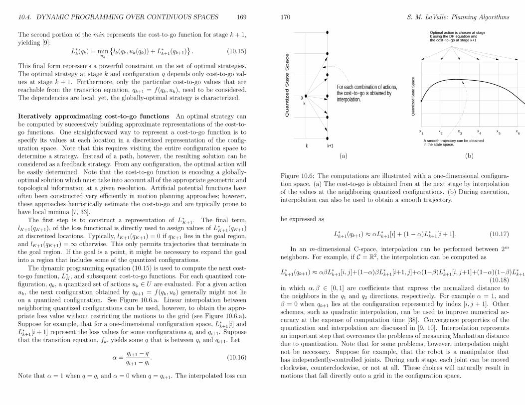
10.4. DYNAMIC PROGRAMMING OVER CONTINUOUS SPACES 169
The second portion of the min represents the cost-to-go function for stage k + 1,yielding [9]:
L∗k(qk) = minuk
lk(qk, uk(qk)) + L∗k+1(qk+1)
. (10.15)
This final form represents a powerful constraint on the set of optimal strategies.The optimal strategy at stage k and configuration q depends only cost-to-go val-ues at stage k + 1. Furthermore, only the particular cost-to-go values that arereachable from the transition equation, qk+1 = f(qk, uk), need to be considered.The dependencies are local; yet, the globally-optimal strategy is characterized.
Iteratively approximating cost-to-go functions An optimal strategy canbe computed by successively building approximate representations of the cost-to-go functions. One straightforward way to represent a cost-to-go function is tospecify its values at each location in a discretized representation of the config-uration space. Note that this requires visiting the entire configuration space todetermine a strategy. Instead of a path, however, the resulting solution can beconsidered as a feedback strategy. From any configuration, the optimal action willbe easily determined. Note that the cost-to-go function is encoding a globally-optimal solution which must take into account all of the appropriate geometric andtopological information at a given resolution. Artificial potential functions haveoften been constructed very efficiently in motion planning approaches; however,these approaches heuristically estimate the cost-to-go and are typically prone tohave local minima [7, 33].
The first step is to construct a representation of L∗K+1. The final term,lK+1(qK+1), of the loss functional is directly used to assign values of L∗K+1(qK+1)at discretized locations. Typically, lK+1(qK+1) = 0 if qK+1 lies in the goal region,and lK+1(qK+1) =∞ otherwise. This only permits trajectories that terminate inthe goal region. If the goal is a point, it might be necessary to expand the goalinto a region that includes some of the quantized configurations.
The dynamic programming equation (10.15) is used to compute the next cost-to-go function, L∗K , and subsequent cost-to-go functions. For each quantized con-figuration, qk, a quantized set of actions uk ∈ U are evaluated. For a given actionuk, the next configuration obtained by qk+1 = f(qk, uk) generally might not lieon a quantized configuration. See Figure 10.6.a. Linear interpolation betweenneighboring quantized configurations can be used, however, to obtain the appro-priate loss value without restricting the motions to the grid (see Figure 10.6.a).Suppose for example, that for a one-dimensional configuration space, L∗k+1[i] andL∗k+1[i+ 1] represent the loss values for some configurations qi and qi+1. Supposethat the transition equation, fk, yields some q that is between qi and qi+1. Let
α =qi+1 − q
qi+1 − qi. (10.16)
Note that α = 1 when q = qi and α = 0 when q = qi+1. The interpolated loss can
170 S. M. LaValle: Planning Algorithms
k+1k
xk
Quantized S
tate
Space
For each combination of actions,the cost−to−go is obtained byinterpolation.
Qua
ntiz
ed S
tate
Spa
ce
1x
2x
3x
4x
5x
6x
Optimal action is chosen at stagek using the DP equation andthe cost−to−go at stage k+1
A smooth trajectory can be obtainedin the state space.
(a) (b)
Figure 10.6: The computations are illustrated with a one-dimensional configura-tion space. (a) The cost-to-go is obtained from at the next stage by interpolationof the values at the neighboring quantized configurations. (b) During execution,interpolation can also be used to obtain a smooth trajectory.
be expressed as
L∗k+1(qk+1) ≈ αL∗k+1[i] + (1− α)L∗k+1[i+ 1]. (10.17)
In an m-dimensional C-space, interpolation can be performed between 2m
neighbors. For example, if C = R2, the interpolation can be computed as
L∗k+1(qk+1) ≈ αβL∗k+1[i, j]+(1−α)βL∗k+1[i+1, j]+α(1−β)L∗k+1[i, j+1]+(1−α)(1−β)L∗k+1[i+1, j+1](10.18)
in which α, β ∈ [0, 1] are coefficients that express the normalized distance tothe neighbors in the q1 and q2 directions, respectively. For example α = 1, andβ = 0 when qk+1 lies at the configuration represented by index [i, j + 1]. Otherschemes, such as quadratic interpolation, can be used to improve numerical ac-curacy at the expense of computation time [38]. Convergence properties of thequantization and interpolation are discussed in [9, 10]. Interpolation representsan important step that overcomes the problems of measuring Manhattan distancedue to quantization. Note that for some problems, however, interpolation mightnot be necessary. Suppose for example, that the robot is a manipulator thathas independently-controlled joints. During each stage, each joint can be movedclockwise, counterclockwise, or not at all. These choices will naturally result inmotions that fall directly onto a grid in the configuration space.
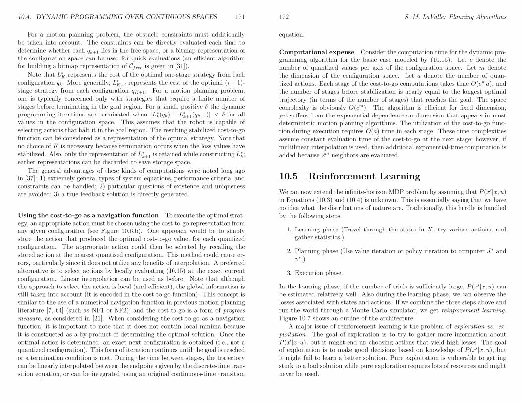
10.4. DYNAMIC PROGRAMMING OVER CONTINUOUS SPACES 171
For a motion planning problem, the obstacle constraints must additionallybe taken into account. The constraints can be directly evaluated each time todetermine whether each qk+1 lies in the free space, or a bitmap representation ofthe configuration space can be used for quick evaluations (an efficient algorithmfor building a bitmap representation of Cfree is given in [31]).
Note that L∗K represents the cost of the optimal one-stage strategy from eachconfiguration qk. More generally, L∗K−i represents the cost of the optimal (i+ 1)-stage strategy from each configuration qK+1. For a motion planning problem,one is typically concerned only with strategies that require a finite number ofstages before terminating in the goal region. For a small, positive δ the dynamicprogramming iterations are terminated when |L∗k(qk) − L∗k+1(qk+1)| < δ for allvalues in the configuration space. This assumes that the robot is capable ofselecting actions that halt it in the goal region. The resulting stabilized cost-to-gofunction can be considered as a representation of the optimal strategy. Note thatno choice of K is necessary because termination occurs when the loss values havestabilized. Also, only the representation of L∗k+1 is retained while constructing L∗k;earlier representations can be discarded to save storage space.
The general advantages of these kinds of computations were noted long agoin [37]: 1) extremely general types of system equations, performance criteria, andconstraints can be handled; 2) particular questions of existence and uniquenessare avoided; 3) a true feedback solution is directly generated.
Using the cost-to-go as a navigation function To execute the optimal strat-egy, an appropriate action must be chosen using the cost-to-go representation fromany given configuration (see Figure 10.6.b). One approach would be to simplystore the action that produced the optimal cost-to-go value, for each quantizedconfiguration. The appropriate action could then be selected by recalling thestored action at the nearest quantized configuration. This method could cause er-rors, particularly since it does not utilize any benefits of interpolation. A preferredalternative is to select actions by locally evaluating (10.15) at the exact currentconfiguration. Linear interpolation can be used as before. Note that althoughthe approach to select the action is local (and efficient), the global information isstill taken into account (it is encoded in the cost-to-go function). This concept issimilar to the use of a numerical navigation function in previous motion planningliterature [7, 64] (such as NF1 or NF2), and the cost-to-go is a form of progressmeasure, as considered in [21]. When considering the cost-to-go as a navigationfunction, it is important to note that it does not contain local minima becauseit is constructed as a by-product of determining the optimal solution. Once theoptimal action is determined, an exact next configuration is obtained (i.e., not aquantized configuration). This form of iteration continues until the goal is reachedor a termination condition is met. During the time between stages, the trajectorycan be linearly interpolated between the endpoints given by the discrete-time tran-sition equation, or can be integrated using an original continuous-time transition
172 S. M. LaValle: Planning Algorithms
equation.
Computational expense Consider the computation time for the dynamic pro-gramming algorithm for the basic case modeled by (10.15). Let c denote thenumber of quantized values per axis of the configuration space. Let m denotethe dimension of the configuration space. Let a denote the number of quan-tized actions. Each stage of the cost-to-go computations takes time O(cma), andthe number of stages before stabilization is nearly equal to the longest optimaltrajectory (in terms of the number of stages) that reaches the goal. The spacecomplexity is obviously O(cm). The algorithm is efficient for fixed dimension,yet suffers from the exponential dependence on dimension that appears in mostdeterministic motion planning algorithms. The utilization of the cost-to-go func-tion during execution requires O(a) time in each stage. These time complexitiesassume constant evaluation time of the cost-to-go at the next stage; however, ifmultilinear interpolation is used, then additional exponential-time computation isadded because 2m neighbors are evaluated.
10.5 Reinforcement Learning
We can now extend the infinite-horizon MDP problem by assuming that P (x′|x, u)in Equations (10.3) and (10.4) is unknown. This is essentially saying that we haveno idea what the distributions of nature are. Traditionally, this hurdle is handledby the following steps.
1. Learning phase (Travel through the states in X, try various actions, andgather statistics.)
2. Planning phase (Use value iteration or policy iteration to computer J ∗ andγ∗.)
3. Execution phase.
In the learning phase, if the number of trials is sufficiently large, P (x′|x, u) canbe estimated relatively well. Also during the learning phase, we can observe thelosses associated with states and actions. If we combine the three steps above andrun the world through a Monte Carlo simulator, we get reinforcement learning.Figure 10.7 shows an outline of the architecture.
A major issue of reinforcement learning is the problem of exploration vs. ex-ploitation. The goal of exploration is to try to gather more information aboutP (x′|x, u), but it might end up choosing actions that yield high losses. The goalof exploitation is to make good decisions based on knowledge of P (x′|x, u), butit might fail to learn a better solution. Pure exploitation is vulnerable to gettingstuck to a bad solution while pure exploration requires lots of resources and mightnever be used.
10.5. REINFORCEMENT LEARNING 173
ReinforcementLearner
MonteCarloSimulator
State and Action
Next State
Loss Value
Figure 10.7: Reinforcement Learning Architecture
10.5.1 Stochastic Iterative Algorithms
Recall that the original evaluation of a particular strategy was:
Jγ(x) = l(x, u) + α∑
x′
P (x′|x, u)Jγ(x′)
But the problem now is that P (x′|x, u) is unknown. Instead, we use what is calleda stochastic iterative algorithm. Jγ(x) will be updated with the following equation.ρ is the learning rate.
Jγ(x) = (1− ρ)Jγ(x) + ρ(l(x, γ(x)) + αJγ(x′))
In this equation, x′ is now observed instead of calculated from f(x, u, θ). Aquestion a keen reader might ask is where have the probabilities gone? They’reconspicuously missing in the above equation. The answer is that they’re reallyembedded in the observations of x′ from nature. In the Monte Carlo simulation,states that have high probability will occur more often and thus will make a biggerinfluence to Jγ. In this manner, over time the probabilities distribution of x′ will
be stored in Jγ.
10.5.2 Finding an Optimal Strategy: Q-learning
So how do we find the optimal strategy? The answer lies in Q: rather thanusing just J∗ : X → R, the expected loss of a particular strategy, now we useQ∗ : X ×U → R. Q∗(x, u) represents the optimal cost-to-go from applying u andthen continuing on the optimal path after that. Note that Q is independent ofthe policy being followed.
Using Q∗(x, u) in the dynamic programming equation yields:
Q∗(x, u) = l(x, u) + α∑
x′
P (x′|x, u) minu′∈U(x′)
(Q∗(x′, u′))
If we make J∗(x) the expected cost for optimal strategy given state x, andQ∗(x, u) be the expected cost for optimal strategy given state x and using cost u,
174 S. M. LaValle: Planning Algorithms
thenJ∗(x) = min
u∈U(x)Q∗(x, u)
However, for reinforcement learning, the probability P (x′|x, u) is unknown, sowe can bring in the stochastic iterative idea again and get
Q∗(x, u) := (1− ρ)Q∗(x, u) + ρ(l(x, u) + α minu′∈U(x′)
Q∗(x, u))
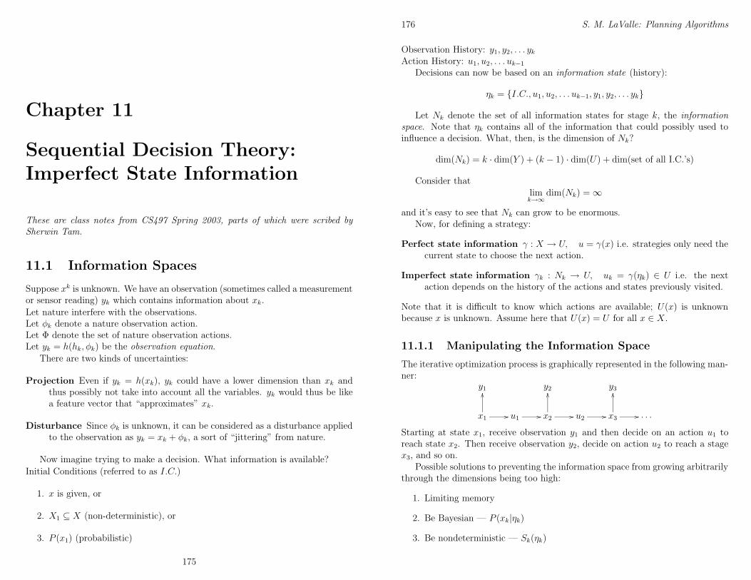
Chapter 11
Sequential Decision Theory:Imperfect State Information
These are class notes from CS497 Spring 2003, parts of which were scribed bySherwin Tam.
11.1 Information Spaces
Suppose xk is unknown. We have an observation (sometimes called a measurementor sensor reading) yk which contains information about xk.
Let nature interfere with the observations.Let φk denote a nature observation action.Let Φ denote the set of nature observation actions.Let yk = h(hk, φk) be the observation equation.
There are two kinds of uncertainties:
Projection Even if yk = h(xk), yk could have a lower dimension than xk andthus possibly not take into account all the variables. yk would thus be likea feature vector that “approximates” xk.
Disturbance Since φk is unknown, it can be considered as a disturbance appliedto the observation as yk = xk + φk, a sort of “jittering” from nature.
Now imagine trying to make a decision. What information is available?
Initial Conditions (referred to as I.C.)
1. x is given, or
2. X1 ⊆ X (non-deterministic), or
3. P (x1) (probabilistic)
175
176 S. M. LaValle: Planning Algorithms
Observation History: y1, y2, . . . ykAction History: u1, u2, . . . uk−1
Decisions can now be based on an information state (history):
ηk = I.C., u1, u2, . . . uk−1, y1, y2, . . . yk
Let Nk denote the set of all information states for stage k, the informationspace. Note that ηk contains all of the information that could possibly used toinfluence a decision. What, then, is the dimension of Nk?
dim(Nk) = k · dim(Y ) + (k − 1) · dim(U) + dim(set of all I.C.’s)
Consider thatlimk→∞
dim(Nk) =∞
and it’s easy to see that Nk can grow to be enormous.Now, for defining a strategy:
Perfect state information γ : X → U, u = γ(x) i.e. strategies only need thecurrent state to choose the next action.
Imperfect state information γk : Nk → U, uk = γ(ηk) ∈ U i.e. the nextaction depends on the history of the actions and states previously visited.
Note that it is difficult to know which actions are available; U(x) is unknownbecause x is unknown. Assume here that U(x) = U for all x ∈ X.
11.1.1 Manipulating the Information Space
The iterative optimization process is graphically represented in the following man-ner:
y1 y2 y3
x1
OO
// u1 // x2
OO
// u2 // x3
OO
// . . .
Starting at state x1, receive observation y1 and then decide on an action u1 toreach state x2. Then receive observation y2, decide on action u2 to reach a stagex3, and so on.
Possible solutions to preventing the information space from growing arbitrarilythrough the dimensions being too high:
1. Limiting memory
2. Be Bayesian — P (xk|ηk)
3. Be nondeterministic — Sk(ηk)
11.1. INFORMATION SPACES 177
4. Approximate Nk
5. Find equivalence classes in Nk
First, a recap of the variables involved:
yk = h(xk, φk)
xk+1 = f(xk, uk, θk)
ηk = I.C., u1, u2, . . . uk−1, y1, y2, . . . yk
Nk = information space
γ : Nk → U (not γ : Y → U , which only would consider the current state)
Limited Memory
With limited memory only the last i stages would be remembered, so ηk =uk−i, . . . , uk−1, yk−i+1, . . . , yk. If i = 1, then the information state would simplybe ηk = uk−1, yk or even just ηk = yk for the last observation on the currentstate, ignoring the last action. Of course, the disadvantage here is that this givesthe learner a short-term memory, and the early information that wasn’t savedcould be important to the current decision. If, for instance, the situation was aduel with guns, and the agreement was to take twenty steps before turning andfiring, someone who only had enough memory to count fifteen steps would be introuble...
Bayesian
Now we consider a probabilistic approach. We first eliminate nature from theequations:
P (θk|xk, uk) givenf−→ P (xk+1|xk, uk) since xk+1 = f(xk, uk, θk)
P (φk|xk) givenh−→ P (yk|xk) since yk = h(xk, φk)
Assume P (x1) for the Initial Condition.First, receive observation y1. Use Bayes Rule to obtain
P (x1|y1) =P (y1|x1)P (x1)
∑
x1P (y1|x1)P (x1)
What do we have now?
P (x2|x1, u1) from f and P (θ)
P (x1|y1) from Bayes Rule
Apply u1 to obtain x2:
P (x2|u1, y1) =∑
x∈XP (x2|x1, u1)P (x1|y1)
178 S. M. LaValle: Planning Algorithms
Note that y1 is missing from P (x2|x1, u1), since y1 is conditionally independentfrom x2 (no need for a previous observation if the action’s already been deter-mined). Also, u1 is missing from P (x1|y1) because u1 has no bearing on x1, beingthe action to determine x2.
For the more general case, use induction: given P (xk|ηk), determine P (xk+1|ηk+1):
ηk+1 = ηk ∪ uk, yk+1
First handle uk:
P (xk+1|ηk, uK) =∑
xk∈XP (xk+1|xk, uk)P (xk|ηk)
Now handle yk+1:
P (xk+1|ηk, uk, yk+1) = P (xk+1|ηk+1) =P (yk+1|xk+1)P (xk+1|ηk, uk)
∑
xk+1P (yk+1|xk+1)P (xk+1|ηk, uk)
This means that an information state for Markov Decision Processes can beviewed as a probability distribution
ηk → P (xk|ηk)
It’s possible that two different information spaces lead to the same probability,i.e. P (xk|ηk) = P (xK |η
′k). However, even if the histories are different, since the
probabilities are the same, then then information state for an MDP is essentiallythe same.
Nondeterministic
X1 ⊆ X is the set of possible initial states.Let Sk(∼) ⊆ X denote the set of possible states given the information in ∼,
where ∼ is the same conditions given in a Bayesian probability P (xk| ∼).Here we’re assuming Φ, the set of observable actions by nature, is given. From
this we obtain Sk(yk) ⊆ X:
Sk(yk) = xk ∈ X | ∃φk ∈ Φ for which xk = h(yk, φk)
Starting with the Initial Condition S1(I.C.) = X1, observe y1:
S1(I.C., y1) = S1(η1) = S(y1) ∩X1
Now, choose u1:
S2(u1, η1) = x2 ∈ X | ∃θ1 ∈ Θ, ∃x1 ∈ S1(η1), for which x2 = f(x1, u1, θ1)
11.2. PREIMAGES AND FORWARD PROJECTIONS 179
Alternately, this can also be represented as
S2(u1, η1) =⋃
θ1∈Θ
⋃
x1∈S1(η1)
f(x1, u1, θ1)
That is, S2 is equal to the union of all possible states reachable by applyingaction u1 and nature’s influence θ1 to all the states in S1(η1). Thus, an infinitenumber of information states is reduced to a number of sets for any given stage,i.e. S1(η1), S2(η2), S3(η3) . . . and so on.
Now, if we observe y2:
S2(u1, y2, η1) = S(η2) = S2(u1, η1) ∩ S2(y2)
where S2(y2) is derived from the Sk(yk) formula from before.In general, assuming Sk(ηk) is given, how do we find Sk+1(ηk+1)?Use Sk(ηk) to obtain Sk+1(uk, ηk) after choosing uk, as above:
Sk+1(uk, ηk) =⋃
θk∈Θ
⋃
xk∈Sk(ηk)
f(xk, uk, θk)
Receive yk+1:
Sk+1(ηk, uk, yk+1) = Sk+1(ηk+1) = Sk+1(uk, ηk) ∩ Sk+1(yk+1)
11.2 Preimages and Forward Projections
11.3 Dynamic Programming on Information Spaces
11.4 Kalman Filtering
11.5 Localization
cover Bayesian, the approach of Guibas, Motwani, Raghavan, and also perceptualequivalence classes of Donald, Jennings.
11.6 Sensorless Manipulation
11.7 Other Searches on Information Spaces
180 S. M. LaValle: Planning Algorithms
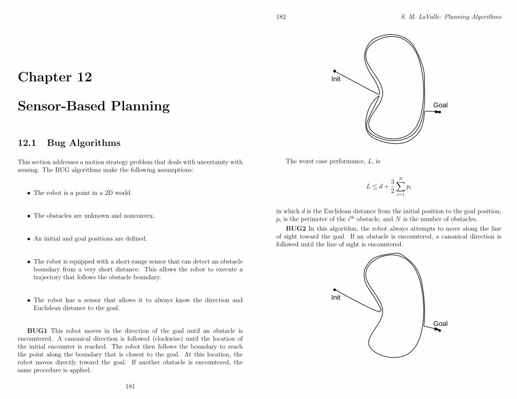
Chapter 12
Sensor-Based Planning
12.1 Bug Algorithms
This section addresses a motion strategy problem that deals with uncertainty withsensing. The BUG algorithms make the following assumptions:
• The robot is a point in a 2D world.
• The obstacles are unknown and nonconvex.
• An initial and goal positions are defined.
• The robot is equipped with a short-range sensor that can detect an obstacleboundary from a very short distance. This allows the robot to execute atrajectory that follows the obstacle boundary.
• The robot has a sensor that allows it to always know the direction andEuclidean distance to the goal.
BUG1 This robot moves in the direction of the goal until an obstacle isencountered. A canonical direction is followed (clockwise) until the location ofthe initial encounter is reached. The robot then follows the boundary to reachthe point along the boundary that is closest to the goal. At this location, therobot moves directly toward the goal. If another obstacle is encountered, thesame procedure is applied.
181
182 S. M. LaValle: Planning Algorithms
Init
Goal
The worst case performance, L, is
L ≤ d+3
2
N∑
i=1
pi
in which d is the Euclidean distance from the initial position to the goal position,pi is the perimeter of the ith obstacle, and N is the number of obstacles.
BUG2 In this algorithm, the robot always attempts to move along the lineof sight toward the goal. If an obstacle is encountered, a canonical direction isfollowed until the line of sight is encountered.
Init
Goal
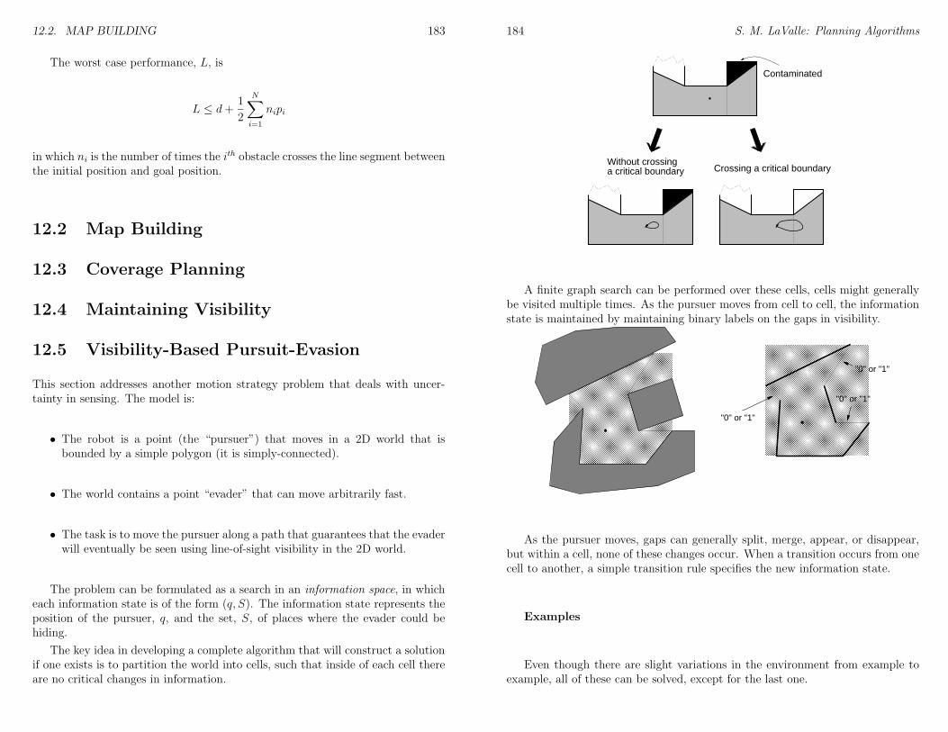
12.2. MAP BUILDING 183
The worst case performance, L, is
L ≤ d+1
2
N∑
i=1
nipi
in which ni is the number of times the ith obstacle crosses the line segment betweenthe initial position and goal position.
12.2 Map Building
12.3 Coverage Planning
12.4 Maintaining Visibility
12.5 Visibility-Based Pursuit-Evasion
This section addresses another motion strategy problem that deals with uncer-tainty in sensing. The model is:
• The robot is a point (the “pursuer”) that moves in a 2D world that isbounded by a simple polygon (it is simply-connected).
• The world contains a point “evader” that can move arbitrarily fast.
• The task is to move the pursuer along a path that guarantees that the evaderwill eventually be seen using line-of-sight visibility in the 2D world.
The problem can be formulated as a search in an information space, in whicheach information state is of the form (q, S). The information state represents theposition of the pursuer, q, and the set, S, of places where the evader could behiding.
The key idea in developing a complete algorithm that will construct a solutionif one exists is to partition the world into cells, such that inside of each cell thereare no critical changes in information.
184 S. M. LaValle: Planning Algorithms
Crossing a critical boundaryWithout crossinga critical boundary
Contaminated
A finite graph search can be performed over these cells, cells might generallybe visited multiple times. As the pursuer moves from cell to cell, the informationstate is maintained by maintaining binary labels on the gaps in visibility.
"0" or "1"
"0" or "1"
"0" or "1"
As the pursuer moves, gaps can generally split, merge, appear, or disappear,but within a cell, none of these changes occur. When a transition occurs from onecell to another, a simple transition rule specifies the new information state.
Examples
Even though there are slight variations in the environment from example toexample, all of these can be solved, except for the last one.
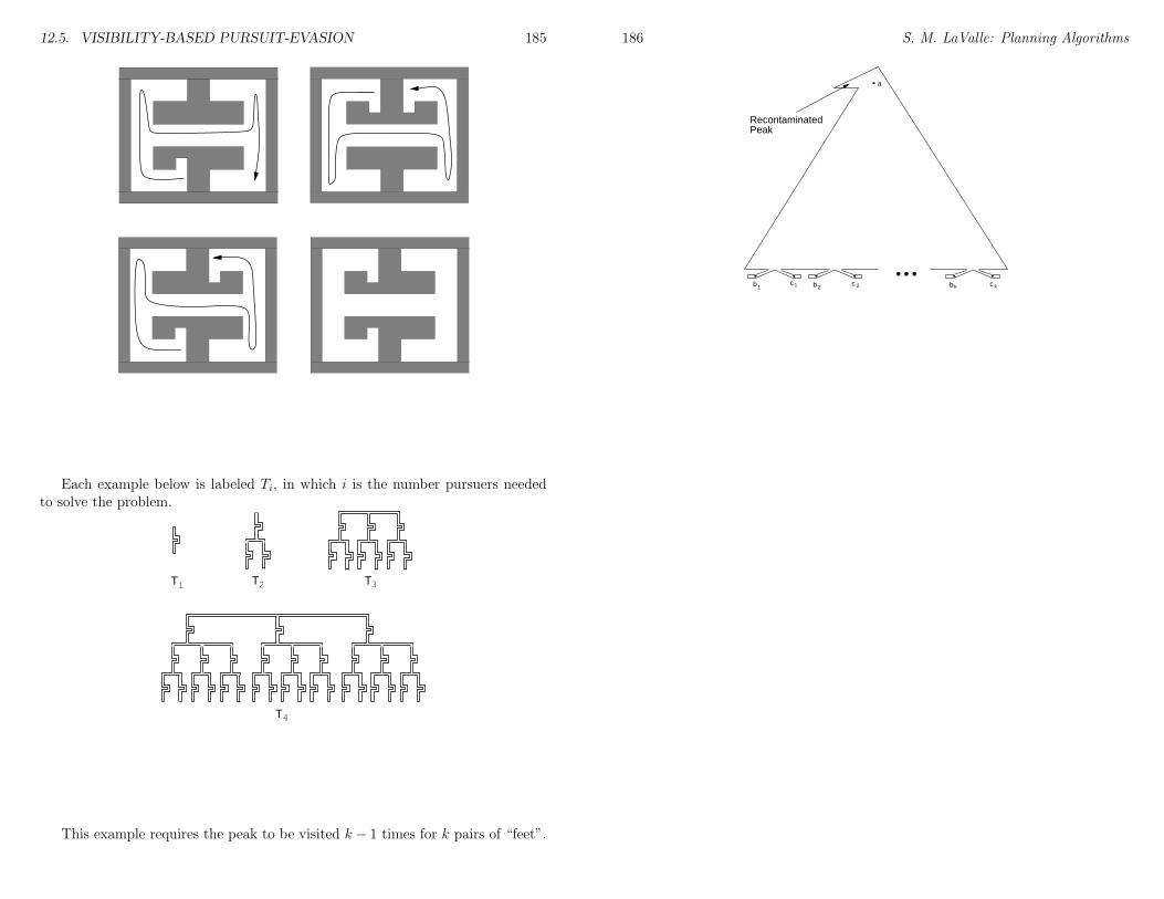
12.5. VISIBILITY-BASED PURSUIT-EVASION 185
Each example below is labeled Ti, in which i is the number pursuers neededto solve the problem.
T1 T2 T3
T4
This example requires the peak to be visited k − 1 times for k pairs of “feet”.
186 S. M. LaValle: Planning Algorithms
a
b k2b1b c1 c 2 c k
RecontaminatedPeak
Chapter 13
Game Theory
Parts of the current contents come from my class notes of CS497 Spring 2003,which were scribed by Shamsi Tamara Iqbal, Benjamin Tovar.
13.1 Overview
In a game, several decision makers strive to maximize their (expected) utility bychoosing particular courses of action, and each agent’s final utility payoffs dependon the courses of action chosen by all decision makers. The interactive situationspecified by the set of participants, the possible courses of action of each agent,and the set of all possible utility payoffs, is called a game; the decision makers’playing’ a game are called the players.Game theory is a set of analytical tools designed to help us understand the phe-nomena that we observe when decision-makers interact. The basic assumptionsthat underlie the theory are that decision-makers pursue well-defined exogenousobjectives (they are rational) and take into account their knowledge or expecta-tions of other decision-makers’ behavior (they reason strategically).Some of the areas of game theory that we are going to look into are:
• Multiple Decision Makers: There will be two or more decision makers,trying to make decisions at the same time.
• Single stage v Multiple stage
• Zero sum v Non zero sum games: Zero-sum games are games where theamount of “winnable goods” (or resources ) is fixed. Whatever is gained byone agent, is therefore lost by the other agent: the sum of gained (positive)and lost (negative) is zero.In Non-zero-sum games there is no universally accepted solution. That is,there is no single optimal strategy that is preferable to all others, nor is therea predictable outcome. Non-zero-sum games are also non-strictly competi-tive, as opposed to the completely competitive zero-sum games, because such
187
188 S. M. LaValle: Planning Algorithms
games generally have both competitive and cooperative elements. Playersengaged in a non-zero sum conflict have some complementary interests andsome interests that are completely opposed.
• Different Information States for each player: Each player has an infor-mation set corresponding to the decision nodes, which are used to representsituations where the player may not have complete knowledge about every-thing that happens in a game. Information sets are unique for each player.
• Deterministic v Randomized Strategies: When the player uses a deter-ministic or pure strategy, the player specifies a choice from his informationset. When a player uses a mixed strategy, he plays unpredictably in orderto keep the opponent guessing.
• Cooperative v Noncooperative: A player may be interpreted as anindividual or as a group of individuals making a decision. Once we definethe set of players, we may distinguish between two types of models: thosein which the sets of possible actions of individual players are primitives andthose in which the sets of possible joint actions of groups of players areprimitives. Models of the first type can be referred to as ”noncooperative”,while those of the second type can be referred to as ”cooperative”.
The following table summarizes some of the above mentioned features. Wemake the following two assumptions:
• Players know each other’s loss functionals.
• Players are rational decision makers.
# of players # of steps Nature ? Loss Functionals Example1 1 N 1 Classical Optimization1 1 Y 1 Decision Theory> 1 1 N > 1 Matrix Games> 1 1 Y > 1 Markov Games (probabilistic)1 >1 N 1 Optimal Control Theory1 >1 Y 1 Stochastic Control>1 >1 N/Y > 1 Dynamic Game Theory1 1 N > 1 Multi-objective Optimality>1 >1 N/Y 1 Team Theory
13.2 Single-Stage Two-Player Zero Sum Games
The most elementary type of two-player zero sum games are matrix games. Themain features of such games are:
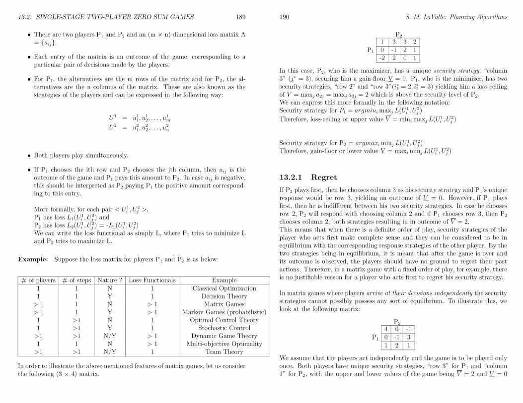
13.2. SINGLE-STAGE TWO-PLAYER ZERO SUM GAMES 189
• There are two players P1 and P2 and an (m × n) dimensional loss matrix A= aij.
• Each entry of the matrix is an outcome of the game, corresponding to aparticular pair of decisions made by the players.
• For P1, the alternatives are the m rows of the matrix and for P2, the al-ternatives are the n columns of the matrix. These are also known as thestrategies of the players and can be expressed in the following way:
U1 = u11, u12, . . . , u
1m
U2 = u21, u22, . . . , u
2n
• Both players play simultaneously.
• If P1 chooses the ith row and P2 chooses the jth column, then aij is theoutcome of the game and P1 pays this amount to P2. In case aij is negative,this should be interpreted as P2 paying P1 the positive amount correspond-ing to this entry.
More formally, for each pair < U 1i , U2j >,
P1 has loss L1(U1i , U
2j ) and
P2 has loss L2(U1i , U
2j ) = -L1(U
1i , U
2j )
We can write the loss functional as simply L, where P1 tries to minimize Land P2 tries to maximize L.
Example: Suppose the loss matrix for players P1 and P2 is as below:
# of players # of steps Nature ? Loss Functionals Example1 1 N 1 Classical Optimization1 1 Y 1 Decision Theory> 1 1 N > 1 Matrix Games> 1 1 Y > 1 Markov Games (probabilistic)1 >1 N 1 Optimal Control Theory1 >1 Y 1 Stochastic Control>1 >1 N/Y > 1 Dynamic Game Theory1 1 N > 1 Multi-objective Optimality>1 >1 N/Y 1 Team Theory
In order to illustrate the above mentioned features of matrix games, let us considerthe following (3 × 4) matrix.
190 S. M. LaValle: Planning Algorithms
P2
P1
1 3 3 20 -1 2 1-2 2 0 1
In this case, P2, who is the maximizer, has a unique security strategy, “column3” (j∗ = 3), securing him a gain-floor V = 0. P1, who is the minimizer, has twosecurity strategies, “row 2” and “row 3”(i∗1 = 2, i∗2 = 3) yielding him a loss ceilingof V = maxj a2j = maxj a3j = 2 which is above the security level of P2.We can express this more formally in the following notation:Security strategy for P1 = argminimaxj L(U
1i , U
2j )
Therefore, loss-ceiling or upper value V = minimaxj L(U1i , U
2j )
Security strategy for P2 = argmaximinj L(U1i , U
2j )
Therefore, gain-floor or lower value V = maximinj L(U1i , U
2j )
13.2.1 Regret
If P2 plays first, then he chooses column 3 as his security strategy and P1’s uniqueresponse would be row 3, yielding an outcome of V = 0. However, if P1 playsfirst, then he is indifferent between his two security strategies. In case he choosesrow 2, P2 will respond with choosing column 2 and if P1 chooses row 3, then P2chooses column 2, both strategies resulting in in outcome of V = 2.This means that when there is a definite order of play, security strategies of theplayer who acts first make complete sense and they can be considered to be inequilibrium with the corresponding response strategies of the other player. By thetwo strategies being in equilibrium, it is meant that after the game is over andits outcome is observed, the players should have no ground to regret their pastactions. Therefore, in a matrix game with a fixed order of play, for example, thereis no justifiable reason for a player who acts first to regret his security strategy.
In matrix games where players arrive at their decisions independently the securitystrategies cannot possibly possess any sort of equilibrium. To illustrate this, welook at the following matrix:
P2
P1
4 0 -10 -1 31 2 1
We assume that the players act independently and the game is to be played onlyonce. Both players have unique security strategies, “row 3” for P1 and “column1” for P2, with the upper and lower values of the game being V = 2 and V = 0
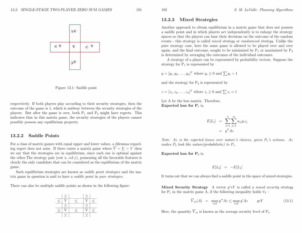
13.2. SINGLE-STAGE TWO-PLAYER ZERO SUM GAMES 191
Figure 13.1: Saddle point
respectively. If both players play according to their security strategies, then theoutcome of the game is 1, which is midway between the security strategies of theplayers. But after the game is over, both P1 and P2 might have regrets. Thisindicates that in this matrix game, the security strategies of the players cannotpossibly possess any equilibrium property.
13.2.2 Saddle Points
For a class of matrix games with equal upper and lower values, a dilemma regard-ing regret does not arise. If there exists a matrix game where V = V = V thenwe say that the strategies are in equilibrium, since each one is optimal againstthe other.The strategy pair (row x, col y), possessing all the favorable features isclearly the only candidate that can be considered as the equilibrium of the matrixgame.
Such equilibrium strategies are known as saddle point strategies and the ma-trix game in question is said to have a saddle point in pure strategies.
There can also be multiple saddle points as shown in the following figure:
≥ ≥≤ V ≤ V ≤≥ ≥
≤ V ≤ V ≤≥ ≥
192 S. M. LaValle: Planning Algorithms
13.2.3 Mixed Strategies
Another approach to obtain equilibrium in a matrix game that does not possessa saddle point and in which players act independently is to enlarge the strategyspaces so that the players can base their decisions on the outcome of the randomevents - this strategy is called mixed strategy or randomized strategy. Unlike thepure strategy case, here the same game is allowed to be played over and overagain, and the final outcome, sought to be minimized by P1 or maximized by P2is determined by averaging the outcomes of the individual outcomes.
A strategy of a player can be represented by probability vectors. Suppose thestrategy for P1 is represented by
y = [y1, y2, . . . , yn]T where yi ≥ 0 and
∑
yi = 1
and the strategy for P2 is represented by
z = [z1, z2, . . . , zn]T where zi ≥ 0 and
∑
zi = 1
Let A be the loss matrix. Therefore,Expected loss for P1 is,
E[L1] =n∑
i=1
m∑
j=1
aijyizj
= yTAz
Note: Az is the expected losses over nature’s choices, given P1’s actions. Azmakes P2 look like nature(probabilistic) to P1.
Expected loss for P2 is,
E[L2] = −E[L1]
It turns out that we can always find a saddle point in the space of mixed strategies.
Mixed Security Strategy A vector y∗εY is called a mixed security strategyfor P1 in the matrix game A, if the following inequality holds ∀Y :
V m(A) = maxzεZ
y∗′Az ≤ maxzεZ
y′Az yεY (13.1)
Here, the quantity V m is known as the average security level of P1.
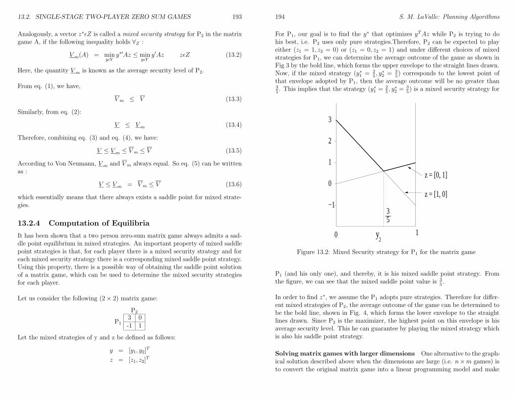
13.2. SINGLE-STAGE TWO-PLAYER ZERO SUM GAMES 193
Analogously, a vector z∗εZ is called a mixed security strategy for P2 in the matrixgame A, if the following inequality holds ∀Z :
V m(A) = minyεY
y∗′Az ≤ minyεY
y′Az zεZ (13.2)
Here, the quantity V m is known as the average security level of P2.
From eq. (1), we have,
V m ≤ V (13.3)
Similarly, from eq. (2):
V ≤ V m (13.4)
Therefore, combining eq. (3) and eq. (4), we have:
V ≤ V m ≤ V m ≤ V (13.5)
According to Von Neumann, V m and V m always equal. So eq. (5) can be writtenas :
V ≤ V m = V m ≤ V (13.6)
which essentially means that there always exists a saddle point for mixed strate-gies.
13.2.4 Computation of Equilibria
It has been shown that a two person zero-sum matrix game always admits a sad-dle point equilibrium in mixed strategies. An important property of mixed saddlepoint strategies is that, for each player there is a mixed security strategy and foreach mixed security strategy there is a corresponding mixed saddle point strategy.Using this property, there is a possible way of obtaining the saddle point solutionof a matrix game, which can be used to determine the mixed security strategiesfor each player.
Let us consider the following (2× 2) matrix game:
P2
P13 0-1 1
Let the mixed strategies of y and z be defined as follows:
y = [y1, y2]T
z = [z1, z2]T
194 S. M. LaValle: Planning Algorithms
For P1, our goal is to find the y∗ that optimizes yTAz while P2 is trying to dohis best, i.e. P2 uses only pure strategies.Therefore, P2 can be expected to playeither (z1 = 1, z2 = 0) or (z1 = 0, z2 = 1) and under different choices of mixedstrategies for P1, we can determine the average outcome of the game as shown inFig 3 by the bold line, which forms the upper envelope to the straight lines drawn.Now, if the mixed strategy (y∗1 = 2
5, y∗2 = 3
5) corresponds to the lowest point of
that envelope adopted by P1, then the average outcome will be no greater than35. This implies that the strategy (y∗1 =
25, y∗2 =
35) is a mixed security strategy for
0 1y2
−1
0
1
2
3
z = [0, 1]
z = [1, 0]
35
Figure 13.2: Mixed Security strategy for P1 for the matrix game
P1 (and his only one), and thereby, it is his mixed saddle point strategy. Fromthe figure, we can see that the mixed saddle point value is 3
5.
In order to find z∗, we assume the P1 adopts pure strategies. Therefore for differ-ent mixed strategies of P2, the average outcome of the game can be determined tobe the bold line, shown in Fig. 4, which forms the lower envelope to the straightlines drawn. Since P2 is the maximizer, the highest point on this envelope is hisaverage security level. This he can guarantee by playing the mixed strategy whichis also his saddle point strategy.
Solving matrix games with larger dimensions One alternative to the graph-ical solution described above when the dimensions are large (i.e. n×m games) isto convert the original matrix game into a linear programming model and make
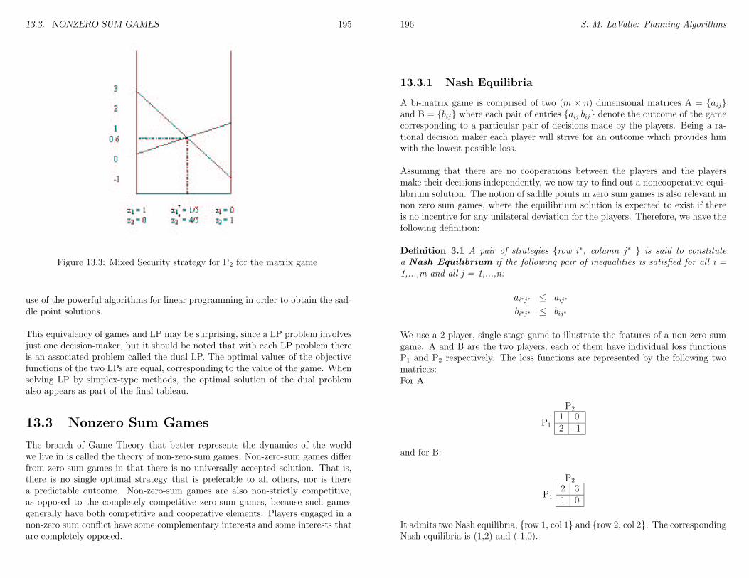
13.3. NONZERO SUM GAMES 195
Figure 13.3: Mixed Security strategy for P2 for the matrix game
use of the powerful algorithms for linear programming in order to obtain the sad-dle point solutions.
This equivalency of games and LP may be surprising, since a LP problem involvesjust one decision-maker, but it should be noted that with each LP problem thereis an associated problem called the dual LP. The optimal values of the objectivefunctions of the two LPs are equal, corresponding to the value of the game. Whensolving LP by simplex-type methods, the optimal solution of the dual problemalso appears as part of the final tableau.
13.3 Nonzero Sum Games
The branch of Game Theory that better represents the dynamics of the worldwe live in is called the theory of non-zero-sum games. Non-zero-sum games differfrom zero-sum games in that there is no universally accepted solution. That is,there is no single optimal strategy that is preferable to all others, nor is therea predictable outcome. Non-zero-sum games are also non-strictly competitive,as opposed to the completely competitive zero-sum games, because such gamesgenerally have both competitive and cooperative elements. Players engaged in anon-zero sum conflict have some complementary interests and some interests thatare completely opposed.
196 S. M. LaValle: Planning Algorithms
13.3.1 Nash Equilibria
A bi-matrix game is comprised of two (m × n) dimensional matrices A = aijand B = bij where each pair of entries aij bij denote the outcome of the gamecorresponding to a particular pair of decisions made by the players. Being a ra-tional decision maker each player will strive for an outcome which provides himwith the lowest possible loss.
Assuming that there are no cooperations between the players and the playersmake their decisions independently, we now try to find out a noncooperative equi-librium solution. The notion of saddle points in zero sum games is also relevant innon zero sum games, where the equilibrium solution is expected to exist if thereis no incentive for any unilateral deviation for the players. Therefore, we have thefollowing definition:
Definition 3.1 A pair of strategies row i∗, column j∗ is said to constitutea Nash Equilibrium if the following pair of inequalities is satisfied for all i =1,...,m and all j = 1,...,n:
ai∗j∗ ≤ aij∗
bi∗j∗ ≤ bij∗
We use a 2 player, single stage game to illustrate the features of a non zero sumgame. A and B are the two players, each of them have individual loss functionsP1 and P2 respectively. The loss functions are represented by the following twomatrices:For A:
P2
P11 02 -1
and for B:
P2
P12 31 0
It admits two Nash equilibria, row 1, col 1 and row 2, col 2. The correspondingNash equilibria is (1,2) and (-1,0).
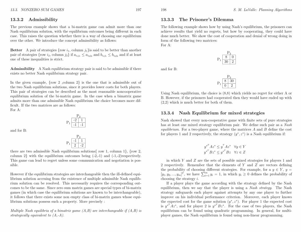
13.3. NONZERO SUM GAMES 197
13.3.2 Admissibility
The previous example shows that a bi-matrix game can admit more than oneNash equilibrium solution, with the equilibrium outcomes being different in eachcase. This raises the question whether there is a way of choosing one equilibriumover the other. We introduce the concept admissibility as follows:
Better A pair of strategies row i1, column j1is said to be better than anotherpair of strategies row i2, column j2 if ai1j1 ≤ ai2j2 and bi1j1 ≤ bi2j2 and if at leastone of these inequalities is strict.
Admissibility A Nash equilibrium strategy pair is said to be admissible if thereexists no better Nash equilibrium strategy pair.
In the given example, row 2 ,column 2 is the one that is admissible out ofthe two Nash equilibrium solutions, since it provides lower costs for both players.This pair of strategies can be described as the most reasonable noncooperativeequilibrium solution of the bi-matrix game. In the case when a bimatrix gameadmits more than one admissible Nash equilibrium the choice becomes more dif-ficult. If the two matrices are as follows:For A:
P2
P1-2 1-1 -1
and for B:
P2
P1-1 12 -2
there are two admissible Nash equilibrium solutions row 1, column 1, row 2,column 2 with the equilibrium outcomes being (-2,-1) and (-1,-2)respectively.This game can lead to regret unless some communication and negotiation is pos-sible.
However if the equilibrium strategies are interchangeable then the ill-defined equi-librium solution accruing from the existence of multiple admissible Nash equilib-rium solution can be resolved. This necessarily requires the corresponding out-comes to be the same. Since zero sum matrix games are special types of bi-matrixgames (in which case the equilibrium solutions are known to be interchangeable),it follows that there exists some non empty class of bi-matrix games whose equi-librium solutions possess such a property. More precisely :
Multiple Nash equilibria of a bimatrix game (A,B) are interchangeable if (A,B) isstrategically equivalent to (A,-A).
198 S. M. LaValle: Planning Algorithms
13.3.3 The Prisoner’s Dilemma
The following example shows how by using Nash’s equilibrium, the prisoners canachieve results that yield no regrets, but how by cooperating, they could havedone much better. We show the cost of cooperation and denial of wrong doing inform of the following two matrices:For A:
P2
P18 030 2
and for B:
P2
P18 300 2
Using Nash equilibrium, the choice is (8,8) which yields no regret for either A orB. However, if the prisoners had cooperated then they would have ended up with(2,2) which is much better for both of them.
13.3.4 Nash Equilibrium for mixed strategies
Nash showed that every non-cooperative game with finite sets of pure strategieshas at least one mixed strategy equilibrium pair. We define such pair as a Nashequilibrium. For a two-player game, where the matrices A and B define the costfor players 1 and 2 respectively, the strategy (y∗, z∗) is a Nash equilibrium if:
y∗T
Az∗ ≤ yT
Az∗ ∀y ∈ Y
y∗T
Bz∗ ≤ y∗T
Bz ∀z ∈ Z
in which Y and Z are the sets of possible mixed strategies for players 1 and2 respectively. Remember that the elements of Y and Z are vectors definingthe probability of choosing different strategies. For example, for a y ∈ Y , y =[y1, y2, ..., ym]
T , we have∑m
i=1 yi = 1, in which yi ≥ 0 defines the probability ofchoosing the strategy i.
If a player plays the game according with the strategy defined by the Nashequilibrium, then we say that the player is using a Nash strategy. The Nashstrategy safeguards each player against attempts by any one player to furtherimprove on his individual performance criterion. Moreover, each player knowsthe expected cost for the game solution (y∗, z∗). For player 1 the expected costis y∗
T
Az∗, and for player 2 is y∗T
Bz∗. For the case of two players, the Nashequilibrium can be found using quadratic programming. In general, for multi-player games, the Nash equilibrium is found using non-linear programming.
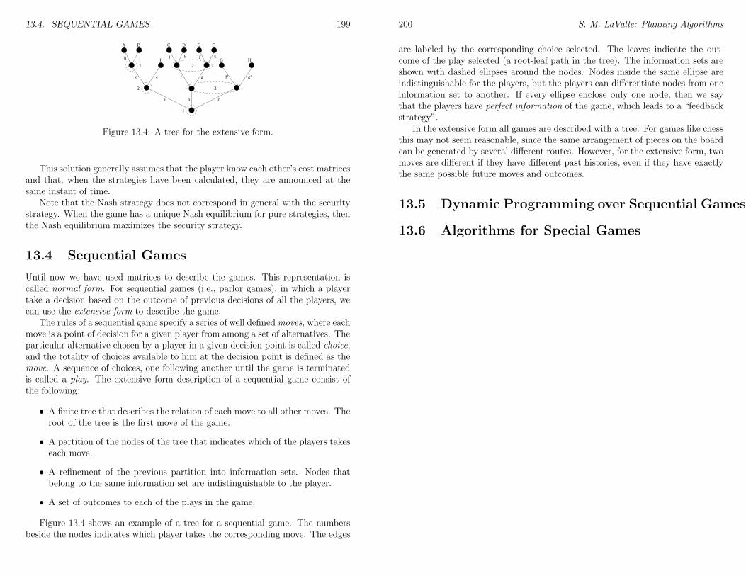
13.4. SEQUENTIAL GAMES 199
A B C D E F
G H
2 2
1
a
d
b c
e f g f’ g’
1 2Ih i j k j’ k’
Figure 13.4: A tree for the extensive form.
This solution generally assumes that the player know each other’s cost matricesand that, when the strategies have been calculated, they are announced at thesame instant of time.
Note that the Nash strategy does not correspond in general with the securitystrategy. When the game has a unique Nash equilibrium for pure strategies, thenthe Nash equilibrium maximizes the security strategy.
13.4 Sequential Games
Until now we have used matrices to describe the games. This representation iscalled normal form. For sequential games (i.e., parlor games), in which a playertake a decision based on the outcome of previous decisions of all the players, wecan use the extensive form to describe the game.
The rules of a sequential game specify a series of well definedmoves, where eachmove is a point of decision for a given player from among a set of alternatives. Theparticular alternative chosen by a player in a given decision point is called choice,and the totality of choices available to him at the decision point is defined as themove. A sequence of choices, one following another until the game is terminatedis called a play. The extensive form description of a sequential game consist ofthe following:
• A finite tree that describes the relation of each move to all other moves. Theroot of the tree is the first move of the game.
• A partition of the nodes of the tree that indicates which of the players takeseach move.
• A refinement of the previous partition into information sets. Nodes thatbelong to the same information set are indistinguishable to the player.
• A set of outcomes to each of the plays in the game.
Figure 13.4 shows an example of a tree for a sequential game. The numbersbeside the nodes indicates which player takes the corresponding move. The edges
200 S. M. LaValle: Planning Algorithms
are labeled by the corresponding choice selected. The leaves indicate the out-come of the play selected (a root-leaf path in the tree). The information sets areshown with dashed ellipses around the nodes. Nodes inside the same ellipse areindistinguishable for the players, but the players can differentiate nodes from oneinformation set to another. If every ellipse enclose only one node, then we saythat the players have perfect information of the game, which leads to a “feedbackstrategy”.
In the extensive form all games are described with a tree. For games like chessthis may not seem reasonable, since the same arrangement of pieces on the boardcan be generated by several different routes. However, for the extensive form, twomoves are different if they have different past histories, even if they have exactlythe same possible future moves and outcomes.
13.5 Dynamic Programming over Sequential Games
13.6 Algorithms for Special Games

Part IV
Continuous-Time Planning
201
Chapter 14
Differential Models
14.1 Motivation
In the models and methods studied so far, it has been assumed that a path caneasily between obtained between any two configurations if there are no collisions.For example, the randomized roadmap approach assumed that two nearby config-urations could be connected by a “straight line” in the configuration space. Theconstraints on the path are global in the sense that the restrictions are on the setof allowable configurations.
For the next few chapters, local constraints will be introduced. One of thesimplest examples is a car-like robot. Imagine a trying to automate the motionsof a typical automobile that has a limited steering angle. Consider the difficultyof moving a car sideways, while the rear wheels are always pointing forward. Itwould certainly make parallel parking easy if it was possible to simply turn all fourwheels toward the curb. The orientation limits of the wheels, however, prohibitthis motion. At any configuration, there are constraints on the velocity of the car.In other words, it is permitted only to move along certain directions to ensurethat the wheels roll.
Although the motion is constrained in this way, most of us are experiencedwith making very complex driving maneuvers to parallel park a car. We wouldgenerally like to have algorithms that can maneuver a car-like robot and a varietyof other nonholonomic systems while avoiding collisions. This will be the subjectof nonholonomic planning.
14.2 Representing Differential Constraints
Implicit velocity constraints
Suppose that X represents an n-dimensional manifold that serves as the statespace. Let x ∈ X represent a state. It will often be the case that X = C;however, a state could include additional information. It will be assumed that
203
204 S. M. LaValle: Planning Algorithms
X is differentiable at every point. To enable this formally, one must generallycharacterize the X by using multiple coordinate systems, each of which covers asubset of X [68]. We avoid these technicalities in the concepts that follow becausethey are not critical for understanding the material.
Consider a moving point, x ∈ X. Let x denote the velocity vector,
x =
[
dx1dt
dx2dt· · ·
dxndt
]
.
Let xi denote dxi/dt. At most places in this chapter where differentiation occurs,it can be imagined that X = Rn. Recall that any manifold of interest can beconsidered as a rectangular region in Rn with identification of some boundaries.Multiple coordinate systems are generally used to ensure differentiability proper-ties across these identifications. Imagining that X = Rn will be reasonable exceptat the identification points. For example, if X = R2 × S1, then special care mustbe given if θ = 0. Motions in the negative θ direction will actually cause θ toincrease because of the identification.
Suppose that a classical path planning problem has been defined, resulting inX = C, and that a collision-free path, τ has been computed. Recall that τ wasdefined as τ : [0, 1]→ Cfree. Although it did not matter before, suppose now that[0, 1] represents an interval of time. At time t = 0 the state is x = qinit, and attime t = 1, the state is x = qgoal. The velocity vector is x = dτ/dt.
Up to now, there have been no constraints placed on x, which means thatany velocity vector is possible. Suppose that the velocity magnitude is bounded,‖x‖ ≤ 1. Does this make the classical path planning problem more difficult?It does not because any path τ : [0, 1] → Cfree can be converted into anotherpath, τ ′ which satisfies the bound by lengthening the time interval. For example,suppose s denotes the maximum speed (velocity magnitude) along τ . A new path,τ ′ : [0, s] → Cfree, can be defined by τ ′(t) = τ(t/s). For τ ′, the velocity will bebounded by one for all time.
Suppose now that a constraint such as x1 ≤ 0 is added. This implies thatfor any path, the variable x1 must be monotonically nonincreasing. For example,consider path planning for a rigid robot in the plane, yielding X = R2 × S1.Suppose that constraint θ ≤ 0 is imposed. This implies that the robot is onlycapable of clockwise rotations!
In general, we allow constraints of the implicit form hi(x, x) = 0 to be imposed.Thus, the constrained velocity can depend on the state, x. Inequality constraintsof the form hi(x, x) < 0 and hi(x, x) ≤ 0 are also permitted. Each constraintrestricts the set of allowable velocities at any state x ∈ X.
The state transition equation
Although the implicit constraints are general, it is often difficult to work directlywith them. A similar difficulty exists with plotting solutions to an implicit function
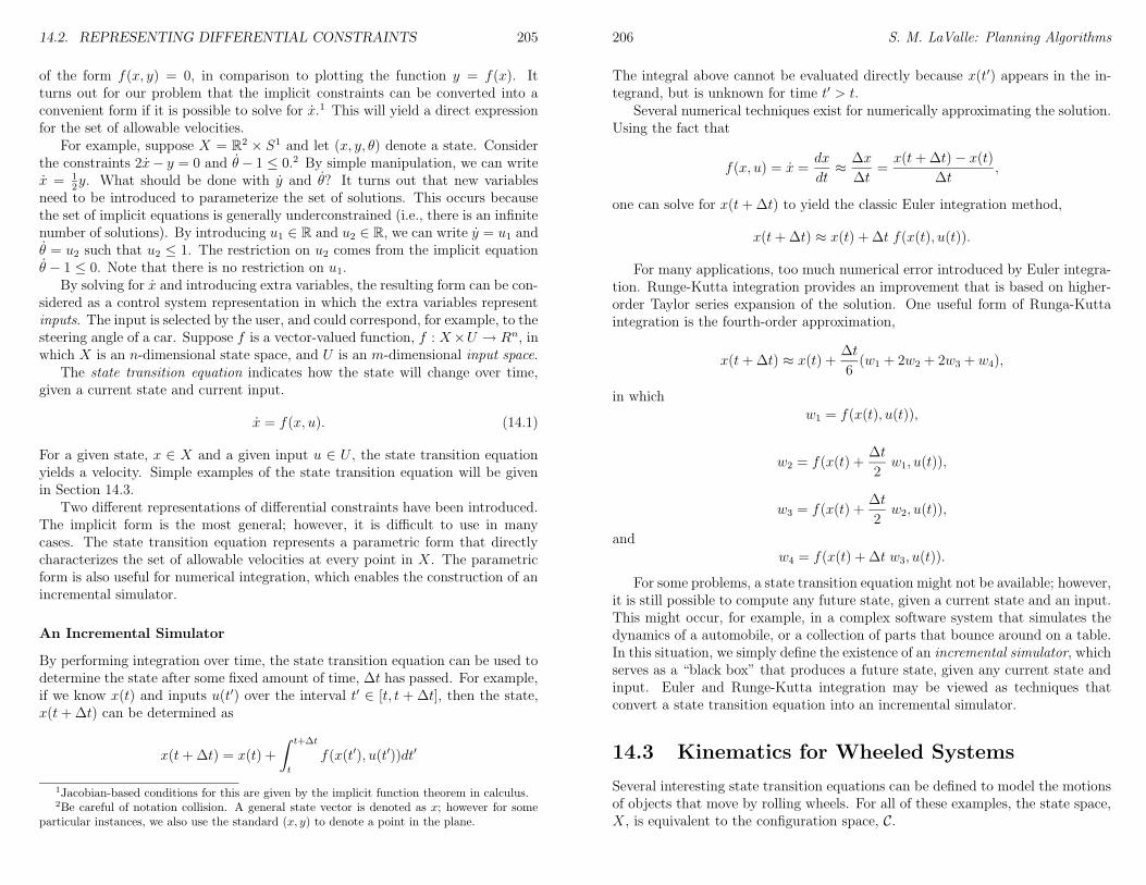
14.2. REPRESENTING DIFFERENTIAL CONSTRAINTS 205
of the form f(x, y) = 0, in comparison to plotting the function y = f(x). Itturns out for our problem that the implicit constraints can be converted into aconvenient form if it is possible to solve for x.1 This will yield a direct expressionfor the set of allowable velocities.
For example, suppose X = R2 × S1 and let (x, y, θ) denote a state. Considerthe constraints 2x− y = 0 and θ− 1 ≤ 0.2 By simple manipulation, we can writex = 1
2y. What should be done with y and θ? It turns out that new variables
need to be introduced to parameterize the set of solutions. This occurs becausethe set of implicit equations is generally underconstrained (i.e., there is an infinitenumber of solutions). By introducing u1 ∈ R and u2 ∈ R, we can write y = u1 andθ = u2 such that u2 ≤ 1. The restriction on u2 comes from the implicit equationθ − 1 ≤ 0. Note that there is no restriction on u1.
By solving for x and introducing extra variables, the resulting form can be con-sidered as a control system representation in which the extra variables representinputs. The input is selected by the user, and could correspond, for example, to thesteering angle of a car. Suppose f is a vector-valued function, f : X×U → Rn, inwhich X is an n-dimensional state space, and U is an m-dimensional input space.
The state transition equation indicates how the state will change over time,given a current state and current input.
x = f(x, u). (14.1)
For a given state, x ∈ X and a given input u ∈ U , the state transition equationyields a velocity. Simple examples of the state transition equation will be givenin Section 14.3.
Two different representations of differential constraints have been introduced.The implicit form is the most general; however, it is difficult to use in manycases. The state transition equation represents a parametric form that directlycharacterizes the set of allowable velocities at every point in X. The parametricform is also useful for numerical integration, which enables the construction of anincremental simulator.
An Incremental Simulator
By performing integration over time, the state transition equation can be used todetermine the state after some fixed amount of time, ∆t has passed. For example,if we know x(t) and inputs u(t′) over the interval t′ ∈ [t, t + ∆t], then the state,x(t+∆t) can be determined as
x(t+∆t) = x(t) +
∫ t+∆t
t
f(x(t′), u(t′))dt′
1Jacobian-based conditions for this are given by the implicit function theorem in calculus.2Be careful of notation collision. A general state vector is denoted as x; however for some
particular instances, we also use the standard (x, y) to denote a point in the plane.
206 S. M. LaValle: Planning Algorithms
The integral above cannot be evaluated directly because x(t′) appears in the in-tegrand, but is unknown for time t′ > t.
Several numerical techniques exist for numerically approximating the solution.Using the fact that
f(x, u) = x =dx
dt≈
∆x
∆t=x(t+∆t)− x(t)
∆t,
one can solve for x(t+∆t) to yield the classic Euler integration method,
x(t+∆t) ≈ x(t) + ∆t f(x(t), u(t)).
For many applications, too much numerical error introduced by Euler integra-tion. Runge-Kutta integration provides an improvement that is based on higher-order Taylor series expansion of the solution. One useful form of Runga-Kuttaintegration is the fourth-order approximation,
x(t+∆t) ≈ x(t) +∆t
6(w1 + 2w2 + 2w3 + w4),
in whichw1 = f(x(t), u(t)),
w2 = f(x(t) +∆t
2w1, u(t)),
w3 = f(x(t) +∆t
2w2, u(t)),
andw4 = f(x(t) + ∆t w3, u(t)).
For some problems, a state transition equation might not be available; however,it is still possible to compute any future state, given a current state and an input.This might occur, for example, in a complex software system that simulates thedynamics of a automobile, or a collection of parts that bounce around on a table.In this situation, we simply define the existence of an incremental simulator, whichserves as a “black box” that produces a future state, given any current state andinput. Euler and Runge-Kutta integration may be viewed as techniques thatconvert a state transition equation into an incremental simulator.
14.3 Kinematics for Wheeled Systems
Several interesting state transition equations can be defined to model the motionsof objects that move by rolling wheels. For all of these examples, the state space,X, is equivalent to the configuration space, C.
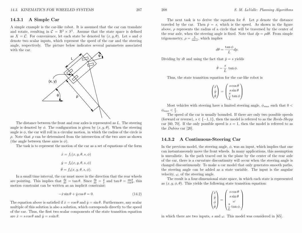
14.3. KINEMATICS FOR WHEELED SYSTEMS 207
14.3.1 A Simple Car
A simple example is the car-like robot. It is assumed that the car can translateand rotate, resulting in C = R2 × S1. Assume that the state space is definedas X = C. For convenience, let each state be denoted by (x, y, θ). Let s and φdenote two scalar inputs, which represent the speed of the car and the steeringangle, respectively. The picture below indicates several parameters associatedwith the car.
L
ρ
φ
θ
(x, y)
The distance between the front and rear axles is represented as L. The steeringangle is denoted by φ. The configuration is given by (x, y, θ). When the steeringangle is φ, the car will roll in a circular motion, in which the radius of the circle isρ. Note that ρ can be determined from the intersection of the two axes as shown(the angle between these axes is φ).
The task is to represent the motion of the car as a set of equations of the form
x = f1(x, y, θ, s, φ)
y = f2(x, y, θ, s, φ)
θ = f3(x, y, θ, s, φ).
In a small time interval, the car must move in the direction that the rear wheelsare pointing. This implies that dy
dx= tan θ. Since dy
dx= y
xand tan θ = sin θ
cos θ, this
motion constraint can be written as an implicit constraint:
−x sin θ + y cos θ = 0. (14.2)
The equation above is satisfied if x = cos θ and y = sin θ. Furthermore, any scalarmultiple of this solution is also a solution, which corresponds directly to the speedof the car. Thus, the first two scalar components of the state transition equationare x = s cos θ and y = s sin θ.
208 S. M. LaValle: Planning Algorithms
The next task is to derive the equation for θ. Let p denote the distancetraveled by the car. Then p = s, which is the speed. As shown in the figureabove, ρ represents the radius of a circle that will be traversed by the center ofthe rear axle, when the steering angle is fixed. Note that dp = ρdθ. From simpletrigonometry, ρ = L
tanφ, which implies
dθ =tanφ
Ldp.
Dividing by dt and using the fact that p = s yields
θ =s
Ltanφ.
Thus, the state transition equation for the car-like robot is
xy
θ
=
s cos θs sin θs
Ltanφ
Most vehicles with steering have a limited steering angle, φmax such that 0 <φmax <
π2.
The speed of the car is usually bounded. If there are only two possible speeds(forward or reverse), s ∈ −1, 1, then the model is referred to as the Reeds-Sheppcar [60, 70]. If the only possible speed is s = 1, then the model is referred to asthe Dubins car [20].
14.3.2 A Continuous-Steering Car
In the previous model, the steering angle, φ, was an input, which implies that onecan instantaneously move the front wheels. In many applications, this assumptionis unrealistic. In the path traced out in the plane by the center of the rear axleof the car, there is a curvature discontinuity will occur when the steering angle ischanged discontinuously. To make a car model that only generates smooth paths,the steering angle can be added as a state variable. The input is the angularvelocity, ω, of the steering angle.
The result is a four-dimensional state space, in which each state is representedas (x, y, φ, θ). This yields the following state transition equation:
xy
φ
θ
=
s cos θs sin θω
s
Ltanφ,
in which there are two inputs, s and ω. This model was considered in [65].
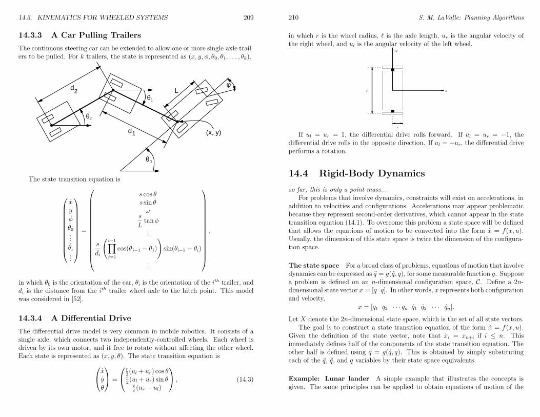
14.3. KINEMATICS FOR WHEELED SYSTEMS 209
14.3.3 A Car Pulling Trailers
The continuous-steering car can be extended to allow one or more single-axle trail-ers to be pulled. For k trailers, the state is represented as (x, y, φ, θ0, θ1, . . . , θk).
Lφ
(x, y)
θ0
1θ
2θ
d1
d2
The state transition equation is
xy
φ
θ0...
θi...
=
s cos θs sin θω
s
Ltanφ
...
s
di
(
i−1∏
j=1
cos(θj−1 − θj)
)
sin(θi−1 − θi)
...
,
in which θ0 is the orientation of the car, θi is the orientation of the ith trailer, anddi is the distance from the ith trailer wheel axle to the hitch point. This modelwas considered in [52].
14.3.4 A Differential Drive
The differential drive model is very common in mobile robotics. It consists of asingle axle, which connects two independently-controlled wheels. Each wheel isdriven by its own motor, and it free to rotate without affecting the other wheel.Each state is represented as (x, y, θ). The state transition equation is
xy
θ
=
r2(ul + ur) cos θr2(ul + ur) sin θr`(ur − ul)
, (14.3)
210 S. M. LaValle: Planning Algorithms
in which r is the wheel radius, ` is the axle length, ur is the angular velocity ofthe right wheel, and ul is the angular velocity of the left wheel.
x
y
`
r
If ul = ur = 1, the differential drive rolls forward. If ul = ur = −1, thedifferential drive rolls in the opposite direction. If ul = −ur, the differential driveperforms a rotation.
14.4 Rigid-Body Dynamics
so far, this is only a point mass...For problems that involve dynamics, constraints will exist on accelerations, in
addition to velocities and configurations. Accelerations may appear problematicbecause they represent second-order derivatives, which cannot appear in the statetransition equation (14.1). To overcome this problem a state space will be definedthat allows the equations of motion to be converted into the form x = f(x, u).Usually, the dimension of this state space is twice the dimension of the configura-tion space.
The state space For a broad class of problems, equations of motion that involvedynamics can be expressed as q = g(q, q), for some measurable function g. Supposea problem is defined on an n-dimensional configuration space, C. Define a 2n-dimensional state vector x = [q q]. In other words, x represents both configurationand velocity,
x = [q1 q2 · · · qn q1 q2 · · · qn].
Let X denote the 2n-dimensional state space, which is the set of all state vectors.The goal is to construct a state transition equation of the form x = f(x, u).
Given the definition of the state vector, note that xi = xn+i if i ≤ n. Thisimmediately defines half of the components of the state transition equation. Theother half is defined using q = g(q, q). This is obtained by simply substitutingeach of the q, q, and q variables by their state space equivalents.
Example: Lunar lander A simple example that illustrates the concepts isgiven. The same principles can be applied to obtain equations of motion of the
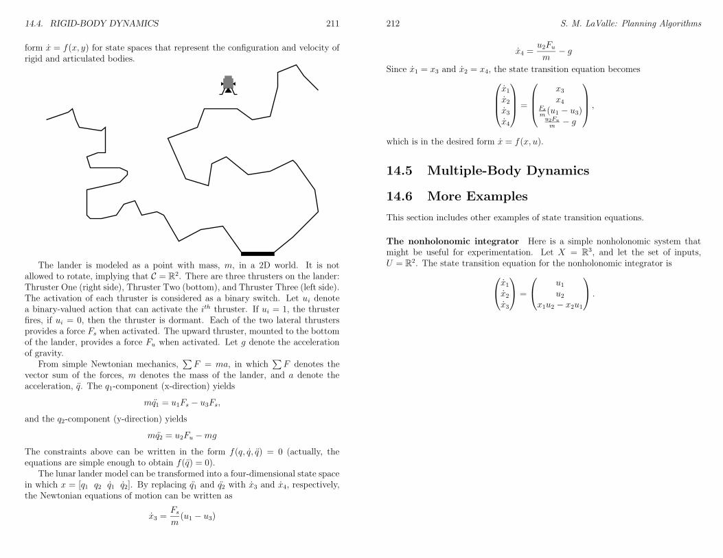
14.4. RIGID-BODY DYNAMICS 211
form x = f(x, y) for state spaces that represent the configuration and velocity ofrigid and articulated bodies.
The lander is modeled as a point with mass, m, in a 2D world. It is notallowed to rotate, implying that C = R2. There are three thrusters on the lander:Thruster One (right side), Thruster Two (bottom), and Thruster Three (left side).The activation of each thruster is considered as a binary switch. Let ui denotea binary-valued action that can activate the ith thruster. If ui = 1, the thrusterfires, if ui = 0, then the thruster is dormant. Each of the two lateral thrustersprovides a force Fs when activated. The upward thruster, mounted to the bottomof the lander, provides a force Fu when activated. Let g denote the accelerationof gravity.
From simple Newtonian mechanics,∑
F = ma, in which∑
F denotes thevector sum of the forces, m denotes the mass of the lander, and a denote theacceleration, q. The q1-component (x-direction) yields
mq1 = u1Fs − u3Fs,
and the q2-component (y-direction) yields
mq2 = u2Fu −mg
The constraints above can be written in the form f(q, q, q) = 0 (actually, theequations are simple enough to obtain f(q) = 0).
The lunar lander model can be transformed into a four-dimensional state spacein which x = [q1 q2 q1 q2]. By replacing q1 and q2 with x3 and x4, respectively,the Newtonian equations of motion can be written as
x3 =Fsm
(u1 − u3)
212 S. M. LaValle: Planning Algorithms
x4 =u2Fum− g
Since x1 = x3 and x2 = x4, the state transition equation becomes
x1x2x3x4
=
x3x4
Fs
m(u1 − u3)u2Fu
m− g
,
which is in the desired form x = f(x, u).
14.5 Multiple-Body Dynamics
14.6 More Examples
This section includes other examples of state transition equations.
The nonholonomic integrator Here is a simple nonholonomic system thatmight be useful for experimentation. Let X = R3, and let the set of inputs,U = R2. The state transition equation for the nonholonomic integrator is
x1x2x3
=
u1u2
x1u2 − x2u1
.
Chapter 15
Nonholonomic System Theory
This chapter deals with the analysis of problems that involve differential con-straints. One fundamental result is the Frobenius theorem, which allows one todetermine whether the state transition equation represents a system is actuallynonholonomic. In some cases, it may be possible to integrate the state transitionequation, resulting in a problem that can be described without differential models.Another result is Chow’s theorem, which indicates whether a system is control-lable. Intuitively, this means that the differential constraints can be completelyovercome by generating arbitrarily short maneuvers. The car-like robot enjoys thecontrollability property, which enables it to move itself sideways by performingparallel parking maneuvers.
15.1 Vector Fields and Distributions
A special form of the state transition equation Most of the concepts in thischapter are developed under the assumption that the state transition equation,x = f(x, u) has the following form:
x = α1(x)u1 + α2(x)u2 + · · ·+ αm(x)um, (15.1)
in which each αi(x) is a vector-valued function of x, and m is the dimension ofU (or the number of inputs). The αi functions can also be arranged in an n×mmatrix,
A(x) = [α1(x) α2(x) · · · αm(x)].
It will usually be assumed that m < n.In this case, the state transition equation can be expressed as
x = A(x)u.
For the rest of the chapter, it will be assumed that the matrix A(x) is nonsin-gular. In other words, the rows of A(x) are linearly independent for all x. Todetermine whether A(x) is nonsingular, one must find at least one m×m cofactor(or submatrix) of A(x) which has a nonzero determinant.
213
214 S. M. LaValle: Planning Algorithms
Vector fields A vector field, ~V , on a manifold X, is a function that associateswith each x ∈ X, a vector, ~V (x). The velocity field is a special vector field
that will be used extensively. Each vector ~V (x) in a velocity field represents theinfinitesimal change in state with respect to time,
x =
[
dx1dt
dx2dt· · ·
dxndt
]
, (15.2)
evaluated at the point x ∈ X.Note that for a fixed u, any state transition equation, x = f(x, u) defines a
vector field because x is expressed as a function of x.
Distributions Each input u ∈ U can be used to define a vector field. It will beconvenient to define the set of all vector fields that can be generated using inputs.Assume that a state transition equation of the form in (15.1) is given for a statespace X, and an input space U = Rm. The set of all vector fields that can begenerated using inputs u ∈ U is called the distribution, and is denoted by 4(X)or 4.
The distribution can be considered as a vector space. Note that each αi canbe interpreted as a vector field. Any vector field in 4 can be expressed as alinear combination of the αi functions, which serve as a basis of the vector space.Consider the effect of inputs of the form
[1 0 0 · · · 0 0 0 · · · 0]
[0 1 0 · · · 0 0 0 · · · 0]
...
[0 0 0 · · · 0 1 0 · · · 0]
...
[0 0 0 · · · 0 0 0 · · · 1].
If ui = 1, and uj = 0 for j 6= i, then the state transition equation yields x = αi(x).Thus, each input in this form can be used to generate a basis vector field. Thedimension of the distribution the number of vector fields in its basis (in otherwords, the maximum number of linearly-independent vector fields that can begenerated).
In terms of basis vector fields, a distribution is expressed as
4 = spanα1(x), α2(x), . . . , αn(x)
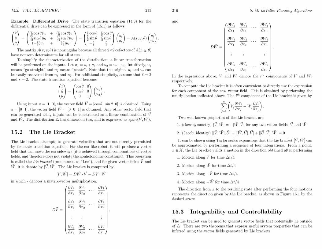
15.2. THE LIE BRACKET 215
Example: Differential Drive The state transition equation (14.3) for thedifferential drive can be expressed in the form of (15.1) as follows:
xy
θ
=
( r2cos θ)ul + ( r
2cos θ)ur
( r2sin θ)ul + ( r
2sin θ)ur
(− r`)ul + ( r
`)ur
=
r2cos θ r
2cos θ
r2sin θ r
2sin θ
− r`
r`
(
ulur
)
= A(x, y, θ)
(
ulur
)
.
The matrixA(x, y, θ) is nonsingular because all three 2×2 cofactors ofA(x, y, θ)have nonzero determinants for all states.
To simplify the characterization of the distribution, a linear transformationwill be performed on the inputs. Let u1 = ul+ur and u2 = ur−ul. Intuitively, u1means “go straight” and u2 means “rotate”. Note that the original ul and ur canbe easily recovered from u1 and u2. For additional simplicity, assume that ` = 2and r = 2. The state transition equation becomes
xy
θ
=
cos θ 0sin θ 00 1
(
u1u2
)
.
Using input u = [1 0], the vector field ~V = [cos θ sin θ 0] is obtained. Using
u = [0 1], the vector field ~W = [0 0 1] is obtained. Any other vector field that
can be generated using inputs can be constructed as a linear combination of ~Vand ~W . The distribution 4 has dimension two, and is expressed as span~V , ~W.
15.2 The Lie Bracket
The Lie bracket attempts to generate velocities that are not directly permittedby the state transition equation. For the car-like robot, it will produce a vectorfield that can move the car sideways (it is achieved through combinations of vectorfields, and therefore does not violate the nonholonomic constraint). This operation
is called the Lie bracket (pronounced as “Lee”), and for given vector fields ~V and~W , it is denote by [~V , ~W ]. The Lie bracket is computed by
[~V , ~W ] = D ~W · ~V −D~V · ~W
in which · denotes a matrix-vector multiplication,
D~V =
∂V1∂x1
∂V1∂x2
· · ·∂V1∂xn
∂V2∂x1
∂V2∂x2
· · ·∂V2∂xn
......
...
∂Vn∂x1
∂Vn∂x2
· · ·∂Vn∂xn
,
216 S. M. LaValle: Planning Algorithms
and
D ~W =
∂W1
∂x1
∂W1
∂x2· · ·
∂W1
∂xn
∂W2
∂x1
∂W2
∂x2· · ·
∂W2
∂xn
......
...
∂Wn
∂x1
∂Wn
∂x2· · ·
∂Wn
∂xn
.
In the expressions above, Vi and Wi denote the ith components of ~V and ~W ,respectively.
To compute the Lie bracket it is often convenient to directly use the expressionfor each component of the new vector field. This is obtained by performing themultiplication indicated above. The ith component of the Lie bracket is given by
n∑
j=1
(
Vj∂Wi
∂xj−Wj
∂Vi∂xj
)
.
Two well-known properties of the Lie bracket are:
1. (skew-symmetry) [~V , ~W ] = −[ ~W, ~V ] for any two vector fields, ~V and ~W
2. (Jacobi identity) [[~V , ~W ], ~U ] + [[ ~W, ~U ], ~V ] + [[~U, ~V ], ~W ] = 0
It can be shown using Taylor series expansions that the Lie bracket [~V , ~W ] canbe approximated by performing a sequence of four integrations. From a point,x ∈ X, the Lie bracket yields a motion in the direction obtained after performing
1. Motion along ~V for time ∆t/4
2. Motion along ~W for time ∆t/4
3. Motion along −~V for time ∆t/4
4. Motion along − ~W for time ∆t/4
The direction from x to the resulting state after performing the four motionsrepresents the direction given by the Lie bracket, as shown in Figure 15.1 by thedashed arrow.
15.3 Integrability and Controllability
The Lie bracket can be used to generate vector fields that potentially lie outsideof 4. There are two theorems that express useful system properties that can beinferred using the vector fields generated by Lie brackets.
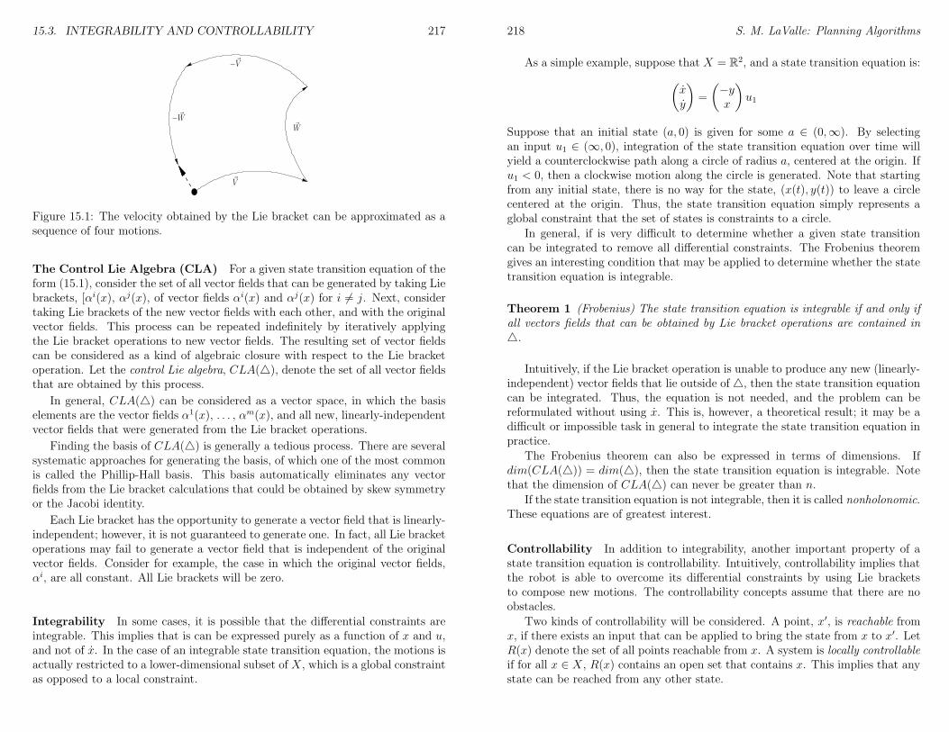
15.3. INTEGRABILITY AND CONTROLLABILITY 217
~V
~W
−~V
− ~W
Figure 15.1: The velocity obtained by the Lie bracket can be approximated as asequence of four motions.
The Control Lie Algebra (CLA) For a given state transition equation of theform (15.1), consider the set of all vector fields that can be generated by taking Liebrackets, [αi(x), αj(x), of vector fields αi(x) and αj(x) for i 6= j. Next, considertaking Lie brackets of the new vector fields with each other, and with the originalvector fields. This process can be repeated indefinitely by iteratively applyingthe Lie bracket operations to new vector fields. The resulting set of vector fieldscan be considered as a kind of algebraic closure with respect to the Lie bracketoperation. Let the control Lie algebra, CLA(4), denote the set of all vector fieldsthat are obtained by this process.
In general, CLA(4) can be considered as a vector space, in which the basiselements are the vector fields α1(x), . . . , αm(x), and all new, linearly-independentvector fields that were generated from the Lie bracket operations.
Finding the basis of CLA(4) is generally a tedious process. There are severalsystematic approaches for generating the basis, of which one of the most commonis called the Phillip-Hall basis. This basis automatically eliminates any vectorfields from the Lie bracket calculations that could be obtained by skew symmetryor the Jacobi identity.
Each Lie bracket has the opportunity to generate a vector field that is linearly-independent; however, it is not guaranteed to generate one. In fact, all Lie bracketoperations may fail to generate a vector field that is independent of the originalvector fields. Consider for example, the case in which the original vector fields,αi, are all constant. All Lie brackets will be zero.
Integrability In some cases, it is possible that the differential constraints areintegrable. This implies that is can be expressed purely as a function of x and u,and not of x. In the case of an integrable state transition equation, the motions isactually restricted to a lower-dimensional subset of X, which is a global constraintas opposed to a local constraint.
218 S. M. LaValle: Planning Algorithms
As a simple example, suppose that X = R2, and a state transition equation is:
(
xy
)
=
(
−yx
)
u1
Suppose that an initial state (a, 0) is given for some a ∈ (0,∞). By selectingan input u1 ∈ (∞, 0), integration of the state transition equation over time willyield a counterclockwise path along a circle of radius a, centered at the origin. Ifu1 < 0, then a clockwise motion along the circle is generated. Note that startingfrom any initial state, there is no way for the state, (x(t), y(t)) to leave a circlecentered at the origin. Thus, the state transition equation simply represents aglobal constraint that the set of states is constraints to a circle.
In general, if is very difficult to determine whether a given state transitioncan be integrated to remove all differential constraints. The Frobenius theoremgives an interesting condition that may be applied to determine whether the statetransition equation is integrable.
Theorem 1 (Frobenius) The state transition equation is integrable if and only ifall vectors fields that can be obtained by Lie bracket operations are contained in4.
Intuitively, if the Lie bracket operation is unable to produce any new (linearly-independent) vector fields that lie outside of 4, then the state transition equationcan be integrated. Thus, the equation is not needed, and the problem can bereformulated without using x. This is, however, a theoretical result; it may be adifficult or impossible task in general to integrate the state transition equation inpractice.
The Frobenius theorem can also be expressed in terms of dimensions. Ifdim(CLA(4)) = dim(4), then the state transition equation is integrable. Notethat the dimension of CLA(4) can never be greater than n.
If the state transition equation is not integrable, then it is called nonholonomic.These equations are of greatest interest.
Controllability In addition to integrability, another important property of astate transition equation is controllability. Intuitively, controllability implies thatthe robot is able to overcome its differential constraints by using Lie bracketsto compose new motions. The controllability concepts assume that there are noobstacles.
Two kinds of controllability will be considered. A point, x′, is reachable fromx, if there exists an input that can be applied to bring the state from x to x′. LetR(x) denote the set of all points reachable from x. A system is locally controllableif for all x ∈ X, R(x) contains an open set that contains x. This implies that anystate can be reached from any other state.
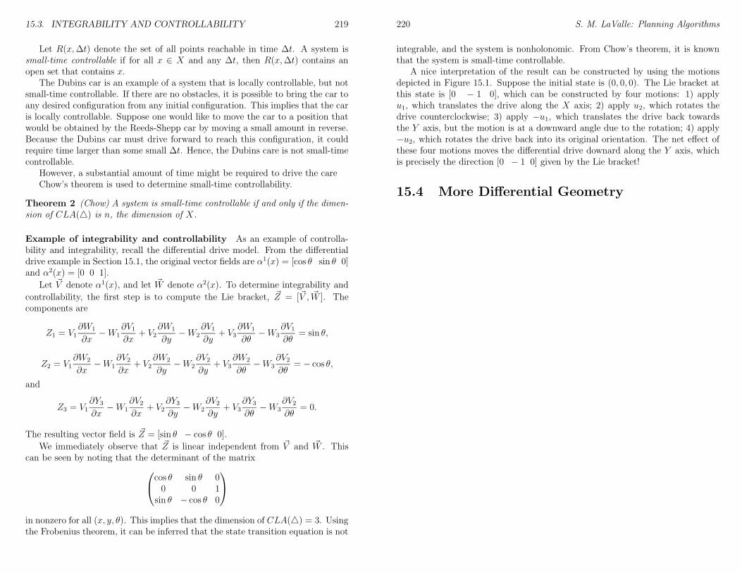
15.3. INTEGRABILITY AND CONTROLLABILITY 219
Let R(x,∆t) denote the set of all points reachable in time ∆t. A system issmall-time controllable if for all x ∈ X and any ∆t, then R(x,∆t) contains anopen set that contains x.
The Dubins car is an example of a system that is locally controllable, but notsmall-time controllable. If there are no obstacles, it is possible to bring the car toany desired configuration from any initial configuration. This implies that the caris locally controllable. Suppose one would like to move the car to a position thatwould be obtained by the Reeds-Shepp car by moving a small amount in reverse.Because the Dubins car must drive forward to reach this configuration, it couldrequire time larger than some small ∆t. Hence, the Dubins care is not small-timecontrollable.
However, a substantial amount of time might be required to drive the careChow’s theorem is used to determine small-time controllability.
Theorem 2 (Chow) A system is small-time controllable if and only if the dimen-sion of CLA(4) is n, the dimension of X.
Example of integrability and controllability As an example of controlla-bility and integrability, recall the differential drive model. From the differentialdrive example in Section 15.1, the original vector fields are α1(x) = [cos θ sin θ 0]and α2(x) = [0 0 1].
Let ~V denote α1(x), and let ~W denote α2(x). To determine integrability and
controllability, the first step is to compute the Lie bracket, ~Z = [~V , ~W ]. Thecomponents are
Z1 = V1∂W1
∂x−W1
∂V1∂x
+ V2∂W1
∂y−W2
∂V1∂y
+ V3∂W1
∂θ−W3
∂V1∂θ
= sin θ,
Z2 = V1∂W2
∂x−W1
∂V2∂x
+ V2∂W2
∂y−W2
∂V2∂y
+ V3∂W2
∂θ−W3
∂V2∂θ
= − cos θ,
and
Z3 = V1∂Y3∂x−W1
∂V2∂x
+ V2∂Y3∂y−W2
∂V2∂y
+ V3∂Y3∂θ−W3
∂V2∂θ
= 0.
The resulting vector field is ~Z = [sin θ − cos θ 0].
We immediately observe that ~Z is linear independent from ~V and ~W . Thiscan be seen by noting that the determinant of the matrix
cos θ sin θ 00 0 1
sin θ − cos θ 0
in nonzero for all (x, y, θ). This implies that the dimension of CLA(4) = 3. Usingthe Frobenius theorem, it can be inferred that the state transition equation is not
220 S. M. LaValle: Planning Algorithms
integrable, and the system is nonholonomic. From Chow’s theorem, it is knownthat the system is small-time controllable.
A nice interpretation of the result can be constructed by using the motionsdepicted in Figure 15.1. Suppose the initial state is (0, 0, 0). The Lie bracket atthis state is [0 − 1 0], which can be constructed by four motions: 1) applyu1, which translates the drive along the X axis; 2) apply u2, which rotates thedrive counterclockwise; 3) apply −u1, which translates the drive back towardsthe Y axis, but the motion is at a downward angle due to the rotation; 4) apply−u2, which rotates the drive back into its original orientation. The net effect ofthese four motions moves the differential drive downard along the Y axis, whichis precisely the direction [0 − 1 0] given by the Lie bracket!
15.4 More Differential Geometry

Chapter 16
Planning Under DifferentialConstraints
This chapter presents several alternative planning methods. For each method, it isassumed that a state transition equation or incremental simulator has been definedover a state space. The state could represent configuration or both configurationand velocity.
16.1 Functional-Based Dynamic Programming
16.2 Tree-Based Dynamic Programming
The forward dynamic programming (FDP) method is similar to an RRT in that itgrows a tree from xinit. The key difference is that FDP uses dynamic programmingto decide how to incrementally expand the tree, as opposed to nearest-neighbors ofrandom samples. FDP performs a systematic exploration over fine-resolution gridthat is placed over the state space. This limits is applicability to low-dimensionalstate spaces (up to 3 or 4 dimensions).
The configuration space, X, is divided into a rectangular grid (typically thereare a hundred grid points per axis). Each element of the grid is called a cell, whichdesignates a rectangular subset of X. One of three different labels can be appliedto each cell:
• OBST: The cell contains points in Xobs.
• FREE: The cell has not yet been visited by the algorithm, and it lies entirelyin Xfree.
• VISITED: The cell has been visited, and it lies entirely in Xfree.
Initially, all cells are labeled either FREE or OBST by using an collision detectionalgorithm.
221
222 S. M. LaValle: Planning Algorithms
Let Q represent a priority queue in which the elements are configurations,sorted in increasing order according to L, which represents the cost accumulatedalong the path constructed so far from xinit to x. This cost can be assigned inmany different ways. It could simply represent the time (number of ∆t steps), orcould count the number of times a car changes directions.
The algorithm proceeds as follows:
FORWARD DYNAMIC PROGRAMMING(xinit, xgoal)1 Q.insert(xinit, L);2 G.init(xinit);3 while Q 6= ∅ and FREE(xgoal)4 xcur → Q.pop();5 for each x ∈ NBHD(xcur)6 if FREE(x)7 Q.insert(x, L);8 G.add vertex(x);9 G.add edge(xcur, x);10 Label cell that contains x as VISITED;11 Return G;
The algorithm iterative grows a tree, G, which it rooted at xinit. The NHBDfunction tries the possible inputs, and returns a set of configurations that can bereached in time ∆t. For each of these configurations, if the cell that contains itis FREE, then G is extended. At any given time, there is at most one vertexper cell. The algorithm terminates when the cell that contains the goal has beenreached.
16.3 Geodesic Curve Families
Need to include Balkcom-Mason curves, Dubins, etc.
A common theme for many planning approaches is to divide the problem intotwo phases. In the first phase, a holonomic planning method is used by pro-ducing a collision-free path that ignores the nonholonomic constraints. In thesecond phase, an iterative method attempts to replace portions of the holonomicpath with portions that satisfy the nonholonomic constraints, yet still avoid ob-stacles. In general, this will lead to an incomplete algorithm because there is noguarantee that the original path provides a correct starting point for obtaining anonholonomic solution. However, it typically leads to a fast planning algorithm.
In this section, we describe this approach for the case of a car-like robot.Assume that a fast holonomic planning method has been selected for the firstphase. Suppose that a path, τ : [0, 1] → Cfree has been computed. The pathcan be iteratively improved as follows. Randomly select two real numbers α1 ∈[0, 1] and α2 ∈ [0, 1]. Assuming α2 > α1 (if not, then swap them), attempt to
16.4. STEERING METHODS 223
replace the portion of τ from τ(α1) to τ(α2) with a path segment that satisfiesthe nonholonomic constraints. This implies that τ is broken into three segments,τ1 : [0, α1] → Cfree, τ2 : [α1, α2] → Cfree, and τ3 : [α2, 1] → Cfree. Note thatτ1(α1) = τ2(α1) and τ2(α2) = τ3(α2). The portions τ1 and τ3 remain fixed, but τ2is replaced with a new path, τ ′ : [α1, α2]→ Cfree, that satisfies the nonholonomicconstraints. Note that τ ′ must also avoid collisions, τ ′(α1) = τ1(α1), and τ
′(α2) =τ3(α2). This procedure can be iterated multiple times until eventually, the originalpath is completely transformed into a nonholonomic path. Note that α1 = 0 andα2 = 1 must each have nonzero probability of being chosen in each iteration. Inmany iterations, the path substitution will fail; in this case, the previous path isretained.
To make this and related approaches succeed, a fast technique is needed thatconstructs a nonholonomic path between any two configurations. Although thismight appear as difficult as the original nonholonomic planning problem, it isassumed that the obstacles are ignored. In general, this is referred to as thesteering problem, which as received a considerable amount of attention in recentyears, particularly for car-like robots that pull trailers. For the case of a simplecar-like robot with a limited steering angle, there are some analytical solutionsto the problem of finding the shortest path between two configurations. In 1957,Dubins showed that for a car that can only go forward, the optimal path will takeone of the six following forms:
LRL, LSL, LSR, RLR, RSR, RSL.
Each sequence of labels indicates the type of path. For example, “LRL” indicatesa path that consists of a sharp left turn, immediately followed by a sharp rightturn, immediately followed by a sharp left turn. Above, “S” denotes a straightsegment. For a given pair of configurations, one can simply attempt to connectthem using all six path types. The one with the shortest path length among thesix choices is known to be the minimum-length path out of all possible paths.This path provides a nice substitution for τ2, as described above.
For the case of a car-like robot that can move forward or backwards, Reedsand Shepp showed in 1990 that the optimal path between two configurations willtake one of 48 different forms. Although this situation is more complicated, thesame general strategy can be applied as for the case of a forward-only car.
16.4 Steering Methods
CBHD formulas, flat systems, etc.
16.5 RRT-Based Methods
Need to cover stuff done by Frazzoli, and possibly Cerven and Bullo, and alsoCheng and LaValle.
224 S. M. LaValle: Planning Algorithms
The RRT planning method can be easily adapted to the case of nonholonomicplanning. All references to configurations are replaced by references to states; thisis merely a change of names. The only important difference between holonomicplanning and nonholonomic planning with an RRT occurs in the EXTEND pro-cedure. For holonomic planning, the function NEW CONFIG generated a config-uration that lies on the line segment that connects q to qnear. For nonholonomicplanning, motions must be generated by applying inputs. The NEW CONFIGfunction is replaced by NEW STATE, which attempts to apply all of the inputsin U , and selects the input that generates an xnew that is closest to xnear withrespect to the metric ρ. If U is infinite, then it can be approximated with a finiteset of inputs.
16.6 Other Methods
Bibliography
[1]
[2] N. M. Amato and Y. Wu. A randomized roadmap method for path andmanipulation planning. In IEEE Int. Conf. Robot. & Autom., pages 113–120, 1996.
[3] B. D. Anderson and J. B. Moore. Optimal Control: Linear-Quadratic Meth-ods. Prentice-Hall, Englewood Cliffs, NJ, 1990.
[4] M. A. Armstrong. Basic Topology. Springer-Verlag, New York, NY, 1983.
[5] S. Arya, D. M. Mount, N. S. Netanyahu, R. Silverman, and A. Y. Wu. Anoptimal algorithm for approximate nearest neighbor searching. Journal ofthe ACM, 45:891–923, 1998.
[6] T. Basar and G. J. Olsder. Dynamic Noncooperative Game Theory. AcademicPress, London, 1982.
[7] J. Barraquand and J.-C. Latombe. A Monte-Carlo algorithm for path plan-ning with many degrees of freedom. In IEEE Int. Conf. Robot. & Autom.,pages 1712–1717, 1990.
[8] S. Basu, R. Pollack, and M.-F. Roy. Computing roadmaps of semi-algebraicsets on a variety. Submitted for publication, 1998.
[9] R. E. Bellman. Dynamic Programming. Princeton University Press, Prince-ton, NJ, 1957.
[10] D. P. Bertsekas. Convergence in discretization procedures in dynamic pro-gramming. IEEE Trans. Autom. Control, 20(3):415–419, June 1975.
[11] V. Boor, N. H. Overmars, and A. F. van der Stappen. The gaussian samplingstrategy for probabilistic roadmap planners. In IEEE Int. Conf. Robot. &Autom., pages 1018–1023, 1999.
[12] A. E. Bryson and Y.-C. Ho. Applied Optimal Control. Hemisphere PublishingCorp., New York, NY, 1975.
225
226 BIBLIOGRAPHY
[13] J. Canny and J. Reif. New lower bound techniques for robot motion planningproblems. In Proc. IEEE Conf. on Foundations of Computer Science, pages49–60, 1987.
[14] J. F. Canny. The Complexity of Robot Motion Planning. MIT Press, Cam-bridge, MA, 1988.
[15] G. S. Chirikjian and A. B. Kyatkin. Engineering Applications of Noncom-mutative Harmonic Analysis. CRC Press, Boca Raton, 2001.
[16] J. H. Conway and N. J. A. Sloane. Sphere Packings, Lattices, and Groups.Springer-Verlag, Berlin, 1999.
[17] T. H. Cormen, C. E. Leiserson, and R. L. Rivest. An Introduction to Algo-rithms. MIT Press, Cambridge, MA, 1990.
[18] J. J. Craig. Introduction to Robotics. Addison-Wesley, Reading, MA, 1989.
[19] M. de Berg, M. van Kreveld, M. Overmars, and O. Schwarzkopf. Computa-tional Geometry: Algorithms and Applications. Springer, Berlin, 1997.
[20] L. E. Dubins. On curves of minimal length with a constraint on averagecurvature, and with prescribed initial and terminal positions and tangents.American Journal of Mathematics, 79:497–516, 1957.
[21] M. Erdmann. Understanding action and sensing by designing action-basedsensors. Int. J. Robot. Res., 14(5):483–509, 1995.
[22] L. J. Guibas, D. Hsu, and L. Zhang. H-Walk: Hierarchical distance computa-tion for moving convex bodies. In Proc. ACM Symposium on ComputationalGeometry, pages 265–273, 1999.
[23] J. H. Halton. On the efficiency of certain quasi-random sequences of pointsin evaluating multi-dimensional integrals. Numer. Math., 2:84–90, 1960.
[24] J. M. Hammersley. Monte-Carlo methods for solving multivariable problems.Ann. New York Acad. Sci., 86:844–874, 1960.
[25] R. S. Hartenburg and J. Denavit. A kinematic notation for lower pair mech-anisms based on matrices. J. Applied Mechanics, 77:215–221, 1955.
[26] F. J. Hickernell. Lattice rules: How well do they measure up? In P. Bickel, ed-itor, Random and Quasi-Random Point Sets, pages 109–166. Springer-Verlag,Berlin, 1998.
[27] F. J. Hickernell, H. S. Hong, P. L’Ecuyer, and C. Lemieux. Extensible latticesequences for quasi-monte carlo quadrature. SIAM Journal on ScientificComputing, 22:1117–1138, 2000.
BIBLIOGRAPHY 227
[28] C. M. Hoffmann. Geometric and Solid Modeling. Morgan Kaufmann, SanMateo, CA, 1989.
[29] P. Indyk and R. Motwani. Approximate nearest neighbors: Towards remov-ing the curse of dimensionality. In Proceedings of the 30th Annual ACMSymposium on Theory of Computing, pages 604–613, 1998.
[30] L. Kavraki and J.-C. Latombe. Randomized preprocessing of configurationspace for path planning. In IEEE Int. Conf. Robot. & Autom., pages 2138–2139, 1994.
[31] L. E. Kavraki. Computation of configuration-space obstacles using the FastFourier Transform. IEEE Trans. Robot. & Autom., 11(3):408–413, 1995.
[32] L. E. Kavraki, P. Svestka, J.-C. Latombe, and M. H. Overmars. Probabilisticroadmaps for path planning in high-dimensional configuration spaces. IEEETrans. Robot. & Autom., 12(4):566–580, June 1996.
[33] O. Khatib. Real-time obstacle avoidance for manipulators and mobile robots.Int. J. Robot. Res., 5(1):90–98, 1986.
[34] C. L. Kinsey. Topology of Surfaces. Springer-Verlag, Berlin, 1993.
[35] J. J. Kuffner and S. M. LaValle. RRT-connect: An efficient approach tosingle-query path planning. In Proc. IEEE Int’l Conf. on Robotics and Au-tomation, pages 995–1001, 2000.
[36] P. R. Kumar and P. Varaiya. Stochastic Systems. Prentice-Hall, EnglewoodCliffs, NJ, 1986.
[37] R. E. Larson. A survey of dynamic programming computational procedures.IEEE Trans. Autom. Control, 12(6):767–774, December 1967.
[38] R. E. Larson and J. L. Casti. Principles of Dynamic Programming, Part II.Dekker, New York, NY, 1982.
[39] J.-C. Latombe. Robot Motion Planning. Kluwer Academic Publishers,Boston, MA, 1991.
[40] J. P. Laumond, S. Sekhavat, and F. Lamiraux. Guidelines in nonholonomicmotion planning for mobile robots. In J.-P. Laumond, editor, Robot MotionPlannning and Control, pages 1–53. Springer-Verlag, Berlin, 1998.
[41] S. M. LaValle. A Game-Theoretic Framework for Robot Motion Planning.PhD thesis, University of Illinois, Urbana, IL, July 1995.
[42] S. M. LaValle and J. J. Kuffner. Randomized kinodynamic planning. In Proc.IEEE Int’l Conf. on Robotics and Automation, pages 473–479, 1999.
228 BIBLIOGRAPHY
[43] M. C. Lin and J. F. Canny. Efficient algorithms for incremental distancecomputation. In IEEE Int. Conf. Robot. & Autom., 1991.
[44] M. C. Lin, D. Manocha, J. Cohen, and S. Gottschalk. Collision detection:Algorithms and applications. In J.-P. Laumond and M. Overmars, editors,Algorithms for Robotic Motion and Manipulation, pages 129–142. A K Peters,Wellesley, MA, 1997.
[45] S. R. Lindemann and S. M. LaValle. Incremental low-discrepancy latticemethods for motion planning. In Proc. IEEE International Conference onRobotics and Automation, 2003.
[46] J. Matousek. Geometric Discrepancy. Springer-Verlag, Berlin, 1999.
[47] E. Mazer, J. M. Ahuactzin, and P. Bessiere. The Ariadne’s clew algorithm.J. Artificial Intell. Res., 9:295–316, November 1998.
[48] B. Mirtich. V-Clip: Fast and robust polyhedral collision detection. TechnicalReport TR97-05, Mitsubishi Electronics Research Laboratory, 1997.
[49] B. Mishra. Algorithmic Algebra. Springer-Verlag, New York, NY, 1993.
[50] B. Mishra. Computational real algebraic geometry. In J. E. Goodman andJ. O’Rourke, editors, Discrete and Computational Geometry, pages 537–556.CRC Press, New York, 1997.
[51] M. E. Mortenson. Geometric Modeling. Wiley, New York, NY, 1985.
[52] R. M. Murray and S. Sastry. Nonholonomic motion planning: Steering usingsinusoids. Trans. Automatic Control, 38(5):700–716, 1993.
[53] H. Niederreiter. Random Number Generation and Quasi-Monte-Carlo Meth-ods. Society for Industrial and Applied Mathematics, Philadelphia, USA,1992.
[54] H. Niederreiter and C. P. Xing. Nets, (t,s)-sequences, and algebraic geometry.In P. Hellekalek and G. Larcher, editors, Random and Quasi-Random PointSets, Lecture Notes in Statistics, Vol. 138, pages 267–302. Springer-Verlag,Berlin, 1998.
[55] C. H. Papadimitriou. An algorithm for shortest-path planning in three di-mensions. Information Processing Letters, 20(5):259–263, 1985.
[56] R. P. Paul. Robot Manipulators: Mathematics, Programming, and Control.MIT Press, Cambridge, MA, 1981.
[57] L. Piegl. On NURBS: A survey. IEEE Trans. Comp. Graph. & Appl.,11(1):55–71, Jan 1991.
BIBLIOGRAPHY 229
[58] I. Pohl. Bi-directional and heuristic search in path problems. Technicalreport, Stanford Linear Accelerator Center, 1969.
[59] S. Quinlan. Efficient distance computation between nonconvex objects. InIEEE Int. Conf. Robot. & Autom., pages 3324–3329, 1994.
[60] J. A. Reeds and L. A. Shepp. Optimal paths for a car that goes both forwardsand backwards. Pacific J. Math., 145(2):367–393, 1990.
[61] J. H. Reif. Complexity of the mover’s problem and generalizations. In Proc.of IEEE Symp. on Foundat. of Comp. Sci., pages 421–427, 1979.
[62] J. H. Reif and M. Sharir. Motion planning in the presence of moving obstacles.In Proc. of IEEE Symp. on Foundat. of Comp. Sci., pages 144–154, 1985.
[63] J. H. Reif and S. R. Tate. Continuous alternation: The complexity of pursuitin continuous domains. Algorithmica, 10:157–181, 1993.
[64] E. Rimon and D. E. Koditschek. Exact robot navigation using artificialpotential fields. IEEE Trans. Robot. & Autom., 8(5):501–518, October 1992.
[65] A. Scheuer and Ch. Laugier. Planning sub-optimal and continuous-curvaturepaths for car-like robots. In IEEE/RSJ Int. Conf. on Intelligent Robots &Systems, pages 25–31, 1998.
[66] J. T. Schwartz and M. Sharir. On the piano movers’ problem: II. Generaltechniqies for computing topological properties of algebraic manifolds. Com-munications on Pure and Applied Mathematics, 36:345–398, 1983.
[67] I. H. Sloan and S. Joe. Lattice Methods for Multiple Integration. OxfordScience Publications, Englewood Cliffs, NJ, 1990.
[68] M. Spivak. Differential Geometry. Publish or Perish, Inc., 1979.
[69] A. G. Sukharev. Optimal strategies of the search for an extremum. U.S.S.R.Computational Mathematics and Mathematical Physics, 11(4), 1971. Trans-lated from Russian, Zh. Vychisl. Mat. i Mat. Fiz., 11, 4, 910-924, 1971.
[70] H. Sussman and G. Tang. Shortest paths for the Reeds-Shepp car: A workedout example of the use of geometric techniques in nonlinear optimal control.Technical Report SYNCON 91-10, Dept. of Mathematics, Rutgers University,1991.
[71] P. Svestka and M. H. Overmars. Coordinated motion planning for multiplecar-like robots using probabilistic roadmaps. In IEEE Int. Conf. Robot. &Autom., pages 1631–1636, 1995.
230 BIBLIOGRAPHY
[72] S. Tezuka. Quasi-monte carlo: The discrepancy between theory and practice.In K.-T. Fang, F. J. Hickernell, and H. Niederreiter, editors, Monte Carlo andQuasi-Monte Carlo Methods 2000, pages 124–140. Springer-Verlag, Berlin,2002.
[73] D. Vallejo, C. Jones, and N. Amato. An adaptive framework for ”single shot”motion planning. Texas A&M, October 1999.
[74] J. G. van der Corput. Verteilungsfunktionen I. Akad. Wetensch., 38:813–821,1935.
[75] X. Wang and F. J. Hickernell. An historical overview of lattice point sets. InK.-T. Fang, F. J. Hickernell, and H. Niederreiter, editors, Monte Carlo andQuasi-Monte Carlo Methods 2000, pages 158–167. Springer-Verlag, Berlin,2002.
[76] H. Weyl. Uber die Gleichverteilung von Zahlen mod Eins. Math. Ann.,77:313–352, 1916.