MPP 806 Estimation Tools #1: Trend lines and Regression Tool

1

MPP 806 Estimation Tools #1: Trend lines and Regression Tool

This Assignment is to introduce you to some of the ways you can estimate equations from Data using different excel tools. Estimations of equations are typically used for (a) testing the strength of the relationship, and (b) forecasting future values. As such, excel can supply you with both the estimated equation (usually linear) and statistics that will help you draw conclusions about the strength of the estimate Instructions:

Download excel file forecast1.xlsx NOW: Save the file using your name for the file i.e. KevinWainwright.xlsx

Once you have completed the assignment, you are to email your finished file to me and a copy to Stephen [A] Basic Linear Estimate Go to worksheet labelled A-Slope Intercept You will see two columns of Data, X and Y. First you are going to estimate the line that fits this data. Remember that the formula for a line is

Y = mX + b Where m is the slope and b is the intercept. In cell A2 type “Intercept” and in cell A3 type “slope” In cell B2 type the formula “=intercept” and then hold down the Ctrl key and press A (don’t hit enter) This will give you the dialog box

Enter the values for Y and X (use the mouse to hi-light the appropriate cells)

2

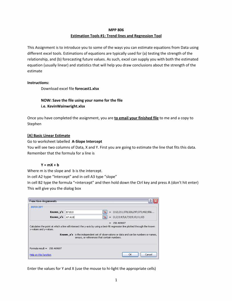
In cell B3 type the formula “=slope” and then hold down the Ctrl key and press A (don’t hit enter)

Once finished, you should have the information needed to fill in the equation. You should have:

Y = 39.979X + 158.4697

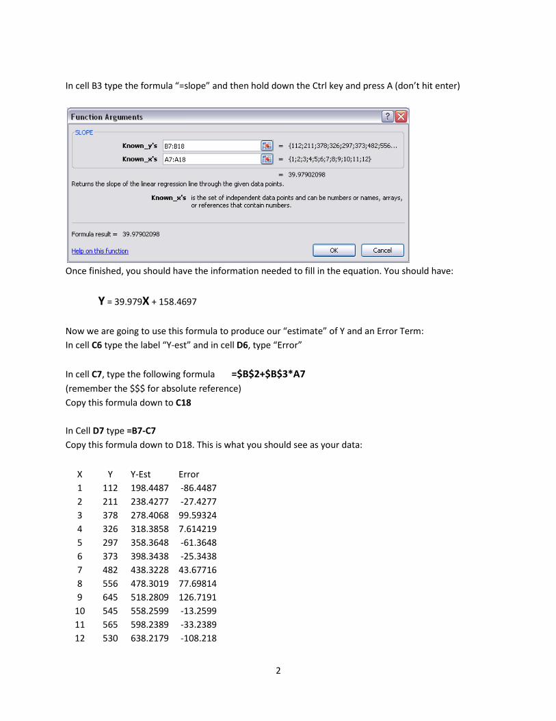
Now we are going to use this formula to produce our “estimate” of Y and an Error Term: In cell C6 type the label “Y-est” and in cell D6, type “Error”

In cell C7, type the following formula =$B$2+$B$3*A7 (remember the $$$ for absolute reference) Copy this formula down to C18 In Cell D7 type =B7-C7 Copy this formula down to D18. This is what you should see as your data:

X Y Y-Est Error 1 112 198.4487 -86.4487 2 211 238.4277 -27.4277 3 378 278.4068 99.59324 4 326 318.3858 7.614219 5 297 358.3648 -61.3648 6 373 398.3438 -25.3438 7 482 438.3228 43.67716 8 556 478.3019 77.69814 9 645 518.2809 126.7191

10 545 558.2599 -13.2599 11 565 598.2389 -33.2389 12 530 638.2179 -108.218

3

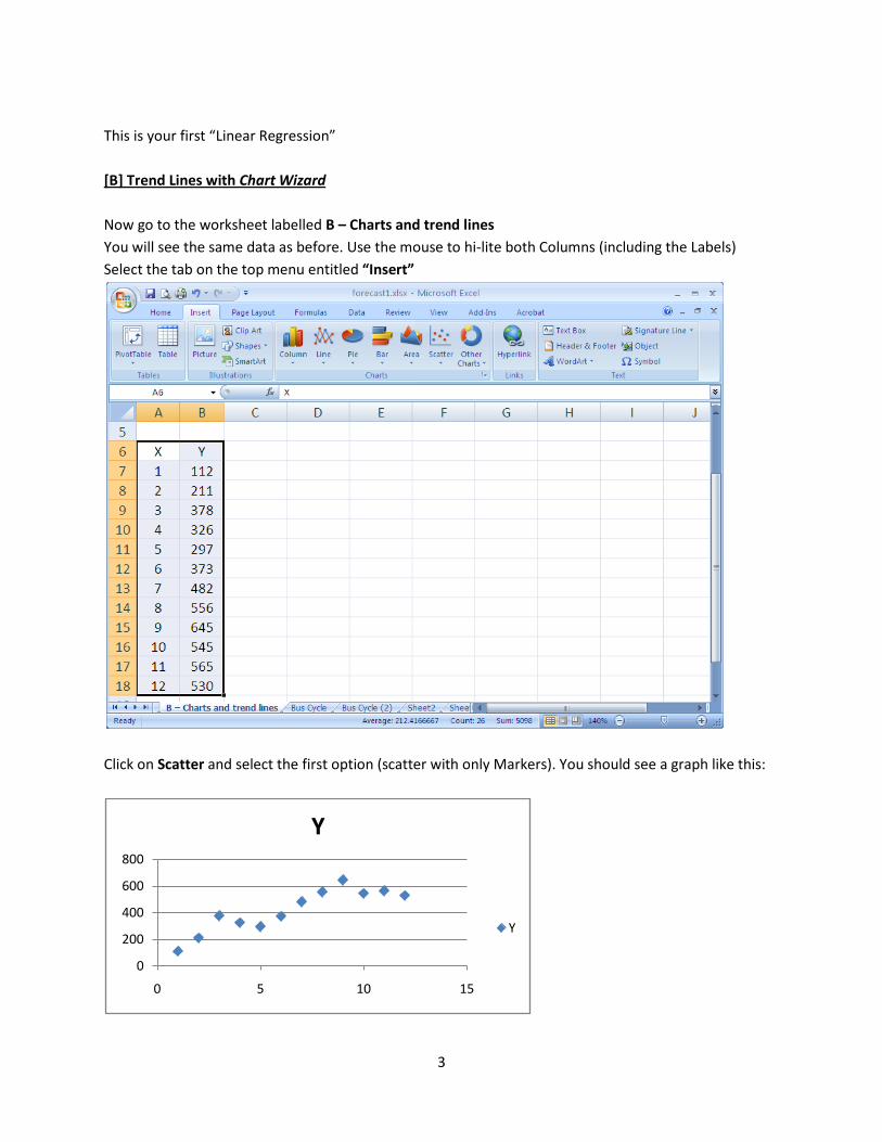
This is your first “Linear Regression” [B] Trend Lines with Chart Wizard Now go to the worksheet labelled B – Charts and trend lines You will see the same data as before. Use the mouse to hi-lite both Columns (including the Labels) Select the tab on the top menu entitled “Insert”

Click on Scatter and select the first option (scatter with only Markers). You should see a graph like this:

0

200

400

600

800

0 5 10 15

Y

Y

4

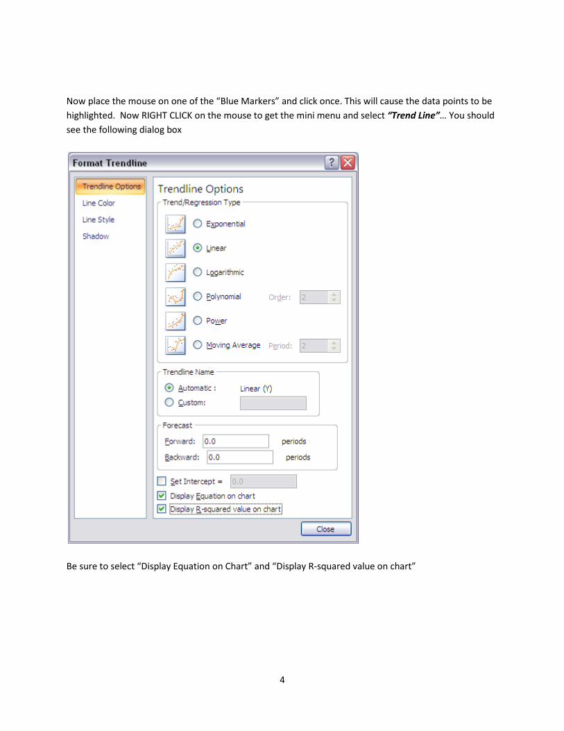
Now place the mouse on one of the “Blue Markers” and click once. This will cause the data points to be highlighted. Now RIGHT CLICK on the mouse to get the mini menu and select “Trend Line”… You should see the following dialog box

Be sure to select “Display Equation on Chart” and “Display R-squared value on chart”

5

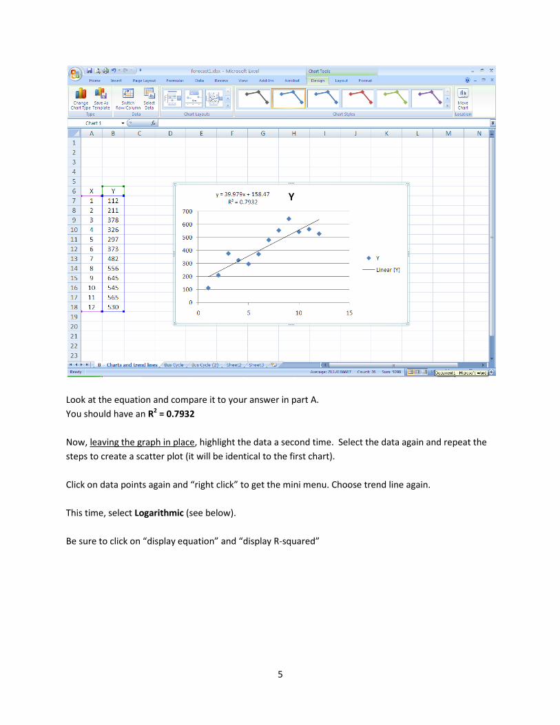
Look at the equation and compare it to your answer in part A. You should have an R2 = 0.7932 Now, leaving the graph in place, highlight the data a second time. Select the data again and repeat the steps to create a scatter plot (it will be identical to the first chart). Click on data points again and “right click” to get the mini menu. Choose trend line again. This time, select Logarithmic (see below). Be sure to click on “display equation” and “display R-squared”

6

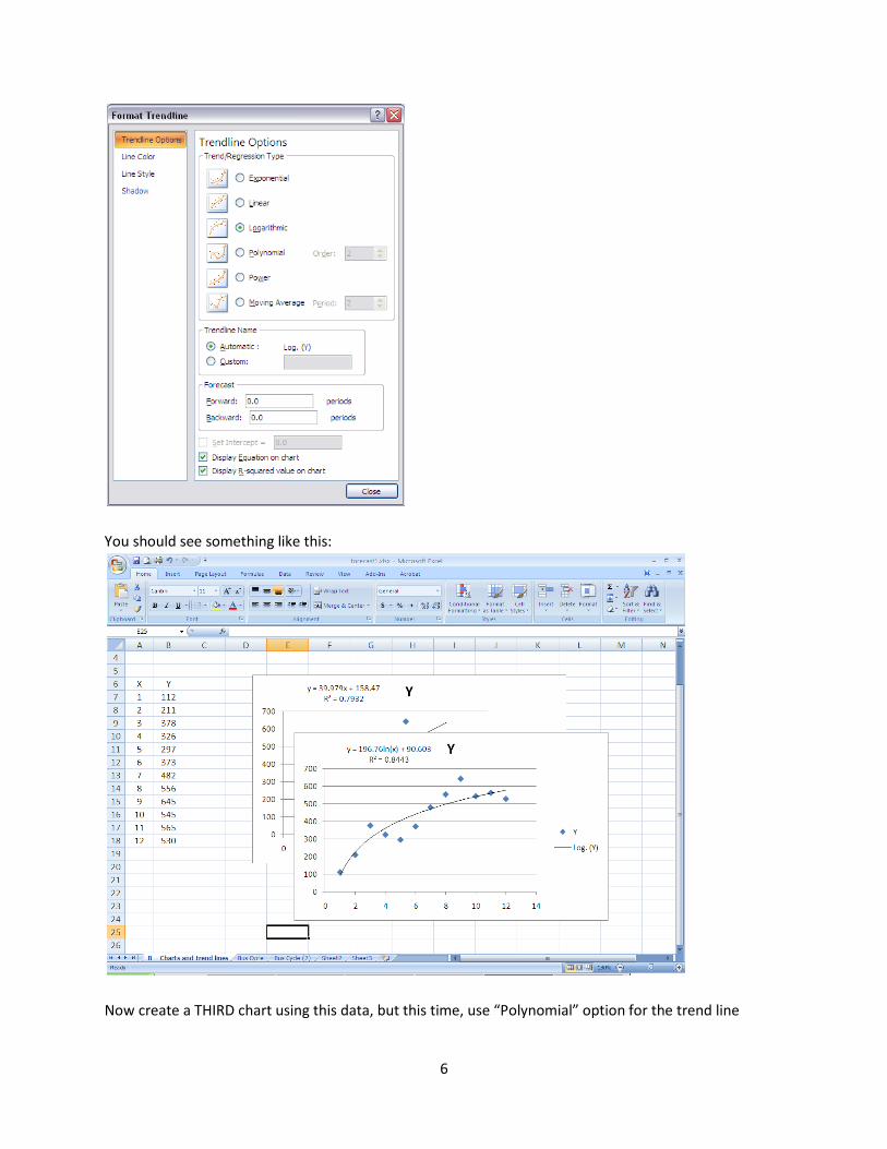
You should see something like this:

Now create a THIRD chart using this data, but this time, use “Polynomial” option for the trend line

7

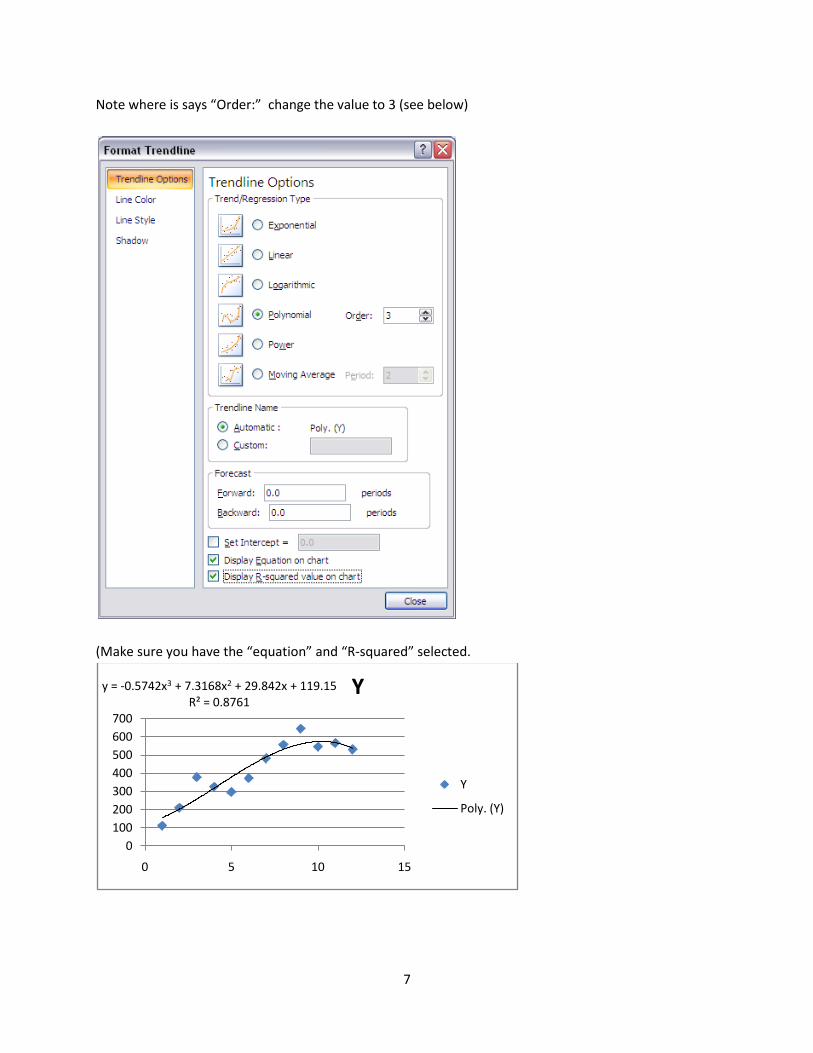
Note where is says “Order:” change the value to 3 (see below)

(Make sure you have the “equation” and “R-squared” selected.

y = -0.5742x3 + 7.3168x2 + 29.842x + 119.15R² = 0.8761

0100200300400500600700

0 5 10 15

Y

Y

Poly. (Y)

8

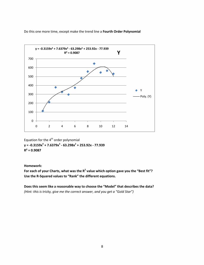
Do this one more time, except make the trend line a Fourth Order Polynomial

Equation for the 4th order polynomial y = -0.3159x4 + 7.6379x3 - 63.298x2 + 253.92x - 77.939 R² = 0.9087 Homework: For each of your Charts, what was the R2 value which option gave you the “Best fit”? Use the R-Squared values to “Rank” the different equations. Does this seem like a reasonable way to choose the “Model” that describes the data? (Hint: this is tricky, give me the correct answer, and you get a “Gold Star”)

y = -0.3159x4 + 7.6379x3 - 63.298x2 + 253.92x - 77.939R² = 0.9087

0

100

200

300

400

500

600

700

0 2 4 6 8 10 12 14

Y

Y

Poly. (Y)

9

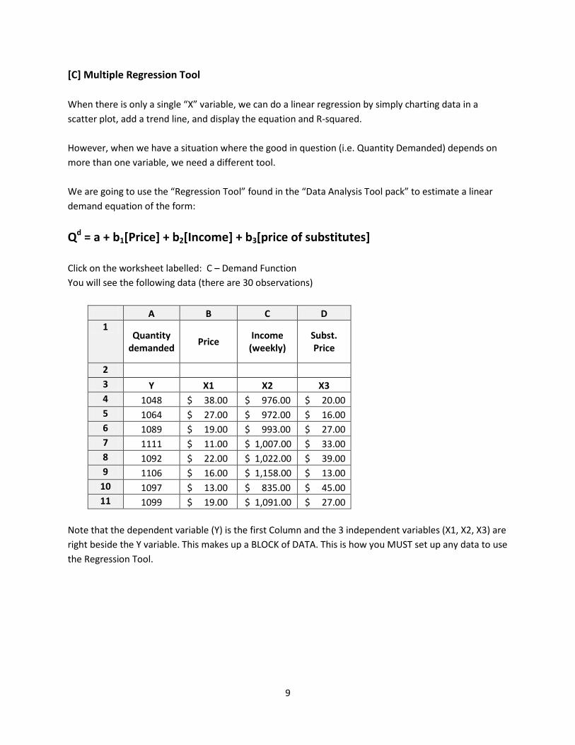
[C] Multiple Regression Tool When there is only a single “X” variable, we can do a linear regression by simply charting data in a scatter plot, add a trend line, and display the equation and R-squared. However, when we have a situation where the good in question (i.e. Quantity Demanded) depends on more than one variable, we need a different tool. We are going to use the “Regression Tool” found in the “Data Analysis Tool pack” to estimate a linear demand equation of the form:

Qd = a + b1[Price] + b2[Income] + b3[price of substitutes] Click on the worksheet labelled: C – Demand Function You will see the following data (there are 30 observations)

A B C D 1

Quantity demanded

Price Income

(weekly) Subst. Price

2 3 Y X1 X2 X3

4 1048 $ 38.00 $ 976.00 $ 20.00 5 1064 $ 27.00 $ 972.00 $ 16.00 6 1089 $ 19.00 $ 993.00 $ 27.00 7 1111 $ 11.00 $ 1,007.00 $ 33.00 8 1092 $ 22.00 $ 1,022.00 $ 39.00 9 1106 $ 16.00 $ 1,158.00 $ 13.00

10 1097 $ 13.00 $ 835.00 $ 45.00 11 1099 $ 19.00 $ 1,091.00 $ 27.00

Note that the dependent variable (Y) is the first Column and the 3 independent variables (X1, X2, X3) are right beside the Y variable. This makes up a BLOCK of DATA. This is how you MUST set up any data to use the Regression Tool.

10

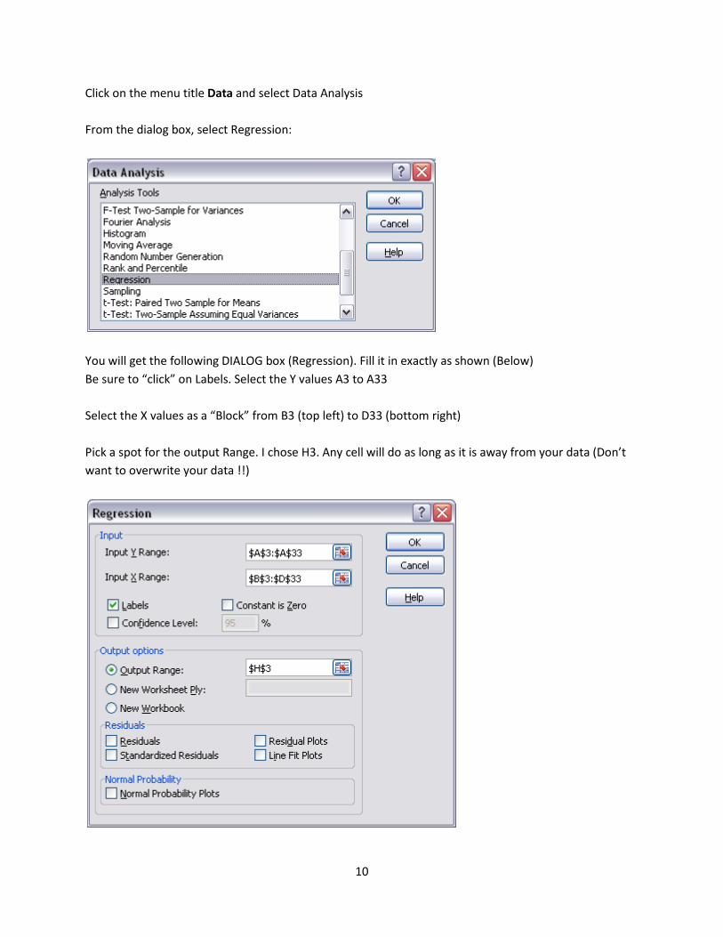
Click on the menu title Data and select Data Analysis From the dialog box, select Regression:

You will get the following DIALOG box (Regression). Fill it in exactly as shown (Below) Be sure to “click” on Labels. Select the Y values A3 to A33 Select the X values as a “Block” from B3 (top left) to D33 (bottom right) Pick a spot for the output Range. I chose H3. Any cell will do as long as it is away from your data (Don’t want to overwrite your data !!)

11

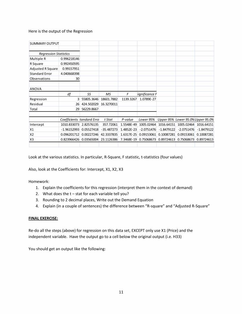
Here is the output of the Regression

Look at the various statistics. In particular, R-Square, F statistic, t-statistics (four values) Also, look at the Coefficients for: Intercept, X1, X2, X3 Homework:

1. Explain the coefficients for this regression (interpret them in the context of demand) 2. What does the t – stat for each variable tell you? 3. Rounding to 2 decimal places, Write out the Demand Equation 4. Explain (in a couple of sentences) the difference between “R-square” and “Adjusted R-Square”

FINAL EXERCISE: Re-do all the steps (above) for regression on this data set, EXCEPT only use X1 (Price) and the independent variable. Have the output go to a cell below the original output (i.e. H33) You should get an output like the following:

SUMMARY OUTPUT

Regression StatisticsMultiple R 0.996218146R Square 0.992450595Adjusted R Square 0.99157951Standard Error 4.040668398Observations 30

ANOVAdf SS MS F Significance F

Regression 3 55805.3646 18601.7882 1139.3267 1.0789E-27Residual 26 424.502029 16.3270011Total 29 56229.8667

Coefficients tandard Erro t Stat P-value Lower 95% Upper 95% Lower 95.0%Upper 95.0%Intercept 1010.833073 2.82576135 357.72061 1.5548E-49 1005.02464 1016.64151 1005.02464 1016.64151X1 -1.96152993 0.05527418 -35.487273 1.4852E-23 -2.0751476 -1.8479122 -2.0751476 -1.8479122X2 0.096201712 0.00227246 42.3337835 1.6317E-25 0.09153061 0.10087281 0.09153061 0.10087281X3 0.823966426 0.03565004 23.1126386 7.3468E-19 0.75068673 0.89724613 0.75068673 0.89724613

12

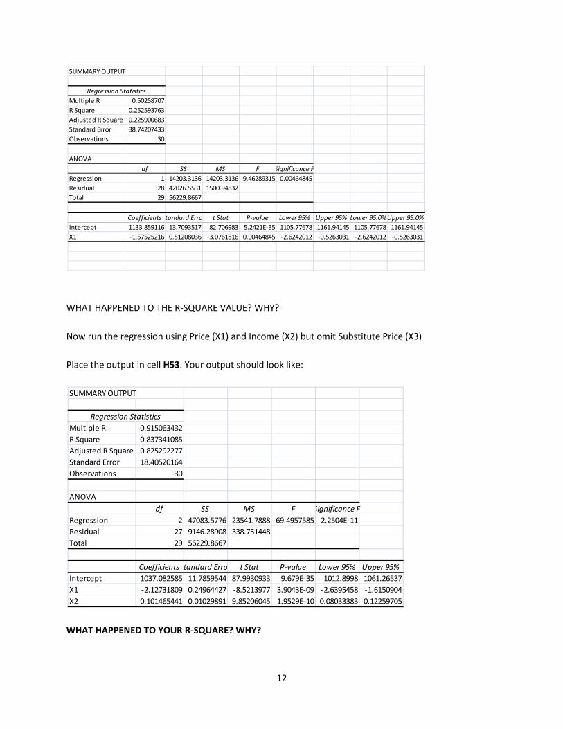
WHAT HAPPENED TO THE R-SQUARE VALUE? WHY? Now run the regression using Price (X1) and Income (X2) but omit Substitute Price (X3) Place the output in cell H53. Your output should look like:

WHAT HAPPENED TO YOUR R-SQUARE? WHY?

SUMMARY OUTPUT



Regression 1 14203.3136 14203.3136 9.46289315 0.00464845Residual 28 42026.5531 1500.94832Total 29 56229.8667

Coefficients tandard Erro t Stat P-value Lower 95% Upper 95% Lower 95.0%Upper 95.0%Intercept 1133.859116 13.7093517 82.706983 5.2421E-35 1105.77678 1161.94145 1105.77678 1161.94145X1 -1.57525216 0.51208036 -3.0761816 0.00464845 -2.6242012 -0.5263031 -2.6242012 -0.5263031

SUMMARY OUTPUT



Regression 2 47083.5776 23541.7888 69.4957585 2.2504E-11Residual 27 9146.28908 338.751448Total 29 56229.8667

Coefficients tandard Erro t Stat P-value Lower 95% Upper 95%Intercept 1037.082585 11.7859544 87.9930933 9.679E-35 1012.8998 1061.26537X1 -2.12731809 0.24964427 -8.5213977 3.9043E-09 -2.6395458 -1.6150904X2 0.101465441 0.01029891 9.85206045 1.9529E-10 0.08033383 0.12259705

Documents

MPP 806 Estimation Tools #1: Trend lines and Regression Tool