Embed Size (px)
Citation preview

1

2
MR Dampers in Smart Structures with Nonlinear Non-affine Dynamics
improvising Intelligent Control
By
Zeinab Movassaghi
A thesis submitted in fulfilment
of the requirements for the degree of
Doctor of Philosophy
Faculty of Engineering
School of Civil and Environmental Engineering
University of Technology, Sydney
Australia
June 2014

3
Executive Summary
The increasing complexity of high-rise buildings, cable-stayed long-span bridges, deep-sea
offshore structures or suspension systems demands effective tools for control and health
monitoring. These infrastructure systems are usually integrated with actuation, sensing,
computation resources and information networks, taking advantage of the synergy of civil
engineering and mechatronics in an emerging area called civiltronics. Towards the
achievement of high performance smart structures, semi-active vibration control in complex
civil structures has been very promising, particularly in the mitigation of external excitations
and dynamic loadings owing to its meritorious features of low cost, strong robustness and
high reliability against various loading sources. Structural behavior and energy efficiency can
be improved via directly controlling the input of the smart devices. For example, semi-active
controlled dampers, from the dissipation point of view by using suitable control schemes for
parameterized relationships describing the system dynamics of the structure integrated with
the smart devices with respect to the applied electrical signal. This research is concerned with
the problem of controlling the nonlinear, non-affine dynamics of smart structures with
magneto-rheological (MR) dampers. A laboratorial set-up of a one-storey steel frame and a
benchmark five-storey building model integrated with MR dampers are used in this research.
These smart structures are subject to scaled earthquake vibrations excited by a shake table. A
static hysteresis model is adopted for the MR damper, in which current-dependent nonlinear
functions are used to represent the damper force-velocity characteristics. Here the semi-active
control problem of the smart structure system is formulated in current-input non-affine
nonlinear state space equations. The complications in the design are tackled by using
intelligent control, whereby adaptive fuzzy logic control is proposed to deal with nonlinearity
of the control dynamics and non-affinity in the control input, assuming the availability of the
displacement and velocity information of the last floor. Here, self-organising adaptive fuzzy
logic control is developed to prevent cases that the resulting fuzzy inference system may be
unnecessarily large or too small to adequately represent the complex dynamics of the smart
structure under control. The main objectives of this research are thus to model the overall
smart structure system and to develop self-organising adaptive fuzzy logic schemes for the
continuous-time multiple-input multiple-output uncertain nonlinear dynamics of the structure.
The proposed control algorithms are implemented in MATLAB and SIMULINK. To illustrate

4
their effectiveness in seismic vibration suppression of civil structures due to earthquake
excitations, simulation results are presented together with discussions on performance
evaluation and further remarks on the implementation aspects.

5
CERTIFICATE OF AUTHORSHIP/ORIGINALITY
I certify that the work in this thesis has not been submitted for a similar degree nor has it been
submitted as part of requirements for any other degree.
I also certify that the thesis has been written by me. Any help I have received in my research
work and the preparation of this thesis itself has been acknowledged. In addition, I certify
that all the information sources and literature used are referenced in the thesis.
Zeinab Movassaghi

6
This thesis is especially dedicated to my dearest father, mother, sisters and brother
for their love, blessings and encouragement.

7
PUBLICATIONS
The following technical papers have been published based on the work of this thesis:
1. Movassaghi, Z., Ha, Q., Samali, B., “A Self-structuring Adaptive fuzzy Control
Scheme for Non-affine nonlinear systems used in Smart Structures”, Sixth
International conference on Structural Health Monitoring of Intelligent
Infrastructure (ISHMII-6), Hong Kong, 9-11 December, 2013
2. Movassaghi, Z., Samali, B., Ha, Q., “Smart Structures Embedded with MR
dampers Using Non-Affine Fuzzy Control”, 22nd Australasian Conference on the
Mechanics of Structures and Materials (ACMSM), Sydney, Australia, 11-14
December 2012
3. Royel,S., Movassaghi, Z., Kwok, N., and Ha,Q., “Structural control Using MR
dampers with Second Order Sliding Mode Controller”, Proceedings of the 1st
international conference on control automation and information sciences
(ICCAIS), Ho Chi Minh City, Vietnam, 26-29 November 2012
4. Movassaghi, Z., “Considering Active Tuned mass dampers in two different
structures”, Australian Control Conference (AUCC), Sydney, Australia, 15-16
November 2012
5. Movassaghi, Z., Samali, B., Ha, Q., “Adaptive Neuro-Fuzzy Modelling of a high-
rise structure equipped with an Active Tuned Mass Damper”, 6th Australasian
Congress on Applied Mechanics, ACAM 6, Perth, Australia, 12-15 December 2010

8
ACKNOWLEDGEMENTS The research project reported in this thesis was supported by the Centre for Built
Infrastructure Research (CBIR) of the University of Technology, Sydney. This financial
support is greatly acknowledged and appreciated.
I am greatly thankful and indebted to my supervisors, A/Prof. Quang Ha, Prof. Bijan Samali
and Prof. Vute Sirivivatnanon for their support and guidance in all aspects of my research
activities.
Finally, I would like to express my special thanks to my family for their encouragement and
love throughout my candidature.

9
TABLE OF CONTENTS
Page EXECUTIVE SUMMARY iii
CERTIFICATE OF AUTHORSHIP/ORIGINALITY v
DEDICATION vi
PUBLICATIONS vii
ACKNOWLEDGEMENT viii
TABLE OF CONTENTS ix
LIST OF TABLES xii
LIST OF FIGURES xiii
NOTATIONS xviii
TABLE OF CONTENTS
1. CHAPTER 1: INTRODUCTION...........................................................................................19
1.1. Problem statement...................................................................................................................19
1.2. Objectives and scope of the thesis...........................................................................................21
1.3. Contribution of this thesis........................................................................................................21
1.4. Thesis Layout...........................................................................................................................22
2. CHAPTER 2: LITERATURE REVIEW.................................................................................24
2.1. Introduction..............................................................................................................................24
2.2. Passive vibration control systems ...........................................................................................26
2.3. Active vibration control devices..............................................................................................32
2.4. Hybrid vibration control devices.............................................................................................35
2.5. Semi-active vibration control devices.....................................................................................38
2.5.1. Variable orifice damper...........................................................................................................39
2.5.2. Variable friction damper..................................................................................................... .....43
2.5.3. Controllable tuned liquid damper............................................................. ...............................44
2.5.4. Controllable fluid damper........................................................................................................45
2.6. MR fluids and devices ............................................................................................................50
2.7. Characteristics of MR fluids................................................................................................. ...52
2.8. MR devices and applications...................................................................................................53
2.9. MR damper modelling................................................................................................ ..............58
2.9.1. Bingham model........................................................................................................................59
10
2.9.2. Bouc-Wen model.....................................................................................................................62
2.9.3. Modified Bouc-Wen model.....................................................................................................63
2.9.4. Static hysteresis model of MR damper....................................................................................65
2.10. Lyapunov control.................................................................................................................. ...67
2.11. Linear quadratic regulator (LQR) control................................................................. ...............67
2.12. Fuzzy logic...............................................................................................................................68
2.13. Fuzzy logic control for structural vibration reduction ............................................................70
2.14. Summary............................................................................................................ ......................70
3. CHAPTER 3: STRUCTURES WITH ACTIVE TUNED MASS DAMPERS……………….71
3.1. Introduction …………………………………………………………………………………...71
3.2. Structural System ......................................................................................................................72
3.3. Building Structure equipped with Tuned Mass Dampers .........................................................73
3.4. Structural model of a five storey building structure .................................................................74
3.4.1. Fuzzy Logic Controller design for the five storey structure .....................................................74
3.5. Structural model of a fifteen storey building structure .............................................................77
3.5.1. Fuzzy Logic Controller design for the fifteen storey structure .................................................78
3.6. Structural Response considering different changes in Active Tuned Mass Dampers for the five
storey and fifteen storey structure .........................................................................................................80
3.7. Structural Response considering Tuned Mass Dampers in different locations for the five and
fifteen storey structure ..........................................................................................................................84
3.8. Conclusion .................................................................................................................................87
4. CHAPTER 4: ACTIVE VIBRATION CONTROL OF TWO BENCHMARK STRUCTURES
EQUIPPED WITH MULTIPLE TUNED MASS DAMPERS…………………………………......…89
4.1. Introduction ……………………………………………………………………………..........89
4.2. Structural Model of bench mark structures ……………………………………………..........90
4.3. Multiple tuned mass damper configuration ……………………………………………..........92
4.4. Active Vibration Control of the two benchmark structures ……………………………........92
4.5. Structural Modelling of the five storey structure ………………………………………........94
4.6. Structural Modelling of the fifteen storey structure …………………………………….......96
4.7. Conclusion …………………………………………………………………………….….....98
5. CHAPTER 5: SELF-ORGANISING ADAPTIVE FUZZY LOGIC CONTROL FOR NON-
AFFINE NONLINEAR SYSTEMS..................................................................................................100
5.1. Introduction...........................................................................................................................100
5.2. Affine state space equations versus non-affine state space equations..................................100
5.3. Self- organising adaptive fuzzy system description..............................................................102
5.3.1. Description of fuzzy systems................................................................................................102
5.3.2. Self-organising algorithm.....................................................................................................103

11
5.4. Self-organising adaptive fuzzy logic control for affine nonlinear systems........................105
5.5. Self-organising adaptive fuzzy logic control for non-affine nonlinear systems................109
5.6. Numerical examples...........................................................................................................112
1) Example 1............................................................................................ .......................................112
2) Example 2...................................................................................................................................119
5.7. Summary............................................................................................................................122
6. CHAPTER 6: SEMI-ACTIVE CONTROLLED BUILDINGS UNDER EXCITATIONS
………………………………………………………………………………………………….....124
6.1. Introduction........................................................................................................................124
6.2. Structural system................................................................................................................124
6.3. Structure equipped with MR dampers................................................................................126
6.4. Damper modelling and setup..............................................................................................126
6.5. Structures with embedded MR dampers.............................................................................129
6.6. Fuzzy logic controller.........................................................................................................129
6.7. Simulations of a one storey structure embedded with MR dampers and different
controller..........................................................................................................................................130
6.7.1. Structural model of a one storey building...........................................................................130
6.7.2. Simplified evaluation model...............................................................................................131
6.7.3. Designing the fuzzy logic controller....................................................... ............................133
6.7.4. Designing the self-organising adaptive fuzzy logic controller............................................136
6.7.5. Simulation results of the one storey structure.....................................................................137
6.7.6. Evaluation criteria...............................................................................................................148
6.7.7. Response ratios.............................................................................................................. ......149
6.7.8. Summary..............................................................................................................................150
6.8. Simulation of a five-storey structure embedded with MR dampers and different controllers
..........................................................................................................................................................150
6.8.1. Introduction............................................................................................................... ...........150
6.8.2. Structural model of a five storey building............................................................................151
6.8.3. Simplified evaluation model................................................................................................152
6.8.4. Designing the fuzzy logic controller....................................................................................152
6.8.5. Designing the self-organising adaptive fuzzy logic controller............................................154
6.8.6. Simulation results of the five storey structure.....................................................................155
6.9. Evaluation criteria................................................................................. ...............................160
6.10. Response ratios.............................................................................................................. .......160
6.11. Summary...............................................................................................................................162
7. CHAPTER 7: THESIS CONCLUSION..............................................................................163
7.1. Summary...............................................................................................................................163

12
7.2. Contributions................................................................................................................ .........163
7.3. Conclusion.............................................................................................................................165
7.4. Direction for future work......................................................................................... ..............165
REFERENCES............................................................................................................................. ......167
APPENDIX ........................................................................................................... .............................180
APPENDIX A: PROOF OF LEMMA 3 IN CHAPTER 5.................................................................180
APPENDIX B:MATLAB CODES FOR ONE STOREY STRUCTURE..........................................183
APPENDIX C:MATLAB CODES FOR FIVE STOREY STRUCTURE...................................…..201
APPENDIX D: FUZZY LOGIC………………………………………........................................….220
List of Tables Table 2-1- Characteristics of three different types of MR fluids (LORD Corporation) ........................51
Table 2-2- Typical characteristics of ER and MR fluids .......................................................................53
Table 2-3- Characteristics of the 20ton MR damper .............................................................................54
Table 3-1- Fuzzy Variables ...................................................................................................................75
Table 3-2- Fuzzy associative memory (FAM) of the Fuzzy Logic controller .......................................76
Table 3-3- Parameters of the fifteen storey structural system ..............................................................77
Table 3-4- Rule base definition for the fuzzy logic controllers in the fifteen storey structure .............79
Table 3-5- Rules for the fuzzy logic controller in the fifteen storey structure ......................................79
Table 3-6- Scaling factors for the actuators installed in the fifteen storey building .............................80
Table 4-1- Rule base definition for the fuzzy logic controller ..............................................................93
Table 4-2- Structural characteristics of the sole ATMD, five storey structure ......................................94
Table 4-3- Structural characteristics of the 3ATMDs, five storey structure, equal mass ......................95
Table 4-4- Structural characteristics of the 3ATMDs, five storey structure, non-equal mass ...............95
Table 4-5- Structural characteristics of the sole ATMD, fifteen storey structure .................................96
Table 4-6- Structural characteristics of the 3TMDs, fifteen storey structure, equal mass ....................97
Table 4-7- Structural characteristics of the 3TMDs, fifteen storey structure, non-equal mass ............97
Table 4-8- Maximum displacement (mm) of the last storey for the five and fifteen storey structures.98
Table 6-1- Fuzzy Variables …………………………………......…………………………………...133
Table 6-2- Different set ups ................................................................................................................136
Table 6-3- Configurations of RD-1005-3 MR damper .......................................................................148
Table 6-4- Response ratios ..................................................................................................................149
Table 6-5- Fuzzy Variables .................................................................................................................153
Table 6-6- Different set ups ................................................................................................................154
Table 6-7- Configurations of RD-1005-3 MR damper .......................................................................160
Table 6-8- Response ratios ..................................................................................................................161

13
List of Figures Figure 2.1. Classification of structural control devices ……………………....………………………26
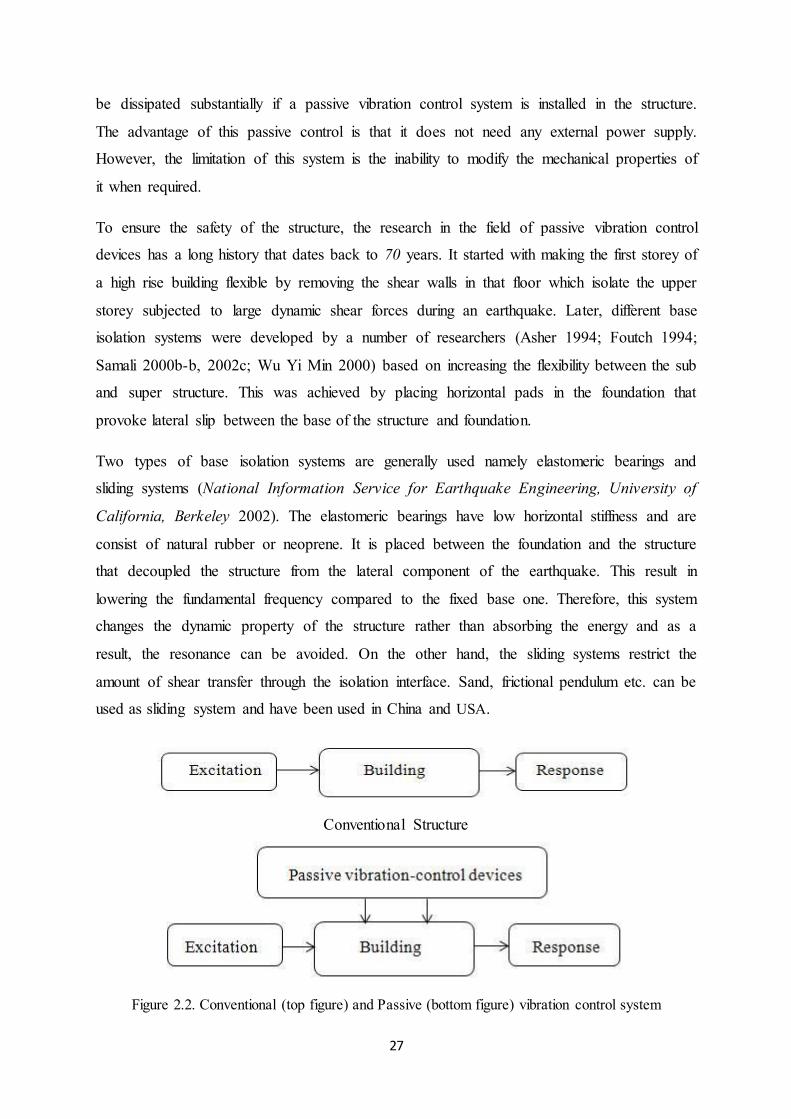
Figure 2.2. Conventional and passive vibration control system …………………………...................27
Figure 2.3. Example of base isolated structures ……………………………...……………………….28
Figure 2.4. Utah state capitol in USA....................................................................................................29
Figure 2.5. Example of structures equipped with Viscoelastic damper and Tuned mass damper…....30
Figure 2.6. Tokyo Skytree.....................................................................................................................31
Figure 2.7. One Wall Centre in Vancouver, equipped with tuned liquid dampers at the top storey.....32
Figure 2.8. Active vibration control system Diagram……..…………………………………………..33
Figure 2.9. Control System Block Diagram…….……………………………………………….…….33
Figure 2.10. Examples of structures equipped with Active mass damper………….………………....35
Figure 2.11. Hybrid vibration control system diagram…………….………………………………….36
Figure 2.12. Experimental structure of the smart base isolation system……………………………....37
Figure 2.13. Examples of structures equipped with Hybrid mass damper…………………………....37
Figure 2.14. Canton tower in Guangzhou, China, completed in 2010..................................................38
Figure 2.15. Typical schematic diagram of semi-active vibration control system ……………..........39
Figure 2.16. Schematic diagram of variable orifice damper ……………………………………........40
Figure 2.17. Kajima Shizuoka building constructed with semi-active hydraulic dampers ……..........41
Figure 2.18. Schematic diagram of variable stiffness device …………………………………...........42
Figure 2.19. Schematic diagram of variable friction damper …………………………………...........43
Figure 2.20. Semi-active TLCD system……………………………………………………………….45
Figure 2.21. Schematic diagram of controllable fluid damper ……………………………….............46
Figure 2.22. Proposed electro rheological fluid damper ………………………………………...........46
Figure 2.23. Schematic of the full-scale 20 ton MR fluid damper …………………………………....47
Figure 2.24. Tokyo national museum installed with 30-t MR fluid dampers …………………...........48
Figure 2.25. MR dampers installation on the Dongting lake bridge, China …………………….........48
Figure 2.26. MR fluid without (left) and with magnetic field (right) …………………………….......50
Figure 2.27. MR fluid when a magnetic field is applied ………………………………………….......51
Figure 2.28. Yield stress vs. magnetic field strength of MRF-122-2ED (LORD Corporation) ……......52
Figure 2.29. Magnetic properties of MRF-122-2ED (LORD Corporation) ………………………….....52
Figure 2.30. Three typical operating modes for MR fluid devices ………............................................53
Figure 2.31. Small-scale SD-1000 MR fluid damper ……………..…………………….......................55
Figure 2.32. Large-scale 20ton MR fluid damper ………….…………………………........................55
Figure 2.33. MR damper RD-1005-3 …………......………...…………......……………………...........55
Figure 2.34. MR dampers installed in a bridge ……….......…………………………………………..56

14
Figure 2.35. Examples of MR dampers installed in a building ………………………………….........56
Figure 2.36. MR damper installed in a washing machine ……………………..……………...............57
Figure 2.37. MR damper applied in lower leg prosthesis ……………....……………………..............57
Figure 2.38. Heavy duty seat suspension with MR damper ………………...………………...............58
Figure 2.39. Characteristics of damper force for different currents provided: (a) non-linearly in force
versus displacement and (b) hysteresis in force versus velocity ………………………...……............58
Figure 2.40. Bingham model for a fluid damper ...............…………....................................................60
Figure 2.41. Verifying the Bingham model with the experimental results ….......................................60
Figure 2.42. Extended Bingham model …………………………........................................................61
Figure 2.43. Verifying the Bingham model with the experimental results ….......................................62
Figure 2.44. Bouc-Wen model of MR damper ……….…..……….......………………………............62
Figure 2.45. Verifying the Bouc Wen model with experimental results .................…….....................63
Figure 2.46. Modified Bouc-Wen model of MR damper ................…………………..........................64
Figure 2.47. Verifying the modified Bouc-Wen model with the experimental results ………...…......64
Figure 2.48. Hysteresis parameters for static hysteresis model of MR damper ……………………....66
Figure 2.49. Boolean functions categorising structural damage............................................................69
Figure 2.50. Fuzzy functions categorising structural damage............................... ................................69
Figure 3.1. El Centro earthquake acceleration time history, normalised to 2g .....................................73
Figure 3.2. Five storey benchmark steel frame .....................................................................................74
Figure 3.3. Membership function for; (a) the acceleration at levels 4 and 5; (b) control force ...........75
Figure 3.4. Simulink model of the five storey building with Fuzzy Logic controllers ........................76
Figure 3.5. Closed-loop model of the fifteen storey structure with fuzzy logic controllers .................78
Figure 3.6. Membership functions of (a) error (e), (b) derivative of error (de/dt), (c) control signal
(u)...........................................................................................................................................................79
Figure 3.7. Displacement of the last storey (m) versus time, ATMD mass ratio of 1%, under El Centro
quake, five storey structure ................................................................................... ................................80
Figure 3.8. Displacement of the last storey (m) versus time, ATMD mass ratio of 2%, under El Centro
quake, five storey structure ............................................................................................. ......................81
Figure 3.9. Displacement of the last storey (m) versus time, ATMD mass ratio of 3%, under El Centro
quake, five storey structure ................................................................................................ ...................81
Figure 3.10. Displacement of the last storey (m) versus time, ATMD mass ratio of 4%, under El Centro
quake, five storey structure ...................................................................................................................81
Figure 3.11. Displacement of sole ATMD at the top floor (m) versus time, under El Centro, five
storey structure ......................................................................................................................................82
Figure 3.12. Displacement of the last storey (m) versus time, ATMD mass ratio of 1%, under El
Centro quake, fifteen storey structure ...................................................................................................82
15
Figure 3.13. Displacement of the last storey (m) versus time, ATMD mass ratio of 2%, under El
Centro quake, fifteen storey structure ..................................................................... ..............................82
Figure 3.14. Displacement of the last storey (m) versus time, ATMD mass ratio of 3%, under El
Centro quake, fifteen storey structure ..................................................................... ..............................83
Figure 3.15. Displacement of the last storey (m) versus time, ATMD mass ratio of 4%, under El
Centro quake, fifteen storey structure .................................................................... ...............................83
Figure 3.16. Displacement of sole ATMD at the top floor (m) versus time, under El Centro, fifteen
storey structure ......................................................................................................................................83
Figure 3.17. Displacement of the fifth floor (m) versus time, 1st floor ATMD + 5th floor ATMD, under
El Centro quake, five storey structure .................................................................... ...............................84
Figure 3.18. Displacement of the fifth floor (m) versus time, 3rd floor ATMD + 5th floor ATMD, under
El Centro quake, five storey structure .................................................................. .................................85
Figure 3.19. Displacement of the third floor (m) versus time, 3rd floor ATMD + 15th floor ATMD,
under El Centro quake, fifteen storey structure ....................................................................................85
Figure 3.20. Displacement of the fifteenth floor (m) versus time, 3rd floor ATMD + 15th floor ATMD,
under El Centro quake, fifteen storey structure ....................................................................................85
Figure 3.21. Displacement of the seventh floor (m) versus time, 7th floor ATMD + 15th floor ATMD,
under El Centro quake, fifteen storey structure ....................................................................................86
Figure 3.22. Displacement of the fifteenth floor (m) versus time, 7th floor ATMD + 15th floor ATMD,
under El Centro quake, fifteen storey structure ....................................................................................86
Figure 3.23. Displacement of the thirteenth floor (m) versus time, 13th floor ATMD + 15th floor ATMD,
under El Centro quake, fifteen storey structure ............................................................. .......................87
Figure 3.24. Displacement of the fifteenth floor (m) versus time, 13th floor ATMD + 15th floor ATMD,
under El Centro quake, fifteen storey structure .............................................. ......................................87
Figure 4.1. Active Multiple Tuned Mass Dampers (AMTMDs) ...........................................................91
Figure 4.2. Last storey displacement (mm) versus time with a sole ATMD on top, the five storey
structure .................................................................................................................................................94
Figure 4.3. Last storey displacement (mm) versus time, equal mass, five storey structure, 3ATMDs on
top .........................................................................................................................................................95
Figure 4.4. Last storey displacement (mm) versus time, non-equal mass, five storey structure,
3ATMDs on top .................................................................................................................. ..................96
Figure 4.5. Last storey displacement (mm) versus time with a sole ATMD on top, fifteen storey
structure ....................................................................................................................... ..........................96
Figure 4.6. Last storey displacement (mm) versus time, equal mass, fifteen storey structure, 3ATMDs
on top ....................................................................................................................................................98
Figure 4.7. Last storey displacement (mm) versus time, non-equal mass, fifteen storey structure,
3ATMDs on top .....................................................................................................................................98

16
Figure 5.1. Self-organising algorithm flowchart …………………………………….……………...104
Figure 5.2. Initial membership functions for all input and output variables ………….…….............113
Figure 5.3. Output versus desired output ……………………………………………………………113
Figure 5.4 Tracking error …………………………………………………………….……………...113
Figure 5.5. Control signal ………………………………………………………….………………..114
Figure 5.6. Number of rules and self-organising flag ……………………………………………....114
Figure 5.7. Final membership functions for input 1 ………………………………………………...115
Figure 5.8. Final membership functions for input 2 ………………………………………………...115
Figure 5.9. Final membership functions for input 3 ………………………………………………...115
Figure 5.10. Initial membership functions for all input and output variables ……………………....116
Figure 5.11. Output versus desired output ………………………..…………………………………116
Figure 5.12. Tracking error ………………………………………………………………......……...117
Figure 5.13. Control signal ……………………………………………………………………….....117
Figure 5.14. Number of rules and self-organising flag …………………………………...................117
Figure 5.15. Final membership functions for input 1 ………………………………………….........118
Figure 5.16. Final membership functions for input 2 ……………………………………………….118
Figure 5.17. Final membership functions for input 3 ……………………………………………….118
Figure 5.18. Initial membership functions for all input and output variables …………...............….120
Figure 5.19. Output versus desired output ………………………………………………………......120
Figure 5.20. Tracking error …………………………………………………………………………120
Figure 5.21. Control signal ………………………………………………………………………….121
Figure 5.22. Number of rules and self-organising flag ……………………………………………...121
Figure 5.23. Final membership functions for input 1 ……………………………………………….121
Figure 5.24. Final membership functions for input 2 ……………………………………………….122
Figure 5.25. Final membership functions for input 3 ……………………………………………….122
Figure 6.1. System schematic diagram ……………………………………………………………...126
Figure 6.2. Damper differential configurations ……………………………………………………..127
Figure 6.3. System block diagram.......................................................................................................131
Figure 6.4. El Centro earthquake acceleration time history …………………………………………132
Figure 6.5. Schematic of a one storey structure equipped with MR dampers ……………………....133
Figure 6.6. The first input of the fuzzy logic controller……………………………………………...134
Figure 6.7. The second input of the fuzzy logic controller…………………………………………..134
Figure 6.8. The third input of the fuzzy logic controller……………………………………………..134
Figure 6.9. Adaptive fuzzy logic controller ………………………………………………………....135
Figure 6.10. Self-organising adaptive fuzzy logic controller ………………………………………..136
Figure 6.11. Simulink model of a one storey building model without MR dampers and fuzzy logic
controller …………………………………………………………….................................................138
17
Figure 6.12. Simulink model of a one storey building model with MR dampers and fuzzy logic
controller ……………………………………………...………………………………......................140
Figure 6.13. Simulink model of a one storey building model with MR dampers and self-organising
adaptive fuzzy logic controller …………………………………………………………....................141
Figure 6.14. Simulink block of the adaptive fuzzy logic controller ………………...........................142
Figure 6.15. Simulink block of non-affine nonlinear system …………………….............................143
Figure 6.16. Displacement time history (m) of the one storey structure …………………………....144
Figure 6.17. Acceleration time history (m/s2) of the one storey structure …………………………..144
Figure 6.18. Initial membership functions for all three input variables ……………………………..145
Figure 6.19. Final membership function for input 1 …………………………………………….......145
Figure 6.20. Final membership function for input 2 …………………………………………….......146
Figure 6.21. Final membership function for input 3 …………………………………………….......146
Figure 6.22. Number of rules and self-organising flag – time …………………………......…..........146
Figure 6.23. Tracking error – time …………………………………………………………………..147
Figure 6.24. Current produced by the controller (A) – time ………………………………………...147
Figure 6.25. Control force provided by the MR damper (N) – time ………………………………....147
Figure 6.26. Five storey benchmark steel frame ………………………………………………….....151
Figure 6.27. Self-organising adaptive fuzzy logic controller for non-affine nonlinear systems….....155
Figure 6.28. Simulink of the five storey structure ………………………………………………......156
Figure 6.29. Displacement time history (m) of the fifth storey ……………………………………..157
Figure 6.30. Initial membership function for all three input variables ……………………………...157
Figure 6.31. Final membership function for input 1 …………………………………………….......158
Figure 6.32. Final membership function for input 2 ………………………………………………...158
Figure 6.33. Final membership function for input 3 ………………………………………………...158
Figure 6.34. No. of rules and self-organising flag – time …………………………………………...159
Figure 6.35. Tracking error – time …………………………………………………………………..159
Figure 6.36. Current produced by the controller – time ……………………………………………..159
Figure 6.37. Control force provided by the MR damper ………….………………………………....160

18
NOTATIONS
A System matrix
B Input matrix for control
C Output matrix
D Matrix to represent direct coupling between input and output for control force
E Input matrix for wind/earthquake excitations
F Matrix to represent direct coupling between input and output for wind/earthquake
excitations
J1-J6 Evaluation criteria
Performance index
u Control force
v Measured noise vector
W External excitations (wind/earthquake)
x State vector (in the control matrix)
Displacement of the storey
Velocity of the storey
Acceleration of the storey
Ground acceleration
Measured output vector
Controlled output vector
Mass matrix
Damping matrix
Stiffness matrix
19
CHAPTER 1
INTRODUCTION
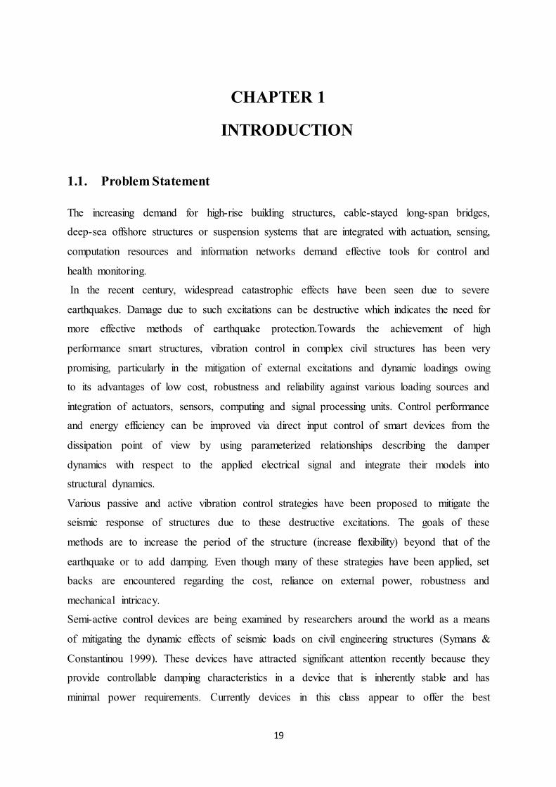
1.1. Problem Statement
The increasing demand for high-rise building structures, cable-stayed long-span bridges,
deep-sea offshore structures or suspension systems that are integrated with actuation, sensing,
computation resources and information networks demand effective tools for control and
health monitoring.
In the recent century, widespread catastrophic effects have been seen due to severe
earthquakes. Damage due to such excitations can be destructive which indicates the need for
more effective methods of earthquake protection.Towards the achievement of high
performance smart structures, vibration control in complex civil structures has been very
promising, particularly in the mitigation of external excitations and dynamic loadings owing
to its advantages of low cost, robustness and reliability against various loading sources and
integration of actuators, sensors, computing and signal processing units. Control performance
and energy efficiency can be improved via direct input control of smart devices from the
dissipation point of view by using parameterized relationships describing the damper
dynamics with respect to the applied electrical signal and integrate their models into
structural dynamics.
Various passive and active vibration control strategies have been proposed to mitigate the
seismic response of structures due to these destructive excitations. The goals of these
methods are to increase the period of the structure (increase flexibility) beyond that of the
earthquake or to add damping. Even though many of these strategies have been applied, set
backs are encountered regarding the cost, reliance on external power, robustness and
mechanical intricacy.
Semi-active control devices are being examined by researchers around the world as a means
of mitigating the dynamic effects of seismic loads on civil engineering structures (Symans &
Constantinou 1999). These devices have attracted significant attention recently because they
provide controllable damping characteristics in a device that is inherently stable and has
minimal power requirements. Currently devices in this class appear to offer the best
20
opportunity for widespread acceptance of these innovative control techniques by the civil
engineering community. Examples of such devices include variable orifice fluid dampers,
variable friction dampers, adjustable tuned liquid dampers and controllable fluid dampers.
Magneto Rheological (MR) dampers are classified as controllable fluid devices (Spencer et al.
1997). These devices have demonstrated a great deal of promise for civil engineering
applications in studies. Both experimental and analytical studies have demonstrated that the
performance of MR dampers is superior to that of comparable passive and active control
systems.
Due to the high nonlinearity of MR devices, one of the main challenges in the application of
this technology is in the development of suitable control algorithms. A variety of semi-active
control algorithms have been developed, including Lyapunov, decentralized bang-bang,
modulated homogeneous friction, bi-state control, fuzzy logic control methods (Sun & Goto
1994), adaptive nonlinear control and clipped-optimal. Previous analytical investigations of a
selection of these algorithms have demonstrated that the performance of control systems
based on MR dampers is highly dependent on the choice of algorithms employed (Jansen &
Dyke 2000).
In this study, fuzzy logic controllers are proposed for the control. They have shown to be
especially effective in the control of mathematically ill-understood processes; fuzzy logic
controllers thus can address directly important issues of intelligent control such as robustness
and conformability to the linguistic rules (Tong, Li & Chai 1999).
An adaptive fuzzy controller can be defined as a controller, in which adaptive fuzzy systems
are employed and adaptive control theory is used to derive training algorithms such that
stability and performance of the closed-loop system are guaranteed. Lyapunov stability
techniques play a critical role in the design and stability analysis of the adaptive systems. A
Lyapunov function candidate is a mathematical function designed to provide a simplified
scalar measure of the control objectives. The control objectives are met when the chosen
Lyapunov function is driven to zero.
Now, fixed-structured adaptive fuzzy logic control (Wang 1994) requires designers to choose
the rule base and membership functions by trial and error. This task is not trivial as long as
exact mathematical models of plants are not known. Quite often, the structure used is either
unnecessarily large or too small to adequately represent a plant.
From this perspective, self-structuring adaptive fuzzy logic control is more advantageous as it
can automatically add and remove rules from a fuzzy system. Park et al (Park, Park, et al.
2005b) proposed a self-structuring fuzzy system, in which rules are added to the rule base

21
when exploring the input space. However no mechanism to remove rules is proposed therein.
Gao and Er (2003) proposed a self-organizing fuzzy neural system, in which rules are
generated using the system error and completeness and an error reduction ratio concept is
used for rule pruning. In (Phan & Gale 2008), a self-organising adaptive fuzzy logic
controller is presented, which employs the system error, the -completeness and a simple
algorithm to replace rules.
1.2. Objectives and scope of the Thesis
This research is concerned with a numerical analysis of a one and five storey steel structure
integrated with a pair of Magneto Rheological (MR) dampers in addition to fuzzy logic
controllers. The building structural model is subject to scaled earthquake records. The static
hysteresis model is adopted for the MR damper, in which nonlinear functions are used to
represent hysteresis in the damper characteristics. In this thesis, the current-controlled
problem of the smart structure system is formulated in non-affine state space equations.
Adaptive fuzzy logic control is proposed to deal with nonlinearity of the control dynamics
and non-affinity in the control input, assuming the availability of the input of the fuzzy logic
controller. Most adaptive fuzzy logic controller schemes employ fuzzy inference systems
with fixed structures. In which, a designer must specify the number of membership functions
and the rule base by trial and error. In many cases, this task is not trivial as exact
mathematical models of plants are generally not known. Thus, it is often known that the
fuzzy inference system used is unnecessarily large or too small to adequately represent the
plant. Therefore, self-organising adaptive fuzzy logic control is proposed in this thesis to
overcome this setback. To illustrate the effectiveness of the proposed control scheme on
seismic vibration suppression of the structures due to earthquake excitations, simulation
results are presented together with discussions on its evaluation and further remarks on the
implementation aspect.
1.3. Contribution of this thesis
The development of this thesis is firstly focusing on the fixed adaptive fuzzy logic control
which requires designers to choose the rule base and membership functions by trial and error.
Then, the main contribution of this research is to design self-organising adaptive fuzzy logic
controllers as it can automatically add and remove rules from a fuzzy inference system. This
22
contribution is of significance, given the nonlinearity and non-affinity of the structural
control system model.
1.4. Thesis Layout
Chapter one gives a background of the research project, outlines the objectives of this
research study and the approaches taken.
Chapter two details most of the related literature review for this study. It begins with a
detailed description of passive and active vibration control systems and then moves on to
semi-active vibration control systems and focuses on their advantages compared to the active
and passive ones. This chapter also focuses on MR fluids and devices and its applications.
Modelling and control of MR dampers are also discussed. In the final section of this chapter,
the control algorithms used to drive the active or semi-active control system are described. It
starts with the description of Lyapunov and linear quadratic regulator (LQR) and then a brief
review on fuzzy logic control is presented.
Chapter three considers active tuned mass dampers in two different structures, five and
fifteen storey structures. Different mass ratios (mass of ATMD/mass of total structure)
ranging from 1 to 4% have been assumed for the two structures and the seismic vibration
reduction (displacement of the last storey) is compared in different cases. In another case, two
ATMDs are installed in different floors for both the two structures and the displacement of the
last storey is seen to be reduced in different cases.
Chapter four describes the application of multiple tuned mass dampers (MTMD) in two
different structures, five and fifteen storey structures. The reduction in displacement of the
last storey is compared in different scenarios; a sole ATMD on the top floor, multiple ATMDs
with equal and non-equal mass on the top floor, both for the five and fifteen storey structures.
Chapter five describes self-organising adaptive fuzzy logic controllers. A description is
presented along with its application in affine and non-affine nonlinear systems. Numerical
examples are provided to further explain the approach.

23
Chapter six focuses on the description of controlled buildings and excitations, the equation of
motion of the structure with semi-active vibration suppression devices is given and the non-
affine nonlinear equations encountered are discussed. In addition, the simulation of a one and
five storey structure embedded with MR dampers and earthquake excitations are subjected on
it. The design of fuzzy logic controller is compared to self-organising adaptive fuzzy logic
controller. Simulation results of this one and five storey structure are presented. Some
evaluation criteria are defined to compare the results with an uncontrolled structure with no
MR damper and no controller.
Chapter seven discusses the final conclusions of this thesis and further considerations for
future researches.

24
CHAPTER 2
LITERATURE REVIEW
2.1. Introduction
Building structures subjected to external loads; earthquake or wind induce catastrophic
vibrations in the structure which may result in severe damage and reduce the durability.
Therefore, it is important to ensure the safety of the occupants inside the structure and the
structure itself by mitigating or controlling these vibrations. To achieve this, different types
of control devices are developed over the past few decades and still are the focus of research.
Yao (1972) developed the concept of structural control, and this idea has been adopted and
applied in different types of structures.
Soong (Soong 1990) suggested to consider four main criteria in order to develop any
structural control system. These are as follows:
Nowadays many high rise structures are constructed to accommodate the increasing
population. Therefore, these structures are very stiff and unable to reduce the
vibration under the extreme environmental load. Hence, the flexibility of the structure
needs to be increased to mitigate the effect of external load on it.
The high rise buildings are usually complex and also expensive which requires the
increase of safety levels.
It is essential to ensure the best performance of the building in terms of serviceability
and strength within the safety limits.
The materials should be used in such a way that it is cost efficient and safe.
In USA and Japan, extensive usages of structural control devices are observed for buildings
and bridges. The structural control system is a multi-disciplinary area which covers the field
of wind and earthquake engineering, structural dynamics, control theory, sensing technology,
computer science, data processing and material science.
The main idea of the structural control system is to change the property of the structure when
it is subjected to earthquake excitation in order to withstand the external load safely. This can
be attained by reducing the excitation subjected to the structures or by providing additional
25
damping device for the dissipation of energy. The structural control system can be
categorised as following
Passive vibration control devices: To operate this system, it is not required to have
external power supply.
Active vibration control devices: External power supply is essential in significant
amount for the functional operation of the system.
Hybrid vibration control devices: It combines both the passive and active devices.
Semi-active vibration control system: Only an optimum amount of external power is
required to run this system and therefore, can be considered as a compromise of
passive and active control system.
Frequency is the key parameter for the structural control devices and classification of the
system is illustrated in figure 2.1. Both the frequency dependent and frequency independent
systems are used as control devices as shown in the figure. Frequency dependent systems
dissipate the energy of the excitation subjected on the structure and are independent of the
natural frequency of the structure. The frequency dependent can be further divided into
resonant and non-resonant types that can prevent resonance. Tuned mass damper and hybrid
mass damper are considered as resonant type whereas base isolation and active variable
stiffness are the examples of non-resonant types since they reduced the energy produced by
the earthquake. Frequency independent system is subdivided into passive, active and semi-
active devices. Viscous damper is a passive control device, while active mass driver and
active tendon are categorised as active control devices due to producing counteracting control
forces using external energy supplied. Some examples of frequency independent semi-active
devices are controllable fluid (electro rheological/ER, magneto rheological/MR) damper,
variable friction damper, variable orifice damper, etc.
Different control algorithms are available to implement for controlling the structures
(Friedland 1986; Leipholz & Abdel-Rohman 1986; Nguyen 1998; Ogata 1967, 1987; Ogata
& Yang 1970). A control system commands the device installed in the structure to regulate it
and also to control itself. A control system is comprised of actuators, controllers, sensors,
plants, etc. and can be applied in a building, bridge, heating furnace or even in a chemical
reactor. A control algorithm defines the specification of the control signal that operates in
each time interval, and it is influential to different factors including stability, reliability,
economy, efficiency and performance. Consequently, control algorithm is considered as the

26
key element for any structural control system. Depending on the requirements of the
structures, a selection of control algorithm may differ and hence, various control algorithms
are available. For instance, linear quadratic regulator (LQR), sliding mode control, neural
networks (NN), fuzzy logic controls (FLC) are widely used control algorithms.
This chapter describes the concept of different structural vibration control systems,
development of the control devices and the control algorithms. As this research project
mainly focuses on the semi-active vibration control system and therefore, a brief explanation
of this system will be presented in the later section of the chapter.
2.2. Passive vibration control systems
The prime goal of the passive vibration control system is to reduce the structural response by
dissipating the energy which is achieved by improving the motion of the structure in order to
produce relative motions within the passive devices. The energy dissipation capacity
influences the amplitude of the vibration which needs to be controlled. A control system with
large energy dissipation capacity will reduce the amplitude of the vibration to a great extent.
The increase in energy dissipation capacity can be achieved by different methods which
results in enhancing the performance of the passive vibration control system.
The difference between a conventional structure and a structure with a vibration control
system is demonstrated in figure 2.2. A conventional structure cannot control the vibration
due to the increase in energy from the earthquake. Subsequently, there is a direct effect on the
structure that may lead to the collapse of the structure. In contrast, the earthquake energy can
Figure 2.1. Classification of Structural control Devices
27
be dissipated substantially if a passive vibration control system is installed in the structure.
The advantage of this passive control is that it does not need any external power supply.
However, the limitation of this system is the inability to modify the mechanical properties of
it when required.
To ensure the safety of the structure, the research in the field of passive vibration control
devices has a long history that dates back to 70 years. It started with making the first storey of
a high rise building flexible by removing the shear walls in that floor which isolate the upper
storey subjected to large dynamic shear forces during an earthquake. Later, different base
isolation systems were developed by a number of researchers (Asher 1994; Foutch 1994;
Samali 2000b-b, 2002c; Wu Yi Min 2000) based on increasing the flexibility between the sub
and super structure. This was achieved by placing horizontal pads in the foundation that
provoke lateral slip between the base of the structure and foundation.
Two types of base isolation systems are generally used namely elastomeric bearings and
sliding systems (National Information Service for Earthquake Engineering, University of
California, Berkeley 2002). The elastomeric bearings have low horizontal stiffness and are
consist of natural rubber or neoprene. It is placed between the foundation and the structure
that decoupled the structure from the lateral component of the earthquake. This result in
lowering the fundamental frequency compared to the fixed base one. Therefore, this system
changes the dynamic property of the structure rather than absorbing the energy and as a
result, the resonance can be avoided. On the other hand, the sliding systems restrict the
amount of shear transfer through the isolation interface. Sand, frictional pendulum etc. can be
used as sliding system and have been used in China and USA.
Conventional Structure
Figure 2.2. Conventional (top figure) and Passive (bottom figure) vibration control system

28
The base isolation system has been applied to many structures across the world over the last
two decades. Figure 2.3 shows the first base isolated building built in USA in 1985 which was
the office of Foothill community law and justice centre. This was a four storey frame
structures incorporating braced frames in some bays to stiffen the building and also, a
basement and sub-basement for the isolation system. There were a total of 98 isolators of
multi-layered natural rubber bearings in this base isolation system. The system was
reinforced with steel plates. Another application of base isolation system is the University of
Southern California teaching hospital, Los Angeles (1991), which is an eight storey braced
steel frame. It consists of 68 lead rubber isolators and 81 elastomeric isolators. During the
Northridge earthquake in 1994, this building performed well which explains the effectiveness
of the system.
Foothill Communities and Justice Centre (1985) University of Southern California Teaching Hospital (1991)
Figure 2.3. Example of base isolated structures
Besides USA, Japan also implemented base isolation systems, and the first one constructed
was the Yachiyo-Dai House (1983). By the end of 1998, there were approximately 550 base
isolation building built in the USA and Japan, respectively. The Matsumura-Gumi research
laboratory and the West Japan postal savings computer centre are also examples of base
isolation systems and survived the destructive Kobe earthquake in Japan.
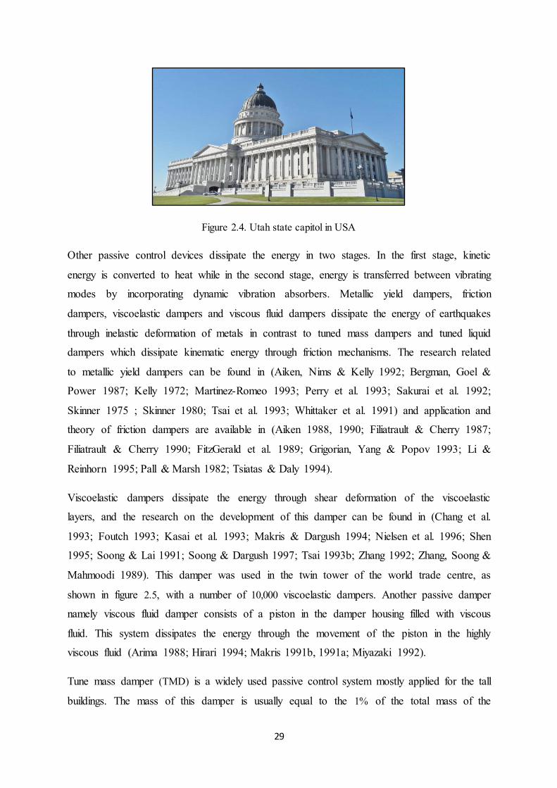
The Utah state capitol in USA, finished in 2008 is shown in figure 2.4. It stands in an
earthquake zone where seismic monitoring stations record more than 700 earthquakes each
year. This is a monumental, four storeys, reinforced concrete building with granite cladding
and a large copper-clad concrete dome. The base isolation system consists of 265 isolators,
each weighing 5000 pounds.
29
Figure 2.4. Utah state capitol in USA
Other passive control devices dissipate the energy in two stages. In the first stage, kinetic
energy is converted to heat while in the second stage, energy is transferred between vibrating
modes by incorporating dynamic vibration absorbers. Metallic yield dampers, friction
dampers, viscoelastic dampers and viscous fluid dampers dissipate the energy of earthquakes
through inelastic deformation of metals in contrast to tuned mass dampers and tuned liquid
dampers which dissipate kinematic energy through friction mechanisms. The research related
to metallic yield dampers can be found in (Aiken, Nims & Kelly 1992; Bergman, Goel &
Power 1987; Kelly 1972; Martinez-Romeo 1993; Perry et al. 1993; Sakurai et al. 1992;
Skinner 1975 ; Skinner 1980; Tsai et al. 1993; Whittaker et al. 1991) and application and
theory of friction dampers are available in (Aiken 1988, 1990; Filiatrault & Cherry 1987;
Filiatrault & Cherry 1990; FitzGerald et al. 1989; Grigorian, Yang & Popov 1993; Li &
Reinhorn 1995; Pall & Marsh 1982; Tsiatas & Daly 1994).
Viscoelastic dampers dissipate the energy through shear deformation of the viscoelastic
layers, and the research on the development of this damper can be found in (Chang et al.
1993; Foutch 1993; Kasai et al. 1993; Makris & Dargush 1994; Nielsen et al. 1996; Shen
1995; Soong & Lai 1991; Soong & Dargush 1997; Tsai 1993b; Zhang 1992; Zhang, Soong &
Mahmoodi 1989). This damper was used in the twin tower of the world trade centre, as
shown in figure 2.5, with a number of 10,000 viscoelastic dampers. Another passive damper
namely viscous fluid damper consists of a piston in the damper housing filled with viscous
fluid. This system dissipates the energy through the movement of the piston in the highly
viscous fluid (Arima 1988; Hirari 1994; Makris 1991b, 1991a; Miyazaki 1992).
Tune mass damper (TMD) is a widely used passive control system mostly applied for the tall
buildings. The mass of this damper is usually equal to the 1% of the total mass of the

30
structures and installed at the top of the building by means of spring. The primary goal of
TMD is to increase the damping of the structure by tuning it with the primary structure. A
number of research were conducted, both numerically and experimentally, to determine the
efficiency of TMD and concluded that the effectiveness varies with earthquakes (Villaverde
1994). TMD can reduce the vibration of the fundamental mode given that it is tuned with the
first natural frequency of the structure. However, the higher order modes may suppress
slightly or may even amplify. To overcome this limitation, Clark (Clark 1988) proposed the
use of multiple tuned mass dampers where each one is tuned to a different dominant
frequency. It is important to consider the amount of added on the top of the building and also
the movement of TMD relative to the building while designing it. The research on the
improvement of TMD is available in (Li, Shen & Choo 1994; Matsuhisa 1994; Setareh 1994;
Xu 1992; Yamaguchi & Harnpornchai 1993). Some application of TMD can be found in
Sydney centre point tower (Australia), the Citicorp centre in New York City and the John
Hancock tower in Boston (USA) and Chiba port tower (Japan), as shown in figure 2.5.
World Trade Centre (1969) Centre point Tower (1980) Chiba Port Tower (1986)
Figure 2.5. Example of structures equipped with Viscoelastic damper and tuned mass damper
The Tokyo Skytree, as shown in figure 2.6, is a broadcasting, restaurant, and observation
tower in Tokyo, Japan. It became the tallest structure in Japan in 2011, with a full height of
634.0 metres (2,080 ft). Two types of vibration control system are used in this structure; TMDs
on the top and the Core Column System. As a tower that is used for terrestrial digital
broadcasting, it is necessary to suppress the wind response of the gain tower at the top of the
tower on which the broadcasting antennae are installed. Specifically, the velocity of the

31
oscillations of the gain tower due to normal wind, which has a high frequency of occurrence,
was required to be maintained less than a specified value. For this purpose two TMDs were
installed on the top of the tower.
Figure 2.6. Tokyo Skytree
Tuned liquid damper (TLD) and tuned liquid column damper (TLCD) are also passive
vibration control devices where structural energy is absorbed by the viscous actions of the
fluid in TLD, and the dissipation of energy is attained by the passage of liquid through an
orifice in TLCD. The performance of TLD and TLCD in a building is reported in (Fujino et al.
1988; Mayol 2002; Samali 2000b-a, 2000a; Tamura 1995; Yeh 1996b).
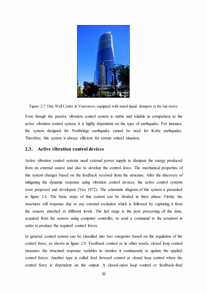
One Wall Centre, as shown in figure 2.7, also known as the Sheraton Vancouver Wall Centre
hotel, is a 48-storey skyscraper hotel with residential condominiums in Vancouver, Canada
which was completed in 2001. To counteract possible harmonic swaying during high winds,
this structure has a tuned water damping system at the top level which consists of two
specially designed 50,000-imperial-gallon (60,000 U.S. gal; 227,300 L) water tanks. These tanks
are designed so that the harmonic frequency of the sloshing of the water in the tanks
counteracts the harmonic frequency of the swaying of the building.
32
Figure 2.7. One Wall Centre in Vancouver, equipped with tuned liquid dampers at the top storey
Even though the passive vibration control system is stable and reliable in comparison to the
active vibration control system, it is highly dependent on the type of earthquake. For instance,
the system designed for Northridge earthquake cannot be used for Kobe earthquake.
Therefore, this system is always efficient for certain critical situation.
2.3. Active vibration control devices
Active vibration control systems need external power supply to dissipate the energy produced
from an external source and also to develop the control force. The mechanical properties of
this system changes based on the feedback received from the structure. After the discovery of
mitigating the dynamic response using vibration control devices, the active control systems
were proposed and developed (Yao 1972). The schematic diagram of this system is presented
in figure 2.8. The basic steps of this system can be divided in three phase. Firstly, the
structures will response due to any external excitation which is followed by capturing it from
the sensors attached at different levels. The last stage is the post processing of the data,
acquired from the sensors using computer controller, to send a command to the actuators in
order to produce the required control forces.
In general, control system can be classified into two categories based on the regulation of the
control force, as shown in figure 2.9. Feedback control or in other words, closed loop control
measures the structural response variables to monitor it continuously to update the applied
control forces. Another type is called feed forward control or closed loop control where the
control force is dependent on the output. A closed-open loop control or feedback-feed

33
forward control is defined as utilizing both the structural responses and external excitation in
the control design development phase.
Figure 2.8.Active vibration control system Diagram
Figure 2.9. Control System Block Diagram
Similar to the passive vibration control system, several researches were carried out to develop
the control algorithms for active vibration control systems in order to enhance the
performance of the control system. Different active vibration control devices can be found in
the literature and also in the application, such as, pulse control (Masri 1980, 1981; Miller et
al. 1988; Reinhorn, Manolis & Wen 1987; Udwadia 1981), active bracing (Dyke et al. 1995;
Loh, Lin & Chung 1999), active tendons (Abdel-Rohman & Leipholz 1983; Agrawal, Yang
& Wu 1998; Samali, Yang & Liu 1985; Soong et al. 1991; Spencer, Dyke & Deoskar 1998;
Yang 1982; Zhang et al. 1993), active mass damper(Adhikari 1998; Hoare 1994; Kobori et al.
1991; Koshika et al. 1992; Samali 2000c; Suhardjo, Spencer Jr & Kareem 1992), etc.

34
To specify a control strategy for determining required control force applicable to the
structure, control algorithm plays a vital role. Therefore, this is an important area of research,
and so, many researchers developed and proposed different control algorithms depending on
the requirements, which includes, Linear quadratic regulator/LQR(Yang 1982),(Abdel-
Rohman & Leipholz 1983),(Chang & Soong 1980; Chung, Reinhorn & Soong 1988; Ikeda
1998; Indrawan et al. 1994; Soong et al. 1991; Watanabe 1992; Yang, Li & Vongchavalitkul
1994),(Soong & Spencer Jr Reviewer 1992), robust control (Dyke, Spencer Jr, Quast, et al.
1996; Spencer Jr, Suhardjo & Sain 1994; Suhardjo, Spencer & Sain 1990; Yoshida 1998),
sliding mode control (Adhikari 1998; Cai et al. 2000; Edwards & Spurgeon 1998; Jianchun &
Bijan 2002; Li 2001; Singh 1998; Yang, Wu & Agrawal 1995a, 1995b; Yang et al. 1997;
Yang et al. 1996; Yang 1994b, 1994d; Yang et al. 1994), adaptive control (Baba 1998; Smith,
Burdisso & Suarez 1994) neural network control (Bani-Hani & Ghaboussi 1998; De Stefano
1999; Ghaboussi & Joghataie 1995; Hung, Kao & Lee 2000; Hung & Lai 2001), nonlinear
control (Agrawal & Yang 1997; Agrawal & Yang 1996; Hatada 1998; Spencer et al. 1996),
fuzzy logic control (Al-Dawod et al. 1999a, 1999b; Aldawod et al. 1999; Aldawod et al.
2001; Casciati & Giorgi 1996; Kawamura & Yao 1990; Naghdy et al. 1998; Samali & Al-
Dawod 2003), etc.
Due to the advantages of utilising active vibration control system for full scale application,
many structures can be found across the world equipped with active vibration control devices.
The first building was built in Tokyo in 1989, named Kyobashi Seiwa building, as shown in
figure 2.7. This is an11 storey commercial building equipped with two active mass dampers
as vibration control devices which are a pendulum type dual mass system. These dampers are
able to control lateral and torsional vibration excited from moderate earthquake or strong
wind. Another application of this system can be observed at Riverside Sumida central tower
in Tokyo, completed in1994. This is a 33 storey building and equipped with two active mass
dampers placed at the roof of the tower (Suzuki et al. 1994; Watanabe et al. 1994).
In comparison to passive vibration control systems, the efficiency of the active vibration
control systems is more beneficial in terms of its capability to control the structural response
at any desired level. Additionally, the influences of ground motion, geographical and site
location have less effect on this system. The biggest concern and shortcoming of this system
is the requirement of a large amount of external power supply which may be unavailable
during a strong earthquake and will eventually lead to the system failure.

35
2.4. Hybrid vibration control devices Hybrid vibration control system utilizes the benefits of the passive and active vibration
control system in order to overcome the shortcomings of these two systems, and therefore,
perform better than passive and active vibration control system alone. This system can work
as a passive system when there is a power failure due to a strong earthquake. Similarly, it
uses the advantage of an active control system by enhancing the performance of a passive
control system. Also, this system requires less energy compared to an active vibration control
system.
Hybrid vibration control system can be used as hybrid base isolation system or as a hybrid
mass damper. The hybrid base isolation system is the combination of an active device and
base isolation, whereas the hybrid mass dampers (HMD) combine passive tuned mass damper
with an active actuator.
Kyobashi Seiwa Building (1989) Riverside Sumida Central Tower (1994) Figure 2.10. Examples of structures equipped with Active mass damper
The development of hybrid mass dampers can be found in a number of researches, this
includes, an arch-shaped HMD developed for bridge tower construction, building response
reduction and ship roll stabilization (Tanida et al. 1991), a V-shaped HMD, which is an
extension of the arch-shaped HMD having an easily adjustable fundamental period (Koike et
al. 1994), a multistep pendulum HMD (Yamazaki, Nagata & Abiru 1992), a structure
equipped with a DUOX HMD to achieve high control efficiency with a small actuator force
(Kobori 1996; Ohrui et al. 1994), etc.
36
The experimental verification has been conducted by many researchers and can be found in
(Kelly, Leitmann & Soldatos 1987; Reinhorn & Riley 1994; Reinhorn, Soong & Wen 1987;
Yoshida, Kang & Kim 1994). The combination of an active vibration control device with a
base isolator installed in the structure improves the performance of the system in terms of
reducing the absolute acceleration and inters storey drift as the base isolator alone needs a
large absolute base displacement. As a result, it is possible to reduce the inter-storey drift and
maximum base displacement by adding an active vibration control device to form a combined
system.
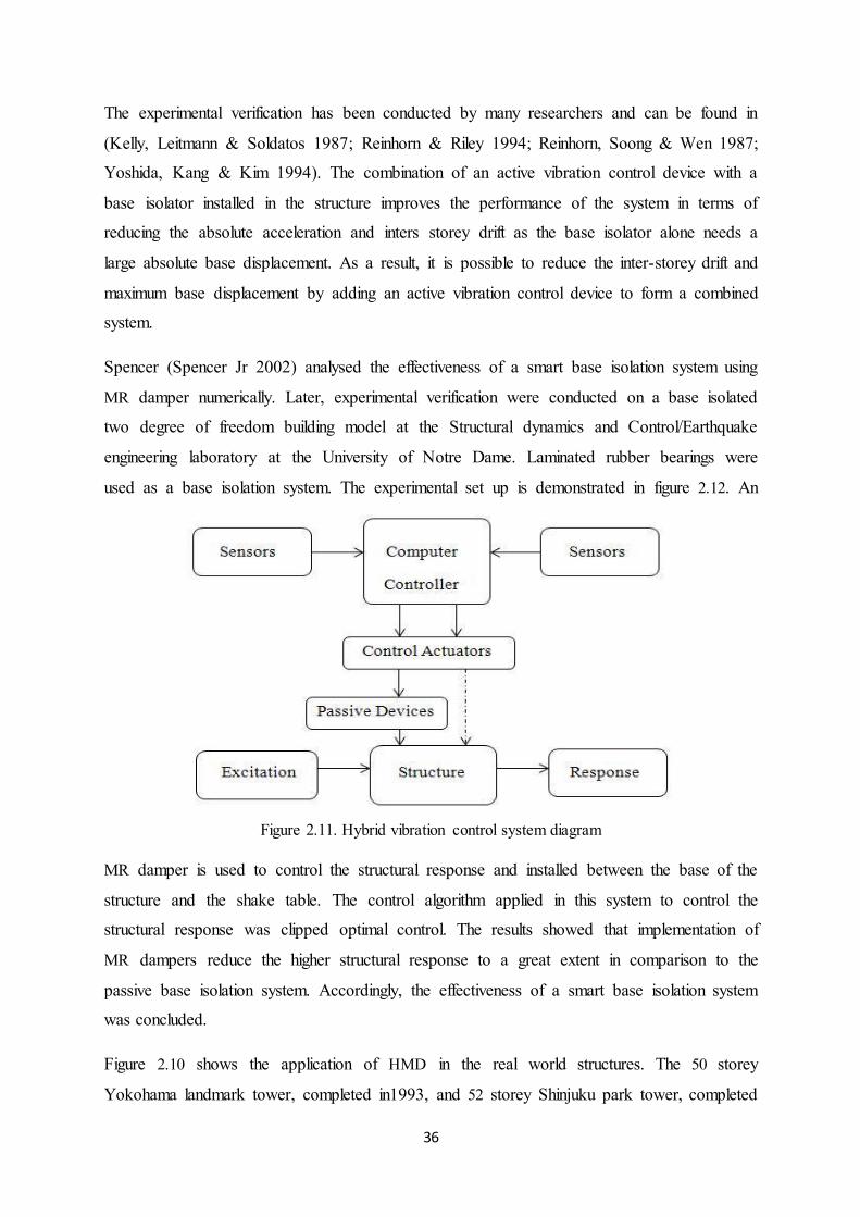
Spencer (Spencer Jr 2002) analysed the effectiveness of a smart base isolation system using
MR damper numerically. Later, experimental verification were conducted on a base isolated
two degree of freedom building model at the Structural dynamics and Control/Earthquake
engineering laboratory at the University of Notre Dame. Laminated rubber bearings were
used as a base isolation system. The experimental set up is demonstrated in figure 2.12. An
MR damper is used to control the structural response and installed between the base of the
structure and the shake table. The control algorithm applied in this system to control the
structural response was clipped optimal control. The results showed that implementation of
MR dampers reduce the higher structural response to a great extent in comparison to the
passive base isolation system. Accordingly, the effectiveness of a smart base isolation system
was concluded.
Figure 2.10 shows the application of HMD in the real world structures. The 50 storey
Yokohama landmark tower, completed in1993, and 52 storey Shinjuku park tower, completed
Figure 2.11. Hybrid vibration control system diagram

37
in1994, are examples of HMD where the former one is equipped with two multi-step
pendulum HMDs and latter one contains three V-shaped HMDs. Another example of this
system is the 7 storey Kansai International airport control tower located in Osaka, Japan
which was completed in 1992.
Figure 2.12. Experimental structure of the smart base isolation system
Yokohama Landmark Tower (1993) Shinjuku Park Tower (1994)
Figure 2.13. Examples of structures equipped with Hybrid mass damper
Canton tower, as shown in figure 2.14, is a landmark of the city centre business area of China,
with a total height of 600 meters, completed in 2010. It houses a restaurant, observatory and
telecommunications facilities. The main tower is 454 meters tall with a 146 meter tall antenna
on top. The HMD is composed of a passive tuned mass damper with two-stage damping level,
and a compact active mass damper, which is driven by linear induction motors mounted on
the tuned mass damper. In case of a failure in HMD control system, the system would become
a passive TMD.
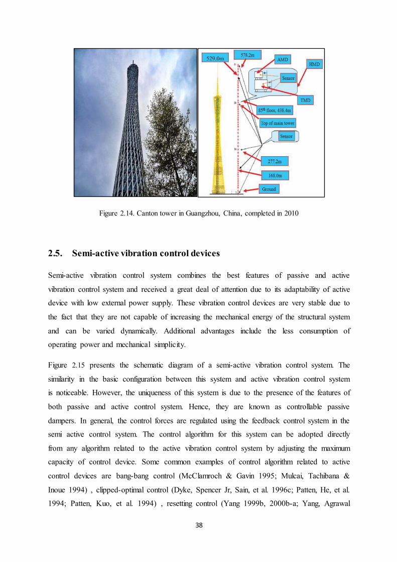
38
Figure 2.14. Canton tower in Guangzhou, China, completed in 2010
2.5. Semi-active vibration control devices
Semi-active vibration control system combines the best features of passive and active
vibration control system and received a great deal of attention due to its adaptability of active
device with low external power supply. These vibration control devices are very stable due to
the fact that they are not capable of increasing the mechanical energy of the structural system
and can be varied dynamically. Additional advantages include the less consumption of
operating power and mechanical simplicity.
Figure 2.15 presents the schematic diagram of a semi-active vibration control system. The
similarity in the basic configuration between this system and active vibration control system
is noticeable. However, the uniqueness of this system is due to the presence of the features of
both passive and active control system. Hence, they are known as controllable passive
dampers. In general, the control forces are regulated using the feedback control system in the
semi active control system. The control algorithm for this system can be adopted directly
from any algorithm related to the active vibration control system by adjusting the maximum
capacity of control device. Some common examples of control algorithm related to active
control devices are bang-bang control (McClamroch & Gavin 1995; Mulcai, Tachibana &
Inoue 1994) , clipped-optimal control (Dyke, Spencer Jr, Sain, et al. 1996c; Patten, He, et al.
1994; Patten, Kuo, et al. 1994) , resetting control (Yang 1999b, 2000b-a; Yang, Agrawal
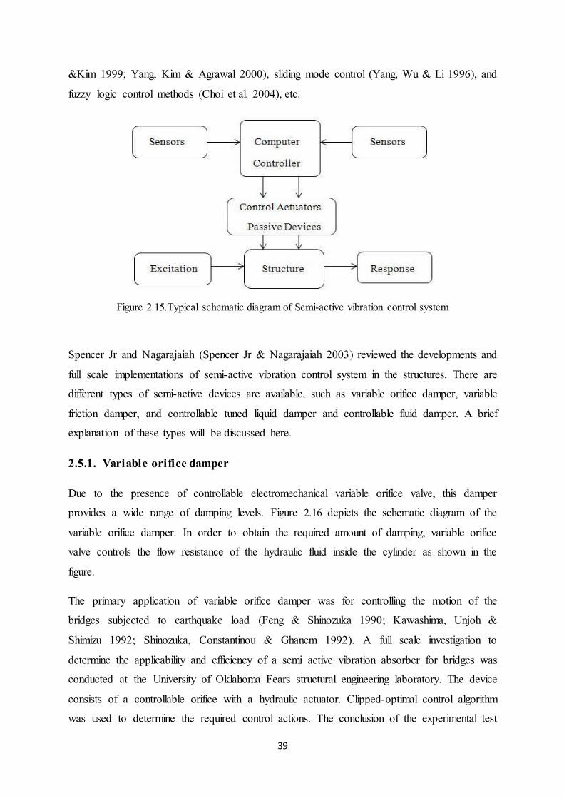
39
&Kim 1999; Yang, Kim & Agrawal 2000), sliding mode control (Yang, Wu & Li 1996), and
fuzzy logic control methods (Choi et al. 2004), etc.
Figure 2.15.Typical schematic diagram of Semi-active vibration control system
Spencer Jr and Nagarajaiah (Spencer Jr & Nagarajaiah 2003) reviewed the developments and
full scale implementations of semi-active vibration control system in the structures. There are
different types of semi-active devices are available, such as variable orifice damper, variable
friction damper, and controllable tuned liquid damper and controllable fluid damper. A brief
explanation of these types will be discussed here.
2.5.1. Variable orifice damper
Due to the presence of controllable electromechanical variable orifice valve, this damper
provides a wide range of damping levels. Figure 2.16 depicts the schematic diagram of the
variable orifice damper. In order to obtain the required amount of damping, variable orifice
valve controls the flow resistance of the hydraulic fluid inside the cylinder as shown in the
figure.
The primary application of variable orifice damper was for controlling the motion of the
bridges subjected to earthquake load (Feng & Shinozuka 1990; Kawashima, Unjoh &
Shimizu 1992; Shinozuka, Constantinou & Ghanem 1992). A full scale investigation to
determine the applicability and efficiency of a semi active vibration absorber for bridges was
conducted at the University of Oklahoma Fears structural engineering laboratory. The device
consists of a controllable orifice with a hydraulic actuator. Clipped-optimal control algorithm
was used to determine the required control actions. The conclusion of the experimental test

40
reported that a reduction of 65 – 70% in peak amplitude can be achieved by using this system
(Patten, He, et al. 1994; Patten, Kuo, et al. 1994; Sack & Patten 1994; Varadarajan &
Nagarajaiah 2004; Wongprasert & Symans 2005). The numerical simulation and
experimental studies have been conducted to demonstrate the performance of variable orifice
damper to mitigate the excitation of a building under seismic load (Hrovat, Barak & Rabins
1983; Mizuno et al. 1992).
Figure 2.16. Schematic diagram of Variable orifice damper
Both the analytical and experimental researches were carried out for the development of
active variable damping system (Kurata 1994, 1996). The component of this control device
comprised of a variable hydraulic damper and a damping force controller. The latter one
consists of a piston, a double rod cylinder and a flow control valve that controlled the
opening level of the valve. The required damping force was controlled by the opening of the
flow control valve. The power consumed by this control device was 30 watts and velocity
sensors and a control computer were attached with the device. The control algorithm used for
this device was the velocity feedback control based on optimal control. The investigation
showed that the generation of required damping force with this control device was very close
to the control force command. Besides, the reduction of the structural response of the active
variable damping system was significantly satisfactory.

41
In the real world, the use of semi-active hydraulic damper can be observed where the
variation of the opening rate of the control valve controls the damping force (Kurata 2001;
Kurata et al. 2000; Kurata et al. 1998; Matsunaga 1998). A full scale installation of a semi
active hydraulic damper took place at Kajima, Japan in 1998, as depicted in figure 2.17.
Kajima Shizoka is an office building where the installed semi-active vibration control device
can produce a maximum damping force of 1000kN using an electric power of 70 watts. To
measure the response of the building, velocity sensors were used in the control system. The
minimization of the structural response is obtained by determining the required damping. The
control computers are programmed to command the damper to generate the necessary
damping force. Also, effective and continuous operation was ensured by installing a power
supply unit in case of power shut down due to an earthquake. The control algorithm used in
the building is linear quadratic regulator which is based on relative and absolute velocity
feedback. The results ensured an effective reduction in structural response of the structure
with this semi-active damper.
In some research, active variable stiffness systems have been considered as seismic response
control systems (Kamagata & Kobori 1994; Kobori & Kamagata 1992; Kobori et al. 1993;
Nasu et al. 1996).This system controls the structural characterises of a building, such as
stiffness, by mitigating the structural response when subjected to external excitations. In these
works, variable stiffness devices (VSD) were installed between the intersection of braced
frames and beams which ensures the flexibility of the connections. The required adjustable
stiffness of the building to withstand the external excitation was achieved by VSD. This
device can lock and unlock the connection between the frame and beams to employ the
Figure 2.17. Kajima Shizuoka Building constructed with semi-active hydraulic dampers
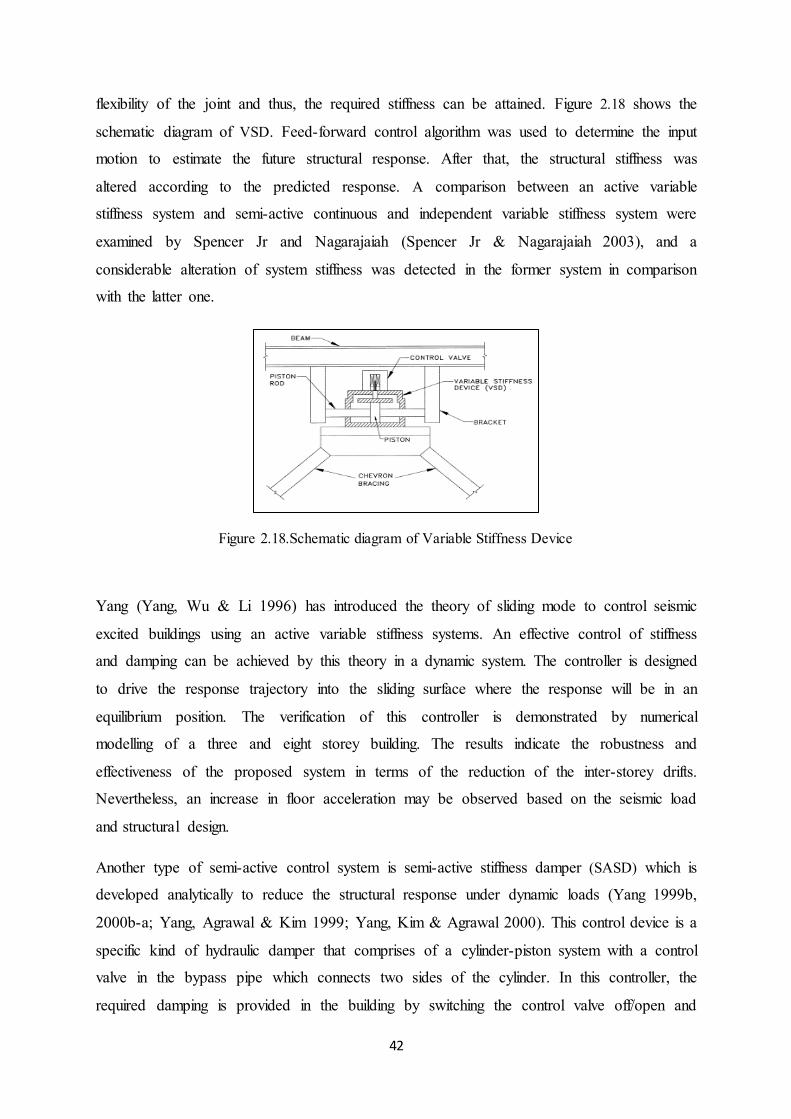
42
flexibility of the joint and thus, the required stiffness can be attained. Figure 2.18 shows the
schematic diagram of VSD. Feed-forward control algorithm was used to determine the input
motion to estimate the future structural response. After that, the structural stiffness was
altered according to the predicted response. A comparison between an active variable
stiffness system and semi-active continuous and independent variable stiffness system were
examined by Spencer Jr and Nagarajaiah (Spencer Jr & Nagarajaiah 2003), and a
considerable alteration of system stiffness was detected in the former system in comparison
with the latter one.
Figure 2.18.Schematic diagram of Variable Stiffness Device
Yang (Yang, Wu & Li 1996) has introduced the theory of sliding mode to control seismic
excited buildings using an active variable stiffness systems. An effective control of stiffness
and damping can be achieved by this theory in a dynamic system. The controller is designed
to drive the response trajectory into the sliding surface where the response will be in an
equilibrium position. The verification of this controller is demonstrated by numerical
modelling of a three and eight storey building. The results indicate the robustness and
effectiveness of the proposed system in terms of the reduction of the inter-storey drifts.
Nevertheless, an increase in floor acceleration may be observed based on the seismic load
and structural design.
Another type of semi-active control system is semi-active stiffness damper (SASD) which is
developed analytically to reduce the structural response under dynamic loads (Yang 1999b,
2000b-a; Yang, Agrawal & Kim 1999; Yang, Kim & Agrawal 2000). This control device is a
specific kind of hydraulic damper that comprises of a cylinder-piston system with a control
valve in the bypass pipe which connects two sides of the cylinder. In this controller, the
required damping is provided in the building by switching the control valve off/open and

43
on/closed. The adopted control algorithm in this system is based on Lyapunov method and
known as resetting control. In order to verify the effectiveness of this algorithm, a
comparison was carried out with the switching control algorithm. The results ensured the
functionality of SASD with respect to the reduction of the structural system under earthquake.
Nonetheless, the effectiveness of different algorithms is earthquake-dependent and hence, the
type of earthquake excitation should be taken into account for developing an efficient control
algorithm to ensure the robustness of the system.
2.5.2. Variable friction damper
Variable friction damper is another type of semi-active device and the research on this device
can be found in (Akbay & Aktan 1991; Akbay & Aktan 1990). The idea behind this damper
is to dissipate energy from a structural system through surface friction. Figure 2.19 illustrates
the schematic diagram of the variable friction damper. There are different types of variable
friction damper; this one consists of a friction shaft that is installed at the bracing of the
structure. The force generated at the frictional interface is adjusted by allowing slippage in a
controlled amount. Investigation were conducted to determine the functionality of the damper
using a one-storey model and a 20 storey building (Nishitani & Nittta 2001). The slip force
level is controlled to exhibit a hysteresis with a constant ductility factor. Stammers and
Sireteanu (Stammers & Sireteanu 2000) reported up to 50% reduction of structural response
in comparison to the passive case using a semi-active friction damper.
Figure 2.19. Schematic diagram of Variable friction damper
Developments of different control algorithm are reported by different researchers to enhance
the performance of a damper in term of energy dissipation. Dowdell and Cherry (Dowdell
&Cherry 1994) proposed two semi-active control algorithms, a variable slip force semi
active friction damper and an alternative damper utilizing simplified ‘off-on’ control

44
algorithm. The slip force is variable in these algorithms with respect to the structural response
in order to reduce the RMS inter-storey drift. The performance of these proposed algorithms
is compared with the constant slip force friction damper and a fully active tendon system.
Dupont and Stokes (Dupont & Stokes 1995) developed a simple bang-bang control algorithm
for friction dampers. This control algorithm improves the effectiveness of friction dampers by
increasing the energy dissipation in an instantaneous sense. The modulation of the normal
force can be seen at the friction interface, whereas the induction of friction dynamic resulted
is due to the effect of displacement and velocity. Both numerical and experimental studies
confirm the performance of the proposed control system.
2.5.3. Controllable tuned liquid damper
Controllable tuned liquid damper is another example of semi-active device which improves
the performance of passive devices, such as tuned liquid damper (TLD) or tuned liquid
column damper (TLCD). A TLD can be considered similar to TMD in which liquid is used
instead of mass. Similarly, A TLCD is one type of TLD which benefits from the motion of the
liquid column in a U shaped tube to decrease the structural response. Since the passive
vibration control devices are highly dependent on the type of excitation, the required damping
may not be possible to control. However, the efficiency of the system can be improved by
reducing the structural response when upgrading the device to a semi-active vibration
controller (Kareem 1994; Yeh 1996a). TLD can also be improved by altering the length of the
sloshing tank which will change the natural frequency of the liquid damper (Lou, Lutes & Li
1994). Haroun et.al (Haroun, Pires & Won 1994) reported the usage of a semi-active device
based on a TLCD by introducing variable orifice.
Yalla and Kareem investigated the process of controllable tuned dampers and reported the
method of achieving optimum amount of damping in the TLCD. Two optimal absorber
parameters, the frequency range and damping ratio, of each damper needs to be determined
first, and the desired damping level can be attained with the adjustment of the head-loss
coefficient by controlling the orifice opening ratio.
For the semi-active tuned liquid dampers, different control algorithms can be found in the
literature. These algorithms are applied for this system and are compared with passive
systems. Three types of control strategies are numerically analysed by Yalla et al. (Yalla,
Kareem & Kantor 2001) and demonstrated in figure 2.20. The model, as shown in the figure,
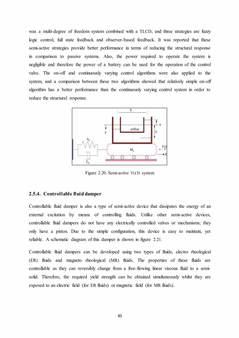
45
was a multi-degree of freedom system combined with a TLCD, and three strategies are fuzzy
logic control, full state feedback and observer-based feedback. It was reported that these
semi-active strategies provide better performance in terms of reducing the structural response
in comparison to passive systems. Also, the power required to operate the system is
negligible and therefore the power of a battery can be used for the operation of the control
valve. The on-off and continuously varying control algorithms were also applied to the
system, and a comparison between these two algorithms showed that relatively simple on-off
algorithm has a better performance than the continuously varying control system in order to
reduce the structural response.
Figure 2.20. Semi-active TLCD system
2.5.4. Controllable fluid damper
Controllable fluid damper is also a type of semi-active device that dissipates the energy of an
external excitation by means of controlling fluids. Unlike other semi-active devices,
controllable fluid dampers do not have any electrically controlled valves or mechanisms; they
only have a piston. Due to the simple configuration, this device is easy to maintain, yet
reliable. A schematic diagram of this damper is shown in figure 2.21.
Controllable fluid dampers can be developed using two types of fluids, electro rheological
(ER) fluids and magneto rheological (MR) fluids. The properties of these fluids are
controllable as they can reversibly change from a free-flowing linear viscous fluid to a semi-
solid. Therefore, the required yield strength can be obtained simultaneously whilst they are
exposed to an electric field (for ER fluids) or magnetic field (for MR fluids).

46
Figure 2.21. Schematic diagram of Controllable fluid damper
Several researches have been carried out for the development, modelling and testing of ER
fluid dampers to investigate the vibration control for civil structures (Ehrgott & Masri 1994;
Gavin, Hose & Hanson 1994; Leitmann & Reithmeier 1993; Makris et al. 1995; McClamroch
& Gavin 1995; Rav 1994; Xu, Qu & Ko 2000). The model used by Burton et al. and Markis
et al. (Burton et al. 1996; Makris et al. 1996)for ER fluid damper is presented in figure 2.22.
The physical configuration of this damper contains an outer cylinder and a double-ended
piston rod that pushes the ER fluid through a stationary annular duct. The created electric
field is normal to the fluid flow. To implement the semi-active ER damper in the civil
structure, modelling the response of this damper has been investigated. Sims et al. (Sims et al.
2000) presented a new modelling technique for semi-active ER dampers and also verified it
through experimental tests. This model consisted of spring, mass and damper which were
connected in series. Fluid bulk modulus and mass can be determined from the spring stiffness
and fluid density, respectively. The damping characteristic was estimated by modifying a
non-dimensional Bingham plastic function. Some key benefits of this model are the
capability of predicting observed response and the suitability of using the algebraic sum for
the control system.
Figure 2.22. Proposed Electro rheological fluid damper

47
As mentioned earlier, MR fluid damper is also a controllable fluid damper used for vibration
control in structures subjected to external loads (Carlson, Catanzarite & St. Clair 1996;
Carlson & Spencer Jr 1996; Dyke & Spencer Jr 1996, 1997; Dyke, Spencer Jr, Sain, et al.
1996a, 1996b, 1996c; Dyke et al. 1997; Jansen & Dyke 2000; Ohtori et al. 2004; Spencer Jr
& Dyke 1996; Yoshida & Dyke 2004). MR fluids are more beneficial than ER fluids in terms
of predicting seismic response and thus, have a good potential to ensure safety under any
seismic event. The first advantage of MR fluids over ER fluids is its ability to provide higher
yield stress which makes them capable of generating large forces. Secondly, MR fluids are
insensitive to contaminants or impurities occurring during manufacture and usage. Besides,
they can be operated using batteries due to its lower power consumption. It requires less than
50 watts of power, approximately 12 to 24 volts of voltage and current driven power supply
outputting only ~ 1- 2 amps.
The development of phenomenological models of MR dampers was conducted to predict the
behaviour of MR dampers by researchers (Choi, Lee & Park 2001; Spencer et al. 1996;
Spencer et al. 1997; Yang et al. 2002). The model used in these researches is the modified
Bouc-Wen model which is an extension of the Bingham model.
LORD corporation investigated the applicability and efficiency of MR dampers by designing a
full-scale 20 ton MR damper and installed in the real structure (Spencer Jr et al. 1997;
Spencer Jr et al. 1998; Yang 2001; Yang, Jung & Spencer Jr ; Yang 2000b-b) as illustrated in
figure 2.23. To build the damper, an outer cylindrical housing is used which is a part of
magnetic circuit. In addition, two shafts are attached on both ends to support the damper. The
final configuration of the damper consists of an inside diameter of 20.3cm with a stroke of 8
cm, 1m in length and a mass of 250 kg with 5 litres of MR fluid.
Figure 2.23. Schematic of the full-scale 20ton MR fluid damper

48
In 2001, the Tokyo national museum of emerging science and innovation applied these
dampers. This building is equipped with two 30 ton MR fluid dampers which are installed
between the third and fifth floor as depicted in figure 2.24. The MR fluid built used in this
building was manufactured by Lord corporation (Spencer Jr & Nagarajaiah 2003).
The first application of MR dampers in actual bridge structures was applied in a cable-stay
bridge (Dongting Lake Bridge in China). This bridge consists of long steel cables which are
subjected to vibration caused by the bridge itself or different weather conditions. For
example, wind combined with rain that may cause cable galloping. Two LORD SD-1005 MR
dampers are installed on each cable to reduce the vibration of the cable as demonstrated in
figure 2.25.
Figure 2.25. MR damper installed on Dongting Lake Bridge, China
Figure 2.24. Tokyo National Museum installed with 30-t MR fluid dampers

49
Magnetorheological (MR) dampers are capable of offering the adaptability of active devices
and stability and reliability of passive devices. One of the challenges in the application of the
MR dampers is to develop an effective control strategy that can fully exploit the capabilities
of the MR dampers. Bitaraf et al (Maryam Bitaraf, 2010) proposed two semi-active control
methods for seismic protection of structures using MR dampers. The first method is the
Simple Adaptive Control method which is classified as a direct adaptive control method. By
using this method, the controlled system is forced to track the response of the system with
desired behaviour. The controller developed using this method can deal with the changes that
occur in the characteristics of the structure because it can modify its parameters during the
control procedure. The second controller is developed using a genetic-based fuzzy control
method. In particular, a fuzzy logic controller whose rule base determined by a multi-
objective genetic algorithm is designed to determine the command voltage of MR dampers. In
order to evaluate the effectiveness of the proposed methods, the performances of semi-active
controllers were compared with some other control algorithms. Results revealed that the
developed controllers can effectively control both displacement and acceleration response of
the considered structure.
Another study discusses the modelling and application of MR dampers in semi-adaptive
structures (A. Dominguez, 2008), as these fluids possess mechanical simplicity, high
dynamic range, lower power requirements, large force capacity, robustness and safe manner
operation in case of structural failure. A nonlinear new model based on the Bouc-Wen model,
is employed to simulate the hysteresis behaviour of the damper. The model considers the
frequency, amplitude and current excitation as dependent variables. The finite element model
(FEM) of the MR damper element has also been developed based on the proposed model.
Subsequently finite element of the adaptive structure embedded with MR dampers has been
established and the nonlinear response of the whole structure is obtained.
In another study, the effectiveness of various seismic control devices for interconnecting two
adjacent buildings for earthquake hazard mitigation has been investigated (S.D. Bharti,
2010). The effectiveness is examined for seismic response mitigation of adjacent multi story
buildings under coupled building control scheme, involving passive-off, passive-on and semi
active control strategies. In addition, the influence of damper location and maximum
command voltage, on control performance has been examined.

50
The different types of vibration control devices considering their advantages and limitations
have been discussed so far. In the next section, a brief introduction of MR fluids and devices
is presented.
2.6. MR fluids and devices
Passive vibration control devices absorb the vibration energy subjected on the structure by
external excitation. Active vibration control devices, on the other hand, need a significant
amount of external power supply to be capable of producing control forces to neutralise the
destructive energy of the external excitation. Semi-active vibration control devices advantage
of the features of both passive and active vibration control devices. Therefore, when the
external excitation is subjected and there is a power failure where the active control devices
are not functioning, the passive control devices can compromise for it and reduce the
vibrations subjected on the structure with their mechanical characteristics. Magneto
Rheological (MR) dampers are typical examples of semi-active vibration control devices as
they are highly efficient in the vibration reduction in addition to requiring subtle amounts of
electricity which can easily be provided by batteries. MR fluids are typical examples of
controllable fluids. These fluids were discovered in the late 1940s by Rabinow (Rabinow
1948, 1951). There exists micron-sized magnetisable particles suspended in a carrier liquid
which when a magnetic field is applied, these particles align in the direction of the magnetic
field giving the liquid the capability of transforming from a free-flowing viscous fluid to a
semi-solid in milliseconds, as shown in figure 2.26. The reaction of the MR fluid due to a
magnetic field is shown in figure 2.27.
Figure 2.26. MR Fluid without (left) and with magnetic field (right)

51
MR fluids have 20 to 40% of their volume consisting of carbonyl iron particles which are only
3 to 5 micrometres in diameter. The particles are suspended in non-magnetic fluids like
hydrocarbon oil or silicon oil. The strength of an MR fluid is a measure of the saturation
magnetisation of the iron particles it consists of. As the saturation magnetisation of these
particles increases, the MR fluid has stronger magnetic capacity. Experimental tests indicate
the most efficient saturation magnetisation of iron particles to be 2.4 Tesla. Therefore,
producing such particles is not cost-effective. In practical assumptions, the saturation
magnetisation of iron particles is assumed to be 2.15 Tesla.
Figure 2.27.MR Fluid when a magnetic field is applied
MR fluids are manufactured by LORD Corporation. Table 2-1 compares the main
characteristics of three types of controllable fluids used in MR fluids: MRF-240BS (water-
based), MRF-132AD (hydrocarbon-based) and MRF-36AG (silicon-based). The characteristics
of yield stress, magnetic field strength and magnetic induction of the LORD MRF-122-2ED are
shown in figure 2.28 and figure 2.29.
Table 2-1.Characteristics of three different types of MR fluids (LORD Corporation)
MR FLUID MRF-132AD MRF-240BS MRF-33AG
Base fluid Hydrocarbon Water Silicone
Operating temperature ( -40-130 0-70 -40-150
Density (g/cc) 3.09 3.818 3.45
Solids Weights (%) 81.64 83.54 82.02
Specific Heat@ 25 0.80 0.98 0.68
Thermal Conductivity (w/m ) 0.25-1.06 0.83-3.68 0.20-1.88
Flash Point ( ) >150 >93 >200

52
Figure 2.28. Yield stress vs. magnetic field strength of MRF-122-2ED (LORD Corporation)
Figure 2.29. Magnetic properties of MRF-122-2ED (LORD Corporation)
2.7. Characteristics of MR fluids
The main characteristics of typical ER and MR fluids are presented in table 2-2. MR fluids are
not very sensitive to the impurities it consists of which makes them easier to manufacture. In
contrast to ER fluids, MR fluids are capable of operating in a broader range and with very low
demanding voltage. In addition, the yield stress provided by MR fluids is greater than its ER
counterparts. Since the iron is used as the solute, the density increases significantly in
contrast to ER fluids. Even though both ER and MR fluids possess equal energy requirements,
only MR fluids can easily function with very low voltage power (Carlson, Catanzarite & St.
Clair 1996; Carlson 1996). MR devices are controllable with low voltage, current-driven
power supply (1-2 amps) in contrast to ER devices which require a high voltage power source
(~2000-5000 volts). In addition, this high voltage is capable of posing safety hazards. Table 2-
2 provides the features of both fluids.

53
Table 2-2. Typical characteristics of ER and MR fluids (Carlson, Catanzarite & St. Clair 1996)
Property MR fluid ER fluid
Max. Yield Stress 50-100 kPa 2-5 kPa
Maximum Field ~250 kA/m ~4 kV/mm
Apparent Plastic Viscosity 0.1-10 Pa-s 0.1-10 Pa-s
Operable Temp. Range -40-150 +10-90
Stability Unaffected by most impurities Cannot tolerate impurities
Density 3-4 g/cm3 1-2g/cm3
10-11-10-10 s/Pa 10-8-10-7 s/Pa
Maximum Energy Density 0.1 Joules/cm3 0.001 Joules/cm3
Power Supply(typical) 2-50V, 1-2A 2000-5000V, 1-10mA
2.8. MR devices and Applications
Devices consisting of MR fluids are categorised in three operating modes: (a) valve mode, (b)
direct shear mode, or (c) squeeze mode, as shown in figure 2.30 (Butz & Von Stryk 2002;
Yang 2001). The valve mode is a fixed-magnetic pole mode, mainly implemented in servo-
valves, dampers and shock absorbers. The shear mode is used mainly in clutches, brakes and
dampers. The squeeze mode, which is a combination of the valve and the direct shear mode,
is mainly used in small amplitude vibration dampers.
Figure 2.30. Three typical operating modes for MR fluid devices (Butz & Von Stryk 2002)
In actual structural implications, the required displacements and damping forces are very high
in magnitude. Therefore, MR dampers operating with shear or squeeze mode are not
applicable. Usually, valve mode combined with direct shear mode is taken into account.
Typical examples of MR dampers are presented in the following section.

54
A small scale SD-1000 MR damper is produced by LORD Corporation (Takenaka
Corporation; Carlson 1996; Dyke, Spencer Jr, Sain, et al. 1996b; Jolly, Bender & Carlson
1999) as shown in figure 2.31. MR fluids flow from a high pressure chamber to a low pressure
chamber using an orifice located in the piston head. The main cylinder has a diameter of
3.8cm and the length of the damper exceeds to 21.5 cm. The main cylinder consists of the
piston, the magnetic circuit, an accumulator, and 50 ml of MR fluid. A stroke of 2.5cm is
provided by this damper.
A20 ton prototype large-scale MR fluid damper is manufactured in the LORD Corporation in
collaboration with the Structural Dynamics and Earthquake Engineering Laboratory at the
University of Notre Dame (Spencer Jr et al. 1998; Yang et al. 2002). The main feature of this
damper is presented in table 2-3.
The magnetic field is perpendicular to the fluid flow which is provided by an electromagnet
in the piston head. This damper is capable of producing forces of up to 3000 N.
Table 2-3. Characteristics of the 20ton MR damper
Stroke 8cm
Maximum velocity 10 cm/s
Nominal cylinder bore 20.32 cm
Maximum input power <50 watts
Normal maximum force 200,000N
Effective axial pole length ~5.5-8.5cm
Coils ~3 1000turns
Maximum yield stress ~70kPa
Apparent fluid plastic viscosity 1.5 Pa-s
2 s/Pa
Gap ~1.5-2mm
Active fluid volume ~90
Wire 16 gauge
Inductance ~6H
Resistance ~3 7

55
The most common type of MR dampers is the RD-1005-3 damper manufactured by LORD
Corporation, as shown in figure 2.33. As a magnetic field is applied, this damper is highly
efficient in controllability, energy density and responsiveness.
Figure 2.31. Small-scale SD-1000 MR Fluid damper (Yang 2001)
Figure 2.32. Large-scale 20ton MR Fluid damper (Yang 2001)
Figure 2.33. MR damper RD-1005-3
A variety of products manufactured by LORD Corporation with the rheonetic systems
trademark exists. Some examples include:
Automotive suspension devices

56
These devices improvised MR fluids instead of hydraulic shock absorbers. A controller is
used for the damping features in real-time.
MR passenger protection devices
These devices improvise MR fluids in airbag systems, seatbelts and the vehicle seats,
therefore safety factors are guaranteed.
Seismic Protection
Due to rapid time response and low power requirements, MR dampers are widely used in
structures to mitigate the hazardous energy of the external excitations, as shown in figure 2.34
and 2.35.
Figure 2.34.MR dampers installed in a bridge
Figure 2.35. Examples of MR dampers installed in a building

57
Washing machines
MR dampers manufactured by LORD Corporation are applied in washing machines and other
electrical appliances to reduce the noise and vibrations produced in these devices, as shown
in figure 2.36.
Figure 2.36.MR damper installed in a washing machine
Prosthesis devices for amputated legs
These prosthesis devices are produced by a German firm (Biedermann OT Vertrieb) which
improvised MR dampers in their device to improve stability and energy efficiency and also
reduce the response time to milliseconds.
Figure 2.37.MR damper applied in lower leg prosthesis
Vehicle seat suspension
This suspension is mainly used for buses and truck seats to enhance comfort. They have a
better performance in comparison to air-suspension seats as they are adaptable to the varying
weight of different drivers and the road oscillations, as shown in figure 2.38.

58
Figure 2.38. Heavy duty seat suspension with MR damper
2.9. MR damper modelling
Control algorithms that improvise the characteristics of MR dampers need to be developed.
For the parameter identification and model evaluations, experimental data (displacement,
velocity and damping forces) for various ranges of control currents and frequencies is
required, as shown in figure 2.39.
Force versus velocity or force versus plots varies based on the control current. The forces
versus displacement plots of MR damper pursues a clockwise path due to the increase in time
in contrast to the forces versus velocity plot which pursues a counter-clockwise pace due to
increase in time. The force versus velocity features of MR dampers are demonstrated by
curves with considerable hysteresis for lower velocities (pre-yield) and linear force for higher
velocities (post-yield). The current approaches zero when the smallest hysteresis indicates a
viscous characteristic. As the control current increases, the damper force increases
accordingly.
Figure 2.39.Characteristics of damper force for different currents provided: (a) non-linearly in force versus displacement and (b) hysteresis in force versus velocity

59
Various models known as quasi-static and dynamic models are established to take into
account the non-linear and hysteresis characteristics of MR dampers (Lee & Wereley 2000;
Wang & Gordaninejad 2000). These models are efficient for the force versus displacement
behaviour of MR dampers whilst they have poor performance when modelling the nonlinear
force versus velocity curve of the damper (Yang 2001). Therefore, these models are
insufficient for the analysis and design of structural control algorithms.
To overcome this setback, dynamic models are proposed. Two classifications exist for
dynamic models: a) non-parametric models and b) parametric models. The non-parametric
model in which the performance of the MR damper through various experimental set ups is
required. Good examples are Chebychev polynomials (Ehrgott & Masri 1992; Gavin 1996),
neural networks (Chang & Roschke 1998; Wang & Liao 2001; Xia 2003; Zhang & Roschke
1998), and neuro-fuzzy systems (Schurter & Roschke 2000).
Parametric models improvise mechanical characteristics (mass, damping and stiffness) to
provide the features of the device. These parametric models are presented below:
2.9.1. Bingham model
The stress-strain behaviour of MR fluids can be modelled by the Bingham model. As defined
in this model, the MR damper has a solid behaviour until a minimum yield stress is
surpassed and afterwards shows a linear behaviour for the stress and changes in shear .
Therefore, the shear stress for this fluid is presented below:
; (2.1)
where (field) is the yield stress provided by the magnetic field and is the fluid velocity.
According to the Bingham model, Stanway, Sproston and Stevens (Stanway, Sproston &
Stevens 1985; Stanway, Sproston & Stevens 1987) established a mechanical model with the
same name which includes a Coulomb frictional element with a dashpot in parallel to it, as
shown in figure 2.36. Spencer (Spencer et al. 1997) used this model for a small MR fluid
damper. The MR damper force is presented as:
; (2.2)
where is the damping force, is the friction force, sgn(.) the signum function, the
velocity, the displacement, the viscous coefficient and is the initial value for the
damper force which is the mean produced by the accumulator.

60
Figure 2.40. Bingham model for a fluid damper (Stanway, Sproston & Stevens 1985; Stanway, Sproston & Stevens 1987)
Figure 2.41. Verifying the Bingham model with the experimental results (Spencer et al. 1997)
As an implementation, this model is tested with a 2Hz sinusoidal response function in which
the voltage provided is 1.5V. The model characteristics are: , , and
. As illustrated in figure 2.41, even though the behaviour of the fluid is described
well beyond the yield point, it does not define the behaviour of the damper in the vicinity of
zero velocity in which the pre-yield region is encountered. This model is not efficient when
defining the nonlinear force-velocity curve of the damper when the displacement and velocity
have the same sign and small magnitude velocities are encountered. Therefore, this model is
efficient when the response needs to be analysed.

61
The Bingham model is extended by Gamota and Filisko in 1991(Gamota & Filisko 1991). In
which a solid model in series with the original Bingham model is considered, as shown in
figure 2.42. The force in the damper is presented by the equations below:
; (2.3)
where , , and are the linear solid parameters and is the Bingham model damping
coefficient.
The frequency and voltage are the same as the Bingham model in the previous section. The
model parameters are , , , ,
and . The predicted response versus the experimental data is
presented in figure 2.39. Based on this model, the force versus displacement of the MR
damper is accurately verified by the experimental results. But the main setback of this model
is not having the near zero velocity hysteresis relationship between the force and velocity of
the MR damper. Therefore, when this model is used for numerical means very small
simulation steps need to be defined (Spencer et al. 1997).
Figure 2.42. Extended Bingham model (Gamota & Filisko 1991)

62
Figure 2.43. Verifying the Bingham model with the experimental results (Spencer et al. 1997)
2.9.2. Bouc-Wen model
The Bouc-Wen model was first proposed by Spencer (1997), as shown in figure 2.44. This
method of verifying the response of the hysteresis system of the MR damper is similar to Wen
(1976). The force produced by the MR damper is presented below:
; (2.4)
where is the viscous coefficient, is the linear spring stiffness, is the initial
displacement of the spring, is the scaling coefficient in the yield stress of the MR fluid and
z is an evolutionary variable defined by the equation below:
. (2.5)
Figure 2.44. Bouc-Wen model of MR damper

63
The MR damper parameters are: , , ,
, , , and . A comparison between the predicted
response and the experimental data is shown in figure 2.45. Even though this model is capable
of defining the characteristics of MR dampers it is not capable of defining the force/velocity
in the vicinity of small velocities (Spencer et al. 1997).
Figure 2.45. Verifying the Bouc Wen model with experimental results (Spencer et al. 1997)
2.9.3. Modified Bouc-Wen model
The modified Bouc-Wen model was first proposed by Spencer (1997) to capture the
hysteresis behaviour of the MR damper, as shown in figure 2.46. The force equilibrium in this
figure results in the equation below:
; (2.6)
in which the equation covering the evolutionary variable is presented below:
. (2.7)
When the equation (2.6) is solved, the results are as below:
(2.8)
. (2.9)

64
The total force from equation (2.6) can be written as the form below:
. (2.10)
Figure 2.46. Modified Bouc-Wen model of MR damper (Spencer et al. 1997)
Figure 2.47. Verifying the Modified Bouc-Wen model with the experimental results (Spencer et al. 1997)
The parameters of the MR damper are: , , , , ,
, , , and .
The verification between the predicted response and the experimental data is shown in figure
2.47. As anticipated, this model is highly efficient in defining the damper behaviour in all
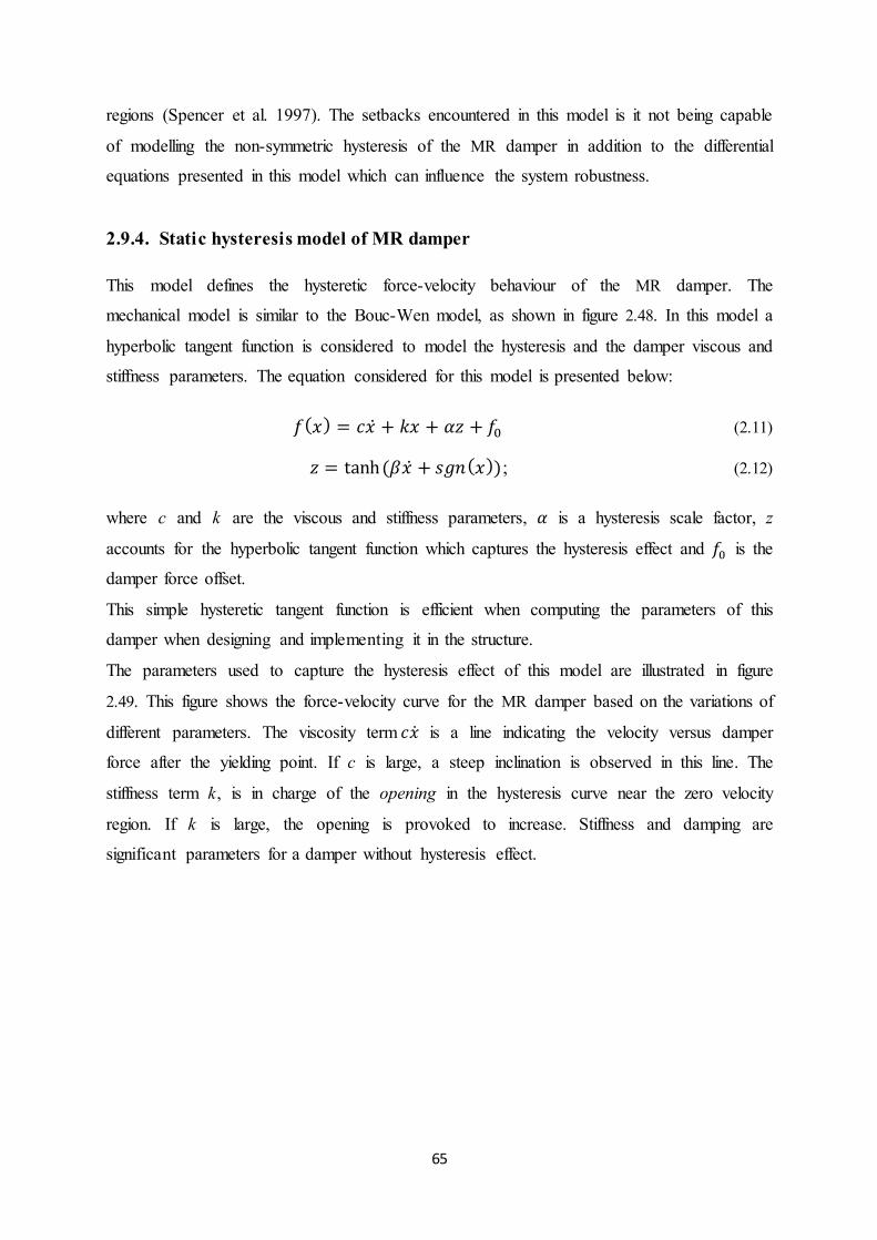
65
regions (Spencer et al. 1997). The setbacks encountered in this model is it not being capable
of modelling the non-symmetric hysteresis of the MR damper in addition to the differential
equations presented in this model which can influence the system robustness.
2.9.4. Static hysteresis model of MR damper
This model defines the hysteretic force-velocity behaviour of the MR damper. The
mechanical model is similar to the Bouc-Wen model, as shown in figure 2.48. In this model a
hyperbolic tangent function is considered to model the hysteresis and the damper viscous and
stiffness parameters. The equation considered for this model is presented below:
(2.11)
; (2.12)
where c and k are the viscous and stiffness parameters, is a hysteresis scale factor, z
accounts for the hyperbolic tangent function which captures the hysteresis effect and is the
damper force offset.
This simple hysteretic tangent function is efficient when computing the parameters of this
damper when designing and implementing it in the structure.
The parameters used to capture the hysteresis effect of this model are illustrated in figure
2.49. This figure shows the force-velocity curve for the MR damper based on the variations of
different parameters. The viscosity term is a line indicating the velocity versus damper
force after the yielding point. If c is large, a steep inclination is observed in this line. The
stiffness term k, is in charge of the opening in the hysteresis curve near the zero velocity
region. If k is large, the opening is provoked to increase. Stiffness and damping are
significant parameters for a damper without hysteresis effect.

66
Figure 2.48. Hysteresis Parameters for Static hysteresis model of MR damper
As shown in figure 2.48, the initial hysteresis loop is smaller and is dependent on the scale
factor of the damper velocity in the hysteresis curve . In which, the larger value of , the
steeper the slope will be. The width of the hysteresis is dependent on ; the sign
function of the displacement and the scale factor . The height of the hysteresis is dependent
on the coefficient . The offset value shifts the initial hysteresis loop (Nguyen 2009).
To this point, MR fluids, their behaviour and the modelling formulas have been discussed. A
setback encountered when applying MR fluids is its nonlinear characteristics. Therefore, the
control algorithm that considers this nonlinearity is significant. The non-parametric models;
Bouc-Wen and modified Bouc-Wen model, are efficient for modelling MR devices. However,
these models do not consider the non-symmetric hysteresis in the force-velocity curve.
Therefore, proposing a model of MR damper that can overcome this setback is a challenging
task.
The control algorithms chosen is highly influential on the performance of a structural control
system (Jung et al. 2006). In the following chapter, various control algorithms are discussed;
Lyapunov based controller, linear quadratic regulator (LQG) control, fuzzy logic control and
etc.
In this section, different control algorithms for MR dampers have been discussed. Brief
information on the theory and design of Lyapunov-based control and linear quadratic
regulator (LQR) has been provided. Furthermore, intelligent control (fuzzy logic control) has
also been introduced and discussed.

67
2.10. Lyapunov Control
There are several structural control systems based on the Lyapunov stability method (Gavin
2001; Kuehn & Stalford 2000; Leitmann 1994; Wang & Gordaninejad 2002); in which a
Lyapunov function must be assumed. This function is required to be a positive definite
function. Based on the Lyapunov stability method, the system is stable for an equilibrium
point if the derivative of Lyapunov function is negative. In control theory, the Lyapunov
function is of the form below:
; (2.13)
where is P-norm of the state variables as shown below:
. (2.14)
In equation (4.3), Q is a real, symmetric, positive-definite matrix. Therefore, to achieve
stability in the system, the derivative of the Lyapunov function is required to be negative
definite. If the system is linear, the matrix P is achieved when the Lyapunov equation is
solved:
. (2.15)
where is the system matrix in the generic form of the state space equation and is
assumed to be a positive definite matrix.
2.11. Linear quadratic regulator(LQR) control
Linear quadratic regulator (LQR) control is commonly used for semiactive vibration devices
as it is simple and stable. The desired control force is achieved when the performance index
below is minimised:
; (2.16)
where the desired control function is achieved:
; (2.17)
where is the system and is the input matrix in the generic form of the state space
equations and Q is a given positive definite matrix, R is a given positive matrix, and P is a
positive definite matrix when the Riccati equation is solved, as shown below:
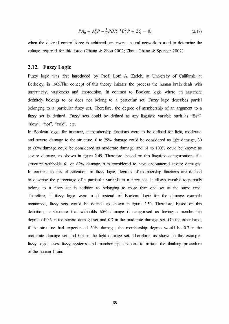
68
. (2.18)
when the desired control force is achieved, an inverse neural network is used to determine the
voltage required for this force (Chang & Zhou 2002; Zhou, Chang & Spencer 2002).
2.12. Fuzzy Logic Fuzzy logic was first introduced by Prof. Lotfi A. Zadeh, at University of California at
Berkeley, in 1965.The concept of this theory imitates the process the human brain deals with
uncertainty, vagueness and imprecision. In contrast to Boolean logic where an argument
definitely belongs to or does not belong to a particular set, Fuzzy logic describes partial
belonging to a particular fuzzy set. Therefore, the degree of membership of an argument to a
fuzzy set is defined. Fuzzy sets could be defined as any linguistic variable such as “fast”,
“slow”, “hot”, “cold”, etc.
In Boolean logic, for instance, if membership functions were to be defined for light, moderate
and severe damage to the structure, 0 to 29% damage could be considered as light damage, 30
to 60% damage could be considered as moderate damage, and 61 to 100% could be known as
severe damage, as shown in figure 2.49. Therefore, based on this linguistic categorisation, if a
structure withholds 61 or 62% damage, it is considered to have encountered severe damages.
In contrast to this classification, in fuzzy logic, degrees of membership functions are defined
to describe the percentage of a particular variable to a fuzzy set. It allows variable to partially
belong to a fuzzy set in addition to belonging to more than one set at the same time.
Therefore, if fuzzy logic were used instead of Boolean logic for the damage example
mentioned, fuzzy sets would be defined as shown in figure 2.50. Therefore, based on this
definition, a structure that withholds 60% damage is categorised as having a membership
degree of 0.3 in the severe damage set and 0.7 in the moderate damage set. On the other hand,
if the structure had experienced 30% damage, the membership degree would be 0.7 in the
moderate damage set and 0.3 in the light damage set. Therefore, as shown in this example,
fuzzy logic, uses fuzzy systems and membership functions to imitate the thinking procedure
of the human brain.

69
Figure 2.49. Boolean functions categorising structural damage
Figure 2.50. Fuzzy functions categorising structural damage
A very useful application of fuzzy logic in civil engineering is fuzzy logic control. In which,
fuzzy rules are defined to determine the action that needs to be taken, based on the sensed
response of the structure. Research has been conducted on their application in seismic
vibration reduction of structures due to external excitations; active and semi-active control.
This method is advantageous over other methods as it acquires simple algorithms, its suitable
for real-time control, there is no requirement for information on the structural and vibration
characteristics of the plant, the system is robust in terms of performance and implementation
(Wong et al.1999)
Fuzzy logic control improvises expert knowledge instead of rigorous equations to describe
the behaviour of a system. It uses fuzzy information to dictate desirable control actions and is
used in complex systems in which there is no simple mathematical model, the system is
highly nonlinear or there is ambiguity or vagueness in the system
(Pacific Northwest National Laboratory and Batelle Memorial Institute 1997).

70
2.13. Fuzzy Logic Control for Structural Vibration Reduction As mentioned above, fuzzy control consists of the rules in the format of IF...THEN statements,
which relate the input variables to the desirable output, or control action. The procedure starts
with defining membership functions for the inputs and outputs using linguistic terms. In
structural control, the inputs are usually the sensed structural responses: displacement,
velocity or acceleration. The crisp input values obtained from the sensors are assigned
membership functions and degrees of membership. This step is known as the fuzzification
step. The next step is the decision making step, in which predetermined rules are used to
relate the fuzzy input values to fuzzy outputs. In the end, the output values are defuzzifed, in
which they are converted into crisp values which can be used as control actions. The
inference rules and the membership functions determine the effectiveness of the fuzzy logic
controller.
Inactive seismic vibration control, fuzzy logic control is used to determine the desired control
force to be applied to the actuator (Casciati et al.1994 a,b,c, Casciati and Yao 1994, Furuta et
al. 1994, Iiba et al. 1994, Goto et al. 1994, Yamada et al. 1994, Yeh et al. 1994, Fujitani et al.
1995, Battaini et al. 1997, 1998, Aldawood et al. 2001, Mitsui et al. 2002)
In semi-active control, however, fuzzy logic is used to vary the mechanical properties of the
device. It is applied to seismic vibration reduction bridges due to earthquakes or traffic
loading with variable dampers (Sun and Goto 1994), or control of structural vibrations with
hybrid systems consisting of base isolation and semi-active dampers (Nagarajaiah 1994,
Symans and Kelly 1999, Wongpresert and Symans 2001).
2.14. Summary In this chapter, a literature review of different types of vibration control devices has been
discussed and recent achievements have been introduced. MR dampers and their applications
have been analysed, therefore a background regarding the semi-active vibration control
concerned in this research has been provided. The efficiency of MR dampers in seismic
vibration suppression has been analysed. Further discussion in addition to two case studies
has been provided in the following chapters.

71
CHAPTER 3
STRUCTURES WITH ACTIVE TUNED MASS DAMPERS
3.1. Introduction Mitigation of external vibrations such as winds and earthquakes has been a critical aspect in
designing buildings. Recent advances in technology allow engineers to design intelligent
structures capable of counteracting undesirable vibrations by using active control devices in
the design of a modern structure. Passive, semi-active and active control is becoming a
specific part in the structural system. Active tuned mass dampers (ATMD) have been a
popular area of research for some time and progress has been seen in this field (Nerves C,
1995), (Soong T, 1993). Fuzzy Logic controllers are one of the best active control algorithms
since they are model free approaches to system identification and control which makes the
system easier to design than developing an accurate mathematical model of the structural
system needed for control system design (Samali B, 2003).
Tuned Mass Dampers dissipate vibratory energy through a set of damper and spring
connecting a small mass to the main structure; they have a great effect in vibration
suppression caused by low frequency loads and loads with frequencies near the fundamental
frequency of the structure. Despite these advantages they have shown poor behaviour due to
stochastic loads with high frequencies such as earthquakes. Therefore, Active Tuned Mass
Dampers are the alternatives suggested. In this approach, two benchmark structures are being
analysed; a five storey structure (Samali B, 2003) and a fifteen storey structure (Guclu R,
2008). The active vibration control is conducted by Fuzzy Logic controllers since they are
one of the best active vibration control methods. Their behaviour in different mass ratios
(mass of structure to mass of damper) and different locations in the structure is being
investigated. Also the structure is imposed to El Centro earthquake. The main goal is
comparing the displacement of the last storey and the inter-storey drifts due to the
aforementioned changes for the two benchmarks.

72
3.2. Structural System
The building structure is considered to have n-degrees-of-freedom. The external excitations
can be wind or earthquake. The equation of motion is presented below:
; (3.1)
where m is the mass of the structure, c is the damping of the structure, k is the stiffness of the
structure, is the displacement matrix, is the velocity matrix, is the acceleration
matrix of the building structure;
, ,
, .
Matrix is the gain matrix determining the control effect on the building, is a distribution
matrix, f is the control force provided by the controller and is the ground acceleration
of the earthquake.
The mass matrix is considered as below:
. (3.2)
The stiffness matrix is as below:
. (3.3)
The damping matrix is as below:
. (3.4)
The equation of motion is transformed into state space equations in which a system state is
defined and has the below form:
; (3.5)
, , ; (3.6)

73
where A is the system matrix, B is the gain matrix and E is the external excitation matrix.
3.3. Building Structure equipped with Tuned Mass Dampers The structural parameters (mass, stiffness and damping) as assumed (Samali B, 2003)(Guclu
R, 2008) for the five and fifteen storey structures, are constant for every storey of the
structure. The Tuned Mass Damper has a mass of 1, 2, 3 and 4 % of the total structural mass in
different assumptions, and its frequency is tuned to the fundamental frequency of the
structure and since it is located at the top of the structure, it is considered to be the sixteenth
degree of freedom with its structural parameters (mass, stiffness and damping) being constant
as if there were another storey on the last floor. The earthquake subjected to the structure is
El Centro (Mw= 7.1), normalized to 2g as shown in figure 3.1. This quake is given by the
strong motion database provided in Berkeley University (PEER berkeley Strong Motion Data
base).
Figure 3.1. El Centro earthquake acceleration time history, normalised to 2g
As shown in equation 3.1, the earthquake is subjected to the structure. After the earthquake,
the structure experiences a free vibration period in which there is no input exciting the
structure. The force produced by the active control device throughout the earthquake
excitation and the free vibration afterwards mitigates the energy of the external excitation.

74
3.4. Structural model of a five storey building structure The five storey benchmark model, 3.6 m tall steel frame designed and manufactured at the
University of Technology Sydney is used for this study as shown in figure 3.2. The model
has a footprint of 1.5m x 1.0m. It consists of two bays in one direction and a single bay in the
other. The beams making up the bulk of each floor are 75 x 75x 4 mm square hollow steel
sections. The model lateral stiffness is provided by six high strength 24 x 24 mm square steel
sections. The model is designed to have the first floor heights of 0.7m. Taking advantage of
the fact that masses are effectively lumped at the first floor levels, simplifies the analyses and
hence the frame is represented by a five lumped mass dynamic system, yielding a 5 x 5
diagonal mass matrix for both orthogonal directions. The analysis, however, is a 2D analysis
focusing on the motion of the frame along its longer two bay directions. The total mass of the
model is 1636.5 kg. The five natural frequencies of the model are 2.95, 9.02, 15.68, 21.26 and
25.23 Hz, respectively, and the corresponding damping ratios are 0.4%, 0.69%, 0.63%, 0.2%
and 0.14% of critical damping, respectively (Samali B, 2003).
Figure 3.2. Five storey benchmark steel frame
3.4.1. Fuzzy Logic Controller design for the five storey structure
Fuzzy Logic control has been extensively introduced in Appendix D. The design of the Fuzzy
controller uses crisp data directly from a number of sensors; these data are then converted
into linguistic or Fuzzy membership functions through the fuzzification process. The number
of sensors used in the system is dependent on the number of input variables used in the
controller. The controller is designed using two input variables, each one having seven
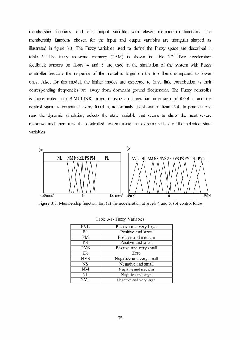
75
membership functions, and one output variable with eleven membership functions. The
membership functions chosen for the input and output variables are triangular shaped as
illustrated in figure 3.3. The Fuzzy variables used to define the Fuzzy space are described in
table 3-1.The fuzzy associate memory (FAM) is shown in table 3-2. Two acceleration
feedback sensors on floors 4 and 5 are used in the simulation of the system with Fuzzy
controller because the response of the model is larger on the top floors compared to lower
ones. Also, for this model, the higher modes are expected to have little contribution as their
corresponding frequencies are away from dominant ground frequencies. The Fuzzy controller
is implemented into SIMULINK program using an integration time step of 0.001 s and the
control signal is computed every 0.001 s, accordingly, as shown in figure 3.4. In practice one
runs the dynamic simulation, selects the state variable that seems to show the most severe
response and then runs the controlled system using the extreme values of the selected state
variables.
Figure 3.3. Membership function for; (a) the acceleration at levels 4 and 5; (b) control force
Table 3-1- Fuzzy Variables
PVL Positive and very large PL Positive and large PM Positive and medium PS Positive and small
PVS Positive and very small ZR Zero
NVS Negative and very small NS Negative and small NM Negative and medium NL Negative and large
NVL Negative and very large
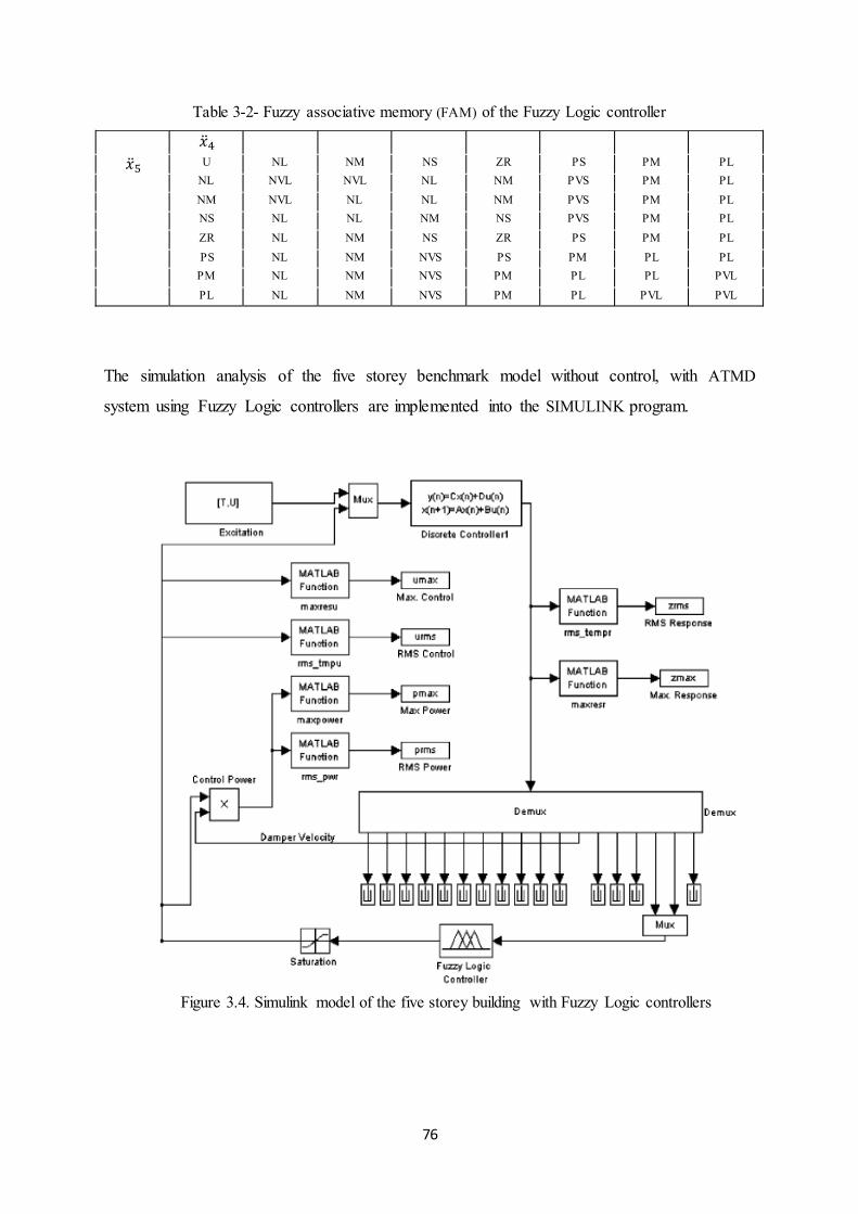
76
Table 3-2- Fuzzy associative memory (FAM) of the Fuzzy Logic controller
U NL NM NS ZR PS PM PL
NL NVL NVL NL NM PVS PM PL NM NVL NL NL NM PVS PM PL NS NL NL NM NS PVS PM PL ZR NL NM NS ZR PS PM PL PS NL NM NVS PS PM PL PL PM NL NM NVS PM PL PL PVL PL NL NM NVS PM PL PVL PVL
The simulation analysis of the five storey benchmark model without control, with ATMD
system using Fuzzy Logic controllers are implemented into the SIMULINK program.
Figure 3.4. Simulink model of the five storey building with Fuzzy Logic controllers

77
3.5. Structural model of a fifteen storey building structure The structure has fifteen degrees of freedom all in horizontal direction. Since the destructive
effect of earthquakes is the result of horizontal vibrations, in this study the degrees of
freedom have been assumed only in this direction. The system is modelled including the
dynamics of a linear motor which is used as the active isolator. An important element of an
active control strategy is the actuators (R. Agarwala, 2000).These are active control devices
that expend energy to attenuate disturbances at the corresponding subsystems or reduce the
storey vibration on which they are installed.
During an earthquake, the maximum inter-storey shear force occurs on the first storey.
Assuming equivalent storey stiffness and ultimate capacities, the destructive effect of an
earthquake is expected to be the largest on the first storey. Therefore, the active control was
applied on the first storey using a linear motor. It supplies control voltage directly to suppress
the magnitude of undesirable earthquake vibrations.
It is well known that the maximum displacements and accelerations are expected from the top
storey of structures during an earthquake. Because of that an ATMD with active and passive
elements, which are optimally tuned for the first mode of the structural system, is placed over
the top storey and a linear motor is used as the active isolator.
The system parameters of the real structure (Gozukizil, 2000) are presented in table 3-3.
Table 3-3- Parameters of the fifteen storey structural system Mass parameters (kg) Stiffness parameters (N/m) Damping parameters (N s/m)
m1 = 450,000 k1 = 18,050,000 c1 =26,170
m2 = 345,600 k2 = 340,400,000 c2 = 293,700
m3 = 345,600 k3 = 340,400,000 c3 = 293,700 m4= 345,600 k4 = 340,400,000 c4 = 293,700 m5= 345,600 k5 = 340,400,000 c5 = 293,700 m6 = 345,600 k6 = 340,400,000 c6 = 293,700 m7= 345,600 k7 = 340,400,000 c7 = 293,700 m8 = 345,600 k8 = 340,400,000 c8 = 293,700 m9= 345,600 k9 = 340,400,000 c9 = 293,700
m10 = 345,600 k10 = 340,400,000 c10 = 293,700 m11 = 345,600 k11 = 340,400,000 c11 = 293,700 m12 = 345,600 k12 = 340,400,000 c12 = 293,700 m13 = 345,600 k13 = 340,400,000 c13 = 293,700 m14 = 345,600 k14 = 340,400,000 c14 = 293,700 m15 = 345,600 k15 = 340,400,000 c15 = 293,700

78
3.5.1. Fuzzy Logic Controller design for the fifteen storey structure The Fuzzy Toolbox in MATLAB in SIMULINK is used. In the fuzzy logic control for the
structural system, the errors (e = - ; = - ) in the second storey and fifteenth storey
motion and their derivatives (de/dt = - ), (de1/dt = - ) are used as the input variable
while the control voltages ( ) and ( ) are the outputs. Reference values ( ; ) and
( ; ) are considered to be zero in the closed-loop model of the system (figure 3.5).
A model of the two similar rule bases developed by heuristics with error in body bounce
motion, pitch motion and velocity as input variables are given in table3-4, where P, N, Z, B, M,
S represent positive, negative, zero, big, medium and small, respectively. Trial and error
approach with triangular membership functions has been used to achieve a good controller
performance. The membership functions for both scaled inputs (e,de) and output (u) of the
controller have been defined on the common interval [-1, 1] (Figure 3.5). Scaling factors (Se,
Sde, Su and Se1, Sde1, Su1) are used to set e, de and u in figure 3.5 (R.K. Mudi, 1999) and
introduced in table 3-6.
Figure 3.5. Closed-loop model of the fifteen storey structure with fuzzy logic controllers
The first rule in table 3-4is given as IF e is XNB and de/dt is VN, THEN u is UNB.
All the rules are written using Mamdani method to apply to fuzzification presented below. In
this study, the centroid method is used in defuzzification.

79
Table 3-4- Rule base definition for the fuzzy logic controllers in the fifteen storey structure
Error (e) Velocity of the error (de/dt) VN VZ VP
XNB UNB UNM UNS XNS UNM UNS UZ XZ UNS UZ UPS XPS UZ UPS UPM XPB UPS UPM UPB
Figure 3.6. Membership functions of (a) error (e), (b) derivative of error (de/dt), (c) control signal (u)
Table 3-5- Rules for the fuzzy logic controller in the fifteen storey structure
If (e is XNB) and (de is VN) then (u is UNB) If (e is XNB) and (de is VZ) then (u is UNM) If (e is XNB) and (de is VP) then (u is UNS) If (e is XNS) and (de is VN) then (u is UNM) If (e is XNS) and (de is VZ) then (u is UNM) If (e is XNS) and (de is VP) then (u is UNM) If (e is XZ) and (de is VN) then (u is UNS) If (e is XZ) and (de is VZ) then (u is UZ) If (e is XZ) and (de is VP) then (u is UNS) If (e is XPS) and (de is VN) then (u is UZ) If (e is XPS) and (de is VZ) then (u is UPS) If (e is XPS) and (de is VP) then (u is UPM) If (e is XPB) and (de is VN) then (u is UPS) If (e is XPB) and (de is VZ) then (u is UPM) If (e is XPB) and (de is VP) then (u is UPS)

80
Table 3-6- Scaling factors for the actuators installed in the fifteen storey building
FLC input–output scaling factors for actuator which is installed first storey
FLC input–output scaling factors for ATMD
Se = 40 Se1 = 5 Sde = 0.9 Sde1 = 0.9
Su = 5,800,000 Su1 = 24,700,000
In all the above cases, the Fuzzy Logic controller for the five storey structure is defined in
Samali (Samali B, 2003) and for the fifteen storey structure is defined in Guclu (Guclu R,
2008).
3.6. Structural Response considering different changes in Active Tuned Mass Dampers for the five and fifteen storey structures
Different cases are being considered in which the active tuned mass damper has different
mass ratios for the five and fifteen storey structure. In all the below cases, the active control
device is at the top floor and the controller is a Fuzzy Logic controller. This controller has a
tool box in MATLAB.
The first case considered here is:
For the five storey structure, the Active Tuned Mass Damper has different mass
ratios, 1 to 4% of the mass of the total structure mass and is tuned in all cases to the
fundamental frequency of the main structure. For the five storey structure, the displacement
of the last storey is shown in figures 3.7 to 3.10 and for the fifteen storey structure; it is shown
in figures 3.12 to 3.15. Figures 3.11 and 3.16 are the displacements of the sole ATMD at the
top floor for the five and fifteen storey structure.
Figure 3.7. Displacement of the last storey (m) versus time, ATMD mass ratio of 1%, under El Centro quake, five storey structure

81
Figure 3.8. Displacement of the last storey (m) versus time, ATMD mass ratio of 2%, under El Centro quake, five storey structure
Figure 3.9. Displacement of the last storey (m) versus time, ATMD mass ratio of 3%, under El Centro quake, five storey structure
Figure 3.10. Displacement of the last storey (m) versus time, ATMD mass ratio of 4%, under El Centro quake, five storey structure

82
Figure 3.11. Displacement of sole ATMD at the top floor (m) versus time, under El Centro, five storey structure
The second case considered here is:
For the fifteen storey structure, the Active Tuned Mass Damper has different mass
ratios, 1 to 4% of the mass of the total structure mass and is tuned in all cases to the
fundamental frequency of the main structure.
Figure 3.12. Displacement of the last storey (m) versus time, ATMD mass ratio of 1%, under El Centro quake, fifteen storey structure
Figure 3.13. Displacement of the last storey (m) versus time, ATMD mass ratio of 2%, under El Centro quake, fifteen storey structure

83
Figure 3.14. Displacement of the last storey (m) versus time, ATMD mass ratio of 3%, under El Centro quake, fifteen storey structure
Figure 3.15. Displacement of the last storey (m) versus time, ATMD mass ratio of 4%, under El Centro quake, fifteen storey structure
Figure 3.16. Displacement of sole ATMD at the top floor (m) versus time, under El Centro quake, fifteen storey structure

84
3.7. Structural Response considering Tuned Mass Dampers in different locations for the five and fifteen storey structure
The third case considered here is:
For the five storey structure, the ATMD is in one case, on top of the structure and in
another case there are two ATMDs one at the top, the second one at the third floor or at the
first floor being compared.
The fourth case considered here is:
For the fifteen storey structure, the ATMD is in one case, on top of the structure and in
another case there are two ATMDs one at the top, the second one at the eleventh floor or at
the seventh floor or at the third floor being compared.
The displacements of some storeys are shown when the ATMDs are in different locations for
the five and fifteen storey structures.
For the five storey structure, figure 3.17 shows the displacement of the last storey
when one ATMD is installed on the first and one on the fifth storey. Figure 3.18 shows the
displacement of the ATMDs when one is on the third floor and one on the fifth floor.
Figure 3.17. Displacement of the fifth floor (m) versus time, 1st floor ATMD + 5th floor ATMD, under El Centro quake, five storey structure
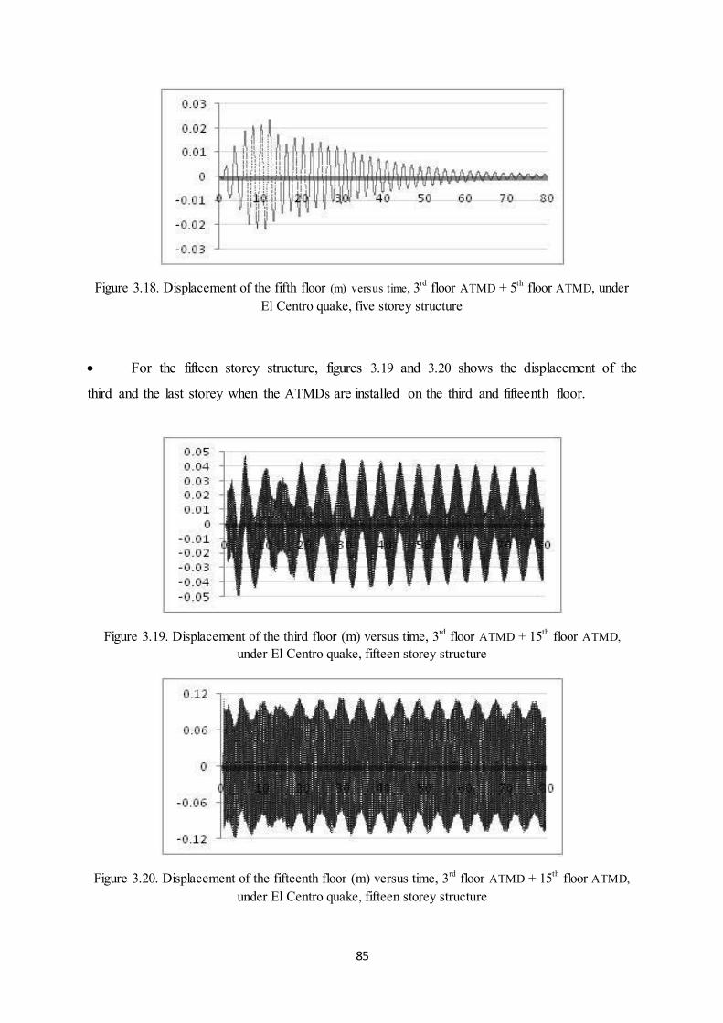
85
Figure 3.18. Displacement of the fifth floor (m) versus time, 3rd floor ATMD + 5th floor ATMD, under El Centro quake, five storey structure
For the fifteen storey structure, figures 3.19 and 3.20 shows the displacement of the
third and the last storey when the ATMDs are installed on the third and fifteenth floor.
Figure 3.19. Displacement of the third floor (m) versus time, 3rd floor ATMD + 15th floor ATMD, under El Centro quake, fifteen storey structure
Figure 3.20. Displacement of the fifteenth floor (m) versus time, 3rd floor ATMD + 15th floor ATMD, under El Centro quake, fifteen storey structure

86
For the fifteen storey structure, figures 3.21 and 3.22 shows the displacement of the
seventh and last storey when the ATMDs are installed on the seventh and fifteenth floor.
Figure 3.21. Displacement of the seventh floor (m) versus time, 7th floor ATMD + 15th floor ATMD, under El Centro quake, fifteen storey structure
Figure 3.22. Displacement of the fifteenth floor (m) versus time, 7th floor ATMD + 15th floor ATMD, under El Centro quake, fifteen storey structure
For the fifteen storey structure, figures 3.23 to 3.24 shows the displacement of the
thirteenth and last storey when the ATMDs are installed on the thirteenth and fifteenth floor.
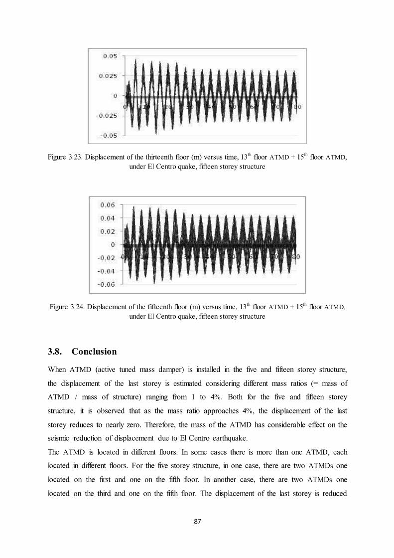
87
Figure 3.23. Displacement of the thirteenth floor (m) versus time, 13th floor ATMD + 15th floor ATMD, under El Centro quake, fifteen storey structure
Figure 3.24. Displacement of the fifteenth floor (m) versus time, 13th floor ATMD + 15th floor ATMD, under El Centro quake, fifteen storey structure
3.8. Conclusion
When ATMD (active tuned mass damper) is installed in the five and fifteen storey structure,
the displacement of the last storey is estimated considering different mass ratios (= mass of
ATMD / mass of structure) ranging from 1 to 4%. Both for the five and fifteen storey
structure, it is observed that as the mass ratio approaches 4%, the displacement of the last
storey reduces to nearly zero. Therefore, the mass of the ATMD has considerable effect on the
seismic reduction of displacement due to El Centro earthquake.
The ATMD is located in different floors. In some cases there is more than one ATMD, each
located in different floors. For the five storey structure, in one case, there are two ATMDs one
located on the first and one on the fifth floor. In another case, there are two ATMDs one
located on the third and one on the fifth floor. The displacement of the last storey is reduced

88
considerably in the case when there is one ATMD at the top and one in mid-height of the
structure in contrast to one ATMD at the top storey and one at the first storey. For the fifteen
storey structure, in one case, there are two ATMDs one located on the third floor and one at
the last floor. In the second case, there are two ATMDs one located on the seventh floor and
one at the last floor. In the third case, there are two ATMDs one located on the thirteenth floor
and one at the last floor. The simulation results show one ATMD being located on the mid-
height of the structure and one at the top has the highest effect on the seismic vibration
reduction due to El Centro earthquake.

89
CHAPTER 4 ACTIVE VIBRATION CONTROL OF TWO BENCHMARK
STRUCTURES EQUIPPED WITH MULTIPLE TUNED MASS DAMPERS
4.1. Introduction The tuned mass damper (TMD) is an energy dissipation device, which suppresses structural
vibration by transferring some of the structural vibration energy to the TMD and dissipates
the energy through the damping of the TMD (Hong-Nan Li, 2007). However, single tuned mass
damper (STMD) is sensitive to the frequency ratio between the TMD and the structure and the
damping ratio of the TMD. The effectiveness of STMD is reduced significantly due to the
mistuning or off optimum damping. As a result, the use of more than one TMD with different
dynamic characteristics has been proposed by Xu and Igusa (K. Xu, 1992 ) in order to
improve the effectiveness and robustness.
The multiple tuned mass dampers (MTMDs) for controlling the structural vibration consist of
a large number of small TMDs whose natural frequencies are distributed around the natural
frequency of a controlled mode of the structure (Hong-Nan Li, 2007).
Xu and Igusa (K. Xu, 1992 ) studied the case of multiple substructures with light damping
and equal spacing over a frequency range can be more effective and more robust than a single
TMD with equal total mass when the system is excited by a wide band random excitation.
In this chapter, the two benchmark structures from the previous chapter are being analysed; a
five storey structure (Samali B, 2003) and a fifteen storey structure (Guclu R, 2008) this time
equipped with Multiple Active Tuned Mass Dampers. Multiple mass dampers are used with
the intention of covering a higher frequency range compared to sole tuned mass dampers. The
active control is carried out by Fuzzy Logic controllers for each of the dampers on the top
floor. These controllers all have the same membership functions and same rules in which
during the earthquake subjected to the structure and the free vibration afterwards, the
actuators are producing control forces in each time step to mitigate the external vibration
damaging the structure.
The tuned mass dampers are considered in two cases. In the first case, they have equivalent
mass; considering different frequency parameters. In the second case, they have equivalent
stiffness and damping parameters; considering different mass.
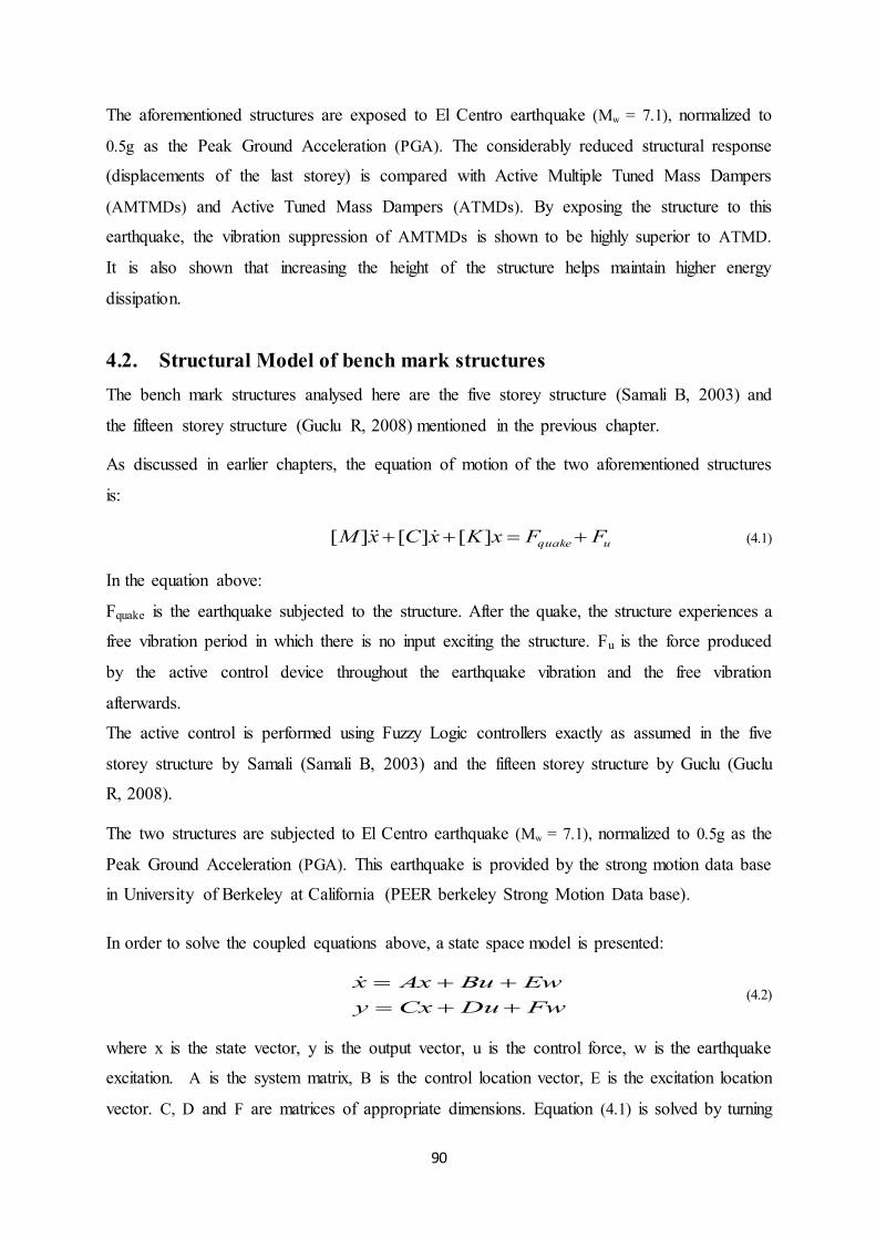
90
The aforementioned structures are exposed to El Centro earthquake (Mw = 7.1), normalized to
0.5g as the Peak Ground Acceleration (PGA). The considerably reduced structural response
(displacements of the last storey) is compared with Active Multiple Tuned Mass Dampers
(AMTMDs) and Active Tuned Mass Dampers (ATMDs). By exposing the structure to this
earthquake, the vibration suppression of AMTMDs is shown to be highly superior to ATMD.
It is also shown that increasing the height of the structure helps maintain higher energy
dissipation.
4.2. Structural Model of bench mark structures The bench mark structures analysed here are the five storey structure (Samali B, 2003) and
the fifteen storey structure (Guclu R, 2008) mentioned in the previous chapter.
As discussed in earlier chapters, the equation of motion of the two aforementioned structures
is:
uquake FFxKxCxM ][][][ (4.1)
In the equation above:
Fquake is the earthquake subjected to the structure. After the quake, the structure experiences a
free vibration period in which there is no input exciting the structure. Fu is the force produced
by the active control device throughout the earthquake vibration and the free vibration
afterwards.
The active control is performed using Fuzzy Logic controllers exactly as assumed in the five
storey structure by Samali (Samali B, 2003) and the fifteen storey structure by Guclu (Guclu
R, 2008).
The two structures are subjected to El Centro earthquake (Mw = 7.1), normalized to 0.5g as the
Peak Ground Acceleration (PGA). This earthquake is provided by the strong motion data base
in University of Berkeley at California (PEER berkeley Strong Motion Data base).
In order to solve the coupled equations above, a state space model is presented:
FwDuCxyEwBuAxx
(4.2)
where x is the state vector, y is the output vector, u is the control force, w is the earthquake
excitation. A is the system matrix, B is the control location vector, E is the excitation location
vector. C, D and F are matrices of appropriate dimensions. Equation (4.1) is solved by turning

91
it into the form of equation (4.2), so it can be solved numerically in MATLAB. The structural
responses are provided by SIMULINK in MATLAB.
In the Multiple Tuned Mass Damper case for equation (4.1), the mass, stiffness and damping
matrices are different to the sole Tuned Mass Damper case. In the sole Tuned Mass Damper
case, the structure is modelled with a mass on top which has constant values for mass and
stiffness and damping throughout the earthquake and the free vibration afterwards and so an
additional degree of freedom is added to the structure which is modelled as another storey on
top. For the Multiple Tuned Mass Damper case, there are multiple additional degrees of
freedom added to the structure. The configuration of these dampers is shown in figure 4.1.
Figure 4.1. Active Multiple Tuned Mass Dampers (AMTMDs)
As mentioned above, in the case of Multiple Tuned Mass Dampers, the mass and stiffness
and damping matrices differ compared to Tuned Mass Dampers. These matrices are shown
below (Hong-Nan Li, 2007):
T
ntts xxxxx ...21 , n = No. of TMDs (4.3)
tntts mmmmdiagM ...21 , mtj = mass of the jth damper (4.4)
nn
n
n
kks
kk
kkkk
kkkkk
K
00
0000
22
11
211
(4.5)

92
(4.6)
nn
n
n
kks
cc
cccc
ccccc
C
00
0000
22
11
211
4.3. Multiple tuned mass damper configuration The structural modelling of the five and fifteen storey structures equipped with multiple
tuned mass dampers is presented here. Two cases are being considered, but first some terms
need to be explained (Siyassi, 2003):
Average frequency of MTMDs: n
k
kT n1
, n = No. of MTMDs (4.7)
Frequency space for the MTMDs:
T
n 1 (4.8)
Frequency of the jth MTMD:
1)
21(
nnjTj
jTj
, j = 1, 2,…, n
(4.9)
Mass ratio:
s
n
jj
m
m1
, ms = mass of the total structure
(4.10)
Average stiffness of the MTMDs:
n
j j
sT
mK
12
1.
(4.11)
Mass of the jth MTMD:
2j
Tj
Km
(4.12)
4.4. Active Vibration Control of the two benchmark structures The active vibration control is performed by Fuzzy Logic Controllers. There are five
membership functions for each input and nine for the output. All of these are triangular. The

93
inputs are the displacement (XNB, XNS, XZ, XPS, XPB) and velocity (VNB, VNS, VZ, VPS,
VPB) of the particular storey and the output is the control force (UNBB, UNB, UNM, UNS, UZ,
UPS, UPM, UPB, UPBB) produced by the controller. The fuzzy logic procedure is performed
by the fuzzy logic toolbox provided in MATLAB.
Table 4-1- Rule base definition for the fuzzy logic controller
Error (e)
Velocity of the error (de/dt) VNB VNS VZ VPS VPB
XNB UNBB UNB UNM UNS UZ
XNS UNB UNM UNS UZ UPS
XZ UNM UNS UZ UPS UPM
XPS UNS UZ UPS UPM UPB
XPB UZ UPS UPM UPB UPBB
The fuzzy rules are as follows: 1. If (x2 is XNB) and (v2 is VNB) then (u2 is UNBB) 2. If (x2 is XNB) and (v2 is VNS) then (u2 is UNB) 3. If (x2 is XNB) and (v2 is VZ) then (u2 is UNM) 4. If (x2 is XNB) and (v2 is VPS) then (u2 is UNS) 5. If (x2 is XNB) and (v2 is VPB) then (u2 is UZ) 6. If (x2 is XNS) and (v2 is VNB) then (u2 is UNB) 7. If (x2 is XNS) and (v2 is VNS) then (u2 is UNM) 8. If (x2 is XNS) and (v2 is VZ) then (u2 is UNS) 9. If (x2 is XNS) and (v2 is VPS) then (u2 is UZ) 10. If (x2 is XNS) and (v2 is VPB) then (u2 is UPS) 11. If (x2 is XZ) and (v2 is VNB) then (u2 is UNM) 12. If (x2 is XZ) and (v2 is VNS) then (u2 is UNS) 13. If (x2 is XZ) and (v2 is VZ) then (u2 is UZ) 14. If (x2 is XZ) and (v2 is VPS) then (u2 is UPS) 15. If (x2 is XZ) and (v2 is VPB) then (u2 is UPM) 16. If (x2 is XPS) and (v2 is VNB) then (u2 is UNS) 17. If (x2 is XPS) and (v2 is VNS) then (u2 is UZ) 18. If (x2 is XPS) and (v2 is VZ) then (u2 is UPS) 19. If (x2 is XPS) and (v2 is VPS) then (u2 is UPM) 20. If (x2 is XPS) and (v2 is VPB) then (u2 is UPB) 21. If (x2 is XPB) and (v2 is VNB) then (u2 is UZ) 22. If (x2 is XPB) and (v2 is VNS) then (u2 is UPS) 23. If (x2 is XPB) and (v2 is VZ) then (u2 is UPM) 24. If (x2 is XPB) and (v2 is VPS) then (u2 is UPB) 25. If (x2 is XPB) and (v2 is VPB) then (u2 is UPBB)

94
where P, N, Z, B, M and S stand for positive, negative, zero, big, medium and small and X, V
and U represent displacement, velocity and voltage.
4.5. Structural Modelling of the five storey structure In the first case, there is only one ATMD at the top of the structure and the mass of this
damper is 1% of the sum of the total mass of the structure. The critical damping is 0.02 of the
critical damping of the structure. The active vibration control procedure is performed by only
one Fuzzy Logic controller and the active control device is on the last floor. The fuzzy
membership functions and rules are discussed above. The structure is exposed to El Centro
earthquake, normalized to 0.5g. The response of the structure due to these external vibrations
and the vibration suppression due to the active control device is shown in the figures below.
Table 4-2- Structural characteristics of the sole ATMD, five storey structure
mt1(kgr) 17
Kt1(N/m) 2500
Ct1(Ns/m) 8
Figure 4.2. Last storey displacement (mm) versus time with a sole ATMD on top, the five storey
structure
In the second case, there are three ATMDs at the top of the structure and the sum of the mass
of these dampers is 1% of the sum of the total structures mass, the critical damping is 0.02 of
the critical damping of the structure. The active vibration control procedure is performed by
three Fuzzy Logic controllers for each of the tuned mass dampers and the active control
devices are at the last floor. The fuzzy membership functions and rules are discussed above.
The frequency space ( ) is 0.3. This case is divided into two sub cases. In the first sub case,
the mass of the AMTMDs is equal and in the second sub case, the damping and stiffness of
the AMTMDs are equal. The structural characteristics of the AMTMDs for the two cases and

95
the two sub cases are mentioned in the table below. Note that in all the fuzzy controllers the
type and number of the membership functions and the rules are the same.
Table 4-3- Structural characteristics of the 3ATMDs, five storey structure, equal mass
mt1(kgr) 6 mt2(kgr) 6 mt3(kgr) 6 Kt1(N/m) 600 Kt2(N/m) 900 Kt3(N/m) 1200 Ct1(Ns/m) 2 Ct2(Ns/m) 3 Ct3(Ns/m) 4
Table 4-4- Structural characteristics of the 3ATMDs, five storey structure, non-equal mass
mt1(kgr) 7 mt2(kgr) 5 mt3(kgr) 4 Kt1(N/m) 840 Kt2(N/m) 840 Kt3(N/m) 840 Ct1(Ns/m) 3 Ct2(Ns/m) 3
Ct3(Ns/m) 3
The last storey displacement for the five storey structure with AMTMDs on top, with equal
mass is shown in figure 4.3. The last storey displacement for the five storey structure with
AMTMDs on top, with non-equal mass is shown in figure 4.4.
Figure 4.3. Last storey displacement (mm) versus time, equal mass, five storey structure, 3ATMDs on
top

96
Figure 4.4. Last storey displacement (mm) versus time, non-equal mass, five storey structure, 3ATMDs
on top
4.6. Structural Modelling of the fifteen storey structure In the first case, there is only one ATMD at the top of the structure and the mass of this
damper is 2% of the sum of the total structures mass, the critical damping is 0.02 of the
critical damping of the structure. The active control procedure is performed by only one
Fuzzy Logic controller and the active control device is on the last floor. The fuzzy
membership functions and rules are discussed above. The structure is exposed to El Centro
earthquake, normalized to 0.5g. The response of the structure due to these external vibrations
and the vibration suppression due to the active control device is shown in the figures below.
Table 4-5- Structural characteristics of the sole ATMD, fifteen storey structure
mt1(kgr) 106000
Kt1(kN/m) 260 Ct1(kNs/m) 400000
Figure 4.5. Last storey displacement (mm) versus time with a sole ATMD on top, fifteen storey
structure

97
In the second case, there are three ATMDs at the top of the structure and the sum of the mass
of these dampers is 2% of the sum of the total structures mass, the critical damping is 0.02 of
the critical damping of the structure. The active control procedure is performed by only one
Fuzzy Logic controller and the active control device is on the last floor. The fuzzy
membership functions and rules are discussed above. The frequency space ( ) is 0.25. This
case is divided into two sub cases. In the first sub case, the mass of the AMTMDs is equal and
in the second sub case, the damping and stiffness of the AMTMDs are equal. The structural
characteristics of the AMTMDs for the two cases and the two sub cases are listed in the table
below. Table 4-6- Structural characteristics of the 3TMDs, fifteen storey structure, equal mass
mt1(kgr) 35000 mt2(kgr) 35000
mt3(kgr) 35000 Kt1(kN/m) 53000
Kt2(kN/m) 70000 Kt3(kN/m) 88000
Ct1(kNs/m) 34 Ct2(kNs/m) 44
Ct3(kNs/m) 56
Table 4-7- Structural characteristics of the 3TMDs, fifteen storey structure, non-equal mass
mt1(kgr) 45000
mt2(kgr) 34000
mt3(kgr) 27000
Kt1(kN/m) 135000
Kt2(kN/m) 135000
Kt3(kN/m) 135000
Ct1(kNs/m) 86
Ct2(kNs/m) 86
Ct3(kNs/m) 86
The last storey displacement for the fifteen storey structure with AMTMDs on top, with equal
mass is shown in figure 4.5. The last storey displacement for the fifteen storey structure with
AMTMDs on top, with non-equal mass is shown in figure 4.6.
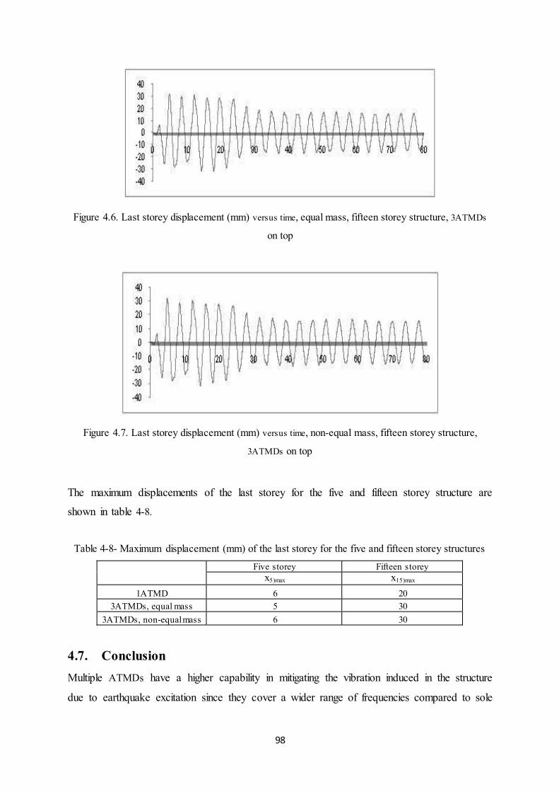
98
Figure 4.6. Last storey displacement (mm) versus time, equal mass, fifteen storey structure, 3ATMDs
on top
Figure 4.7. Last storey displacement (mm) versus time, non-equal mass, fifteen storey structure,
3ATMDs on top
The maximum displacements of the last storey for the five and fifteen storey structure are
shown in table 4-8.
Table 4-8- Maximum displacement (mm) of the last storey for the five and fifteen storey structures
Five storey Fifteen storey x5)max x15)max
1ATMD 6 20 3ATMDs, equal mass 5 30
3ATMDs, non-equal mass 6 30
4.7. Conclusion Multiple ATMDs have a higher capability in mitigating the vibration induced in the structure
due to earthquake excitation since they cover a wider range of frequencies compared to sole

99
ATMDs. AMTMDs have a more compact volume; this is because sum of the mass of the
AMTMD is the mass ratio (= mass of ATMD / mass of entire structure) in contrast to ATMDs.
As observed in this chapter, for the five storey structure, when 3ATMDs with equal mass are
installed at the top of the structure, the reduction in the last storey displacement is more
considerable compared to 3ATMDs with non-equal mass or a sole ATMD on the top floor.
After the earthquake, for the free-vibration period, the 3ATMDs with equal mass have the
same effect on the vibration reduction of the last storey.
As the height of the structure is increased to fifteen stories, a sole ATMD on top has
considerable effect on the reduction of the last storey displacement. The effect of 3ATMDs
with equal mass or non-equal mass on seismic vibration reduction is not observable.
Therefore multiple ATMDs are mainly effective in low-rise structures in contrast to a sole
ATMD which is very effective in high rise structures.

100
CHAPTER 5
SELF-ORGANISING ADAPTIVE FUZZY LOGIC CONTROL FOR NON-AFFINE NONLINEAR
SYSTEMS
5.1. Introduction
Adaptive fuzzy logic control (Alata, Su & Demirli 2001; Chai & Tong 1999; Cho, Yee &
Park 1999; Ge et al. 2010; Han, Su & Stepanenko 2001; Islam & Liu 2011; J.T. Spooner
2001b; Phan & Gale 2007; Rubaai 1999; Wang, Liu & Lin 2002; Wang 1994) have fixed
structures after the user has defined the membership functions by trial and error. Due to not
having knowledge on the mathematical modelling for different plants, this trial and error
takes considerable time. Therefore, self-organising adaptive fuzzy logic controllers are
proposed as it does not have a fixed structure and can change and structure itself as it can
automatically add and remove membership functions and therefore rules from the fuzzy
inference system.
Self-organising adaptive fuzzy logic controllers (Gao & Er 2003; Park, Park, et al. 2005b;
Phan & Gale 2008; Qi & Brdys 2009) do not date back to more than a decade. Park (Park,
Park, et al. 2005b) propose a self-structuring adaptive fuzzy logic controllers wherein
membership functions and therefore rules are added or replaced to the input space. Gao and
Er (2003) proposed a self-organizing fuzzy neural system, in which the rule generation
criteria was based on the system error and the -completeness, and for rule pruning an error
reduction ratio was defined. In (Phan & Gale 2008), a self-structuring adaptive fuzzy logic
controller is defined particularly for affine nonlinear systems which defines a simple
flowchart algorithm to add or replace rules based on two criteria defined; the tracking error
and the -completeness. Qi and Brdys (2009)proposed a self-organising fuzzy logic controller
for affine, nonlinear discrete systems taking advantage of online subtractive clustering and
recursive least square methods.
5.2. Affine state space equations versus non-affine state space equations The contributions mentioned above are only applicable for affine state space equations, as

101
presented below:
; (5.1)
where represents the state vector defined by the user, is the
output vector, and is the input control.
The aforementioned contribution is further improved by (Phan & Gale 2008) to self-
organising adaptive fuzzy logic control of non-affine state space equations presented below:
. (5.2)
Non-affine nonlinear state space equations have been very challenging to tackle over the
passing decade. Park (2005a) has proposed online self-structuring adaptive fuzzy logic
control to overcome this challenge. The setback encountered in non-affine nonlinear systems
is not having the control input explicitly seen in the state space equations, therefore the
popular feedback linearization scheme could not be used. In (Park & Park 2003), the non-
affinity in the state space equations is turned into affine as a result of using the Taylor series.
In (Du, Shao & Yao 2006), the Nussbaum-Gain and the mean value method is considered to
deal with the non-affinity in the state space equations. (Ge et al. 2010),(Essounbouli &
Hamzaoui 2006) considered using the mean value method and the implicit function procedure
to deal with the control feedback not being visible in the state space equations. In (Park, Park,
et al. 2005a),(Calise, Hovakimyan & Idan 2001; Park, Huh, et al. 2005) pseudo-control
method is considered in which the pseudo-error needs to be reduced using an adaptive neural
network as the output. Liu et al (Liu, Tong & Li 2010) proposed an adaptive neural network
method for multi-input multi-output feedback systems by taking into account the mean value
and the implicit function method to deal with the non-affinity.

102
Not only the ideal control needs to be defined, restrictions need to be made on the control
gain . On one hand, the condition for controllability needs to be satisfied ,
on the other hand a lower bound needs to be defined in which (Castro
1995) or a design parameter needs to be considered in which . (Park, Park, et
al. 2005a),(Calise, Hovakimyan & Idan 2001; Park, Huh, et al. 2005). Other researchers(Ge
et al. 2010),(Essounbouli & Hamzaoui 2006) proposed that needs to be bounded and
a design parameter needs to be defined in which , being the unknown positive
constant. For single-input single-output systems, Liu (Liu, Tong & Li 2010) defined a series
of design parameters , in which , being the order of the system,
and being the higher and lower bounds for the control gains.
The conditions defined above indicate the complex characteristics of the controllers in non-
affine case compared to affine case (Chai & Tong 1999; Cho, Yee & Park 1999; Rubaai
1999; Wang, Liu & Lin 2002). Therefore to deal with these setbacks several methods are
presented. In the first step, the ideal control needs to be defined, the implicit function method
is used similar to (Ge et al. 2010),(Essounbouli & Hamzaoui 2006),(Liu, Tong & Li 2010). In
the second step, the system stability needs to be checked, wherein the universal
approximation theory is introduced. This method is simple as extra mathematical equations
only involve in the stability check, therefore there is no restriction for the control gain. The
controller is the same for both cases, affine and non-affine state space equations making this
method more efficient. In this chapter, the adaptive fuzzy logic system is defined and the self-
organising process is introduced. Section 3, discusses the application of this defined adaptive
fuzzy system in the control of affine nonlinear state space equations. Section 4, the universal
approximation method is considered to make the stability check similar to the affine case. In
section 5, some examples are provided to discuss the aforementioned method in practice. In
the end, discussions and conclusion are presented in section 6.
5.3. Self- organisingAdaptive fuzzy system description
5.3.1. Description of Fuzzy systems
The zero order Takagi-Sugeno fuzzy systems are used in which the point fuzzification
procedure, product-type inference and centre-average defuzzifier is considered as the fuzzy
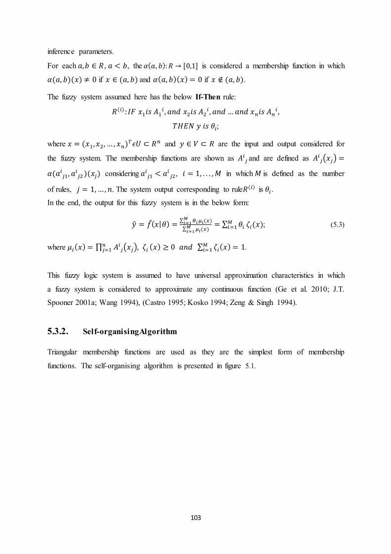
103
inference parameters.
For each , , the is considered a membership function in which
if and if .
The fuzzy system assumed here has the below If-Then rule:
;
where and are the input and output considered for
the fuzzy system. The membership functions are shown as and are defined as
considering , in which is defined as the number
of rules, . The system output corresponding to rule is .
In the end, the output for this fuzzy system is in the below form:
; (5.3)
where .
This fuzzy logic system is assumed to have universal approximation characteristics in which
a fuzzy system is considered to approximate any continuous function (Ge et al. 2010; J.T.
Spooner 2001a; Wang 1994), (Castro 1995; Kosko 1994; Zeng & Singh 1994).
5.3.2. Self-organisingAlgorithm
Triangular membership functions are used as they are the simplest form of membership
functions. The self-organising algorithm is presented in figure 5.1.

104
Figure 5.1. Self-organising algorithm flowchart
a) Assumed criteria for rule production
The two criteria considered for rule production are tracking error (system error) and -
completeness:
Tracking error (system error):
Tracking error or system error is the difference between the desired output defined by the
user and the fuzzy system output. A parameter error_threshold is defined in which if the
system error exceeds this parameter a new membership function is added to the input with the
highest number of fired membership functions.
The completeness:
This criteria is satisfied if for any input there is a membership function in which the
membership degree does not exceed . Therefore, , n being the number of inputs. If
there exists a membership degree exceeding , a new membership function will therefore be
added to the input.

105
b) The parameters of the added membership functions need to be determined
The centre of the newly added membership function is considered to be the value of the input
variable. The centre of the left and right adjacent membership functions are the left and right
points of this new membership function. Therefore, the adjacent membership functions are
defined to satisfy the -completeness criteria. Other design parameters are defined;
max_mf_distance and min_mf_distance in case there is no adjacent membership function. In
which the left (or right) point of the newly added membership is determined to have a centre
distance equivalent to max_mf_distance; a value defined by the user. In some cases,
membership functions become too close to each other, when the centre distance of the newly
added membership functions and the centre of the adjacent membership functions exceed
min_mf_distance, a value defined by the user.
c) The added rules are determined
By adding a new membership function, new rules will automatically be added to the
rule base, being the number of inputs. The newly added rules will be produced in addition
to their consequences adding to the fuzzy system output.
d) Deleting an existing membership function
By adding a new membership function, the new number of rules must not exceed . If
exceeded, the furthest membership function must be deleted, taking all its relevant rules with
it.
5.4. Self-organising adaptive fuzzy logic control for Affine nonlinear systems
An adaptive fuzzy logic controller for a single-input single-output system in affine nonlinear
systems is shown in the state space format presented in the equation below:
(5.4)
;

106
where is the control input; is the system output; and are unknown continuous
functions; and is the state vector of the system.
Assumption 5.1: is considered to be continuous with a known sign in being
the controllability zone.
As the controllability condition in equation (5.3) implies and being continuous
for the controllability region, with the assumption of for this entire region.
The control objective is defining a self-organising adaptive fuzzy logic controller in which
the output is tracking a desired reference .
Considering known functions for and , the ideal control signal is defined below:
; (5.5)
where , , . By substitution of equation (5.3)
the error function is transformed into the below form:
; (5.6) is chosen in a way to satisfy the Hurwitz stability of equation (5.6) in which the error is
reduced to zero as time exceeds infinity or in other words the output tracks the desired output.
Therefore, the objective of the control is met.
It is assumed that . Equation (5.5) turns into the below format:
; (5.7) where , . Assuming and as unknown functions, the fuzzy logic controller in equation (5.3) is
used to approximate as shown below:
. (5.8)
Assumption 5.2 The upper bound for the rule generation ruleB is selected so the controller
would not be capable of exceeding the suitable size in the fuzzy inference system. In
addition, this assumption is more flexible compared to fixed adaptive fuzzy logic controllers
where the main objective is to define a fuzzy rule base satisfying the desirable approximation.
Assuming the upper bound for the required number of rules ruleB , the self-organising
algorithm will automatically produce the fuzzy inference system.

107
The adaptive parameter vector for the final fuzzy logic controller is considered to be
in which .
Therefore , where , are the active
parameters in the vector of adaptive parameters, and are the
inactivated parameters which do not interfere in the controller design process. Therefore, the
output of the controller is in the form below:
. (5.9)
Assumption 5.3 The ideal control needs to be bounded into lower and higher bounds as
shown below:
, . Therefore, an actuator that can satisfy the above conditions is required. Based on this
assumption, the boundedness of the adaptive parameters is satisfied.
By substituting the controller output with and adding and
subtracting to equation (5.3), the equation for error dynamics is achieved below:
. (5.10)
Lemma 1. Assuming , can be presented in the vector form of
in addition to assuming an ideal parameter vector
where:
; (5.11)
where and are positive values.
Proof
The lemma above is proven in (Phan & Gale 2006, 2008). The following sections discuss the
extended form of this lemma, in addition to the proof provided in appendix A.
When lemma 1 is applied to equation (5.10), the error dynamic is resulted in the format
below:
.
The vector format is presented below:

108
; (5.12)
where
, ;
where C is a stable matrix and a positive definite symmetric nn matrix Q is assumed in
which the Lyapunov function below needs to be satisfied:
; (5.13)
where P is derived from the function above and is a positive definite matrix.
Remark 1 The error dynamic equation (5.12) is very popular in adaptive intelligent control.
Therefore, for the stability check, lemma 1 is presented. In the following discussions in
section 3, the extended form of this lemma to change the error dynamics for non-affine
systems to the format in equation (5.12) is presented.
Theorem 1 Based on system (5.4) and the assumptions discussed above, the controller in
equation (5.9) and the self-organising adaptive fuzzy logic control algorithm in section 2, the
adaptive law is defined as below:
; (5.14)
where the adaptive parameters and the tracking error need to be bounded as shown below:
, (5.15)
, ; (5.16)
where , is assumed based on the initial conditions and is required to be
109
positive, and being a positive value used in tuning the adaptive parameter .
The control system needs to be uniformly ultimately bounded (UUB), in which the error
function is a compact set as defined below:
. (5.17)
Proof:
The proof is presented in (Phan & Gale 2008).
5.5. Self-organising adaptive fuzzy logic control for Non-affine nonlinear
systems
The state space equations for a single-input single-output system taking into account
nonlinearity and non-affinity is presented in the equations below:
(5.18)
;
where is the input control, is the output, being the non-affinity format of this
state space equation as a nonlinear continuous function which is
unknown, is the state vector of this system.
The control objective is the same as the affine case:
Control objective is designing a fuzzy logic controller which is adaptive in which the closed
loop system is stable in which the variables are obliged to be bounded. The output has to
track the reference signal .
Assumption 5.4: The controllability of the non-affine nonlinear function needs to be
checked:
; (5.19)
where belongs to the controllability region .

110
Assumption 5.5 The upper bound for the rules needs to be defined so the fuzzy
inference size does not exceed a certain specific value.
Assumption 5.6 The bounds for the ideal control signal needs to be determined:
, .
In contrast to the affine state space equations, the explicit form of the ideal control signal is
not available in the state space equation. Therefore, the implicit function theorem is
considered to present the ideal control law as discussed below:
1) Ideal control law is presented:
Considering , , and in which the
Hurwitz stability of the polynomial is satisfied. The ideal control law
is presented in the form below:
;
in which the tracking error is expected to reach zero.
Assume:
. (5.20)
In order to have the non-affinity in the ideal control law, v needs to be added and subtracted
to equation (5.18) resulting in the equation below:
; (5.21)
in which an ideal control signal is established as below:
for .
Lemma 2.This lemma was previously introduced in lemma 2.8 as the proof is presented in
(Ge et al. 2010), in which f is a continuously differentiable function and is
bounded by a positive constant in which for all .
Therefore a continuous function exists wherein .
Proof is presented in (Ge et al. 2010).
Assuming and .
in which
as and (assumption 1).
Therefore, lemma 1 is applied for in which a continuous function exists so
111
that or:
. (5.22)
2) The stability needs to be checked
The stability of the control system is confirmed if the error dynamics in equation (5.21) is
changeable to the standard format in equation (5.12). If this condition is satisfied, the
controller presented in theorem 1 is approved to have close-loop stability.
Based on equation (5.21) and (5.22), the error dynamics is presented below:
. (5.23)
The same as discussed in section 2, considering the adaptive parameters as
for the final fuzzy logic controller, in which the activated
adaptive parameters need to be defined. A fuzzy logic system as discussed in section 2 to
approximate is defined below:
. (5.24)
The universal approximation method, as discussed in the previous sections, is used to indicate
the existence of a fuzzy logic controller with the format shown in equation (5.24) to predict an
ideal control signal approximating the fuzzy controller output.
Lemma 3. Assume , is presented. Assuming an
ideal parameter vector in which:
; (5.25)
and and are some positive constants.
Proof
The proof is similar to the proof of the universal approximation method presented in (Castro
1995).
The error dynamics is achieved when the equation (5.25) is substituted into equation (5.23):
. (5.26)
As shown below, the vector format of the error dynamics is:
; (5.27)
where

112
, .
Equation (5.27) is similar to equation (5.12). Therefore, the error dynamics of a non-affine
nonlinear system is transferred to the extended format of the universal approximation error
method, as discussed in lemma 6.2. Therefore, the controller presented in theorem 1 promises
the closed loop stability of the system.
The following sections present two examples of non-affine nonlinear systems.
5.6. Numerical Examples
1) Example 1
This example depicts the design procedure of a particular system with non-affinity and
nonlinearity in the state space equations (Essounbouli & Hamzaoui 2006; Ge et al. 2010;
Park, Huh, et al. 2005; Park, Park, et al. 2005a):
. (5.28)
The controllability condition needs to be checked . The initial condition for this
system is . The main objective is to track the output when a desired
reference is defined .
The input has been chosen in the below form:
.
The parameters of the controller are chosen as below:
, , , , , .
The learning parameters for the adaptive controller are defined as below:
, ,
, , .
In the first step, the fuzzy system has only 1 rule with 1 membership function for each input,
as shown in the figure below:

113
Figure 5.2. Initial membership functions for all input and output variables
As seen in figure 5.3, the controller output has successfully tracked the desired
output .
Figure 5.3. Output versus desired output
As shown in figure 5.4, after about 10 seconds the tracking error starts to converge to zero
indicating that the output has tracked the desired reference output defined by the user.
Figure 5.4. Tracking error
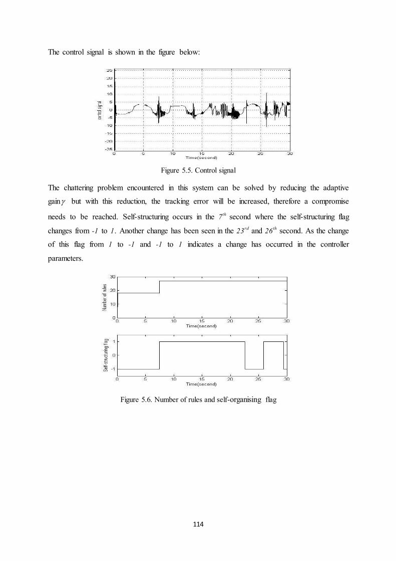
114
The control signal is shown in the figure below:
Figure 5.5. Control signal
The chattering problem encountered in this system can be solved by reducing the adaptive
gain but with this reduction, the tracking error will be increased, therefore a compromise
needs to be reached. Self-structuring occurs in the 7th second where the self-structuring flag
changes from -1 to 1. Another change has been seen in the 23rd and 26th second. As the change
of this flag from 1 to -1 and -1 to 1 indicates a change has occurred in the controller
parameters.
Figure 5.6. Number of rules and self-organising flag

115
Figure 5.7. Final membership functions for input 1
Figure 5.8. Final membership functions for input 2
Figure 5.9. Final membership functions for input 3
The final membership functions for the three inputs are also triangular. As can be seen, three
membership functions have been defined after the self-organising criteria for the fuzzy logic
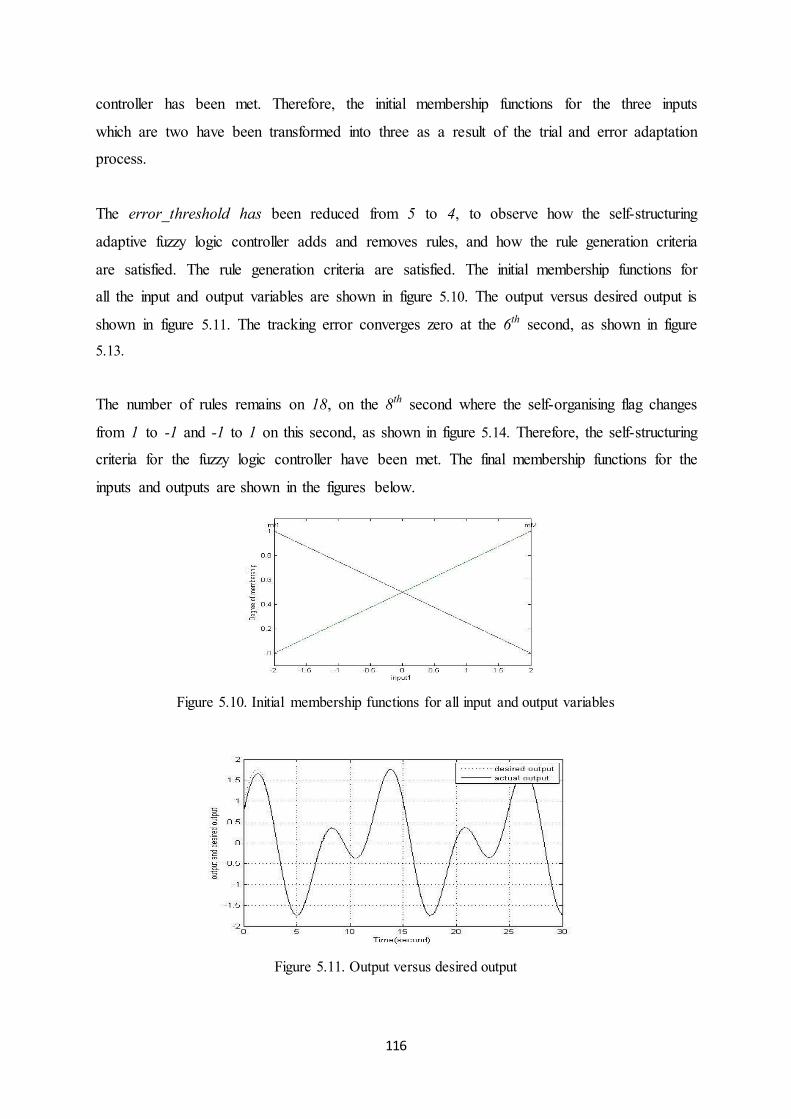
116
controller has been met. Therefore, the initial membership functions for the three inputs
which are two have been transformed into three as a result of the trial and error adaptation
process.
The error_threshold has been reduced from 5 to 4, to observe how the self-structuring
adaptive fuzzy logic controller adds and removes rules, and how the rule generation criteria
are satisfied. The rule generation criteria are satisfied. The initial membership functions for
all the input and output variables are shown in figure 5.10. The output versus desired output is
shown in figure 5.11. The tracking error converges zero at the 6th second, as shown in figure 5.13.
The number of rules remains on 18, on the 8th second where the self-organising flag changes
from 1 to -1 and -1 to 1 on this second, as shown in figure 5.14. Therefore, the self-structuring
criteria for the fuzzy logic controller have been met. The final membership functions for the
inputs and outputs are shown in the figures below.
Figure 5.10. Initial membership functions for all input and output variables
Figure 5.11. Output versus desired output

117
Figure 5.12. Tracking error
Figure 5.13. Control signal
Figure 5.14. Number of rules and self-organising flag

118
Figure 5.15. Final membership functions for input 1
Figure 5.16. Final membership functions for input 2
Figure 5.17. Final membership functions for input 3
As can be seen, the initial membership functions for the three inputs are two triangular
membership functions for each input. As the self-organising criteria for the fuzzy logic
controller has been met, a third membership function is added to each of the inputs.
Therefore, reducing the error_threshold from 5 to 4, results in a much quicker convergence
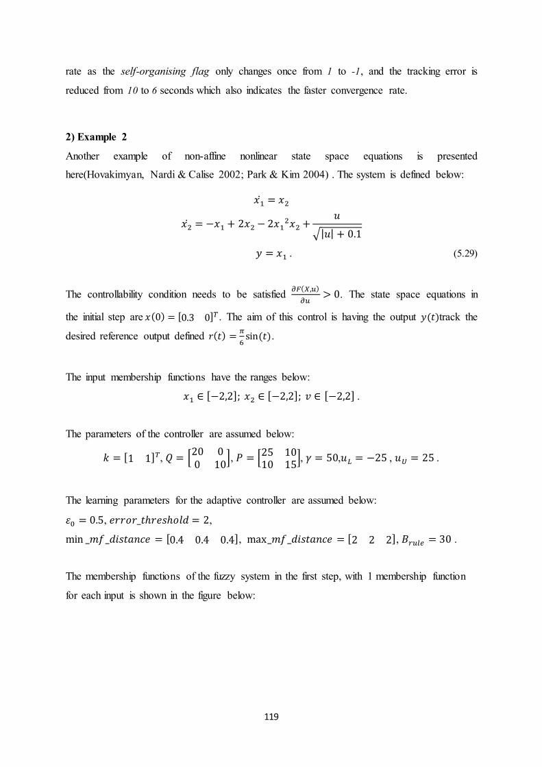
119
rate as the self-organising flag only changes once from 1 to -1, and the tracking error is
reduced from 10 to 6 seconds which also indicates the faster convergence rate.
2) Example 2
Another example of non-affine nonlinear state space equations is presented
here(Hovakimyan, Nardi & Calise 2002; Park & Kim 2004) . The system is defined below:
. (5.29)
The controllability condition needs to be satisfied . The state space equations in
the initial step are . The aim of this control is having the output track the
desired reference output defined .
The input membership functions have the ranges below:
.
The parameters of the controller are assumed below:
, , , , , .
The learning parameters for the adaptive controller are assumed below:
, ,
, , .
The membership functions of the fuzzy system in the first step, with 1 membership function
for each input is shown in the figure below:

120
Figure 5.18. Initial membership functions for all input and output variables
The controller in this non-affine nonlinear system has the objective to track the desired
reference signal , as shown in figure 5.19 and figure 5.20.
Figure 5.19. Output versus desired output
Figure 5.20. Tracking error
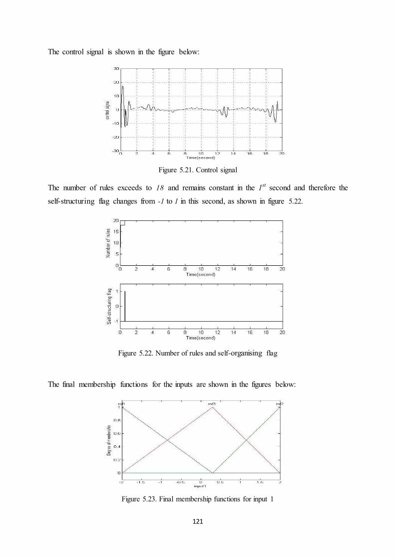
121
The control signal is shown in the figure below:
Figure 5.21. Control signal
The number of rules exceeds to 18 and remains constant in the 1st second and therefore the
self-structuring flag changes from -1 to 1 in this second, as shown in figure 5.22.
Figure 5.22. Number of rules and self-organising flag
The final membership functions for the inputs are shown in the figures below:
Figure 5.23. Final membership functions for input 1
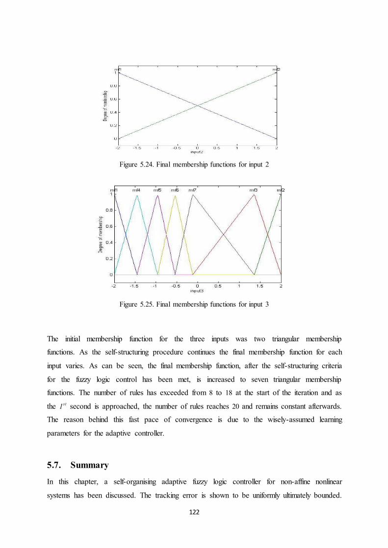
122
Figure 5.24. Final membership functions for input 2
Figure 5.25. Final membership functions for input 3
The initial membership function for the three inputs was two triangular membership
functions. As the self-structuring procedure continues the final membership function for each
input varies. As can be seen, the final membership function, after the self-structuring criteria
for the fuzzy logic control has been met, is increased to seven triangular membership
functions. The number of rules has exceeded from 8 to 18 at the start of the iteration and as
the 1st second is approached, the number of rules reaches 20 and remains constant afterwards.
The reason behind this fast pace of convergence is due to the wisely-assumed learning
parameters for the adaptive controller.
5.7. Summary
In this chapter, a self-organising adaptive fuzzy logic controller for non-affine nonlinear
systems has been discussed. The tracking error is shown to be uniformly ultimately bounded.

123
All the adaptive parameters and the tracking error are shown to be bounded. The stability
checks consist of two stages. First, the implicit function theorem is used to show the
existence of the ideal control. Afterwards, for the Lyapunov stability check an extension form
of universal approximation theory is discussed. In contrast, the other control algorithms
proposed in the introduction of this chapter, this method does not have any restrictions. The
controller proposed in the non-affine nonlinear system is also applicable for much simpler
state space equations in the affine case. In the end, two examples are presented to discuss this
method in practice.

124
CHAPTER 6
SEMI-ACTIVECONTROLLED BUILDINGS UNDER EXCITATIONS
6.1. Introduction When seismic vibration suppression devices are installed in building structures, these
structures are considered to be smart structures. The optimised placement of sensors,
actuators and vibration suppression devices is very efficient in reducing the vibration induced
in structures when subjected to external excitations (Adeli 2008). Research has been
conducted for decades on vibration suppression of structures due to external excitations or
dynamic loading such as wind or heavy traffic (Nishitani & Inoue 2001). Semi-active
vibration devices take into account both the features of passive and damping vibration
suppression devices (Symans & Constantinou 1999).The typical semi-active vibration control
devices include fluid viscous dampers and magneto rheological (MR) dampers. The MR
damper requires lower voltage which is easily supplied by batteries, therefore making it very
popular (Carlson, Catanzarite & St. Clair 1996). When using MR dampers, a control
algorithm needs to be defined which can incorporate its nonlinear characteristics, as well as
the nonlinear non-affine state space equations encountered when dealing with the equation of
motion of the building structure. In this chapter, a more efficient type of fuzzy logic
controller is defined known as self-organising adaptive fuzzy logic control. This intelligent
control proposed here is very efficient in dealing with the aforementioned non-affine
nonlinear state space equations.
Simulation on a one-storey and five-storey structure has been conducted. Both structures are
equipped with a pair of MR dampers. Fuzzy logic controllers and self-organising adaptive
fuzzy logic controllers have individually been used and their efficiency in reducing the
earthquake-induced vibrations has been compared.
6.2. Structural System A n-degree-of-freedom building structure is considered. The external excitations can be wind
or earthquake. The equation of motion is presented below:

125
; (6.1)
where m is the mass of the structure, c is the damping of the structure, k is the stiffness of the
structure, is the displacement matrix, is the velocity matrix, is the acceleration
matrix of the building structure;
, ,
, .
Matrix is the gain matrix determining the control effect on the building, is a distribution
matrix, f is the control force provided by the controller and is the ground acceleration
of the earthquake.
The mass matrix is considered as below:
. (6.2)
The stiffness matrix is as below:
. (6.3)
The damping matrix is as below:
. (6.4)
The equation of motion is transformed into state space equations in which a system state is
defined and has the below form:
; (6.5)
, , ;
(6.6)
where A is the system matrix, B is the gain matrix and E is the external excitation matrix.

126
6.3. Structure equipped with MR dampers An n-storey structure is subjected to external excitations, in this case earthquakes, in which
MR dampers are installed in the structure and the control forces, are provided by the
controller. The equation of motion of this structure takes the form presented in equation (6.1)
in which the control input is the control force which is known as an ‘indirect’ control
algorithm.
For the direct control algorithm, the current is the control input which is supplied to the MR
damper. This damper is modelled by the static hysteresis model, as discussed in chapter 2.
The schematic diagram of an n-storey structure equipped with a pair of MR dampers in each
floor and subjected to seismic excitation is shown in figure 6.1.
Figure 6.1. System schematic diagram
6.4. Damper modeling and setup A set up of two MR dampers installed in one storey is shown in the figure below:

127
Figure 6.2. Damper differential configurations
The static hysteresis model, introduced in chapter 2, is used for the direct control in which the
control input is the current supplied to the MR damper. The damper forces generated are
presented below:
; (6.7)
where are for the left and right damper in the figure above and the damper
parameters , , , , , ; depend on the current supplied to the MR
damper. The damper parameters and current is a polynomial of order one or two (Kwok et al.
2006).
Based on the setup in the figure above, the displacements of the two dampers are opposite in
sign, in which:
, . (6.8)
Therefore, the coefficients which are dependent on the current (Kwok et al. 2006) have the
below form:
, ; (6.9)
where is the current provided to the damper on the right. The forces of the damper are
presented below:
(6.10)
. (4.11)
The effective damping force is the difference of the two MR damper forces, , as
presented in the equations below:

128
. (6.12)
Assuming equal currents supplied to the dampers, therefore , then
. (6.13)
Assuming the offset forces , . For similar dampers; , and
therefore, the offset forces cancel each other. Therefore, the total force in equation (6.13)
takes the form below:
. (6.14)
Assuming the hysteretic parameters as below:
(6.15)
. (6.16)
Assuming the dampers are identical and the currents supplied to these dampers are equal, the
hysteresis variable takes the below form:
(6.17)
; (6.18)
where .Therefore . The total force eventually takes
the form below:
; (6.19)
where , , ,
and .
Based on the assumptions above, the offset forces are cancelled in contrast to the stiffness
and damping of the damper forces which are added up in the overall force for the MR
damper, which is dependent on the current supplied. If this cancellation was not possible, the
equation (6.19) would have extra parameters, for example, , and therefore a robust
controller would be required.

129
6.5. Structures with embedded MR dampers The equation of motion for an arbitrary floor when a pair of MR dampers are installed in
it, takes the form below:
; (6.20)
where , and are the mass, damping and stiffness.
Assuming pairs of dampers are embedded on the ,.., ,.. and floors with the current
vector , the state space equation takes the form below:
; (6.21)
where
,
(6.22)
, , ;
where all the elements of matrix and are the same as and in equation (6.2), except the
floor, where the MR dampers are installed and , and
(k=1,2,..,n). Matrix results from the inaccuracy in modelling or not identical MR dampers
installed in one floor.
6.6. Fuzzy logic controller
Fuzzy logic is a model-free approach as it does not require elaborate mathematical functions
to tackle in its design. Fuzzy logic systems are efficient when solving rigorous control

130
problems. The best features of fuzzy logic systems are that they can be nonlinear, adaptive,
and handle uncertainty in the system.
The fuzzy logic controller uses data from the sensors and converts them into linguistic or
fuzzy membership functions by the fuzzification process.
This chapter focuses on the structural model of an nth storey structure. The structure discussed
has a pair of MR dampers embedded in it and fuzzy logic controllers as the control devices.
The equation of motion of the structure with the nonlinear characteristics of the MR damper
has been considered and discussed. In the following sections, two case studies; a one storey
and a five storey structure are being discussed.
6.7. Simulations of a one storey structure embedded with MR dampers
and different controllers The building under consideration is a benchmark one storey model with one pair of identical
MR dampers defined by Ha (2008) for studies on response control of earthquake-excited
buildings. An earthquake is subjected to this structure and the vibrations due to this external
excitation are shown to be reduced dramatically via the dampers installed and the fuzzy logic
controller versus the self-organising adaptive fuzzy logic controller.
6.7.1. Structural model of a one storey building The numerical modeling of a one storey steel structure is presented here. The external
excitation is an earthquake, El Centro, in this case. The fundamental frequency of this
earthquake is 1.5 Hz whilst the fundamental frequency of the structure is 4 Hz; therefore the
destructive effect of resonance is prevented. The 1st vibration mode (fundamental frequency
of the structure) is considered. A pair of magnetorheological (MR) dampers are used here as
semi-active vibration control devices. A static hysteresis model is used to model the damper
formula and incorporate it in the equation of motion of the structure. The current-controlled
problem of the smart structure system is formulated in non-affine nonlinear state space
equations due to the nonlinear characteristics of this damper. The objective is to mitigate the
vibration of the structure therefore the desired output is the displacements that are converging
to zero. Self-organising adaptive fuzzy logic systems are used to overcome the non-affine

131
nonlinear state space equations encountered when solving the equation of motion of the
structure.
6.7.2. Simplified evaluation model Numerical simulations were conducted in MATLAB and SIMULINK to test the efficiency of
the control algorithms developed. This can be seen from the block diagram of the system:
Figure 6.3. System block diagram
The equation of motion of the building equipped with a pair of MR dampers installed in the
first storey and a fuzzy logic controller can be presented as:
;
(6.23)
where
;
where is the acceleration vector, is the velocity vector, is the displacement vector of
the first floor. is the mass, is the damping, is the stiffness of the first storey. is the
current produced by the fuzzy logic controller and provided to the MR damper.
The equation of motion of the structure, in equation (6.23), can be transformed into state
space equations as shown below:
;

132
where
, . (6.24)
In the simulation:
, , .
The characteristics of the MR damper are:
; ; ; ;
; ;
; ;
; .
The external excitation subjected to the structure is the El Centro earthquake (Mw=7.1),
normalized to 2g as the peak ground acceleration (PGA), as shown in figure 6.4. This
earthquake is provided by the strong motion data base in University of Berkeley at California
(Pacific Earthquake Engineering Research Centre).
Figure 6.4. El Centro earthquake acceleration time history

133
Figure 6.5. Schematic of a one storey structure equipped with MR dampers
6.7.3. Designing the fuzzy logic controller The fuzzy logic controller is designed using three inputs, all having two triangular
membership functions, and one output having eight constant membership functions. The
inputs are the displacement ( ) and velocity ( ) of the first storey and the variations of
current with respect to time . The output is the current (i) provided to the MR damper.
The fuzzy variables are defined in table 6-1.
Table 6-1- Fuzzy Variables
XN Negative Displacement
XP Positive Displacement
VN Negative Velocity
VP Positive Velocity
N(Idot) Negative Variations in Current
P(Idot) Positive Variations in Current

134
The membership functions for the input variables are shown below:
- For the first input which is the displacement:
Figure 6.6. The first input of the fuzzy logic controller
- For the second input which is the velocity:
Figure 6.7. The second input of the fuzzy logic controller
- For the third input which is the variations of current:
Figure 6.8. The third input of the fuzzy logic controller
The membership functions for the output variable are constant:

135
.
The fuzzy logic controller rules are as below:
1. If is XN and is VN and is N(Idot), Then is .
2. If is XN and is VN and is V(Idot) , Then is .
3. If is XN and is VP and is N(Idot) , Then is .
4. If is XN and is VP and is V(Idot), Then is .
5. If is XP and is VN and is N(Idot), Then is .
6. If is XP and is VN and is V(Idot) , Then is .
7. If is XP and is VP and is N(Idot) , Then is .
8. If is XP and is VP and is V(Idot) , Then is .
Figure 6.9. Adaptive fuzzy logic controller
The control objective is to make the displacement of the first storey track the
reference signal which is defined as zero matrices. The flowchart algorithm of adaptive fuzzy
logic controllers is shown in figure 6.9.
The operating variable ranges are chosen as follows:
; ; .
The parameters of the controller are chosen as follows:
; ; ; .

136
6.7.4. Designing the self-organising adaptive fuzzy logic controller
As mentioned in the previous chapter, fixed-structured adaptive fuzzy logic control requires
designers to choose the rule base and membership functions by trial and error. This task is not
trivial as long as exact mathematical models of plants are not known. Quite often, the
structure used is either unnecessarily large or too small to adequately represent a plant. From
this perspective, self-organising adaptive fuzzy logic control is more advantageous as it can
automatically add and remove rules from a fuzzy system.
A variable called self-organising flag is used to indicate when the self-organising performs.
When the self-organising flag switches from 1 to -1 or -1 to 1, it indicates a change in the
fuzzy system structure has occurred.
Table 6-2- Different set ups
mf threshold
Error Threshold
center distance
threshold
Set up 1 0.5 0.5 [1 1 1] [0.5 0.5 0.5] 100 Set up 2 0.5 2 [2 2 2] [0.5 0.5 0.5] 15 Set up 3 0.5 0.5 [1 1 1] [0.5 0.5 0.5] 20 Set up 4 0.5 0.5 [0.5 0.5 0.5] [0.25 0.25 0.25] 20 Set up 5 0.5 0.5 [0.5 0.5 0.5] [0.25 0.25 0.25] 20 Set up 6 0.5 0.5 [0.25 0.25 0.25] [0.125 0.125 0.125] 20 Set up 7 0.5 2 [0.5 0.5 0.5] [0.25 0.25 0.25] 15 Set up 8 0.5 2 [0.5 0.5 0.5] [0.125 0.125 0.125] 20 Set up 9 0.5 0.25 [0.5 0.5 0.5] [0.25 0.25 0.25] 20
Different setups for the structure-learning parameters are performed, as shown in table 6-2;
setup 2 has shown the best results. is half of the maximum predefined spreads of the
triangular membership functions in each dimension.
The SIMULINK block in MATLAB, used for self-organising adaptive fuzzy logic controller
for non-affine nonlinear systems is shown in figure 6.10.
Figure 6.10. Self-organising adaptive fuzzy logic controller

137
In this SIMULINK block, a reference signal is defined. As mentioned in the previous sections,
this signal is a zero matrix, defined for the desired displacement of this one storey building
structure since the main objective of these vibration control devices is to suppress the
displacement resulting from the external excitations. The block for the adaptive fuzzy logic
controller is shown in figure 6.14, in which the desired reference and the plant output are the
inputs to this block. The output of this block is the current. The input is defined based on a
series of trial and error presented in table 6-2, in which the best structure-learning parameters
are chosen for the adaptive control. The SIMULINK block for the non-affine nonlinear system
is shown in figure 6.15, in which the non-affinity in the state space equations is modeled into
a series of blocks where the exact mathematical calculations seen in the state space equations
are presented. The external excitation is a scaled earthquake subjected to the structure. The
structural characteristics (mass, damping and stiffness), the MR damper equations and the
fuzzy logic controller are modeled in the non-affine nonlinear system block. The input to this
block is the current provided from the adaptive fuzzy logic controller block which is given to
the MR damper. The output is the displacement and velocity of the first storey of the
structure. The loop in figure 6.10 continues until the tracking error converges to zero. The
tracking error is the difference between the displacement output and the desired displacement
output. It is an indicator of the convergence of the system, or in other words, the termination
of the iteration procedure. Then, the fuzzy logic controller is known to be adapted. Therefore,
there is an initial set of membership functions assumed for the inputs and the outputs and a
final set of membership functions after the adaptation of the fuzzy logic controller, presented
in figures 6.18 to 6.21.
6.7.5. Simulation results of the one storey structure
The simulation analysis of the one storey building with MR dampers and fuzzy logic
controller is incorporated into the SIMULINK program in MATLAB, using a variable
integration time step. The differential equation of motion is solved using the fourth-order
Runge-Kutta. The external excitation subjected to the structure is the El Centro earthquake
(Mw=7.1) normalized to 2g.
The one storey building structure without either MR dampers or any other controllers (fuzzy
logic controllers or self-organising adaptive fuzzy logic controllers) due to El Centro
earthquake is shown in figure 6.14.
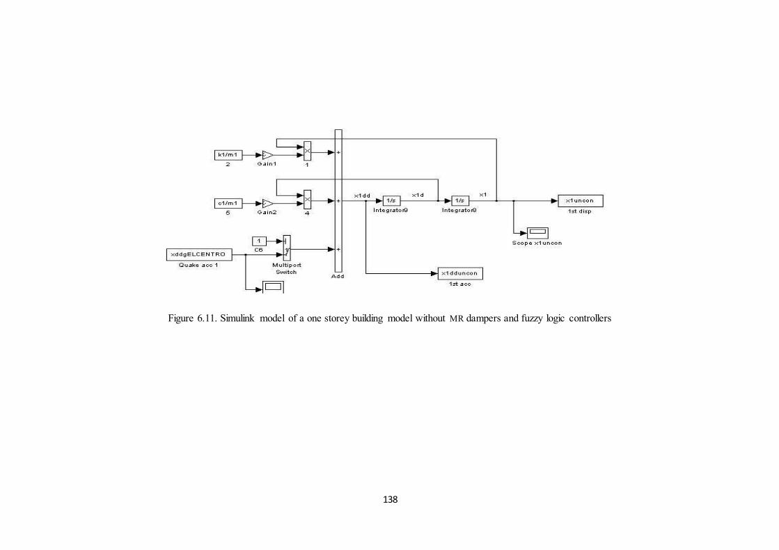
138
Figure 6.11. Simulink model of a one storey building model without MR dampers and fuzzy logic controllers

139
The SIMULINK model in MATLAB of the one storey building structure embedded with MR
dampers and fuzzy logic controller due to El Centro earthquake excitations is shown in figure 6.12.
The SIMULINK model in MATLAB of the one storey structure embedded with MR dampers
and self-organising adaptive fuzzy logic controller due to El Centro earthquake excitations is
shown in figure 6.13.
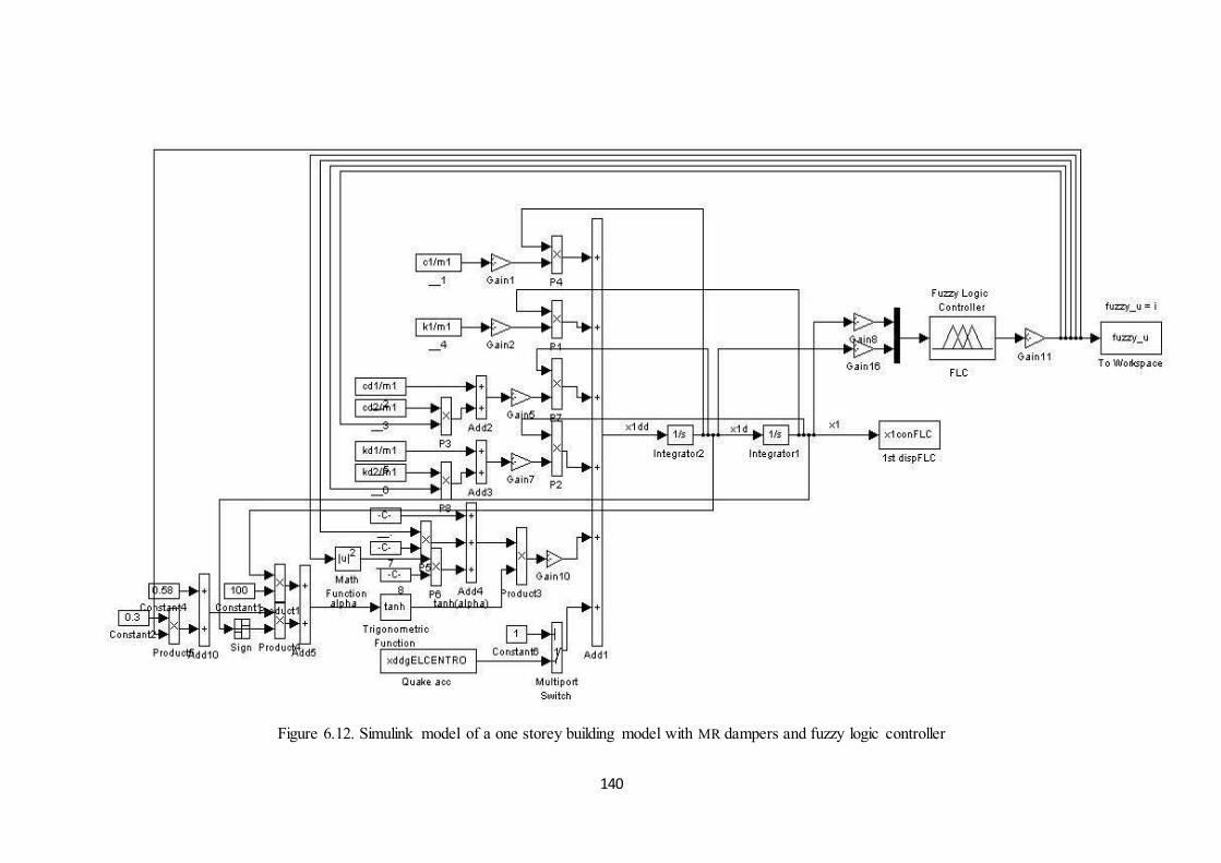
140
Figure 6.12. Simulink model of a one storey building model with MR dampers and fuzzy logic controller
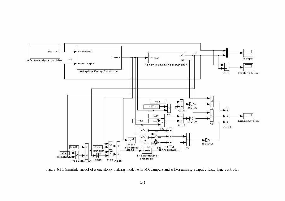
141
Figure 6.13. Simulink model of a one storey building model with MR dampers and self-organising adaptive fuzzy logic controller

142
Figure 6.14. Simulink block of the adaptive fuzzy logic controller
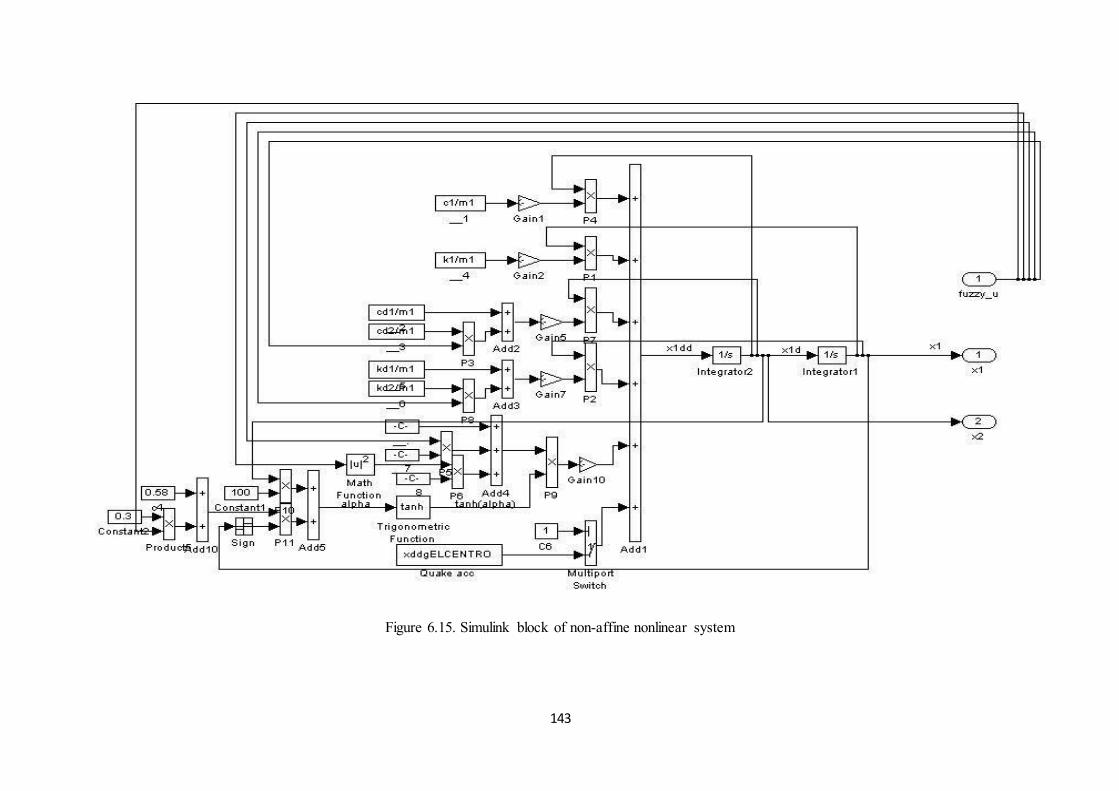
143
Figure 6.15. Simulink block of non-affine nonlinear system
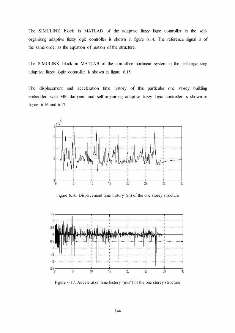
144
The SIMULINK block in MATLAB of the adaptive fuzzy logic controller in the self-
organising adaptive fuzzy logic controller is shown in figure 6.14. The reference signal is of
the same order as the equation of motion of the structure.
The SIMULINK block in MATLAB of the non-affine nonlinear system in the self-organising
adaptive fuzzy logic controller is shown in figure 6.15.
The displacement and acceleration time history of this particular one storey building
embedded with MR dampers and self-organising adaptive fuzzy logic controller is shown in
figure 6.16 and 6.17.
Figure 6.16. Displacement time history (m) of the one storey structure
Figure 6.17. Acceleration time history (m/s2) of the one storey structure

145
The initial fuzzy logic controller has 8 rules with two membership functions in each input
dimension, as shown in figure 6.18.
Figure 6.18. Initial membership functions for all three input variables
The simulation results are shown below. A variable called self-organising flag is used to
indicate when the self-organising performs. When the self-organising flag switches from 1 to
-1 or -1 to 1, it indicates a change in the fuzzy system structure has occurred.
It can be observed that the controller successfully controls the non-affine nonlinear system to
track the reference signal. Self-organising happens in the 2nd second, as shown in figure 6.22.
The tracking error is within the range as shown in figure 6.23. The current
produced by the controller is shown in figure 6.24.
The damping force produced by the damper is the maximum of 3500 N in the 3rd second, as
shown in figure 6.25, which can be provided by a RD-1005-3 MR damper. Configurations of
this damper are shown in table 6-3.
Figure 6.19. Final membership function for input 1

146
Figure 6.20. Final membership function for input 2
Figure 6.21. Final membership function for input 3
Figure 6.22. Number of rules and Self-organising flag – time
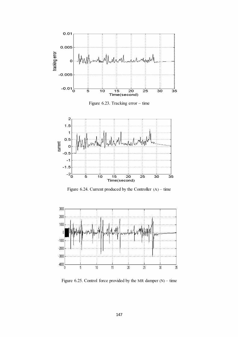
147
Figure 6.23. Tracking error – time
Figure 6.24. Current produced by the Controller (A) – time
Figure 6.25. Control force provided by the MR damper (N) – time

148
Table 6-3- Configurations of RD-1005-3 MR damper Piston-rod movement journey 53mm
Maximal damping force 4 450 N
Maximal input voltage 12 V
Maximal electric current 2 A
6.7.6. Evaluation criteria The effectiveness on reductions in earthquake-induced vibrations on the structure is further
evaluated by a set of performance indices comparing the controlled response against the
results obtained from the no-control cases. The criteria, adopted from (Djajakesukma, Samali
& Nguyen 2002),(Ohtori et al. 2004) encompass ratios of storey displacements and
accelerations. They are formulated as follows:
1. Absolute storey displacement ratio
(6.25)
in which the subscript stands for the n-storey indices and subscripts c and u stand
for controlled and uncontrolled displacement.
2. Absolute storey acceleration ratio
(6.26)
in which the notation represents the storey acceleration.
3. Inter-storey drift ratio
(6.27)
in which the inter-storey displacement is given by ,
4. Root mean-squared storey displacement ratio
(6.28)
in which the root mean-square (RMS) values are calculated from ,
is the sampling time and T is the total excitation time.

149
5. RMS storey acceleration ratio
(6.29)
in which the RMS values are calculated as above.
6. Average applied current
(6.30)
This is the current considered for when the damper is supplied from a battery.
6.7.7. Response ratios The evaluation ratio for three different earthquakes; El Centro, Kobe and Northridge, for a
one storey structure equipped with a pair of MR dampers in the first floor for two cases; fuzzy
logic controller and self-organising adaptive fuzzy logic controller, is shown in table 6-4.
Table 6-4- Response ratios
Different Controller Fuzzy logic controller Self-organising adaptive fuzzy logic control El Centro
J1 1.86 0.67 J2 1.17 0.99 J3 1.86 0.67 J4 0.54 0. 3
J5 2.19 1.29 J6 1.25 0.29
Kobe J1 5.17 0.7 J2 5.01 0.98 J3 5.16 0.7
J4 0.51 0.4 J5 5.21 2.82 J6 1.33 0.35
Northridge J1 0.87 0.77 J2 1 0.72
J3 0.87 0.77 J4 0.8 0.55 J5 4.41 2.37
J6 1.68 0.3
It is indicated for El Centro earthquake (Mw = 6.9), that the displacements have had more
reduction in the case of self-organising adaptive fuzzy logic controllers for this one storey
structure embedded with MR dampers. The accelerations seem to have the same amount of

150
reduction, respectively for both controllers. The current provided to the MR damper is four
times less in the case of the self-organising adaptive fuzzy logic controller being used.
For Kobe earthquake (Mw= 7.3), the reduction in displacements and accelerations are much
more considerable in the case of self-organising adaptive fuzzy logic controllers in
comparison to fuzzy logic controllers for this particular one storey structure embedded with
MR dampers. The current provided to the MR damper is four times less in the case of self-
organising adaptive fuzzy logic controller compared to the fuzzy logic controller.
For Northridge earthquake (Mw= 6.7), the reduction in displacements and accelerations is not
much different in both cases. The current provided to the MR dampers is five times less in the
case of self-organising adaptive fuzzy logic controllers compared to the fuzzy logic controller
being used.
6.7.8. Summary Self-organising adaptive fuzzy logic systems are used to overcome thenon-affine nonlinear
state space equations encountered when solving the equation of motion of the structure. As
can be seen, the numerical simulation for self-organising adaptive fuzzy logic controller
when dealing with non-affine nonlinear systems is very promising as the explicit formula of
the current is not needed and this method is very generic, in the sense that it can be applied to
other systems.
In addition, as mentioned earlier, fixed-structured fuzzy logic control requires designers to
choose the rule base and membership functions by trial and error, which is a very time-
consuming task. Therefore, self-organising adaptive fuzzy logic controller is more
advantageous as it can automatically add and remove rules from a fuzzy system.
6.8. Simulation of a five-storey structure embedded with MR dampers
and different controllers
6.8.1. Introduction The building under consideration is a benchmark five storey model with one pair of identical
MR dampers defined by (Samali & Al-Dawod 2003) for studies on response control of
earthquake-excited buildings. An earthquake is subjected to this structure and the vibrations
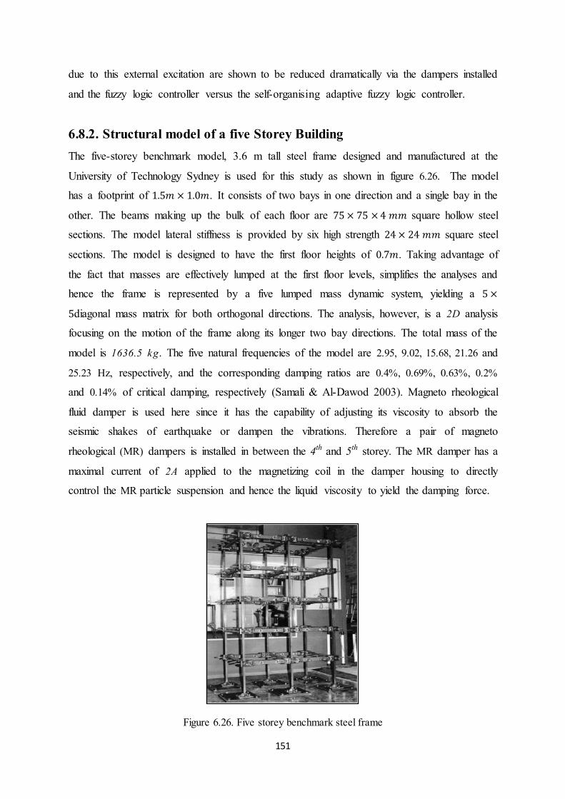
151
due to this external excitation are shown to be reduced dramatically via the dampers installed
and the fuzzy logic controller versus the self-organising adaptive fuzzy logic controller.
6.8.2. Structural model of a five Storey Building The five-storey benchmark model, 3.6 m tall steel frame designed and manufactured at the
University of Technology Sydney is used for this study as shown in figure 6.26. The model
has a footprint of . It consists of two bays in one direction and a single bay in the
other. The beams making up the bulk of each floor are square hollow steel
sections. The model lateral stiffness is provided by six high strength square steel
sections. The model is designed to have the first floor heights of . Taking advantage of
the fact that masses are effectively lumped at the first floor levels, simplifies the analyses and
hence the frame is represented by a five lumped mass dynamic system, yielding a
diagonal mass matrix for both orthogonal directions. The analysis, however, is a 2D analysis
focusing on the motion of the frame along its longer two bay directions. The total mass of the
model is 1636.5 kg. The five natural frequencies of the model are 2.95, 9.02, 15.68, 21.26 and
25.23 Hz, respectively, and the corresponding damping ratios are 0.4%, 0.69%, 0.63%, 0.2%
and 0.14% of critical damping, respectively (Samali & Al-Dawod 2003). Magneto rheological
fluid damper is used here since it has the capability of adjusting its viscosity to absorb the
seismic shakes of earthquake or dampen the vibrations. Therefore a pair of magneto
rheological (MR) dampers is installed in between the 4th and 5th storey. The MR damper has a
maximal current of 2A applied to the magnetizing coil in the damper housing to directly
control the MR particle suspension and hence the liquid viscosity to yield the damping force.
Figure 6.26. Five storey benchmark steel frame

152
The external excitation subjected to the structure is the El Centro earthquake (Mw=7.1),
normalized to 2g as the peak ground acceleration (PGA), as shown in figure 6.4. This quake is
provided by the strong motion data base in University of Berkeley at California (Pacific
Earthquake Engineering Research Centre).
6.8.3. Simplified Evaluation Model The equation of motion of the building equipped with a pair of MR dampers in the kth storey
can be presented as:
(6.31)
Where and are respectively the velocity and acceleration of the entire storey, is the
current supplied to the pair of dampers (Nguyen 2009).
In this case study, a pair of MR dampers are installed in between the 4th and 5th storey and a
fuzzy logic controller is in the last storey. The characteristics of the MR damper are (Ha et al.
2008) :
; ; ;
;
;
; .
6.8.4. Designing the fuzzy logic controller The fuzzy logic controller has three inputs and one output. The first two inputs are the
relative displacement and relative velocity of the 4th and 5th storey (the MR damper is
situated in between these storeys) and the third input is the variations of the current with
respect to time . The output is the current provided to the MR damper.
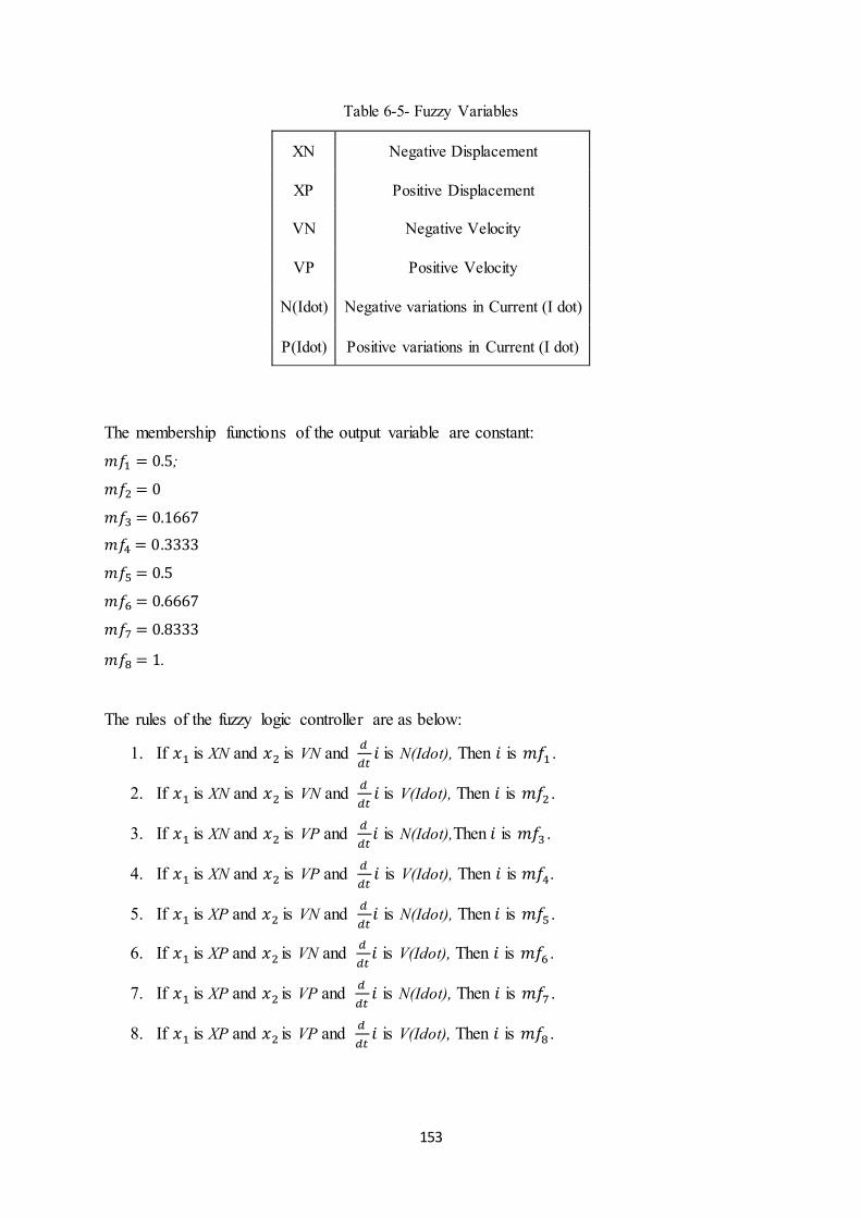
153
Table 6-5- Fuzzy Variables
XN Negative Displacement
XP Positive Displacement
VN Negative Velocity
VP Positive Velocity
N(Idot) Negative variations in Current (I dot)
P(Idot) Positive variations in Current (I dot)
The membership functions of the output variable are constant: ;
.
The rules of the fuzzy logic controller are as below:
1. If is XN and is VN and is N(Idot), Then is .
2. If is XN and is VN and is V(Idot), Then is .
3. If is XN and is VP and is N(Idot),Then is .
4. If is XN and is VP and is V(Idot), Then is .
5. If is XP and is VN and is N(Idot), Then is .
6. If is XP and is VN and is V(Idot), Then is .
7. If is XP and is VP and is N(Idot), Then is .
8. If is XP and is VP and is V(Idot), Then is .

154
Due to the direct control proposed by Ha et al (2008) and the nonlinear characteristics of MR
dampers, non-affine nonlinear state space equations are encountered. Therefore to deal with
these equations, non-affine fuzzy logic control (Movassaghi 2012) is proposed.
The control objective is to make the displacement of the 5th storey track the
reference signal which is defined as zero matrices as the displacements are meant to be
reduced completely; converging to zero.
The operating variable ranges are chosen as follows:
; ; .
The parameters of the controller are chosen as follows:
; ; ; .
6.8.5. Designing the self-organising adaptive fuzzy logic controller As mentioned in chapter 3, fixed-structured adaptive fuzzy logic control requires designers to
choose the rule base and membership functions by trial and error. This task is not trivial as
long as exact mathematical models of plants are not known. Quite often, the structure used is
either unnecessarily large or too small to adequately represent a plant. From this perspective,
self-organising adaptive fuzzy logic control is more advantageous as it can automatically add
and remove rules from a fuzzy system.
Table 6-6- Different set ups
mf threshold
error threshold
center distance
threshold
Set up 1 0.5 0.5 [1 1 1] [0.5 0.5 0.5] 100
Set up 2 0.5 0.5 [0.5 0.5 0.5] [0.25 0.25 0.25] 20
Set up 3 0.5 2 [1 1 1] [0.5 0.5 0.5] 15
Set up 4 0.5 0.5 [0.25 0.25 0.25] [0.125 0.125 0.125] 20
Different set ups for the structure learning parameters are performed, as shown in table 6-6;
set up 3 has shown the best results. is half of the maximum predefined spreads of the
triangular membership functions in each dimension.

155
The SIMULINK block in MATLAB, used for self-organising adaptive fuzzy logic controller
for non-affine nonlinear systems is shown in figure 6.27.
Figure 6.27. Self-organising adaptive fuzzy logic controller for non-affine nonlinear systems
6.8.6. Simulation results of the five storey structure The five storey structure embedded with MR dampers and self-organising adaptive fuzzy
logic controllers due to El Centro earthquake excitations is modeled in SIMULINK in
MATLAB, as shown in figure 6.28.

156
Figure 6.28. Simulink of the five storey structure
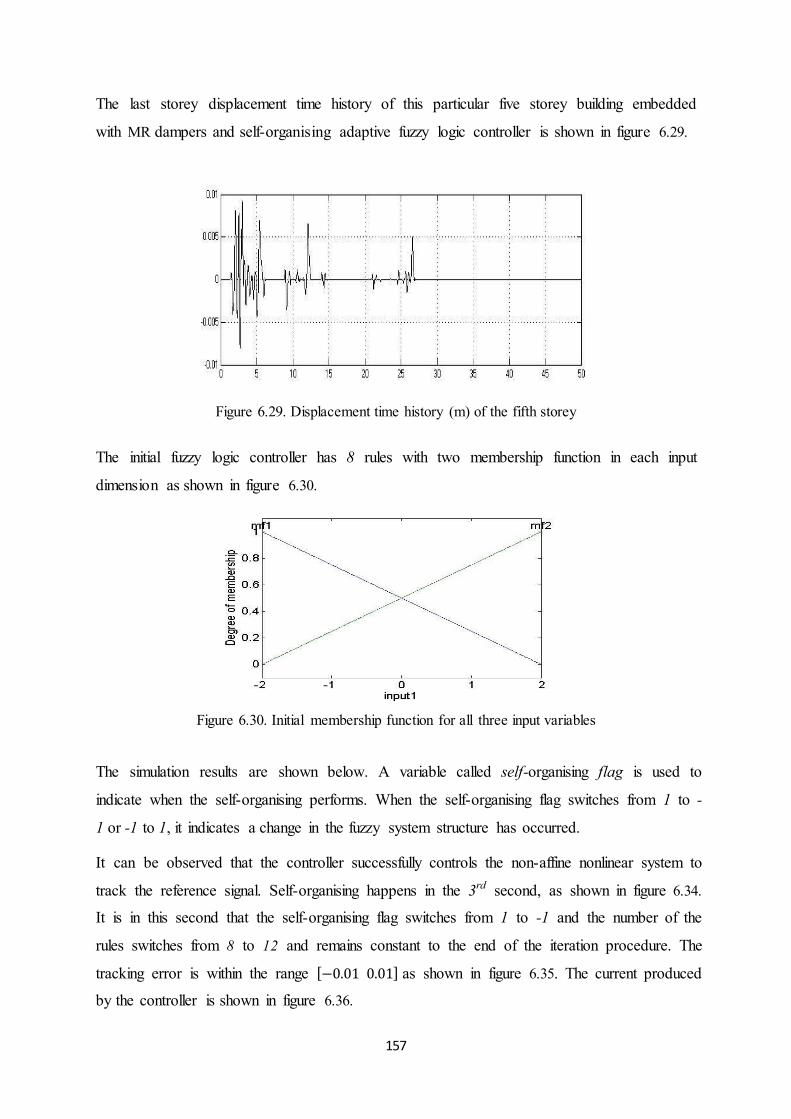
157
The last storey displacement time history of this particular five storey building embedded
with MR dampers and self-organising adaptive fuzzy logic controller is shown in figure 6.29.
Figure 6.29. Displacement time history (m) of the fifth storey
The initial fuzzy logic controller has 8 rules with two membership function in each input
dimension as shown in figure 6.30.
Figure 6.30. Initial membership function for all three input variables
The simulation results are shown below. A variable called self-organising flag is used to
indicate when the self-organising performs. When the self-organising flag switches from 1 to -
1 or -1 to 1, it indicates a change in the fuzzy system structure has occurred.
It can be observed that the controller successfully controls the non-affine nonlinear system to
track the reference signal. Self-organising happens in the 3rd second, as shown in figure 6.34.
It is in this second that the self-organising flag switches from 1 to -1 and the number of the
rules switches from 8 to 12 and remains constant to the end of the iteration procedure. The
tracking error is within the range as shown in figure 6.35. The current produced
by the controller is shown in figure 6.36.

158
The damping force produced by the damper is the maximum of 3500 N in the 3rd second, as
shown in figure 6.37, which can be provided by a RD-1005-3 MR damper. Configurations of
this damper are shown in table 6-7.
Figure 6.31. Final membership function for input 1
Figure 6.32. Final membership function for input 2
Figure 6.33. Final membership function for input 3

159
Figure 6.34. Number of rules and self-organising flag versus time
Figure 6.35. Tracking error versus time
Figure 6.36. Current produced by the controller – time

160
Figure 6.37. Control force provided by the MR damper
Table 6-7- Configurations of RD-1005-3 MR damper
Piston-rod movement journey 53mm
Maximal damping force 4 450 N
Maximal input voltage 12 V
Maximal electric current 2A
6.9. Evaluation criteria The effectiveness on reductions in earthquake-induced vibrations on the building structure is
further evaluated by a set of performance indices comparing the controlled response against
the results obtained from the no-control cases. The criteria, adopted from (Djajakesukma,
Samali & Nguyen 2002),(Ohtori et al. 2004) encompass ratios of storey displacements and
accelerations.
6.10. Response ratios The evaluation ratio for three different earthquakes, El Centro, Kobe and Northridge for a
five storey structure equipped with a pair of MR dampers in between the 4th and 5th floors for
two cases; fuzzy logic controller and self-organising adaptive fuzzy logic controller, is shown
in table 6-8.

161
Table 6-8- Response ratios
Different Controller Fuzzy logic controller Self-organising adaptive fuzzy logic control
Floor 1 2 3 4 5 1 2 3 4 5
El Centro J1 0.26 0.15 0.15 0.24 0.14 0.26 0.14 0.14 0.18 0.12
J2 1.95 1.7 1.08 1.3 0.26 0.42 0.22 0.26 0.73 0.27
J3 0.6 0.53 0.13 0.23 0.4 0.26 0.3 0.11 0.1 0.04
J4 0.1 0.07 0.07 0.07 0.06 0.04 0.03 0.02 0.01 0.01
J5 0.18 0.12 0.17 0.36 0.1 0.07 0.03 0.05 0.11 0.03
J6 0.82 0.26
Kobe J1 0.38 0.32 0.27 0.32 0.27 0.34 0.24 0.22 0.2 0.13
J2 3.1 4.7 2.8 5.6 6.5 0.52 0.37 0.36 0.62 0.39
J3 1.3 2.4 2.3 3.1 3.7 0.34 0.4 0.38 0.91 0.53
J4 0.18 0.13 0.12 0.3 0.4 0.02 0.08 0.07 0.02 0.01
J5 0.21 0.14 0.2 0.33 0.14 0.01 0.05 0.06 0.28 0.13
J6 0.47 0.19
Northridge J1 0.27 0.15 0.17 0.34 0.17 0.22 0.12 0.16 0.26 0.15
J2 1.4 1.8 2.8 3.1 3.8 0.41 0.18 0.28 0.52 0.21
J3 0.27 0.3 0.03 0.05 0.09 0.12 0.03 0.01 0.04 0.07
J4 0.3 0.5 0.5 0.4 0.6 0.05 0.02 0.06 0.03 0.04
J5 0.19 0.22 0.3 0.32 0.45 0.13 0.11 0.16 0.24 0.28
J6 0.47 0.19
It is indicated for El Centro earthquake (Mw = 6.9), that the reduction in quake-induced
displacements is respectively the same for both controllers. On the other hand, there is a
subtle increase in the acceleration despite the ability in reducing the displacements. The self-
organising adaptive fuzzy logic controller seems to be more efficient in reducing both the
displacement and accelerations induced in the structure in comparison to the fuzzy logic
controller. The required current for the fuzzy logic controller is four times the current
required for the self-organising adaptive fuzzy logic controller.
For Kobe earthquake (Mw = 7.3), the reduction in displacement for both controllers is
respectively the same. As for the acceleration, the self-organising adaptive fuzzy logic
controller is more effective in comparison to the fuzzy logic controller. The required current
for the fuzzy logic controller is twice the current essential for the self-organising adaptive
fuzzy logic controller.

162
For Northridge earthquake (Mw = 6.7), the reduction in displacement for both controllers is
relatively the same. The acceleration does not have a dramatic increase for the self-organising
adaptive fuzzy logic controller in comparison to the fuzzy logic controller despite its
effectiveness in reducing these excitations. The required current for the fuzzy logic controller
is twice that required for the self-organising adaptive fuzzy logic controller.
6.11. Summary Self-organising adaptive fuzzy logic systems are used to overcome thenon-affine nonlinear
state space equations encountered when solving the equation of motion of the structure. As
can be seen, the numerical simulation for self-organising adaptive fuzzy logic controller
when dealing with non-affine nonlinear systems is very promising because the explicit
formula of the current is not needed and this method is very generic, in the sense that it can
be applied to other systems.
In addition, as mentioned earlier, fixed-structured fuzzy logic control requires designers to
choose the rule base and membership functions by trial and error, which is a very time-
consuming task. Therefore, self-organising adaptive fuzzy logic controller is more
advantageous as it can automatically add and remove rules from a fuzzy system without the
help of the intelligent user.

163
CHAPTER 7
THESIS CONCLUSION
7.1. Summary
This thesis has described in detail the seismic vibration suppression process in building
structures subject to external excitations. As observed in the recent centuries, widespread
catastrophic effects have been seen due to severe earthquakes. Damage due to such
excitations can be destructive which indicates the need for more effective methods of
earthquake protection.Towards the achievement of high performance smart structures,
vibration control in complex civil structures has been very promising, particularly in the
mitigation of external excitations and dynamic loadings owing to its advantages of low cost,
robustness and reliability against various loading sources and integration of actuators,
sensors, computing and signal processing units. Control performance and energy efficiency
can be improved via direct input control of smart devices from the dissipation point of view
by using parameterized relationships describing the damper dynamics with respect to the
applied electrical signal and integrate their models into structural dynamics.
Therefore, to deal with these destructive excitations, semi-active seismic vibration
suppression control has been discussed in this thesis. Magneto rheological (MR) dampers are
embedded within the building structure to mitigate the seismic vibration. Fuzzy logic
controllers are the control devices used in this case to produce control forces to neutralize the
destructive forces of the external excitations. These two have been implemented in a one and
five storey benchmark building structure and their seismic reduction capability is compared
with the case when there is neither of these installed in the structure. Considerable vibration
reduction has been seen and their implementation in actual building structures is effortless.
7.2. Contributions
The contributions made to this field are:
i. When ATMD (active tuned mass damper) is installed in the five and fifteen storey
structure, the displacement of the last storey is estimated considering different mass
ratios (= mass of ATMD / mass of structure) ranging from 1 to 4%. Both for the five
164
and fifteen storey structure, it is observed that as the mass ratio approaches 4%, the
displacement of the last storey reduces to nearly zero.
ii. The ATMD installed in the five and fifteen storey structure is located in different
floors. For the five storey structure, in one case there are two ATMDs, one located on
the first and one on the fifth floor. In another case, there are two ATMDs one located
on the third and one on the fifth floor. The displacement of the last storey is reduced
considerably in the case when there is one ATMD at the top and one in mid-height of
the structure in contrast to one ATMD at the top storey and one at the first storey. For
the fifteen storey structure, in one case, there are two ATMDs one located on the third
floor and one at the last floor. In the second case, there are two ATMDs one located on
the seventh floor and one at the last floor. In the third case, there are two ATMDs one
located on the thirteenth floor and one at the last floor.
iii. Multiple ATMDs have a higher capability in mitigating the vibration induced in the
structure due to earthquake excitation since they cover a wider range of frequencies
compared to sole ATMDs. For the five storey structure, when 3ATMDs with equal
mass are installed at the top of the structure, the reduction in the last storey
displacement is more considerable compared to 3ATMDs with non-equal mass or a
sole ATMD on the top floor. After the earthquake, for the free-vibration period, the
3ATMDs with equal mass have the same effect on the vibration reduction of the last
storey.
iv. As the height of the structure is increased to fifteen stories, a sole ATMD on top has
considerable effect on the reduction of the last storey displacement. The effect of
3ATMDs with equal mass or non-equal mass on seismic vibration reduction is not
observable. Therefore multiple ATMDs are mainly effective in low-rise structures in
contrast to a sole ATMD which is very efficient in high rise structures.
v. Self-organising adaptive fuzzy logic controller is the main contribution of this
research. When solving the equation of motion of a building structure equipped with
MR dampers and intelligent control, non-affinity and nonlinearity is encountered.
Therefore, to solve these equations, self-organising adaptive fuzzy logic controllers
are proposed.
vi. The considerable vibration reductions observed in this case have been compared with
the case of only fuzzy logic controllers and MR dampers. Several evaluation criteria
have been introduced which indicate the amount of seismic vibration reduction when
165
self-organising adaptive fuzzy logic controllers are applied in comparison to fuzzy
logic controllers.
vii. The limitations encountered in using self-organising adaptive fuzzy logic controllers
proposed in this research, is the membership functions which can only acquire a
triangular shape. Therefore, in case other types of membership functions required, the
MATLAB codes provided is not applicable. Another limitation is when the structure
becomes nonlinear, the control algorithm which cannot distinguish the nonlinearity in
the structural parameters (mass, stiffness and damping) as MATLAB is only a
numerical software used here for the control algorithm and not a Structural
Engineering software.
7.3. Direction for future work
To enhance the findings of this research, several suggestions are listed as follows:
i. The experimental implementation can be done and different design scenarios can be
compared. In addition to this, other control algorithms could be proposed to deal with
the non-affine nonlinear state space equations encountered when implementing these
semi-active vibration control devices due to external excitations.
ii. A high-rise building structure could be considered, e.g. the 76 storey benchmark
building (Samali et al.) the model reduction methods could be used to simplify the
simulation procedure. The performance of this structure could be checked, due to wind
excitations as the external excitations subjected on the structure and the performance
of the aforementioned structures could be compared with different design scenarios or
uncontrolled cases or any other control algorithm defined.
7.4. Conclusion
Active tuned mass dampers are installed in the five and fifteen storey structures; the
displacement of the last storey is estimated considering different mass ratios. As the mass
of the ATMD increases from 1 to 4% the effect on the seismic reduction of displacement
due to El Centro earthquake is very considerable. When two ATMDs are each installed in
different levels of the structure, a considerable seismic reduction is observed when one
ATMD is installed on mid-height and one at the top of the structure, especially in low-rise

166
structures. ATMDs are not as effective in seismic vibration reduction as a sole ATMD in
high-rise structures which are prone to external excitation.
Self-organising adaptive fuzzy logic controllers have been introduced in this research
work. It has been shown that these types of intelligent controllers are more effective than
fuzzy logic controllers in terms of seismic vibration reduction of building structures, as
shown in the previous chapter. In addition, fuzzy logic controllers have a fixed structure
after the intelligent user has defined the membership functions by trial and error. Since
mathematical modeling of different plants requires knowledge on the plant and this may
not be accessible, the trial and error process for rule defining is very time-consuming.
Self-organising adaptive fuzzy logic controllers are advantageous as they can
automatically add and remove rules to a fuzzy inference system.
167
REFERENCE Abdel-Rohman, M. & Leipholz, H.H. 1983, 'Active control of tall buildings', Journal of Structural
Engineering, vol. 109, no. 3,pp. 628-45. Adeli, H. 2008, 'Smart structures and building automation in the 21st century', The 25th international
symposium on automation and robotics in construction, pp. 5-10. Adhikari, R., Yamaguchi, H., Yamazaki, T. 1998, 'Model space sliding mode control of structures',
Earthquake engineering& structural dynamics, vol. 27, no. 11,pp. 1303-14. Agrawal, A. & Yang, J. 1997, 'Static output polynomial control for linear structures', Journal of
engineering mechanics, vol. 123, no. 6,pp. 639-43. Agrawal, A., Yang, J. & Wu, J. 1998, 'Application of optimal polynomial controller to a benchmark
problem', Earthquake Engineering and Structural Dynamics, vol. 27, no. 11,pp. 1291-302. Agrawal, A.K. & Yang, J.N. 1996, 'Optimal polynomial control of seismically excited linear
structures', Journal of engineering mechanics, vol. 122, no. 8,pp. 753-61. Aiken, I.D., Kelly, J.M., Pall, A.S., 1990, 'Earthquake Simulator Testing and Analytical Studies of
Two Energy-absorbing Systems for Multi-storey Structures', Rep.No. UCB/EERC-90-03, University of California, Berkeley.
Aiken, I.D., Kelly, J.M., Pall, A.S., 1988, 'Seismic Response of a Nine-storey Steel Frame with Friction Damped Cross-Bracing', Rep. No.UCB/EERC 88/17, Environment Engineering Research Council, , University of California, Berkeley.
Aiken, I.D., Nims, D. & Kelly, J.M. 1992, 'Comparative study of four passive energy dissipation systems', Bull. New Zealand Nat. Soc. For Earthquake Engrg, vol. 25, no. 3,pp. 175-92.
Akbay, Z. & Aktan, H. 1991, 'Actively regulated friction slip devices', Proc., 6th Can. Conf. On Earthquake Engrg, pp. 367-74.
Akbay, Z. & Aktan, H.M. 1990, 'Intelligent energy dissipation devices', Proc., 4th US Nat. Conf. On Earthquake Engrg. V, vol. 1, pp. 427-35.
Al-Dawod, M., Samali, B., Naghdy, F. & Kwok, K. 1999a, 'Application of a robust fuzzy controller to a wind excited structure', Proc., Asia-Pacific Vibration control’99, pp. 812-87.
Al-Dawod, M., Samali, B., Naghdy, F. & Kwok, K. 1999b, 'Application of fuzzy controller to a 2DOF wind excited structure', Proc., Int. Conf. on Application of Model Analysis’ 99.
Alata, M., Su, C.-Y. & Demirli, K. 2001, 'Adaptive control of a class of nonlinear systems with a first-order parameterized Sugeno fuzzy approximator', Systems, Man, and Cybernetics, Part C: Applications and Reviews, IEEE Transactions on, vol. 31, no. 3,pp. 410-9.
Aldawod, M., Naghdy, F., Samali, B. & Kwok, K. 1999, 'Active control of wind excited structures using fuzzy logic', Fuzzy systems Conference Proceedings, 1999. FUZZ-IEEE'99. 1999 IEEE International, vol. 1, IEEE, pp. 72-7.
Aldawod, M., Samali, B., Naghdy, F. & Kwok, K. 2001, 'Active control of along wind response of tall building using a fuzzy controller', Engineering Structures, vol. 23, no. 11,pp. 1512-22.
Alvarez, L. & Jimenez, R. 2003, 'Semi-active control of civil structures using magnetorheological dampers', American Control Conference, 2003. Proceedings of the 2003, vol. 2, IEEE, pp. 1428-33.
Arima, F., Miyazaki, M., Tanaka, H., Yamazaki, Y. 1988, 'A Study on Building with Large Damping Using Viscous Damping Walls', Proceedings of the Ninth WCEE, vol. vol. 5, pp. pp.821-6.
Asher, J.W., Young, R.P., Ewing, R.D., 1994, 'Seismic Isolation Design of the San Bernardino County Medical Centre Replacement Project', paper presented to the Proceeding of the First World Conference on Structural control.
Baba, K., Yabushita, N., Kasumoto, H., Murakami, H., Inoue, H. 1998, 'Model reference adaptive control on soil structure interaction systems under earthquake disturbance', Proceedings of the 2nd World Conference on Structural control, vol. 2, pp. 1549-59.
Bani-Hani, K. & Ghaboussi, J. 1998, 'Neural networks for structural control of a benchmark problem, active tendon system', Earthquake Engineering and Structural Dynamics, vol. 27, no. 11,pp. 1225-46.

168
Bergman, D.M., Goel, S.C. & Power, B.W. 1987, Evaluation of cyclic testing of steel-plate devices for added damping and stiffness, Department of Civil Engineering, University of Michigan.
Burton, S.A., Makris, N., Konstantopoulos, I. & Antsaklis, P. 1996, 'Modeling the response of ER damper: phenomenology and emulation', Journal of engineering mechanics, vol. 122, no. 9,pp. 897-906.
Butz, T. & Von Stryk, O. 2002, 'Modelling and simulation of electro-and magnetorheological fluid dampers', ZAMM, vol. 82, no. 1,p. 3.
Cai, G.p., Huang, J.z., Sun, F. & Wang, C. 2000, 'Modified sliding mode bang–bang control for seismically excited linear structures', Earthquake engineering & structural dynamics, vol. 29, no. 11,pp. 1647-57.
Calise, A.J., Hovakimyan, N. & Idan, M. 2001, 'Adaptive output feedback control of nonlinear systems using neural networks', Automatica, vol. 37, no. 8,pp. 1201-11.
Carlson, J., Catanzarite, D. & St. Clair, K. 1996, 'Commercial magneto-rheological fluid devices', International Journal of Modern Physics B, vol. 10, no. 23n24,pp. 2857-65.
Carlson, J. & Spencer Jr, B. 1996, 'Magneto-rheological fluid dampers for semi-active seismic control', Proc. of the 3rd Int. Conf. on Motion and Vibr. Control, pp. 35-40.
Carlson, J.D., Spencer Jr., B.F. 1996, 'Magnetorheological fluid dampers:scalability and design issues for application to dynamic hazard mitigation', Proceedings of 2nd workshop on structural control: Next generation of Intelligent structures, Hong Kong, China, pp. 99-109.
Casciati, F. & Giorgi, F. 1996, 'Fuzzy controller implementation', Proceedings of the 2nd International Workshop on Structural control, IASC, Research Centre HKUST, Hong Kong, pp. 119-25.
Castro, J.L. 1995, 'Fuzzy logic controllers are universal approximators', Systems, Man and Cybernetics, IEEE Transactions on, vol. 25, no. 4,pp. 629-35.
Chai, T. & Tong, S. 1999, 'Fuzzy direct adaptive control for a class of nonlinear systems', Fuzzy sets and Systems, vol. 103, no. 3,pp. 379-87.
Chang, C.-C. & Roschke, P. 1998, 'Neural network modeling of a magnetorheological damper', Journal of Intelligent Material Systems and Structures, vol. 9, no. 9,pp. 755-64.
Chang, C.-C. & Zhou, L. 2002, 'Neural network emulation of inverse dynamics for a magnetorheological damper', Journal of Structural Engineering, vol. 128, no. 2,pp. 231-9.
Chang, J.C. & Soong, T.T. 1980, 'Structural control using active tuned mass dampers', Journal of the Engineering Mechanics Division, vol. 106, no. 6,pp. 1091-8.
Chang, K., Soong, T., Lai, M. & Nielsen, E. 1993, 'Viscoelastic dampers as energy dissipation devices for seismic applications', Earthquake Spectra, vol. 9, no. 3,pp. 371-87.
Cho, S.-W., Jung, H.-J. & Lee, I.-W. 2005, 'Smart passive system based on magnetorheological damper', Smart Materials and Structures, vol. 14, no. 4,p. 707.
Cho, Y.-W., Yee, Y.-H. & Park, M. 1999, 'An indirect model reference adaptive fuzzy control for SISO Takagi-Sugeno model', Fuzzy systems Conference Proceedings, 1999. FUZZ-IEEE'99. 1999 IEEE International, vol. 1, IEEE, pp. 474-9.
Choi, K.M., Cho, S.W., Jung, H.J. & Lee, I.W. 2004, 'Semi active fuzzy control for seismic response reduction using magnetorheological dampers', Earthquake engineering & structural dynamics, vol. 33, no. 6,pp. 723-36.
Choi, S.-B., Lee, S.-K. & Park, Y.-P. 2001, 'A hysteresis model for the field-dependent damping force of a magnetorheological damper', Journal of sound and vibration, vol. 245, no. 2,pp. 375-83.
Chung, L., Reinhorn, A. & Soong, T. 1988, 'Experiments on active control of seismic structures', Journal of engineering mechanics, vol. 114, no. 2,pp. 241-56.
Clark, A.J. 1988, 'Multiple passive tuned mass damper for reducing earthquake induced building motion', Proc, vol. 9, pp. 779-84.
Datta, T. 2003, 'A state-of-the-art review on active control of structures', ISET Journal of earthquake technology, vol. 40, no. 1,pp. 1-17.
De Stefano, A., Sabia, D., Sabia, L. 1999, 'Probabilistic neural networks for seismic damage mechanism prediction ', Earthquake engineering & structural dynamics, vol. 28, pp. 807-21.
Djajakesukma, S., Samali, B. & Nguyen, H. 2002, 'Study of a semi active stiffness damper under various earthquake inputs', Earthquake engineering & structural dynamics, vol. 31, no. 10,pp. 1757-76.

169
Dowdell, D. & Cherry, S. 1994, 'Structural control using semi-active friction dampers', Proc., First World Conf. on Struct. Control, FA1, pp. 59-68.
Du, H., Shao, H. & Yao, P. 2006, 'Adaptive neural network control for a class of low-triangular-structured nonlinear systems', Neural Networks, IEEE Transactions on, vol. 17, no. 2,pp. 509-14.
Dupont, P. & Stokes, A. 1995, 'Semi-active control of friction dampers', Decision and Control, 1995., Proceedings of the 34th IEEE Conference on, vol. 4, IEEE, pp. 3331-6.
Dyke, S., Spencer, B., Quast, P., Kaspari, D. & Sain, M. 1996, 'Implementation of an active mass driver using acceleration feedback control', Computer Aided Civil and Infrastructure Engineering, vol. 11, no. 5,pp. 305-23.
Dyke, S. & Spencer Jr, B. 1996, 'Seismic response control using multiple MR dampers', Proc.,, 2nd Int. Workshop on Struct. Control, pp. 163-73.
Dyke, S. & Spencer Jr, B. 1997, 'A comparison of semi-active control strategies for the MR damper', Intelligent Information Systems, 1997. IIS'97. Proceedings, IEEE, pp. 580-4.
Dyke, S., Spencer Jr, B., Quast, P. & Sain, M. 1995, 'Role of control-structure interaction in protective system design', Journal of engineering mechanics, vol. 121, no. 2,pp. 322-38.
Dyke, S., Spencer Jr, B., Quast, P., Sain, M., Jr, D.K. & Soong, T. 1996, 'Acceleration feedback control of MDOF structures', Journal of engineering mechanics, vol. 122, no. 9,pp. 907-18.
Dyke, S., Spencer Jr, B., Sain, M. & Carlson, J. 1996a, 'Experimental verification of semi-active structural control strategies using acceleration feedback', Proc. of the 3rd Intl. Conf. on Motion and Vibr. Control, vol. 3, pp. 291-6.
Dyke, S., Spencer Jr, B., Sain, M. & Carlson, J. 1996b, 'Modeling and control of magnetorheological dampers for seismic response reduction', Smart Materials and Structures, vol. 5, no. 5,p. 565.
Dyke, S., Spencer Jr, B., Sain, M. & Carlson, J. 1996c, 'Seismic response reduction using magnetorheological dampers', Proceedings of the IFAC world congress, vol. 50, pp. 145-50.
Dyke, S., Spencer Jr, B., Sain, M. & Carlson, J. 1997, 'On the efficacy of magnetorheological dampers for seismic response reduction', Proceedings of the ASME 16th Biennial Conference on Mechanical Vibration and Noise, Paper No. DETC97VIB3828.
Dyke, S., Spencer Jr, B., Sain, M. & Carlson, J. 1998, 'An experimental study of MR dampers for seismic protection', Smart Materials and Structures, vol. 7, no. 5,p. 693.
Edwards, C. & Spurgeon, S.K. 1998, Sliding mode control: theory and applications, vol. 7, CRC Press.
Ehrgott, R. & Masri, S. 1992, 'Modeling the oscillatory dynamic behaviour of electrorheological materials in shear', Smart Materials and Structures, vol. 1, no. 4,p. 275.
Ehrgott, R. & Masri, S. 1994, 'Experimental characterization of an electrorheological material subjected to oscillatory shear strains', Journal of vibration and acoustics, vol. 116, no. 1,pp. 53-60.
Essounbouli, N. & Hamzaoui, A. 2006, 'Direct and indirect robust adaptive fuzzy controllers for a class of nonlinear systems', International Journal of Control Automation and Systems, vol. 4, no. 2,p. 146.
Feng, Q. & Shinozuka, M. 1990, 'Use of a variable damper for hybrid control of bridge response under earthquake', Proc., US Nat. Workshop on Struct. Control Res.,, USC Publ. No. CE-9013.
Filiatrault, A. & Cherry, S. 1987, 'Performance evaluation of friction damped braced steel frames under simulated earthquake loads', Earthquake Spectra, vol. 3, no. 1,pp. 57-78.
Filiatrault, A. & Cherry, S. 1990, 'Seismic design spectra for friction-damped structures', Journal of Structural Engineering, vol. 116, no. 5,pp. 1334-55.
FitzGerald, T., Anagnos, T., Goodson, M. & Zsutty, T. 1989, 'Slotted bolted connections in aseismic design for concentrically braced connections', Earthquake Spectra, vol. 5, no. 2,pp. 383-91.
Foutch, D.A., Garza-Tamez, F., Tobias, D.H. 1994, 'A Seismic Base Isolation System Based on Pendular Action', paper presented to the Proceedings of the First World Conference on Structural control.
Foutch, D.A., Wood, S.L., Brady, P.A. 1993, 'Seismic Retrofit of Non-ductile Reinforced concrete Frames using Viscoelastic Dampers', Proceedings of ATC 17-1 on Seismic Isolation, Passive Energy and Active Control, vol. vol.2, pp. 605-10.
170
Friedland, B. 1986, Control System Design-An Introduction to State Space Method, Mc Graw-Hill. Fujino, Y., Pacheco, B.M., Chaiseri, P. & Sun, L.M. 1988, 'Parametric studies on tuned liquid damper
(TLD) using circular containers by free-oscillation experiments', Struct. Engrg./Earthquake Engrg, vol. 5, no. 2.
Gamota, D. & Filisko, F. 1991, 'Dynamic mechanical studies of electrorheological materials: moderate frequencies', Journal of Rheology, vol. 35, p. 399.
Gao, Y. & Er, M.J. 2003, 'Online adaptive fuzzy neural identification and control of a class of MIMO nonlinear systems', Fuzzy systems, IEEE Transactions on, vol. 11, no. 4,pp. 462-77.
Gavin, H., Hose, Y. & Hanson, R. 1994, 'Design and control of electrorheological dampers', Proc., First World Conf. on Struct. Control, WP3, pp. 83-92.
Gavin, H.P. 2001, 'Control of seismically excited vibration using electrorheological materials and Lyapunov methods', Control Systems Technology, IEEE Transactions on, vol. 9, no. 1,pp. 27-36.
Gavin, H.P., Hanson, R.D., Filisko, F.E. 1996, 'Electrorheological dampers, Part1: Testing and modelling', Journal of Applied Mechanics, vol. vol.63, pp. 676-82.
Ge, S., Hang, C.C., Lee, T.H. & Zhang, T. 2010, Stable adaptive neural network control, Springer Publishing Company, Incorporated.
Ghaboussi, J. & Joghataie, A. 1995, 'Active control of structures using neural networks', Journal of engineering mechanics, vol. 121, no. 4,pp. 555-67.
Grigorian, C.E., Yang, T.-S. & Popov, E.P. 1993, 'Slotted bolted connection energy dissipators', Earthquake Spectra, vol. 9, no. 3,pp. 491-504.
Ha, Q., Kwok, N., Nguyen, M., Li, J. & Samali, B. 2008, 'Mitigation of seismic responses on building structures using MR dampers with Lyapunov based control', Structural control and Health Monitoring, vol. 15, no. 4,pp. 604-21.
Han, H., Su, C.-Y. & Stepanenko, Y. 2001, 'Adaptive control of a class of nonlinear systems with nonlinearly parameterized fuzzy approximators', Fuzzy systems, IEEE Transactions on, vol. 9, no. 2,pp. 315-23.
Haroun, M.A., Pires, J.A. & Won, A. 1994, 'Active orifice control in hybrid liquid column dampers', Proceedings of the First World Conference on Wind Engineering, vol. 1, Los Angeles, USA.
Hatada, T., Smith, H.A. 1998, 'Nonlinear controller using variable damping devices for tall buildings', Proceedings of the 2nd World Conference on Structural control, vol. 2, pp. 1539-48.
Hiemenz, G.J., Choi, Y.T. & Wereley, N.M. 2003, 'Seismic Control of Civil Structures Utilizing Semi–Active MR Braces', Computer Aided Civil and Infrastructure Engineering, vol. 18, no. 1,pp. 31-44.
Hirari, J., Harada. Abiru, H., Fukuoka, S, 1994, 'Study on the Vibration control System for the Earthquake Applied to the Boiler Frame', Proceedings of First World Conference on Structural control, vol. vol.1, pp. WP4-87-WP4-96.
Hoare, T., Samali, B., Kwok, K. 1994, 'control of tall buildings using acceleration feedback method applied to active mass dampers', paper presented to the 2nd International Conference on Motion and Vibration control, Yokohama, Japan.
Hovakimyan, N., Nardi, F. & Calise, A.J. 2002, 'A novel error observer-based adaptive output feedback approach for control of uncertain systems', Automatic Control, IEEE Transactions on, vol. 47, no. 8,pp. 1310-4.
Hrovat, D., Barak, P. & Rabins, M. 1983, 'Semi-active versus passive or active tuned mass dampers for structural control', Journal of engineering mechanics, vol. 109, no. 3,pp. 691-705.
Hung, S.-L., Kao, C. & Lee, J. 2000, 'Active pulse structural control using artificial neural networks', Journal of engineering mechanics, vol. 126, no. 8,pp. 839-49.
Hung, S.L. & Lai, C. 2001, 'Unsupervised fuzzy neural network structural active pulse controller', Earthquake engineering & structural dynamics, vol. 30, no. 4,pp. 465-84.
Ikeda, Y. 1998, 'The optimal weighting parameters for active tuned mass damper system on the linear quadratic regulator problem', paper presented to the 2nd World Conference on Structural control, Kyoto, Japan.
Indrawan, B., Kobori, T., Sakamoto, M. & Koshika, N. 1994, 'Analytical study on a new power-efficient active control method', Second International Conference on Motion and Vibration control, pp. 687-92.

171
Islam, S. & Liu, P.X. 2011, 'Robust adaptive fuzzy output feedback control system for robot manipulators', Mechatronics, IEEE/ASME Transactions on, vol. 16, no. 2,pp. 288-96.
J.S.Roger Jang, N.G., 'MATLAB Fuzzy logic Toolbox, User's Guide, Version 1'. J.T. Spooner, M.M., R. Ordóñez, and K.M. Passino 2001a, Stable Adaptive Control and Estimation
for Nonlinear Systems: Neural and Fuzzy Approximation Techniques, Wiley-Interscience. J.T. Spooner, M.M., R. Ordóñez, K.M. Passino 2001b, Stable Adaptive Control and Estimation for
Nonlinear Systems: Neural and Fuzzy Approximator Techniques, Wiley-Interscience. Jansen, L.M. & Dyke, S.J. 2000, 'Semiactive control strategies for MR dampers: comparative study',
Journal of engineering mechanics, vol. 126, no. 8,pp. 795-803. Jianchun, L. & Bijan, S. 2002, 'Variable structure control of seismically excited structure with shape
memory alloy actuators'. Jolly, M.R., Bender, J.W. & Carlson, J.D. 1999, 'Properties and applications of commercial
magnetorheological fluids', Journal of Intelligent Material Systems and Structures, vol. 10, no. 1,pp. 5-13.
Jung, H.J., Choi, K.M., Spencer, B.F. & Lee, I.W. 2006, 'Application of some semi active control algorithms to a smart base isolated building employing MR dampers', Structural control and Health Monitoring, vol. 13, no. 2 3,pp. 693-704.
Kamagata, S. & Kobori, T. 1994, 'Autonomous adaptive control of active variable stiffness system for seismic ground motion', Proc., First World Com". on Struct. Control, TA4 , pp. 33-42.
Kareem, A. 1994, 'The next generation of tuned liquid dampers', Proc., First World Conf. on Struct. Control, FPS, pp. 19-28.
Karkoub, M.A. & Zribi, M. 2006, 'Active/semi-active suspension control using magnetorheological actuators', International Journal of Systems Science, vol. 37, no. 1,pp. 35-44.
Kasai, K., Munshi, J.A., Lai, M. & Maison, B. 1993, 'Viscoelastic damper hysteretic model: theory, experiment and application', Proc., ATC, pp. 17-1.
Kawamura, H. & Yao, J. 1990, 'Application of fuzzy logic to structural control motion of civil engineering structures', Proc. of NAFIPS, vol. 90, pp. 67-70.
Kawashima, K., Unjoh, S. & Shimizu, K. 1992, 'Experiments on dynamics characteristics of variable damper', Proc., Japan Nat. Syrnp. on Struct. Response Control, vol. 121.
Kelly, J., Leitmann, G. & Soldatos, A. 1987, 'Robust control of base-isolated structures under earthquake excitation', Journal of Optimization Theory and Applications, vol. 53, no. 2,pp. 159-80.
Kelly, J.M., Skinner, R., Heine, A. 1972, 'Mechanisms of Energy Absorption in Special Devices for Use in Earthquake Resistance Structures', paper presented to the Bull.N.Z.Society for earthquake engineering, .
Kobori, T. 1996, 'Future Direction on Research and Development of Seismic Response Controlled Structures', Computer Aided Civil and Infrastructure Engineering, vol. 11, no. 5,pp. 297-304.
Kobori, T. 1998, 'Mission and perspective towards future structural control research', Proceedings of the 2nd World Conference on Structural control, vol. 1, Kyoto, Japan: John Wiley and Sons, pp. 25-34.
Kobori, T. & Kamagata, S. 1992, 'Active variable stiffness system-active seismic response control', Proceedings of the US–Italy–Japan Workshop/Symposium on Structural control and Intelligent Systems, vol. 17, Genoa, Italy, pp. 140-53.
Kobori, T., Koshika, N., Yamada, K. & Ikeda, Y. 1991, 'Seismic response controlled structure with active mass driver system. Part 1: Design', Earthquake engineering & structural dynamics, vol. 20, no. 2,pp. 133-49.
Kobori, T., Takahashi, M., Nasu, T., Niwa, N. & Ogasawara, K. 1993, 'Seismic response controlled structure with active variable stiffness system', Earthquake engineering & structural dynamics, vol. 22, no. 11,pp. 925-41.
Koike, Y., Murata, T., Tanida, K., Kobori, T., Ishii, K. & Takenaka, Y. 1994, 'Development of V-shaped hybrid mass damper and its application to high-rise buildings', Proc., First World Conf. on Struct. Control, FA2, pp. 3-12.
Koshika, N., Sakamoto, M., Sasaki, K., Ikeda, Y. & Kobori, T. 1992, 'Control effect of active mass driver system during earthquakes and winds', Proc. 1st Int’l Conference on Motion and Vibration control.
172
Kosko, B. 1994, 'Fuzzy systems as universal approximators', Computers, IEEE Transactions on, vol. 43, no. 11,pp. 1329-33.
Kuehn, J.L. & Stalford, H.L. 2000, 'Stability of a Lyapunov controller for a semi-active structural control system with nonlinear actuator dynamics', Journal of mathematical analysis and applications, vol. 251, no. 2,pp. 940-57.
Kurata, N. 2001, 'Actual seismic response control building with semi-active damper system', Proc., Structural Congress 2001.
Kurata, N., Kobori, T., Takahashi, M., Ishibashi, T., Niwa, N., Tagami, J. & Midorikawa, H. 2000, 'Forced vibration test of a building with semi active damper system', Earthquake engineering & structural dynamics, vol. 29, no. 5,pp. 629-45.
Kurata, N., Kobori, T., Takahashi, M. & Niwa, N. 1998, 'Semi-active damper system in large earthquakes', Proceedings Second World Conference on Structural control, pp. 359-66.
Kurata, N., Kobori, T., Takahashi, M., Niwa, N. 1996, 'Study on active variable damping system for high-rise buildings in large earthquake', Proceedings of the First European Conference on Structural control, Barcelona, Spain, pp. 402-9.
Kurata, N., Kobori, T., Takahashi, M., Niwa, N., Kurino, H. 1994, 'Shaking table experiment of active variable damping system', paper presented to the First world conference on Structural control, Los Angeles. California.
Kwok, N., Ha, Q., Nguyen, T., Li, J. & Samali, B. 2006, 'A novel hysteretic model for magnetorheological fluid dampers and parameter identification using particle swarm optimization', Sensors and Actuators A: Physical, vol. 132, no. 2,pp. 441-51.
Lee, D.-Y. & Wereley, N.M. 2000, 'Analysis of electro-and magneto-rheological flow mode dampers using Herschel-Bulkley model', SPIE's 7th Annual International Symposium on Smart Structures and Materials, International Society for Optics and Photonics, pp. 244-55.
Leipholz, H.H. & Abdel-Rohman, M. 1986, Control of structures, M. Nijhoff. Leitmann, G. 1994, 'Semiactive control for vibration attenuation', Journal of Intelligent Material
Systems and Structures, vol. 5, no. 6,pp. 841-6. Leitmann, G. & Reithmeier, E. 1993, 'Semiactive control of a vibrating system by means of
electrorheological fluids', Dynamics and Control, vol. 3, no. 1,pp. 7-33. Li, C. & Reinhorn, A. 1995, 'Experimental and analytical investigation of seismic retro t of structures
with supplemental damping: part 2—friction devices', NCEER Rep, pp. 95-0009. Li, G., Shen, Z. & Choo, B. 1994, 'A ring-like pendulum for reducing seismic response of tall
chimneys', Proc., First World Conf. on Struct. Control, vol. 1. Li, J., Samali, B 2001, 'Comparison of different control algorithms for SMA actuators', Proceedings
of the Eight East Asia-Pacific Conference on Structural Engineering & Construction, Singapore.
Lin, P., Chung, L. & Loh, C. 2005, 'Semiactive control of building structures with semiactive tuned mass damper', Computer Aided Civil and Infrastructure Engineering, vol. 20, no. 1,pp. 35-51.
Liu, Y.-J., Tong, S. & Li, Y. 2010, 'Adaptive neural network tracking control for a class of non-linear systems', International Journal of Systems Science, vol. 41, no. 2,pp. 143-58.
Loh, C.-H., Lin, P.-Y. & Chung, N.-H. 1999, 'Experimental verification of active control for a seismic-excited full-scaled building', SPIE proceedings series, Society of Photo-Optical Instrumentation Engineers, pp. 444-50.
Lou, J.Y., Lutes, L.D. & Li, J.J. 1994, 'Active tuned liquid damper for structural control', Proc., First World Conf. on Struct. Control, TP1, pp. 70-9.
Makris, N., Burton, S.A., Hill, D. & Jordan, M. 1996, 'Analysis and design of ER damper for seismic protection of structures', Journal of engineering mechanics, vol. 122, no. 10,pp. 1003-11.
Makris, N., Constantinou, M.C. 1991a, 'Fractional-derivative Maxwell Model for Viscous damper', Journal of Structural Engineering, ASCE, vol. vol. 117, no. no. 9,pp. 2708-24.
Makris, N., Constantinou, M.C., Dargush, G.F. 1991b, 'Analytical Model of Viscoelastic Liquid Dampers', Journal of Structural Engineering, ASCE, vol. vol. 117, no. no.9,pp. 2708-24.
Makris, N. & Dargush, G.F. 1994, 'Generalized boundary element formulation for dynamic analysis of viscoelastic systems', Proc., First World Conf. on Struct. Control, vol. 3.

173
Makris, N., Hill, D., Burton, S. & Jordan, M. 1995, 'Electrorheological fluid damper for seismic protection of structures', Smart Structures & Materials' 95, International Society for Optics and Photonics, pp. 184-94.
Martinez-Romeo, E. 1993, 'Experiences on the use of supplemental energy dissipators on building structures', Earthquake Spectra, vol. vol. 9, no. no.3,pp. 581-624.
Masri, S., Bekey, C., Caughey, T. 1981, ' Optimal Pulse Control of Flexible Structures', Applied Mechanics, vol. vol. 48, pp. pp. 619-26.
Masri, S., Bekey, C., Udwadia, F. 1980, On-line Pulse Control of Tall Buildings, H.H. Leipholz (Ed) North Holland Publishing Company.
Matsuhisa, H., Gu, R., Nishihara, O., Otake, Y., Sato, K. 1994, 'Vibration Reduction of a Gondola Lift by Dynamic Absorbers', paper presented to the 1st World Conference on Structural control, California.
Matsunaga, Y., Kobori, T., Takashashi, M., Niwa, N., Kurata, N., Mizuno, T. 1998, 'Development of actual size semi-active hydraulic damper for large earthquakes', Proceedings of the second world conference on structural control, Kyoto, Japan, pp. 1615-21.
Mayol, E., Samali, B., Kwok, K.C.S, Wood, G., Mack, A., Hitchcock, P. 2002, 'Damping Enhancement of Liquid Column Vibration Absorbers for Structural control', Proceedings of the 17th Australiasian Conference on The Mechanics of Structures and Materials, ACMSM17, pp. 715-20.
McClamroch, N.H. & Gavin, H. 1995, 'Closed loop structural control using electrorheological dampers', American Control Conference, 1995. Proceedings of the, vol. 6, IEEE, pp. 4173-7.
Miller, R., Masri, S., Dehghanyar, T. & Caughey, T. 1988, 'Active vibration control of large civil structures', Journal of engineering mechanics, vol. 114, no. 9,pp. 1542-70.
Miyazaki, M., Mitsusaka, Y. 1992, 'Design of Building with 20% or Greater Damping', Proceedings of 10 WCEE, vol. vol. 7, pp. 4143-8.
Mizuno, T., Kobori, T., Hirai, J.-i., Matsunaga, Y. & Niwa, N. 1992, 'Development of adjustable hydraulic dampers for seismic response control of large structure', Proc., ASME PVP Conf, vol. 229, pp. 163-70.
Movassaghi, Z., Samali, B,Ha. Q 2012, 'Smart Structures Embedded with MR dampers Using Non-Affine Fuzzy Control', paper presented to the 22nd Australasian Conference on the Mechanics of Structures and Materials (ACMSM), Sydney, Australia.
Mulcai, Y., Tachibana, E. & Inoue, Y. 1994, 'Experimental study of active n system for wind-induced structural vibrations"', Proc., First World Conf. on Struct. Control, WP2-52-WP2-61.
Naghdy, F., Samali, B., Kwok, K. & Lam, V. 1998, 'Intelligent active control of wind excited structures', Proc., 4th Int. Conf. on Motion and Vibration control, pp. 1195-9.
Nasu, T., Kobori, T., Takahashi, M. & Kunisue, A. 1996, 'Analytical study on the active variable stiffness system applied to a high-rise building subjected to the records in osaka plain during the 1995 hyogo-ken nanbu earthquake', Journal of Structural Engineering, vol. 42, no. 8,pp. 1-8.
National Information Service for Earthquake Engineering, University of California, Berkeley 2002 Nguyen, H. 1998, 'Analogue and Digital Control', Faculty of Engineering, University of Technology. Nguyen, M.T. 2009, 'Modelling and Control of Smar Structures embedded with Magneto rheological
Dampers',University of Technology, Sydney. Nielsen, E.J., Lai, M.-L., Soong, T. & Kelly, J.M. 1996, 'Viscoelastic damper overview for seismic
and wind applications', 1996 Symposium on Smart Structures and Materials, International Society for Optics and Photonics, pp. 138-44.
Nishitani, A. & Inoue, Y. 2001, 'Overview of the application of active/semiactive control to building structures in Japan', Earthquake engineering & structural dynamics, vol. 30, no. 11,pp. 1565-74.
Nishitani, A. & Nittta, Y. 2001, 'Variable-damping-based semiactive control: analogy between structural and suspension systems', Earthquake Engineering Frontiers in the New Millennium: Proceedings of the China-Us Millennium Symposium on Earthquake Engineering, Beijing, 8-11 November 2000, Taylor & Francis, p. 311.
Ogata, K. 1967, State space analysis of control systems, Prentice-Hall Englewood Cliffs.

174
Ogata, K. 1987, Discrete-time control systems, vol. 1, Prentice-Hall Englewood Cliffs, NJ. Ogata, K. & Yang, Y. 1970, 'Modern control engineering'. Ohrui, S., Kobori, T., Sakamoto, M., Koshika, N., Nishimura, I., Sasaki, K., Kondo, A. & Fukushima,
I. 1994, 'Development of Active-Passive Composite Tuned mass damper and an Application to the High Rise Building', First World Conference on Structural control.
Ohtori, Y., Christenson, R., Spencer Jr, B. & Dyke, S. 2004, 'Benchmark control problems for seismically excited nonlinear buildings', Journal of engineering mechanics, vol. 130, no. 4,pp. 366-85.
Ok, S.-Y., Kim, D.-S., Park, K.-S. & Koh, H.-M. 2007, 'Semi-active fuzzy control of cable-stayed bridges using magneto-rheological dampers', Engineering Structures, vol. 29, no. 5,pp. 776-88.
Pacific Earthquake Engineering Research Centre, U.o.C.B., Strong Motion Data Base, <http://peer.berkeley.edu/>.
Pall, A.S. & Marsh, C. 1982, 'Response of friction damped braced frames', Journal of Structural Engineering, vol. 108, no. 9,pp. 1313-23.
Park, J.-H., Huh, S.-H., Kim, S.-H., Seo, S.-J. & Park, G.-T. 2005, 'Direct adaptive controller for nonaffine nonlinear systems using self-structuring neural networks', Neural Networks, IEEE Transactions on, vol. 16, no. 2,pp. 414-22.
Park, J.-H. & Kim, S.-H. 2004, 'Direct adaptive output-feedback fuzzy controller for a nonaffine nonlinear system', Control Theory and Applications, IEE Proceedings-, vol. 151, IET, pp. 65-72.
Park, J.-H., Park, G.-T., Kim, S.-H. & Moon, C.-J. 2005a, 'Direct adaptive self-structuring fuzzy controller for nonaffine nonlinear system', Fuzzy sets and Systems, vol. 153, no. 3,pp. 429-45.
Park, J.-H., Park, G.-T., Kim, S.-H. & Moon, C.-J. 2005b, 'Output-feedback control of uncertain nonlinear systems using a self-structuring adaptive fuzzy observer', Fuzzy sets and Systems, vol. 151, no. 1,pp. 21-42.
Park, J.H. & Park, G.T. 2003, 'Robust adaptive fuzzy controller for non affine nonlinear systems with dynamic rule activation', International Journal of Robust and Nonlinear Control, vol. 13, no. 2,pp. 117-39.
Patten, W., He, Q., Kuo, C., Liu, L. & Sack, R. 1994, 'Suppression of vehicle induced bridge vibration via hydraulic semi-active vibration dampers', Proc, First World Conf. on Struct. Control, FAI, pp. 3-38.
Patten, W., Kuo, C., He, Q., Liu, L. & Sack, R. 1994, 'Seismic structural control via hydraulic semi-active vibration dampers (SAVD)', Proc. 1st World Conference on Structural control, pp. 83-9.
Perry, C.L., Fierro, E.A., Sedarat, H. & Scholl, R.E. 1993, 'Seismic upgrade in San Francisco using energy dissipation devices', Earthquake Spectra, vol. 9, no. 3,pp. 559-79.
Phan, P.A. & Gale, T. 2007, 'Two-mode adaptive fuzzy control with approximation error estimator', Fuzzy systems, IEEE Transactions on, vol. 15, no. 5,pp. 943-55.
Phan, P.A. & Gale, T.J. 2006, 'Direct adaptive fuzzy control with less restrictions on the control gain', Computational Intelligence for Modelling, Control and Automation, 2006 and International Conference on Intelligent Agents, Web Technologies and Internet Commerce, International Conference on, IEEE, pp. 168-.
Phan, P.A. & Gale, T.J. 2008, 'Direct adaptive fuzzy control with a self-structuring algorithm', Fuzzy sets and Systems, vol. 159, no. 8,pp. 871-99.
Qi, R. & Brdys, M. 2009, 'Indirect adaptive controller based on a self-structuring fuzzy system for nonlinear modeling and control'.
Rabinow, J. 1948, 'The magnetic fluid clutch', Electrical Engineering, vol. 67, no. 12,pp. 1167-. Rabinow, J. 1951, 'RABINOW', Google Patents. Rav, F., Gordaninejad, A., Bindu, R. 1994, 'Vibration control of structures using hybrid ER/Viscous
fluid dampers', First World Conference on Structural control: proceedings, 3-5 August 1994, Los Angeles, California, USA., vol. 2, International Association for Structural control.
Reinhorn, A., Manolis, G. & Wen, C. 1987, 'Active control of inelastic structures', Journal of engineering mechanics, vol. 113, no. 3,pp. 315-33.

175
Reinhorn, A. & Riley, M.A. 1994, 'Control of bridge vibrations with hybrid devices', Proc., First World Conf. on Struct. Control, TA2, pp. 50-9.
Reinhorn, A., Soong, T. & Wen, C. 1987, 'Base-isolated structures with active control', Proc., ASME PVP Conf. PVP-127, pp. 413-20.
Rubaai, A. 1999, 'Direct adaptive fuzzy control design achieving H< sup> </sup> tracking for high performance servo drives', Energy Conversion, IEEE Transactions on, vol. 14, no. 4,pp. 1199-208.
Sack, R.L. & Patten, W. 1994, 'Semiactive hydraulic structural control', Proceedings of the International Workshop on Structural control, USC Publication Number CE-9311, pp. 417-31.
Sakurai, T., Shibata, K., Watanabe, S., Endoh, A., Yamada, K., Tanaka, N. & Kobayashi, H. 1992, 'Application of joint damper to thermal power plant buildings', Proc, vol. 10, pp. 4149-54.
Samali, B. & Al-Dawod, M. 2003, 'Performance of a five-storey benchmark model using an active tuned mass damper and a fuzzy controller', Engineering Structures, vol. 25, no. 13,pp. 1597-610.
Samali, B., Al-Dawod, M., Nguyen, H., Murphy, G. 2000c, 'Design and Performance verification of an active mass damper', paper presented to the 5th International Conference on Motion and Vibration control, Sydney, Australia.
Samali, B., Mayol, E., Kwok, K., Mack, A., Hitchcock, P. 2000a, 'Characteristics of Liquid Column Vibration Absorbers using Computational Fluid Dynamics', Proceedings of the Fifth International Conference on Motion and Vibration control, pp. 905-10.
Samali, B., Wu, Y.M., Li, J. 2002c, 'Torsional Response of A Base-Isolated Eccentric Building Model', Proceeding of the 17th Australiasian Conference on The Mechanics of Structures and Materials, ACMSM17, pp. 769-74.
Samali, B., Wu, Y.M., Nguyen, H.T. 2000b-a, 'Analytical Study of the Seismic Response of a Base Isolated Five Storey Benchmark Model', Proceedings of the Fifth International Conference on Motion and Vibration control, pp. pp. 463-8.
Samali, B., Wu, Y.M., Nguyen, H.T. 2000b-b, 'Analytical Study of the Seismic Response of a Base Isolated Five Storey Benchmark Model', Proceedings of the Fifth International Conference on Motion and Vibration control, pp. 463-8.
Samali, B., Yang, J. & Liu, S. 1985, 'Active control of seismic-excited buildings', Journal of Structural Engineering, vol. 111, no. 10,pp. 2165-80.
Schurter, K.C. & Roschke, P.N. 2000, 'Fuzzy modeling of a magnetorheological damper using ANFIS', Fuzzy systems, 2000. FUZZ IEEE 2000. The Ninth IEEE International Conference on, vol. 1, IEEE, pp. 122-7.
Setareh, M. 1994, 'Use of the doubly-tuned mass dampers for passive vibration control', Proa, First World Conf. on Struct. Control, vol. 1.
Shen, K.L., Soong, T.T. 1995, 'Modeling of Viscoelastic Dampers for Structural Application', Journal Engineering Mechanics, ASCE, , vol. vol.121, no. no.6,pp. 694-701.
Shinozuka, M., Constantinou, M. & Ghanem, R. 1992, 'Passive and active fluid dampers in structural applications', Proc. US/China/Japan Workshop on Struct. Control, pp. 507-16.
Sims, N., Peel, D., Stanway, R., Johnson, A. & Bullough, W. 2000, 'The electrorheological long-stroke damper: A new modelling technique with experimental validation', Journal of sound and vibration, vol. 229, no. 2,pp. 207-27.
Singh, M., Matheu, E. 1998, 'Nonlinear sliding mode controller for seismic response control structures', paper presented to the 2nd World Conference on Structural control, Kyoto, Japan.
Skinner, R., Kelly, J., Heine, A, 1975 'Hysteresis Dampers for Earthquake Resistant Structures', Earthquake Engineering and Structural Dynamics, no. no.3,pp. 287-96.
Skinner, R.I., Tyler, R.G., Heine, A.J., Robinson, W.H. 1980, 'Hysteresis dampers for the protection of structures from earthquakes ', paper presented to the Bull.N.Z.Soc. For earthquake engineering, .
Smith, J.P., Burdisso, R. & Suarez, L.E. 1994, 'An experimental investigation of adaptive control of secondary systems', Proc, First World Conf. Struct. Control, TA4, pp. 13-22.
Soong, T. & Lai, M. 1991, 'Correlation of experimental results and predictions of viscoelastic damping of a model structure', Proceedings of Damping, vol. 91, San Diego, California:[sn].

176
Soong, T., Reinhorn, A., Wang, Y. & Lin, R. 1991, 'Full-scale implementation of active control. I: Design and simulation', Journal of Structural Engineering, vol. 117, no. 11,pp. 3516-36.
Soong, T. & Spencer Jr Reviewer, B. 1992, 'Active structural control: theory and practice', Journal of engineering mechanics, vol. 118, no. 6,pp. 1282-5.
Soong, T.T. 1990, Active Structural control: Theory and practise, Longman Scientific &Technical. Soong, T.T. & Dargush, G.F. 1997, 'Passive energy dissipation systems in structural engineering'. Spencer, B., Dyke, S. & Deoskar, H. 1998, 'Benchmark problems in structural control: part I-active
mass driver system', Earthquake Engineering and Structural Dynamics, vol. 27, no. 11,pp. 1127-40.
Spencer, B., Dyke, S., Sain, M. & Carlson, J. 1996, 'Nonlinear identification of semi-active control devices', Engineering Mechanics (1996), ASCE, pp. 164-7.
Spencer, B., Dyke, S., Sain, M. & Carlson, J. 1997, 'Phenomenological model for magnetorheological dampers', Journal of engineering mechanics, vol. 123, no. 3,pp. 230-8.
Spencer Jr, B. 2002, 'Technological frontiers of smart damping for protection of civil infrastructure', US-Taiwan Workshop on Natural Disaster Reduction: Enabling Technologies and Integrated Mitigation Approaches, Rockville, Maryland, USA.
Spencer Jr, B., Carlson, J.D., Sain, M. & Yang, G. 1997, 'On the current status of magnetorheological dampers: Seismic protection of full-scale structures', American Control Conference, 1997. Proceedings of the 1997, vol. 1, IEEE, pp. 458-62.
Spencer Jr, B. & Dyke, S. 1996, 'Semi-active structural control: system identification for synthesis and analysis', Proc. of the First European Conference on Structural control.
Spencer Jr, B. & Nagarajaiah, S. 2003, 'State of the art of structural control', Journal of Structural Engineering, vol. 129, no. 7,pp. 845-56.
Spencer Jr, B. & Soong, T. 1999, 'New applications and development of active, semi-active and hybrid control techniques for seismic and non-seismic vibration in the USA', Proceedings of international post-SMiRT conference seminar on seismic isolation, passive energy dissipation and active control of vibration of structures, Cheju, Korea, pp. 23-5.
Spencer Jr, B., Suhardjo, J. & Sain, M. 1994, 'Frequency domain optimal control strategies for aseismic protection', Journal of engineering mechanics, vol. 120, no. 1,pp. 135-58.
Spencer Jr, B.F., Nagarajaijah, S. 2003, 'State of the Art of Structural control', Journal of structural Engineering, vol. vol. 7, pp. 845-56.
Spencer Jr, B.F., Soong, T.T. 1999, 'New Application and Development of Active, Semi-active and Hybrid Control Techniques for Seismic and Non-seismic Vibration in USA', paper presented to the Proceedings of International Post-SMiRT Conference Seminar on Seismic Isolation, Passive Energy Dissipation and Active Control of Vibration of Structures, Cheju, Korea, .
Spencer Jr, B.F., Yang, G., Carlson, J.D. & Sain, M.K. 1998, 'Smart dampers for seismic protection of structures: a full-scale study', Proceedings of the Second World Conference on Structural control (2WCSC), Kyoto, Japan, vol. 1, pp. 417-26.
Stammers, C. & Sireteanu, T. 2000, 'Control of building seismic response by means of three semi-active friction dampers', Journal of sound and vibration, vol. 237, no. 5,pp. 745-59.
Stanway, R., Sproston, J. & Stevens, N. 1985, 'Non-linear identification of an electrorheological vibration damper', IFAC Identification and System Parameter Estimation, vol. 7, pp. 195-200.
Stanway, R., Sproston, J. & Stevens, N. 1987, 'Non-linear modelling of an electro-rheological vibration damper', Journal of Electrostatics, vol. 20, no. 2,pp. 167-84.
Suhardjo, J., Spencer, B. & Sain, M. 1990, 'Feedback-feedforward control of structures under seismic excitation', Structural Safety, vol. 8, no. 1,pp. 69-89.
Suhardjo, J., Spencer Jr, B. & Kareem, A. 1992, 'Frequency domain optimal control of wind-excited buildings', Journal of engineering mechanics, vol. 118, no. 12,pp. 2463-81.
Sun, L. & Goto, Y. 1994, 'Application of fuzzy theory to variable dampers for bridge vibration control', Proc, First World Conf. Struct. Control, WP1, pp. 31-40.
Suzuki, T., Kageyama, M., Nobata, A., Inaba, S. & Yoshida, O. 1994, 'Active vibration control system installed in a high-rise building', Proc. of the First World Conference on Structural control.
Symans, M.D. & Constantinou, M.C. 1999, 'Semi-active control systems for seismic protection of structures: a state-of-the-art review', Engineering Structures, vol. 21, no. 6,pp. 469-87.
177
Takenaka Corporation, <http://www.takenaka.co.jp/takenaka_e/>. Tamura, Y., Fujii, K., Ohtsuki, T., Wakahara, T., Koshaka, R. 1995, 'Effectiveness of Tuned Liquid
Dampers under Wind Excitations', Engineering Structures, vol. vol. 17, pp. pp. 609-21. Tanida, K., Koike, Y., Mutaguchi, K. & Uno, N. 1991, 'Development of hybrid active-passive
damper', Active and Passive Damping, vol. 2, pp. 21-6. Tong, S.C., Li, Q. & Chai, T. 1999, 'Fuzzy adaptive control for a class of nonlinear systems', Fuzzy
sets and Systems, vol. 101, no. 1,pp. 31-9. Tsai, K.-C., Chen, H.-W., Hong, C.-P. & Su, Y.-F. 1993, 'Design of steel triangular plate energy
absorbers for seismic-resistant construction', Earthquake Spectra, vol. 9, no. 3,pp. 505-28. Tsai, K.C., Lee, H.H., 1993b, 'Application of Viscoelastic Dampers to High-rise Buildings', Journal
of Structural Engineering, ASCE, , vol. vol. 119, no. no. 4,pp. 1222-33. Tsiatas, G. & Daly, K. 1994, 'Controlling vibrations with combination viscous/friction mechanisms',
Proc, First World Conf. on Struct. Control, vol. 1. Udwadia, F., Sayeed, T. 1981, 'Pulse Control of Structural and Mechanical Systems', Engineering
Mechanics, ASCE, vol. vol. 107, no. no. 6,pp. 1011-28. Varadarajan, N. & Nagarajaiah, S. 2004, 'Wind response control of building with variable stiffness
tuned mass damper using empirical mode decomposition/Hilbert transform', Journal of engineering mechanics, vol. 130, no. 4,pp. 451-8.
Villaverde, R. 1994, 'Seismic Control of Structures with Damped Resonant Appendage', paper presented to the 1st World Conference on Structural control,, California, .
Wang, C.-H., Liu, H.-L. & Lin, T.-C. 2002, 'Direct adaptive fuzzy-neural control with state observer and supervisory controller for unknown nonlinear dynamical systems', Fuzzy systems, IEEE Transactions on, vol. 10, no. 1,pp. 39-49.
Wang, D.-H. & Liao, W.-H. 2001, 'Neural network modeling and controllers for magnetorheological fluid dampers', Fuzzy systems, 2001. The 10th IEEE International Conference on, vol. 3, IEEE, pp. 1323-6.
Wang, E.R., Ma, X.Q., Rakheja, S. & Su, C.-Y. 2003, 'Semi-active control of vehicle vibration with MR-dampers', Decision and Control, 2003. Proceedings. 42nd IEEE Conference on, vol. 3, IEEE, pp. 2270-5.
Wang, L.-X. 1994, Adaptive fuzzy systems and control: design and stability analysis, Prentice-Hall, Inc.
Wang, X. & Gordaninejad, F. 2000, 'Field-controllable electro-and magneto-rheological fluid dampers in flow mode using Herschel-Bulkley theory', SPIE's 7th Annual International Symposium on Smart Structures and Materials, International Society for Optics and Photonics, pp. 232-43.
Wang, X. & Gordaninejad, F. 2002, 'Lyapunov-based control of a bridge using magneto-rheological fluid dampers', Journal of Intelligent Material Systems and Structures, vol. 13, no. 7-8,pp. 415-9.
Watanabe, T., Yoshida, K., Shimogou, T., Suzuki, T., Kageyama, M. & Nohata, A. 1994, 'Reduced-order active vibration control for high-rise buildings', JSME international journal. Ser. C, Dynamics, control, robotics, design and manufacturing, vol. 37, no. 3,pp. 482-7.
Watanabe, T., Yoshida, K., Shimogo, T. 1992, 'Reduced order active vibration control for high rise building', paper presented to the 1st International Conference on Motion and Vibration control, Yokohama, Japan.
Wen, Y.-K. 1976, 'Method for random vibration of hysteretic systems', Journal of the Engineering Mechanics Division, vol. 102, no. 2,pp. 249-63.
Whittaker, A.S., Bertero, V.V., Thompson, C.L. & Alonso, L.J. 1991, 'Seismic testing of steel plate energy dissipation devices', Earthquake Spectra, vol. 7, no. 4,pp. 563-604.
Wongprasert, N. & Symans, M. 2005, 'Experimental evaluation of adaptive elastomeric base-isolated structures using variable-orifice fluid dampers', Journal of Structural Engineering, vol. 131, no. 6,pp. 867-77.
Wu Yi Min, S., B., Nguyen, H.T. 2000, 'Shake Table Tests on the Seismic Response of a Five Storey Benchmark Model Isolated with Rubber Bearings', Proceedings of the Fifth International Conference on Motion and Vibration control, pp. 353-8.

178
Xia, P.-Q. 2003, 'An inverse model of MR damper using optimal neural network and system identification', Journal of sound and vibration, vol. 266, no. 5,pp. 1009-23.
Xu, K., Igusa, T. 1992, 'Dynamic Characteristics of Multiple Sub-structures under Closely Spaced Frequencies', Earthquake Engineering and Structural Dynamics vol. vol. 21, pp. 1059-70.
Xu, Y., Qu, W. & Ko, J. 2000, 'Seismic response control of frame structures using magnetorheological/electrorheological dampers', Earthquake engineering & structural dynamics, vol. 29, no. 5,pp. 557-75.
Yalla, S.K. & Kareem, A. 2000, 'Optimum absorber parameters for tuned liquid column dampers', Journal of Structural Engineering, vol. 126, no. 8,pp. 906-15.
Yalla, S.K., Kareem, A. & Kantor, J.C. 2001, 'Semi-active tuned liquid column dampers for vibration control of structures', Engineering Structures, vol. 23, no. 11,pp. 1469-79.
Yamaguchi, H. & Harnpornchai, N. 1993, 'Fundamental characteristics of multiple tuned mass dampers for suppressing harmonically forced oscillations', Earthquake engineering & structural dynamics, vol. 22, no. 1,pp. 51-62.
Yamazaki, S., Nagata, N. & Abiru, H. 1992, 'Tuned active dampers installed in the Minato Mirai (MM) 21 landmark tower in Yokohama', Journal of Wind Engineering and Industrial Aerodynamics, vol. 43, no. 1,pp. 1937-48.
Yang, G. 2001, 'Large-scale magnetorheological fluid damper for vibration mitigation: modeling, testing and control',University of Notre Dame.
Yang, G., Jung, H. & Spencer Jr, B., 'Dynamic model of full-scale MR dampers for civil engineering applications', US-Japan Workshop on Smart Structures for Improved Seismic Performance in Urban Region, pp. 14-6.
Yang, G., Spencer Jr, B., Carlson, J. & Sain, M. 2002, 'Large-scale MR fluid dampers: modeling and dynamic performance considerations', Engineering Structures, vol. 24, no. 3,pp. 309-23.
Yang, J., Li, Z. & Vongchavalitkul, S. 1994, 'Generalization of optimal control theory: linear and nonlinear control', Journal of engineering mechanics, vol. 120, no. 2,pp. 266-83.
Yang, J., Wu, J. & Agrawal, A. 1995a, 'Sliding mode control for nonlinear and hysteretic structures', Journal of engineering mechanics, vol. 121, no. 12,pp. 1330-9.
Yang, J., Wu, J. & Agrawal, A. 1995b, 'Sliding mode control for seismically excited linear structures', Journal of engineering mechanics, vol. 121, no. 12,pp. 1386-90.
Yang, J., Wu, J., Agrawal, A. & Hsu, S. 1997, 'Sliding mode control with compensator for wind and seismic response control', Earthquake engineering & structural dynamics, vol. 26, no. 11,pp. 1137-56.
Yang, J., Wu, J. & Li, Z. 1996, 'Control of seismic-excited buildings using active variable stiffness systems', Engineering Structures, vol. 18, no. 8,pp. 589-96.
Yang, J., Wu, J., Reinhorn, A., Riley, M., Schmitendorf, W. & Jabbari, F. 1996, 'Experimental verifications of H and sliding mode control for seismically excited buildings', Journal of Structural Engineering, vol. 122, no. 1,pp. 69-75.
Yang, J.N. 1982, 'Control of tall building under earthquake excitation', Journal of the Engineering Mechanics Division, vol. 108, no. 5,pp. 833-49.
Yang, J.N., Agrawal, A.K. & Kim, J.-H. 1999, 'A semi-active stiffness damper for vibration control of civil engineering structures', Society for Experimental Mechanics, Inc, 17 th International Modal Analysis Conference., vol. 1, pp. 437-43.
Yang, J.N., Agrawal, A.K., He, W. 2000b-a, 'Response control of nonlinear structures using a semi-active stiffness damper', Proceedings of The International Conference on Advances in Structural Dynamics, Hong Kong, China, pp. 349-56.
Yang, J.N., Agrawal, A.K., He, W. 2000b-b, 'Response control of nonlinear structures using a semi active stiffness damper', Proceedings of the International Conference on Advances in Structural Dynamics, Hong Kong, China, pp. 349-56.
Yang, J.n., Agrawal, A.K., Wu, J.C. 1994d, 'Sliding mode control for structures subjected to seismic loads', First World Conference on Structural control, vol. 1, pp. 13-22.
Yang, J.N., Kim, J.-H. & Agrawal, A.K. 2000, 'Resetting semiactive stiffness damper for seismic response control', Journal of Structural Engineering, vol. 126, no. 12,pp. 1427-33.

179
Yang, J.N., Kim, J.H., Agrawal, A.K. 1999b, 'Seismic response control using a semi-active stiffness damper', Proceeding International Workshop on Base Isolation, Energy Dissipation and Control of Structures, Guangzhou, China.
Yang, J.N., Wu, J., Agrawal, A. & Li, Z. 1994, 'Sliding mode control for seismic-excited linear and nonlinear civil engineering structures', Technical Report NCEER, vol. 94.
Yang, J.N., Wu, J.C., Hsu, S.Y. 1994b, 'Parametric control of seismic excited structures', paper presented to the 1st World Conference on Structural control, California.
Yao, J.T. 1972, 'Concept of structural control', Journal of the Structural Division, vol. 98, no. 7,pp. 1567-74.
Yeh, H., Reed, D., Yu, J., Gardarson, S. 1996a, 'Performance of tuned liquid dampers under large amplitude excitation', 2nd International workshop on Structural control, pp. 432-43.
Yeh, H., Reed, D., Yu, J., Gardarson, S. 1996b, 'Performance of Tuned Liquid Dampers Under Large Amplitude Excitation', Proceedings of the 2nd International Workshop on Structural control, pp. 432-43.
Yoshida, K., Kang, S. & Kim, T. 1994, 'LQG control and H control of vibration isolation for multi-degree-of-freedom systems', Proc. 1st World Conf. on Struct. Control, pp. 43-52.
Yoshida, K., Watanabe, T., Yoshida, S. 1998, 'Robust vibration control methods accommodating disturbance', paper presented to the 2nd World Conference on Structural control, Kyoto, Japan.
Yoshida, O. & Dyke, S.J. 2004, 'Seismic control of a nonlinear benchmark building using smart dampers', Journal of engineering mechanics, vol. 130, no. 4,pp. 386-92.
Zeng, X.-J. & Singh, M.G. 1994, 'Approximation theory of fuzzy systems-SISO case', Fuzzy systems, IEEE Transactions on, vol. 2, no. 2,pp. 162-76.
Zhang, J. & Roschke, P.N. 1998, 'Neural network simulation of magnetorheological damper behavior', Proc. Int. Conf. on Vibration Engineering’98.
Zhang, L., Yang, C., Chajes, M. & Cheng, A.-D. 1993, 'Stability of active-tendon structural control with time delay', Journal of engineering mechanics, vol. 119, no. 5,pp. 1017-24.
Zhang, R.H., Soong, T. & Mahmoodi, P. 1989, 'Seismic response of steel frame structures with added viscoelastic dampers', Earthquake engineering & structural dynamics, vol. 18, no. 3,pp. 389-96.
Zhang, R.H., Soong, T.T. 1992, 'Seismic Design of Viscoelastic Dampers for Structural Application', Journal of Structural Engineering, ASCE, vol. vol. 118, no. no.5,pp. 1375-92.
Zhou, L., Chang, C.-C. & Spencer, B. 2002, 'Intelligent technology-based control of motion and vibration using MR dampers', Earthquake Engineering and Engineering Vibration , vol. 1, no. 1,pp. 100-10.

180
APPENDIX
APPENDIX A
PROOF OF LEMMA 3 IN CHAPTER 5
Step1: Let is a point in set . Since is continuous with respect to
, according to the Mean Value Theorem, there exists a positive constant such
that
(A.1)
Since is continuous at , for each dimension
there exists a constant such that
(A.2)
Substituting (A.1) to (A.2) gives
(A.3)
In which .
In other words, (A.3) implies that for every point there exists a non-empty set
, , such that can be
approximated by with an arbitrary accuracy .
As is compact, there exists a finite points , dimension such that
(A.4)
Step 2: Now, consider a fuzzy system with M rules centered at , , satisfying
(A.3) and (A.4). The membership function of rule , in dimension ,
, , are chosen such that
(A.5)
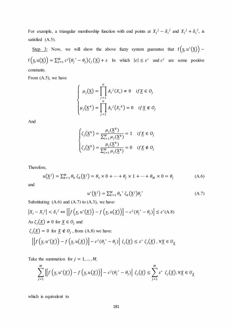
181
For example, a triangular membership function with end points at and , is
satisfied (A.5).
Step 3: Now, we will show the above fuzzy system guarantee that
In which and are some positive
constants.
From (A.5), we have
And
Therefore,
(A.6)
and
(A.7)
Substituting (A.6) and (A.7) to (A.3), we have:
(A.8)
As for and
for , from (A.8) we have:
,
Take the summation for ,
which is equivalent to

182
Since , we have:
which is equivalent to
Since , we have:
APPENDIX B
MATLAB CODES FOR ONE STOREY STRUCTURE %************************************************************************** clc % ONE STOREY STRUCTURE %************************************************************************** % EQUIPPED WITH A PAIR OF MR DAMPERS ON THE LAST FLOOR % DUE TO ELCENTRO QUAKE (normalised to 2g) WITH A FUZZY LOGIC CONTROLLER % ******************* % THE FUZZY LOGIC CONTROLLER INPUTS : % x1(RELATIVE DISP OF 1ST FLOORS) + v1 (RELATIVE VELO OF 1ST FLOORS) % THE FUZZY LOGIC CONTROLLER OUTPUT : % i (CURRENT). % ******************* % THE MR DAMPER CHARACTERISTICS ARE: alpha2=-488;alpha1=1836;alpha0=64;beta1=100;delta11=0.3;delta10=0.58; kd1=10200;kd2=-3400;cd1=2464;cd2=3858; % ******************* % THE FIVE STOREY STRUCTURE'S CHARACTERISTICS ARE: % f=4; % f is the fundamental frequency of the structure (Hz) % f(quake)=1.5; % f is the fundamental frequency of the earthquake (Hz) % saay=2; % saay is the critical damping m1=1000;% m in N. k1=576000;% k in N/m. c1=100000;% c in Ns/m. % ******************* % THE CURRENT(i) IS THE OUTPUT OF THE FUZZY LOGIC CONTROLLER % THE INPUT TO THE MR DAMPER : 0 < i < imax = 2A % ******************* % PLOT

183
% ******************* h=plot(x1con,'red'); hold on hh=plot(x1uncon); set(h,{'DisplayName'},{'x1con(m)'}') set(hh,{'DisplayName'},{'x1uncon(m)'}') legend show %ii=plot(i,'red'); %set(q,{'DisplayName'},{'current(i)'}') %legend show % %det([k]-(w^2)*[m])=0 % function [fuzzy_output,indicator1] = structure_learning(z,fuzzy_input,error,structure_learning_params,current_output) % This function performs structure learning of the fuzzy system. This % function can only be used for rectangular-mf fuzzy systems. % % error is the output error or tracking error % current output is the current value of the fuzzy system output % mf_threshold is a threshold that a new mf is considered if the max mf % degree in any input dimension is smaller than this value % error_threshold is a threshold that a new mf is considered if the output % error (or tracking error) is smaller than this value % a0 is the matrix specifies the 1/2 the maximum predefined spreads of % rectangular mfs in each dimension % mf_degree_threshold (which characterizes the similarity between the mf center and the input) is the threshold that a mf should be % replaced by a new one if the mf degree of the input is larger or equal to this % value mf_threshold = structure_learning_params.mf_threshold; error_threshold = structure_learning_params.error_threshold; a0 = structure_learning_params.a0; center_distance_threshold = structure_learning_params.center_distance_threshold; max_N_rules = structure_learning_params.max_N_rules; persistent indicator if isempty(indicator) indicator = 1; end %==========initialize the first rule to the first input entered====== % ====================================================================== % ======= Part 3================

184
if abs(error) >= error_threshold % then a new mf is added or replaced % Determine the most firing rule [most_firing_rule_strength,most_firing_rule_index]=max(current_output.ARR); % The result of evaluating input values through mfs of the most firing rule mf_degree_vector = current_output.IRR(most_firing_rule_index,:); % mf_degree_vector contains the result of evaluating input % values through mfs of the most firing rule % Determine the dimension in which the max mf degree obtains [max_mf_degree,var_index] = max(mf_degree_vector);% var_index2 is the dimension in which max mf degree obtains % Determine new_N_rules would be reached when adding one more mf. Num_Input_MFs = getfis(fuzzy_input,'NumInputMFs'); new_Num_Input_MFs = Num_Input_MFs; new_Num_Input_MFs(var_index) = Num_Input_MFs(var_index)+1; new_N_rules = prod(new_Num_Input_MFs); % Determine if a new mf should be considered based on the similarity % measure. If center_distance is smaller than center_distance_threshold, a new rule % should not be added. most_activated_mf_index = 0; Rulelist = getfis(fuzzy_input,'Rulelist'); most_activated_mf_index = Rulelist(most_firing_rule_index,var_index); most_activated_mf_params = getfis(fuzzy_input,'input',var_index,'mf',most_activated_mf_index,'params'); center_distance = abs(z(var_index)-most_activated_mf_params(2)); similarity_measure = 1; if center_distance<center_distance_threshold(var_index) similarity_measure = 1; % "1" represents "similar" else similarity_measure = 0; % "0" represents "not similar" end if (similarity_measure == 0)&&(new_N_rules > max_N_rules) % replace a mf by a new one % Determine the mf_to_be_replaced which is the farest mf farest_mf_index = 0; max_abs_distance = 0; for i=1:getfis(fuzzy_input,'input',var_index,'nummfs') current_params = getfis(fuzzy_input,'input',var_index,'mf',i,'params'); distance = current_params(2)-z(var_index); if abs(distance)>max_abs_distance max_abs_distance = abs(distance); farest_mf_index = i; end end mf_to_be_replaced_index = farest_mf_index;

185
% Determine the left, right mfs left_mf_index = 0; right_mf_index = 0; min_left_distance = -4; min_right_distance = 4; for i=1:getfis(fuzzy_input,'input',var_index,'nummfs') current_params = getfis(fuzzy_input,'input',var_index,'mf',i,'params'); distance = current_params(2)-z(var_index); if (distance<0) && (distance>min_left_distance) && (i ~= mf_to_be_replaced_index) min_left_distance = distance; left_mf_index = i; end if (distance>0) && (distance<min_right_distance) && (i ~= mf_to_be_replaced_index) min_right_distance = distance; right_mf_index = i; end end % Replace the mf_to_be_replaced by a new one fuzzy_input = replace_mf_and_rules(fuzzy_input,var_index,a0,left_mf_index,z(var_index),right_mf_index,mf_to_be_replaced_index,current_output.output); indicator =indicator*(-1); end if (similarity_measure == 0)&&(new_N_rules <= max_N_rules) % then add a new mf % Determine the left, right mfs left_mf_index = 0; right_mf_index = 0; min_left_distance = -4; min_right_distance = 4; for i=1:getfis(fuzzy_input,'input',var_index,'nummfs') current_params = getfis(fuzzy_input,'input',var_index,'mf',i,'params'); distance = current_params(2)-z(var_index); if (distance<0) && (distance>min_left_distance) min_left_distance = distance; left_mf_index = i; end if (distance>0) && (distance<min_right_distance) min_right_distance = distance; right_mf_index = i; end end fuzzy_input = add_mf_and_rules(fuzzy_input,var_index,a0,left_mf_index,z(var_index),right_mf_index,current_output.output); indicator =indicator*(-1); end else % ====================Part 1=================== if getfis(fuzzy_input,'NumRules')>1

186
[IRR_max,rule_index_vector] = max(current_output.IRR); % IRR_max is the vector of the max values of inputs through membership % functions in each dimension % rule_index_vector is the vector containing indexes of rules that max values % of inputs through mfs achieve in each dimension. [min_IRR_max,var_index] = min(IRR_max); % min_IRR_max is the min value of IRR_max. % var_index is the dimension which the min value of IRR_max achieves rule_index = rule_index_vector(var_index); % rule_index is the index of rule that min value of IRR_max achieves else rule_index = 1; [min_IRR_max,var_index] = min(current_output.IRR); end Rulelist = getfis(fuzzy_input,'Rulelist'); mf_index = Rulelist(rule_index,var_index); % mf_index indicates the membership function which the min value archieves % ====================Part 2=================== if min_IRR_max<mf_threshold % then a new mf is added or replaced to either sides % add 1 rectangular mf in var_index dimension. This script can only be % used for rectangular mfs, it needs modification to be used for % gaussian membership functions % Determine new_N_rules would be reached when adding one more mf. Num_Input_MFs = getfis(fuzzy_input,'NumInputMFs'); new_Num_Input_MFs = Num_Input_MFs; new_Num_Input_MFs(var_index) = Num_Input_MFs(var_index)+1; new_N_rules = prod(new_Num_Input_MFs); if new_N_rules > max_N_rules % then we need to replace an existing mf by a new mf % Determine the farest mf farest_mf_index = 0; max_abs_distance = 0; for i=1:getfis(fuzzy_input,'input',var_index,'nummfs') current_params = getfis(fuzzy_input,'input',var_index,'mf',i,'params'); distance = current_params(2)-z(var_index); if abs(distance)>=max_abs_distance max_abs_distance = abs(distance); farest_mf_index = i; end end mf_to_be_replaced_index = farest_mf_index; % Determine the left, right, excluding the mf_to_be_replaced left_mf_index = 0; right_mf_index = 0; min_left_distance = -4; min_right_distance = 4; center = 0; for i=1:getfis(fuzzy_input,'input',var_index,'nummfs') current_params = getfis(fuzzy_input,'input',var_index,'mf',i,'params');

187
distance = current_params(2)-z(var_index); if (distance<0) && (distance>min_left_distance) && (i ~= mf_to_be_replaced_index) min_left_distance = distance; left_mf_index = i; left_mf_params = getfis(fuzzy_input,'input',var_index,'mf',i,'params'); center = left_mf_params(3); end if (distance>0) && (distance<min_right_distance) && (i ~= mf_to_be_replaced_index) min_right_distance = distance; right_mf_index = i; right_mf_params = getfis(fuzzy_input,'input',var_index,'mf',i,'params'); center = right_mf_params(1); end end fuzzy_input = replace_mf_and_rules(fuzzy_input,var_index,a0,left_mf_index,center,right_mf_index,mf_to_be_replaced_index,current_output.output); % Set indicator = 1 or -1 if this case occurs indicator = indicator*(-1); else%add a new mf and add rules % Determine the left, right mfs left_mf_index = 0; right_mf_index = 0; min_left_distance = -4; min_right_distance = 4; for i=1:getfis(fuzzy_input,'input',var_index,'nummfs') current_params = getfis(fuzzy_input,'input',var_index,'mf',i,'params'); distance = current_params(2)-z(var_index); if (distance<0) && (distance>min_left_distance) min_left_distance = distance; left_mf_index = i; left_mf_params = getfis(fuzzy_input,'input',var_index,'mf',i,'params'); center = left_mf_params(3); end if (distance>0) && (distance<min_right_distance) min_right_distance = distance; right_mf_index = i; right_mf_params = getfis(fuzzy_input,'input',var_index,'mf',i,'params'); center = right_mf_params(1); end end fuzzy_input = add_mf_and_rules(fuzzy_input,var_index,a0,left_mf_index,z(var_index),right_mf_index,current_output.output); indicator =indicator*-1; end

188
% Recalculate the output after the fuzzy system changes % [output, IRR, ORR, ARR]= evalfis(z,fuzzy_input); end end fuzzy_output = fuzzy_input; indicator1 = indicator; %========================================================================== functionfuzzy_output = replace_mf_and_rules(fuzzy_input,var_index,a0,left_mf_index,center,right_mf_index,mf_to_be_replaced_index,initial_value) % Modify the mf neibouring to the farest mf (it is either left or right neibouring mf) % Determine the neibouring mf of the farest mf farest_mf_params = getfis(fuzzy_input,'input',var_index,'mf',mf_to_be_replaced_index,'params'); left_farest_mf_index = 0; right_farest_mf_index = 0; min_left_farest_distance = -4; min_right_farest_distance = 4; for i=1:getfis(fuzzy_input,'input',var_index,'nummfs') current_params = getfis(fuzzy_input,'input',var_index,'mf',i,'params'); distance = current_params(2)-farest_mf_params(2); if (distance<0) && (distance>min_left_farest_distance) min_left_farest_distance = distance; left_farest_mf_index = i; end if (distance>0) && (distance<min_right_farest_distance) min_right_farest_distance = distance; right_farest_mf_index = i; end end % Modify the left param if the neibouring mf of the farest mf is on the left if left_farest_mf_index ~= 0 left_farest_mf_params = getfis(fuzzy_input,'input',var_index,'mf',left_farest_mf_index,'params'); left_farest_mf_params(3) = left_farest_mf_params(2)+a0(var_index); fuzzy_input = setfis(fuzzy_input,'input',var_index,'mf',left_farest_mf_index,'params',left_farest_mf_params); end % Modify the right param if the neibouring mf of the farest mf is on the right if right_farest_mf_index ~= 0 right_farest_mf_params = getfis(fuzzy_input,'input',var_index,'mf',right_farest_mf_index,'params'); right_farest_mf_params(1) = right_farest_mf_params(2)-a0(var_index);
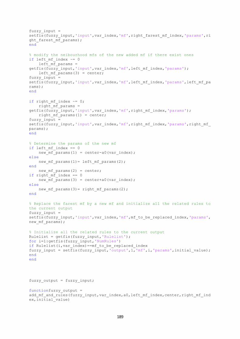
189
fuzzy_input = setfis(fuzzy_input,'input',var_index,'mf',right_farest_mf_index,'params',right_farest_mf_params); end % modify the neibourhood mfs of the new added mf if there exist ones if left_mf_index ~= 0 left_mf_params = getfis(fuzzy_input,'input',var_index,'mf',left_mf_index,'params'); left_mf_params(3) = center; fuzzy_input = setfis(fuzzy_input,'input',var_index,'mf',left_mf_index,'params',left_mf_params); end if right_mf_index ~= 0; right_mf_params = getfis(fuzzy_input,'input',var_index,'mf',right_mf_index,'params'); right_mf_params(1) = center; fuzzy_input = setfis(fuzzy_input,'input',var_index,'mf',right_mf_index,'params',right_mf_params); end % Determine the params of the new mf if left_mf_index == 0 new_mf_params(1) = center-a0(var_index); else new_mf_params(1)= left_mf_params(2); end new_mf_params(2) = center; if right_mf_index == 0 new_mf_params(3) = center+a0(var_index); else new_mf_params(3)= right_mf_params(2); end % Replace the farest mf by a new mf and initialize all the related rules to the current output fuzzy_input = setfis(fuzzy_input,'input',var_index,'mf',mf_to_be_replaced_index,'params',new_mf_params); % Initialize all the related rules to the current output Rulelist = getfis(fuzzy_input,'Rulelist'); for i=1:getfis(fuzzy_input,'NumRules') if Rulelist(i,var_index)==mf_to_be_replaced_index fuzzy_input = setfis(fuzzy_input,'output',1,'mf',i,'params',initial_value); end end fuzzy_output = fuzzy_input; functionfuzzy_output = add_mf_and_rules(fuzzy_input,var_index,a0,left_mf_index,center,right_mf_index,initial_value)
190
% modify the neibourhood mfs if there exist ones if left_mf_index ~= 0 left_mf_params = getfis(fuzzy_input,'input',var_index,'mf',left_mf_index,'params'); left_mf_params(3) = center; fuzzy_input = setfis(fuzzy_input,'input',var_index,'mf',left_mf_index,'params',left_mf_params); end if right_mf_index ~= 0; right_mf_params = getfis(fuzzy_input,'input',var_index,'mf',right_mf_index,'params'); right_mf_params(1) = center; fuzzy_input = setfis(fuzzy_input,'input',var_index,'mf',right_mf_index,'params',right_mf_params); end % Determine the params of the new mf if left_mf_index == 0 new_mf_params(1) = center-a0(var_index); else new_mf_params(1)= left_mf_params(2); end new_mf_params(2) = center; if right_mf_index == 0 new_mf_params(3) = center+a0(var_index); else new_mf_params(3)= right_mf_params(2); end % Add a new mf added_mf_index = getfis(fuzzy_input,'input',var_index,'Nummfs')+1; % the index indicates the new mf mf_name = strcat('mf',num2str(added_mf_index)); fuzzy_input = addmf(fuzzy_input,'input',var_index,mf_name,'trimf',new_mf_params); % Add rules using generate_rules function fuzzy_input=generate_rules(fuzzy_input,var_index,added_mf_index,initial_value); fuzzy_output = fuzzy_input; function SOAFS(block) setup(block); function setup(block) block.NumDialogPrms = 3;

191
% get the initial number of adaptive parameters = number of rules fuzzy_u = block.DialogPrm(1).Data; % AFS_params = block.DialogPrm(2).Data; structure_learning_params = block.DialogPrm(3).Data; % no_of_rules = getfis(fuzzy_u,'NumRules'); block.NumInputPorts = 2; block.NumOutputPorts = 3; block.SetPreCompInpPortInfoToDynamic; block.SetPreCompOutPortInfoToDynamic; block.InputPort(1).Complexity = 'Real'; block.InputPort(1).DataTypeId = 0; block.InputPort(1).SamplingMode = 'Sample'; block.InputPort(1).Dimensions = 1; block.InputPort(2).Complexity = 'Real'; block.InputPort(2).DataTypeId = 0; block.InputPort(2).SamplingMode = 'Sample'; block.InputPort(2).Dimensions = getfis(fuzzy_u,'NumInputs'); block.OutputPort(1).Complexity = 'Real'; block.OutputPort(1).DataTypeId = 0; block.OutputPort(1).SamplingMode = 'Sample'; block.OutputPort(1).Dimensions = 1; block.OutputPort(2).Complexity = 'Real'; block.OutputPort(2).DataTypeId = 0; block.OutputPort(2).SamplingMode = 'Sample'; block.OutputPort(2).Dimensions = structure_learning_params.max_N_rules; block.OutputPort(3).Complexity = 'Real'; block.OutputPort(3).DataTypeId = 0; block.OutputPort(3).SamplingMode = 'Sample'; block.OutputPort(3).Dimensions = 2; block.SampleTimes = [0 0]; block.RegBlockMethod('Start', @Start); block.RegBlockMethod('Outputs', @Outputs); block.RegBlockMethod('Derivatives', @Derivatives); block.RegBlockMethod('Terminate', @Terminate); % set the block' number of continuous states block.NumContStates=structure_learning_params.max_N_rules; %end setup function function Start(block) globalfuzzy_u; fuzzy_u= block.DialogPrm(1).Data; no_of_rules = getfis(fuzzy_u,'NumRules'); % initialize the continuous state vector output_params= getfis(fuzzy_u,'OutMFParams');

192
block.ContStates.Data(1:length(output_params)) = output_params(:,1); %end function function Outputs(block) globalfuzzy_u %fuzzy_u = block.DialogPrm(1).Data; no_of_rules = getfis(fuzzy_u,'NumRules'); X=block.InputPort(2).data; inRange = getfis(fuzzy_u,'inRange'); X=saturation_ppa(X,inRange); % see function saturation_ppa in "my m files" for instructions x = block.ContStates.Data(1:no_of_rules); fuzzy_u=setfis(fuzzy_u,'OutMFParams',x); [current_output.output, current_output.IRR, current_output.ORR, current_output.ARR]= evalfis(X,fuzzy_u); block.OutputPort(1).Data = current_output.output; block.OutputPort(2).Data(1:no_of_rules) = x; [fuzzy_u,indicator1] = structure_learning(X,fuzzy_u,block.InputPort(1).data,block.DialogPrm(3).Data,current_output); block.OutputPort(3).Data(1) = indicator1; block.OutputPort(3).Data(2) = getfis(fuzzy_u,'NumRules'); %endfunction function Derivatives(block) globalfuzzy_u; %fuzzy_u = block.DialogPrm(1).Data; E=block.InputPort(1).data; % the first input is the error(adaptive signal); X=block.InputPort(2).data; % the other inputs are the state vector of the system inRange = getfis(fuzzy_u,'inRange'); X=saturation_ppa(X,inRange); % see function saturation_ppa in "my m files" for instructions %fuzzy_u = block.DialogPrm(1).Data; AFS_params = block.DialogPrm(2).Data; gamma = AFS_params.gamma; sigma = AFS_params.sigma; theta_U = AFS_params.theta_U; theta_L = AFS_params.theta_L; theta_0 = AFS_params.theta_0;

193
% structure_learning_params = block.DialogPrm(3).Data; % fuzzy_u = structure_learning(X,fuzzy_u,E,block.DialogPrm(3).Data); x= getfis(fuzzy_u,'OutMFParams'); %outRange = [theta_L theta_U]; %x = saturation_ppa2(x,outRange); block.ContStates.Data(1:length(x(:,1))) = x(:,1); [a,b,c,d]=evalfis(X,fuzzy_u); if sum(d)==0, J=zeros(length(d),1); else J = d/sum(d); end for i=1:length(x(:,1)) if [(x(i)>=theta_U)&(gamma*E*J(i)>=sigma*(x(i)-theta_0))]|[(x(i)<=theta_L)&(gamma*E*J(i)<=sigma*(x(i)-theta_0))], block.Derivatives.Data(i) = -sigma*(x(i)-theta_0); else block.Derivatives.Data(i) = gamma*E*J(i)-sigma*(x(i)-theta_0); end end % block.Derivatives.Data(length(x):) %endfunction function Terminate(block) globalfuzzy_u; globalfuzzy_final; clear indicator; fuzzy_final = fuzzy_u; %endfunction
% To run the simulation: % Step 1: Load the fuzzy controller ( as "u") to the workspace % Step 2: Run 1 of the initializing parameters files %========================================================== %=====Controller parameters========= k=[1;1]; Q=[20 0;0 10]; % ================================== V=0.367; bc=[0;1]; A=[0 1;-k(1) -k(2)]; %Q=q*eye(size(A)); P=lyap(transpose(A),Q);

194
%P=[7 1;1 2]; %Q=-(transpose(A)*P+P*A); % ================================== %system order% n=2; %=====Fuzzy system f's parameters=== fuzzy_u=readfis('FC_NNS1_3'); %name of the fuzzy controller globalfuzzy_final; %initialize the final fuzzy system Mu=length(fuzzy_u.rule); % number of rules. This is needed to display the correct number of adaptive parameters AFS_params.gamma=100; AFS_params.sigma=0.05; AFS_params.theta_U=2; AFS_params.theta_L=-2; AFS_params.theta_0=0; %===========Structure Learning parameters====% clear structure_learning_params; structure_learning_params.mf_threshold = 0.5; structure_learning_params.error_threshold = 2; structure_learning_params.a0 = [2 2 2]; structure_learning_params.center_distance_threshold = [0.5 0.5 0.5]; structure_learning_params.max_N_rules = 15; %----------- %eB=0.01; %lamda_w=1; %zeta_w=0.005; %w0=0.1; %w_max=2; %e1=20; %======================================% %e10=0.00; %e11=0.00; %E0=0.002; %T0=20; function fis_out=generate_rules(fuzzy_input,var_index,mf_index,initial_value) %========================================================================== % This function is use to generate all the rules when a new mf is added in a dimension. % % var_index and mf_index indicate the dimension and the index of the added % mf. % % initial_value is the value that the outputs of the rules will be % initialized to. %========================================================================== %=========================Adding membership functions to output============ %===Determine the number N_output_mfs of required output membership functions=== Num_Input_MFs = getfis(fuzzy_input,'NumInputMFs');
195
N_available_mfs = Num_Input_MFs; % N_available_mfs is the matrix of number of available mfs for creating new rules N_available_mfs(var_index) = 1; N_added_output_mfs = prod(N_available_mfs); %============================================================== if N_added_output_mfs ~= 0 %===Adding constant membership functions (and initilize them to initial_value) to output=============== current_N_rules = getfis(fuzzy_input,'NumRules'); for i=1:N_added_output_mfs, mf_name=strcat('mf',num2str(current_N_rules+i)); fuzzy_input=addmf(fuzzy_input,'output',1,mf_name,'constant',initial_value); end %========================Adding rules to the fuzzy system================== %===determine the rulelist======================================== Rulelist=[]; Matrix_out=[]; %===initiate matrix_out which contains for i=1:getfis(fuzzy_input,'input',1,'NumMFs') Matrix_out=[Matrix_out;i]; end for i=2:getfis(fuzzy_input,'NumInputs') Matrix_out=combine_matrix(Matrix_out,N_available_mfs(i)); end for i=1:N_added_output_mfs Rulelist=[Rulelist;Matrix_out(i,:) (current_N_rules+i) 1 1]; end mf_index_vector = ones(N_added_output_mfs,1)*mf_index; Rulelist(:,var_index) = mf_index_vector; %===Adding rules================================================== fuzzy_input=addrule(fuzzy_input,Rulelist); end fis_out=fuzzy_input; function Matrix_out=combine_matrix(Matrix_in,N_mfs) Matrix_out=[]; for i=1:length(Matrix_in(:,1)) for j=1:N_mfs Matrix_out=[Matrix_out;Matrix_in(i,:) j]; end end
196
function [sys,x0,str,ts] = estimator(t,x,u,flag,k,P,bc) %SFUNTMPL General M-file S-function template % With M-file S-functions, you can define you own ordinary differential % equations (ODEs), discrete system equations, and/or just about % any type of algorithm to be used within a Simulink block diagram. % % The general form of an M-File S-function syntax is: % [SYS,X0,STR,TS] = SFUNC(T,X,U,FLAG,P1,...,Pn) % % What is returned by SFUNC at a given point in time, T, depends on the % value of the FLAG, the current state vector, X, and the current % input vector, U. % % FLAG RESULT DESCRIPTION % ----- ------ -------------------------------------------- % 0 [SIZES,X0,STR,TS] Initialization, return system sizes in SYS, % initial state in X0, state ordering strings % in STR, and sample times in TS. % 1 DX Return continuous state derivatives in SYS. % 2 DS Update discrete states SYS = X(n+1) % 3 Y Return outputs in SYS. % 4 TNEXT Return next time hit for variable step sample % time in SYS. % 5 Reserved for future (root finding). % 9 [] Termination, perform any cleanup SYS=[]. % % % The state vectors, X and X0 consists of continuous states followed % by discrete states. % % Optional parameters, P1,...,Pn can be provided to the S-function and % used during any FLAG operation. % % When SFUNC is called with FLAG = 0, the following information % should be returned: % % SYS(1) = Number of continuous states. % SYS(2) = Number of discrete states. % SYS(3) = Number of outputs. % SYS(4) = Number of inputs. % Any of the first four elements in SYS can be specified % as -1 indicating that they are dynamically sized. The % actual length for all other flags will be equal to the % length of the input, U. % SYS(5) = Reserved for root finding. Must be zero. % SYS(6) = Direct feedthrough flag (1=yes, 0=no). The s-function % has direct feedthrough if U is used during the FLAG=3 % call. Setting this to 0 is akin to making a promise that % U will not be used during FLAG=3. If you break the promise % then unpredictable results will occur. % SYS(7) = Number of sample times. This is the number of rows in TS. % % % X0 = Initial state conditions or [] if no states. % % STR = State ordering strings which is generally specified as []. % % TS = An m-by-2 matrix containing the sample time % (period, offset) information. Where m = number of sample

197
% times. The ordering of the sample times must be: % % TS = [0 0, : Continuous sample time. % 0 1, : Continuous, but fixed in minor step % sample time. % PERIOD OFFSET, : Discrete sample time where % PERIOD > 0 & OFFSET < PERIOD. % -2 0]; : Variable step discrete sample time % where FLAG=4 is used to get time of % next hit. % % There can be more than one sample time providing % they are ordered such that they are monotonically % increasing. Only the needed sample times should be % specified in TS. When specifying than one % sample time, you must check for sample hits explicitly by % seeing if % abs(round((T-OFFSET)/PERIOD) - (T-OFFSET)/PERIOD) % is within a specified tolerance, generally 1e-8. This % tolerance is dependent upon your model's sampling times % and simulation time. % % You can also specify that the sample time of the S-function % is inherited from the driving block. For functions which % change during minor steps, this is done by % specifying SYS(7) = 1 and TS = [-1 0]. For functions which % are held during minor steps, this is done by specifying % SYS(7) = 1 and TS = [-1 -1]. % Copyright (c) 1990-1998 by The MathWorks, Inc. All Rights Reserved. % $Revision: 1.12 $ % % The following outlines the general structure of an S-function. % switch flag, %%%%%%%%%%%%%%%%%% % Initialization % %%%%%%%%%%%%%%%%%% case 0, [sys,x0,str,ts]=mdlInitializeSizes; %%%%%%%%%%%%%%%%%%% % Unhandled flags % %%%%%%%%%%%%%%%%%%% case {1,2,4,9} sys=[]; %%%%%%%%%%% % Outputs % %%%%%%%%%%% case 3, sys=mdlOutputs(t,x,u,k,P,bc); %%%%%%%%%%%%%%%%%%%% % Unexpected flags % %%%%%%%%%%%%%%%%%%%% otherwise error(['Unhandled flag = ',num2str(flag)]);

198
end % end sfuntmpl % %============================================================================= % mdlInitializeSizes % Return the sizes, initial conditions, and sample times for the S-function. %============================================================================= % function [sys,x0,str,ts]=mdlInitializeSizes % % call simsizes for a sizes structure, fill it in and convert it to a % sizes array. % % Note that in this example, the values are hard coded. This is not a % recommended practice as the characteristics of the block are typically % defined by the S-function parameters. % sizes = simsizes; sizes.NumContStates = 0; sizes.NumDiscStates = 0; sizes.NumOutputs = 3; sizes.NumInputs = -1; sizes.DirFeedthrough = 1; sizes.NumSampleTimes = 1; % at least one sample time is needed sys = simsizes(sizes); % % initialize the initial conditions % x0 = []; % % str is always an empty matrix % str = []; % % initialize the array of sample times % block.SampleTimes = [-1 0]; ts = [-1 0]; % end mdlInitializeSizes % % %============================================================================= % mdlOutputs % Return the block outputs.

199
%============================================================================= % function sys=mdlOutputs(t,x,u,k,P,bc) a=transpose(k)*u; b=transpose(u)*P*bc; c=transpose(u)*P*u/2; sys = [a;b;c]; % end mdlOutputs % % PLOTTING THE FIGURES % output and desired output figure; plot(output.time,output.signals.values(:,1),'k:',output.time,output.signals.values(:,2),'k-'); axis([0 35 -0.01 0.01]); ylabel('output and desired output'); xlabel('Time(second)'); legend('desired output','actual output'); grid on; % tracking error figure; plot(tracking_error.time,tracking_error.signals.values(:,1),'k-'); axis([0 35 -0.01 0.01]); ylabel('tracking error'); xlabel('Time(second)'); grid on; % current figure; plot(control_signal(:,1),-1*control_signal(:,2),'k'); axis([0 35 -2 2]); ylabel('current'); xlabel('Time(second)'); grid on; % no of rules and switching flags figure; subplot(2,1,1); plot(flags(:,1),flags(:,3),'k'); axis([0 35 0 20]); %ylabel('Angular Displacement(rad)'); xlabel('Time(second)'); ylabel('Number of rules'); % axis([0 40 -.02 .8]); % legend('application 1','application 2','application 3'); subplot(2,1,2); plot(flags(:,1),flags(:,2),'k'); axis([0 35 -1.5 1.5]); xlabel('Time(second)'); ylabel('Self-structuring flag');

200
% plot membership functions figure; plotmf(fuzzy_u,'input',1); figure; plotmf(fuzzy_final,'input',1); figure; plotmf(fuzzy_final,'input',2); figure; plotmf(fuzzy_final,'input',3);

201
APPENDIX C
MATLAB CODES FOR FIVE STOREY STRUCTURE
%************************************************************************** clc % FIVE STOREY STRUCTURE %************************************************************************** % EQUIPPED WITH A PAIR OF MR DAMPERS IN BETWEEN THE 4TH & 5TH FLOORS % DUE TO ELCENTRO QUAKE (normalised to 2g) WITH FUZZY LOGIC CONTROLLERS % ******************* % THE FUZZY LOGIC CONTROLLER INPUTS : % x4-x5(RELATIVE DISP OF 4TH&5TH FLOORS) + % v4-v5 (RELATIVE VELO OF 4TH&5TH FLOORS) % THE FUZZY LOGIC CONTROLLER OUTPUT : % i (CURRENT). % ******************* % THE MR DAMPER CHARACTERISTICS ARE: alpha2=-488;alpha1=1836;alpha0=64;beta=100;delta11=0.3;delta10=0.58; kd1=10200;kd2=-3400;cd1=2464;cd2=3858; % ******************* % THE FIVE STOREY STRUCTURE'S CHARACTERISTICS ARE: f=2.95; % f is the fundamental frequency (Hz) saay=0.004; % saay is the critical damping m1=3273;m2=3273;m3=3273;m4=3273;m5=3273; % m in N. k1=778000;k2=1160000;k3=1160000;k4=1160000;k5=1160000; % k in N/m. c1=485;c2=485;c3=485;c4=485;c5=485; % c in Ns/m. % ******************* % THE CURRENT(i) IS THE OUTPUT OF THE FUZZY LOGIC CONTROLLER % THE INPUT TO THE MR DAMPER : 0 < i < imax = 2A % ******************* % PLOT % ******************* %h=plot(x5con,'red'); %hold on %hh=plot(x5uncon); %set(h,{'DisplayName'},{'x5con(m)'}') %set(hh,{'DisplayName'},{'x5uncon(m)'}') %legend show %ii=plot(i,'red'); %set(q,{'DisplayName'},{'current(i)'}') %legend show % ********************** % det([k]-(w^2)*[m])=0 % ********************** %[m]=diag([m1,m2,m3,m4,m5]); %[k]=diag([k1,k2,k3,k4,k5]); %[k]=[k]+diag([k2,k3,k4,k5,0]); %[k]=[k]+zeros(5,5); %k(1,2)=-k2;k(2,3)=-k3;k(3,4)=-k4;k(4,5)=-k5; %k(2,1)=-k2;k(3,2)=-k3;k(4,3)=-k4;k(5,4)=-k5; %[c]=diag([c1,c2,c3,c4,c5]); %[c]=[c]+diag([c2,c3,c4,c5,0]); %[c]=[c]+zeros(5,5); %c(1,2)=-c2;c(2,3)=-c3;c(3,4)=-c4;c(4,5)=-c5; %c(2,1)=-c2;c(3,2)=-c3;c(4,3)=-c4;c(5,4)=-c5; % ********************* % display(m) % display(k)
202
% display(c) % ********************* %syms w A2 %A1=[k]-([m]*((w)^2)); %A2=det(A1); %A3=solve(A2); %w=A3; %f=(1/(2*pi))*w % LEARNING PARAMETERS FOR THE ADAPTIVE FUZZY SYSTEM function [fuzzy_output,indicator1] = structure_learning(z,fuzzy_input,error,structure_learning_params,current_output) % This function performs structure learning of the fuzzy system. This % function can only be used for rectangular-mf fuzzy systems. % % error is the output error or tracking error % current output is the current value of the fuzzy system output % mf_threshold is a threshold that a new mf is considered if the max mf % degree in any input dimension is smaller than this value % error_threshold is a threshold that a new mf is considered if the output % error (or tracking error) is smaller than this value % a0 is the matrix specifies the 1/2 the maximum predefined spreads of % rectangular mfs in each dimension % mf_degree_threshold (which characterizes the similarity between the mf center and the input) is the threshold that a mf should be % replaced by a new one if the mf degree of the input is larger or equal to this % value mf_threshold = structure_learning_params.mf_threshold; error_threshold = structure_learning_params.error_threshold; a0 = structure_learning_params.a0; center_distance_threshold = structure_learning_params.center_distance_threshold; max_N_rules = structure_learning_params.max_N_rules; persistent indicator if isempty(indicator) indicator = 1; end %==========initialize the first rule to the first input entered====== % ====================================================================== % ======= Part 3================ if abs(error) >= error_threshold % then a new mf is added or replaced % Determine the most firing rule

203
[most_firing_rule_strength,most_firing_rule_index]=max(current_output.ARR); % The result of evaluating input values through mfs of the most firing rule mf_degree_vector = current_output.IRR(most_firing_rule_index,:); % mf_degree_vector contains the result of evaluating input % values through mfs of the most firing rule % Determine the dimension in which the max mf degree obtains [max_mf_degree,var_index] = max(mf_degree_vector);% var_index2 is the dimension in which max mf degree obtains % Determine new_N_rules would be reached when adding one more mf. Num_Input_MFs = getfis(fuzzy_input,'NumInputMFs'); new_Num_Input_MFs = Num_Input_MFs; new_Num_Input_MFs(var_index) = Num_Input_MFs(var_index)+1; new_N_rules = prod(new_Num_Input_MFs); % Determine if a new mf should be considered based on the similarity % measure. If center_distance is smaller than center_distance_threshold, a new rule % should not be added. most_activated_mf_index = 0; Rulelist = getfis(fuzzy_input,'Rulelist'); most_activated_mf_index = Rulelist(most_firing_rule_index,var_index); most_activated_mf_params = getfis(fuzzy_input,'input',var_index,'mf',most_activated_mf_index,'params'); center_distance = abs(z(var_index)-most_activated_mf_params(2)); similarity_measure = 1; if center_distance<center_distance_threshold(var_index) similarity_measure = 1; % "1" represents "similar" else similarity_measure = 0; % "0" represents "not similar" end if (similarity_measure == 0)&&(new_N_rules > max_N_rules) % replace a mf by a new one % Determine the mf_to_be_replaced which is the farest mf farest_mf_index = 0; max_abs_distance = 0; for i=1:getfis(fuzzy_input,'input',var_index,'nummfs') current_params = getfis(fuzzy_input,'input',var_index,'mf',i,'params'); distance = current_params(2)-z(var_index); if abs(distance)>max_abs_distance max_abs_distance = abs(distance); farest_mf_index = i; end end mf_to_be_replaced_index = farest_mf_index; % Determine the left, right mfs left_mf_index = 0; right_mf_index = 0; min_left_distance = -4;

204
min_right_distance = 4; for i=1:getfis(fuzzy_input,'input',var_index,'nummfs') current_params = getfis(fuzzy_input,'input',var_index,'mf',i,'params'); distance = current_params(2)-z(var_index); if (distance<0) && (distance>min_left_distance) && (i ~= mf_to_be_replaced_index) min_left_distance = distance; left_mf_index = i; end if (distance>0) && (distance<min_right_distance) && (i ~= mf_to_be_replaced_index) min_right_distance = distance; right_mf_index = i; end end % Replace the mf_to_be_replaced by a new one fuzzy_input = replace_mf_and_rules(fuzzy_input,var_index,a0,left_mf_index,z(var_index),right_mf_index,mf_to_be_replaced_index,current_output.output); indicator =indicator*(-1); end if (similarity_measure == 0)&&(new_N_rules <= max_N_rules) % then add a new mf % Determine the left, right mfs left_mf_index = 0; right_mf_index = 0; min_left_distance = -4; min_right_distance = 4; for i=1:getfis(fuzzy_input,'input',var_index,'nummfs') current_params = getfis(fuzzy_input,'input',var_index,'mf',i,'params'); distance = current_params(2)-z(var_index); if (distance<0) && (distance>min_left_distance) min_left_distance = distance; left_mf_index = i; end if (distance>0) && (distance<min_right_distance) min_right_distance = distance; right_mf_index = i; end end fuzzy_input = add_mf_and_rules(fuzzy_input,var_index,a0,left_mf_index,z(var_index),right_mf_index,current_output.output); indicator =indicator*(-1); end else % ====================Part 1=================== if getfis(fuzzy_input,'NumRules')>1 [IRR_max,rule_index_vector] = max(current_output.IRR); % IRR_max is the vector of the max values of inputs through membership % functions in each dimension

205
% rule_index_vector is the vector containing indexes of rules that max values % of inputs through mfs achieve in each dimension. [min_IRR_max,var_index] = min(IRR_max); % min_IRR_max is the min value of IRR_max. % var_index is the dimension which the min value of IRR_max achieves rule_index = rule_index_vector(var_index); % rule_index is the index of rule that min value of IRR_max achieves else rule_index = 1; [min_IRR_max,var_index] = min(current_output.IRR); end Rulelist = getfis(fuzzy_input,'Rulelist'); mf_index = Rulelist(rule_index,var_index); % mf_index indicates the membership function which the min value archieves % ====================Part 2=================== if min_IRR_max<mf_threshold % then a new mf is added or replaced to either sides % add 1 rectangular mf in var_index dimension. This script can only be % used for rectangular mfs, it needs modification to be used for % gaussian membership functions % Determine new_N_rules would be reached when adding one more mf. Num_Input_MFs = getfis(fuzzy_input,'NumInputMFs'); new_Num_Input_MFs = Num_Input_MFs; new_Num_Input_MFs(var_index) = Num_Input_MFs(var_index)+1; new_N_rules = prod(new_Num_Input_MFs); if new_N_rules > max_N_rules % then we need to replace an existing mf by a new mf % Determine the farest mf farest_mf_index = 0; max_abs_distance = 0; for i=1:getfis(fuzzy_input,'input',var_index,'nummfs') current_params = getfis(fuzzy_input,'input',var_index,'mf',i,'params'); distance = current_params(2)-z(var_index); if abs(distance)>=max_abs_distance max_abs_distance = abs(distance); farest_mf_index = i; end end mf_to_be_replaced_index = farest_mf_index; % Determine the left, right, excluding the mf_to_be_replaced left_mf_index = 0; right_mf_index = 0; min_left_distance = -4; min_right_distance = 4; center = 0; for i=1:getfis(fuzzy_input,'input',var_index,'nummfs') current_params = getfis(fuzzy_input,'input',var_index,'mf',i,'params'); distance = current_params(2)-z(var_index); if (distance<0) && (distance>min_left_distance) && (i ~= mf_to_be_replaced_index)

206
min_left_distance = distance; left_mf_index = i; left_mf_params = getfis(fuzzy_input,'input',var_index,'mf',i,'params'); center = left_mf_params(3); end if (distance>0) && (distance<min_right_distance) && (i ~= mf_to_be_replaced_index) min_right_distance = distance; right_mf_index = i; right_mf_params = getfis(fuzzy_input,'input',var_index,'mf',i,'params'); center = right_mf_params(1); end end fuzzy_input = replace_mf_and_rules(fuzzy_input,var_index,a0,left_mf_index,center,right_mf_index,mf_to_be_replaced_index,current_output.output); % Set indicator = 1 or -1 if this case occurs indicator = indicator*(-1); else%add a new mf and add rules % Determine the left, right mfs left_mf_index = 0; right_mf_index = 0; min_left_distance = -4; min_right_distance = 4; for i=1:getfis(fuzzy_input,'input',var_index,'nummfs') current_params = getfis(fuzzy_input,'input',var_index,'mf',i,'params'); distance = current_params(2)-z(var_index); if (distance<0) && (distance>min_left_distance) min_left_distance = distance; left_mf_index = i; left_mf_params = getfis(fuzzy_input,'input',var_index,'mf',i,'params'); center = left_mf_params(3); end if (distance>0) && (distance<min_right_distance) min_right_distance = distance; right_mf_index = i; right_mf_params = getfis(fuzzy_input,'input',var_index,'mf',i,'params'); center = right_mf_params(1); end end fuzzy_input = add_mf_and_rules(fuzzy_input,var_index,a0,left_mf_index,z(var_index),right_mf_index,current_output.output); indicator =indicator*-1; end % Recalculate the output after the fuzzy system changes % [output, IRR, ORR, ARR]= evalfis(z,fuzzy_input);

207
end end fuzzy_output = fuzzy_input; indicator1 = indicator; %========================================================================== % GENERATING RULES FOR THE FUZZY SYSTEM functionfuzzy_output = replace_mf_and_rules(fuzzy_input,var_index,a0,left_mf_index,center,right_mf_index,mf_to_be_replaced_index,initial_value) % Modify the mf neibouring to the farest mf (it is either left or right neibouring mf) % Determine the neibouring mf of the farest mf farest_mf_params = getfis(fuzzy_input,'input',var_index,'mf',mf_to_be_replaced_index,'params'); left_farest_mf_index = 0; right_farest_mf_index = 0; min_left_farest_distance = -4; min_right_farest_distance = 4; for i=1:getfis(fuzzy_input,'input',var_index,'nummfs') current_params = getfis(fuzzy_input,'input',var_index,'mf',i,'params'); distance = current_params(2)-farest_mf_params(2); if (distance<0) && (distance>min_left_farest_distance) min_left_farest_distance = distance; left_farest_mf_index = i; end if (distance>0) && (distance<min_right_farest_distance) min_right_farest_distance = distance; right_farest_mf_index = i; end end % Modify the left param if the neibouring mf of the farest mf is on the left if left_farest_mf_index ~= 0 left_farest_mf_params = getfis(fuzzy_input,'input',var_index,'mf',left_farest_mf_index,'params'); left_farest_mf_params(3) = left_farest_mf_params(2)+a0(var_index); fuzzy_input = setfis(fuzzy_input,'input',var_index,'mf',left_farest_mf_index,'params',left_farest_mf_params); end % Modify the right param if the neibouring mf of the farest mf is on the right if right_farest_mf_index ~= 0 right_farest_mf_params = getfis(fuzzy_input,'input',var_index,'mf',right_farest_mf_index,'params'); right_farest_mf_params(1) = right_farest_mf_params(2)-a0(var_index); fuzzy_input = setfis(fuzzy_input,'input',var_index,'mf',right_farest_mf_index,'params',right_farest_mf_params);

208
end % modify the neibourhood mfs of the new added mf if there exist ones if left_mf_index ~= 0 left_mf_params = getfis(fuzzy_input,'input',var_index,'mf',left_mf_index,'params'); left_mf_params(3) = center; fuzzy_input = setfis(fuzzy_input,'input',var_index,'mf',left_mf_index,'params',left_mf_params); end if right_mf_index ~= 0; right_mf_params = getfis(fuzzy_input,'input',var_index,'mf',right_mf_index,'params'); right_mf_params(1) = center; fuzzy_input = setfis(fuzzy_input,'input',var_index,'mf',right_mf_index,'params',right_mf_params); end % Determine the params of the new mf if left_mf_index == 0 new_mf_params(1) = center-a0(var_index); else new_mf_params(1)= left_mf_params(2); end new_mf_params(2) = center; if right_mf_index == 0 new_mf_params(3) = center+a0(var_index); else new_mf_params(3)= right_mf_params(2); end % Replace the farest mf by a new mf and initialize all the related rules to the current output fuzzy_input = setfis(fuzzy_input,'input',var_index,'mf',mf_to_be_replaced_index,'params',new_mf_params); % Initialize all the related rules to the current output Rulelist = getfis(fuzzy_input,'Rulelist'); for i=1:getfis(fuzzy_input,'NumRules') if Rulelist(i,var_index)==mf_to_be_replaced_index fuzzy_input = setfis(fuzzy_input,'output',1,'mf',i,'params',initial_value); end end fuzzy_output = fuzzy_input; functionfuzzy_output = add_mf_and_rules(fuzzy_input,var_index,a0,left_mf_index,center,right_mf_index,initial_value) % modify the neibourhood mfs if there exist ones if left_mf_index ~= 0

209
left_mf_params = getfis(fuzzy_input,'input',var_index,'mf',left_mf_index,'params'); left_mf_params(3) = center; fuzzy_input = setfis(fuzzy_input,'input',var_index,'mf',left_mf_index,'params',left_mf_params); end if right_mf_index ~= 0; right_mf_params = getfis(fuzzy_input,'input',var_index,'mf',right_mf_index,'params'); right_mf_params(1) = center; fuzzy_input = setfis(fuzzy_input,'input',var_index,'mf',right_mf_index,'params',right_mf_params); end % Determine the params of the new mf if left_mf_index == 0 new_mf_params(1) = center-a0(var_index); else new_mf_params(1)= left_mf_params(2); end new_mf_params(2) = center; if right_mf_index == 0 new_mf_params(3) = center+a0(var_index); else new_mf_params(3)= right_mf_params(2); end % Add a new mf added_mf_index = getfis(fuzzy_input,'input',var_index,'Nummfs')+1; % the index indicates the new mf mf_name = strcat('mf',num2str(added_mf_index)); fuzzy_input = addmf(fuzzy_input,'input',var_index,mf_name,'trimf',new_mf_params); % Add rules using generate_rules function fuzzy_input=generate_rules(fuzzy_input,var_index,added_mf_index,initial_value); fuzzy_output = fuzzy_input;
% GENERATING THE SELF ORGANIZING ADAPTIVE FUZZY LOGIC CONTROLLER function SOAFS(block) setup(block); function setup(block) block.NumDialogPrms = 3; % get the initial number of adaptive parameters = number of rules fuzzy_u = block.DialogPrm(1).Data; % AFS_params = block.DialogPrm(2).Data; structure_learning_params = block.DialogPrm(3).Data; % no_of_rules = getfis(fuzzy_u,'NumRules');

210
block.NumInputPorts = 2; block.NumOutputPorts = 3; block.SetPreCompInpPortInfoToDynamic; block.SetPreCompOutPortInfoToDynamic; block.InputPort(1).Complexity = 'Real'; block.InputPort(1).DataTypeId = 0; block.InputPort(1).SamplingMode = 'Sample'; block.InputPort(1).Dimensions = 1; block.InputPort(2).Complexity = 'Real'; block.InputPort(2).DataTypeId = 0; block.InputPort(2).SamplingMode = 'Sample'; block.InputPort(2).Dimensions = getfis(fuzzy_u,'NumInputs'); block.OutputPort(1).Complexity = 'Real'; block.OutputPort(1).DataTypeId = 0; block.OutputPort(1).SamplingMode = 'Sample'; block.OutputPort(1).Dimensions = 1; block.OutputPort(2).Complexity = 'Real'; block.OutputPort(2).DataTypeId = 0; block.OutputPort(2).SamplingMode = 'Sample'; block.OutputPort(2).Dimensions = structure_learning_params.max_N_rules; block.OutputPort(3).Complexity = 'Real'; block.OutputPort(3).DataTypeId = 0; block.OutputPort(3).SamplingMode = 'Sample'; block.OutputPort(3).Dimensions = 2; block.SampleTimes = [0 0]; block.RegBlockMethod('Start', @Start); block.RegBlockMethod('Outputs', @Outputs); block.RegBlockMethod('Derivatives', @Derivatives); block.RegBlockMethod('Terminate', @Terminate); % set the block' number of continuous states block.NumContStates=structure_learning_params.max_N_rules; %end setup function function Start(block) globalfuzzy_u; fuzzy_u= block.DialogPrm(1).Data; no_of_rules = getfis(fuzzy_u,'NumRules'); % initialize the continuous state vector output_params= getfis(fuzzy_u,'OutMFParams'); block.ContStates.Data(1:length(output_params)) = output_params(:,1); %end function

211
function Outputs(block) globalfuzzy_u %fuzzy_u = block.DialogPrm(1).Data; no_of_rules = getfis(fuzzy_u,'NumRules'); X=block.InputPort(2).data; inRange = getfis(fuzzy_u,'inRange'); X=saturation_ppa(X,inRange); % see function saturation_ppa in "my m files" for instructions x = block.ContStates.Data(1:no_of_rules); fuzzy_u=setfis(fuzzy_u,'OutMFParams',x); [current_output.output, current_output.IRR, current_output.ORR, current_output.ARR]= evalfis(X,fuzzy_u); block.OutputPort(1).Data = current_output.output; block.OutputPort(2).Data(1:no_of_rules) = x; [fuzzy_u,indicator1] = structure_learning(X,fuzzy_u,block.InputPort(1).data,block.DialogPrm(3).Data,current_output); block.OutputPort(3).Data(1) = indicator1; block.OutputPort(3).Data(2) = getfis(fuzzy_u,'NumRules'); %endfunction function Derivatives(block) globalfuzzy_u; %fuzzy_u = block.DialogPrm(1).Data; E=block.InputPort(1).data; % the first input is the error(adaptive signal); X=block.InputPort(2).data; % the other inputs are the state vector of the system inRange = getfis(fuzzy_u,'inRange'); X=saturation_ppa(X,inRange); % see function saturation_ppa in "my m files" for instructions %fuzzy_u = block.DialogPrm(1).Data; AFS_params = block.DialogPrm(2).Data; gamma = AFS_params.gamma; sigma = AFS_params.sigma; theta_U = AFS_params.theta_U; theta_L = AFS_params.theta_L; theta_0 = AFS_params.theta_0; % structure_learning_params = block.DialogPrm(3).Data; % fuzzy_u = structure_learning(X,fuzzy_u,E,block.DialogPrm(3).Data); x= getfis(fuzzy_u,'OutMFParams');

212
%outRange = [theta_L theta_U]; %x = saturation_ppa2(x,outRange); block.ContStates.Data(1:length(x(:,1))) = x(:,1); [a,b,c,d]=evalfis(X,fuzzy_u); if sum(d)==0, J=zeros(length(d),1); else J = d/sum(d); end for i=1:length(x(:,1)) if [(x(i)>=theta_U)&(gamma*E*J(i)>=sigma*(x(i)-theta_0))]|[(x(i)<=theta_L)&(gamma*E*J(i)<=sigma*(x(i)-theta_0))], block.Derivatives.Data(i) = -sigma*(x(i)-theta_0); else block.Derivatives.Data(i) = gamma*E*J(i)-sigma*(x(i)-theta_0); end end % block.Derivatives.Data(length(x):) %endfunction function Terminate(block) globalfuzzy_u; globalfuzzy_final; clear indicator; fuzzy_final = fuzzy_u; %endfunction % GENERATING THE LEARNING PARAMETERS FOR THE ADAPTIVE FUZZY LOGIC CONTROLLER % To run the simulation: % Step 1: Load the fuzzy controller ( as "u") to the workspace % Step 2: Run 1 of the initializing parameters files %========================================================== %=====Controller parameters========= k=[1;1]; Q=[20 0;0 10]; % ================================== V=0.367; bc=[0;1]; A=[0 1;-k(1) -k(2)]; %Q=q*eye(size(A)); P=lyap(transpose(A),Q); %P=[7 1;1 2]; %Q=-(transpose(A)*P+P*A);

213
% ================================== %system order% n=2; %=====Fuzzy system f's parameters=== fuzzy_u=readfis('FC_NNS1_3'); %name of the fuzzy controller globalfuzzy_final; %initialize the final fuzzy system Mu=length(fuzzy_u.rule); % number of rules. This is needed to display the correct number of adaptive parameters AFS_params.gamma=100; AFS_params.sigma=0.05; AFS_params.theta_U=2; AFS_params.theta_L=0; AFS_params.theta_0=0; %===========Structure Learning parameters====% clear structure_learning_params; structure_learning_params.mf_threshold = 0.5; structure_learning_params.error_threshold =2; structure_learning_params.a0 = [1 1 1]; structure_learning_params.center_distance_threshold = [0.5 0.5 0.5]; structure_learning_params.max_N_rules = 15; %----------- %eB=0.01; %lamda_w=1; %zeta_w=0.005; %w0=0.1; %w_max=2; %e1=20; %======================================% %e10=0.00; %e11=0.00; %E0=0.002; %T0=20; % GENERATING RULES FOR THE FUZZY SYSTEM function fis_out=generate_rules(fuzzy_input,var_index,mf_index,initial_value) %========================================================================== % This function is use to generate all the rules when a new mf is added in a dimension. % % var_index and mf_index indicate the dimension and the index of the added % mf. % % initial_value is the value that the outputs of the rules will be % initialized to. %========================================================================== %=========================Adding membership functions to output============ %===Determine the number N_output_mfs of required output membership functions=== Num_Input_MFs = getfis(fuzzy_input,'NumInputMFs');

214
N_available_mfs = Num_Input_MFs; % N_available_mfs is the matrix of number of available mfs for creating new rules N_available_mfs(var_index) = 1; N_added_output_mfs = prod(N_available_mfs); %============================================================== if N_added_output_mfs ~= 0 %===Adding constant membership functions (and initilize them to initial_value) to output=== current_N_rules = getfis(fuzzy_input,'NumRules'); for i=1:N_added_output_mfs, mf_name=strcat('mf',num2str(current_N_rules+i)); fuzzy_input=addmf(fuzzy_input,'output',1,mf_name,'constant',initial_value); end %========================Adding rules to the fuzzy system================== %===determine the rulelist======================================== Rulelist=[]; Matrix_out=[]; %===initiate matrix_out which contains for i=1:getfis(fuzzy_input,'input',1,'NumMFs') Matrix_out=[Matrix_out;i]; end for i=2:getfis(fuzzy_input,'NumInputs') Matrix_out=combine_matrix(Matrix_out,N_available_mfs(i)); end for i=1:N_added_output_mfs Rulelist=[Rulelist;Matrix_out(i,:) (current_N_rules+i) 1 1]; end mf_index_vector = ones(N_added_output_mfs,1)*mf_index; Rulelist(:,var_index) = mf_index_vector; %===Adding rules================================================== fuzzy_input=addrule(fuzzy_input,Rulelist); end fis_out=fuzzy_input; function Matrix_out=combine_matrix(Matrix_in,N_mfs) Matrix_out=[]; for i=1:length(Matrix_in(:,1)) for j=1:N_mfs Matrix_out=[Matrix_out;Matrix_in(i,:) j]; end end

215
% GENERATING THE ESTIMATOR FUNCTION FOR THE SELF-ORGANISING FLAG function [sys,x0,str,ts] = estimator(t,x,u,flag,k,P,bc) %SFUNTMPL General M-file S-function template % With M-file S-functions, you can define you own ordinary differential % equations (ODEs), discrete system equations, and/or just about % any type of algorithm to be used within a Simulink block diagram. % % The general form of an M-File S-function syntax is: % [SYS,X0,STR,TS] = SFUNC(T,X,U,FLAG,P1,...,Pn) % % What is returned by SFUNC at a given point in time, T, depends on the % value of the FLAG, the current state vector, X, and the current % input vector, U. % % FLAG RESULT DESCRIPTION % ----- ------ -------------------------------------------- % 0 [SIZES,X0,STR,TS] Initialization, return system sizes in SYS, % initial state in X0, state ordering strings % in STR, and sample times in TS. % 1 DX Return continuous state derivatives in SYS. % 2 DS Update discrete states SYS = X(n+1) % 3 Y Return outputs in SYS. % 4 TNEXT Return next time hit for variable step sample % time in SYS. % 5 Reserved for future (root finding). % 9 [] Termination, perform any cleanup SYS=[]. % % % The state vectors, X and X0 consists of continuous states followed % by discrete states. % % Optional parameters, P1,...,Pn can be provided to the S-function and % used during any FLAG operation. % % When SFUNC is called with FLAG = 0, the following information % should be returned: % % SYS(1) = Number of continuous states. % SYS(2) = Number of discrete states. % SYS(3) = Number of outputs. % SYS(4) = Number of inputs. % Any of the first four elements in SYS can be specified % as -1 indicating that they are dynamically sized. The % actual length for all other flags will be equal to the % length of the input, U. % SYS(5) = Reserved for root finding. Must be zero. % SYS(6) = Direct feedthrough flag (1=yes, 0=no). The s-function % has direct feedthrough if U is used during the FLAG=3 % call. Setting this to 0 is akin to making a promise that % U will not be used during FLAG=3. If you break the promise % then unpredictable results will occur. % SYS(7) = Number of sample times. This is the number of rows in TS. % % % X0 = Initial state conditions or [] if no states. %

216
% STR = State ordering strings which is generally specified as []. % % TS = An m-by-2 matrix containing the sample time % (period, offset) information. Where m = number of sample % times. The ordering of the sample times must be: % % TS = [0 0, : Continuous sample time. % 0 1, : Continuous, but fixed in minor step % sample time. % PERIOD OFFSET, : Discrete sample time where % PERIOD > 0 & OFFSET < PERIOD. % -2 0]; : Variable step discrete sample time % where FLAG=4 is used to get time of % next hit. % % There can be more than one sample time providing % they are ordered such that they are monotonically % increasing. Only the needed sample times should be % specified in TS. When specifying than one % sample time, you must check for sample hits explicitly by % seeing if % abs(round((T-OFFSET)/PERIOD) - (T-OFFSET)/PERIOD) % is within a specified tolerance, generally 1e-8. This % tolerance is dependent upon your model's sampling times % and simulation time. % % You can also specify that the sample time of the S-function % is inherited from the driving block. For functions which % change during minor steps, this is done by % specifying SYS(7) = 1 and TS = [-1 0]. For functions which % are held during minor steps, this is done by specifying % SYS(7) = 1 and TS = [-1 -1]. % Copyright (c) 1990-1998 by The MathWorks, Inc. All Rights Reserved. % $Revision: 1.12 $ % % The following outlines the general structure of an S-function. % switch flag, %%%%%%%%%%%%%%%%%% % Initialization % %%%%%%%%%%%%%%%%%% case 0, [sys,x0,str,ts]=mdlInitializeSizes; %%%%%%%%%%%%%%%%%%% % Unhandled flags % %%%%%%%%%%%%%%%%%%% case {1,2,4,9} sys=[]; %%%%%%%%%%% % Outputs % %%%%%%%%%%% case 3, sys=mdlOutputs(t,x,u,k,P,bc); %%%%%%%%%%%%%%%%%%%% % Unexpected flags %

217
%%%%%%%%%%%%%%%%%%%% otherwise error(['Unhandled flag = ',num2str(flag)]); end % end sfuntmpl % %============================================================================= % mdlInitializeSizes % Return the sizes, initial conditions, and sample times for the S-function. %============================================================================= % function [sys,x0,str,ts]=mdlInitializeSizes % % call simsizes for a sizes structure, fill it in and convert it to a % sizes array. % % Note that in this example, the values are hard coded. This is not a % recommended practice as the characteristics of the block are typically % defined by the S-function parameters. % sizes = simsizes; sizes.NumContStates = 0; sizes.NumDiscStates = 0; sizes.NumOutputs = 3; sizes.NumInputs = -1; sizes.DirFeedthrough = 1; sizes.NumSampleTimes = 1; % at least one sample time is needed sys = simsizes(sizes); % % initialize the initial conditions % x0 = []; % % str is always an empty matrix % str = []; % % initialize the array of sample times % block.SampleTimes = [-1 0]; ts = [-1 0]; % end mdlInitializeSizes % %

218
%============================================================================= % mdlOutputs % Return the block outputs. %============================================================================= % function sys=mdlOutputs(t,x,u,k,P,bc) a=transpose(k)*u; b=transpose(u)*P*bc; c=transpose(u)*P*u/2; sys = [a;b;c]; % end mdlOutputs % % PLOTTING THE FIGURES % output and desired output figure; plot(output.time,output.signals.values(:,1),'k:',output.time,output.signals.values(:,2),'k-'); axis([0 50 -0.01 0.01]); ylabel('output and desired output'); xlabel('Time(second)'); legend('desired output','actual output'); grid on; % tracking error figure; plot(tracking_error.time,tracking_error.signals.values(:,1),'k-'); axis([0 50 -0.01 0.01]); ylabel('tracking error'); xlabel('Time(second)'); grid on; % current figure; plot(control_signal(:,1),control_signal(:,2),'k'); axis([0 50 -0.5 2.5]); ylabel('current'); xlabel('Time(second)'); grid on; % no of rules and switching flags figure; subplot(2,1,1); plot(flags(:,1),flags(:,3),'k'); axis([0 50 0 20]); %ylabel('Angular Displacement(rad)'); xlabel('Time(second)'); ylabel('Number of rules'); % axis([0 40 -.02 .8]); % legend('application 1','application 2','application 3'); subplot(2,1,2); plot(flags(:,1),flags(:,2),'k');

219
axis([0 50 -1.5 1.5]); xlabel('Time(second)'); ylabel('Self-structuring flag'); % plot membership functions figure; plotmf(fuzzy_u,'input',1); figure; plotmf(fuzzy_final,'input',1); figure; plotmf(fuzzy_final,'input',2); figure; plotmf(fuzzy_final,'input',3);

220
APPENDIX D 7.5. Fuzzy logic
7.5.1. Fuzzy sets
Fuzzy set is the first concept to be introduced in fuzzy logic. It is a set with no clear
boundary. It takes into account elements with partial degree of memberships.
Classical sets are the second concept to be introduced in fuzzy logic. A classical set is a
classification which includes or excludes any elements provided. The days of the week are a
good example which includes Monday, Thursday, and Saturday. It obviously does not
include butter, biscuit, and jam etc.
Figure 1. Days of the week
This set is called a classical set as it dates back to many years ago. Aristotle established the
law of the Excluded Middle. According to this law, X must either be in set A or in set not-A.
A better definition could be like this:
Of any subject, one thing must be either asserted or denied.
Another example; “Of any subject (for example Saturday), one thing (being a day of the
week) must be either asserted or denied (I assert that Saturday is a day of the week).” Based
on this law, the two classifications A and not-A, should include the whole universe.
Everything is either in one group or the other. There is no classification that belongs to both
groups.

221
Figure 2. Days of the weekend
Considering the days of the weekend, as shown in the figure above, it is obvious that
Saturday and Sunday belong in the weekend days but not Friday. Friday can be partially a
weekend day but not fully. Therefore it is categorised as belonging partly to the group of the
weekend days, in contrast to the definition of classical sets.
As observed in the above paragraph, a certain classification is not taken into account; even
the dictionary is not precise when defining the weekend days as “the duration between Friday
night and Saturday to Monday morning”. Therefore, a new classification is defined, a
classification when sharp yes-no logic is not acceptable in which fuzzy reasoning defines an
in between classification of the previous classifications. And so the basic foundations of
fuzzy logic have been introduced.
In fuzzy logic, the truth of any statement is considered a matter of degree.
Fuzzy logic introduces the boundary between clear Boolean logic. It discusses the bounds
between specific Boolean logic where it introduces boundaries in between, where answers are
not quite true or not quite false, but somewhat in between like 0.153 and 0.91. For example,
the set of days for the weekend;
Q: Is Sunday considered a weekend day?
A: 1 (yes, or true)
Q: Is Wednesday considered a weekend day?
A: 0 (no, or false)
Q: Is Monday considered a weekend day?
A: 0.8 (for the most part yes, but not entirely)
Q: Is Sunday considered a weekend day?
A: 0.95 (yes, but not quite as much as Saturday).
The chart below demonstrates the “weekend-ness” for the set of days considered as the
weekend. The chart on the left demonstrates absolute values (0,1) where the set of days are
either 0 or 1 in contrast to the chart on the right which explains the in between values for
“weekend-ness”. Therefore, some days of the week are more or less assumed to be
considered as the weekend.
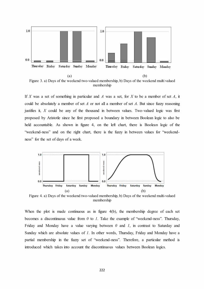
222
(a) (b)
Figure 3. a) Days of the weekend two-valued membership, b) Days of the weekend multi valued membership
If X was a set of something in particular and A was a set, for X to be a member of set A, it
could be absolutely a member of set A or not all a member of set A. But since fuzzy reasoning
justifies it, X could be any of the thousand in between values. Two-valued logic was first
proposed by Aristotle since he first proposed a boundary in between Boolean logic to also be
held accountable. As shown in figure 4, on the left chart, there is Boolean logic of the
“weekend-ness” and on the right chart, there is the fuzzy in between values for “weekend-
ness” for the set of days of a week.
(a) (b)
Figure 4. a) Days of the weekend two-valued membership, b) Days of the weekend multi-valued membership
When the plot is made continuous as in figure 4(b), the membership degree of each set
becomes a discontinuous value from 0 to 1. Take the example of “weekend-ness”. Thursday,
Friday and Monday have a value varying between 0 and 1, in contrast to Saturday and
Sunday which are absolute values of 1. In other words, Thursday, Friday and Monday have a
partial membership in the fuzzy set of “weekend-ness”. Therefore, a particular method is
introduced which takes into account the discontinuous values between Boolean logics.

223
The curve that maps the input space (day of the week) to the output space (weekend-ness) is
known as the membership function.
Another good example for fuzzy set is the seasons. Seasons vary from the northern
hemisphere to the southern hemisphere. Therefore, there is not an absolute rigid method for
the duration of each season. Therefore, there needs to be a smooth function that varies for
different methods as the seasons change from the northern hemisphere to the southern
hemisphere. Figure 5 shows two different membership functions which map different seasons
to different months.
(a) (b)
Figure 5. a) Rectangular membership functions, b) Gaussian membership functions for seasons of the year
7.5.2. Membership functions
A membership function (MF) is a curve that maps the input to a membership value ranging
between 0 and 1, known as the universe of discourse.
A common example of fuzzy sets is the set of tall people. The universe of discourse consists
of all heights, from 3 to 9 feet. For different tall to short heights, different universes of
discourses are matched. It can be assumed that all heights greater than eight feet are
considered “tall” and all heights smaller than eight feet to be considered “short”, but these
categorisations are absurd as it is unreasonable to assign one person “short” and another
person “tall” as there are differences in height by the width of a hair. Therefore, there must be
in between sets where someone can be to a percentage short and to a percentage tall.

224
Figure 6. Membership function for different heights
Therefore, the classification discussed so far is unacceptable. Similar to the figure for the set
of days assigned to be weekend, this degree of membership figure ranges from 0 to 1. It
defines the transition between tall and not-tall with a smooth curve in contrast to the previous
definition which had an absolute curve for either tall or not-tall and nothing defined for the in
between.
Figure 7. Comparing different membership functions for different heights
Subjective classification is also defined in fuzzy sets. It should be defined whether the term
“tall” refers to a ten year old child or an adult.
7.5.2.1. Membership functions in the fuzzy logic toolbox
The membership function only varies from 0 to 1. It can be defined as a smooth curve or a
rectangular shaped figure depending on how the case needs to be categorised.
An assumed classical set is in the form below:

225
. (7)
The extended form of a classical set is a fuzzy set. The fuzzy set A is X is shown in the below
form:
; (8)
where is the membership function of x in A. The membership function assigns each
element of X to a value between 0 and 1.
There are a number of built-in membership functions in the fuzzy logic toolbox in MATLAB.
These functions are: linear functions, the Sigmoid curves, Gaussian distribution function and
quadratic and cubic polynomial curves.
The simple forms of membership functions consist of a series of straight lines. The triangular
and trapezoidal membership functions are good examples, as shown in figure 8. The
trapezoidal membership function which is a truncated form of triangular membership
functions.
(a) (b)
Figure 8. a) Triangular membership function, b) Trapezoidal membership function
From the Gaussian distribution curve, two membership functions can be derived which are
gaussmf and gauss2mf.
The generalized bell membership function is defined by one more parameter than the
Gaussian membership function as it has three parameters when defined. Gaussian and bell
membership functions owe their popularity to their smooth and concise characteristics.

226
(a) (b) (c)
Figure 9. a) gaussmf , b) gauss2mf , c) gbellmf
But despite their smoothness, they are not capable of defining asymmetric membership
functions. These kinds of membership functions can be specified using two sigmoidal
functions. In addition to the sigmoidal membership functions, the difference and product of
the sigmoidal membership functions known as dsigmf and psigmf, can also be used for
asymmetric functions.
(a) (b) (c)
Figure 10. a) sigmf, b) dsigmf, c) psigmf Polynomial shaped membership functions are Z, S, and Pi curves, as their shape resemble
these characters. The Z membership function is an asymmetric curve which opens to the left
in contrast to the S membership function which opens to the right and Pi starts and ends with
zero with a maximum range in the middle.
(a) (b) (c)
Figure 11. a) Z, b) Pi, c) S

227
The selection of membership functions in the fuzzy logic toolbox is very wide. In addition,
this toolbox provides the user the advantage of creating its own arbitrary membership
functions. The simplest way would be using the simplest membership functions; the triangle
and trapezoid functions, as using unusual or complicated membership functions are not
appropriate for simple fuzzy inference systems. More details are presented further in this
chapter.
7.5.2.2. Membership functions in summary
Fuzzy sets take into account ambiguous values and map them to some value in
between 0 (absolute false) and 1 (absolute true), in which partial memberships are
introduced (Friday is partly a weekend and Mary is to some extent short).
Membership values map an input value input value (universe of discourse) to a fuzzy
set using appropriate membership functions defined by user.
7.5.3. Logical operations
The term fuzzy in fuzzy logic has been discussed. The reasoning behind the term “logic” is
discussed in this section. Fuzzy logical reasoning is a subset of Boolean logic where fuzzy
values can be mapped to the extreme values of 1 (absolutely true) and 0 (absolutely false).
The Boolean logic concept is shown in the table below:
Figure 12. Boolean logic
As mentioned above, in fuzzy logic the truth of an input values is mapped to a degree
between 0 and 1. Therefore, a function needs to be defined to perform the AND operator for
AANDB. The min (A, B) seems to be best alternative. Similar to this for OR operation where
max (A, B)is the solution suggested. Eventually, the operation NOT A which is equivalent to
the operation 1-A is defined, as shown in figure 13.
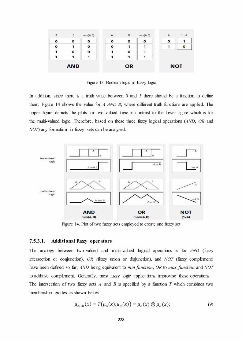
228
Figure 13. Boolean logic in fuzzy logic
In addition, since there is a truth value between 0 and 1 there should be a function to define
them. Figure 14 shows the value for A AND B, where different truth functions are applied. The
upper figure depicts the plots for two-valued logic in contrast to the lower figure which is for
the multi-valued logic. Therefore, based on these three fuzzy logical operations (AND, OR and
NOT) any formation in fuzzy sets can be analysed.
Figure 14. Plot of two fuzzy sets employed to create one fuzzy set
7.5.3.1. Additional fuzzy operators
The analogy between two-valued and multi-valued logical operations is for AND (fuzzy
intersection or conjunction), OR (fuzzy union or disjunction), and NOT (fuzzy complement)
have been defined so far, AND being equivalent to min function, OR to max function and NOT
to additive complement. Generally, most fuzzy logic applications improvise these operations.
The intersection of two fuzzy sets A and B is specified by a function T which combines two
membership grades as shown below:
; (9)

229
where is a binary operator for the function T. These fuzzy intersection operators, usually
known as T-norm (Triangular norm) operators, meet the basic obligations.
A T-norm operator is defined below:
boundary: T(0, 0) = 0, T(a, 1) = T(1, a) = a
monotonicity: T(a, b) <= T(c, d) if a <= c and b <= d
commutativity: T(a, b) = T(b, a)
associativity: T(a, T(b, c)) = T(T(a, b), c) . (10)
The first requirement fulfils a generalized form of crisp sets. The second requirement
indicates that a decrease in the membership values in A or B could not provoke an increase in
the membership value in A intersection B. The third requirement indicates the irrelevance of
the operator to the order of the fuzzy sets. In the end, the fourth requirement takes the
intersection of any number of sets. Like fuzzy intersection, the fuzzy union operator is
indicated by the S function:
; (11)
where is a binary operator for the function S. These fuzzy union operators T-conorm (or S-
norm operators) meet the following criteria:
boundary: S(1, 1) = 1, S(a, 0) = S(0, a) = a
monotonicity: S(a, b) <= S(c, d) if a <= c and b <= d
commutativity: S(a, b) = S(b, a)
associativity: S(a, S(b, c)) = S(S(a, b), c) .
(12)
The proof of these basic requirements is similar to the T-norm operator.
T-norms and dual T-conorms have been established to vary the “gain” on the function making
it very restrictive.
7.5.4. If-Then Rules
Fuzzy sets and fuzzy operators are exclusively popular terms in fuzzy logic. Conditional
sentences, if-then rules make fuzzy logic more practical.

230
A fuzzy if-then rule has the below form:
If x is A then y is B ;
Where A and B are linguistic values introduced by fuzzy sets on the universes of discourse of
x and y. The if-part of the rule, “x is A” known as the antecedent and the then-part, “y is B” is
the consequent or conclusion. A good example is the rule below:
If service is good, then tip is average ;
where the antecedent is a linguistic term indicating a single number between 0 and 1 in
contrast to the consequent which maps the fuzzy set B to the output variable y. Therefore, the
term “is” gets used in phrases, the antecedent and the consequent. In MATLAB language, this
is the difference between a relational format where “==” is used and a variable assignment
where “=” is used. Or in other words:
If service == good then tip = average ;
So the input to if-then rule is the input variable (service) and the output is the fuzzy set
(average).
The if-then rule consists of several distinct sections: first section considers the antecedent
(which takes into account fuzzifying the input and involves fuzzy operators) and second
section considers the consequent (implication). For binary logic, the if-then rules are simple.
If the antecedent is true then the precedent will be true as well.
If the antecedent is true to some extent, then the consequent is true to that same extent. For
example:
In binary logic: (p and q are either true or false)
In fuzzy logic: (partial antecedents are partially involved)
The antecedent of a if-then rule is capable of having multiple sections:
If the sky is grey and the wind is strong and the barometer is falling, then...
In which all the multiple consequents are influenced by the antecedent. The procedure in
which the consequent is influenced by the antecedent is discussed further in this chapter. The
consequent assigns a fuzzy set to the output. The fuzzy set is assigned to a degree modified
by the antecedent by means of the implication function. Truncation using the min function is

231
the most popular output modifying for the fuzzy sets in which the fuzzy set is chopped off, as
shown in figure 15. Scaling using the prod function is another method, in which the output
fuzzy set is squashed. Both methods are presented in the fuzzy logic toolbox.
Figure 15. Fuzzy IF-THEN rules for “dinner at restaurant” example
7.5.4.1. If-Then rules in summary
There are three steps when defining the if-then rules:
1. Inputs need to be fuzzified
All fuzzy terms in the antecedent are transformed into a membership degree between 0 and 1.
2. Fuzzy operator is applied
Fuzzy logic operators are applied to the antecedent to assign it to a number between 0 and 1.
3. The implication process is applied
The consequent of the if-then rule allocates a fuzzy set to the output. This fuzzy set is
truncated based on the implication method applied.
When defining a particular case in fuzzy logic language using fuzzy if-then rules, one rule is
not effective. It is required that several rules be defined. The output of each rule is a fuzzy
set. In the end, the final output for all the fuzzy sets is a single crisp number. In which first
the output fuzzy sets for each rule is aggregated into an output fuzzy set. In the next step, this

232
fuzzy set is defuzzified or transformed into a single number. The entire procedure is explained
in the following section.
7.5.5. Fuzzy inference systems
Fuzzy inference systems match the membership functions of the fuzzy inputs to the
membership functions of the fuzzy output using if-then rules and extracting a final single
number through defuzzification.
The application of fuzzy inference systems is quite wide; control automation systems,
classification of data and modelling. Therefore it has been given several names: fuzzy-rule-
based system, fuzzy associative memory, fuzzy logic controller, and simply fuzzy logic
systems.
7.5.5.1. “Dinner at restaurant” example
The fuzzy logic application for the aforementioned example, “dinner at restaurant” is
explained in this section. Service and food are the two inputs and the tip paid to the waitress
is considered as the output. There are three rules matching the inputs to the outputs, in which
all rules are evaluated in parallel using fuzzy reasoning. The results of the rules are combined
and distilled through the defuzzification process. The final result is a crisp, non-fuzzy number
which is the output, in this example, the tip. The description of the fuzzy inference for this
example is shown in figure 16. Each of the fuzzy inference terms are defined further in this
chapter.
Figure 16. Fuzzy Rules for “dinner at restaurant” example

233
Step 1. Fuzzify Inputs The first step is to define the inputs and assign the membership functions which are the
degree the inputs belong to the fuzzy sets. The input is in the universe of discourse of the
input variable and the output is always between 0 and 1. Therefore, the inputs and outputs
need to be defuzzified. The example in this section for the “dinner at restaurant” uses fuzzy
membership functions to map the inputs to the different linguistic terms. For example, when
the input is food and the food is delicious, based on the delicious membership function curve,
the extent to which the food is delicious is defined. This input is fuzzified with the fuzzy
operators and for a supposed food (rated from 0 to 10) fitting the linguistic term “delicious”,
the result of fuzzification for the rate of 8 in the food is equivalent to 0.7 based on the defined
membership function.
Figure 17. Fuzzify inputs for “dinner at restaurant” example
Step 2. Application of Fuzzy operator After the input fuzzification step, each part of the antecedent in the fuzzy if-then rule is
satisfied to a certain degree for every rule. If there is more than one part in the antecedent, the
fuzzy operator estimates this degree which is a number allocated to that particular rule. This
number is considered in the evaluation for the final output function. The inputs for a fuzzy
operator are membership values whilst the output is a crisp number.
As mentioned in the previous sections, a well-defined method can be a substitute for the
fuzzy logic operations, AND or OR. In the fuzzy logic toolbox, two functions are defined for
AND operation which are: min(minimum) and prod(product) and two functions are defined for
the OR operation which are: max (maximum), and the probabilistic OR method (probor) or
(the algebraic sum). The equation for this method is given below:
probor(a,b) = a + b – ab. (13)
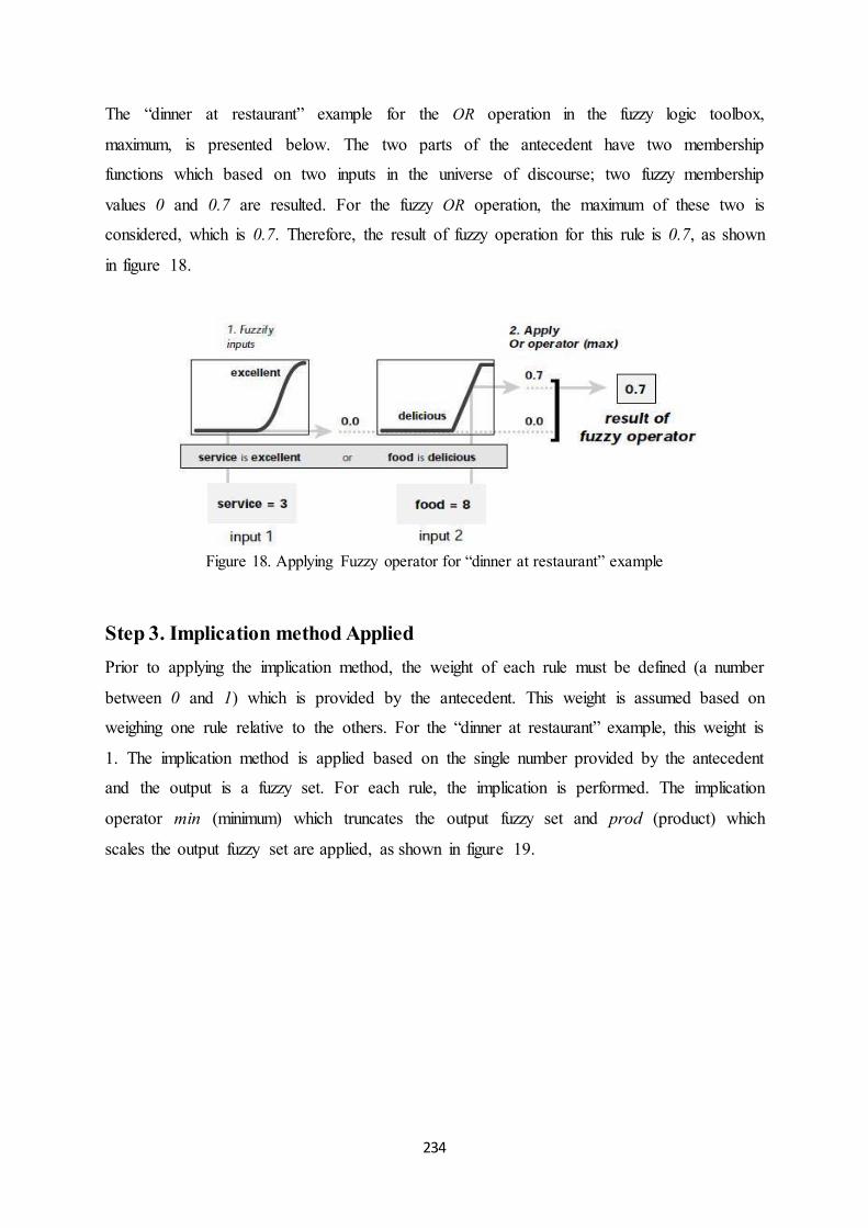
234
The “dinner at restaurant” example for the OR operation in the fuzzy logic toolbox,
maximum, is presented below. The two parts of the antecedent have two membership
functions which based on two inputs in the universe of discourse; two fuzzy membership
values 0 and 0.7 are resulted. For the fuzzy OR operation, the maximum of these two is
considered, which is 0.7. Therefore, the result of fuzzy operation for this rule is 0.7, as shown
in figure 18.
Figure 18. Applying Fuzzy operator for “dinner at restaurant” example
Step 3. Implication method Applied Prior to applying the implication method, the weight of each rule must be defined (a number
between 0 and 1) which is provided by the antecedent. This weight is assumed based on
weighing one rule relative to the others. For the “dinner at restaurant” example, this weight is
1. The implication method is applied based on the single number provided by the antecedent
and the output is a fuzzy set. For each rule, the implication is performed. The implication
operator min (minimum) which truncates the output fuzzy set and prod (product) which
scales the output fuzzy set are applied, as shown in figure 19.

235
Figure 19. Applying Implication method for “dinner at restaurant” example
Step 4. Aggregation of the Outputs In the aggregation step, the outputs of each rule are unified, in which all the fuzzy sets for the
output of each rule is combined into a single fuzzy set which is provided to the defuzzification
step. Therefore, after the implication operation, in this example min (minimum) is applied.
The result of the implication for each rule which is the truncation of the output function is
aggregated for each output variable in each rule. This aggregation process is changeable;
therefore the execution order for each rule is not very significant. The method for aggregation
is built in the fuzzy logic toolbox. They are: max (maximum), probor (probabilistic or) and
sum (sum of the output set of each rule).
Figure 20 is a typical example of the aggregation of all outputs for the “dinner at restaurant”
example.

236
Figure 20. Aggregating all outputs for “dinner at restaurant” example
Step 5. Defuzzification of the aggregated output The aggregated output from the previous step is a fuzzy set to be defuzzified in this step in
which the defuzzified output is a single crisp number. Therefore, the defuzzification process
takes a fuzzy set as the input and returns a single number to the output. The defuzzification
method which is the most common is the centroid method, wherein the centre of the area
from the aggregation step is returned. For the “dinner at restaurant” example, the centroid is
chosen as the defuzzification method and the crisp output number is the final output, which is
the tip given based on the food and service provided as the inputs, as shown in figure 21.
There are other defuzzification methods largest of maximum, smallest of maximum and
middle (average) of maximum.

237
Figure 21. Defuzzification for “dinner at restaurant” example
7.5.6. The Fuzzy inference diagram
In the fuzzy inference diagram, the processes of how all the aforementioned steps are
performed are shown. The flow of information for this section is shown in figure 22. This
flow proceeds from each of the inputs to the outputs and finally from all the outputs of all the
rules defined to a single crisp number to be the final defuzzification output. The MATLAB
implementation of this diagram is shown in the fuzzy logic toolbox (J.S.Roger Jang).
Figure 22. Defining the Fuzzy inference diagram

238