MR-RST Madison ISU LIDAR Applications and Tests Iowa State University Shauna Hallmark Reg Souleyrette

MR-RST MadisonISU LIDAR Applications and Tests

Iowa State University

Shauna HallmarkReg Souleyrette

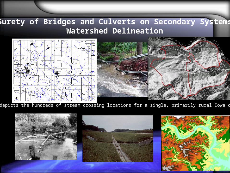
Surety of Bridges and Culverts on Secondary SystemsWatershed Delineation

The graphic depicts the hundreds of stream crossing locations for a single, primarily rural Iowa county

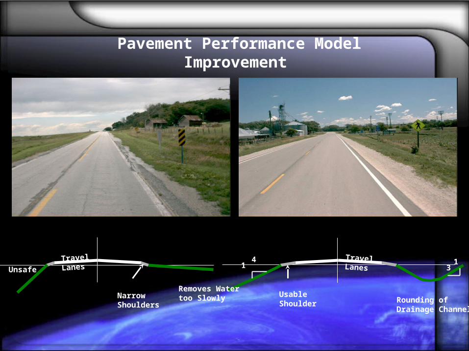
Pavement Performance Model Improvement

Travel Lanes

UsableShoulder Rounding of

Drainage Channel

41 3

1Travel Lanes

NarrowShoulders

Removes Water too Slowly

Unsafe

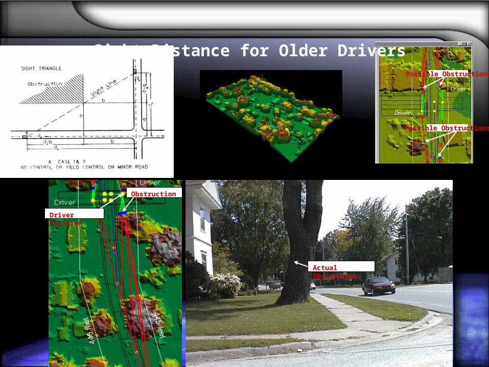
Obstruction

Driver Position

Actual Obstruction

Possible Obstructions

Possible Obstructions

Sight Distance for Older Drivers

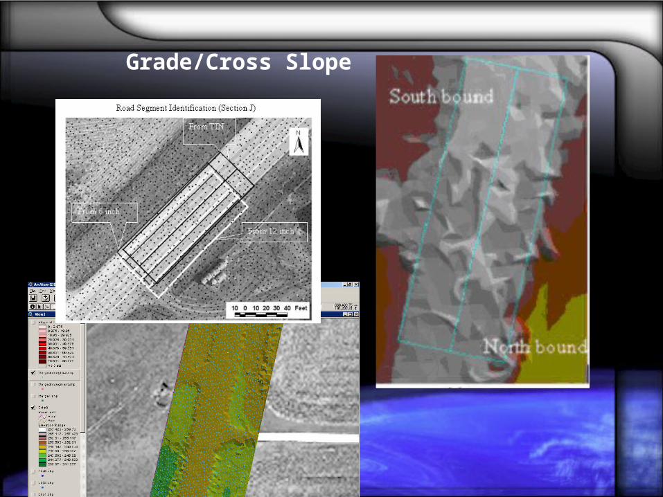
Grade/Cross Slope

Residual Plot for Cross-slope Determination Segment F

-0.6

-0.4

-0.2

0

0.2

0.4

0.6

-30 -20 -10 0 10 20 30

Centerline Distance (feet)

Res

idu

als

(fee

t)

Shoulder

Pavement

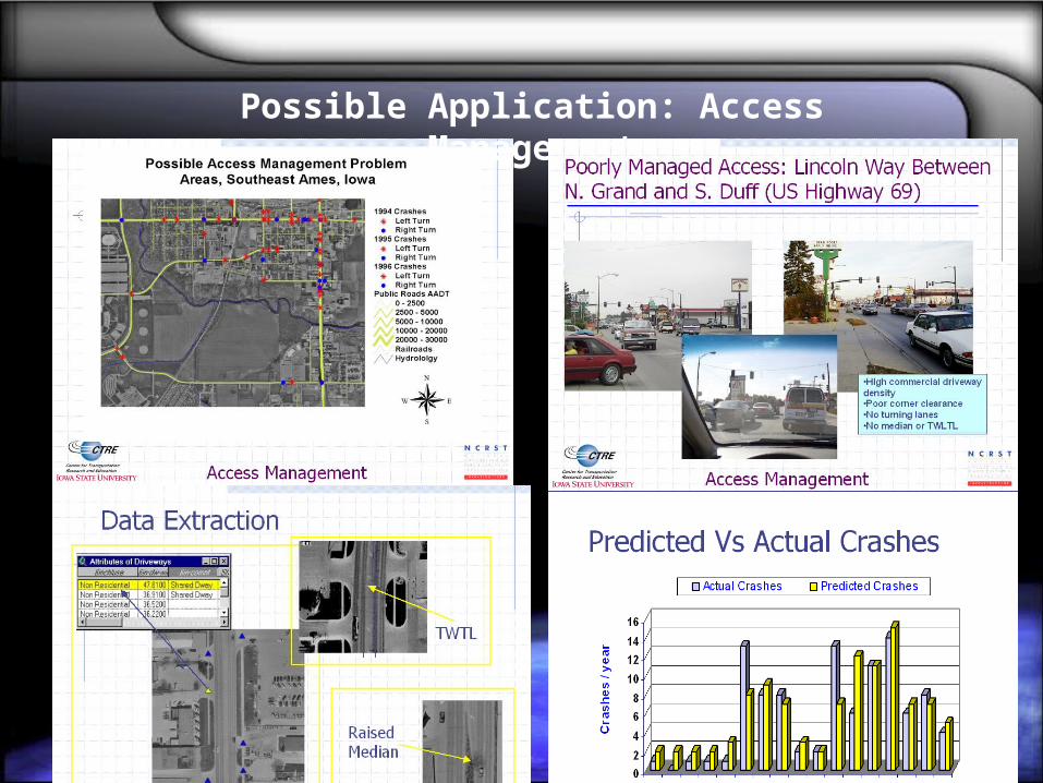
Possible Application: Access Management

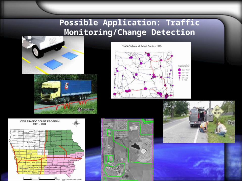
Possible Application: Traffic Monitoring/Change Detection

Evaluation of LIDAR-Derived Terrain Data in Highway Planning

and Design

Introduction

• Highway location depends on: – Engineering (terrain, safety, design)– Cost– Social Aspects (land use, etc.)– Ecology (pollution)– Aesthetics (scenic value)

Introduction

• One key requirement: up-to-date terrain information

• Uses– Determining the best route between termini– Finding the optimum combination of

alignments, grades, etc.

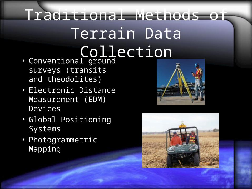
Traditional Methods of Terrain Data Collection

• Conventional ground surveys (transits and theodolites)

• Electronic Distance Measurement (EDM) Devices

• Global Positioning Systems

• Photogrammetric Mapping

Introduction

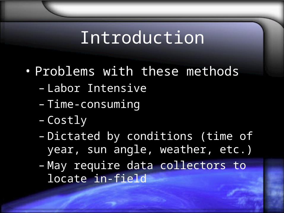
• Problems with these methods– Labor Intensive– Time-consuming– Costly– Dictated by conditions (time of year, sun angle,

weather, etc.) – May require data collectors to locate in-field

Introduction

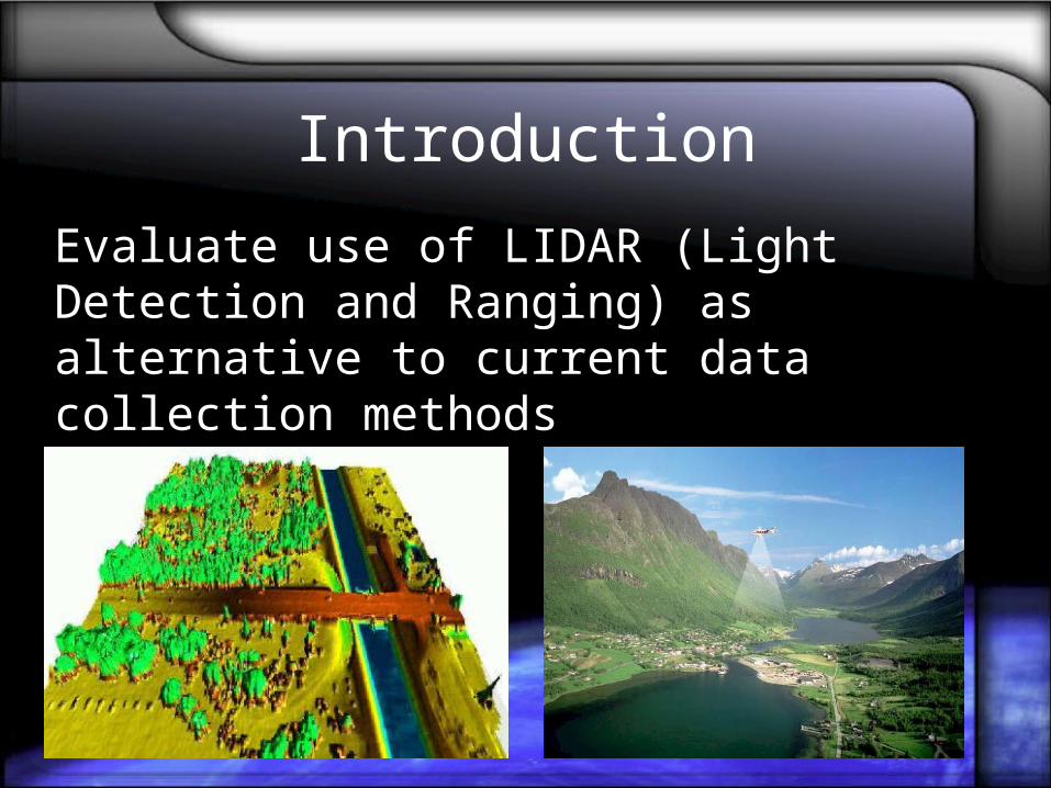
Evaluate use of LIDAR (Light Detection and Ranging) as alternative to current data collection methods

Anticipated Benefits of LIDAR in Location Process

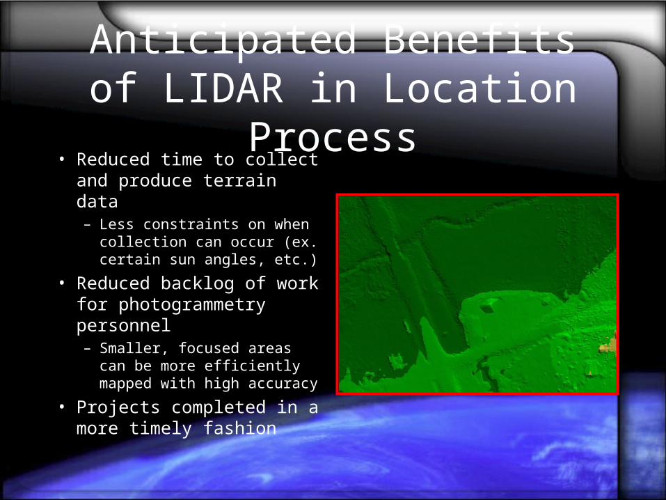
• Reduced time to collect and produce terrain data– Less constraints on when

collection can occur (ex. certain sun angles, etc.)

• Reduced backlog of work for photogrammetry personnel– Smaller, focused areas can be

more efficiently mapped with high accuracy

• Projects completed in a more timely fashion

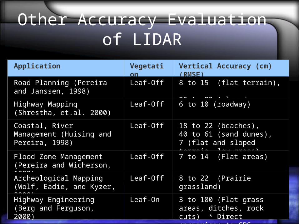
Other Accuracy Evaluation of LIDAR

Application Vegetation Vertical Accuracy (cm) (RMSE)

Road Planning (Pereira and Janssen, 1998)

Leaf-Off 8 to 15 (flat terrain), 25 to 38 (sloped terrain)

Highway Mapping (Shrestha, et.al. 2000)

Leaf-Off 6 to 10 (roadway)

Coastal, River Management (Huising and Pereira, 1998)

Leaf-Off 18 to 22 (beaches),40 to 61 (sand dunes),7 (flat and sloped terrain, low grass)

Flood Zone Management (Pereira and Wicherson, 1999)

Leaf-Off 7 to 14 (Flat areas)

Archeological Mapping (Wolf, Eadie, and Kyzer, 2000)

Leaf-Off 8 to 22 (Prairie grassland)

Highway Engineering (Berg and Ferguson, 2000)

Leaf-On 3 to 100 (Flat grass areas, ditches, rock cuts) * Direct comparison to GPS derived DTM

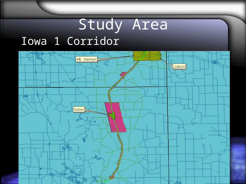
Study AreaIowa 1 Corridor

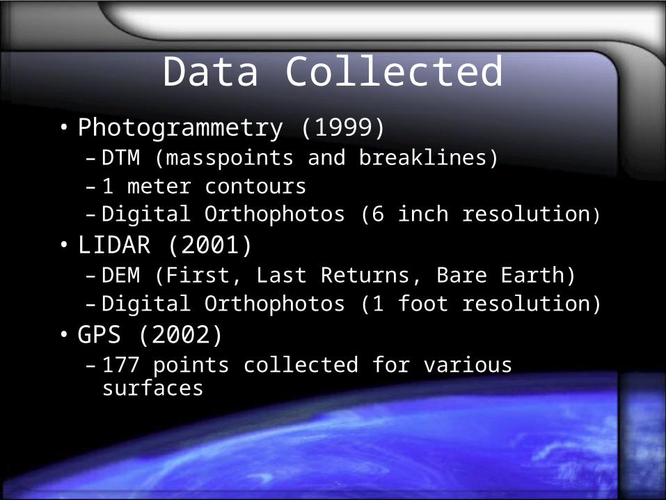
Data Collected• Photogrammetry (1999)

– DTM (masspoints and breaklines)– 1 meter contours– Digital Orthophotos (6 inch resolution)

• LIDAR (2001)– DEM (First, Last Returns, Bare Earth)– Digital Orthophotos (1 foot resolution)

• GPS (2002)– 177 points collected for various surfaces

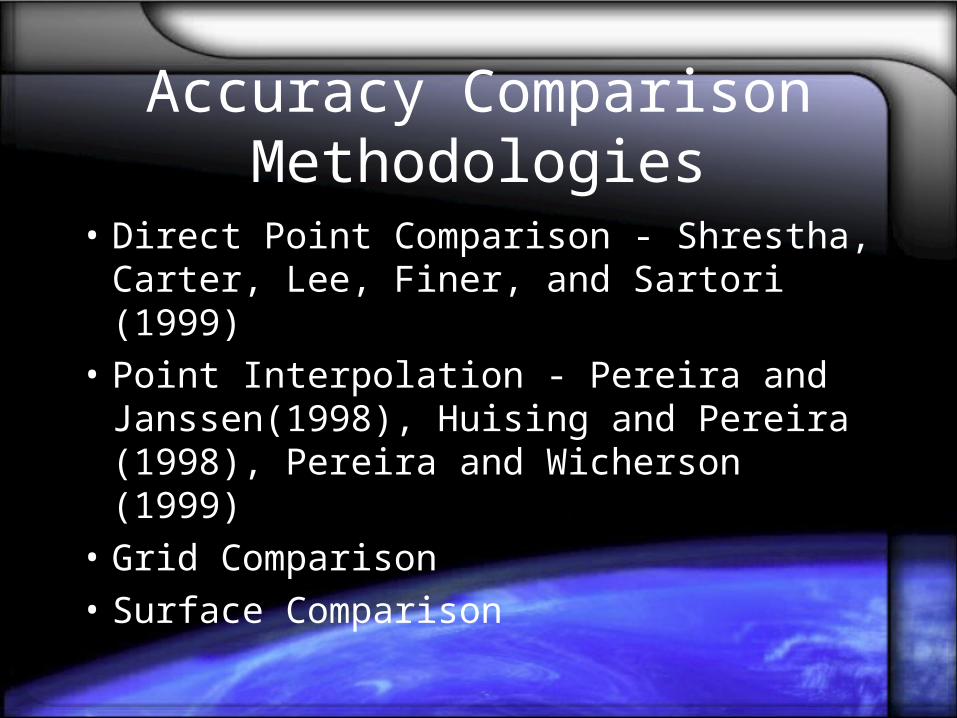
Accuracy Comparison Methodologies

• Direct Point Comparison - Shrestha, Carter, Lee, Finer, and Sartori (1999)

• Point Interpolation - Pereira and Janssen(1998), Huising and Pereira (1998), Pereira and Wicherson (1999)

• Grid Comparison

• Surface Comparison

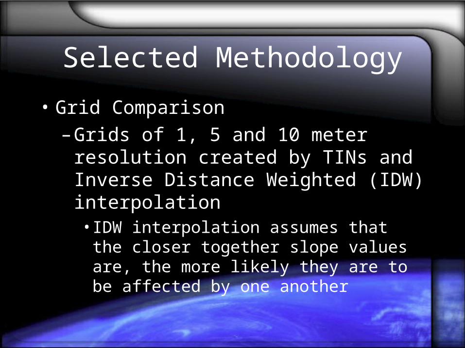
Selected Methodology

• Grid Comparison

– Grids of 1, 5 and 10 meter resolution created by TINs and Inverse Distance Weighted (IDW) interpolation• IDW interpolation assumes that the closer

together slope values are, the more likely they are to be affected by one another

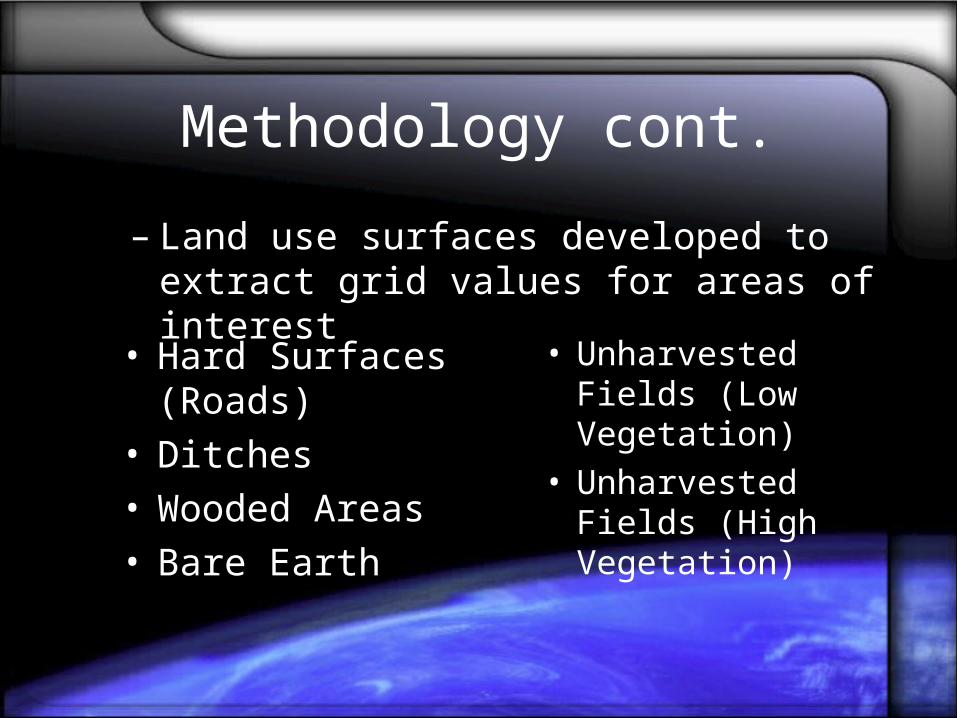
Methodology cont.

– Land use surfaces developed to extract grid values for areas of interest

• Hard Surfaces (Roads)• Ditches• Wooded Areas• Bare Earth

• Unharvested Fields (Low Vegetation)

• Unharvested Fields (High Vegetation)

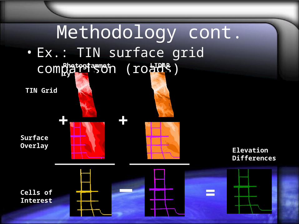
Methodology cont.• Ex.: TIN surface grid comparison (roads)

Photogrammetry LIDAR

TIN Grid

Surface Overlay

+ +

=Cells of Interest

Elevation Differences

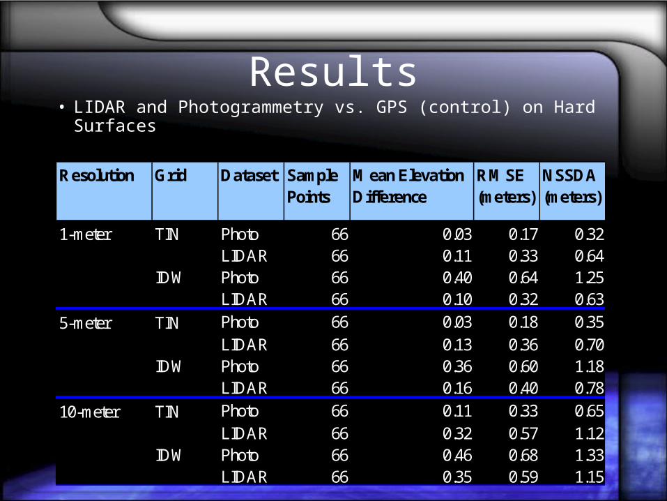
Results• LIDAR and Photogrammetry vs. GPS (control) on Hard Surfaces

Mean ElevationDifference

Photo 66 0.03 0.17 0.32LIDAR 66 0.11 0.33 0.64Photo 66 0.40 0.64 1.25LIDAR 66 0.10 0.32 0.63Photo 66 0.03 0.18 0.35LIDAR 66 0.13 0.36 0.70Photo 66 0.36 0.60 1.18LIDAR 66 0.16 0.40 0.78Photo 66 0.11 0.33 0.65LIDAR 66 0.32 0.57 1.12Photo 66 0.46 0.68 1.33LIDAR 66 0.35 0.59 1.15

RMSE (meters)

NSSDA (meters)

1-meter TIN

IDW

Resolution Grid Dataset Sample Points

5-meter TIN

IDW

10-meter TIN

IDW

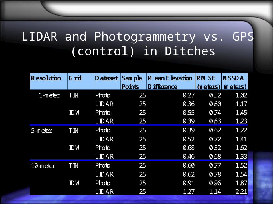
LIDAR and Photogrammetry vs. GPS (control) in Ditches



5-meter TIN

IDW

10-meter TIN

IDW

RMSE (meters)

NSSDA (meters)

1-meter TIN

IDW


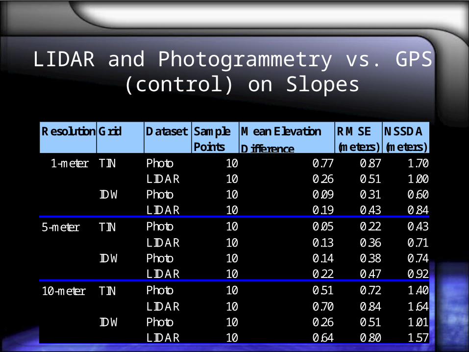
LIDAR and Photogrammetry vs. GPS (control) on Slopes

Mean Elevation

DifferencePhoto 10 0.77 0.87 1.70LIDAR 10 0.26 0.51 1.00Photo 10 0.09 0.31 0.60LIDAR 10 0.19 0.43 0.84Photo 10 0.05 0.22 0.43LIDAR 10 0.13 0.36 0.71Photo 10 0.14 0.38 0.74LIDAR 10 0.22 0.47 0.92Photo 10 0.51 0.72 1.40LIDAR 10 0.70 0.84 1.64Photo 10 0.26 0.51 1.01LIDAR 10 0.64 0.80 1.57

RMSE (meters)

NSSDA (meters)

1-meter TIN

IDW


5-meter TIN

IDW

10-meter TIN

IDW

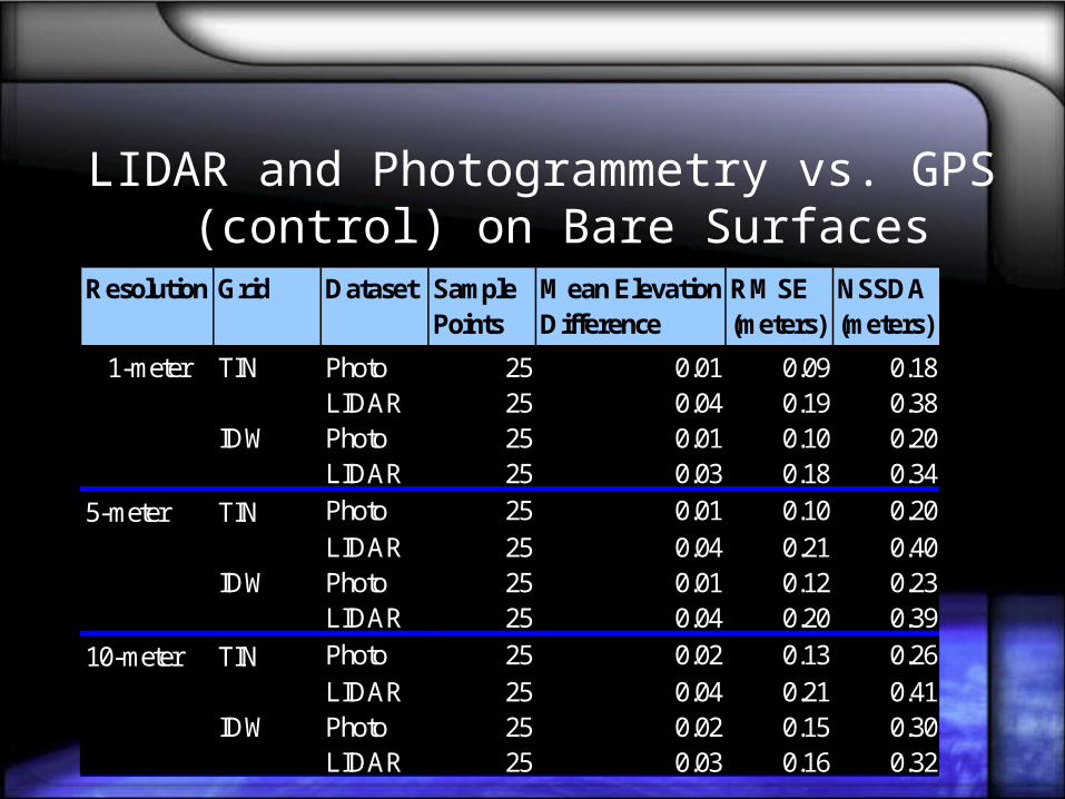
LIDAR and Photogrammetry vs. GPS (control) on Bare Surfaces



RMSE (meters)

NSSDA (meters)

1-meter TIN

IDW


5-meter TIN

IDW

10-meter TIN

IDW

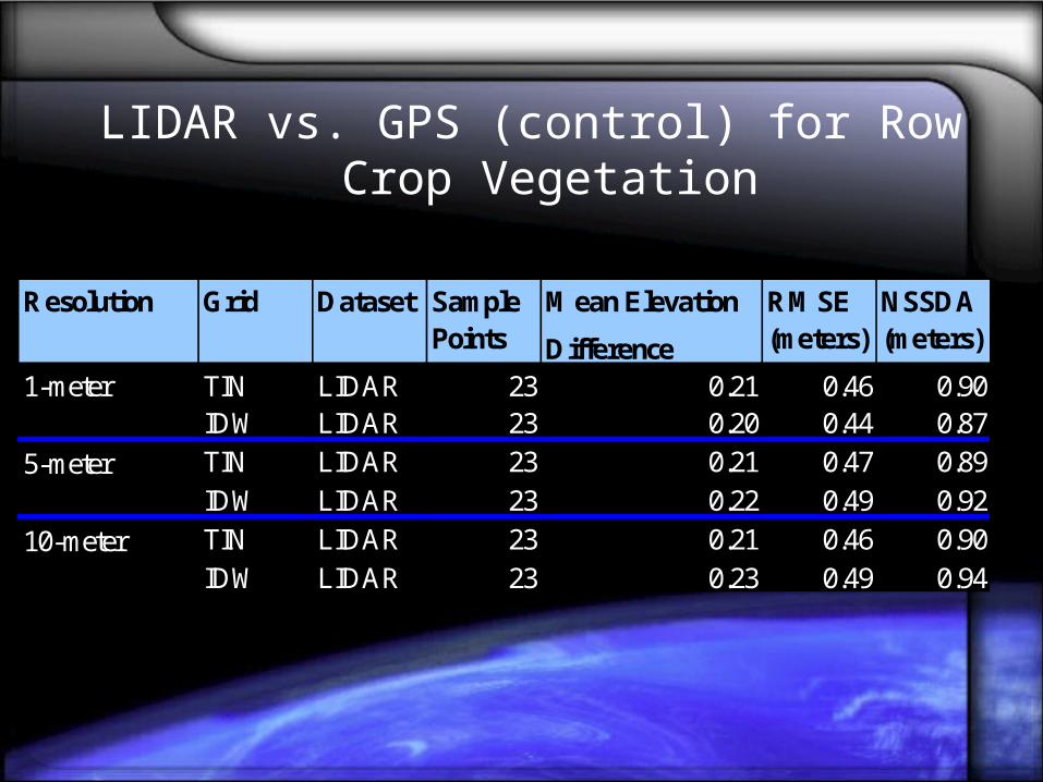
LIDAR vs. GPS (control) for Row Crop Vegetation

Mean Elevation

DifferenceTIN LIDAR 23 0.21 0.46 0.90IDW LIDAR 23 0.20 0.44 0.87TIN LIDAR 23 0.21 0.47 0.89IDW LIDAR 23 0.22 0.49 0.92TIN LIDAR 23 0.21 0.46 0.90IDW LIDAR 23 0.23 0.49 0.94

10-meter

RMSE (meters)

NSSDA (meters)

1-meter

5-meter


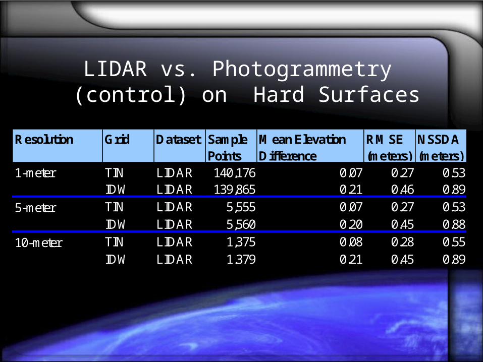
LIDAR vs. Photogrammetry (control) on Hard Surfaces


TIN LIDAR 140,176 0.07 0.27 0.53IDW LIDAR 139,865 0.21 0.46 0.89TIN LIDAR 5,555 0.07 0.27 0.53IDW LIDAR 5,560 0.20 0.45 0.88TIN LIDAR 1,375 0.08 0.28 0.55IDW LIDAR 1,379 0.21 0.45 0.89

10-meter

RMSE (meters)

NSSDA (meters)

1-meter

5-meter


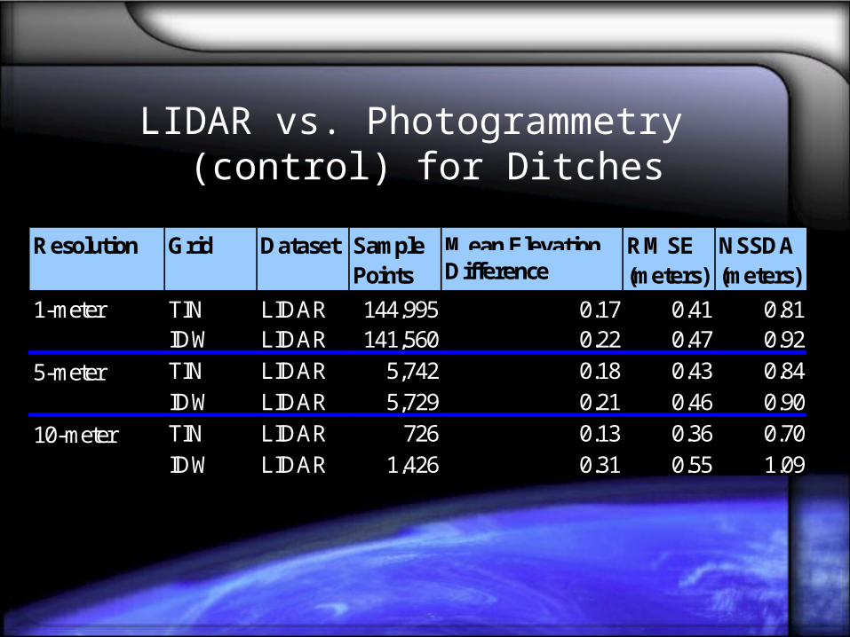
LIDAR vs. Photogrammetry (control) for Ditches


TIN LIDAR 144,995 0.17 0.41 0.81IDW LIDAR 141,560 0.22 0.47 0.92TIN LIDAR 5,742 0.18 0.43 0.84IDW LIDAR 5,729 0.21 0.46 0.90TIN LIDAR 726 0.13 0.36 0.70IDW LIDAR 1,426 0.31 0.55 1.09

10-meter

RMSE (meters)

NSSDA (meters)

1-meter

5-meter


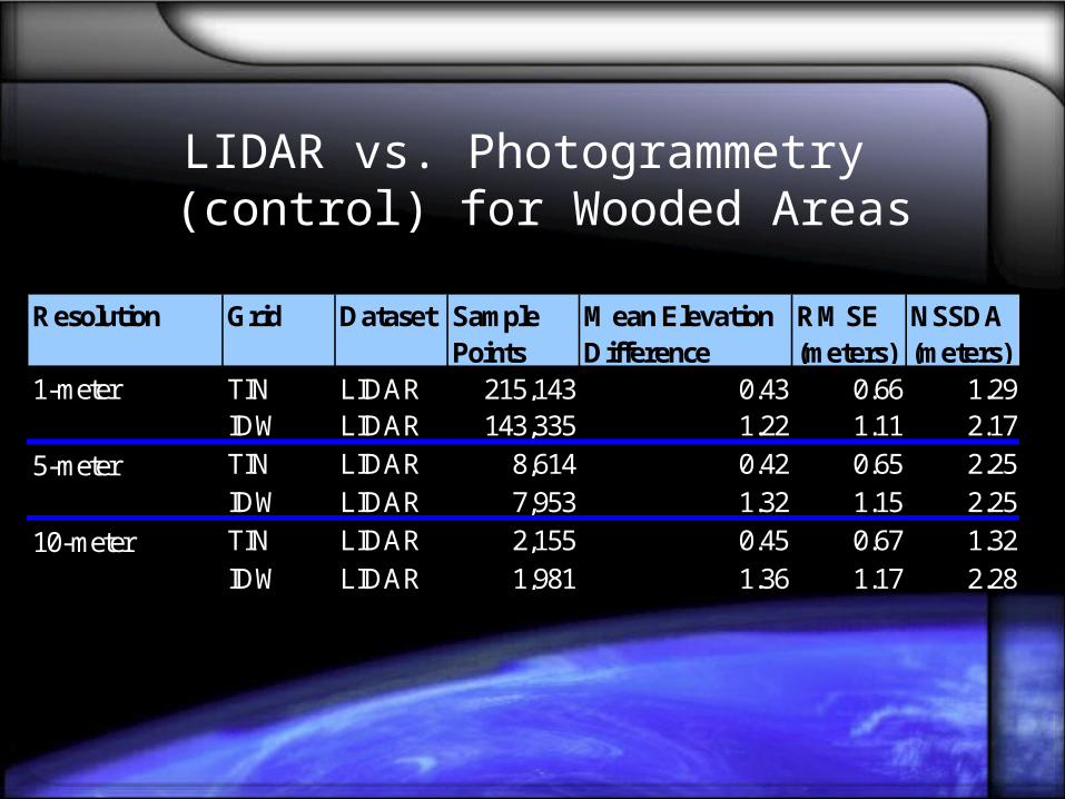
LIDAR vs. Photogrammetry (control) for Wooded Areas


TIN LIDAR 215,143 0.43 0.66 1.29IDW LIDAR 143,335 1.22 1.11 2.17TIN LIDAR 8,614 0.42 0.65 2.25IDW LIDAR 7,953 1.32 1.15 2.25TIN LIDAR 2,155 0.45 0.67 1.32IDW LIDAR 1,981 1.36 1.17 2.28

10-meter

RMSE (meters)

NSSDA (meters)

1-meter

5-meter


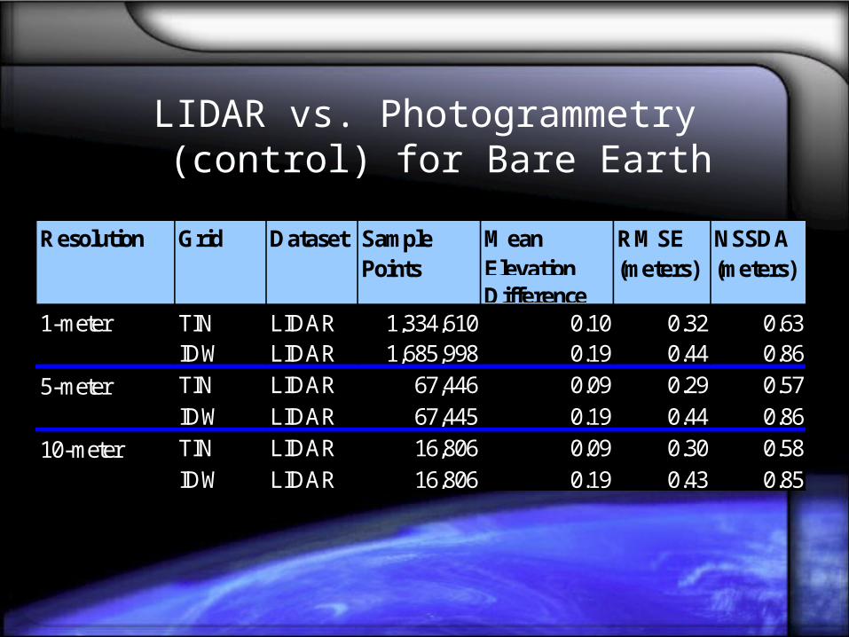
LIDAR vs. Photogrammetry (control) for Bare Earth


TIN LIDAR 1,334,610 0.10 0.32 0.63IDW LIDAR 1,685,998 0.19 0.44 0.86TIN LIDAR 67,446 0.09 0.29 0.57IDW LIDAR 67,445 0.19 0.44 0.86TIN LIDAR 16,806 0.09 0.30 0.58IDW LIDAR 16,806 0.19 0.43 0.85

10-meter

RMSE (meters)

NSSDA (meters)

1-meter

5-meter


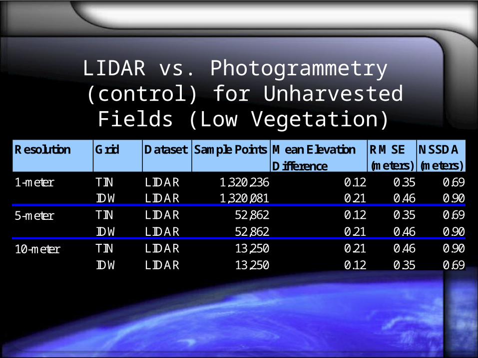
LIDAR vs. Photogrammetry (control) for Unharvested Fields (Low Vegetation)



10-meter

RMSE (meters)

NSSDA (meters)

1-meter

5-meter


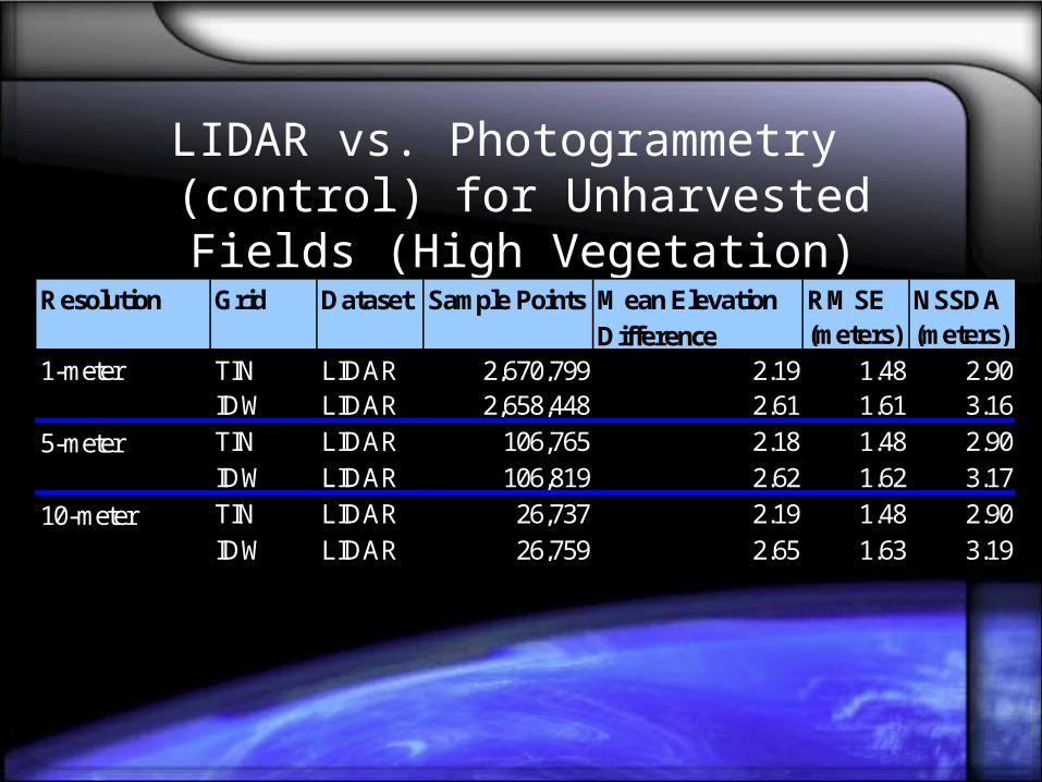
LIDAR vs. Photogrammetry (control) for Unharvested Fields (High Vegetation)



10-meter

RMSE (meters)

NSSDA (meters)

1-meter

5-meter


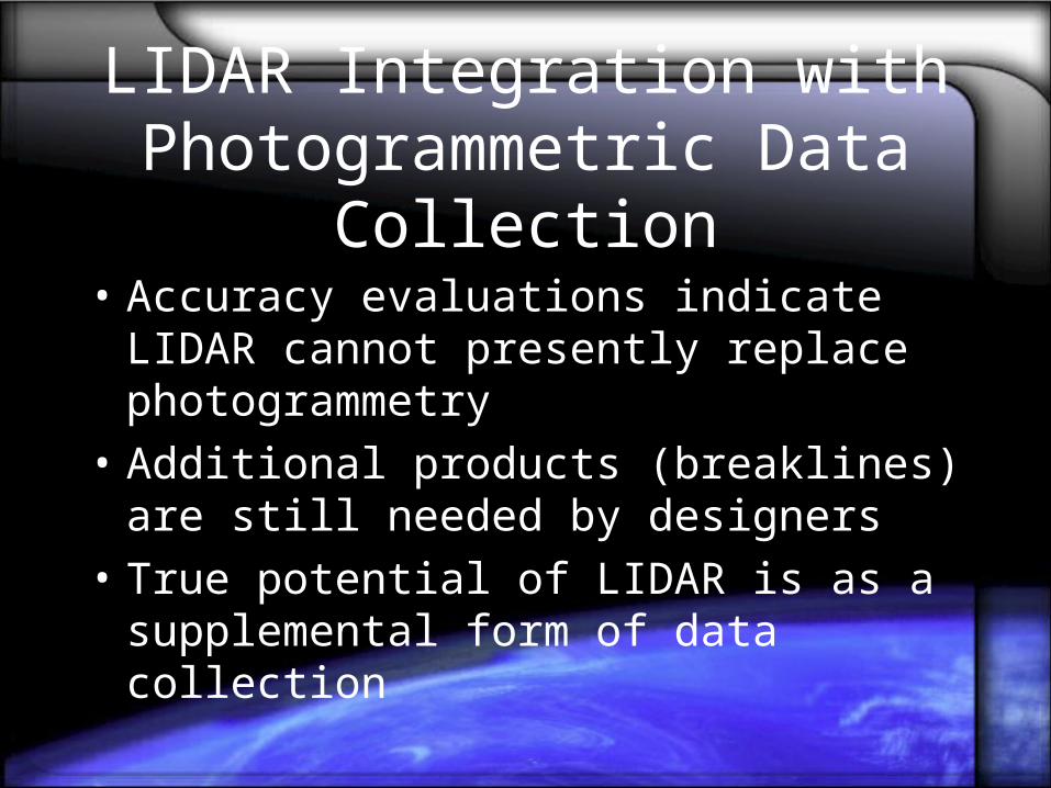
LIDAR Integration with Photogrammetric Data Collection

• Accuracy evaluations indicate LIDAR cannot presently replace photogrammetry

• Additional products (breaklines) are still needed by designers

• True potential of LIDAR is as a supplemental form of data collection

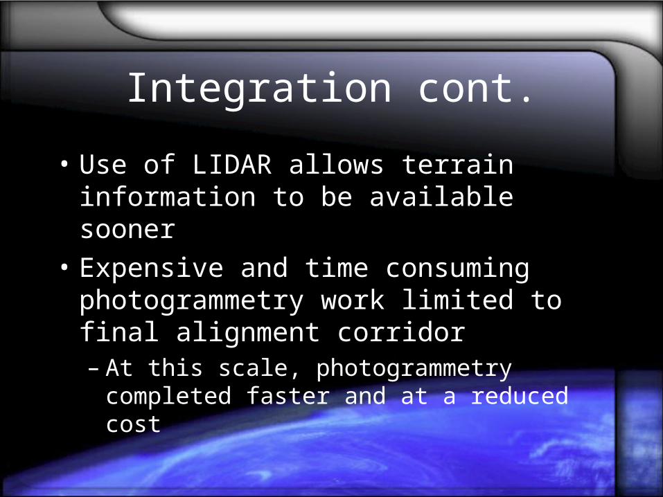
Integration cont.

• Use of LIDAR allows terrain information to be available sooner

• Expensive and time consuming photogrammetry work limited to final alignment corridor– At this scale, photogrammetry completed faster

and at a reduced cost

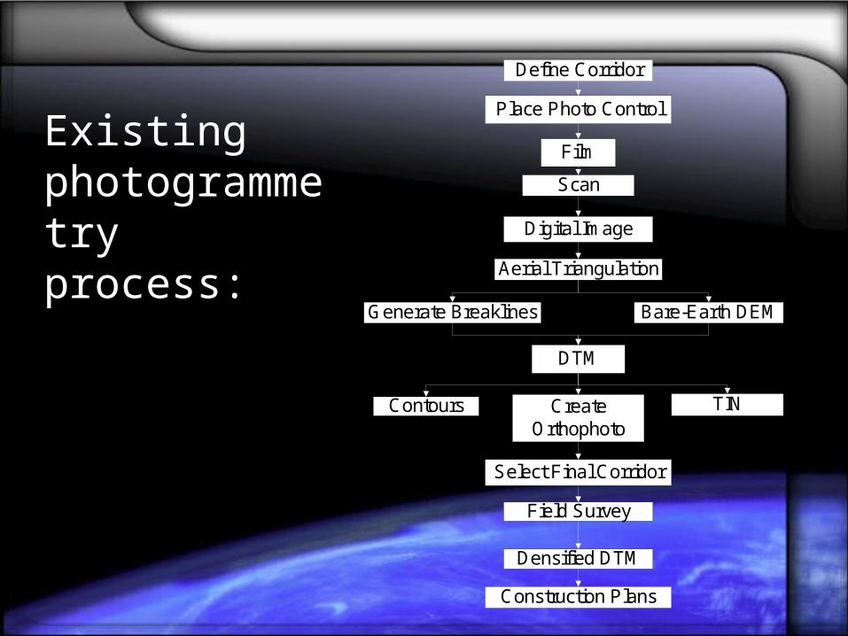
Define Corridor

Film

Place Photo Control

Scan

Digital Image

Aerial Triangulation

Generate Breaklines

DTM

Bare-Earth DEM

CreateOrthophoto

Contours TIN

Select Final Corridor

Field Survey

Densified DTM

Construction Plans

Existing photogrammetry process:

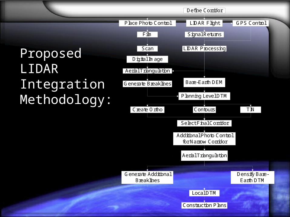
Define Corridor

Place Photo Control GPS Control

Film Signal Returns

LIDAR Flight

LIDAR ProcessingScan

Digital Image


Generate Breaklines Bare-Earth DEM

Planning Level DTM

Create Ortho Contours TIN

Select Final Corridor

Additional Photo Controlfor Narrow Corridor


Generate AdditionalBreaklines

Densify Bare-Earth DTM

Local DTM

Construction Plans

Proposed LIDAR Integration Methodology:

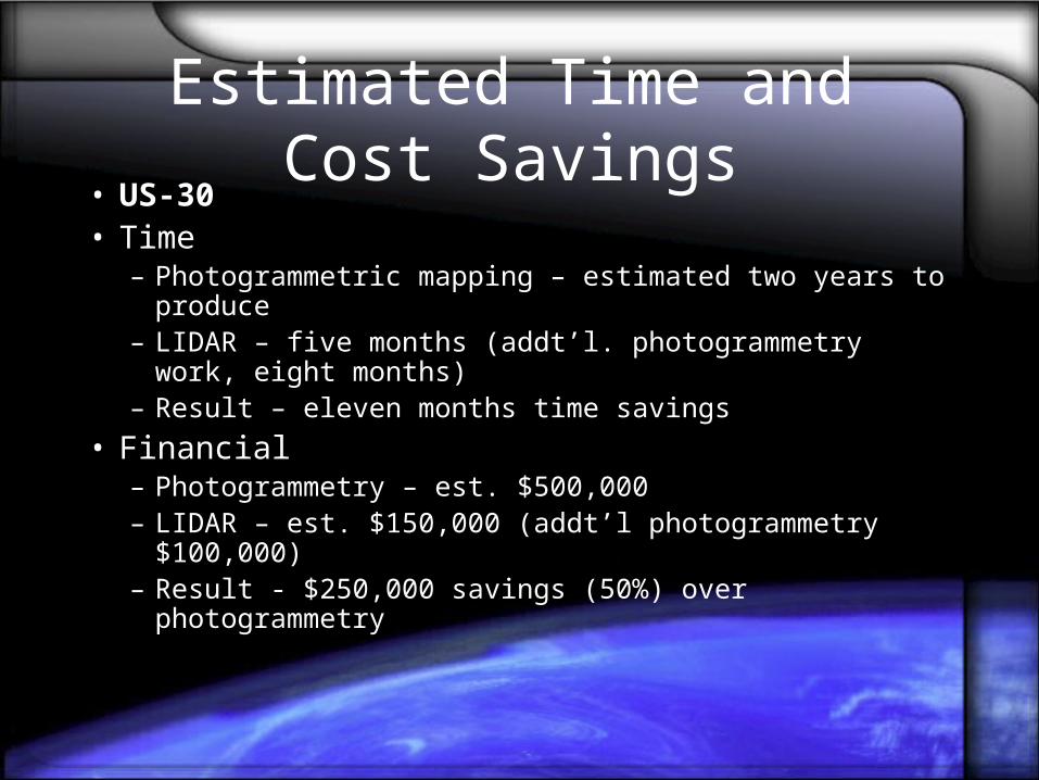
Estimated Time and Cost Savings• US-30• Time

– Photogrammetric mapping – estimated two years to produce

– LIDAR – five months (addt’l. photogrammetry work, eight months)

– Result – eleven months time savings

• Financial– Photogrammetry – est. $500,000– LIDAR – est. $150,000 (addt’l photogrammetry $100,000)– Result - $250,000 savings (50%) over photogrammetry

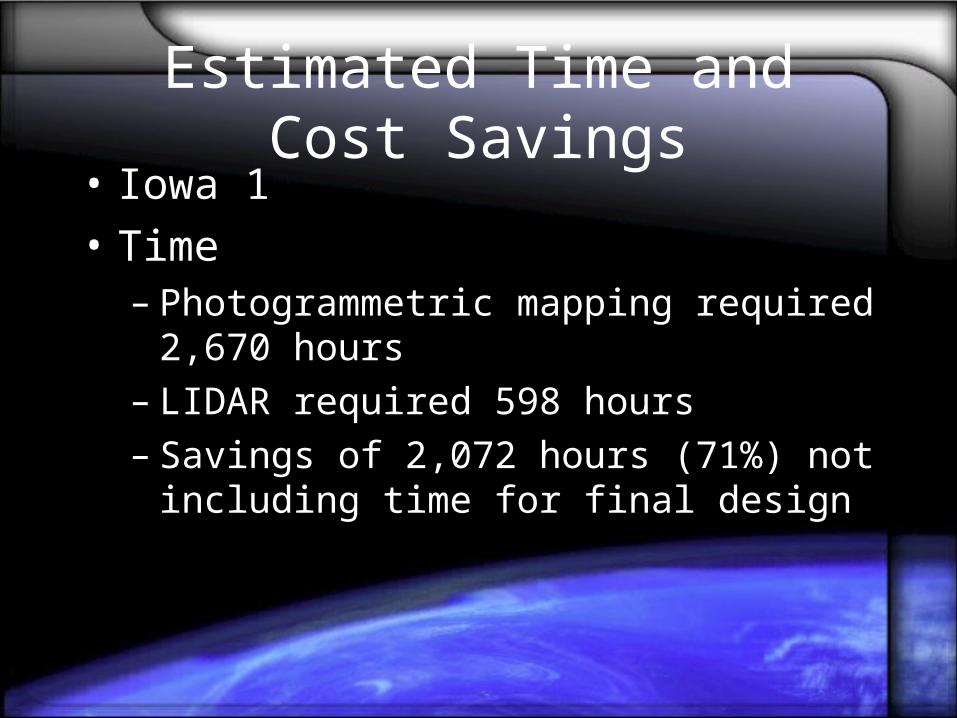
Estimated Time and Cost Savings• Iowa 1

• Time– Photogrammetric mapping required 2,670 hours– LIDAR required 598 hours– Savings of 2,072 hours (71%) not including

time for final design

Conclusions

• LIDAR Advantages– Less dependant on environmental conditions– Faster data collection and delivery– Potential for allowing data to be available to

designers sooner

Conclusions cont.

• LIDAR Disadvantages– LIDAR not presently capable of replacing

photogrammetry in location and design functions

– Elevation accuracy not comparable to photogrammetry

– LIDAR not capable of penetrating thick vegetation

– Supplemental information (breaklines) cannot be derived from LIDAR

Research Limitations

• Data collected under leaf-on conditions

• Photogrammetry and LIDAR data collected and produced at different times– Minor changes in the study area were possible

Questions…

Documents

MR-RST Madison ISU LIDAR Applications and Tests Iowa State University Shauna Hallmark Reg Souleyrette