Embed Size (px)
Citation preview
Extreme Value Model for Rainfall
DistributionCase Study of Lagos and Edo States, Nigeria
BY
OLUMIDE MICHAEL OYALOLAB.Tech (Hons) Industrial Mathematics, FUTA
MATRIC NUMBER : 176473
THESIS SUBMITTED TO THE DEPARTMENT OF STATISTICS,
FACULTY OF SCIENCE
IN PARTIAL FULFILMENT OF THE REQUIREMENTS
FOR THE AWARD OF THE DEGREE OF MASTER OF SCIENCE (M.Sc.)
IN STATISTICS OF THE UNIVERSITY OF IBADAN, OYO STATE, NIGERIA.
March, 2015

i
DEDICATION
This academic work piece is dedicated :
To my parents Mr Emmanuel Bamidele & Mrs Olasimbo Elizabeth Oyalola; for sticking with
me and supporting me all through.
To Dr. Obisesan K.O.; for being a mentor, friend and role model.
To Anuoluwapo; my darling fiancee; for seeing the diamond in me before any other person
could spot it and for loving me unconditionally.
To my Lord and saviour Jesus Christ; my only source of infinite wisdom, in you I live, in you I
move, in you I have my being.
Olumide Michael Oyalola
ii
Certification
This certified that this research work was carried out by OLUMIDE MICHAEL OYALOLA
with matriculation number 176473 of department of statistics, University of Ibadan, Oyo State,
Nigeria.
............................
Date
........................
Supervisor
Dr. K.O. OBISESAN
Department of Statistics,
University of Ibadan,
Ibadan, Oyo State, Nigeria.
............................
Date
........................
Head of Department
Dr. ADEDAYO A. ADEPOJU
Department of Statistics,
University of Ibadan,
Ibadan, Oyo State, Nigeria.
............................
Date
........................
External Examiner
Prof. O.E. ASIRIBO
Department of Statistics,
FUNAAB,
Abeokuta, Ogun State, Nigeria.
Olumide Michael Oyalola

iii
Acknowledgment
To say this academic work-piece is solely my effort overstates the case. Without the significant
contributions (financial/moral supports) made by other people, this thesis would certainly not
exist.
At the top of the list is Mr Emmanuel Bamidele & Mrs Olasimbo Elizabeth Oyalola God’s
co-creator of me. Many thanks for the supports right from cradle up to this point. I will never
forget the day I was to be registered in a local primary school and I could not recite English
alphabet correctly neither could I recite 1 to 20 without a leap despite all the years I spent in
pre-primary school classes. My mum, did an awesome job that day that not only could I recite
off hand but I could write correctly as well. Mum...Muchas Gracias! My dad always assist me
with my assignment. He was the one that told me that people that watched football matches in
the stadium are called spectator. Dad...Obrigado!.
In addition, I would like to thank Dr. K.O. Obisesan my ever reliable supervisor, friend and
mentor. Sir, you are a good source of inspiration. You are highly instrumental in helping me
identify some of my potentials. Thanks for sticking with me all through.
Furthermore, I would like to thank Dr. Femi Barnabas Adebola of the Statistics Department
at the Federal University of Technology, Akure, Ondo State, Nigeria. You introduced me to
statistics about a decade ago. It’s good to let you know that the affinity I have for statistics, is
growing from strength to strength (monotonically increasing). Many thanks for your supports
and advice during my undergraduate years at the university.
I can’t forget my good friends Ayodele Ayodeji Theophilus, Stanley Chike Agbakansi,
Habeeb Adedeji Raji, Justina Ikudehinbu, Alexander Emeka Okwuaku. many thanks for your
strong advice and for sticking with me all through my days in the valley. Moreover, I will at this
point like to recognize some members of staff of Computer Warehouse Group, Plc (Lagos Of-
fice): Mrs Patricia Odubote (Head Quality Assurance & Metrics Units), Ms. Oluwabunmi
Elizabeth Adewunmi (my highly-valued colleague), Ms. Adeyinka Ologun, Mr. Andrew
iziogba,...(please pardon me if I omit your name). You all are a BIGPLUS to my career and
Olumide Michael Oyalola

iv
academic pursuit. Many thanks to Mr. Oludare Alatise, Johnson Essiet, Bernard Ohimor (all
my former colleague at Practical Sampling International, Limited - Lagos office).
I sincerely appreciate the following individuals for their enduring supports: Kayode Shodipo,
Olumide Abogun, Gbenga Olukanye, Dansu Emmanuel Jesuyon, Adebukola Adegbulu, Akin-
wunmi Adeoye, Ayodeji Omotoye, Henry Davies Ojo-Kolawole, Femi Emmanuel Ologunleko,
Nasirat Adejumo, Ikedichi Azuh, Ogechukwu Orakwe, Funke Oluwafemi, Grace Abosede
Apadija.
I belong to a christian movement that is making massive wave for God from Lagos State,
Nigeria and touching lives both locally and across the shores of Nigeria. I am indebted to
Pastor Bolaji Idowu and the pastorate of Harvesters International Christian Centre, for the
life enriching words that you always make available weekly. I am glad that I belong to the
harvesters family. Moreover, I belong to a small group where I use my skill and time to serve
God. Many thanks to Emmanuel Omuojine, Kanyinsola Aroyewun, Tina Akibor, Anthony
Abu, Joseph Adetula all members of membership information unit.
I am highly indebted to Mrs. Bukola Oluwaseun Okueso (Nee Oyalola) my life-long sister,
many thanks for your supports and for believing in me.
More so, I would like to acknowledge Mr. Olalekan Oyalola, Mrs. Bimpe Ajayi (Nee
Oyalola), Mr. Toyin & Mrs. Nkechi Oyalola.
I am extremely indebted to Mr. Fidelis Ademola & Mrs Adejoke Deborah Abulude, Mr.
Yinka & Mrs Ibukun Abulude, Mr. Ibukun Abulude for extending a strong hand of love to me
and making me a part of the family.
Finally, I am deeply thankful for my great good fortune to having Ms. Anuoluwapo Eliza-
beth Abulude as a fiancee. With few years spent together in this life enriching and ever growing
marital relationship, she continues to put up with my somewhat neurotic nature and propensity
to become consumed with professional and academic projects such as this one. Not only is she
my most helpful critic, but she is also my deepest and most enduring support. The wisest man
that ever lived said in one of his writings ... a virtous woman who can find... I am grateful to
God that I found one... So, King Solomon... Yeh, I did!
Olumide Michael Oyalola
v
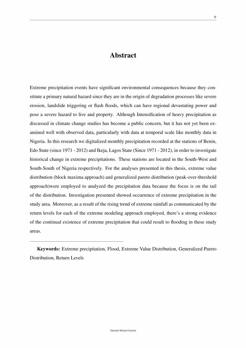
Abstract
Extreme precipitation events have significant environmental consequences because they con-
stitute a primary natural hazard since they are in the origin of degradation processes like severe
erosion, landslide triggering or flash floods, which can have regional devastating power and
pose a severe hazard to live and property. Although Intensification of heavy precipitation as
discussed in climate change studies has become a public concern, but it has not yet been ex-
amined well with observed data, particularly with data at temporal scale like monthly data in
Nigeria. In this research we digitalized monthly precipitation recorded at the stations of Benin,
Edo State (since 1971 - 2012) and Ikeja, Lagos State (Since 1971 - 2012), in order to investigate
historical change in extreme precipitations. These stations are located in the South-West and
South-South of Nigeria respectively. For the analyses presented in this thesis, extreme value
distribution (block maxima approach) and generalized pareto distribution (peak-over-threshold
approach)were employed to analyzed the precipitation data because the focus is on the tail
of the distribution. Investigation presented showed occurrence of extreme precipitation in the
study area. Moreover, as a result of the rising trend of extreme rainfall as communicated by the
return levels for each of the extreme modeling approach employed, there’s a strong evidence
of the continual existence of extreme precipitation that could result to flooding in these study
areas.
Keywords: Extreme precipitation, Flood, Extreme Value Distribution, Generalized Pareto
Distribution, Return Levels
Olumide Michael Oyalola
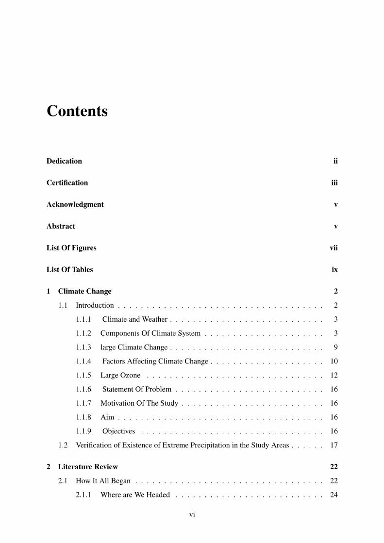
Contents
Dedication ii
Certification iii
Acknowledgment v
Abstract v
List Of Figures vii
List Of Tables ix
1 Climate Change 2
1.1 Introduction . . . . . . . . . . . . . . . . . . . . . . . . . . . . . . . . . . . . 2
1.1.1 Climate and Weather . . . . . . . . . . . . . . . . . . . . . . . . . . . 3
1.1.2 Components Of Climate System . . . . . . . . . . . . . . . . . . . . . 3
1.1.3 large Climate Change . . . . . . . . . . . . . . . . . . . . . . . . . . . 9
1.1.4 Factors Affecting Climate Change . . . . . . . . . . . . . . . . . . . . 10
1.1.5 Large Ozone . . . . . . . . . . . . . . . . . . . . . . . . . . . . . . . 12
1.1.6 Statement Of Problem . . . . . . . . . . . . . . . . . . . . . . . . . . 16
1.1.7 Motivation Of The Study . . . . . . . . . . . . . . . . . . . . . . . . . 16
1.1.8 Aim . . . . . . . . . . . . . . . . . . . . . . . . . . . . . . . . . . . . 16
1.1.9 Objectives . . . . . . . . . . . . . . . . . . . . . . . . . . . . . . . . 16
1.2 Verification of Existence of Extreme Precipitation in the Study Areas . . . . . . 17
2 Literature Review 22
2.1 How It All Began . . . . . . . . . . . . . . . . . . . . . . . . . . . . . . . . . 22
2.1.1 Where are We Headed . . . . . . . . . . . . . . . . . . . . . . . . . . 24
vi
Contents vii
2.1.2 Climate Change Scenario in Nigeria . . . . . . . . . . . . . . . . . . . 25
2.1.3 Climate Change Modelling . . . . . . . . . . . . . . . . . . . . . . . . 31
2.1.4 Extreme Value Theory and Extreme Value Modelling . . . . . . . . . . 35
3 Methodology 38
3.1 Methodology: Brief Introduction . . . . . . . . . . . . . . . . . . . . . . . . . 38
3.1.1 Extreme Value Theory - Historical Perspective . . . . . . . . . . . . . 38
3.2 Classical Extreme Value Theory . . . . . . . . . . . . . . . . . . . . . . . . . 39
3.2.1 Model Formulation . . . . . . . . . . . . . . . . . . . . . . . . . . . 39
3.3 Generalized Extreme Value Distribution (GEV) and Block Maxima . . . . . . . 41
3.3.1 Practical Implementation . . . . . . . . . . . . . . . . . . . . . . . . 42
3.3.2 Inference for the GEV Distribution . . . . . . . . . . . . . . . . . . . 43
3.3.3 Inference for Return Levels . . . . . . . . . . . . . . . . . . . . . . . 44
3.3.4 Graphical Model Checking . . . . . . . . . . . . . . . . . . . . . . . . 44
3.3.5 Threshold Selection : Mean Residual Life Plot . . . . . . . . . . . . . 47
3.3.6 Parameter Estimation . . . . . . . . . . . . . . . . . . . . . . . . . . . 49
3.3.7 Model Checking . . . . . . . . . . . . . . . . . . . . . . . . . . . . . 49
4 Data Analysis and Discussion 51
4.1 Data Description and Preliminary Data Analysis . . . . . . . . . . . . . . . . . 51
4.2 Generalized Extreme Value Fit . . . . . . . . . . . . . . . . . . . . . . . . . . 52
4.3 Generalized Pareto Distribution Fit . . . . . . . . . . . . . . . . . . . . . . . . 55
4.4 Discussion of Results . . . . . . . . . . . . . . . . . . . . . . . . . . . . . . . 58
4.4.1 Data Visualization . . . . . . . . . . . . . . . . . . . . . . . . . . . . 58
5 Summary, Conclusion and Recommendation 62
5.1 Summary and Conclusion . . . . . . . . . . . . . . . . . . . . . . . . . . . . . 62
5.2 Recommendation . . . . . . . . . . . . . . . . . . . . . . . . . . . . . . . . . 63
Olumide Michael Oyalola
List of Figures
1.1 Schematic view of the components of the climate system and of their potential
changes . . . . . . . . . . . . . . . . . . . . . . . . . . . . . . . . . . . . . . 4
1.2 The Atmosphere . . . . . . . . . . . . . . . . . . . . . . . . . . . . . . . . . . 5
1.3 Radiative Forcing . . . . . . . . . . . . . . . . . . . . . . . . . . . . . . . . . 6
1.4 Cloud Processes . . . . . . . . . . . . . . . . . . . . . . . . . . . . . . . . . . 6
1.5 Snow and Ice Cover . . . . . . . . . . . . . . . . . . . . . . . . . . . . . . . . 7
1.6 Biosphere . . . . . . . . . . . . . . . . . . . . . . . . . . . . . . . . . . . . . 8
1.7 Oceans . . . . . . . . . . . . . . . . . . . . . . . . . . . . . . . . . . . . . . . 9
1.8 Formation and Depletion of Ozone Layer . . . . . . . . . . . . . . . . . . . . 14
1.9 Evidence of Climate Change . . . . . . . . . . . . . . . . . . . . . . . . . . . 15
1.10 Global climate change leads to melting ice caps . . . . . . . . . . . . . . . . . 15
1.11 Normality Test Using Q-Q Plot . . . . . . . . . . . . . . . . . . . . . . . . . . 18
1.12 Kernel Density Plot of Rainfall Data . . . . . . . . . . . . . . . . . . . . . . . 19
1.13 HistogramPlot . . . . . . . . . . . . . . . . . . . . . . . . . . . . . . . . . . . 19
1.14 BoxPlot . . . . . . . . . . . . . . . . . . . . . . . . . . . . . . . . . . . . . . 20
1.15 TimePlot & TrendPlot . . . . . . . . . . . . . . . . . . . . . . . . . . . . . . . 20
2.1 Gas Flaring Activity in Nigeria . . . . . . . . . . . . . . . . . . . . . . . . . . 26
2.2 Climate Change and Conflict in Nigeria: A Basic Casual Mechanism . . . . . . 30
3.1 Extreme Value Families of Distribution . . . . . . . . . . . . . . . . . . . . . 41
3.2 GP Distribution . . . . . . . . . . . . . . . . . . . . . . . . . . . . . . . . . . 48
4.1 Yearly Rainfall . . . . . . . . . . . . . . . . . . . . . . . . . . . . . . . . . . 51
4.2 Extreme (Maxima) Plot . . . . . . . . . . . . . . . . . . . . . . . . . . . . . . 52
4.3 GEV Fit Diagnostic Plot for Edo State Rainfall . . . . . . . . . . . . . . . . . 54
viii

List of Figures ix
4.4 GEV Fit Diagnostic Plot for Lagos State Rainfall . . . . . . . . . . . . . . . . 54
4.5 Mean Life Plot for Edo & Lagos Rainfall . . . . . . . . . . . . . . . . . . . . 55
4.6 GPD Fit Diagnostic Plot for Edo State Rainfall . . . . . . . . . . . . . . . . . 58
4.7 GPD Fit Diagnostic Plot for Lagos State Rainfall . . . . . . . . . . . . . . . . 58
Olumide Michael Oyalola
List of Tables
1.1 Descriptive Statistics of the Rainfall Experience in Lagos & Edo State from
1971 - 2012 . . . . . . . . . . . . . . . . . . . . . . . . . . . . . . . . . . . . 18
2.1 Summary of Emissions from the Nigerian Energy Sector 2003 Emissions . . . 26
2.2 Per Capital Sectorial and Gross Emissions in Nigeria for 2003 . . . . . . . . . 27
4.1 Summary of Extreme Value Distribution Result for Lagos & Edo States . . . . 59
4.2 Summary of Extreme Value Distribution Result for Lagos & Edo States . . . . 60
1
Chapter 1
Climate Change
1.1 Introduction
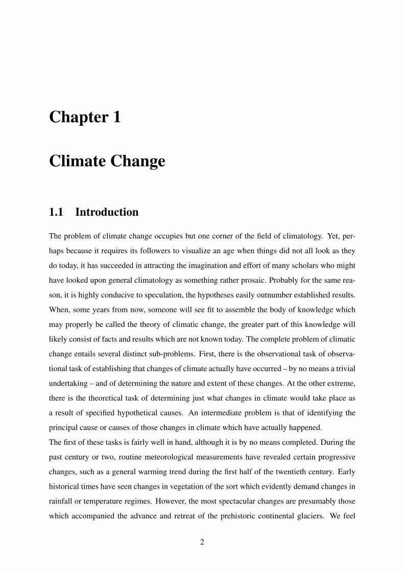
The problem of climate change occupies but one corner of the field of climatology. Yet, per-
haps because it requires its followers to visualize an age when things did not all look as they
do today, it has succeeded in attracting the imagination and effort of many scholars who might
have looked upon general climatology as something rather prosaic. Probably for the same rea-
son, it is highly conducive to speculation, the hypotheses easily outnumber established results.
When, some years from now, someone will see fit to assemble the body of knowledge which
may properly be called the theory of climatic change, the greater part of this knowledge will
likely consist of facts and results which are not known today. The complete problem of climatic
change entails several distinct sub-problems. First, there is the observational task of observa-
tional task of establishing that changes of climate actually have occurred – by no means a trivial
undertaking – and of determining the nature and extent of these changes. At the other extreme,
there is the theoretical task of determining just what changes in climate would take place as
a result of specified hypothetical causes. An intermediate problem is that of identifying the
principal cause or causes of those changes in climate which have actually happened.
The first of these tasks is fairly well in hand, although it is by no means completed. During the
past century or two, routine meteorological measurements have revealed certain progressive
changes, such as a general warming trend during the first half of the twentieth century. Early
historical times have seen changes in vegetation of the sort which evidently demand changes in
rainfall or temperature regimes. However, the most spectacular changes are presumably those
which accompanied the advance and retreat of the prehistoric continental glaciers. We feel
2
1.1. Introduction 3
confident that only a climate different from today’s could have produced and maintained the
great ice sheets, while, conversely, the presence of the ice must have produced and maintained a
climate different from today’s. When however, we ask how greatly the ancient temperature and
precipitation patterns differed from the current ones, we find no general agreement (Edward N
Lorenz, 1970).
1.1.1 Climate and Weather
Climate refers to the distribution of the state of the atmosphere, oceans, and biosphere at time
scales of decades, centuries, millennia. It can be viewed as a forced/diffusive system, with com-
plex and long-range interactions between the oceans, the land mass, and the atmosphere. Ex-
amples of climatic events are the Ice Ages, droughts and the current global warming. Weather,
on the other hand, refers to the state of the above coupled systems at much shorter spatio-
temporal scales. Its behavior can be very sensitive to initial conditions and so is often difficult
to predict. Examples of weather events are more familiar to us: storm systems, hurricanes or
tornados. The distribution of weather events over a long period of time and at a given location
is the climate.
1.1.2 Components Of Climate System
The term climate system refers to the many elements that contribute to creating a climate in a
particular place or region. Components include the atmosphere and oceans, the land, ice, and
biosphere (plant and animal life), as well as cities and other parts of the ”built environment.”
Although the components of the climate system are very different in their composition,
physical and chemical properties, and structure and behaviour, they are all linked by fluxes of
mass, heat and momentum. They continuously interact among themselves. The components of
climate system are explicitly described in the subsequent paragraphs.
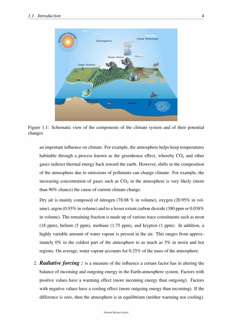
1. The Atmosphere: The atmosphere is the envelope of gas that surrounds Earth’s sur-
face. It is separated into five distinct layers based on a number of factors including
density, movement, chemistry and temperature: They are: (1) the Troposphere; (2) the
Stratosphere; (3) the Mesosphere: (4) the Thermosphere; and, (5) the Exosphere. The
lower atmosphere (the Troposphere) is where we live and breathe. It is responsible for
the wind and weather we experience day to day. The composition of the atmosphere has
Olumide Michael Oyalola
1.1. Introduction 4
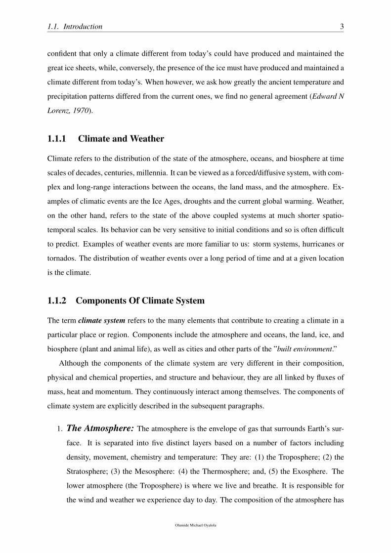
Figure 1.1: Schematic view of the components of the climate system and of their potentialchanges
an important influence on climate. For example, the atmosphere helps keep temperatures
habitable through a process known as the greenhouse effect, whereby CO2 and other
gases redirect thermal energy back toward the earth. However, shifts in the composition
of the atmosphere due to emissions of pollutants can change climate. For example, the
increasing concentration of gases such as CO2 in the atmosphere is very likely (more
than 90% chance) the cause of current climate change.
Dry air is mainly composed of nitrogen (78.08 % in volume), oxygen (20.95% in vol-
ume), argon (0.93% in volume) and to a lesser extent carbon dioxide (380 ppm or 0.038%
in volume). The remaining fraction is made up of various trace constituents such as neon
(18 ppm), helium (5 ppm), methane (1.75 ppm), and krypton (1 ppm). In addition, a
highly variable amount of water vapour is present in the air. This ranges from approx-
imately 0% in the coldest part of the atmosphere to as much as 5% in moist and hot
regions. On average, water vapour accounts for 0.25% of the mass of the atmosphere.
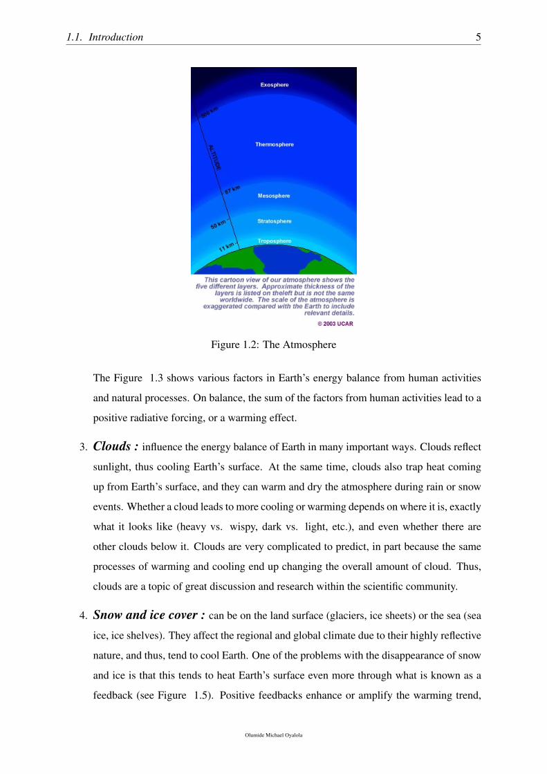
2. Radiative forcing : is a measure of the influence a certain factor has in altering the
balance of incoming and outgoing energy in the Earth-atmosphere system. Factors with
positive values have a warming effect (more incoming energy than outgoing). Factors
with negative values have a cooling effect (more outgoing energy than incoming). If the
difference is zero, then the atmosphere is in equilibrium (neither warming nor cooling).
Olumide Michael Oyalola
1.1. Introduction 5
Figure 1.2: The Atmosphere
The Figure 1.3 shows various factors in Earth’s energy balance from human activities
and natural processes. On balance, the sum of the factors from human activities lead to a
positive radiative forcing, or a warming effect.
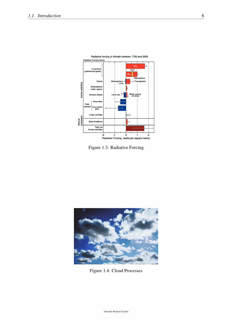
3. Clouds : influence the energy balance of Earth in many important ways. Clouds reflect
sunlight, thus cooling Earth’s surface. At the same time, clouds also trap heat coming
up from Earth’s surface, and they can warm and dry the atmosphere during rain or snow
events. Whether a cloud leads to more cooling or warming depends on where it is, exactly
what it looks like (heavy vs. wispy, dark vs. light, etc.), and even whether there are
other clouds below it. Clouds are very complicated to predict, in part because the same
processes of warming and cooling end up changing the overall amount of cloud. Thus,
clouds are a topic of great discussion and research within the scientific community.
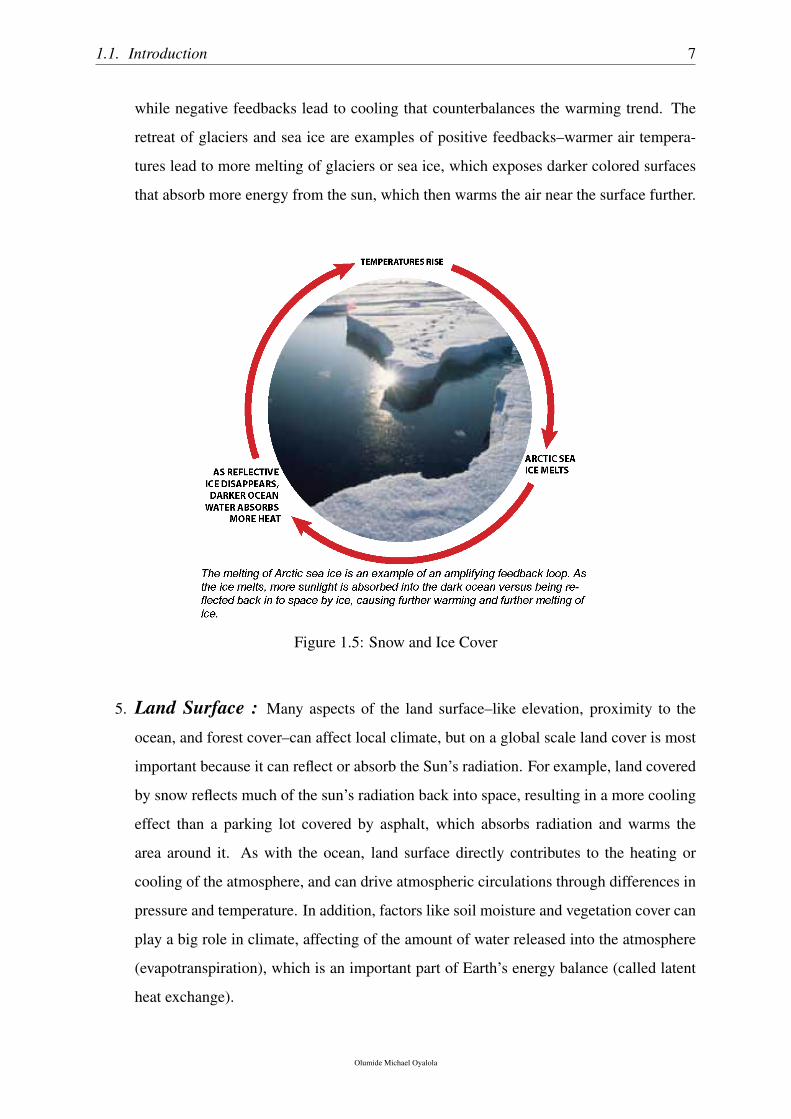
4. Snow and ice cover : can be on the land surface (glaciers, ice sheets) or the sea (sea
ice, ice shelves). They affect the regional and global climate due to their highly reflective
nature, and thus, tend to cool Earth. One of the problems with the disappearance of snow
and ice is that this tends to heat Earth’s surface even more through what is known as a
feedback (see Figure 1.5). Positive feedbacks enhance or amplify the warming trend,
Olumide Michael Oyalola
1.1. Introduction 6
Figure 1.3: Radiative Forcing
Figure 1.4: Cloud Processes
Olumide Michael Oyalola
1.1. Introduction 7
while negative feedbacks lead to cooling that counterbalances the warming trend. The
retreat of glaciers and sea ice are examples of positive feedbacks–warmer air tempera-
tures lead to more melting of glaciers or sea ice, which exposes darker colored surfaces
that absorb more energy from the sun, which then warms the air near the surface further.
Figure 1.5: Snow and Ice Cover
5. Land Surface : Many aspects of the land surface–like elevation, proximity to the
ocean, and forest cover–can affect local climate, but on a global scale land cover is most
important because it can reflect or absorb the Sun’s radiation. For example, land covered
by snow reflects much of the sun’s radiation back into space, resulting in a more cooling
effect than a parking lot covered by asphalt, which absorbs radiation and warms the
area around it. As with the ocean, land surface directly contributes to the heating or
cooling of the atmosphere, and can drive atmospheric circulations through differences in
pressure and temperature. In addition, factors like soil moisture and vegetation cover can
play a big role in climate, affecting of the amount of water released into the atmosphere
(evapotranspiration), which is an important part of Earth’s energy balance (called latent
heat exchange).
Olumide Michael Oyalola
1.1. Introduction 8
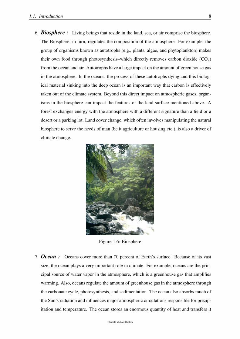
6. Biosphere : Living beings that reside in the land, sea, or air comprise the biosphere.
The Biosphere, in turn, regulates the composition of the atmosphere. For example, the
group of organisms known as autotrophs (e.g., plants, algae, and phytoplankton) makes
their own food through photosynthesis–which directly removes carbon dioxide (CO2)
from the ocean and air. Autotrophs have a large impact on the amount of green house gas
in the atmosphere. In the oceans, the process of these autotrophs dying and this biolog-
ical material sinking into the deep ocean is an important way that carbon is effectively
taken out of the climate system. Beyond this direct impact on atmospheric gases, organ-
isms in the biosphere can impact the features of the land surface mentioned above. A
forest exchanges energy with the atmosphere with a different signature than a field or a
desert or a parking lot. Land cover change, which often involves manipulating the natural
biosphere to serve the needs of man (be it agriculture or housing etc.), is also a driver of
climate change.
Figure 1.6: Biosphere
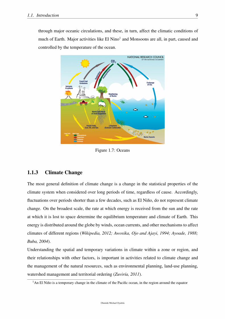
7. Ocean : Oceans cover more than 70 percent of Earth’s surface. Because of its vast
size, the ocean plays a very important role in climate. For example, oceans are the prin-
cipal source of water vapor in the atmosphere, which is a greenhouse gas that amplifies
warming. Also, oceans regulate the amount of greenhouse gas in the atmosphere through
the carbonate cycle, photosynthesis, and sedimentation. The ocean also absorbs much of
the Sun’s radiation and influences major atmospheric circulations responsible for precip-
itation and temperature. The ocean stores an enormous quantity of heat and transfers it
Olumide Michael Oyalola
1.1. Introduction 9
through major oceanic circulations, and these, in turn, affect the climatic conditions of
much of Earth. Major activities like El Nino1 and Monsoons are all, in part, caused and
controlled by the temperature of the ocean.
Figure 1.7: Oceans
1.1.3 Climate Change
The most general definition of climate change is a change in the statistical properties of the
climate system when considered over long periods of time, regardless of cause. Accordingly,
fluctuations over periods shorter than a few decades, such as El Nino, do not represent climate
change. On the broadest scale, the rate at which energy is received from the sun and the rate
at which it is lost to space determine the equilibrium temperature and climate of Earth. This
energy is distributed around the globe by winds, ocean currents, and other mechanisms to affect
climates of different regions (Wikipedia, 2012; Awosika, Ojo and Ajayi, 1994; Ayoade, 1988;
Buba, 2004).
Understanding the spatial and temporary variations in climate within a zone or region, and
their relationships with other factors, is important in activities related to climate change and
the management of the natural resources, such as environmental planning, land-use planning,
watershed management and territorial ordering (Zuvirıa, 2011).
1An El Nino is a temporary change in the climate of the Pacific ocean, in the region around the equator
Olumide Michael Oyalola
1.1. Introduction 10
1.1.4 Factors Affecting Climate Change
The earth intercepts the radiation from the sun, and it is this energy that derives our weather
and climate. Of this energy, one third of it is reflected back into space and the rest is absorbed
by different parts of the climate system, such as the atmosphere, oceans, ice, land, and various
forms of life. The earth then sends its energy out into space, or re-radiates, in the form of
long waves of radiation. Some of the energy is again absorbed and remitted through a process
known as the Greenhouse effect, and the rest is lost to space.
The earth must maintain balance between the outgoing radiation and the incoming solar
energy always. If there is any change in the factors that affect this process of incoming and
outgoing energy, or change the energy distribution itself the earth’s climate will change and
effect many aspects of the environment. According to Tamuno (2009), there are two major
causes of climate change that threaten this fragile balance, namely: anthropogenic and natu-
ral. Anthropogenic causes relate to those activities of man which help to change the chemical
composition of the atmosphere as they relate to increasing the volume of greenhouse gases like
Carbon dioxide (CO2), Methane (CH4), Sulphur Dioxide (SO2), etc. The combined effects of
the anthropogenic and natural causes actually bring about climate change in the ratio of about
60 : 40 respectively.
Natural Factors Affecting Climate
1. Changes in Solar Output: the amount of energy radiating from the earth’s sun is not
constant.
2. Changes in the Earth’s Orbit: Slow variations in the Earth’s orbit around the sun change
where and when energy is received on earth. This affects the amount of energy that is
reflected and absorbed.
3. The Greenhouse Effect: When energy from the sun enters the Earth’s atmosphere, about
a third of it is reflected back to space. Of the rest, the atmosphere absorbs some, but most
of it is absorbed by the surfaces of the earth. The Earth emits energy at longer wave-
length. Some of this energy escapes to space but some is absorbed again and remitted
by clouds and the greenhouse gases such as water vapor, carbon dioxides, methane and
Olumide Michael Oyalola
1.1. Introduction 11
nitrous oxide. This helps to warm the surface and the troposphere (lowest layer of the
atmosphere), keeping it 330C warmer than it would be otherwise be.
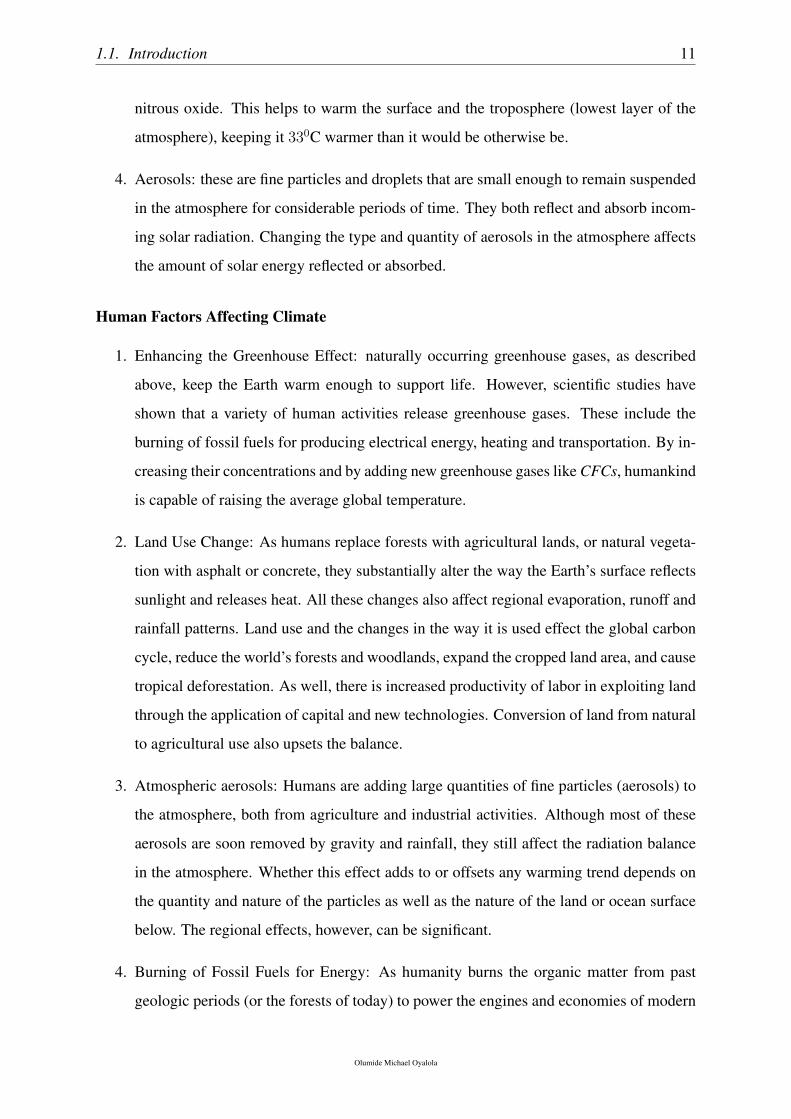
4. Aerosols: these are fine particles and droplets that are small enough to remain suspended
in the atmosphere for considerable periods of time. They both reflect and absorb incom-
ing solar radiation. Changing the type and quantity of aerosols in the atmosphere affects
the amount of solar energy reflected or absorbed.
Human Factors Affecting Climate
1. Enhancing the Greenhouse Effect: naturally occurring greenhouse gases, as described
above, keep the Earth warm enough to support life. However, scientific studies have
shown that a variety of human activities release greenhouse gases. These include the
burning of fossil fuels for producing electrical energy, heating and transportation. By in-
creasing their concentrations and by adding new greenhouse gases like CFCs, humankind
is capable of raising the average global temperature.
2. Land Use Change: As humans replace forests with agricultural lands, or natural vegeta-
tion with asphalt or concrete, they substantially alter the way the Earth’s surface reflects
sunlight and releases heat. All these changes also affect regional evaporation, runoff and
rainfall patterns. Land use and the changes in the way it is used effect the global carbon
cycle, reduce the world’s forests and woodlands, expand the cropped land area, and cause
tropical deforestation. As well, there is increased productivity of labor in exploiting land
through the application of capital and new technologies. Conversion of land from natural
to agricultural use also upsets the balance.
3. Atmospheric aerosols: Humans are adding large quantities of fine particles (aerosols) to
the atmosphere, both from agriculture and industrial activities. Although most of these
aerosols are soon removed by gravity and rainfall, they still affect the radiation balance
in the atmosphere. Whether this effect adds to or offsets any warming trend depends on
the quantity and nature of the particles as well as the nature of the land or ocean surface
below. The regional effects, however, can be significant.
4. Burning of Fossil Fuels for Energy: As humanity burns the organic matter from past
geologic periods (or the forests of today) to power the engines and economies of modern
Olumide Michael Oyalola
1.1. Introduction 12
society, we are re-injecting our fossil carbon legacy into the atmosphere at incredibly
accelerated rate. Carbon dioxide is dumped into the atmosphere at a much faster rate
than it can be withdrawn or absorbed by the oceans or living things in the biosphere. The
carbon dioxide buildup is a principal controlling factor of the climate change.
1.1.5 Ozone
Without ozone, life on Earth would not have evolved in the way it has. The first stage of single
cell organism development requires an oxygen-free environment. This type of environment
existed on earth over 3000 million years ago. As the primitive forms of plant life multiplied and
evolved, they began to release minute amounts of oxygen through the photosynthesis reaction
(which converts carbon dioxide into oxygen) [3]. The buildup of oxygen in the atmosphere
led to the formation of the ozone layer in the upper atmosphere or stratosphere. This layer
filters out incoming radiation in the cell-damaging ultraviolet (UV) part of the spectrum. Thus
with the development of the ozone layer came the formation of more advanced life forms.
Ozone is a form of oxygen. The oxygen we breathe is in the form of oxygen molecules (O2)
- two atoms of oxygen bound together. Normal oxygen which we breathe is colourless and
odourless. Ozone, on the other hand, consists of three atoms of oxygen bound together (O3).
Most of the atmosphere’s ozone occurs in the region called the stratosphere. Ozone is colourless
and has a very harsh odour. Ozone is much less common than normal oxygen. Out of 10
million air molecules, about 2 million are normal oxygen, but only 3 are ozone. Most ozone
is produced naturally in the upper atmosphere or stratosphere. While ozone can be found
through the entire atmosphere, the greatest concentration occurs at altitudes between 19 and
30 km above the Earth’s surface. This band of ozone-rich air is known as the ”ozone layer”
[4]. Ozone also occurs in very small amounts in the lowest few kilometres of the atmosphere,
a region known as the troposphere. It is produced at ground level through a reaction between
sunlight and volatile organic compounds (VOCs) and nitrogen oxides (NOx), some of which are
produced by human activities such as driving cars. Ground-level ozone is a component of urban
smog and can be harmful to human health. Even though both types of ozone contain the same
molecules, their presence in different parts of the atmosphere has very different consequences.
Stratospheric ozone blocks harmful solar radiation - all life on Earth has adapted to this filtered
solar radiation. Ground-level ozone, in contrast, is simply a pollutant. It will absorb some
incoming solar radiation, but it cannot make up for ozone losses in the stratosphere.
Olumide Michael Oyalola
1.1. Introduction 13
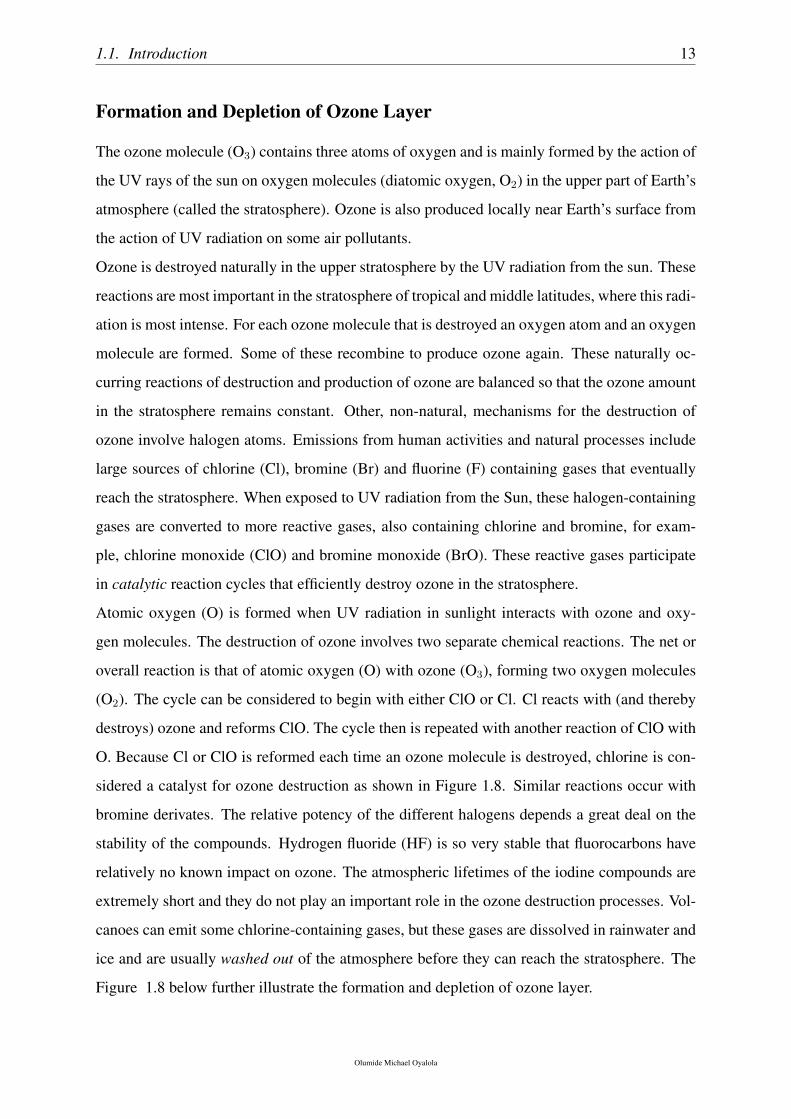
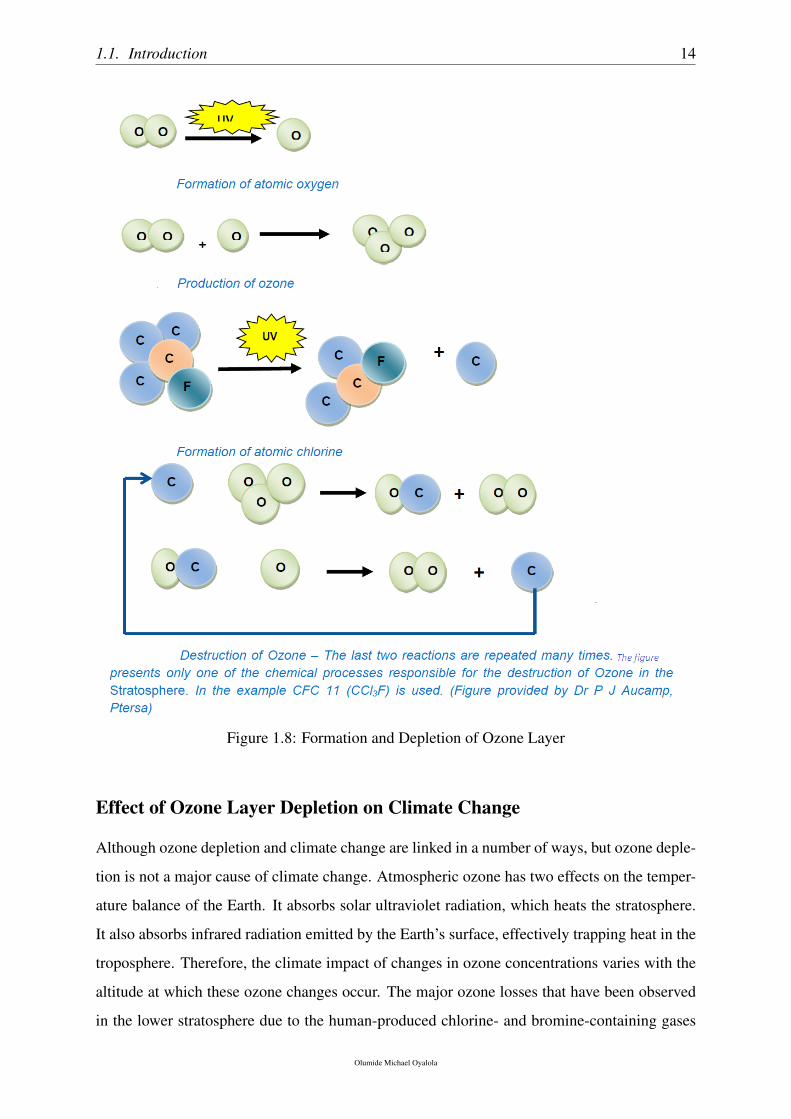
Formation and Depletion of Ozone Layer
The ozone molecule (O3) contains three atoms of oxygen and is mainly formed by the action of
the UV rays of the sun on oxygen molecules (diatomic oxygen, O2) in the upper part of Earth’s
atmosphere (called the stratosphere). Ozone is also produced locally near Earth’s surface from
the action of UV radiation on some air pollutants.
Ozone is destroyed naturally in the upper stratosphere by the UV radiation from the sun. These
reactions are most important in the stratosphere of tropical and middle latitudes, where this radi-
ation is most intense. For each ozone molecule that is destroyed an oxygen atom and an oxygen
molecule are formed. Some of these recombine to produce ozone again. These naturally oc-
curring reactions of destruction and production of ozone are balanced so that the ozone amount
in the stratosphere remains constant. Other, non-natural, mechanisms for the destruction of
ozone involve halogen atoms. Emissions from human activities and natural processes include
large sources of chlorine (Cl), bromine (Br) and fluorine (F) containing gases that eventually
reach the stratosphere. When exposed to UV radiation from the Sun, these halogen-containing
gases are converted to more reactive gases, also containing chlorine and bromine, for exam-
ple, chlorine monoxide (ClO) and bromine monoxide (BrO). These reactive gases participate
in catalytic reaction cycles that efficiently destroy ozone in the stratosphere.
Atomic oxygen (O) is formed when UV radiation in sunlight interacts with ozone and oxy-
gen molecules. The destruction of ozone involves two separate chemical reactions. The net or
overall reaction is that of atomic oxygen (O) with ozone (O3), forming two oxygen molecules
(O2). The cycle can be considered to begin with either ClO or Cl. Cl reacts with (and thereby
destroys) ozone and reforms ClO. The cycle then is repeated with another reaction of ClO with
O. Because Cl or ClO is reformed each time an ozone molecule is destroyed, chlorine is con-
sidered a catalyst for ozone destruction as shown in Figure 1.8. Similar reactions occur with
bromine derivates. The relative potency of the different halogens depends a great deal on the
stability of the compounds. Hydrogen fluoride (HF) is so very stable that fluorocarbons have
relatively no known impact on ozone. The atmospheric lifetimes of the iodine compounds are
extremely short and they do not play an important role in the ozone destruction processes. Vol-
canoes can emit some chlorine-containing gases, but these gases are dissolved in rainwater and
ice and are usually washed out of the atmosphere before they can reach the stratosphere. The
Figure 1.8 below further illustrate the formation and depletion of ozone layer.
Olumide Michael Oyalola
1.1. Introduction 14
Figure 1.8: Formation and Depletion of Ozone Layer
Effect of Ozone Layer Depletion on Climate Change
Although ozone depletion and climate change are linked in a number of ways, but ozone deple-
tion is not a major cause of climate change. Atmospheric ozone has two effects on the temper-
ature balance of the Earth. It absorbs solar ultraviolet radiation, which heats the stratosphere.
It also absorbs infrared radiation emitted by the Earth’s surface, effectively trapping heat in the
troposphere. Therefore, the climate impact of changes in ozone concentrations varies with the
altitude at which these ozone changes occur. The major ozone losses that have been observed
in the lower stratosphere due to the human-produced chlorine- and bromine-containing gases
Olumide Michael Oyalola
1.1. Introduction 15
have a cooling effect on the Earth’s surface. On the other hand, the ozone increases that are es-
timated to have occurred in the troposphere because of surface-pollution gases have a warming
effect on the Earth’s surface, thereby contributing to the greenhouse effect. In comparison to
the effects of changes in other atmospheric gases, the effects of both of these ozone changes are
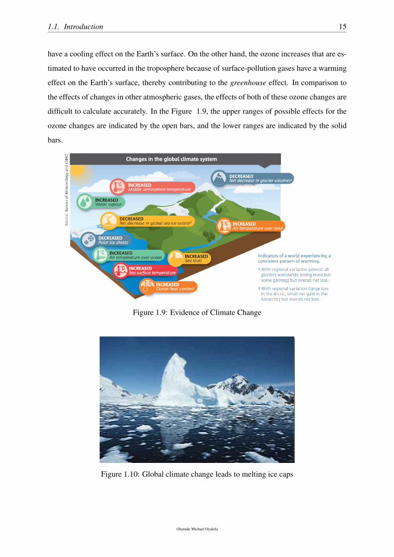
difficult to calculate accurately. In the Figure 1.9, the upper ranges of possible effects for the
ozone changes are indicated by the open bars, and the lower ranges are indicated by the solid
bars.
Figure 1.9: Evidence of Climate Change
Figure 1.10: Global climate change leads to melting ice caps
Olumide Michael Oyalola

1.1. Introduction 16
1.1.6 Statement Of Problem
Rainfall is the principal phenomenon driving many hydrological extremes such as floods, droughts,
landslides, debris and mud-flows; its analysis and modeling are typical problems in applied
hydro-meteorology. Moreover, rainfall exhibits a strong variability in time and space across
the globe. Hence, its stochastic modeling is necessary for the prevention of natural disaster
(Raheem M.A. et. al, (2015)).
1.1.7 Motivation Of The Study
Weather and climate touch all aspects of Human life. What we experience here in Nigeria is
part of the global climate system.
Climate unpredictability and change in climatic parameters have direct influence on environ-
ment and human existence. A negative change in the climate, always have its corresponding
dysfunctional impacts on man and the ecosystem globally or locally. Flooding, poor agricul-
tural yields, famine, and even death are some of the catastrophic effects of drastic climate
change. Knowledge and information on the climatic variation parameters in an environment is
very vital for environmental study assessment and proper planning. As a result, the importance
of knowing the future climatic variation parameters cannot be under-estimated.
1.1.8 Aim
According to the recent works by scientist and climatologists, it has now been widely accepted
that the earth is warming and will continue to warm as the concentration of greenhouse gases
rise in the future. These greenhouse gases such as carbon dioxide (CO2) have been shown to
lead to changes in climate conditions such as temperature, precipitation, soil moisture, and sea
level. This work is aimed at modeling climate change problem which includes extreme precip-
itation that often results in flooding experiences in two states in Nigeria.
In particular, The study will help decision makers to make informed decisions and to avoid
or at least reduce flood caused damage to life and property.
1.1.9 Objectives
1. To assess the distributional pattern of rainfall in the study areas.
Olumide Michael Oyalola
1.2. Verification of Existence of Extreme Precipitation in the Study Areas 17
2. Model extreme rainfall events using forty-one years of monthly data (1971−2012) based
on extreme value theory for two cities in Nigeria.
3. Predict possible return levels and periods based on the extreme value model.
1.2 Verification of Existence of Extreme Precipitation in the
Study Areas
Data visualization or EDA can be described as the simple procedures that may be applied or
carried out on some data-sets so as to uncover any hidden fact thereby allowing the data to
speak for themselves. However, this serves only as a prelude before carrying out a more so-
phisticated analysis. Because almost all environmental data seem to have errors associated with
them and therefore need a lot of careful checks. Moreover, we can also see clearly if anything
is wrong with the data from the beginning.
Furthermore, data visualization process can be used to suggest assumptions that may plausibly
be held in the initial stages of the subsequent analysis, to guide the choice of analysis strategy.
As a results of all the aforementioned facts, it is expedient to using data visualization techniques
to accessing the data suitability for the intending methodology.
Different forms of data visualizations ranging from Histogram, Boxplot, TimePlot, etc were
employed to uncover the hidden nature of the dataset.
Secondary monthly rainfall data set collected at NIMET2 stations in Lagos & Edo states of
the Federation between 1971 - 2012 will be used for the purpose of this study.
Preliminary Analysis
The table below shows the descriptive view of the data used for the study
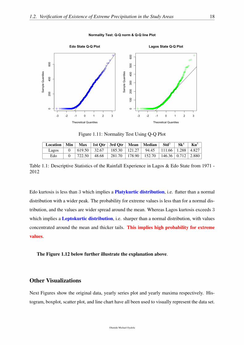
It would be observed from the table above that Edo & Lagos rainfall data skewness is
greater than 0 which implies that the distribution is Right skewed distribution i.e. most val-
ues are concentrated on left of the mean, with extreme values to the right. On the other hand,
2Nigerian Meteorological Agency
Olumide Michael Oyalola
1.2. Verification of Existence of Extreme Precipitation in the Study Areas 18
-3 -2 -1 0 1 2 3
020
040
060
0Edo State Q-Q Plot
Theoretical Quantiles
Sam
ple
Qua
ntile
s
-3 -2 -1 0 1 2 3
010
020
030
040
050
060
0
Lagos State Q-Q Plot
Theoretical QuantilesS
ampl
e Q
uant
iles
Normality Test: Q-Q norm & Q-Q line Plot
Figure 1.11: Normality Test Using Q-Q Plot
Location Min Max 1st Qtr 3rd Qtr Mean Median Std3 Sk4 Ku5
Lagos 0 619.50 32.67 185.30 121.27 94.45 111.66 1.288 4.827Edo 0 722.50 48.68 281.70 178.90 152.70 146.36 0.712 2.880
Table 1.1: Descriptive Statistics of the Rainfall Experience in Lagos & Edo State from 1971 -2012
Edo kurtosis is less than 3 which implies a Platykurtic distribution, i.e. flatter than a normal
distribution with a wider peak. The probability for extreme values is less than for a normal dis-
tribution, and the values are wider spread around the mean. Whereas Lagos kurtosis exceeds 3
which implies a Leptokurtic distribution, i.e. sharper than a normal distribution, with values
concentrated around the mean and thicker tails. This implies high probability for extreme
values.
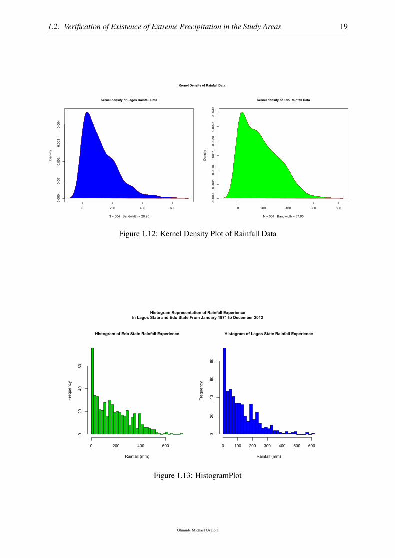
The Figure 1.12 below further illustrate the explanation above.
Other Visualizations
Next Figures show the original data, yearly series plot and yearly maxima respectively. His-
togram, boxplot, scatter plot, and line chart have all been used to visually represent the data set.
Olumide Michael Oyalola
1.2. Verification of Existence of Extreme Precipitation in the Study Areas 19
0 200 400 600
0.00
00.
001
0.00
20.
003
0.00
4
Kernel density of Lagos Rainfall Data
N = 504 Bandwidth = 28.95
Den
sity
0 200 400 600 8000.
0000
0.00
050.
0010
0.00
150.
0020
0.00
250.
0030
Kernel density of Edo Rainfall Data
N = 504 Bandwidth = 37.95
Den
sity
Kernel Density of Rainfall Data
Figure 1.12: Kernel Density Plot of Rainfall Data
Histogram of Edo State Rainfall Experience
Rainfall (mm)
Fre
quen
cy
0 200 400 600
020
4060
Histogram of Lagos State Rainfall Experience
Rainfall (mm)
Fre
quen
cy
0 100 200 300 400 500 600
020
4060
80
Histogram Representation of Rainfall Experience In Lagos State and Edo State From January 1971 to December 2012
Figure 1.13: HistogramPlot
Olumide Michael Oyalola
1.2. Verification of Existence of Extreme Precipitation in the Study Areas 20
1971 1975 1979 1983 1987 1991 1995 1999 2003 2007 2011
010
020
030
040
050
060
0
Boxplot of rainfall experience in Lagos State delimited by years
Year
Rai
nfal
l (m
m)
Boxplot of Rainfall Experience in Lagos and Edo State Delimited by Year
1971 1975 1979 1983 1987 1991 1995 1999 2003 2007 20110
200
400
600
Boxplot of rainfall experience in Edo State delimited by years
Year
Rai
nfal
l (m
m)
Figure 1.14: BoxPlot
Edo State
Year
Rai
nfal
l (m
m)
1970 1980 1990 2000 2010
020
040
060
0 Original Series
Trend
Lagos State
Year
Rai
nfal
l (m
m)
1970 1980 1990 2000 2010
020
040
060
0
Original Series
Trend
Plot of Average Rainfall (mm) Experience In Lagos State and Edo State Delimited by Year From 1971 to 2012
Figure 1.15: TimePlot & TrendPlot
Olumide Michael Oyalola
1.2. Verification of Existence of Extreme Precipitation in the Study Areas 21
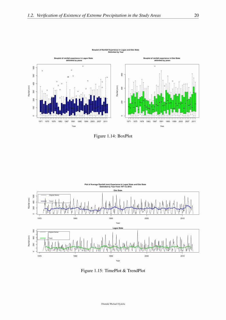
The boxplot i.e Figure 1.14 was used to determine the nature of the dataset for the presence
of extreme values which could be termed as outliers. Moreover, Figure 1.13 was used to access
the distributional form of the precipitation recorded at the stations.
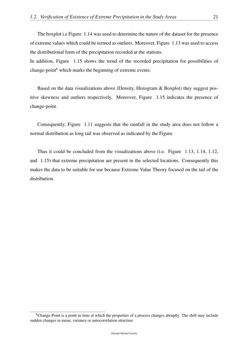
In addition, Figure 1.15 shows the trend of the recorded precipitation for possibilities of
change-point6 which marks the beginning of extreme events.
Based on the data visualizations above (Density, Histogram & Boxplot) they suggest pos-
itive skewness and outliers respectively. Moreover, Figure 1.15 indicates the presence of
change-point.
Consequently, Figure 1.11 suggests that the rainfall in the study area does not follow a
normal distribution as long tail was observed as indicated by the Figure.
Thus it could be concluded from the visualizations above (i.e. Figure 1.13, 1.14, 1.12,
and 1.15) that extreme precipitation are present in the selected locations. Consequently this
makes the data to be suitable for use because Extreme Value Theory focused on the tail of the
distribution.
6Change-Point is a point in time at which the properties of a process changes abruptly. The shift may includesudden changes in mean, variance or autocorrelation structure.
Olumide Michael Oyalola
Chapter 2
Literature Review
2.1 How It All Began
About 80 years ago, a seemingly harmless chemical was invented called Chlorofluorocarbons
(CFC’s); which are used in Air conditioners, Refrigerators, and aerosol cans. However, 50
years after this invention, scientists discovered that the huge amounts of CFC molecules were
being released into the air during the course of usage and that CFC’s were floating past the
Troposphere to the Stratosphere where the ultra violet rays had been breaking them down into
the constituent Chlorine & Fluorine. They also discovered that these liberated chemicals float
around in the stratosphere and break-up the Ozone molecules in the massive Ozone Layer that
nature has positioned to protect Planet Earth from harmful UV rays from the sun. After the
breaking-up of ozone molecules, space is created within the ozone layer where UV rays from
the sun penetrate to planet Earth. - This space is generally referred to as The Ozone Hole.
The initial facts on Global Warming points to the fact that excessive heat from the sun due to
this Ozone hole is a major contributor to the high temperature regimes on planet earth. Upon
full realization of the relationship between CFC’s and other greenhouse gasses in the Ozone
depletion cycle and the Global Warming phenomenon, there was a global consensus to ban
the continued use of CFC’s. Also numerous concerns were raised by authorities around the
world which resulted in meetings, evaluations by technical groups and mini conferences on the
matter. Danger seems more imminent because according to Earth Observatory - NASA, The
last time global temperatures were one degree or warmer than today, sea levels were 6 meters
(20 feet) higher, with the water mainly from the melting of the Greenland and West Antarctic
ice sheets (we know that many coastal cities around the world already lie below sea level and
22
2.1. How It All Began 23
would be submerged if the oceans of the world rise to levels far beyond the extra 10 degree
mark to about 2.5-100 F). Evidence obtained from meteorological records points to the fact
that there have been slight upward variations in ‘in – coming solar radiation, since early 20th
century. However, recent changes in regional and global temperatures of this era have already
exceeded expected limits of Natural Solar Variability. Apart from meteorological records, sev-
eral other confirmations were made from indirect indications such as Sea Ice and Ice – Core
data ground temperature profiles from deep Boreholes were also analysed for further confirma-
tions by Duchkov and Devyatkin, (1992); Gosnold et al. (1997) and Lachenbruch and Marshall
(1986). Results from all these studies have made scientists and Climatologists to attribute the
current global warming to anthropogenic factors rather than stochastic factors.
Ozone depletion and climate change have usually been thought of as environmental issues with
little in common other than their global scope and the major role played in each by CFCs and
other halocarbons. With increased understanding of these issues, however, has come a growing
recognition that a number of very important linkages exist between them. These linkages will
have some bearing on how each of these problems and the atmosphere as a whole evolve in
the future. Some of the most important of these linkages involve the way that ozone-depleting
substances and greenhouse gases alter radiation processes in the atmosphere so as to enhance
both global warming and stratospheric ozone depletion. These changes result in a warming of
the troposphere (the bottom 8–16km of the atmosphere) and a cooling of the stratosphere (the
layer above that extends to an altitude of about 50km and contains the ozone layer). Strato-
spheric cooling creates a more favourable environment for the formation of polar stratospheric
clouds (PSCs), which are a key factor in the development of polar ozone holes. Enhancement
of the greenhouse effect may also be causing changes in circulation patterns in the troposphere
that are, in turn, altering the circulation in the stratosphere. It is suspected that these changes
are increasing the cooling forces acting on the stratosphere over the poles and are thus making
the formation of ozone holes more likely. There is evidence as well that changes in the strato-
spheric circulation may be altering weather patterns in the troposphere. Other linkages between
climate change and ozone depletion are related to the effect of increased levels of ultraviolet
radiation on sun-driven chemical reactions in the atmosphere and to changes in biological pro-
cesses that affect the composition of the atmosphere. The net effect of these linkages is an
intensification of both climate change and ozone depletion and possibly a delay in the recovery
of the ozone layer as it responds to diminishing levels of CFCs and other ozone-depleting sub-
Olumide Michael Oyalola
2.1. How It All Began 24
stances. To understand these connections better, researchers are now looking more closely at
how the troposphere and stratosphere interact. Environment Canada scientists are contributing
to this research in a variety of ways, including the monitoring of ozone concentrations and so-
lar radiation levels and collaboration in balloon-based stratospheric research and atmospheric
modelling. Both greenhouse warming and the thinning of the stratospheric ozone layer are a
result of human activities that have changed the composition of the atmosphere in subtle but
profound ways since the beginning of the industrial revolution more than 200 years ago. By
taking an integrated approach to ozone depletion and climate change, governments and sci-
entists will have a better chance of understanding and moderating the enormous changes that
human activities have had and will continue to have on the atmosphere.
Sivasakthivel.T, et al. (2011), in a study carried out to review the origin, causes, mechanisms
and bio effects of ozone layer depletion as well as the protective measures of this vanishing
layer. They opined that the chlorofluorocarbon and the halons are potent ozone depletors. They
further asserted that one of the main reasons for the widespread concern about depletion of
the ozone layer is the anticipated increase in the amounts of ultraviolet radiation received at
the surface of the earth and the effect of this on human health and on the environment. The
prospects of ozone recovery remain uncertain. In the absence of other changes, stratospheric
ozone abundances should rise in the future as the halogen loading falls in response to regula-
tion. However, the future behaviour of ozone will also be affected by the changing atmospheric
abundances of methane, nitrous oxide, water vapour, sulphate aerosol, and changing climate.
Although, Ozone depletion and climate change are linked in a number of ways, but ozone de-
pletion is not a major cause of climate change.
2.1.1 Where are We Headed
Experts have used comparative analysis of both empirical data and simulated equilibrium for
future predictions and have asserted the impending doom if no urgent action is taken. For
now, air temperature records are being used to monitor changes in Regional details of Climate
Change. The global efforts in this regard involves thee measurement of Mean Monthly Air
Temperatures from data available in about 7,000 weather stations (Global Historical Climatol-
ogy Network Temperature Database. For now the observable effects of climate change can be
itemised as follows:
Olumide Michael Oyalola
2.1. How It All Began 25
• Steady rise in global surface temperatures including extreme temperature regimes in
some cases.
• Increase in Drought situations and its consequent Hunger and Starvation in some regions
of the world.
• Increased Desertification
• High frequency of incidences of coastal erosion
• Gradual Ice melts in the Arctic region.
• Lengthening of growing season in Agriculture due to erratic precipitation.
• Increased incidence of flooding and physical habitat destruction due to irregular and
storm laden rainfall around the world.
• Increase in Hurricanes due to warmer ocean surface temperature.
• Slow but systematic impact on eco-system and Biodiversity.
• All of the forgoing effects of Global Warming have also impacted on the global socioeco-
nomic and political environment including explosive urbanization, community vulnera-
bility, human individual behaviour, and individual vulnerability and associated Emotional
complexities.
• Health effects of Global Warming on Human Health are unquantifiable because all of the
climate change events enumerated above have consequences on
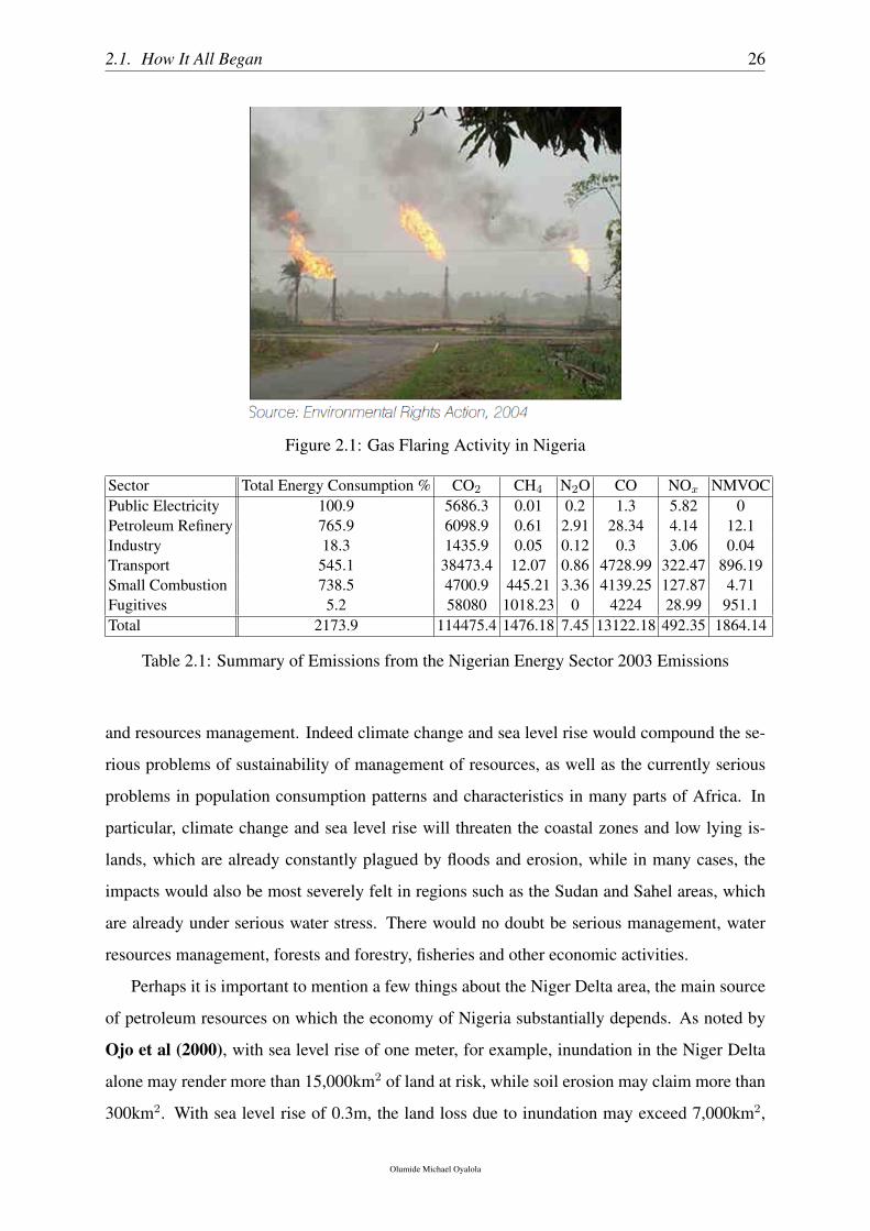
2.1.2 Climate Change Scenario in Nigeria
Nigeria contributes significantly to the greenhouse emissions for example, land use change
and forestry (LULUCF) sector generated about 40% of gross national emissions into the atmo-
sphere. Also significant as sources of C02 emission are gas flaring and transportation, which
account for 30% and 20% respectively.
No matter the level of uncertainties in the knowledge of the characteristics and future trends
of the climate, climate change and sea level rise creating problems for sustainable development
Olumide Michael Oyalola
2.1. How It All Began 26
Figure 2.1: Gas Flaring Activity in Nigeria
Sector Total Energy Consumption % CO2 CH4 N2O CO NOx NMVOCPublic Electricity 100.9 5686.3 0.01 0.2 1.3 5.82 0Petroleum Refinery 765.9 6098.9 0.61 2.91 28.34 4.14 12.1Industry 18.3 1435.9 0.05 0.12 0.3 3.06 0.04Transport 545.1 38473.4 12.07 0.86 4728.99 322.47 896.19Small Combustion 738.5 4700.9 445.21 3.36 4139.25 127.87 4.71Fugitives 5.2 58080 1018.23 0 4224 28.99 951.1Total 2173.9 114475.4 1476.18 7.45 13122.18 492.35 1864.14
Table 2.1: Summary of Emissions from the Nigerian Energy Sector 2003 Emissions
and resources management. Indeed climate change and sea level rise would compound the se-
rious problems of sustainability of management of resources, as well as the currently serious
problems in population consumption patterns and characteristics in many parts of Africa. In
particular, climate change and sea level rise will threaten the coastal zones and low lying is-
lands, which are already constantly plagued by floods and erosion, while in many cases, the
impacts would also be most severely felt in regions such as the Sudan and Sahel areas, which
are already under serious water stress. There would no doubt be serious management, water
resources management, forests and forestry, fisheries and other economic activities.
Perhaps it is important to mention a few things about the Niger Delta area, the main source
of petroleum resources on which the economy of Nigeria substantially depends. As noted by
Ojo et al (2000), with sea level rise of one meter, for example, inundation in the Niger Delta
alone may render more than 15,000km2 of land at risk, while soil erosion may claim more than
300km2. With sea level rise of 0.3m, the land loss due to inundation may exceed 7,000km2,
Olumide Michael Oyalola
2.1. How It All Began 27
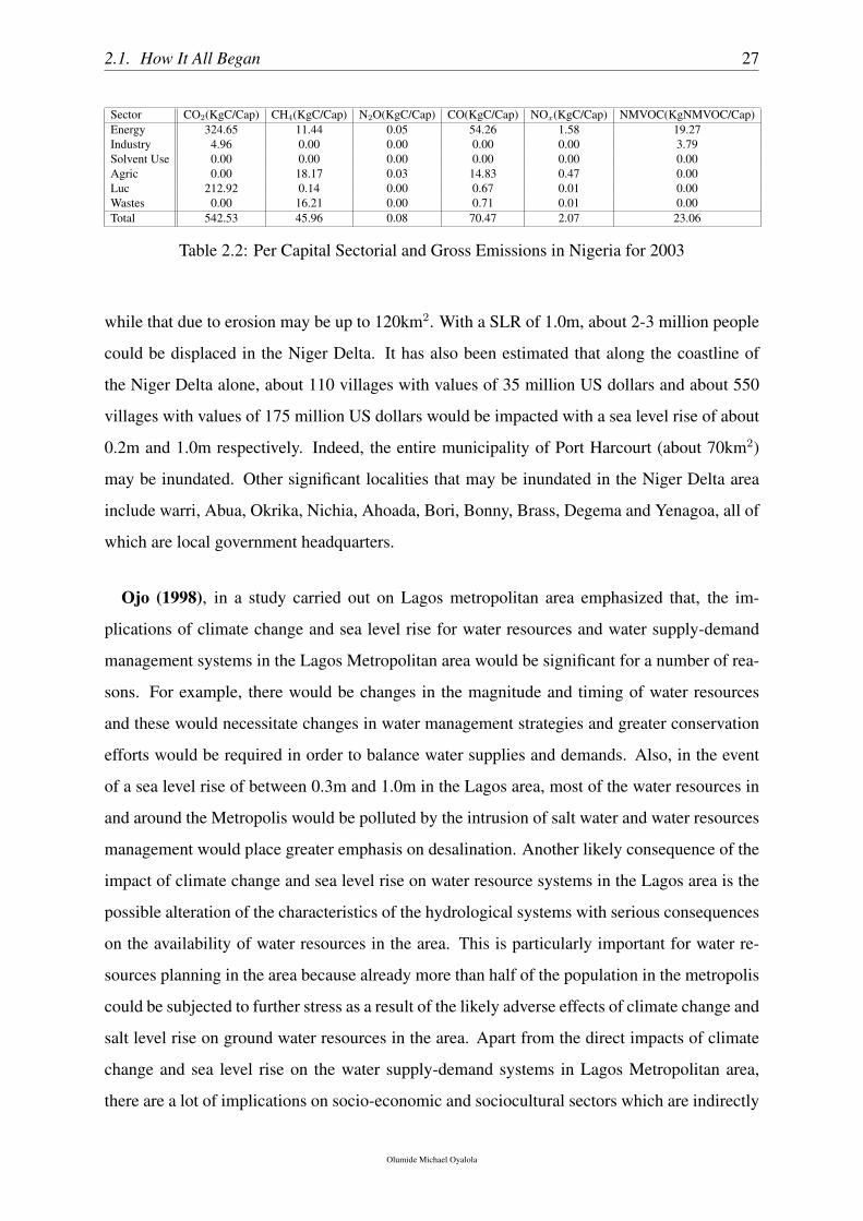
Sector CO2(KgC/Cap) CH4(KgC/Cap) N2O(KgC/Cap) CO(KgC/Cap) NOx(KgC/Cap) NMVOC(KgNMVOC/Cap)Energy 324.65 11.44 0.05 54.26 1.58 19.27Industry 4.96 0.00 0.00 0.00 0.00 3.79Solvent Use 0.00 0.00 0.00 0.00 0.00 0.00Agric 0.00 18.17 0.03 14.83 0.47 0.00Luc 212.92 0.14 0.00 0.67 0.01 0.00Wastes 0.00 16.21 0.00 0.71 0.01 0.00Total 542.53 45.96 0.08 70.47 2.07 23.06
Table 2.2: Per Capital Sectorial and Gross Emissions in Nigeria for 2003
while that due to erosion may be up to 120km2. With a SLR of 1.0m, about 2-3 million people
could be displaced in the Niger Delta. It has also been estimated that along the coastline of
the Niger Delta alone, about 110 villages with values of 35 million US dollars and about 550
villages with values of 175 million US dollars would be impacted with a sea level rise of about
0.2m and 1.0m respectively. Indeed, the entire municipality of Port Harcourt (about 70km2)
may be inundated. Other significant localities that may be inundated in the Niger Delta area
include warri, Abua, Okrika, Nichia, Ahoada, Bori, Bonny, Brass, Degema and Yenagoa, all of
which are local government headquarters.
Ojo (1998), in a study carried out on Lagos metropolitan area emphasized that, the im-
plications of climate change and sea level rise for water resources and water supply-demand
management systems in the Lagos Metropolitan area would be significant for a number of rea-
sons. For example, there would be changes in the magnitude and timing of water resources
and these would necessitate changes in water management strategies and greater conservation
efforts would be required in order to balance water supplies and demands. Also, in the event
of a sea level rise of between 0.3m and 1.0m in the Lagos area, most of the water resources in
and around the Metropolis would be polluted by the intrusion of salt water and water resources
management would place greater emphasis on desalination. Another likely consequence of the
impact of climate change and sea level rise on water resource systems in the Lagos area is the
possible alteration of the characteristics of the hydrological systems with serious consequences
on the availability of water resources in the area. This is particularly important for water re-
sources planning in the area because already more than half of the population in the metropolis
could be subjected to further stress as a result of the likely adverse effects of climate change and
salt level rise on ground water resources in the area. Apart from the direct impacts of climate
change and sea level rise on the water supply-demand systems in Lagos Metropolitan area,
there are a lot of implications on socio-economic and sociocultural sectors which are indirectly
Olumide Michael Oyalola
2.1. How It All Began 28
linked to water resources. For example, the impacts of climate change and sea level rise would
include damages and losses due to flood, erosion, inundations and loss of vegetation and pos-
sible displacement of people from flooded areas Ojo et al (2000) also emphasized that Lagos
State, which consists of large areas of lowlands is very vulnerable to the impacts of climate
change and sea level rise. This is particularly so because the State is generally characterized
by low lying areas, most of which are below 5m. The summary of the results of the stud-
ies shows that considerable physical, ecological and socio-economic losses would be incurred
with the expected rise in sea level of between 0.5m and 1.0m, if adequate response measures
are not taken. For example, almost all parts of the Eti-Osa, Ibeju, Lekki, Lagos Island, Ojo,
Shomolu and Badagry Local Government areas will be inundated, resulting in considerable
physical ecological and socioeconomic consequences. In particular, all the 189km2 land of the
Eti-Osa Local Government Area, about 230km2 of land in Lagos Mainland LGA and about
445km2 of land in Shomolu LGA will be inundated with an expected SLR of about 1.0m. In
the Eti-Osa Local Government areas of the metropolis (this includes the Victoria Island and
Ikoyi, which form the most expensive areas in Nigeria), for example, more than 200 industrial
establishments worth more than US$45 billion will be lost.
Apata (2010), in a study carried out on an empirical analysis of the effects of global warm-
ing on Nigerian agriculture and estimation of the determinants of adaptation to climate change.
This study analyzed determinants of farm-level climate adaptation measures using a Multino-
mial choice and stochastic-simulation model to investigate the effects of rapid climatic change
on grain production and the human population in Nigeria. Data used for this study are from
both secondary and primary sources. The set of secondary sources of data helped to examine
the coverage of the three scenarios (1971-1980; 1981-1990 and 1991-2000). The primary data
set consists of 900 respondents’ but only 850 cases were useful. The model calculates the pro-
duction, consumption and storage of grains under different climate scenarios over a 10-year
scenery. In most scenarios, either an optimistic baseline annual increase of agricultural output
of 1.85% or a more pessimistic appraisal of 0.75% was used. The rate of natural increase of the
human population exclusive of excess hunger-related deaths was set at 1.65% per year. Results
indicated that hunger-related deaths could increase if grain productions do not keep pace with
population growth in an unfavourable climatic environment. However, Climate change adapta-
tions have significant impact on farm productivity.
Olumide Michael Oyalola
2.1. How It All Began 29
Aye G.C., Ater P.I. (2012), in a study carried out on the impact of climate change on Nige-
ria’s cereal grain yields, variance and covariance. Climatic conditions and water availability
may influence the mix of crop and livestock productions. As climatic conditions vary, crop
production patterns could change since different crops could react differently to the alterations
in climatic conditions. The timing and level of precipitation will impact the seeding and other
field operations, and changes in the temperature level will affect the length of growing season
and crop evapo transpiration Maize and rice were selected based on their distinct production in
almost all the States in Nigeria. A panel data stochastic production model with heteroscedas-
ticity was employed in analyzing the data. The data consists of a panel of eight States and
18 time periods. The eight states spans across the six geopolitical zones. The cereal grains
considered are rice and maize. The simulation results show that there would be an increase in
rice yield whereas its variance would increase. The contrary holds for maize. The covariance
of the two crops would reduce in future due to climate change. The results have implications
for allocations of agricultural land among crops, for crop production mix, and for adaptation
and mitigation policies.
According to the special report documented by Aaron Sayne for the United States institute
for peace on climate change adaptation and conflict in Nigeria, Nigeria’s climate is likely to
see growing shifts in temperature, rainfall, storms, and sea levels throughout the twenty-first
century. However, poor adaptive responses to these shifts could help fuel violent conflict in
some areas of the country.
She further stated that a basic causal mechanism links climate change with violence in Nigeria.
Under it, poor responses to climatic shifts create shortages of resources such as land and wa-
ter. Shortages are followed by negative secondary impacts, such as more sickness, hunger, and
joblessness. Poor responses to these, in turn, open the door to conflict.
Drawing lines of causation between climate change and conflict in specific areas of Nigeria
calls for caution, however, particularly as the scientific, social, economic, and political impli-
cations of the country’s changing climate are still poorly understood. The Federal Government
of Nigeria needs to initiate a serious program of research and policy discussion before taking
major adaptive steps.
Olumide Michael Oyalola
2.1. How It All Began 30
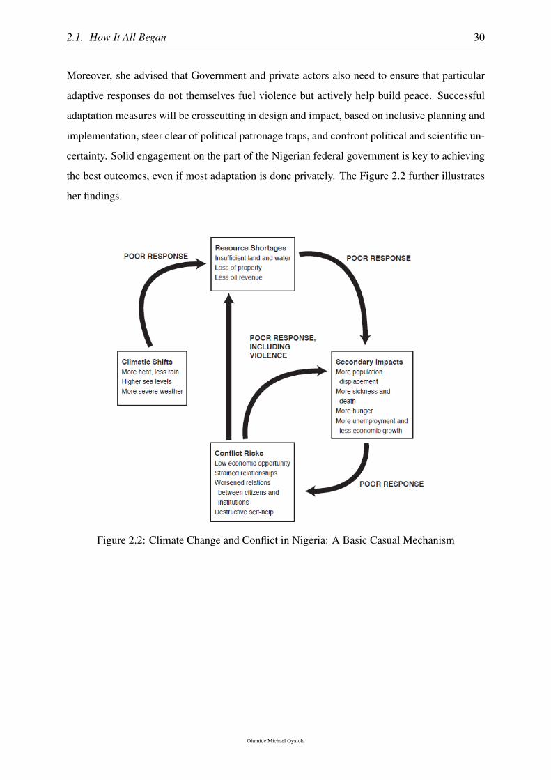
Moreover, she advised that Government and private actors also need to ensure that particular
adaptive responses do not themselves fuel violence but actively help build peace. Successful
adaptation measures will be crosscutting in design and impact, based on inclusive planning and
implementation, steer clear of political patronage traps, and confront political and scientific un-
certainty. Solid engagement on the part of the Nigerian federal government is key to achieving
the best outcomes, even if most adaptation is done privately. The Figure 2.2 further illustrates
her findings.
Figure 2.2: Climate Change and Conflict in Nigeria: A Basic Casual Mechanism
Olumide Michael Oyalola
2.1. How It All Began 31
2.1.3 Climate Change Modelling
It is well known that atmosphere–ocean general circulation models (AOGCMs) are the standard
tools for grasping the complexity of climate system and simulating its behaviour, in the past as
well as in future scenarios. In particular, they allow us to reconstruct and forecast the climate
at large scale.
Several mathematics scholars including Edward N Lorenz have used mathematical models to
model climate variability. Linear differential equation, nonlinear differential equation and cou-
pled equations are examples of the mathematical models that have been used to model climate
variability. However, it should be noted that because of the deterministic nature of the models,
they are chaotic in some circumstances. Chaos is important because it further undermines the
idea that nature is deterministic. the existence of chaos means that even if we can perfectly
describe the workings of some natural system with a deterministic mathematical model, this
does not necessarily mean that we can predict its behaviour far into the future. If the system
is chaotic, then no matter how accurately we measure its state, the error left in the measure-
ment will always mean that the error in our predictions will eventually grow so large that they
become useless. This is exactly the problem that faces weather forecasters. They never know
the state of the atmosphere perfectly, and in any case cannot produce a model that is a per-
fect description of the atmosphere. Because the atmosphere and models of it often behave in
a chaotic way, these errors mean that forecasts can only ever be short term. Chaos is another
reason for considering alternatives to the often hopeless goal of producing models to predict
exactly what a system will do: that is to work with statistical models that deal with probabil-
ities of particular system behaviours. Clair and Ehrman, (2010) applied an artificial neural
network (ANN) model to evaluate for the first time the influence of climate change on riverine
ecosystems and flow, and the application of ANNs to climate change and hydrological ecosys-
tems has been advancing in recent years [26]. To analyze climatic factors that influence runoff,
Chen et al. (2005) used an ANN model to build up the effectual relationship between monthly
precipitation, temperature, and runoff from data acquired from a station situated on Bayinbu-
luke. Based on regional climate models, they applied potential climate change scenarios under
conditions of increasing CO2 by a magnitude of two in northwestern China, and estimated the
effect of climate change on surface runoff. Results show that annual runoff increased from
approximately 6.7% to 25% when temperature increased by approximately 1 to 30C, and that
Olumide Michael Oyalola

2.1. How It All Began 32
annual runoff increased from approximately 1.4% to 11% when precipitation increased from
approximately 5% to 25%. Therefore temperature has a greater influence on local runoff than
rainfall. Although rising temperatures and increasing rainfall help ease the current state of
drought in northwestern China, the increase in runoff concentrated within a 7- and 8-month pe-
riod increases the risk of flooding during the summer months, to the extent that it will change
the mode of development and project planning in relation to the use of water resources. Fur-
thermore, Zou and Wang, (2007) verified the validity of applying a neural network model to
predict the effectiveness of river water quality. Their results show that considerable errors in
long-term predictability of river systems exist during the continuous forecasting of water qual-
ity, while short-term predictability generates fewer errors. Short-term predictability, however,
requires an increase in data acquisition and takes more time to calculate. Seasonal tempera-
ture and precipitation changes have an important effect on the research of carbon, phosphorus,
and nitrogen in watershed systems. Holmberg et al. (2006) generated daily temperature and
precipitation values between the years 2040 and 2069 using CLIGEN and modeled daily total
organic carbon (TOC), total nitrogen (Ntot), and total phosphorus (Ptot) in a river system using
an ANN. They were able to simulate the flux under future climate change scenarios, and found
that TOC, Ntot, and Ptot flux increased in stream water and that this condition was dependent
primarily upon changes in the amount of runoff rather than concentrations. Although the ANN
model did not obtain all extreme values in relation to TOC, Ntot, and Ptot flux in stream water,
its output was consistent with observations for most of the dynamic values. A clearer division
between the effects of temperature and runoff should be identified when selecting network pa-
rameters. Particularly in relation to dry conditions, the annual output value is more important
than the concentration of extreme values acquired using observation and through simulation
experiments.
Moreover, Kin C. Luk et al.(2001), modeled the rainfall process which was assumed to be a
Markovian process, which means that the rainfall value at a given location in space and time is
a function of a finite set of previous realisations. With this assumption, a model structure can
be expressed as
X (t+ 1) = g (X (t) , X (t− 1) , X (t− 2, . . . , X (t− k + 1))) + e (t) (2.1)
where; X (t) represents a vector of rainfall values x1t, x2t, . . . , xNt at N different locations
at time t,
Olumide Michael Oyalola
2.1. How It All Began 33
g () is a nonlinear mapping function, which will be approximated using an ANN,
e (t) is a mapping error (to be minimized), and
k is the unknown number of past rainfall realizations contributing to rainfall at the next time-
step; usually, k refers to the lag of the network; if k = 1, the rainfall at the next time-step is
related only to the present rainfall, thus giving a lag-l network.
They further highlighted the steps involved in the development of an ANN for rainfall
forecasting which include;
• select an appropriate ANN to represent the Markovian process;
• estimate the lag for the ANN, i.e., to determine the number of past rainfall values to be
included as inputs;
• determine the optimal complexity of the ANN appropriate to the problem, i.e., to deter-
mine the number of hidden layers, and number of nodes in a hidden layer.
Moreover, they further identified three types of ANNs suitable for modelling rainfall, they
are;
• Multilayer feedforward neural network (MLFN),
• Elman partial recurrent neural network (Elman), and
• Time delay neural network (TDNN)
All the above alternative networks could make reasonable forecast of rainfall one time step (15
minutes) ahead for 16 gauges concurrently. In addition, the following points were observed;
• For each type of network, there existed an optimal complexity, which was a function of
the number of hidden nodes and the lag of the network.
• All three networks had comparable performance when they were developed and trained
to reach their optimal complexities.
• Networks with lower lag tended to outperform the ones with higher lag. This indicates
that the 15-minutes rainfall time series have very short term memory characteristics.
Chandler (2001), in a study of the Irish rainfall, used logistic regression to model the
sequence of wet and dry days at each site and then to fit gamma distribution to the amount of
Olumide Michael Oyalola
2.1. How It All Began 34
rain on wet days. He referred to this as occurrence and amounts models respectively. below is
the description of the models used;
1. Logistic regression for rainfall occurrence (pattern of dry/wet days):
lnpi
1− pi= x′iβ (2.2)
where pi is the probability of rain for the ith case in the data set conditional on a covariate
vector xi with coefficient vector β.
2. Gamma distribution for Rainfall amounts during wet days. The rainfall amount for ith
wet day has, conditional on a covariate vector ηi and coefficient vector γ, a gamma dis-
tribution with mean µi, where:
ln (µi) = η′iγ (2.3)
Furthermore, Obisesan K.O, et al (2013) stressed the relevance of data visualization in a
research carried out on data visualization and change-point detection in environmental data: the
case of water pollution in Oyo state, Nigeria. The authors, stated that data visualization being
a component of environmental statistics, makes it possible to see clearly from the beginning
if anything is wrong with the data. The work is centered on using statistical methodologies to
explaining environmental processes with a view of achieving some methodological changes in
the approach to environmental data analysis, and to investigate change-point1 in water pollution
data, and use data visualization to explain environmental pollution data. Data supplied by the
Water Corporation of Oyo State for Asejire & Eleyele from 2003 - 2007 was used for the anal-
ysis. However to access the environmental pollution level, both WHO2 & SON3 standards were
used as benchmark and samples from Eleyele & Asejire reservoirs were collected and moni-
tored for presence of some physico-chemical variables. The results show that the values such
as turbidity, total solids, colour, alkalinity and many more variables at Eleyele are higher than
those from Asejire reservoir. Consequently, a change-point model was applied to the available
data. David Hinkley’s approach to change-point modelling was adopted. It was discovered that
the change-point in the two reservoirs are very close. However, 51 for Asejire corresponds to
2007 and change-point 48 for Eleyele corresponds to 2006.1Change-Point is a point in time at which the properties of a process changes abruptly. The shift may include
sudden changes in mean, variance or autocorrelation structure.2World Health Organization3Standards Organization of Nigeria
Olumide Michael Oyalola
2.1. How It All Began 35
2.1.4 Extreme Value Theory and Extreme Value Modelling
Extreme value theory is a powerful and yet fairly robust framework in which to study the
tail behavior of a distribution. Even though extreme value theory has previously found large
applicability in climatology and hydrology, there have also been a number of extreme value
studies in the finance literature in recent years.
de Haan, Jansen, Koedijk, and de Vries (1994) study the quantile estimation using ex-
treme value theory. McNeil (1997, 1998) study the estimation of the tails of loss severity distri-
butions and the estimation of the quantile risk measures for financial time series using extreme
value theory. Embrechts et al. (1998) overview the extreme value theory as a risk management
tool. Muller et al. (1998) and Pictet et al.(1998) study the probability of exceedances for the
foreign exchange rates and compare them with the GARCH and HARCH models. Embrechts
(1999,2000a) studies the potentials and limitations of the extreme value theory. McNeil (1999)
provides an extensive overview of the extreme value theory for risk managers. McNeil and
Frey (2000) study the estimation of tail-related risk measures for heteroskedastic financial
time series. Embrechts (2000b),Embrechts et al. (1997) are a comprehensive source of the
extreme value theory to the finance and insurance literature.
Sarma, et al. (2010) work which was aimed at studying some of the aspects of excess
and deficit in summer monsoon rainfall through probability methods and statistical theory pro-
posed by Gumbel for the extreme value distribution of all Andhra Pradesh in the context of
increased variability of SW monsoon system over India and its adjoins because of the in-
creased prevalence of ENSO episodes especially from the latter half of the 20th century. They
further reported the impact of ENSO on the summer monsoon rainfall over the three regions
(Coastal Andhra, Rayalaseema and Telangana) that constitute Andhra Pradesh (AP) and
pointed out that Telangana’s mean rainfall during June - September is 715mm and is higher
compared with 508mm and 427mm for Coastal and Rayalaseema, respectively. The consoli-
dation of above reports inform that it is high time to go for advance contingent plans in manag-
ing the adverse climate conditions in a scientific way for a better crop sustenance to overcome
the problem of food shortage of the coming years in the context of climate extremities under
the anthropogenic sceptre of the climate change. The years 2002 and 2004 witnessed drought
situation in the country whereas the crop loss in AP has been RS 5, 227 and RS 1, 550 crores,
respectively.
Olumide Michael Oyalola
2.1. How It All Began 36
The anomalies of the rainfall for summer monsoon months of June, July, August and
September obtained from the climatology and the analysis of the test month was studied. The
rainfall data of all Andhra Pradesh was obtained by averaging monthly values of the three ge-
ographical regions of AP. The extreme values of rainfall vary in both space and time scales
gaining importance in the context of climate change because of the increased frequency of ex-
treme weather events such as droughts and floods. Extreme value statistic was used to model
the extreme dry and wet spells to determine the likely recurrence of the events. In the present
study, an attempt was made in analyzing the APSMR using extreme value analysis and the
Gumbel statistical theory for extremes in obtaining the threshold number of years for the pos-
sible exceedance. The standard Gumbel distribution function used is as follows:
G (x) = exp
(− exp
(−(x− α)
β
))(2.4)
Where, α and β represent the location and scale parameters that are also known as shape
parameters that can be obtained from the given data; and x, is the variable (here the variate is
rainfall). The parameters α and β are generally estimated from the maximum likelihood method
and the values obtained by means of numerical solver after getting the following equations:
α = −β ln
(n−1Σ exp
(−xiβ
))(2.5)
and
β − n−1Σxi +Σ(xi exp
(−xiβ
))Σ(
exp(−xiβ
)) = 0 (2.6)
where, i = 1, 2, . . . , n; and n, is the number of observations for the variate under consid-
eration. To compute the chance of exceeding the extreme event, one has to find 1−G (x) and
the threshold level of the year (T − year) can be estimated by 1(1−G(x))
. The study was of help
in knowing the equivocal situations from the point of view of the climate scenario over AP.
The study unravels that the ENSO or LNSO short term climate signal - is one of the global
teleconnections that causes perturbations in the performance of the SW monsoon over India
in terms of subnormal and abnormal monsoon weather triggering drought and flood situation,
respectively. The magnitude of the return period of the event increases as the return period
increases.
Olumide Michael Oyalola

2.1. How It All Began 37
In the section beneath, I present the parametric framework for the study. Within the EVT
context, there are two approaches to study the extremal events. One of them is the direct
modeling of the distribution of minimum or maximum realizations. The other one is modeling
the exceedances of a particular threshold.
Olumide Michael Oyalola
Chapter 3
Methodology
3.1 Methodology: Brief Introduction
Rainfall forecasting is important for many catchment management applications, in particular
for flood warning systems. The variability of rainfall in space and time, however, renders quan-
titative forecasting of rainfall extremely difficult. The depth of rainfall and its distribution in
the temporal and spatial dimensions depends on many variables, such as pressure, temperature,
and wind speed and direction. Due to the complexity of the atmospheric process by which
rainfall is generated and the lack of available data on the necessary temporal and spatial scales,
it is not feasible generally to forecast rainfall using a physically based process model.
These very interesting research give an excellent springboard for the discussion of some issues
in contemporary extremal analysis of precipitation in Nigeria.
It seems worthwhile first to make some general points about the statistics of extremes, which
differs from much of mainstream statistics in the sense that its primary goal is extrapolation into
the tail of a distribution, typically based on limited relevant data. Any extrapolation is fraught
with risks,and hence one seeks a principled basis for it.
3.1.1 Extreme Value Theory - Historical Perspective
• Emil Gumbel was born and trained as a statistician in Germany, forced to move to France
and then the U.S. because of his pacifist and socialist views. He was a pioneer in the
application of extreme value theory, particularly to climate and hydrology.
• Waloddi Weibull was a Swedish engineer famous for his pioneering work on reliability,
38
3.2. Classical Extreme Value Theory 39
providing a statistical treatment of fatigue, strength, and lifetime.
• Maurice Frechet was a French mathematician who made major contributions to pure
mathematics as well as probability and statistics. He also collected empirical examples
of heavy-tailed distributions.
• Other names include Fisher and Tippet (1928), Gnedenko (1943) etc.
3.2 Classical Extreme Value Theory
3.2.1 Model Formulation
The core of the extreme value theory is the study of the statistical behaviour of
Mn = max {X1, X2, . . . , Xn} (3.1)
where {X1, X2, . . . , Xn} is a sequence of independent random variables having a common
distribution function F .
In applications, variables Xi usually represent values of a process measured on a regular
time-scale, as for example the 10 minutes average (or maximum) wind speed. Then Mn is the
maximum of the observed process over n time units. The distribution function of Mn verifies:
P (Mn ≤ z) = P (X1 ≤ z, . . . , Xn ≤ z) = P (X1 ≤ z) . . . P (Xn ≤ z) = (F (z))n (3.2)
Thus, a way to study Mn is to estimate F from the available data (for example the 10
minutes speed records measured during certain interval of time) and then to substitute this
estimation in the previous formula to estimate Mn . The problem of this approach is that small
deviances in the estimation of F lead to large discrepancies for F n(z).
idea is similar to that used to estimate the distribution of the sample mean average. Follow-
ing this way it is necessary to study the behaviour of F n(z) as n tends to infinity. However,
since F (z) < 1 for z < zsup , where zsup is the smallest value of z such that F (z) = 1, we have
F (z) → 0 as n → ∞ . To overcome this difficulty, reaching a limit different from 0, we use
the following linear normalization of Mn :
M∗n =
Mn − bnan
(3.3)
Olumide Michael Oyalola
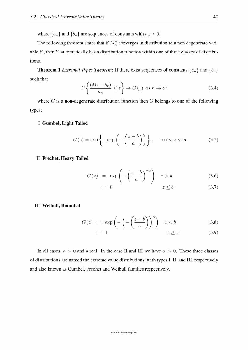
3.2. Classical Extreme Value Theory 40
where {an} and {bn} are sequences of constants with an > 0.
The following theorem states that if M∗n converges in distribution to a non degenerate vari-
able Y , then Y automatically has a distribution function within one of three classes of distribu-
tions.
Theorem 1 Extremal Types Theorem: If there exist sequences of constants {an} and {bn}
such that
P
{(Mn − bn)
an≤ z
}→ G (z) as n→∞ (3.4)
where G is a non-degenerate distribution function then G belongs to one of the following
types;
I Gumbel, Light Tailed
G (z) = exp
{− exp
(−(z − ba
))}, −∞ < z <∞ (3.5)
II Frechet, Heavy Tailed
G (z) = exp
(−(z − ba
)−α)z > b (3.6)
= 0 z ≤ b (3.7)
III Weibull, Bounded
G (z) = exp
(−(−(z − ba
))α)z < b (3.8)
= 1 z ≥ b (3.9)
In all cases, a > 0 and b real. In the case II and III we have α > 0. These three classes
of distributions are named the extreme value distributions, with types I, II, and III, respectively
and also known as Gumbel, Frechet and Weibull families respectively.
Olumide Michael Oyalola
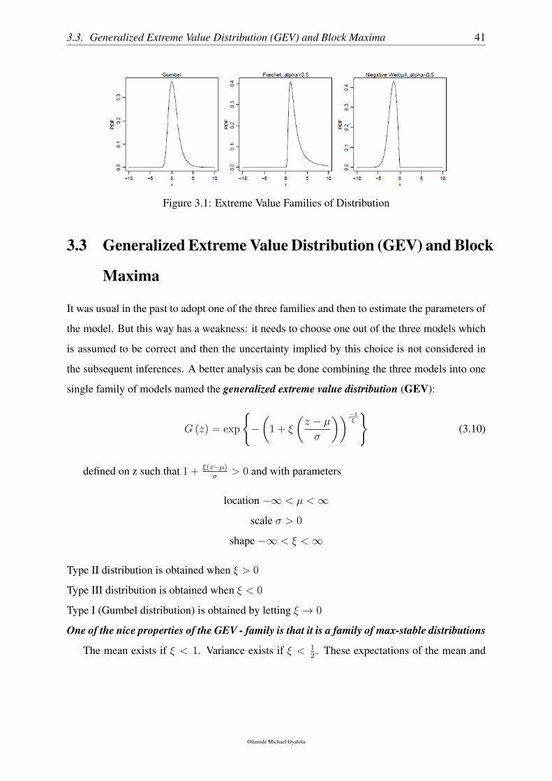
3.3. Generalized Extreme Value Distribution (GEV) and Block Maxima 41
Figure 3.1: Extreme Value Families of Distribution
3.3 Generalized Extreme Value Distribution (GEV) and Block
Maxima
It was usual in the past to adopt one of the three families and then to estimate the parameters of
the model. But this way has a weakness: it needs to choose one out of the three models which
is assumed to be correct and then the uncertainty implied by this choice is not considered in
the subsequent inferences. A better analysis can be done combining the three models into one
single family of models named the generalized extreme value distribution (GEV):
G (z) = exp
{−(
1 + ξ
(z − µσ
))−1ξ
}(3.10)
defined on z such that 1 + ξ(z−µ)σ
> 0 and with parameters
location −∞ < µ <∞
scale σ > 0
shape −∞ < ξ <∞
Type II distribution is obtained when ξ > 0
Type III distribution is obtained when ξ < 0
Type I (Gumbel distribution) is obtained by letting ξ → 0
One of the nice properties of the GEV - family is that it is a family of max-stable distributions
The mean exists if ξ < 1. Variance exists if ξ < 12. These expectations of the mean and
Olumide Michael Oyalola
3.3. Generalized Extreme Value Distribution (GEV) and Block Maxima 42
variance are
E (X) = µ+σ
ξ{Γ (1− ξ)− 1} (ξ < 1) (3.11)
V ar (X) = E{
(X − E (X))2} (3.12)
=σ2
ξ2
{Γ (1− 2ξ)− Γ2 (1− ξ)
} (ξ <
1
2
)(3.13)
When ξ = 0, these expectations become:
E (X) = µ+ σγ ; V ar (X) =σ2π2
6(3.14)
Where γ ≈ 0.5772 (Euler’s constant).
3.3.1 Practical Implementation
The above results lead to the following approach for modelling extremes of a series of inde-
pendent and identically distributed (iid) observations X1, X2, . . . , Xn The first step consists in
blocking the data into sequences of n observations, n being sufficiently large. Then the maxima
Zi of each block i is calculated and, finally, the GEV distribution is fitted to this series of block
maxima Z1, Z2, . . . , Zn. In most environmental applications the length of the blocks usually is
one year, and the we use as data the annual maximum Zi of year i.
Once the GEV distribution has been fitted, let say for the annual maxima, we can calculate the
quantile function, zp , for the annual maximum distribution as:
zp = µ−(σ
ξ
)(1− (− log (1− p))−ξ
)for ξ 6= 0 (3.15)
= µ− σ log (− log (1− p)) for ξ = 0 (3.16)
Observe that G(zp) = 1− p . In our terminology, this is the return level associated with the
return period 1p
. That is, zp is the level that is expected to be exceeded, in average, once every1p
years. Equivalently, zp is the level that is exceeded by the annual maximum in any particular
year with probability p. By using yp = − log (1− p) , this quantile function can be expressed
as
Olumide Michael Oyalola
3.3. Generalized Extreme Value Distribution (GEV) and Block Maxima 43
zp = µ−(σ
ξ
)(1− y−ξp
)for ξ 6= 0 (3.17)
= µ− σ log yp for ξ = 0 (3.18)
If zp is plotted against log yp the plot is linear in the case of ξ = 0 ; the plot is convex in the
case of ξ < 0 with asymptotic limit as p tends to 0 to (µ−σ)ξ
and the plot is concave for ξ > 0
and has not finite bound.
This graph is named a return level plot and it is useful as validation tool as well as a way
of presenting the fitted model.
3.3.2 Inference for the GEV Distribution
The choice of the length of blocks implies a trade off between bias and variance. When the
length of the blocks is small, then the approximation of the distributions by the limit is quite
poor and this is leading to bias in estimation and extrapolation. Long blocks on the other hand
generate only few data leading to large estimation variance. The method most commonly used
to estimate the parameters is the likelihood method. One difficulty of this approach is that the
regularity conditions for its application are not satisfied by the GEV distributions because the
end-point of the distribution depends on the parameter values. This violation means that the
standard asymptotic likelihood results are not automatically applicable. This problem has been
studied in detail with the following results:
• When ξ > −0.5 the maximum likelihood estimators have the usual asymptotic proper-
ties.
• When −1 < ξ < −0.5 the maximum likelihood estimators can be obtained in general
but they do not have the standard asymptotic properties.
• When ξ < −1 the maximum likelihood estimators are unlikely to be obtainable.
Observe that the case ξ < −0.5 corresponds to distributions with a very short bounded
upper tail, which is rarely the case in real applications of extreme value modelling.
By denoting Z1, Z2, . . . , Zm the block maxima and under the assumption that they are indepen-
Olumide Michael Oyalola
3.3. Generalized Extreme Value Distribution (GEV) and Block Maxima 44
dent variables having a GEV distribution, the log-likelihood for the GEV when ξ 6= 0 is
l (µ, σ, ξ) = −m log σ−(
1 +1
ξ
)Σmi=1 log
(1 + ξ
Zi − µσ
)−Σm
i=1
(1 + ξ
Zi − µσ
)−1ξ
(3.19)
provided that(1 + ξ Zi−µ
σ
)> 0 for i = 1, . . . ,m. When this condition is not satisfied then
the likelihood is zero and the log-likelihood is minus infinity.
In the Gumbel case (ξ = 0), the log-likelihood is:
l (µ, σ) = −m log σ − Σmi=1
Zi − µσ
− Σmi=1 exp
(−Zi − µ
σ
)(3.20)
By maximizing these log-likelihood functions, we obtain the maximum likelihood estimates(µ, σ, ξ
). The optimization is made using numerical optimization algorithms.
The classical theory of maximum likelihood estimation establishes that the distribution of(µ, σ, ξ
)is approximately normal with mean (µ, σ, ξ) and variance covariance matrix equal to
the inverse of the observed information matrix evaluated at the maximum likelihood estimate.
Confidence intervals are obtained from this approximate normality of the estimator.
3.3.3 Inference for Return Levels
The maximum likelihood estimate of the 1p
return level zp for 0 < p < 1 is
zp = µ−(σ
ξ
)(1− y−p ξ
)for ξ 6= 0 (3.21)
= µ− σ log yp for ξ = 0 (3.22)
where yp = − log (1− p) . Confidence intervals can be set using the normal approximation
of the estimator distribution, but caution is required in the interpretation, especially for return
levels corresponding to long return periods because the normal approximation may be poor. A
better approximation is generally obtained from the profile likelihood function.
3.3.4 Graphical Model Checking
Though it is impossible to check the validity of an extrapolation based on the GEV model,
assessment can be done with reference to the observed data.
Olumide Michael Oyalola
3.3. Generalized Extreme Value Distribution (GEV) and Block Maxima 45
Probability Plot
A probability plot is a comparison of the empirical and fitted distribution functions. The em-
pirical distribution function evaluated in the i− th ordered block maximum, Z(i) is G(Z(i)
)=
i(m+1)
, and the fitted distribution function in the same point is
G(Z(i)
)= exp
{−(
1 + ξ
(Z(i) − µ
σ
))−1
ξ
}. (3.23)
In order to have a good model it is necessary that G(Z(i)
)= G
(Z(i)
)In practise the
plot of points(G(Z(i)
), G(Z(i)
))i = 1, . . .m, should lie close to the first diagonal. But
because both functions are bounded to approach 1 as the values of Z increase, the plot is least
informative in this region. The following graph avoids this deficiency.
Quantile Plot
The quantile plot is a representation of the points(G−1
(i
(m+1)
), Z(i)
)i = 1, . . . ,m, where
G−1
(i
(m+ 1)
)= µ− σ
ξ
(1−
(− log
i
m+ 1
)−ξ)i = 1, . . . ,m. (3.24)
In the ideal situations the plot should show a linear function. Departures from linearity in
the quantile plot also indicate model failure.
Return Level Plot
The return level plot represents the points (log yp, zp) 0 < p < 1. Confidence intervals are
usually added to this plot to increase its information. The importance of return periods in
engineering is due to the fact that the return period is used as a design criterion. Furthermore,
to use this plot as a model diagnostic one, the empirical estimates of the return level function
are also added. For suitable models the model based curve and empirical estimates should be
in agreement.
In general, we are not only interested in the maxima of observations, but also in the be-
haviour of large observations which exceed a high threshold. This is because modelling only
block maxima implies that we waste a lot of data if a detailed recording of the studied phe-
nomenon is available. Now we propose another alternative analysis that is more efficient in
Olumide Michael Oyalola
3.3. Generalized Extreme Value Distribution (GEV) and Block Maxima 46
the use of data. One method of extracting extremes from a sample of observations, Xt, t =
1, 2, . . . , n with a distribution function F (x) = Pr {Xt ≤ x} is to take the exceedance of a
threshold u occurs when Xt > u for any t in t = 1, 2, . . . , n. An excess over u is defined by
y = Xi − u. Given a high threshold u, the probability distribution of excess values of X over
threshold u is defined by
Fu (y) = Pr {X − u ≤ y|X > u} (3.25)
which represents the probability that the value of X exceeds the threshold u by at most an
amount y given that X exceeds the threshold u. This conditional probability may be written as
Fu (y) =Pr {X − u ≤ y,X > u}
Pr (X > u)(3.26)
=F (y + u)− F (u)
1− F (u). (3.27)
Since x = y + u for X > u, we have the following representation
F (x) = [1− F (u)]Fu (y) + F (u) . (3.28)
Notice that this representation is valid only for X > u. The following result gives an ap-
proximation to this probability for high values of the threshold u.
Theorem 2 Let X1, . . . , Xn be a sequence of independent and identically dis-
tributed random variables with a common distribution functionF andMn = max {X1, . . . , Xn}
satisfying the conditions to the approximated by a GEV, that is, for large n:
Pr {Mn ≤ z} = G (z) (3.29)
where
G (z) = exp
{−(
1 + ξ
(z − µσ
))−1ξ
}(3.30)
Then, for large enough u, the distribution function of (X − u), conditioned to
Olumide Michael Oyalola
3.3. Generalized Extreme Value Distribution (GEV) and Block Maxima 47
X > u, is approximately given by
H (y) = 1−(
1 +ξy
σ
)−1ξ
GENERALIZED PARETO DISTRIBUTION
(3.31)
defined on{y|y > 0 and
(1 + ξy
σ
)> 0}
, and where σ = σ + ξ (u− µ). This result relates
the two approximations to study the distribution of the maximum. We see how the parameters
of the Generalized Pareto Distribution (GDP) are uniquely determined by the parameters of
the associated GEV distribution of block maxima. Observe that this imply that if we change
the size of blocks in the GEV analysis then the parameter ξ remains unperturbed while the
parameters µ and σ change but compensating their values to provide a fixed value for σ.
As for the GEV distribution the ξ parameter is dominant for determining the qualitative
behaviour of the GPD distribution:
• If ξ < 0, then the distribution of excesses is bounded by u− σξ.
• If ξ > 0, then the distribution is unbounded.
• If ξ = 0, then the distribution is also unbounded and is in the exponential family with
parameter 1σ
.
The expected value and the variance of a GPD distribution are;
E (Y ) =σ∗
1− ξ(3.32)
V ar (Y ) =σ∗2
(1− ξ)2 (1− 2ξ)(3.33)
E (Y − u|y > w) =σ∗ + ξw
1− ξ(3.34)
where w is a value greater than 0.
3.3.5 Threshold Selection : Mean Residual Life Plot
Let {x1, . . . , xn} be the original data and let us consider as extreme events those that excess a
threshold u, say, x1, . . . , xk. We denote the excesses over the threshold by yj = xj−u. Because
of the previous theorem, when the threshold u is large enough, the values yj can be viewed as
independent realizations of a variable distributed according to a GPD, whose parameters have
Olumide Michael Oyalola
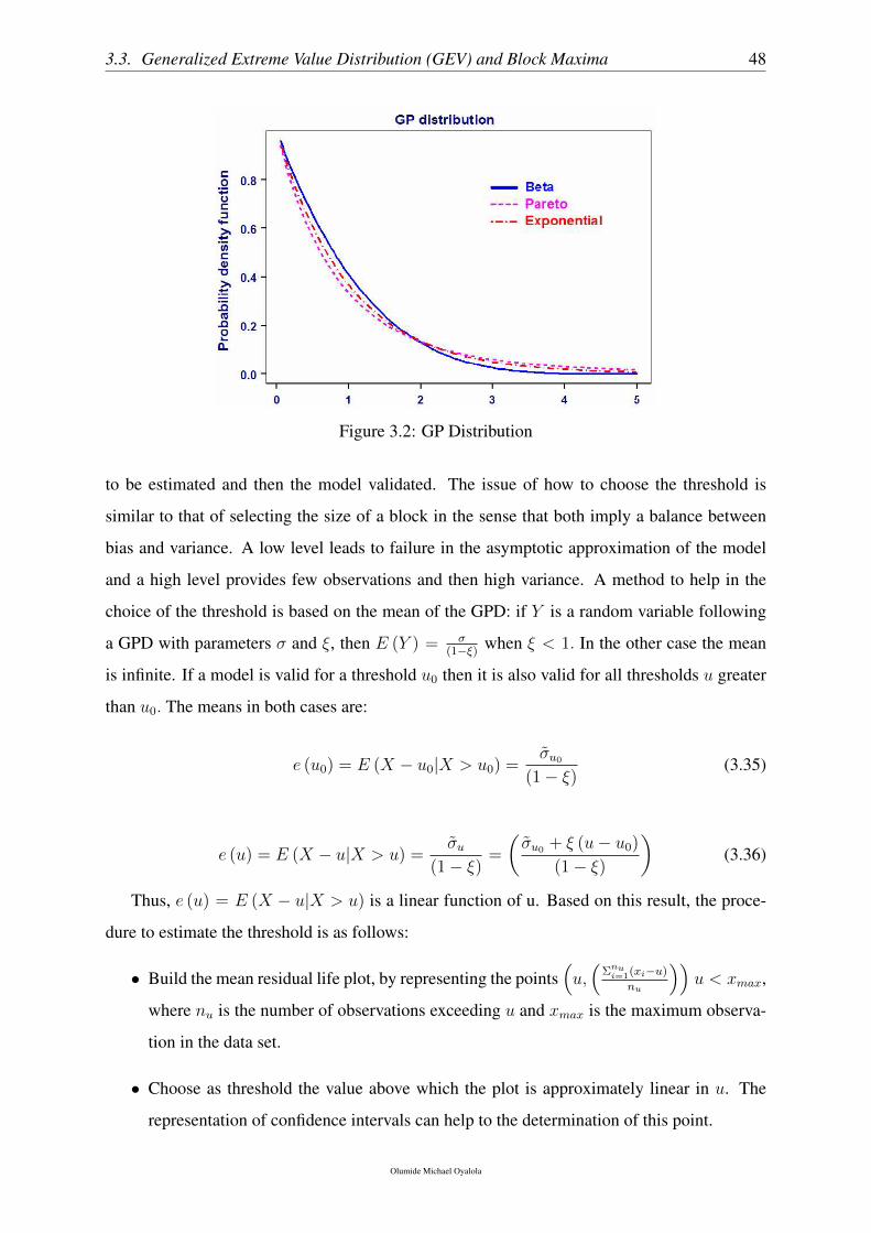
3.3. Generalized Extreme Value Distribution (GEV) and Block Maxima 48
Figure 3.2: GP Distribution
to be estimated and then the model validated. The issue of how to choose the threshold is
similar to that of selecting the size of a block in the sense that both imply a balance between
bias and variance. A low level leads to failure in the asymptotic approximation of the model
and a high level provides few observations and then high variance. A method to help in the
choice of the threshold is based on the mean of the GPD: if Y is a random variable following
a GPD with parameters σ and ξ, then E (Y ) = σ(1−ξ) when ξ < 1. In the other case the mean
is infinite. If a model is valid for a threshold u0 then it is also valid for all thresholds u greater
than u0. The means in both cases are:
e (u0) = E (X − u0|X > u0) =σu0
(1− ξ)(3.35)
e (u) = E (X − u|X > u) =σu
(1− ξ)=
(σu0 + ξ (u− u0)
(1− ξ)
)(3.36)
Thus, e (u) = E (X − u|X > u) is a linear function of u. Based on this result, the proce-
dure to estimate the threshold is as follows:
• Build the mean residual life plot, by representing the points(u,(
Σnui=1(xi−u)
nu
))u < xmax,
where nu is the number of observations exceeding u and xmax is the maximum observa-
tion in the data set.
• Choose as threshold the value above which the plot is approximately linear in u. The
representation of confidence intervals can help to the determination of this point.
Olumide Michael Oyalola
3.3. Generalized Extreme Value Distribution (GEV) and Block Maxima 49
3.3.6 Parameter Estimation
Once the threshold has been estimated, the next step is to estimate the parameters of the GPD,
for example by maximum likelihood. If we denote by y1, . . . , yk the k excesses over the thresh-
old, the log-likelihood function, in the case that ξ is not zero, is:
l (σ, ξ) = −k log σ −(
1 +1
ξ
)Σki=1 log
(1 +
ξyiσ
), (3.37)
when(1 + ξyi
σ
)> 0, in other case L (σ, ξ) = −∞ In the case ξ = 0, the log-likehood is
l (σ) = −k log σ − σ−1Σki=1yi
Return Levels
To calculate the return levels, first we need an expression for the unconditional distribution of
variablesX . Denoting by δu = Pr (X > u) and from the conditional distribution Pr {X > x|X > u} =(1 + ξ (x−u)
σ
)−1ξ
we obtain that
Pr {X > x} = δu
(1 + ξ
(x− u)
σ
)−1ξ
(3.38)
Hence, the level xm that is exceeded on average once every m observations is the solution
of1
m= δu
(1 + ξ
(xm − u)
σ
)−1ξ
, (3.39)
which is
xm = u+σ
ξ
((mδu)
ξ − 1)
(3.40)
This expression is valid for values m leading to xm > u.
In the case ξ = 0 the return level is xm = u+ σ log (mδu) , again for m enough large. The
estimation of these return levels requires the substitution of parameters by their estimates. In
the case of the probability δu = Pr (X > u) , the maximum estimator is the sample proportion
of observations over the threshold u, that is, δu = kn
.
3.3.7 Model Checking
Another tool to help in the choice of threshold u
Olumide Michael Oyalola
3.3. Generalized Extreme Value Distribution (GEV) and Block Maxima 50
As mentioned earlier, when the GPD is a valid model for a threshold u0 then it is also a
valid model for any u > u0. At both levels the parameter ξ is the same and the scale parameters
are related by σu = σu0 + ξ (u− u0). Thus, the new parameter σ∗ = σu − ξu is constant with
respect to u. Consequently, estimates of σ∗ and ξ should be constant above u0, when it is a valid
threshold. This argument leads to plot σ∗ and ξ against u, together with confident intervals for
them and selecting u0 as the lowest value of u for which the estimates remain near-constant.
Probability plots, quantile plots and return level plots are used for assessing the quality of
a fitted generalized Pareto model. Assuming a threshold u, ordered excesses yi, . . . , yk and an
estimated model H for the GPD, then we have:
Probability plot . It represents the points(
i(k+1)
, H (yi))i = 1, . . . , k.
Quantile plot . It represents the points(H−1
(i
(k+1)
), yi
)i = 1, . . . , k. When the model
is valid, in both plots the points are almost linearly placed.
When ξ 6= 0 the estimations are : H (y) = 1−(
1 + ξyσ
)−1
ξ and H−1 (p) = σ
ξ
((1− p)−ξ − 1
)When ξ = 0 the expressions are: y = 1− exp
(−yσ
), and H−1 (p) = −σ ln ((1− p))
Return Level plot . It represents the points (m, xm) , where as we have seen before
for ξ 6= 0 xm = u+ σ
ξ
((mδu
)ξ− 1
),
for the case ξ = 0 the return level is xm = u+ σ log (mσu) .
Recall that xm is the estimated value that is exceeded on average once everym observations.
Olumide Michael Oyalola
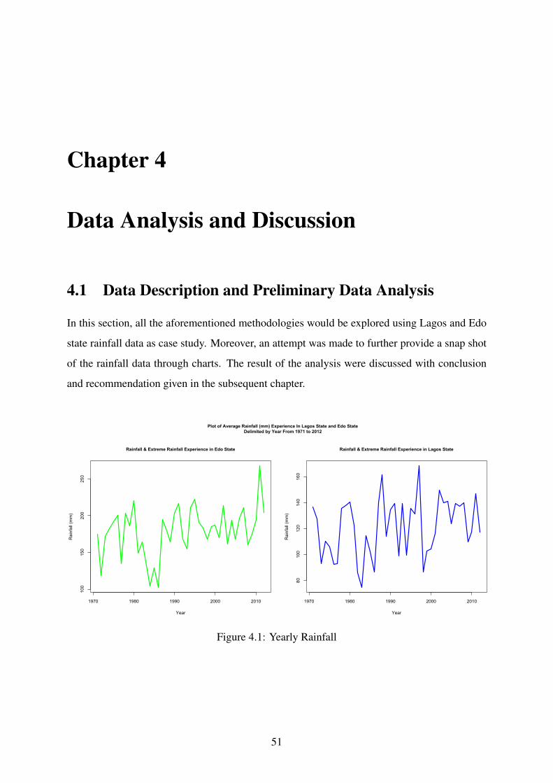
Chapter 4
Data Analysis and Discussion
4.1 Data Description and Preliminary Data Analysis
In this section, all the aforementioned methodologies would be explored using Lagos and Edo
state rainfall data as case study. Moreover, an attempt was made to further provide a snap shot
of the rainfall data through charts. The result of the analysis were discussed with conclusion
and recommendation given in the subsequent chapter.
1970 1980 1990 2000 2010
100
150
200
250
Rainfall & Extreme Rainfall Experience in Edo State
Year
Rai
nfal
l (m
m)
1970 1980 1990 2000 2010
8010
012
014
016
0
Rainfall & Extreme Rainfall Experience in Lagos State
Year
Rai
nfal
l (m
m)
Plot of Average Rainfall (mm) Experience In Lagos State and Edo State Delimited by Year From 1971 to 2012
Figure 4.1: Yearly Rainfall
51
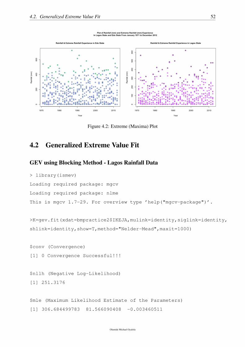
4.2. Generalized Extreme Value Fit 52
1970 1980 1990 2000 2010
020
040
060
0
Rainfall & Extreme Rainfall Experience in Edo State
Year
Rai
nfal
l (m
m)
1970 1980 1990 2000 2010
010
020
030
040
050
060
0
Rainfall & Extreme Rainfall Experience in Lagos State
Year
Rai
nfal
l (m
m)
Plot of Rainfall (mm) and Extreme Rainfall (mm) Experience In Lagos State and Edo State From January 1971 to December 2012
Figure 4.2: Extreme (Maxima) Plot
4.2 Generalized Extreme Value Fit
GEV using Blocking Method - Lagos Rainfall Data
> library(ismev)
Loading required package: mgcv
Loading required package: nlme
This is mgcv 1.7-29. For overview type ’help("mgcv-package")’.
>K=gev.fit(xdat=bmpractice2$IKEJA,mulink=identity,siglink=identity,
shlink=identity,show=T,method="Nelder-Mead",maxit=1000)
$conv (Convergence)
[1] 0 Convergence Successful!!!
$nllh (Negative Log-Likelihood)
[1] 251.3176
$mle (Maximum Likelihood Estimate of the Parameters)
[1] 306.684499783 81.566090408 -0.003460511
Olumide Michael Oyalola
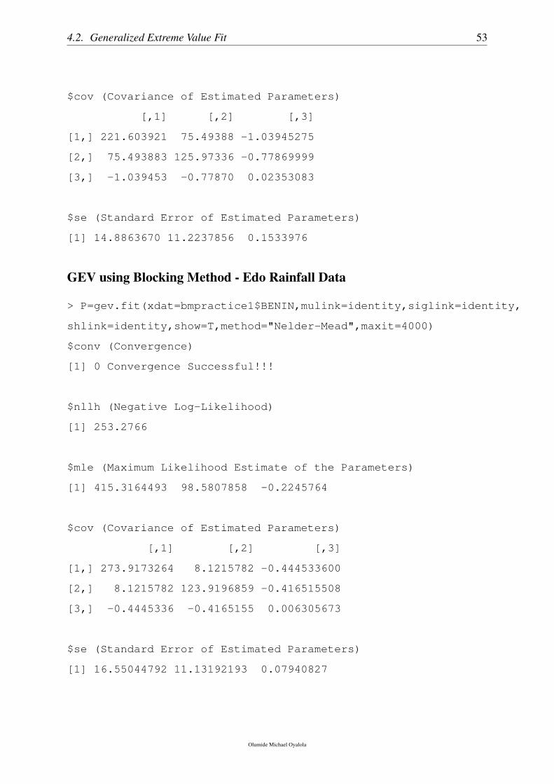
4.2. Generalized Extreme Value Fit 53
$cov (Covariance of Estimated Parameters)
[,1] [,2] [,3]
[1,] 221.603921 75.49388 -1.03945275
[2,] 75.493883 125.97336 -0.77869999
[3,] -1.039453 -0.77870 0.02353083
$se (Standard Error of Estimated Parameters)
[1] 14.8863670 11.2237856 0.1533976
GEV using Blocking Method - Edo Rainfall Data
> P=gev.fit(xdat=bmpractice1$BENIN,mulink=identity,siglink=identity,
shlink=identity,show=T,method="Nelder-Mead",maxit=4000)
$conv (Convergence)
[1] 0 Convergence Successful!!!
$nllh (Negative Log-Likelihood)
[1] 253.2766
$mle (Maximum Likelihood Estimate of the Parameters)
[1] 415.3164493 98.5807858 -0.2245764
$cov (Covariance of Estimated Parameters)
[,1] [,2] [,3]
[1,] 273.9173264 8.1215782 -0.444533600
[2,] 8.1215782 123.9196859 -0.416515508
[3,] -0.4445336 -0.4165155 0.006305673
$se (Standard Error of Estimated Parameters)
[1] 16.55044792 11.13192193 0.07940827
Olumide Michael Oyalola

4.2. Generalized Extreme Value Fit 54
0.0 0.2 0.4 0.6 0.8 1.0
0.0
0.2
0.4
0.6
0.8
1.0
Probability Plot
Empirical
Mod
el
300 400 500 600
300
500
700
Quantile Plot
Model
Em
piric
al
1e-01 1e+00 1e+01 1e+02 1e+03
300
500
700
Return Period
Ret
urn
Leve
l
Return Level Plot Density Plot
z
f(z)
200 300 400 500 600 700 800
0.00
00.
002
0.00
4
Generalized Extreme Value Model Diagnostic Plot Case Study: Edo State
Figure 4.3: GEV Fit Diagnostic Plot for Edo State Rainfall
0.0 0.2 0.4 0.6 0.8 1.0
0.2
0.4
0.6
0.8
1.0
Probability Plot
Empirical
Mod
el
200 300 400 500 600
200
300
400
500
600
Quantile Plot
Model
Em
piric
al
1e-01 1e+00 1e+01 1e+02 1e+03
200
400
600
800
Return Period
Ret
urn
Leve
l
Return Level Plot Density Plot
z
f(z)
200 300 400 500 600
0.00
00.
002
0.00
4
Generalized Extreme Value Model Diagnostic Plot Case Study: Lagos State
Figure 4.4: GEV Fit Diagnostic Plot for Lagos State Rainfall
Olumide Michael Oyalola
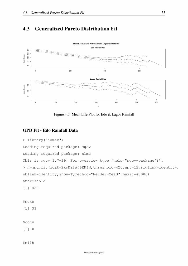
4.3. Generalized Pareto Distribution Fit 55
4.3 Generalized Pareto Distribution Fit
0 200 400 600
050
100
150
200
u
Mea
n E
xces
s
Edo Rainfall Data
0 100 200 300 400 500 600
050
100
u
Mea
n E
xces
s
Lagos Rainfall Data
Mean Residual Life Plot of Edo and Lagos Rainfall Data
Figure 4.5: Mean Life Plot for Edo & Lagos Rainfall
GPD Fit - Edo Rainfall Data
> library("ismev")
Loading required package: mgcv
Loading required package: nlme
This is mgcv 1.7-29. For overview type ’help("mgcv-package")’.
> n=gpd.fit(xdat=ExpData$BENIN,threshold=420,npy=12,siglink=identity,
shlink=identity,show=T,method="Nelder-Mead",maxit=40000)
$threshold
[1] 420
$nexc
[1] 33
$conv
[1] 0
$nllh
Olumide Michael Oyalola
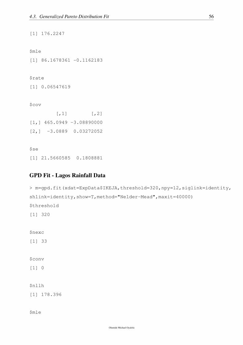
4.3. Generalized Pareto Distribution Fit 56
[1] 176.2247
$mle
[1] 86.1678361 -0.1162183
$rate
[1] 0.06547619
$cov
[,1] [,2]
[1,] 465.0949 -3.08890000
[2,] -3.0889 0.03272052
$se
[1] 21.5660585 0.1808881
GPD Fit - Lagos Rainfall Data
> m=gpd.fit(xdat=ExpData$IKEJA,threshold=320,npy=12,siglink=identity,
shlink=identity,show=T,method="Nelder-Mead",maxit=40000)
$threshold
[1] 320
$nexc
[1] 33
$conv
[1] 0
$nllh
[1] 178.396
$mle
Olumide Michael Oyalola
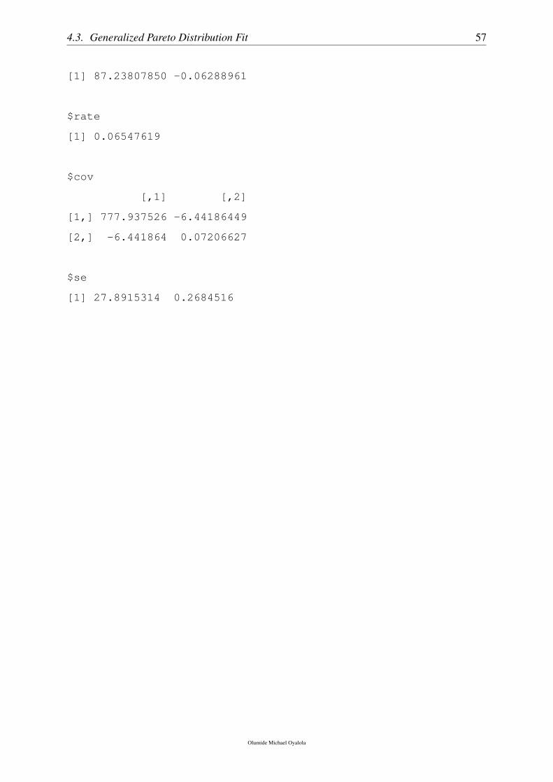
4.3. Generalized Pareto Distribution Fit 57
[1] 87.23807850 -0.06288961
$rate
[1] 0.06547619
$cov
[,1] [,2]
[1,] 777.937526 -6.44186449
[2,] -6.441864 0.07206627
$se
[1] 27.8915314 0.2684516
Olumide Michael Oyalola
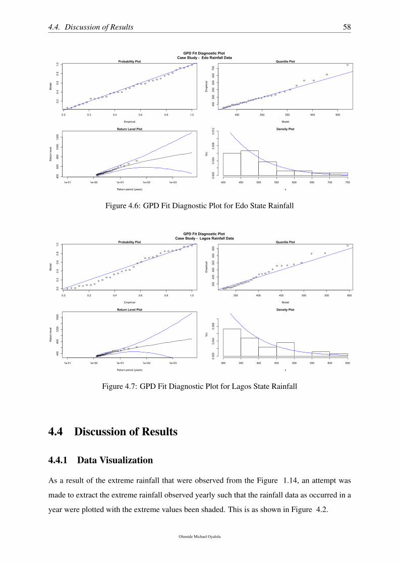
4.4. Discussion of Results 58
0.0 0.2 0.4 0.6 0.8 1.0
0.2
0.4
0.6
0.8
1.0
Probability Plot
Empirical
Mod
el
450 500 550 600 650
450
500
550
600
650
700
Quantile Plot
Model
Em
piric
al
1e-01 1e+00 1e+01 1e+02 1e+03
400
600
800
1000
1200
Return Level Plot
Return period (years)
Ret
urn
leve
l
Density Plot
x
f(x)
400 450 500 550 600 650 700 750
0.00
00.
004
0.00
80.
012
GPD Fit Diagnostic Plot Case Study - Edo Rainfall Data
Figure 4.6: GPD Fit Diagnostic Plot for Edo State Rainfall
0.0 0.2 0.4 0.6 0.8 1.0
0.0
0.2
0.4
0.6
0.8
1.0 Probability Plot
Empirical
Mod
el
350 400 450 500 550 600
350
400
450
500
550
600
Quantile Plot
Model
Em
piric
al
1e-01 1e+00 1e+01 1e+02 1e+03
400
800
1200
1600
Return Level Plot
Return period (years)
Ret
urn
leve
l
Density Plot
x
f(x)
300 350 400 450 500 550 600 650
0.00
00.
004
0.00
8
GPD Fit Diagnostic Plot Case Study - Lagos Rainfall Data
Figure 4.7: GPD Fit Diagnostic Plot for Lagos State Rainfall
4.4 Discussion of Results
4.4.1 Data Visualization
As a result of the extreme rainfall that were observed from the Figure 1.14, an attempt was
made to extract the extreme rainfall observed yearly such that the rainfall data as occurred in a
year were plotted with the extreme values been shaded. This is as shown in Figure 4.2.
Olumide Michael Oyalola
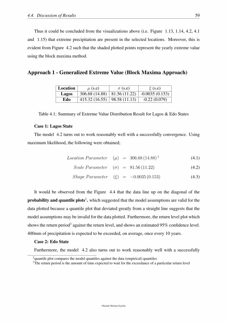
4.4. Discussion of Results 59
Thus it could be concluded from the visualizations above (i.e. Figure 1.13, 1.14, 4.2, 4.1
and 1.15) that extreme precipitation are present in the selected locations. Moreover, this is
evident from Figure 4.2 such that the shaded plotted points represent the yearly extreme value
using the block maxima method.
Approach 1 - Generalized Extreme Value (Block Maxima Approach)
Location µ (s.e) σ (s.e) ξ (s.e)Lagos 306.68 (14.88) 81.56 (11.22) -0.0035 (0.153)Edo 415.32 (16.55) 98.58 (11.13) -0.22 (0.079)
Table 4.1: Summary of Extreme Value Distribution Result for Lagos & Edo States
Case 1: Lagos State
The model 4.2 turns out to work reasonably well with a successfully convergence. Using
maximum likelihood, the following were obtained;
Location Parameter (µ) = 306.68 (14.88) 1 (4.1)
Scale Parameter (σ) = 81.56 (11.22) (4.2)
Shape Parameter (ξ) = −0.0035 (0.153) (4.3)
It would be observed from the Figure 4.4 that the data line up on the diagonal of the
probability and quantile plots2. which suggested that the model assumptions are valid for the
data plotted because a quantile plot that deviated greatly from a straight line suggests that the
model assumptions may be invalid for the data plotted. Furthermore, the return level plot which
shows the return period3 against the return level, and shows an estimated 95% confidence level.
400mm of precipitation is expected to be exceeded, on average, once every 10 years.
Case 2: Edo State
Furthermore, the model 4.2 also turns out to work reasonably well with a successfully
2quantile plot compares the model quantiles against the data (empirical) quantiles3The return period is the amount of time expected to wait for the exceedance of a particular return level
Olumide Michael Oyalola
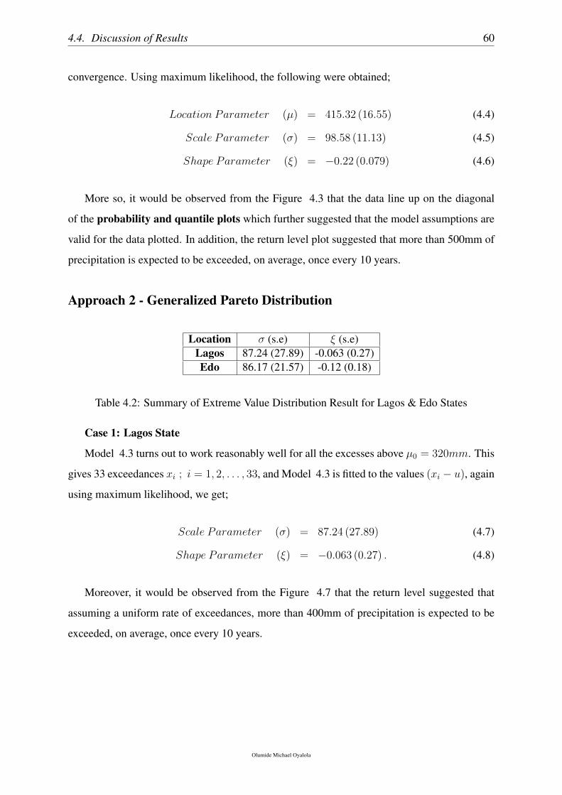
4.4. Discussion of Results 60
convergence. Using maximum likelihood, the following were obtained;
Location Parameter (µ) = 415.32 (16.55) (4.4)
Scale Parameter (σ) = 98.58 (11.13) (4.5)
Shape Parameter (ξ) = −0.22 (0.079) (4.6)
More so, it would be observed from the Figure 4.3 that the data line up on the diagonal
of the probability and quantile plots which further suggested that the model assumptions are
valid for the data plotted. In addition, the return level plot suggested that more than 500mm of
precipitation is expected to be exceeded, on average, once every 10 years.
Approach 2 - Generalized Pareto Distribution
Location σ (s.e) ξ (s.e)Lagos 87.24 (27.89) -0.063 (0.27)Edo 86.17 (21.57) -0.12 (0.18)
Table 4.2: Summary of Extreme Value Distribution Result for Lagos & Edo States
Case 1: Lagos State
Model 4.3 turns out to work reasonably well for all the excesses above µ0 = 320mm. This
gives 33 exceedances xi ; i = 1, 2, . . . , 33, and Model 4.3 is fitted to the values (xi − u), again
using maximum likelihood, we get;
Scale Parameter (σ) = 87.24 (27.89) (4.7)
Shape Parameter (ξ) = −0.063 (0.27) . (4.8)
Moreover, it would be observed from the Figure 4.7 that the return level suggested that
assuming a uniform rate of exceedances, more than 400mm of precipitation is expected to be
exceeded, on average, once every 10 years.
Olumide Michael Oyalola
4.4. Discussion of Results 61
Case 2: Edo State
Consequently, model 4.3 turns out to work reasonably well for all the excesses above
µ0 = 420mm. This also gives 33 exceedances xi ; i = 1, 2, . . . , 33, and Model 4.3 is fitted to
the values (xi − u), again using maximum likelihood, we get;
Scale Parameter (σ) = 86.17 (21.57) (4.9)
Shape Parameter (ξ) = −0.12 (0.18) . (4.10)
In addition, it would be observed from the Figure 4.6 that the return level suggested that
assuming a uniform rate of exceedances, more than 600mm of precipitation is expected to be
exceeded, on average, once every 10 years.
Olumide Michael Oyalola
Chapter 5
Summary, Conclusion and
Recommendation
5.1 Summary and Conclusion
Several complications occur in our environment both in urban and rural settlements as a result
of extreme events from extreme wind to extreme precipitation among others. These extreme
events often leave an indelible mark whenever they occur as they could result into loss of lives
and properties. Flooding, poor agricultural yields, famine, and even death are some of the catas-
trophic effects of extreme precipitation. Knowledge and information on the climatic variation
parameters in an environment is very vital for environmental study assessment and proper plan-
ning. As a result, the importance of knowing the future climatic variation parameters cannot
be under-estimated. This work is aimed at modeling climate change problem which includes
extreme precipitation that often results in flooding experiences in two states in Nigeria. In par-
ticular, The study will help decision makers to make informed decisions and to avoid or at least
reduce flood caused damage to life and property. In clear terms, the objectives of the work is to
assess the distributional pattern of rainfall in the study areas and model extreme rainfall events
using forty-one years of monthly data (1971−2012) based on extreme value theory for the two
cities.
Mathematical modeling approach was not employed because models from this approach are
chaotic1 in nature because of the deterministic nature of the models.1The existence of chaos means that even if we can perfectly describe the workings of some natural system
with a deterministic mathematical model, this does not necessarily mean that we can predict its behaviour farinto the future. If the system is chaotic, then no matter how accurately we measure its state, the error left in the
62
5.2. Recommendation 63
Two approaches of Extreme Value Theory were employed; Extreme Value Distribution (using
Block Maxima Technique) and Generalized Pareto Distribution (using Peak-Over-Threshold
Technique). The results as contained in the body of the work differed slightly for each of the
approach i.e. EVD2 and GPD3. This is because EVD is often plagued by loss of data which
could affect the result obtained from such a model.
In conclusion, as a result of the rising trend of extreme rainfall as communicated by the
return levels for each of the extreme modeling approach employed, there’s a strong evidence
of the existence of extreme precipitation in these study areas. The result of this study is in
consonance with works of some climatologists. The fundamental foundation of their findings
is based on high level of Carbon-dioxide i.e. CO2 that is resident in the atmosphere which
caused the atmosphere to hold more water vapour than it could originally. Moreover, whenever
the cloud if fully formed, it will result to rain and the rainfall could be extreme.
5.2 Recommendation
Truly, it’s a valid argument that not all extreme rainfall would result into flooding that could
affect both lives and properties. This is because the frequency (in terms of consistency) of the
extreme rainfall event and the present state of the drainage systems and other environmental
infrastructures that could be used to mitigate the occurrence of flooding need to be accessed.
Leveraging on the result of the analysis, it’s recommended that a continual and never ending
improvement of drainage systems and other environmental infrastructure need to be continually
accessed to combat the possible devastating effects that could be caused by extreme rainfall.
Moreover, the Ministry of Environment both at the Federal and State levels need to leverage on
the internet of things that could be used to generate environmental big data so as to make an
improved decision from the analyzed data.
measurement will always mean that the error in our predictions will eventually grow so large that they becomeuseless. This is exactly the problem that faces weather forecasters.
2Extreme Value Distribution3Generalized Pareto Distribution
Olumide Michael Oyalola
Bibliography
[1] A A L N Sarma, T V Lakshmi Kumar & K Koteswara Rao, Extreme Value Analysis of
Summer Monsoon Rainfall Over Andhra Pradesh, Indian Journal of Radio & Space Physics,
Vol. 39, February 2010, pp. 32-38
[2] Aaron Sayne, Climate Change Adaptation and Conflict in Nigeria. United States Institute
for Peace.
[3] Adalemo, LA (1983) Design for Development Inaugural lecture Delivered at the University
of Lagos, Wednesday Dec. 21, 1983.
[4] Albritton, Daniel, What Should Be Done in a Science Assessment In Protecting the Ozone
Layer: Lessons, Models, and Prospects, 1998.
[5] Andelin and John, Analysis of the Montreal Protocol, Staff report, U.S. Congress, Office
of Technology Assessment, Jan. 13, 1988.
[6] Angus Fergusson, Ozone depletion and climate change: understanding the linkages Mete-
orological Service of Canada 2011.
[7] Apata, T.G, Effects of Global Climate Change on Nigeria Agriculture: An Empirical Anal-
ysis. CBN Journal of Applied Statistics Vol. 2 No. 1.
[8] Aye G.C., Ater P.I, Impact of Climate Change on Grain Yield Variability in Nigeria: A
stochastic Production Model Approach. Mediterranean journal of Social Sciences. Vol 3
(16) December 2012.
[9] Angus Fergusson, Ozone depletion and climate change: understanding the linkages Mete-
orological Service of Canada 2011.
[10] Ayoade, J.O (1995). Climate and Human Welfare. Inaugural lecture Delivered at the Uni-
versity of Ibadan. Dept of Geography.
64
Bibliography 65
[11] Chen X, Wu J L, Wang L. Prediction of climate change impacts on stream flow of lake
bosten using artificial neural network model (in Chinese). J Lake Sci, 2005, 17: 207–212
[12] Chiara Ambrosino, Statistical downscaling with GLIMCLIM: Generalized Linear Mod-
elling of daily Climate sequences, downscaling training school, value, 6-15, November 2012,
Satander, Spain.
[13] Davison A.C., Discussion of the papers by Dankers and Feyen, Cooley, and Keef, Swiss
National Science Foundation.
[14] De Haan, L., Jansen, D. W., Koedijk, K. G., & De Vries, C. G.(1994). Safety first portfolio
selection, extreme value theory and long run asset risks. In J. Galambos, J. Lechner, & E.
Simiu (Eds.), Extreme value theory and applications (pp. 471– 488). Dordrecht: Kluwer.
[15] Edward N Lorenz, Climate Change as a Mathematical Problem. Journal of Applied Me-
teorology Vol. 9 No. 3, June 1970.
[16] Edward Omey, Fermin Mallor, Eulalia Naulart, An introduction to statistical modelling of
extreme values application to calculate extreme wind speeds, Hub Research Paper 2009/36;
Nov 2009
[17] Embrechts, P. (1999). Extreme value theory in finance and insurance.
[18] Embrechts, P. (2000a). Extreme value theory: Potentials and limitations as an integrated
risk management tool. Manuscript. Zurich, Switzerland: Department of Mathematics, ETH,
Swiss Federal Technical University.
[19] Embrechts, P. (2000b). Extremes and integrated risk management. London: Risk Books
and UBS Warburg.
[20] Embrechts, P., Kluppelberg, C., & Mikosch, C. (1997). Modeling extremal events for
insurance and finance. Berlin: Springer.
[21] Embrechts, P., Resnick, S., & Samorodnitsky, G. (1998). Extreme value theory as a risk
management tool. Manuscript. Zurich, Switzerland: Department of Mathematics, ETH,
Swiss Federal Technical University.
[22] FGN (2003). Nigeria’s First National Communication under the United Nations Frame-
work Convention on Climate Change (UNFCCC)
Olumide Michael Oyalola
Bibliography 66
[23] Holmberg M, Forsius M, Starr M, et al. An application of artificial neural networks to
carbon, nitrogen and phosphorus concentrations in three boreal streams and impacts of
climate change. Ecol Model, 2006, 195: 51–60
[24] Jan Beirlant, Yuri Goegebeur, Johan Segers, Jozef Teugels, Statistics of Extremes, Theory
& Application, Wiley Series in Probability and Statistics, 2004
[25] Jonathan Starkweather, Bayesian Generalized Linear Models in R, as published in bench-
marks RSS matters, January 2011.
[26] Kin C. Luk, J.E. Ball and A. Sharma, An Application of Artificial Neural Networks for
Rainfall Forecasting, Mathematical & Computer Modelling 33 (2001) 683-693.
[27] Liu Z L, Peng C H, Xiang W H, et al. Application of artificial neural networks in global
climate change and ecological research: An overview. Chinese Sci Bull, 2010.
[28] Raheem M.A., Yahya W.B., Obisesan K.O. (2015). A Markov Chain Approach on Pattern
of Rainfall Distribution. Journal of Environmental Statistics (2015) Vol 18, No 8.
[29] McNeil, A. J. (1997). Estimating the tails of loss severity distributions using extreme value
theory. ASTIN Bulletin, 27,1117 – 1137.
[30] McNeil, A. J. (1998). Calculating quantile risk measures for financial time series using
extreme value theory. Manuscript. Zurich, Switzerland: Department of Mathematics, ETH,
Swiss Federal Technical University.
[31] McNeil, A.J. (1999). Extreme value theory for risk managers. Internal modeling and CAD
II, Risk books. London, UK, pp. 93– 118.
[32] McNeil, A. J., & Frey, R. (2000). Estimation of tail-related risk measures for het-
eroscedastic financial time series: An extreme value approach. Journal of Empirical Finance,
7, 271– 300.
[33] Morrisette, Peter M. The Evolution of Policy Responses to Stratospheric Ozone Depletion.
Natural Resources Journal, vol. 29, 1995.
[34] Muller, U. A., Dacorogna, M. M., & Pictet, O. V. (1998). Heavy tails in high-frequency
financial data. In R. J. Adler, R. E. Feldman, & M. S. Taqqu (Eds.), A practical guide to
heavy tails: Statistical techniques and applications ( pp. 55 – 77). Boston: Birkhauser
Olumide Michael Oyalola
Bibliography 67
[35] Obisesan K.O., Lawal M., Bamiduro T.A., & Adelakun A.A.(2013). Data Visualization
and Change-point detection in Environmental Data: The Case of Water Pollution in Oyo
State Nigeria. Journal of Science Research (2013) Vol 12: 181-190.
[36] Ogundele, F.O., Ayo Omotayo, Taiwo, I.S. (2011): The dilemma of ozone layer depletion,
global warming and climate change in tropical countries; A review. Academic Research
International
[37] Ojo, A.O (1988). Urbanization and Thermal Problems in Tropical Cities: The Lagos
Experience, in Sada P.O and Odemerho, F.O (Eds). Environmental Issues and Management
in Nigeria.
[38] Ojo, A (1990). Aspects of the Urban Climate of Lagos, Nigeria. African Urban Quarterly
5 (1 and 2):76-90.
[39] Ojo, O (1977). The Climates of West Africa. Heinemann. London. PP218.
[40] Ojo, K, (1998). The Development of Urban and Regional Planning Laws in Lagos State:
A Planner’s Perspective.
[41] Ojo, K. (2000). Social Issues of Sustainable Water Supply Management in Nigeria. In
Odumosu, T, et al.
[42] Pictet, O. V., Dacorogna, M. M., & Muller, U. A. (1998). Hill, bootstrap and jackknife
estimators for heavy tails. In Taqqu, M. (Ed.), A Practical Guide to Heavy Tails: Statistical
Techniques and Applications ( pp. 283 – 310). Boston, MA: Birkhauser.
[43] Pieter J Aucamp, Lars Olof Bjorn, Questions and answers about the Environmental Ef-
fects of the Ozone Layer Depletion and Climate Change: 2010 Update. Environmental Ef-
fects Assessment Panel: 2010, United Nations Environmental Programme.
[44] Ramazan Gencay, Faruk Selcuk (2004). Extreme Value Theory and Value-at-Risk: Rel-
ative Performance in emerging markets, international journal of forecasting 20, (pp. 287 -
303).
[45] Richard .E. Chandler, Methodologies for probabilistic uncertainty assessment, Newton
institute satellite workshop, Exeter, September 2010.
Olumide Michael Oyalola
Bibliography 68
[46] Richard .E. Chandler, Advanced analytical methods for climate research, institute of at-
mospheric physics Beijing, 2001.
[47] Sivasakthivel.T, K.K.Siva Kumar Reddy, Ozone layer depletion and its effects: A review.
International Journal of Environmental Science and Development, Vol.2, No.1, February
2011
[48] Stephen O., E. Thomas Morehouse, Jr., and Alan Miller, The Military’s Role in Protection
of the Ozone Layer. Environmental Science and Technology, vol 28, no. 13, 1994.
[49] Zou Z H, Wang X L. The errors analysis for river water quality prediction based on BP
modeling (in Chinese). Acta Sci Circums, 2007, 27: 1038–1042
Olumide Michael Oyalola