Embed Size (px)
Citation preview

i
A SIMPLIFIED ANALYSIS OF THE VIBRATION OF VARIABLE LENGTH BLADE AS MIGHT BE USED IN WIND TURBINE SYSTEMS by KWANDA TARTIBU Dissertation submitted in fulfilment of the requirements for the degree MASTER OF TECHNOLOGY: Mechanical Engineering in the
FACULTY OF ENGINEERING
at the
CAPE PENINSULA UNIVERSITY OF TECHNOLOGY
Supervisor: MARK KILFOIL Co-supervisor: Dr ALETTA VAN DER MERWE Cape Town November 2008

ii
DECLARATION
I, KWANDA TARTIBU, declare that the contents of this thesis represent my own unaided
work, and that the dissertation/thesis has not previously been submitted for academic
examination towards any qualification. Furthermore, it represents my own opinions and not
necessarily those of the Cape Peninsula University of Technology.
Signed Date

iii
ABSTRACT
Vibration is an inherent phenomenon in dynamic mechanical systems. The work
undertaken in this thesis is to identify natural frequencies of a variable length blade.
Therefore designers can ensure that natural frequencies will not be close to the
frequency (or integer multiples) of the main excitation forces in order to avoid
resonance. For a wind turbine blade, the frequency range between 0.5 Hz and 30 Hz
is relevant. The turbine blade is approximated by a cantilever, therefore, it is fully
constrained where attached to a turbine shaft/hub. Flap-wise, edge-wise and torsional
natural frequencies are calculated.
The MATLAB program “BEAMANALYSIS.m” has been developed for the finite
element analysis of a one dimensional model of the beam. Similarly, a three
dimensional model of the beam has been developed in a finite element program
Unigraphics NX5. The results found using the MATLAB program are compared with
those found with NX5. Satisfactory agreement between the results is found for
frequencies up to almost 500 Hz. Additionally, the frequencies one might expect in an
experiment are identified.
Experimental modal analysis has been performed on a uniform and stepped beam
made of mild steel to extract the first five flap-wise natural frequencies. The results
found have been compared to numerical results and the exact solution of an Euler-
Bernoulli beam. Concurrence is found for the frequency range of interest. Although,
some discrepancies exist at higher frequencies (above 500 Hz), finite element
analysis proves to be reliable for calculating natural frequencies.
Finally, the fixed portion and moveable portion of the variable length blade are
approximated respectively by a hollow and a solid beam which can be slid in and out.
Ten different configurations of the variable length blade, representing ten different
positions of the moveable portion are investigated. A MATLAB program named
VARIBLADEANALYSIS.m was developed to predict natural frequencies. Similarly
three dimensional models of the variable length blade have been developed in the
finite element program Unigraphics NX5.

iv
ACKNOWLEDGEMENTS
I want to express my heartfelt appreciation to all individuals who have in one way or
the other contributed to the success of this project and my studies:
Firstly to my parents, you made me who I am and for that I thank them. I’d like to
thank also my family for their confidence in me that enabled me to complete this
work. I should also acknowledge some of my relatives for their motivation.
I received a Postgraduate Award scholarship to conduct my research and I am
grateful for this financial support. Dr. Oswald Franks is acknowledged for his help in
obtaining funding for me.
Part of the thesis work was done while I was performing my experiment at IDEAS
Solutions. It is a pleasure to thank Farid Hafez-Ismail for his support.
Finally, I would like to sincerely thank my supervisors. Mark Kilfoil and Dr. Van Der
Merwe were ideal supervisors. They gave me the direction I needed whilst allowing
me the freedom I desired. Their experience and knowledge was an asset. I can only
hope that some of it wore off onto me.

v
DEDICATION
To my family

vi
TABLE OF CONTENTS DECLARATION ..................................................................................................................................... ii
ABSTRACT ........................................................................................................................................... iii
ACKNOWLEDGEMENTS ................................................................................................................... iv
DEDICATION ......................................................................................................................................... v
TABLE OF CONTENTS ...................................................................................................................... vi
LIST OF FIGURES ............................................................................................................................... ix
LIST OF TABLES ................................................................................................................................. xi
LIST OF APPENDICES ...................................................................................................................... xii
GLOSSARY ......................................................................................................................................... xiii
CHAPTER 1 ...........................................................................................................................................1
INTRODUCTION ...................................................................................................................................1
1.1 Thesis Structure ....................................................................................................................1
1.2 Wind turbine technology and design concepts .................................................................2
1.2.1 Wind energy ............................................................................................................ 2
1.2.2 Types of wind turbines ............................................................................................. 3
1.2.3 Components of wind energy systems ...................................................................... 3
1.2.4 Working principle of a wind turbine .......................................................................... 6
1.3 Wind turbine power output and variable length blade concept ................................. 8
1.4 Vibration and Resonance .................................................................................................. 12
1.5 Problem statement ............................................................................................................. 14
1.6 Aims and objectives ........................................................................................................... 14
CHAPTER 2 ........................................................................................................................................ 16
LITERATURE REVIEW ..................................................................................................................... 16
2.1. Vibration ............................................................................................................................... 16
2.1.1 Classification of previous research ........................................................................ 16
2.1.2 Presenting natural frequency data ......................................................................... 16
2.2 Beam models ...................................................................................................................... 18
2.3 Rotating beams/ blades..................................................................................................... 19
2.4 Extendable blades .............................................................................................................. 20
2.5 Summary and Conclusion ................................................................................................. 21
CHAPTER 3 ........................................................................................................................................ 22
STRUCTURAL DYNAMIC CONSIDERATIONS IN WIND TURBINE DESIGN ........................ 22
3.1. Introduction .......................................................................................................................... 22
3.2. Fundamentals of vibration analysis ................................................................................. 22
3.3. Turbine loadings and their origins ................................................................................... 26
3.4. Rotor excitations and resonances ................................................................................... 28
3.5. Beam: theory and background ......................................................................................... 29

vii
3.5.1 Equation of motion for a uniform beam .................................................................. 29
3.5.2 Natural frequencies and modes shapes ................................................................ 31
3.6 Summary ............................................................................................................................. 33
CHAPTER 4 ........................................................................................................................................ 34
EXPERIMENTAL VERIFICATION ................................................................................................... 34
4.1. Introduction .......................................................................................................................... 34
4.2 Theory of experimental modal analysis .......................................................................... 34
4.2.1 Discrete blade motion ............................................................................................ 34
4.2.2 Extraction of modal properties ............................................................................... 36
4.3 Experimental setup ............................................................................................................ 38
4.3.1 Measurement method............................................................................................ 38
4.3.2 Exciting modes with impact testing ........................................................................ 39
4.3.3 Determination of natural frequencies ..................................................................... 39
4.4 Modal analysis technique .................................................................................................. 43
4.5 Summary ............................................................................................................................. 43
CHAPTER 5 ........................................................................................................................................ 44
NUMERICAL SIMULATION .............................................................................................................. 44
5.1 Introduction .......................................................................................................................... 44
5.2 Modelling theory ................................................................................................................. 44
5.3 Euler-Bernoulli beam element .......................................................................................... 44
5.4 One-dimensional models: MATLAB ................................................................................ 47
5.4 Three-dimensional model: NX5 ....................................................................................... 49
5.5 Summary ............................................................................................................................. 50
CHAPTER 6 ........................................................................................................................................ 51
RESULTS AND DISCUSSION ......................................................................................................... 51
6.1 Introduction .......................................................................................................................... 51
6.2 Convergence test for finite element models ................................................................... 51
6.3 Results for uniform beam .................................................................................................. 53
6.3.1 Exact solution ........................................................................................................ 54
6.3.2 MATLAB program .................................................................................................. 56
6.3.3 NX5 model ............................................................................................................ 56
6.3.4 Experimental modal analysis results ...................................................................... 57
6.3.5 Comparison of natural frequencies ........................................................................ 58
6.4 Results for stepped beam ................................................................................................. 60
6.4.1 MATLAB program .................................................................................................. 60
6.4.2 NX5 model ............................................................................................................ 61
6.4.3 Experimental modal analysis results ...................................................................... 62
6.4.4 Comparison of natural frequencies ........................................................................ 63

viii
6.5 Results for variblade .......................................................................................................... 64
6.5.1 NX5 and MATLAB results comparison for variblade .............................................. 64
6.5.2 Influence of blade length ....................................................................................... 67
6.5.3 Effect of rotation .................................................................................................... 68
6.6. Contextualization of the findings ...................................................................................... 69
CHAPTER 7 ........................................................................................................................................ 71
CONCLUSIONS AND RECOMMENDATIONS FOR FUTURE WORK ..................................... 71
7.1 Conclusions ......................................................................................................................... 71
7.2 Recommendations ............................................................................................................. 72
7.2.1 Finite element analysis .......................................................................................... 72
7.2.2 Experimental modal analysis ................................................................................. 73
BIBLIOGRAPHY/REFERENCES ..................................................................................................... 74
APPENDICES ..................................................................................................................................... 80

ix
LIST OF FIGURES
Figure 1.1: Two basic wind turbines, horizontal axis and vertical axis .................................... 3
Figure 1.2: Major components of a horizontal axis wind turbine ............................................. 4
Figure 1.3: Hub options .......................................................................................................... 5
Figure 1.4: Lift and drag on the rotor of a wind turbine ........................................................... 6
Figure 1.5: Blade element force-velocity diagram .................................................................. 7
Figure 1.6: Power output from a wind turbine as a function of wind speed ............................. 8
Figure 1.7: Wind turbine schematic ........................................................................................ 9
Figure 1.8: Wind turbine with variable length blades with the blades extended and retracted
............................................................................................................................................ 12
Figure 1.9: Terms used for representing displacements, loads and stresses on the rotor. ... 13
Figure 1.10: Edge-wise and flap-wise vibrations of the blade ............................................... 15
Figure 2.1: Campbell Diagram for a hypothetical wind turbine ............................................. 17
Figure 2.2: Mod-1 system natural frequencies ..................................................................... 18
Figure 2.3: Typical fibreglass blade cross-section ................................................................ 19
Figure 3.1: Single degree of freedom mass-spring-damper system ..................................... 22
Figure 3.2: Quasi-static response. Solid line: excitation force, and dashed line: simulated
response. ............................................................................................................................. 23
Figure 3.3: Resonant response. Solid line: excitation force, and dashed line: simulated
response. ............................................................................................................................. 23
Figure 3.4: Inertia dominated response. Solid line: excitation force, and dashed line:
simulated response. ............................................................................................................. 24
Figure 3.5: Frequency response function. Upper figure: magnitude versus frequency, and
lower figure: phase lag versus frequency. ............................................................................ 25
Figure 3.6: Sources of wind turbine loads ............................................................................ 27
Figure 3.7: Exciting forces and degrees of vibrational freedom of a wind turbine ................. 28
Figure 3.8: Soft to stiff frequency intervals of a three-bladed, constant rotational speed wind
turbine ................................................................................................................................. 29
Figure 3.9: A beam in bending ............................................................................................. 30
Figure 4.1: The degrees of freedom for a wind turbine blade ............................................... 35
Figure 4.2: Impact testing .................................................................................................... 39
Figure 4.3: Dimensions of the uniform beam used in the experiment ................................... 40
Figure 4.4: Dimensions of the uniform and stepped beam used in the experiment ............... 40
Figure 4.5: Clamping details ................................................................................................ 41
Figure 4.6: Impact hammer .................................................................................................. 41

x
Figure 4.7: Accelerometer .................................................................................................... 42
Figure 4.8: Dynamic signal analyser .................................................................................... 42
Figure 5.1: Euler-Bernoulli beam element ............................................................................ 45
Figure 5. 2: Variblade ........................................................................................................... 48
Figure 5.3: Ten configurations of variblade .......................................................................... 49
Figure 5.4: Simulation part with constraint ........................................................................... 50
Figure 6.1: MATLAB program convergence test results ....................................................... 52
Figure 6.2: NX convergence test results .............................................................................. 53
Figure 6.3: Uniform beam deflections .................................................................................. 57
Figure 6.4: Measured transfer functions imported into Vib-Graph ........................................ 58
Figure 6.5: Stepped beam deflections .................................................................................. 61
Figure 6.6: Measured transfer functions imported into Vib-Graph ........................................ 62
Figure 6.7: Flap-wise, edge-wise and torsional deflection for configuration 1 ....................... 65
Figure 6.8: Flap-wise, edge-wise and torsional deflection for configuration 5 ....................... 65
Figure 6.9: Flap-wise, edge-wise and torsional deflection for configuration 10 ..................... 66
Figure 6.10: MATLAB and NX5 results comparison ............................................................. 67
Figure 6.11: Natural frequencies .......................................................................................... 68

xi
LIST OF TABLES Table 3.1: Frequency equation and mode shape for the transverse vibration of a cantilever 33
Table 6.1: Material and geometric properties of the beam ................................................... 52
Table 6.2: Material and geometric properties of the uniform beam ....................................... 53
Table 6.3: MATLAB natural frequencies............................................................................... 56
Table 6.4: NX5 natural frequencies ...................................................................................... 57
Table 6.5: Measured and computed natural frequencies ...................................................... 59
Table 6.6: Material and geometric properties of the stepped beam ...................................... 60
Table 6.7: MATLAB natural frequencies............................................................................... 61
Table 6.8: NX5 natural frequencies ...................................................................................... 62
Table 6.9: Measured and computed natural frequencies ...................................................... 63
Table 6.10: Material and geometric properties of the variblade ............................................ 64
Table 6.11: Computed natural frequencies (NX5) ................................................................ 67
Table 6.12: Computed natural frequencies (MATLAB) ......................................................... 68
Table 6.13: Natural frequencies of the rotating variblade ..................................................... 69

xii
LIST OF APPENDICES
Appendix A: Instrument specifications ................................................................................. 80
Appendix B: MATLAB program for uniform and stepped beam ............................................ 82
Appendix C: MATLAB Program explanation: 3 elements mesh ............................................ 88
Appendix D: MATLAB program for VARIBLADE ................................................................ 101
Appendix E: NX5 results .................................................................................................... 109
Appendix F: NX5 and MATLAB results comparison ........................................................... 119

xiii
GLOSSARY
Terms/Acronyms/Abbreviations
Definition/Explanation
a’ and a
Rotational and axial interference factors
A Cross-section area
BC
Before Christ
C
Damping matrices
PC
Power capture efficiency
BetzPC .
Betz’s Coefficient
tC
Rotor thrust coefficient
D
Resultant drag force
DOF
Degree of freedom
E
Modulus of elasticity
f
Natural frequency
0,1f
Natural frequency for the non-rotating blade
Rf ,1 Natural frequency for the rotating blade
)(tF
Harmonic excitation force
),( txf
External force
)(ωF
Fourier transform of a force )(tf
FRF
Frequency response function
tF
Thrust load
G
Shear modulus
HAWT
Horizontal axis wind turbine
ijH
Transfer function
I
Moment of inertia
KE
Kinetic energy
L Length of beams

xiv
fL
Resultant lift force
M
Mass matrices
),( txM
Bending moment
bN
Number of rotor blades
P
Power
PE
Potential energy
Pr
Rated output of the turbine
r
Radius
S
Stiffness matrices
)(xS i
Shape function
T
Thickness of beams
U
Motion of the cross section
PU
Axial component of wind
TU
Rotational component of wind
xU
Edge-wise deflection
yU
Flap-wise deflection
V
Wind speed
VAWT
Vertical axis wind turbine
Vc
Cut in speed
Vf
Furling speed
Vr
Rated speed
0V
Upstream undisturbed wind speed
tipV
Tip speed
wV
Relative wind vector
),( txV
Shear force
W Width of beams

xv
Wh
Wall thickness
),( txw
Transverse vibrations
)(ωX
Fourier transform of the response )(tx
Angle of attack
v
Poisson’s ratio
1v , 2v
Displacements of the endpoints of the beam element
kv
Eigenvectors
1 , 2
Rotational displacements at the end of the beam element
Section pitch angle
t
Torsional deflection
Angle of relative wind velocity
Air density
Torque
P
Power train efficiency
Rotating speed of the rotor
r
Rotor angular velocity
k
Eigenvalues
k
Damping factor
k
Logarithmic decrements
1
CHAPTER 1
INTRODUCTION
1.1 Thesis Structure
The research described in this thesis is directed towards a better understanding of
the structural dynamic characteristics of a variable length blade for wind turbines.
Three basic shapes representing the wind turbine blade have been investigated:
A uniform beam;
a stepped beam and,
a variable length blade (variblade).
Chapter 1 includes background on wind turbines in general, partly for the purpose of
contextualising the problem and making the thesis accessible to non-specialists. This
chapter leads to the concept of a variable length blade for wind turbines and to the
goal of the research.
In Chapter 2, a literature survey is given.
In Chapter 3, structural dynamic considerations related to wind turbine blade are
presented. Excitations and resonances have been described. Moreover, the
frequency equation and mode shapes for an uniform Euler-Bernoulli beam has been
investigated.
Chapter 4 describes experimental modal analysis performed on a uniform beam and
stepped beam for three purposes:
To gain insight into experimental verification;
to measure flap-wise natural frequencies and,
to validate numerical results.
In Chapter 5, finite element analysis is discussed:
To gain insight into the numerical simulation by developing a MATLAB program
for a one-dimensional model and three-dimensional model in NX5;
to calculate natural frequencies of a uniform beam and a stepped beam and,
to calculate natural frequencies of a composite variblade.
Chapter 6 presents, compares and discusses the results.
Chapter 7 summarises the contribution of this thesis. The chapter also includes
recommendations for further research.
Appendices present instruments specifications, the purpose written MATLAB codes
and numerical results.

2
1.2 Wind turbine technology and design concepts
1.2.1 Wind energy
“A wind turbine is a machine which converts the wind’s kinetic energy into mechanical
energy. If the mechanical energy is used directly by machinery, such as a pump or
grinding stones, the machine is usually called a windmill. If the mechanical energy is
converted to electricity, the machine is described as wind generator, or more
commonly a wind turbine (wind energy converter WEC)” (Burton et al., 2008). Wind
turbines are classified according to their size and power output. Small wind turbines
supply energy for battery charging systems and large wind turbines, grouped on wind
farms supply electricity to a grid. Whatever the size or output, the basic arrangement
of electricity generating turbines remains identical.
Wind energy has been used for centuries. The first field of application was to propel
boats along the River Nile around 5000 BC (United States Department of Energy,
2005). By comparison, wind turbines are a more modern invention. The first simple
windmills were used in Persia as early as the seventh century for irrigation purposes
and for milling grain (Edinger & Kaul, 2000). The modern concept of windmills began
around the time of the industrial revolution. However, as the industrial revolution
proceeded, industrialisation sparked the development of larger wind turbines to
generate electricity. The first electricity generating wind turbine was developed by
Poul la Cour in 1897 (Danish Wind Turbine Manufacturers Association, 2003).
“Today, wind energy is the world’s fastest growing energy technology”. Wind energy
installations have surged from a capacity of less than 2 GW in 1990 to about 94 MW
(October 2008) (Wind Power Monthly, 2008).
An abundance of wind energy resources, vast tracts of open land and electricity
distribution infrastructure give South Africa a potential to become a “wind
powerhouse” (Kowalik & Coetzee, 2005). According to wind power revolution
pioneers in South Africa, “the Western Cape has prevailing winds from the south-east
and north-west and they often blow during peak electricity consumption periods.
These winds have a potential to generate 10 times the official national wind energy
estimates” (Kowalik & Coetzee, 2005). There are two pilot wind power projects in
South Africa: At Klipheuwel and Darling, both in the Western Cape (Kowalik &
Coetzee, 2005).

3
1.2.2 Types of wind turbines
The most common turbine design is the horizontal axis wind turbine (HAWT). There
are also vertical axis wind turbines (VAWT). The HAWT is more practical than the
VAWT and is the focus of remainder of the discussion here for the following reasons
(Manwell et al, 2004):
Horizontal axis wind turbines are more efficient, since the blades always move
perpendicularly to the wind, receiving power through the entire rotation. In contrast,
all vertical axis wind turbines require aerofoil surfaces to backtrack against the wind
for part of the cycle. Backtracking against the wind leads to inherently lower
efficiency.
Vertical axis wind turbines use guy wires to keep them in place and put stress
on the bottom bearing as all the weight of the rotor is on the bearing. Guy wires
attached to the top bearing increase downward thrust during wind gusts. Solving this
problem requires a superstructure to hold a top bearing in place to eliminate the
downward thrusts of gusts in guy wired models.
Figure 1.1: Two basic wind turbines, horizontal axis and vertical axis
(Adapted from Ontario Ministry of Energy, 2008)
1.2.3 Components of wind energy systems
The principal subsystems of a typical horizontal axis wind turbine are shown in
Figure 1.2. These include: rotor; drive train, nacelle and main frame, including wind
turbine housing and bedplate, yawing system, tower and foundation, machine
controls, alternator and balance of the electrical system (Manwell et al, 2004).

4
Figure 1.2: Major components of a horizontal axis wind turbine
(Adapted from Manwell et al, 2004)
The rotor
The rotor (the hub and blades of a wind turbine) is often considered to be the most
important component from performance and overall cost standpoints. The rotor
assembly may be placed in the following two directions (Manwell et al, 2004):
Upwind of the tower and nacelle, therefore, it receives unperturbed wind and
must be actively yawed by an electrical motor.
Downwind of the tower, this enables self-alignment of the rotor with the wind
direction (yawing), but the tower causes deflection and turbulence before the
wind arrives at the rotor (tower shadow).
Some rotors include a pitch drive. This system controls the pitch of the blades to
achieve an optimum angle to handle the wind speed and the desired rotation speed.
For lower wind speed, an almost perpendicular pitch increases the energy harnessed
by the blades; at high wind speed, a parallel pitch minimizes the blade surface area
and prevents over speeding the rotor. Typically one motor controls each blade.
Many types of materials are used in wind turbines construction. The following list
provides materials in general use for blade manufacture (Burton et al, 2004):
Wood (including laminated wood composites)
Alternator

5
Synthetic composites (usually a polyester or epoxy matrix reinforced by glass
fibres)
Metals (predominantly steel or aluminium alloys)
The drive train
The drive train consists of the rotating parts of the wind turbine (exclusive of the
rotor). These, typically, include shafts, gearbox, bearings, a mechanical brake and an
alternator. Blades are connected to the main shaft and ultimately the rest of the drive
train by the hub. There are three basic types of hub design which have been applied
in modern horizontal wind turbines (Figure 1.3):
Rigid hubs;
teetering hubs and,
hinged hubs.
Figure 1.3: Hub options
(Adapted from Manwell et al, 2004)
The nacelle and yaw system
This category includes the wind housing, machine bedplate or mainframe and the
yaw orientation system. The main frame provides for the mounting and proper
alignment of the drive train components. A yaw orientation system for upwind turbines
is required to ensure the rotor shaft remains parallel with the wind.
Tower and the foundation
This includes the tower structure and supporting foundation. The tower of a wind
turbine supports the nacelle assembly and elevates the rotor to a height at which the
wind velocity is significantly greater and less perturbed than at ground level.

6
Controls and Balance of electrical system
A wind turbine control system includes the following components: Sensors,
controllers, power amplifiers and actuators. In addition to the alternator, the wind
turbine utilises a number of other electrical components such as cables, switchgear,
transformers and possibly electronic power converters, power factor correction
capacitors, yaw and pitch motors.
Alternator
The most common types encountered in wind turbines are induction and synchronous
alternators. In addition, some smaller turbines use DC machines (generators).
1.2.4 Working principle of a wind turbine
Modern wind turbines work on an aerodynamic lift principle, just as do the wings of an
aeroplane. The wind does not "push" the turbine blades, but instead, as wind flows
across and passes a turbine blade, the difference in pressure on either side of the
blade produces a lifting force, causing the rotor to rotate and cut across the wind as
illustrated in Figure 1.4.
Figure 1.4: Lift and drag on the rotor of a wind turbine
(Adapted from Aerowind Systems, n.d.)
A section of a blade at radius r is illustrated in Figure 1.5, with the associated
velocities, forces and angles indicated.

7
The relative wind velocity vector at radius r, denoted by wV , is the resultant of
the axial component PU and the rotational component TU
The axial velocity PU is reduced by a component 0V a, because of the wake
effect or retardation imposed by the blades, where 0V is the upstream
undisturbed wind speed.
The rotational component is the sum of the velocity from to the blade’s motion,
r , and the swirl velocity of the air, r a’.
The a’ and a terms represent rotational and axial interference factors respectively.
= Section pitch angle
= Angle of attack
= + = Angle of relative wind velocity
fL = Resultant lift force
D = Resultant drag force
Figure 1.5: Blade element force-velocity diagram
(Adapted from Lee & Flay, 2000)
Wind turbines are designed to work between certain wind speeds. When the wind
speed increases above a certain velocity, known as the “cut in” speed (typically about
3 to 4 m/s) the turbine will begin to generate electricity and continue to do so until the
wind speed reaches “cut out” speed (about 25 m/s). At this point the turbine shuts
down, rotates the blades out of the wind and waits for the wind speed to drop to a
suitable speed which will allow the turbine to restart. The “cut out” speed is
wV
fL

8
determined by any particular machine’s ability to withstand high wind (Research
Institute for Sustainable Energy, 2006). The turbine will have an optimum operating
wind speed (“rated speed”) at which maximum output will be achieved; typically about
13 to 16 m/s. The “rated speed” is the wind speed at which a particular machine
achieves its design output power. Above this speed it may have mechanisms to
maintain the output at a constant value with increasing wind speed (see Figure 1.6).
Figure 1.6: Power output from a wind turbine as a function of wind speed
(Adapted from Research Institute for Sustainable Energy, 2006)
Figure 1.6 details an ideal power curve for a small wind turbine with a furling
mechanism. The machine starts to produce power at Vc (cut in speed), it reaches its
rated power at Vr (rated speed) and shuts down to avoid damage at Vf (the furling
speed). Pr is the rated output of the turbine. This curve is typical of a horizontal-axis
two- or three-bladed machine. The curve is ideal, as the machine follows the peak
power available from the wind until it reaches alternator capacity, then regulates to
maintain a steady output until shut down.
1.3 Wind turbine power output and variable length blade concept
The power P of the wind that flows at speed V through an area A is given by the
expression (Ackermann, 2000):
P = 3
2
1AV Equation 1.1
= air density
A = area is the cross-sectional area of the flowing air
V = wind speed

9
Figure 1.7: Wind turbine schematic
(Adapted from Ontario Ministry of Energy, 2008)
The power in the wind is the total available energy per unit time. This power is
converted into the mechanical-rotational energy of the wind turbine rotor, resulting in
a reduced speed of the air mass.
There are three basic physical laws governing the amount of energy available from
the wind (Research Institute for Sustainable Energy, 2006).
Firstly, the power generated by a turbine is proportional to the cube of wind
speed. For example if the wind speed doubles, the power available increases
by a factor of eight; if the wind speed triples then 27 times more power is
available. Conversely, there is little power in the wind at low speed;
secondly, power available is directly proportional to the swept area of the
blades. Hence, the power is proportional to the square of the blade length. For
example, doubling the blade length will increase the potential for power
generation four times; tripling blade length increases the potential for power
generation nine times and,
finally, power in the wind cannot be extracted completely by a wind turbine.
The theoretical optimum for utilizing the power by reducing its velocity was
first discovered by Betz in 1926. He argued the theoretically maximum power
to be extracted from the wind is given by (Ackermann, 2000):

10
BetzP = 2
1 A
3V BetzPC . =2
1 A
3V 0.59 Equation 1.2
Hence, even if power extraction without any loss was possible, only 59% of the power
in the wind could be utilized by a wind turbine (Ackermann, 2000).
The energy capture at low wind speed (below Vc in Figure 1.6) is proportional to the
rotor’s swept area, which in turn is proportional to the rotor diameter squared. From
Equation 1.2, it can be seen that significant increases in the output power can be
achieved only by increasing the swept area of the rotor, or locating the wind turbines
on sites with higher wind speeds. If a large rotor relative to the size of the alternator is
suddenly acted upon by high winds, it might produce more electricity than the
alternator can absorb and additionally overstress the structure. Conversely, in time of
low winds, if a rotor is too small for the alternator, wind turbine efficiency may be low
and the system only achieves a small proportion of its energy producing potential.
What is required is a wind turbine able to adjust to handling varying wind speed
conditions efficiently, while attempting to maximise energy capture for a given support
structure. This constitutes the basic concept of the variable length blade for wind
turbine. The variable length blade considered here:
Allows the rotor to yield significant increases in power capture through
increase of its swept area and,
provides a method of controllably limiting mechanical loads, such as torque,
thrust, blade lead-lag (in-plane), blade flap (out-of-plane), or tower top bending
loads, delivered by the rotor to the power train below a threshold value.
Achieving this goal enables a single extended rotor blade configuration to
operate within an adjustable load limit.
The torque ( ) delivered by the rotor to the power train is given by (U.S. Patent No
6,726,439 B2, 2004)
=r
P
Equation 1.3
where P is power and r is rotor angular velocity. When the angular velocity is
limited by tip speed ( tipV ), the torque can be shown to be related to the rotor radius,
r , as
= rV
P
tip
Equation 1.4

11
To hold torque below a set design limit, lim , the maximum power the rotor can
produce, while remaining within the tip speed and torque limit, can be seen to be
inversely proportional to the rotor radius, as given by (U.S. Patent No 6,726,439 B2,
2004)
r
VP
tiplim
max
Equation 1.5
Then, if we observe that power for a given wind speed V and density is given as
(U.S. Patent No 6,726,439 B2, 2004)
PCVrP 32
2
1 Equation 1.6
where PC is the power capture efficiency of a given rotor geometry at a specified
rotor angular velocity and wind speed. The relationship between rotor radius and wind
velocity can be shown to be
3lim21
P
tip
C
V
Vr
Equation 1.7
This means as wind speed increases, the rotor radius must decrease almost as much
as the inverse of this increase ( PC may vary slightly as this occurs) to remain within
torque limitations. However, in practice a wind turbine will measure its power output
(via electrical current for instance) and rotor speed. Therefore, one may determine the
appropriate radius by (U.S. Patent No 6,726,439 B2, 2004)
P
Vr
Ptip lim Equation 1.8
where P is the approximate power train efficiency at a given observed output power,
P. The thrust load ( tF ) is calculated as (U.S. Patent No 6,726,439 B2, 2004)
tt CVrF 22
2
1 Equation 1.9
where tC is the rotor thrust coefficient at a given flow velocity, rotor speed and blade
pitch angle. If the thrust is held below the nominal limit ( lim,tF ), then the rotor radius
can be seen to vary as
t
t
C
F
Vr
lim,21 Equation 1.10
where the rotor radius must decrease nearly as much as the inverse of an increase in
velocity, similar to Equation 1.7.

12
Variable length blade (variblade) is possible if there are two parts: an inboard portion
and an outboard part. The outboard portion is mounted inside the inboard portion,
guided to be telescoped relative to the inboard portion. An actuator system moves the
outboard portion of the blade radially to adjust the wind turbine’s rotor diameter. A
controller will measure electrical power and retract the outboard portion of the blade
when rated power is reached, or nearly reached (Pasupulati et al., 2005). However,
the mechanism is beyond the scope of this research. Design manufacture and testing
of variable length blade for wind turbine is being undertaken by another student.
Figure 1.8: Wind turbine with variable length blades with the blades extended and retracted
(Adapted from Pasupulati et al., 2005)
1.4 Vibration and Resonance
The term vibration refers to the limited reciprocating motion of a particle or an object
in an elastic system (Manwell et al, 2004). In most mechanical systems, vibrations are
undesirable and dangerous if the vibratory motion becomes excessive. However, in a
rotating system, such as in a wind turbine, vibrations are unavoidable. Wind turbines
are partially elastic structures and operate in an unsteady environment that tends to
result in vibrating response. Therefore, the interplay of the forces from the external
environment, primarily because of the wind and the motion of the various components
of the wind turbine, results not only in the desired energy production from the turbine,
but also in stresses in its constituent materials. For the turbine designer these
stresses are of primary concern, as they directly affect the strength of the turbine and
how long it will last. In order to be viable for providing energy, a wind turbine must:
Produce energy;
survive and,

13
be cost-effective.
That means that the turbine design must not only be functional in terms of extracting
energy. It must also be structurally sound so that it can withstand the loads it
experiences and the costs to make it structurally sound must be commensurate with
the value of energy produced.
Hence, a key to good wind turbine design is to minimize vibrations by avoiding
resonance. Resonance is a phenomenon occurring in a structure when an exciting or
forcing frequency equals or nearly equals one of the natural frequencies of the
system (Burton et al., 2004). It is characterized by a large increase in displacements
and internal loads. Damping reduces these displacements and loads. That is why
some turbines blades are partially filled with a foam material, which helps dampen the
vibration of a blade in turbulent wind conditions (Composites world, 2008). This
reduces the chances of the blade generating a resonant response.
In a rotating system the exciting frequencies are integer multiples of the rotational
speed. The designer must ensure the resonant frequencies are not excited
excessively. Although dynamic loads on the blades will, in general, also excite the
tower dynamics, in this study, tower head motion is excluded from consideration, in
order to focus exclusively on blade dynamic behaviour.
For a wind turbine blade, the deflections of interest are lateral translations (flap-wise,
edge-wise) and cord rotation (about the blade’s longitudinal axis) (Hau, 2000). Most
directions and loads referred to are illustrated in Figure 1.9. The chordwise direction
is often called edge-wise direction.
Figure 1.9: Terms used for representing displacements, loads and stresses on the rotor.
(Adapted from Hau, 2000)

14
The design of a wind turbine structure involves many considerations such as
strength, stability, cost and vibration. Reduction of vibration is a good measure for a
successful design in blade structure (Maalawi & Negm 2002). Dealing with vibration in
an early phase of the design process avoids costly modification of a prototype after
detection of a problem. Therefore, both experimental and theoretical methods are
required for studying the structural characteristics of turbine blades in order to avoid
vibration problems.
1.5 Problem statement
The amplitude of the generated vibrations of a wind turbine blade depends on its
stiffness (Jureczko et al. 2005) which is a function of material, design and size. One
issue a variable length blade design presents to blade designers is that of structural
dynamics. A wind turbine blade has certain characteristic natural frequencies and
mode shapes which can be excited by mechanical or aerodynamic forces. Variable
length blade design presents additional challenges as stiffness and mass distribution
change as the moveable blade portion slides in and out of the fixed blade portion.
This vibration analysis has the aim of verifying dynamic stability and the absence of
resonance within the permissible operating range. Although material properties are an
important factor, this analysis does not include the effect of material choice.
However, it provides tools which enable wind turbine blade designers to investigate
the effect of material choices.
1.6 Aims and objectives
The previous section indicated that vibration problems in a variable length blade
results in two needs:
To verify the dynamic stability and absence of resonance and
to understand structural dynamic characteristics.
In engineering, there is a prerequisite for accurate numerical models. Computational
fluid dynamics for new aircraft, the finite element method for structural analysis and
finite difference programs for heat transfer are examples of numerical methods
essential to a design process. In such applications, numerical models provide design
performance prediction which facilitates making decisions early in the design process,
thus saving money and ultimately delivering a better product. Numerical models allow

15
the comparison of design alternatives, normally prohibitively expensive to conduct
using manufactured prototypes.
The goals of this project are:
To develop computer models of a variblade. The model chosen is of a single
blade fitted with a telescoping mechanism to vary length;
to calculate the natural frequencies of the variblade with the computer models for
the two main vibration directions (flap-wise and edge-wise);
Figure 1.10: Edge-wise and flap-wise vibrations of the blade
(Adapted from Grabau & Petersensvej, 1999)
to gain insight into experimental modal analysis, finite element analysis and
analytical methods;
to compare the output of a computer model with the experimental data and,
to use the computer model to make recommendations on design and operation of
variblades.

16
CHAPTER 2
LITERATURE REVIEW
2.1. Vibration
2.1.1 Classification of previous research
Vibration in wind turbines is a recognised phenomenon. As far back as the Middle
Ages, the post windmill of that time was also called a “rocking mill”, as the mounting
of the entire mill house on a trestle led to a rocking motion. This drawback then
became the stimulus to continued development, from which evolved the more stable
Dutch windmill which ran more smoothly (Hau, 2000).
Patil et al. classified the previous research on the structural dynamics of HAWTs into
three groups:
The first group of studies analyzed isolated blades;
studies on rotor/tower or rotor/yaw coupling problems form the second group and,
a third group of studies considers the complete system dynamics of HAWTs.
An isolated variable length blade constitutes the focus of this research and this study
fits quite well in the first group of studies.
2.1.2 Presenting natural frequency data
Historically, the most basic requirement of structural dynamics analysis was to identify
structural resonances and ensure they were not close to the frequency or harmonics
of main rotor excitation forces (Thresher, 1982). In wind turbines, as with other
rotating structures, exciting forces are generated by the rotating structure before
being transmitted to the fixed structure at the frequencies which are integer multiples
of the rotation rate.
A common way to present natural frequency data and to look for possible resonances
is to plot a Campbell Diagram. Figure 2.1 taken from Sullivan (Sullivan, 1981), is a
Campbell Diagram for a hypothetical wind turbine. It consists of:
A plot of natural frequencies of a system versus the rotor speed and
a set of star-like straight lines which pass through the origin and express the
relationship between the possible exciting frequencies and the rotor speed.

17
Because it is expected that excitation frequencies will always be integer multiples of
the rotor speed, the intersection of one of the straight lines with one of the natural
frequency curves indicates a potential for resonant vibration near the rotor speed of
the intersection point.
Figure 2.1: Campbell Diagram for a hypothetical wind turbine
(Adapted from Sullivan, 1981)
Another way to present this same information is to make a tabulation as shown in
Figure 2.2. In this presentation of the Mod-1 (a horizontal axis wind turbine) system
natural frequencies, also from Sullivan, the per revolution frequencies of various
important motions are tabulated in columns. Regions of possible resonance near
integer multiples of the rotational speed have been designated as regions to be
avoided.

18
Figure 2.2: Mod-1 system natural frequencies
(Adapted from Sullivan, 1981)
2.2 Beam models
The blades of a wind turbine rotor are generally regarded as the most critical
component of the wind turbine system (Kong et al, 2000). A concentrated study was
made by Zhiquan et al. (Zhiquan et al., 2001). They used both experimental and
theoretical methods to study the structural dynamic characteristics of rotor blades to
avoid sympathetic vibration. Experimental and theoretical modal analyses were
performed on a blade from a 300 W machine. In the experiments, to extract modal
parameters, a DAS (dynamic signal analysis and fault diagnosis system) was used by
measuring vibrations at various locations along the blade’s surface. For the
theoretical modal analysis a finite element analysis method was used. The effects of
different constraint conditions of the finite element model were discussed. The results
calculated using “Bladed for Windows” of Garrad Hassan and Partners Ltd. (UK) are
compared with those found previously and satisfactory agreement between them
obtained. The test indicated the natural frequencies of flap-wise vibrations as being
lower than the torsional vibrations; flap-wise vibration being the main vibration mode
of the rotor blade.
From a modelling viewpoint, properties such as mass and stiffness distributions are of
great importance for the dynamic behaviour of the wind turbine blade (Mckittrick et al.,
2001). The spar (Figure 2.3) is the most important part for structural analysis and acts

19
as a main beam. The blade can, therefore, be treated as a beam structure and a
classical beam element is often used (Spera, 1994). There are several beam element
types available. The most common types are based on the Euler-Bernoulli or the
Timoshenko beam theories. The Euler-Bernoulli beam can be chosen because of the
slender nature of the structure, which makes shear effects small. The blade is
modelled as a cantilever, therefore, it is fully constrained where attached to the
turbine shaft/hub.
Figure 2.3: Typical fibreglass blade cross-section
(Adapted from Manwell et al., 2004)
2.3 Rotating beams/ blades
A detailed analysis of the blade undertaken by Bechly and Clausent (Bechly &
Clausent, 1997) indicates the natural frequencies of a rotating blade are higher than
those of its non-rotating counterpart, because of stress-stiffening. Therefore,
mechanical systems, such as helicopter or turbine blades, robotic arms and satellite
appendages, will often be represented by an Euler-Bernoulli cantilever beam
attached to a rotating body. A well-known result from a free vibration analysis is that
as the rotation speed increases, the natural frequencies of the beam also increase
(Bazoune, 2001). In fact, this “stiffening'' effect has been measured on rotor blades in
the helicopter and engine industries. Since significant variations of dynamics
characteristics result from rotational motion of such structures, they have been
investigated for many years.
Southwell and Gough suggested an analytical model to calculate natural frequencies
of a rotating cantilever beam (Southwell & Gough, 1921). They established a simple
equation, relating the natural frequency to the rotating frequency of a beam based on
the Raleigh Energy Theorem. This equation is known as the Southwell Equation. The
stiffening effect due to centrifugal forces could be estimated by using the Southwell
Equation, (Southwell & Gough, 1921)

20
2
1
2
0,1,1 ff R Equation 2.1
in which 0,1f is the corresponding frequency for the non-rotating blade and the
rotating speed of the rotor. The 1 value is dependent on the mass and stiffness
distribution and is typically set to 1.73 (Madsen, 1984). With knowledge of:
The speed of rotation;
the out-of-plane frequencies for the non-rotating blade;
the in-plane frequencies the non-rotating blade and,
the Southwell Equation.
the in-plane or out-of-plane frequency of the rotating blade is easily investigated
without recourse to further extensive calculations. Therefore, the Southwell Equation
provides a suitable tool for natural frequency estimates of rotating beams at a
preliminary design stage.
2.4 Extendable blades
Extendable rotor blades have been recognised since the 1930’s (U.S. Patent No
2,163,482, 1939). Numerous specific mechanical designs have been shown:
The torque tube and spar assembly for a screw-driven extendable rotor blade
(U.S. Patent No 5,636,969, 1997);
The mounting arrangement for variable diameter rotor assemblies (U.S. No
Patent 5,655,879, 1997);
The variable diameter rotor blade actuation with system retention straps wound
around a centrally actuated drum (U.S. Patent No 5,642,982, 1997);
A locking mechanism and safety stop against over extension for a variable
diameter rotor (U.S. No Patent 4,080,097, 1978);
A variable diameter rotor with offset twist (U.S. No Patent 5,253,979, 1993) and,
A drive system for changing the diameter of a variable rotor using right angle
gears to interface with screw-driven retraction mechanism (U.S. Patent No
5,299,912, 1994).
U.S. Patent No 6,902,370, to Dawson and Wallace, granted in June 2005, entitled
“Telescoping wind turbine blade” disclosed a wind turbine blade made of a fixed
section attached to a wind turbine hub. A moveable blade section is attached to the
fixed section so that it is free to move in a longitudinal direction relative to the fixed
blade section. A positioning device allows the rotor diameter to be increased to
provide high power output in low wind conditions. Diameter can be decreased in

21
order to minimize loads in high wind conditions. U.S. Patent No 6,972,498, to
Jamieson, Jones, Moroz and Blakemore, granted in December 2003, entitled
“Variable diameter wind turbine rotor blades”, discloses a system and method for
changing wind turbine rotor diameters to meet changing speeds and control system
loads. U.S. Patent No 6,726,439, to Mikhail and Deane, granted in March 2003,
entitled “Retractable rotor blades for power generating wind and ocean current
turbines and means for operating below set rotor torque limits” discloses a method of
controlling wind or ocean current turbines in a manner that increases energy
production, while constraining torque, thrust, or other loads below a threshold value.
An advantage of the invention is it enables an extended rotor blade configuration to
operate within adjustable torque and thrust load limits
2.5 Summary and Conclusion
Based on the Campbell diagram (see Figure 2.1), regions of possible resonance may
be determined and avoided. Through the use of experimental, numerical and
theoretical methods, natural frequencies can be determined. A cantilever beam can
be used to approximate the blade. Once properties such as mass and stiffness
distribution are available from the design process, they can be used as input data in a
computer simulation for calculating natural frequencies. Using the Southwell equation
(Equation 2.1), the effects of rotation on natural frequencies can be understood.
When all this is accomplished, knowledge of the structural behaviour of a wind turbine
blade can be gained.
An area that has not been widely considered is the structural dynamics of a variable
length blade for wind turbines. Such study could assist wind turbine designers to
optimise many aspects of wind turbine design. Stiffness and mass distribution change
when the moveable portion of the blade slides in and out of the fixed portion.
Moreover, since the natural frequencies are functions of the geometry of the structure
and the variable length blade will have different configurations (position of the
outboard portion of the blade), its natural frequencies will also vary. Numerical
modelling is an efficient way to determine the natural frequencies for each
configuration.

22
CHAPTER 3
STRUCTURAL DYNAMIC CONSIDERATIONS IN WIND TURBINE DESIGN
3.1. Introduction
Problems of structural dynamics can be subdivided into two broad classifications
(Knight, 1993):
The first deals with the determination of natural frequencies of vibration and
corresponding mode shapes. Usually, these natural frequencies of the structure
are compared to frequencies of excitation. In design, it is usually desirable to
assure these frequencies are well separated.
A second investigates how the structure moves with time under prescribed loads
and/or motions of its supports; in other words, a time history analysis has to be
performed.
In this study, the focus is on determining natural frequencies.
3.2. Fundamentals of vibration analysis
The importance of proper modelling of the structural dynamics can be most
conveniently illustrated by considering a single degree of freedom mass-spring-
damper system as shown in Figure 3.1.
Figure 3.1: Single degree of freedom mass-spring-damper system
(Adapted from Van Der Tempel & Molenaar, 2002)
When a harmonic excitation force (i.e. a sinusoid) )(tF is applied to a mass, the
magnitude and phase of the resulting displacement u strongly depends on the
frequency of excitation . Three response regions can be distinguished:
Quasi-static (or stiff);
resonance and,
inertia dominated (or soft).

23
For frequencies of excitation well below the natural frequency of the system, the
response will be quasi-static as illustrated in Figure 3.2: the displacement of the
mass follows the time-varying force almost instantaneously (i.e. with a small phase
lag) as if it had been excited by a static force.
Figure 3.2: Quasi-static response. Solid line: excitation force, and dashed line: simulated
response.
Figure 3.3 presents a typical response for frequencies of excitation within a narrow
region around the system’s natural frequency. In this region the spring force and
inertia force (almost) cancel, producing a response a number of times larger than it
would be statically (the resulting amplitude is governed by the damping present in the
system).
Figure 3.3: Resonant response. Solid line: excitation force, and dashed line: simulated
response.

24
For frequencies of excitation well above the natural frequency, the mass can no
longer “follow” the movement. Consequently, the response level is low and almost in
counter-phase as illustrated in Figure 3.4. In this case the inertia of the system
dominates the response and is, therefore, classified as “soft”.
Figure 3.4: Inertia dominated response. Solid line: excitation force, and dashed line: simulated response.
In all three figures the magnitude of the excitation force )(tF is identical, but it is
applied at different excitation frequencies. The normalised ratios of the amplitude of
the Figures 3.2-3.4 illustrate that:
In steady state, sinusoidal inputs applied to a linear system generate sinusoidal
outputs of the same frequency and,
the magnitude and phase (i.e. shift between the sinusoidal input and output) are
different.
The magnitude and phase modifying property of linear systems can be conveniently
summarised by plotting the frequency response function (FRF). This depicts the ratio
of output to input amplitudes, as well as the corresponding phase shift as functions of
the frequency of excitation. Figure 3.5 shows the FRF of the single degree of freedom
system depicted in Figure 3.1.

25
Figure 3.5: Frequency response function. Upper figure: magnitude versus frequency, and lower
figure: phase lag versus frequency.
(Adapted from Van Der Tempel & Molenaar, 2002)
The peak in Figure 3.5 corresponds to the system’s natural frequency. The height of
the peak is determined by damping. In structural dynamics, the frequency of the
excitation force is at least as important as its magnitude. Resonant behaviour can
result in severe load cases, even failure; but it is most feared for fatigue problems
(Hau, 2000). Fatigue of materials occurs due to time varying external loads, when
cracks develop causing internal damage. Wind turbines are subject to fluctuating
loads, which can cause such material failure. The lifetime of a wind turbine blade
Fig 3.3
Fig 3.2
Fig 3.4

26
depends, among other factors, on the intensity and frequency of these loads. For
structures subject to dynamics loads, detailed knowledge of the expected frequencies
of the excitation forces and the natural frequencies of the structure and its
substructures becomes vital.
Strictly speaking, the vibrational behaviour of a system with several degrees of
freedom can be treated only as a total system. This is true above all, when the
dynamic coupling of the excited degrees of freedom is so strong that complex
vibrational coupling modes produce natural frequencies which deviate distinctly from
the separate natural frequencies of the components involved. This is basically the
situation found in wind turbines (Hau, 2000). In addition, aerodynamic forces,
gravitational forces, structural and aerodynamic damping and control characteristics
must also be included in the calculation.
Before beginning with a mathematical simulation of such an overall system, it is
helpful to discover as much as possible about the basic vibrational character of the
turbine so that critical vibration modes can be recognised. In most cases, isolated
mathematical treatment of the components of a specific subsystem of the turbine is
feasible. For this purpose, the first and some higher natural frequencies of the
variblade are calculated.
3.3. Turbine loadings and their origins
In this section, the term “load” refers to forces or moments that may act upon the
turbine. Wind turbines are, by necessity, installed in areas with relatively consistent
and often strong winds. As a result, wind loads are one of the dominant concerns in
regard to the structural behaviour and life of a wind turbine blade. The load on a wind
turbine during operation is complex. The multitude of loads of varying frequencies
and amplitudes can result in potentially dangerous dynamic structural responses.
During design and operation of a wind turbine, it is necessary:
To understand turbine loads and,
to understand the response of the turbine due to these loads.
Wind turbine loads can be considered in five categories (Manwell et al., 2004):
Steady loads include those because of mean wind speed, centrifugal forces
in the blades due to the rotation, weight of the machine on the tower, etc;
cyclic loads are those which arise due to the rotation of the rotor. The most
basic periodic load is that experienced at the blade roots (of a HAWT) from

27
gravity. Other periodic loads arise from wind shear, cross wind (yaw error),
vertical wind, yaw velocity and tower shadow. Mass imbalances or pitch
imbalances can also give rise to periodic loads;
stochastic loads are from turbulence or short-term variations in wind speed,
both in time and space across the rotor. These can cause rapidly varying
aerodynamic forces on the blades. The variations appear random, but may be
described in statistical terms;
transient loads are those which occur occasionally and, because of events of
limited duration. The most common transient loads are associated with
starting and stopping. Other transient loads arise from sudden wind gusts,
change in wind direction, blade pitching motions or teetering. However, wind
turbines are seldom erected in areas where gusts are frequent and,
resonance-induced loads arise as a result of some part of the structure
being excited at one of its natural frequencies. The designer tries to avoid the
possibility of that taking place, but response to turbulence often inevitably
excites some resonant response.
These loads and their origins are summarised and illustrated in Figures 3.6 and 3.7.
Figure 3.6: Sources of wind turbine loads
(Adapted from Manwell et al., 2004)
Mean wind
Wind shear Yaw error Yaw motion Gravity
Turbulence
Gusts Starting Stopping Pitch motion Teeter
Steady loads
Cyclic loads
Stochastic loads
Transient loads
Resonance-induced loads
Structure and Excitation

28
.
Figure 3.7: Exciting forces and degrees of vibrational freedom of a wind turbine
(Adapted from Hau, 2000)
3.4. Rotor excitations and resonances
In this section, the dynamic approach presented in Section 3.2 is applied to a wind
turbine system. To translate the basic model to a wind turbine system, first excitation
frequencies are examined.
The most visible source of excitation in a wind turbine system is the rotor. In this
example a constant speed turbine will be investigated. The constant rotational speed
is the first excitation frequency, mostly referred to as 1P. The second excitation
frequency is the rotor blade passing frequency emanating from the wake generated
by the tower when the rotor revolves downwind of the support: NbP in which N
b is the
number of rotor blades (2P for a turbine equipped with two rotor blades, 3P for a
three-bladed rotor). To avoid resonance, the structure should be designed so its first
natural frequency does not coincide with either 1P or NbP (Van Der Tempel &
Molenaar, 2002). This leaves three possible intervals of safe operation. Using a
three-bladed turbine as an example, a very stiff structure, with a high natural
frequency, above 3P (stiff-stiff), a natural frequency between 1P and 3P: soft-stiff and
a very soft structure below 1P: soft-soft (Figure 3.8).

29
Figure 3.8: Soft to stiff frequency intervals of a three-bladed, constant rotational speed wind
turbine
(Adapted from Van Der Tempel & Molenaar, 2002)
Most large wind turbines have three blades; smaller turbines may use two blades for
ease of construction and installation. Vibration intensity decreases with increasing
number of blades (Van Der Tempel & Molenaar, 2002). Noise and wear generally
diminish, but efficiency improves when using three instead of two blades. Turbines
with larger numbers of smaller blades operate at a lower Reynolds number and so
are less efficient. Small turbines, with four or more blades, suffer further losses as
each blade operates partly in the wake of other blades. Also, as the number of blades
increases, usually cost also increases (Van Der Tempel & Molenaar, 2002).
3.5. Beam: theory and background
In order to determine the dynamic behaviour of a mechanical system, one needs to
develop an appropriate mathematical model. This section deals with vibration of
beams. The equation of motion for a beam is described and a free vibration solution
derived. Investigation is made in terms of natural frequencies and modes shapes by
considering the case of a cantilever. [The source of most of the material presented in
Sections 3.5.2 and 3.5.3 is Rao, 2004].
3.5.1 Equation of motion for a uniform beam
Consider a free-body diagram of an element of a beam shown in Figure 3.9(a). The
transverse vibrations are denoted as ),( txw . The cross-sectional area is )(xA , the
modulus of elasticity is )(xE , the density is )(x and the moment of inertia is )(xI .
The external force applied to the beam per unit length is denoted by ),( txf . The
bending moment ),( txM is related to the beam deflection ),( txw by
0P
Soft-Soft Soft-Stiff Stiff-Stiff

30
2
2 ),()()(),(
x
txwxIxEtxM
Equation 3.1
Figure 3.9: A beam in bending
(Adapted from Rao, 2004)
),( txV is the shear force at the left end of the element dx and dxx
txVtxV
),(),( is
the shear force at the right end of the element. One can consider an infinitesimal
element of the beam, shown in Figure 3.9(b) and determine the model of transverse
vibrations. It is assumed the deformation is small enough such that the shear
deformation is far smaller than ),( txw . The force equation of motion in the y direction
gives
2
2 ),()()(),(),(
),(),(
t
txwdxxAxdxtxftxVdx
x
txVtxV
Equation 3.2
And the equation simplifies to
2
2
∂
),(∂)()(),(
∂
),(∂
t
txwxAxtxf
x
txV Equation 3.3
The term on the right hand side of the equation is the inertia force of the element.
The moment equation of motion about the z axis passing through point O in Figure
3.9(b) leads to
02
),(),(
),(),(),(
),(
dxdxtxfdxdx
x
txVtxVtxMdx
x
txMtxM Equation 3.4
O

31
Assuming that the rotary inertia of the element dx is negligible; the right hand side of
Equation 3.4 is zero. Simplification of this expression leads to
0)(2
),(),(),(
),( 2
dx
txf
x
txVdxtxV
x
txM Equation 3.5
Since dx is small, it is assumed that 2)(dx is negligible and the above expression
takes the form
x
txMtxV
),(),( Equation 3.6
This expression relates shear force and the bending moment. Substituting Equation
3.6 in Equation 3.3 leads to
2
2
2
2 ),()()(),(),(
t
txwxAxtxftxM
x
Equation 3.7
Substituting Equation 3.1 in Equation 3.7 leads to
),(),(
)()(),(
)()(2
2
2
2
2
2
txfx
txwxIxE
xt
txwxAx
Equation 3.8
If no external force is applied 0),( txf . The equation of motion for free vibration of
the beam (0< x < L , t>0) is then given as
0),(
)()(),(
)()(2
2
2
2
2
2
x
txwxIxE
xt
txwxAx Equation 3.9
The above expression (Equation 3.9) is a fourth-order partial differential equation,
which governs the free vibration of a non-uniform Euler-Bernoulli beam. If the
parameters )(xE , )(xA , )(xI and )(x are constant then Equation 3.9 can be further
simplified to give
0),(),(
4
42
2
2
x
txwc
t
txw, Equation 3.10
Where
A
EIc
Equation 3.11
3.5.2 Natural frequencies and modes shapes
The equation of motion (Equation 3.10) contains a fourth-order derivative with respect
to position x and a second-order derivative with respect to time t. Hence, in order to
determine a unique solution for ),( txw , four boundary conditions and two initial
conditions are required. Usually, the values of displacement and velocity are specified
at time t=0, and so the initial conditions can be given as,

32
,0)0,( xw and 0)0,( xw , Equation 3.12
where dots denote derivates with respect to time. The method of separation of
variables is used to determine the free vibration solution,
)()(),( tTxVtxw Equation 3.13
Substituting Equation 3.2 in Equation 3.10 and rearranging leads to
2
2
2
4
42 )(
)(
1)(
)(
dt
tTd
tTdx
xVd
xV
c Equation 3.14
Here 2 is a positive constant. The above equation can now be written as two
ordinary differential equations as shown below.
,0)()( 4
4
4
xVdx
xVd Equation 3.15
,0)()( 2
2
2
tTdt
tTd Equation 3.16
Where
EI
A
c
2
2
24
Equation 3.17
The solution to Equation 3.15 is assumed as to be of the form
sxexV )( Equation 3.18
Where and s are constants and we derive the auxiliary equation
044 s
The roots of this equation are
,2,1 s ,4,3 is Equation 3.19
Hence, the solution to Equation 3.15 can be given as
xixixx eeeexV 4321)( Equation 3.20
Equation 3.20 can also be expressed as
xxxxxV sinhcoshsincos)( 4321
Or
)sinh(sin)sinh(sin)cosh(cos)cosh(cos)( xxxxxxxxxV 4321
where ,1 ,2 3 and 4 are arbitrary constants.
The function )(xV is known as the normal mode or characteristic function of the
beam. The frequency equation and the mode shapes for the transverse vibration of
the cantilever is obtained by applying the four boundary conditions to )(xV . The
natural frequency of the beam can therefore be computed from Equation 3.17. The

33
frequency equation and the mode shapes (normal functions) for cantilevered beams
are given in Table 3.1. The natural frequency of the beam is obtained from
4
2
22 AL
EILf
Equation 3.21
The value of in Equation 3.21 can be determined from the third column in Table
3.1.
Table 3.1: Frequency equation and mode shape for the transverse vibration of a cantilever
Frequency equation Mode shape (normal function) Value for Ln
1LL nn coshcos )]cosh(cossinh[sin)( xxxxxV nnnnnnn
Where
LL
LL
nn
nnn
coshcos
sinhsin
L1 =1.875104
L2 =4.694091
L3 =7.854757
L4 =10.995541
L5 =14.137168
3.6 Summary
Structural dynamic considerations related to the wind turbine blade have been presented;
Excitations and resonances described.
The wind turbine blade can be approximated by an Euler-Bernoulli beam. For this purpose,
the five first natural frequencies and the vibration modes of the beam are presented for a
non-rotating condition. To validate numerical and modal testing results, those natural
frequencies will be compared to these available solutions.

34
CHAPTER 4
EXPERIMENTAL VERIFICATION
4.1. Introduction
This chapter examines the experimental modal analysis techniques applied in
experiments using a uniform and a stepped beam. These simplified shapes are
representative of the non-extendable blades. The aims are:
To gain an insight into experimental modal analysis;
to provide an overview of this theory and,
to explain some of the experimental tasks related to that theory.
In Chapter 6, comparison will be made between those experimental results and
numerical results. Therefore, the simplified shapes shown on Page 40 (Figure 4.3 and
Figure 4.4) were chosen.
4.2 Theory of experimental modal analysis
Modal analysis provides information on the dynamic characteristics of structural elements
at resonance, and thus helps in understanding the detailed dynamic behaviour of these
(Ewins, 2000). Modal analysis can be accomplished through experimental techniques. It
is the most common method for characterising the dynamic properties of a mechanical
system. The modal parameters are:
The modal frequency;
the damping factor and,
the mode shape.
The free dynamic response of the wind turbine blade can be reduced to these discrete
set of modes. It should be noted that determination of the damping properties is usually
considered to be somewhat uncertain, which relates to the small quantities of the
damping characteristics (Larsen et al., 2002).
4.2.1 Discrete blade motion
Real structures have an infinite number of degrees of freedom (DOFs) and an infinite
number of modes. They can be sampled spatially at as many DOFs as is desired from a
testing point of view. There is no limit to the number of unique DOFs between which FRF
(frequency response function) measurements can be made. However, time and cost

35
constraints, result in only a small subset of the FRFs being measured on a structure. The
modes that are within the frequency range of the measurements can be accurately
defined, from this small subset of FRFs. The more the surface of the structure is spatially
sampled by taking more measurements, the more definition is given to its mode shapes.
Because a wind turbine blade is generally a large structure (length >20m) it is necessary
to treat it in successive cross-sections. The modal analysis of the wind turbine blade is
performed by exciting it at a fixed point during the test. This excitation represents the
input signal to the system. The output signal consists of accelerations measured in cross
sections along the blade. A finite number of degrees of freedom are used to describe
blade motion. The mode shapes of the blade are assumed to be described by deflection
in the flap-wise and edge-wise directions as well as by rotation of the chord about the
pitch axis (torsion). The rigid body motion can be described by three DOFs in each cross-
section. Two flap-wise DOFs describe the flap-wise deflection and torsion (denoted yU
and t ) and one edge-wise DOF describes the edge-wise deflection (denoted xU ). The
rigid body motion (response) can be derived as a function of the three amplitudes of the
DOFs in the following form:
AxU Equation 4.1
where U is the motion of the cross-section and x (excitation) is the corresponding
amplitudes in the three DOFs of the cross-section.
t
y
x
U
U
U
and
2
1
i
i
i
x
x
x
x
and A (the FRFs) is a three by three matrix given by the positions of the three DOFs.
Figure 4.1: The degrees of freedom for a wind turbine blade
(Adapted from Larsen et al., 2002)

36
Using Equation 4.1 a mode shape of the blade can be estimated in a number of cross-
sections, presuming the corresponding modal amplitudes (U and x ) have been
measured in the three DOFs of each cross-section.
4.2.2 Extraction of modal properties
a. Modal properties from an eigenvalue problem
To introduce this mathematical concept the linear equation of free motion for the blade is
considered. The motion of the blade is described by N DOFs as shown in Figure 4.1. The
deflection in DOF i is denoted ix , and the vector x describes the discretized motion of
the blade. Assuming small deflections and moderate rotation of the blade cross-sections,
the linear equation of motion can be written as (Larsen et al., 2002):
0 SxxCxM , Equation 4.2
where dots denote derivates with respect to time, and the matrices M ,C and S are the
mass, damping and stiffness matrices. Inserting the solution tvex into Equation 4.2
yields
0)( 2 vSCM , Equation 4.3
which is an eigenvalue problem. The solution to this problem is the eigenvalues k and
the corresponding eigenvectors kv for k = 1, 2, . . ., N. The eigenvalues of a damped
blade are complex and given by:
kkk i
where k and k are respectively the damping factor and the modal frequency for
mode k . The relationship between natural frequencies ( kf ), logarithmic decrements
( k ) and the eigenvalues are:
2
k
kf and kkk f/ Equation 4.4
The natural frequencies and logarithmic decrements are obtained from the eigenvalues,
and mode shapes are obtained from the eigenvectors of the eigenvalue problem. The
above eigenvalue problem indicates that the problem of determining natural frequencies,
logarithmic decrements, and mode shapes of a blade could be solved if one had a way to
measure mass, damping, and stiffness matrices. Such measurements are, however,
37
impossible. Instead one can measure transfer functions in the frequency domain which
hold enough information to extract the modal properties.
b. From transfer functions to modal properties
A transfer function describes in the frequency domain what the response is in one DOF
due to a unity forcing function in another DOF. It is defined as (Larsen et al., 2002):
)(/)()( jiij FXH Equation 4.5
where,
is the frequency of excitation
)(iX is the Fourier transform of the response )(txi in DOF i
)(jF is the Fourier transform of a force )(tf j acting in DOF number j.
By measuring the response ix and the forcing function jf , and performing the Fourier
transformations, the transfer function ijH can be calculated from Equation 4.5. This
transfer function is one of N × N transfer functions which can be measured for the blade
with N DOFs. The complete set of functions is referred to as the transfer matrix H . To
understand this basic principle of modal analysis, consider the linear equation of motion
(Equation 4.2) for the blade with external excitation.
SxxCxM = f )(t Equation 4.6
Where the vector f is a forcing vector containing the external forces )(tf j which may be
acting in the DOFs j = 1, 2, . . ., N.
The transfer matrix can be derived as (Larsen et al., 2002):
N
k
N
k kkkk
T
kk
kiiii
vvHH
1 1 ))(()()(
Equation 4.7
This relation is the basis of modal analysis. It relates the measurable transfer functions to
the modal properties k , k , and kv . Each mode k contributes a modal transfer matrix
kH to the complete transfer matrix. Hence, a measured transfer function can be
approximated by a sum of modal transfer functions (Larsen et al., 2002):
N
k
ijkij HH1
, )()( , Equation 4.8
where the modal transfer functions )(, ijkH by decomposition can be written as (Larsen
et al., 2002)

38
k
ijk
k
ijk
ijkpi
r
pi
rH
--)(
,,
,
Equation 4.9
where the bar denotes the complex conjugate. kkk ip is called the pole of mode
k and jkikijk vvr ,,, is called the residue of mode k at DOF i with reference to DOF j .
Thus, a pole is a complex quantity describing the natural frequency and damping of the
mode. A residue is a complex quantity describing the product of two complex modal
amplitudes. The modal properties are extracted from measured transfer functions by
curve fitting functions derived from Equation 4.8 and Equation 4.9, with poles and
residues as fitting parameters.
4.3 Experimental setup
4.3.1 Measurement method
There are several methods available to measure the frequency response functions
needed to perform a modal analysis. The most important differences between these
methods are in the number of inputs and outputs and in the excitation method used:
The single input single output (SISO) methods and,
the multiple input multiple output (MIMO) methods.
The two most common excitation methods are
Excitation using an impact hammer and,
excitation using an electrodynamical shaker.
Each of these methods has specific advantages and disadvantages which determine the
most suitable measurement in a specific case. The advantages and disadvantages of
each method are discussed by Ewins (Ewins, 2000). In order to measure the frequency
response functions of the turbine blade model a single input, single output impact test
with fixed boundary conditions is performed. The reasons behind the choice for this type
of test are:
The test has been performed to extract only the natural frequencies;
all the test equipment needed for an impact test were readily available making an
impact test cheaper than alternative methods for which most of the equipment
required is not available and,
the extra sensors and data processing capability needed to implement an alternative
testing method were also unavailable.

39
4.3.2 Exciting modes with impact testing
Impact testing is a quick, convenient way of finding the modes of machines and
structures. Impact testing is shown in Figure 4.2. The equipment required to perform an
impact test in one direction are:
1. An impact hammer with a load cell attached to its head to measure the input force.
2. An accelerometer to measure the response acceleration at a fixed point and in a
fixed direction.
3. A two channel FFT analyser to compute frequency response function (FRFs).
4. Post-processing modal software for identifying modal parameters and displaying
the mode shapes in animation.
Figure 4.2: Impact testing
(Adapted from Schwarz & Richardson, 1999)
4.3.3 Determination of natural frequencies
Experimental modal analysis has been performed successively on uniform and stepped
beams, to extract natural frequencies. The uniform beam was chosen as a starting point
because the analytical solution is available (Chapter 3). The stepped beam is an
approximation for a tapered wind turbine blade.

40
Figure 4.3: Dimensions of the uniform beam used in the experiment
Figure 4.4: Dimensions of the uniform and stepped beam used in the experiment
Modal testing has been performed in order to extract the natural frequencies of the test
beam. The following material gives a brief description of the set-up, necessary equipment
and procedure for performing the test
(i) Test Beam
A test beam is fastened to a table with a clamp at one location. Clamping details are
shown in Figure 4.5.

41
Figure 4.5: Clamping details
(ii) Impact Hammer
Model 086C02 from PCB Piezotronics is used to cause an impact. It consists of an
integral ICP quartz force sensor mounted on the striking end of the hammerhead. The
hammer range is about 440 N. Its resonant frequency is near 22 kHz. Figure 4.6
shows a picture of the hammer and the beam. Some relevant properties of this impact
hammer are presented in Appendix A.
Figure 4.6: Impact hammer
(iii) Accelerometer
IEPE Accelerometer, Model IA11T, from IDEAS SOLUTION is used in the test. The
range of frequencies is from 0.32 Hz to 10 kHz and voltage sensitivity is 10.2
)//( 2smmV . The relevant properties of this accelerometer are presented in Appendix A.
Clamp
Test beam
Table
Hammer
Test Beam

42
Figure 4.7: Accelerometer
(iv) Dynamic Signal Analyser
Measurement of the force and acceleration signals is performed using a “OneproD MVP-
2C” 2-channel dynamic signal analyser. Some properties of this dynamic signal analyser
are shown in Appendix A. The dynamic signal analyser samples the voltage signals
emanating from the impact hammer and accelerometer. The sensitivity information of the
sensors is used to convert the voltages to equivalent force and acceleration values. The
dynamic signal analyser also performs the transformations and calculations necessary to
convert the two measured time domain signals into a frequency response function.
Measurement data may be processed on a computer using Vib-Graph software.
Figure 4.8: Dynamic signal analyser
Accelerometer
Test beam

43
4.4 Modal analysis technique
The idea of exciting a structure with an impact hammer is actually simple:
One strikes a structure at a particular location and in a particular direction with an
impact hammer. The uniform and stepped beams are successively excited in flap-
wise direction;
the force transducer in the tip of the impact hammer measures the force used to
excite the structure;
responses are measured by means of accelerometers mounted successively at the
tip of the uniform and stepped beams;
the force input and corresponding responses are then used to compute the FRFs
(frequency response functions) and,
desktop or laptop computer with suitable software collects the data, estimates the
modal parameters and displays results.
For this work a program named Vib-Graph was used. It is special software for the
measurement of frequency response functions of structures. Using the transfer function
measurements, it determines the dynamic parameters of a system.
4.5 Summary
This chapter describes the theory and laboratory setup of the experimental modal
analysis that was performed on a uniform and a stepped beam. The purpose is to gain
insight in modal testing and to use experimental results to validate finite element results.

44
CHAPTER 5
NUMERICAL SIMULATION
5.1 Introduction
There are two main approaches to wind turbine blade dynamics analysis. For existing
blades, dynamics can be measured using experimental techniques as discussed in
Chapter 4. Although this is considered a rapid approach, it requires the experimental set-
up to be available. Prediction of the blade dynamics during the design is critical where
dynamics analysis is required. Obviously, testing is not a possible technique in this case.
Finite element analysis (and similar methods) constitutes the second approach. It can be
used to predict the dynamics.
5.2 Modelling theory
The goal of this analysis is to determine at what frequencies a structure vibrates if it is
excited by a load applied suddenly, then removed. As mentioned in section 1.2, these
frequencies are described as natural frequencies and are dependent on the fundamental
characteristics of the structure, such as geometry, density and stiffness. These same
characteristics may be included in a finite element model of a structural component. The
finite element model can be used to determine the natural modes of vibration and
corresponding frequencies. Once the geometry, density, and elastic material models
have been defined for the finite element model, in the absence of damping, the dynamic
character of the model can be expressed in matrix form as (Mckittrick et al., 2001):
MVKV 2 Equation 5.1
Here K is the stiffness matrix, M is the mass matrix, is the angular frequency of
vibration for a given mode and V is the mode vector that expresses the corresponding
mode shape. A finite element program uses iterative techniques to determine a set of
frequencies and shapes that satisfy the finite element matrix equation.
5.3 Euler-Bernoulli beam element
The beam element is shown in Figure 5.1

45
Figure 5.1: Euler-Bernoulli beam element
(Adapted from Palm, 2007)
The variables 1v and 2v are the displacements of the endpoints. The variables 1 and
2 are the rotational displacements at the end of the beam element. Thus we defined the
displacement vector of the beam element to be
2
2
1
1
v
v
V Equation 5.2
This displacement vector is linked to the solution ),( txw of the Euler-Bernoulli beam
Equation 3.9 by the conditions
)(),0( 1 tvtw
)(),0(
1 tx
tw
)(),( 2 tvtLw
)(),(
tx
tLw2
),( txw

46
It is assumed that ),( txw , the solution of the distributed-parameter model, is
approximated by
32 +++≈ x)t(dx)t(cx)t(b)t(a)t,x(w
Applying the boundary conditions, we find that
)(=)( 1 tvta
)t(θ)t(b 1=
)]()()()([)( tLtvtLtvL
tc 22112323
1
)](+)(2-)(+)(2[1
=)( 22113 tθLtvtθLtvL
td
Thus ),( txw has the form
)()(+)()(+)()(+)()(≈),( 24231211 tθxStvxStθxStvxStxw Equation 5.3
where the )(xS i terms are the following shape functions:
32
1 231)(
L
x
L
xxS Equation 5.4
32
2 2)(
L
xL
L
xLxxS Equation 5.5
32
3 23)(
L
x
L
xxS Equation 5.6
32
4 )(
L
xL
L
xLxS Equation 5.7
With the assumed mode shape, the kinetic energy of the beam can be expressed as
follows: ∫ ∫ )()()()()()()()(∂
∂L L
dxtxStvxStxStvxSAdxt
wAKE
0 0
2
24231211
2
2
1
2
1
Evaluation of the integrals gives
vMvALρ
KE T 420
=
where
2
2
1
1
v
v
v
The mass matrix of the beam element is (Rao, 2004)

47
22
22
422313
221561354
313422
135422156
420
LLLL
LL
LLLL
LL
ALM
Equation 5.8
The stiffness matrix K can be derived from the potential energy expression for the beam
element, as follows:
L
T Kvvdxx
vEIPE
0
2
2
2
2
1
Using Equation 5.3 and calculating the integrals gives (Rao, 2004)
22
22
3
4626
612612
2646
612612
LLLL
LL
LLLL
LL
L
EIK Equation 5.9
5.4 One-dimensional models: MATLAB
Although many commercial finite element codes exist which are capable of modelling the
beam structure, it was decided that a code would be written within MATLAB to do all the
modelling. This provides the benefit of being able to run the code on any computer using
MATLAB. The basis for the MATLAB code was the one-dimensional Euler-Bernoulli
beam element. Two different programs (BEAMANALYSYS.m and
VARIBLADEANALYSIS.m) were developed. The natural frequencies are provided by the
solution of the resulting eigenvalue problem.
The purpose of this study is to predict the dynamic properties of a variable length blade.
Before building a computer model of a variable length blade, a uniform beam and a
stepped beam were investigated. The first MATLAB program (BEAMANALYSIS.m) was
written for the purpose of:
Validate and update the computer model, by comparing it to the experimental
result obtained after performing modal testing on a stepped beam and a uniform
beam (Figure 4.3) and,
adapt changes (geometries and materials properties) to the blade being
designed.
The program requires the following input data, supplied in an m-file (Appendix B):

48
Beam dimensions (length , width and thickness);
material properties (Young’s modulus, density);
global degree of freedom;
vibration direction (flap-wise or edge-wise) and,
element definition (number of elements).
BEAMANALYSIS.m uses this input data and constructs element stiffness and mass
matrices according to the formulas for the Euler-Bernoulli element in Section 5.3. These
element stiffness and mass matrices are transformed into global coordinates and added
to appropriate locations in the global stiffness and mass matrices. A detailed program
explanation is given in Appendix C.
A wind turbine blade can be seen as beam of finite length with airofoil profiles as cross
sections. A rectangular cross section representing a cross section of the blade can give
qualitatively appropriate results in a simpler way. Therefore, such a model has been
adopted for this analysis. The fixed portion and the moveable portion of the variable
length blade have been approximated respectively by a hollow beam and a solid beam
which can be slid in and out as shown in Figure 2.
Figure 5. 2: Variblade
The second MATLAB program (VARIBLADEANALYSIS.m) has been developed for a
one- dimensional model for the variblade. The geometry, material properties, vibration
modes (flap-wise or edge-wise), number of elements and configuration of the variblade
have been made as selectable parameters which allow analysis of blades with different
sizes and properties. The program requires the following input data, supplied in an m-file
(Appendix D):
Portion1
Portion2

49
Beam dimensions (length of beam portions, width of hollow and solid beam,
thickness of hollow and solid beam),
material properties sets: Young’s modulus, density;
global degree of freedom;
vibration direction (flap-wise or edge-wise);
element definition (number of element) and,
beam configuration (position of moveable portion).
Both flap-wise and edge-wise natural frequencies have been calculated for ten different
configurations. The ten different configurations depending on the position of the second
portion of the variblade are represented below. These configurations change from zero
extension to full extension in ten equal steps.
Figure 5.3: Ten configurations of variblade
5.4 Three-dimensional model: NX5
Three-dimensional models of all the different previous beams have been developed in
the commercial finite element analysis program Unigraphics NX5. Those models are
designed to capture three-dimensional behaviour. The blade has been modelled as a
cantilever, therefore, is fully constrained at the end of the inboard portion (where it is
attached to the turbine shaft/hub). The outputs of the simulation are the natural
frequencies of vibration: flap-wise, edge-wise and torsional natural frequencies as well as
their mode shapes.
Configuration 1
Configuration 2
Configuration 3
Configuration 4
Configuration 5
Configuration 6
Configuration 7
Configuration 8
Configuration 9
Configuration 10

50
One end in each model has been fully constrained. The geometrical model of the beams
is meshed by using a tetrahedral mesh. Nastran-SEMODES103 has been used as solver
for modal analysis. Normal modes and natural frequencies have been evaluated.
Damping is not considered and loads are irrelevant (Figure 5.4). The mode shapes were
identified by examining the deformation plot (flap-wise, edge-wise and torsional
deformation) and by the animated mode shape display.
Figure 5.4: Simulation part with constraint
5.5 Summary
A one-dimensional model and a three-dimensional model of a uniform beam and stepped
beam have been investigated, to gain insight into finite element modelling. A MATLAB
program for a one dimensional model (BEAMANALYSIS.m) has been used, the results
(natural frequencies) found will be compared to those of a three-dimensional model built
in NX5.
Subsequently, to gain insight into the nature of the vibration problem for the variblade, a
rectangular cross-section model with two portions have been used to approximate the
blade. That model has been chosen in this analysis for reason of simplicity. A MATLAB
program for a one-dimensional model (VARIBLADEANALYSIS.m) has been developed
to predict natural frequencies of a variblade.
In Chapter 6, the results found will be compared to those found using a three-
dimensional model in NX5.

51
CHAPTER 6
RESULTS AND DISCUSSION
6.1 Introduction
In this study the natural frequencies of three different beams have been investigated:
A uniform beam (Figure 4.3);
a stepped beam (Figure 4.4) and,
a variblade (Figure 4.5).
The main objective of this work is to calculate natural frequencies of the variblade
using commercial software. A secondary aim is to gain insight in experimental modal
analysis, finite element modelling and analytical methods. Therefore, a uniform beam
and a stepped beam have been investigated.
Four different methods are used for obtaining the natural frequencies:
Exact solution of Euler-Bernoulli beam equations;
MATLAB program for one-dimensional finite element models;
NX5 three dimensional models and,
experimental modal analysis.
To validate results, the outputs from different methods are evaluated and compared.
Finally, the effect of varying blade length is examined. Some suggestions concerning
blade design conclude the chapter.
6.2 Convergence test for finite element models
The number of elements used in finite element analysis affects the quality of the
solution. As the number of elements increases, natural frequencies converge to
values independent of the mesh size. However, a finer mesh with more elements
places greater demands on the computing resources than does a coarse mesh. A
good compromise is to select the coarsest mesh for which natural frequencies are
independent of mesh size. Such a mesh can be found by using finer meshes to
model the structure until the results converge; the coarsest mesh for which results are
adequate can then be selected and used in future simulations. Convergence tests on
the finite element models have been conducted to confirm a fine enough
discretisation has been used. Several models with different mesh sizes have been
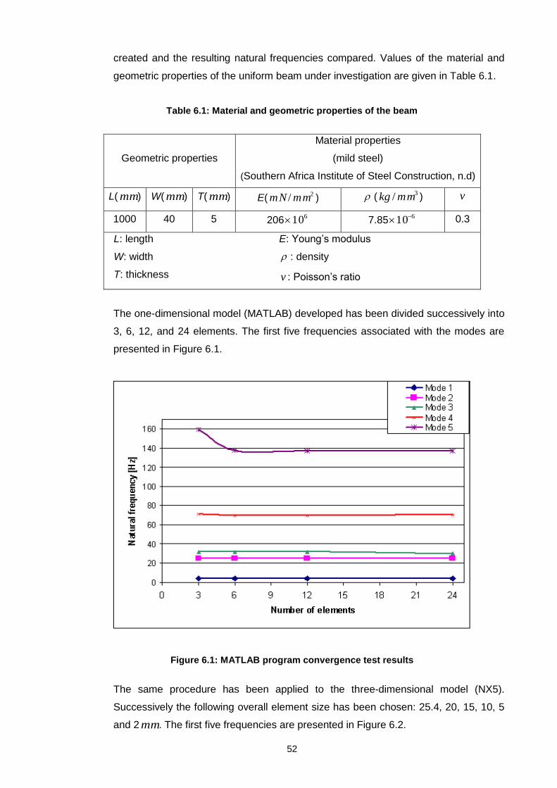
52
created and the resulting natural frequencies compared. Values of the material and
geometric properties of the uniform beam under investigation are given in Table 6.1.
Table 6.1: Material and geometric properties of the beam
Geometric properties
Material properties
(mild steel)
(Southern Africa Institute of Steel Construction, n.d)
L( mm) W( mm) T( mm) E(2/ mmmN ) (
3/ mmkg ) v
1000 40 5 206610 7.85
610 0.3
L: length
W: width
T: thickness
E: Young’s modulus
: density
v : Poisson’s ratio
The one-dimensional model (MATLAB) developed has been divided successively into
3, 6, 12, and 24 elements. The first five frequencies associated with the modes are
presented in Figure 6.1.
Figure 6.1: MATLAB program convergence test results
The same procedure has been applied to the three-dimensional model (NX5).
Successively the following overall element size has been chosen: 25.4, 20, 15, 10, 5
and 2 mm. The first five frequencies are presented in Figure 6.2.

53
Figure 6.2: NX convergence test results
The two previous tests indicated the predicted frequencies are not influenced
significantly by mesh size in the range chosen for investigation. Therefore, for the
simulations presented here, a minimum of 12 elements and overall element size of 10
mm were chosen respectively for the one-dimensional and the three-dimensional
models.
6.3 Results for uniform beam
The uniform beam had a rectangular cross-section with width W and thickness T. The
length of the beam was L. The values of these dimensions are shown in Table 6.2.
Table 6.2: Material and geometric properties of the uniform beam
Geometric properties
Material properties
(mild steel)
(Southern Africa Institute of Steel Construction, n.d)
L( mm) W( mm) T( mm) E(2/ mmmN ) (
3/ mmKg ) v
795 40 4.45 206610 7.85
610 0.3
L: length
W: width
T: thickness
E: Young’s modulus
: density
v : Poisson’s ratio

54
6.3.1 Exact solution
The exact solution was established in Section 3.5. The natural frequency of the beam
can be calculated from Equation 3.21 as follows
A
EIf
2
2
=
4
2
2 AL
EIL
Values of L are shown in Table 3.1
L1 1.875104
L2 4.6940914
L3 7.8547577
L4 10.995541
L5 14.137168
Values of can be obtained by dividing those previous values by length L =
795 mm, as follows:
1 0023586210795
8751041.
.
The cross-section A and the area moment of inertia I are given as follow
A W × T
45440 .
1782mm
For flap-wise modes,
I 12
1(W T
3)
12
1 ( 40 3454. )
74293 .4mm
The natural frequencies can be calculated as follows:
4
2
11
2 AL
EILf
2
00235862102
.46
6
79517810857
7429310206
.
.
5.83 Hz
Similarly
2f 36.5 Hz
3f 102 Hz

55
=4f 200 Hz
=5f 331 Hz
For edge-wise modes,
I 12
1(W
3 T)
12
1 (
340 454. )
23733.33 4mm
Hence,
4
2
11
2 AL
EILf
2
00235862102
.46
6
79517810857
332373310206
.
.
452= . Hz
Similarly
=2f 328 Hz
=3f 919 Hz
=4f 1800 Hz
=5f 2977 Hz
The frequencies of torsional modes of a rectangular cantilever with a width to
thickness ratio greater than six may be approximated by (Harris, 1988):
=nf
G
W
T
L
n 2
4
12 )-(
Where the shear modulus G is given by:
)v(
EG
+12=
).( 3012
10206 6
79230769.23
Therefore, the torsional modes become:
=1f 610857
2379230769
40
4542
7954
112
.
.).(
)(
)-(
224.79 Hz
Similarly
=2f 449.57 Hz

56
=3f 674.36 Hz
=4f 899.14 Hz
=5f 1123.93Hz
6.3.2 MATLAB program
The MATLAB program (BEAMANALYSIS) found in Appendix C is used to compute
successively flap-wise and edge-wise natural frequencies. Material and geometric
properties used as input data are given in Table 6.2. As mentioned before, this
program is based on the Euler-Bernoulli model. The following first five flap-wise and
edge-wise natural frequencies have been found:
Table 6.3: MATLAB natural frequencies
Natural frequencies (Hz)
Flap-wise Edge-wise
5.89 52.52
36.92 327.86
103.45 919.92
202.76 1801.63
335.34 2980.97
6.3.3 NX5 model
The three dimensional model shown in Figure 5.4 is designed to capture three
dimensional behaviour. Therefore flap-wise, edge-wise and additionally torsional
natural frequencies have been found. As previously, material and geometric
properties are given in Table 6.2. The mode shape associated with a specific
frequency indicates whether it is a flap-wise, edge-wise or torsional frequency. Some
examples of mode shapes are given in Figure 6.3.

57
Flap-wise deflection (Mode 2) Edge-wise deflection (Mode 7)
Torsional deflection (Mode 6)
Figure 6.3: Uniform beam deflections
The first five flap-wise, edge-wise and torsional natural frequencies are:
Table 6.4: NX5 natural frequencies
Natural frequencies (Hz)
Flap-wise Edge-wise Torsional
5.918 52.34 219.4
37.08 324.2 659.1
103.8 891.6 1102
203.5 1704 1549
336.6 2734 2005
6.3.4 Experimental modal analysis results
The performed modal analysis gives estimates of only flap-wise natural frequencies.
The results are based on the measurements performed on uniform beam as
described in Chapter 4. Figure 6.4 shows a screenshot of Vib-Graph after measured
transfer functions are imported. Crosses (+) indicate natural frequencies. The natural
frequencies, obtained from the modal analysis, are presented in Table 6.5.

58
Figure 6.4: Measured transfer functions imported into Vib-Graph
6.3.5 Comparison of natural frequencies
The results found using the four different methods have been compared. It should be
noted that:
The experimental modal analysis provides only the first five flap-wise natural
frequencies and,
The MATLAB program provides only flap-wise and edge-wise natural
frequencies.
Therefore, the comparison has been limited to the data available.

59
Table 6.5: Measured and computed natural frequencies
Exact solution [Hz] Measured frequencies [Hz] Computed frequencies [Hz]
MATLAB NX5
Fla
p-w
ise
5.83 5.62 5.89 5.918
36.5 32.5 36.92 37.08
102 99.3 103.45 103.8
200 198.75 202.76 203.5
331 315.62 335.34 336.6
Ed
ge-w
ise
52.4
52.52 52.34
328 327.86 324.2
919 919.92 891.6
1800 1801.63 1704
2977 2980.97 2734
Tors
iona
l
224.79
219.4
449.57 659.1
674.36 1102
899.14 1549
1123.93 2005
Some conclusions can be drawn from the previous table:
As expected, there are no significant discrepancies between the exact solution
and MATLAB results;
highest edge-wise frequencies introduce some discrepancies between MATLAB
and NX5 results. This may be due to the limitation of the one dimensional model
(MATLAB) compared to the three dimensional model (NX5) when it comes to
computing higher natural frequencies;
highest torsional frequencies produce also some discrepancies between exact
solution and NX5 results for similar reason as above. Interestingly, Larsen et al.
(Larsen et al., 2002) in their study compares the results from the modal analysis
with the corresponding results from the finite element analysis. Better agreement
has been found for the deflection components associated with low natural
frequencies than for deflection components associated with higher natural
frequencies. The same tendency was also observed in the estimation of natural
frequencies. The bending torsion coupling has been identified as a reason for
those discrepancies. It has been found that these deflections are difficult to
resolve experimentally (due to small signal levels) as well as numerically (due to
lack of sufficiently detailed information on the material properties). The numerical

60
model is seen to over-estimate the structural couplings. Although, torsional
natural frequencies are not included in experimental results, this may also explain
discrepancies at higher frequencies.
the closeness between the experimental (for at least the first five flap-wise and
edge-wise and the first torsional) results and the finite element analysis results
means that finite element analysis can be used as a good computational tool and,
the closeness between the analytical results, the measured frequencies and the
computed frequencies means that natural frequencies can be predicted
accurately by either of those methods.
6.4 Results for stepped beam
The stepped beam (Figure 4.4) had a rectangular cross-section with width W1, W2,
W3 and thickness T. The length of each portion was given by L1, L2, L3. The values
of these dimensions are shown in Table 6.6.
Table 6.6: Material and geometric properties of the stepped beam
Geometric properties Material properties
(Southern Africa Institute of Steel Construction, n.d)
L( mm) W( mm) T( mm) E(2/ mmmN ) (
3/ mmkg ) v
Portion1 295 40 4.5 206610 7.85
610 0.3
Portion2 250 36 4.5 206610 7.85
610 0.3
Portion3 250 30 4.5 206610 7.85
610 0.3
L: length
W: width
T: thickness
E: Young’s modulus
: Density
v : Poisson’s ratio
Hereafter the MATLAB, NX5 and experimental modal analysis results are presented.
No exact solution is available for the stepped beam.
6.4.1 MATLAB program
The MATLAB program (BEAMANALYSIS) found in Appendix C is used to compute
successively flap-wise and edge-wise natural frequencies. The following first five flap-
wise and edge-wise natural frequencies have been found:

61
Table 6.7: MATLAB natural frequencies
Natural frequencies (Hz)
Flap-wise Edge-wise
6.61 57.62
37.88 305.41
103.55 807.10
202.72 1587.27
335.28 2628.71
6.4.2 NX5 model
A three-dimensional stepped beam (Figure 4.4) has been built in the finite element
program NX5. Flap-wise, edge-wise and additionally torsional natural frequencies
have been found. The mode shapes corresponding to the natural frequencies are
used to determine whether a particular frequency is flap-wise, edge-wise or torsional.
Flap-wise deflection (Mode 2) Edge-wise deflection (Mode 7)
Torsional deflection (Mode 6)
Figure 6.5: Stepped beam deflections

62
The first five flap-wise, edge-wise and torsional natural frequencies are:
Table 6.8: NX5 natural frequencies
Natural frequencies (Hz)
Flap-wise Edge-wise Torsional
6.636 57.55 282.6
38.02 301.9 742.1
103.9 786 1202
203.5 1516 1733
336.2 2447 2249
6.4.3 Experimental modal analysis results
The performed modal analysis gives estimates of only flap-wise natural frequencies.
The results are based the measurements performed on the stepped beam described
in Chapter 4. Figure 6.6 shows a screenshot of Vib-Graph after measured transfer
functions are imported. Crosses (+) indicates natural frequencies. The natural
frequencies, obtained from the modal analysis, are presented in Table 6.9.
Figure 6.6: Measured transfer functions imported into Vib-Graph

63
6.4.4 Comparison of natural frequencies
The results found previously have been compared. This comparison has been limited
to the data available.
Table 6.9: Measured and computed natural frequencies
Measured frequencies [Hz] Computed frequencies [Hz]
MATLAB NX5
Fla
p-w
ise
5.62 6.61 6.636
35.62 37.88 38.02
99.37 103.55 103.9
201.87 202.72 203.5
307.5 335.28 336.2
Ed
ge-w
ise
57.62 57.55
305.41 301.9
807.10 786
1587.27 1516
2628.71 2447
It can be seen that the measured frequencies results and the computed frequencies
remain close. However, as previously, some discrepancies can be observed for
highest frequencies. Interestingly, Jaworski and Dowell (Jaworski & Dowell, 2007) in
their study predicted the three lowest natural frequencies of a multiple-stepped beam
using:
A classic Rayleigh–Ritz formulation;
commercial finite element code ANSYS and,
experimental results from impact testing data.
It has been shown that:
Classical Rayleigh–Ritz provides more accurate results at the highest
frequency for global parameters once sufficient degrees-of-freedom are
introduced and,
the disagreement between beam model and experimental results is attributed
to non-beam effects present in the higher-dimensional elasticity models, but
absent in Euler–Bernoulli and Timoshenko beam theories. This conclusion is
corroborated by predictions from one-, two-, and three-dimensional finite
element models.

64
It should be specified, however, that this study is not concerned with higher natural
frequencies.
6.5 Results for variblade
6.5.1 NX5 and MATLAB results comparison for variblade
Since finite element analysis has been established as an important tool in vibration
analysis and proven reliable in this study, it has been used to provide an
approximation for the variblade being designed.
As explained before the variable length blade has been approximated to a variblade
with two portions (Figure 5.2). Ten different configurations (Figure 5.3) depending of
the position of the outboard portion are investigated. These configurations change
from zero extension to full extension in ten equal steps of 100 mm. Values of the
material and geometric properties of the two portion of the variblade under
investigation are given in Table 6.10. No exact solution and experimental modal
analysis results are available.
Table 6.10: Material and geometric properties of the variblade
Geometric properties
Material properties
(Carbon fiber composite)
(Zweben et al., 1989)
L( mm) W( mm) T( mm) Wh( mm) E(2/ mmmN ) (
3/ mmkg ) v
Portion1 1000 60 20 5 230610 1.8
610 0.3
Portion2 1000 50 10 N/A 230610 1.8
610 0.3
L: length
W: width
T: thickness
Wh: wall thickness
E: Young’s modulus
: density
v : Poisson’s ratio
This section contains examples of the results obtained with NX5 for three different
configurations of the variblade. Flap-wise, edge-wise and torsional deflections are
represented.

65
Mode 3 (Flap-wise) Mode 5 (Edge-wise)
Mode 6 (Torsional)
Figure 6.7: Flap-wise, edge-wise and torsional deflection for configuration 1
Mode 3 (Flap-wise) Mode 5 (Edge-wise)
Mode 9 (Torsional)
Figure 6.8: Flap-wise, edge-wise and torsional deflection for configuration 5

66
Mode 4 (Flap-wise) Mode 8 (Edge-wise)
Mode 10 (Torsional)
Figure 6.9: Flap-wise, edge-wise and torsional deflection for configuration 10
The complete set of NX5 results are presented in Appendix E.
The MATLAB program VARIBLADEANALYSIS.m (Appendix D) has been used to
compute natural frequencies. The results found using this MATLAB program have
been compared to those found using NX5. The first five natural frequencies (flap-wise
and edge-wise) of the variblade are calculated successively for ten different
configurations. Torsional natural frequencies obtained with NX5 have been ignored
because the MATLAB program can calculate only flap-wise and edge-wise natural
frequencies. Figure 6.10 represents the results obtained for configuration 1,
configuration 5 and configuration 10. The complete results comparison for all
configurations is presented in Appendix F.

67
Figure 6.10: MATLAB and NX5 results comparison
6.5.2 Influence of blade length
The influence of varying the blade length has been studied and the results are shown
in Figure 6.11 for the first five natural frequencies related to the configurations of the
variblade. Table 6.11 and Table 6.12 provide values of these first five natural
frequencies calculated for each configuration of the variblade shown in Figure 5.3.
Table 6.11: Computed natural frequencies (NX5)
Configuration
number
Computed natural frequencies (Hz)
Mode1 Mode2 Mode3 Mode4 Mode5
1 36.6 109 229 640 675
2 33.1 94.6 205 560 589
3 29.5 82.2 174 422 509
4 26.4 72.7 140 302 434
5 23.6 64.7 108 250 364
6 21.0 57.8 83.8 225 305
7 18.7 51.8 67.8 205 259
8 16.5 46.5 57.2 184 224
9 14.5 41.9 50.0 162 198
10 12.7 37.8 45.2 141 178

68
Table 6.12: Computed natural frequencies (MATLAB)
Configuration
number
Computed natural frequencies (Hz)
Mode1 Mode2 Mode3 Mode4 Mode5
1 36.6 111 229 641 684
2 33.4 95.5 204 562 589
3 30.2 79.6 175 426 525
4 27.1 73.2 142 304 441
5 23.9 65.3 108 251 369
6 20.7 63.7 84.4 226 302
7 19.1 47.8 68.4 205 255
8 15.9 47.8 57.3 184 223
9 14.3 47.8 49.3 162 206
10 12.7 40.0 44.6 142 175
Figure 6.11: Natural frequencies
6.5.3 Effect of rotation
Referring to Equation 2.1, it has been shown that there is an increase of the first
mode frequency due to centrifugal stiffening.
2
1
2
0,1,1 ff R
The natural frequencies calculated (Table 6.7) correspond to 0,1f . The value of 1
depends on the blade mass and stiffness distribution, and Madsen and al. (Madsen
and al., 1984) suggest the value of 1.73 for wind turbine blade flap-wise oscillations.

69
In the case of blade rotating at 30 r.p.m and for 1 =1.73, the following natural
frequencies will be obtained:
Table 6.13: Natural frequencies of the rotating variblade
Configuration
number 0,1f [Hz]
Rf ,1[Hz] Percentage increase [%]
1 36.6 36.606 0.016
2 33.1 33.107 0.020
3 29.5 29.507 0.025
4 26.4 26.408 0.031
5 23.6 23.609 0.039
6 21.0 21.010 0.049
7 18.7 18.712 0.062
8 16.5 16.513 0.079
9 14.5 14.515 0.103
10 12.7 12.717 0.134
6.6. Contextualization of the findings
During design of a wind turbine blade, the 1st flap-wise, 2nd flap-wise, 1st edge-wise
and the 1st torsional natural frequencies shall be determined as a minimum (Larsen et
al., 2002). It can be seen (Figure 6.10) there is good agreement between the
MATLAB and NX5 results for the first five natural frequencies.
It should be noted that only the frequency range between 0.5 Hz and 30 Hz (Larsen
et al., 2002) is of relevance to wind turbine blades. In that range, MATLAB and NX5
provide identical results. Torsional natural frequencies have been calculated using
NX5. The lowest torsional natural frequency (configuration 10) determined is 595 Hz
(Appendix E). It can be concluded that torsional natural frequencies are not a concern
for this variblade model as they are out of the range of interest.
The study of the influence of blade length on natural frequencies represented in
Figure 6.11 has shown that with increasing blade length, the natural frequencies
decrease. This is probably because the blade becomes more flexible as its length
increases. The excitation loads are concentrated in the interval 0.5 Hz-30 Hz. As
shown in Table 6.11 and Table 6.12, mode 1 (included in the interval 12.7 Hz-36.6

70
Hz) may coincide with these excitation frequencies. Therefore the first mode may be
subjected to excitation.
The relative effect of the centrifugal loads is small because of the small size of the
model under investigation. In fact, the longer the length of the model, the lower the
natural frequencies will be. The increase in the first mode frequency for edge-wise
oscillations from centrifugal force is 0.134 % for configuration10; the largest expected
increase; which is probably small enough to be ignored.

71
CHAPTER 7
CONCLUSIONS AND RECOMMENDATIONS FOR FUTURE WORK
7.1 Conclusions
A variblade can be seen as beam of finite length with aerofoils as cross sections. A
rectangular cross-section model, representing the variblade, can give qualitatively
appropriate results in a simpler way than considering a blade with aerofoil profiles.
Therefore, such a model has been adopted for this analysis. The fixed and sliding
portions of the blade have been approximated by a hollow beam and a solid beam. As
the outboard portion of the blade can be slid in and out of the inboard portion, 10 different
configurations have been investigated. A one-dimensional model and a three-
dimensional model have been investigated
The following expected conclusions have been drawn:
Good agreement between NX5 and MATLAB results has been confirmed for the
frequency range of interest using a composite material variblade. Therefore both NX5
and the MATLAB program can be use to calculate natural frequencies for any other
isotropic material. This means that an effective method to compute natural
frequencies of a variblade was developed;
natural frequencies are a function of configuration number and,
increasing the blade length reduces natural frequencies.
More specifically for variblades, the following conclusions have been drawn:
The range between 0.5 Hz and 30 Hz is of relevance to wind turbine blades.
Although the first five natural frequencies have been calculated, only the first flap-
wise natural frequency is of concern. Higher flap-wise natural frequencies, all edge-
wise and all torsional natural frequencies are out of this range of concern.
the first mode (included in the interval 12.7-36.6 Hz) (Table 6.11 and Table 6.12) may
coincide with the excitation frequencies, therefore during operation this range of
frequencies should be avoided;
modal testing only needs to be performed to extract the first flap-wise natural
frequency in each configuration of the variblade and,
influence of rotation on natural frequencies is small enough to be ignored.
72
Non-obvious advantages of the variblades is the following: The higher the rotor
speed, the smaller the blade length becomes and, therefore the higher the natural
frequency is. Similarly, as the rotor speed decreases, natural frequency decreases.
For the variblade, it can be seen that a smaller blade size (Table 6.11 and Table
6.12) (configuration 1, configuration 2 and configuration 3) does not present a risk for
the variblade, since those natural frequencies are out of the range of concern.
Therefore, reducing the blade length reduces the chances of resonance. Although it
is an obvious conclusion, it is an non-obvious benefit.
Due to variation in blade length, natural frequency is not constant. Even if one found
that the first flap-wise natural frequency is in the region of concern, that frequency is
not constant, thus reducing chances of resonance.
7.2 Recommendations
7.2.1 Finite element analysis
The models developed include some approximation. The results for these simplified
models shows further research with a more accurate model is required since the first
mode may be subjected to excitation. The blade profile needs to be taken into
account for more accurate results;
the MATLAB program was written to be applicable to different blade shapes and
materials, therefore, the cross section can be taken into account for the variblade
being designed;
the two portions of the blade have been considered as one body in finite element
analysis. Further studies can be undertaken to investigate the the effect of modelling
the blade with the two portions joined in a more realistic way (e.g. with gap or contact
elements) and,
since discrepancies between results have been found for frequencies above 500 Hz,
further research can be undertaken in order to assess the ability of finite element
analysis software to compute higher natural frequencies.

73
7.2.2 Experimental modal analysis
Experimental verification for the variblade is left for future studies to extend the work
presented in this thesis;
experimental modal analysis should be performed on the variblade being designed:
o To verify the accuracy of the computed natural frequencies.
o to verify the method considering the two portions of the blade as one portion
in finite element analysis and,
higher natural frequencies (edge-wise and torsional natural frequencies) should also
be measured in order to assess the ability of the finite element software to accurately
compute higher natural frequencies.

74
BIBLIOGRAPHY/REFERENCES
Ackermann, T. and Söder, L. 2000. Wind energy technology and current status: a review.
Renewable and sustainable energy reviews, 4(4): 315-374. December.
Aerowind Systems. n.d. Basic Aerodynamic Operating Principles of Wind Turbines.
http://www.aerowinds.co.uk/a11.html
[13 October 2008].
Bazoune, A. 2005. Relationship between softening and stiffening effects in terms of
Southwell coefficients. Journal of sound and vibration, 287: (4-5). November.
Bechly, M.E. and Clausent, P.D. 1997. Technical note: Structural Design of a Composite
Wind Turbine Blade using finite element analysis. Computers & Structures. 63(3): 639–646.
Bir, G. and Stol, C. 2000. Modal Analysis of a Teetered-Rotor Wind Turbine Using the
Floquet Approach. In Proceedings of the ASME Wind Energy Symposium, Reno, Nevada.
23–33. January.
Bir, G. S. and Butterfield, C. P. 1997. Modal Dynamics of a Next-Generation Flexible-Rotor
Soft-Tower Wind Turbine. In Proceedings of the 15th International Modal Conference,
Orlando, Florida, 76–84.
Burton, T., Sharpe, D., Jenkins, N. & Bossanyi, E. 2004. Wind Energy Handbook.
Chichester: Wiley.
Cameron, P. 1939. Aircraft having rotative sustaining means. U.S. Patent 2,163,482.
Chopra, I. and Dugundji, J. 1979. Non-Linear Dynamic Response of a Wind Turbine Blade.
Journal of Sound and Vibration. 63(2): 265–286.
Composites world. 2008. Getting To The Core Of Composite Laminates.
http://www.compositesworld.com/
[13 October 2008].

75
Danish Wind Turbine Manufacturers Association. 2003. The Wind Energy Pioneer— Poul la
Cour. http://www.windpower.org/en/pictures/lacour.htm
[13 October 2008].
Edinger, R. and Kaul, S. 2000. Renewable Resources for Electric Power: Prospects and
challenges. Quorum: Westport.
Ewins, D.J. 2000. Modal Testing: Theory, Practice and Application, Research Studies Press
Ltd, Baldock, UK.
Fradenburgh, E. A. and Miller, G. G. 1994. A drive system for changing the diameter of a
variable rotor. U.S. Patent 5,299,912.
Fradenburgh, E. A., Davis, J. S., Moffitt, R. C. and Visintainer, J. A. 1993. Variable diameter
rotor having an offset twist. U.S. Patent 5,253,979.
Garrad, A. D. and Quarton, D. C. 1986. Symbolic Computing as a Tool in Wind Turbine
Dynamics. Journal of Sound and Vibration. 109(1): 65–78.
Grabau, P. & Petersensvej, H.C. 1999. Wind turbine with stress indicator. World International
Property Organization, WO 99/57435 A1: 1-26. November 11.
Hager, L. N., Fradenburgh, E. A. and Yarm, J. M. 1978. Locking control and over travel
safety stop system for variable length rotor blades. U.S. Patent 4,080,097.
Hansen, A. C. 1992. Yaw Dynamics of Horizontal Axis Wind Turbines. Final Subcontract
Report NICH Report No. TP- 442-4822, NREL, 1992.
Harris, C. M. 1988. Shock & Vibration Handbook. 3rd Ed. New York, NY: McGraw-Hill.
Hau, E. 2000. Wind turbines: Fundamentals, Technologies, Application and Economics.
München: Springer.
Jamieson, P. M. 2005. Variable diameter wind turbine rotor blades. U.S. Patent 6,972,498
B2.

76
Jaworski, J. W. and Dowell, E. H. 2007. Free vibration of a cantilevered beam with multiple
steps: Comparison of several theoretical methods with experiment. Journal of Sound and
Vibration 312: 713–725.
Jureczko, M., Pawlak M. & Mężyk, A. 2005. Optimisation of wind turbine blades. Materials
Processing Technology, 167(3-5): 463-471. August 30.
Kaza, K. R. V. and Hammond, C. E. 1976. Investigation of Flap-lag Stability of Wind Turbine
Rotors in the Presence of Velocity Gradients and Helicopters in Forward Flight. In
Proceedings of the Seventeenth Structures, Structural Dynamics, and Materials Conference,
King of Prussia, Pennsylvania, May 5-7, 421–431.
Kiely, E. F. and Beatty, R. D. 1997. The mounting arrangement for variable diameter rotor
assemblies. U.S. Patent 5,655,879.
Knight, C.E. 1993. The Finite Element Method in Mechanical Design. Boston: PWS-Kent
publishing company.
Kong C., Kim H. and Kim J. A. 2000. Study on structural and aerodynamic design of
composite blade for large scale HAWT system. Final report, Hankuk Fiber Ltd.
Kottapalli, S. B. R., Friedmann, P. and Rosen, A. 1978. Aeroelastic Stability and Response of
Horizontal Axis Wind Turbine Blades. In Proceedings of the 2nd International Symposium on
Wind Energy Systems, Amsterdam Netherlands, October.
Kowalik, P. and Coetzee, K. 2005. The Scope of the Energy Industry in the Western Cape.
http://www.capegateway.gov.za/other/2005/11/final_first_paper_energy_printing.pdf
[13 October 2008].
Larsen, G.C., Hansen, M.H., Baumgart, A., Carlen, I. 2002. Modal Analysis of
Wind Turbine Blades. Risø National Laboratory.
Lee, A.T. and Flay, R. G. J. 2000. Compliant blades for passive power control of wind
turbines. Wind engineering. 24(1): 3-11. January.

77
Maalawi, K.Y. & Negm, H.M. 2002. Optimal frequency design of wind turbine blades. Wind
Engineering and Industrial Aerodynamics, 90(8): 961-986. August.
Madsen, P.H., Frandsen, S., Holley, W. E. and Hansen, J. C. 1984. Dynamics and fatigue of
wind turbine rotors during steady operation. Riso National Laboratory, R-152. Riso National
Laboratory, Roskilde, Denmark.
Manwell, J. F., McGowan, J. G. and Rogers. A. L. 2002. Wind Energy Explained. Chichester:
John Wiley & Sons.
Matuska, D. G. and Gronenthal, E. W. 1997. Retraction/extension mechanism for variable
diameter rotors. U.S. Patent 5,642,982.
Matuska, D. G., Gronenthal, E. W. and Jepson, D. W. 1997. Torque tube/spar assembly for
variable diameter helicopter rotors. U.S. Patent 5,636,969.
Mckittrick, L.R., Cairns, D.S., MandelI, J., Combs, D.C., Rabem, D.A. & VanLuchene, R.D.
2001. Analysis of a Composite Blade Design for the AOC 15/50 Wind Turbine Using a Finite
Element Model.
Mikhail, A. S. and Deane. G. F. 2004. Retractable rotor blades for power generating wind
and ocean current turbines and means for operating below set rotor torque limits. U.S. Patent
6,726,439 B2.
Molenaarx, D. and Dijkstra, S. 1998. Modeling of Structural Dynamics of Lagerwey LW-
50/750 Wind Turbine. Wind Engineering. 22(6): 253–264.
Oelsner, H. F. W. 2001. Harvesting the wind in Southern Africa. Darling, South African Wind
Energy Association.
Olorunsola, O. 1986. On the Free Yaw Behaviour of Horizontal Axis Wind Turbine.
International Journal of Energy Research. 10(4): 343–355.
Ontario Ministry of Energy. 2008. Electricity Generation Using Small Wind Turbines At Your
Home Or Farm. http://www.omafra.gov.on.ca/english/engineer/facts/03-047.htm
[13 October 2008].

78
Ormiston, R. A. 1975. Dynamic Response of Wind Turbine Rotor Systems. In Proceedings of
the 31st Annual National Forum of the American Helicopter Society, Washington, D.C.
Palm, W. J. 2007. Mechanical Vibration. 1st Ed. John Wiley.
Pasupulati S., Wallace J. & Dawson M. 2005. Variable Length Blades Wind Turbine. IEEE
Power Engineering Society General Meeting, Conference article (CA), Jun 12-16 2005,
Pages 2097-2100.
Putter, S. and Manor, H. 1978. Natural frequencies of radial rotating beams. Journal of
Sound and Vibration, 56 (2): 175-185.
Rao, S. S. 2004. Mechanical Vibrations. 4th Ed. New Jersey: Prentice Hall, Upper Saddle
River.
Reference.com. 2008. Wind power.
http://www.reference.com/browse/wiki/Wind_power
[13 October 2008].
Research institute for sustainable energy. 2006. Wind Electric.
http://www.rise.org.au/info/Tech/wind/electric.html
[13 October 2008]
Schwarz, B. J. and Richardson, M. H. 1999. Experimental modal analysis. CSI Reliability
Week, Orlando, FL.
Southern Africa Institute of Steel Construction. n.d. Specification of weldable structural steel.
http://www.saisc.co.za
[14 October 2008].
Southwell, R.V. and Gough, B. S. 1921. On the free transverse vibrations of airscrew blades.
British A.R.C. Reports and Memoranda No. 766 (Ae. 26), 358–368.
Spera. D. A. 1994. Wind turbine technology: fundamental concepts of wind turbine
engineering. ASME PRESS, New York.

79
Sullivan, T.L. 1981. A Review of Resonance Response in Large Horizontal-Axis Wind
Turbines. Proceedings for the Wind Turbine Dynamics Workshop, NASA Conference
Publications 2185/ DOE CONF-810226, 24-26.
Thresher RW. 1982. Structural dynamic analysis of wind turbine systems. J. Solar Energy
Engineering. 104:89-95.
United States Department of Energy. 2005. Wind Energy Program: History of Wind Energy
Use. http://www1.eere.energy.gov/windandhydro/wind_history.html
[13 October 2008].
Van Der Tempel, J. & Molenaar, D.P. 2002. Wind Turbine Structural Dynamics: A Review of
the Principles for Modern Power Generation, Onshore and Offshore. Wind Engineering,
26(4): 211-220.
Warmbrodt, W. and Friedmann, P. P. 1979. Formulation of the Aeroelastic Stability and
Response Problem of Coupled Rotor/ tower Systems. In Proceedings of the Twentieth
Structures, Structural Dynamics and Materials Conference, St. Louis, Missouri. 39–52, AIAA
Paper 79-0732. April.
Wind Power Monthly. 2008. Wind energy facts and figures from Wind power
Monthly. http://windpower-monthly.com/spis/runisa.dll?WPM:WINDICATOR:910351.
[13 October 2008].
Zhiquan Y., Haomin M., Nengsheng B., Yan C. and Kang D. 2001. Structure dynamic
analysis of a HAWT using a modal analysis method. Wind Engineering. 25(4): 237–248.
July.
Zweben, C., Thomas, H. H. and Chou, T. W. 1989. Mechanical behaviour and properties of
composite materials. Technomic Publishing Co., Inc. Vol. 1.

80
APPENDICES
Appendix A: Instrument specifications
This appendix presents a summary of the hardware used and evaluated in the
experimental investigations performed. The product identification and product
specifications are given.
ICP IMPACT HAMMER
Model Number 086C02
PERFORMANCE ENGLISH SI
Sensitivity (±15 %) 50 flbmV / 11.2 NmV /
Measurement Range ±100 flb pk ±440 N pk
Resonant Frequency ≥22 kHz ≥22 kHz
Non-Linearity ≤1 % ≤1 %
ACCELEROMETER
Model IA11T
DYNAMIC PERFORMANCE ENGLISH SI
Sensitivity (±10%) 100 gmV / 10.2 )//( 2smmV
Measurement Range ±50 g ±490 2/ sm
Frequency Range: (±3 dB) 20 – 600k cpm 0.32 – 10k Hz
Mounted Resonant Frequency 1320k cpm 22k Hz
Amplitude Linearity ±1% ±1%
Transverse Sensitivity ≤7% ≤7%

81
DYNAMIC SIGNAL ANALYSER
The OneproD MVP-2C Portable Analyser is a modular, fully adaptable machinery
analyser that can be configured at any time to be a two-channel vibration analyser, data
collector, balancer, and data recorder to suit a wide variety of condition monitoring
needs.
Specifications (Short Form)
1 or 2 channels;
cross-channel functions with 2-channel configuration;
resonance Analysis, bump test etc;
running machine resonance/bump test;
128MB internal memory (-+ 20,000 Spectra @ 3200 lines);
12 800 lines of resolution;
true zoom;
USB/Ethernet communications;
built-in laser tachometer;
built-in pyrometer (infra-red thermometer) with laser sighting;
8 hours battery life (Li-On);
remote route loading/unloading with E-route option;
balancing option: 1 or 2 channels up to 4 planes;
order analysis (run-up and run-down) and,
long time-record acquisition for slow speed machines and event capture.

82
Appendix B: MATLAB program for uniform and stepped beam
%****************************************************************************
%****************************************************************************
%************************ BEAMANALYSIS ***********************************
%****************************************************************************
%************************* Written by ******************************************
%****************************************************************************
%******************* TARTIBU KWANDA 2008 **********************************
%****************************************************************************
%****************************************************************************
%****************************************************************************
%Uniform beam and Stepped beam finite element program. Selectable number of step and %number of
elements. Solves for eigenvalues and eigenvectors of a beam with user defined %dimensions. This
program is able to calculate the natural frequencies of different uniform and %stepped beam geometries
and material’s properties.
%default values are included in the program for the purpose of showing how to input data.
echo off
clf;
clear all;
inp = input('Input "1" to enter beam dimensions, "Enter" to use default ... ');
if (isempty(inp))
inp = 0;
else
end
if inp == 0
% input size of beam and material
% xl(i) = length of element (step)i
% w(i) = width of element (step)i
% t(i) = thickness of element (step)i
% e = Young's modulus
% bj = global degree of freedom number corresponding to the jth local degree
% of freedom of element i
% a(i) = area of cross section of element i
% ne = number of elements
% n = total number of degree of freedom
% no = number of nodes
format short
% INPUT DATA

83
xl = [40 32 24];
xi = [1.333333 6.75 0.08333];
w = [4 6 2];
t = [2 3 1];
e = 206e+6;
rho = 7.85e-6;
bj = [1 2 3 4;3 4 5 6;5 6 7 8];
ne = 3;
n = 8;
else
ne = input ('Input number of elements, default 3 ... ');
if (isempty(ne))
ne = 3;
else
end
xl = input ('Input lengths of stepped beam, default [40 32 24], ... ');
if (isempty(xl))
xl = [40 32 24];
else
end
w = input ('Input widths of stepped beam, default [4 6 2], ... ');
if (isempty(w))
w = [4 6 2];
else
end
t = input ('Input thickness of stepped beam, default [2 3 1], ... ');
if (isempty(t))
t = [2 3 1];
else
end
% INPUT SIZE OF STEPPED BEAM AND MATERIAL

84
e = input('Input modulus of material, mN/mm^2, default mild steel 206e+6 ... ');
if (isempty(e))
e=206e+6;
else
end
rho = input('Input density of material,kg/mm^3 , default mild steel 7.85e-6 ... ');
if (isempty(rho))
rho = 7.85e-6;
else
end
bj = input('Input global degree of freedom, default global degree of freedom [1 2 3 4;3 4 5 6;5 6 7 8] ...
');
if (isempty(bj))
bj = [1 2 3 4;3 4 5 6;5 6 7 8];
else
end
end
% Calculate area (a), area moment of Inertia (xi) and mass per unit of length (xmas) of
% the stepped beam
a = w.*t;
% Define area moment of inertia according to flap-wise or edge-wise
% vibration of the stepped beam.
vibrationdirection = input('enter "1" for edge-wise vibration, "enter" for flap-wise vibration ... ');
if (isempty(vibrationdirection))
vibrationdirection = 0;
else
end
if vibrationdirection == 0
xi=w.*t.^3/12;
else
% CALCULATION

85
xi=t.*w.^3/12;
end
for i=1:ne
xmas(i)=a(i)*rho;
end
% Size the stiffness and mass matrices
no = ne+1;
n = 2*no;
bigm = zeros(n,n);
bigk = zeros(n,n);
% Now build up the global stiffness and consistent mass matrices, element
% by element
ai = zeros(4,n);
i1=bj(ii,1);
i2=bj(ii,2);
i3=bj(ii,3);
i4=bj(ii,4);
ai(1,i1)=1;
ai(2,i2)=1;
ai(3,i3)=1;
ai(4,i4)=1;
xm(1,1)=156;
xm(1,2)=22*xl(ii);
xm(1,3)=54;
xm(1,4)=-13*xl(ii);
xm(2,2)=4*xl(ii)^2;
xm(2,3)=13*xl(ii);
xm(2,4)=-3*xl(ii)^2;
xm(3,3)=156;
xm(3,4)=-22*xl(ii);
xm(4,4)=4*xl(ii)^2;
xk(1,1)=12;
% BUILDING OF MATRICES

86
xk(1,2)=6*xl(ii);
xk(1,3)=-12;
xk(1,4)=6*xl(ii);
xk(2,2)=4*xl(ii)^2;
xk(2,3)=-6*xl(ii);
xk(2,4)=2*xl(ii)^2;
xk(3,3)=12;
xk(3,4)=-6*xl(ii);
xk(4,4)=4*xl(ii)^2;
for i=1:4
for j=1:4
xm(j,i)=xm(i,j);
xk(j,i)=xk(i,j);
end
end
for i=1:4
for j=1:4
xm(i,j)=(((xmas(ii)*xl(ii))/420))*xm(i,j);
xk(i,j)=((e*xi(ii))/(xl(ii)^3))*xk(i,j);
end
end
for i=1:n
for j=1:4
ait(i,j)=ai(j,i);
end
end
xka=xk*ai;
xma=xm*ai;
aka=ait*xka;
ama=ait*xma;
for i=1:n
for j=1:n
bigm(i,j)=bigm(i,j)+ama(i,j);
bigk(i,j)=bigk(i,j)+aka(i,j);
end
end

87
end
% Application of boundary conditions
% Rows and columns corresponding to zero displacements are deleted
bigk(1:2,:) = [];
bigk(:,1:2) = [];
bigm(1:2,:) = [];
bigm(:,1:2) = [];
% Calculation of eigenvector and eigenvalue
[L, V] = eig (bigk,bigm)
% Natural frequency
V1 = V.^(1/2)
W = diag(V1)
f =W/(2*pi)
% CALCULATION OF NATURAL FREQUENCY

88
Appendix C: MATLAB Program explanation: 3 elements mesh
%: MATLAB treats all the information after the % on that line as a comment. MATLAB ignores this
comment line when you run the M-file.
echo off: Turns off the echoing of commands in all script files
clf: deletes from the current figure all graphics objects whose handles are not hidden
clear all: removes all variables, functions, and MEX-files from memory, leaving the workspace empty
format long: scaled fixed point format with 14 to 15 digits after the decimal point for double; and 7
digits after the decimal point for single.
xl = [xl1 xl2 xl3]
xl1 = length of step 1 (ii = 1)
xl2 = length of step 2 (ii = 2)
xl3 = length of step 3 (ii = 3)
xi = [xi1 xi2 xi3]
xi1 = area moment of inertia step 1
xi2 = area moment of inertia step 2
xi3 = area moment of inertia step 3
w = [w1 w2 w3]
w1 = width of step 1
w2 = width of step 2
w3 = width of step 3
t = [t1 t2 t3]
t1 = thickness of step 1
t2 = thickness of step 2
t3 = thickness of step 3
bj = [1 2 3 4;3 4 5 6;5 6 7 8] =
8765
6543
4321
a = w.*t = [w1 w2 w3].* [t1 t2 t3] = [w1*t1 w2*t2 w3*t3] = [a1 a2 a3]
xi = w.*t.^3/12 = [w1 w2 w3].* [t1 t2 t3].^3/12 = [w1*t1^3 w2*t2^3 w3*t3^3]/12
xmas1 = a1*rho for i = 1
xmas2 = a2*rho for i = 2
xmas3 = a3*rho for i = 3

89
bigm =
00000000
00000000
00000000
00000000
00000000
00000000
00000000
00000000
bigk =
00000000
00000000
00000000
00000000
00000000
00000000
00000000
00000000
ai(i,j) =
00000000
00000000
00000000
00000000
i1 = bj(1,1) = 1 for ii = 1 or bj(2,1) = 1 for ii = 2 or bj(3,1) = 1 for ii = 3
i2 = bj(1,2) = 1 for ii = 1 or bj(2,2) = 1 for ii = 2 or bj(3,2) = 1 for ii = 3
i1 = bj(1,3) = 1 for ii = 1 or bj(2,3) = 1 for ii = 2 or bj(3,3) = 1 for ii = 3
i1 = bj(1,4) = 1 for ii = 1 or bj(2,4) = 1 for ii = 2 or bj(3,4) = 1 for ii = 3
For ii = 1 ai(i,j) =
00001000
00000100
00000010
00000001
For ii = 2 ai(i,j) =
00100000
00010000
00001000
00000100

90
For ii = 3 ai(i,j) =
10000000
01000000
00100000
00010000
xm =
2)^(*4)(*22)(*3)(*13
)(*22156)(*1354
2)^(*3)(*132)^(*4)(*22
)(*1354)(*22156
iixliixliixliixl
iixliixl
iixliixliixliixl
iixliixl
for ii = 1:3
xk =
2)^(*4)(*6)(*2)(*6
)(*612)(*66
2)^(*2)(*62)^(*4)(*22
)(*612)(*612
iixliixliixliixl
iixliixl
iixliixliixliixl
iixliixl
for ii = 1:3
xm(i,j) = (xmas(ii)*xl(ii)/420)*
2)^(*4)(*22)(*3)(*13
)(*22156)(*1354
2)^(*3)(*132)^(*4)(*22
)(*1354)(*22156
iixliixliixliixl
iixliixl
iixliixliixliixl
iixliixl
xm(i,j) =
axmaxmaxmaxm
axmaxmaxmaxm
axmaxmaxmaxm
axmaxmaxmaxm
44434241
34333231
24232221
14131211
for ii = 1
xm(i,j) =
bxmbxmbxmbxm
bxmbxmbxmbxm
bxmbxmbxmbxm
bxmbxmbxmbxm
44434241
34333231
24232221
14131211
for ii = 2
xm(i,j) =
cxmcxmcxmcxm
cxmcxmcxmcxm
cxmcxmcxmcxm
cxmcxmcxmcxm
44434241
34333231
24232221
14131211
for ii = 3
xk(i,j) = (e*xi(ii)/(xl(ii)^3))*
2)^(*4)(*6)(*2)(*6
)(*612)(*66
2)^(*2)(*62)^(*4)(*22
)(*612)(*612
iixliixliixliixl
iixliixl
iixliixliixliixl
iixliixl

91
xk(i,j) =
axkaxkaxkaxk
axkaxkaxkaxk
axkaxkaxkaxk
axkaxkaxkaxk
44434241
34333231
24232221
14131211
for ii = 1
xk(i,j) =
bxkbxkbxkbxk
bxkbxkbxkbxk
bxkbxkbxkbxk
bxkbxkbxkbxk
44434241
34333231
24232221
14131211
for ii = 2
xk(i,j) =
cxkcxkcxkcxk
cxkcxkcxkcxk
cxkcxkcxkcxk
cxkcxkcxkcxk
44434241
34333231
24232221
14131211
for ii = 3
For ii = 1 ait(i,j) = ai(j,i) =
0000
0000
0000
0000
1000
0100
0010
0001
For ii = 2 ait(i,j) =
0000
0000
1000
0100
0010
0001
0000
0000

92
For ii = 3 ait(i,j) =
1000
0100
0010
0001
0000
0000
0000
0000
For ii = 1
xka=
axkaxkaxkaxk
axkaxkaxkaxk
axkaxkaxkaxk
axkaxkaxkaxk
44434241
34333231
24232221
14131211
*
00001000
00000100
00000010
00000001
=
000044434241
000034333231
000024232221
000014131211
axkaxkaxkaxk
axkaxkaxkaxk
axkaxkaxkaxk
axkaxkaxkaxk
xma=
axmaxmaxmaxm
axmaxmaxmaxm
axmaxmaxmaxm
axmaxmaxmaxm
44434241
34333231
24232221
14131211
*
00001000
00000100
00000010
00000001
=
000044434241
000034333231
000024232221
000014131211
axmaxmaxmaxm
axmaxmaxmaxm
axmaxmaxmaxm
axmaxmaxmaxm
For ii = 2
xka=
bxkbxkbxkbxk
bxkbxkbxkbxk
bxkbxkbxkbxk
bxkbxkbxkbxk
44434241
34333231
24232221
14131211
*
00100000
00010000
00001000
00000100
=

93
004443424100
003433323100
002423222100
001413121100
bxkbxkbxkbxk
bxkbxkbxkbxk
bxkbxkbxkbxk
bxkbxkbxkbxk
xma=
bxmbxmbxmbxm
bxmbxmbxmbxm
bxmbxmbxmbxm
bxmbxmbxmbxm
44434241
34333231
24232221
14131211
*
00100000
00010000
00001000
00000100
=
004443424100
003433323100
002423222100
001413121100
bxmbxmbxmbxm
bxmbxmbxmbxm
bxmbxmbxmbxm
bxmbxmbxmbxm
For ii = 3
xka=
cxkcxkcxkcxk
cxkcxkcxkcxk
cxkcxkcxkcxk
cxkcxkcxkcxk
44434241
34333231
24232221
14131211
*
10000000
01000000
00100000
00010000
=
cxkcxkcxkcxk
cxkcxkcxkcxk
cxkcxkcxkcxk
cxkcxkcxkcxk
444342410000
343332310000
242322210000
141312110000
xma=
cxmcxmcxmcxm
cxmcxmcxmcxm
cxmcxmcxmcxm
cxmcxmcxmcxm
44434241
34333231
24232221
14131211
*
10000000
01000000
00100000
00010000
=
cxmcxmcxmcxm
cxmcxmcxmcxm
cxmcxmcxmcxm
cxmcxmcxmcxm
444342410000
343332310000
242322210000
141312110000

94
For ii = 1
aka =
0000
0000
0000
0000
1000
0100
0010
0001
*
000044434241
000034333231
000024232221
000014131211
axkaxkaxkaxk
axkaxkaxkaxk
axkaxkaxkaxk
axkaxkaxkaxk
=
00000000
00000000
00000000
00000000
000044434241
000034333231
000024232221
000014131211
axkaxkaxkaxk
axkaxkaxkaxk
axkaxkaxkaxk
axkaxkaxkaxk
ama =
0000
0000
0000
0000
1000
0100
0010
0001
*
000044434241
000034333231
000024232221
000014131211
axmaxmaxmaxm
axmaxmaxmaxm
axmaxmaxmaxm
axmaxmaxmaxm
=
00000000
00000000
00000000
00000000
000044434241
000034333231
000024232221
000014131211
axmaxmaxmaxm
axmaxmaxmaxm
axmaxmaxmaxm
axmaxmaxmaxm

95
For ii = 2
aka =
0000
0000
1000
0100
0010
0001
0000
0000
*
004443424100
003433323100
002423222100
001413121100
bxkbxkbxkbxk
bxkbxkbxkbxk
bxkbxkbxkbxk
bxkbxkbxkbxk
=
00000000
00000000
004443424100
003433323100
002423222100
001413121100
00000000
00000000
bxkbxkbxkbxk
bxkbxkbxkbxk
bxkbxkbxkbxk
bxkbxkbxkbxk
ama =
0000
0000
1000
0100
0010
0001
0000
0000
*
004443424100
003433323100
002423222100
001413121100
bxmbxmbxmbxm
bxmbxmbxmbxm
bxmbxmbxmbxm
bxmbxmbxmbxm
=
00000000
00000000
004443424100
003433323100
002423222100
001413121100
00000000
00000000
bxmbxmbxmbxm
bxmbxmbxmbxm
bxmbxmbxmbxm
bxmbxmbxmbxm

96
For ii = 3
aka =
1000
0100
0010
0001
0000
0000
0000
0000
*
cxkcxkcxkcxk
cxkcxkcxkcxk
cxkcxkcxkcxk
cxkcxkcxkcxk
444342410000
343332310000
242322210000
141312110000
=
cxkcxkcxkcxk
cxkcxkcxkcxk
cxkcxkcxkcxk
cxkcxkcxkcxk
444342410000
343332310000
242322210000
141312110000
00000000
00000000
00000000
00000000
ama =
1000
0100
0010
0001
0000
0000
0000
0000
*
cxmcxmcxmcxm
cxmcxmcxmcxm
cxmcxmcxmcxm
cxmcxmcxmcxm
444342410000
343332310000
242322210000
141312110000
=
cxmcxmcxmcxm
cxmcxmcxmcxm
cxmcxmcxmcxm
cxmcxmcxmcxm
444342410000
343332310000
242322210000
141312110000
00000000
00000000
00000000
00000000

97
bigm=
00000000
00000000
00000000
00000000
000044434241
000034333231
000024232221
000014131211
axmaxmaxmaxm
axmaxmaxmaxm
axmaxmaxmaxm
axmaxmaxmaxm
+
00000000
00000000
004443424100
003433323100
002423222100
001413121100
00000000
00000000
bxmbxmbxmbxm
bxmbxmbxmbxm
bxmbxmbxmbxm
bxmbxmbxmbxm
+
cxmcxmcxmcxm
cxmcxmcxmcxm
cxmcxmcxmcxm
cxmcxmcxmcxm
444342410000
343332310000
242322210000
141312110000
00000000
00000000
00000000
00000000

98
bigk=
00000000
00000000
00000000
00000000
000044434241
000034333231
000024232221
000014131211
axkaxkaxkaxk
axkaxkaxkaxk
axkaxkaxkaxk
axkaxkaxkaxk
+
00000000
00000000
004443424100
003433323100
002423222100
001413121100
00000000
00000000
bxkbxkbxkbxk
bxkbxkbxkbxk
bxkbxkbxkbxk
bxkbxkbxkbxk
+
cxkcxkcxkcxk
cxkcxkcxkcxk
cxkcxkcxkcxk
cxkcxkcxkcxk
444342410000
343332310000
242322210000
141312110000
00000000
00000000
00000000
00000000

99

100
bigk(1:2,:) = [];
bigk(:,1:2) = [];
bigm(1:2,:) = [];
bigm(:,1:2) = [];
bigm=
cxmcxmcxmcxm
cxmcxmcxmcxm
cxmcxmcxmbxmcxmbxmbxmbxm
cxmcxmcxmbxmcxmbxmbxmbxm
bxmbxmbxmaxmbxmaxm
bxmbxmbxmaxmbxmaxm
4443424100
3433323100
2423224421434241
1413123411333231
00242322442143
00141312341133
bigk=
cxkcxkcxkcxk
cxkcxkcxkcxk
cxkcxkcxkbxkcxkbxkbxkbxk
cxkcxkcxkbxkcxkbxkbxkbxk
bxkbxkbxkaxkbxkaxk
bxkbxkbxkaxkbxkaxk
4443424100
3433323100
2423224421434241
1413123411333231
00242322442143
00141312341133

101
Appendix D: MATLAB program for VARIBLADE
%****************************************************************************
%****************************************************************************
%********************VARIBLADEANALYSIS **********************************
%****************************************************************************
%************************* Written by ******************************************
%****************************************************************************
%******************* TARTIBU KWANDA 2008**********************************
%****************************************************************************
%****************************************************************************
%****************************************************************************
%Variable length blade finite element program. Two portions of beam: hollow beam %(fixed portion)
and solid beam (moveable portion). Solves for eigenvalues and eigenvectors of %stepped beam with
user defined dimensions and configurations. This program can calculate the %natural frequencies of
different beam geometries and configurations ( position of moveable portion)
%default values are included in the program for the purpose of showing how to input data.
echo off
clf;
clear all;
inp = input('Input "1" to enter beam dimensions, "Enter" to use default ... ');
if (isempty(inp))
inp = 0;
else
end
if inp == 0
% input beam's geometries and material's properties
% xl(i) = length of element (step)i
% w(i) = width of element (step)i
% t(i) = thickness of element (step)i
% e = Young's modulus
% bj = global degree of freedom number corresponding to the jth local degree
% of freedom of element i
% a(i) = area of cross section of element i
% ne = number of elements
% n = total number of degree of freedom
% no = number of nodes
% wa = width of hollow for the first portion of stepped beam
% ta = thickness of hollow for the first portion of stepped beam
% INPUT DATA

102
format long
beamconfiguration = 1;
n1 = 10;
n2 = 10;
l1 = 1000;
l2 = 1000;
h1 = 1000/10;
h2 = 1000/10;
xl = [h1*ones(1,n1) h2*ones(1,beamconfiguration-1)];
w1 = 60;
w2 = 50;
w = [w1*ones(1,n1) w2*ones(1,beamconfiguration-1)];
t1 = 20;
t2 = 10;
t = [t1*ones(1,n1) t2*ones(1,beamconfiguration-1)];
wh = 50;
th = 10;
wa = [wh*ones(1,beamconfiguration-1) 0*ones(1,n2)];
ta = [th*ones(1,beamconfiguration-1) 0*ones(1,n2)];
% configurations of stepped beam:
% beamconfiguration ≤ n1 & n2
% for configuration 1, w = [w1*ones(1,n1) w2*ones(1,1-1)],
% t = [t1*ones(1,n1) t2*ones(1,1-1)]
% wa = [wh*ones(1,1-1) 0*ones(1,n2)],
% ta = [th*ones(1,1-1) 0*ones(1,n2)]
% for configuration 2, w = [w1*ones(1,n1) w2*ones(1,2-1)]
% t = [t1*ones(1,n1) t2*ones(1,2-1)]
% wa = [wh*ones(1,2-1) 0*ones(1,n2)]
% ta = [th*ones(1,2-1) 0*ones(1,n2)]
% for configuration 3, w = [w1*ones(1,n1) w2*ones(1,3-1)]
% t = [t1*ones(1,n1) t2*ones(1,3-1)]
% wa = [wh*ones(1,3-1) 0*ones(1,n2)]
% ta = [th*ones(1,3-1) 0*ones(1,n2)]
% for configuration 4, w = [w1*ones(1,n1) w2*ones(1,4-1)]
% t = [t1*ones(1,n1) t2*ones(1,4-1)]
% wa = [wh*ones(1,4-1) 0*ones(1,n2)]
% ta = [th*ones(1,4-1) 0*ones(1,n2)]
% for configuration 5, w = [w1*ones(1,n1) w2*ones(1,5-1)]

103
% t = [t1*ones(1,n1) t2*ones(1,5-1)]
% wa = [wh*ones(1,5-1) 0*ones(1,n2)]
% ta = [th*ones(1,5-1) 0*ones(1,n2)]
xi = [40000 40000 40000 40000 40000 40000 40000 40000 40000 40000];
a = [1200 1200 1200 1200 1200 1200 1200 1200 1200 1200];
e = 206e+6;
rho = 7.85e-6;
bj = [1 2 3 4;3 4 5 6;5 6 7 8;7 8 9 10;9 10 11 12;11 12 13 14;13 14 15 16;15 16 17 18;17 18 19
20;19 20 21 22;21 22 23 24;23 24 25 26;25 26 27 28;27 28 29 30;29 30 31 32; 31 32 33 34;33 34 35
36;35 36 37 38;37 38 39 40;39 40 41 42];
ne = 20;
n = 22;
else
beamconfiguration = input ('Input beamconfiguration of stepped beam, default 1 ... ');
if (isempty(beamconfiguration))
beamconfiguration = 1;
else
end
n1 = input ('Input number of elements for the first portion of stepped beam, default 10 ... ');
if (isempty(n1))
n1 = 10;
else
end
n2 = input ('Input number of elements for the second portion of stepped beam, default 10 ... ');
if (isempty(n2))
n2 = 10;
else
end
l1 = input ('Input length of first portion of stepped beam, default 1000, ... ');
if (isempty(l1))
l1 = 1000;
else
% INPUT SIZE OF STEPPED BEAM AND MATERIAL

104
end
l2 = input ('Input length of second portion of stepped beam, default 1000, ... ');
if (isempty(l2))
l2 = 1000;
else
end
w1 = input ('Input width of first portion of stepped beam, default 60, ... ');
if (isempty(w1))
w1 = 60;
else
end
w2 = input ('Input width of second portion of stepped beam, default 50, ... ');
if (isempty(w2))
w2 = 50;
else
end
t1 = input ('Input thickness of first portion of stepped beam, default 20 , ... ');
if (isempty(t1))
t1 = 20;
else
end
t2 = input ('Input thickness of second portion of stepped beam, default 10 , ... ');
if (isempty(t2))
t2 = 10;
else
end
wh = input ('input width of hollow of first portion of stepped beam, default 50, ... ');
if (isempty(wh))
wh = 50;
else
end
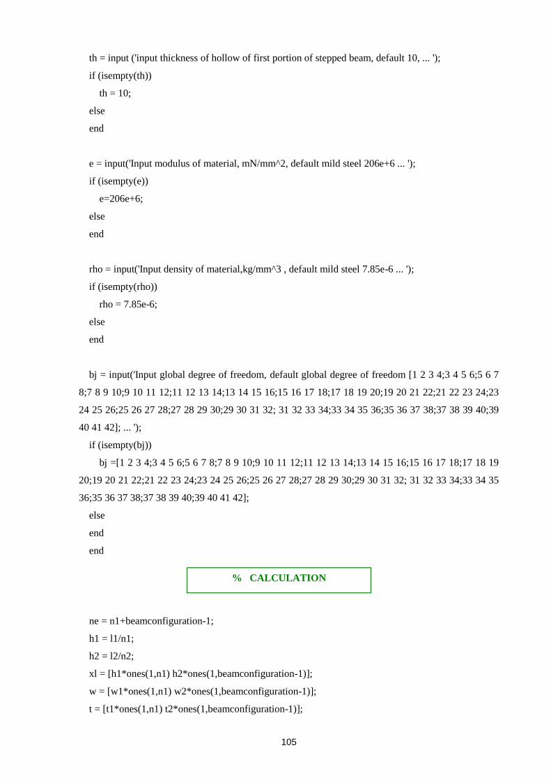
105
th = input ('input thickness of hollow of first portion of stepped beam, default 10, ... ');
if (isempty(th))
th = 10;
else
end
e = input('Input modulus of material, mN/mm^2, default mild steel 206e+6 ... ');
if (isempty(e))
e=206e+6;
else
end
rho = input('Input density of material,kg/mm^3 , default mild steel 7.85e-6 ... ');
if (isempty(rho))
rho = 7.85e-6;
else
end
bj = input('Input global degree of freedom, default global degree of freedom [1 2 3 4;3 4 5 6;5 6 7
8;7 8 9 10;9 10 11 12;11 12 13 14;13 14 15 16;15 16 17 18;17 18 19 20;19 20 21 22;21 22 23 24;23
24 25 26;25 26 27 28;27 28 29 30;29 30 31 32; 31 32 33 34;33 34 35 36;35 36 37 38;37 38 39 40;39
40 41 42]; ... ');
if (isempty(bj))
bj =[1 2 3 4;3 4 5 6;5 6 7 8;7 8 9 10;9 10 11 12;11 12 13 14;13 14 15 16;15 16 17 18;17 18 19
20;19 20 21 22;21 22 23 24;23 24 25 26;25 26 27 28;27 28 29 30;29 30 31 32; 31 32 33 34;33 34 35
36;35 36 37 38;37 38 39 40;39 40 41 42];
else
end
end
ne = n1+beamconfiguration-1;
h1 = l1/n1;
h2 = l2/n2;
xl = [h1*ones(1,n1) h2*ones(1,beamconfiguration-1)];
w = [w1*ones(1,n1) w2*ones(1,beamconfiguration-1)];
t = [t1*ones(1,n1) t2*ones(1,beamconfiguration-1)];
% CALCULATION

106
wa = [wh*ones(1,beamconfiguration-1) 0*ones(1,n2)];
ta = [th*ones(1,beamconfiguration-1) 0*ones(1,n2)];
% calculate area (a), area moment of Inertia (xi) and mass per unit of length (xmas) of
% the stepped beam
a = (w.*t)-(wa.*ta);
% define area moment of inertia according to flap-wise or edge-wise
% vibration of the stepped beam.
vibrationdirection = input('enter "1" for edge-wise vibration, "enter" for flap-wise vibration ... ');
if (isempty(vibrationdirection))
vibrationdirection = 0;
else
end
if vibrationdirection == 0
xi=((w.*t.^3)-(wa.*ta.^3))/12;
else
xi=((t.*w.^3)-(ta.*wa.^3))/12;
end
for i=1:ne
xmas(i)=a(i)*rho;
end
% Size the stiffness and mass matrices
no = ne+1;
n = 2*no;
bigm = zeros(n,n);
bigk = zeros(n,n);
% Now build up the global stiffness and consistent mass matrices, element
% by element
ai = zeros(4,n);
i1=bj(ii,1);
i2=bj(ii,2);
i3=bj(ii,3);
i4=bj(ii,4);
ai(1,i1)=1;
% BUILDING OF MATRICES

107
ai(2,i2)=1;
ai(3,i3)=1;
ai(4,i4)=1;
xm(1,1)=156;
xm(1,2)=22*xl(ii);
xm(1,3)=54;
xm(1,4)=-13*xl(ii);
xm(2,2)=4*xl(ii)^2;
xm(2,3)=13*xl(ii);
xm(2,4)=-3*xl(ii)^2;
xm(3,3)=156;
xm(3,4)=-22*xl(ii);
xm(4,4)=4*xl(ii)^2;
xk(1,1)=12;
xk(1,2)=6*xl(ii);
xk(1,3)=-12;
xk(1,4)=6*xl(ii);
xk(2,2)=4*xl(ii)^2;
xk(2,3)=-6*xl(ii);
xk(2,4)=2*xl(ii)^2;
xk(3,3)=12;
xk(3,4)=-6*xl(ii);
xk(4,4)=4*xl(ii)^2;
for i=1:4
for j=1:4
xm(j,i)=xm(i,j);
xk(j,i)=xk(i,j);
end
end
for i=1:4
for j=1:4
xm(i,j)=(((xmas(ii)*xl(ii))/420))*xm(i,j);
xk(i,j)=((e*xi(ii))/(xl(ii)^3))*xk(i,j);
end
end
for i=1:n
for j=1:4
ait(i,j)=ai(j,i);

108
end
end
xka=xk*ai;
xma=xm*ai;
aka=ait*xka;
ama=ait*xma;
for i=1:n
for j=1:n
bigm(i,j)=bigm(i,j)+ama(i,j);
bigk(i,j)=bigk(i,j)+aka(i,j);
end
end
end
% Application of boundary conditions
% Rows and columns corresponding to zero displacements are deleted
bigk(1:2,:) = [];
bigk(:,1:2) = [];
bigm(1:2,:) = [];
bigm(:,1:2) = [];
% Calculation of eigenvector and eigenvalue
[L, V] = eig (bigk,bigm)
% Natural frequency
V1 = V.^(1/2)
W = diag(V1)
f =W/(2*pi)
% CALCULATION OF NATURAL FREQUENCY

109
Appendix E: NX5 results
A. Configuration1
Mode1 (flap-wise) Mode2 (Edge-wise)
Mode3 (Flap-wise) Mode4 (Flap-wise)
Mode5 (Edge-wise) Mode6 (Torsional): 985.3 Hz

110
B. Configuration2
Mode1 (Flap-wise) Mode2 (Edge-wise)
Mode3 (Flap-wise) Mode4 (Flap-wise)
Mode5 (Edge-wise) Mode6 (Torsional): 947.6 Hz

111
C. Configuration3
Mode1 (Flap-wise) Mode2 (Edge-wise)
Mode3 (Flap-wise) Mode4 (Flap-wise)
Mode5 (Edge-wise) Mode7 (Torsional) : 905.4 Hz
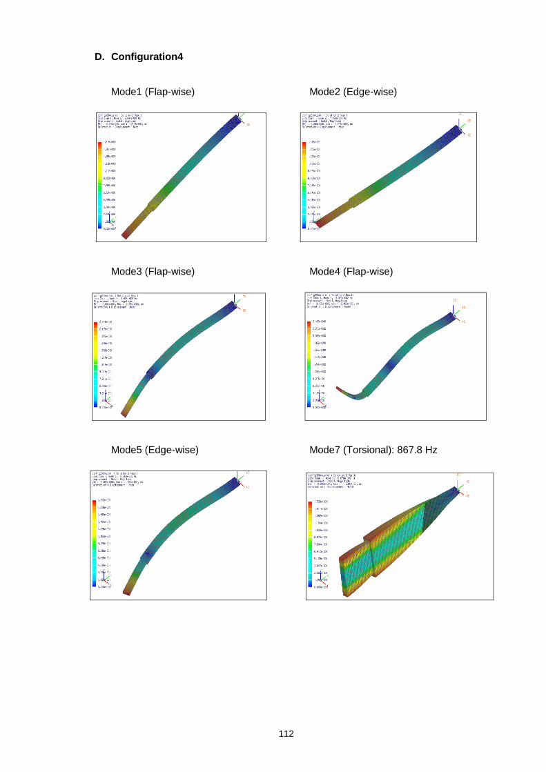
112
D. Configuration4
Mode1 (Flap-wise) Mode2 (Edge-wise)
Mode3 (Flap-wise) Mode4 (Flap-wise)
Mode5 (Edge-wise) Mode7 (Torsional): 867.8 Hz

113
E. Configuration5
Mode1 (Flap-wise) Mode2 (Edge-wise)
Mode3 (Flap-wise) Mode4 (Flap-wise)
Mode5 (Edge-wise) Mode7 (Torsional) : 829.9 Hz
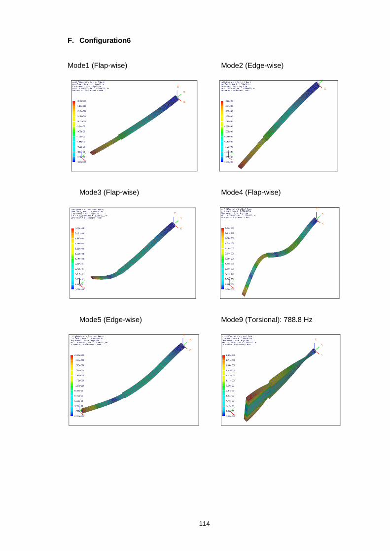
114
F. Configuration6
Mode1 (Flap-wise) Mode2 (Edge-wise)
Mode3 (Flap-wise) Mode4 (Flap-wise)
Mode5 (Edge-wise) Mode9 (Torsional): 788.8 Hz
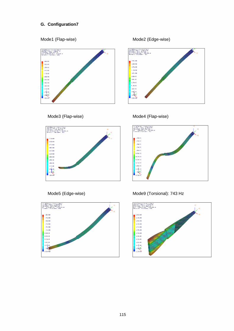
115
G. Configuration7
Mode1 (Flap-wise) Mode2 (Edge-wise)
Mode3 (Flap-wise) Mode4 (Flap-wise)
Mode5 (Edge-wise) Mode9 (Torsional): 743 Hz

116
H. Configuration8
Mode1 (Flap-wise) Mode2 (Edge-wise)
Mode3 (Flap-wise) Mode4 (Flap-wise)
Mode5 (Edge-wise) Mode9 (Torsional) : 693.5 Hz

117
I. Configuration9
Mode1 (Flap-wise) Mode2 (Edge-wise)
Mode3 (Flap-wise) Mode4 (Flap-wise)
Mode5 (Edge-wise) Mode9 (Torsional) : 643.2 Hz

118
J. Configuration10
Mode1 (Flap-wise) Mode2 (Edge-wise)
Mode3 (Flap-wise) Mode4 (Flap-wise)
Mode5 (Edge-wise) Mode9 (Torsional) : 595 Hz

119
Appendix F: NX5 and MATLAB results comparison

120