Embed Size (px)
Citation preview

Mueller Industries Inc.
Amanda Miller – [email protected] Park Hunter – [email protected]
Shyla Walton – [email protected] Austin Head – [email protected]
Josh Jacobsen – [email protected]

2
Table of Contents
Executive Overview……………………………………………………………………………………………….6 Company Overview………………….………………………………………………………………………….13 Business & Industry Analysis…………..…………………………………………………………..……….15 Five Forces Model……………………………………………………………………………………………….16 Rivalry Among Existing Firms……………………………………………………………………..16 Industry Growth……………………………….……………………………………………..17 Concentration…………………………….……………………………………………………19 Differentiation…………………………………………………………………….…………..21 Switching Costs……………………………………………………………………………….22 Economies of Scale………………..………………………………………………………..22 Learning Economies………………..……………………………………………………….23 Fixed to Variable Costs……………..……………………………………………………..24 Excess Capacity…………………………………………………..…………………………..25 Exit Barriers………………………………………………….…………………………………26 Conclusion…………………………………………………..………………………………….26 Threat of New Entrants…………………………….……………………………………………….27 Economies of Scale……………………………………….…………………………………27 First Mover Advantages………………………………………….………………………..28 Channels of Distribution & Relationships…………….……………………………..29 Legal Barriers………………………………………………….………………………………29 Conclusion…………………………………………………….………………………………..30 Threat of Substitute Products……………………………………………………………………..31 Relative Price and Performance…………………………………………………………31 Buyers Willingness to Switch…………………………………………………………….32 Conclusion………………………………………………………………………………………32 Bargaining Power of Customers…………………………………………………………………..33 Price Sensitivity……………………………………………………………………………….33 Relative Bargaining Power………………………………………………………………..34 Conclusion………………………………………………………………………………………35 Bargaining Power of Suppliers…………………………………………………………………….36 Conclusion………………………………………………………………………………………37 Five Forces Conclusion…………………………………………………………………………………………37 Key Success Factors of the Industry………………………………………………………………………38 Economies of Scale……………………………………...………………………..………………….38 Economies of Scope…………………………………………………………..……………………...39 Efficient Methods and Cost Control………………..……………………………………………41 Input & Distribution Costs…………………………………………..……………………………..42 Research, Development & Advertising…………………………..…………………………….43 Summary………………………..…………………………………………..……………………………44 Competitive Advantage Analysis……………………………………………………………………..…….45 Large Scale Production……………………….……………………………………………………..45

3
Production Efficiency……………………….…………………………………………………………46 Other Advantages…………………………….……………………………………………………….48 Summary………………………………………………………………………………………………….48 Accounting Analysis…………………………………………………………………………………………….49 Key Accounting Policies………………………………………….…………………………………………...50 Goodwill………………………………………………………..………………………………………….50 Pension Plan & Retirement Compensation………..………………………………………….52 Hedging Activities……………………………………….…………………………………………….53 Management of Fixed Costs…………………………..……………………………………………54 Capital & Operating Leases……………………….………………………………………………..55 Degree of Potential Flexibility……………….………………………………………………………………56 Goodwill………………………………………………..………………………………………………….56 Pension Plan & Retirement Compensation…….……………………………………………..57 Hedging Activities……………………………………………………………………………………..58 Management of Fixed Costs………………….……………………………………………………59 Capital & Operating Leases…………………………………………………………………………59 Actual Accounting Strategy…………………………………………………………………………….……60 Goodwill……………………………………………………………………………………………………60 Pension Plan & Retirement Compensation…………..……………………………………….62 Hedging Activities………………………………………………………………………………………63 Management of Fixed Costs……………………..…………………………………………………64 Capital & Operating Leases…………………………………………………………………………64 Evaluate Quality of Disclosure………………………………………………………………………………66 Qualitative Analysis………………………………………..……………………………………………………66 Goodwill……………………………………………………….…………………………………………..66 Pension Plan & Retirement Compensation……………………………………………………67 Hedging Activities………………………………………………………………………………………69 Management of Fixed Costs…………………………………………..……………………………70 Capital & Operating Leases…………………………………………………………………………71 Quantitative Analysis……………………………………………………………………………………………72 Expense Manipulation Diagnostics…………….…………………………………………………72 Asset Turnover………………..………………………………………………………………72 CFFO/OI………………………………………………….………………………………………74 CFFO/Net Operating Assets………………………………………………………………75 Total Accruals/Sales…………………………………………………………………………76 Pension Expense/ SG&A……………………………………………………………………77 Other Employment Expense/ SG&A……………..…………………………………….78 Conclusion………………………………………………………………………………………79 Revenue Manipulation Diagnostics………………………………………………………………80 Net Sales/ Cash from Sales………………………….……………………………………80 Net Sales/ Net Accounts Receivable……………..……………………………………81 Net Sales/ Inventory………………………………..………………………………………83 Conclusion………………………………………………………………………………………84 Potential Red Flags……………………………………………..………………………………………………85

4
Undo Accounting Distortions………………………………………………………………………………..85 Financial Analysis, Forecasting & Cost of Capital Estimation…….………………………………88
Liquidity Ratio Analysis………………………………………….……..……………………………88 Current Ratio………………………………………..…………………………………………89 Quick Asset Ratio…………………………………………………………………………….90 Accounts Receivable Turnover……………….…………………………………………91 Days in Accounts Receivable…………………………………………………………….92 Inventory Turnover………………………………………………………………………….93 Days Supply of Inventory…………………………………………………………………94 Working Capital Turnover…………………………………………………………………95 Cash to Cash Cycle………………………………………………………………………….96 Conclusion……………………………………………………………………………………..97
Capital Structure Ratios……………………………….…………………………………………….98 Debt to Equity...................................................................................98
Times Interest Earned…………………………………………………………………….100 Debt Service Margin…………..…………………………………………………………..101 Credit Risk…………………….………………………………………………………………102 Conclusion………………………………….…………………………………………………103 Profitability Ratio Analysis…………………………………………………………………………104 Gross Profit Margin…………………………………………………………………………104 Operating Expense Ratio…………………………………………………………………105 Operating Profit Margin…………………………………………………………………..106 Net Profit Margin………………..………………………………………………………….107 Asset Turnover………………………………………………………………………………108 Return on Assets…………..……………………………………………………………….109 Return on Equity……………………………………………………………………………110 Internal Growth Rate………..……………………………………………………………111 Sustainable Growth Rate…………………………………………………………………112 Conclusion…………………….………………………………………………………………113 Financial Statement Forecasting……………….…………………………………………………………114 Income Statement……………….………………………………………………………………….114 Balance Sheet………………………..……………………………………………………………….121 Statement of Cash Flows………….………………………………………………………………127 Cost of Capital Estimation………………………..…………………………………………………………132 Cost of Equity………………………….………………………………………………………………132 Backdoor Cost of Equity……………………………………………………………………………135 Cost of Debt……………………………………………………………………………………………136 Weighted Average Cost of Capital………………….………………………………………….138 Valuation Methods…………….……………………………………………………………………………….140 Method of Comparables……………………………………………….…………………………………….141 Price to Earnings Trailing…………….……………………………..……………………………142 Price to Earnings Forward………….…………………………………………………………….143 Price to Book............………………………………………………………………………………143 Dividends to Price…………………….……………………………………………………………..144

5
Price Earnings Growth…………………………..………………………………………………….144 P/EBITDA……………………………..…………………………………………………………………145 P/FCF………………………………..……………………………………………………………………145 EV/EBITDA………………………………………………………………………………………………146 Conclusion………………..…………………………………………………………………………….146 Intrinsic Valuation Models………………………………..…………………………………………………148 Discounted Dividends Model……………………………………………………………………..149 Discounted Free Cash Flows……………………………………………………………………..152 Residual Income………………………………………………………………………………………156 Long Run Residual Income……………………………………………………………………….159 Abnormal Earnings Growth……………………….………………………………………………163 Conclusion………………………….…………………………………………………………………..165 Appendix………………………………………………………………………………………………………….166 Sales Manipulation Diagnostics…………………………………………………..……………..166 Expense Manipulation Diagnostics………………………………..……………………………167 Effects on Restatement of Goodwill…………………………….…………………………….169 Liquidity Ratios…………………………………………….………………………………………….173 Profitability Ratios…………………………………….……………………………………………..175 Capital Structure Ratios………………….………………………………………………………..177
Altman’s Z-score……………………………………………………………………………………..178 Cost of Capital Regression Outputs………………….………………………………………..189 Cost of Equity, Debt & WACC………………………………..………………………………….194 Method of Comparables Tables…………………..…………..………………………………..195 Intrinsic Valuations…………………………….…………………………………………………….197 References………………………………………………………………………………………………………205

6
Executive Summary
Investment Recommendation: Overvalued Sell as of November 1st, 2008
52 Week Range: 2003 2004 2005 2006 2007Revenue: $2.74 B As Stated 4.57 2.48 3.21 4.23 4.09Market Capitalization: $865.27 M Restated 4.51 2.53 3.20 4.29 4.18Shares Outstanding: $37.14 M Percent Institutional Ownership: 96.10%
As Stated RestatedBook Value Per Share: $19.13 $15.77 As Stated RestatedROE: 19.61% 23.58% Trailing P/E: $12.23 $10.39ROA: 9.10% 9.94% Forward P/E: $41.86 N/A
P/B: $10.62 $8.75D/P: $6.65 N/A
R^2 Beta Ke P.E.G: - N/A3 Month 36.03% 1.49 18.31% P/EBITDA: $19.54 $17.252 Year 36.05% 1.49 18.28% P/FCF: $20.02 N/A5 Year 35.89% 1.49 18.22% EV/EBITDA: $12.38 $9.927 Year 35.81% 1.48 18.19%10 Year 35.72% 1.48 18.16%
As Stated RestatedUpper and Lower Ke: Discounted Dividends: $10.12 N/APublished Beta: 0.88 Discounted FCF: $35.28 $39.57Back Door Ke: 14.52% Residual Income: $10.35 $10.09Cost of Debt: 5.99% Long Run Redisual Income: $14.33 $11.82WACC (BT) 12.02% A.E.G.: $7.16 N/AUpper and Lower WACC (BT)
Altman's Z-ScoresMLI - NYSE (Nov 1, 2008) $23.31
Cost of Capital Estimate (Including 2.3% Size Premium)
Current Market Share Price (Nov 1, 2008) $23.31
Financial Based Valuations
8.76% - 15.27%
11.64% - 24.92%
Intrinsic Valuations
$17.57 - $35.66

7
Industry Analysis Overview
Mueller competes in the metal fabrication industry and makes all types of pipes,
tubes, and fittings that are sold to a variety of customers across various industries. Our
analysis of the industry consists of Mueller and its three closest publicly traded
competitors: Alcoa, Madeco and Wolverine Tube Inc. Together these companies supply
firms from automotive and housing all of the way to aerospace and electrical industries.
As companies in the metal fabrication industry tend to make relatively simple and
generic products, cost becomes the main source of competition. Cost control and
operation management are imperative to being successful in this industry.
The five forces model allows us to identify threats that are present throughout
the industry as a whole and discuss the methods that are necessary for success. The
following is a brief summary of the model and its conclusions.
Results of the Five Forces Model
It is important to become familiar with the environment of a company’s
competition if one wishes to fairly evaluate it. Our discussion of the metal fabrication
industry illustrates the external matters a company will face. The model describes the
high concern of substitute products as each company makes more or less the same
products. It also suggests the unlikely occurrence of new entrants as the industry
requires a large amount of assets in order to be competitive. These and other concerns
are addressed in the industry analysis section.
Rivalry Among Existing Firms High
Threat of New Entrants Low
Threat of Substitute Products High
Bargaining Power of Customers High
Bargaining Power of Supplies Medium
8
Accounting Analysis Overview
The numbers that are published in the quarterly and annual reports are
supposed to accurately reflect the businesses activities of each company. There are
many regulations imposed by the SEC and GAAP as to how a company can account for
their processes. In an accounting analysis, the first step is to identify the key
accounting policies that can be examined to evaluate a company’s transparency. These
policies should be looked at closely as they provide potential for distortion and
manipulation that can shine a company in a false light.
We used revenue manipulation diagnostics ratios to demonstrate how current
assets and current liabilities relate to net sales. These ratios also help us determine if
there is anything out of the industry norm that could potentially be a “red flag” in the
financial statements. Most of the revenue manipulation diagnostics looked within the
industry norm. The only ratios that had stood out were the net sales divided by net
accounts receivables and net sales divided by inventory. However, we concluded that
both of these slight differences were due to fluctuating copper prices in the market and
did not qualify as a “red flag”.
We did identify one major red flag when examining Mueller’s accounting
practices, this being how the company accounts for goodwill. Over the past five years
Mueller has been involved in a number of mergers and acquisitions, thus adding to their
goodwill. However, they only impaired a small fraction of it. Goodwill does not last a
lifetime; in fact, it should really have a useful life of about five years. Since Mueller
keeps goodwill on their books for much longer than five years, we believe this
significantly distorts the true value of the firm. We undid this distortion by taking the
goodwill balance in 2003 and writing it off for the next five years, adjusting for new
mergers and acquisitions along the way. We restated Muller’s income statement and
balance sheet to reflect these changes. This helps give investors a better picture of the
true value of the firm.

9
On the other hand, analysis of other policies allows us to verify Mueller’s ‘as
stated’ version. For instance, operating leases only account for 5.79% of total long term
liabilities and thus suggests that the company gives a fair view of its lease liabilities.
Likewise, the disclosure of hedging activities appears fair and reliable. The accounting
analysis section compares these and other accounting policies that will have an impact
on our valuation.

10
Financial Analysis, Forecasting and Cost of Capital Estimation
We begin the financial analysis by looking at a number of liquidity, profitability
and capital structure ratios. These ratios give us an idea of Mueller’s financial position
and allow us to put them up against their competitors. In doing so, we are able to see
what aspects the company excels at and in what aspects they are lacking. The day’s
supply of inventory is one that Mueller has to its advantage as it is able to turn
inventory into sales relatively quicker than its competitors.
Profitability ratios measure how well a firm’s revenues cover its expenses. The
ratios show a percentage of sales, where sales equal 100%. Overall, Mueller was
efficient in covering its expenses compared to the metal fabrications industry. Mueller
was average using operating profit margin and net profit margin. Mueller outperformed
the industry average in gross profit margin, operating expense ratio, asset turnover,
return on assets, and return on equity. After analyzing these profitability ratios, we
concluded that Mueller has kept a strong competitive strategy over the past 5 years by
continually being either average or above average in the industry.
Liquidity ratios determine the ability at which a firm is able to handle its short
term assets, these assets include: cash, accounts receivables, and inventory. Knowing
how well a firm is able handle its short term assets also explains to analysts how well a
firm is able to pay of its short-term debt. In the case of Mueller, its liquidity ratios
seemed to be average in comparison to competitors within the metal fabrication
industry. The table below states how each of Mueller’s liquidity ratios did in comparison
to the industry average (above, equal, and below).
Results of Liquidity Ratios
Current Quick
Asset
A/R
Turnover
Days in
A/R
Inventory
Turnover
Days in
Inventory
Working
Capital
Turnover
Cash to
Cash Cycle
Above Above Below Below Above Above Below Equal
Forecasting financial statements are important as it allows us to get a view of the
company into the near future. Forecasting will never end up exactly as planned, but the

11
analysis of financial ratios helps us improve our accuracy. There are a number of
estimates that go into forecasting, such as growth rates, discount rates and prediction
of the economy in general. Forecasting financial statements involves looking at a
company’s current and past financial data to predict how the company will perform in
the future. The most crucial forecast was had to make was sales growth. We could not
simply look at Mueller’s sales growth over the past few years to predict the future,
mainly because the country is headed into a recession which is sure to affect Mueller’s
revenues. Therefore, we looked back at Mueller’s sales growth during the last major
recession to see how the company was affected. We mirrored our sales growth based
off of these numbers, but assumed Mueller would be hit slightly harder by this
recession. Also, a lot of our forecasts were based upon our previously calculated
financial ratios. For example, we used the asset turnover ratio to link the income
statement and balance sheet. Lastly, we forecasted the statement of cash flows, where
we forecasted out cash flow from operations, cash flow from investing activities, and
dividends. It is also important to note we forecasted out Mueller’s restated financial
statements as well since the changes we made to goodwill significantly altered Mueller’s
financial statements.
The final subject discussed in this section is the cost of capital for Mueller. This is
the return that investors expect to receive for investing in Mueller’s stock. We calculated
this return by running a regression of U.S. Treasury rates and S&P 500 returns over the
last seven years. Using multiple periods and their treasury rates, we are able to
estimate the beta, or risk for investing with Mueller specifically. With these pieces in
place, we were given an estimated cost of capital for Mueller Industries of 18.28%. This
rate serves as our discount rate in the following section of valuation analysis. Full
discussion of financial ratios, forecasting and cost of capital is disclosed in the
corresponding section.

12
Valuation Analysis
Our method of valuation for Mueller Industries can be divided into two parts.
First, the method of comparables allows us to derive a share price for Mueller based on
the performance of its competitors. Ratios such as the price to earnings ratio and price
to book ratio are calculated for each competitor, and by setting Mueller equal to the
industry average, we can solve for the share price of each equation and thus estimate
Mueller’s value. This method does have significant flaws in that it prices the company
solely on the performance of its competitors. This means that any competitive
advantage that Mueller may have can be overlooked if it is not involved in the ratio.
With this is mind, we found the method of comparables to be less useful than the
intrinsic valuation models.
The intrinsic valuation models hold more weight in our determination of the
value of Mueller as they are based on the actual operations of the company instead of
comparisons to competitors. Our forecasts played a huge part in these valuations as the
share price was based on the present value of future financial estimations. Because
these forecasts are based on multiple estimates, we used five different models before
concluding on Mueller as being an overvalued company. Out of the five models, the
discounted free cash flow model was the only one that did not give Mueller and
overvalued rating. Models such as the discounted dividend model and residual income
model use the cost of equity as the discount rate to turn future estimates into present
value. In models that use net income as a starting point (an after tax figure), our
weighted average cost of capital before tax is used as the discount rate. In turning to
our valuation section, one can see that Mueller appears to be overvalued and
individuals holding shares would be advised to sell them.
13
Company Overview
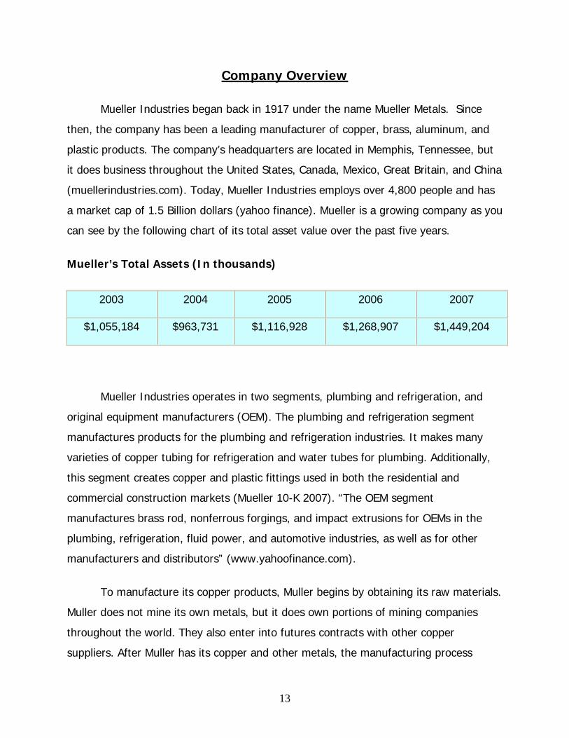
Mueller Industries began back in 1917 under the name Mueller Metals. Since
then, the company has been a leading manufacturer of copper, brass, aluminum, and
plastic products. The company’s headquarters are located in Memphis, Tennessee, but
it does business throughout the United States, Canada, Mexico, Great Britain, and China
(muellerindustries.com). Today, Mueller Industries employs over 4,800 people and has
a market cap of 1.5 Billion dollars (yahoo finance). Mueller is a growing company as you
can see by the following chart of its total asset value over the past five years.
Mueller’s Total Assets (In thousands)
2003 2004 2005 2006 2007
$1,055,184 $963,731 $1,116,928 $1,268,907 $1,449,204
Mueller Industries operates in two segments, plumbing and refrigeration, and
original equipment manufacturers (OEM). The plumbing and refrigeration segment
manufactures products for the plumbing and refrigeration industries. It makes many
varieties of copper tubing for refrigeration and water tubes for plumbing. Additionally,
this segment creates copper and plastic fittings used in both the residential and
commercial construction markets (Mueller 10-K 2007). “The OEM segment
manufactures brass rod, nonferrous forgings, and impact extrusions for OEMs in the
plumbing, refrigeration, fluid power, and automotive industries, as well as for other
manufacturers and distributors” (www.yahoofinance.com).
To manufacture its copper products, Muller begins by obtaining its raw materials.
Muller does not mine its own metals, but it does own portions of mining companies
throughout the world. They also enter into futures contracts with other copper
suppliers. After Muller has its copper and other metals, the manufacturing process
14
begins. This consists of casting, extruding, drawing, forming, joining and finishing.
Through this process, the copper is transformed into finished products to meet the
needs and demands of Muller’s customers.
Mueller Industries competes with various companies in the metal fabrication
industry. Some of its competitors include Wolverine Tube Inc. (WLVT.OB), Madeco S.A.
(MAD), and Alcoa Inc. (AA). Wolverine is Mueller’s most direct competitor because both
companies create copper, aluminum, and brass products for the housing and
construction industries. While not direct competitors, Madeco and Alcoa also compete
with Mueller across certain product lines. Madeco, located in Chile, manufactures and
sells products created from copper, aluminum, and related metals, while Alcoa produces
mainly aluminum products (Madeco and Alcoa 10-Ks 2007).
While the industry is highly competitive, the sales growth among the firms is
very inconsistent as shown in the graph below. All the companies show similar zigzag
patterns of sales growth from 2004 to 2007. This means sales decreased, increased,
and then decreased again across all firms. From this, it clear that there has been an
inconsistency in the market over the past few years. There is nothing an individual
company is doing to cause such fluctuations, but rather the conditions in the industry or
economy are to blame. There is a large decrease in sales growth from 2006- 2007,
mainly because of the United State’s declining economy. Since all the firms in this
industry are very “sensitive to changes in general economic conditions, including, in
particular, conditions in the housing and commercial construction industry” (Mueller’s
2008 10-K 2008, Pg 11), they will all be affected by the recession. Sales will most likely
continue to decline for the next few years.

15
Sales Growth
-20.00%-10.00%
0.00%10.00%20.00%30.00%40.00%50.00%60.00%70.00%
2004 2005 2006 2007
Year
Sale
s gr
owth
as
perc
anta
ge
MuellerWolverineAlcoaMadecoIndustry
Business and Industry Analysis
Mueller produces various pipes, tubes and accessories that are sold to
wholesalers of industries with residential/commercial construction, refrigeration, heating
and plumbing involvement. Like its competitors in the industry, a focus is held on cost
leadership and large scale production as this is the best way to achieve stability in the
market. Maintaining strong relationships with customers and suppliers is important as
there are multiple choices for each to do business with. This is going to be very
important now, since the United States is in a recession. Competition among firms in
the industry is going to be extremely high and most everyone will see a decline is sales
for the next few years. It will be harder for companies to focus on cost leadership and
large scale production, especially when their costs for raw materials and such are going
up as well. The industry as a whole is dependent on prices of raw materials and inputs
that are used by all competitors. Further analysis of how the industry competes on
these and other variables of concern are discussed below.

16
Five Forces Model
When valuing a firm, it is important to understand the nature of the industry it
competes in. The five forces model allows analysts to identify and examine five
competitive forces that shape the industry. The model shows that when analyzing the
degree of actual and potential competition, you need to be aware of the rivalry among
existing firms, the threat of new entrants, and the threat of substitute products. It also
takes into the account the bargaining power of customers and suppliers. With these
five forces identified, an analyst can fully understand the competitive nature of the
industry and the things that create value. The flowing table shows our analysis of the
five forces impacting the metal fabrication industry, and the degree of competition
produced by each one.
Results of the Five Forces Model
Rivalry Among Existing Firms High
Threat of New Entrants Low
Threat of Substitute Products High
Bargaining Power of Customers High
Bargaining Power of Supplies Medium
Rivalry among Existing Firms
When applying the Five Forces Model in the valuation of a corporation, one must
contemplate the rivalry amongst existing firms in order to achieve a complete industry
analysis. The rival among existing firms is measured by nine significant categories,
these being: Industry growth, Concentration, Differentiation, Switching costs, Scale,
Learning Economies, Fixed-Variable Costs, Excess Capacity, and Exit Barriers. In using
these nine distinct categories we hope to express our corporation’s industry as a whole,

17
whether that may be by the pricing of our products compared to those of our
competitors, or by some other non-price related differentiation.
Industry Growth
The growth of an industry has a major role in determining how a corporation
must function when it comes to competing with other firms. For example, existing
firms entrenched in an industry booming with growth are less likely to have to strongly
compete with each other in order grow themselves. The opposite of this situation being
if an industry’s growth is in the decline or remaining constant, then the firms within the
industry will have to battle for their individual market share. The best way of measuring
an industry’s growth is by breaking down the total number of sales over the past five
years from all the existing firms involved in the industry and comparing each firm’s
annual percentage change.
0.00%
5.00%
10.00%
15.00%
20.00%
25.00%
Gro
wth
%
2004 2005 2006 2007
Year
Industry Sales Growth
*Percentages computed by the revenues of: Mueller Industries, Wolverine Tube, Madeco S.A., & Alcoa.
18
Industry Sales (In Thousands)
0
5,000,000
10,000,000
15,000,000
20,000,000
25,000,000
30,000,000
35,000,000
40,000,000
2003 2004 2005 2006 2007
Year
Sale
s
*Percentages computed by the revenues of: Mueller Industries, Wolverine Tube, Madeco S.A., & Alcoa.
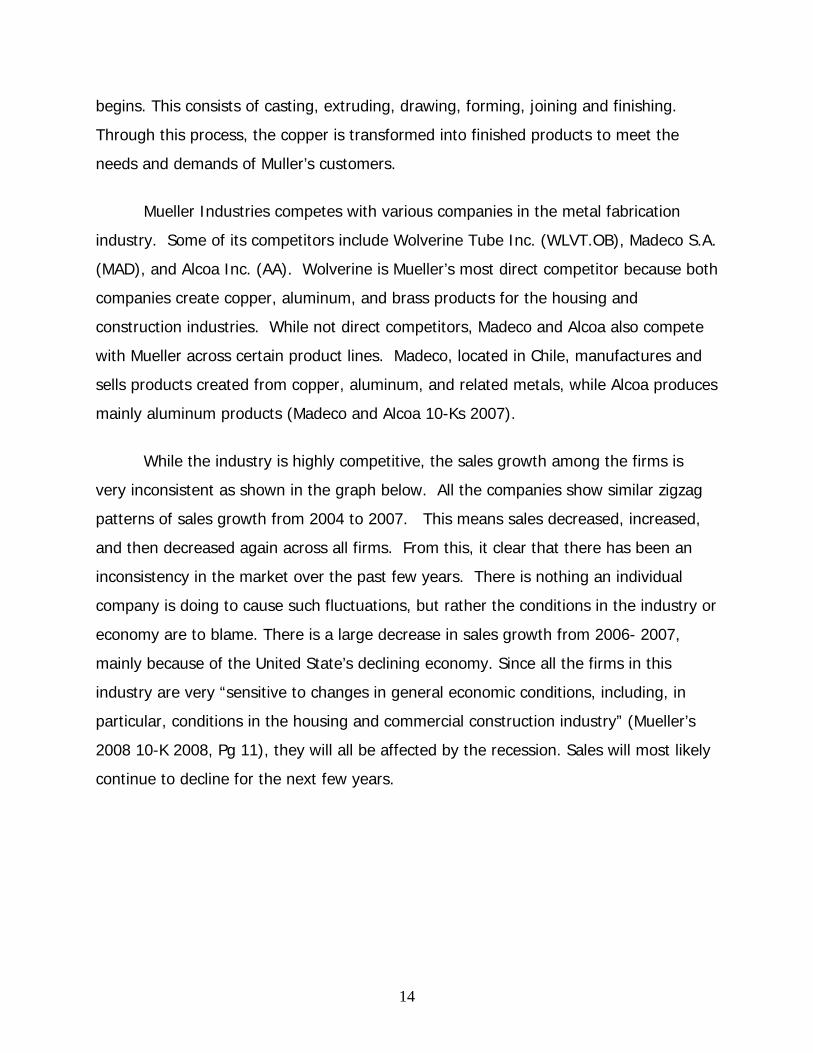
These graphs show that the industry is continuously growing year by year. They
also show that there was a huge growth in the industry from 2005-2006. This is due in
large part to an increase in market demand. Then, from 2006-2007 market demand
drastically reduced, which would explain why growth in the industry was not as
impressive as it was in past years. In this particular industry there happens to be a
fairly abundant amount of privately held corporations in both America and worldwide,
which makes the industry’s actual growth a little more difficult to predict. Also, both
Madeco S.A. and Alcoa produce extensive lines of products that go beyond what Mueller
and Wolverine produce, which in turn would alter these numbers as well. However, it is
still apparent that industry growth decreased from 2006-2007, and will continue to do
so for the next few years due to the U.S.’s declining economy. As mentioned earlier,
since all the firms in this industry are very “sensitive to changes in general economic
conditions, including, in particular, conditions in the housing and commercial
construction industry” (Mueller’s 2008 10-K 2008, Pg 11), they will all be affected by the
recession. Even though Madeco is not located in the United States, it will still be
indirectly affected by it mainly because their “risk factors depend not only on the
growth in South America, but the growth in the company’s export markets” (Madeco

19
Annual Report 2007). Since the United States is one of their export markets, their sales
will probably decrease as well. Also, “Alcoa’s operations consume substantial amounts
of energy, and profitability may decline if energy costs rise or if energy supplies are
interrupted” (Alcoa 10-k 2007). During 2007 energy costs such as oil were on the rise.
This adversely affected Alcoa’s sales during 2007, along with other firms in the metal
fabrication industry that consume a lot of energy. Because of the very weak and volatile
economic conditions the U.S. is facing, sales in the metal industry are likely to decrease
over the next two or three years.
Concentration
The concentration and balance of firms in an industry is the determining factor
which tells us which competitors have the power in the industry. The fewer
competitors that exist in an industry, the higher the concentration will be and vice
versa. The amount of concentration in an industry usually determines how a
corporation is going to set their prices, and other business shifts, in comparison to their
competitors. Wolverine stated in their most recent 10-k that in some of its product
lines “certain competitors have significantly larger market shares than us, and tend to
be price leaders in the industry” (Wolverine 10-k 2007). Since Wolverine has
significantly lower market share, they are forced to set their prices based upon what the
market leaders are charging for the same products. Of course, a monopoly would be
the best case scenario for any corporation who wanted a high concentration, but with
monopolies being regulated, companies just hope to take the biggest portion of market
share they can get.

20
2003 Market Share
Mueller
Wolverine
Madeco
2004 Market Share
Mueller
Wolverine
Madeco
2005 Market Share
Mueller
Wolverine
Madeco
2006 Market Share
MuellerWolverineMadeco
2007 Market Share
MuellerWolverineMadeco
Some of the fortunate companies are able to maintain a high market share and
concentration by becoming a dominant figure in their industry (i.e. Microsoft).
However, most companies must deal with stringent competition, as such in the metal
fabrication industry. In these competitive industries, companies must use an unspoken
understanding of prices in order to avoid an extreme driving down of prices within the
given industry. The graphs above show the break down of market share over the past
five years in the metal industry. Alcoa was excluded because it is a much more
expansive firm than the others, in that they do more than just manufacture
metal/plastic fittings, tubes, rods, and bars. If it was included in the pie chart it would
consume over 90% of the pie. Knowing this one can make the assumption that Alcoa is
not a true direct competitor. Nevertheless, the graphs indicate that Mueller has the
highest market share, followed by Madeco, then Wolverine. However, the three firms
have been fighting over market share. Over the past five years, Wolverine went from
having 28% market share to 24%, Madeco went from 21% to 25%, and Mueller has
fluctuated right around 51%. There are not any dramatic changes, but it is still evident
that competition over market share exists among firms in the industry.

21
Another important factor to consider in regards to concentration would be to find
out if firms within the industry mine their own metals. After much research one could
come to the conclusion that some firms in this industry do mine their own metals, and
some of them do in fact own portions of mining companies throughout the world.
Everyday worldwide Alcoa Mines 86,300 tons of bauxite, an aluminum ore (Alcoa 10-k
2007). Also, Mueller owns 49.5% of Jiangsu Mueller-Xingrong Mining Company, and
25% of Ruby Hill Mining Company (Mueller 10-k 2007). By mining their own metals
and having ownership in mining companies, firms within the metal fabrication industry
are able to cover their costs of buying raw materials by technically buying it from
themselves.
Differentiation
Firms that are able to differentiate their products within the industry are better
suited when it comes to combating with the competitors they are up against. For
example, a firm that has a certain product that is superior to that of its competitors is
going to have more leverage in the market, such as Apple’s iPhone in the cell phone
market. Having a product, in the iPhone, that stands out from the rest allows Apple to
charge whatever they please for this product. Consumers are forced to purchase at
Apple’s price if they wish to have this product, because none of its competitors have
anything like it. However, in an industry of little product differentiation, firms are
regulated to compete solely on who has the lower price. This is due to the fact that
consumers are not going to pay more for a product that is identical to every other
product manufactured in the industry.
This industry’s products consist of different types of materials such as copper,
brass, plastic, and aluminum. These materials are used to produce items that include
tubing, non-iron forgings, impact extrusions, and brass rods. These products are used
in the air-conditioning, refrigerating, and plumbing industries. One must also take into
account that firms included in the measurement of this industry such as Alcoa produce
a much more extensive line of products.

22
In the metal fabrication industry, there is going to be very little differentiation
amongst the competitors. “Minimal product differentiation among competitors in the
U.S. wholesale product categories creates a pricing structure that enables customers to
select products almost exclusively on price” (Wolverine 10-k 2007). It also does not
help that two of the more important factors in making products dissimilar are almost
non-existent in this industry, these two factors being: technology and innovation.
Switching Costs
Switching costs refers to a company’s ability to switch to a producing a different
product or service. These are the costs subjected to the company if it were to switch to
a completely different industry. When switching costs are high, companies are more
inclined to continue producing the same type of product due to the high cost of
changing businesses. In the case of the metal fabrication industry, research and
development spending for most firms involved is almost non-existent, leading to lower
levels of switching costs. However, there is a lot of money invested in machinery,
equipment, and plants which are meant to build the distinctive products designed by
the corporation, thus leading to higher levels of switching costs. Conversely, one could
make the argument that this equipment and machinery could be used to manufacture
products in another industry. This assumption, of course, would be in accordance to
what the equipment/machinery are actually capable of doing. The evidence presented
would have to conclude that the metal fabrication industry would typically have
moderate levels of switching costs.
Economies of Scale
The economies of scale in the metal fabrication industry are remotely large
because the entire industry does not have much product differentiation along with the
fact that there is very little spending on research and development. With little product
differentiation and many different competitors, the biggest firm in the industry really

23
has an advantage over the smallest one, in terms of capital. This is because the little
guy is offering the exact same product at the exact same price as the bigger firms in
the industry, leading to the assumption that one must have large numbers of capital
and production in order to maximize profits. These large numbers of capital help the
larger firms produce mass quantities of products compared to that of smaller firms, and
the more products you can produce at an efficient rate, the cheaper the price you are
able to offer. This is tremendously important in an industry in which prices play the
most vital role. The following chart shows the total assets of each firm in the industry.
It is obvious that Alcoa has the most capital, but once again it is because it is a much
larger firm that the rest, and therefore, it is not considered a direct competitor. When
looking at the other companies, Mueller and Wolverine have continued to increase their
capital, while Wolverine’s capital has slightly decreased. This could help explain why
Wolverine’s market share has decreased over the past five years and Madeco’s has
increased. Firm’s with greater capital have a distinct advantage in a cost competitive
industry.
Total Assets (In Thousands) 2003 2004 2005 2006 2007
Mueller 1,055,184 963,731 1,116,928 1,268,907 1,449,204
Madeco 622,805 637,328 683,801 841,533 979,066
Wolverine 553,258 587,458 568,765 455,330 456,673
Alcoa 31,711,000 32,609,000 33,696,000 37,183,000 38,803,000
Learning Economies
Similar to the economies of scale, the lack of use of the research and
development in the metal fabrication industry makes the learning curve in this particular
industry very minuscule. There are not many new innovations or technological
advances being discovered when it comes to making rods, bars, shapes, forgings,
impact extrusions, pipes, valves, tubes, faucets, and fittings from different types of
metals and plastics.

24
Ratio of Fixed to Variable Costs
Determining whether an industry usually has more fixed or variable costs is
important when valuing an individual firm within that industry. In the metal fabrication
industry, firms are more likely to have an equal volume of fixed costs compared to
variable costs. This is mostly due in part to the fact that the firms within the metal
fabrication industry usually outsource their finished products to other companies such
as the auto, refrigeration, and plumbing industries. Along with the outsourcing of
finished products, much of the firms in the metal fabrication industry also categorize
their ownership of giant factories, mills, buildings, machinery and equipment as fixed
costs.
The variable costs that exist in this industry are very prevalent as well. For
example, “escalating production costs and cooling commodity prices are dragging down
once-mighty mining and metal companies” (Wall Street Journal). In order for firms to
manufacture their product, they must first purchase the metals needed from their
suppliers. Firms must first pay the market price for metals such as copper and brass in
order to manufacture their products. This would be considered a variable cost to the
company because these prices are never the same from year to year, and sometimes
even vary from day to day. Although one must take in to account that even though
these metals are variable costs to a firm, every other firm within the same industry
must pay the exact same price as other. This importance of each firm having to pay
the same price for these materials is; if high raw material costs were to occur for one
firm, the same outcome would arise for the other industry firms as well, thus creating
no particular advantage for any firm in terms of these costs.
Another important factor to take into account in regards to an industry’s fixed to
variable costs ratio, would be research and development costs. Research and
development usually plays a vital role in the costs a firm incurs, but as aforementioned
in previous sections, R&D is limited in the metal fabrication industry.

25
Excess Capacity
Excess capacity is defined in our book as: If consumer demand is lower than the
capacity of the industry, then the firms within that particular industry will have to most
likely lower their prices in order to restore capacity. (Palepu & Healy P. 2-3) The
opposite of this situation being if the consumers demand is greater than supply, then
the competitors are not going to have to compete with each other when it comes to
prices. In this industry however, consumer demand is not very high as of late, this is
fact is stated in Mueller’s 10-K, “The majority of the Company’s manufacturing facilities
operated at moderate levels during 2005 and the first half of 2006. In the latter half of
2006, and in 2007, the Company’s manufacturing facilities operated at low levels due to
reduced market demand.” (Mueller Industries 10-K Filed February 26th, 2008, Pg. 4, Pg
6 on Adobe Reader). Wolverine also stated in its 10-k that because of the excess
capacity in the copper tube manufacturing markets, they have had little success in
selling their used equipment.
These numbers in the diagram above state each firm in the industry’s total
revenue divided by their total property, plant, and equipment. This is important
because it shows how well a firm is able to convert assets into revenue. Most of the
firms which deal directly with only the metal fabrication industry seem to have
extremely successful efficiency in their management of excess capacity.
Sales / Total Property, Plant & Equipment
2003 2004 2005 2006 2007
Mueller 2.89 4.10 5.64 7.97 8.76
Madeco 1.46 2.16 2.52 3.78 3.82
Wolverine 2.72 3.74 4.47 9.89 18.62
Alcoa 1.69 1.86 2.03 2.17 1.82

26
Exit Barriers
Similar to switching costs, a company’s barriers to exit depend on the on the
number of specialized fixed assets they have. The greater number of specialized assets
that exist in a given industry will in turn make the barriers of exit greater as well. This
is because with specialized assets companies become limited to that certain industry,
thus forcing them to stay in the industry they’re in and continue to battle it out with
their existing competitors. As mentioned earlier, Wolverine had trouble selling its used
equipment because of excess capacity in the industry, but it was also because the
equipment was very specialized. “Many times the equipment we have tried to sell, while
productive and essential to the operations for which they were originally purchased, has
been modified or built for specialized processes and products” (Wolverine 10-k 2007).
Other companies in the industry are likely to have similar specialized machinery. In the
metal fabrication industry, since machinery is highly specialized, it leads us to the
conclusion that the industry has medium to high exit barriers.
Conclusion
In the Five Forces Model all five sections play a significant role in the defining of
an industry. The Rivalry of Existing Firms may be only one of these sections but has to
be the one of the more noteworthy. In this section we drew conclusions about the
entire industry, some of its competitors, and how they all factor into the 9 distinct
categories: industry growth, concentration, differentiation, switching-costs, economies
of scale, learning economies, ratio of fixed vs. variable costs, excess capacity, and exit
barriers.
In the industry growth section we learned that growth in the industry is based
greatly upon market demand. The concentration section taught us that this industry
deals with low levels of concentration, in that most of the firms are roughly the same
size with the exception of Alcoa. We also learned that firms within the metal fabrication
industry deal with high levels of differentiation, moderate levels of switching-costs and

27
exit barriers, and low levels of economies of scale and learning economies. Through all
this information we can conclude that the metal fabrication industry is highly
competitive when it comes to the Rivalry of Existing Firms.
Threat of New Entrants
Aside from dealing with the competition and rivalry that exists between current
firms in the market, a company must also be weary of potential new competitors
entering into the market. In an industry of low concentration, like metal fabrication, a
firm cannot afford to lose what market share it already has. With the earning of
abnormal profits being low in this industry, the threat of new entrants is low as well. If
the industry were less established and not as stable, the potential for profit would be
much higher resulting in a higher threat of new companies entering the industry. The
various aspects that will better determine the risk of new firms are discussed below.
Economies of Scale
Success in the metal fabrication industry can be achieved through a few means.
The first being the ability to produce and move large amounts of product in the most
cost-efficient manner. This involves being able to take advantage of the benefits of
producing in large volume. In a highly competitive market, profits come by selling mass
quantities at the competitive price that is set by the market as a whole. Companies
unable to produce at the large scale will be forced to take a cut on profit due to their
lack of quantity produced, thus forcing them to surrender market share to those
companies who can produce at a large level. This implies that in order for a new
company to be successful in this industry, they must be able to attain the capital and
resources that will be large enough to meet this high quantity standard. The difficulty in
doing so is one of the reasons the threat of new entrants is relatively low. A simple
chart showing each firm’s assets will illustrate the scale necessary to be successful in
this industry.

28
Total Assets
(In thousands of dollars)
2003 2004 2005 2006 2007
Mueller 1,055,184 963,731 1,116,928 1,268,907 1,449,204
Madeco 622,805 637,328
683,801
841,533
979,066
Wolverine 553,258 587,458 568,765 455,330 456,673
Alcoa 31,711,000 32,609,000 33,696,000 37,183,000 38,803,000
*All data obtained from 10-K of each company
The magnitude of the numbers above proves quite a hurdle that any incoming
company would have to clear. The magnitude of the business activities necessary to
account for such assets is immense. It would be very difficult for a competitor to step in
and obtain enough resources to be able to compete against these already established
companies. The large scale of assets needed is only one of the difficulties new entrants
will face in the metal fabrication industry.
First Mover Advantages
A second aspect involving threat of new companies has to do with the benefits
gained by the early pioneers of the industry. In a setting where low production costs
can be the difference between life and death, one can understand how being among
the first companies of the industry will benefit from building the best relationships in
each of the businesses activities. This leaves each company in succession less and less
of a chance to find cost efficient alternatives that their other competitors have not
already taken advantage of. Among these problems is the difficulty a newcomer might
face in acquiring the copper, brass and other raw materials necessary to compete.
These inputs are by no means infinite, and thus they can at times become scarce. A
company’s ability to lock down purchase agreements can prove challenging and the

29
room left for new entrants is slim. Take industry giant Alcoa for instance, who has
already secured $9,067 billion dollars in raw material and service agreements for the
next five years alone (Alcoa Annual Report 2007). This further highlights the troubles
faced by prospective companies and why the first mover advantage is so crucial in this
industry.
Access to Channels of Distribution and Relationships
With the industrial sector making goods that are relatively widely used, multiple
channels of distribution is one thing that can be beneficial to new entrants. A lot of the
goods here are generic and companies that use these products may be indifferent
between which company supplies them. This puts further stress on the importance of
relationships between a company in the metal fabrication industry and those they
distribute to. Most of the companies in this industry supply to wholesalers who in turn
sell to the company making the refrigerator, air conditioner, etc. Since these customers
will go with the company selling at the lowest price, every step in the distribution
process is crucial. Mueller notes that, “a growing portion of our products are…acquired
from suppliers in lower cost regions” and this effort early in the process keeps costs low
which allows the company to sell to its customers without passing on the extra costs
incurred in the distribution process (Mueller 10-K 2007). Maintaining positive and open
relationships are vital to firms of this industry as the threat of substitution and losing
market share is one that is very threatening.
Legal Barriers
The list of legal issues facing companies in the metal fabrication industry is not
long, but that does not mean these companies don’t face legal challenges. Perhaps the
greatest legal issue in this industry is the environmental standard enforced by the
government and its agencies. With the growing concern of humanity’s effect on the
planet, these standards are only going to get higher and the costs continue to fall on

30
the companies. Wolverine notes that their operating facilities are, “subject to extreme
environmental laws and regulations [and they are] currently involved in various
proceedings relating to environmental matters.” They continue to disclose that they
“are not involved in any other legal proceedings” which suggests that environmental
standards account for most of the legal barriers faced in this industry (Wolverine 10-K
2007). While this may be one of the only legal concerns facing a company, it is one that
companies must meet in order to make their product . Each company has discussed
various ‘monitoring costs’ that are necessary to comply with the environmental
standards they face. As one can expect, these costs will be incorporated into the price
of their product, and is one more cost that new entrants will have to deal with in their
effort to compete in a low cost industry.
Conclusion
Overall, the threat of new entrants is low in this industry. For the firms already in
existence, this serves as motivation to push their limits and to be cautious of
complacency. Due to the large scale of production and the advantages of already being
established, it is not likely that a new company can intrude on a company’s current
success without suffering serious difficulty. The advantage of moving first is seen in
customer relationships and agreements and has already been captured by the
established firms. Environmental monitoring to meet legal standards is one more cost
that new companies will have to deal with in their effort to keep costs as low as
possible. All of these issues would prove challenging for any newcomer trying to
compete. Should a new company enter and bring its production to the par of the
industry, existing companies would want to ensure that their current practices are at
maximum capacity; however the likelihood of this occurrence is slim.

31
Threat of Substitute Products
The third measure of competition in the industry is the threat of substitute
products. Substitute products have a major impact on the metal industry. While no
two firms have the exact same product lines, many of their products do overlap. These
products, such as copper tubes, steel pipes, copper fittings, and valves are all
standardized products. They are created to standard specifications to serve mainly the
housing and commercial construction industries (www.muellerindustries.com). Thus,
these highly standardized products are easily substituted for one another, causing the
firms to compete primarily on price.
Relative Price and Performance
In the metal fabrication industry, prices for the same products are extremely
similar. This is because standards established by customers and governmental bodies
extremely limit the industries ability to differentiate their products. A particular product
will have to abide by a certain size, measurement, and function (www.wlv.com). Thus,
companies are creating almost identical products. This leads to high price competition
across all product lines.
The prices of the products are based upon the prices and availability of the raw
materials used to manufacture them, like copper for example. All the firms in the
industry who use copper to make a particular product will experience its price
fluctuations. So, no firm will have a definite advantage over another firm when
purchasing raw materials. However, a firm that can create an identical product by using
a material that does not suffer from price fluctuations will have a distinct advantage.
“Certain products such as plumbing tube are competing with products made of
alternative materials, such as polybutylene plastic” (Wolverine 10-k 2007). Alcoa, who
mainly produces aluminum products, also competes with products made out of glass.
Products made of plastic and glass are becoming substitutes for products originally
made of copper and other metals. While Mueller Industries manufactures both metal

32
and plastic products, most other firms in the industry need to be aware of the threat
these substitute products pose.
Buyer’s Willingness to Switch
Customers for metal fabrication products are primarily the housing and
commercial construction type industries. These businesses demand particular products
at competitive prices. They are very sensitive to price and product availability because
these factors have a major influence on their financial performance (Mueller 10-K
2007). Because competitors in the industry provide the same products, customers’
willingness to switch is fairly high. Customer’s have the ability to shop around for the
products they need, so other factors such as customer service and product availability
tend to influence who they do business with.
Another important factor relating to buyer’s willingness to switch is the existence
of substitute products that are composed of different materials, such as polybutylene
plastic. These materials can be used to create some of the same products sold in the
industry. Many of the buyer’s are willing to switch to these products because they can
be created to the same design features as copper and other materials and they perform
the same function at a lower price. As the price of copper and other metals rise,
copper products will become less attractive and people will be willing to buy products
made of plastic instead. The use of substitute products can have major negative effects
on all businesses in the metal fabrication industry. Madeco’s brass mills unit suffered
and 91% drop in earnings due partly to the strong presence of substitute products
(Madeco Annual Report 07).
Conclusion
Since firms in this industry tend to create similar, if not identical, products, it
forces them to compete by creating perceived value through customer service, product
availability, and price (Mueller 10-K 07). These are the only ways for firms in this

33
industry to differentiate themselves from one another. Companies also need to be
aware of substitute products such as plastic tubing that can negatively affect their
earnings and profitability. Buyers are more than willing to purchase various substitute
products that perform the same function as metal products for a lower price. For these
reasons, the threat of substitute products in the metal industry is very high.
The Bargaining Power of Customers
The bargaining power of customers in an industry is primarily determined by
price sensitivity and relative bargaining power. In order to clearly assess the industry
and these determinants, one must understand the industry structure. When evaluating
any industry, analysts must focus on the direct suppliers and direct customers and the
relationship from company to each of these. Customers of the metal fabrications
industry typically include the following markets: residential and commercial air
conditioning manufacturers, plumbing, refrigeration, electronic, lighting, aerospace, and
other metal joining industries (Wolverine 10-k 2007). In the following section, we will
analyze the metal fabrications industry and their customers in order to determine who
holds the bargaining power of the two.
Price Sensitivity
Price is a major decision-making factor in the buying process of the metal
fabrications industry. Price sensitivity is determined by looking at a number of different
aspects of an industry. For example, if the product has lower switching costs and is a
lesser part of the customer’s overall cost, then customers tend to be more price
sensitive. The main portions of the products sold in the metal fabrications industry are
ultimately sold to the domestic residential and commercial construction markets
(Mueller 10K 2007 pg. 5). The switching costs for these two markets would be
relatively low since the companies in this industry have similar product lines. Because
of the many generic products in the industry such as copper tube, steel pipe, copper

34
and plastic fittings, valves, etc., customers have the ability to easily choose between
suppliers (www.muellerindustries.com). Therefore, price, customer service and quality
greatly determine who the customers do business with.
Another aspect of determining price sensitivity is the importance of the product
to the buyers’ own product quality (Palepu & Healy). Customers of the metal
fabrications industry typically do not look at quality as a key determinate in choosing
their product because the products sold to buyers are made out of high quality metals
such as copper, brass, steel, etc. throughout the entire industry. Furthermore, since
there is not much differentiation due to the standards established by customers and
governmental bodies, the customer will usually want to do business with the company
that does the job at the lowest price. Like Wolverine states in its 10-k, “minimal
product differentiation enables customers to select products almost exclusively on price”
(Wolverine 10-k 2007). Overall, the metal fabrications industry seems to have high price
sensitivity.
Relative Bargaining Power
Relative bargaining power establishes the amount to which the customers will
succeed in driving the price down. Depending on the cost to each party of not doing
business with the other party, the relative bargaining power will be high or low. There
are several factors in determining the industry’s bargaining power including volume of
purchases by a single customer and differentiation. As stated earlier, the metal
fabrication industry’s main customer is the residential and commercial construction
markets. Therefore, because the main customers are typically entire markets or
businesses, the volume of purchases for each customer is usually in excess. “In 2007,
2006, and 2005, Wolverine’s ten largest customers accounted for approximately 60.2%,
51.2%, and 49.7%, respectively, of their consolidated net sales” (Wolverine 10-k 2007).
Since customers typically buy in mass quantities, they have more bargaining power over
price because they control so much of each company’s inventory.

35
Additionally, differentiation can always have an impact on who has the relative
bargaining power. Since tubes and fittings are not very unique, these same products
can be found in almost any company within the industry. Customers that do not agree
with the price that one company has set can buy the same products at another
company with ease. Whereas if our products were unlike any other, customers would
be forced to pay the prices that the companies set. As stated in Mueller’s 2007 10K,
“The markets we serve are competitive across all product lines. Some consolidation of
customers has occurred and may continue, which could shift buying power to
customers. In some cases, customers have moved production to low-cost countries
such as China…These conditions could have a material adverse impact on our ability to
maintain margins and profitability” (Mueller 10K 2007 pg. 11). Because this industry is
not very differentiated, there is a high amount of competition between the companies.
Customers have such a high amount of bargaining power over the firms in this industry
that they can even move production to low-cost countries in order to keep the price
lower for them.
Conclusion
Due to the high sensitivity of price and high relative bargaining power of
customers, buyers in the industry seem to have a high importance to the overall
profitability of the industry firms. We have determined that customers are relatively
sensitive to price because of the low switching cost to change from one company’s
products to another. We have also concluded that customers have a high bargaining
power over the metal fabrications industry because of the lack of differentiation and the
high volume per buyer. Because of these factors, customer service, quality, product
availability and continued relationships with existing customers are essential in order to
be successful in the metal fabrications industry.

36
Bargaining Power of Suppliers
Bargaining power of suppliers is the power that suppliers have over their
customers. This analysis is a mirror image of the bargaining power of customers,
analyzing switching costs, differentiation, the importance of product costs and quality,
number of suppliers and volume per supplier. The major difference between the
powers of customers compared to suppliers is that supply heavily influences a firm’s
profits and market share within the industry. When there are few substitute products
or materials available to firms, suppliers have more power over them.
In the metal fabrication industry suppliers do have power over their customers.
This power is somewhat limited compared to other industries since raw materials in
scrap form such as copper, metal, and aluminum are set by market price. Most
competitors in the industry acquire raw materials through short-term supply contracts.
“The major portion of Mueller's base metal requirements (primarily
copper) is normally obtained through short-term supply contracts with
competitive pricing provisions (for cathode) and the open market (for
scrap).” (Mueller Inc. 10k)
Suppliers in the metal fabrication industry sell a generic product which allows buyers
the power to choose from many different suppliers. This limits some of the supplier’s
power over its customers. Most of the power suppliers hold is exercised through short
term contracts including price, quality and most importantly quantity. In recent years,
the demand for copper and other raw materials have increased dramatically over seas,
thus raising prices. So far, the new demand has not affected firm’s supply in the US.
At the same time, supplier’s raw materials in the metal fabrication industry are
vital to a company’s entire business. Without necessary supply, companies could
experience exponential losses. Suppliers use this to their advantage allowing them to
dictate delivery options. Many suppliers take advantage of this and have a developed a
good track record within the industry. Alcoa a steel fabrication company operates as

37
both a fabricator and as a supplier because the company is so large. “Slightly more than
half of Alcoa’s alumina production is sold under supply contracts to third parties
worldwide, while the remainder is used internally.” (Alcoa ’07 10k). Most suppliers have
been supplying the metal fabrication industry for many years. Firms buying vital
supplies are not normally willing to risk buying from an unproven supplier due to the
possible consequences that could follow.
Conclusion
In the metal fabrication industry supply is a deciding factor for most firm’s
profits. It is important to have bargaining power for both sides so that there is a
balance of power. Factors such as generic product, large number of suppliers and
overall necessity of product lead us to conclude that the bargaining power of suppliers
is neither high, nor low.
Five Forces Conclusion
After fully analyzing the five forces that impact the metal fabrication industry, we
concluded that this industry is highly competitive. There is a high rivalry among existing
firms in the industry, a high threat of substitute products, high bargaining among
customers, and moderate bargaining power of suppliers. These factors lead firms in the
industry to create a competitive advantage based on cost leadership rather than
differentiation. Companies are creating essentially the same products, and therefore,
cost leadership is one of the only ways to become profitable in the industry.

38
Key Success Factors of the Industry
In general there are two avenues that a business can take to achieve competitive
success. Cost leadership applies to those industries that tend to produce homogeneous
products where the threat of substitute products is high. However consumers will also
pay for differentiated products that compete on innovation and features that distinguish
their product from another. This price premium is relative to the amount of brand
imaging, research and development and sheer creativity that firms in the industry use
to set themselves apart from the pack. Fabrication of plastic and metal piping and
accessories utilizes many more traits of costs leadership as there are many firms in the
industry making essentially the same products. What allows for gaining a step on the
competition is how the company can diminish cost across all aspects of business as well
as maintain the capacity to supply to as many customers as possible. Continued below
are the specifics of cost leadership and how these strategies are used in the industry.
Economies of Scale
It has been established that large amounts of production are necessary to be
successful for various reasons. Economies of scale imply a lower average unit cost due
to producing at high output. A large volume of production further displaces the high
fixed costs of assets that are fundamental to operating in this industry. The more that
can be made and sold with the given capital will result in a higher return on capital,
which in turn allows for further expansion for a firm. Competing on cost implies being a
price taker, meaning that the price that customers will pay for your product is set by
the industry as a whole. The price is not set by means of a committee or any form of
official system, but rather by the informal actions of the industry altogether. This is
because customers of the metal fabrication industry will go with the supplier that can
get them what they want at the lowest cost. With products of the industry unable to
differentiate themselves, cost becomes the sole concern. If one company can sell for a
lower price, it requires all other firms to move to that price, thus resulting in a stable

39
price for the market. The table below highlights the large amount of assets that are
needed to compete in this industry. Such large numbers imply that the larger the
amount of output, the lower the unit cost will be. As low costs are the name of the
game, economies of scale are vital in this industry.
Total Assets
(In thousands of dollars)
2003 2004 2005 2006 2007
Mueller 1,055,184 963,731 1,116,928 1,268,907 1,449,204
Madeco 622,805 637,328
683,801
841,533
979,066
Wolverine 553,258 587,458 568,765 455,330 456,673
Alcoa 31,711,000 32,609,000 33,696,000 37,183,000 38,803,000
*All data obtained from 10-K of each company
Economies of Scope
There is often confusion in the difference between economies of scale and
scope. We have previously defined economies of scale as a firm’s necessity to produce
large volumes of output when they are dependent on large amounts of fixed assets to
run their operations. This lowers the average unit cost, and thus creates more profit on
the sale price. Economies of scope are present when, “the total cost of producing [two
goods] Q1 and Q2 together is less than the total cost of producing [them] separately”
(Managerial Economics and Business Strategy, p.188). This idea is common sense to
most people, and it is present in every company of the industry. In other words, a
company makes multiple types of pipes, fittings, and accessories because it is more cost
efficient to do so. It would not make sense for company A to have such large amounts
of assets to only make copper pipe, while company B spends the same on assets to

40
make plastic pipe, and company C produces only fittings and accessories. Since making
most of these products requires using more or less the same machinery, it is more
efficient for one company to produce all of these under one roof, using the same
assets. The table below illustrates the economies of scope that are present due to each
company’s multitude of products.
Economies of Scope in the Metal Fabrication Industry
Company Products Alcoa A primary producer of aluminum products including casts,
industrial fasteners, and food service packages as well as making contributions to the aerospace and electrical/electronic
industries Mueller Makes copper, brass, plastic and aluminum pipes, tubes and
accessories for heating, refrigerating and other industries Madeco Maker of pipes, bars, and other products used in the
construction sector; they make a variety of copper, brass, and aluminum products
Wolverine Produces a variety of copper alloy tube and metal joining products; their product line is wide enough to supply to commercial air conditioning manufacturers, appliance manufacturers, automotive manufacturers, industrial equipment manufacturers, refrigeration equipment manufacturers, and plumbing fittings and fixture
manufacturers *All data from yahoo.finance.com

41
Efficient Production Methods and Cost Control
A basic requirement of cost leadership is how efficiently a firm in the industry
can make its product. Efficiency can be attributed to a number of things including
machinery processes, material acquisition, personnel decisions and means of
distribution. One thing that is key in all of these categories is organization. Having
various process segmented allows for each to operate at the best of its ability while still
being part of the company as a whole. Subdivisions can be divided based on where
they fall in the process line as well as what geographic area they deal with. Having
these segments reduces the level of complication that may be encountered when
multiple processes are involved to make a product, and allows each branch to operate
as efficiently as possible. It also enables a branch to make changes that are of concern
to that branch in particular.
For example, if the capacity for production were to increase, expansions could
be made to the molding and fabrication sector without interference of other segments.
Organization will also give a more structured illustration of how the company stands,
and will make planning for the future much easier. Assessments of raw materials will be
easier, and will allow arrangements for materials to be made for further in the future
that will be of much benefit to the company as a whole.
It is important for a company to minimize costs where it can as there are some
costs that will be out of their control. Madeco notes that, “the increase in the costs of
sales is basically caused by the increase in…raw materials like copper, aluminum and
other plastics materials” (Madeco Annual Report 2007). As certain costs like raw
materials are unable to be controlled, it is necessary to be efficient in the production
methods that are under the company’s control.
Perhaps the biggest step towards efficiency is through mergers and acquisitions
involving two companies sharing the same interests. For a company that acquires
another, there is no bigger indicator of market dominance and company progression
than by obtaining a company with which one has a strong interest in. The ability to
control another step in the business process implies fewer points of view and other

42
complications that one company may suffer when dealing with another. A business
merger or acquisition is in essence the definition of efficiency. Here we will refer to
Mueller’s acquisition table to highlight this idea of efficiency in the industry.
Mueller’s Acquisitions and Mergers Date Level of
Involvement Company Activities Means of
AcquisitionAug. 2004
Acquisition Vemco
(England)
Important distributor of
plumbing products
in UK and Ireland
Acquired 100% of stock O/S
Aug.
2005
Acquisition Brassware
(England)
Important distributor of plumbing and
residential heating products
Acquired 100% of stock O/S
Dec.
2005
Joint Venture Jiangsu Xingrong & Jiangsu
Buiyand Ind.
(China)
Producer of various tubes and tube
coils
50.5% interest in
joint venture
Feb.
2007
Acquisition Extruded Metals
(Michigan)
Manufacturer of brass rod products
Acquired 100% of stock O/S
*All data from Mueller 10-K 2007
Lower Input/Distribution Costs
By now it should be clear that the main goal of the industry is to lower costs and
increase quantity to achieve success. One should keep in mind the two dimensions of
price associated with this and other cost leadership industries. It has been discussed
that companies in this industry are price takers and therefore are at the mercy of the
price level that has been established by the industry as a whole. It is important to note
that this indicates a level playing field as all competitors are pushed to sell at the same
price. The potential to increase profit lies in the other aspect of price, however.
43
The price at which a company pays for its inputs and capital, as well as how
much they spend to distribute the product is extremely relevant. These advantages are
important as one firm’s success can cause another’s demise. Wolverine looks to,
“[consolidate] our purchases [to be] more efficient and provide more opportunities to
purchase materials from secondary markets” (Wolverine 10-K 2007). The cheaper a
company can produce and export its product, the more leverage it has in the industry.
This leverage can be used to put more pressure on competitors by setting prices below
the current level, or benefiting from larger profits. Bulk purchases appear to be one
strategy used by Wolverine and other companies to lower input costs. The importance
of input and distribution cost is stressed in businesses competing in cost leadership.
Research, Development, and Advertising
Companies that compete on innovation and creativity make large investments
into research and development and making sure people know about their product.
Those who spend notable amounts in research and development always know that
there is risk involved with such ventures. Putting a million dollars into R&D does not
ensure that a company will get a million dollars worth of benefit, sometimes it’s higher
and sometimes it’s nothing. Companies that want to be successful in pipe and tubing
will spend very little in R&D and advertising. With a well-refined process that is more or
less used industry-wide, it would take something groundbreaking to be worth extensive
development. Mueller notes that they are “not materially dependent on patents,
trademarks, [or] licenses” and that “research and development activities were not
material in 2007, 2006, or 2005” (Mueller 10-K 2007). This appears to be a trend for
the industry as well.
As far as advertising is concerned, personal relationships with buyers and
suppliers become much more important than billboards and newspaper ads. Any chance
of being unreliable, unable to meet a clients needs, or unfriendly in working conditions
will result in a direct loss of market share as the client will greet a competitor without
hesitation. This further highlights the importance of building healthy relationships with

44
buyers that can secure market presence and keep new companies from entering the
industry. There is little mention of R&D and barely any mention of advertising in any of
the annual reports in this industry, leading one to believe that these activities are not of
much concern.
Summary
Typical companies of an industry will compete on cost leadership, differentiation,
or a combination of the two. Companies manufacturing metal and plastic pipe will
compete in cost leadership almost exclusively. These companies are also price takers
meaning that they are forced to sell at the price that is established by the entire market
for the industry. With price fixed, success is achieved by maximizing the amount of
quantity that can be produced and sold, as well as by minimizing input and production
costs. There are a number of ways to achieve such success, one being the scale on
which production occurs. In order to sell at high quantity, the capital and resources
must be obtained to meet such requirements.
A large economy of scale is essential to succeed in cost leadership. As is clear by
the magnitude of each company’s assets, their success depends on their ability to
produce at a large scale. The ability to sell a wide scope of products also helps even out
the high costs of fixed assets of operation over a wide variety of products. Efficiency in
production methods and cost control is another necessary step in minimizing costs to
increase profit. Organization of the various sub-segments involved producing pipe and
tubing will allow each segment to produce at optimal levels by reducing complications
that arise with multiple processes occurring at once.
Mergers and acquisitions are key in helping to lower input and distribution costs,
allowing a company to increase profits and thus expand its business. Research,
development, and advertising may be beneficial to those industries that focus on
product differentiation but show little importance compared to the relationships and
business reliability that can make or break a company in this industry.

45
Mueller Competitive Advantage Analysis
Mueller exhibits effort to participate in all of the above mentioned aspects of cost
leadership in the metal fabrication industry. It is hoped that the following sections
below will provide more detail as to how the company meets these challenges
specifically, and how they will continue to do so in the future.
Large Scale Production
With each of the two business segments having over ten operating facilities
worldwide, the company has definitely succeeded the requirements necessary to reach
success in the industry. While the majority of these facilities are located in the US,
Mueller is also represented in Mexico, Europe, and Asia giving it a global presence. The
ability to produce in these markets is a big advantage against competitors of the
industry. It is one thing to do business with multiple geographic areas, but to have a
physical presence there allows for communication and relationships to unfold that
otherwise might not have been. The chart below can be used to compare Mueller’s
value of property, plant and equipment to that of its competitors. Alcoa’s large product
range and production capacity often leads us to throwing them out of discussions
involving Mueller, as they are more or less irrelevant as a direct competitor. With Alcoa
out, it is clear that Mueller is every bit as strong as its competitors. A company’s PPE
value can be a direct relation to its ability to produce, which is necessary to succeed in
this industry. Mueller’s management believes that, “no single competitor offers such a
wide-ranging product line” as their company (Mueller 10-K 2007).

46
Property, Plant and Equipment (in thousands of US dollars)
Company 2005 2006 2007 Mueller 307,046 315,064 308,383 Madeco 287,678
298,726
335,568
Wolverine 181,238 133,259 65,762
Alcoa 13,163,000 14,007,000 16,879,000 *All data from 10-K of each company
Production Efficiency
The division of the Plumbing & Refrigeration (P&R) segment from the Original
Equipment Manufacturers (OEM) segment is just the beginning of the way that Mueller
organizes its company to achieve more efficient production. These segments are further
divided by the physical locations of the plants that reflect a certain step or aspect of the
production process. Consider the P&R segment which has a copper tube mill in
Mississippi, a copper fittings plant in Tennessee, and a plastic fittings plant in Florida.
Outside of the country there is a pipe nipple plant in Mexico and another copper tube
mill in the UK (www.muellerindustries.com). Each of these processes of Mueller’s
process is given its own facilities and location in order for it to produce optimally. Some
facilities are grouped near each other (Mississippi has four different facilities in the
same town) in order to operate as efficiently as possible. In Fulton, MS, copper billets
are casted in the copper tube mill and then prepared for sale in the nearby packaging
and bar code facility.
By having separate facilities, each one can easily determine when and what
amount of input materials will be needed, making future planning and budgeting easier.
As of December 2007, the company is involved in various agreements including short
term supply contracts and commitments from refined copper producers to ensure
having enough copper for 2008. The totality of these agreements results in 48.9 million
dollars in open fixed price agreements and 400.1 million dollars of contractual supply
commitments (www.muellerindustries.com). Being able to better predict the future will

47
allow for agreements to be made further in advance, thus having better luck on
hedging and entering into supply contracts that will keep costs low. The organization
and scope of facilities is one of Mueller’s strongest attributes.
Mueller has also utilized various mergers and acquisitions to further improve the
efficiency of its operations. The following table represents the timeline in which Mueller
has achieved such consolidation of its business processes.
Mueller’s Acquisitions and Mergers Date Level of
Involvement Company Activities Means of
AcquisitionAug. 2004
Acquisition Vemco (England)
Important distributor of
plumbing products in UK and Ireland
Acquired 100% of stock O/S
Aug. 2005
Acquisition Brassware (England)
Important distributor of plumbing and
residential heating products
Acquired 100% of stock O/S
Dec. 2005
Joint Venture Jiangsu Xingrong & Jiangsu
Buiyand Ind. (China)
Producer of various tubes and tube
coils
50.5% interest in
joint venture
Feb. 2007
Acquisition Extruded Metals (Michigan)
Manufacturer of brass rod products
Acquired 100% of stock O/S
*All data from Mueller 10-K 2007
It is important to note here when considering its incorporation in 1990 that these
moves have happened very recently in the businesses history. This should be an
indicator of the status that the company has achieved in its industry, as well as
evidence of the momentum that it is carrying into the future. Given the information
above it is clear that Mueller has strong interests in expanding worldwide, already
tapping into various markets around the globe. The joint venture in China displays the
company’s ability to cooperate well with other businesses and build relationships that
will further its progress dramatically.

48
Other Advantages
Following the discussion on how to succeed in an industry defined by cost
leadership, there are still other ways in which Mueller maintains its advantage amongst
competitors. The company defines its involvement in R&D as “materially nonexistent”
due to the slim possibility of achieving worthwhile success in such an area
(www.muellerindustries.com). Instead they move their focus to customer service,
availability of product, and price. Once again this highlights the importance placed on
relationships with their buyers and suppliers. Availability is especially stressed as the
company knows that failure to meet a buyer’s requests can close that option for good,
leaving a potential customer wide open for its competitors. By treating availability as a
main focus of business, the company reiterates its competitive attitude and hunger for
market share.
Summary
Mueller’s large numbers of property, plant and equipment show its capability to
successfully produce in the metal fabrication industry. The expansion of its presence
worldwide satisfies one requirement of a price-fixed industry, maximization of quantity
sold. The other requirement in such an industry is tight cost control and lowering of
input costs, both of which the company treats with strong importance. The division and
organization of business processes allows for each segment to produce as efficiently as
possible, and the various acquisitions further allow the company to increase efficiency
and minimize cost. Planning to the future is one of strong concern, and is illustrated by
Mueller’s large investments in supply contracts and recent expansion. The importance
placed on customer service and product availability allows the company to continue to
hold sufficient market share and heavily compete in the industry. The momentum
caused by the business’ capacity and expansion suggests that the company is one that
will continue to have a strong presence in the future.

49
Accounting Analysis
When looking at a firm’s financial statements it is important to understand that
they may not accurately portray the economic consequences of the firm’s business
activities. They can subject to a lot of noise and bias. Often times, managers are under
extreme pressure to report favorable earnings. This can cause them to try and distort
their numbers in their favor. That is why it is important to perform an accounting
analysis when valuing a firm. By performing a proper accounting analysis, one can
asses “the degree to which a firm’s accounting captures is underlying business reality”
(Palepu & Healy).
The analysis begins with identifying the accounting policies that have an effect
on the key success factors of the firm. Once those are identified, the next step is to
asses the degree of accounting flexibility related to those items. It is important to
understand if managers have a choice on how they record a particular business activity.
If they have flexibility, they have the potential to hide unfavorable conditions. Next,
there is the need to evaluate the actual accounting strategy of the firm. This is how a
company utilizes their accounting flexibility. Do they take a more conservative approach
or are they more aggressive? After that, we will evaluate the quality of disclosure in the
financial statements. Managers have a lot of choice on how much information they wish
to reveal. Then, we will identify the potential “red flags” that need to be looked at more
closely. Lastly, if the analysis suggests something may be misleading, it is important to
undo those accounting distortions. Once these six steps are performed, one has a
much better idea of the firm’s true economic picture.

50
Key Accounting Policies
Key accounting policies are derived from the firm’s key success factors. As stated
previously, the key success factors in the metal fabrication industry include economies
of scale and scope, efficient production methods and cost control, lower input costs,
and little research and development. The accounting policies that directly affect these
factors include the recording of goodwill, pension plans, hedging activities, and how the
firm manages fixed costs. It is important to look at each policy individually and
evaluate how companies in the industry use each one to measure key factors and risks.
Goodwill
Goodwill is a very important part of every firm in the metal fabrication industry’s
key accounting policies, including Mueller Industries. Goodwill occurs in the process of
which one firm purchases another firm, whether this firm is in the same particular
industry or not, it does not matter. During this transaction, goodwill is recognized as
the difference in price between the companies purchased fair market value and the fair
market value of assets.
In the past goodwill was calculated and recorded in a company’s balance sheet
as intangible asset, and was amortized over an extended period of time. However, this
rule has recently changed, amortization no longer take place in the recording of
goodwill. Goodwill is still recorded as intangible asset now, but instead of amortizing it
over an extended period of time it is examined for impairments each year. If
impairments of goodwill within a company’s financial statements go unrecognized each
year, an overstatement of assets as well as equity will occur. This along with the fact
that expenses will also be affected in an understated way causes problems when trying
to give a quality valuation of a firm. The following charts show the amount of goodwill
for each company in years 2003-2007, and the amount of goodwill as a percentage of
total long term assets.

51
Goodwill (In Thousands)
2003 2004 2005 2006 2007Mueller 104,849 136,615 152,171 155,653 153,263Wolverine 77,159 77,313 77,064 77,243 46,703Alcoa 6,443,000 6,541,000 6,108,000 4,885,000 4,806,000Madeco 43,855 40,432 35,745 34,291 28,265
Goodwill as a Percentage of Non-Current Assets
2003 2004 2005 2006 2007Mueller 21.63% 20.62% 21.28% 21.28% 20.60%Wolverine 25.76% 26.43% 27.52% 34.40% 65.63%Alcoa 25.74% 25.65% 25.28% 22.35% 20.98%Madeco 11.95% 12.31% 11.91% 11.77% 10.78%
As these charts show, goodwill can have a major impact on how a company’s
financials are perceived. The amount of goodwill within each firm’s financial statements
is fairly significant in size. It becomes very obvious when looking at each company’s
goodwill as a percentage of non-current assets. With the exception of Madeco, goodwill
represents about 20-25% of the companies’ non-current assets. It is also apparent that
these companies do not make a lot of impairments to their goodwill. One should be
able to recognize the importance of a distortion in these goodwill numbers. The reason
being, if such a distortion were to take place, these numbers could drastically influence
a firm’s entire financial statements. Assets, equity, and net income are all overstated,
while expenses are understated. Liabilities and revenue are not affected.
Goodwill Assets Liabilities Equity Revenues Expenses Net Income In the case of overstatement
O N O N U O

52
Pension Plans & Retirement Compensation
A company knows that retirement compensation is huge in attracting and
keeping the employees they hire. Medical care and post-retirement benefits are
important factors when an employee is choosing a firm to work for. Pension plans are
a popular type of retirement plan created by companies for the future benefit of their
employees once they retire from the company. With many significant details of a
pension plan based on estimates, companies competing on cost leadership will find it
important to make these estimates as carefully as possible. Seeing as tight cost control
creates most of a company’s value, failure to accurately assess these obligations can
distort corporate value and mislead investors. This stresses the importance placed on
the information that companies disclose regarding the estimates used, how those
estimates were derived, and the impact that these liabilities will have on the company in
the future.
When analyzing a company’s retirement program, it is important to note the
variables that estimates are based on. When a company assesses the obligation of
future benefits to employees, these numbers are discussed at their present value for
the time of disclosure. This involves using a discount rate to predict how the time value
of money will affect the future payments. These discount rates should be available to
the public so assessments can be made on how well a company is accounting for these
activities. By comparing the rates used by one company to those of its competitors, an
analyst can determine the quality of these statements relative to the industry. Should
one company appear to be an outlier among its competitors, a concern for distortion
would be clear. Other factors being estimated are the average age that an employee
retires as well as the age that they will die. These numbers are important as they
identify when the average employee will begin receiving benefits and at what point the
company will have to stop paying them. Take into account the number of employees a
company has and a fair estimate of these liabilities can be calculated.

53
Hedging Activities
“Hedging is defined as making an investment to reduce the risk of adverse price
movements in an asset. Firms use this strategy when they are unsure of what the
market will do” (investopedia.com). Hedging is a key accounting policy in the metal
fabrication industry because companies are exposed to many market risks, and hedging
can help reduce those risks. Mueller and its competitors have to worry about changes
in raw material prices, interest rates, energy costs, and foreign currency exchange
rates. Increasing costs and interest rates can have negative effects on the firm’s
performance. For these reasons, the companies all use financial instruments to hedge
these market risks. Risk management is very important in an industry where the focus
in on cost control.
Metal represents the majority of all the firm’s raw materials, and the cost of
metal is subject to price fluctuations beyond the control of the firms. While Mueller,
Wolverine, Alcoa, and Madeco all try to set their prices based on the cost of their raw
materials, they cannot always pass these costs down to their customers. To avoid
losses from rising metal costs, they enter into fixed-price commitments, also known as
futures contracts. In addition, all four companies use interest rate swaps to hedge the
risk associated with changing interest rates. “Interest rate swaps are simply the
exchange of one set of cash flows for another. They are sought by firms that desire a
type of interest rate structure that another firm can provide less expensively”
(investopedia.com). By engaging in interest rate swaps, companies do not have to
worry about their rates increasing. Firms in this industry are also exposed to fluctuating
foreign currency exchange rates since they all sell products overseas. They occasionally
enter into forward contracts to reduce the risk of increasing and decreasing exchange
rates. This can help avoid major losses. Lastly, Mueller, Wolverine, and Alcoa also enter
into forward contracts to purchase natural gas to reduce the risk of increasing energy
costs.

54
Managing Fixed Costs
Because the metal fabrications industry competes on a cost leadership basis, the
coverage of fixed costs could greatly impact the analysis of a particular company.
Coverage of fixed costs consists of processes and procedures the company goes
through to keep its costs at a minimal level. Low production costs are essential in an
industry where one of the principle methods of competition is price (Mueller 10K 2007
pg. 6). Accordingly, investors and analysts must examine the managers accounting
flexibility that could distort one into thinking that the company has lower costs and
higher profits than its competitors.
A couple of ways that companies in the metal fabrications industry keep their
costs low are by dividing their company into individual segments and determining
production capacity. Because of the variety of products created by the companies in
this industry, it is imperative that each company divide their products into different
segments. Not only does this help investors analyze the company but it is also a
requirement of the Statement of Financial Accounting Standards (SFAS) for disclosure
purposes (Mueller 10K 2007 pg. 4). Another way to keep production costs low is to
determine the production capacity. For example, if a company has many fixed costs,
running at a lower production capacity does not necessarily better the company
because it still doesn’t lower the costs of the large fixed assets it possesses.
Coverage of fixed costs is an important factor that analysts must look at to
determine the cost leadership of a particular company in the metal fabrications industry.
One must take notice of the procedures that a company goes through to keep its costs
low. Consequently, analysts must also examine the accounting flexibility to fully
evaluate a company.

55
Capital and Operating Leases
Many companies create value through assets that involve lease agreements with
another party, and these can be classified as one of two types. An operating lease is
one in which an agreement is made and the company expenses the lease payments
throughout the contract. The company never obtains ownership of the asset and
typically discloses the lease terms in their notes. A capital lease is one that is recorded
as an asset and liability on the company’s balance sheet for the present value of the
lease payments. An operating lease is considered off the books and can be shadowed
from those who don’t know how to find it. Distinguishing the difference between an
operating and a capital lease can be done a number of ways. A lease agreeing with any
of the following questions is to be classified as a capital lease.
(Courtesy Sattell Johnson Appel).
Does the lease:
1. Transfer ownership from the lessor to the lessee by the end of the
lease term?
2. Contain a bargain purchase option?
3. Term equal 75% or more of the estimated economic life of the leased
property?
4. Payments' present value equal to 90% or more of the fair value?
Agreeing to one of the above terms suggests that the lease is of strong interest
to the company and meets the qualification of an asset/liability. Leases tend to be made
on important parts of operation that the company relies heavily on, such as facilities
and machinery. GAAP requires capital leases to be recognized as the above statements
suggest the lease is of notable importance to the company and factors strongly into its
value.
56
Degree of Potential Accounting Flexibility
It is also important to understand accounting flexibility when performing an
accounting analysis. Flexibility refers to the options mangers have when recording the
consequences of their business activities. Managers should use accounting flexibility to
show a true picture of the firm’s performance. However, managers can take advantage
of this flexibility and use it to distort their financial statements. Below, the degree of
accounting flexibility for each key accounting policy is evaluated.
Goodwill
A company’s flexibility in how they are able to measure and alter goodwill is
essential in the determination of a good accounting analysis. Similar to what was
mentioned in the previous goodwill section, goodwill is no longer regulated in the way
that it can be amortized over a period of many years but is taken away in the form of
impairments. However, impairment testing takes in effect an estimated fair market
value of an asset(s). This in turn makes a company’s accounting flexibility a significant
factor when it comes to analyzing a firm’s value.
In the case of goodwill, companies are able to be exceedingly flexible on how
they are able to record goodwill on their balance sheets and other financial statements.
This creates an opportunity for upper management to slightly distort some of their
individual firm’s goodwill numbers in order to enhance their asset and equity numbers.
The job of a valuator of a firm is to be able to recognize such minor distortions, and fix
them to the best of their knowledge and abilities. One example of this being, if a firm’s
goodwill makes up at a least ten percent of the firm’s long term assets, then the firm’s
goodwill should be subtracted by twenty percent of its total goodwill numbers.
When these goodwill numbers are broken down by twenty percent of their total
worth, changes are visible throughout the entire financial statement portion of a firm’s
annual 10-K. This furthermore proves that the higher the accounting flexibility and the

57
more accounting changes that are able to made, the greater the difficulty in
determining a company’s total worth.
Pension Plans & Retirement Compensation
The numbers representing businesses decisions of post-retirement activities are
based merely on strings of estimates. One thing to be aware of is the concern of basing
estimates on other estimates. Multiple estimates that are just slightly off can magnify to
a conclusion that is considerably flawed. This stresses the importance of making each
estimate as close as possible. While predicting actual reality will never happen, honest
estimates and methods will have a better chance of statement distortion.
There is a notable amount of freedom that managers have in deciding upon the
numbers used to estimate post retirement liabilities. Perhaps the greatest area of
concern has to do with the discount rate used to calculate the present value of these
long term liabilities. The discount rate used can have a significant impact on the
perceived value of a company, allowing managers the ability to create or diminish the
firm’s value simply by what rate is chosen. For instance, consider a firm in which a
discount rate is used that may be too large. This rate would lead to the present value of
long term liabilities to be deflated. This understating of liabilities directly causes an
increase in the firms overall value on the balance sheet. Thus, the relationship between
the discount rate chosen and the firm’s liabilities is an inverse one; the higher the
discount rate, the lower the corresponding liability.
Other retirement estimates are simply man-made predictions as well and can be
manipulated to a company’s preference. Estimating retirement dates and retirement
lives of a firm’s employees is open to multiple interpretations. A conservative standpoint
would find earlier retirement dates and longer retirement lives of its employees, thus
resulting in a larger amount withheld for employee benefits. This approach would begin
to understate the company’s value as the estimates grew greater than reality. On the
other hand, an aggressive accounting approach would conclude shorter retirement

58
obligations and therefore fewer liabilities that would lead to an increase in the value of
the firm.
Hedging Activities
There is not a high degree of flexibility when it comes to accounting for
derivatives and hedging activities. According to GAAP, companies must follow statement
number 133. It requires that a company must “recognize all derivatives as either assets
or liabilities in the [balance sheet] and measure those instruments at fair value”
(www.fasb.org). The accounting for the changes in fair value depends on the nature of
the hedge. “The change will either be offset against the change in the fair value of the
hedged assets, liabilities, or firm commitments through earnings or recognized as
component of comprehensive income until the hedged item is recognized in earnings”
(Mueller 10-k 2007). Mueller, along with its competitors all follow these guidelines set
forth by GAAP. The only degree of flexibility when recording hedging activities comes
from estimating the fair value of the hedge. These estimates do require some
judgment and are not always one hundred percent accurate. Both Mueller and
Wolverine state in their 10-ks that the fair value of their derivative contracts are
determined by references to quoted market prices. They do not go into further detail
about when they measure the fair value, or how often they measure it. Alcoa states in
its 10-k that it measures the effectiveness of its hedging activities at least quarterly. It
seems like they might have slightly better fair value estimates compared to Mueller and
Wolverine, but it would not be significant. It is evident after analyzing the degree of
accounting flexibility, or lack there of, that there is no room for managers to really
manipulate their financials with regards to hedging activities. While there is not a high
degree of flexibility, the amount of information a company chooses to disclose about
their hedging activities can vary. This will be addressed in the next step of the
accounting analysis.

59
Managing Fixed Costs Flexibility
In regard to managing fixed costs, there is not a high degree of accounting
flexibility. There are a few reasons why managers have little room for distortion when
analyzing coverage of fixed costs. First, as previously stated, reportable segments of a
company are required by the SFAS No. 131 (Mueller 10K 2007 pg. 4) and therefore give
managers little room for distortion. Many of the fixed costs associated with the
companies in the metal fabrications industry are publicly traded information and set by
the market such as fixed income securities on pension plans, fixed mortgage rates, etc.
Also, companies within the industry also use forward fixed-price contracts and
agreements when buying and selling copper because of its fluctuating price.
Capital and Operating Leases
The accounting of a lease can lead to two different views of a company. In an
operating lease, payments are made to the terms of lease specifications and are
expensed on the income statement. These expenses take away from gross profit and
result in a lower net income. A capital lease differs in that it is recorded as an asset and
a liability on the balance sheet. It also creates expenses on the income statement
through interest and depreciation, but it affects valuation measures from the balance
sheet as well. Changing an operating lease to a capital lease will increase net income by
the amount that the operating expense outlives the capital lease’s depreciation and
interest expense. Net income will change for the amount that these expenses differ.
Being aware of this possibility highlights the importance on checking the classification of
a firm’s leases. A manager has potential to polish these numbers and any possibility of
distorting the company’s value must be checked out and assessed accordingly.
The disclosure can affect the value of a company in another way as well. The
ratios and measurements that are commonly used to compare and determine the well
being of a company are affected as well. Measurements involving current and long term

60
liabilities and operating assets are affected as well as others in the quantitative
disclosure below. The use of these leases to flatter the perception of the company is
significant to any analyst. The flexibility of this lease disclosure can give two different
pictures of a company. Analyzing this strategy for Mueller and its competitors will give a
better idea as to how this flexibility is treated by the companies. Addressing concerns
will help give a more accurate view of a company’s value.
Evaluate Actual Accounting Strategy
Flexibility allows companies the ability to report their earnings fairly, or to hide
their true performance. That is why there is a need to asses how companies disclose
the consequences of their business activities. High disclosure means the company goes
beyond what is required by GAAP and discloses information that is helpful to investors
making decisions about the firm. Low disclosure is reporting the minimum required to
satisfy GAAP. This type of disclosure could lead investors to make assumptions about
the firm that are incorrect. Mueller shows an average degree of disclosure and uses a
conservative approach (with the exception of goodwill) when preparing its financial
statements. This is evident when analyzing how the company records and discloses its
key accounting policies.
Goodwill
The way a company records its goodwill is very important factor in the
accounting analysis section of a valuation, this section of Accounting Strategy is
designed to explain just that. Just like every other firm in the metal fabrication industry
Mueller records goodwill as an intangible asset, in the long-term assets portion of their
balance sheet.
The numbers for goodwill are recorded as previously mentioned in the goodwill
section of key accounting policies section, as the difference between the fair market

61
value and the fair market value of assets of the firm purchased. In order to recognize if
impairments are being made fairly, one must take a look at how much the company is
actually impairing. The following chart shows the amount of Mueller’s goodwill on their
books in years 2003-2007 and the amount of goodwill they impaired in those years.
These numbers were extracted from Mueller’s 10-Ks.
Goodwill for Mueller Inc.
(In Thousands) 2003 2004 2005 2006 2007Goodwill 104,849 136,615 152,171 155,653 153,263Impairment charge 0 3,941 0 0 2,756
This can be the telling tale of how a company might impair their numbers in
order to inflate total assets. It is obvious that Mueller continues to increase its goodwill
through mergers and acquisitions over the five years; however, they fail to properly
impair their goodwill. Mueller uses a very aggressive approach when accounting for its
goodwill. Because they fail to properly impair their goodwill, they are significantly
overstating their assets.
Another important factor in determining Mueller’s accounting strategy of goodwill
is how their goodwill is accounted for. In Mueller’s case, they distribute their goodwill
into two different company segments, these being the: Plumbing and Refrigeration
Segment and the OEM Segment. After these two tables are set up Mueller’s states
which acquisition numbers affected each segment in the current 10-K year, followed by
an addition/subtraction of the foreign currency translation adjustment, as well as the
subtraction of what they figure to believe is the impairment charge for the given year.
This information is not only important to this portion of accounting analysis but also
should be taken in strong consideration during the Quality of Disclosure Section as well.

62
Pension Plans & Retirement Compensation
The numbers created by Mueller and competitor’s business activities gives an
opportunity for further analysis on how post-retirement obligations affect a company.
Breaking down Mueller’s actual strategy allows for more in-depth assessment of their
disclosure. This allows for relative comparisons to be made, determining how well
Mueller discloses information compared to other firms of the industry, as well as
identifying objective points that can be used to assess disclosure as well. One of the
first places to start in looking at a company’s actual strategy involves discount rates.
The following table shows the discount rates used by Mueller and its competitors over
the past five years:
There are some aspects of the table that stick out and should be addressed
before further examination of the data. One being Madeco’s general disclosure of the
discount rate and lack of disclosure on growth rates. While there are many details
regarding the nature of their benefit or ‘indemnity service’ obligations and processes,
specifics are lacked on the rates used (Madeco 10-K; 2003-2007). While a full percent
of wiggle room is made for a manager, being in the six to seven percent area suggests
that the company is in the aggressive range and would tend to understate its liabilities
and overstate value relative to its competitors. It might also help to note that this
Employee Benefit Discount Rates and Compensation Growth Rates in Industry
*The following is displayed as disc. rate %/growth rate% 2003 2004 2005 2006 2007 Avg.
Mueller 6.08/4.25 5.91/4.50 5.59/4.00 5.40/4.00 6.18/4.43 5.83/4.24Alcoa 6.25/5.00 6.00/4.50 5.70/4.00 5.95/4.00 6.20/4.00 6.02/4.30
Madeco 6-7%/NA 6-7%/NA 6-7%/NA 6-7%/NA 6-7%/NA 6-7%/NAWolverine 6.25/3.50 6.00/3.50 5.75/3.00 5.92/3.00 6.55/NA 6.09/3.25
*All data obtained from the 10-K of each company for corresponding year

63
difference could be linked to geographic relevance as the South-American Madeco is the
only company in the table without American roots.
Mueller appears to use a noticeably lower discount rate than its competitors,
implying a conservative approach and a tendency to state a greater amount of liabilities
over the industry. The company seems to maintain an average of about two-tenths of a
percent lower than its competitors on discount rate estimations. Considering that these
estimates are being applied to millions of dollars, the impact of this difference is
material and of notice to an investor. Mueller and Alcoa estimate the growth in cost of
benefits to be about the same, and much greater than Wolverine. Wolverine is nearly
one percent lower on these estimates compared to its competitors, and in a world with
medical and healthcare costs on the rise, this lower average could be an attempt to
inflate company value.
Hedging Activities
As stated earlier, GAAP does not allow for much accounting flexibility when
accounting for hedging activities. The rules are very straightforward and Mueller abides
by those rules. Its accounts for its derivative instruments according to statement
number 133 just like all the other firms in the industry. Mueller records its derivatives as
either an asset or liability on the balance sheet, measured at fair value. It then
calculates the changes in fair value based on market prices and recognizes them in
earnings or comprehensive income. Mueller’s fair value estimates are based on relative
market information about the underlying financial instrument at specific period. This
goes for Wolverine, Alcoa, and Madeco as well. Since they all base their estimates on
the same market prices, there are going to have very similar changes in fair values. A
company is not going to be able to distort this information. Therefore, because of the
lack of accounting flexibility, it becomes clear that Mueller exercises neither a
conservative nor aggressive accounting approach when recording its derivative
instruments.

64
Managing Fixed Costs
To become an effective cost leader in the metal fabrications industry, Mueller
must have excellent coverage of its fixed costs. Mueller has little accounting flexibility
due to rules and regulations, so coverage of fixed costs is well represented in its
financial statements and disclosures. One process that Mueller uses to keep its price
low is to divide the company into individual segments. As previously stated, individual
segments are a great way to establish clarity of a company and to keep costs down. In
particular, Mueller breaks the company down into two reportable segments: the
Plumbing & Refrigeration segment and the Original Equipment Manufacturers (OEM)
segment. By doing this, they are making it easier for customers, suppliers, and
investors to clearly understand the company and maintain low costs at the same time.
Another way that Mueller covers its fixed costs is by entering into forward fixed-price
contracts to manage price risk associated with inventory (Mueller 10K 2007 pg. F-10).
Mueller does many things that cover fixed costs with little accounting flexibility. Overall,
we can conclude that Mueller has neither a conservative nor aggressive accounting
strategy when it comes to managing fixed costs because of the lack of accounting
flexibility.
Capital and Operating Leases
The way in which a company accounts for the leases that they are involved in
can affect the validity of financial statements. An operating lease is off the balance
sheet and is expensed on the income statement. A capital lease is taken on as an
asset/liability by the company as the company takes full responsibility for the lease.
Capital leases will have an impact on long term debt for the present value of the
amount of future payments. To look at how Mueller discloses this information
specifically is to get a better understanding on the actual value of the company and can
assess the distortion of financial numbers due to these business activities.

65
Mueller discloses the amount spent on operating leases in the annual report for
each year. By comparing the amount spent on operating leases to total long-term debt,
we can get a reference to the importance of these numbers and continue assessment
from there. Mueller has also given the future obligation to operating leases, as well as
future projections of long term debt. This furthers our ability to understand such
activities, and gives backing evidence for judgments made on their accounting strategy.
The company also assures that they have, “no off-balance sheet financing
arrangements except for the operating leases identified” (Mueller 10-K 2007, p. 35).
The table below illustrates the importance of these operating leases for 2006, 2007 and
the near future of the company.
Importance of Operating Leases for Mueller Inc. Op. Lease Expense Long‐term Debt Op. Lease Exp./ L.T. Debt %
2006 $9,400,000 $308,154,000 3.05%
2007 $10,400,000 $281,738,000 3.69%
2008‐2012 (total) $27,000,000 $354,500,000 7.62%
All data obtained from Mueller 10‐K 2007
As the table clearly shows, Mueller’s operating leases are very small compared to
their long-term debt. This implies that the company does a good job in following
accounting standards and records each lease as it should be. A larger percentage of
operating leases to long-term debt would suggest that the company could be distorting
value, keeping certain leases off of the balance sheet to show the company in a more
flattering light. By the assessment here, it can be concluded that the company has done
a good job, and no potential for distortion exists in this area of activities.

66
Evaluate the Quality of Disclosure
Qualitative Analysis
Management has a lot of control when it comes to how much information they
disclose about the company and its business activities. GAAP requires firms to report a
minimum level of disclosure, but the rest is left up to managers. They can report as
much information as they want, or as little as they want. This is why the quality of
disclosure is so important. More information allows others the ability to value the firm
more accurately while low levels of disclosure can paint a misleading picture of the firm.
As mentioned earlier, Mueller displays an average degree of disclosure, meaning the
overall transparency of their financial reporting information is fair.
Goodwill
Just as using percentages and ratios in the other accounting analysis portions of
goodwill, a firm’s ability to disclose their goodwill information within their annual report
is very important factor as well. Mueller’s disclosure of goodwill information is above
average compared to most in the industry, they state what acquisitions were made as
well as how some of the impairments were calculated. Some examples of this being;
“During its required annual assessment of goodwill in 2007, the Company revised the
projected future cash flows as well as other estimates and assumptions related to its
Mexican Operations. Based upon the changes in discounted future cash flows, the
Company recognized an impairment charge of $2.8 million reducing the carrying value
of the business. (Mueller’s 2008 Annual Report, pg F-3)”
Goodwill in Mueller’s annual report is also explained in its own goodwill
paragraph within the financial statements portion of the annual report. In this
paragraph, it says Mueller is subject to impairment testing just like any other firm within
the industry in regards to goodwill. This is measured once again by the comparison of
carrying values versus fair values of the assets in question. Mueller also states that

67
they perform their impairment assessment on the “first day of the fourth quarter of
each fiscal year, unless circumstances dictate more frequent assessments.” (Mueller
2008 Annual Report p. F-28)
Some more examples of which Mueller discloses their goodwill information are
shown in many other previous company annual reports as well, such as these examples
from their 2006 Report, “During 2004, the Company recognized a $3.9 million
impairment charge related to its subsidiary, Overstreet-Hughes Co., of which $2.3
million was goodwill and the remainder, was property, plant, and equipment.” (Mueller
2006 Annual Report p. F-4) The other example is regarding Mueller’s acquiring of KX
Group LTD (Brassware) in 2005. “The excess of the purchase price over the estimated
fair value of assets acquired and liabilities assumed of $11.2 million was allocated to
goodwill of the Plumbing & Refrigeration Segment as the this acquisition will broaden
the Company’s product line in the U.K.” (Mueller’s 2006 Annual Report p. F-45) I would
say even though Mueller’s annual report does state these examples, they do probably
the poorest job amongst the competitors in their industry at disclosing goodwill
information. There are only two conclusions that can be drawn from the shoddier
disclosure by Mueller, either they really just don’t do as good job as their competitors,
or just have made less acquisitions in their past.
Pension Plans & Retirement Compensation
The amount of disclosure relative to pension plans and other retirement
obligations is a big part of assessing a company’s overall accounting strategy. After
looking through the data and statements pertaining to these issues, the quality of the
information given must be decided. Does the company discuss the specifics of the
plan’s process? Are forecasts made? How well does the disclosure stack up against that
of the competitors? Addressing these questions can help one determine if a company is
honestly presenting their information or attempting to give a flattering perspective.

68
Some companies may use a defined benefit plan in which the company
determines benefits based on, “a formula using factors such as salary history and
duration of employment.” The company bears the risk as, “employers will need to dip
into the companies earnings in the event that the returns from the investments…result
in a funding shortfall” (investopedia.com). The return on invested funds, which typically
pays these benefits, can cause the employer to pay from their own earnings in the
event that return on investments is not high enough. Since the company has
guaranteed a certain benefit at retirement, they are required to deliver that benefit
regardless of the company’s performance. A company may also use a defined
contribution plan in which the employee gives a designated amount to fund that will be
invested for the employee by the company. The company is responsible for its
contribution to the fund, but the risk associated with the future benefit ultimately lies
on the performance of the investment itself. There is no guarantee of any certain
benefit, only a guarantee on the contribution put fourth by the employer. The degree to
which these and other specifics are outlined in a company’s statements determines the
quality of their disclosures.
Mueller’s disclosure of such activities is viewed as fair, and definitely respectable
amongst its competitors. For a relatively short annual report, the subject of pension
plans and retirement is subject to frequent discussion. Aside from discount and growth
rates, areas of beneficial disclosure include: forecasting of next five years obligations (p.
60), weighted average of supporting assets (p.59), and corrections made to previous
years estimates (p.32) (Mueller 10-K 2007). Current news is discussed involving the
merger of various employee benefit plans into the single ‘Mueller Pension Plan’ (Mueller
10-K; p. 61). Also discussed is the effect of SFAS 158 from 2006 which requires firms
to, “report their plans’ funded status as either an asset or a liability on their balance
sheets… which is the net of a firm’s pension assets, liabilities, and unrecognized
amounts” (The CPA Journal). This requires firms to immediately disclose plan
amendments or balance sheet gains/losses which were rarely disclosed previously.
Both Wolverine and Alcoa matched up similarly with Mueller. Their discussion is
consistent with Mueller and suggests no real concern. Wolverine participated in

69
extensive coverage, most of which was due to current restructuring of retirement plans
and therefore necessary. South American Madeco lacks disclosure of retirement plans in
comparison to the other companies, but this is perhaps due to the lacking maturity of
these. They have addressed the issue of developing, “beneficial support programs for
its personnel” (Madeco Annual Report, 2007 p.32). The important thing to note is that
Mueller does not lack disclosure, and is therefore fairly addressing their post-retirement
obligations.
Hedging Activities
Mueller does a fair job of disclosing information about its hedging activities. Like
its competitors, Mueller hedges its raw materials, energy costs, interest rates, and
foreign currency exchange rates. They hedge these particular items because of the
nature of the industry. Companies in the meal fabrication industry use large amounts
of metal as raw material, require a lot of energy to operate their business, pay high
dollars on interest, and are exposed to foreign currency when they do business
overseas. They engage in hedging activities to solely reduce risk and help keeps their
costs low, not for trading purposes.
Under a section called “Market Risks” in their 10-k, Mueller discusses each
hedging activity individually. Beginning with raw materials, Mueller says it enters into
fixed-price arrangements with certain customer to purchase copper, and at the end of
2007 they had open contracts to purchase $11.5 million worth. They also disclosed that
they may use futures contracts to purchase natural gas, but at the end of 2007 there
were no open contracts. Moving on to interest rates, they discuss the amount of debt
the company has and how they engage in interest rate swaps to reduce the risk
associated with changing interest rates. Lastly, Mueller talks about their exposure to
foreign currency. Their foreign currency exposure arises when they do business outside
the United States and get paid in another currency. “The primary currencies to which
the company is exposed to includes the Canadian dollar, the British pound sterling, the

70
Euro, the Mexican peso, and the Chinese renminbi” (Mueller 10-k 2007). Mueller enters
into forward contracts to help reduce losses associated with fluctuating exchange rates.
In addition, Mueller also discloses how they account for their derivative activities in a
separate section of their 10-k. It tells us that they follow statement number 133. They
record their hedges at fair value on the balance sheet, and periodically estimate the
changes in fair value. As stated earlier, they base these estimates on market prices.
After examining Mueller’s 10-k, along with the 10-ks of its competitors, it
becomes clear they all present about the same information. Some of the other
companies like Madeco and Alcoa do use charts to disclose the changes in fair value of
their derivative contracts at the end of each year, while Mueller and Wolverine do not.
These changes can only be found when calculating the changes from the financial
statements and even then, it is not broken up hedging activity. Other than that, there
is nothing that really sets another company apart from another when it comes to the
amount of disclosure. Therefore, Mueller’s amount of disclosure is standard when
compared to that of its competitors although there is some room for improvement.
Managing Fixed Costs
The quality of disclosure for Mueller Industries coverage of fixed costs is good.
The company states many of its processes and procedures that it goes through to keep
the costs low throughout the years. For example, one major cost that Mueller must
focus on keeping low is the price of copper in the market. In order to do this, Mueller
uses forward-fixed price contracts and agreements to control the fluctuating price of
copper. Another way that keeps copper prices relatively low and more stable is the fact
that copper prices are set by the COMEX market. Mueller makes sure to keep its
investor, analysts, and customers informed about how they handle fluctuating copper
prices by stating that “The Company attempts to minimize the effects of fluctuations in
material costs by passing these costs through to its customers” and that they “will
continue our emphasis on being the low cost manufacturer and vigorously defend our
market position” (Mueller 10K 2002 pg. 5). Since Mueller competes on a cost

71
leadership basis, it must adequately reflect these prices to customers and investors in
order to keep them fully informed. Overall, we feel that Mueller’s quality of disclosure is
good for managing fixed costs.
Capital and Operating Leases
Mueller gives adequate disclosure of their capital and operating lease activities in
the 10-K. They supply the information necessary to give a fair assessment of their
accounting strategy and to prove or disprove the concern for red flags. Not only do they
give the amount spent on operating leases for previous years of operation, but they
extend a forecast into the future to allow determinations to be made about where the
company is headed as well. As discussed before, there is little concern for distortion as
far as lease activities go. The tiny proportion of operating leases to total long-term debt
indicates that accounting activities are being done correctly and fairly. It is for these
reasons that our analysis has been important, but of no effect to the valuation of the
company. Instead we can focus on more pressing issues that will be of relevance to the
firm’s value.

72
Quantitative Analysis
Expense Manipulation Diagnostics
Expense manipulation diagnostics, like that of sales manipulation diagnostics,
measures the extent of which the metal fabrication industry manipulates their numbers
in order to create a greater value. In the expense manipulation diagnostics section this
is measured by breaking down six different expensed based ratios. These ratios are
made up of Mueller’s as well as three other metal fabrication industry competitors’
financial numbers from the past five years.
Asset Turnover
Asset turnover ratio is derived and computed by the division of the firm’s current
sales by the firm’s assets. The qualitative response to these numbers would be
understood as the number of sales made from each of the company’s assets. This
obviously is stating that the higher the ratio is the greater number of sales has been
made per asset. These ratios can be distorted in many ways, the most significant
method of this being; a firm’s manipulation of not properly impairing or depreciating
their assets, such as goodwill or equipment. A company could make their assets as well
as the asset turnover ratio look much greater by not breaking down their assets,
creating an imprecise view of the firm’s total worth. On the graph visually, a firm with
a flatter, less volatile line is seen to be the best case scenario for a firm in regards to
the asset turnover ratio.
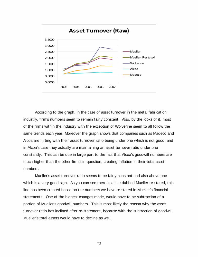
73
Asset Turnover (Raw)
0.0000
0.5000
1.0000
1.5000
2.0000
2.5000
3.0000
3.5000
2003 2004 2005 2006 2007
Mueller
Mueller‐ Restated
Wolverine
Alcoa
Madeco
According to the graph, in the case of asset turnover in the metal fabrication
industry, firm’s numbers seem to remain fairly constant. Also, by the looks of it, most
of the firms within the industry with the exception of Wolverine seem to all follow the
same trends each year. Moreover the graph shows that companies such as Madeco and
Alcoa are flirting with their asset turnover ratio being under one which is not good, and
in Alcoa’s case they actually are maintaining an asset turnover ratio under one
constantly. This can be due in large part to the fact that Alcoa’s goodwill numbers are
much higher than the other firm’s in question, creating inflation in their total asset
numbers.
Mueller’s asset turnover ratio seems to be fairly constant and also above one
which is a very good sign. As you can see there is a line dubbed Mueller re-stated, this
line has been created based on the numbers we have re-stated in Mueller’s financial
statements. One of the biggest changes made, would have to be subtraction of a
portion of Mueller’s goodwill numbers. This is most likely the reason why the asset
turnover ratio has inclined after re-statement, because with the subtraction of goodwill,
Mueller’s total assets would have to decline as well.

74
Cash Flows from Operations/Operating Income
Another important ratio in measuring expense manipulation diagnostics is the
Cash Flow from Operations/Operating Income (CFFO/OI) ratio. CFFO/OI is calculated
by the difference in a firm’s operating income and cash flow from operations. A firm
hopes for their CFFO/OI ratio to come out around 1. This ideal 1:1 ratio is stating that
a firm’s cash collected is directly related to its operating income.
CFFO/ OI (Raw)
(1.0000)
(0.5000)
0.0000
0.5000
1.0000
1.5000
2.0000
2003 2004 2005 2006 2007
Mueller
Mueller‐ Restated
Wolverine
Alcoa
Madeco
According to this CFFO/OI graph, most all the firms within the metal fabrication
industry have CFFO/OI ratio that is less than 1. Firms such as Wolverine, Alcoa, and
Madeco all have CFFO/OI ratios that remained fairly constant however remain well
below the preferred 1:1 ratio. In regards to Mueller’s situation, in 2003 Mueller’s
CFFO/OI ratio was almost 1.5:1 and then took a steep decline over a period of two
years from 2004 to 2006. This decline could be considered a possible “red flag” in that
Mueller’s recognition of cash received must have been much greater in comparison to
their operating income information. Mueller’s ratio has been very volatile over the past
five years but in 2007 Mueller almost perfected the 1:1 CFFO/OI ratio.
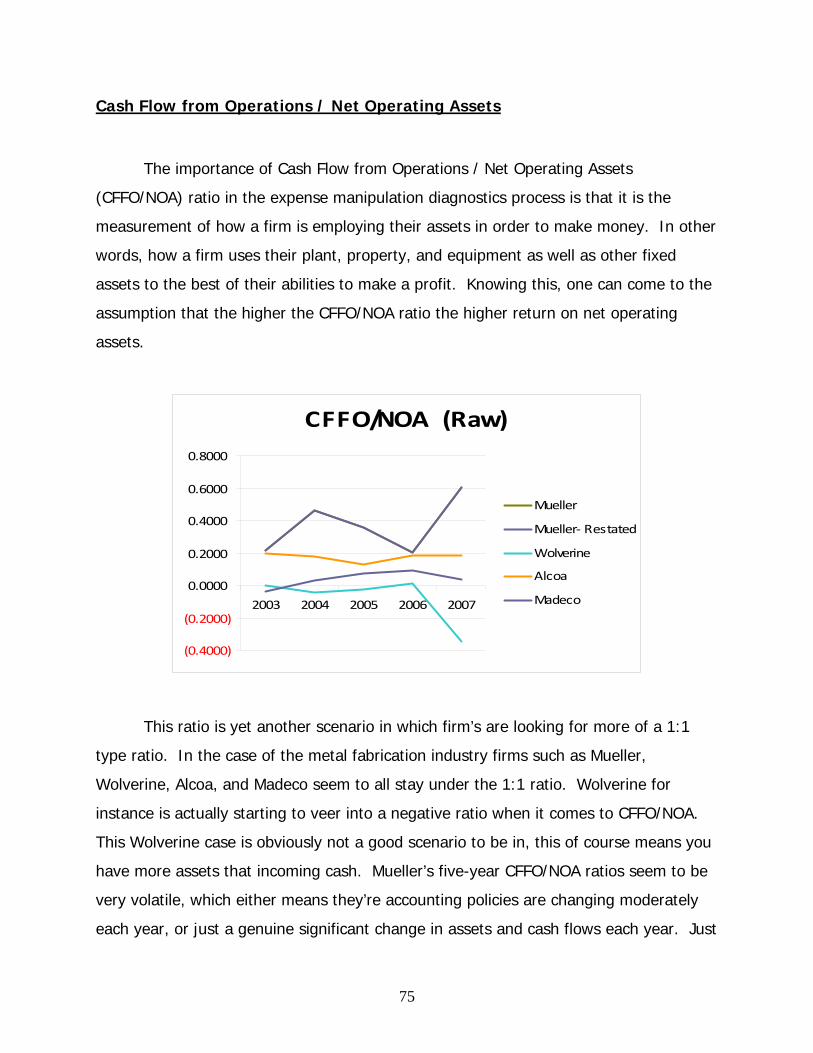
75
Cash Flow from Operations / Net Operating Assets
The importance of Cash Flow from Operations / Net Operating Assets
(CFFO/NOA) ratio in the expense manipulation diagnostics process is that it is the
measurement of how a firm is employing their assets in order to make money. In other
words, how a firm uses their plant, property, and equipment as well as other fixed
assets to the best of their abilities to make a profit. Knowing this, one can come to the
assumption that the higher the CFFO/NOA ratio the higher return on net operating
assets.
CFFO/NOA (Raw)
(0.4000)
(0.2000)
0.0000
0.2000
0.4000
0.6000
0.8000
2003 2004 2005 2006 2007
Mueller
Mueller‐ Restated
Wolverine
Alcoa
Madeco
This ratio is yet another scenario in which firm’s are looking for more of a 1:1
type ratio. In the case of the metal fabrication industry firms such as Mueller,
Wolverine, Alcoa, and Madeco seem to all stay under the 1:1 ratio. Wolverine for
instance is actually starting to veer into a negative ratio when it comes to CFFO/NOA.
This Wolverine case is obviously not a good scenario to be in, this of course means you
have more assets that incoming cash. Mueller’s five-year CFFO/NOA ratios seem to be
very volatile, which either means they’re accounting policies are changing moderately
each year, or just a genuine significant change in assets and cash flows each year. Just

76
like any other ratio, large jumps and spikes from year to year like this should definitely
be looked into, because there could be potential for a red flag in that assets or
something else in the financial statements could be incorrectly stated.
Total Accruals / Change in Sales
Total accruals are the calculated as the difference between operating income and
cash flow from operations. This ratio is used to define how much of a firm’s sales are a
result of accounts receivables. So knowing this one can come to the assumption that if
this particular ratio is high, than that means the firm is making most of it sales by
receivable transactions. The opposite of this first assumption being if the firm’s ratio is
lower than 1, then the firm must be acquiring cash for most of their sales transactions.
Once again this is another example of a ratio that a firm would prefer to be 1:1.
Total Accruals/ Sales (Raw)
(0.0400)
(0.0200)
0.0000
0.0200
0.0400
0.0600
0.0800
2003 2004 2005 2006 2007
Mueller
Mueller‐ Restated
Wolverine
Alcoa
Madeco
As seen in the graph, the metal fabrication industry’s total accruals/sales ratios
are very unpredictable each year. They all seem to stay in a range below one and
above zero, however there are times when some of the firm’s dip into the negative

77
range. Madeco seems to stay in the negative range the entire time and during the year
2006 Mueller even dips into the negative ratio range as well. These yearly ratios would
seem to indicate that most of the firms within the industry operate mostly with cash
transactions rather than receivables.
Pension Expense / SG&A
The pension expense to selling, general, and administrative expenses ratio
expresses what fraction of operating expenses is made up of pension expense. If the
pension expense/SG&A ratio is high, then there is a good chance that a firm has
mismanaged its employee retirement benefit plans. The firm must have over-stated
and over-paid its pension plans, thus creating higher expense numbers which in turn
would lead to the lowering of the firm’s net income. The opposite of this outcome
being if the ratio is low, then the firm in question must not be spending much money
on their employee pension plans.
Pension Expense/ SG&A (Raw)
(0.0200)0.00000.02000.04000.06000.08000.10000.12000.14000.16000.18000.2000
2003 2004 2005 2006 2007
Mueller
Mueller‐ Restated
Wolverine
Alcoa
In this graph, firms within the industry have a very unpredictable approach when
it comes to recording their pension expenses. This is easily understood because

78
pension plans and expenses are very imprecise, upper management pretty much makes
estimations when determining their pension expenses. In Mueller’s case, their pension
expense ratios from year to year stay fairly constant. Mueller’s ratios are also very low
from year to year, thus meaning they are not spending very much on employee
retirement pension plans.
Other Employment Expenses / SG&A
This expense manipulation ratio measures how much of the firm’s total expenses
are related to employee benefit costs. Employee benefits include heath care costs, life
insurance, defined benefit plans, etc. This ratio helps one to see how much a firm
spends on these benefits and if it is an increasing amount of total expenses throughout
the years.
Mueller provides few employee benefit costs compared to some of its
competitors but overall, it follows a normal curve. In 2006, Mueller’s employee benefit
expenses increased a little bit due to the company adopting the recognition and
disclosure provisions of SFAS No. 158, which required Mueller to recognize the funded
79
status of its pension and postretirement plans in the Balance Sheet (Mueller 10K 2007
pg. F-39). This ratio is very small for each company in the industry and therefore, we
have come to the conclusion that employee benefits are a small fraction of selling,
general and administrative expenses and are not very significant.
Conclusion
The expense manipulation diagnostics ratios section illustrates how the metal
fabrication industry records their expenses, and in Mueller’s case shows that they
typically maintain good accounting policies in the recording of their expenses. Mueller
seems to stay consistent in comparison to the other firms on each graph. Although in
some instances with the restatement of goodwill as well as other aspects within Mueller
financial statements seems to create a small yet fairly significant change on each graph,
and this is very important factor to consider in ratios such as these.

80
Revenue Manipulation Diagnostics
To evaluate the possibility of manipulation in Mueller Industry’s revenues, we
looked Mueller, as well as its top competitors, balance sheets, income statements, and
any additional disclosures made by management over the past 5 years. The following
ratios allow us to easily determine if there is something out of the industry norm and
conclude the potential reason for it. Through ratio analysis, we can observe the effect
of current assets and current liabilities on net sales and compare the results to the rest
of the industry. By the end of this analysis, we will be able to determine if there are
any “red flags” within the companies in the metal fabrications industry.
Net Sales / Cash from Sales
Net sales divided by cash from sales is an important ratio that allows us to
determine the actual amount of cash that the company received from their sales
compared to the amount of revenue recognized from sales during the period. This ratio
should always be close to (1:1) because when firms sell their goods and services they
want to receive compensation. If the ratio is very far off from one, then this could very
possibly be a ‘red flag’ because firms are either recognizing too much sales or not
recognizing enough sales.

81
As the graph shows, the ratio is very close to one for Mueller and its competitors.
All of the ratios seem to correspond with each other over the past 5 years, and there is
no need for a ‘red flag’ to be raised. Overall, questions should not be raised concerning
the quality of accounting disclosure for Mueller and its competitors.
Net Sales / Net Accounts Receivable
Net sales divided by accounts receivable allows us to distinguish if the company’s
total sales will cover their sales on credit. It is important to determine the relationship
of sales to receivables because it is a good indication of the firm’s ability to produce
cash from sales. If the ratio is high, it is apparent that the amount of sales sold on
account was high and if the ratio is low, the amount of cash from sales is generally
high.

82
When comparing the ratios between the different companies in the industry,
most of the companies are relatively similar throughout the years. However, one major
difference is Wolverine’s large increase in 2006 and then large decrease in 2007. One
factor that led to the dramatic change in Wolverine’s ratio is the major increase in net
sales from 2005 to 2006. The cause for this is that the 2006 copper prices reached
historical high levels and dramatically increased by 84% (Wolverine 10K 2006 pg 25).
However, the reason that this drastic change is not considered a potential ‘red flag’ is
because of the ever changing copper prices. Not only do copper prices change quite
frequently, but these prices are established by the COMEX market as well. Therefore,
the extreme increase of net sales in 2006 has nothing to do with the managers
distorting or changing the company’s information. Although Mueller has stayed fairly
constant with the industry norm, it is also important to notice that during the same time
period that Wolverine had a sharp increase, the other companies all slightly increased
as well. This reinstates the fact that there were no ‘red flags’ found in this ratio
because the market price of copper will obviously affect every company in the metal
fabrications industry in some way.
Net Sales / Inventory

83
The Net Sales/Inventory ratio demonstrates whether or not a firm’s sales are
supported by their inventory levels. Firms will have a higher ratio if net sales are
increasing and inventory is decreasing. Typically, if a firm has large amounts of
inventory and don’t quickly covert this surplus into revenue, their net sales to inventory
ratio will be low and could be detrimental to the company in the future. At the same
time, if a company has little inventory, they are more likely to use up the inventory and
have a higher ratio.
In the graph above, Mueller’s ratio was steadily increasing over time until 2007
when it suddenly decreased. There could be two potential reasons for this decrease;
net sales decreased or inventory increased. After looking at Mueller’s 10K from 2007, it
shows that the inventory did indeed slightly increase which caused Mueller’s ratio to
decrease from 2006 to 2007. Because of Mueller’s overall increase over the past 5
years, the firm forecasted that it should continue to increase inventory as it had been
doing. However, because companies in the metal fabrications industry rely so heavily
on the market, it is difficult to go by what the firm has done in the past. This decrease
was caused by the fluctuating market and the slight decrease in demand which caused
some of Mueller’s inventory to not be converted into revenue during the year. Mueller’s

84
numbers and disclosures verify that this was the reason for the decrease and therefore
it is not a potential ‘red flag’.
Conclusion
The revenue manipulation diagnostic ratios demonstrate how current assets and
current liabilities relate to net sales in an industry. At first glance, a few questions
could arise about some of the graphs. But when you take note of the fluctuating
market in the metal fabrications industry, it is normal to see some changes from one
company to another. First, we examined net sales divided by cash from sales and
found that all of the companies that we looked at had ratios close to one, meaning that
the industry receives its cash payments quickly. Next, we looked at net sales divided by
net accounts receivable. In this graph, we discovered one company with a sharp
change in numbers but concluded it was because of the fluctuating copper prices. Last,
we examined sales divided by inventory and found that the industry’s dependability on
the market prices was the reason for the changes between companies. Therefore, we
conclude that there were no “red flags” discovered in the companies analyzed from the
metal fabrications industry.

85
Identify Potential “Red Flags”
After examining how Mueller accounts for goodwill, it becomes clear they are not
adequately writing it off. Over the past five years they have been involved in a number
of mergers and acquisitions, thus adding to their goodwill. However, they only impair a
small fraction of it. Goodwill does not last a lifetime. In fact, it should really have a
useful life of about five years. That means 20% of goodwill needs to be written off each
year. Since Mueller keeps goodwill on their books for much longer than five years, we
believe this significantly distorts the true value of the firm.
Undo Accounting Distortions
Goodwill is recorded when a company purchases another company. Over the
years, Mueller has increased goodwill by $48,414,000 through mergers and
acquisitions. However, they fail to recognize adequate impairment of this asset. They
only wrote off $6,697,000 of goodwill in the last five years. In 2004 and 2007 they only
wrote off 3.7% and 1.9% of goodwill, respectively. Such low impairments tend to
distort the company’s financial statements and do not allow for investors to asses the
true value of the firm. We began to undo this distortion by taking the balance in 2003
and writing it off over the next five years, adjusting for new mergers and acquisitions
along the way. Mueller was on pace to write off goodwill over a period of around 25
years. A 20% impairment of goodwill per year is a better reflection of the actual life of
goodwill. The following table shows the amount of goodwill in years 2003-2007 before
and after restatement. Mueller’s financial statements, before and after the restatement
of goodwill, can be found in the appendices.

86
(In thousands) 2003 2004 2005 2006 2007
Goodwill Before Restatement 104,849 136,615 152,171 155,653 153,263
Goodwill After Restatement 83,879 89,310 75,220 48,360 18,384
Another business activity that requires some attention is the use of operating
leases. Some companies use operating leases even though capital leases would be
more appropriate. Operating leases allow for “off balance sheet” financing. This means
that the company does not have to record an asset or a liability for the amount of the
lease, but rather they just make periodic lease payments. This can significantly distort
the company’s financials. However, when looking at the amount of Mueller’s operating
leases, it appears to be a relatively small amount. We were able to determine this by
first finding the company’s future lease payments. We then discounted back the lease
payments to find the present value of the payments at the end of 2007. We used a
discount rate of 6.18%. The discount rate of 6.18% was taken from the discount rates
used to discount pension liabilities for Mueller’s employees. This rate was the highest
rate from the multiple discount rates used for pension liabilities (Mueller 10-k 2007).
Our calculations are shown below.
(In Thousands)
2008 2009 2010 2011 2012 2013 2014
Future Lease Payments 6,200 4,500 4,000 3,200 2,300 3,450 3,450
PV of the Lease Payments 5,840 3,990 3,340 2,520 1,700 2,410 2,270
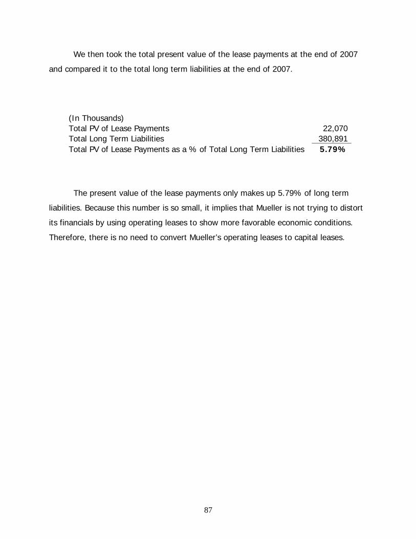
87
We then took the total present value of the lease payments at the end of 2007
and compared it to the total long term liabilities at the end of 2007.
(In Thousands) Total PV of Lease Payments 22,070Total Long Term Liabilities 380,891Total PV of Lease Payments as a % of Total Long Term Liabilities 5.79%
The present value of the lease payments only makes up 5.79% of long term
liabilities. Because this number is so small, it implies that Mueller is not trying to distort
its financials by using operating leases to show more favorable economic conditions.
Therefore, there is no need to convert Mueller’s operating leases to capital leases.

88
Financial Analysis, Forecast Financials, & Cost of Capital
Estimation
In this section we will perform ratio analysis, financial forecasting, and cost of
capital estimation to learn more about Mueller’s financial position. First we will calculate
liquidity, profitability, and capital structure ratios for Mueller and it competitors. These
will show different aspects of Mueller’s financial position, compared to that of its
competitors. Next, we will use some of those ratios to forecast out Mueller’s financial
statements for the next ten years to get an idea of where the company is headed in the
future. Finally, we will compute Mueller’s cost of capital, which is the return that
investors expect to receive for investing in the company.
Liquidity Ratio Analysis
A firm’s liquidity is a very important aspect in the determination of a firm’s ability
to pay for its debt and incurred expenses. When measuring a firm’s liquidity, financial
analysts use a particular set of liquidity ratios. These liquidity ratios consist of eight
different types: Current Ratio, Quick Asset Ratio, Accounts Receivable Turnover, Days in
Accounts Receivable, Inventory Turnover, Days in Inventory, Working Capital Turnover,
and Cash to Cash Cycle. Analyzing these ratios will enable us to determine whether a
firm has high liquidity or not. Obviously any firm wishes to have high liquidity, because
high liquidity shows that the company has the resources to back up any of its particular
liabilities when need be.

89
Current Ratio
Current Ratio
0
1
2
3
4
5
6
2002 2003 2004 2005 2006 2007
Mueller as S tated
Mueller Restated
Wolverine
Alcoa
Madeco
Industry Average
The numbers found for the current ratio of each company are derived by dividing
a firm’s current assets by its current liabilities. The current ratio answer describes how
many short-term assets make up each short-term liability that a particular firm
comprises. Another way of looking at the current ratio is that with a higher current
ratio, a firm shows that they are easily able to pay off their short-term liabilities.
In the case of Mueller, during 2002 and 2003 their current ratio was vastly
greater than any other firm throughout the industry, however from 2003 to 2004 they
saw a steep decline in their current ratio from around 4 to around 2.5. Since then
(2004-2007), Mueller has seen a fairly consistent current ratio which fluctuated around
2.4-3. Mueller’s current ratio numbers look to be fairly respectable especially in
comparison to their competitors who have current ratios that have fluctuated in a very
volatile range between 1 and 3 for the past six years. When it comes to Mueller’s
current ratio, one can conclude that they do a very good job in their ability to pay off
liabilities, and in most cases outperform all the competitors within the industry.

90
Quick Asset Ratio
Quick Asset Ratio
0
1
1
2
2
3
3
4
4
2002 2003 2004 2005 2006 2007
Mueller as S tated
Mueller Restated
Wolverine
Alcoa
Madeco
Industry Average
The quick asset ratio, also known as the acid test ratio, is very similar to the
current ratio in that it is measuring current assets over current liabilities. The difference
between the two being that the quick asset ratio takes into account only the most liquid
of current assets versus all current assets. These most liquid assets include cash,
accounts receivables, securities, and any cash-like equivalents. Just like current ratio, a
firm hopes to have a quick asset ratio greater than one, because if not it means they
don’t have enough liquid assets to cover their short-term liabilities.
Mueller’s quick asset ratio just like their current ratio proved to be most
impressive from 2002 to 2003, but took a steep decline from 2003 to 2004. Also just
like the current ratio Mueller maintains a constant quick asset ratio from 2004 on. The
quick asset ratio number for Mueller from 2004 on stays consistent around 1.5-1.9.
How these quick asset ratio numbers stack up against Mueller’s competitors seem to
also be consistent with the current ratio as well. Mueller maintains a greater quick
asset ratio from 2002 to 2007 than all existing competitors within the metal fabrication
industry.

91
Accounts Receivable Turnover
A/R Turnover
0
5
10
15
20
25
2002 2003 2004 2005 2006 2007
Mueller as S tated
Mueller Restated
Wolverine
Alcoa
Madeco
Industry Average
Accounts receivable turnover ratio is computed by taking a firm’s sales within the
given year divided by the number of accounts receivables. Accounts receivable
turnover is calculated to measure how much accounts receivable is turned over each
year, or in other words how prompt they are in their ability to collect cash for their
account accounts receivables within a given year. Accounts receivable turnover
ultimately states the firm’s effectiveness in their collecting from accounts outstanding.
Mueller’s accounts receivable turnover is not looking as promising in comparison
to the other liquidity ratios and competitors accounts receivable turnover within the
industry. The industry average of accounts receivable turnover over the past six years
has been around 9.04, while Mueller’s average account receivable turnover over the
past six years has been 7.43. This is a very noticeable gap between Mueller’s accounts
receivables turnover versus that of its competitors within the metal fabrication industry.
Knowing this one may determine that Mueller is much less efficient when it comes to
collecting account receivables compared to that of its competitors.

92
Days in Accounts Receivable
Days Supply of Receivables
0
10
20
30
40
50
60
70
2002 2003 2004 2005 2006 2007
Days
Mueller as S tated
Mueller Restated
Wolverine
Alcoa
Madeco
Industry Average
Days in accounts receivable just like current ratio and quick asset ratio is closely
related to its previous section of accounts receivable turnover. This is because
accounts receivable turnover measures how well a firm collects its accounts receivable
while days in accounts receivable is the measurement of the amount of days it takes a
firm to collect money for its account receivables. The formula for days in accounts
receivables is 365 days divided by accounts receivable turnover ratio or sales divided by
accounts receivable. Firms want their days supply of accounts receivables number to
be as low as possible, because the greater this number is the longer it takes for the firm
to convert accounts receivables into cash.
Just as in accounts receivable turnover Mueller does not do a very good job in
their days in accounts receivable. The industry average in days of accounts receivables
is 43.76 while Mueller’s average days of accounts receivable is 49.94, and if it were not
for Madeco this margin could be even greater due in part that Madeco is actually higher
than Mueller in most years. This means that Mueller does a very below average job
when it comes to the collecting time of their accounts receivables in general as well as
in comparison to the rest of industry. One could easily come to the assumption based

93
on the graph and the numbers, that Mueller has a lot of room for improvement when it
comes to the efficiency of collecting their receivables.
Inventory Turnover
Inventory Turnover
0
2
4
6
8
10
12
2002 2003 2004 2005 2006 2007
Mueller as S tated
Mueller Restated
Wolverine
Alcoa
Madeco
Industry Average
Inventory ratio just like any other turnover ratio, measures the rate that
inventory is turned over each year. Inventory turnover is computed by taking the firm’s
total cost of goods sold for a given year divided by the firm’s inventory from that same
year. This ratio states how well a firm is able to replenish their inventory after selling
off goods. When this ratio declines it means the firm is not getting rid of its inventory,
furthermore meaning that they are not selling any goods. So knowing this firms wish
for their inventory turnover number to increase or stay steady from year to year,
because this means they are generating normal to high levels of sales.
In the case of Mueller, they have maintained a great inventory turnover ratio
over the past six years. Mueller’s numbers have steadily increased over the years and
have maintained an average well above that of the industry average. Mueller’s average
inventory turnover ratio from 2003-2007 was around 6.92. While the industry average
from 2003-2007 was 5.97. This shows that Mueller’s inventory turnover is very

94
impressive in comparison to that of its competition with the exception of Wolverine. It
also shows that Mueller does a good job at turning over their inventory, which is always
an encouraging sight when trying to determine the value of a firm.
Days Supply of Inventory
Days Supply of Inventory
0102030405060708090100
2002 2003 2004 2005 2006 2007
Days
Mueller as S tated
Mueller Restated
Wolverine
Alcoa
Madeco
Industry Average
The day’s supply of inventory ratio just like the accounts receivable turnover and
days in accounts receivables is complementary to the inventory turnover ratio. The
day’s supply of inventory measures how many days it takes for inventory to become
revenue for the firm. The DSI ratio is computed by taking 365 (number of days in a
year of course) and dividing that number by the inventory turnover ratio or cost of
goods sold divided by inventory (365/ (COGS/Inventory)). A higher number of days in
this scenario of DSI are not good, because that means it is taking the firm more time to
convert inventory into sales. Knowing this one can come to the assumption that firms
are hoping their day’s supply of inventory is as little as possible.
Mueller’s day’s supply of inventory just like their inventory turnover ratio is very
good. They have maintained a declining day’s from 2002-2007, which means they are
doing job in converting their inventory into revenues. Mueller does another great job

95
once again in comparison to its competitors on a given liquidity ratio. The industry
average number of day’s supply of inventory was around 66.42 days from 2002-2007,
while Mueller’s day’s supply of inventory from 2002-2007 was around 54.26. So in
regards to day’s supply of inventory, Mueller does another marvelous job in
outperforming competition within the industry as well as steadily trying to improve from
year to year.
Working Capital Turnover
Working Capital Turnover
‐10‐50510152025303540
2002 2003 2004 2005 2006 2007
Mueller as Stated
Mueller Restated
Wolverine
Alcoa
Madeco
Industry Average
Working capital turnover is computed by taking the current years sales divided
by the company’s working capital or current assets minus current liabilities (Sales /
Current Assets – Current Liabilities). The ratio is used to determine how many sales are
created from the firm’s working capital. If a company’s working capital turnover ratio is
low then that means that they are not effectively generating sales from their working
capital or assets. The opposite of this being if the working capital ratio is high then the
firm is effectively using their working capital in order to make revenues, thus meaning
that firms hope that their working capital turnover is high.
I think an important thing to point out in this graph is how vast the difference is
in Mueller’s stated working capital turnover and its re-stated working capital turnover.

96
If you based your ideas about Mueller’s working capital turnover on their stated
numbers then they would have an absolutely amazing working capital turnover ratio.
However, when Mueller’s re-stated working capital turnover ratio maintains an average
around all of its competitors. The industry average for working capital turnover from
2002 to 2007 is around 8.97, while Mueller’s six year working capital turnover average
was around 3.9 which are absolutely horrible in comparison to industry. Only Madeco
maintains a worse working capital turnover average than Mueller, which means that
Mueller has some work to do when it comes to effectively using their capital to produce
revenue.
Cash to Cash Cycle
Cash to Cash Cycles
0
20
40
60
80
100
120
140
160
2003 2004 2005 2006 2007
Days
Mueller as S tated
Mueller Restated
Wolverine
Alcoa
Madeco
Industry Average
The cash to cash cycle shows us how well firms within the metal fabrication
industry are able to transform cash spent on assets into cash inflows generated by
accounts receivable. The assets in this case would come in the form of inventory. In
other words, the cash to cash cycle states the number of days it takes for money put in
inventories to become accounts receivables. The actual formula for the Cash to Cash

97
cycle is, days supply in inventory plus the days supply in receivables.
(365/(COGS/Inventory)) + (365/(Sales/AR))
Knowing how the cash to cash ratio is computed and how it is defined one can
come to the conclusion that firms prefer to have a lesser number of days. The reason
why a lesser number of days are preferred is because firms wish to convert inventory
into receivables as soon as possible. Mueller’s cash to cash cycle has been in a steady
decline from 2003-2007. This decline over the years is a very positive sign for Mueller,
because it means that they are improving each year in regards to their cash to cash
cycle. In comparison to its competitors, Mueller’s has maintained an average Cash to
Cash Cycle around 102.12, while its competitors have maintained an average Cash to
Cash Cycle around 111.68. This means that Mueller maintains a greater Cash to Cash
Cycle ratio compared to that of most of their competitors. Only Wolverine has
consistently outperformed Mueller when it comes to the Cash to Cash Cycle ratio. This
information states that Mueller does a great job in the time it takes to convert inventory
into accounts receivables, compared to that of the rest of the industry.
Conclusion
As mentioned in the liquidity ratios introduction paragraph, liquidity ratios are
exceedingly important in regards to the valuation of a firm. Taking into account these
eight ratios, one can determine the level of liquidity that a firm has. We found out in
Mueller’s case that they preformed exceedingly well in ratios such as: current ratio,
quick asset turnover ratio, inventory turnover ratio, days in inventory turnover, and
Cash to Cash Cycle. These ratios showed that Mueller excelled in the areas of making
their inventory liquid, having enough assets to cover their liabilities, and also being able
to convert inventory into accounts receivables in short amounts of time. However,
Mueller did a below average job in showing liquidity with ratios such as: accounts
receivable turnover ratio, days in accounts receivable, and working capital turnover.

98
These ratios showed that Mueller had room for improvement in the areas of turning
over accounts receivable and using their working capital effectively to increase revenue.
Capital Structure Ratios
The capital structure ratios determine how well a company finances itself
through assets. After analyzing these ratios, we will be able to tell if the firm’s assets
are financed by debt or equity. Firm’s that finance their assets through debt usually
borrow money from a lender; whereas, firm’s that finance their assts though equity
usually obtain money by selling shares of stock to investors. Either way the company
chooses to finance its assets, it is important to understand the efficiency and
productivity of the firm. By analyzing the capital structure ratios, analysts should be
able to determine the amount of debt relative to the amount of equity as well as the
firm’s financial leverage.
Debt to Equity Ratio
Debt to Equity Ratio
0.00
1.00
2.00
3.00
4.00
5.00
6.00
2002 2003 2004 2005 2006 2007
Mueller as S tated
Mueller Restated
Wolverine
Alcoa
Madeco
Industry Average

99
The debt to equity ratio is used as measurement of how much of a firm is
financed by its total debt or liabilities compared to its total equity. The debt to equity
ratio is computed by taking a firm’s total liabilities and dividing them by the firm’s total
equity. If a firm has a debt to equity ratio of 2, then that would mean for every dollar
amount of equity there would be twice as many liabilities.
Mueller’s debt to equity ratio number jumped drastically from 2003 to 2004,
however after 2004 Mueller maintained a relatively constant debt to equity ratio around
1.6. After 2005, one can come to the assumption that Mueller was working on lowering
their debt to equity ratio. This is because Mueller’s debt to equity numbers from 2004-
2005 were 1.93 in 2004, and 1.92 in 2005, but during years following Mueller’s debt to
equity ratio was 1.33 and 1.20 in 2006 and 2007 respectively. In regards to Mueller
versus the rest of the industry, Mueller has had a debt to equity average of 1.17 over
the past six years while the industry average was around 1.88. These numbers prove
that in most cases Mueller has maintained a history of having a smaller debt to equity
ratio compared to that of their competitors. This means that Mueller comprises more
equity in the total liabilities and equity portion of their balance sheet, than that of their
competitors within the metal fabrication industry.

100
Times Interest Earned
Times Interest Earned
‐10
0
10
20
30
40
50
60
70
2002 2003 2004 2005 2006 2007
Mueller as S tated
Mueller Restated
Wolverine
Alcoa
Madeco
Industry Average
The times interest earned ratio states how well a firm’s income from operations
covers their interest expenses. This times interest earned ratio is computed by taking
the firms income from operations from a given year and diving that number by the
firm’s interest expenses from the same year. It is important to also consider that this
ratio can be very unstable due to the fact that interest rates are going to directly affect
interest expenses, and interest rates are always changing.
Mueller’s times interest earned ratio was in a steady decline from 2002 to 2005,
but from 2005 on it looks as if Mueller has be able to flatten out these numbers.
Another positive about Mueller’s recent times interest earned ratio is that well, it has
stayed positive. Firms such as Wolverine have actually had their times interest earned
ratio dip into or stay constant in the negative range which is never a good thing.
Having a negative times interest earned ratio means that their interest expense is
actually greater than their income from operations. This also means that their income
from operations is actually in the negative range which is absolutely horrible for a firm.
In comparison to its competitors Mueller’s average times interest earned ratio over the
past six years was 18.36 while its competitors average times interest earned ratio was

101
23.49. From these numbers one can come to the determination that Mueller does an
average to below average job in maintaining a greater number of operating income
versus interest expense in comparison to all of its competitors.
Debt Service Margin
Debt Service Margin
(10)
0
10
20
30
40
50
60
2003 2004 2005 2006 2007
Mueller as S tated
Mueller Restated
Wolverine
Alcoa
Madeco
Industry Average
The debt service margin ratio measures how well a firm is able to cover its debt
by its cash flow from operations. The debt service margin numbers for the past six
years are found by taking the firms cash flow from operations from the given year and
dividing that number by the firms previous years long term notes payable or long-term
debt. The reason for taking the previous years debt is because we want to take into
account the current installment due on long-term debt for the year being calculated.
Obviously having a large debt service margin number is greatly appreciated by any firm,
and should be looked at by any investor as a positive sign.
Mueller’s debt service margin has been very volatile over the last five years, it
has been anywhere from 5.16 to 54.56. The 54.56 meaning that Mueller had much
more cash flow from operations than long term debt, and the 5.16 meaning that
although they had more cash flow from operations than long term debt it wasn’t as

102
great as before. Mueller maintains a debt service margin similar to that of most of its
competitors in most recent years. Mueller’s five year debt service margin averaged
somewhere around 22.72, while the industry average debt service margin around
11.76. With the industry average being around 11.76, this means that Mueller does a
better job than its competitors when it comes to debt service margin.
Credit Risk
The Altman Z-score is a measure of a company’s risk of bankruptcy. It allows the
analyst to assess credit distress and predict the chance of struggling company to turn
around. The Z-score offers a quantitative measurement using a weighted formula
involving five ratios appropriate to measure such risk. On page 10-15, Business Analysis
and Valuation outlines the Z-score in the following way:
Where:
net working capital/total assets (measure of liquidity)
retained earnings/total assets (measure of cumulative profitability)
EBIT/total assets (measure of return on assets)
MVE/ BVL (measure of market leverage)
sales/total assets (measure of sales generating potential of assets)
Bankruptcy is predicted when Z< 1.81. A concern for bankruptcy lies between a
score of 1.81 and 2.67. Using the above formula, we computed the Z-score for Mueller
and its competitors over the past five years.

103
Altman's Z-Score 2003 2004 2005 2006 2007
Mueller as Stated 4.5650 2.4761 3.2087 4.2311 4.0939 Mueller Restated 4.5079 2.5329 3.1994 4.2944 4.1777
Wolverine 2.9889 3.3677 3.3283 4.8634 5.8124 Alcoa 3.4832 3.5593 3.8040 3.9812 3.8501
Madeco 2.2799 3.2250 3.5048 4.1075 3.4808
Mueller entered into the grey area in 2004, which could be illustrated by the dip
in the quick asset ratio during the same year. With assets being a factor in four of the
five variables of the Z-score, a lower score for 2004 would be expected. In the following
years, Mueller climbs out of that hole and establishes a more secure score into the
present year. Aside from the 2004 slide, Mueller appears to perform as good as its
competitors in having good credit.
Conclusion
The capital structure ratios that we have just analyzed help investors determine
the amount a firm is financed through equity and/or debt. Determining a company’s
financial leverage and efficiency is a crucial part to evaluating a firm. First, we
examined the debt to equity ratio and discovered that Mueller had a smaller ratio than
its competitors. By taking note of this, we can conclude that Mueller is financed more
through debt. Next, we looked the times interest ratio. After comparing these numbers
to the rest of the industry, we concluded that Mueller is under-performing the rest of its
competitors due to its large interest expense. However, Mueller’s average debt service
margin is slightly higher than competitors, meaning Mueller is better at covering debt
than others in the industry. Mueller’s credit risk appears non-threatening and is in line
with its competitors. Overall, Mueller is performing in line compared to the metal
fabrications industry average.

104
Profitability Ratio Analysis
The profitability ratio analysis tells us how well a firm’s revenues cover its
expenses. The ratios show a percentage of sales, where sales equal 100% using the
common-size income statement. Analysts can tell which company is generating more
profit if the ratio’s percentage is higher. The 7 ratios we used to analyze Mueller
Industries and its competitors are gross profit margin, operating expense ratio,
operating profit margin, net profit margin, asset turnover, return on assets, and return
on equity.
Gross Profit Margin
Gross profit margin measures gross profit, sales minus cost of goods sold,
divided by sales. Gross profit margin demonstrates the profitability of a company after
subtracting fixed and overhead costs, involved in managing inventory. This ratio is the
first to assess the operating efficiency of the company, therefore affecting the other
ratios derived from the income statement. The higher a firm’s gross profit margin, the

105
greater the company’s profitability, proving the company’s efficiency at covering their
expenses.
As the graph shows, Mueller and Alcoa have both stayed high above the industry
average. Mueller has averaged 17% compared to the industry average of about 13%.
When you factor out the major outlier, Wolverine, it is still obvious that Mueller’s gross
profit margin is higher than the industry average. Mueller is proving efficient at
covering their expenses and increasing profitability.
Operating Expense Ratio
The operating expense ratio is calculated by dividing selling, general, and
administrative expenses by sales. This ratio tells us what percentage of selling, general,
and administrative expenses eliminate gross profit. Over time, the operating expense
ratio will tell analysts if it is possible to increase operations without considerably
increasing expenses. Therefore, it is better for a firm to have a smaller operating
expense ratio.
Although Mueller’s operating expense ratio is higher than the industry average, it
continues to decrease over the years. Due to the fact that the metal fabrications

106
industry relies so heavily on market prices, Mueller’s net sales will fluctuate depending
on new raw material costs. However, it is obvious that Mueller continues to find ways
to decrease selling, general, and administrative costs in order to compensate for these
fluctuations and decrease their operating expense ratio.
Operating Profit Margin
Operating profit margin is the operating income as a percentage of sales.
Operating profit is calculated as gross profit minus selling, general, and administrative
expenses. The higher the ratio, the more efficient a firm is at creating a profit after
deducting operating expenses.
From 2002 to 2003, there is a slight decrease in Mueller’s operating profit
margin. But from 2003 to 2007, the ratio steadily increases and continues to stay
above the industry average. As you can see in the above graph, Mueller’s restated
numbers show a lower ratio than the stated numbers. The accounting distortions in
these numbers obviously have an impact on Mueller’s income statement and show us a
slightly different aspect of the firm. Even though the restated numbers are somewhat
different, Mueller continues to stay above the average of the metal fabrications
industry. This shows us that the firm is efficient at creating a profit after deducting
operating expenses.

107
Net Profit Margin
Net profit margin is one of the most important profitability ratios. It compares
the bottom line of the income statement, net income, to revenue. This ratio shows the
percentage of sales that will be converted into net income after deducting expenses and
taxes. Net profit margin shows how well a firm is at managing their expenses as well as
the amount of net income that will be available for investors of the company. Since the
net profit margin shows the profitability of a firm, the bigger the ratio the better.
Mueller Industries has had a consistent profit margin over the past 5 years. They
have also kept above the industry average the whole time. This illustrates that Mueller
has been efficient at managing their costs and continue to have high profitability
compared to the competitors in the metal fabrications industry. Because of the
consistency of Mueller’s net profit margin as well as the ratios previously described,
managers and investors can rely on Mueller to stay on top in the industry and continue
to generate profits.

108
Asset Turnover
Asset turnover is the relationship between sales and total assets. This ratio
shows us how much a firm produces for every $1 of sales. If a company has an asset
turnover greater than 1, then it is fully utilizing its assets. If a company has an asset
turnover less than 1, it is investing too much in assets and not generating enough sales.
Mueller has held a steady, increasing trend in asset turnover. As the graph
above shows, Mueller has had an asset turnover greater than 1 for all 5 years. Not only
that, Mueller has seen a steady increase also. Mueller’s highest year was in 2006,
where it generated $2.41 of sales for every $1 in total assets. As an industry, most of
the companies have had very similar numbers for asset turnover, all above 1, which is
great for investors that are interested in the metal fabrications industry.

109
Return on Assets
Return on assets is calculated by dividing the current year’s net income by the
previous year’s total assets. When calculating this ratio, you use the assets from the
previous year because you generate profit in the current year from the assets already
used, not the assets just purchased. A firm with a higher return on assets is better
because it will have more profitability from generating higher earnings from assets.
Once again, Mueller is above the industry average throughout the years. Mueller
steadily increases each year, except a slight decrease in 2007. After looking at the
income statement, this drop is due to a decrease in net income from 2006 to 2007. A
copper litigation settlement and an impairment charge are two significant reasons that
net income decreased (Mueller 10K 2007 pg. F-15). These two events both occurred in
2007 but not in the years prior to that. Overall, Mueller is generating a high return on
its assets and continues to be a leader in the metal fabrications industry.

110
Return on Equity
Return on equity is very similar to return on assets. It is calculated by dividing
the current year’s net income by the previous year’s total equity. Return on equity
measures how much revenue a firm produces with the money invested by
shareholders; therefore, this ratio is very important to investors of a company. The
higher a company’s return on equity compared to its competitors in an industry, the
better. If a firm has a relatively high ROE, it is more capable of generating cash within
the company.
Mueller Industries has a great return on equity, proving its capabilities of
generating profits through its stockholder’s equity. Mueller is far above the metal
fabrication industry average and continues to increase up until 2006 where there it
slightly decreases. This decrease is once again due to the decrease in net income from
2006 to 2007. Analysts and investors that examine this ratio could easily determine that
Mueller makes a high return on its equity, especially compared to the rest of the
industry.

111
Internal Growth Rate
The internal growth rate, also known as IGR, measures the rate at which a firm
can grow without acquiring outside financing. This ratio tells analysts that if the firm
invests without using external finances, the company’s assets for the next year will be
taken right into net income. It is calculated by multiplying the return on assets by one
minus the dividend payout ratio. The dividend payout ratio is measured by taking
dividends divided by net income. This tells us the amount of earnings left for
investment to supply future earnings growth.
Mueller has stayed well above the industry average for all 5 years. The industry
average tends to be around .6%, while Mueller’s average is about 7%. Not only is
Mueller above average but it is steadily increasing from 2003 to 2006. Because Mueller
has such a high growth rate compared to its competitors, one can determine that
Mueller is very efficient in internal funding. Having a high IGR also means that Mueller
would be efficient at taking on debt if it ever needed to. Being able to reinvest
resources back into a company is a great sign that once again proves Mueller to be a
leader in the metal fabrications industry.

112
Sustainable Growth Rate
Sustainable growth rate is another way to determine a firm’s potential growth.
SGR measures how much a firm can grow without having to obtain more loans to do
so. It is calculated by taking the internal growth rate multiplied by one plus the debt to
equity ratio. Sustainable growth is a good way to measure the firm’s financial leverage,
an important aspect that investors and analyzers need to understand about a company.
Mueller continues to have a higher than average ratio which means that Mueller
is a very efficient company when it comes to growth. Mueller’s average SGR is about
18%, while the industry average is only around -6%, which is really low. However, if
we take out the industry outlier, Wolverine, the industry average would still prove to be
lower that Mueller’s SGR. In the graph above, it is noticeable that most of the
companies in the industry began around the same percentage in 2003. But by 2007,
Mueller has seen more steady increases than its competitors. The numbers show that
Mueller is efficient in both its internal and external rates.
113
Conclusion
By analyzing the effect of the 7 profitability ratios, we are able to determine that
Mueller’s overall efficiency compared to other firm’s the metal fabrications industry.
Mueller has been average with the industry when analyzing operating profit margin and
net profit margin. Mueller has outperformed or been just above the industry average in
gross profit margin, operating expense ratio, asset turnover, return on assets, and
return on equity. Mueller has obviously kept a strong competitive strategy and has
continued to have great profitability over the past 5 years. Compared to the rest of the
industry, Mueller has usually kept either average or well above the rest. This is a
positive sign for investors of this company and gives great insight into the rest of the
metal fabrications industry as well.

114
Financial Statement Forecasting
Forecasting financial statements involves looking at a company’s current and
past financial data to predict how the company will perform in the future. We
forecasted out Mueller’s income statement, balance sheet, and statement of cash flows
for the next ten years. Forecasts are made on a number of different assumptions, and if
a good job of forecasting is done, we can get a fair picture of the future expectations of
the firm. Our forecasts were based upon various growth rates, trends, and ratios.
It also should be noted that we forecasted out Mueller’s restated financial
statements as well. As discussed earlier, Mueller did a poor job of impairing goodwill.
We corrected this distortion by taking the beginning balance of goodwill in 2003 and
writing it off over the next five years, adjusting for new mergers and acquisitions along
the way. We then restated Mueller’s financial statements to reflect the change.
Because the changes we made to goodwill significantly altered Mueller’s financial
statements, we felt it was necessary to forecast Mueller’s actual financial statements, as
well as our restated ones.
The Income Statement
We began by forecasting the income statement. The income statement is the
easiest statement to forecast, but probably the most important since the assumptions
we make there flow into both the balance sheet and statement of cash flows. To allow
for easier comparisons, we computed a common sized income statement. Every item on
the income statement was presented as a percentage of sales. This helped us make
important assumptions about the future performance of the company.
The first item we forecasted was sales growth. We could not simply look at
Mueller’s sales growth over the past few years to predict the future, mainly because the
country is headed into a recession which is sure to affect Mueller’s revenues. Therefore,
we looked back at Mueller’s sales growth during the last major recession to see how the

115
company was affected during that time. The last major recession was during the years
2000-2002, following the aftermath of the “dot com bubble”. The following chart shows
Mueller’s sales growth in the years surrounding the last recession.
The graph shows that during the recession Mueller’s had negative sales growth
for two years and then sales began to grow again once the recession had ended. We
modeled our forecasted sales growth after these numbers. First, we looked at Mueller’s
most recent quarterly report and we were able to determine that the company would
most likely have positive sales growth for 2008, but it would not be much greater than
sales in 2007. Therefore, we assumed a 3% growth rate. We believe the recession
would not affect sales growth until year 2009. We also thought this recession would
have a larger impact than the last recession because Mueller’s sales growth is semi-
dependent on the construction industry. Its plumbing and refrigeration segment makes
copper and plastic tubing used in both residential and commercial construction markets.
Since the construction of new buildings is declining, we believe Mueller will be hit
harder by this recession. Thus, for years 2009 and 2010 during the recession we
predicted negative sales growth of 15% and 10% respectively. After 2010, we think the
recession will be over and sales will start to grow again. For that reason, we predicted
sales growth to be 5% in 2011 and 12% in 2012, and then sales would level off at 8%
for the remaining five years.
The next item we forecasted was the cost of goods sold. Here we looked at the
common sized income statement to see what the percentages of cost of goods sold to
sales were in the past six years. The average was slightly over 82% so we used this
number as a basis for our forecasting. We multiplied it by sales to get cost of good sold.
From there, we were also able to estimate gross profit because it is simply the cost of
goods sold subtracted from sales.
Sales Growth
1998-1999 1999-2000 2000-2001 2001-2002 2002-2003 2003-2004
25.75% 3.20% -13.38% -8.79% 4.84% 38.03%

116
We used the same method used for estimating the cost of goods sold to forecast
selling, general, and administrative expenses, operating income, and finally net income.
We looked at the common sized income statement to find average percentages over the
past six years and based our forecasts on those numbers.
When comparing both the income statements, before and after restated, there is
not much difference between the two. The only difference is the impairment charge of
goodwill is higher on the restated income statement, thus lowering net income. This
however did not have an effect on our forecasts. While we impaired most of the
goodwill over the last five years, there is no way to tell how goodwill will change in the
future due to mergers and acquisitions. Also, we cannot forecast out how Mueller will
impair their goodwill in the future. Since we cannot forecast out these items regarding
goodwill, net income will be the same for both forecasted financial statements.
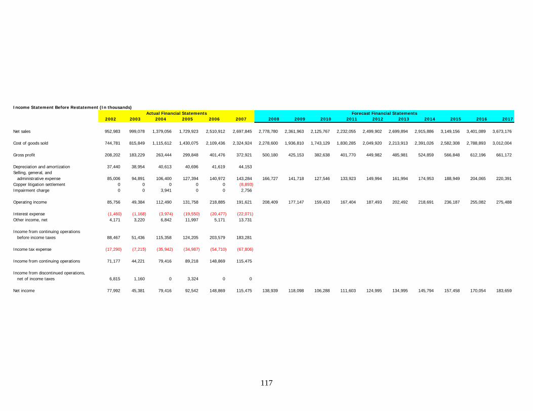
117
2002 2003 2004 2005 2006 2007 2008 2009 2010 2011 2012 2013 2014 2015 2016 2017
Net sales 952,983 999,078 1,379,056 1,729,923 2,510,912 2,697,845 2,778,780 2,361,963 2,125,767 2,232,055 2,499,902 2,699,894 2,915,886 3,149,156 3,401,089 3,673,176
Cost of goods sold 744,781 815,849 1,115,612 1,430,075 2,109,436 2,324,924 2,278,600 1,936,810 1,743,129 1,830,285 2,049,920 2,213,913 2,391,026 2,582,308 2,788,893 3,012,004
Gross profit 208,202 183,229 263,444 299,848 401,476 372,921 500,180 425,153 382,638 401,770 449,982 485,981 524,859 566,848 612,196 661,172
Depreciation and amortization 37,440 38,954 40,613 40,696 41,619 44,153Selling, general, and administrative expense 85,006 94,891 106,400 127,394 140,972 143,284 166,727 141,718 127,546 133,923 149,994 161,994 174,953 188,949 204,065 220,391Copper litigation settlement 0 0 0 0 0 (8,893)Impairment charge 0 0 3,941 0 0 2,756
Operating income 85,756 49,384 112,490 131,758 218,885 191,621 208,409 177,147 159,433 167,404 187,493 202,492 218,691 236,187 255,082 275,488
Interest expense (1,460) (1,168) (3,974) (19,550) (20,477) (22,071)Other income, net 4,171 3,220 6,842 11,997 5,171 13,731
Income from continuing operations before income taxes 88,467 51,436 115,358 124,205 203,579 183,281
Income tax expense (17,290) (7,215) (35,942) (34,987) (54,710) (67,806)
Income from continuing operations 71,177 44,221 79,416 89,218 148,869 115,475
Income from discontinued operations, net of income taxes 6,815 1,160 0 3,324 0 0
Net income 77,992 45,381 79,416 92,542 148,869 115,475 138,939 118,098 106,288 111,603 124,995 134,995 145,794 157,458 170,054 183,659
Actual Financial Statements Forecast Financial StatementsIncome Statement Before Restatement (In thousands)

118
2002 2003 2004 2005 2006 2007 2008 2009 2010 2011 2012 2013 2014 2015 2016 2017
Net sales 100% 100% 100% 100% 100% 100% 100.00% 100.00% 100.00% 100.00% 100.00% 100.00% 100.00% 100.00% 100.00% 100.00%
Cost of goods sold 78.15% 81.66% 80.90% 82.67% 84.01% 86.18% 82.00% 82.00% 82.00% 82.00% 82.00% 82.00% 82.00% 82.00% 82.00% 82.00%
Gross profit 21.85% 18.34% 19.10% 17.33% 15.99% 13.82% 18.00% 18.00% 18.00% 18.00% 18.00% 18.00% 18.00% 18.00% 18.00% 18.00%
Depreciation and amortization 3.93% 3.90% 2.94% 2.35% 1.66% 1.64%Selling, general, and administrative expense 8.92% 9.50% 7.72% 7.36% 5.61% 5.31% 6.00% 6.00% 6.00% 6.00% 6.00% 6.00% 6.00% 6.00% 6.00% 6.00%Copper litigation settlement 0.00% 0.00% 0.00% 0.00% 0.00% -0.33%Impairment charge 0.00% 0.00% 0.29% 0.00% 0.00% 0.10%
Operating income 9.00% 4.94% 8.16% 7.62% 8.72% 7.10% 7.50% 7.50% 7.50% 7.50% 7.50% 7.50% 7.50% 7.50% 7.50% 7.50%
Interest expense -0.15% -0.12% -0.29% -1.13% -0.82% -0.82%Other income, net 0.44% 0.32% 0.50% 0.69% 0.21% 0.51%
Income from continuing operations before income taxes 9.28% 5.15% 8.36% 7.18% 8.11% 6.79%
Income tax expense -1.81% -0.72% -2.61% -2.02% -2.18% -2.51%
Income from continuing operations 7.47% 4.43% 5.76% 5.16% 5.93% 4.28%
Income from discontinued operations, net of income taxes 0.72% 0.12% 0.00% 0.19% 0.00% 0.00%
Net income 8.18% 4.54% 5.76% 5.35% 5.93% 4.28% 5.00% 5.00% 5.00% 5.00% 5.00% 5.00% 5.00% 5.00% 5.00% 5.00%
Actual Financial Statements Forecast Financial StatementsCommon Sized Income Statement Before Restatement

119
2002 2003 2004 2005 2006 2007 2008 2009 2010 2011 2012 2013 2014 2015 2016 2017
Net sales 952,983 999,078 1,379,056 1,729,923 2,510,912 2,697,845 2,778,780 2,361,963 2,125,767 2,232,055 2,499,902 2,699,894 2,915,886 3,149,156 3,401,089 3,673,176
Cost of goods sold 744,781 815,849 1,115,612 1,430,075 2,109,436 2,324,924 2,278,600 1,936,810 1,743,129 1,830,285 2,049,920 2,213,913 2,391,026 2,582,308 2,788,893 3,012,004
Gross profit 208,202 183,229 263,444 299,848 401,476 372,921 500,180 425,153 382,638 401,770 449,982 485,981 524,859 566,848 612,196 661,172
Depreciation and amortization 37,440 38,954 40,613 40,696 41,619 44,153Selling, general, and administrative expense 85,006 94,891 106,400 127,394 140,972 143,284 166,727 141,718 127,546 133,923 149,994 161,994 174,953 188,949 204,065 220,391Copper litigation settlement 0 0 0 0 0 (8,893)Impairment charge 0 0 3,941 0 0 2,756Additional Impairment charge 20,970 26,335 29,646 30,342 27,586
Operating income 85,756 28,414 86,155 102,112 188,543 164,035 208,409 177,147 159,433 167,404 187,493 202,492 218,691 236,187 255,082 275,488
Interest expense (1,460) (1,168) (3,974) (19,550) (20,477) (22,071)Other income, net 4,171 3,220 6,842 11,997 5,171 13,731
Income from continuing operations before income taxes 88,467 30,466 89,023 94,559 173,237 155,695
Income tax expense (17,290) (7,215) (35,942) (34,987) (54,710) (67,806)Change in tax expense 2,941 8,206 8,351 8,153 10,207New Income tax expense (4,274) (27,736) (26,636) (46,557) (57,599)
Income from continuing operations 71,177 26,192 61,287 67,923 126,680 98,096
Income from discontinued operations, net of income taxes 6,815 1,160 0 3,324 0 0
Net income 77,992 27,352 61,287 71,247 126,680 98,096 138,939 118,098 106,288 111,603 124,995 134,995 145,794 157,458 170,054 183,659
Actual Financial Statements Forecast Financial StatementsIncome Statement After Restatement (In Thousands)
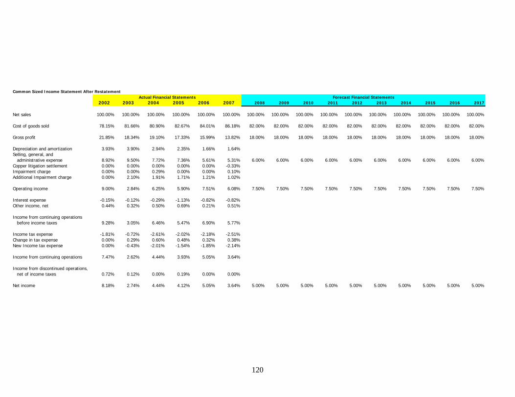
120
2002 2003 2004 2005 2006 2007 2008 2009 2010 2011 2012 2013 2014 2015 2016 2017
Net sales 100.00% 100.00% 100.00% 100.00% 100.00% 100.00% 100.00% 100.00% 100.00% 100.00% 100.00% 100.00% 100.00% 100.00% 100.00% 100.00%
Cost of goods sold 78.15% 81.66% 80.90% 82.67% 84.01% 86.18% 82.00% 82.00% 82.00% 82.00% 82.00% 82.00% 82.00% 82.00% 82.00% 82.00%
Gross profit 21.85% 18.34% 19.10% 17.33% 15.99% 13.82% 18.00% 18.00% 18.00% 18.00% 18.00% 18.00% 18.00% 18.00% 18.00% 18.00%
Depreciation and amortization 3.93% 3.90% 2.94% 2.35% 1.66% 1.64%Selling, general, and administrative expense 8.92% 9.50% 7.72% 7.36% 5.61% 5.31% 6.00% 6.00% 6.00% 6.00% 6.00% 6.00% 6.00% 6.00% 6.00% 6.00%Copper litigation settlement 0.00% 0.00% 0.00% 0.00% 0.00% -0.33%Impairment charge 0.00% 0.00% 0.29% 0.00% 0.00% 0.10%Additional Impairment charge 0.00% 2.10% 1.91% 1.71% 1.21% 1.02%
Operating income 9.00% 2.84% 6.25% 5.90% 7.51% 6.08% 7.50% 7.50% 7.50% 7.50% 7.50% 7.50% 7.50% 7.50% 7.50% 7.50%
Interest expense -0.15% -0.12% -0.29% -1.13% -0.82% -0.82%Other income, net 0.44% 0.32% 0.50% 0.69% 0.21% 0.51%
Income from continuing operations before income taxes 9.28% 3.05% 6.46% 5.47% 6.90% 5.77%
Income tax expense -1.81% -0.72% -2.61% -2.02% -2.18% -2.51%Change in tax expense 0.00% 0.29% 0.60% 0.48% 0.32% 0.38%New Income tax expense 0.00% -0.43% -2.01% -1.54% -1.85% -2.14%
Income from continuing operations 7.47% 2.62% 4.44% 3.93% 5.05% 3.64%
Income from discontinued operations, net of income taxes 0.72% 0.12% 0.00% 0.19% 0.00% 0.00%
Net income 8.18% 2.74% 4.44% 4.12% 5.05% 3.64% 5.00% 5.00% 5.00% 5.00% 5.00% 5.00% 5.00% 5.00% 5.00% 5.00%
Actual Financial Statements Forecast Financial StatementsCommon Sized Income Statement After Restatement

121
The Balance Sheet
After forecasting the income statement, we moved on to the balance sheet. The
two statements can be linked through the asset turnover ratio. Mueller had an average
asset turnover rate of 1.7 before restatement and 1.79 after restatement. Using this
ratio, we were able to forecast total assets. Total assets were found by taking the next
years sales divided by the asset turnover ratio. After forecasting total assets, we looked
at the current asset percentage of total assets over the past six years. Current assets
were approximately 60% of total assets before restatement and 70% after restatement.
We used these percentages to calculate forecasted current assets. Non-current assets
were found by subtracting current assets from total assets. When looking at the asset
section of both forecasted balance sheets, the effect our restatement of goodwill had
on assets becomes apparent. Both non-current assets and total assets are significantly
smaller after restatement due to the previous impairment of goodwill.
Next, we looked to forecast retained earnings. Retained earnings are calculated
by taking last years retained earnings, adding this year’s net income, and then
subtracting this year’s dividend. We were able to use our forecasted net income and
forecasted dividends to forecast retained earnings for the next ten years. Once we have
retained earnings, we can forecast total stockholder’s equity by adding the change in
retained earnings to the previous year’s stockholder’s equity. Therefore, both retained
earnings and stockholder’s equity both grow by the amount of net income generated
minus the amount of dividends paid out. Once again it is apparent how the impairment
of goodwill has affected forecasted retained earnings and total stockholder’s equity.
Retained earnings and stockholder’s equity are both lower after the restatement of
goodwill.
After owner’s equity is forecasted, total liabilities becomes a plug figure. Owner’s
equity is subtracted from total assets to get total liabilities. Once total liabilities were
forecasted, we looked at the percentage of liabilities that were current. In the last few
years, current liabilities have been approximately 40% of total liabilities both before and
after restatement. Therefore, we used this percentage to forecast total current

122
liabilities. Then non-current liabilities were found by subtracting current liabilities from
total liabilities.

123
2002 2003 2004 2005 2006 2007 2008 2009 2010 2011 2012 2013 2014 2015 2016 2017
AssetsCurrent assets Cash and cash equivalents 217,601 255,088 47,449 129,685 200,471 308,618 Accounts receivable, less allowance for doubtful accounts of 5,015 in 2007 and 6,806 in 2006 132,427 163,006 196,762 260,685 281,679 323,003 Inventories 142,953 14,048 187,853 196,987 258,647 269,032 Current deferred income taxes 4,506 9,035 15,276 19,900 21,421 19,853 Other current assets 2,860 2,678 7,991 17,019 13,976 19,841
Total current assets 500,347 570,355 455,331 624,276 776,194 940,347 833,634 750,271 787,784 882,318 952,904 1,029,136 1,111,467 1,200,384 1,296,415 1,400,128
Property, plant, and equipment, net 352,469 345,537 335,610 307,046 315,064 308,383
Goodwill 105,551 104,849 136,615 152,171 155,653 153,263
Other assets 29,580 34,443 36,175 33,435 21,996 47,211
Total Non-Current Assets 487,600 484,829 508,400 492,652 492,713 508,857 555,756 500,180 525,189 588,212 635,269 686,091 740,978 800,256 864,277 933,419 Total Assets 987,947 1,055,184 963,731 1,116,928 1,268,907 1,449,204 1,389,390 1,250,451 1,312,974 1,470,531 1,588,173 1,715,227 1,852,445 2,000,641 2,160,692 2,333,547
Liabilities and Stockholders' EquityCurrent liabilities Current portion of long-term debt 4,161 2,835 5,328 4,120 35,998 72,743 Accounts payable 41,004 42,081 79,723 124,216 96,095 140,497 Accrued wages and other employee costs 26,199 25,631 37,992 38,095 43,281 39,984 Other current liabilities 34,987 48,314 57,775 97,251 80,145 81,829
Total current liabilities 106,351 118,861 180,818 263,682 255,519 335,053 223,207 126,534 114,554 138,739 142,298 146,141 150,292 154,775 159,617 164,845
Long-term debt, less current portion 14,005 11,437 310,650 312,070 308,154 281,738Pension liabilities 22,364 18,077 19,611 21,721 19,900 14,805Postretirement benefits other than pensions 13,186 13,566 13,556 13,515 16,699 21,266Environmental reserves 9,110 9,560 9,503 9,073 8,907 8,897Deferred income taxes 59,269 58,379 67,479 63,944 46,408 52,156Other noncurrent liabilities 9,718 10,238 10,361 3,078 2,206 2,029
Total non-current liabilities 127,652 121,257 431,160 423,401 402,274 380,891 334,811 189,800 171,831 208,109 213,447 219,212 225,438 232,163 239,425 247,268 Total liabilities 234,003 240,118 611,978 687,083 657,793 715,944 558,018 316,334 286,386 346,848 355,745 365,353 375,730 386,938 399,041 412,114
Minority interest in subsidiaries 421 208 67 6,937 22,300 22,765
Stockholders' equity Preferred stock - 1.00 par value; shares authorized 5,000,000; none outstanding 0 0 0 0 0 0 Common stock - .01 par value; shares authorized 100,000,000; issued 40,091,502; outstanding 37,079,903 in 2007 and 37,025,285 in 2006 401 401 401 401 401 401 Additional paid-in capital 258,939 259,110 252,931 252,889 256,906 259,611 Retained earnings 610,114 655,495 175,537 253,433 386,038 484,534 605,411 708,156 800,627 897,722 1,006,467 1,123,913 1,250,754 1,387,742 1,535,689 1,695,473 Accumulated other comprehensive income (21,133) (5,586) 3,085 (8,848) 12,503 31,808 Treasury common stock, at cost (94,798) (94,562) (80,268) (74,967) (67,034) (65,859)
Total stockholders' equity 753,523 814,858 351,686 422,908 588,814 710,495 831,372 934,117 1,026,588 1,123,683 1,232,428 1,349,874 1,476,715 1,613,703 1,761,650 1,921,434
Total Liabilities and Stockholders' Equity 987,947 1,055,184 963,731 1,116,928 1,268,907 1,449,204 1,389,390 1,250,451 1,312,974 1,470,531 1,588,173 1,715,227 1,852,445 2,000,641 2,160,692 2,333,547
Balance Sheet before Restatement (In Thousands)Actual Financial Statements Forecast Financial Statements

124
2002 2003 2004 2005 2006 2007 2008 2009 2010 2011 2012 2013 2014 2015 2016 2017
AssetsCurrent assets Cash and cash equivalents 22.03% 24.17% 4.92% 11.61% 15.80% 21.30% Accounts receivable, less allowance for doubtful accounts of 5,015 in 2007 and 6,806 in 2006 13.40% 15.45% 20.42% 23.34% 22.20% 22.29% Inventories 14.47% 1.33% 19.49% 17.64% 20.38% 18.56% Current deferred income taxes 0.46% 0.86% 1.59% 1.78% 1.69% 1.37% Other current assets 0.29% 0.25% 0.83% 1.52% 1.10% 1.37%
Total current assets 50.65% 54.05% 47.25% 55.89% 61.17% 64.89% 60.00% 60.00% 60.00% 60.00% 60.00% 60.00% 60.00% 60.00% 60.00% 60.00%
Property, plant, and equipment, net 35.68% 32.75% 34.82% 27.49% 24.83% 21.28%
Goodwill 10.68% 9.94% 14.18% 13.62% 12.27% 10.58%
Other assets 2.99% 3.26% 3.75% 2.99% 1.73% 3.26%
Total Non-Current Assets 49.35% 45.95% 52.75% 44.11% 38.83% 35.11% 40.00% 40.00% 40.00% 40.00% 40.00% 40.00% 40.00% 40.00% 40.00% 40.00% Total Assets 100.00% 100.00% 100.00% 100.00% 100.00% 100.00% 100.00% 100.00% 100.00% 100.00% 100.00% 100.00% 100.00% 100.00% 100.00% 100.00%
Liabilities and Stockholders' EquityCurrent liabilities Current portion of long-term debt 0.42% 0.27% 0.55% 0.37% 2.84% 5.02% Accounts payable 4.15% 3.99% 8.27% 11.12% 7.57% 9.69% Accrued wages and other employee costs 2.65% 2.43% 3.94% 3.41% 3.41% 2.76% Other current liabilities 3.54% 4.58% 5.99% 8.71% 6.32% 5.65%
Total current liabilities 10.76% 11.26% 18.76% 23.61% 20.14% 23.12% 16.07% 10.12% 8.72% 9.43% 8.96% 8.52% 8.11% 7.74% 7.39% 7.06%
Long-term debt, less current portion 1.42% 1.08% 32.23% 27.94% 24.28% 19.44%Pension liabilities 2.26% 1.71% 2.03% 1.94% 1.57% 1.02%Postretirement benefits other than pensions 1.33% 1.29% 1.41% 1.21% 1.32% 1.47%Environmental reserves 0.92% 0.91% 0.99% 0.81% 0.70% 0.61%Deferred income taxes 6.00% 5.53% 7.00% 5.72% 3.66% 3.60%Other noncurrent liabilities 0.98% 0.97% 1.08% 0.28% 0.17% 0.14%
Total Non-Current Liabilities 12.92% 11.49% 44.74% 37.91% 31.70% 26.28% 24.10% 15.18% 13.09% 14.15% 13.44% 12.78% 12.17% 11.60% 11.08% 10.60% Total liabilities 23.69% 22.76% 63.50% 61.52% 51.84% 49.40% 40.16% 25.30% 21.81% 23.59% 22.40% 21.30% 20.28% 19.34% 18.47% 17.66%
Minority interest in subsidiaries 0.04% 0.02% 0.01% 0.62% 1.76% 1.57%
Stockholders' equity Preferred stock - 1.00 par value; shares authorized 5,000,000; none outstanding 0.00% 0.00% 0.00% 0.00% 0.00% 0.00% Common stock - .01 par value; shares authorized 100,000,000; issued 40,091,502; outstanding 37,079,903 in 2007 and 37,025,285 in 2006 0.04% 0.04% 0.04% 0.04% 0.03% 0.03% Additional paid-in capital 26.21% 24.56% 26.24% 22.64% 20.25% 17.91% Retained earnings 61.76% 62.12% 18.21% 22.69% 30.42% 33.43% 43.57% 56.63% 60.98% 61.05% 63.37% 65.53% 67.52% 69.36% 71.07% 72.66% Accumulated other comprehensive income -2.14% -0.53% 0.32% -0.79% 0.99% 2.19% Treasury common stock, at cost -9.60% -8.96% -8.33% -6.71% -5.28% -4.54%
Total stockholders' equity 76.27% 77.22% 36.49% 37.86% 46.40% 49.03% 59.84% 74.70% 78.19% 76.41% 77.60% 78.70% 79.72% 80.66% 81.53% 82.34%
Total Liabilities and Stockholders' Equity 100.00% 100.00% 100.00% 100.00% 100.00% 100.00% 100.00% 100.00% 100.00% 100.00% 100.00% 100.00% 100.00% 100.00% 100.00% 100.00%
Actual Financial Statements Forecast Financial StatementsCommon Sized Balance Sheet before Restatement

125
2002 2003 2004 2005 2006 2007 2008 2009 2010 2011 2012 2013 2014 2015 2016 2017
AssetsCurrent assets Cash and cash equivalents 217,601 255,088 47,449 129,685 200,471 308,618 Accounts receivable, less allowance for doubtful accounts of 5,015 in 2007 and 6,806 in 2006 132,427 163,006 196,762 260,685 281,679 323,003 Inventories 142,953 14,048 187,853 196,987 258,647 269,032 Current deferred income taxes 4,506 9,035 15,276 19,900 21,421 19,853 Other current assets 2,860 2,678 7,991 17,019 13,976 19,841
Total current assets 500,347 570,355 455,331 624,276 776,194 940,347 923,673 831,306 872,871 977,615 1,055,825 1,140,290 1,231,514 1,330,035 1,436,438 1,551,353
Property, plant, and equipment, net 352,469 345,537 335,610 307,046 315,064 308,383
Goodwill 105,551 83,879 89,310 75,220 48,360 18,384
Other assets 29,580 34,443 36,175 33,435 21,996 47,211
Total Non-Current Assets 487,600 463,859 461,095 415,701 385,420 373,978 395,860 356,274 374,087 418,978 452,496 488,696 527,792 570,015 615,616 664,865 Total Assets 987,947 1,034,214 916,426 1,039,977 1,161,614 1,314,325 1,319,533 1,187,579 1,246,958 1,396,593 1,508,321 1,628,986 1,759,305 1,900,050 2,052,054 2,216,218
Liabilities and Stockholders' EquityCurrent liabilities Current portion of long-term debt 4,161 2,835 5,328 4,120 35,998 72,743 Accounts payable 41,004 42,081 79,723 124,216 96,095 140,497 Accrued wages and other employee costs 26,199 25,631 37,992 38,095 43,281 39,984 Other current liabilities 34,987 48,314 57,775 97,251 80,145 81,829 Less imcome taxes payable (2,941) (8,206) (8,351) (8,153) (10,207)
Total current liabilities 106,351 115,920 172,612 255,331 247,366 324,846 245,133 151,254 138,017 159,033 160,226 161,514 162,905 164,407 166,030 167,782
Long-term debt, less current portion 14,005 11,437 310,650 312,070 308,154 281,738Pension liabilities 22,364 18,077 19,611 21,721 19,900 14,805Postretirement benefits other than pensions 13,186 13,566 13,556 13,515 16,699 21,266Environmental reserves 9,110 9,560 9,503 9,073 8,907 8,897Deferred income taxes 59,269 58,379 67,479 63,944 46,408 52,156Other noncurrent liabilities 9,718 10,238 10,361 3,078 2,206 2,029
Total non-current liabilities 127,652 121,257 431,160 423,401 402,274 380,891 367,699 226,880 207,025 238,549 240,339 242,271 244,357 246,611 249,045 251,674 Total liabilities 234,003 237,177 603,772 678,732 649,640 705,737 612,832 378,134 345,042 397,582 400,564 403,784 407,262 411,018 415,075 419,456
Minority interest in subsidiaries 421 208 67 6,937 22,300 22,765
Stockholders' equity Preferred stock - 1.00 par value; shares authorized 5,000,000; none outstanding 0 0 0 0 0 0 Common stock - .01 par value; shares authorized 100,000,000; issued 40,091,502; outstanding 37,079,903 in 2007 and 37,025,285 in 2006 401 401 401 401 401 401 Additional paid-in capital 258,939 259,110 252,931 252,889 256,906 259,611 Retained earnings 610,114 655,495 154,567 206,128 309,087 377,241 Changes in goodwill net of taxes (18,029) (18,129) (21,295) (22,189) (17,379) New Retained earnings 637,466 136,438 184,833 286,898 359,862 480,739 583,485 675,955 773,050 881,796 999,241 1,126,082 1,263,070 1,411,018 1,570,801 Accumulated other comprehensive income (21,133) (5,586) 3,085 (8,848) 12,503 31,808 Treasury common stock, at cost (94,798) (94,562) (80,268) (74,967) (67,034) (65,859)
Total stockholders' equity 753,523 796,829 312,587 354,308 489,674 585,823 706,700 809,446 901,916 999,011 1,107,757 1,225,202 1,352,043 1,489,031 1,636,979 1,796,762
Total Liabilities and Stockholders' Equity 987,947 1,034,214 916,426 1,039,977 1,161,614 1,314,325 1,319,533 1,187,579 1,246,958 1,396,593 1,508,321 1,628,986 1,759,305 1,900,050 2,052,054 2,216,218
Balance Sheet After Restatement (In Thousands)Actual Financial Statements Forecast Financial Statements

126
2002 2003 2004 2005 2006 2007 2008 2009 2010 2011 2012 2013 2014 2015 2016 2017
AssetsCurrent assets Cash and cash equivalents 22.03% 24.66% 5.18% 12.47% 17.26% 23.48% Accounts receivable, less allowance for doubtful accounts of 5,015 in 2007 and 6,806 in 2006 13.40% 15.76% 21.47% 25.07% 24.25% 24.58% Inventories 14.47% 1.36% 20.50% 18.94% 22.27% 20.47% Current deferred income taxes 0.46% 0.87% 1.67% 1.91% 1.84% 1.51% Other current assets 0.29% 0.26% 0.87% 1.64% 1.20% 1.51%
Total current assets 50.65% 55.15% 49.69% 60.03% 66.82% 71.55% 70.00% 70.00% 70.00% 70.00% 70.00% 70.00% 70.00% 70.00% 70.00% 70.00%
Property, plant, and equipment, net 35.68% 33.41% 36.62% 29.52% 27.12% 23.46%
Goodwill 10.68% 8.11% 9.75% 7.23% 4.16% 1.40%
Other assets 2.99% 3.33% 3.95% 3.21% 1.89% 3.59%
Total Non-Current Assets 49.35% 44.85% 50.31% 39.97% 33.18% 28.45% 30.00% 30.00% 30.00% 30.00% 30.00% 30.00% 30.00% 30.00% 30.00% 30.00% Total Assets 100.00% 100.00% 100.00% 100.00% 100.00% 100.00% 100.00% 100.00% 100.00% 100.00% 100.00% 100.00% 100.00% 100.00% 100.00% 100.00%
Liabilities and Stockholders' EquityCurrent liabilities Current portion of long-term debt 0.42% 0.27% 0.58% 0.40% 3.10% 5.53% Accounts payable 4.15% 4.07% 8.70% 11.94% 8.27% 10.69% Accrued wages and other employee costs 2.65% 2.48% 4.15% 3.66% 3.73% 3.04% Other current liabilities 3.54% 4.67% 6.30% 9.35% 6.90% 6.23% Less imcome taxes payable 0.00% -0.28% -0.90% -0.80% -0.70% -0.78%
Total current liabilities 10.76% 11.21% 18.84% 24.55% 21.30% 24.72% 18.58% 12.74% 11.07% 11.39% 10.62% 9.91% 9.26% 8.65% 8.09% 7.57%0.00% 0.00% 0.00% 0.00% 0.00% 0.00%
Long-term debt, less current portion 1.42% 1.11% 33.90% 30.01% 26.53% 21.44%Pension liabilities 2.26% 1.75% 2.14% 2.09% 1.71% 1.13%Postretirement benefits other than pensions 1.33% 1.31% 1.48% 1.30% 1.44% 1.62%Environmental reserves 0.92% 0.92% 1.04% 0.87% 0.77% 0.68%Deferred income taxes 6.00% 5.64% 7.36% 6.15% 4.00% 3.97%Other noncurrent liabilities 0.98% 0.99% 1.13% 0.30% 0.19% 0.15%
Total non-current liabilities 12.92% 11.72% 47.05% 40.71% 34.63% 28.98% 27.87% 19.10% 16.60% 17.08% 15.93% 14.87% 13.89% 12.98% 12.14% 11.36% Total liabilities 23.69% 22.93% 65.88% 65.26% 55.93% 53.70% 46.44% 31.84% 27.67% 28.47% 26.56% 24.79% 23.15% 21.63% 20.23% 18.93%
Minority interest in subsidiaries 0.04% 0.02% 0.01% 0.67% 1.92% 1.73%
Stockholders' equity Preferred stock - 1.00 par value; shares authorized 5,000,000; none outstanding 0.00% 0.00% 0.00% 0.00% 0.00% 0.00% Common stock - .01 par value; shares authorized 100,000,000; issued 40,091,502; outstanding 37,079,903 in 2007 and 37,025,285 in 2006 0.04% 0.04% 0.04% 0.04% 0.03% 0.03% Additional paid-in capital 26.21% 25.05% 27.60% 24.32% 22.12% 19.75% Retained earnings 61.76% 63.38% 16.87% 19.82% 26.61% 28.70% Changes in goodwill net of taxes 0.00% -1.74% -1.98% -2.05% -1.91% -1.32% New Retained earnings 0.00% 61.64% 14.89% 17.77% 24.70% 27.38% Accumulated other comprehensive income -2.14% -0.54% 0.34% -0.85% 1.08% 2.42% Treasury common stock, at cost -9.60% -9.14% -8.76% -7.21% -5.77% -5.01%
Total stockholders' equity 76.27% 77.05% 34.11% 34.07% 42.15% 44.57% 53.56% 68.16% 72.33% 71.53% 73.44% 75.21% 76.85% 78.37% 79.77% 81.07%
Total Liabilities and Stockholders' Equity 100.00% 100.00% 100.00% 100.00% 100.00% 100.00% 100.00% 100.00% 100.00% 100.00% 100.00% 100.00% 100.00% 100.00% 100.00% 100.00%
Actual Financial Statements Forecast Financial StatementsCommon Sized Balance Sheet After Restatement

127
The Statement of Cash Flows
The statement of cash flows was the last financial statement we forecasted. We
began by forecasting cash flow from operating activities. To do this we looked at the
following ratios: cash flow from operations/sales, cash flow from operations/net income,
and cash flow from operations/operating income. We were looking for an apparent
pattern or trend. After examining these ratios over the past six years, we found cash
flow from operations/net income to be our best estimate for forecasting cash flow from
operations. We choose to exclude year 2006 because it was an outlier. We found the
average cash flow from operations/net income to be 159.02%. We took this average
ratio of 159.02% and multiplied it by net income to get the cash flow provided by
operating activities.
Next, we forecasted cash flow from investing activities. For this item, we looked
at the change in non-current assets. The change from year to year represents the cash
flow from investing activities because cash is either used to purchase these assets, or
cash is received from the sale of these assets. The forecasted cash flow from investing
activities on the restated balance sheet will differ from the forecasted cash flow from
investing activities on the original balance sheet because of the difference in non-
current assets between the two.
Lastly, for cash flow from financing activities, we only were able to forecast out
dividends. Dividends were forecasted as a portion of net income. The higher the net
income, the more dividends a company usually pays out. Over the past four years
Mueller has paid dividends to its shareholders. We examined the average percentage of
dividends paid out compared to net income. We excluded year 2004 because they paid
an abnormally large amount of dividends that year. We found that dividends were
approximately 13% of net income, so we used this estimate to forecast future dividend
payout. Dividends were the same for both before and after restated statement of cash
flows.

128
2002 2003 2004 2005 2006 2007 2008 2009 2010 2011 2012 2013 2014 2015 2016 2017
Operating activities:Net income 71,177 44,221 79,416 92,542 148,869 115,475 138,939 118,098 106,288 111,603 124,995 134,995 145,794 157,458 170,054 183,659Reconciliation of net income to net cash provided by operating activities: Depreciation 36,979 38,531 40,316 40,398 41,179 43,605 Amortization of intangibles 461 423 297 298 440 548 Amortization of Subordinated Debenture costs 0 0 26 162 236 324 Stock-based compensation expense 0 0 0 2,789 2,737 Income tax benefit from exercise of stock options 13,243 18 31,778 991 (1,065) (73) Impairment charge 0 0 3,941 0 0 2,756 Deferred income taxes 9,686 (287) 2,711 (9,556) (19,339) 3,094 Provision for doubtful accounts receivable 374 3,172 1,404 1,911 1,109 (177) Minority interest in subsidiaries, net of dividend paid 150 (213) (141) 9 2,610 (781) Gain on sale of equity investment 0 0 0 0 (1,876) 0 Gain on early retirement of debt 0 0 0 0 (97) 0 (Gain) loss on disposal of properties (485) 290 (5,729) (3,665) 2,620 (2,468) Equity in earnings unconsolidated subsidiary 0 460 2,026 (4,480) (964) 0 Changes in assets and liabilities, net of businesses acquired: Receivables 6,021 (35,129) (15,722) (64,905) (15,459) (7,937) Inventories (13,744) 2,948 (26,208) (5,979) (56,786) 20,411 Other assets (4,154) 3,240 (6,689) 1,764 1,449 (4,120) Current liabilities 3,683 14,620 45,274 66,435 (41,357) 12,704 Other liabilities (91) (54) 296 (5,894) (2,578) 1,809 Other, net 917 1,176 1,765 (590) 2,759 (2,063)
Net cash provided by operating activities 124,217 73,416 154,761 109,441 64,539 185,844 220,946 187,804 169,024 177,475 198,772 214,674 231,848 250,396 270,427 292,061
Investing activities:Proceeds from sale of Utah Railway Company 55,403 0 0 0 0 0Capital expenditures (23,265) (27,236) (19,980) (18,449) (41,206) (29,870)Acquisition of businesses, net of cash received (20,457) 0 (56,946) (6,937) 3,632 (32,243)Proceeds from sales of properties and equity investment 8,165 1,412 6,334 10,112 23,528 3,809Purchase of Conbraco Industries, Inc. common stock (7,320) (10,806) 0 0 0 0Escrowed IRB proceeds 2,445 449 0 0 0 0Net deposits into restricted cash balances 0 0 0 0 0 (4,194)
Net cash used in investing activities 14,971 (36,181) (70,592) (15,274) (14,046) (62,498) (46,899) 55,576 (25,009) (63,023) (47,057) (50,822) (54,887) (59,278) (64,020) (69,142)
Financing activities:Repayments of long-term debt (34,119) (3,894) (6,608) (1,091) (2,058) (18,765)Dividends paid 0 0 (259,882) (14,646) (14,776) (14,825) (18,062) (15,353) (13,817) (14,508) (16,249) (17,549) (18,953) (20,470) (22,107) (23,876)Proceeds from issuance of long-term debt 0 0 0 0 28,759 16,635Acquisition of treasury stock (14,754) 0 (42,641) (551) (1,092) (54)Issuance of shares under incentive stock option plans from treasury 3,204 389 18,978 4,819 7,701 1,124Income tax benefit from exercise of stock options 0 0 0 0 1,065 73Subordinated Debenture issuance costs 0 0 (2,187) 0 0 0
Net cash (used in) provided by financing activities (45,669) (3,505) (292,340) (11,469) 19,599 (15,812)
Effect of exchange rate changes on cash 719 3,505 532 (462) 694 613Net cash provided by operating activities of discontinued operations 1,501 252 0 3,324 0 0
Increase in cash and cash equivalents 94,238 37,487 (207,639) 82,236 70,786 108,147Cash and cash equivalents at the beginning of the year 121,862 217,601 255,088 47,449 129,685 200,471
Cash and cash equivalents at the end of the year 217,601 255,088 47,449 129,685 200,471 308,618
Statement of Cash Flows Before Restatement (In Thousands)Actual Financial Statements Forecast Financial Statements

129
Common Sized Statement of Cash Flows Before Restatement
2002 2003 2004 2005 2006 2007 2008 2009 2010 2011 2012 2013 2014 2015 2016 2017
Operating activities:Net income 57.30% 60.23% 51.32% 84.56% 230.67% 62.14% 62.88% 62.88% 62.88% 62.88% 62.88% 62.88% 62.88% 62.88% 62.88% 62.88%Reconciliation of net income to net cash provided by operating activities: Depreciation 29.77% 52.48% 26.05% 36.91% 63.80% 23.46% Amortization of intangibles 0.37% 0.58% 0.19% 0.27% 0.68% 0.29% Amortization of Subordinated Debenture costs 0.00% 0.00% 0.02% 0.15% 0.37% 0.17% Stock-based compensation expense 0.00% 0.00% 0.00% 0.00% 4.32% 1.47% Income tax benefit from exercise of stock options 10.66% 0.02% 20.53% 0.91% -1.65% -0.04% Impairment charge 0.00% 0.00% 2.55% 0.00% 0.00% 1.48% Deferred income taxes 7.80% -0.39% 1.75% -8.73% -29.96% 1.66% Provision for doubtful accounts receivable 0.30% 4.32% 0.91% 1.75% 1.72% -0.10% Minority interest in subsidiaries, net of dividend paid 0.12% -0.29% -0.09% 0.01% 4.04% -0.42% Gain on sale of equity investment 0.00% 0.00% 0.00% 0.00% -2.91% 0.00% Gain on early retirement of debt 0.00% 0.00% 0.00% 0.00% -0.15% 0.00% (Gain) loss on disposal of properties -0.39% 0.40% -3.70% -3.35% 4.06% -1.33% Equity in earnings unconsolidated subsidiary 0.00% 0.63% 1.31% -4.09% -1.49% 0.00% Changes in assets and liabilities, net of businesses acquired: Receivables 4.85% -47.85% -10.16% -59.31% -23.95% -4.27% Inventories -11.06% 4.02% -16.93% -5.46% -87.99% 10.98% Other assets -3.34% 4.41% -4.32% 1.61% 2.25% -2.22% Current liabilities 2.96% 19.91% 29.25% 60.70% -64.08% 6.84% Other liabilities -0.07% -0.07% 0.19% -5.39% -3.99% 0.97% Other, net 0.74% 1.60% 1.14% -0.54% 4.27% -1.11%
Net cash provided by operating activities 100.00% 100.00% 100.00% 100.00% 100.00% 100.00% 100.00% 100.00% 100.00% 100.00% 100.00% 100.00% 100.00% 100.00% 100.00% 100.00%
Investing activities:Proceeds from sale of Utah Railway Company 370.07% 0.00% 0.00% 0.00% 0.00% 0.00%Capital expenditures -155.40% 75.28% 28.30% 120.79% 293.36% 47.79%Acquisition of businesses, net of cash received -136.64% 0.00% 80.67% 45.42% -25.86% 51.59%Proceeds from sales of properties and equity investmentPurchase of Conbraco Industries, Inc. common stock -48.89% 29.87% 0.00% 0.00% 0.00% 0.00%Escrowed IRB proceeds 16.33% -1.24% 0.00% 0.00% 0.00% 0.00%Net deposits into restricted cash balances 0.00% 0.00% 0.00% 0.00% 0.00% 6.71%
Net cash used in investing activities 100.00% 100.00% 100.00% 100.00% 100.00% 100.00% 100.00% 100.00% 100.00% 100.00% 100.00% 100.00% 100.00% 100.00% 100.00% 100.00%
Financing activities:Repayments of long-term debt 74.71% 111.10% 2.26% 9.51% -10.50% 118.68%Dividends paid 0.00% 0.00% 88.90% 127.70% -75.39% 93.76% n/a n/a n/a n/a n/a n/a n/a n/a n/a n/aProceeds from issuance of 0.00% 0.00% 0.00% 0.00% 0.00% 0.00% long-term debt 0.00% 0.00% 0.00% 0.00% 146.74% -105.20%Acquisition of treasury stock 32.31% 0.00% 14.59% 4.80% -5.57% 0.34%Issuance of shares under incentive 0.00% 0.00% 0.00% 0.00% 0.00% 0.00% stock option plans from treasury -7.02% -11.10% -6.49% -42.02% 39.29% -7.11%Income tax benefit from exercise of 0.00% 0.00% 0.00% 0.00% 0.00% 0.00% stock options 0.00% 0.00% 0.00% 0.00% 5.43% -0.46%Subordinated Debenture issuance costs 0.00% 0.00% 0.75% 0.00% 0.00% 0.00%
Net cash (used in) provided by financing activities 100.00% 100.00% 100.00% 100.00% 100.00% 100.00% 100.00% 100.00% 100.00% 100.00% 100.00% 100.00% 100.00% 100.00% 100.00% 100.00%
Effect of exchange rate changes on cashNet cash provided by operating activities of discontinued operations
Increase in cash and cash equivalentsCash and cash equivalents at the beginning of the year
Cash and cash equivalents at the end of the year
Actual Financial Statements Forecast Financial Statements

130
2002 2003 2004 2005 2006 2007 2008 2009 2010 2011 2012 2013 2014 2015 2016 2017
Operating activities:Net income 71,177 44,221 79,416 92,542 148,869 115,475 138,939 118,098 106,288 111,603 124,995 134,995 145,794 157,458 170,054 183,659Reconciliation of net income to net cash provided by operating activities: Depreciation 36,979 38,531 40,316 40,398 41,179 43,605 Amortization of intangibles 461 423 297 298 440 548 Amortization of Subordinated Debenture costs 0 0 26 162 236 324 Stock-based compensation expense 0 0 0 2,789 2,737 Income tax benefit from exercise of stock options 13,243 18 31,778 991 (1,065) (73) Impairment charge 0 0 3,941 0 0 2,756 Deferred income taxes 9,686 (287) 2,711 (9,556) (19,339) 3,094 Provision for doubtful accounts receivable 374 3,172 1,404 1,911 1,109 (177) Minority interest in subsidiaries, net of dividend paid 150 (213) (141) 9 2,610 (781) Gain on sale of equity investment 0 0 0 0 (1,876) 0 Gain on early retirement of debt 0 0 0 0 (97) 0 (Gain) loss on disposal of properties (485) 290 (5,729) (3,665) 2,620 (2,468) Equity in earnings unconsolidated subsidiary 0 460 2,026 (4,480) (964) 0 Changes in assets and liabilities, net of businesses acquired: Receivables 6,021 (35,129) (15,722) (64,905) (15,459) (7,937) Inventories (13,744) 2,948 (26,208) (5,979) (56,786) 20,411 Other assets (4,154) 3,240 (6,689) 1,764 1,449 (4,120) Current liabilities 3,683 14,620 45,274 66,435 (41,357) 12,704 Other liabilities (91) (54) 296 (5,894) (2,578) 1,809 Other, net 917 1,176 1,765 (590) 2,759 (2,063)
Net cash provided by operating activities 124,217 73,416 154,761 109,441 64,539 185,844 220,946 187,804 169,024 177,475 198,772 214,674 231,848 250,396 270,427 292,061
Investing activities:Proceeds from sale of Utah Railway Company 55,403 0 0 0 0 0Capital expenditures (23,265) (27,236) (19,980) (18,449) (41,206) (29,870)Acquisition of businesses, net of cash received (20,457) 0 (56,946) (6,937) 3,632 (32,243)Proceeds from sales of properties and equity investment 8,165 1,412 6,334 10,112 23,528 3,809Purchase of Conbraco Industries, Inc. common stock (7,320) (10,806) 0 0 0 0Escrowed IRB proceeds 2,445 449 0 0 0 0Net deposits into restricted cash balances 0 0 0 0 0 (4,194)
Net cash used in investing activities 14,971 (36,181) (70,592) (15,274) (14,046) (62,498) (21,882) 39,586 (17,814) (44,890) (33,518) (36,200) (39,096) (42,223) (45,601) (49,249)
Financing activities:Repayments of long-term debt (34,119) (3,894) (6,608) (1,091) (2,058) (18,765)Dividends paid 0 0 (259,882) (14,646) (14,776) (14,825) (18,062) (15,353) (13,817) (14,508) (16,249) (17,549) (18,953) (20,470) (22,107) (23,876)Proceeds from issuance of long-term debt 0 0 0 0 28,759 16,635Acquisition of treasury stock (14,754) 0 (42,641) (551) (1,092) (54)Issuance of shares under incentive stock option plans from treasury 3,204 389 18,978 4,819 7,701 1,124Income tax benefit from exercise of stock options 0 0 0 0 1,065 73Subordinated Debenture issuance costs 0 0 (2,187) 0 0 0
Net cash (used in) provided by financing activities (45,669) (3,505) (292,340) (11,469) 19,599 (15,812)
Effect of exchange rate changes on cash 719 3,505 532 (462) 694 613Net cash provided by operating activities of discontinued operations 1,501 252 0 3,324 0 0
Increase in cash and cash equivalents 94,238 37,487 (207,639) 82,236 70,786 108,147Cash and cash equivalents at the beginning of the year 121,862 217,601 255,088 47,449 129,685 200,471
Cash and cash equivalents at the end of the year 217,601 255,088 47,449 129,685 200,471 308,618
Statement of Cash Flows Before Restatement (In Thousands)Actual Financial Statements Forecast Financial Statements

131
Common Sized Statement of Cash Flows After Restatement
2002 2003 2004 2005 2006 2007 2008 2009 2010 2011 2012 2013 2014 2015 2016 2017
Operating activities:Net income 57.30% 60.23% 51.32% 84.56% 230.67% 62.14% 62.88% 62.88% 62.88% 62.88% 62.88% 62.88% 62.88% 62.88% 62.88% 62.88%Reconciliation of net income to net cash provided by operating activities: Depreciation 29.77% 52.48% 26.05% 36.91% 63.80% 23.46% Amortization of intangibles 0.37% 0.58% 0.19% 0.27% 0.68% 0.29% Amortization of Subordinated Debenture costs 0.00% 0.00% 0.02% 0.15% 0.37% 0.17% Stock-based compensation expense 0.00% 0.00% 0.00% 0.00% 4.32% 1.47% Income tax benefit from exercise of stock options 10.66% 0.02% 20.53% 0.91% -1.65% -0.04% Impairment charge 0.00% 0.00% 2.55% 0.00% 0.00% 1.48% Deferred income taxes 7.80% -0.39% 1.75% -8.73% -29.96% 1.66% Provision for doubtful accounts receivable 0.30% 4.32% 0.91% 1.75% 1.72% -0.10% Minority interest in subsidiaries, net of dividend paid 0.12% -0.29% -0.09% 0.01% 4.04% -0.42% Gain on sale of equity investment 0.00% 0.00% 0.00% 0.00% -2.91% 0.00% Gain on early retirement of debt 0.00% 0.00% 0.00% 0.00% -0.15% 0.00% (Gain) loss on disposal of properties -0.39% 0.40% -3.70% -3.35% 4.06% -1.33% Equity in earnings unconsolidated subsidiary 0.00% 0.63% 1.31% -4.09% -1.49% 0.00% Changes in assets and liabilities, net of businesses acquired: Receivables 4.85% -47.85% -10.16% -59.31% -23.95% -4.27% Inventories -11.06% 4.02% -16.93% -5.46% -87.99% 10.98% Other assets -3.34% 4.41% -4.32% 1.61% 2.25% -2.22% Current liabilities 2.96% 19.91% 29.25% 60.70% -64.08% 6.84% Other liabilities -0.07% -0.07% 0.19% -5.39% -3.99% 0.97% Other, net 0.74% 1.60% 1.14% -0.54% 4.27% -1.11%
Net cash provided by operating activities 100.00% 100.00% 100.00% 100.00% 100.00% 100.00% 100.00% 100.00% 100.00% 100.00% 100.00% 100.00% 100.00% 100.00% 100.00% 100.00%
Investing activities:Proceeds from sale of Utah Railway Company 370.07% 0.00% 0.00% 0.00% 0.00% 0.00%Capital expenditures -155.40% 75.28% 28.30% 120.79% 293.36% 47.79%Acquisition of businesses, net of cash received -136.64% 0.00% 80.67% 45.42% -25.86% 51.59%Proceeds from sales of properties and equity investment 54.54% -3.90% -8.97% -66.20% -167.51% -6.09%Purchase of Conbraco Industries, Inc. common stock -48.89% 29.87% 0.00% 0.00% 0.00% 0.00%Escrowed IRB proceeds 16.33% -1.24% 0.00% 0.00% 0.00% 0.00%Net deposits into restricted cash balances 0.00% 0.00% 0.00% 0.00% 0.00% 6.71%
Net cash used in investing activities 100.00% 100.00% 100.00% 100.00% 100.00% 100.00% 100.00% 100.00% 100.00% 100.00% 100.00% 100.00% 100.00% 100.00% 100.00% 100.00%
Financing activities:Repayments of long-term debt 74.71% 111.10% 2.26% 9.51% -10.50% 118.68%Dividends paid 0.00% 0.00% 88.90% 127.70% -75.39% 93.76% n/a n/a n/a n/a n/a n/a n/a n/a n/a n/aProceeds from issuance of long-term debt 0.00% 0.00% 0.00% 0.00% 146.74% -105.20%Acquisition of treasury stock 32.31% 0.00% 14.59% 4.80% -5.57% 0.34%Issuance of shares under incentive stock option plans from treasury -7.02% -11.10% -6.49% -42.02% 39.29% -7.11%Income tax benefit from exercise of stock options 0.00% 0.00% 0.00% 0.00% 5.43% -0.46%Subordinated Debenture issuance costs 0.00% 0.00% 0.75% 0.00% 0.00% 0.00%
Net cash (used in) provided by financing activities 100.00% 100.00% 100.00% 100.00% 100.00% 100.00% 100.00% 100.00% 100.00% 100.00% 100.00% 100.00% 100.00% 100.00% 100.00% 100.00%
Effect of exchange rate changes on cashNet cash provided by operating activities of discontinued operations
Increase in cash and cash equivalentsCash and cash equivalents at the beginning of the year
Cash and cash equivalents at the end of the year
Actual Financial Statements Forecast Financial Statements

132
Cost of Capital Estimation
In order to assess the value of a firm, it will be important to take a close look as
to how the firm is leveraged. By this we mean how the firm provides for the assets and
other methods that allow products to be made and sold. This leverage is made of two
components: debt and equity. Equity can be defined as the portion of a company’s
value that belongs to the shareholders holding an interest in the company through
stock ownership. A company also obtains resources by borrowing from banks and other
institutions that supply funds. It is through both of these activities that a company is
able to support itself, and analysis of these activities will better illustrate the company’s
health. Further discussion of both of these methods is continued below.
Cost of Equity
Individuals investing in the stock market aim to increase their wealth by allowing
other firms and companies to use their funds. An investor hopes to benefit financially
from the company’s performance that was made possible by their investment. The risk
of investing should be proportionate to the possible rewards, meaning that the larger
the gain an individual wishes to make, the larger the risk they will have to endure. The
US Treasury defines a benchmark for this risk through their treasury bills (t-bills) which
are deemed a ‘risk free’ investment. The difference between the return an investor
could gain in the market (Rm) and the return on the t-bill (Rf) is called the market risk
premium (MRP) and signifies the additional compensation an investor expects for their
more risky investment.
A security can measure its systematic risk, or general risk associated with
investing, against that of the market using the beta coefficient (B). The beta tells how a
specific stocks risk moves with the market as a whole. A beta of one indicates that the
stock moves in direct correlation with the market, while greater than one and less than
one means the security has more and less volatility, respectively.

133
Using the variables we have defined above, we are now able to estimate
Mueller’s cost of equity using the Capital Asset Pricing Model or CAPM. This model
“describes the relationship between risk and expected return and is used in the pricing
of risky securities” (investopedia.com). The CAPM model goes as follows:
Where Ke is the cost of equity, Rf is the risk-free rate, B is the beta of the company
being valued, and Rm is the return on the market. (Rm-Rf) is the market risk premium
(MRP) and signifies the difference between the return on the market and the risk free
rate. This is the premium that investors expect for taking on the additional risk of
investing in a company. The MRP is then multiplied by the beta of the firm to estimate
the risk associated with this specific investment, and all of this is added on top of the
risk-free rate because the investment must return higher than the US t-bill, otherwise
no one would invest in anything else.
While such information can be obtained from any financial website, we aim to
use our deeper understanding of the company and run a regression of our own to
determine the beta and corresponding cost of equity. We gathered the closing stock
prices for Mueller over the past seven years. We also gathered the past seven years of
returns on the S&P 500 to serve as our market return or Rm. Using the St. Louis
Federal Reserve website, we were able to find the treasury rate (Rf) for 3 months, 2
years, 5 years, 7 years and 10 years. In each of those periods, we ran a regression for
time periods of 24, 36, 48, 60, and 72 months to see the variance of our beta
throughout different durations. We ran five different periods per treasury rate in order
to test the stability of our beta. If our beta varied widely across these periods, this
would suggest a lack of consistency that would increase risk. However, the betas we
computed ranged from about 1.36 to 1.64 in every period, suggesting that Mueller’s
beta was relatively stable.
We then looked at the R squared (R^2) variable from each regression, and took
the beta with the largest one we could find. The largest R^2 signifies that the

134
corresponding beta has the most explanatory power in determining risk. We said earlier
that the beta is the relationship between a firm’s systematic risk against the market as
a whole. A beta with a higher R^2 means this beta better ‘explains’ the relationship
between the market and the specific firm. Thus, when running a regression of seven
years worth of market returns, the beta with the highest R^2 will be best suited for
most accurately determining the risk associated with Mueller. The following table
summarizes the best R^2 for each time period of the regression.
Cost of Equity
(Before Size Premium) Time
Period Best Length of
Regression (Months)
Beta Risk-free Rate
Adjusted R Squared
Cost of Equity
3 Months 24 1.498 4.02 0.3603 16.01% 2 Year 24 1.495 4.02 0.3605 15.98% 5 Year 24 1.486 4.02 0.3589 15.91% 7 Year 24 1.483 4.02 0.3581 15.89% 10 Year 24 1.479 4.02 0.3572 15.85%
Each regression yielded the 24 month length as showing the highest explanatory
power. Out of the various time periods we computed, the 2-year regression gave the
highest R^2 at 0.3605, with a beta of 1.49 and a cost of equity at 15.98%. This means
a Ke of 15.98% will best capture the return necessary for Mueller in its operations. It is
also important to notice the consistency of the betas and R^2 across the 3 mo – 10 yr
time period. The R^2 ranged from 35.72-36.05% (within .5%) and the beta ranged
from 1.479-1.498 (within .2). This stability suggests Mueller is a good long term
investment. With a stable beta across such a wide interval of time, one will be better
able to predict the performance of this investment into the future.
According to the Palepu & Healy textbook Business Analysis and Evaluation:
Using Financial Statements, the CAPM model leaves the cost of equity “incomplete” as it
appears there is a “size effect” that is determined by the firm’s market cap. This size
effect claims that, “smaller firms tend to generate higher returns in subsequent
periods… [and could mean] that smaller firms are riskier than indicated by the CAPM”

135
(Palepu & Healy, p. 8-3). To remedy this effect, a size premium is to be added to the
cost of equity based on which decile the firm’s market cap lies. Using the table on page
8-4 of the book suggests that Mueller (with a market cap of 865.76 million) lies in the
third decile and is deserving of a 2.3% return in excess of that given by the CAPM. This
gives us:
Ke (including size premium) = 15.98% + 2.3% = 18.28%
The regression also gives an upper and lower bound for Ke with which we have
95% confidence. This confidence interval has an upper bound (including 2.3% size
premium) of 24.92% and the lower bound (including 2.3% size premium) of 11.64.
These bounds will be used to create a confidence interval for a weighted average cost
of capital in the following section. This interval allows us to calculate the bounds for the
sensitivity analysis of our valuation models in the coming sections of our report.
Backdoor Cost of Equity
Since there are many estimations and assumptions that go into calculating the
cost of equity, we will also derive Ke in an alternate manner and compare it with what
we got from our regressions. Had our regressions not yielded enough explanatory
power, we would use this backdoor method to calculate our weighted average cost of
capital. Since our explanatory power was sufficient, this will serve as a way to verify our
Ke, as they should be fairly close. The backdoor cost of equity is calculated in the
following manner:
Where ROE is the average from our 10 year forecast, and g is the average earnings
growth rate from the forecast. We calculated an average ROE of 12.05% and 13.68%
for before and after restatement respectively. Our average g came to 5.23% and
7.36% before and after restatement respectively. To calculate the market to book ratio,

136
we multiplied the 9/27/08 stock price of $26.83 by the 37,136,000 shares outstanding
(Yahoo finance). Dividing this market value by the $710,945,000 book value of equity
from the most recent 10-Q (also at 9/27/08) gives us a market to book ratio of 1.30.
Plugging everything into the above formula allows us to isolate Ke and solve to get our
backdoor cost of equity. Doing so, we get 10.47% before restatement and 12.22%
after restatement. Adding the 2.3% size premium gives us a 14.52% restated cost of
equity using this method. We will not be using this value though; instead we will use
the 18.28% from our regressions for our Ke and the upper and lower bounds with
which we have 95% confidence. The table below summarizes our methods and allows
for comparison.
Backdoor Cost of Equity Estimation Before Restatement After Restatement
Avg. 10-year Forecast ROE 12.05% 13.68% Avg. 10-year Forecast
Earnings Growth Rate (g)
5.23% 7.36%
Estimated Ke (before size premium)
10.47% 12.22%
Estimated Ke (after 2.3% size premium)
12.77% 14.52%
Cost of Debt
The other way to leverage a company is to borrow money from lenders to fund a
company’s operations. The company will have to pay interest on this debt; however this
rate will be less than the cost of equity because the lenders are assuming less risk than
the investors who supply the firm’s equity. This is because, in the case of bankruptcy,
the sale of the firm’s assets will go to pay back the lenders who have specific
agreements with the company before any investors will be compensated.
As interest rates never remain stable, the various debts associated with a
company will undoubtedly have different rates. While our aim here is to determine the
cost associated with the entire debt of Mueller, we will need to determine a weighted

137
average of each debt to the whole. This can be achieved by taking each category of
debt with a different interest rate and determining its proportion to the entire debt of
the company. Now that each has been weighted, we can multiply it by the
corresponding interest rate and add them all together to get a weighted average cost of
debt. Showing how we did this with Mueller specifically will better illustrate this concept.
The disclosure given by Mueller concerning the interest rates paid on their debt
is below par. Compared to their competitors, there were many holes in their discussion
of debt activities. We made due with what information was given and found the
weighted average of each line of debt. We multiplied this weighted average by the
interest rate given and added each line up to reach a weighted average cost of debt
equal to 5.99%. The table below summarizes the calculations made in achieving this
number.
Cost of Debt Current Portion: Debt
(In Thousands) Int. Rate Weight WACD
Mueller-Xingrong Line of Credit with Interest
$46,627 0.0648 0.0632 0.409%
Other current liabilities $288,420 0.0608 0.3905 2.374% Long Term Portion:
Subordinated Debentures $297,688 0.0600 0.4029 2.417% Series IRBs with Interest Due
$10,000 0.0616 0.0135 0.0008%
Capital Lease Obligations $166 0.0618 0.0002 0.00001% Post Retirement Benefits $36,071 0.0618 0.0489 0.3022% Other L/T Liabilities $59,737 0.0608 0.0808 0.4913% Total: $738,709 5.99%
*All data from Mueller 10-k 2007 Estimations that had to be made include the ‘other current liability’ and ‘other
long-term liability’ lines. We took the average of our long term interest rates of 6% and
6.16% to get the 6.08% that was used for these other portions. It should be noted that
these estimated portions represent a significant amount of our liabilities and is further
support for Mueller’s lack of disclosure, however it was the best we could do with the
information given.

138
Weighted Average Cost of Capital
Now that we have the cost of equity and the cost of debt, we are able to find the
average cost that the company must pay to finance its activities. This works in a similar
fashion to the way we did the weighted average for the cost of debt. We determine the
proportion (or percent) of both liabilities and equity to their total sum. We then multiply
each by its cost that we determined above and add them together to reach the
weighted average cost of capital (WACC). The WACC can be expressed either before or
after tax, the difference being that the after tax method takes our weighted cost of debt
and multiplies it by (1- tax rate). This will result in the after tax method being lower and
is due to the tax breaks that companies receive from financing activities through
borrowing. The interest expense paid on debt is tax-deductible and gives companies an
incentive to debt financing over the raising of equity, which receives no tax breaks. The
table below summarizes the WACC for Mueller both before (BT) and after tax (AT):
Weighted Average Cost of Capital Cost of
Debt(%) L/(L+E) Tax
Rate Cost of
Equity(%)E/(L+E) WACC(%)
WACC BT 5.99 738,709/ 1,449,204
0.00 18.28 710,495/ 1,449,204
12.0152
WACC AT
5.99 738,709/ 1,449,204
0.37 18.28 710,495/ 1,449,204
10.8854
Using the 95% confidence interval described above, we can compute the upper
and lower bounds for WACC BT that we will use in our valuations. In doing so, we get
an upper WACC BT of 15.27% and a lower WACC BT of 11.64%. The table below
summarizes the 95% confidence interval that we have for WACC BT.

139
WACC BT 95% C.I. Cost
of Debt (%)
L/(L+E) Tax Rate
Cost of Equity(
%)
E/(L+E) WACC(%)
WACC BT (upper bound)
5.99 738,709/ 1,449,204
0.00 24.92 710,495/ 1,449,204
15.270
WACC BT 5.99 738,709/ 1,449,204
0.00 18.28 710,495/ 1,449,204
12.0152
WACC BT (lower bound)
5.99 738,709/ 1,449,204
0.00 11.64 710,495/ 1,449,204
8.760

140
Valuation Methods
The main objective of our analysis thus far has been to lay the groundwork for
an equity valuation of Mueller Industries. We have looked into the metal fabrication
industry and seen what it takes to be successful. We have determined key accounting
policies, assessed their transparency of the company’s activities, and in cases that we
feel necessary we have restated financials in order to give a more accurate view. We
have analyzed various sets of ratios and diagnostics and derived the company’s cost of
capital.
All previous sections have been done in order to reach this valuation section. It is
here that we will give our valuation of Mueller and suggest what action should be taken
on shares of their stock. Our valuation section can be broken down into two main
components: the method of comparables and intrinsic valuations.
The method of comparables gives a relative share price for Mueller by comparing
the company’s performance on certain ratios to that of their competitors. This method
makes the assumption that a company can be valued based on the performance of their
competitors, and we will come to find that it does not result in the best valuation
method. Nonetheless, it is still important to try this method because it is possible that it
could be useful. The intrinsic valuation methods derive a share price based on Mueller’s
business activities alone. Using five separate models and our forecasted financial
information, it is our aim that the five ratios will share some sort of continuity that will
allow us to declare a value for the company. The following section contains our
valuation methods in detail.

141
Method of Comparables
One way to value the stock price of a firm is to use the method of comparables.
This method matches various ratios up with other companies in the industry and gives a
stock price based on how the company compares relative to the market. The basic idea
is simple, first calculate each ratio for the competitors and find the average. Next, use
Mueller’s numbers to fill in the ratio (leaving P as a variable) and solve for P to get the
estimated share price. Although we consider our valuation date Nov. 1, 2008, the
market was not open on that day. Therefore, a model is considered fairly valued if it
gives a price within a 15% confidence range of the Nov. 3, 2008 share price of Mueller
of $23.31.
While this idea is simple, the method has significant flaws. If the company
creates value through a certain means that are not reflected in the model, the true
value of the company may not be visible. Furthermore, it assumes that the operations
of competitors are capable of giving an accurate measure of Mueller’s value. Each
company runs its business differently, and although they compete in the same industry,
it does not necessarily mean their ratios should be comparable. It is important to
remember that some of Mueller’s closest competitors are privately held, and thus the
competitors we are able to analyze may not be sufficient. We were unable to provide
many ratios for Wolverine and Madeco, and the many that were provided seemed to be
outliers. Alcoa’s magnitude leads to a distortion in the average as well. Nonetheless, the
following is a review of each model and how it was calculated. The table below
summarizes our findings in the method of comparables; however the intrinsic valuations
further in the report will prove more valuable.

142
Model Suggested Price Valuation P/E (Trailing) $10.39 Overvalued P/E (Forward) $41.86 Undervalued
P/B $8.75 Overvalued D/P $6.65 Overvalued
P.E.G. -$0.01 Throw Out P/EBITDA $17.25 Overvalued
P/FCF $20.02 Fairly Valued EV/EBITDA $9.92 Overvalued
The price is considered fairly valued if:
Price to Earnings (Trailing)
P/E (Trailing) Mueller EPS (trailing): 3.109; 2.641 (restated)
Company PPS EPS P/E (Trailing) Mueller PPS
Alcoa 11.88 2.24 5.3 $12.23
(as stated) Wolverine 0.20 N/A N/A
Madeco 5.71 2.22 2.57 $10.39
(restated) Avg. 3.935
The price to earnings trailing (P/E Trailing) ratio uses the previous year’s
earnings per share (EPS) and the Nov. 1, 2008 price per share (PPS). We found each
company’s 2007 earnings from their 10-K and got the Nov. 1 stock price from Yahoo
finance. With Yahoo being a widely used and respected source, we consider it
appropriate to use their numbers to define our ratios. Unable to calculate for Wolverine,
we formed an average of Alcoa and Madeco and multiplied this average by Mueller’s
trailing EPS to get a PPS for Mueller. We did this ratio with both as stated and restated
EPS and came out with a $10.39 restated price for Mueller that suggests the company
as overvalued.

143
Price to Earnings (Forward)
P/E (Forward) Mueller EPS (forward): 3.741
Company PPS EPS (forward) P/E (Forward) Mueller PPS
Alcoa 11.88 1.06 11.19 $41.86
Wolverine 0.20 N/A N/A
Madeco 5.71 N/A N/A
Avg. 11.19
This ratio is basically the same as the previous one except the EPS used are the
one year ahead forecasted earnings. To get the EPS for Mueller, we used our
forecasted earnings for next year and divided it by the number of shares outstanding to
get EPS per share. One drawback in this ratio is the sensitivity of our forecasted
earnings. As a forecast is only an estimate, too conservative of a forecast will lead to a
distorted stock price in this model. On top of that, we were unable to obtain the
forecasted EPS for both Wolverine and Madeco, which leaves us in direct comparison
with industry-giant Alcoa. This flaw is clear in the $41.86 suggested price we get from
multiplying the Alcoa ‘average’ by Mueller’s forward EPS of 3.741, giving us a very
misleading undervalued price for Mueller. The vast difference between the suggested P
given by our first two models indicates the concern with this method.
Price to Book
P/B Mueller BVE (per share): 19.13; 15.77 (restated)
Company PPS BPS P/B Mueller PPS Alcoa 11.88 21.60 0.55 $10.62
(as stated) Wolverine 0.20 2.00 0.10 (outlier) Madeco 5.71 10.20 0.56 $8.75
(restated) Avg. 0.555 The price to book (P/B) ratio compares a company’s price per share to its book
value of equity (BVE) per share. We left Wolverine out of our average calculation due to
the close proximity that Alcoa and Madeco have with each other. Using both an as

144
stated and restated BVE of Mueller, we were able to compute an as stated price of
$10.62 and a restated price of $8.75 by multiplying the BVE by the 0.55 average from
the industry. This price fails to reach our fairly valued range and thus gives us an
overvalued price for Mueller.
Dividend to Price
D/P Mueller DPS: 0.40
Company PPS DPS D/P Mueller PPS Alcoa 11.88 1.27 0.107 $6.65
Wolverine 0.20 0.10 0.502 (outlier) Madeco 5.71 0.07 0.0135
Avg. 0.06
The dividend to price (D/P) ratio compares the annual dividends per share to the
price per share. This is a measure of the percent of the stock’s value that the holder
receives in dividends. Mueller’s quarterly dividend of $0.10 gives it an annual value of
$0.40 for use in the model. Looking at the competitors, it appears that Wolverine is
once again an outlier and a more accurate value will be reached if we omit them from
the average. Dividing Mueller’s dividend of $0.40 by the average ratio of 0.06 gives us a
$6.65 stock price and thus overvalued compared to the actual share price of $23.31.
Price Earnings Growth (P.E.G.)
P.E.G. Mueller g: -1.0%, forward EPS: 3.741
Company P/E G P.E.G. Mueller PPS Alcoa 11.19 27.29 0.41 -$0.01 (throw
out)
Wolverine N/A N/A N/A Madeco N/A N/A N/A
Avg. 0.41
The P.E.G. takes the price earnings forward ratio and divides by the estimated
earnings growth rate. While we did not do an in depth analysis of our competitors, we
will use the P.E.G. from Yahoo finance to calculate our average. Like the P/E (forward)
ratio, Alcoa was the only available ratio and once again puts Mueller in direct

145
comparison. Due to the current state of the economy, we have an estimated g of -1%
from our forecasts, as we predict growth to slow down during the recession. To solve
for P, we multiply the industry average of 0.41 by our growth rate and then multiply
that quantity by the forward EPS of 3.741 which results in a share price of -%0.01. This
is obviously a valuation that is worth throwing out as the lack of competitor’s
information and our negative growth rate result in a negative share price.
Price over EBITDA
P/EBITDA Mueller EBITDA (per share): 6.348; 5.605 (restated)
Company PPS EBITDA(PS) P/EBITDA Mueller PPS Alcoa 11.88 5.27 2.255 $19.54
(as stated) Wolverine 0.20 0.92 0.217 (outlier) Madeco 5.71 1.46 3.898 $17.25
(restated) Avg. 3.077 Price over EBITDA takes the share price and divides it by earnings plus interest,
taxes, depreciation and amortization per share. This shows share price as a measure of
cash flow from operations as EBITDA is its basic measure. Once again, Wolverine is
omitted from the 3.077 average that is composted of our other two competitors based
on Yahoo finance numbers. Multiplying the average by Mueller’s EBITDA per share
(both as stated and restated), gives us a restated price of $17.25 that is just shy of our
15% tolerance and thus overvalued compared to the Nov. 1st share price.
Price over Free Cash Flows
P/FCF Mueller FCF (per share): 3.321
Company PPS FCF(PS) P/FCF (per share) Mueller PPS Alcoa 11.88 1.97 6.029 $20.02
Wolverine 0.20 -0.67 -.2972 (omit) Madeco 5.71 -0.11 -51.02 (omit)
Avg. 6.029 P/FCF begins by calculating the FCF for each company. FCF is calculated by
taking cash flow from operations (CFFO) and adding or subtracting cash flow from

146
investing (CFFI) depending on its value. In doing so, Wolverine yielded -$19,817,000
and Madeco had an FCF of -$16,777,000. These negative values were omitted from our
average (as they would imply a negative share price) and once again Mueller is
compared directly with Alcoa. We calculated a FCF per share of 3.321 for Mueller, and
when multiplying this with the average we obtained our first fairly valued share price of
$20.02.
Enterprise Value over EBITDA
EV/EBITDA Mueller Inputs (as stated, per share): EBITDA = 6.348, BVL = 19.27, Cash and Fin. Invstmt. = 8.31 Mueller Inputs (restated, per share): EBITDA = 5.605, BVL = 19.002, Cash and Fin. Invstmt. = 8.31 Company EV/EBITDA Mueller PPS
Alcoa 4.614 $12.38 (as stated) Wolverine N/A
Madeco 2.743 $9.92 (restated) Avg. 3.678
EV/EBITDA is perhaps the most difficult ratio of this method. First we start by
calculating enterprise value which is the market cap (price * shares outstanding) plus
the book value liabilities (BVL) minus short term cash and financial investments. We
then divided this value by EBITDA to calculate each ratio for our competitors. Wolverine
was omitted from our 3.678 average that is composed solely of Alcoa and Madeco. In
the table above we put our inputs on a per share basis that will allow us to rearrange
the equation and solve for P to get a share value. Rearranging the equation results in
the following isolation of P:
Since each input is on a per share basis, solving for P we get an as stated price of
$12.38 and a restated price of $9.92 and thus overvalued.
Conclusion
It is obvious that this method is of little use in obtaining an accurate value of
Mueller. The method shows little consistency and is better left out of our discussion.
Many of the models involved outliers or numbers that were unable to be obtained.

147
Comparing Mueller’s value solely to the performance of the industry can leave out their
value creation processes and skew the value in an unfair manner. This method may be
beneficial in comparing companies who operate closely in more or less in the same
manner, but proves invaluable as far as our discussion goes. The following intrinsic
valuation methods will give a better idea of the value of Mueller Ind.

148
Intrinsic Valuation Models
The intrinsic valuation models estimate value based on a number of activities
that go on within the firm. This results in a more accurate valuation as our judgments
are based on processes and operations that are independent of the industry and focus
on the internal structure of the company. This solves many of the concerns that arise in
the method of comparables and its interest in external happenings based on historical
information that may or may not give a fair value of a company. Here we will look at
five models that use forecasted future information as a means of estimating the share
price for Mueller Industries. These models include: the discount dividends model, the
free cash flow model, the residual income model, the long run residual income model,
and the abnormal earnings growth model. Comparing our findings with the observed
share price on 11/1/08 will help us better assess the value of the company using these
intrinsic methods.
With the models based on forecasted information, each is accompanied with a
sensitivity analysis that shows the impact of possible variations in the estimates
involved. This will allow us to see how sensitive a model is to a variation in inputs. This
analysis will be crucial if we are aiming to provide the best valuation possible. A model
that is more sensitive will yield less convincing results as a variation from our estimates
will result in a greater change to the share price. In contrast, a relatively stable model
will give better estimates as any variation will have less of an impact on the share price,
thus giving us more confidence. The following table gives a brief overview of each
model’s conclusion before we continue an in depth discussion below.
Intrinsic Valuation Results Model Conclusion
Discounted Dividends Overvalued Free Cash Flows Undervalued Residual Income Overvalued
L/R Residual Income Overvalued Abnormal Earnings
Growth Overvalued

149
Discounted Dividends Model
One method to value a company is to measure the present value of all expected
future dividends that will be paid. It is a common financial principle that the value of
something today is the sum of all discounted future cash flows to be received. If we can
estimate the present value of all future dividends, we will be able to estimate a share
price and compare that with the actual share price on our valuation date of 11/1/08.
The method begins with our 10 year forecasted dividends from the forecast
section earlier in the paper. Dividing each year’s dividends by the number of shares
outstanding will give us annual dividends on a per share basis (DPS). We kept the
number of shares outstanding at the current level of 37,140,000 throughout the ten
year forecast in order to keep our valuation comparable with our 11/1/08 share price.
With our ten year-by-year DPS in place, we discounted each back at our 18.28% cost of
equity (Ke) by multiplying each years DPS by a present value factor to get a value as of
12/31/07. The following formula describes how our present value factors were
calculated:
where t is the number of years out from 2007. For example, our 2010 present value
factor will use t = 3. To get the present value of 2010 dividends, we simply multiply the
DPS by this present value factor. With each of our forecasted DPS now at present
value, we added up all ten to get a present value of the ten year forecasted dividends
per share of $2.05.
The valuation also requires a second part, the terminal value perpetuity, which
will account for all dividends beyond our ten year forecast and into the indefinite future.
This perpetuity is necessary because it gives us a way to value all the dividends to be
received beyond our ten year forecast as they will continue to add value to each share
purchased. We estimated a dividend eleven years (2018) out by growing our year 10
dividend by 8%. This seems logical as the dividends appear to be growing at that 8%
rate for about the previous six years (from 2011 to 2017). The following perpetuity

150
formula was used to account for all future dividends from 2018 on, with Ke being cost
of equity and g the dividend growth rate.
This perpetuity is expressed in year ten dollars, so we will use the same PV factor
from year ten to discount back to 12/31/07, giving us a perpetuity value of $6.75. Now
that we have the two parts for this valuation, we add the year-by-year time adjusted
value of $2.05 to the perpetuity time adjusted value to get an estimated share price as
of 12/31/07 of $8.80. In order to compare this value with our November 11, 2008 share
price, we will have to move our estimate forward ten months to get a time consistent
value of $10.12. The following future value equation was used to achieve this:
where (1+Ke) is raised to (10/12) to account for the ten months out of the year that
are necessary to get from 12/31/07 to 11/1/08.
Sensitivity Analysis
0% 2% 4% 6% 8% 10% 12%11.64% 9.48 10.83 12.90 16.43 23.85 49.34 n/a14.00% 8.23 9.16 10.45 12.38 15.61 22.06 41.4216.00% 7.44 8.14 9.08 10.38 12.35 15.62 22.17
Ke 18.28% 6.72 7.26 7.94 8.86 10.12 12.00 15.0720.00% 6.28 6.72 7.29 8.01 8.97 10.32 12.3422.00% 5.84 6.21 6.66 7.23 7.96 8.94 10.3124.92% 5.31 5.60 5.95 6.37 6.89 7.56 8.42
Growth Rates
Undervalued > 26.8119.81 < Fairly Valued < 26.81Overvalued <19.81
The sensitivity analysis above illustrates the effects that a change in Ke or g will
have on our estimated share price. This model appears relatively sensitive to changes in
growth and discount rates. At our estimated 18.28% Ke, changing our 8% growth rate
by two percentage points in either direction will result in nearly a two dollar change to
our share price. At our estimated 8% g, a two percent change in our Ke will result in a
$1.50 to $2.00 change in the share price as well. However, the one thing that is

151
apparent from this model is the overwhelming consensus that Mueller is overvalued as
the majority of our estimated share prices fall significantly short of the $23.31 observed
share price on 11/1/08.
There are some limitations that should be addressed regarding the discounted
dividends model, the first being the general difficulty in dealing with dividends. A
company’s dividends can be extremely difficult to forecast as their payment is one of
the few aspects of business that is left completely to the company itself. Even a stable
historical pattern of dividend payments is no guarantee of future occurrences. Another
concern with this model specifically is the percentage of value that is determined by the
far reaching perpetuity. If the perpetuity accounts for $6.75 of our initial non time
consistent value of $8.80, this means that 77% of the value derived from this model is
based on future happenings that are beyond ten years out. As errors are magnified the
further out they are used, this means that over three quarters of our estimated value
comes from an extremely sensitive prediction. Even a relatively minimal difference from
our estimates can significantly skew the share price. These limitations give more reason
for us to use a variety of models in estimating Mueller’s value.

152
Discounted Free Cash Flows Model
The discounted free cash flow model uses the firm’s forecasted free cash flows
to estimate the value of the firm, or more specifically, the value of the firm’s assets.
Like the previous valuation, this will be done using our ten year-by-year values as well
as a terminal value perpetuity. Using the most recent book value of liabilities (BVL), we
can subtract them from the value of assets previously calculated to determine the value
of equity for the firm. Dividing by the number of shares outstanding will give us a share
price that we can compare with the historical price to conclude the firm’s value.
Free cash flows (FCF) are determined by adding our forecasted cash flows from
operations (CFFO) to the forecasted cash flows from investing activities (CFFI). Of
course, in cases where CFFI are negative, this would result in subtracting them as
opposed to adding them. The resulting FCF gives us the estimated value of the firm’s
assets. One can observe that it is here where our restatements are noticed in the
model. Our analysis of Mueller has led us to restate CFFI by a noticeable reduction.
More detail on the restatements can be found in the forecast section of the paper.
Nonetheless, as most of our CFFI’s tend to be negative (and thus subtracted from
CFFO), our restated and reduced CFFI will lead to an average higher value of assets
than the ‘as stated’ version.
Similar to the discounted dividends model, we will discount each year’s asset
value back to 12/31/07 by multiplication of a present value factor. The free cash flow
model differs, however, by using our WACC BT as the discount rate instead of Ke.
Seeing that net income is already an after tax value, the before tax version of WACC is
used to prevent accounting for taxes twice. One can look to the earlier cost of capital
section to find Mueller’s WACC BT equal to 12.02%. Calculating the present value factor
is done using the following method:
where t is the number of years out from 2007. For example, our 2010 present value
factor will use t = 3. We are now able to discount each of our year-by-year asset values

153
back to 12/31/07 and add them together to get the first part of our total asset value. In
doing so, we get $993,915,000 and $1,062,252,000 before and after restatement
respectively. As mentioned earlier, we will need to calculate a perpetuity to account for
the indefinite future cash flows. The first step is to grow our 2017 FCF value of assets
one additional year. Once again, we continued the trend in our forecast by getting our
2018 seed value as an 8% increase of the previous year. The perpetuity is then
calculated by dividing this seed value by WACC BT minus our perpetuity growth rate.
Our group decided that the 8% growth rate from our forecast is too large to be carried
into the future, and thus decided that a 3% perpetuity rate is more appropriate. As the
perpetuity claims almost half of the asset value, this assumption was done in the effort
to end with a more reasonable value. The equation below demonstrates how we
calculated the perpetuity:
As this perpetuity is in year ten value, we multiplied it by our year ten present value
factor to discount it back to 12/31/07.
Adding our year-by-year value to the perpetuity value, we now have a market
value of assets as of 12/31/07. Subtracting the book value of liabilities from 12/31/07,
we arrive at a market value of equity for the end of 2007. Dividing this by the
37,140,000 shares outstanding, we are able to get both the as stated and restated
market values of equity on a per share basis. To move these values forward ten months
to an 11/1/08 time consistent price, we used the following formula.
This gives us a $35.28 and $39.57 price per share before and after restatement
respectively, giving us our only undervalued share price for Mueller.

154
Sensitivity Analysis (As Stated)
0% 1% 2% 3% 4% 5% 6%8.76% 49.05 53.76 59.85 68.07 79.74 97.61 128.43
W 10.00% 39.63 42.83 46.84 51.99 58.85 68.46 82.88A 11.00% 33.61 36.02 38.97 42.66 47.40 53.71 62.56C 12.02% 28.53 30.37 32.58 35.28 38.65 42.99 48.76C 13.00% 24.41 25.85 27.56 29.61 32.11 35.24 39.26
(BT) 14.00% 20.82 21.96 23.29 24.86 26.75 29.06 31.9515.27% 16.94 17.80 18.80 19.95 21.31 22.93 24.90
Growth Rates
Overvalued <19.81 19.81 < Fairly Valued < 26.81 Undervalued > 26.81
Sensitivity Analysis (Restated)
0% 1% 2% 3% 4% 5% 6%8.76% 54.43 59.53 66.14 75.05 87.69 107.06 140.46
W 10.00% 44.25 47.72 52.06 57.64 65.08 75.49 91.11A 11.00% 37.74 40.36 43.55 47.55 52.68 59.53 69.11C 12.02% 32.25 34.25 36.64 39.57 43.22 47.92 54.18C 13.00% 27.81 29.37 31.22 33.44 36.15 39.54 43.90
(BT) 14.00% 23.93 25.17 26.61 28.32 30.36 32.87 35.9915.27% 19.75 20.69 21.76 23.01 24.48 26.24 28.38
Growth Rates
Overvalued <19.81 19.81 < Fairly Valued < 26.81 Undervalued > 26.81
It is clear that both versions of the model give Mueller an undervalued share
price. Looking closely around the area of our initial estimates of a 12.02% WACC BT
and 3% growth rate, it is apparent that this model is also quite sensitive. Moving WACC
one percentage point in either direction results in about a $6.00 change in share price
keeping the same 3% growth rate. Keeping our WACC constant, a one percentage
change to the growth rate in either direction will result in a three to four dollar change
in share price. This type of sensitivity leaves us unlikely to rely heavily on this model
and look to more stable models for our valuation.
Aside from its high sensitivity, the discounted FCF model comes with other
difficulties as well. Not only estimating CFFO but also CFFI proves a large challenge to
match up with what will happen in the future. Creating a measure of the firm’s future
value of assets based on two series of estimates leaves plenty of room for variation,

155
which is bad news for a model with high sensitivity. Once again, with 48% of our
estimated value lying in the perpetuity, any small variation from our estimates will be
magnified. Not only that, the fact that this is the only model out of agreement with the
others suggests that we are unlikely to pay much attention to it. We will continue with
the last three models and our discussion of the value of Mueller Industries.

156
Residual Income Valuation Model
When estimating the true value of the firm’s equity, the residual income model is
the most reliable valuation tool. This is because the sensitivity of the model is a lot
lower compared to that of the discounted free cash flows model and the discounted
dividends model. The residual income model focuses more on the firm’s book value of
equity and the present value of annual residual income, as opposed the present value
of the terminal perpetuity. Therefore, it is also less sensitive to changes in the cost of
equity and the growth rate. For these reasons, this model has the highest explanatory
power.
The first step in the residual income model is to find the book value of equity in
year 2007, the base year, which was found on the most recent 10-k issued. Next, we
took our forecasted net income and dividends and plugged them into the model. The
book value of equity was then calculated by taking the ending balance of equity from
the previous year, adding the current year’s net income, and subtracting the current
year’s dividends. After the book value of equity was found for the next ten years, we
multiplied them by our cost of equity, Ke, to find our benchmark annual income. Next,
annual residual income was found by taking the difference between our forecasted net
income and our benchmark net income. Mueller had negative residual income in each
year from 2009 and forward. This means the company has been destroying value.
After we had annual residual income for each forecasted year, we had to put these
numbers into current years’ dollars. This was done by multiplying residual income by its
corresponding present value factor, shown below.
We then added up all those numbers to get the total present value of residual income,
which equaled $-226,011 thousand.
Now we moved on to calculating the terminal value of the perpetuity. We looked
at the changes in residual income over the past 10 forecasted years and determined it

157
was growing at about 10% each year. Therefore, the perpetuity was 10% greater than
residual income in year 2017, the last forecasted year. In order to get this perpetuity in
2017 dollars, we divided it by our cost of equity minus our growth rate. It is important
to note that for the residual income model uses negative growth rates. This is because
in equilibrium theory, residual income should converge to zero in the long run. We then
discounted the perpetuity back to 2007 dollars by multiplying it by the present value
factor in year 2017.
Now that all our numbers are in 2007 dollars we were able to find our market
value of equity at the end of 2007 by simply adding the initial book value of equity, the
total present value of residual income, and the present value of the perpetuity. At an
18.28% cost of equity and a -10% growth rate, our market value of equity was
$334,058 thousand. We then divided this number by the number of shares
outstanding, 37,140 thousand, to come up with our share price at the end of 2007,
$8.89. Since we are valuing Mueller as of November 1st, 2008, we calculated a time
consistent price multiplying the $8.89 by the formula below.
Our time consistent price was $10.35 per share. We then compared this number to the
observed share price as of November 1st, 2008, which was $23.31.
Sensitivity Analysis (As Stated)
-10% -20% -30% -40% -50%11.64% 20.73 21.06 21.24 21.35 21.4214.00% 15.93 16.62 16.99 17.23 17.3916.00% 12.93 13.37 14.18 14.47 14.67
Ke 18.28% 10.35 11.16 11.63 11.95 12.1720.00% 8.83 9.61 10.08 10.40 10.6222.00% 7.42 8.15 8.59 8.90 9.1224.92% 5.87 6.49 6.89 7.17 7.37
Overvalued < 19.81 Undervalued > 26.8119.81 < Fairly Valued < 26.81
Growth Rates

158
Sensitivity Analysis (Restated)
-10% -20% -30% -40% -50%11.64% 20.22 20.33 20.39 20.42 20.4514.00% 15.54 16.04 16.32 16.49 16.6116.00% 12.61 13.26 13.62 13.86 14.02
Ke 18.28% 10.09 10.78 11.19 11.45 11.6420.00% 8.61 9.29 9.70 9.97 10.1722.00% 7.24 7.88 8.27 8.54 8.7324.92% 5.73 6.29 6.65 6.89 7.07
Growth Rates
Overvalued <19.81 19.81 < Fairly Valued < 26.81 Undervalued > 26.81
The first table shows the sensitivity analysis based upon the residual model
before the restatement of goodwill. We also performed the model based on Muller’s
forecasted numbers after restatement. The only difference between the two was the
book value of equity was consistently lower after restatement. Net income and
dividends were unaffected. By using a 15% margin, any model number between $19.81
and $26.81 indicates the share price is considered fairly valued. Any number over
$26.81 indicates Mueller is undervalued, and any number under $19.81 means it is
overvalued. When looking at both sensitivity analysis, it is obvious that Mueller is
continually overvalued using these different costs of equity and growth rates. Only at
an improbable 11.64% cost of equity, is Muller fairly valued.

159
Long Run Residual Income Valuation Model
The long run residual income model is very similar to the previous residual
income model. The main difference is that it does not include dividends; it focuses
solely earnings to arrive at a book value of equity. However, this model is more
sensitive to changes in the cost of equity, return on equity, and the growth rate.
Like the residual income model, this model starts by finding the book value of
equity at the end of 2007 from the most recent 10-k issued. Next, our forecasted
earnings are plugged into the model. The book value of equity in 2008 is then found by
taking the ending balance of equity in 2007 plus earnings in 2008. This process is
repeated until the ending book value of equity is found for all the forecasted years. It is
important to note that we ran the model using numbers both before and after the
restatement of goodwill. Like the residual income model, the only difference between
the two is that the book value of equity is consistently lower after the restatement of
goodwill. Net income is not affected. We then found our long run return on equity, both
before and after the restatement of goodwill. The average was about 12% before
restatement and 13% after restatement. We used these averages along with our cost of
equity derived earlier, 18.28%, and an average growth rate of 6%, and plugged them
into the following formula to find an estimated value of equity:
By plugging these numbers into the model we got an estimated share price of
$9.35 before restatement and $8.99 after restatement as of the end of 2007. We had to
carry these number forward 10 months to get the share price as of November 1st, 2008.
This was done by multiplying our year end model prices by 1+ ke^(10/12). Our time
consistent prices were $10.75 before restatement and $10.34 after restatement. Next,
we performed a sensitivity analysis using different costs of equity, returns on equity,
and growth rates. The first three tables represent the sensitivity analysis before
restatement and the latter three represent the analysis after restatement.

160
Sensitivity Analysis (As Stated)
ROE=12%0% 2% 4% 6% 8% 10% 12%
11.64% 21.62 21.75 21.96 22.31 23.04 25.57 n/a14.00% 18.29 17.78 17.07 16.00 14.22 10.67 n/a16.00% 16.24 15.46 14.43 12.99 10.82 7.22 n/a
Ke 18.28% 14.44 13.52 12.33 10.75 8.56 5.31 n/a20.00% 13.36 12.37 11.13 9.54 7.42 4.45 n/a22.00% 12.32 11.29 10.03 8.47 6.45 3.76 n/a24.92% 11.09 10.05 8.81 7.30 5.44 3.09 n/a
Growth Rates
Overvalued <19.81 19.81 < Fairly Valued < 26.81 Undervalued > 26.81
Growth Rate=6%8% 10% 12% 14% 16% 18% 20%
11.64% 7.44 14.87 22.31 29.74 37.18 44.61 52.0514.00% 5.33 8.66 12.99 17.32 21.65 25.98 30.3116.00% 4.33 7.93 11.89 15.86 19.82 23.79 27.75
Ke 18.28% 3.58 7.17 10.75 14.33 17.92 21.50 25.0820.00% 3.18 6.80 10.21 13.61 17.01 20.41 23.8222.00% 2.82 6.36 9.54 12.73 15.91 19.09 22.2724.92% 2.43 4.87 7.30 9.74 12.17 14.61 17.04
ROE
Overvalued <19.81 19.81 < Fairly Valued < 26.81 Undervalued > 26.81
Ke=18.28%0% 2% 4% 6% 8% 10% 12%
8.00% 9.63 8.11 6.16 3.58 n/a n/a n/a10.00% 12.04 10.81 9.24 7.17 4.28 n/a n/a12.00% 14.44 13.52 12.33 10.75 8.56 5.31 n/a
ROE 14.00% 16.85 16.22 15.41 14.33 12.84 10.63 7.0116.00% 19.26 18.92 18.49 17.92 17.12 15.94 14.0118.00% 21.67 21.62 21.57 21.50 21.40 21.26 21.0220.00% 24.07 24.33 24.65 25.08 25.68 26.57 28.03
Overvalued <19.81 19.81 < Fairly Valued < 26.81 Undervalued > 26.81
Growth Rates
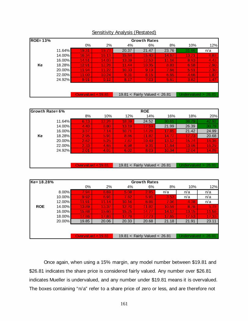
161
Sensitivity Analysis (Restated)
ROE=13%0% 2% 4% 6% 8% 10% 12%
11.64% 19.31 19.73 20.37 21.47 23.76 31.66 n/a14.00% 16.34 16.13 15.84 15.40 14.67 13.21 8.8316.00% 14.51 14.03 13.39 12.50 11.16 8.93 4.43
Ke 18.28% 12.91 12.26 11.44 10.35 8.83 6.58 2.9020.00% 11.94 11.22 10.33 9.19 7.66 5.51 2.3022.00% 11.00 10.24 9.31 8.15 6.65 4.66 1.8724.92% 9.91 9.12 8.17 7.03 5.61 3.82 1.47
Growth Rates
Overvalued <19.81 19.81 < Fairly Valued < 26.81 Undervalued > 26.81
Growth Rate=6%8% 10% 12% 14% 16% 18% 20%
11.64% 6.13 12.26 18.39 24.52 30.65 38.79 42.9214.00% 4.40 8.80 13.19 17.59 21.99 26.39 30.7916.00% 3.57 7.14 10.71 14.28 17.85 21.42 24.99
Ke 18.28% 2.95 5.91 8.86 11.82 14.77 17.73 20.6820.00% 2.62 5.25 7.87 10.49 13.12 15.74 18.3622.00% 2.33 4.65 6.98 9.31 11.64 13.96 16.2924.92% 2.01 4.01 6.02 8.03 10.04 12.04 14.05
ROE
Overvalued <19.81 19.81 < Fairly Valued < 26.81 Undervalued > 26.81
Ke=18.28%0% 2% 4% 6% 8% 10% 12%
8.00% 7.94 6.69 5.08 2.95 n/a n/a n/a10.00% 9.92 8.91 7.62 5.91 3.53 n/a n/a12.00% 11.91 11.14 10.16 8.86 7.06 4.38 n/a
ROE 14.00% 13.89 13.37 12.70 11.82 10.59 8.76 5.7816.00% 15.88 15.60 15.25 14.77 14.12 13.15 11.5618.00% 17.86 17.83 17.79 17.73 17.65 17.53 17.3320.00% 19.85 20.06 20.33 20.68 21.18 21.91 23.11
Growth Rates
Overvalued <19.81 19.81 < Fairly Valued < 26.81 Undervalued > 26.81
Once again, when using a 15% margin, any model number between $19.81 and
$26.81 indicates the share price is considered fairly valued. Any number over $26.81
indicates Mueller is undervalued, and any number under $19.81 means it is overvalued.
The boxes containing “n/a” refer to a share price of zero or less, and are therefore not

162
applicable. By looking at all of the tables, both before and after the restatement of
goodwill, it is clear that the models indicate that Mueller’s stock is overvalued.

163
Abnormal Earnings Growth (AEG) Valuation Model
The AEG model is probably the second best valuation model after the residual
income model because it is not very sensitive to changes in costs of equity or growth
rates. The model is based around the firm’s abnormal earnings. Abnormal earnings are
calculated by adding forecasted net income and dividend reinvestment earnings, then
subtracting the normal or benchmark earnings. Dividend reinvestment (DRIP) is
calculated by taking the previous year’s dividend and multiplying it by the cost of
equity. This is based on the assumption that when a firm pays dividends, an investor
will invest those dividends at the cost of equity. Normal or benchmark earnings are
calculated by taking the previous year’s net income and multiplying it by 1 plus the cost
of equity. Mueller has negative abnormal earnings growth for every forecasted year.
At this point, now that we have AEG, we can utilize a check figure to make sure
we are calculating the model properly. Our AEG for each year should equal the change
in residual income for the same year that we calculated in the residual income model.
The numbers do in fact equal each other as shown below.
AEG (42,937) (30,592) (11,589) (4,357) (9,879) (10,669) (11,523) (12,445) (13,440)Residual Income Check Figure (42,937) (30,592) (11,589) (4,357) (9,879) (10,669) (11,523) (12,445) (13,440)
Next, we discounted AEG back to the appropriate year, just like we did in the
previous models. We then added these numbers up to get the total present value of the
abnormal earnings growth. Next, we accounted for the abnormal earnings perpetuity.
After looking at the change in AEG over the ten forecasted years, we found that it has
been growing at about 8% each year. The value of the abnormal earnings perpetuity
was then calculated by taking AEG in year 2017 and increasing it by 8%. We discounted
it back to year 2017 by taking this number and dividing it by the cost of equity, ke,
minus the growth rate, g. We then discounted it back again to year 2008. Next, we took
the sum of net income in 2008, the present value of AEG, and the abnormal earnings
perpetuity to get the total average net income perpetuity. After we divided this number

164
by the average number of shares outstanding, we got average earnings per share of
the perpetuity. To get this back to a 2007 number we divided this by our cost of equity
to get the intrinsic value per share as of December 31st, 2007. Lastly, we carried the
share price forward ten months to get a share price as of our valuation date, November
1st, 2008.
We then performed a sensitivity analysis based upon different costs of equity
and growth rates. Like the residual income model, the growth rates for this model are
negative based upon the assumption that abnormal earnings should converge to zero in
the long run. We only had to perform the one AEG model because the model uses net
income and dividends starting in year 2008, our first forecasted year. Net income and
dividends are the same for both before and after the restatement of goodwill starting in
year 2008 and from then on forward.
Sensitivity Analysis
-10% -20% -30% -40% -50%11.64% 18.29 18.83 19.11 19.28 19.3914.00% 12.51 13.13 13.47 13.69 13.8316.00% 9.47 10.05 10.38 10.59 10.73
Ke 18.28% 7.16 7.66 7.96 8.15 8.2920.00% 5.94 6.38 6.64 6.82 6.9422.00% 4.90 5.26 5.49 5.64 5.7524.92% 3.83 4.11 4.29 4.42 4.51
Overvalued <19.81 19.81 < Fairly Valued < 26.81
Growth Rates
Undervalued > 26.81
By using a 15% margin, any model number between $19.81 and $26.81
indicates the share price is considered fairly valued. Any number over $26.81 indicates
Mueller is undervalued, and any number under $19.81 means it is overvalued. When
looking at the sensitivity analysis, every number in the model is below $19.81 per
share, meaning Muller’s stock is overvalued.

165
Conclusion
When looking at all of the intrinsic valuation models, we can see that Mueller is
overvalued in the market. The only model that showed Mueller as being undervalued
was the discounted free cash flows model. The discounted free cash flows model is a
model in which we do not put a lot of trust into since it is highly sensitive to changes in
the costs of capital and growth rates. Besides that model, the discounted dividend
model, residual income model, long run residual income model, and the abnormal
earnings growth model, all found Mueller to be overwhelmingly overvalued. For this
reason we suggest investors should sell their shares of Mueller to avoid any additional
loss.
Intrinsic Valuation Results Model Conclusion
Discounted Dividends Overvalued Free Cash Flows Undervalued Residual Income Overvalued
L/R Residual Income Overvalued Abnormal Earnings
Growth Overvalued

166
Appendices
Sales Manipulation Diagnostic Ratios
Sales/ Cash From Sales 2003 2004 2005 2006 2007Mueller 1.0316 1.0286 1.0279 1.0134 1.0156Mueller- Restated 1.0316 1.0286 1.0279 1.0134 1.0156Wolverine 0.9828 0.9955 0.9833 0.9648 0.9479Alcoa 1.0062 1.0087 1.0088 0.9958 0.9940Madeco 1.0463 1.0397 1.0315 1.0549 1.0094
Sales/ Net AR 2003 2004 2005 2006 2007Mueller 6.1291 6.8475 6.9644 8.9141 8.3524Mueller- Restated 6.1291 6.8475 6.9644 8.9141 8.3524Wolverine 6.8681 8.4913 7.7652 21.0443 11.4426Alcoa 8.4639 8.7149 8.7682 10.8963 11.8171Madeco 6.4298 6.8372 6.5834 6.6821 7.0989
Sales/ Inventory 2003 2004 2005 2006 2007Mueller 6.9889 9.8120 9.2089 12.7466 10.4306Mueller- Restated 6.9889 9.8120 9.2089 12.7466 10.4306Wolverine 5.5213 5.2499 5.5147 10.7031 11.0921Alcoa 8.4200 7.9104 7.4067 8.9879 9.2447Madeco 4.5134 4.5799 4.9195 5.7288 4.7376
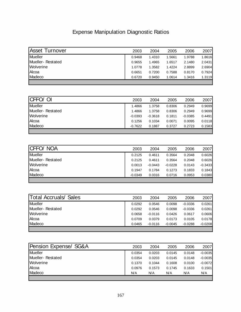
167
Expense Manipulation Diagnostic Ratios
Asset Turnover 2003 2004 2005 2006 2007Mueller 0.9468 1.4310 1.5661 1.9788 1.8616Mueller- Restated 0.9655 1.4965 1.6517 2.1480 2.0431Wolverine 1.0778 1.3582 1.4224 2.8899 2.6904Alcoa 0.6651 0.7200 0.7588 0.8170 0.7924Madeco 0.6720 0.9450 1.0614 1.3416 1.3119
CFFO/ OI 2003 2004 2005 2006 2007Mueller 1.4866 1.3758 0.8306 0.2949 0.9699Mueller- Restated 1.4866 1.3758 0.8306 0.2949 0.9699Wolverine -0.0393 -0.3618 0.1811 -0.0385 0.4491Alcoa 0.1256 0.1034 0.0071 0.0095 0.0118Madeco -0.7622 0.1887 0.3727 0.2723 0.1583
CFFO/ NOA 2003 2004 2005 2006 2007Mueller 0.2125 0.4611 0.3564 0.2048 0.6026Mueller- Restated 0.2125 0.4611 0.3564 0.2048 0.6026Wolverine 0.0013 -0.0443 -0.0228 0.0143 -0.3433Alcoa 0.1947 0.1784 0.1273 0.1833 0.1843Madeco -0.0349 0.0316 0.0716 0.0953 0.0380
Total Accruals/ Sales 2003 2004 2005 2006 2007Mueller 0.0292 0.0546 0.0098 -0.0336 0.0261Mueller- Restated 0.0292 0.0546 0.0098 -0.0336 0.0261Wolverine 0.0658 -0.0116 0.0426 0.0617 0.0606Alcoa 0.0709 0.0379 0.0173 0.0105 0.0178Madeco 0.0465 -0.0116 -0.0045 -0.0288 -0.0208
Pension Expense/ SG&A 2003 2004 2005 2006 2007Mueller 0.0354 0.0203 0.0145 0.0148 -0.0035Mueller- Restated 0.0354 0.0203 0.0145 0.0148 -0.0035Wolverine 0.1370 0.1044 0.1608 0.0100 -0.0072Alcoa 0.0976 0.1573 0.1745 0.1633 0.1501Madeco N/A N/A N/A N/A N/A

168
Other Employment Expenses/ SG&A 2003 2004 2005 2006 2007Mueller 0.0085 0.0074 0.0061 0.0059 0.0210Mueller- Restated 0.0085 0.0074 0.0061 0.0059 0.0210Wolverine 0.0296 0.0297 0.1136 0.0058 0.0023Alcoa 0.2120 0.2173 0.2301 0.2126 0.1732Madeco N/A N/A N/A N/A N/A

169
The Effects of Restating Goodwill
2002 2003 2004 2005 2006 2007
Net sales 952,983 999,078 1,379,056 1,729,923 2,510,912 2,697,845
Cost of goods sold 744,781 815,849 1,115,612 1,430,075 2,109,436 2,324,924
Gross profit 208,202 183,229 263,444 299,848 401,476 372,921
Depreciation and amortization 37,440 38,954 40,613 40,696 41,619 44,153Selling, general, and administrative expense 85,006 94,891 106,400 127,394 140,972 143,284Copper litigation settlement 0 0 0 0 0 (8,893)Impairment charge 0 0 3,941 0 0 2,756
Operating income 85,756 49,384 112,490 131,758 218,885 191,621
Interest expense (1,460) (1,168) (3,974) (19,550) (20,477) (22,071)Other income, net 4,171 3,220 6,842 11,997 5,171 13,731
Income from continuing operations before income taxes 88,467 51,436 115,358 124,205 203,579 183,281
Income tax expense (17,290) (7,215) (35,942) (34,987) (54,710) (67,806)
Income from continuing operations 71,177 44,221 79,416 89,218 148,869 115,475
Income from discontinued operations, net of income taxes 6,815 1,160 0 3,324 0 0
Net income 77,992 45,381 79,416 92,542 148,869 115,475
Income Statement Before Restatement (In thousands)

170
2002 2003 2004 2005 2006 2007
Net sales 952,983 999,078 1,379,056 1,729,923 2,510,912 2,697,845
Cost of goods sold 744,781 815,849 1,115,612 1,430,075 2,109,436 2,324,924
Gross profit 208,202 183,229 263,444 299,848 401,476 372,921
Depreciation and amortization 37,440 38,954 40,613 40,696 41,619 44,153Selling, general, and administrative expense 85,006 94,891 106,400 127,394 140,972 143,284Copper litigation settlement 0 0 0 0 0 (8,893)Impairment charge 0 0 3,941 0 0 2,756Additional Impairment charge 20,970 26,335 29,646 30,342 27,586
Operating income 85,756 28,414 86,155 102,112 188,543 164,035
Interest expense (1,460) (1,168) (3,974) (19,550) (20,477) (22,071)Other income, net 4,171 3,220 6,842 11,997 5,171 13,731
Income from continuing operations before income taxes 88,467 30,466 89,023 94,559 173,237 155,695
Income tax expense (17,290) (7,215) (35,942) (34,987) (54,710) (67,806)Change in tax expense 2,941 8,206 8,351 8,153 10,207New Income tax expense (4,274) (27,736) (26,636) (46,557) (57,599)
Income from continuing operations 71,177 26,192 61,287 67,923 126,680 98,096
Income from discontinued operations, net of income taxes 6,815 1,160 0 3,324 0 0
Net income 77,992 27,352 61,287 71,247 126,680 98,096
Income Statement After Restatement (In Thousands)

171
2002 2003 2004 2005 2006 2007
AssetsCurrent assets Cash and cash equivalents 217,601 255,088 47,449 129,685 200,471 308,618 Accounts receivable, less allowance for doubtful accounts of 5,015 in 2007 and 6,806 in 2006 132,427 163,006 196,762 260,685 281,679 323,003 Inventories 142,953 14,048 187,853 196,987 258,647 269,032 Current deferred income taxes 4,506 9,035 15,276 19,900 21,421 19,853 Other current assets 2,860 2,678 7,991 17,019 13,976 19,841
Total current assets 500,347 570,355 455,331 624,276 776,194 940,347
Property, plant, and equipment, net 352,469 345,537 335,610 307,046 315,064 308,383
Goodwill 105,551 104,849 136,615 152,171 155,653 153,263
Other assets 29,580 34,443 36,175 33,435 21,996 47,211
Total Non-Current Assets 487,600 484,829 508,400 492,652 492,713 508,857 Total Assets 987,947 1,055,184 963,731 1,116,928 1,268,907 1,449,204
Liabilities and Stockholders' EquityCurrent liabilities Current portion of long-term debt 4,161 2,835 5,328 4,120 35,998 72,743 Accounts payable 41,004 42,081 79,723 124,216 96,095 140,497 Accrued wages and other employee costs 26,199 25,631 37,992 38,095 43,281 39,984 Other current liabilities 34,987 48,314 57,775 97,251 80,145 81,829
Total current liabilities 106,351 118,861 180,818 263,682 255,519 335,053
Long-term debt, less current portion 14,005 11,437 310,650 312,070 308,154 281,738Pension liabilities 22,364 18,077 19,611 21,721 19,900 14,805Postretirement benefits other than pensions 13,186 13,566 13,556 13,515 16,699 21,266Environmental reserves 9,110 9,560 9,503 9,073 8,907 8,897Deferred income taxes 59,269 58,379 67,479 63,944 46,408 52,156Other noncurrent liabilities 9,718 10,238 10,361 3,078 2,206 2,029
Total non-current liabilities 127,652 121,257 431,160 423,401 402,274 380,891 Total liabilities 234,003 240,118 611,978 687,083 657,793 715,944
Minority interest in subsidiaries 421 208 67 6,937 22,300 22,765
Stockholders' equity Preferred stock - 1.00 par value; shares authorized 5,000,000; none outstanding 0 0 0 0 0 0 Common stock - .01 par value; shares authorized 100,000,000; issued 40,091,502; outstanding 37,079,903 in 2007 and 37,025,285 in 2006 401 401 401 401 401 401 Additional paid-in capital 258,939 259,110 252,931 252,889 256,906 259,611 Retained earnings 610,114 655,495 175,537 253,433 386,038 484,534 Accumulated other comprehensive income (21,133) (5,586) 3,085 (8,848) 12,503 31,808 Treasury common stock, at cost (94,798) (94,562) (80,268) (74,967) (67,034) (65,859)
Total stockholders' equity 753,523 814,858 351,686 422,908 588,814 710,495
Total Liabilities and Stockholders' Equity 987,947 1,055,184 963,731 1,116,928 1,268,907 1,449,204
Balance Sheet before Restatement (In Thousands)

172
2002 2003 2004 2005 2006 2007
AssetsCurrent assets Cash and cash equivalents 217,601 255,088 47,449 129,685 200,471 308,618 Accounts receivable, less allowance for doubtful accounts of 5,015 in 2007 and 6,806 in 2006 132,427 163,006 196,762 260,685 281,679 323,003 Inventories 142,953 14,048 187,853 196,987 258,647 269,032 Current deferred income taxes 4,506 9,035 15,276 19,900 21,421 19,853 Other current assets 2,860 2,678 7,991 17,019 13,976 19,841
Total current assets 500,347 570,355 455,331 624,276 776,194 940,347
Property, plant, and equipment, net 352,469 345,537 335,610 307,046 315,064 308,383
Goodwill 105,551 83,879 110,280 122,525 125,311 125,677
Other assets 29,580 34,443 36,175 33,435 21,996 47,211
Total Non-Current Assets 487,600 463,859 482,065 463,006 462,371 481,271 Total Assets 987,947 1,034,214 937,396 1,087,282 1,238,565 1,421,618
Liabilities and Stockholders' EquityCurrent liabilities Current portion of long-term debt 4,161 2,835 5,328 4,120 35,998 72,743 Accounts payable 41,004 42,081 79,723 124,216 96,095 140,497 Accrued wages and other employee costs 26,199 25,631 37,992 38,095 43,281 39,984 Other current liabilities 34,987 48,314 57,775 97,251 80,145 81,829 Less imcome taxes payable (2,941) (8,206) (8,351) (8,153) (10,207)
Total current liabilities 106,351 115,920 172,612 255,331 247,366 324,846
Long-term debt, less current portion 14,005 11,437 310,650 312,070 308,154 281,738Pension liabilities 22,364 18,077 19,611 21,721 19,900 14,805Postretirement benefits other than pensions 13,186 13,566 13,556 13,515 16,699 21,266Environmental reserves 9,110 9,560 9,503 9,073 8,907 8,897Deferred income taxes 59,269 58,379 67,479 63,944 46,408 52,156Other noncurrent liabilities 9,718 10,238 10,361 3,078 2,206 2,029
Total non-current liabilities 127,652 121,257 431,160 423,401 402,274 380,891 Total liabilities 234,003 237,177 603,772 678,732 649,640 705,737
Minority interest in subsidiaries 421 208 67 6,937 22,300 22,765
Stockholders' equity Preferred stock - 1.00 par value; shares authorized 5,000,000; none outstanding 0 0 0 0 0 0 Common stock - .01 par value; shares authorized 100,000,000; issued 40,091,502; outstanding 37,079,903 in 2007 and 37,025,285 in 2006 401 401 401 401 401 401 Additional paid-in capital 258,939 259,110 252,931 252,889 256,906 259,611 Retained earnings 610,114 655,495 175,537 253,433 386,038 484,534 Changes in goodwill net of taxes (18,029) (18,129) (21,295) (22,189) (17,379) New Retained earnings 637,466 157,408 232,138 363,849 467,155 Accumulated other comprehensive income (21,133) (5,586) 3,085 (8,848) 12,503 31,808 Treasury common stock, at cost (94,798) (94,562) (80,268) (74,967) (67,034) (65,859)
Total stockholders' equity 753,523 796,829 333,557 401,613 566,625 693,116
Total Liabilities and Stockholders' Equity 987,947 1,034,214 937,396 1,087,282 1,238,565 1,421,618
Balance Sheet After Restatement (In Thousands)

173
Liquidity Ratios
Current Ratio 2002 2003 2004 2005 2006 2007Mueller as Stated 4.7047 4.7985 2.5182 2.4344 3.0377 2.8066Mueller Restated 4.7047 4.9202 2.6379 2.4450 3.1378 2.8947Wolverine 4.3114 3.2199 3.1576 2.6955 3.2993 1.9232Alcoa 1.4050 1.3257 1.1858 1.1930 1.2143 1.1284Madeco 0.6732 1.8501 2.3778 2.2869 2.8947 2.1649Industry Average 2.1299 2.1319 2.2404 2.0585 2.4694 1.7388
Quick Asset Ratio 2002 2003 2004 2005 2006 2007Mueller as Stated 3.2913 3.5175 1.3762 1.5039 1.8869 1.8851Mueller Restated 3.2913 3.6067 1.4148 1.5289 1.9491 1.9444Wolverine 2.3451 1.6869 1.3779 1.2291 1.2999 1.2118Alcoa 0.6450 0.6780 0.5429 0.5571 0.5226 0.4934Madeco 0.1993 0.5007 0.7928 0.8627 1.1056 0.7698Industry Average 1.0631 0.9552 0.9045 0.8830 0.9761 0.8250
Accounts Receivable Turnover 2002 2003 2004 2005 2006 2007Mueller as Stated 7.1963 6.1291 6.8475 6.9644 8.9141 8.3524Mueller Restated 7.5444 6.1291 7.0088 6.6361 8.9141 8.3524Wolverine 8.4421 6.8681 8.4913 7.7652 21.0443 11.4426Alcoa 8.6197 8.2789 8.6251 8.7682 10.8963 11.8171Madeco 7.9837 6.4298 6.8372 6.5834 6.6821 7.0989Industry Average 8.3485 7.1922 7.9845 7.7056 12.8742 10.1195
Days Supply of Receivables 2002 2003 2004 2005 2006 2007Mueller as Stated 50.7206 59.5521 53.3042 52.4094 40.9464 43.7001Mueller Restated 48.3805 59.5521 52.0777 55.0025 40.9464 43.7001Wolverine 43.2359 53.1441 42.9853 47.0043 17.3444 31.8983Alcoa 42.3451 44.0882 42.3184 41.6278 33.4975 30.8875Madeco 45.7179 56.7672 53.3848 55.4427 54.6239 51.4164Industry Average 43.7663 51.3332 46.2295 48.0249 35.1552 38.0674
Inventory Turnover 2002 2003 2004 2005 2006 2007Mueller as Stated 5.2100 5.8048 5.9387 7.2597 8.1557 8.6418Mueller Restated 5.7071 5.8048 5.9387 7.2597 8.1557 8.6418Wolverine 5.7564 5.1433 4.8309 5.4119 10.3268 10.5182Alcoa 6.7635 6.5840 6.2227 5.9977 6.8988 7.2904Madeco 4.4269 3.9583 3.9097 4.2204 4.9074 4.1822Industry Average 5.6489 5.2285 4.9878 5.2100 7.3777 7.3303

174
Days Supply of Inventory 2002 2003 2004 2005 2006 2007Mueller as Stated 70.0580 62.8793 61.4607 50.2773 44.7542 42.2365Mueller Restated 63.9553 62.8793 61.4607 50.2773 44.7542 42.2365Wolverine 63.4082 70.9666 75.5554 67.4436 35.3451 34.7017Alcoa 53.9664 55.4375 58.6561 60.8568 52.9076 50.0656Madeco 82.4506 92.2113 93.3564 86.4844 74.3772 87.2738Industry Average 66.6084 72.8718 75.8560 71.5949 54.2100 57.3470
Working Capital Turnover 2002 2003 2004 2005 2006 2007Mueller as Stated 2.4188 2.2128 5.0236 4.7974 4.8224 4.4571Mueller Restated 2.5358 2.1985 4.8778 4.6888 4.7481 4.3832Wolverine 3.2727 3.4093 3.9506 4.4593 8.1737 7.5478Alcoa 11.2685 12.6033 19.9280 17.9803 20.6099 33.4217Madeco -4.3702 3.5604 3.6972 4.0868 3.6776 4.1725Industry Average 3.3904 6.5243 9.1919 8.8421 10.8204 15.0474
Cash To Cash Cycle 2003 2004 2005 2006 2007Mueller as Stated 122.6200 113.6300 102.6100 85.8200 85.9300Mueller Restated 122.6200 113.6300 102.6100 85.8200 85.9300Wolverine 136.6000 129.3100 114.5000 52.8200 66.5500Alcoa 99.5300 100.9700 102.4800 86.4100 80.9500Madeco 149.1100 146.3800 142.0100 128.9600 138.6800Industry Average 126.9700 122.5700 115.4000 88.5000 93.0300

175
Profitability Ratios
Gross Profit Margin 2002 2003 2004 2005 2006 2007Mueller as Stated 21.8474% 18.3398% 19.1032% 17.3330% 15.9893% 13.8229%Mueller Restated 18.3398% 18.3398% 19.1032% 17.3330% 15.9893% 13.8229%Wolverine 10.6155% 6.8463% 7.9813% 1.8631% 3.5165% 5.1738%Alcoa 20.0637% 20.5502% 20.7041% 19.0238% 23.2430% 21.1396%Madeco 12.367% 12.298% 14.632% 14.211% 14.338% 11.723%Industry Average 14.349% 13.232% 14.439% 11.699% 13.699% 12.679%
Operating Profit Margin 2002 2003 2004 2005 2006 2007Mueller as Stated -0.1532% 4.9430% 8.1570% 7.6164% 8.7174% 7.1027%Mueller Restated 4.9430% 2.8440% 6.2474% 5.9027% 7.5089% 6.0802%Wolverine 5.0543% -1.0622% 2.9937% -2.8205% -3.7545% -4.0907%Alcoa 2.4942% 4.9896% 6.0551% 4.9163% 7.1134% 8.3615%Madeco 1.562% 3.137% 7.770% 7.617% 9.258% 6.278%Industry Average 3.3082% 1.0377% 5.3816% 2.3984% 2.7518% 1.0934%
Net Profit Margin 2002 2003 2004 2005 2006 2007Mueller as Stated 7.4689% 4.4262% 5.7587% 5.3495% 5.9289% 4.2803%Mueller Restated 4.5423% 2.7377% 4.4441% 4.1185% 5.0452% 3.6361%Wolverine 0.9994% -6.8119% 0.0479% -4.7731% -6.0206% -9.3543%Alcoa 2.0638% 4.4943% 5.6378% 4.8224% 7.3998% 8.3388%Madeco -15.672% -7.041% 2.627% 3.287% 5.402% 3.077%Industry Average -4.2031% -3.1196% 2.7709% 1.1122% 2.2604% 0.6870%
Operating Expense Ratio 2002 2003 2004 2005 2006 2007Mueller as Stated 8.9200% 9.4979% 7.7154% 7.3641% 5.6144% 5.3111%Mueller Restated 9.4979% 9.4979% 7.7154% 7.3641% 5.6144% 5.3111%Wolverine 5.5613% 5.3835% 4.6698% 4.5152% 2.3280% 2.6420%Alcoa 5.6852% 5.8502% 5.3882% 5.0649% 4.6150% 4.7873%Madeco -10.8053% -9.1607% -6.8627% -6.5938% -5.0804% -5.4455%Industry Average 0.1471% 0.6910% 1.0651% 0.9954% 0.6209% 0.6613%
Asset Turnover 2003 2004 2005 2006 2007Mueller as Stated 1.0113 1.3069 1.7950 2.2731 2.1261Mueller Restated 1.0113 1.3334 1.8877 2.4144 2.3225Wolverine 1.0828 1.4421 1.3772 2.3136 2.6984Alcoa 0.7001 0.7327 0.7841 0.9016 0.8269Industry Average 0.8915 1.0874 1.0806 1.6076 1.7627

176
Return on Assets 2003 2004 2005 2006 2007Mueller as Stated 4.5935% 7.5263% 9.6025% 13.4767% 9.1004%Mueller Restated 4.4760% 7.6789% 10.0981% 14.3146% 9.9409%Wolverine -7.0787% 0.1164% -6.5734% -13.9291% -21.3098%Alcoa 3.1466% 4.1311% 3.7812% 6.6714% 6.8956%Madeco -5.3692% 2.5403% 3.7435% 8.9186% 4.6958%Industry Average -3.1005% 2.2626% 0.3171% 0.5536% -3.2395%
Return on Equity 2003 2004 2005 2006 2007Mueller as Stated 6.0225% 9.7460% 26.3138% 35.2013% 19.6115%Mueller Restated 5.8686% 9.9665% 29.6052% 42.0168% 23.5820%Wolverine -19.4303% 0.3591% -18.4323% -48.5138% -108.8073%Alcoa 9.4490% 10.8489% 9.2707% 16.8100% 17.5244%Madeco -20.4610% 6.0882% 8.0984% 14.9528% 7.7801%Industry Average -10.1474% 5.7654% -0.3544% -5.5837% -27.8343%

177
Capital Structure Ratios
Debt to Equity Ratio 2002 2003 2004 2005 2006 2007Mueller as Stated 0.3105 0.2947 1.7401 1.5956 1.1171 1.0077Mueller Restated 0.3105 0.2977 1.9315 1.9157 1.3267 1.2047Wolverine 1.7449 2.0848 1.8041 2.4829 4.1060 5.5637Alcoa 1.8727 1.5152 1.3453 1.4176 1.4184 1.2692Madeco 2.6759 1.3293 1.0981 0.6269 0.6112 0.7603Industry Average 2.0978 1.6431 1.4158 1.5091 2.0452 2.5311
Times Interest Earned 2002 2003 2004 2005 2006 2007Mueller as Stated 0.8908 42.2808 28.3065 6.7395 10.6893 8.6820Mueller Restated 42.2808 24.3272 21.6797 5.2231 9.2075 7.4322Wolverine 1.4138 -0.2985 1.1451 -1.1357 -2.3336 -2.3906Alcoa 38.2171 44.8248 58.5498 52.1209 51.7708 51.6883Madeco 2.0038 12.8959 30.6790 37.8061 33.6545 12.1274Industry Average 13.88 19.14 30.12 29.60 27.70 20.48
Debt Service Margin 2003 2004 2005 2006 2007Mueller as Stated 17.6438 54.5894 20.5407 15.6648 5.1626Mueller Restated 17.6438 54.5894 20.5407 15.6648 5.1626Wolverine 0.0129 -0.2901 -0.1272 0.0544 -0.8363Alcoa 29.3253 4.2046 29.4035 44.2586 6.1000Madeco -0.7600 7.3180 12.2435 14.6709 30.8606Industry Average 9.5261 3.7441 13.8399 19.6613 12.0414
IGR 2003 2004 2005 2006 2007Mueller as Stated 4.5935% 7.5263% 9.6025% 13.4767% 9.1004%Mueller Restated 2.7686% 5.9259% 7.7744% 12.1810% 8.4448%Wolverine 0.9991% -7.3421% 0.0650% -6.7894% -17.3992%Alcoa 3.1466% 4.1311% 3.7812% 6.6714% 6.8956%Madeco -5.3692% 2.5403% 3.7435% 8.9186% 4.6958%Industry Average -0.4079% -0.2236% 2.5299% 2.9335% -1.9359%
SGR 2003 2004 2005 2006 2007Mueller as Stated 5.9470% 20.6229% 24.9242% 28.5322% 18.2705%Mueller Restated 3.5927% 17.3721% 22.6676% 28.3413% 18.6182%Wolverine 3.0819% -20.5879% 0.2265% -34.6667% -114.2039%Alcoa 7.9143% 9.6887% 9.1415% 16.1339% 15.6473%Madeco -12.5067% 5.3298% 6.0903% 14.3699% 8.2662%Industry Average -0.5035% -1.8565% 5.1528% -1.3876% -30.0968%

178
Altman’s Z-Score
Altman’s Z-Score is calculated as follows:
1.2(Working Capital/Total Assets) + 1.4(Retained Earnings/Total assets) + 3.3(Earnings Before Interest and Taxes/Total assets) + 0.6(Market Value of Equity/Book Value of
Liabilities) + 1.0(Sales/ total assets)
2003 2004 2005 2006 2007Mueller as Stated 4.5650 2.4761 3.2087 4.2311 4.0939Mueller Restated 4.5079 2.5329 3.1994 4.2944 4.1777Wolverine 2.9889 3.3677 3.3283 4.8634 5.8124Alcoa 3.4832 3.5593 3.8040 3.9812 3.8501Madeco 2.2799 3.2250 3.5048 4.1075 3.4808
Altman's Z-Score

179
3 Month Rates SUMMARY OUTPUT 72 MONTHS
Regression StatisticsMultiple R 0.556024749R Square 0.309163522Adjusted R Square 0.299294429Standard Error 0.067837663Observations 72
ANOVAdf SS MS F Significance F
Regression 1 0.144162657 0.144162657 31.32643858 3.96544E-07Residual 70 0.322136395 0.004601948Total 71 0.466299052
Coefficients Standard Error t Stat P-value Lower 95% Upper 95% Lower 95.0% Upper 95.0%Intercept 0.004309241 0.008032914 0.536448123 0.593349688 -0.011711899 0.020330382 -0.011711899 0.020330382X Variable 1 1.370180198 0.244806066 5.597002642 3.96544E-07 0.881929901 1.858430495 0.881929901 1.858430495 SUMMARY OUTPUT 60 MONTHS
Regression StatisticsMultiple R 0.576492385R Square 0.33234347Adjusted R Square 0.320832151Standard Error 0.07013699Observations 60
ANOVAdf SS MS F Significance F
Regression 1 0.142022216 0.142022216 28.87101438 1.43245E-06Residual 58 0.285313444 0.004919197Total 59 0.42733566
Coefficients Standard Error t Stat P-value Lower 95% Upper 95% Lower 95.0% Upper 95.0%Intercept 0.005373855 0.009102683 0.590359516 0.557242969 -0.012847144 0.023594855 -0.012847144 0.023594855X Variable 1 1.639669054 0.305158294 5.373175446 1.43245E-06 1.028828366 2.250509742 1.028828366 2.250509742

180
SUMMARY OUTPUT 48 MONTHS
Regression StatisticsMultiple R 0.60366917R Square 0.364416467Adjusted R Square 0.350599434Standard Error 0.067722826Observations 48
ANOVAdf SS MS F Significance F
Regression 1 0.120963219 0.120963219 26.37443642 5.56895E-06Residual 46 0.210973535 0.004586381Total 47 0.331936755
Coefficients Standard Error t Stat P-value Lower 95% Upper 95% Lower 95.0% Upper 95.0%Intercept 0.00357668 0.00978847 0.365397255 0.716489749 -0.016126488 0.023279848 -0.016126488 0.023279848X Variable 1 1.655431152 0.322343954 5.135604777 5.56895E-06 1.006586435 2.304275868 1.006586435 2.304275868 SUMMARY OUTPUT 36 MONTHS
Regression StatisticsMultiple R 0.566300174R Square 0.320695887Adjusted R Square 0.300716354Standard Error 0.072629402Observations 36
ANOVAdf SS MS F Significance F
Regression 1 0.08467067 0.08467067 16.05122055 0.000317937Residual 34 0.179351021 0.00527503Total 35 0.264021691
Coefficients Standard Error t Stat P-value Lower 95% Upper 95% Lower 95.0% Upper 95.0%Intercept 0.005940195 0.012206528 0.486640841 0.629635263 -0.018866454 0.030746844 -0.018866454 0.030746844X Variable 1 1.510494751 0.377020695 4.006397453 0.000317937 0.744296519 2.276692983 0.744296519 2.276692983

181
SUMMARY OUTPUT 24 MONTHS
Regression StatisticsMultiple R 0.623027061R Square 0.388162718Adjusted R Square 0.360351933Standard Error 0.072002184Observations 24
ANOVAdf SS MS F Significance F
Regression 1 0.072358891 0.072358891 13.95727272 0.001145914Residual 22 0.114054919 0.005184314Total 23 0.18641381
Coefficients Standard Error t Stat P-value Lower 95% Upper 95% Lower 95.0% Upper 95.0%Intercept -0.000536778 0.015037306 -0.035696396 0.97184636 -0.031722242 0.030648687 -0.031722242 0.030648687X Variable 1 1.498995187 0.401236059 3.73594335 0.001145914 0.666882534 2.33110784 0.666882534 2.33110784

182
2 Year Rates SUMMARY OUTPUT 72 MONTHS
Regression StatisticsMultiple R 0.555574725R Square 0.308663275Adjusted R Square 0.298787036Standard Error 0.06786222Observations 72
ANOVAdf SS MS F Significance F
Regression 1 0.143929392 0.143929392 31.25311939 4.07022E-07Residual 70 0.32236966 0.004605281Total 71 0.466299052
Coefficients Standard Error t Stat P-value Lower 95% Upper 95% Lower 95.0% Upper 95.0%Intercept 0.004811214 0.008027631 0.599331686 0.550886648 -0.011199391 0.020821818 -0.011199391 0.020821818X Variable 1 1.368762903 0.244839532 5.590448944 4.07022E-07 0.88044586 1.857079946 0.88044586 1.857079946 SUMMARY OUTPUT 60 MONTHS
Regression StatisticsMultiple R 0.580322469R Square 0.336774168Adjusted R Square 0.32533924Standard Error 0.069903881Observations 60
ANOVAdf SS MS F Significance F
Regression 1 0.143915611 0.143915611 29.45135849 1.1738E-06Residual 58 0.283420049 0.004886553Total 59 0.42733566
Coefficients Standard Error t Stat P-value Lower 95% Upper 95% Lower 95.0% Upper 95.0%Intercept 0.010173188 0.009024642 1.127267692 0.264271355 -0.007891596 0.028237972 -0.007891596 0.028237972X Variable 1 1.656057642 0.305156611 5.426910584 1.1738E-06 1.045220323 2.26689496 1.045220323 2.26689496

183
SUMMARY OUTPUT 48 MONTHS
Regression StatisticsMultiple R 0.604117003R Square 0.364957353Adjusted R Square 0.351152078Standard Error 0.067694004Observations 48
ANOVAdf SS MS F Significance F
Regression 1 0.121142759 0.121142759 26.43608002 5.45731E-06Residual 46 0.210793995 0.004582478Total 47 0.331936755
Coefficients Standard Error t Stat P-value Lower 95% Upper 95% Lower 95.0% Upper 95.0%Intercept 0.003943409 0.009788288 0.402870118 0.688910091 -0.015759393 0.023646211 -0.015759393 0.023646211X Variable 1 1.65448535 0.321783964 5.141602865 5.45731E-06 1.006767836 2.302202864 1.006767836 2.302202864
SUMMARY OUTPUT 36 MONTHS
Regression StatisticsMultiple R 0.56628801R Square 0.32068211Adjusted R Square 0.300702172Standard Error 0.072630138Observations 36
ANOVAdf SS MS F Significance F
Regression 1 0.084667033 0.084667033 16.0502055 0.000318052Residual 34 0.179354658 0.005275137Total 35 0.264021691
Coefficients Standard Error t Stat P-value Lower 95% Upper 95% Lower 95.0% Upper 95.0%Intercept 0.006070388 0.012210883 0.497129344 0.622297453 -0.018745112 0.030885889 -0.018745112 0.030885889X Variable 1 1.506507988 0.376037486 4.006270772 0.000318052 0.742307877 2.270708099 0.742307877 2.270708099

184
SUMMARY OUTPUT 24 MONTHS
Regression StatisticsMultiple R 0.623168858R Square 0.388339426Adjusted R Square 0.360536672Standard Error 0.071991785Observations 24
ANOVAdf SS MS F Significance F
Regression 1 0.072391832 0.072391832 13.96766069 0.001142063Residual 22 0.114021978 0.005182817Total 23 0.18641381
Coefficients Standard Error t Stat P-value Lower 95% Upper 95% Lower 95.0% Upper 95.0%Intercept -0.000444484 0.015040221 -0.02955304 0.976689979 -0.031635994 0.030747025 -0.031635994 0.030747025X Variable 1 1.495115357 0.400048701 3.737333367 0.001142063 0.665465135 2.324765579 0.665465135 2.324765579
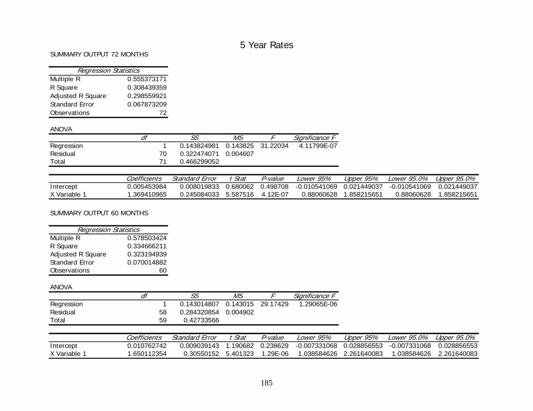
185
5 Year Rates SUMMARY OUTPUT 72 MONTHS
Regression StatisticsMultiple R 0.555373171R Square 0.308439359Adjusted R Square 0.298559921Standard Error 0.067873209Observations 72
ANOVAdf SS MS F Significance F
Regression 1 0.143824981 0.143825 31.22034 4.11799E-07Residual 70 0.322474071 0.004607Total 71 0.466299052
Coefficients Standard Error t Stat P-value Lower 95% Upper 95% Lower 95.0% Upper 95.0%Intercept 0.005453984 0.008019833 0.680062 0.498708 -0.010541069 0.021449037 -0.010541069 0.021449037X Variable 1 1.369410965 0.245084033 5.587516 4.12E-07 0.88060628 1.858215651 0.88060628 1.858215651 SUMMARY OUTPUT 60 MONTHS
Regression StatisticsMultiple R 0.578503424R Square 0.334666211Adjusted R Square 0.323194939Standard Error 0.070014882Observations 60
ANOVAdf SS MS F Significance F
Regression 1 0.143014807 0.143015 29.17429 1.29065E-06Residual 58 0.284320854 0.004902Total 59 0.42733566
Coefficients Standard Error t Stat P-value Lower 95% Upper 95% Lower 95.0% Upper 95.0%Intercept 0.010762742 0.009039143 1.190682 0.238629 -0.007331068 0.028856553 -0.007331068 0.028856553X Variable 1 1.650112354 0.30550152 5.401323 1.29E-06 1.038584626 2.261640083 1.038584626 2.261640083

186
SUMMARY OUTPUT 48 MONTHS
Regression StatisticsMultiple R 0.603611222R Square 0.364346508Adjusted R Square 0.350527954Standard Error 0.067726553Observations 48
ANOVAdf SS MS F Significance F
Regression 1 0.120939997 0.12094 26.36647 5.58355E-06Residual 46 0.210996757 0.004587Total 47 0.331936755
Coefficients Standard Error t Stat P-value Lower 95% Upper 95% Lower 95.0% Upper 95.0%Intercept 0.004247161 0.009796741 0.433528 0.666658 -0.015472655 0.023966977 -0.015472655 0.023966977X Variable 1 1.648693871 0.321080567 5.134829 5.58E-06 1.002392222 2.29499552 1.002392222 2.29499552 SUMMARY OUTPUT 36 MONTHS
Regression StatisticsMultiple R 0.565780547R Square 0.320107628Adjusted R Square 0.300110793Standard Error 0.072660843Observations 36
ANOVAdf SS MS F Significance F
Regression 1 0.084515357 0.084515 16.00792 0.000322905Residual 34 0.179506334 0.00528Total 35 0.264021691
Coefficients Standard Error t Stat P-value Lower 95% Upper 95% Lower 95.0% Upper 95.0%Intercept 0.006272652 0.012222986 0.513185 0.611141 -0.018567443 0.031112747 -0.018567443 0.031112747X Variable 1 1.499567054 0.37479907 4.000989 0.000323 0.737883706 2.261250402 0.737883706 2.261250402

187
SUMMARY OUTPUT 24 MONTHS
Regression StatisticsMultiple R 0.621875997R Square 0.386729756Adjusted R Square 0.358853836Standard Error 0.072086451Observations 24
ANOVAdf SS MS F Significance F
Regression 1 0.072091767 0.072092 13.87326 0.001177593Residual 22 0.114322043 0.005196Total 23 0.18641381
Coefficients Standard Error t Stat P-value Lower 95% Upper 95% Lower 95.0% Upper 95.0%Intercept -0.000147255 0.015078648 -0.009766 0.992296 -0.031418456 0.031123946 -0.031418456 0.031123946X Variable 1 1.486906327 0.399203574 3.724682 0.001178 0.65900879 2.314803865 0.65900879 2.314803865

188
7 Year Rates SUMMARY OUTPUT 72 MONTHS
Regression StatisticsMultiple R 0.555280708R Square 0.308336664Adjusted R Square 0.29845576Standard Error 0.067878248Observations 72
ANOVAdf SS MS F Significance F
Regression 1 0.143777094 0.143777 31.20531 4.14009E-07Residual 70 0.322521958 0.004607Total 71 0.466299052
Coefficients Standard Error t Stat P-value Lower 95% Upper 95% Lower 95.0% Upper 95.0%Intercept 0.005756642 0.008016708 0.718081 0.475098 -0.010232178 0.021745462 -0.010232178 0.021745462X Variable 1 1.369740515 0.245202037 5.586171 4.14E-07 0.880700479 1.858780552 0.880700479 1.858780552 SUMMARY OUTPUT 60 MONTHS
Regression StatisticsMultiple R 0.577749179R Square 0.333794114Adjusted R Square 0.322307806Standard Error 0.070060753Observations 60
ANOVAdf SS MS F Significance F
Regression 1 0.142642128 0.142642 29.06017 1.34222E-06Residual 58 0.284693532 0.004909Total 59 0.42733566
Coefficients Standard Error t Stat P-value Lower 95% Upper 95% Lower 95.0% Upper 95.0%Intercept 0.011043832 0.009045613 1.220905 0.227062 -0.007062929 0.029150593 -0.007062929 0.029150593X Variable 1 1.647499007 0.305615981 5.390749 1.34E-06 1.03574216 2.259255854 1.03574216 2.259255854

189
SUMMARY OUTPUT 48 MONTHS
Regression StatisticsMultiple R 0.603360882R Square 0.364044353Adjusted R Square 0.350219231Standard Error 0.067742648Observations 48
ANOVAdf SS MS F Significance F
Regression 1 0.120839701 0.12084 26.33209 5.64703E-06Residual 46 0.211097053 0.004589Total 47 0.331936755
Coefficients Standard Error t Stat P-value Lower 95% Upper 95% Lower 95.0% Upper 95.0%Intercept 0.004428832 0.009801482 0.451853 0.653498 -0.015300528 0.024158191 -0.015300528 0.024158191X Variable 1 1.646359873 0.320835282 5.13148 5.65E-06 1.000551957 2.292167789 1.000551957 2.292167789
SUMMARY OUTPUT 36 MONTHS
Regression StatisticsMultiple R 0.565587498R Square 0.319889217Adjusted R Square 0.299885959Standard Error 0.072672513Observations 36
ANOVAdf SS MS F Significance F
Regression 1 0.084457692 0.084458 15.99186 0.000324768Residual 34 0.179563999 0.005281Total 35 0.264021691
Coefficients Standard Error t Stat P-value Lower 95% Upper 95% Lower 95.0% Upper 95.0%Intercept 0.006408536 0.01222968 0.524015 0.603668 -0.018445164 0.031262236 -0.018445164 0.031262236X Variable 1 1.496837675 0.374304697 3.998982 0.000325 0.736159015 2.257516335 0.736159015 2.257516335

190
SUMMARY OUTPUT 24 MONTHS
Regression StatisticsMultiple R 0.621327838R Square 0.386048282Adjusted R Square 0.358141386Standard Error 0.072126492Observations 24
ANOVAdf SS MS F Significance F
Regression 1 0.071964731 0.071965 13.83344 0.001192941Residual 22 0.114449079 0.005202Total 23 0.18641381
Coefficients Standard Error t Stat P-value Lower 95% Upper 95% Lower 95.0% Upper 95.0%Intercept 3.48343E-05 0.015098436 0.002307 0.99818 -0.031277406 0.031347074 -0.031277406 0.031347074X Variable 1 1.483626214 0.398895792 3.719333 0.001193 0.656366978 2.310885449 0.656366978 2.310885449

191
10 Year Rates SUMMARY OUTPUT 72 MONTHS
Regression StatisticsMultiple R 0.555090745R Square 0.308125736Adjusted R Square 0.298241817Standard Error 0.067888597Observations 72
ANOVAdf SS MS F Significance F
Regression 1 0.143678738 0.143679 31.17445 4.18583E-07Residual 70 0.322620314 0.004609Total 71 0.466299052
Coefficients Standard Error t Stat P-value Lower 95% Upper 95% Lower 95.0% Upper 95.0%Intercept 0.006069888 0.008014466 0.757367 0.451372 -0.009914459 0.022054235 -0.009914459 0.022054235X Variable 1 1.369169691 0.245221113 5.583409 4.19E-07 0.88009161 1.858247772 0.88009161 1.858247772 SUMMARY OUTPUT 60 MONTHS
Regression StatisticsMultiple R 0.577028555R Square 0.332961953Adjusted R Square 0.321461297Standard Error 0.070104496Observations 60
ANOVAdf SS MS F Significance F
Regression 1 0.142286516 0.142287 28.95156 1.39328E-06Residual 58 0.285049144 0.004915Total 59 0.42733566
Coefficients Standard Error t Stat P-value Lower 95% Upper 95% Lower 95.0% Upper 95.0%Intercept 0.011364144 0.009052255 1.255394 0.21437 -0.006755913 0.0294842 -0.006755913 0.0294842X Variable 1 1.644343506 0.305602251 5.380666 1.39E-06 1.032614143 2.25607287 1.032614143 2.25607287

192
SUMMARY OUTPUT 48 MONTHS
Regression StatisticsMultiple R 0.603034814R Square 0.363650987Adjusted R Square 0.349817313Standard Error 0.067763596Observations 48
ANOVAdf SS MS F Significance F
Regression 1 0.120709129 0.120709 26.28738 5.7307E-06Residual 46 0.211227626 0.004592Total 47 0.331936755
Coefficients Standard Error t Stat P-value Lower 95% Upper 95% Lower 95.0% Upper 95.0%Intercept 0.004669411 0.009807911 0.476086 0.636266 -0.01507289 0.024411712 -0.01507289 0.024411712X Variable 1 1.643302933 0.320511795 5.127122 5.73E-06 0.998146162 2.288459704 0.998146162 2.288459704
SUMMARY OUTPUT 36 MONTHS
Regression StatisticsMultiple R 0.565354736R Square 0.319625978Adjusted R Square 0.299614977Standard Error 0.072686575Observations 36
ANOVAdf SS MS F Significance F
Regression 1 0.084388191 0.084388 15.97251 0.000327028Residual 34 0.1796335 0.005283Total 35 0.264021691
Coefficients Standard Error t Stat P-value Lower 95% Upper 95% Lower 95.0% Upper 95.0%Intercept 0.006609539 0.012239205 0.54003 0.592696 -0.018263517 0.031482596 -0.018263517 0.031482596X Variable 1 1.493577574 0.373715536 3.996563 0.000327 0.734096232 2.253058915 0.734096232 2.253058915

193
SUMMARY OUTPUT 24 MONTHS
Regression StatisticsMultiple R 0.620625251R Square 0.385175702Adjusted R Square 0.357229143Standard Error 0.072177729Observations 24
ANOVAdf SS MS F Significance F
Regression 1 0.07180207 0.071802 13.78258 0.001212864Residual 22 0.11461174 0.00521Total 23 0.18641381
Coefficients Standard Error t Stat P-value Lower 95% Upper 95% Lower 95.0% Upper 95.0%Intercept 0.000293355 0.015125609 0.019395 0.984701 -0.031075238 0.031661947 -0.031075238 0.031661947X Variable 1 1.479657547 0.398562049 3.71249 0.001213 0.653090451 2.306224643 0.653090451 2.306224643

194
Backdoor Cost of Equity, Cost of Debt, and Weighted Average Cost of Capital
Backdoor Cost of Equity Estimation Before Restatement After Restatement
Avg. 10-year Forecast ROE
12.05% 13.68%
Avg. 10-year Forecast Earnings
Growth Rate (g)
5.23% 7.36%
Estimated Ke (before size premium)
10.47% 12.22%
Estimated Ke (after 2.3% size premium)
12.77% 14.52%
Cost of Debt
Current Portion: Debt (In Thousands)
Int. Rate Weight WACD
Mueller-Xingrong Line of Credit with Interest
$46,627 0.0648 0.0632 0.409%
Other current liabilities $288,420 0.0608 0.3905 2.374% Long Term Portion:
Subordinated Debentures
$297,688 0.0600 0.4029 2.417%
Series IRBs with Interest Due
$10,000 0.0616 0.0135 0.0008%
Capital Lease Obligations $166 0.0618 0.0002 0.00001%
Post Retirement Benefits $36,071 0.0618 0.0489 0.3022%
Other L/T Liabilities $59,737 0.0608 0.0808 0.4913% Total: $738,709 5.99%
Weighted Average Cost of Capital Cost of
Debt(%) L/(L+E) Tax
Rate Cost of
Equity(%)E/(L+E) WACC(%)
WACC BT 5.99 738,709/ 1,449,204
0.00 18.28 710,495/ 1,449,204
12.0152
WACC AT 5.99 738,709/ 1,449,204
0.37 18.28 710,495/ 1,449,204
10.8854

195
Method of Comparables
P/E (Trailing) Mueller EPS (trailing): 3.109; 2.641 (restated)
Company PPS EPS P/E (Trailing) Mueller PPS Alcoa 11.88 2.24 5.3 $12.23
(as stated) Wolverine 0.20 N/A N/A Madeco 5.71 2.22 2.57 $10.39
(restated) Avg. 3.935
P/E (Forward) Mueller EPS (forward): 3.741
Company PPS EPS (forward) P/E (Forward) Mueller PPS Alcoa 11.88 1.06 11.19 $41.86
Wolverine 0.20 N/A N/A Madeco 5.71 N/A N/A
Avg. 11.19
P/B Mueller BVE (per share): 19.13; 15.77 (restated)
Company PPS BPS P/B Mueller PPS Alcoa 11.88 21.60 0.55 $10.62
(as stated) Wolverine 0.20 2.00 0.10 (outlier) Madeco 5.71 10.20 0.56 $8.75
(restated) Avg. 0.555
D/P Mueller DPS: 0.40
Company PPS DPS D/P Mueller PPS Alcoa 11.88 1.27 0.107 $6.65
Wolverine 0.20 0.10 0.502 (outlier) Madeco 5.71 0.07 0.0135
Avg. 0.06
P.E.G. Mueller g: -1.0%, forward EPS: 3.741
Company P/E G P.E.G. Mueller PPS Alcoa 11.19 27.29 0.41 -$0.01 (throw
out)
Wolverine N/A N/A N/A Madeco N/A N/A N/A
Avg. 0.41

196
P/EBITDA
Mueller EBITDA (per share): 6.348; 5.605 (restated) Company PPS EBITDA(PS) P/EBITDA Mueller PPS
Alcoa 11.88 5.27 2.255 $19.54 (as stated) Wolverine 0.20 0.92 0.217 (outlier)
Madeco 5.71 1.46 3.898 $17.25 (restated) Avg. 3.077
P/FCF
Mueller FCF (per share): 3.321 Company PPS FCF(PS) P/FCF (per share) Mueller PPS
Alcoa 11.88 1.97 6.029 $20.02
Wolverine 0.20 -0.67 -.2972 (omit) Madeco 5.71 -0.11 -51.02 (omit)
Avg. 6.029
EV/EBITDA Mueller Inputs (as stated, per share): EBITDA = 6.348, BVL = 19.27, Cash and Fin. Invstmt. = 8.31 Mueller Inputs (restated, per share): EBITDA = 5.605, BVL = 19.002, Cash and Fin. Invstmt. = 8.31 Company EV/EBITDA Mueller PPS
Alcoa 4.614 $12.38 (as stated) Wolverine N/A
Madeco 2.743 $9.92 (restated) Avg. 3.678

197
Valuations
Discounted Free Cash Flow Before Restatement (In Thousands)
0 1 2 3 4 5 6 7 8 9 10 Perpituity2007 2008 2009 2010 2011 2012 2013 2014 2015 2016 2017
Cash Flow From Operations 220,946 169,024 135,219 186,349 208,711 225,407 243,440 262,915 283,949 306,664Cash Flow From Investing Activities (46,899) 55,576 (25,009) (63,023) (47,057) (50,822) (54,887) (59,278) (64,020) (69,142)
FCF Firm's Assets 174,047 224,599 110,210 123,326 161,654 174,586 188,553 203,637 219,928 237,522 256,524PV Factor (WACC) 0.8927 0.7969 0.7114 0.6351 0.5669 0.5061 0.4518 0.4033 0.3600 0.3214PV YBY Free Cash Flows 155,371 178,985 78,403 78,320 91,645 88,356 85,185 82,128 79,181 76,339
Total PV YBY FCF 993,915Continuing (terminal) Value Perpituity 2,134,143PV of terminal Value perpetuity 685,911Market Value of Assets 12/31/2007 1,679,826Book Value Debt & Preferred Stock 715,944Market Value of Equity 963,882 0% 1% 2% 3% 4% 5% 6%Number of Shares Outstanding 37,140 8.76% 49.05 53.76 59.85 68.07 79.74 97.61 128.43PPS at 12/31/2007 25.95 W 10.00% 39.63 42.83 46.84 51.99 58.85 68.46 82.88Time consistent Price 11/1/2008 28.53 A 11.00% 33.61 36.02 38.97 42.66 47.40 53.71 62.56Oberved Share Price 11/1/2008 23.31 C 12.02% 28.53 30.37 32.58 35.28 38.65 42.99 48.76
C 13.00% 24.41 25.85 27.56 29.61 32.11 35.24 39.26WACC(BT) 12.02% (BT) 14.00% 20.82 21.96 23.29 24.86 26.75 29.06 31.95Perpituity Growth Rate (g) 0.00% 15.27% 16.94 17.80 18.80 19.95 21.31 22.93 24.90
Growth Rates
Overvalued <19.81 19.81 < Fairly Valued < 26.81 Undervalued > 26.81

198
Discounted Free Cash Flow After Restatement (In Thousands)
0 1 2 3 4 5 6 7 8 9 10 Perpituity2007 2008 2009 2010 2011 2012 2013 2014 2015 2016 2017
Cash Flow From Operations 220,946 169,024 135,219 186,349 208,711 225,407 243,440 262,915 283,949 306,664Cash Flow From Investing Activities (21,882) 39,586 (17,814) (44,890) (33,518) (36,200) (39,096) (42,223) (45,601) (49,249)
FCF Firm's Assets 199,065 208,610 117,405 141,458 175,192 189,208 204,344 220,692 238,347 257,415 278,008PV Factor (WACC) 0.8927 0.7969 0.7114 0.6351 0.5669 0.5061 0.4518 0.4033 0.3600 0.3214PV YBY Free Cash Flows 177,705 166,243 83,522 89,835 99,320 95,756 92,320 89,007 85,812 82,733
Total PV YBY FCF 1,062,252Continuing (terminal) Value Perpituity 2,312,881PV of terminal Value perpetuity 743,357Market Value of Assets 12/31/2007 1,805,610Book Value Debt & Preferred Stock 715,944Market Value of Equity 1,089,666 0% 1% 2% 3% 4% 5% 6%Number of Shares Outstanding 37,140 8.76% 54.43 59.53 66.14 75.05 87.69 107.06 140.46PPS at 12/31/2007 $29.34 W 10.00% 44.25 47.72 52.06 57.64 65.08 75.49 91.11Time consistent Price 11/1/2008 $32.25 A 11.00% 37.74 40.36 43.55 47.55 52.68 59.53 69.11Oberved Share Price 11/1/2008 $23.31 C 12.02% 32.25 34.25 36.64 39.57 43.22 47.92 54.18
C 13.00% 27.81 29.37 31.22 33.44 36.15 39.54 43.90WACC(BT) 12.02% (BT) 14.00% 23.93 25.17 26.61 28.32 30.36 32.87 35.99Perpituity Growth Rate (g) 0.00% 15.27% 19.75 20.69 21.76 23.01 24.48 26.24 28.38
Growth Rates
Overvalued <19.81 19.81 < Fairly Valued < 26.81 Undervalued > 26.81
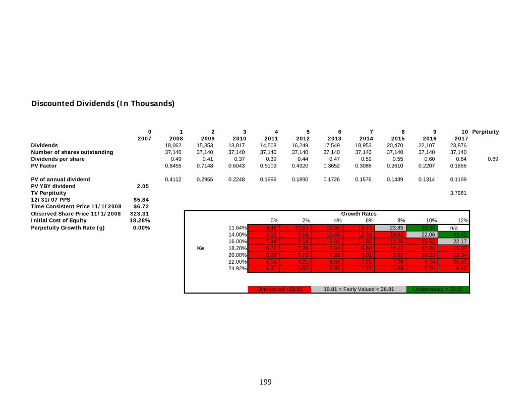
199
Discounted Dividends (In Thousands)
0 1 2 3 4 5 6 7 8 9 10 Perpituity2007 2008 2009 2010 2011 2012 2013 2014 2015 2016 2017
Dividends 18,062 15,353 13,817 14,508 16,249 17,549 18,953 20,470 22,107 23,876Number of shares outstanding 37,140 37,140 37,140 37,140 37,140 37,140 37,140 37,140 37,140 37,140Dividends per share 0.49 0.41 0.37 0.39 0.44 0.47 0.51 0.55 0.60 0.64 0.69PV Factor 0.8455 0.7148 0.6043 0.5109 0.4320 0.3652 0.3088 0.2610 0.2207 0.1866
PV of annual dividend 0.4112 0.2955 0.2248 0.1996 0.1890 0.1726 0.1576 0.1439 0.1314 0.1199PV YBY dividend 2.05TV Perpituity 3.798112/31/07 PPS $5.84Time Consistent Price 11/1/2008 $6.72Observed Share Price 11/1/2008 $23.31Initial Cost of Equity 18.28% 0% 2% 4% 6% 8% 10% 12%Perpetuity Growth Rate (g) 0.00% 11.64% 9.48 10.83 12.90 16.43 23.85 49.34 n/a
14.00% 8.23 9.16 10.45 12.38 15.61 22.06 41.4216.00% 7.44 8.14 9.08 10.38 12.35 15.62 22.17
Ke 18.28% 6.72 7.26 7.94 8.86 10.12 12.00 15.0720.00% 6.28 6.72 7.29 8.01 8.97 10.32 12.3422.00% 5.84 6.21 6.66 7.23 7.96 8.94 10.3124.92% 5.31 5.60 5.95 6.37 6.89 7.56 8.42
Growth Rates
Undervalued > 26.8119.81 < Fairly Valued < 26.81Overvalued <19.81

200
Residual Income Before Restatement (In Thousands)
0 1 2 3 4 5 6 7 8 9 10 Perp2007 2008 2009 2010 2011 2012 2013 2014 2015 2016 2017
Net Income 138,939 118,098 106,288 111,603 124,995 134,995 145,794 157,458 170,054 183,659Total Dividends 18,062 15,353 13,817 14,508 16,249 17,549 18,953 20,470 22,107 23,876Book Value Equity 710,495 831,372 934,117 1,026,588 1,123,683 1,232,428 1,349,874 1,476,715 1,613,703 1,761,650 1,921,434
Annual Normal Income (Benchmark) 129,878 151,975 170,757 187,660 205,409 225,288 246,757 269,943 294,985 322,030Annual Residual Income 9,061 (33,877) (64,468) (76,058) (80,414) (90,293) (100,963) (112,486) (124,930) (138,371) (152,208)PV factor 0.8455 0.7148 0.6043 0.5109 0.4320 0.3652 0.3088 0.2610 0.2207 0.1866YBY PV RI 7,660 (24,215) (38,959) (38,859) (34,736) (32,975) (31,173) (29,363) (27,572) (25,819)RI check (42,937) (30,592) (11,589) (4,357) (9,879) (10,669) (11,523) (12,445) (13,440)Book Value Equity 710,495Total PV of YBY RI (276,011)Continuing (Terminal) Value Perpituity (538,218)PV of Terminal Value Perpetuity (100,426)MVE 12/31/2007 334,058Number of Shares Outstanding 37,140Model Price on 12/31/2008 $8.99 -10% -20% -30% -40% -50%Time consistent Price 11/1/2008 $10.35 11.64% 20.73 21.06 21.24 21.35 21.42
14.00% 15.93 16.62 16.99 17.23 17.39Observed Share Price 11/1/2008 $23.31 16.00% 12.93 13.37 14.18 14.47 14.67Initial Cost of Equity 18.28% Ke 18.28% 10.35 11.16 11.63 11.95 12.17Perpetuity Growth Rate (g) -10.00% 20.00% 8.83 9.61 10.08 10.40 10.62
22.00% 7.42 8.15 8.59 8.90 9.1224.92% 5.87 6.49 6.89 7.17 7.37
Overvalued < 19.81 Undervalued > 26.8119.81 < Fairly Valued < 26.81
Growth Rates

201
Residual Income After Restatement (In Thousands)
0 1 2 3 4 5 6 7 8 9 10 Perp2007 2008 2009 2010 2011 2012 2013 2014 2015 2016 2017
Net Income 138,939 118,098 106,288 111,603 124,995 134,995 145,794 157,458 170,054 183,659Total Dividends 18,062 15,353 13,817 14,508 16,249 17,549 18,953 20,470 22,107 23,876Book Value Equity 585,823 706,700 809,446 901,916 999,011 1,107,757 1,225,202 1,352,043 1,489,031 1,636,979 1,796,762
Annual Normal Income (Benchmark) 107,088 129,185 147,967 164,870 182,619 202,498 223,967 247,153 272,195 299,240Annual Residual Income 31,851 (11,087) (41,678) (53,268) (57,624) (67,503) (78,173) (89,696) (102,140) (115,581) (129,451)PV factor 0.8455 0.7148 0.6043 0.5109 0.4320 0.3652 0.3088 0.2610 0.2207 0.1866YBY PV RI 26,928 (7,925) (25,187) (27,216) (24,891) (24,652) (24,137) (23,414) (22,542) (21,566)
Book Value Equity 585,823Total PV of YBY RI (174,602)Continuing (Terminal) Value Perpetuity (457,746)PV of Terminal Value Perpituity (85,411)MVE 12/31/2007 325,811Number of Shares Outstanding 37,140Model Price on 12/31/2007 $8.77 -10% -20% -30% -40% -50%Time consistent Price 11/1/2008 $10.09 11.64% 20.22 20.33 20.39 20.42 20.45
14.00% 15.54 16.04 16.32 16.49 16.61Observed Share Price 11/1/2008 $23.31 16.00% 12.61 13.26 13.62 13.86 14.02Initial Cost of Equity 18.28% Ke 18.28% 10.09 10.78 11.19 11.45 11.64Perpetuity Growth Rate (g) -10.00% 20.00% 8.61 9.29 9.70 9.97 10.17
22.00% 7.24 7.88 8.27 8.54 8.7324.92% 5.73 6.29 6.65 6.89 7.07
Growth Rates
Overvalued <19.81 19.81 < Fairly Valued < 26.81 Undervalued > 26.81

202
Long Run ROE Residual Income Before Restatement (In Thousands)
2007 2008 2009 2010 2011 2012 2013 2014 2015 2016 2017Beginning Book Value of Equity 710,495 849,434 967,532 1,073,821 1,185,423 1,310,418 1,445,413 1,591,207 1,748,665 1,918,720Earnings 138,939 118,098 106,288 111,603 124,995 134,995 145,794 157,458 170,054 183,659Ending Book Value of Equity 710,495 849,434 967,532 1,073,821 1,185,423 1,310,418 1,445,413 1,591,207 1,748,665 1,918,720 2,102,378
Long Run Return on Equity 0.1956 0.1390 0.1099 0.1039 0.1054 0.1030 0.1009 0.0990 0.0972 0.0957Long Run Growth Rate in Equity 0.1636 0.1221 0.0990 0.0941 0.0954 0.0934 0.0916 0.0900 0.0886 0.0874Cost of Equity 18.28%Average ROE 12% ROE=12%Average Growth 6% 0% 2% 4% 6% 8% 10% 12%Shares Outstanding 37,140 11.64% 21.62 21.75 21.96 22.31 23.04 25.57 n/aEstimated Share price 12/31/2007 $9.35 14.00% 18.29 17.78 17.07 16.00 14.22 10.67 n/aTime Consistent Price 11/1/2008 $10.75 16.00% 16.24 15.46 14.43 12.99 10.82 7.22 n/a
Ke 18.28% 14.44 13.52 12.33 10.75 8.56 5.31 n/aObserved Share Price 11/1/2008 $23.31 20.00% 13.36 12.37 11.13 9.54 7.42 4.45 n/a
22.00% 12.32 11.29 10.03 8.47 6.45 3.76 n/a24.92% 11.09 10.05 8.81 7.30 5.44 3.09 n/a
Growth Rate=6%8% 10% 12% 14% 16% 18% 20%
11.64% 7.44 14.87 22.31 29.74 37.18 44.61 52.0514.00% 5.33 8.66 12.99 17.32 21.65 25.98 30.3116.00% 4.33 7.93 11.89 15.86 19.82 23.79 27.75
Ke 18.28% 3.58 7.17 10.75 14.33 17.92 21.50 25.0820.00% 3.18 6.80 10.21 13.61 17.01 20.41 23.8222.00% 2.82 6.36 9.54 12.73 15.91 19.09 22.2724.92% 2.43 4.87 7.30 9.74 12.17 14.61 17.04
Ke=18.28%0% 2% 4% 6% 8% 10% 12%
8.00% 9.63 8.11 6.16 3.58 n/a n/a n/a10.00% 12.04 10.81 9.24 7.17 4.28 n/a n/a12.00% 14.44 13.52 12.33 10.75 8.56 5.31 n/a
ROE 14.00% 16.85 16.22 15.41 14.33 12.84 10.63 7.0116.00% 19.26 18.92 18.49 17.92 17.12 15.94 14.0118.00% 21.67 21.62 21.57 21.50 21.40 21.26 21.0220.00% 24.07 24.33 24.65 25.08 25.68 26.57 28.03
ROE
Growth Rates
Overvalued <19.81 19.81 < Fairly Valued < 26.81 Undervalued > 26.81
Overvalued <19.81 19.81 < Fairly Valued < 26.81 Undervalued > 26.81
Overvalued <19.81 19.81 < Fairly Valued < 26.81 Undervalued > 26.81
Growth Rates

203
Long Run ROE Residual Income After Restatement (In Thousands)
2007 2008 2009 2010 2011 2012 2013 2014 2015 2016 2017Beginning Book Value of Equity 585,823 724,762 842,860 949,149 1,060,751 1,185,746 1,320,741 1,466,535 1,623,993 1,794,048Earnings 138,939 118,098 106,288 111,603 124,995 134,995 145,794 157,458 170,054 183,659Ending Book Value of Equity 585,823 724,762 842,860 949,149 1,060,751 1,185,746 1,320,741 1,466,535 1,623,993 1,794,048 1,977,706
Long Run Return on Equity 0.2372 0.1629 0.1261 0.1176 0.1178 0.1138 0.1104 0.1074 0.1047 0.1024Long Run Growth Rate in Equity 0.1917 0.1401 0.1120 0.1052 0.1054 0.1022 0.0994 0.0970 0.0948 0.0929Cost of Equity 18.28%Average ROE 20% ROE=13%Average Growth 12% 0% 2% 4% 6% 8% 10% 12%Shares Outstanding 37,140 11.64% 19.31 19.73 20.37 21.47 23.76 31.66 n/aEstimated Share price 12/31/2007 $20.09 14.00% 16.34 16.13 15.84 15.40 14.67 13.21 8.83Time Consistent Price 11/1/2008 $23.11 16.00% 14.51 14.03 13.39 12.50 11.16 8.93 4.43
Ke 18.28% 12.91 12.26 11.44 10.35 8.83 6.58 2.90Observed Share Price 11/1/2008 $23.31 20.00% 11.94 11.22 10.33 9.19 7.66 5.51 2.30
22.00% 11.00 10.24 9.31 8.15 6.65 4.66 1.8724.92% 9.91 9.12 8.17 7.03 5.61 3.82 1.47
Growth Rate=6%8% 10% 12% 14% 16% 18% 20%
11.64% 6.13 12.26 18.39 24.52 30.65 38.79 42.9214.00% 4.40 8.80 13.19 17.59 21.99 26.39 30.7916.00% 3.57 7.14 10.71 14.28 17.85 21.42 24.99
Ke 18.28% 2.95 5.91 8.86 11.82 14.77 17.73 20.6820.00% 2.62 5.25 7.87 10.49 13.12 15.74 18.3622.00% 2.33 4.65 6.98 9.31 11.64 13.96 16.2924.92% 2.01 4.01 6.02 8.03 10.04 12.04 14.05
Ke=18.28%0% 2% 4% 6% 8% 10% 12%
8.00% 7.94 6.69 5.08 2.95 n/a n/a n/a10.00% 9.92 8.91 7.62 5.91 3.53 n/a n/a12.00% 11.91 11.14 10.16 8.86 7.06 4.38 n/a
ROE 14.00% 13.89 13.37 12.70 11.82 10.59 8.76 5.7816.00% 15.88 15.60 15.25 14.77 14.12 13.15 11.5618.00% 17.86 17.83 17.79 17.73 17.65 17.53 17.3320.00% 19.85 20.06 20.33 20.68 21.18 21.91 23.11
Growth Rates
Overvalued <19.81 19.81 < Fairly Valued < 26.81 Undervalued > 26.81
Growth Rates
Overvalued <19.81 19.81 < Fairly Valued < 26.81 Undervalued > 26.81
ROE
Overvalued <19.81 19.81 < Fairly Valued < 26.81 Undervalued > 26.81

204
AEG (In Thousands)
0 1 2 3 4 5 6 7 8 9 Perpituity2007 2008 2009 2010 2011 2012 2013 2014 2015 2016 2017
Net Income 138,939 118,098 106,288 111,603 124,995 134,995 145,794 157,458 170,054 183,659Total Dividends 18,062 15,353 13,817 14,508 16,249 17,549 18,953 20,470 22,107 23,876Dividends Reinvested at 18.28% (Drip) 3,302 2,806 2,526 2,652 2,970 3,208 3,465 3,742 4,041Cum-Dividend Earnings 121,400 109,095 114,129 127,647 137,965 149,002 160,922 173,796 187,700Normal Earnings 164,337 139,687 125,718 132,004 147,844 159,672 172,445 186,241 201,140Abnormal Earning Growth (AEG) (42,937) (30,592) (11,589) (4,357) (9,879) (10,669) (11,523) (12,445) (13,440) (14,516)
PV Factor 0.8455 0.7148 0.6043 0.5109 0.4320 0.3652 0.3088 0.2610 0.2207PV of AEG (36,301) (21,867) (7,004) (2,226) (4,267) (3,896) (3,558) (3,249) (2,966)Residual Income Check Figure (42,937) (30,592) (11,589) (4,357) (9,879) (10,669) (11,523) (12,445) (13,440)
Core Net Income 138,939Total PV of AEG (85,334)Continuing (Terminal) Value (51,328)PV of Terminal Value (11,328)Total PV of AEG (96,662)Total Average Net Income Perp (t+1) 42,277 -10% -20% -30% -40% -50%
11.64% 18.29 18.83 19.11 19.28 19.39Divided by shares to Get Average EPS Perp 1.14 14.00% 12.51 13.13 13.47 13.69 13.83Capitalization Rate (perpetuity) 18.28% 16.00% 9.47 10.05 10.38 10.59 10.73
Ke 18.28% 7.16 7.66 7.96 8.15 8.29Intrinsic Value Per Share 12/31/2007 $6.23 20.00% 5.94 6.38 6.64 6.82 6.94Time consistent implied price 11/1/2008 $7.16 22.00% 4.90 5.26 5.49 5.64 5.75Observed Price 11/1/2008 $23.31 24.92% 3.83 4.11 4.29 4.42 4.51Ke 18.28%Perpituity Growth Rate (g) -10.00%
AEG (42,937) (30,592) (11,589) (4,357) (9,879) (10,669) (11,523) (12,445) (13,440)Residual Income Check Figure (42,937) (30,592) (11,589) (4,357) (9,879) (10,669) (11,523) (12,445) (13,440)Difference 0 0 0 0 0 0 0 0 0
Overvalued <19.81 19.81 < Fairly Valued < 26.81
Growth Rates
Undervalued > 26.81

205
References
Alcoa Website: www.alcoa.com CPA Journal: http://www.nysscpa.org/cpajournal/2008/308/essentials/p32.htm FASB Website: www.fasb.org Investopedia: www.investopedia.com Madeco Website: www.madeco.cl MSN Money Central: http://msn.moneycentral.com Mueller Website: www.muellerindustries.com Sattell, Johnson, Apell Website: www.sattell.com Wall Street Journal: www.wsj.com Wolverine Website: www.wlv.com Yahoo Finance: www.finance.yahoo.com