Multi-class ClassifiersMachine Learning

Hamid Beigy

Sharif University of Technology

Fall 1395

Hamid Beigy (Sharif University of Technology) Multi-class Classifiers Fall 1395 1 / 12

Table of contents

1 Introduction

2 One-against-all classification

3 One-against-one classification

4 C−class discriminant function

5 Error correcting coding classification

Hamid Beigy (Sharif University of Technology) Multi-class Classifiers Fall 1395 2 / 12

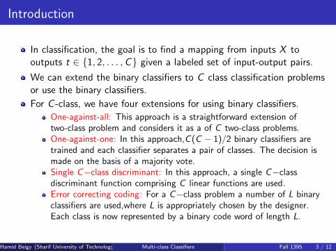
Introduction

In classification, the goal is to find a mapping from inputs X tooutputs t ∈ {1, 2, . . . ,C} given a labeled set of input-output pairs.

We can extend the binary classifiers to C class classification problemsor use the binary classifiers.

For C -class, we have four extensions for using binary classifiers.

One-against-all: This approach is a straightforward extension oftwo-class problem and considers it as a of C two-class problems.One-against-one: In this approach,C (C − 1)/2 binary classifiers aretrained and each classifier separates a pair of classes. The decision ismade on the basis of a majority vote.Single C−class discriminant: In this approach, a single C−classdiscriminant function comprising C linear functions are used.Error correcting coding: For a C−class problem a number of L binaryclassifiers are used,where L is appropriately chosen by the designer.Each class is now represented by a binary code word of length L.

Hamid Beigy (Sharif University of Technology) Multi-class Classifiers Fall 1395 3 / 12

One-against-all classification

The extension is to consider a set of C two-class problems.

For each class, we seek to design an optimal discriminant function,gi (x) (for i = 1, 2, . . . ,C ) so that gi (x) > gj(x), ∀j ̸= i , if x ∈ Ci .

Adopting the SVM methodology, we can design the discriminantfunctions so that gi (x) = 0 to be the optimal hyperplane separatingclass Ci from all the others. Thus, each classifier is designed to givegi (x) > 0 for x ∈ Ci and gi (x) < 0 otherwise.

Classification is then achieved according to the following rule:

Assign x to class Ci if i = argmaxk

gk(x)

Hamid Beigy (Sharif University of Technology) Multi-class Classifiers Fall 1395 4 / 12

Properties of one-against-all classification

The number of classifiers equals to C .Each binary classifier deals with a rather asymmetric problem in thesense that training is carried out with many more negative thanpositive examples. This becomes more serious when the number ofclasses is relatively large.This technique, however,may lead to indeterminate regions, wheremore than one gi (x) is positive

Hamid Beigy (Sharif University of Technology) Multi-class Classifiers Fall 1395 5 / 12

Properties of one-against-all classification

The implementation of OVA is easy.

It is not robust to errors of classifiers. If a classifier make a mistake, itis possible that the entire prediction is errorneous.

Theorem (OVA error bound)

Suppose the average binary error of C binary classifiers is ϵ. Then theerror rate of the OVA multi–class classifier is at most (C − 1)ϵ.

Please prove the above theorem.

Hamid Beigy (Sharif University of Technology) Multi-class Classifiers Fall 1395 6 / 12

One-against-one classification

In this case,C (C − 1)/2 binary classifiers are trained and eachclassifier separates a pair of classes.

The decision is made on the basis of a majority vote.

The obvious disadvantage of the technique is that a relatively largenumber of binary classifiers has to be trained.

Hamid Beigy (Sharif University of Technology) Multi-class Classifiers Fall 1395 7 / 12

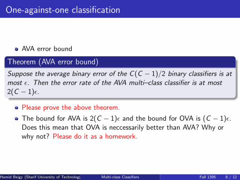
One-against-one classification

AVA error bound

Theorem (AVA error bound)

Suppose the average binary error of the C (C − 1)/2 binary classifiers is atmost ϵ. Then the error rate of the AVA multi–class classifier is at most2(C − 1)ϵ.

Please prove the above theorem.

The bound for AVA is 2(C − 1)ϵ and the bound for OVA is (C − 1)ϵ.Does this mean that OVA is neccessarily better than AVA? Why orwhy not? Please do it as a homework.

Hamid Beigy (Sharif University of Technology) Multi-class Classifiers Fall 1395 8 / 12

C−class discriminant function

We can avoid the difficulties of privous methods by considering asingle C−class discriminant comprising C linear functions of the form

gk(x) = wTk x + wk0

Then assigning a point x to class Ck if gk(x) > gj(x) for all j ̸= k.The decision boundary between class Ck and class Cj is given bygk(x) = gj(x) and corresponds to hyperplane

(wk − wj)T x + (wk0 − wj0) = 0

This has the same form as decision boundary for the two-class case.184 4. LINEAR MODELS FOR CLASSIFICATION

Figure 4.3 Illustration of the decision regions for a mul-ticlass linear discriminant, with the decisionboundaries shown in red. If two points xA

and xB both lie inside the same decision re-gion Rk, then any point bx that lies on the lineconnecting these two points must also lie inRk, and hence the decision region must besingly connected and convex.

Ri

Rj

Rk

xA

xB

x̂

where 0 ! λ ! 1. From the linearity of the discriminant functions, it follows that

yk(!x) = λyk(xA) + (1 − λ)yk(xB). (4.12)

Because both xA and xB lie inside Rk, it follows that yk(xA) > yj(xA), andyk(xB) > yj(xB), for all j ̸= k, and hence yk(!x) > yj(!x), and so !x also liesinside Rk. Thus Rk is singly connected and convex.

Note that for two classes, we can either employ the formalism discussed here,based on two discriminant functions y1(x) and y2(x), or else use the simpler butequivalent formulation described in Section 4.1.1 based on a single discriminantfunction y(x).

We now explore three approaches to learning the parameters of linear discrimi-nant functions, based on least squares, Fisher’s linear discriminant, and the percep-tron algorithm.

4.1.3 Least squares for classificationIn Chapter 3, we considered models that were linear functions of the parame-

ters, and we saw that the minimization of a sum-of-squares error function led to asimple closed-form solution for the parameter values. It is therefore tempting to seeif we can apply the same formalism to classification problems. Consider a generalclassification problem with K classes, with a 1-of-K binary coding scheme for thetarget vector t. One justification for using least squares in such a context is that itapproximates the conditional expectation E[t|x] of the target values given the inputvector. For the binary coding scheme, this conditional expectation is given by thevector of posterior class probabilities. Unfortunately, however, these probabilitiesare typically approximated rather poorly, indeed the approximations can have valuesoutside the range (0, 1), due to the limited flexibility of a linear model as we shallsee shortly.

Each class Ck is described by its own linear model so that

yk(x) = wTk x + wk0 (4.13)

where k = 1, . . . , K. We can conveniently group these together using vector nota-tion so that

y(x) = "WT#x (4.14)

Hamid Beigy (Sharif University of Technology) Multi-class Classifiers Fall 1395 9 / 12

Error correcting coding classification

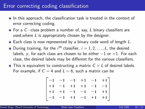
In this approach, the classification task is treated in the context oferror correcting coding.

For a C−class problem a number of, say, L binary classifiers areused,where L is appropriately chosen by the designer.

Each class is now represented by a binary code word of length L.

During training, for the i th classifier, i = 1, 2, . . . , L, the desiredlabels, y , for each class are chosen to be either −1 or +1. For eachclass, the desired labels may be different for the various classifiers.

This is equivalent to constructing a matrix C × L of desired labels.For example, if C = 4 and L = 6, such a matrix can be

Hamid Beigy (Sharif University of Technology) Multi-class Classifiers Fall 1395 10 / 12

Error correcting coding classification (cont.)

For example, if C = 4 and L = 6, such a matrix can be

During training, the first classifier (corresponding to the first columnof the previous matrix) is designed in order to respond(−1,+1,+1,−1) for examples of classes C1,C2,C3,C4, respectively.

The second classifier will be trained to respond (−1,−1,+1,−1), andso on.

The procedure is equivalent to grouping the classes into L differentpairs, and, for each pair, we train a binary classifier accordingly.

Each row must be distinct and corresponds to a class.

Hamid Beigy (Sharif University of Technology) Multi-class Classifiers Fall 1395 11 / 12

Error correcting coding classification (cont.)

When an unknown pattern is presented, the output of each one of thebinary classifiers is recorded, resulting in a code word.

Then,the Hamming distance (number of places where two code wordsdiffer) of this code word is measured against the C code words, andthe pattern is classified to the class corresponding to the smallestdistance.

This feature is the power of this technique. If the code words aredesigned so that the minimum Hamming distance between any pair ofthem is, say, d , then a correct decision will still be reached even if thedecisions of at most ⌊d−1

2 ⌋ out of the L, classifiers are wrong.

Hamid Beigy (Sharif University of Technology) Multi-class Classifiers Fall 1395 12 / 12