Embed Size (px)
Citation preview
Multi Omics Clustering
1ABDBM © Ron Shamir
Outline
• Introduction
• Cluster of Clusters (COCA)
• iCluster
• Nonnegative Matrix Factorization (NMF)
• Similarity Network Fusion (SNF)
• Multiple Kernel Learning (MKL)
ABDBM © Ron Shamir 2
Outline
• Introduction
• Cluster of Clusters (COCA)
• iCluster
• Nonnegative Matrix Factorization (NMF)
• Similarity Network Fusion (SNF)
• Multiple Kernel Learning (MKL)
ABDBM © Ron Shamir 3
Omics
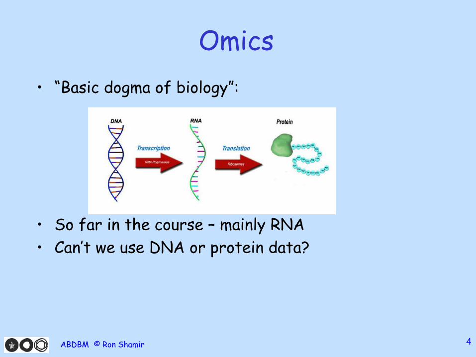
• “Basic dogma of biology”:
• So far in the course – mainly RNA
• Can’t we use DNA or protein data?
ABDBM © Ron Shamir 4
Omics
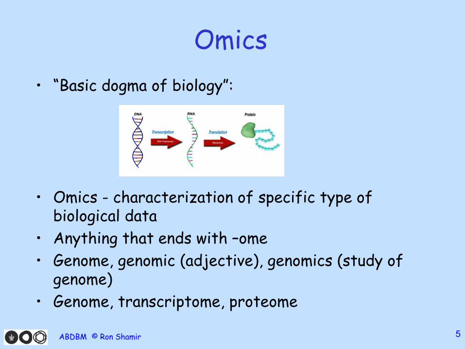
• “Basic dogma of biology”:
• Omics - characterization of specific type of biological data
• Anything that ends with –ome
• Genome, genomic (adjective), genomics (study of genome)
• Genome, transcriptome, proteome
ABDBM © Ron Shamir 5
Additional Omics
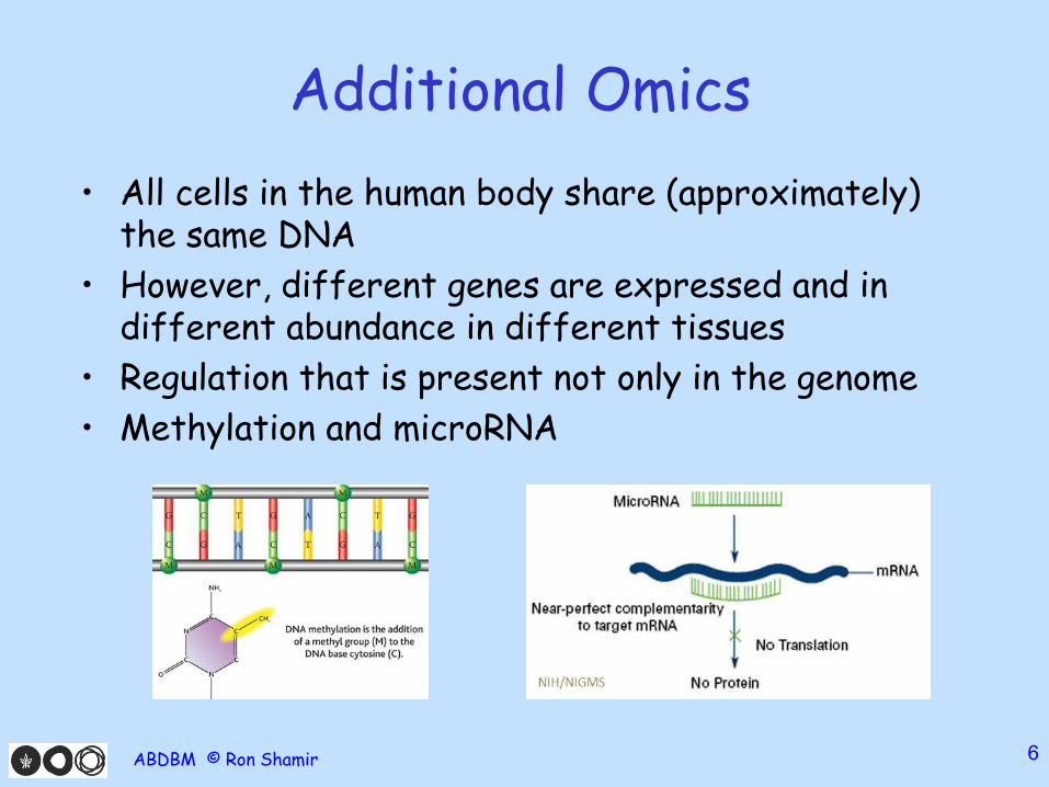
• All cells in the human body share (approximately) the same DNA
• However, different genes are expressed and in different abundance in different tissues
• Regulation that is present not only in the genome
• Methylation and microRNA
ABDBM © Ron Shamir 6
Additional Omics
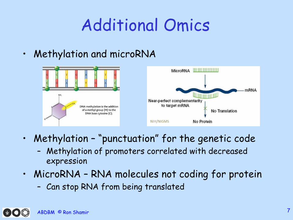
• Methylation and microRNA
• Methylation – “punctuation” for the genetic code– Methylation of promoters correlated with decreased
expression
• MicroRNA – RNA molecules not coding for protein– Can stop RNA from being translated
ABDBM © Ron Shamir 7
Additional Omics
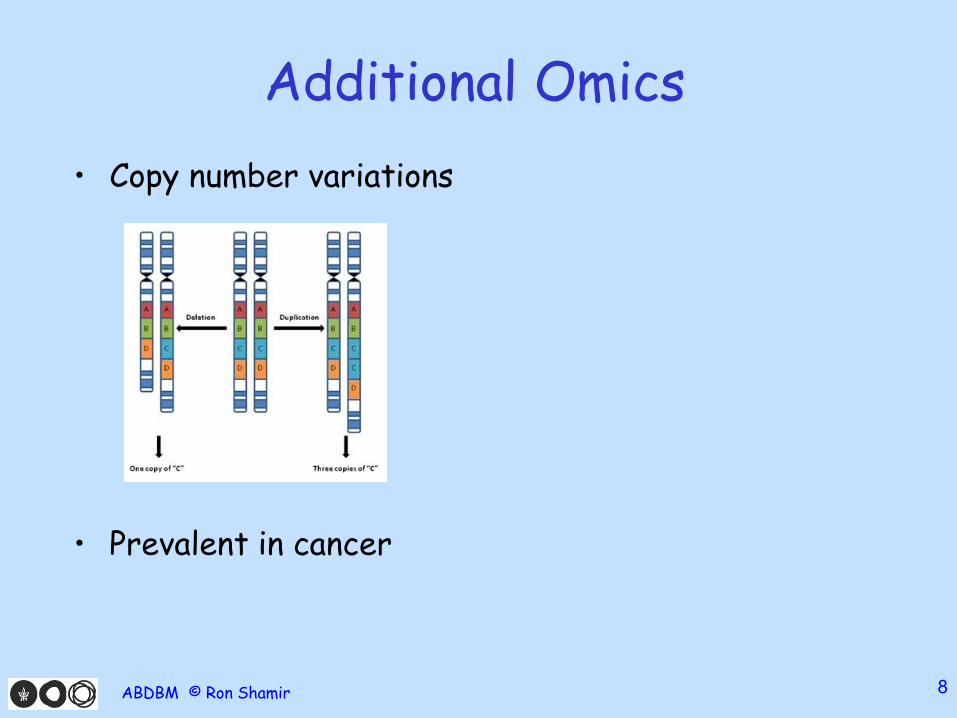
• Copy number variations
• Prevalent in cancer
ABDBM © Ron Shamir 8
Additional Omics
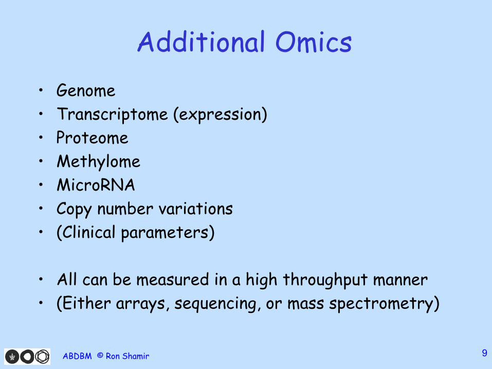
• Genome
• Transcriptome (expression)
• Proteome
• Methylome
• MicroRNA
• Copy number variations
• (Clinical parameters)
• All can be measured in a high throughput manner
• (Either arrays, sequencing, or mass spectrometry)
ABDBM © Ron Shamir 9
Additional Omics
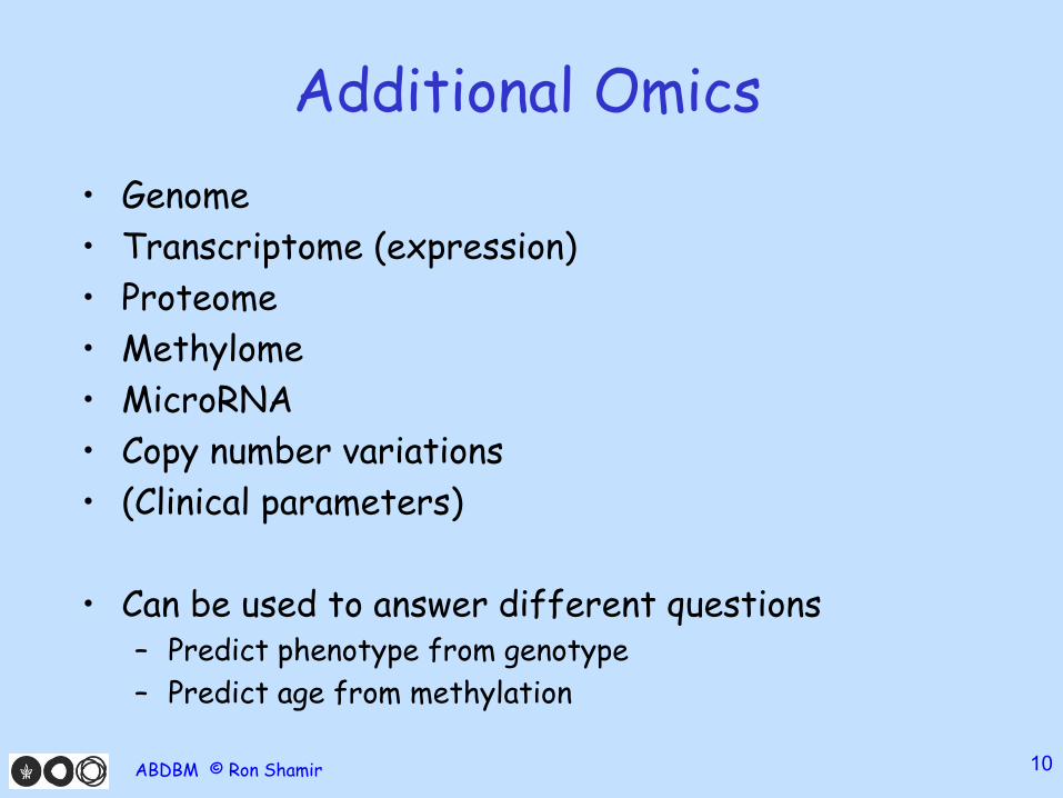
• Genome
• Transcriptome (expression)
• Proteome
• Methylome
• MicroRNA
• Copy number variations
• (Clinical parameters)
• Can be used to answer different questions– Predict phenotype from genotype
– Predict age from methylation
ABDBM © Ron Shamir 10
Multi Omics
• Using several types of omics data
• Multi omics clustering
• Multi omics dimension reduction
• Multi omics predictions
• …
• This talk: multi omics clustering for cancer subtyping
ABDBM © Ron Shamir 11
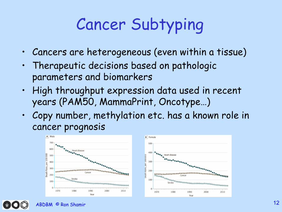
Cancer Subtyping
• Cancers are heterogeneous (even within a tissue)
• Therapeutic decisions based on pathologic parameters and biomarkers
• High throughput expression data used in recent years (PAM50, MammaPrint, Oncotype…)
• Copy number, methylation etc. has a known role in cancer prognosis
ABDBM © Ron Shamir 12
TCGA
• The Cancer Genome Atlas
• Collect and analyze data from cancer patients using high throughput technologies
• Samples from 11000 patients, more than 30 tumor types
• (Hundreds of millions of dollars)
ABDBM © Ron Shamir 13
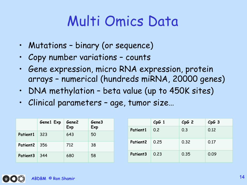
Multi Omics Data
• Mutations – binary (or sequence)
• Copy number variations – counts
• Gene expression, micro RNA expression, protein arrays – numerical (hundreds miRNA, 20000 genes)
• DNA methylation – beta value (up to 450K sites)
• Clinical parameters – age, tumor size…
ABDBM © Ron Shamir 14
Gene3 Exp
Gene2 Exp
Gene1 Exp
50643323Patient1
38712356Patient2
58680344Patient3
CpG 3CpG 2CpG 1
0.120.30.2Patient1
0.170.320.25Patient2
0.090.350.23Patient3
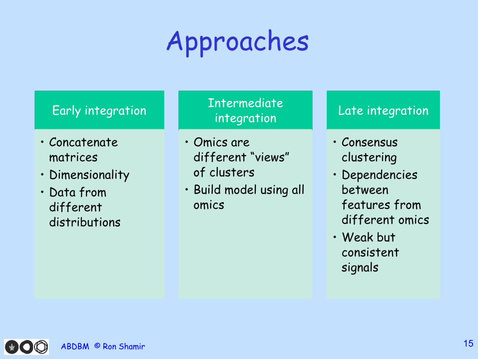
Approaches
ABDBM © Ron Shamir 15
Early integration
• Concatenate matrices
• Dimensionality
• Data from different distributions
Intermediate integration
• Omics are different “views” of clusters
• Build model using all omics
Late integration
• Consensus clustering
• Dependencies between features from different omics
• Weak but consistent signals
Approaches
• Support for any omic data type– General
– Loses knowledge of the biological role
– (Continuous vs. discrete)
• Omic specific methods– For example – expression is increasing in copy number
• Omic specific feature representation– Replace genes with pathways
ABDBM © Ron Shamir 16
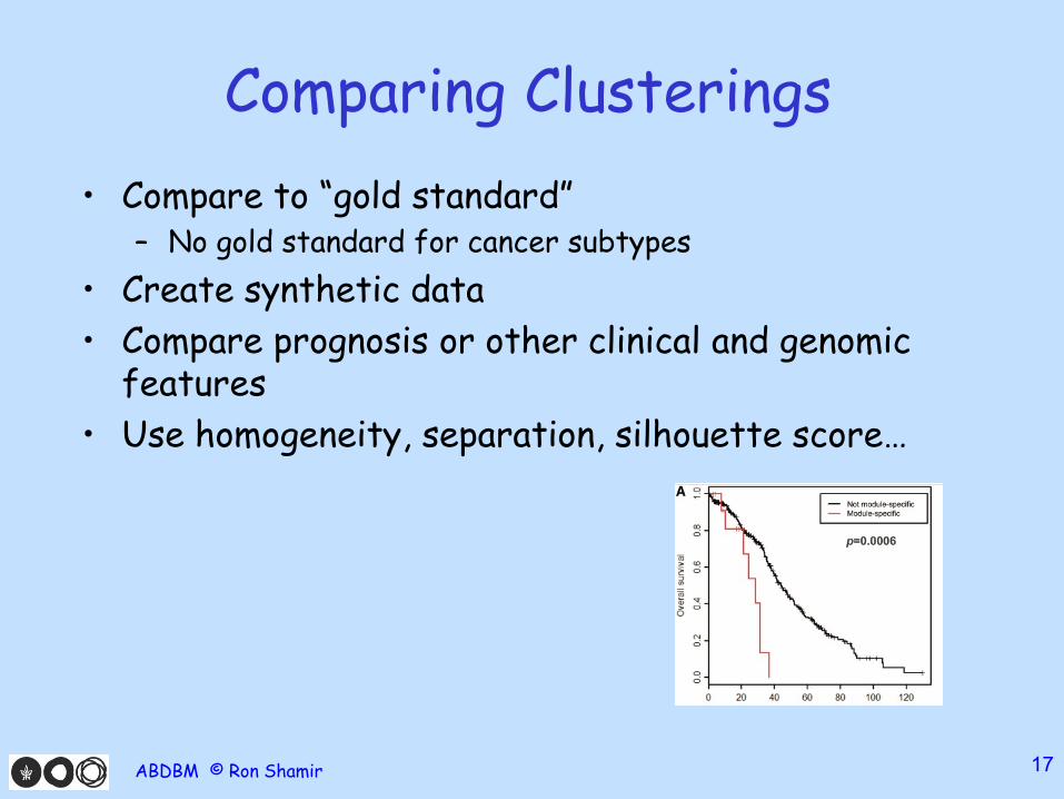
Comparing Clusterings
• Compare to “gold standard”– No gold standard for cancer subtypes
• Create synthetic data
• Compare prognosis or other clinical and genomic features
• Use homogeneity, separation, silhouette score…
ABDBM © Ron Shamir 17
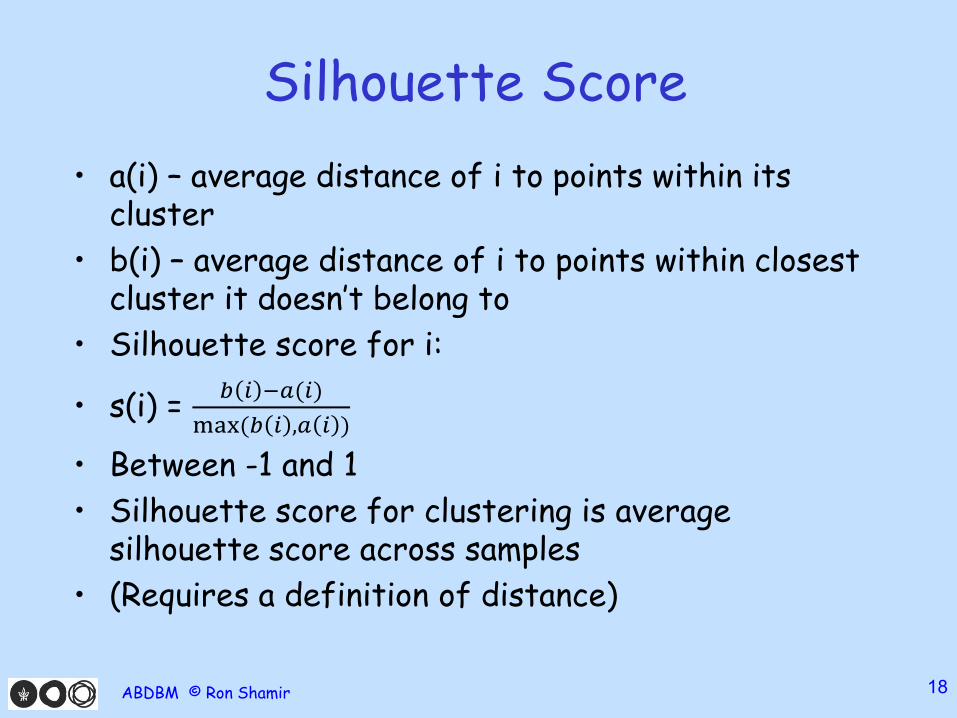
Silhouette Score
• a(i) – average distance of i to points within its cluster
• b(i) – average distance of i to points within closest cluster it doesn’t belong to
• Silhouette score for i:
• s(i) = 𝑏 𝑖 −𝑎(𝑖)
max(𝑏 𝑖 ,𝑎 𝑖 )
• Between -1 and 1
• Silhouette score for clustering is average silhouette score across samples
• (Requires a definition of distance)
ABDBM © Ron Shamir 18
Introduction - Recap
• Omics
• Multi omics and how the datasets look
• Cancer subtyping
• TCGA
• Multi omics clustering approaches
• Comparing clusterings
ABDBM © Ron Shamir 19

Outline
• Introduction
• Cluster of Clusters (COCA)
• iCluster
• Nonnegative Matrix Factorization (NMF)
• Similarity Network Fusion (SNF)
• Multiple Kernel Learning (MKL)
ABDBM © Ron Shamir 20
Cluster of Clusters (COCA)
• Hoadley et. al (Cell, 2014)– (as part of The Cancer Genome Atlas Research Network)
• Late integration method
• Tissue of origin is heavily used for therapeutic decision making
• Cluster TCGA samples from multiple tissues
• What are the clusters? Do they match the tissue of origin?
ABDBM © Ron Shamir 21
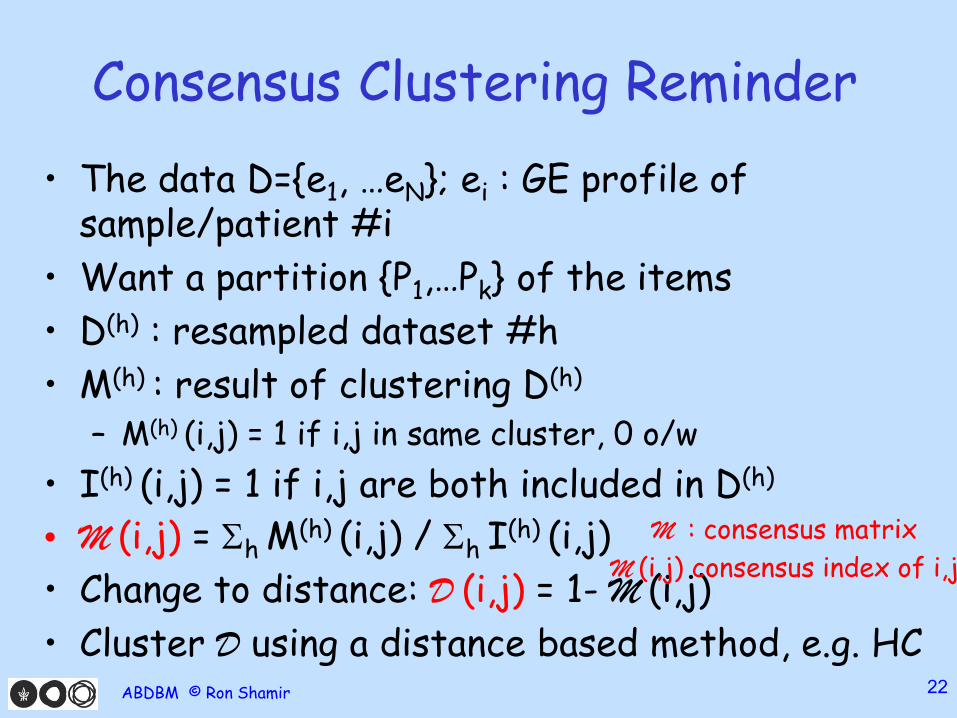
Consensus Clustering Reminder
• The data D={e1, …eN}; ei : GE profile of sample/patient #i
• Want a partition {P1,…Pk} of the items
• D(h) : resampled dataset #h
• M(h) : result of clustering D(h)
– M(h) (i,j) = 1 if i,j in same cluster, 0 o/w
• I(h) (i,j) = 1 if i,j are both included in D(h)
• M (i,j) = h M(h) (i,j) / h I
(h) (i,j)
• Change to distance: D (i,j) = 1- M (i,j)
• Cluster D using a distance based method, e.g. HCABDBM © Ron Shamir 22
M : consensus matrix
M (i,j) consensus index of i,j
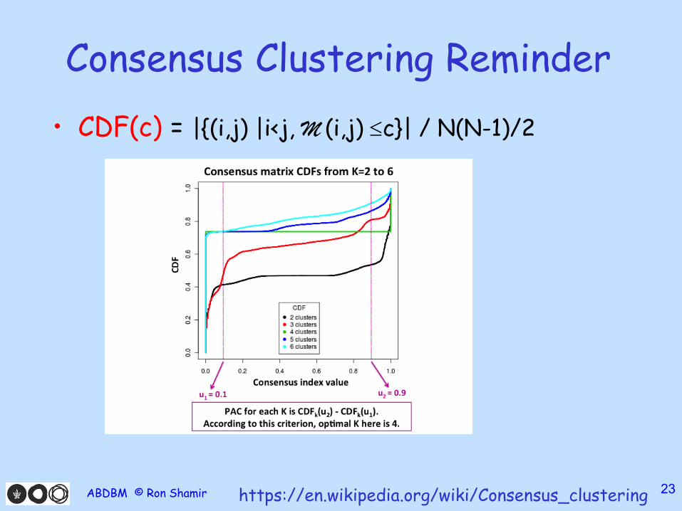
Consensus Clustering Reminder
• CDF(c) = |{(i,j) |i<j, M (i,j) c}| / N(N-1)/2
ABDBM © Ron Shamir 23https://en.wikipedia.org/wiki/Consensus_clustering
COCA
• Cluster each omic separately– Can use any clustering algorithm for each omic
– different omics can use different k
• Represent each sample by an indicator vector of the single omic cluster memberships:– Sample is in cluster 3 out of 5 in omic 1: (0, 0, 1, 0, 0)
– Sample is in cluster 2 out of 3 in omic 2: (0, 1, 0)
– Sample representation: (0, 0, 1, 0, 0, 0, 1, 0)
• Run consensus clustering on the new representation (80% sampling, hierarchical clustering algorithm) for the samples and return its output
ABDBM © Ron Shamir 24
COCA - Results
• Run on all (3527) TCGA samples from 12 cancer tissues
• Use expression, methylation, miRNA, copy number, RPPA (protein arrays)
• Each with different clustering scheme -hierarchical, NMF, consensus clustering…
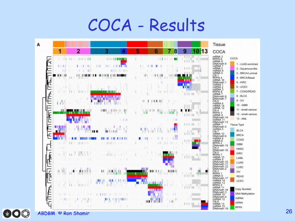
• 11 clusters, 5 nearly identical to tissue of origin
• Lung squamous, head and neck cluster together
• Bladder cancer split into 3 pan-cancer subtypes
ABDBM © Ron Shamir 25
COCA - Results
ABDBM © Ron Shamir 26
COCA - Results
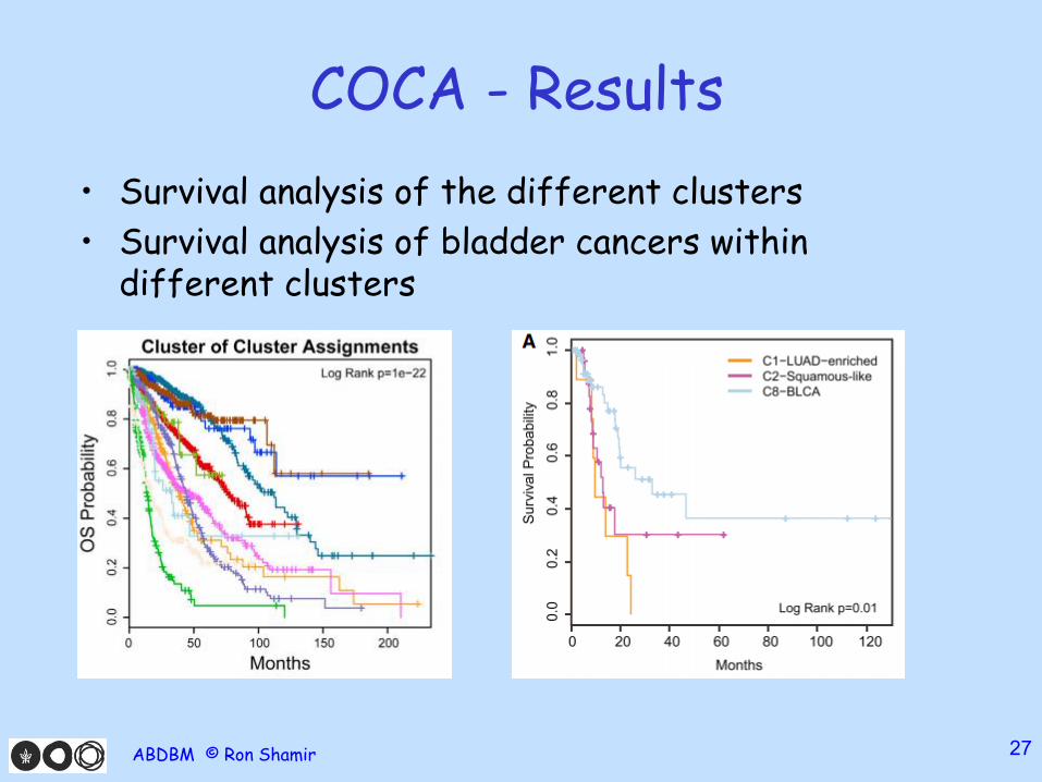
• Survival analysis of the different clusters
• Survival analysis of bladder cancers within different clusters
ABDBM © Ron Shamir 27
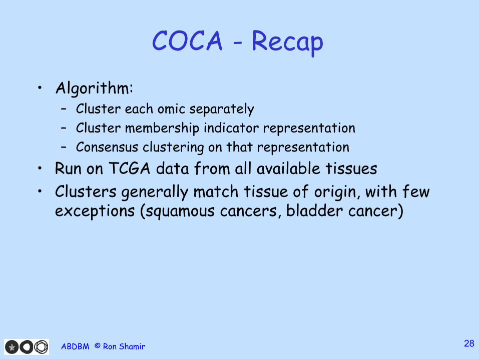
COCA - Recap
• Algorithm:– Cluster each omic separately
– Cluster membership indicator representation
– Consensus clustering on that representation
• Run on TCGA data from all available tissues
• Clusters generally match tissue of origin, with few exceptions (squamous cancers, bladder cancer)
ABDBM © Ron Shamir 28
Outline
• Introduction
• Cluster of Clusters (COCA)
• iCluster
• Nonnegative Matrix Factorization (NMF)
• Similarity Network Fusion (SNF)
• Multiple Kernel Learning (MKL)
ABDBM © Ron Shamir 29
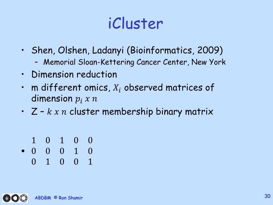
iCluster
• Shen, Olshen, Ladanyi (Bioinformatics, 2009)– Memorial Sloan-Kettering Cancer Center, New York
• Dimension reduction
• m different omics, 𝑋𝑖 observed matrices of dimension 𝑝𝑖 𝑥 𝑛
• Z – 𝑘 𝑥 𝑛 cluster membership binary matrix
•1 0 1 0 00 0 0 1 00 1 0 0 1
ABDBM © Ron Shamir 30
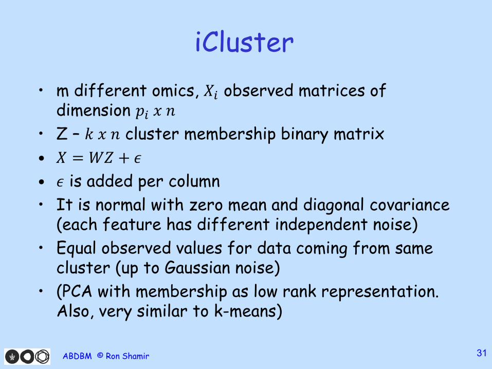
iCluster
• m different omics, 𝑋𝑖 observed matrices of dimension 𝑝𝑖 𝑥 𝑛
• Z – 𝑘 𝑥 𝑛 cluster membership binary matrix
• 𝑋 = 𝑊𝑍 + 𝜖
• 𝜖 is added per column
• It is normal with zero mean and diagonal covariance (each feature has different independent noise)
• Equal observed values for data coming from same cluster (up to Gaussian noise)
• (PCA with membership as low rank representation. Also, very similar to k-means)
ABDBM © Ron Shamir 31
iCluster
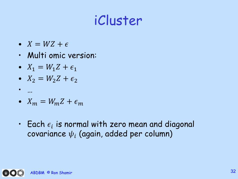
• 𝑋 = 𝑊𝑍 + 𝜖
• Multi omic version:
• 𝑋1 = 𝑊1𝑍 + 𝜖1• 𝑋2 = 𝑊2𝑍 + 𝜖2• …
• 𝑋𝑚 = 𝑊𝑚𝑍 + 𝜖𝑚
• Each 𝜖𝑖 is normal with zero mean and diagonal covariance 𝜓𝑖 (again, added per column)
ABDBM © Ron Shamir 32
Bayesian Statistics
• First, Frequentist statistics
• Tossing a coin n times with probability p to heads
• Can estimate p by maximizing the likelihood: Pr(data | p)
• Why maximize Pr(data | p) and not Pr(p | data)?
• p is not a random variable, it is a number!
ABDBM © Ron Shamir 33
Bayesian Statistics
• In Bayesian statistics, parameters are random variables
• Pr(p) – prior probability for parameter p (e.g. uniform[0,1])
• Natural way to incorporate domain knowledge to the model
• Pr(p | data) = Pr(data | p) * Pr(p) / Pr(data)
• Can maximize Pr(p|data) or take E[p | data]
ABDBM © Ron Shamir 34
iCluster
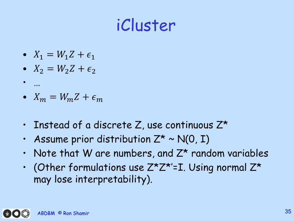
• 𝑋1 = 𝑊1𝑍 + 𝜖1• 𝑋2 = 𝑊2𝑍 + 𝜖2• …
• 𝑋𝑚 = 𝑊𝑚𝑍 + 𝜖𝑚
• Instead of a discrete Z, use continuous Z*
• Assume prior distribution Z* ~ N(0, I)
• Note that W are numbers, and Z* random variables
• (Other formulations use Z*Z*’=I. Using normal Z* may lose interpretability).
ABDBM © Ron Shamir 35
iCluster
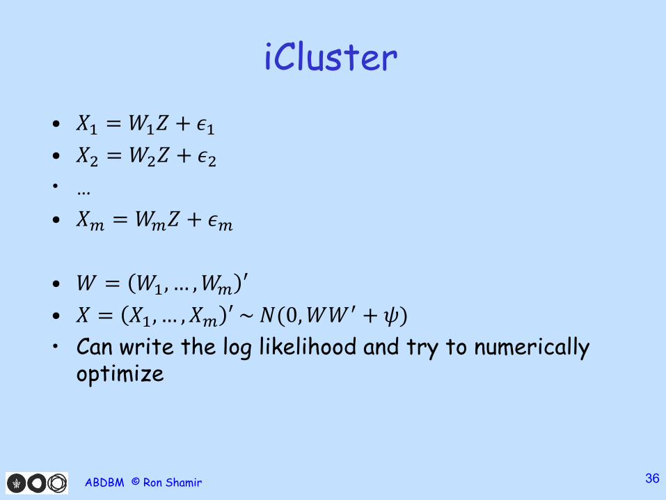
• 𝑋1 = 𝑊1𝑍 + 𝜖1• 𝑋2 = 𝑊2𝑍 + 𝜖2• …
• 𝑋𝑚 = 𝑊𝑚𝑍 + 𝜖𝑚
• 𝑊 = 𝑊1, … ,𝑊𝑚 ′
• 𝑋 = 𝑋1, … , 𝑋𝑚 ′ ~ 𝑁(0,𝑊𝑊′ + 𝜓)
• Can write the log likelihood and try to numerically optimize
ABDBM © Ron Shamir 36
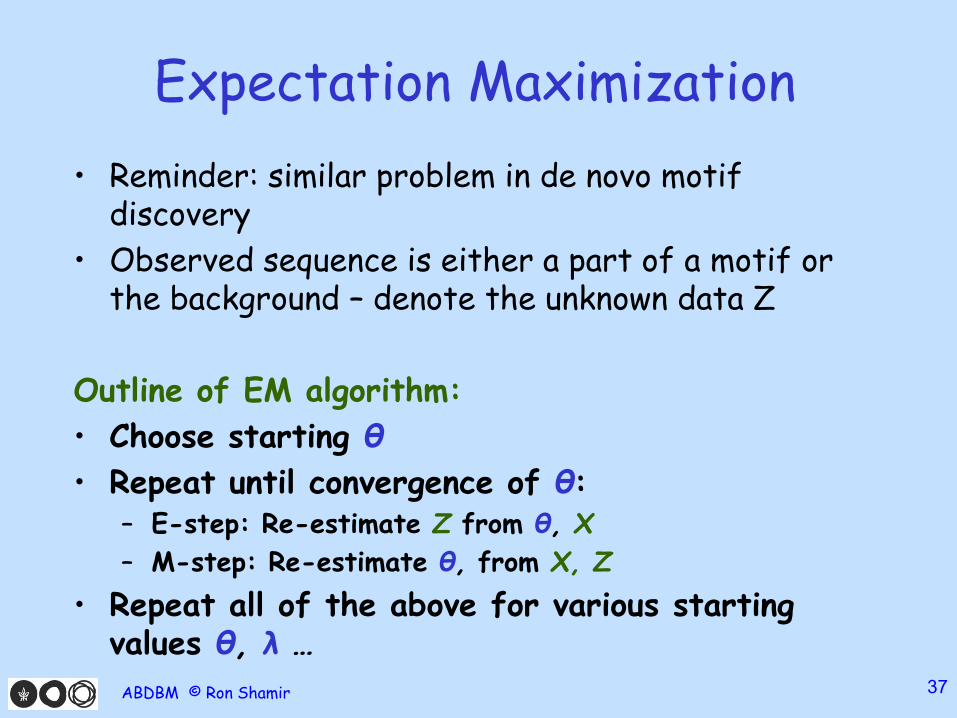
Expectation Maximization
• Reminder: similar problem in de novo motif discovery
• Observed sequence is either a part of a motif or the background – denote the unknown data Z
Outline of EM algorithm:
• Choose starting θ
• Repeat until convergence of θ:– E-step: Re-estimate Z from θ, X
– M-step: Re-estimate θ, from X, Z
• Repeat all of the above for various starting values θ, λ …
ABDBM © Ron Shamir 37
Expectation Maximization
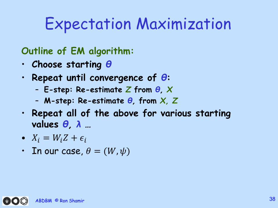
Outline of EM algorithm:
• Choose starting θ
• Repeat until convergence of θ:– E-step: Re-estimate Z from θ, X
– M-step: Re-estimate θ, from X, Z
• Repeat all of the above for various starting values θ, λ …
• 𝑋𝑖 = 𝑊𝑖𝑍 + 𝜖𝑖• In our case, 𝜃 = (𝑊,𝜓)
ABDBM © Ron Shamir 38
EM for iCluster
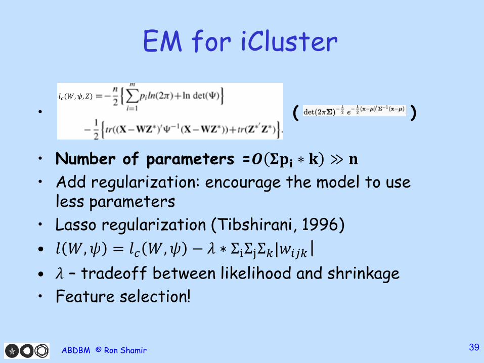
• ( )
• Number of parameters =𝑶 𝚺𝐩𝐢 ∗ 𝐤 ≫ 𝐧
• Add regularization: encourage the model to use less parameters
• Lasso regularization (Tibshirani, 1996)
• 𝑙 𝑊,𝜓 = 𝑙𝑐 𝑊,𝜓 − 𝜆 ∗ ΣiΣjΣ𝑘|𝑤𝑖𝑗𝑘|
• 𝜆 – tradeoff between likelihood and shrinkage
• Feature selection!
ABDBM © Ron Shamir 39
𝑙𝑐(𝑊,𝜓, 𝑍)
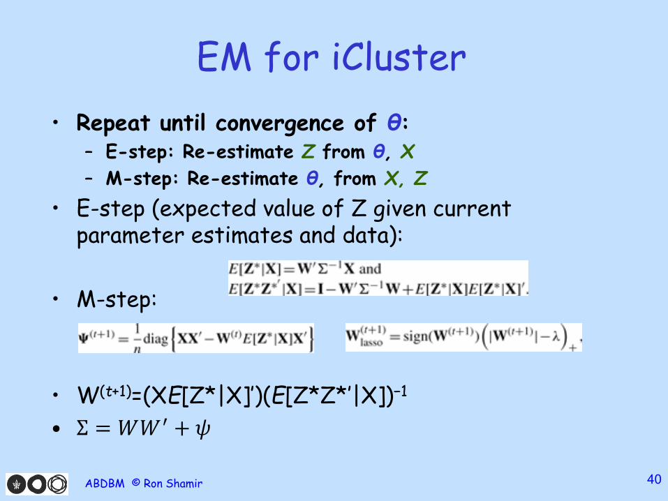
EM for iCluster
• Repeat until convergence of θ:– E-step: Re-estimate Z from θ, X
– M-step: Re-estimate θ, from X, Z
• E-step (expected value of Z given current parameter estimates and data):
• M-step:
• W(t+1)=(XE[Z*|X]′)(E[Z*Z*′|X])−1
• Σ = 𝑊𝑊′ + 𝜓
ABDBM © Ron Shamir 40
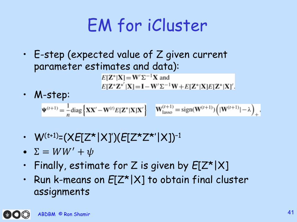
EM for iCluster
• E-step (expected value of Z given current parameter estimates and data):
• M-step:
• W(t+1)=(XE[Z*|X]′)(E[Z*Z*′|X])−1
• Σ = 𝑊𝑊′ + 𝜓
• Finally, estimate for Z is given by E[Z*|X]
• Run k-means on E[Z*|X] to obtain final cluster assignments
ABDBM © Ron Shamir 41
iCluster Model Selection
• How to choose k and 𝜆?
• E[Z*|X]’ E[Z*|X] is n x n matrix
• For cluster matrix Z, ordered by cluster membership, E[Z|X]’ E[Z|X] is a perfect 1-0 block matrix
• Measure distance of absolute values between observed normalized E[Z*|X]’ E[Z*|X], and perfect one
• Measures the posterior probability that two samples belong to the same cluster
• Choose k and 𝜆 that minimize the distance
ABDBM © Ron Shamir 42
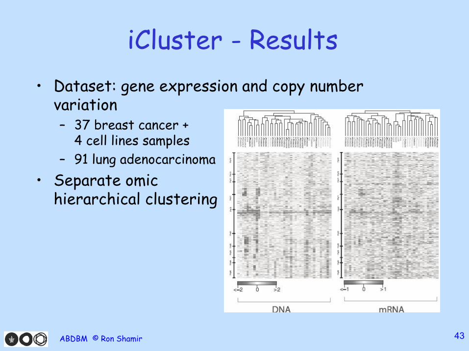
iCluster - Results
• Dataset: gene expression and copy number variation– 37 breast cancer +
4 cell lines samples
– 91 lung adenocarcinoma
• Separate omichierarchical clustering
ABDBM © Ron Shamir 43
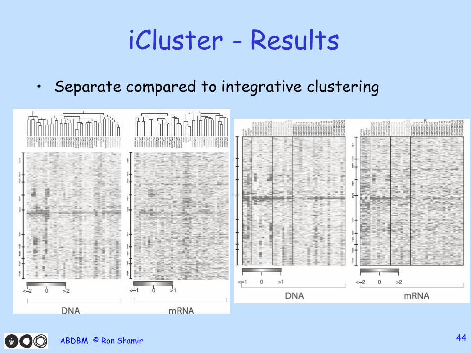
iCluster - Results
• Separate compared to integrative clustering
ABDBM © Ron Shamir 44
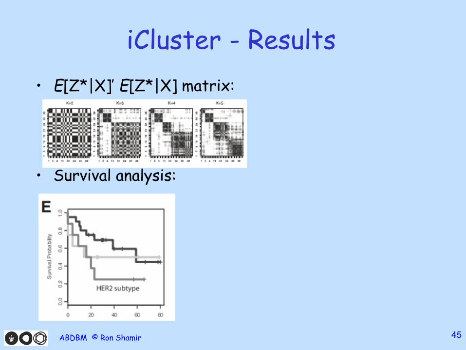
iCluster - Results
• E[Z*|X]’ E[Z*|X] matrix:
• Survival analysis:
ABDBM © Ron Shamir 45
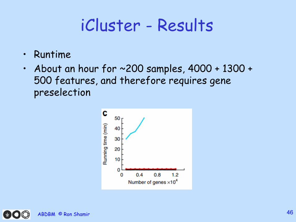
iCluster - Results
• Runtime
• About an hour for ~200 samples, 4000 + 1300 + 500 features, and therefore requires gene preselection
ABDBM © Ron Shamir 46
iCluster - Recap
• Low dimension + probabilistic model
• 𝑋𝑖 = 𝑊𝑖𝑍 + 𝜖𝑖• Z and 𝜖𝑖 have normal distribution
• Find parameters using EM with regularization for a sparse model
• Use deviation from perfect clustering matrix to determine k and 𝜆
• Run on breast and lung adenocarcinoma samples
ABDBM © Ron Shamir 47
Outline
• Introduction
• Cluster of Clusters (COCA)
• iCluster
• Nonnegative Matrix Factorization (NMF)
• Similarity Network Fusion (SNF)
• Multiple Kernel Learning (MKL)
ABDBM © Ron Shamir 48
Joint NMF
• Shihua Zhang, …, Jasmine Zhou (2012, bioinformatics)– University of Southern California, now at UCLA
• NMF = Nonnegative Matrix Factorization
• Dimension reduction –basic idea similar to iCluster
• Model can be used for clustering, but in this work the main goal is to find “md-modules”: (possibly overlapping) sets of features from all omics that define the patients’ molecular profile
ABDBM © Ron Shamir 49
NMF
• NMF = Nonnegative Matrix Factorization
• Given a non negative matrix X, factorize it as 𝑋= 𝑊𝐻 𝑠. 𝑡 𝑊,𝐻 ≥ 0,
• 𝑥.𝑗 = Σ𝑘𝑤.𝑘ℎ𝑘𝑗 = 𝑊ℎ.𝑗
• Higher interpretability, makes sense where data is comprised of several parts
• Minimize 𝑋 −𝑊𝐻𝐹
2( 𝐴
𝐹= Σ𝑖Σ𝑗𝑎𝑖𝑗
2 )
• Often optimized using multiplicative update rule:
• 𝐻𝑎𝑏 = 𝐻𝑎𝑏𝑊𝑇𝑋
𝑎𝑏
𝑊𝑇𝑊𝐻 𝑎𝑏,𝑊𝑎𝑏 = 𝑊𝑎𝑏
𝑋𝐻𝑇𝑎𝑏
𝑋𝐻𝐻𝑇𝑎𝑏
ABDBM © Ron Shamir 50

NMF – Proof Sketch
• Lee and Seung, NIPS 2000
• Minimize 𝑋 −𝑊𝐻𝐹
2
• Will show proof sketch for H update rule
• Minimize F h = 𝑥 −𝑊ℎ𝐹
2
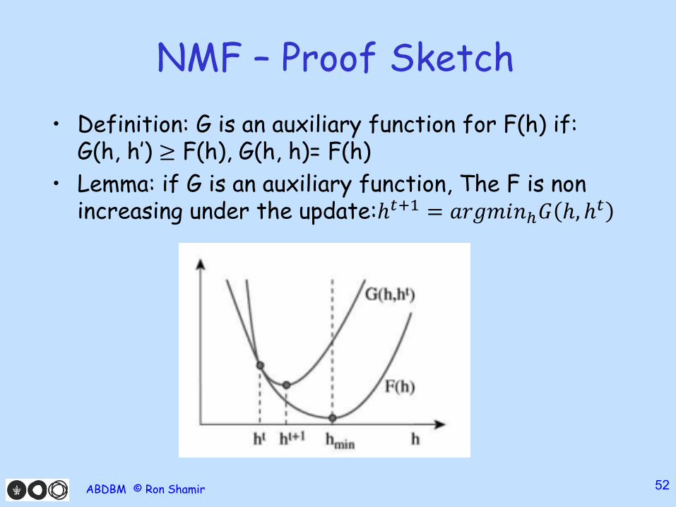
• Definition: G is an auxiliary function for F(h) if:G(h, h’) ≥ F(h), G(h, h)= F(h)
• Lemma: if G is an auxiliary function, then F is non increasing under the update:ℎ𝑡+1 = 𝑎𝑟𝑔𝑚𝑖𝑛ℎ𝐺 ℎ, ℎ𝑡
• Proof: 𝐹 ℎ𝑡+1 ≤ 𝐺 ℎ𝑡+1, ℎ𝑡 ≤ 𝐺 ℎ𝑡 , ℎ𝑡 = 𝐹(ℎ𝑡)
ABDBM © Ron Shamir 51
NMF – Proof Sketch
• Definition: G is an auxiliary function for F(h) if:G(h, h’) ≥ F(h), G(h, h)= F(h)
• Lemma: if G is an auxiliary function, The F is non increasing under the update:ℎ𝑡+1 = 𝑎𝑟𝑔𝑚𝑖𝑛ℎ𝐺 ℎ, ℎ𝑡
ABDBM © Ron Shamir 52
NMF – Proof Sketch
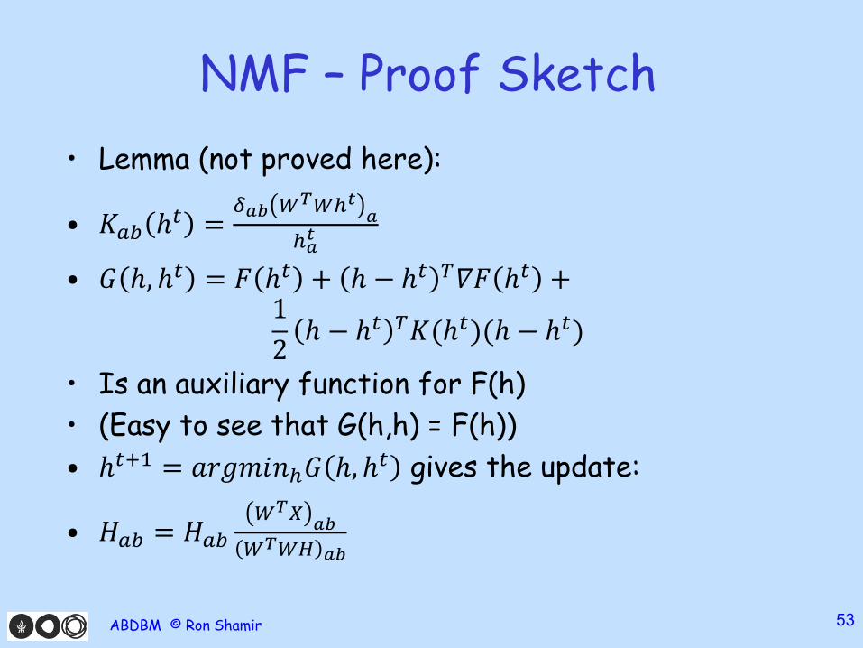
• Lemma (not proved here):
• 𝐾𝑎𝑏 ℎ𝑡 =𝛿𝑎𝑏 𝑊𝑇𝑊ℎ𝑡
𝑎
ℎ𝑎𝑡
• 𝐺 ℎ, ℎ𝑡 = 𝐹 ℎ𝑡 + ℎ − ℎ𝑡 𝑇𝛻𝐹 ℎ𝑡 +1
2ℎ − ℎ𝑡 𝑇𝐾(ℎ𝑡)(ℎ − ℎ𝑡)
• Is an auxiliary function for F(h)
• (Easy to see that G(h,h) = F(h))
• ℎ𝑡+1 = 𝑎𝑟𝑔𝑚𝑖𝑛ℎ𝐺 ℎ, ℎ𝑡 gives the update:
• 𝐻𝑎𝑏 = 𝐻𝑎𝑏𝑊𝑇𝑋
𝑎𝑏
𝑊𝑇𝑊𝐻 𝑎𝑏
ABDBM © Ron Shamir 53
NMF
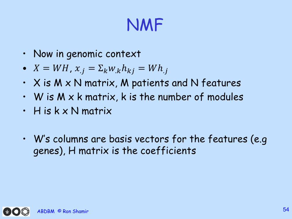
• Now in genomic context
• 𝑋 = 𝑊𝐻, 𝑥.𝑗 = Σ𝑘𝑤.𝑘ℎ𝑘𝑗 = 𝑊ℎ.𝑗
• X is M x N matrix, M patients and N features
• W is M x k matrix, k is the number of modules
• H is k x N matrix
• W’s columns are basis vectors for the features (e.ggenes), H matrix is the coefficients
ABDBM © Ron Shamir 54
Joint NMF
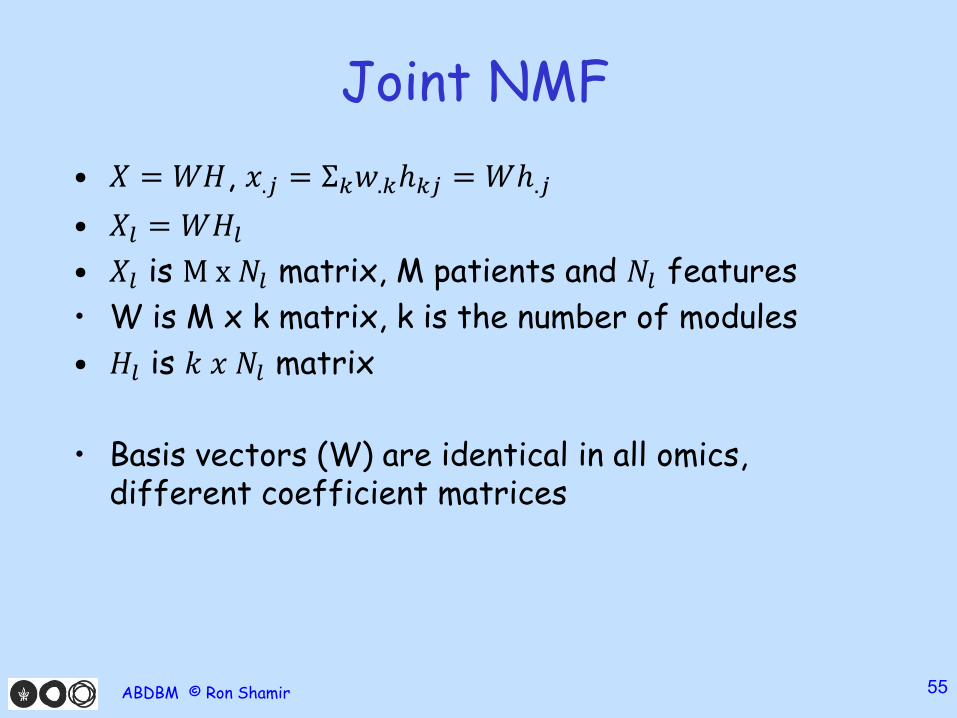
• 𝑋 = 𝑊𝐻, 𝑥.𝑗 = Σ𝑘𝑤.𝑘ℎ𝑘𝑗 = 𝑊ℎ.𝑗
• 𝑋𝑙 = 𝑊𝐻𝑙• 𝑋𝑙 is M x 𝑁𝑙 matrix, M patients and 𝑁𝑙 features
• W is M x k matrix, k is the number of modules
• 𝐻𝑙 is 𝑘 𝑥 𝑁𝑙 matrix
• Basis vectors (W) are identical in all omics, different coefficient matrices
ABDBM © Ron Shamir 55
Joint NMF
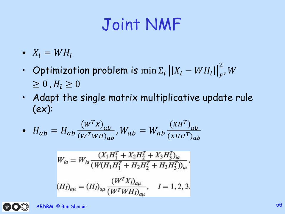
• 𝑋𝑙 = 𝑊𝐻𝑙
• Optimization problem is min Σ𝑙 𝑋𝑙 −𝑊𝐻𝑙 𝐹
2,𝑊
≥ 0 ,𝐻𝑙 ≥ 0
• Adapt the single matrix multiplicative update rule (ex):
• 𝐻𝑎𝑏 = 𝐻𝑎𝑏𝑊𝑇𝑋
𝑎𝑏
𝑊𝑇𝑊𝐻 𝑎𝑏,𝑊𝑎𝑏 = 𝑊𝑎𝑏
𝑋𝐻𝑇𝑎𝑏
𝑋𝐻𝐻𝑇𝑎𝑏
ABDBM © Ron Shamir 56
Joint NMF
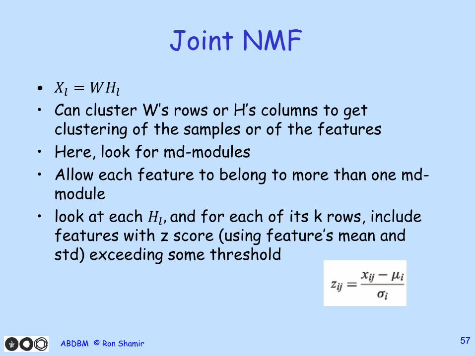
• 𝑋𝑙 = 𝑊𝐻𝑙• Can cluster W’s rows or H’s columns to get
clustering of the samples or of the features
• Here, look for md-modules
• Allow each feature to belong to more than one md-module
• look at each 𝐻𝑙 , and for each of its k rows, include features with z score (using feature’s mean and std) exceeding some threshold
ABDBM © Ron Shamir 57
Joint NMF
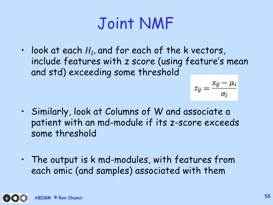
• look at each 𝐻𝑙 , and for each of the k vectors, include features with z score (using feature’s mean and std) exceeding some threshold
• Similarly, look at Columns of W and associate a patient with an md-module if its z-score exceeds some threshold
• The output is k md-modules, with features from each omic (and samples) associated with them
ABDBM © Ron Shamir 58
Joint NMF - Results
• Use ovarian cancer data from TCGA
• 385 samples
• 3 omics: gene expression, methylation and miRNA expression
• Negative values – double all features, one with positive and one with absolute value of negative
• K = 200 md-modules
• Cover ~3000 genes, ~2000 methylation sites, 270 miRNAs
• Average module sizes are ~240 genes, ~162 methylation sites and ~14 miRNAs (high overlap)
ABDBM © Ron Shamir 59
Joint NMF - Results
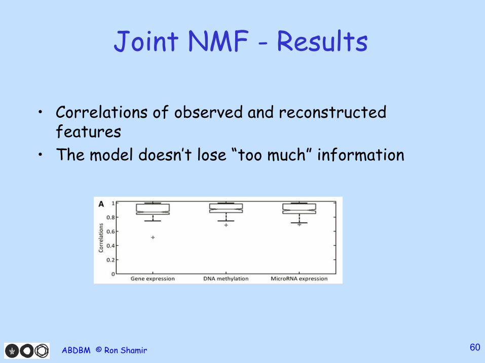
• Correlations of observed and reconstructed features
• The model doesn’t lose “too much” information
ABDBM © Ron Shamir 60
Joint NMF - Results
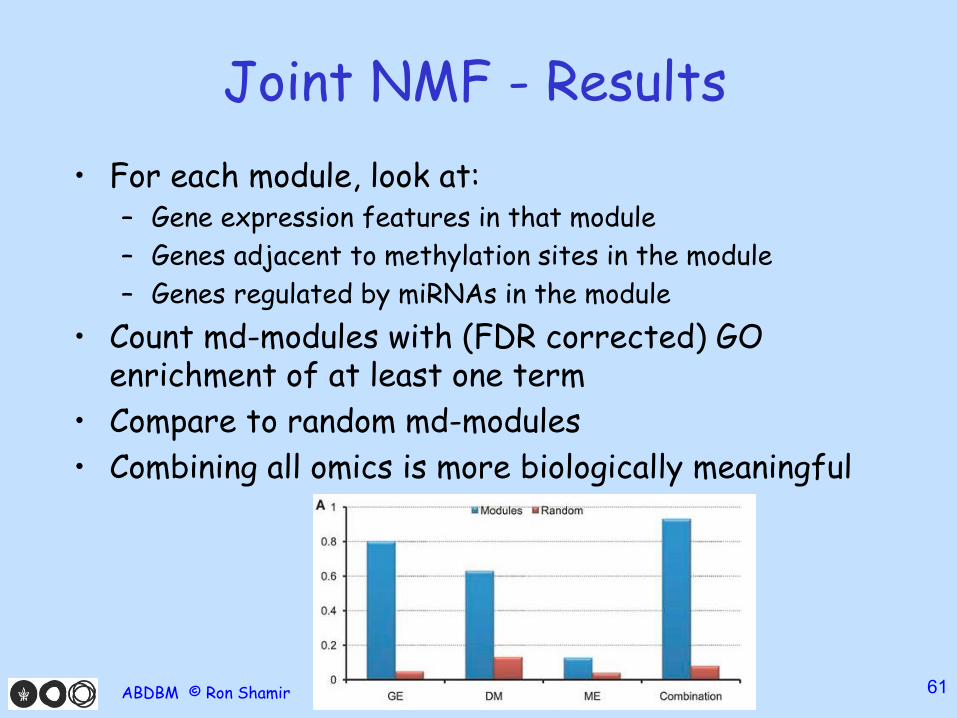
• For each module, look at:– Gene expression features in that module
– Genes adjacent to methylation sites in the module
– Genes regulated by miRNAs in the module
• Count md-modules with (FDR corrected) GO enrichment of at least one term
• Compare to random md-modules
• Combining all omics is more biologically meaningful
ABDBM © Ron Shamir 61
Joint NMF - Results
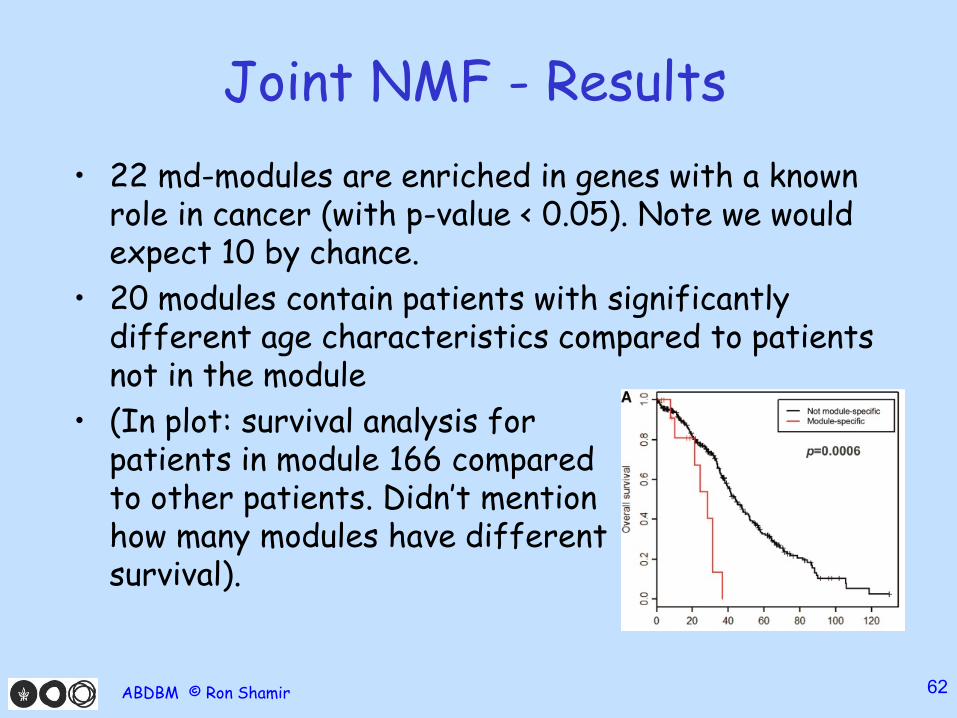
• 22 md-modules are enriched in genes with a known role in cancer (with p-value < 0.05). Note we would expect 10 by chance.
• 20 modules contain patients with significantly different age characteristics compared to patients not in the module
• (In plot: survival analysis for patients in module 166 compared to other patients. Didn’t mentionhow many modules have differentsurvival).
ABDBM © Ron Shamir 62
Joint NMF - Recap
• Low dimension + non negativity constraint
• 𝑋𝑙 = 𝑊𝐻𝑙• Optimized using multiplicative update rules
• Look for md-modules: sets of features from all omics that largely determine the observed data
• Md-modules calculated from the factorization with z-score
• Run on TCGA ovarian cancer data
• Looking at all omics gives higher enrichment in md-modules compared to each omic alone
ABDBM © Ron Shamir 63
Outline
• Introduction
• Cluster of Clusters (COCA)
• iCluster
• Nonnegative Matrix Factorization (NMF)
• Similarity Network Fusion (SNF)
• Multiple Kernel Learning (MKL)
ABDBM © Ron Shamir 64
Similarity Network Fusion
• Bo Wang, …, Anna Goldenberg (Nature Methods, 2014)– University of Toronto
• Number of features >> number of samples
• Dimension reduction methods’ complexity depends on the number of features
• Formulations with non-convex / no closed form solution objective functions, so have to try many different initialization points
ABDBM © Ron Shamir 65
Similarity Network Fusion
• Idea: cluster based only on patients’ similarity
• Aside from similarity computation, complexity is a function of the number of patients
• Less sensitivity to feature selection in practice
• More difficult to give interpretation to features as part of the model
• (Can still do analysis once we have the clusters, e.g. differentially expressed genes)
ABDBM © Ron Shamir 66
Similarity Network Fusion
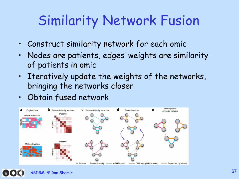
• Construct similarity network for each omic
• Nodes are patients, edges’ weights are similarity of patients in omic
• Iteratively update the weights of the networks, bringing the networks closer
• Obtain fused network
ABDBM © Ron Shamir 67
Similarity Network Fusion
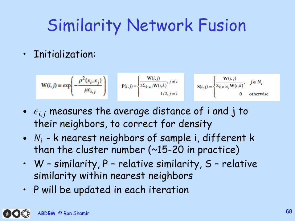
• Initialization:
• 𝜖𝑖,𝑗 measures the average distance of i and j to their neighbors, to correct for density
• 𝑁𝑖 - k nearest neighbors of sample i, different k than the cluster number (~15-20 in practice)
• W – similarity, P – relative similarity, S – relative similarity within nearest neighbors
• P will be updated in each iteration
ABDBM © Ron Shamir 68

Similarity Network Fusion
• W – similarity, P – relative similarity, S – relative similarity within nearest neighbors
• (Assume for now we have two omics)
• P is updated in each iteration:
ABDBM © Ron Shamir 69
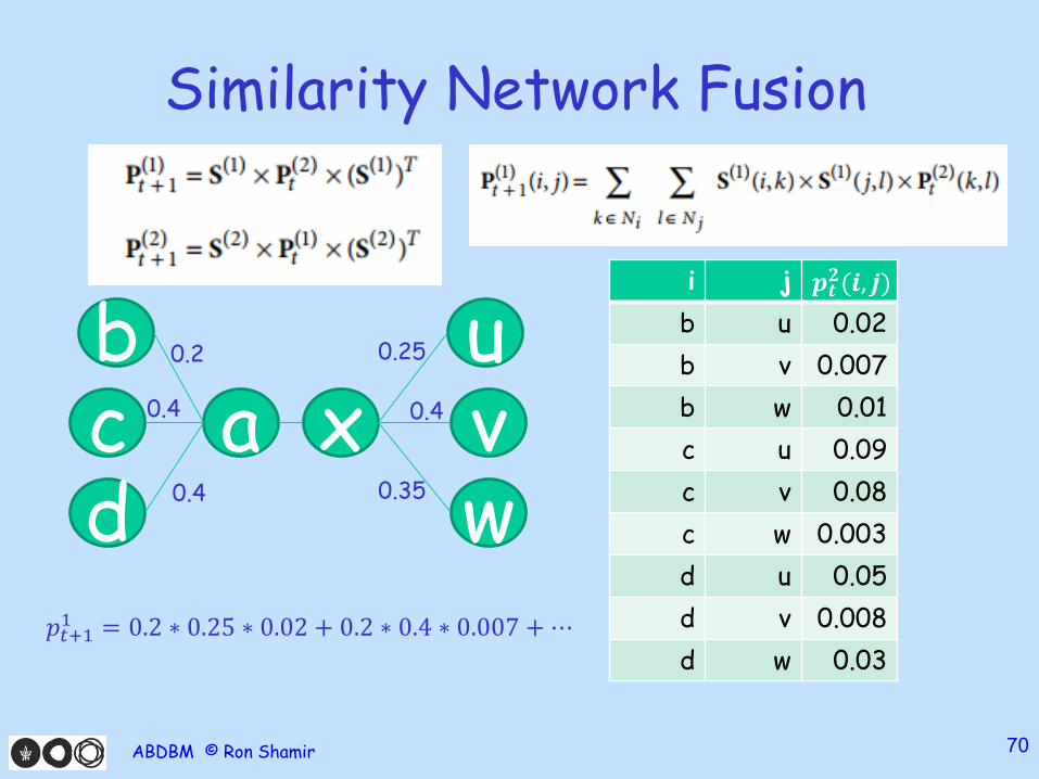
Similarity Network Fusion
ABDBM © Ron Shamir 70
a xdcb
wvu
𝒑𝒕𝟐(𝒊, 𝒋)ji
0.02ub
0.007vb
0.01wb
0.09uc
0.08vc
0.003wc
0.05ud
0.008vd
0.03wd
0.2
0.4
0.4
0.25
0.4
0.35
𝑝𝑡+11 = 0.2 ∗ 0.25 ∗ 0.02 + 0.2 ∗ 0.4 ∗ 0.007 + ⋯
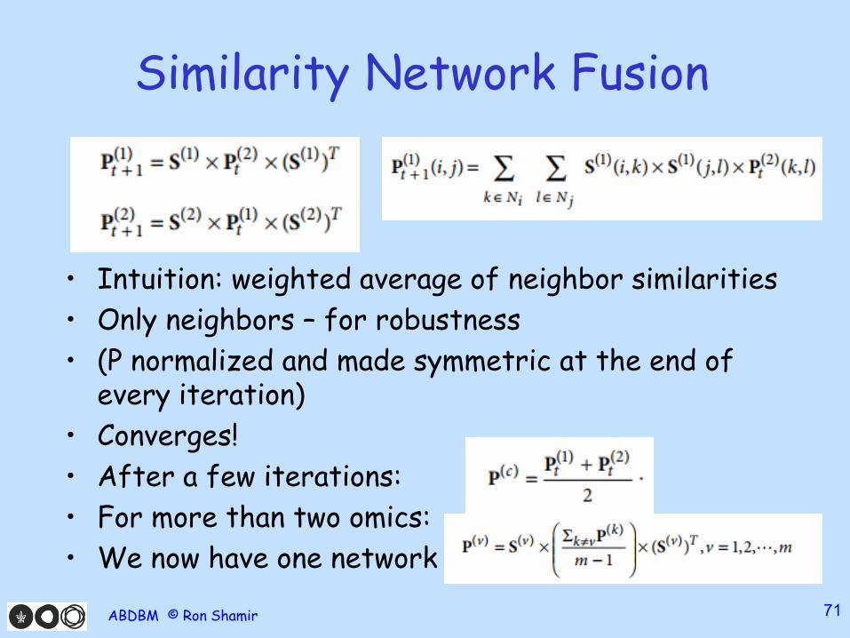
Similarity Network Fusion
• Intuition: weighted average of neighbor similarities
• Only neighbors – for robustness
• (P normalized and made symmetric at the end of every iteration)
• Converges!
• After a few iterations:
• For more than two omics:
• We now have one network
ABDBM © Ron Shamir 71
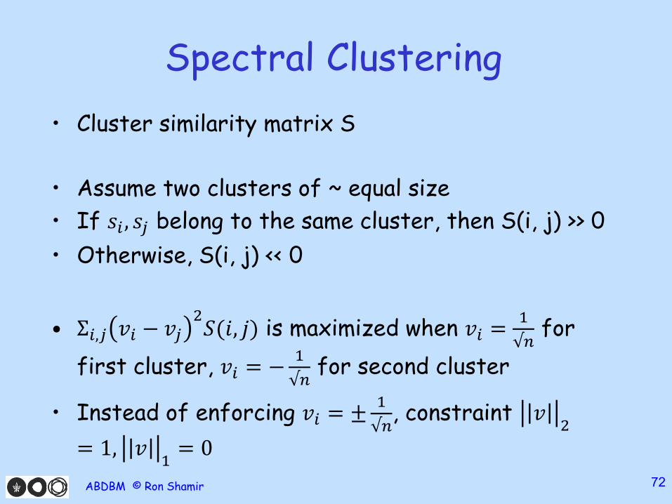
Spectral Clustering
• Cluster similarity matrix S
• Assume two clusters of ~ equal size
• If 𝑠𝑖 , 𝑠𝑗 belong to the same cluster, then S(i, j) >> 0
• Otherwise, S(i, j) << 0
• Σ𝑖,𝑗 𝑣𝑖 − 𝑣𝑗2𝑆(𝑖, 𝑗) is maximized when 𝑣𝑖 =
1
√𝑛for
first cluster, 𝑣𝑖 = −1
√𝑛for second cluster
• Instead of enforcing 𝑣𝑖 = ±1
√𝑛, constraint 𝑣
2
= 1, 𝑣1= 0
ABDBM © Ron Shamir 72
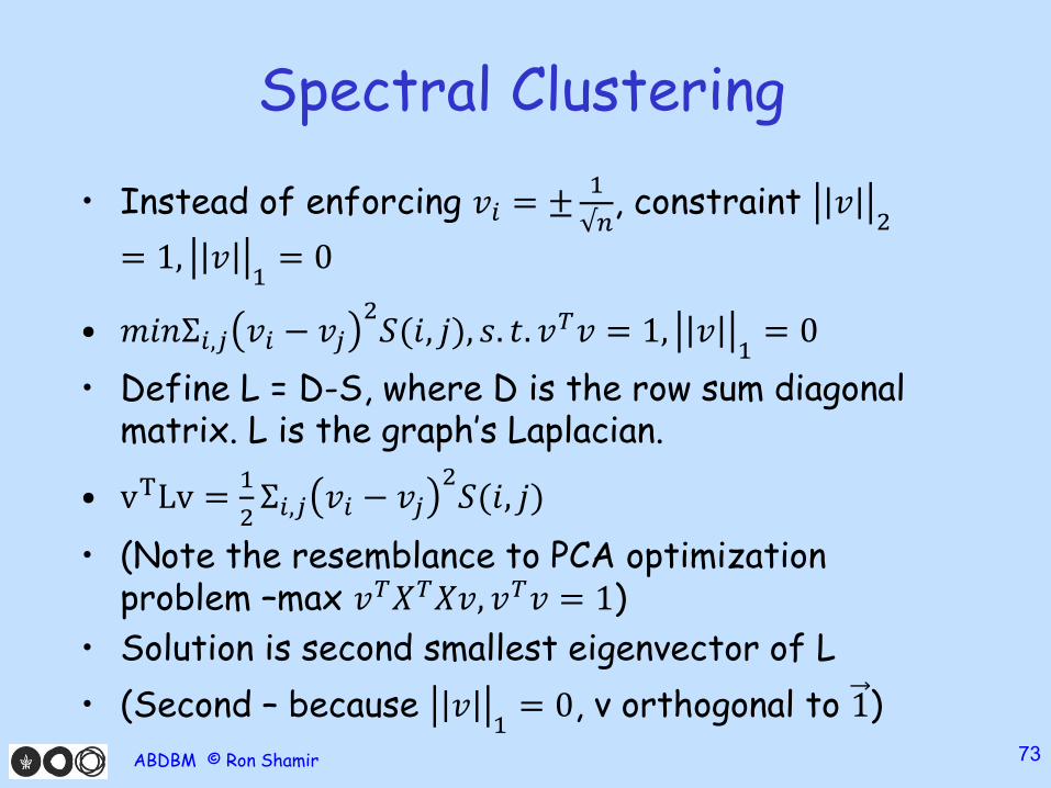
Spectral Clustering
• Instead of enforcing 𝑣𝑖 = ±1
√𝑛, constraint 𝑣
2
= 1, 𝑣1= 0
• 𝑚𝑖𝑛Σ𝑖,𝑗 𝑣𝑖 − 𝑣𝑗2𝑆(𝑖, 𝑗), 𝑠. 𝑡. 𝑣𝑇𝑣 = 1, 𝑣
1= 0
• Define L = D-S, where D is the row sum diagonal matrix. L is the graph’s Laplacian.
• vTLv =1
2Σ𝑖,𝑗 𝑣𝑖 − 𝑣𝑗
2𝑆(𝑖, 𝑗)
• (Note the resemblance to PCA optimization problem –max 𝑣𝑇𝑋𝑇𝑋𝑣, 𝑣𝑇𝑣 = 1)
• Solution is second smallest eigenvector of L
• (Second – because 𝑣1= 0, v orthogonal to 1)
ABDBM © Ron Shamir 73
Spectral Clustering
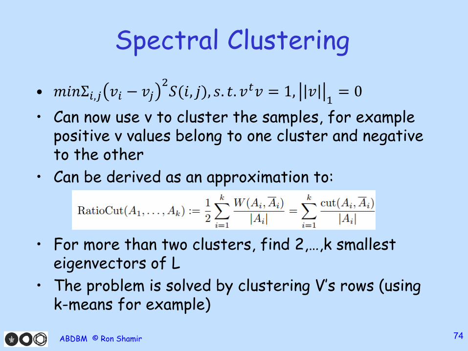
• 𝑚𝑖𝑛Σ𝑖,𝑗 𝑣𝑖 − 𝑣𝑗2𝑆(𝑖, 𝑗), 𝑠. 𝑡. 𝑣𝑡𝑣 = 1, 𝑣
1= 0
• Can now use v to cluster the samples, for example positive v values belong to one cluster and negative to the other
• Can be derived as an approximation to:
• For more than two clusters, find 2,…,k smallest eigenvectors of L
• The problem is solved by clustering V’s rows (using k-means for example)
ABDBM © Ron Shamir 74
Similarity Network Fusion
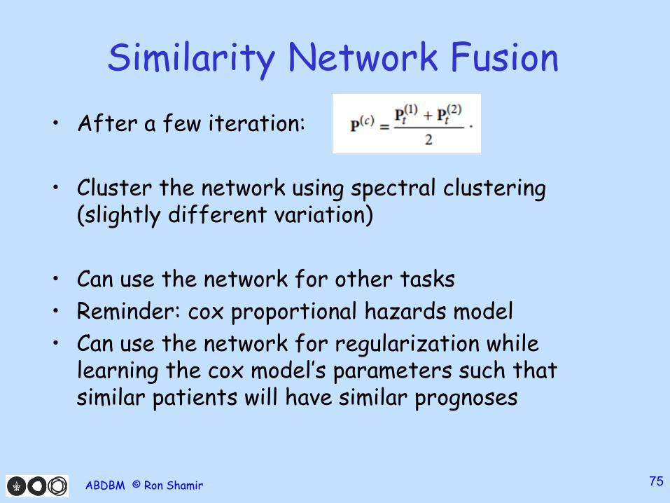
• After a few iteration:
• Cluster the network using spectral clustering (slightly different variation)
• Can use the network for other tasks
• Reminder: cox proportional hazards model
• Can use the network for regularization while learning the cox model’s parameters such that similar patients will have similar prognoses
ABDBM © Ron Shamir 75
SNF - Results
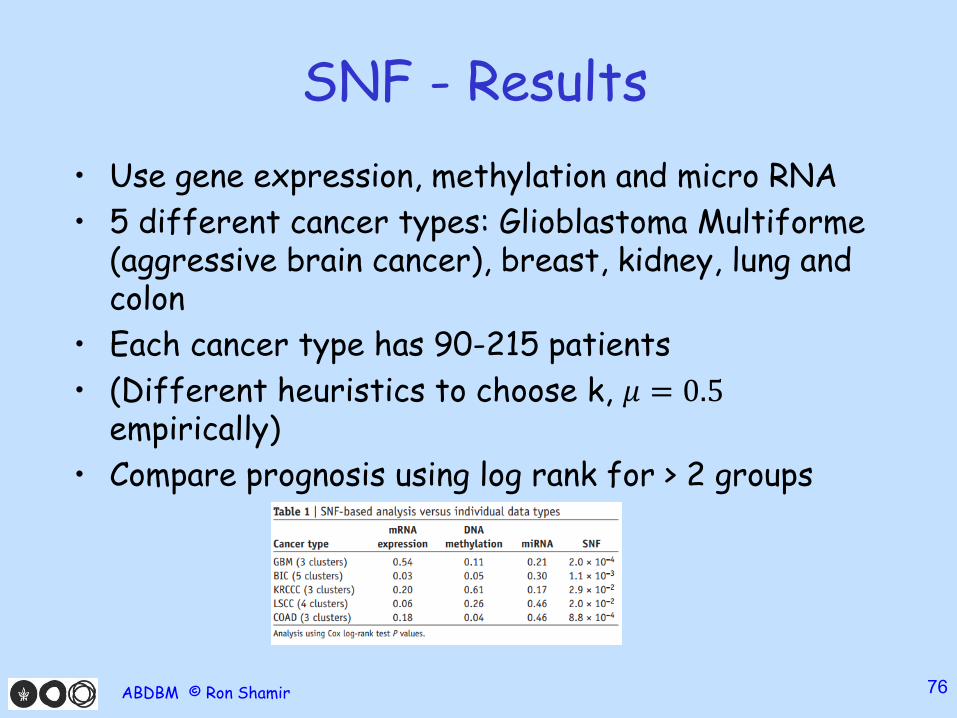
• Use gene expression, methylation and micro RNA
• 5 different cancer types: Glioblastoma Multiforme(aggressive brain cancer), breast, kidney, lung and colon
• Each cancer type has 90-215 patients
• (Different heuristics to choose k, 𝜇 = 0.5empirically)
• Compare prognosis using log rank for > 2 groups
ABDBM © Ron Shamir 76
SNF - Results
ABDBM © Ron Shamir 77
SNF - Recap
• Similarity based
• Patient similarity network per omic, followed by iteratively bringing the networks close to one another, until we have one network
• Cluster the network with spectral clustering
• Additional usages for the network
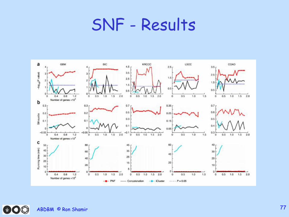
• Run on TCGA data from multiple tissues, and compare to iCluster, single omic and concatenation
ABDBM © Ron Shamir 78
Outline
• Introduction
• Cluster of Clusters (COCA)
• iCluster
• Nonnegative Matrix Factorization (NMF)
• Similarity Network Fusion (SNF)
• Multiple Kernel Learning (MKL)
ABDBM © Ron Shamir 79
Multiple Kernel Learning
• Speicher and Pfeifer (2015, bioinformatics)– Max Planck Institute for Informatics
• Similarity based method
• Multiple Kernel Learning – the general idea of using several kernels
• Have been used on single data type, mainly in supervised context but also in unsupervised
• Idea: use different kernels for different omics, together with multiple kernel dimension reduction algorithms
ABDBM © Ron Shamir 80

Graph Embedding
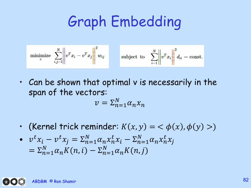
• 𝑥𝑖 are input vectors, W is input similarity graph, D is diagonal constraint matrix
• Look for v that projects x vectors to a line such that similarities are kept
• (D matrix is mainly in order to avoid the trivial solution)
• (Difference from spectral clustering?)
ABDBM © Ron Shamir 81
Graph Embedding
• Can be shown that optimal v is necessarily in the span of the vectors:
𝑣 = Σ𝑛=1𝑁 𝛼𝑛𝑥𝑛
• (Kernel trick reminder: 𝐾 𝑥, 𝑦 = < 𝜙 𝑥 , 𝜙 𝑦 >)
• 𝑣𝑡𝑥𝑖 − 𝑣𝑡𝑥𝑗 = Σ𝑛=1𝑁 𝛼𝑛𝑥𝑛
𝑡𝑥𝑖 − Σ𝑛=1𝑁 𝛼𝑛𝑥𝑛
𝑡𝑥𝑗= Σ𝑛=1
𝑁 𝛼𝑛𝐾(𝑛, 𝑖) − Σ𝑛=1𝑁 𝛼𝑛𝐾(𝑛, 𝑗)
ABDBM © Ron Shamir 82
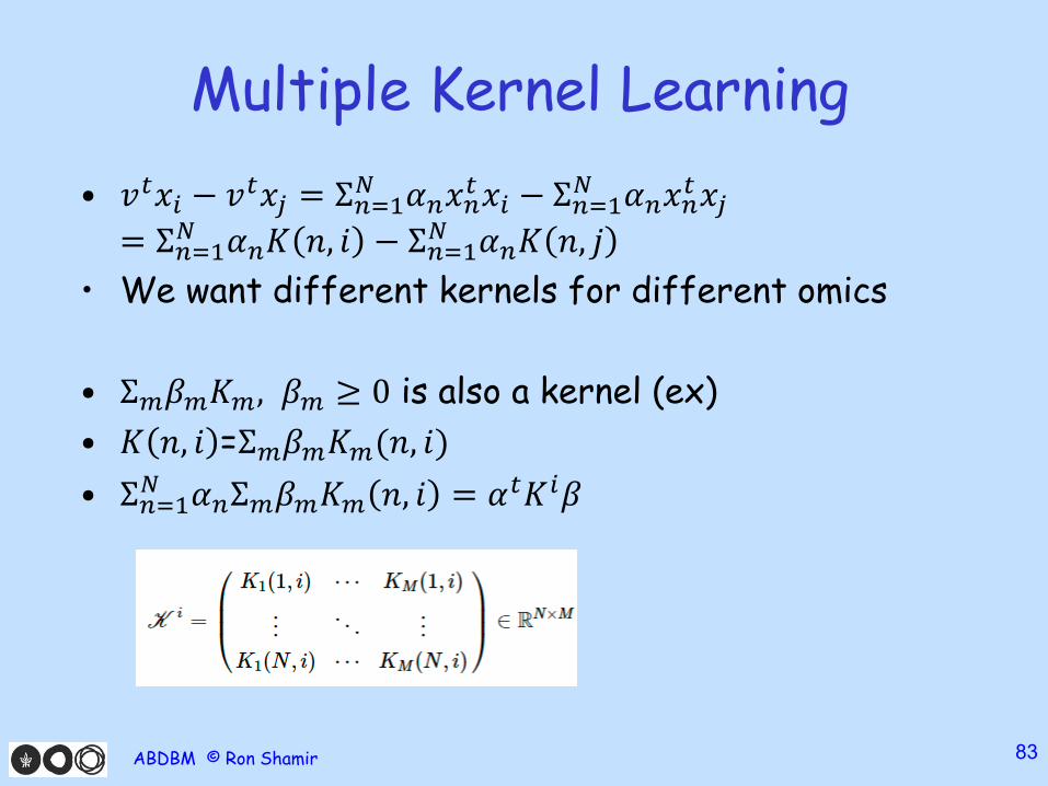
Multiple Kernel Learning
• 𝑣𝑡𝑥𝑖 − 𝑣𝑡𝑥𝑗 = Σ𝑛=1𝑁 𝛼𝑛𝑥𝑛
𝑡𝑥𝑖 − Σ𝑛=1𝑁 𝛼𝑛𝑥𝑛
𝑡𝑥𝑗= Σ𝑛=1
𝑁 𝛼𝑛𝐾 𝑛, 𝑖 − Σ𝑛=1𝑁 𝛼𝑛𝐾 𝑛, 𝑗
• We want different kernels for different omics
• Σ𝑚𝛽𝑚𝐾𝑚, 𝛽𝑚 ≥ 0 is also a kernel (ex)
• 𝐾 𝑛, 𝑖 =Σ𝑚𝛽𝑚𝐾𝑚(𝑛, 𝑖)
• Σ𝑛=1𝑁 𝛼𝑛Σ𝑚𝛽𝑚𝐾𝑚 𝑛, 𝑖 = 𝛼𝑡𝐾𝑖𝛽
ABDBM © Ron Shamir 83
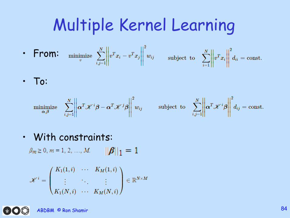
Multiple Kernel Learning
• From:
• To:
• With constraints:
ABDBM © Ron Shamir 84
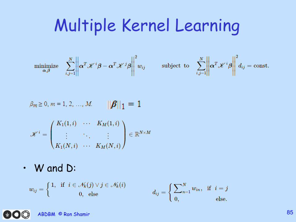
Multiple Kernel Learning
• W and D:
ABDBM © Ron Shamir 85
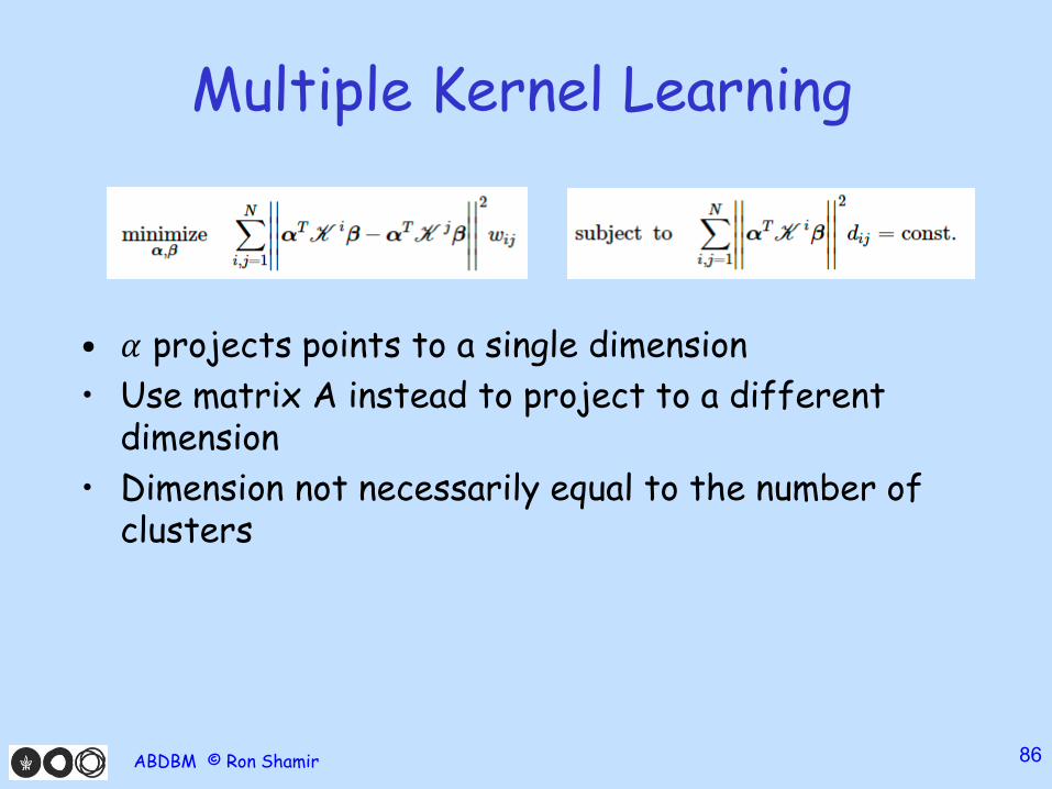
Multiple Kernel Learning
• 𝛼 projects points to a single dimension
• Use matrix A instead to project to a different dimension
• Dimension not necessarily equal to the number of clusters
ABDBM © Ron Shamir 86
Multiple Kernel Learning
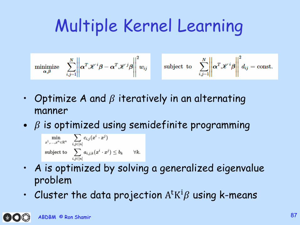
• Optimize A and 𝛽 iteratively in an alternating manner
• 𝛽 is optimized using semidefinite programming
• A is optimized by solving a generalized eigenvalue problem
• Cluster the data projection AtKi𝛽 using k-means
ABDBM © Ron Shamir 87

MKL - Results
• Run on GBM, breast, lung, kidney and colon cancer (SNF dataset, ~90-215 patients per subtype)
• Use either 1 or 5 kernels per dataset:
• 𝛾 =1
2𝑑2, 𝛾𝑛 = 𝑐𝑛𝛾, 𝑐𝑛 ∈ {10−6, 10−3, 1, 103, 106}
• Fix the dimension to 5, and choose k using silhouette score
• β values measure the effect of each kernel
ABDBM © Ron Shamir 88
MKL - Results
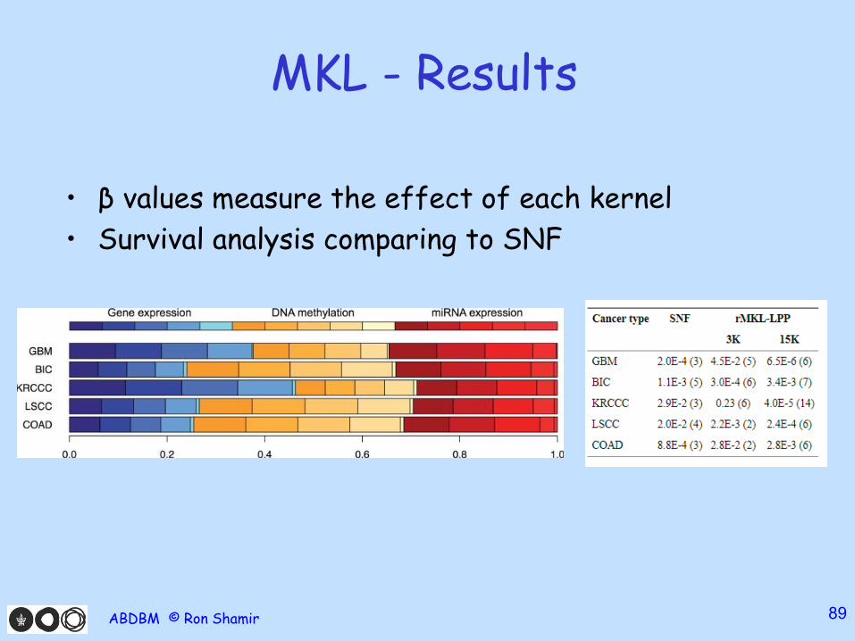
• β values measure the effect of each kernel
• Survival analysis comparing to SNF
ABDBM © Ron Shamir 89
MKL - Results
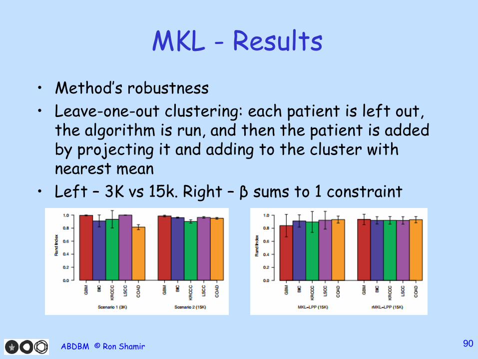
• Method’s robustness
• Leave-one-out clustering: each patient is left out, the algorithm is run, and then the patient is added by projecting it and adding to the cluster with nearest mean
• Left – 3K vs 15k. Right – β sums to 1 constraint
ABDBM © Ron Shamir 90
MKL - Results
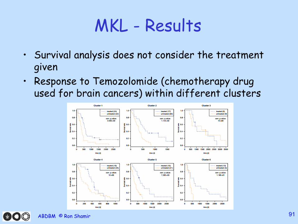
• Survival analysis does not consider the treatment given
• Response to Temozolomide (chemotherapy drug used for brain cancers) within different clusters
ABDBM © Ron Shamir 91
MKL - Recap
• Similarity based
• Graph embedding: dimension reduction such that neighbors in the original dimension remain close in the low dimension
• Use the kernel trick + different kernel(s) for each omic
• Compare prognosis to SNF and show the effect of multiple kernels on robustness
ABDBM © Ron Shamir 92
Summary
• Omic
• Multi omics data
• In this talk – methods that apply to numerical omics
• COCA – late integration
• Shared subspace models:– iCluster – probabilistic linear model
– NMF – factorization with non negativity constraints
ABDBM © Ron Shamir 93
Summary
• Shared subspace models:– iCluster – probabilistic linear model
– NMF – factorization with non negativity constraints
• Similarity based models:– Similarity network fusion – creating a unified similarity
network
– Multiple kernel learning – using different kernels for each omic
• Complexity and non-numerical omics vs. analysis of the feature within the model
• (Do different omics share the same underlying clustering?)
ABDBM © Ron Shamir 94

FIN
95ABDBM © Ron Shamir