MULTI-PROJECT SCHEDULING WITH 2-STAGE DECOMPOSITION

1

MULTI-PROJECT SCHEDULING WITH

2-STAGE DECOMPOSITION1

Anıl Can

Sabancı University, Orhanlı, Tuzla 34956

Istanbul, Turkey

[email protected]

Gündüz Ulusoy

Sabancı University, Orhanlı, Tuzla 34956

Istanbul, Turkey

Phone: ++90 2164839503

Fax: ++902164839550

[email protected]

ABSTRACT

We consider a non-preemptive, zero time lag multi-project scheduling problem

with multiple modes and limited renewable and nonrenewable resources. A 2-

stage decomposition approach is adopted to formulate the problem as a hierarchy

of 0-1 mathematical programming models. In stage one; each project is reduced to

a macro-activity with macro-modes. The macro-activities are combined into a

single macro-activity network over which the macro-activity scheduling problem

(MP) is defined, where the objective is the maximization of the net present value

with positive cash flows and the renewable resource requirements are time-

dependent. An exact solution procedure and a genetic algorithm (GA) approach

are proposed for solving the MP. A GA is also employed to generate an initial

solution for the exact solution procedure. The first stage terminates with a post-

processing procedure to distribute the remaining resource capacities. Using the

start times and the resource profiles obtained in stage one, each project is

scheduled in stage two for minimum makespan. Three new test problem sets are

generated with 81, 84 and 27 problems each, and three different configurations of

solution procedures are tested.

Keywords: Multiple projects, multiple modes, scheduling, decomposition,

genetic algorithm.

1. INTRODUCTION

The resource constrained multi-project scheduling problem with multiple

modes (MRCMPSP) is one of the more challenging problems in project

management. As a result of the global expansion of the IT sector and the increase

in research and development (R&D) and engineering services activities, project

1NOTICE: This is the authors' version of the paper that was accepted for publication

in Annals of Operations Research, 2014.

2

based management is used increasingly as a management paradigm. In particular,

R&D organizations (Liberatore and Titus, 1983) and large construction companies

(Liberatore et al., 2001) regularly execute multi-project scheduling procedures.

Payne (1995)suggested that up to 90%, by value, of all projects occur in a multi-

project context. As markets become more competitive, the obligation for firms to

simultaneously carry out multiple projects by managingscarce resources becomes

even more critical, increasing the need to build appropriate management structures

to reduce the risk offailures resulting fromdecisions made at different managerial

levels. The frequencies, time horizons and details of these decisions are suitable

for a hierarchical management scheme such as the one presented by Hans et al.

(2007).

One of the arrangements frequently used for managing multiple projects is

the dual level management structure (Yang and Sum, 1993), which consists of

anupper-level manager and several project managers. While the project managers

work at the operational level and are responsible for scheduling and controlling

individual projectactivities, the upper-level manager works on a more tactical

level and is responsible for all the projects and project managers. At the higher

level, projects are scheduled as individual entities to generate the start times and

due dates for each project. Then, based on these start times and due dates, each

project is scheduled individually by employing renewable and non-renewable

resource capacities imposed at the higher level. This dual level managerial

mechanism provides for a decision-making environment where decision-making

approaches with different performance criteria can be combined. This reasoning

also motivated researchers to exploit a similar approach by introducing dual level

decomposition methodologies to multi-project planning and scheduling as in

Speranza and Vercellis (1993).

This paper is organized as follows. Section 2 provides a brief description of

the problem environment and a survey on the related work in the literature. The

mathematical models and the solution methodology are presented in section 3. In

section 4, a genetic algorithm (GA) for solving multi-mode resource constrained

project scheduling problems with positive discounted cash flows (MRCPSPDCF)

and time dependent renewable resource requirements is introduced. Section 5

provides the computational study and the results. In section 6, the summary and

some suggestions for future work are presented.

3

2. PROBLEM DESCRIPTION AND RELATED LITERATURE

This study considers a multi-project scheduling problem with multiple

modes and limited renewable and non-renewable resources. The activities are

non-preemptive with finish-to-start zero time lag type precedence relations and

deterministic durations. Activity-on-node project networks are employed. The

start and completion activities of each network are represented by dummy

activities with a single mode of zero duration and resource requirement. There are

no due dates for the projects and no precedence relations among the projects.

Although the problem is not formulated as a multi-objective programming

problem, two objectives are considered in two consecutive decision stages. The

first stage corresponds to the tactical level aiming to determine the start times of

the projects and resource allocations such thatthe net present value (NPV) of the

relevant cash flows is minimized. The second stage corresponds to the operational

level of activity schedulingwith the objective of minimizing the makespan values

of the individual projects based onthe results of the first stage. Hence, both

tactical and operational levels are treated by one model.

Three types of cash flows are employed in this study. Revenues: A lump

sum payment is made at the end of the completion period of each project. Fixed

Costs: The project'sfixedcosts are resource independent and incurred initially at

the start of the first period for each project. Variable Costs: The resource usage

costs for the renewable and the non-renewable resources are incurred periodically

throughout each activity. It is assumed that an activity's consumption of non-

renewable resources as well as the variable cost distribution associated with this

consumption are uniform over the execution periods of that activity.The variable

costs associated with an activity are discounted to the starting point of that

activity. The resource usage cost for a resource is taken to be the same over all

projects and over all periods.

The resource constrained multi-project scheduling problem (RCMPSP)

consists of scheduling a collection of projects that share limited resources. The

scheduling output consists of the start times of the projects and their activities and

the allocation of resources to activities. A large body of literature for RCMPSP,

with or without multiple modes, reflects implicitly or explicitly a single level

management scheme for the planning and the scheduling of multiple projects. A

0-1 linear programming formulation of this problem was introduced by Pritsker et

4

al. (1969), and three possible objective functions were discussed: minimizing total

throughput time for all projects; minimizing the completion time for all projects,

and minimizing the total lateness or lateness penalty for all projects.Some

heuristic sequencing rules introduced by different researchers have been

categorized by Kurtulus and Davis (1982). Considering the penalties due to

project delays, Kurtulus and Narula (1985) analyzed six penalty functions with

four priority rules and determined that the MAXPEN (Maximum Penalty First)

rule performed best for minimizing the weighted project delay. Kim and

Schniederjans (1989) presented a heuristic framework for RCMPSPand

demonstrated a practical application. Bock and Patterson (1990) studied a rule-

based heuristic approach to setting due dates and the preemption of resources

from one project to another in a multi-project environment. A scheduling heuristic

with an update routine for control purposes was developed by Tsubakitani and

Deckro (1990) based on actual housing data. For RCMPSP with the objective of

minimizing weighted tardiness costs, Lawrence and Morton (1993) developed a

cost-benefit scheduling policy with resource pricing. Lova and Tormos (2001)

analyzed the effect of schedule generation schemes and priority rules in multi-

project and single-project environments. Kumanan et al. (2006) established a

heuristic and a GA for scheduling a multi-project environment to minimize the

makespan of the projects. Gonçalves et al. (2008) presented a GA for RCMPSP

with a chromosome representation employing random keys and chromosome

evaluation using a parameterized active schedule generating heuristic based on

priorities, delay times and release times. Zapata et al. (2008) presented three

models that attempted to overcome the limitations of the indexing of task

execution modes, the indexing of time periods and the discrete nature of

resources. In Mittal and Kanda (2009), new two-phase heuristics for RCMPSP

were developed and compared with existing methods.

Hans et al. (2007) proposed a positioning framework to distinguish between

different types of project-driven organizations and aid project management in

choosingamong the various existing planning approaches. In line with the

approach taken here, a group of papers dealt with the dual level management

approach for planning and scheduling multiple projects.Speranza and Vercellis

(1993) suggested decomposing the problem into a hierarchy of integer

programming models reflecting the dual level project management structure.

5

Yang and Sum (1997) followed their prior work mentioned above (Yang and

Sum, 1993) and examined the performance of due date, resource allocation,

project release, and activity scheduling rules in a multi-project environment. For

the decentralized version of RCMPSP, in which local and autonomous decision

makers (project managers) contribute to decision making, some multi-agent

system based solution procedures were discussed as in Lee et al. (2003),

Confessore et al. (2007), Homberger (2007), and Homberger (2010).

The starting point of our paper is the decomposition concept of Speranza

and Vercellis (1993).Here, we aim to develop an effective and viable 2-stage

decomposition approach reflecting the dual level project management structure

and based on the concepts of macro-activity and macro-mode introduced by

Speranza and Vercellis (1993).Our approach differs from that of Speranza and

Vercellis in the following respects. We employ a different cost structure.Our

procedure for generating macro-modes differs in that we use a streamlined

procedure for searching over budgets when generating macro-modes. A GA is

designed to solve the macro-activity scheduling problem, which is a special kind

of multi-mode resource constrained project scheduling problem (MRCPSP) with

discounted positive cash flows and time dependent renewable resource

requirements. The time horizon employed in this problem is obtained through a

heuristic procedure developed for this purpose. A post-processing routine is

applied to the solution of the macro-activity scheduling problem to utilize the

resources remaining idle. An extensive computational study is providedthat covers

both stages of the decomposition approach.

3. SOLUTION APPROACH

Due to the complexity of the problem at hand, we apply a 2-stage

decomposition approach as an approximation. The scheduling problem is

formulated as a hierarchy of 0-1 mathematical programming models in two stages.

In the first stage, each project is transformed into a macro-activity, and different

macro-modes are formed by evaluating various combinations of resource

allocationsby solving single project MRCPSP with a budget based on the

resourceusage cost involved. After the macro-modes are determined, a proper

time horizon is generated to build a macro-activity model with the objective of

NPV maximization. The macro-activities representing individual projects are

scheduled subject to general resource capacities and maximizing the NPV of the

6

discounted cash flows. Scheduling the macro-activities is a special kind of

MRCPSP with discounted cash flows (MRCPSPDCF), where the cash flows are

positive and the renewable resource requirements are time dependent. A GA

approach is developed for solving this problem.In the computational studies, this

GA approach is also employed for generating starting solutions for the exact

solution procedure. The result of the first stage is subjected to a post-processing

procedure to distribute the remaining resource capacities. The start times and the

resource allocations for the projects are determined by the start times of the

macro-activities and by the selection of the macro-modes. Using the start times

and resource profiles obtained in stage one, each project is scheduled to minimize

the makespanin stage two. Employing these two objectives separately in two

consecutive stages reflect a multi-objective environment. For single project

scheduling problems, resource availabilities may differ from period to period. In

stage two, tight resource constraints make it easier to computationally solve the

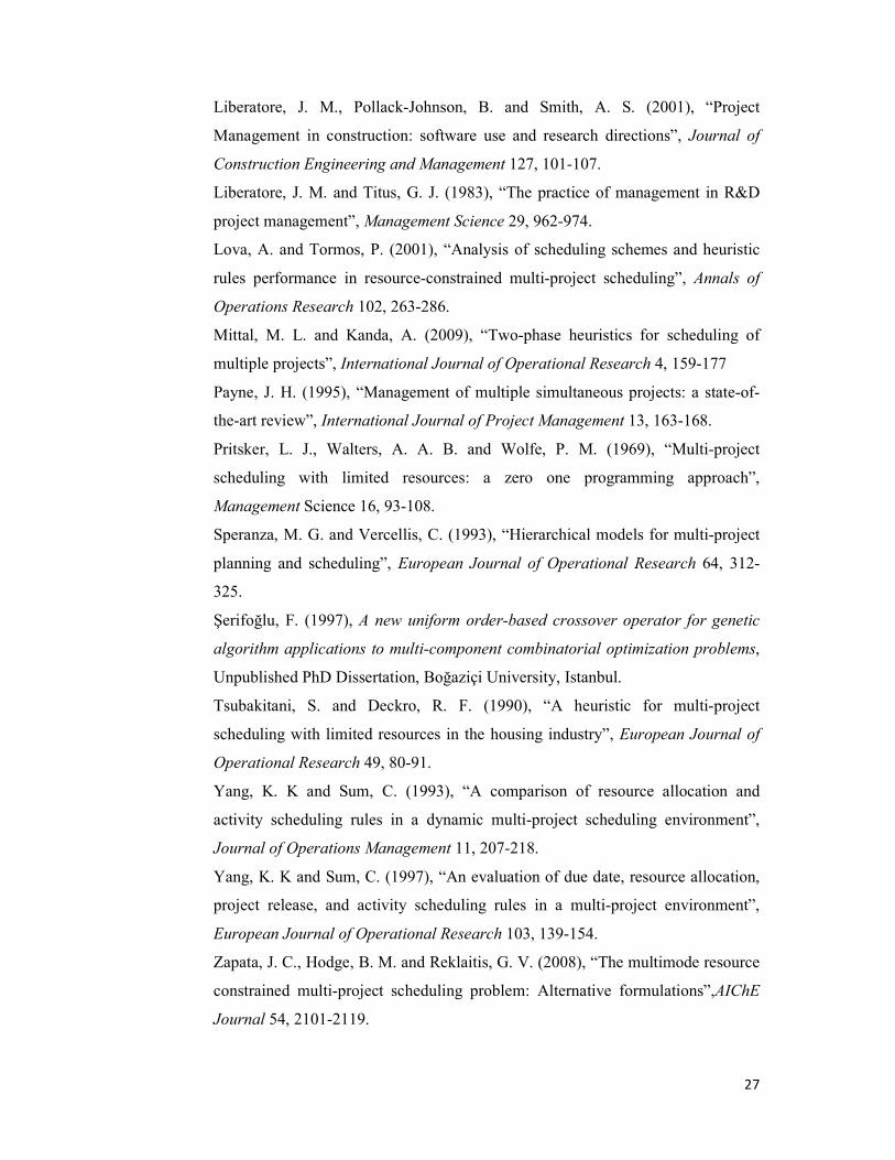
problems. The flow of the proposed 2-stage decomposition procedure is

summarized in Figure 1.

Place Figure 1 about here

The sets, indices and parameters used in these models are listed below.

Sets and Indices: � :set of all projects Sa :set of all actual projects � : project indices ��: set of activities of project � , �: activity indices ��: completionactivity of project�; �� : set of precedence relations between all activities �� in project � ��: set of modes of activity of project � � : activity execution mode indices; � �� 1, … , |��|� �� : setof the macro-modes forproject � � : macro-mode indices; � �� = �1, … , |��|� � : set of renewable resources � : renewable resource indices; � � � �1, … , |�|�

7

� : set of non-renewable resources � : non-renewable resource indices; � � � �1, … , |�|� � : set of periods �� : set of periods for project � �, : periodindices Parameters: ! : discount rate "�# : processing time for activity performed employing mode � "$�% : processing time for macro-activity � performed employing macro-mode � &� : early start period for activity '� : late start period for activity &� : early start period for macro-activity � '$� : late start period for macro-activity � )* : amount of renewable resource � available )*+ : amount of renewable resource � available in period � ,-: amount of non-renewable resource � available .�#*: amount of renewable resource � utilized by activity performed in mode � /�%*+ : amount of renewable resource � utilized by macro-activity � performed in

mode � in period � 0�#- : amount of non-renewable resource � consumed by activity performed in

mode � 1�%- : amount of non-renewable resource � utilized by macro-activity � performed

in mode � 2�3: lump sum payment made at the completion of project � 2�4: project fixed cost to be incurred initially to start project � 5*: unit resource usage cost of utilizing one unit of renewable resource � for one period 6-: resource usage cost of consuming one unit of non-renewable resource � 7�#: resource usage cost for activity performed in mode � 3.1 Macro-Mode Generation

When generating macro-modes, it is extremely significant to balance the

trade-off between the diversity of the macro-modes and the size of the macro-

activity scheduling model. Although increasing the number of macro-modes

8

increases the number of possible outcomes and thus may lead to a better solution,

it also increases the computational effort. For each project �8�9,the corresponding macro-mode generation is performed by solving two interacting mathematical

programming models,��:�;and ��:�<, respectively. The first model employed

for this purpose, ��:�;, is adopted from the shrinking model introduced by

Speranza and Vercellis (1993). The second model, ��:�<, is introduced as a search systematic for generating representative macro-modes. The interaction

between these two models is explained later in this section.

In the following formulations, ei and li for activity �� are calculated using the critical path method. For that purpose, the length of the time horizon �� for that purpose is determined using the time horizon setting method explained in

section 3.2.

Model ==>?@ AB � �C D� E�,FG A1C �. �. I I �JK#+

LM+NOM# PGM

Q I IR"�# S �TJ�#+LU

+NOU# PGUA, �C �� A2C

I I I .�#*J�#WXYZALU[\U]^;, +C

WN_àAOU, +^\U][;C# PGU� bGc )* � �, � �� A3C

I I 0�#- I J�#+LU

+NOU# PGU� bGc ,- � � A4C

I I J�#+LU

+NOU# PGU� 1 �� A5C

I I I 7�#J�#+LU

+NOU# PGU� bGc g� A6C

J�#+ � i 1, if activity starts in period � using mode �0, {/. } �� , � ��, � �� A7C

The objective A1C is the minimization of the makespan for project

sdenoted by E�,FG . Constraint sets regarding precedence relations within project sA2C, renewable resource capacities A3C, nonrenewable resource capacities (4) and

9

assignments A5C are included in Model ��:�;. The resource usage costs, 7�#, are calculated as in A8C and constrained by abudgetg� for project s (6). 7�# � I "�#.�#*5** 3 S I 0�#-6-- � �� , � �� A8C

Model ��:�; can be classified as an MRCPSP but with a budget

constraint on resource usage costs. The resource constraints are not very tight

since the capacities )*and ,- are bounds for the whole set of projects.

Model ==>?�AB � �C D� g� A9C �. �. EFG c E�� A10C g� Q 0 B � � A11C A2C � A7C from Model��:�;

In Model ��:�<, the budget g� is treated as a decision variable constituting the objective function A9C. Constraint (10) provides the definition of g� in terms of the variable resource usage costs and the decision variables.

Constraint A11C sets a parametric upper bound, E��, on the makespan of the

project. The specification ofE��is is explained below. Note that there is a negative relation between the project makespan and the budget consisting of the resource

usage costs 7�# for the selected activity modes, which are by definition positive.

Macro-mode generation procedure is initialized by calculating the mode costs as

expressed in (8). Then mode costs are made to start from zero by calculating the

minimal mode costs, 7�X�- for each activity �� and subtracting it from each

mode cost for each mode � ��. A mode �of an activity is called inefficient, if there exists another mode ��

for activity with "�# Q "�#� and .�#* Q .�#�* for each renewable resource � � and 0�#- Q 0�#�- for each non-renewable resource n N (Kolisch et al., 1995). Inefficient modesare removed from further consideration.

The maximum budget required, g�X9�, is computed by determining the

highest mode cost 7�X9� for each activity �� and summing these costs. The

bounds on the duration range ��X�-, ��X9�� for E�� are computed by solving

Model ��:�; for g� � 0 and for g� � g�X9�. The duration range for E�� signifies

10

the durations for possible macro-modes that can be generated. Solving Model ��:�<results in a schedule with a makespan less than or equal to E�� and mode

selections that minimize the budget requirements. Starting with ��X�-, E�� is increased by one at each step until ��X9� is reached. At each step, Model ��:�< is solved and, if g� is lower than the previous solution, a new macro-mode �is generated based on the optimal solution of ��:�;expressed by J�#W� and added to

the macro-mode set �� of project �. Note that� is one of several macro-modes

that might be generated for the same E��value. The duration, the renewable resource profile A12C and the non-renewable resource consumption A13C obtained in the solution of the Model ��:�<define the new macro-mode �. /�%*+ � I I I .�#*J�#W�XYZALU[\U]^;, +C

WN_àAOU, +^\U][;C# PGU� bG� �, � ��, � �, � �1, … , E��A12C

1�%- � I I 0�#- I J�#W�LU+N��# �� bG

� �, � �� , � � A13C The cash flow associated with a macro-activity �(project s) and a macro-

mode � ��is denoted by 2�%and defined in A14C. 2�%isobtained by

subtractingthe expenditures incurred for the correspondingproject fixed cost from

the lump sum payment received at the completion of the macro-activity s, and the

resource usage costs are discounted to the start of macro-activity� using a discount factor !. 2�% � 2�3A1 S !C^\�G� � 2�4

� � I A1 S !C^W\�G�^;WN� �I 5*/�%*W* 3 S I 6- 1�%-"$�%- � �� , � �� A14C

3.2 Macro-Activity Scheduling

The macro-activity scheduling problem is designated as Model ��.

Model =�

D5J �� I I I A1 S !C^+[;2�%J��%+L$G

+NOG% P�G� � A15C s.t.

11

I I I /�%*A+^W[;CJ��%WXYZAL$G["��^;, +C

WN_àAOG, +^"��[;C% P�G� � c )* � �, � � A16C I I 1�%- I J��%+

L$G+NOG% P�G� � c ,- � � A17C

I I J��%+L$G

+NOG% P�G� 1 � � A18C

J��%+ � � 1, if macro � activity�startsinperiod�using macro mode�0, {/. } � �, � ��, � � A19C

The cash flows 2�% in the objective function are definedaboveA14Cand represent the NPV of the return and all the costs involved for macro-activity s and

macro-mode � ��discounted to the start time of macro-activity s.Hence, the

objective function is the total discounted NPV of all cash flowsfor all macro-

activities (i.e., projects). Constraint set A16C is the capacity constraint for the renewable resources determined based on the schedules evaluated in the macro-

mode generation step. Constraint set A17C is the capacity constraint for the non-renewable resources. Constraint set A18C ensures that a macro-mode alternative is

selected for each project and started in the interval �&��, '$��. The time horizon �employed in Model MP is obtained through a heuristic

procedure developed here for this purpose and called the Relaxed Greedy

Heuristic (RGH). In RGH, a simple binary integer programmingmodel with non-

renewable resource capacity and macro-mode assignment constraintsis solved to

obtain the non-renewable resource feasible list of macro-mode selections with the

greatest sum of cash returns. Then, these macro-modes are listed in non-

decreasing order of cash flows and scheduled using a serial scheduling scheme

(see e.g., Kolisch, 1995; Kolisch, 1996) that takes the renewable resource

capacities into consideration. In addition, an initial feasible solution, which is a

lower bound for the actual problem, is obtained while determining the time

horizon value.

12

3.3 Post-Processing for Macro-Activity Scheduling

In this section, we introduce a post-processing procedure to redistribute

resources to the projects.This procedure includes renewable resources,)*+� A20C, and non-renewable resources,,-� A21C, that are left over after the macro-activity

scheduling whereJ��%W� represents the best solution obtained for Model ��. )*+� � )* � I I I /�%*A+^W[;CJ��%W�XYZAL$G["��^;, +C

WN_àAOG, +^"��[;C% P�G� � � �, � � A20C ,-� � ,- � I I 1�%- I J��%+�L$G

+NOG% P�G� � � � A21C To benefit from the left-over capacities, a new macro-mode ��[is generated

for each project s by solving Model ��:�� .When trying to improve the NPV of

the schedule, one can change the macro-mode selection,alter the start time of

projects or do both. Here, thestart time for each project is kept the same to limit

the search since we seek local improvement resulting in a relatively small

computational burden. Model ��:�� is an MRCPSPDCF with variable capacities

for the renewable resources and positive and negative cash flows. The new macro-

mode ��[ is generated to maximize the project ��A22Cby assuming all of the

extra resource capacities along with the currently assigned resource capacities are

made available for project � as expressed in the constraint sets A23C and A24C. The objective function is defined by including the project fixed cost, the lump sum

payment at the completion of the project and the variable resource usage costs,

which are incurred on a periodic basis and calculated as in A25C. The NPV of the newly created alternative ��[ is at least as large as that of the macro-mode ��, which was selected by solving Model ��.

Model ==>?�AB � �C max �� I A1 S !C^+2�3

L$ G+NO G

JFG;+ � 2�4

� I I IA1 S !C^+[; � I A1 S !C^W\U]^;WN� �I 5*.�#** 3 S I 6- 0�#-"�#- � �� J�#+

LU+NOU# PGU� bG

A22C �. �. I I 0�#- I J�#+

LU+NOU# PGU� bG

c ,-� S 1�%�- � � A23C

13

I I I .�#*J�#WXYZALU[\U]^;, +C

WN_àAOU, +^\U][;C# PGU� bGc )*A¡G�[+^;C� S .�%�*+ � �, � ¢1, … , "$�%�£ A24C

A2C, A5C andA7¤Cfrom Model ��:�; where E�� is the start time of project � obtained from the solution of the

Model ��, "�� is the duration of the macro-mode �� and A7¤C differs from A7C in that J�#+ is defined in (24) over � �1, … , "�� rather than over � ��.

Once the new macro-mode ��[ is formed for each actual project s,

theresulting changes in the NPV and the resource capacities due to macro-mode

shifts are calculated. 2��, thebenefit gained in NPV due to the macro-mode shift in

project �, is calculated as in A25C. Changes in renewable resource capacities, )�*+�� and in non-renewable resource capacities, ,�-�� , are defined in A26C andA27C, respectively. 2�� A2�%¥ � 2�%�CA1 S !CA¡G�^;C� �9 A25C ,�-�� ,�%¥- � ,�%�-� �9, � � A26C )�*+�� )�%¥*+ � )�%�*+ � �9, � �, � �1, … , "�%�� A27C

It may not be possible to simultaneously shift the macro-modes for all

projects because of conflicting needs for the common leftover capacities. On the

other hand, making a macro-mode shift for project � may assign some left-over

capacities to project � but it may also release some of the resources that are no

longer required once the shift is realized. These possible macro-mode shifts are

linked with each other. Hence, decisions on macro-mode shifts should be made by

simultaneously considering the projects and solving Model MMS.

In Model ��, the aim is to maximize the total NPV gain by applying the

macro-mode shift (28) to select projects. Model�� is a knapsack-type

formulation with renewable resource capacities that vary over time.

Model ==¦ D5J I 2��§�� A28C �. �. I ,�-�� §�� c ,-� � � A29C

I I )�*W�� §�¡G�[\�G��^;

WN¡G�� c )*+� � �, � � A30C

14

§� � i 1, if project� is selected for macro � mode shift0, {/. } � � A31C Constraint sets A29C and A30C ensure that the total resource availability

bounds are not violated. Variable §� defined in A31C indicates whether or not a macro-mode shift is applied to a project.

After applying the macro-mode shifts to the selected projects, individual

projectsare scheduled as follows.

3.4 Scheduling Each Individual Project

After setting the resource capacities and the start times of the projects, each

project is individually scheduled to minimize the project makespan. The

scheduling problem is formulated for each project � �as an MRCPSP with non-

renewable resource capacities ,�-�and renewable resource capacities )�*+� that vary over time. The resulting model is denoted by�� is given below:

Model ¦?AB � �C D� EFG A32C �. �. I I 0�#- I J�#+

LU+NOU# PGU� bG

c ,�-� � � A33C I I I .�#*J�#W

XYZALU[\U]^;, +CWN_àAOU, +^\U][;C# PGU� bG

c )�*+� � �, � �� A34C A2C, A5C and A7C from Model��:�;

We expected that the time dependence of the resource capacity levels would

cause a significant increase in computation time, but this did not occur because

the resource capacities were quite tight. Recall that the resource capacities are

determined by the selection of the macro-modes, which were generated

byrepeatedly solving a very similar model.

4.A GENETIC ALGORITHM APPROACH FOR THE MACRO-ACTIVITY

SCHEDULING PROBLEM

The macro-activity scheduling problem MP introduced in section 3.2 is an

MRCPSPDCF and hence, an NP-hard problem (Herroelen, 1997). Therefore, the

15

use of a heuristic procedure is justified to solve the problem.A GA was developed

for this purpose,and itwill be presented in this section.

4.1 Representation

The problem is a version of the multi-component combinatorial optimization

problem with sequencing and selection components. Hence, a common

chromosome structure including two serial lists is used to represent a chromosome

for the problem as in Şerifoğlu (1997).The first list is a permutation of the non-

dummy activities representing the priority order of activities for scheduling, and

the second is a list of the mode selections for the activities. Hartmann (1998) also

employs a list representation in his GA for RCPSP, which he later extended to the

multi-mode case (Hartmann, 2001). Simulation experiments performed by

Hartmann and Kolisch (2000) reveal that the performance of activity-list

representation is superior to other discussed representations (Kolisch and

Hartmann, 1999).

4.2 Evaluation of the Chromosomes

The fitness of a chromosome is determined by calculating NPV values and

considering the positive cash flows incurred at the start of each activity. Start

times are determined by obtaining the specific schedule represented by the lists

stored in the chromosome. Since all cash flows are positive, starting the macro-

activities as soon as possible is more desirable for achieving higher NPVs. A

serial scheduling scheme is used to schedule the macro-activities based on the

priority sequence in the first list and the mode selections in the second list of the

chromosome.

4.3 Operators

4.3.1 Crossover Operator

Considering that there are no precedence feasibility issues among the

activities corresponding to a project, a 2-point crossover method is employed. In a

2-point crossover procedure, two random genes from the first parent are picked,

and then genes before the first randomly selected gene and after the second

randomly selected gene are directly passed on to the child. Then, the genes

associated with the activities that are missing fromthe child's priority order list are

16

acquired from the second parent according to its priority order list and associated

modes.

4.3.2 Mutation Operators

Two mutation operators are used to randomly modify the newborn and

reproduced chromosomes:

Swap mutation:This mutation is executed on the priority order list to obtain

different sequences, which may or may not lead to a different schedule, by

swapping the locations of two randomly selected activities. The activities are

swapped while preserving their assigned modes.

Bit mutation: An activity is selected randomly on the priority order list and

its mode is replaced with another randomlychosen mode value. Bit mutation is not

permitted to produce a non-renewable resource infeasible solutionby restricting a

priori the range of modes to feasible ones with respect to non-renewable

resources.

4.4 Population Management

An initial population is formed as follows: First, a mode selection list is

generated by selecting a random mode for each activity.If the mode selections are

not feasible with regard to the non-renewable resource capacities, a new list is

formed from scratch. Note that Kolisch and Drexl (1997) have proven that the

feasibility problem for |�| Q 2 is NP-complete. The non-renewable resource

feasible mode selection list is then combined with a random sequence of

activities. In addition, any existing solutions can be included in the initial solution.

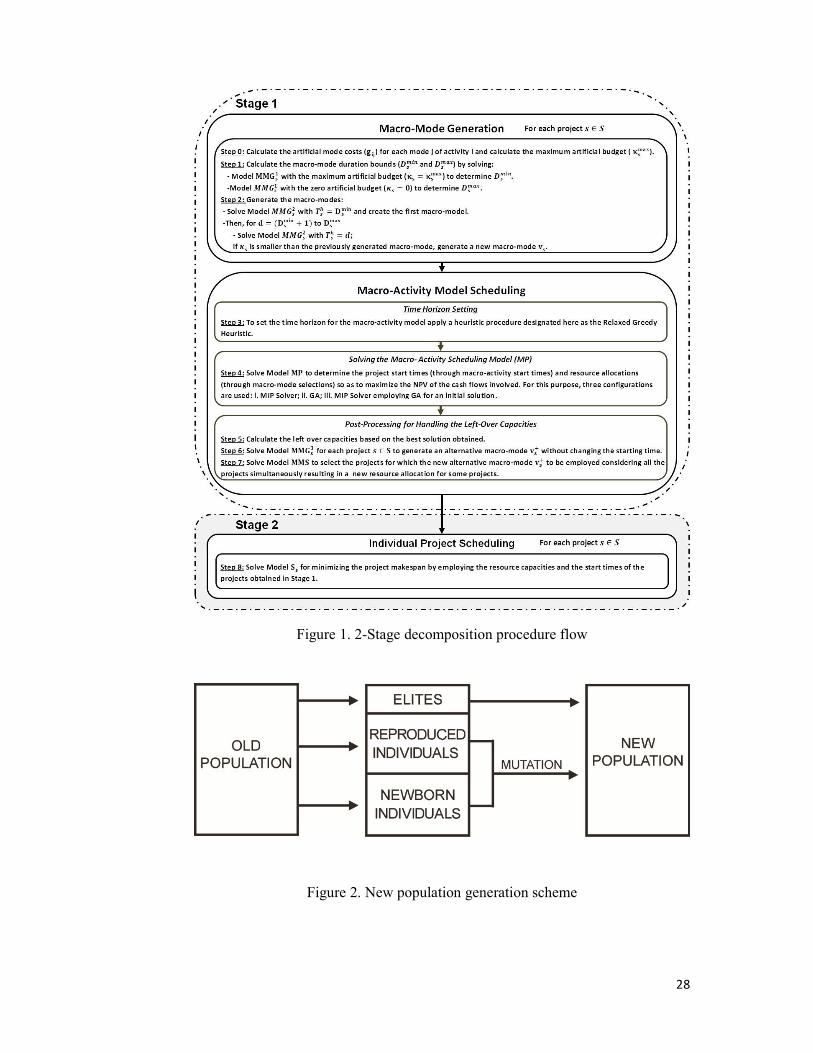
At each iteration, a new population is created as follows: A number of new

members, which corresponds to a ratio �-Oª of the population size �«¬«, are created by using the 2-point crossover with members randomly selected from the

current population and added to the new population along with two elite

individuals. Two distinct individuals with the highest fitness values in the current

populationare selected as the elite individuals. Any ties are broken arbitrarily.The

additional number of individuals needed to increase the population size of the new

populationto �«¬«is then reproduced from the current population with the elite

individuals deleted using the roulette wheel selection method, where each

individual is assigned a probability for selection proportional to its fitness value.

Finally, except for the elite individuals, each individual is considered first for a

17

swap mutation with probability �ª9«and then for a bit mutation with probability ®�+. This new population generation scheme is given in Figure 2.

Place Figure 2 about here

4.5 Restart

To avoid the possibility of early convergence and to refresh the population,

a restart is applied after each �*O� generations,if the ratio of identical individuals in the population exceeds 30%. If this is not the case, then the algorithm is run for

another �*O�generations. In each restart, all the members in the population except

the elites are replaced by randomly generated new members.

4.6 Termination

The procedure is carried out for a predetermined number of

generations.Once this maximum generation limit �¯O- is reached, the procedure is terminated.

4.7 Fine Tuning the Design Parameters

A series of experiments is performed to finetune the design parameters for

the proposed GA algorithm. Various values of the design parameters shown in

Table 1 are tested to arrive at a combination of design parameter values, which

will result in a relatively better performance. The number of elite individualsis set

to 2, and representative values are evaluated for each remaining design parameter.

Place Table 1 about here

A test data set is formed consisting of 17 instanceswhere optimal values are

determined using an MIP solver. These instances are sampled from the main data

set, which is described in section 5, and tested for various design parameter value

combinations. For each test data set and parameter combination, five replications

are executed, and the average best solutions and the average computation times

are calculated. Considering that the primary intention is to obtain solutions that

are as good as possible and the computational time required for GA application is

relatively small, the combination performances are evaluated based primarily on

18

the closeness of the best solution to the optimal solution. The computational time

is used as a secondary performance measure.

Parameter value combinations are tested in two phases. In the first phase,

324 combinations of the parameters �«¬«, �¯O-, �-Oª, �ª9«and ®�+are analyzed and fixed. Then, using the parameter values fixed previously, 3 combinations per

restartcheck are tested in the second level.

Comparing the performances of the parameter value combinations obtained,

excluding the restart possibility, we observed that �«¬« � 100and �¯O- �500perform better as expected since larger values allow for more computations,

which cannot have a negative effect on the objective function value. However, we

realized that there was no significantly dominant set of values for the parameters �-Oª, �ª9«and ®�+, and combinations worked quite well with small differences

between one other. To resolve this issue,a small segment of the best-performing

parameter combinations from each data instance were combined. Based on the

frequency of combinations among the representative combinations over all data

instances, we observed that a combination with �-Oª � 0.6, �ª9« � 0.5, ®�+ � 0.2 performed better. Fixing the parameter values determined so far, �*O�was tested. �*O� � 100 performed better for the majority of the data

instances. Hence, we decided to use the combination �«¬« � 100, �¯O- � 500, �-Oª � 0.6, �ª9« � 0.5, ®�+ � 0.2 and �*O� � 100 for all the following computations.

5. COMPUTATIONAL STUDY

To analyze the performance of the proposed 2-stage decomposition method

for the multi-project scheduling problem, a series of computational experiments

are carried out. These experiments are meant to observe and examine the effects

of various factors that shape the problem environment on the results and the

computational effort.

Since no benchmark problem sets with the required structure are available

currently, new problem sets are generated using the single project cases taken

from PSBLIB (Kolisch and Sprecher, 1996). Various cases with different numbers

of jobs from PSPLIB are combined into multi-project problems by assigning cash

flow values, general resource capacities, and resource utilization costs.

19

5.1 Resource Conditions

The Resource Factor A�°±C, which measures the usage/consumption, and the

Resource Strength (��±), which measures the availability, are defined to represent

the resource-based conditions of resource categories ² ��, ��. These factors, which were shown to have (Kolisch et al., 1995) a strong effect on the behavior of

RCPSP solution procedures, are adapted here for multi-project scheduling

environments. �°3 is given by A35C and A36C; and �°�is given by (37) and (38). yY´µ � i 1, wY´µ · 00, o/w } �� , � ��, � �A35C �°3 � 1|�| 1|�| � 2 I 1|��| � 2 I 1|��|

|��|�1�2 I I §��

|�|�1��2 A36C

��#- � i 1, 0�#- · 00, {/. } �� , � ��, � �A37C �°� � 1|�| 1|�| � 2 I 1|��| � 2 I 1|��|

|��|�1�2 I I ��

|�|�1��2 A38C

The resource availability for each renewable resource � � is given as: * � *X�- S �{¹�"¢��R *X9� � *X�-T£ � � A39C

where *X�- � maxY¢min´�.�#*�£, and the maximum level *X9� is determined by

the peak per period usage of the renewable resource � required in the early finish schedule obtained through forward recursion and the selection of activity modes

with maximum requirements for the renewable resource �. The resource availability for each non-renewable resource � � is given as:

- � -X�- S �{¹�"¢��R -X9� � -X�-T£ � � A40C where ¸-X9� � ∑ D5J#¢0�#-£� and -X�- � ∑ D�#� ¢0�#-£. 5.2 Financial Parameters

The discount rate (!) is selected to be 0.05 per period for all cases and constant throughout the time horizon. The parameters 5* and 6- are assumed to be

3. Due to the nature of the problem and the solution procedure, cash flows for

macro-modes cannot be known initially, but they can be calculated by considering

the lump sum payments at the completion times of the projects, »�3; the fixed cost

20

to be invested to start a project, »�4; and the resource-based variable costs, 5* and 6-, as the macro-modes created one by one. This condition arises from the

necessity to seek a sensible approach to set »�3 and »�4 for each project � �.These parametersare determined by using A42C and A43C, where 2��, a base cost related with resource usages as expressed in A41C, is multiplied by a factor drawn from

the uniform distribution ¼~A0, 1C, and the factors ¾3 for lumpsum payments and ¾4 for investment costs. ¾3 � 18and¾4 � 0.2 are used here in all problem casesto

ensure positive cash flows for the macro-mode generation process.

2�� I 1|��| I �I "�#5*.�#** 3 S I 6-0�#-- � �# PGU� bG A41C

»�3 � 2��¾3R1 S A¼~A0, 1CCT A42C »�4 � 2��¾4R1 S A¼~A0, 1CCT A43C 5.3 Problem Sets

Three problem sets denoted by A,B,C are created to represent a variety of

different environmental factors.

Problem set A is formed to analyze the effect of resource based factors

while fixing other factors. Set A includes multi-project caseswith the same

number of projects and the same number of activities but different resource

requirements and resource availability levels, categorized by �� and �° values for renewable and non-renewable resources. Each instance includes 14 projects

consisting of 10 activities each as shown in the first two columns of Table 2.

Three levels are selected for each factor including �°3, �°�, ��3 and �� as given in the last four columns of Table 2. To avoid any infeasibilities due to

insufficient non-renewable resources, a minimum value for�� ,��X�-, is

determined by simple testing, and a medium level is also calculated by ��X�\ ��X�- S R1 � ��X�-T/2 . Combinations of these four variable factors with three

levels of each result in problem set A gave 81 total instances.


Problem set B focuses on the effects of different number of projects and

activities. In these multi-project instances, three levels are set for the number of

21

projects and seven levels are set for the number of activities as provided in the

first two columns of Table 3. The�° values for renewable and non-renewable resources are fixed at 0.5 as shown in the third and fourth columns of Table 3.

Two levels are determined for ��3 and �� as shown in the last two columns of

Table 4. The levels for the��values are set using ��X�\; � ��X�- SR1 � ��X�-T/3 and ��X�\< � ��X�- S 2 � R1 � ��X�-T/3. Combinations of

these four variable factors with different levels results in problem set B with

84instances.


In problem set C, a multi-project environment that is heterogeneous in terms

of project sizes, is emphasized by grouping projects consisting of different

number of activities (Table 4). Three multi-project groups are formed, and

different levels of resource strengths are assigned. In the first group, equal

numbers of relatively small, medium and large projects are combined. In group

two, a few larger projects are grouped together with a collection of smaller sized

projects. In the third group, a few smaller projects are added to a group of

relatively large projects.The levels for the�� values are set as for problem set A.

Combinations of these three multi-project groups with three resource strength

levels result in 27 instances.


5.4 Software and Hardware Information

All codes are written in GNU C#, and the MIP solver is CPLEX 12.1. All

experiments were performed on a HP Compaq dx 7400 Microtower with a 2.33

GHz Intel Core 2 Quad CPU Q8200 processor and 3.46 GB of RAM.

5.5 2-Stage Decomposition Method Performance Analysis

For assessing the performance of the 2-stage decomposition procedure as

well as the GA approach presented in section 4, three configurations were

designed with the methods used in this work. Besides the GA approach employed

for solving the macro-activityscheduling model (Model MP),all of the

22

mathematical programming models presented as part of the proposed 2-stage

decomposition procedure are solved using an MIP solver. In Configuration 1,

Model MP is solved by the GA approach, whereas in Configuration 2it is solved

by the MIP solver. In Configuration 3,Model MP is solved by the MIP solver but

this time an initial solution is provided to the MIP solver, which is obtained by the

GA approach.

5.6 Results

In this section, we present the results obtained by running the algorithm with

all three configurations forproblem sets A, B and C. A two-hour time limit is set

for the MIP solver when solving Model MP. For some of the instances in problem

sets B and C, this computational time limit was reached before an optimal solution

was obtained. Such instances are not reportedin theseresults. The number of

instances,where Model MP is solved optimally,isreported in Table 5.


The computational results associated with the solution of Model MP are

reported in Table 6. Model MP is solved both by GA and the MIP solver without

and with an initial solution obtained by GA. These are referred to in the Table as

GA, MIP, GA+MIP, respectively. The average CPU values, CPUMP, for GA are

relatively much lower than required by the MIP solver results in both MIP and

GA+MIP over all problem sets. For the average NPV values, NPVMP, we observe

that for problem sets A, B and C, the GA results differ from the optimal solutions

by 0.11%, 0.59% and 0.56%, respectively.


Table 7reports NPVAve and CPUTotal for all configurations and all problem

sets. The average objective function value for stage 1 is designated as NPVAve.

CPUTotal corresponds to the average CPU time required to solve both stages of the

solution procedure. Although for Configuration 1 the percentage of optimal

solutions is relatively low, the NPVAvevalues are very close to the optimal

solutions obtained by the other two Configurations differing by 0.07%, 0.45% and

0.36% for the problem sets A, B and C, respectively.CPUTotal for Configuration 1

23

is relatively much less than those for Configurations 2 and 3 over all problem sets.

Table 7 also shows that Configuration 3 performs slightly better than

Configuration 2 for the problem sets B and C in terms of the computational effort

required. Note that the problems in these sets require in general more computation

time and hence, the effort of generating an initial solution obtained employing GA

appears to pay off.

Place Table 7about here

The post-processing procedure improves the objective function value

considerably with relatively little computational effort as shown in Table 8.


Table 9shows that the resource strength,RS, has a significant effect on the

computational effort required for the macro-activity scheduling step. For a given

RSN level, the required computational effort increases to a maximum level as ��3, which indicates the level of renewable resource availabilities, increases to a certain medium level (��3=0.6) and subsequently decreases dramatically as the

renewable resource availabilities climb to higher levels.


Table 10presents the average CPUTotal required to solve the instances from

problem set B using Configurations 2 and 3 different numbers of projects.

Columns2 and 3 report the average values including only the instances where the

macro-project scheduling problem is solved optimally within the time limit. The

fact that the CPUTotalvalues increase with the number of projects coincides with

the expectation that the number of projects in the problem environment has a

significant impact on the problem difficulty.


6. SUMMARY AND FUTURE WORK

24

We present an operationally effective and viable 2-stage decomposition

approach reflecting the dual-level project management structure and based on the

concepts of macro-activity and macro-mode introduced by Speranza and Vercellis

(1993). We introduce several different formulations and solution procedures.

The macro-mode generation procedure in the first stage of the

decomposition is applied with the introduction of a new search systematic for the

macro-modes. We introduce a budget based on the different types of costs

involved. The use of such a budget enables the generation of representative modes

via ��; and ��<. To reduce the number of variables in the formulation for MRCPSPDCF

with positive cash flows, three different time horizon setting methods are

developed and tested.

A GA approach is proposed for solving MRCPSPDCF with time dependent

renewable resource requirements. Compared to optimal solutions it is shown to be

extremely effective both in terms of the objective function value obtained and the

CPU time required. The GA is employed as a standalone solution procedure as

well as to generate initial solutions for the exact solution procedure.

An efficient post-processing procedure is introduced to distribute left over

resources from stage one to the projects to search for any improvements.

To analyze the performance and behavior of the proposed 2-stage

decomposition method, new data sets are formed using the single project cases

taken from PSBLIB compiled by Kolisch and Sprecher (1996), and a series of

computational experiments are carried out.

Although this study deals with MRCMPSP, some specific versions of

MRCPSP are dealt with directly as well due to the nature of the decomposition

based approach, e.g., an MRCPSP with time-dependent renewable resource

capacities.

There are several possible directions to extend this work in the future.

• Precedence relations between projects can also be included by considering that,

in practice, some projects need to precede others for technological reasons.

• Project termination deadlines can be specified and penalty costs for violating

these deadlines can be included in the cost structure, or a just-in-time

environment can be considered.

25

Considering the relevance of the problem treated here to manufacturing

firms as well as project-based firms, we conclude that resource-constrained multi-

project scheduling with hierarchical decomposition-based approaches is a rich

topic for further investigation.

ACKNOWLEDGEMENT:

We gratefully acknowledge the support given by the Scientific and Technological

Research Council of Turkey through Project Number MAG 109M571.

REFERENCES

Bock, D. B. and Patterson, J. H. (1990), “A comparison of due date setting,

resource assignment and job preemption heuristics for multi-project scheduling

problem”, Decision Sciences, 21, 387-402.

Confessore, G., Giordani, S. and Rismondo, S. (2007), “A market-based multi-

agent system model for decentralized multi-project scheduling”, Annals of

Operations Research 150, 115-135.

Gonçalves, J. F., Mendes, J. J. M. and Resende, M. G. C. (2008), “A genetic

algorithm for the resource constrained multi-project problem”, European Journal

of Operational Research 189, 1171-1190.

Hans, E. W., Herroelen, W., Leus, R. and Wullink, G. (2007), “A hierarchical

approach to multi-project planning under uncertainty”, Omega 35, 563-577.

Hartmann, S. (1998), “A competitive genetic algorithm forresource-constrained

projectscheduling”,Naval Research Logistics45,733-750.

Hartmann, S., Kolisch, R. (2000) “Experimental evaluation of state-of-the-art

heuristics for the resource-constrained project scheduling problem”, European

Journal of Operational Research, 127(2):394--407.

Hartmann, S. (2001), “Project scheduling with multiple modes: A genetic

algorithm”,Annals of Operations Research102,733-750.

Herroelen, W.S., Van Dommelen, P., Demeulemeester, E.L. (1997), “Project

network models with discounted cash flows: a guided tour through recent

developments”, European Journal of Operational Research 100, 97-121.

Homberger, J. (2007), “A multi-agent system for the decentralized resource-

constrained multi-project scheduling problem”, International Transactions in

Operational Research, 14, 565-589.

Homberger, J. (2012), “A (µ, λ)–coordination mechanism for agent–based multi–

project scheduling”, OR Spectrum, 34, 107-132.

26

Kim, S. O. and Schniederjans, M. J. (1989), “Heuristic framework for the

resource constrained multi-project scheduling problem” Computers and


Kolisch, R. (1995), Project Scheduling under Resource Constraints-Efficient

Heuristics for Several Problem Classes, Physica-Verlag, Heidelberg.

Kolisch, R., Sprecher, A. and Drexl, A. (1995), “Characterization of generation of

a general class of resource-constrained project scheduling problems”,

Management Science 41, 1693-1703.

Kolisch, R. (1996), Serial and parallel resource-constrained project scheduling

methods revisited: Theory and computation, European Journal of Operational

Research 90, 320-333.

Kolisch, R. and Sprecher, A. (1996), “PSPLIB – A project scheduling problem

library”, European Journal of Operational Research 96, 205-216.

Kolisch, R. and Drexl, A. (1997), “Local search for non-preemptive multi-

moderesource-constrained project scheduling”, IIE Transactions, 29, 987-999.

Kolisch, R., Hartmann, S. (1999) “Heuristic algorithms for the resource-

constrained project scheduling problem: Classification and computational

analysis”, In Project Scheduling: Recent Models, Algorithms and Applications,

J.Weglarz (Editor),147-178,Springer Science + Business Media, New York.

Kumanan, S., JeganJ.G. and Raja K. (2006), “Multi-project scheduling using an

heuristic and a genetic algorithm”, International Journal of Advanced

Manufacturing Technology 31, 360-366.

Kurtulus, I. and Davis, E. W. (1982), “Multi-project scheduling: categorization of

heuristic rules performance”, Management Science 28, 161-172.

Kurtulus, I. S. and Narula, S. C. (1985), “Multi-project scheduling: analysis of

project performance”, IIE Transactions 17, 58-66.

Lawrence, S. R. and Morton, E. T. (1993), “Resource-constrained multi-project

scheduling with tardy costs: comparing myopic, bottleneck, and resource pricing

heuristics”, European Journal of Operational Research 64, 168-187.

Lee, Y., Kumara, S. R. T. and Chatterjee, K. (2003), “Multiagent based dynamic

resource scheduling for distributed multiple projects using a market mechanism”,

Journal of Intelligent Manufacturing 14, 471-484.

27

Liberatore, J. M., Pollack-Johnson, B. and Smith, A. S. (2001), “Project

Management in construction: software use and research directions”, Journal of

Construction Engineering and Management 127, 101-107.

Liberatore, J. M. and Titus, G. J. (1983), “The practice of management in R&D

project management”, Management Science 29, 962-974.

Lova, A. and Tormos, P. (2001), “Analysis of scheduling schemes and heuristic

rules performance in resource-constrained multi-project scheduling”, Annals of


Mittal, M. L. and Kanda, A. (2009), “Two-phase heuristics for scheduling of

multiple projects”, International Journal of Operational Research 4, 159-177

Payne, J. H. (1995), “Management of multiple simultaneous projects: a state-of-

the-art review”, International Journal of Project Management 13, 163-168.

Pritsker, L. J., Walters, A. A. B. and Wolfe, P. M. (1969), “Multi-project

scheduling with limited resources: a zero one programming approach”,

Management Science 16, 93-108.

Speranza, M. G. and Vercellis, C. (1993), “Hierarchical models for multi-project

planning and scheduling”, European Journal of Operational Research 64, 312-

325.

Şerifoğlu, F. (1997), A new uniform order-based crossover operator for genetic

algorithm applications to multi-component combinatorial optimization problems,

Unpublished PhD Dissertation, Boğaziçi University, Istanbul.

Tsubakitani, S. and Deckro, R. F. (1990), “A heuristic for multi-project

scheduling with limited resources in the housing industry”, European Journal of

Operational Research 49, 80-91.

Yang, K. K and Sum, C. (1993), “A comparison of resource allocation and

activity scheduling rules in a dynamic multi-project scheduling environment”,

Journal of Operations Management 11, 207-218.

Yang, K. K and Sum, C. (1997), “An evaluation of due date, resource allocation,

project release, and activity scheduling rules in a multi-project environment”,

European Journal of Operational Research 103, 139-154.

Zapata, J. C., Hodge, B. M. and Reklaitis, G. V. (2008), “The multimode resource

constrained multi-project scheduling problem: Alternative formulations”,AIChE

Journal 54, 2101-2119.

28

Figure 1. 2-Stage decomposition procedure flow

Figure 2. New population generation scheme

29

Table 1. Design parameters and their range of values for fine-tuning

Design Parameters Identifier Values

Number of elites �OL�+O {2}

Population size �«¬« {50, 75, 100}

Number of generations �¯O- {200, 300, 400, 500}

Ratio of newborn �-Oª {0.4, 0.6, 0.8}

Probability of swap mutation �ª9« {0.2, 0.5, 0.8}

Probability of bit mutation ®�+ {0.2, 0.5, 0.8}

Number of generations per injection check �*O� {0, 50, 100}

Table 2. Problem set A

noProj noAct �°3 �°� ��3 �� 14 10 {0.5, 0.75, 1} {0.5, 0.75, 1} {0.3, 0.6, 0.9} {��X�-,��X�\,1}

Table 3. Problem set B

noProj noAct �°3 �°� ��3 �� {10, 15, 20} {10, 12, 14, 16, 18, 20, 30} 0.5 0.5 {0.4, 0.7} {��X�\;,��X�\<}

Table 4. Problem set C

noProj&noAct �°3 �°� ��3 �� {(5 * J10, 5 * J20, 5 * J30);

(8 * J10, 8 * J12, 2 * J30);

(3 * J10, 7 * J18, 7 * J20)}

0.5 0.5 {0.3, 0.6,

0.9} {{��X�-,��X�\,1}

30

Table 5. Number of instances solved to optimality

Configuration Problem Set A

(81 problems)

Problem Set B

(84 problems)

Problem Set C

(27 problems)

1 60 74.0% 25 29.8% 7 25.9%

2 81 100% 69 82.1% 24 88.9%

3 81 100% 72 85.7% 24 88.9%

Table 6. Performance of GA solving Model MP over problem sets A, B and C

Model MP

solved by

AverageNPVMP andCPUMP (sec)

Problem Set A Problem Set B Problem Set C

NPVMP CPUMP NPVMP CPUMP NPVMP CPUMP

GA 97,444.5 13.32 98,482.6 12.62 131,821.2 9.89

MIP 97,552.5 204.28 99,069.6 795.41 132,565.0 781.32

GA+MIP 97,552.5 212.00 99,069.6 707.90 132,565.0 717.61

Table 7. 2-stage decomposition results for problem sets A, B and C

Configuration

AverageNPVAve andCPUTotal (sec)


NPVAve CPUTotal NPVAve CPUTotal NPVAve CPUTotal

1 101,839.3 20.69 99,390.8 29.71 133,719.9 29.92

2 101,912.7 211.46 99,843.4 812.96 134,200.4 801.12

3 101,906.9 231.84 99,836.6 737.40 134,200.4 747.16

31

Table 8. Performance of post-processing routine

Configuration

Average Post-Processing NPV Improvement (%)


1 4.23 1.01 1.41

2 4.20 0.85 1.20

3 4.19 0.85 1.20

Configuration

Average CPU (sec) for Post-Processing


1 0.60 0.43 0.96

2 0.52 0.40 0.66

3 0.51 0.41 0.66

Table 9.Effects of �� factor on computational effort required – Problem set A

with Configuration 3

Average CPUTotal(sec) �� X�- �� X�\ �� 1 ��3 = 0.3 237.24 181.44 187.57 ��3 = 0.6 488.12 413.11 406.54 ��3 = 0.9 49.09 61.72 61.73

Table 10. Effect of number of projects – Problem set Bwith Configurations 2 and 3

Average CPUTotal(sec) of Number of instances solved to

optimality

noProj Configuration 2 Configuration 3 Configuration 2 Configuration 3

10 122.72 104.72 28 out of 28 28 out of 28

15 1,122.55 1,124.59 25 out of 28 26 out of 28

20 1,537.13 1,839.36 16 out of 28 18 out of 28

Documents

MULTI-PROJECT SCHEDULING WITH 2-STAGE DECOMPOSITION