Embed Size (px)
Citation preview
Acta Cybernetica 24 (2020) 315–341.
Multibody Dynamics in Natural Coordinates
through Automatic Differentiation and
High-Index DAE Solving∗
John D. Prycea and Nedialko S. Nedialkovb
Abstract
The Natural Coordinates (NCs) method for Lagrangian modelling andsimulation of multibody systems is valued for giving simple, sparse models.We describe our version of it and compare with the classical approach of Jalonand Bayo (JBNCs). Our NCs use the high-index differential-algebraic equa-tion solver Daets. Algorithmic differentiation, not symbolic algebra, formsthe equations of motion from the Lagrangian. We obtain significantly smallerequation systems than JBNCs, at the cost of a non-constant mass matrix forfully 3D models—a minor downside in the Daets context. Examples in 2Dand 3D are presented, with numerical results.
Keywords: Lagrangian mechanics, differential-algebraic equations, naturalcoordinates, simulation, algorithmic differentiation, Yaml
1 Introduction
1.1 Context and aims
We are concerned with simulating multibody systems (MBS, aka mechanisms),built mainly from rigid bodies, with joints and other ways to interact. Recall someadvantages of a Lagrangian approach [6, 20] to forming their equations of motion.
Economy. Lagrangians, in contrast to direct use of Newton’s three laws, can omitmention of forces that do no work, e.g. reaction force of smooth sliding contact.
Flexibility. One is free to choose generalised coordinates q = (q1, . . . , qnq) to
specify system position. Among all possible motions of the system, the actualone is a stationary point of the action integral
∫Ldt of the Lagrangian function
L = T − V , where T (t,q, q) and V (t,q) are the system’s kinetic and potential
∗N. Nedialkov was funded by the Natural Sciences and Engineering Research Council (NSERC)of Canada.
aCardiff University - corresponding author, E-mail: [email protected] University, E-mail: [email protected]
DOI: 10.14232/actacyb.24.3.2020.4
316 John D. Pryce and Nedialko S. Nedialkov
energies. This is an inherent system property, so the equations of motion thatcome from the Euler–Lagrange variational conditions:
d
dt
∂L∂qj− ∂L∂qj
+
nc∑i=1
λi∂Ci∂qj
= Qj(t), j = 1, . . . , nq, (1)
Ci = 0, i = 1, . . . , nc, (2)
describe the same set of possible motions, independent of the chosen q. The ncequations (2) are constraints on the motion due to rigidity etc., with associatedLagrange multipliers λi. The Qj(t) are generalised external force components ifany, whose definition also involves ∂/∂qj . We assume holonomic constraints, i.e.independent of velocities, so of the form Ci(t,q) = 0; the positional and velocitydegrees of freedom are then equal:
dof = nq − nc. (3)
So the system state is locally fixed at any t by dof values qj and dof values qj .
If constraints are absent (nc = 0), then (1) is reducible to an ordinary differentialequation system (ODE). If present (nc > 0), it is a differential-algebraic equationsystem (DAE)—usually true when q consists of cartesian coordinates, because rigid-body constraints must be included. It has index 3, in the classical differential indexsense [1], when solved as an initial-value problem. High-index DAEs have beenseen as hard to solve numerically, so much effort has gone into making nc = 0, i.e.finding representations that lead to constraint-free coordinates, typically angles.
We argue firstly, that an efficient high-index DAE solver changes the balance ofadvantage, thereby encouraging the use of Natural Coordinates with their benefitsof simple, sparse, human-readable equations. We use the C++ code Daets (DAEby Taylor Series) [11, 12] that can integrate numerically arbitrary index DAEs.
Secondly, we avoid symbolic manipulation to convert the Lagrangian L into theequations of motion (1) given to a numerical solver. Daets’s built in algorithmicdifferentiation (AD) system does this at run time—the Lagrangian facility [19].
Thirdly, only shown briefly by examples here, the mechanism facility reads atrun time a “MechSpec” text file describing a mechanism, and constructs from it aNatural Coordinates model of the Lagrangian and constraints, which is passed tothe Lagrangian facility and thence to Daets for numerical solution.
This article is about purely continuous systems and does not touch on the largearea of hybrid systems, with a mixture of continuous and discrete-event behaviour.
In the following, Section 2 is about Natural Coordinates: §2.1 describes differ-ences between other versions of NCs and ours, and §2.2 presents ours in detail.Section 3 outlines our numerical infrastructure. Section 4 gives to 2D and 3D ex-amples, with numerical results. Section 5 summarises the effect of our method’stheory and software architecture, and discusses the resulting system’s friendliness,in particular in a teaching context.
Multibody Dynamics in Natural Coordinates through AD and DAE Solving 317
2 Natural Coordinates
2.1 Our method compared with others
As with other Natural Coordinates (NCs) methods, our q holds mainly cartesiancoordinates in the world-frame (WF) of points or vectors (PVs) fixed on mechanismparts. We compare with the 1994 de Jalon and Bayo presentation (JBNCs) in [4]and later ones by von Schwerin [22] and Kraus et al. [8]; see also the surveys byNikravesh (2004) [15], and de Jalon (2007) [3].
Four-PVs versus three-PVs NCs. Maybe influenced by classical finite ele-ments, these authors put emphasisis on computing a mechanism’s mass matrix Mand on methods that lead to a constant M, independent of system position.
This leads them, see [4, pp. 44–51], [22, p. 54], [8, end of §1], to define a general3D rigid body’s position by four PVs—i.e. 12 scalar coordinates. E.g. from [3, §1]“When all the bodies contain at least two points and two unit vectors the inertiamatrix is constant and there aren’t velocity dependent inertia forces”.
A free rigid body has 6 DOF so there must be 12−6=6 scalar constraints toimpose rigidity, per body. For us, constant M is nearly irrelevant because of theunderlying algorithm architecture, see below. Hence, we choose three PVs, 9 scalarcoordinates, to define a body’s position. In JBNC terminology, these are basic PVs,or BPVs. To produce 6 DOF, we use 9− 6 = 3 rigidity constraints per body.
Frame definition and rigidity. Three BPVs determine the origin and x, y di-rections of an orthonormal frame. We define the z direction by a cross product—anonlinear operation, which is what makes our M a function of q in general. In 2DM is always constant, and for simple mechanisms in 3D can often be made so bya good choice of BPVs. The cross product makes our frames positively oriented,which need not hold in the other approaches.
JBNC devote several pages [4, pp. 47–51] to setting up the frame and therigidity constraints for various cases of points/vectors defining body position; andmore (pp 130–143) to cases of computing the mass matrix. Mostly they aim at aconstant M, but include a case [4, p. 139, see Fig 4.7] of defining the frame by across product exactly as we do, leading to a varying M. By contrast, we have oneunified method, that treats point and vector frame elements in the same way. (Anexception, that applies to all approaches, is the case of a dimensionally deficientpart such as a particle or a thin rod, for which a 3D frame makes no sense.)
Kraus et al. [8, §4] trade increased model size for the benefit of increased simplic-ity and sparsity. They define frames in a unified way close to how our method wouldwork if we used a “four PVs” rather than “three PVs” representation; if one makesa QR factorisation of their matrix X (the R is constant so can be precomputed;the Q is varying), the methods become very similar.
Von Schwerin does not give great detail of his NCs but [22, p. 48] says “one ofthe advantages of the natural coordinate approach is that the resulting mass matrixM is constant”, suggesting he only considers a “four PVs” system.
318 John D. Pryce and Nedialko S. Nedialkov
Basic and dependent PVs. For us, points/vectors fixed to a body R are eitherbasic or dependent. Basic ones, BPVs, are either fixed in the WF, or moving. Vectorq comprises all moving BPVs1, plus some needed scalars such as turn angles. Wespecify a dependent PV by giving its coordinates in the frame defined by the BPVs.It might be part of defining a joint, or a point where a force is applied to R, etc.
Since each BPV is either fixed or a component of q, each dependent PV is anexplicit function of q. Jalon–Bayo [4, p. 51] describe this dependent point method,but merely as a useful trick for bodies with many PVs, not as a primary technique.
Dynamics data. We specify R’s dynamics by storing the local coordinates of thecentroid, the mass, and the inertia matrix about the centroid. This seems morenatural than the method, described in [15, §4.4], of “lumping” the mass into virtualparticles at the BPVs in such a way as to preserve the inertial properties.
Assembly process. We assemble L one part at a time. Think of the method asa function whose input is the values q, q at current time and whose output is L,plus rigidity and joint constraints as a vector of residual values to be driven to zero.Fixed PVs are global constants, dependent PVs are local variables (temporaries).
For each part, in a loop, use q, q to find its current WF position and linearand angular velocity. Using its dynamics data, find the part’s kinetic and whererelevant its potential energy and accumulate these into L. Include (the residualsof) the part’s rigidity equations in the constraints array.
Similarly loop over joints to add their constraints, over any springs to add theirPE contributions, and so on.
The objects to which this is all done are not numbers but Taylor series. Theoutput is passed to the Lagrangian facility, which uses automatic differentiation todo the needed d/dt, ∂/∂q and ∂/∂q that converts them into the Euler–LagrangeDAE in a form Daets can handle.
Relevant matrices. The mass matrix M is not mentioned in the above steps.However Daets produces for any DAE, from analysing its structure, a numericalsystem Jacobian matrix J that is central to its Taylor expansion process. In ourcontext, the DAE was created by the Lagrangian facility, so J is formed by theinterplay between the latter and Daets. J turns out to be exactly the symmetricmatrix
[M GT
G 0
]that is ubiquitous in numerical treatment of MBS. Here M is the
mass matrix and G is the constraint Jacobian. In general, for our method both Mand G depend on q. But each instance of J is re-used 12 to 20 times (to solve linearsystems) as part of the high-order Taylor series expansion, so the cost of evaluatingand factorising it is well amortised.
Descriptor form. This is a point of theory that seems to affect how MBS aresolved in practice. The Euler–Lagrange DAE (1, 2) is usually manipulated into thedescriptor form, e.g. as given in [22, p. 25, eq. (1.2.8a,b)]
M(q)q = f(t,q, q)−G(q)Tλ
g(q) = 0
1That always works, but one can often get a smaller q via dependency analysis.
Multibody Dynamics in Natural Coordinates through AD and DAE Solving 319
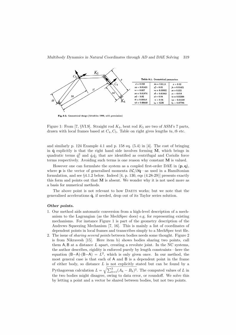
Figure 1: From [7, §VI.9]. Straight rod K4, bent rod K5 are two of ASM’s 7 parts,drawn with local frames based at C4, C5. Table on right gives lengths ta, tb etc.
and similarly p. 124 Example 4.1 and p. 158 eq. (5.4) in [4]. The cost of bringingin q explicitly is that the right hand side involves forming M, which brings inquadratic terms q2i and qiqj that are identified as centrifugal and Coriolis forceterms respectively. Avoiding such terms is one reason why constant M is valued.
However one can formulate the system as a coupled first-order DAE in (p,q),where p is the vector of generalised momenta ∂L/∂q—as used in a Hamiltonianformulation, and see §4.1.2 below. Indeed [4, p. 130, eqs (4.28-29)] presents exactlythis form and points out that M is absent. We wonder why it is not used more asa basis for numerical methods.
The above point is not relevant to how Daets works; but we note that thegeneralised accelerations q, if needed, drop out of its Taylor series solution.
Other points.
1. Our method aids automatic conversion from a high-level description of a mech-anism to the Lagrangian (as the MechSpec does) e.g. for representing existingmechanisms. For instance Figure 1 is part of the geometry description of theAndrews Squeezing Mechanism [7, 16]. This is mainly a list of coordinates ofdependent points in local frames and transcribes simply to a MechSpec text file.
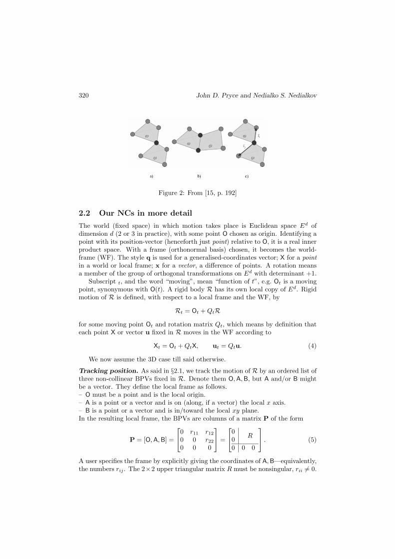
2. The issue of sharing several points between bodies needs some thought. Figure 2is from Nikravesh [15]. Here item b) shows bodies sharing two points, callthem A,B at a distance L apart, creating a revolute joint. In the NC systems,the author describes, rigidity is enforced purely by length constraints—here theequation (B−A)·(B−A) = L2, which is only given once. In our method, themost general case is that each of A and B is a dependent point in the frameof either body, so distance L is not explicitly stated but can be found by a
Pythagorean calculation L =√∑3
k=1(Ak −Bk)2. The computed values of L in
the two bodies might disagree, owing to data error, or roundoff. We solve thisby letting a point and a vector be shared between bodies, but not two points.
320 John D. Pryce and Nedialko S. Nedialkov
Figure 2: From [15, p. 192]
2.2 Our NCs in more detail
The world (fixed space) in which motion takes place is Euclidean space Ed ofdimension d (2 or 3 in practice), with some point O chosen as origin. Identifying apoint with its position-vector (henceforth just point) relative to O, it is a real innerproduct space. With a frame (orthonormal basis) chosen, it becomes the world-frame (WF). The style q is used for a generalised-coordinates vector; X for a pointin a world or local frame; x for a vector, a difference of points. A rotation meansa member of the group of orthogonal transformations on Ed with determinant +1.
Subscript t, and the word “moving”, mean “function of t”, e.g. Ot is a movingpoint, synonymous with O(t). A rigid body R has its own local copy of Ed. Rigidmotion of R is defined, with respect to a local frame and the WF, by
Rt = Ot +QtR
for some moving point Ot and rotation matrix Qt, which means by definition thateach point X or vector u fixed in R moves in the WF according to
Xt = Ot +QtX, ut = Qtu. (4)
We now assume the 3D case till said otherwise.
Tracking position. As said in §2.1, we track the motion of R by an ordered list ofthree non-collinear BPVs fixed in R. Denote them O,A,B, but A and/or B mightbe a vector. They define the local frame as follows.– O must be a point and is the local origin.– A is a point or a vector and is on (along, if a vector) the local x axis.– B is a point or a vector and is in/toward the local xy plane.In the resulting local frame, the BPVs are columns of a matrix P of the form
P = [O,A,B] =
0 r11 r120 0 r220 0 0
=
00
R
0 0 0
. (5)
A user specifies the frame by explicitly giving the coordinates of A,B—equivalently,the numbers rij . The 2×2 upper triangular matrix R must be nonsingular, rii 6= 0.
Multibody Dynamics in Natural Coordinates through AD and DAE Solving 321
Usually rii > 0, but this need not be so, e.g. by setting r11 < 0, the user puts A onthe negative side of the x axis.
Example 1. Let OA, OB have lengths 3 and 2√
2 and make an acute angle 45o.We may give coordinates A = (3, 0, 0)T along x direction, or A = (−3, 0, 0)T in theopposite direction. Any of (±2,±2, 0)T can be coordinates of B.
We form the unit vectors x = (1, 0, 0)T and y = (0, 1, 0)T in R as follows. InP = [O,A,B], if A [resp. B] is a point, we must replace it by the vector A−O [resp.B− O]. We write the subtraction(s) as PS, where
S =
−α −β1 00 1
, α =
{1 if A is a point,
0 if A is a vector,
similarly for β and B.
(6)
Denoting U = SR−1, we have
[x, y] =
1 00 10 0
= PU. (7)
During motion, the time-varying matrix in the WF corresponding to (5) is
Pt = [Ot,At,Bt].
The properties of rigid motion (4) imply that the relation (7) in the local framemust hold in the WF for all t, that is
[xt, yt] = Pt U = [Ot,At,Bt]U ; (8)
xt, and yt are the first two columns of Qt. Its third column is, by the assumedpositive orientation,
zt = xt×××yt. (9)
We write (8, 9) compactly as follows. For a 3 × 2 matrix M , let M ש be the3× 3 result of appending the cross product of its columns to it:
[u,v] ש = [u,v,u×××v]. (10)
Combining (8, 9, 10), finding the moving Qt from BPVs Ot,At,Bt is given, for allpoint/vector combinations of BPVs, by one formula
[xt, yt, zt] = Qt =([Ot,At,Bt] U
)ש . (11)
Dependent PVs in R are defined by giving their coordinates in the local frame.Once Ot and Qt are found, we simply compute by (4). For instance, if M is the(fixed) position of the centroid in the local frame, then at any time Mt = Ot+QtM.
Henceforth we drop the t.
322 John D. Pryce and Nedialko S. Nedialkov
Example 2. Let R be a 30o60o90o triangle ABC with long side AB of length 2.
Define the frame by points A =[000
]and B =
[200
]and a vector c =
[√310
]in the
direction AC. Then
S =
−1 01 00 1
, R =
[2√
30 1
], and U = SR−1 =
−1/2√
3/2
1/2 −√
3/20 1
.At time t, we are given computed A,B and c, and (8, 9) say
[x, y] = [A,B, c] U =[− 1
2A + 12B,
√32 A−
√32 B + c
], z = x×××y.
Tracking velocities and kinetic energy. Just as BPVs are in q or computabletherefrom, the velocities O, A, B are in q or computable therefrom. To express R’sKE in terms of them, differentiate (11). Eq. (8) is linear in the BPVs, so
[ ˙x, ˙y] = [O, A, B]U,
and from (9), on differentiating the bilinear operation x×××y,
Q = [ ˙x, ˙y, ˙z] where ˙z = ˙x×××y + x××× ˙y. (12)
Let M be the constant position of R’s centroid in its local frame. Then by (4, 12),the WF velocity M of this centroid is
M = O + QM, (13)
Recall that differentiating QTQ = I shows QT Q is a skew-symmetric matrix
equal to[ 0 −ω3 ω2ω3 0 −ω1−ω2 ω1 0
], where ωi are the components of the angular velocity vector
ωωω as seen from R’s frame. Extracting the relevant matrix entries, we have
ωωω =
z · ˙y
x · ˙z
y · ˙x
. (14)
From (13, 14), we obtain R’s kinetic energy T as a function of q and q:
T = 12mM2 + 1
2ωωωT IIIωωω, (15)
where m is R’s mass, and III is the moment of inertia matrix about axes throughthe centroid parallel to the local frame axes.
Multibody Dynamics in Natural Coordinates through AD and DAE Solving 323
Example 3. Consider a Free Top: a general rigid body R moving under no forces,except the constraint that its centroid is fixed at the WF origin O. Define the localframe by O and two orthogonal unit vectors u,v fixed in R. Let I be the inertiamatrix in this frame. In the working leading to (11), xt and yt equal ut and vt sowe use the latter, whence Qt = [ut,vt,wt] where wt = ut×××vt. Let q = (u,v).
There is no potential energy so the Lagrangian is just the kinetic energy, whichis purely rotational. Thus the complete formulation, in terms of q and q, is
w = u×××v, w = u×××v + u×××v, ωωω =
w · vu · wv · u
, L = 12ωωω
T IIIωωω, C =
u·u− 1v·v − 1
u·v
,
where the t have been dropped, L is the Lagrangian, and C is the vector of (residualsof) constraints. See the example code for this in §3 Lagrangian facility.
Kinematic constraints. As with JBNCs, we make a pin joint in 2D and aspheric joint in 3D happen implicitly, without generating constraint equations, justby sharing a point between two bodies. Similarly, a revolute joint in 3D can happenimplicitly by sharing a point on, and a vector along, the joint spine.
We try to use linear algebra ideas valid in any number of dimensions. E.g. in3D, to say line AB is in the direction of u, do not use cross product u×××(B−A) = 0,which makes three equations but only two are independent. Instead say B−A = µu:3 scalar equations plus a new scalar variable µ, correctly removing 3−1 = 2 DOF.Usually µ must be put in q. If this is part of the definition of a cylindric or prismaticjoint, µ might have the practical meaning of an actuator position.
One may reduce the number of coordinates by using assignments. E.g. thecylindrical joint in §4.2 is modelled in B−A = µu form, with A on one body, B onanother, and u shared between the bodies. But by the assignment B := A + µu,we keep B out of q and make the joint happen implicitly. Doing this depends onhow q’s components relate to the joint and is not always possible.
Shared vectors and points. One of the main uses of vectors is to be sharedbetween parts, e.g. the definition of the revolute and cylindric joints in the RSCRmechanism of §4.2 involves the joined parts having a common vector. We use vectorsto give direction, not distance. Any positive multiple has the same meaning: ineffect, vector v denotes the unit vector v/|v|. JBNCs (see [4, §1.2.2]) also use thispolicy, that for vectors, direction is relevant but length isn’t.
Shared points give no difficulty when two bodies have at most one in common.But as mentioned in §2.1, with two shared points they do, so we forbid this. Thedesired effect is gained by sharing a point and a vector.
2.3 The 2D case
This is similar to 3D but with smaller matrices:• There are two BPVs O,A, where O must be a point.
324 John D. Pryce and Nedialko S. Nedialkov
• The local frame is the one in which [O,A] =
[0 r110 0
], then R = [r11] is 1×1.
• (6) becomes S =
[−α1
], with α as there.
• ש acts on a 2×1 matrix
[uv
]to produce the 2×2 matrix
[uv
]ש =
[u −vv u
].
• U = SR−1 as before, and (11) becomes [x, y] = Q =([O,A] U
)ש.
• QT Q =
[0 −ωω 0
]with scalar angular velocity ω, and (14, 15) become
ω = y · ˙x, T = 12mM2 + 1
2I ω2,
where I is the scalar moment of inertia about the centroid.
3 The numerical infrastructure
The DAETS solver. The Daets (DAE by Taylor Series) solver [11, 12] acceptsa system of n DAEs in n state variables xj(t), 1 ≤ j ≤ n :
fi( t, the xj and derivatives of them ) = 0, 1 ≤ i ≤ n. (16)
The fi can be arbitrary expressions built from the xj and t using arithmetic oper-ations, standard functions (sin, exp, etc.), and the dp/dtp operation. We assumethe fi are sufficiently differentiable and hence exclude functions such as abs, min,and max in their definitions.
This solver implements a variable-stepsize, fixed-order2, explicit Taylor series(TS) method, where a typical order is in the range 12–20. Since the underlyingmethod for computing TS is not affected by the index, Daets handles any indexDAE. Furthermore, ODEs and pure algebraic systems are handled as a particularcase of the general formulation (16).
We outline how TS are computed for the simple pendulum given as a second-order, index-3 DAE:
0 = u+ λu
0 = v + λv −G0 = u2 + v2 − L.
Here(u(t), v(t)
)is position, λ(t) is a Lagrange multiplier, G is gravity, and L is
the length of the pendulum.
2An order is chosen at the beginning of an integration and is fixed throughout it.
Multibody Dynamics in Natural Coordinates through AD and DAE Solving 325
Write (at t = 0 without loss) u(t) = u0 + u1t+ u2t2 + · · · and similarly for v(t)
and λ(t). Substituting them into
a(t) = u+ λu (17)
b(t) = v + λv −G (18)
c(t) = u2 + v2 − L, (19)
we have for the coefficients in the expansions of a(t), b(t), and c(t): a0 = 2u2 + λ0u0b0 = 2v2 + λ0v0 −Gc0 = u20 + v20 − L2
(20)
a1 = 6u3 + λ0u1 + λ1u0b1 = 6v3 + λ0v1 + λ1v0c1 = 2u0u1 + 2v0v1
(21)
a2 = 24u4 + λ0u2 + λ1u1 + λ2u0b2 = 24v4 + λ0v2 + λ1v1 + λ2v0c2 = 2u0u2 + u21 + 2v0v2 + v21
(22)
and so on. We refer to the above coefficients as Taylor coefficients (TCs). Byequating the TCs in (20, 21, 22) to zero, we solve for the TCs of u, v, λ. This is notobvious from (20, 21, 22), but proceeds as follows.
Given initial values for u0 and v0, check if they satisfy the constraint
0 = c0 = u20 + v20 − L2, (23)
and if not adjust u0 or v0 or both.Using u0, v0 as constants, and given values for u1 and v1, check if they satisfy
the constraint
0 = c1 = 2(u0u1 + v0v1), (24)
and if not adjust u1 or v1 or both.Then for k = 0 up to some order K, we solve a linear system
0 = ak+0, bk+0, ck+2 for uk+2, vk+2, λk+0 (25)
using previously computed coefficients as constants. E.g., when k = 0, we solve
0=a0=2u2+λ0u00=b0=2v2+λ0v0−G0=c2=2u0u2+2v0v2+u21+v21
, i.e.
2 0 u00 2 v0
2u0 2v0 0
u2v2λ0
=
0G
−u21−v21
(26)
for u2, v2, λ0 using u0, v0, u1, v1 as known.The computational scheme for TCs is guided by two nonnegative integer vectors,
equation offsets ci and variable offsets dj , here (0, 0, 2) and (2, 2, 0), respectively;
326 John D. Pryce and Nedialko S. Nedialkov
cf. (25). These vectors are found by Pryce’s structural analysis (SA) [18], detailsomitted. There is a set of “SA-amenable” DAEs that (when smooth enough) canbe expanded in TS in a similar way. This is the same set on which one can usePantelides SA [17] and the Mattsson–Soderlind dummy derivative method [10]. Itincludes all index-3 Euler-Lagrange DAEs [18, Theorem 5.3].
From
u(t) ≈ u(t) =
K+2∑i=0
uiti, v(t) ≈ v(t) =
K+2∑i=0
viti, λ(t) ≈ λ(t) =
K∑i=0
λiti,
given stepsize h, we compute an approximate TS solution at t1 = h, and by differ-entiating u(t) and v(t), we approximate u and v at t1 and repeat the above processstarting at t1.
We present a few implementation details below. Daets requires a templatedC++ function for evaluating the fi’s. The simple pendulum is encoded e.g. as
template <typename T>
void fcn(T t, const T* x, T* f, void* param) {
double G = 9.81, L = 10.0;
T u = x[0], v = x[1], lam = x[2];
f[0] = Diff(u, 2) + lam * u;
f[1] = Diff(v, 2) + lam * v - G;
f[2] = sqr(u) + sqr(v) - sqr(L);
}
On input, t is the time variable (not used here), x[j-1] contains the jth statevariable; on output f[i-1] stores fi. The last argument, param (not used here), isto pass parameters from the solver. The Diff(·, p) function implements dp/dtp.
Before integration starts, Daets performs SA by executing the fi’s code, herefcn, through operator overloading to find the DAE index, dof, and the offsetvectors. Then the solver executes the same function with FADBAD++’s Taylorseries class to build in memory a computational graph, which is evaluated on eachintegration step to compute TCs for the fi’s; in our example (20, 21, 22).
The constraints of the problem are satisfied by orthogonal projection. For ex-ample, denoting u = (u, v), u0 = (u0, v0), (23) is done by solving
minu‖u− u0‖2 s.t. 0 = u2 + v2 − L2;
similarly for (24).Since the stepsize is selected based on a tolerance specified by the user, the TS
solution on each integration step is very close to satisfying the constraints, and oneor two iterations of Gauss-Newton suffice to project this solution. On the first stepthough, the IVs given by the user may not be close to satisfying the constraints:here we use the Ipopt [23] optimisation package, see below. In terms of IVs, theuser can fix one of the values for u and v, and Daets would try to solve for theother; similarly for u, v.
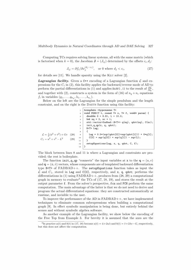
Multibody Dynamics in Natural Coordinates through AD and DAE Solving 327
Computing TCs requires solving linear systems, all with the same matrix (whichis factorised when k = 0), the Jacobian J = (Jij) determined by the offsets ci, dj :
Jij = ∂fi/∂x(dj−ci)j , or 0 where dj < ci, (27)
for details see [11]. We handle sparsity using the Klu solver [2].
Lagrangian facility. Given a C++ encoding of a Lagrangian function L and ex-pressions for the Ci in (2), this facility applies the backward/reverse mode of AD toperform the partial differentiations in (1) and applies Diff(·, 1) to the result of ∂L
∂qj,
and together with (2), constructs a system in the form of (16) of nq +nc equationsfi in variables (q1, . . . , qnq
, λ1, . . . , λnc).
Below on the left are the Lagrangian for the simple pendulum and the lengthconstraint, and on the right is the Daets function using this facility:
L = 12
(u2 + v2) +Gv (28)
C1 = u2 + v2 − L2 (29)
1 template <typename T>
2 void PEND(T t, const T* x, T* f, void* param) {
3 double G = 9.81, L = 10.0;
4 int nq = 2, nc = 1;
5 std::vector<fadbad::B<T>> q(nq), qdot(nq), C(nc);
6 init_q_qp(x, q, qdot);
7 B<T> Lag;
8 {
9 Lag = 0.5*(sqr(qdot[0])+sqr(qdot[1])) + G*q[1];
10 C[0] = sqr(q[0]) + sqr(q[1]) - sqr(L);
11 }
12 setupEquations(Lag, x, q, qdot, C, f);
13 }
The block between lines 8 and 11 is where a Lagrangian and constraints are pro-vided; the rest is boilerplate.
The function init_q_qp “connects” the input variables at x to the q = (u, v)and q = (u, v) vectors, whose components are of templated backward differentiationtype B<T> of FADBAD++. The setupEquations function takes as input theL and C1, stored in Lag and C[0], respectively, and x, q, qdot; performs thedifferentiations in (1) using FADBAD++, produces from (28, 29) a computationalgraph in memory to evaluate3 the TCs of (17, 18, 19), and stores the result at theoutput parameter f. From the solver’s perspective, fcn and FCN perform the samecomputation. The main advantage of the latter is that we do not need to derive andprogram the actual differentiated equations: they are constructed automatically atruntime, and invisible to the user.
To improve the performance of the AD in FADBAD++, we have implementedtechniques to eliminate common subexpressions when building a computationalgraph [9]. In effect symbolic manipulation is being done, but entirely behind thescenes and without symbolic algebra software.
As another example of the Lagrangian facility, we show below the encoding ofthe Free Top from Example 3. For brevity it is assumed that the axes are the
3In practice a(t) and b(t) in (17, 18) become a(t) = u+2uλ and b(t) = v+2λv−G, respectively,but this does not affect the computation.
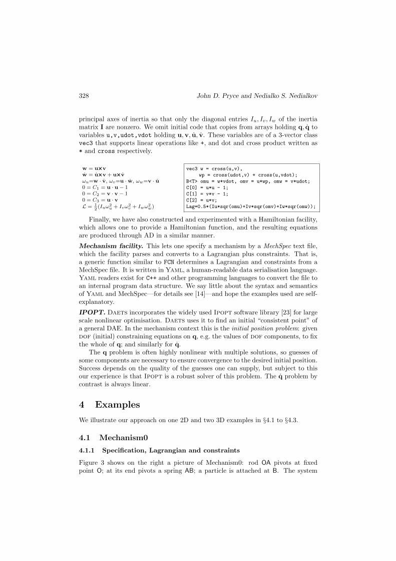
328 John D. Pryce and Nedialko S. Nedialkov
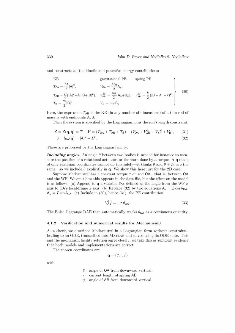
principal axes of inertia so that only the diagonal entries Iu, Iv, Iw of the inertiamatrix I are nonzero. We omit initial code that copies from arrays holding q, q tovariables u,v,udot,vdot holding u,v, u, v. These variables are of a 3-vector classvec3 that supports linear operations like +, and dot and cross product written as* and cross respectively.
w = u×××vw = u×××v + u×××vωu=w · v, ωv=u · w, ωw=v · u0 = C1 = u · u− 10 = C2 = v · v − 10 = C3 = u · vL = 1
2(Iuω2
u + Ivω2v + Iwω2
w)
vec3 w = cross(u,v),
wp = cross(udot,v) + cross(u,vdot);
B<T> omu = w*vdot, omv = u*wp, omw = v*udot;
C[0] = u*u - 1;
C[1] = v*v - 1;
C[2] = u*v;
Lag=0.5*(Iu*sqr(omu)+Iv*sqr(omv)+Iw*sqr(omw));
Finally, we have also constructed and experimented with a Hamiltonian facility,which allows one to provide a Hamiltonian function, and the resulting equationsare produced through AD in a similar manner.
Mechanism facility. This lets one specify a mechanism by a MechSpec text file,which the facility parses and converts to a Lagrangian plus constraints. That is,a generic function similar to FCN determines a Lagrangian and constraints from aMechSpec file. It is written in Yaml, a human-readable data serialisation language.Yaml readers exist for C++ and other programming languages to convert the file toan internal program data structure. We say little about the syntax and semanticsof Yaml and MechSpec—for details see [14]—and hope the examples used are self-explanatory.
IPOPT. Daets incorporates the widely used Ipopt software library [23] for largescale nonlinear optimisation. Daets uses it to find an initial “consistent point” ofa general DAE. In the mechanism context this is the initial position problem: givendof (initial) constraining equations on q, e.g. the values of dof components, to fixthe whole of q; and similarly for q.
The q problem is often highly nonlinear with multiple solutions, so guesses ofsome components are necessary to ensure convergence to the desired initial position.Success depends on the quality of the guesses one can supply, but subject to thisour experience is that Ipopt is a robust solver of this problem. The q problem bycontrast is always linear.
4 Examples
We illustrate our approach on one 2D and two 3D examples in §4.1 to §4.3.
4.1 Mechanism0
4.1.1 Specification, Lagrangian and constraints
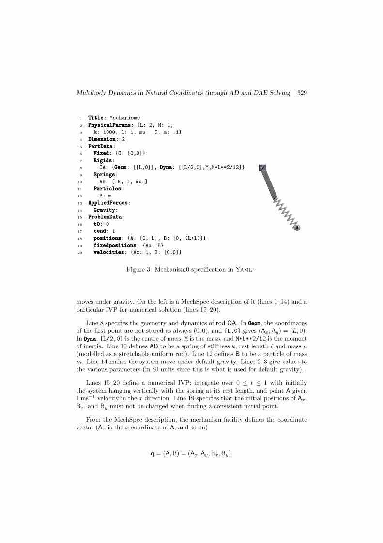
Figure 3 shows on the right a picture of Mechanism0: rod OA pivots at fixedpoint O; at its end pivots a spring AB; a particle is attached at B. The system
Multibody Dynamics in Natural Coordinates through AD and DAE Solving 329
1 TitleTitleTitle: Mechanism0 ##
2 PhysicalParamsPhysicalParamsPhysicalParams: {L: 2, M: 1, ##
3 k: 1000, l: 1, mu: .5, m: .1} ##
4 DimensionDimensionDimension: 2 ##
5 PartDataPartDataPartData: ##
6 FixedFixedFixed: {O: [0,0]} ##
7 RigidsRigidsRigids:
8 OA: {GeomGeomGeom: [[L,0]], DynaDynaDyna: [[L/2,0],M,M*L**2/12]} ##
9 SpringsSpringsSprings:
10 AB: [ k, l, mu ] ##
11 ParticlesParticlesParticles:
12 B: m ##
13 AppliedForcesAppliedForcesAppliedForces: ##
14 GravityGravityGravity: ##
15 ProblemDataProblemDataProblemData: ##
16 t0t0t0: 0
17 tendtendtend: 1
18 positionspositionspositions: {A: [0,-L], B: [0,-(L+l)]}
19 fixedpositionsfixedpositionsfixedpositions: {Ax, B} ##
20 velocitiesvelocitiesvelocities: {Ax: 1, B: [0,0]} ##
Figure 3: Mechanism0 specification in Yaml.
moves under gravity. On the left is a MechSpec description of it (lines 1–14) and aparticular IVP for numerical solution (lines 15–20).
Line 8 specifies the geometry and dynamics of rod OA. In GeomGeomGeom, the coordinatesof the first point are not stored as always (0, 0), and [L,0] gives (Ax,Ay) = (L, 0).In DynaDynaDyna, [L/2,0] is the centre of mass, M is the mass, and M*L**2/12 is the momentof inertia. Line 10 defines AB to be a spring of stiffness k, rest length ` and mass µ(modelled as a stretchable uniform rod). Line 12 defines B to be a particle of massm. Line 14 makes the system move under default gravity. Lines 2–3 give values tothe various parameters (in SI units since this is what is used for default gravity).
Lines 15–20 define a numerical IVP: integrate over 0 ≤ t ≤ 1 with initiallythe system hanging vertically with the spring at its rest length, and point A given1 ms−1 velocity in the x direction. Line 19 specifies that the initial positions of Ax,Bx, and By must not be changed when finding a consistent initial point.
From the MechSpec description, the mechanism facility defines the coordinatevector (Ax is the x-coordinate of A, and so on)
q = (A,B) = (Ax,Ay,Bx,By).
330 John D. Pryce and Nedialko S. Nedialkov
and constructs all the kinetic and potential energy contributions:
KE gravitational PE spring PE
TOA =M
6|A|2, VOA =
Mg
2Ay,
TAB =µ
6(|A|2+A · B+|B|2), V
[g]AB =
µg
2(Ay+By), V
[s]AB =
k
2(|B− A| − `)2 ,
TB =m
2|B|2, VB = mg By.
(30)
Here, the expression TAB is the KE (in any number of dimensions) of a thin rod ofmass µ with endpoints A,B.
Then the system is specified by the Lagrangian, plus the rod’s length constraint:
L = L(q, q) = T − V = (TOA + TAB + TB)− (VOA + V[g]AB + V
[s]AB + VB), (31)
0 = lOA(q) = |A|2 − L2. (32)
These are processed by the Lagrangian facility.
Including angles. An angle θ between two bodies is needed for instance to mea-sure the position of a rotational actuator, or the work done by a torque. A q madeof only cartesian coordinates cannot do this safely—it thinks θ and θ + 2π are thesame—so we include θ explicitly in q. We show this here just for the 2D case.
Suppose Mechanism0 has a constant torque τ on rod OA—that is, between OAand the WF. We omit how this appears in the data file, but the effect on the modelis as follows. (a) Append to q a variable θOA defined as the angle from the WF xaxis to OA’s local-frame x axis. (b) Replace (32) by two equations Ax = L cos θOA,Ay = L sin θOA. (c) Include in (30), hence (31), the PE contribution
V[τ ]OA = −τ θOA. (33)
The Euler–Lagrange DAE then automatically tracks θOA as a continuous quantity.
4.1.2 Verification and numerical results for Mechanism0
As a check, we described Mechanism0 in a Lagrangian form without constraints,leading to an ODE, transcribed into Matlab and solved using its ODE suite. Thisand the mechanism facility solution agree closely; we take this as sufficient evidencethat both models and implementations are correct.
The chosen coordinates are
q = (θ, r, φ)
with
θ : angle of OA from downward vertical;r : current length of spring AB;φ : angle of AB from downward vertical.
Multibody Dynamics in Natural Coordinates through AD and DAE Solving 331
With these coordinates, we have positions and velocities
A = L (sin θ,− cos θ), B = A + r (sinφ,− cosφ),
A = L (cos θ, sin θ)θ, B = A + (sinφ,− cosφ)r + r (cosφ, sinφ)φ.
}
The Lagrangian is still given by (31) with extra term (33). Now (30) becomes
KE gravitational PE spring or torque PE
TOA = 16ML2θ2, VOA= − 1
2MgL cos θ V
[τ ]OA = −τθ
TAB = 12µ(L2θ2 + L sin(φ− θ)θr + Lr cos(φ− θ)θφ+ 1
3(r2 + r2φ2)
),
V[g]AB = −µg(L cos θ + 1
2r cosφ), V
[s]AB = 1
2k (r − `)2 ,
TB = 12m(L2θ2 + 2L sin(φ− θ)θr + 2Lr cos(φ− θ)θφ+ r2 + r2φ2
),
VB= −mg(L cos θ + r cosφ),
where θOA has been changed to θ in the torque PE, which is valid because thesetwo angles differ by a constant. This gives three equations of motion
d
dt
∂L∂q
=∂L∂q
, call the latter F (q, q). (34)
For the numerics, introduce the Hamiltonian generalised momentum vector
p = ∂L/∂q, here, q = (θ, r, φ).
Now p = M(q)q—linear in q—where M is the symmetric mass matrix. Here
M = M(θ, r, φ) = (13M + µ+m
)L2 ( 1
2µ+m)L sin(φ− θ) ( 12µ+m)Lr cos(φ− θ)
( 12µ+m)L sin(φ− θ) 1
3µ+m 0( 12µ+m)Lr cos(φ− θ) 0 ( 1
3µ+m)r2
Now (34) becomes two first-order vector ODEs, making 6 scalar equations:
q = M(q)−1p, p = F (q, q).
Note the block triangular structure: find q first, and use it to find p.The mechanism facility program and the Matlab program read the same Yaml
problem file. The IVs specify the position and velocity of A = (Ax,Ay) and B =
(Bx,By). They might not be consistent: A might not lie on, and A might notbe tangential to, the circle of radius L round O. Daets finds consistent pointsby calling the optimisation code Ipopt. To make the result predictable, we useDaets’s ability to specify some IVs “fixed”, not to be modified by Ipopt. Here,one of Ax,Ay may be fixed and also one of Ax, Ay. To ensure both codes solve thesame IVP, the Matlab code is made to do the same, e.g. if Ax is “fixed” it sets
332 John D. Pryce and Nedialko S. Nedialkov
0 1 2 3 4 5 6 7 8 9 10time t
10-14
10-12
10-10
10-8
10-6
10-4
10-2
norm
(OD
E s
ol -
DA
ET
S s
ol)
Mechanism0: difference of solutions including both position & velocity
tol=1e-5tol=1e-7tol=1e-9tol=1e-11tol=1e-13
(a)
0 1 2 3 4 5 6 7 8 9 10time t
10-14
10-12
10-10
10-8
10-6
10-4
10-2
norm
(OD
E s
ol -
DA
ET
S s
ol)
Mechanism0: approx global error including both position & velocitytol=1e-5tol=1e-7tol=1e-9tol=1e-11tol=1e-13
(b)
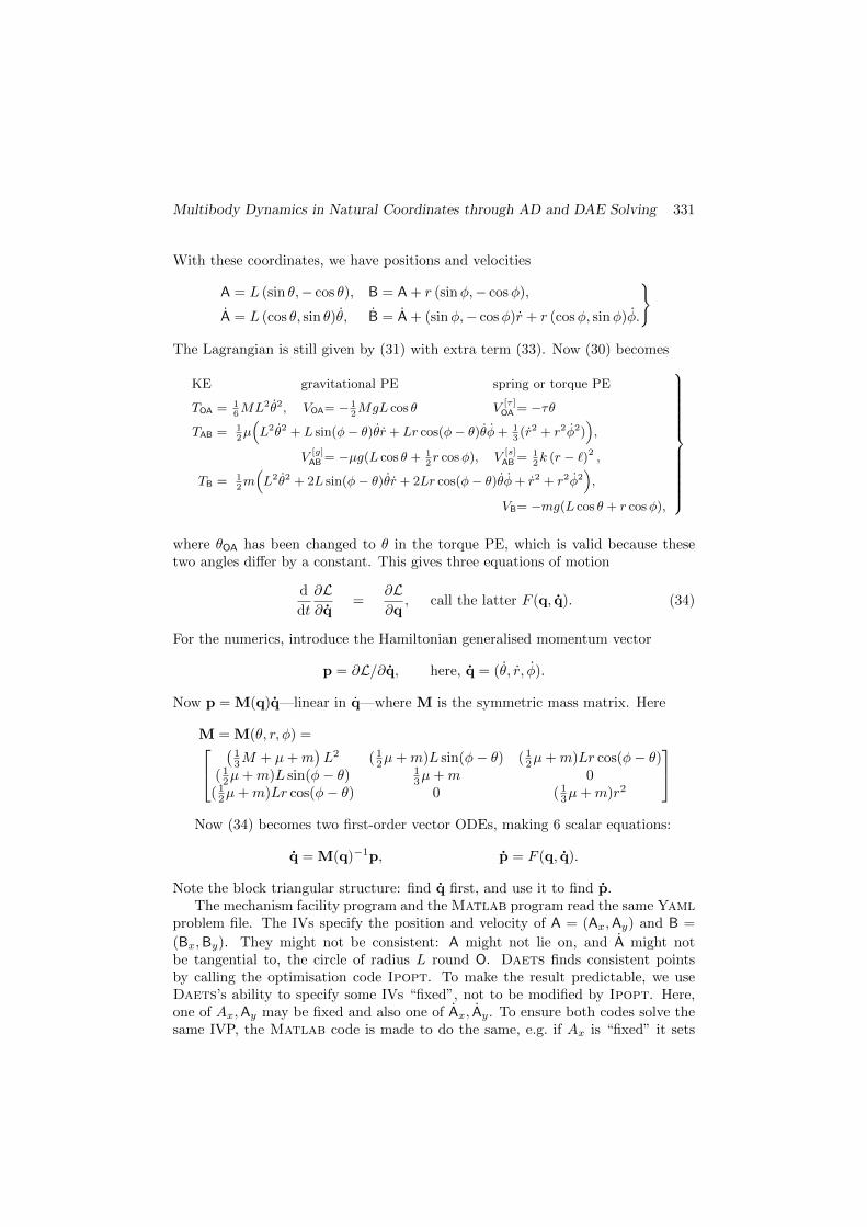
Figure 4: (a) Comparison of Daets and ode113 solutions at different tolerances.(b) Estimated global error: (ode113 solution at tol = 2.2e-14) – (Daets solution).
Ay = ±√L2 −A2
x. We omit details to do with choice of sign and possible numericalill-conditioning.
To test agreement between Daets and ODE solution, we used ode113. Foreach tolerance tol, the 8-element vector v = (A,B, A, B) (positions and velocities)was formed for each solver at each t. A feature of the Matlab ODE suite is thatoutput can be produced, to full accuracy, at each t in a vector of values that is givenas input to the solver call. That is, we produced output with ode113 at points tselected by Daets.
Figure 4(a) shows ‖vDaets − vODE‖2 against t for 5 tolerances tol, with avertical log scale. The growth of the difference is much the same for each tol:about 3 orders of magnitude over the range. The curves at different tol obviouslyare strongly correlated; so far we have not looked into why this is.
Figure 4(a) shows an assessment of the global error of the Daets solution.Namely vODE (at the given tol) is replaced by a reference solution vref which wetook to be the ode113 solution with tol = 2.2e-14, about the smallest toleranceit allows. So it plots ‖vDaets−vref‖2 against t for each tol. The plots show theseerrors grow more slowly than the differences on the left: they are about ten timessmaller at t = 10. This suggests the difference vDaets−vODE is mostly due to globalerror in the ode113 solutions, and Daets is somewhat more accurate than ode113.
4.2 The RSCR mechanism
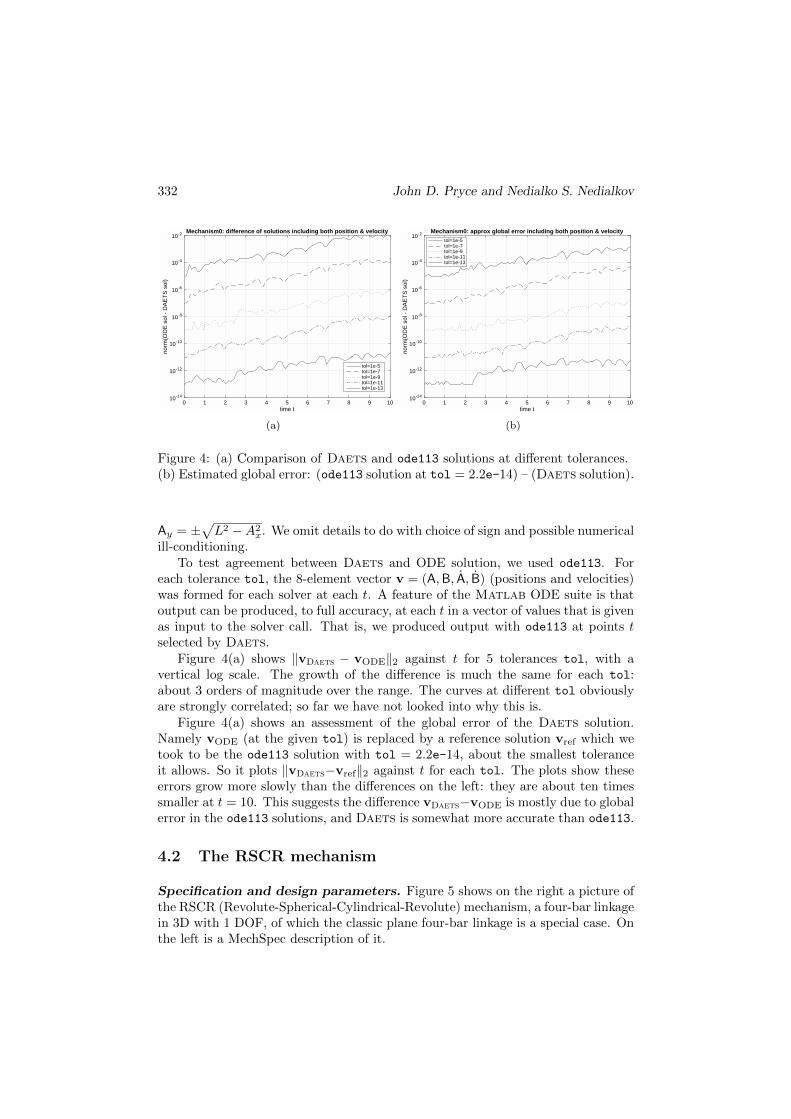
Specification and design parameters. Figure 5 shows on the right a picture ofthe RSCR (Revolute-Spherical-Cylindrical-Revolute) mechanism, a four-bar linkagein 3D with 1 DOF, of which the classic plane four-bar linkage is a special case. Onthe left is a MechSpec description of it.
Multibody Dynamics in Natural Coordinates through AD and DAE Solving 333
1 DimensionDimensionDimension: 3
2 PartDataPartDataPartData:3 FixedFixedFixed:4 D: [0,0,0]
5 A: [-L0,0,0]
6 w: [cos(d2r*d),sin(d2r*d),0]
7 u: [cos(d2r*a)*sin(d2r*b),
8 sin(d2r*a)*sin(d2r*b),cos(d2r*b)]
9 RigidsRigidsRigids:10 ABu: {GeomGeomGeom:[[L1],[0,1]],11 DynaDynaDyna:[[L1/2],m1,m1*L1**2/12]}12 CBv: {GeomGeomGeom:[[L2],[0,1]],13 DynaDynaDyna:[[L2/2],m2,m2*L2**2/12]}14 DC1wv: {GeomGeomGeom:[[L3],[0,1],[0,cos(c),sin(c)]],15 DynaDynaDyna:[[L3/2],m3,m3*L3**2/12]}16 Collinears: {C1vC}
Figure 5: RSCR mechanism. MechSpec text on the left. The 8 parameters definingthe geometry are L0, L1, L2, L3 (lengths DA, AB, BC, C1D), and α, β, γ, δ (angles,see text), written a,b,c,d in the MechSpec; d2r stores π/180. By a “paddingconvention”, omitted trailing coordinates are zero, e.g. [L1] means [L1,0,0], thepoint (L1, 0, 0).
As a mnemonic, WF-fixed items are underlined, e.g. A for a point, u for a vector;others are moving. The moving parts are 1©, 2©, 3©, with joints at A, B, C, D. Thejoint spines at A and D are fixed in the WF, along vectors u and w respectively.Point C1 is fixed on 3© and on the cylindric joint spine which is along v. We canput A,C,C1,D anywhere along the relevant spines, so without loss assume• line AB ⊥ (perpendicular to) spine at A;• line CB ⊥ spine at C;• line DC1 ⊥ spines at both D and C1.We fix the WF to have origin at D with DA the negative x axis, A at (−L0, 0, 0),
and the joint spine at D in the xy plane. The latter’s direction w is arbitrary inthis plane, say w = (cos δ, sin δ, 0)T . The spine at A is now in an arbitrary WFdirection, say u = (cosα sinβ, sinα sinβ, cosβ)T with spherical polar angless α, β.
In 3©, the cylindric and the revolute joint spines are skew, non-intersecting linesin general. Projected on a plane normal to DC1, the former, at C1, is rotated anarbitrary γ from the latter, at D, so in 3©’s local frame it is along
v = (0, cos γ, sin γ)T (35)
Vector v moves in the WF and is fixed in both 2© and 3©.
Local frames and coordinate vector. We choose 1©’s local origin at A, 2©’s atC, 3©’s at D, and in each case the x axis along the part’s length, and the xy planedefined by a unit vector along the joint spine that passes through the local origin.Since these spines are orthogonal to the part lengths by construction, the R matrix(5) of each frame is diagonal.
334 John D. Pryce and Nedialko S. Nedialkov
Table 1: RSCR: assignments and equations.
Bring in Assign Equate DOF
3©: DC1wv rigidity.
C1
x3 := C1/L3
z3 := x3×××w
v := cos(γ)w + sin(γ)z3
0 = C21 − L2
3
0 = C1 ·w+3 − 2 (37)
2©: CBv rigidity, and specify cylindric joint
B, µ C := C1 + µv0 = (B− C)2 − L2
2
0 = (B− C) · v+3 + 1 − 2 (38)
1©: ABu rigidity
0 = (B− A)2 − L21
0 = (B− A) · u− 2 (39)
Net DOF: 1 = +7 − 6
To specify the constraints in Table 1, only 3© needs full frame details, given bythe BPVs DC1w in that order, so from (5, 6, 8), its U -matrix U3 comes from
A3=[D,C1,w]=
0 L3 00 0 10 0 0
, U3 =
−1 01 00 1
[L3 00 1
]−1=
− 1L3
01L3
0
0 1
.The moving basic points are C1,B. Bringing in parts in order 3©, 2©, 1© as in
Table 1, we express v by an assignment in terms of C1, then C by an assignmentin terms of C1, v and a scalar µ. So the coordinate vector need only be
q = (C1,B, µ) with 3× 2 + 1 = 7 scalar components. (36)
Kinematics: the constraint equations. Here all positions and vectors are in theWF. The joints, handled as in §2.2 Kinematic constraints, generate no equations,so the only constraints are rigidity equations. Namely for each part: (i) a linejoining two points has specified length and (ii) a unit vector is orthogonal to thisline. This makes 2 equations per part, a total of 6.
The moving frame of 3© is needed to define vector v along the spine of thecylindric joint. Denote its unit vectors (the columns of Q3) as x3, y3, z3, where x3
along DC1 is defined by
x3 = (C1 − D)/L3 = C1/L3. (40)
Multibody Dynamics in Natural Coordinates through AD and DAE Solving 335
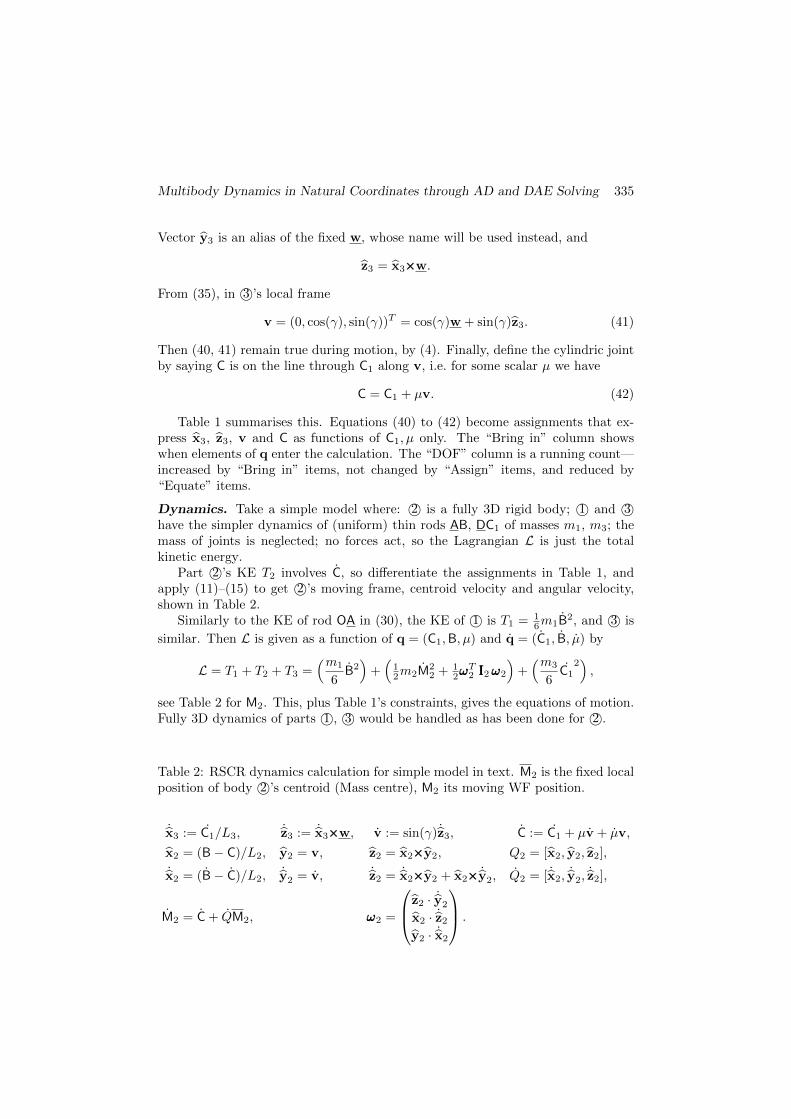
Vector y3 is an alias of the fixed w, whose name will be used instead, and
z3 = x3×××w.
From (35), in 3©’s local frame
v = (0, cos(γ), sin(γ))T = cos(γ)w + sin(γ)z3. (41)
Then (40, 41) remain true during motion, by (4). Finally, define the cylindric jointby saying C is on the line through C1 along v, i.e. for some scalar µ we have
C = C1 + µv. (42)
Table 1 summarises this. Equations (40) to (42) become assignments that ex-press x3, z3, v and C as functions of C1, µ only. The “Bring in” column showswhen elements of q enter the calculation. The “DOF” column is a running count—increased by “Bring in” items, not changed by “Assign” items, and reduced by“Equate” items.
Dynamics. Take a simple model where: 2© is a fully 3D rigid body; 1© and 3©have the simpler dynamics of (uniform) thin rods AB, DC1 of masses m1, m3; themass of joints is neglected; no forces act, so the Lagrangian L is just the totalkinetic energy.
Part 2©’s KE T2 involves C, so differentiate the assignments in Table 1, andapply (11)–(15) to get 2©’s moving frame, centroid velocity and angular velocity,shown in Table 2.
Similarly to the KE of rod OA in (30), the KE of 1© is T1 = 16m1B
2, and 3© is
similar. Then L is given as a function of q = (C1,B, µ) and q = (C1, B, µ) by
L = T1 + T2 + T3 =(m1
6B2)
+(
12m2M
22 + 1
2ωωωT2 III2ωωω2
)+(m3
6C1
2),
see Table 2 for M2. This, plus Table 1’s constraints, gives the equations of motion.Fully 3D dynamics of parts 1©, 3© would be handled as has been done for 2©.
Table 2: RSCR dynamics calculation for simple model in text. M2 is the fixed localposition of body 2©’s centroid (Mass centre), M2 its moving WF position.
˙x3 := C1/L3, ˙z3 := ˙x3×××w, v := sin(γ) ˙z3, C := C1 + µv + µv,
x2 = (B− C)/L2, y2 = v, z2 = x2×××y2, Q2 = [x2, y2, z2],
˙x2 = (B− C)/L2, ˙y2 = v, ˙z2 = ˙x2×××y2 + x2××× ˙y2, Q2 = [ ˙x2, ˙y2,˙z2],
M2 = C + QM2, ωωω2 =
z2 · ˙y2
x2 · ˙z2y2 · ˙x2
.
336 John D. Pryce and Nedialko S. Nedialkov
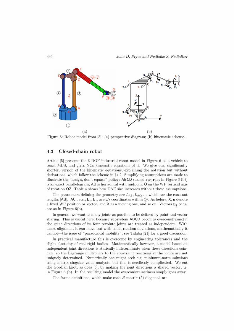
(a) (b)
Figure 6: Robot model from [5]: (a) perspective diagram; (b) kinematic scheme.
4.3 Closed-chain robot
Article [5] presents the 6 DOF industrial robot model in Figure 6 as a vehicle toteach MBS, and gives NCs kinematic equations of it. We give our, significantlyshorter, version of the kinematic equations, explaining the notation but withoutderivations, which follow the scheme in §4.2. Simplifying assumptions are made toillustrate the “assign, don’t equate” policy: ABCD (called r2r3r4r5 in Figure 6 (b))is an exact parallelogram; AB is horizontal with midpoint O on the WF vertical axisof rotation OZ. Table 4 shows how DAE size increases without these assumptions.
The parameters defining the geometry are LAB, LAC, . . . which are the constantlengths |AB|, |AC|, etc.; Ex,Ez, are E’s coordinates within 5©. As before, X,u denotea fixed WF position or vector, and X,u a moving one, and so on. Vectors u1 to u5
are as in Figure 6(b).
In general, we want as many joints as possible to be defined by point and vectorsharing. This is useful here, because subsystem ABCD becomes overconstrained ifthe spine directions of its four revolute joints are treated as independent. Withexact alignment it can move but with small random deviations, mathematically itcannot—the issue of “paradoxical mobility”, see Talaba [21] for a good discussion.
In practical manufacture this is overcome by engineering tolerances and theslight elasticity of real rigid bodies. Mathematically however, a model based onindependent joint directions is statically indeterminate when these directions coin-cide, so the Lagrange multipliers to the constraint reactions at the joints are notuniquely determined. Numerically one might seek e.g. minimum-norm solutionsusing matrix singular value analysis, but this is needlessly complicated. We cutthe Gordian knot, as does [5], by making the joint directions a shared vector, u3
in Figure 6 (b). In the resulting model the overconstrainedness simply goes away.
The frame definitions, which make each R matrix (5) diagonal, are
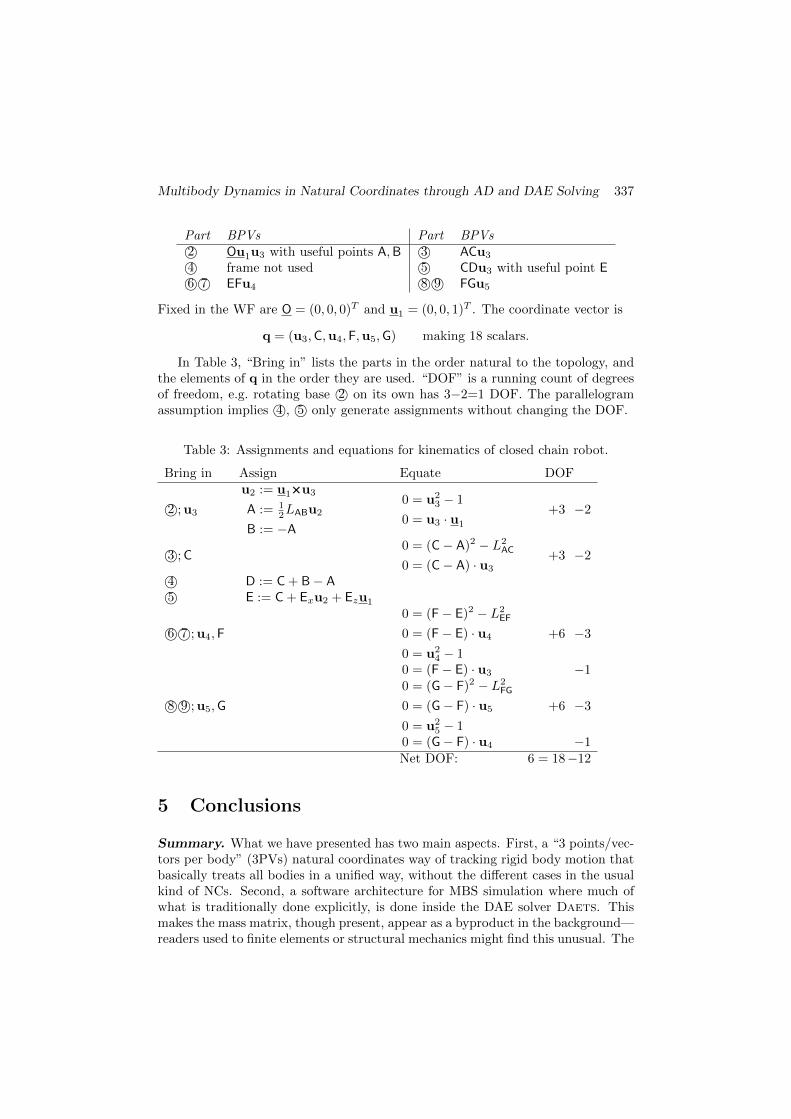
Multibody Dynamics in Natural Coordinates through AD and DAE Solving 337
Part BPVs Part BPVs2© Ou1u3 with useful points A,B 3© ACu3
4© frame not used 5© CDu3 with useful point E6© 7© EFu4 8© 9© FGu5
Fixed in the WF are O = (0, 0, 0)T and u1 = (0, 0, 1)T . The coordinate vector is
q = (u3,C,u4,F,u5,G) making 18 scalars.
In Table 3, “Bring in” lists the parts in the order natural to the topology, andthe elements of q in the order they are used. “DOF” is a running count of degreesof freedom, e.g. rotating base 2© on its own has 3−2=1 DOF. The parallelogramassumption implies 4©, 5© only generate assignments without changing the DOF.
Table 3: Assignments and equations for kinematics of closed chain robot.
Bring in Assign Equate DOF
2©; u3
u2 := u1×××u3
A := 12LABu2
B := −A
0 = u23 − 1
0 = u3 · u1
+3 −2
3©;C0 = (C− A)2 − L2
AC
0 = (C− A) · u3
+3 −2
4© D := C + B− A5© E := C + Exu2 + Ezu1
6© 7©; u4,F
0 = (F− E)2 − L2EF
0 = (F− E) · u4
0 = u24 − 1
+6 −3
0 = (F− E) · u3 −1
8© 9©; u5,G
0 = (G− F)2 − L2FG
0 = (G− F) · u5
0 = u25 − 1
+6 −3
0 = (G− F) · u4 −1Net DOF: 6 = 18−12
5 Conclusions
Summary. What we have presented has two main aspects. First, a “3 points/vec-tors per body” (3PVs) natural coordinates way of tracking rigid body motion thatbasically treats all bodies in a unified way, without the different cases in the usualkind of NCs. Second, a software architecture for MBS simulation where much ofwhat is traditionally done explicitly, is done inside the DAE solver Daets. Thismakes the mass matrix, though present, appear as a byproduct in the background—readers used to finite elements or structural mechanics might find this unusual. The
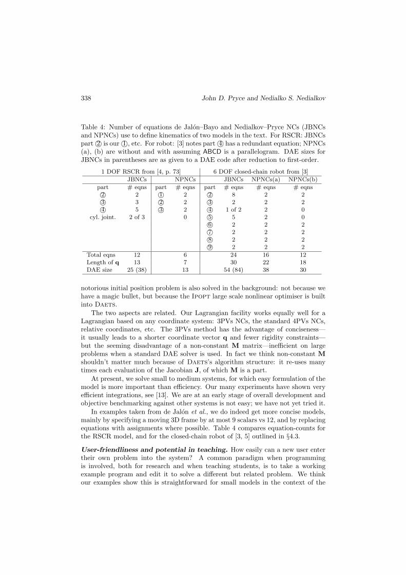
338 John D. Pryce and Nedialko S. Nedialkov
Table 4: Number of equations de Jalon–Bayo and Nedialkov–Pryce NCs (JBNCsand NPNCs) use to define kinematics of two models in the text. For RSCR: JBNCspart 2© is our 1©, etc. For robot: [3] notes part 4© has a redundant equation; NPNCs(a), (b) are without and with assuming ABCD is a parallelogram. DAE sizes forJBNCs in parentheses are as given to a DAE code after reduction to first-order.
1 DOF RSCR from [4, p. 73] 6 DOF closed-chain robot from [3]
JBNCs NPNCs JBNCs NPNCs(a) NPNCs(b)
part # eqns part # eqns part # eqns # eqns # eqns2© 2 1© 2 2© 8 2 23© 3 2© 2 3© 2 2 24© 5 3© 2 4© 1 of 2 2 0
cyl. joint. 2 of 3 0 5© 5 2 06© 2 2 27© 2 2 28© 2 2 29© 2 2 2
Total eqns 12 6 24 16 12Length of q 13 7 30 22 18DAE size 25 (38) 13 54 (84) 38 30
notorious initial position problem is also solved in the background: not because wehave a magic bullet, but because the Ipopt large scale nonlinear optimiser is builtinto Daets.
The two aspects are related. Our Lagrangian facility works equally well for aLagrangian based on any coordinate system: 3PVs NCs, the standard 4PVs NCs,relative coordinates, etc. The 3PVs method has the advantage of conciseness—it usually leads to a shorter coordinate vector q and fewer rigidity constraints—but the seeming disadvantage of a non-constant M matrix—inefficient on largeproblems when a standard DAE solver is used. In fact we think non-constant Mshouldn’t matter much because of Daets’s algorithm structure: it re-uses manytimes each evaluation of the Jacobian J, of which M is a part.
At present, we solve small to medium systems, for which easy formulation of themodel is more important than efficiency. Our many experiments have shown veryefficient integrations, see [13]. We are at an early stage of overall development andobjective benchmarking against other systems is not easy; we have not yet tried it.
In examples taken from de Jalon et al., we do indeed get more concise models,mainly by specifying a moving 3D frame by at most 9 scalars vs 12, and by replacingequations with assignments where possible. Table 4 compares equation-counts forthe RSCR model, and for the closed-chain robot of [3, 5] outlined in §4.3.
User-friendliness and potential in teaching. How easily can a new user entertheir own problem into the system? A common paradigm when programmingis involved, both for research and when teaching students, is to take a workingexample program and edit it to solve a different but related problem. We thinkour examples show this is straightforward for small models in the context of the
Multibody Dynamics in Natural Coordinates through AD and DAE Solving 339
Lagrangian facility. One forms the mathematical Lagrangian and constraints byhand, and transcribes to C++ code in a natural way as shown by examples in §4.
mechanism specificationYAML file
output data file
animation
solve numerically by DAETS
animate by animate3Dmech.manimatemech.m
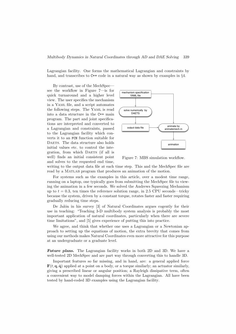
Figure 7: MBS simulation workflow.
By contrast, use of the MechSpec—see the workflow in Figure 7—is forquick turnaround and a higher levelview. The user specifies the mechanismin a Yaml file, and a script automatesthe following steps. The Yaml is readinto a data structure in the C++ mainprogram. The part and joint specifica-tions are interpreted and converted toa Lagrangian and constraints, passedto the Lagrangian facility which con-verts it to an FCN function suitable forDaets. The data structure also holdsinitial values etc. to control the inte-gration, from which Daets (if all iswell) finds an initial consistent pointand solves to the requested end time,writing to the output data file at each time step. This and the MechSpec file areread by a Matlab program that produces an animation of the motion.
For systems such as the examples in this article, over a modest time range,running on a laptop, one typically goes from submitting the MechSpec file to view-ing the animation in a few seconds. We solved the Andrews Squeezing Mechanismup to t = 0.3, ten times the reference solution range, in 2.5 CPU seconds—trickybecause the system, driven by a constant torque, rotates faster and faster requiringgradually reducing time steps.
De Jalon in his survey [3] of Natural Coordinates argues cogently for theiruse in teaching: “Teaching 3-D multibody system analysis is probably the mostimportant application of natural coordinates, particularly when there are severetime limitations”, and [5] gives experience of putting this into practice.
We agree, and think that whether one uses a Lagrangian or a Newtonian ap-proach to setting up the equations of motion, the extra brevity that comes fromusing our methods makes Natural Coordinates even more attractive for this purposeat an undergraduate or a graduate level.
Future plans. The Lagrangian facility works in both 2D and 3D. We have awell-tested 2D MechSpec and are part way through converting this to handle 3D.
Important features so far missing, and in hand, are: a general applied forceF(t,q, q) applied at a point on a body, or a torque similarly; an actuator similarly,giving a prescribed linear or angular position; a Rayleigh dissipative term, oftena convenient way to model damping forces within the Lagrangian. All have beentested by hand-coded 3D examples using the Lagrangian facility.
340 John D. Pryce and Nedialko S. Nedialkov
References
[1] Brenan, Kathy E., Campbell, Stephen L., and Petzold, Linda R. NumericalSolution of Initial-Value Problems in Differential-Algebraic Equations. SIAM,Philadelphia, second edition, 1996. DOI: 0.1137/1.9781611971224.
[2] Davis, Timothy A. and Palamadai Natarajan, Ekanathan. Algorithm 907:KLU, a direct sparse solver for circuit simulation problems. ACM Trans. Math.Softw., 37(3):36:1–36:17, September 2010. DOI: 10.1145/1824801.1824814.
[3] de Jalon, Javier Garcıa. Twenty-five years of natural coordinates. MultibodySystem Dynamics, 18(1):15–33, 2007. DOI: doi.org/crvphq.
[4] de Jalon, Javier Garcia and Bayo, Eduardo. Kinematic and Dynamic Simula-tion of Multibody Systems: The Real Time Challenge. Springer-Verlag, Berlin,Heidelberg, 1994.
[5] de Jalon, Javier Garcıa, Shimizu, Nobuyuki, and Gomez, David. Naturalcoordinates for teaching multibody systems with Matlab. In Proc. IDETC/-CIE 2007, September 4–7, 2007, Las Vegas, Nevada, USA, volume 5, pages1539–1548. ASME, 2007. DOI: 10.1115/DETC2007-35358.
[6] Greiner, Walther. Classical Mechanics: Systems of Particles and HamiltonianDynamics. Number v. 1 in Classical theoretical physics. Springer, 2003. DOI:10.1007/978-3-642-03434-3.
[7] Hairer, E. and Wanner, G. Solving Ordinary Differential Equations II. Stiffand Differential–Algebraic Problems. Springer Verlag, Berlin, second edition,1991. DOI: 10.1007/978-3-642-05221-7.
[8] Kraus, C., Winckler, M., and Bock, H.G. Modeling mechanical DAE us-ing natural coordinates. Mathematical and Computer Modelling of DynamicalSystems, 7(2):145–158, 2001. DOI: 10.1076/mcmd.7.2.145.3645.
[9] Li, Xiao. Incremental computation of Taylor series and system Jacobian inDAE solving using automatic differentiation. Master’s thesis, ComputationalScience and Engineering, McMaster University, Hamilton, Ontario, Canada,2017. DOI: hdl.handle.net/11375/22521.
[10] Mattsson, Sven Erik and Soderlind, Gustaf. Index reduction in differential-algebraic equations using dummy derivatives. SIAM J. Sci. Comput.,14(3):677–692, 1993. DOI: 10.1137/0914043.
[11] Nedialkov, Nedialko S and Pryce, John D. Solving differential-algebraic equations by Taylor series (III): the DAETScode. JNAIAM J. Numer. Anal. Indust. Appl. Math,3:61–80, 2008. DOI: jnaiamcont.org/new/uploads/files/
b4e0bdaa7990bbd1896fa3fafdd09f71.pdf.
Multibody Dynamics in Natural Coordinates through AD and DAE Solving 341
[12] Nedialkov, Nedialko S. and Pryce, John D. DAETS user guide. TechnicalReport CAS 08-08-NN, Department of Computing and Software, McMasterUniversity, Hamilton, ON, Canada, June 2013. 68 pages, DAETS is availableat http://www.cas.mcmaster.ca/~nedialk/daets.
[13] Nedialkov, Nedialko S. and Pryce, John D. Multi-body Lagrangian simula-tions, 2017. YouTube channel,https://www.youtube.com/channel/UCCuLchOx0W0yoNE9KOCYlVQ.
[14] Nedialkov, Nedialko S. and Pryce, John D. YAML specification of 2D mech-anisms for the DAETS Lagrangian facility. Technical report, Department ofComputing and Software, McMaster University, 2018. In preparation.
[15] Nikravesh, Parviz E. An overview of several formulations for multibody dy-namics. In Talaba, D. and Roche, T., editors, Product Engineering, pages181–207. Springer, Dordrecht, 2004. DOI: doi.org/bj6272.
[16] OpenSim. OpenSim implementation of MBS Benchmark, 2008 (accessed July2017). rehabenggroup.github.io/MBSbenchmarksInOpenSim/index.html.
[17] Pantelides, Costas C. The consistent initialization of differential-algebraic sys-tems. SIAM J. Sci. Stat. Comput., 9:213–231, 1988. DOI: 10.1137/0909014.
[18] Pryce, John D. A simple structural analysis method for DAEs. BIT NumericalMathematics, 41(2):364–394, 2001. DOI: 10.1023/A:1021998624799.
[19] Pryce, John D., Nedialkov, Nedialko S., Tan, Guangning, and Li, Xiao. HowAD can help solve differential-algebraic equations. Optimization Methods andSoftware, 33(4-6):729–749, 2018. DOI: 10.1080/10556788.2018.1428605.
[20] Susskind, L. and Hrabovsky, G. Classical Mechanics: The Theoreti-cal Minimum. The theoretical minimum. Penguin Books, 2014. DOI:10.1119/1.4816681.
[21] Talaba, Doru. Mechanical models and the mobility of robots and mechanisms.Robotica, 33(1):181–193, 2015. DOI: 10.1017/S0263574714000149.
[22] von Schwerin, Reinhold. Multibody system simulation: numerical methods,algorithms, and software, volume 7. Springer Science & Business Media, 2012.DOI: 10.1007/978-3-642-58515-9, Softcover reprint of the original 1st ed.1999.
[23] Wachter, Andreas and Biegler, Lorenz T. On the implementationof an interior-point filter line-search algorithm for large-scale nonlinearprogramming. Mathematical programming, 106(1):25–57, 2006. DOI:10.1007/s10107-004-0559-y.