Multidimensional Calculus: Mainly Differential Theory

9

Multidimensional Calculus:Mainly Differential Theory

In the following, we will attempt to quickly develop the basic differential theory of calculus in

multidimensional spaces. You’ve probably already seen much of this theory. Hopefully, we will

develop a better understanding of the material than is usually imparted in the more elementary

treatments, and see how to extend it to more general spaces and coordinate systems.

By the way, in keeping with the common practice in physics of denoting the position of a

moving object by r , I will relent and often use this notation instead of x .

9.1 Motion, Curves, Arclength, Acceleration and theChristoffel Symbols

For all the following, assume we are considering motion in some space of positions S , and that

{(x1, x2, . . . , x N

)}

is any coordinate system for this space. As before,

{h1, h2, . . . , hN } , {ε1, ε2, . . . , εN } and {e1, e2, . . . , eN }

are the associated scaling factors, tangent vectors and normalized tangent vectors.

We also assume that we have some position-valued function r(t) that traces out a curve

C as t varies over some interval (t0, t1) . Since this is a math/physics course, we naturally

view r(t) as being the position of an object, say, George the Gerbil, at time t . In terms of our

coordinate system, we have some coordinate formula for r

r(t) ∼(

x1(t), x2(t), . . . , x N (t))

for t0 < t < t1 .

Velocity and Speed

The formula for velocity v at any given time is easily computed using the chain rule:

v =dr

dt=

N∑

i=1

∂ r

∂x i

dx i

dt=

N∑

i=1

hi ei

dx i

dt,

11/24/2013

Chapter & Page: 9–2 Multidimensional Calculus: Differential Theory

which we may prefer to rewrite as

v =dr

dt=

N∑

i=1

hi

dx i

dtei or v =

dr

dt=

N∑

i=1

dx i

dtεi .

The corresponding speed, then, is

ds

dt=

∥∥∥∥dr

dt

∥∥∥∥ =

√√√√[

N∑

i=1

hi

dx i

dtei

]·

[N∑

j=1

h j

dx j

dte j

].

That is,

ds

dt=

√√√√N∑

i=1

N∑

j=1

hi h j

dx i

dt

dx j

dtei · e j =

√√√√N∑

i=1

N∑

j=1

dx i

dt

dx j

dtgi j . (9.1)

If the coordinate system is orthogonal, this reduces to

ds

dt=

√√√√N∑

i=1

(hi

dx i

dt

)2

. (9.2)

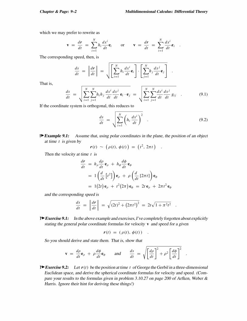
!◮Example 9.1: Assume that, using polar coordinates in the plane, the position of an object

at time t is given by

r(t) ∼(ρ(t), φ(t)

)=

(t2, 2π t

).

Then the velocity at time t is

dr

dt= hρ

dρ

dteρ + hφ

dφ

dteφ

= 1

(d

dt

[t2

])eρ + ρ

(d

dt[2π t]

)eφ

= 1(2t

)eρ + t2

(2π

)eφ = 2t eρ + 2π t2 eφ

and the corresponding speed is

ds

dt=

∥∥∥∥dr

dt

∥∥∥∥ =

√(2t)2 +

(2π t2

)2= 2t

√1 + π2t2 .

?◮Exercise 9.1: In the above example and exercises, I’ve completely forgotten about explicitly

stating the general polar coordinate formulas for velocity v and speed for a given

r(t) = ( ρ(t), φ(t) ) .

So you should derive and state them. That is, show that

v =dρ

dteρ + ρ

dφ

dteφ and

ds

dt=

√[dρ

dt

]2

+ ρ2

[dφ

dt

]2

.

?◮Exercise 9.2: Let r(t) be the position at time t of George the Gerbil in a three-dimensional

Euclidean space, and derive the spherical coordinate formulas for velocity and speed. (Com-

pare your results to the formulas given in problem 3.10.27 on page 200 of Arfken, Weber &

Harris. Ignore their hint for deriving these things!)

Motion, Curves, Arclength, Acceleration and the Christoffel Symbols Chapter & Page: 9–3

Distance Traveled / Arclength

The distance traveled by our object (George) as t goes from t0 to t1 (i.e., the arclength of the

curve traced out by the object) is simply the integral of the speed,

arclength =

∫ t1

t0

ds

dtdt =

∫ t1

t0

‖v(t)‖ dt .

In general, the coordinate formula for this is

arclength =

∫ t1

t=t0

√√√√N∑

i=1

N∑

j=1

hi h j

dx i

dt

dx j

dtei · e j dt =

∫ t1

t=t0

√√√√N∑

i=1

N∑

j=1

dx i

dt

dx j

dtgi j dt ,

which reduces to

arclength =

∫ t1

t=t0

√√√√N∑

i=1

(hi

dx i

dt

)2

dt

when the coordinate system is orthogonal, and further reduces to

arclength =

∫ t1

t=t0

√√√√N∑

i=1

(dx i

dt

)2

dt

if the space is Euclidean and the coordinate system is Cartesian.

!◮Example 9.2: Consider the curve C parameterized in polar coordinates by

r(t) ∼(ρ(t), φ(t)

)=

(t2, 2π t

)for 0 < t < 2 ,

as in example 9.1 on page 9–2. Its arclength is

arclength =

∫ t1

t=t0

√√√√N∑

i=1

(hi

dx i

dt

)2

dt

=

∫ 2

0

√(hρ

dρ

dt

)2

+

(hφ

dφ

dt

)2

dt

=

∫ 2

0

√(1

d

dt

[t2

])2

+

(ρ

d

dt[2π t]

)2

dt

=

∫ 2

0

2t√

1 + π2t2 dt

=2

3π2

(1 + π2t2

)3/2

∣∣∣∣2

0

=2

3π2

[(1 + 4π2

)3/2 − 1

].

version: 11/24/2013


Acceleration and the Christoffel SymbolsComputing Acceleration

The acceleration a of George at each instant of t is, of course,

a =dv

dt=

d

dt

N∑

i=1

hi ei

dx i

dt=

N∑

i=1

d

dt

[dx i

dthi ei

].

If the coordinate system is basis based, then the scaling factors and local basis vectors do not

vary, and the above simplifies to

a =dv

dt=

N∑

i=1

d2x i

dt2hi ei .

This is certainly the case when our coordinate system is Cartesian. If, however, the scaling factor

and/or local basis vectors vary from point to point (as with polar coordinates), then we must use

the product ruled

dt

[dx i

dthi ei

]=

d2x i

dt2hi ei +

dx i

dt

d[hi ei ]

dt.

yielding

a =dv

dt=

N∑

i=1

[d2x i

dt2hi ei +

dx i

dt

d[hi ei ]

dt

].

Recalling that

εi = hi ei ,

we can rewrite the above in the slightly more convenient form

a =dv

dt=

N∑

i=1

[d2x i

dt2εi +

dx i

dt

dεi

dt

].

Applying the chain rule to the derivatives of the εi ’s , we get1

dx i

dt

dεi

dt=

dx i

dt

N∑

k=1

dxk

dt

∂εi

∂xk=

N∑

k=1

dx i

dt

dxk

dt

∂εi

∂xk.

So,

a =dv

dt=

N∑

i=1

[d2x i

dt2εi +

N∑

k=1

dx i

dt

dxk

dt

∂εi

∂xk

]. (9.3)

The last acceleration formula is probably the most important “new” formula of this section.

Rather than memorizing it, you can always easily rederive it using the product and chain rules

from calculus.

However, to use formula (9.3), we still need to know each ∂εi/∂xk . Since this a partial

derivative of the vector-valued function εi , it is, itself, a vector-valued function. That is, for

1 I’m cheating. We’ve not verified the chain rule for the differentiation of vector-valued functions, only for scalar-

and position-valued functions. The chain rule used here with a vector-valued function can be rigorously justified

in a Euclidean space or in a non-Euclidean space contained in a Euclidean space (trust me). Justifying it in a more

general space is more involved and requires clever definitions.


each position p in S , each ∂εi/∂xk is a vector in the tangent vector space at that point p . So

each ∂εi/∂xk can be expressed in terms of the {ε1, ε2, . . . , εN } basis at each point in space. This

means that, for each point of the space S , there must be corresponding scalars Ŵ1ik , Ŵ2

ik , . . .

and ŴNik such that

∂εi

∂xk=

N∑

m=1

Ŵmik εm . (9.4)

These Ŵmik’s are called the Christoffel symbols (for the coordinate system).2 They are just the

components of each ∂εi/∂xk with respect to the {ε1, ε2, . . . , εN } basis at each point.

Using the Christoffel symbols, formula (9.3) becomes

a =dv

dt=

N∑

i=1

[d2x i

dt2εi +

N∑

k=1

N∑

m=1

dx i

dt

dxk

dtŴm

ikεm

]

=

N∑

i=1

d2x i

dt2εi +

N∑

i=1

N∑

k=1

N∑

m=1

dx i

dt

dxk

dtŴm

ikεm .

With a little relabeling of the indices, we have

N∑

i=1

N∑

k=1

N∑

m=1

dx i

dt

dxk

dtŴm

ikεm =

N∑

j=1

N∑

k=1

N∑

i=1

dx j

dt

dxk

dtŴi

jkεi ,

which allows us to rewrite the last formula for acceleration as

a =dv

dt=

N∑

i=1

d2x i

dt2+

N∑

j=1

N∑

k=1

dx j

dt

dxk

dtŴi

jk

εi . (9.5)

Equivalently,

a =dv

dt=

N∑

i=1

d2x i

dt2+

N∑

j=1

N∑

k=1

dx j

dt

dxk

dtŴi

jk

hi ei . (9.5 ′)

Of course, for the above to be useful, we need to find the values of the Christoffel symbols.

Computing ∂εi/∂xk and the Christoffel Symbols

Since the Christoffel symbols are, at each point in S , components of vectors with respect to the

basis {ε1, ε2, . . . , εN } , we can use what we learn earlier this term about “finding components”

to find the Ŵijk’s , provided we can, somehow, compute each

∂ε j

∂xk.

The simplest case is where the coordinate system is basis based. Then the scaling factors

and local basis vectors do not vary. Thus,

∂ε j

∂xk= 0 ,

2 More precisely, they are Christoffel symbols of the second kind.

version: 11/24/2013


and equation (9.4) becomes

0 =∂ε j

∂xk=

N∑

i=1

Ŵijk εi ,

which means that, for every j , k and i ,

Ŵijk = 0 .

Remember, this is only if the coordinate system is basis based.

More generally, if the coordinate system is orthogonal, then (as you showed in 2.19 on page

2–153), the Ŵijk’s in

∂ε j

∂xk=

N∑

i=1

Ŵijk εi

are given by

Ŵijk =

∂ε j

∂xk· εi

‖εi‖2

.

By the definitions of the scaling factors and normalized tangent vectors, this can also be written

as

Ŵijk =

1

hi2

∂ε j

∂xk· εi =

1

hi

∂[h j e j ]

∂xk· ei . (9.6)

We should also note that we do have some symmetry in these computations. This is because

∂ε j

∂xk=

∂

∂xk

∂ r

∂x j=

∂

∂x j

∂ r

∂xk=

∂εk

∂x j.

Hence,

Ŵijk = Ŵi

k j ,

a fact that can reduce the number of computations we may have to carry out.

Of course, computing formula (9.6) requires that we can compute this dot product. If the

space is Euclidean and you’ve determined how to express the εi ’s and ei ’s in terms of the

orthonormal basis corresponding to a Cartesian system, then computing the Ŵijk’s by the above

equation is relatively straightforward.

!◮Example 9.3: Consider the polar coordinate system {(ρ, φ)} . In example 8.9 on page 8–33

we saw that

hρ = 1 and hφ = ρ ,

and, in terms of the standard basis associated with the Cartesian system {(x, y)} ,

eρ = cos(φ) i + sin(φ) j and eφ = − sin(φ) i + cos(φ) j .

So,

∂ερ

∂ρ=

∂[hρeρ]

∂ρ=

∂

∂ρ

[cos(φ) i + sin(φ) j

]= 0 (9.7a)

3 I.e., that if a basis {b1,b2, . . . ,bN } is orthogonal, then v =∑N

i=1 vi bk H⇒ vi =v · bi

‖bi ‖2

.


and

∂ερ

∂φ=

∂[hρeρ]

∂φ=

∂

∂φ

[cos(φ) i + sin(φ) j

]= − sin(φ) i + cos(φ) j . (9.7b)

Just plugging into formula (9.6), above, we get

Ŵρρρ =1

hρ

∂[hρeρ]

∂ρ· eρ =

1

10 · eρ = 0 ,

Ŵφρρ =1

hφ

∂[hρeρ]

∂ρ· eφ =

1

ρ0 · eφ = 0 ,

Ŵρ

ρφ =1

hρ

∂[hρeρ]

∂φ· eρ =

1

1

[− sin(φ) i + cos(φ) j

]·[cos(φ) i + sin(φ) j

]= 0

and

Ŵφ

ρφ =1

hφ

∂[hρeρ]

∂φ· eφ =

1

ρ

[− sin(φ) i + cos(φ) j

]·[− sin(φ) i + cos(φ) j

]=

1

ρ.

Thus (using (9.4)),

∂ερ

∂ρ= Ŵρρρερ + Ŵφρρεφ = 0ερ + 0εφ = 0

and∂ερ

∂φ= Ŵ

ρ

ρφερ + Ŵφ

ρφεφ = 0ερ +1

ρεφ =

1

ρεφ .

In terms of the normalized tangent vectors,

∂ερ

∂ρ= 0 and

∂ερ

∂φ= eφ .

Keep in mind that the important quantities are the partial derivatives of the ε j ’s . If we

can compute these, as we did in equation set (9.7), above, then the only value of the Christoffel

symbols is to help us express those partial derivatives in terms of the coordinate system’s tangent

vectors ε1 , ε2 , . . . (instead of i , j , . . . ). With some coordinate systems, though, you can just

look at your initial formulas for these partial derivatives and, without using Christoffel symbols,

write out the formulas in terms of the ε j ’s . Certainly, for example, we did not really need to

find the Christoffel symbols to derive

∂ερ

∂ρ= 0 and

∂ερ

∂φ=

1

ρεφ = eφ

from formulas (9.7).

?◮Exercise 9.3: Continue the work in the last example. In particular:

a: Verify that

Ŵρ

φρ = 0 , Ŵφ

φρ =1

ρ, Ŵ

ρ

φφ = −ρ and Ŵφ

φφ = 0 .

version: 11/24/2013


b: Verify that

∂εφ

∂ρ=

1

ρεφ = eφ and

∂εφ

∂φ= −ρερ = −ρeρ .

two ways: first, by inspecting these partial derivatives computed in terms of i and j , then

using the Christoffel symbols.

c: Write out the full formula for acceleration in polar coordinates. Corresponding to a

function of position r(t) ∼ (ρ(t), φ(t)) , you should get something like

a =

[d2ρ

dt2− ρ

(dφ

dt

)2]

eρ +

[ρ

d2φ

dt2+ 2

dρ

dt

dφ

dt

]eφ .

d: Compute the acceleration at time t when, in polar coordinates,

r(t) ∼(ρ(t), φ(t)

)=

(t2, 2π t

),

as in example 9.1.

?◮Exercise 9.4 (spherical coordinates): Let {(r, θ, φ)} be the spherical coordinate system

described at the start of section 8.3, page 8–9. Recall that you found the associated scaling

factors and tangent vectors (in terms of i , j and k ) in exercise 8.21 on page 8–34.

a: Find the nine partial derivatives

∂εr

∂r,

∂εr

∂θ,

∂εr

∂φ,

∂εθ

∂r, · · · and

∂εφ

∂φ.

(You might not need the Christoffel symbols for this.)

b: How many Christoffel symbols are there? Find a few.

c: Let r(t) ∼ (r(t), θ(t), φ(t)) be the position at time t of George the Gerbil in a three-

dimensional Euclidean space, and derive the spherical coordinate formulas for his accelera-

tion. (Compare your results to the formula given in problem 3.10.27 on page 200 of Arfken,

Weber & Harris. Again, ignore their hint for deriving this!)

?◮Exercise 9.5: Once again, consider the circular paraboloid S we discussed in examples

8.3, 8.5, 8.8 and 8.10 (pages 8–16, 8–22 and 8–27 and 8–34). Recall that the coordinate

system corresponding to polar coordinates, {(ρ, φ)} is orthogonal and that

ερ = cos(φ) i + sin(φ) j + 2ρk ,

εφ = −ρ sin(φ) i + ρ cos(φ) j ,

hρ =√

1 + 4ρ2 ,

and

hφ = ρ .

Now, compute the Christoffel symbols, and write out the full formula for acceleration for an

object at position r(t) ∼ (ρ(t), φ(t)) .

Scalar and Vector Fields Chapter & Page: 9–9

Final Comments on Christoffel Symbols and Acceleration

Using the above, we can find formulas for acceleration (and Christoffel symbols) in Euclidean

spaces and in nonEuclidean subpaces contained in Euclidean spaces (e.g., curves and spheres

in Euclidean three-space), at least when the coordinates on the subspace are a subset of the

coordinates of the coordinates of the larger Euclidean space. To compute the Christoffel symbols

when we do not have a convenient Cartesian system lying around, we will need to further develop

the “metric tensor”. We will do that in the next chapter. (If you want, you can glance at the resulting

formula in theorem 11.2 on page 11–16.)

9.2 Scalar and Vector FieldsBasic Definitions and Concepts

In the following, all points/positions refer to points in some N -dimensional space S .

A scalar field Ψ (on S ) is a scalar-valued function of position,

Ψ (x) = some scalar value corresponding to position x in S .

Some examples:

T (x) = temperature at position x ,

Φ(x) = the gravitational potential at x due to the surrounding masses ,

x2(x) = the second coordinate of x with respect to some given coordinate system

and

r(x) = “distance between x and some fixed point O ” = dist(x, O) .

The coordinate formula for a scalar field Ψ with respect to a given coordinate system

{(x1, x2, . . . , x N )} is just the formula ψ(x1, x2, . . . , x N ) for computing the value of Ψ (x)

from the coordinates for x . So

Ψ (x) = ψ(x1, x2, . . . , x N ) with x ∼ (x1, x2, . . . , x N ) .

For example, if our space is a plane and we are using Cartesian coordinates {(x, y)} with O as

the origin, then

the coordinate formula for r(x) = dist(x, O) is√

x2 + y2 .

If, instead, we are using polar coordinates {(ρ, φ)} with O as the origin, then

the coordinate formula for r(x) = dist(x, O) is ρ .

A vector field (on S ) is a vector-valued function of position,

V(x) = some vector corresponding to position x in S .

version: 11/24/2013


Some examples:

V(x) = wind velocity at x ,

F(x) = force of gravity on some object at position x

and

εk =∂x

∂xk= ‘rate of change’ in position as the kth coordinate varies .

At each point x , V(x) will be a vector in the tangent space at that point. Often, though,

we will be dealing with a subspace (say, a curve or a sphere in a three-dimensional space), in

which case V(x) may or may not be in the tangent space of that subspace, depending on how V

is generated. For example, V may be the velocity of some object moving on a curve, in which

case V(x) is tangent to the curve at each point x . On the other hand, V(x) may be a vector

field perpendicular to a sphere in Euclidean three-space, in which case V(x) will not be in the

tangent space of the sphere at any x in the sphere.

Because V(x) is in the tangent space of our overall space at x , it will have components

with respect to both of our associated bases. It can be expressed in terms of the εi ’s ,

V(x) =

N∑

i=1

V i(x1, x2, . . . , x N ) εi where x ∼ (x1, x2, . . . , x N ) ,

and it can be expressed in terms of the ei ’s ,

V(x) =

N∑

i=1

vi(x1, x2, . . . , x N ) ei where x ∼ (x1, x2, . . . , x N ) .

These formulas for V(x) should be refered to as coordinate/component formulas for V . In

practice, it is more common for a vector field to be expressed in terms of the normalized tangent

vectors (the ek’s ) than the εk’s . Still, there are occasions where using the other representation

is convenient.

Since εi = hi ei , these components are related by

vi = hi Vi .

Note that these component functions are denoted with superscripts. That is standard when dealing

with the slightly more general theory we are developing here. In practice, though, expect a lot

of people to use subscripts.

On the other hand, there is no real convention on how to notationally distinguish components

with respect to the εi ’s from components with respect to the ei ’s . My use here of V i and vi

will not be consistently followed — not even by me.

If the coordinate system is orthogonal, then {e1, . . . , eN } is orthonormal at each point, and,

so, the corresponding components of V are given by

vi = V · ei .

?◮Exercise 9.6: Show that, if the coordinate system is orthogonal, then the components of

vector field V with respect to the εk’s are given by

V i =V · εi

(hi )2

.

Scalar and Vector Fields Chapter & Page: 9–11

?◮Exercise 9.7: Using the product rule, show that

∂V

∂x j=

N∑

k=1

[∂V k

∂x j+

N∑

i=1

V iŴki j

]εk .

What would this be in terms of the unit tangents e1 , …, eN ? (By the way, the expression

inside the brackets in the above equation is known as a “covariant derivative”. of V )

Some Warnings

1. Many authors use the terms “scalar” and “vector” when they mean “scalar field” and

“vector field”.

2. People often use the same symbols to denote both a scalar/vector field and its coordinate

formula. This is not particularly bad if there is only one coordinate system being used

(and everyone knows which system that is), but it can be quite confusing when we have

multiple coordinate systems.

Change of Coordinates and the Coordinate Formulas

For us, this should be simple:

Suppose

ψ(x1, x2, . . . , x N

)

is the coordinate formula for some scalar field Ψ using some coordinate system {(x1, x2, . . . , x N )} .

To obtain the coordinate formula for Ψ using a different coordinate system {(x1′, x2′

, . . . , x N ′)} ,

we simply replace each xk in the formula for

ψ(x1, x2, . . . , x N

)

with the kth change of coordinates formula,

xk = xk(x1′, x2′

, . . . , x N ′)

.

If we have a coordinate formula for vector field V ,

V(x) =

N∑

i=1

V i(x1, x2, . . . , x N ) εi or V(x) =

N∑

i=1

vi(x1, x2, . . . , x N ) ei

where

x ∼ (x1, x2, . . . , x N ) ,

then, in addition to converting the formulas to corresponding formulas in term of the xk ′, we

need to express V in terms of the local bases associated with {(x1′, x2′

, . . . , x N ′)} ,

V(x) =

N∑

i=1

V i ′(x1′, x2′

, . . . , x N ′) εi

′or V(x) =

N∑

i=1

vi ′(x1′, x2′

, . . . , x N ′) ei

′

version: 11/24/2013


where

x ∼ (x1′, x2′

, . . . , x N ′) .

For this, we can use what we learned earlier about “change of basis”. In particular, if our coordinate

systems are orthogonal (so that the sets of associated normalized tangent vectors are orthonormal

at every point), then

v1′

v2′

...

vN ′

= |V〉B′ = MB′B |V〉B =

v1

v2

...

vN

where

B = {e1, e2, . . . , eN } , B′ =

{e1

′, e2

′, . . . , eN

′}

and

[MB′B]i j = ei′· e j .

Further details will probably be assigned as exercises.

A Few Words About Continuity and Differentiability

Because our goal is to develop a substantial amount of “applicable multidimensional calculus”

in a relatively short time, we are glossing over some of the mathematical fine points. Still, a few

words on continuity and differentiability are in order, since there will be some issues involving

the continuity and differentiability of scalar and vector fields.

Continuity is easy to rigorously define: We say that a scalar field Ψ and a vector field V

are continuous at a point p if and only if

limx→ p

Ψ (x) = Ψ ( p) and limx→ p

V(x) = V( p) .

We then say that Ψ and V are continuous in some region if they are continuous at each point

in the region.

Differentiability is a bit more difficult to rigorously define without going into more mathe-

matical details than appropriate for this course. Here is a working definition for us:

Ψ is k-times differentiable (at a point or in a region) if and only if, using any reason-

able coordinate system {(x1, x2, . . . , x N )} , the coordinate formula ψ(x1, x2, . . . , x N )

for Ψ , as well as all partial derivatives of ψ up to order k , exist and are continuous

(at the point or in the region).4

A similar working definition works for vector fields.

If the order of differentiability k is not mentioned, you should normally assume k = 1 .

That is, “Ψ is differentiable” means “Ψ is 1-time differentiable”. If, however, we say “Ψ

is suitably differentiable”, then assume k is the order of the highest order derivative relevant to

whatever we are discussing.

4 Actually, mathematicians call this “k-times continuous differentiability” or “smoothness”.

The Classic Gradient, Divergence and Curl Chapter & Page: 9–13

9.3 The Classic Gradient, Divergence and CurlBasic Definitions in Euclidean Space

For expediency, we will first define the classical differential operators for scalar and vector fields

in a Euclidean space E using the “del operator”. Moreover, we will assume that our coordinate

system {(x1, x2, . . . , x N )} is Cartesian.

The del operator is the “vector differential operator” given in our Cartesian system by

−→∇ = ∇ =

N∑

k=1

∂

∂xkek =

N∑

k=1

ek

∂

∂xk=

N∑

k=1

∂x

∂xk

∂

∂xk.

For any sufficiently differentiable scalar field Ψ and vector field F with corresponding coordi-

nate formulas

Ψ (x) = ψ(x1, x2, . . . , x N

)and F(x) =

N∑

k=1

Fk(x1, x2, . . . , x N

)ek ,

we define

the gradient of Ψ = grad(Ψ ) = ∇Ψ ,

the divergence of F = div(F) = ∇ · F ,

and

the curl of F = curl(F) = ∇ × F

by the coordinate formulas

grad(Ψ ) = ∇Ψ =

N∑

k=1

ek

∂

∂xkψ

(x1, x2, . . . , x N

)=

N∑

k=1

ek

∂ψ

∂xk=

N∑

k=1

∂ψ

∂xkek ,

div(F) = ∇ · F =

[N∑

k=1

∂

∂xkek

]·

N∑

j=1

F j(x1, x2, . . . , x N

)e j

=

N∑

k=1

∂Fk

∂xk,

and

curl(F) = ∇ × F =

[N∑

k=1

∂

∂xkek

]×

N∑

j=1

F j(x1, x2, . . . , x N

)e j

=

∣∣∣∣∣∣∣∣∣

e1 e2 e3

∂

∂x1

∂

∂x2

∂

∂x3

F1 F2 F3

∣∣∣∣∣∣∣∣∣

=

[∂F3

∂x2−∂F2

∂x3

]e1 −

[∂F3

∂x1−∂F1

∂x3

]e2 +

[∂F2

∂x1−∂F1

∂x2

]e3 .

Both grad(Ψ ) and div(F) can be defined assuming our space is of any dimension. However,

curl(F) requires that our space be three-dimensional (in which case,we usually use the traditional

{(x, y, z)} and {i, j,k} notation).

version: 11/24/2013


Observe that grad(Ψ ) and curl(F) are vector fields, while div(F) is a scalar field.

One thing not obvious from the above definitions is why anyone would be interested in these

things. There are good reasons arising from both basic mathematics and from physics. The

“geometric/physical significance” of grad(Ψ ) will be discussed in a little bit. The importance

of the divergence and curl of a vector field will be discussed later, in conjunction with some

classic integral theorems. In anticipation of that discussion, let me introduce some terminology

that you may encounter in homework:

“ F is solenoidal” ⇐⇒ “ F is divergence free” ⇐⇒ ∇ · F = 0

and

“ F is irrotational” ⇐⇒ “ F is curl free” ⇐⇒ ∇ × F = 0 .

Invariance Under Change of Cartesian Coordinates

Because these formulas are given in terms of one Cartesian coordinate system, there is the issue

of what these formulas become when we switch to any other Cartesian coordinate system. (Hope-

fully, these formulas are “Cartesian coordinate system independent”.) To examine this issue, let

{(x1′, x2′

, . . . , x N ′)} be another Cartesian coordinate system corresponding to an orthonormal

basis {e1′, e2

′, . . . , eN

′} . Remember, in problem J 1 of Homework Handout VII you showed

(among other things) that

e j′

=

N∑

k=1

∂x j ′

∂xkek .

Using the chain rule from elementary calculus and the above, we get

∇ =

N∑

k=1

∂

∂xkek =

N∑

k=1

N∑

j=1

∂x j ′

∂xk

∂

∂x j ′ek =

N∑

j=1

∂

∂x j ′

N∑

k=1

∂x j ′

∂xkek =

N∑

j=1

∂

∂x j ′e j

′.

This shows that the basic formula

∇ =

N∑

k=1

∂

∂xkek

is invariant under any change of Cartesian coordinates. Consequently, the formulas given for

∇Ψ and ∇ · F and ∇ × F are valid using any Cartesian coordinate system, and yield the same

vector or scalar fields.

Product and Chain Rules

Using the Cartesian formulas and elementary calculus, we can derive or verify a number of

“product rules” and “chain rules” that might simplify calculations later on. In particular, if Ψ

and Φ are suitably differentiable scalar fields, and F and G are suitably differentiable vector

fields, then

∇(ΦΨ ) = Ψ∇Φ + Φ∇Ψ , (9.8a)

∇ · (ΦF) = (∇Φ) · F + Φ∇ · F , (9.8b)

∇ × (ΦF) = (∇Φ)× F + Φ(∇ × F) (9.8c)

The General Gradient Operator Chapter & Page: 9–15

and

∇ · (F × G) = (∇ × F) · G − F · (∇ × G) . (9.8d)

These are multidimensional versions of the product rule (note the “ − ” in (9.8d) due to the

antisymmetry in the cross product). You can easily derive or verify any of them, yourself.

?◮Exercise 9.8 a: Verify equation (9.8a).

b: Pick any one of the other equations in set (9.8), and verify it.

Now let f be a real-valued function on R (so f (a real number) = a real number ). Then,

for each position x , we can plug the real number Φ(x) into f , getting a ‘new’ scalar field

f (Φ(x)) .

You can then easily verify the chain rule

∇ [ f (Φ(x))] =[

f ′(Φ(x))]∇Φ(x) . (9.9)

?◮Exercise 9.9: Verify equation (9.9).

Another chain rule involving the gradient will be derived in the next section.

9.4 The General Gradient OperatorGeometric Significance of ∇Ψ

Consider a function f of the form

f (t) = Ψ (x(t))

where Ψ (x) is some scalar field on a Euclidean space E and x(t) is any (sufficiently smooth)

position-valued function (with t being in some interval (α, β) ). Both Ψ and x(t) will have

coordinate formulas

x(t) ∼(

x1(t), x2(t), . . . , x N (t))

for α < t < β

and

Ψ (x) = ψ(x1, x2, . . . , x N

)where x ∼

(x1, x2, . . . , x N

).

Taking the composition of the two,

f (t) = Ψ (x(t)) = ψ(

x1(t), x2(t), . . . , x N (t))

for α < t < β ,

gives us an ordinary real-valued function f such as you studied in “Calc. III”. Its derivative can

be found by the classical chain rule developed in that course. Computing this derivative, we see

version: 11/24/2013


that, at least if the coordinate system is Cartesian,

d f

dt=

d

dt[Ψ (x(t))]

=d

dt

[ψ

(x1(t), x2(t), . . . , x N (t)

)]

=∂ψ

∂x1

dx1

dt+

∂ψ

∂x2

dx2

dt+ · · · +

∂ψ

∂x N

dx N

dt

=

[∂ψ

∂x1e1 +

∂ψ

∂x2e2 + · · · +

∂ψ

∂x NeN

]·

[dx1

dte1 +

dx2

dte2 + · · · +

dx N

dteN

]

=

[N∑

k=1

∂ψ

∂xkek

]·

[N∑

k=1

dxk

dtek

].

But remember

∇Ψ =

N∑

k=1

∂ψ

∂xkek and

dx

dt=

N∑

k=1

dxk

dtek .

So the above boils down tod

dt[Ψ (x(t))] = ∇Ψ ·

dx

dt. (9.10)

This is another multidimensional “chain rule”. Keep in mind that the ∇Ψ in this equation is

being evaluated at the position corresponding to whatever value of t is relevant. To be a little

more precise, we should write this last equation as

d

dt[Ψ (x(t))]

∣∣∣∣t0

=[∇Ψ |x(t0)

]·

[dx

dt

∣∣∣∣t0

],

but most of us are too lazy.

Some consequences of equation (9.10) can be seen if we rewrite this dot product as

d

dt[Ψ (x(t))] = ‖∇Ψ ‖

∥∥∥∥dx

dt

∥∥∥∥ cos(θ) where θ = angle between ∇Ψ anddx

dt.

“Clearly”, then:

1. As a function of θ , the above is maximum when θ = 0 . That is,d

dtΨ (x(t)) is largest

when ∇Ψ and dx/dt are lined up. With a little thought, you’ll realize this means that, at

each point x0 in space, ∇Ψ evaluated at x0 points in the direction in which Ψ (x) is

increasing most rapidly as x moves through position x0 .

2. On the other hand, if S is a curve or surface5 on which Ψ is constant, and if x(t) traces

out a curve in S (with x ′(t) being nonzero), then Ψ (x(t)) is a constant function of t .

Hence

‖∇Ψ ‖

∥∥∥∥dx

dt

∥∥∥∥ cos(θ) =d

dtΨ (x(t)) = 0 ,

which means that θ = π/2 (or ∇Ψ = 0 ). In other words, at each point on this surface,

∇Ψ must be perpendicular to this curve or surface S .

5 or “hyper-surface” if E has dimension greater than three.

The General Gradient Operator Chapter & Page: 9–17

General Definition and Formula for the Gradient

Look, again, at equation (9.10). It gives a coordinate-free description of the gradient; namely,

that ∇Ψ is the vector field making that equation true. Being coordinate-free, this is actually a

better description for the gradient than the Cartesian formula given in the previous section. It

can even apply when our space is not Euclidean.

So let us drop our old definition of the gradient, and, instead, define the gradient of a scalar

field Ψ to be the vector field — denoted by either grad(Ψ ) or ∇Ψ — such that

d

dt[Ψ (r(t))] = [∇Ψ (r(t))] ·

dr

dt(9.11)

whenever r is a differentiable position-valued function. Note that this definition is free of

coordinates, and does not require the space to be Euclidean.

Since ∇Ψ is a vector field, it has a coordinate/component formula in terms of the local

basis at each point,

∇Ψ =

N∑

i=1

(∇Ψ )i ei . (9.12)

For convenience, we’ve used (∇Ψ )i to denote the i th component of ∇Ψ with respect to the

local basis. Keep in mind that each (∇Ψ )i is a scalar field, and may vary with position just as

∇Ψ and each ek varies with position. To find the coordinate formulas for these components,

let us see what the left and right sides of equation (9.11) (defining the gradient) become when

using an arbitrary position-valued function with its coordinate formula,

r(t) ∼(

x1(t), x2(t), . . . , x N (t))

.

First look at what we get when using this with the coordinate formula for Ψ in the left side of

equation (9.11). Applying the chain rule from elementary calculus,

d

dt[Ψ (r(t))] =

d

dt

[ψ

(x1(t), x2(t), . . . , x N (t)

)]=

N∑

i=1

∂ψ

∂x i

dx i

dt. (9.13)

On the other hand, using the coordinate/component formulas for ∇Ψ and d r/dt in the right side

of (9.11) yields:

[∇Ψ (r(t))] ·dr

dt=

[N∑

i=1

(∇Ψ )i ei

]·

N∑

j=1

∂ r

∂x j

dx j

dt

=

[N∑

i=1

(∇Ψ )i ei

]·

N∑

j=1

h j

dx j

dte j

Assuming the coordinate system is orthogonal, the local basis {e1, . . . , e2} is orthonormal, the

last set of equations reduces to

[∇Ψ (r(t))] ·dr

dt=

N∑

i=1

(∇Ψ )i h j

dx j

dt. (9.14)

Thus, using equations (9.13) and (9.14) and any choice of

r(t) ∼(

x1(t), x2(t), . . . , x N (t))

,

version: 11/24/2013


we can now rewrited

dt[Ψ (r(t))] = [∇Ψ (r(t))] ·

dr

dt

asN∑

i=1

∂ψ

∂x i

dx i

dt=

N∑

i=1

(∇Ψ )i hi

dx i

dt.

This “clearly” means that6

∂ψ

∂x i= (∇Ψ )i hi for i = 1, 2, . . . , N .

Hence

(∇Ψ )i =1

hi

∂ψ

∂x ifor i = 1, 2, . . . , N ,

and the coordinate/component formula for the gradient when using any orthogonal coordinate

system is

∇Ψ =

N∑

i=1

1

hi

∂ψ

∂x iei . (9.15)

!◮Example 9.4: In polar coordinates for the Euclidean plane, {(ρ, φ)} ,

∇Ψ =

N∑

i=1

1

hi

∂ψ

∂x iei =

1

hρ

∂ψ

∂ρeρ +

1

hφ

∂ψ

∂φeφ .

Recalling that hρ = 1 and hφ = ρ , we see that

∇Ψ =∂ψ

∂ρeρ +

1

ρ

∂ψ

∂φeφ .

In particular, if the polar coordinate formula for Ψ is

ψ(ρ, φ) = ρ2 sin(φ)

then, for x ∼ (ρ, φ) ,

∇Ψ (x) =∂ψ

∂ρeρ +

1

ρ

∂ψ

∂φeφ

= 2ρ sin(φ) eρ +1

ρ

[ρ2 cos(φ)

]eφ = 2ρ sin(φ) eρ + ρ cos(φ) eφ .

?◮Exercise 9.10: Find the formula for the gradient in spherical coordinates.

6 If this isn’t clear, first fix your position x0 ∼(

x10, x2

0, . . . , x N

0

)and choose

r(t) ∼(

x1(t), x2(t), . . . , x N (t))

=(

t, x20 , . . . , x N

0

).

Then

dx i

dt=

{1 if i = 1

0 if i 6= 1

and equation (9.14) reduces to∂ψ

∂x1= (∇Ψ )1h1 .

General Formulas for the Divergence and Curl Chapter & Page: 9–19

9.5 General Formulas for the Divergence and Curl

Later, we will discover the geometric significance of the divergence and the curl of a vector field.

Then, using those, we can both redefine divergence and curl in a coordinate-free manner, and

obtain more general formulas for these. This will come from our development of the divergence

(or Gauss’s) theorem and the Stokes’ theorem. In the meantime, I will simply tell you what those

formulas are, and we will use them, as needed, with the understanding that, eventually, we will

see how to derive them.

As usual, let

{(x1, x2, . . . , x N

)}

be an orthogonal coordinate system for our space S with

{h1, h2, . . . , hN } , {ε1, ε2, . . . , εN } and {e1, e2, . . . , eN }

being the associated scaling factors, tangent vectors and normalized tangent vectors at each point.

Assume F is a vector field with component/coordinate formula

F(x) =

N∑

i=1

F i(x1, x2, . . . , x N

)ei where x ∼

(x1, x2, . . . , x N

).

The corresponding formulas for the divergence of F depend somewhat on the dimension

N of the space, though the pattern will become obvious. If N = 2 , then

∇ · F =1

h1h2

{∂

∂x1

[F1h2

]+

∂

∂x2

[F2h1

]}. (9.16a)

If N = 3 , then

∇ · F =1

h1h2h3

{∂

∂x1

[F1h2h3

]+

∂

∂x2

[F2h1h3

]+

∂

∂x3

[F3h1h2

]}. (9.16b)

If N = 4 , then

∇ · F =1

h1h2h3h4

{∂

∂x1

[F1h2h3h4

]+

∂

∂x2

[F2h1h3h4

]

+∂

∂x3

[F3h1h2h4

]+

∂

∂x4

[F4h1h2h3

]}.

(9.16c)

And so on.

The curl still only makes sense if the dimension N is three. Using Stokes’ theorem, we will

version: 11/24/2013


be able to show that

∇ × F =1

h1h2h3

∣∣∣∣∣∣∣∣∣

h1e1 h2e2 h3e3

∂

∂x1

∂

∂x2

∂

∂x3

h1 F1 h2 F2 h3 F3

∣∣∣∣∣∣∣∣∣

=1

h2h3

(∂

∂x2

[h3 F3

]−

∂

∂x3

[h2 F2

])e1

−1

h1h3

(∂

∂x1

[h3 F3

]−

∂

∂x3

[h1 F1

])e2

+1

h1h2

(∂

∂x1

[h2 F2

]−

∂

∂x2

[h1 F1

])e3 .

(9.17)

?◮Exercise 9.11: Verify that the above formulas reduce to the Cartesian formulas originally

given when the coordinate system is Cartesian.

?◮Exercise 9.12: Using the above, verify that the two-dimensional formula for divergence

using polar coordinates {(r, φ)} is

∇ · F =1

ρ

{∂

∂ρ

[ρFρ

]+

∂Fφ

∂φ

},

?◮Exercise 9.13: Verify that the the three-dimensional formulas for divergence and curl are,

using cylindrical coordinates {(ρ, φ, z)} ,

∇ · F =1

ρ

{∂

∂ρ

[ρFρ

]+

∂Fφ

∂φ

}+

∂F z

∂z,

and

∇ × F =

[1

ρ

∂F z

∂φ−∂Fφ

∂z

]eρ +

[∂Fρ

∂z−∂F z

∂ρ

]eφ +

1

ρ

[∂

∂ρ

(ρFφ

)−∂Fρ

∂φ

]ez .

?◮Exercise 9.14: Find the formulas for the divergence and curl in spherical coordinates.

?◮Exercise 9.15: Let S3 be a sphere of radius 3 with the two-dimensional spherical co-

ordinates system {(φ, θ)} described in exercise 8.15 on page 8–27. Find the corresponding

coordinate formula for the divergence of a vector field on S3 . (Use the above along with the

results derived in exercise 8.15.)

It should be noted that you can also derive the formulas in the above exercises by taking

the Cartesian coordinate formulas for these entities and carefully converting these formulas to

polar/cylindrical/spherical coordinates.

Repeated Applications of the Del Operator Chapter & Page: 9–21

9.6 Repeated Applications of the Del OperatorGeneral Observations

For any sufficiently differentiable scalar field ψ and vector field F , we can compute

∇ · (∇ψ) , ∇ × (∇ψ) ,

∇ (∇ · F) , ∇ · (∇ × F) and ∇ × (∇ × F) .

I’ve included parentheses to emphasize that we are taking a “del operation” on an object resulting

from a previous “del operation”. However, except for the last expression, the parentheses are not

really necessary and are not usually written.

?◮Exercise 9.16 a: Which of the above ends up being

i: a scalar field?

ii: a vector field?

b: Give an example of an expression involving repeated use of ∇ that is “nonsense”.

Some of these formulas simplify greatly, with the verifications being rather straightforward

(at least when our space is Euclidean). Consider, for example, ∇×∇ψ . If we are in a Euclidean

space, then we can easily compute this using a standard Cartesian coordinate system:

∇ × ∇ψ = ∇ ×

[∂ψ

∂xi +

∂ψ

∂yj +

∂ψ

∂zk

]

=

∣∣∣∣∣∣∣∣∣

i j k

∂

∂x

∂

∂y

∂

∂z∂ψ

∂x

∂ψ

∂y

∂ψ

∂z

∣∣∣∣∣∣∣∣∣

=

(∂2ψ

∂y ∂z−

∂2ψ

∂z ∂y

)i −

(∂2ψ

∂x ∂z−

∂2ψ

∂z ∂x

)j −

(∂2ψ

∂x ∂y−

∂2ψ

∂y ∂x

)k

But remember, the order in which we compute two partial derivatives of a sufficiently differen-

tiable function is irrelevant. So

∂2ψ

∂y ∂z=

∂2ψ

∂z ∂y,

∂2ψ

∂x ∂z=

∂2ψ

∂z ∂xand

∂2ψ

∂x ∂y=

∂2ψ

∂y ∂x,

and the above computations reduce to

∇ × ∇ψ = 0 .

In fact, this equation holds more generally.

version: 11/24/2013


?◮Exercise 9.17: Use the more general formulas for the gradient and curl to verify that

∇ × ∇ψ = 0

even when the space is nonEuclidean (but still three-dimensional).

?◮Exercise 9.18: Verify that ∇ · ∇ × F = 0

a: when the space is Euclidean.

b: when the space is arbitrary.

One other identity that can be “easily verified” by simply computing things out in Cartesian

coordinates is

∇ × (∇ × F) = ∇ (∇ · F) − ∇ · ∇F

where ∇ · ∇F actually denotes the “Laplacian of F ”, which is discussed (briefly) at the end of

the next subsection.

The Laplacian

Because many problems in physics involve “conservative, divergence-free vector fields” (to be

discussed later), the expression ∇ · ∇ψ arises fairly often in applications. Because of this, a

shorthand has been universally adopted of using either ∇2 or 1 for ∇ · ∇ ,

1ψ = ∇2ψ = ∇ · ∇ψ .

This operator, whether denoted 1 or ∇2 , is called the Laplacian. In Cartesian coordinates,

∇2ψ = ∇ · ∇ψ = ∇ ·

[N∑

k=1

∂ψ

∂xkek

]=

N∑

k=1

∂

∂xk

(∂ψ

∂xk

)=

N∑

k=1

∂2ψ

∂xk 2.

Using the material developed a few pages ago, you can easily verify that, in polar coordinates,

{(ρ, φ)} ,

∇2ψ =

1

ρ

∂

∂ρ

[ρ∂ψ

∂ρ

]+

1

ρ2

∂2ψ

∂φ2,

and in spherical coordinates, {(r, θ, φ)} ,

∇2ψ =

1

r2

∂

∂r

[r 2 ∂ψ

∂r

]+

1

r2 sin(θ)

∂

∂θ

[sin(θ)

∂ψ

∂θ

]+

1

r2 sin2(θ)

∂2ψ

∂φ2.

?◮Exercise 9.19: Using the material developed a few pages ago, derive the above polar and

spherical coordinate formulas for the Laplacian.

Of course, using the even more general formulas for divergence and gradient given in sec-

tion 9.5, you can derive more general formulas for the Laplacian for arbitrary two- and three-

dimensional spaces.

Repeated Applications of the Del Operator Chapter & Page: 9–23

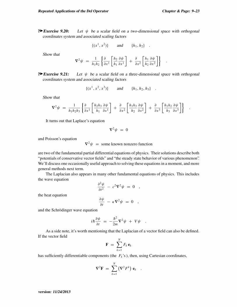
?◮Exercise 9.20: Let ψ be a scalar field on a two-dimensional space with orthogonal

coordinates system and associated scaling factors

{(x1, x2)} and {h1, h2} .

Show that

∇2ψ =

1

h1h2

{∂

∂x1

[h2

h1

∂ψ

∂x1

]+

∂

∂x2

[h1

h2

∂ψ

∂x2

]}.

?◮Exercise 9.21: Let ψ be a scalar field on a three-dimensional space with orthogonal

coordinates system and associated scaling factors

{(x1, x2, x3)} and {h1, h2, h3} .

Show that

∇2ψ =

1

h1h2h3

{∂

∂x1

[h2h3

h1

∂ψ

∂x1

]+

∂

∂x2

[h1h3

h2

∂ψ

∂x2

]+

∂

∂x3

[h1h2

h3

∂ψ

∂x3

]}.

It turns out that Laplace’s equation

∇2ψ = 0

and Poisson’s equation

∇2ψ = some known nonzero function

are two of the fundamental partial differential equations of physics. Their solutions describe both

“potentials of conservative vector fields” and “the steady state behavior of various phenomenon”.

We’ll discuss one occasionally useful approach to solving these equations in a moment, and more

general methods next term.

The Laplacian also appears in many other fundamental equations of physics. This includes

the wave equation∂2ψ

∂t2− c2

∇2ψ = 0 ,

the heat equation∂ψ

∂t− κ∇2ψ = 0 ,

and the Schrödinger wave equation

i h̄∂ψ

∂t= −

h̄2

2m∇

2ψ + Vψ .

As a side note, it’s worth mentioning that the Laplacian of a vector field can also be defined.

If the vector field

F =

N∑

k=1

Fk ek

has sufficiently differentiable components (the Fk’s ), then, using Cartesian coordinates,

∇2F =

N∑

k=1

(∇

2 Fk)

ek .

version: 11/24/2013


9.7 Multidimensional Differential Operators underRadial Symmetry

Many problems in physics (and mathematics and engineering) involve radially symmetric scalar

or vector fields in an N -dimensional Euclidean space. So let us restrict ourselves to an N -

dimensional Euclidean space E to consider such things. Let us even assume that we’ve chosen

some point to be the origin O . Remember, in such cases we can define the corresponding

position vector for each point

r(x) =−→Ox .

Along with this position vector, we have the corresponding radial distance (distance from the

origin)

r = r(x) =

∥∥∥−→Ox

∥∥∥ ,

and the unit radial vector at each point

r̂ = r̂(x) =r(x)

r(x).

A scalar field Ψ and a vector field F on E are said to be radially symmetric if (and only

if) there are functions ψ and f on (0,∞) such that

9(x) = ψ(r) and F(x) = f (r) r̂(x) .

Arfken, Weber and Harris somewhat discuss these functions and their gradients, divergences,

curls, and Laplacians (mainly for the case with N = 3 ). However, you can better develop (and

may already have done so) this material yourself in the homework (problems O, P and Y in of

Homework Handout VIII). In particular, you will show (or have shown) that,

Lemma 9.1

If Ψ is a radially symmetric scalar field on an N -dimensional Euclidean space,

Ψ (x) = ψ(r) where r =

∥∥∥−→Ox

∥∥∥ ,

then

∇2Ψ = ψ ′′(r) +

N − 1

rψ ′(r) .

An immediate consequence is that Laplace’s equation reduces to the simple (and easily

solved) ordinary differential equation

ψ ′′(r) +N − 1

rψ ′(r) = 0

when we can assume radial symmetry.

Documents

Multidimensional Calculus: Mainly Differential Theory