Multilevel ordinal models for examination grades

Antony Fielding* University of Birmingham, UK

Min Yang

Institute of Education, University of London, UK

Harvey Goldstein, Institute of Education, University of London ,UK

Abstract: In multilevel situations graded category responses are often converted to points scores and linear models for continuous normal responses fitted. This is particularly prevalent in educational research. Generalised multilevel ordinal models for response categories are developed and contrasted in some respects with these normal models. Attention is given to the analysis of a large database of the General Certificate of Education Advanced Level examinations in England and Wales. Ordinal models appear to have advantages in facilitating the study of institutional differences in more detail. Of particular importance is the flexibility offered by logit models with non-proportionally changing odds. Examples are given of the richer contrasts of institutional and sub-group differences that may be evaluated. Appropriate widely available software for this approach is also discussed. Keywords: Educational grades, GCE Advanced Level, Logit, MLwiN, MULTICAT, Multilevel models, Non-proportional odds, Ordinal responses * Contact Author e-mail: A.Fielding@bham.ac.uk (Submitted to Statistical Modelling, March 2002, revision re-submitted October 2002, final version March 2003)

-1-

1. Introduction

In the England and Wales public examinations systems the reporting of pass results is by

grades: A* - E for General Certificate of Secondary Education (GCSE) and grades A-E

for the Advanced (A) level General Certificate of Education. Principally for purposes of

selection to higher education, the A-level grades are converted to a University Central

Admissions Service (UCAS) tariff of points scores. These are scored for each subject

examination taken (A=10, B=8, C=6, D=4, E=2, with F indicating unclassified or fail at

0). They are then often summed to provide a total point score for each candidate in

assessing student achievement. Typical diets are three or four of these subjects but some

students take more or less, with the latter also offering on occasion other qualifications at

this level.

Most research on A-level examinations to date, particularly in studies of school

effectiveness, has used either the point score by subject or such summative scores and

they are used in this form by government in the production of ‘performance indicators’ or

‘league tables’ (O’Donoghue et al., 1996). One of the drawbacks to the use of scores is

that information is lost about the actual distribution over grades in particular subjects,

when inferences are made at the level of the school. A school mean score in a particular

subject could be the result of different individual student grade distributions. Thus an

average score could be produced by most students performing very close to the median

grade or by some performing very well and some very badly; the distinction between two

such schools potentially being important.

The present paper develops explanatory models for the actual grades and compares these

with the standard point scoring system. The aim is to gain additional insights from using

the former as opposed to the latter models. This is done using multilevel models which

recognise the essentially hierarchical nature of examination data with students nested

within schools. For the point scoring system standard Normal theory models are applied,

whilst for the grades less well known ordered categorical response models are used. A

-2-

technical advantage of the latter lies in the fact that they do not require strong scaling

assumptions, merely the existence of an ordering. They are also not subject to estimation

problems arising from grouped observations of an assumed continuous response scale.

Further they do not require a basic normality assumption over the scale, although this is

not problematic in the point scores used in our examples. It is also possible that the use of

the ordered categorical models will result in models with fewer higher order fixed or

random effect parameters to fit the data. Many of these comparative criteria are reviewed

in Fielding (1999, 2002).

In Section 2 we discuss the source of our database, the variables available and the

educational context of the application. Section 3 reviews normal theory continuous

response multilevel models and we stress the importance in our context of allowing

random regression coefficients. Multilevel models for ordered categories are introduced

in Section 4 . Existing work on such models using a variety of estimation procedures

(e.g. Ezzett and Whitehead,1991; Jansen, 1990; Harville and Mee, 1984; Hedeker and

Gibbons, 1994, 1996; Saei and McGilchrist, 1996; Saei et al, 1996; Chan et al, 1998) is

extended since methods in our software allows more flexibility in allowing random

coefficient specifications. We also consider estimation of specific random residual

effects. Section 5 compares results on the normal points score and ordered models for

our application and highlights methodological and substantive points of interest. Section

6, 7 and 8 detail some important consequences about prior ability GCSE effects, the

prediction of A level grades, and the use of residual estimates for institution value added.

In Section 9 we extend ordinal logit models by considering non proportional changing

odds for fixed effect variables such as gender in similar ways to Hedeker and

Mermelstein (1998). Saei and McGilchrist (1998) also allow non proportional fixed time

effects in panel data. However we entertain the possibility of more complexity and also

consider developments by considering non proportional multilevel random effects for our

institutions. The latter prove very informative in the context of our application. We

conclude in the discussion by focusing on the practical significance of the results, show

that the more complex models may improve fit, and consider future directions.

-3-

Whilst a central thrust of this paper is methodological, some important substantive results

emerge, especially in terms of gender differences and institutional variation. These are

highlighted by the use of the variants of the multilevel ordered category response

models considered.

2. Data and source

In this paper we utilise information provided by the U.K. Department for Education and

Employment (DfEE) from its database of linked A/AS-level and GCSE examination

results (O'Donoghue et al., 1996). The AS (Advanced Supplementary) qualifications are

intermediate ones usually taken after one year of study. Grades are usually scored at one

half the corresponding A level grade. Each individual’s outcomes for each subject and

qualification are recorded. Additionally a limited range of information is available on

certain background factors. We have student’s gender, date of birth and previous

educational achievements, as well as the type of their educational establishment, local

education authority, region and examination board.

In this study, we concentrate on A level outcomes in 1997 for two subjects: Chemistry

and Geography. There are a number of reasons for these particular choices of subjects.

The principal reason is that these two subjects are popular, giving a reasonable number of

entries which could be matched to previous General Certificate of Secondary (GCSE)

results. These will be used as prior achievement variables. They are the normal secondary

school qualifications taken by most students at the end of compulsory education prior to

any further advanced study. Total A-level entries are 30,910 in 2409 institutions for

Chemistry and 33,276 in 2317 institutions for Geography. AS-level entries are only 3.5%

and 3.8% respectively of combined totals. Given this small incidence and also noting that

for present purposes modelling essentially different outcomes simultaneously would add

to model complexity, the AS entries are not included in analyses In both these subjects

only 1.8% of students had several A-level entries and in these cases all entries except the

final one scored zero. Thus single best entry, indicative of achievement in that subject,

was entered into our analyses without loss of substantive meaning. Another reason for the

-4-

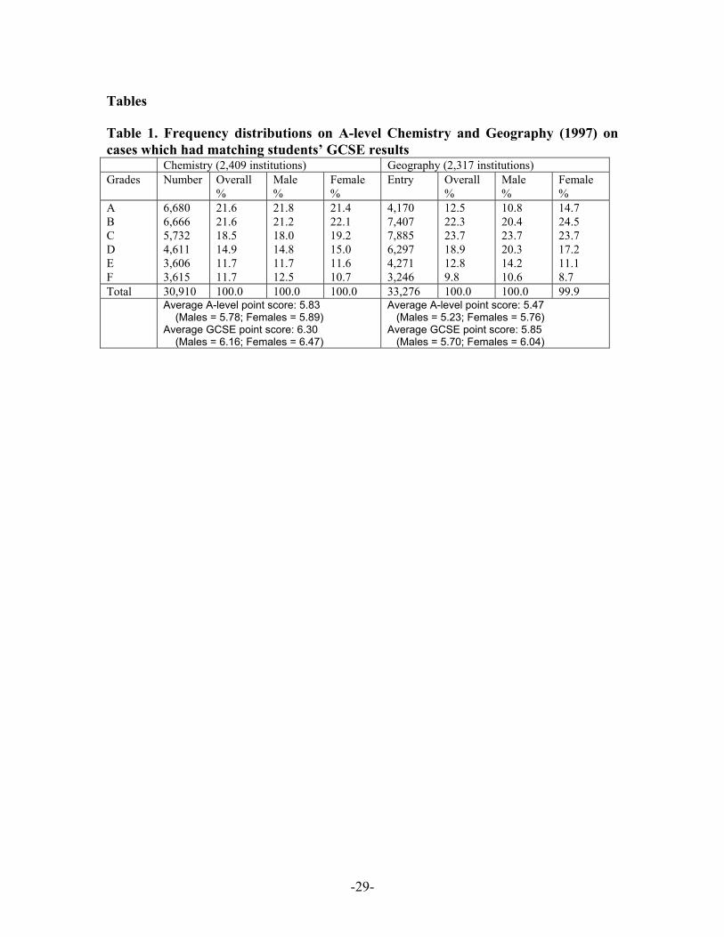
choice of these two subjects is that they have distinct distributions of grades. As Table 1

shows, the grade distribution for Chemistry was skewed towards grades A and B, whilst

that for Geography was more nearly symmetrical. They therefore provide good examples

in comparing model sensitivities to distributional shape.

(Table 1 about here)

It was also decided to omit extreme small outlying groups of 0.36% of Chemistry and

0.37% of Geography students who had very low average GCSE scores well separated

from the main distribution (3 or less using scores discussed below).

In many analyses of aggregate educational performance scores, transformation by

normalising has been a practical way of overcoming problems in modelling due to the

presence of marked ceilings and floors in the score range. This also helps with model

assumptions of normal errors (Goldstein, 1995). In this paper with single subject grade

score responses experimentation with normalising transformations did not noticeably

improve the error distribution of the data compared to using the raw point score. With a

limited number of discrete values the effect of grouping is a likely caveat, but this is

present even under transformation. A further point is that effects are more easily

interpretable on the raw points score scale and also make comparisons between models

for scores and the grades more direct.

A mean centred average GCSE score, GA, is derived from all GCSE subjects of the

student with scores A*=7, A=6, B=5, C=4, D=3, E=2. This is used as a prior attainment

covariate in modelling. Also used are available student level covariates, gender of the

student (Females=1; Males=0) and centred age. The cohort is aged between 18 and 19

years with a mean of 18.5 years. We also introduce the mean of GA (Sch-GA) and

standard deviation of GA (Sch-SD) at the level of the institution as possible institution

level effects. Institutions were also formed into 11 categories according to their

admission policy and type of funding. Most are publicly funded at the local level as Local

Education Authority (LEA) Maintained Schools. Of these schools in LEAs having no

-5-

selection by ability at entry (most LEAs) are Comprehensive (M/C). In selective areas

schools are usually either Selective (M/S) with the rest designated Modern (M/M). There

are also Grant Maintained Institutions funded directly from central government with a

similar selection typology according to their local area (GM/C, GM/S, GM/M).

Independent schools are privately funded and usually fee-paying and are either Selective

or Non-Selective (IND/S, IND/NS). Sixth Form Colleges (SFC) and Further Education

Colleges (FE) are institutions catering specifically for students beyond the compulsory

education age of 16 and are funded directly by central government through a funding

council. In the main there is a heavier concentration of A-level work in the SFCs. There

is a small miscellaneous range of other types (Other). In models dummy explanatory

variables were formed with M/C as the base category. The examination boards involved

in the study were Associated Examining Board (AEB), Cambridge (Camb), London,

Oxford, Joint Matriculation Board (JMB), Oxford-Cambridge joint delegacy (OXCAM),

and the Welsh board, WJEC. The latter has only a few entries and did not show obvious

difference from AEB in data exploration. Thus these two boards were combined to form

the base of dummies for other boards . Fuller details of these variables and their

educational context in the UK is given by Yang and Woodhouse (2001).

3. Statistical models for point scores

As a base for evaluating further developments we can formulate a standard variance

components model for points with institutions at level 2 and students at level 1:

0 ijojij uy eβ= + + (1).

Here denotes the UCAS scored response for the grade of an A level subject offered

by the i student from the school. The term u is the institution random

effect and assumed ~ . The within institution student level disturbance is

. We note an implicit normality assumption for the response which further

means it is assumed continuous. For our grade scored data this is strictly untenable but

ijy

th

0N(

thj20u,σ )

ojthj

0N(

2ij ee ~ ),σ

-6-

may sometimes be assumed to hold approximately for the arbitrary scale on which the

points are located.

We can now add to the model covariates such as are introduced in the previous section..

We can allow covariates which are polynomial terms in continuous variables, interactions

between main factors and so on. We write

0 0= + + +ij ij j ijy u eβ X β (2).

Here is a vector of fixed effect coefficients associated with such factors and covariates

in the data vector . Goldstein (1995) gives terminology and details of fitting such

types of model.

β

ijX

As other researchers have shown, we need in general to fit random coefficients models to

adequately describe institution level variation (O'Donoghue et al, 1996; Goldstein and

Spiegelhalter,1996; Yang and Woodhouse, 2001). Extending by these means we have a

model of the form

= + +ij ij ij j ijy eX β Z u with

1 11 1= =ij ij ij ij ,x ..., ,z ...X Z . (3).

Tβ is now with u . 0 1 β ,β ..., 0 1=Tj j j u ,u ...

Usually, but not always, most of the Z variables are a subset of the X variables. The

elements of u are random variables at the institution level and are assumed dependent

multivariate normal with expectation zero.

Tj

In the following analyses variants of models of types (1), (2), (3) are developed for A

level Chemistry and Geography point scores separately.

-7-

4. Multilevel models for ordered categories

We now exposit parallel formulations modelling ordered grade responses directly without

reference to explicit scoring scales. The six categories of response A-F are denoted by

integer labels s=1,2,3,4,5,6. Following the single level model methods of McCullagh and

Nelder (1989) we use generalised linear models with cumulative probabilities associated

with responses as dependent. For the i student from the institution the probability

of a grade higher than that represented by s is denoted by . We have

. We note that although probabilities for s are

cumulated upwards those of the ordered grades are cumulated downwards. This proves

convenient for interpretation. It is the changing nature of this whole probability

distribution for individuals in response to fixed and random explanatory effects that we

now wish to model. In continuous (normal) response models by contrast we model

conditional expectations given the set of these effects.

th thj(s)

ijγ(1) (2) (5)0 ...ij ij ijγ γ γ< < < < < ij

( )6 1γ =

However, we usually desire models in which effects operate in a linear and additive

fashion. A monotonic ‘link’ transformation of a set of cumulative probabilities on the

[0, 1] scale to the real line usually facilitates this in generalised linear models. In general

this link transformation can be any inverse distribution function of a continuous variable.

In particular the logit (inverse logistic), complementary log-log (inverse Weibull) and

probit (inverse normal) are frequently used. Conceptually a set of thresholds or cut-points

on this link scale for each individual are determined by the individual’s probability

distribution over the grades and vice-versa (Bock, 1975). Thus in our case a link

transformation of (s=1,2….6) corresponds to sequential positions on the whole

real line,

γ )(sij

(2)ijα α(1) (3) (4) (5)( , , , , ,ij ij ij ijα α α )+∞ , with constituting thresholds for the

grades. Fixed and random effects operate linearly on these thresholds and hence

indirectly on the probabilities over the ordered grades. A related conception used in

)(sijα

-8-

ordinal models by many researchers (e.g. McCullagh, 1980; Hedeker & Gibbons, 1994;

Fielding, 1999) is through the notion of an unmeasured and arbitrarily scaled latent

variable. This is assumed to underlie the ordered grades and varies continuously along

the real line. The ordered categories represent contiguous intervals on this variable with

unknown but fixed thresholds. The latent response is assumed governed by a linear

model, and in our case a multilevel linear model. Different distributional assumptions

about the latent variable may be shown to generate particular generalised linear models

for ordered categories of the type under consideration. There are some advantages in

these ideas since interpretation of results can be made directly on the scale of the latent

variable. However, here we shall not be directly concerned with such an interpretation

since our principal aim is to compare the different kinds of inferences arising from the

Normal points and ordinal models. However, Fielding and Yang (1999) further discuss

this idea. Also, when we allow more complexity in randomly varying thresholds as we do

later in the paper, it is not clear that latent variable interpretations can be easily adapted.

Goldstein (1995) discusses the formulation of these models in a multilevel context. In the

main we deal with logit models. Comparable to the base variance components model (1)

is

( )

( ) ( ) ( )0( )logit log

1

= = = −

s

s ij s sij jsij

ij

uα αγ

γγ

+ (s=1,2,3,4,5) (4).

A fit to model (4) estimates a series of marginal location cut-points conceptually similar

to the intercept of model (1). Again for the educational establishment there is a

single random effect u which is assumed ~

thj

(0,N0 j 0

2 )uσ . Individual responses follows a

multinomial distribution determined by their set of grade probabilities, although

estimation procedures can allow for extra-multinomial variation (Goldstein, 1995)1.

1 Even when multinomial variation may be assumed there may be advantages in estimator quality by allowing an extra multinomial parameter to operate (see Yang, 1997; Fielding and Yang, 1999)). We have allowed it in our present analyses though its estimate usually suggests multinomial variation is appropriate.

-9-

Analogously to model (2) we extend the basic model by adding to the model appropriate

fixed effect covariates. We now have

( )( )

( ) ( )0( )

( )logit log1

= = = + −

s

ij s sij ij js

ij

s uij α αγ

γγ

X β + (5)2.

This model possess the proportional odds property (McCullagh, 1980). For all s the fixed

or random effects operate on cumulative odds by a constant multiplicative factors. More

detailed explanation of this and an illustration of parameter interpretation is given by

Yang (2001).

Further, by analogy with the random coefficients model (3) we have

( )( )

( ) ( )( )

( )logit log1

s

ij s sij ij ij js

ij

sij α α

γγ

γ

= = = + −

X β Z u+

(6).

This has similar normality assumptions about the vector of random components . ju

5. Comparison of results between the Normal point score and the ordinal models

To fit the normal models we use the iterative generalised least squares (IGLS) procedures

of MLwiN (Rasbash et al, 1999). Ordinal model results all use penalised quasi-likelihood

in the MLwiN macros MULTICAT (Yang et al, 1999), incorporating the improved

2 A referee of this paper has suggested that as written this model might imply that the sign of a β k is the reverse of the direction of the effect of a variable on the underlying response. This is usually a consequence of an upward shift in probabilities cumulated upwards on the ordered scale implying a downward shift in the response. This often causes confusion in interpreting results. Attempts to remove this by inserting negative signs before the β k and random effects have often been suggested, but this may cause further confusion (Fielding, 1999). In our formulation and as defined our cumulation is downward on the grade scale and both these interpretational difficulties are removed. The signs of the coefficients will be the same as the direction of effects on the underlying response. We feel that this may possibly be adopted in standard practice to good effect.

-10-

second order procedures (PQL2) of Goldstein and Rasbash (1996). Yang (1997)

discusses the validity and statistical properties of these estimators.

In this section we compare parameter estimates and individual institution residual

estimates for the normal and ordinal models. Table 2 provides the comparative results for

base models (1) and (4). Tables 3 and 4 give results for two variants of models (2) and

(5). Firstly we adjust for a range of background characteristics of student, institution, and

exam board but exclude the main intake ability characteristic, student GCSE average.

Table 4 then adds variables derived from the latter in various ways. In particular

polynomial terms in GA are introduced (GA^2, GA^3, GA^4), interactions of these with

gender (GA-F, GA^2-F, GA^3-F), and the aggregated institutional level intake score.

This is a useful extension since it draws a distinction between control for extraneous

factors affecting raw performance and assessing progress using initial intake

achievement covariates. This is standard in educational performance research where it is

desired to highlight types of control on institutional effects (Willms (1992)). We do not

attempt model selection here and include many relevant parameter estimates that on

diagnosis are not statistically significant. Our purpose is a broad comparison of the

models within frameworks familiar in educational research.

Since the parameters associated with the same variable relate to different scales under the

model type comparisons we report as precision measures the standardised t-ratios of

parameter estimates to estimated standard errors. The broad pattern of covariate effects

are the same under normal and ordinal model assumptions. Generally , Ezzett and

Whitehead (1992) have commented that major effects will emerge and are relatively

insensitive to model formulation, though we may expect size of estimates to differ

somewhat. In our case precision measures of regression parameter estimates are very

similar between model types. Formal tests on these yield the same inferential

conclusions. Impressions from either model type closely agree. No real difference in

impact on broad substantive interpretation emerges. Precision of the school level variance

is slightly higher in all cases for ordinal models but the improvement is barely

discernable

-11-

(Tables 2 and 3 about here)

We can comment on the broadly similar patterns of covariate effects for models of

Table 3, which do not adjust for intake achievement. In general, better performances

come from females and younger students. Compared to the base M/C schools, selective

schools of all types have significantly higher achievement. Modern schools have lower

performance but this is not statistically discernable for M/M in Chemistry. Sixth form

colleges and others (mainly sixth form centres in schools) also perform better but in

neither case are results statistically significant for Geography. FE colleges have much

lower achievement generally. GM/C and IND/NS schools are not significantly different

from their maintained comprehensive (MC) counterparts. The estimates of dummy

parameters for boards relative to AEB / WJEC reveal significantly higher average grade

performances for OXCAM, JMB and CAMB Chemistry examinations. Oxford has

significantly worse performance in Geography. Other board effects are not significantly

different from the base.

The results in Table 4 additional have the additional prior achievement covariates at both

institutional and student levels. Effect estimates in this table thus relate to 'adjusted

performance' and relate to progress over the course of A level study. As before,

conclusions from models (2b) and (5b) are comparable. In both subjects younger students

make more progress in addition to having higher general achievement. However, boys

now make more progress than girls despite girls being higher achievers, as also noted by

O'Donoghue et al. (1996). M/S and GM/S selective schools now lose their significant

comparative advantage when progress rather than raw performance is the criterion.

However, the effect of IND/S is statistically significant in both subjects. M/M, GM/C and

IND/NS schools make no significantly different progress from M/C in either subject.

GM/M seem to do worse but the effect is significant only for Geography. Sixth form

colleges achieve higher progress in Chemistry than the base M/C type but no longer have

the advantage in Geography. FE colleges show significantly lower progress in Geography

but this does not carry over for Chemistry. The pattern of board effects for adjusted

-12-

performance in Chemistry is similar to those on raw performance exhibited in Table 3.

However, CAMB now joins Oxford in having significantly worse adjusted performance

in Geography. Other board effects are again not distinguishable. All these general

substantive findings are similar to those of Yang & Woodhouse (2001) based on

aggregate A/AS points scores for the whole database.

(Table 4 about here)

6. The nature of GCSE effects

Prior achievement as measured by GCSE results have formed an input into the second

group of models. It is this fact that often enables researchers to treat institutional effects

as ‘adjusted’ and form a basis for a ‘value-added’ criterion. The way it operates in

combination with other factors has been likened to economic concept of an educational

production function. This paper and others (Goldstein & Thomas, 1996; O’Donoghue et

al, 1997; Yang & Woodhouse, 2001) show that this production function should include

many non-linear terms in the covariates. Thus in Table 4 polynomial terms of order up to

four in prior achievement have been included to allow a possibly necessary fine non-

linear graduation of the response to this variable particularly at the extremes. Institution

context factors such as Sch-GA and Sch-SD will also often have a discernible influence.

Sch-D may , for instance, be useful in examining what, if any, is the impact of

homogeneity of school intake on progress. The gender differentiation of GCSE effects is

represented by terms for the interaction with the female gender dummy variable.

As indicated by the t-ratio precision measures Table 4 the normal model evidenced

significant polynomial terms in GCSE average up to the fourth order. The ordinal logit

model required only a quadratic function. As a result of polynomial effects, the nature of

the interaction of gender with prior ability cannot be simply expressed as a single

additive element. However, the normal model exhibited interactions for both subjects but

the ordinal model only for Chemistry. This may be due to the skewed nature of its

response distribution over grades or could be related to differential impacts of ceilings

and floors. In the context of primary school progress, Fielding (1999) notes that ordered

-13-

category models seem to be more parsimonious in many circumstances and require fewer

complex fixed effect terms. It is further noted there that this requirement may be

conditioned by the response distributions. The results here seem to confirm these

impressions. The normal model seems much more sensitive to the actual values of GCSE

scores than the logit model.

In both types of model the effects of school intake contexts appear relatively small but

with Sch-GA having a marginally significant effect in Chemistry and within school

heterogeneity (Sch-SD) having a positive effect in Geography.

7. The use of ordinal models in predicting grade distributions

In A level work teachers are expected to predict A level performances for university

entrance purposes. Normal models give score predictions which may be difficult to relate

to grades. A more useful approach might be to evaluate the 'chances' that a certain student

will achieve certain grade thresholds. Ordinal models have a very useful role in this area

by predicting directly the probability that students with given background characteristics

and initial ability will achieve certain grades. Normal models can only do this indirectly

from the conditional means and variances and assumptions that grade boundaries are

placed appropriately along the points scale (5.0 to 7.0, for instance for grade C). Using

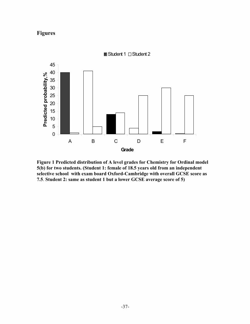
estimates from Model 5(b) in Table 4, we illustrate in Figure 1 the ‘chances’ of

achievement estimated for two female students having the same set of background

covariate values but different GCSE average scores. Student 1, with a high GCSE score

of 7.5, has a very high chance of achieving a Chemistry grade no less than B on A level

Chemistry; while Student 2, with a GCSE score of 5, is most likely to achieve a grade no

higher than D. Estimates from Model 2(b) in Table 4 for these two students give A level

point score predictions as 9.8 and 1.9 respectively. Although they are roughly equivalent

to grades A and E, they represent conditional expectations only. Using individual level

variance estimates a predicted grade distribution could also be calculated from the

assumed normal ( e.g. probability of grade C would be found from the area between 5

and 6 ). However, assumed normality on the underlying arbitrary raw points scale is

-14-

crucial when applied in this context. Model estimates may be reasonably robust to

departures from the normality assumption. Interval predictions may not be quite so

robust. Even relatively small departures from normality in the true distribution over the

raw points scale might yield quite different predictions. This is a further aspect of

sensitivity to the arbitrary score scale and normal assumptions over it. No such fixing of

a scale or constraining distributional assumptions are required for ordinal models.

(Figure 1 about here)

8. Value added estimates using school residuals

We have also incorporated random coefficients in the models as in (3) and (6). Detailed

results are not illustrated here. However, significant random coefficients at the

institutional level for both model types and subjects were the female gender and the first

order GA term. Thus we now have three random effects for each institution which could

be estimated by MlwiN residual procedures. Models 3 and 6 in our discussion and

diagram below relate to fits of models with these two extra random effects added to the

models of Table 4. However, we focus on the intercept residual estimates only. Since GA

was centred these represent institution average adjusted effects or 'value added', as they

often termed in the educational literature. They relate to males with an average GCSE

score, having allowed in the model for possible differential institutional effects on

students of different gender and prior achievement. This approach gave us a set of

homogenous institution residual estimates that enable us to investigate mild changes of

assessment of institutional ‘added value’ between the model approaches. We also

diagnostically checked certain model assumptions for ensuring the comparability

between models. The distributions of the standardised institution intercept residuals for

the two models on both A-level subjects are very close to normality as seen by the

normal plots in Figures 2 and 3. Residuals from the model approaches are closely related.

The correlation coefficients and rank correlations between the institution residual

estimates from each pair of models are:

Chemistry Geography

Establishment residuals 0.982 0.968

-15-

Ranks of establishment residuals 0.983 0.970

Note that these correlations are somewhat inflated because of 'shrinkage' factors

Nevertheless, they and inspection of the residual scatter plots, not illustrated here,

suggest a strong agreement between model types for institution ‘value added’ estimates.

Given the fairly complex and full modelling of covariates and effects we would usually

not expect otherwise. However, they are not perfect and there is scope for some

movement in the positioning of individual institutions. Correlations can be relatively

insensitive to these. Even mild sensitivity to model formulation is potentially of

substantive interest. In particular, we might investigate any dependency on models of the

identification of institutions at the extremes of the range of effects.

[Figures 2 and 3 about here]

Thus we now examine in detail some selected institutions. We choose four for each

subject. Two of these are in the middle of the distribution of the institution residual

estimates for Chemistry normal models . These are also examined for Geography.

Further, for each subject separately, two extreme institutions are selected. Some details

on the selected institutes are listed in Table 5. Table 6 shows the ranks of the residuals of

the selected institutions in each model, the residual estimates and their standard errors.

Also shown are 95% overlap intervals (Goldstein and Healy 1995) converted into

equivalent intervals of ranks.

[Tables 5 and 6 about here]

The results show that extreme schools are detected with either model. In the middle of

the distribution, however, there are often considerable differences in rankings. There is

important sensitivity of 'league table' position to the chosen adjustment model even when

both include the same covariates. The intervals for institutions 1 and 2 on Chemistry,

whose ranks are only 66 apart (1317 – 1251), overlap considerably for the normal model.

However, even in the ordinal model for this case where rankings are about 1000 apart

-16-

(1706 – 702), and much more clearly separated, there is still considerable overlap of the

intervals. For Geography, institutions 1 and 2 being less concentrated in the middle of the

rank range, have separable intervals under both models, but less clearly so for the ordinal

model. However, it requires rankings differing by 1502 and 1472 respectively to achieve

these separations. Although the extreme institutions have a much more consistent ranking

there are one or two other features worthy of note. For Geography, institution 5 (highest

ranked on the ordinal model) and 2 have relatively short rank differences of 111 and 300

for normal and ordinal models respectively. However, at the top end of the range their

intervals do not overlap for the ordinal model and only just for the normal. Rank intervals

for extreme cases are very short. There appears to be a clearer separation between pairs

as we move away from the middle of the distribution. The same phenomenon occurs at

the lower end.

9. Extensions of the ordinal model

So far the ordinal logit models have the proportional odds feature implied by fixed cut-

point thresholds not varying across observations. However, more flexibility can be

introduced by allowing interactions of thresholds with covariates or allowing random

thresholds effects across level 2. For example, as it stands, the fitted ordinal model in

Table 4 suggests that the additive main effect of gender on the cumulative log-odds is

the same across grades. Covariate changes shift only the location of the entire grade

distribution keeping the relative odds proportional. We can relax this by interacting

covariates with cut-points. For instance, interacting with gender means the cut-points for

males and females are no longer separated by a single additive gender effect, and gender

can affect cumulative odds non proportionally across grades. Indeed , there is some

preliminary evidence that a proportional odds gender effect may not be tenable. In Table

1 in Geography, for instance, more female students achieved the top two grades than

males and vice versa for the bottom two grades. The distributional differences between

genders may be more complex than a constant shift in cumulative log-odds. The

suggested non-proportional extensions can be fitted fairly readily by adaptation of the

quasi-likelihood procedures in the MLwiN MULTICAT macros that we use.

-17-

9.1. Model with non-proportional changing odds

Model 7 below extends the fixed part of Model 5 in these directions. We focus on non-

proportional gender effects since these have evoked our interest. For ease of exposition

we revert to the model with a single variance at level 2. We have investigated extensions

to Model 6 with little difference of substance to the arguments we present. This type of

model has been called a multilevel thresholds of change model (MTCM) by Hedeker &

Mermelstein (1998).

Letting be 1 if the i person from institute is female, we write ijt th j

( ) ( ) ( ) ( )0

( )logit = = + + +s s sij ij ij j

s tij α α ωγ X β u (7).

Estimates of the cut-points ( )sα determine the cumulative grade distribution of males

conditional on other explanatory variables, and estimates of ( ) ( )( )+s sα ω those of

females. Similar terms could be introduced for other explanatory covariates and higher

order interactions are also possible3.

(Table 7 about here)

The results of fitting model 7 are displayed in Table 7. They suggest definite interactions

of cut points with gender and hence a non proportional effect of gender on cumulative

odds.

(Figure 4 about here)

3 McCullagh and Nelder (1989, p155) and also Hedeker and Mermelstein (1998) comment that for continuous covariates this may unfortunately lead to negative fitted values for some values of covariates. In our case we have checked that this would not occur inside the observed range if we were to entertain non proportional odds for covariates in our data such as GA.

-18-

The ratios of cumulative odds of males to females at each threshold are displayed in

Figure 4 and contrasted with the constant proportional odds ratios of Model 5. It is

clearly seen that the overall negative effect of females estimated by model 5 on

Geography was mainly because female students achieve relatively few high grades,

having adjusted for their GCSE average score. For Chemistry there is a different pattern

with relatively more females in middle grades and slightly more failures than a

proportionality assumption would warrant. Differences in skewness of the distributions

of grades in the two subjects may play a role and the importance of these is underlined by

this type of ordinal model.

9.2. Random institution effects on cut-points for the distribution over grades

In the same way that we consider odds changing non-proportionally for different values

of covariates we can allow non-proportionality of the random institution effect. This is

achieved by allowing the cut points to vary randomly across institutions. Thus we now

generalise model (7), which had a single random effect, by incorporating a set of grade

specific cut-points ( ( ) ( )s s

ojuα + , s = 1, 2, 3, 4, 5) for each institution. The model is

( ) ( ) ( ) ( ) ( )( )logit = = + + +s s sij ij ij oj

s tij α α ωγ X β su (8).

Here, u 0 . 0

(1) (2) (5)0 0 0 , ,........ ~ ( , )′=oj j j j uu u u MVN Ω

The Ω is a (5 x 5) covariance matrix of the separate random effects. For simplicity

we also assume that the interacting gender coefficients are fixed, that is, there is no

differential institutional effect by gender.

ou

The estimates for model 8 are also given in Table 7. The institution random effect

parameters are shown separately in the lower part of Table 8. The fixed part results show

main effects similar to those estimated by model 7 for both Chemistry and Geography

but there are some changes to the base (male) and female cut-points. From the random

-19-

parameter estimates we see that there is relatively more institutional variation at grade A

and F thresholds in Geography. For Chemistry the F threshold parameter exhibits most

variation. Such sources of institutional variation at crucial thresholds may be potentially

of more substantive interest then overall average levels of adjusted performance.

(Table 8 about here)

Detailed diagnostic normal plots of all estimated standardised residuals from model (8),

though not illustrated, showed good agreement with the normality assumption for both

subjects.

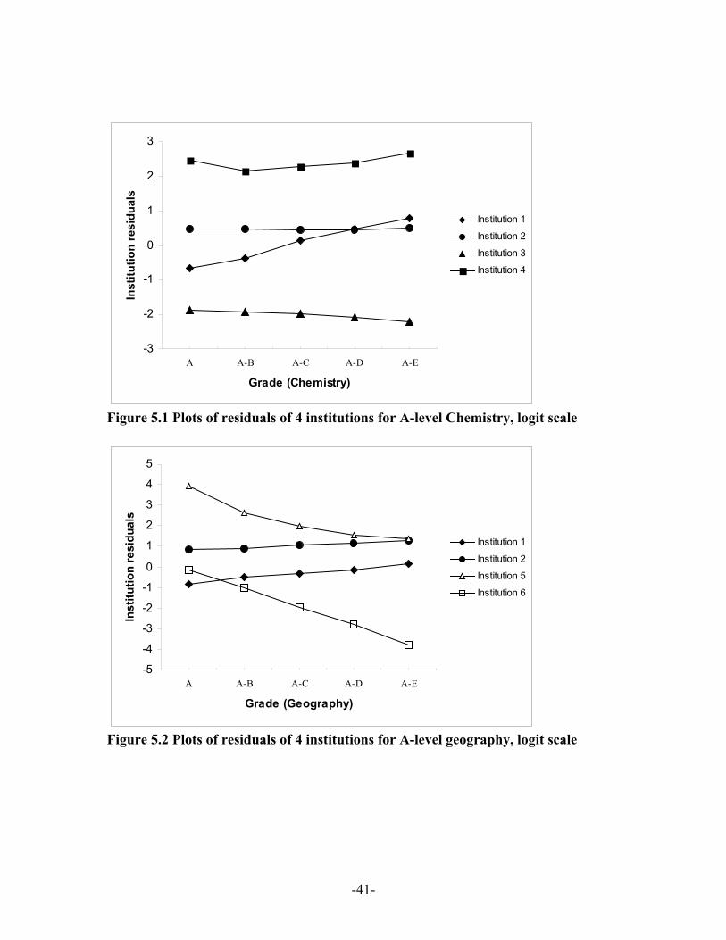
For the same institutions previously investigated in Section 8 estimates of the full set of

cut point residuals in model 8 are illustrated in Figures 5.1 and 5.2. These show a

relatively constant pattern of effects over the grades on Chemistry for institutions 2, 3

and 4 and are not much different from results observed in Table 6. These institutions

could be interpreted as having relatively uniform effect on students across all levels of

ability. Institution 1 has a below average conditional expectation of achieving at least

either of the top two thresholds, about the same as average for above grade C, and above

average for the proportion not failing or achieving above grade D. It would be interesting

to examine the practice at this institution , which seems to have a better than expected

overall pass rate but a relatively lower than expected achievement at the top end of the

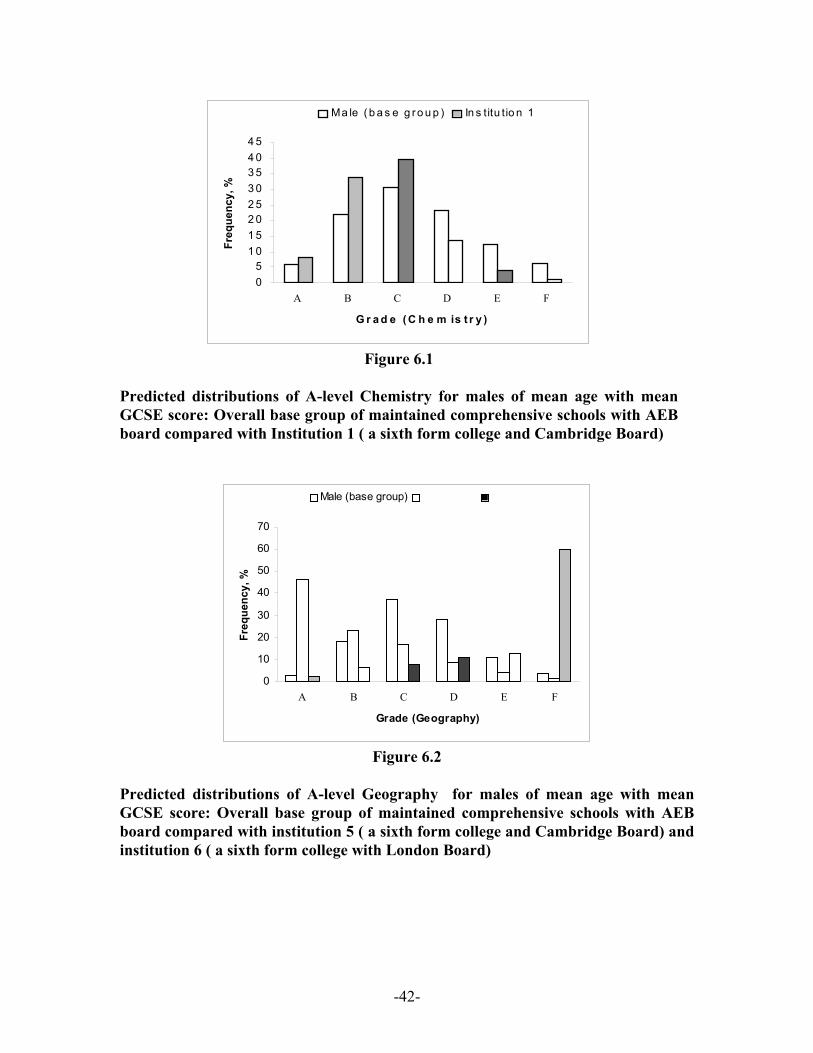
grading. This pattern is further displayed in detail for males in Figure 6.1 which contrasts

the predicted A level grades in Chemistry for typical males in Institution 1 with similar

males in the base group of students. It will be noted that compared to the similar base

group there appear relatively fewer in the bottom three categories but much higher

proportions in Grades B and C.

For Geography the effect of Institutions 1 and 2 are approximately proportional across

grade thresholds. Institutions 5 and 6, occupying the highest and lowest positions in

Table 6, have a profile of threshold effects that are parallel and consequently with a

similar relative pattern but at different absolute levels. Given their general levels, the size

of their effects declines relative to all institutions as we move through the grade

-20-

thresholds. They are relatively rather better at targeting top grades than they are at

getting students above low thresholds and passing. Institution 6, for instance, is not too

far from average in its effect on top grade chances (and better than Institution 1) but its

low overall position is due to ‘deficiencies’ at lower thresholds. Figure 6.2 presents the

predicted distributions of A level Geography grades for males of mean age with mean

GCSE in Institution 5 at the top of the scale and Institution 6 at the bottom. Although as

expected Institution 5 has a much higher proportion of Grade A’s, there is little

difference between Institution 6 and that of the base group in this respect. The impact of

failures on the overall position of Institution 6 is obvious from this diagram. There is a

further important general caveat for predictions for particular institutions. These use

residual estimates which have uncertainty and require some caution as stressed by

Goldstein & Spiegelhalter (1996). Often the residuals are based on relatively small

numbers of students so that the standard errors of estimates can be quite large. Thus, for

example, in the present comparisons in Geography Institution 1 has a standard error for

the grade B cut-point of 0.299. Conditional on the fixed point estimates a 95%

confidence interval for the logit can be constructed. Converting to the cumulative

probabilities gives an approximate interval of 28.1% to 56.1% for above grade B. In

principle, for more detailed analysis, intervals can be constructed for overall predictions

of full grade distributions for each institution.

[Figures 5 and 6 about here]

10 Discussion

In this paper we have demonstrated a flexible range of models for educational grades

treated as ordered responses. The operational definition of the outcome variable is at no

higher a level of measurement than this. Assumptions of continuous response multilevel

models with scores may thus be inappropriate, particularly since there are few scored

grades. Statistical objections have ranged from those about the scaling implied by

arbitrariness in scoring through to continuous distribution properties applied to discrete

measurements and to bias in estimation due to grouping. A review of some literature on

-21-

this is given by Fielding (1999) and a recent general contribution is Kampen and

Swyngedouw (2000).

From a practical and substantive view normal linear models are certainly useful and have

the virtue of familiarity with very accessible methodology and software. Certainly, this

paper shows that the general scale of fixed effects is relatively insensitive to model

formulation. Estimated precision of the fixed effect estimates are also comparable,

although little is known about how the estimated precision is affected by the discrete

nature of the observed data. However, for institution specific details there are

considerable differences between the models. In this respect it may be argued that ordinal

models make fewer restrictive assumptions about the response distribution and provide

conclusions which are less open to substantive query. Although the intercept residuals

from models 3 and 6 are highly correlated, the location of specific institutions in their

range can vary greatly. For instance, Institution 2 for Chemistry is at the 29th percentile

of ranked residuals on the ordinal model and at the 55th percentile for the normal model

(see Table 6). It is true that these positions are both subject to uncertainty but the

question arises as to the appropriateness of the modelling if we want to draw substantive

‘value added’ conclusions.

From a practical point of view in educational research the ordinal models also offer as

much information as do normal models, and it could be argued more. The ‘newness’ of

ordinal models and (until recently) lack of suitable software may have acted as practical

deterrent, but this is being remedied. The ability to convey predictive information

through probability distributions, which cannot easily be done using standard models, is a

particular advantage. Since grades and levels are standard modes of reporting it may

obviously be useful to relate the interpretations of results to these. A predicted point

score for an individual, even when contextualised in terms of the conditional mean of a

continuous distribution, has less ready an interpretation when grades and levels are the

medium of converse. The implications of the use of ordinal models in such practical areas

as target setting within schools may be clear.

-22-

Ordinal models also seem to be capable of extension in substantively useful ways. Their

characterisation in terms of grade probability responses permits flexible parameterisation

for a variety of conditions. Our analyses have mainly been concerned to comment on the

practical significance of this. However, these additional complexities also considerably

improves the fit of models. A simultaneous Wald test ( available in MlwiN) on

parameters , the interactions between the gender variable and the cut-points in the

fixed part of (7) yielded significant

ω )(s

2

5χ =132.8 for Geography and =580.8 for

Chemistry. Secondly, a restriction that all 15 variance and covariance parameters of the

separate random effects at the institution level in (8) are equal to a common parameter

value reduces it to the single effect model of (7). An approximate Wald test on this

yields very significant χ =164.9 for Geography and

2

5χ

2

14

2

14χ =261.7 for Chemistry. From a

practical view we have seen, for instance, that by allowing cut-points to interact with

gender we can study gender differences in distributions in greater detail. As discussed

these differences go further than simply differences in average performance. By allowing

random cut-points institutional differences can also be exhibited in more meaningful

ways. They can be compared at important thresholds rather than through simple mean

levels of adjusted achievements. Thus Institution 1 in Chemistry has lower grade A

achievements than expected but it also has lower failures. Institution 6 in Geography has

a considerable failure rate but does quite well in achieving high grades compared to other

typical institutions. Differences between institutions in such respects might well engage

the interest of effectiveness researchers and policy makers as of much if not more

relevance than differences in ‘average’ achievement or progress.

An aspect of ordinal model we have not discussed in any detail is the nature of the link

function. We have focused on the familiar logit. However, we have also carried out some

investigations using a probit link which will be available in the latest issue of

MULTICAT. A probit link is often interpreted in terms of normally distributed latent

variable. Thus it might seem to fit more easily into comparisons with normal linear

models. There is a conventional wisdom in the generalised linear modelling literature

-23-

(e.g. McCullagh and Nelder, 1989; Greene, 2000) that important results are relatively

insensitive to this choice of link. This is often attributed to the similarity of the logistic

and normal distributions except at the tails. Preliminary results show some differences

but none are startling. However, methodological work comparing logit, probit and other

links in the multilevel context is under way and needs further advancing.

If, as we claim, ordinal models are worthy of more extensive application they need also

to be developed further in a number of important directions. Ordinal models with cross-

classified random effects at higher levels have been considered by Fielding & Yang

(1999). Multivariate response multilevel models for continuous variables are developed

and quite widely used in education (Goldstein and Sammons, 1997; Yang et al , 2001 ).

In our investigations with Model 7 we compared the two sets of cut-point residuals for

institutions which had Geography and Chemistry in common. A general impression

conveyed was that there were two major groups of institutions. One group was those

institutions whose effects for the two subjects were similar relative to all schools.

However, another major group had relatively high ‘adjusted’ performances in one subject

together with a low achievement in the other. There are some interesting practical

questions here about the differential 'effectiveness' of schools in different A level subjects

and the relationships between subject grades at both student and institutional level.

Multivariate ordinal response multilevel model developments are required for this. Their

characterisation is not so easy as the analogous continuous variable specifying normal

correlation structures. Nor would their estimation be as easily adaptable from standard

available procedures. Promising lines of inquiry which we have started to investigate for

multilevel structures is log-linear characterisation of the multivariate distributions and

multivariate logit and probit (Joe, 1997; Lesaffre and Molenberghs, 1991; Molenberghs

and Lesaffre, 1994) Other developments we envisage are multivariate models for mixed

continuous and ordered category responses, and to parallel the longitudinal binary

response models of Yang et al. (2000), variants for ordered categorisations. The latter

situation has received some attention in the generalised estimating equation (GEE)

literature (Lipsitz and Kim, 1994)) but these are population averaging methods As such

-24-

they concentrate mainly on ways of obtaining efficient fixed effects estimates and cannot

at present be used to investigate the detailed structure of multilevel effects.

Acknowledgements

This study is part of the project Application of Advanced Multilevel Modelling Methods

for the Analysis of Examination Data, supported by the Economic and Social Research

Council (ESRC) of U.K. under the Grant award R000237394. The Department of

Education and Employment (DfEE) kindly provided the raw exam data. The ESRC has

also given support to Antony Fielding’s Visiting Research Fellowship at the Multilevel

Models Project under award H51944500497 of the Analysis of Large and Complex

Datasets programme. Valuable comments were received from James Carpenter and

reviewers of an earlier version of the paper.

References

Bock RD (1975) Multivariate statistical methods in behavioral research. New York: McGraw-Hill.

Chan JSK, Kuk AYC, Bell J, McGilchrist CE (1998) The analysis of methadone clinic data using marginal and conditional logistic models with mixture or random effects. Australian and New Zealand Journal of Statistics, 40 (1), 1-10.

DfEE (1995) The development of a national framework for estimating value added at GCSE A/AS level, technical annex to GCSE to GCE A/AS value added: Briefing for schools and colleges. London: Department for Education and Employment.

Ezzett F, Whitehead J (1991) A random effects model for ordinal responses from a crossover trial. Statistics in Medicine, 10, 901-907.

Fielding A, (1999) Why use arbitrary points scores?: ordered categories in models of educational progress. Journal of the Royal Statistical Society Series A, A, 162, 303-330.

Fielding A, (2002) Ordered category responses and random effects in multilevel and other complex structures: scored and generalised linear models, in Multilevel Modelling: Methodological Advances, Issues and Applications, S. Reise & N. Duan ( eds.). New Jersey: Erlbaum .

Fielding A, Yang M, (1999) Random effects models for ordered category responses and complex structures in educational progress. University of Birmingham Department of Economics Discussion Paper 99-20, (submitted for publication).

-25-

Goldstein H, (1995) Multilevel Statistical Models (2nd edition). London: Edward Arnold.

Goldstein H, Spiegelhalter DJ (1996). League tables and their limitations: statistical issues in comparisons of institutional performance (with discussion). Journal of the Royal Statistical Society Series A, 159, 385-443.

Goldstein H, Healy M.JR (1995) The graphical presentation of a collection of means. Journal of the Royal Statistical Society Series A, 158, 505-513.

Goldstein H, Rasbash J (1996) Improved estimation in multilevel models with binary responses. Journal of the Royal Statistical Society Series A, 159, 505-513.

Goldstein H, Sammons P (1997) The influence of secondary and junior schools on sixteen year examination performance: a cross-classified multilevel analysis. School Effectiveness and School Improvement, 8, 219-230.

Goldstein H, Thomas S (1996) Using examination results as indicators of school and college performance. Journal of the Royal Statistical Society Series A, 159, 149-163.

Gray J, Jesson D, Goldstein H, Hedger K, Rasbash J (1995) A multi-level analysis of school improvement: changes in schools’ performance over time. School Effectiveness and School Improvement, 6, 97-114.

Greene WH (2000) Econometric analysis (4th Edition). Upper Saddle Valley, New Jersey: Prentice-Hall.

Gray J, Goldstein H, Jesson D (1996) Changes and improvements in schools’ effectiveness: trends over five years. Research Papers in Education, 11(1), 35-51.

Harville DA, Mee RW (1984) A Mixed-model procedure for analysing ordered categorical data. Biometrics, 40, 393-408.

Hedeker D, Gibbons RD (1994) A random-effects ordinal regression model for multilevel analysis. Biometrics, 50, 933-944.

Hedeker D, Gibbons R D (1996). MIXOR: A computer program for mixed effects ordinal regression analysis. Computer Methods and Programs in Biomedicine, 49, 157-176

Hedeker D, Mermelstein J (1998) A multilevel thresholds of change model for analysis of stages of change data. Multivariate Behavioral Research, 33 (4), 427-455.

Jansen J (1990) On the statistical analysis of ordinal data when extra-variation is present. Applied Statistics, 39, 1, 75-84

Joe H (1997) Multivariate models and dependency concepts. Boca Raton, Florida: CHC

Kampen J, Swyngedouw M (2000) The ordinal controversy revisited. Quality & Quantity, 34, 87-102.

Lesaffre E Molenberghs G (1991) Multivariate probit analysis: A neglected procedure in medical statistics. Statistics in Medicine, 10, 1391-1403

-26-

Lipsitz SR, Kim K, Zhao L (1994) Analysis of repeated categorical data using generalised estimating equations. Statistics in Medicine, 13, 1149-1163.

McCullagh P (1980) Regression models for ordinal data (with discussion). Journal of the Royal Statistical Society Series B, 42, 109-142.

McCullagh P, Nelder JA (1989) Generalised Linear Models ( 2nd Edition). London: Chapman and Hall.

Molenberghs G Lesaffre E (1994) Marginal modelling of correlated ordinal data using a multivariate Plackett distribution. Journal of the American Statistical Association, 89, 633-644

O’Donoghue C, Thomas S, Goldstein H, Knight, T (1997) 1996 DfEE study of value added for 16-18 year olds in England, DfEE Research Series, March, . London: Department for Education and Employment.

Rasbash J, Browne W, Goldstein H, Yang M, Plewis I, Healy M, Woodhouse G, Draper D, (1999) A user’s guide to MLwiN. London: Multilevel Models Project, Institute of Education, University of London.

Saei A, McGilchrist CA (1996) Random component threshold models. Journal of Agricultural, Biological and Environmental Statistics, 1, 288-296.

Saei A, Ward J, McGilchrist CA (1996) Threshold models in a methadone programme evaluation. Statistics in Medicine, 15, 20, 2253-2260

Saei A, McGilchrist C.A (1998) Longitudinal threshold models with random components. Journal of the Royal Statistical Society Series D (The Statistician) , 47, 365-375

Willms JD (1992) Monitoring school performance: A guide for educators. Lewes : Falmer Press

Yang M (1997) Multilevel models for multiple category responses by MLn simulation. Multilevel Modelling Newsletter, 9, 1, 9-15, Institute of Education, University of London.

Yang M (2001) Multinomial Regression in A. Leyland & H. Goldstein (eds), Multilevel Modelling of Health Statistics. Chichester: Wiley

Yang M, Goldstein H, Heath A (2000) Multilevel models for repeated binary outcomes: Attitudes and voting over the electoral cycle. Journal of the Royal Statistical Society Series A, 163, 49-62.

Yang M, Rasbash J, Goldstein H (1998) MlwiN macros for advanced multilevel modelling. London: Multilevel Models Project, Institute of Education, University of London.

-27-

Yang M, Woodhouse G (2001) Progress from GCSE to A and AS level: institutional and gender differences, and trends over time. British Journal of Education Research, 27, 2. Yang M, Goldstein H, Browne W, Woodhouse G (2001) Multivariate multilevel analysis of examination results. Journal of the Royal Statistical Analysis Series A, 165, 137-153

-28-

Tables

Table 1. Frequency distributions on A-level Chemistry and Geography (1997) on cases which had matching students’ GCSE results Chemistry (2,409 institutions) Geography (2,317 institutions) Grades Number Overall

% Male %

Female %

Entry Overall %

Male %

Female %

A B C D E F

6,680 6,666 5,732 4,611 3,606 3,615

21.6 21.6 18.5 14.9 11.7 11.7

21.8 21.2 18.0 14.8 11.7 12.5

21.4 22.1 19.2 15.0 11.6 10.7

4,170 7,407 7,885 6,297 4,271 3,246

12.5 22.3 23.7 18.9 12.8 9.8

10.8 20.4 23.7 20.3 14.2 10.6

14.7 24.5 23.7 17.2 11.1 8.7

Total 30,910 100.0 100.0 100.0 33,276 100.0 100.0 99.9 Average A-level point score: 5.83

(Males = 5.78; Females = 5.89) Average GCSE point score: 6.30 (Males = 6.16; Females = 6.47)

Average A-level point score: 5.47 (Males = 5.23; Females = 5.76) Average GCSE point score: 5.85 (Males = 5.70; Females = 6.04)

-29-

Table 2. Model estimates for variance component model (1) and basic ordinal model (4)

Model (1) Model (4) Param. Chemistry Geography Param. Chemistry Geography Estimate Precision

* Estimate Precision Estimate Precision Estimate Precision

0β 5.349 5.250 ( )1α -1.881 -2.405

( )2α -0.668 -0.913

( )3α 0.248 0.230

( )4α 1.106 1.274

( )5α 2.089 2.406

u2σ

2.829 24.90 2.017 24.41 u2σ

1.190 25.50 0.995 25.38

e2σ

8.507 7.228 Extra-multinomial variation

0.945 0.959

*Note: Precision=estimate/standard error. This measure was not calculated for the intercept in the Normal point score model nor for the thresholds in the ordinal model, or for level 1 parameters, as they relate to non comparable quantities across the two approaches.

-30-

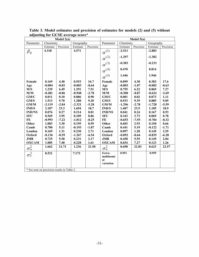
Table 3. Model estimates and precision of estimates for models (2) and (5) without adjusting for GCSE average score*

Model 2(a) Model 5(a) Parameter Chemistry Geography Parameter Chemistry Geography Estimate Precision Estimate Precision Estimate Precision Estimate Precision

0β 4.318 4.571 ( )1α -2.511 -2.883

( )2α -1.297 -1.382

( )3α -0.383 -0.233

( )4α 0.470 0.814

( )5α 1.446 1.946

Female Age M/S M/M GM/C GM/S GM/M IND/S IND/NS SFC FE Other Camb London Oxford JMB OXCAM

0.169 -0.004 1.239 -0.481 0.011 1.513 -2.119 2.187 0.076 0.569 -0.993 1.083 0.700 0.169 -0.136 0.725 1.085

4.40 -0.82 6.49 -0.86 0.10 9.70 -2.84 23.3 0.27 3.95 -7.22 3.30 5.11 1.31 -0.59 5.50 7.48

0.553 -0.003 1.291 -0.948 0.086 1.288 -2.321 1.694 0.214 0.109 -1.012 0.195 -0.193 0.230 -1.267 0.231 0.228

16.7 -0.64 7.51 -2.78 0.90 9.20 -5.28 18.7 0.81 0.86 -8.25 0.59 -1.87 2.71 -6.54 2.17 1.61

Female Age M/S M/M GM/C GM/S GM/M IND/S IND/NS SFC FE Other Camb London Oxford JMB OXCAM

0.099 -0.003 0.755 -0.300 0.001 0.933 -1.296 1.407 0.041 0.343 -0.653 0.603 0.441 0.097 -0.092 0.458 0.654

4.30 -1.07 6.22 -0.87 0.02 9.39 -2.78 23.5 0.24 3.73 -7.55 2.93 5.19 1.20 -0.64 5.55 7.27

0.383 -0.002 0.869 -0.624 0.073 0.885 -1.728 1.185 0.167 0.069 -0.704 0.150 -0.122 0.149 -0.835 0.149 0.123

17.6 -0.63 7.27 -2.69 1.11 9.05 -5.59 18.9 0.93 0.78 -8.32 0.66 -1.71 2.55 -6.28 2.04 1.26

u2σ 1.662 21.71 1.236 21.50

u2σ 0.698 22.83 0.623 22.57

e2σ 8.521 7.173 Extra-

multinomial variation

0.951 0.959

* See note on precision results in Table 2.

-31-

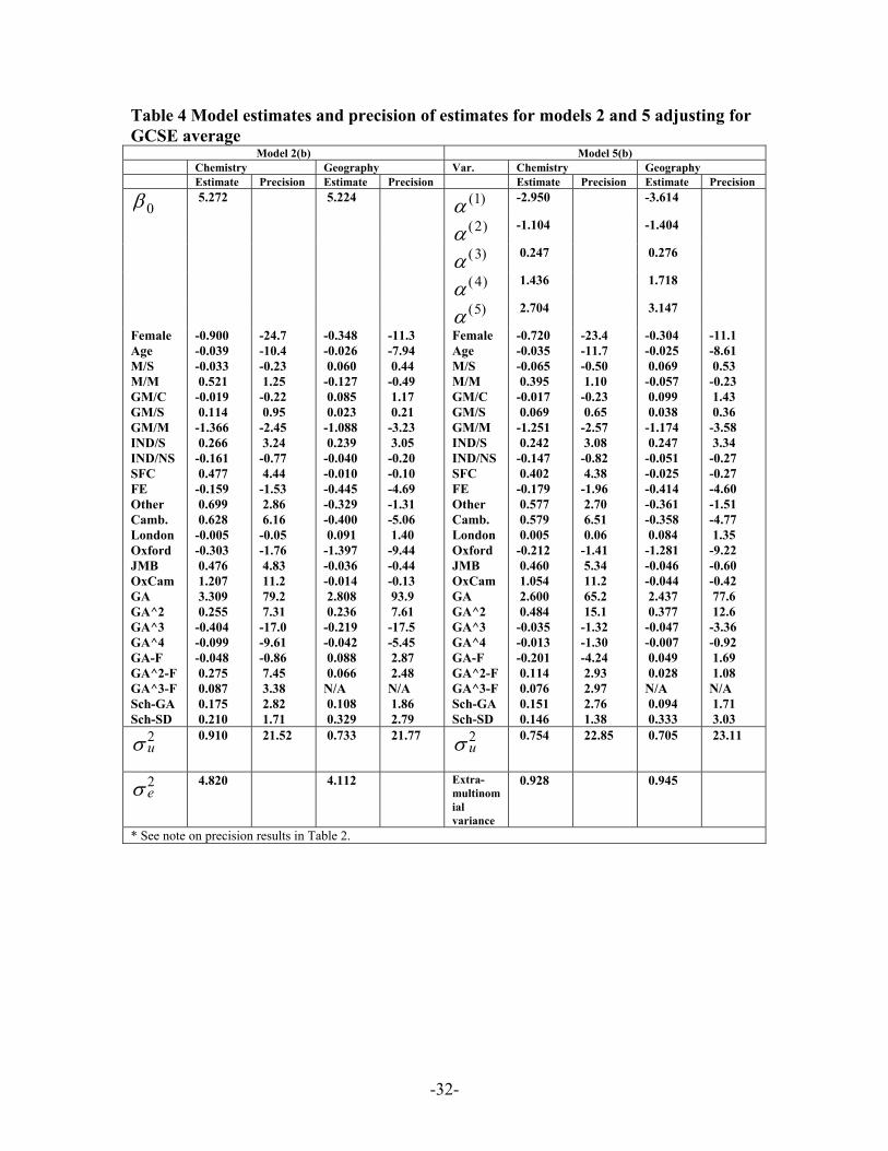
Table 4 Model estimates and precision of estimates for models 2 and 5 adjusting for GCSE average

Model 2(b) Model 5(b) Chemistry Geography Var. Chemistry Geography Estimate Precision Estimate Precision Estimate Precision Estimate Precision

0β 5.272 5.224 ( )1α -2.950 -3.614

( )2α -1.104 -1.404

( )3α 0.247 0.276

( )4α 1.436 1.718

( )5α 2.704 3.147

Female Age M/S M/M GM/C GM/S GM/M IND/S IND/NS SFC FE Other Camb. London Oxford JMB OxCam GA GA^2 GA^3 GA^4 GA-F GA^2-F GA^3-F Sch-GA Sch-SD

-0.900 -0.039 -0.033 0.521 -0.019 0.114 -1.366 0.266 -0.161 0.477 -0.159 0.699 0.628 -0.005 -0.303 0.476 1.207 3.309 0.255 -0.404 -0.099 -0.048 0.275 0.087 0.175 0.210

-24.7 -10.4 -0.23 1.25 -0.22 0.95 -2.45 3.24 -0.77 4.44 -1.53 2.86 6.16 -0.05 -1.76 4.83 11.2 79.2 7.31 -17.0 -9.61 -0.86 7.45 3.38 2.82 1.71

-0.348 -0.026 0.060 -0.127 0.085 0.023 -1.088 0.239 -0.040 -0.010 -0.445 -0.329 -0.400 0.091 -1.397 -0.036 -0.014 2.808 0.236 -0.219 -0.042 0.088 0.066 N/A 0.108 0.329

-11.3 -7.94 0.44 -0.49 1.17 0.21 -3.23 3.05 -0.20 -0.10 -4.69 -1.31 -5.06 1.40 -9.44 -0.44 -0.13 93.9 7.61 -17.5 -5.45 2.87 2.48 N/A 1.86 2.79

Female Age M/S M/M GM/C GM/S GM/M IND/S IND/NS SFC FE Other Camb. London Oxford JMB OxCam GA GA^2 GA^3 GA^4 GA-F GA^2-F GA^3-F Sch-GA Sch-SD

-0.720 -0.035 -0.065 0.395 -0.017 0.069 -1.251 0.242 -0.147 0.402 -0.179 0.577 0.579 0.005 -0.212 0.460 1.054 2.600 0.484 -0.035 -0.013 -0.201 0.114 0.076 0.151 0.146

-23.4 -11.7 -0.50 1.10 -0.23 0.65 -2.57 3.08 -0.82 4.38 -1.96 2.70 6.51 0.06 -1.41 5.34 11.2 65.2 15.1 -1.32 -1.30 -4.24 2.93 2.97 2.76 1.38

-0.304 -0.025 0.069 -0.057 0.099 0.038 -1.174 0.247 -0.051 -0.025 -0.414 -0.361 -0.358 0.084 -1.281 -0.046 -0.044 2.437 0.377 -0.047 -0.007 0.049 0.028 N/A 0.094 0.333

-11.1 -8.61 0.53 -0.23 1.43 0.36 -3.58 3.34 -0.27 -0.27 -4.60 -1.51 -4.77 1.35 -9.22 -0.60 -0.42 77.6 12.6 -3.36 -0.92 1.69 1.08 N/A 1.71 3.03

u2σ

0.910 21.52 0.733 21.77 u2σ

0.754 22.85 0.705 23.11

e2σ

4.820 4.112 Extra-multinomial variance

0.928 0.945

* See note on precision results in Table 2.

-32-

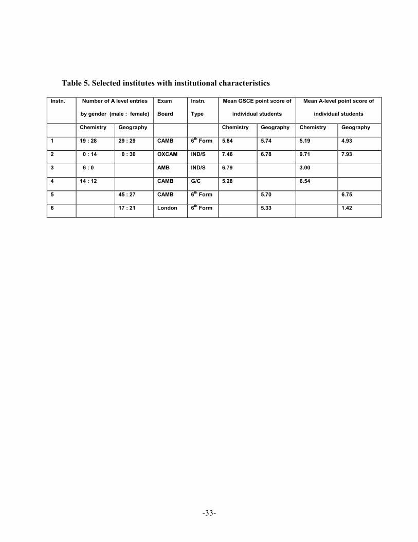
Table 5. Selected institutes with institutional characteristics

Instn. Number of A level entries

by gender (male : female)

Exam

Board

Instn.

Type

Mean GSCE point score of

individual students

Mean A-level point score of

individual students

Chemistry Geography Chemistry Geography Chemistry Geography

1 19 : 28 29 : 29 CAMB 6th Form 5.84 5.74 5.19 4.93

2 0 : 14 0 : 30 OXCAM IND/S 7.46 6.78 9.71 7.93

3 6 : 0 AMB IND/S 6.79 3.00

4 14 : 12 CAMB G/C 5.28 6.54

5 45 : 27 CAMB 6th Form 5.70 6.75

6 17 : 21 London 6th Form 5.33 1.42

-33-

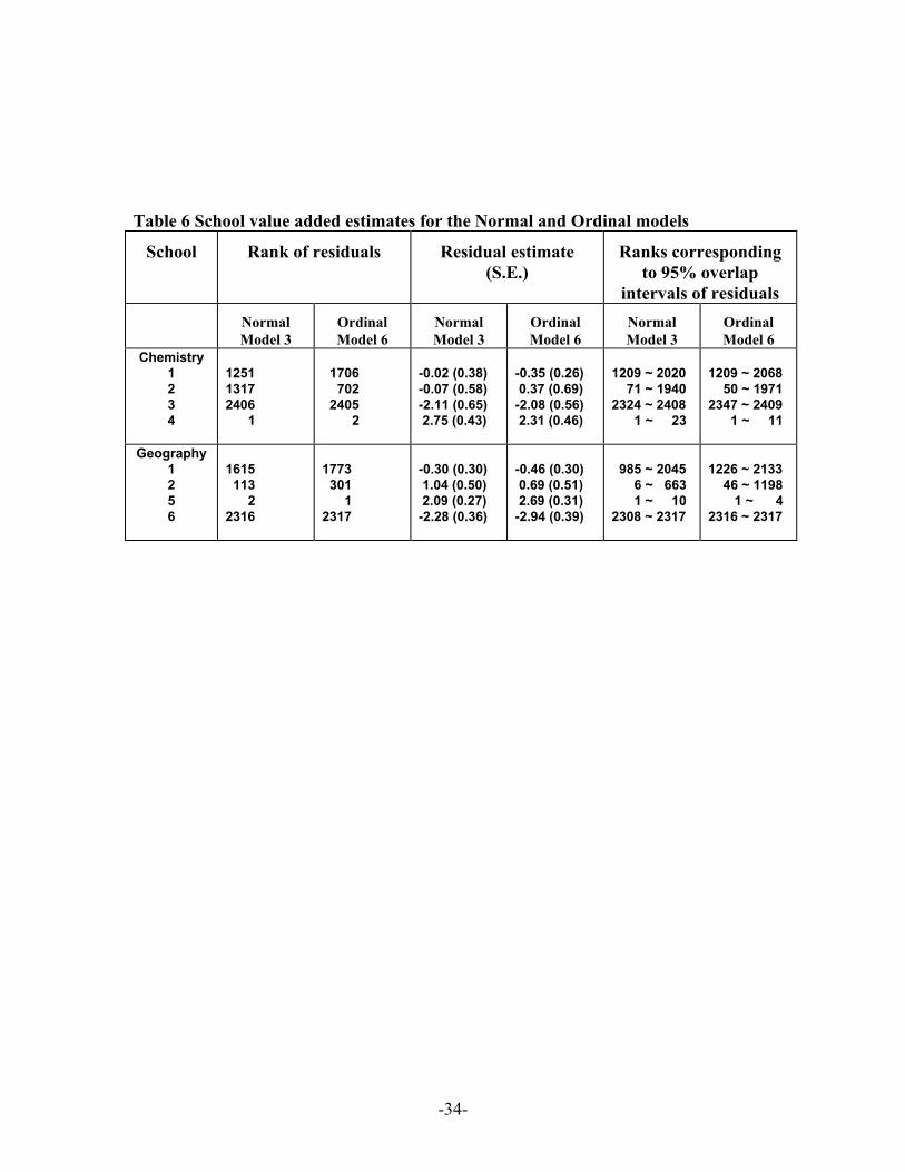
Table 6 School value added estimates for the Normal and Ordinal models

School Rank of residuals Residual estimate (S.E.)

Ranks corresponding to 95% overlap

intervals of residuals

Normal Model 3

Ordinal Model 6

Normal Model 3

Ordinal Model 6

Normal Model 3

Ordinal Model 6

Chemistry 1 2 3 4

1251 1317 2406 1

1706 702 2405 2

-0.02 (0.38) -0.07 (0.58) -2.11 (0.65) 2.75 (0.43)

-0.35 (0.26) 0.37 (0.69) -2.08 (0.56) 2.31 (0.46)

1209 ~ 2020 71 ~ 1940 2324 ~ 2408 1 ~ 23

1209 ~ 2068 50 ~ 1971 2347 ~ 2409 1 ~ 11

Geography 1 2 5 6

1615 113 2 2316

1773 301 1 2317

-0.30 (0.30) 1.04 (0.50) 2.09 (0.27) -2.28 (0.36)

-0.46 (0.30) 0.69 (0.51) 2.69 (0.31) -2.94 (0.39)

985 ~ 2045 6 ~ 663 1 ~ 10 2308 ~ 2317

1226 ~ 2133 46 ~ 1198 1 ~ 4 2316 ~ 2317

-34-

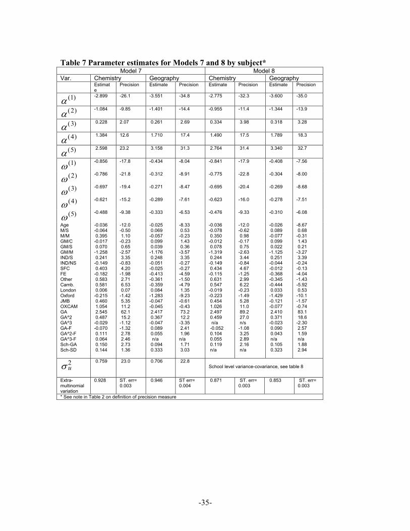
Table 7 Parameter estimates for Models 7 and 8 by subject*

Model 7 Model 8 Var. Chemistry Geography Chemistry Geography Estimat

e Precision Estimate Precision Estimate Precision Estimate Precision

( )1α -2.899 -26.1 -3.551 -34.8 -2.775 -32.3 -3.600 -35.0

( )2α -1.084 -9.85 -1.401 -14.4 -0.955 -11.4 -1.344 -13.9

( )3α 0.228 2.07 0.261 2.69 0.334 3.98 0.318 3.28

( )4α 1.384 12.6 1.710 17.4 1.490 17.5 1.789 18.3

( )5α 2.598 23.2 3.158 31.3 2.764 31.4 3.340 32.7

( )1ω -0.856 -17.8 -0.434 -8.04 -0.841 -17.9 -0.408 -7.56

( )2ω -0.786 -21.8 -0.312 -8.91 -0.775 -22.8 -0.304 -8.00

(3)ω -0.697 -19.4 -0.271 -8.47 -0.695 -20.4 -0.269 -8.68

( )4ω -0.621 -15.2 -0.289 -7.61 -0.623 -16.0 -0.278 -7.51

(5)ω -0.488 -9.38 -0.333 -6.53 -0.476 -9.33 -0.310 -6.08

Age M/S M/M GM/C GM/S GM/M IND/S IND/NS SFC FE Other Camb. London Oxford JMB OXCAM GA GA^2 GA^3 GA-F GA^2-F GA^3-F Sch-GA Sch-SD

-0.036 -0.064 0.395 -0.017 0.070 -1.258 0.241 -0.149 0.403 -0.182 0.583 0.581 0.006 -0.215 0.460 1.054 2.545 0.487 -0.029 -0.070 0.111 0.064 0.150 0.144

-12.0 -0.50 1.10 -0.23 0.65 -2.57 3.35 -0.83 4.20 -1.98 2.71 6.53 0.07 -1.42 5.35 11.2 62.1 15.2 -1.12 -1.32 2.78 2.46 2.73 1.36

-0.025 0.069 -0.057 0.099 0.039 -1.176 0.248 -0.051 -0.025 -0.413 -0.361 -0.359 0.084 -1.283 -0.047 -0.045 2.417 0.367 -0.047 0.089 0.055 n/a 0.094 0.333

-8.33 0.53 -0.23 1.43 0.36 -3.57 3.35 -0.27 -0.27 -4.59 -1.50 -4.79 1.35 -9.23 -0.61 -0.43 73.2 12.2 -3.35 2.41 1.96 n/a 1.71 3.03

-0.036 -0.078 0.350 -0.012 0.078 -1.319 0.244 -0.149 0.434 -0.115 0.631 0.547 -0.019 -0.223 0.454 1.026 2.497 0.459 n/a -0.052 0.104 0.055 0.119 n/a

-12.0 -0.62 0.98 -0.17 0.75 -2.63 3.44 -0.84 4.67 -1.25 2.99 6.22 -0.23 -1.49 5.28 11.0 89.2 27.0 n/s -1.08 3.25 2.89 2.16 n/a

-0.026 0.089 -0.077 0.099 0.022 -1.125 0.251 -0.044 -0.012 -0.368 -0.345 -0.444 0.033 -1.429 -0.121 -0.077 2.410 0.371 -0.023 0.090 0.043 n/a 0.105 0.323

-8.67 0.68 -0.31 1.43 0.21 -3.27 3.39 -0.24 -0.13 -4.04 -1.43 -5.92 0.53 -10.1 -1.57 -0.74 83.1 18.6 -2.30 2.57 1.59 n/a 1.88 2.94

u2σ

0.759 23.0 0.706 22.8 School level variance-covariance, see table 8

Extra-multinomial variation

0.928 ST. err= 0.003

0.946 ST err= 0.004

0.871 ST. err= 0.003

0.853 ST. err= 0.003

* See note in Table 2 on definition of precision measure

-35-

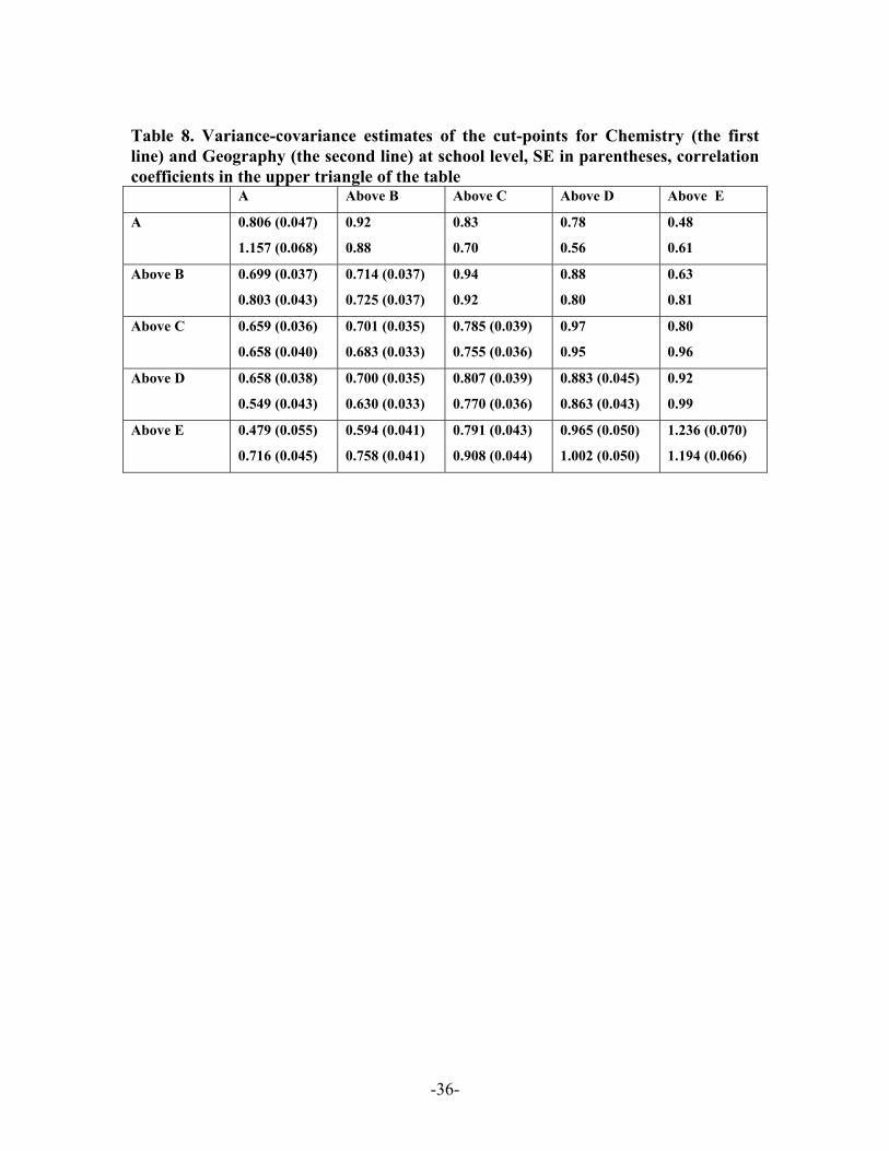
Table 8. Variance-covariance estimates of the cut-points for Chemistry (the first line) and Geography (the second line) at school level, SE in parentheses, correlation coefficients in the upper triangle of the table A Above B Above C Above D Above E

A 0.806 (0.047)

1.157 (0.068)

0.92

0.88

0.83

0.70

0.78

0.56

0.48

0.61

Above B 0.699 (0.037)

0.803 (0.043)

0.714 (0.037)

0.725 (0.037)

0.94

0.92

0.88

0.80

0.63

0.81

Above C 0.659 (0.036)

0.658 (0.040)

0.701 (0.035)

0.683 (0.033)

0.785 (0.039)

0.755 (0.036)

0.97

0.95

0.80

0.96

Above D 0.658 (0.038)

0.549 (0.043)

0.700 (0.035)

0.630 (0.033)

0.807 (0.039)

0.770 (0.036)

0.883 (0.045)

0.863 (0.043)

0.92

0.99

Above E 0.479 (0.055)

0.716 (0.045)

0.594 (0.041)

0.758 (0.041)

0.791 (0.043)

0.908 (0.044)

0.965 (0.050)

1.002 (0.050)

1.236 (0.070)

1.194 (0.066)

-36-

Figures

05

1015202530354045

A B C D E F

Grade

Pred

icte

d pr

obab

ility

,%

Student 1 Student 2

Figure 1 Predicted distribution of A level grades for Chemistry for Ordinal model 5(b) for two students. (Student 1: female of 18.5 years old from an independent selective school with exam board Oxford-Cambridge with overall GCSE score as 7.5. Student 2: same as student 1 but a lower GCSE average score of 5)

-37-

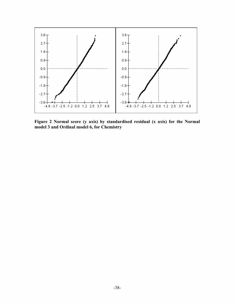
Figure 2 Normal score (y axis) by standardised residual (x axis) for the Normal model 3 and Ordinal model 6, for Chemistry

-38-

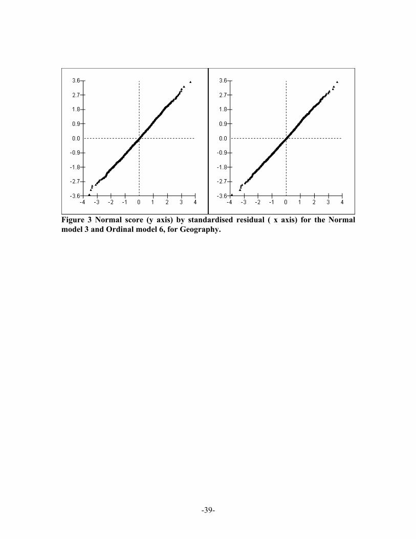
Figure 3 Normal score (y axis) by standardised residual ( x axis) for the Normal model 3 and Ordinal model 6, for Geography.

-39-

0.4

0.5

0.6

0.7

0.8

A A-B A-C A-D A-E

Grade

Cum

ulat

ive

odds

ratio

s

Model 5 Chemistry

Model 7 Chemistry

Model 5 Geography

Model 7 geography

Figure 4 Gender effects on grade threshold probabilities: ratios of cumulative odds

between females and males estimated by models 5 and 7

-40-

-3

-2

-1

0

1

2

3

A A-B A-C A-D A-E

Grade (Chemistry)

Inst

itutio

n re

sidu

als

Institution 1

Institution 2

Institution 3

Institution 4

Figure 5.1 Plots of residuals of 4 institutions for A-level Chemistry, logit scale

-5

-4

-3

-2

-1

0

1

2

3

4

5

A A-B A-C A-D A-E

Grade (Geography)

Inst

itutio

n re

sidu

als

Institution 1

Institution 2

Institution 5

Institution 6

Figure 5.2 Plots of residuals of 4 institutions for A-level geography, logit scale

-41-

05

1 01 52 02 53 03 54 04 5

A B C D E F

G r a d e ( C h e m is t r y )

Freq

uenc

y, %

Ma le ( b a s e g r o u p )

Figure 6.1

Predicted distributions of A-level Chemistry for males of mean age with mean GCSE score: Overall base group of maintained comprehensive schools with AEB board compared with Institution 1 ( a sixth form college and Cambridge Board)

In s titu tio n 1

Institution 5 Institution 6

0

10

20

30

40

50

60

70

A B C D E F

Grade (Geography)

Freq

uenc

y, %

Male (base group)

Figure 6.2

Predicted distributions of A-level Geography for males of mean age with mean GCSE score: Overall base group of maintained comprehensive schools with AEB board compared with institution 5 ( a sixth form college and Cambridge Board) and institution 6 ( a sixth form college with London Board)

-42-