Embed Size (px)
Citation preview
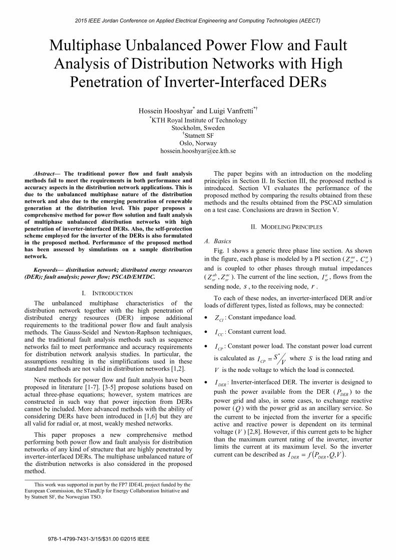
Multiphase Unbalanced Power Flow and Fault Analysis of Distribution Networks with High
Penetration of Inverter-Interfaced DERs
Hossein Hooshyar* and Luigi Vanfretti*† *KTH Royal Institute of Technology
Stockholm, Sweden †Statnett SF
Oslo, Norway [email protected]
Abstract— The traditional power flow and fault analysis methods fail to meet the requirements in both performance and accuracy aspects in the distribution network applications. This is due to the unbalanced multiphase nature of the distribution network and also due to the emerging penetration of renewable generation at the distribution level. This paper proposes a comprehensive method for power flow solution and fault analysis of multiphase unbalanced distribution networks with high penetration of inverter-interfaced DERs. Also, the self-protection scheme employed for the inverter of the DERs is also formulated in the proposed method. Performance of the proposed method has been assessed by simulations on a sample distribution network.
Keywords— distribution network; distributed energy resources (DER); fault analysis; power flow; PSCAD/EMTDC.
I. INTRODUCTION The unbalanced multiphase characteristics of the
distribution network together with the high penetration of distributed energy resources (DER) impose additional requirements to the traditional power flow and fault analysis methods. The Gauss-Seidel and Newton-Raphson techniques, and the traditional fault analysis methods such as sequence networks fail to meet performance and accuracy requirements for distribution network analysis studies. In particular, the assumptions resulting in the simplifications used in these standard methods are not valid in distribution networks [1,2].
New methods for power flow and fault analysis have been proposed in literature [1-7]. [3-5] propose solutions based on actual three-phase equations; however, system matrices are constructed in such way that power injection from DERs cannot be included. More advanced methods with the ability of considering DERs have been introduced in [1,6] but they are all valid for radial or, at most, weakly meshed networks.
This paper proposes a new comprehensive method performing both power flow and fault analysis for distribution networks of any kind of structure that are highly penetrated by inverter-interfaced DERs. The multiphase unbalanced nature of the distribution networks is also considered in the proposed method.
The paper begins with an introduction on the modeling principles in Section II. In Section III, the proposed method is introduced. Section VI evaluates the performance of the proposed method by comparing the results obtained from these methods and the results obtained from the PSCAD simulation on a test case. Conclusions are drawn in Section V.
II. MODELING PRINCIPLES
A. Basics Fig. 1 shows a generic three phase line section. As shown
in the figure, each phase is modeled by a PI section ( aasrZ , a
srC ) and is coupled to other phases through mutual impedances ( ab
srZ , acsrZ ). The current of the line section, a
srI , flows from the sending node, s , to the receiving node, r .
To each of these nodes, an inverter-interfaced DER and/or loads of different types, listed as follows, may be connected:
• CIZ : Constant impedance load.
• CCI : Constant current load.
• CPI : Constant power load. The constant power load current
is calculated as VSICP
*= where S is the load rating and
V is the node voltage to which the load is connected.
• DERI : Inverter-interfaced DER. The inverter is designed to push the power available from the DER ( DERP ) to the power grid and also, in some cases, to exchange reactive power (Q ) with the power grid as an ancillary service. So the current to be injected from the inverter for a specific active and reactive power is dependent on its terminal voltage (V ) [2,8]. However, if this current gets to be higher than the maximum current rating of the inverter, inverter limits the current at its maximum level. So the inverter current can be described as ( )VQPfI DERDER ,,= .
This work was supported in part by the FP7 IDE4L project funded by the European Commission, the STandUp for Energy Collaboration Initiative and by Statnett SF, the Norwegian TSO.
2015 IEEE Jordan Conference on Applied Electrical Engineering and Computing Technologies (AEECT)
978-1-4799-7431-3/15/$31.00 ©2015 IEEE

aasrZa
srI
asDERI
asI1
ansI
arI 1
armIaS ar
absrZ
acsrZ
from other line sections
asCCI a
sCPI asCIZ
to other line sections
arDERI
arCCIa
rCPIarCIZ
KVL
bphase
cphase
aphase
2
asrC
2
ansC
21asC
21
arC
2
asrC
2
armC
Fig. 1. A generic three phase line section.
B. Formulation We start by deriving a KVL equation as illustrated by the
solid arrow in Fig. 1. The voltage drop across the phase ‘a’ of the line section can be determined as:
csr
acsr
bsr
absr
asr
aasr
ar
as IZIZIZVV ++=− (1)
On the other hand, asV and a
rV can be obtained from the following equations:
( ) ⎟⎠
⎞⎜⎝
⎛ −−−+= ∑=
asCP
asCC
asr
asDER
n
i
ais
as
asCI
as IIIIIZcZV
1|| (2)
( ) ⎟⎠
⎞⎜⎝
⎛ −−−+= ∑=
arCP
arCC
m
i
ari
arDER
asr
ar
arCI
ar IIIIIZcZV
1|| (3)
where asZc and a
rZc represent the total capacitive impedances connected to nodes s and r , and are calculated as:
2
1
1∑
=
= nodeatoconnectedbranchesall
iiC
j
Zc
ω
(4)
Now by replacing asV and a
rV in (1) by (2) and (3), we get to the following equation:
( ) ( )
( )( )( ) ( )( )a
rCParCC
arDER
ar
arCI
asCP
asCC
asDER
as
asCI
csr
acsr
bsr
absr
m
i
ari
ar
arCI
asr
ar
arCI
aasr
as
asCI
n
i
ais
as
asCI
IIIZcZIIIZcZ
IZIZIZcZ
IZcZZZcZIZcZ
−−−−−
=++−
+++−
∑
∑
=
=
||||
||
||||||
1
1
(5)
Following the same logic, (6) and (7) give the same relation for phases ‘b’ and ‘c’, respectively.
( ) ( )
( )( )( ) ( )( )b
rCPbrCC
brDER
br
brCI
bsCP
bsCC
bsDER
bs
bsCI
csr
bcsr
asr
absr
m
i
bri
br
brCI
bsr
br
brCI
bbsr
bs
bsCI
n
i
bis
bs
bsCI
IIIZcZIIIZcZ
IZIZIZcZ
IZcZZZcZIZcZ
−−−−−
=++−
+++−
∑
∑
=
=
||||
||
||||||
1
1
(6)
( ) ( )
( )( )( ) ( )( )c
rCPcrCC
crDER
cr
crCI
csCP
csCC
csDER
cs
csCI
bsr
bcsr
asr
acsr
m
i
cri
cr
crCI
csr
cr
crCI
ccsr
cs
csCI
n
i
cis
cs
csCI
IIIZcZIIIZcZ
IZIZIZcZ
IZcZZZcZIZcZ
−−−−−
=++−
+++−
∑
∑
=
=
||||
||
||||||
1
1
(7)
Note that the unknown variables in (5) to (7) are the line currents, a
srI , bsrI , c
srI . As indicated in the equations, the contributions of DERs, constant power loads, and constant current loads in the power flow are considered by current sources whereas those of the constant impedance loads are considered by impedances. The currents of DERs and constant power loads are determined by the models introduced in the previous section assuming that the terminal voltages, V , are known. It is worth mentioning that the line section parameters are the only essentials elements of the derived equations, i.e., all other parameters (DER and/or loads) can be simply set to zero in case they don’t exist.
Also, note that the currents directions can be determined arbitrarily. In this study, the directions of currents are assumed to be from the nodes with the lower numbers to the nodes with the higher numbers.
Deriving the same type of equations, for all line sections of a distribution network with N lines, results in a system of ∑
=
N
iik
1
linear equations with ∑=
N
iik
1
variables where ik is the number of
the phases of the thi line section. These equations will be used in the next section to form the system matrices.
III. THE PROPOSED COMPREHENSIVE METHOD FOR POWER FLOW AND FAULT ANALYSIS
A. Formation of System Matrices The equations derived in the previous Section are put into
matrix form as expressed in (8). Note that in this equation, the state variables are the currents of the line sections.
[ ][ ] [ ]ZIIlineZbus = (8)
where, for a system with N line sections, [ ]Zbus is a symmetric NN× block matrix containing the system impedances, [ ]Iline
2015 IEEE Jordan Conference on Applied Electrical Engineering and Computing Technologies (AEECT)

[ ]=Zbus
blocksN
bloc
ksN
[ ] =Iline
[ ] =ZI
11 kk ×
1kkN ×
bloc
ksN
11 ×k
bloc
ksN
1×NkNN kk ×
Nkk ×1
11 ×k
1×Nk
Fig. 2. Structure of the system matrices.
is a 1×N block matrix containing the line section currents as the system state variables, and [ ]ZI is a 1×N block matrix containing the information of the loads and DERs connected to the line sections. Fig. 2 illustrates the structures of the matrices.
The line sections can be numbered in an arbitrary order. A building algorithm for these matrices can be developed as follows. Note that, in all equations throughout this paper, the numeric superscripts of the parameters represent the arbitrary number of the phases and should not be confused with mathematical power.
• [ ]Zbus : As shown in Fig. 2, [ ]Zbus consists of N blocks of rows and N blocks of columns. The diagonal and off-diagonal blocks should be constructed as follows:
Diagonal blocks: Each diagonal block belongs to a line section and is sized as ii kk × . (9) shows how to construct the diagonal block of a line section with ik phases. (10), (11), and (12) are examples showing the diagonal blocks of a single-phase, a two-phase, and a three-phase line section, respectively.
[ ]
⎥⎥⎥
⎦
⎤
⎢⎢⎢
⎣
⎡
++
++
=×
iiiiiii
i
ii
kr
krCI
kksr
ks
ksCI
ksr
ksrrrCIsrssCI
iikk
ZcZZZcZZ
ZZcZZZcZ
Zbus
||||...:...:
...||||
1
1111111
),(
(9)
[ ] [ ]ar
arCI
aasr
as
asCI
ii ZcZZZcZZbus ||||),(11 ++=× (10)
[ ]
⎥⎦
⎤⎢⎣
⎡
++++
=×
br
brCI
bbsr
bs
bsCI
absr
absr
ar
arCI
aasr
as
asCI
ii
ZcZZZcZZZZcZZZcZ
Zbus
||||||||
),(22
(11)
[ ] =×),(
33iiZbus (12)
⎥⎥⎥
⎦
⎤
⎢⎢⎢
⎣
⎡
++++
++
cr
crCI
ccsr
cs
csCI
bcsr
acsr
bcsr
br
brCI
bbsr
bs
bsCI
absr
acsr
absr
ar
arCI
aasr
as
asCI
ZcZZZcZZZZZcZZZcZZZZZcZZZcZ
||||||||
||||
Off-diagonal blocks: The off-diagonal blocks, ( )thji, and ( )thij, , sized as ji kk × and ij kk × respectively, refer to the interconnection between the thi and the thj line sections and should be constructed as shown in (13). If there is no interconnection between the thi and the thj line sections, the corresponding ( )thji, and ( )thij, blocks are null matrices.
[ ] [ ]( )
( )
( )⎥⎥⎥
⎦
⎤
⎢⎢⎢
⎣
⎡
±
±
==
−
−
××
ii
ijji
kcn
kcnCI
cncnCI
Tijkk
jikk
ZcZ
ZcZ
ZbusZbus
||...0:...:0...|| 11
),(),(
(13)
where subscript cn refers to the common node of thi and thj line sections. Note that the matrix entries in (13),
cnCIZ − and cnZc , are the constant impedance load and the total capacitive impedance at cn , respectively. The ‘ ± ’ sign is ‘ + ’ if the line sections are interconnected via sending or receiving sides at the cn ; otherwise, i.e. one side is sending and the other side is receiving, it’s ‘ − ’. Equations (14), (15), and (16) are examples showing the off-diagonal blocks corresponding to the connections between a single-‘a’-phase and a three-phase line section, a double-‘ab’-phase and a three-phase line section, and two three-phase line sections, respectively.
[ ] [ ]( ) ( )[ ]00||),(13
),(31
acn
acnCI
Tijji ZcZZbusZbus −×× ±== (14)
[ ] [ ]( )
( )( ) ⎥
⎦
⎤⎢⎣
⎡
±±
==
−
−
××
0||000||
),(23
),(32
bcn
bcnCI
acn
acnCI
Tijji
ZcZZcZ
ZbusZbus (15)
[ ] [ ]( )
( )( )
( )⎥⎥⎥
⎦
⎤
⎢⎢⎢
⎣
⎡
±±
±
==
−
−
−
××
ccn
ccnCI
bcn
bcnCI
acn
acnCI
Tijji
ZcZZcZ
ZcZ
ZbusZbus
||000||000||
),(33
),(33
(16)
Finally note that the building algorithm of [ ]Zbus is not based on the system topology, therefore the method can be used for both radial and meshed distribution networks.
2015 IEEE Jordan Conference on Applied Electrical Engineering and Computing Technologies (AEECT)

• [ ]Iline : [ ]Iline is a vector of N blocks as shown in Fig. 2. Each block, sized as 1×ik , contains the currents of the thi line section as indicated in (17):
[ ]⎥⎥⎥
⎦
⎤
⎢⎢⎢
⎣
⎡
=×i
iksr
sri
k
I
IIline :
1
)(1
(17)
• [ ]ZI : As shown in Fig. 2, [ ]ZI is a vector of N blocks. Each block, sized as 1×ik , contains the information of the loads and DERs connected to the thi line section as indicated in (18):
[ ]( )( ) ( )( )
( )( ) ( )( )⎥⎥⎥
⎦
⎤
⎢⎢⎢
⎣
⎡
−−−−−
−−−−−
=×
iiiiiiiiii
i
krCP
krCC
krDER
kr
krCI
ksCP
ksCC
ksDER
ks
ksCI
rCPrCCrDERrrCIsCPsCCsDERssCI
ik
IIIZcZIIIZcZ
IIIZcZIIIZcZ
ZI
||||:
|||| 1111111111
)(1
(18)
B. Incorporating Fault in System Matrices Fig. 3 shows a generic fault, occurring at the arbitrary node
s . As shown in the figure, applying a fault at s corresponds to adding the line section, sn . This leads to addition of a diagonal block, sized as ff kk × , as the ( )thN 1+ diagonal block entry of [ ]Zbus , as shown in Fig. 4. Also, for each line sections, connected to the faulted node s , two off-diagonal blocks are added to the ( )thN 1+ row and the ( )thN 1+ column. Fig. 4 shows the added off-diagonal blocks, sized as if kk × and fi kk × , assuming that the thi line section is connected to the faulted node s . Determination of fk and construction of the added blocks are done differently for grounded and ungrounded faults, as discussed below.
• Grounded faults: Following the same logic, used in Section II.B, deriving KVL equation for phase ‘a’, as shown by solid arrows in Fig. 3, leads to (19) if a single-‘a’-phase to ground, (20) if a double-‘ab’-phase to ground, and (21) if a three-phase to ground fault is applied.
( ) ( )( )( )a
sCPasCC
asDER
as
asCI
af
gf
af
as
asCI
n
i
ais
as
asCI
IIIZcZ
IRRZcZIZcZ
−−
=+++− ∑=
||
||||1
(19)
( ) ( )( )( )a
sCPasCC
asDER
as
asCI
bf
gf
af
gf
af
as
asCI
n
i
ais
as
asCI
IIIZcZIR
IRRZcZIZcZ
−−=
++++− ∑=
||
||||1
(20)
bsI1
csI 1
cnsI
bS
cS
bnsI
KVL
KVL
KVL
afI
bfI
cfI
afR
bfR
cfR
gfRn
asDERI
asI1
ansI aS
from other line sections
asCCI a
sCPI asCIZ
2
asrC
2
ansC
21asC
bsDERI
from other line sections
bsCCI b
sCPI bsCIZ
2
bsrC
2
bnsC
21bsC
csDERI
from other line sections
csCCI c
sCPI csCIZ 2
csrC
2
cnsC
21csC
KVL
KVL
abfI
bcfI
Fig. 3. Applying a generic fault at an arbitrary node.
[ ]=Zbus
blocksN 1+
bloc
ksN
1+
[ ] =Iline
[ ]=ZI
11 kk ×
1kkN ×
11 ×k
1×NkNN kk ×
Nkk ×1
ff kk ×if kk ×
fi kk ×
0
000
bloc
ksN
1+
1×fk
11 ×k
1×Nk
bloc
ksN
1+
1×fk
Fig. 4. Extesion of system matrices as a result of applying a fault.
2015 IEEE Jordan Conference on Applied Electrical Engineering and Computing Technologies (AEECT)

( ) ( )( )( )a
sCPasCC
asDER
as
asCI
cf
gf
bf
gf
af
gf
af
as
asCI
n
i
ais
as
asCI
IIIZcZIRIR
IRRZcZIZcZ
−−=+
++++− ∑=
||
||||1
(21)
Similar equation to those shown by the solid arrows in Fig. 3 can be derived for other phases if any type of grounded faults is applied. Rearranging the derived equations into the form of matrix, results in the additional diagonal and off-diagonal blocks to be constructed as follows:
[ ]
⎥⎥⎥
⎦
⎤
⎢⎢⎢
⎣
⎡
++
++
=++×
gf
kf
ks
ksCI
gf
gf
gffssCI
NNkk
RRZcZR
RRRZcZ
Zbus
fff
ff
||...:...:
...|| 111
)1,1(
(22)
[ ] [ ]( )
( )
( )⎥⎥⎥
⎦
⎤
⎢⎢⎢
⎣
⎡
±
±
== +×
+×
ff
fiif
ks
ksCI
ssCI
TNikk
iNkk
ZcZ
ZcZ
ZbusZbus
||...0:...:0...|| 11
)1,(),1(
(23)
where fk is the number of faulted phases. As the faulted node s is always the sending side for the fault branch sn , the ‘ ± ’ sign is ‘ + ’ if the thi line section is interconnected via its sending side; otherwise, it’s ‘ − ’.
Equations (24) and (25), (26) and (27), and, (28) and (29) are examples showing the diagonal and off-diagonal blocks for a single-‘a’-phase to ground, a double-‘ab’-phase to ground, and a three-phase to ground fault, respectively. In all of these examples, it’s assumed that the thi line section, connected to the faulted node, is a three-phase line section.
[ ] [ ]gf
af
as
asCI
NN RRZcZZbus ++=++× ||)1,1(11
(24)
[ ] [ ]( ) ( )[ ]00||)1,(13
),1(31
as
asCI
TNiiN ZcZZbusZbus ±== +×
+× (25)
[ ]
⎥⎥⎦
⎤
⎢⎢⎣
⎡
++++
=++×
gf
bf
bs
bsCI
gf
gf
gf
af
as
asCI
NN
RRZcZRRRRZcZ
Zbus
||||
)1,1(22
(26)
[ ] [ ]( )
( )( ) ⎥
⎦
⎤⎢⎣
⎡
±±
== +×
+×
0||000||
)1,(23
),1(32
bs
bsCI
as
asCI
TNiiN
ZcZZcZ
ZbusZbus (27)
[ ]
⎥⎥⎥
⎦
⎤
⎢⎢⎢
⎣
⎡
++++
++
=++×
gf
cf
cs
csCI
gf
gf
gf
gf
bf
bs
bsCI
gf
gf
gf
gf
af
as
asCI
NN
RRZcZRRRRRZcZRRRRRZcZ
Zbus
||||
||
)1,1(33
(28)
[ ] [ ]( )
( )( )
( )⎥⎥⎥
⎦
⎤
⎢⎢⎢
⎣
⎡
±±
±
== +×
+×
cs
csCI
bs
bsCI
as
asCI
TNiiN
ZcZZcZ
ZcZ
ZbusZbus
||000||000||
)1,(33
),1(33
(29)
(30) and (31) show the added blocks to [ ]Iline and [ ]ZI , respectively.
[ ]⎥⎥⎥
⎦
⎤
⎢⎢⎢
⎣
⎡
=+×
f
fkf
fNk
I
IIline :
1
)1(1
(30)
[ ]( )( )
( )( )⎥⎥⎥
⎦
⎤
⎢⎢⎢
⎣
⎡
−−
−−=+
×fffff
fksCP
ksCC
ksDER
ks
ksCI
sCPsCCsDERssCIN
k
IIIZcZ
IIIZcZZI
||:
|| 11111
)1(1
(31)
• Ungrounded faults: Similar to the grounded-faults, KVL equations can be derived between the faulted phases as shown by the dotted arrows in Fig. 3. Rearranging the derived equations into the form of matrix, results in (32) to (35) showing the added blocks if ungrounded phase-to-phase fault is applied, and (36) to (39) showing the added blocks if ungrounded three-phase fault is applied. Note that, for ungrounded faults, fk is equal to the number of faulted phases minus 1. This is because, in this type of faults, the number of independent fault current variables is always equal to the number of faulted phases minus 1.
[ ] [ ]222111)1,1(11 |||| ssCIffssCI
NN ZcZRRZcZZbus +++=++×
(32)
[ ] [ ]( )( ) ( )[ ]0...||...0...||...0 2211
)1,(1
),1(1
ssCIssCI
TNik
iNk
ZcZZcZ
ZbusZbusii
∓±
== +×
+× (33)
[ ] [ ]12)1(11 f
N IIline =+× (34)
[ ]( )( ) ( )( )[ ]2222211111
)1(11
|||| sCPsCCsDERssCIsCPsCCsDERssCI
N
IIIZcZIIIZcZ
ZI
−−−−−
=+× (35)
2015 IEEE Jordan Conference on Applied Electrical Engineering and Computing Technologies (AEECT)

[ ]
( )⎥⎥⎦
⎤
⎢⎢⎣
⎡
++++−−+
=++×
333222333
222111
)1,1(22
||||||||||
ssCIffssCIfssCI
fssCIfssCI
NN
ZcZRRZcZRZcZRZcZRZcZ
Zbus (36)
[ ] [ ]( )
( ) ( )( ) ( )⎥⎦
⎤⎢⎣
⎡
±±
== +×
+×
3322
2211
)1,(2
),1(2
||||00||||
ssCIssCI
ssCIssCI
TNik
iNk
ZcZZcZZcZZcZ
ZbusZbusii
∓∓
(37)
[ ]⎥⎥⎦
⎤
⎢⎢⎣
⎡=+
× 23
12)1(
12f
fN
II
Iline (38)
[ ]( )( ) ( )( )( )( ) ( )( )⎥⎦
⎤⎢⎣
⎡
−−−−−−−−−−
=+×
3333322222
2222211111
)1(12
||||||||
sCPsCCsDERssCIsCPsCCsDERssCI
sCPsCCsDERssCIsCPsCCsDERssCI
N
IIIZcZIIIZcZIIIZcZIIIZcZ
ZI(39)
C. Calculation of System Voltage As discussed in Section II.A, the currents of the line
sections, [ ]Iline , are obtained through (8). Using the calculated currents together with the information of DERs and loads, the node voltages can be easily determined. (40) gets the voltage of an arbitrary phase ‘a’ node illustrated in Fig. 5. The calculated node voltages will be then used to update the values of the currents of DERs and constant power loads.
( ) ⎟⎠
⎞⎜⎝
⎛ −−+= ∑=
aCP
aCC
n
i
ai
aDER
aaCIa IIIIZcZV
1
|| (40)
from line sections connected to this node
aI1
aV
anI
asDGI
asCCI a
sCPI asCIZ
21aC
2
anC
Fig. 5. DER and loads connected to an arbitrary phase ‘a’ node.
D. The Proposed Method Fig. 6 shows the proposed algorithm for the power flow
solution of a distribution network with high penetration of DERs. As shown in the figure, the network solution, proposed
in the previous Sections, calculates the state variables, [ ]Iline , from which the bus voltages, [ ]V , are determined. The bus voltages are then passed to the models of DERs and constant power load, introduced in Section II, to update the values of the currents of DERs and constant power loads. This iteration runs until convergence is reached. Note that the characteristics of constant impedance and constant current loads do not need to be updated as they are represented with constant values in the network solution.
The algorithm, illustrated in Fig. 6, gives the power flow solution and can also be used for the fault analysis as the fault can be modeled in system matrices. However, the values given for fault analysis are valid only for the first moments after the fault occurrence. This is because the DERs employ self-protection systems which disconnect them from the grid in such conditions. The disconnection time for different DERs is not the same as, for each DER, it depends on DER’s distance to the fault and also the type of the employed self-protection system. Hence, as a result of DERs disconnecting at different times from the grid, the fault currents will be varying [2]. Thus, in order to be able to determine such a fault current profile, the proposed algorithm is extended, as shown in Fig. 7. As shown in the figure, the response of the DER self-protection is emulated in each iteration in order to determine the DERs that will be disconnected by their protection system, and how long it will take for the protection system to disconnect them. This loop is repeated until the DER protection does not disconnect any more DER.
Network Solutionfrom (8)
from (40)
V
DERCP II ,
[ ]IlineModels of
DER and Constant Power Load [ ]V
Fig. 6. Power flow solution for a multiphase unbalanced DER-dominated distribution network.
IV. TEST CASE To evaluate the performance of the proposed methods on a
multiphase unbalanced distribution network, the IEEE 34 node test feeder is used as the test case in this study. Since the original test feeder contains only radial sub-feeders, a number of lines have been added to create a meshed distribution network. Fig. 8 shows the modified test feeder. It’s assumed that each customer has a PV system (as DER) that can generate up to its maximum load of the customer unit (100% penetration). For this study, this system is simulated using PSCAD in order to get detailed time domain responses and to use them for comparison with the proposed method.
The PV system is simulated by adopting a typical model, which uses average models for the converters, and includes maximum power point tracking [9]. The PVs’ self-protection system is IEEE 929 complaint [10].
2015 IEEE Jordan Conference on Applied Electrical Engineering and Computing Technologies (AEECT)

Network Solutionfrom (8)
from (40)
Disconnect DER Simulate DER Protection
t = t + Δtyes
EndDER Disconnect?no
V
V
DERCP II ,
[ ]IlineModels of
DER and Constant Power Load [ ]V
Fig. 7. Fault analysis for a multiphase unbalanced DER-dominated distribution network.
Tables I to IV compare the results from the proposed methods with the results obtained from PSCAD simulations for a number of selected nodes. The simulation results have been gathered after the initial transients were damped. The results are obtained for two different conditions of zero PV generation at night and maximum PV generation at noon. These results show that the proposed methods estimates are very close to the ones from simulations. As indicated in the tables, the maximum difference between the results calculated by the proposed method and obtained from the simulations is less than 1.4%.
Note that when the PVs generation are at the maximum level, the fault currents will have two different values, as shown in Table IV. This is because, due to low system voltage during the fault, the PVs self-protections disconnect the PV systems from the grid 0.1s after the fault occurrence which, in turn, results in a step in the fault current profile. Fig. 9 shows such changes in the fault current profile for a three-phase fault occurring at node 862 with fault resistance of 3Ω. As shown in the figure, the transients captured by the simulation results are not included in calculated results. Also, the simulations results
contain the inherent delay of the RMS measuring blocks which does not exist in the results obtained from the proposed method.
It is worth noting that the proposed method and also the test feeder have been coded in MATLAB to calculate the presented power flow and fault analysis results.
V. CONCLUSION This paper proposed a new comprehensive method for
power flow solution and fault analysis of multiphase unbalanced distribution networks with high penetration of inverter-interfaced DERs. The proposed method can be used for distribution networks of any kind of structure, i.e. radial and meshed. Also, the self-protection scheme employed for the
TABLE I. POWER FLOW RESULTS (NO PV-NIGHT)
Node Phase |V|p.u. (Simulation)
|V|p.u. (Proposed Method)
<V deg. (Simulation)
<V deg. (Proposed Method)
802 a 0.9974 0.9974 -0.0333 -0.0333 b 0.9976 0.9976 -120.0505 -120.0505 c 0.9978 0.9978 119.9542 119.9542
816 a 0.9124 0.9124 -0.8528 -0.8528 b 0.9568 0.9568 -120.2738 -120.2736 c 0.9214 0.9214 119.6667 119.6667
862 a 0.8607 0.8607 -0.9947 -0.9969 b 0.9315 0.9315 -119.9604 -119.9592 c 0.8486 0.8486 119.946 119.9459
Max. Dif. = 0.0000% Max. Dif. = 0.2212%
TABLE II. POWER FLOW RESULTS (MAX. PV-NOON)
Node Phase |V|p.u. (Simulation)
|V|p.u. (Proposed Method)
<V deg. (Simulation)
<V deg. (Proposed Method)
802 a 0.999 0.999 0.0647 0.0654 b 0.9989 0.9989 -119.9514 -119.9507 c 0.999 0.999 120.0501 120.0507
816 a 0.9697 0.9702 2.3249 2.3444 b 0.9859 0.9861 -118.9451 -118.9369 c 0.9746 0.9751 122.203 122.2142
862 a 0.9542 0.955 3.8982 3.9259 b 0.9818 0.9822 -118.1724 -118.1625 c 0.9575 0.9584 124.5343 124.5512
Max. Dif. = 0.0940% Max. Dif. = 1.0819%
Fig. 8. Test case – Modified IEEE 34 node test feeder.
2015 IEEE Jordan Conference on Applied Electrical Engineering and Computing Technologies (AEECT)

inverter of the DERs can be formulated in the proposed method. As shown in the paper, the maximum difference between the results calculated by the proposed method and obtained from the simulations is less than 1.4%, indicating that the method provides quite accurate estimates with low computational burden when contrasted to PSCAD simulation.
TABLE III. FAULT CURRENT VALUES (NO PV-NIGHT)
Rf = 0Ω
Node Phase If-3LG (kA) (Simulation)
If-3LG (kA)
(Proposed Method)
If-LG (kA) (Simulation)
If-LG (kA)
(Proposed Method)
802 a 16.1057 16.105 12.7462 12.7457 b 17.3865 17.3857 - - c 16.4279 16.4272 - -
816 a 0.4941 0.4941 0.3982 0.3982 b 0.7308 0.7309 - - c 0.5176 0.5176 - -
862 a 0.2526 0.2526 0.2119 0.2119 b 0.4867 0.4868 - - c 0.2667 0.2666 - -
Rf = 3Ω
802 a 3.8895 3.8894 3.7889 3.7888 b 3.9861 3.9861 - - c 3.9636 3.9635 - -
816 a 0.4483 0.4483 0.3725 0.3725 b 0.6473 0.6474 - - c 0.4728 0.4728 - -
862 a 0.2383 0.2383 0.2035 0.2035 b 0.4467 0.4468 - - c 0.2524 0.2524 - -
Max. Dif. = 0.0375% Max. Dif. = 0.0039%
TABLE IV. FAULT CURRENT VALUES (MAX. PV-NOON)
Rf = 0Ω
Node Phase If-3LG (kA) (Simulation)
If-3LG (kA)
(Proposed Method)
If-LG (kA) (Simulation)
If-LG (kA)
(Proposed Method)
802
a 16.1335 16.1559 12.715 12.7382 16.1057 16.105 12.7445 12.744
b 17.3322 17.3167 - - 17.3865 17.3857 - -
c 16.4434 16.4416 - - 16.4279 16.4272 - -
816
a 0.486 0.4924 0.3411 0.3458 0.4941 0.4941 0.3945 0.3946
b 0.779 0.7735 - - 0.7308 0.731 - -
c 0.469 0.4703 - - 0.5176 0.5177 - -
862
a 0.3194 0.317 0.2615 0.2601 0.2615 0.2615 0.2164 0.2162
b 0.541 0.5444 - - 0.4864 0.4866 - -
c 0.3225 0.3221 - - 0.2665 0.2665 - -
Rf = 3Ω
802 a 3.8976 3.8978 3.7978 3.798 b 3.9938 3.9939 - - c 3.9701 3.9702 - -
816
a 0.5187 0.5171 0.4177 0.4169 0.4483 0.4483 0.3691 0.3691
b 0.7036 0.6987 - - 0.6474 0.6475 - -
c 0.5127 0.5124 - - 0.4728 0.4729 - -
862
a 0.3006 0.3003 0.2633 0.2604 0.2467 0.2467 0.2077 0.2076
b 0.5105 0.5077 - - 0.4464 0.4465 - -
c 0.3217 0.3195 - - 0.2522 0.2523 - -
Max. Dif. = 1.3169% Max. Dif. = 1.3779%
Fig. 9. Fault current profile for a three-phase fault at node 862 with Rf = 3Ω.
A. References [1] J. Teng, “A direct approach for distribution system load flow solutions,”
IEEE Transactions on Power Delivery, vol. 18, no. 3, pp. 882–887, July 2003.
[2] H. Hooshyar, M. E. Baran, “Fault analysis on distribution feeders with high penetration of PV systems,” IEEE Trans. Power Sys, vol. 28, no. 3, pp. 2890-2896, Aug. 2013.
[3] S.M. Halpin, “Fault analysis of multi-phase unbalanced nonradial power distribution systems,” IEEE Transactions on Industry Applications, vol. 31, no. 3, pp. 528-534, May/June 1995.
[4] R.M. Ciric, “Fault analysis in four-wire distribution networks,” IEE Proceedings on Generation Transmission and Distribution, vol. 152, no. 6, pp. 977-982, Nov. 2005.
[5] K.S. Swarup, “Unbalanced distribution system short circuit analysis — an object-oriented approach,” IEEE TENCON Conference, pp. 1–6, 19-21 Nov. 2008.
[6] J. Teng, “Systematic short-circuit-analysis method for unbalanced distribution systems,” IEE Proceedings on Generation Transmission and Distribution, vol. 152, no. 4, pp. 549-555, July 2005.
[7] M. E. Baran, H. Hooshyar, Z. Shen, A. Huang, “Accommodating high PV penetration on distribution feeders,” IEEE Transactions on Smart Grid, vol. 3, no. 2, pp. 1039-1046, June 2012.
[8] Q. Wang, N Zhou, L. Ye, “Fault analysis for distribution networks with current-controlled three-phase inverter-interfaced distributed generators,” IEEE Transactions on Power Delivery, vol. 30, no. 3, pp. 1532-1542, June 2015.
[9] Model available on the website of ECEE department at the University of Colorado at Boulder (http://ecee.colorado.edu/~ecen2060/matlab.html).
[10] IEEE 929, “IEEE recommended practice for utility interface of photovoltaic (PV) systems”, 2000.
curr
ent (
kA)
simulation —proposed method ---b
c a
2015 IEEE Jordan Conference on Applied Electrical Engineering and Computing Technologies (AEECT)