Multiple Hypothesis Testing - Statpower

Multiple Hypothesis Tests

James H. Steiger

Department of Psychology and Human DevelopmentVanderbilt University

James H. Steiger (Vanderbilt University) General Approaches 1 / 42

Multiple Hypothesis Tests1 Introduction

Probability of At Least One Type I Error

2 Some Key Concepts

Primary Hypotheses

Closure

Hierarchical Sets and Minimal Hypotheses

Families

Type I Error Control

Power

p-Value and Adjusted p-Value

Closed Test Procedures

3 Methods Based on Ordered p-Values

Methods Based on the First-Order Bonferonni Inequality

Methods Based on the Simes Equality

Methods Controlling the False Discovery Rate

4 An Example


Introduction

Introduction

As we saw in Psychology 310, when we test any statistical hypothesis, werealize that our decision may be wrong.

We design a procedure to control the probability of false rejection at α.

Unfortunately, if our data analysis involves many hypothesis tests, theprobability of at least one Type I error increases rather sharply with thenumber of tests.


Introduction Probability of At Least One Type I Error

IntroductionProbability of At Least One Type I Error

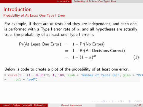
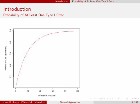
For example, if there are m tests and they are independent, and each oneis performed with a Type I error rate of α, and all hypotheses are actuallytrue, the probability of at least one Type I error is

Pr(At Least One Error) = 1− Pr(No Errors)

= 1− Pr(All Decisions Correct)

= 1− (1− α)m (1)

Below is code to create a plot of the probability of at least one error.

> curve(1 - (1 - 0.05)^x, 1, 100, xlab = "Number of Tests (m)", ylab = "Pr(At Least One Type I Error)",

+ col = "red")


Introduction Probability of At Least One Type I Error

IntroductionProbability of At Least One Type I Error

0 20 40 60 80 100

0.2

0.4

0.6

0.8

1.0

Number of Tests (m)

Pr(

At L

east

One

Typ

e I E

rror

)


Some Key Concepts

Some Key Concepts

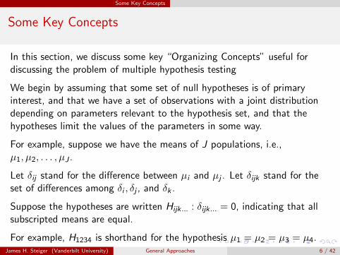
In this section, we discuss some key “Organizing Concepts” useful fordiscussing the problem of multiple hypothesis testing

We begin by assuming that some set of null hypotheses is of primaryinterest, and that we have a set of observations with a joint distributiondepending on parameters relevant to the hypothesis set, and that thehypotheses limit the values of the parameters in some way.

For example, suppose we have the means of J populations, i.e.,µ1, µ2, . . . , µJ .

Let δij stand for the difference between µi and µj . Let δijk stand for theset of differences among δi , δj , and δk .

Suppose the hypotheses are written Hijk... : δijk... = 0, indicating that allsubscripted means are equal.

For example, H1234 is shorthand for the hypothesis µ1 = µ2 = µ3 = µ4.James H. Steiger (Vanderbilt University) General Approaches 6 / 42

Some Key Concepts Primary Hypotheses

Some Key ConceptsPrimary Hypotheses

The primary hypotheses in a testing situation are the elements of theuniversal set of all hypotheses of interest.


Some Key Concepts Closure

Some Key ConceptsClosure

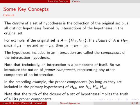
The closure of a set of hypotheses is the collection of the original set plusall distinct hypotheses formed by intersections of the hypotheses in theoriginal set.

For example, if the original set is A = {H12,H13}, the closure of A is H123,since if µ1 = µ3 and µ2 = µ3, then µ1 = µ2 = µ3.

The hypotheses included in an intersection are called the components ofthe intersection hypothesis.

Note that technically, an intersection is a component of itself. So weintroduce the notion of proper component, representing any othercomponent of an intersection.

In the preceding example, the proper components (so long as they areincluded in the primary hypotheses) of H123 are H12,H13,H23.

Note that the truth of the closure of a set of hypotheses implies the truthof all its proper components.


Some Key Concepts Hierarchical Sets and Minimal Hypotheses

Some Key ConceptsHierarchical Sets and Minimal Hypotheses

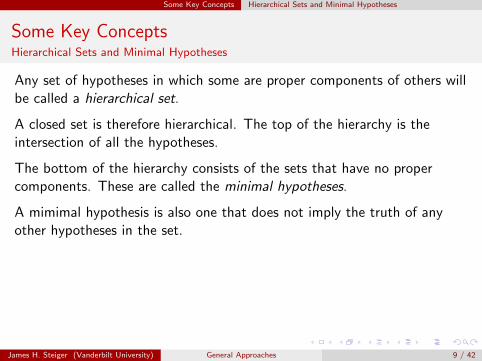
Any set of hypotheses in which some are proper components of others willbe called a hierarchical set.

A closed set is therefore hierarchical. The top of the hierarchy is theintersection of all the hypotheses.

The bottom of the hierarchy consists of the sets that have no propercomponents. These are called the minimal hypotheses.

A mimimal hypothesis is also one that does not imply the truth of anyother hypotheses in the set.


Some Key Concepts Families

Some Key ConceptsFamilies

A key decision in analyzing data is to decide on the set of hypotheses toconsider as a family.

A family is a set for which significance statements and related error rateswill be controlled jointly.

Note: In the early multiple comparisons literature (e.g., Ryan, 1959,1960), the term “experiment” was used instead of “family.”

As research grew more complex, the use of the term “experiment” wasfound to be limiting. Consider, for example, factorial experiment or a largesurvey.

Because of the inverse relationship between control of Type I errors andpower, it would be unreasonable to expect the probability of a Type I errorto be controlled over the entire experiment at conventional levels like 0.05.


Some Key Concepts Families

Some Key ConceptsFamilies

Even within the same data set, different families may be analyzed fordifferent reasons. For example, suppose you have data for 50 schools. Youmay be interested in all the pairwise comparisons among the schools. Onthe other hand, the principal of school A may only be interested in thefamily of pairwise comparison of her school with the other 49.


Some Key Concepts Type I Error Control

Some Key ConceptsType I Error Control

Strong error rate control methods control the Type I error rates (of variouskinds) for any combination of true and false null hypotheses in a family.

Weak error rate control methods control the various Type I error rates onlywhen all the null hypotheses in a family are simultaneously true.

We will concentrate on methods with strong control.




The error rate per hypothesis, often called the error rate per comparison orPCER, is the Type I error rate for each individual hypothesis test.




The error rate per family, or PFER, is the expected number of falserejections in the family.




The familywise error rate (FWER) is the probability of at least one Type Ierror in the family of tests.




Let Vm stand for the number of Type I errors committed in a family oftests, and Rm be the number of rejected hypotheses. The generalizedfamilywise error rate gFWER(k) = Pr(Vm > k), or chance of at least(k + 1) false positives. The special case k = 0 corresponds to the usualfamily-wise error rate, FWER.




The False Discovery Rate (FDR) is (Vm/Rm), the long run proportion ofrejections that are Type I errors.


Some Key Concepts Power

Some Key ConceptsPower

Just as there are multiple ways of looking at Type I error rates, there areseveral conceptualizations of the notion of power in multiple hypothesistesting. In the context of pairwise mean comparisons, these have beenreferred to as

1 Any-pair power. The probability of rejecting at least one false nullhypothesis.

2 Per-pair power. The average probability of rejecting a false nullhypothesis.

3 All-pairs power. The probability of rejecting all false null hypothesesin the set.


Some Key Concepts p-Value and Adjusted p-Value

Some Key Conceptsp-Value and Adjusted p-Value

Many scientists now report p-values rather than simply giving a teststatistic and the result of the hypothesis test.

Extension of the idea of a p-value to multiple testing is not straightforward.

Some authors have championed the use of the adjusted p-value, which isthe value of the error rate for the entire procedure that, if it had beenemployed on the entire set of test statistics under consideration, wouldhave resulted in the null hypothesis for a particular hypothesis test barelyrejecting.


Some Key Concepts Closed Test Procedures

Some Key ConceptsClosed Test Procedures

The most powerful procedures designed to control FWER are in the classof closed test procedures.

Assume a set of hypotheses of primary interest, add hypotheses asnecessary to form the closure of this set, and recall that the closed setconsists of a hierarchy of hypotheses.

The closure principle is as follows: A hypothesis is rejected at level α ifand only if it and every hypothesis directly above it in the hierarchy (i.e.every hypothesis that includes it in an intersection and thus implies it) isrejected at level α.




Consider a hypothesis set involving 4 means, with the highest hypothesisin the hierarchy H1234 and the six hypotheses Hij , i 6= j = 1, 2, 3, 4 as theminimal hypotheses.

No hypotheses below H1234 can be rejected unless H1234 is rejected.Suppose H1234 is rejected. Then H12, for example, cannot be rejectedunless H124, H123 are rejected.

But since the intersection hypothesis H12 ∩ H34 is also implied by H1234

yet is formally distinct from it, this intersection hypothesis ranks belowH1234 but above H12.

So the intersection hypothesis H12 ∩ H34 must be tested and rejected atthe α level before H12 is tested by itself at the α level. It is only when thefinal test is rejected that one declares µ1 and µ2 to be significantlydifferent.




The proof that Closed Test Procedures control FWER is straightforward,and is given in a Biometrika article by Marcus et al.(1976). Let’s considerthe proof in connection with the following situation. There are 4 means,and µ1 = µ2 = µ3 6= µ4. In this case, HP = H123 is the closure of all truehypotheses. the intersection of all Hij that are true.

Consider every possible true situation, each of which can berepresented as the intersection of null hypotheses and theiralternatives. Only one of these can be the true one. In our currentexample, this is

HQ = H12 ∩ H13 ∩ H23 ∩ H14 ∩ H24 ∩ H34

Now, consider HT , the closure of the Hij that are true.

HT = H12 ∩ H13 ∩ H23

.

The probability under a closed testing procedure of rejecting HT is≤ α. Why? (continued on next slide)




All true null hypotheses in the primary set are contained in HQ , andnone of them can be rejected unless that configuration is rejected.Let A be the event that all hypotheses in HQ ranking above HT andincluding elements of HT are rejected. Clearly Pr(A) ≤ 1. Let B bethe event that HT is rejected. Since B can only occur when A hasalready occurred, B = A ∩ B, and soPr(B) = Pr(A ∩ B) = Pr(A) Pr(B|A). But Pr(B|A) = α, since onceone arrives at the point of testing HT , that test is performed at the αlevel.

Consequently Pr(B) ≤ α. And since rejection of any primaryhypothesis requires event B, the probability of one or more suchrejections must be less than or equal to Pr(B), and so must also beless than or equal to α.

In other words, when working through the hierarchy, when one encountersthe first hypothesis at the top of the hierarchy of true hypotheses, theprobability of rejecting it is ≤ α. If it is rejected, then a Type I error hasoccurred. If not, no more tests below that point in the hierarchy can bedone. So the Type I error rate at the head of the hierarchy is also theFWER.


Methods Based on Ordered p-Values

Methods Based on Ordered p-Values

A finite set of minimal hypotheses Hi , i = 1, . . . ,m is to be tested.Corresponding to the Hi are test statistics Ti (or their absolute values)such that pi corresponding to each hypothesis may be computed.

Assume that the pi are ordered such that p1 ≤ p2 ≤ . . . ≤ pm. With theexception of the methods in the the subsection on False Discovery Rate,these methods provide strong FWER control.


Methods Based on Ordered p-Values Methods Based on the First-Order Bonferonni Inequality

Methods Based on Ordered p-ValuesMethods Based on the First-Order Bonferonni Inequality

The Simple Bonferonni Method.

The first-order Bonferroni inequality states that, for events Ai , i = 1, . . . , n,

Pr

(m⋃i=1

Ai

)≤

m∑i=1

Pr(Ai ) (2)

This inequality is the basis for several general methods.




The simple method is, reject Hi if pi ≤ αi , where∑m

i=1 αi = α.

This method controls FWER at or below α.

Usually, all αi are set equal to α/m, a procedure sometimes called theunweighted simple Bonferroni method.

Of course, with this method, power suffers increasingly as m becomeslarge.




Holm’s Sequentially Rejective Bonferonni Method

The unweighted method is as follows. At the first stage, H1 is rejected ifp1 ≤ α/m.

If H1 is not rejected, all subsequent hypotheses are accepted withoutfurther testing.

If H1 is rejected, H2 is tested at the α/(m − 1) level. If H2 is not rejected,all subsequent hypotheses are accepted without further testing.

The procedure continues, with the ith test performed at the α/(m− i + 1)level, until the first non-rejection occurs.




Proof.

First imagine all m hypotheses are true, and remember that an acceptancecan never be followed by a rejection with this procedure. So, if there isgoing to be any incorrect rejection, it has to occur on the first test of atrue hypothesis, because otherwise there will be no further tests.

So if all hypotheses are true, the probability of at least one rejection is theprobability of getting a rejection on the first test, which is α/m. Whathappens after that is irrelevant to the FWER, because all patterns ofsubsequent results will fit the definition of a Familywise Error havingoccurred. (continued on next slide)




Now imagine that there are k ≤ m true null hypotheses in the collection ofm hypotheses to be tested. Suppose k = m − 1. Then the first truehypothesis will be tested in position 1 or 2, and so the probability of aFamilywise Error can be no more than α/(m − 1).

If k = m − 2, the first true hypothesis will be tested in position 1, 2, or 3and so the probability of a Familywise Error can be no more thanα/(m − 2), etc.

If there is only one true null hypothesis, and it is tested last, theprobability of a rejection is α.

This completes the proof.




An Enhancement for Independent (and some Dependent) Tests.

If tests are independent, α/m may be replaced by 1− (1− α)1/m, which isalways greater than α/m.

For certain other classes of tests that are positive orthant dependent, thisenhancement may also be applied. This includes the set of pairwisetwo-sided t-tests in a 1-way ANOVA layout.


Methods Based on Ordered p-Values Methods Based on the Simes Equality

Methods Based on Ordered p-ValuesMethods Based on the Simes Equality

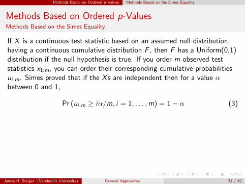
If X is a continuous test statistic based on an assumed null distribution,having a continuous cumulative distribution F , then F has a Uniform(0,1)distribution if the null hypothesis is true. If you order m observed teststatistics x1:m, you can order their corresponding cumulative probabilitiesui :m. Simes proved that if the X s are independent then for a value αbetween 0 and 1,

Pr (ui :m ≥ iα/m, i = 1, . . . ,m) = 1− α (3)


Methods Based on Ordered p-Values Methods Based on the Simes Equality

Methods Based on Ordered p-ValuesMethods Based on the Simes Equality

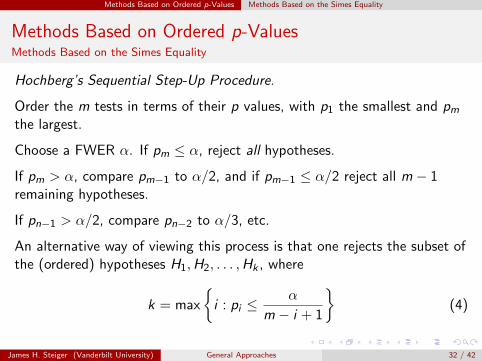
Hochberg’s Sequential Step-Up Procedure.

Order the m tests in terms of their p values, with p1 the smallest and pm

the largest.

Choose a FWER α. If pm ≤ α, reject all hypotheses.

If pm > α, compare pm−1 to α/2, and if pm−1 ≤ α/2 reject all m − 1remaining hypotheses.

If pn−1 > α/2, compare pn−2 to α/3, etc.

An alternative way of viewing this process is that one rejects the subset ofthe (ordered) hypotheses H1,H2, . . . ,Hk , where

k = max

{i : pi ≤

α

m − i + 1

}(4)


Methods Based on Ordered p-Values Methods Controlling the False Discovery Rate

Methods Based on Ordered p-ValuesMethods Controlling the False Discovery Rate

As articulated by Benjamini and Hochberg (1995) in the quote below, ifthere are a lot of rejections expected in a set of m tests, control of FWERmay not be feasible, because of its damaging effect on power.

(b) Classical procedures that control the FWER in the strongsense, at levels conventional in single-comparison problems, tendto have substantially less power than the per comparisonprocedure of the same levels.

(c) Often the control of the FWER is not quite needed. Thecontrol of the FWER is important when a conclusion from thevarious individual inferences is likely to be erroneous when atleast one of them is. This may be the case, for example, whenseveral new treatments are competing against a standard, and asingle treatment is chosen from the set of treatments which aredeclared significantly better than the standard. However, atreatment group and a control group are often compared bytesting various aspects of the effect (different end points inclinical trials terminology). The overall conclusion that thetreatment is superior need not be erroneous even if some of thenull hypotheses are falsely rejected.


Methods Based on Ordered p-Values Methods Controlling the False Discovery Rate

Methods Based on Ordered p-ValuesMethods Controlling the False Discovery Rate

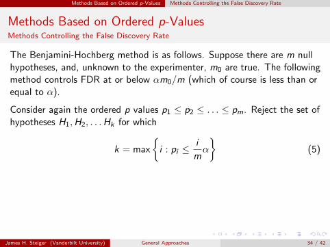
The Benjamini-Hochberg method is as follows. Suppose there are m nullhypotheses, and, unknown to the experimenter, m0 are true. The followingmethod controls FDR at or below αm0/m (which of course is less than orequal to α).

Consider again the ordered p values p1 ≤ p2 ≤ . . . ≤ pm. Reject the set ofhypotheses H1,H2, . . .Hk for which

k = max

{i : pi ≤

i

mα

}(5)


An Example

An Example

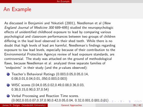
As discussed in Benjamini and Yekutieli (2001), Needleman et al (NewEngland Journal of Medicine 300 689–695) studied the neuropsychologiceffects of unidentified childhood exposure to lead by comparing variouspsychological and classroom performances between two groups of childrendiffering in the lead level observed in their shed teeth. While there is nodoubt that high levels of lead are harmful, Needleman’s findings regardingexposure to low lead levels, especially because of their contribution to theEnvironmental Protection Agencys review of lead exposure standards, arecontroversial. The study was attacked on the ground of methodologicalflaws, because Needleman et al. analyzed three separate families of“endpoints” in their study (and the p-values observed):

1 Teacher’s Behavioral Ratings (0.003,0.05,0.05,0.14,0.08,0.01,0.04,0.01,.050,0.003,0.003)

2 WISC scores (0.04,0.05,0.02,0.49,0.08,0.36,0.03,0.38,0.15,0.90,0.37,0.54)

3 Verbal Processing and Reaction Time scores.(0.002,0.03,0.07,0.37,0.90,0.42,0.05,0.04, 0.32,0.001,0.001,0.01)


An Example

An Example

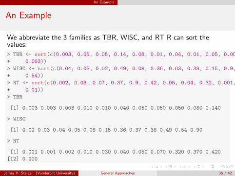
We abbreviate the 3 families as TBR, WISC, and RT R can sort thevalues:

> TBR <- sort(c(0.003, 0.05, 0.05, 0.14, 0.08, 0.01, 0.04, 0.01, 0.05, 0.003,

+ 0.003))

> WISC <- sort(c(0.04, 0.05, 0.02, 0.49, 0.08, 0.36, 0.03, 0.38, 0.15, 0.9, 0.37,

+ 0.54))

> RT <- sort(c(0.002, 0.03, 0.07, 0.37, 0.9, 0.42, 0.05, 0.04, 0.32, 0.001, 0.001,

+ 0.01))

> TBR

[1] 0.003 0.003 0.003 0.010 0.010 0.040 0.050 0.050 0.050 0.080 0.140

> WISC

[1] 0.02 0.03 0.04 0.05 0.08 0.15 0.36 0.37 0.38 0.49 0.54 0.90

> RT

[1] 0.001 0.001 0.002 0.010 0.030 0.040 0.050 0.070 0.320 0.370 0.420

[12] 0.900


An Example

An Example

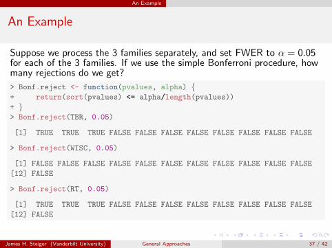
Suppose we process the 3 families separately, and set FWER to α = 0.05for each of the 3 families. If we use the simple Bonferroni procedure, howmany rejections do we get?

> Bonf.reject <- function(pvalues, alpha) {+ return(sort(pvalues) <= alpha/length(pvalues))

+ }> Bonf.reject(TBR, 0.05)

[1] TRUE TRUE TRUE FALSE FALSE FALSE FALSE FALSE FALSE FALSE FALSE

> Bonf.reject(WISC, 0.05)

[1] FALSE FALSE FALSE FALSE FALSE FALSE FALSE FALSE FALSE FALSE FALSE

[12] FALSE

> Bonf.reject(RT, 0.05)


[12] FALSE


An Example

An Example

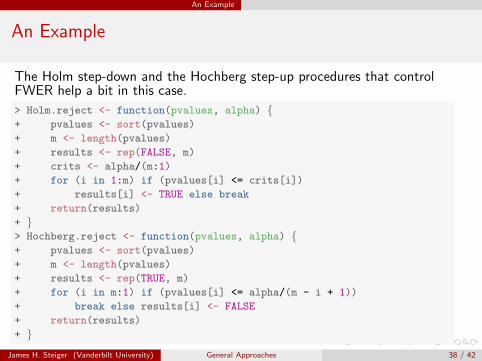
The Holm step-down and the Hochberg step-up procedures that controlFWER help a bit in this case.

> Holm.reject <- function(pvalues, alpha) {+ pvalues <- sort(pvalues)

+ m <- length(pvalues)

+ results <- rep(FALSE, m)

+ crits <- alpha/(m:1)

+ for (i in 1:m) if (pvalues[i] <= crits[i])

+ results[i] <- TRUE else break

+ return(results)

+ }> Hochberg.reject <- function(pvalues, alpha) {+ pvalues <- sort(pvalues)


+ results <- rep(TRUE, m)

+ for (i in m:1) if (pvalues[i] <= alpha/(m - i + 1))

+ break else results[i] <- FALSE

+ return(results)

+ }


An Example

An Example

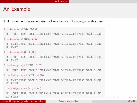
Holm’s method the same pattern of rejections as Hochberg’s, in this case.

> Holm.reject(TBR, 0.05)


> Holm.reject(WISC, 0.05)


[12] FALSE

> Holm.reject(RT, 0.05)


[12] FALSE

> Hochberg.reject(TBR, 0.05)


> Hochberg.reject(WISC, 0.05)


[12] FALSE

> Hochberg.reject(RT, 0.05)


[12] FALSE


An Example

An Example

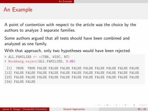
A point of contention with respect to the article was the choice by theauthors to analyze 3 separate families.

Some authors argued that all tests should have been combined andanalyzed as one family.

With that approach, only two hypotheses would have been rejected.

> ALL.FAMILIES <- c(TBR, WISC, RT)

> Hochberg.reject(ALL.FAMILIES, 0.05)

[1] TRUE TRUE FALSE FALSE FALSE FALSE FALSE FALSE FALSE FALSE FALSE



[34] FALSE FALSE


An Example

An Example

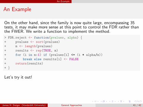
On the other hand, since the family is now quite large, encompassing 35tests, it may make more sense at this point to control the FDR rather thanthe FWER. We write a function to implement the method.

> FDR.reject <- function(pvalues, alpha) {+ pvalues <- sort(pvalues)


+ results <- rep(TRUE, m)

+ for (i in m:1) if (pvalues[i] <= (i * alpha/m))

+ break else results[i] <- FALSE

+ return(results)

+ }

Let’s try it out!


An Example

An Example

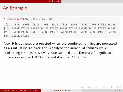
> FDR.reject(ALL.FAMILIES, 0.05)

[1] TRUE TRUE TRUE TRUE TRUE TRUE TRUE TRUE TRUE FALSE FALSE



[34] FALSE FALSE

Now 9 hypotheses are rejected when the combined families are processedas a unit. If we go back and reanalyze the individual families whilecontrolling the false discovery rate, we find that there are 5 significantdifferences in the TBR family and 4 in the RT family.


Documents

Multiple Hypothesis Testing - Statpower