Multiple Optimal Solutions in Quadratic …ageconsearch.umn.edu/bitstream/32089/1/08020141.pdfMultiple Optimal Solutions in Quadratic Programming Models Quirino Paris The problem of

Multiple Optimal Solutions in

Quadratic Programming Models

Quirino Paris

The problem of determining whether quadratic programming models possess either unique

or multiple optimal solutions is important for empirical analyses which use a mathematical

programming framework. Policy recommendations which disregard multiple optimal solutions

(when they exist) are potentially incorrect and less than efficient. This paper proposes a strategy

and the associated algorithm for finding all optimal solutions to any positive semidefinite linear

complementarity problem. One of the main results is that the set of complementary solutions

is convex. Although not obvious, this proposition is analogous to the well-known result in linear

programming which states that any convex combination of optimal solutions is itself optimal.

The importance of not overlookingmultiple optimal solutions in empiricalstudies based on linear programming (LP)models was discussed by Paris in a recentarticle. In the last decade, however, qua-dratic programming (QP) models havebeen used at an increasing rate for ana-lyzing problems of choice under marketand general equilibria as well as underrisky environments.

While conditions leading to alternateoptimal solutions in LP have been knownfor a long time, knowledge of the struc-tural causes underlying multiple optimalsolutions in QP, and of criteria for theirdetection is rather limited. The study ofthis subject is of recent vintage. The re-sults obtained so far are confined either tospecialized journals or unpublished pa-pers.

The existence of either unique or mul-tiple optimal solutions in QP models hassignificant consequences in the formula-tion of policy recommendations. Unfor-tunately, commercial computer programsfor solving QP problems are completelysilent about this aspect and leave it en-tirely to the enterprising researcher to find

Quirino Paris is a Professor of Agricultural Econom-

ics at the University of California, Davis.

Giannini Foundation Paper No. 688.

convenient ways for assessing the numberof optimal solutions and their values.

Multiple optimal solutions are an ap-pealing feature of programming modelsat least for two reasons. First of all, theyallow greater diversification of activitiesrepresenting an economic environment. Inother words, all the activities specified inthe model can potentially be operated atpositive levels regardless of the number ofconstraints. Secondly, a policy maker hasgreater flexibility in choosing the strategyto implement knowing that he need notsacrifice economic efficiency.

For many years, references to unique-ness of solutions in QP models have beenscant. A reference to a sufficient conditionfor uniqueness of a part of the solutionvector in a QP model, namely the positivedefiniteness of the quadratic form, is foundin Takayama and Judge (p. 164). How-ever, it is not necessary to have positivedefinite quadratic forms to have uniquesolutions. The relevant aspect of the prob-lem is, therefore, to know both the nec-essary and sufficient conditions foruniqueness. Hence, a more interestingproblem can be stated as follows: If thequadratic form in a QP model is positivesemidefinite (as are the quadratic formsin many empirical problems presented inthe literature), how do we know whetherthe given problem has a unique solution

Western Journal of Agricultural Economics, 8(2): 141-154© 1983 by the Western Agricultural Economics Association

Western Journal of Agricultural Economics

or it admits multiple optimal solutions?This paper addresses this problem andpresents an algorithmic approach to its so-lution. The algorithm is relatively simpleand can be implemented efficiently on acomputer even for large scale models. Aparticularly interesting result of this studyis that the set of multiple optimal solutionsin positive semidefinite QP models is con-vex. The possibility of diversified policystrategies is based upon this finding.

The paper relies heavily on numericalexamples to illustrate the seemingly intri-cate structure associated with eitheruniqueness or multiplicity of solutions.After discussing the convexity of the setof multiple optimal solutions, the same al-gorithm is applied to a LP and a QP prob-lem to illustrate its numerical feasibility.A remarkable feature of the discussionpresented below is that for finding allmultiple optimal solutions of a QP prob-lem it is sufficient to solve an associatedlinear programming problem.

The Linear Complementarity Problem

One promising way to gain insight intothis rather complex problem is to regardthe quadratic program as a linear com-plementarity (LC) problem. Consider thefollowing symmetric QP problem

max {c'x - k,x'Ds/2 - kyy'Ey/2} (1)

subject to:

Ax - kEy < b, x > 0, y > 0,

where A is an (m x n) matrix, D and Eare symmetric positive semidefinite (PSD)matrices of order n and m, respectively.Parameters k, and kV are nonnegative sca-lars suitable for representing various eco-nomic scenarios, from perfect and imper-fect market equilibria to risk anduncertainty problems. It can be easilyshown that the necessary and sufficientKuhn-Tucker conditions corresponding to(1) can be written in the form of the fol-

lowing LC problem: find an [(n + m) x 1]vector z such that

w =Mz + q > 0, z> 0 (2)

and:

z'w = 0,

where w is an [(n + m) x 1] vector of slackvariables, q' = [-c', b'], z' = [x', y'] and

M = k kE is an [(m + n) x (m + n)]

PSD matrix (for any A). It should be ap-parent that when E is the null matrix,problem (1) represents the traditionalasymmetric quadratic program, and whenboth D and E are null a LP problem isobtained.

It is well known that when multiple op-timal solutions exist in a LP problem, theirset constitutes a face of the convex poly-tope of all feasible solutions. This propertycan be extended to the LC problem (2).First of all, notice that the linear inequal-ities of problem (2) form a convex set offeasible solutions. Of course, we are notmerely interested in the set of feasible so-lutions but in the set of feasible as well ascomplementary solutions, that is those so-lutions (w, z) which satisfy the feasibilityconditions w > 0, z > 0 and also the com-plementarity condition w'z = 0. All com-plementary solutions to (2) are optimal so-lutions for the QP problem (1).

In LP problems, the set of optimal so-lutions is convex. This well known factimplies that a convex combination of anytwo optimal solutions is itself an optimalsolution. From an empirical viewpoint thisis an important result because it admitsthat the number of positive componentsof an optimal solution be greater than thenumber of independent constraints.Hence, when multiple optimal solutionsexist, one can select a more diversified so-lution for policy recommendation. It turnsout that, as in LP, the set of optimal so-lutions in QP problems is convex. To dem-onstrate this less known proposition it is

142

December 1983

Multiple Solutions in QP Models

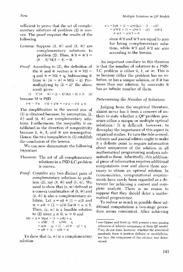
sufficient to prove that the set of comple-mentary solutions of problem (2) is con-vex. The proof requires the results of thefollowing

Lemma: Suppose (z, w) and (z, w) arecomplementary solutions toproblem (2). Then, w'2 = w'2 =(z - 2)'M(z - 2) = 0.

Proof: According to (2), the definition ofthe w and w vectors is w = Mz +q and w = M2 + q. Subtracting wfrom w: (w - wI) = M(z - z). Pre-multiplying by (z - z)' the aboveresult gives:

(z - z)'(w - w) = (2 - 2)'M(2 - z) > 0 (3)

because M is PSDz 'w - zw - zw + z'w = -z'w - z'w < 0.

The simplification in the second row of(3) is obtained because, by assumption, (z,w) and (z, w) are complementary solu-tions. Furthermore, the inequality is es-tablished in the direction of nonpositivitybecause z, w, z, and w are nonnegative.Hence, the two inequalities in (3) establishthe conclusion of the lemma.

We can now demonstrate the followingimportant

Theorem: The set of all complementarysolutions in a PSD-LC problemis convex.

Proof: Consider any two distinct pairs ofcomplementary solutions to prob-lem (2), say (2, w) and (2, w). Weneed to show that (z, w) defined asa convex combination of (z, ~w) and(z, w) is also a complementary so-lution. Let z = a2 + (1 - a)2 andw = aw + (1- ca)w for0 < a < 1.Then, (z, w) is a feasible solutionto (2) since z > 0, w > 0 and

Mz + q = M[a2 + (1 - a)2] + q=aMz + (1 - a)M2 + q= a(w - q) + (1 - a)(w - q) + q= aw + (1 - a)w¢ = w.

To show that (z, w) is a complementarysolution

w'z = [aw + (1 - a)wv]'[az + (1 - a)z]= c2w'z + (1 - ca)2 w'z + a(l - a)wi'2

+ a(1 - a)w'2 = 0

since w'z and xw'z are equal to zerofor being complementary solu-tions, while w'z and w'z are zeroaccording to the lemma.

An important corollary to this theoremis that the number of solutions to a PSD-LC problem is either 0, 1, or oo. This isso because either the problem has no so-lution, or has a unique solution, or if it hasmore than one solution, by convexity ithas an infinite number of them.

Determining the Number of Solutions

Judging from the empirical literature,almost never has it been a concern of au-thors to state whether a QP problem pos-sesses either a unique or multiple optimalsolutions.' It is difficult, however, todownplay the importance of this aspect inempirical studies. To turn the tide around,referees and journal editors ought to makeit a definite point to require informationabout uniqueness of the solution in allmathematical programming analyses sub-mitted to them. Admittedly, this addition-al piece of information requires additionalcomputations over and above those nec-essary to obtain an optimal solution. Ineconometrics, computational require-ments have rarely been regarded as a de-terrent for achieving a correct and com-plete analysis. There is no reason tosuppose that they should deter a mathe-matical programmer.

To reduce as much as possible these ad-ditional computations a two-stage proce-dure seems convenient. After achieving

von Oppen and Scott (p. 440) present a rare passingreference of solution uniqueness of their QP model.They do not state, however, whether the associatedquadratic form is positive definite or semidefinite,nor how the uniqueness of the solution was deter-mined.

143

Paris


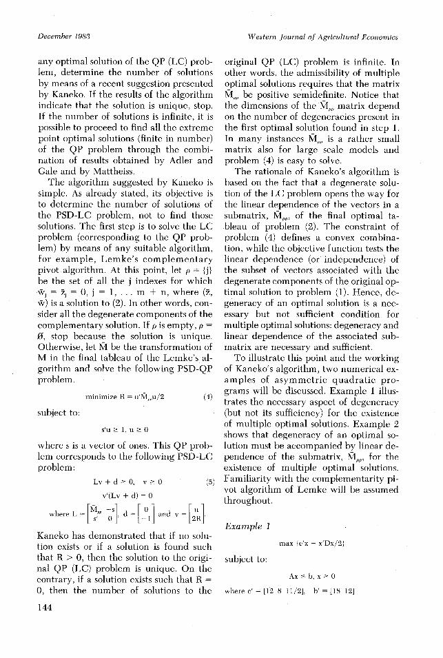
any optimal solution of the QP (LC) prob-lem, determine the number of solutionsby means of a recent suggestion presentedby Kaneko. If the results of the algorithmindicate that the solution is unique, stop.If the number of solutions is infinite, it ispossible to proceed to find all the extremepoint optimal solutions (finite in number)of the QP problem through the combi-nation of results obtained by Adler andGale and by Mattheiss.

The algorithm suggested by Kaneko issimple. As already stated, its objective isto determine the number of solutions ofthe PSD-LC problem, not to find thosesolutions. The first step is to solve the LCproblem (corresponding to the QP prob-lem) by means of any suitable algorithm,for example, Lemke's complementarypivot algorithm. At this point, let p = {j}be the set of all the j indexes for whichwj =j = 0, j = 1,... m + n, where (z,w) is a solution to (2). In other words, con-sider all the degenerate components of thecomplementary solution. If p is empty, p =0, stop because the solution is unique.Otherwise, let M be the transformation ofM in the final tableau of the Lemke's al-gorithm and solve the following PSD-QPproblem.

minimize R = u'Mppu/2 (4)

subject to:

s'u > 1, u > 0

where s is a vector of ones. This QP prob-lem corresponds to the following PSD-LCproblem:

Lv + d > 0, v > 0 (5)

v'(Lv + d) = 0

where L= [-P oSd , d = v [2R.

Kaneko has demonstrated that if no solu-tion exists or if a solution is found suchthat R > 0, then the solution to the origi-nal QP (LC) problem is unique. On thecontrary, if a solution exists such that R =0, then the number of solutions to the

144

original QP (LC) problem is infinite. Inother words, the admissibility of multipleoptimal solutions requires that the matrixMp, be positive semidefinite. Notice thatthe dimensions of the Mpp matrix dependon the number of degeneracies present inthe first optimal solution found in step 1.In many instances Moo is a rather smallmatrix also for large scale models andproblem (4) is easy to solve.

The rationale of Kaneko's algorithm isbased on the fact that a degenerate solu-tion of the LC problem opens the way forthe linear dependence of the vectors in asubmatrix, MPP, of the final optimal ta-bleau of problem (2). The constraint ofproblem (4) defines a convex combina-tion, while the objective function tests thelinear dependence (or independence) ofthe subset of vectors associated with thedegenerate components of the original op-timal solution to problem (1). Hence, de-generacy of an optimal solution is a nec-essary but not sufficient condition formultiple optimal solutions: degeneracy andlinear dependence of the associated sub-matrix are necessary and sufficient.

To illustrate this point and the workingof Kaneko's algorithm, two numerical ex-amples of asymmetric quadratic pro-grams will be discussed. Example 1 illus-trates the necessary aspect of degeneracy(but not its sufficiency) for the existenceof multiple optimal solutions. Example 2shows that degeneracy of an optimal so-lution must be accompanied by linear de-pendence of the submatrix, Mp,, for theexistence of multiple optimal solutions.Familiarity with the complementarity pi-vot algorithm of Lemke will be assumedthroughout.

Example 1

max {c'x- x'Dx/2}

subject to:

Ax <b, x 0

where c' = [12 8 11/2], b' = [18 12]

December 1983


TABLEAU 1. Initial Tableau of Example 1.

BasicVari-

W, W2 W3 W4 W5 Z1 Z2 Z3 Z4 z5 Zo q ables

1 -3 -2 -3/2 -6 -4 -1 -12 w,1 -2 -4/3 -1 -4 -3 -1 -8 W2

1 -3/2 -1 -3/2 -2 -1 -1 -11/2 W31 6 4 2 0 0 -1 18 W4

1 4 3 1 0 0 -1 12 W5

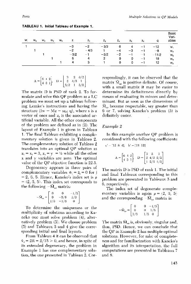
f64 2i 3 2 3 / 21= 431 D= 2 4/3 1

=[ l ] [ 3/2 1 3/2J

The matrix D is PSD of rank 2. To for-mulate and solve this QP problem as a LCproblem we must set up a tableau follow-ing Lemke's instructions and having thestructure (Iw - Mz - szo; q), where s is avector of ones and zo is the associated ar-tificial variable. All the other componentsof the problem are defined as in (2). Thelayout of Example 1 is given in Tableau1. The final Tableau exhibiting a comple-mentary solution is given in Tableau 2.The complementary solution of Tableau 2translates into an optimal QP solution asZ, = Xi = 3, Z4 = Y1 = 1/2 while all the otherx and y variables are zero. The optimalvalue of the QP objective function is 22.5.

Degeneracy appears in three pairs ofcomplementary variables Wj = Zj = 0 for j= 2, 3, 5. Hence, Kaneko's index set is p= {2, 3, 5}. This index set corresponds tothe following -MpK, matrix:

0 0 -1/3-M = 0 -5/6 1/3 .

1/3- -1/3 0

To determine the uniqueness or themultiplicity of solutions according to Ka-neko one must solve problem (4), alter-natively problem (5). We choose problem(5) and Tableaux 3 and 4 give the corre-sponding initial and final layouts.

From Tableau 4 it can be observed thatv4 = 2R = 2/15 > 0, and hence, in spite ofits extended degeneracy, the problem inExample 1 has one complementary solu-tion, the one presented in Tableau 2. Cor-

respondingly, it can be observed that thematrix Mpp is positive definite. Of course,with a small matrix it may be easier todetermine its definiteness directly bymeans of evaluating its minors and deter-minant. But as soon as the dimensions ofMpp become respectable, say greater than6 or 7, solving Kaneko's problem (5) isdefinitely easier.

Example 2

In this example another QP problem isconsidered with the following coefficients:

c' =[12 8 4], b' =[18 12]

A 4 3= 2 4/ 2/312/3 1/3

The matrix D is PSD of rank 1. The initialand final Tableaux corresponding to thisproblem are presented in Tableaux 5 and6, respectively.

The index set of degenerate comple-mentary variables is again p = {2, 3, 5}and the corresponding -MVIp matrix is:

0 0 -1/3-M =0 0 1/3 .

1/3 -1/3 0

The matrix Mpp is, obviously, singular and,thus, PSD. Hence, we can conclude thatthe QP in Example 2 has multiple optimalsolutions. However, for sake of complete-ness and for familiarization with Kaneko'salgorithm and its interpretation, the fullcomputations are presented in Tableaux 7and 8.

145

Paris


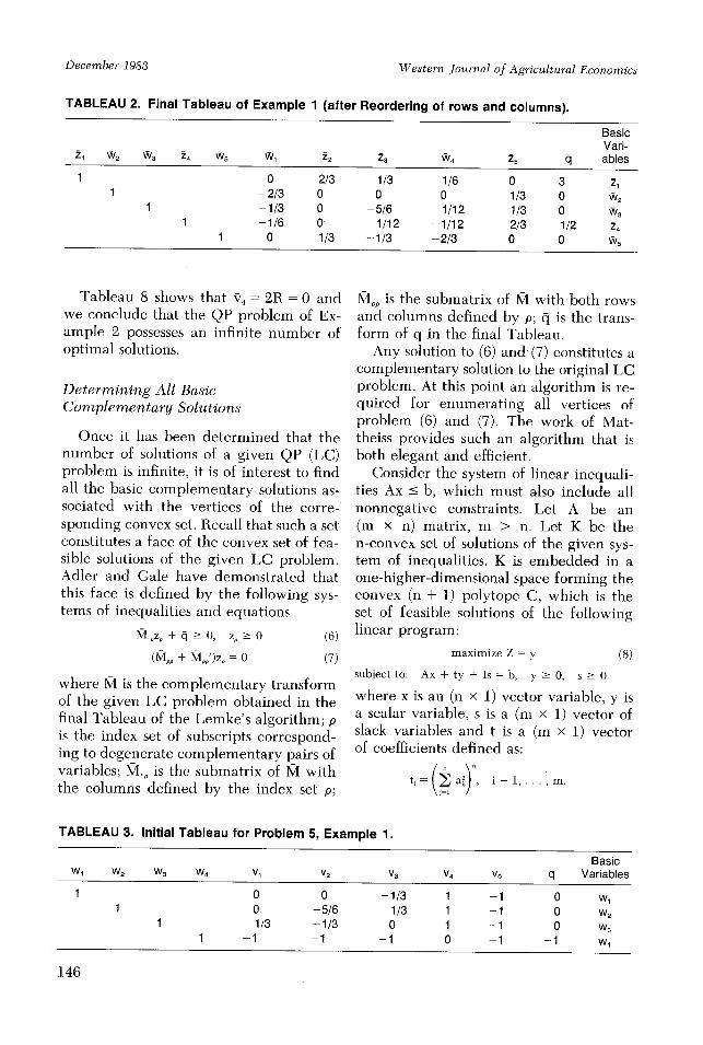
TABLEAU 2. Final Tableau of Example 1 (after Reordering of rows and columns).

BasicVari-

21 W2 W3 24 WV5 Wv1 2 23 wV4 25 q ables

1 0 2/3 1/3 1/6 0 3 211 -2/3 0 0 0 -1/3 0 W2

1 -1/3 0 -5/6 1/12 1/3 0 W31 -1/6 O 1/12 -1/12 2/3 1/2 24

1 0 1/3 -1/3 -2/3 0 0 W5

Tableau 8 shows that V4 = 2R = 0 andwe conclude that the QP problem of Ex-ample 2 possesses an infinite number ofoptimal solutions.

Determining All BasicComplementary Solutions

Once it has been determined that thenumber of solutions of a given QP (LC)problem is infinite, it is of interest to findall the basic complementary solutions as-sociated with the vertices of the corre-sponding convex set. Recall that such a setconstitutes a face of the convex set of fea-sible solutions of the given LC problem.Adler and Gale have demonstrated thatthis face is defined by the following sys-tems of inequalities and equations

M.pz + q >- 0, zp

(M,, + Mp')z, = 0

(6)

(7)

where M is the complementary transformof the given LC problem obtained in thefinal Tableau of the Lemke's algorithm; pis the index set of subscripts correspond-ing to degenerate complementary pairs ofvariables; M.p is the submatrix of M withthe columns defined by the index set p;

MP1 is the submatrix of M with both rowsand columns defined by p; q is the trans-form of q in the final Tableau.

Any solution to (6) and (7) constitutes acomplementary solution to the original LCproblem. At this point an algorithm is re-quired for enumerating all vertices ofproblem (6) and (7). The work of Mat-theiss provides such an algorithm that isboth elegant and efficient.

Consider the system of linear inequali-ties Ax < b, which must also include allnonnegative constraints. Let A be an(m x n) matrix, m > n. Let K be then-convex set of solutions of the given sys-tem of inequalities. K is embedded in aone-higher-dimensional space forming theconvex (n + 1) polytope C, which is theset of feasible solutions of the followinglinear program:

maximize Z = y

subject to: Ax + ty + Is = b, y > 0, s > 0

(8)

where x is an (n x 1) vector variable, y isa scalar variable, s is a (m x 1) vector ofslack variables and t is a (m x 1) vectorof coefficients defined as:

tn \

TABLEAU 3. Initial Tableau for Problem 5, Example 1.

BasicW, W2 W3 W4 V, V2 V3 V

4Vo q Variables

1 0 0 -1/3 1 -1 0 w,1 0 -5/6 1/3 1 -1 0 w2

1 1/3 -1/3 0 1 -1 0 W31 -1 - 1 - 1 -1 -1 W4

146

December 1983


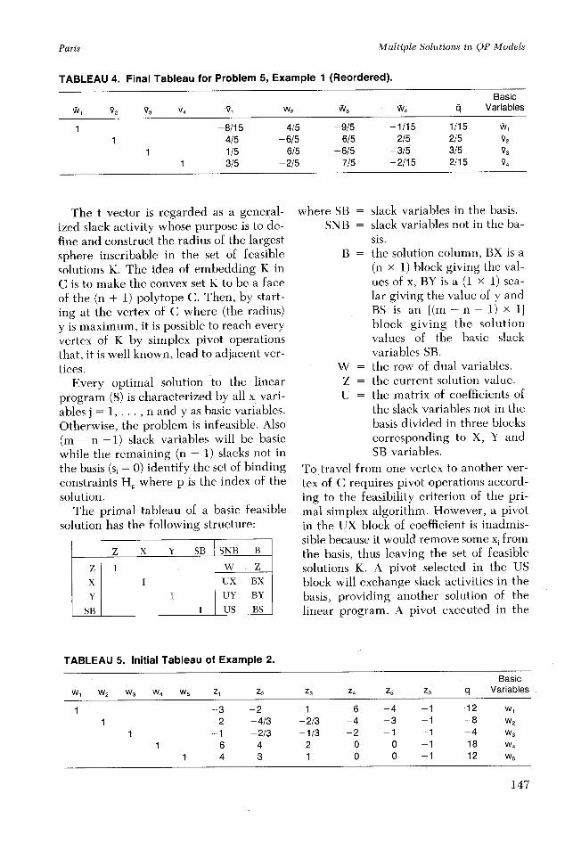
TABLEAU 4. Final Tableau for Problem 5, Example 1 (Reordered).

BasicW1 V2 V3 V4 V W2v3 v :W4q Variables

1 -8/15 4/5 -9/5 -1/15 1/15 W,

1 4/5 -6/5 6/5 -2/5 2/5 V2

1 1/5 6/5 -6/5 -3/5 3/5 V3

1 3/5 -2/5 7/5 -2/15 2/15 V4

The t vector is regarded as a general-ized slack activity whose purpose is to de-fine and construct the radius of the largestsphere inscribable in the set of feasiblesolutions K. The idea of embedding K inC is to make the convex set K to be a faceof the (n + 1) polytope C. Then, by start-ing at the vertex of C where (the radius)y is maximum, it is possible to reach everyvertex of K by simplex pivot operationsthat, it is well known, lead to adjacent ver-tices.

Every optimal solution to the linearprogram (8) is characterized by all xj vari-ables j = 1,..., n and y as basic variables.Otherwise, the problem is infeasible. Also(m - n -1) slack variables will be basicwhile the remaining (n - 1) slacks not inthe basis (si = 0) identify the set of bindingconstraints Hp where p is the index of thesolution.

The primal tableau of a basic feasiblesolution has the following structure:

zXY

SB

z x Y SB

1

I

1

I

SNB B

w zUX BX

UY BY

US BS

where SB = slack variables in the basis.SNB = slack variables not in the ba-

sis.B = the solution column, BX is a

(n x 1) block giving the val-ues of x, BY is a (1 x 1) sca-lar giving the value of y andBS is an [(m - n - 1) x 1]block giving the solutionvalues of the basic slackvariables SB.

W = the row of dual variables.Z = the current solution value.U = the matrix of coefficients of

the slack variables not in thebasis divided in three blockscorresponding to X, Y andSB variables.

To travel from one vertex to another ver-tex of C requires pivot operations accord-ing to the feasibility criterion of the pri-mal simplex algorithm. However, a pivotin the UX block of coefficient is inadmis-sible because it would remove some xj fromthe basis, thus leaving the set of feasiblesolutions K. A pivot selected in the USblock will exchange slack activities in thebasis, providing another solution of thelinear program. A pivot executed in the


BasicW, W2 W3

W4 W5 Z1 Z2Z3 Z4

Z5 Zo q Variables

1 -3 -2 -1 -6 -4 -1 -12 W,1 -2 -4/3 -2/3 -4 -3 -1 -8 w2

1 -1 -2/3 -1/3 -2 -1 -1 -4 W3

1 6 4 2 0 0 -1 18 W4

1 4 3 1 0 0 -1 12 W5

147

Paris

I

II I


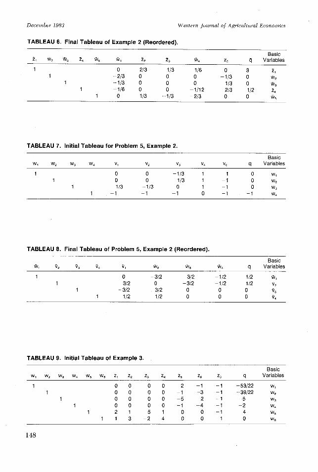
TABLEAU 6. Final Tableau of Example 2 (Reordered).

BasicZ1 W 2 W3 4 W5 W1 22 23 W4 25 Variables

1 0 2/3 1/3 1/6 0 3 211 -2/3 0 0 0 0 -1/3 0 W2

1 -1/3 0 0 0 1/3 0 W3

1 -1/6 0 0 -1/12 2/3 1/2 Z41 0 1/3 -1/3 -2/3 0 0 W,

TABLEAU 7. Initial Tableau for Problem 5, Example 2.

BasicW1 W2 W3 W4 V1 V2 V3 V4 Vo q Variables

1 0 0 -1/3 1 -1 0 W11 0 0 1/3 1 -1 0 w2

1 1/3 -1/3 0 1 -1 0 W31 -1 -1 1 0 -1 -1 W4

TABLEAU 8. Final Tableau of Problem 5, Example 2 (Reordered).

BasicW1 V2 V3 V4 VI W2 W3 W4 Variables

1 0 - 3/2 3/2 - 1/2 1/2 Wi1 3/2 0 -3/2 -1/2 1/2 V2

1 -3/2 3/2 0 0 0 3

1 1/2 1/2 0 0 0 V


BasicW1 W2 W3 W4 W5 W6 Z1 Z2 Z3 Z4 Z5 Z6 Z0 q Variables

1 0 0 0 0 -2 -1 -1 -53/22 w11 0 0 0 0 -1 -3 -1 -39/22 w2

1 0 0 0 0 -5 2 -1 -5 W31 0 0 0 0 -1 -4 -1 -2 W4

1 2 1 5 1 0 0 -1 4 W51 1 3 -2 4 0 0 -1 0 w6

148

December 1983


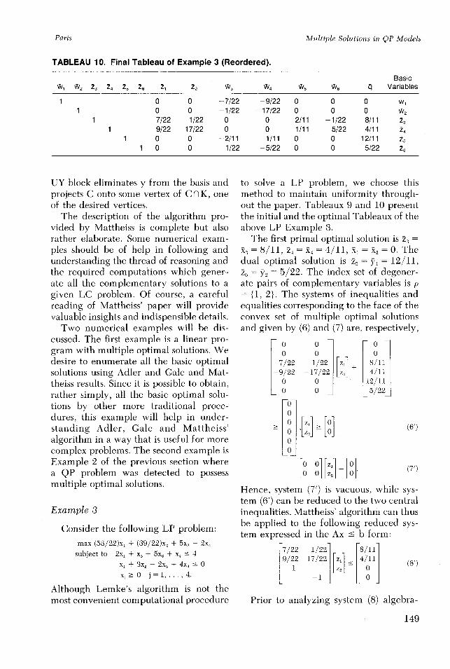
TABLEAU 10. Final Tableau of Example 3 (Reordered).

BasicW1 W2 23 24 25 26 Z1 22 W3 W4 W5 W6 q Variables

1 0 0 -7/22 -9/22 0 0 0 wv1 0 0 -1/22 -17/22 0 0 0 W2

1 7/22 1/22 0 0 2/11 -1/22 8/11 23

1 9/22 17/22 0 0 1/11 5/22 4/11 24

1 0 0 -2/11 -1/11 0 0 12/11 251 0 0 1/22 -5/22 0 0 5/22 26

UY block eliminates y from the basis andprojects C onto some vertex of C K, oneof the desired vertices.

The description of the algorithm pro-vided by Mattheiss is complete but alsorather elaborate. Some numerical exam-ples should be of help in following andunderstanding the thread of reasoning andthe required computations which gener-ate all the complementary solutions to agiven LC problem. Of course, a carefulreading of Mattheiss' paper will providevaluable insights and indispensible details.

Two numerical examples will be dis-cussed. The first example is a linear pro-gram with multiple optimal solutions. Wedesire to enumerate all the basic optimalsolutions using Adler and Gale and Mat-theiss results. Since it is possible to obtain,rather simply, all the basic optimal solu-tions by other more traditional proce-dures, this example will help in under-standing Adler, Gale and Mattheiss'algorithm in a way that is useful for morecomplex problems. The second example isExample 2 of the previous section wherea QP problem was detected to possessmultiple optimal solutions.

Example 3

Consider the following LP problem:

max (53/22)x, + (39/22)x2 + 5x3 + 2x4

subject to 2x, + X3 + 5x3 + x4 < 4

x, + 3x2 - 2x3 + 4x4 < 0

xj > 0 j = 1,..., 4.

Although Lemke's algorithm is not themost convenient computational procedure

to solve a LP problem, we choose thismethod to maintain uniformity through-out the paper. Tableaux 9 and 10 presentthe initial and the optimal Tableaux of theabove LP Example 3.

The first primal optimal solution is z3 =X3 = 8/11, z4 = , = 4/11, Xi = x2 = O. Thedual optimal solution is 25 = Y1 = 12/11,2, = Y2 = 5/22. The index set of degener-ate pairs of complementary variables is p= {1, 2}. The systems of inequalities andequalities corresponding to the face of theconvex set of multiple optimal solutionsand given by (6) and (7) are, respectively,

0 0 0

7/22 -1/22 8/11-9/22 -17/ 22 Z2 4/11

0 0 12/11_ 0 0 _ 5/22

_O__ , °° [-

0 0 i

0 0 Z2 0 ,

(6')

(7')

Hence, system (7') is vacuous, while sys-tem (6') can be reduced to the two centralinequalities. Mattheiss' algorithm can thusbe applied to the following reduced sys-tem expressed in the Ax < b form:

7/22 1/22 8/119/22 17/22 z 4/11 (8')

P-1 0

Prior to analyzing system (8) algebra-

149

Paris


z2

- Constraint 3

Constraint 1

Constraint 2XlConstraint 4

Z1

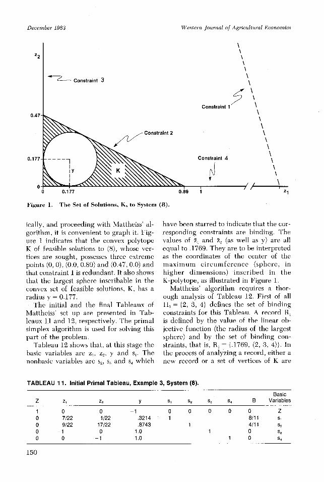
Figure 1. The Set of Solutions, K, to System (8).

ically, and proceeding with Mattheiss' al-gorithm, it is convenient to graph it. Fig-ure 1 indicates that the convex polytopeK of feasible solutions to (8), whose ver-tices are sought, possesses three extremepoints (0, 0), (0.0, 0.89) and (0.47, 0.0) andthat constraint 1 is redundant. It also showsthat the largest sphere inscribable in theconvex set of feasible solutions, K, has aradius y = 0.177.

The initial and the final Tableaux ofMattheiss' set up are presented in Tab-leaux 11 and 12, respectively. The primalsimplex algorithm is used for solving thispart of the problem.

Tableau 12 shows that, at this stage thebasic variables are z1, z2, y and s,. Thenonbasic variables are S2, S3 and S4 which

have been starred to indicate that the cor-responding constraints are binding. Thevalues of z2 and 22 (as well as y) are allequal to .1769. They are to be interpretedas the coordinates of the center of themaximum circumference (sphere, inhigher dimensions) inscribed in theK-polytope, as illustrated in Figure 1.

Mattheiss' algorithm requires a thor-ough analysis of Tableau 12. First of allHi = {2, 3, 4} defines the set of bindingconstraints for this Tableau. A record R1is defined by the value of the linear ob-jective function (the radius of the largestsphere) and by the set of binding con-straints, that is, R, = {.1769, (2, 3, 4)}. Inthe process of analyzing a record, either anew record or a set of vertices of K are

TABLEAU 11. Initial Primal Tableau, Example 3, System (8).

BasicZ Zy Z2 Y S1 s2 S3 S4 B Variables

1 0 0 -1 0 0 0 0 0 Z0 7/22 1/22 .3214 1 8/11 S10 9/22 17/22 .8743 1 4/11 S2

0 -1 0 1.0 1 0 S30 0 -1 1.0 1 0 S4

150

December 1983


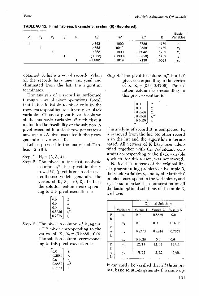
TABLEAU 12. Final Tableau, Example 3, system (8) (Reordered).

BasicZ 22 23 y s1 S2* S3* S4* B Variables

1 .4863 .1990 .3758 .1769 Z1 .4863 -. 8010 .3758 .1769 21

1 .4863 .1990 -. 6242 .1769 221 (.4863) (.1990) (.3758) .1769 y

1 -. 3332 .1819 .2120 .6061 S,

obtained. A list is a set of records. Whenall the records have been analyzed andeliminated from the list, the algorithmterminates.

The analysis of a record is performedthrough a set of pivot operations. Recallthat it is admissible to pivot only in therows corresponding to either y or slackvariables. Choose a pivot in each columnof the nonbasic variables s* such that itmaintains the feasibility of the solution. Apivot executed in a slack row generates anew record. A pivot executed in the y rowgenerates a vertex of K.

Let us proceed to the analysis of Tab-leau 12, (R,).

Step 1. H, = {2, 3, 4}.Step 2. The pivot in the first nonbasic

column, s2*, is a pivot in the yrow, UY, (pivot is enclosed in pa-rentheses) which generates thevertex of K, Z, = (0, 0). In fact,the solution column correspond-ing to this pivot execution is:

0.0 z0.0 Z0.0 Z20.3636 s2*0.7273 s,

Step 3. The pivot in column S3* is, again,a UY pivot corresponding to thevertex of K, Z2 = (0.8889, 0.0).The solution column correspond-ing to this pivot execution is:

0.0 z0.8889 2,

0.0 Z2

0.8889 S3*0.4444 sl

Step 4. The pivot in column S4* is a UYpivot corresponding to the vertexof K, Z3 = (0.0, 0.4706). The so-lution column corresponding tothis pivot execution is:

0.00.00.47060.47060.7059

Z

Z,

s4*

S1

The analysis of record R, is completed. R,is removed from the list. No other recordis in the list and the algorithm is termi-nated. All vertices of K have been iden-tified together with the redundant con-straint corresponding to the slack variablesi which, for this reason, was not starred.

Notice that in terms of the original lin-ear programming problem of Example 3,the slack variables s, and s2 of Mattheiss'problem correspond to the variables X3 andx4. To summarize the enumeration of allthe basic optimal solutions of Example 3,we have:

Optimal Solutions

Variables Vertex 1 Vertex 2 Vertex 3

P X, 0.0 0.8889 0.0RI x2 0.0 0.0 0.4706MA X3 0.7273 0.4444 0.7059L

0.3636 0.0 0.0

D Yi 12/11 12/11 12/11UA Y2 5/22 5/22 5/22L

It can easily be verified that all three pri-mal basic solutions generate the same op-

151

Paris


z2

1.

//

Constraint 2

//

/

//

Constraint 1

3

3 3.27

z3

Figure 2. The Set of Solutions to system (9).

timal value of the linear objective func-tion in Example 3, that is 48/11 - 4.3636.

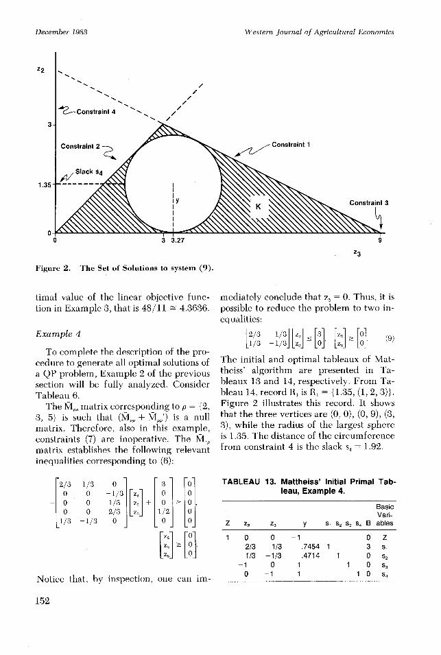
Example 4

To complete the description of the pro-cedure to generate all optimal solutions ofa QP problem, Example 2 of the previoussection will be fully analyzed. ConsiderTableau 6.

The Mpp matrix corresponding to p = {2,3, 5} is such that (MPp + M ') is a nullmatrix. Therefore, also in this example,constraints (7) are inoperative. The M.,matrix establishes the following relevantinequalities corresponding to (6):

2/30

- 0

1/31/3

1/3000

-1/3

O

-1/3

0 3 0-1/3 Z, 0 01/3 Z3 + 0 > 0 ,2/3 z, . 1/2 0

~0 ~ z 0 0Z, 5

LZ,- o0

Notice that, by inspection, one can im-

mediately conclude that z5 = 0. Thus, it ispossible to reduce the problem to two in-equalities:

2/3 1/3 [Z] 3 [ ] (93o1/3 -1/3 z3- ' z - (9

The initial and optimal tableaux of Mat-theiss' algorithm are presented in Ta-bleaux 13 and 14, respectively. From Ta-bleau 14, record RI is R, = {1.35, (1, 2, 3)}.Figure 2 illustrates this record. It showsthat the three vertices are (0, 0), (0, 9), (3,3), while the radius of the largest sphereis 1.35. The distance of the circumferencefrom constraint 4 is the slack s4 = 1.92.

TABLEAU 13. Mattheiss' Initial Primal Tab-leau, Example 4.

BasicVari-

Z z2 Z3 y S1 S2 S3 S4 B ables

1 0 0 1 0 Z2/3 1/3 .7454 1 3 s,1/3 -1/3 .4714 1 0 s2

-1 0 1 1 0 s30 -1 1 1 0 S4

152

December 1983


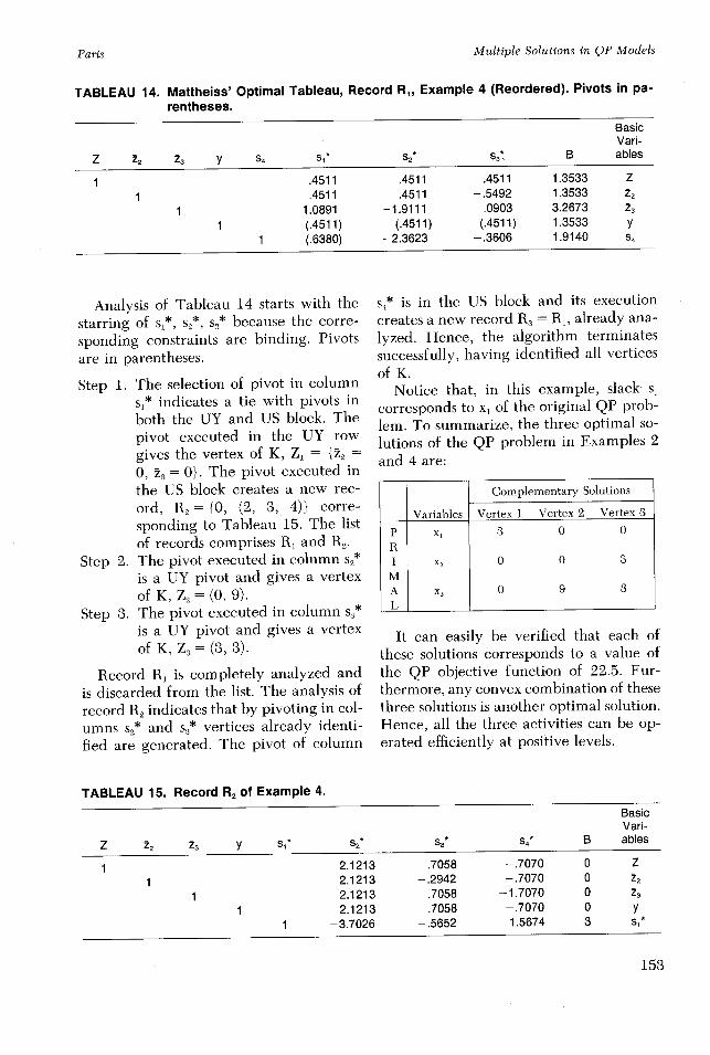
TABLEAU 14. Mattheiss' Optimal Tableau, Record R1, Example 4 (Reordered). Pivots in pa-rentheses.

BasicVari-

Z 22 23 Y S4S1 S2* S3' B ables

1 .4511 .4511 .4511 1.3533 Z1 .4511 .4511 -. 5492 1.3533 22

1 1.0891 -1.9111 .0903 3.2673 231 (.4511) (.4511) (.4511) 1.3533 y

1 (.6380) -2.3623 -. 3606 1.9140 S4

Analysis of Tableau 14 starts with thestarring of s1*, s2*, S3 * because the corre-sponding constraints are binding. Pivotsare in parentheses.

Step 1. The selection of pivot in columns,* indicates a tie with pivots inboth the UY and US block. Thepivot executed in the UY rowgives the vertex of K, Z1 = {Z2 =

0, Z3 = 0}. The pivot executed inthe US block creates a new rec-ord, R2 = {0, (2, 3, 4)} corre-sponding to Tableau 15. The listof records comprises R1 and R2.

Step 2. The pivot executed in column s2*is a UY pivot and gives a vertexof K, Z = (0, 9).

Step 3. The pivot executed in column s3'is a UY pivot and gives a vertexof K, Z= (3, 3).

Record R1 is completely analyzed andis discarded from the list. The analysis ofrecord R2 indicates that by pivoting in col-umns s2* and S3* vertices already identi-fied are generated. The pivot of column

S4* is in the US block and its executioncreates a new record R3 = R1, already ana-lyzed. Hence, the algorithm terminatessuccessfully, having identified all verticesof K.

Notice that, in this example, slack s,corresponds to x, of the original QP prob-lem. To summarize, the three optimal so-lutions of theand 4 are:

QP problem in Examples 2

It can easily be verified that each ofthese solutions corresponds to a value ofthe QP objective function of 22.5. Fur-thermore, any convex combination of thesethree solutions is another optimal solution.Hence, all the three activities can be op-erated efficiently at positive levels.

TABLEAU 15. Record R2 of Example 4.BasicVari-

Z 22 23 y s1 * s2* S3* S4* B ables

1 2.1213 .7058 -. 7070 0 Z1 2.1213 -. 2942 -. 7070 0 22

1 2.1213 .7058 -1.7070 0 231 2.1213 .7058 -. 7070 0 y

1 -3.7026 -. 5652 1.5674 3 S*

153

Complementary Solutions

Variables Vertex 1 Vertex 2 Vertex 3

P x, 3 0 0RI x2, 0 0 3MA x3 0 9 3

L

Paris


Conclusions

In the 1980s, the determination of thenumber and the value of multiple optimalsolutions in QP is a feasible problem. Allbasic optimal solutions can be obtained ina rather efficient way if the computationalscheme illustrated in this paper is adopt-ed. This applies also to LP problems.

There remains the problem of choosingthe solution to recommend or to imple-ment among all the multiple optimal so-lutions. Depending on the goals of the em-pirical study, different criteria may beadopted for this task. A particularly ap-pealing one is to choose that optimal so-lution which minimizes the squared dis-tance from present practices, as suggestedby Paris. This procedure requires theidentification of all basic optimal solutionsfirst and, secondly, the computation of theoptimal weights for combining these basicsolutions into an optimal convex combi-nation. Another possibility is to computefirst any optimal solution and its corre-sponding value of the objective function,say Z*. Then, by extending a suggestionby McCarl and Nelson, an optimal solu-tion having the property of minimizingthe distance from present practices can becomputed by solving the following non-linear problem

minimize (x - x)'(x,- x)/2subject to c'x - kx'Dx/2 > Z*

Ax < b, x> 0

where xa is the vector of activity levelsactually operated. This problem is qua-dratic both in the objective function andin one crucial constraint. Suitable algo-rithms already exist for solving such aproblem. Its main advantage lies with thefact that it does not require the enumer-ation of all the basic optimal solutions. Its

disadvantage consists in the nonlinearconstraint. Furthermore, this proceduredoes not yield any information on howdifferent various optimal basic solutionsmight be. The computation of all basicoptimal solutions is more informative be-cause it provides a complete analysis ofthe given QP (LC) problem.

References

Adler, I. and D. Gale. "On the Solutions of the Pos-itive Semi-Definite Complementarity Problem."Report ORC 75-12, Department of Industrial En-gineering and Operations Research, University ofCalifornia, August 1975.

Kaneko, I. "The Number of Solutions of a Class ofLinear Complementarity Problems." Mathemati-cal Programming, 17(1979): 104-5.

Lemke, C. E. "On Complementary Pivot Theory,"in Mathematics for the Decision Sciences, Part I,G. B. Dantzig and A. F. Veinott, Jr., editors, Prov-idence, Rhode Island: American Mathematical So-ciety, 1968, pp. 95-114.

McCarl, B. and C. H. Nelson. "Multiple OptimalSolutions in Linear Programming Models: Com-ment." American Journal of Agricultural Eco-nomics, 65(1983): 181-83.

Mattheiss, T. H. "An Algorithm for Determining Ir-relevant Constraints and All Vertices in Systems ofLinear Inequalities." Operations Research,21(1972): 247-60.

Paris, Q. "Multiple Optimal Solutions in Linear Pro-gramming Models." American Journal of Agri-cultural Economics, 63(1981): 724-27,

Takayama, T. and G. G. Judge. Spatial Temporaland Price Allocation Models. Amsterdam: NorthHolland Pub. Co., 1971.

von Oppen, M. and J. Scott. "A Spatial EquilibriumModel For Plant Location and InterregionalTrade." American Journal of Agricultural Eco-nomics, 58(1978): 437-45.

154

December 1983

Documents

Multiple Optimal Solutions in Quadratic …ageconsearch.umn.edu/bitstream/32089/1/08020141.pdfMultiple Optimal Solutions in Quadratic Programming Models Quirino Paris The problem of