Multiproxy characterization and budgeting of terrigenous

Article

Volume 13, Number 1

29 September 2012

Q0AO01, doi:10.1029/2012GC004148

ISSN: 1525-2027

Multiproxy characterization and budgeting of terrigenousend-members at the NW African continental margin

Janna JustMARUM – Center for Marine and Environmental Sciences and Faculty of Geosciences, University ofBremen, PO Box 330440, DE-28334 Bremen, Germany ([email protected])

David HeslopResearch School of Earth Sciences, Australian National University, Canberra, ACT 0200, Australia([email protected])

Tilo von Dobeneck and Torsten BickertMARUM – Center for Marine and Environmental Sciences and Faculty of Geosciences, University ofBremen, PO Box 330440, DE-28334 Bremen, Germany ([email protected]; [email protected])

Mark J. DekkersPaleomagnetic Laboratory “Fort Hoofddijk,” Department of Earth Sciences, Faculty of Geosciences,Utrecht University, Budapestlaan 17, NL-3584 CD Utrecht, Netherlands ([email protected])

Thomas FrederichsMARUM – Center for Marine and Environmental Sciences and Faculty of Geosciences, University ofBremen, PO Box 330440, DE-28334 Bremen, Germany ([email protected])

Inka MeyerMARUM – Center for Marine and Environmental Sciences and Faculty of Geosciences, University ofBremen, PO Box 330440, DE-28334 Bremen, Germany

Now at Alfred Wegener Institute for Polar and Marine Research, 25 Am Handelshafen 12, DE-27570Bremerhaven, Germany ([email protected])

Matthias ZabelMARUM – Center for Marine and Environmental Sciences and Faculty of Geosciences, University ofBremen, PO Box 330440, DE-28334 Bremen, Germany ([email protected])

[1] Grain-size, terrigenous element and rock magnetic remanence data of Quaternary marine sedimentsretrieved at the NW African continental margin off Gambia (gravity core GeoB 13602–1, 13�32.71′N,17�50.96′W) were jointly analyzed by end-member (EM) unmixing methods to distinguish and budget pastterrigenous fluxes. We compare and cross-validate the identified single-parameter EM systems and developa numerical strategy to calculate associated multiparameter EM properties. One aeolian and two fluvial EMswere found. The aeolian EM is much coarser than the fluvial EMs and is associated with a lower goethite/hematite ratio, a higher relative concentration of magnetite and lower Al/Si and Fe/K ratios. Accumulationrates and grain sizes of the fluvial sediment appear to be primarily constrained by shore distance (i.e., sealevel fluctuations) and to a lesser extent by changes in hinterland precipitation. High dust fluxes occurredduring the Last Glacial Maximum (LGM) and during Heinrich Stadials (HS) while the fluvial inputremained unchanged. Our approach reveals that the LGM dust fluxes were �7 times higher than today’s.

©2012. American Geophysical Union. All Rights Reserved. 1 of 18

http://dx.doi.org/10.1029/2012GC004148

However, by far the highest dust accumulation occurred during HS 1 (�300 g m�2 yr �1), when dust fluxeswere �80 fold higher than today. Such numbers have not yet been reported for NW Africa, and emphasizestrikingly different environmental conditions during HSs. They suggest that deflation rate and areal extentof HSs dust sources were much larger due to retreating vegetation covers. Beyond its regional and temporalscope, this study develops new, in principle, generally applicable strategies for multimethod end-memberinterpretation, validation and flux budgeting calibration.

Components: 10,600 words, 9 figures, 2 tables.

Keywords: end-member; modeling; multiproxy; paleoclimate.

Index Terms: 0473 Biogeosciences: Paleoclimatology and paleoceanography (3344, 4900); 1512 Geomagnetism andPaleomagnetism: Environmental magnetism; 1622 Global Change: Earth system modeling (1225, 4316).

Received 14 March 2012; Revised 16 August 2012; Accepted 21 August 2012; Published 29 September 2012.

Just, J., D. Heslop, T. von Dobeneck, T. Bickert, M. J. Dekkers, T. Frederichs, I. Meyer, and M. Zabel (2012), Multiproxycharacterization and budgeting of terrigenous end-members at the NW African continental margin, Geochem. Geophys.Geosyst., 13, Q0AO01, doi:10.1029/2012GC004148.

Theme: Magnetism From Atomic to Planetary Scales: Physical Principlesand Interdisciplinary Applications in Geosciences and Planetary Sciences

1. Introduction

[2] Climate reconstructions of arid and humid con-ditions during the geological past can be obtained byinvestigation of sedimentary proxy records. Varia-tions in Quaternary terrigenous element ratios andgrain-size distributions of NW African continentalmargin sediments have been linked to changes influvial and aeolian inputs, which are in turn associ-ated with fluctuations of continental humidity[Schneider et al., 1997; Zabel et al., 2001] and windstrength [Koopmann, 1981; Sarnthein et al., 1981;Matthewson et al., 1995; Holz et al., 2007]. Palyno-logical analyzes of vegetation types [Bouimetarhanet al., 2009] and the isotopic composition of plantwaxes in marine sediments [Schefuß et al., 2005;Castanñda et al., 2009; Niedermeyer et al., 2010;Collins et al., 2011] have been used to reconstructpast vegetation distributions.

[3] On glacial-interglacial time scales, climatic con-ditions in NW Africa changed significantly. Recon-structions from marine sediment cores [Sarntheinet al., 1981; Balsam et al., 1995; Matthewson et al.,1995; Kohfeld and Harrison, 2001; Larrasoañaet al., 2003] supported by numerical modeling[Mahowald et al., 1999, 2006] indicate that the dustinput to the North Atlantic Ocean was substantiallyhigher during the Last Glacial Maximum (LGM)compared to recent times. This phenomenon waslinked to higher wind speeds [Sarnthein et al.,1981; Matthewson et al., 1995; Ruddiman, 1997]

and enhanced deflation due to reduced vegetationcover [Mahowald et al., 1999]. Pollen distributionsin marine sediments indicate that wind strength wasintensified during late Quaternary cold stages.Especially during the LGM, trade winds wereblowing in a more southerly direction than atpresent [Hooghiemstra et al., 2006, and referencestherein]. Also, paleohydrological proxy data indi-cate arid conditions on the continent during theLGM [e.g., Gasse, 2000, 2001, 2006].

[4] Large North Atlantic freshwater releases duringHeinrich Stadials (HS) induced a slow-down of themeridional overturning circulation causing a short-term southward displacement of the Inter TropicalConvergence Zone (ITCZ) and an associated con-traction of the African rain belt [Mulitza et al.,2008; Itambi et al., 2009; Collins et al., 2011].This resulted in more arid conditions in NorthernAfrica, in particular in the modern Sahel Belt, andintensified zonal winds at the level of the AfricanEasterly Jet (AEJ) [Mulitza et al., 2008].

[5] Episodic phases of humid conditions occurredin the Sahara during the Late Pleistocene and theearly Holocene resulting in a dense vegetationcover [Sarnthein, 1978; COHMAP Members, 1988;deMenocal et al., 2000a, 2000b; Castañeda et al.,2009]. The latest of these so-called AfricanHumid periods (AHP) lasted from 14.8 ka to about5.5 ka and was only interrupted by the YoungerDryas stadial at �12 ka [deMenocal et al., 2000b].

GeochemistryGeophysicsGeosystems G3G3 JUST ET AL.: MULTIPROXY END-MEMBERS 10.1029/2012GC004148

2 of 18

[6] While the timing, scale, and causes of thesemassive climate changes in NW Africa are wellestablished, it is still difficult to estimate relatedchanges in dust flux and river runoff during thehighly contrasting climate periods of the past 80 kyrs.The transport pathways, fractionation processes, andpost-depositional alterations must be understood asthey all may significantly modify the fingerprint ofthe source. It is best practice to compare and cross-validate proxy-based terrigenous flux reconstructionsfrom several, not intrinsically correlated parameters.

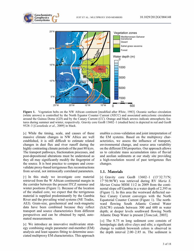
[7] In this study we investigate core materialretrieved from the W African continental margin inthe corridor between the present ITCZ summer andwinter positions (Figure 1). Because of the locationof the studied core, we expect that the terrigenousmaterial is supplied predominantly by the GambiaRiver and the prevailing wind systems (NE Trades,AEJ). Grain-size, geochemical and rock-magneticdata have been combined because they reflecttransport and source characteristics from differentperspectives and can be obtained by rapid, auto-mated measurements.

[8] We introduce an innovative multivariate strat-egy combining single parameter end-member (EM)analysis and least squares fitting to determine asso-ciated multiproxy EM characteristics. This approach

enables a cross-validation and joint interpretation ofthe EM systems. Based on the multiproxy char-acteristics, we assess the influence of transport,environmental change, and source area variabilityon the different EM properties. Our approach allowsus to calculate mass accumulation rates of fluvialand aeolian sediments at our study site providinga high-resolution record of past terrigenous fluxchanges.

1.1. Materials

[9] Gravity core GeoB 13602–1 (13�32.71′N;17�50.96′W) was retrieved during RV Maria S.Merian Cruise MSM 11/2 in 2009 from the conti-nental slope off Gambia in a water depth of 2,395 m(Figure 1). In this area the westward deflected sur-face Canary Current converges with the NorthEquatorial Counter Current (Figure 1). The north-ward flowing South Atlantic Central Water(SACW) extends between 300 and 600 m waterdepth; at deeper levels southward flowing NorthAtlantic Deep Water is present [Tomczak, 2003].

[10] The 8.75 m long sediment core consists ofhemipelagic dark olive clays and silts; a significantchange to reddish brownish colors is observed inthe depth interval 2.00–2.85 m. The sediment is

Figure 1. Vegetation belts on the NW African continent [modified after White, 1983]. Oceanic surface circulation(white arrows) is controlled by the North Equator Counter Current (NECC) and associated anticyclonic circulationaround the Guinea Dome (GD) and by the Canary Current (CC). Orange and black arrows indicate atmospheric fea-tures during summer and winter, respectively. Gravity core GeoB 13602–1 (studied here) is depicted in red and GeoB9528–3 [Castañeda et al., 2009] in black.


3 of 18

undisturbed except for a small scale distal turbiditeat 3.90–4.00 m depth.

[11] Gravity core GeoB 13602–1 was sampled at5 cm intervals. All samples were freeze-driedbefore analysis. An age model for this core by Justet al. [2012] is based on correlation of the oxygenisotope record of epibenthic Cibicoides wuellestorfito that of MD 95–2042 [Shackleton et al., 2000]and five radiocarbon ages (see auxiliary material).1

For the age-model construction the depth interval ofthe turbidite was excluded. GeoB 13602–1 spansthe last 76 ka and thus Marine Isotope Stages (MIS)1 through 4 and the end of MIS 5. The averagedsedimentation rate is �11 cm kyr�1 and, accord-ingly, sampling at 5 cm intervals corresponds to amean resolution of 450 years and permits the res-olution of millennial scale climatic variations suchas HSs.

1.2. Source Areas and Transport ofTerrigenous Material

[12] Two main source areas for the mobilization ofaeolian dust from N Africa have been identified:The Bodélé Depression in Chad, which represents atpresent the most productive dust source in the world[Prospero et al., 2002], and an area in northern Maliand Mauretania where emissions are less intense butthe area is much larger than the Bodélé Depression[Engelstaedter et al., 2006].

[13] Dry and deep atmospheric convection initiatesnear-surface turbulence and suspends soil particles[Engelstaedter et al., 2006]. Dust is uplifted byvertical convection and transported westward withinthe Saharan Air Layer by the AEJ [e.g., Pye, 1987].Coarse, more proximal dust is transported to theAtlantic Ocean by NE trade winds mainly duringwinter [e.g., Sarnthein et al., 1981; Prospero, 1996].The relative contributions of these two transportmechanisms are still a matter of debate.

[14] The Gambia River originates in Eastern Sene-gal and has only a few small contributories. It flowsin a westerly direction through Senegal and Gambiato the Atlantic Ocean. The drainage basin comprisesan area of 78,000 km2 and is dominated by savannavegetation types [Lesack et al., 1984] (cf. Figure 1).With respect to other rivers in NW Africa, e.g., theSenegal River, whose drainage basin is 3.5 timeswider and covers different vegetation zones, thefluvial discharge of the Gambia reflects regionalchanges in precipitation and mirrors the geology of

the drainage basin and most importantly their ped-ogenic products.

[15] Outcrops of the West African Shield consistof metamorphic schists, basic volcanics, sedimen-tary rocks, and granites. In the SE of the drainagearea these formations are overlain by Paleozoicmetamorphic schists and quartzites, sandstonesand dolomites. Locally, dolerites and rhyolites arepresent. In the western part of the drainage area,Mesozoic to Tertiary sediments are found [Lesacket al., 1984, and references therein]. In the north-ern part of the catchment, ferruginous soils withtypical assemblages of kaolinitic and minor illiticclays with low organic matter occur. Further to thesouth, ferralitic soils are dominated by kaoliniteand iron and aluminum oxides, with a high organicmatter content [Lesack et al., 1984; FAO et al.,2009, and references therein].

[16] A further component, which may contribute tothe fluvial load, is material advected from farthersouth (e.g., Geba River in Guinea-Bissau). How-ever, since the current velocities are moderate [Justet al., 2012, Figure 1b], it is reasonable to assumethat such advected material makes only a minorcontribution to the sediment reaching the study site.

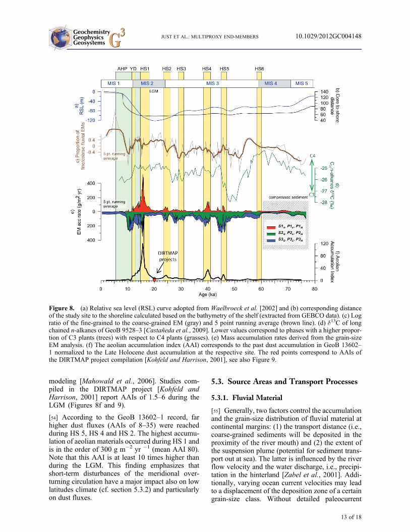
2. Methods

2.1. Geochemistry

[17] For geochemical analyses, 4–5 g of freeze-driedsediment samples were homogenized. The elementalcomposition was measured by energy dispersivepolarization X-ray fluorescence spectroscopy using aSPECTRO XEPOS instrument [Wien et al., 2005].Quality control was assessed by repeated measure-ments of standard reference material MAG-1[Govindaraju, 1994]. For a complete description seeMulitza et al. [2008].

2.2. Grain-Size Analysis

[18] To analyze the grain-size distribution of the lithicfraction, the biogenic compounds were removedfrom the sediment. Organic matter was removed byboiling 0.5 g of bulk sediment with H2O2 (35%).Afterwards, the sample was boiled with HCl (10%)and demineralized water to remove CaCO3. Theamount of opal is relatively low (1–5 weight %, datanot shown) and was not dissolved. After the aboveprocedure, the approximate terrigenous fraction isobtained. Grain-size distributions were measuredusing a Beckman Coulter laser particle sizer LS200in 92 logarithmically spaced size classes ranging1Auxiliary materials are available in the HTML. doi:10.1029/

2012GC004148.


4 of 18

from 0.39 to 2000 mm. Grains coarser than 133 mmare not present in the samples. For the later end-member unmixing and visualization the 64 fractionsfrom 0.39 to 133 mm were pooled into 32 sizeclasses to smooth the data.

2.3. Rock Magnetic Analyses

[19] Isothermal remanent magnetization (IRM)acquisition curves are indicative for the magneticmineral assemblage and the concentration of thedifferent minerals. Just et al. [2012] measured IRMacquisition curves using an automated 2-G Enter-prises 755R DC superconducting magnetometer forfields up to 700 mT and by using an “external”pulse magnetizer (2-G Enterprises) for fields up2700 mT. For further detail see Just et al. [2012].

2.4. Dry Bulk Density and MassAccumulation Rates

[20] To determine the dry bulk density and estimatethe mass fraction of terrigenous sediments, 10 cm3

of sediment were freeze-dried and weighed. Massaccumulation rates (MARs, mTOT) are calculated bymultiplication of dry bulk density and sedimenta-tion rate. The terrigenous MARs (mTER) were cal-culated by subtracting the biogenic (carbonate)mass fractions (cBIO, data from Just et al. [2012],see Figure S1 in the auxiliary material):

mTER ¼ mTOT* 1� cBIOð Þ: ð1Þ

2.5. End-Member Analysis

[21] Downcore measurements of element con-centrations, grain-size distributions, and IRMacquisition curves (adopted from Just et al. [2012])reflecting mixtures of different source materialswere unraveled by EM unmixing. The employedalgorithm was developed by Heslop and Dillon[2007] based on an approach similar to that ofWeltje [1997]. Under the assumption of linearmixing, such an EM mixing system can be writtenin matrix notation as

X ¼ ASþ E ð2Þ

where X represents the n-by-m data matrix of nsamples (one per row) and m variables (e.g., grain-size classes, relative element abundances) in thecolumns. Matrix A (n by l) denotes the abundanceof l EMs (one per column) for each sample (one perrow). Matrix S represents the m properties of thel EMs, and E is the error matrix of residuals.Because the contributions of each EM have to be

positive and the variables (e.g., grain-size classes,elemental abundances) of each EM must add up toones, non-negativity constraints (A ≥ 0; S ≥ 0) and asum-to-one constraint for the rows in S and A areincluded in the unmixing algorithm.

[22] Residuals of the EM model include instrumen-tal noise, compositional variations of the individualsources over time and non-identified additionalsources that were not detected due to low or onlybrief activity. Before performing the unmixing, low-rank representations and their coefficients of deter-mination (R2) with the input data are calculated byprincipal component analysis (PCA). The decisionon the number of EMs to include in the final mixingmodel is a compromise between keeping the numberof components low while maintaining a reasonablygood approximation of the input data. Additionally,the number of EMs should also be reasonable in thegeological context of the study [Weltje, 1997;Weltjeand Prins, 2007]. For a more detailed descriptionabout the mathematical approach of the algorithmwe refer the reader toWeltje [1997] and Heslop andDillon [2007].

[23] For performing the EM unmixing of the geo-chemical data set, the mass concentrations of themost abundant ‘terrigenous’ elements Mg, Al, Si, K,Ti, Fe were normalized to a sum of 1. Since we areonly interested in the terrigenous fraction, Ca wasexcluded as it is highly correlated with the biogenicfraction.

3. Results

3.1. Geochemistry

[24] Three different element ratios (Al/Si, Ti/Fe,Fe/K) are used to characterize the downcore varia-tions in chemical composition (Figure 2). The Al/Siand Fe/K ratios of terrigenous sediments reflect thedegree of weathering of the terrigenous sedimentcomponents [Govin et al., 2012]. Because of itsassociation to heavy minerals, the Ti (here nor-malized to Fe) content is indicative of physicalgrain-size. It was shown that off NW Africa theseelemental ratios are distinctively different for aeo-lian and fluvial material [Gac and Kane, 1986;Chiapello et al., 1997; Moreno et al., 2006] (cf.Table 1). Glacial stages MIS 2 and MIS 4 havelower Al/Si and Fe/K and slightly elevated Ti/Feratios in comparison with MIS 1 and MIS 3. TheMIS 4/3 and MIS 2/1 transitions are sharp, whilethe MIS 3/2 transition is more smooth. Al/Si andFe/K rather gradually decrease from the beginningof MIS 3 until MIS 2, whereas Ti/Fe remains stable.


5 of 18

[25] Remarkably low values mark HS 5, 4 and 2 inthe Fe/K and Al/Si records. Ti/Fe shows significantpeaks only during HS 2 and 4. HS 1 is character-ized by the most extreme values of all reportedelement ratios. It is marked by a sharp increase inTi/Fe at its beginning. Notably, however, Al/Siand Fe/K show a more gradual decrease than thecorresponding increase in Ti/Fe. Furthermore, allelement ratios show a characteristic double peakand trough, respectively. The Younger Dryas (YD)is expressed by lower Al/Si and Fe/K and slightlyelevated Ti/Fe ratios. A drop in Fe/K occurs at theend of the African Humid Period (AHP) around6 ka.

3.2. Grain-Size Distribution

[26] Since off NW Africa the grain-sizes of fluvialmaterial are finer compared to aeolian dust [Koopmann,1981], coarsening and fining grain sizes correspondto increasing proportions of aeolian and fluvialmaterial, respectively.

[27] Generally, a bimodal grain-size distributionprevails throughout the record (Figure 3). Onefraction spans grain-size classes from 2 to 20 mm,the other one comprises coarser grain sizes between25 and 90 mm. During late MIS 5, sediments arerelatively uniform and fine, while from MIS 4 toMIS 1 two modes are distinct. During MIS 3 andMIS 1 the distribution is dominated by the finergrain-size classes while MIS 2 has coarser fractions.In the Holocene, the coarse fraction is entirelymissing, and sediments are mostly finer than 9 mm.Intervals of significant coarse modes correspond toHS 5, HS 4, HS 2, the LGM and HS 1.

3.3. Differences and Similaritiesin Proxy Records

[28] The general patterns in all proxy records cor-respond to environmental changes between dry andhumid conditions, i.e., high contributions of aeolianand fluvial material, respectively. These climaticchanges are inferred from decreasing Al/Si and

Figure 2. Elemental ratios of GeoB 13602–1. Minima in Al/Si and Fe/K ratios and maxima in Ti/Fe ratios denote dryconditions on the African continent. MIS: Marine Isotope Stage, LGM: Last Glacial Maximum, HS: Heinrich Stadial,YD: Younger Dryas, AHP: African Humid Period. HSs are adopted from the timing of Heinrich Events [Sarntheinet al., 2001].

Table 1. Elemental Ratios of Dust and Fluvial Material off NW Africaa

Sample Al/Si Fe/K Ti/Fe Reference

Dust Cap Verdes (Sal Island) 0.49 2.82 Chiapello et al. [1997]0.45 2.310.43 2.09

HAR (aeolian deposit) 0.21 2.71 0.17 Moreno et al. [2006]MON (aeolian deposit) 0.19 3.10 0.27Senegal 0.54 4.77 0.08 Gac and Kane [1986]

aThe abbreviations correspond to aeolian deposits in SW Niger by northeasterly winter Harmattan (HAR) andsouthwesterly summer monsoon (MON) winds.


6 of 18

Fe/K ratios and a coarsening of grain size. Addi-tionally, in GeoB 13602–1 the Ti/Fe ratio appearsto be a significant indicator of higher aeolian inputsince Ti is enriched in coarse sediments [Boyle,1983; Zabel et al., 1999] (cf. Table 1). The moststriking features in all parameter sets are the peaksthat occur during HSs. These features support ear-lier findings of dry conditions in NW Africa duringcold periods in the northern N Atlantic [Jullienet al., 2007; Mulitza et al., 2008; Itambi et al.,2009]. However, the drying trend deduced fromdecreasing Al/Si during MIS 3 and especially dur-ing the LGM is not expressed in the grain-size data.On the other hand, drier conditions during HS 1 areindicated by extremes in Fe/K, Ti/Fe, and a coarsergrain size. The double-peak of the element ratios isnot clearly expressed in the grain-size data. DuringMIS 1, the decrease in Fe/K corresponds to a finingin the physical grain sizes.

3.4. End-Member Unmixing

[29] Contrasting patterns in the proxy recordsemphasize that factors influencing sediment ele-mental composition and grain size are diverse. Jointanalyses have a potential to deliver more informa-tion about these individual factors. We suggest thatboth source area variability and changes in trans-port processes are reflected in contrasting patterns.To evaluate their relationships further, we apply an

EM unmixing approach to the different parametersets. The EM unmixing results of the grain-size andelemental data will be presented in this study, whilethe EM analysis of IRM acquisition curves (seeFigure 5f) is reported by Just et al. [2012].

3.4.1. Element End-Members

[30] The element EM analysis shows an excellentfit (R2 = 0.99 from the PCA, Figure 4) with onlytwo EMs (S1E and S2E, the index E denotes ele-mental data). Their relative element contents weretransformed into elemental ratios (Table 2, part a,and Figure 5b). The contrasts in the element ratiosof S1E and S2E resemble contrasts in the

Figure 3. Grain-size data of GeoB 13602–1. Two modes of grain sizes are apparent. The fine mode corresponds tograins finer than 10 mm, the coarser mode is composed of grains in the range of 20–70 mm. During dry periods, inMIS 2 and the HSs, the sediments are coarser. For abbreviations see Figure 2.

Figure 4. Coefficients of determination (R2) obtainedby principal component analyses as a decision criterionfor the number of end-members used for the unmixingapproach of the element and grain-size data.


7 of 18

geochemical composition of present-day dust andsuspension load samples of the Senegal River (cf.,Table 1).

[31] The end of MIS 5, and MIS 3 and 1 are dom-inated by S2E (Figure 5a), while MIS 4 and 2 aredominated by S1E. A gradual increase of S1E con-tribution is apparent throughout MIS 3 until MIS 2.Occasional increases in S1E coincide with HSs andthe YD, of which HS 1 is the most pronounced. Thedouble-peak formerly observed in the downcore

element ratios, is present, but less well expressed inthe EM contributions.

3.4.2. Grain-Size End-Members

[32] For the EM analysis of the granulometricdata, a three EM solution appears to be optimal(R2 = 0.96, Figure 4). The obtained grain-size end-members are referred to as S1G, S2G and S3G(Figures 5c and 5d). S1G and S2G have clear unim-odal distributions, with modes of 10 and 40 mm,

Table 2. (a) Calculated Elemental Composition and Element Ratios of Element EMs (SE) and (b) PredictedAssociated Properties (PE) of the Grain-Size End-Members

Al Si K Ti Fe Mg Al/Si Fe/K Ti/Al Ti/Fe

a) S1E 0.174 0.700 0.030 0.013 0.056 0.027 0.249 1.843 0.076 0.238S2E 0.249 0.554 0.027 0.018 0.122 0.030 0.450 4.506 0.070 0.144

b) P1E 0.170 0.728 0.027 0.013 0.041 0.021 0.233 1.542 0.074 0.306P2E 0.230 0.586 0.028 0.017 0.110 0.029 0.392 3.935 0.074 0.154P3E 0.250 0.552 0.028 0.017 0.119 0.033 0.453 4.229 0.068 0.143

Figure 5. End-member models of the element, grain-size and rock-magnetic data. (a) Cumulative downcore contri-bution of element EMs (SE). (b) Elemental ratios calculated based on the elemental composition of the EMs(cf. Table 2, part a). (c) Cumulative downcore contribution of grain-size EMs SG. (d) Grain-size distributions ofS1G–S3G. (e) Cumulative downcore contributions of the aeolian and fluvial magnetic SM [Just et al., 2012]. (f) TheIRM acquisition curves are indicative of the magnetic mineralogy of the aeolian S1M and fluvial S2M. S3M corre-sponds to bacterial magnetite and S4M represents a relict phase of magnetic minerals after reductive diagenesis.


8 of 18

respectively, while S3G has a broad distribution(1–4 mm) and small peak around 20 mm. Inclu-sion of an additional EM would split the mediumgrained S2G (10 mm) into two EMs with higher(14 mm) and lower (6 mm) modes and closely co-varying contributions (data not shown). This bearsa risk of over interpretation of the data, thereforethis EM solution (and those with higher numberof EMs) was not considered. Typically, aeolianmaterial is coarser than fluvial material off NWAfrica [Koopmann, 1981]. This hints to aeoliantransport for the coarse S1G and fluvial transportfor the fine S3G. The transport pathway of S2G,however, cannot be inferred at this point.

[33] S2G and S3G are generally anticorrelated, witha higher contribution of S2G except during theLGM and the late Holocene. The contribution ofS1G is generally low; but increasing abundancefrom 50 ka until HS 1 is observed. Peaks in S1Goccur during HS 5, 4, 2 and 1. HS 1 is associatedwith a very high contributions of S1G, forming adouble-peak.

3.4.3. Comparison of the End-Member Modelsand Relation to Rock-Magnetic End-Members

[34] The comparison of the abundances of theindividual EM unmixing reveals that S1G and S1Epeak during HSs. The rock-magnetic EM analysisof GeoB13602–1 reveals that four EMs are neededto unmix the IRM acquisition curve data set [Just etal., 2012]. S1M corresponds to aeolian material and,from its calculated IRM acquisition curve, is char-acterized by a higher hematite/goethite ratio and ahigher concentration of magnetite with respect tofluvial EM S2M (Figure 5f). S3M represents bacte-rial magnetite which was formed in situ and S4Mcorresponds to a magnetic relict phase due toreductive dissolution in the lower part of the core,and within a near-surface layer [Just et al., 2012].For further details about the EM characteristics werefer the reader to Just et al. [2012]. Their aeolianEM S1M peaks during HS 4, the LGM and has itsmaximum during HS 1 (Figure 5e). This co-varia-tion is in line with the inferred aeolian nature ofS1G and S1E as suggested by grain-size distribu-tions and elemental ratios and the interpretation forthe analogous rock-magnetic end-member S1M ofJust et al. [2012].

4. Multiproxy Approach

[35] The modeled abundances of the EMs estimatethe mixing proportions with respect to the input

data (Figure 6): Grain-size EMs correspond tovolume fractions, element EMs relate to massfractions with regard to the total mass of the ele-ments considered and rock magnetic EMs relate tosaturation isothermal remanent magnetization(SIRM [Just et al., 2012]) of each EM. Because thecontent of magnetic minerals within terrigenoussediments from different sources may differ, reca-librations are needed to transfer the IRM intensitiesinto volume and mass percentages of the respectiveterrigenous fractions they are associated with. Cal-ibration factors depend on the concentration ofmagnetic minerals within a certain volume (ormass) of bulk material and on the magnetic mineralassemblage, since magnetic minerals have differentSIRMs [Peters and Dekkers, 2003].

[36] The grain-size EM analysis indicates that threeenergetic regimes exist for the transport of terrige-nous sediments. It can be assumed that the differentkinds of sediment properties are associated to eachother, i.e., a grain-size class which is transported bya certain mechanism mirrors the distinct geochem-istry and the magnetic mineralogy of the soils in thesource area or experiences similar gravitationalsorting processes. Therefore proportional differ-ences between the grain-size EM fractions shouldbe reflected in compositional differences of ele-ments and magnetic minerals, respectively.

[37] From this assumption we developed a newapproach for finding multiproxy properties of ageneralized EM system. We use volumetric grain-size EM abundances AG to predict geochemical,PE, and rock magnetic properties, PM that areassociated to the grain-size EM properties (SG).Formally

XE ¼ AGPE þ R ¼ X⌢E þ EE ð3Þ

and

XM ¼ AGPM þ R ¼ X⌢M þ EM ð4Þ

are equivalent EM mixing formulations ofequation (2). EE and EM are matrices of resi-duals for the element and magnetic data sets,respectively.

[38] Since there is only one unknown, this linearproblem can be solved using nonnegative leastsquares fitting (NNLSQ [Löfberg, 2004]), whichrespects the non-negativity constraint P ≥ 0. Sincethe element abundances are scaled to a sum of 1,the cumulative element abundances of the associ-ated properties PE must also be constrained to addup to 1.


9 of 18

[39] In order to apply this approach to the IRM data,some pre-processing had to be performed. It waspreviously shown that one of the magnetic EMs(S3M) corresponds to biogenic magnetite [Justet al., 2012] which is formed in situ and hence isnot representing any terrigenous fraction. We mul-tiplied the IRM acquisition curve of the bacterialS3M (Figure 5f) by its contribution to SIRM of eachsample (A3M, Figure 5e) and subtracted this datamatrix from the original IRM acquisition curves(Figure 6).

[40] After the pre-processing the residual IRMacquisition curves should only represent the terrig-enous magnetic inventory. IRM was measured onthe bulk sediment, which consists of mixed terrig-enous and biogenic material (mainly carbonate),which does not have an IRM. In contrast, grain-sizedata were analyzed on a carbonate-free basis bydissolving the carbonate prior to the grain-size

analyses. To predict magnetic properties (i.e., IRMacquisition curves) from the volumetric mixingproportions of the grain-size EMs, their proportionsmust therefore be corrected for the missing volumeof carbonate AC (Figure 6). The volume of car-bonate AC was calculated by multiplying the massconcentration of carbonate (auxiliary material) bythe dry bulk density.

[41] Additionally, we excluded the top interval andthe lower part of the core where substantial reduc-tive diagenesis has modified the magnetic miner-alogy [Just et al., 2012].

[42] To assess the quality of the multiproxy model,the correlation between the input data, X, and theestimates, X

⌢, derived by NNLSQ was calculated.

In the case of the IRM data set, which is non-normalized and thus free of a sum-to-one constraint,the Pearson product-moment correlation coefficient

Figure 6. Schematic overview of the multiproxy EM approach. Each individual data set was unmixed using the EMunmixing algorithm of Heslop and Dillon [2007] yielding relative abundances A and properties S. The grain-size EMcontributions AG were successively used to calculate associated geochemical (PE) and rock-magnetic properties (PM)by nonnegative least squares (NNLSQ) fitting. The obtained PE and PM have identical volume contributions as the SGand are helpful to interpret the nature of the EMs. The comparison of SM and PM and SE and PE may be used to verifyif changes in methodologically different EM analyses lead to consistent solutions (multiproxy validation). For themagnetic data, the contribution of the bacterial magnetite identified by Just et al. [2012] and carbonate (AC) contentwas corrected for (see text).


10 of 18

was calculated. For the compositional data set ofelement relative abundances we performed thecentered-log-ratio transformation [Aitchison, 1982]to bring the dataXE and estimatesX

⌢E into real space.

Afterwards a correlation coefficient analogous tothe Pearson product-moment correlation coefficientfor compositional data was calculated. In both casesthe significance of the correlation was assessedusing a Monte Carlo randomization test with 104

iterations. For X⌢

and XM the coefficient of deter-mination is 0.51 (corresponding to a significancelevel of <0.0001). When comparing XE and X

⌢E the

calculated squared correlation is 0.63 (significant ata level of <0.0001).

4.1. Multiproxy Properties

[43] The elemental ratios PE associated to the grain-size EMs are given in Table 2, part b. A strikingfeature is that the associated elemental compositionP1E of the coarse grain-size EM S1G is distinctlydifferent from P2E and P3E. P1E has low Al/Si andFe/K and high Ti/Fe ratios while both fine-grainedEMs are associated to high Al/Si and Fe/K and lowTi/Fe ratios.

[44] Likewise, the IRM acquisition curve of P1Mis distinctively different from P2M and P3M(Figure 7a), while the latter two curves are very

similar. To compare the shape of the curves, whichis indicative of the magnetic mineralogy, we nor-malized them to one (Figure 7b). Again, the shapeof P1M is distinctively different; the slope starts torise at lower fields and is flatter at high fieldscompared to P2M and P3M. This indicates that P1Mcontains a higher proportion of magnetite andhigher hematite/goethite, compared to P2M andP3M. A comparison of the associated properties ofthe grain-size EMs with the EMs obtained by directunmixing of the magnetic and geochemical datareveals large similarities between both solutions(Figure 7b and Table 2, parts a and b) and can beused to verify each solution (Figure 6).

5. Discussion

5.1. Multiproxy Properties of TerrigenousEnd-Members

[45] Since the associated properties of the grain-sizeEMs appear to provide a good representation of theEMs of the individual analysis, we can elucidate thenature of the grain-size EMs from a geochemicaland rock-magnetic perspective. The coarse mode ofS1G is in the range of typical grain sizes (8–42 mm)for dust collected off NW Africa [Stuut et al.,2005]. The associated geochemical properties P1E(Table 2) are similar to aeolian deposits in SWNiger [Moreno et al., 2006] and low Fe/K ratio ofpresent-day dust samples collected at Sal Island[Chiapello et al., 1997] (Table 1). However, theAl/Si ratio of the Sal Island samples is significantlyhigher, than in P1E. This phenomenon is mostlikely attributed to gravitational sorting duringtransport, suggesting a shorter distance between ourcore location and the dust source compared to thedeposits from Sal Island. This interpretation is inline with the coarse grain-size distribution S1G.Further, the normalized IRM acquisition curve P1Mresembles the IRM acquisition curve of S1M whichhas been identified as an aeolian EM [Just et al.,2012] with a magnetic inventory containing a highconcentration of magnetite and a high hematite/goethite ratio.

[46] According to their associated properties, themedium (10 mm) and fine grained EMs (1–4 mm)have similar elemental compositions and magneticmineralogies, which yields several clues for theirinterpretation: (a) The present-day suspension loadat the mouth of the Gambia river consists of grainsfiner than 10 mm [Gac and Kane, 1986, and refer-ences therein]. (b) The elemental ratios P2E andP3E resemble fluvial samples of the suspension

Figure 7. (a) IRM acquisition curves of PM obtainedby the least squares fitting approach. P1M has a muchhigher SIRM than P2M and P3M. (b) Normalized IRMcurves PM in comparison to SM obtained by unmixingthe IRM data [Just et al., 2012]. The strong similarityindicates that the mixing proportions of grain-size end-member SG can be equally used for unmixing the IRMacquisitions curves, as the mixing proportions obtainedby IRM end-member analysis (see Figure 5).


11 of 18

load of the Senegal river [Gac and Kane, 1986](Table 1). (c) The IRM acquisition curves P2M andP3M are similar to S2M which was interpreted as afluvial EM with a lower hematite/goethite ratio anda lower relative concentration of magnetite [Justet al., 2012].

[47] The similar elemental compositions and mag-netic mineralogies demonstrate that both EMs cor-respond to sediments that originate from the samesource area (i.e., Gambia River catchment), but aretransported under different energetic conditions.Since the Gambia River drainage basin is relativelywell vegetated, its potential for aeolian deflation ofmaterial is low and thus both the medium- and fine-grained EMs must have been transported by theGambia River. The medium grained EM (10 mm)falls into the range of present-day dust collected offNW Africa [Stuut et al., 2005] and might thereforecorrespond to a mixture of aeolian and fluvialmaterial. However, given the strong similarity ofelemental ratios (P2E) and magnetic mineralogy(P2M) to the fine grained EM (P3E, P3M), themedium grained EM must be dominated by fluvialsediments and the bias introduced by aeolianmaterial must be small.

[48] Only the joint characterization of the multipa-rameter properties enables the identification of themedium grained EM S2G as a fluvial EM. By theirvery nature, magnetic and geochemical data are moreindicative for source area characteristics, while grainsize is primarily controlled by transport conditions.We will further discuss differences in the grain-sizedistribution of the fluvial EMs in section 5.3.

5.2. Budgeting the Accumulation ofTerrigenous End-Members

[49] Because only the grain-size EM system repre-sents volumetric contribution of aeolian and fluvialfractions, we used the grain-size EM contributionsto quantify the fluxes of terrigenous sediments tothe continental margin off Gambia.

[50] The total MARs in core GeoB 13602–1 varybetween 30 g m�2 yr�1 and 700 g m�2 yr�1

(Figure 8e). Note that in the lowest part of the core(MIS 5 and 4) the mass accumulation rates areprobably underestimated because squeezing out ofsediments during gravity coring is likely [Just et al.,2012]. The accumulation of the fluvial EMs(Figure 8e) is on average higher than that of theaeolian EM with a few exceptions during HSs andthe LGM. This is in accordance with the calcula-tions of Collins et al. [2011] who investigated the

dust/river ratio in sediment cores of a transect from21�N to 23�S off W Africa. At 12�N, they found adust/river proportion of �0.3 in the Holocene andratios of �1.2 and �2.5 during the LGM and HS 1,respectively. Our analysis reveals a similar pattern.However, it seems that also during HSs the accu-mulation of fluvial material increases. This patternis most probably an artifact of the age modelbecause of the short-term character of HSs and theirextremely high accumulation rates. The lack of age-control points leads to blurring of fluvial accumu-lation rates before and after the punctured peaks ofhigh dust input.

[51] However, since fluvial sediment accumulationdid not completely diminish during HSs we suggestthat reported dry conditions only affected thesource areas of aeolian material (i.e., their arealextent) but seem to have had little influence onrainfall in the Gambia River catchment and respec-tively the fluvial discharge of suspended material.

[52] Exceptionally high MARs during HS 1 showmassive levels of aeolian input. The deglaciationuntil �10 ka is marked by high accumulation ratesof fluvial material in the range of 100 to300 g m�2 yr�1. Subsequently, MARs of the fluvialEMs are reduced to 40 g m�2 yr�1 while theaccumulation of aeolian material diminishes to lessthan 10 g m�2 yr�1. This dust accumulation rateduring the Holocene is in good accordance withother studies in the region [Kohfeld and Harrison,2001] and estimates obtained by numerical model-ing [Mahowald et al., 2006].

[53] Difficulties arise when comparing absolutedust accumulation rates from different sites, sincethe deposition is influenced by regional conditionsi.e., the presence of potential dust sources in thehinterland and the source-to-sink distance. Tocompare flux changes at different sites, it is usefulto normalize the dust input to a site specific refer-ence. The data compilation in the DIRTMAP proj-ect [Kohfeld and Harrison, 2001] uses the moderndust accumulation at each site as a reference.Accordingly, we use the calculated dust accumu-lation at GeoB 13602–1 during the Late Holoceneas a reference to express the proportion of dustthroughout our record and the Holocene as theaeolian accumulation index (AAI, Figures 8f and9). The averaged accumulation rates of aeolianmaterial in GeoB 13602–1 during MIS 3 and theLGM correspond to AAIs of 3 and 7, respec-tively. The value for the LGM is in the order ofthe dust deposition estimates for our study areaduring the LGM obtained from numerical


12 of 18

modeling [Mahowald et al., 2006]. Studies com-piled in the DIRTMAP project [Kohfeld andHarrison, 2001] report AAIs of 1.5–6 during theLGM (Figures 8f and 9).

[54] According to the GeoB 13602–1 record, farhigher dust fluxes (AAIs of 8–35) were reachedduring HS 5, HS 4 and HS 2. The highest accumu-lation of aeolian materials occurred during HS 1 andis in the order of 300 g m�2 yr �1 (mean AAI 80).Note that this AAI is at least 10 times higher thanduring the LGM. This finding emphasizes thatshort-term disturbances of the meridional over-turning circulation have a major impact also on lowlatitudes climate (cf. section 5.3.2) and particularlyon dust fluxes.

5.3. Source Areas and Transport Processes

5.3.1. Fluvial Material

[55] Generally, two factors control the accumulationand the grain-size distribution of fluvial material atcontinental margins: (1) the transport distance (i.e.,coarse-grained sediments will be deposited in theproximity of the river mouth) and (2) the extent ofthe suspension plume (potential for sediment trans-port out at sea). The latter is influenced by the riverflow velocity and the water discharge, i.e., precipi-tation in the hinterland [Zabel et al., 2001]. Addi-tionally, varying ocean current velocities may leadto a displacement of the deposition zone of a certaingrain-size class. Without detailed paleocurrent

Figure 8. (a) Relative sea level (RSL) curve adopted from Waelbroeck et al. [2002] and (b) corresponding distanceof the study site to the shoreline calculated based on the bathymetry of the shelf (extracted from GEBCO data). (c) Logratio of the fine-grained to the coarse-grained EM (gray) and 5 point running average (brown line). (d) d13C of longchained n-alkanes of GeoB 9528–3 [Castañeda et al., 2009]. Lower values correspond to phases with a higher propor-tion of C3 plants (trees) with respect to C4 plants (grasses). (e) Mass accumulation rates derived from the grain-sizeEM analysis. (f) The aeolian accumulation index (AAI) corresponds to the past dust accumulation in GeoB 13602–1 normalized to the Late Holocene dust accumulation at the respective site. The red points correspond to AAIs ofthe DIRTMAP project compilation [Kohfeld and Harrison, 2001], see also Figure 9.


13 of 18

reconstructions, the latter effect is hard to quantify.Numerical modeling approaches indicate that thenet N-S horizontal volume transport in the easternAtlantic Ocean did not differ substantially duringthe LGM [Schäfer-Neth and Paul, 2004]. However,the stratification and depth of oceanographicboundary layers were different; a shallowing ofnorthern sourced waters and ingression of SACW isevident [Sarnthein et al., 1994; Bickert andMackensen, 2004; Lynch-Stieglitz et al., 2007]. Tothe best of our knowledge there are no regionalpaleocurrent reconstructions which integrate overthe entire water column and could be indicative for achange in the deposition center of suspended oradvected material in our study area. Therefore weassume that the integrated net transport of sus-pended material did not vary significantly duringthe last glacial on a regional scale and is essentiallythe same as today. We focus here on the potentialeffects of transport distance (i.e., distance from thecore location to the river mouth) and transportenergy.

[56] During MIS 4 and MIS 3 sea level was 60–80 m lower than today [Waelbroeck et al., 2002]and reached its lowest position during MIS 2(LGM, Figure 8a). Accordingly, the distance fromthe core location to the river mouth reached a min-imum. Due to the morphology of the flat-toppedshelf, the core-to-shore distance remained relativelystable (�55 km) once sea level fall reached athreshold of �60 m (Figure 8b). A major trans-gression occurred during the deglaciation whichended at 8 ka, resulting in the present-day core-to-shore distance of �140 km.

[57] The sea-level fall and rise during MIS 5 andMIS 1, respectively, and the related distance-to-shore curve, coincide roughly with total accumu-lation of fluvial material (Figure 8e), indicating thatthe distance from the river mouth to the study siteplays an important role. However, the proportion offine- and coarse-grained fluvial sediments espe-cially during MIS 4, 3 and 2 cannot be explained bysea-level variations alone.

[58] It can be hypothesized that during humid peri-ods, and thus times of higher water discharge, thefan of suspended material was more extensive andthus coarse particles were transported farther out atsea, leading to a coarsening of the fluvial depositsand to a lowering of the dust/river proportion. Toconsider the transport energy of the river, i.e., thewater discharge, we investigate published proxystudies focusing on precipitation on the continentitself and compare them to the ratio between thefine- and coarse-grained fluvial EM fractions(Figure 8c). Castañeda et al. [2009] measured thed13C of long-chained n-alkanes (Figure 8d) on sed-iment core GeoB 9528–3 (09�09.96N, 17�39.81W,Figure 1). These plant waxes are contained in aeo-lian material of which the source area is assumed tobe at the Sahara-Sahel boundary [Castañeda et al.,2009]. The variations in d13C can be regarded as aproxy for the relative proportions of C4 (grasses)and C3 plants (trees, shrubs), of which occurrence inNW Africa depends on humidity [Castañeda et al.,2009, and references therein]. A relative increase inC4 vegetation at the end of MIS 5 and MIS 4(Figure 8d) indicates drying conditions whileincreasing humidity (relative increase of C3 plants)occurs at the beginning of MIS 3 (50–45) ka.

[59] The aridification during MIS 5 and MIS 4 isexpressed by a relative decrease in fluvial inputwith respect to the aeolian fraction. During MIS 3,the strong relative increase in C3 vegetation isroughly correlated to an increase of the fine/coarse

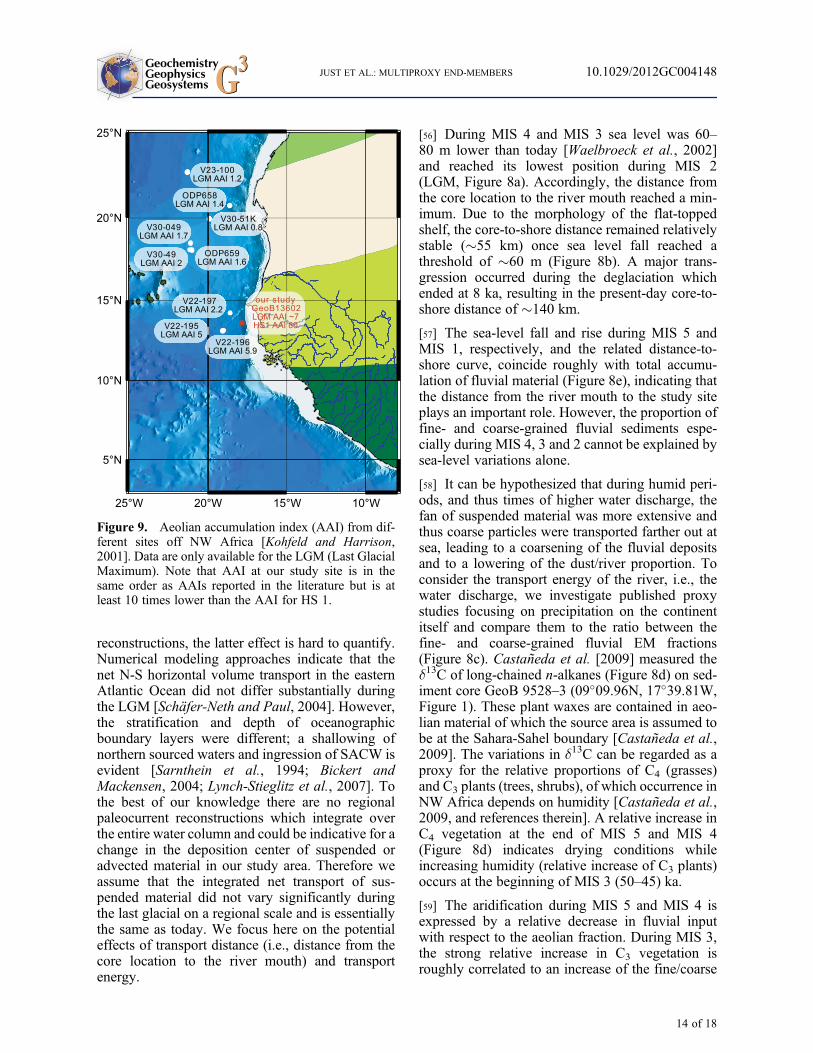
Figure 9. Aeolian accumulation index (AAI) from dif-ferent sites off NW Africa [Kohfeld and Harrison,2001]. Data are only available for the LGM (Last GlacialMaximum). Note that AAI at our study site is in thesame order as AAIs reported in the literature but is atleast 10 times lower than the AAI for HS 1.


14 of 18

fluvial EM ratio (Figure 8c). However, the promi-nent peak in C3 vegetation around 50 ka has nocounterpart in the coarse fluvial EM. In the begin-ning of MIS 2, the proportion of fine/coarse fluvialEMs increases, which might point to lower waterdischarge of the Gambia River in line with drierconditions, i.e., less precipitation, suggested byincreased C4 proportion [Castañeda et al., 2009]and modeling approaches [Van Meerbeeck et al.,2008]. Similarly, a record of dD ratios of n-alkanesin a sediment core off the Senegal River indicatesdecreasing rainfall at the MIS 3/2 transition[Niedermeyer et al., 2010].

[60] During more humid last deglacial conditionsthe fraction of the coarse fluvial EM (S2G) isagain enhanced. During the Mid-Holocene AHP[deMenocal et al., 2000b] - which has beenascribed the most humid period during the entireHolocene in sub-tropical and arid NW Africa[deMenocal et al., 2000b; Collins et al., 2011;Meyer et al., 2011] - the fine fluvial EM is re-established, which seems to be in conflict with therelationship outlined above. However, this periodcorresponds to the time of major sea-level rise, andthus a dramatic increase of the distance betweencore location and river mouth. This sea-level effectis apparently more important for the deposition offluvial materials than higher precipitation.

[61] Significant drops in the proportion of fine tocoarse fluvial EMs mark HS 2 and 3, which is ratherunexpected, given the consideration of a higherproportion of fine/coarse fluvial material during aridthan during humid conditions. We suppose that thispeak corresponds to a non-perfect unmixing of flu-vial and aeolian material for HS 2; relatively fine-grained dust is mingled with the coarse-grainedfluvial EM. Since the input of aeolian materialappears to be rather low during HS 3 (see Figures 8eand 8f), we infer that the pattern during HS 3 is notassociated with the same unmixing error. Also, forHS 1, 4 and 5 no significant minima are observed.Wethus conclude that the unmixing procedure workedproperly for most of the record and aeolian materialis mainly represented by S1G (cf. section 5.1).

5.3.2. Aeolian Material

[62] The accumulation of aeolian material is con-trolled by wind strength, frequency of dust out-breaks, source-to-sink distance, and areal extent ofdust sources. The latter is dependent on vegetationcover in the hinterland, primarily a function ofprecipitation. Widely exposed shelf areas may be

subject to deflation under dry conditions and act asadditional sources, especially during times of lowsea level. The high dust flux during MIS 3, MIS 2and particularly during HS 1 (Figures 8e and 8f)implies very different environmental conditions inNW Africa during those periods. The recognizablecorrelation between vegetation cover and propor-tion of aeolian material, especially at the MIS 3/2transition, indicates that the expansion and con-traction of the desert is the main driving mechanismfor dust export from the continent. The rising sealevel during the last deglaciation coincides with adecrease in dust contribution pointing to the influ-ence of exposed shelves and regional dust sourcesduring MIS 4 to MIS 2. Southward advancing dunefields [Maley, 2000] during the LGM could alsohave constituted additional dust sources. However,our approach reveals that the magnetic mineralogyand geochemical composition of dust did not vary.It may therefore be inferred that regional remobi-lized sediments correspond to deposits originatingfrom the Sahara. Since the most extensive exposedshelves existed during the LGM, the high dustaccumulation during HS 1 cannot solely be attrib-uted to desiccated shelf-areas and should ratherresult from southerly expanded deserts.

[63] It has been suggested that during the LGM theTrades were much stronger compared to present-day [Hooghiemstra et al., 2006, and referencestherein] and that the zonal wind field (AEJ) wasalso enhanced during Heinrich Stadials [Mulitzaet al., 2008]. This should affect the accumulationof the aeolian fraction and its grain size. Since onlyone EM is resolved in our study, the inferredcoarsening is not apparent in our EM unmixing.Since the grain-size spectrum of the aeolian EMintegrates over a certain grain-size range, it remainsquestionable, whether EM modeling is capable ofdetecting changes in wind strength, at least with thepresent input parameters.

[64] Our data suggests that dust events were morefrequent (i.e., longer ‘dusty’ seasons during HS 1)and dust sources were larger. Likewise, Collinset al. [2011] inferred a shorter wet season for theLGM and HS 1 from vegetation proxies. The doublepeak observed in the proxy data and EM modelsindicates that during HS 1, environmental condi-tions may have changed rapidly. Higher resolutionrecords are needed to understand if such changesduring HS 1 are associated to separate NorthAtlantic freshwater injections features, i.e., pre-cursors of iceberg discharge in advance of Heinrich


15 of 18

Events [e.g., Grousset et al., 2001; Jullien et al.,2007].

6. Conclusion

[65] A combined strategy of end-member analysisand least squares-fitting techniques enabled us todetermine volume calibrated multiparameter prop-erties for each identified EM. Geochemical elementand rock magnetic EM abundances correspond tototal mass or saturation remanence contributions,respectively, but are not intrinsically volume cali-brated. NNLSQ fitting of the volumetric grain-sizeEM contributions with the geochemical and rock-magnetic sample properties provides such a volumecalibration.

[66] While only two magnetic or two element EMssuffice to unmix the terrigenous sediment fractionof core GeoB 13602–1, three grain-size EMs wererequired to fit all observed grain-size distributions.The associated EM properties reveal that the fine(<4 mm) and medium (mode 10 mm) grain-size EMshave very similar magnetic and geochemical sig-natures indicative of fluvial sediments in sub-tropi-cal Africa. A coarse grain-size aeolian EM (mode40 mm) has a contrasting composition marked bylower Al/Si and Fe/K and higher Ti/Fe ratios, con-sistent with earlier dust studies, as well as a higherhematite to goethite ratio in line with soil formationunder more arid climates.

[67] In combination, the granulometric, geochemicaland rock-magnetic characteristics enable univocalinterpretations and validations of all single-parameterEMs: Grain-sizes can discriminate fluvial and aeo-lian fractions only if transport energies differ signif-icantly. Geochemical composition and the magneticmineralogy are distinctive, if sediments originatefrom petrologically and/or pedogenically contrastingsources. After the identification of aeolian and fluvialEMs by their multiproperty characteristics, theirvolume fractions permit their individual accumula-tion rates to be budgeted.

[68] At our core position, fluvial sediment accu-mulation is generally higher than dust deposition,although, during HSs and the LGM the ratio ofaeolian/fluvial material can reach �1. The accu-mulation and grain-sizes of the fluvial fraction areprimarily controlled by the distance between rivermouth and core location, i.e., sea level variations,and secondarily by precipitation in the hinterland.

[69] According to our analysis, the flux of aeolianmaterial during the LGM was 7 times higher than

today, but not higher than during MIS 3–4. Themost extreme dust input (�300 g m�2 yr�1)occurred during HS 1, 80 times higher compared tomodern times. The driving factor for dust accumu-lation is the presence of freshly exposed or desic-cated source areas for deflation. Exposed shelvesmay have served as additional dust sources but onlya rapid vegetation retreat can explain the observedfluxes during HSs. The fluvial input does notappear to be significantly reduced during HSs,suggesting that aridification during HSs did notreach the catchment region of the Gambia River.

Acknowledgments

[70] We thank the crew and scientific party ofMaria S. Meriancruise MSM 11/2 for helping to collect the studied cores. Weacknowledge the helpful comments of three anonymousreviewers. This study was funded by the Deutsche Forschungs-gemeinschaft (DFG) through the international graduate collegeEUROPROX- Proxies in Earth History and through DFG-Research Center / Cluster of Excellence “The Ocean in theEarth System” MARUM – Center for Marine EnvironmentalSciences. DH was supported by the Australian Research Coun-cil (grant DP110105419). The data for this study available in thePANGAE database http://doi.pangaea.de/10.1594/PANGAEA.788181.

References

Aitchison, J. (1982), The statistical analysis of compositionaldata, J. R. Stat. Soc., B, 44, 139–177.

Balsam, W. L., B. L. Otto-Bliesner, and B. C. Deaton (1995),Modern and Last Glacial Maximum eolian sedimentationpatterns in the Atlantic Ocean interpreted from sediment ironoxide content, Paleoceanography, 10(3), 493, doi:10.1029/95PA00421.

Bickert, T., and A. Mackensen (2004), Last Glacial to Holo-cene changes in South Atlantic deep water circulation, inThe South Atlantic in the Late Quaternary - Reconstructionof Material Budget and Current Systems, edited by G. Wefer,S. Mulitza, and V. Ratmeyer, pp. 671–695, Springer, Berlin,doi:10.1007/978-3-642-18917-3_29.

Bouimetarhan, I., L. Dupont, E. Schefuß, G. Mollenhauer,S. Mulitza, and K. Zonneveld (2009), Palynological evidencefor climatic and oceanic variability off NW Africa during thelate Holocene, Quat. Res., 72, 188–197, doi:10.1016/j.yqres.2009.05.003.

Boyle, E. A. (1983), Chemical accumulation variations underthe Peru Current during the past 130,000 years, J. Geophys.Res., 88, 7667–7680, doi:10.1029/JC088iC12p07667.

Castañeda, I., S. Mulitza, E. Schefuß, R. A. Lopes dos Santos,J. S. Sinninghe Damsté, and S. Schouten (2009), Wet phasesin the Sahara/Sahel region and human migration patternsin North Africa, Proc. Natl. Acad. Sci. U. S. A., 106,20,159–20,163, doi:10.1073/pnas.0905771106.

Chiapello, I., G. Bergametti, B. Chatenet, P. Bousquet, F. Dulac,and E. S. Soares (1997), Origins of African dust transported


16 of 18

over the northeastern tropical Atlantic, J. Geophys. Res., 102,13,701–13,709, doi:10.1029/97JD00259.

COHMAP Members (1988), Climatic changes of the last18,000 years: Observations and model simulations, Science,241, 1043–1052, doi:10.1126/science.241.4869.1043.

Collins, J. A., et al. (2011), Interhemispheric symmetry ofthe tropical African rainbelt over the past 23,000 years, Nat.Geosci., 4, 42–45, doi:10.1038/ngeo1039.

deMenocal, P., J. Ortiz, T. Guilderson, and M. Sarnthein(2000a), Coherent high- and low-latitude climate variabilityduring the Holocene Warm Period, Science, 288, 2198–2202,doi:10.1126/science.288.5474.2198.

deMenocal, P., J. Ortiz, T. Guilderson, J. Adkins, M. Sarnthein,L. Baker, and M. Yarusinsky (2000b), Abrupt onset andtermination of the African Humid Period: Rapid climateresponses to gradual insolation forcing, Quat. Sci. Rev.,19, 347–361, doi:10.1016/S0277-3791(99)00081-5.

Engelstaedter, S., I. Tegen, and R. Washington (2006), NorthAfrican dust emissions and transport, Earth Sci. Rev., 79,73–100, doi:10.1016/j.earscirev.2006.06.004.

FAO, IIASA, ISRIC, ISSCAS, and JRC (2009), HarmonizedWorld Soil Database (version 1.1), software, FAO, Rome.

Gac, J. Y., and A. Kane (1986), Le fleuve Sénégal: I Bilanhydrologique et flux continentaux der matières particulairesa l’embouchure, Sci. Geol. Bull., 39, 99–130.

Gasse, F. (2000), Hydrological changes in the African tropicssince the Last Glacial Maximum, Quat. Sci. Rev., 19,189–211, doi:10.1016/S0277-3791(99)00061-X.

Gasse, F. (2001), Paleocliamte: Hydrological changes in Africa,Science, 292, 2259–2260, doi:10.1126/science.1061940.

Gasse, F. (2006), Climate and hydrological changes in tropicalAfrica during the past million years, C. R. Palevol, 5, 35–43,doi:10.1016/j.crpv.2005.09.012.

Govin, A., U. Holzwarth, D. Heslop, L. Ford Keeling,M. Zabel, S. Mulitza, J. A. Collins, and C. M. Chiessi(2012), Distribution of major elements in Atlantic surfacesediments (36�N-49�S): Imprint of terrigenous input andcontinental weathering, Geochem. Geophys. Geosyst., 13,Q01013, doi:10.1029/2011GC003785.

Govindaraju, K. (1994), 1994 Complilation of working valuesand sample description for 383 geostandards, Geostand.Newsl., 18, 1–158, doi:10.1111/j.1751-908X.1994.tb00502.x.

Grousset, F. E., E. Cortijo, S. Huon, L. Hervé, T. Richter,D. Burdloff, J. Duprat, and O. Weber (2001), Zoomingin on Heinrich layers, Paleoceanography, 16, 240–259,doi:10.1029/2000PA000559.

Heslop, D., and M. Dillon (2007), Unmixing magnetic rema-nence curves without a priori knowledge, Geophys. J. Int.,170, 556–566, doi:10.1111/j.1365-246X.2007.03432.x.

Holz, C., J.-B. W. Stuut, R. Henrich, and H. Meggers (2007),Variability in terrigenous sedimentation processes off north-west Africa and its relation to climate changes: Inferencesfrom grain-size distributions of a Holocene marine sedimentrecord, Sediment. Geol., 202, 499–508, doi:10.1016/j.sedgeo.2007.03.015.

Hooghiemstra, H., A.-M. Lézine, S. A. G. Leroy, L. Dupont,and F. Marret (2006), Late Quaternary palynology in marinesediments: A synthesis of the understanding of pollen distri-bution patterns in the NW African setting, Quat. Int., 148,29–44, doi:10.1016/j.quaint.2005.11.005.

Itambi, A. C., T. von Dobeneck, S. Mulitza, T. Bickert,and D. Heslop (2009), Millennial-scale northwest Africandroughts related to Heinrich events and Dansgaard-Oeschgercycles: Evidence in marine sediments from offshore Senegal,Paleoceanography, 24, PA1205, doi:10.1029/2007PA001570.

Jullien, E., et al. (2007), Low-latitude “dusty events” vs. high-latitude “icy Heinrich events”, Quat. Res., 68, 379–386,doi:10.1016/j.yqres.2007.07.007.

Just, J., M. J. Dekkers, T. von Dobeneck, A. van Hoesel, andT. Bickert (2012), Signatures and significance of aeolian, flu-vial, bacterial and diagenetic magnetic mineral fractions inLate Quaternary marine sediments off Gambia, NW Africa,Geochem. Geophys. Geosyst., 13, Q0AO02, doi:10.1029/2012GC004146.

Kohfeld, K. E., and S. P. Harrison (2001), DIRTMAP: Thegeological record of dust, Earth Sci. Rev., 54, 81–114,doi:10.1016/S0012-8252(01)00042-3.

Koopmann, B. (1981), Sedimentation von Saharastaub im sub-tropischen Nordatlantik während der letzten 25.000 Jahre,Meteor Forschungergeb., 35, 23–59.

Larrasoaña, J. C., A. P. Roberts, E. J. Rohling, M. Winklhofer,and R. Wehausen (2003), Three million years of mon-soon variability over the northern Sahara, Clim. Dyn., 21,689–698, doi:10.1007/s00382-003-0355-z.

Lesack, L. F. W., R. E. Hecky, and J. M. Melack (1984),Transport of carbon, nitrogen, phosphorus, and major solutesin the Gambia River, West Africa, Limnol. Oceanogr., 29,816–830, doi:10.4319/lo.1984.29.4.0816.

Löfberg, J. (2004), YALMIP: A toolbox for modeling and opti-mization in MATLAB, paper presented at CACSD Confer-ence, Taipei, Taiwan.

Lynch-Stieglitz, J., et al. (2007), Atlantic meridional overturn-ing circulation during the Last Glacial Maximum, Science,316, 66–69, doi:10.1126/science.1137127.

Mahowald, N., K. Kohfeld, M. Hansson, Y. Balkanski, S. P.Harrison, I. C. Prentice, M. Schulz, and H. Rodhe (1999),Dust sources and deposition during the last glacial maximumand current climate: A comparison of model results withpaleodata from ice cores and marine sediments, J. Geophys.Res., 104, 15,895–15,916, doi:10.1029/1999JD900084.

Mahowald, N. M., D. R. Muhs, S. Levis, P. J. Rasch,M. Yoshioka, C. S. Zender, and C. Luo (2006), Change inatmospheric mineral aerosols in response to climate: Last gla-cial period, preindustrial, modern, and doubled carbon diox-ide climates, J. Geophys. Res., 111, D10202, doi:10.1029/2005JD006653.

Maley, J. (2000), Last Glacial Maximum lacustrine and fluvia-tile formations in the Tibesti and other Saharan mountains,and large-scale climatic teleconnections linked to the activityof the Subtropical Jet Stream, Global Planet. Change, 26,121–136, doi:10.1016/S0921-8181(00)00039-4.

Matthewson, A. P., G. B. Shimmield, D. Kroon, and A. E.Fallick (1995), A 300 kyr High-Resolution Aridity Recordof the North African Continent, Paleoceanography, 10,677–692, doi:10.1029/94PA03348.

Meyer, I., G. R. Davies, and J.-B. W. Stuut (2011), Grain sizecontrol on Sr-Nd isotope provenance studies and impact onpaleoclimate reconstructions: An example from deep-seasediments offshore NWAfrica,Geochem. Geophys. Geosyst.,12, Q03005, doi:10.1029/2010GC003355.

Moreno, T., X. Querol, S. Castillo, A. Alastuey, E. Cuevas,L. Herrmann, M. Mounkaila, J. Elvira, and W. Gibbons(2006), Geochemical variations in aeolian mineral particlesfrom the Sahara-Sahel Dust Corridor, Chemosphere, 65,261–270, doi:10.1016/j.chemosphere.2006.02.052.

Mulitza, S., M. Prange, J. B. Stuut, M. Zabel, T. von Dobeneck,A. C. Itambi, J. Nizou, M. Schulz, and G.Wefer (2008), Sahelmegadroughts triggered by glacial slowdowns of Atlanticmeridional overturning, Paleoceanography, 23, PA4206,doi:10.1029/2008PA001637.


17 of 18

Niedermeyer, E. M., E. Schefuß, A. L. Sessions, S. Mulitza,G. Mollenhauer, M. Schulz, and G. Wefer (2010), Orbital-and millennial-scale changes in the hydrologic cycle andvegetation in the western African Sahel: Insights from indi-vidual plant wax [delta]D and [delta]13C, Quat. Sci. Rev.,29, 2996–3005, doi:10.1016/j.quascirev.2010.06.039.

Peters, C., and M. J. Dekkers (2003), Selected room tem-perature magnetic parameters as a function of mineralogy,concentration and grain size, Phys. Chem. Earth, Parts A, B,and C, 28, 659–667, doi:10.1016/S1474-7065(03)00120-7.

Prospero, J. M. (1996), The atmospheric transport of particlesto the ocean, in Particle Flux in the Ocean, edited byV. Ittekkott, S. Honjo, and P. J. Depetris, pp. 19–52, JohnWiley, New York.

Prospero, J. M., P. Ginoux, O. Torres, S. E. Nicholson, andT. E. Gill (2002), Environmental characterization of globalsources of atmospheric soil dust identified with the NIMBUS7 Total Ozone Mapping Spectrometer (TOMS) absorbingaerosol product, Rev. Geophys., 40(1), 1002, doi:10.1029/2000RG000095.

Pye, K. (1987), Aeolian Dust and Dust Deposits, 334 pp.,Academic, London.

Ruddiman, W. F. (1997), Tropical Atlantic terrigenous fluxessince 25,000 yrs B.P, Mar. Geol., 136, 189–207, doi:10.1016/S0025-3227(96)00069-2.

Sarnthein, M. (1978), Sand deserts during glacial maximumand climatic optimum, Nature, 272, 43–46, doi:10.1038/272043a0.

Sarnthein, M., G. Tetzlaff, B. Koopmann, K. Wolter, andU. Pflaumann (1981), Glacial and interglacial wind regimesover the eastern subtropical Atlantic and North-West Africa,Nature, 293, 193–196, doi:10.1038/293193a0.

Sarnthein, M., K. Winn, S. J. A. Jung, J.-C. Duplessy,L. Labeyrie, H. Erlenkeuser, and G. Ganssen (1994), Changesin East Atlantic Deepwater circulation over the last30,000 years: Eight time slice reconstructions, Paleoceano-graphy, 9, 209–267, doi:10.1029/93PA03301.

Sarnthein, M. et al. (2001), Fundamental modes and abruptchanges in North Atlantic circulation and climate over thelast 60 ky - Concepts, reconstruction, and numerical model-ling, in The Northern North Atlantic: A Changing Environ-ment, edited by P. Schäfer et al., pp. 365–410, Springer,Berlin, doi:10.1007/978-3-642-56876-3_21.

Schäfer-Neth, C., and A. Paul (2004), The Atlantic Ocean atthe Last Glacial Maximum: 2. Reconstructing the currentsystems with a global ocean model, in The South Atlanticin the Late Quaternary - Reconstruction of Material Budgetand Current Systems, edited by G. Wefer, S. Mulitza, andV. Ratmeyer, pp. 549–583, Springer, Berlin.

Schefuß, E., S. Schouten, and R. R. Schneider (2005), Climaticcontrols on central African hydrology during the past 20,000years, Nature, 437, 1003–1006, doi:10.1038/nature03945.

Schneider, R. R., B. Price, P. J. Müller, D. Kroon, andI. Alexander (1997), Monsoon related variations in Zaire(Congo) sediment load and influence of fluvial silicate supplyon marine productivity in the East Equatorial Atlantic duringthe last 200,000 years, Paleoceanography, 12, 463–481,doi:10.1029/96PA03640.

Shackleton, N. J., M. A. Hall, and E. Vincent (2000),Phase relationships between millennial-scale events 64,000–24,000 years ago, Paleoceanography, 15, 565–569, doi:10.1029/2000PA000513.

Stuut, J.-B., M. Zabel, V. Ratmeyer, P. Helmke, E. Schefuß,G. Lavik, and R. Schneider (2005), Provenance of present-day eolian dust collected off NW Africa, J. Geophys. Res.,110, D04202, doi:10.1029/2004JD005161.

Tomczak, M. (2003), Regional Oceanography: An Introduc-tion, Daya Publ. House, Delhi.

Van Meerbeeck, C. J., H. Renssen, and D. M. Roche (2008),How did Marine Isotope Stage 3 and Last Glacial Maximumclimates differ? Perspectives from equilibrium simulations,Clim. Past Discuss., 4, 1115–1158, doi:10.5194/cpd-4-1115-2008.

Waelbroeck, C., L. Labeyrie, E. Michel, J. C. Duplessy, J. F.McManus, K. Lambeck, E. Balbon, and M. Labracherie(2002), Sea-level and deep water temperature changes derivedfrom benthic foraminifera isotopic records, Quat. Sci. Rev.,21, 295–305, doi:10.1016/S0277-3791(01)00101-9.

Weltje, G. (1997), End-member modeling of compositionaldata: Numerical-statistical algorithms for solving the explicitmixing problem, Math. Geol., 29, 503–549, doi:10.1007/BF02775085.

Weltje, G. J., and M. A. Prins (2007), Genetically meaningfuldecomposition of grain-size distributions, Sediment. Geol.,202, 409–424, doi:10.1016/j.sedgeo.2007.03.007.

White, F. (1983), Vegetation of Africa: A Descriptive Memoirto Accompany the UNESCO/AETFAT/UNSO VegetationMap of Africa, Nat. Resour. Res., 20, 356 pp.

Wien, K., D. Wissmann, M. Kölling, and H. D. Schulz (2005),Fast application of X-ray fluorescence spectrometry aboardship: How good is the new portable Spectro Xepos analyser?,Geo Mar. Lett., 25, 248–264, doi:10.1007/s00367-004-0206-x.

Zabel, M., T. Bickert, L. Dittert, and R. R. Haese (1999),Significance of the sedimentary Al/Ti ratio as an indicator forvariations in the circulation patterns of the equatorial NorthAtlantic, Paleoceanography, 14, 789–799, doi:10.1029/1999PA900027.

Zabel, M., R. R. Schneider, T. Wagner, A. T. Adegbie, U. deVries, and S. Kolonic (2001), Late Quaternary climatechanges in Central Africa as inferred from terrigenous inputto the Niger Fan, Quat. Res., 56, 207–217, doi:10.1006/qres.2001.2261.


18 of 18

Documents

Multiproxy characterization and budgeting of terrigenous