Contents lists available at ScienceDirect

Journal of the Mechanics and Physics of Solids

Journal of the Mechanics and Physics of Solids 59 (2011) 237–250

0022-50

doi:10.1

� Cor

E-m

journal homepage: www.elsevier.com/locate/jmps

Multiscale modeling and characterization of granular matter:From grain kinematics to continuum mechanics

J.E. Andrade a,�, C.F. Avila a, S.A. Hall b, N. Lenoir c, G. Viggiani b

a Applied Mechanics, California Institute of Technology, Pasadena, CA 91125, USAb Laboratoire 3S-R, Universite Joseph Fourier, 38041 Grenoble Cedex 9, Francec Material Imaging, UR Navier, 77420 Champs-sur-Marne, France

a r t i c l e i n f o

Article history:

Received 2 March 2010

Received in revised form

7 October 2010

Accepted 30 October 2010Available online 4 November 2010

Keywords:

Micro-structures

Constitutive behavior

Granular material

Multiscale

X-ray computed tomography

96/$ - see front matter & 2010 Elsevier Ltd. A

016/j.jmps.2010.10.009

responding author.

ail address: jandrade@caltech.edu (J.E. Andrad

a b s t r a c t

Granular sands are characterized and modeled here by explicitly exploiting the discrete-

continuum duality of granular matter. Grain-scale kinematics, obtained by shearing a

sample under triaxial compression, are coupled with a recently proposed multiscale

computational framework to model the behavior of the material without resorting to

phenomenological evolution (hardening) laws. By doing this, complex material behavior

is captured by extracting the evolution of key properties directly from the grain-scale

mechanics and injecting it into a continuum description (e.g., elastoplasticity). The

effectiveness of the method is showcased by two examples: one linking discrete element

computations with finite elements and another example linking a triaxial compression

experiment using computed tomography and digital image correlation with finite

element computation. In both cases, dilatancy and friction are used as the fundamental

plastic variables and are obtained directly from the grain kinematics. In the case of the

result linked to the experiment, the onset and evolution of a persistent shear band is

modeled, showing—for the first time—three-dimensional multiscale results in the post-

bifurcation regime with real materials and good quantitative agreement with experi-

ments.

& 2010 Elsevier Ltd. All rights reserved.

1. Introduction

Granular materials are defined as those composed of smaller particles, and in our case, those whose mechanical behavior isgoverned by the interaction between particles. Within this description, we embrace the discontinuum–continuum nature ofgranular materials (Muir Wood, 2004). At the grain scale, the material is clearly discontinuum and is mostly governed byNewtonian mechanics (for large enough particles). On the other hand, at a larger scale (e.g., meter scale), the material can becollectively described as a continuum, using standard continuum mechanics arguments. The seemingly disparate nature ofthe discontinuum–continuum duality in granular matter has fostered the development of models that rely on either discreteor continuum philosophies and has hence contributed to a gap in our knowledge of the material.

So far, the backbone of our models has been furnished by numerical techniques such as the finite element method (FEM)(Belytschko et al., 2000; Hughes, 1987) and the discrete element method (DEM) (Cundall and Strack, 1979). The FEM modelshave relied on continuum mechanics techniques that ultimately invoke phenomenological constitutive models (Desai andSiriwardane, 1984). These phenomenological models have occupied an important place in geomechanics due to their

ll rights reserved.

e).

J.E. Andrade et al. / J. Mech. Phys. Solids 59 (2011) 237–250238

versatility and ability to capture many of the most salient features in geomaterials such as soils, rocks and concrete (Andradeand Borja, 2006; Bazant et al., 2000; Dafalias and Popov, 1975; DiMaggio and Sandler, 1971; Grueschow and Rudnicki, 2005;Vermeer and de Borst, 1984). However, current models face limitations when dealing with applications outside thephenomenological realm: how can a phenomenological model accommodate changes in the micro-structure due to thermo-chemo-hydro-mechanical coupling during radioactive disposal or changes in the constitutive response once a landslide istriggered? Even basic features, such as deformation bands, governing the failure of geosystems, pose significant challengesfor the constitutive description of the material inside the band (Desrues et al., 1996; Oda et al., 2004; Rechenmacher, 2006;Santamarina, 2001).

To understand and predict the behavior of granular materials at the continuum scale, one must recognize that theirmechanical behavior is encoded at the grain scale. The discrete element method (DEM) was introduced to explicitly accountfor the grain as the fundamental block in these materials (Bardet and Proubet, 1991; Ng, 2009; Rothenburg and Bathurst,1989). Unfortunately, DEM models suffer from two major shortcomings: high computational cost and, related to this,inability to capture grain shape accurately. Enlargement of particles and use of smooth particles such as spheres andellipsoids renders the model as just another phenomenological method, where parameters—albeit physically intuitive—aretuned to capture the desired behavior (Tu and Andrade, 2008). Particle angularity and relevant scales cannot be accuratelymodeled by classical discrete methods at this point. However, it is clear that DEM is able to access the fundamental scale ofgranular materials and, as it becomes more accurate and computational power continues to increase, it will allow for faithfulrepresentation of granular materials from their most basic granular scale. Consequently, it is clear that a multi-scale approachcombining the strengths of the FEM and DEM methods, while capturing the main features of the material, has yet to emerge.

Multiscale methods have emerged lately in mechanics to bridge different material scales ranging from atomic scale tocontinuum scale. These methods aim at obtaining constitutive responses at the continuum scale, without resorting tophenomenology. The pioneering quasi-continuum method proposed the use of the so-called Cauchy–Born rule to obtain acontinuum energy density function from molecular dynamics computations within a finite region of interest (Tadmor et al.,1996). Another similar multiscale method is the recently proposed virtual power domain decomposition (Liu and McVeigh,2008), which has been used to do concurrent and hierarchical simulations in solids with heterogeneities at multiple scales.Very recently, a FE2 algorithm was proposed by Belytschko et al. (2008) to aggregate discontinuities across scales in highlydistorted areas in solids. Even though the method has only been used within a continuum formulation so far, it promises tolink particulate or molecular dynamics with continuum mechanics. Unfortunately, none of the aforementioned methods hasfocused on granular materials within a multiscale framework.

In the area of geomechanics, multiscale methods are beginning to emerge. Some efforts are being made to obtain morerealistic models based on a multiscale philosophy, see, for example, Dascalu and Cambou (2008) and Wellmann et al. (2007).At this point, techniques linking the granular and continuum scales are dependent on homogenization theory (Nitka et al.,2009; Wellmann et al., 2007). Recently, a new multicale technique has been proposed to update plastic internal variables incontinuum plasticity models based on micro-mechanical calculations at a unit cell, without resorting to phenomenologicalhardening laws or classic homogenization (Andrade and Tu, 2009; Tu et al., 2009). However, there are still fundamentalquestions that need to be addressed to better understand and model the mechanics and physics of granular matter acrossscales.

This paper presents a multiscale method that will help answer two fundamental questions in the context of granularmaterials such as sands:

1.

What is the fundamental set of information to be passed between scales in a discrete-continuum material? 2. What is the role of micro-structure in the determination of material behavior at the continuum level?

The first question is pertinent to all multiscale methods and is vital to faithfully capture micro-mechanical behavior. Thesecond question pertains to accurate modeling of real materials, since in the case of real sands and other geologic materials,grain shape plays a central role in influencing macroscopic mechanical response (Santamarina, 2001). We propose ahierarchical scheme with the objective of answering the aforementioned questions. The technique is coupled tocomputations and experiments to extract key micro-mechanical information. In particular, we extract the frictionalresistance and dilatancy, which are known to be key variables in the macroscopic description of granular materials (MuirWood, 1990; Reynolds, 1885). The coupling with computations helps us show that these two parameters are sufficient todescribe the macroscopic behavior of the underlying granular model (hence answer the first question above). In a way this is averification process, rather than validation in the sense that predictions by the multiscale process are only as accurate as theunderlying discrete model.

To furnish a validation process, we use advanced experimental data obtained at the European Synchrotron RadiationFacility (ESRF). These rich experimental data, allow us to characterize the grain kinematics of real sands while sheared underaxisymmetric compression (Hall et al., 2010). From these data, we also extract dilatancy and friction (using a stress-dilatancyrelation) evolutions amenable to multiscale analysis. A persistent shear band appearing in the experiment is modeledaccurately by invoking the multiscale technique within a finite element framework. Clearly, current micro-mechanicalmodels are incapable of capturing the complex behavior of real granular materials such as sands. Nevertheless, the multiscalemodel is able to leverage the rich data obtained from the experiments and capture the kinematics and macroscopic response

J.E. Andrade et al. / J. Mech. Phys. Solids 59 (2011) 237–250 239

implied by the persistent shear band in three dimensions for the first time. This example sheds light into answering thesecond question above and opens the door to developing more powerful models that rely on physics rather thanphenomenology for granular matter.

The paper is organized in three parts: Introduction, multiscale framework, and representative multiscale computations.The multiscale framework describes the classic continuum elastoplastic model for granular matter, depicting clearly the roleof the plastic internal variables friction and dilatancy. Also, the micro-mechanical description is furnished in this section bythe discrete element method and grain kinematics obtained from experimental data using X-ray computed tomography anddigital image correlation. Coupling approaches are introduced at the end of this section. Representative multiscalecomputations using both discrete element method and experimental data are shown next. Finally, the paper is concludedbased on the presented model and the results obtained.

As for notations and symbols used in this paper, bold-faced letters denote tensors and vectors; the symbol ‘ � ’ denotes aninner product of two vectors (e.g., a � b¼ aibi) or a single contraction of adjacent indices of two tensors (e.g., c � d¼ cijdjk); thesymbol ‘:’ denotes an inner product of two second-order tensors (e.g., c : d¼ cijdij) or a double contraction of adjacent indicesof tensors of rank two and higher (e.g., C : ee ¼ Cijklee

kl); the symbol ‘ � ’ denotes a juxtaposition, e.g., ða� bÞij ¼ aibj. Finally,for any symmetric second order tensors a and b, ða� bÞijkl ¼ aijbkl, ða� bÞijkl ¼ aikbjl, and ða� bÞijkl ¼ ailbjk.

2. Multiscale framework

2.1. Continuum description: elastoplasticity

Consider the classical two-invariant linear elastic–plastic Drucker-Prager model. The elastic portion of the materialbehavior is given by the isotropic elastic tangent

ce ¼ Kd� dþ2G I�1

3d� d

� �ð2:1Þ

where K and G are the elastic bulk and shear moduli, and I and d are the fourth- and second-order identity tensors. As usual,the stress increment is related to the elastic strain increment via the generalized Hooke’s law, i.e., _r ¼ ce : _ee. Also, the strainrate is split into elastic and plastic components by the additive decomposition assumption

_e ¼ _eeþ _ep

ð2:2Þ

The inelastic response is encapsulated in the yield surface and plastic potential given by the first two invariants of thestress tensor, namely,

p¼1

3tr r and q¼

ffiffiffi3

2

rJdev rJ ð2:3Þ

with tr&¼& : d and dev&¼&�1=3ðtr&Þd as the trace and deviatoric operators for a second-order tensor, respectively, andJ&J¼

ffiffiffiffiffiffiffiffiffiffiffiffiffiffiffi& :&p

as the L2-norm for a second-order tensor. Usually, p is referred to as the mean stress and q as the deviatoricstress, thus describing independent invariants of the stress tensor. Similarly, one can define the first two invariants for thestrain rate tensor _e so that

_ev ¼ tr _e and _es ¼

ffiffiffi2

3

rJdev _eJ ð2:4Þ

Using the aforementioned invariants of the stress tensor, the yield surface and plastic potential for a Drucker–Prager-typenonassociative model for cohesionless materials can be postulated, i.e.,

Fðp,q,mÞ ¼ qþmp¼ 0 ð2:5Þ

Q ðp,q,bÞ ¼ qþbp�c ð2:6Þ

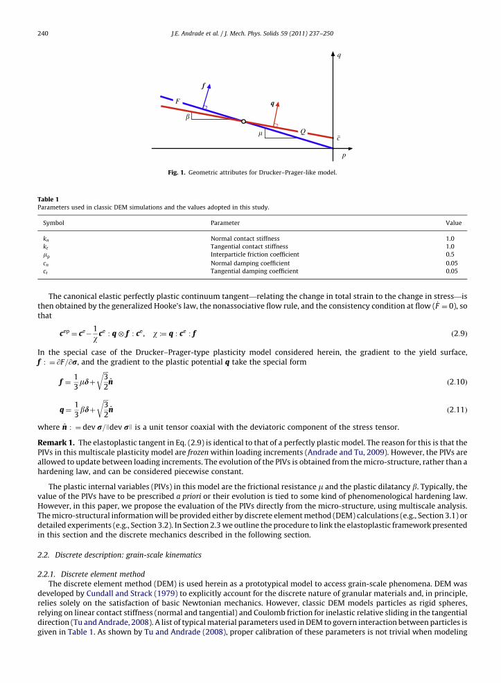
withm typically referred to as the generalized friction coefficient,b is the plastic dilatancy, and c is a free parameter so that theplastic potential crosses the yield surface at the same stress state (p,q). Fig. 1 shows a schematic of the yield surface and plasticpotential and the geometric meaning for the plastic internal variables (PIVs): m, b, and c . Finally, the nonassociative flow ruleis given in the classic form with the direction of the plastic strain rate determined by the normal to the plastic potential so that

_ep¼ _lq ð2:7Þ

with q : ¼ @Q=@r. The scalar _l is called the consistency parameter and controls the magnitude of plastic strain rate. Using thedefinitions for the strain rate invariants and the particular form for q emanating from the Drucker–Prager model, one canobtain that

_epv ¼

_lb, _eps ¼

_l, b¼_ep

v

_eps

ð2:8Þ

where it is clear that the plastic dilatancy b controls the volumetric plastic strain rate for a given deviatoric strain rate.

f

q

�

p

�

q

c

F

Q

Fig. 1. Geometric attributes for Drucker–Prager-like model.

Table 1Parameters used in classic DEM simulations and the values adopted in this study.

Symbol Parameter Value

kn Normal contact stiffness 1.0

kt Tangential contact stiffness 1.0

mp Interparticle friction coefficient 0.5

cn Normal damping coefficient 0.05

ct Tangential damping coefficient 0.05

J.E. Andrade et al. / J. Mech. Phys. Solids 59 (2011) 237–250240

The canonical elastic perfectly plastic continuum tangent—relating the change in total strain to the change in stress—isthen obtained by the generalized Hooke’s law, the nonassociative flow rule, and the consistency condition at flow ( _F ¼ 0), sothat

cep ¼ ce�1

wce : q� f : ce, w :¼ q : ce : f ð2:9Þ

In the special case of the Drucker–Prager-type plasticity model considered herein, the gradient to the yield surface,f : ¼ @F=@r, and the gradient to the plastic potential q take the special form

f ¼1

3mdþ

ffiffiffi3

2

rn ð2:10Þ

q¼1

3bdþ

ffiffiffi3

2

rn ð2:11Þ

where n : ¼ dev r=Jdev rJ is a unit tensor coaxial with the deviatoric component of the stress tensor.

Remark 1. The elastoplastic tangent in Eq. (2.9) is identical to that of a perfectly plastic model. The reason for this is that thePIVs in this multiscale plasticity model are frozen within loading increments (Andrade and Tu, 2009). However, the PIVs areallowed to update between loading increments. The evolution of the PIVs is obtained from the micro-structure, rather than ahardening law, and can be considered piecewise constant.

The plastic internal variables (PIVs) in this model are the frictional resistance m and the plastic dilatancy b. Typically, thevalue of the PIVs have to be prescribed a priori or their evolution is tied to some kind of phenomenological hardening law.However, in this paper, we propose the evaluation of the PIVs directly from the micro-structure, using multiscale analysis.The micro-structural information will be provided either by discrete element method (DEM) calculations (e.g., Section 3.1) ordetailed experiments (e.g., Section 3.2). In Section 2.3 we outline the procedure to link the elastoplastic framework presentedin this section and the discrete mechanics described in the following section.

2.2. Discrete description: grain-scale kinematics

2.2.1. Discrete element method

The discrete element method (DEM) is used herein as a prototypical model to access grain-scale phenomena. DEM wasdeveloped by Cundall and Strack (1979) to explicitly account for the discrete nature of granular materials and, in principle,relies solely on the satisfaction of basic Newtonian mechanics. However, classic DEM models particles as rigid spheres,relying on linear contact stiffness (normal and tangential) and Coulomb friction for inelastic relative sliding in the tangentialdirection (Tu and Andrade, 2008). A list of typical material parameters used in DEM to govern interaction between particles isgiven in Table 1. As shown by Tu and Andrade (2008), proper calibration of these parameters is not trivial when modeling

J.E. Andrade et al. / J. Mech. Phys. Solids 59 (2011) 237–250 241

quasi-static problems, as Newtonian mechanics imply dynamic processes and inertia effects and damping coefficients tend tolose physical meaning when applied to quasi-static situations.

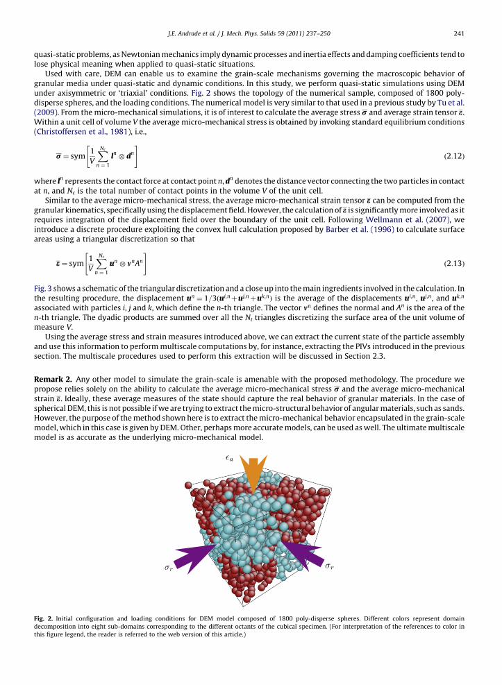
Used with care, DEM can enable us to examine the grain-scale mechanisms governing the macroscopic behavior ofgranular media under quasi-static and dynamic conditions. In this study, we perform quasi-static simulations using DEMunder axisymmetric or ‘triaxial’ conditions. Fig. 2 shows the topology of the numerical sample, composed of 1800 poly-disperse spheres, and the loading conditions. The numerical model is very similar to that used in a previous study by Tu et al.(2009). From the micro-mechanical simulations, it is of interest to calculate the average stress r and average strain tensor e.Within a unit cell of volume V the average micro-mechanical stress is obtained by invoking standard equilibrium conditions(Christoffersen et al., 1981), i.e.,

r ¼ sym1

V

XNc

n ¼ 1

ln� dn

" #ð2:12Þ

where ln represents the contact force at contact point n, dn denotes the distance vector connecting the two particles in contactat n, and Nc is the total number of contact points in the volume V of the unit cell.

Similar to the average micro-mechanical stress, the average micro-mechanical strain tensor e can be computed from thegranular kinematics, specifically using the displacement field. However, the calculation of e is significantly more involved as itrequires integration of the displacement field over the boundary of the unit cell. Following Wellmann et al. (2007), weintroduce a discrete procedure exploiting the convex hull calculation proposed by Barber et al. (1996) to calculate surfaceareas using a triangular discretization so that

e ¼ sym1

V

XNt

n ¼ 1

un � mnAn

" #ð2:13Þ

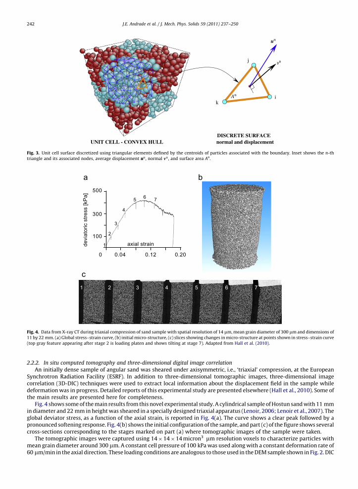
Fig. 3 shows a schematic of the triangular discretization and a close up into the main ingredients involved in the calculation. Inthe resulting procedure, the displacement un ¼ 1=3ðui,nþuj,nþuk,nÞ is the average of the displacements ui,n, uj,n, and uk,n

associated with particles i, j and k, which define the n-th triangle. The vector mn defines the normal and An is the area of then-th triangle. The dyadic products are summed over all the Nt triangles discretizing the surface area of the unit volume ofmeasure V.

Using the average stress and strain measures introduced above, we can extract the current state of the particle assemblyand use this information to perform multiscale computations by, for instance, extracting the PIVs introduced in the previoussection. The multiscale procedures used to perform this extraction will be discussed in Section 2.3.

Remark 2. Any other model to simulate the grain-scale is amenable with the proposed methodology. The procedure wepropose relies solely on the ability to calculate the average micro-mechanical stress r and the average micro-mechanicalstrain e. Ideally, these average measures of the state should capture the real behavior of granular materials. In the case ofspherical DEM, this is not possible if we are trying to extract the micro-structural behavior of angular materials, such as sands.However, the purpose of the method shown here is to extract the micro-mechanical behavior encapsulated in the grain-scalemodel, which in this case is given by DEM. Other, perhaps more accurate models, can be used as well. The ultimate multiscalemodel is as accurate as the underlying micro-mechanical model.

Fig. 2. Initial configuration and loading conditions for DEM model composed of 1800 poly-disperse spheres. Different colors represent domain

decomposition into eight sub-domains corresponding to the different octants of the cubical specimen. (For interpretation of the references to color in

this figure legend, the reader is referred to the web version of this article.)

UNIT CELL - CONVEX HULLDISCRETE SURFACEnormal and displacement

ik

�n

An

un

j

Fig. 3. Unit cell surface discretized using triangular elements defined by the centroids of particles associated with the boundary. Inset shows the n-th

triangle and its associated nodes, average displacement un , normal mn , and surface area An.

100

300

500

devi

ator

ic s

tress

[kP

a]

axial strain

0.04 0.12 0.200

1 2 3 4 5 6 7

6 75

4

3

1

2

Fig. 4. Data from X-ray CT during triaxial compression of sand sample with spatial resolution of 14 mm, mean grain diameter of 300 mm and dimensions of

11 by 22 mm. (a) Global stress–strain curve, (b) initial micro-structure, (c) slices showing changes in micro-structure at points shown in stress–strain curve

(top gray feature appearing after stage 2 is loading platen and shows tilting at stage 7). Adapted from Hall et al. (2010).

J.E. Andrade et al. / J. Mech. Phys. Solids 59 (2011) 237–250242

2.2.2. In situ computed tomography and three-dimensional digital image correlation

An initially dense sample of angular sand was sheared under axisymmetric, i.e., ‘triaxial’ compression, at the EuropeanSynchrotron Radiation Facility (ESRF). In addition to three-dimensional tomographic images, three-dimensional imagecorrelation (3D-DIC) techniques were used to extract local information about the displacement field in the sample whiledeformation was in progress. Detailed reports of this experimental study are presented elsewhere (Hall et al., 2010). Some ofthe main results are presented here for completeness.

Fig. 4 shows some of the main results from this novel experimental study. A cylindrical sample of Hostun sand with 11 mmin diameter and 22 mm in height was sheared in a specially designed triaxial apparatus (Lenoir, 2006; Lenoir et al., 2007). Theglobal deviator stress, as a function of the axial strain, is reported in Fig. 4(a). The curve shows a clear peak followed by apronounced softening response. Fig. 4(b) shows the initial configuration of the sample, and part (c) of the figure shows severalcross-sections corresponding to the stages marked on part (a) where tomographic images of the sample were taken.

The tomographic images were captured using 14�14�14 micron3 mm resolution voxels to characterize particles withmean grain diameter around 300 mm. A constant cell pressure of 100 kPa was used along with a constant deformation rate of60 mm/min in the axial direction. These loading conditions are analogous to those used in the DEM sample shown in Fig. 2. DIC

Original Displacement Field Smooth Displacement Field

Plate and/or membrane effect

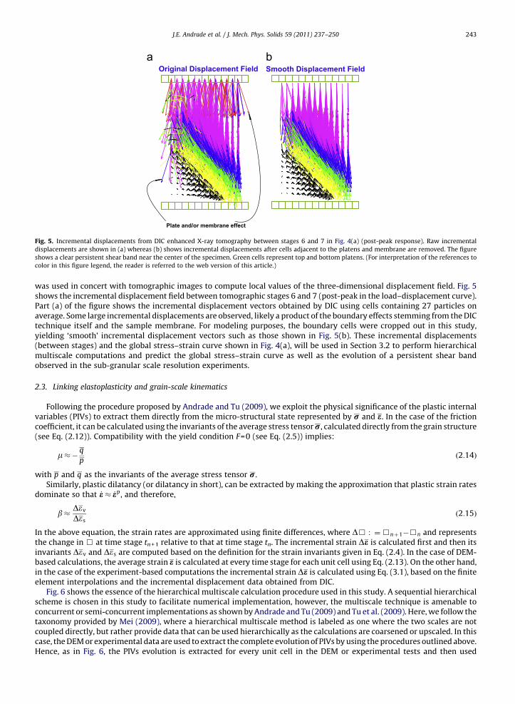
Fig. 5. Incremental displacements from DIC enhanced X-ray tomography between stages 6 and 7 in Fig. 4(a) (post-peak response). Raw incremental

displacements are shown in (a) whereas (b) shows incremental displacements after cells adjacent to the platens and membrane are removed. The figure

shows a clear persistent shear band near the center of the specimen. Green cells represent top and bottom platens. (For interpretation of the references to

color in this figure legend, the reader is referred to the web version of this article.)

J.E. Andrade et al. / J. Mech. Phys. Solids 59 (2011) 237–250 243

was used in concert with tomographic images to compute local values of the three-dimensional displacement field. Fig. 5shows the incremental displacement field between tomographic stages 6 and 7 (post-peak in the load–displacement curve).Part (a) of the figure shows the incremental displacement vectors obtained by DIC using cells containing 27 particles onaverage. Some large incremental displacements are observed, likely a product of the boundary effects stemming from the DICtechnique itself and the sample membrane. For modeling purposes, the boundary cells were cropped out in this study,yielding ‘smooth’ incremental displacement vectors such as those shown in Fig. 5(b). These incremental displacements(between stages) and the global stress–strain curve shown in Fig. 4(a), will be used in Section 3.2 to perform hierarchicalmultiscale computations and predict the global stress–strain curve as well as the evolution of a persistent shear bandobserved in the sub-granular scale resolution experiments.

2.3. Linking elastoplasticity and grain-scale kinematics

Following the procedure proposed by Andrade and Tu (2009), we exploit the physical significance of the plastic internalvariables (PIVs) to extract them directly from the micro-structural state represented by r and e. In the case of the frictioncoefficient, it can be calculated using the invariants of the average stress tensor r, calculated directly from the grain structure(see Eq. (2.12)). Compatibility with the yield condition F=0 (see Eq. (2.5)) implies:

m�� q

pð2:14Þ

with p and q as the invariants of the average stress tensor r.Similarly, plastic dilatancy (or dilatancy in short), can be extracted by making the approximation that plastic strain rates

dominate so that _e � _ep, and therefore,

b�Dev

Desð2:15Þ

In the above equation, the strain rates are approximated using finite differences, where D& : ¼&nþ1�&n and representsthe change in & at time stage tn +1 relative to that at time stage tn. The incremental strain De is calculated first and then itsinvariants Dev and Des are computed based on the definition for the strain invariants given in Eq. (2.4). In the case of DEM-based calculations, the average strain e is calculated at every time stage for each unit cell using Eq. (2.13). On the other hand,in the case of the experiment-based computations the incremental strain De is calculated using Eq. (3.1), based on the finiteelement interpolations and the incremental displacement data obtained from DIC.

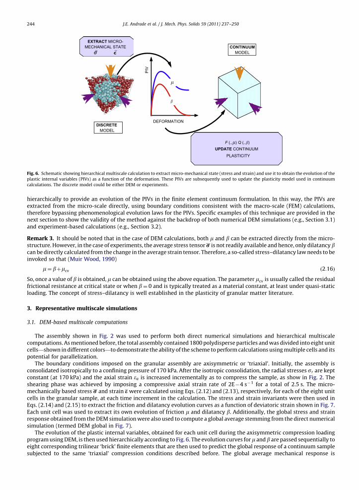
Fig. 6 shows the essence of the hierarchical multiscale calculation procedure used in this study. A sequential hierarchicalscheme is chosen in this study to facilitate numerical implementation, however, the multiscale technique is amenable toconcurrent or semi-concurrent implementations as shown by Andrade and Tu (2009) and Tu et al. (2009). Here, we follow thetaxonomy provided by Mei (2009), where a hierarchical multiscale method is labeled as one where the two scales are notcoupled directly, but rather provide data that can be used hierarchically as the calculations are coarsened or upscaled. In thiscase, the DEM or experimental data are used to extract the complete evolution of PIVs by using the procedures outlined above.Hence, as in Fig. 6, the PIVs evolution is extracted for every unit cell in the DEM or experimental tests and then used

�

�

PIV

DEFORMATION

UPDATE CONTINUUM PLASTICITY

DISCRETEMODEL

CONTINUUMMODEL

EXTRACT MICRO-MECHANICAL STATE

F (.,�) Q (.,�)

Fig. 6. Schematic showing hierarchical multiscale calculation to extract micro-mechanical state (stress and strain) and use it to obtain the evolution of the

plastic internal variables (PIVs) as a function of the deformation. These PIVs are subsequently used to update the plasticity model used in continuum

calculations. The discrete model could be either DEM or experiments.

J.E. Andrade et al. / J. Mech. Phys. Solids 59 (2011) 237–250244

hierarchically to provide an evolution of the PIVs in the finite element continuum formulation. In this way, the PIVs areextracted from the micro-scale directly, using boundary conditions consistent with the macro-scale (FEM) calculations,therefore bypassing phenomenological evolution laws for the PIVs. Specific examples of this technique are provided in thenext section to show the validity of the method against the backdrop of both numerical DEM simulations (e.g., Section 3.1)and experiment-based calculations (e.g., Section 3.2).

Remark 3. It should be noted that in the case of DEM calculations, both m and b can be extracted directly from the micro-structure. However, in the case of experiments, the average stress tensor r is not readily available and hence, only dilatancy bcan be directly calculated from the change in the average strain tensor. Therefore, a so-called stress–dilatancy law needs to beinvoked so that (Muir Wood, 1990)

m¼ bþmcv ð2:16Þ

So, once a value of b is obtained, m can be obtained using the above equation. The parameter mcv is usually called the residualfrictional resistance at critical state or when b¼ 0 and is typically treated as a material constant, at least under quasi-staticloading. The concept of stress–dilatancy is well established in the plasticity of granular matter literature.

3. Representative multiscale simulations

3.1. DEM-based multiscale computations

The assembly shown in Fig. 2 was used to perform both direct numerical simulations and hierarchical multiscalecomputations. As mentioned before, the total assembly contained 1800 polydisperse particles and was divided into eight unitcells—shown in different colors—to demonstrate the ability of the scheme to perform calculations using multiple cells and itspotential for parallelization.

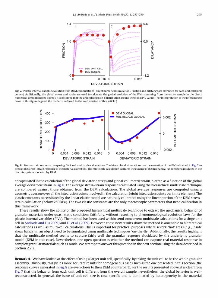
The boundary conditions imposed on the granular assembly are axisymmetric or ‘triaxial’. Initially, the assembly isconsolidated isotropically to a confining pressure of 170 kPa. After the isotropic consolidation, the radial stresses sr are keptconstant (at 170 kPa) and the axial strain ea is increased incrementally as to compress the sample, as show in Fig. 2. Theshearing phase was achieved by imposing a compressive axial strain rate of 2E�4 s�1 for a total of 2.5 s. The micro-mechanically based stress r and strain e were calculated using Eqs. (2.12) and (2.13), respectively, for each of the eight unitcells in the granular sample, at each time increment in the calculation. The stress and strain invariants were then used inEqs. (2.14) and (2.15) to extract the friction and dilatancy evolution curves as a function of deviatoric strain shown in Fig. 7.Each unit cell was used to extract its own evolution of friction m and dilatancy b. Additionally, the global stress and strainresponse obtained from the DEM simulation were also used to compute a global average stemming from the direct numericalsimulation (termed DEM global in Fig. 7).

The evolution of the plastic internal variables, obtained for each unit cell during the axisymmetric compression loadingprogram using DEM, is then used hierarchically according to Fig. 6. The evolution curves form andb are passed sequentially toeight corresponding trilinear ‘brick’ finite elements that are then used to predict the global response of a continuum samplesubjected to the same ‘triaxial’ compression conditions described before. The global average mechanical response is

DEVIATORIC STRAIN0

FRIC

TIO

N

0

1.0

1.4

DEM UNIT CELL

0.016

DEM GLOBAL

0 0.016-1.2

0.0

0.6

DIL

ATA

NC

Y

� �

Fig. 7. Plastic internal variable evolution from DEM computations (direct numerical simulation). Friction and dilatancy are extracted for each unit cell (pink

curves). Additionally, the global stress and strain are used to calculate the global evolution of the PIVs stemming from the entire sample in the direct

numerical simulation (red points). It is observed that the unit cells furnish a distribution around the global PIV values. (For interpretation of the references to

color in this figure legend, the reader is referred to the web version of this article.)

VO

LUM

ETR

IC S

TRA

IN

-0.002

0

0.002

0.004 0.008 0.012 0.016

DE

VIA

TOR

IC S

TRE

SS

, kP

a

400

300

200

100

0.004 0.008 0.012 0.016 000

DEM GLOBALMULTISCALE GLOBAL

DEVIATORIC STRAIN DEVIATORIC STRAIN

Fig. 8. Stress–strain response comparing DNS and multiscale calculations. The hierarchical simulations use the evolution of the PIVs obtained in Fig. 7 to

predict the stress–strain response of the material using FEM. The multiscale calculation captures the essence of the mechanical response encapsulated in the

discrete system modeled by DEM.

J.E. Andrade et al. / J. Mech. Phys. Solids 59 (2011) 237–250 245

encapsulated in the calculation of the global deviatoric stress and global volumetric strain, plotted as a function of the globalaverage deviatoric strain in Fig. 8. The average stress–strain responses calculated using the hierarchical multiscale techniqueare compared against those obtained from the DEM calculations. The global average responses are computed using ageometric average over all the integration points involved in the calculation (eight integration points per finite element). Theelastic constants necessitated by the linear elastic model are naturally calibrated using the linear portion of the DEM stress–strain calculation (below 250 kPa). The two elastic constants are the only macroscopic parameters that need calibration inthis framework.

These results show the ability of the proposed hierarchical multiscale technique to extract the mechanical behavior ofgranular materials under quasi-static conditions faithfully, without resorting to phenomenological evolution laws for theplastic internal variables (PIVs). The method has been used within semi-concurrent multiscale calculations for a singe unitcell in Andrade and Tu (2009) and Tu et al. (2009). However, these new results show the method is amenable to hierarchicalcalculations as well as multi-cell calculations. This is important for practical purposes where several ‘hot’ areas (e.g., insideshear bands) in an object need to be simulated using multiscale techniques ‘on-the-fly’. Additionally, the results highlightthat the multiscale method seems to capture fairly well the granular response elucidated by the underlying granularmodel (DEM in this case). Nevertheless, one open question is whether the method can capture real material response incomplex granular materials such as sands. We attempt to answer this question in the next section using the data described inSection 2.2.2.

Remark 4. We have looked at the effect of using a larger unit cell, specifically, by taking the unit cell to be the whole granularassembly. Obviously, this yields more accurate results for homogeneous cases such as the one presented in this section (theresponse curves generated in Fig. 8 are even closer to their DEM counterpart). For the results presented above, it is clear fromFig. 7 that the behavior from each unit cell is different from the overall sample, nevertheless, the global behavior is well-reconstructed. In general, the issue of unit cell size is case-specific and is dominated by heterogeneity in the material

J.E. Andrade et al. / J. Mech. Phys. Solids 59 (2011) 237–250246

response. For example, Oda et al. (2004) showed clear evidence of the heterogeneity of void spaces inside shear bands. On theother hand, Tordesillas and Shi (2009) showed the importance of force chains in the behavior of granular matter, especiallynear and after failure. Unit cell sizes will have to be selected such that the key features of the material behavior are captured.In this paper, we do not focus on the rigorous selection of unit cell sizes per se. Rather, our discussion focuses on theinformation to be passed between scales such that these meso-scale effects are implied in the stress–strain relation at themacro-scale. More studies around the impact of unit cell sizes will be conducted in the near future.

3.2. Experiment-based multiscale computations

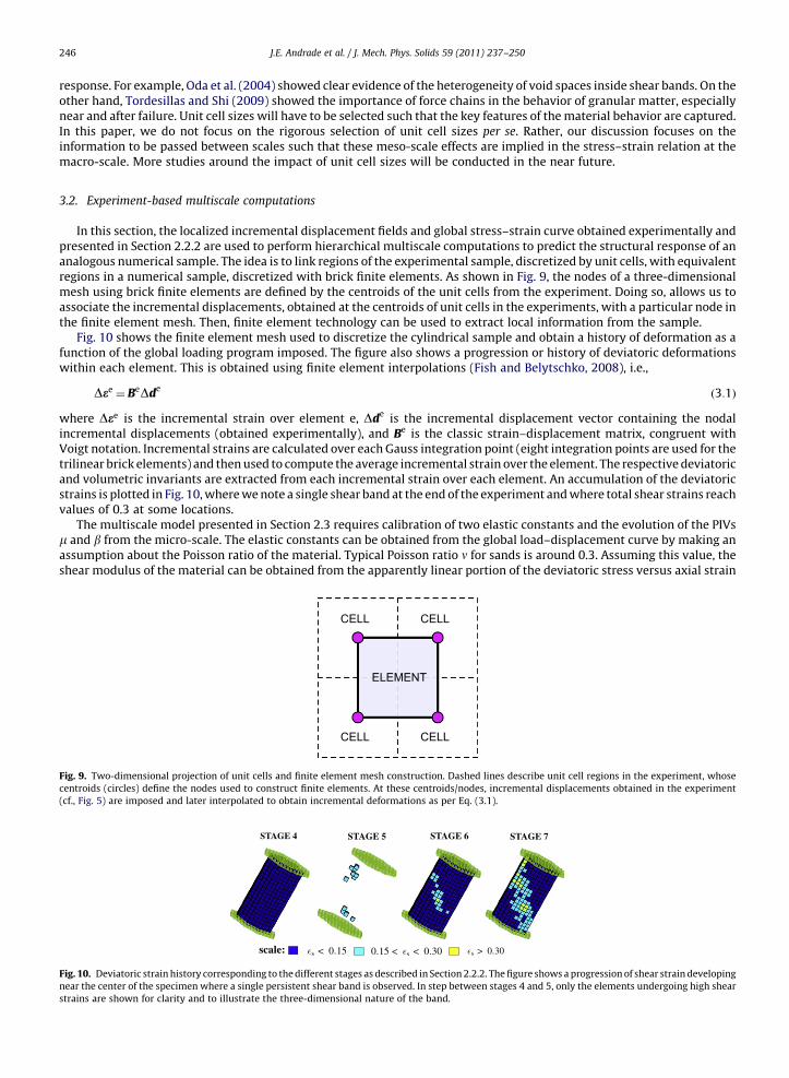
In this section, the localized incremental displacement fields and global stress–strain curve obtained experimentally andpresented in Section 2.2.2 are used to perform hierarchical multiscale computations to predict the structural response of ananalogous numerical sample. The idea is to link regions of the experimental sample, discretized by unit cells, with equivalentregions in a numerical sample, discretized with brick finite elements. As shown in Fig. 9, the nodes of a three-dimensionalmesh using brick finite elements are defined by the centroids of the unit cells from the experiment. Doing so, allows us toassociate the incremental displacements, obtained at the centroids of unit cells in the experiments, with a particular node inthe finite element mesh. Then, finite element technology can be used to extract local information from the sample.

Fig. 10 shows the finite element mesh used to discretize the cylindrical sample and obtain a history of deformation as afunction of the global loading program imposed. The figure also shows a progression or history of deviatoric deformationswithin each element. This is obtained using finite element interpolations (Fish and Belytschko, 2008), i.e.,

Dee ¼ BeDdeð3:1Þ

where Dee is the incremental strain over element e, Dde is the incremental displacement vector containing the nodalincremental displacements (obtained experimentally), and Be is the classic strain–displacement matrix, congruent withVoigt notation. Incremental strains are calculated over each Gauss integration point (eight integration points are used for thetrilinear brick elements) and then used to compute the average incremental strain over the element. The respective deviatoricand volumetric invariants are extracted from each incremental strain over each element. An accumulation of the deviatoricstrains is plotted in Fig. 10, where we note a single shear band at the end of the experiment and where total shear strains reachvalues of 0.3 at some locations.

The multiscale model presented in Section 2.3 requires calibration of two elastic constants and the evolution of the PIVsm and b from the micro-scale. The elastic constants can be obtained from the global load–displacement curve by making anassumption about the Poisson ratio of the material. Typical Poisson ratio n for sands is around 0.3. Assuming this value, theshear modulus of the material can be obtained from the apparently linear portion of the deviatoric stress versus axial strain

ELEMENT

CELL CELL

CELLCELL

Fig. 9. Two-dimensional projection of unit cells and finite element mesh construction. Dashed lines describe unit cell regions in the experiment, whose

centroids (circles) define the nodes used to construct finite elements. At these centroids/nodes, incremental displacements obtained in the experiment

(cf., Fig. 5) are imposed and later interpolated to obtain incremental deformations as per Eq. (3.1).

Fig. 10. Deviatoric strain history corresponding to the different stages as described in Section 2.2.2. The figure shows a progression of shear strain developing

near the center of the specimen where a single persistent shear band is observed. In step between stages 4 and 5, only the elements undergoing high shear

strains are shown for clarity and to illustrate the three-dimensional nature of the band.

J.E. Andrade et al. / J. Mech. Phys. Solids 59 (2011) 237–250 247

curve shown in Fig. 4(a). We assume linear elastic behavior up to stage 4, around 0.05 axial strain. Note the sample is loadedunder a constant radial stress of 100 kPa and there was no direct measure of radial strains. The estimated shear modulus of thematerial G comes up to be 2.6 MPa. Together, G and n dictate the elastic behavior of the material, cf. Eq. (2.1).

Unlike in numerical simulations by DEM, the experimental results cannot be used to extract measurements of the stresseslocally (at least not yet). As shown in Eq. (3.1), only local deformation fields can be reconstructed from the experimental data.Hence, only dilatancy b can be inferred from the experimental data. The frictional resistance m is a function of the state ofstress and will be inferred indirectly in this study. To approximate the value of dilatancy, we recur to a well-establishedconcept in soil mechanics: a stress–dilatancy relationship (Muir Wood, 1990; Schofield and Wroth, 1968). A typical stress–dilatancy relation is given in Remark 3 in Eq. (2.16). We will use this stress–dilatancy relation and will hence need to calculatethe value of frictional resistance at constant volume mcv during the critical state or when dilatancy is all spent (b¼ 0). Weassume that the value of mcv is a material constant and it is hence the same for the entire specimen. Since we have assumedthat the material is linear-elastic (and homogeneous) up to loading stage 4 (up to about 0.05 axial strain in the triaxialcompression experiment), we further assume that plastic deformations follow after stage 4 and that dilatancy is nil at thebeginning of the plastic process. Accordingly, the residual frictional strength at that point, according to the stress–dilatancyrelation, would be m¼ mcv ¼�q=p and, therefore, the corresponding residual strength mcv � 300=200¼ 1:5 for the entiresample.

Remark 5. The assumption of elastic deformations up to stage 4 or about 0.05 axial strain is mostly based on the apparentlinear portion observed in Fig. 4(a). Furthermore, this assumption facilitates greatly the modeling process. Also, it mesheswell with the dilatancy (and plastic) process starting from zero, since the sample does compress during the elastic process, asexpected from a relatively dense sample. Subsequent positive dilation will be responsible for the ensuing dilative process.

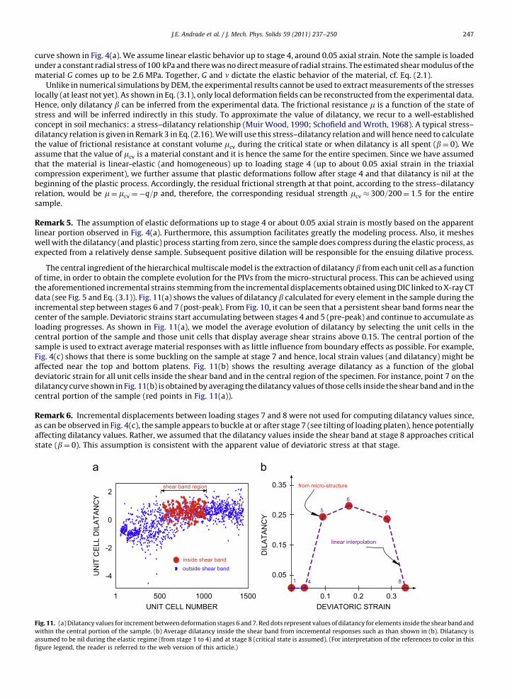
The central ingredient of the hierarchical multiscale model is the extraction of dilatancy b from each unit cell as a functionof time, in order to obtain the complete evolution for the PIVs from the micro-structural process. This can be achieved usingthe aforementioned incremental strains stemming from the incremental displacements obtained using DIC linked to X-ray CTdata (see Fig. 5 and Eq. (3.1)). Fig. 11(a) shows the values of dilatancy b calculated for every element in the sample during theincremental step between stages 6 and 7 (post-peak). From Fig. 10, it can be seen that a persistent shear band forms near thecenter of the sample. Deviatoric strains start accumulating between stages 4 and 5 (pre-peak) and continue to accumulate asloading progresses. As shown in Fig. 11(a), we model the average evolution of dilatancy by selecting the unit cells in thecentral portion of the sample and those unit cells that display average shear strains above 0.15. The central portion of thesample is used to extract average material responses with as little influence from boundary effects as possible. For example,Fig. 4(c) shows that there is some buckling on the sample at stage 7 and hence, local strain values (and dilatancy) might beaffected near the top and bottom platens. Fig. 11(b) shows the resulting average dilatancy as a function of the globaldeviatoric strain for all unit cells inside the shear band and in the central region of the specimen. For instance, point 7 on thedilatancy curve shown in Fig. 11(b) is obtained by averaging the dilatancy values of those cells inside the shear band and in thecentral portion of the sample (red points in Fig. 11(a)).

Remark 6. Incremental displacements between loading stages 7 and 8 were not used for computing dilatancy values since,as can be observed in Fig. 4(c), the sample appears to buckle at or after stage 7 (see tilting of loading platen), hence potentiallyaffecting dilatancy values. Rather, we assumed that the dilatancy values inside the shear band at stage 8 approaches criticalstate (b¼ 0). This assumption is consistent with the apparent value of deviatoric stress at that stage.

0.05

0.15

0.25

0.35

4

5

6

7

1 8

0.1 0.2 0.3DEVIATORIC STRAIN

from micro-structure

linear interpolation

DIL

ATA

NC

Y

-4

-2

0

2

1 500 1000 1500UNIT CELL NUMBER

UN

IT C

ELL

DIL

ATA

NC

Y

shear band region

inside shear bandoutside shear band

Fig. 11. (a) Dilatancy values for increment between deformation stages 6 and 7. Red dots represent values of dilatancy for elements inside the shear band and

within the central portion of the sample. (b) Average dilatancy inside the shear band from incremental responses such as than shown in (b). Dilatancy is

assumed to be nil during the elastic regime (from stage 1 to 4) and at stage 8 (critical state is assumed). (For interpretation of the references to color in this

figure legend, the reader is referred to the web version of this article.)

J.E. Andrade et al. / J. Mech. Phys. Solids 59 (2011) 237–250248

Remark 7. As pointed out above, platen effects seem to appear around stage 6 in the loading program. These effects havebeen neglected in the current study for the sake of simplicity, as the objective of the paper is to establish an appropriatemultiscale framework. However, more detailed studies about the effect of inhomogeneities, material and geometry will beconducted in the near future.

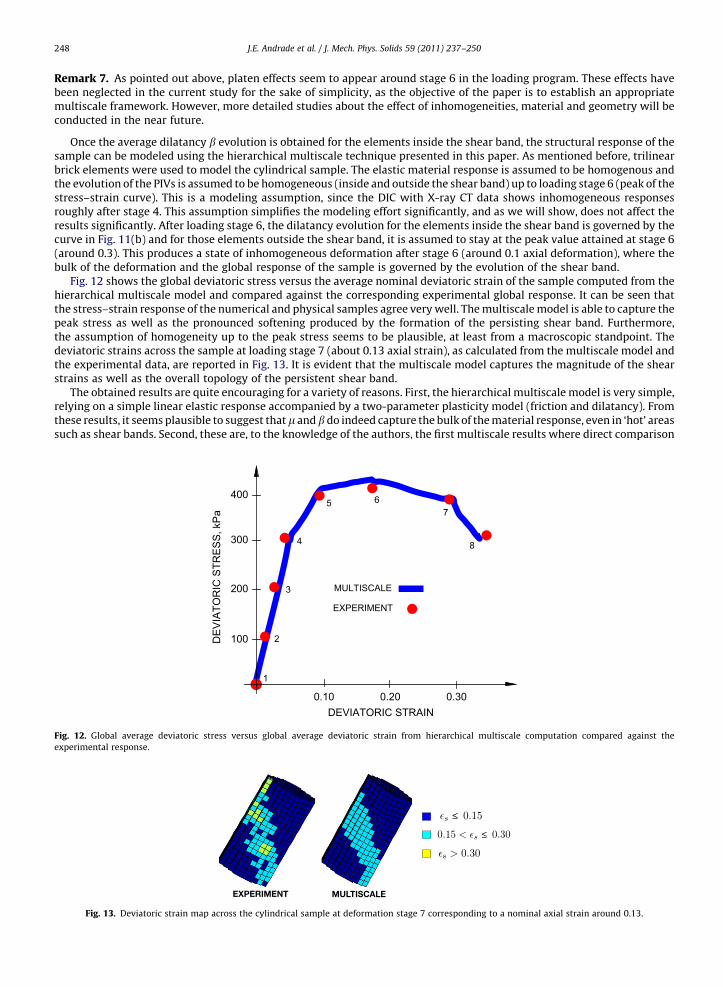
Once the average dilatancy b evolution is obtained for the elements inside the shear band, the structural response of thesample can be modeled using the hierarchical multiscale technique presented in this paper. As mentioned before, trilinearbrick elements were used to model the cylindrical sample. The elastic material response is assumed to be homogenous andthe evolution of the PIVs is assumed to be homogeneous (inside and outside the shear band) up to loading stage 6 (peak of thestress–strain curve). This is a modeling assumption, since the DIC with X-ray CT data shows inhomogeneous responsesroughly after stage 4. This assumption simplifies the modeling effort significantly, and as we will show, does not affect theresults significantly. After loading stage 6, the dilatancy evolution for the elements inside the shear band is governed by thecurve in Fig. 11(b) and for those elements outside the shear band, it is assumed to stay at the peak value attained at stage 6(around 0.3). This produces a state of inhomogeneous deformation after stage 6 (around 0.1 axial deformation), where thebulk of the deformation and the global response of the sample is governed by the evolution of the shear band.

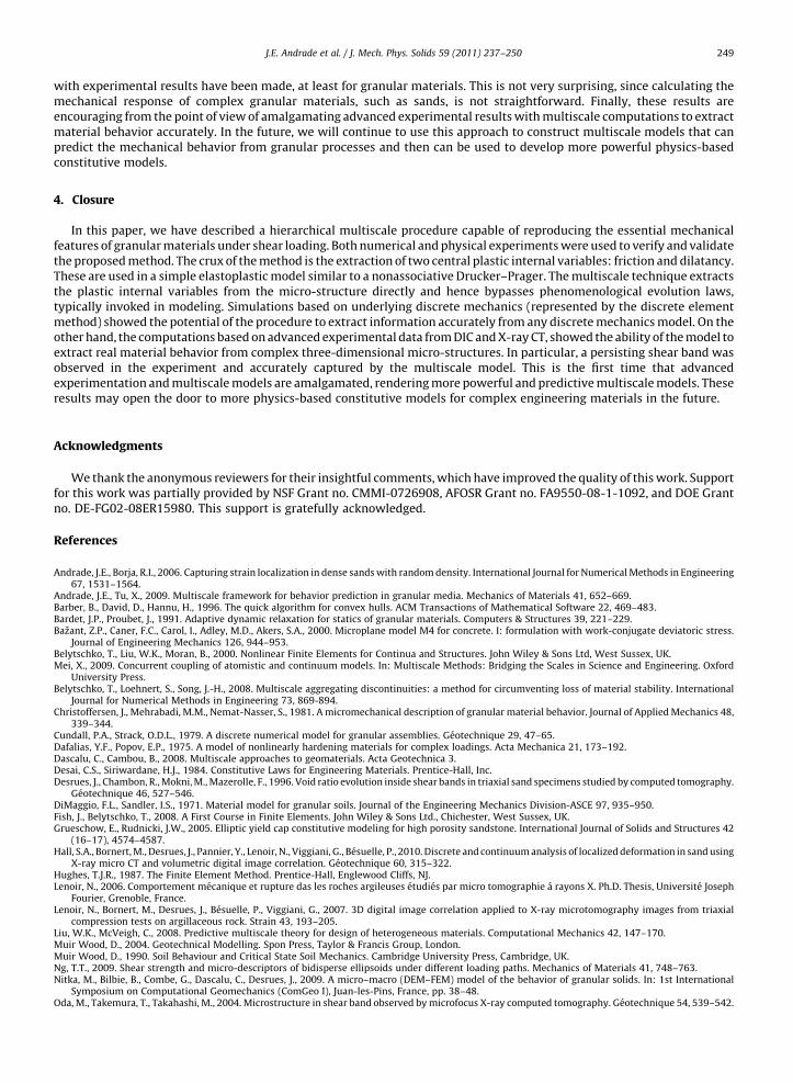
Fig. 12 shows the global deviatoric stress versus the average nominal deviatoric strain of the sample computed from thehierarchical multiscale model and compared against the corresponding experimental global response. It can be seen thatthe stress–strain response of the numerical and physical samples agree very well. The multiscale model is able to capture thepeak stress as well as the pronounced softening produced by the formation of the persisting shear band. Furthermore,the assumption of homogeneity up to the peak stress seems to be plausible, at least from a macroscopic standpoint. Thedeviatoric strains across the sample at loading stage 7 (about 0.13 axial strain), as calculated from the multiscale model andthe experimental data, are reported in Fig. 13. It is evident that the multiscale model captures the magnitude of the shearstrains as well as the overall topology of the persistent shear band.

The obtained results are quite encouraging for a variety of reasons. First, the hierarchical multiscale model is very simple,relying on a simple linear elastic response accompanied by a two-parameter plasticity model (friction and dilatancy). Fromthese results, it seems plausible to suggest thatm andb do indeed capture the bulk of the material response, even in ‘hot’ areassuch as shear bands. Second, these are, to the knowledge of the authors, the first multiscale results where direct comparison

100

200

300

400

0.10 0.20 0.30

DE

VIA

TOR

IC S

TRE

SS

, kP

a

MULTISCALE

EXPERIMENT

1

2

3

4

5 67

8

DEVIATORIC STRAIN

Fig. 12. Global average deviatoric stress versus global average deviatoric strain from hierarchical multiscale computation compared against the

experimental response.

Fig. 13. Deviatoric strain map across the cylindrical sample at deformation stage 7 corresponding to a nominal axial strain around 0.13.

J.E. Andrade et al. / J. Mech. Phys. Solids 59 (2011) 237–250 249

with experimental results have been made, at least for granular materials. This is not very surprising, since calculating themechanical response of complex granular materials, such as sands, is not straightforward. Finally, these results areencouraging from the point of view of amalgamating advanced experimental results with multiscale computations to extractmaterial behavior accurately. In the future, we will continue to use this approach to construct multiscale models that canpredict the mechanical behavior from granular processes and then can be used to develop more powerful physics-basedconstitutive models.

4. Closure

In this paper, we have described a hierarchical multiscale procedure capable of reproducing the essential mechanicalfeatures of granular materials under shear loading. Both numerical and physical experiments were used to verify and validatethe proposed method. The crux of the method is the extraction of two central plastic internal variables: friction and dilatancy.These are used in a simple elastoplastic model similar to a nonassociative Drucker–Prager. The multiscale technique extractsthe plastic internal variables from the micro-structure directly and hence bypasses phenomenological evolution laws,typically invoked in modeling. Simulations based on underlying discrete mechanics (represented by the discrete elementmethod) showed the potential of the procedure to extract information accurately from any discrete mechanics model. On theother hand, the computations based on advanced experimental data from DIC and X-ray CT, showed the ability of the model toextract real material behavior from complex three-dimensional micro-structures. In particular, a persisting shear band wasobserved in the experiment and accurately captured by the multiscale model. This is the first time that advancedexperimentation and multiscale models are amalgamated, rendering more powerful and predictive multiscale models. Theseresults may open the door to more physics-based constitutive models for complex engineering materials in the future.

Acknowledgments

We thank the anonymous reviewers for their insightful comments, which have improved the quality of this work. Supportfor this work was partially provided by NSF Grant no. CMMI-0726908, AFOSR Grant no. FA9550-08-1-1092, and DOE Grantno. DE-FG02-08ER15980. This support is gratefully acknowledged.

References

Andrade, J.E., Borja, R.I., 2006. Capturing strain localization in dense sands with random density. International Journal for Numerical Methods in Engineering67, 1531–1564.

Andrade, J.E., Tu, X., 2009. Multiscale framework for behavior prediction in granular media. Mechanics of Materials 41, 652–669.Barber, B., David, D., Hannu, H., 1996. The quick algorithm for convex hulls. ACM Transactions of Mathematical Software 22, 469–483.Bardet, J.P., Proubet, J., 1991. Adaptive dynamic relaxation for statics of granular materials. Computers & Structures 39, 221–229.Bazant, Z.P., Caner, F.C., Carol, I., Adley, M.D., Akers, S.A., 2000. Microplane model M4 for concrete. I: formulation with work-conjugate deviatoric stress.

Journal of Engineering Mechanics 126, 944–953.Belytschko, T., Liu, W.K., Moran, B., 2000. Nonlinear Finite Elements for Continua and Structures. John Wiley & Sons Ltd, West Sussex, UK.Mei, X., 2009. Concurrent coupling of atomistic and continuum models. In: Multiscale Methods: Bridging the Scales in Science and Engineering. Oxford

University Press.Belytschko, T., Loehnert, S., Song, J.-H., 2008. Multiscale aggregating discontinuities: a method for circumventing loss of material stability. International

Journal for Numerical Methods in Engineering 73, 869-894.Christoffersen, J., Mehrabadi, M.M., Nemat-Nasser, S., 1981. A micromechanical description of granular material behavior. Journal of Applied Mechanics 48,

339–344.Cundall, P.A., Strack, O.D.L., 1979. A discrete numerical model for granular assemblies. Geotechnique 29, 47–65.Dafalias, Y.F., Popov, E.P., 1975. A model of nonlinearly hardening materials for complex loadings. Acta Mechanica 21, 173–192.Dascalu, C., Cambou, B., 2008. Multiscale approaches to geomaterials. Acta Geotechnica 3.Desai, C.S., Siriwardane, H.J., 1984. Constitutive Laws for Engineering Materials. Prentice-Hall, Inc.Desrues, J., Chambon, R., Mokni, M., Mazerolle, F., 1996. Void ratio evolution inside shear bands in triaxial sand specimens studied by computed tomography.

Geotechnique 46, 527–546.DiMaggio, F.L., Sandler, I.S., 1971. Material model for granular soils. Journal of the Engineering Mechanics Division-ASCE 97, 935–950.Fish, J., Belytschko, T., 2008. A First Course in Finite Elements. John Wiley & Sons Ltd., Chichester, West Sussex, UK.Grueschow, E., Rudnicki, J.W., 2005. Elliptic yield cap constitutive modeling for high porosity sandstone. International Journal of Solids and Structures 42

(16–17), 4574–4587.Hall, S.A., Bornert, M., Desrues, J., Pannier, Y., Lenoir, N., Viggiani, G., Besuelle, P., 2010. Discrete and continuum analysis of localized deformation in sand using

X-ray micro CT and volumetric digital image correlation. Geotechnique 60, 315–322.Hughes, T.J.R., 1987. The Finite Element Method. Prentice-Hall, Englewood Cliffs, NJ.Lenoir, N., 2006. Comportement mecanique et rupture das les roches argileuses etudies par micro tomographie a rayons X. Ph.D. Thesis, Universite Joseph

Fourier, Grenoble, France.Lenoir, N., Bornert, M., Desrues, J., Besuelle, P., Viggiani, G., 2007. 3D digital image correlation applied to X-ray microtomography images from triaxial

compression tests on argillaceous rock. Strain 43, 193–205.Liu, W.K., McVeigh, C., 2008. Predictive multiscale theory for design of heterogeneous materials. Computational Mechanics 42, 147–170.Muir Wood, D., 2004. Geotechnical Modelling. Spon Press, Taylor & Francis Group, London.Muir Wood, D., 1990. Soil Behaviour and Critical State Soil Mechanics. Cambridge University Press, Cambridge, UK.Ng, T.T., 2009. Shear strength and micro-descriptors of bidisperse ellipsoids under different loading paths. Mechanics of Materials 41, 748–763.Nitka, M., Bilbie, B., Combe, G., Dascalu, C., Desrues, J., 2009. A micro–macro (DEM–FEM) model of the behavior of granular solids. In: 1st International

Symposium on Computational Geomechanics (ComGeo I), Juan-les-Pins, France, pp. 38–48.Oda, M., Takemura, T., Takahashi, M., 2004. Microstructure in shear band observed by microfocus X-ray computed tomography. Geotechnique 54, 539–542.

J.E. Andrade et al. / J. Mech. Phys. Solids 59 (2011) 237–250250

Rechenmacher, A.L., 2006. Grain-scale processes governing shear band initiation and evolution in sands. Journal of the Mechanics and Physics of Solids 54,22–45.

Reynolds, O., 1885. On the dilatancy of media composed of rigid particles in contact. Philosophical Magazine and Journal of Science 20, 468–481.Rothenburg, L., Bathurst, R.J., 1989. Analytical study of induced anisotropy in idealized granular materials. Geotechnique 39, 601–614.Santamarina, J.C., 2001. Soils and Waves. John Wiley & Sons Ltd., New York.Schofield, A., Wroth, P., 1968. Critical State Soil Mechanics. McGraw-Hill, New York.Tadmor, E., Ortiz, M., Phillips, R., 1996. Quasicontinuum analysis of defects in solids. Philosophical Magazine A 73, 1529–1563.Tordesillas, A., Shi, J., 2009. Micromechanical analysis of failure propagation in frictional materials. International Journal for Numerical and Analytical

Methods in Geomechanics 33, 1737–1768.Tu, X., Andrade, J.E., 2008. Criteria for static equilibrium in particulate mechanics computations. International Journal for Numerical Methods in Engineering

75, 1581–1606.Tu, X., Andrade, J.E., Chen, Q., 2009. Return mapping for nonsmooth and multiscale elastoplasticity. Computer Methods in Applied Mechanics and

Engineering 198, 2286–2296.Vermeer, P.A., de Borst, R., 1984. Non-associated plasticity for soils, concrete and rock. Heron 29, 1–62.Wellmann, C., Lillie, C., Wriggers, P., 2007. Homogenization of granular material modeled by a three-dimensional discrete element method. Computers and

Geotechnics 35, 394–405.