Embed Size (px)
Citation preview
HAL Id: hal-01569043https://hal.archives-ouvertes.fr/hal-01569043
Submitted on 26 Jul 2017
HAL is a multi-disciplinary open accessarchive for the deposit and dissemination of sci-entific research documents, whether they are pub-lished or not. The documents may come fromteaching and research institutions in France orabroad, or from public or private research centers.
L’archive ouverte pluridisciplinaire HAL, estdestinée au dépôt et à la diffusion de documentsscientifiques de niveau recherche, publiés ou non,émanant des établissements d’enseignement et derecherche français ou étrangers, des laboratoirespublics ou privés.
MULTIVARIATE DISTRIBUTION CORRECTION OFCLIMATE MODEL OUTPUTS: A GENERALISATION
OF QUANTILE MAPPING APPROACHESLéonard Deckens, Sylvie Parey, Mathilde Grandjacques, D Dacunha-Castelle
To cite this version:Léonard Deckens, Sylvie Parey, Mathilde Grandjacques, D Dacunha-Castelle. MULTIVARI-ATE DISTRIBUTION CORRECTION OF CLIMATE MODEL OUTPUTS: A GENERALISA-TION OF QUANTILE MAPPING APPROACHES. Environmetrics, Wiley, 2017, 28 (6), pp.e2454.�10.1002/env.2454�. �hal-01569043�

1
MULTIVARIATE DISTRIBUTION CORRECTION OF CLIMATE MODEL 1
OUTPUTS: A GENERALISATION OF QUANTILE MAPPING APPROACHES 2
3
Multivariate bias adjustment for climate change studies 4
5
Research article 6
7
L Dekens1,2, S Parey1, M Grandjacques3, D Dacunha-Castelle4 8
1 : EDF Recherche et Développement site de Chatou, MFEE, France 9
2 : Ecole Normale Supérieure de Lyon et université Claude Bernard Lyon 1, France 10
3 : Lianes (Laboratoire d’Intelligence Artificielle pour les Nouvelles Energies), Institut LIST, 11
CEA, Université Paris-Saclay, F-91120, Palaiseau, France 12
4 : Université Paris Sud, Orsay, France 13
14
Corresponding author : S Parey, EDF Recherche et Developpement 6 quai Watier 78401 15
Chatou France, [email protected] 16
17
2
18
Abstract: Climate change impact studies necessitate the estimation of climate variables 19
evolution in the future. These are given by climate model simulations made under different 20
greenhouse gas and aerosol emission scenarios agreed at the international level. However 21
climate model outputs have biases, especially at the local scale, and need to be corrected against 22
observations. Common bias-correction methods are distribution based and form the well-known 23
quantile mapping approaches. This paper presents a generalization of such techniques to the 24
consideration of multivariate distributions. This approach uses the basic lemma of Lévy-25
Rosenblatt which allows the transport of a distribution on another one, in every dimension. It 26
needs convenient non parametric estimations of conditional repartitions. The approach is first 27
tested in a controlled framework, by use of statistical simulations, then in the real setting of 28
climate simulation, in the bivariate case. An important issue of these types of distribution 29
corrections is the different kinds of hypotheses of stationarity over a long enough period: 30
stationarity of the link between model and observations whatever the period or stationarity of 31
the change between present and future for model and observations. This choice differentiates 32
approaches like Quantile Mapping and CDFt for example in the univariate framework, and 33
makes them more efficient, in the univariate as well as in the multivariate context, when the 34
data to be corrected best verify the assumed hypothesis. 35
Keywords: climate change, statistics, multivariate distributions, bias adjustment 36
1 Introduction 37
Since climate change is now attested (IPCC, 2013), and mitigation still underway, adaptation 38
has to be anticipated in parallel to mitigation. The first step in adaptation is an estimation of the 39
possible consequences of climate change at the scale of human societies and their activities. 40
These estimations are commonly done through impact studies, based for example on specific 41
models run with climatic variables. Observed variables are used to represent current conditions, 42
3
while climate model outputs are used to project future conditions. Climate models are numerical 43
tools based on physical representations of the dynamics of the components, atmosphere, ocean, 44
ice or land surface, and of their interactions, through physical or biochemical processes. 45
Although such tools are more and more sophisticated, including more and more detailed 46
processes, their outputs may still differ significantly from the local observations commonly 47
used by impact models. Therefore, bias correction and downscaling techniques have become 48
an active area of research in the last decade or so. The approach here, like other quantile 49
mapping approaches, can be used for bias adjustment or bias adjustment and downscaling 50
depending on the spatial scale of the reference dataset. When used with local observations it 51
aims at predicting, in statistical terms, local climate variables using more global data provided 52
by a climate model working at a larger scale. 53
Statistical bias correction methods are widely used to correct the distribution of the climate 54
model variables so that they match that of some local observations. Such techniques are 55
commonly recommended for impact studies (Teutschbein and Seibert, 2012; Gudmundsson et 56
al., 2012; Chen et al., 2013). The most used techniques are the so called quantile mapping 57
approaches (Panofsky and Brier, 1958; Haddad and Rosenfeld, 1997; Wood et al. 2004; Déqué 58
2007; Piani et al. 2010), and their variants like CDFt (Michelangeli et al., 2009). A limitation 59
of such techniques is however that the correction is applied independently to the different 60
variables when more than one climatic variable is needed for an impact study, with the risk of 61
degrading the consistency between them. Recent approaches have been proposed to tackle this 62
caveat, and correct two variables, essentially temperature and rainfall, in a consistent way 63
(Zhang and Georgakakos, 2012; Piani and Hearter, 2012; Li et al., 2014). Vrac and Friederichs, 64
2014 go further and propose an approach, based on the empirical copula (by reordering 65
univariate bias-corrected variables), potentially able to tackle both the inter-variable and spatial 66
consistencies. One issue with the approach is however that it can only reproduce the historical 67
4
temporal sequencing, which is an important limitation for climate impact studies. Cannon, 2016 68
suggests a methodology based on the correction of the marginal distributions again by quantile 69
mapping with then an iterative scheme to push either the Pearson correlation dependence 70
structure or the Spearman rank correlation dependence structure towards observed values. 71
The approach proposed and tested in this paper is a generalization of the quantile mapping 72
techniques to the correction of multivariate distributions. The chosen setting is the typical 73
problem faced with impact studies: over an historical period, time series of different climate 74
variables are available from both climatic databases and climate model simulations, while for a 75
future period, necessarily, only the climate model time series are available. Then, as climate 76
model outputs have biases compared to the observations, the aim of the correction is to estimate 77
for the future period, specific characteristics of time series at the desired location closer to that 78
of the observations. Then, what is expected is not the precise sequencing in time of the variables, 79
which is not an expected result of climate models, but rather characteristics as their distribution, 80
which are quite invariant for time periods with adequate length, not too long to be able to neglect 81
climate trends but not too short to be able to estimate characteristics like distributions. The 82
methodology will be described in the fully multivariate context, considering p dimensions, but 83
in practice, a dimension larger than 2 means much longer time series for the distribution 84
estimations. This methodology uses as basic trick the transportation of a distribution on ℝ𝑝onto 85
another one fixed in advance. This is done by repeated applications of the lemma of Levy –86
Rosenblatt (Grandjacques 2015, Grandjacques et al. 2015). This approach allows to clarify 87
which kind of stationarities are required and also gives a natural way of making clear which 88
period lengths are concerned by all these approaches. 89
The theory underlying the methodology is presented in section 2, and section 3 explains the 90
estimation choices made. Then, section 4 presents an application in a controlled framework, by 91
use of bivariate Gaussian distributions, in order to evaluate when our bivariate bias-correction 92
5
is best justified. Bivariate Gaussian distributions are easy to handle, although climate variables 93
are generally not normally distributed. The aim here is only to better understand the involved 94
transformations. Finally, section 5 is devoted to an application to real climate variables, before 95
coming to the conclusion and discussion in section 6. 96
2 Theoretical framework 97
2.1 The problem to be solved 98
As previously exposed, the aim here is to simultaneously bias correct different climatic 99
variables according to available observations. We have then 2 time series with values in ℝ𝑝: 100
- a time series (Yt)tP0 given over the period P0=(1, … , n0) only, and corresponding 101
to the observations 102
- a time series (Xt) over a much larger period and given by a numerical climate model 103
simulation for example. 104
The aim is then to obtain for a future period P, later than P0, a projection of some characteristics 105
of (Yt)tP, based on assumptions made about the link between X and Y. In order to make it easier 106
in the following, we will suppose that P and P0 are of same length and P corresponds to Pk = 107
{kn0+1, … , (k+1)n0}. 108
The proposed methodology is based on the following assumptions. 109
110
Hypothesis H1: for each kℕ, there is a process Xk,t, restriction of Xt when tPk, which 111
is stationary and weakly mixing. Similarly, it is supposed that there is a process (Yt)t 112
stationary and weakly mixing, for which (Yt)tP0 is a restriction to the period P0. 113
H1 allows to deal with the intrinsic non stationarity of the data by selecting long enough periods 114
over which it can reasonably be considered as stationary. If n0 is large enough, this assumption 115
allows valid estimations for some characteristics such as the distributions of (Yt)tP0 or (Xk,t)tPk 116
for k in ℕ, since both processes have good ergodic properties. “Large enough” here means 117
6
sufficiently large to apply the law of large number for the needed estimations but not too large 118
to avoid too strong trend effects. The distributions of (Yt)tP0 and (Xk,t)tPk are respectively noted 119
F0 and Gk. 120
121
Hypothesis H2: distributions F0 and Gk are continuous with densities f0 and gk 122
respectively, with f0 and gk, k ℕ strictly positive on the interior of their support. 123
H2 avoids having to take conventions to compute inverse functions for the Cumulative 124
Distributions Functions (CDFs), which we will have to consider in the methodology (in fact 125
there is of course no inverse repartition in dimension>1 but a set of p one dimensional ones 126
which are defined later using the Levy-Rosenblatt lemma). Such conventions would lead to 127
very complex formulations. If one of the components of Yt is continuous with the exception of 128
a mass on one point, as is the case for rainfall, what follows can easily be extended to consider 129
such a behavior. 130
131
2.2 Distribution transfer on ℝ𝑝 132
Definition: If F and G are distributions defined on ℝ𝑝 and verifying H2, and UP the uniform 133
distribution on ℝ𝑝, product of p uniform distributions on ℝ, then transferring distribution G to 134
F will be defined as an application T : ℝ𝑝 → ℝ𝑝 such that T(G) = F, T(G) being the distribution 135
image of G through T. 136
In what follows T is first defined as an application T : ℝ𝑝 → ℝ𝑝 and then used as operator on 137
distributions, defined for any borelian set I by T(G)(I)=G( TH-1 (I)), H being the distribution of 138
I. 139
The notations used for the conditional distributions and their inverses are the following: 140
7
If Z is a vector with distribution H on ℝ𝑝, Z = (Z1, Z2, … , ZP), F1 is the distribution of Z1 and 141
for each k in {2, …, p}, Fk/1,…,k-1(z1, …, zk) is the conditional distribution of Zk for fixed Z1, .., Zk-142
1. Thus, 143
𝐹𝑘1,..,𝑘−1⁄
(𝑧1, … , 𝑧𝑘−1, 𝑧𝑘) = 𝑃(𝑍𝑘 ≤ 𝑧𝑘|𝑍
1 = 𝑧1, … , 𝑍𝑘−1 = 𝑧𝑘−1) 144
Then the inverse function of each strictly increasing function h: ℝ → ℝ is noted h-1. 145
The following lemma proven by Paul Lévy and better known as the Rosenblatt lemma 146
(Grandjaques, 2015, Grandjacques et al., 2015) defines a transfer function for each distribution 147
H (verifying H2 in our case) on ℝ𝑝. H is used here for genericity and stands for any distribution 148
as F or G mentioned earlier. 149
Lemma 1: if U is defined as 150
{
𝑈1 = 𝐻1(𝑍1)
𝑈𝑘 = 𝐻𝑘1,…,𝑘−1⁄
(𝑍1, … , 𝑍𝑘)
𝑈𝑝 = 𝐻𝑝1,…,𝑝−1⁄
(𝑍1, … , 𝑍𝑝)
151
then the distribution of U = (Uk)k=1,..,P is UP, uniform with independent marginal distributions. 152
Thus if TH is the above described transformation, TH(H) = Up and its inverse TH-1: ℝ𝑝→ 153
ℝ𝑝 , such that TH-1(UP) = H is defined as: 154
{
𝑍1 = 𝐻1−1(𝑈1)
𝑍𝑘 = 𝐻𝑘1…𝑘−1⁄
−1 (𝑈1, … , 𝑈𝑘)
𝑍𝑝 = 𝐻𝑝1…𝑝−1⁄
−1 (𝑈1, … , 𝑈𝑝)
155
Remark: TH is obviously not the only transformation allowing a distribution transfer, different 156
versions can be proposed depending for example on the order according to which each 157
8
component of Z is considered. TH is sequential with respect to the space dimension; this is a 158
useful property in the applications. Note that in the Gaussian case it is not at all the classical 159
transformation obtained by diagonalization of the covariance matrix, which is not sequential. 160
The analogy is more with a Gramm-Schmidt orthogonalization (Greub, 1975). 161
Lemma 2: transfer of G onto F 162
If 𝑇𝐺,𝐹 = 𝑇𝐹−1(𝑇𝐺) then TG,F transfers the distribution G onto the distribution F, because 163
TG(G)=U and TF-1(U)=F. 164
2.3 Application to the projection of the distribution of Y over the future period 165
Pk 166
The projection of the distribution of Yt over the future period Pk relies on another assumption 167
H3 complementing H2 and which relates the dynamics of X and Y. 168
At this stage, different hypotheses concerning time invariance can be made: 169
Hypothesis H3-1: let TGk,Fk k≥1 be the transformation transferring the distribution Gk of 170
(Xk,t) tPk, restriction of Xt over Pk, to that of (Yk,t), restriction of Y over Pk, then TGk,Fk does not 171
depend on k. 172
TGk,Fk = TG,F for each k in ℕ 173
Thus: 174
𝑇𝐹−1(𝑇𝐺) = 𝑇𝐹𝑘
−1(𝑇𝐺𝑘) and 𝑇𝐹𝑘−1 = 𝑇𝐹
−1(𝑇𝐺 (𝑇𝐺𝑘−1)) 175
and the projection over future period Pk can be obtained through: 176
�̂�𝑘,𝑡 = 𝑇𝐹𝑘−1(𝑇𝐺𝑘(𝑋𝑘,𝑡)) = 𝑇𝐹
−1(𝑇𝐺(𝑋𝑘,𝑡)) with kℕ, tPk 177
9
This hypothesis means that the link between both series is invariant in time or that it does not 178
depend on trends. 179
For univariate bias-correction, this is the hypothesis leading implicitly to the same estimation 180
as with the techniques linked to Empirical Quantile Matching (Déqué et al., 2007). 181
Hypothesis H3-2: The transformation between two periods is the same for the 182
observation and for the climate model 183
It is therefore quite different from our hypothesis H3-1, which states that the transformation 184
between X and Y is invariant in time. 185
TF,Fk = TG,Gk for every k in ℕ 186
Thus: 187
𝑇𝐹−1(𝑇𝐹𝑘) = 𝑇𝐺
−1(𝑇𝐺𝑘) and �̂�𝑘,𝑡 = 𝑇𝐺−1(𝑇𝐺𝑘(𝑌0,𝑡)) 188
However, if Yk,t in the future is directly computed from the observations recorded over the 189
observation period, then it will keep the observed interannual variability, since the distribution 190
only is corrected. Thus to avoid this unrealistic behavior, because there is no reason that 191
interannual variability in the future will mimic that of the recent past period, one can rather 192
compute: 193
𝑇𝐹𝑘 = 𝑇𝐹(𝑇𝐺−1(𝑇𝐺𝑘)) 194
and the desired bias corrected time series over future period Pk can be obtained through: 195
�̂�𝑘,𝑡 = (𝑇𝐹𝑘)−1(𝑇𝐺𝑘(𝑋𝑘,𝑡)) = (𝑇𝐺𝑘)
−1(𝑇𝐺(𝑇𝐹
−1 (𝑇𝐺𝑘(𝑋𝑘,𝑡))) with kℕ, 196
tPk 197
10
For univariate bias correction, this estimation is the same as the one obtained by the CDFt 198
correction for example (Cumulative Distribution Function transform, Michelangeli et al., 199
2009). 200
We use both approaches in the generalization to multivariate bias correction. 201
H1 means that the distributions are stationary over long enough periods Pk. H3 hypotheses mean 202
either that the link between the deformations of the distributions of the modeled time series Xt 203
and of the observed ones Yt over these periods of stationarity does not vary over time (H3-2), or 204
that the link between the distributions of Xt and Yt does not depend on time t (H3-1). But, as H3 205
only concerns instantaneous distributions, it does not imply the transfer of the entire dynamic 206
from one time series to the other. This could be done partially for example if what has been 207
previously described is not applied to F and G but to the distributions of (Yt-1,Yt) and (Xt-1,Xt), 208
which could be possible according to H2. Nevertheless, intuitively, it can be seen that some 209
trajectory properties will bring additional consistency between F0 and Fk. For example, if F has 210
2 components, Yt1 and Yt
2, such consistency is due to the consideration of the whole temporal 211
dependency, for example that of Yt1 and Yt-1
2. 212
This justifies the idea proposed by different authors (Vrac and Friederich, 2014) of reordering 213
the time series Yk,t, kℕ, tPk with regard to Yt, tP0. Remaining in dimension 2, if 214
Rt = (rt1,rt
2), tP0 is the rank vector computed for each component independently, 215
then the transformations to period Pk are the simple permutations such that 216
(rt1, tPk) = (rt
1, tP0) and (rt2, tPk) = (rt
2, tP0). 217
However, this implies that the temporal sequencing of the variables over period P0 is imposed 218
to the future period Pk, which means in particular that the interannual variability in the period 219
Pk remains that of period P0. This is a very strong assumption, probably too strong because it is 220
11
physically very unlikely that this will be the case for climate time series. This is not the case 221
for two historical periods, and it can be anticipated that climate change will impact not only the 222
mean, but also the variability, and even the whole dynamics, both daily and interannually. 223
With our proposed approach, we have: 224
Yt = TF-1(Ut) for tP0 225
Yk,t = TFk-1(Uk,t) for tPk, with: 226
𝑈𝑘,𝑡 = 𝑇𝐹𝑘(𝑌𝑡) and Vk,t = TGk(Xt) 227
The components of Ut and Vt are independent, which allows reordering and applying the 228
reordering transformation independently for each component. Such a reordering could be 229
added, but there is still a strong risk of over fitting. This will not be considered here but rather 230
left for a forthcoming paper. 231
2.4 Validation 232
Once the estimations have been made using functional estimations described in section 2, 233
validation is undertaken in the following way. 234
The historical period P0 is divided into two sub-periods Q0 and Q1. Then, Q0 is used to calibrate 235
F and G and Q1 is used for validation. If �̂�𝑡, tQ1 is the corrected time series, the aim is to 236
validate the bias-correction using both hypotheses H3-1 and H3-2, then either 237
�̂�1−1 = 𝑇𝐹0
−1(𝑇𝐺0(𝐺1−1)) 238
or 239
�̂�1 = 𝑇𝐹0(𝑇𝐺0−1(𝐺1 )) 240
F0 and G0 being the distribution functions over Q0 and G1 over Q1. 241
12
Validation consists then in comparing �̂�1 to F1 which can be estimated here. If d is a distance 242
between distributions in ℝ𝑝, the level of correction will be defined as: 243
𝑟 =𝑑(𝐹1,�̂�1)
𝑑(𝐹1,𝐺1) 244
Then the choice of d may be quite arbitrary. If 𝐻(𝑧) = 𝑃(𝑍1 ≤ 𝑧1, … , 𝑍𝑝 ≤ 𝑧𝑝) is the 245
distribution associated to the distribution H of Z on ℝ𝑝, the distance which naturally generalizes 246
the distance on ℝ for continuous distributions is given by 𝑑(𝐻,𝐾) = 𝑠𝑢𝑝𝑧∈ℝ𝑝|𝐻(𝑧) − 𝐾(𝑧)|. 247
Under the assumption that H and K have densities and , a distance Lp like 248
𝑑𝑝(𝐻, 𝐾) = (∫ |𝜑(𝑧) − 𝜓(𝑧)|𝑝ℝ𝑝
)1𝑝⁄
can be used. 249
These distances have been chosen here but others could have been used like the “divergences” 250
proposed by Rust et al, 2010. 251
3 Distribution estimations 252
The distributions F, G and Gk are at first unknown and still to be estimated so that the 253
transformations TF, TG and TGk can be obtained explicitly. This implies the estimation of one 254
dimensional conditional distributions, but with a conditioning on 2 to p-1 dimensions. 255
According to hypothesis H1 and H2, all considered distributions have a probability density 256
function on ℝ𝑝, which allows the use of non-parametric smoothing methods like kernel density 257
estimation techniques. Two main approaches exist to estimate conditional distributions: 258
- direct use of a kernel estimator adjusted through an indicator function (Hall et al., 259
1999 ) 260
- estimation of a conditional density and integration afterwards (Hyndmann et al., 261
1996) 262
13
We will use this last approach, which allows the computation of different validation criteria. 263
The numerical examples in parts 3 and 4 are given for 2 variables (p=2). Even if the theory is 264
general and valid regardless of the number of dimensions, in practice the number of values 265
necessary for a reliable estimation of the densities increases in a polynomial way with 266
dimension p. 267
Let us consider a time series Xt = (Xt1,Xt
2) which verifies hypotheses H1 and H2. The estimation 268
of the density of Xt1 is classical and has good asymptotical properties (for a sufficiently large 269
number of data) thanks to hypothesis H1. This density will be noted g1(x1) and its estimator 270
�̂�1(𝑥1). 271
Then, 𝑔21⁄(𝑥1, 𝑥2) =
𝑔(𝑥1,𝑥2)
𝑔1(𝑥1). The classical kernel density estimator is given by: 272
�̂�21⁄(𝑥1, 𝑥2) =
1
𝑛ℎ(1)ℎ(2)∑ 𝐾(1)
|𝑥1−𝑋𝑖1|
ℎ(1)𝐾(2)
|𝑥2−𝑋𝑖2|
ℎ2𝑛𝑖=1
1
𝑛ℎ1∑ 𝐾(1)
|𝑥1−𝑋𝑖1|
ℎ(1)𝑛𝑖=1
273
where the kernels K(1) and K(2) are positive functions ℝ → ℝ, with integral 1 and whose square 274
can be integrated. The smoothing parameters h(1) and h(2) are chosen according to the data used 275
for the estimation. 276
Different types of kernels are generally used: 277
- Gaussian: 𝐾(𝑥) =1
√2𝜋exp (−
𝑥2
2), 278
- Epanechnikov: 𝐾(𝑥) =3
4(1 − 𝑥2)1{|𝑥|≤1}, 279
- Student: 1
√𝜋
Γ((ν+1) 2)⁄
Γ(𝜈 2⁄ )(1 +
𝑥2
𝜈)−𝜈+1
2 280
We have chosen the Gaussian kernel. 281
14
To estimate parameters h(1) and h(2) we use the R package “hdrcde” developed by R. Hyndmann 282
and based on the methods described in Hyndmann et al., 1996, Bashtannyck and Hyndmann, 283
2001, Hall et al., 1999, Fan et al., 1996, De Gooijer and Gannoun, 2000, Liebscher, 1996 and 284
Hyndmann and Yao, 2002, valid under hypotheses H1 and H2. The choice of h(1), h(2) is then 285
made either by using asymptotical results based on H2 to which a condition C2 (stating that all 286
partial derivatives of g have to be twice continuously differentiable) has to be added, or by 287
cross-validation using blocks in order to deal with the weak dependence. The criterion to be 288
minimized in order to choose h(1) and h(2) is generally the L2 norm between the densities and 289
their estimates. We have also used methods based on sub-sampling and regression (Hall et al., 290
1999) or kernels with polynomial weights (Bashtannyck and Hyndmann, 2001), and in practice, 291
the approach used in the R package “hdrcde” (which mixes regression and sub-sampling for 292
kernel estimation Hyndmann et al., 1996, Bashtannyck and Hyndmann, 2001, Hyndmann and 293
Yao, 2002) is efficient, that is easy to handle and giving good results in a reasonable computing 294
time. 295
4 When is it justified? 296
The previously described methodology aims at bias-correcting the joint distribution of 2 or 297
more variables at the same time. This brings more complexity and needs more data than the 298
usual univariate distribution correction. Thus, in order to judge if there are best suited conditions 299
for the use of such a technique, it has been decided to first test the approach with statistically 300
simulated data. 301
4.1 Design of the simulation study 302
Since shuffling is not considered here, the corrections are only based on the distribution of the 303
data. So, it has been decided to test the approach with data generated by chosen parametric 304
distributions. 305
15
The aim is thus to simulate 4 bivariate distributions: 306
- 1 corresponding to the observations over the current period: F0 307
- 1 corresponding to the model simulation over the same current period: G0 308
- 1 corresponding to the model simulation over a future period: Gk 309
- 1 corresponding to the observations over a future period, which is not known a 310
priori and only used to validate the approach: Fk 311
It has been decided to simulate bivariate Gaussian distributions, which is a simple design. 312
4.2 Design of the tests 313
The parameters for the bivariate Gaussian distribution of the current period observations F0 314
have been chosen based on summer temperature distributions for 2 distant points in Europe, 315
chosen arbitrarily as Hamburg and Orly. The means, variances and co-variances are estimated 316
from the EOBS daily mean temperature time series over the period 1979-2014 for the month of 317
July: 318
m1 = 17.5 m2 = 20.0 v11 = 10 v22 = 9 v12 = v21 = 6 319
with m1 and m2 respectively the means for variables 1 and 2, v11 and v22 their variances and v12 320
their co-variance. This leads to a linear correlation between both variables. 321
The values corresponding to the observations over current period are thus simulated by a 322
bivariate Gaussian distribution with the above mentioned parameters and 2000 values are 323
produced. 324
Then, some hypotheses have to be made to simulate the data for the model simulations (current 325
and future periods) and for the observations over future period used for verification. 326
To do so, model errors have first been postulated, additive for the means and multiplicative for 327
the variances and co-variances, noted em1 and em2 for the mean errors and es11, es22 and es12 328
16
for the variance, co-variance errors. The data corresponding to the model simulations for each 329
variable over current period (2000 values) are thus produced by a bivariate Gaussian 330
distribution G0 with parameters: 331
m1+em1 m2+em2 v11 x es11 v22 x es22 v12 x es12 (=v21 x es21) 332
Then, climate shifts due to climate change are postulated in the same way, that is as additive 333
for the means and multiplicative for the variances and co-variances, and noted dm1, dm2, ds11, 334
ds22 and ds12 respectively. The 2000 values corresponding to the model simulation over future 335
period are produced by a bivariate Gaussian distribution Gk with parameters: 336
m1+em1+dm1 ; m2+em2+dm2 ; v11 x es11 x ds11 ; v22 x es22 x ds22 ; v12 x es12 x ds12 337
and the data corresponding to the observations over future period (2000 values) are produced 338
by a bivariate Gaussian distribution Fk with parameters: 339
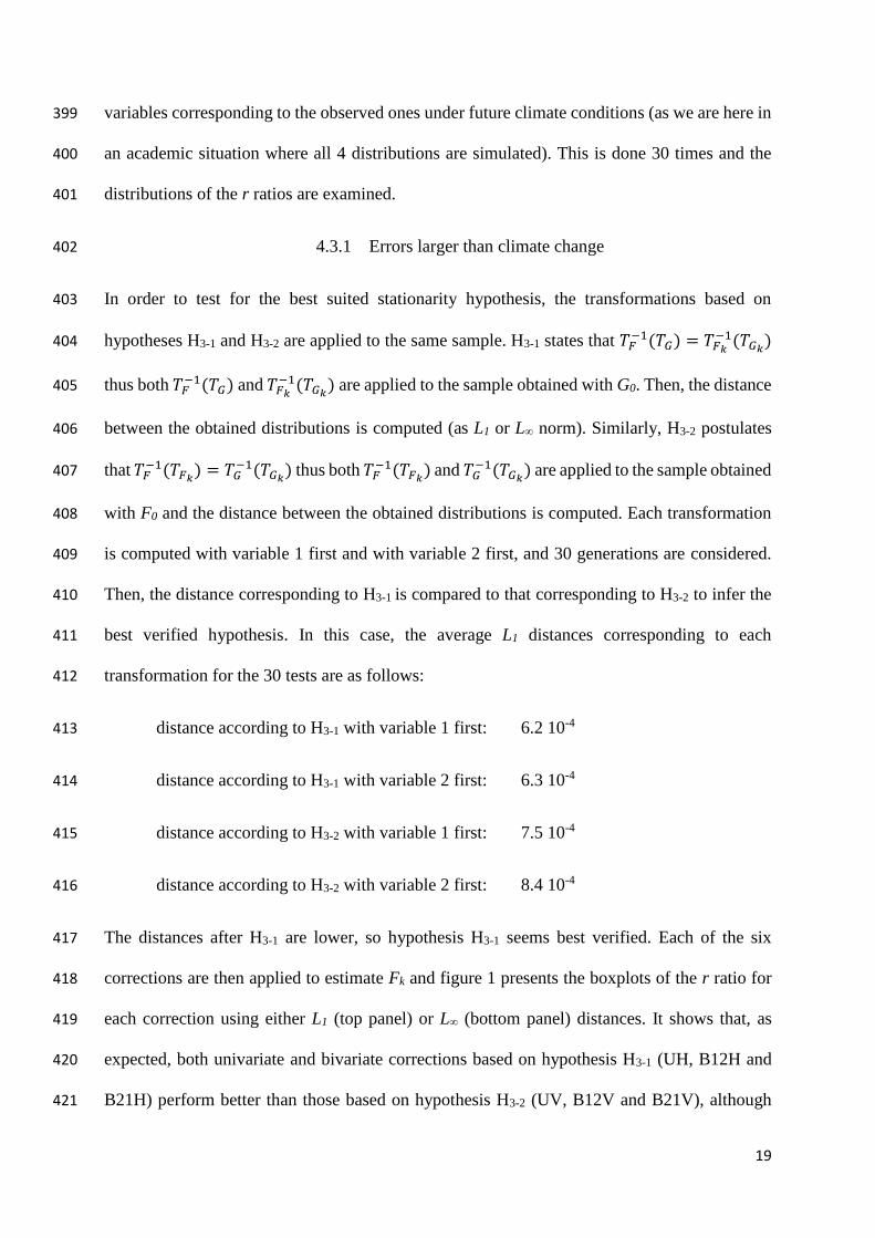
m1+dm1 m2+dm2 v11 x ds11 v22 x ds22 v12 x ds12 (=v21 x ds21) 340
The validation criterion is the ratio r defined in section 1.4 with both L1 and L∞ norms, which 341
is the distance between bias-corrected and observed distributions divided by the distance 342
between simulated and observed distributions, both estimated over the future period. 343
The aim of the applied bias corrections, either univariate or bivariate, is to estimate the bivariate 344
distribution of the observations for a future period (�̂�𝑘) from that of the observations and model 345
simulation over current period (F0 and G0) and of model simulation over future period (Gk). 346
Then, the previously defined ratio r measures the performance of the correction in making the 347
corrected distribution closer to that of the observations over future period Fk than was the 348
distribution of the model simulation over future period Gk if r<1. 349
Six bias corrections are applied and compared: 350
17
- each variable is independently corrected under hypothesis H3-1 (stationarity of the 351
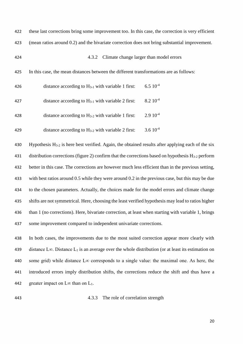
transformation between model and observations) 352
- each variable is independently corrected under hypothesis H3-2 (stationarity of the 353
transformation between present and future periods) 354
- bivariate correction under hypothesis H3-1 with variable 1 corrected first 355
- bivariate correction under hypothesis H3-1 with variable 2 corrected first 356
- bivariate correction under hypothesis H3-2 with variable 1 corrected first 357
- bivariate correction under hypothesis H3-2 with variable 2 corrected first 358
denoted respectively UH, UV, B12H, B21H, B12V, B21V. 359
UH and UV are similar to empirical quantile mapping and CDFt respectively. Here since we 360
only deal with distributions, the bivariate distribution correction under hypothesis H3-2 is 361
computed directly from Y0 through 𝑇𝐺−1(𝑇𝐺𝑘). The univariate bias corrections are computed in 362
the same way as the correction of the first variable in the bivariate corrections, and not taken 363
from the R packages for Quantile Mapping or CDFt, in order to remain consistent in the 364
comparisons. 365
Two cases have been considered in order to better discriminate hypotheses H3-1 and H3-2 and 366
the consequences of using a correction technique which may not be the best adapted. As a 367
matter of fact, when dealing with climate model simulations, it is difficult to test which 368
stationarity is best verified (because we do not have the observations in the future), and Quantile 369
Mapping or CDFt are generally indifferently used. The chosen cases correspond to: 370
- one case with model errors larger than climate change 371
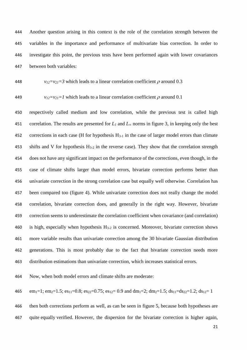
- one case with climate change larger than model errors 372
In order to be able to test the order of variable corrections in the bivariate corrections, the errors 373
and climate change shifts are not equal for each variable. The test cases are made with: 374

18
- em1=4; em2=5; es11=es22=es12= 0.5 and dm1=2; dm2=1.5; ds11=ds22=1.2 ; ds12= 1 375
- em1=1; em2=1.5; es11=0.8 ;es22=0.75 ;es12= 0.9 and dm1=4; dm2=5; ds11=ds22=1.5; 376
ds12= 1 377
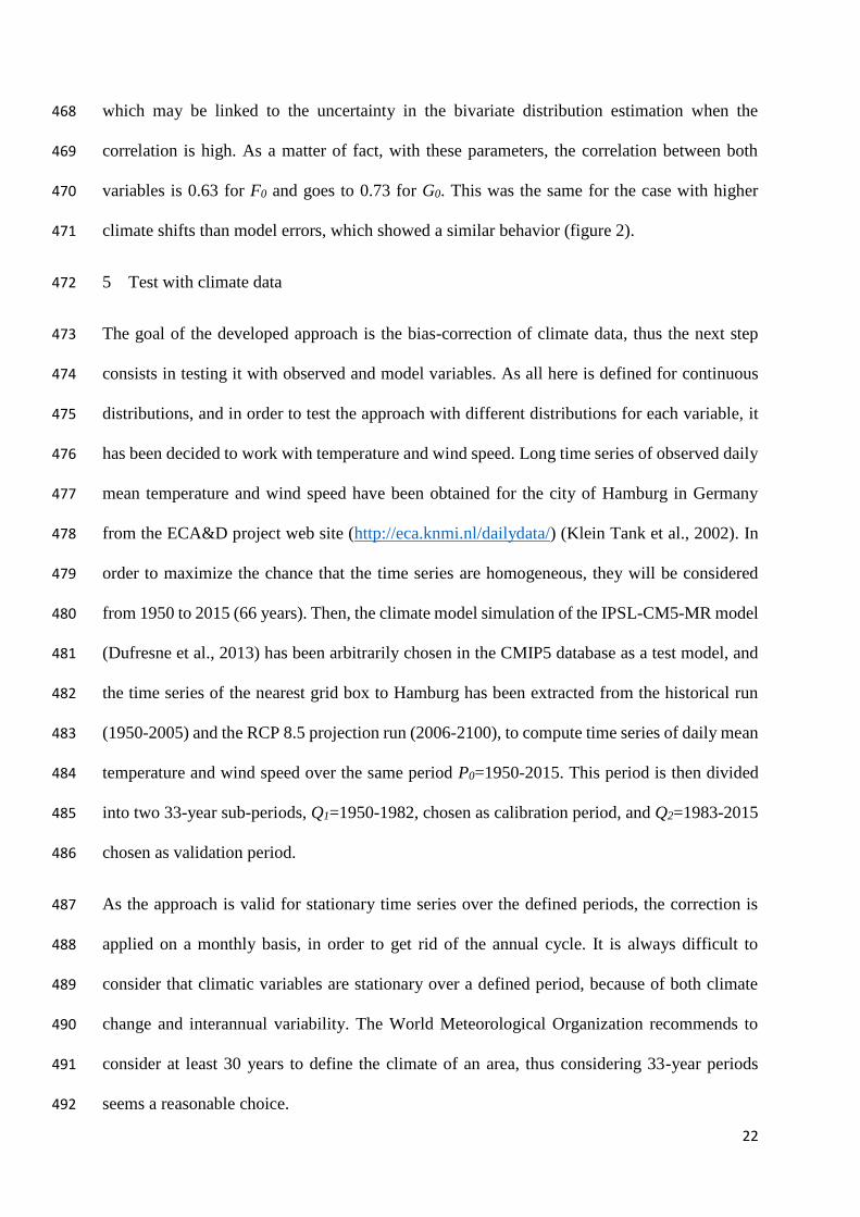
The choices have been made in considering observed model errors and climate change changes: 378
climate models tend to underestimate the variances and in summer, both the means and the 379
variances increase. Then this behavior has been exaggerated to produce large errors and large 380
climate shifts. 381
4.3 Results 382
As previously described, we first simulate 2000 values with Gaussian bivariate distributions 383
using fixed means and variances/co-variances, from which we then non-parametrically estimate 384
bivariate distributions to compute distances and compare the different bias corrections. The 385
non-parametrical estimation is based on the R function “kde2d” of package MASS, and with 386
2000 values only, such an estimation is uncertain. It has thus first been verified that the distances 387
between the bivariate distributions with the chosen errors and climate change shifts are 388
significantly larger than the distances between 2 sets of 2000 points taken from the same 389
distribution. This is preferred to the consideration of a much larger number of values, because 390
firstly, this considerably increases computing time for the corrections and secondly, in climate 391
change studies, when corrections have to be made it is generally done on a monthly basis, we 392
do not dispose of much more values. Thus 4 sets of 2000 points are produced by use of a 393
bivariate Gaussian distribution: one mimicking 2 variables as observed under current climate 394
conditions, another for current climate as simulated by a climate model and the 2 other sets 395
mimicking observed and modeled variables under future climate conditions. Then the 396
previously defined 6 bias corrections are applied to the set corresponding to the modeled 397
variables under future climate conditions so that its distribution gets closer to that of the 398
19
variables corresponding to the observed ones under future climate conditions (as we are here in 399
an academic situation where all 4 distributions are simulated). This is done 30 times and the 400
distributions of the r ratios are examined. 401
4.3.1 Errors larger than climate change 402
In order to test for the best suited stationarity hypothesis, the transformations based on 403
hypotheses H3-1 and H3-2 are applied to the same sample. H3-1 states that 𝑇𝐹−1(𝑇𝐺) = 𝑇𝐹𝑘
−1(𝑇𝐺𝑘) 404
thus both 𝑇𝐹−1(𝑇𝐺) and 𝑇𝐹𝑘
−1(𝑇𝐺𝑘) are applied to the sample obtained with G0. Then, the distance 405
between the obtained distributions is computed (as L1 or L∞ norm). Similarly, H3-2 postulates 406
that 𝑇𝐹−1(𝑇𝐹𝑘) = 𝑇𝐺
−1(𝑇𝐺𝑘) thus both 𝑇𝐹−1(𝑇𝐹𝑘) and 𝑇𝐺
−1(𝑇𝐺𝑘) are applied to the sample obtained 407
with F0 and the distance between the obtained distributions is computed. Each transformation 408
is computed with variable 1 first and with variable 2 first, and 30 generations are considered. 409
Then, the distance corresponding to H3-1 is compared to that corresponding to H3-2 to infer the 410
best verified hypothesis. In this case, the average L1 distances corresponding to each 411
transformation for the 30 tests are as follows: 412
distance according to H3-1 with variable 1 first: 6.2 10-4 413
distance according to H3-1 with variable 2 first: 6.3 10-4 414
distance according to H3-2 with variable 1 first: 7.5 10-4 415
distance according to H3-2 with variable 2 first: 8.4 10-4 416
The distances after H3-1 are lower, so hypothesis H3-1 seems best verified. Each of the six 417
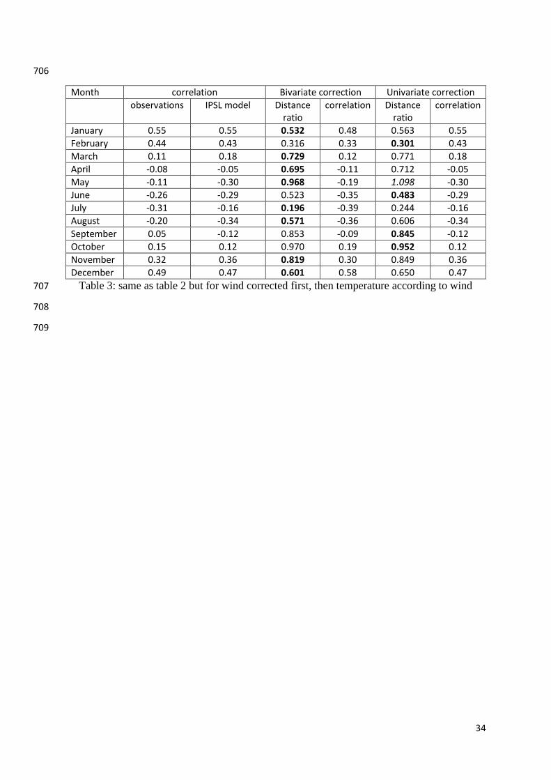
corrections are then applied to estimate Fk and figure 1 presents the boxplots of the r ratio for 418
each correction using either L1 (top panel) or L∞ (bottom panel) distances. It shows that, as 419
expected, both univariate and bivariate corrections based on hypothesis H3-1 (UH, B12H and 420
B21H) perform better than those based on hypothesis H3-2 (UV, B12V and B21V), although 421
20
these last corrections bring some improvement too. In this case, the correction is very efficient 422
(mean ratios around 0.2) and the bivariate correction does not bring substantial improvement. 423
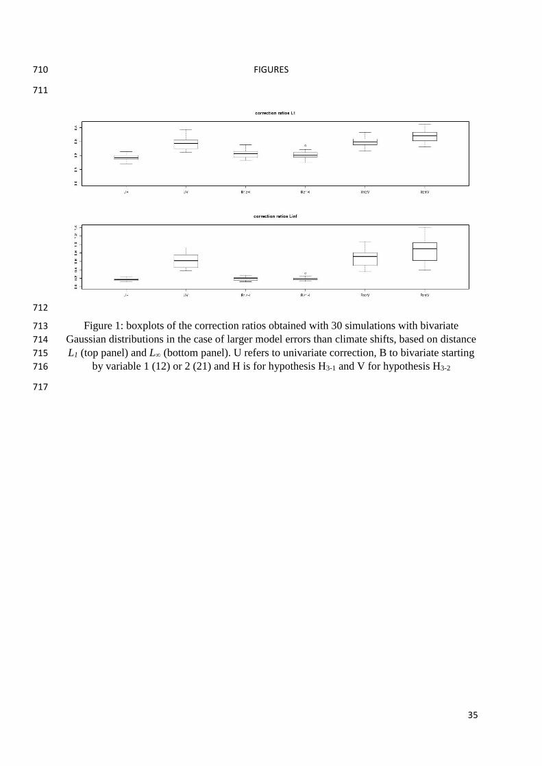
4.3.2 Climate change larger than model errors 424
In this case, the mean distances between the different transformations are as follows: 425
distance according to H3-1 with variable 1 first: 6.5 10-4 426
distance according to H3-1 with variable 2 first: 8.2 10-4 427
distance according to H3-2 with variable 1 first: 2.9 10-4 428
distance according to H3-2 with variable 2 first: 3.6 10-4 429
Hypothesis H3-2 is here best verified. Again, the obtained results after applying each of the six 430
distribution corrections (figure 2) confirm that the corrections based on hypothesis H3-2 perform 431
better in this case. The corrections are however much less efficient than in the previous setting, 432
with best ratios around 0.5 while they were around 0.2 in the previous case, but this may be due 433
to the chosen parameters. Actually, the choices made for the model errors and climate change 434
shifts are not symmetrical. Here, choosing the least verified hypothesis may lead to ratios higher 435
than 1 (no corrections). Here, bivariate correction, at least when starting with variable 1, brings 436
some improvement compared to independent univariate corrections. 437
In both cases, the improvements due to the most suited correction appear more clearly with 438
distance L∞. Distance L1 is an average over the whole distribution (or at least its estimation on 439
some grid) while distance L∞ corresponds to a single value: the maximal one. As here, the 440
introduced errors imply distribution shifts, the corrections reduce the shift and thus have a 441
greater impact on L∞ than on L1. 442
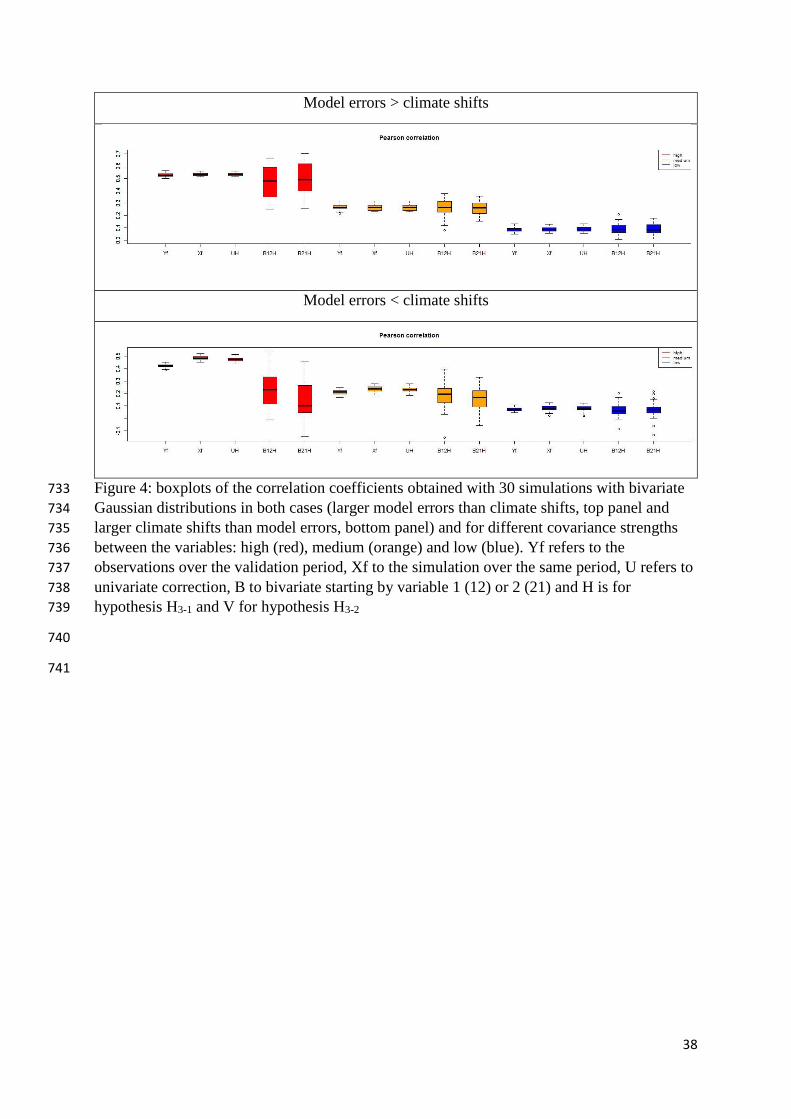
4.3.3 The role of correlation strength 443
21
Another question arising in this context is the role of the correlation strength between the 444
variables in the importance and performance of multivariate bias correction. In order to 445
investigate this point, the previous tests have been performed again with lower covariances 446
between both variables: 447
v12=v21=3 which leads to a linear correlation coefficient around 0.3 448
v12=v21=1 which leads to a linear correlation coefficient around 0.1 449
respectively called medium and low correlation, while the previous test is called high 450
correlation. The results are presented for L1 and L∞ norms in figure 3, in keeping only the best 451
corrections in each case (H for hypothesis H3-1 in the case of larger model errors than climate 452
shifts and V for hypothesis H3-2 in the reverse case). They show that the correlation strength 453
does not have any significant impact on the performance of the corrections, even though, in the 454
case of climate shifts larger than model errors, bivariate correction performs better than 455
univariate correction in the strong correlation case but equally well otherwise. Correlation has 456
been compared too (figure 4). While univariate correction does not really change the model 457
correlation, bivariate correction does, and generally in the right way. However, bivariate 458
correction seems to underestimate the correlation coefficient when covariance (and correlation) 459
is high, especially when hypothesis H3-2 is concerned. Moreover, bivariate correction shows 460
more variable results than univariate correction among the 30 bivariate Gaussian distribution 461
generations. This is most probably due to the fact that bivariate correction needs more 462
distribution estimations than univariate correction, which increases statistical errors. 463
Now, when both model errors and climate shifts are moderate: 464
em1=1; em2=1.5; es11=0.8; es22=0.75; es12= 0.9 and dm1=2; dm2=1.5; ds11=ds22=1.2; ds12= 1 465
then both corrections perform as well, as can be seen in figure 5, because both hypotheses are 466
quite equally verified. However, the dispersion for the bivariate correction is higher again, 467
22
which may be linked to the uncertainty in the bivariate distribution estimation when the 468
correlation is high. As a matter of fact, with these parameters, the correlation between both 469
variables is 0.63 for F0 and goes to 0.73 for G0. This was the same for the case with higher 470
climate shifts than model errors, which showed a similar behavior (figure 2). 471
5 Test with climate data 472
The goal of the developed approach is the bias-correction of climate data, thus the next step 473
consists in testing it with observed and model variables. As all here is defined for continuous 474
distributions, and in order to test the approach with different distributions for each variable, it 475
has been decided to work with temperature and wind speed. Long time series of observed daily 476
mean temperature and wind speed have been obtained for the city of Hamburg in Germany 477
from the ECA&D project web site (http://eca.knmi.nl/dailydata/) (Klein Tank et al., 2002). In 478
order to maximize the chance that the time series are homogeneous, they will be considered 479
from 1950 to 2015 (66 years). Then, the climate model simulation of the IPSL-CM5-MR model 480
(Dufresne et al., 2013) has been arbitrarily chosen in the CMIP5 database as a test model, and 481
the time series of the nearest grid box to Hamburg has been extracted from the historical run 482
(1950-2005) and the RCP 8.5 projection run (2006-2100), to compute time series of daily mean 483
temperature and wind speed over the same period P0=1950-2015. This period is then divided 484
into two 33-year sub-periods, Q1=1950-1982, chosen as calibration period, and Q2=1983-2015 485
chosen as validation period. 486
As the approach is valid for stationary time series over the defined periods, the correction is 487
applied on a monthly basis, in order to get rid of the annual cycle. It is always difficult to 488
consider that climatic variables are stationary over a defined period, because of both climate 489
change and interannual variability. The World Meteorological Organization recommends to 490
consider at least 30 years to define the climate of an area, thus considering 33-year periods 491
seems a reasonable choice. 492

23
First, the distances after transformations of the same sample according to each H3-1 and H3-2 493
hypothesis are computed for each month to infer which one is best verified. Table 1 summarizes 494
the results for each month, together with an indication of the correlation between wind and 495
temperature as observed over period Q1 according to the linear Pearson correlation coefficient 496
or the rank Spearman one. Except for July, for which H3-1 seems clearly best verified, for all 497
other months, either H3-1 show a small preference or it is difficult to discriminate both 498
hypothesis. Therefore, the multivariate correction will be applied according to H3-1, which 499
corresponds to estimations similar as those made by Empirical Quantile Mapping, since 500
between 2 recent past periods the climate shift is not too high. Here, the functions of the R 501
package qmap have been used for the univariate corrections in order to compare our proposed 502
approach to standard ones used in climate studies. Daily temperature and wind speed are 503
generally moderately correlated (positively in winter, negatively in summer) except in 504
September. 505
5.1 Temperature first, then wind 506
The first test is made by correcting temperature first, and then wind according to temperature 507
as described in sections 1 and 2. The ratios of the distance between the bivariate distribution of 508
the corrected variables and the observed ones divided by the distance between the modeled 509
variables and the observed ones over the validation period are compared for both bivariate and 510
independent univariate bias-corrections for each month (table 2). Here only the L1 norm is 511
considered as both used norms lead to the same conclusions in the previous section. The first 512
outcome is that, generally bias-correction improves the distance to the observations (ratio <1), 513
and bivariate correction gives slightly better results than univariate corrections for 7 months. 514
The worst correction is obtained for the month of May, while the best occurs in July, both for 515
univariate and bivariate corrections. Figure 6 allows the comparison of the bivariate 516
distributions in May, for observations and model over the calibration (Q1) and validation (Q2) 517
24
periods and for Q1 and Q2 for the model and the observations. It shows that the model errors are 518
rather low, and that there is very little change between both periods, for the model as well as 519
for the observations. It is thus not surprising that the correction is modest in this case, as shown 520
in figure 7. On the contrary, in July (figure 8) the model errors are quite large, and climate 521
change is modest. The situation is more similar to that of our academic case with large model 522
errors and moderate climate shift which previously lead to the best corrections based on 523
hypothesis H3-1 (section 4.3.1). Figure 9 illustrates the distributions before and after corrections 524
and shows that bivariate correction brings some improvement. As far as correlation is 525
concerned, univariate bias correction does not have any impact on the model correlation, 526
whereas bivariate correction does, and generally improves the correlation. This can be seen in 527
table 2 for example for May, when the model anti-correlation is stronger than observed and this 528
is better after bivariate correction or for July when model anti-correlation is weaker than 529
observed and increased by the bivariate bias correction. This is shown for the Spearman rank 530
correlation coefficient but the results are similar with the Pearson correlation coefficient. Thus 531
bivariate corrections clearly improve the situation if the correlations for observation and model 532
are different enough to allow the correction being larger than the statistical errors due to the 533
dimension. 534
5.2 Wind first then temperature 535
The same corrections have then been tested again but by correcting wind speed first, and then 536
temperature according to wind speed. The ratios of distances after and before correction are 537
summarized in table 3, together with the Spearman rank correlation coefficients. The results are 538
similar even though the months for which univariate correction gives slightly better results are 539
not always the same. July shows again the best performance for the corrections while May 540
remains the worst corrected, with a small advantage to bivariate correction though. 541
6 Conclusion and perspectives 542

25
In this paper, a new approach for bias-correcting multivariate distributions of climate model 543
simulations according to observations has been proposed and tested in controlled conditions, 544
by use of statistical simulations, and in real conditions, with a climate model simulation and 545
observations for wind speed and temperature. This approach is based on the Lévy-Rosenblatt 546
lemma and generalizes the univariate distribution corrections like empirical quantile mapping 547
or CDFt. 548
The development of the technique first showed that depending on the hypothesis made 549
(invariance of the transformation between model and observations in time or invariance of the 550
transformation between two periods for observed and model variables), the correction is similar 551
to empirical quantile mapping or to CDFt. 552
Then, the tests with bivariate Gaussian distributions allowed to compare the performances of 553
the corrections in controlling the model errors and climate shifts, as well as the strength of the 554
variables correlation. The parameters are based on observed and model July temperature for 555
two distant points, and willingly exaggerated in order to better see the differences in the 556
approaches. It shows that the verification of the chosen stationary hypothesis: H3-1 (stationarity 557
of the link between model and observations) or H3-2 (stationarity of the link between present 558
end future conditions) has a stronger importance for the correction performance than univariate 559
or bivariate correction, whatever the correlation strength between both variables. Furthermore, 560
the order of variable corrections does not seem to have important consequences in this 561
framework. 562
Then a last test is made in a more real setting, with daily mean temperature and wind speed 563
time series observed over period 1950-2015 and simulated by the IPSL-CM5-MR model in 564
Hamburg. The corrections are applied on a monthly basis, in order to meet as closely as possible 565
the hypothesis of stationarity, in a cross-validation setting, 1950-1982 being the calibration 566
period and 1983-2015 the validation period. Daily temperature and wind speed are moderately 567
26
correlated in each month, with a positive correlation in winter and a negative one in summer, 568
with lower correlation in fall and spring (and almost no correlation in September). As the 569
periods are close, the conditions of a more reliable application of corrections based on 570
hypothesis H3-1 are generally met and this technique is applied. The results show that bivariate 571
correction generally leads to a slightly better correction. 572
This study opens some questions before the application of such a correction can be generalized. 573
First it can be extended to the case of at least one variable with non-continuous distribution. 574
Most applications have to deal with temperature and rainfall rather than temperature and wind 575
speed. Two ways can be tested to do so: 576
- Correction of the number of rainy days (based on the differences between model and 577
observations if H3-1 is considered or on the change between present and future if H3-578
2 is considered), then of the amount of rainfall on rainy days and finally of 579
temperature according to rainfall (in managing again rainy and non-rainy days) 580
- Transformation of the rainfall distribution so that it becomes more continuous as 581
proposed in Vrac et al 2016 582
Then although the methodology is generic and theoretically works regardless of the number of 583
variables, extension to more than two variables will need more data for the estimations to be 584
reliable. Furthermore, the need to estimate more distributions increases the statistical errors and 585
the improvement is more obvious if the discrepancies to be corrected are large. 586
Lastly, the very important question of stationarity remains. Applying the correction on a 587
monthly basis is the easiest solution. However, because of interannual variability, it is necessary 588
to calibrate the correction over a long enough period (at least 30 years). Then in the climate 589
change context, the conditions of application of empirical quantile mapping like approaches 590
(based on hypothesis H3-1), that the distributions are invariant in time, cannot hold, and then, 591
27
CDFt like approaches (based on hypothesis H3-2) are more adapted, but may bring a lower 592
improvement. Besides, using Quantile Mapping like corrections in such cases may worsen the 593
situation. It seems then important to think at techniques able to stationarize the distributions 594
and let them be closer in time and between observation and model. This can be done by 595
removing seasonalities and trends, at least in the mean and the variance. However, part of the 596
bias is embedded in the estimation of such quantities for the model time series and they have to 597
be corrected too. In a univariate context, this can be made in an additive or multiplicative way. 598
But in a multivariate context, this implies to think at a way of consistently correcting these parts 599
of the signal as well. Future work will consist in clarifying these questions of non stationarity 600
by working with a parameterization of the two kinds of dynamic deformations we have 601
formalized in hypotheses H3-1 and H3-2. Such parameterization should be more complex than a 602
simple shift but still simple enough to be applied routinely. 603
Acknowledgements 604
The authors would like to acknowledge funding for the European Climatic Energy Mixes (ECEM) project by the 605
Copernicus Climate Change Service, a programme being implemented by the European Centre for Medium-Range 606
Weather Forecasts 5 (ECMWF) on behalf of the European Commission. The specific grant number is 607
2015/C3S_441_Lot2_UEA. 608
609
7 References 610
Bashtannyk D. M., Hyndmann R. J., 2001: Bandwidth selection for kernel conditional density 611
estimation, Computational Statistics & Data Analysis 612
Cannon A. J., 2016: Multivariate Bias Correction of Climate Model Output: Matching Marginal 613
Distributions and Intervariable Dependence Structure. Journal of Climate, 29, 7045-7064, DOI: 614
10.1175/JCLI-D-15-0679.1 615
28
Chen J., Brissette F. P., Chaumont D., and Braun M., 2013: Finding appropriate bias correction 616
methods in downscaling precipitation for hydrologic impact studies over North America. Water 617
Resources Research, 49 (7), 4187–4205, doi:10.1002/wrcr.20331 618
De Gooijer J.G. and Gannoun A., 2000: Nonparametric conditional predictive regions for time 619
series, Computational Statistics and Data Analysis 33, 259–275. 620
Déqué M., 2007: Frequency of precipitation and temperature extremes over France in an 621
anthropogenic scenario: Model results and statistical correction according to observed values, 622
Global Planet. Change, 57, 16– 26 623
Dufresne J-L, Foujols M-A, Denvil S, Caubel A, Marti O, Aumont O, Balkanski Y, Bekki S, 624
Bellenger H, Benshila R, Bony S, Bopp L, Braconnot P, Brockmann P, Cadule P, Cheruy F, 625
Codron F, Cozic A, Cugnet D, de Noblet N, Duvel J-P, Ethé C, Fairhead L, Fichefet T, Flavoni 626
S, Friedlingstein P, Grandpeix J-Y, Guez L, Guilyardi E, Hauglustaine D, Hourdin F, Idelkadi 627
A, Ghattas J, Joussaume S, Kageyama M, Krinner G, Labetoulle S, Lahellec A, Lefebvre M-P, 628
Lefevre F, Levy C, Li ZX, Lloyd J, Lott F, Madec G, Mancip M, Marchand M, Masson S, 629
Meurdesoif Y, Mignot J, Musat I, Parouty S, Polcher J, Rio C, Schulz M, Swingedouw D, Szopa 630
S, Talandier C, Terray P, Viovy N, Vuichard N, 2013: Climate change projections using the 631
IPSLCM5 earth system model: from CMIP3 to CMIP5. Climate Dynamics 40(9):2123–2165 632
Fan J., Yao Q and Tong H., 1996: Estimation of conditional densities and sensitivity measures 633
in nonlinear dynamical systems. Biometrika, 83 (1). pp. 189-206. 634
Grandjacques, M., 2015 : Analyse de sensibilité pour des modèles stochastiques à entrées 635
dépendantes : application en énergétique du bâtiment. Thèse Université de Grenoble 636
Grandjacques M., Delinchant B., Adrot O. Pick and Freeze, 2015: estimation of sensitivity 637
index for static and dynamic models with dependent inputs - hal.archives-ouvertes.fr 638
29
Greub W. H., 1975: Linear Algebra, 4th edition, Springer Verlag 639
Gudmundsson L., Bremnes J., Haugen J., and Engen-Skaugen T., 2012: Technical note: 640
Downscaling RCM precipitation to the station scale using statistical transformations–a 641
comparison of methods. Hydrology & Earth System Sciences, 16 (9), 3383–3390, 642
doi:10.5194/hess-16-3383-2012 643
Haddad, Z. and D. Rosenfeld, 1997: Optimality of empirical z-r relations. Q. J. R. Meteorol. 644
Soc., 123, 1283-1293 645
Hall P, Wolff R, Yao Q, 1999: Methods for estimating a conditional distribution function, 646
Journal of the American Statistical Association, 94 (445). pp. 154-163 647
Hyndmann R, Bashtannyk D M, Grunwald G K, 1996: Estimating and visualizing conditional 648
densities, Journal of Computational and Graphical Statistics, 1996 649
Hyndmann R, Yao Q, 2002: Nonparametric estimation and symmetry test for conditional 650
density functions, Nonparametric statistics 651
IPCC, “Climate change 2013; The physical basis - summary for policymakers,” Fifth 652
Assessment Report of the Intergovernemental Panel on Climate Change, 2013 653
Klein Tank, A. M. G., et al., 2002: Daily dataset of 20th-century surface air temperature and 654
precipitation series for the European Climate Assessment, International Journal of Climatology, 655
22, 1,441–1,453, Data and metadata available at http://eca.knmi.nl. 656
Liebscher E., 1996: Strong convergence of sums of c-mixing random variables with 657
applications to density estimation. Stochastic Processes and their Applications 65 658
Li C., Sinha E., Horton D.E., Diffenbaugh N.S., and Michalak A.M., 2014: Joint bias correction 659
of temperature and precipitation in climate model simulations. Journal of Geophysical 660
Research: Atmospheres, 119 (23), 13–153, doi:10.1002/2014JD022514 661
30
Michelangeli P.-A., Vrac M., and Loukos H., 2009: Probabilistic downscaling approaches: 662
Application to wind cumulative distribution functions, Geophys. Res. Lett., 36, L11708, 663
doi:10.1029/2009GL038401 664
Panofsky H. and Brier G., 1958: Some applications of statistics to meteorology. Tech. rep., 665
University Park, Penn. State Univ., 224 pp 666
Piani, C., Haerter J., and Coppola E., 2010: Statistical bias correction for daily precipitation in 667
regional climate models over Europe. Theoretical and Applied Climatology, 99, 187-192, 668
doi:10.1007/s00704-009-0134-9 669
Piani, C. and Haerter J.O., 2012: Two dimensional bias correction of temperature and 670
precipitation copulas in climate models. Geophys. Res. Lett., doi:10.1029/2012GL053839 671
Rust H., Vrac M., Lengaigne M., Sultan B.: Quantifying Differences in Circulation Patterns 672
Based on Probabilistic Models. J. Climate, 23:6573-6589, 2010 673
Teutschbein, C., and Seibert J., 2012: Bias correction of regional climate model simulations for 674
hydrological climate-change impact studies: Review and evaluation of different methods. 675
Journal of Hydrology, 456, 12–29, doi:10.1175/JAMC-D-11-0149.1 676
Vrac, M. and Friederichs P., 2015: Multivariate-intervariable, spatial, and temporal-bias 677
correction. Journal of Climate, 28 (1), 218–237, doi:10.1175/JCLI-D-14-00059.1 678
Wood A., Leung L., Sridhar V. and Lettenmaier D., 2004: Hydrologic implications of 679
dynamical and statistical approaches to downscaling climate model outputs. Clim. Change, 62 680
(189-216). 681
Vrac M., Noël T., Vautard R., 2016 : Bias correction of precipitation through Singularity 682
Stochastic Removal: Because occurrences matter. Journal of Geophysical Research 683
Atmosphere, doi: 10.1002/2015JD024511 684

31
Zhang F., and Georgakakos A.P., 2012: Joint variable spatial downscaling. Climatic Change, 685
111 (3-4), 945–972, doi:10.1007/s10584-011-0167-9 686
687
688
32
TABLES 689
690
Month H3-1 T first
H3-1 w first
H3-2 T first
H3-2 w first
correlation
observations IPSL simulation
L1 (10-4)
L1 (10-4)
L1 (10-4)
L1 (10-4)
Pearson Spearman Pearson Spearman
January 7.0 6.6 9.5 9.0 0.47 0.50 0.50 0.54
February 7.0 6.3 10.5 8.1 0.36 0.35 0.40 0.43
March 14.7 13.2 14.0 13.8 0.11 0.10 0.17 0.18
April 18.0 17.1 17.1 17.3 -0.15 -0.15 -0.07 -0.06
May 13.7 12.6 19.0 17.6 -0.17 -0.17 -0.32 -0.33
June 21.5 20.8 21.6 21.3 -0.28 -0.28 -0.27 -0.26
July 13.2 12.2 26.2 28.5 -0.37 -0.39 -0.19 -0.15
August 15.0 16.2 17.3 20.0 -0.21 -0.22 -0.32 -0.30
September 14.5 14.8 19.3 22.9 -0.01 0.00 -0.14 -0.13
October 13.3 9.6 10.5 9.3 0.17 0.16 0.10 0.11
November 8.2 11.6 12.2 13.3 0.33 0.33 0.39 0.40
December 9.4 8.7 11.7 11.2 0.46 0.48 0.47 0.50
Table 1: L1 distance between the bivariate distributions obtained with transformations based 691
on hypothesis H3-1 with temperature (T) or wind (w) first (first two columns) and between the 692
bivariate distributions obtained with transformations based on hypothesis H3-2 with 693
temperature (T) or wind (w) first (columns 3 and 4), correlation between temperature and 694
wind (Pearson and Spearman coefficients for the observations (columns 6 and 7) and for the 695
IPSL model simulation (columns8 and 9) for each month 696
697
33
698
Month correlation Bivariate correction Univariate correction
observations IPSL model Distance ratio
correlation Distance ratio
correlation
January 0.55 0.55 0.522 0.62 0.563 0.55
February 0.44 0.43 0.328 0.39 0.301 0.43
March 0.11 0.18 0.758 0.17 0.771 0.18
April -0.08 -0.05 0.713 -0.14 0.712 -0.05
May -0.11 -0.30 0.992 -0.21 1.098 -0.30
June -0.26 -0.29 0.496 -0.33 0.483 -0.29
July -0.31 -0.16 0.179 -0.40 0.244 -0.16
August -0.20 -0.34 0.600 -0.36 0.606 -0.34
September 0.05 -0.12 0.855 -0.03 0.845 -0.12
October 0.15 0.12 0.934 0.17 0.952 0.12
November 0.32 0.36 0.788 0.36 0.849 0.36
December 0.49 0.47 0.671 0.45 0.650 0.47
Table 2: correlation (Spearman rank correlation coefficient) over the validation period and 699
ratio of the distance (between the bivariate distributions of the corrected and observed 700
variables divided by that of the modeled and observed variables) and correlation over the 701
validation period after bivariate bias correction with temperature corrected first and 702
independent univariate bias-correction. Bold indicates the lowest ratios obtained when 703
correction is efficient 704
705
34
706
Month correlation Bivariate correction Univariate correction
observations IPSL model Distance ratio
correlation Distance ratio
correlation
January 0.55 0.55 0.532 0.48 0.563 0.55
February 0.44 0.43 0.316 0.33 0.301 0.43
March 0.11 0.18 0.729 0.12 0.771 0.18
April -0.08 -0.05 0.695 -0.11 0.712 -0.05
May -0.11 -0.30 0.968 -0.19 1.098 -0.30
June -0.26 -0.29 0.523 -0.35 0.483 -0.29
July -0.31 -0.16 0.196 -0.39 0.244 -0.16
August -0.20 -0.34 0.571 -0.36 0.606 -0.34
September 0.05 -0.12 0.853 -0.09 0.845 -0.12
October 0.15 0.12 0.970 0.19 0.952 0.12
November 0.32 0.36 0.819 0.30 0.849 0.36
December 0.49 0.47 0.601 0.58 0.650 0.47
Table 3: same as table 2 but for wind corrected first, then temperature according to wind 707
708
709
35
FIGURES 710
711
712
Figure 1: boxplots of the correction ratios obtained with 30 simulations with bivariate 713
Gaussian distributions in the case of larger model errors than climate shifts, based on distance 714
L1 (top panel) and L∞ (bottom panel). U refers to univariate correction, B to bivariate starting 715
by variable 1 (12) or 2 (21) and H is for hypothesis H3-1 and V for hypothesis H3-2 716
717
36
718
719
Figure 2: boxplots of the correction ratios obtained with 30 simulations with bivariate 720
Gaussian distributions in the case of larger climate shifts than model errors, based on distance 721
L1 (top panel) and L∞ (bottom panel). U refers to univariate correction, B to bivariate starting 722
by variable 1 (12) or 2 (21) and H is for hypothesis H3-1 and V for hypothesis H3-2 723
724

37
725
Model errors > climate shifts
Model errors < climate shifts
Figure 3: boxplots of the correction ratios obtained with 30 simulations with bivariate 726
Gaussian distributions in both cases (larger model errors than climate shifts, top panel and 727
larger climate shifts than model errors, bottom panel) based on distances L1 and L∞ and for 728
different correlation strengths between the variables: high (red), medium (orange) and low 729
(blue). U refers to univariate correction, B to bivariate starting by variable 1 (12) or 2 (21) and 730
H is for hypothesis H3-1 and V for hypothesis H3-2 731
732
38
Model errors > climate shifts
Model errors < climate shifts
Figure 4: boxplots of the correlation coefficients obtained with 30 simulations with bivariate 733
Gaussian distributions in both cases (larger model errors than climate shifts, top panel and 734
larger climate shifts than model errors, bottom panel) and for different covariance strengths 735
between the variables: high (red), medium (orange) and low (blue). Yf refers to the 736
observations over the validation period, Xf to the simulation over the same period, U refers to 737
univariate correction, B to bivariate starting by variable 1 (12) or 2 (21) and H is for 738
hypothesis H3-1 and V for hypothesis H3-2 739
740
741
39
742
743
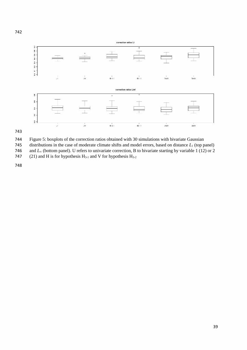
Figure 5: boxplots of the correction ratios obtained with 30 simulations with bivariate Gaussian 744 distributions in the case of moderate climate shifts and model errors, based on distance L1 (top panel) 745 and L∞ (bottom panel). U refers to univariate correction, B to bivariate starting by variable 1 (12) or 2 746 (21) and H is for hypothesis H3-1 and V for hypothesis H3-2 747
748
40
749
750
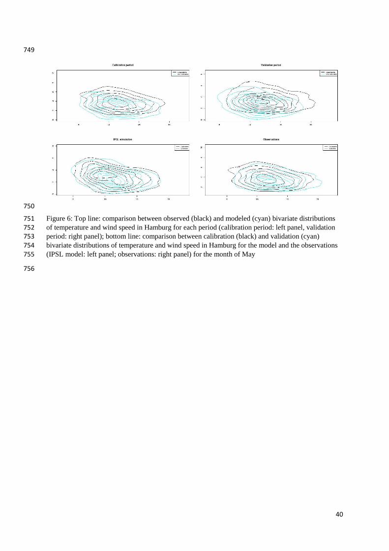
Figure 6: Top line: comparison between observed (black) and modeled (cyan) bivariate distributions 751 of temperature and wind speed in Hamburg for each period (calibration period: left panel, validation 752 period: right panel); bottom line: comparison between calibration (black) and validation (cyan) 753 bivariate distributions of temperature and wind speed in Hamburg for the model and the observations 754 (IPSL model: left panel; observations: right panel) for the month of May 755
756

41
757
Univariate correction
Bivariate correction Temperature first then Wind speed
Bivariate correction wind speed first then temperature
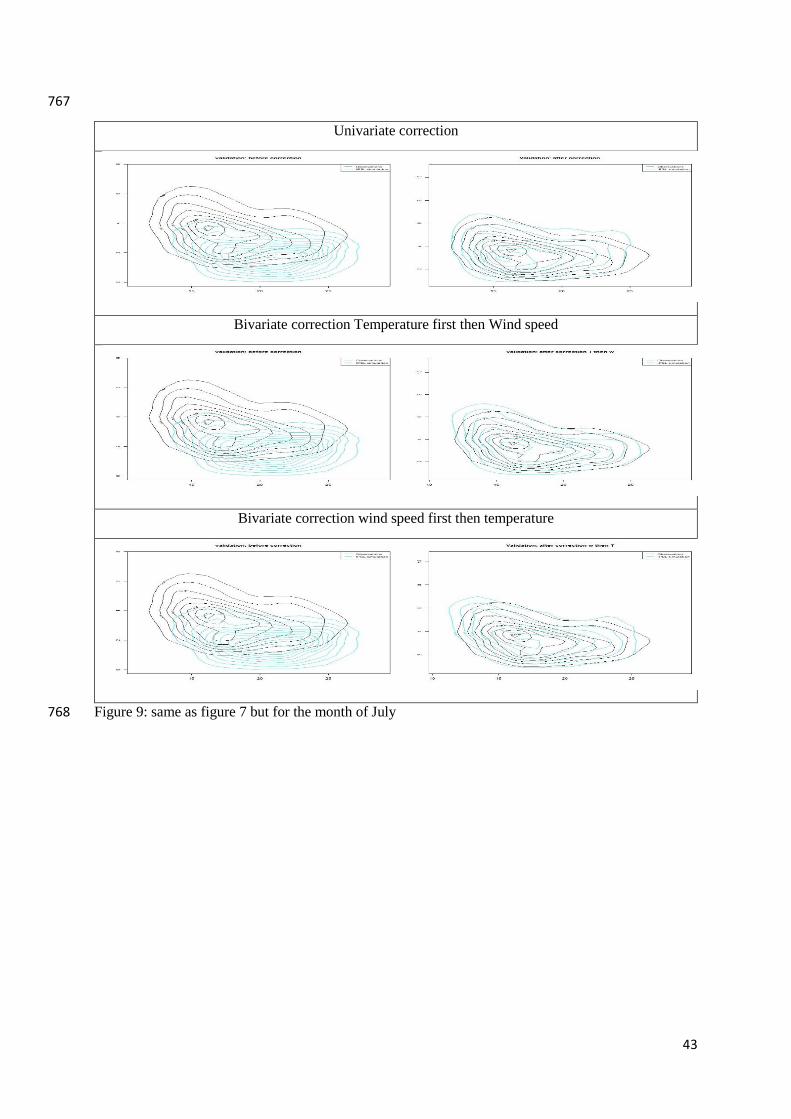
Figure 7: comparison between observed (black) and modeled (cyan) bivariate distributions of 758 temperature and wind speed in Hamburg for the validation period before correction (left panels) and 759 after univariate correction (top right), bivariate correction with temperature first (medium right) and 760 wind speed first (bottom right) for the month of May 761
762
763
42
764
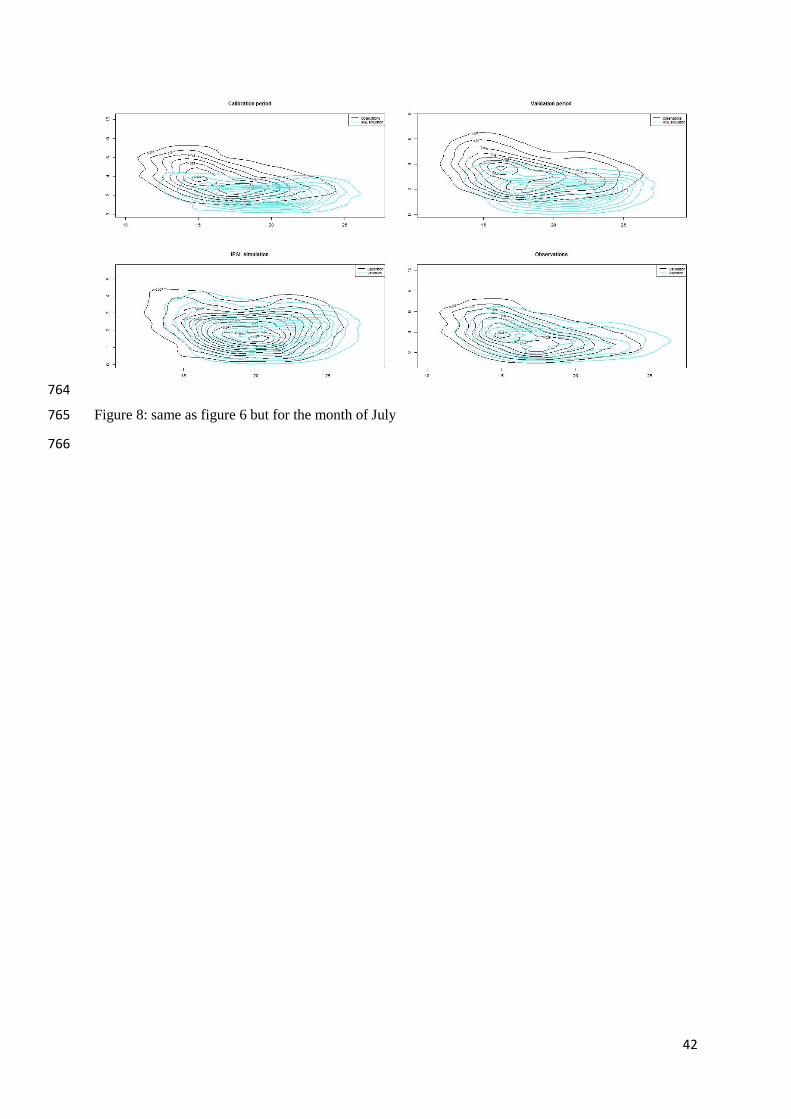
Figure 8: same as figure 6 but for the month of July 765
766
43
767
Univariate correction
Bivariate correction Temperature first then Wind speed
Bivariate correction wind speed first then temperature
Figure 9: same as figure 7 but for the month of July 768