Embed Size (px)
DESCRIPTION
Multivariate Normal Distribution MATLAB code
Citation preview

J. Elder CSE 4404/5327 Introduction to Machine Learning and Pattern Recognition
MULTIVARIATE NORMAL DISTRIBUTION
Last updated: Sept 20, 2012

Probability & Bayesian Inference
J. Elder CSE 4404/5327 Introduction to Machine Learning and Pattern Recognition
2
Linear Algebra
¨ Tutorial this Wed 3:00 – 4:30 in Bethune 228 ¨ Linear Algebra Reviews:
¤ Kolter, Z., avail at http://cs229.stanford.edu/section/cs229-linalg.pdf
¤ Prince, Appendix C (up to and including C.7.1) ¤ Bishop, Appendix C ¤ Roweis, S., avail at
http://www.cs.nyu.edu/~roweis/notes/matrixid.pdf

Probability & Bayesian Inference
J. Elder CSE 4404/5327 Introduction to Machine Learning and Pattern Recognition
3
Credits
¨ Some of these slides were sourced and/or modified from: ¤ Christopher Bishop, Microsoft UK ¤ Simon Prince, University College London ¤ Sergios Theodoridis, University of Athens & Konstantinos
Koutroumbas, National Observatory of Athens
Probability & Bayesian Inference
J. Elder CSE 4404/5327 Introduction to Machine Learning and Pattern Recognition
4
The Multivariate Normal Distribution: Topics
1. The Multivariate Normal Distribution 2. Decision Boundaries in Higher Dimensions 3. Parameter Estimation
1. Maximum Likelihood Parameter Estimation 2. Bayesian Parameter Estimation

Probability & Bayesian Inference
J. Elder CSE 4404/5327 Introduction to Machine Learning and Pattern Recognition
5
The Multivariate Normal Distribution: Topics
1. The Multivariate Normal Distribution 2. Decision Boundaries in Higher Dimensions 3. Parameter Estimation
1. Maximum Likelihood Parameter Estimation 2. Bayesian Parameter Estimation

Probability & Bayesian Inference
J. Elder CSE 4404/5327 Introduction to Machine Learning and Pattern Recognition
6
The Multivariate Gaussian
MATLAB Statistics Toolbox Function: mvnpdf(x,mu,sigma)

Probability & Bayesian Inference
J. Elder CSE 4404/5327 Introduction to Machine Learning and Pattern Recognition
7
Orthonormal Form
where Δ ≡ Mahalanobis distance from µ to x
See Linear Algebra Review Resources on Moodle site for a review of eigenvectors.
Let ui and λi represent the ith eigenvector/eigenvalue pair of Σ : Σui = λiui
MATLAB Statistics Toolbox Function: mahal(x,y)
MATLAB Functions: [V, D]= eig(A) [V, D]= eigs(A, k)
Let A∈D×D . λ is an eigenvalue and u is an eigenvector of A if Au = λu.

Probability & Bayesian Inference
J. Elder CSE 4404/5327 Introduction to Machine Learning and Pattern Recognition
8
Orthonormal Form
Since it is used in a quadratic form, we can assume that Σ−1 is symmetric.This means that all of its eigenvalues and eigenvectors are real.
We are also implicitly assuming that Σ, and hence Σ−1, are invertible (of full rank).
Thus Σ can be represented in orthonormal form: Σ =UΛUt ,where the columns of U are the eigenvectors ui of Σ, and
Λ is the diagonal matrix with entries Λ ii = λi equal to the corresponding eigenvalues of Σ.
Thus the Mahalanobis distance Δ2 can be represented as:
Δ2 = x − µ( )t Σ−1 x − µ( ) = x − µ( )t UΛ−1Ut x − µ( ).
Let y =Ut x − µ( ). Then we have,
Δ2 = y tΛ−1y = yiΛ ij−1y j
ij∑ = λi
−1yi2
i∑ ,
where yi = uit x − µ( ).

Probability & Bayesian Inference
J. Elder CSE 4404/5327 Introduction to Machine Learning and Pattern Recognition
9
Geometry of the Multivariate Gaussian
Δ = Mahalanobis distance from µ to x
where (u
i,λ
i) are the ith eigenvector and eigenvalue of Σ.
or y = U(x - µ)

Probability & Bayesian Inference
J. Elder CSE 4404/5327 Introduction to Machine Learning and Pattern Recognition
10
Moments of the Multivariate Gaussian
thanks to anti-symmetry of z

Probability & Bayesian Inference
J. Elder CSE 4404/5327 Introduction to Machine Learning and Pattern Recognition
11
Moments of the Multivariate Gaussian

5.1 Application: Face Detection

Probability & Bayesian Inference
J. Elder CSE 4404/5327 Introduction to Machine Learning and Pattern Recognition
13
Model # 1: Gaussian, uniform covariance
Pixel 1
Pixe
l 2
m face m non-face
Fit model using maximum likelihood criterion
s Face
59.1
s non-face
69.1 Face ‘template’
1/ 2

Probability & Bayesian Inference
J. Elder CSE 4404/5327 Introduction to Machine Learning and Pattern Recognition
14
Model 1 Results
0 0.2 0.4 0.6 0.8 10
0.1
0.2
0.3
0.4
0.5
0.6
0.7
0.8
0.9
1
Pr(H
it)
Pr(False Alarm)
Results based on 200 cropped faces and 200 non-faces from the same database.
How does this work with a real image?
Receiver-Operator Characteristic (ROC)

Probability & Bayesian Inference
J. Elder CSE 4404/5327 Introduction to Machine Learning and Pattern Recognition
15
Model # 2: Gaussian, diagonal covariance
Pixel 1
Pixe
l 2
m face m non-face Fit model using maximum likelihood criterion
s Face
s non-face
1/ 2
Probability & Bayesian Inference
J. Elder CSE 4404/5327 Introduction to Machine Learning and Pattern Recognition
16
0 0.2 0.4 0.6 0.8 10
0.1
0.2
0.3
0.4
0.5
0.6
0.7
0.8
0.9
1
Model 2 Results Pr
(Hit)
Pr(False Alarm)
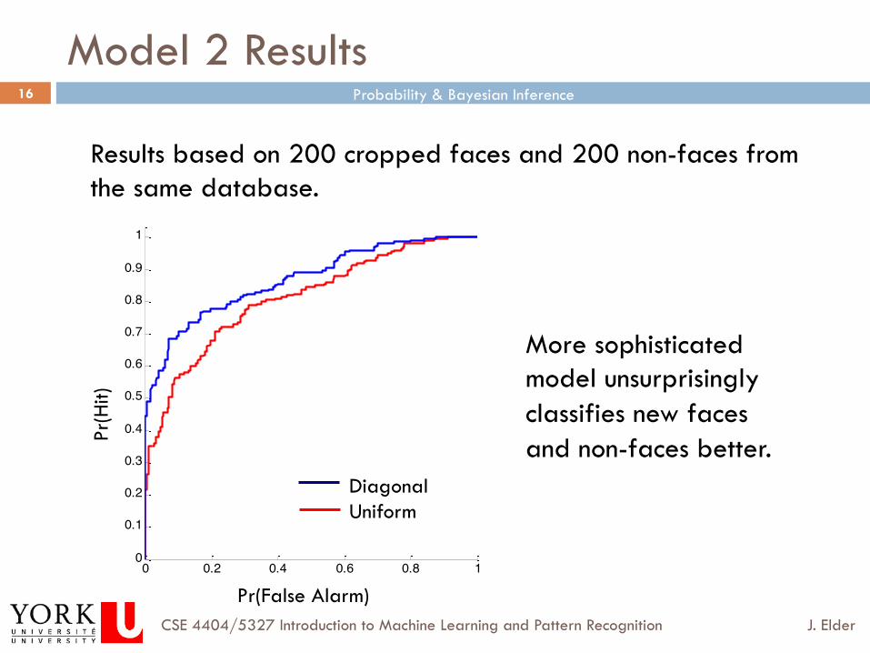
Results based on 200 cropped faces and 200 non-faces from the same database.
Diagonal Uniform
More sophisticated model unsurprisingly classifies new faces and non-faces better.
Probability & Bayesian Inference
J. Elder CSE 4404/5327 Introduction to Machine Learning and Pattern Recognition
17
Model # 3: Gaussian, full covariance
Pixel 1
Pixe
l 2
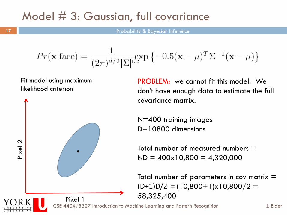
Fit model using maximum likelihood criterion
PROBLEM: we cannot fit this model. We don’t have enough data to estimate the full covariance matrix. N=400 training images D=10800 dimensions Total number of measured numbers = ND = 400x10,800 = 4,320,000 Total number of parameters in cov matrix = (D+1)D/2 = (10,800+1)x10,800/2 = 58,325,400
1/ 2

Probability & Bayesian Inference
J. Elder CSE 4404/5327 Introduction to Machine Learning and Pattern Recognition
18
The Multivariate Normal Distribution: Topics
1. The Multivariate Normal Distribution 2. Decision Boundaries in Higher Dimensions
3. Parameter Estimation 1. Maximum Likelihood Parameter Estimation 2. Bayesian Parameter Estimation

Probability & Bayesian Inference
J. Elder CSE 4404/5327 Introduction to Machine Learning and Pattern Recognition
19
19
Decision Surfaces
¨ If decision regions Ri and Rj are contiguous, define�
¨ Then the decision surface �
separates the two decision regions. g(x) is positive on one side and negative on the other.�
�
Ri : P ω i | x( ) > P ω j | x( )
Rj : P ω j | x( ) > P ω i | x( )
g(x) ≡ P(ω i | x) − P(ω j | x)
+ - g(x) = 0 g(x) = 0

Probability & Bayesian Inference
J. Elder CSE 4404/5327 Introduction to Machine Learning and Pattern Recognition
20
Discriminant Functions
20 ¨ If f (.) monotonic, the rule remains the same if we use:
¨ is a discriminant function
¨ In general, discriminant functions can be defined in other ways, independent of Bayes.
¨ In theory this will lead to a suboptimal solution
¨ However, non-Bayesian classifiers can have significant advantages:
¤ Often a full Bayesian treatment is intractable or computationally prohibitive.
¤ Approximations made in a Bayesian treatment may lead to errors avoided by non-Bayesian methods.
x → ω i if: f (P (ω i x )) > f (P (ω j x)) ∀ i ≠ j
gi (x) ≡ f (P (ω i | x))

Probability & Bayesian Inference
J. Elder CSE 4404/5327 Introduction to Machine Learning and Pattern Recognition
21
Multivariate Normal Likelihoods
21 ¨ Multivariate Gaussian pdf
p(x ω i ) =1
(2π )D2 Σi
12exp − 1
2 (x − µ i )Τ Σi
−1 (x − µ i )⎛
⎝⎜⎞
⎠⎟
µ i = E x ω i⎡⎣
⎤⎦
Σi = E (x − µ i )(x − µ i )Τ ω i
⎡⎣
⎤⎦

Probability & Bayesian Inference
J. Elder CSE 4404/5327 Introduction to Machine Learning and Pattern Recognition
22
Logarithmic Discriminant Function
22
¨ is monotonic. Define: ln(⋅)
gi (x) = ln p x | ω i( )P ω i( )( ) = ln p x | ω i( ) + lnP (ω i )
= − 12 (x − µ i )
T Σi−1 (x − µ i ) + lnP (ω i ) + Ci
whereCi = − D
2 ln2π − 12 ln Σi
p(x ω i ) =1
(2π )D2 Σi
12exp − 1
2 (x − µ i )Τ Σi
−1 (x − µ i )⎛
⎝⎜⎞
⎠⎟

Probability & Bayesian Inference
J. Elder CSE 4404/5327 Introduction to Machine Learning and Pattern Recognition
23
−10−5
05
10
−10
−5
0
5
100
0.1
0.2
0.3
0.4
0.5
Quadratic Classifiers
¨ Thus the decision surface has a quadratic form. ¨ For a 2D input space, the decision curves are quadrics (ellipses,
parabolas, hyperbolas or, in degenerate cases, lines).
gi (x) = − 1
2 (x − µ i )T Σi
−1 (x − µ i ) + lnP (ω i ) + Ci

Probability & Bayesian Inference
J. Elder CSE 4404/5327 Introduction to Machine Learning and Pattern Recognition
24
Example: Isotropic Likelihoods
24
¨ Suppose that the two likelihoods are both isotropic, but with different means and variances. Then
¨ And will be a quadratic equation in 2 variables. gi (x) = − 1
2σ i2 (x1
2 + x22) + 1
σ i2 (µi 1x1 + µi2x2) −
12σ i
2 (µi 12 + µi2
2 ) + ln P ω i( )( ) + Ci
gi (x) − gj (x) = 0
gi (x) = − 1
2 (x − µ i )T Σi
−1 (x − µ i ) + lnP (ω i ) + Ci

Probability & Bayesian Inference
J. Elder CSE 4404/5327 Introduction to Machine Learning and Pattern Recognition
25
Equal Covariances
¨ The quadratic term of the decision boundary is given by
¨ Thus if the covariance matrices of the two likelihoods are identical, the decision boundary is linear.
gi (x) = − 1
2 (x − µ i )T Σi
−1 (x − µ i ) + lnP (ω i ) + Ci
12 xT Σ j
−1 − Σi−1( )x

Probability & Bayesian Inference
J. Elder CSE 4404/5327 Introduction to Machine Learning and Pattern Recognition
26
Linear Classifier
¨ In this case, we can drop the quadratic terms and express the discriminant function in linear form:
gi (x) = − 1
2 (x − µ i )T Σ−1 (x − µ i ) + lnP (ω i ) + Ci
gi (x) = w iT x +wio
w i = Σ−1µ i
wi 0 = lnP (ω i ) −12 µ
TiΣ
−1µ i
Probability & Bayesian Inference
J. Elder CSE 4404/5327 Introduction to Machine Learning and Pattern Recognition
27
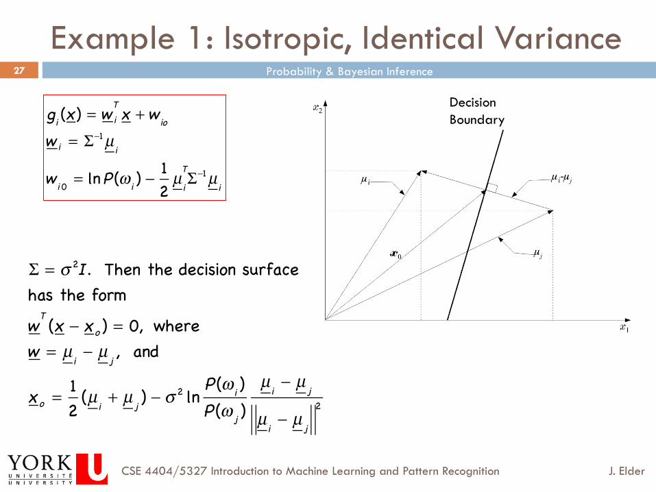
Example 1: Isotropic, Identical Variance
Σ = σ 2I. Then the decision surface has the formwT (x − xo ) = 0, wherew = µ i − µ j , and
xo = 12 (µ i + µ j ) − σ 2 ln P (ω i )
P (ω j )µ i − µ j
µ i − µ j
2
gi (x) = w iT x +wio
w i = Σ−1µ i
wi 0 = lnP (ω i ) −12 µ
TiΣ
−1µ i
Decision Boundary

Probability & Bayesian Inference
J. Elder CSE 4404/5327 Introduction to Machine Learning and Pattern Recognition
28
Example 2: Equal Covariance
gi (x) = w iT x +wio
w i = Σ−1µ i
wi 0 = lnP (ω i ) −12 µ
TiΣ
−1µ i
gij (x) = wT (x − x 0) = 0
w = Σ−1 (µ i − µ j ),
x 0 = 12 (µ i + µ j ) − ln P (ω i )
P (ω j )⎛
⎝⎜
⎞
⎠⎟
µ i − µ j
µ i − µ j
2
Σ−1
,
and
xΣ−1 ≡ (xT
Σ−1x)12
where

Probability & Bayesian Inference
J. Elder CSE 4404/5327 Introduction to Machine Learning and Pattern Recognition
29
Minimum Distance Classifiers
¨ If the two likelihoods have identical covariance AND the two classes are equiprobable, the discrimination function simplifies:
gi (x) = − 1
2 (x − µ i )T Σi
−1 (x − µ i ) + lnP (ω i ) + Ci
gi (x) = − 1
2 (x − µ i )T Σ−1 (x − µ i )

Probability & Bayesian Inference
J. Elder CSE 4404/5327 Introduction to Machine Learning and Pattern Recognition
30
Isotropic Case
¨ In the isotropic case,
¨ Thus the Bayesian classifier simply assigns the class that minimizes the Euclidean distance de between the observed feature vector and the class mean.
gi (x) = − 1
2 (x − µ i )T Σ−1 (x − µ i ) = − 1
2σ 2 x − µ i2
de = x − µ i

Probability & Bayesian Inference
J. Elder CSE 4404/5327 Introduction to Machine Learning and Pattern Recognition
31
General Case: Mahalanobis Distance
¨ To deal with anisotropic distributions, we simply classify according to the Mahalanobis distance, defined as�
Δ = gi (x) = (x − µ i )T Σ−1 (x − µ i )( )1/2
Let y =Ut x − µ( ). Then we have,
Δ2 = y tΛ−1y = yiΛ ij−1y j
ij∑ = λi
−1yi2
i∑ ,
where yi = uit x − µ( ).

Probability & Bayesian Inference
J. Elder CSE 4404/5327 Introduction to Machine Learning and Pattern Recognition
32
General Case: Mahalanobis Distance
Thus the curves of constant Mahalanobis distance c have ellipsoidal form.
Let y =Ut x − µ( ). Then we have,
Δ2 = y tΛ−1y = yiΛ ij−1y j
ij∑ = λi
−1yi2
i∑ ,
where yi = uit x − µ( ).

Probability & Bayesian Inference
J. Elder CSE 4404/5327 Introduction to Machine Learning and Pattern Recognition
33
Given ω 1 , ω2 : P (ω 1 ) = P(ω2 ) and p(x ω 1 ) = N(µ1 , Σ), p(x ω2 ) = N(µ2 , Σ),
µ1 =00
⎡
⎣⎢
⎤
⎦⎥ , µ2 = 3
3⎡
⎣⎢
⎤
⎦⎥ , Σ = 1.1 0.3
0.3 1.9⎡
⎣⎢
⎤
⎦⎥
classify the vector x = 1.02.2
⎡
⎣⎢
⎤
⎦⎥ using Bayesian classification:
• Σ-1 = 0.95 −0.15
−0.15 0.55⎡
⎣⎢
⎤
⎦⎥
• Compute Mahalanobis dm from µ1 , µ2 :
d2m,1 = 1.0, 2.2⎡⎣ ⎤⎦ Σ
−1 1.02.2
⎡
⎣⎢
⎤
⎦⎥ = 2.952, d2
m,2 = −2.0, −0.8⎡⎣ ⎤⎦ Σ−1 −2.0−0.8
⎡
⎣⎢
⎤
⎦⎥ = 3.672
• Classify x → ω 1. Observe that dE ,2 < dE ,1
Example:

Probability & Bayesian Inference
J. Elder CSE 4404/5327 Introduction to Machine Learning and Pattern Recognition
34
The Multivariate Normal Distribution: Topics
1. The Multivariate Normal Distribution 2. Decision Boundaries in Higher Dimensions 3. Parameter Estimation
1. Maximum Likelihood Parameter Estimation 2. Bayesian Parameter Estimation

Probability & Bayesian Inference
J. Elder CSE 4404/5327 Introduction to Machine Learning and Pattern Recognition
35
Maximum Likelihood Parameter Estimation
35
Suppose we believe input vectors x are distributed as
p(x) ≡ p(x;θ ), where θ is an unknown parameter.
Given independent training input vectors X = x1,x2 , ...xN{ }we want to compute the maximum likelihood estimate θML for θ.
Since the input vectors are independent, we have
p(X;θ ) ≡ p(x 1, x2 , ...xN;θ ) = Πk=1
N
p(xk;θ )
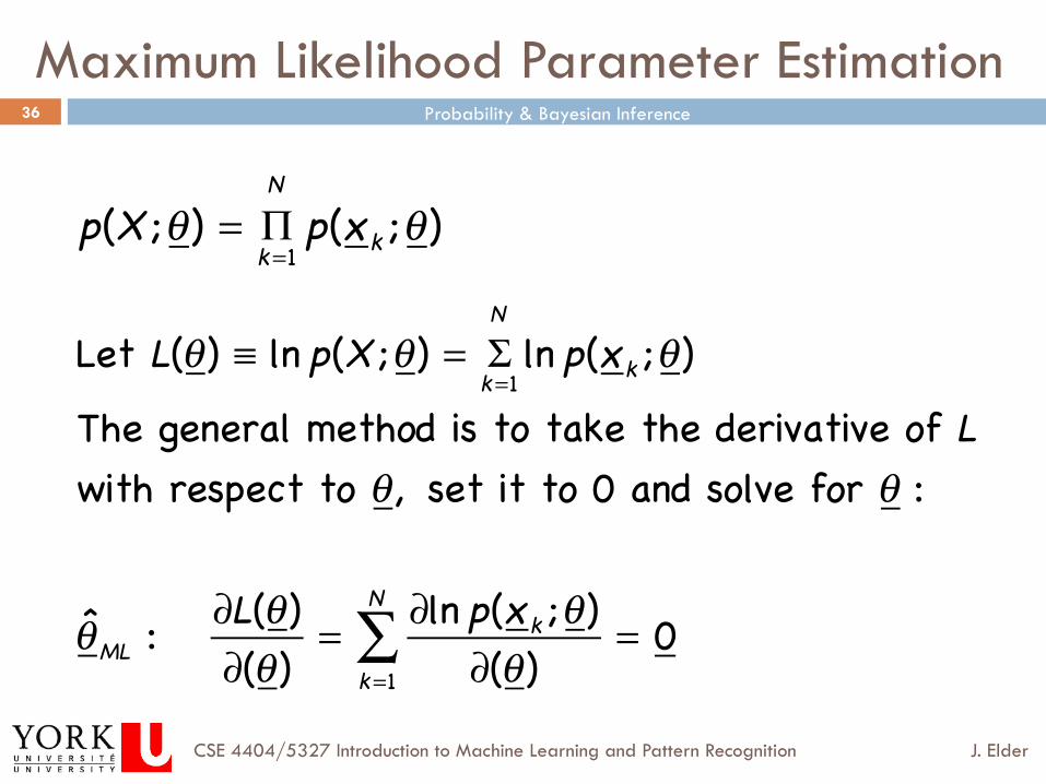
Probability & Bayesian Inference
J. Elder CSE 4404/5327 Introduction to Machine Learning and Pattern Recognition
36
Maximum Likelihood Parameter Estimation
36
p(X;θ ) = Π
k=1
N
p(xk;θ )
Let L(θ ) ≡ ln p(X;θ ) = Σk=1
N
ln p(xk;θ )
The general method is to take the derivative of L
with respect to θ , set it to 0 and solve for θ :
θ̂ML : ∂L(θ )
∂(θ )=
∂ln p(xk;θ )
∂(θ )k=1
N
∑ = 0

Probability & Bayesian Inference
J. Elder CSE 4404/5327 Introduction to Machine Learning and Pattern Recognition
37
Properties of the Maximum Likelihood Estimator
37
Let θ 0 be the true value of the unknown parameter vector.ThenθML is asymptotically unbiased: lim
N→∝E[θML ] = θ 0
θML is asymptotically consistent: limN→∞
E θ̂ML − θ 02= 0

Probability & Bayesian Inference
J. Elder CSE 4404/5327 Introduction to Machine Learning and Pattern Recognition
38
Example: Univariate Normal
Likelihood func6on

Probability & Bayesian Inference
J. Elder CSE 4404/5327 Introduction to Machine Learning and Pattern Recognition
39
Example: Univariate Normal

Probability & Bayesian Inference
J. Elder CSE 4404/5327 Introduction to Machine Learning and Pattern Recognition
40
Example: Univariate Normal
Thus σML is biased (although asymptotically unbiased).

Probability & Bayesian Inference
J. Elder CSE 4404/5327 Introduction to Machine Learning and Pattern Recognition
41
Example: Multivariate Normal
¨ Given i.i.d. data , the log likeli-hood function is given by

Probability & Bayesian Inference
J. Elder CSE 4404/5327 Introduction to Machine Learning and Pattern Recognition
42
Maximum Likelihood for the Gaussian
¨ Set the derivative of the log likelihood function to zero,
¨ and solve to obtain
¨ One can also show that
Recall: If x and a are vectors, then ∂∂x
xta( ) =
∂∂x
atx( ) = a
⎛⎝⎜
⎞⎠⎟

Probability & Bayesian Inference
J. Elder CSE 4404/5327 Introduction to Machine Learning and Pattern Recognition
43
The Multivariate Normal Distribution: Topics
1. The Multivariate Normal Distribution 2. Decision Boundaries in Higher Dimensions 3. Parameter Estimation
1. Maximum Likelihood Parameter Estimation 2. Bayesian Parameter Estimation

Probability & Bayesian Inference
J. Elder CSE 4404/5327 Introduction to Machine Learning and Pattern Recognition
44
¨ Assume is known. Given i.i.d. data , the likelihood function for is given by
¨ This has a Gaussian shape as a function of (but it is not a distribution over ).
σ2
µ
µ
µ
Bayesian Inference for the Gaussian (Univariate Case)

Probability & Bayesian Inference
J. Elder CSE 4404/5327 Introduction to Machine Learning and Pattern Recognition
45
Bayesian Inference for the Gaussian (Univariate Case)
¨ Combined with a Gaussian prior over ,
¨ this gives the posterior
¨ Completing the square over , we see that
µ
µ

Probability & Bayesian Inference
J. Elder CSE 4404/5327 Introduction to Machine Learning and Pattern Recognition
46
Bayesian Inference for the Gaussian
¨ … where
¨ Note:
Shortcut: p µ | X( ) has the form C exp −Δ2( ).
Get Δ2 in form aµ2− 2bµ +c = a(µ −b / a)2 + const and identify
µN= b / a
1
σN
2= a
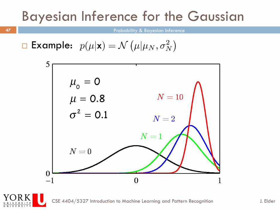
Probability & Bayesian Inference
J. Elder CSE 4404/5327 Introduction to Machine Learning and Pattern Recognition
47
Bayesian Inference for the Gaussian
¨ Example:
µ0= 0
µ = 0.8
σ2= 0.1

Probability & Bayesian Inference
J. Elder CSE 4404/5327 Introduction to Machine Learning and Pattern Recognition
48
Maximum a Posteriori (MAP) Estimation
In MAP estimation, we use the value of µ that maximizes
the posterior p µ | X( ) :µ
MAP= µ
N.

Probability & Bayesian Inference
J. Elder CSE 4404/5327 Introduction to Machine Learning and Pattern Recognition
49
Full Bayesian Parameter Estimation
¨ In both ML and MAP, we use the training data X to estimate a specific value for the unknown parameter vector θ, and then use that value for subsequent inference on new observations x:
¨ These methods are suboptimal, because in fact we are always uncertain about the exact value of θ, and to be optimal we should take into account the possibility that θ assumes other values.
p x | θ( )

Probability & Bayesian Inference
J. Elder CSE 4404/5327 Introduction to Machine Learning and Pattern Recognition
50
Full Bayesian Parameter Estimation
¨ In full Bayesian parameter estimation, we do not estimate a specific value for θ.
¨ Instead, we compute the posterior over θ, and then integrate it out when computing :
p x | X( )
p(x X ) = p(x θ )p(θ X )dθ∫
p(θ X ) =p(X θ )p(θ )
p(X )=
p(X θ )p(θ )
p(X θ )p(θ )dθ∫
p(X θ ) = Πk=1
N
p(xk θ )

Probability & Bayesian Inference
J. Elder CSE 4404/5327 Introduction to Machine Learning and Pattern Recognition
51
Example: Univariate Normal with Unknown Mean
Consider again the case p(x µ) N µ,σ( )where σ is known and µ N µ0,σ 0( ) We showed that p µ|X( ) N µN ,σ N
2( ) , where
In the MAP approach, we approximate p(x X ) N µN ,σ 2( )
In the full Bayesian approach, we calculate p(x X ) = p(x | µ)p(µ X ) dµ∫
which can be shown to yield p(x X ) N µN ,σ 2 + σ N2( )
Probability & Bayesian Inference
J. Elder CSE 4404/5327 Introduction to Machine Learning and Pattern Recognition
52
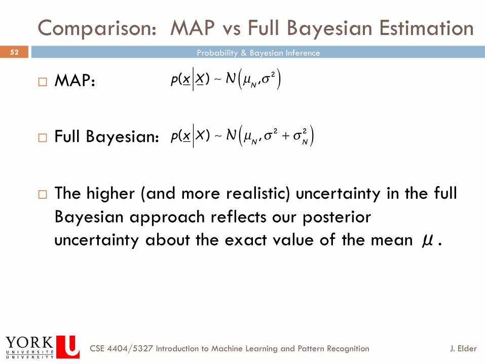
Comparison: MAP vs Full Bayesian Estimation
¨ MAP:
¨ Full Bayesian:
¨ The higher (and more realistic) uncertainty in the full Bayesian approach reflects our posterior uncertainty about the exact value of the mean μ.
p(x X ) N µN ,σ 2( )
p(x X ) N µN ,σ 2 + σ N2( )

![STATISTICAL APPLICATIONS OF THE MULTIVARIATE SKEW NORMAL ... · arXiv:0911.2093v1 [stat.ME] 11 Nov 2009 STATISTICAL APPLICATIONS OF THE MULTIVARIATE SKEW-NORMAL DISTRIBUTION A.Azzalini](https://img.pdfslide.net/doc/110x75/5b40be297f8b9a91078d8f73/statistical-applications-of-the-multivariate-skew-normal-arxiv09112093v1.jpg)