Multivariate Markov switching dynamic conditional correlation GARCH representations for contagion analysis

DOI: 10.1007/s10260-005-0108-8Statistical Methods & Applications (2005) 14: 145–161

c© Springer-Verlag 2005

Multivariate Markov switchingdynamic conditional correlation GARCHrepresentations for contagion analysis�

Monica Billio, Massimiliano Caporin��

Universita Ca’ Foscari di Venezia, San Giobbe, 873 30121 Venezia, ItalySchool for Advanced Studies in Venice Foundation, Rio Novo 3488, 30123 Venezia, Italy

Abstract. This paper provides an extension of the Dynamic Conditional Correla-tion model of Engle (2002) by allowing both the unconditional correlation and theparameters to be driven by an unobservable Markov chain. We provide the estima-tion algorithm and perform an empirical analysis of the contagion phenomenon inwhich our model is compared to the traditional CCC and DCC representations.

Key words: Dynamic correlations, Markov switching models, contagion

1. Introduction

Since the seminal work of Bollerslev (1990), multivariate GARCH models attractedconsiderable interest given their direct application in both financial and economicempirical researches. By now, they represent a fundamental tool for asset and riskmanagement and are employed in most financial market analyses. They have beenextended and updated following the enormous literature of the univariate GARCHmodels, trying to taken into account the empirical findings in a multivariate setting.However, a first order of problems came into play when considering large dimensionmultivariate GARCH models: we refer to the complexity of parameter estimationprocedures, which directly derives from the high number of coefficients. A secondset of problems concerns the asymptotic properties of the quasi maximum likelihood

� We acknowledge financial support from the Italian national research project on “The Euro andEuropean financial market volatility: contagion, interdependence and volatility transmission” financedby the Italian Ministry of University and Research. Furthermore, we thank William De Pieri for researchassistance and are grateful to Loriana Pelizzon, Claudio Pizzi, Domenico Sartore and the participantsat the Forecasting Financial Markets 2004 conference and at the XLII Annual Meeting of the ItalianStatistical Society for helpful comments. Usual disclaimer applies.�� (e-mai: [email protected])

Correspondence to: M. Billio ([email protected])

146 M. Billio, M. Caporin

estimators for this type of models, which is not yet theoretically derived. In fact,Jeantheau (1998) provides conditions for QMLE consistency using a pointwiseconvergence criterion whereas a uniform convergence is required.

The high number of parameter problems motivated for the search of a simpleand easy-to-estimate GARCH representation, and, at the same time, prevented fora direct use of generalised representations when the number of variables increases.This paper belongs to this research area and provides an up-to-date review of currentfeasible multivariate GARCH representation.

In particular, we extend the DCC model of Engle (2002) introducing Markovswitches in the unconditional correlation matrix and in the DCC parameters. Fromthe methodological point of view, this is a natural extension of the model recentlyproposed by Pelletier (2004). Moreover, the interest for this extension comes fromthe opportunity to use these DCC GARCH representations for contagion analysis.

In fact, the 1990s were punctuated by a series of severe financial and cur-rency crises: the 1992 European monetary system attacks, the 1994 Mexican pesocollapse, the 1997 EastAsian crises, the 1998 Russian collapse, the 1998 LTCM cri-sis, the 1999 Brazilian devaluation, and the 2000 technological crisis. One strikingcharacteristic of several of these crises was how an initial country-specific shockwas rapidly transmitted to markets of very different sizes and structures aroundthe globe. This has prompted a surge of interest in “contagion” and this is a rele-vant issue from the empirical and theoretical point of view. Volatility transmissionand contagion are relevant at an international level by themselves and have impor-tant consequences for monetary policy, optimal asset allocation, risk measurement,capital adequacy, and asset pricing.

In this paper, contagion – as opposed to interdependence – conveys the ideathat international propagation mechanisms are discontinuous and then a hiddenMarkov chain can be useful to describe this discontinuity. However, there is noagreement on this definition and many other definitions have been proposed. In theempirical applications, we show the presence of the loss of interdependence phe-nomenon, which supports the thesis of discontinuities in the volatility propagationmechanisms.

Section 2 reviews the currently available multivariate GARCH models thatconsider dynamic conditional correlations. In Sect. 3 we introduce the Markovswitching DCC model (MS-DCC). Sect. 4 shortly presents the contagion issue andSect. 5 describes the empirical application to a set of European stock market indices.Section 5 concludes.

2. Multivariate GARCH with dynamic correlations

The Vech-GARCH of Engle and Kroner (1995) is one of the more general repre-sentations; it is characterised by the following equations (the GARCH orders havebeen restricted to one for the sake of exposition, but higher orders can easily behandled):

Yt = f(It−1; θ

)+ εt, εt|It−1 ∼ iid (0, Ht) (1)

V ech (Ht) = C + AV ech (εtε′t) + BV ech (Ht−1)

Multivariate Markov switching dynamic conditional correlation GARCH representations 147

where Yt is a k-dimensional vector of variables whose mean can be time depen-dent; It−1 is the information set at time t − 1; εt is the vector of residuals thatare independently and identically distributed following a multivariate unspecifieddistribution with time-dependent variance-covariance matrix Ht; furthermore, Ht

follows a multivariate GARCH(1,1)-type representation in which the parametermatrices are of dimension n × n with n = k × (k + 1) /2 and V ech (X) stacksthe lower triangular elements of X .

The constraints required to ensure the positivity of conditional variances and thepositive semi-definiteness of the variance-covariance matrix create many problemsboth in the implementation and in the optimisation steps. For this reason, the largestpart of the literature focuses on finding a representation that reduces the computa-tional burden of a Vech-Multivariate GARCH. Among others, we cite the diagonalVech and BEKK representations of Engle and Kroner (1995). However, the mostused structure is the Constant Conditional Correlation, introduced by Bollerslev(1990).

The basic idea of the CCC-GARCH is in noting that the variance-covariancematrix can be represented as the product of a correlation matrix by a standarddeviation matrix:

Ht = diag (σ1t, σ2t...σkt) R diag (σ1t, σ2t...σkt) = DtRDt (2)

where R is a correlation matrix and Dt is a diagonal matrix of standard deviations.This simplification allows both the overcoming of most parameter restrictions (onlythe coefficients of the conditional variances have to be bounded using the standardunivariate inequality) and of a simple two-step estimation strategy that considersunivariate GARCH estimation in the first step, while in the second step the correla-tion matrix is estimated by its sample estimator. Therefore, this approach is feasibleeven for very large systems.

More recently, attention has been drawn to a direct modelisation of the correla-tion matrix, leaving aside the conditional variances. This new field was started byEngle (2002) who suggested generalising the CCC-GARCH model of Bollerslev(1990), allowing the conditional correlations to vary over time. Equation (2) is thenreplaced by

Ht = DtRtDt (3)

where the correlation matrix follows a time dependent relation as follows

Rt = Q∗−1t QtQ

∗−1t (4)

Qt = (1 − α − β) Q + αηt−1η′t−1 + βQt−1

Q∗t = diag

(√q11,t,

√q22,t...

√qkk,t

)

Q =1T

T∑i=1

ηt−1η′t−1

In this model, Q represents the unconditional correlations, Q∗t guarantees that Rt is

a correlation matrix (qii,t, i = 1, ..., k are the elements of the diagonal of Qt) and ηt

are the standardised residuals, ηt = D−1t Et where Dt = diag (σ1t, σ2t...σkt). It is


worth noting that the DCC just impose a GARCH-type structure on the conditionalcorrelations and uses only two parameters to add a dynamic behaviour. A verysimilar approach was contemporaneously suggested by Tse and Tsui (2002), withthe only difference that they use small sample correlation estimates (instead of thestandardised residuals ηt) to avoid the further standardisation of Q∗

t .It has also to be noted that the simplicity of the suggested approaches is coupled

with a strong restriction: the dynamic of correlation is constant among all thevariables. This constraint can be removed, as suggested by Engle (2002) estimatingan unrestricted DCC (or Generalised DCC, let us call it GDCC), where

Qt = (ii′ − A − B) � Q + A � ηt−1η′t−1 + B � Qt−1 (5)

and A and B are full square matrices of dimension k, i is a vector of ones and� is the Hadamard product (i.e. the element by element product). Conditions forpositive definiteness of Qt are provided in Ding and Engle (2001). Clearly, theunrestricted DCC model creates the well-known problem of the high number ofparameters, a motivation that was at the base of the development of the CCC andDCC model classes. Therefore, we no longer consider this structure.

Now a lot of work is done on the modelisation of the correlation matrix. Forexample, Franses and Hafner (2003) propose a restricted parameterisation of theGDCC, suggest that A = aa′, where a is vector of dimension k and B = β is ascalar and impose the positive definiteness by modifying the intercept term of theGDCC equation (let us call this model the Franses-Hafner DCC, FH-DCC). Thismodel adds flexibility and the number of parameters decreases sensibly, but it losesthe property of correlation targeting, since the unconditional mean of FH-DCC isnot the unconditional correlation, as in the DCC model.

Other extensions of the DCC model have been suggested. Cappiello et al. (2003)propose to add a term in the DCC equation to take into account the asymmetry(Asymmetric DCC – ADCC). Their model is fairly general to include all previouscases, however the to impose the positive definiteness is a very hard computationalproblem.

Further extensions of DCC models are developed by Billio et al. (2004) andBillio and Caporin (2004). The first paper introduces the Flexible DCC model(FDCC) where the GDCC of Engle (2002) is modified by the introduction of aconstant and of a parameter matrix structure similar to the one used by Franses andHafner (2003). The model is represented by the following equation

Qt = cc′ � Q + aa′ � ηt−1η′t−1 + bb′ � Qt−1 (6)

where a, b and c are partitioned parameter vectors (e.g. a = [a1i (m1) , a2i (m2) ,· · · , awi (mw)]′, where w is the number of partitions and i (mj) is a row vectorof one of dimension mj with

∑j mj = k). The FDCC model loses the correlation

targeting property as the FH-DCC but also reduces the number of parameters.Clearly, the number of parameters depends on the number of partitions imposedon the coefficient vectors, which can include several assets. Finally, the modelprovides a positive definite Qt since it is composed by the sum of positive definiteand semi-definite matrices.


Billio and Caporin (2004) generalise the FDCC to the Quadratic FDCC(QFDCC), which is similar to the model of Cappiello et al. (2003) and uses thestructure of the FDCC. The QFDCC model is characterised by the following struc-ture

Qt = CQC ′ + Aηt−1η′t−1A

′ + BQt−1B′ (7)

where A, B and C are partitioned parameter matrices. If the parameter matricesare diagonal the QFDCC model collapses on the FDCC one. The QFDCC modelprovides positive definite correlation matrices if the eigenvalues of A + B arein modulus less than one and the matrix CQC ′ is positive definite. This resultsderive from Engle and Kroner (1995) noting that the QFDCC is similar to a BEKKrepresentation for the correlation matrix.

Finally, Chan et al. (2003) suggest a slightly different approach. They provide ageneral representation for a dynamic correlation model with stochastic coefficientsthat nests all the previous DCC-type models. The most important issue consideredby Chan et al. (2003) pertains the asymptotic properties of their GARCC model:in fact they provide the regularity conditions under which the Quasi MaximumLikelihood estimator is consistent. Moreover, they show how the DCC of Engle(2002) is included as a particular case of their GARCC and argue that even theGDCC is a particular case of their representation.

Even if all these representations are useful to deal with high dimension prob-lems and thus can be helpful for volatility transmission analysis (following Kingand Wadhwani (1990), King et al. (1994) and Ramchard and Susmel (1998)), theycannot account for discontinuities. In fact, the standard DCC model and its gener-alisations provide a feasible structure for the treatment of large systems, but theyimpose a fix unconditional correlation over the sample and for long samples thismay be questionable. A change in the unconditional correlation levels can be hy-pothesize to explain some empirical findings and this change can be associated witha regime switch between two or more unconditional correlation levels.

The idea of adding Markov switching regimes to the correlation has already beenconsidered by Pelletier (2004), who restricted his attention to a CCC model withregime switches (MS-CCC thereon). In particular, Pelletier suggested the followingrestricted representation for the correlation matrix

Rt = Γλ (st) + Ik [1 − λ (st)] (8)

where λ (st) is a state-dependent variable assuming only positive values and st =1, 2, ..., S. This representation is motivated by the computational problems relatedto a full estimation of S state specific correlation matrices, which clearly involvea very high number of parameters. However, this approach does not allow thecorrelations to change sign and this possibility cannot be excluded a priori.

In the next section we extend the DCC class by allowing both the unconditionalcorrelation and the parameters to be driven by a latent Markov chain.

2.1. The estimation issue

The class of DCC models can be estimated with a two-step Quasi Maximum Like-lihood approach, as demonstrated by Engle (2002). The full log-likelihood can be


represented as

LogL (Y ) =1T

T∑t=1

log L (Yt) =1T

T∑t=1

[−1

2(log |Ht| + ε′

tH−1t εt

)](9)

but recalling that Ht = DtRtDt and that |DtRtDt| = |Dt| |Rt| |Dt| we have

LogL (Y ) = − 12T

T∑t=1

[2 log |Dt| + log |Rt| + ε′

tD−1t R−1

t D−1t εt

](10)

Therefore, replacing in a first step the correlation matrix by an identity matrix,we can maximise only with respect to the parameters appearing in Dt. In a secondstage, the estimation will then be performed conditionally on the estimate variances,i.e. on

LogL (Y |D) = − 12T

T∑t=1

[log |Rt| + η′

tR−1t ηt

](11)

Engle (2002) and Engle and Sheppard (2002) provide the asymptotic propertiesof the standard DCC model estimators, a result which is generalised by Chan et al.(2003).

3. A DCC model with Markov switching regimes: the MS-DCC model

To modelise a possible change in the unconditional correlations, we follow Pel-letier (2004) and introduce a regime switch between two or more unconditionalcorrelation levels. Moreover, we allow for changes in the sign of the switching cor-relations, a possibility which is excluded in Pelletier (2004) but cannot be excludeda priori.

Differently from Pelletier (2004), we consider the standard DCC model in thefollowing reformulation:

Qt = [1 − α (st) − β (st)] Q (st) + α (st) ηt−1η′t−1 + β (st) Qt−1 (12)

where both the unconditional correlation matrix and the parameters driving thesystem dynamics can be regime dependent. The Markov chain is governed by thefollowing transition matrix

P = {pji i, j = 1, ...S} (13)

where S is the number of regimes. In the following we refer to this model as theMS(S)-DCC.

As in Pelletier (2004), we restrict the regime dependent structure only to thecorrelations excluding any effect on variances. This restriction allows us to considera two-step estimation procedure. In fact, a full Markov switching model will becomehighly unstable given the huge number of switching parameters.


Given the joint presence of regime switches and dynamic correlations the es-timation of model (12) is very difficult being the Hamilton filter useless. In fact,since the matrix Qt is not observed, the equation (12) should be modified into

Qijt = [1 − αj − βj ] Qj + αjηt−1η

′t−1 + βjQ

lit−1 (14)

where Qj = Q(st = j) and the upperscript j, i refers to the state in t, t − 1,respectively; the dynamic structure of Qt induce the dependence of the currentregime to all the past regimes. Using equation (14) in a standard Hamilton filter,an S-fold increase of possible combinations is created at any new point in time.Therefore, some approximation is needed.

According to Kim (1994), we consider the following modified Hamilton filter:

[i] given the filtered probabilities Pr(st−1 = i|It−1

)as inputs, determine

the joint probabilities:

Pr(st = j, st−1 = i|It−1) = Pr (st = j|st−1 = i) Pr

(st−1 = i|It−1)

i, j = 1...S

[ii] evaluate the regime dependent likelihood:

Qijt = [1 − αj − βj ] Qj + αjηt−1η

′t−1 + βjQ

it−1 i, j = 1...S

Qijt = diag

(√qij11,t,

√qij22,t...

√qijkk,t

)

Rijt =

(Qij

t

)−1Qij

t

(Qij

t

)−1

LogLt(Yt|Dt, st = j, st−1 = i, It−1) = − 12T

(log

∣∣∣Rijt

∣∣∣ + η′t

(Rij

t

)−1ηt

)

[iii] evaluate the likelihood of observation t:

LogLt(Yt|Dt, It−1) =

S∑j=1

S∑i=1

LogLt(Yt|Dt, st

= j, st−1 = i, It−1)× Pr

(st = j, st−1 = i|It−1)

LogL(Yt, . . . , Y1) = LogL(Yt−1, . . . , Y1) + LogLt(Yt|Dt, It−1)

[iv] update the joint probabilities:

Pr(st = j, st−1 = i|It

)

=LogLt(Yt|Dt, st = j, st−1 = i, It−1) Pr

(st = j, st−1 = i|It−1

)LogLt(Yt|Dt, It−1)


for i, j = 1...S;

[v] compute the filtered probabilities:

Pr(st = j|It

)=

S∑i=1

Pr(st = j, st−1 = i|It

)j = 1...S

[vi] update the correlation matrix using the following approximation:

Qjt =

∑Si=1 Pr (st = j, st−1 = i|It) Qij

t

Pr (st = j|It)

[vii] iterate [i] to [vi] until the end of the sample.

Note that the last equation collapses an S2-fold into an S-fold by an approxima-tion based on the current state probabilities (the well-known Kim approximation).To initialise the filter, the regime probabilities could be set equal to the uncondi-tional probabilities while Qj

0 can be obtained with a sample correlation estimatorcomputed in two different subset of the full sample, possibly distinguishing beforeand during a crisis period. For this operation, some relevant information can beobtained by a preliminary analysis.

We should also specify a smoother for the hidden regimes. Given the approxi-mation used in the filter, the smoother will include itself an implicit approximationas discussed by Kim and Nelson (1998). The algorithm requires as inputs the filteredprobabilities obtained with the approximated filter and the transition probabilities.Since Pr

(sT = j|IT

)is known (it is obtained in the last iteration of the filter), it

can be used to initialise the smoother, which is the following:

Pr(st = j, st+1 = m|IT

)

=Pr

(st+1 = m|IT

)Pr (st = j|It) Pr (st+1 = m|st = j)Pr (st+1 = m|It)

Pr(st = j|IT

)=

S∑m=1

Pr(st = j, st+1 = m|IT

)(15)

for j, m = 1...S.In large systems the MS-DCC model may have some convergence problems

given the high number of parameters involved. In this case the parameterisationsuggested by Pelletier (2004) can be used also in our framework. We should thenrearrange equation (14), letting Qj = Γλ (st = j) + Ik [1 − λ (st = j)]where jis the regime in t. Thus, a single correlation matrix has to be estimated, sensiblyreducing the number of parameters; however, as in Pelletier (2004), changes in thecorrelation sign are not allowed.

Finally, the MS structure can easily be extended to all the other DCC modelsreviewed in Sect. 2.


4. Contagion definitions and literature

The last two decades have experienced a series of financial and currency crises,many of them carrying regional or even global consequences: the 1987 Wall Streetcrash, the 1992 European monetary system collapse, the 1994 Mexican pesos crisis,the 1997 “Asian Flu”, the 1998 “Russian Cold”, the 1999 Brazilian devaluation, the2000 Internet bubble burst and the default crisis in Argentina of July 2001. Most ofthese crises hit emerging markets, which are more sensitive to shocks because oftheir underdeveloped financial markets and their large public deficits. The commonfeature shared by these events was that a country specific shock spreads rapidly toother markets of different sizes and structures all around the world.

It is still quite puzzling to justify the reason why a country reacts to a crisisaffecting another country to which the former is not linked by any economic funda-mentals. Many authors dealing with the topic of international propagation of shockshave referred to this circumstance as a contagion phenomenon, even if there is stillno agreement on which factors lead to identify a contagion event precisely, and itis not yet clear how to define the contagion event itself.

Referring to theWorld Bank’s classification, we can distinguish three definitionsof contagion:

– Broad definition: contagion is identified with the general process of shock trans-mission across countries. The latter is supposed to work both in tranquil andcrisis periods, and contagion is not only associated with negative shocks butalso with positive spillover effects;

– Restrictive definition: this is probably the most controversial definition. Conta-gion is the propagation of shocks between two countries (or group of countries)in excess of what should be expected by fundamentals and considering theco-movements triggered by the common shocks. If we adopt this definition ofcontagion, we must be aware of what constitutes the underlying fundamentals.Otherwise, we are not able to appraise effectively whether excess co-movementshave occurred and then whether contagion is displayed.

– Very restrictive definition: this is the one adopted by Forbes and Rigobon (2000).Contagion should be interpreted as the change in the transmission mechanismsthat takes place during a turmoil period. For example, the latter can be inferredby a significant increase in the cross-market correlation. As we have said, thisis the definition that will be used in this paper.

Many papers have focused on the question of contagion, testing for its existencewith statistical methods. Their approaches vary with regard to the definition ofcontagion they choose as a starting point. As we have anticipated we will use thethird definition.

Why do we concentrate on this aspect of contagion? Why is this definitionof contagion important as is its exploration? Because, as observed by Forbes andRigobon, the other definitions of contagion and relative approaches of analysis areunable to shed light on three main issues: international diversification, evaluationof the role and the potential effectiveness of international institutions and bail-outfunds, and propagation mechanisms. Indeed, a critical assumption of investment


strategies is that most economic disturbances are country specific. As a conse-quence, stock in different countries should be less correlated. However, if marketcorrelation increases after a bad shock, this would undermine much of the rationalefor international diversification.

The variety of empirical methods developed for the analysis of contagion hasthe aim of testing the stability of parameters in the sphere of a chosen econometricmodel. Evidence of parameter shifts is a signal of a change in the transmissionmechanism, so according to the third definition there has been contagion. If, on thecontrary, the parameters are constant, we should move to an interdependence case.Several methodologies have been used to statistically search for contagion in thisway and others still have to be applied. Rigobon (2001) offers a good survey ofthese procedures, which are mainly based on OLS estimates (including GLS andFGLS), Principal Components, Probit models and correlation coefficient analysis.

However, the methodologies listed above carry some imperfections because thedata often suffer from heteroskedasticity, endogenous and omitted variable prob-lems. Some authors have tried to solve these problems in a similar way, althoughthey have reached different conclusions in terms of contagion. In particular, Forbesand Rigobon (2002) developed a correlation analysis adjusting correlation coeffi-cients only for heteroskedasticity under the assumption of no omitted variables orsimultaneous equations problems. Corsetti et al. (2002) built up a model in whichthe specific shock of the country under crisis does not necessarily act as a globalshock because this could bias the analysis in favour of interdependence instead ofcontagion. The authors therefore introduce more sophisticated assumptions aboutthe ratio between the variance of the country-specific shock and the variance of theglobal factors weighted by factor loadings. Nevertheless, both these tests are stillhighly affected by the presence of omitted variables, the time zone and the windowsused (see Billio and Pelizzon (2003)).

Working with Markov switching models and using regime probabilities (filteredor smoothed) to monitor the volatility transmission process is a relatively innova-tive approach, which has already suggested by Hassler (1995), Ang and Bekaert(1999) and Baele (2003), but which has not yet completely developed in conta-gion analysis (see however Pericoli and Sbracia (2003) for a review of empiricalworks considering Markov switching models, Edward and Susmel (2003), Galloand Otranto (2004) and Billio et al. (2004)).

To combine a DCC-GARCH model with a Markov switching approach allowsus to take into account several important aspects: first of all the heteroskedasticityof the data can be properly modelised; secondly, to consider dynamic correlationpermits to analyse the dynamics of contagion; finally, to consider a latent Markovchain allows the endogenous definition of the crisis periods.


5. Detecting contagion with the MS-DCC model

This section presents an empirical application of the MS-DCC model. We considera set of daily stock market indices: Standard & Poors 500 (S&P), FTSE100 (FTSE),EuroStoxx50 (EX), Nikkey225 (NK), Hang Seng (Hong Kong – HS), Straits (Sin-gapore – STR) and KLSE (Malaysia – KLSE). The analysis is performed on thedaily returns and the series run from January 2000 to December 2003. Data havebeen downloaded from Datastream.

Since holiday days are not common over the stock markets, we consider the fol-lowing cut-off rule: we remove all common holidays while non-common holidaysare replaced by a zero return. This approach has the advantage of not introducingspurious correlation in the data and to preserve all available points in time. Fur-thermore, to avoid any problem due to asynchronous trading we took the two-daymoving average of the returns, as in Forbes and Rigobon (2002).

After this step, we filtered the idiosyncratic heteroskedasticity for each series byfitting univariate GARCH models with asymmetry (see Glosten et al. (1993)). Theresults are reported in Table 1. All indices evidence a relevant asymmetric effect:in all cases the γ parameter is highly significant1.

Table. 1. GJR-GARCH estimatesGJR G RC

0.01730 0.04662 0.15591 0.851100.00013 0.00051 0.00074 0.000810.12299 0.36178 0.18097 0.519870.00095 0.00164 0.00181 0.002030.21468 0.15853 0.18033 0.637040.00318 0.00151 0.00128 0.003500.22473 0.25267 0.06831 0.542640.00507 0.00370 0.00147 0.007090.15593 0.39825 0.17502 0.484290.00143 0.00206 0.00190 0.002470.01693 0.08890 0.09102 0.852190.00011 0.00052 0.00053 0.000630.02205 0.06315 0.13952 0.836080.00019 0.00059 0.00071 0.00097

NK

HS

STR

KLSE

Parameters / Standard Error

S&P

FTSE

EX

Series

On the variance-filtered series we estimated a set of static and dynamic corre-lation models: the CCC, the MS(2)-CCC, the DCC and the MS(2)-DCC; Table 2reports the likelihoods of the four cases.

1 In the GJR-GARCH model (Glosten et al., 1993) the variance equation is

σ2t = ω + αε2

t−1 + γε2t−1I (εt−1) + βσ2

t−1

where I (εt−1) is an indicator function assuming the value 1 for negative values of εt−1 and 0 otherwise.


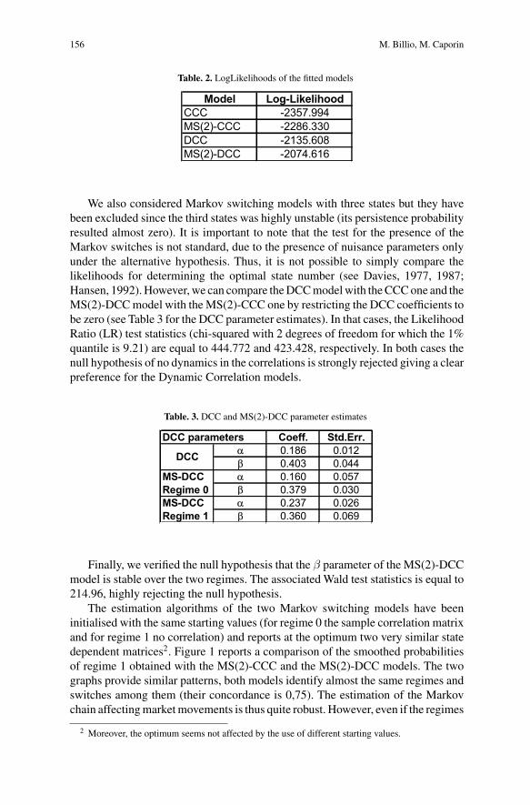
Table. 2. LogLikelihoods of the fitted models

Model Log-LikelihoodCCC -2357.994MS(2)-CCC -2286.330DCC -2135.608MS(2)-DCC -2074.616

We also considered Markov switching models with three states but they havebeen excluded since the third states was highly unstable (its persistence probabilityresulted almost zero). It is important to note that the test for the presence of theMarkov switches is not standard, due to the presence of nuisance parameters onlyunder the alternative hypothesis. Thus, it is not possible to simply compare thelikelihoods for determining the optimal state number (see Davies, 1977, 1987;Hansen, 1992). However, we can compare the DCC model with the CCC one and theMS(2)-DCC model with the MS(2)-CCC one by restricting the DCC coefficients tobe zero (see Table 3 for the DCC parameter estimates). In that cases, the LikelihoodRatio (LR) test statistics (chi-squared with 2 degrees of freedom for which the 1%quantile is 9.21) are equal to 444.772 and 423.428, respectively. In both cases thenull hypothesis of no dynamics in the correlations is strongly rejected giving a clearpreference for the Dynamic Correlation models.

Table. 3. DCC and MS(2)-DCC parameter estimates

DCC parameters Coeff. Std.Err.0.186 0.0120.403 0.044

MS-DCC 0.160 0.057Regime 0 0.379 0.030MS-DCC 0.237 0.026Regime 1 0.360 0.069

DCC

Finally, we verified the null hypothesis that the β parameter of the MS(2)-DCCmodel is stable over the two regimes. The associated Wald test statistics is equal to214.96, highly rejecting the null hypothesis.

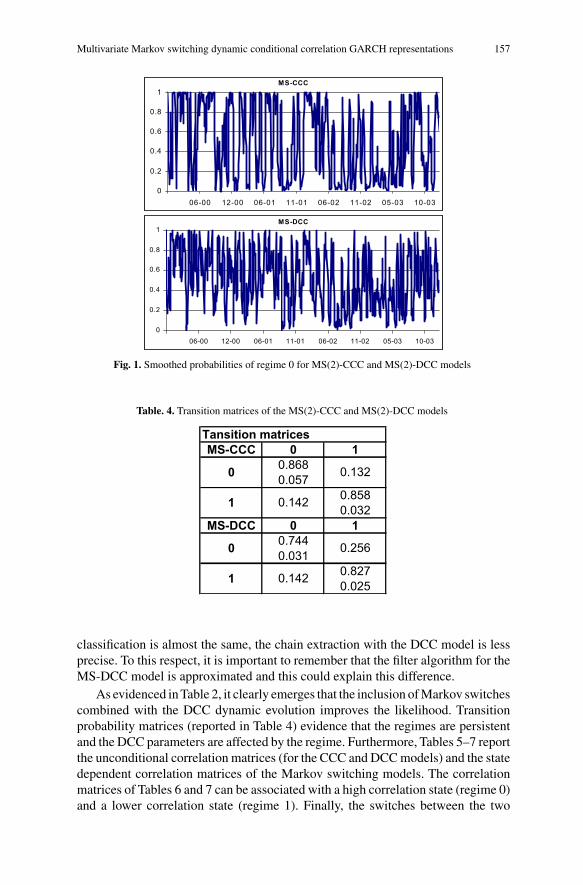
The estimation algorithms of the two Markov switching models have beeninitialised with the same starting values (for regime 0 the sample correlation matrixand for regime 1 no correlation) and reports at the optimum two very similar statedependent matrices2. Figure 1 reports a comparison of the smoothed probabilitiesof regime 1 obtained with the MS(2)-CCC and the MS(2)-DCC models. The twographs provide similar patterns, both models identify almost the same regimes andswitches among them (their concordance is 0,75). The estimation of the Markovchain affecting market movements is thus quite robust. However, even if the regimes

2 Moreover, the optimum seems not affected by the use of different starting values.


MS-CCC

0

0.2

0.4

0.6

0.8

1

06-00 12-00 06-01 11-01 06-02 11-02 05-03 10-03

MS-DCC

0

0.2

0.4

0.6

0.8

1

06-00 12-00 06-01 11-01 06-02 11-02 05-03 10-03

Fig. 1. Smoothed probabilities of regime 0 for MS(2)-CCC and MS(2)-DCC models

Table. 4. Transition matrices of the MS(2)-CCC and MS(2)-DCC models

Tansition matricesMS-CCC 0 1

0.8680.057

0.8580.032

MS-DCC 0 10.7440.031

0.8270.0250.142

1

0 0.132

0.142

0 0.256

1

classification is almost the same, the chain extraction with the DCC model is lessprecise. To this respect, it is important to remember that the filter algorithm for theMS-DCC model is approximated and this could explain this difference.

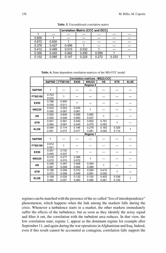
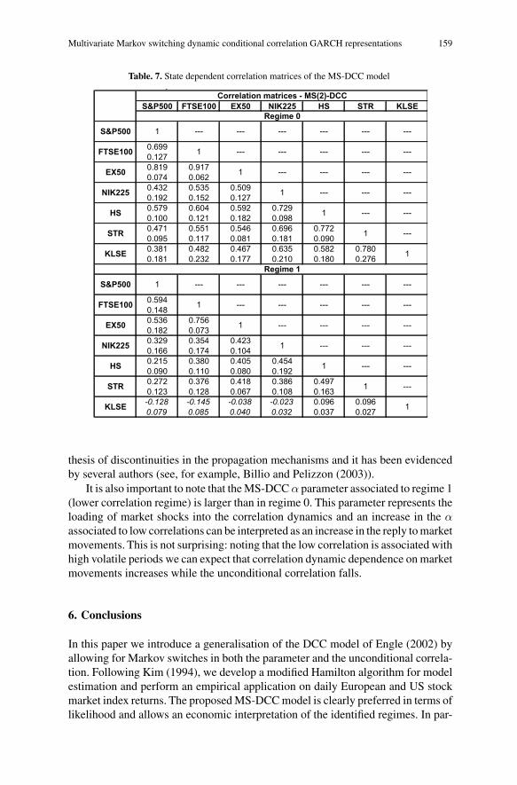
As evidenced in Table 2, it clearly emerges that the inclusion of Markov switchescombined with the DCC dynamic evolution improves the likelihood. Transitionprobability matrices (reported in Table 4) evidence that the regimes are persistentand the DCC parameters are affected by the regime. Furthermore, Tables 5–7 reportthe unconditional correlation matrices (for the CCC and DCC models) and the statedependent correlation matrices of the Markov switching models. The correlationmatrices of Tables 6 and 7 can be associated with a high correlation state (regime 0)and a lower correlation state (regime 1). Finally, the switches between the two


Table. 5. Unconditional correlation matrixTable 5: Unconditional correlation matrix

1 --- --- --- --- --- ---0.659 1 --- --- --- --- ---0.672 0.830 1 --- --- --- ---0.378 0.427 0.456 1 --- --- ---0.412 0.499 0.510 0.532 1 --- ---0.356 0.440 0.462 0.490 0.599 10.102 0.085 0.147 0.225 0.272 0.333 1

Correlation Matrix (CCC and DCC)

Table. 6. State dependent correlation matrices of the MS-CCC model

S&P500 FTSE100 EX50 NIK225 HS STR KLSE

0.7030.0320.786 0.9000.035 0.0110.433 0.553 0.5350.050 0.067 0.0610.550 0.606 0.595 0.6820.052 0.046 0.063 0.0370.501 0.561 0.540 0.652 0.7610.064 0.067 0.045 0.070 0.0520.049 0.114 0.146 0.276 0.163 0.3290.091 0.073 0.077 0.081 0.083 0.110

0.6120.0410.557 0.7520.045 0.0370.318 0.277 0.3680.072 0.075 0.0720.256 0.367 0.408 0.3540.067 0.048 0.064 0.0800.196 0.294 0.372 0.294 0.4150.073 0.058 0.049 0.081 0.0500.159 0.029 0.132 0.153 0.402 0.3360.062 0.057 0.060 0.096 0.061 0.105

Correlation matrices - MS(2)-CCC

Regime 0

1

1

---

1

1

1 --- ---

1

1

1

1

1

1

---

---

------

---

---

---

---

---

---

---

---

---

---

---

---

---

---

---

---

---

---

---

------

---

1

1

Regime 1

1 ------

---

---

---

---

---S&P500

FTSE100 ---

--- --- ------

---

EX50

NIK225

HS

STR

KLSE

S&P500

FTSE100

EX50

NIK225

HS

STR

KLSE

regimes can be matched with the presence of the so-called “loss of interdependence”phenomenon, which happens when the link among the markets falls during thecrisis. Whenever a turbulence starts in a market, the other markets immediatelysuffer the effects of the turbulence, but as soon as they identify the noisy signaland filter it out, the correlation with the turbulent area reduces. In that view, thelow correlation state, regime 1, appear as the dominant regime for example afterSeptember 11, and again during the war operations in Afghanistan and Iraq. Indeed,even if this result cannot be accounted as contagion, correlation falls support the


Table. 7. State dependent correlation matrices of the MS-DCC modelp

S&P500 FTSE100 EX50 NIK225 HS STR KLSE

0.6990.1270.819 0.9170.074 0.0620.432 0.535 0.5090.192 0.152 0.1270.579 0.604 0.592 0.7290.100 0.121 0.182 0.0980.471 0.551 0.546 0.696 0.7720.095 0.117 0.081 0.181 0.0900.381 0.482 0.467 0.635 0.582 0.7800.181 0.232 0.177 0.210 0.180 0.276

0.5940.1480.536 0.7560.182 0.0730.329 0.354 0.4230.166 0.174 0.1040.215 0.380 0.405 0.4540.090 0.110 0.080 0.1920.272 0.376 0.418 0.386 0.4970.123 0.128 0.067 0.108 0.163-0.128 -0.145 -0.038 -0.023 0.096 0.0960.079 0.085 0.040 0.032 0.037 0.027

Correlation matrices - MS(2)-DCC

Regime 0

1 --- --- --- --- --- ---

1 --- --- --- --- ---

1 --- --- --- ---

1 --- --- ---

1 --- ---

1 ---

1

Regime 1

1 --- --- --- --- --- ---

1 --- --- --- --- ---

1 --- --- --- ---

1 --- --- ---

1KLSE

STR

1 --- ---

1 ---

HS

NIK225

EX50

FTSE100

S&P500

KLSE

STR

HS

NIK225

EX50

FTSE100

S&P500

thesis of discontinuities in the propagation mechanisms and it has been evidencedby several authors (see, for example, Billio and Pelizzon (2003)).

It is also important to note that the MS-DCC α parameter associated to regime 1(lower correlation regime) is larger than in regime 0. This parameter represents theloading of market shocks into the correlation dynamics and an increase in the αassociated to low correlations can be interpreted as an increase in the reply to marketmovements. This is not surprising: noting that the low correlation is associated withhigh volatile periods we can expect that correlation dynamic dependence on marketmovements increases while the unconditional correlation falls.

6. Conclusions

In this paper we introduce a generalisation of the DCC model of Engle (2002) byallowing for Markov switches in both the parameter and the unconditional correla-tion. Following Kim (1994), we develop a modified Hamilton algorithm for modelestimation and perform an empirical application on daily European and US stockmarket index returns. The proposed MS-DCC model is clearly preferred in terms oflikelihood and allows an economic interpretation of the identified regimes. In par-


ticular, we point to the presence of the loss of interdependence phenomenon, whichsupports the thesis of discontinuities in the volatility propagation mechanisms.

References

Ang A, Bekaert G (1999) International asset allocation with time-varying correlations. NBER WP n.w7056.

Baele L (2003)Volatility spillover effects in european equity markets: Evidence from a regime switchingmodel. EIFC – Technology and Finance Working Papers 33, United Nations University, Institutefor New Technologies, forthcoming Journal of Financial and Quantitative Analysis

Billio M, Caporin M (2004) A generalised dynamic conditional correlation model for portfolio riskevaluation. Proceedings of the Deloitte Conference in Risk Management 2004, Antwerp, 29–30March 2004

Billio M, Caporin M, Gobbo M (2004) Flexible dynamic conditional correlation multivariate GARCHmodels for asset allocation. Proceedings of the Forecasting Financial Market conference 2003,Paris, 4–6 June 2003 and Working Paper 04.03, GRETA, Venice

Billio M, Lo Duca M, Pelizzon L (2004) Contagion detection with switching regime models: a shortand long run analysis. mimeo GRETA, Venice

Billio M, Pelizzon L (2003) Contagion and interdependence in stock markets: have they been misdiag-nosed? Journal of Economics and Business 55(5/6): 405–426

Bollerslev T (1990) Modelling the coherence in short-run nominal exchangerates: a multivariate gener-alized ARCH approach. Review of Economic Studies 72: 498–505

Cappiello L, Engle RF, Sheppard K (2003) Asymmetric dynamics in the correlations of global equityand bond returns. European Central Bank Working Paper 204

Chan F, Hoti S, McAleer M (2003) Generalised autoregressive conditional correlation. preprint Depart-ment of Economics, University of Western Australia

Corsetti G, Pericoli M, Sbracia M (2002) Some contagion, some interdependence more pitfalls in testsof financial contagion. Discussion Paper n. 3310, CEPR

Davies RB (1977) Hypothesis testing when a nuisance parameter is present only under the alternative.Biometrika 64: 247–254

Davies RB (1987) Hypothesis testing when a nuisance parameter is present only under the alternative.Biometrika 74: 33–43

Ding Z, Engle RF (2001) Large scale conditional covariance matrix modeling estimation and testing.Working paper 01029, Department of Finance, NYU Stern School of Business

Edward S, Susmel R (2003) Interest-Rate volatility in emerging markets. Review of Economics andStatistics 85: 328–348

Engle RF, Kroner KF (1995) Multivariate simultaneous generalized ARCH. Econometric Theory 11:122–150

Engle RF (2002) Dynamic conditional correlation: a new simple calss of multivariate GARCH models.Journal of Business and Economic Statistics 20: 339–350

Engle RF, Sheppard K (2001) Theoretical and empirical properties of dynamic conditional correla-tion multivariate GARCH University of California, San Diego, Discussion paper 2001-15, NBERWorking Paper 8554

Forbes K, Rigobon R (2000) Measuring contagion: conceptual and empirical issues. In: Claessens S,Forbes K (eds) International financial contagion. Kluwer Academic Publishers

Forbes KJ, Rigobon R (2002) No contagion, only interdependence: measuring stock market comove-ments. Journal of Finance 57(5): 2223–2261

Franses PH, Hafner CM (2003) A generalised dynamic conditional correlation model for many assetreturns. Econometric Institute Report EI 2003-18, Erasmus University, Rotterdam

Gallo GM, Otranto E (2004) Contagion and interdependence in financial markets: a new approachFEDRA Working Papers

Glosten L, Jagannathan R, Runkle D (1993) On the relation between the expected value and volatilityof nominal excess returns on stocks. Journal of Finance 46: 1779–1801


Hansen BE (1992) The likelihood ratio test under non-standard conditions: testing the Markov switchingmodel of gnp. Journal of Applied Econometrics 7: S61–S82 Also “Erratum”, Journal of AppliedEconometrics 1996 11: 195–198

Hassler J (1995) Regime shifts and volatility spillover on international stock markets. IIES SeminarPaper n. 603

King M, Sentana E, Wadhwani S (1994) Volatility and links between national stock markets. Econo-metrica 62(4): 901–933

King M, Wadhwani S (1990) Transmission of volatility between stock markets. Review of FinancialStudies 3(1): 5–33

Kim C (1994) Dynamic linear models with Markov switching. Journal of Econometrics 60: 1–22Kim C, CR Nelson (1998) State-Space models with regime switching. MIT pressPelletier D (2004) Regime switching for dynamic correlations. forthcoming in Journal of EconometricsPericoli M, Sbracia M (2003) A primer on financial contagion. Journal of Economic Surveys 17(4):

571–608Ramchand L, Susmel R (1998) Volatility and cross correlation across major stock markets. Journal of

Empirical Finance 5: 397–416Rigobon R (2001) Contagion: how to measure it? NBER Working Paper No. w8118Tse YK, Tsui AKC (2002) A multivariate generalised autoregressive conditional heteroscedasticity

model with time-varying correlations. Journal of Business and Economic Statistics 20(3): 351–362

Documents

Multivariate Markov switching dynamic conditional correlation GARCH representations for contagion analysis