MPRAMunich Personal RePEc Archive

Flower farming and flower marketing inWest Bengal : a study of efficiency andsustainability

Debnarayan Sarker and Sanjukta Chakravorty

Centre for Economic Studies, Department of Economics, PresidencyCollege, 86/1 College Street, Kolkata – 700073 (INDIA)

2005

Online at http://mpra.ub.uni-muenchen.de/33776/MPRA Paper No. 33776, posted 28. September 2011 17:27 UTC

Flower Farming and Flower Marketing in West Bengal :

A Study of Efficiency and Sustainability

Debnarayan Sarker and Sanjukta Chakravorty

Centre for Economic Studies, Presidency College, Kolkata.

[Abstract: For diversification in agriculture, one of the areas that have emerged as a fast

growing sector recently in West Bengal is floriculture. In an attempt to examine

empirically the relative efficiency between commercial traditional floriculture and its

competing main field crops – Paddy, Jute, Potato, Wheat, Groundnut, Mustard, this

paper observes that the economic efficiency related to both individual flower crop

farming and mixed crop farming of all categories maintaince high economic efficiency for

farms provided that selections of crops are made properly. This study does not imply an

orderly marketing system for some categories of major commercial flower crops - rose,

tuberose and bel - produced in alluvial zone in West Bengal, because the farmer -

producers’ interest for fair price of these flowers is not supported to their growers during

lean season. While examining the efficiency of flower marketing system, this paper does

not support that the flower market in alluvial zone of West Bengal is efficient in nature,

but, in general, marketing efficiency decreases with the increase in number of market

intermediaries in a marketing channel.]

Keywords: Productivity, Profitability, Output-input ratio, Technical Efficiency,

Marketing Margin, Marketing Channel, Modified Marketing Efficiency.

1

Flower Farming and Flower Marketing in West Bengal :

A Study of Efficiency and Sustainability

Debnarayan Sarker and Sanjukta Chakravorty

Floriculture has emerged as a fast growing sector recently in West Bengal for

diversification, employment generation and value addition in the primary sector. West

Bengal is a potential state blessed with highly conducive agro- climatic conditions for

floriculture. Though the history of growing flowers and ornamental plants is too old, the

commercial trade on these have generated recently for potential diversification,

employment generation and value addition in the primary sector. These have been made

possible for the boost of its exports1, recent expansion of joint ventures by corporate

sectors for exemption from custom duties on imported plant materials, reduction of duties

on materials for green house, high subsidy on airfreight etc. due to impact of economic

reform (1991-92), trade liberalization and global impact within the framework of WTO.

Following these reforms, West Bengal has started commercial farming on a large scale

from the mid 90‟s of the last century. As per the data available from the Directorate of

Food Processing Industries and Horticulture, Government of West Bengal (Government

of West Bengal, 2001 and 2004), it is observed that the area under flower crop in West

Bengal was 9.8 thousand hectares in 1996-97, but in 2002-03, it stood at 17.33 thousand

hectares, registering around 9.80 per cent increase of compound growth rate per annum

between 1996-97 and 2002-03, whereas production growth was around 16.54 per cent

during that period (Table A and Figure A). But the commercial flower farming is

restricted to certain districts of the state (Government of West Bengal, 2001): 5 districts –

Mednapore, Howrah, Nadia, 24 Parganas (North), 24 Parganas (South) – mainly produce

2

commercial flower crops in West Bengal in alluvial zone and Darjeeling district produces

commercial flower crops in Hill Zone. The traditional commercial flower crops in

alluvial zone are, mainly, rose, tuberose, gladiolus, marigold, jui, bel, and

chrysanthemum. But the flower farming and marketing in alluvial zone and hill zone of

West Bengal have hardly been studied. A study of flower farming conducted by Rahim

and Sarkar (1997), based on two Blocks in Mednapore district, under alluvial zone of

West Bengal, reveals that flower crops like tuberose, marigold, rose, gladiolus are more

productive and profitable than that of the main field corps like paddy and potato. The

study of flower farming and flower marketing in India is also very limited. A

considerable empirical study that throws some light on this area relating to production

and productivity is a combined study along with other horticulture crops, such as fruits,

vegetables. Most of the limited studies on floriculture (Singh et al, 1997; Bal and Bal,

1997; Alagumani et al., 1997; Sharma and Vaidya, 1998; Satya, 1999; Goyal, 1999;

Gangaiah, 2001; Vaidya, 2002) reveals higher productivity and/or higher profitability of

some important commercial flower crops like rose, tuberose, chrysanthemum, corssandra,

gladiolus, mullai, pitchi, jasmine, kakaratan (madras malli) orchid compared with the

production of main field crops like paddy, jute, potato, sugarcane, cotton and groundnut.

This paper, thus, studies the relative efficiency and profitability between commercial

traditional flower crops and their competing field crops, examines the cost of production

of flower crop with their seasonal market prices based on the empirical study on sample

farms which are dominated by marginal and small farms under alluvial zone of West

Bengal. It also examines the extent of marketing efficiency of different commercial

flower crops and the relative efficiency of their marketing channels in alluvial zone of

West Bengal based on price spread and marketing margin among different market

intermediaries in two marketing channels.

3

The rest of the paper is divided into five sections. Section II deals with the

conceptual issues related to efficiency of farms and the efficiency of marketing system

that have emerged in the literature. Section III presents the data and methodology

employed for our empirical exercise. In Section IV empirical results have come to light.

Conclusions and policy implications in the light of our empirical results are contained in

Section V.

II

Economic efficiency is the state of economy in which no one can be made better

off without someone being made worse off. Since high level of economic efficiency and

productivity growth are desirable goals of any economy, therefore, it is important to

define and measure efficiency and productivity in ways that respect economic theory and

provide useful information to policy makers.

The literature on frontier production and cost function and the calculation of

efficiency measures begins with Farrell (1957). He defines efficiency as the ability of a

production organization to produce a good at minimum cost. Efficiency (or more

appropriately productive efficiency) is viewed by him as a relative concept, which is

measured as a deviation from best performance in a representative peer group. He

dichotomized efficiency into two parts, namely, Technical efficiency and Allocative

efficiency.

The empirical estimation of production functions had started long before

Farrrell‟s Paper, essentially around 1928 with the papers of Cobb and Douglas (1928).

Until the 1950s production function were used, largely, as devices for studying the

functional distribution of income between capital and labour at the macro economic level.

The origins of empirical analysis of microeconomic production structures were more

reasonably identified with the work of Dean (1951), Johnson (1959) and Nerlove (1963).

But all these focus on costs rather than production per se, although Nerlove, following on

Samuelson (1938) highlighted the relationship between the two. Nevertheless, the

4

empirical attention to production functions at disaggregated levels has been a fairly

recently developed literature(Hildebrand and lieu (1965).

In the empirical literature production and cost were developed largely

independently of the discourse on production frontier; Least squares, or some variant,

were used routinely to pass a function through the middle of a cloud of points, and

residuals of both signs were, as in other areas of study, not singled out for special

treatment, given a name and face as it were (Greene 1993, P.69). But a basic argument

has been made that these averaging estimators were estimating the “average” rather than

“best practice” technology, but this just rationalizes the least squares techniques after the

fact. Farrell‟s Arguments make an intellectual basis for redirecting attention from the

production function specifically to the deviations from that function and respecifics the

regression and the techniques accordingly.

Two types of measurement of technical efficiency are proposed by Farrell-

output augmenting orientation and input conserving orientation. Output based measure is

computed as the ratio of actual output obtained from a given vector of inputs to

maximum possible output achievable from the same input vector. An input based

measure is calculated as the ratio of best practice input usage to actual input, holding

output constant. A decision making unit is said to achieve allocative efficiency in

production of a given level of output if it could allocate the factors of production at a

given set of factor prices in such a way as the marginal rate of substitution between two

factors becomes equal to their factor price ratio. The allocative, or price, component

refers to the ability to combine inputs and outputs in optimal proportion in the light of

prevailing prices.

Two types of Frontier Production Function (FPF), namely deterministic and

stochastic, are employed for computing technical efficiency. A deterministic FPF

envisages a deterministic optimal relationship between input and output, unaffected by

random events and statistical noise such as measurement error. Thus, in the deterministic

FPF models, the actual level of output of a firm is assumed to lie below the frontier only

due to the existence of technical inefficiency in the production process of a firm. In

reality, however, random events like machine or equipment failures, product defects and

supply bottlenecks in addition to measurement error do occur frequently, which often

affect the optimality planned output of a firm. Consequently, the ex ante output of a firm

becomes, instead of fixed number, a random variable. This led to the conceptualization of

stochastic FPF in which the optimal relationship between inputs and output is considered

to be stochastic, rather than deterministic. The stochastic FPF thus attributes the shortfall

in a firm‟s observed output from the corresponding point in the frontier to the technical

inefficiency as well as to the random events and statistical noise.

Two alternative techniques are employed in the construction of frontier

production function, viz., mathematical programming and econometric technique. The

main advantage of using mathematical programming technique vis-a vis econometric

technique is that it does not impose any explicit functional form (e.g. Cobb-Douglus) on

production function to be estimated. However, the chief limitation of this technique is

that it can estimate only deterministic frontier and produces „estimates‟ which have no

statistical properties such as standard errors or ratios etc. On the contrary, the

econometric approach is capable of estimating deterministic as well as stochastic

frontiers and provides estimates with statistical properties. This paper uses stochastic or

econometric frontier production function approach to examine the relative economic

5

efficiency between flower farming and its competing main field crop farming of sample

farms.

In the area of marketing, the marketing system is considered to be efficient if

the goods move from producers to the consumers at the minimum cost consistent with the

provision of the services and consumers‟ desires or otherwise. The total margin includes

(a) The cost involved in moving the product from the point of production to the point of

consumption (b) the profiles of the various market functionaries involved in moving the

produce from the initial point of production to the ultimate consumer. If a higher

magnitude of marketing margin is not adequately shared by the actual producers, the

greater is the inefficiency in the system and vice-versa. Competitions plays a key role in

minimizing wastes and help to avoid concentration of wealth with few traders.

Conditions of marketing efficiency in marketing are best satisfied by perfectly

competitive conditions. The closer the actual conditions to perfect competition, the

stronger would be the possibilities for minimizing wastes and exploitation and the greater

the tendency for a uniform price to prevail over the entire market area. As a matter of fact

marketing efficiency of all commodities continues to be important aspect in any economy

and can help to avoid concentration of wealth with few traders.

The studies on marketing margin and cost are important, as they reveal many

facets of marketing and the price structure as well as efficiency of the system. The

magnitude of margin relative to the price of product indicates the efficiency of the

marketing system. The larger the margin of intermediaries in percentage of farm harvest

price and also of retail price, greater is the inefficiency in the marketing system or lesser

competitive marketing organization is and vice versa. Both in earlier and in recent

studies2, the extent of price spread between producers‟ price and consumers‟ price of the

same commodity have been employed extensively as a better indicator of marketing

efficiency of marketing system. The study examines the efficiency of marketing system

of flowers in the alluvial zone of West Bengal based on price spread and marketing

margin among different market intermediaries in two important marketing channels .It is

important to mention that efficient marketing system is very essential for accelerating

production because it influence farmers‟ decision in allocating area under a particular

crop in a particular time period.

III

The empirical findings of this study are based on secondary source from a

published book entitled “A Survey on Present Status of Floriculture in West Bengal” by

the Department of Floriculture and Landscaping, Faculty of Horticulture, Bidhan

Chandra Krishi Viswavidyalaya, Mohanpur, Nadia West Bengal. The survey was

conducted by Roychowdhury (2000) in five districts of West Bengal – Mednapore,

Howrah, Nadia, North 24 Parganas, South 24 Parganas – in 1998-99 taking 120 block in

five districts and five growers in each block. Total sample households, which were

selected by random sampling technique, were 100 in number. For selecting block, the

following two criteria were identified: a) Blocks with the highest concentration of flower

6

cultivation, b) Blocks with highest acreage under flowers among all the blocks of the

district. The survey was also carried out in six important flower markets – Mallikghat or

Jagannathghat wholesale flower market in Howrah, Deulia in Mednapore, Dhantala in

Nadia, Thakurnagore in North 24 Parganas, New Market and College Street market in

Calcutta – under the sample area.

In order to study the different aspects of flower farming and flower marketing

under our study, tabular analysis, proportions, averages etc. have been used. Economic

efficiency is measured by comparing output and input values. With quantities only

technical efficiency can be calculated, while with quantities and prices economic

efficiency can be calculated(Lovell, 1996: 6). Defining and measuring economic

efficiency requires the specification of an economic objective and information of market

prices(Lovell, 1996: 14). In order to measure economic efficiency the revenue

maximization problem is solved separately for each household in the sample. The

constrained maximization problem of a household who desire to maximize total revenue

is subjected to the constraints imposed by fixed inputs supplies in physical

terms(Handerson and Quandt, 1980: 95). But as the unit of measurement for both

physical inputs and physical outputs of all commodities under our study are not same(e.g.

quintals, number), we use physical unit of inputs in monetary terms for measuring

economic efficiency of different crops rotation-wise cultivated by sample farms (per acre

per annum) under our study. This paper uses Cobb-Douglas stochastic frontier production

function approach in order to estimate economic efficiency. It is said that the extent by

which a farm lies below its production frontier which sets the limit to the range of

maximum obtainable output is regarded as a measure of inefficiency under frontier

production function approach (Neogi and Ghose, 1998: M19). We measure economic

efficiency of NTFPs following Aigner et al. (1977) and Meeusen and Broeck(1977)

under the stochastic frontier production function, which is popularly known as

7

„composite error‟ model with cross-sectional data. The advantage of stochastic frontier

over the deterministic frontier is that farm-specific efficiency and random error effect can

be separated. We have specified a C-D type stochastic frontier production function in

order to estimate the level of economic efficiency. The C-D functional form is generally

preferred because of its well-known advantages. Kopp and Smith(1980), and Krishna and

Sahota(1991) suggest that functional specification has very little impact on measuring

efficiency(Banik, 1994:73). Krishna and Sahota find that Translog and C-D forms yield

similar results in respect of productivity and efficiency(ibid:73). However, in order to

measure economic efficiency of farm under C-D stochastic frontier production function

we take two independent variables-X1, variable cost; X2, fixed cost. A stochastic frontier

model can be written as

Yi = f( Xi , β ) exp(Vi – Ui)

taking logarithm

In Yi = In βo + β1 In Xi + Vi – Ui

Yi = total revenue(in Rs.)

X1i = total variable cost(in Rs.); X2i total fixed cost( in Rs.)

Vi = a symmetrical random variable and i.i.d.N(0, σv²)

Ui = non-negative, one-sided random variable and i.i.d. with a half-normal

distribution [ Ui ׀N(0, σu²)׀ ]. The density functions of U and V can respectively be

written as 2

2

2exp

1

2

1

1)(

UU

U

UUf

U ≤ 0

= 0 otherwise

– ∞ ≤ V ≤ ∞

2

2

2exp

1

2

1)(

VV

V

VVf

8

As a distribution of the error terms, we assume that Vi follows the normal

distribution and Ui follows the half-normal distribution ׀N(0, σu²)׀, then the log

likelihood function is

ℓ(α, β, σ, λ) = – N In σ – constant +i

iiIn

2

2

1

where εi = Vi – Ui , λ = σu / σv, σ2

=

σv2

+ σu2

, Ф(.) = cumulative distribution

function(cdf) of the standard normal distribution.

Here a producer faces own stochastic frontier f(Xi , β) exp(Vi); a deterministic

part f(Xi , β) common to all producers and a producer-specific part exp(Ui). Thus,

economic efficiency is given by

EEi = f(Xi , β) exp(Vi – Ui) = exp(– Ui) ; 0 < EEi ≤ 1 f(Xi , β) exp(Vi)

Yi achieves its maximum value of f(Xi , β) exp(Vi) and EEi = 1, if Ui = 0.

Otherwise Ui ≠ 0 provides the shortfall of observed value from the maximum potential

value. The above equation is estimated by the maximum likelihood (ML) method.

Although the residual components Ui and Vi are not observed directly, the inefficiency

component Ui must be observed indirectly. As a solution for the problem, Jondrow et al.

(1982) present the point estimator of Ui i.e. E[Ui/εi], given εi = In Yi – (In βo + β1 In Xi)

= Vi – Ui . Once the point estimate of Ui i.e. E[Ui/εi] is obtained, the economic efficiency

of each farm can be obtained from

EEi = exp(– Ui) = exp { – E [Ui/εi]} = 1 – E[Ui/εi]

where E[Ui/εi] = ])/(1

)/([

12

i

i

i. Note (.) is the density

function of the standard normal distribution. The mean efficiency or the mathematical

9

expectation of the farm-specific efficiencies can be calculated for given distributional

assumptions for the inefficiency effects. The mean economic efficiency can be defined by

Mean EE = E( exp{ – E[Ui/εi]}) = E{ 1 – E[Ui/εi]}

Economic Efficiency takes the values between zero and one (0 < EEi 1).

Ideally, one can treat farms with efficiency score equal to unity as efficient farms.

The major constraints, among others3, of these secondary data are that the data

relating to price spread, marketing cost and marketing margin among different marketing

agents for two important channels except others are available. These make difficulties for

researchers to represent data in standard econometric analysis. However , for comparing

the marketing efficiency of different crops related to two marketing channels under our

study, the following methods are used.

1. Producer‟s share in consumer‟s price (in percentage) for each channel =

,100C

P

P

Pwhere PP is the net price received by the producer and PC is the price paid by

the consumer.

2. Share of middlemen‟s profit in consumer‟s price (in percentage) for each

channel = ,100CP

Twhere T is the middlemen‟s profit.

3. Marketing efficiency of individual flower crop for each marketing channel

is calculated with the measure of modified marketing efficiency (Sundaravaradarajan and

Jahanmohan, 2002; Agro Economic Research, 2003). Modified Marketing Efficiency

(MME) = PP/(MC+MM), where MC is the marketing cost and MM is the marketing

margin.

IV

Production: As regards the distribution of farms according to size group, Table 1 reveals

that flower farming in the sample area is dominated by marginal and small farms. Out of

the total sample, 68 per cent farms are marginal, 21 per cent, small and 11 per cent are

10

medium in size and there is no any large farm in the sample. As regards area, production

and productivity in real terms of different flower crops, Table 2 shows that with regard to

the area of cultivation, tuberose and rose are the major flower crops in the sample. About

70 per cent of total area is cultivated by these two crops, the contribution of tuberose and

rose being 38.79 per cent and 31.22 per cent respectively. As the unit of measurement of

production of different flower crops are not same, the comparison of productivity (output

per acre of land) between different flower crops cannot clearly be discerned. However,

as to the unit of measurement in number within three flower crops – rose, gladiolus and

chrysanthemum, chrysanthemum has the highest productivity followed by gladiolus and

rose. Out of the remaining four types of flower crops measured in quintals, marigold has

the highest productivity followed by tuberose, bel and jui.

The comparative study regarding output-input ratio between flower crops and

main field-crops grown by sample farmers indicates that the output-input ratio of all

flower crops except gladiolus are observed to be higher than that of their competing field

crops like groundnut, potato, boro paddy, aman paddy, jute, mustard and wheat (Table-3).

But since the unit of measurement of three types of flower crop (rose, gladiolus and

chrysanthemum), which are measured in number, are not same with that of the remaining

crops, the comparative study relating to output-input ratio between flower crops and field

crops should be judged among those crops which are measured by the same unit.

However, the comparative study of output-input ratio between flower crops and its

competing field crops for the same unit of measurement(quintal) shows that the flower

crops have higher output-input ratio than their competing field crops.

In order to judge the relative profitability in monetary terms, the crop-rotation-

wise net return (Rs.) per acre per annum have been worked out for flower crops and their

main competing field crops (Table-4). Inasmuch as the unit of measurement of different

crops is not same in physical terms, the comparative study seems to be relevant in

11

monetary terms. According to that estimate, the net return (Rs.) per acre per annum of

flower farming is found to be higher than that of any combined farming within field crops

rotation-wise cultivated by sample farms for the same year. Within the flower farming,

gladiolus has the highest net return (Rs.) per acre per annum followed by

Chrysanthemum, Rose, Marigold+Marigold4, Tuberose, Jui, Bel and Marigold. The

appraisal of the net return (Rs.) per acre per annum of flower crop farming among the

sample farms, however, is in conformity with the finding of the average yield per acre (in

physical term) per annum (Table-2) and that of the output-input ratio per annum (Table-

3). Turning to the mixed crop farming between flower crop and field crop, Table-4 also

shows that both flower crops and main field crop farming over an agricultural year to the

same unit of land per acre per annum yield high net return (Rs.) as compared with the

mixed farming within the main field crops for the same year. It is important to mention

that the sample farmers of this study produce only marigold, a flower crop, and

groundnut or aman paddy(field crop) in the same plot of land in an agricultural year.

However, the result is very striking: the net return (Rs.) per acre per annum is

considerably higher for the mixed farming between flower crop (marigold) and field

crop(groundnut or Aman paddy) on the same plot of land than that of any of the mixed

farming within main field crops on the same plot of land for the same agricultural year.

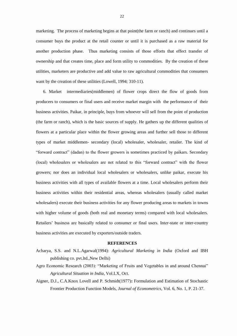
The maximum likelihood (ML) estimation of Cobb–Douglas stochastic production frontier

function and economic efficiency effect model of sample farms for Rotation wise crop per acre per annum

is presented in Table 5.It shows that the explanatory variable X1 (variable cost in Rs) is positive and

statistically significant, whereas X2 (Fixed cost in Rs) is negative and insignificant. The significant

likelihood ratio (LR=20.914) implies high „Goodness of fit‟ of the regression plane to the sample

observation. Regarding economic efficiency which is defined as the ability of a production organization to

produce a good at a minimum cost relative to other farms, Table 6 dose not support that crops yielding

higher net return (in Rs) per acre per annum represented in Table 4,usually possess the higher economic

efficiency because the measurement of productive efficiency / economic efficiency is a relative concept,

12

measured as a deviation from best performance in representative peer group based on optimization

behavior of minimum (e.g. cost) or maximum (e.g. production) attainment. For example Aman Paddy

+Groundnut, a mixed crop farming maintains a lower level of net return (in Rs) per acre, per annum

(Table4) but it succeeds in getting higher level of economic efficiency .As regards individual crop

farming related to flower crop, farms attain higher level of efficiency in an agricultural year per acre for all

individual crop farming except rose (71.58), although the latter maintains a higher level of net economic

return (in Rs.) per acre per annum. Gladiolus has the highest level of economic efficiency (98.77) of all

farming categories –individual farming or mixed farming. Turning to mixed farming all mixed crop

framings are highly efficient for farms except Jute + Mustard and Jute + Wheat. More importantly,

although Jute farming, when cultivated rotation wise either with mustered or with wheat, possesses the

lowest level of efficiency of all, it (jute farming) becomes highly when it is cultivated with potato. So,

rotation wise selection of cropping pattern is an important issue of economic efficiency for farms.

Thus as long as farmers‟ objective are to maximize net return (in Rs.) per unit of

land per annum, individual flower crop farming or mixed farming between flower crop

and field crop have a complete advantage over the mixed crop farming within the field

crops among the sample farms for the same year. But from the standpoint of economic

efficiency both individual flower crop farming and mixed crop farming of all categories

maintain high economic efficiency for farms provided that selection of crops is made

properly. This might lead to a strong favorable implication of potential diversification in

agriculture indicating high value addition and increase in employment within the primary

sector.

Hence a related query is: does producers of flower crops receive positive net

profit in both the seasons- lean and peak, although producers of all flower crops receive

positive net profit annually (i.e. combining all seasons together) Table 7, based on the

published survey report of Roychoudhury (2000), reveals that no stable market price is

observed throughout the year 1997-98 for the same type of flower in the same market as

well as in the different markets. Price becomes higher during peak season when the

demand for flower is very high. The peak season usually comes during puja, ceremonial

13

occasions, national festivals, social occasions, community festivals etc. The market price

for different type of flowers is different in both the seasons. The month of peak season

for all types of flowers are not same; rather it varies over types of flowers. The similarity

is that during peak season of any type of flower, the market price of it is high compared

with lean season and the average cost of production per unit (in Rs.) Of the same type of

flower does not vary across seasons for the same year. What is the most interesting is that

the market price of rose, tuberose and bel during their lean season is lower than their per

unit of cost of production (in Rs.) indicating that the producers of these crops incur loss

(or negative net profit) during lean season. But market price of any type of flower is very

high in relation to its per unit cost during the peak season. It implies that the producer of

all types of flowers might receive positive net profit per unit during peak season. Hence

the relevant issue is: why do the producers of rose, tuberose and bel engage in production

of these types of flowers during lean season when their market price is less than their cost

of production per unit (in Rs.)? Unlike field crops like paddy, jute, wheat, the plants of

these types of flowers last for some seasons. So, the producers of these types of flower

have to carry on their production process during lean season also despite the price per

unit (in Rs.) of these types of flower is less than their respective unit cost of production.

Moreover, the land used for flower crop for any season cannot usually be used for

production of field crops to other season for the same agricultural year because of the

time constraint and maturity period of these two crops does not act as an alternative

between each other in this area .But the farms producing rose, tuberose and bel do not use

all factors of production except land with their full capacity during lean season .

Regarding the cost of production, although Roychoudhury (2000) divided variable cost

and fixed cost of production of flower into 21 items (Roychoudhury, 1998: 13) and 3

items respectively, he did not explicitly mention the cost (in Rs.) of items which

producers were unable to recover during lean season. Variable cost in Roychoudhury‟s

14

work can be divided into two parts – operating cost (cost of fertilizer, chemicals, hired

human labour, transport cost etc.) and capital cost (interest on the use of variable capital,

like, hired power tiller, hired pump-set, hired sprayer etc.). Fixed cost includes land

revenue, imputed interest on own land and interest on fixed capital. We may set up the

profit-maximizing problem of the producer of flower in Kuhn Tucker form.

In keeping with the results of Table7, we assume that during lean season, price

of flower is so low that the producer of commercial flower cannot recover the total

variable cost of production. He incurs loss a part of variable cost (e.g. operating cost)

during lean season and produces flower crop less than his full capacity. On the contrary,

during peak season price per unit of flower is so high that the producer gets abnormal

profit and so he produces flower in accordance with his full capacity. We also assume

that all farms share the economies and diseconomies of production equally.

Let us consider that a profit maximizing farm facing given prices P1 in the peak

season and P2 in the lean season. Output during peak and low seasons are O1 and O2

respectively. The maximum output level is Y, this being produced only in the peak

season (i.e. Y=O1), but output during lean season is less than maximum output (O2 <Y).

Annual operating costs are given by C (O1, O2) and annual capital costs are K (Y). We

also assume that Y, O1, O2 >0. It is assumed that all farms enjoy economics or

diseconomies equally. It can be shown that lean season prices will just cover marginal

operating cost, and peak season prices will exceed marginal operating cost by an amount

equal to marginal capital cost.

The profit-maximizing farm desires to

Maximize = P1O1 + P1O2 – C (O1, O2) –K (Y)

Subject to O1≤Y (multiplier 1)

15

O2≤Y (multiplier 2)

The revenue function is assumed to be concave in the non-negative orthant and

differentiable. The cost function is assumed to be convex in the non-negative orthant and

differentiable for the maximization problem of the farm. The appropriate Lagrange

function is

L = P1O1 + P2O2 –C (O1, O2) – K (Y)+ 1 (Y - O1) + 2 (Y – O2)

and the Kuhn - Tucker conditions are:

L = P1 – C1 – 1 0 O1 0 and O1 L = 0..(1)

O1 O1

L = P2 – C2– 2 0 O2 0 and O2 L = 0 ………………(2)

O2 O2

L = - K (Y) + 1 + 2 0 Y 0 and Y L = 0 …………(3)

Y Y

L = Y – O1 0 1 0 and 1 L = 0 …………………(4)

1 1

L = Y – O2 0 2 0 and 2 L = 0 ………………..(5)

2 2

Since 02 Y, the Kuhn-Tucker theorem gives 2 =0

Hence (2) => P2=C2

and (3) => 1 = K (Y)

So (1) => P1 = C1 + K (Y)

Here, the sufficient conditions will be stated directly in terms of

concavity and convexity. And, in fact, these concepts will be applied not only in the

objective function but to the constraint function as well. Both the conditions are satisfied.

Hence, the Kuhn-Tucker maximum conditions will be necessary and sufficient for a

maximum.

This study does not imply an orderly marketing system for some categories of

major commercial flower crops - rose, tuberose and bel - produced in alluvial zone in

West Bengal, because the farmer - producers‟ interest for fair price of these flowers is not

supported to their growers‟ during lean season. The producer of these types of flowers

16

incur loss during lean season because the market price (in Rs.) of these crops is lower

than their per unit (in Rs.) cost of production.

Marketing:

Marketing of a farm commodity5 and marketing efficiency influence farmers‟

decision in allocating area under a particular crop in a particular time period. A

commodity having higher profit margin or higher producer‟s share in percentage also

influences farmers‟ decision. It is because of the farmer-producer‟s interest for fair price

for his produce. A fair price for a produce might be assured through an orderly

marketing system. Thus the efficient marketing system is very essential for accelerating

production of a particular commodity for a particular time period. At the same time,

marketing efficiency depends to a large extent on the structure and organisation of the

market. Among the six important flower markets under our study, Mallikghat is the

biggest wholesale flower market in Kolkata. Even it is the largest wholesale flower

market in the whole Eastern India (Roychowdhury, 2000:24), because the major portion

of all types of commercial flower crops are regularly traded from this metropolitan

market. The average daily market arrival of flowers (in quintal) at Mallikghat Market

ranges between 699 quintal and 1478 quintal during lean and peak seasons respectively

(Ibid:6). Inter-state, intra-state and inter-country trades of flowers are executed from this

metropolitan market. Although the other five markets under our study are local, these are

also important flower markets within the respective area because large volume of

marketing business of flower crops under the respective districts/metropolitan area are

executed from these local markets (Ibid:21-35).

A large number of market intermediaries6 in the flower markets include

different traders like aratdars(paikars), local(secondary) wholesalers, wholesalers,

retailers and exporters or outside traders. There are 12 marketing channels of flower

crops identified in the study area (Fig.1). This paper limits its study on first two

17

marketing channels-Channel 1 (Producer Paikar/Arathdar Wholesaler

Secondary (Local) Wholesaler Retailer Consumer) and Channel 2 (Producer

Paikar (Aratdar) Wholesaler Retailer Consumer) for non-availability of data for

other marketing channels.

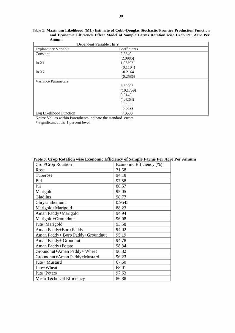
In order to examine the efficiency of marketing system between two marketing

channels channel 1 and channel 2, the price spread of flower crops between different

marketing agents within each marketing channel has been studied. The study of price

spread of flowers not only ascertains the actual price at the various stages of marketing

channels, but also represents the cost incurred in the process of movement of the produce

from farmer to consumer and margin of various intermediaries. Tables-8 and 9 represent

price spread and marketing margin of sample flower crops in Channels-I and II

respectively. They show costs and profit margins at different stages of marketing agents

in both the channels. As to profit margin received by different market intermediaries in

each channel, though no clear pattern is discernable, the retailer is the highest recipient of

profit margin of all market intermediaries in both the channels. The other notable feature

is that producers‟ profit margin are usually lower than the profit margin of most of the

market intermediaries for all crops except rose in both the channels. Thus, out of total

profit margin in each flower crop for both the channels, the major portion of profit

margin of consumers‟ rupee are appropriated by market intermediaries. As regards the

break-up of cost component of marketing margin of sample flower crop, Tables-10 and

11 show that the cost of labour is the most important component of marketing cost,

followed by packaging cost and transport cost in both the channels. The cost structure of

the remaining items meal and tiffin charge, marketing tax and other commission,

storage and maintainance, spoilage are not so important as the cost of labour under

18

each marketing channel. The cost structure of each of the remaining items do not differ

much among one another within each channel.

The extent of marketing efficiency based on price spread and marketing margin

under each marketing channel is examined by three expressions modified marketing

efficiency index, producer‟s share in consumer‟s rupee and trader‟s profit margin in

consumer‟s rupee (Table-12). In the case of modified marketing efficiency index it is

said that higher the numerical value, higher is the marketing efficiency and vice-

versa.Higher the percentage of producer‟s share in consumer‟s rupee (or lower the

trader‟s margin in consumer‟s rupee) in most cases yields higher (lower) efficiency of

marketing and vice-versa. The notable difference is observed for gladiolus which shows

that despite a considerable higher percentage of producer‟s share in consumer‟s rupee,

the level of MME is very lower for both the channels. However among the different

flower crops in each channel, producer‟s share in consumer‟s rupee is the highest in the

case of rose. Similarly, the MME is also observed to be the highest for rose. A

comparative study between two channels reveals that the percentage of producer‟s share

in consumers rupee for all flowers is higher for Channal-2. It implies that the percentage

of trader‟s profit margin in consumers‟ rupee for all flower crops is lower in Channel-2

and out of different flowers in each channel, trader‟s profit margin in consumer‟s rupee is

the lowest for rose. Thus considering all expressions of marketing efficiency, Channel-2

is found to be more efficient than Channel-1 and marketing of rose is more efficient than

any other flower crop under our study. This study, however, does not support that the

flower market in alluvial zone of West Bengal is efficient in nature, but, in general,

marketing efficiency decreases with the increase in number of market intermediaries in a

marketing channel. This study also suggest that flower crops with higher economic

efficiency is usually observed to attain lower modified marketing efficiency or higher

trader‟s margin in consumer‟s rupee and it implies that traders take the advantage of

19

gaining relatively higher profit margin of those flower crops which have higher economic

efficiency.

V

This paper, based on the empirical evidence of flower farming and the structure

of its marketing system, reveals some important phenomena. In the case of production of

flower crops which are dominated by marginal and small farms, there is a clear

indication that output-input ratio of flower cultivation are considerably higher than that of

their competing main field crops like boro paddy, aman paddy, groundnut, potato, jute,

wheat and mustard. Also, the net return (Rs.) per acre per annum of individual flower

crop farming or mixed farming between flower crops and their competing main field

crops in the same unit of land per year is more profitable than that of mixed farming

within the main-field crops and so the former has a complete advantage over the latter.

But from the standpoint of economic efficiency both individual flower crop farming and

mixed crop farming of all categories maintain high economic efficiency for farms

provided that selections of crops are made properly. This might lead to a strong favorable

implication of potential diversification in the area of agriculture for increasing income

and employment in the primary sector of the state. But as the overwhelming majority of

the flower farms are marginal and small in size, to boost up floriculture production as

well as export to a great extent, different floriculture operations should be

commercialised so that it may run like an industry and farms of different sizes may able

to enjoy the economics of large scale production. To this end, the use of modern

agricultural technology by technical experts in this field, expansion of institutional

lending facilities to the flower growers and genuine propagative plant materials for high

quality of production should also be provided to the flower growers.

In the area of marketing system of flower crop, although Channel-II is observed

to be more efficient for greater share of its producers‟ in consumers‟ rupee compared

20

with Channel-I and, in general, marketing efficiency decreases with the increase of

number of intermediaries in a marketing channel, high price spread is the common

phenomena, mainly, because of concentration of market powers in the hands of market

intermediaries who have the main role in this situation. This study also suggest that

flower crops with higher economic efficiency is usually observed to attain lower

modified marketing efficiency or higher trader‟s margin and consumer‟s rupee and it

implies that traders take the advantage of gaining relatively higher profit margin of those

flower crops which have higher economic efficiency. More importantly, the considerable

major profit margin of consumers‟ rupee for all flower crops in both the channels are

appropriated by the market intermediaries/middlemen. This does not indicate that the

trade market of flower crop within the state is efficient in nature. But efficient marketing

system is very essential for accelerating production in this area, because efficient

marketing system makes higher producers‟ profit in consumers‟ rupee which influence

farmers‟ decision in allocating area under a particular crop in a particular time period.

Therefore, more competition in the trade of traditional flower crops are to be introduced.

Mini and small assembling centres may be established in private or cooperative sectors in

flower producing areas, which will save the cost of transportation in assembling labour

charges and distribution phases.

This study does not imply an orderly marketing system for some categories of

major commercial flower crops - rose, tuberose and bel - produced in alluvial zone in

West Bengal, because the farmer - producers‟ interest for fair price of these flowers is not

supported to their growers during lean season. The producer of these types of flowers

incur loss during lean season because the market price (in Rs.) of these crops is lower

than their per unit (in Rs.) cost of production. However, the need for fair price to the

producer of these types of flowers is necessary for accelerating their production. So,

emphasis should be given for adequate storage facilities and the expansion of inter-state,

21

intra-state and inter-country trade \of these flowers, particularly, during lean season when

producers of these crops bear loss Co-operative marketing system can be encouraged in

this regard. Above all, remunerative prices should be assured to the flower growers

during lean reason of these crops, otherwise, the desired growth of flower production as

well as momentum of flower trade will be diminished gradually.

NOTES 1. India is mainly the exporter of cut-flower in the overseas market. Although India‟s

contribution of flower crop in the world trade market is insignificant (below 1 per cent of world

trade), the export earnings (in Rs.) has increased from 5.13 lakhs in 1970-71 to 123.12 lakhs in

2000-01 or 165.86 lakhs in 2002-03.

2. Earlier studies are of Joshi and Sharma (1979),Mirchandrani and Hiranandari (1965),

Chauhan and Sing(1973), Singh, Verma and Agarwal(1974), Desai(1979), Thakur(1974) etc.

Recent studies are of Sunaresaun et.al(2000),Acharya and Agarwal (1994) etc.

3. An important limitation was related to the data of cost of production. Although

Roychowdhury (2000) divided variable cost and fixed cost of production of crops into 21 items

and 3 items (Ibid) respectively, he did not present those data separately. The cost of items (both

real and monetary terms) of a crop was published in an aggregate form. Variable cost in

Roychowdhury‟s work can be divided into two parts – operating cost(cost of fertilizer, chemicals,

hired human labour, transport cost etc.) and capital cost(interest on the use of variable capital, like

hired power tiller, hired pump-set, hired sprayer etc.). Fixed cost includes land revenue, imputed

interest on own land and interest on fixed capital .The other important shortcoming of this

secondary data was that the data of marketing cost and marketing margin of different marketing

agents within each marketing channel were available in an aggregate form of all seasons without

the data of their seasonal variation- lean season and peak season .

4. Marigold is cultivated twice at the same plot of land within one year.

5. The American Marketing Association has defined marketing as the performance of

business activities that direct the flow of goods and services from producer to consumer or final

user. The point of production (the farm or ranch) is the basic source of supply in agricultural

22

marketing. The process of marketing begins at that point(the farm or ranch) and continues until a

consumer buys the product at the retail counter or until it is purchased as a raw material for

another production phase. Thus marketing consists of those efforts that effect transfer of

ownership and that creates time, place and form utility to commodities. By the creation of these

utilities, marketers are productive and add value to raw agricultural commodities that consumers

want by the creation of these utilities (Lowell, 1994; 310-11).

6. Market intermediaries(middlemen) of flower crops direct the flow of goods from

producers to consumers or final users and receive market margin with the performance of their

business activities. Paikar, in principle, buys from whoever will sell from the point of production

(the farm or ranch), which is the basic sources of supply. He gathers up the different qualities of

flowers at a particular place within the flower growing areas and further sell those to different

types of market middlemen- secondary (local) wholesaler, wholesaler, retailer. The kind of

“forward contract” (dadan) to the flower growers is sometimes practiced by paikars. Secondary

(local) wholesalers or wholesalers are not related to this “forward contract” with the flower

growers; nor does an individual local wholesalers or wholesalers, unlike paikar, execute his

business activities with all types of available flowers at a time. Local wholesalers perform their

business activities within their residential areas, whereas wholesalers (usually called market

wholesalers) execute their business activities for any flower producing areas to markets in towns

with higher volume of goods (both real and monetary terms) compared with local wholesalers.

Retailers‟ business are basically related to consumer or final users. Inter-state or inter-country

business activities are executed by exporters/outside traders.

REFERENCES

Acharya, S.S. and N.L.Agarwal(1994): Agricultural Marketing in India (Oxford and IBH

publishing co. pvt.ltd.,New Delhi)

Agro Economic Research (2003): “Marketing of Fruits and Vegetables in and around Chennai”

Agricultural Situation in India, Vol.LX, Oct.

Aigner, D.J., C.A.Knox Lovell and P. Schmidt(1977): Formulation and Estimation of Stochastic

Frontier Production Function Models, Journal of Econometrics, Vol. 6, No. 1, P. 21-37.

23

Alagumani, T., M. Anjugam and R. Rajesh (1997): “Performance of Flower Crops vis-a-vis Field

Crop in Madurai District, Tamil Nadu”, Indian Journal of Agrucultural Economics, Vol.

52, No. 3.

Bal, H.K. and H.S. Bal (1997): “Flower Power in Punjab”, Indian Journal of Agricultural

Economics, Vol. 52 No. 3.

Banik, A. (1994), “Technical Efficiency of Irrigated Farms in a Village of Bangladesh”, Indian

Journal of Agricultural Economics, Vol.49, No.1, January-March.

Banker, R.D., A. Charnes and W.W. Cooper (1984), “Some Models Estimating Technical and

Scale Inefficiencies in Data Envelopment Analysis”. Management Science, Vol. 30. No.9

Brown, P.E.H. (1957), “The Meaning of the Fitted Cobb-Douglas Function”, The Quarterly

Journal of Economics, Vol. 71.

Charnes, A, W.W.Cooper, and E.Rhodes(1978) :| “Measuring the Efficiency of Decision Making

Units‟‟, European Journal of Operational Research 2(6) : 429-444

Charnes, A, W.W.Cooper, and E.Rhodes(1979) : “ Short Communication: Measuring the

Efficiency of Decision Making Units‟‟ European Journal of Operational Research

3(4):339

Charnes, A, W.W.Cooper, and E.Rhodes(1981): “ Evaluting Programme and Managerial

Efficiency: An Application of Data Envelopment Analysis to Program Follow Through,‟‟

Management Science 27(6):668-697.

Chauhan, K.K.S.and R.V.Singh, Marketing of Wheat in Rajasthan , University of Udaypur,

Jobner:1973, Mimeographed

Cobb, S, and P.Douglas(1928), “A Therapy of Production‟‟ American Economic Review 18:139-

165

Dean, J (1951) Managerial Economics Euglewood Cliffs, N.J.: Prentic Hall

Desai V.V. “Dynamics of Price Spread‟‟ Indian Journal of Agricultural Economics ,Bombay

xxxiv (4) 155-160

Farrell, M(1957), “ The Measurement of Productive Efficiency‟‟ Journal of the Royal Statistical

Society (A, General) 120 (P.3): 253-281

Gangaiah, C. (2001): “Floriculture Earns Higher Farm Returns”, Southern Economist, 40(2).

Govt. of West Bengal (2001): “Information on Studies of Major Horticulture Crops: West

Bengal”, Food Processing Industries and Horticulture Directorate, West Bengal.

Govt. of West Bengal (2004): “Information on Studies of Major Horticulture Crops: West

Bengal”, Food Processing Industries and Horticulture Directorate, West Bengal.

Goyal, S.K. (1999): “Economics of Rose Cultivation and Its Marketing in Sonepat District of

Haryana State”, Indian Journal of Agricultural Marketing, 13(3).

Handerson, J.M. and R.Quandt(1971): Microeconomic Theory, McGraw Hill, New York.

24

Hildebrand, G, and T lie (1965), Manufacturing Production Function in The United States.Thaca

N.Y.:Cornell University Press.

Jha, R.and B.S. Sahni (1993), Industrial Efficiency: An Indian Perspective, Wiley Eastern

Limited, New Delhi.

Johnston ,J (1959), Statistical Cost Analysis N.Y.:Mc-Graw Hill

Jondrow, J., C.A.Knox Lovell, I.S.Materov and P. Schmidt(1982): On the Estmation of Technical

Inefficiency in the Stochastic Frontier Production Function Models, Journal of

Econometrics, Vol. 19, Nos. 2/3, P. 233-38.

Joshi, P.K. and V.K. Sharma (1979) , “ Retain Farm Price Of Rice in Selected States of India‟‟

Indian Journal of Agricultural Economics Vol. 34(4) 130-135

Kalirajan, K.P. and R.T. Shand(1994) “Economics in Disequilibrium: An Approach from the

Frontier”, Macmillan India Limited.

Koopmans, T.C(1951), Activity Analysis of Production and Allocation, N.Y.: Wiley

Kopp, R.J. and V.K.Smith(1980): Frontier Production Function Estimates for Steam Electric

Generation: A Comparative Analysis, Southern Economic Journal, Vol. 46, No. 4.

Krishna, K.L. and G.S. Sahota (1991): “Technical Efficiency in Bangladesh Manufacturing

Industries”, Bangladesh Development Studies, Vol. 19, Nos. 1 and 2, March-June.

Lovell, C.A.K. (1993), “Production Frontiers and Productive Efficiency”, in H.O. Fried. C.A.K.

Lovell and P. Schmidt (Eds. (1993), The Measurement of Productive Efficiency:

Techniques and Applications, Oxford University Press, New York, U.S.A.

Lowell, D.H. (1994): “Marketing Agricultural Commodities”, in G.L. Cramer and C.W.

Jensen(Eds), 1994, Agricultural Economics and Agribusiness, John Wiley and Sons, Inc.

Meeusen, W. and Julien van den Broeck(1977): Efficiency Estimation from Cobb-Douglas

Production Functions with Composed Error, International Economic Review, Vol. 18, P.

435-44.

Mirchandam, R.T. and G.J. Hiranandam(1965), “ Regulated Markets-Their Review and Their

Impact of Market Structure and Efficiency‟‟ Seminar Series V, Marketing of Agricultural

Commodities Indian Society of Agricultural Economics, Bombay 72-82

Mythili, G. and K.R. Shanmugam (2000), “Technical Efficiency of Rice Growers in Tamil Nadu,

A Study Based on Panel Data”, Indian Journal of Agricultural Economics, Vol. 55, No.

1, January-March.

Neogi, C. and B. Ghosh (1998), “Impact of Liberalisation on Performance of Indian Industries: A

Firm Level Study”, Economic and Political Weekly, Vol. 33, No. 9, February 28.

Nerlove, M(1963), : “ Returns to Scale in Electricity Supply‟‟ in C.Christ, ed, Measurement in

Economics Stanford, Calif,: Stanford University Press

Pithadia, V.H. (1998): “Floriculture is a Growing Business”, Southern Economists, 36(19).

25

Rahim, K.M. and D. Sarkar (1997): “Techno-organization characteristics of Floriculture in West

Bengal”, Indian Journal of Agricultural Economics, Vol. 52, No. 3.

Roychowdhury, N.(2000): “A Survey on Present Status of Floriculture in West Bengal”,

Department of Floriculture and Landscaping, Faculty of Horticulture, Bidhan Chandra

Krishi Viswavidyalaya, Mohanpur, Nadia, West Bengal.

R.Sundaresan, K.N. Selvaraj, C. Ramasamy and Anil kuravila(2000) “ Agricultural Marketing

Technology and Increasing Market Orientation –Issues and Futures Strategies‟‟ Indian

Journal of Agricultural Marketing ,Conf.Sept.P.51-62

Samuellson,(1938), “ Foundation of Economic Analysis, Cambridge, Mass : Harvard University

press

Satya, S.I. (1999): “Floriculture Coming to Bloom”, Facts for you, 19(8).

Sharma, T.R. and Vaidya, C.S. (1998): “Floriculture in Himachal Pradesh”, Kurukshetra, 46(8).

Shephard, R(1953), Cost and Production Functions , Princeton , N.Y.; Princeton University Press

Singh, R.V.,R.C. Verma and N.L. Agarwal (1974) : “Marketing Cost and Margins of a Co-

operative of Marketing Society and Private Wholesale Trader-A Study‟‟, Agricultural

Marketing Nagpur, XVII(1), April, 14-18

Singh, R.B., R.N. Prasad, H.K. Nigam and R. Saran (1997): “Economics of Flower Production in

District Farrukabad, Uttar Pradesh”, Indian Journal of Agricultural Economics, Vol. 52,

No. 3.

Sundaravaradarajan K.R.and K.R. Jahanmohan (2002): “Marketing Cost, Margin, Price-spread

and Marketing Efficiency of Cashew in Tamil Nadu”, Agricultural Situation in India,

Vol.LIX, April.

Thakur D.S. (1974) “Foodgrain Marketing Efficiency- A case Study of Gujrat‟‟ Indian Journal of

Agricultural Economics, Bombay XXIX(4) Oct-Dec, 61-64

Vaidya, B.V. (2002): “Floriculture: An Innovative Industry for Rural People”, Kurukshetra,

50(9).

William H Greene : (1993) “ The Econometric Approach to Efficiency Analysis‟‟ in Fried , H.O.

Lovel , C.A.K. and Schmidt (eds.). The Measurement of Productive Efficiency

Techniques and Applications, Oxford University Press . N.Y

26

Table A: Area (in thousand hectares) and Production (in thousand metric tonnes) of

Flower Crop in West Bengal during 1996-97 and 2002-03.

Year Area (in thousand

hectares)

Production (in thousand metric

tonnes)

1996-97

1997-98

1998-99

1999-00

2000-01

2001-02

2002-03

9.80

10.00

10.50

11.05

13.50

13.87

17.33

53.90

58.00

62.95

68.75

98.98

103.95

131.24

Figure A: Area (in thousand hectares) and Production (in thousand metric tonnes) of

Flower Crop in West Bengal during 1996-97 and 2002-03.

0

20

40

60

80

100

120

140

19

96-

97

19

97-

98

19

98-

99

19

99-

00

20

00-

01

20

01-

02

20

02-

03

Area(in thousandhectares)

Production(inthousand metrictonnes)

27

Table 1: Size Distribution of Sample Farms in Sample Blocks.

Name of Block Marginal Small Medium Large

Panskura I 2 2 1 –

Panskura II 3 1 1 –

Daspur I 3 1 1 –

Daspur II 4 1 – –

Tamluk II 4 1 – –

Ghatal 3 1 1 –

Ranaghat I 2 2 1 –

Ranaghat II 2 2 1 –

Krishnanagore II 3 1 1 –

Haringhata 5 – – –

Chakdah 4 1 – –

Bagnan I 3 1 – –

Bagnan II 2 2 1 –

Uluberia I 3 1 1 –

Uluberia II 5 – 1 –

Shyampur II 5 – – –

Rajarhat 3 2 – –

Gaighata 4 1 – –

Deganga 5 – – –

Bhangar 3 1 1 –

Total 68

(68)

21

(21)

11

(11) –

Figures within brackets represent percentage.

Source : (Roychowdhury, 2000).

28

Table 2: Area, Production and Productivity of Flowers (in real terms)

Name of the Flower Area (acre) Production (Unit) Productivity

Rose 20.38

(31.22) 1975042 (No.)

+ 9910.79

Tuberose 25.2

(38.79) 774.03 (Qt.)

* 30.5699

Bel 5.75

(8.81) 142.89 (Qt.)

* 24.8504

Jui 4.86

(7.45) 97.73 (Qt.)

* 20.1091

Marigold 4.87

(7.46) 400.75 (Qt.)

* 82.2895

Gladiolus 2.64

(4.04) 132378 (No.)

+ 50143.18

Chrysanthemum 1.45

(2.22) 265014 (No.)

+ 182768.28

Figures within brackets represent percentage. + and * denote number and quintal

respectively.

Source : (Roychowdhury, 2000).

Table 3: Output-Input Ratio of Different Crops (Flowers & Main Field Crops)

Name of the Crop Output-Input Ratio

1. Rose 1.44

2. Tuberose 1.47

3. Bel 1.43

4. Jui 1.44

5. Marigold 1.48

6. Gladiolus 1.29

7. Chrysanthemum 1.39

8. Aman Paddy 1.20

9. Boro Paddy 1.25

10. Wheat 1.11

11. Potato 1.30

12. Mustard 1.14

13. Groundnut 1.35

14. Jute 1.07

Source : (Roychowdhury, 2000).

29

Table 4 : Crop Rotation-wise Net Return (Rs.) in Sample Farms Per Acre Per Annum (in Rs.)

Crop/Crop Rotation Total

Revenue

Total

Cost*

Net

Revenue

Rose 36460 16904 19556

Tuberose 26722 10902 15820

Bel 26412 11572 14840

Jui 27650 12461 15189

Marigold 14441 5111 9330

Gladiolus 55201 12303 42898

Chrysanthemum 42840 15128 27712

Marigold + Marigold 28883 10223 18660

Aman Paddy + Marigold 18135 7520 10615

Marigold + Groundnut 19527 7562 11965

Jute + Marigold 18260 8324 9936

Aman Paddy + Boro Paddy 9600 5708 3892

Aman Paddy + Boro Paddy + Groundnut 14687 8160 6527

Aman Paddy + Groundnut 8780 4859 3921

Aman Paddy + Potato 12864 6849 6015

Groundnut + Aman Paddy + Wheat 11164 6647 4517

Groundnut + Aman Paddy + Mustard 11270 6698 4572

Jute + Mustard 6308 5051 1257

Jute + Wheat 6203 5001 1202

Jute + Potato 12988 7653 5335

Total 20419.75 8731.80 11687.95

Total cost of production includes an aggregate of fixed and variable costs. Variable cost includes

operating cost – cost on plant materials, oilcake, neemcake, bonemeal, fertilizers (nitrogenous,

phosphatic, pottassic), plant protection chemicals, other chemicals- and capital cost (interest on the

use of variable capital, hired power tiller, hired pump set, hired sprayer etc.). Fixed cost includes

land revenue, imputed interest on own land and interest on fixed capital. The data related to cost of

different items (both real and monetary terms) of a crop was published in an aggregate form

(Roychowdhury, 2000).

30

Table 5: Maximum Likelihood (ML) Estimate of Cobb-Douglas Stochastic Frontier Production Function

and Economic Efficiency Effect Model of Sample Farms Rotation wise Crop Per Acre Per

Annum

Dependent Variable : In Y

Explanatory Variable Coefficients

Constant 2.8349

(2.0986)

In X1 1.0539*

(0.1104)

In X2 -0.2164

(0.2586)

Variance Parameters

3.3020*

(10.1759)

0.3143

(1.4263)

0.0905

0.0083

Log Likelihood Function 7.3583

Notes: Values within Parentheses indicate the standard errors

* Significant at the 1 percent level.

Table 6: Crop Rotation wise Economic Efficiency of Sample Farms Per Acre Per Annum

Crop/Crop Rotation Economic Efficiency (%)

Rose 71.58

Tuberose 94.18

Bel 97.58

Jui 88.57

Marigold 95.05

Gladilus 98.77

Chrysanthemum 0.9545

Marigold+Marigold 88.23

Aman Paddy+Marigold 94.94

Marigold+Groundnut 96.08

Jute+Marigold 93.58

Aman Paddy+Boro Paddy 94.02

Aman Paddy+ Boro Paddy+Groundnut 95.19

Aman Paddy+ Grondnut 94.78

Aman Paddy+Potato 98.34

Groundnut+Aman Paddy+ Wheat 96.32

Groundnut+Aman Paddy+Mustard 96.23

Jute+ Mustard 67.50

Jute+Wheat 68.01

Jute+Potato 97.63

Mean Technical Efficiency 86.38

31

Table 7: Cost of production (per unit) and market price of 5 major types of flower produced in 5

major flower producing districts, West Bengal

K.G./Unit in Rs.

Type of Flower and

Unit of Measurement

Cost of production

(Per Unit) (Per Kg)

Market Price (Unit/K.G.)

Lean Season

Rose (Unit) 0.45 - 0.25 0.85

Tuberose (K.G.) - 11.07 10.00 25.00

Bel (K.G.) - 14.00 12.50 35.00

Jui (K.G.) - 17.33 25.00 40.00

Marigold (K.G.) - 2.38 7.00 12.00

Figure 1: Flow Chart of Marketing Channels identified in Marketing System in

Alluvial zone of West Bengal

1. Producer – Paikar – Wholesaler – Secondary Wholesaler – Retailer – Consumer

2. Producer – Paikar – Wholesaler – Retailer – Consumer

3. Producer – Paikar – Wholesaler – Consumer

4. Producer – Paikar – Local Wholesaler – Retailer – Consumer

5. Producer – Paikar – Retailer – Consumer

6. Producer – Wholesaler – Consumer

7. Producer – Wholesaler – Retailer – Consumer

8. Producer – Wholesaler – Local Wholesaler – Retailer – Consumer

9. Producer – Wholesaler Exporter/Outside Trader

10. Producer – Local Wholesaler – Retailer – Consumer

11. Producer – Local Wholesaler – Consumer

12. Producer – Exporter/Outside Trader

Source : (Roychowdhury, 2000).

PRODUCER

PAIKAR/

ARATDAR

WHOLESALER

SECONDARY/

LOCAL

WHOLESALER

RETAILER CONSUMER EXPORTER

/OUTSIDE

TRADER

32

Table 8: Price Spread and Marketing Margin (including Marketing Cost) of Sample Flower Crops in Channel – I.

Traders level & its

marketing factors

Rose

(100 flowers)

Tuberose

(Kg)

Bel

(Kg)

Jui

(Kg)

Marigold

(Kg)

Gladiolus

(Dozen Spike)

Chrysanthemum

(Dozen flowers)

Producer‟s Level

Cost of production

Producer‟s Profit

45.00

21.00

11.07

4.71

14.00

5.98

17.33

7.55

2.38

1.13

17.76

3.00

4.68

0.84

Paikar‟s Level

Cost of Marketing

Paiker‟s Profit

10.38

8.34

3.57

4.52

4.39

6.90

4.52

7.24

3.30

3.56

3.28

2.98

2.83

2.76

Wholesaler‟s Level

Cost of Marketing

Wholesaler‟s Profit

6.19

9.52

2.40

5.27

2.79

8.20

3.06

9.43

2.21

3.08

2.02

3.12

2.02

4.16

Secondary

Wholesaler‟s Level

Cost of Marketing

Secondary

Wholesaler‟s Profit

6.38

19.76

2.48

6.52

2.94

8.75

3.05

10.12

2.15

3.38

2.12

3.52

1.99

5.38

Retailer‟s Level

Cost of Marketing

Retailer‟s Profit

5.12

12.30

1.67

8.76

2.18

10.04

2.26

11.75

1.58

5.12

1.67

6.78

1.566

6.12

Price paid by Consumer

Marketing Margin +

Marketing Cost

134.00

68.00

50.97

35.19

66.17

46.19

76.31

51.43

27.89

24.38

46.25

25.49

32.34

26.82

Source : (Roychowdhury, 2000).

33

Table 9: Price Spread and Marketing Margin (including Marketing cost) of Sample Flowers Crops in Channel – 2.

Traders level & its

marketing factors

Rose

(100 flowers)

Tuberose

(Kg)

Bel

(Kg)

Jui

(Kg)

Marigold

(Kg)

Gladiolous

(Dozen Spike)

Chrysanthemum

(Dozen flowers)

Producer‟s Level

Cost of production

Producer‟s Profit

45.00

21.00

11.07

4.71

14.00

5.98

17.33

7.55

2.38

1.13

17.76

3.00

4.68

0.84

Paikar‟s Level

Cost of Marketing

Paiker‟s Profit

10.38

8.34

3.57

4.52

4.39

6.90

4.52

7.24

3.30

3.56

3.28

2.98

2.83

2.76

Wholesaler‟s Level

Cost of Marketing

Wholesaler‟s Profit

6.97

12.05

2.76

8.58

3.02

10.00

3.26

12.20

2.45

4.27

2.45

5.64

2.30

5.22

Retailer‟s Level

Cost of Marketing

Retailer‟s Profit

5.72

15.65

2.34

10.14

2.54

14.26

2.58

15.50

2.15

6.58

2.13

8.18

2.22

8.92

Price paid by

Consumer

Marketing Margin +

Marketing Cost

125.11

59.11

47.69

31.91

61.09

41.11

70.18

45.30

25.82

22.31

45.42

24.66

29.77

24.25

Source : (Roychowdhury, 2000).

34

Table 10: Cost Component of Marketing of Sample Flower Crop in Channel – 1.

I t e m Rose Tuberose Bel Jui Marigold Gladiolous Chrysanthemum

1. Packing

6.07

(8.93)

2.01

(5.71)

2.56

(5.54)

2.76

(5.37)

1.59

(6.52)

2.08

(8.16)

1.99

(7.42)

2. Labour

9.88

(14.53)

3.06

(8.70)

3.68

(7.97)

3.88

(7.54)

2.96

(12.14)

2.57

(10.08)

2.38

(8.87)

3. Meal and Tiffin

Charge

1.90

(2.79)

0.86

(2.44)

0.95

(2.05)

1.02

(1.98)

0.78

(3.20)

0.61

(2.39)

0.65

(2.42)

4. Transport

4.23

(6.22)

1.74

(4.95)

2.29

(4.96)

2.29

(4.45)

1.74

(7.14)

1.52

(5.97)

1.27

(4.74)

5. Marketing Tax and

Other Commission

1.06

(1.56)

0.69

(1.96)

0.96

(2.08)

0.96

(1.87)

0.69

(2.83)

0.65

(2.55)

0.55

(2.05)

6. Storage and

Maintenance

2.34

(3.44)

1.06

(3.01)

0.97

(2.10)

1.04

(2.02)

0.83

(3.40)

0.75

(2.94)

0.97

(3.62)

7. Spoilage 2.60

(3.82)

0.70

(1.99)

0.89

(1.93)

0.94

(1.83)

0.65

(2.67)

0.91

(3.57)

0.59

(2.20)

8. Trader‟s Profit 39.92

(58.71)

25.07

(71.24)

33.89

(73.37)

38.54

(74.94)

15.14

(62.10)

16.40

(64.34)

18.42

(68.68)

9. Marketing Cost 28.08

(41.29)

10.12

(28.76)

12.30

(26.63)

12.89

(25.06)

9.24

(37.90)

9.09

(35.66)

8.40

(31.32)

10. Marketing Margin

and Marketing Cost

68.00

(100.00)

35.19

(100.00)

46.19

(100.00)

51.43

(100.00)

24.38

(100.00)

25.49

(100.00)

26.82

(100.00)

Figures in brackets represent percentage.

Source : (Roychowdhury, 2000).

35

Table 11: Cost Component of Marketing of Sample Flower Crop in Channel – 2.

I t e m Rose Tuberose Bel Jui Marigold Gladiolous Chrysanthemum

1. Packing

5.17

(8.75)

1.83

(5.73)

2.1

(5.1)

2.23

(4.92)

1.52

(6.81)

1.94

(7.87)

1.80

(7.42)

2. Labour

8.23

(13.92)

2.69

(8.43)

3.05

(7.42)

3.21

(7.09)

2.58

(11.56)

2.27

(9.20)

2.15

(8.86)

3. Meal and Tiffin

Charge

1.60

(2.71)

0.78

(2.44)

0.84

(2.04)

0.87

(1.92)

0.73

(3.27)

0.6

(2.56)

0.59

(2.43)

4. Transport

3.41

(5.77)

1.31

(4.10)

1.73

(4.21)

1.73

(3.82)

1.31

(5.87)

1.17

(4.74)

1.11

(4.58)

5. Marketing Tax and

Other Commission

0.78

(1.32)

0.49

(1.54)

0.71

(1.73)

0.71

(1.57)

0.49

(2.20)

0.47

(1.91)

0.39

(1.61)

6. Storage and

Maintenance

1.82

(3.08)

0.86

(2.70)

0.80

(1.95)

0.84

(1.85)

0.66

(2.96)

0.62

(2.51)

0.53

(2.19)

7. Spoilage 2.06

(3.48)

0.71

(2.23)

0.72

(1.75)

0.77

(1.70)

0.61

(2.74)

0.76

(3.08)

0.78

(3.22)

8. Trader‟s Profit 36.04

(60.97)

23.24

(74.51)

31.16

(75.80)

34.94

(77.13)

14.41

(64.59)

16.80

(68.13)

16.90

(69.69)

9. Marketing Cost 23.07

(39.03)

7.95

(25.49)

9.95

(24.20)

10.36

(22.87)

7.90

(35.41)

7.86

(31.87)

7.35

(30.31)

10. Marketing Margin

And Marketing Cost

59.11

(100.00)

31.19

(100.00)

41.11

(100.00)

45.30

(100.00)

22.31

(100.00)

24.66

(100.00)

24.25

(100.00)

Figures within brackets represent percentage.

Source : (Roychowdhury, 2000).

36

Table 12: Indicators of Marketing Efficiency in Channel 1 & Channel 2.

Name of Flowers

Producers Share in consumer’s

rupee (in Percentage)

Trader’s Profit margin in

consumer’s rupee (in Percentage)

Modified Marketing

Efficiency

Channel – I Channel – II Channel – I Channel - II Channel – I Channel - II

1. Rose

(100 flower) 49.25 52.75 29.79 28.81 0.31 0.36

2. Tuberose (Kg.) 30.96 33.09 49.19 48.73 0.13 0.15

3. Bel (Kg.) 30.19 32.71 51.22 51.01 0.13 0.15

4. Jui (Kg.) 32.60 35.45 50.50 49.79 0.15 0.17

5. Marigold (Kg.) 12.59 13.59 54.28 55.81 0.05 0.05

6. Gladiolus

(Dozen Spikes) 44.89 45.71 35.46 36.99 0.12 0.12

7. Chrysanthemum

(Dozen Flowers) 17.07 18.54 56.96 56.77 0.03 0.03

Source : (Roychowdhury, 2000).