MPRAMunich Personal RePEc Archive

Home financing loans and theirrelationship to real estate bubble: Ananalysis of the U.S. mortgage market

Alam Asadov and Mansur Masih

INCEIF,Malaysia, INCEIF, Malaysia

15 January 2016

Online at https://mpra.ub.uni-muenchen.de/69771/MPRA Paper No. 69771, posted 29 February 2016 07:04 UTC

Home financing loans and their relationship to real estate bubble: An analysis of the

U.S. mortgage market

Alam Asadov 1 and Mansur Masih2

Abstract

It is well reported that the much fluctuations in Real Estate (RE) markets globally are a result

of unequal risk burden caused by deficiencies of financial system and speculative nature of

those markets. However, the evidence is mixed in terms of whether high house prices lead to

over financing of mortgages or vice versa. This work attempted to resolve this issue by using

ARDL approach handy to use for time series data for the United States. The empirical results

of the work have some noteworthy theoretical and policy implications. In the short run, house

prices seem to be causing an increase in money supply and influencing house financing

decisions. However in the long run, availability of new mortgage loans and interest impact

seem to dominate. Thus, the implication from the study suggests that we have to consider

both the short and the long run aspects of policy and its influence on all sectors of the

economy while making such policy decisions.

Keywords: Mortgage loans, Real Estate bubble and Real Estate cycle.

1Alam Asadov, PhD student in Islamic finance at INCEIF, Lorong Universiti A, 59100 Kuala Lumpur, Malaysia.

2 Corresponding author, Professor of Finance and Econometrics, INCEIF, Lorong Universiti A, 59100 Kuala Lumpur,

Malaysia. Phone: +60173841464 Email: mansurmasih@inceif.org

Home financing loans and their relationship to real estate bubble: An analysis of the

U.S. mortgage market

1. Introduction

In his famous article ‘On the efficiency of the financial system’ more than 30 years ago

James Tobin suggested that the financial system is becoming detached from the production of

goods and services and involving more of activities that generate high private rewards which

are disproportionate to their social productivity resulting in negative sum game (Tobin (

1984, p. 14-15). As we can see from the aftermath of 2007 Subprime Mortgage Crisis of the

U.S. this argument of Tobin is even more appropriate for the present day.

Being only second to Great Depression, subprime crisis of 2007 forced us to learn many

lessons. One of those important lessons learned tells us that if methods of financing are

disconnected from real economic factors it could lead to disastrous results. This crisis clearly

showed it in example of home financing which got disconnected from its fundamentals

through use of securitization and derivatives. Additionally, there are many other reasons critic

argues that lead to this crisis which quickly swept all around the world and made millions of

people much poorer in matter of few months. However, one common link that joins those

reasons is detachment of finance from real economic factors, including financing and pricing

of house apart from its fundamentals.

As can be observed in many countries cyclical movement of real estate (RE) prices is

creating problems in economy by forming RE bubbles in some period and consequent

bursting of such bubbles that could lead to prolonged recessions. Among many reasons, two

important reasons for formation RE bubble could be related to low interest rates and easy to

obtain loans (Taipalus, 2006; Mirakhor & Krichene, 2009). There is also theory that suggests

that very high price-rent ratio for housing suggests existence of bubble (Taipalus, 2006). In

fact when Subprime crisis was at verge of emerging this ratio stood at its peaks.

The above analyses suggest that the banks are acting as opportunistic profiteer to take

opportunity of financing irrespective of current RE market situation. In fact it could also be

argued that excessive home financing loans advanced mainly by banks for purchase of houses

during economic boom periods could be one of main reasons for formation of RE bubbles.

Those arguments could be considered as a good research question that needs to be scrutinized

with use of proper data and research methodologies available.

2. Literature review

In many countries cyclical movement of Real Estate (RE) prices is creating problems in

economy by forming RE bubbles in some period and consequent bursting of such bubbles

that could result to recession. Taipalus (2006) point out three reasons why such bubbles

maybe harmful for economy. The first one is related to the asset prices ability to signal for

future inflation growth and to the overall measurement of inflation. Another reason is the

linkage between asset prices and their impact to overall stability of the financial system and

threat banking crises. The linkage between house prices and banking crises seems to be

largely dependent on the way how banks value the collateral and how collateral appreciation

affects their balance-sheets. The third reason why regulators need to pay attention to housing

prices is the reason related to the overall economic development, especially due to the

resource-allocating effects, wealth effects etc.

Of course concerning the wealth effect, the strength of the effect is very much dependent on

whether the house price gains are perceived to be permanent or temporary. Another important

point is the liquidity of the housing financing system, while it affects how well the

households can take advantage of the possible capital gains in house prices (Zhu, 2005).

Concerning the economic performance, Helbling & Terrones (2003) found in their research

that house price busts are associated with output losses twice as large as equity bubbles.

Large crashes with far reaching effects in the real estate prices are more likely to happen

when the prices have been severely mispriced (i.e. in existence of bubble). In this respect

sound developments in the real estate markets would be crucial.

Taipalus (2006) argue that among many reasons, one important reason for formation RE

bubble could be related to low interest rates in respective countries. From her study of prices

for houses both in Europe and the U.S., she found that main driver of high prices after 2000s

in those markets was high demand caused by relatively low rates of interests. Another

variable that could be considered among core variables in determining house prices is the

availability of easy credit. Subprime lending for house purchases could lead to housing

bubble as well. In fact, such easy to get housing loans are considered as main reason behind

housing bubble in the U.S. which led to subsequent crisis of 2007 (Mirakhor & Krichene,

2009).

As defined by Kamil et al. (2010, p. 387) subprime lending is a general term that refers to the

practice of making loans to borrowers who do not qualify for market interest rates because of

problem with their credit history. As mentioned earlier, one of the reasons for the subprime

crisis of 2007 was banks unscrupulous lending to unqualified borrowers. This is because

housing loans are granted to the customers with low credit score, bad history of monthly

repayments, little or no assets, poor income earning prospects and excessive debt from

multiple banks (Johnson & Neave, 2008; Mirakhor and Krichene, 2009). Furthermore, when

prime rate was used as a benchmark for lending and were raised substantially3 by the U.S.

Federal Reserve Bank, it caused hardship and difficulties to the customers in making the

monthly instalments (Johnson & Neave, 2008).

One way to approach the fundamental value in the real estate markets would be to examine

the rent-price ratios in the markets. As known, in a sense rent-price ratios can be comparable

to the dividend-yields in the stock markets as dividends and rents both represent the

underlying capital component (i.e. uncertain future capital flows associated to the asset). In

the financial literature the asset’s fundamental value always equals the sum of its future

payoffs, each being discounted back to its present value by investors using rates that reflect

their preferences (see for example Krainer and Wei, 2004). In the stock markets this

relationship is between discounted dividends and stock prices, but in the housing market this

relationship could be thought to exist between rents and house prices. This theory suggests

that high price-rent ratio of homes could indicate existence of bubble in the real estate market

(Taipalus, 2006).

Krainer’s and Wei’s (2004) describe it as follows: “The fundamental value of a house is the

present value of the future housing service flows that it provides to the marginal buyer. In a

well-functioning market, the value of the housing service flow should be approximated by the

rental value of the house.” This meaning that the price of the house should be approximately

equal to the discounted future flow of rents (if it would be rented). When using the rent-price

ratios, the concept of RE bubble would become easier to define: the developments in the

house prices or rents should not differ too much from each other, while otherwise this would

mean that bubble would appear in the housing markets (Taipalus, 2006).

Bursting of housing bubble of 2007 subprime crisis in the U.S., transmitted by the domino

effect to other developed countries, has resulted to long lasting of economic recession all

around the world. From analysis of relevant literature we could see that the rates of interest

and rigidity credit approval could result to housing bubbles and significant fluctuations in

house prices.

3. Methodology

Theoretical Model and Data:

The pricing process in the real estate markets is regarded as a relatively complex process

where expectations as well as real economic variables together form the final market price.

Among the core variables, which are seen to affect the pricing of the real estate are the

3 Prime rate was raised from its historical low of 4% in June of 2003 to as high as 8.25% in June of 2006 (i.e.

more than double in less than two years). It was as high as 7.75% when early signs of subprime crisis emerged

in October 2007. (Source: http://www.fedprimerate.com).

following: household incomes, interest rates, supply (especially so in the short-run), financial

market institutions, demographic variables, availability of credit, taxes, public policies

directed to housing etc. (see for example ECB 2003, Lamont and Stein 1999, Tsatsaronis and

Zhu 2004 and IMF’s WEO 2004). However, our goal is not to verify the core variables, but

rather to check which variable has largest impact on house prices.

To test the main hypothesis, which has to do with identifying whether easy availability of

mortgage loans and low interest rates could be considered among the main sources of housing

bubbles we are proposing use model similar to Taipalus (2006).

Model will be tested using time-series regression analysis for similar set of data obtained by

the author. Data can be obtained from secondary sources such as OECD main economic

indicators, Bureau of Labour Statistics, Office of Federal Housing Enterprise Oversight

(OFHEO) House Price Index (HPI) and the U.S. Federal Reserve Bank. The data used in this

research will include price indices, housing credit, mortgage rates, national income as well as

rent indices and other measures needed for analysis of the U.S. housing market.

Taipalus (2006) mentioned that there exist many weaknesses related to the usage and

construction of prices and rent indices. Solely related to the price-indices we could list the

following weaknesses: the underlying data comes from various sources and the statistics are

compiled in various ways, the houses are heterogeneous assets and their qualities vary and in

addition there are short-term fluctuations (seasonality etc.). That does not necessarily reflect

any long-term changes in house price trends and the differences in statistics between different

regions could be significant. Indeed, some of the variable may be not directly compable

between different states or cities in the U.S. But, assuming those differences are not major we

can still use aggregate data for the entire country as representative of the general situation in

all of the states.

Using same data sources used in the first objective we are going to simulate following model

of house prices proposed by Égert & Mihaljek (2007). Model assumes some independent

variables including demand and supply of houses to endogenous and solves for general

equilibrium.

On the demand side, key factors are typically taken to be expected change in house prices

(PH), household income (Y), the real rate on housing loans (r), financial wealth (WE),

demographic and labour market factors (D), the expected rate of return on housing (e) and a

vector of other demand shifters (X). The latter may include proxies for the location, age and

state of housing, or institutional factors that facilitate or hinder households’ access to the

housing market, such as financial innovation on the mortgage and housing loan markets:

(3.1)

The supply of housing is usually described as a positive function of the profitability of the

construction business, which is in turn taken to depend positively on house prices and

negatively on the real costs of construction (C), including the price of land (PL), wages of

construction workers (W) and material costs (M):

(3.2)

Assuming that the housing market is in equilibrium, with demand equal to supply at all times,

house prices could be expressed by the following reduced-form equation:

(3.3)

The view that both the supply and demand for housing interact to determine an equilibrium

level for real house prices should not be taken to imply that house prices are necessarily

stable. Authors argue that in many countries it is frequently observed that house prices are

significantly more volatile than would be predicted by the variation in the main determinants

of supply and demand alone.

Some consider various factors that influence price (Pt) of the house (Hott & Monnin, 2006).

Among others Hott & Monnin (2006) include, mortgage rate (mt

price that represents the sum of maintenance cost as, property tax and risk premium; expected

will be written as [ t(Pt+1)-Pt]; they also considered the tax influence but because of its

insignificance ignored it. Thus their resulting imputed rent function (Ht) was as follows:

Ht = mtPt + φPt − (δEt(Pt+1)−Pt) (3.5)

However, since mortgage rate is difficult to obtain authors suggested using long-term interest

rates because of its strong correlation with mortgage rate.

In Davis & Zhu (2011) we can see following equations as main determinants of housing price

(Davis & Zhu (2011), p. 5-6):

(3.6)

(3.7)

(3.8)

(3.9)

Eq. (3.7) is the market demand function, which depends on the number of optimistic buyers

who are willing to purchase housing at the current market price and the borrowing capacity

for each of them. Eq. (3.8) is the adjustment function of the stock of market supply of

b t-1 is the completed new construction

(which was started one period earlier). Most importantly, it increases in current property

prices for the reasons mentioned above. Eq. (3.9) is the market-clearing condition at each

period. As we can see from above equations there are quite a few factors which play role in

determination of house prices.

Ibrahim & Law (2014) looked at the long run behavior of house prices and their dynamic

interactions with bank credits, real output and interest rate for the case of Malaysia. In

general, they observe relation among the aggregate house prices and bank credits found to be

significant and change in them has significant impacts on short-run fluctuation of the output.

Most importantly they found bank credits to have a positively and the long run impact on

house prices (Ibrahim & Law (2014), pp. 117-120).

Some other authors included both short and long term interest rates, as well as equity prices

as determinant of house prices (Hirata et al., 2012). However, we know that house price do

not only depend of financing factor but on general price level as well. Especially, house

supply depends on cost of production. Thus cost of inputs used for production purposes will

be critical for determination of house price. In addition we can suggest that even for demand

general price level could be influential simply because as consumers tend to compare the

price of house to other relative especially expansive purchases they make. Thus inclusion the

general price level could be beneficial as well. But there may be strong correlation between it

and real bank credit, thus we have to be careful in our analysis. However some studies have

included them as well (Goodhart & Hofmann, 2008). Goodhart & Hofmann added CPI and

Money supply to equation as well.

Thus we suggest to include some of the other variables to model suggested by Davis & Zhu

(2011). Besides our focus variable which is index of housing price (HPI), measure of national

income such as nominal GDP4 (GDP), new bank loans for mortgages (NML), prime interest

rates (PR), money supply (MS), started housing construction (HS) and expenditure on those

constructions (CE).

Thus suggested model is as follows.

HPI = f (GDP, NML, PR, MS, HS, CE). (3.10)

Each of those variables was approximated with a proxy most representative variable from

available set of data for United States. Details of the used data as below:

HPI – Standard and Poor's Case-Shiller national house price index of U.S. was used as proxy

GDP – Nominal GDP of United States provide by IMF - International Financial Statistics

NML – Amount of new mortgage loans provided by Federal Housing Finance Board

PR – Quarterly average of Prime rates charges by Bank provided by U.S. Federal Reserve.

MS – Represented by Broad Money (M3) also provide by U.S. Federal Reserve.

HS – No. of new private housing units started provided by U.S. Census Bureau

4 We suggest to use nominal GDP rather than real GDP to cover for impact of price level at the same time.

CE – Total construction expenditure also provide by U.S. Census Bureau

Allow the variables were given in current U.S. dollar values and quarterly data was used.

Period covered was from the first quarter of 1987 till the first quarter of 2014, which included

109 observations. The focus variable was in index form where the first quarter of 2010 was

set equal to 100, one variable (PR) was in percentage returns in U.S. dollars, also one was

measured in numbers (HS), and the rest were in current U.S. dollars. All of the variables

except of HPI and PR were seasonally adjusted.

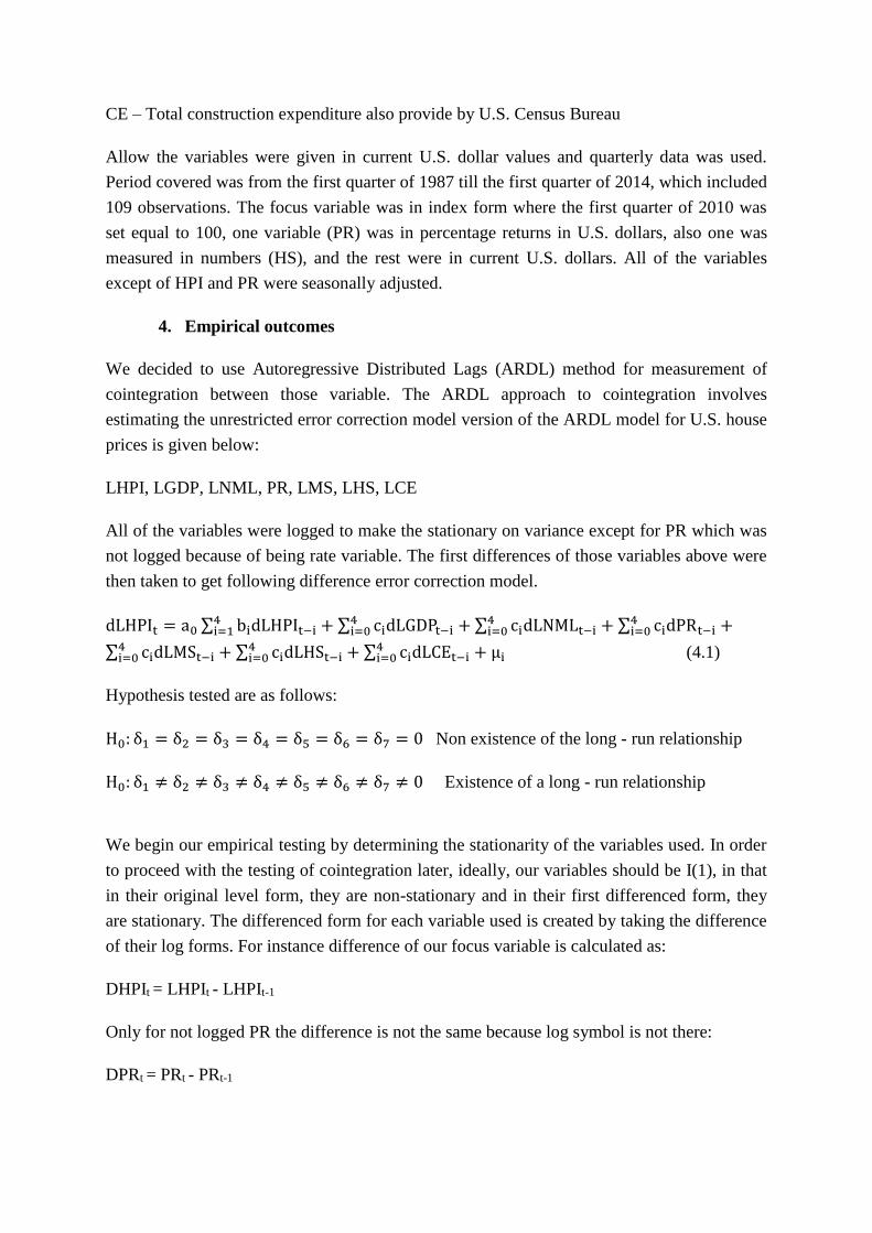
4. Empirical outcomes

We decided to use Autoregressive Distributed Lags (ARDL) method for measurement of

cointegration between those variable. The ARDL approach to cointegration involves

estimating the unrestricted error correction model version of the ARDL model for U.S. house

prices is given below:

LHPI, LGDP, LNML, PR, LMS, LHS, LCE

All of the variables were logged to make the stationary on variance except for PR which was

not logged because of being rate variable. The first differences of those variables above were

then taken to get following difference error correction model.

dLHPIt = a0 ∑ bidLHPIt−i + ∑ cidLGDPt−i4i=0

4i=1 + ∑ cidLNMLt−i

4i=0 + ∑ cidPRt−i

4i=0 +

∑ cidLMSt−i4i=0 + ∑ cidLHSt−i

4i=0 + ∑ cidLCEt−i

4i=0 + μi (4.1)

Hypothesis tested are as follows:

H0: δ1 = δ2 = δ3 = δ4 = δ5 = δ6 = δ7 = 0 Non existence of the long - run relationship

H0: δ1 ≠ δ2 ≠ δ3 ≠ δ4 ≠ δ5 ≠ δ6 ≠ δ7 ≠ 0 Existence of a long - run relationship

We begin our empirical testing by determining the stationarity of the variables used. In order

to proceed with the testing of cointegration later, ideally, our variables should be I(1), in that

in their original level form, they are non-stationary and in their first differenced form, they

are stationary. The differenced form for each variable used is created by taking the difference

of their log forms. For instance difference of our focus variable is calculated as:

DHPIt = LHPIt - LHPIt-1

Only for not logged PR the difference is not the same because log symbol is not there:

DPRt = PRt - PRt-1

Next we conducted the Augmented Dickey-Fuller, Philip-Perron and KPSS test for both level

and differenced forms of each variable. The main difference between ADF or PP tests and

KPSS test is while in former Null hypothesis is that variable is non-stationary in KPSS the

Null is that variable is stationarity. So rejection of Null has opposite implications in those two

sets of tests. The below table summarizes the results of each test.

Table 4.1.1: Augmented Dickey-Fuller (ADF) test results

Variable in Level Form

Variable Test Statistics Critical Value Implication

LHPI -1.8648 -3.4535 Variable is non-stationary

LGDP -.54652 -3.4535 Variable is non-stationary

LNML -1.9265 -3.4535 Variable is non-stationary

PR -3.7075 -3.4535 Variable is stationary5

LMS -1.7834 -3.4535 Variable is non-stationary

LHS -1.4575 -3.4535 Variable is non-stationary

LCE -1.6638 -3.4535 Variable is non-stationary

Variables in Difference Form

Variable Test Statistics Critical Value Implication

DHPI -3.2883 -2.8897 Variable is stationary

DGDP -4.7965 -2.8897 Variable is stationary

DNML -9.7896 -2.8897 Variable is stationary

DPR -3.9050 -2.8897 Variable is stationary

DMS -3.4842 -2.8897 Variable is stationary

DHS -5.4660 -2.8897 Variable is stationary

DCE -3.7252 -2.8897 Variable is stationary

5 Even if Prime rate (PR) is an interest rate where we do not expect to have a trend but only an intercept value,

we still used the results for the Dickey-Fuller regression with an intercept and a linear trend because for given

time period variable seems to have a clear downward trend. See Graph 4.1 above for visualization.

Figure 4.1: Trend of the Prime Rates (PR) of the U.S. banks from 1987Q1 to 2014Q1.

Since our results show that all of the variables are either I(0) or I(1) we can say that use of

ARDL is appropriated. However, we have to have support for our findings using either

Phillips-Perron Unit Root (PP) test or KPSS Stationarity test. We will start with PP test first

for which results are displayed in the below table:

Table 4.1.2: Phillips-Perron Unit Root (PP) test results

Variable in Level Form

Variable Test Statistics Critical Value Implication

LHPI -1.6248 -3.4515 Variable is non-stationary

LGDP -.51704 -3.4515 Variable is non-stationary

LNML -2.7426 -3.4515 Variable is non-stationary

PR -2.1596 -3.4515 Variable is non-stationary

LMS -1.2738 -3.4515 Variable is non-stationary

LHS -1.8098 -3.4515 Variable is non-stationary

LCE -1.3477 -3.4515 Variable is non-stationary

Variables in Difference Form

Variable Test Statistics Critical Value Implication

DHPI -6.8375 -2.8884 Variable is stationary

DGDP -7.8474 -2.8884 Variable is stationary

DNML -12.4357 -2.8884 Variable is stationary

DPR -3.9673 -2.8884 Variable is stationary

DMS -6.5479 -2.8884 Variable is stationary

DHS -8.2450 -2.8884 Variable is stationary

DCE -6.4273 -2.8884 Variable is stationary

Last test we will perform is KPSS Stationarity test. The test results are show in table below:

Table 4.1.3: KPSS Stationarity test results

0

2

4

6

8

10

12

1987Q1

1988Q2

1989Q3

1990Q4

1992Q1

1993Q2

1994Q3

1995Q4

1997Q1

1998Q2

1999Q3

2000Q4

2002Q1

2003Q2

2004Q3

2005Q4

2007Q1

2008Q2

2009Q3

2010Q4

2012Q1

2013Q2

PR

PR

Variable in Level Form

Variable Test Statistics Critical Value Implication

LHPI .093231 .14061 Variable is stationary

LGDP .16791 .14061 Variable is non-stationary

LNML .085987 .14061 Variable is stationary

PR .091719 .14061 Variable is stationary

LMS .14914 .14061 Variable is non-stationary

LHS .12488 .14061 Variable is stationary

LCE .12368 .14061 Variable is stationary

Variables in Difference Form

Variable Test Statistics Critical Value Implication

DHPI .10997 .39896 Variable is stationary

DGDP .50119 .39896 Variable is non-stationary

DNML .078140 .39896 Variable is stationary

DPR .13808 .39896 Variable is stationary

DMS .32984 .39896 Variable is stationary

DHS .080735 .39896 Variable is stationary

DCE .13540 .39896 Variable is stationary

The results of KPSS test in conflicting with implications of ADF and PP tests which is

normal to expect. Former two tests are consistent in their implications about variables that

they are non-stationary in level form and stationary in differenced form. Only exception is

Prime rate (PR), where ADF results show that it is stationary in level form, but PP results tell

that it is stationary. However, KPSS results confirm ADF test’s implications of stationarity in

level form. Thus, in general results are mixed. Since results of our test for non-stationarity are

not consistent we decided to use ARDL method.

However, before we proceed with cointegration test we want to find out the order of the

vector Autoregression (VAR), which shows number of appropriate lags to be used. From the

table below we can see that AIC recommends six lags while SBC recommends only one.

Table 4.1.4: Cointegration test results

Choice of Criteria

AIC SBC

Optimal Lag Order 6 1

Since results are conflicting we decided to take a number in between as four lags.

Next step would be to check for existence of cointegration among variables. If there exists at

least one cointegration it would mean that results are not spurious. The results of Engle-

Granger (E-G) test prove the existence of at least one cointegration:

Table 4.1.5: Engle-Granger (ADF) test statistics

Engle-Granger (ADF) test

T statistics Critical Value for the

Test

-2.6595 -4.36*

*Critical Value is taken from Sjo (2008).

As we can see from above table t statistics is less than critical value, which means we cannot

reject the null hypothesis of non-stationarity. This means chosen variables result into non-

stationary error term. Thus it indicates that there is no cointegration. However, since this

outcome is not appealing we decided to proceed with Johansen cointegration test. The results

of Johansen cointegration test for the Maximal Eigenvalue, Trace, AIC, SBC and HQC

criteria are given in the table below:

Table 4.1.6: Johansen cointegration test results

Criteria Number of Cointegrating

Vectors

Maximal Eigenvalue 4

Trace 5

AIC 7

SBC 2

HQC 7

However, we should not forget that in VAR model Johansen’s log-likelihood Maximal

Eigenvalue and Trace tests are based on cointegration with an intercept but no trend. These

results are both conflicting among themselves and Engle-Granger test results. This may be

VAR approach’s limitation dealing with mixed I(0) and I(1) variables.

Since our interest rate variable (PR) is most likely to be I(0), we will proceed with ARDL

approach which takes care of VAR’s limitations. First, we start with testing for the existence

of long-run relationship among variables using ARDL. Results of those tests are depicted

below:

Table 4.1.7: Results of Long-Run Relationship test in ARDL

Variable F statistics Lower CV at 5%* Upper CV at 5%*

LHPI 8.0766 2.365 3.553

LGDP 3.5865 2.365 3.553

LNML 3.0600 2.365 3.553

PR 2.7926 2.365 3.553

LMS 1.8900 2.365 3.553

LHS 9.6011 2.365 3.553

LCE 4.3173 2.365 3.553

* Lower and Upper Critical Values (CVs) are taken from Pesaran, Shin, & Smith (2001). The

range of Lower and Upper CVs for 1% and 10% levels of significance are 3.027-4.296 and

2.035-3.153 respectively.

As we can see from the table most of F statistics are higher than upper critical value of 3.553.

Only those which are lower are New Mortgage Loans (NML), Prime Rate (PR) and Money

Supply (MS). Since those are usually leading (exogenous) variables therefore it is normal for

us to see them being independent of other variables. Nevertheless, we find F statistics to be

very significant for equation of the our focus variable, House Price Index (HPI), some

variable related to house prices, such as Housing Started (HS) and Construction Expenditure

(CE). This finding show that there seems to clear evidence for existence of long-run

relationship among given variables. Thus, the relationship which exist is not spurious

relationship, but in contrast there is founded long-run relationship among given variables.

Following step will be Error Correction Model (ECM) using ARDL approach. Distinct from

VAR approaches ECM, ARDL lets ECM to choose optimal lags for each variable separately.

Therefore, in this aspect ARDL is considered more advance than regular VAR approach. We

chose to use AIC as criteria for choice of ECM here. Summarized table of ECM coefficients,

standard error, t statistics and p-value are provided below:

Table 4.1.8: Results of Error Correction Model

Variable Coefficient Standard Error T-statistics [P-value]

ecm (-1) dLHPI -.11311 .025687 4.4035[.000]***

ecm (-1) dLGDP -.0034788 .011105 .31326[.755]

ecm (-1) dLNML -.60024 .086363 6.9502[.000]***

ecm (-1) dPR -.10713 .026322 4.0698[.000]***

ecm (-1) dLMS .022545 .017893 1.2600[.211]

ecm (-1) dLHS -.29610 .061887 4.7845[.000]***

ecm (-1) dLCE -.19101 .028289 6.7521[.000]***

Note: ***denotes that coefficient is significant at 1% level.

Cointegration shows existence of long-term relationship, but sometimes there could be

deviations from long-run in short-term relationships. Thus, cointegration does not tell us

much about short-run relationship and how it affects long-run relationship. That is the reason

we used ECM to explain effect of short-run influence on the long-run relationship. Those

equations (variables) which have significant coefficient for their ecm(-1) are found to be

dependent on other variables for determination their values in short run that has long term

effect, thus considered endogenous in the model. Conversely, those variables which don’t

have significant ecm(-1) coefficient do not depend on other for determination of its value,

thus considered exogenous in the model. Furthermore, the coefficient of the error-correction

term tells us about the speed of short-run adjustment of the given variable.

The ECM results tell us that all variables except GDP and Money supply seem to be

endogenous. Variable that converges fastest in the short-run is new mortgage loans (NML).

Our focus variable House price index (HPI) is also among endogenous variables. Thus, GDP

and Money supply seem to have significant impact on house price.

Even if ECM does tell us which variables are endogenous and which are exogenous it does

not tell much about relative ranking of variable from the most exogenous to the most

endogenous. Therefore, we need to employ the Variance Decomposition (VDC) technique to

identify ranking in terms of exogeneity or endogeneity. There are two ways to apply VDC

technique, namely orthogonalized zed and generalized. There is relative shortcoming of each.

In orthogonalized ordering of the variable is vital and ranking is bias towards first in the

order. Therefore, the orthogonalized VDC results are not unbiased. The issue with

generalized VDCs is that sum of the lagged impacts is not normalized to 100%, even if

results are unbiased. Since, results of the generalized VDCs could be normalized to 100%

manually, we prefer later to the orthogonalized ones. Thus we will only concentrate and

report the generalized VDC results. Following table is summary of the results generalized

VDCs which are normalized to 100% for 1 year, 3 year and 10 year time horizons.

Table 4.1.9: Results of Error Correction Model for 1 year (4 quarter) time horizon

Variable Horizon DHPI DGDP DNML DPR DMS DHS DCE

DHPI 4 60.3% 7.2% 2.2% 4.5% 10.2% 7.4% 8.3%

DGDP 4 16.4% 44.0% 1.8% 3.7% 4.8% 16.7% 12.5%

DNML 4 2.6% 4.0% 73.5% 1.6% 8.1% 2.5% 7.6%

DPR 4 16.4% 11.2% 1.4% 50.0% 6.0% 4.8% 10.2%

DMS 4 8.7% 19.2% 4.2% 7.2% 51.0% 6.7% 3.0%

DHS 4 14.5% 17.0% 2.0% 3.7% 4.6% 44.1% 14.2%

DCE 4 14.8% 12.3% 3.9% 4.4% 2.9% 20.2% 41.4%

Table 4.1.10: Results of Error Correction Model for 3 year (12 quarter) time horizon

Variable Horizon DHPI DGDP DNML DPR DMS DHS DCE

DHPI 12 45.4% 5.4% 2.9% 14.5% 18.2% 7.1% 6.6%

DGDP 12 18.7% 36.5% 5.7% 6.5% 4.4% 14.8% 13.5%

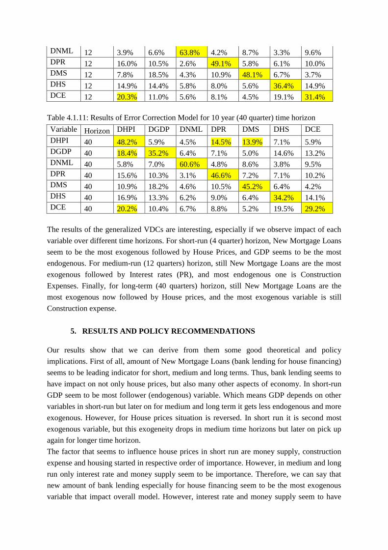
DNML 12 3.9% 6.6% 63.8% 4.2% 8.7% 3.3% 9.6%

DPR 12 16.0% 10.5% 2.6% 49.1% 5.8% 6.1% 10.0%

DMS 12 7.8% 18.5% 4.3% 10.9% 48.1% 6.7% 3.7%

DHS 12 14.9% 14.4% 5.8% 8.0% 5.6% 36.4% 14.9%

DCE 12 20.3% 11.0% 5.6% 8.1% 4.5% 19.1% 31.4%

Table 4.1.11: Results of Error Correction Model for 10 year (40 quarter) time horizon

Variable Horizon DHPI DGDP DNML DPR DMS DHS DCE

DHPI 40 48.2% 5.9% 4.5% 14.5% 13.9% 7.1% 5.9%

DGDP 40 18.4% 35.2% 6.4% 7.1% 5.0% 14.6% 13.2%

DNML 40 5.8% 7.0% 60.6% 4.8% 8.6% 3.8% 9.5%

DPR 40 15.6% 10.3% 3.1% 46.6% 7.2% 7.1% 10.2%

DMS 40 10.9% 18.2% 4.6% 10.5% 45.2% 6.4% 4.2%

DHS 40 16.9% 13.3% 6.2% 9.0% 6.4% 34.2% 14.1%

DCE 40 20.2% 10.4% 6.7% 8.8% 5.2% 19.5% 29.2%

The results of the generalized VDCs are interesting, especially if we observe impact of each

variable over different time horizons. For short-run (4 quarter) horizon, New Mortgage Loans

seem to be the most exogenous followed by House Prices, and GDP seems to be the most

endogenous. For medium-run (12 quarters) horizon, still New Mortgage Loans are the most

exogenous followed by Interest rates (PR), and most endogenous one is Construction

Expenses. Finally, for long-term (40 quarters) horizon, still New Mortgage Loans are the

most exogenous now followed by House prices, and the most exogenous variable is still

Construction expense.

5. RESULTS AND POLICY RECOMMENDATIONS

Our results show that we can derive from them some good theoretical and policy

implications. First of all, amount of New Mortgage Loans (bank lending for house financing)

seems to be leading indicator for short, medium and long terms. Thus, bank lending seems to

have impact on not only house prices, but also many other aspects of economy. In short-run

GDP seem to be most follower (endogenous) variable. Which means GDP depends on other

variables in short-run but later on for medium and long term it gets less endogenous and more

exogenous. However, for House prices situation is reversed. In short run it is second most

exogenous variable, but this exogeneity drops in medium time horizons but later on pick up

again for longer time horizon.

The factor that seems to influence house prices in short run are money supply, construction

expense and housing started in respective order of importance. However, in medium and long

run only interest rate and money supply seem to be importance. Therefore, we can say that

new amount of bank lending especially for house financing seem to be the most exogenous

variable that impact overall model. However, interest rate and money supply seem to have

direct impact on house prices. But, in short-run house prices seem to have influence over

many other variables as well, especially GDP. Thus we can see impact of house prices on

bank lending and GDP in short run, while interest rate and money supply influences it on

long run. This can be seen on impulse response function depicted below:

-0.01

0.00

0.01

0.02

0.03

0 8 16 24 30

Generalised Impulse Responses to one SE shock in the equation for DHPI

DHPI DGDP DNML DMS DHS DCE

-0.020

-0.015

-0.010

-0.005

0.000

0.005

0 8 16 24 30

Generalised Impulse Responses to one SE shock in the equation for DPR

DHPI DGDP DNML DMS DHS DCE

Therefore, we have to consider negative consequences of direct or indirect influence of bank

lending and monetary policy on house and as consequence on national income (GDP). There

is additional benefit from smoothing of house price fluctuations by reducing impact of

financing on it. In one of their studies OECD (2011) summarized the impact of different

changes of house financing policy among its member countries follows:

Table 5.1. The effect of policies on reducing real house price volatility1

From observing above table we can notice that the self imposed (or over-imposed by

regulators) discipline for the banks bring along improvement in bank supervision (i.e. Row

1). Additionally, tightening access to credit would reduce the ratio of loans, also benefits

economy by reducing house price volatility. As this study reports the maximum loan-to-value

ratio – the maximum permitted value of the loan as a share of the market price of the property

is considered as a measure of down payment constraint. It give an estimates suggesting that a

-0.010

-0.005

0.000

0.005

0.010

0.015

0 13 26 39 50

Generalised Impulse Responses to one SE shock in the equation for DMS

DHPI DGDP DNML DMS DHS DCE

10 percentage point increase in the maximum loan-to-value ratio is associated with a 12%

rise in the home ownership rate among younger low-income households (i.e. owners aged 25-

34 years in the second income quartile) compared to a typical household. As we would recall

one of the reasons of subprime crisis was precisely such ease of housing loan provided to

household with unstable income. One of suggestions in our research is similar to effect as

decreasing the maximum loan-to-value ratio.

6. Conclusion

There seems to be strong relations between house prices and the ease of obtaining housing

loan and its cost (as measured by interest rates). However, does increasing price make

lending attractive or does easy lending lead to high prices seems to be a debatable issue. This

study made an attempt to resolve this issue to some extent using data for the United States.

We have employed ARDL approach for time series data to analyze available data with the

use of this time series technique.

The finding of this study suggests, while house prices seem to be the exogenous (leading)

variable in the short-run which influence many other variables such as, construction of new

houses and its cost. However, in both short and long run, the interest rates seem to be

important factor contributing to changes in house prices. New mortgage loans seem to be

exogenous factors in both short and long run impacting house prices both directly and

indirectly. Therefore, we have to reconsider making necessary changes into the current way

of house financing which seems to be causing serious fluctuations in house prices.

7. Bibliography

Davis, E. P., & Zhu, H. (2011). Bank lending and commercial property cycles: Some cross-

country evidence. Journal of International Money and Finance, 30(1), 1–21.

Égert, B. & Mihaljek, D. (2007). Determinants of house prices in central and eastern Europe.

BIS Working Papers No 236.

Goodhart, C., & Hofmann, B. (2008). House prices, money, credit, and the macroeconomy ,

Oxford Review of Economic Policy, 24(1), 180 - 205.

Hott, C., & Monnin, P. (2006). Fundamental Real Estate Prices : An Empirical Estimation

with International Data Swiss National Bank (NCCR Finrisk No. 356).

Johnson, L.D. & Neave, E.H. (2008). The subprime mortgage market: familiar lessons in a

new context. Management Research News, 31(1), 12-26.

Lamont, O. & Stein, J.C. (1999). Leverage and House Price Dynamics in U.S. Cities. Rand

Journal of Economics, Vol. 30 (Autumn), 498–514.

Mirakhor, A. & Krichene, N. (2009). Recent crisis: lessons for Islamic finance. Journal of

Islamic Economics, Banking and Finance, 5 (1), 9-58.

Mohd-Yusof, R., H-Kassim, S., A-Majid, M.S. and Hamid, Z. (2011). Determining the

viability of rental price to benchmark Islamic home financing products: evidence from

Malaysia. Benchmarking: An International Journal, 18(1), 69-85.

Pesaran, M. H., Shin, Y., & Smith, R. J. (2001). Bounds testing approaches to the analysis of

level relationships. Journal of Applied Econometrics, 16 (3), 289–326.