MPRAMunich Personal RePEc Archive

The Exchange Rate and Interest RateDifferential Relationship: Evidence fromTwo Financial Crises

Kui-Wai Li and Douglas K T Wong

Working Paper 2011018, Department of Economics and Finance,City University of Hong Kong

December 2011

Online at https://mpra.ub.uni-muenchen.de/35297/MPRA Paper No. 35297, posted 9 December 2011 14:32 UTC

1

Department of Economics and Finance

Working Paper: 2011018

December 2011

The Exchange Rate and Interest Rate Differential Relationship:

Evidence from Two Financial Crises

http://www.cb.cityu.edu.hk/EF/research/research/workingpapers

Kui-Wai Li, Douglas K T Wong

Abstract

This paper examines the contemporaneous and inter-temporal interaction between real

exchange rate and real interest rate differential in the two financial crises of 1997 and 2008 by

using data from thirteen countries from different world regions. The empirical result shows

that negative contemporaneous relationship exists in most countries. In addition, there is little

evidence on a systematic inter-temporal relationship between the real interest rate

differential and the real exchange rate, and an absence of consistent result in supporting a

negative relationship among the thirteen economies. An extremely low change in the

conditional correlation between real interest rate differential and real exchange rates can be

found in small countries.

© 2011 by Kui-Wai Li. All rights reserved. Short sections of text, not to exceed two paragraphs,

may be quoted without explicit permission provided that full credit, including © notice, is given

to the source.

2

The Exchange Rate and Interest Rate Differential Relationship:

Evidence from Two Financial Crises

Kui-Wai Li and Douglas K T Wong

Abstract

This paper examines the contemporaneous and inter-temporal interaction between real

exchange rate and real interest rate differential in the two financial crises of 1997 and 2008 by

using data from thirteen countries from different world regions. The empirical result shows that

negative contemporaneous relationship exists in most countries. In addition, there is little

evidence on a systematic inter-temporal relationship between the real interest rate differential

and the real exchange rate, and an absence of consistent result in supporting a negative

relationship among the thirteen economies. An extremely low change in the conditional

correlation between real interest rate differential and real exchange rates can be found in small

countries.

Keywords: Contemporaneous, inter-temporal relationship, exchange rate, interest rate

differential, financial crisis

JEL Classification: C22, E43, F32, O57.

____

Corresponding author: Kui-Wai Li, Department of Economics and Finance, City University of

Hong Kong, Tat Chee Avenue, Kowloon, Hong Kong. Tel: +852 34428805; Fax: +852

34420195; E-mail address: efkwli@cityu.edu.hk.

Acknowledgement: The authors would like to thank the City University of Hong Kong for the

research funding under the two Strategic Research Grants (Numbers 7002523 and 7008129).

The authors will be solely responsible for the views and errors found in the paper.

3

I Introduction

It has been argued that an increase in the real interest rate of the home country will lead

to a positive real interest rate differential that attracts capital inflow, which would in turn

impose an upward pressure on the home economy’s real exchange rate. However, given the

contagious movement of the real interest rate across economies, and when the real interest rate

of other economies have caught up to eliminate the real interest rate differential, capital inflow

might not have taken place and remove the upward pressure on the real exchange rate. Thus, the

real interest rate differential and real exchange rate relationship may behave differently between

contemporaneous and inter-temporal situations.

Both the sticky-price and flexible-price approaches have been used to explain the

relationship between real interest rate differential and real exchange rate. The sticky-price

approach predicted a negative relationship between exchange rate and nominal interest rate

differential (Dornbusch, 1976). It argued that the higher interest rate in the home country

relative to the foreign country will attract capital inflow, and hence the home currency will

appreciate instantly. On the contrary, the flexible-price approach argued for a positive

relationship between nominal interest rate differentials and exchange rate, and that a change in

nominal interest rate reflected a change in the expected inflation rate. Given that the nominal

interest rate equals to the sum of the real interest rate and the expected inflation rate, an increase

in nominal interest rate in the home country relative to the foreign nominal interest rate will

result in a depreciation of the home currency as expected inflation rises. The demand for the

domestic currency will therefore fall and the exchange rate will then depreciate (Frankel, 1976;

Bilson, 1978).

4

In addition, rather than the international demand for flows of goods, Frankel (1979)

incorporated the international demand for stocks of assets into exchange rate analysis and

highlighted the importance of expectation and rapid adjustment in capital markets. Hooper and

Morton (1982) further examined large and prolonged changes in real exchange rate, and

empirically found that over half of the variance of real exchange rate during the 1970s was

related to the shifts in the current account and changes in real interest rate differentials. Other

literatures provided empirical evidence that real interest rate differential is a key determinant of

exchange rate movement (Obstfeld and Rogoff, 1984; Boughton, 1987).

Recent studies have applied cointegration technique to study the linkage between real

exchange rate and real interest rate differential (Coughlin and Koedijk, 1990; Blundell-Wignall

and Brown, 1991; MacDonald, 1998; Edison and Melick, 1999). For example, the cointegration

techniques and error-correction models used in Meese and Rogoff (1988) and Edison and Pauls

(1993) did not show a long run relationship between real exchange rate and real interest rate

differential. Sollis and Wohar (2006) used the threshold cointegration methodology and found

some evidence of a nonlinear long-run relationship between real exchange rate and real interest

rate differential. Hoffmann and MacDonald (2009) used the bivariate VAR method to model

the relationship of real interest rate differentials and real exchange rate, and considered the

long-run change in real exchange rate as the sum of period-to-period changes. Bautista (2006)

has provided empirical finding on the inter-temporal relationship between real exchange rate

and real interest differential in six East Asian economies, and found a large decline in the

conditional correlation structure during the Asian Financial Crisis (AFC) period.

5

The world has experienced at least two financial crises that have strong contagious

effects within the decade of 1997/98 and 2007/08. The AFC in 1997/98 began in mid-1990s

with a fall in exports in a number of Asian economies sparked off in July 1997 with the

devaluation of the Thailand currency. The fear of a global fund withdrawal following the

closure of key financial institutions in South Korea and Japan led eventually to a collapse of

financial markets and regional currency depreciations. Both the financial-panic hypothesis that

argued for a substantial downward shift in market expectation and confidence, and the

fundamental-based hypothesis that argued for an unsustainable deterioration in macroeconomic

fundamentals have been put forward as alternative explanations for the AFC (Eichengreen et al.,

1998; Kaminsky et al., 1998; Krugman, 1998a, 1998b; Radelet and Sachs, 1998a, 1998b;

Corsetti et al., 1999). Other studies have considered the herd behavior and the drop in capital

inflow as additional explanations (Chari and Kehoe, 2003; Calvo, 1998; Rigoborn, 1998; Pan et

al., 2001).

The 2008 financial crisis that began with the collapse of the US subprime mortgage

industry in March 2007 and the subsequent emergence of a worldwide credit crunch as many

international hedge funds and banks have invested heavily in sub-prime mortgage-backed

securities. The situation heightened in September 2008 when the US Federal Reserve (Fed)

took over the two largest mortgage-based security companies and the subsequent closure of

Lehman Brothers in New York had led to a financial meltdown that generated a tsunami-like

sequence of contagious effects on other international financial centers in Europe and Asia.

Responses to the 2008 financial crisis including the two G20 meetings in 2009 have

identified two fundamental schools of thought. The financial market fundamental school

6

advocated for the correction in such financial fundamentals as regulations, bank liquidity, moral

hazard and corporate government (for example, International Monetary Fund, 2009; Financial

Services Authority, 2009). On the contrary, the monetarist school believed that the role of

monetary policy and the interest rate are the underlying factors (Meltzer, 2009; Gokhale and

Van Doren, 2009; Schwartz, 2009). Because of the highly integrated worldwide financial

markets, the monetary policy adopted by the US can swiftly influent other world economies

though interest rate and exchange rate mechanisms. Prior to the 2008 financial crisis, for

example, the Fed’s expansionary monetary policy and a prolonged low interest rate regime

were highly contagious from the US to major EU and Asia economies.

This paper examines the possibility of a contemporaneous relationship between real

interest rate differential and change in real exchange rate by using a bivariate structural vector

autoregressive (SVAR) method. Armed with the assumption of rational expectation and

efficient market, the hypothesis is that real exchange rate changes that result from the

adjustment of real interest rate differential will happen in a very short horizon. This means that

the information on real interest rate differential shall only have an immediate impact on the

change in real exchange rate, and hence future exchange rate movement will reflect only future

information and will be independent to current change in real exchange rate. The paper will

then consider the inter-temporal interactions between real interest rate differential and real

exchange rate. Engle (2002) has proposed the dynamic conditional correlation (DCC) model

that allowed for the correlation matrix time dependent by formulating the conditional

correlation as a weighted sum of past correlations. The DCC model can be regarded as

7

nonlinear combinations of univariate generalized autoregressive conditional heteroskedasticity

(GARCH) models.

The dynamic conditional correlations between real interest rate differential and real

exchange rate will be considered. To begin with, the univariate GARCH models will not be

limited to the standard first order GARCH (1, 1) process (Bautista, 2006). Instead, a functional

coefficient autoregression of order ψ(AR(ψ)) with the conditional variance specified as a higher

order univariate GARCH (p, q) model for each series in the estimation process will be

considered. The accurate standardized residuals can then be obtained for estimating the time

varying correlation matrix. Such a specification ensured that the relevant dynamics can be

captured in the correlation structure.

The empirical study shows the experience of thirteen world countries for a period that

covered the two financial crises of 1997/98 and 2007/08, and the performances of the twelve

countries are expressed relative to the performance of the US, which is considered as the

“foreign” country. The twelve world countries include, in the case of Europe, the United

Kingdom, Germany, Greece and Iceland. In general, European countries did not suffer much in

the AFC, but are faced with different degree of difficulties in the 2008 crisis. Iceland has

suffered severely soon after the 2008 financial crisis due obviously to the lack of funds.

Greece’s financial problem took longer and resurfaced in mid-2010 as a result of the inability to

contain public debts. The two countries in the Americas are Canada and Chile. The four AFC-

affected countries in Asia are Japan, South Korea, Singapore and Thailand, while China and

India represent the two emerging countries. A relatively short horizon data have been used in

8

order to lower the effect of “unquantifiable news” from the market. Monthly data is used in the

analysis.

The rest of this paper is organized as follows. Section II discusses the theoretical

underpinnings between changes in the real exchange rate and real interest rate differential

relative to the foreign country. Section III shows the general data description and the results of

descriptive statistics of the sample economies. Sections IV and V show, respectively, the

empirical results of the contemporaneous and inter-temporal relationship between real interest

rate and real exchange rate. The last section concludes the paper.

II The Real Interest Rate and Real Exchange Rate Link

Consider the following uncovered interest parity relation:

*

1( )t t t t tE e e i i , (1)

where Et is the conditional expectation operator, ti (*

ti ) is the domestic (foreign) nominal

interest rate and te is the nominal exchange rate expressed in domestic currency per US dollar.

Equation (1) shows that nominal exchange rate adjustment is expected once the nominal

interest rate differential between home and foreign country exists. The real exchange rate (qt) is

constructed from the nominal exchange rate and consumer price indices as:

*

t t t tq e p p , (2)

where *

tp ( tp ) represents the foreign (home) currency price of the goods produced aboard

(domestically). The real interest rate (rt), expressed in the Fisher equation format, is equal to the

nominal interest rate minus the expected inflation rate:

1( )t t t t tr i E p p . (3)

9

The uncovered interest parity relation with real exchange rate and real interest rate can then be

expressed as:

*

1( )t t t t tE q q r r . (4)

According to Obstfeld and Rogoff (1984), the real exchange rate could adjust

monotonically at the same constant rate to its flexible price value. The real exchange rate

adjustment mechanism can be defined as:

1 1 1( ) ( ), 0 1t t tt t

E q q q q

, (5)

1t t tE q q

, (6)

where 1tE represents the conditional expectations operator at time t+1. θ is the speed of

adjustment parameter and tq

is the real exchange rate that prevails at time t if all prices were

fully flexible. Equation (5) implies that real exchange rate adjusts to its flexible price value

( tq

), while Equation (6) suggests that the ex-ante purchasing power parity holds under perfect

price flexibility and assumes that tq

follows a random walk process. Substituting Equation (6)

into (5) and rearranging the equation, we get:

_

1[ ( )]t t t t tq E q q q , (7)

where 1/( 1) 0 . Substituting Equation (4) into Equation (7), we have:

_*( )t t r t

q r r q . (8)

Equation (8) shows a linear relationship between real exchange rate, real interest rate

differential and flexible-price real exchange rate. Equation (8) will be used for both

contemporaneous and inter-temporal relationships analysis. In accordance with the traditional

Mundell–Fleming–Dornbusch (MFD) model (Mundell, 1961; Fleming, 1962; Dornbusch,

1976), the real exchange rate and real interest rate differential should be negatively related. The

10

coefficient of the real interest rate differential (α) in Equation (8) should be negative. The real

exchange rate would move to the opposite direction if a positive deviation of the real interest

rate differential exists.

III Statistical Performance

The monthly data are obtained from the International Financial Statistics (IFS) CD

ROM issued by the International Monetary Fund (IMF) and DataStream. The sample covered

the period from January 1994 to June 2009, with the exception of Thailand whose sample

period began from June 1994. The real exchange rate is expressed in logarithm and calculated

by adjusting the nominal end-of-period domestic exchange rate against the US dollar by the

domestic and US CPI, as shown in Equation (2). The real interest rate is calculated by the

nominal interest rate minus the ex-post one month realized inflation rate as shown in Equation

(3). The real interest rate differentials are measured by subtracting the real interest rate for the

US from the real interest rate of each country. The lending rate is used as a proxy of nominal

interest rate for China, Chile and Japan, while the money market rate is adopted for all the other

countries.

Figure 1 plots the relative performance of the real interest rate differential (right axis)

and real exchange rate (left axis) for the twelve economies. One observation is that although the

short-term movement of these two variables showed a deviation, their overall movement

seemed to show a correlation. In the case of real interest rate differential, there are not much

significant changes among the sample countries, with the exception of the Asian countries

during the AFC period. The governments of South Korea, Singapore and Thailand during the

11

AFC have increased their interest rates sharply in order to drive away the speculators. In the

case of the real exchange rate, the sudden capital outflow has caused a sharp depreciation in

real exchange rate in most Asian economies, especially in South Korea, Thailand and Singapore.

The pegged exchange regime in Thailand and the managed floating exchange regime in South

Korea have been replaced by a free-floating exchange rate arrangement in 1997 and 1998

respectively.

The 2008 financial crisis started with the collapse of the US sub-prime mortgage

industry in March 2007, the Federal Open Market Committee (FOMC) has lowered on a

stepwise scale the Federal Fund Rate, and hence caused an apparent rising trend in the real

interest rate differential that began from late 2007, with the exception of Iceland, Chile and

Singapore due probably to their increase in inflation expectation. The increase in the real

exchange rate trend that started in late 2008 represented depreciation in the domestic currency

of the sample economies against the US dollar, with the only exception of Japan with the yen

serving as a shelter currency. Due to the deterioration in the US economy, the strength of US

dollar against all depreciated currencies basically reflected a situation of capital fund

repatriation by international investors.

Table 1 shows the descriptive statistics of the real interest rate differential and change in

the real exchange rate. The performance in the real exchange rate showed that many countries

have exhibited a left-skewed distribution in their data series, with the exception of Germany,

Greece, Iceland, Chile and South Korea. As expected, the standard deviation of Thailand and

South Korea is relatively higher than other countries, due probably to the shift in exchange rate

regime during the AFC period. Though India adopted a market determined exchange rate

12

regime, the Reserve Bank of India has actively traded in the foreign exchange market in order

to influence the market price of the Rupee, and hence, the standard deviation of India’s

exchange rate is the lowest among other countries. As for the real interest rate differential,

China has the highest standard deviation as a result of a significant change in inflation rate

between 1994 and 1996. The five countries of Iceland, Chile, Thailand, China and India

exhibited a leptokurtic distribution since their excess Kurtosis coefficients are closed to or

larger than 3.

The Jarque-Bera tests for normality are statistically strong and significant, with the

exception of the real exchange rate in Iceland and the real interest rate differential in United

Kingdom, Japan and Singapore. For both real exchange rate and real interest rate differential,

the Box-Pierce test for the raw series, Q(5), suggested that serial correlation existed in all

countries. The results of Box-Pierce test for squared raw series indicated that a strong presence

of ARCH-structure in all real exchange rate and real interest rate differential with the exception

of Iceland.

The statistic results of the Augmented Dickey-Fuller (ADF) test, the Lagrange

Multiplier test (LM) and the Constant Conditional Correlation test (Engle and Sheppard, 2001)

are reported in Table 2. The ADF result shown in Panel A indicated that all real interest rate

differentials are stationary, and the real exchange rates for all countries are stationary after first

difference. The LM test for the ARCH effect shown in Panel B cannot reject the null that all the

coefficients of the squared residual of real exchange rates of Greece, Canada, Chile, China and

Japan are equal to zero, while only Iceland cannot be rejected in the case of real interest rate

differential. We also test for the constant correlation among the series with the null hypothesis

13

of constant correlation against the alternative hypothesis of time varying correlation. The null of

constant correlation generally cannot be rejected except Greece. However, Engle and Shepard

(2001) stated that the conditional correlation test result is not easy to interpret because the

correlation structures could be time-varying, and the significance depended on the number of

the lags selected. The dynamic conditional correlation model can, therefore, be applied to

determine the significance of the conditional correlation test based on the estimated parameters

of the DCC model.

IV The Contemporaneous Relationship

In order to measure the contemporaneous relationship and the inter-relationship between

real interest rate differential and real exchange rate, the country is described by a Structural

Vector Autoregressive (SVAR) system that expressed the contemporaneous interactions

between real interest rate differential and real exchange rate in the following structural form:

B(L)Yt = γ0 + et , (9)

where B(L) is a 2 x 2 matrix polynomial in the lag operator, L; Yt is a 2 x 1 vector of variables

which included two endogenous variables in the vector:

[

], (10)

and et is a 2 x 1 vector structural disturbances which is identical independent normal and var(et)

= Λ. Λ is a diagonal matrix and the diagonal elements are the variances of structural

disturbances such that each structural disturbance can be assigned explicitly to particular

equations. represented the real interest rate differential at the current level, and the

change in real exchange rate (Δqt) is defined by using the formula Δqt = qt – qt-1.

14

Let B0 be the contemporaneous coefficient matrix on L0 in the structural form, and let

B0(L) be the coefficient matrix in B(L) without contemporaneous coefficient B0. The matrix

polynomial in the lag operator, L, can be expressed as follow:

B(L) = B0 + B0(L) . (11)

Consider the following reduced form VAR equation:

Yt = α0 + A(L)Yt + ut , (12)

where A(L) is a matrix polynomial in lag operator, L, and ut is a vector of reduced-form

disturbances with no structural interpretation. We begin with the SVAR equation, and multiply

to the structural form equation:

( ) ( ) . (13)

Note that the parameters of reduced form VAR equation are related to the parameters of the

SVAR equation:

( ) ( ) . (14)

The reduced form residuals are related to the structural disturbances:

, (15)

and the covariance matrix is:

( )

. (16)

The reduced form residuals become linear combinations of the structural disturbances.

Equation (16) suggests that the covariance matrix of the reduced form residuals is not diagonal,

and the right hand side of the equation has n × (n+1) free parameters to be estimated. Since Σ

contains n × (n+1) / 2 parameters, the parameters in the SVAR equation cannot be identified

without restriction. To achieve identification, n × (n+1) / 2 restrictions are therefore needed. By

15

normalizing the diagonal elements in B0 to unity, the identification requires at least n × (n+1) /

2 restrictions on B0.

In the SVAR analysis, a constant variable is included and the number of lag length in

each model is based on the Akaike information criterion. Table 3 gives the contemporaneous

coefficients of the twelve countries. As expected, nine out of twelve estimated coefficients are

negative though they are mostly statistically insignificant. An interesting phenomenon found in

the European region is that a negative relationship between real interest rate differential and real

exchange rate can be found in Iceland and Greece, while the coefficient of Germany is positive

and significant. On the contrary, the estimated coefficient of most Asian countries is

statistically significant, with the exception of China and India. It suggests that government

intervention on exchange rate would affect the contemporaneous relationship between real

interest rate differentials and real exchange rate.

Figure 2 illustrates the Choleski-decomposition impulse response functions of the

interest rate differential shock (shock 1) and real exchange rate shock (shock 2). The vertical

axis represents the real interest rate differential in panels a) and b), and real exchange rate in

panels c) and d), respectively. The horizontal axis denotes time horizon in months. The upper

and lower dashed line plotted in each graph show the two standard-error bands generated by

using the Monte Carlo techniques.

The impact of real exchange rate to a positive interest rate shock (panel c) is examined

to see how real interest rate differential influences real exchange rate. In the case of European

countries, the overall impression in their panel c) graphs show that a positive interest rate

differential shock can generate a positive effect on real exchange rate in a short time horizon,

16

with the exception of Germany. The impact in general peaked at the second month, but declined

in the third months. An apparent positive initial impact on real exchange rate can be seen

among the Asian countries, and the responses in real exchange rate peaked at the first month

but declined thereafter. The downturn came to a completion around the third or fourth month

before it stabilized. As for Canada, Chile and the two emerging countries of China and India,

the overall results are inconsistent, as the initial effect of real interest rate differential shock on

real exchange rate is negative in Canada and China but positive in Chile and India.

The impulse response analysis provided a quantitative measure on the dynamic effects

of real exchange rate to a real interest rate differential shock. In our response analysis, there are

only three economies with a negative initial effect consistent with the traditional view that a

transitory appreciation of the real exchange rate is associated with an increase in real interest

rate differential. Although one could argue that the dynamic response of the real exchange rate

started to drop at the second month in most cases, the results cannot satisfy the condition of

interest rate parity and the traditional view that expected change in real exchange rate is

generated by the current real interest rate differential. There is little and weak evidence for

supporting the relationship between real interest rate differential and real exchange rate.

V The Dynamic Conditional Correlation Model

Lacking robust evidence that supported the linkage between real interest rate differential

and real exchange rate, the analysis is extended to study the dynamic relationship between these

two variables. The dynamic conditional correlation (DCC) model in Engle (2002) is used to

examine the relationship between changes in real exchange rate and real interest rate

17

differential. The DCC model formulated the conditional correlation as a weighted sum of past

correlations and allowed the conditional correlation matrix time dependent. Assume that the

multivariate GARCH model with 2 x 1 vector of series ty exhibited a conditional normal

distribution of zero mean and covariance matrix tH :

1 ~ (0, )t t ty N H , (17)

where 1t is the information set at time t-1. Under the DCC-GARCH framework, the

covariance matrix is defined as:

t t t tH D R D , (18)

where t itD diag h is a k x k diagonal matrix of time varying standard deviations from

univariate GARCH models with ith on the ith diagonal, and t ij tR is the time varying

correlation matrix containing conditional correlation coefficients. The univariate GARCH (p, q)

is given as:

2

1 1

i iq p

it i ip it p iq it q

q p

h w h

. (19)

The estimation of the DCC-GARCH model is obtained by:

* 1 * 1

t t t tR Q Q Q , (20)

where the evolution of the correlation in the model is given by:

_'

1 1 1 1

(1 ) ( )M N M N

t m n m t m t m n t n

m n m n

Q Q Q

. (21)

itt

ith

is a vector that included the standardized residuals and ~ (0, )t tN R .

_

Q is the

unconditional covariance of t m , and t ij tQ q is regarded as a conditional covariance matrix.

*

tQ is a k x k diagonal matrix containing the square root of the diagonal elements of tQ :

18

11

* 22

0 0

0 0

0

0 0

t

kk

q

qQ

q

. (22)

The time varying conditional correlation is expressed as , ,

, ,

, , , ,

i j t

i j t

i i t j j t

q

q q , which is

included in Rt. The general restriction of non-negativity and stationarity of variances is assumed.

The estimation of DCC model is estimated using a three-stage procedure. Firstly, the univariate

GARCH (p, q) models are fitted into the two series to obtain the estimated standard residuals.

The second stage involves the estimation of the intercept parameters of conditional correlation.

Finally, the coefficients governing the dynamics of correlation are estimated using the intercept

parameters of conditional correlation.

The univariate GARCH model for each of the 24 data series (include real exchange rates

and real interest rate differentials of the 12 countries) are first estimated, and the standardized

residuals are then used to estimate the correlation parameters. In order to obtain a consistent

correlation estimate, the specification of univariate GARCH model in our estimation is not

limited to the standard first order GARCH (1, 1) process. All the univariate model used in the

estimation is AR(Ψ)-GARCH(p,q), where the conditional mean and conditional variance

equation are selected by finding the minimum of the AIC allowing for ρ < 2 , P < 3 and Q < 2 .

The student-t distribution is assumed in the estimation. Table 4 reports the estimated parameters

of the AR(Ψ)-GARCH(p,q) process. The three parameters of w, α and β are the GARCH

parameters from Equation (18), and Ψi are the coefficients of the AR process. A total of five

economies (United Kingdom, Greece, Japan, China and India) are specified as AR (2) process

19

in the conditional mean equation. As for the conditional variance equation, the weights of αt

and βt satisfy the non-negativity constrains and the αt + βt < 1 restriction in all economies.

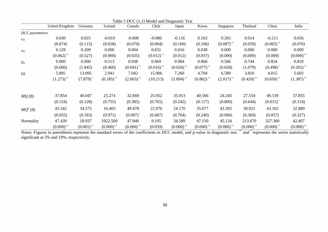
Table 5 shows that some of the DCC estimates of αD and βD are nonnegative scalar

parameters, satisfying the condition αt + βt < 1 and are significantly different from zero.

However, one can note that most of the αD equal to zero, suggesting that the constant

conditional correlation may be more appropriate for these series. On the other hand, there is

little evidence for supporting the relationship between the real interest rate differential and

change in the real exchange rate as the estimated unconditional correlations (ρ21) are

statistically insignificant in most cases. With the exception of Chile, the statistic results of

student distribution (df) are highly significant in all series and the vector normality test gave the

identical results that these series do not follow a multivariate normal distribution. The

multivariate portmanteau test in Hosking (1980) is used to detect the misspecification in the

conditional mean equation and the variance matrix. The results of portmanteau test (MQ) on

standardized residuals are all statistically insignificant, indicating that the serial correlations in

conditional mean have successfully been eliminated by the AR filter. In addition, no serial

correlation in the variance matrix is detected as the results of portmanteau test on squared

standardized residuals (MQ2) are mostly statistically insignificant with 5% significant level. The

diagnostic tests suggested that the model for each economy in general is well specified.

Figure 3 to Figure 6 show the conditional correlation structure between the real interest

rate differential and the change in the real exchange rate for the four European countries

(United Kingdom, Germany, Greece and Iceland), the two countries in the Americas (Canada

and Chile), the four Asian countries (Japan, South Korea, Singapore and Thailand) and the two

20

emerging countries (China and India), respectively. Among the twelve countries, there are a

total of six countries (Iceland, Greece, Canada, Chile, Japan and China) that have a negative

dynamic correlation structure, implying that their negatively correlated performance between

real interest rate differential and real exchange rate is consistent with the theoretical argument.

Contrary to the result shown by Bautista (2006) that an abrupt decline in the conditional

correlation structure appeared in six East Asian countries during the AFC period, our empirical

results show an apparent increase in conditional correlation structure in all Asian countries. The

higher correlation is driven by the higher variances in real exchange rate and real interest rate

differential during the AFC period. The large and sudden change in capital flow did cause

severely depreciation in many Asian countries in 1997. In order to combat against international

speculators, a tightened monetary policy pursued by the Asian governments helped to defend

the exchange rate. A large increase in conditional correlation should, therefore, be found as a

result of a sharp increase in interest rate accompanied by a clear depreciation of the currency.

The observation from the AFC is the sharp increase in the conditional correlation structure

resulted from the increase in interest rate differential and real depreciation of the home currency

among the Asian countries.

During the 2008 financial crisis, the empirical result shows that the conditional

correlation structure of most economies has also increased. Since the real interest rate

differential is the difference between the US and home country real interest rate, each country

in the sample has passively increased its real interest rate differential as the US Fed started to

lower its interest rate in late 2007. In fact, the repatriation of capital by international investors

started in March 2008.

21

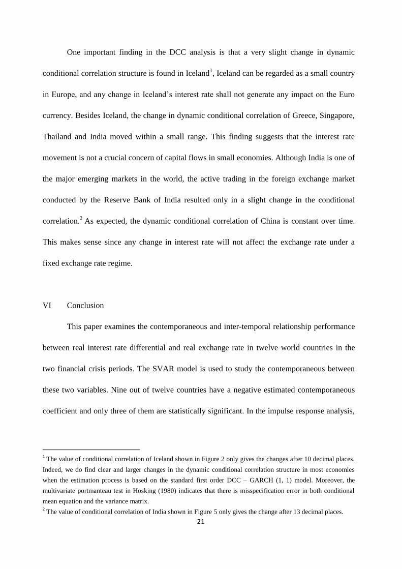
One important finding in the DCC analysis is that a very slight change in dynamic

conditional correlation structure is found in Iceland1, Iceland can be regarded as a small country

in Europe, and any change in Iceland’s interest rate shall not generate any impact on the Euro

currency. Besides Iceland, the change in dynamic conditional correlation of Greece, Singapore,

Thailand and India moved within a small range. This finding suggests that the interest rate

movement is not a crucial concern of capital flows in small economies. Although India is one of

the major emerging markets in the world, the active trading in the foreign exchange market

conducted by the Reserve Bank of India resulted only in a slight change in the conditional

correlation.2 As expected, the dynamic conditional correlation of China is constant over time.

This makes sense since any change in interest rate will not affect the exchange rate under a

fixed exchange rate regime.

VI Conclusion

This paper examines the contemporaneous and inter-temporal relationship performance

between real interest rate differential and real exchange rate in twelve world countries in the

two financial crisis periods. The SVAR model is used to study the contemporaneous between

these two variables. Nine out of twelve countries have a negative estimated contemporaneous

coefficient and only three of them are statistically significant. In the impulse response analysis,

1 The value of conditional correlation of Iceland shown in Figure 2 only gives the changes after 10 decimal places.

Indeed, we do find clear and larger changes in the dynamic conditional correlation structure in most economies

when the estimation process is based on the standard first order DCC – GARCH (1, 1) model. Moreover, the

multivariate portmanteau test in Hosking (1980) indicates that there is misspecification error in both conditional

mean equation and the variance matrix. 2 The value of conditional correlation of India shown in Figure 5 only gives the change after 13 decimal places.

22

there are only three countries that a positive real interest rate differential shock can generate a

negative initial effect to the real exchange rate.

In addition, the dynamic conditional correlations method is used to study the time-

varying conditional correlation structure of these twelve economies with univariate AR(Ψ)-

GARCH(p,q) specification in the first stage of DCC estimation. We find little evidence that

there is a systematic relationship between the real interest rate differential and change in the

real exchange rate, and are unable to find consistent results among these twelve countries in

supporting their negative relationship.

Our empirical results showed that the inter-temporal relationship between these two

variables is weak as the DCC estimates are not statistically significant in most countries. A

sharp increase in the conditional correlation, however, can be found during the two financial

crises. In the AFC period, the large increase in conditional correlation has clearly appeared in

the Asian countries, while the result of the 2008 financial crisis has covered more regions. The

reason for the sharp increase in conditional correlation is due to the severe depreciation in the

real exchange rate accompanied by a tightened monetary policy pursued by the Asian

governments during AFC, but a more passive increase in real increase rate differential during

the 2008 financial crisis.

One encouraging finding is that the inter-temporal relationship between real interest rate

differential and real exchange rates in Iceland, Singapore, Thailand and India is extremely low.

The change in their monetary policy did not generate a significant impact on their capital

movement. This suggests that return from interest earning is not a crucial factor for

international capital fund investing in smaller countries. In addition, a constant conditional

23

correlation structure can be found. Due to the fixed exchange rate regime and the non-

convertibility of the Renminbi in China, there is no significant dynamic relationship between

real interest rate differential and real exchange rate. In fact, it seems that the 2008 financial

crisis has made little influence on the China economy. It can be concluded that exchange rate

stability is crucial in the period of financial crisis.

The empirical findings seem to give a new dimension to the discussion on the negative

relationship between real exchange rate and real interest rate differential. The argument that a

rise in domestic interest rate would attract capital inflow with the ultimate outcome of a

currency appreciation may apply only to a single country, because the rise in the interest rate of

a single country could easily contagion to other countries, resulting in the inter-temporal rise in

the interest rate of other countries. When other countries have caught up with the rise in interest

rate in the next time period, there may not be any capital flow large enough to influence the

price of the currency. As such, there is no pressure for the value of any currency to change.

Hence, real interest rate differential at most has a very temporary effect on real exchange rate

across countries. Once the interest rate of other countries has efficiently been adjusted, there

will not be any impact on real exchange rate.

24

References

Bautista, C. C., (2006), “The exchange rate-interest differential relationship in six East Asian

countries”, Economics Letters, 92, 137-142.

Bilson, J., (1978), “The monetary approach to exchange rate – some empirical evidence,” IMF

Staff Papers, 25, 48-75.

Blundell-Wignall, A. and F. Browne, (1991), Increase Financial Market Integration, Real

Exchange Rates and Macroeconomic Adjustment, OECD Working Paper 96, February.

Boughton, J.M., (1987), “Tests of the performance of reduced-form exchange rate models”,

Journal of International Economics, 23, 41–56.

Calvo, G., (1998), “Capital flows and capital-market crises: the simple economics of sudden

stops”, Applied Economics, 1 November, 35-54.

Chari, V. V. and Kehoe, P. J., (2003), “Hot money”, Journal of Political Economy, 111 (6),

1262-1292.

Corsetti, G., Prsenti, P. and Roubini, N., (1999), “What caused the Asian currency and financial

crisis?”, Japan and the World Economy, 11, 305-373.

Coughlin C. C., and Koedijk, K., (1990), “What do we know about the long-run real exchange

rate?”, St. Louis Federal Reserve Bank Review, 72, 36-48.

Dornbusch, R., (1976), “Expectations and exchange rate dynamics,” Journal of Political

Economy, 84, 1161–1176.

Edison, H. J. and Melick, W. R., (1999), “Alternative approaches to real exchange rates and

real interest rate: Three up and three down”, International Journal of Finance and Economics, 4,

93-111.

Edison, H. J. and Pauls, B., (1993), “A re-assessment of the relationship between real exchange

rate and real interest rates: 1974-1990”, Journal of Monetary Economics, 31 (2), 165-187.

Eichengreen, B., Ito, T., Kawai, M. and Portes, R., (1998), “Recent currency crisis in Asia”,

Journal of the Japanese and International Economies, 12, 535-542.

Engle, R. F. and Sheppard, K., (2001), Theoretical and Empirical Properties of Dynamic

Conditional Correlation Multivariate GARCH, National Bureau of Economic Research,

Working Paper, No. 8554, Cambridge, MA.

Engle, R. F., (2002), “Dynamic conditional correlation - a simple class of multivariate GARCH

models”, Journal of Business and Economics Statistics, 20, 339-350.

25

Frankel, J., (1976), “A monetary approach to exchange rate: Doctrinal aspects and empirical

evidence”, Scandinavian Journal of Economics, 78, 255-276.

Frankel, J., (1979), “On the mark: A theory of floating exchange rates based on real interest

differential”, American Economic Review, 69, 610–622.

Financial Services Authority, (2009), The Turner Review: A Regulatory Response to the Global

Banking Crisis, London, March.

Fleming, J. M., (1962), “Domestic financial policies under fixed and under floating exchange

rates”, IMF Staff Papers, 9, 369–379.

Gokhale, Jagadeesh and Van Doren, Peter, (2009), Would Stricter Fed Policy and Financial

Regulation Have Averted the Financial Crisis?, Cato Institute Policy Analysis, No. 648,

October.

Hoffmann, M. and MacDonald, R., (2009), “Real exchange rates and real interest rate

differentials: A present value interpretation”, European Economic Review, vol. 53(8), 952-970.

Hooper P. and Morton J., (1982), “Fluctuations in the dollar: A model of nominal and real

exchange rate determination”. Journal of International Money and Finance 1, 39–56.

Hosking, J. (1980), “The multivariate portmanteau statistic”, Journal of American Statistical

Association, 75, 602-608.

International Monetary Fund, (2009), Global Financial Stability Report: Responding to the

Financial Crisis and Measuring Systemic Risks, Washington D. C., April.

Kaminsky, G., Lozondo, S. and Reinhart, C., (1998), “Leading indicators of currency crisis”,

IMF Staff Papers, 45 (1) March: 1-48.

Krugman, P., (1998a), What Happened to Asia?, Massachusetts Institute of Technology,

Cambridge: MA.

Krugman, P., (1998b), Fire Sale FDI, Massachusetts Institute of Technology, Cambridge: MA.

MacDonald R., (1998), “What determines real exchange rate: the long and short for it”, Journal

of International Financial Markets, Institutions, and Money, 8, 117 -153.

Meese, R., Rogoff, K. (1988), “Was it real? The exchange rate-interest rate differential relation

over the modern floating-rate period”, Journal of Finance, 43, (4), 933-948.

Meltzer, Allan H. (2009), “Reflections on the financial crisis”, Cato Journal, 29 (1), 25-30.

26

Mundell, R. A., (1961), “A theory of optimum currency areas”, American Economic Review, 51,

657–665.

Obstfeld, M. and Rogoff, K. (1984), “Sticky-price exchange rate models under alternative

price-adjustment rules”, International Economic Review, 25, 159-174.

Pan, M. S., Fok, R. C. W. and Liu, Y. A. (2001), Dynamic Linkages between Exchange Rates

and Stock Prices: Evidence from Pacific Rim Countries, Working Paper, College of Business,

Shippensburg University.

Radelet, S. and Sachs, J., (1998a), The East Asian Financial Crisis: Diagnosis, Remedies and

Prospects, Harvard Institute for International Development, Cambridge: MA.

Radelet, S. and Sachs, J., (1998b), The Onset of the East Asian Financial Crisis, Harvard

Institute for International Development, Cambridge: MA.

Rigobon, R., (1998), Information Speculative Attacks: Good News is No News, Massachusetts

Institute of Technology, Cambridge: MA.

Schwartz, Anna J., (2009), “Origins of the financial market crisis of 2008”, Cato Journal, 29

(1), 19-23.

Sollis, R. and Wohar, M. E., (2006), “The real exchange rate – real interest rate relation:

Evidence from tests for symmetric and asymmetric threshold cointegration”, International

Journal of Finance and Economics, 11, 139-153.

27

Table 1 Descriptive Statistic of Real Interest Rate Differential and Real Exchange Rate United Kingdom Germany Iceland Canada Chile Japan Korea Singapore Thailand China India

Real exchange rate mean -0.508 0.472 4.335 0.276 6.279 4.614 6.993 0.394 3.574 1.955 3.812

std.dev 0.105 0.146 0.150 0.115 0.144 0.156 0.162 0.122 0.177 0.125 0.075

Skewness -0.495 0.462 0.383 -0.433 0.460 -0.799 0.222 -0.663 -0.482 -1.188 -0.823

Kurtosis -0.640 -0.492 -0.026 -0.500 -0.773 0.031 -0.868 -0.983 -0.959 0.411 0.767

min -0.751 0.205 4.026 -0.026 6.046 4.162 6.740 0.155 3.269 1.632 3.597

max -0.337 0.798 4.739 0.462 6.606 4.877 7.476 0.550 3.976 2.107 3.942

Jarque-Bera 10.713 9.263 4.538 7.696 11.123 19.684 7.327 20.989 13.865 44.827 25.422

(0.005)** (0.01)** (0.103) (0.021)** (0.004)** (0.000)** (0.026)** (0.000)**

(0.001)** (0.000)** (0.000)**

757.788 839.572 704.667 828.435 704.667 775.143 704.997 1362.600 809.718 850.825 768.815

(0.000)** (0.000)** (0.000)** (0.000)** (0.000)** (0.000)** (0.000)** (0.000)**

(0.000)** (0.000)** (0.000)**

765.736 844.67 701.751 836.255 701.751 774.384 697.889 1336.490 802.936 853.418 768.953

(0.000)** (0.000)** (0.000)** (0.000)** (0.000)** (0.000)** (0.000)** (0.000)**

(0.000)** (0.000)** (0.000)**

Real interest rate differential mean 1.018 0.398 3.975 0.721 6.069 0.845 3.129 -0.318 0.316 1.404 4.890

std.dev 1.347 1.498 3.512 1.323 3.141 1.874 1.546 1.635 3.143 5.796 3.447

Skewness -0.187 0.541 4.269 0.627 1.841 -0.466 0.036 -0.225 1.440 -2.085 -1.286

Kurtosis -0.254 -0.089 30.509 0.187 6.774 -0.413 -0.257 -0.559 2.869 3.585 2.981

min -2.510 -2.510 -3.260 -1.870 1.080 -4.000 -0.680 -4.330 -5.540 -19.400 -9.800

max 4.210 4.760 32.470 4.460 24.940 4.290 7.310 3.100 13.930 6.970 10.190

Jarque-Bera 1.573 9.841 7736 12.402 458.26 6.945 125.99 3.856 119.29 233.1 119.52

(0.456) (0.007)** (0.000)** (0.000)** (0.000)** (0.031)** (0.000)** (0.145) (0.000)** (0.000)** (0.000)**

478.273 654.073 66.49 557.744 190.388 754.447 494.363 801.125 471.645 785.98 570.788

(0.000)** (0.000)** (0.000)** (0.000)** (0.000)** (0.000)** (0.000)** (0.000)**

(0.000)** (0.000)** (0.000)**

267.373 393.124 0.816 452.156 106.94 639.309 274.015 236.721 362.73 686.888 410

(0.000)** (0.000)** (0.976) (0.000)** (0.000)** (0.000)** (0.000)** (0.000)**

(0.000)** (0.000)** (0.000)**

Note: **

represents statistical significance at 5%.

(5)Q

2(5)Q

(5)Q

2(5)Q

28

Table 2 General Statistic of Real Interest Rate Differential and Real Exchange Rate United Kingdom Germany Iceland Canada Chile Japan Korea Singapore Thailand China India

Panel A: Augmented Dicky-Fuller Test

Real exchange rate

Δqt -3.561** -3.034** -3.253** -3.910** -3.585** -3.616** -3.958** -3.502** -4.519** -2.190** -3.870**

Real interest rate differential *

t rr r -2.526** -2.706** -2.828** -3.742** -2.298** -2.218** -2.076** -3.037** -3.093** -4.433** -3.491**

Panel B: LM ARCH Effect Test

Real exchange rate

Δqt 5.048 7.699 19 0.509 1.284 1.043 8.048 7.430 7.845 1.18 2.921

(0.000)** (0.000)** (0.000)** (0.769) (0.273) (0.394) (0.000)** (0.000)** (0.000)** (0.321) (0.015)

Real interest rate differential *

t rr r 42.09 180.09 0.132 186 20.46 282.9 91.96 4.093 56 1306 180

(0.000)** (0.000)** -0.985 (0.000)** (0.000)** (0.000)** (0.000)** (0.000)** (0.000)** (0.000)** (0.000)**

Panel C: Constant Correlation Test

E-S Test(5) 1.602 4.419 3.578 1.379 9.926 11.952 11.968 6.942 8.057 2.166 8.992

(0.952) (0.620) (0.734) (0.967) (0.128) (0.063) (0.063) (0.326) (0.234) (0.904) (0.174)

Notes: Figures in parenthesis represent the p-values; **

and *

represent statistical significance at 5% and 10%, respectively.

Table 3 Contemporaneous Coefficients in Structural Models

Coefficients Standard Error

United Kingdom

Germany

Greece

Iceland

Canada

Chile

Japan

Korea

Singapore

Thailand

China

India

-0.0004

0.0076

-0.0018

-0.0004

0.0018

-0.0010

-0.0083

-0.0228

-0.0097

-0.0049

0.0035

-0.0006

0.003

0.005*

0.002

0.001

0.004

0.001

0.005*

0.005**

0.002**

0.002**

0.003

0.001

Note: ** and * represent statistical significance at 5% and 10%, respectively.

29

Table 4 Univeriate AR(p) – GARCH( p , q ) Models

ψ0 Std.Error ψ1 Std.Error ψ2 Std.Error wI Std.Error Σαi Σβi

Real exchange rate

United Kingdom -0.001 (0.001) 0.031 (0.079) -0.099 (0.090) 0.899 (0.654) 0.083 0.757

Germany -0.002 (0.002) 0.123 (0.071) * - - 0.515 (0.093)** 0.013 0.918

Iceland 0 (0.003)** 0.184 (0.078)** - - 0.521 (0.170)** 0.171 0.807

Canada 0.001 (0.001) -0.008 (0.069) - - 0.032 (0.023) 0.045 0.955

Chile 0.001 (0.002) 0.221 (0.084)** - - 0.431 (0.471) 0.327 0.662

Japan 0.003 (0.003) 0.138 (0.082)* 0.053 (0.076) 7.400 (1.791)** 0.22 0.071

Korea -0.001 (0.001) 0.123 (0.089) - - 0.935 (0.447)** 0.72 0.358

Singapore -0.001 (0.001) 0.005 (0.074) - - 0.307 (0.143)** 0.185 0.723

Thailand 0.001 (0.003) 0.116 (0.109) - - 2.189 (1.710)** 0.236 0.58

China 0.002 (0.002) 0.606 (0.501) -0.448 (0.645) 0.0678 (0.019) 0.055 0.928

India -0.002 (0.001) 0.103 (0.057) * -0.049 (0.049) 0.246 (0.181) 0.214 0.743

Real interest rate differential

United Kingdom 0.793 (0.458) * 0.695 (0.084)** 0.204 (0.080)** 0.045 (0.042) 0.056 0.852

Germany 0.415 (5.990) 0.978 (0.040)** - - 0.177 (0.129) 0.164 0.034

Iceland 0.012 (0.135) -0.4 (0.107)** - - 1.560 (1.407) 0.144 0.73

Canada 0.23 (0.826) 0.963 (0.023)** - - 0.043 (0.019)** 0.013 0.745

Chile 3.756 (0.536) 0.866 (0.046)** - - 0.018 (0.012) 0.152 0.856

Japan 0.385 (1.107) 1.114 (0.055)** -0.144 (0.058)** 0.035 (0.014)** -0.072 0.919

Korea 3.035 (0.440)** 0.892 (0.032)** - - 0.202 (0.075)** 0.268 0.328

Singapore -0.402 (0.628) 0.922 (0.032)** - - 0.147 (0.040)** 0.144 0.566

Thailand -0.009 (0.619) 0.902 (0.036)** - - 0.039 (0.023)* 0.32 0.672

China 3.343 (3.120) 1.227 (0.189)** -0.247 (0.176) 0.761 (0.293)** 0.054 0.95

India 4.72 (0.973)** 1.216 (0.070)** -0.29 (0.065)** 0.092 (0.049)* 0.104 0.81

Notes: Figures in parenthesis represent the standard errors of the coefficients in univariate GARCH models; **

and *

represent statistical significance at 5%

and 10%, respectively.

30

Table 5 DCC (1,1) Model and Diagnostic Test

United Kingdom Germany Iceland Canada Chile Japan Korea Singapore Thailand China India

DCC parameters

ρ21 0.030 0.025 -0.010 -0.008 -0.086 -0.116 0.163 0.265 0.014 -0.211 0.056

(0.074) (0.115) (0.058) (0.070) (0.064) (0.160) (0.106) (0.087) ** (0.059) (0.065) ** (0.076)

αD 0.129 0.209 0.000 0.004 0.031 0.016 0.038 0.000 0.000 0.000 0.000

(0.062) ** (0.527) (0.000) (0.025) (0.012) ** (0.012) (0.037) (0.000) (0.000) (0.000) (0.000) **

βD 0.000 0.000 0.513 0.938 0.969 0.984 0.868 0.566 0.744 0.834 0.810

(0.606) (1.845) (0.460) (0.041) ** (0.016) ** (0.026) ** (0.077) ** (0.658) (1.079) (0.498) * (0.201) **

Df 5.895 13.095 2.941 7.042 15.906 7.260 4.704 6.589 3.810 4.015 5.602

(1.273) ** (7.879) * (0.185) ** (2.003) ** (10.213) (1.894) ** (0.862) ** (2.017) ** (0.420) ** (0.650) ** (1.387) **

MQ (8) 37.854 40.047 25.274 32.669 25.052 35.013 40.566 24.245 27.554 49.339 37.855

(0.154) (0.128) (0.755) (0.385) (0.765) (0.242) (0.117) (0.800) (0.644) (0.015) * (0.154)

MQ2 (8) 43.342 34.575 16.403 49.478 22.970 24.170 35.077 42.392 30.921 43.102 32.889

(0.055) (0.183) (0.971) (0.007) * (0.687) (0.764) (0.240) (0.066) (0.369) (0.057) (0.327)

Normality 47.439 18.937 1922.500 47.846 9.105 34.589 47.150 45.134 213.670 327.360 42.407

(0.000) ** (0.001) ** (0.000) ** (0.000) ** (0.059) (0.000) ** (0.000) ** (0.000) ** (0.000) ** (0.000) ** (0.000) **

Notes: Figures in parenthesis represent the standard errors of the coefficients in DCC model, and p-value in diagnostic test. **

and * represents the series statistically

significant at 5% and 10%, respectively.

31

32

Figure 1 Time Series of Real Interest Rate Differential and Real Exchange Rate

33

34

35

Figure 2 Impulse Responses Obtained from Choleski decompositions

36

Figure 3 The Dynamic Conditional Correlation Structure between Relative Interest Rate

Differentials and Real Exchange Rates: Europe

Figure 4 The Dynamic Conditional Correlation Structure between Relative Interest Rate

Differentials and Real Exchange Rates: Canada and Chile

37

Figure 5 The Dynamic Conditional Correlation Structure between Relative Interest Rate

Differentials and Real Exchange Rates: Emerging Markets

Figure 6 The Dynamic Conditional Correlation Structure between Relative Interest Rate

Differentials and Real Exchange Rates: Asia