Embed Size (px)
Citation preview
MPRAMunich Personal RePEc Archive
Living arrangements of older adults inIndia: reduced forms for co-residencemodel
Sanjeev Bakshi and Prasanta Pathak
Indian Statistical Institute (Calcutta)
2006
Online at https://mpra.ub.uni-muenchen.de/40516/MPRA Paper No. 40516, posted 6 August 2012 12:23 UTC
1
Living Arrangements of Older Adults in India: Reduced
Forms for Co-residence Model
Sanjeev Bakshi, Junior Research Fellow,
Population Studies Unit, Indian Statistical Institute,
Kolkata, India.
Dr. Prasanta Pathak, Faculty Member,
Population Studies Unit, Indian Statistical Institute,
Kolkata, India.
2
Abstract
Understanding the effects of factors that determine the living arrangements of the older adults
becomes crucial as their care is affected by their living arrangements. In India, the spectrum of social
security schemes for the older adults needs diversification in terms of services provided and coverage.
Therefore a large chunk of the support has to come from family and community. This support is
reflected in their living arrangements. Often the social transition from an agriculture-based economy
to an industrialized economy, with urbanization and nuclearization of families as its consequences, is
cited as a reason for the changing living conditions of the older adults. This study is aimed at
investigating the factors that are associated with the living arrangements of the older adults. It extracts
information on Indian socio-cultural system vis-à-vis the older population from the 42nd
round data of
the National Sample Survey (NSS). The conceptual framework consists of availability factors,
feasibility factors and cultural factors. Each of these factors is represented by a set of variables. The
effect of these factors on the living arrangements of the older adults is analysed. It is asserted that the
state of economic independence, the marital status, the place of residence, the sex and the age are
potential factors determining the living arrangements at older ages. The analysis points to the need of
planning long term policies for caring older adults, given the heterogeneity of the population and their
living arrangements.
Keywords: ageing, living arrangements, co-residence, living alone, social transfers, familial
transfers, modernization
3
1.0 Introduction
An ageing society demands as a prerequisite existence of effective systems of familial1 and social
2
transfers (Palloni 2001). These transfers are synonymous with supports that have a positive influence
on the general well being of the older adults (population units aged sixty and above). The population3
of the older adults in the Indian society has swelled from 5.63 per cent in 1961 to 7.10 per cent in
2001. According to the 2001 census there are 76.62 million older adults in India. The decadal growth
rates of the older adult population in the decades 1961-71, 1971-81, 1981-91 and 1991-2001 were
32.32 per cent, 32.01 per cent, 31.30 per cent and 35.18 per cent respectively. An all-India survey,
conducted during 1995-96, estimates the older adults living alone to be 15 per cent and 12.5 per cent
in rural and urban areas respectively. At the end of 2003 there were 379 old age homes running in
India and the number of beneficiaries was 9575. This figure is mere 0.01 per cent of the older adult
population of India. The per cent of workforce employed in public sector has been recorded 4.28,
5.91, 7.03, 6.66 and 6.13 in the five decadal censuses respectively4. Therefore, a large part of the
workforce will remain devoid of any post-retirement benefits. Old age pensions are also not adequate.
It varies from Rupees 75.00 in Andhra Pradesh state to Rupees 200.00 in Maharashtrra state.This
scenario demands immediate attention concerning their state of well-being. It also gives a clear
indication that the cost of economic, health and psychological support needed by the older adults has
to be borne by the family.
The literature broadly classifies the living arrangements as alone and co-residence. Living alone
covers the living arrangements where the older adults live alone or with spouse. Co-residence
indicates living with children or other such type of arrangement. In India, living with sons at older
ages had been a norm of the society and living in old age homes is still a rare phenomenon. Vlasoff
(1990) has cited the importance of son in India in a case study on widows. Jeffery et al (1992) have
given details of the studies from developed western societies indicating positive relationship between
economic resources of the older adults and the likelihood of independent living. They have also
mentioned studies indicating that disability and poor health decrease the likelihood of continuing to
live separately. Shah (1999) has pointed out that joint households have been an ideal throughout the
Indian society. Sokolovsky (2001), citing the western pacific survey and other case studies conducted
1 The transfers flowing towards older adults originating within the boundaries of kin group or family
2 Transfers flowing towards older adults that include socio-economic resources such as pensions, disability
income, health payments, and transfers in the form of subsidies for institutionalisation, home care and housing 3 Population of India was recorded 439.23 million in 1961 census and 1027.01 million in 2001 census
4 Census of India 1981, Series I India, Paper 3 of 1981, for the years 1970-71 and 1980-81; Statistical Abstracts
1982, 1970, 1962; www.indiastat.com and www.mospi.nic.in for the year 2001
4
in India, has opined that the changing socio-economic environment of this part of developing world
has little impact on likelihood of co-residence. Zimmer et al (2005) have discussed education, marital
status, sex, age, place of residence (rural/urban) of household members as determinants of the
composition of households in the less developed countries, within the modernization5 perspective.
Walter (1960) has discussed the developments in social, economic, medical and technological aspects
that are influencing the living arrangements of the older adults.
The studies conducted in various parts of the developing world indicate that no generalization of the
effects could be made. It seems that these factors differ in their effects on living arrangements from
one social system to another. Moreover, the older adult population is not a homogeneous population.
The older adults differ by sex, marital status, availability of kin, health status and economic resources.
Therefore the preferences for living arrangements are not same for the whole population. For such
reasons, the heterogeneity of the older population should be considered in conducting any study on
living arrangements. The respective socio-cultural system serves as a frame of reference. The
effectiveness of the factors that play significant role in the socio-cultural systems outside India needs
to be tested for its effect in the Indian system and this study is an attempt in this direction.
Present study homogenizes the older adult population by defining sub-groups by marital status and
availability of kin. The health and economic factors, which are considered in earlier studies, are
incorporated in this study also. Socio-cultural factors peculiar to the Indian system namely caste,
religion, education and place of residence are controlled.
The following questions represent the objectives of the present study:
Research Question-1: Are the states of economic dependence and living
arrangements of the older adults associated?
Research Question-2: Do the states of health status affect the living
arrangements?
Research Question-3: What effect does disability (in terms of physical
immobility) has in deciding living arrangements?
5 This approach assumes that living in large and extended households is common in traditional agricultural
societies and becomes less so with development, industrialization and division of labour
5
Research Question-4: For the older adults having children, do older adults
prefer living with son? And if it is so, does having a number of sons ensures
that the older adults live with sons?
Research Question-5: Does place of residence has any effect on the choice of
living arrangements?
2.0 Methodology
In India, at present we lack comprehensive database to study the living arrangements of the older
adults. The 42nd
round data of the NSS is of great help to initiate such studies. The data was collected
in the forty-second round (July 1986-June 1987) of the National Sample Survey Organization
(N.S.S.O), Government of India, to access the nature and dimensions of the socio-economic problems
of the older adults. The survey covered the whole of India except Ladakh and Kargil districts of
Jammu & Kashmir and rural areas of Nagaland. The survey covered 64993 households spread over a
sample of 8312 villages and 4546 U.F.S. blocks.
2.1 Living Arrangements and Supports
The term support stands for co-residents, providing economic, health care, and psychological
supports. This concept is developed further so as to form the core of the conceptual framework for the
present study. From the classification of the living arrangements it is evident that marital status and
availability of kin are deciding factors for the choices available from a set of alternative living
arrangements. For instance, for those older adults having no chid, co-residence with children is not
possible and for never married older adults living with spouse is not possible. This indicates the need
for first homogenising the older adult population with respect to marital status and the availability of
kin so that the available choices of living arrangements are crystallized to facilitate further analytical
exercises. It is also necessary because the prevailing social structure may make the effects of various
factors differ from one homogeneous sub-group to another.
2.2 The Living Arrangements and Homogenous sub-Groups
The data cites seven types of living arrangements namely living with spouse, living with children,
living with grand children, living with other relatives, living with non-relatives, living alone as an
6
inmate of old age home and living alone but not as an inmate of old age home. Those who are living
alone are classified as follows:
1. Living with spouse
2. Living alone but not as an inmate of old age homes
3. Living in old age homes
Those who are co-residing are classified as follows:
1. Living with children
2. Living with grand children
3. Living with relatives
4. Living with non-relatives
The seven states of living arrangements indicated in the survey are classified into four support
groups as shown in Table 1. Living Alone-I indicates spouse as the primary support. When the unit
lives with children or grandchildren and receives support from them, the support is termed as Co-
Residence-I, living and receiving support from relatives or non-relatives classifies the support as Co-
Residence-II, those staying alone or in old-age homes are grouped under Living Alone-II. Though in
principle, all older adults can opt freely for supports Co-residence-II or Living Alone-II the option of
Living Alone-I or Co-Residence-I is constrained by the marital status and the availability of kin.
Availability of kin is indicated by two possible states namely having kin or not having kin. Marital
Status has four states namely currently married, widowed, never married and separated/divorced.
So the group of older adults is divided into eight mutually exclusive homogeneous Sub-Groups
based on their marital status and availability of kin. Based upon the common supports available, four
Sets are formed each consisting of sub-groups sharing common support. Thus, we have U1= {G1},
U2= {G2, G3, G4}, U3= {G5} and U4= {G6, G7, G8} as four Sets. The sub-groups and the supports
available to them are shown in Table 2.
2.3 Conceptual Framework for Analysis
The conceptual framework has been developed based on a framework originally given by Dixon
(1971) and later modified by Jeffery et al (1992) in their study titled “Living Arrangements of the
Unmarried Older adults Hispanic Females”. The original framework groups the factors, namely
marital status, availability of kin, economic factors, knowledge of English and age affecting the living
arrangements of the older adults into Availability, Feasibility and Desirability factors. The present
7
study attempts to control for the cultural factors for their effect on the choice of living arrangements.
Therefore, in the present study the term desirability factor is replaced by cultural factors. The effect of
sub-groups is controlled for in the analysis whenever a set consisting of more than one sub-group is
analysed.
We shall frame the following hypotheses to investigate our research questions:
Research question 1
o Hypothesis 1: Higher economic dependence implies decreased likelihood of
living alone.
Research question 2
o Hypothesis 2-a: Prevalence of chronic diseases decreases the likelihood of
living alone.
OR
When the information about chronic diseases is not taken separately the
hypothesis for this research question is:
o Hypothesis 2-b: The likelihood of living alone decreases with increase in
prevalence of chronic diseases.
Research question 3
o Hypothesis 3: Severe disability or partial disability decreases the likelihood of
living alone.
Research question 4
o Hypothesis 4-a: having no son increases the likelihood of living alone.
o Hypothesis 4-b: less number of sons increases the likelihood of living alone.
Research question 5
o Hypothesis 5: Choices of living arrangement differ by place of residence.
Figure-I gives a pictorial description of the conceptual framework. It shows the links between living
arrangements, supports, homogeneous sub-groups and sets.
2.3.1 Availability Factor
The availability factor is the availability of son, whenever living arrangements of older adults with
children are analyzed. For this group, a further categorization is made into having no son, having one,
two, three and more than three sons to assess the impact of availability of sons. However in situations
8
where the available data are inadequate such detailed categorization is replaced by simple binary
classification as members having son and the ones having no son. For sets U3 and U4 the availability
factor is not relevant. (Figure-II)
2.3.2 Feasibility Factors
The feasibility factors are economic and health factors that may condition living alone kind of living
arrangements. The variables included here under feasibility factors are information on economic
dependency, information on having one or more of seven chronic diseases and information on
physical mobility.
The state of economic dependency of an older adult is captured by a categorical variable with three
states namely dependent on others, partially dependent on others and not dependent on others.
The seven chronic diseases have been chronic cough, pain in joints and limbs, urinary problems,
piles, hypertension, diabetes and heart disease. The chronic diseases are classified into two
categories. The first category includes the diseases that do not need diagnosis for being detected viz.
chronic cough, pain in joints and limbs, urinary problems, piles and the second one includes the
diseases which need diagnosis for being detected viz. hypertension, diabetes and heart disease. For
the former one, a binomial indicator variable, indicating the prevalence or otherwise of the disease is
considered. For the latter one, a categorical variable with three categories, indicating having
knowledge about the presence of the said diseases, having no knowledge about the presence or
absence of the said diseases and having knowledge about the absence of the said diseases has been
considered.
In certain situations, where the size of the data does not permit inclusion of many variables, the
information on presence of the chronic diseases is analysed by using a single categorical variable with
three categories. The categories have been absence of any chronic disease, presence of at most two
chronic diseases and presence of more than two chronic diseases. The category absence of any
chronic disease also includes no knowledge about presence or absence of a chronic disease. This
simply means that the older adult is not aware of the presence of a chronic disease and considers one
self to be free of that particular disease.
For the older adults having difficulty in mobility, support from others is required to carry out day to
day activities. The data provides information on physical mobility. Those, who didn’t have difficulty
in mobility, were questioned about having restriction on mobility. In the present study a categorical
variable is defined to include all the states of mobility. Severe mobility difficulty is a state of being
9
immobile. Partial mobility difficulty indicates some restriction on mobility. No mobility difficulty is
the third state. (Figure-III)
2.3.3 Cultural Factors
The cultural factors are included to take into consideration the effect of cultural differences on living
arrangements that may arise due to religion, caste, educational background and place of residence.
The place of residence is broadly classified as either rural or urban one. The rural one based on
agriculture and other primary occupations whereas the urban one based upon the secondary and
tertiary occupations. Thus, by controlling for place of residence the effect of occupation on the living
arrangements of the older adults can be studied.
There are seven distinct religious groups classified in the data and one group called “others” which
includes any entry other than the previous seven. Living with son in a multigenerational household as
a norm has roots in ancient Indian tradition and the cults indigenous to India do not differ on this
matter. It is for this reason that Hinduism, Sikhism, Jainism and Buddhism have been considered
together under a single category called Indigenous religions. Other religion categories are Islam,
Christianity and Others. The religion has been included, with all the four categories, in the analysis,
where detailed analysis is permitted namely set U1 males, set U1 females (category others excluded),
and set U3 males.
The castes categories included Scheduled Tribes, Scheduled Casts, neo-Buddhists and others. The
variable caste is dichotomized into a binomial variable with Scheduled Tribes, Scheduled Casts and
neo-Buddhists in one category and others in another category.
Level of education is also included as a cultural factor. A categorical variable with three states
namely illiterate, literate but below matriculation and matriculation and above or completed
vocational/technical course defines the level of education for set U1 males. For rest of the analyses a
binomial variate indicating illiterate or otherwise is included (Figure-IV).
2.3.4 Demographic Factors
Sex and age are included as demographic factors in the analysis. Separate analysis is conducted for
older males and older females for sets U1 and U3, for there exist couples in these groups who may not
be independently deciding when comes to living arrangements. Sex is included as a factor in the
analysis of sets U2 and U4 since for this set couple do not exist as members.
10
The living arrangement preferences may differ depending on the age group of the older adults.
Therefore age is the other demographic variable included in the analysis. Three categories of the aged
are defined. The “young old” constitute the 60-64 years age group. The “old” constitute the 65-69
years age group and the “old-old” consists of 70+ age group.
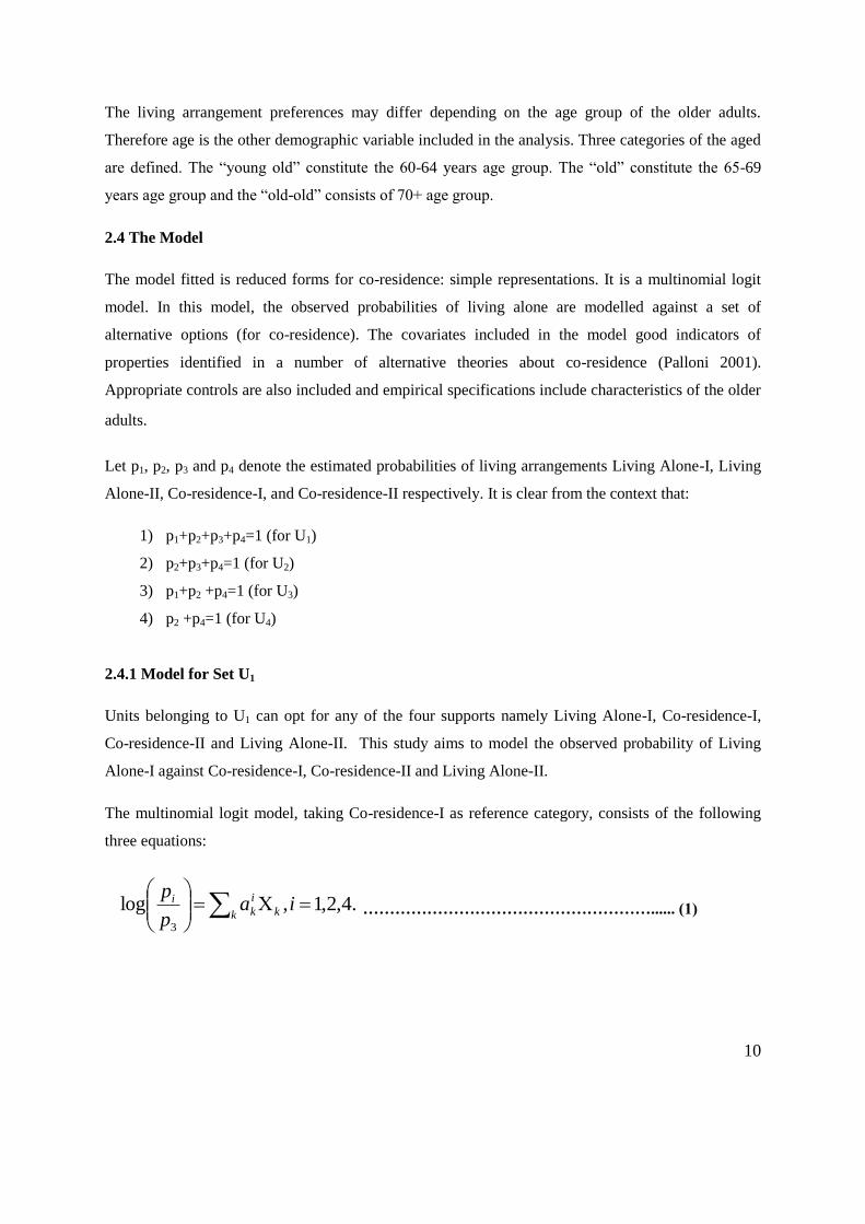
2.4 The Model
The model fitted is reduced forms for co-residence: simple representations. It is a multinomial logit
model. In this model, the observed probabilities of living alone are modelled against a set of
alternative options (for co-residence). The covariates included in the model good indicators of
properties identified in a number of alternative theories about co-residence (Palloni 2001).
Appropriate controls are also included and empirical specifications include characteristics of the older
adults.
Let p1, p2, p3 and p4 denote the estimated probabilities of living arrangements Living Alone-I, Living
Alone-II, Co-residence-I, and Co-residence-II respectively. It is clear from the context that:
1) p1+p2+p3+p4=1 (for U1)
2) p2+p3+p4=1 (for U2)
3) p1+p2 +p4=1 (for U3)
4) p2 +p4=1 (for U4)
2.4.1 Model for Set U1
Units belonging to U1 can opt for any of the four supports namely Living Alone-I, Co-residence-I,
Co-residence-II and Living Alone-II. This study aims to model the observed probability of Living
Alone-I against Co-residence-I, Co-residence-II and Living Alone-II.
The multinomial logit model, taking Co-residence-I as reference category, consists of the following
three equations:
.4,2,1,log3
ia
p
pkk
i
ki
………………………………………………...... (1)
11
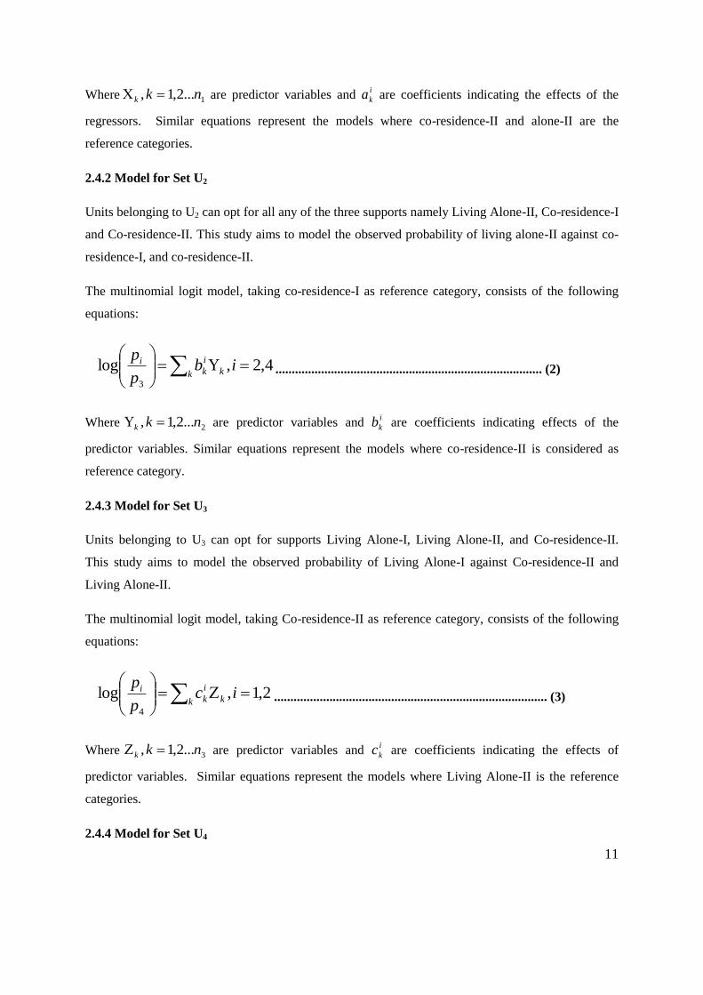
Where 1...2,1, nkk are predictor variables and i
ka are coefficients indicating the effects of the
regressors. Similar equations represent the models where co-residence-II and alone-II are the
reference categories.
2.4.2 Model for Set U2
Units belonging to U2 can opt for all any of the three supports namely Living Alone-II, Co-residence-I
and Co-residence-II. This study aims to model the observed probability of living alone-II against co-
residence-I, and co-residence-II.
The multinomial logit model, taking co-residence-I as reference category, consists of the following
equations:
4,2,log3
ib
p
pkk
i
ki
.................................................................................. (2)
Where 2...2,1, nkk are predictor variables and i
kb are coefficients indicating effects of the
predictor variables. Similar equations represent the models where co-residence-II is considered as
reference category.
2.4.3 Model for Set U3
Units belonging to U3 can opt for supports Living Alone-I, Living Alone-II, and Co-residence-II.
This study aims to model the observed probability of Living Alone-I against Co-residence-II and
Living Alone-II.
The multinomial logit model, taking Co-residence-II as reference category, consists of the following
equations:
2,1,log4
ic
p
pkk
i
ki
.................................................................................... (3)
Where 3...2,1, nkk are predictor variables and i
kc are coefficients indicating the effects of
predictor variables. Similar equations represent the models where Living Alone-II is the reference
categories.
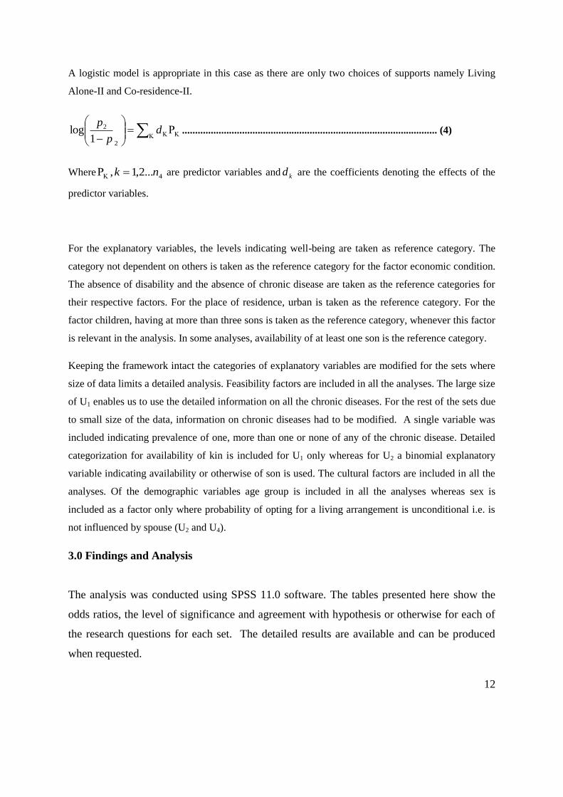
2.4.4 Model for Set U4
12
A logistic model is appropriate in this case as there are only two choices of supports namely Living
Alone-II and Co-residence-II.
d
p
p
2
2
1log .................................................................................................. (4)
Where 4...2,1, nk are predictor variables and kd are the coefficients denoting the effects of the
predictor variables.
For the explanatory variables, the levels indicating well-being are taken as reference category. The
category not dependent on others is taken as the reference category for the factor economic condition.
The absence of disability and the absence of chronic disease are taken as the reference categories for
their respective factors. For the place of residence, urban is taken as the reference category. For the
factor children, having at more than three sons is taken as the reference category, whenever this factor
is relevant in the analysis. In some analyses, availability of at least one son is the reference category.
Keeping the framework intact the categories of explanatory variables are modified for the sets where
size of data limits a detailed analysis. Feasibility factors are included in all the analyses. The large size
of U1 enables us to use the detailed information on all the chronic diseases. For the rest of the sets due
to small size of the data, information on chronic diseases had to be modified. A single variable was
included indicating prevalence of one, more than one or none of any of the chronic disease. Detailed
categorization for availability of kin is included for U1 only whereas for U2 a binomial explanatory
variable indicating availability or otherwise of son is used. The cultural factors are included in all the
analyses. Of the demographic variables age group is included in all the analyses whereas sex is
included as a factor only where probability of opting for a living arrangement is unconditional i.e. is
not influenced by spouse (U2 and U4).
3.0 Findings and Analysis
The analysis was conducted using SPSS 11.0 software. The tables presented here show the
odds ratios, the level of significance and agreement with hypothesis or otherwise for each of
the research questions for each set. The detailed results are available and can be produced
when requested.
13
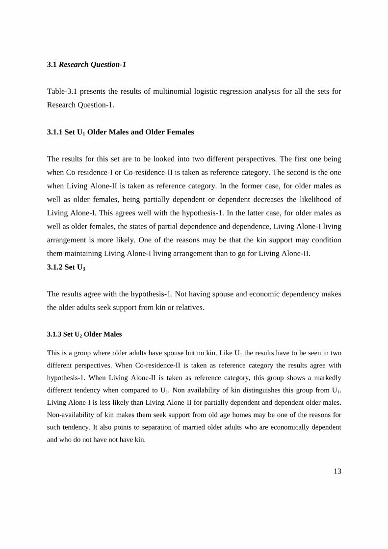
3.1 Research Question-1
Table-3.1 presents the results of multinomial logistic regression analysis for all the sets for
Research Question-1.
3.1.1 Set U1 Older Males and Older Females
The results for this set are to be looked into two different perspectives. The first one being
when Co-residence-I or Co-residence-II is taken as reference category. The second is the one
when Living Alone-II is taken as reference category. In the former case, for older males as
well as older females, being partially dependent or dependent decreases the likelihood of
Living Alone-I. This agrees well with the hypothesis-1. In the latter case, for older males as
well as older females, the states of partial dependence and dependence, Living Alone-I living
arrangement is more likely. One of the reasons may be that the kin support may condition
them maintaining Living Alone-I living arrangement than to go for Living Alone-II.
3.1.2 Set U3
The results agree with the hypothesis-1. Not having spouse and economic dependency makes
the older adults seek support from kin or relatives.
3.1.3 Set U2 Older Males
This is a group where older adults have spouse but no kin. Like U1 the results have to be seen in two
different perspectives. When Co-residence-II is taken as reference category the results agree with
hypothesis-1. When Living Alone-II is taken as reference category, this group shows a markedly
different tendency when compared to U1. Non availability of kin distinguishes this group from U1.
Living Alone-I is less likely than Living Alone-II for partially dependent and dependent older males.
Non-availability of kin makes them seek support from old age homes may be one of the reasons for
such tendency. It also points to separation of married older adults who are economically dependent
and who do not have not have kin.
14
3.2 Research Question-2
Table-3.2.1, Table-3.2.2 and Table-3.2.3 present the results of multinomial logistic regression
analysis for all the sets for Research Question-2.
3.2.1 Set U1 Older Males and Older Females
For older males the analysis includes all the chronic diseases. When Co-residence-I is taken
as a reference category, for older males positive associations between Living Alone-I and
prevalence of chronic diseases namely pain in joints and limbs, piles, hypertension, diabetes
and heart disease is observed. Where as the diseases chronic cough and urinary problems
showed negative association with Living Alone-I. It seems that chronic diseases differ in their
impact on Living Alone-I.
When co-residence-II is taken as a reference category, for older males, negative association is
observed between Living Alone-I and prevalence of chronic diseases namely chronic cough,
pain in joints and limbs, hypertension, diabetes and heart disease. The odds ratios indicate
decreased likelihood of living alone when the above mentioned diseases are prevalent,
agreeing to the earlier studies. For the diseases urinary problems and piles, a positive
association was observed between Living Alone-I and prevalence of the two diseases. Older
males with these diseases are more likely to opt for Living Alone-I type of living
arrangement.
When Living Alone-II is taken as reference category, the prevalence of chronic diseases
namely pain in joints and limbs and urinary problems shows a negative association with
Living Alone-I. Rest of the chronic diseases showed positive association with Living Alone-I.
For older females the severity of prevalence of chronic diseases was defined differently. For
older adults females the associations found are not significant. Except for the case where
Living Alone-II is the reference category, prevalence of chronic diseases showed an
increased likelihood of Living Alone-I. These results disagree with the hypothesis 2-b. For
Living Alone-II as reference category, the state two or less chronic diseases reported showed
15
a decreased likelihood of Living Alone-I, whereas the state more than two chronic diseases
prevalent showed an increased likelihood of Living Alone-I. These results indicate spouse as
a better source of support in case of prevalence of chronic diseases.
3.2.2 Set U3
For this set support of spouse is absent. Interesting to observe is the fact that the effect of
prevalence of any of the seven chronic diseases is not significant. But for prevalence of piles
and heart disease prevalence of all other diseases indicate a decrease in the likelihood of
living arrangement Living Alone-II. Barring piles and heart disease the results are in
agreement with the null hypothesis 2-a.
For Co-residence-II as the reference category, the likelihood of Living Alone-II increased in
case of prevalence of chronic cough, pain in joints and limbs and heart disease. For the rest of
the diseases the results agree with hypothesis 2-a.
3.2.3 Set U3 Older Males
The effects are not significant for any of the categories namely two or less chronic diseases
and more than two chronic diseases. For Co-Residence-II as reference category, living alone
is less likely for the category two or less chronic diseases. For the category more than two
chronic diseases the likelihood of living alone is greater.
With alone-II as reference category, the increasing number of chronic diseases result in
increasing likelihood of alone-I type of living arrangement. The reason may be that in the
absence of kin spouse is a better support than any other possible choice of living
arrangements.
3.3 Research Question 3
Table-3.3 presents the results of multinomial logistic regression analysis for all the sets for
Research Question-3.
16
3.3.1 Set U1 Older Males and Older Females
There are two states of mobility difficulty namely partial mobility difficulty and severe
mobility difficulty. To analyze the effects of these states of disability on the likelihood of
Living Alone-I let us first consider the results obtained by considering Co-residence-I and
Co-residence-II as reference category.
For older males, the effects of categories of mobility difficulty were found to be significant
for the former reference category only. The results indicate that older males with disability
are more likely to opt for Living Alone-I an exception being the state of partial mobility
difficulty when Co-residence-II is considered as reference category. Barring this exception,
all other odds ratios do not agree with the hypothesis 3. It seems that for older males spouse
is a better care provider in case of disability. For older females, the scenario differs from that
of older males. Here the state of severe mobility difficulty has significant negative effect on
the likelihood of Living Alone-I, which is in agreement with the hypothesis 3. The effect of
partial mobility difficulty is not significant for older females. For Co-residence-I as reference
category the state of partial mobility difficulty indicated an increased likelihood of Living
Alone-I and for Co-residence-II as reference category it showed a decreased likelihood of
Living Alone-I. The latter case agreed with the hypothesis 3.
The effect of severe mobility difficulty was significant for older males in case of Living
Alone–II as reference category. For the rest of the cases the effects were not significant. For
older females the results indicated that Living Alone-I state is more likely for all states of
disability. Whereas for older males the state of severe mobility difficulty increased the
likelihood of alone-I and for the state of partial mobility difficulty opposite was observed.
3.3.2 Set U2
The results disagree with the hypothesis-3. The effect of the state of severe mobility difficulty
is highly significant. The results indicate that the state of Living Alone-II is more likely for
17
partial as well as severe mobility difficulty. This group lacks spouse as support and it is
expected that supports Co-residence-I and Co-residence-II would be preferably opted for as
compared to Living Alone-II. But results vary a lot from what general perception could be.
3.3.3 Set U3 Older Males
The effects of the states of mobility difficulty are not found to be significant for this set. The
direction of effects changed with change in reference category. For Co-residence-II as
reference category, the results showed an increased likelihood of Living Alone-I, where as
for Living Alone-II as reference category a decreased likelihood of Living Alone-I was
observed.
3.4 Research Question-4
Table-3.4 presents the results of multinomial logistic regression analysis for all the sets for
Research Question-4.
3.4.1 Set U1 Older Males and Older Females
For this set, the reference category for older males is different than that for older females. The
effect of the state of having no son is significant for older females. The results agree with
hypothesis 4-a. For older males the reference category is having three or more sons. On
the question investigated by hypothesis 4-b, the observations disagree with the hypothesis.
The likelihood of living alone decreases with decreasing number of sons.
3.4.2 Set U2
For this group the effect of the state of having no son was not found to be significant.
3.5 Research Question-5
18
Table-3.5 presents the results of multinomial logistic regression analysis for all the sets for
Research Question-5.
3.5.1 Set U1 Older Males and Older Females
Let us take up the case where Co-residence-I or Co-residence-II is taken as reference
category. For older males as well as older females Living Alone-I is more likely for rural
areas.
For Living Alone-II as reference category, the effect was found significant for older males
but it was not significant for older females. The older males are more likely to go for Living
Alone-I, where as older females are less likely to do so.
3.5.2 Set U2
For this set spouse as a support is not possible. The results are in contrast to those found for
the set U1 (for Co-residence-I and Co-residence-II as reference categories). Living Alone-II is
less likely living arrangement in rural areas. It indicates that for this group supports Co-
residence-I or Co-residence-II serve as supports in rural areas.
3.5.3 Set U3 older males
For this set the results indicate that alone-I living arrangement is more likely in rural areas.
4.0 About Set U3 Older Females and Set U4
There were 140 older females in set U3. Out of these 129 had Living Alone-I type of living
arrangement. For the rest, 7 were in Living Alone-II and 4 in Co-residence-II. For older
males belonging to the set U4, all the 97 units had Co-residence-II living arrangement. For the
older females of set U4, out of 218 units 216 had Co-residence-II living arrangement; the rest
had Alone-II.
19
5.0 Conclusion
Rapid pace of ageing and high levels of co-residence characterize the Indian ageing scenario.
Reports of 42nd
and 52nd
rounds of NSS show a decline in levels of co-residence. In rural
areas the percentage of older adults co-residing with children or other relatives dropped from
54.8 per cent in the 42nd
round to 37.9 per cent in the 52nd
round. For urban areas the decline
was from 58.4 per cent to 40.0 per cent. These changes occurred during a gap of a decade
(1985-86, 1995-96). These changes are phenomenal and represent the effects of changing
socio-economic scenario. It is interesting to observe that trend was similar urban as well as
rural areas.
The present study investigated the effect of factors namely availability of son, health,
economic dependency, disability and place of residence on the likelihood of alone-I living
arrangement. For the older adults having kin, non-availability of son did contribute to the
likelihood of living alone. However, the results obtained after refining the categories of
availability of son, for set U1 males, did reflected a need to pause and rethink. Briefly, more
sons do not indicate increased likelihood of co-residence. This observation points to the need
for in-depth investigation in the cases when more than one son are available and how does the
characteristics of sons affect the living arrangements of the older parents?
Considering economic dependence as a factor affecting the likelihood of Living Alone-I
living arrangement the results are as expected and agree with earlier studies. Increasing
economic dependency leads to decreased likelihood of Living Alone-I as compared to choice
of Co-residence-I or Co-residence-II.
As far as the effect of prevalence of chronic diseases on the likelihood of Living Alone-I or
Living Alone-II is concerned no clear picture emerge in the sense that contrary to expectation
the factors are not effective. This indicates a need for more exhaustive studies connecting
health status and living arrangements of the older adults. The effect of disability also goes
20
contrary to expectation U1 females are an exception. The findings should cause concern to the
policy makers regarding well-being of the disabled older adults.
More likelihood of Alone-I in rural areas demands special attention from policy makers as
co-residents are less likely to act as support.
The present study considers a part of the heterogeneity of the older population and models the
living arrangements as choices available to the older adults. It is limited in its scope as it does
not take into consideration socio-economic characteristics of the children. Any cross sectional
study is limited in its scope as living arrangements of the older adults need to be looked upon
as a process in space and time. This demands more sophisticated models not only taking into
consideration all the factors affecting living arrangements of the older adults but also a
process view of the phenomena.
21
References
Agaresti, Alan. Categorical data Analysis, John Wiley & Sons.
Dixon, R. B. 1971. Explaining cross cultural variations in age at marriage and proportions never
married, Population Studies 25(2): 215-233.
DeMaris, A. 2004. Regression with Social Data: Modeling Continuous and Limited Response
Variables.
Jeffery A. B. and J. E. Mutchler. 1992. The living arrangements of unmarried older adults
Hispanic females, Demography 29(1): 93-112.
NSS Report No. 367, Socio-Economic Profile of the Aged Persons, Report of forty-second round:
July 1986-June 1987, National Sample Survey Organization (N.S.S.O), Government of India,
September 1989.
Palloni, A. 2001. Living arrangements of older persons, Population Bulletin of the United
Nations. Special Issue Nos. 42/43 2001:54-110.
Report No. 446(52/25.0/3), The Aged in India: A Socio-economic Profile, NSS fifty-second
round, July 1995-June 1996, National Sample Survey Organization (N.S.S.O), Department of
statistics, Ministry of Planning and Programme Implementation, Government of India, November
1998.
Retherford, R. D, and Choe, M. K. Structural Models for Causal data Analysis. John Wiley &
sons, INC.
Shah, A. M. 1999. Changes in the family and the older adults, Economic and Political Weekly
May 15-21.
Sokolovsky, J. 2001. Living arrangements of older persons and family support in less developed
countries, Population Bulletin of the United Nations Special Issue Nos. 42/43 2001:162-192.
Vlassoff, C. 1990. The value of sons in an Indian village: how widows see it, Population Studies
44(): 5-20.
Walter, K. V., Housing and community settings for older adults in Tibbits (ed), Handbook of
Social Gerontology, Social Aspects of Aging, The University of Chicago Press, Chicago, pp. 549-
617.
Wolf, D. A, and Soldo, B. J. 1988. Household composition choices of older unmarried women,
Demography 25(1): 387-403.
www.indiastat.com
www.censusindia.net
Zimmer, Z. and Dayton J. 2005. Older adults in sub-Saharan Africa living with children and
grandchildren, Population Studies 59(3): 295-312.
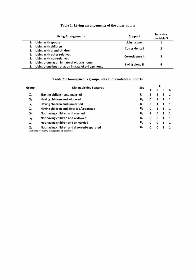
Table 1: Living arrangements of the older adults
Table 2: Homogeneous groups, sets and available supports
Group Distinguishing Features Set S
1 2 3 4
G1 Having children and married U1 1 1 1 1
G2 Having children and widowed U2 0 1 1 1
G3 Having children and unmarried U2 0 1 1 1
G4 Having children and divorced/separated U2 0 1 1 1
G5 Not having children and married U3 1 0 1 1
G6 Not having children and widowed U4 0 0 1 1
G7 Not having children and unmarried U4 0 0 1 1
G8 Not having children and divorced/separated U4 0 0 1 1
1 indicates availability of support and 0 otherwise
Living Arrangements Support Indicator variable S
1. Living with spouse Living alone I 1 1. Living with children 2. Living with grand children
Co-residence I 2
1. Living with other relatives 2. Living with non-relatives
Co-residence II 3
1. Living alone as an inmate of old age home 2. Living alone but not as an inmate of old age home
Living alone II 4
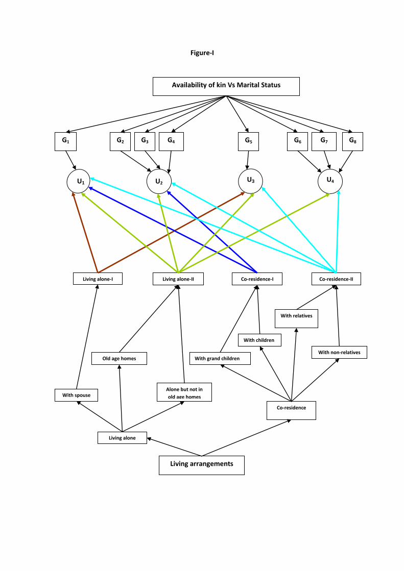
Figure-I
Availability of kin Vs Marital Status
G1
G2
G3
G4
G8
G7
G6
G5
U1 U2 U3 U4
Living arrangements
Living alone
Co-residence
With spouse
Old age homes
Alone but not in
old age homes
With children
With relatives
With grand children
With non-relatives
Living alone-I Living alone-II
Co-residence-I Co-residence-II
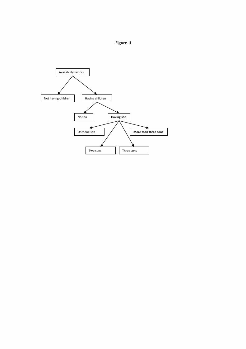
Figure-II
Availability factors
Having children Not having children
No son
Two sons
Only one son
Three sons
Having son
More than three sons
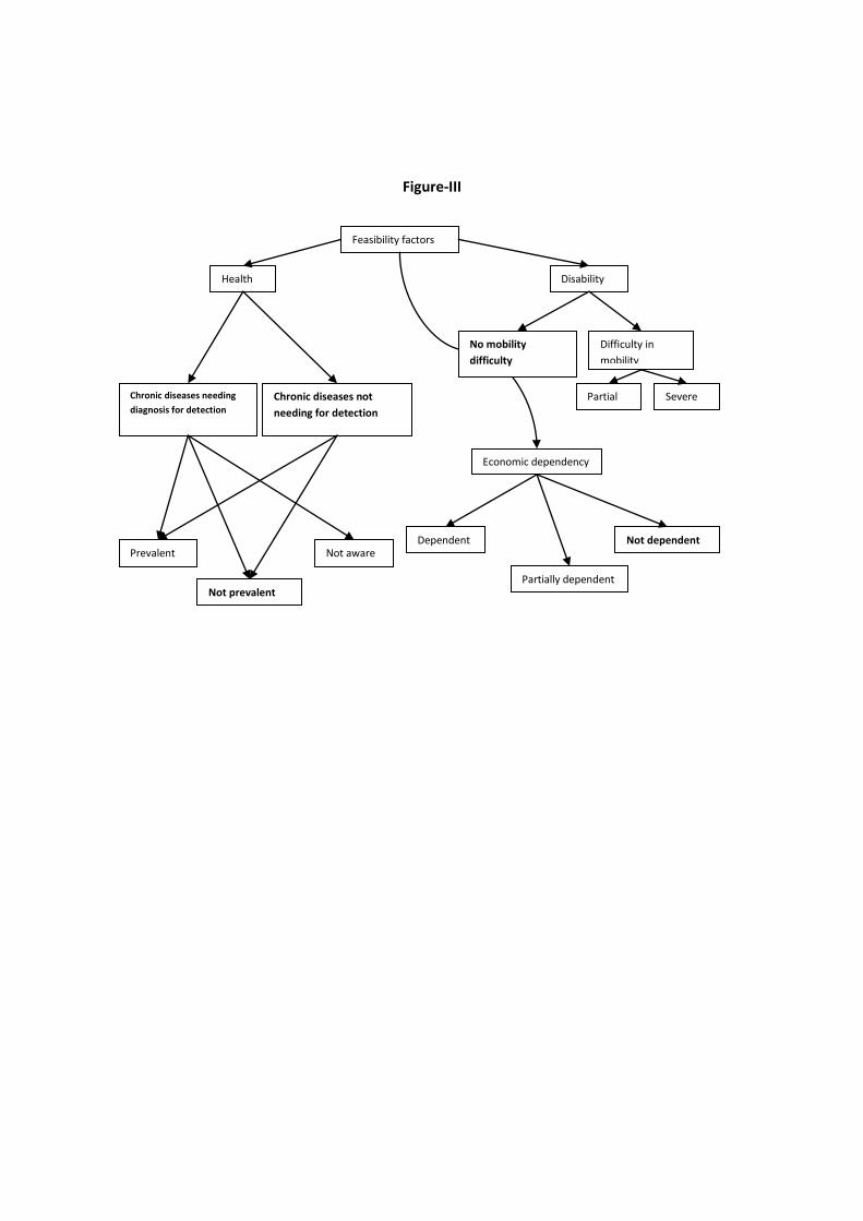
Figure-III
Feasibility factors
Health
Economic dependency
Disability
Chronic diseases needing
diagnosis for detection
Chronic diseases not
needing for detection
Prevalent
Not prevalent
Not aware Dependent
Partial
Partially dependent
Not dependent
No mobility
difficulty
Difficulty in
mobility
Severe
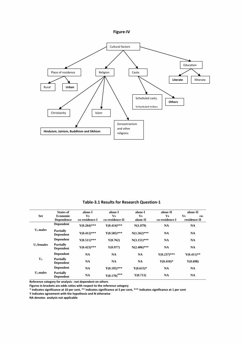
Figure-IV
Table-3.1 Results for Research Question-1
Set
States of
Economic
Dependence
alone-I
Vs
co-residence-I
alone-I
Vs
co-residence-II
alone-I
Vs
alone-II
alone-II
Vs
co-residence-I
alone-II
Vs co-
residence-II
U1 males
Dependent Y(0.264)*** Y(0.414)*** N(1.079) NA NA
Partially
Dependent Y(0.412)*** Y(0.585)*** N(1.562)*** NA NA
U1 females
Dependent Y(0.511)*** Y(0.762) N(3.151)*** NA NA
Partially
Dependent Y(0.423)*** Y(0.977) N(2.406)*** NA NA
U2
Dependent NA NA NA Y(0.237)*** Y(0.411)**
Partially
Dependent NA NA NA Y(0.410)* Y(0.698)
U3 males
Dependent NA Y(0.195)*** Y(0.615)* NA NA
Partially
Dependent NA Y(0.170)*** Y(0.713) NA NA
Reference category for analysis : not dependent on others Figures in brackets are odds ratios with respect to the reference category * indicates significance at 10 per cent, ** indicates significance at 5 per cent, *** indicates significance at 1 per cent Y indicates agreement with the hypothesis and N otherwise NA denotes analysis not applicable
Cultural factors
Place of residence Religion Caste
Education
Rural Urban
Scheduled casts,
Scheduled tribes,
Neo-Buddhists
Illiterate Literate
Others
Hinduism, Jainism, Buddhism and Sikhism
Islam Christianity
Zoroastrianism
and other
religions
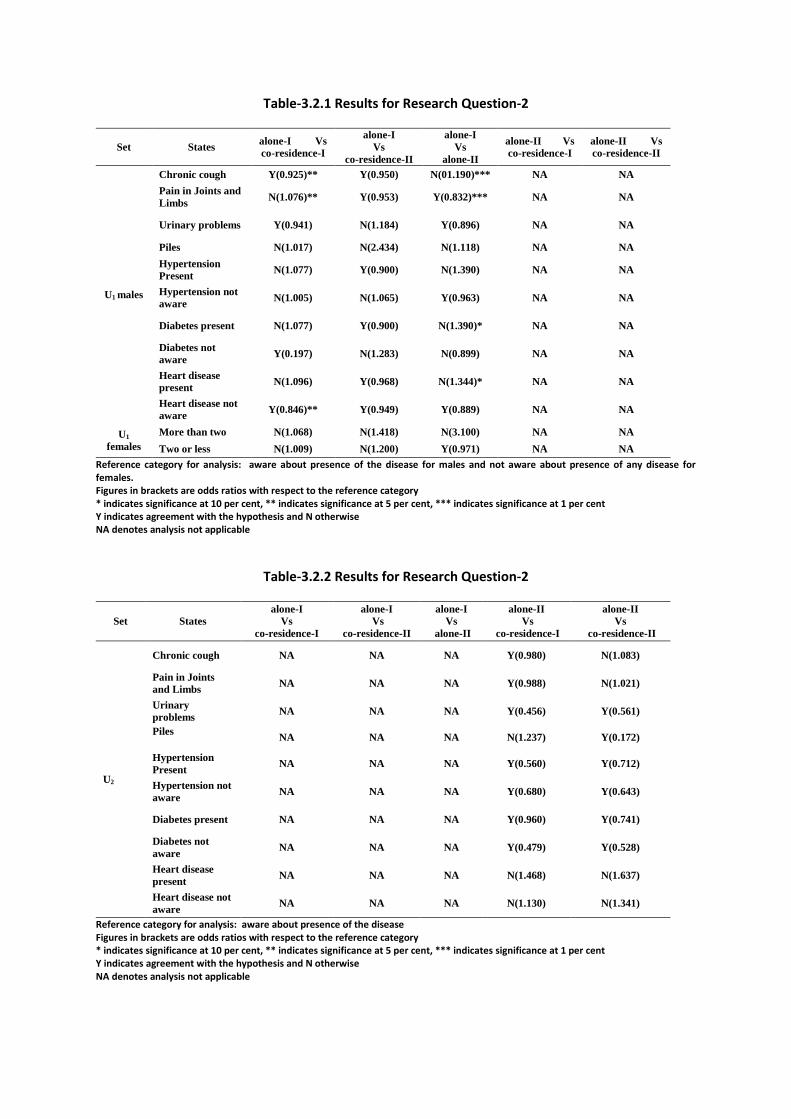
Table-3.2.1 Results for Research Question-2
Set States alone-I Vs
co-residence-I
alone-I
Vs
co-residence-II
alone-I
Vs
alone-II
alone-II Vs
co-residence-I
alone-II Vs
co-residence-II
U1 males
Chronic cough Y(0.925)** Y(0.950) N(01.190)*** NA NA
Pain in Joints and
Limbs N(1.076)** Y(0.953) Y(0.832)*** NA NA
Urinary problems Y(0.941) N(1.184) Y(0.896) NA NA
Piles N(1.017) N(2.434) N(1.118) NA NA
Hypertension
Present N(1.077) Y(0.900) N(1.390) NA NA
Hypertension not
aware N(1.005) N(1.065) Y(0.963) NA NA
Diabetes present N(1.077) Y(0.900) N(1.390)* NA NA
Diabetes not
aware Y(0.197) N(1.283) N(0.899) NA NA
Heart disease
present N(1.096) Y(0.968) N(1.344)* NA NA
Heart disease not
aware Y(0.846)** Y(0.949) Y(0.889) NA NA
U1
females
More than two N(1.068) N(1.418) N(3.100) NA NA
Two or less N(1.009) N(1.200) Y(0.971) NA NA
Reference category for analysis: aware about presence of the disease for males and not aware about presence of any disease for females. Figures in brackets are odds ratios with respect to the reference category * indicates significance at 10 per cent, ** indicates significance at 5 per cent, *** indicates significance at 1 per cent Y indicates agreement with the hypothesis and N otherwise NA denotes analysis not applicable
Table-3.2.2 Results for Research Question-2
Set States
alone-I
Vs
co-residence-I
alone-I
Vs
co-residence-II
alone-I
Vs
alone-II
alone-II
Vs
co-residence-I
alone-II
Vs
co-residence-II
U2
Chronic cough NA NA NA Y(0.980) N(1.083)
Pain in Joints
and Limbs NA NA NA Y(0.988) N(1.021)
Urinary
problems NA NA NA Y(0.456) Y(0.561)
Piles
NA NA NA N(1.237) Y(0.172)
Hypertension
Present NA NA NA Y(0.560) Y(0.712)
Hypertension not
aware NA NA NA Y(0.680) Y(0.643)
Diabetes present NA NA NA Y(0.960) Y(0.741)
Diabetes not
aware NA NA NA Y(0.479) Y(0.528)
Heart disease
present NA NA NA N(1.468) N(1.637)
Heart disease not
aware NA NA NA N(1.130) N(1.341)
Reference category for analysis: aware about presence of the disease Figures in brackets are odds ratios with respect to the reference category * indicates significance at 10 per cent, ** indicates significance at 5 per cent, *** indicates significance at 1 per cent Y indicates agreement with the hypothesis and N otherwise NA denotes analysis not applicable
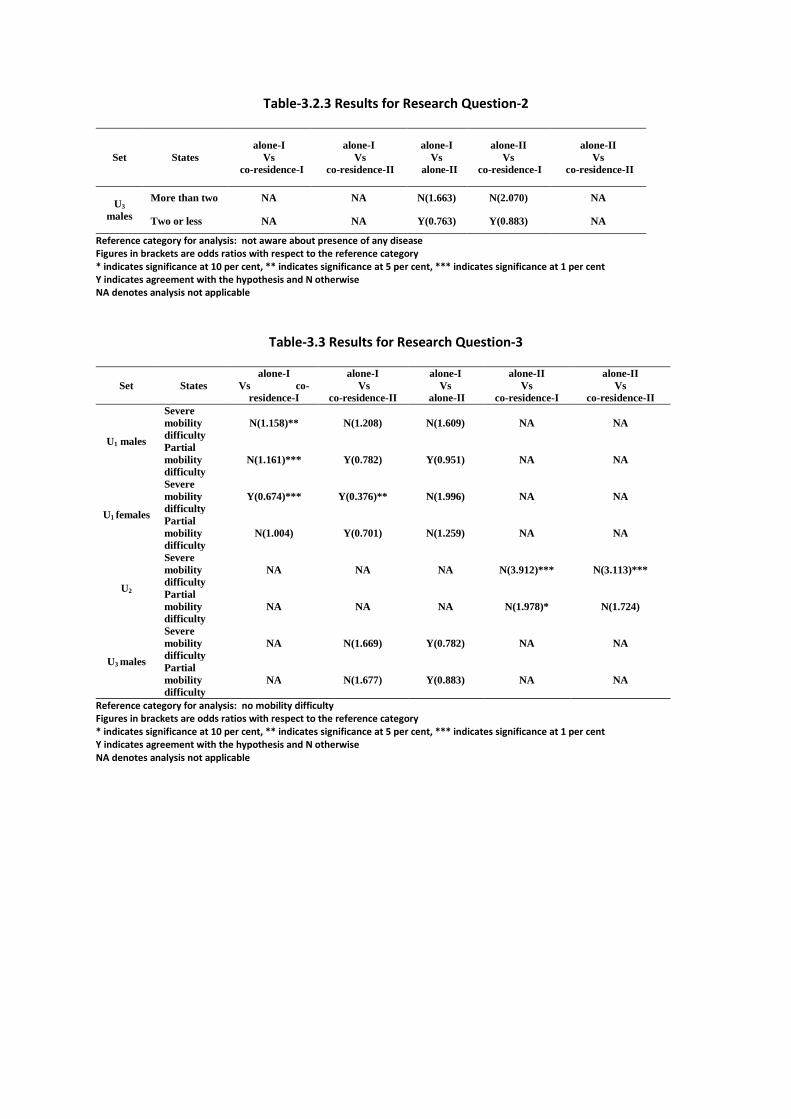
Table-3.2.3 Results for Research Question-2
Set States
alone-I
Vs
co-residence-I
alone-I
Vs
co-residence-II
alone-I
Vs
alone-II
alone-II
Vs
co-residence-I
alone-II
Vs
co-residence-II
U3
males
More than two NA NA N(1.663) N(2.070) NA
Two or less NA NA Y(0.763) Y(0.883) NA
Reference category for analysis: not aware about presence of any disease Figures in brackets are odds ratios with respect to the reference category * indicates significance at 10 per cent, ** indicates significance at 5 per cent, *** indicates significance at 1 per cent Y indicates agreement with the hypothesis and N otherwise NA denotes analysis not applicable
Table-3.3 Results for Research Question-3
Set
States
alone-I
Vs co-
residence-I
alone-I
Vs
co-residence-II
alone-I
Vs
alone-II
alone-II
Vs
co-residence-I
alone-II
Vs
co-residence-II
U1 males
Severe
mobility
difficulty
N(1.158)** N(1.208) N(1.609) NA NA
Partial
mobility
difficulty
N(1.161)*** Y(0.782) Y(0.951) NA NA
U1 females
Severe
mobility
difficulty
Y(0.674)*** Y(0.376)** N(1.996) NA NA
Partial
mobility
difficulty
N(1.004) Y(0.701) N(1.259) NA NA
U2
Severe
mobility
difficulty
NA NA NA N(3.912)*** N(3.113)***
Partial
mobility
difficulty
NA NA NA N(1.978)* N(1.724)
U3 males
Severe
mobility
difficulty
NA N(1.669) Y(0.782) NA NA
Partial
mobility
difficulty
NA N(1.677) Y(0.883) NA NA
Reference category for analysis: no mobility difficulty Figures in brackets are odds ratios with respect to the reference category * indicates significance at 10 per cent, ** indicates significance at 5 per cent, *** indicates significance at 1 per cent Y indicates agreement with the hypothesis and N otherwise NA denotes analysis not applicable
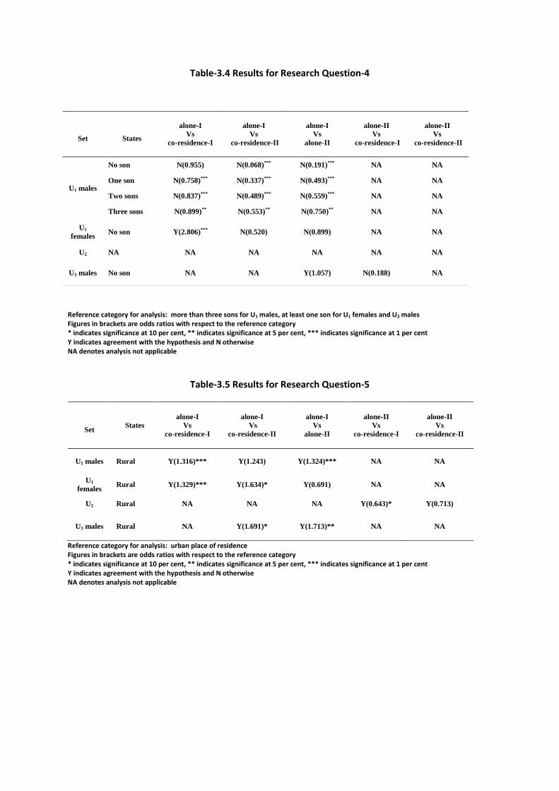
Table-3.4 Results for Research Question-4
Reference category for analysis: more than three sons for U1 males, at least one son for U1 females and U3 males Figures in brackets are odds ratios with respect to the reference category * indicates significance at 10 per cent, ** indicates significance at 5 per cent, *** indicates significance at 1 per cent Y indicates agreement with the hypothesis and N otherwise NA denotes analysis not applicable
Table-3.5 Results for Research Question-5
Set States
alone-I
Vs
co-residence-I
alone-I
Vs
co-residence-II
alone-I
Vs
alone-II
alone-II
Vs
co-residence-I
alone-II
Vs
co-residence-II
U1 males Rural Y(1.316)*** Y(1.243) Y(1.324)*** NA NA
U1
females Rural Y(1.329)*** Y(1.634)* Y(0.691) NA NA
U2 Rural NA NA NA Y(0.643)* Y(0.713)
U3 males Rural NA Y(1.691)* Y(1.713)** NA NA
Reference category for analysis: urban place of residence Figures in brackets are odds ratios with respect to the reference category * indicates significance at 10 per cent, ** indicates significance at 5 per cent, *** indicates significance at 1 per cent Y indicates agreement with the hypothesis and N otherwise NA denotes analysis not applicable
Set
States
alone-I
Vs
co-residence-I
alone-I
Vs
co-residence-II
alone-I
Vs
alone-II
alone-II
Vs
co-residence-I
alone-II
Vs
co-residence-II
U1 males
No son N(0.955) N(0.068)*** N(0.191)*** NA NA
One son N(0.758)*** N(0.337)*** N(0.493)*** NA NA
Two sons N(0.837)*** N(0.489)*** N(0.559)*** NA NA
Three sons N(0.899)** N(0.553)** N(0.750)** NA NA
U1
females No son Y(2.806)*** N(0.520) N(0.899) NA NA
U2 NA NA NA NA NA NA
U3 males No son NA NA Y(1.057) N(0.188) NA