Embed Size (px)
Citation preview
MPRAMunich Personal RePEc Archive
Remittances, Inflation and ExchangeRate Regimes in Small Open Economies
Christopher Ball and Claude Lopez and Javier Reyes
Quinnipiac University, Banque de France, University of Arkansas
July 2012
Online at https://mpra.ub.uni-muenchen.de/39852/MPRA Paper No. 39852, posted 5. July 2012 11:32 UTC
1
Remittances, Inflation and Exchange Rate Regimes in
Small Open Economies
Christopher P. Ball (Quinnipiac University)
Claude Lopez (Banque de France)
Javier Reyes (University of Arkansas)
July 2012
Abstract
Remittances are private monetary transfers across borders and thus, often, involve
different currencies. Yet the rapidly growing literature on the subject often ignores the role that
exchange rate regimes play in determining the effect foreign-currency remittances have on a
recipient economy. This paper uses a theoretical model and panel vector autoregression
techniques to understand the effect of remittances on GDP, inflation, real exchange rate and
money supply, depending on the exchange rate regimes. Furthermore, it allows a more detailed
description of the short-run dynamics as it considers yearly but also quarterly data for 21
emerging countries. Our theoretical model predicts that remittances should temporarily increase
inflation, GDP, the domestic money supply and appreciate the real exchange rate under a fixed
regime, but temporarily decrease inflation, increase GDP, appreciate the real exchange rate and
generate no change in the money supply under a flexible regime. These differences are largely
borne out in the data. This adds to our understanding of the true effect of remittances on
economies by showing that exchange rate regimes matter for the effects of remittances, especially
in the short run for monetary conditions in an economy, and suggests that other results in the
literature that do not control for regimes may be biased.
JEL Classification: F22 - International Migration; F33 - International Monetary Arrangements
and Institutions; F41 - Open Economy Macroeconomics; C32 - Time-Series Models; C33 -
Models with Panel Data
2
I. Introduction
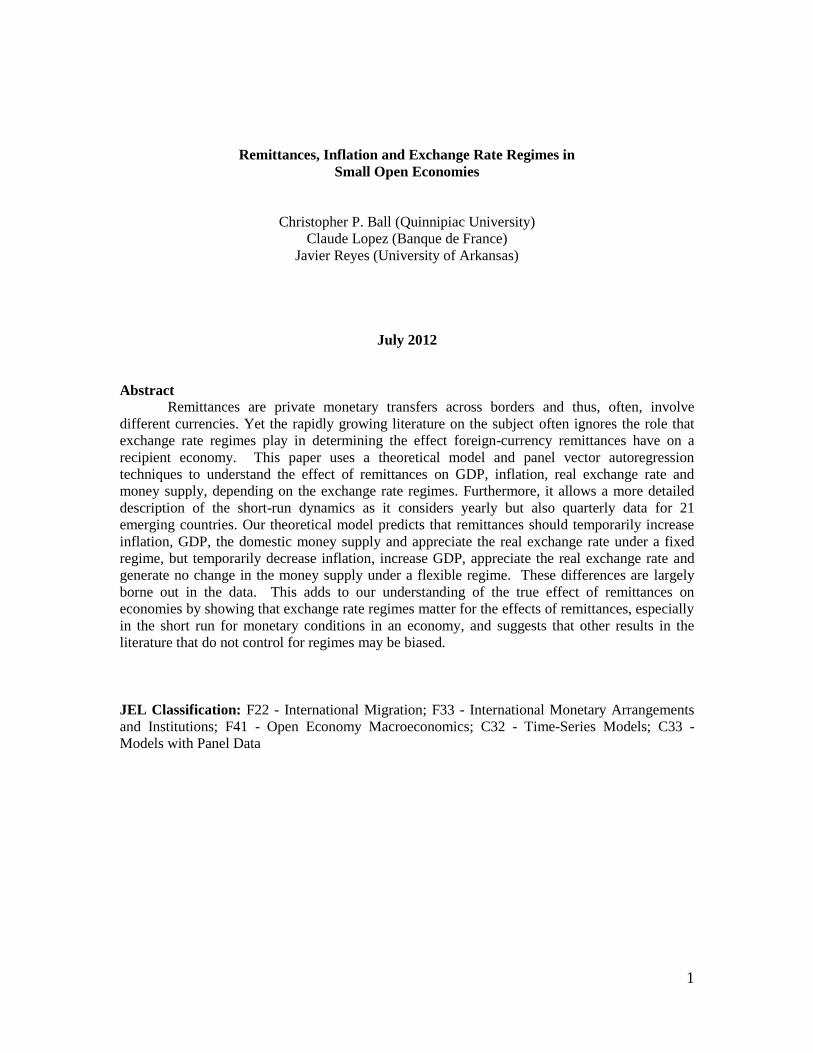
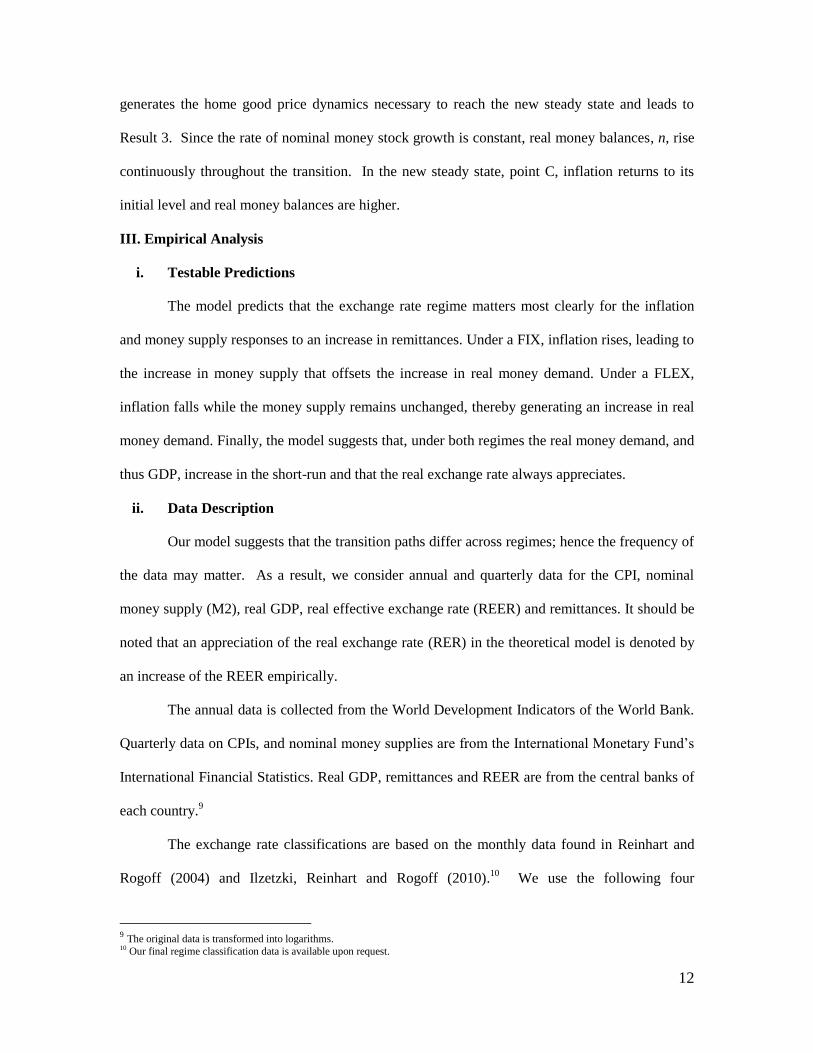
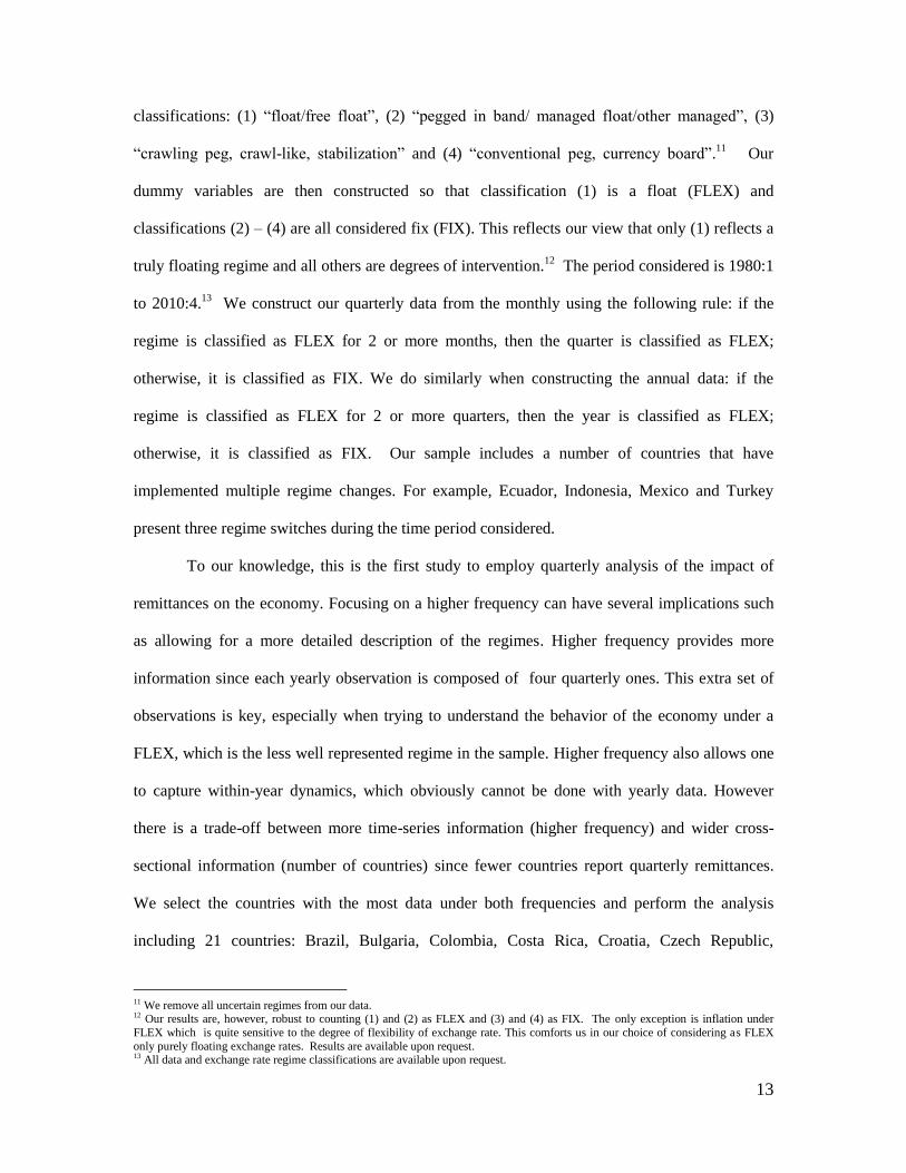
Remittance flows are large, growing, and important for many economies. Beyond the
increase in absolute terms, remittances have gained in importance relative to other flows. Indeed,
Figures 1 and 2 show that remittances exceed foreign direct investment for many countries and
are relatively large capital flows. Hence, understanding the impact of remittances on variables
such as inflation and gross domestic output (GDP) is essential for policy makers of recipient
economies as these are the critical components in policy response functions.
[INSERT FIGURES 1 AND 2]
The recent debate about the effects of remittances mostly focuses on the terms of trade.
Works such as Amuedo-Dorantes and Pozo (2004), Bourdet and Falck (2006) and Lopez, Molina,
and Bussolo (2007) show that remittances have an inflationary effect and lead to a real exchange
rate appreciation (a.k.a., “the Dutch disease”).1 Most recently, Narayan, Narayan, and Mishra
(2011) investigate the short-run and long-run effects of remittances and institutional variables on
inflation across 54 developing countries and confirm the inflationist effect of remittances. Yet, all
these studies assume that the countries follow an unchanged exchange rate regime, which is a
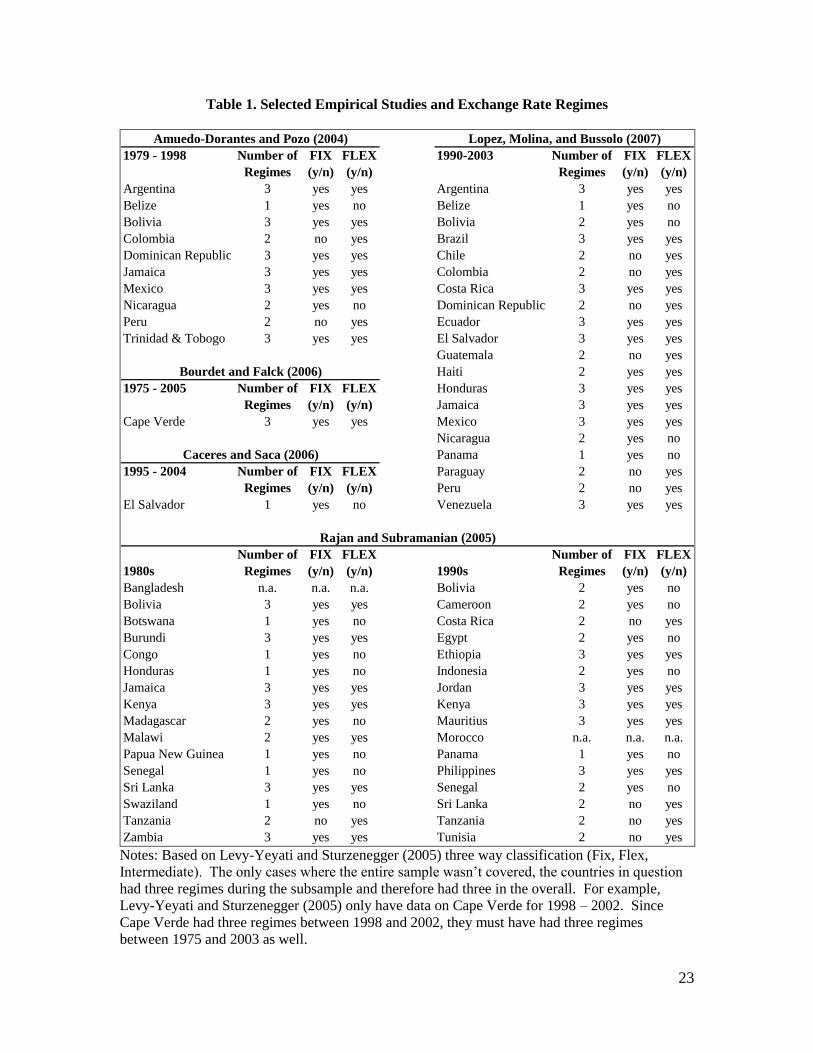
rather strong assumption: Table 1 shows that each one of the countries studied have observed at
least one change in regime for the periods considered.2
As an alternative, Caceres and Saca (2006) explicitly controls for changes in the
exchange rate regime when studying the impact of remittances. Yet, they focus on El Salvador’s
economy while the country remains in a fixed regime and their findings confirm the inflationary
effect of remittances.
[INSERT TABLE 1]
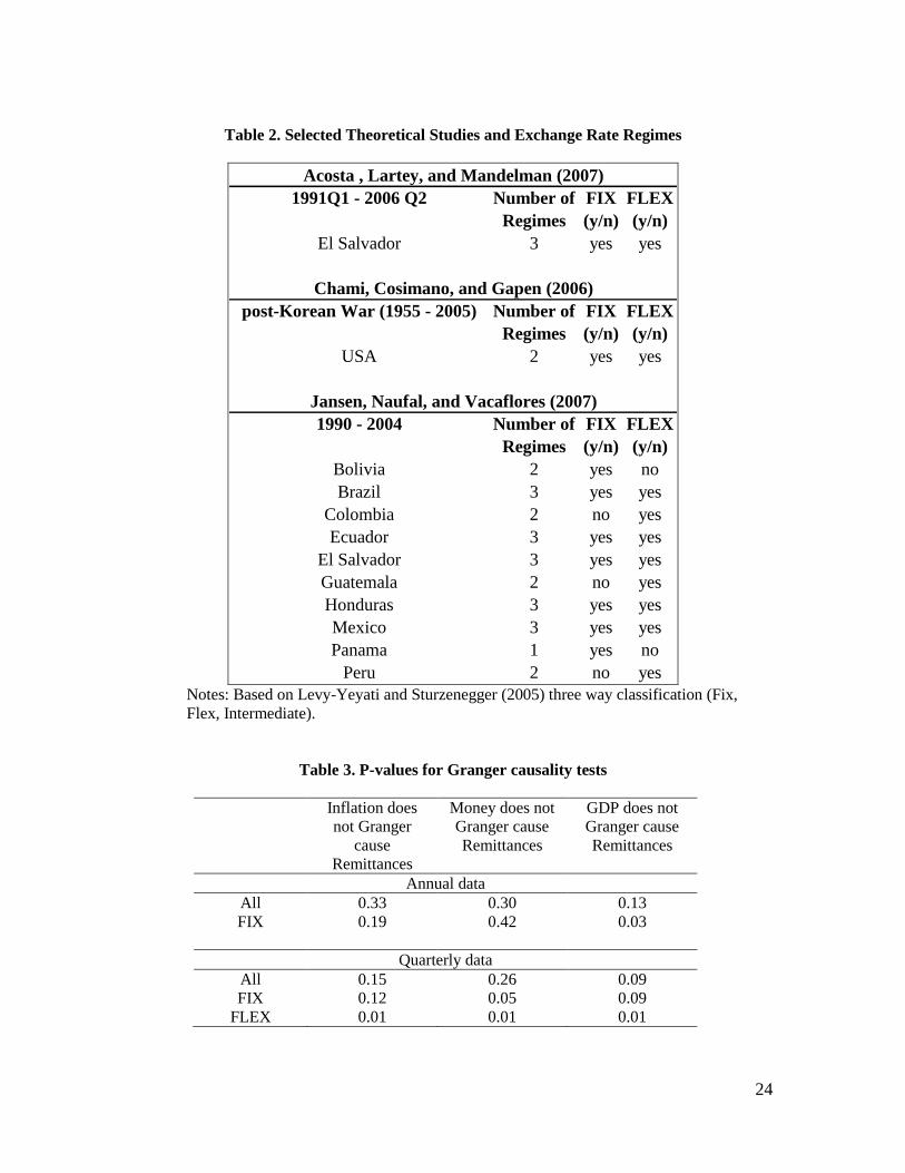
Other studies, such as Chami, Cosimano, and Gapen (2006), Acosta, Lartey, and
Mandelman (2007), and Jansen, Naufal and Vacaflores (2007) use dynamic stochastic general
1 These results are consistent with the findings of other studies, such as Rajan and Subramanian (2005), focusing on foreign aid and
growth.
2 Most of the countries studied in Narayan, Narayan, and Mishra (2011) are already in Table 1.
3
equilibrium (DSGE) analysis to investigate the effect of a change in remittances on an economy
and have reached similar conclusions regarding the positive effects of increases in remittances on
inflation. However, the calibration of their models also assumes no change in the exchange rate
regime while many of the countries studied display changes in regimes for the periods
considered, as shown in Table 2.
Finally, Lartey (2008), looking at capital inflows in general, focuses on the short-run
monetary effects of inflows under a fixed exchange rate regime and an interest-rate-rule-based
flexible regime.3 Interestingly, his DSGE simulations show that the optimal monetary policy in
small open economies facing capital inflows, is an interest-rate-based regime that also responds to
the short-run fluctuations in the nominal exchange rate.
While the literature has offered some consensus regarding the inflationary impact of
remittances, these findings emerged from studies assuming an unchanged exchange rate regime
for all the emerging countries observed. Ignoring the exchange rate regime and its potential
changes may very well lead to spurious results.
[INSERT TABLE 2]
In this paper, we explicitly include the exchange rate regime when analyzing the impact
of remittances on the economy. Furthermore, we use both quarterly and annual data in order to
understand better the short-run effects (i.e at less than annual frequency) of a change in
remittances on inflation, money supply, GDP and the real exchange rate. Unlike Lartey,
Mandelman, and Acosta (2008) we focus on the monetary nature of remittance inflows. 4
Furthermore, we go beyond Lartey (2008) as we clearly focus on remittances themselves, include
flexible exchange rate regimes explicitly and take the theoretical predictions to data.
3 To understand the difference between an interest-rate-rule-based regime like most inflation targeting regimes in general and a
flexible exchange rate regime in particular see Ball and Reyes (2008). 4 Lartey, Mandelman, and Acosta (2008) focus solely on understanding the real exchange rate appreciation that often results from
remittance inflows. In doing this, they consider the role of exchange rate regimes in affecting the path of the real exchange rate. They focus on the actual production of traded and non-traded goods in the economy and employ annual sector-level production data.
4
The theoretical section derives clear predictions regarding the effects of remittances on
inflation, GDP, Real Exchange Rate (RER), and nominal money supply. Under a fixed exchange
rate regime, increased remittance flows temporarily increase the rate of inflation, GDP, the
nominal money supply and cause RER appreciation. In contrast, under a flexible regime,
increased remittance flows temporarily decrease the rate of inflation, increase GDP and cause the
RER to appreciate but do not have any impact on the nominal money supply. Clearly, the model
suggests that remittance flows are inflationary only under a fixed exchange rate.
The empirical section investigates the accuracy of the theoretical predictions using yearly
and quarterly data for 21 emerging countries for the 1980-2010 period. Our findings highlight
two key points. First, the data frequency matters. Indeed, a large portion of the responses occurs
within the first year, which the yearly data is unable to capture. Second, the exchange rate regime
matters. The impulse response functions (IRFs) derived from the panel vector autoregressive
analysis support the theoretical predictions, confirming the increase in GDP for both regimes but
showing a clear difference in responses for the other variables, especially for inflation and money
supply. Such empirical evidence emphasizes the importance of accounting for the exchange rate
regime when investigating the impact of remittances on the economy and when developing
economic policies in order to deal appropriately with the repercussions of remittances.
The rest of the paper is organized as follows. Section 2 describes the theoretical model
and its predictions. Section 3 focuses on the empirical analysis. Finally, Section 4 concludes.
II. A Monetary Model for Remittances
The model imagines a representative individual that maximizes utility based on
consumption of traded and non-traded goods as well as money services. The utility function is
assumed separable in all of its components and over time.
0
, , log( ) (1 ) log( ) log( )T N T N t
t t t t t tU c c m c c m e dt (1)
5
where T
tc , N
tc , and tt
t
Mm
Edenote consumption of the traded good and the non-traded
good, and real money balances in terms of the traded good, respectively. M is the nominal stock
of money and E is the nominal exchange rate. The law of one price holds for tradable goods and
the foreign price for the traded good is equal to one so E is the price of the traded good.
Individuals can hold internationally traded assets yielding the constant world interest rate,
r, earn income from the sale of traded and non-traded goods, receive/give transfers to the
government and receive exogenous foreign-currency remittances from abroad.5 This is expressed
in the following flow budget constraint
N NT Tt t
t t t t t t t t
t t
y ca ra y c i m f
e e (2)
where T
ty represents the traded good, N
ty , the non-traded good, N
t PEe , the real exchange
rate, ta , net asset holdings,
t, government transfers and,
tf , the value of remittances. PN is the
price of the non-traded good.
Production in this economy uses a single input: labor.6 Full employment is assumed
throughout so that total employment is the sum of the levels in each sector. Total employment is
set to unity and tl represents employment in the traded good sector, leaving 1 tl in the non-
traded sector. The production functions in each sector are:
0 1T
t t ty Al (3.a)
and
5 We assume exogenous remittance flows for a number of reasons. First, there is no consensus in the literature on how they are
endogenous with respect to the domestic economy. Modeling remittances as depending positively or negatively on either domestic output or the real exchange rate would reflect a bias that is not founded on any empirical or theoretical grounds. This is similar to
modeling a stochastic variable as being uniformly distributed when one has no reliable information on its true distribution. Second, as
shown in Section 5, the exogeneity assumption does not drive our empirical results. Finally, we are interested on the nominal effects of an increase in remittances and the degree to which exchange rate regimes matter in determining those effects. To that end, why
remittances increase is much less important than the increase itself. 6 Including labor this way was inspired by Chapter 4 of Carlos A Végh’s manuscript under preparation for his forthcoming book,
current version (2007).
6
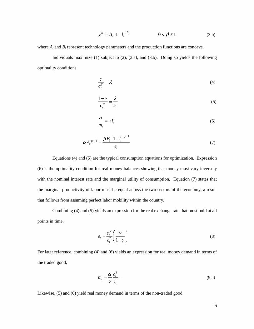
1 0 1N
t t ty B l (3.b)
where At and Bt represent technology parameters and the production functions are concave.
Individuals maximize (1) subject to (2), (3.a), and (3.b). Doing so yields the following
optimality conditions.
T
tc (4)
1
t
N
tec
(5)
t
t
im
(6)
1
11t t
t t
t
B lAl
e (7)
Equations (4) and (5) are the typical consumption equations for optimization. Expression
(6) is the optimality condition for real money balances showing that money must vary inversely
with the nominal interest rate and the marginal utility of consumption. Equation (7) states that
the marginal productivity of labor must be equal across the two sectors of the economy, a result
that follows from assuming perfect labor mobility within the country.
Combining (4) and (5) yields an expression for the real exchange rate that must hold at all
points in time.
1
N
tt T
t
ce
c (8)
For later reference, combining (4) and (6) yields an expression for real money demand in terms of
the traded good,
T
tt
t
cm
i. (9.a)
Likewise, (5) and (6) yield real money demand in terms of the non-traded good
7
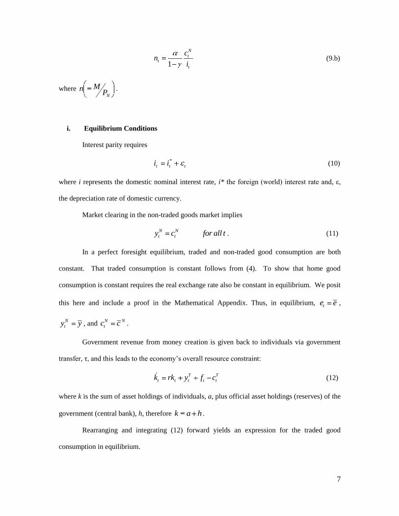
1
N
tt
t
cn
i (9.b)
where NP
Mn .
i. Equilibrium Conditions
Interest parity requires
ttt ii * (10)
where i represents the domestic nominal interest rate, i* the foreign (world) interest rate and, ε,
the depreciation rate of domestic currency.
Market clearing in the non-traded goods market implies
N N
t ty c for all t . (11)
In a perfect foresight equilibrium, traded and non-traded good consumption are both
constant. That traded consumption is constant follows from (4). To show that home good
consumption is constant requires the real exchange rate also be constant in equilibrium. We posit
this here and include a proof in the Mathematical Appendix. Thus, in equilibrium, te e ,
N
ty y , and N N
tc c .
Government revenue from money creation is given back to individuals via government
transfer, τ, and this leads to the economy’s overall resource constraint:
T T
t t t t tk rk y f c (12)
where k is the sum of asset holdings of individuals, a, plus official asset holdings (reserves) of the
government (central bank), h, therefore k a h .
Rearranging and integrating (12) forward yields an expression for the traded good
consumption in equilibrium.
8
0
T Tc rk y f , (13)
which says traded good consumption depends on the flow of returns from the initial asset
holdings, the constant flow of remittances and traded good production. It is known to be constant
(piecewise linear) by (4).
Combining (13) and (11) with (8) yields an expression for the equilibrium real exchange
rate.
1
0 fyrk
ye
T
N
(14)
where yN and y
T are given by (3.a) and (3.b).
ii. Monetary Regimes and Economic Dynamics
To generate dynamics in this model, we assume that non-traded good prices adjust
according to a Calvo-type (Calvo, 1983) pricing mechanism.
0NN
tt yc (18)
whereNy is the steady state level of non-traded good production and θ is a constant parameter.
Under this formulation the non-traded good price level is pre-determined at every point in time,
but the rate of change of the non-traded good price level – i.e., “the inflation rate” – is not. In the
short-run, output is assumed to be demand determined so that non-traded goods market
equilibrium as described by (11) is maintained at all times.7
Fixed Exchange Rate Regime (FIX)
Under a FIX the initial level of the nominal exchange rate, 0E , and its rate of change, ,
are set by the central bank. The central bank maintains this regime by adjusting international
reserve levels (and hence the nominal money supply) endogenously. By interest parity, constant
currency depreciation implies that the nominal interest rate is constant in this regime, *ii .
By (9.a), in steady state, where μ is the rate of nominal money supply growth.
7 Note that this is actually Calvo's (1983) original formulation which was done in continuous time.
9
The economy’s behavior is governed by the following two differential equations.
1N T
t ty l e c (19)
)( ttee (20)
where 1Ny l B l . Thus, changes in the steady state employment allocation change the
steady state level of non-traded good production. (19) governs the control and (20) the state
variable in this economy.
Result 1. Under a fixed exchange rate regime, an increase in remittances generates an
increase in inflation. For a proof see the Mathematical Appendix.
Result 2. Under a fixed exchange rate regime, an increase in remittances generates an
increase in the nominal money supply. For a proof see the Mathematical Appendix.
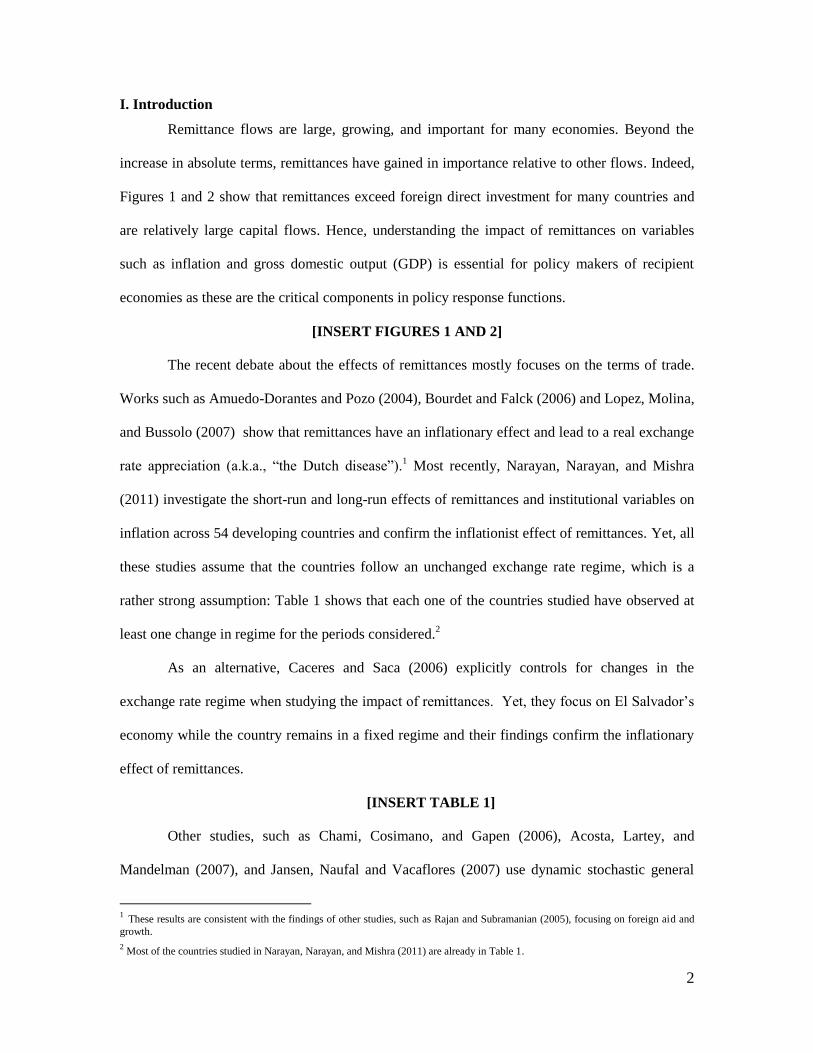
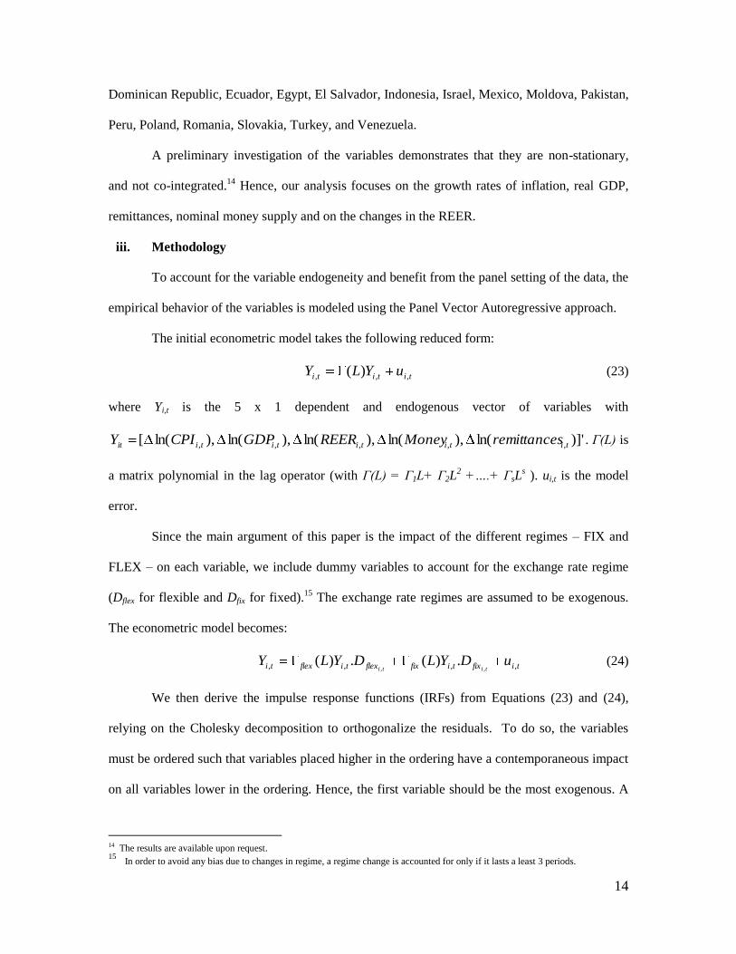
[ INSERT FIGURE 3 ]
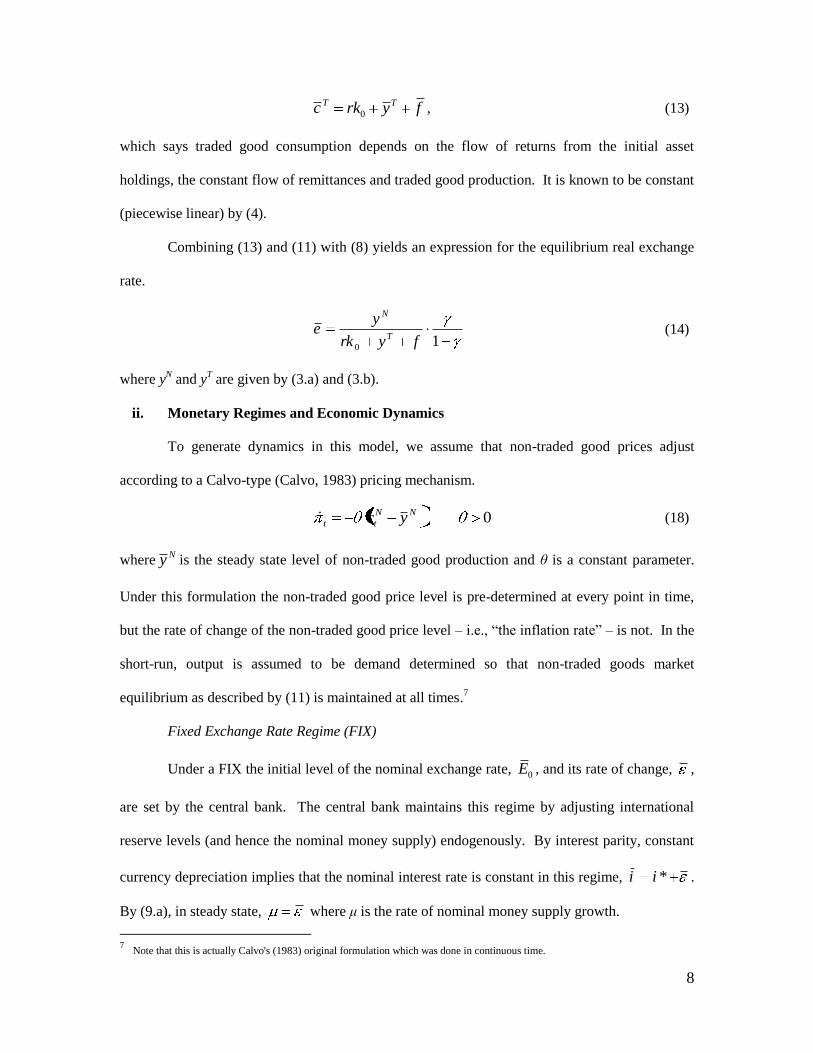
Figure 3 is the phase diagrammatic representation of the model under a FIX, the
dynamics of which are described by equations (19) and (20). In Figure 3, the economy’s initial
steady state is at point A. Since increased remittances always lead to an appreciation of the real
exchange rate (i.e.,the "Dutch disease"), the final steady state must have a lower real exchange
rate, N
t PEe . Under a FIX regime, the nominal exchange rate, E, is constant while an
increase in home goods prices leads to a fall in e during the transition. More specifically, the
initial impact of increased remittance flows is an increase in real money demand. Since output is
demand determined in this model and real money demand reflects the representative individual’s
underlying demand for goods and services, the increase in real money demand results in an
increase in GDP. The central bank responds by increasing the nominal money supply to offset the
increase in money demand and maintain equilibrium in the money market, leaving the nominal
interest rate and exchange rate unchanged as required by the FIX regime, leading to Result 2.
10
Upon impact, inflation jumps upward to point B, leaving the real exchange rate unchanged. This
generates the home good price dynamics necessary to reach the new steady state. As the
economy adjusts to the new level of inflows, the real exchange rate and inflation fall continuously
which leads to Result 1 throughout transition. In the new steady state, point C, inflation returns to
its initial level and the real exchange rate is at a lower level.
Flexible Exchange Rate Regime (FLEX)
Under a FLEX the initial level, 0M , and the rate of growth of the nominal money supply,
, are set by the central bank. The central bank maintains the regime by allowing the nominal
exchange rate to adjust endogenously. By ( )tm m and 0 m , it follows that in
steady state. Likewise, constant currency depreciation implies by interest parity that the nominal
interest rate is constant, *ii , in steady state.
The system’s dynamics are captured in terms of real money balances, of the non-traded
good, / Nn M P , and the non-traded good inflation rate, π. Under a FLEX, n is a
predetermined variable since M is exogenous and constant and PN is predetermined. π remains a
control variable. Differentiating the definition of real money balances with respect to time yields
)( ttt nn . (21)
Using (8) and (9.a), substitute into (18) for cN and rearrange to obtain
1N
t t ty l i n (22)
where, again, 1Ny l B l .
Result 3. Under a flexible exchange rate regime, an increase in remittances generates a
decrease in inflation. For a proof see the Mathematical Appendix.
11
Result 4. Under a flexible exchange rate regime, an increase in remittances implies no
change in the nominal money supply, by assumption.8
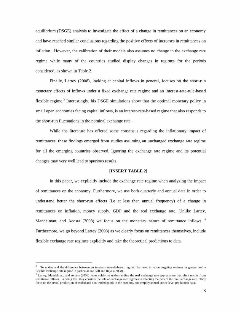
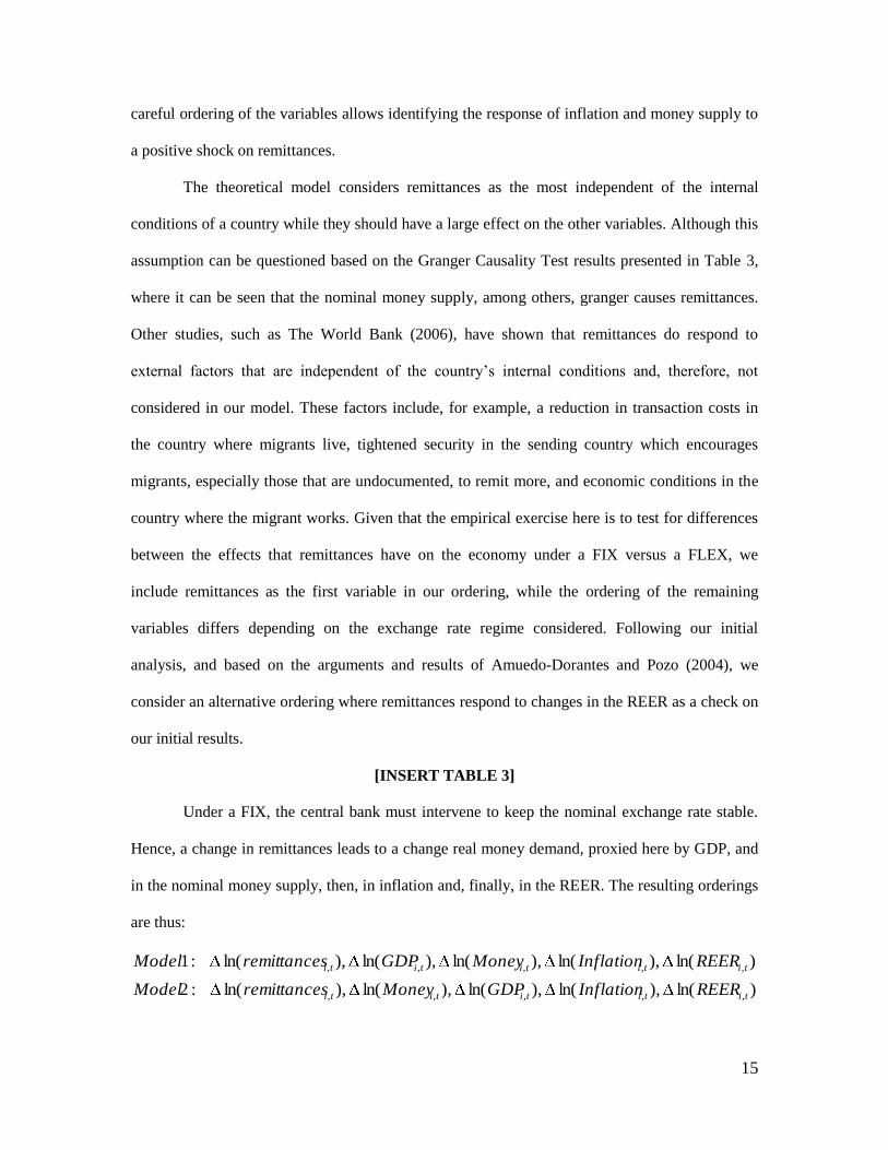
[ INSERT FIGURE 4 ]
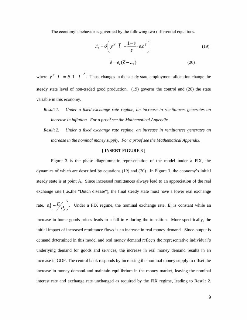
Figure 4 is the phase diagrammatic representation of the model under a FLEX, the
dynamics of which are described by equations (21) and (22). In Figure 4, the economy’s initial
steady state is at point A. Since increased remittances always lead to an appreciation of the real
exchange rate (i.e.,the "Dutch disease"), the final steady state must have a lower real exchange
rate, N
t PEe . Under a FLEX regime, the nominal exchange rate, E, jumps to its new, lower
steady state value immediately. PN, a state variable, is slower to adjust. The initial impact of the
increased remittance flow is an increase in real money demanded. Since output is demand
determined and real money demand reflects the representative individual’s underlying demand
for goods and services, the increase in real money demand again results in an increase in GDP.
Under a FLEX, the central bank does not respond by changing the nominal stock of money which
leads to Result 4. The drop in the nominal exchange rate clears the real money market in terms of
the traded good. But this leaves the real money balances in terms of the non-traded good, n,
unchanged and thus the n-money market out of equilibrium (relatively to steady state). To reach
the new steady state equilibrium in this market, real money balances, NP
Mn , must increase
during transition. Since the nominal stock of money, M, remains constant, the price of non-traded
goods must decrease. From a real economy perspective, this comes about because the nominal
exchange rate fell, lowering returns to producing the traded good and thus encouraging a
reallocation of resources from traded and into non-traded good production. This is an increase in
non-traded good production relative to non-traded good demand and thus leads to a decline in the
price of non-traded goods. Graphically, upon impact, inflation jumps downward to point B. This
8 No formal proof here is needed since Result 4 holds by our assumptions of the flexible exchange rate regime. That is, we have
assumed that the central bank holds the stock of nominal money constant and allows the nominal exchange rate to adjust.
12
generates the home good price dynamics necessary to reach the new steady state and leads to
Result 3. Since the rate of nominal money stock growth is constant, real money balances, n, rise
continuously throughout the transition. In the new steady state, point C, inflation returns to its
initial level and real money balances are higher.
III. Empirical Analysis
i. Testable Predictions
The model predicts that the exchange rate regime matters most clearly for the inflation
and money supply responses to an increase in remittances. Under a FIX, inflation rises, leading to
the increase in money supply that offsets the increase in real money demand. Under a FLEX,
inflation falls while the money supply remains unchanged, thereby generating an increase in real
money demand. Finally, the model suggests that, under both regimes the real money demand, and
thus GDP, increase in the short-run and that the real exchange rate always appreciates.
ii. Data Description
Our model suggests that the transition paths differ across regimes; hence the frequency of
the data may matter. As a result, we consider annual and quarterly data for the CPI, nominal
money supply (M2), real GDP, real effective exchange rate (REER) and remittances. It should be
noted that an appreciation of the real exchange rate (RER) in the theoretical model is denoted by
an increase of the REER empirically.
The annual data is collected from the World Development Indicators of the World Bank.
Quarterly data on CPIs, and nominal money supplies are from the International Monetary Fund’s
International Financial Statistics. Real GDP, remittances and REER are from the central banks of
each country.9
The exchange rate classifications are based on the monthly data found in Reinhart and
Rogoff (2004) and Ilzetzki, Reinhart and Rogoff (2010).10
We use the following four
9 The original data is transformed into logarithms. 10 Our final regime classification data is available upon request.
13
classifications: (1) “float/free float”, (2) “pegged in band/ managed float/other managed”, (3)
“crawling peg, crawl-like, stabilization” and (4) “conventional peg, currency board”.11
Our
dummy variables are then constructed so that classification (1) is a float (FLEX) and
classifications (2) – (4) are all considered fix (FIX). This reflects our view that only (1) reflects a
truly floating regime and all others are degrees of intervention.12
The period considered is 1980:1
to 2010:4.13
We construct our quarterly data from the monthly using the following rule: if the
regime is classified as FLEX for 2 or more months, then the quarter is classified as FLEX;
otherwise, it is classified as FIX. We do similarly when constructing the annual data: if the
regime is classified as FLEX for 2 or more quarters, then the year is classified as FLEX;
otherwise, it is classified as FIX. Our sample includes a number of countries that have
implemented multiple regime changes. For example, Ecuador, Indonesia, Mexico and Turkey
present three regime switches during the time period considered.
To our knowledge, this is the first study to employ quarterly analysis of the impact of
remittances on the economy. Focusing on a higher frequency can have several implications such
as allowing for a more detailed description of the regimes. Higher frequency provides more
information since each yearly observation is composed of four quarterly ones. This extra set of
observations is key, especially when trying to understand the behavior of the economy under a
FLEX, which is the less well represented regime in the sample. Higher frequency also allows one
to capture within-year dynamics, which obviously cannot be done with yearly data. However
there is a trade-off between more time-series information (higher frequency) and wider cross-
sectional information (number of countries) since fewer countries report quarterly remittances.
We select the countries with the most data under both frequencies and perform the analysis
including 21 countries: Brazil, Bulgaria, Colombia, Costa Rica, Croatia, Czech Republic,
11 We remove all uncertain regimes from our data. 12 Our results are, however, robust to counting (1) and (2) as FLEX and (3) and (4) as FIX. The only exception is inflation under
FLEX which is quite sensitive to the degree of flexibility of exchange rate. This comforts us in our choice of considering as FLEX
only purely floating exchange rates. Results are available upon request. 13 All data and exchange rate regime classifications are available upon request.
14
Dominican Republic, Ecuador, Egypt, El Salvador, Indonesia, Israel, Mexico, Moldova, Pakistan,
Peru, Poland, Romania, Slovakia, Turkey, and Venezuela.
A preliminary investigation of the variables demonstrates that they are non-stationary,
and not co-integrated.14
Hence, our analysis focuses on the growth rates of inflation, real GDP,
remittances, nominal money supply and on the changes in the REER.
iii. Methodology
To account for the variable endogeneity and benefit from the panel setting of the data, the
empirical behavior of the variables is modeled using the Panel Vector Autoregressive approach.
The initial econometric model takes the following reduced form:
tititi uYLY ,,, )( (23)
where Yi,t is the 5 x 1 dependent and endogenous vector of variables with
)]'ln(),ln(),ln(),ln(),ln([ ,,,,, tititititiit tancesremitMoneyREERGDPCPIY . Γ(L) is
a matrix polynomial in the lag operator (with Γ(L) = Γ1L+ Γ2L2 +….+ ΓsL
s ). ui,t is the model
error.
Since the main argument of this paper is the impact of the different regimes – FIX and
FLEX – on each variable, we include dummy variables to account for the exchange rate regime
(Dflex for flexible and Dfix for fixed).15
The exchange rate regimes are assumed to be exogenous.
The econometric model becomes:
tifixtifixflextiflexti uDYLDYLYtiti ,,,, ,,
.)(.)( (24)
We then derive the impulse response functions (IRFs) from Equations (23) and (24),
relying on the Cholesky decomposition to orthogonalize the residuals. To do so, the variables
must be ordered such that variables placed higher in the ordering have a contemporaneous impact
on all variables lower in the ordering. Hence, the first variable should be the most exogenous. A
14 The results are available upon request. 15
In order to avoid any bias due to changes in regime, a regime change is accounted for only if it lasts a least 3 periods.
15
careful ordering of the variables allows identifying the response of inflation and money supply to
a positive shock on remittances.
The theoretical model considers remittances as the most independent of the internal
conditions of a country while they should have a large effect on the other variables. Although this
assumption can be questioned based on the Granger Causality Test results presented in Table 3,
where it can be seen that the nominal money supply, among others, granger causes remittances.
Other studies, such as The World Bank (2006), have shown that remittances do respond to
external factors that are independent of the country’s internal conditions and, therefore, not
considered in our model. These factors include, for example, a reduction in transaction costs in
the country where migrants live, tightened security in the sending country which encourages
migrants, especially those that are undocumented, to remit more, and economic conditions in the
country where the migrant works. Given that the empirical exercise here is to test for differences
between the effects that remittances have on the economy under a FIX versus a FLEX, we
include remittances as the first variable in our ordering, while the ordering of the remaining
variables differs depending on the exchange rate regime considered. Following our initial
analysis, and based on the arguments and results of Amuedo-Dorantes and Pozo (2004), we
consider an alternative ordering where remittances respond to changes in the REER as a check on
our initial results.
[INSERT TABLE 3]
Under a FIX, the central bank must intervene to keep the nominal exchange rate stable.
Hence, a change in remittances leads to a change real money demand, proxied here by GDP, and
in the nominal money supply, then, in inflation and, finally, in the REER. The resulting orderings
are thus:
)ln(),ln(),ln(),ln(),ln(:2
)ln(),ln(),ln(),ln(),ln(:1
,,,,,
,,,,,
tititititi
tititititi
REERInflationGDPMoneytancesremitModel
REERInflationMoneyGDPtancesremitModel
16
Under a FLEX, the central bank does not intervene. Hence, a change in remittances leads to a
change in real money demand (i.e., GDP) and in RER then in inflation and, finally, in the nominal
money supply. The resulting orderings are:
)ln(),ln(),ln(),ln(),ln(:4
)ln(),ln(),ln(),ln(),ln(:3
,,,,,
,,,,,
tititititi
tititititi
MoneyInflationREERGDPtancesremitModel
MoneyInflationGDPREERtancesremitModel
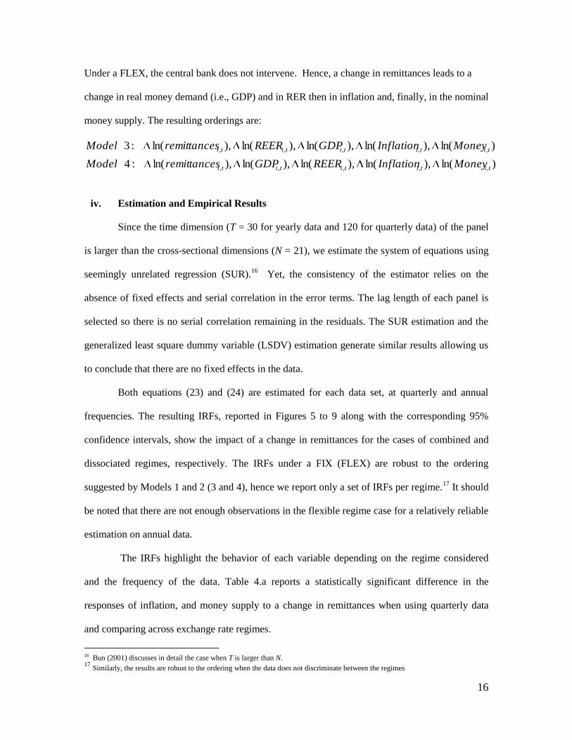
iv. Estimation and Empirical Results
Since the time dimension (T = 30 for yearly data and 120 for quarterly data) of the panel
is larger than the cross-sectional dimensions (N = 21), we estimate the system of equations using
seemingly unrelated regression (SUR).16
Yet, the consistency of the estimator relies on the
absence of fixed effects and serial correlation in the error terms. The lag length of each panel is
selected so there is no serial correlation remaining in the residuals. The SUR estimation and the
generalized least square dummy variable (LSDV) estimation generate similar results allowing us
to conclude that there are no fixed effects in the data.
Both equations (23) and (24) are estimated for each data set, at quarterly and annual
frequencies. The resulting IRFs, reported in Figures 5 to 9 along with the corresponding 95%
confidence intervals, show the impact of a change in remittances for the cases of combined and
dissociated regimes, respectively. The IRFs under a FIX (FLEX) are robust to the ordering
suggested by Models 1 and 2 (3 and 4), hence we report only a set of IRFs per regime.17
It should
be noted that there are not enough observations in the flexible regime case for a relatively reliable
estimation on annual data.
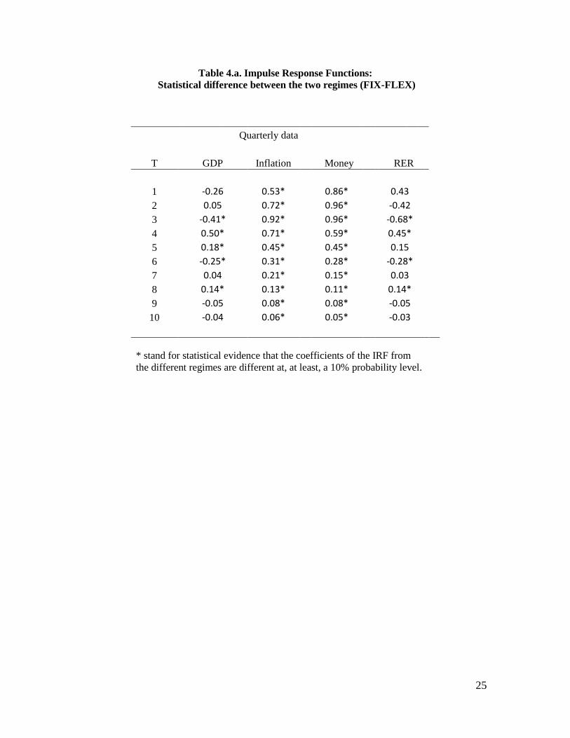
The IRFs highlight the behavior of each variable depending on the regime considered
and the frequency of the data. Table 4.a reports a statistically significant difference in the
responses of inflation, and money supply to a change in remittances when using quarterly data
and comparing across exchange rate regimes.
16 Bun (2001) discusses in detail the case when T is larger than N. 17
Similarly, the results are robust to the ordering when the data does not discriminate between the regimes
17
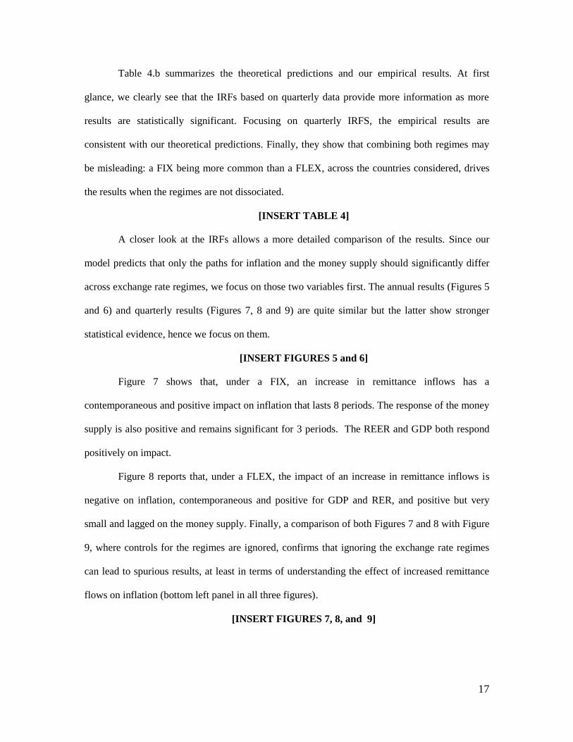
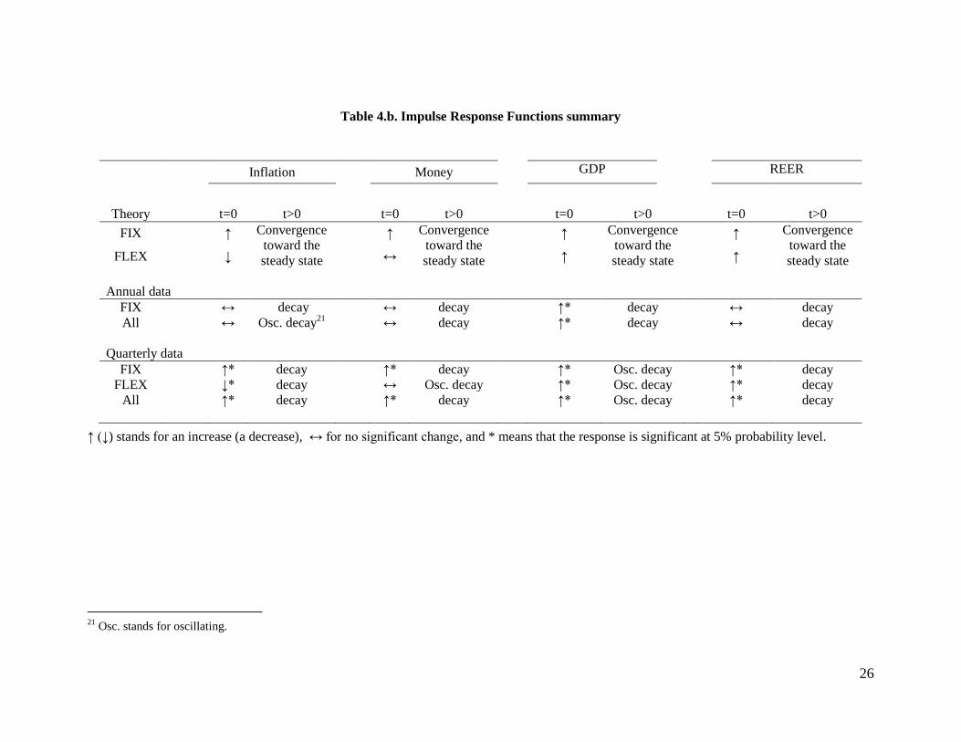
Table 4.b summarizes the theoretical predictions and our empirical results. At first
glance, we clearly see that the IRFs based on quarterly data provide more information as more
results are statistically significant. Focusing on quarterly IRFS, the empirical results are
consistent with our theoretical predictions. Finally, they show that combining both regimes may
be misleading: a FIX being more common than a FLEX, across the countries considered, drives
the results when the regimes are not dissociated.
[INSERT TABLE 4]
A closer look at the IRFs allows a more detailed comparison of the results. Since our
model predicts that only the paths for inflation and the money supply should significantly differ
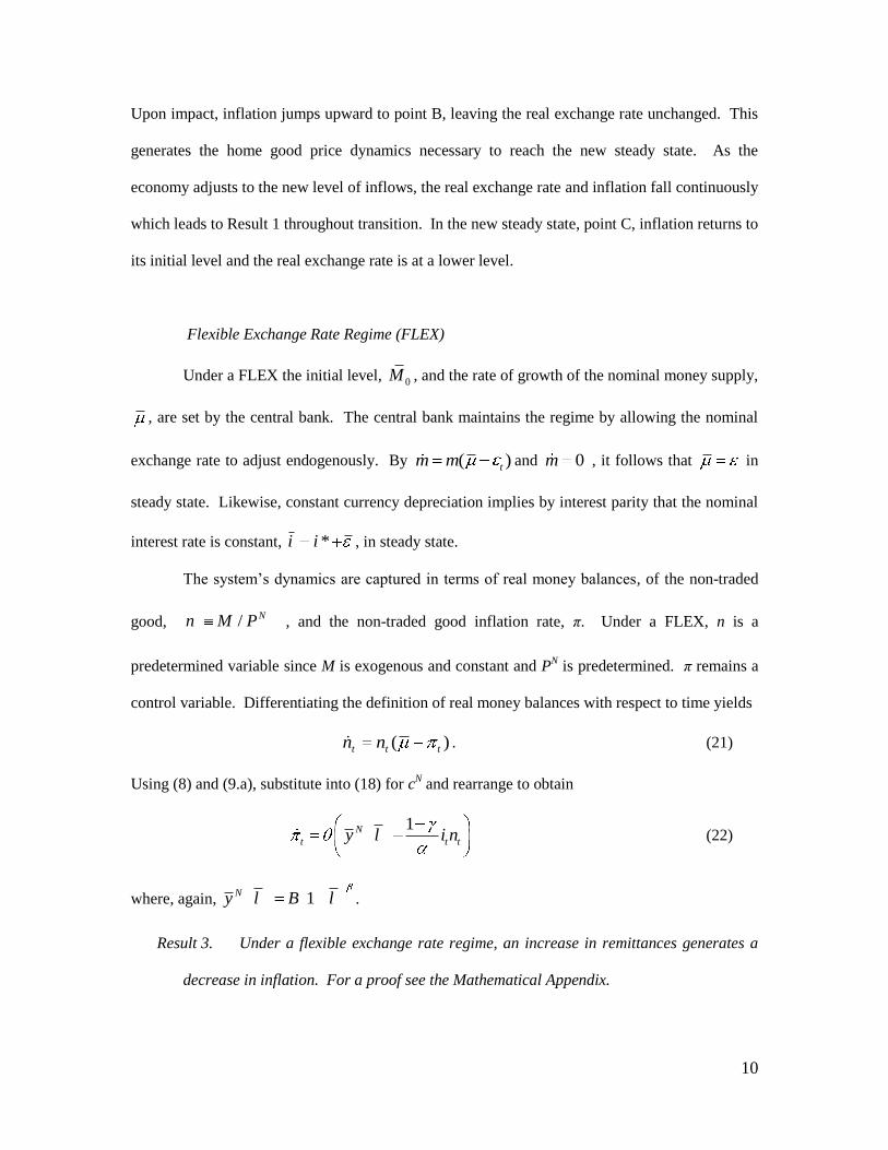
across exchange rate regimes, we focus on those two variables first. The annual results (Figures 5
and 6) and quarterly results (Figures 7, 8 and 9) are quite similar but the latter show stronger
statistical evidence, hence we focus on them.
[INSERT FIGURES 5 and 6]
Figure 7 shows that, under a FIX, an increase in remittance inflows has a
contemporaneous and positive impact on inflation that lasts 8 periods. The response of the money
supply is also positive and remains significant for 3 periods. The REER and GDP both respond
positively on impact.
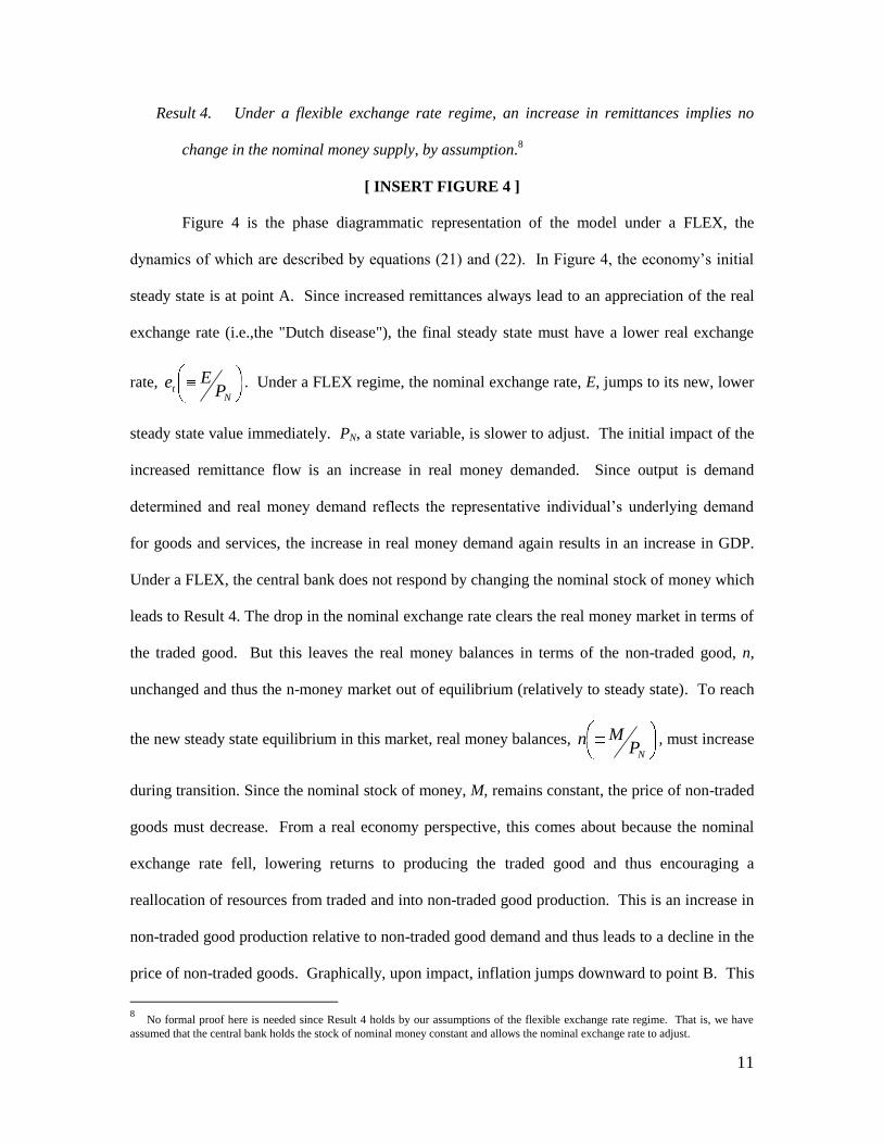
Figure 8 reports that, under a FLEX, the impact of an increase in remittance inflows is
negative on inflation, contemporaneous and positive for GDP and RER, and positive but very
small and lagged on the money supply. Finally, a comparison of both Figures 7 and 8 with Figure
9, where controls for the regimes are ignored, confirms that ignoring the exchange rate regimes
can lead to spurious results, at least in terms of understanding the effect of increased remittance
flows on inflation (bottom left panel in all three figures).
[INSERT FIGURES 7, 8, and 9]
18
Overall, the variables’ responses to increased remittances agree in direction and timing
across the annual and quarterly results for the FIX regime.18
Furthermore, the increase in
frequency allows a better understanding of the short-run dynamic, which, in turn, presents the
most significant responses in line with the theoretical prediction.
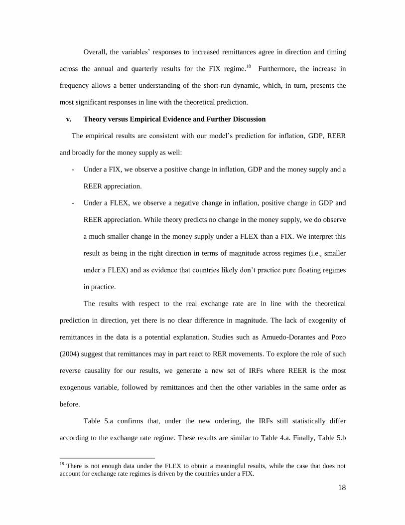
v. Theory versus Empirical Evidence and Further Discussion
The empirical results are consistent with our model’s prediction for inflation, GDP, REER
and broadly for the money supply as well:
- Under a FIX, we observe a positive change in inflation, GDP and the money supply and a
REER appreciation.
- Under a FLEX, we observe a negative change in inflation, positive change in GDP and
REER appreciation. While theory predicts no change in the money supply, we do observe
a much smaller change in the money supply under a FLEX than a FIX. We interpret this
result as being in the right direction in terms of magnitude across regimes (i.e., smaller
under a FLEX) and as evidence that countries likely don’t practice pure floating regimes
in practice.
The results with respect to the real exchange rate are in line with the theoretical
prediction in direction, yet there is no clear difference in magnitude. The lack of exogenity of
remittances in the data is a potential explanation. Studies such as Amuedo-Dorantes and Pozo
(2004) suggest that remittances may in part react to RER movements. To explore the role of such
reverse causality for our results, we generate a new set of IRFs where REER is the most
exogenous variable, followed by remittances and then the other variables in the same order as
before.
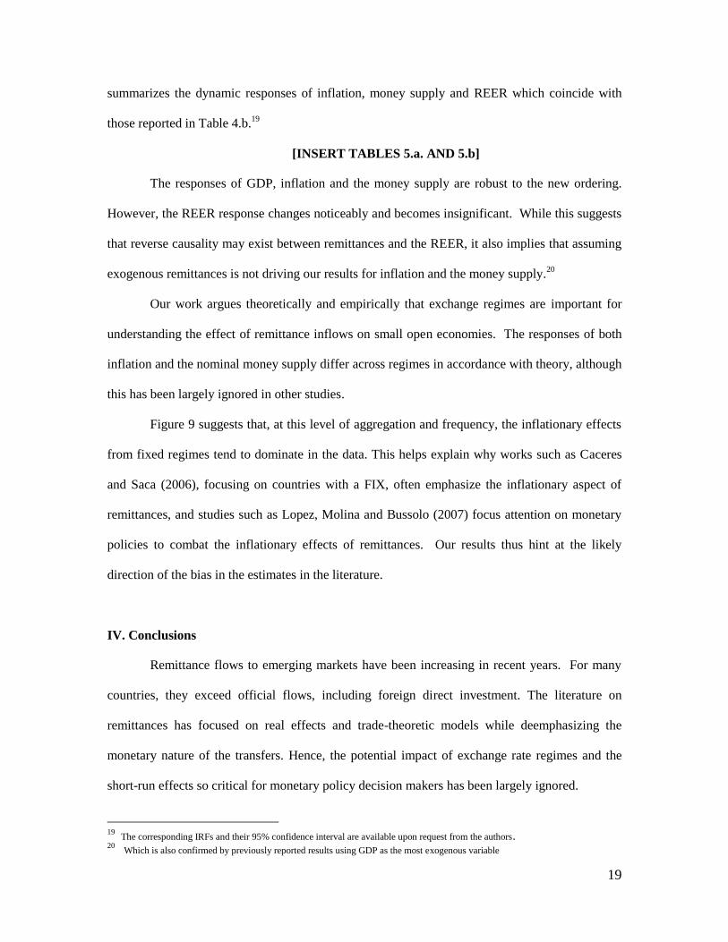
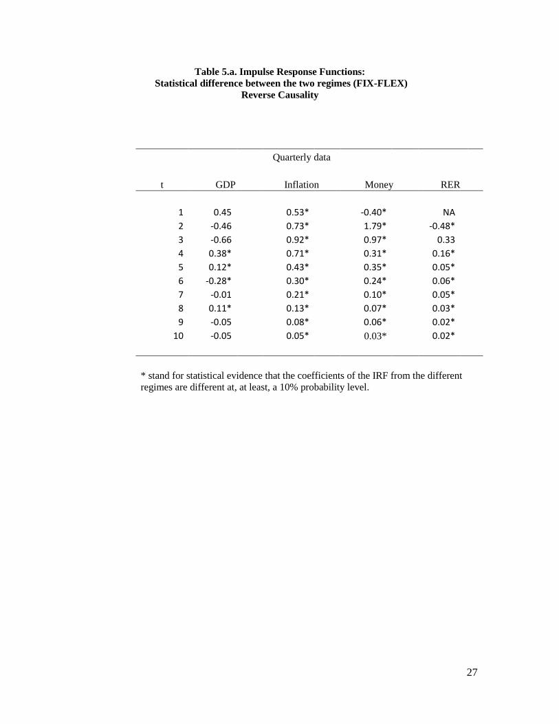
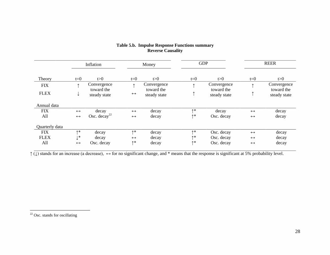
Table 5.a confirms that, under the new ordering, the IRFs still statistically differ
according to the exchange rate regime. These results are similar to Table 4.a. Finally, Table 5.b
18
There is not enough data under the FLEX to obtain a meaningful results, while the case that does not
account for exchange rate regimes is driven by the countries under a FIX.
19
summarizes the dynamic responses of inflation, money supply and REER which coincide with
those reported in Table 4.b.19
[INSERT TABLES 5.a. AND 5.b]
The responses of GDP, inflation and the money supply are robust to the new ordering.
However, the REER response changes noticeably and becomes insignificant. While this suggests
that reverse causality may exist between remittances and the REER, it also implies that assuming
exogenous remittances is not driving our results for inflation and the money supply.20
Our work argues theoretically and empirically that exchange regimes are important for
understanding the effect of remittance inflows on small open economies. The responses of both
inflation and the nominal money supply differ across regimes in accordance with theory, although
this has been largely ignored in other studies.
Figure 9 suggests that, at this level of aggregation and frequency, the inflationary effects
from fixed regimes tend to dominate in the data. This helps explain why works such as Caceres
and Saca (2006), focusing on countries with a FIX, often emphasize the inflationary aspect of
remittances, and studies such as Lopez, Molina and Bussolo (2007) focus attention on monetary
policies to combat the inflationary effects of remittances. Our results thus hint at the likely
direction of the bias in the estimates in the literature.
IV. Conclusions
Remittance flows to emerging markets have been increasing in recent years. For many
countries, they exceed official flows, including foreign direct investment. The literature on
remittances has focused on real effects and trade-theoretic models while deemphasizing the
monetary nature of the transfers. Hence, the potential impact of exchange rate regimes and the
short-run effects so critical for monetary policy decision makers has been largely ignored.
19
The corresponding IRFs and their 95% confidence interval are available upon request from the authors. 20
Which is also confirmed by previously reported results using GDP as the most exogenous variable
20
In this paper, we aim to fill this gap by analyzing the responses of inflation, GDP, the
RER, and the nominal money supply to changes in remittances, under different monetary
regimes.
First, our work shows theoretically how exchange rate regimes matter and makes simple
predictions. Under a fixed regime, increased remittance flows temporarily increase inflation,
GDP, the nominal money supply and cause RER appreciation. Under a flexible regime, increased
remittance flows temporarily lower inflation, increases GDP and cause RER appreciation.
Second, our work shows empirically how these predictions hold in the data. Using a
panel vector autoregressive approach that controls for regime differences, we explore impulse
response functions specific to each regime and to two different levels of frequency in the data:
annual and quarterly. While most studies use annual data, to our knowledge, this is the first study
to also use quarterly data for a panel with remittances. Our results highlight two key points. First,
the data frequency matters since the biggest part of the responses to an increase in remittances
occurs within the first year. Hence yearly data is unable to capture fully these short-run dynamics.
Second, the theoretical predictions for inflation, RER, GDP and the money supply are largely
borne out in the data, especially in the quarterly case, and our results are robust to the potential
for reverse causality between the real exchange rate and remittances. As a result, we conclude
that the impact of remittances on the economy’s inflation and money supply differs depending on
exchange rate regimes. Hence, exchange rate regimes do matter and should not be ignored when
investigating the effects of remittance flows on economies and deriving economic policies
appropriate for dealing with them.
21
References
Acosta, Pablo, Emmanuel, Lartey, and Federico Mandelman, 2007. Remittances and the Dutch
Disease. Federal Reserve Bank of Atlanta, Working Paper 2007-8.
Amuedo-Dorantes, Catalina and Susan Pozo. 2004. Workers’ Remittances and the Real Exchange
Rate: A Paradox of Gifts. World Development, 32: 1407-1417.
Ball, Christopher and Javier Reyes. 2008. Inflation Targeting or Fear of Floating in Disguise : A
Broader Perspective. Journal of Macroeconomics, 30 (1): 308 - 326.
Bourdet, Yves and Hans Falck. 2006. Emigrants’ Remittances and Dutch Disease in Cape Verde.
International Economic Journal, 20: 267-284.
Caceres, Luis Rene and Nolvia N. Saca. 2006. What Do Remittances Do? Analyzing the Private
Remittance Transmission Mechanism in El Salvador. International Monetary Fund Working
Paper, WP/06/250.
Chami, Ralph, Thomas F. Cosimano, and Michael T. Gapen. 2006. Beware of Emigrants Bearing
Gifts: Optimal Fiscal and Monetary Policy in the Presence of Remittances. International
Monetary Fund Working Paper, WP/06/61.
Chami, Ralph, Adolfo Barajas, Thomas Cosimano, Connel Fullenkamp, Michael Gapen, and
Peter Montiel. 2008. Macroeconomic Consequences of Remittances. International Monetary
Fund Occasional Paper 259.
Ilzetzki, Ethan, Carmen Reinhart and Kenneth Rogoff. 2010. Country Chronology Update to
Reinhart, Carmen M. and Kenneth S. Rogoff. 2004. The Modern History of Exchange Rate
Arrangements: A Reinterpretation. Quarterly Journal of Economics, 1: 1-48.
Jansen, Dennis; Naufal, George; and Diego Vacaflores, 2007. The Macroeconomic Consequences
of Remittances, Working Paper Department of Economics, Texas A&M University.
Lartey, Emmanuel K.K. 2008. Capital Inflows, Dutch Disease Effects, and Monetary Policy in a
Small Open Economy. Review of International Economics, 16 (5): 971-989.
Lartey, Emmanuel K.K., Federico S. Mandelman, and Pablo A. Acosta. 2008. Remittances,
Exchange Rate Regimes, and the Dutch Disease: A Panel Data Analysis. The Federal Reserve
Bank of Atlanta. Working Paper 2008-12.
Levy-Yeyati, Eduardo and Federico Sturzenegger. 2005. Classifying Exchange Rate Regimes:
Deeds vs. Words. European Economic Review, 29: 1603-1635.
Lopez, Humberto, Luis Molina, and Maurizio Bussolo. 2007. Remittances and the Real Exchange
Rate. World Bank Policy Research Working Paper, WPS 4213, April.
Narayan, Parresh Kumar, Seema Narayan, and Sagarika Mishra. 2011. Do Remittances Induce
Inflation? Fresh Evidence from Developing Countries. Southern Economic Journal, 77 (4): 914-
933.
22
Rajan, Raghuram G. and Arvind Subramanian. 2005. What Undermines Aid’s Impact on
Growth? International Monetary Fund Working Paper, WP/05/126.
Reinhart, Carmen M. and Kenneth S. Rogoff. 2004. The Modern History of Exchange Rate
Arrangements: A Reinterpretation. Quarterly Journal of Economics, 1: 1-48.
The World Bank, 2006. Global Economic Prospects: Economic Implications of Remittances and
Migration. Chapter 4: 85-115.
The World Bank, 2011. World Development Indicators.
Vegh, Carlos, 2007. Non-Traded Goods and Relative Prices. In Open Economy Macroeconomics
in Developing Countries. MIT press, Chapter 4. Forthcoming.
http://www.econ.umd.edu/~vegh/Book/chapters/chapter4.pdf
23
Table 1. Selected Empirical Studies and Exchange Rate Regimes
1979 - 1998 Number of FIX FLEX 1990-2003 Number of FIX FLEX
Regimes (y/n) (y/n) Regimes (y/n) (y/n)
Argentina 3 yes yes Argentina 3 yes yes
Belize 1 yes no Belize 1 yes no
Bolivia 3 yes yes Bolivia 2 yes no
Colombia 2 no yes Brazil 3 yes yes
Dominican Republic 3 yes yes Chile 2 no yes
Jamaica 3 yes yes Colombia 2 no yes
Mexico 3 yes yes Costa Rica 3 yes yes
Nicaragua 2 yes no Dominican Republic 2 no yes
Peru 2 no yes Ecuador 3 yes yes
Trinidad & Tobogo 3 yes yes El Salvador 3 yes yes
Guatemala 2 no yes
Haiti 2 yes yes
1975 - 2005 Number of FIX FLEX Honduras 3 yes yes
Regimes (y/n) (y/n) Jamaica 3 yes yes
Cape Verde 3 yes yes Mexico 3 yes yes
Nicaragua 2 yes no
Panama 1 yes no
1995 - 2004 Number of FIX FLEX Paraguay 2 no yes
Regimes (y/n) (y/n) Peru 2 no yes
El Salvador 1 yes no Venezuela 3 yes yes
Number of FIX FLEX Number of FIX FLEX
1980s Regimes (y/n) (y/n) 1990s Regimes (y/n) (y/n)
Bangladesh n.a. n.a. n.a. Bolivia 2 yes no
Bolivia 3 yes yes Cameroon 2 yes no
Botswana 1 yes no Costa Rica 2 no yes
Burundi 3 yes yes Egypt 2 yes no
Congo 1 yes no Ethiopia 3 yes yes
Honduras 1 yes no Indonesia 2 yes no
Jamaica 3 yes yes Jordan 3 yes yes
Kenya 3 yes yes Kenya 3 yes yes
Madagascar 2 yes no Mauritius 3 yes yes
Malawi 2 yes yes Morocco n.a. n.a. n.a.
Papua New Guinea 1 yes no Panama 1 yes no
Senegal 1 yes no Philippines 3 yes yes
Sri Lanka 3 yes yes Senegal 2 yes no
Swaziland 1 yes no Sri Lanka 2 no yes
Tanzania 2 no yes Tanzania 2 no yes
Zambia 3 yes yes Tunisia 2 no yes
Rajan and Subramanian (2005)
Amuedo-Dorantes and Pozo (2004) Lopez, Molina, and Bussolo (2007)
Bourdet and Falck (2006)
Caceres and Saca (2006)
Notes: Based on Levy-Yeyati and Sturzenegger (2005) three way classification (Fix, Flex,
Intermediate). The only cases where the entire sample wasn’t covered, the countries in question
had three regimes during the subsample and therefore had three in the overall. For example,
Levy-Yeyati and Sturzenegger (2005) only have data on Cape Verde for 1998 – 2002. Since
Cape Verde had three regimes between 1998 and 2002, they must have had three regimes
between 1975 and 2003 as well.
24
Table 2. Selected Theoretical Studies and Exchange Rate Regimes
1991Q1 - 2006 Q2 Number of FIX FLEX
Regimes (y/n) (y/n)
El Salvador 3 yes yes
post-Korean War (1955 - 2005) Number of FIX FLEX
Regimes (y/n) (y/n)
USA 2 yes yes
1990 - 2004 Number of FIX FLEX
Regimes (y/n) (y/n)
Bolivia 2 yes no
Brazil 3 yes yes
Colombia 2 no yes
Ecuador 3 yes yes
El Salvador 3 yes yes
Guatemala 2 no yes
Honduras 3 yes yes
Mexico 3 yes yes
Panama 1 yes no
Peru 2 no yes
Acosta , Lartey, and Mandelman (2007)
Chami, Cosimano, and Gapen (2006)
Jansen, Naufal, and Vacaflores (2007)
Notes: Based on Levy-Yeyati and Sturzenegger (2005) three way classification (Fix,
Flex, Intermediate).
Table 3. P-values for Granger causality tests
Inflation does
not Granger
cause
Remittances
Money does not
Granger cause
Remittances
GDP does not
Granger cause
Remittances
Annual data
All 0.33 0.30 0.13
FIX 0.19 0.42 0.03
Quarterly data
All 0.15 0.26 0.09
FIX 0.12 0.05 0.09
FLEX 0.01 0.01 0.01
25
Table 4.a. Impulse Response Functions:
Statistical difference between the two regimes (FIX-FLEX)
Quarterly data
T GDP Inflation Money RER
1 -0.26 0.53*
0.86*
0.43 2 0.05 0.72*
0.96*
-0.42
3 -0.41* 0.92*
0.96*
-0.68* 4 0.50* 0.71*
0.59*
0.45*
5 0.18* 0.45*
0.45*
0.15 6 -0.25* 0.31*
0.28*
-0.28*
7 0.04 0.21*
0.15*
0.03 8 0.14* 0.13*
0.11*
0.14*
9 -0.05 0.08*
0.08*
-0.05 10 -0.04 0.06*
0.05*
-0.03
* stand for statistical evidence that the coefficients of the IRF from
the different regimes are different at, at least, a 10% probability level.
26
Table 4.b. Impulse Response Functions summary
↑ (↓) stands for an increase (a decrease), ↔ for no significant change, and * means that the response is significant at 5% probability level.
21
Osc. stands for oscillating.
Inflation Money GDP REER
Theory t=0 t>0 t=0 t>0 t=0 t>0 t=0 t>0
FIX ↑ Convergence
toward the
steady state
↑ Convergence
toward the
steady state
↑ Convergence
toward the
steady state
↑ Convergence
toward the
steady state FLEX ↓ ↔ ↑ ↑
Annual data
FIX ↔ decay ↔ decay ↑* decay ↔ decay
All ↔ Osc. decay21
↔ decay ↑* decay ↔ decay
Quarterly data
FIX ↑* decay ↑* decay ↑* Osc. decay ↑* decay
FLEX ↓* decay ↔ Osc. decay ↑* Osc. decay ↑* decay
All ↑* decay ↑* decay ↑* Osc. decay ↑* decay
27
Table 5.a. Impulse Response Functions:
Statistical difference between the two regimes (FIX-FLEX)
Reverse Causality
Quarterly data
t GDP Inflation Money RER
1 0.45
0.53*
-0.40*
NA 2 -0.46
0.73*
1.79*
-0.48* 3 -0.66
0.92*
0.97*
0.33 4 0.38*
0.71*
0.31*
0.16* 5 0.12*
0.43*
0.35*
0.05* 6 -0.28*
0.30*
0.24*
0.06* 7 -0.01
0.21*
0.10*
0.05* 8 0.11*
0.13*
0.07*
0.03* 9 -0.05
0.08*
0.06*
0.02* 10 -0.05
0.05*
0.03*
0.02*
* stand for statistical evidence that the coefficients of the IRF from the different
regimes are different at, at least, a 10% probability level.
28
Table 5.b. Impulse Response Functions summary
Reverse Causality
↑ (↓) stands for an increase (a decrease), ↔ for no significant change, and * means that the response is significant at 5% probability level.
22
Osc. stands for oscillating
Inflation Money GDP REER
Theory t=0 t>0 t=0 t>0 t=0 t>0 t=0 t>0
FIX ↑ Convergence
toward the
steady state
↑ Convergence
toward the
steady state
↑ Convergence
toward the
steady state
↑ Convergence
toward the
steady state FLEX ↓ ↔ ↑ ↑
Annual data
FIX ↔ decay ↔ decay ↑* decay ↔ decay
All ↔ Osc. decay22
↔ decay ↑* Osc. decay ↔ decay
Quarterly data
FIX ↑* decay ↑* decay ↑* Osc. decay ↔ decay
FLEX ↓* decay ↔ decay ↑* Osc. decay ↔ decay
All ↔ Osc. decay ↑* decay ↑* Osc. decay ↔ decay
Figure 1.
Figur
Remittanc (as per
Sourc
re 2. Top 20 (
Sourc
ces versus Forcentage of G
e: World Ba
Remittance(Millions of
e: World Ba
oreign DirecGDP), 2010
ank (2011).
e Recipient CUS$)
ank (2011).
ct Investmen
Countries
nt
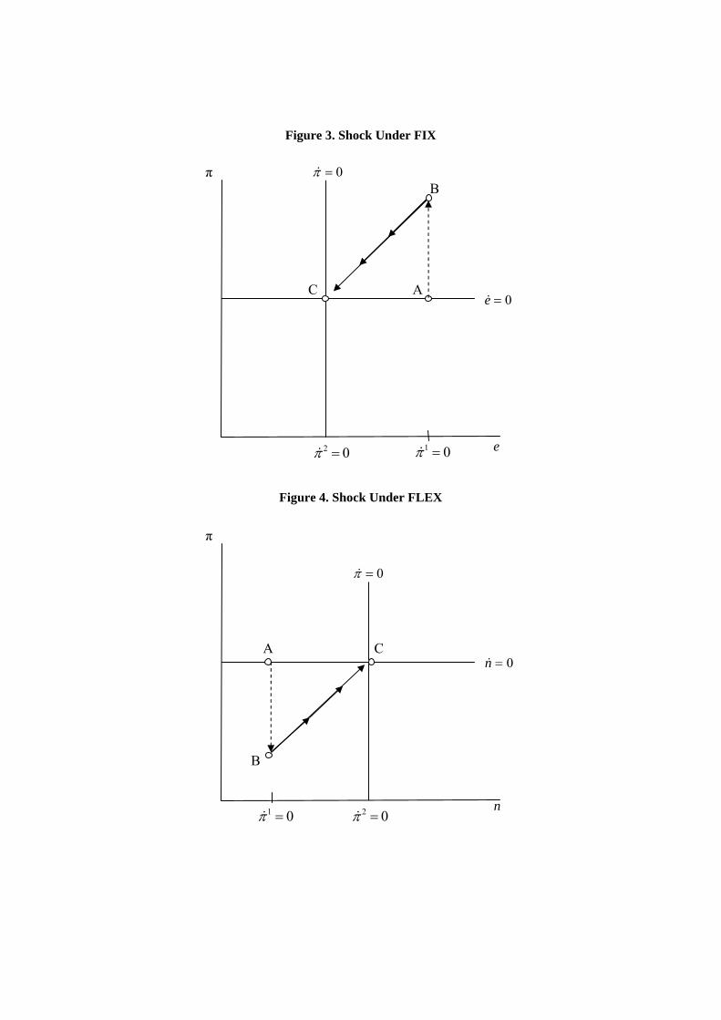
Figure 3. Shock Under FIX
Figure 4. Shock Under FLEX
0n =&
0π =&
n
π
2 0π =&
CA
B
1 0π =&
0e =&
0π =&
e
π
2 0π =&
C A
1 0π =&
B
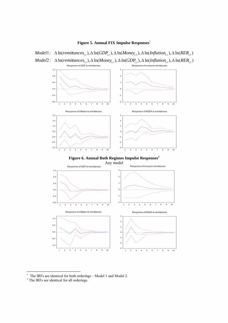
Figure 5. Annual FIX Impulse Responses1
)ln(),ln(),ln(),ln(),ln(:2)ln(),ln(),ln(),ln(),ln(:1
,,,,,
,,,,,
tititititi
tititititi
RERInflationGDPMoneytancesremitModelRERInflationMoneyGDPtancesremitModel
∆∆∆∆∆
∆∆∆∆∆
Figure 6. Annual Both Regimes Impulse Responses2 Any model
1 The IRFs are identical for both orderings – Model 1 and Model 2. 2 The IRFs are identical for all orderings.
-0.8
-0.4
0.0
0.4
0.8
1.2
1 2 3 4 5 6 7 8 9 10
Response of GDP to remittances
-2
-1
0
1
2
3
1 2 3 4 5 6 7 8 9 10
Response of moneyto remittances
-1.0
-0.5
0.0
0.5
1.0
1.5
2.0
1 2 3 4 5 6 7 8 9 10
Response of inflation to remittances
-3
-2
-1
0
1
2
3
1 2 3 4 5 6 7 8 9 10
Response of REER to remittances
-0.8
-0.4
0.0
0.4
0.8
1.2
1 2 3 4 5 6 7 8 9 10
Response of GDP to remittances
-1.0
-0.5
0.0
0.5
1.0
1 2 3 4 5 6 7 8 9 10
Response of inflation to remittances
-2
-1
0
1
2
3
1 2 3 4 5 6 7 8 9 10
Response of moneyto remittances
-3
-2
-1
0
1
2
3
1 2 3 4 5 6 7 8 9 10
Response of REER to remittances
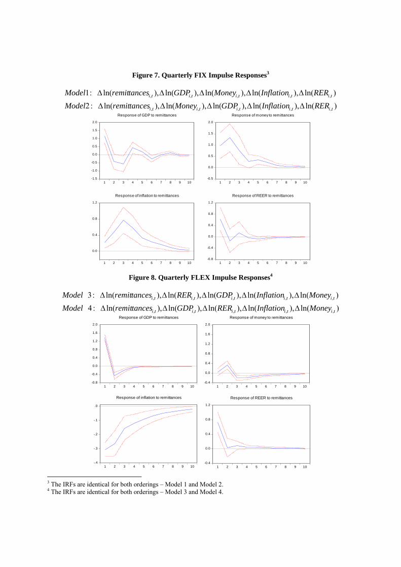
Figure 7. Quarterly FIX Impulse Responses3
)ln(),ln(),ln(),ln(),ln(:2)ln(),ln(),ln(),ln(),ln(:1
,,,,,
,,,,,
tititititi
tititititi
RERInflationGDPMoneytancesremitModelRERInflationMoneyGDPtancesremitModel
∆∆∆∆∆
∆∆∆∆∆
Figure 8. Quarterly FLEX Impulse Responses4
)ln(),ln(),ln(),ln(),ln(:4)ln(),ln(),ln(),ln(),ln(:3
,,,,,
,,,,,
tititititi
tititititi
MoneyInflationRERGDPtancesremitModelMoneyInflationGDPRERtancesremitModel
∆∆∆∆∆
∆∆∆∆∆
3 The IRFs are identical for both orderings – Model 1 and Model 2. 4 The IRFs are identical for both orderings – Model 3 and Model 4.
-1.5
-1.0
-0.5
0.0
0.5
1.0
1.5
2.0
1 2 3 4 5 6 7 8 9 10
Response of GDP to remittances
-0.5
0.0
0.5
1.0
1.5
2.0
1 2 3 4 5 6 7 8 9 10
Response of moneyto remittances
0.0
0.4
0.8
1.2
1 2 3 4 5 6 7 8 9 10
Response of inflation to remittances
-0.8
-0.4
0.0
0.4
0.8
1.2
1 2 3 4 5 6 7 8 9 10
Response of REER to remittances
-0.4
0.0
0.4
0.8
1.2
1 2 3 4 5 6 7 8 9 10
Response of REER to remittances
-0.8
-0.4
0.0
0.4
0.8
1.2
1.6
2.0
1 2 3 4 5 6 7 8 9 10
Response of GDP to remittances
-.4
-.3
-.2
-.1
.0
1 2 3 4 5 6 7 8 9 10
Response of inflation to remittances
-0.4
0.0
0.4
0.8
1.2
1.6
2.0
1 2 3 4 5 6 7 8 9 10
Response of money to remittances
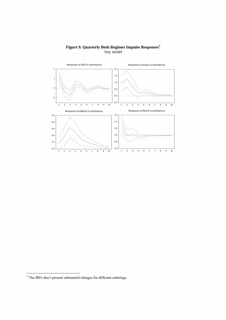
Figure 9. Quarterly Both Regimes Impulse Responses5
Any model
5 The IRFs don’t present substantial changes for different orderings.
-1
0
1
2
1 2 3 4 5 6 7 8 9 10
Response of GDP to remittances
0.0
0.2
0.4
0.6
0.8
1.0
1 2 3 4 5 6 7 8 9 10
Response of inflation to remittances
-0.5
0.0
0.5
1.0
1.5
2.0
1 2 3 4 5 6 7 8 9 10
Response of money to remittances
-1.0
-0.5
0.0
0.5
1.0
1.5
1 2 3 4 5 6 7 8 9 10
Response of REER to remittances
29
Mathematical Appendix
Most of the proofs in this section rely on one or more of the following equations. We present
them here to avoid clutter in the exposition below.
Differentiating (14) yields
(A.1.) 2
0
01
N
T
de y
df rk y f.
Implicitly differentiating (7) yields
(A.2.) 2 21
10
1 1 1 1
dl
B Bdel l l l
A A
.
(A.1) and (A.2) together imply
(A.3.) 0dl dl de
df de df.
Using (3.b) in equilibrium condition (11) and differentiating with respect to remittances,
(A.4.) 1
1 0N
tdc dlB l
df df
Since cN increases while the real exchange rate falls, by (15), c
T must also increase and by more
than the increase in cN. From (13) with (3.a) and using (15) to sign,
(A.5) 1 1 0
T
tdc dlAl
df df.
Proof that Real Exchange Rate Is Constant in Equilibrium
Suppose instead that the real exchange rate increases. An increase in the real exchange
rate generates an increase in labor in the traded sector, by (A.2). By (3.b), an increase in l leads to
a contraction in non-traded good output which, by (11), leads to a fall in non-traded consumption.
But, by (5), this leads to a contradiction since we can’t have an increase in the real exchange rate
and a fall in non-traded consumption. Similar logic holds for a decrease in the real exchange rate,
proving the proposition that the only equilibrium is one where the real exchange rate is constant.
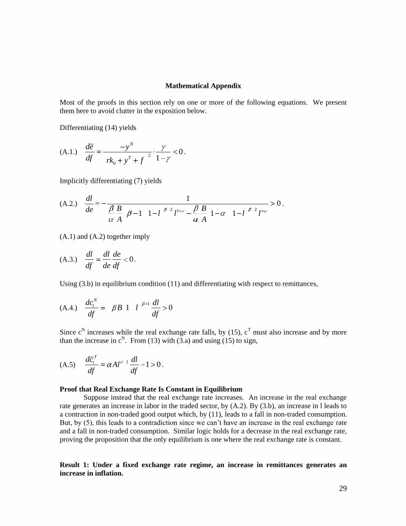
Result 1: Under a fixed exchange rate regime, an increase in remittances generates an
increase in inflation.
30
Proof: Across steady states the increase in remittances leads to a lower real exchange
rate, e, by (A.1), to higher traded and non-traded good consumption, Tc and
Nc , by (A.4) and
(A.5), and thus to higher non-traded good output, Ny , by (11). On impact, traded good
consumption and the steady state level of non-traded good production in equation (19) both jump
to their new, higher levels. Since the real exchange rate will be lower in the new steady state, it
must be that traded good consumption changes by more than the steady state non-traded good
output. Starting from steady state and given that the real exchange rate, e, is a predetermined, it
follows that the right hand side of (19) turns negative upon impact of the shock to remittances.
For this to hold and for the real exchange rate to reach it’s new, lower steady state level, the
inflation rate must increase upon impact to generate the necessary dynamics according to (20).
This is represented in the phase diagram in Figure 1 and proves Result 1.
Result 2: Under a fixed exchange rate regime, an increase in remittances generates an
increase in the nominal money supply.
Proof: This result follows from the central bank maintaining a fixed nominal exchange
rate. Rewriting (9.a) as
T
t t
t t
M c
E i. When remittances increase, traded good consumption
jumps upward once upon impact by (A.5). By open economy interest parity (10), the nominal
interest rate can only change if the foreign nominal interest rate or rate of nominal currency
depreciation change. Neither have changed and thus the domestic nominal interest rate is constant
as well. By the fixed regime, the nominal exchange rate is constant as well. Everything else in
(9.a) is a constant parameter. Thus, the increase in traded good consumption on the right-hand
side of (9.a) must be offset by an increase in the nominal stock of money on the left-hand side of
(9.a) for this optimality condition to hold at all points in time. This proves Result 2.
Result 3: Under a flexible exchange rate regime, an increase in remittances generates a
decrease in inflation.
Proof: Across steady states the increase in remittances leads to a lower real exchange
rate by (A.1), to higher traded and non-traded good consumption, Tc and
Nc , by (A.4) and
(A.5), and thus to higher non-traded good output, Ny , by (11). Real money balances in terms of
the non-traded good, n, is predetermined and thus constant on impact. Likewise, i remains
unchanged since under the FLEX, the nominal exchange rate jumps to its new level on impact to
maintain equilibrium in the money market described by (9.a). The steady state level of non-
traded good production is not constant, however, and jumps on impact to its new, higher level.
The result is that, the right hand side of (22) turns positive upon impact. For this to hold and for
the real exchange rate to reach it’s new, lower steady state level, the inflation rate must decrease
upon impact to generate the necessary dynamics according to (22). This is represented in the
phase diagram in Figure 2 and proves Result 3.
Remittances and The Real Economy: Effects of the “Dutch disease”
In our model, remittances will always cause a real appreciation and a resource
allocation á la the “Dutch disease” independent of the economy’s monetary regime. To
see this, equate (7) and (14), use (3.a) and (3.b), and rearrange to obtain an expression in
31
terms of labor, remittances, and parameters.23
Totally differentiating this shows that
increasing remittances, f, requires a fall in the amount of labor employed in the traded
good sector, l. This is the so-called “resource movement effect”.
(A.6) 2 1 1
10
11 1
t t t
dl
dfAB l AB l A l
To see the “spending effect” (i.e., the effect on the real exchange rate), rewrite (7) in
terms of the real exchange rate24
and differentiate with respect to traded good sector
labor.
(A.7) 2 111 1 1 1 0
del l l l
dl
which says that an increase in labor to the traded sector increases the real exchange rate.
Combining (A.6) and (A.7), gives the full “Dutch disease” effect.
(A.8) 0de de dl
df dl df.
That is, an increase in remittances always generates a fall in the real exchange rate in this
economy.
Furthermore, the income effect from increased wealth in the form of remittance
inflows leads to an increase in consumption of both goods. By (A.8) and (8) the final
change in both levels of consumption must be such that traded good consumption
increases by more than home good consumption. Analytically, by (3.b) and (11),
(A.9) 1
1 0N
tdc dlB l
df df.
Again, since cN increases yet the real exchange rate falls, by (A.8), c
T must also increase
and by more than the increase in cN. From (13) with (3.a) and using (A.8) to sign,
(A.10) 1 1 0
T
tdc dlAl
df df
23
1
0 01 1
t t t tAB l AB l ra Al f
24
1
1
1B le
An
32
which imposes a restriction on the magnitude of the resource allocation effect in the
traded sector such that 1 1
dlAl
df.