Munich Personal RePEc Archive - uni-muenchen.de Personal RePEc Archive Variety-Skill Complementarity: A Simple Resolution of the Trade-Wage Inequality Anomaly Yoshinori Kurokawa University

MPRAMunich Personal RePEc Archive

Variety-Skill Complementarity: A SimpleResolution of the Trade-Wage InequalityAnomaly

Yoshinori Kurokawa

University of Tsukuba

April 2010

Online at https://mpra.ub.uni-muenchen.de/29875/MPRA Paper No. 29875, posted 6. April 2011 22:41 UTC

http://mpra.ub.uni-muenchen.de/

https://mpra.ub.uni-muenchen.de/29875/

Variety-skill complementarity: a simple resolution

of the trade-wage inequality anomaly

Yoshinori Kurokawa�

University of Tsukuba

April 13, 2010(Published in Economic Theory, 46 (2011), 297-325.)

Abstract

The Stolper-Samuelson theorem predicts that the relative wage of high-

skilled to low-skilled labor will increase in the high-skill abundant U.S. but

decrease in low-skill abundant Mexico after trade liberalization, while it ac-

tually began to rise in both countries in the late 1980s. We present a simple

resolution of this "trade-wage inequality anomaly" in a model of variety trade.

Variety trade increases the variety of intermediate goods used by the �nal good.

If the varieties and high-skilled labor are complements, the skill premium rises

in both countries. This linking of imports of new foreign varieties� the exten-

sive margin� to wage inequality is compatible with evidence. Our numerical

examples illustrate that small amounts of variety trade can produce a signi�-

cant increase in relative wage.

Keywords Trade, Wage inequality, Variety-skill complementarity, Extensive

margin

JEL Classi�cation F12, F16

�Tel.&Fax: +81-29-853-7426, E-mail address: [email protected]. I am very gratefulto Timothy Kehoe for his invaluable guidance and to Cristina Arellano, Michele Boldrin, and TerryRoe for their helpful advice. I am also grateful to Pedro Amaral, Winston Chang, Julian Diaz,Koichi Hamada, Katsuhito Iwai, Hiroshi Mukunoki, Michihiro Ohyama, Martin Schneider, Yoshi-masa Shirai, the editor Nicholas Yannelis, and two anonymous referees for their detailed commentsand suggestions. I wish to thank seminar participants at the Trade and Development Workshop atMinnesota, the Minneapolis Fed, Tokyo, Santa Clara, West Virginia, Keio, SUNY-Bu¤alo, Hitot-subashi, the MVEA 43rd Annual Meeting, the MEA 71st Annual Meeting, the Spring 2007 MidwestInternational Economics Meetings, the 2007 JEA Annual Spring Meeting, and the 2008 MidwestMacro Meetings for their useful comments. I also thank Andrew Cassey and Kim Strain for theircareful correction of my English and Daniel Chiquiar and Gordon Hanson for their help with Mexicandata. However, the remaining errors are exclusively mine.

1

1 Introduction

One of the most well documented empirical facts in recent U.S. economic history is

that, as Fig. 1 shows, the relative wage of high-skilled to low-skilled labor began

to rise in manufacturing industries in the late 1980s, and this fact was observed in

Mexico as well.1 As can be seen, these two countries showed a surprisingly similar

timing of the rise in relative wage in the late 1980s and early 1990s.2 The data

also show that, as in Fig. 2, U.S.-Mexican trade (as a percent of U.S. GDP) was

dramatically increasing during the same period.3 Hence, this increased trade might

have contributed to the recent increase in skill premium in these countries. However,

there are a number of criticisms on this line of thought.

One criticism is based on a "trade-wage inequality anomaly." The standard Heckscher-

Ohlin (H-O) model demonstrates a discrepancy between the model and data. The

Stolper-Samuelson theorem of the H-O model predicts that the relative wage of high-

skilled to low-skilled labor will increase in the high-skill abundant U.S. but decrease in

low-skill abundant Mexico after trade liberalization. The H-O model thus generates a

positive relationship between the trade and wage inequality in the U.S. but generates

a negative relationship in Mexico. On the other hand, as we have seen in Fig. 1 and

2, the data generated a positive relationship between the trade and wage inequality

in both countries in the late 1980s and early 1990s. This is a "trade-wage inequality

anomaly."

A second criticism is based on price movements. The Stolper-Samuelson theorem

predicts the same direction of movement of the relative price of high-skill to low-skill

intensive goods and the relative wage of high-skilled to low-skilled labor since the rise

1Here, we use non-production and production workers as an index for high-skilled and low-skilledworkers in the U.S. and Mexican manufacturing industries (Berman et al. 1994; Robertson 2004).We calculate the U.S. relative wage during the period 1980-2000 on the basis of the U.S. AnnualSurvey of Manufactures (ASM). On the other hand, we calculate the Mexican relative wage on thebasis of the Mexican Monthly Industrial Survey (Encuesta Industrial Mensual, or EIM) by �rstcalculating the average monthly wage of non-production relative to production labor. The annualaverage is then produced by averaging this monthly relative wage.

2As shown in Fig. 1, the non-production/production wage ratio in Mexico reached a plateau afterthe North American Free Trade Agreement (NAFTA) was enacted in 1994. Esquivel and Rodríguez-López (2003) also show the same movements of Mexican wages. Robertson (2004) argues, using theMexican Industrial Census, that the Mexican skill premium declined from 1994 to 1998. We alsonote that the U.S. and Mexican relative wages are shown on di¤erent scales in Fig. 1, for here wewant to emphasize the qualitative movements of these series. In Section 4, we will emphasize thequantitative di¤erence of the same series during the period 1987-1994.

3Here, U.S.-Mexican trade is de�ned by the sum of U.S. exports to and U.S. imports from Mexico.The data for trade and GDP are from the International Trade Administration and the Bureau ofEconomic Analysis.

2

in the relative wage of high skill should be driven by the rise in the relative price

of high-skill intensive good in the high-skill abundant U.S. However, data show that

the relative prices of high-skill intensive goods were declining or constant during the

1980s while the relative wage of high skill was increasing in the U.S. (Lawrence and

Slaughter 1993).

A third criticism is based on the volume of trade. Trade-based explanations have

often been criticized due to the small volume of trade as has been shown in Fig. 2.

Krugman (1995) provides a theoretical argument to explain why the small volume of

trade in the U.S. makes it unlikely that trade can account for the change in wages.4

Thus, mainly due to these criticisms, trade-based explanations for rising wage

inequality have been minor in economic academia.5 Rather, major explanations have

been based on technological change. A sharp decline in equipment prices in the 1980s

led to an increase in the demand for high-skilled workers, who were complements

for this equipment, and a decline in the demand for low-skilled workers, who were

substitutes (Krusell et al. 2000).6 This technology-based explanation is consistent

with the decline in the price of high-tech goods and the increase in the wage inequality

both in the U.S. and in Mexico.

We now propose a simple theoretical framework to illustrate the possibility of an

increase in wage inequality in each of the trading countries as a result of even small

amounts of trade, and this can happen without a rise in the relative price of high-skill

intensive good.

We �rst present a simple resolution of the trade-wage inequality anomaly. Our

resolution is based on a straightforward application of the well-known model of variety

trade in intermediate goods due to Ethier (1982).7 Ethier�s model demonstrates that

the variety of intermediate goods, which �nal goods producers can use, increases

4It should be noted that Krugman (2008) argues that, due to the increase in U.S. trade with poorcountries and the growing fragmentation of production, it is no longer safe to assume that the e¤ectof trade on wage inequality is very minor, although he admits that it is hard to prove the actuale¤ect.

5Many papers relate trade to wage inequality in the U.S. and Mexico. For example, Borjas andRamey (1994) show how trade volumes can be linked to U.S. inequality, and Harrigan and Balaban(1999) estimate an econometric general equilibrium model of U.S. wages as a function of prices,technology, and factor supplies. Hanson and Harrison (1999) and Revenga (1997) link changes inMexican inequality to changes in trade policy, and Verhoogen (2008) links quality upgrading forexport to Mexican inequality. See Feenstra and Hanson (2003) for a survey on trade and inequality.

6Berman et al. (1994), Karni and Zilcha (1995), Berman et al. (1998), and Katz and Autor(1999) also relate technological change to wage/income inequality. Kremer and Maskin (1996) linktechnological change or skill-distribution to both wage inequality and segregation by skill, and theirmodel is extended by McCann and Trokhimtchouk (2010).

7Ethier�s (1982) model is an intermediate-good version of Krugman�s (1979) variety-trade model.

3

in both countries after trade and, therefore, their production increases through the

higher productivity caused by increased number of inputs. Let us emphasize again

that Ethier says something increases in both countries after trade.

Upon application of this logic, we show that the variety trade in di¤erentiated

intermediate goods increases the variety of intermediate goods used by the �nal good

in both countries. The increased variety of inputs then can mean the increased variety

of tasks to be handled and thus corresponds to higher demand for high-skilled labor.

Through this variety-skill complementarity, the relative wage of high skill� the skill

premium� rises in both countries. Thus our model provides a resolution of the trade-

wage inequality anomaly.8 Moreover, our model manages to capture an interesting

di¤erence in U.S. and Mexican wages: the smaller country Mexico shows a much

larger increase in the skill premium than the larger country U.S. does as shown in

Fig. 1.

We next argue that our model, though simple, has the capability of being applied

to real world data, although a de�nitive answer must wait for more serious empirical

work. In fact, the linking of imports of new foreign varieties� the extensive margin�

to wage inequality is compatible with available empirical evidence. The correlation

between the growth in the extensive margin and the growth in the relative wage

of high-skilled labor was high, over 0.93, in both U.S. and Mexican manufacturing

industries during the period 1980-2000. The variety-skill complementarity appears

to be a plausible assumption as shown by the facts in regards to U.S. production

organization. The movements of the relative price of high-skill to low-skill intensive

goods and the relative wage of high-skilled to low-skilled labor are also consistent with

the observations in the U.S., so our model does not require the Stolper-Samuelson

price-wage mechanism.

We �nally show several numerical examples with plausible parameters to see if

we can obtain a signi�cant increase in skill premium with relatively small amounts of

trade. In fact, our numerical examples illustrate the possibility that increased U.S.-

Mexican manufacturing variety trade, which is a small fraction of U.S. manufacturing

GDP, is capable of signi�cantly contributing to the increase in skill premium in both

U.S. and Mexican manufacturing industries from 1987 to 1994. We also show that

trade and technological change are complementary in that they both can contribute

8Dinopoulos et al. (2009) also link variety trade to wage inequality. Their model, however,modi�es the standard one-sector variety-trade model by introducing quasi-homothetic preferencesfor varieties and non-homothetic technology in the production of each variety, thus relating anincrease in the output of each variety� not an increase in the number of variety� to an increase inthe relative demand for high-skilled labor by each variety.

4

to increased skill premium in both countries.

Of course, other economists have also been successful in resolving the anomaly on

the basis of trade models. One major explanation is based on foreign direct invest-

ment. Feenstra and Hanson (1996) show that foreign direct investment shifts produc-

tion activities from the North to the South� an endogenous transfer of technology�

and thus increases the North�s outsourcing the low-skill intensive goods to the South,

and these goods are high-skill intensive goods by the South standards.9

A second major explanation is based on the Schumpeterian mechanism. Dinopou-

los and Segerstrom (1999) show that trade increases the relative price of innovation

(the reward for innovation relative to the current level of R&D di¢ culty), thus en-

couraging high-skill intensive R&D investment in each country.10 Acemoglu (2003)

shows that trade "induces" skill-biased technological change in the U.S., and this

improved technology can be transferred to other countries by spillover e¤ects. Thus

these explanations also demonstrate the rise in the relative wage of high-skilled labor

in each of the trading countries.11

Compared to these past studies, without introducing any foreign direct invest-

ment or dynamic Schumpeterian mechanism, this paper is successful in formulating

a simpler trade model in which trade between two countries can cause an increase in

wage inequality in both countries. Moreover, this paper is the �rst to quantitatively

show the possibility that trade, even small in volume, signi�cantly contributes to the

increase in skill premium both in the U.S. and in Mexico.

The rest of this paper is organized as follows. In Section 2, we formulate a very

simple model of variety trade, and we provide a resolution of the trade-wage inequality

anomaly. Section 3 shows that our model is compatible with available empirical

evidence. In Section 4, we present our numerical examples. Finally, we summarize

main results and mention future research in Section 5.9Zhu and Tre�er (2005) also show a mechanism closely related to this mechanism by Feenstra and

Hanson (1996). We note that Feenstra and Hanson (1996) resolve the trade-wage inequality anomalyobserved during the 1980s on the basis of a skill intensity reversal: intermediate goods� previouslyproduced in the North but now produced in the South� are relatively high-skill intensive in theSouth but relatively low-skill intensive in the North. This assumption, however, poses an empiricalchallenge since past research has found little evidence for the so-called "factor intensity reversal"over the period. We, however, resolve the anomaly without assuming this skill intensity reversal.10Dinopoulos and Segerstrom (1999) show that a contemporaneous correlation between an index

of the relative price of innovation and an index of the U.S. skill premium was 0.80 during the period1963-1989.11Acemoglu (2003) might not be successful in explaining the fact that the U.S. and Mexico showed

the surprisingly similar timing of the rise in skill premium. This is because the rise in skill premiumin Mexico should be driven by the spillover e¤ects in his model but this spillover process usuallytakes many years.

5

2 The Model

In this section, we �rst formulate our model. Second, we explicitly solve the model

and show that variety trade can increase the skill premium in both countries. Finally,

we discuss some economic implications of the derived results.

2.1 Ingredients of the Model

Consider an economy with a �nal good sector and an intermediate goods sector.

There are two types of skills: high-skilled and low-skilled labor. Their endowments

are given by �H and �L, respectively. These skills di¤er in that the high-skilled labor

can do both high-skill and low-skill tasks while the low-skilled labor can do only a

low-skill task. As will be shown later, this excludes the possibility that the relative

wage of high-skilled to low-skilled labor is less than one in equilibrium.

The production side is as follows. The �nal good sector is perfectly competitive

and non-traded. It uses a continuum [0; n] of di¤erentiated intermediate goods and

the high skill. The technology is given by the following constant returns to scale

production function:

y =

"�Z n

0

x (j)� dj

��=�+H�

#1=�;

where y is the output of �nal good, x (j) and H are the demand for di¤erentiated

intermediate good j and high skill, and 0 < � < 1. In our model, handling a variety

of inputs is represented as handling a variety of tasks and thus corresponds to a high-

skill task.12 We thus assume that � < 0, that is, the elasticity of substitution between

the varieties and high skill is given by � = 1= (1� �) < 1. We de�ne this case � < 0(� < 1) as the case where the varieties and the high skill are complements.13

On the other hand, the di¤erentiated intermediate goods sector is monopolistically

competitive. Firms are symmetric and follow Cournot pricing rules.14 There is also

12In some papers, the number of inputs plays a role in a related way. Blanchard and Kremer (1997)de�ne the index of complexity which relates the increased number of inputs to more complexityin production processes. Kremer (1993) shows that higher skill workers will use more complextechnologies that incorporate more tasks.13We note that we can generalize the production function of the �nal good by assuming that

the �nal good uses three factors: varieties, high-skilled labor, and low-skilled labor. The results,however, are unchanged as long as we assume that the varieties are more complementary to thehigh-skilled labor than to the low-skilled labor. We also note that, as will be noted in footnote 15,switching the role of high-skilled and low-skilled labor but assuming � > 0 (the varieties and the lowskill are substitutes) gives the same results in this model.14In this model with a continuum [0; n] of di¤erentiated intermediate goods, Bertrand pricing rules

give the same results as the Cournot pricing rules do.

6

free entry and exit. The intermediate goods can be traded. Each variety does not

require handling a variety of inputs and thus can use the low-skill. The technology of

each variety is given by the following increasing returns to scale production function:

x (j) =

�1

b

�max [l (j)� f; 0] ;8j;

where l (j) is the demand for low skill to produce each variety j, f is the �xed cost

in terms of low skill, and b is the unit low-skill requirement. We note that the high

skill can also do this low-skill task.

The demand side is as follows. For simplicity, we focus on a representative con-

sumer who has the endowments of high skill and low skill: �H and �L. He or she

consumes the �nal good. His or her utility function is given by:

u(c) = c;

where c is the quantity of the �nal good he or she consumes. His or her budget

constraint is given by:

pyc = wHHS + wLL

S;

where py is the price of the �nal good, wH is the wage for the high skill, and wL is

the wage for the low skill. HS is the supply of high skill for the �nal sector, and LS

is the supply of low skill for the intermediate sector, which can include the high skill.

We assume 0 � HS � �H, �L � LS � �L+ �H, and HS + LS = �H + �L.

The feasibility conditions for high-skilled labor and low-skilled labor are:

H = HS;Z n

0

l (j) dj = LS:

2.2 Explicit Solutions and the Autarky Equilibrium

We explicitly solve our model. First, we derive the solutions in the intermediate goods

sector.

Given an arbitrary n, each producer of a variety facing the indirect demand by

the �nal good sector maximizes the pro�t p (j)x (j)� wLbx (j)� wLf where p (j) isthe price of intermediate good j. By using the symmetry x (j) = �x, each variety�s

7

output �x and price �p corresponding to this n can be given by:

�x =

"�wLb

pyn(�=�)�1�

��=(1��)� n�=�

#�1=�H;8j;

�p =wLb

�;8j:

Since the price does not depend on the number of varieties n, the price when

the pro�t of each variety becomes zero by the free entry and exit is also given by

�p = wLb=�, and the zero pro�t condition �p�x � b�x � f = 0 gives the output �x of

each variety. The equality of labor demand and supply in intermediate goods sector,

�n (b�x+ f) = LS, gives the number of varieties �n. Thus the price �p and output �x of

each variety and the number of varieties �n are given by:

�p =wLb

�;8j;

�x =f�

b (1� �) ;8j;

�n =LS (1� �)

f:

We next derive the solutions in the �nal good sector.

In our model with the CES production function, it is not di¢ cult to obtain an

explicit solution for the demand for each variety by the �nal good sector, but we

solve the maximization problem for the �nal good sector by means of the following

short-cut method. De�ne a new good

X =

�Z n

0

x (j)� dj

�1=�and its price pX , and we can show desired results more easily.

The pro�t of the �nal good sector now becomes:

py (X� +H�)1=� � pXX � wHH:

First, by solving the cost minimization problem for the good X, we �nd that the

price of X is:

pX =

�Z n

0

p (j)�=(��1) dj

�(��1)=�:

8

By symmetry p (j) = �p, this becomes:

pX = n(��1)=��p;

where �p = wLb=�.

Dividing both sides by wL gives:

pXwL

= n(��1)=�b

�: (1)

Second, we solve for X. Since the technology of the �nal good shows the constant

returns to scale with X and H, we have the following equality:

y =pXX + wHH

py:

On the other hand, the demand for the �nal good is given by:

c =wHH

S + wLLS

py:

The �nal good market clearing y = c and the feasible condition for the high skill

H = HS then give:

X =wLL

S

pX: (2)

Third, we solve for the relative wage of high-skilled to low-skilled labor wH=wL.

The �rst order conditions with respect to X and H for the �nal sector give:�X

H

��1=pXwH:

By using (2) and H = HS, in autarky equilibrium the relative wage of high-skilled

labor wH=wL is given by:

wHwL

=

�pXwL

��LS

HS

�1��: (3)

This autarky equilibrium is represented in Fig. 3-a and 3-b. The demand for high

skill and low skill by the production side, H and L, is represented by the isoquant

curve of the �nal good: y = [ (wLL=pX)� +H�]

1=� which is given by y = (X� +H�)1=�

and (2). On the other hand, the supply of labor for each sector, HS and LS, is

represented by AB. The autarky equilibrium is then achieved at A in Fig. 3-a or C

9

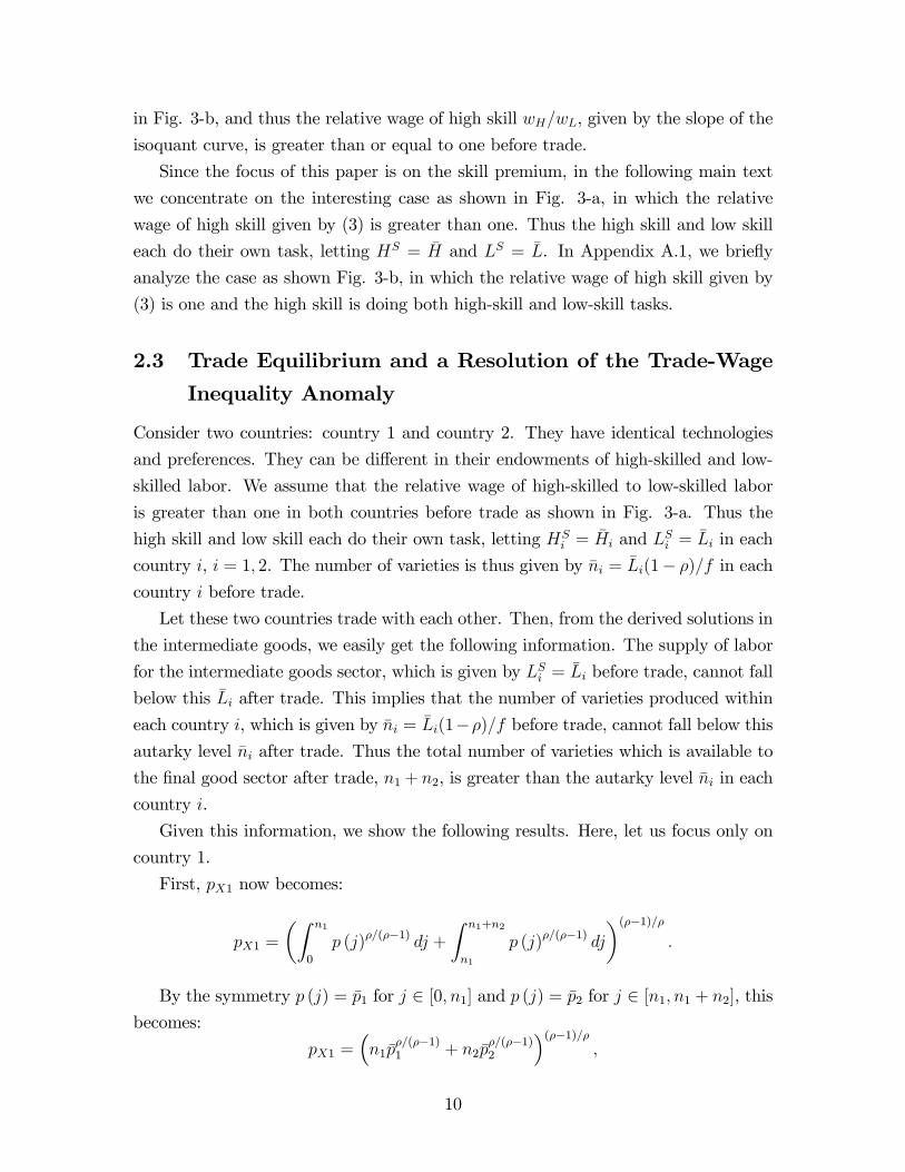
in Fig. 3-b, and thus the relative wage of high skill wH=wL, given by the slope of the

isoquant curve, is greater than or equal to one before trade.

Since the focus of this paper is on the skill premium, in the following main text

we concentrate on the interesting case as shown in Fig. 3-a, in which the relative

wage of high skill given by (3) is greater than one. Thus the high skill and low skill

each do their own task, letting HS = �H and LS = �L. In Appendix A.1, we brie�y

analyze the case as shown Fig. 3-b, in which the relative wage of high skill given by

(3) is one and the high skill is doing both high-skill and low-skill tasks.

2.3 Trade Equilibrium and a Resolution of the Trade-Wage

Inequality Anomaly

Consider two countries: country 1 and country 2. They have identical technologies

and preferences. They can be di¤erent in their endowments of high-skilled and low-

skilled labor. We assume that the relative wage of high-skilled to low-skilled labor

is greater than one in both countries before trade as shown in Fig. 3-a. Thus the

high skill and low skill each do their own task, letting HSi = �Hi and LSi = �Li in each

country i, i = 1; 2. The number of varieties is thus given by �ni = �Li(1� �)=f in eachcountry i before trade.

Let these two countries trade with each other. Then, from the derived solutions in

the intermediate goods, we easily get the following information. The supply of labor

for the intermediate goods sector, which is given by LSi = �Li before trade, cannot fall

below this �Li after trade. This implies that the number of varieties produced within

each country i, which is given by �ni = �Li(1��)=f before trade, cannot fall below thisautarky level �ni after trade. Thus the total number of varieties which is available to

the �nal good sector after trade, n1 + n2, is greater than the autarky level �ni in each

country i.

Given this information, we show the following results. Here, let us focus only on

country 1.

First, pX1 now becomes:

pX1 =

�Z n1

0

p (j)�=(��1) dj +

Z n1+n2

n1

p (j)�=(��1) dj

�(��1)=�:

By the symmetry p (j) = �p1 for j 2 [0; n1] and p (j) = �p2 for j 2 [n1; n1 + n2], thisbecomes:

pX1 =�n1�p

�=(��1)1 + n2�p

�=(��1)2

�(��1)=�;

10

where �p1 = wL1b=� and �p2 = wL2b=�.

Dividing both sides by wL1 gives:

pX1wL1

=

n1 + n2

�wL2wL1

��=(��1)!(��1)=�b

�: (1�)

Thus we see that the trading level of pX1=wL1 given by (1�) becomes lower than the

autarky level pX1=wL1 = �n(��1)=�1 b=� given by (1) since the coe¢ cient of b=� becomes

smaller due to n1 + n2 (wL2=wL1)�=(��1) > �n1 and (�� 1) =� < 0.

Second, from (2) we see that X1 increases after trade since pX1=wL1 decreases

and LS1 , which is �L1 before trade, does not decrease. This implies that the marginal

product of high-skilled labor given by MPH1 = (X�1 +H

�1)(1=�)�1H��1

1 increases for

any H1. That is, the demand for high skill by the �nal good shifts upward. Since the

supply of high skill for the �nal good, which is �H1 before trade, does not increase,

this implies that the real wage of high skill wH1=py1 increases.

Finally, from (3) we see that since � < 0 (� < 1), that is, since the vari-

eties and high skill are complements, the relative wage of high skill wH1=wL1�

the skill premium� increases after trade. This is because (pX1=wL1)� increases and�

LS1 =HS1

�1��, which is

��L1= �H1

�1��before trade, does not decrease.15

Thus it follows that the high skill and low skill each do their own task after trade

as well as before trade. That is, the supply of labor for the �nal and intermediate

sectors remains atHS1 =

�H1 and LS1 = �L1, respectively. Hence, the number of varieties

produced within country 1 after trade remains at the autarky level �n1 = �L1 (1� �) =f .We note that the above results are also obtained in country 2. Hence, we get the

following results.

The variety trade in intermediate goods causes the total number of varieties avail-

able to the �nal good sector to simply increase from �ni to �n1 + �n2, the sum of the

autarky levels, in each country i. This causes pXi=wLi to decline and thus causes Xi

to increase in both countries. Consequently, the demand for high skill shifts upward,

thus increasing the real wage of high skill wHi=pyi in both countries. Moreover, since

the varieties and high skill are complements, the decrease in pXi=wLi also increases

the relative wage of high skill wHi=wLi� the skill premium� in both countries. Thus

our model has provided a resolution of the trade-wage inequality anomaly.

We can derive more results from the above discussion. First, since the number

of varieties before trade is given by �ni = �Li(1 � �)=f in each country i, the ratio15We note that switching the role of high-skilled and low-skilled labor but assuming � > 0 (the

varieties and the low skill are substitutes) gives the same results in this model.

11

of the number of varieties produced within each country before trade is given by

�n1=�n2 = �L1=�L2. This implies that the rate of increase in �ni is smaller in a country

with the larger size of �Li, and, therefore, the rate of decrease in pXi=wLi is also smaller

as can be seen in (1�). Hence, the rise in the relative wage of high skill wHi=wLi is

smaller in a country with the larger size of �Li as can be seen in (3).16

Second, if � = 0 (� = 1), that is, if the production function of the �nal good is

given by the Cobb-Douglas function, from (3) we see that the relative wage of high

skill wHi=wLi is not a¤ected by the decrease in pXi=wLi and therefore does not change

after trade in either country.

2.4 Economic Implications of the Results

Before moving on to Section 3, we need to consider economic implications of some of

the results which have been shown in Section 2.3 on the basis of the explicit solutions

to the model. First, we explain the economic reason why the good X increases after

trade, that is, why the MPH increases after trade.

As we have seen, the activities in the intermediate goods sector never change at

all in each country after trade. Some changes, however, do occur after trade. The

number of varieties used by the �nal good sector increases, while the input quantity

of each variety used by the �nal good sector decreases in each country since each

variety is shared by two countries.

Can the e¤ect of increase in the number of varieties be canceled by the e¤ect of

decrease in the input quantity of each variety? The answer is no. This is because the

e¤ect of increase in the number of varieties is greater than the e¤ect of decrease in the

input quantity of each variety. This is the crucial e¤ect in the variety-trade models

which Ethier (1982) called the "international returns to scale." That is, the increased

number of inputs translates into higher productivity. Thus the good X increases after

trade, that is, the MPH increases after trade.

We next explain the economic reason why the relative wage of high skill can rise

after trade. Now the �nal good market clearings yi = ci in each country i, i = 1,2,

before trade are given by:

yi =wHi �Hi + wLi �Li

pyi:

16In fact, this prediction is compatible with the following observations: the number of productionworkers in manufacturing industries was much greater in the U.S. than in Mexico during the period1980-1994. As shown in Fig. 1, the U.S. skill premium increased by 12.5 percent from 1980 to 1994,while the Mexican skill premium increased by 48.9 percent.

12

Since wHi=pyi =MPHi, this becomes the following:

yi =MPHi � �Hi +wLipyi

�Li:

As we have seen, the marginal product of high skill increases in each country after

trade. For the same reason, the output of �nal good also increases in each country

after trade.

Since MPHi =�X�i +

�H�i

� (1=�)�1 �H��1i and yi =

�X�i +

�H�i

� 1=�, it can be shown

that the rate of increase inMPHi is greater than the rate of increase in yi since � < 0,

that is, since the varieties and high skill are complements. This relationship and the

�nal good market clearing condition yi =MPHi � �Hi+wLi=pyi � �Li imply that the rateof increase in MPHi should be greater than the rate of change in wLi=pyi. In other

words, the rate of increase in the real wage of high skill wHi=pyi is greater than the

rate of change in the real wage of low skill wLi=pyi . Thus the relative wage of high

skill wHi=wLi can increase in each country i.

3 Indirect Evidence for Mechanism

In this section, we �rst show that the linking of imports of new foreign varieties� the

extensive margin� to wage inequality is compatible with available empirical evidence.

Second, we claim that variety-skill complementarity appears to be a plausible assump-

tion. We �nally show that our model demonstrates price movement consistent with

observed facts.

3.1 Extensive Margin and the Relative Wage of High-Skilled

Labor

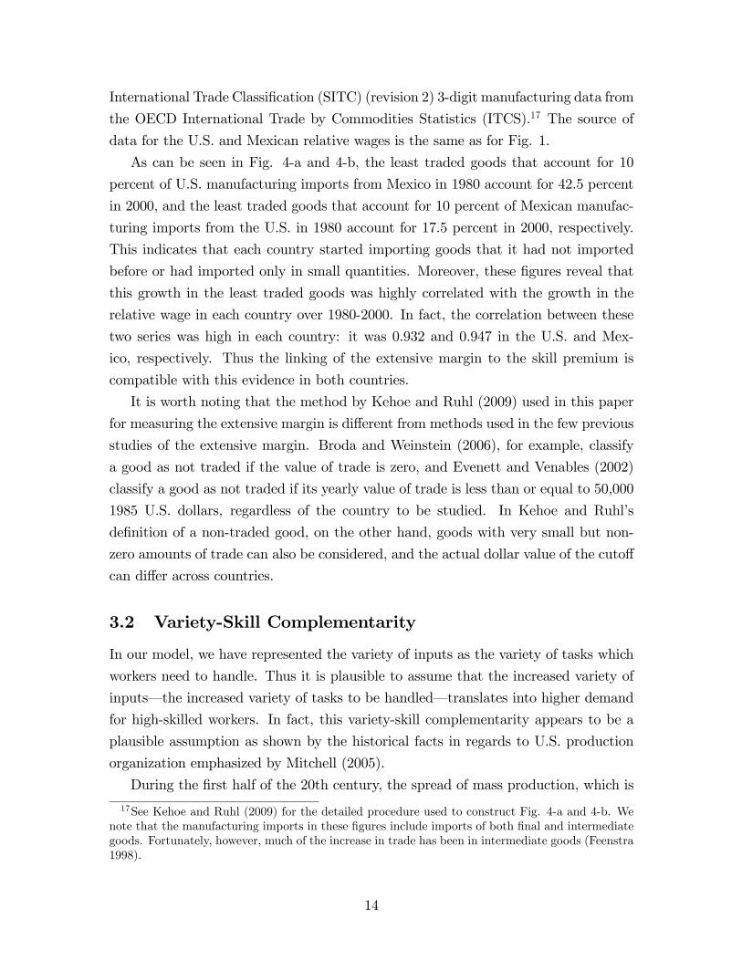
Fig. 4-a plots the 1980-2000 data on the growth in what Kehoe and Ruhl (2009)

call the "least traded goods" in U.S. manufacturing imports from Mexico and on the

relative wage of high-skilled to low-skilled labor in U.S. manufacturing industries.

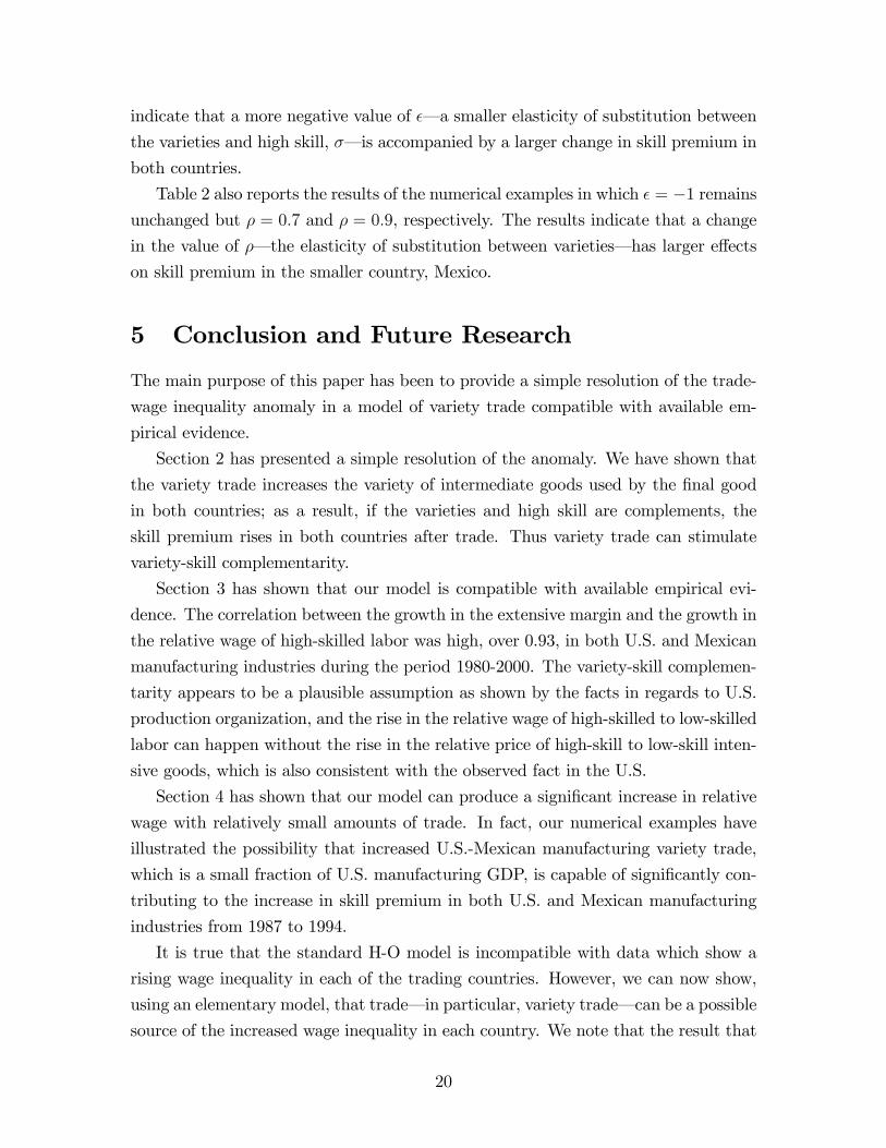
Fig. 4-b, on the other hand, plots the growth in the least traded goods in Mexican

manufacturing imports from the U.S and the relative wage in Mexican manufacturing

industries during the same period.

Kehoe and Ruhl classify the set of goods which accounts for only 10 percent of

trade as the least traded goods. Here, we use the least traded goods for measuring

the extensive margin. The data for the least traded goods growth are the Standard

13

International Trade Classi�cation (SITC) (revision 2) 3-digit manufacturing data from

the OECD International Trade by Commodities Statistics (ITCS).17 The source of

data for the U.S. and Mexican relative wages is the same as for Fig. 1.

As can be seen in Fig. 4-a and 4-b, the least traded goods that account for 10

percent of U.S. manufacturing imports from Mexico in 1980 account for 42.5 percent

in 2000, and the least traded goods that account for 10 percent of Mexican manufac-

turing imports from the U.S. in 1980 account for 17.5 percent in 2000, respectively.

This indicates that each country started importing goods that it had not imported

before or had imported only in small quantities. Moreover, these �gures reveal that

this growth in the least traded goods was highly correlated with the growth in the

relative wage in each country over 1980-2000. In fact, the correlation between these

two series was high in each country: it was 0.932 and 0.947 in the U.S. and Mex-

ico, respectively. Thus the linking of the extensive margin to the skill premium is

compatible with this evidence in both countries.

It is worth noting that the method by Kehoe and Ruhl (2009) used in this paper

for measuring the extensive margin is di¤erent from methods used in the few previous

studies of the extensive margin. Broda and Weinstein (2006), for example, classify

a good as not traded if the value of trade is zero, and Evenett and Venables (2002)

classify a good as not traded if its yearly value of trade is less than or equal to 50,000

1985 U.S. dollars, regardless of the country to be studied. In Kehoe and Ruhl�s

de�nition of a non-traded good, on the other hand, goods with very small but non-

zero amounts of trade can also be considered, and the actual dollar value of the cuto¤

can di¤er across countries.

3.2 Variety-Skill Complementarity

In our model, we have represented the variety of inputs as the variety of tasks which

workers need to handle. Thus it is plausible to assume that the increased variety of

inputs� the increased variety of tasks to be handled� translates into higher demand

for high-skilled workers. In fact, this variety-skill complementarity appears to be a

plausible assumption as shown by the historical facts in regards to U.S. production

organization emphasized by Mitchell (2005).

During the �rst half of the 20th century, the spread of mass production, which is

17See Kehoe and Ruhl (2009) for the detailed procedure used to construct Fig. 4-a and 4-b. Wenote that the manufacturing imports in these �gures include imports of both �nal and intermediategoods. Fortunately, however, much of the increase in trade has been in intermediate goods (Feenstra1998).

14

characterized by Ford�s factories, led to the larger size of manufacturing plants. On

the other hand, during the second half of the century, �exible machine tools have

allowed plants to operate at a smaller scale. The organization of production has

changed from mass production with a traditional assembly line to smaller customized

batches, thus making the size of plants smaller.18

Workers on the assembly line have a single routine task to perform; however,

workers in each batch are no longer as highly specialized in a single routine task.

Each batch is highly customizable and requires a worker who can handle a wide

variety of tasks depending on the custom features of the batch. The change in the

production organization therefore a¤ected the number of tasks and therefore a¤ected

the importance of skills. As the tasks shifted from a single routine task to a wide

variety of tasks, the required skill shifted from low skill to high skill.

Our assumption of the variety-skill complementarity is thus compatible with these

historical facts in regards to U.S. production organization, although a de�nitive an-

swer must wait for serious empirical work.19

3.3 Relative Price of High-Skill Intensive Goods

The standard H-O model predicts the same direction of movement of the relative

price of high-skill to low-skill intensive goods and the relative wage of high-skilled to

low-skilled labor since the rise in the relative wage of high skill should be driven by

the rise in the relative price of high-skill intensive good in the high-skill abundant U.S.

However, data show that the relative prices of high-skill intensive goods were declining

or constant during the 1980s while the relative wage of high skill was increasing in

the U.S. (Lawrence and Slaughter 1993).

Our model demonstrates price movement consistent with this observed fact whereas

the H-O model cannot. In Section 2.4, it has been shown that the rate of change in

wLi=pyi should be smaller than the rate of increase inMPHi since � < 0. This implies

that wLi=pyi can rise (but it should rise less than MPHi), and, therefore, the price

of high-skill intensive �nal good relative to the low-skill wage, pyi=wLi, can decline.

Here, let us recall that the price of the low-skill intensive variety relative to the low-

skill wage, �pi=wLi, is constant at b=� before and after trade. Hence, the relative price

of high-skill to low-skill intensive goods, (pyi=wLi)=(�pi=wLi), can decline while the rel-

18Milgrom and Roberts (1990) present the empirical facts on a change in the size of U.S. manu-facturing plants.19The above historical observation is compatible with the theoretical result obtained by Kremer

(1993) referred to in footnote 12.

15

ative wage of high skill rises, letting � < 0. Thus the rise in the relative wage of high

skill can happen without the rise in the relative price of high-skill intensive good.20

4 Numerical Examples

We have shown that trade� in particular, variety trade� can theoretically cause the

increase in skill premium in two countries and that our model is compatible with

available empirical evidence. This section shows several numerical examples with

plausible parameters to see if relatively small amounts of variety trade can produce

a signi�cant increase in skill premium without technological change.21

An increase in variety trade is here represented as a tari¤ reduction, for a tari¤

reduction in each country can mean that each country can use more foreign varieties.22

Technological change, on the other hand, is here represented as a decrease in �xed cost

f . A decrease in f can cause an increase in the number of varieties, n = �L (1� �) =f ,without an increase in variety trade and thus can cause an increase in the demand

for the high skill.23

4.1 Model with Tari¤s

We introduce tari¤s into our simple model and assume that each country i, i =

us;mex, imposes iceberg tari¤s � i on imports from the other country, that is, the

import quantity of a foreign variety is equal to the sum of the input quantity of the

foreign variety used by the �nal good and the iceberg tari¤s. We also introduce the

share parameter �, 0 < � < 1, into the production function of the �nal good:

yi =

"�

�Z nus+nmex

0

x (j)�i dj

��=�+ (1� �)H�

i

#1=�; i = us;mex:

We note that the de�nition of an equilibrium with tari¤s and all the derivations

of equations below are shown in Appendix A.2. We also note that our focus is on

20We note that the price of �nal good can be constant or increase if � << 0:21Our model is very simple and thus cannot perform full-scale calibrations capturing many facts.

Here, we just want to show several numerical examples with plausible parameters.22In Section 2, we have looked at the movement from autarky to trade in order to show our idea

in the simplest way. However, here we begin with a trade equilibrium in order to compare our modelwith actual trade data. Thus variety trade can increase due to the increased import volumes ofexisting foreign varieties as well as the imports of new foreign varieties.23We note that in our model "technological change" refers to non-trade-based technological change

which can occur without trade, although it is possible to interpret the increased number of inputsdue to trade as trade-based technological change.

16

wHi=wLi > 1, thus HSi =

�Hi and LSi = �Li, i = us;mex.

The relative wages of high skill are now given by:

wHuswLus

=1� ��

(1� �)f

�b

�

��=(��1) �Lus + �Lmex

�(1 + �us)

wLmexwLus

��=(��1)!!�(��1)=�� Lus�Hus

�1��;

(4)

wHmexwLmex

=1� ��

(1� �)f

�b

�

��=(��1) �Lus

�(1 + �mex)

wLuswLmex

��=(��1)+ �Lmex

!!�(��1)=�� Lmex�Hmex

�1��:

(5)

The volume of U.S.-Mexican variety trade relative to U.S. GDP is given by:

2�Lus �Lmex (1 + �us)

�=(��1)

�Lus (wLus=wLmex) + �Lmex (1 + �us)�=(��1)= (wHus=wLus)

�Hus + �Lus; (6)

where wHus=wLus is given by (4).

4.2 Numerical Examples: Variety Trade and the Skill Pre-

mium

We simulate our model, "backcasting" from 1994 to 1987, to see what changes in U.S.

and Mexican skill premium between 1987 and 1994 are predicted by the model.24

We �rst give plausible values to some parameters. The value of � = 0:83 (= 1/1.2)

is chosen so that the markup charged by each variety is 1.2. Norrbin (1993) and Basu

(1996) both obtained empirical estimates of 1.05-1.4 for markups for intermediate

goods, indicating that our choice is plausible. We normalize b = 10 and f = 100, the

choice of which leaves our results (percent changes in skill premium) unchanged. We

note that by keeping f constant from 1987 to 1994, we assume that no technological

change occurs. The labor endowments �Li and �Hi, i = us;mex, are constructed

from the OECD Structural Analysis (STAN), the ASM, and the EIM data. U.S.

endowments are �rst chosen from the data. We then calculate �Lmex so that the ratio�Lus=�Lmex matches with the observed ratio wLus �Lus=wLmex �Lmex in each year (e¤ective

labor units). This is because, as will be shown later, the balance of trade holds at

24Bergoeing and Kehoe (2003) quantitatively test the "new trade theory" by "backcasting" from1990 to 1961. Due to data constraint, here we use data from 1987 to 1994. Fortunately, however,Mexico acceded to the General Agreement on Tari¤s and Trade (GATT) in 1986 and agreed toa major liberalization of bilateral trade relations with the U.S. in 1987. Though the time-seriesmovements of the inequality over 1987-1994 are outside the scope of this paper, it is worth notingthat recent studies on the dynamics and persistence of inequality are, for example, Ray (2006) andAlexopoulos and Cavalcanti (2009).

17

wLus=wLmex = 1 in each year under our choice of parameters. We also calculate �Hmexso that the ratio �Hmex=�Lmex matches with the observed ratio.25

We then perform our simulations with the following method.

Step 1: We choose the value of �.

Step 2: We simulate our model to 1994 data. We normalize �us;1994 = 0:01 and

then calculate the values of � and �mex;1994 so that the U.S. relative wage in

1994 given by (4) matches with the corresponding data, satisfying the balance

of trade in 1994 at wLus=wLmex = 1.

Step 3: We "backcast" to 1987. We calculate the values of tari¤s �us;1987 and�mex;1987 so that the change in (6) between 1987 and 1994 is the same as the

observed change in the volume of U.S.-Mexican manufacturing variety trade

relative to U.S. manufacturing GDP, satisfying the balance of trade in 1987 at

wLus=wLmex = 1 as well.

Step 4: We calculate how much the U.S. and Mexican relative wages (4) and (5)increase from 1987 to 1994.

Table 1-a reports the results of our benchmark numerical example in which � = �1(� = 0:5). Here, the volume of U.S.-Mexican manufacturing variety trade is measured

by multiplying the Grubel-Lloyd index (a measurement of the variety-trade share) and

the volume of U.S.-Mexican total manufacturing trade. The index for a country is a

weighted average over SITC (revision 2) 3-digit manufacturing industries as follows:

1�P

k jEXk � IMkjPk (EXk + IMk)

;

where EXk and IMk represent exports and imports of industry k. These data are

obtained from the OECD ITCS and the OECD STAN.26 The data for the U.S. and

Mexican relative wages are extracts from Fig. 1. The parameters in the model are

listed separately: free parameters in (a) and calculated parameters in (b).

As can be seen, the U.S. relative wage in 1994 is the same as the observed data,

1.780, and the volume of U.S.-Mexican manufacturing variety trade relative to U.S.

25U.S. endowments are: �Hus;1987 = 6707:6; �Lus;1987 = 12242:7; �Hus;1994 = 6274:3; �Lus;1994 =11845:3 (in thousands of workers). Mexican endowments are: �Hmex;1987 = 94:6; �Lmex;1987 =222:5; �Hmex;1994 = 210:0; �Lmex;1994 = 481:2; which satisfy: �Lus;1987=�Lmex;1987 = 55:03;�Lus;1994=�Lmex;1994 = 24:61; �Hmex;1987=�Lmex;1987 = 0:425; �Hmex;1994=�Lmex;1994 = 0:436:26We note that the manufacturing variety trade includes variety trade in both �nal and interme-

diate goods. Fortunately, however, variety trade between the U.S. and Mexico primarily involvesintermediate goods (Ray 1991).

18

manufacturing GDP increases by 158.2 percent as do the corresponding data. As a

result, the U.S. relative wage increases by 6.8 percent from 1987 to 1994 while the

data show a 9.2 percent increase, and the Mexican relative wage increases by 34.2

percent while the data show a 43.6 percent increase.

Thus the results indicate that increased variety trade accounts for 73.8 percent of

the change in U.S. skill premium and accounts for 78.5 percent of the change in Mex-

ican skill premium in the manufacturing industries during the period 1987-1994. We

have here illustrated the possibility that U.S.-Mexican manufacturing variety trade,

which is a small fraction of U.S. manufacturing GDP, can signi�cantly contribute to

the increase in wage inequality.27

We note, however, that U.S.-Mexican manufacturing variety trade is not small

from the Mexican viewpoint. In fact, U.S.-Mexican manufacturing variety trade as a

fraction of Mexican manufacturing GDP was 50.2 percent in 1987 and 75.5 percent

in 1994 as shown in the table. The table also shows the corresponding results in the

model, but the results are far from the data in terms of the percent change. This is

because much of the �uctuations in the trade to GDP ratio in Mexico were caused by

�uctuations in GDP and in the real exchange rate. Our model cannot capture these

�uctuations.

Table 1-b reports the results of the numerical example in which the reduction

in f� technological change� occurs together with the tari¤ reduction from 1987 to

1994. The results indicate that if f decreases by 10.6 percent together with the same

tari¤ reduction as in the previous benchmark example, then this can cause U.S. skill

premium to increase by the same as data and can account for 85.4 percent of the

increase in Mexican skill premium.28

Thus the results indicate that trade and technological change are complementary

in that they both can contribute to increased skill premium in both countries.

4.3 Sensitivity Analysis

The results obviously depend on the values of � and �. We present some calculations

for a variety of � and �.

Table 2 reports the results of the numerical examples in which � = 0:83 remains

unchanged but � = �0:5 (� = 0:66) and � = �1:5 (� = 0:4), respectively. The results27It should be noted that even if we use data on trade in intermediate goods instead of data on

variety trade, the numerical results would be little changed. This is because evidence suggests thata considerable amount of trade in intermediate goods is variety trade (Turkcan 2005).28We note that the 10.6 percent decrease in f is equivalent to the 10.6 percent increase in the

number of �rms, n = �L (1� �) =f , in each country.

19

indicate that a more negative value of �� a smaller elasticity of substitution between

the varieties and high skill, �� is accompanied by a larger change in skill premium in

both countries.

Table 2 also reports the results of the numerical examples in which � = �1 remainsunchanged but � = 0:7 and � = 0:9, respectively. The results indicate that a change

in the value of �� the elasticity of substitution between varieties� has larger e¤ects

on skill premium in the smaller country, Mexico.

5 Conclusion and Future Research

The main purpose of this paper has been to provide a simple resolution of the trade-

wage inequality anomaly in a model of variety trade compatible with available em-

pirical evidence.

Section 2 has presented a simple resolution of the anomaly. We have shown that

the variety trade increases the variety of intermediate goods used by the �nal good

in both countries; as a result, if the varieties and high skill are complements, the

skill premium rises in both countries after trade. Thus variety trade can stimulate

variety-skill complementarity.

Section 3 has shown that our model is compatible with available empirical evi-

dence. The correlation between the growth in the extensive margin and the growth in

the relative wage of high-skilled labor was high, over 0.93, in both U.S. and Mexican

manufacturing industries during the period 1980-2000. The variety-skill complemen-

tarity appears to be a plausible assumption as shown by the facts in regards to U.S.

production organization, and the rise in the relative wage of high-skilled to low-skilled

labor can happen without the rise in the relative price of high-skill to low-skill inten-

sive goods, which is also consistent with the observed fact in the U.S.

Section 4 has shown that our model can produce a signi�cant increase in relative

wage with relatively small amounts of trade. In fact, our numerical examples have

illustrated the possibility that increased U.S.-Mexican manufacturing variety trade,

which is a small fraction of U.S. manufacturing GDP, is capable of signi�cantly con-

tributing to the increase in skill premium in both U.S. and Mexican manufacturing

industries from 1987 to 1994.

It is true that the standard H-O model is incompatible with data which show a

rising wage inequality in each of the trading countries. However, we can now show,

using an elementary model, that trade� in particular, variety trade� can be a possible

source of the increased wage inequality in each country. We note that the result that

20

trade can theoretically increase wage inequality is not necessarily negative, for our

model shows that the real wage of both high skill and low skill can rise despite the

increase in inequality.29

Of course, room for future research still exists. First, this paper has made a the-

oretical contribution in formulating a simple trade model to illustrate the possibility

of an increase in skill premium as a result of variety trade. It, however, has not yet

provided a compelling empirical analysis, although it has shown several numerical

examples. This is because (a) trade in �nal goods is ignored in this paper, (b) much

of output is services, which are largely non-traded but ignored in this paper, and (c)

trade is not balanced in data.

Thus, in another paper, we formulate a more general version of our variety-trade

model which can resolve problems (a)-(c) and allow us to perform a full-scale cali-

bration.30 In the model calibrated to the Mexican input-output data for 1987, our

numerical experiments show that the increase in U.S.-Mexican manufacturing variety

trade can account for approximately 12 percent of the actual increase in Mexican skill

premium over 1987-2000. The result indicates that our mechanism is an important

factor contributing to the increase in skill premium in its own right, but it seems to be

quantitatively less important than other mechanisms such as technological change.31

Second, intermediate goods are horizontal in nature in our model, but it would be

interesting to modify the model to consider vertical integration as in Yi (2003). Third,

we can analyze the relationship between competition policies and wage inequality. In

our model, the change in the number of varieties is related to wage inequality. This

implies that government can a¤ect wage inequality by entry policies which adjust

the number of �rms. Finally, our model has been applied to the problems of trade

between the U.S. and Mexico, but we can also directly apply it to the problems of

intra-trade among EU nations.

29In fact, the real wage of non-production labor has increased, and, further, the real wage ofproduction workers have slightly increased since the 1980s.30See Atolia and Kurokawa (2009).31Berman et al. (1994) argue, using a regression, that skill-biased technological change can account

for 40 percent of the shift in demand away from low-skilled and toward high-skilled labor in U.S.manufacturing during the 1980s. Krusell et al. (2000) �nd, using a calibrated model, that mostof the wage inequality shift of the last 30 years in the U.S. can be explained by the capital-skillcomplementarity hypothesis.

21

Appendix

A.1 The Movement of High-Skilled Labor

In Section 2, we have focused on the interesting case in which the relative wage wH=wLgiven by (3) is greater than one before trade. Thus the high skill and low skill each

do their own task, letting HS = �H and LS = �L. In this appendix, we brie�y analyze

the other case in which the relative wage wH=wL given by (3) is one and the high

skill is doing both high-skill and low-skill tasks before trade.

In the autarky equilibrium as shown in Fig. 3-b, the relative wage wH=wL given

by (3) is one at C, and part of high skill is doing the low-skill task in the intermediate

goods sector. This movement of high skill from A to C maximizes the output of �nal

good, that is, the consumer�s utility.

As we have seen in Section 2.3, the case as shown in Fig. 3-a let us conclude that

the skill premium rises after trade. On the other hand, if it is one before trade as

shown in Fig. 3-b, it can be shown that the relative wage wH=wL rises or remains

after trade, and, in any case, the number of varieties used by the �nal good surely

increases.

A.2 Model with Tari¤s

A.2.1 Equilibrium

De�nition 1 An equilibrium is prices pyus, pymex, p (j), j 2 [0; nus + nmex], wHus,wHmex, wLus, wLmex, and quantities cus, cmex, yus, ymex, x (j)us, x (j)mex, x (j), j 2[0; nus + nmex], Hus, Hmex, l (j), j 2 [0; nus + nmex], HS

us, HSmex, L

Sus, L

Smex, and the

number of �rms in the intermediate sectors nus, nmex, given iceberg tari¤s �us and

�mex, such that

1. Final good: Given prices pyi, p (j), and wHi, quantities yi, x (j)i, and Hi solve

(a) U.S.

max pyusyus �Z nus

0

p (j)x (j)us dj �Z nus+nmex

nus

p (j) (1 + �us)x (j)us dj � wHusHus

s,t,

yus =

"�

�Z nus+nmex

0

x (j)�us dj

��=�+ (1� �)H�

us

#1=�;

22

(b) Mexico

max pymexymex�Z nus

0

p (j) (1 + �mex)x (j)mex dj�Z nus+nmex

nus

p (j)x (j)mex dj�wHmexHmex

s,t,

ymex =

"�

�Z nus+nmex

0

x (j)�mex dj

��=�+ (1� �)H�

mex

#1=�;

2. Intermediate goods: Given price wLi, quantity x (j) solves

(a) U.S. j 2 [0; nus]

max p (j)x (j)� wLusbx (j)� wLusf; where x (j) = x (j)us + (1 + �mex)x (j)mex ;

(b) Mexican j 2 [nus; nus + nmex]

max p (j)x (j)� wLmexbx (j)� wLmexf; where x (j) = (1 + �us)x (j)us + x (j)mex ;

3. Consumer: Given prices pyi, wHi, and wLi, quantities ci, HSi , L

Si solve

(a) U.S.

max cus s,t, pyuscus = wHusHSus + wLusL

Sus;

(b) Mexico

max cmex s,t, pymexcmex = wHmexHSmex + wLmexL

Smex;

4. Market clearing:

cus = yus; cmex = ymex;

x (j)us + (1 + �mex)x (j)mex = x (j) ; j 2 [0; nus] ;

(1 + �us)x (j)us + x (j)mex = x (j) ; j 2 [nus; nus + nmex] ;

Hus = HSus; Hmex = H

Smex;Z nus

0

l (j) dj = LSus; j 2 [0; nus] ;Z nus+nmex

nus

l (j) dj = LSmex; j 2 [nus; nus + nmex] :

Note : (1 + �mex)x (j)mex, j 2 [0; nus], means that the imports of a U.S. variety

by Mexico, and (1 + �us)x (j)us, j 2 [nus; nus + nmex], means that the imports of aMexican variety by the U.S. We note that the U.S. and Mexican �nal good can use

only x (j)us and x (j)mex as input, respectively.

23

A.2.2 Solutions

Intermediate GoodsIntroducing tari¤s does not change the solutions in the intermediate goods sector.

By the symmetry p (j) = �pus for j 2 [0; nus] and p (j) = �pmex for j 2 [nus; nus + nmex],the price and output of each variety and the number of varieties in each country are

now given by:

�pus =wLusb

�; j 2 [0; nus] ; �pmex =

wLmexb

�; j 2 [nus; nus + nmex] ;

�xus =f�

b (1� �) ; j 2 [0; nus] ; �xmex =f�

b (1� �) ; j 2 [nus; nus + nmex] ;

�nus =�Lus (1� �)

f; �nmex =

�Lmex (1� �)f

:

Final GoodThe pro�t of the �nal good sector now becomes:

pyi (�X�i + (1� �)H�

i )1=� � pXiXi � wHiHi; i = us;mex:

By solving the cost minimization problem for the good X, we can �nd that the price

of X in each country is:

pXus =

�Z nus

0

p (j)�=(��1) dj +

Z nus+nmex

nus

((1 + �us) p (j))�=(��1) dj

�(��1)=�;

pXmex =

�Z nus

0

((1 + �mex) p (j))�=(��1) dj +

Z nus+nmex

nus

p (j)�=(��1) dj

�(��1)=�:

By the symmetry p (j) = �pus for j 2 [0; nus] and p (j) = �pmex for j 2 [nus; nus + nmex],

pXus =�nus�p

�=(��1)us + nmex ((1 + �us) �pmex)

�=(��1)�(��1)=�

;

pXmex =�nus ((1 + �mex) �pus)

�=(��1) + nmex�p�=(��1)mex

�(��1)=�:

The good X in each country is now given by:

Xus =wLus �LuspXus

; Xmex =wLmex �LmexpXmex

:

24

The relative wage of high-skilled to low-skilled labor in each country is now given by:

wHuswLus

=1� ��

�pXuswLus

�� Lus�Hus

�1��;wHmexwLmex

=1� ��

�pXmexwLmex

�� Lmex�Hmex

�1��:

By substituting pXi, �ni, and �pi, i = us;mex, into the above formula, the equilibrium

relative wages are rewritten as follows:

wHuswLus

=1� ��

(1� �)f

�b

�

��=(��1) �Lus + �Lmex

�(1 + �us)

wLmexwLus

��=(��1)!!�(��1)=�� Lus�Hus

�1��;

(4)

wHmexwLmex

=1� ��

(1� �)f

�b

�

��=(��1) �Lus

�(1 + �mex)

wLuswLmex

��=(��1)+ �Lmex

!!�(��1)=�� Lmex�Hmex

�1��:

(5)

A.2.3 Trade

Step 1: Balance of trade.The balance of trade (U.S. exports = U.S. imports) is given by the following:

�nus�pus (1 + �mex) �xus;mex = �nmex�pmex (1 + �us) �xmex;us;

where (1 + �mex) �xus;mex means that the imports of a U.S. variety by Mexico, and

(1 + �us) �xmex;us means that the imports of a Mexican variety by the U.S.

Step 2: The �rst order conditions for each variety by the �nal good.The �rst order conditions for each variety by the �nal good give:

�xmex;us = (1 + �us)1=(��1) �xus;us; �xus;mex = (1 + �mex)

1=(��1) �xmex;mex:

Step 3: The ratio of each country�s share in each variety.From Steps 1 and 2, we obtain the followings:

(1 + �us) (1 + �us)1=(��1) �xus;us

(1 + �mex) �xus;mex=

�nus�pus�nmex�pmex

;

(1 + �us) �xmex;us

(1 + �mex) (1 + �mex)1=(��1) �xmex;mex

=�nus�pus�nmex�pmex

:

Thus, by substituting �ni and �pi, i = us;mex, into the above formula, the ratio of the

demand for a U.S. variety by the U.S. to the demand for a U.S. variety by Mexico

25

becomes:

�xus;us= (1 + �mex) �xus;mex = �LuswLus=�LmexwLmex (1 + �us)�=(��1) :

The ratio of the demand for a Mexican variety by the U.S. to the demand for a

Mexican variety by Mexico also becomes:

(1 + �us) �xmex;us=�xmex;mex = �LuswLus (1 + �mex)�=(��1) =�LmexwLmex:

Step 4: Trade.The volume of U.S.-Mexican variety trade is represented as the sum of U.S. exports

and imports:

�nus�pus (1 + �mex) �xus;mex + �nmex�pmex (1 + �us) �xmex;us:

From Step 3, this becomes:

�nus�pus�LmexwLmex (1 + �us)

�=(��1)

�LuswLus + �LmexwLmex (1 + �us)�=(��1) �xus+�nmex�pmex

�LuswLus (1 + �mex)�=(��1)

�LuswLus (1 + �mex)�=(��1) + �LmexwLmex

�xmex:

By substituting �ni, �pi and �xi, i = us;mex, into the above formula, the volume of

U.S.-Mexican variety trade is given by:

�LuswLus �Lmex (1 + �us)�=(��1)

�Lus (wLus=wLmex) + �Lmex (1 + �us)�=(��1)+

�LmexwLmex �Lus (1 + �mex)�=(��1)

�Lus (1 + �mex)�=(��1) + �Lmex (wLmex=wLus)

;

where the balance of trade requires the following equality:

�LuswLus �Lmex (1 + �us)�=(��1)

�Lus (wLus=wLmex) + �Lmex (1 + �us)�=(��1) =

�LmexwLmex �Lus (1 + �mex)�=(��1)

�Lus (1 + �mex)�=(��1) + �Lmex (wLmex=wLus)

:

Accordingly, the volume of U.S.-Mexican variety trade is simply given by:

2�LuswLus �Lmex (1 + �us)

�=(��1)

�Lus (wLus=wLmex) + �Lmex (1 + �us)�=(��1) :

Thus the volume of U.S.-Mexican variety trade relative to U.S. GDP is given by:

2�Lus �Lmex (1 + �us)

�=(��1)

�Lus (wLus=wLmex) + �Lmex (1 + �us)�=(��1)= (wHus=wLus)

�Hus + �Lus: (6)

26

References

Acemoglu, D.: Patterns of skill premia. Rev Econ Stud 70, 199-230 (2003)

Alexopoulos, J., Cavalcanti, T. V. de V.: Cheap home goods and persistent inequal-

ity. Econ Theory (2009). doi: 10.1007/s00199-009-0495-4

Atolia, M., Kurokawa, Y.: Variety trade and skill premium in a calibrated general

equilibrium model: the case of Mexico. Tsukuba Economics Working Papers

No. 2009-006, Department of Economics, University of Tsukuba (2009)

Basu, S.: Procyclical productivity: increasing returns or cyclical utilization? Q J

Econ 111, 719-751 (1996)

Bergoeing, R., Kehoe, T.J.: Trade theory and trade facts. Federal Reserve Bank of

Minneapolis Research Department Sta¤ Report No. 284 (2003)

Berman, E., Bound, J., Griliches, Z.: Changes in the demand for skilled labor within

U.S. manufacturing: evidence from the Annual Survey of Manufactures. Q J

Econ 109, 367-397 (1994)

Berman, E., Bound, J., Machin, S.: Implications of skill-biased technological change:

international evidence. Q J Econ 113, 1245-1279 (1998)

Blanchard, O., Kremer, M.: Disorganization. Q J Econ 112, 1091-1126 (1997)

Borjas, G.J., Ramey, V.A.: Time series evidence on the sources of trends in wage

inequality. Am Econ Rev (Papers and Proceedings) 84, 10-16 (1994)

Broda, C., Weinstein, D.E.: Globalization and the gains from variety. Q J Econ

121, 541-585 (2006)

Dinopoulos, E., Segerstrom, P.: A Schumpeterian model of protection and relative

wages. Am Econ Rev 89, 450-472 (1999)

Dinopoulos, E., Syropoulos, C., Xu, B.: Intraindustry trade and wage-income in-

equality. Working Paper, Department of Economics, University of Florida

(2009)

Dixit, A.K., Stiglitz, J.E.: Monopolistic competition and optimum product diversity.

Am Econ Rev 67, 297-308 (1977)

27

Esquivel, G., Rodríguez-López, J.A.: Technology, trade, and wage inequality in

Mexico before and after NAFTA. J Dev Econ 72, 543-565 (2003)

Ethier, W.J.: National and international returns to scale in the modern theory of

international trade. Am Econ Rev 72, 389-405 (1982)

Evenett, S.J., Venables, A.J.: Export growth in developing countries: market entry

and bilateral trade �ows. Working Paper, University of Bern and London School

of Economics (2002)

Feenstra, R.C.: Integration of trade and disintegration of production in the global

economy. J Econ Perspect 12, 31�50 (1998)

Feenstra, R.C., Hanson, G.H.: Foreign investment, outsourcing and relative wages.

In: Feenstra, R.C., Grossman, G.M., Irwin, D.A. (eds.) The Political Economy

of Trade Policy: Papers in Honor of Jagdish Bhagwati, pp. 89-127. Cambridge,

MA: MIT Press (1996)

Feenstra, R.C., Hanson, G.H.: Global production sharing and rising inequality: a

survey of trade and wages. In: Choi, K., Harrigan, J. (eds.) Handbook of

International Trade, pp. 146-187. Oxford: Basil Blackwell (2003)

Grubel, H.G., Lloyd, P.J.: Intra-Industry Trade: The Theory and Measurement of

International Trade in Di¤erentiated Products. New York: John Wiley and

Sons (1975)

Hanson, G.H., Harrison, A.: Trade liberalization and wage inequality in Mexico.

Ind Lab Relat Rev 52, 271-288 (1999)

Harrigan, J., Balaban, R.A.: U.S. wages in general equilibrium: the e¤ects of prices,

technology, and factor supplies, 1963-1991. NBER Working Paper No. 6981

(1999)

Karni, E., Zilcha, I.: Technological progress and income inequality. Econ Theory 5,277-294 (1995)

Katz, L.F., Autor, D.H.: Change in the wage structure and earnings inequality. In:

Ashenfelter, O., Card, D. (eds.) Handbook of Labor Economics, Vol. 3A, pp.

1463-1555. Amsterdam: North-Holland (1999)

28

Kehoe, T.J., Ruhl, K.J.: How important is the new goods margin in international

trade? Federal Reserve Bank of Minneapolis Research Department Sta¤Report

No. 324 (2009)

Kremer, M.: The O-ring theory of economic development. Q J Econ 108, 551-575(1993)

Kremer, M., Maskin, E.: Wage inequality and segregation by skill. NBER Working

Paper No. 5718 (1996)

Krugman, P.R.: Increasing returns, monopolistic competition, and international

trade. J Int Econ 9, 469-479 (1979)

Krugman, P.R.: Growing world trade: causes and consequences. Brookings Pap

Econ Act, 327-377 (1995)

Krugman, P.R.: Trade and wages, reconsidered. Brookings Pap Econ Act, 103-154

(2008)

Krusell, P., Ohanian, L.E., Rios-Rull, J.-V., Violante, G.L.: Capital-skill comple-

mentarity and inequality: a macroeconomic analysis. Econometrica 68, 1029-1053 (2000)

Lawrence, R.Z., Slaughter, M.J.: International trade and American wages in the

1980s: giant sucking sound or small hiccup? Brookings Pap Econ Act: Micro-

economics, 161-226 (1993)

McCann, R.J., Trokhimtchouk, M.: Optimal partition of a large labor force into

working pairs. Econ Theory 42, 375-395 (2010)

Milgrom, P., Roberts, J.: The economics of modern manufacturing: technology,

strategy, and organization. Am Econ Rev 80, 511-528 (1990)

Mitchell, M.F.: Specialization and the skill premium in the 20th century. Int Econ

Rev 46, 935�955 (2005)

Norrbin, S.C.: The relationship between price and marginal cost in U.S. industry: a

contradiction. J Polit Econ 101, 1149-1164 (1993)

Ray, D.: On the dynamics of inequality. Econ Theory 29, 291�306 (2006)

Ray, E.J.: U.S. protection and intra-industry trade: the message to developing

countries. Econ Dev Cult Change 40, 169-187 (1991)

29

Revenga, A.: Employment and wage e¤ects of trade liberalization: the case of Mex-

ican manufacturing. J Lab Econ 15, 20-43 (1997)

Robertson, R.: Relative prices and wage inequality: evidence from Mexico. J Int

Econ 64, 387-409 (2004)

Turkcan, K.: Determinants of intra-industry trade in �nal goods and intermedi-

ate goods between Turkey and selected OECD countries. Istanbul University

Econometrics and Statistics e-Journal 1, 21-40 (2005)

Verhoogen, E.A.: Trade, quality upgrading and wage inequality in the Mexican

manufacturing sector. Q J Econ 123, 489-530 (2008)

Yi, K.-M.: Can vertical specialization explain the growth of world trade? J Polit

Econ 111, 52-102 (2003)

Zhu, S.C., Tre�er, D.: Trade and inequality in developing countries: a general

equilibrium analysis. J Int Econ 65, 21-48 (2005)

30

Table 1-a Results for benchmark numerical example

1987 1994 ChangeData

Manuf. Variety Trade/U.S. Manuf. GDP 0.018 0.046 158.2%Manuf. Variety Trade/Mex. Manuf. GDP 0.502 0.755 50.4%U.S. Skill Premium 1.630 1.780 9.2%Mex. Skill Premium 2.020 2.900 43.6%

Model

73.0,05.0,18.0,55.0(b)

01.0,100,83.0,1(a)

1987,1987,1994,

1994,

====

===−=

mexusm ex

usf

τττα

τρε


Table 1-b Results for benchmark numerical example with technologicalchange



Model

82.111,73.0,05.0,18.0,55.0(b)

01.0,100,83.0,1(a)

1987

1987,1987,1994,

1994,1994

=

====

===−=

f

f

mexusmex

us

τττα

τρε


31

Table 2 Results for numerical examples with di¤erent � and �



Model

72.0,05.0,18.0,53.0(b)

01.0,100,83.0,5.0(a)

1987,1987,1994,

1994,

====

===−=

mexusme x

usf

τττα

τρε


74.0,05.0,18.0,57.0(b)

01.0,100,83.0,5.1(a)

1987,1987,1994,

1994,

====

===−=

mexusmex

usf

τττα

τρε


06.2,09.0,22.0,93.0(b)01.0,100,7.0,1(a)

1987,1987,1994,

1994,

====

===−=

mexusme x

usfτττα

τρε


38.0,03.0,14.0,34.0(b)01.0,100,9.0,1(a)

1987,1987,1994,

1994,

====

===−=

mexusmex

usfτττα

τρε


32

Fig. 1 Relative wage of high-skilled to low-skilled labor in U.S. andMexican manufacturing industries, 1980-2000

Fig. 2 U.S.-Mexican trade as percent of U.S. GDP, 1980-2000

33

Fig. 3-a Autarky equilibrium with wH=wL > 1

H

LA

The autarky equilibrium is achieved at A,and the slope at A is 1>LH ww .The high skill and low skill each do theirown task.

1>LH ww

y

B

SLL,

SHH ,

Fig. 3-b Autarky equilibrium with wH=wL = 1

L

H

B

The autarky equilibrium is achieved at Cbetween A and B, and 1=LH ww .Part of the high skill denoted by xH isdoing the lowskill task.

A

1=LH ww

ySLL,

SHH ,

C

xHH −

xHL+

34

Fig. 4-a Least traded goods growth: U.S. manufacturing imports fromMexico, 1980-2000

Fig. 4-b Least traded goods growth: Mexican manufacturing importsfrom U.S., 1980-2000

35

Documents

Munich Personal RePEc Archive - uni-muenchen.de Personal RePEc Archive Variety-Skill Complementarity: A Simple Resolution of the Trade-Wage Inequality Anomaly Yoshinori Kurokawa University