Mutual Region Growing for Adaptive Segmentation ofGeographical Images

Naoto Mikami and Yukio Kosugi

Interdisciplinary Graduate School of Science and Engineering, Tokyo Institute of Technology, Yokohama, 226-8502 Japan

SUMMARY

In this paper we propose a new technique of mutualregion growing for solving land-cover sorting problems.Land-cover classification subdivides regions of aerial pho-tographs and satellite photographic images into distinctregions, and automation is required for large-scale investi-gations. In the conventional division method and regiongrowing scheme used for classification without tutorialdata, the processing algorithm is simple. However, muchlabor is required to find the appropriate processing rules,depending on the type of images. In this study, we proposea method of region growing using the structural features ofadjacent pixels in the tutorial image, while also utilizing thefeatures of region growing which organize regions withidentical properties.

In our new method, we aim at flexibly acquiringclassification rules by referring to the classification resultsfor the tutorial data. We propose a region growing methodin which region growing is performed in the tutorial imageby using characteristics based on the neighboring structuresof the pixel under consideration. In this technique, thefeatures of the region to be classified in the tutorial imageare expressed in the output image by using an agreementindex. This index can be obtained by comparing the imagestructures of the input image and the tutorial image. We alsoattempt to speed up processing by rearranging the image

structure in the teacher image, using a statistical technique.© 2004 Wiley Periodicals, Inc. Syst Comp Jpn, 35(14):64–77, 2004; Published online in Wiley InterScience(www.interscience.wiley.com). DOI 10.1002/scj.10688

Key words: segmentation; region growing; super-vised classification; satellite image; aerial photograph.

1. Introduction

It has recently become necessary to investigate landcover and land use forms widely, sometimes on a globalscale, for effective utilization of land resources, such asresource mapping and environmental preservation. Geo-graphic images can now be used in place of conventionalground surveys as a means of land investigation [1], sinceaerial photographs and satellite images are easily obtained.In this activity, efficient automated processing with in-creased capacity is necessary.

Image segmentation techniques already proposed in-clude region growing scheme and region dividing methods,multilayer neural networks with learning by error back-propagation, and genetic algorithms for feature quantityselection. Classification both without a teacher and with ateacher are used. The region growing and region dividingmethods involve summarizing the pixels within a predeter-mined threshold difference. Although the algorithm is sim-ple, the adaptability to changes of the type of object imageis insufficient. In neural networks and genetic algorithmswith learning procedure, the results can be made to expressadaptive segmentation rules by providing examples, be-

© 2004 Wiley Periodicals, Inc.

Systems and Computers in Japan, Vol. 35, No. 14, 2004Translated from Denshi Joho Tsushin Gakkai Ronbunshi, Vol. J86-D-II, No. 9, September 2003, pp. 1329–1340

Contract grant sponsor: Funded in part by the Ministry of Education,Science and Culture, Japan, under the project “Chinese–Japanese JointResearch on a Spatial–Temporal Information System Framework forEnvironmental Protection and Disaster Prevention.”

64

cause tutorial data are used. However, pretreatment andmanual adjustment of the input data sets are required inorder to provide sufficient learning sets. The most difficultpart of these problems is the preparation of learning datasuited to each algorithm, resulting in the effective expres-sion of features for segmentation. In this paper, a new regiongrowing scheme for adaptive segmentation is proposed inwhich the adjacency structure of the relative positions ofthe image provides the features, and these features areutilized in a form considering their reliability as tutorialdata.

2. The Mutual Region Growing Scheme(Proposed Technique)

2.1. Formulation of the problem

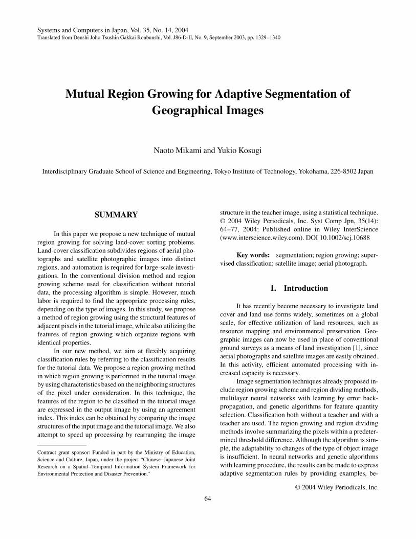
As shown in Fig. 1, we define the segmentationproblem as the problem of automatically classifying aspecific region in satellite images and color images, such asaerial photographs or pseudocolor images, from image dataof wider scope, using data classified by hand or groundsurvey results (ground truth).

Definition of the image

In our proposed method, the five image types shownin Fig. 1 are used.

• The input tutorial image is a geographic imagecontaining a region to be used for tutorial data.Abbreviation GTS (Geographical TutorialSource). The GTS is not always extracted from theimage to be used for segmentation.

• The output tutorial image is a binary output imageobtained by segmentation of the tutorial inputimage. This image is made by hand. AbbreviationGTD (Geographical Tutorial Destination).

• The input image is the object image to be seg-mented. Abbreviation GIN (Geographical In).

• The output image is the image obtained as a resultof segmentation. Abbreviation as GOUT (Geo-graphical Out).

• The output image for evaluation is the image usedto determine the segmentation accuracy. It is pre-pared manually. Abbreviation GEVA (Geographi-cal Evaluation).

2.2. Outline and definition

The mutual region growing (MRG) scheme definedin this section is a method of seeking region in the inputimage GIN and the input tutorial image GTS that are similarto each other. Given a point Q in the GIN and a point R inthe GTS, the result is mutually grown regions of the sameshape in which points Q and R correspond in the GIN andGTS. The region defined as an interconnected region sur-rounds the center points Q in the GIN and R in the GTS andsatisfies the following rules:

• The pixels at points Q and R are homogeneous.• The region is connected with the center points (Q,

R).• The region has the same structure in the GIN and

GTS.

Here the “structure” is the relative configuration of the pixelvalues surrounding points Q and R.

2.3. Generation of interconnected regions

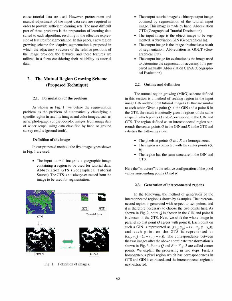
In the following, the method of generation of theinterconnected region is shown by examples. The intercon-nected region is generated with respect to two points, andit is therefore necessary to choose the two points first. Asshown in Fig. 2, point Q is chosen in the GIN and point Ris chosen in the GTS. Next, we shift the whole image inparallel so that point Q agrees with point R. Each point onsuch a GIN is represented as ((xq0

, yq0) = (x − xq, y − yq)),

and each point on the GTS is represented as((xr0

, yr0) = (x − xr, y − yr)). The correspondence between

the two images after the above coordinate transformation isshown in Fig. 3. Points Q and R in Fig. 3 are called centerpoints. We explain the processing in two steps. First, ahomogeneous pixel region which has correspondences inGTS and GIN is extracted, and the interconnected region isnext extracted.Fig. 1. Definition of images.

65

The condition that the homogeneous pixel regionmust satisfy is defined in the RGB space as follows:

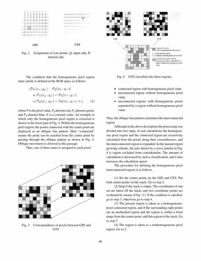
where P is the pixel value, PR denotes red, PG denotes green,and PB denotes blue. E is a constant value. An example inwhich only the homogeneous pixel region is extracted isshown in the lower part of Fig. 4. Within this homogeneouspixel region, the points connected with the center point aredisplayed as an oblique line pattern. Here “connected”means the point can be reached from the center point bypassing through the oblique pattern as shown in Fig. 4.Oblique movement is allowed in this passage.

Thus, one of three states is assigned to each pixel:

• connected region with homogeneous pixel value• unconnected region without homogeneous pixel

value• unconnected regions with homogeneous pixels

separated by a region without homogeneous pixelvalue

Thus, the oblique line pattern constitutes the interconnectedregion.

Although in the above description the processing wasdivided into two steps, in real calculations the homogene-ous pixel region and the connected region are recursivelycalculated from the pixels along their circumference, andthe interconnected region is expanded. In the mutual regiongrowing scheme, the part shown by a wavy pattern in Fig.4 is region excluded from consideration. The amount ofcalculation is decreased by such a classification, and it alsoincreases the calculation speed.

The procedure for defining the homogeneous pixelinterconnected region is as follows.

(1) Set the center points on the GIN and GTS. Putboth center points on the stack. Go to step 2.

(2) Stop if the stack is empty. The coordinates of oneset are taken off the stack, and two coordinate points areevaluated by means of Eq. (1). If the condition is satisfied,go to step 3, otherwise go to step 4.

(3) The present region is taken as a homogeneous-pixel connected region, and if the surrounding eight pointsare an unchecked region and the region is within a fixedrange from the center point, add this region to the stack. Goto step 2.

(4) The region is taken as a nonhomogeneous pixelregion. Go to 2.

(1)

Fig. 3. Correspondence of pixels between GIN andGTS.

Fig. 4. GTS classified into three regions.

Fig. 2. Assignment of core points. Q: input side; R:tutorial side.

66

In this technique, multiple R points are created forone Q point, and MRG is performed for each R. There isthe advantage that the comparison size may not be fixed,because unnecessary regions are not compared in the MRGcalculation (real calculations are kept within a constantvalue from the center point). A highly precise coincidenceregion can be calculated by using important features of thenearby pixel structure as criteria for image comparisonrather than using only single-pixel luminance values.

2.4. Utilization of the mutual region area value

It is possible to find the degree of similarity bycomparing the input data with the tutorial data. Below, thearea of the interconnected region is expressed by the mutualregion area value [MRG value = S(Q, R)] as an agreementindex. In the example of Fig. 4, S(Q, R) = 22. In thefollowing sections, this value is used as a measure ofagreement.

3. The Proposed Algorithm

In this section, we present two concrete algorithmswhich effectively utilize the properties of the mutual regiongrowing scheme.

3.1. Algorithm A

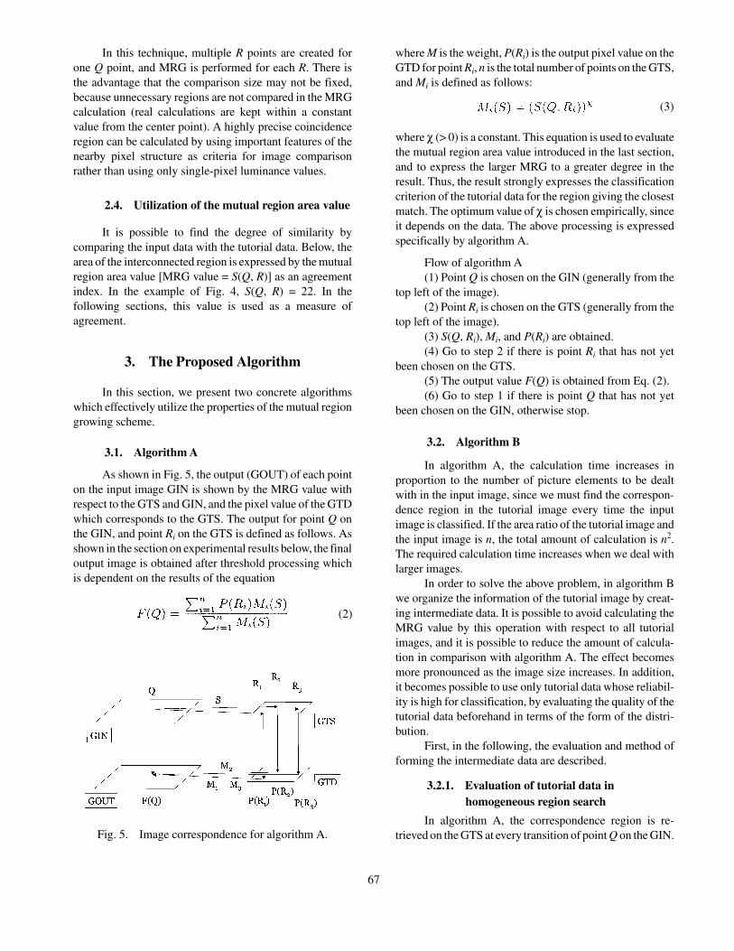
As shown in Fig. 5, the output (GOUT) of each pointon the input image GIN is shown by the MRG value withrespect to the GTS and GIN, and the pixel value of the GTDwhich corresponds to the GTS. The output for point Q onthe GIN, and point Ri on the GTS is defined as follows. Asshown in the section on experimental results below, the finaloutput image is obtained after threshold processing whichis dependent on the results of the equation

where M is the weight, P(Ri) is the output pixel value on theGTD for point Ri, n is the total number of points on the GTS,and Mi is defined as follows:

where χ (> 0) is a constant. This equation is used to evaluatethe mutual region area value introduced in the last section,and to express the larger MRG to a greater degree in theresult. Thus, the result strongly expresses the classificationcriterion of the tutorial data for the region giving the closestmatch. The optimum value of χ is chosen empirically, sinceit depends on the data. The above processing is expressedspecifically by algorithm A.

Flow of algorithm A(1) Point Q is chosen on the GIN (generally from the

top left of the image).(2) Point Ri is chosen on the GTS (generally from the

top left of the image).(3) S(Q, Ri), Mi, and P(Ri) are obtained.(4) Go to step 2 if there is point Ri that has not yet

been chosen on the GTS.(5) The output value F(Q) is obtained from Eq. (2).(6) Go to step 1 if there is point Q that has not yet

been chosen on the GIN, otherwise stop.

3.2. Algorithm B

In algorithm A, the calculation time increases inproportion to the number of picture elements to be dealtwith in the input image, since we must find the correspon-dence region in the tutorial image every time the inputimage is classified. If the area ratio of the tutorial image andthe input image is n, the total amount of calculation is n2.The required calculation time increases when we deal withlarger images.

In order to solve the above problem, in algorithm Bwe organize the information of the tutorial image by creat-ing intermediate data. It is possible to avoid calculating theMRG value by this operation with respect to all tutorialimages, and it is possible to reduce the amount of calcula-tion in comparison with algorithm A. The effect becomesmore pronounced as the image size increases. In addition,it becomes possible to use only tutorial data whose reliabil-ity is high for classification, by evaluating the quality of thetutorial data beforehand in terms of the form of the distri-bution.

First, in the following, the evaluation and method offorming the intermediate data are described.

3.2.1. Evaluation of tutorial data inhomogeneous region search

In algorithm A, the correspondence region is re-trieved on the GTS at every transition of point Q on the GIN.Fig. 5. Image correspondence for algorithm A.

(2)

(3)

67

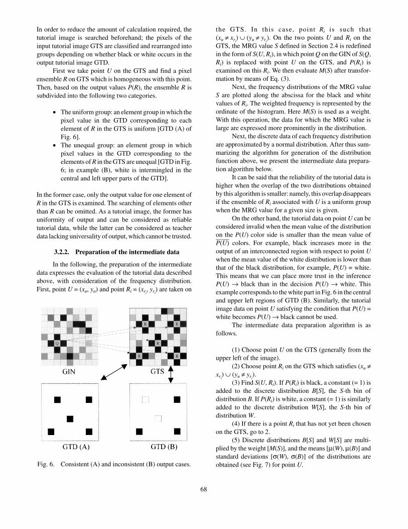
In order to reduce the amount of calculation required, thetutorial image is searched beforehand; the pixels of theinput tutorial image GTS are classified and rearranged intogroups depending on whether black or white occurs in theoutput tutorial image GTD.

First we take point U on the GTS and find a pixelensemble R on GTS which is homogeneous with this point.Then, based on the output values P(R), the ensemble R issubdivided into the following two categories.

• The uniform group: an element group in which thepixel value in the GTD corresponding to eachelement of R in the GTS is uniform [GTD (A) ofFig. 6].

• The unequal group: an element group in whichpixel values in the GTD corresponding to theelements of R in the GTS are unequal [GTD in Fig.6; in example (B), white is intermingled in thecentral and left upper parts of the GTD].

In the former case, only the output value for one element ofR in the GTS is examined. The searching of elements otherthan R can be omitted. As a tutorial image, the former hasuniformity of output and can be considered as reliabletutorial data, while the latter can be considered as teacherdata lacking universality of output, which cannot be trusted.

3.2.2. Preparation of the intermediate data

In the following, the preparation of the intermediatedata expresses the evaluation of the tutorial data describedabove, with consideration of the frequency distribution.First, point U = (xu, yu) and point Ri = (xri

, yri) are taken on

the GTS. In this case, point Ri is such that(xu ≠ xri

) ∪ (yu ≠ yri). On the two points U and Ri on the

GTS, the MRG value S defined in Section 2.4 is redefinedin the form of S(U, Ri), in which point Q on the GIN of S(Q,Ri) is replaced with point U on the GTS, and P(Ri) isexamined on this Ri. We then evaluate M(S) after transfor-mation by means of Eq. (3).

Next, the frequency distributions of the MRG valueS are plotted along the abscissa for the black and whitevalues of Ri. The weighted frequency is represented by theordinate of the histogram. Here M(S) is used as a weight.With this operation, the data for which the MRG value islarge are expressed more prominently in the distribution.

Next, the discrete data of each frequency distributionare approximated by a normal distribution. After thus sum-marizing the algorithm for generation of the distributionfunction above, we present the intermediate data prepara-tion algorithm below.

It can be said that the reliability of the tutorial data ishigher when the overlap of the two distributions obtainedby this algorithm is smaller: namely, this overlap disappearsif the ensemble of Ri associated with U is a uniform groupwhen the MRG value for a given size is given.

On the other hand, the tutorial data on point U can beconsidered invalid when the mean value of the distributionon the P(U) color side is smaller than the mean value ofP(U)____

colors. For example, black increases more in theoutput of an interconnected region with respect to point Uwhen the mean value of the white distribution is lower thanthat of the black distribution, for example, P(U) = white.This means that we can place more trust in the inferenceP(U) → black than in the decision P(U) → white. Thisexample corresponds to the white part in Fig. 6 in the centraland upper left regions of GTD (B). Similarly, the tutorialimage data on point U satisfying the condition that P(U) =white becomes P(U) → black cannot be used.

The intermediate data preparation algorithm is asfollows.

(1) Choose point U on the GTS (generally from theupper left of the image).

(2) Choose point Ri on the GTS which satisfies (xu ≠xri

) ∪ (yu ≠ yri).

(3) Find S(U, Ri). If P(Ri) is black, a constant (= 1) isadded to the discrete distribution B[S], the S-th bin ofdistribution B. If P(Ri) is white, a constant (= 1) is similarlyadded to the discrete distribution W[S], the S-th bin ofdistribution W.

(4) If there is a point Ri that has not yet been chosenon the GTS, go to 2.

(5) Discrete distributions B[S] and W[S] are multi-plied by the weight [M(S)], and the means [µ(W), µ(B)] andstandard deviations [σ(W), σ(B)] of the distributions areobtained (see Fig. 7) for point U.Fig. 6. Consistent (A) and inconsistent (B) output cases.

68

(6) If there is a point U that has not yet been chosenon the GTS, go to 1. Otherwise, stop after saving the meansand standard deviations.

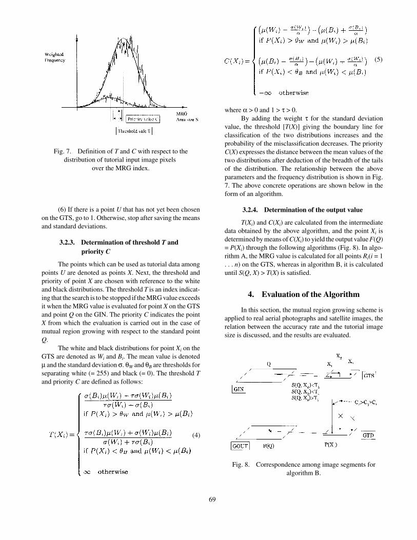
3.2.3. Determination of threshold T andpriority C

The points which can be used as tutorial data amongpoints U are denoted as points X. Next, the threshold andpriority of point X are chosen with reference to the whiteand black distributions. The threshold T is an index indicat-ing that the search is to be stopped if the MRG value exceedsit when the MRG value is evaluated for point X on the GTSand point Q on the GIN. The priority C indicates the pointX from which the evaluation is carried out in the case ofmutual region growing with respect to the standard pointQ.

The white and black distributions for point Xi on theGTS are denoted as Wi and Bi. The mean value is denotedµ and the standard deviation σ. θW and θB are thresholds forseparating white (= 255) and black (= 0). The threshold Tand priority C are defined as follows:

where α > 0 and 1 > τ > 0.By adding the weight τ for the standard deviation

value, the threshold [T(X)] giving the boundary line forclassification of the two distributions increases and theprobability of the misclassification decreases. The priorityC(X) expresses the distance between the mean values of thetwo distributions after deduction of the breadth of the tailsof the distribution. The relationship between the aboveparameters and the frequency distribution is shown in Fig.7. The above concrete operations are shown below in theform of an algorithm.

3.2.4. Determination of the output value

T(Xi) and C(Xi) are calculated from the intermediatedata obtained by the above algorithm, and the point Xi isdetermined by means of C(Xi) to yield the output value F(Q)= P(Xi) through the following algorithms (Fig. 8). In algo-rithm A, the MRG value is calculated for all points Ri(i = 1. . . n) on the GTS, whereas in algorithm B, it is calculateduntil S(Q, X) > T(X) is satisfied.

4. Evaluation of the Algorithm

In this section, the mutual region growing scheme isapplied to real aerial photographs and satellite images, therelation between the accuracy rate and the tutorial imagesize is discussed, and the results are evaluated.

Fig. 7. Definition of T and C with respect to thedistribution of tutorial input image pixels

over the MRG index.

(4)

(5)

Fig. 8. Correspondence among image segments foralgorithm B.

69

Algorithm for determination of output value

(1) From the intermediate file, T(Xi) and C(Xi) aredetermined for all X points on the GTS from Eqs. (4) and(5) (Fig. 8).

(2) Points Xi are rearranged in terms of the size ofC(Xi).

(3) Point Q is chosen from the GIN, and the first pointXi is chosen. Go to 4.

(4) If S(Q, Xi) > T(Xi), then go to 6. Otherwise, go to5.

(5) The next point Xi is chosen. Go to 4. If point Xi

cannot be chosen, go to 7 with F(Q) = indefinite value.(6) The output value F(Q) is set equal to P(Xi).(7) When the output values for all Q have been

determined, stop. Otherwise, go to step 3.

4.1. Images used in the experiments

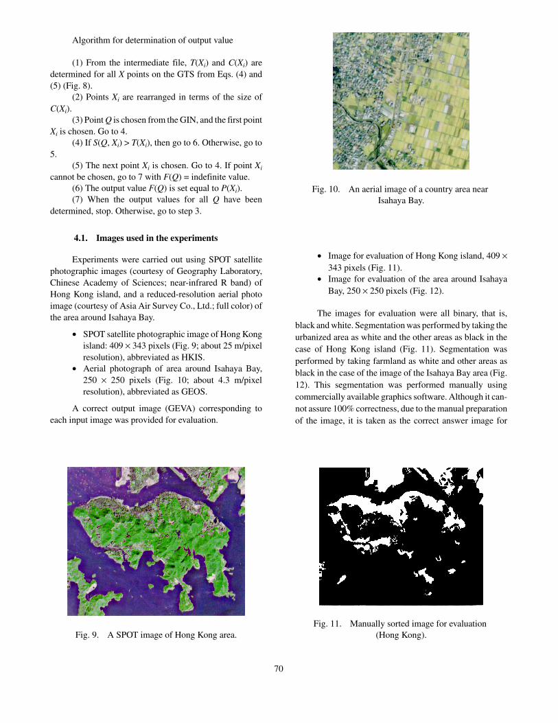
Experiments were carried out using SPOT satellitephotographic images (courtesy of Geography Laboratory,Chinese Academy of Sciences; near-infrared R band) ofHong Kong island, and a reduced-resolution aerial photoimage (courtesy of Asia Air Survey Co., Ltd.; full color) ofthe area around Isahaya Bay.

• SPOT satellite photographic image of Hong Kongisland: 409 × 343 pixels (Fig. 9; about 25 m/pixelresolution), abbreviated as HKIS.

• Aerial photograph of area around Isahaya Bay,250 × 250 pixels (Fig. 10; about 4.3 m/pixelresolution), abbreviated as GEOS.

A correct output image (GEVA) corresponding toeach input image was provided for evaluation.

• Image for evaluation of Hong Kong island, 409 ×343 pixels (Fig. 11).

• Image for evaluation of the area around IsahayaBay, 250 × 250 pixels (Fig. 12).

The images for evaluation were all binary, that is,black and white. Segmentation was performed by taking theurbanized area as white and the other areas as black in thecase of Hong Kong island (Fig. 11). Segmentation wasperformed by taking farmland as white and other areas asblack in the case of the image of the Isahaya Bay area (Fig.12). This segmentation was performed manually usingcommercially available graphics software. Although it can-not assure 100% correctness, due to the manual preparationof the image, it is taken as the correct answer image for

Fig. 9. A SPOT image of Hong Kong area.

Fig. 10. An aerial image of a country area near Isahaya Bay.

Fig. 11. Manually sorted image for evaluation (Hong Kong).

70

convenience. It is impossible to make the result 100%correct without performing a ground survey.

Evaluation method

The boundary regions between white and black areasin the evaluation images consist mainly of mixels (pixelscovering multiple regions), which hinders accurate evalu-ation. Therefore, the evaluation was performed after thispart was excluded, as shown in Fig. 13, by edge extraction.The area ratio of the evaluation region to the totality of eachimage—the evaluation region rate—is given below. In thecase of Fig. 13, the white part is the evaluated region andthe black part (edge) is the nonevaluated region.

• In the Hong Kong island image (409 × 343 pixels),the evaluation region rate is 92.3471% (Fig. 13).

• In the Isahaya Bay image (250 × 250 pixels), theevaluation region rate is 86.7328%.

The accuracy of the classification result was evalu-ated by comparing the pixel values of the isolocation of theoutput image and evaluation image in the evaluation region.The rates at which black (correct answer) is represented byblack (result) and white (correct answer) is represented bywhite (result) are shown using a confusion matrix. Goodresults are those for which the rate of representation of black(correct answer) by black (result) and of white (correctanswer) by white (result) is close to 1.0. The overall accu-racy rate is defined as (pixels of black → black and white→ white)/(total pixels of evaluation region). Good resultsare those for which the accuracy rate is close to 1.0. Thegray areas on GOUT are indefinite regions where decisionwas not possible. Though the definitions are different inalgorithms A and B, as explained below, the indefiniteregions do not belong to either of the regions.

The parameter χ is included in both algorithms withwhich the evaluation experiment was carried out. In algo-rithm A, χ was set to 4 in order to emphasize the size of theS value in the result. In algorithm B, the effect of theprocessing added in Section 3.2.3 was reduced when χ wasset to 4, and the performance as a whole deteriorated. Thus,since classification information of higher reliability thanthat provided by algorithm A was obtained, χ was setslightly lower, as 2.

The evaluation was carried out both in terms of theaccuracy rate of the entire confusion matrix, and by takingthe lower value of white (correct answer) → white (result)and black (correct answer) → black (result) from the con-fusion matrix.

4.2. Experimental results

4.2.1. Tutorial images

Figures 9 and 10 were used as the input images andFigs. 11 and 12 for evaluation. The mixel-removal maskshown in Fig. 13 was used in the evaluation.

The following images were used for the input tutorialimage (GTS) and output tutorial image (GTD):

• For HKIS, the GTS was Fig. 14 and the GTD wasFig. 15.

• For GEOS, the GTS was Fig. 16 and the GTD wasFig. 17.

In this experiment, the tutorial image was prepared frompart of the input image.

Fig. 12. Manually sorted image for evaluation (Isahaya Bay).

Fig. 13. Evaluated area (white) and nonevaluated area(black).

71

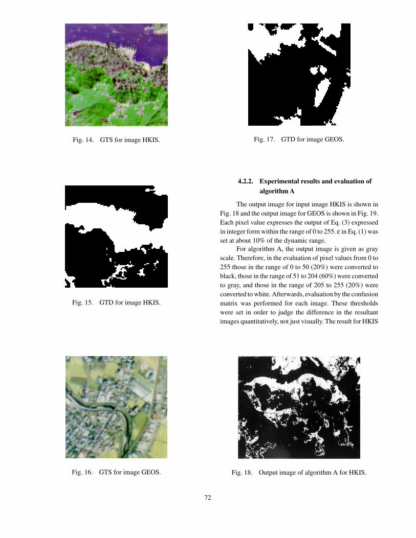
4.2.2. Experimental results and evaluation of

algorithm A

The output image for input image HKIS is shown inFig. 18 and the output image for GEOS is shown in Fig. 19.Each pixel value expresses the output of Eq. (3) expressedin integer form within the range of 0 to 255. ε in Eq. (1) wasset at about 10% of the dynamic range.

For algorithm A, the output image is given as grayscale. Therefore, in the evaluation of pixel values from 0 to255 those in the range of 0 to 50 (20%) were converted toblack, those in the range of 51 to 204 (60%) were convertedto gray, and those in the range of 205 to 255 (20%) wereconverted to white. Afterwards, evaluation by the confusionmatrix was performed for each image. These thresholdswere set in order to judge the difference in the resultantimages quantitatively, not just visually. The result for HKIS

Fig. 17. GTD for image GEOS.

Fig. 16. GTS for image GEOS.

Fig. 15. GTD for image HKIS.

Fig. 14. GTS for image HKIS.

Fig. 18. Output image of algorithm A for HKIS.

72

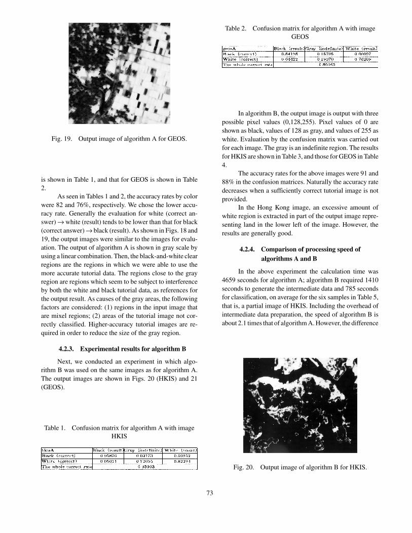
is shown in Table 1, and that for GEOS is shown in Table2.

As seen in Tables 1 and 2, the accuracy rates by colorwere 82 and 76%, respectively. We chose the lower accu-racy rate. Generally the evaluation for white (correct an-swer) → white (result) tends to be lower than that for black(correct answer) → black (result). As shown in Figs. 18 and19, the output images were similar to the images for evalu-ation. The output of algorithm A is shown in gray scale byusing a linear combination. Then, the black-and-white clearregions are the regions in which we were able to use themore accurate tutorial data. The regions close to the grayregion are regions which seem to be subject to interferenceby both the white and black tutorial data, as references forthe output result. As causes of the gray areas, the followingfactors are considered: (1) regions in the input image thatare mixel regions; (2) areas of the tutorial image not cor-rectly classified. Higher-accuracy tutorial images are re-quired in order to reduce the size of the gray region.

4.2.3. Experimental results for algorithm B

Next, we conducted an experiment in which algo-rithm B was used on the same images as for algorithm A.The output images are shown in Figs. 20 (HKIS) and 21(GEOS).

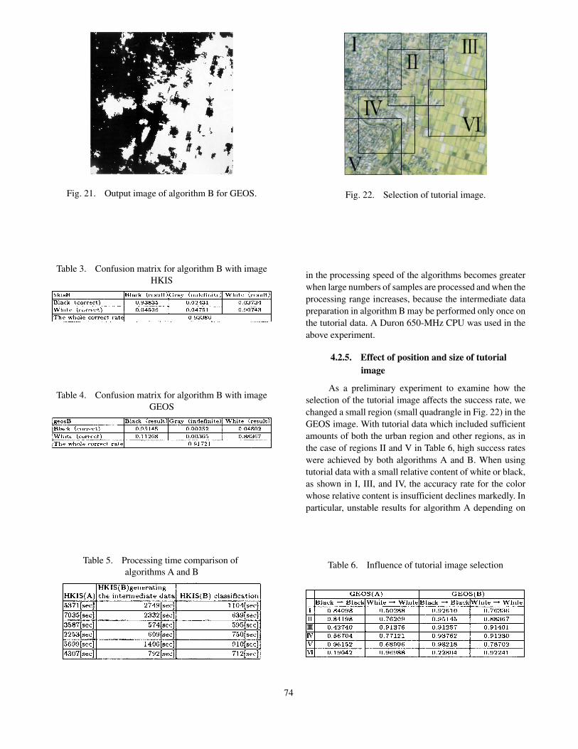
In algorithm B, the output image is output with threepossible pixel values (0,128,255). Pixel values of 0 areshown as black, values of 128 as gray, and values of 255 aswhite. Evaluation by the confusion matrix was carried outfor each image. The gray is an indefinite region. The resultsfor HKIS are shown in Table 3, and those for GEOS in Table4.

The accuracy rates for the above images were 91 and88% in the confusion matrices. Naturally the accuracy ratedecreases when a sufficiently correct tutorial image is notprovided.

In the Hong Kong image, an excessive amount ofwhite region is extracted in part of the output image repre-senting land in the lower left of the image. However, theresults are generally good.

4.2.4. Comparison of processing speed ofalgorithms A and B

In the above experiment the calculation time was4659 seconds for algorithm A; algorithm B required 1410seconds to generate the intermediate data and 785 secondsfor classification, on average for the six samples in Table 5,that is, a partial image of HKIS. Including the overhead ofintermediate data preparation, the speed of algorithm B isabout 2.1 times that of algorithm A. However, the difference

Table 1. Confusion matrix for algorithm A with imageHKIS

Table 2. Confusion matrix for algorithm A with imageGEOS

Fig. 19. Output image of algorithm A for GEOS.

Fig. 20. Output image of algorithm B for HKIS.

73

in the processing speed of the algorithms becomes greaterwhen large numbers of samples are processed and when theprocessing range increases, because the intermediate datapreparation in algorithm B may be performed only once onthe tutorial data. A Duron 650-MHz CPU was used in theabove experiment.

4.2.5. Effect of position and size of tutorialimage

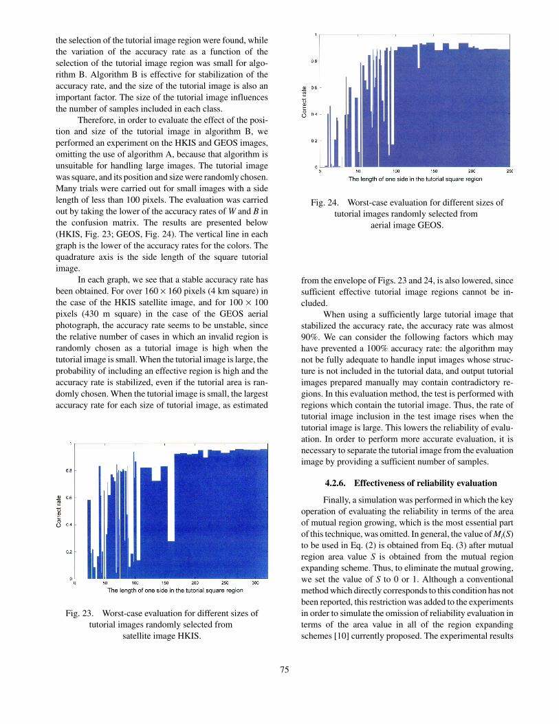
As a preliminary experiment to examine how theselection of the tutorial image affects the success rate, wechanged a small region (small quadrangle in Fig. 22) in theGEOS image. With tutorial data which included sufficientamounts of both the urban region and other regions, as inthe case of regions II and V in Table 6, high success rateswere achieved by both algorithms A and B. When usingtutorial data with a small relative content of white or black,as shown in I, III, and IV, the accuracy rate for the colorwhose relative content is insufficient declines markedly. Inparticular, unstable results for algorithm A depending on

Fig. 21. Output image of algorithm B for GEOS.

Table 3. Confusion matrix for algorithm B with imageHKIS

Table 4. Confusion matrix for algorithm B with imageGEOS

Table 5. Processing time comparison of algorithms A and B

Fig. 22. Selection of tutorial image.

Table 6. Influence of tutorial image selection

74

the selection of the tutorial image region were found, whilethe variation of the accuracy rate as a function of theselection of the tutorial image region was small for algo-rithm B. Algorithm B is effective for stabilization of theaccuracy rate, and the size of the tutorial image is also animportant factor. The size of the tutorial image influencesthe number of samples included in each class.

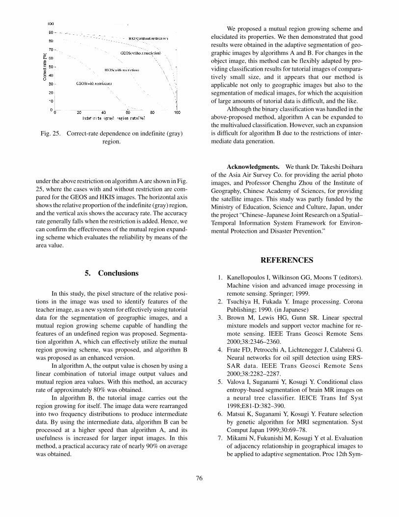
Therefore, in order to evaluate the effect of the posi-tion and size of the tutorial image in algorithm B, weperformed an experiment on the HKIS and GEOS images,omitting the use of algorithm A, because that algorithm isunsuitable for handling large images. The tutorial imagewas square, and its position and size were randomly chosen.Many trials were carried out for small images with a sidelength of less than 100 pixels. The evaluation was carriedout by taking the lower of the accuracy rates of W and B inthe confusion matrix. The results are presented below(HKIS, Fig. 23; GEOS, Fig. 24). The vertical line in eachgraph is the lower of the accuracy rates for the colors. Thequadrature axis is the side length of the square tutorialimage.

In each graph, we see that a stable accuracy rate hasbeen obtained. For over 160 × 160 pixels (4 km square) inthe case of the HKIS satellite image, and for 100 × 100pixels (430 m square) in the case of the GEOS aerialphotograph, the accuracy rate seems to be unstable, sincethe relative number of cases in which an invalid region israndomly chosen as a tutorial image is high when thetutorial image is small. When the tutorial image is large, theprobability of including an effective region is high and theaccuracy rate is stabilized, even if the tutorial area is ran-domly chosen. When the tutorial image is small, the largestaccuracy rate for each size of tutorial image, as estimated

from the envelope of Figs. 23 and 24, is also lowered, sincesufficient effective tutorial image regions cannot be in-cluded.

When using a sufficiently large tutorial image thatstabilized the accuracy rate, the accuracy rate was almost90%. We can consider the following factors which mayhave prevented a 100% accuracy rate: the algorithm maynot be fully adequate to handle input images whose struc-ture is not included in the tutorial data, and output tutorialimages prepared manually may contain contradictory re-gions. In this evaluation method, the test is performed withregions which contain the tutorial image. Thus, the rate oftutorial image inclusion in the test image rises when thetutorial image is large. This lowers the reliability of evalu-ation. In order to perform more accurate evaluation, it isnecessary to separate the tutorial image from the evaluationimage by providing a sufficient number of samples.

4.2.6. Effectiveness of reliability evaluation

Finally, a simulation was performed in which the keyoperation of evaluating the reliability in terms of the areaof mutual region growing, which is the most essential partof this technique, was omitted. In general, the value of Mi(S)to be used in Eq. (2) is obtained from Eq. (3) after mutualregion area value S is obtained from the mutual regionexpanding scheme. Thus, to eliminate the mutual growing,we set the value of S to 0 or 1. Although a conventionalmethod which directly corresponds to this condition has notbeen reported, this restriction was added to the experimentsin order to simulate the omission of reliability evaluation interms of the area value in all of the region expandingschemes [10] currently proposed. The experimental results

Fig. 23. Worst-case evaluation for different sizes oftutorial images randomly selected from

satellite image HKIS.

Fig. 24. Worst-case evaluation for different sizes oftutorial images randomly selected from

aerial image GEOS.

75

under the above restriction on algorithm A are shown in Fig.25, where the cases with and without restriction are com-pared for the GEOS and HKIS images. The horizontal axisshows the relative proportion of the indefinite (gray) region,and the vertical axis shows the accuracy rate. The accuracyrate generally falls when the restriction is added. Hence, wecan confirm the effectiveness of the mutual region expand-ing scheme which evaluates the reliability by means of thearea value.

5. Conclusions

In this study, the pixel structure of the relative posi-tions in the image was used to identify features of theteacher image, as a new system for effectively using tutorialdata for the segmentation of geographic images, and amutual region growing scheme capable of handling thefeatures of an undefined region was proposed. Segmenta-tion algorithm A, which can effectively utilize the mutualregion growing scheme, was proposed, and algorithm Bwas proposed as an enhanced version.

In algorithm A, the output value is chosen by using alinear combination of tutorial image output values andmutual region area values. With this method, an accuracyrate of approximately 80% was obtained.

In algorithm B, the tutorial image carries out theregion growing for itself. The image data were rearrangedinto two frequency distributions to produce intermediatedata. By using the intermediate data, algorithm B can beprocessed at a higher speed than algorithm A, and itsusefulness is increased for larger input images. In thismethod, a practical accuracy rate of nearly 90% on averagewas obtained.

We proposed a mutual region growing scheme andelucidated its properties. We then demonstrated that goodresults were obtained in the adaptive segmentation of geo-graphic images by algorithms A and B. For changes in theobject image, this method can be flexibly adapted by pro-viding classification results for tutorial images of compara-tively small size, and it appears that our method isapplicable not only to geographic images but also to thesegmentation of medical images, for which the acquisitionof large amounts of tutorial data is difficult, and the like.

Although the binary classification was handled in theabove-proposed method, algorithm A can be expanded tothe multivalued classification. However, such an expansionis difficult for algorithm B due to the restrictions of inter-mediate data generation.

Acknowledgments. We thank Dr. Takeshi Doiharaof the Asia Air Survey Co. for providing the aerial photoimages, and Professor Chenghu Zhou of the Institute ofGeography, Chinese Academy of Sciences, for providingthe satellite images. This study was partly funded by theMinistry of Education, Science and Culture, Japan, underthe project “Chinese–Japanese Joint Research on a Spatial–Temporal Information System Framework for Environ-mental Protection and Disaster Prevention.”

REFERENCES

1. Kanellopoulos I, Wilkinson GG, Moons T (editors).Machine vision and advanced image processing inremote sensing. Springer; 1999.

2. Tsuchiya H, Fukada Y. Image processing. CoronaPublishing; 1990. (in Japanese)

3. Brown M, Lewis HG, Gunn SR. Linear spectralmixture models and support vector machine for re-mote sensing. IEEE Trans Geosci Remote Sens2000;38:2346–2360.

4. Frate FD, Petrocchi A, Lichtenegger J, Calabresi G.Neural networks for oil spill detection using ERS-SAR data. IEEE Trans Geosci Remote Sens2000;38:2282–2287.

5. Valova I, Suganami Y, Kosugi Y. Conditional classentropy-based segmentation of brain MR images ona neural tree classifier. IEICE Trans Inf Syst1998;E81-D:382–390.

6. Matsui K, Suganami Y, Kosugi Y. Feature selectionby genetic algorithm for MRI segmentation. SystComput Japan 1999;30:69–78.

7. Mikami N, Fukunishi M, Kosugi Y et al. Evaluationof adjacency relationship in geographical images tobe applied to adaptive segmentation. Proc 12th Sym-

Fig. 25. Correct-rate dependence on indefinite (gray)region.

76

posium on Functional Figure Information Systems, p17–24, 2001. (in Japanese)

8. Mikami N, Kosugi Y. Mutual region growing for landcover classification problems. Proc LUCC Symp,CD-ROM (7 pages), 2001.

9. Susaki J, Shibazaki R. Land cover classificationmethod with consideration of mixel existence andrepresentativeness of training data, using time-series

and low spatial resolution satellite images. J Jpn SocPhotogramm Remote Sens 2001;40:14–24. (in Japa-nese)

10. Jiang H, Suzuki H, Toriwaki J. Comparative perform-ance evaluation of segmentation methods based onregion growing and division. Trans IEICE 1992;J75-D-II:1120–1131. (in Japanese)

AUTHORS (from left to right)

Naoto Mikami received his B.E. degree from Tokyo Institute of Technology in 2000 and M.E. degree in 2002. His studentresearch dealt with image processing. He is now affiliated with Fujitsu Laboratories.

Yukio Kosugi received his B.E. degree from Shizuoka University in 1970, and M.S. and D.Eng. degrees from TokyoInstitute of Technology in 1972 and 1975, both in electronics. From 1975 to 1985 he was affiliated with the Research Laboratoryof Precision Machinery and Electronics, Tokyo Institute of Technology, and from 1985 to 1999, he was an associate professorat the Interdisciplinary Graduate School of Science and Engineering. From 1998 to 2000, he conducted the project “R&D ofBrain-like Information Systems” at the Frontier Collaborative Research Center, Tokyo Institute of Technology. He is currentlya professor at the Interdisciplinary Graduate School of Science and Engineering, Tokyo Institute of Technology, and also avisiting professor at Tsukuba Advanced Research Alliance, Tsukuba University. His research interests include informationprocessing in the nervous system and neural network-aided image processing in medical and geographic fields. He is a memberof IEEE and IEICE.

77