NUSC Report No. NL-3013

*41

N Spectrum of a Signal Reflected from aTime-Varying Random Surface

ALBERT !1. NUTTALL

Office of the Associate Technical Directorfor Research

BENJAMIN F. CRONOcean Sciences Division

SD Dq>

, OV US 1970

25 August 1970 U

kepreducod byNATIONAL TECHNICALINFORMATION SERVICE

SPAIngfi.Id. Va. 22151

NAVAL UNDERWATER SYSTEMS CENTER

New London Laboratory

This document has been approved for public release and sale;its distribution is unlimited.

/1_3

REVIEWED AND APPROVED: 25 August 1970

A 1~C/4. VU44k&L.1- J W. A. Von Winkle

r" swI IAssociate Technical Directorfor Research

New London Laboratory

-.

Corresponidence concerning this report should be oddeessed as follows:

Officer in ChargeNew London Lckoratory

Naval Underwater Systems CenterNew London, Connecticut 06320

ABSTRACT

The power density spectrum of the received acoustic waveform after reflection off the time-varyingrandom sea surface is evaluated at an arbitrary observation point in the farfield. For a monochrormatictransmitted signal and a narrow-band Gaussian surface-height variation, the received acoustic spectrumis shown to consist of an impulse at the transmitted acoustic frequency plus sidelobes centered at fre-quencies separated from the transmitted f'-.quency by multiples of the surface center frequency. Thepowers in the coherent component and scatteted sideband cemponents of the received pressure waveformare evaluated in terms of the surface roughness and spatial-temporal correlation function of the surface.For the special case of elliptical contours of iso-correlationat zero time delay, the sideband powers andscattering strengths are evaluated in terms of two fundamental parameters that include the geometry ofthe experiment, the incident acoustic frequency, the root mean square (rms) surface height, and tI;esurface correlation distances.

Tie rms bandwidths of the sideband scatter components are evaluated for small surface roughness andshown to be approximately proportional to the square root of the sideband number. Numerous examples ofsideband scattering strengths for a variety of spatial correlation functions, including exponential andGaussian decay as special cases, are given.

ADMINISTRATIVE INFORMATION

This study was performed under New London Laboratory Project No. A-041-00-00, "Statistical Com-munication Through Applications" (U), Principal* Invetigator, Dr. A. H. Nuttall, Code 2021, andNavy Subproject and Task No. ZF XX 112 001, Program Manager, J. H. Huth, DLP/MAT 033 and NewLondon Laboratory Project No. A-055-00-00, "Acoustical Statistical Studies" (U), Principal Investigator,B. Cron, Code 2211, and Navy Subproject and Task No. ZR 011 01 01, Program Manager, J. H. Huth,DLP/MAT 033.

The Technical Reviewer for this report was Dr. H. W. Marsh, Senior Research Associate, Office ofthe Technical Director, New London Laboratory.

REVERSE BLANK

I

TABLE OF CONTENTS

Page

ABSTRACT ... .

ADMINISTRATIVE INFORMATION .

LIST OF TABLES . *

LIST OF ILLUSTRATIONS .

GLOSSARY . ... ix

Sectioq

1 INTRODUCTION

1

2 RF•: LECTION FROM A GENERAL TIME-VARYING SURFACE • 3

2.1 Received Pressure Waveform Reflected from a Time-Varying Surface 3

2.2 Coherent and Scatter Components for a Random Surface . 6

3 REFLECTION FROM A NARROW-BAND, TIME-VARYING SURFACE 10

3. 1 Narrow-Band Components of Received Pressure Waveform .10

3.2 Spectra and Power of Individual Narrow-Band Components 12

3.3 Special Form of Surface Correlation . . 16

3.4 Narrow-Band Sideband Spectra for Small Roughness • . 20

3.5 Rms Bandwidth of Sidebands for Small Roughness . . . 21

4 RELATION OF SURFACE CORRELATION FUNCTION TO DIRECTIONAL

WAVE SPECTRUM . • . " " " 22

4.1 General Relations . . . .23

4.2 Elliptical Surface Correlation . . .. . 23

4.3 Examples . • • • " " 25

5 SCATTERING STRENGTHS OF S1DEBAND COMPONENTS . . .34

6 DISCUSSION . . . . . . . 74

LIST OF REFERENCFS . . . . . .77

APPENDIX A - GEOMETRY FACTOR . . . .. . 79

APPENDIX B - CORRELATION PROPERTIES OF SINGLE-SIDED PROCESS 81

iii

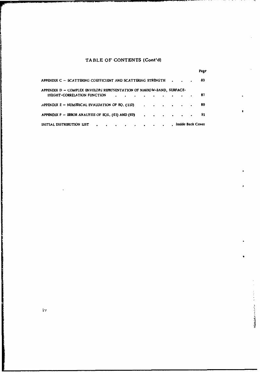
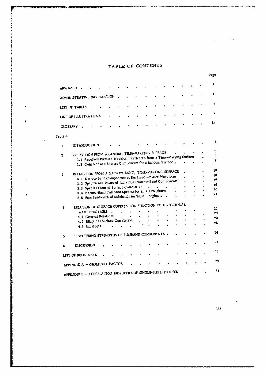
TABLE OF CONTENTS (Cont'd)

Page

APPENDIX C - SCATTERING COEFFICIENT AND SCATTERING STRENGTH 83

APPENDIX D - COMPLEX ENVELOPEi REPRFSENTATION OF NARROW-BAND, SURFACE-HEIGHT-CORRELATION FUNCTION . . 87

APPENDIX E - NUMERICAL EVALUATION OF EQ. (112) . . .. 89

APPENDIX F - ERROR ANALYSIS OF EQS. (61) AND (63) 91

INITIAL DISTRIBUTION LIST . . . . . . . . Inside Back Cover

i-7

LIST OF TABLES

Table Page

I Approximate Locations of Maximum Values of Vm (a, ) 58

LIST OF ILLUSTRATIONS

Figure

I Scattering Geometry . . .. 32 Received Acoustic Spectrum . . 113 Surface-Height Spectrum for Exponeptially Modulated Cosine Spatial

Correlation 274 Surface-Height Spectrum for Exponentially Modulated Bessel Function

Spatial Correlation 305 Surface-Height Spectrum for Gmassianly Modulated Cosine Spatial

Correlation 316 Surface-Height Spectrum for Gaussianly Modulated Bessel Function

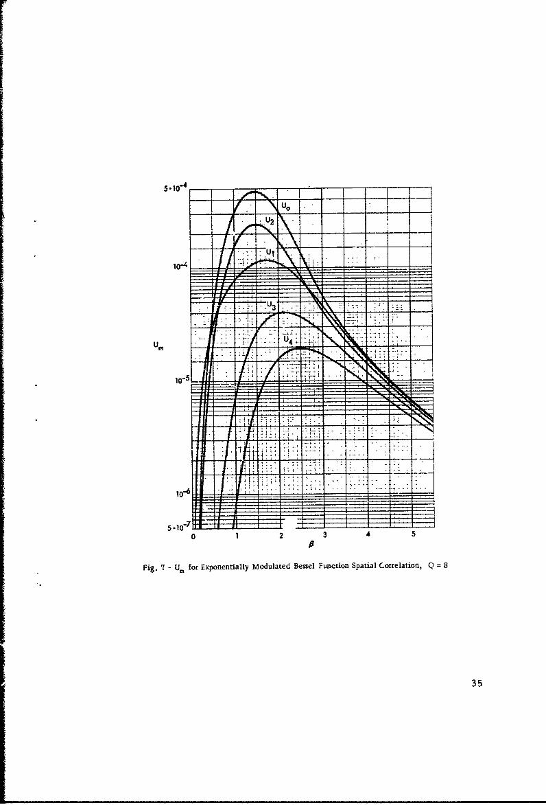
Spatial Correlation 337 U. for Exponentially Modulated Bessel Function Spsiial Correlation,

Q=8 358 Ur for Exponentially Modulated Bessel Function Spatial Correlation,

Q=4 369 UM for Exponential Spatial Correlation 37

J10 Ur for Gaussianly Modulated Bessel Function Spatial Correlation,Q=8 38

11 Us for Gaussianly Modulated Bessel Function Spatial Correlation,

Q = 4 3912 UM for Gaussian Spatial Correlation 40

13 Vo for Exponentially Modulated Bessel Function Spatial Correlation,Q=8(V0 =.268 10- t at a=151/3,(3=1.6) 42

14 V for Exponentially Modulated Bessel Function Spatial Correlation,Q = 8 (VI =.763 - 10" at a = 8, • = 1.0) 43

15 V2 for Exponentially Modulated Bessel Function Spatial Correlation,

Q =8(V2 =.144 - 10-1 at a = 15 1/3, is = 1.6 ) 4416 V3 for Exponentially Modulated Bessel Function Spatial Correlation,

Q = 8 (V 3 =.678 _ 10.2 at a = 20, J = 2.4) 45

17 V4 for Exponentially Modulated Bessel -Function Spatial Correlation,Q = 8 (V4 =.392 • 10-2 at a = 20, • = 2.9) 46

V

I

LIST OF ILLUSTRATIONS (Cont'd)Figure Page

18 0 for Exponentially Modulated Bessel Function Spatial Correlation,

Q - 4 1V 0 - •196 • 10- 1 at a = 7 2/3, 13 = 1.6) .1 .' 47

i9 V 1 for Exponentially Modulated Bessel Function Spatial Correlation,

Q '-4(VI = .395. 10- at a=41/3, 3- 1.0) . .. 1 . 48

20 V2 for Exponentially Modulated Bessel Functiot' Spatial Correlation,

Q = 4(V2 =.106 • 10-1 at a=8, P =l.7) .1 49

21 V, for Exponentially Modulated Bessel Function Spatial Correlation,

Q =4 (V3--.6 01 _ 10-2 at a= 17,( A=2.9) .. 50

22 V4 for Exponentially Modulated Bessel Function Spatial Correlation,Q = 4 (V4 = .425 . 10-2 at a = 20,(3 = 3.4) . 51

23 V0 for Exponential Spatial Correlation (V0 = .106 - 10- 1 at a = 4,

3 = 1.7 . . 52

24 V1 for Exponential Spatial Correlation (V1 = .120 10- 1 at a = 1 2/3,! /A = 1. 1) ... . 53

25 V 2 for Exponential Spatial Correlation (V 2 =.643• 10-2 at a =62/3,

(3 = 2.2) . I. .. . I 54

26 V 3 for Exponential Spatial Correlation (V3 - 460. 10-2 at a = 14 1/3,÷ ~f3 = 3.2) , 1 - :. - 55

27 V 4 for Exponential Spatial Correlation (V 4 = .352 - 10-2 at a = 20,

S= 39) • .) .. . . 56

28 V0 for Gaussianly Modulated Bessel Function Spatial Correlation, t

Q=8(V 0 =.325. 10-1 at a=15,(P= 1.6) . 59

29 V1 for Gaussianly Modulated Bessel Function Spatial Correlation,

Q =8 (VI = .705 • 10-1 at a=8 1/3, P = 1.0) . 60

30 V 2 for Gaussianly Modulated Bessel Function Spatial Correlation,

Q = 8 (V2 =. 177 • 10- 1 at a = 15 1/3,(3 = 1. 7 ). 61

31 V3 for Gaussianly Modulated Bessel Function Spatial Correlation,

Q=8(V3 =.890 _ 10-2 at a=20, 16 =2.7) . . 62

32 V for Gaussianly Modulated Bessel Function Spatial Correlation,

Q=8(V4 =.570 . 10-2 at a=20,S=- :1.1) . .. 63

33 V0 for Gaussianly Modulated Bessel Function Spatial Correlation,

Q = 4 (V 0 = .249 • 10- 1 at a = 7 2/3, 13 = 1.6) .. 64

34 VI for Gaussianly Modulated Bessel Function Spatial Correlation,

Q=4 (V = .398 - I0"1 at a = 42/3,16 = 1.1) . 65

35 V 2 for Gaussianly Modulated Bessel Function Spatial Correlation,

Q=4(V 2 =.141. 10- at a=8, 8 = 1.8) . 66

36 V 3 for Gaussianly Modulated Bessel Function Spatial Correlation,

Q = 4 (V3 = .903 . 10-2 at a = 13 1/3, 6 = 3.1) • 67

vi

I

LIST OF ILLUSTRATIONS (Cont'd)Figure Page

37 V4 for Gaussianly Modulated Bessel Function Spatial Correlation,

Q =4(V 4 -.690 • I0- 2 at a- =18, 1=4.1) . 68

38 V0 for Gaussian Spatial Correlation (V0 .210 - 10-1 at a = 3,

JS = 1.7) . . . 69

39 V1 for Gaussian Spatial Correlation (V 1 =.237 . 10-1 at a= 2,is = 1. 1) . 7040 V2 for Gaussian Spatial Correlation (V 2 •=.125 • 10-1 at a 4,

S = 2.2) . .7141 V3 for Gaussian Spatial Correlation (V 3 .886. 10-2 at a =6 1/3,

S= 3.3) . 7 242 V4 for Glussian Spatial Correlation 'V 4 =.683 • 10-2 at a = 8,

fl=4. 1) 73

Appendix B

8-1 Hilbert Transform 81

vii/viiiREVERSE BILANK

GLOSSARY

Q Iocation of acoustic source

A Location of observation point

0 Origin of coordinates

Ro Distance from origin to observation point

u ,uA Unit vectors from origin in direction of source and receiver, respectivelySi~j,k Unit vectors in x,y,z directions, respectively

ae,bQ,Co Direction cosines of source

a A' bA' cA Direction cosines of receiver

a,b,c Sums of direction cosines

t Time

x.y Position

C(x,y,t) Surface height at position x,y at time t

f FrequenLy

f. Acoustic frequency

P(t) Received pressure waveform

A Acoustic wavelengtha

ka Acoustic wave number

B Geometric scale factor (See Appendix Al

p,(x.y) Incident pressure fieldS(t) General transmitted signal pressure waveform

S(f) Voltage density spectrum of s(t)

r(t) Received pressure waveform

v Propagation velocity

H(fa; t) Instantaneous transfer function of surfacePC(t) Coherent component of received presure waveform

fý Characteristic function of surfaceq1 , q 2 Probability density functions of surface heights

P Auxiliary function, Eq. (9)p s(t) Scatter component of received pressure waveform

J Autocorrelation function of incident illumination

S Scattering strtngtb

h,O Amplitude and phase of surface-height variation

f Center frequency of surface-height variation

m Order of sideband

Am Complex amplitude of mth sideband component02 Mean square surface height

R Correlation function of received pressurep

R, Correlation function of scatter pressure

*In order of appearance.

ix

FGLOSSARY (Cont'd)

p Normalized spatial-temporal correlation function of surface

0 Surface roughness parameter, Eq. (42)

G Spectrum of scatter components

P Complex envelope of p

4ki Kronecker delta (= 1 if k = 1; 0 otherwise)

Tm Spectral shape of mth sideband

Sm Scattering strength of md sideband

pl Special form of spatial-,emporal correlation, Eq. (52)

L,,L y,L Correlation distances

p 2 Auxiliary function, Eq. (54)

a Surface correlation parameter, Eq. (58)

Um Auxiliary function pr .. 3rtional to scattering strength in specular direction, Eq. (60)

Vm Auxiliary function proportional to scattering strength in nonspecular directions,

Eq. (62)

g Low-pass spectrum (See Appendix D)

Bs Rms bandwidth of surface-height spectrum.

BM Rms bandwidth of mth sidebandA2 Directional wave spectrum

g Acceleration of gravity

A2 Directional wave spectrum (polar form)

40 Surface-height spectrumA2 Special form of direcuonal wave spectrum, Eq. (87)

R,Q Parameters of the spatial correlation decay (See Section 4.3)

$ Dimensionless auxiliary function proportional to surface-height spectrum, Eq. (96)

2 Dimensionless parameter proportional to frequency, Eq. (97)

x(t) Stationary single-sided process (See Appecdix B)x,(t),x1 (t) Real and imaginary parts of x(t), respectively

9 Hilbert transform

I Average scatter intensity (See Appendix C)

.Q Solid angle of receiver

as Scattering coefficient or scattering cross section (See Appendix C)

Iscat Average scatter intensityJ.nc Average incident intensity

Aeff Effective area of insonification

g(u,v,f) Normalized cross-spectrum (See Appendix D)

g+,p+ Auxiliary single-sided functions (See Appendix D)

PH Hilbert transform of p

q Auxiliary variable (= Q/R; see Appendix E)L Limit of integration (See Appendix F)

E Error of integration (See Appendir F)

x

GLOSSARY (Cont'd)

overbar Ensemble average

Conjugaterms Root mean square

xi/xiiREVERSE BLANK

SPECTRUM OF A SIGNAL REFLECTED FROM ATIME-VARYING RANDOM SURFACE

1. INTRODUCTION

The purpose of this study is to determine the spectrum of an acousticsignal reflected from a time-varying random surface. Of the manyscientists who have investigated scattering from such a surface, wewill mention only a few. Rayleigh considered a sinusoidal fixed surfaceand solved for the reflected pressure for a given incident monochromaticwave. Eckart's classic work [I] on scattering from a random surfaceemployed the Kirchoff method# i. e., he assumed that the surface couldbe represented by the tangent plane to the surface at each pointof incidence. Starting with the Helmnholtz equation, Beckmann andSpizzichino [2] alsoused the Kirchoff approximation, but, in their deri-vation, they differentiated with respect to the normal to the surfaceinstead of the vertical axis, andused an integration by parts to eliminate

edge effects. Thus, they obtained a different geometric factor from thatof Eckart [1] for the reflected pressure. LaCasce and Tamarkin [3] per-formed experimental studies on the reflection off a fixed sinusoidalpressure-release surface. Horton and Muir [4] also performed experi-mental studies on the scattering from a rough random surface, comparedtheir results with a modified version of the Eckart theory, and foundgood agreement. Wagner [5] considered a Gaussian surface, andusingthe parameters of root-mean-square (rms) height and correlation ofsurface heights, and treating the incident waves as rays, determinedthe amount of shadowing as a function of the grazing angle of the incidentacoustic wave. From these results, a correction value for the shadowing

effect was made by Wagner [5] to the Eckart [1] and Beckmann andSpizzichino [2] theories. Marsh [6] also utilized the Rayleigh methodand considered the signal reflected from a random surface to consistof an infinite set of plane waves. By applying boundary conditions onthe surface, he solved for the scattering coefficient of the surfacereflection.

The number of investigations of a time-varying random surface isconsiderably less than that of a fixed surface. Of these, we will mention

only the works of Roderick and Cron [7] and Parkins [8]. Roderickand Cron considered a sinusoidal traveling surface wave, where, for asingle-frequency incident acoustic wave, the frequency of the reflectionin the specular direction is the same as the incident frequency, and thefrequencies in the nonspecular directions are equal to the incident fre-

quency plus multiples of the surface frequency. They compared thetheoretical predictions of the amplitudes of these components with ex-periment. Parkins considered a time-varying random surface, a jointGaussian distribution of heights, and a Neumann-Pierson surface -heightspectrum. For both small and large surface roughness, he obtainedthe scattered acoustic spectrum.

In our work, we start with the assumptions used b, .:

o the Kirchoff method [2, p. 20] - the methodof physical optics -is used,

* the insonified area is in the farfield (Fraunhofer region) of thesource,

* the observation point is in the farfield of the insonified area,

*the surface is pressure-release,

*no shadowing or multiple reflections occur,

*a directional source is used, and

ethe surface particle velocity is small compared with the speed

of sound.

Starting with the Helmholtz integral and a given incident single-frequency acoustic source, we obtain the (complex) pressure at the

observation point. The surface height is designated a function of positionx, y, and time t; the first- and second-order probability distributions

of height are assumed independent of absolute position and time anddependent only on tie differences in the x and y coordinates and time.That is, the surface is assumed homogeneous and stationary. Theautocorrelation function of the received acoustic complex pressureis obtained by using these properties. The Fourier transform of theautocorrelation function then yields the received acoustic power spectrum.

2

IThe equation for the power spectrum is then specialized to the case

of a joint Gaussian distribution of surface heights and a narrow-band,surface-height spectrumat a point; for this case, the spatial-temporalcorrelation function of the surface can be re'-resented as a sinusoidaloscillation in time-delay with a slowly varying amplitude and phase. Itis then assumed that the iso-values of the surface-correlation functionis an ellipse; for this case, it is shown that the received acoustic spec-trum consists of a series of spectral '.bes or sidebands, each separatedfrom the incident acoustic frequency by multiples of the center fre-quency of the surface variation, plus an impulse at the incident acousticfrequency. The relative powers in these sideband components areevaluated in terms of two fundamental parameters: the first is thesurface-roughness parameter, and the second is related to the corre-lation distances of the surface (the horizontal separation for which thesurface correlation falls to e- 1 of its origin value). The powers inthe sidebands are numerically evaluated and plotted versus these twoparameters, for both specular and nonspecular directions, for a varietyof spatial correlation functions, including exponential and Gaussiandecay as special cases.

2. REFLECTION FROM A GENERAL TIME-VARYING SURFACE

Z. 1 RECEIVED PRESSURE WAVEFORM REFLECTED FROMA TIME-VARYING SURFACE

The geometry of the scattering experiment is depicted in Fig. 1.

z-axis

Q •.,• •f y-axis

(ILLUMINATED AREA OF SURFACE

Fig. 1 - Scattering Geometry

3

The source o- acoustic radiation is at Q, and the observation point is

at A. The symbol 0 is an origin of coordinates. Let the unit vectors

in the x, y, z directions be i,j,k, respectively, and let iUQ and i!be unit vectors from 0 in the directions of source Q and receiverA, respectively. Then,

U Qj + ,

uaf =faA I Aa)i +bAJCAk ,

where (a^, b, cQ ) and (a A, bA, C A) are the direction cosines of thesource an% re~ceiver, respectively.

Let the sums of direction cosines be denoted by

a =a Q+a A,

b =bQ +bA, (2)

c•= c Q +CA

The specular direction corresponds to a= b = 0; i.e., aA= -aQ,

bA = -bQ, and cA = CQ. It is the direction in which all the reflected

energy would occur for a mirror-like surface.

The height of the reflecting surface at position x, y fluctuates with

time and is denoted by C(x, y, t). The average surface height correspondsto C = 0. Under the assumptions given in Section 1, the (complex) re-

ceivedpressure at A, for a single-frequency excitation exp(iZlrf~t) at

Q, is givenby [8, Eqs. (1) and (10)1; 1, Es. (1) and (6)2; 4, Eq. (9);9, Eqs. (6. 9) and (6.24)]

Bp(r) = -i exp[i(2yfat -kRo)] -ffdxdy-i (xy)

a .R (3)

exp[ik.(ax+by +cC(x,y,t)) ,

where3

f. = acoustic frequency,

A = acoustic wavelength,

'The factor s6+ is missing in (10) of Ref. 8.2The exponent inside the integral in (6) of Ref. 1 should be negative; see also Ref. 4, footnote 6.3Strictly, the argument t in C should be replaced by the retarded time taken by a signal to

travel from a reflecting point (x, y) to A. However, for a slowly fluctuating surface that does notchange much in the tin-e taker for sound to piopagate across the illuminated region, a good approxi-mation is t-R0 /v, where v is the propagation velocity. The delay Ro/v hai been dropped in C in(q) for notational simplicity. Also integrals without limits are over the range of nonzero integrand.

4

k acoustic wave number (2f/A.),

R. - distance from origin 0 to observation point A,

Pi(x,y) - spatially dependent component of the incident pressure field on the reflectingsuriace (without the phase factor due to propagation over the distance from Qto 0), and

B - real scale factor depending only on the geometry of the experiment.(See Ap-pendix A for further details on this factor.)

(Since some authors assume an excitation of the form exp(iZrfat),differences in sign with (3) will occur in those references).

For a general signal s(t) transmitted, with voltage density spectrumS(f), the received pressure waveform r(t) is given by

r(t) = fdf. p(t; fa) S(fa)(4a)

=fdfaexp(i2flfat)H(f,;t)S(f.)

where BH(fa;t) M -i exp(-ik.R.) - ffdxdy ^(,( y)

ýaP.R (4b)

exp[ik,(ax+by +cZ(x,y,t))I

We have indicatedexplicitly the dependence of receivedpressure pon acoustic frequency f.(p, is also dependent on f.) and used (3). Therepresentation in (4a) shows that the surface can be viewed as a lineartime-varying filter on transmitted acoustic waveforms with instantaneoustransfer function H(f ; t) given by (4b).

For a real sinusoidal acoustic signal transmitted,

s(t) cos(21rfat) = Relexp(i2nfft)I , (5)

the real receivedpressure is given by Relp(t)l . Thepower in the realreceived signals is

;e2 p(t)I=!.Ip(t)+p*(t)12 =-ip(t)I 2 , (6)4 2(6

where we have used the fact that p 2(t) = 0; this follows from (3) uponnoting that if 4 is stationary, then p(t) is stationary, narrow-band, andcentered around frequency f.. and has its spectral content confined topositive frequencies. (See Appendix B.) Under the reasonable assumptionthat surface height C(x, y, t) varies slowly with time, as compared•4

with exp(iZir fat), p(t) is narrowband. Thus, attention can be focused on4 For example, surface-height variations typically have spectral content in the neighborhood

of fractions of Hertz, whereas acoustic frequencies are of the order of tens of Hertz (and greater).

5

complex pressure p(t) and appropriate real parts or factors of 1/2applied later whet. necessary.

2.2 COHERENT AND SCATTER COMPONENTS FOR A RANDOMSURFACE

The received pressure for a single-frequency excitation is givenby (3). The coherent component [2, Section 7.3] of this waveform isdefined as its mean value (ensemble average over all possible surfacestates):

BSPc(t) ýp(t) =-i exp[i(2rtft-k.Ro)] ffd dyp^,(z, y)•

SR, (7)exp[ik.(ax + by)I fC(kac)

where

f (ka) 0 exp[ikac 4(x, y, t)1

=fd 4exp(ikac4) q1 (0) (8)

is the first-order characteristic function (CF) of the surface waveheight. Since we are assuming a homogeneous stationary surface, q,is the first-order probability density function (PDF) of the surfacewave height and is independent of absolute position x, y and time t.The first-order CF contains all first-order statistical informationabout the surface wave-height variation since it is a Fourier transformof the first-order PDF.

If we define the double integral in (7) as P,

ffdxdy•i(x,y) exp[ika(ax + by)] = P(k a, kjb) , (9)

the coherent component is given byB

Pc(t) =-i expRi(2nfýt -k 8 Ro)I-P(ka,k b) f (k c) (10)nao

This is a general relation for the received coherent component ofpressure for any surface statistics, degree of roughness, and obser-vation point.

Since the effective extents of the incident illumination on the surfaceare much larger than the acoustic wavelength, P takes on appreciablevalues only when a ý-' 0, b 2 0, which corresponds to the speculardirection. (This follows upon noting that P in (9) is a double Fouriertransform of the incident pressure Pýi .) Therefore, the coherentcomponent is appreciable only near the specular direction.

6

For a perfectly smooth surface, • = 0, and the first-order CFequals unity. As the surface roughness increases, the magnitude of theCF decreases, thereby causing the amplitude of the coherent componentto decrease. The coherent component is not identically zero for arough surface; however, it is negligible for a very rough surface.

From (101, since the only dependence of p, (t) on time is via theterm exp(i.,-fat), the spectrum of the coherent component must bean impulse at frequency f., just like the transmitted signal spectrum.However, the amplitude and phase shift of the coherent component de-pend on the physical locations of the transmission and observationpoints and the degree of surface roughness.

The scatter component of the received pressure is defined as theremainder

P s(t) ---P (t) - p -(t) --P (t) - p tt) ,( 1which has zero mean. In order to evaluate the mean-square value, of

the scatter component, we note that

IP =(t)t2 = P() 12 _I p =(t)t 2 TP(012 - f t) 12 (12)

That is, the mean square value of the scatter component p. is equalto the mean square value of the total received pressure p less thesquared magnitude of the coherent component pC . Using (3), we obtain

p t) I 2 R 0) fffdxl dy I dx2 dy 2 .i(xl Y 1) ^i* (x 2 1 Y2 ) (13)

exp[ikaa(x 1 -X2) +ik b(y 1 -y 2)]f (k c,-kac;x 1 -Z 2,y 1 -Y 2,'0)

wheref t(kaC,-kaC;u,v, r) = expiikacý(x,y, t)-ikacý(x-u,y-v, t-r)I

= ffd 4 d 2 exp(ikaC -ikac¢,)q 2( : 1 .t;u,v,r)

is the second-order CF of the surface wave heights. Since the surfaceis homogeneous and stationary, q. is the second-order PDF ofsurface wave heights and depends only on differences in position andtime. If we let u = xI - x2 , v = YI - Y2 in (13), there follows

( fBdudv J(uv) exp[ik (au+bv)lfClk c,-kac; u,v,O) (15)

R

5 Me-n magnitude-squared value, more precisely.

7

LA

where J is the autocorrelatLon of the illumination ^. incident on the

surface:

l(u, v) = ffdx dy ^, (x, y) U (x-u, y -v) (16)

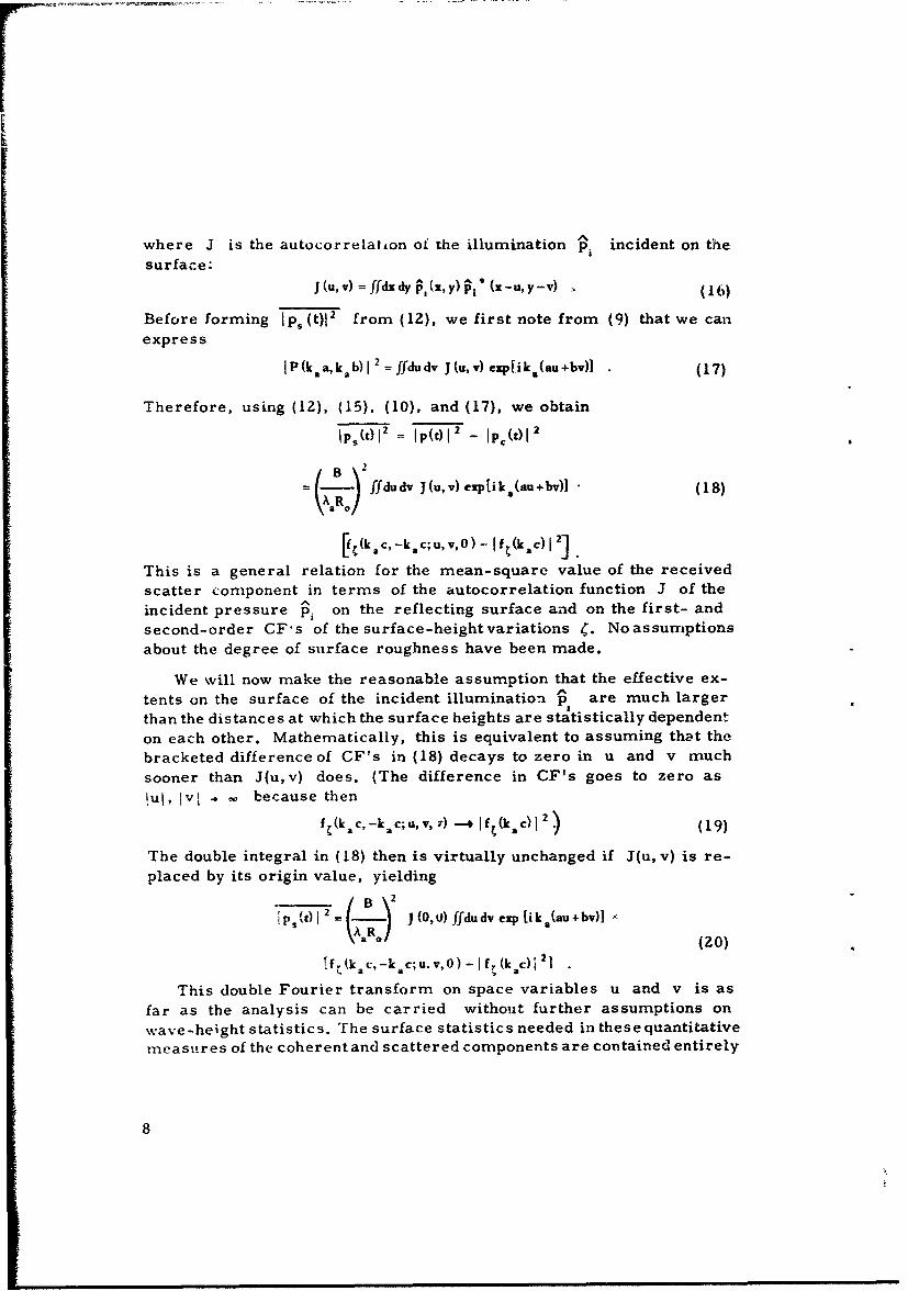
Before forming I ps (t) 2 from (12), we first note from (9) that we can

express

IP(kaa,kab)I 2 =ffdudv J(u,v) exp [ika(au+bv)] (17)

Therefore, using (12), (15), (10), and (17), we obtain

Ip (t) 2 Ip(t)1 2 _ Ip"(t)12

S ffdu dv j (u, v) exp Ii k (au + bv)] (18)

If (k. c, -k .c;u,v,0)- I f(k.0 I

This is a general relation for the mean-square value of the received

scatter component in terms of the autocorrelation function J of the

incident pressure P, on the reflecting surface and on the first- and

second-order CF's of the surface-height variations C. No assumptions

about the degree of surface roughness have been made.

We will now make the reasonable assumption that the effective ex-

tents on the surface of the incident illumination jp are much larger

than the distances at which the surface heights are statistically dependent

on each other. Mathematically, this is equivalent to assuming that the

bracketed difference of CF's in (18) decays to zero in u and v much

sooner than J(u,v) does. (The difference in CF's goes to zero as

!uj, IvI because thenf (kc, ,-k.ac;u, V, T) f- Cf (k.c0 12 (19)

The double integral in (18) then is virtually unchanged if J(u, v) is re-

placed by its origin value, yielding

(A) 2 = J (O, 0) ffdudv exp [i (au +bv)] (0(20)

[f•(kac,-kac;u.v,O) - If•(kac)j121

This double Fourier transform on space variables u and v is as

far as the analysis can be carried without further assumptions on

wave-height statistics. The surface statistics needed in these quantitative

measures of the coherent and scattered components are contained entirely

8

in the first- and second-order surface height CF's. Arbitrary surface

roughness is allowed.

As the surface roughness decreases, the difference in CF's in (18)and (19) goes to zero (because C - 0). In this case, the scattered com-ponent disappears, as indeed it must for a smooth surface.

In Appendix C, the scattering strength6 S of the surface, defined

as the ratioave~age scatter - ntensity at receiver due to unit

scatterirg art %, referred to unit distance(21)

aw era4 .cident intensity on surface

is shown to be given by

s .. W.R.. (22)

CQJ (0,0)

If we substitute (20) into (22), the above equation becomesB 2 1. f

S - ffdudvexp[ik.(au+bv)]CQ a (23)

!;[f( CN,c,-ka c;u U , 0') - If f(k C) 1 21

This is a dimensionless quantity. The dimensionless factor B 2 /CQdepends solely on the geometry of the experiment.

For a surface of very slight roughness, i.e.,

k aC max I4(x,y,t)i <«1 , (24)

we can approximate the exponential in (3) as

explikc (25)epiac C6x, y, t)1 1 + i k ac C (x1 Y, t) (5

Then, (3) becomes

I(t) W-i exp[i (2nfat - k a Ro) B [P(kaa,kab)8a 2 0 R 0(2 6)

+ ik cffdxdyp1 (x,y) exp[ik8 (ax+by)I 4(xyt)1

6The term "scattering strength" is used in this report as an intensity ratio and is not convertedto decibels.

9

i

The first term of (26) is the coherent component, and the second termof (26) is the scatter component. This equation for the coherent com-ponent is a special case of (10), where CF fC(k.c) is approximatelyunity. Thus, the general results (10) and (18) can be reduced to specialcases, including very slight roughness (or very rough surfaces), asdesired, by appropriate choice of CF's. Also (23) is a general relationfor the scattering strength, which is applicable to any degree of rough-ness and surface statistics.

3. REFLECTION FROM A NARROW-BAND, TIME-VARYINGSURFACE

In this section, we restrict consideration to the case where thesurface-height variation at each point of space is a narrow-band functionof time [10, pp. 347-348 and Section 8.5]; this is the case, for example,when the sea surface is characterized as swell [10, Section 1. 2].

3.1 NARROW-BAND COMPONENTS OF RECEIVED PRESSUREWAVEFORM

The surface height for this case of narrow-band variation can berepresented as

ý(x,y,t) =h(x,y, t)cos[2vf,ft +0(X,y, t)] (27)

where, for fixed position x, y, the amplitude h and phase 0 varyslowly with time t in comparison with cos(ZiTfst). The center fre-quency of the surface-height variation is f. If we substitute (27) into(3) for the received pressure and use the expansion [11, 8. 5114]

explikach cos(2,rfEt+0)1

1 _ i`j,(k bch) expIim(21rfft + 0)1 (28)m •-OC

the received pressure can be represented as

p (t) A W A&) exp[iZw(fa+mfs)t] (29)

where

AW exp(-ikSRO) B imJffdxdyfi(x,y)J,[k ch(x,y,t)1 (Amt)- ieA(-k Ro) (30)

exp[ik.(ax+by) ÷im0(x,y,t)

10

I

Since h and 0 vary slowly with time, so also does A.(t). However,if k ch... >> I or m >> 1, the rate of variation of Am(t) is muchfaster than that of h or 0. This may be seen by noting that Besselfunction J (x) is an oscillatory functionof x; thus, Jj[kach] can gothrough many cycles of variation while h goes through but one, ifk ch >> 1. Alsio, if m>> 1, exp(im0) varies much faster than 0.The upshot is that A,(t) of (30) will contain a considerably higherfrequency content than either h or 0 if either of the above conditionsare satisfied.

Equation (29) expresses the received pressure waveform as a sumof narrow-band components (if k ch and m are not much largerat mini.

than unity), with the mth component being centered at frequency f. + mfr.That is, the received pressure has spectral IoLes displaced from thetransmitted acoustic frequency fa by multiples of the surface centerfrequency fs . In addition, there is the coherent component at f,. Thisbehavior is depicted in Fig. 2.

i, COHERENT COMPONENT

fo-2f -f1 fa + f , +2f

Fig. 2 - Received Acoustic Spectrum

As a special case of (30), consider a travelir.g sinusoidal surfaceof fixed amplitude:

b(z,y,t)=h

O(x,y,t) =c 1 K+c2 y+c 3 (31)

c, and c2 are related to the direction of travel of the surface waveand its velocity of propagation, and c3 is thephaseat x = y = 0. Then,using (9), (30) becomes

A, (t --- i exp (-i k.R.) Bi'j,(kach) ezV(imc3) P(kaa+mc,, ka b+mc.) ,(32)

which is independent of time. This case has been investigated previously[7, Appendix].

11

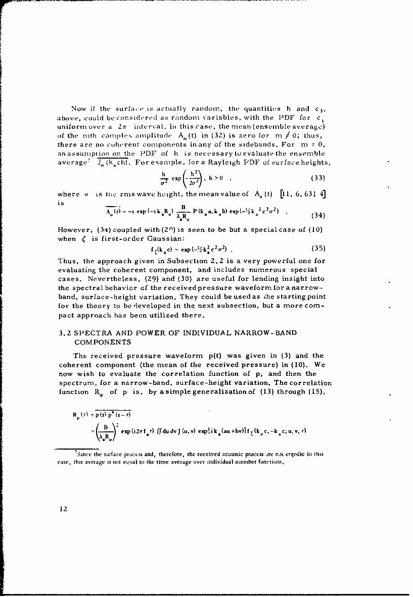
Now if the surface is actually random, the quantities h and c 3,

above, could beconsidered as r;tndom variables, with the PDF for cuniform over a 2

Tr interval. In this case, the mean (ensemble average)of the mith complex amplitude A.,(t) in (32) is zero for m / 0; thus,

there are no coherent components in any of the sidebands. For m = 0,an assumption on the PDF of h is necessary th evaluate the ensembleaverage Jm (kach). For example, for a Rayleigh PDF of surface heights,

I exp ,2 h>0 (33)

where a is the rms wave height, the mean value of A. (t) [11, 6.631 4]isB

is T~) -1 erp (-i k R.) - P(k~aa k.b) exp(-i/k, 2 C2 a,2 ) (340 0 aR a

However, (34) coupled with (21) is seen to be but a special case of (10)when C is first-order Gaussian:

f (k ac) - exp(-/ k C2 2 ) . (35)

Thus, the approach given in Subsection 2. 2 is a very powerful one forevaluating the coherent component, and includes numerous special

cases. Nevertheless, (29) and (30) are useful for lending insight into

the spectral behavior of the received pressure waveform for a narrow-band, surface -height variation. They could be used as che starting point

for the theory to be developed in the next subsection, but a more com-pact approach has been utilized there.

3.2 SPECTRA AND POWER OF INDIVIDUAL NARROW-BAND

COMPONENTS

The received pressure waveform p(t) was given in (3) and the

coherent component (the mean of the received pressure) in (10). Wenow wish to evaluate the correlation function of p, and then the

spectrum, for a narrow-band, surface-height variation. The correlationfunction RP of p is, by asimplegeneralizationof (13) through (15),

R (r) =p(t) p*(t-r)

- exp i2Iffr) 'fdudvJ'tu,v) exp[ik,(au+bv)lf (k ac,-k ac;uV, r)

7 Since the surface proct.ss and, therefore, the received acoustic process ire ntn ergodic in this

case, this average is net equal to the time average over individual member functions.

12

•'p(t) p't-r) + B 2 ezp(i2nfar) ffdudvj(u,v) expz ik.(au+bv)-

(36)[ft(kac,-k c;u,v,r)- f (kac)0 21

where we have used (10) and (17). We define the covariance function ofp as the correlation function of the ac component (i. e., scatter com-ponent) of p:

Rs(r) = Ps(t) Ps* (t- r)

= [p W) -UA [p* (Ct- r) - p* (t - r)]

exp(i21rf,r) ffdudvJ(u,v) exp[ik(au+bv)1 (

[f (kaC?,-ka c;u, v, r) - I ft(k.c)12] .

Equation (37), a general relation for the correlation function of thescatter component, reduces to the mean-square pressure of (18) for" = 0.

Again we make the assumption that the effective extents on thesurface of the incident illumination pi are much larger than the dis-tances at which the surface heights are statistically dependent on eachother, and get the approximation (See (18)through (20)) for the correlationof the scatter component:

R = exp(i2nf.f) J (0,0) ffdudvexpik(au+bv)1 (8T~a a(38)[fC(k.c,-kac;u.v,T)- IfC(kac) 121

At this point, we make an assumption about the statistics of the surfaceheights, namely, that the second-order PDF of surface heights is jointGaussian (10, pp. 343-345]. Then [IZ, Eq. (8-23)],

f -p(u,v,r)I] , (39)

where a is the rms wave height and p is the normalized spatial-temporal correlation function of surface heightsý, assumed homogeneousand stationary:

2p(uv"-)= •(x,y,t•(x-u~y-v,t-r) .1

13

i

If we substitute (39) into (38) and use (19), there follows for thecorrelation function of the scatter component

R (r) = "- exp (i2nf r) 1(0,0) exp(-B 2) ffdudvexp[ik.(au+bv)] (41)

[exptI3 2p(u,v,2)i1-1

where we have defined the surface roughness parameter £2, p. 82, Eq. (10)]

f-=k8 ca (42)

The mean-square value of the scatter component for the Gaussian surfaceis given by substituting r = 0 into (41); then only knowledge aboutp(u, v, Or, the normalized correlation between two separated surfaceheights at the same instant of time, is required.

Thus far, the surface correlation function p(uv,r) has beengeneral. The spectrum G. of the scatter component is given by theFourier transform of (41),

G,(f) =fdrexp(-i217fr) R,(r) , (43)

and generally can be numerically evaluated by a Fast Fourier Transform,(FFT). Thus, the received scatter-pressure spectrum could beevaluated from (41) and (43) for any degree of surface roughness, withno assumptions about narrow-band surface variation and narrow-bandcomponents of the received pressure. However, a double integral andan FFT is involved.

The approach taken in this report is to specialize to the case of anarrow-band, surface-height spectrum. Then, p takes the form (SeeAppendix D )

p(u, v, r) = Re Q (u, v, r) exp(i2wfsr)I

=- I (u, v, r) cos [2n1fsr+ argg(u, v, Tr)I (44)

where p(u,v,r) is the complex envelope of p(u,v,r), and variesslowly with 7 as compared to exp(i2nfsr).

Upon substitution of (44) into (41), and us ing the expansion [11, 8.511 4

and 8. 406 3]

exp(xcos.)ý- Ira (N) exp(imt6) , (45)

14

we get

200

RS(r) B.Z. eiP(i2itf r) j(0,0 exp(-/ 2 ) • ffdudv (46)

exp [ik . (au + bv)) 11 (13' 1 a(u, v, r) 1) - 80o] exp0(i2fmf.r+imarg p(u,v,r)I)

where 8S. is the Kronecker delta.

The spectrum of the scatter component is obtained by Fourier

transforming (46):

G J(0,0) 1 T.(f-f.-mf) 47(a )

where

T, (f) fdrexp(-i2yrfr) ep (-j 2) ff dudvexp[ika(au+bv).

[Im(p 2 IP(U OV ,T) I) _8. - exp (i m arg I g v, 0 1) (4 8)

Thus, the scatter spectrum is composed of spectral lobes, or sidebands,centered at frequencies equal to the acoustic frequency f. plusmultiples of the surface center frequency fS as anticipated by (29)and (30) and shown in Fig. 2. The mth order sideband is defined asthat spectral lobe centered at frequency f. + mf.. The zeroth ordersideband is centered at f., but is spread in frequency; it is distinctfrom the coherent component of the received pressure, which has a

delta function at frequency f..

For a given surface spatial-temporal correlation function p,

observation point (a, b, c), and surface roughness P, (48) can be

numerically evalaated (by a double integral and FFT) for the spectrumof the mth sideband component of the received scatter pressure. Thetotal power in the mth sideband is obtained by integrating the mth termin (47) over all frequencies, and is denoted by

IP-.(t) 12 = J(0,0) ep(-3 2) ffdudvezp[ik8 (au+bv)-a 0 (49)

[I= (021 e(u, V, 0) 1) - g.] exp(imargt.(u, v,0)I)

The scattering strength of the mth sideband is defined in a mannersimilar to (C-1Z) in Appendix C as

IsP. [ '(t) 12 R2 82 1o= e (_= j B ep(-P)ffdudvexp[ik,(au+bv)]

CQJ(oo) 7 7 (50)(,82 1 P( I, ) -)_ xp m ri

The scattering strength S. depends on the spatial-tempcral correlationfunction 9.(u,v, r) at zero time delay (r = 0).

3.3 SPECLL FORM OF SURFACE CORRELATION

Thus far, the spatial-temporal surface correlation function p(t,v, r)has beengeneral, except for the narrow-band assumption. Wenow wishto specialize to a particular form. Note first that if z is purely real,but perhaps negative,

Ira( Izl) exp(imarglzD)=I,(z) (51)

Now consider that correlation function p has the form

\L/, ,V) -) (, u

That is, for a fixed delay r , contours of iso-correlation values areelliptical! (There is no need to consider a rotated ellipse if the x, yaxes are aligned with local surface directional properties.) DistancesLX and L, are the (correlation) distances in the x and y directions,respectively, at which the correlation is down to a specified fraction(e. g., I/e) of its peak value.

Several important special cases of surface correlation can besubsumed by (5Z). For example, if the correlation distances L. andL. are equal, the surface is isotropic. However, if one of the corre-lation distance is infinite, the surface correlation function is one-dimensional; i. e., it depends ononly one of the variables u, v. Furtherspecialization of the "one -dimensional" surface-correlation functionwould be a periodic "one-dimensional" surface -correlation function,and as a particular case of the latter, a sinusoidal surface-correlation

sSee for example, Ref. 13, p. 81, where experimental results of this form have been obtained.

16

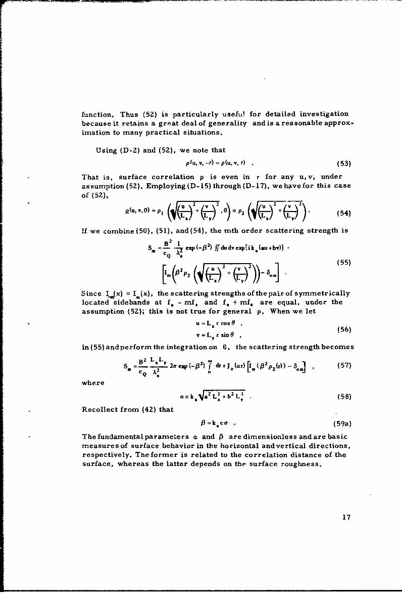
function. Thus (52) is particularly usefuL for detailed investigationbecause it retains a great deal of generality and is a reasonable approx-

imation to many practical situations.

Using (D-2) and (52), we note that

p(u, v, -r) = p(u,v, r) (53)

That is, surface correlation p is even in r for any u,v, under

assumption (52). Employing (D-15) through (D-17), we have for this case

of (52),_uv, =PI L '2+ Pv , -2 + (54)

If we combine (50), (51), and(54), the mth order scattering strength is

= B. 1 exp(_,S2) ffdudvexp[ik.(au+bv) •

Q a+ q 2)

Since I(x) = I(x), the scattering strengths of the pair of symmetricallylocated sidebands at f. - mfs and f, + mf, are equal, under theassumption (52); this is not true for general p. When we let

u=L rcosO ,(56)

v-=L, isin0

in (55) and perform the integration on 6, the scattering strength becomes

SB 2ý LILYI 2rv eV ( 2)7dr r J. (at)[J(p2p,(r))~4 (57)C 2 L LMCQ a2 o

where

am-k.4a2L2+b2 L (58)

Recollect from (42) that

fl=kca -"(59a)

The fundamentalparamet.ers a and P are dimensionless and are basicmeasures of surface behavior in the horizontal and vertical directions,respectively. Tne former is related to the correlation distance of thesurface, whereas the latter depends on the surface roughness.

17

The quantity a in (58) can take values in the range from zero to

very large values compared with unity. For example, in the specular

direction, a = b = 0 and a = 0. However, for other directions, if the

ratio of correlation distance to acoustic wavelength is much larger

than unity, a takes on large values. Of course- a can not become

arbitrarily large by letting the correlation distances increase, because

they have been assumed less than the illuminated extents. (See text

following (18).) The quantity P in (59) can take values in the rangefrom zero to values of the order of 10 without violating the conditions

stated in the paragraph following (30). Thus, for a smooth surface,

P = 0, whereas, for a rough surface, P can take onvery large values.But, in this latter case, the sideband components in Fig. 2 of the received

scatterpressure would spread out significantly infrequency and over-

lap each other. These sidebands can not be separated at the receiver

by a filter, and the scattering strength S. would lose its meaning.

It would be necessary to resort to the general case given in (41) and

(43) for the received scatter spectrum to find how much power lies in

a particular spectral band.

The scatter correlation function for the elliptical spatial correlation

case is obtained by substituting (52) into (41):

Rr(r) = 21L L i: - exp (i2nfar) J (0,0) exp(-• 2 )(59b'

f dr r Jo(ar) [exp I 2 p,(r, r)I-

However, for our purposes in this report, in order to retain physical

significance and interpretation for -scattering strength S. , we consider

a and P upper-limited to values of the order of 10.

For the specular direction, (57) becomes (See Appendix A)

S. -C Q (k L)LY)UM(le), (60)

where

The function Ur (P) in (61) depends on surface roughness P and

the form of the spatial correlation function P2 . In Section 5, plots of

UM (P) versus P for several forms of spatial correlation P 2 are

given, including exponential and Gaussian spatial correlation and

18

I

exponential and Gaussian modulation of a sinusoid or Bessel function forthe spatialcorrelation The factor preceding U, (.) in(60) is held con-stant for these plots; thus, the geometry, acoustic frequency, and corre-lation distances are considered fixed. Each plot, therefore, measuresthe dependence of the mth scattering strength S. on surface roughness

Sas the rms wave h-tight a is varied.

For directions other than specular, a / 0, and a change of variablein (57) yields

so L B2 V.(a,•) , (62)CQ(a2 X+b2.~

where

v.(a3)-(2w)-'ezp(-1 2 ) 0ds j. ()[I (," p,( - .] (63)

The function V. (a,•) in (63) depends on a, P, and theform of thespatial correlation'function P2 . If the factor preceding V6 in (62) isheld constant, the geometry and the ratio of correlation distances mustbe considered fixed. Then, the function V, measures the dependence ofscattering strength on a as the correlation distances L. and L. arevaried (although their ratio is fixed) and on P as the rms wave height ais varied. Plots of V. (a, P) versus a and P for several forms of

P2 are also presented in Section 5.

For the particular surface correlation function form assumed in(5Z), the general expression for the correlation function of the receivedscatter pressure waveform given in (41) takes a special form. It is,using (56),

R(r) B2 (kaL.) (k Ly x)ep(i2rrf.r) (270) 1 expf(- 2) 7 dr rR.2

0 (64)

jo(ar)[e•zjpf3 2 p(r,'r)1-1]

Thus, only a single integral need be evaluated in order to obtain thescatter correlation function. The scatter spectrum follows from (43).Arbitrary surface roughness is allowed. The scattering strength for thetotal scatter power is, using (C-12) and (54),

19

R,(0) R2 B2

S , L.) (koa-L ,)(2yr)-! exp(-.3 2 ) f dr rCQJ(0,0) C Q

0 (65)jo (ar)[exp lie 2 p 2 (r)' - 1]

Again, a zingle integral must be evaluated for the scattering strength,

and arbitrary sut'face roughness is allowed.

3.4 NARROW-BAND SIDEBAND SPECTRA FOR SMALL ROUGHNESS

The spxectrum of the received scatter pressure was representedas a sum of narrow-band lobes in (47) and (48) for general surfaceroughness P and narrow-band correlation p,. (SeeFig. 2.) For small3, a useful approximation to (48) can be made: first note [11, 8.445]that 2

.W -= for X <<1 (66)(x/2)'

When we employ this approximation in, (48) and use (D-7), there follows

To (f) =L"/31 exp (_f 2) fdu dv exp[ik4(au+bv) fdw.j(u, v, w)* (u,v, w-f)4

* (f) -L p 2 exp (-_32) ffdu dv exp [i k (au + bv)] g(u, v, f) (67)

2(f) 1#4 exp(-/3 2) ffdudvexptik.(au+bv)] fdwi(u,v,w)g(u,v,f-w)

The largest term is T1 (f), which is proportional to p 2 and to thedouble Fourier transform of the low-pass spectrum g of the surfacecorrelation. T, (f) is not simply proportional to g(O, 0, f), the low-pass spectrum at a point of the surface-height variation. T0 (f) is pro-portional to P4 and is related to the autocorrelation of the low-passspectrum g. T 2 (f) is proportional to p4 and related to the convolutionof the low-pass spectrum g.

For the special case when the spatial-temporal surface correlation

function is separable in space and time variables,

20

P(U'V' r) = P3(u'v) p 4 (r) , (68)

g(u,v.f) is also separable,

g(u, v. f) = P3 (u, v) - 4 (f) (69)

and the frequency-dependent terms of (67) are given by

aw-84 (w) g(w-f) , (70a)

g4 (f) , (70b)

fdw 94 (w) 94 (f-w) (70c)

respectively. Since, from (69),

g(0,O,f) =g 4=(f) • (71)

g 4 (f) is proportional to the surface-height spectrum at a point and,therefore, is real. Equation (70) states that the zeroth-order scattersideband spectrum T0 (f) is directly proportional to tb- autocorrelationof the wave-height spectrum and is even about f = 0 ',which correspondsto f = f. in the received acoustic spectrum). Also, the first-ordersideband spectrum is directly proportional to the wave-height spectrum,and the second-order sideband spectrum is proportional to the convo-lution of the wave-height spectrum and need not be even about f = 0(which corresponds to f = f + 2f, in the received acoustic spectrum).

The mth order sideband T, (f) is proportional to p2, for smallSand Imn _ 1. This sideband involves higher order convolutions of

the low-pass spectrum, thereby causing significant spreading in fre-quency. This is consistent with the observations made in the textfolluwing (30).

3.5 RMS BANDWIDTH OF SIDEBANDS FOR SMALL ROUGHNESS

It is of interest to know quantitatively the amount of frequencyspreading that each sideband undergoes. One simple measure of thisspreading, short of evaluating the actual sideband spectrum, is therms bandwidth of each sideband. We start by defining the rms band-width B of the surface-height spectrum g for the special case of(68) according to

21

B2 = fdff 2 g(0,0,f) - fdff2 _g4(f = fdff2 M4(f7 Sfdf g (0, 0, f) fdf g 4 (f) (72)

where we have used Appendix D and the fact that

p31(0,0) = P4 = 1, (73)

since p(0,0,0) = 1.

For small roughness, the spectra of the zeroth and first- and second-order sidebands are given in (70). From (70b), it follows immediately,using (72), that the rms bandwidth B, of the first-order sideband isequal to B,, the rms surface-spectrum bandwidth. The zeroth orderrms bandwidth B. is available from (70a) as

B2 =fdff2 f'dw g 4 (w) g 4 (w-f)B= =-2B 2 (74)0 fdf fdw1g4 (w) -94 (W-f) S

utilizing the fact that

fdff g4(f) W , (75)

from (D- 5), (D-6), and (69). Similarly, it may be shown, in general,that the rms bandwidth of the mth order sideband is given by

B , (76)

if P << 1. Thus, the zerothandsecond-ordersidebandsare ,/ý wider

than the surface spectrum, and the higher order bandwidths increaseas the square root of the order number. For the small roughness case,the correlation distances or direction cosines do not enter into thisrelation.

4. RELATION OF SURFACE CORRELATION FUNCTION TODIRECTIONAL WAVE SPECTRUM

The results in the previous section require specific forms for thespatial-temporal surface correlation p for their numerical evaluation.In this section, we shall use the relation between the surface correlation

22

function p and the directional wave spectrum for a wind-generatedsea composed entirely of gravity waves, and specialize to severalcases of interest.

4.1 GENERAL RELATIONS

For a homogeneous surface, the spatial-temporal surface corre-lation function p(u, v, ) can be expressed in terms of the directionalwave spectrum g2 (ý,v) [13, Part 8; 10, Chapter 8].'

2 p(u, v, r) = ffdp dv ý2 (IL, v, cos[ul+vv--g"' ( 2 +V 2),4 T1 (77)

where g is the acceleration of gravity and ai and v are the wavenumbers in rectangular coordinates. In particular, the temporal corre-lation of the surface-height variation at a point is given by

r2 , 2(o, 0, r) = fdia dv .2 (j, v) cos[g½ ( 2 j ) , (78)

An alternate representation of the directional wave spectrum in termsof the polar form A 2

ýL,v) is often used:g½ A2 (g½(2v•,tn

^2 ( 9, A) =- (ft 2 +V 2 )% tan-' (79)A (p, 0 = - 2 (IL1 2 + V 2) Y (9

If we substitute (79) into (78) and make the substitutions . = (2ir f) 2 cos 0/g,v = (2irf)2 sin9/g, the surface-height temporal correlation becomes

W ra 2 p(0,0, r)=2rf dfcos(2rifr) f dOA 2 (2r.f, 0) (80)

0 -17

The (doable-sided) surface-height spectrum (at a point) is denoted by$(f) and is the Fourier transform of (80):

i7

(fW = fdrexp(-i2m fr) a2 p(0,0, r) = a f dO A2(2irf. ,0)-7r

=(2r,)4 g92 Ifl3f d%0 2(4r2ifcosO0 , 4r 2f2 sinO (81)

The last form follows from (79).

4.2 ELLIPTICAL SURFACE CORRELATION

The results above are for general directional wave spectra. Herewe will consider a special case of particular interest. We assume firstthat the directional wave spectrum R2 possesses 1800 symmetry.'

23

2 X_ 2 ,(82)

This is done for mathematical tractability, rather than for any under-lying physical reason. Then. from (77), p(u,v, r) is even in r forall u, v:

p(u,v,-r)=o(u,v,?) (83)

When we use (D-15) thrcough (D-17) and (77), there follows

p(u, v,O) =p(u,v,O) =ffdpidv A-2 • 2 (, v) cos %tA+vv) (84)

But this 'relation can be inverted by a double Fourier transform toobtain the dircctional wave spactrum ýt2 (i±,V) in terms of a(u, v, 0):

0-2 ;2(14p)-=(2r)"2 ffdudvexp[-i(Lu+vv)]p(u,v,O) (85)

We have used the symmetry of Jt2 in obtaining (85).

For the elliptical correlation form assumed in (52), we had ini (54)

P(•, v, 0) (u)2 1+ (v2' (86)

If we substitute (86) into (85), the directional wave spectrum takes theform

(• •) 2 L0L (2r 1 -I d r P 2 (r) j. (87)

22

Thus, the directional wave spectrum is aiso elliptical if the surfacecorrelation is elliptical at zero delay. (An isztropic surface is a specialcase of (87).) EquatiL 1 (87) may be expressed compactly as

A 2 (174 =a 2 L LL(Th) 1 f drrp 2 (r) Jo(r) .7 (88)2 V 2

For any particular form of spatial correlation p2 9 (88) can be evalu.-alted numecically; then, (87) yields the directional wave spectrum.

Conversely, if the directional wave spectrum t2 is elliptical, soalso is g(u, v, 0). The exact relation is obtained by setting

24

III

(14 ((L (89)

in (84). There follows

SP(u, V, 0) =(a2L L)" 2,7 dr/r/A2 67) Jo +LFV

- \Z Y ) (90)-P2 ( H, + ' Y

or more compactly,

p2 (r) = (a2 L Ly)"1 2v 7 dr/V A2 (1() J , (r9) (91)

Equations (88) and (91) are a Hankel-transform pair of order zero[14, p. 136]. Specification of either p2 or A2 determines the other.

The surface-height spectrum O(f) for the elliptical surface corre-lation is obtained by substituting (89) into (81):

fr sin2 -42" -, (24D(j)=(2v) 4 g72 If13 - dA•(LicosO) 2 +(LY 4a

For the special case of an isotropic surface, L. = Ly -= L, (92) becomes

•(• (2v) 5 9- 2 IfI3 A 2 4v (93a)

and (91) takes the more familiar form

Uý P2 (r) f df D0OW]J, tI -fJL (93b)

Here, 20(f) is the equivalent single-sided surface-heght spectrum.

4.3 EXAMPLES

Four examples of the elliptical surface correlation function given in

(86) will be considered. The first is exponential decay of a cosinusoidalspatial variation:

25

P2 (r) - exp(-Rr) cos (Qr), r_> 0 (94)

For Q equal to zero, simple exponential decay of the spatial corre-

lation is realized. R is of the order of unity. When we substitute (94)

into (88), it follows that [11, 6. 623 2]

1 1+i Q/RA2(q) =a 2 L.L (2n)' R-2 Re (95)2 V ý[41 + iQiR) 2 + 67/R)213/2

The surface-height spectrum for the elliptical surface correlation then

r,;quires the numerical evaluation of (92). For an isotropic surface,

1, = LY = L, substitution of (95) into (93a) yields for the surface-height,,pectrum

VA0 = bra L 'Da (1)I FgR (96)

where the dimensionless parameter x is defined as

x = 2nf1r4 (97)

and the dimensionless function $ is defined asS I+iQ/R

4(X) =Ix 3 Re/(98)[1+ i Q/R) 2 + X413/2 (8

A plot of the frequency-dependent term $ is given in Fig. 3 for several

values of Q/R<. 1. As x -- 0+, the Re component of (98) approachesI -4Q/R)2

( 9[I +(Q/R)2]2

Since the surface-height spectrum can not be negative, it is necessary

(but not sufficient) that Q/R < 1 'n order for (94) to be a valid fo-m of

spatial correlation. The spectrum of (96) decays as If - 3 for large

frequencies.

Since Q was upper-limited to a value of unity in the above example,

the surface-height spectrum can not be made arbitrarily narrow. It is,

therefore, of interest to demonstrate that arbitrarily narrow spectra are

possible through a slightly modified spatial correlation, namely, ex-

ponential decay of a Bessel function.

26

- J -F

IT

-!= I.o: ---

0.5'

4- li

0.2

-4-

0.1

i I J >-

0- 1 2 4 5

X

Fig. 3 - Surface-Height Spectrum for Exponentially Modulated Cosine Spatial Correlation

27

p2 (r)=exp(-Rr)J.(Qr),r>0>.0 (100)

This function also oscillates with r, but decays slightly faster than(94) because the envelope of J. (t) decays as t-% for large t. if wesubstitute (100) into (88), there follows [15, pp. 314-316, Eqs. (11), (14),and (19)]

A 2 (7)= u2 L.Ly (20)- 1 drrexp(-Rr) Jo(Qr) J,(i6r)2 V 0or 2L L . 1 45) (101)

.2 R + -[R+ (2 2-) E(.) (101)

where F,(.) is a complete elliptic integral of the second kind withmodulus (16, Chapter 17; see especially p. 590]

Q q 7 Q(102)k= RR +R R+'(1or parameter

m =4-.2- Q +q -+ -jj . (103)R RLR /

The surface-height spectrum follows upon substitution of (101) into(92) for the elliptical surface correlation case. Since A2 ('1) of (101)is positive for all choices of Q and R [16, p. 609; m of (103) isalways less than unity], the surface-height spectrum q(f) of (92) isnonnegative; therefore, we consider the spatial correlation form in(100) for arbitrary values of Q and R.

Rather than evaluate (92) numerically, we restrict attention hereto the isotropic surface and use (93a) to obtain the surface-heightspectrum:

4)(f = 2o2 I L(x) , (104)V;R

where

x a- 2fff L (105)

and

2 [ -) E(-) (106)

28

The parameter m of the complete elliptic integral is given by

m =4 2.-x2 +(2+,)] (107)

The frequency-dependent function $(x) is plotted versus x in Fig. 4for several values of Q/R. The spectrum decays as If 1-3 for largefrequencies. The narrow-band character of the surface-height spectrumfor large Q/R is evident.

The third example of spatial surface correlation is Gaussian decayof a cosine 9 :

p2 (r)=exp(-R 2 r2)cos(Qr),r>O (108)

Substituting (108) into (88), we obtain

L (2Y Rfdtx(2)Os ( 2R-t) J(R"t (109)

The surface-height spectrum for an isotropic surface follows uponsubstituting (109) into (93a):

Cif)=21r2 (X) (110);gLR

where

x=2f L (111)

and

O(X)=iX13 dttexp(-.r 2) COS(112)~t

This function is plotted in Fig. 5 for several values of Q/R. (The methodfor evaluating (112) is given in Appendix E. For Q/R> 1.848, $(x)goes negative at the origin, thereby invalidating (108) in that range.)

The fourth example of surface correlation to be considered isGaussian decay of a Bessel function:

P2 (r)=exp(-R 2 r2)J '(Qr),r>0 (113)

Q equal to zero corresponds to Gaussian spatial decay of the correlation.When we substitute (113) into (88), there follows [11, 6.633 2]

9 This is a form treated by Lysanov (Ref. 17) ane suggested by Schulkin (Ref. 18, p. 42).

29

1.0 i VFF ,

-i' -F--- - - - {-I0.8...- - - -T

! 1 - 2

0, t

__$.-_-.-

0 1 2 3_4_

i > i ' L II !I

0.4- -i--------_I L.

X

Fig. 4 - Surface-Hlcight Spectrum for Exponentially Modulated Bessel Function Spatial Correlation

30

- .- ----- ---- - - • - - -- - ' -. - - - -

IT

-I fS' ---'-- ' ~-- --v- - ,i

a< -V_ , . I" - - --

0.1/'t 1i 4j' 'V1I I '

0.32 1 j # 4 i t I

*R

0 i -- y I I i I°"1 i,, !!

0 1 2 2.75I x

Fig. b - Surface-Height Spectrum Gaussianly Modulatpd Cosine Spatial Correlation

31

21 Q2+q I /Qq\(14Y(4R 2 / \RZ/(14

The surface-height spectrum follows upon substituting (114) into (92)for the elliptical surface correlation case. Since A2(,) of (114) ispositive for all choices of Q and R, the surface-height spectrum4b(f) of (92) is nonnegativeC therefore, we consider the spatial correlationform in (113) for all Q and R.

The exponential and Bessel function in (114) can be expressed as

(_ZR ))R R

Since the fu •ction exp(-t) I. (t) is weakly dependent on t, it is seen thatA2 (1) possesses a peak approximately at q = Q of width proportionalto R. The integralof(92) for 4t(f) tends to smooth this peak. However,the isotropic surface-height spectrum of (93) does not involve thissmoothing and is a peaked spectrum; a measure of the peakedness isthe "quality" ratio of center frequency to bandwidth, and is related tothe ratio Q/R for this example.

The surface-height spectrum for an isotropic surface is obtainedby substituting (114) into (93a), and is given by

4(f) = 2 2 b , (116)ýgR

where

x =- 2 rf (117)

and

$(z)= I z13 exp 4 • (118)

The frequency-dependent term $ is plotted versus the dimensionlessparameter x in Fig. 6 for several values of Q/R. The spectrumdecays as exp(ocf 4 ) for large frequencies.

The narrow-band character of the surface-height spectrum isevident from Figs. 4 and 6 when the ratio Q/R is large compared tounity.

32

I.O

10r P F - -'. I -1]

1- I

0.6-----

r"- ," ----

0.4

0 1 2 3

Fig. 6 - Surface-Height Spectrum for Gaussianly Modulated Bessel Function Spatial Correlation

33

5 SCATTERING STRENGTHS OF SIDEBAND COMPONENTS

i'or the case of a narrow-band surface-height spectrum, the scat-tered acoustic spectrum at a receiving point may be obtained from (47)and (48). The general form of the received acoustic spectrum was shownin Fig. 2 to consist of a series of spectral lobes or sidebands, eachseparated from the incident acoustic frequency fa by multiples of thecenter frequency f of the surface variation, plus an impulse at theS

acoustic frequency f.. This impulse is the coherent component.

The total acoustic power in each spectral lobe, or equivalently thescattering strength, may be obtained from (60) and (61) for t.he sp, :ulardirection, and from (62) and (63) for the nonspecular di-ection. In

this section, we will evaluate Um(P) and V (a, P), as given by (61)and (63), respectively. As mentioned in Subsection 3.4, if the factorpreceding U... (P) is held constant, the geometry, acoustic frequency,and correlation distances are considered fixed. The plot of U. (P),therefore, measures the dependence of the mth scattering strengthon the surface rms wave height a through the roughness parameter3. V, (a, P) measures the der.-ndence of the mth scattering strength

on the correlation distances L and L (although their ratio is fixed)through a, andon therms wave height a through P. (Integrals (61)and (63) we,-e numerically evaluated by Simpson's Rule; the erroranalysis is contained in Appendix F.)

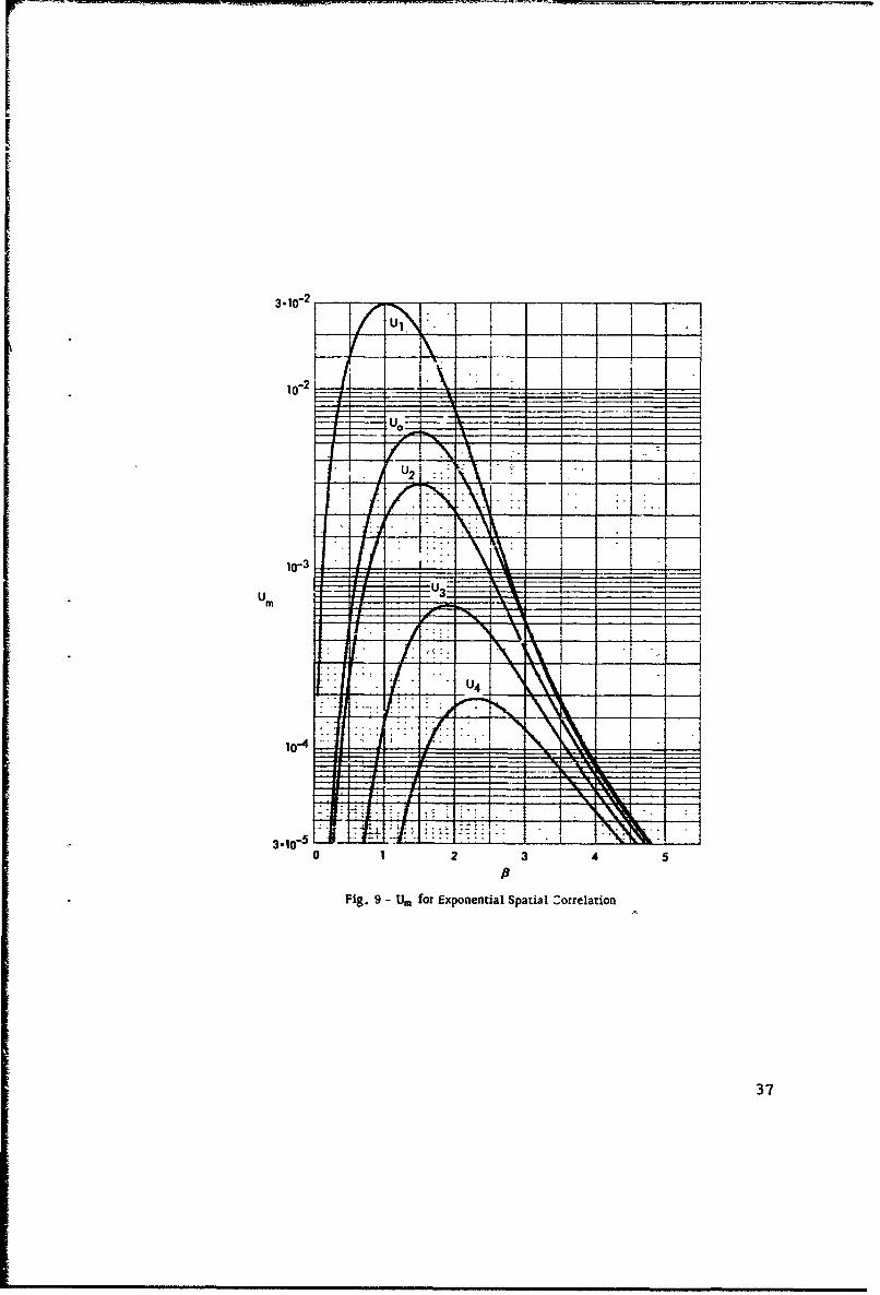
In Figs. 7through9, U. (P) isplottedversus P for m = 0,1,2,3,4for an exponentially modulated Bessel function spatial correlation,

p2(r) = exp(-r) Jo(Qr) , (119)

for values of Q = 8, 4, 0. In Figs. 10 through 12, a similar set of curvesis plotted, the only difference being that the spatial correlation is aGaussianly modulated Bessel function.

p 2(r) = exp(-r 2) j0 (Qr) (120)

To better explain these figures, let us concentrate temporarily onFig. 12; here Q = 0, meaning the spatial correlation is Gaussian.U1 (P) corresponds to the scattering strength in the first sideband(eithe:- above or below the acoustic frequency f.). Since a = 0, weare considering only the specular direction. P = 0 corresponds to aflat surface; for this value of 3, there is no scattered power in the

34

r-0-'NkU

I_ 10-

51O~ - - - -

33

U2

--------U3

1 -5~

Fig. 8-U. for Exponentially Modulated Bessel Function Spatial Correlation, Q 4

36

3.1o-[f 2.

/1. , - u= - -

U2

"" ."--"-' "-

Um -- -.. - " __ ,- 1

-zi

,or4 __!_, \u 3=- , _

umm

0 1 2 3 4 5

0

Fig. 9 - Um for Exponential Spatial Correlation

37

1-3.

10-4I

383

2 1U-3.. - --- - .- " : t. --

Ul-

-7-71I ." .1.

10-5 -.

2- -. . - I -t

1 - . -, -.. -, 9

- .. -

0 1 2 3 4 5

0

Fig. 11 - Um for Gaussianly Modulated Bessel Function Spatial Correlation, Q = 4

39

Urn2

10-3T .

o 1 2I3A

400

sidebands since all the reflected power appears in the coherent com-ponent. As P increases, there is iess power in the coherent component,and more scattered power appears in the sidebands. The power in thefirst sideband reaches a maximum value when the surface roughnessparameter P is approximately unity, and decreases thereafter. Forthese larger values of P, the surface is rougher, and more of thescattered power will appear in higher-order sidebands in directionsother than specular. We have plotted the zeroth through fourth-ordersideband scattering strength factors U. (P) ii Figs. 7 through 12. Allthe curves initially increase as A increases from zero, retach amaximum, and then decrease. For large P, there is little diffe-encein power between the various sidebands.

For Q = 4, or 8, the gross features of the sideband powers aresimilar to those for Q = 0, whether the modulation is exponential orGaussian. However, whereas for Q = 0, U1 (P) is larger than U.(0)for a large range of P, the reverse is true for Q = 4 and 8. For largerQ, the zeroth and second-order sidebands contain most of the scatteredpower in the specular direction. As Q increases, the power in eachsideband, for. a given roughness P, decreases. The reason for thisis that the total scattered power in the specular direction decreaseswith increasing Q, since the correlation distance decreases. (Thislatter effect is due to the factor J. (Qr) in (119) aud (120), which decayswith r in addition to the exponential terms.)

For small P, the power in the first sideband is proportional to

12 , and the powers in the zeroth and second-order sidebands behaveas 14 (See (67)). This is not apparent in Fig. 10 for the Gaussianmodulated case for Q = 8, because the effect occurs at smallervalues than plotted.

The major difference between the exponentially modulated andGaussianly modulated curves occurs at larger values of P. Here thesideband powers are much larger for the Gaussian case than for the

exponential case. This is true for all Q and all orders of sidebandsplotted.

In Figs. 13 through 27, three-dimensional plots of V3 (a, 13) versusa and P are given for m = 0, 1,2, 3,4 and for an exponentiallymodulated Bessel function spatial correlation (See (119)) for values of

41

Fig. 13 - Vo for Exponentially Modulated Bessel Function Spatial Correlation, Q = 8

(vo = .268 . lO- at a = 15 1/3, j = 1.6)

42

(t

Fig. 14 - V for Exponentially Modulated Bessel Function Spatial Correlation, 0 = 8

(V 1 =.763" -0-lat a=8, )3=1.O)

43

IC

Fig. 15 V2 for Exponentially Modulattd Bessel Function Spatial Correlation, Q =8

44

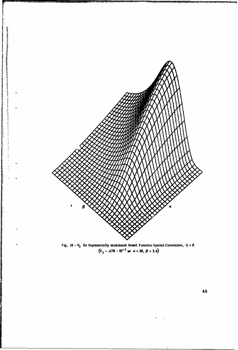
Fig. 1.6 - V3 for Exponentially Modulated Bessel Function Spatial Correlation, Q=8

(V3 =.678.lO0- 2 at a = 20, S= 2.4)

I4

I

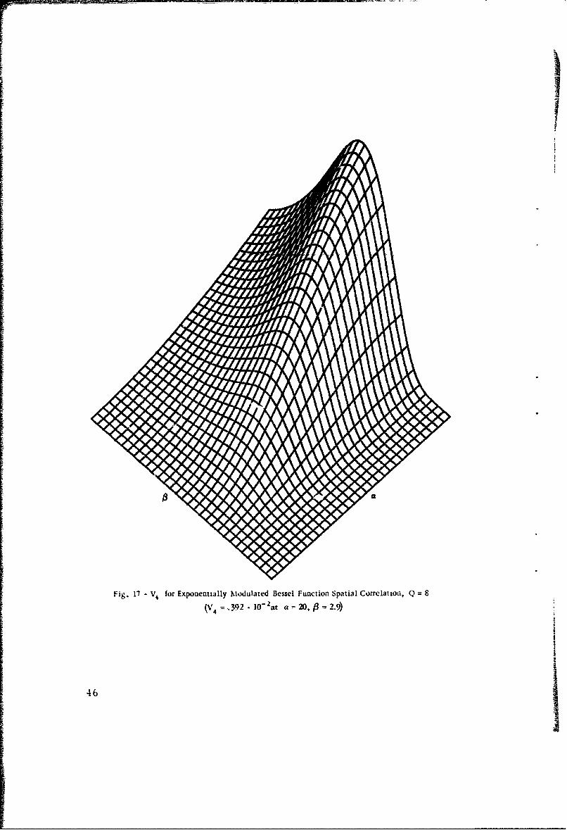
Fig. 17- V for Exponentially Modulated Bessel Function Spatial Correlation, Q 8

(V4 = 392 • l10 2at a -20, 6 2.9)

46

•'•Fig. 18 - V0 for Exponentially Modulated Bessel Function Spatial Correlation, 0 =4r . 10v1 --. t •o•= 72/3, 1.6)

Ii

if

P1 4Iii

ii

I

Fig. 19 - V for Exponentially Modulated Bessel Function Spatial Correlation, 0 = 4

(VI =.395 • 1o01 at a - 4 i3, 1.o)

48

I

Fig. 20 - V2 for Exponentially Modulated Bessel Function Spatial Correlation, Q 4

(v 2 1.06.10-1 a t a-, -8 1.4)

49

Fig. 21 - V3 for Exponentially Mcdulatcd 8essel Function Spatial Comrelaticnh, (1 4

(V, =.601. _o-•2 . • a=17, 2.9)

50

4-1

Fig. 22 - V4 for Exponentially M.-dulattd Bessel Fouction bpatial Corrclati, 1 CQ 4

(v4 -. 425. l0-2 at a - 20, 13 -- 3.4)

51

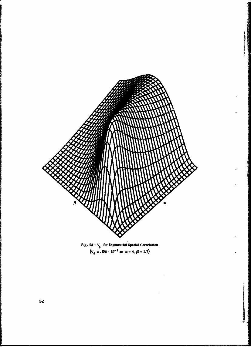
Fig. 23 - V for Exponential Spatial Correlation0

52

Fig. 24 - V for Expoomiol Spatial Correlation

(V .120o- 10-1 at a 12/3, f 1.1)

53

Fig. 25 - V2 for Exponential Spatial Correlation

(V2 = .643- 10-2 at a = 6 2/3, 1 = 2.2)

54

Fig. 26 - V3 for E:xponential Spatial Correlation

(v3 = .460. o-z 10- 2 t = 14 j/3, J3 = 3.2,)

55

Fig. 27 - V4 fr~ Exponential Spatial Cotnelation4

(V4 .352 -1-2 at a . 2, 133.9)

156

OEM

Q = 8,4,0. In Figs. 28 through 42, a similar set of curves is plotted;the only difference iq that the spatial correlation is a Gaussianlymodulated Bessel function of the form of (120). These functions were

computed for a = 0(1/3)20 and • = 0(. 1)6. The maximum.valuesattained by V, (a, P) at this grid structure are presented in Table Iand are noted on each plot. (These values are not necessarily themaximum values of V (a, P), but simply the maximum values at thesample points investigated.) Since the plots are isometric, values ofV. (a, P) at other values of a, can be obtained by measuring thevertical distance above the a, 3 plane and scaling according to thevalues given.

To explain the detailed behavior of these plots, it is helpful toconsider P as a measure of the surface vertical roughness, and aas a measure of the surface horizontal roughness. As P increases,the surface becomes rougher in the vertical direction; also as adecreases, i.e., the correlation distances decrease, the surfacebecomes rougher in the horizontal direction. For a given a, thebehavior of V* (a,•) with • is similar to that observed in Figs. 7through 12.

For • = 0, VE (a,[) is zero for all a since the surface is flatand there is no scattered power. As P increases, the scattered powerincreases, reaching a maximum. As P increases still further, thecurve decreases, indicating that more of the scattered power appearsin higher order sidebands. Note from the plots that for a given sur-face spatial correlation and a given Q, the location (a, P), at whichV3 (a, P) reaches a maximum value, increases as m increases; i.e..the peak location recedes from the origin.

For a given P (fixed roughness) and a large a (large correlationdistances), the surface is very planar, resulting in most of the re-flected power appearing in the specular direction. As a decreasesfrom large values, the surface becomes less planar, more power isscattered in the nonspecular direction, and V. increases. However,as a decreases still further, the surface becomes rougher in thehorizontal direction, and more of the scattered power appears in thehigher order sidebands, so that each particular V* (a, P) decreaseswith a in this range. The ratio P/a is a measure of the averageslope of the surface; as this ratio increases, more of the scattered

57

ITable I

APPROXIMATE LOCATIONS OF MAXIMUMVALUES OF V. (a*,3)

Fig. v.No.

13 151'3 1.6 .268" 10"14 8 1.0 .763" 10-115 151/3 1.6 .144 • 10-'16 20 2.4 .678" 10-2

17 20 2.9 .392 - 10-2

18 7 2',3 1.6 .196 - 10-119 4 '3 1.0 .395 • 10-120 8 1.7 .106. 10-121 17 2.9 .601• 10-2

22 20 3.4 .425 - 10-2

23 4 1.7 .106 - 10-124 123 1.1 .120 - 10-_! 6223 2.2 .643. 10-2

26 141 3 3.2 .460 - 10-2

27 20 3.9 .352 - 10-2

28 15 1.6 .325- 10-129 8 1/3 1.0 .705 - 10-1

30 151/3 1.7 .177. 10-1

31 20 2.7 .890- 10-2

32 20 3.1 .570- 10-233 72/3 1.6 .249- 10-'34 42/3 1.1 .398- 10-'

35 8 1.8 .141 - 10'-

36 13 '3 3.1 .903 - 10"2

37 18 4.1 .690 - 10-2

38 3 1.7 .210- 10"'39 2 1.1 .237" 10-'40 4 2.2 .125. 10-'41 61/3 3.3 .886. 10-2

42 8 4.1 .683- 10-2

58

Fig. 28 - Vo for Gaussianly Modulated Jesel Function Spatial Correlation, Q 8

(V0 =.325- 10- at aa 15,3 1.6)

59

I

F+

F+

I!L

Fig. 29 - VI for Gaussi-anly M•odutlated Bemsl Functio Spatial Correlation, Q -8

(vI .705 - 10-1, at a • 8 --n, .o

60

F1

I1

IIFi

Ih

r=

Fig; 30 - V, fow Gausianly Modulated Besel F unction Spatial Correlaloa, Q 8

(v 2 .177 lo a a =15•1/3, - 1.7)

61

aI

Fig. 31 - V5 for Gaussianly Modulated Bessel Function Spatial Correlation, 0 = 8

(v .8901.-2 ta 2=O, -2.7)

6Z

FO

Fig. 32 - V4 for Gaussianly Modulatw-d Belel iFunction Spatial Correlation, 0 = 8

(V4 .. 570. 10o2 at a= 2, P =3.1)

63

I2

Ia

Fig. 3"1 - %0 fo Gaussianly Modalated Dessel Function Spatial Correlation, 0 .4

(Vo -. 249. lo"- 0 t a 7 23, .

1 ~64j

Fig. 34 - VI for Gaussianly Modulated Bessel Function Spatial Correlation, Q 4

(VI .398 -10-1at a 4 2/3,I3ll

65

Fig. 35 - V2 fo Gat~mianly Modulated Reuel Functloa Spatial Correlartion, Q :4

(2( =.141 o-' ,,- ata 8, P -•8)

66 •

Jil FýIjl III

IFig. 36 -V 3 for Gaussianly i.odulated IBe~l Function Spatial Correlation, 0 =4.

(V 3= .97. 1- 2 at a= 111/3, 3 3. 1)

1 67

Fig. 3? -V4 for Gaunianly M•odulated Bessel Fistctiout Spatial Correlation, Q 4

(v4 = .69o. -o 1- &t a - 18-, =4-1)

68

!

[

Fig. 38 - V0 for Gaussian Spatial Correlation

(V0 .210O.10- 1 at a=3, 1i.7)

69

I ______________________________

1 3

Fig. 39 - V1 for Gaussian Spatial Correlation

(VI=.237.10-1 at a=2, =1.1)

70

Fig. 40 - V2 f Gaimian Spatial Correlation

Nv-•• 10-1 at a,- 4, jS -2. )

71

Fig. 41 - V for Gaussian Spatial Correlation3(v3 =.886. 1"2 t c- 6 3, --3.3)

72

Fig. 42 - V4 for Gaussian Spatial Correlation

(V 4 = .683. -1 2 z at a - 8, z = 4.1)

73

I

power appears in the higher order sidebands. This behavior can occurthrough eiLher increased A (roughness)or decreased a (correlationdistances).

As a approaches zero, for the nonspecular direction, the corre-lation distances approach zero. For this case, the surface becomesvery rough and, in the limit of zero-correlation distances, has theproperties of white noise. Although mathematically, for a = 0, theamount of scattered energy in the sidebands is zero, the initial as-sumptions (See Section 1) are violated for small correlation distances;therefore, this portion of the plots does not have physical significance.

Curves of V (a, P) for p2 (r) = exp(-r) cos(Qr), Q = 1, were alsoobtained, but have not been included because they are very similar tothe corresponding curves for p2 (r) = exp(-r) J (Qr); in particular, theomitted curves are more peaked than exp(-r), but not as peaked asexp(-r) Jo (4r). Similarly, curves of V. (a, P) for p2 (r) = exp(-r 2 ).cos(Qr), Q = 1. 8482777,'0 were also obtained and exhibited behaviorintermediate to that of exp(-r 2 ) and exp(-r ) J. (4r).

Let us now compare the exponentially modulated Bessel functionplots with those of the Gaussian modulated Bessel function plots. Forlarge A, the Gaussian case has more power in a given sideband thanthat of the corresponding exponential case. This behavior is similarto that of the U curves in Figs. 7 through 12. For 0 = 0, the corre-sponding exponential and Gaussian plots are somewhat dissimilar.However, for Q = 4, the corresponding curves of the exponential caseare more nearly similar to those of the Gaussian case, whereas forQ = 8, the two sets of curves are almost identical. Thus, for small Q,the envelope of the spatial correlation of the heights is the controllingfactor, butas Q increases, the number of oscillations per given distanceof J* (Qr) increases, and J. (Or) becomes the controlling factor inspatial correlation.

6. DISCUSSION

In summary, an analysis was made of a time-varying randomsurface statistically stationary in both space and time. The reflected

10These choices of 0 are the largest possible consistent with a nonnegative surface-height spectrum;see Subsection 4.3.

74

i • acoustic spectrum was obtained in terms of the first- and second-order

characteristic functions of the surface-height variation. For the specialcase of a Gaussian distribution of surface heights, a narrow-bandsurface spectrum, and a surface spatial-temporal correlation functionthat is stationary in the wide sense, the mathematical equation for thereceived acoustic spectrum showed that the scatter spectrum is com-posed of spectral lobes, or sidebands, centered at frequencies equalto the acoustic frequency plus multiples of the surface-center frequency(See (47) and (48)). For the special case of a surface spatial correla-tion that has elliptical contours, the evaluation of the complete spectrumcan be ekpressed as a Fourier transform of a single integral. The com-plete spectrum was not numerically evaluated in this report, but shouldbe obtained in future work. In addition, the restriction to a symmetricdirectional wave spectrum, (82), should be eliminated. For example,received spectra for hemispherical directional wave spectra should becomputed; this will yield unequal scattered sideband powers.

The power in each sideband was evaluated for a variety of conditionsand spatial correlations. It was found that the zeroth and second-ordersideband powers had a very similar behavior with surface roughness,whereas the other sidebands had a somewhat different dependence. Ithas been assumed that there is not an appreciable overlap of the side-bands; for large surface roughness, there would be an appreciableoverlap of sidelobes, and the complete spectrum would have to beobtained for this case.

It is worthwhile to discuss the difference between the surfacetreated in this report and the fixed-amplitude sinusoidal surface con-sidered by Roderick and Cron [7]. We have considered a narrow-bandspectrum for the height variation at apointon the surface, and assumedthe Joint probability density of the surface heights to be Gaussian. Asthe bandwidth of the surface variation decreases and approaches zero,the properties of this surface process do not approach the fixed-am-plitude sinusoidal surface case. For example., the distribution ofheights remains Gaussian and is, therefore, different from the prob-ability density associated with a sinusoid. The scattered powers inthe sidebands, as given by the narrow-band Gaussian theory, aredifferent from those of the single-frequency sinusoidal theory.

75

In mathematical terms, the first-order-characteristic function of afixed-amplitude sinusoid is a Bessel function. If we average this Besselfunction with the Rayleigh distribution of sine wave amplitudes, weobtain the Gaussian first-order-characteristic function. Thus, our re-suits can be viewed as a particular average over the sinusoidal surfacecase.

However, a narrow-band time function with center frequency f,and bandwidth W resembles a sine waveof frequency f, over a shortperiod of time, but will differ from a sine wave over a longe- periodof time. The difference will show up on the order of W-1 sec. Thus,if we obtain a short sample of the reflected signal from a narrow-bandsurface, and determine the received acoustic spectrum from it, thesingle-frequency theory (with the current surface-height amplitude)should accurately predict that spectrum. However, for a long-timeaverage over the statistical properties of the surface, the narrow-bandGauss ian theory, not the fixed -amplitude single-frequency theory, mustbe used to predict the expected behavior of the spectrum.

This report has concentrated on the spectral quantities of the re-flected signal. However, the probability distributions of the envelopeof the individual sidebands can also be obtained in at least one importantcase. If the area of insonification is much larger than the correlationarea of the surface (product of correlation distances), we can appealto the Central Limit Theorem and state that the envelope and phase dis-tributions of the mth component of the received scatter pressure fieldare Rayleigh and uniform, respectively, for m / 0. For m = 0, thescatter component combined with the coherent component results in aBeckmann distribution (2, Chapter 7]. (Of course, as the coherentcomponent tends to zero, the Beckmann distribution tendb to the Rayleighdistribution.) It should be noted that the assumption of Gaussian surfacestatistics, i.e., 4(x, y, t) Gaussian, does not necessarily imply thatthe received pressure is Gaussian, because the received pressure isobtained via a nonlinear transformation on 4 (See (3)); rather, it isthe assumption of a large number of independently reflecting surfaceportions that yields the Gaussian behavior.

76

I-I

LIST OF REFERENCES

1. C. Eckart, "The Scattering of Sound from the Sea Surface, Journalof the Acoustical Society of America, vol. 25, no. 3, May 1953,pp. 566-570.

2. P. Beckmann and A. Spizzichino, The Scattering of ElectromagneticWaves from RoughSurfaces, The MacMillan Co., New York, 1963.

3. E. 0. LaCasce and P. Tamarkin, "Underwater Sound Reflectionfrom a Corrugated Surface, "Journal of Applied Physics, vol. 27,1956, pp. 138-148.

4. C. W. Hortonand T. G. Muir, "TheoreticalStudies of the Scatteringof Acoustic Waves from a Rough Surface, " Journal of the AcousticalSociety of America, vol. 41, no. 3, March 1967, pp. 627-634.

5. R. J. Wagner, "Shadowing of Randomly Rough Surfaces, "Journalof the Acoustical Society of America, vol. 41, no. 1, January 1967,pp. 138-147.

6. H. W. Marsh, "Exact Solution of Wave Scattering by IrregularSurfaces, "Journal of the Acoustical Society of America, vol. 33,no. 3, March 1961, pp. 330-333.

7. W. I. Roderick and B. F. Cron, "Frequency Spectra of Forward-Scattered Sound from the OceanSurface, " NUSLO ReportNo. 1010,I July 1969. (Accepted for publication in the September 1970 issueof the Journal of the Acoustical Society of America.)

8. B. E. Parkins, "Scattering from the Tim-!-Varying Surface of theOcean, "Journal of the Acoustical Society of America, vol. 42,no. 6, December 1967, pp. 1262-1267.

9. I. Tolstoyand C. S. Clay, Ocean Acoustics, McGraw-Hill BookCo.,New York, 1966.

10. B. Kinsman, Wind Waves, Prentice-Hall, Inc., New York, 1965.

11. I. S. Gradshteyn and I. W. Ryzhik, Table of Integrals, Series, andProducts, Academic Press, New York, 1965.

*Reports prepared by the New London Laboratory prior to 1 July 1970 bear the Laboratory'searlier acronym NUSL.

77

r

12. W. B. Davenport and W. L. Root, An Introduction to the Theoryof Random Signals and Noise, McGraw-Hill Book Co., New York,1958.

13. W.eJ. Pierson, Jr. (editor), Meteorological Papers, vol. 2, no. 6,New York University, 1960.

14. W. Magnus and F. Oberhettinger, Functions of MathematicalPhysics, Chelsea Publishing Co., New York, 1954.

15. Y. L. Luke, Integrals of Bessel Functions, McGraw-Hill Book Co.,New York, 1962.

16. Handbook of Mathematical Functions, U. S. Department of Com-merce, National Bureau of Standards, Applied MathematicsSeries 55, June 1964.

17. Y. P. Lysanov, I"Average Decay Law in a Surface Sound Channelwith an Uneven Boundary, " Soviet Physics - Acoustics, vol. 12,1967, pp. 425-427.

18. M. Schulkin, The Propagation of Sound in Imperfect Ocean SurfaceDucts, NUSL Report No. 1013, 22 April 1969.

19. R. J. Urick, Principles of Underwater Sound for Engineers,McGraw-Hill Book Co., New York, 1967.

20. A. Papoulis, The Fourier Integral and Its Applications, McGraw-Hill Book Co., New York, 1962.

78

Appendix A

GEOMETRY FACTOR

The factor B in (3) is given different values by different authors.For example, the values for B given by Parkins Al and Beckmann and

SpizzichinoA 2 using the notation in this report, are

I+ui 5"A Ii + a + bb + CcB . A.A. (A-Q Qc cQ +Ca

CQ A

whereas EckartA3 gives the following value for B:

c CQ + cB= =Q (A-2)2 2

Beckmann and SpizzichinoA4 attribute the discrepancy to the replace-

ment of the normal to the surface by a vector in the z-direction, anapproximation that is valid only for surfaces with very gentle slopes.

For the specular direction,

aA =-aQbA=-bQCA=CQ 9 (A-3)

both forms for B above become c.. Thus, there is no difference inthe specular direction. However, there can be significant differences

for other cases. For example, the second form for B depends only onthe direction cosines with respect to the z-axis, but the first form

depends on all direction cosines. Thus, at normal incidence.

aQ -- Q = 0, CQ = , (A-4)

B. E. Parkins, "Scattering from the Tine-Varying Surface of the Ocean," Journal of theAcousical Society of America, vol. 42, no. 6, December 1967, Eq. (10), p. 1263.

A2P. Beckmann and A. Spizzichino, The Scattering of Electromagnetic Waves from RoughSurfaces, The Macmillan Co., New York, 1963, Eqs. (11) and (12), p. 27, and Eqs. (29) and (32),pp. 22-23.

AC. Eckart, "The Scattering of Sound from the Sea Surface," Journal of the AcousticalSociety of Amerca vol. 25, no. 3, May 1953, Eq. (6), p. 567.

A4Beckmann and Splzzichino, Appendix A, op. cit.

79

IA

and the two forms for B become

l'and %(l+€A c (A- 5)

respectively. For an observation point near grazing, these terms differby a factor of 2 in pressure.

Rather than attempt to resolve the differences in the scale factor,we have expressed all our quantities in terms of the general symbol Band leave it to the reader to make his choice as to the correct factor.For a fixed geometry, so far as the relative spectral content of thereceived acoustic waveform is concerned, the exact geometric factoris not important under the assumptions of the present theory.

i

Appendix B

CORRELATION PR)PERTIES OF SINGLE-SIDED PROCESS

Suppose x(t) is a wide-sense stationary single-sided8 l (complex)process with no dc component. Let

(B- 1)

where

+ • (t) I Y [x (t) +," (t0]S~(B-2)

Denoting the Hilbert transform by • I, we haveU l * , t W I % i, X[ 1 Z Wx I + 9~ i (1]*W 1 3

(B-3)

where the single-sided character of x(t) and its lack of dc has beenutilized. The Hilbert transform is represented by a linear networkwithtransfer function -i sgn(f). Therefore, the transformation between

. x,(t) and x, (t) can be represented as in Fig. B-I.

I M

Fig. B-I - Hilbert Transform

Thus, we have derived the fact that the imaginary part of a wide-sensestationary single-sided process is the Hilbert transform of the realpart.3 2 When the properties of linear networks are used, it followsfrom Fig. B-I thatI $Single-sided means that the power density spectrum is confined to positive frequencies.

B2 This Is the conves•e of the usual situation where a waveform plus i times its Hilbert transformIs shown to be single-sided.

81

x (t) x(t-r) S (W) x(t-r)

x it ,,(t- ) =-xi(t) It r)(B-4)

Combining these properties, we find that

Wt) x(t-r) =0 for all r (B-5)

Of course, x(t) x (t-r) / 0.

82

Appendix C

SCATTERING COEFFICIENT AND SCATTERING STRENGTH

The received(complex)pressure p(t) at the observation point wasgiven in (3). The scatter component p,(t) was defined in (11), and themean-square value of p,(t) was evaluated in (18) and (Z0). In thisappendix, we will relate the scattering coefficient and scattering strengthto these quantities.

The average scatter intensity (power/unit area) at the receiver fora real sinusoidal signal transmittal is

Ip '(t)12/2,(C-l)

pv

where p is the densityof the fluidand v is the propagation velocity.cIIf the receiver at A subtends a solid angle 0, as seen from origin 0in Fig. 1, the average received scatter power is

Io2 a , (C-Z)

and the average received scatter power per steradian is0 . IIpv t) R . (C-3)

Since the incident pressure on the surface at xy is Pi (x, y)(See (3)), the incident intensity at x, y is

27 -I^p (I. y) 12 (C-4)

Therefore, the total incident power on the surface is

* c~ff dldy.......IP(K 12-= CQ J(o,o) (C-5)

using (16).

The scattering coefficient or scattering cross section a. is defined

by Eckartc 2 as

C' The factor of 1/2 follows in a manner similar to that in (5) and (6).

C2C. Eckart, "The Scattering of Sound from the Sea Surface, " Journal of the AcousticalSociety of Am-rice, vojl. 25, no. 3, May 1953, Eq. (18), p. 568, and Eq. (10), p. 567.

83

1p.(W1I R.'s j (0, 0)( - )

which can be manipulated into the forms

jp.t)I -R, I Ro2

Sffdxdy IfU(x,y) i2 ffdxdy _- I (x, y) I2

average received scatter power per steradian (C-7)

incident power on surface / CQ

where we have used (16), (C-3), and (C-5).

For purposes of this report, the "scattering strength" S is definedasC3

S.ica (C-8)"mic

where I is the average scatter intensity at the receiver due to unitscatteringarea, referred tounit distance, and I is the average inci-dent intensity on the surface. If we let Aeft be the effective area ofinsonification in the x, y plane (e. g.,

A.eff .ffo~• "z dy1jY c-9)scattering area (C40

then

I-ct- LR2 p.(t)l R°' (C-10)

Aeff 2y Aeff

using (C-l). Also,incident power on the surface

Inc A eff

CQ J (0,0) (C-A11)• -•V Aeft

using (C-5). Taking the ratio of (C-10) and (C-ll), we note that the

scattering strength becomes

s ... !,W (C-12)cQ J (o, 0) cQ

C3 R. 3. Urick, Principles of Underwater Sound for Engineers, McGraw-Hill Book Co., New York,1967, p. 118, Section 8.2. Actually, Urick has a decibel ratio rather than a linear power ratio.,

84

using (C-6). Thus, the scattering strength equals the scattering coef-ficient divided by the direction cosine of the incident pressure with re-spect to the normal to the surface. This latter quantity, a, /c,,, whichis exactly what has been recommended by some authorsc4 as prefer-able to a. alone, has been adopted in this report.

Notice that the exact definition of Aff did not enter into S becauseit cancelled in the ratio (C-8); therefore, (C-9) is merely one possibledefinition of this quantity. An alternate definition of S, which avoidsthis quantity altogether, is available upon substitution of (C -7) into (C- 12):

S average received scatter power per steradian (C-13)incident power on surface

C4C. W. Horton, Sr., and T. G. Muir, "Theoretical Studies of the Scattering Acoustic Waves

from a Rough Surface," Journal of the Acoustical Society of America, vol. 41, no. 3, March 1967,Section II.C., p. 630.

85/86REVERSE BLANK

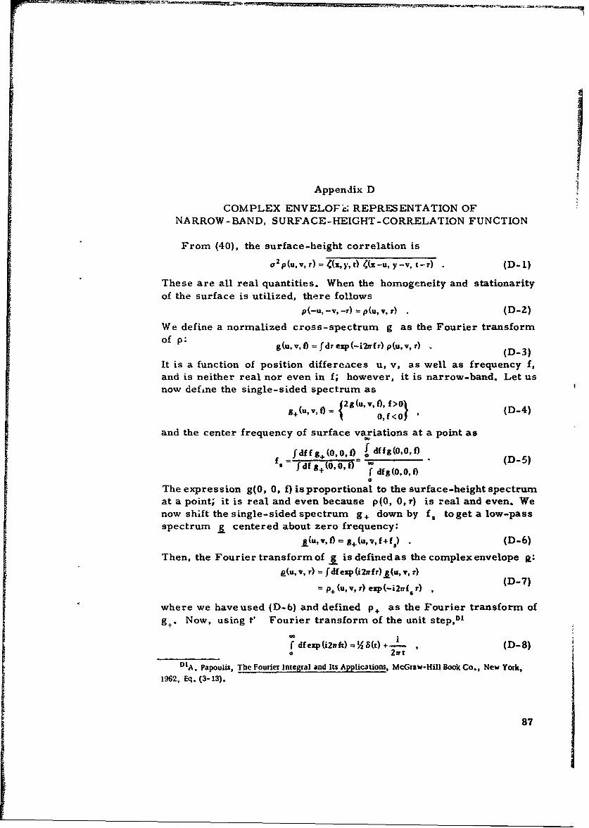
L

Appendix D

COMPLEX ENVELOPi; REPRESENTATION OFNARROW-BAND, SURFACE-HEIGHT-CORRELATION FUNCTION

From (40), the surface-height correlation isa 2P(UV, r) -- •'(,.,t)4(X--uy-v, t-T) .(D-1)

These are all real quantities. When the homogeneity and stationarityof the surface is utilized, there follows

p(-U,-v, -r)= p(u, v, r) (D-2)

We define a normalized cross-spectrum g as the Fourier transformof p; g(u,v,t) =fdrexp(-i2*rfr)p(u,v,r) (D-3)

It is a function of position differences u, v, as well as frequency f,and is neither real nor even in f; however, it is narrow-band. Let usnow define the single-sided spectrum as

g+(u,v,f) = {2g(u,v,t), f>O (D-4)

and the center frequency of surface variations at a point asfdffg+(O,0,f) • dffg(0,O,f)

f,= fdffg+o,(0,f) 0 f (D-5)f df g (0,0,0 0

The expression g(O, 0, f) is proportional to the surface-height spectrumat a point; it is real and even because p(0, r) is real and even. Wenow shift the single-sided spectrum g+ down by f. toget a low-passspectrum g centered about zero frequency:

(u,v,f)=g+(u,'v,f+f) (D-6)

Then, the Fourier transform of g is defined as the complex envelope a:

p(uv, r)= fdfexp(i2wfr).(u,v,r)=p+ (u, v, r)exP (-i2v(,•r),

where we have used (D-6) and defined p+ as the Fourier transform ofg+. Now, using t' Fourier transform of the unit stepDI

fdfexp(i2vft) - 8(t) +- , (D-8)o 2vt

VIA. Papoulis, The Fourier Integral and Its Applications, McGraw-Hill Book Co., New York,1962, Eq. (3-13).

87

p+ can be evaluated f'om (D-4) as

p+(u,v, )=p(u,V,,r)+ipH(u,v,) ,I (D-9)

where PH is the Hilbert transform of p:I (,u, V, w)pn(u, V, r) =.-(D 10

PH ru p-W) (D--10)

Combining (D-9) and (D-7), we obtain

p(u,v, r) =ReIp+(u,v,r)I(D-11)

=Re Ip(u, v, r) exp (i2Off fwhich is the property desired in (44).

An additional property of complex envelope Q that will be necessary

is now derived from (D-10):PH (-U, -V, - r) =-PH (uv, •) (D-12Z)

Substituting into (D-9), we note thatP+(-u,-V,-I)=P+(uv, r) (D- 13)

and then from (D-7), we getP.(-U ,-v , -r) = .."(U , v ,) (D - 14)

For the special case where p(u, v, r) is even in r for all u, v, i. e.,

p(u,v,-I)=p(U,v, ) , (D-15)

F (u, v, 0) is purely real and is given by

P 5(U,v,00)-0. (D-16)

This may be seen as follows: From (D-10), using the evenness of p,PH (U~VW0) = 0. (D- 17)

Then, using (D-9) and (D-7), (D-16) follows.

88

Appendix E

NUMERICAL EVALUATION OF EQ. (112)

In (112), the surface-height spectrum was given in terms of anintegral:

C(x) - IX 1 f dt tezp(-t2)cos(qt)J0 (x2t) (E-.1)0

where q a Q/R. To evaluate this integral, we expand cos(qt) in apowerseries in t and obtain

I .x i3 q f d2 t2a+ ezp(-(t) Jo(z 2 t) (E-2)

-=0 (270 0The integral in (E-2), from Gradshteyn and RyzhikEl is

% a! exp(-4/4) L. /4) , (E-3)

where L. is a Laguerre polynomial. Ther -ore,

= x exp(_x4/4) ! (-q 2)' .n! LW(1 /4) (E-4)(~ 20)! a

This series, which car. be easily evaluated byusing rerirrence relationson the Laguerre polynomials, is plotted in Fig. 5.

For x near zero, 0(x) becomes negative if q is made too large.

From (E-1), it maybe seen that the largest value of q allowed is whenfdttezp(-t2 )cos(rj)_O •E-5)0

That is, from Gradshteyn and Ryzhik,' 2

The solution for the smallest value of q satisfying (E-6) is

q -- 1.482777 (E-7)R

Therefore, (112) has been plotted only for Q/R less than this value.

"1. S. Gradshteyn and 1. W. Rya"ik, Table of Integrals, Seies=, and Producs, Academic Press,

New York, 1965, Eq. 6.631 10.

E2 Ibid., Eq. 3.952 8.

89/90REVERSE BLANK

41

Appendix F

ERROR ANALYSIS OF EQS. (61) AND (63)

The infinite integral of (61) must be approximated by a finite integral,up to Value L, say. In order to determine how large L must be fornegligible error, we note that for small x

(z/2) 2 M

U>)x 8. (F-i1)(x/2)" _>

Therefore, for large values of r,

f2P2 (r)) - Io. -. (F-2)•[%•p22 (jr)] IM

The slowest decaying order is m = 1; therefore, the largest error interminating the integral (61) at L is approximately

E = (2v) 'exp(-fP 2) f drr!4f92 P2 (r) (F-3)L

When spatial correlation p2 is an exponential modulation of either acosine or a Bessel function,

P2 (r) exp(-r) cos(Qr) or ezp(-r) Jo(Qr) , (F-4)

(F-3) is upper-bounded by 00E ((2n)" es (-3•2) %ft' f dr r ezp(-r)

L (F-5)(4fr)" 1 q2 exp (_162) (L + 1) exp (-L)

The largest value of p2 exp(_p2 ) occurs at P = 1, yielding

E _..(4ve). (L+1) exp(-L) (F-6)

For L = 25, E <5.10-1. The limit 25 was used in evaluating (61) forthe exponentially modulated spatial correlation; all the values of U. inFigs. 7, 8, and 9 are much larger than 10-11.

For a Gaussianly modulated zpatial correlation,

p2 (r) = ezp(-r2) cos(Qr) or ,(_-r2) j (Qr) ; (F-7)

91

I

the bound corresponding to (F-6) is

E <(B'e)lexp(-_L) (F-8)

For L = 5, E.S2 x 10". The limit of 5 was used in evaluating (61)for the Gaussianly modulated spatial correlation; all the values of U.nin Figs. 10, 11, and 12 are much larger than 2 x 10"-'

For integral (63), we can upper-bound the integrand by replacingthe Bessel function by unity. The slowest decaying order is again m = I.An analysis similar to that in(F-1) through (F-3) yields, for exponentialmodulation, the upper bound on the error

E <(4ffe)- 1 a(L+l) ezp(-L) , (F-9)

whereas, for Gaussianmodulation, the upper bound on the error Is given by

E <(8e)°' a2 ezp(-L 2 ) (F-10)

For L = 25, (F-9)yields 10-11a2; for L = 5, (F-10) yields 2 x 10"3Q2 .

The interval (0, L), used in evaluating (61) and (63), was repeatedlycut in half and evaluated by Simpson's rule until insignificant changeoccurred in the sum.

92

Ii

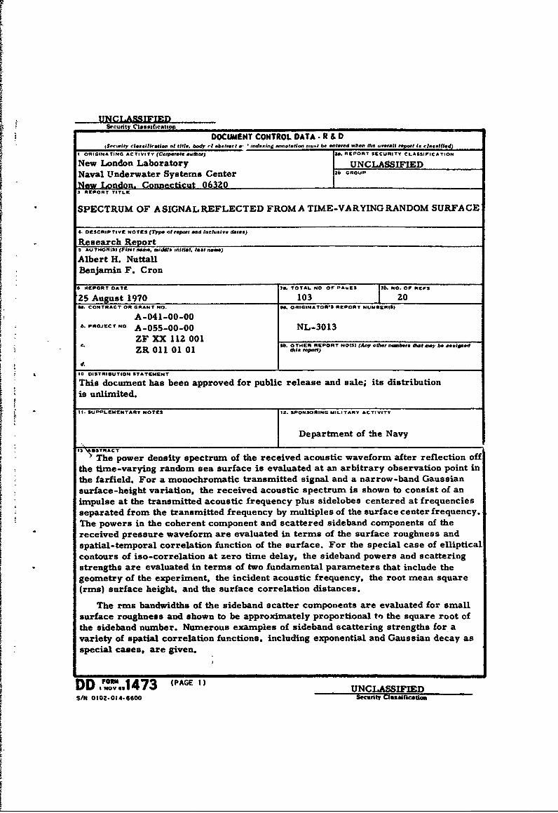
UNCLASSIFIEDSecurity Classification

DOCUMENT CONTROL DATA - R & DISerwify claseifcaltion of title, body r' abstract a, * indexing annotation rnust be entered when the overall repoH Is classifled)

I ORIGINATING ACTIVITY (Crporafte allthor) 2a. REPORT SECURITY CLASSIFICATION

New London Laboratory UNCLASSIFIED

Naval Underwater Systems Center 2b GROUP

New London. Connecticut 063203 REPORT TITLE

SPECTRUM OF A SIGNAL REFLECTED FROM A TIME-VARYING RANDOM SURFA CE

4. DESCRIPTIVE NOTES (7'pe ot rport and inclusive dates)

Research ReportS AU THORISI (First na.e, middle Initial. ltatw name)

Albert H. NuttallBenjamin F. Cron

0 REPORT DATE 70. TOTAL NO OF PA.ES 7b. NO. OF REFS

'25 August 1970 103 20Ba. CONTRACT OR GRANT NO. a. ORIGINATOR'S REPORT NUMNER(S)

A-041-00-00b. PROJECT NO A-055-00-00 NL-3013

ZF XX 112 001C.Sb. OTNER REPORT NOM)I (Any DOtW onuftera that may be esel ded

ZR O11 01 01 thisarePort)

d.

10 DISTRISUTION STATEMENT

This document has been approved for public release and sale; its distributionis unlimited.

It- SUPPLEMENTARY NOTES 12. SPONSORING MILITARY ACTIVITY

Department of the Navy

S13 STRACT

The power density spectrum of the received acoustic waveform after reflection offthe time-varying random sea surface is evaluated at an arbitrary observation point inthe farfield. For a monochromatic transmitted signal and a narrow-band Gaussiansurface-height variation, the received acoustic spectrum is shown to consist of animpulse at the transmitted acoustic frequency plus sidelobes centered at frequenciesseparated from the transmitted frequency by multiples of the surface center frequency.The powers in the coherent component and scattered sideband components of thereceived pressure waveform are evaluated in terms of the surface roughness andspatial-temporal correlation function of the surface. For the special case of ellipticalcontours of iso-correlation at zero time delay, the sideband powers and scatteringstrengths are evaluated in terms of two fundamental parameters that include thegeometry of the experiment, the incident acoustic frequency, the root mean square(rms) surface height, and the surface correlation distances.

The rms bandwidths of the sideband scatter components are evaluated for small

surface roughness and shown to be approximately proportional to the square root ofthe sideband number. Numerous examples of sideband scattering strengths for avariety of spatial correlation functions, including exponential and Gaussian decay asspecial cases, are given.

, 1473 (PAGE 1)UNCLASSIFIED

S/N 0102.014-6600 Security Clasaincaom

se-uty 401.1101114:8110

4 LINK A LINK a LINK CKIY WORDS )

"ROLK WYT RO*L WT ROLE WT

Exponentially Modulated Bessel FunctionSpatial Correlation

Exponentially Modulated Cosine SpatialCorrelation

Gaussianly Modulated Bessel Function SpatialCorrelation

Gaussianly Modulated Cosine Spatial

Correlation

Monochromatic Transmitted Signal

Time-Varying Random Surface

SDD ".",173w UmS(PAGE 2) Security 4AMIFtIED

I