Embed Size (px)
Citation preview

NASA Contractor Report 187561 _--
<../
PROGRESS IN MULTIRATE DIGITAL
CONTROL SYSTEM DESIGN
Martin C. Berg and Gregory S. Mason
UNIVERSITY OF WASHINGTON
Seattle, Washington
Grant NAGI-1055
June 1991
National Aeronautics and
Space Adminislralion
Langley Research CenterHanllOlOn, Virginia 23665-5225
( %'A C A- C "t- ] :_ 7 :!,(, I ) P ° LJ,P ,,.'_c ._ _ IN
_.._Tb[|AL t.. ' _T;_:mL -_YSTc # c_;:qIG'4
{_.;giliil+_t_ofl uriiv. ) _r-,.,._ _,
MULTI _ A T ,£_
Final Ft,:'porfC g g L O <3;
_; Jlo:!
NO l-27,:;77
https://ntrs.nasa.gov/search.jsp?R=19910018563 2019-05-04T18:09:23+00:00Z


FINAL REPORT
NASA Langley Research Grant NAG-1-1055
Progress in Multirate Digital Control System Design
1 September 1989 - 31 December 1990
Martin C. Berg
Assistant Professor
Mechanical Engineering Department, FU-IO
University of Washington
Seattle, Washington 98195
Gregory S. Mason
Graduate Student
Mechanical Engineering Departmcnt, FU-I0
University of Washington
Seattle, Washington 98 i 95

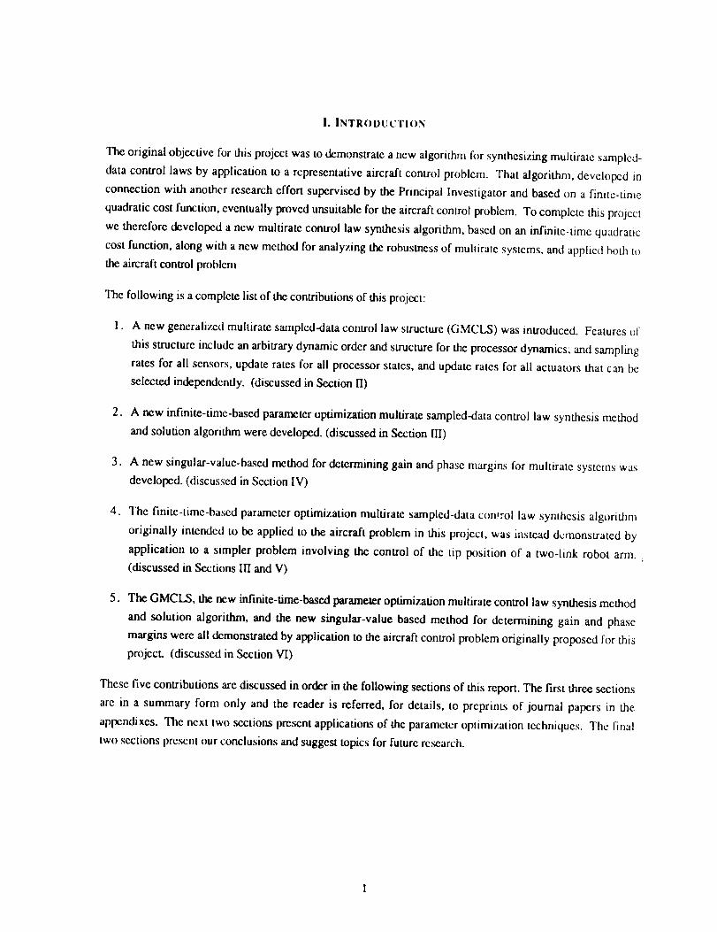
ABS'FRACT
A new methodology ff)r multirate sampled-data control systcm design based or, (I) a new gcncrahzcd
control law structure, (2) two new parameter-optimization-based control law synthesis methods, and (3) a
new singular-value-based robusmess analysis method is described. Thc control law structure can represent
multirate sampled-data control laws of arbitrary structure and dynamic ordcr, with arbitrarily prescribed
sampling rates for all sensors and update rates for all processor statcs and actuators. The two control law
synthesis methods employ numerical optimization to determine valucs for the control law parameters tt)
minimize a quadratic cost function, possibly subject to constraints on those parameters. The robustncss
analysis method is based on the multivariable Nyquist criterion applied to the loop transfer function tot the
sampling period equal to the period of repetition of the system's completc sampling/update schedule. The
complete methodology is demonstrated by application to the design of a combination yaw damper and modal
suppression system for a commcrcial aircraft.
I LItOOmAU.V
°_o
111
PRECEDING i-:A:3E BLAMK NOT FILMED


VII.
VIII.
CONTENTS
I. Introduction ................................................................................................. 1
II. The Generalized Multirate Sampled-Data Control Law Structure ..................................... 2
III. Parameter Optimization Control Law Synthesis Methods .............................................. 5
IV. Gain and Phasc Margins for Multirate Systems Using Singular-Values .............................. c)
V. Application of the Finite-Time-Based Parameter Optimization Algorithm to a Two Link
Robot Arm Control Problem ............................................................................ 1 l
VI. Application of the Infinite-Time-Based Parameter Optimization Algorithm to a
Yaw-Damper and Modal Suppression System for a Commercial Aircraft ......................... 15
Summary and Conclusions ............................................................................... 25
Suggestions for Future Research ....................................................................... 25
References .................................................................................................. 26
Appendix A: Preprint of Reference
Appendix B: Preprint of Reference
Appendix C: Preprint of Reference
.......... , ........................................................ 27
5 ................................................................... 6()
6 ................................................................... 83
v

I. INTRODUCTION
The original objective for this project was to demonstrate a new algorithm h)r synthesizing multirate sampled-
data control laws by application to a representative aircraft control problem. That algorithm, developed in
connection with anothcr research effort supervised by the Principal Investigator and based on a finite-time
quadratic cost function, eventually proved unsuitable for the aircraft control problem. To complete this project
we therefore developed a new muhirate control law synthesis algorithm, based on an infinite time quadratic
cost function, along with a new method for analyzing the robustness of multirate systcms, and applicd bolh h_
the aircraft control problcm
The following is a complete list of the contributions of this project:
. A new generalized multirate sampled-data control law structure (GMCLS) was introduced. Features of
this structure include an arbitrary dynamic order and structure for the processor dynamics; and sampling
rates for all sensors, update rates for all processor states, and update rates for all actuators that c an be
selected independently. (discussed in Section II)
2. A new infinite-time-based parameter optimization multirate sampled-data control law synthesis method
and solution algorithm were developed. (discussed in Section !]])
3. A new singular-value-based method for determining gain and phase margins for muhirate systems was
developed. (discussed in Section IV)
. The finite-time-based parameter optimization multirate sampled-data con,rol law synthesis algorithm
originally intended to be applied to the aircraft problem in this project, was instead demonstrated by
application to a simpler problem involving the control of the tip position of a two-link robot arm.
(discussed in Sections III and V)
. The GMCLS, the new infinite-time-based parameter optimization muhirate control law synthesis method
and solution algorithm, and the new singular-value based method for determining gain and phase
margins were all demonstrated by application to the aircraft control problem originally proposed for this
project. (discussed in Section VI)
These five contributions are discussed in order in the following sections of this report. The first three sections
are in a summary form only and the reader is referred, for details, to prcprints of journal papers in the
appendixes. The next two sections present applications of the parameter optimization techniques. The final
two sections present our conclusions and suggest topics for future research.

il. TilE (;ENERALIZED MULTIRATE SAMPLED-DATA C()N'I'R()I. I.AW _TRI _'Tt;RE
A key point often ignored by the developers of multirate sampled-data control law synthesis methods is that, in
order for any such method to be practically useful, it must provide the control law designer with the flexibility
to independently choose the sampling rate for every sensor, the update rate for every processor state, and the
update rate for every actuator. Such flexibility is frequently essential for efficient utilization of real-time
control hardware, and for systems that include distributed processing and/or utilize sensors that provide only
discrete-time signals at fixed sampling rates [1]. In this section we present a general-purpose, rnuhiratc
sampled-data control law structure (GMCLS) that provides that flexibility.
To understand the GMCLS, it is necessary to establish a certain notation regarding the scheduling of sampling
and update activities for a multirate system. Figure 1 shows an example of the time lines for the sampling and
update activities of a muhirate system. We define the shortest time period (STP) as the greatest common
divisor of all of the sampling, update and delay periods; and we define the bestir: time period (BTP) as the lea_t
common multiple of all of the sampling, update and delay periods. We reserve the symbol T to represent the
STP, and the symbol P to represent the (integer) number of STP's per BTP. Finally, we frequently make use
of a doubly-indexed independent (time) variable, so that, for example, x(m,n) represents x at the start of the
(n+l)th STP of the (m+l)th BTP, for m=0,1 .... and n=0,1 ..... P-I.
A block diagram of the GMCLS is shown in Figure 2. y represents the incoming, noise-free, continuous-
time sensor signal; v is the discrete-time sensor noise signal; and _ is the continuous-time control signal. The
sampling period of the one sampler is the STP of the complete system's sampling/update schedule. The delay
blocks are one-STP delays; and the ZOH block represents a zero-order hold.
Time I.ines lot Sampling/UpdateActivities:
T Time (Seconds) 2.5,/"
0 4T 8"1" 12T 167" 20T 24T
0 3T 67" 91" 12T 15T 1ST 211 24"I
Figure I Example Multirate Sampling/Update Schedule

Figure 2 Generalized Multirate Sampled-Data Control Law Structure
A key feature of the GMCLS is its use of the switching matrices, Sy(n), Sz(n), and Su(n), for n=O,1 ..... P-l,
to represent the variations in the sensor sampling, processor state update, and control update activities,
respectively. We define a switching matrix as a binary, diagonal matrix. Sy(n) is the switching matrix that
describes the sensor sampling activities at the start of the (n+l)th STP (of every BTP). If the ith diagonal
element of Sy(n) is 1, then the ith sensor's signal is sampled at the start of the (n+ 1)th STP of every BTP, and
the sampled value, with the sensor noise v added, is immediately stored as the izh element of Y. If the ith
diagonal element of Sy(n) is 0, then the same element oft is simply held at those instants. The update activities
for the processor state vector z and for the actuator hold state vector u, in Figure 1, are similarly represented
by the switching matrices Sz(n), and Su(n), respectively, for n=0,1 ..... P-I.
For a detailed discussion of the GMCLS see [1]. The key points are:
1. The switching matrices Sy(n), Sz(n), and S,(n) are completely determined by the system's sampling and
update activities schedule.
2. The only unknowns are the processor matrices Az(n ), Bz(n ), Cz(n), and Dz(n)
3. The dynamic order of the processor dynamics (i.e., the dimension of z) is arbitrary.
For design purposes, the implications of these points are the following:
, The GMCLS provides complete flexibility with regard to the selection of sampling rates for all sensors,
update rates for all processor states, and update rates for all actuators. The single constraint is that the
ratio of all sampling, update and delay rates must be rational, so that the complete sampling/update
schedule is periodic.
. The GMCLS provides complete flexibility with regard to the dynamic order and structure of the control
law; i.e., the input-output dynamics of virtually any multirate sampled-data control law of practical
interest can be realized with the GMCLS.
3
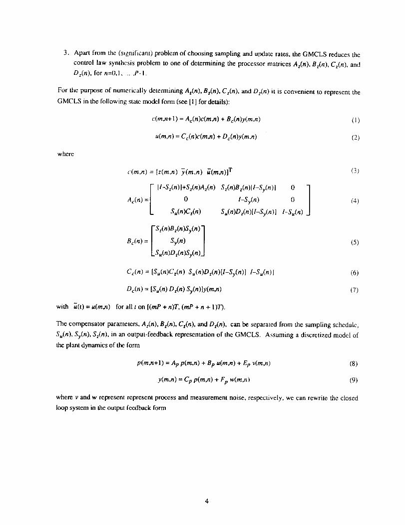
3. Apartfromthe(significant)problemofchoosingsamplingandupdaterates,theGMCLSreducesthecontrollawsynthcsisproblemtooneof determiningtheprocessormatricesAz(n), Bz(n), Cz(n), and
Dz(n ), for n=O,1 ..... P-I.
For the purpose of numerically determining Az(n), Bz(n), Cz(n), and Dz(n) it is convenient to represent the
GMCLS in the following state model form (see [1] for details):
c(rn,n+ I ) = Ac(n)c(rn,n) + Bc(n)y(m,n) ( 1)
u(m,n) = Cc(n)c(m,n ) + D c(n)y(m,n ) (2)
where
c(m,n) = [z(m,n) -y(m,n) u(m,n)] T
ll-Sz(n)l+Sz(n)Az(n)Ac(n ) = 0
S,,(n)Cz(n)
FSz(n)Bz(n)Sy(n) _
R#n)= / S,(n) I
LSu(n)Dz(n)Sy(n)J
Sz(n)Bz(n)[I-Sy(n)ll-sy(n) O0 ]Su(n)Dz(n)[l-Sy(n)] l-Su(n)
(3)
f4)
(5)
Co(n) = [S,,(n)Cz(n) Su(n)Dz(n)[l-Sy(n)l 1-Su(n)] (6)
De(n) = [S,(n) Oz(n) Sy(n)]y(ra,n) (7)
with u(t) = u(ra,n) for all t on [(raP + n)T, (raP + n + 1)T).
The compensator parameters, Az(n ), Bz(n), Cz(n), and Dz(n ), can be separated from the sampling schedule,
Su(n), Sy(n), Sz(n), in an output-feedback representation of the GMCLS. Assuming a discretized modcl of
the plant dynamics of the form
p(ra,n+ l ) = Ap p(ra,n) + Bp u(m,n) + Ep v(m,n) (8)
y(m,n) = Cp p(ra,n) + F e w(m,n) (9)
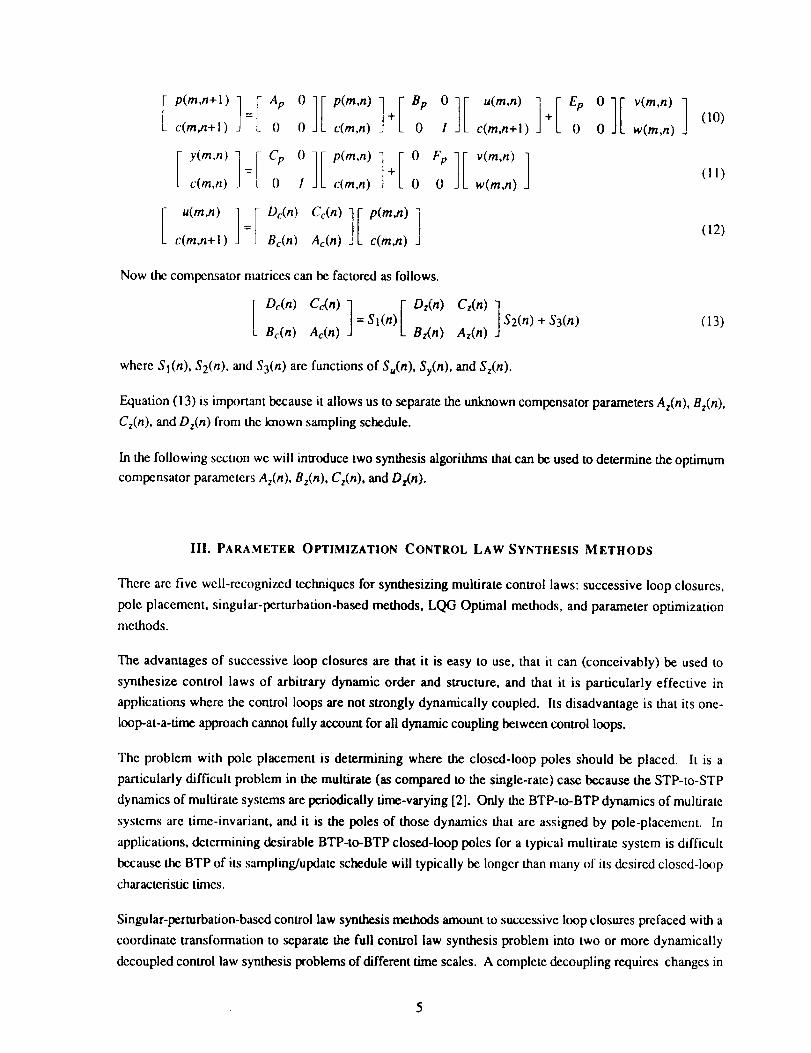
where v and w represent represent process and measurement noise, respectively, we can rewrite the closed
loop system in the output feedback form
ta. [., 0][ ] 0][v m.,]= + + (I0)c(m,n+l ) 0 0 c(m,n) 0 I c(m,n+l ) 0 0 w(m,n)
= + (11)c(mm) _ 0 ! c(m,n) 0 0 w(m,n)
[ u(m,n) =i-De(n)Cc(n)][p(rn,n)c(m,n+l) ] Be(n) Ac(n) c(m,n) ] (12)
Now the compensator matrices can be factored as follows.
[ Dc(n)Cc(n)]=Sl(n) [ Dz(n)Be(n) Ac(n) Bz(n)
C_(n) 1| S2(n) + S3(n)
Az(n) _J(13)
where Sl(n ), S2(rt), and S3(n ) are functions of Su(n), Sy(n), and Sz(n).
Equation (13) is important because it allows us to separate the unknown compensator parameters Az(n), Bz(n),
Cz(n), and Dz(n) from the known sampling schedule.
In the following section we will introduce two synthesis algorithms that can be used to determine the optimum
compensator parameters Az(n ), Bz(n ), Cz(n), and Dz(n).
Ill. PARAMETER OPTIMIZATION CONTROL LAW SYNTHESIS METHODS
There are five well-recognized techniques for synthesizing multirate control laws: successive loop closures,
pole placement, singular-perturbation-based methods, LQG Optimal methods, and parameter optimization
methods.
The advantages of successive loop closures are that it is easy to use, that it can (conceivably) be used to
synthesize control laws of arbitrary dynamic order and structure, and that it is particularly effective in
applications where the control loops are not strongly dynamically coupled. Its disadvantage is that its one-
loop-at-a-time approach cannot fully account for all dynamic coupling between control loops.
The problem with pole placement is determining where the closed-loop poles should be placed. It is a
particularly difficult problem in the muitirate (as compared to the single-rate) case because the STP-to-STP
dynamics of multirate systems are periodically time-varying [2]. Only the BTP-to-BTP dynamics of multirate
systems are time-invariant, and it is the poles of those dynamics that are assigned by pole-placemcnc In
applications, determining desirable BTP-to-BTP closed-loop poles for a typical multirate system is difficult
because the BTP of its sampling/update schedule will typically be longer than many of its desired closed-lo_)p
characteristic tinles.
Singular-perturbation-based control law synthesis methods amount to successive loop closures prefaced with a
coordinate transformation to separate the full control law synthesis problem into two or more dynamically
decoupled control law synthesis problems of different time scales. A complete decoupling requires changes in

notjust thestatecoordinates,butin theinputandoutputcoordinatesaswell. Sucha dccouplingisnotpossiblein themultiratecasebecausetheinputandoutputcoordinatesrepresentphysicalsensorandactuatorsignalsdestinedtobesanlpled/updatedatdifferentrates.
Theadvantagesof theLQGoptimalcontrollawsynthesismethodsare that stabilizing control laws arc
relatively easy to obtain and that the control laws for all control loops are synthesized simultaneously, taking
full advantage of all dynamic coupling between the control loops. The disadvantages are that the dynamic
order and structure of the control law is fixed, that stability robustness objectives are difficult to achieve, and
that the resulting control laws are periodically time-varying 121-[31.
We favor parameter optimization methods for control law synthesis for muitirate systems because they offer
the principal advantages of the successive loop closures and LQG optimal synthesis methods. These
advantages are that control laws of arbitrary dynamic order and structure can be synthesized, and that control
laws for all control loops can be synthesized simultaneously, taking full advantage of all dynamic coupling
between control loops. The disadvantage of parameter optimization methods is that a numerical search is
required to determine the control law parameters.
In this section we present two parameter optimization methods for synthesizing multirate control laws. Both
utilize the GMCLS discussed in Section II. The first is based on a finite-time quadratic cost function while the
second is based on an infinite-time quadratic cost function. Both methods solve the multirate compensator
synthesis problem by using a gradient-type numerical search to find a set of compensator parameters that
minimize a quadratic cost function.
The multirate optimization problem is as follows.
Given:
1. The plant dynamics represented by
(14)
y(t)= C't'p(t) (15)
Here _ is the plant state vector, fi is the control input vector, _ is the noise-free measurement output
vector, and _ is the noise input vector.
2. The complete sampling and update schedule for the compensator. This amounts to specifying Su(n ),
Sy(n), and St(n), h)r n=0,1 ..... P-I.
3. The order for the pr_x:essor dynamics (the number of elements in z in (3)).
4. The desired structure (e.g., a diagonal structure) for the processor matrices, Az(n ), Bz(n), Cz(n), and
Dz(n), for n=0,1 ..... P-1.
5. The number of distinct sets of processor matrices and when they are active. The optimization algorithms
allow Az(n), Bz(n), Cz(n), and Dz(n ) to be periodically time varying. The designer can specify equality

.
7.
relations among the compensator matrices. For example, if a rune invanant compensator is desired then
the designer can specify that Az(O) = Az(l) ..... Az(P-I ), and similarly for B z ,C z and D z.
The power spectral density _' of the process noise _ (in (8)).
The covariance W(n), for n=0,1 ..... P-l, of the sensor noise w (in Fig. 2). w is assumed to be a
periodically stationary, gaussian, purely random sequence, with period equal to the BTP of the
sampling/update schedule.
8. The time t/and non-negative dcf'mite weighting matrices 0 and R for the pcrtbrmancc index
Y(tl)= E 2_ L_(t)J 0
whereE istheexpectedvalueoperator.
,_ Lu(t)J(16)
In the finite time optimization problem tfmust be a multiple of the BTP of the sampling/update schedule.
Find:
tim J(tf)tf_ oo
In the infinite time optimization problem tf _ and Jin17nite-lime=
A set of processor matrices, Az(n), Bz(n), Cz(n), and Dz(n), for n=0.1 ..... P-l, such that the performance
index
is minimized.
This optimization problem can be solved using either the finite-time cost function or the infinite-time cost
function.
Solution Method Usin_ the Finite-Time Cost Function.
The f'mite-time optimization algorithm was developed in connection with another research effort supervised by
the Principal Investigator. This method synthesizes the multirate compensator that minimizes J(tf) for a finite
t/. A detailed discussion of this method can be found in [11. A summary of the solution procedure follows.
1. Determine closed-form expressions for the performance index J(tf), and for its gradients with respect to
the elements of the processor matrices At(n), Bz(n), Cz(n), and Dz(n), for n=0,1 ..... P-1.
2. Use a gradient-type numerical optimization algorithm to determine a set of processor matrices, Az(n),
Bz(n), Cz(n), and Dz(n), for n=0,1 .... ,P-l, that minimizes J(tf).
7

3. Obtain a steady-state solution by re-optimizing for larger and larger tf unlil tfgets to be large compared to
all of the closed-loop system's characteristic times.
The advantage of this method is that with t/finite, the cost function J(tf) remains finite even if the compensator
is destabilizing. The designer does not need to find a stabilizing compensator to start the optimization process
as long as tfis small enough that J(tf) does not exceed the numerical limits of the computer performing the
optimization.
The disadvantage of this method is that the closed-form expressions that have been developed thus far for the
performance index J(tf) and for its gradients with respect to the elements of the processor matriccs arc very
complex and computationally intensive. In addition, we encountered difficulties when applying this method to
the aircraft control problem because our solution algorithm lacked provisions for automatic scaling of the
control law parameters (,.e., the independent variables) during the numerical search. The sheer complexity of
the finite-time performance index and gradient expressions prevented us from adding the automatic scaling
provisions that would have allowed us to apply this method to the aircraft control problem.
Solution Method Using Infinite-Time Cost Function
Instead of modifying our existing finite-time-based algorithm to alleviate the scaling problem discussed in the
previous paragraph, we chose to develop a new infinite-time-based multirate sampled-data control law
synthesis method, based on corresponding developments for single-rate systems by Mukhopadhyay [4], for
which much simpler performance index and gradient expressions are easy to derive. For a complete
description of that method, and the solution algorithm we developed to implement it see [51. A summary of
the solution procedure follows.
. Find an initial stabilizing guess for the processor matrices Az(n), Bz(n ), Cz(n), and Dz(n ), for
n=0,1 ..... P-I. The finite-time solution algorithm requires an initial stabilizing compensator because
Jss is infinite when the closed loop system is unstable. From our experience, many multirate problems
can be stabilized using successive loop closures. The aircraft problcm was open loop stable, and so
determining a stabilizing compensator was trivial.
. Determine the necessary conditions (given in [51) for the processor matrices, As(n), Bz(n ), Cz(n ), and
Dz(n), for n=0,1 ..... P-I to minimize Jss. These are represented by three sets of coupled matrix
equations. Two sets are Lyapunov equations, one governs the steady state covariance of the plant and
control states, and the other governs a Lagrange multiplier. The third represents the gradient of Jss with
respect to the compensator parameters.
3. Use a gradient-type numerical search to solve the necessary conditions and determine a set of processor
matrices, Az(n), Bz(n), Cz(n), and Dz(n), for n=0,1 ..... P-l, that minimizes Jss.
The advantage of this method is that the gradient of Jss with respect to the compensator parameters is easy to
evaluate via the necessary conditions. For a given problem, the infinite-time optimization algorithm typically
requires fewer computations to find the optimum compensator parameters than does the finite-time
optimization algorithm even when both algorithms are initialized with the same stabilizing compensator.

Eventhoughthefinite-time and infinite-time based .solution algorithms can determine optimum comIx'rtsalor
parameters, there is no guarantee that the design will be robust. In the following section we prcsem a mcth_._d
for analyzing the robustness of a muhiratc control system.
IV. GAIN AND PHASE MARGINS FOR MULTIRATE SYSTEMS USING SINGULAR-VALUES
There are many established methods for synthesizing multirate compensators, see Section I/I, but surpnsingl_
few methods for analyzing the robustness of these systems. Current robustness analysis methods rely
principally on the transfer function of the system. A multirate transfer function, in the traditional sense, does
not exist, becau_ muhirate systems are periodically time varying. Wilhout modification, cstahlishcd single-
rate analysis methods cannot be applied directly to muhirate systems.
As part of this project, we developed an approach for extending the nyquist criterion and singular value
analysis to multirate and periodically time varying systems. For a detailed discussion of this approach,
including application of structured singular value robustness analysis to multirate systems, see [6]. In this
section we present a summary of the important ideas from that paper used to calculate gain and phase margins
of multirate systems using singular values.
As we saw in Section [I, a multirate compensator can be modeled as a linear periodically time varying system
(1)-(2). Equations (i)-(2) from Section II can be written as
c(m,n+ i ) = Ac(n)c(m,n) + Bc(n)y(ra,n)
u(m,n) = Cc(n)c(ra,n) + Dc(n)y(m.n)
(17)
(18)
This system (17)-(18) can then be transformed to an equivalent single-rate system (ESRS) by repeated
application of (17)-(18) over the BTP 17]. The ESRS has the form:
c(m+l,0) Aec(m,O) + ^-- BeY(m,O ) (19)
A_(m,O) = Cec(m,O) + Dey(m,0) (20)
r y(m,O) _ f u(m,O) 7
= it ] u(m,l).wherep(m,0)| Y(7")| uA(m,0) = (21,JLy(m,P- I )J Lu(m,P- I )
The transfer function for the ESRS is
?_(ze ) = Ge(ze)_(z e)
where G p( zP) = C e( l zP - A e) ' IB e + D e
(22)
(23)

For a detailed discussion of the ESRS, see [6]. The key points are:
I. The ESRS is a time invariant single-rate system with a sampling period of one BTP and the unique
properly that the inputs are time correlated and the outputs are lime correlated.
. In general Gp(z P) has a very complicated form, but it can be shown that if the system is time in_ ariant
with G(z) equal to a constant, then Gp(z P) will also be constant and block diagonal with G(z) on the
diagonal.
. The ESRS allows us to manipulate time invariant and periodically time varying systems (e.g. muhiratc)
as if they were both time invariant. The state space or transfer functions descriptions can be used to
calculate input-output relations for systems in series or in a feedback loop just as in classical control [8 I.
For example, to calculate the ESRS of a muhirate compensator in series with a time invariant plant, wc
would calculate the ESRS of the plant and compensator individually and then combine thcm using block
diagram arithmetic.
4. Kono [9] has shown that ff the ESRS is stable then the multiratc systcm from which it was derived will
be stable.
5. Single-rate robustness analysis techniques can be applied to the ESRS as long as the results are
interpreted in light of the fact that some of its inputs and outputs are time correlated.
Generalized gain and phase margins for the ESRS (and equivalently the muhirate system) can be calculated
using singular value analysis. If we assume a plant uncertainty of the form
G (Z)Actual = G (Z)Nominatke]O (24)
then the ESRS plant uncertainty has the form
Gp(zP)actuat = Gt,(zt')lVorai,tal(kdO)p
(kei°)e = diag[ke tO, k.d 0 ..... /¢d O] with P blocks
[Recall that if H(z) is constant, Ht,(z ?) is block diagonal with H(z) on the diagonal. ]
(25)
The multirate system is guaranteed to remain stable whenever
_((K,,/°)-l-l) <_a(l + Ge(ze)) on the nyquist contour (26)
Traditional gain margins can be obtained by setting O = 0 and solving (26) for k. Phase margins can be found
by setting k = 0 and solving (26) for 0.
As with most singular value robustness analysis methods, the k and 0 found using (26) are conservativc. If,
however, k.d ° is diagonal, the conservativeness associated with (26) can be reduced by diagonally scaling
Gp(zP). We used Osborne's method of preconditioning matrices to increase the Iowcr bound for Gp(z P) and
thus to improve our estimate of the gain and phase margins.
10

V. APPLICATION OF THE FINITE-TIME-BASED PARAMETER OPTIMIZATION ALGORITHM TO
A TWO LINK ROBOT ARM CONTROL PROBLEM
The original proposal for this project called for the finite-lime-based parameter optimization multirate sampled-
data control law synthesis method of Section 1II to be applied to an aircraft control system design problem.
That method and a solution algorithm to implement it had been previously developed as part of another
research effort supervised by the Principal Investigator. Due to the solution algorithm's lack of adequate
provisions for automatic scaling of the control law parameters (i.e., the independent variables) during the
numerical search, we were not able to apply it successfully to the aircraft control problem. We maintain,
however, that the problems we encountered with it were a consequence of problems with the solution
algorithm and are not necessarily indicative of problems with the synthesis method.
In this section we therefore present an application of the finite-time-based multirate sampled-data control law
synthesis method to a two-link robot arm (TLA) control problem. The robot arm application demonstrates the
utility of the method without being so poorly conditioned that automatic scaling of the control law parameters
was required during the numerical search.
The two-link robot arm system we dealt with is shown in Figure 3. The first link is long and massive, for
large-scale slewing motions. The second is short and lightweight so high-bandwidth control of the tip position
can be achieved with a relatively small motor at the second joint. The pin joint, rotational spring, and
rotational damper at the midpoint of the first link model flexibility in that link. The control inputs are the motor
torques, T I and T2. The measured outputs are the joint angle 0 and the tip position & The spring constant (k)
and damping coefficient (b) values (in Fig. 3) yield an open-loop vibration mode with a 10 Hz natural
frequency and 1% damping.
Parameters: Mass Length
Lt 0.5kg 0.5mL2 0.5 kg 0.5 m k = 37.33 N/radL3 0.04kg 0.2m b=0.012N, s/m
The natural frequency of the vibration mode is 10 hz.
Inputs: Torques TI andT2
Outputs: 0 and
Figure 3 Two-Link Robot Arm System
11

We used the finite-time-bascd multirate control law synthesis method of Section III to synthesize multiratc
sampled-data control laws for this system. Our performance objective was high-bandwidth control of the tip
position 8, and it is intuitively clear that this can best be accomplishcd, given a fixed real-time computation
capability, by trading low-bandwidth control at T 1 for high-bandwidth control at T 2. Thus, for an 8-to-I
control bandwidth ratio, we chose the sampling/update rate for _i and "1"2 to be 8-times faster than that for 0 and
T 1. For comparison purposes, we also designed corresponding analog and single-rate sample-data'control
laws.
Td.AKonua[J.,a_
For the TLA system, the tip position (8) responses to a commanded step c "hange in the tip position obtained
with the analog, single-rate and multirate control laws we synthesized are shown in Figure 4. See [ 1] tot
additional results and details. A summary description of those designs follows.
LQR Analog Design The LQR Analog response was obtained with an analog LQR (full state feedback)
control law that is optimal with respect to a quadratic performance index that yields 0.7071 damping
(41 = 42 = 0.7071) and an 8-to-I ratio of characteristic frequencies (to,t2/to,_ 1 = 8) for the two closed-loop
modes.
Third-Order Analog Successive Loop Closures Design The Third-Order Analog Successive Loop Closures
response was obtained with a successive loop closures control law that consisted of a single lead network from
0 to T 1, and two identical cascaded lead networks from 8 to T 2. The gains, and zero and pole locations were
chosen to yield dominant closed-loop poles coincident with those obtained with the LQR Analog control law.
Third-Order Multirate Tustin Design The Third-Order Multirate Tustin response was obtained with a
muitirate sampled-data control law obtained by discretizing the lead compensators of the Third-Order Analog
Successive Loop Closures design using Tustin's method [10]. The 0-to-T 1 control-loop sampling/update rate
is a factor of 8 times the characteristic frequency of the lower-frequency closed-loop mode from the Third-
Order Analog Successive Loop Closures design; and the &to-T 2 sampling/update rate is the same multiple of
the characteristic frequency of the higher-frequency closed-loop mode from the Third-Order Analog
Successive Loop Closures design.
Optimized Third-Order Muhirate Tustin Design The Optimized Third-Order Muitirate Tustin response was
obtained with a control law synthesized by the finite-time-based muitirate sampled-data control law synthesis
method of Section III. This control law is the Third-Order Multirate Tustin control law, but with its gains and
its pole and zero locations optimized to minimize the same performance index as is minimized by the LQR
Analog control law.
Analog Third-Order Design The Analog Third-Order response was obtained with a third-order, generally-
structured, analog control law synthesized using Ly's Sandy algorithm [111-[12] to minimize the same
performance index as is minimiTed by the LQR Analog cona'ol law.
12

0.25
0.15
0.1
0.05
{}.2
00
LQRAnalog...... Third-OrderAnalogSuccessiveLoopClosures........ Third-OrderMullirateTustin...... OptimizedThird-OrderMultiratcTustin
0.5 i 1.5 2 2.5 3 3.5 4Seconds
Figure 4a Robot Arm Tip Position {8) Responses to a Tip Position Step Command
0.25
0.2
0.15
0. I
0.05
Analog Third-Order....... Multirate First-Order...... Multirate Second-Order........ Muitirate Third-Order
...... Single-Rate Third-Order
00
Figure 41} Robot Arm Tip Position (8) Responses to a Tip Positron Step Command
13

Multirate First-Order, Second-Order & Third-Order Designs The Muhirate First-Order, Second-Order, and
Third-Order responses were obtained with multirate, generally-structured, sampled-data control Laws
synthesized by the finite-time-based multirate sampled-data control law synthesis method of Section HI to
minimize the same performance index as is minimized by the LQR Analog control law. The sensor sampling
and actuator update rates are the same as in the Third-Order Multirate Tustin control law. In the First-Order
case, the update rate for the one processor state is the same as the faster sensor-sampling/actuator-update rate.
In the Second-Order case, one processor state is updated at the faster rate and the other at the slower rate. In
the Third-Order case, two processor states are updated at the faster rate and one is updated at the slower rate.
Single-Rate Third-Order Design Finally, the Single-Rate Third-Order control law response was obtained
with a single-rate, generally-structured, sampled-data control law synthesized by the t-mite-time-based mull.irate
sampled-data control law synthesis method to minimize the same performance index as is minimized by the
LQR Analog control law. Its single sampling/update rate was chosen to require the same average number of
computations per unit time for real-time operation as is required for real-time operation of the Multirate Third-
Order control law.
The TLA results in Figure 4 demonstrate some of the benefits of multirate control. For example, the tip
position overshoot (5) with the multirate compensator is much less than with its equivalent single-rate
counterpart. But more importantly, the results demonstrate that the finite-time-based multirate sampled-data
control law synthesis method can be used to synthesize multirate control laws of arbitrary structure and
dynamic order, with arbitrarily selected sampling rates for all sensors, and update rates for all processors states
and actuators. The third-order multirate compensator, for example, uses two different update rates for the
processor states, inputs and outputs, and a general compensator structure with full coupling between inputs,
outputs and processor states of different rates.
14

VI. APPLICATION OF THE INFINITE-TIME-BASED PARAMETER OPTIMIZATION ALGORITHM
TOA YAW DAMPER AND MODAL SUPPRESSION SYSTEM FOR A COMMERCIAL AIRCRAFT
A practical application of multirate control can be found in aircraft. The limited computational resources of
aircraft dictate that their control systems must function efficiently. Multirate control allows the designer to
efficiently allocate these resources by trading slow sampling and update rates in control loops associated with
low-bandwidth control functions for fast sampling and update rates in control loops associated with high-
bandwidth control functions. In this section we consider a particular application of multirate control: a
combination yaw-damper and modal suplxession system for a commercial aircraft.
In the interest of weight reduction for fuel efficiently, aircraft are being constructed with less structural rigidity.
Structural vibration modes can be excited in such aircraft by wind gusts or by movemenLs of control surfaces.
These vibrations affect not only the structural integrity of the fuselage but also passenger ride quality. In the
lateral direction, such vibrations are often induced by rudder activity associated with the yaw-damper. A
"modal suppression system" can be added to the yaw-damper loop to suppress these vibrations. The modal
suppression system would traditionally be designed by successive loop closures.
In this section we describe the design of a multirate combination yaw-damper and modal suppression system
for a commercial aircraft using the infinite-time-based multirate compensator synthesis algorithm and
robustness analysis technique discussed in Sections III and IV. For comparison purposes we also designed
corresponding analog and single-rate sample-data systems.
The goal for each compensator design was to increase the damping of the dutch-roll mode to 0.6, and to
decrease the covariance of lateral accelerations at the nose and aft of the airplane, particularly those components
associated with low frequency flexible modes. The performances of the compensators were compared by
comparing the closed loop dutch-roU damping, the covariances of lateral accelerations at the nose and aft of the
aircraft due to a unit covariance gaussian white noise disturbance, and the PSD plots of the lateral accelerations
at the nose and aft of the aircraft for either a white noise disturbance (analog designs) or a gust pulse
disturbance (sampled-data designs).
Ope_nLoop Aircraft
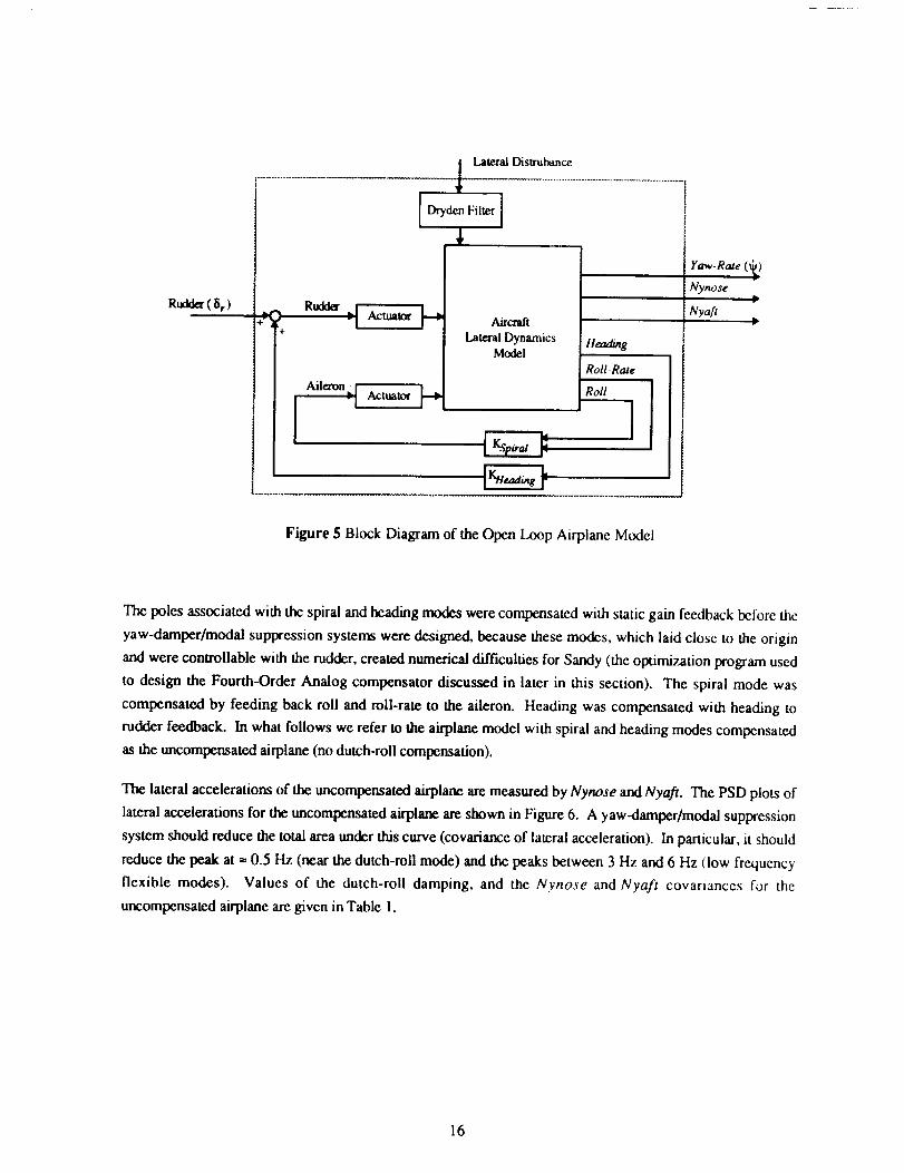
A block diagram of the airplane model is shown in Figure 5. The lateral dynamics model consists of 4 rigid
body modes (heading, spiral, dutch roll and roll) and 11 flexible modes. Actuator/power control units for the
aileron and rudder are modeled as second-order lags.
20(25)30(35) G(s)auer°n = 20)(s +G(s)R_ter = (s + 30)(s + 35) (s + 25) (27)
The lateral gust disturbances are filtered by a second-order Dryden gust model
17.496s + 2.1617G(s) = 21.836s 2 + 9.3458s ÷ ! (28)
15
Rudda (8 r )
Aileron, I"I
+
JActuator H Aircraft
Lateral Dynamics
Model
Actualor
Heading
Roll-Rate
Roll
I
Yaw-Rate (_)Nynose
b
Ny_
Figure 5 Block Diagram of the Open Loop Airplane Model
The poles associated with the spiral and heading modes were compensated with static gain feedback before the
yaw-damper/modal suppression systems were designed, because these modes, which laid close to the origin
and were controllable with the rudder, created numerical difficulties for Sandy (the optimization program used
to design the Fourth-Order Analog compensator discussed in later in this section). The spiral mode was
compensated by feeding back roll and roll-rate to the aileron. Heading was compensated with heading to
rudder feedback. In what follows we refer to the airplane model with spiral and heading modes compensated
as the uncompensated airplane (no dutch-roll compensation).
The lateral accelerations of the uncompemated airplane are measured by Nynose and Nyaft. The PSD plots of
lateral accelerations for the uncompensated airplane are shown in Figure 6. A yaw-damper/modal suppression
system should reduce the total area under this curve (covariance of lateral acceleration). In particular, it should
reduce the peak at = 0.5 Hz (near the dutch-roll mode) and the peaks between 3 Hz and 6 Hz flow frequency
flexible modes). Values of the dutch-roll damping, and the Nynose and Nyaft covariances for the
uncompensated airplane are given in Table i.
16

ft 2
5
4.5
4
3.5
3
2.5
1.5
1
0.5
00
Nvnose..... Nvafi
1 2 3 4 5 6 7 8 9
Hz
10
Figure 6 PSD of Nynose and Nyaft for Uncompensated Airplane with UnitCovariance Gaussian White Noise Lateral Disturbance
Table 1
De_sign
Results for Analog Designs with a Unit Covariance Gaussian White Noise
UncompensatedAnalog Yaw-Damper OnlyLQR Analog
, Fourth-Order Analog
Lateral Disturbance
Dutch-Roll Damping
0.08
0.60.6
0.55
Nynose Cov.(ft2/sec 3)
.... 51i5.02.4
2.5
] Nyaft Coy.(ft2/SeC 3)
21.8
6.13.1
2.4
Analo_ Yaw-Damper/Modal Sup_oression System Designs
Three analog compensators were designed: a yaw-damper only system, a full state feedback yaw-
damper/modal suppression system, and a fourth-order yaw-damper/modal suppression system. PSD plots of
Nynose and Nyaft for the analog designs are shown in Figure 8; Nynose and Nyaft covariances are
summarized in Table 1. These analog designs provide a base line for comparison with the sampled-data
designs and were used to determine appropriate values for cost function weighting matrices. Following is a
summary of these designs.
17

Analog Yaw-Damper Only Design The yaw-damper only design uses static feedback from _ to 8 r, using a
gain kaa,_er. We chose kaa,m,er such that the dutch-roll damping was 0.6 using classical root locus. While the
peak on the PSD plot associated with the dutch-roll mode (=0.5 Hz) has been reduced significantly from the
uncompensated case, the peak near 3 Hz has increased (see Fig. 8). This is the problem with using static gain
feedback. As you "press" on one peak of the PSD another "pops" up due to the input coupling between the
dutch-roll and low frequency flexible modes.
LQR Analog Design The LQR design uses full state feedback to improve the dutch-roll damping and reduce
the covarianee of Nynose and Nyafl. The compensator was designed to minimize the following cost ftmction.
II 1TE lr 1Jss lira E Nynose 0. )1 0 Nynose= + 1.68 (29)
t/_ -- (L Nya_ A 0.004 L Nyaft j
Weighting matrices for (29) were chosen such that the covariances of Nynose and Nyafi were reduced from
the yaw-damper only case by the same percent, and the dutch-roll mode had a damping of 0.6. Figure 8
shows that the LQR design significantly reduces the dutch-roll peak as well as the peaks associated with the
flexible modes.
Fourth-Order Analog Design The Fourth-Order Analog compensator is a yaw damper/modal suppression
system designed using Sandy [ 11 ]. A block diagram of this compensator is shown in Figure 7. This design
minimizes the same cost function as the LQR design (29) with the weighting on 8 r adjusted to achieve close to
the desired 0.6 dutch-roll damping. An unexpected result is that the covariance at Nyaft for the Fourth-Order
Analog design is actually better than for the LQR Analog design. This is a consequence of adjusting the cost
function weighting matrices to achieve the desired the dutch-roll damping.
s,
I L_teral Disturbance
Uncompensated Airplane
Fourth- Order AnalogCompensator
Nynose
Nyafl
Figure 7 Block Diagram of Airplane with Fourth-Order Analog Compensator
18

4.5
4
3.5
3
AnalogYaw-DamperOnly...... LQRAnalog....... Fourth-OrderAnalog
I
ft2 2.5 I
2
1.5
1
0.5
00 1 2 3 4 5 6 7 8 9 10
Hz
Figure 8a PSD of Nynose for Airplane with Analog Compensators for UnitCovariance Gaussian White Noise Lateral Disturbance
fl 2
5
,_.54 t
3.5
3
2.5
2
1.5
1
O.5
00 1 2
Analog Yaw-Damper Only...... LQR Analog........ Fourth-Order Analog
t
3 4 5 6 7 8 9
Hz
10
Figure 8b PSD of Nyafl for Airplane with Analog Compensators for UnitCovariance Gaussian Whi""te Noise Lateral Disturbance
19

Sampled-Data Yaw-Darner/Modal Suppression System Desigm
Three sampled-data compensators were designed: a single-rate yaw-damper only system, a fourth-order
muitirate compensator and a fourth-order single-rate compensator. Both fourth-order compensators were
synthesized using our infinite-time-based multirate control law synthesis algorithm to minimize the same cost
function as the LQR Analog design.
The sampled-data compensator designs were based on a maximum sample/update rate of 50 Hz. This is 10
times the rudder actuator roll off frequency and 8 times faster than the fastest flexible mode which contributes
significantly to the PSD of the lateral acceleration. This sample rate is close to the slowest practical sample rate
which could be used.
PSD plots for the sampled-data designs were generated using a gust pulse (a rectangular pulse) at the
disturbance input, as opposed to the gaussian white noise used for the analog designs. For the analog
designs, the PSD plots were based on transfer functions from the disturbance input to Nynose and Nyaft.
Multirate compensators are periodically time varying so that transfer functions for them, in the traditional
_nse, do not exist. For this reason, we used the gust pulse disturbance input to generate the PSD plots for the
sampled-data designs.
The gust pulse input PSD has a connection to the white noise input PSD. For a time invariant continuous
system, the PSD plots generated using either gaussian white noise or a continuous impulse input are exactly
the same. This is because the Fourier transform of the impulse respomc is the same as the bode plot, and the
PSD of gaussian white noise is a constant. If a continuous system, given by J(t) = Ax(t) + Bu(t), is such that
rpB = u [e'arBdr (30)
where u can be selected arbitrarily and Tp is much shorter than the observation time, then a continuous impulse
can be approximated by a pulse of duration Tp and magnitude u. For the airplane problem addressed in this
project, (30) is satisfied for
Tp = 0.02 seconds and u = 50 ft/sec. (31)
PSD plots of Nynose and Nyaft for the sampled-data designs are shown in Figure 11. Nynose and Nyaft
covariances for these designs are summarized in Table 2. Following is a summary of the sampled-data
designs.
Single-Rate Yaw-Damper Only Design The Single-Rate Yaw-Damper Only design is similar to the Analog
Yaw-Damper design except that a sampler is used at the output _t and a zero order hold is used at the input fir
Both the sampler and zero order hold operate at 50 Hz. The performance of the sampled-data yaw damper is
very close to that of the analog damper (Figs. 8 and 11).
20

Multirate Fourth-Order Design The muhirate compensator is shown in Figure 9. It was designed to
minimize the same cost function as the LQR Analog design with the weighting on _ir adjusted to achieve the
desired dutch-roll damping. The compensator uses two sampling/update rates. The rudder is updated and the
lateral accelerations are sampled at 50 Hz; _ is sampled at a slower rate, 12.5 Hz, because it is composcd
primarily of the slow dutch-roll mode.
Two of the processor states for this multirate compensator are updated at the fast rate, 50 Hz, and two are
updated at the slow rate, 12.5 Hz. Initially a compensator was designed in which all of the processor states
were updated at 50 Hz, but we found that there was no noticeable performance degradation if two of the
processor states were updated at the slower rate. Slowing the update rate of these states reduces the number of
computations required per unit time for real time implementation of the muhirate compensator.
Table 2 Results for Sampled-Data Designs with a Unit Covariance Gaussian WhiteNoise Lateral Disturbance
Design
Uncompensated
Single-Rate Yaw-Damper OnlyMultirate Fourth-Order
Single-Rate Fourth-Order
Dutch-Roll Damping Nynose Coy.(ft2/sec 3)
0.080.6
0.6
0.6
I Nyaft Coy.(ft2/sec 3)
5.1 !4.3 I
3.6 i3.5
1
21.8
5.4
4.74.7
T--.O.02_
I Lateral Disturbance
Uncarnl_nsaled A_p_ne
Mulfirale Fourth-Order
Compensator
Cl,C 2 updated at T=.O2sc3,c 4 updated at T=.08s
T=0.08s/._
Nynose T--0.O2sf_
Nya_ r___002_,,1
Figure 9 Block Diagram of Airplane with Muitirate Fourth-Order Compensator
21
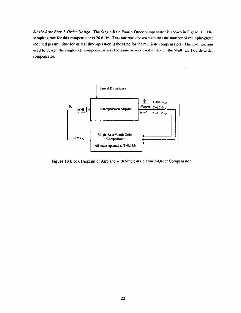
Single-Rate Fourth-Order Design The Single-Rate Fourth-Order compensator is shown in Figure I 0. The
sampling rate for this compensator is 28.6 Hz. That rate was chosen such that the number of multiplications
required per unit time for its real time operation is the same for the muhirate compensators. The cost function
used to design the single-rate compensator was the same as was used to design the Muhirate Fourth-Order
compensator.
T=0.035s
l.,ateral Disturbance
Uncompensated Airplane
Single-Rate Fom'th-(hderCompensator
All sates updated at T=O.O35s
T=0.035s/,_
Nynose T--0.035s/_
Nyaft T--O.035s/_]
Figure 10 Block Diagram of Airplane with Single-Rate Fourth-Order Compensator
22

5
4.5
4
3.5 •
3ft 2
2.5
2
1.5
JO.5
o - _ .... ,,,,. -_0 1 2 3 4 5 6 7 8 9 10
Hz
Figure lla PSD of Nynose for Airplane with Sampled-Data Compensators forGust Pulse Lateral Disturbance
ft 2
se'Y_Oc
5
4.5
4
3.5
3
2.5
Single-Rale Yaw-Damper Only...... Multirate Fourth-Order
........ Single-Rate Fourth-Order
2
1.5
0.5
O _.t.
0 1 2 3 4 6 75 8 9Hz
10
Figure IIb PSD of Nyaft for Airplane with Sampled-Data Compensators for GustPulse Lateral Disturbance
23

Qajn and Phase Margin.5 .for Sampled-Data Desiim_;
Gain and phase margins at the control input (St) were evaluated for the Muhirate Fourth-Order and Single-Rate
Fourth-Order compensators using the robusmess analysis methods of Section IV. Table 3 summarizes the
traditional gain and phase margins for the these compensators. Figure 12 shows the region of guarantecd
stability for simultaneous changes in k and 0 for both compensators.
Table 3 Traditional Gain and Phase Margins
Design
Mulrirate Fourth-Order
Single-Rate Fourth-Order
Gain Margin (db) [0 = Ol
[-3.8, 7.11[-3.3, 5.51
Phase Margin (Deg) [k = 0db]
+ 32"+ 27"
t:D
40
35
30
25
20
15
10
5
0
System with Multlrate Comp_satot isstable fo_ Gain and Phase combinations
ms,de....th,s teg,on _ Sysmm with Single Raw Equivalent
ns in,tide this region
I , I t
-4 -2 0 2 4 6 8 10
Gain k in db
Figure 12 Stability Region for Simultaneous Gain and Phase Uncertainty for Fourth-Order Sampled-Data Compensators
24

Conclusions
Figures 8 and 11 show that the yaw-damper/modal suppression systems significantly decrease the covariance
of the lateral acceleration at the nose and aft of the airplane while attaining the desired 0.6 dutch-roll damping.
It should be no surprise that the analog compensators out performed the sampled-data compensators because
the sampled-data compensators were designed using a slow sampling rate. Still, both fourth-order sampled-
data compensators reduce the peak accelerations of Nynose and Nyaft by 175% and 50% respectively over the
yaw-damper only systems. The performance of the Single-Rate Fourth-Order compensator is nearly as good
as that of the multirate compensator, but, for input gain and phase uncertainty, the multirate compensator is
more robust than the single-rate compensator.
VII. SUMMARY AND CONCLUSIONS
In this report we have presented a methodology for designing multirate control systems. We have introduced
the Generalized Multirate Control Law Structure (GMCLS) which allows complete flexibility with regard to
the dynamic order and structure of the control law, and with regard to the sampling rates for all sensors and the
update rates for all processor states and actuators. We have presented two parameter optimization multirate
control law synthesis algorithms, one based on an infinite-time cost function and the other based on a finite-
time cost function, which can be used to find optimum values for the GMCLS parameters. We have presented
a technique for determining gain and phase margins for multirate systems. Finally, we have demonstrated our
methodology by applying it to the design of a two link robot arm control system and to the design of a
combination yaw-damper and modal suppression system for a commercial aircraft. The application to the
aircraft control problem, in particular, demonstrates that the methodology can be applied to design problems of
a scale that one might expect to encounter in practice.
VIII. SUGGESTIONS FOR FUTURE RESEARCH
The results presented here demonstrate a methodology for multirate digital control system design that is
applicable to practical problems. Before this methodology can be routinely applied in practice, however, the
following need to be developed:
1. A means for direcdy synthesizing robust multirate control laws.
2. Numerical optimization algorithms incorporating auto-scaling of the independent variables and other
features that more effectively deal with the practical difficulties of parameter optimization applied to
multirate control law synthesis.
With regard to direct synthesis for robustness, there are several possibilities. One would add the multiple-
plant-condition design for robustness ideas of Ly [ 10]-[ 11 ]. A second would add direct nonlinear robustness
constraints on the control law parameters during the numerical optimization. The latter approach has been
25

successfullyappliedby Mukhopadhyay[4] to synthesizerobustsingle-ratecontrollawsby parameteroptimization.
Inadditiontotheoreticalwork,asecondmajorresearcheffortinmuluratecontrolneedstobedirected lo_ard
experimental research. Now that a bonafide multirate control system design methodology has been developed,
we strongly believe that further substantive progress in the field can best bc made in conjunction with bonafide
hardware applications of that methodology in the laboratory.
REFERENCES
1. Berg, M.C., Mason, G.S., and Yang, G.S., "A New Muitirate Sampled-Data Control Law Structure
and Synthesis Algorithm," to be presented at the 1991 American Control Conference. Preprint in
Appendix A.
2. Berg, M.C., Amit N. and Powell J.D., "Multirate Digital Control system Design," IEEE Trans Auto
Contr., Vol AC-33, Dec 1988, pp.1139-1150.
3. Glasson, D.P., "A New Technique for Multirate digital control Design and Sample Rate Selection,"
AIAA Jour. GUM., Contr and Dynamics, Vol. 5, Aug 1982, pp. 379-382.
4. Mukhopadhyay, V., "Digital Robust Control Law Synthesis Using Constrained Optimization," A1AA
Jour. Guid., Contr. and Dynamics, Vol. 12, March-April 1989, pp. 175-181.
5. Mason, G.S. and Berg, M.C., "Reduced Order Multirate Compensator Synthesis," to be presented at
the 1991 American Control Conference and accepted for publication in the A/AA Jour. Guid., Contr.
and Dynamics. Preprint in Appendix B.
6. Mason, G.S., and Berg, M.C., "Robustness Analysis of Multirateand PeriodicallyTime Varying
Systems with Structured and Unstructured Uncertainty." to be presented at the 1991 AIAA Guidance
and Control Conference. Preprint in Appendix C.
7. Meyer, R.A., and Burrus, C.S., "A Unified Analysis of Multirate and Periodically Time-Varying
Digital Filters," IEEE Trans. Circuits in Systems, Vol. CAS-22, No. 3, March 1975, pp. 162-108.
8. Khargonekar, P.P, Poolla, K., and Tannenbaum, A., "Robust Control of Linear Time-lnvariant Plants
Using Periodic Compensation," IEEE Trans. Auto. Contr., Vol. AC-30, No. !1, Nov 1985, pp1088-1096
9. Kono, M., "Eigenvalue Assignment in Linear Periodic Discrete-Time Systems," Int. J. Control, Vol.
32, No. 1, 1980, pp. 149-158.
10. Franklin, G.F., Powell, J. David, and Workman, M.L., Digital Contol of Dynamic Systems,
Addison-Wesley Pub. Co. 1990.
1 1. Ly, U.L., "A Design Algorithm for Robust Low-Order Controllers." PhD Thesis, Stanford Univ.,
Stanford, CA, 1982.
12. Ly, U.L., "Robust Control Design Using Nonlinear Constrained Optimization," Proc. Amer. Contr
Con_., San Diego, CA, May 1990, pp. 968-969.
26

APPENDIX A
PREPRINT OF REFERENCE 1
27

Submitted to the AIAA Journal of Guidance, Control and Dynamics
A NEW MULTIRATE SAMPLED-DATA CONTROL LAW STRUCTURE
ANI_ SYNTHESIS ALGORITHM
Martin C.BergAssistant Professor
Mechanical Engineering Department, FU-10
University of Washington, Seattle, Washington, 98195
Telephone: 206-543-5288
Gregory S. MasonGraduate Student
Mechanical Engineering Department, FU-10
University of Washington, Seattle, Washington, 98195
Telephone: 206-685-2429
Gen-Sheng YangAssociate Scientist
Chung-Shan Institute of Science and TechnologyP.O. Box 90008-15-15
Lung-Tan, Tao-YuanTaiwan, R.O.C.
Telephone: 886-2-712-8529
ABSTRACT
A new multirate sampled-data control law structure is defined and a new parameter-optimization-
based synthesis algorithm for that structure is introduced. The synthesis algorithm can be applied
to multirate, multiple-input multiple-output, sampled-data control laws having a prescribed
dynamic order and structure, and apriori-specified sampling/update rates for all sensors, processor
states, and control inputs. The synthesis algorithm is applied to design two-input, two-output tip
position controllers of various dynamic orders for a sixth-order, two-link robot arm model.
KEY WORDS
Control, Multirate, Sampled-Data, Digital, Synthesis
RESEARCH SUPPORTED BY
NASA Langley Research Grant NAG-l-1055The Government of Taiwan
['REFERRED ADDRESS FOR CORRESPONDENCE
Martin C. Berg
Mechanical Engineering Department, FU-10
University of Washington
Seattle, Washington 98195
Telephone: 206-543-5288
28

I. INTRODUCTION
Evenin this age of fast, low-cost microprocessors there remain several important motivati(ms
for multirate sampling in sampled-data control systems. One need only consider large space
structure control problems to realize that the cost, bulk, and weight of real-time computing
hardware continues to be an important control system design issue. Multirate sampling provides
the opportunity to allocate sampling rates, and thus real-time computing power, more efficiently.
In two-time-scale control problems, for example, multirate sampling allows slow sampling in
control loops associated with low-bandwidth control functions to be traded for fast sampling in
those associated wilh high-bandwidth control functions.
As with microproces_)rs, the costs of analog-to-digital and digital-to-analog converters are also
computation-rate dependent. Multirate sampling thus provides another opportunity to reduce
hardware costs because the computation rates required of analog-to-digital and digital-to-analog
converters frequently depend upon their sampling rates. Multirate sampling can even be used to
reduce the total number analog-to-digital and/or digital-to-analog converters required by a system,
by sample-dependent scheduling of multiple conversion tasks to a lesser number of conversion
devices.
A third "motivation" for multirate sampling is becoming increasingly important: sometimes
multirate sampling is the only choice. This situation can arise when an apriori decision has been
made to include in a system a sensor that provides a discrete-time signal at a fixed sampling rate. A
head position control system for a computer disk drive is a good example of such a system. The
disk head, which is suspended atop the rotating disk, includes a sensor that reads the head position
directly from certain diametrically-spaced segments on the disk. The sensor's sampling rate is thus
fixed by the disk's rotation speed. To increase the control bandwidth beyond that dictated by that
sampling rate, a second, faster-rate sensor must be added.
A key point often ignored by developers of multirate control law synthesis methods is that
these motivations for multirate sampling dictate also certain flexibilities required to meet the needs
of engineering practice. Specifically, muitirate control law synthesis methods, to meet the needs of
engineering practice, must allow the sampling rates for all sensors, the update rates for all processor
29

states,and the update rates for all actuators to be specified independently. The one generally
accepted restriction, with regard to these rates, is that the ratio of all combinations of sampling and
update rates must be rational, so that the complete sampling/update schedule will always be
periodic. (We assume that all sampling and update events are synchronized to the same clock.
The asynchronous case is treated elsewhere [1 ]3
Time lines representing such a periodic sampling schedule are shown in Fig. 1. We define the
Basic Time Period (BTP) of such a schedule as the least common multiple of all of its sampling and
update periods. The BTP is the period of repetition of the sampling/update schedule. We define
the Shortest Time Period (STP) as the greatest common divisor of all of its sampling and update
periods. We reserve the symbol P to represent the (integer) number of STP's per BTP, and we shall
frequently use a double-indexing scheme for the independent variable so that, for example, x(m,n)
represents x at start of the (n+l)th STP of the (m+l)th BTP, for m = 0,1 ..... and n = 0 ..... P - 1.
There are five well-recognized methods for synthesizing multirate sampled-data control laws:
successive loop closures, pole placement, the singular perturbation method, the LQG (linear
quadratic Gaussian) method, and parameter optimization methods. Successive loop closures [2] is
arguably the most important because it is the single one of the five that is widely used in industry.
The advantages of successive loop closures are that its one-loop-at-a-time approach requires no
new multirate synthesis techniques, and that the sampling/update rate for each control loop can be
specified independently. The problem with successive loop closures is that its one-loop-at-a-time
approach cannot fully account for all dynamic coupling between control loops.
Pole placement [3,4,5,6,7] for multirate systems has received considerable recent attention in the
wake of reports on the capacity for periodically time-varying output feedback controllers to place
closed-loop poles. In Ref. 3, for example, it is shown that given any controllable and observable
continuous-time plant with m inputs, it is always possible to construct a periodically time-varying,
pure-gain, output feedback control law that places the closed-loop poles arbitrarily, provided that
the outputs are all sampled at a suitably chosen single sampling rate l/T 0, and that the inputs are
updated at the rates NI/T o, ..., Nm/T o, where the N i are certain positive integers.
3O

Theproblemwith poleplacementfor multiratesystemsis the same as with pole placement for
single-rate systems: how to determine where the closed-loop poles should be placed? It is a
particularly difficult problem in the multirate case because multirate systems are periodically time
varying [2,8]. The periodicity of multirate systems implies that their eigenstructure can only be
defined based on their (time-invariant) BTP-to-BTP dynamics. Determining desirable closed-loop
poles for a multirate system is typically difficult because the BTP of a multirate system is typically
much longer than the characteristic times of many of its faster dynamics.
Singular perturbation control law synthesis methods [9,10,11,12,13,14,15] were first developed
for continuous-time control systems to take advantage of the multiple-time-scale dynamics that
often occur in control systems. It would seem that an extension to multirate sampled-data systems
should follow naturally, given that a principal motivation for multirate sampling has always been
to take advantage of those same multiple time scales, but that has not been the case in practice.
The problem is the singular perturbation method's inherant dependence on a coordinate
transformation to separate the full control law synthesis problem into two (or more) dynamically
decoupled control law synthesis problems of different time scales. Such a coordinate
transformation is the first step in control law synthesis by the singular perturbation method. The
state coordinates are easily decoupled because they represent only the plant's internal dynamics.
The input and ouput coordinates cannot be so manipulated because they represent the plant's
external sensor and actuator signals. Consequently, during the second control law synthesis step,
when the control laws for the different-time-scale state vector components are synthesized
separately, every control input vector element and every sensor ouput vector element remains
coupled to every state coordinate so that, just as with successive loop closures, all dynamic coupling
between control loops cannot be accounted for.
Various schemes have been developed to circumvent this difficulty. None have been
completely successful, in Ref. 13, for example, a state feedback control law is synthesized by the
singular perturbation method, and the lack of a completely decoupling transformation gives rise to
a requirement for the slow component of the plant state vector to be estimated between slow-
sampler updates, and a requirement for every control input to be updated at every
sampling/update instant.
31

Theadvantageof theLQGmethod[2,16,17,18]for multiratesampled-datacontrollawsynthesis
is that the control laws for all control loops are synthesized simultaneously, taking into account all
dynamic coupling between control loops. The disadvantages are the same as with the LQG method
for continuous-time control law synthesis: that practical performance and stability robustness
objectives are often difficult to achieve via the minimization of a quadratic performance index, and
that the resulting control laws are often unnecessarily complex. LQG control laws are even less
desirable in the multirate as compared to the single-rate case because multirate Kalman filter and
LQR state feedback gains are periodically time-varying [2]. In short, LQG multirate sampled-data
control laws can provide a useful benchmark for performance comparisions, but they are not
practical for applications.
Parameter optimization methods [2,19] for multirate sampled-data control law synthesis
combine the principal advantages of the LQG and successive loop closures synthesis methods. They
allow the synthesis of muitirate sampled-data control laws of practical structure, and
simultaneously account for all dynamic coupling between control loops. The typical parameter
optimization method requires that the control law structure and its parameters to be optimized be
prescribed. A numerical search is used to determine values for those parameters such that a
performance index is minimized, possibly subject to constraints on those parameters. The
disadvantage of parameter optimization methods is that they inevitably require a numerical search
to determine the control law parameters.
A new parameter optimization method for synthesizing multirate sampled-data control laws is
described in Sec. Ill of this paper. It is the second generation of the method described in Refs. 2 and
20. Unlike its predecessor, which accomodates only partial state feedback control laws, this new
method accomodates a general, dynamic, multiple-input multiple-output control law structure.
This new control lawstructure is described in Sec. II of this paper. Section IV describes an
application of this new method to a design problem involving a two-link robot arm model.
Conclusions are given in Sec. V.
32

II. CONTROL LAW STRUCTURE
This ,section describes the multirate sampled-data control law structure in Fig. 2. In Fig. 2, _, is
the noise-free, continuous-time sensor signal, v is the discrete-time sensor noise signal, and _ is
the continuous-time control signal. The one sampler in Fig. 2 operates at the sampling rate l/T,
where T is the STP of the system's complete sampling/update schedule. The Delay blocks are one-
STP delays. The ZOH block is a zero-order hold.
The sensor sample-and-hold dynamics are represented by
_(m,n+l) = II - Sy(n)l _(m,n) + Sy(n) y(m,n) (1)
where y is the sensor signal hold state vector. The matrix Sy(n) is the sensor switching matrix for
the (n+ l)th STP. We define a switching matrix as a diagonal matrix with l or 0 at every diagonal
position. If the ith diagonal element of Sy(n) is 1, the continuous-time signal from the ith sensor is
sampled at the start of the (n+ l)th STP of every BTP and that sampled value is immediately stored
as the ith element of Y; otherwise, the same element of y is held at those instants. The key point is
that y always contains the most recent sampled sensor data.
The processor dynamics are represented by
z(m,n+l) = [I - Sz(n)lz(m,n) + Sz(n) {Az(n) z(m,n)
+ Bz(n) {[1 - Sy(n)]_(m,n) + Sy(n) y(m,n)}} (2)
C,(m,n) = Cz(n) z(m,n)
+ Dz(n) {[l- Sy(n)i ._(m,n) + Sy(n) y(m,n)} (3)
where z is the processor state vector, and fl is the processor output vector. The matrix Sz(n) is the
processor state switching matrix. If the ith diagonal element of Sz(n) is 1, the ith processor state is
updated at the start of the (n+l)th STP of every BTP; otherwise, the same element of z is held at
those instants. The matrices Az(n), Bz(n), Cz(n), and Dz(n) are the processor state model matrices,
33

whose determination constitutes the control law synthesis problem. Note that a nonzero Dz(n)
results in direct feedthrough of sensor data to t_(m,n).
The control signal update-and-hold dyamics are represented by
_(m,n+l) = [I- Su(n)l _(m,n) + Su(n) Cl(m,n) (4)
where _ is the control signal hold state vector. The matrix Su(n) is the control signal switching
matrix. If the ith diagonal element of Su(n) is 1, the ith element of _ is updated at the start of the
(n+ l)th STP of every BTP; otherwise the same element of _ is held at those instants.
Finally, the continuous-time control signal fi is generated by
A
fi(t) = [I -Su(n)] u(m,n) + Su(n) u(m,n) (5)
for all t on [(mP + n)T, (mP + n + I)T).
The advantage of the control law structure of (1) through (5) is that it can be used to represent
virtually any sampled-data control law structure of practical interest. Its form, however, is not
standard. Straightforward algebra, applied to (l) through (5), yields the following more standard
form:
c(m,n+l) = Ac(n) c(m,n) + Bc(n) y(m,n) (6)
u(m,n) = Cc(n) c(m,n) + Dc(n) y(m,n) {7)
where
c(m,n) = Iz(m,n) Li(m,n) _(m,n)l T (8)
34
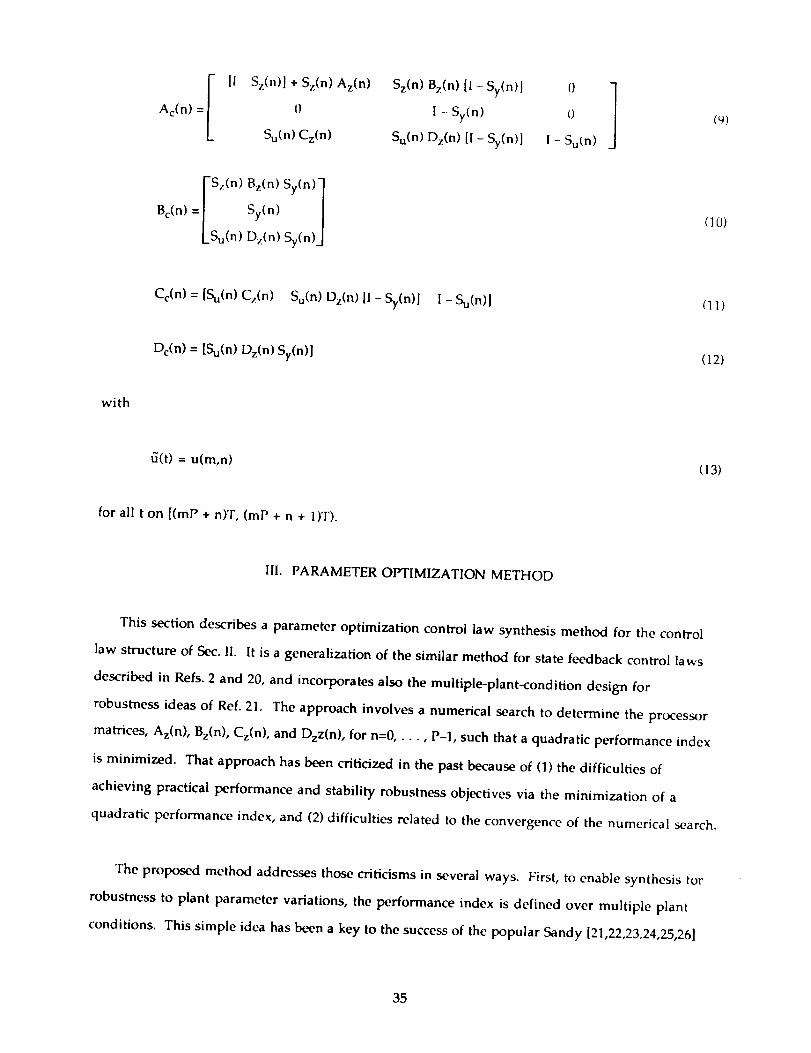
I [I - Sz(n)] + Sz(n) Az(n) Sz(n) Bz(n) [l - Sy(n)] 0 ]]Ac(n ) = 0 l - Sy(n) 0
Su(n) Cz(n) Su(n) Dz(n) [I - Sy(n)] I - Sutn)
(9)
Sz(n) Bz(n) Sy(n)]Bc(n ) = Sy(n) //
LS_(n) Dgn) Sy(n)]
(10)
Cc(n) = {Su(n) Cz(n) Su(n) Dz(n) [I - Sy(n)l I - Su(n)l (11)
De(n) = ISu(n) Dz(n) Sy(n)l (12)
with
_(t) = u(m,n) (13)
for all t on [(mP + n)T, (mP + n + I)T).
III. PARAMETER OPTIMIZATION METHOD
This section describes a parameter optimization control law synthesis method for the control
law structure of Sec. II. It is a generalization of the similar method for state feedback control laws
described in Refs. 2 and 20, and incorporates also the multiple-plant-condition design for
robustness ideas of Ref. 21. The approach involves a numerical search to determine the processor
matrices, Az(n), Bz(n), Cz(n), and Dzz(n), for n=0 ..... P-I, such that a quadratic performance index
is minimized. That approach has been criticized in the past because of (1) the difficulties of
achieving practical performance and stability robustness objectives via the minimization of a
quadratic performance index, and (2) difficulties related to the convergence of the numerical search.
The proposed method addresses those criticisms in several ways. First, to enable synthesis for
robustness to plant parameter variations, the performance index is defined over multiple plant
conditions. This simple idea has been a key to the success of the popular Sandy [21,22,23,24,25,26]
35

algorithm for synthesizing robust continuous-time control laws. Second, to improve the
convergence of the numerical search, the performance index and its gradients with respect to the
control law parameters are calculated exactly, at every iteration, using closed-form expressions.
Third, so that a stabilizing initial guess for the control law is not required, and to eliminate
problems with destabilizing control laws encountered during the search, a finite-time performance
index is used. Finally, to lessen the difficulties of achieving practical performance and stability
robustness objectives via the minimization of a quadratic performance index, linear and nonlinear
constraints can be imposed on the control law parameters.
The continuous-time plant dynamics at plant condition i are assumed to be represented by:
- (i):(i) t) ---(i) u(i)(t) :(i) _(i)t_p(i)(t)=Ap p ( +B_ +Upw ,., (14)
_(i)(t ) = _(pi) _)(i)(t) (15)
where _(i) is the plant state vector, 6(i) is the control input vector, _(i) is the sensor output vector,
and @(i) is a stationary, zero mean, gaussian white noise input vector of known power spectral
density.
The performance index is assumed to be
N
Lo L <i (t)Ji=l
(16)
where Np is the number of plant conditions; E is the expected value operator; t t is the final time
and is a multiple of the BTP of the system's complete sampling/update schedule; and (_(i) and _(i)
are the state and control weighting matrices for the ith plant condition and are non-negative
definite matrices.
36

Based upon the description of the continuous-time plant dynamics in (14) and (15), a complete
description of the complete system's sampling/update schedule, the perfL_rmance index in (16), and
the control law in (6) through (13), closed-form expressions for the performance index J and for its
gradients with respect to the processor matrices Az(n), Bz(n), Cz(n), and Dz(n), for n=0 ..... P-l, are
derived in Refs. 19 and 27. Those derivations and the resulting closed-form expressions are
lengthy, and will not be repeated here. The key points are that the resulting expressions are closed-
form, and that the number of computations required for their evaluation is independent of tf. The
single restriction for those expressions to be valid is that the state transition matrix for the BTP-to-
BTP closed-loop system must be diagonalizable [19]. That is not a serious restriction because that
matrix is rarely nondiagonalizable in practice.
Thus far nothing has been said about synthesizing other than periodically time-varying control
laws. To that end, the performance index and gradient derivations in Refs. 19 and 27 assume that
the processor matrices are constrained to satisfy
Bz(n) Az(n) r=O _z(r ) _,z(r)
(17)
with M • [1,..., P}, and with the 0t functions constrained to satisfy
1 ifp=q0c(n,p) ct(n,q) = 0 if p ¢ q (18)
Equations (17) and (18) constrain the number of different ,_ts of prt_'essor matrices to M. The
function (_(r,n) determines which set of processor matrices is active at the (n+ 1)th STP. Equation
(18) guarantees that only one set of processor matrices is active per STP.
Based on the description of the continuous-time plant dynamics in (14) and (15), a complete
description of the complete system's sampling/update schedule, the performance index in (16), the
control law in (6) through (13), the constraint relations in (17) and (18), and the closed-form
expressions l_or the performance index J, and for its gradients with respect to the processor matrices
_,z(r), Bz(r), Cz(r), and I)z(r), for r=0, ..., M-l, in Refs. 19 and 27, we have developed a computer
37

algorithm to numerically determine a set of processor matrices that minimizes J. A numerical
search is used to determine the processor matrices ,_z(r), Bz(r), Cz(r), and Dz(r), for r = 0 ..... M-l,
given an initial guess for those matrices. The NPSOL nonlinear programming algorithm is used
for the numerical search. N_L [28] is a powerful nonlinear programming package with good
convergence properties as a result of its use of exact performance index and gradient evaluations at
every iteration. In addition, NPSOL accomodates linear and/or nonlinear constraints on the
independent variables. This means that linear and/or nonlinear constraints on the control law
parameters can be combined with the usual performance index minimization objectives to achieve
practical performance and stability robustness objectives.
Additional important features of this new synthesis algorithm include automatic discretization
of the continuous-time plant model and of the continuous-time performance index [27]. These are
important design features because they effectively decouple the sampling/update rates selection
problem from the problem of determining a suitable performance index. This means that the
performance index can be determined first, based on a continuous-time design, and that this new
algorithm can then be used to determine a multirate sampled-data design that minimizes the same
performance index.
In summary, the inputs required to apply this new synthesis algorithm are the following:
• A state model description of the continuous-time plant dynamics at each of the Np
plant conditions.
• State and control weighting matrices for the performance index at each of the Np plant
conditions.
• The final time tt for the performance index.
• The power spectral density of the continuous-time white pr(x:ess noise at each of the
Np plant conditions.
• A complete description of the complete system's sampling/update schedule.
38
• The integer M and the ct functions that constrain the periodicity of the processor
matrices via (17) and (18).
• The desired dynamic order and structure for the processor matrices.
• The covariance matrix for the discrete-time sensor noise at each of the Np plant
conditions.
• A complete description of all linear and/or nonlinear constraints to be imposed on the
elements of the processor matrices.
• An initial guess for the processor matrices.
A disadvantage of most parameter optimization control law synthesis methods is that they
require a stabilizing initial guess for the control law. That is not the case with this method because
of its finite-time performance index. The finite time ensures that the performance index and its
gradients will be finite whether or not the closed-loop system is stable. A disadvantage of the finite
time is that a steady-state solution, i.e., for
Jss a-- lim J (19)tf--_
cannot be obtained directly. A steady-state solution is easily obtained, in practice, however, by
choosing a finite time tf that is large compared to the characteristic times of all of the closed-loop
system's poles. Because the number of computations required to evaluate the performance index
and gradient expressions of Refs. 19 and 27 does not depend upon tf, this can be done without
penalty in terms of the computation time for the numerical search.
In practice, because digital computers cannot store arbitrarily large finite numbers, a steady-state
solution usually cannot be obtained by simply initially setting tf to a large value. Instead, it is
usually necessary to complete first (i.e., when the current best guess for the control law parameters
39

is poor) an optimization for a small tf, and to then re-optimize, for larger and larger tf, until t t gets
to be large compared to the characteristic times of all closed-loop poles.
The final key issue regarding this new synthesis algorithm concerns the requirement that the
structure of the processor matrices be specified. The key point is that the imposed structure should
guarantee that the free parameters for the numerical search constitute an independent set with
respect to the control law's input-output dynamics. When the processor dynamics in (2) and (3) are
considered, with the constraints in (17) and (18) in effect, it is straightforward to see that the
complete set of the elements of Az(r), Bz(r), Cz(r) and E)z(r), for r = 0 ..... M-l, do not constitute
such an independent set because, for example, an arbitrary change in one element of Bz(0) can be
compensated for by changes to the elemets of Cz(0), and to the other elements of Bz(0), such that the
processor's input-output dynamics are unchanged.
Thus, additional structure, or, equivalently, additional constraints, must be imposed on the
elements of the processor matrices to guarantee that the free parameters for the numerical search
constitute an independent set with respect to the control iaw's input-output dynamics. In practice,
a suitable set of such constraints can frequently be determined based on "classical" control law
structures (e.g., combinations of lead and lag compensators and notch filters).
More generally structured control law can, of course, also be accomodated. What constitutes an
optimal structure for the processor matrices for the general case is a topic of current research. We
have successfully applied the following structure (shown for the n-is-even case) for the particular
case where the constraints in (17) and (18) are applied with M = l (the time-invariant case):
E °22 I 1Az(O) = block diag { },• - o i -_o i -2(I i
i = 1,..., n/2 (20)
(21)
40

l_z(0 ) = ¢21
Cpl
[)z (0) =[ dlldpl
,]c_
Cpm
(22)
(23)
The appendix shows that the (m+ p)n+ mp o i, ta i, bij, cij and dij parameters of this structure
constitute an independent set with respect to the control law's input-output dynamics (for any
non-trivial sampling/update schedule) provided that no eigenvalues o i + j00i of the processor
dynamics are repeated.
IV. EXAMPLES
This section describes the design of a tip position control system for a planar two-link robot
arra. The robot arm system is shown in Fig. 3. The first link is long and massive, for large-scale
slewing motions. The second is relatively short and lightweight, so that high-bandwidth control of
the arm's tip position can be achieved using a relatively small motor at the second joint. The pin
joint, rotational spring and rotational damper at the midpoint of the first link models flexibility in
that link. The second link is assumed to be rigid. The motor torques T l and T 2 are the control
inputs, and it is assumed that only the joint angle 0 and the tip position 8 are measured. The
linearized dynamical equations for this system for small e - 0 and small _ - e are easily derived.
The spring constant (k) and damping coefficient (b) values (in Fig. 3) were chosen based on that
model to achieve 1 percent damping and a 10 Hz natural frequency for the open-loop vibration
mode.
Figures 4 through 6 show the closed-loop arm responses, based on the linearized arm
dynamics, to a step change in the commanded tip position with nine different control laws. The tip
position (6) responses are shown in Fig. 4. The simultaneous control torque (T 1 and T2) responses
are shown in Figs. 5 and 6. The nine different control laws are briefly described as follows:
41

LQRAnalog:The continuous-time LQR (full-state-feedback) control law that minimizes
tf
J = lim _t _2102 + (pfi)2l + + dttf--} o_
0
(24)
with
[3 = 32 rad -1 (25)
p = 14 rad/m (26)
T2max = 0.00335 N-m (27)
Tlmax/T2max = 8 (28)
The T2ma× value is the T 2 torque that achieves(_ = 2_ rad/sec in I sec with 0(0 --- _(t) = 0 and(_(0) = 0.
The Tlma×/T2ma× value represents a typical ratio of peak motor torques at the respective joints. The
]3 and p values were chosen by trial and error to achieve the closed-loop poles in Table 1. Note that
the ratio of the characteristic frequencies of the rigid-body closed-loop pole pairs is eight; and that
the characteristic frequency of the faster closed-loop rigid-body pole pair is a factor of five less than
the characteristic frequency of the closed-loop vibration mode.
Third-Order Analog Successive Loop Closures: The third-order, continuous-time, successive loop
closures control law in Fig. 7, which consists of a single lead compensator in the 0-to-T 1 loop and
twin, cascaded lead compensators in the 6-to-T 2 loop. The closed-loop poles for this design are in
Table 2. Note that the rigid body and vibration mode closed-loop poles match those of the LQR
Analog design.
Third-Order Multirate Tustin: A multirate sampled-data approximation to the Third-Order
Analog Successive Loop Closures design obtained via Tustin's approximations of the continuous-
time transfer functions in Fig. 7. The sampling/update rates (in samples/updates per second) of the
42

0-to-T1 and 6-to-T 2 loops are eight times the characteristic frequencies (in cycles per second) of the
slow and fast, respectively, rigid body closed-loop pole pairs from the Third-Order Analog
Successive Loop Closures design.
Optimized Third-Order Multirate Tustin: The same as the Third-Order Multirate Tustin design,
but with the lead compensator gain, zero, and pole locations optimized, by the paramether
optimization control law synthesis method of Sec. Ill, to minimize the same performance index as
in the LQR Analog design. To synthesize this control law, continuous-time process noise and
discrete-time sensor noise inputs were added to the robot arm model. The former were taken to be
white noise disturbance torques w! and w2, coincident with the respective control torques, with
E{[Wl(t) [ 4.9x10 -5w2(t) ] [wl('0 w2(_)i } = 0 1.6x10 -5 6(t - z) (29)
where 8 is the Dirac delta function. The latter were taken to be stationary, purely random
sequences, v I and v2, for the 0 and 8 measurements, respectively, with
[vl(m,n)-_ I 8.1x10⁻⁵ 0 1E{ v2(m,n ) j [vl(m,n) v2(m,n)] } = 0 lxl0 -'4 (30)
Multirate Third-Order: The same as the Optimized Third-Order Multirate Tustin design, but using
the third-order, generaliz_._, time-invariant structure in (20) through (23) for the processor
matrices. Just as with the Optimized Third-Order Multirate Tustin design, two of the processor
states are updated at the faster sampling/update rate, and the third is updated at the slower
sampling/update rate.
Multirate Second-Order: The same as the Muitirate Third-Order design, but using the second-
order, generalized, time-invariant structure in (20) through (23) for the processor matrices. One of
the processor states is updated at the faster sampling/update rate, and the other is updated at the
slower sampling/update rate.
43
Multirate First-Order: 'Fhe same as the Multirate Third-Order design, but using the first-order,
generalized, time-invariant structure of (20) through (23) for the processor matrices. The one
processor state is updated at the faster sampling/update rate.
Single-Rate Third Order: The same as the Multirate Third-Order design, but single-rate, with the
single sampling/update rate chosen to yield the same number of real-time computations per unit
time as the Multirate Third-Order design.
Analog Third-Order: The continuous-time equivalent to the Multirate and Single-Rate Third-
Order designs. The processor matrices have the same structure as in the Muitirate and Single-Rate
Third-Order designs. The control law was synthesized using the Sandy algorithm [21] to minimize
the same performance index as in the Multirate and Single-Rate Third-Order designs.
The LQR Analog responses in Figs. 4a, 5a and 6a constitute the optimal responses for the
performance index in (24), assuming full state feedback, no process or sensor noise, and infinitely
fast sampling. The Third-Order Analog Successive Loop Closures responses in the same figures
have low tip position overshoot, but include also a relatively large contribution from the vibration
mode (see especially Figs. 5a and 6a).
The Third-Order Multirate Tustin responses in Figs. 4a, 5a and 6 are unacceptable. This is
somewhat suprising, but not totally unexpected given the (low) factor-of-eight sampling/update
rate-to-characteristic frequency ratio for this design.
The Optimized Third-Order Multirate Tustin responses in Figs. 4a, 5a and 6a are acceptable, and
demonstrate that the parameter optimization control law synthesis algorithm of Sec. llI can be used
to optimize the parameters of classically-structured control laws.
The Multirate Third-Order, Second-Order and First-Order responses in Figs. 4b, 51o and 6b
demonstrate that the same parameter optimization control law synthesis algorithm can be used to
synthesize multirate sampled-data control laws having a prescribed dynamic order and a
prescribed, but general, structure, with apriori specified sampling/update rates for all sensors,
processor states, and control inputs.
44

The Single-Rate Third-Order and Analog Third-Order responses in the same figures put the
multirate responses in perspective. The Single-Rate Third-Order control law is the single-rate
equivalent to the Multirate Third-Order control law because it (1) was synthesized to minimize the
same performance index, using the same process and sensor noise characteristics; and (2) requires
the same number of computations per unit time for real-time operation.
The Analog Third-Order responses in the same figures are the responses that would have been
obtained with the Multirate Third-Order control law and Singe-Rate Third-Order control laws if
sampling and update rates were not an issue, and very fast sampling and update rates were
everywhere used.
V. CONCLUSIONS
With the possible exception of successive loop closures, the multirate sampled-data control law
synthesis methods available today fail to provide the designer with sufficient flexibility to prescribe
sensor sampling rates and processor state and control input update rates. A new parameter-
optimization-based method for synthesizing multirate sampled-data control laws of arbitrary
dynamic order that provides that flexibility is described in this paper. This new method, described
in Sec. III, determines, by numerical optimization, the free parameters of the general purpose
multiple-input, multiple-output, sampled-data control law structure in Fig. 2, to minimize a
quadratic performance index, possibly subject to linear and/or nonlinear constraints on those
parameters. A stabilizing initial guess for the control law is not required because the performance
index is finite-time. To enable the synthesis of robust control laws, the performance index can be
defined over multiple plant conditions.
An application of this new method to the design of a tip position control system for a sixth-
order, two-link robot arm was described. Multirate sampled-data control laws of various dynamic
orders synthesized by various methods were compared to confirm that the new synthesis method
can be used to synthesize multirate sampled-data control laws having a prescribed dynamic order
and structure, with apriori specified sampling/update rates for all sensors, processor states, and
control inputs.
45

REFERENCES
1. Ritchey, V.S. and Franklin, G.F., "A Stability Criterion for Asynchronous Multirate LinearSystems," IEEE Trans. Auto. Contr., Vol. 34, May 1989, pp. 529-535.
2. Berg, M.C., Amit N. and Powell, J.D., "Multirate Digital Control System Design," IEEE Trans.
Auto. Contr., Vol. AC-33, Dec. 1988, pp. 1139-1150.
3. Araki, M. and Hagiwara, T., "Pole Assignment by Muitirate Sampled-Data Output Feedback,"
Int. Jour. Contr., Voi. 44, 1986, pp. 1661-1673.
4. Chammas, A. and Leondes, C, "Pole Assignment by Piecewise Constant Output Feedback," Int.Jour. Contr., Vol. 29, 1979, pp. 31-38.
. Hagiwara, T. and Araki, M, "Design of a Stable State Feedback Controller Based on the
Multirate Sampling of the Plant output," IEEE Trans. Auto. Contr., Vol. 33, Sep. 1988, pp. 812-819.
6. Hernandez, V. and Urbano A., "Pole-Assignment for Discrete-Time Linear Periodic Systems,"
Int. Jour. Contr., Vol. 46, 1987, pp. 687-697.
7. Patel, Y. and Patton, R.J., "A Robust Approach to Multirate Controller Design Using
Eigenstructure Assignment," Proc. Amer. Contr. Conf., San Diego, CA, May 1990, pp. 945-951.
. Araki, M. and Yamamoto, K., "Multivariable Multirate Sampled-Data Systems: State-Space
Description, Transfer Characteristics, and Nyquist Criterion," IEEE Trans. Auto. Contr., Vol.
AC-31, 1986, pp. 145-154.
9. Saksena, V.R., O'Reilly, J. and Kokotovic, P.V., "Singular Perturbations and Time-Scale
Methods in Control Theory: Survey 1976-1983," Automatica, Voi. 20, 1984, pp. 273-293.
10. Calise, A.J., Prasad, J.V.R. and Siciliano, B., "Design of Optimal Output Feedback Compensators
in Two-Time Scale Systems," IEEE Trans. Auto. Contr., Vol. 35, Apr 1990, pp. 488-492.
11. Kando, H. and Iwazumi, T., "Multirate Digital Control Design of an Optimal Regulator via
Singular Perturbation Theory," Int. Jour. Contr., Vol. 44, 1986, pp. 1555-1578.
12. Lennartson, B., "Multirate Sampled-Data Control of Two-Time-Scale Systems," IEEE Trans.Aut. Contr., Vol. 34, 1989, pp. 642-644.
13. Litkouhi, B. and Khalii, H., "Muitirate and Composite Control of Two-Time-Scale Discrete-
Time Systems," IEEE Trans. Aut. Contr., Vol. AC-30, 1985, pp. 645-651.
14. Litkouhi, B. and Khalil, H., "Infinite-Time Regulators for Singularly Perturbed Difference
Equations," Int. Jour. Contr., Vol. 39, 1984, pp. 587-598.
15. Naidu, D.S. and Price, D.B., "Time-scale Synthesis of a Closed-Loop Discrete Optimal Control
System," AIAA Jour. Guid. Contr., Voi. 10, 1987, pp. 417-421.
16. Amit, N., "Optimal Control of Multirate Digital Control Systems," PhD Thesis, Stanford Univ.,Stanford, CA, 1980.
17. Glasson, D.P., "A New Technique for Multirate Digital Control Design and Sample Rate
Selection," AIAA Jour. Guid. Contr., Vol. 5, Aug. 1982, pp. 379-382.
46

18. AI-Rahmani, H.M. and Franklin, G.F., "A New Optimal Muitirate Control of Linear Periodic
and Time-lnvariant Systems," IEEE Trans. Auto. Contr., Vol. 35, Apt 1990, pp. 406-415.
19. Berg, M.C. and Yang, G.S., "A New Algorithm for Multirate Digital Control Law Synthesis,"
Proc. IEEE Conf. Decision Contr., Dec. 1988, Austin, TX, pp. 1685-1690.
20. Berg, M.C., "Design of Multirate Digital Control Systems," PhD Thesis, Stanford Univ.,Stanford, CA, 1986.
21. Ly, U.L., "A Design Algorithm for Robust Low-Order Controllers," PhD Thesis, Stanford Univ.,
Stanford, CA, 1982.
22. Ly, U.L., "Robust Control Design Using Nonlinear Constrained Optimization," Proc. Amer.Contr. Conf., San Diego, CA, May 1990, pp. 968-969.
23. Voth, C.T. and Ly, U.L., "Total Energy Control System Autopilot Design with Constrained
Optimization," Proc. Amer. Contr. Conf., San Diego, CA, May 1990, pp. 1332-1337.
24. Gangsaas, D., Bruce, K.R., Blight, J.D., and Ly, U.L., "Application of Modern Synthesis to
Aircraft Control: Three Case Studies," IEEE Trans. Auto. Contr., Vol. AC-31, Nov. 1986, pp. 995-1014.
25. Bossi, J.A., Jones, R.D. and Ly, U.L., "Multivariable Regulator Design for Robustness and
Performance: A Realistic Example," Proc. Amer. Contr. Conf., Seattle, WA, 1986, pp. 285-288.
26. Ly, U.L., "Optimal Low-Order Flight Critical Pitch Augmentation Control Law for a TransportAirplane," Proc. AIAA Guid. Contr. Conf., 1984, pp. 743-757.
27. Yang, G.S., "A Generalized Synthesis Method for Muitirate Feedback Control Systems," PhD
Thesis, Univ. of Washington, Seattle, WA, 1988.
28. Gill, P.E., Saunders, M.A. and Wright, M.H., "User's Guide for NPSOL," Tech. Rep. SOL 86-2,Dept. Operations Research, Stanford Univ., Stanford, CA, 1986.
47
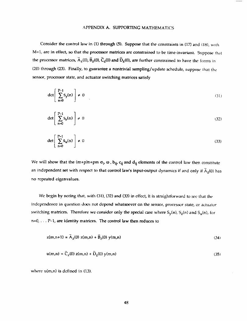
APPENDIX A. SUPPORTING MATHEMATICS
Consider the control law in (1) through (5). Suppose that the constraints in (17) and (18), with
M=l, are in effect, so that the processor matrices are constrained to be time-invariant. Suppose that
the processor matrices, Az(0), Bz(0), Cz(0) and E)z(0), are further constrained to have the forms in
(20) through (23). Finally, to guarantee a nontrivial sampling/update schedule, suppose that the
sensor, processor state, and actuator switching matrices satisfy
I P-1 1det _Sy(n) _ 0n=0
(31)
P-1 ]det _Sz(n) _ 0n=0
02)
I ]det _E_Su(n) _ 0n=0
(33)
We will show that the (m+p)n+pm oi, co, bij, ¢ij and dij elements of the control law then constitute
an independent set with respect to that control law's input-output dynamics if and only if _,z(0) has
no repeated eigenvalues.
We begin by noting that, with (31), (32) and (33) in effect, it is straightforward to see that the
independence in question does not depend whatsoever on the sensor, processor state, or actuator
switching matrices. Therefore we consider only the special case where Sy(n), Sz(n) and Su(n), for
n=0 .... P-l, are identity matrices. The control law then reduces to
z(m,n+l) = _,z(0) z(m,n) + Bz(0) y(m,n) (34)
u(m,n) = Cz(O) z(m,n) + E)z(O) y(m,n) (35)
where u(m,n) is defined in (13).
48

Considerfirst thecontrol law
z(k+l) = A z(k) + By(k) 06)
u(k) =Cz(k) +Dy(k) (37)
where
z= y= u=
P
_38)
I _.i 0 0 1A = 0 "'. 0 (39)
0 0
and B, C and D have the forms in (21) through (23). So that the control iaw's impulse response will
be purely real, the _.i's and the corresponding columns of C and rows of B must be either real, or
must occur in complex-conjugate pairs, and D must be purely real.
Lemma: The (m+p)n+pm _-i, bij, cij, and dij parameters (counting a real element as one parameter,
and a complex conjugate pair of elements as two parameters) of the control law in (36) and (37)
constitute an independent set with respect to that control iaw's input-output dynamics if and only
if _.itkj, for i#j.
Proof: Consider the related control law
z(k+l) = A z(k) + B y(k) (40)
u(k) =Cz(k) (41)
with
49

Cll
Cpl
Cln
Cpn
(42)
Its input-output dynamics are represented by
_I(z) = C (z I-A) -1 B =
i=1
(43)
where Ct is the i th column of (2, and Bi is the ith row of B. The Xi, bij and cij parameters of this
control law are dependent with respect the control law's input-output dynamics if and only if, for
an arbitrary change in one, the others can be changed so that kt(z) is unchanged.
Case 1: No repeated _-i 's.
From (41), for the case of no repeated _.i 's, it is straightforward to see that when one of the gi's is
changed by an arbitrary amount, it will not be possible to change the remaining gi, bij and cij
elements so that _l(z} is unchanged. But when bij is multiplied by a nonzero but otherwise
arbitrary (z, we can multiply the remaining elements of B1by 0b and divide (Zj by (z, so that _I(z) is
unchanged. Thus, the Xi, bij and cij parameters of the control law in (40) and (41) are dependent
with respect to that control law's input-output dynamics.
If, however, one element of every column of C is fixed, as is the case in the C matrix of (22), it is
similarly straightforward to see that it will not be possible to compensate for an arbitrary change in
any Ki, bij or cij element by changing the remaining Ki, btj and cij elements so that _t(z) is
unchanged. Thus, for the case of no repeated Ki's, with one element of every column of C fixed,
the _-i, bij and cij parameters of the control law in (40) and (41) constitute an independent set with
respect to that control law's input-output dynamics.
Case 2: Repeated gi's.
Consider again the control law in (40) and (41), but this time suppose that Xl=_. 2. That control law's
input-output dynamics are represented by
50

Fl(z) = C (z I-A) -1 B = C1B1+C2_ 2CtBiz-x, ÷i=3
(44)
From (42), it is straightforward to see that, with or without one element of every column of C fixed,
the remaining bij and cij elements of C1, BI, C2, and B2 can be changed to compensate for an
arbitrary change in any one element of CI, B1, C2, or B2 so that FI(z) is unchanged. Thus, for the
case of repeated Xi's, with or without one element of every column of C fixed, the ki, bij and cij
parameters of the control law of (40) and (41) are dependent with respect to that control law's input-
output dynamics.
General Case: We conclude that the (m+p)n ki, bij, and cij parameters of the control law in (36) and
(37), with D= 0, constitute an independent set with respect to that control law's input-output
dynamics if and only if _,i#_,j, for i#j. A nonzero D matrix simply adds pm parameters to that set.
Theorem: For the control law in (1) through (5); with the constraints in (17) and (18), with M=I, in
effect, so that the processor matrices are constrained to be time-invariant; with Az(0), Bz(0), C__z(0)
and E)z(0) further constrained to have the forms in (20) through (23); and assuming that the sensor,
processor state, and actuator switching matrices satisfy (31) through (33); the (m+p)n+pm a i, ¢0i, bij,
cij and dij elements of that control law constitute an independent set with respect to that control
law's input-output dynamics if and only if Az(0) has no repeated eigenvalues.
Proof: The control law in (34) and (35) has the same number of free parameters as the control law
in (36) and (37), and the two are related by the similarity transformation x= M z, where
[ oi+jm i 1 ]M = block diag { 2-j_i -O'i+j(0 i -1 , i = 1, .... n/2 } (45)
with (_i = Re(_'i) and 01i = Iml(Xi).
51

Closed-Loop Damping CharactensticPole Ratio Frequency
Rigid Body -1.10 +/1.10 0.71 ().25 Hz
Rigid Body -8.81 +j8.83 0.71 2.0 Hz
Vibration M_.x:le -0.649 +j 62.8 0.01 10 Hz
Table 1 LQR Analog Design Closed-Loop Poles
Closed-Loop Damping CharacteristicPole Ratio Frequency
Rigid Body -1.10+j 1.11 0.71 0.25 Hz
Rigid Body -8.88 +j 8.84 0.71 2.0 Hz
Vibration Mode -1.35 _+j 63.9 0.02 10 Hz
Compensator -10.5 - 1.7 Hz
Compensator -33.2 +j 34.0 0.70 7.6 Hz
Table 2 Third-Order Analog Successive Loop Closures Design Closed-Loop Poles
52

Time Lines for Sampling/Update Activities:
TTime (Seconds) 25T
? ? ? ? ? ? ?0 4T 8T 12T 16T 20T 24T
?0
? ? ? ? ? ? ?3T 6T 9T 12T 15T 1ST 21T 24T
8re qFig. 1 Example Multirate Sampling/Update Schedule
53

l-i
1.4
_J
0
cj
pul
°..I
54

Parameters: Mass Length
L l 0.5 kg 0.5 mL2 0.5 kg 0.5 m
L3 0.04 kg 0.2 m
k = 37.33 N/radb = 0.012 N. s/m
The natural frequency of the vibration mode is 10 hz.
Inputs: Torques Tt and T2
Outputs: 0 and 5
Fig. 3 Two-Link Robot Arm
55

0.25
i ..
0.2 _-
LOR Analog..... Third-Order Analog SuccessiveLoop Closures....... Third-Order Multirate Tusun
...... Optimized Third-Order Multirate Tustin
-F,
0.05
I i I J IO0 0.5 I I. 2 2.5 3
Fig. 4a Tip Position (5) Responses to Tip Position Step Command
0.25
0.2
0.15
:_ O.t
0.05
00
Fig. 4b Tip Position (5) Responses to Tip Position Step Command
56

1.2
I
t ! , ! v _ .
I
II
J* LQR AnalogII
,, ....... Third-Order Analog Successive Loop Closures'* .............. Third-Order Multirate Tustin0.8 Jl
v,j.) ,) , ......... Optimized Third-Order Multirate TustinK. _ 4 r-0.6LX P l_ ,' ,i
I ' ""'I i_iI li
0.4_- ,%", ' ,','i'_i .a _, i _I I I I% l
_.Hi:il_ ' ,,,;,;, ,,,,,-_ 0.2 '\i _ ',' ,,'',;:_!,",,!,
" 0 1 '!i " \ ' • _l _t_lll'.e.., ........... : ........
_ r "i : "_"_i*''v'''';'''''';:;<_--'_---''--_''''-_0.ul_,"d ......: _;-_:"" "i
fI
-0.4 i
-0.60
J I I I I I I I
0.5 1 1.5 2 2.5 3 3.5 4Seconds
Fig. 5a Control Torque T1 Responses to Tip Position Step Command
O
z
1.2
1
0.8
0.6
0.4
0.2
o_
-0.2
-0.4
-0.60
.I.-- I I
m i
f ,',.L.--'.-' . ",,.. il
- N'_ , I
i i s i v | !
Analog Third-OrderMultirate First-OrderMultirate Second-OrderMultirate Third-Order
Single-Rate Third-Order
• _ .f "f._--: ........ .d
i,--. I i
_',_. I I
\'_ "1
....;.-.i',, I _ ,
"--- f'--°l
i, \ .-.=.4.... _jJ
i I I i I I I
0.5 1 1.5 2 2.5 3 3.5
Fig. 5b Control Torque T_ Responses to Tip Position Step Command
4Seconds
57

,2 i | _ ! i ! 1
Z
LQR Analog....... Third-Order Analog Successive Loop Closures.............. Third-Order MuItirate Tustin
......... Optimized Third-Order Multirate Tustin
I I I I I I I
0.5 1 1.5 2 2.5 3 3.5 4Seconds
Fig. 6a Control Torque T2 Responses to Tip Position Step Command
1.2
1
0.8
0.6
0.4
0.2
;" 0
Z -0.2
Analog Third-OrderMultirate First-orderMultirate Second-OrderMultirate Third-Order
Single-Rate Third-Order
I l I I I I I
0.5 1 1.5 2 2.5 3 3.5
Fig. 6b Control Torque/'2 Responses to Tip Position Step Command
4Seconds
58

O,ef +_ 9.3(s+l)s+13
Fig. 7 Third-Order Analog Successive Loop Closures Design
59

APPENDIX B
REPRINT OF REFERENCE 5
60

Reduced Order Multirate Compensator Synthesis
Gregory S. Mason* and Marlin C. Berg**
University of Washington
ABSTRACT
A method for synthesizing reduced order muhirate compensators is presented. Necessary conditions for
which the compensator parameter values minimize an infinite time quadratic cost function are dcrived. An
algorithm for finding compensator parameter values which satisfy the necessary conditions is described. This
algorithm is then used to design several tip position controllers for a two link robot arm.
INTRODUCTION
In many cases a multirate compensator can provide better performance than a single rate compensator
requiring the same number of real-time computations. Berg, for example, was able to reduce the steady state
RMS response of states and controls to a disturbance for a simple mass-spring-mass system nearly 20% by
using a muhirate compensator over a single rate compensator [1]. Numerous other examples have been
provided in the literature by Berg [11-[3], Amit [41-[51, and Yang [61. While multirate compensators can
provide improved performance over single rate compensators, they are also, in general, more complicated to
design.
The complexity of multirate compensators stems from the fact that they are by nature time varying,
periodically time varying for most practical applications. Not only must designers choose multiple
sampling/update rates for the compensator, but they must also determine the parameter values for a time
varying compensator.
One method for designing multirate compensators is multirate LQG [4]. Multirate LQG is the multirate
equivalent of single rate LQG and is straightforward to solve because the equations governing the solution are
similar to those for the single rate case. Multirate LQG, however, results in a full order compensator which
' Graduate StudenL Department of Mechanical Engineering FU-I0, University of Washington. Seattle WA 98195
** AIAA Member, Assistant Professor, Department of Mechanical Engineering FU-10, University of Washington. SeattleWA 98195
61

hasperiodicallytimevaryinggains.Formanyapplicationsfull ordertimevaryingcompensatorsarcnot
practical.
A GeneralizedAlgorithmforMultirateSynthesis(GAMS)[6t was developed by Yang to overcome n_,my
c)f the shortcomings of multirate LQG. Yang's algorithm can synthesize reduced order multirate compensators
with or without time varying gains by using a numerical gradient type search to find optimum compensator
parameter values. His algorithm uses a t'mite time cost function in its problem formulation, unlike muhirate
and single rate LQG which use an infinite time cost function. By using a finite time cost function Yang's
:algorithm eliminates the numerical problem that arises when a destabilizing compensator is encountered during
the numerical search. Even though Yang's algorithm uses a closed form expression for the gradient, the
calculations necessary to perform the gradient-type search are extremely cumbersome.
In this paper we present a new algorithm for synthesizing reduced order multirate compensators with or
without time varying gains. The algorithm utilizes the compensator structure of Yang's algorithm, but the
problem is formulated using an infinite time, instead of a finite time, cost function. This allows us to derive
necessary conditions for which the multirate compensator minimizes the cost function. The equations for the
necessary conditions are fairly simple and can be solved directly using a standard nonlinear equation solver,
eliminating many of the numerical complexities of Yang's algorithm.
THE GENERAL MULTIRATE COMPENSATOR
Before deriving the equations governing a reduced order multirate compensator, we will first present the
structure for a general multirate compensator. We restrict our discussion for now to compensators with time
invariant gains and sampling/update rates whose ratios are rational numbers.
A general multirate compensator is shown in Figure 1. Each input (y), output (u), and state (_') is
sampled/updated at a rate which, in general, represents the desired bandwidth of the input or output with
which it is associated, y is the value ofy currently available to the digital processor from the zero order hold;
while _ is the current output from the digital processor which is held with a zero order hold to form the output
u. When the sampling/update rates have ratios which are rational numbers the sampling/update schedule is
periodically time varying. We define the greatest common divisor of all the sampling/update periods as the
shortest time period (STP) and the least common multiple of all the sampling/update periods as the basic time
period (BTP) (see Figure 2).
62

ThestateequationsforthemultiratecompensatorpicturedinFigure1are:
[l-s,,k]+sz.kY
= 0
I Su,k C
sz._t-sy_] o
ft-sy_] o -i } sz.kBsy.k"y 4" S y ,k
"_ k s,.kOs_.k
Yk (1_
u,:[su,iC su.kLi[l-s,.k] [l-su,_]] y +[su.kDsy,k!yk
_k
¢2)
is a hold state used to model the sampler and zero order hold between _ and u. Sy.k, sz, k, and su, k are
switching matrices for y, 2", and u respectively that model the system's sampling/update activity at the start of
the kth STP. s.,k has the form:
I r I 0 0 --- 0
0 r2 0 --- 0
S,,k =
0 ... 0 r,n..l 0
0 ... 0 0 rm.
where1 if the jth ,,.,, (y, y, or u) is sampled/updatedrj= at the start of the k th STP0 otherwise
mz = the number of states (z-")
my = the number of inputs (y)
m u = the number of outputs (u)
A more complete discussion of this compensator structure can be found in [6]-[7].
Equations (1) and (2) can be written more compactly as:
Zk+ 1 = AkZk + Bky k
uk = Ckz k + DfYI_
(3)
(4)
63
where zk- _"
Equations (3) and (4) form a single rate periodically time varying system with a sampling rate of one STP
and a period of one BTP. If N=BTP/STP, then A k = Ak+N, B k = Bk+ N, C k = Ck+N, and D k = Dk+ N.
Even though A t, B k, Ck and D k are periodically time varying, the muhirate compensator gains, 7[, B. C,
and D, are time invariant. The periodicity of the multirate compensator is due to multirate sampling/updating,
not the compensator gains. In the remainder of this section we will demonstrate how the time invariant
compensator gains, 7[, B, C, and/), can be separated from the periodic compensator matrices A k, B k, C k and
D k •
Define the composite compensator matrix as
ptt=[ Dk Ck ] (5)Bk Ak
and factor Pk as follows:
where
Pk =SIt, PS2k + S3k (6)
(7)
suat 0
0 Sz.kS tJ, = 0 0
s u,]c 0
(8)
Sv'=[ s_j'o 0 l-sy,k 0]/ 0 0 _9)
S3k =
0 0 0 i-su.k
0 l-sz)t 0 0
sy.k 0 l-syjx 0
0 0 0 l-s,,_
(10)
Equation (6) is a key result. It allows us to factor the time invariant compensator gains, the unknown
parameters we will solve for in the next section, out of the time varying compensator.
It is important to note the difference between Pk and P in (6). Pk (with a subscript) is a periodically time
varying matrix defined by (5). It includes all the information about the compensator gains and the
64

sampling/update schedule. P is a constant matrix which contains only the gains for the compensator. Pk can
be written in terms of P and Slk, S2k, and S3k using equation (6). Stk, S2k, and S3k are periodically time
varying matrices which contain a description of the sampling/update scheme.
DERIVATION OF THE NECESSARY CONDITIONS
In this section we will use the results of the previous section to derive the necessary conditions for the
reduced order multirate compensator. The multirate problem to be solved is as follows:
Given: the discrefized plant model
= + (12)
where F, G, 1_ and/4 are obtained by discretizing the analog plant matrices at one STP; w k and vie are
discrete-time Gaussian white noise inputs; _ is the control input from the compensator, and _ is the sampled
sensor output.
Find: the multirate control law with a prescribed dynamic order and sampling schedule, of the form of (1)-
(2), which minimizes a quadratic cost function of the form:
(13)
where E is the expected value operator, and the summation from ! to N accounts for the fact that the closed
loop system is periodically time varying. A prescribed sampling schedule implies that the values of st, k, sy.k,
and Su,k are known.
Using (3)-(4) it is easy to see that this problem is essentially a time varying feedback problem - a time
invariant plant with a periodically time varying compensator. One thing that makes this problem difficult is
that the compensator has an explicit form, that of (1)-(2), in which only certain parameters, 2[, B-, C, and/5,
can he adjusted to minimize J.
65
To solve the multirate control problem we cast it into output feedback form and follow a derivation similar
to Mukhopadhyay's for the single rate case [8]-[9]. Using (3)-(4), and (11)-(12) we write the output feedback
equations:
(14)
1///_, o _ +[oo v,}t zt 1 J/zi /
(15)
/I Zk+ I = Bk Ak Zk
(16)
Equations (14)-(16) can be written more compactly as
xk+ I = Fx k + Gu k + WOk (I7)
Yk = Hxk + Vrlk (18)
uk = P/dk (19)
It is important to keep in mind that Pk in equation (19) corresponds to the P_ in equation (5), a periodically
time varying matrix which contains all the information about the muhirate compensator gains and
sampling/update rates.
The closed loop system is
where
Xk+l = FckXk + Gckrlk (20)
Fck = F + GPkH (21)
Gck = W + GPkH (22)
The state covariance propagation for this system obeys:
Xk+ t = FckXiFTck + GckRGTk (23)
66

where
Equations (20)-(22) represent a periodically time varying system with a period of one BTP. We can
generate a single rate system by repeated application of equation (20) over one BTP [10]. The single rate
system can be written as
where
Xk+N= Fbkxk+ Gbkrlbk (24)
Fbk= F_k÷N-I>F_k+N-2)F_k+#-3)''-F_k
Gbk = [Fc(k+N.DFc(k+Iv-2)'".Fc(k+t)GckI
Fcfk+N-l)Fc(k+N-2)"-Fcfk+2)Gc(k+1)I "'" IG_k+N-l)]
(25)
(26)
Tlk
Ok+ 1rib k =
r_k+t¢.!
This single rate system has exactly the same values for x as the periodically time varying closed loop
system at each BTP. However, the values ofx at the intermediate STP's are lost because x is incremented by
N in (24) but only by 1 in (20). There are N such single rate systems associated with (20). They can be
written as:
xk+t¢+i= Fb_k+OXk+i+ G_k+_)rlk+i for i=l,2...,N (27)
If Fbk is stable, then the periodically time varying system (20) is stable [11]. We can calculate the steady
state covariance for x using the following Lyapunov equations:
Xk = FbkXkFTk + GbkRbGTbk for k=1,2 ..... N (28)
R.0.--0
Rb= 0 R...0• ".. "
O00R
67

Note that X_ is periodic, that is it varies within one BTP, but from BTP to BTP ,k"k = Xk+ N. Once we
have calculated X k at any k using (28), we can use (23) to propagate it over the BTP. This eliminates the need
to solve equation (28) N times.
Now, using (23), (13), and the properties of the Trace (Tr) operator we can write the cost function for the
stabilized system as (see 181-191)
N
J = _., Tr{[Q, + MPJ4 + {MPkH) T + (PkHJTQ2PkH]Xk + (P_VIrQzPkVR}k=l
(29)
Adjoin the covariance constraints (23) to the costJ using Lagrange multipliers, Ak, to obtain:N
J= Y_ Tr{[Q1 + MPkH +(MPkH} r +{VkHJrQzVk1-l]Xk +{PkV)rQ2PkVRk=l
T T+ ATl[FckXkFck + GckRGck-Xk+i]}
with X 1 = XN+ 1.
Necessary conditions for minimum J are
(30)
In addition,
by=0, 3] -0, and -_ =0
3Xk 3Ak+ t 3P
-- must be positive definite for a minimum J._2
Substituting (30) into (31) and replacing Pk with P/t---SI_'S2k+S3k from (6) we obtain:
(31)
3J = 0 Q, + MPkH + {MPkH} T + (PkH}TQ2pkH r= + FcA,Ak+lFcIc - Ak0Xk
for k=l,2 .... ,N with A k = Ak+ N
(32)
fork= 1,2 .... .N withX k=Xk+ N
(33)
3P _= t
+[ M r +G l"Ak+ IFIxkH T}S fk
(34)
68

Equations (32)-(34) are a set of coupled matrix equations. They make up necessary conditions for P,
which is comprised of the multirate compensator gain matrices _, B, C, and 17, in equation (1)-(2_, to
minimize the cost function J. Values of2[, B, C, and D, found by solving (32)-(34) can be substituted into
(1)-(2), along with the definition of the sampling schedule, Sz,k, Su,k, and Sy,k, to form the complete time
varying multirate compensator.
To ensure that the compensator gains satisfying (32)-(34) minimize J, we should also check that the
Hessian of ] with respect to P is positive definite. Our present algorithm does not calculate the Hessian
cxplicitly, but uses an approximate value calculated by the numerical search algorithm discussed in the next
_ction.
Equations (32)-(34) were derived assuming time invariant compensator gains. We can easily derive the
corresponding equations for periodically time varying gains. Let
A =Ak, B = Bk, C =Ct, andD =Dk (35)
with the restriction that A--k÷u= Ak, Ok+,v= Bk, Ck+u = C--t,and Dk+_"-- D--k
Defme the composite periodically dine varying compensator matrix:
(36)
qhen replace P with Pk in (30) and differentiate with respect to Pk to obtain
a/--=-:o: sh t[Q +o'A,+to]e,[nx,nT+vR:]3Pk
+[Mr+GrAk.tF]X_Hr}S_k for k = 1,2,...N
(37)
Thus for every new set of compensator gains we obtain one new equation of the form of (37).
Equations (32)-(34) are very similar to the single rate equations. In fact, if we set Slk, S2k and S3k so
they correspond to a single rate system, and N=I, we obtain the exact results derived by Mukhopadhyay for
the single rate case 181.
69
IMPLEMENTATION
In order to find a reduced order multirate compensator that minimizes the cost function J, we need to solve
(32)-(34) for the compensator gains P. A flow chart of the algorithm used to determine the compensator gains
is shown in Figure 3. Using the prescribed sampling schedule the algorithm first discretizes the analog plant
model, analog cost function, and analog process noise model. See [2] for a discussion of the relevant
discretization procedures. Equations (32)-(34) are then solved for the compensator gains using a gradient type
search in MATLAB [12]. We chose a gradient type search to solve (32)-(34) because it allows us to easily add
constraints on the parameters values - simple equality constraints were used to find the optimized
compensators in the next section. The equations necessary to solve for the Lagrange multipliers are located in
the Appendix, (A.3)--(A.4). To ensure that the solution represents a minimum J, the algorithm checks that the
Hessian of J with respect to the free parameters in P is positive definite at the solution point.
Because (32)-(34) are not valid when the closed loop system is unstable, the algorithm 1) must be
provided with an initial stabilizing compensator, and 2) must result in a stabilizing compensator at every
iteration. From our experience, finding an initial stabilizing compensator is generally not a problem. Many
systems suitable for multi.rate control can be stabilized using successive loop closure with minimal cross
coupling between the control loops. A stabilizing multirate compensator can then be obtained by discretizing
the individual continuous control loops at the desired sampling rates. When there are no constraints on its
structure, a stabilizing compensator can also be obtained using the boot strapping method of Boussard [13]-
[14]. For difficult multirate control problems, where a stabilizing compensator cannot be found using either of
the preceeding two methods, one can always use Yang's algorithm to find a stabilizing compensator and then
to switch to our algorithm to complete the optimization. In our experience Yang's algorithm usually converges
to a stabilizing solution quickly - it is the optimization of the compensator parameters that is time consuming.
To avoid the problem of destabilizing compensators during the iteration process we included a check in the
algorithm which systematically reduces the step size to ensure that the compensator is stabilizing. Because the
gradient of the cost function with respect to the compensator parameters becomes very large near the stability
boundary, the algorithm is always forced away from a destabilizing solution as long as it never steps over the
stability boundary into an unstable region.
Even though our algorithm was programmed as an interpreted Matlab M-File we found that it still
performed better than Yang's algorithm which runs as compiled FORTRAN. The primary difference between
the two algorithms is in the complexity of the expression for the gradient of 2"with respect to the compensator
70

parameters. Calculation of the gradient expression for Yang's problem involves diagonalization of the closed
loop system and evaluation of several matrix equations with nested summations. Compare equations (32)-(34)
with equations (112-115) in [31 to see the difference in the complexity of the two gradient expressions.
Two LINK ROBOT ARM EXAMPLE
We used a math model of a planar two link robot ann (TLA) to demonstrate the capabilities of our
algorithm. This is the same model used by Yang [6], and so we were able to verify our results by direct
comparison. A diagram of the TLA is shown in Figure 4.
The goal of our design was to control the tip position (8) of the arm via a multirate compensator. We used
the following analog cost function and process noise covariance matrices from [6].
[ [0.21 0 0
0 18.5
0 0
0
0X+
0
0o00,0069444]
where x =
wT _io.6o]0.01(39)
We assumed perfect measurement and that plant disturbances enter the system coincident with the control
torques. The sampling/update rates are given in Table 1.
Table 1: Samplin[/Update Rates for TLA
S ample_fl,Jpdate Rate
0 0.225 s
6 0.028125 s
T1 0.225 s
"1"2 0.028125 s
71

Fivedifferentcompensatorsweredesigned: an analog LQR, a muhirate lead/lead, an optimized muhiratc
lead/lead, an optimized multirate general 2ad order, and an optimized single rate general 2nd order. We used a
smooth slep input to 5refand Ore/defined as follows:
8tel(t) Tc = 0.125 sex:Ore1(t)=L1 + L2 '
(40)
and the servo configuration shown in Figure 5 to measure the performance of the different compensators. The
response of the TLA for the five compensators is shown in Figures 6a-6c.
The analog LQR compensator used full state feed back. We provided this compensator as an example of
the response possible using the cost function weighting matrices of (38).
The multirate lead/lead was found using successive loop closures. We designed the control loops in the
discrete domain so that the eigenvalues of the closed loop system matched those we obtained using LQR
transformed to discrete time. This compensator consists of two simple lead loops: one from 8 to T 2 operating
at the fast sampling/update rate, and one from 0 to T 1operating at the slow sampling/update rate.
The final three compensators were synthesized using our new algorithm and the cost weighting matrices
used to design the analog LQR compensator. The optimized multirate lead/lead was found by optimizing the
pole/zero locations and gains of the lead/lead compensator found by successive loop closures.
The optimized multirate general 2nd order compensator uses the same sampling/update scheme as the
lead/lead compensators but has the compensator structure of (41), where aij, bij, cij, and dij are the parameters
_vhich were optimized. This compensator has the maximum number of independent free parameters possible
for a second order system 171.
,_=[ all 0 ] B-=[ 1 b12] C=[ clt cl2] _=[ dll d12] (41)0 a22 b2 ! 1 c21 c22 d21 d22
The optimized single rate general 2nd order compensator is a single rate equivalent of the multirate general
2nd order compensator. It has the same structure as the multirate general 2 'u/order compensator, (41), but uses
a single sampling rate. This sampling rate was chosen such that the number of computations required to
implement either the multirate or single rate compensators during real-time operation are the same.
72

OurresultsarethesameasthoseobtainedusingYang'salgorithm.Theydemonstratehowmultirate
compensatorscanprovidebetterperformancethansinglerate compensators by trading lower bandwtdth
control of the slow modes for higher bandwidth control of the fast modes. In this example we were able to
reduce the tip response over shoot 40% and the peak control torque 25% by using a multirate controller o,,er a
single rate controller.
CONCLUSIONS
In this paper we have presented a new algorithm for synthesizing reduced order multirate compensators. It
can be use to design compensators of arbitrary structure and dynamic order, with independent sampling/update
rates for the compensator inputs, outputs and states. This algorithm provides the versitility of Yang's alorithm
with out the numerical complexities associated with the finite time cost function.
Finally, we do not want to discount Yang's algorithm altogether because, while our algorithm requires an
initial stabilizing compensator, Yang's does not. For those problems where finding an initial stabilizing
compensator is difficult, we can always use Yang's algorithm to find a stabilizing compensator and then
quickly optimize the compensator parameter values with our algorithm.
ACKNOWLEDGMENT
This research was supported by NASA Langley Research Grant NAG-I-1055.
REFERENCES
1 Berg, M.C., Amit N. and Powell J.D., "Multirate Digital Control system Design," IEEE Trans.
Auto. _"onlr., Vol AC-33, Dec 1988, pp.1139-1150.
2 Berg, M.C., "Design of Multirate Digital Control Systems," Ph.D. Thesis, Stanford Univ.,
Stanford, CA, 1986.
3 Berg, M.C., and Yang, G.S., "A New Algorithm for Multirate Digital Control Law Synthesis,"
Proc. IEEE Conf. Decision Contr., Dec 1988, Austin, TX, pp. 1685-1690.
4 Amit, N., "Optimal Control of Multirate Digital Control Systems," Ph.D. Thesis, Dep. Aero. Astro.
Stanford Univ., Stanford, CA, Rep. 523, 1980.
73

5Amit,N., andPowellJ.D.,"OptimalControlof MultirateSystems,"Proc. AIAA Guid. Contr
Cozlf, Albuquerque, NM, 1981.
6 Yang, G.S., "A Generalized Synthesis Method for Multiratc Fccdback Control Systems," Ph.D.
Thesis, Univ. of Washington, Seattle, WA, 1988.
7 Berg, M.C., Mason, G.S., and Yang, G.S., "A New Muitirate Sampled-Data Control Law Structure
and Synthesis Algorithm," 1991 American Control Conference, Boston, MA, June 1991.
8 Mukhopadhyay, V., "Digital Robust Control Law Synthesis Using Constrained Optimization,"
AIAA Jour. Guid., Contr. and Dynamics, Voi. 12, March-April 1989, pp. 175-181.
9 Mukhopadhyay, V., Newsom, J.R., and Abel, I., "A Method for Obtaining Reduced-Order Control
Laws for High-Order Systems Using Optimization," NASA Tech. Paper 1876, August 1981.
10 Meyer, R.A., and Burrus, C.S., "A Unified Analysis of Multirate and Periodically Time-Varying
Digital Filters," IEEE Trans. Circuits in Systems, Vol. CAS-22, No. 3, March 1975, pp. 162-168.
11 Kono, M., "Eigenvalue assignment in Linear Periodic Discrete-Time Systems," Int. J. Control,
Vol. 32, No. 1, 1980, pp. 149-158.
12 Pro-Matlab Users Guide, The Mathworks Inc., 1989.
13 Broussard, J.R., and Halyo, N., "Optimal Multirate Output Feedback," Proceed. 23 rd Conf. Decis.
Contr., Las Vegas NV, Dec 1984, pp. 926-929.
14 Halyo, N., and Broussard, J.R., "A Convergent Algorithm for the Stocastic Infinite-Time Discrete
Optimal Output Feedback Problem," Proceed. Joint Autom. Contr. Conf., Charlottesville VA, 1981, Vol. 1,
Section WA-1E.
74

APPENDIX
Given a Pk which stabilizes the multirate system we can calculate the steady state values of A k where A k is
def'med by equation (32) rewritten here as (A.1).
0 Q! + MPkH + (MPtI'I) r + (PtHfQ2PtJ'I + r= F_tAk+lF_t- Ak
for k=l,2 .... ,N with A k = Ak+ N
(A.O
First simplify (A. 1) by defining
IQ' 1Q3=- Mr {22 PkH
I is an identity mauix
(A.2)
Then (A.I)can be writtenas
Ak=jfQ3yk+ rFetAk+lFct for k=l,2 .... ,N with A t = Ak+ N (A.3)
Equation (A.3) represents a periodically time varying Lyapunov equation. We can create an equivalent
single rate system by repeated application of (A.3).
At = JrkQal_ + F_A.AtFdk for k=l,2 .... ,N with A t ffi Ak+ N (A.4)
Fat = Fc(k+N.l)Fc(k+N.2)Fc(k+N.3)...Fck
Jdk _"
"Y(k+N.I)Fc(t+N-2Fc(k+N-3)... Fck
J(k+/V-2)Fc(t+N-3)'' "Fck
Yk
(A.5)
(A.6)
Qd=[ 0 Q3:
75

Equation (A.4) is a time invariant Lyapunov equation which can be solved for A k. Once any A k has been
found, the propagation equation (A.3) can be used to find the remaining A k.
76
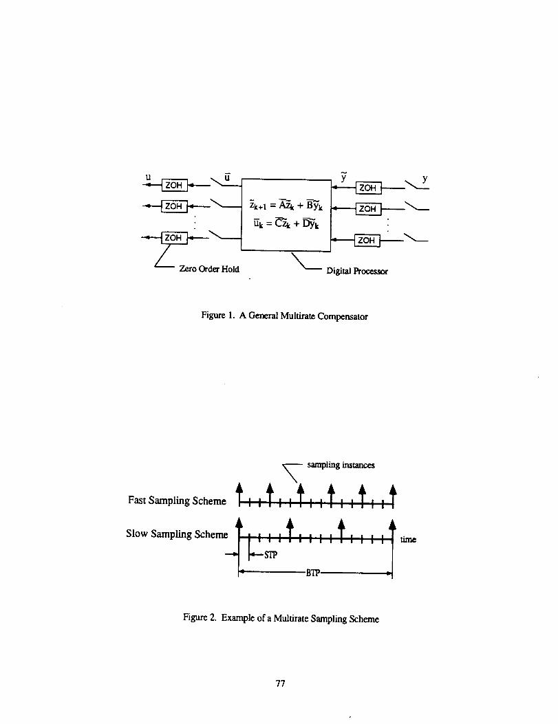
_"- Digital Processor
Figure 1. A General Multirate Compensator
Fast Sampling Scheme
- sampling instances
I!11 I
BTP
Figure 2. Example of a Multirate Sampling Scheme
77

Discretize the analog plant, weighting matrices
and process noise covariance
¢Build the matrices F, G, W, H, V, and P
using (14) - (16)
Get a stabilizing compensator
I Calculate X 1 using (28) then propagateX 1using (23) to obtain X 2, X 3 ..... X N
Calculate AN using (A.4) then propagateA N using (A.3) to obtain AN. I..... A 1
Calculate _- using (34)
Calculate the step direction and length
!
Calculate the next guess for the compensator l
No
No
if the Hessian is not positive [definite notify the user 11
I Optimum compensator matrices 1A, 8, C, and D found
Reduce the
step size
Figure 3. Flow Chart of Optimization Algorithm
78

Parameters: Mass Length
L 1 1.235 kg 0.965 m0.163 kg 0.167 m
Inputs: Torque T 1and T 2
Outputs: 0 and _5
Figure 4. Planar Two Link Robot Arm
ref
Compensator Two Link Arm
Figure 5. TLA Plant/Compensator Configuration
79

0.016
0.014 t
0.012
0.01
_ 0.008
0.006
0.004
0.002
0 o
_ w i i | i i w
i!
,VIilb _ LQR Analog
i!t - ...... Multir_ Lead/Lead by Succ. Loop Closure.']l .............. Optimized Multi.rate Lead/lead.
lit ......... Optimized Multirate General 2 na order
0.2 0.4 0.6 0.8 1 1.2 1.4 1.6 .8
Time (Sea_mi_)
Figure 6a. Tip (8) Response to a Smooth Step Command to Tip Position
80

".3
A
Z
0.25
0.2
0.15
0.1
0.05
0
-0.05
-0.1 -
-0.15 0
i i i ! ! 1
i ." .-7. ; .-? ." .'7 ." .-?" ,I
i |i I
I I
| I
LQR Analog....... Multirate Lead/Lead by Succ. Loop Closure.............. Optimized Multirate Lead/Lead......... Optimized Multirate General 2 "d order................. Optimized Single Rate General 2 nd order
I I
I
t ............. I
I, I I I I I I I
0.2 0.4 0.6 0.8 1 1.2 1.4 1.6 1.8
_tme (Seconds)
Figure 6b. Control Torque T1 Response to a Smooth Step Command to Tip Position
81

0.03.......
0.02 i
|, ._,
oo,
Z
-0.03
-0._-
-0.05 , , i0 0.2 0.4 0.6
! i z
+,+iilift++ii -- LQRAn_og.,.. ....... MulRr_ _ad by Succ.Loop Closure
i ..............Optimized Multiram Lead/l_adi .........Optimized Mulfiram General2noorder
--J Optimized Single Rate General 2 _ order
I I , I
0.8 1 1.2 1.4I
1.6 1.8
Tune (Seconds)
Figure 6c. ControlTorque T2 ResponsetoaSnmoth StepCommand toTipPosition
82

A PPENDIX C
PREPRINT OF REFERENCE 6
83

Draft Version
Robustness Analysis of Multirate and Periodically Time Varying Systems
Gregory S. Mason
Graduate Student
Mechanical Engineering Department, FU-10
University of Washington, Seattle, Washington, 98195
Telephone: 206-685-2429
Martin C. Berg
Assistant Professor
Mechanical Engineering Department, FU-10
University of Washington, Seattle, Washington, 98195
Telephone: 206-543-5288
84

1. INTRODUCTION
There are many established methods for synthesizing multirate compensators [Berg, Yang, Mason,
Glasson, Amit] but surprisingly few methods for analyzing the robustness of these systems. Current
robustness analysis methods rely principally on the transfer function of the system. A muhirate transfer
function, in the traditional sense, ck)es not exist, because most multirate systems are periodically time varying.
Without some modification, established analysis methods cannot be applied directly to multirate systems.
[Thompson] and [Apostolakisl have both proposed ways to extend existing robustness analysis techniques
to multirate systems. Thompson used "Kranc" operators to transform a special class of multirate systems,
derived from sampled continuous systems, into MIMO single rate systems. Apostolakis transformed the
general multirate system into a discrete time single rate MIMO system and then used impulse modulation to
produce a continuous MIMO system [Boykin's]. In both cases, the inputs and outputs of the new MIMO
system were comprised of delayed samples of the inputs and outputs of the multirate system. Thompson and
Apostolakis then used multivariable nyquist criterion and/or unstructured singular value analysis to calculate
the gain and phase margins for the multirate system.
In this paper we will present an alternative approach for extending nyquist criterion and singular value
analysis to multirate and periodically time varying systems. Like Apostolakis, we transform the original
system into an equivalent time invariant single rate system. However, we perform the robustness analysis in
the "z" domain. By working in the "z" domain we can establish relationships between a multirate/periodically
time varying system and its time invariant single rate equivalent. These relationships clarify the limitations of
nyquist and singular value analysis using single rate equivalent systems.
The paper is divided into five section. Section I provides some back ground information about multirate
systems and discusses transfer functions for multirate and periodically time varying systems. Section 17
discusses the application of the nyquist stability criterion to these systems; Section lIl discusses the
application of structured and unstructured singular values analysis to these systems. Section IV contains a
example of robustness analysis using structured singular values for a multirate system. Concluding remarks
follow in Section V.
L MULTIRATE AND PERIODICALLY TIME VARYING SYSTEMS
Before discussing robustness analysis we will first establish the relationship between multirate and
periodically time varying systems. Then we will define an equivalent single rate system which will allow us to
combine periodically time varying, multirate and time invariant systems using traditional block diagram
techniques.
A general multirate compensator is shown in Figure 1. Each input (y), output (u), and state (_') is
sampled/updated at a rate which, in general, represents the desired bandwidth of the input or output with
which it is associated, y is the value of y currendy available to the digital processor from the zero order hold;
while I/is the current output from the digital processor which is held with a zero order hold to form the output
u. A discussion of this compensator structure can be found in [Berg & Mason, and Yang].
Associated with this multirate compensator is a multirate sampling schedule which specifies the
sampling/update rate for each input, output and state. We define the greatest common divisor of all the
sampling/update periods as the shortest time period (STP) and the least common multiple of all the
sampling/update periods as the basic time period (BTP). The integer N is defined as:
85

N - BTP (1)STP
When the sampling/update rates have ratios which are rational numbers, the sampling/update schedule is
periodically dine varying and the multirate compensator can be modeled as a linear periodically time varying
system of the form [Mason & Bergl:
x(k+l) = A(k)x(k) + B(k)u(k) (2)
yk) = C(k)x(k) + Dk)u(k) (3)
where A(k) = A(k+N), B(k) = B(k+N), C(k) = C(k+N), and D(k) = D(k+N)
The sampling period for (2)-(3) is one STP and the period of repetition is one BTP.
Any practical multirate system can be modeled as linear periodically time varying system of the form of
(2)-(3). Therefore, we will focus the remainder of the discussion on linear periodically time varying systems,
of which multirate and single rate are a special case.
Given a periodically time varying system of the form of (2)-(3), we can create an equivalent time invariant
system by repeated application of (2)-(3) over the BTP [Meyer & Burrus]. The equivalent time invariant
system is
Where
x(N(k+l))= ax(Nk)+ n;(Nk)
_(Nk)= Cx(Nk)+ D_(Nk)
A = A(N- 1)A(N-2). • .A(0)
(4)
(5)
(6)
B = [A(N- I)A (N-2)...A(1)B(0) [ A(N- I)A(N-2). • .A(2)B(I) I "-'
c(o) 1c = c(_0(°)
C(N- 1)A(/V-2) • • .A(0)
D(O)
c( oo(o)C(2)A(I)B(0)
C(N- l )a(N-2). • .A(2)B(0)0
DO)C(2)B(I))
C(N- 1 )A(N-2). • .A(2)B( l )
• .. o o
.. 0 0
D(N-2) 0
• .. C(N-1)B(N-2) D(N-I)
I B(N-l)l (7)
(8)
(9)
where _Nk)-l y(Nk) 1y(Nk,I)
(Nk._-N-_)
and ;(Nk)=
u(Nk)u(Nk+ 1)
u(N k+N- 1 )
(10)
86

Equations(6)-(10)transformsthelinearperiodicallytimevaryingsystem,(2)-(3), with p inputs, q outputs
and a sampling period of one STP to a linear time invariant system, (4)-(5), with Np inputs, Nq outputs and a
sampling period of one BTP. We will refer to (4)-(5) as the equivalent single rate system (ESRS) of (2)-(3).
It is important to keep in mind that the inputs and outputs of an ESRS are comprised of samples of the inputs
and outputs of a time varying system. A consequence of this is the relationship:
1 112= IlyII2 (I 1)
[hen
We can calculate the transfer function of (4)-(5) using the following definitions for the Z Transform. l_._t
Z(x(k))=_ x(i)z-i (12)i=0
ZN(x(k))=_ x(iN)z "_ (13)i=0
y(zN,l) = Zo(y(k+l) ) (14)
F Z y(k)} ]
l Z,dy(}+1)IIt J
(15)
with a similar definitions for "_(zN) and u(zN,l).
The transfer function for the ESRS, (4)-(5), is
_(z _ = GN(z _(z_ (I6)
where GN(Z N) = C(h _v - A)'IB + D (17)
The transfer function is written as GN(Z Iv) to emphasize that the sampling period of the ESRS is one BTP, or
N times the sampling period of the time varying system (2)-(3).
So far, the ESRS has only been applied to periodically time varying systems. We could, however,
calculate the ESRS of a time invariant system - in this case N can be any integer.
The transfer function for the ESRS of a time invariant system can be calculate using (17). Alternatively,
GN(Z N) can be calculated directly in terms of the transfer function of the time invariant system, G(z). Given
y(z) = G(z)u(z) ' 1_)
and foUowing I Meyers & Burrusl we can write
N-I
y(z) = _._ z'ty(zN,l) (19)I=0
N-1
Y(zN'l) = &N zl_'_ $'tiY(Z$i) (20)i=0
87

Combine(18)-(20)toobtain
_v
where _ =e '_
N-I N-I
i=0 m=0
z _d: i(t"n)G (z¢ i)u(zN,m) (21)
From (15) and (21) the Ith row and mth column of GN(Z lv) is given by
N-I
i=0
For a time invariant system, GN(Z N) is made up of time and frequency shifted versions of G(z). A special
case of(22) occurs when G(z_ i) = G(z) for i = 0.1 .... ,N-I.
G(z) ifl=mIf G(zCJ i) = G(z) for i=0,1 .... ,N-I then GN(zN)t.,n = 0 otherwise (23)
The simplest G(z) satisfying (23) is G(z) = constant. Equation (23) is an important relationship which will be
used in Sections II and HI.
Equations (6)-(10), (16)-(17) or (21) can be used to compute state space and transfer function descriptions
for the ESRS of a periodically time varying or time invariant system. The advantage of the ESRS is that is it
allows us to manipulate time invariant and periodically time varying systems (e.g. multirate) as if they were
both time invariant. The state space or transfer functions descriptions can be used to calculate input-output
relations for systems in series or in a feedback loop just as in classical control [Khargonekar]. In addition,
[Kono] has shown that if the ESRS is stable then the time varying system from which it was derived will be
stable. So, we need only worry about the stability of the ESRS.
ii. NYQUIST STABILITY CRITERION
We can determine the stability of the periodically time varying system in Figure 2 by applying standard
multiloop nyquist [McFarlane ...1 criterion to the ESRS, since the periodically time varying system will be
stable if its ESRS is stable. The ESRS return difference is given by
!- GN(z_AN(z N) (24)
and the nyquist contour is
zN = eJ aJ O__w < 21t
When the periodically time varying system is SISO, we can determine traditional gain and phase margins
from the nyquist plot. Recall that when A(zdp i) = A(z), AN(z N) is a diagonal transfer function matrix with A(z)
on the diagonal. Thus, the ESRS for Figure 2 with gain and phase uncertainty can be written as
G N( ZlC)ac,uat = GN( zN)no,,,i_dNz/ckeJo (25)
Phase and gain margins from the nyquist plot can be interpreted in the traditional sense even though the ESRS
is MIMO because the inputs and outputs are correlated in time and a constant gain applies equally over all time.
IThompson] arrived at this same results using Kranc operators.
88

WhenthetimevaryingsystemisMIMO,thestandardMIMOnyquistrestrictionsapply.ForMIMOtimevaryingsystems,it isbesttouseanormbasedapproachsuchassingularvalueanalysis.
III. STRUCTURED AND UNSTRUCTURED SINGULAR VALUES ANALYSIS
In the previous section we saw that the multiloop nyquist stability criterion can be applied to an ESRS to
determine the stability of a periodically time varying system. In this section we will see that. with some
limitations, both structured and unstructured singular value analysis can be applied to the ESRS to determine
the robustness properties of a periodically time varying system.
Given stable transfer functions G(z) and A(z) it has been shown that the closed loop system will remain
stable through out continuous changes in A(z) if
det (I - G(z)A(z)) _ 0
or _(t-G(z)A(z))>O
(26)
(27)
is satisfied around the nyquist contour, subject to certain restriction on Gz) and A(z) [Maciejousky .... ]. By
direct application of (26)-(27), a periodically time varying system will be stable if
det (i - GN(zN)AN(zU)) _ 0
or ff(l - GN(zN)AN(zN)) > 0
(28)
(29)
is satisfied around the nyquist contour, because a periodically time varying system will be stable if its ESRS is
stable. From (28)-(29) it follows that most singular value robustness tests can be applied directly to a ESRS to
determine the robustness properties of a periodically time varying system. The results, though, must be
interpreted in light of the fact that some of the inputs and outputs of the ESRS are time correlated. In the
following paragraphs we will discuss the important differences between a single rate system and an ESRS and
how these affect singular value analysis.
1) There are qN, not q, singular values associated with each point on the nyquist contour for the ESRS of
a time varying system with only q inputs and outputs. The additional singular values come from the time
correlated inputs and outputs of the ESRS. Remember that the sampling period of the ESRS is one BTP, N
times slower than the time varying system from which it was derived; but the ESRS has N times as many
inputs and outputs as the original time varying system. The key point is that all of these singular values are
important in determining the robustness of a periodically time varying system.
If an ESRS is generated from a time invariant system, the singular values of the ESRS and the singular
values of the original single rate system are related by the following expression.
oGn(eJ m°) = [oG(¢ °eJa'), oa(¢ leya'), • • - oG(c# tC-le#°)] (30)
In (30), singular values associated with frequencies above I/BTP in G(z) are reflected back to lower
frequencies in GMzN). It follows directly from (30) that
89

HG_z_I.. = IIG(z)JL (3])
where ]}G(z)L =scoup8 [G(eJ_)]
2) The ESRS imposes a structure on any uncertainty Ate Any AN in (28)-(29) must obey (17) or (2.2);
this automatically imposes a structure on AN.. The problem is, we are often interested in a time invariant plant
uncertainty, A, that destabilizes the system and not in AN. _(AN) found using unstructured singular value
analysis is often overly conservative because it accounts for not only the fictitious perturbations normally
associated unstructured singular values but also for time varying and non-causal perturbations. It is important
to remember that _(AN) found using unstructured singular values can be extremely conservative and may not
reflex _(A).
Structured singular values provides a mechanism for finding A. For an ESRS with a time invariant
uncertainty, A(z), the definition of the structured singular value, Ix, can be written as
0 if det(/- GN(zN)AN(z_V)) ¢ 0 for any A 4 ABD (32)
ABD is the form of the permissible block diagonal perturbations A; and the structure of A N must satisfy
equation (22).
Unfortunately for a general A(z), the structure of AN(z) is often very complex and finding a good estimate
of size of A is difficult. However, when A is a constant, as is the case for many problems,
AN = diag(A, A .... A) with N blocks (33)
and structured singular value analysis can be used to determine A.
When A is a time varying, but not a function of "z", AN becomes
AN = diag(A(l), A(2) .... A(N)) (34)
and has no repeated blocks. Equation (34) must be interpreted with care - (34) implies that the value of A(k) is
constant over the sampling interval, STP, and changes instantaneously to A(k+l) at the next sampling instant.
This may not be a good model of time varying m'_rtainty.
3) When A is a constant then each A block of AN can be scaled independently. Using the block diagonal
scaling property of Ix [Maciejowskil, and (33) or (34) it is straightforward to see that
If A is a p by p matrix then IJ.(DG_z OD -_) = II(GN(z_)
where D = (dll p, d21p.... dNlp) and I is ap byp identity matrix
(35)
In addition ff A is block diagonal then each of sub-block of A can be scaled in a similar manner.
An interesting result of (35) is that the upper bound for IX(G_zN)) given by
9O

ll(G_z N)) <_i_f(DG_ztC)D-l ) (36)
is the same whether A is periodically time varying or time invariant, subject to the interpretation of a time
varying A mentioned in item 2. The upper bound for the time invariant case found using (36) is of course
more conservative.
4) Singular value plots of ESRS transfer function matrices should not be interpreted in the frequency
domain. The ESRS has time correlated inputs and outputs. The response from one input to one output
represents only part of the total signal between the input and output of the periodically time varying system
A meaningful quantity for an ESRS is its infinity norm. From (11) and [Francis] we can write that
1 112 Ilyll: ., N'
supi- 2= sup1i 2 --IIC (z )tl. for ilull2<00(37)
Thus,IIG, ='¢il.canbe interpreted as tlae maximum gain of the system for all u with a bounded two norm,
just as in the single rate case. For the single'rate case the maximum gain occurs when u is sinusoidal - this is
not necessarily true for the periodically time varying system.
Singular value analysis of an ESRS, both. structured and unstructured, can be used to determine the
robustness of periodically time varying system. As we have discussed, there are limitations to this analysis
because the inputs and outputs of an ESRS are time correlated.
IV. TWO LINK ARM EXAMPLE
The results of the previous sections will be illustrated by calculating the gain margins for a planar two link
robot arm (TLA) using structured singular values. Two different cases are considered: 1) the TLA with a 2"a
order multirate compensator and 2) the TLA with a 2ndorder single rate compensator.
The TLA is shown in Figure 3 and is described further in [Berg and Yang]. The two compensators were
designed to minimize a cost function quadratic in the states and controls using the optimization method
described in [Mason & Berg]. , . .
The 2nd order muitirate compensator uses the compensator structure of (38), where aij, bij, cij, and dij are
the parameters which were optimized.
0 a22 1321 1 c21 c221_ d2! d22
The sampling/update rates for the compensator are listed in Table 1. In addition the compensator state
associated with 0 and T I is updated at the slow rate while the state associated with 5 and T 2 is updated at _e
fast rate. For the multirate compensator STP = .028125, BTP = .225 and N = 8
91

Multiram Compensator
0 0.225 s
0.028125 s
TI 0.225 s
"1"2 0.028125 s
Ta_el.
Single Rate Compensator
0.05 s
0.05 s
0.05 s
0.05 s
Sampling/Update Periods for the Compensators
The single rate 2nd order compensator is the single rate equivalent of the muhirate compensator. It has the
same structure as the 2nd order multh'ate compensator and minimizes the same cost function, but uses a single
sampling/update rate. This sampling/update rate was chosen such that the number of computations required to
implement either the multirate or single rate compensators during real-time operation is the same. The
sampling/update rate for the compensator is shown in Table 1.
A block diagram of the TLA, compensator, and output gain uncertainty is shown in Figure 4. The bock
diagram in Figure 4 can be cast into the standard structured uncertainty model shown in Figure 5 where the
gains k 1 and k2 are allowed to vary independently. An upper bound on the structured singular values for the
muhirate and the single rate cases was calculated using the following [Safonov].
It(Q) <- i_f_DQD 1) < _,t'(Q)
where _.p(Q) is the Perron-Frobenius eigenvalue of Q
(39)
For the multirate case, the ESRS for the plant, compensator and uncertainty was calculated for N = 8.
They were combined as shown in Figure 5 and an upper bound for It, as z traversed the n);quist contour, was
calculated using (39). A lower bound on the maximum singular value of the gain matrix is given in Table 2.
For the single rate case an upper bound on t.t was calculated using two different methods. First, I_ was
calculated directly for the single rate system, N -- 1. An exact value for I.t can be calculated because there are
only two blocks in the uncertainty matrix [Doyle]. Next, an ESRS was constructed for the single rate case
using N = 8. An upper bound for It was calculated using (39). For the ESRS system, the uncertainty matrix
has 8, 2 by 2 blocks. These results are summarized in Table 2.
Design
Multirate 2ndOrder
Single Rate 2na Order
Sin$1e Rate 2na Order usin$ ESRS
Gain Margin _ k_ _ 1 = 1-
0.535
0.513
0.389
Table 2. Gain Margins for TLA with Multirate and Single Rate Compensator
The two It estimates for the single rate case illustrate the disadvantage of using (39) to calculate the upper
bound of It for an ESRS systems. As in the multirate case, the ESRS single rate case accounts for periodically
time varying uncertainties, resulting in a conservative estimate of g. See item 3, Section III.
92

For the assumed uncertainty model the muhirate compensator was slightly more robust, even given the
conservativeness of the estimate for It. The muhirate compensator is able to compensate for larger gain
uncertainty because it has higher bandwidth control of the second link than does the single rate compensator.
V. SUMMARY AND CONCLUSIONS
In this paper we have shown how nyquist criterion and singular value analysis can be applied to muhirate
and periodically time varying systems using their ESRS. For SISO systems, traditional gain and phase
margins can be found by direct application of the nyquist criterion to the ESRS. For MIMO systems,
structured singular values can be used to determine the maximum size of an uncertainty. The results of
singular value analysis, though, must be interpreted in light of the fact that some of the inputs and outputs of
the ESRS are time correlated. We pointed out several important resulting limitations of singular value analysis
using an ESRS. Finally we demons_ated robustness analysis for a two link arm with a multirate compensator
using structured singular value.
93

APPENDIX
= r o )_o. (yG(_Nle)oJ)]Lemma: aG_eJ N'°) !cG(_p e ), (IG(_ leja_),...
Proof: From the definition of a transfer function we can write
"f(z) = G(z)_(z)
From(12),
where _'(z) =
y(O°z)
y(_lz)
y(¢Nlz)
(;(0%)
0(/(z)=
0
N-I
0
G(¢ tz)
0
, _(z) =
0
u(O°z)
u(¢ )z)
u(c, N Iz)
0 ]
0
G(¢Ulz)
y(z) = Z z-tY(ZN'I) so that we can write y'(z) = Ty(z N)1=0
(A.l)
(A.2)
I zql ... z-(N-I)I
i (O)z) ll (_tz) -(N4)Iwhere T =
I (¢N-Iz)li .-. (q_NIz)(NI)!
has the property th_at TT* = N!T
appropriate dimensions.
Then
y(z u) = T )G(z)Tu(z N) so that GN(Z N) = T 1G(z)T
(A.3)
if z is evaluated on the unit circle and I is an identity matrix of
(A.4)
Now using the fact that o2(A) equals the eigenvalues of A'A, and that the eigenvalues of a block diagonal
matrix are the eigenvalues of the individual block it follows that
OGN(e) N_') = [oG(¢°e)_'), c_G(0 re Jag,. • • (_c(_N'lc-/°)i (A.5)
94
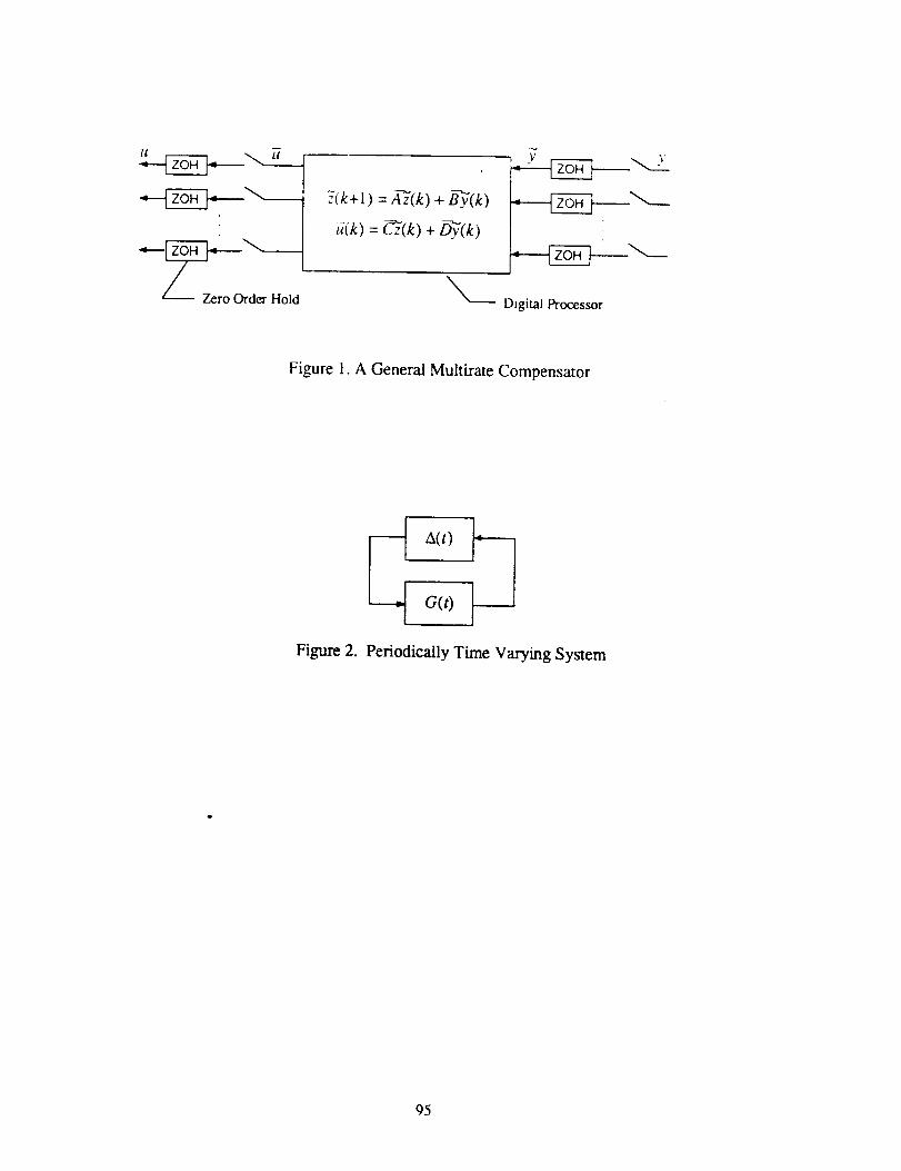
___ro OrderHol_
Figure 1. A General Multirate Compensator
Figure 2. Periodically Time Varying System
95

L2
2 8
JParameters: Mass Length
L 1 1.235 kg 0.965 mL 2 0.163 kg 0.167 m
Inputs: Torque T 1 and T 2
Outputs: 0 and 8
Figure 3: Diagram of the Two Link Arm
96

T 1
T_
TLA Plant
=t
I+[ kl k2]
Gain Uncertainty
Compensator
i
I
1Figure 4. TLA Feedback Loop with Output Gain Uncertainty
_N
___ TLA Plant andCompensator
AN =diag{[ kl k211, [ kl k212, ""[ kl k21N}
Figure 5. Structured Uncertainty Model for TLA
97

,_A Report Documentation PageN<+,'ic+r,al Aerol'm_tJ<_ and
Soao_ k:lmir_i'Ara t _
1 Report No 2. Government Accession No. 3 Recipient '_.Catalog No.
NASA CR-]8755]
4 Title and Subtitle 5 _l_t _),fq)_l
Progress in Multiratc l)igital Control System Design
7 Author(s)
Martin C. Berg and Gregory S. Mason
9. Performing Organization Name and Address
University of Washington
Mechanical Engineering Department
Seattle, WA 98195
12 Sponsoring Agency Name and Address
NASA Langley Research CenterHampton, VA 23665-5225
6. Pertorming Organization Codu
8. Performing Organization Report No
10 Work Unit No
505-64-30-01
11 Contract or Grant No.
NAG 1-1055
13 Type of Report and Period Covered
Contractor Report
14 Sponsoring Agency Code
15 Supplementary Notes
Langley '1'ethnical Monitor: A;tron J. Ostrol-f
Final Report
f 6 Abstract
A new methodology for multirate sampled-data control system design based on (1) a newgeneralized control law structure, (2) two new parameter-optimization-based control lawsynthesis methods, and (3) a new singular-value-based robustness analysis method isdescribed. The control law structure can represent muhirate sampled-data control lawsof arbitrary structure and dynamic order, with arbitrarily prescribed sampling rates forall sensors and update rates for all processor states and actuators. The two control lawsynthesis methods employ numerical optimization to determine values for the control lawparameters to minimize a quadratic cost function, possibly subject to constraints onthose parameters. The robustness analysis method is based on the multivariable Nyquistcriterion applied to the loop transfer function for the sampling period equal to theperiod of repetition of the system's complete sampling/update schedule. The completetnclhodology is demonstrated by application to the design of a combination yaw damper andmodal suppression system for a commercial aircraft.
17 Key Words (Suggested by Author(s))
Control, Multirate, Sampled-Data,Digital, Synthesis
t8 Distribution Statement
Unclassified - Unlimited
Subject Category 63
19 Security Classif. (of this report) [ 20 Security Classif. (of this page) ] 21. No. of pagesUnclassified Unclassified 101
NASA FORM 1626 OCT 86 For sale by the National Technical Information Service, Springfield, VA 22161-217t
22 Price
A06


![, NASA Contractor Report ]72 8](https://img.pdfslide.net/doc/110x75/61f5f30f5bdb351c3b2be492/-nasa-contractor-report-72-8.jpg)