Embed Size (px)
Citation preview

NASA / TM--2002-211786
NASA Marshall EngineeringModel-Version 2.0
Thermosphere
J.K. Owens
Marshall Space Flight Center, Marshall Space Flight Center, Alabama
June 2002
https://ntrs.nasa.gov/search.jsp?R=20020052422 2019-03-20T17:42:06+00:00Z

The NASA STI Program Oflice...in Profile
Since its founding, NASA has been dedicated to
the advmlcement of aeronautics and spacescience. The NASA Scientific and Technical
Infommtkm (STI) Program Office plays a key
part in helping NASA maintain this impollant
role.
The NASA STI Program Office is operated by
Langley Research Center, the lead center l\)rNASA's scientific and technical information. The
NASA STI Program Office provides access |o the
NASA STI Database, the largest collection of
aeronautical and space science STI in the world. The
Program Office is also NASA' s institutional
mechanism fi)r dissemina|ing the results of its
research and development activities. These results
are published by NASA in the NASA STI Report
Series, which includes the following report types:
TECHNICAL PUBHCATION. Reporls of
completed research or a major significant phase
of research that present tile results of NA S A
progrmns and include extensive data or
theoretical analysis. Includes compilations of
significant scientific and technical data and
infi_rmation deemed to be of contimfing relerence
value. NASA's counterpart of peer--reviewed
formal professional papers but has less stringent
limilatkms on manuscrip| length and extent of
graphic presentations.
TECttNICAL MEMORANDUM. Scientific and
technical findings that are prelmfinary or of
specialized interest, e.g., quick release reports,
working papers, and bibliographies that containminmml aimotation. Does not contain ex|ensive
analysis.
CONTRACTOR REPORT. Scientific mid
technical findings by NASA-sponsored
contractors and grantees.
CONFERENCE PUBLICATION. Collected
papers from scientific and teclmical conferences,
symposia, seminm's, or other meetings sponsored
or cosponsored by NASA.
SPECIAL PUBLICATION. Scientific, technical,
or historical infolTnation fi'om NAS A programs,
projects, and mission, often concerned with
subjects having substantial public interest.
TECHNICAL TtC4NSLATION.
English-language translations of foreign scientific
and technical material pertinent to NASA'smission.
Specialized services flint complement the STI
Program Office's diverse offerings include creating
cns|om thesauri, building cns|omized databases,
organizing and publishing research results.., even
providing videos.
For more inlormation about the NASA STI Program
Office, see the fl_llowing:
® Access the NASA STI Program Home Page at
http://www.stimasa.gov
. E-mail your question via the Internet to
help @ sit.nasa, gov
= Fax your question to the NASA Access Help
Desk at (301) 621----0134
* Telephone the NASA Access Help Desk at
(301) 621-0390
Write to:
NASA Access ttelp Desk
NASA Center lk_r AeroSpace Information7121 Standard Drive
ttanover, MD 21076-1320

NASA / TM--2002-211786
NASA Marshall EngineeringModel-Version 2.0
Thermosphere
J.K. Owens
Marshall Space Flight Center, Marshall Space Flight Center, Alabama
National Aeronautics and
Space Administration
Marshall Space Flight Center o MSFC, Alabama 35812
June 2002

Acknowledgments
The author recognizes and acknowledges the pioneering work of Luigi (]_ Jacchia and Jack W. Slowey, Smithsonian
Astrophysical ()bservatory, on which tile NASA. Marshall iqngineering Thermosphere Model is based.
In addition, the author wishes to thank (2.(3.3ustus, Computer Sciences Corporation, for his contributions to the fairing
routine between tile lower thermosphere and the altitudes where seasonal/latitudinal variation of helium is importanL His
input has greatly improved the performance of the computer program in this altitude region. 17{is contributions to the sub-
routine for calculating solar position are also gratefully acknowledged_ The author is also grateful to Keith O. Niehuss,
Marshall Space Flight Center, and Steven Smith, Computer Sciences Corporation, for their considerable help and contribu-
tions toward solving computer programming issues. Thanks to their efforts, the computer program operates on a variety of
platforms.
Finally; the author is grateful to William W. Vaughan, The University of Alabama in ftuntsville, for his contributions
and exten sire proofreading of the manuscript. His efforts have improved the cl ari ty and readability of the document
considerably. Naturally, any errors or omissions are the sole responsi bility of the author.
Available from:
NASA Center for AeroSpace Information
7121 Standard Drive
Hanove,; MD 21076-1320
(301) 621-0390
National Technical Information Service
5285 Port Royal Road
Springfield, VA 22161
(703) 487-465(11
TABLE OF CONTENTS
1. BACKGROUND ..........................................................................................................................
2. DEVELOPMENT .........................................................................................................................
2.1 Jacchia 1964 Model ...............................................................................................................
2,2 Jacchia 1970 Model ...............................................................................................................
2.3 Jacchia 1971 Model ...............................................................................................................
2.4 MSFC/J70 Orbital Atmosphere Model ..................................................................................
2,5 NASA Marshall Engineering Thermosphere Model-1988 Version ......................................
2.6 NASA Marshall Engineering Thermosphere Model-1999 Version ......................................
3. DESCRIPFION ............................................................................................................................
3.1 Density Distribution ..............................................................................................................3.2 Variations ...............................................................................................................................
3.3 Fairing Between Lower and Upper Thermosphere ................................................................3.4 Solar Position .........................................................................................................................
3.5 Thermodynamic Quantities ...................................................................................................
4. PROGRAM USAGE ....................................................................................................................
4,1 Input Parameters ....................................................................................................................
4.2 Output Parameters .................................................................................................................
4.3 Sample Calculation ................................................................................................................
5. CONCd_dJDING REMARKS .......................................................................................................
APPENDIX-- CORRESPONDENCE BY .lACK W, SLOWEY, SMITHSONIAN
ASTROPHYSICAL OBSERVATORY, MARCH 27, 1978 ................................................................
REFERENCES ...................................................................................................................................
BIBLIOGRAPHY ..............................................................................................................................
2
2
2
3
3
3
4
5
6
10
15
15
17
19
19
21
22
24
25
29
30
iii
LIST OF FIGURES
.
2,
3.
Statistical evaluation of thermospheric neutral density models ...........................................
Variation in daily F10.7 flux in 1983 .....................................................................................
Variation in 3 hourly geomagnetic index, ap, in 1983 ..........................................................
5
10
12
.
2.
LIST OF TABLES
INDATA array definition ......................................................................................................
Summary of output parameters ............................................................................................
19
22
iv
LIST OF ACRONYMS AND SYMBOLS
Ar
CH
CME
CPU
EUV
GRAM-99
I--te
ISES
J64
J70
J71
JD
MET
MET-V2.0
MKS
MSFC
N2
O
[Ol
02
[0 2]
SAO
UT
UTC
UV
argon
coronal hole
coronal mass cjection
central processing unit
extreme ultrmTiolet
Global Reference Atmosphere Model-- 1999 Version
helium
International Space Environment Service
.lacchia 1964
Jacchia 1970
.lacchia 1971
Julian date
Marshall Engineering Thermosphere
Marshall Engineering Thermosphere Model-Version 2.0
meter-kilogram-second
Marshall Space Flight Center
nitrogen oxide
oxygen
atomic oxygen
oxide
molecular oxygen density
Smithsonian Astrophysical Observatory
universal time
coordinated universal time
ultraviolet

NOMENCLATURE
Ap
a
ap
b
CN
C
C n
Cp
C v
d
E
F10.7
F10.7
g
g
go
Gx
H
i
K
k
L
M
M
1H
N
NA
planetary geomagnetic index (24-hr average)
average (13-mo smoothed) planetary geomagnetic index
coefficient
planetary geomagnetic index (3-hr value)
coefficient
coefficient
coefficient
coefficient
constant pressure
constant volume
number of days
diflerence between the apparent solar time and the mean solar time (equation of time)
solar flux
average over six solor rotations
acceleration due to gravity
mean anomaly
gravitational acceleration at sea level
gradient
solar hour angle
individual species (index)
logarithmic representation of geomagnetic measurements
planeta_ S geomagnetic index
coefficient
mean longitude
constant
molecular mass
parameter
number density
Avogadro's number
vi
NOMENCLATURE (Continued)
n
P
qo
R
R E
T
t
IL
Y
Zb
13
7
A
A
P
number of Julian days
constant
volume fraction of a species m the atmosphere
quantity; universal gas constant
effective radius assuming a spherical Earth
local temperature
UT m minutes
exospheric temperature
length of a tropical year
altitude
base fairing height
thermal diffusion factor; solar right ascension
constant
constant
incremental change
solar declination
obliquity of the ecliptic
longitude of the point for which the calculation is being performed
solar ecliptic longitude
total mass density
vii

TECHNICALMEMORANDUM
NASA MARSItALL ENGINEERING THERMOSPHERE MODEL-VERSION 2.0
1. BACKGROUND
The region of the Earth's atmosphere between about 90- and 500-km altitude is known as
the thermosphere. The region above _:500 km is known as the exosphere. The temperature m the lower
thermosphere increases rapidly with increasing altitude from a minimum near 90 km but eventually
becomes altitude independent at upper thermospheric altitudes. This asymptotic temperature, known
as the exospheric temperature, does not vary with height at any given time due to the extremely short
thermal conduction time. However, the exospheric temperature does vary with time because of solar
activity and other factors discussed below.
The neutral thermosphere is important for two reasons: (1) Even at its low density, it produces
significant torques and drag on orbiting spacecraft and orbital debris, and (2) the density/height profile
of the atmosphere above 100-km altitude modulates the flux of trapped radiation encountered at orbital
altitudes. The state of the neutral thermosphere is most conveniently described m terms of a mean, with
spatial and temporal variations about that mean.
The NASA Marshall Engineering Thermosphere (MET) model of the Earth's atmosphere at
spacecraft orbital altitudes has evolved, based on work conducted at Marshall Space Flight Center
(MSFC), over a long period of time. The model is based on the extensive work of Luigi Jacchia and his
colleagues at the Smith sonian Astrophysical Observatory (SAO) during the 1960's and 1970's and was
developed primarily for application to satellite orbital lifetime prediction, mission analysis relative to
fllture reboost requirements, etc. This Technical Memorandum describes the second version of the MET
model, attributes of the atmosphere at orbital altitudes, and the methods used to model those attributes.
Short-period atmospheric waves are localized in both time and space in a way that has thus far
been unpredictable. Consequently, these waves are not explicitly included in NASA Marshall Engineer-
ing Thermosphere Model-Version 2.0 (MET-V 2.0). Thermospheric winds are also not included. At low
latitudes (less than 28.5°), wind speeds range from 100 to 200 m/s. At high latitudes (greater than about
65°), speeds can be 1,500 m/s or more. Rapid (minutes) changes in wind direction (to 180°), probably
driven by gravity waves, have been observed by a satellite.

2. DEVELOPMENT
2.1 Jacchia 1964 Model
Reference 1 contains a description of the Jacchia 1964 (J64) model. It provides tables of atmo-
spheric density and composition computed for a wide range of exospheric temperatures, starting from
a fixed set of boundary conditions at 120 km. The diffusion equation is integrated following empirical
temperature profiles of exponential form capable of reproducing the densities derived from atmospheric
drag effects on satellites. Formulae are given that relate the exospheric temperature to solar and geomag-
netic activity and allow for the diurnal and semiannual variations. The response of the density at the
200-kin level to different types of heating is briefly discussed.
In the mid-1960's, personnel of the Aerospace Environment Division at MSFC were responsible
for providing orbital altitude density inputs for satellite orbital decay prediction. They began studies to
determine which atmospheric model, when combined with the appropriate orbit propagation program,
would most accurately predict the observed decay histories of 39 satellites. Since the observed satellite
decay histories were already available, a number of available models of the thermosphere were selected
for testing in appropriate orbital lifetime computer programs. Because the satellites had decayed prior to
the start of the study, actual values of proxy input parameters (described in sec. 3) required by the rood-
ells were used. These proxy parameters were representative of actual solar conditions that occurred
during the decay periods of the satellites. The .I64 model, described in reference 1, had the best perfor-
mance statistically of the models studied and, therefore, was selected for use by MSFC.
2.2 Jacchia 1970 Model
The .lacchia 1970 (J70) model, described m reference 2, is patterned after the 1964 model. The
main differences consist in the lower height (90 km instead of 120 km) of the constant boundary surface
and a higher ratio of atomic oxygen to molecular oxygen density ([O]: [02] ) = 1.5 at 120 km instead of
1.0). Mixing is assumed to prevail to a height of 105 kin; diffusion occurs above this height. All the
recognized variations that could be connected with solar, geomagnetic, temporal, and geographic
parameters are represented by empirical equations.
Due to the great similarity between the 1964 and 1970 models, and confirmation from observed
data of the existence of the major differences, the decision was made by MSFC personnel to use the
newer model. One key difference fiom the J64 model, in which the temperature-induced density bulge
remained on the equator all year, was that the J70 model bulge followed the latitudinal excursions ofthe Sun.
2

2.3 Jacchia1971 Model
In 1971, SAO published the Jacchia 1971 (J71) model) Although an effort was made m the
earlier models to increase the ratio of [O] to [O2], new observational evidence showed that the increase
had not been large enough. This model was an attempt to meet as closely as possible the composition
and density data derived for a height of 150 km by Von Zahn 4 on the basis of all the available mass
spectrometer and extreme ultraviolet (EUV) absorption data. Mixing is assumed to prevail to a height
of 100 kin; diffusion occurs above this height. All the recognized variations that can be connected with
solar, geomagnetic, temporal, and geographic parameters are represented by empirical equations. Some
of the previous Jacchia model equations have been revised, not only in their numerical coefficients but
also in their form, as a result of new analyses. The J71 model was not considered to be as representative
of the atmospheric density as the .U0 model relative to use in satellite orbital lifetime prediction pro-
grams. However, it contained some aspects that proved useful m improving MSFC's thermospheric
modeling capability.
2.4 MSFC/J70 Orbital Atmosphere Model
An unpublished study by em'ironmental personnel at MSFC showed that the J70 model could
be improved by incorporating the J7l model formulations of seasonal/latitudinal variations in the lower
thermosphere density below 170 km and seasonal/latitudinal variations m helium (He) above 500 kin,
while retaining the orbital decay prediction accuracy of the J64 model.
Reference 5 contains a description of the MSFC/J70 Orbital Atmospheric Density model,
a modified version of the J70 model. The algorithms describing the MSFC/J70 model are provided
as well as a listing of the computer program. The estimated future 13-too smoothed values of solar
flux ( F10.7 ) and geomagnetic index (Ap), which are required as inputs for the MSFC/J70 model
when computing future estimates of orbital altitude density conditions, are also discussed.
2.5 NASA Marshall Engineering Thermosphere Model-1988 Version
The modifications made and used in the MSFC/J70 Orbital Atmosphere Density model spuri-
ously introduced step function increases in density requiring minor fairing modifications for their
elimination. In the late 1980's, this fairing routine was added, minor programming errors were corrected,
and the complete program was made more understandable and user friendly. In addition, the calculation
of atmospheric thermodynamic properties was included, and the entire program was updated from
FORTRAN IV to FORTt_-_N 77. These modifications and additions produced the first version to beknown as the MET model used at MSFC.
Reference 6 contains a description of the MET model-1988 Version, which is a modified
version of the MSFC/J70 Orbital Atmospheric Density model. The modifications to the MSFC/J7()
model required for the MET model are described, graphical and numerical examples of the models are
included, as is a listing of the MET model computer program. Major differences between the numerical
output from the MET model and the MSFC/J70 model are discussed.

In thecourseof usingthismodelandplottingtheresults,it wasdiscoveredthatdensitydiscontinuitieswereoccasionallypresentovercertaingeographiclocations.Theseweretracedto anoccasionalproblem,with the integrationroutineusedin themodel.It wasreplacedwithamoreaccuratenumericalintegrationalgorithmto solvetheproblem.Reference7 containsadetaileddescriptionof thereplacementintegrationschemefor theintegrationof thebarometricanddiffusionequationsin theMETmodel.Thisintegrationschemeis baseduponGaussianquadrature.Extensivenumericaltestingrevealsit to benumericallyfaster,moreaccurate,andmorereliablethantheMSFC/J70modelintegrationscheme(amodifiedform.of Simpson'srule),whichwaspreviouslyusedin theMETmodel.Numerousgraphicalexamplesareprovided,alongwitha listingof themodifiedformof theMET modelin whichsubroutineINTEGRATE(usingSimpson'srule)is replacedbysubroutineGAUSS(whichusesGaussianquadrature).
2.6 NASA Marshall Engineering Thermosphere Model-1999 Version
While reviewing the 1988 version of MET, it was determined that the model would not correctly
adapt to the change of the approaching new millennium While performing this update, it was decided
to also update the calculation of the solar position to use the more recent standard epoch, J2000.0,
which corresponds to January 1.5, 2000, or Julian date (JD) 2451545.0. This is the standard epoch now
recommended for use in dynamical astronomy.
An improvement to the model was also achieved m calculating the solar coordinates. A low
precision ephemeris for the Sun can be calculated using relatively simple equations. 8 This simpler
scheme for computing the solar position requires fewer arithmetic calculations, yet it maintains more
than adequate accuracy. The apparent coordinates of the Sun are obtained to a precision of 0°.01; i.e.,
better than an arc minute, and the equation of time to a precision of 0.1 min between 1950 and 2050.
The other significant modification to the 1988 version of the MET model is in the fairing
subroutine, which controls the transition from the lower altitude density profile to that of the upper
altitude region where seasonal/latitudinal variation of He is significant. The previous version of this
subroutine made the transition in a series of small steps. The new scheme introduced in MET-V 2.0
provides a smooth functional form for the transition. The developmental MET-1999 Version was incor-
porated into the MSFC Global Reference Atmosphere Model-1999 Version (GRAM-99). 9
4

3. DESCRIPTION
TheMET-V 2.0 isasemiempiricalmodelusingthestaticdiffusionmethodwithcoefficientsobtainedfrom satellitedraganalyses.It isbasedon the1988version6,7 of MET and work done on the
1999 version, developed flom the Jacchia series of models. Most of the following description also
applies to the 1988 and 1999 versions of the MET model. With the proper input parameters, specified
below, an approximate exospheric temperature can be calculated. With exospheric temperature specified,
the temperature can be calculated for an3,' altitude between 90 and 2,5(i)(i)km from an empirically deter-
mined temperature profile. In the original development phase of the Jacchia model, the prime objective
was to model the total neutral mass density of the thermosphere by adjusting temperature profiles until
agreement between modeled and measured total densities (derived from satellite drag observations)
was achieved. Agreement between modeled temperatures and those derived from later satellite drag
and in situ measurements was not always achieved. Thomson-scatter radar temperature measurements
generally show that the diurnal temperature maximum lags the density maximum by a couple of hours,
whereas in the MET-V 2.(i)model, the temperature and the density maxima and minimal are in phase.
Studies of the accuracy with which thermospheric models estimate the neutral density have
shown that an apparent "barrier" exists at the 15-percent level, and models have not thus far been able
to achieve better performance. A recent study of this type by Marcos et al. 9 has shown that, historically,
this level of accuracy was first achieved by the J70 and J71 models. Figure 1 illustrates this point. The
MET-V 2.0 model was not explicitly included in this study. However, since MET-V 2.0 incorporates
the best aspects of Jacchia's 1970 and 1971 models, it clearly perfbrms at the current 15-percent accu-
racy state-of-the-art in thermospheric neutral density calculation, while being easier to use than other
approaches. It was also derived explicitly for use in operational satellite/spacecraft drag applications,
unlike most then-nosphenc density models. The MET-V 2.0 model reflects the J70/J71 models' accuracyresults.
35
3O
"7"_.2. 25
20"N,
15
{10
US62 J64
g AE-C (68 °)[] AE-D (90 °)
B AE-E (20 °)
m $3-1 (98 °)
IIII--'i'--iU166 170 171 173 J77 MSI877
Nedel and Year
MSIS79 MSIS83 MSB86
Figure 1. Statistical evaluation of thermospheric neutral density models.
5

Theessenceof theMET-V 2.0modelis thecalculationof atmosphericdensityin two majorregions:thelowerthermosphere(altitude90km_ z -< 105 kin) and the upper thermosphere (z > 105 km).
Between the base of the thermosphere (assumed here to be at 9(i)kin) and 105 km, turbulent mixing is
assumed to predominate, and diffusion dominates at higher altitudes. The density lot all points on the
globe at 90-km altitude is assumed constant and mixing of atmospheric constituents prevails to 105 km
Between these two altitudes, the mean molecular mass varies as a result of dissociation of [02] to [O].
An empirical process is employed in the determination of the mean molecular mass distribution between
90 and 105 km, such that the ratio of [0] to [(i)2] is 1.5 at 120 kin. This makes it agree more closelywith observations as reviewed by Von Zahn. 4 The input parameters required by the program are altitude,
latitude, longitude, date (month, day, and year), time (hour and minute), 3 hourly geomagnetic index
(linear or logarithmic), and the daily 10.7-cm solar radio flux and its average over six solar rotations
referenced to the midpoint. These parameters and their application will be discussed further m section 4.
They are essentially the same as provided by the 1988 version of the MET model, but with changes
made to the computer program to improve the representativeness of the model's output products
and efficiency of the computation.
3.1 Density Distribution
3.1.1 Barometric and Diffusion Equations
Density between 90 and 105 km is calculated by integration of the barometric equation. In the
lower thermosphere, the atmospheric density is computed by integrating the barometric equation:
P(z)=P9°(_JIT_)JexPI-J:o RT(z) '
(1)
m
where M is the mean molecular mass, g is the acceleration due to gravity, T is the local temperature (all
of which are functions of altitude z), and R is the universal gas constant 8.31432 J K -1 mole -1. The lower
boundary (z90 = 90 kin) is assumed to have the following conditions:
P90 = 3.46 × 10...9g cm ---s
r90 : 183K
Mg0 = 28.878 g mole ---1.
For altitudes above 105 km, the diffusion equation for each of the individual species (0 2, O, N 2,
He, and Ar) is integrated upward from the 105-km level. The number density for an individual species in
the altitude range 90 _<z -< 105 is calculated using a partition function based upon the sea level composi-
tion, and this calculation establishes the values for N105 used below. For N 2, Ar, and He, the number
density is given by
n(i) = %(5P(Z)NA
28.96(2)
6

wherei denotes the species (N 2, Ar, or He), qo(i) is the appropriate volume fraction for species i, and NA
is Avogadro's number. The values of qo(i) used in Mt?TI'-V 2.(i) are 0.78110 for N 2, (i).2(i)955 for (i)2,
1.289 × 1(i)-5 for He, and 0.009343 for At. For O and 02, the equations used are
and
l
n - 2P(Z)NA_ 1 M(z)
M(z) 28.96
(3)
P(Z)NA [n- __ _--[1+qo(O2)]-1 Ja(z) [28.96
(4)
respectively.
In the upper thermosphere (z > 105 km), the density computation is accomplished by integrating
the diffusion equation:
N(z)=NI05(_) exp- )5 RT(z)(5)
where N is the number density of the specms for which the calculation is being done, c_,is the thermal
diffusion factor (zero for all species except He, for which a value of -4).380 is used), and the lower
boundary is at 105 kin. It should be noted that, in this case, the molecular mass Mis a constant, since
the concern is for only one species at a time. In both cases, MET-V 2.0 computes the integral using
Gaussian quadrature.
The number density of H is assumed to be negligible below 500 km and in diffusive equilibrium
above this altitude. Thus, the lower boundary is taken to be at 500 km for this constituent, and its num-
ber density at this lower boundary is given empirically by
log10 NSO 0 = 73.13 - 39.401og10 Too+ 5.5(log10 Too)2 , (6)
where 1_ is the exospheric temperature given by equation (25). The integration of the diffusion equation
then proceeds upward from 500-kin. altitude.
3.1.2 Composition
In the lower thermosphere (90 km _<_ _<105 kin), the mean molecular mass is computed
empirically using the equation
7

6= % (z,- 100;*
n----O(7)
where the coefficients, c n, are used to fit the profile in this region. The result of equation (7) is then
used m the barometric equation, equation (1), to calculate the total mass density, p. The values of cn used
in the MET-V 2.0 model are, following Jacchia, 2 28.15204, -0.085586, 1.284 x 10⁻⁴, -1.0056 × 10⁻⁵,
-1.021 × 10 -5, ] .()544 × 10-6, and 9.9826 × 10⁻⁸, respectively.
In the upper thermosphere (z > 105 kin), the number densities for the individual species are
determined by integrating the diffusion equation; i.e., from equation (5), with the values at the lower
boundary (105 km) given by equations (2)-(4). The total mass density is then given by
and the mean molecular weight is
6 Mi(z)N i(g)
i =1 NA(8)
M. (z) - P(Z)N A6
i=1
where i denotes the individual species (N 2, 02, O, Ar, He, or H).
3.1.3 Gravity Field
The altitude coordinate system used in the MET-V 2.0 model is referenced to the "surface"
of the geoid. However, the gravitational field is computed by assuming a spherical planet with
an effective radius, R E = 6356.766 kin, where the gravitational acceleration at sea level is assumed
to be go = 9.80665 m s2. These two values are self-consistent and correspond to values of go and R E
at a latitude of 45 ° 32' 40" with centrifugal acceleration included. Thus, the gravitational acceleration
as a function of altitude is given, for purposes of the model, by the equation
(9)
3.1.4 Temperature Profile
g(z) - go
Il+-J
The temperature varies both temporally and spatially, but its basic profile is defined by a bound-
ary value it90 = 183 K and an reflection point at zx = 125 kin. The temperature at the inflection point is
defined empirically by
8

Tx = a + bT_o + c exp(k-T ) ,
where the coefficients a, b, c, and k- are 444.3807, 0.02385, 392.8292, and 0.0021357, respectively 2
and T is the exospheric temperature from equation (25). For the low altitude portion of the profile;
i.e., for 90 < z < 125, the temperature is defined by a fourth degree polynomial:
(11)
4
T(Z) = Tx + _cn(Z-Zx) n
n=l
(12)
where the coefficients c_ are determined by requirements placed on the derivatives of the profile. Since
the lower boundary of the MET-V 2.0 model is taken to be, essentially, the mesopause, the temperature
there must be T(90) = 190 = 183 K, and the gradient there (being a minimum) must be G o = 0. At the
inflection point, the second derivative must be zero, and the gradient G x must satisfy the condition
4 z x - 9(i)< Gx < 2 (13)
in order to have no inflections in the region 90 < z < zx. A value of 1.90 for G x was found
by experimentation to be best 2, so MET-V 2.0 uses
1.9 77v- 7i_0 Tv- 790" -1.9 "C 1
z x - 90 35(14)
c 2 - 0 (15)
% = -1.7 7;. - _")o _ _.7_7_-- _")o (16)(z x - 90) 3 353
,4 =-0.8 L. - 7;0 __0.8 _C- 7;0 07)(,7.x - 90) 4 354
For z > _.:r;i.e., ,7.> 125 km, the temperature profile is calculated using the empirical relation
T(z) Tx+Atan -1 ' -z X= z I+B z-z x , (18)
where A= 2(7_, - 7_.), B = 4.5 × 10---6for z in kin, and u = 2.5.
9

3.2 Variations
3.2.1 Solar Activity
Solar electromagnetic radiation at ultraviolet (UV) and EUV wmTelengths changes substantially
with the level of solar activity. Thus, thermospheric density is strongly dependent on the level of solar
activity. An average 11-yr solar cycle variation exists; similarly, a "typically" 27-day variation in density
exists, which is related to the average 27-day solar rotation period. Variations, however, tend to be
slightly longer than 27 days early in the solar cycle when active regions occur more frequently at higher
solar latitudes and slightly shorter than 27 days later in the solar cycle when the active regions occur
more frequently closer to the Sun's equator. Coronal holes and active longitudes also affect this average
27-day variation. Changes in the thermospheric density related to changes in level of solar (and geomag-
netic) activity; e.g., flares, eruptions, coronal mass ejections (CMEs), and coronal holes (CHs), can
begin ahnost instantaneously (minutes to hours), although more often a lag of a day or more occurs.
Various surrogate radices are used to quantify levels of solar activity; one is the 10.7-cm solar
radio flux, designated t" 10.7. Although EUV radiation heats the atmosphere, this radiation cannot be
measured flom the ground. The Fro7 can be measured flom the ground and correlates well with the
EUV radiation. Figure 2 shows the variability of the Fro7 index during a period of low solar activity.
200
180
160
140
A
g 120
100
_=* 80 -
60-
40-
20 ....
0 .... i-31
T ] T 7--7 f f T--T T i_
61 91 121 151 181 211 241 211 301 331 361
Day Number
Figure 2. Variation in daily/"10.7 flux m 1983.
The exospheric temperature is computed in the MET-V 2.0 model from a base state temperature
parameterized using the 10.7-cm solar radio flux. Then several variations due to diurnal variations,
geomagnetic activity, and semiannual variations are added to the base state to form an empirical estimate
10
of the exospheric temperature. The base state equation is for the global minimum of the exospheric
temperature distribution (which occurs at night) when the planetary geomagnetic index ap (or Kp)is zero (see sec. 3 for an explanmion of these indices):
_. = 383 + 332__._ 10.7 + 18(F10.7 -/T10.7) (19)
where f'10.7 is the 10.7-cm (2,800 MHz) solar radio flux in units of 104 Jansky (a Jansky is defined
as 1(i).26 W 111.2 Hz -1 bandwidth). The bar over F10.7 indicates an average over three solar rotations
prior to the day for which we are doing calculations and three solar rotations alierward; i.e., six solar
rotations, for a total of 162 days as used by Jacchia in the model development. (See appendix.)
3.2.2 Diurnal
Rotation of the Earth induces a diurnal (24-hr period) variation (diurnal tide) m thermospheric
temperature and density. Due to a lag in response of the thermosphere to the EUV heat source, density
maximizes around 2 p.m. local solar time for orbital altitudes at a latitude approximately equal to the
subsolar point. The lag decreases with decreasing altitude. Similarly, minimum density occurs between
3 and 4 a.m local solar time at about the negative of the subsolar latitude; i.e., in the diametrically
opposite hemisphere. In the lowest regions of the thermosphere (120 km and bellow), where characteris-
tic thermal conduction time is on the order of a day or more, the diurnal variation is not a predominanteffect.
Harmonics of the diurnal tide are also induced in the Earth's atmosphere. A semidiumal tide
(period of 12 hr) and a terdiurnal tide (period of 8 hr) are important in the lower thermosphere (below
,-=160 km fk)r the semidiurnal tide and much lower fk)r the terdiurnal tide). Because of large damping
effects of molecular viscosity, these diurnal harmonic tides are not important at orbital altitudes.
The diurnal variation is included in MET-V 2.0 under the assumption that the daytime maxmmm
7)_4 and nighttime minimum temperatures occur at latitudes which are diametrically opposed to one
another on the geoid; i.e., they occur at latitudes q) equal to _+5s, respectively, where ?5s is the solar
declination. This is accomplished by writing the exospheric temperature as
I _d(COSmTl--sinmOllTl:_:(l+RsinmO) l+Rc°sn-7_ 77+R_ )]'
where the fitting parameters are R = 0.31, m = 2.5, and n = 3 and the arguments of the trigonometric
functions are I"1= Id)+ 8sl/2, 0 = IO+ 8sl / 2, Vd = H + [3+ p sin (H + ?9.
The diurnal variation is contained in the expression for rd in which H is the solar hour angle
measured from upper culmination (the computation of which will be discussed in section 3.4) and the
constants fi, p, and ?'are determined from obserwttions to be -0.6457718, 0.1047198, and 0.75()49] 6,
respectively; i.e., -37 °, 6 °, and 43 °, respectively. The quantity R is really 7_i/2 _,-1 and is known to be
correlated with solar activity and with geomagnetic activity) Reference 2 provided equations for
(20)
11
computingR from mmual running means of/k)_ or from averaged F10.7. It was concluded from lateranalyses that the available data were insufficient to establish the rules of the variation, so using a con-
stant, average value of R was the best approach. 3 MET-V 2.0 uses the average value from the J70
model, 2 as reflected in the 1988 version of MET.
3.2.3 Geomagnetic Activity
Interaction of solar wind with the Earth's magnetosphere (referred to as geomagnetic activity)
leads to a high-latitude heat and momentum source for the thermospheric gases. Some of this heat and
momentum is convected to low latitudes. Geomagnetic activity varies, usually having one peak in activ-
ity just prior to and another just after the peak activity of the solar cycle as defined by the 10.7-cm solar
radio flux. Also, larger solar cycle peaks are associated with more intense geomagnetic activity.
A seasonal variation of geomagnetic activity occurs with maxima in March (_+_+1too) and September
(_+1 mo) each year. This variation is possibly related to the tilt of the Sun's rotational axis toward theEarth.
There are two geomagnetic indices that may be used in the MET-V 2.0 model. A logarithmic
representation of the maximum range over which the magnetic field components vary is designated K.
Values of K may range from zero to 9, and cover a 3-hr interval. The K values from 12 standard stations
at latitudes from 48 ° to 63 ° and l_drly evenly distributed in longitude are averaged to obtain the planetary
index, Kp, used in MET-V 2.(i). The other index, which may be used m MET-V 2.0, is ap, which is a
linear index derived from Kp and ranges from zero to 400. Sometimes a 24-hr average of the 3 hourly a o
values is quoted, in which case the convention is to designate it Ap. Although high-latitude ionosphericcurrent fluctuations drive the magnetic field fluctuations observed at these stations, the magnetic field
fluctuations do not drive the thermosphere. Thus, good correlations are not always found between
observed density changes and the ap index. Pigure 3 shows a year of ap data during a period of low solaractivity.
25O
20O
150
=_ lOO@
50
Figure 3.
61 91 121 151 181 211 241 271 301 331 361
DayNumber
Variation in 3 hourly geomagnetic index, ap, m 1983.
12

WhenthelogarithmicKv index is used, MET-V 2.0 computes the adjustment to the exospherictemperature using
Big = 28 Kp + 0.03 exp(hp) (21)
but if the linear av index is used, the equation
Arlg = ap + 10011 - exp(-0.08 ap)] (22)
is used. There is a time lag between changes m the geomagnetic indices and temperature variations
which averages -_6.7 hi; so, whichever index is used, its value should be from a time =6.7 hr prior
to the time for which the exospheric temperature is to be computed.
3.2.4 Semiannual
This variation in thermospheric density is still poorly understood, but it is believed to be
a conduction mode of oscillation driven by a semiannual variation in Joule heating in the high-latitude
thermosphere (as a consequence of a semiannual variation m geomagnetic activity). The variation
is latitudinally independent and is modified by compositional effects. The amplitude of the variation
is height dependent and variable from year to year with a primary minimum in July, primary maximum
in October, secondary minimum in January, followed by a secondary maximum in April. Magnitude
and altitude dependence of the semiannual oscillation vary considerably from one solar cycle
to another. This variation is important at orbital altitudes.
The MET-V 2.0 formulation of the semiannual variation is accomplished through the exospheric
temperature. The variation is roughly propo_ional to the 10.7-cm solar radio flux and may be computed
as
where
(23)
d 1+si + 42o3_rs=__+0.1145,, / _ k _ . __
Y 2(24)
with d being the number of days since January 1 and Ythe length of a tropical year; i.e., 365.2422 days.
Note that d is not the day number of the year.
13

Havingcomputedthevariousadjustmentsasdescribedabove,theexospherictemperatureisgivenby
(25)
whichprovidestheappropriatevaluefor usein equations(6)and(11)for computingtheH numberdensityat500km andthetemperatureattheinflectionpointof thetemperatureprofile,respectively.
3.2.5 Seasonal/Latitudinal
Thetotalmassdensityis modifiedfurtherbytheeffectsof seasonal/latitudinaldensityvariationof thelowerthermospherebelow170-kinaltitudeandseasonal/latitudinalvariationsof Heabove500km.ThesetwoeffectswereincorporatedintoMET-V 2.0usingtheequationsdevelopedby Jacchiafor his1971themlosphericmodel)
3.2.&1 LowerThermosphere.Thebarometricanddiffusiondifferentialequationsweresolvedbyassumingfxed boundaryconditionsatz = 90 km. In reality, the values at that height vary as a func-
tion of both season and latitude. These seasonal/latitudinal variations are driven in the thermosphere by
the dynamics of the lower atmosphere (mesosphere and below). Amplitude of the variation maximizes in
the lower thermosphere between about 105 and 120 km and diminishes to zero around 200 kin. Although
the temperature oscillation amplitude is quite large, corresponding density oscillation amplitude is small.
This variation is not important at orbital altitudes.
Computation of this variation in MET-V 2.0 follows the J71 model) In the interest of simplicity,
the boundary conditions are left fixed, and the density variations are computed using the empiricalrelation
where
Alogl0 p(z) = S(z,) _ P sin 2 q) ,(26)
and
S(z) = 0.014(z- 90) exp[-0.0013(z - 90) 2](27)
P=sm d+100 . (28)
This equation is only applied below z = 170 kin, since the effect on density variation is negligible abovethis altitude,
14

3.2.$.2Helium. Satellitemassspectrometershavemeasuredastrongincreasein Heabovethewinterpole.Overayear,theHenumberdensityvariesby afactorof 42at275km,12at4(i)(i)kin,andafactorof 3 or4 above500km Formationof thewinterHebulgeisprimarilydueto effectsof globalscalewindsthatblowfromthesummerto thewinterhemisphere.Amplitudeof thebulgedecreaseswithincreasinglevelsof solaractivitydueto increasedeffectivenessof exospherictranspo(tabove500kin,carryingHebacktothesummerhemisphere.Also,averyweakdependenceexistsof Hebulgeampli-tudeonmagnitudeof thelowerthermosphericeddydiffusivity.
As wasjust noted,theseasonal/latitudinalvariationof Hedecreaseswith increasingaltitude.However,He isasufficientlysmallfractionof thetotaldensityatlow altitudesthatits seasonal/latitudinalvariationisnegligiblebelow_0500kin.Above500kin, MET-V 2.0usestheequation
lOgl0n(He) = lOgl0 n(He) + 0.65 _-_ [sin3/4 _) 8s/-sin3 41216,1)(29)
where g is the obliquity of the ecliptic, following the J71 model)
3.3 Fairing Between Lower and Upper Thermosphere
In order to produce a smoother, more continuous transition from the densities computed below
500 km to those computed above, a fairing algorithm is applied to the base 10 logarithm of the total
density and He number density for altitudes between 44() and 500 km. The faired density is given by
p(z) = pl(Z)C(z) + p2(z)[1- C(z)] , (30)
where p_ is the density before adj usting for the seasonal/latitudinal variation of He and ,92 i s the density
afterward, and the fairing coefficient is
C(S) = cos 2 [3(Z-Zb)/2] , (31)
where zb is the base fairing height at which the fairing calculation begins, 440 km in this case. The
fairing coefficients have been chosen such that a gradual transition occurs from the density variationbelow 440 km to the variation above 500 kin.
3.4 Solar Position
It is evident from the preceding discussion that a key element in the computation of densities in
the MET-V 2.0 model is the exospheric temperature, which in turn depends upon the solar hour angle
and decimation. The solar declination is given by
6 s = sin-1 (sine sin )_s) , (32)
15

wheree. is the obliquity of the ecliptic; i.e., the angle between the plane defined by the Earth's equator
and the ecliptic plane, and '_s is the solar ecliptic longitude. Due to Earth's nutation, the obliquity of
the ecliptic is not constant. (Nutation is the slight periodic wobbling motion of the Earth's rotation axis
caused by the varying distances and relative directions of the Sun and Moon.) In MET-V 2.0, it is
computed as
(33)
and
g = 357°.528+ 0°.9856003n , (37)
respectively.
The solar hour angle is the angle between the local meridian and the right ascension of the Sun.
It is given by
tH = -- - 180°.0 + A + E , (38)
4
where t is UT in minutes, A is the longitude of the point for which the calculation is being performed,
and E is the difference between the apparent solar time and the mean solar time. E is known as the
equation of time, and it may be computed to a good approximation by
E=L-a ,
where the solar right ascension cx is given by
o: = tan -1 (cose tan _s) •
(39)
(4O)
16
= 23°.439- 0°.0000004n ,
where n is the number of Julian days from J2000.0 for the Julian date (JD) corresponding to the date
specified m the input
n = JD- 2451545.0 . (34)
The Julian date is computed using the Eli egel and Van Flandem algorithm.l°
The solar ecliptic longitude can be computed by
_'s = L + l°.915sing + 0°.020sin2g , (35)
where L is the mean longitude corrected for aberrations and g is the mean anomaly; i.e., the mean angle
from pericenter travelled from some arbitrary starting time assuming constant angular speed. These may
be computed from
L = 280 ° .460 + 0° .9856474n (36)

3.5 Thermodynamic Quantities
As an option, MET-V 2.0 computes some thermodynamic quantities, which were computed
without option in the 1988 version of MET, but were not included in previous neutral thermosphere
codes used by MSFC. The change to have these calculations be optional was incorporated to provide
economy of CPU time for those applications; e.g., total density for satellite lifetime predictions, that do
not use these thermodynamic quantities. These include the pressure, pressure scale height, specific heat
at constant pressure, specific heat at constant volume, and the ratio of the specific heats. The equations
used to calculate these quantities are presented in sections 3.5.1 through 3.5.3.
3.&l Pressure
The pressure is calculated directly from the equation of state under the assumption that the
atmosphere behaves essentially as an ideal gas. Since the number of moles of gas is given by the ratio
of the mass of the gas to its molecular weight and the ratio of the mass of the gas to its volmne is its
density, the pressure at altitude z is given by
p(z) = . (41)M(z)
3.5.2 Pressure Scale Height
The pressure scale height is, by definition, the inverse of the integrand in equation (1). It may be
observed from equation (1) that this is.just the change in height required to change the density of a gas
of molecular mass M by e -1 in an isothermal atmosphere. To compute this quantity in the MET-V 2.(i)
model, it was observed that solving equation (41) lbr RT and substituting the result into the definition
of the scale height gives
p(z) (42)It(z) -p(z)g(z)
where t-I(_) is the pressure scale height at altitude r.
3.5.3 Specific Heat Capacities
Under the assumption of an ideal gas, it can be shown by statistical mechanical methods that the
molar specific heat at constant volume, cv of a monatomic gas is 3R/2, and for a diatomic gas it is 5R/2.
It can also be shown from the definitions of cv and cv (the molar specific heat at constant pressure) that,
assuming an ideal gas, cp is the sum of cv and the universal gas constant R. Then, the ratio of the specific
heats, 7 - cp / c v , is 5/3 for a monatomic gas and 7/5 for a diatomic gas. Therefore, the ratio of specificheats in the thermosphere is calculated in the MET-V 2.0 model using the weighted average
17

1.67[n(O) + n(Ar) + n(He) + n(H)] + 1.4[n(O2) + n(N2) ]
n(O) + n(Ar) + n(He) + n(H) + n(O2) + n(N2)
(43)
Using the equation of state and the fact that R = cp- cv in equation (43) yields 6
H(z)g(z) (44)
Then, the specific heat at constant pressure is
%(z) = 7(z)% (z) . (45)
18
4. PROGRAM USAGE
4.1 Input Parameters
The MET-V 2.0 model (code available from author) is designed to be very easy to use. Four
basic types of input parameters are required by the model: time, location, solar activity, and geomagnetic
activity. These may be provided to the model using the sample driver program provided, which reads an
input data. file, puts the data into the INDATA array, and calls the primary subroutine MET. The user is
free to replace the driver program with his/her own, or to integrate MET-V 2.0 model into a larger
program, to suit the needs of the project. Note that the INDATA array, and therefore all of its elements,
is REAL*4.
Table 1 presents a summary of the contents of the INI_-)ATA array. Note that the year is input
as a four-digit number, while the month, day, hour, and minute are all required to be input as two-digit
numbers. The first column contains the array element number; the second colmnn identifies the corre-
sponding parameter; the third column indicates the appropriate range of values, where applicable; and
the fourth column identifies the proper units for that parameter, where applicable. Note that INDF/FA(9)
controls whether INDATA(12) is interpreted as ap or Kp, and INDATA(13) controls whether the addi-
tional thermodynamic quantities are calculated.
Table 1. INDATA array definition.
ElementNn. Parameter Range Units
1
2
3
4
5
6
7
8
9
10
11
12
13
Altitude
Latitude
Longitude
Year
90 to 2,500
....90 to 90
-180 to 180
1950 to 2050
Month
Day
Hour
Minute
Geomagneticindextype
10.7--cmsolar flux
Average10.7-cm solar flux
Geomagneticactivity index
Thermodynamicsflag
01 to 12
01 to 31
O0to 23
O0to 59
1(Kp)or 2(ap)
0 to 400
0 to 250
0 to 400 (ap)
0 to 9 (Kp)
0 or 1
Kilometers
Degrees
Degrees
104 Jansky
104Jansky
19
There are three general categories of applications for the MET-V 2.0 model: (1) After-the-fact
calculations of densities, (2) real-time (or near real-time) calculations of densities, and (3) future appli-
cations in which density estimates are required for sometime in the future. In each case, the time and
location inputs are selected and entered according to the same rules. When entering the time, the year
is entered in four-digit lbrm, while the month, day, hour, and minute for which the calculation is to be
done are each entered in two-digit form with the hour and minute being the coordinated universal time
(UTC). For the position desired, enter the altitude in kilometers and geographic latitude and longitude in
decimal degrees of the spacecraft location at the time of application. Note that the longitude is measured
fi:om the Greenwich meridian eastward. The selection of inputs for the solar and geomagnetic activity
parameters depends upon which application category applies to the calculation as discussed in sections
4.1.1 through 4.1.3.
4.1.1 After-the-Fact Calculations
This type of calculation is required for times more than 81 days in the past, such as the analysis
of data from a space mission or testing model performance using observed orbital parameters for one
or more spacecraft. In this case, solar activity is specified using the prexious day's value of the lO.7-cm
solar radio flux and the centered (about the day for which the calculation is to be done) average of the
lO.7-cm solar radio flux over six solar rotations (162 days), /-510.7.The geomagnetic index, either ap
or Ap, is the 3 hourly index value from 6 to 7 hr prior to the time of application.
4.1.2 Real-Time Calculations
When the application requires that the density calculations be made for the current time, or less
than 81 days in the past or future, averaging the observed 10.7-cm flux over six solar rotations as
described above is clearly not possible. In this case, the previous day's value of the 10.7-cm solar radio
flux is still used for the daily F10.7 value. However, for the average value, observed values are usedwhere available, and the estimated future 13-mo smoothed value of the 10.7-cm solar radio flux is
used as an estimate for the balance of the time period (for which observed daily/"m7 values are not
available). These estimated future values of/=10.7 are published by the International Space Environment
Service (ISES) and are available electronically via the internet (connect to http://sec.noaa.gov/SolmCycle
and retrieve the "Table of Predicted Values With Expected Ranges"). The observed ap or Kp from6 to 7 hr prior to time of application is still appropriate for this application category except for the time
period up to 81 days in the future, when the estimated future value of Ap is used.
4.1.3 Future Calculations
When the calculations of densities must be done for a date more than 81 days in the future; e.g.,
for estimating orbital lifetimes, the problem becomes more dependent upon estimates of future average
values for the 10.7-cm solar radio flux, F!l0.7, and the average planetary geomagnetic index, Ap. Nowneither the daily nor the ] 62-day average 10.7-cm solar radio flux is known from observations, nor is the
3 hourly geomagnetic activity. In this case, the future estimate of the 13-too smoothed value of F10.7
from ISES, as described in section 4.1.2, is used as an estimate of both the previous day's value of the
10.7-cm solar radio flux input and of the 162-day average value. On average, a value of _12 may be used
for the 13-mo smoothed estimate of the A-p index for use as an estimate of the 3 hourly geomagneticindex input.
2O

Forfutureneutraldensitycalculations,theaccuracyof thecalculationdependsprimarily upontwo l_lctors:
(1) Theabilityof thethermosphericmodelto representtheobservedneutraldensityusingtheobservedvaluesof solarradioflux (proxyfor solarEUV heating)andgeomagneticactivityusedin thedevelopmentof themodel.
(2) Theaccuracywith whichfuturesolarradioflux andgeomagneticactivitycanbeestimatedfor useasinputsto thethermosphericmodel.
As notedin section3, theMET-V2.0 modelhasanaccuracyof _15percent,whichis thecurrentstate-of-the-allfor thermosphericdensitymodelcalculations.However,asnotedbyVaughanetal.,12themajorsourceof nncertaintyfor futurethermosphericneutraldensitycalculationsis theestimationof futuresolarEUVheatinput.
4.2 Output Parameters
Upon completion of the calculation, the MET-V 2.0 model passes the results back to the calling
routine through the OUTDATA and AUXDATA arrays, both of which are REAL*4. These calculated
results include the exospheric temperature, temperature at the input altitude (z), number densities for
each constituent, the mean molecular mass, total mass density and its logarithm., and when desired,
gravitational acceleration at z, total pressure, pressure scale height, molar specific heat capacities at
constant pressure and constant volume, and the ratio of the specific heat capacities. All of these param-
eters are expressed in MKS units. Table 2 details the output arrays. The first column identifies which
element of which output array contains the data for the parameter in the second column. The notation
used is AUX for the AUXDATA array (produced when themlodynamic quantities are computed) and
OUT for the OUTDATA array. For example, AUX 2 indicates element 2 of the AUXDATA array, and
OUT 5 indicates element 5 of the OI.£I'DATA array. The third column gives the MKS units for the
parameter identified in column 2. The total mass density, temperature, and individual species number
densities all have the same phase variation in the MET-V 2.0 model.
21

Table2. Summaryof outputparameters.
Location
OUT 1 Exospheric temperature
OUT 2 Temperature
OUI-3 N2number derlsity
OUl-4 02 number density
OUT 5 0 number density
OUT6 Ar nurnber density
OUT7 He number density
OUT 8 Hnumber density
OUT 9 Average molecular weight
OUT 10 Total mass density
OUT 11 Loglo mass density
ou-r 12 Total pressure
AUX 1 Local graviIy acceleration
AUX 2 Ratio--specific heats
AUX 3 Pressure scale height
AUX 4 Specific heat constant p
AUX 5 Specific heat constant v
Parameter Units
Kelvin (K)
Kelvin (K)
Molecules per cubic meter (m -3)
Molecules per cubic meter (rn4)
Atoms per cubic meter (m-3)
Atoms per cubic meter (m-3)
Atoms per cubic meter (m-3)
Atoms per cubic meter (m-3)
Kilograms per kilo-mole (kg kmol-1)
Kilograms per cubic rneter (kg rn-3)
Pascal (Pa)
Meters pet second squared (rn s-2)
Meters (m)
m2 s-2 K-1
m2 s--2K--1
4.3 Sample Calculation
Suppose one wants MET-V 2.0 model results, including thermodynamic quantities, for a point
at lat. 45 ° N., long. ] 20 ° W:, and 350-kin altitude on January 20, 1969, at 19:11 UTC. The 10.7-cm
solar radio flux for the preceding day (136 × 104 Jan sky) would fJrst be found, then the average 10.7-cm
solar radio flux be computed over six solar rotations (162 days, _+81 days) centered on January 20, 1969
(155 x 104 Jansky). Then find the value of the geomagnetic index (ap = 9) at =6.7 hr earlier; i.e.,at about 12:29 UTC on January 20, 1969. Using these values for a sample run with the driver program
supplied with MET-V 2.0, the input data file (see table 1) reads as follows:
Altitude = 350.00
Latitude = 45.00
Longitude = -120.00Year = 1969.00
Month = 1.00
l:)ay = 20.00Hour = ] 9.00
Minute = 11.00
Geomagnetic Index Type = 2.0010.7-cm Solar Flux = 136.00
Average 10.7-cm Solar Flux = 155.00
Geomagnetic Activity Index = 9.(:)(:)Thermodynamics Flag = ] .00
22
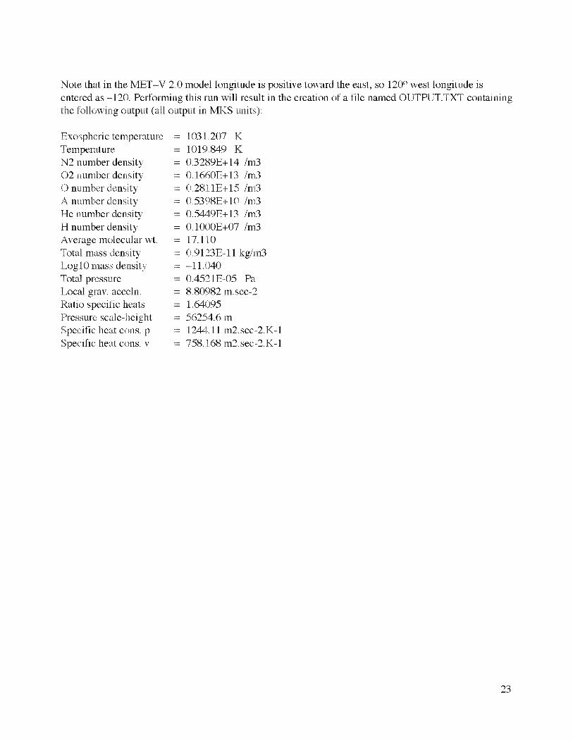
Notethatin theMET-V 2.0modellongitudeispositivetowardtheeast,so120° westlongitudeisenteredas-120.Performingthisrunwill resultin thecreationof afile namedOUTPUT.TXTcontainingthefollowingoutput(all outputin MKS units):
ExospherictemperatmeTemperatureN2nm-nberdensity02 numberdensityOnumberdensityA numberdensityHenmnberdensityH numberdensityAveragemolecularwt.TotalmassdensityLog10massdensityTotalpressureLocalgray.acceln.RatiospecificheatsPressurescale-heightSpecificheatcons.pSpecificheatcons.v
= 1031.207K= 1019.849K= 0.3289E+14/m3
= 0.1660E+ 13 /m3
= 0.2811E+15 /m3
= 0.5398E+10 /m3
= 0.5449E+13 /m3
= 0.1000E+07 /m3
= 17.110
= ().9123E-11 kg/m3
= -11.040
= 0.4521E-05 Pa
= 8.80982 m, sec-2
= 1.64095
= 56254.6 m
= 1244.11 m2.sec-2.K-1
= 758.168 m2.sec-2.K-1
23
5. CONCLUDING REMARKS
Using current or past observations of solar radio flux and geomagnetic activity as inputs to
the MET-V2.0 model will produce thermospheric density estimates with an accuracy of _15 percent.
However, using future estimates of these input values from generally accepted statistical models
01o physical solar model is currently available for use) will result in significantly (order of magnitude
effects) reduced accuracy for the calculated thermospheric density values. These are key considerations
to the prediction and statistical confidence of satellite orbital lifetimes, orbital insertion altitudes, reboost
requirements, etc. for which the MET-V2.0 model (and its predecessors) was developed.
24
APPENDIX--CORRESPONDENCEBY JACK W. SLOWE_ SMITHSONIAN
ASTROPHYSICAL OBSERVATORY, MARCH 27, 1978
25

SMITHSONIAN INSTITUTION
ASTROPHYSICAL OBSERVATORY
60 GARDEN STREET CAMBRIDGE, NIASSACHUSETTS 02138
TELEPHONE 617 864-7910
Dr. William W. Vaughan, Chief
Atmospheric Sciences Division
ES811 Bui]_dii_g 448]_
George C. Marshall Space Flig_rt Cerrter
Marshall Space F]_ig_rt Cerrter, Alabama 36812
March 27, 1.978
Dear B:J_]_I:
It occurs to me that I promised to get back to you on the subject of smooth-
ing to obtain the mean value of the solar flux. This hasn't quite reached the top
of my list of "things to do today," but I' 11 have a go at it anyway.
Concerning the gaussian smoothing procedure given on page 20 of the 1977
Jacchia model, the "recoma-c_ended" value of _ should have been 70 days. This is the
value we _ ve used since we first began to use the method ourselves. Of course, I'm
sure that we couldn't distinguish between this and the value of 71 days that kS
quoted. The association with "three solar rotations" may have been the result of
poor arithmetic following this lesser corruption but, chicken or egg, it is not
appropriate and should be deleted.
In the gaussian method, the scale factor _ should not be confused with the
larger interval over which the iuean is to be taken. At an interval _ from the time
in question the weight of an included value of F would be 1/e .... .37, which is quite
appreciable. You have to go to an interval of about 3T before the weights really
become insignificant. It is this limit, 3T .... 210 days, that we apply to determine
"final_*' values of F with the gaussian method. It should be emphasized that the
limit is applied both forward and backward in time: as in the older method, F is
assumed to be a centered mean of the values of F.
Concerning the older iuethod, in whioh F is taken as an unweighted running
mean, the statement on the same page of the 1977 model that the model was based on
means take--over s total of six solar rotations is oorreot. The unfortunate as---
sociation of F with the mean over three solar rotations that was made in both the
1970 and 1971 models is, again, not a correct reflection of our actual practice. I
can' t recall the exact chronology, but we may still have been getting F from a
hand--drawn curve through the monthly mear:s wber: these models were published. In any
event, when we did finally put the determination of F on a more formal basis, we
found that a total of six rotations were necessary to represent F "correctly" as we
saw it. We have used this value (i 3 rotations) ever since. In particular, I have
used this interval in connection with this kind of smoothing in all of the model
computations I' ve made concerning Skylab.
26

-2-
Of course, I don' t claim that anything we do with regard to the determination
of F is necessarily "best." It is all based on our own subjective feelings in the
matter. I hope, however, that I have clarified what is consistent with our practice
and _recommended " for use with the atmospheric models that result.
Sincerely yours,
JWS/p1
P.S. If I can possibly meet deadlines for New York meeting, I" 11 be happy to submit
a paper.
27

REFERENCES
1. Jacchia,12.(_3.:"Stalc I)i ffusionModelsof theUpperAtmospherewith EmpiricalTemperatureProfiles,"Smithsonian Contributions to Astrophysics, Vol. 8, pp. 215-257, 1965.
2. Jacchia, L.G.: "New Static Models of the Thermosphere and Exosphere with Empirical Temperature
Profiles," Smithsonian Astrophysical Observatory Special Report No. 313, 1970.
3. Jacchia, L.G.: "Revised Staic Models of the Themlospllere and Exosphere With Empirical
Temperature Profiles," Smithsonian Astrophysical Observatory Special Report No. 332, 1971.
4. Von Zahn, U.: "Mass Spectrometric Measurements of Atomic Oxygen in the Upper Atmosphere:
A Critical Review," J. Geophys. Res., Vol. 72, pp. 5933-5937, 1967.
5. Johnson, D.L.; and Smith, R.E.: "The MSFC/J70 Orbital Atmosphere Model and the Data Bases
for the MSFC Solar Activity Prediction Technique," NASA IM-86522, Marshall Space Flight
Center, AL, November 1985.
6. Hickey, M.P: "The NASA Marshall Engineering Thermosphere Model," NASA CR-179359,
Marshall Space Flight Center, AL, July 1988.
7. Hickey, M.P: "An Improvement in the Integration Procedure Used in the NASA Marshall Engineer-
ing Thermosphere Model," NASA CR-179389, Marshall Space Night Center, AL, August 1988.
8. Anon., The Astronomical Ahnanacfor llle Year 1991, p. C24, U.S. Government Printing O_lice,
Washington, DC, 1990.
9. Justus, C.G.; and Johnson, D.L.: "The NASA/MSFC Global Reference Atmosphere Model-1999
Version (GRAM-99)," NASA I37[--1999-209630, Marshall Space Flight Center, AL, May 1999.
10. Marcos, EA.; Bass, J.N.; Baker, C.R.; and Borer, W.S.: "Neutral Density Models for Aerospace
Applications," AL4A 94.---0589, 32d Aerospace Sciences Meeting and Exhibit, Reno, NV,
January 10-13, 1994.
11. Fliegel, H.E; and Van Flandern, T.C.: "A Machine Algorithm for Processing Calendar Dates,"
Commtm. Assoc. Comp. Mach., Vol. 11, p. 657, 1968.
12. Vaughan, W W.; Owens, J.K; Niehuss, KO.; and Shea, M.A.: "The NA SA Marshall Solar Activity
Model For Use In Predicting Satellite Lifctime," Adv. ,Space Res., Vol. 23, No. 4, pp. 715-719,1999.
29

BIBLIOGRAPHY
Anderson,B.J.;andSmith,R.E.:"NaturalOrbitalEnvironmentGuidelinesfor UseinAerospaceVehicleDevelopment,"NASA I3/I-4527, June 1994.
Anon., "Guide to Reference and Standald Atmosphere Models," AIAA G-OO3A-1996, American
Institute of Aeronautics and Astronautics, Reston, VA, 1997.
Anon., "Models of Earth's Atmosphere (90 to 2,500 km)," NASA SP---8021, March 1973.
Anon, UIS. Standard Almosphere, 1976, U.S. Government Printing Office, Washington, DC,October 1976.
Banks, R M.; and Kockarts, (3.: Aeronomy, Academic Press, New York, 1973.
Bates, D.R.: "Some Problems Concerning the Terrestrial Atmosphere Above About the 100-kin Level,"
Proc. Royal Soc. London, Vol. 253A, pp. 451--462, 1959.
Bramson, A.S.; and Slowey, J.W.: "Some Recent hmovations in Atmospheric Density Programs,"
Af'CRL----TR----74----0370, Air Force Cambridge Research Laboratories, Hanscomb Air labrce Base, MA,
August 15, 1974.
Chamberlain, J.W.; and Hunten, D.M.: 7?wory of Planetary Atmospheres. An Inm)duction to Their
Physics and Chemistry, Academic Press, Orlando, FL, 1987.
Champion, K.S.W.; Cole, A.E.; and Kanto_; A.J.: "Standard and Reference Atmospheres," in Handbook
of Geophysics and the Space Environment, A.S. Jursa (ed.), pp. 14-1-14-43, Air Force Geophysics
Laboratoly, Hanscomb Air Force Base, MA, 1985.
Crowley, G.,:"Dynamics of the Earth's Thermosphere: A Review," in U.S. National Report lo Inlerna-
lional Union of Geodesy and Geophysics, M.A. Shea (ed.), pp. 1143-1165, American Geophysical
Union, Washington, DC, 1991.
De Lafontaine, J.; and Hughes, R: "An Analytic Version of Jacchia's 1977 Model Atmosphere," Celes.
Mech., Vol. 29, pp. 3-26, 1983.
Dreher, RE.; and Lyons, A.T.: "Long-Term Orbital Lifetime Predictions," NASA TP-3058, 1990.
Fuller-Rowell, TJ.; Rees, D.; Quegan, S.; Moffett, R.J.; and Bailey, GJ.: "Interactions Between Neutral
Thermospheric Composition and the Polar Ionosphere Using a Coupled Thermosphere-Ionosphere
Model," J. Geopkys. Res., Vol. 92, pp. 77447748, 1987.
3O

Jacchia,L.G.:"ThermosphericTemperature,Density,andComposition:NewModels,"SAC)SpecialReportNo.375,SmithsonianAstrophysicalObservatory,Cambridge,MA, March1977.
Johnson,D.L.: "Sensitivity/ComparisonStudyBetweentheJacchia1970,1971,and1977UpperAtmosphereDensityModels,"NASA _IM-82534, 1983.
Johnson, R.M.; and Killeen, T.L. (eds.), The Upper Mesosphere and Lower Thermsophere: A Review
of E_7)erimenl and "lheory, American Geophysical Union, Washi ngton, DC, 1995.
Justus, C.G.; Jeffries III, W.R; Yung, S.R; and Johnson, D.L.: "The NASA/MSFC Global Reference
Atmospheric Model-1995 Version (GRAM-95)," NASA _IM-4715, Marshall Space Flight Center, AL,
August 1995.
Marcos, E A. ;Bass, J.N. ;Baker, C.R.; and Borer, W.S.: "Neutral Density Models for Aerospace Applica-
tions," AIAA 94---0589, 32d Aerospace Sciences Meeting & Exhibit, Reno, NV, January 10-13, 1994.
Mueller, A.C.: "Jacchia-Lineberry Upper Atmosphere Density Model," JSC-18507, NASA Johnson
Space Center, Houston, TX, October 1982.
Nazarenko, A.I.; Kravchenko, S.N.; and Tatevian, S.K.: "The Space-Temporal Variations of the Upper
Atmosphere Density Derived from Satellite Drag Dma," Adv. Space Res., V_>l. ] 1, pp. (6)155-(6)160,1991.
Rees, D. (ed.): 7he COSPAR International Reference Atmosphere 1986, Part I: 7he 7_ermosphere,
Pergamon Press, Oxford, NY, 1989.
Rees, M.H.: Physics and Chemistry of the Upper Atmo,sphere, Cambridge Univ. Press, Cambridge, UK,1989.
Rishbeth, H.: "F-Region Storms and Thermospheric Dynamics," J. Geomag. Geoelectr. Suppl., Vol. 43,
pp. 513-524, 1991.
Roble, RG.; Ridley, E.C.; Richmond, A.D.; and Dickinson, R.E.: "A Coupled Thermosphere/Ionosphere
General Circulation Model," Geophys. Res. [,ell., Vol. 15, pp. 1325-1328, 1988.
Smith, R.E.: "The Marshall Engineering Thermosphere (MET) Model," Physitron, Inc., December 1995.
Vallance Jones, A. (ed.), Environmenzal _ffects on Spacecrafl Pos#ioning and Trajectories, Geophysical
Monograph 73, IUGG Vol. 13, American Geophysical Union, Washington, DC, 1993.
Whitten, R.C.; and Poppoff, I.G.: Fumlamentals of Aeronomy, John Wiley & Sons, New York, 1971.
31

REPORT DOCUMENTATION PAGE Fc_rmApprovedOMB No. 0704-0188
PuNic reporting burden for this collection of information is estimated to average 1 hour per response, including the time for reviewing instructions, searching existing data sources,
gathering and maintaining the data needed, and completing and reviewing the collection of information Send comments regarding this burden estimate or any other aspect of this
collection of information, including suggestions for reducing this burden, to Washington Headquarters Services, Directorate for Information Operation and Reports. 1215 Jefferson
Davis Highwav Suite 1204 Arlington, VA 22202-4302, and to the ©ffice of Management and Budget, Paperwork Reduction Project (0704=0188), Washington, DC 20503
1, AGENCY USE ONLY (Leave Blank) 2, REPORT DATE 3, REPORT TYPE AND DATES COVERED
June 2002 Technical Memorandum
5, FUNDING NUMBERS4. TITLE AND SUBTITLE
NASA Marshall Engineering Thermosphere Model-Version 2.0
6. AUTHORS
J.K. Owens
7. PERFORMING ORGANIZATION NAMES(S) AND ADDRESS(ES)
George C. Marshall Space Flight Center
Marshall Space Flight Center, AL 35812
9. SPONSORING/MONITORING AGENCY NAME(S) AND ADDRESS(ES)
National Aeronautics and Space Administration
Washington, DC 20546-0001
8, PERFORMING ORGANIZATION
REPORT NUMBER
M-1051
10. SPONSORING/IVlONITORING
AGENCY REPORT NUMBER
NASA/TM-- 2002-211786
11. SUPPLEMENTARY NOTES
Prepared by Space Science Department, Science Directorate
12a. DIBTRIBUTION/AVAILABILITYBTATEMENT 12b. DISTRIBUTION CODE
Unclassified-Unlimited
Subject Category 46Nonstandard Distribution
13. ABSTRACT (Maximum 200 words)
This Technical Memorandum describes the NASA Marshall Engineering Thermosphere Model--Version 2.0
(MET-V 2.0) and contains an explanation on the use of the computer program along with an example of theMET-V 2.0 model products. The MET-V 2.0 provides an update to the 1988 version of the model. Itprovides information on the total mass density, temperature, and individual species number densities for any
altitude between 90 and 2,500 km as a function of latitude, longitude, time, and solar and geomagneticactivity. A description is given for use of estimated future 13-too smoothed solar flux and geomagneticindex values as input to the model.
Address technical questions on the MET-V 2.0 and associated computer program to Jerry K. Owens,Spaceflight Experiments Group, Marshall Space Flight Center, Huntsville, AL 35812 (256-961-7576;
e-mail Jerry.Owens @msfc.nasa.gov).
14. SUBJECT TERMS 15. NUMBER OF PAGES
4Othermosphere, atmospheric on-orbit density, satellite orbital lifetime _. PRICECODE
_z.SEcuRi_c[ABsi_i_ATiON _ SECURiTYCLASSiFiCATiON191SECURITYCLASSIFICATION20i LiMiTATIONOFABSTRACTOF REPORT OF THIS PAGE OF ABSTRACT
Uncl assi fled Unclassified Uncl assi fled Unlimited
NSN 7540-01-280-5500 Standard Form 298 (Rev, 2-89)
Prescribed by ANSI Std. 239 18298 102

National Aeronautics and
Space AdministrationAD33
George C. Marshall Space Flight Center
Marshall Space Flight Center, Alabama35812