Embed Size (px)
Citation preview

NASA Technic a I Memorandum
COMPONENT RESPONSE TO RANDOM VIBRATORY MOTION OF THE CARRIER VEHICLE
By L. P. Tuell
Structures and Dynamics Laboratory Science and Engineering Directorate
June 1987
I i A l C C W V X E B A T C f i l E O l I C l k OP I tE CASBIEB VEBICLB ( N A S A ) € 8 p Ava i l : b 9 l S EC ACS/BF A01 CSCL 20K Unclas
63/39 00677 10
National Aeronautics and Space Administration George C. Marshall Space Flight Center
MSFC ~ Form 3190 (Rev. May 1983)
https://ntrs.nasa.gov/search.jsp?R=19870016963 2018-06-29T23:16:40+00:00Z

TABLE OF CONTENTS
Page
SECTION 1. INTRODUCTION ................................................ 1
1 SECTION 2. k'UNL)AMENTAI, RELATIONS .................................... TABLES. . .................................................................... 22
I. FIGURES ..................................................................... 24
REFERENCES ................................................................. 39
DEFINITIONS. . . .............................................................. 40 *
..................................... APPENDIX A - SUBSIDIARY RELATIONS 45
APPENDIX B - ON THE CONSEQUENCES OF CERTAIN SPECIFICATIONS.. .... 49
APPENDIX C - SAMPLE OUTPUT OF PROGRAM AUXRBM ..................... 5 3
APPENDIX D - SAMPLE OUTPUT OF PROGRAM TRROBM 69 .....................
iii

TECHNICAL MEMORANDUM
COMPONENT RESPONSE TO RANDOM VIBRATORY MOTION OF THE CARRIER VEHICLE
SECTION 1. INTRODUCTION
In this treatment of component response to local random vibratory motion of the carrier vehicle, the component plus supporting structure is modeled as the system shown in Figure 1. translational and one rotational, and is excited by a random translatory motion of the
presumed known. indicated by the inset in Figure 2 which admits the analytical representation appear- ing beneath the diagram of Figure 3.
The component model is allowed two degrees-of-freedom, one
v base whose acceleration power spectral density (PSD) , herein denoted by Gii(f), is Prescription of the base acceleration PSD is done in the manner
Since the base motion is prescribed only to the extent that its acceleration PSD is given, the "time response,11 i.e. , a time history of the system configuration coor- dinates and their first and second time derivatives, is out of the question. "responsetr is here to be interpreted as "mean square response," that implying the mean squares of the system coordinates and their time derivatives pertinent to the frequency interval over which G;i(f) is specified.
The word
SECTION 2. FUNDAMENTAL RELATIONS
Whether interest lies in "time responsev1 or "mean square responseY1? the source of certain fundamental relations, necessary to computation, is the system of differential equations descriptive of the motion. rigid body, invoking Newton and the principle of angular momentum, and making the usual s m a l l angle approximations, the equations of motion may be written as equations (1) and (2 ) .
Treating the component model as a perfectly
- L1 e - U ) - C l ( X - D1 6 - iX) S T , 1 m 2 = -mg - K1 (x - 6
+ L2 e - U ) - C2 ( X + D2 6 - U) ' S T , 2 - IE2 (x -
IG= K L ( X - 6 S T , 1 - L, 1 1 - U) + CIDl (2 - D1 6 - U)
+ L~ e - U) - C ~ D ~ (X + D~ 6 - U) - K2L2 (x - 6 S T , 2
Recognizing the simplifications possible via the relations ( 3) , the conditions for static equilibrium ,

K 1 ' ST , l + K 2 ' S T , 2 = m g Y K 1 L 1 * S T , l = K 2 L2 ' S T , 2 '
one can write the matrix equivalent of equations ( 1 ) and ( 2 ) as
[. P] -
x
e +
c 1 + c2
C2D2 - C I D l
C2D2 - C I D l
2 C P 1 2 + C 2 D 2 .
- K 1 + K 2 K2L2 - "'"'1 2 E] - K2L2 - K I L l K ~ L ~ ~ + K ~ L ~
[:I c 1 + c 2
C2D2 - CIDl 1 K 1 + K 2
K2L2 - KILl
If the (y , 6)-description of system configuration is preferred to the (x , €))-description, then one has only to make the substitution x = y+u in equation ( 4 ) to get
c1 + c 2 C2D2 - C l D l [r :] [:I + [C2D2 - CIDl C1D12 + C2D2
( 5 )
The transfer functions T (s), 5 = x ,y , e , essential to computation of the mean 5 /u squares of the system output variables, may be found by applying the Laplace trans- formation to equations ( 4 ) and (5) , assuming zero initial conditions, and solving for the transform ratios ~ ( C ) / ~ ( u ) , 5 = x,y,€). apply the transformation to both equations (4 ) and (5) since one can choose to work with either equation ( 4 ) or (51, then, having found either S f ( x ) / z ( u ) or J?(y)/Z(u), find the other via the relation x = y+u.) As should be expected, the expression for
(s ) as determined by equation ( 4 ) is equivalent to that determined by equation
(51, Thus,
(Obviously, it is not necessary to
e/u

all(s) = m s 2 + (C1 + C2) s + K1 + K 2
a12(s) = (C2D2 - CID1) s + K2L2 - KILl
Having found T PSD of 6, G ( f ) , by appealing to the well known general relation (valid for linear systems and accepted here without dispute)
( s ) , 5 = x,y ,e , it is an easy matter to find an expression for the 5 /u 5
the symbol 5 denoting an output quantity of a system with input q. Obviously,
But, since it is Gc(f) that is prescribed, not G U ( f ) , equation (11) will not completely define G ( f ) until an expression for Gu(f) is found. To that end one can write
5
3

which, in conjunction with equation ( 10) , yields
It is important to point out that in equation ( 1 2 ) the dimension of G ( f ) is supposed
in.2/Hz, thereby requiring that GG(f) have the dimension (in./sec2p/Hz, the use of the tilde (-) serving to distinguish between Gii(f) and G G ( f ) , which has the dimension
g /Hz.
5
2 In terms of G C ( f ) .
G U ( f ) = y f -4 Gc( f )
where the numerical value of y is given by
y = (386.08858)2/(2~) 4 ,
2 it being assumed that the local acceleration due to gravity is 386.08858 (in./sec 1.
In a manner similar to that of arriving at equation (13), one can argue that
G;(f) = y' f q 2 GU(f ) . The dimension of Gc(f) is (in. /sec) /HZ and y' is given by 2
y' = (386.08858/21~)~ . Between GU(f ) and G i ( f ) is the obvious relation
G U ( f ) = ( 2 IT f ) - 2 G;(f) .
Among other obvious relations are the following :
4

Gg(f ) = (386.08858) 2 I T e / u ( 2 ~ f ) l 2 G;.(f)
. The numerical factor was introduced in equation ( 17) because as mentioned before, 2 the dimension of Gi;(f) is g /HZ.
The most efficient sequence of instructions to be executed in computing the mean
1.
Squares and root mean squares of both input and output variables is the following:
Assign a value to f and compute G,.(f) in accordance with the expressions (defining the curve fit) appearing beneath the hypothetical plot of Figure 3.
Compute and store G;(f) in accordance with equation (14).
Compute and store GU(f) in accordance with equation (15).
Compute and store G..(f) in accordance with equations ( 16) and (17) , 5 = XYYY8.
2.
3.
4. 5
5. Compute and store G . ( f ) in accordance with equation (18), 5 = x , y , 8.
6. Compute and store G ( f ) in accordance with equation (19) , 5 = x,y,8.
7. Increase f by A f .
5
5
8. Repeat 1 through 7 until the frequency interval over which Gii( f ) is pre-
scribed has been covered. (In this paragraph f l and fN will denote the left and right extremes of that interval.)
9. Via some numerical integration scheme, compute the mean square of 5 , denoted by 5 (f lyfN) pertinent to the interval ( f 1 , f N ) in accordance with
- 2
- fN G g ( f ) df , 5 = u , u y u , x y x , x y ~ y ~ , 8 , y , y y y .
2 10. Extract the square root of 5 ( f l , fN) to get the root mean square (RMS) of 5.
(f ,f ) = { & f l Y f N ) } l l2 , 5 = u,u,u,x,xY~,yYYYyYe,e,B ~ R M S 1 N
5

In numerically evaluating the integral in equation (201, the author has found that the simple trapezoidal rule gives satisfactory results, provided a wise choice of A f is made; but, at this writing, can offer no failure proof method for selecting the
the value to be assigned to A f . value of Af in a given case. Usually, one relies on experience’ in deciding
To find the mean squares of u , G , and u it is not necessary to resort to any numerical integration scheme since closed expressions are available for their computa- tion. From Reference 1
1
(bi#- 1)
, (1 1. i 5 NSEG) i
( bi=- 1)
, (1 I i s NSEG) , i
(b.=l) 1
+ y c i l n ( fEX ,i+l ) , ( 1 s i i N S E G ) . i fEX , i
1. A visual examination of the plot of G ( f ) could be of some use in deciding whether to pronounce a Specific Value of A f as satisfactory or unsatisfactory.
5
6

.
In equations (21) , (22 ) , and (23) , the symbols fEx ,i and fEx ,i+l denote, respectively, the abscissa of the left extremity and right extremity of the ith straight line segment in the log-log plot of G;;(f), there being NSEG such segments (see Figure 31, and
f l Notice that equations (22) and (23) have meaning
f I f I fN , equations ( 2 1 ) , (22), and (23) become equations (21) ' , (22)' , and (23)',
respectively.
fEx,l , fN i fEX,NSEG+l. only if f N > f l 0, and further, that when G c ( f ) = W(g 2 / H Z ) = a constant for
1
While dwelling on "closed expressions, mention should be made of the existence of
closed expressions for x , 8, e , 8, y , and y in the very special case wherein Gii(f) is constant for 0 I f < O J . In this case, it is not difficult, with the aid of the table
of integrals in Reference 2 (see also References 3 and 4 , both of which cite Reference 2), to show that the mean square of 5 , pertinent to the semi-infinite frequency inter- val ( 0 , m ) , is given in closed form by
.. 2
where W denotes the constant value of Gi ( f ) and the numerical factor y* depends upon which of the variables 5 represents, that is,
'* = I (386.08858)2 if 5 = e,b,e,y,y
2. In the jargon of vibration engineers the base acceleration in this case is termed "white noise.71
I 7

The subscript 5 on the right brace in the numerator of equation (24) serves to indicate that the BK (K = 0,1,2,3) are pertinent to the particular 5 being dealt with.
The AK (K = 0 , 1 , 2 , 3 , 4 ) are the same for all 5 , AK being the coefficient of SK in the system characteristic polynomial, A ( S ) , defined by the last of equations (9) . performing the indicated multiplications in equation ( 9 ) and collecting terms one wil l find
On
A. = K1K2 (L1 + L2) 2
A = m I . 4
Pertinent to x , the BK, K = 0 , 1 , 2 , 3 , are
Bo = A.
B1 = A1
B~ = A - rn ( K , L , ~ + K ~ L ~ 2 2
B 3 = I (C1 + C2)
Pertinent to e , the B K , K = 0 , 1 , 2 , 3 , are
B o = 0
8

B 1 = 0
B 2 = m (K2L2 - K,L1)
B 3 = m (C2D2 - CIDl)
Pertinent to 6 , the B K , K = 0 , 1 , 2 , 3 , are "
B o = 0
B 1 = m (K2L2 - KIL1)
B 2 = 0
B 3 = 0
Pertinent to 6, the B K , K = 0 , 1 , 2 , 3 , are
B o = m (K2L2 - KIL1)
B 1 = B - B = O . 2 - 3
Pertinent to y , the B K , K = 0 , 1 , 2 , 3 , are
B o = 0
B~ = m ( K ~ L ~ ~ + K ~ L ~ 2
= m ( c ~ D ~ ~ + C ~ D ~ 2 B 2
B 3 = m I .
Pertinent to y , the BE;, K = 0 , 1 , 2 , 3 , are
B~ = m (K,L,' + K ~ L ~ 2
9
n CI
B1 = m (CID1' + C2D2'>
B = mI 2
B 3 = 0 .
The structure of the transfer functions relevant to x , x , and $ is such as to pre- clude use of the referenced list of integrals to find ihe inean squares of 2, x , and y.
Equations (1) through ( 2 3 ) , plus attendant rdntions (Appendix A ) , constitute the basis for program TRROBM (a mnemonic for Trans1atjo:ial arid Rotational Response to Base Motion") which has been operational since 1983. 11 recent revision of the 1983
version was made so that the program output would inc.lude items of importance to the author in dealing with a related assignment. Before further comment regarding the related assignment is made, the author would like to call attention to Table 1 which shows the remarkably close approximations, afforded by equation (20 ) , to the mean squares 6 ( O , - ) , 6 = x ,0 ,6 ,0 ,y ,y , whose exact values are determined by equation ( 2 4 ) .
Below the table are the specifications defining the case which was processed by pro- gram TRROBM to get the entries in the third column. The coding of program TRROBM requires that the input include the items appearing in the left hand column of Table 2.
Consequently, when certain of the system parameters are "indirectly" specified , as in the manner beneath Table 1, one must resort to some preliminary computation in accordance with the equations of APPENDIX B to determine the numerical values of
- 2
C1' c y D1' D2' K1, K2' L1, L2' and I.
Not shown in the list of input items in Table 2 are other input items which are "impliedT1 by the presence of Gii(f) in that list and by the expressions for the curve fit parameters under the diagram of Figure 3.
( i = l , . . . ,NSEG+l), NCORN, GCORN, and ADB(i,i+l). i = 1 ,... ,NSEG, all essential in
the computation of G;;(f) for a given value of f . In program TRROBM the fEX, i and ADB(i, i+l) are embedded in the one-dimensional arrays identified by the FORTRAN symbols FEX and DELDB , respectively. By mere inspection of the PSD specification, one has immediately the input data designated NSEG, FEX, DELDB, NCORN, and GCORN.
These items include NSEG, f E X , i
Pertinent to the sample PSD of Figure 2 these items are
10

NSEG =
FEX E
NCORN 1
GCORN 0.15
I
%X , l
fEX, 2
fEX, 3
fEX, 4
fEX, 5
fEX, 6
f E X , 7
fEX , 8
2 3 4 5 6 7 8
0.32 0.32 1.0 1.0 1 . 7 1 .7 0.075
NCORN = 1 ,
20.
30.
120.
210.
400.
480.
900.
2000.
GCORN
DELDB =
n
: 0.15 (g'/HZ)
+6.
0
+6.
0
+9.
0.
-12 .
(DB /OCTAVE)
The choice of the combination NCORN = 1, GCORN = 0.15 was but one of several available. The admissible combinations of NCORN and GCORN in this case are shown in the following table.
It is evident from Table 2 that the entries in the second column of Table 1 are Instead, they are the not to be found among the items output by program TRROBM.
output of a smaller program, an auxiliary to TRROBM (aptly named program AUXRBM) , which was coded only recently, in July 1986. developed program TRROBM and two similar programs3 that he learned, through
browsing the literature (References 2 , 3 , and 4 in particular), of the existence of the table of integrals which served as a guide in writing equation ( 2 4 ) upon which program AUXRBM is based. Neither was he aware, until he surveyed the literature, that much of the work he had done in developing the two programs described in the footnote had already been done years ago.
It was long after the author had
3. Program RESPBM (response to base motion) treats the single d.0.f. mass-spring- damper system excited by the random vibratory motion of the base whose accelera- tion PSD is prescribed as in this paper. base driven 2 mass-2 d.0.f. system, the two d.o.f.'s being translational.
Program RESBMB deals with the randomly
11

Program AUXRBM, a sample output of which is given in Appendix C , provided the numerical data necessary to the construction of the firmilies4 of curves in Figures 4 through 11. greater cost of computer time, not to mention the slight inaccuracies in the data due to the necessity of restricting the mean square computation to a finite frequency interval whose left extremity must be positive. tends to unjustly discredit program TRRORM. should point out that even in those cases wherein GG(f) is constant, which is the only kind of case to which AUXRBM is applicable, there is hardly a discernible difference between the plots5 of RMS's made from the output of TRROBM and those made from the output of AUXRBM (after the numerical values have been rounded to at most three significant digits and plotting is done using the s3me scales for both sets of output). a case by TRROBM, a wise choice of A f is made, and further, that a sufficiently wide assertion, the author invites the reader to compare the values of eRMS, eRMS, ORMS,
Appendix D with the appropriate encircled values or inset tabular entries of Figures 6 through 11.
The data could have been generated by program TRROBM but at a
The use of the word "inaccuracies" In defense of TRROBM the author
The author has made this assertion on the assumption that, in processing
6 frequency interval is used in the mean square computation. A s support of his
and :RMS found among the items of the sample TRROBM output in YRMS 9 ~ M S 9
The source of the RMS's in Figures 1 2 , 13, and 1 4 was program TRROBM. In each of these figures the prevailing conditions are the same as those pertinent to the encircled points of Figure 6 .
program AUXRBM, were of no utility in the computation of x2 , 2, and y2 because, as mentioned in a previous paragraph, the rational functions
The previously cited tables of - integrals, and - hence,
4. For the purpose of comparing the behavior of the plotted function, as depicted by the solid curves, with its behavior under slightly different conditions, some of the figures have either an inset table of values or encircled values of the function corresponding to the changes in system parameters.
Plots of RMS's versus rf (holding rL constant).
Confining the mean square computation to the interval ( l . , 2f2c) results in excellent npproximntioiis .
5.
6.
. -
1 2

and
do not have the requisite structure. is that no attempt has been made to draw a "best fit" curve through any of the several sets of points, the reason being an insufficient number of points to accurately determine the behavior of the variable plotted.
The first thing one wil l notice about these figures
All of the programs described in this paper are coded in FORTRAN V for a punched card machine (one of the UNIVAC series in particular). the expertise can translate the FORTRAN language into that of another computer. A fellow employee here at MSFC has, in fact, already effected the translation of pro- gram RESPBM, described in one of the footnotes, into TEKTRONIX language (models 4051, 4052, and 4054).
However, one with
7
When the author was approached by his supervisor with questions about the mean values of system' kinetic energy, potential energy and energy dissipated, his first thought was of the system coordinate velocities whose mean squares are not a part of the output of the 1983 version of TRROBM. It was the need for the mean squares of the coordinate velocities, as well as yp2 (whose need will become apparent later), that prompted the 1986 revision of the 1983 version of TRROBM. In response to the questions asked, the author has developed the following expressions for the mean values of the kinetic energy (KE) and potential energy (PE), the symbol E in E ( S ) being the familiar expectation operator or mean value operator.
9 -
2 2 nx 2 I 'ne 2 1 2 2
E(P.E.) = 7 yRMS + - 2 0~~~ + 2~ (K2L2 - KiLi) (YP,RMS - YRMS m u
P
n n L
1 ':e 2 1 2 2 m u nx 2 E(P.E.) = 7 yRMS + - 2 0~~~ + 2~ (K2L2 - KiLi) (YP,RMS - YRMS
P
7. Pat Lewallen, ED24. 8. See Figure 1. 9. When the work which culminated in the 1983 version of TRROBM was done, interest
was primarily in accelerations and displacements. 13

2 2 The definitions of unx, uno, yp, and Lp are given elsewhere but are repeated here.
2 nx w = (K1 + K 2 ) / m ,
2 2 w ne = ( K ~ L ~ ~ + K ~ L ~ / I ,
yp = displacement of arbitrary point P (not the CM) relative to the base
Lp = lateral distance of point P from the CM, positive or negative according as point P is right or left of the cm .
The expression for E(PE) was derived on the assumption that the mean value of u , the base displacement, is zero, and that the zero level for gravitational potential energy is the static equilibrium level of the CM. Assuming further that D1 = D 2 = D
and C, = C, = C, it is not difficult to show that the mean value of the rate at which I L
energy is dissipated through viscous damping is 2C(yRMs * + D2 6iMs). Development of the expressions for the mean values in this paragraph was the "related assignment'' alluded to earlier.
7
Attention is now called to Figure 4 wherein the symbol {x2(O,m)leE0 denotes the mean square of x (for 0 s f < m ) when component rotation has been suppressed entirely by enforcing the relations KILl - K2L2 = 0 and CIDl - C2D2 = 0 so that 8
is identically zero (provided 8 and 6 are initially zero). this family of curves reveals that suppressing rotation merely serves to increase the mean square of x (otherwise, the plotted mean square ratios would be greater than one).
A cursory examination of
It is evident in Figure 5 that for some combinations of rf and rL, which admit rotation, the mean square of y is larger than it is when there is no rotation while for other combinations it is smaller.
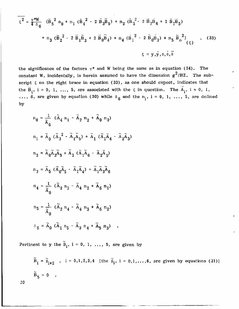
Figures 6 through 11 show whether the imposition of the conditions {D1 = D2,
Di # Li, i = 1 , 2 ) instead of {Di = Li, i = 1,2}, other conditions being the same, results in nn increase 01' decrease in the RMS of the response variable in question. These figures, when complemented by the output of TRROBM plotted in Figures 1 2 ,
13, and 14, provide the RMS's of the system coordinates and their first two time
14

derivatives for both the (x,O) and (y,O) descriptions of system configuration. collection o f figures does not represent an exhaustive parameter study, but is
exemplary of parameter studies made possible by program TRROBM (with or without
the support of its auxiliary AUXRBM, which is of limited application).
This
At least one paragraph should be devoted to stability, if only to go so far as to write the conditions (on the system parameters) whose satisfaction guarantees
L system stability. Such conditions are indirectly realized by conditions on the coeffi- 4
i = O cients of the system characteristic polynomial, A(S) = Aisi [see equations (9) ] ,
those conditions being available via the Routh-Hurwit z criterion. array pertinent to A(S) is the following:
The Routh-Hurwitz
By the expressions defining them, A4, A3, and A,, are intrinsically positive. by the Routh-Hurwitz criterion for stability, system stability is assured if the other
two elements in the first column of the array are positive, or, equivalently, if both of the inequalities
Hence,
are satisfied. in this paper. is zero wil l be found in the literature.
The problem of assessing the !'degree" of stability will not be addressed The technique for handling the situation wherein a left column element
15

The author has given some thought to models other than that of Figure 1,
those of Figure 15 in particular, which, in certain cases, could be more "credible" or "plausible" models. the models in Figures 1 and 15-a, that difference due, obviously to the elastically supported dampers in Figure 15-a, there is a marked difference between the respective mathematical descriptions of model motion. the motion of the model in Figure 1 are of second order, those determining the motion of that in Figure 15-a are of third order.
Though there is slight difference between the llappearances" of
While the differential equations governing
Pertinent to Figure 15-a, the author has derived the following equations.
m(y+u) = - ( K 1 + K z ) y + ( K I L 1 - K2L2> 8 - C1 ($ - Die> - C2 (y + D2e>
+ [ K I L 1 2 + K r p 2 + D2 (KIL1 - K2L2)1 e>
- [ K I L 1 2 + K2L2 2 - D1 (KIL1 - K2L2)1 6 }
.. I 8 = ( K I L 1 - K2L2) y - ( K I L 1 + K2L22> 8 + CIDl (G - D16) - C2D2 (i + D26)
- CIDl { I *I$ ' - m D 2 (y +'u) + [ K 2 L 2 - KIL1 - D2 ( K 1 + K 2 ) I Y - K 1( D l+D 1
16
t

N N
Notice that if one makes the substitution x = y + u and allows K 1 and K 2 to become infinite , equations (25) and (26) become, in v iew of relations ( 3 ) , the equations of motion of the model in Figure 1 pertinent to the (x , 0) description of system configura- tion, the equivalent of the matrix equation ( 4 ) ; o r , if one merely permits K1 and K 2
to approach infinity, equations (25) and (26) become the equivalent of equation ( 5 ) .
N -
Considerable simplification of equations (25) and ( 2 6 ) is realized in the special - N - case wherein K1 = K 2 = K , C1 = C2 = C , K 1 = K 2 = K . In that case they read as
equations (27 ) and ( 2 8 ) .
C ; j ; + m j ; + 2 ~ $ + 2 K y + C [D2 - D1 + K (L2 - Ll)] 4 K
- K
+ K ( L 2 - L 1 ) e = - ; - -mC ... u - m u .. K
+ $ (LI2 + L22)] + K (L12 + L2 2 ) e K
IC *-.
K e + ~ e + c
Having written the equations of motion, the next step toward a mean square computa- tion is the deduction of the relevant transfer functions. comprised of equations ( 2 7 ) and ( 2 8 ) , it is easily deduced that
Pertinent to the system
6 6 - T ( s ) = Fi Si / x. Si Y /U 1
i = O i=O
4 6 N
(s) = Ti si / c xi si . e/u i = O i = O
where
17

2 2 (L1 + L2)
v
A. = K
2 2 K I . ' %
A1 = 2 K C D1 + D2' - (D2 - D1) (L2 - L1) + L1
2 K 5
A2 = m K (L12 + L2') + 2 K I + 2 C2 (1 + :)[ D12 + D 2 + K (LI2 + LZ2)]
2 - C 2 k2 - D1 + K - (L2 - L1q K
( 3 0 )
(L,2 + ~ ~ 2 ) + I + m c + D~ 2 K + ( L ~ m K C K
A = - 3 K K
+ 2 I c (1 +; )
(L12 +
h
A~ = 2 m I c / ii
i 6 = m 1 c 2 / K -2
2 rr
B~ = - m K (L~' + L~
c - - 2 m C K (L12 + L2 2 1 E B3 - - m C (D12 + D2 2 1
P2 -m c2 [D1' + D 2 2 K + - K K
B 4 =
c v
fig = - 2 m C I / K
I j 6 = - m 1 c / K 2 @ 2
18

2
y 2 = m K ( L 2 - L1)
K K K
-<
yq = ms b2 - D1 + (L2 - Ll)] .
Imposition of the additional conditions D1 = L1 and D2 = L z , as in Figure 15-b, results in a simplification of equations (27) through (32). by setting = K.
Further simplification is possible
Upon examining the structure of the transfer functions in equation ( 2 9 ) , along wi th that of the five Laplace transform ratios
it - is evident, in light of the table of integrals previously cited, that the mean squares 5 , 5 = y , y , 6, 6 , i, are expressible in closed form when G..(f) is constant for
2 0 I f c 0 0 . In the notation of this paper, the closed expression for 5 is
2 - U
19
L
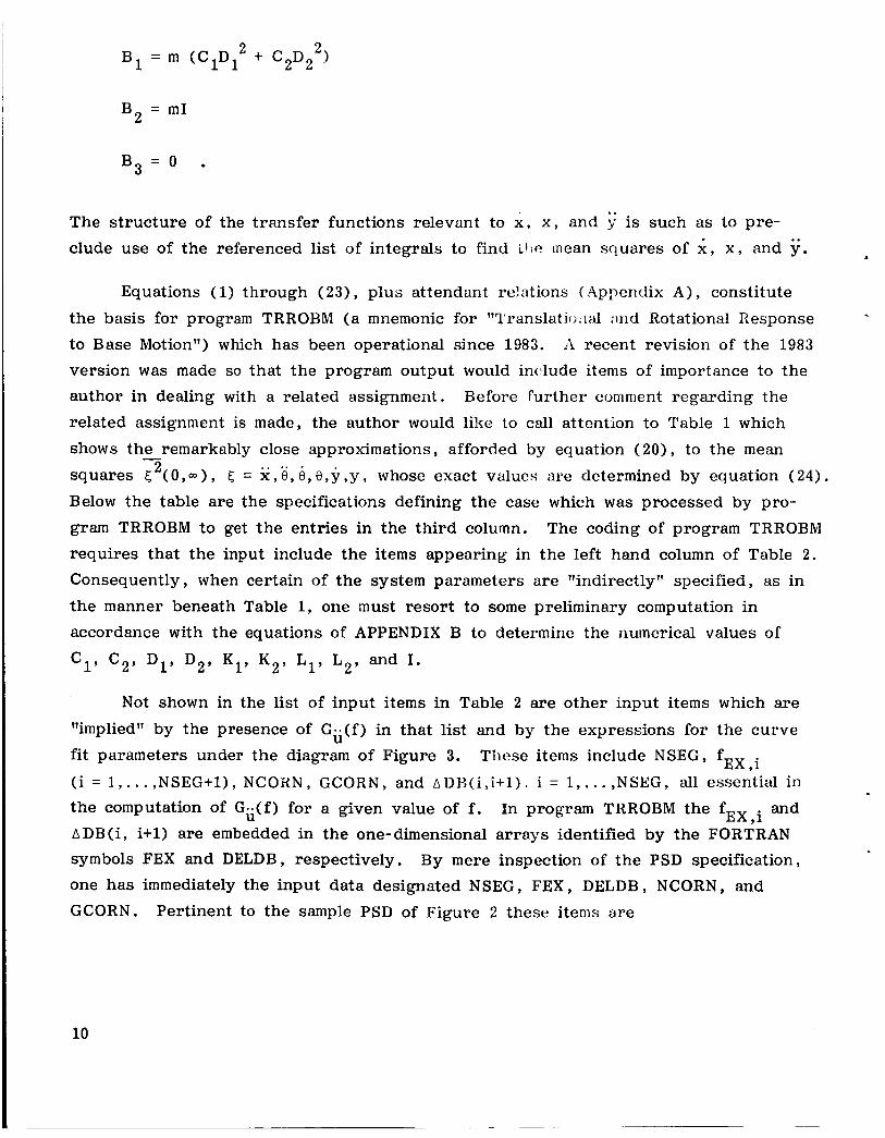
+ n3 ( i i 2 2 - 2 B ii + 2 BOB4) + n4 (BI2 - 2 BOB2) + n5 go2} Y (33) ( 5 ) 1 3
the significance of the factors y* and W being the same as in equation (24) . constant W, incidentally, is herein assumed to have the dimension g /HZ. script 5 on the right brace in equation (33), as one should expect, indicates that the Bi, i = 0 , 1, ..., 5, are associated with the 5 in question. . . . , 6 , are given by equation (30) while A 6 and the ni, i = 0 , 1, . . .
The The sub- 2 .
.a
The Ai' i = 0, 1,
5 , are defined
by
- - - - - - I -
n2 = A A A t A~ (A1A6 - A2A5) 0 3 5
1 - ( A ~ n3 - A4 n2 + As nl)
I (A2 n4 - A4 n3 + A6 n2)
n 6 = A. (A1 n5 - A3 n4 + A5 n3)
5
Pertinent to y the Bi, i = 0, 1, ... , 5, are given by
- - - Bi = 4 + 2 i = 0 , 1 , 2 , 3 , 4 [the Bi, i = 0 , 1 , ..., 6 , are given by equations (31)]
20

.
Pertinent to 5 , - -
B. = B , i = O , l , ..., 5 1 i+l
Pertinent to i',
- c
Bi = yi
B 5 = 0 . , i = 0,1,2,3,4 [the ti, i = 0,1 , . . . ,4 , are given by equations ( 3 2 ) ]
-
Pertinent to 6,
- - B. = y , i = 0,1,2,3 1 i+l
c - B = B = O . 4 5
Pertinent to e ,
- c
, i = 0,1 ,2 i+2 B. = y 1
To date, no attempt has been made to code a program based on equations (25) Programming, on the part of the author, and (26) o r any of their simplified forms.
has been pursued only so fa r as programs TRROBM and AUXRBM, which mark the culmination of the author's effort in this area.
21

TABLE 1
l o 3 (0.78567859) ( g2)
l o 4 (0.20118432) (rad. /sec2I2
2 10- ( 0.50960584) (rad. /see)
(0.12217110) (rad.)2
lo3 (0.29642678) (in.
(0.75068497) ( in.)2
VIA EQ. (24)
l o 3 (0.78498616) ( g2)
l o 4 (0.20111040) (rad. /sec2)2
10-1 (0.51124543) (rad.
(0.12244709) (rad.)2
lo3 (0.29412964) (in. / s e e )
(0.75001788) ( in.)2 VIA EQ. (20)
Percent E r r o r
0.088
0.037
0.32
0.23
0.77
0.089
SPECIFICATIONS:
Gii(f) = 0 . 1 (g2 /HZ) , 1 5 f 5 200.0
K1/K2 = l., C /C = l . , D1/D2 = l., 5, - - = 0.01, fnx = 100. (HZ) , 1 2
rf = 0.1, rL = 2 / 3
in = 1 .0 , ) , p = 5. ( in.) 2
, lb . *see in.
VALUES O F I , K1, K 2 , C1, C2, D1, D 2 , L1, L2 (ENFORCED BY THE
SPECIFICATIONS) :
I = 25. (lb.*sec 2 *in.)
K1 = K 2 = 10 6 (0.19739209) ( l b h . )
C1 = C 2 = 10 (0.62831853) ( l b / ( i n . / s e c ) )
D1 = D, = 10 (0.15811388) ( in . )
L t = 0.39223227 , L2 = 0.58834841 ( in . )
I
c

Program Input
A f
c 1
Dl
D2
K 1
m
I
TABLE 2
PROGRAM TRROBM
Program Output*
.. . .. . .. . .. . .. . 5 = u,u ,u ,x ,x ,x Y 0 9 8 9 0,Y YY YY ,Yp,Yp Jp I -
5 2 (f l ’ fN)
i = 1 , 2 9
Modal Column Corresponding to fic i = 1 , 2
fnx
fn 8
* A print of all tabulated functions of frequency i s optional
23

FIGURE 1

ORIGINAI: PAGE B OF POOR Q U m
25

I I f q 2
F w I f ' 3 i
I:IGURE 3
26

OP.IGIN.AU PAGE 19 OF POOR QVALITY
-t- I
-4- - I
i
c , 1 ; I..:; i . . . .
_. L ... . . . . . . . .
. . . . . . . . - + . . . . .
I -_
I I I 1 I I
i I i i i I l ' I 1 i ........ i I
I
pi
,w I i
' i
. . ! . .
. . , I
. . i I . . .
-\: -: 1 j
27

28
m- , . . . . . .
. . . . . ._ - --
. . . , I . : I

FIGURE 6
29

--I-- !
I
I i I
I - I , - I-
1
I
I . . . 1 . I
~
+ T
. '4-
1
I
--I!-
.......... .- .
i t ~ -
-- 1;- 7 . _ . .
- . . .
_. . . . . . . . . . .
. *..
2 .
I 7- . .
. . I
1
c
h
u
c-
r.
L,
30
ORIGINAL PAGE is OF POOR QUAUT;H

I
IO1 1
.i
7 -
J
3
40” + I
IO
n 9
7
6
5
4
3
FIGURE 8
31
- - - - I I I
I . .. . . -.
I -4 i 71 I t
&- I I, ~- !?
I
_ _ _ _ _ _ . . ., I I -
. . 1 . . .
: - L, <
1 j I
... . I . -
1
t - i I' I . I I I ,
1
. . . . . . . , . . . .
~. . 1- . - . . . . . . . .
_ _ - . . .
- - . . . . . -. .
. . . . . . .
. . .
I .
I . . . I -2 I
I
1 . I 1
I !
32

~
. . . . . . . . . . . . . . .
. . . . _ , . ~T _ _
. . . . . . . I . . -
-t- . . _ _
PT. +- -+T - ! ~ . '
1 :::
$*&r
. . . .
. . . . -:-- ' I '
+ . . . . . . . t . . . . . . .
~ : ~ ~ : : l ~ ~ : ~ . . . . . . . . . . . . . . . .
- . . . . . . . .
. . . . . .
. . .
. . . . .
.
I
0 4
W a' 3
Frl s
I 7 -- ----I -
i
I
f . . . .
. . -
. .
I
-+- --
. . I _i -4-
:.I . .
33

I
. I
- - T
n 4
. . . . * . I-.
I ------I*
I - -1
i I ' U
i --------/E.
---I
I I I
+-. \. I I t - -
I
34

ORIGIRTdL PAGE IS OF POOR Q U A U T y
0
t
b
. .
I
- 1 I
i
/ . . .
. . d
35
!
0
0
Y
d
I
. I
Y ti Y H
36

37

FIGURE 15
38

REFERENCES
1 . Tuell, L. P. : Unpublished work, NASA/MSFC , Huntsville, AL, 1980- 1983.
2. James, H. H . ; Nichols, N . B . ; and Phillips, R . S. : Theory of Servomechanisms. Vol. 25, M . I. T . Radiation Laboratory Series, New York , New York , McGraw- €Iill 1947.
3 . Seifert, W . W . , and Steeg, C. W . : Control Systems Engineering. McGraw-Hill, 1960.
4. Grandall, S. H., and Mark, W. D.: Random Vibration in Mechanical Systems. Academic Press, 1963.
5. Tse, F. S . ; Morse, 1. E. ; and Hinkle, R . T.: Mechanical Vibrations. Allyn and Bacon, 1963.
39

DEFINITIONS
Damping coefficient [lb/(in./scc)] of viscous damper i , i = 1,2
Lateral distance (in.) between CM and point at which damper i is attached to model, i = 1 , 2 (D. L 0)
1
Frequency (HZ), fl I f s f N
Frequency ( H Z ) of undamped coupled natural mode i , i = 1,2
Frequency (H Z ) of undamped uncoupled translational mode
Frequency (HZ) of undamped uncoupled rotational mode
2 Acceleration due to gravity (in. /sec )
PSD or ii ( g 2 / ~ z )
PSD of 1; [ ( i n . / ~ e c ) ~ / H Z ]
PSD of u (in.'/HZ)
PSD of (g2/HZ)
PSD of x [ ( i n . / s e ~ ) ~ / H Z ]
PSD of x (in.2/HZ)
PSD of 'e' [(rad. / ~ e c ~ ) ~ / H Z l
PSD of 6 [(rad. / ~ e c ) ~ / H z ]
PSD of 8 (rad.2/HZ)
PSD of y ( g 2 / H Z )
PSD of y [ ( i n . / s e ~ ) ~ / H Z ]
PSD o f y (in.2/HZ)
PSD of' yp (g / I I Z ) 2

0
i,
e *.
.. ( 1 ’ fN
.. Y
.. Yrms(fl’fN)
YP
PSD of iP [(in. / ~ e c ) ~ / H Z l
PSD of yp (in.2/HZ)
Angular displacement (rad. ) of model from static equilibriuiii orient at ion
Angular velocity (rad. Isec) of model
Angular acceleration (rad. /sec 2 ) of model
2 Mean square value (rad. ) of 6 in the interval (fl,fN)
Root mean square (rad.) of 8 on the interval (fl,fN)
Mean square value, (rad. /sec)2, of 6 on the interval (fl,fN)
Root mean square (rad./sec) of 6 on the interval (fl,fN)
Mean square value [(rad./sec ) ] of
Root mean square (rad./sec ) of ‘e’ on the interval (fl,fN)
Displacement (in.) of model CM relative to the base
Velocity (in. /sec) of model CM relative to the base
Acceleration (in./sec ) of model CM relative to the base
Mean square value (in.2) of y on the interval (fl,fN)
2 2 on the interval (fl,fN)
2
2
Root mean square (in.) of y on the interval (fl,fN)
Mean square value, (in. /sec)2, of on the interval (f, ,fN)
Root mean square (in./sec) of $ on the interval (fl,fN)
Mean square value (g ) of 2 on interval (fl,fN)
Root mean square ( g ) of on the interval (fl,fN)
Displacement (in. ) of point P relative to the base
Velocity (in. /sec) of point P relative to the base
41

2 Acceleration (in. /sec ) of point P relative to the base YP
Mean square value (in. 2, of y, on the interval ( f l , fN)
Root mean square (in.) of y, on the interval (fl,fN)
Mean square value, (in. /sec) 2 of ip on the interval ( f l y f N )
Root mean square (in. /sec) of y, on the interval ( f l y f N )
Mean square value ( g 2 1 of j ; , on the interval ( f l 9 f N )
Root mean square (g) of y, on the interval (fl,fN)
Static deflection (in.) of spring i , i = 1,2 (considered positive despite my sign convention)
2nfic (rad./sec), i = 1,2 w ic
A f Both the print step ( H Z ) and the frequency increment ( H Z ) used in the numerical evaluation of the definite integrals defining the mean squares
Displacement (in. ) of the base from its static equilibrium position U
U Base velocity (in. /see)
Base acceleration (in. /sec ) 2 ..
U
Mean square value (in.2) of u on the interval ( f l y f N )
u ( f Y f 1 r m s 1 N Root mean square value (in.) of u on the interval ( f l , fN)
2 Mean square value (in. /set) of 6 on the interval ( f l 9fN)
Root mean square value (in./sec) of 1; on the interval ( f 1 y f N )
2 Mean square value ( g ) of u on the interval (f , ,fN)
.. U r m s ( f l y f N ) Root mean square value (g) of u on the interval ( f l Y f N )
Displacement (in. ) of model CM from its static equilibrium position (x is an absolute displacement)
X
X Absolute velocity (in. /sec) of model CM
42

2 Absolute acceleration (in. /sec ) of model Chl I.
X
Mean square value (in.2) of x on the interval (fl ,fN)
Root mean square (in.) of x on the interval ( f l , f N )
Mean square value (in./sec)' of k on the interval (fl,fN)
Root mean square value (in. /sec) of on the interval (fl,fN)
2 Mean square value (g 1 of 2 on the interval ( f l , f N )
x ( f , f ) r m s 1 N Root mean square (g) of x on the interval (fl,fN)
The complex variable of the laplace transformation (rad. /sec) S
Square of the magnitude of the frequency response function between 6 and u (dimensionless), 6 = x y y y y p ( j = a) Square of the magnitude of the frequency response function between e and u (rad./ in.)2
I Moment of inertia about an axis through the CM and perpendicular to the plane of motion (lb*sec2*in. )
Ki
Ki z
Stiffness (lb/in.) of linear spring i , i = 1,2
Stiffness (lb/in.) of elastic support of damper i in alternate model (Fig. 15), i = 1 , 2
Li Lateral distance (in.) between model CM and the point at which spring i is attached to the model, i = 1 , 2
L r L1 /L2
Mass of component [lb/(in. /sec 2 ) 3 m
P
LP
Radius of gyration (in.)
Lateral distance (in. ) between model Lp < 0 according as point P is right
CM and point P (Lp > 0 or or left of the CM)
fn e'fnx 'f
Fraction of critical damping associated with translation
Fraction of critical damping associated with rotation
43

bi, c. Parameters appearing in the analytical representation of Gii(f) on the interval ( fEx , i , fEX,i+l), i = 1,. . . ,NSEG 1
NSEG Number of straight line segments in the log-log plot of the prescribed base acceleration PSD
Abscissa ( H Z ) of the i'th "corner" point in the log-log plot of G;i(f), i = 1, ... NSEG+1 fEX ,i
NCORN A positive integer specifying that %orner" point of the straight line segment representation of the input base acceleration PSD on log-log graph paper at which the value. of the input base acceleration PSD is given
GCORN 2 The value ( g / H Z ) of the input base acceleration PSD at the "corner1' point specified by the integer NCORN
A DB ( i , i+ 1) Rate of change, in decibels/octave, of the input base acceleration PSD as the frequency f varies from f EX,^ to f ~ ~ , i + ~ ' i = 1, ... NSEG
4 4

APPENDIX A
SUBSIDIARY RELATIONS
R = KlK2 (L1 + L2)' - [I(K1 + K2) + ClC2 (D1 + D2> 2 1 (2nf) 2 X
n n
R e = - m (K2L2 - KIL1) ( 2 d ) 2
4 = - m ( c ~ D ~ - c,D,) ( z n f ) 3 e
+ I (c, + C,)I ( 2 d 1 3
45
(K1L12 + K2L2 2 1 + m 1 (kl + K 2 1
- 1 (KlL12 + K 2 L 2 2 1 1 + m ( K 1 + K 2 > I
2 4 K1K2 (L1 + L2> mI I + K2L22) + m ( K 1 1 + K 2 1 -
fic = LdiiC/2n , i = 1 , 2
u2 = K 1 + K 2 nx rn
2 2 u 2 = K I L l + K2L2 ne I
f = w / 2 T nx nx
fne = w / 2 T ne
46
2 "' 1c -
FOUR ADMISSIBLE EXPRESSIONS FOR THE UNDAMPED MODAL MATRIX (NON-NORMALIZED)
(KIL1 # K2L2 PRESUMED)
I
L K2L21- KIL1
2 w 2 c
1
- I
K2L2 - K I L l I
1 K2L2 - KILl I
I
K2L2 - K l L l I
w 2 - K1 + K2 2 c m
I
K2L2 - K I L l m
K1 + K, - - 2
1c rn
K2L2 - K1L1 m
2 K 1 + K 2 wlc - m
K2L2 - KIL1 1 m
2 w 2 c -
2 w 2 c -
K 1 + K 2 m
2 KIL1 + K2L22 I
I
K2L2 - KILl
L
47


APPENDIX B
ON THE CONSEQUENCES OF CERTAIN SPECIFICATIONS
When the coupling coefficients vanish simultaneously. that is , when I i 1L
= 0 and CIDl - C2D2 = 0, the equations of motion, (1) and ( 2 ) , assume their
-
K L
uncoupled forms (B- 1) and ( B - 2 ) . 2 2
m x + (cl + c2) i + ( K ~ + K ~ ) x = (cl + c 2 ) b + (K 1 + K 2 u (B-1)
(B-2 ) I; + ( c , D , ~ + C ~ D ~ 2 ’ e + ( K ~ L ~ + K2L2 2 1 0 = 0
Upon inspecting equations (B-1) and ( B - 2 )
undamped natural frequencies and damping ratios satisfy it is easily seen that the uncoupled
2 - K1 + K 2 - c1 + c 2 m 9 2 5, Wnx - w - nx m 9
If one imposes the conditions
K 1 = K 2 c1 = c2 2 D1 = D
and assigns values to m, P , unx, cX, rfy rL, where
rf = une’Wnx = f ne /f nx and r L = L1/L2
then some simple algebraic manipulation (bearing in mind the definition p = fi) will show that the numerical values of Di, Ci, Liy and Ki, i = 1 , 2 , are determined by
C i = m 5 w 9 i = 1 , 2 x nx
49

K . = m w 2 /Z , i = 1 , 2 1 nx
112 2 = 'f (q2+ 1)
L 1 = r L L 2 '
If the condition D1 = D 2 is replaced by Di = Li, i = 1 , 2 , the numerical values
of G;;(f), m , p , wnx, c,, r f , and r L I , K 1 , K2 , C1, C Z y L1, and L2 are the same as before, but the equality of Di and L. , i = 1 , 2 , requires that ce = rf 5,.
being prescribed as before, the expressions for
In this case one will find 1
3 4
K=O K=O
4 2 2 5, w n x 3 rf2 (1 + rL) 2 unx rf2 (1 + rL)
2 ( l + r L 1 Y 2 A =
1 + rL 2 1 A = 0
A = 1 . 4
, B = 2 < w 2 2 2 2 nx 'f 3 x nx 1 , B = A - w B = A o , B 1 = A 0
3 4
K=O K=O
50

4 4
K=O K=O
5, unx 9 B 4 = -1 . B~ = - rf2 u2 2 B o = B 1 = 0 , nx , B 3 = - 2 rf
If neither the condition D1 = D 2 nor the condition Di = L i = 1 , 2 , is imposed, i ' while enforcing the conditions K
values of' G . - ( f ) , m , p , unx, c,,, c8, rf , rL, and rD = D1/D2, there is still no change in the expressions for I , K1, K 2 , C1, and C2, but D1 and D 2 will be determined by
= K 2 , C1 = C 2 , and prescribing the numerical 1
U
D 2 = P I , D = r D 1 D 2 '
I n this special case, the transfer functions relevant to x, 8, and y are
3 4
K =O K=O
A K ' = AK of the preceding paragraph for K = 0 , 3 , 4
r 0 1
L J
B K 1 = BK of the preceding paragraph for K = 0 ,3
51

2 2 B l l = All , B 2 ' = A ' - 2 ("nx 'f
3 4
K=O K =O
yK1 = y K of the preceding paragraph for K = 0 , 1 , 2
4 4
k=O K=O
B K ' = BK of the preceding paragraph for K = 0 , 1 , 2 , 4
It is worthy of note, insofar as economy of computer time is concerned, that the moduli of the transfer functions of this and the preceding paragraph are unchanged (for a specific value of the complex variable s) if both rL and rD are replaced by their reciprocals. The same can be said of the transfer functions defined by equa- tions (6), (7), and (8) when their numerator and denominator coefficients are such as to meet specifications similar to those beneath Table 1.
APPENDIX C
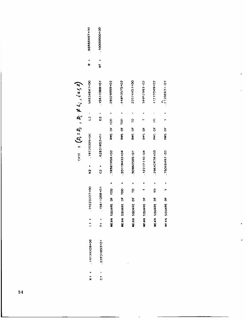
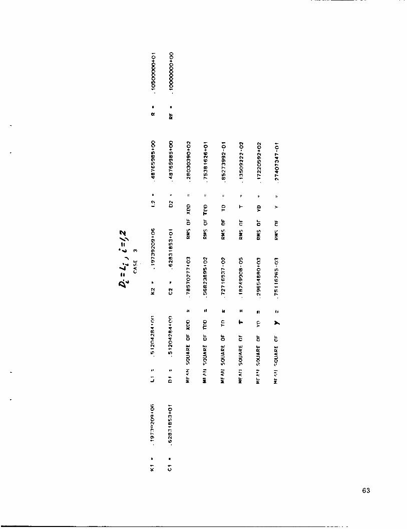
SAMPLE OUTPUT OF PROGRAM AUXRBM
.. .. Symbol X t)
FORTRAN Equivalent XDD TDD
On the following pages of this Appendix are two sets of mean squares and RRIS's .. .. of x , e , 6 , e , i , and y as found by program AUXRBM in two computer runs, there being seven cases processed in each run. In both runs rL assumes the values 2 / 3 ,
1 . 0 , 1.05, 1 . 2 , 1 .5 , 2 . 0 , and 10, in turn, and
8 8 Y Y 'L 'f K 1 K2
TD T YD Y R RF K 1 K 2
rf = 0.1 , fnx = 100. ( H Z ) , 5, = 0.01 ,
D1
2 K 1 = K , C1 = C 2 , p = 5. (in.) , m = 1 . 0 (lb*sec /in.) ,
D2 C1 C2 RMS
2 G$f) = 0.1 (g / H Z ) for 0 f < OD .
In one run the conditions D1 = D 2 and Di # Li (i = 1 , 2 ) apply, while in the other Di = L. (i = 1 , 2 ) .
1
Observe that in each run the output mean squares in case 5 duplicate those of case 1, that being due to the fact that the values of rL and rD in case 5 are the reciprocals of those in case 1. See Appendix B (last two sentences).
Notice also that the numerical results in case 2 of each run verify that 8 is
identically zero (assuming zero initial conditions) when the relations CIDl = CBD2 and
KILl = K2L2 hold.
The following table will serve to define the FORTRAN symbols appearing on the AUXRBM printout.
1
RMS L1 I L 2 I Dl I D2 I 1 c 2 I __t I I I I I
I I I I i
s c c
u. U U U U L O Q O O D C
In I K
m I cr z
K
L'. f Q
u? I 0
5 4

I m
a u U
w m V a
IC Q! c
.. m PI u)
N V
a m P In
c
U I1 I1 I 1 II I1
8 ' 0
It I1
c c Y O
55

I
c
s I t
u
e
8 m m m W l-
w
a
a
I t
CY d
0 P (Y m D r- 5
n
(Y Y
8 0
N 0 0
m
a
2
I t
c
-I
W P
II
c Y
8 ,I c
I
U a
t
'? OD
m a
a c c
m c
I t
ri a
L
0 m m
m m (Y W
t
z
II
N V
c
'? a m a
m c c
sc
II
c n
c
9 ? m m
0
N (0
a
(I
c
V
N
9 t
m m 0 m 0 a cy
I8
a n X
LL 0 v, z P
FJ 0 m 7- c c r- m oc r-
I
C
x U 0 w a
n
a s
E"
ln 2 a
c
9 (Y P m (D m In In
a
II
n n c U 0 In L P
cy
9 0 0 c
0 P N
m c
I
n n c U 0 u 0 a 3 0 ln
5 r"
c
? z r
0,
(Y
a c\
e LL 0 v, z P
? r+ P t
b, r-
ll
C c
LL 0 w o!
2 In
z a. w I
m ? P 0, 0 In N r- N P
11
I-
LL 0 In z 0
W
7- m c) f U. N a
0
c
U
t
U 0 Y P a 3 0 In
2 a r"
N
? c
m (D 0 N R
7- .- I*
C >
U 0 V. I u
m 0 E N m In (D m cy
I1
n >
LL 0
0: a 3 0 In
2 a Y I
Y
c
? b, Q, P r- 0 0 7- N
11
>
k 0 In
E
m
m 0 7-
m (c
? c
r c
I1
>
k 0 Y P
3 In
2 a r"

c
? OD OD P) c -
8 N
? t
? * iu m
- 0 m + c
+ W N In 0
c N I- C
m 2
r; m In t
W VI c u
m 9
c
? h
m B
P) 0
)I
N X
n
(Y V t
w H n w I II
57

8 I- N
N 0
N
? 0 m 01 N m 01 9 m
c
N c
c
? c m 0
m m I- N
m
II
In
W v: 4 V
II
N Y
L L U U U L L U 0 0 0 0 0 0
c
m
N 0
c
0 B 7 ffi r- x 9 W m
I U
x u f c
58

I1 N
P U P
8 cy 0
N
P I m
.. N
a 0 0
F J 0 8 W
In 4 V
+ N 0
N -e t- OD W m m
c Ln hl N 0 m N
I1
N Y
Y
cy V
8 e
5? c! OD m
v
0
Y n 0
0 t
LA 0
n t
LL 0
t
LL 0
n >
LL 0
>
U 0
+ m 0 In Ln U
U 0
5 9

c
0
N
r-
w v,
u a
I 1
N x
8 + Y)
H
PJ V
Y 0
U. 0
U 0
U. 0
U 0
0 N Y) m N
U 0 G I a
o
0 0 U 03 (0 P (P I-
?
C ) U Y L L U U . U . - 0 0 0 0 0 0 f
,I H
c c Y V

F 8
W "1 ? - w
8 &
N 0
t
? * c 0 OD 0 0 OD
m rn
(c c c
0 c
8 N
N + c
h m OD N (t
8 (s 0
0
M f
P c
(7
0 0 l- m c
W v) Q V
c Y
m x
ll
N V
N U 0 h
U, l-
n II
Y V c c
61

6 2
8 c
P c 0
c
?
t
r- m cy cp
N 0
r. c (c h ffi
I!
N Y
I
N V
f h m
- L
c
v. r- c
II II
c. I t
E t: t X
U 0
C I-
LL 0
L C
LL 0
I
C W P c 3 C v,
w a < 3 0 1r
Lc m
I I
c
-I
z
E
C LL
- L c Lc 5.
63

N ?
N
P 8 N
? z r-
c
? m f
N oc N 0 6 N
c m (7 0 m c
N : c
(7 r L
c) 0
(7 0 8 F
0 0 0
FJ
N m
+ r-
h
N X
I1
N u
64

8 + 8 c
? N 0
c
F: ~ * I- N N
C P
- m m I- s
c
0 L
0, C P I- N
0 m cv
h I- c
c -
p: I-
0. P
? N
p: c s a n Ln c
m 0 (7
(t (3
P L
I!
c. Y
I 1
r: 0
N lo cn
H U
c c x u
65

66

c
? t
0
P F, c
c
'? I-
u rr m OJ N
c 0
N 0 c (0 c) 0 P * t . i
c
? c
iu r:
II I I * I: II II II I,
L L L I& L L O Q Q C C C
Y
V
4-J g I t
h r- C: f
I
h Y
D a? N (0
b
cy L'
(7
E; N 0 1 r- i (7 U. I- I-
c
0 I-
N
0 W 0 - . m. (7 a2 0 L
(I U
c c x u
67

APPENDIX D
SAMPLE OUTPUT OF PROGRAM TRROBM
2 2 The specifications C;;(f) = 0.1 (g I H Z ) , m = 1.0 (lb*sec /in.), p = 5. ( in . ) , f = 100. (HZ), 5, = ce = 0.01 , K 1 = K 2 , C1 = C D1 = D Di # Li (i = 1,2) , nx 2' 2' rf = 2.0, 1. f I 4 0 0 . , A f = 0.5, and
1.05, (Case 1)
1 . 2 , (Case 2)
1 .5 , (Case 3)
2.0 , (Case 4)
led to the numerical values of I , K1, K2, L1, La , C1, C2 , D1, D 2 , and other items (with the exception of L ) essential to the mean square computation, shown on the input print which precedes the output print of program TRROBM. five cases processed by TRROBM, the frequency interval (l . , 400. ) HZ was slightly less in length than the recommended interval (l . , 2f2c) H Z , but the approximations to the mean squares and RMS's were surprisingly good.
P In each of the
The reader should compare
encircled values and inset tabular values, corresponding to rf = 2.0, in Figures 6
through 11.
The reader is due an explanation of the items appearing on the last page of the output print for each case. A s it pertains to matrices, the word adjoint has its usual meaning, that is , the adjoint of a matrix is the transpose of the associated matrix of cofactors. The 2 x 2 matrix identified as "ADJOINT CORRESPONDING TO OMEGAlC" is merely the adjoint of the characteristic matrix, to be defined subse- quently, when the elements of the characteristic matrix are evaluated at w = w l C .
A similar statement applies to the matrix identified as "ADJOINT CORRESPONDING TO
OMEGAZC" (with wlC replaced by w ~ ~ ) .
Ch(H,w ), is given by The characteristic matrix, here denoted by
2
* The author has exercised the option to avoid printing all tabulated functions of frequency.
69

1. 0
Ch(H,w 2 = u2 [ - H
where H , known as the dynamic matrix, is defined by
H = M - ~ K ,
the matrices M and K being, respectively, the system mass matrix and stiffness matrix, that is [see equation ( 4 ) or (5 )1 ,
2 1 . ~ = r :] 3 '=[K2L2 - KIL1 KILl + K2L2
K1 + K 2 K2L2 - KIL1
2
2 The equation formed by setting the determinant of Ch(H ,w ) to zero is a quadratic in u 2 whose roots, wIc and uZc, are the characteristic values (or eigenvalues of H ) and also the squares of the undamped coupled natural frequencies. A s the charac- teristic vector (or eigenvector) of H corresponding to wic, one may choose any non- zero scalar multiple of either column of the adjoint of the matrix Ch(H,wiC), i = 1 , 2 .
Program TRROBM selects the second column of the adjoint and the reciprocal of the 2 , 2 element as the scalar multiplier to get the vectors identified as "normalized" characteristic vectors on the output print.
2 2
2 2
The vectors of the preceding paragraph could also be called modal columns of the "undamped" modal matrix. Notice that the modal columns have been "normalized" in a certain fashion, the "fashion" indicated. The author has not declared that such a normalization renders the modal matrix normalized with respect to the mass matrix. If it is desired that the modal matrix be normalized with respect to the mass matrix, one should select one of the four admissible expressions for the undamped modal matrix* , here denoted by
-- *See Appendis A .
70

and post multiply it by the diagonal matrix
where q1 and n2 are computed by
The expressions for n l and n 2 were found by simply demanding that the matrix Y = @ q be such as to satisfy
71

c
? m c
L'r
? P- W 3 P
cy m
r- $ c m
d W 0
(D
? 0 ?
N 0
0 0 G
- 0
m 00 N
c c c c W
a - I-
N 0
N G + -
- P m
.b K W z
0 2
U c m 5
I1
c
-1
II
r
2
I t
c
d
II
F
r Y
- 0
8 c
? * I-
? 8
m a H A . W 0
w a - X I a . 3 0
P 0-
H c
I 1 I1
v) v) a f
I1
c Y
I1
c Y
II
c
Y
1,
r
Y
I1
c 0
u w In z
72

5 &
I- N 3 -
c 3 I- o
3 U:
P w VI .. L
t z c
0 0 h
+ IY w n r,
I,
1
i
V c X u1
I,
c I-
w CY a
V a w > 0 ii C
I' - z Y c L"
I- v, I LL
C CL Y 3
V C -I
i C' e 4
i
>
V 9 - ku
V L' 4
c w > LL
C L 3
z C L, z
LL 0
r
- 3
io z IY
Y 3 z
4
C d
z
a Q W
73

3
D
f n >
3 n z a X
3
0 2 a t-
3
0 z 4
> z 3
W U'
I-
z 3
W W
I- W 03
I- W p3
z z c
I- LL m
W n; z
0 I c
c V 2 3
u z -I Y L
w CL
W LZ >
LL' cy
LZ
> V z W 3 0 w Ly LL
w A
I-
> c; z W 3 C
cy w
LL
> V z 3 0 W Iy LL
W
w .L c Y c Y a - > U L
2 0 m m a W I I-
LL C
V z W 3 O W LZ LL
v,
c7 W I t-
LL 0
W
t-
LL
I
0
5 C'
W I,? < D:
LL' v, 4 M W I I-
O I-
W
2 I-
-1 W cy
a
a
I L,
Y 0 L."
ffi a I c
W I
U t
c I
U m
E
w I-
a
- - O I-
W >
w 3 -1 C >
W 3 J
> w I-
a
2 0 v, m a
w z I C LI LL
I V
W I I-
LL 0 c
m c7 b
V d .z L1:
w c! c W
I- > -I 0 V, m a W I I-
L 0
a - m Ln a I
W I- 3 -I 0 VI a! a
L - C I
c L If C !i
I-
-I W cy
a u 0 -I w >
W
I-
LL
I
0
- I-
-I W cy
G
a W
I-
LL 0
I
L
2 I Lu V C
LL 0
W
I-
LL 0
I LL 0
c z I U LL
0 z C c
w
t- I I-
C [L LL -
L 0
LL: cy
3 0 vl
a w c <
I- LL LZ a I, C m
c -9 L c
C c
a c: ld
U. 0 c
< > L
LL C z 0 CI
I-
$ c
.L e c 3
C i L V, M
n w > ,-. I-
J W cy
a
2 El ,. L
c <
c r
J LL 0
W
t- I n
v, J I-
a cy W
iil > I
n c CY W J W V V a
w + v, W c
f
> c I
L L
VI W L
m C Iy
J 3 e z
a
a
V 0 J W >
I-
J W ci
W 1 I-
VI W I-
a d
3 C
W I c
VI W
W I t-
V, w r
w A.
t-
W I t-
VI W c
N t + c -
W
c m Lu
I
c
w I
Ln w
r
W I I-
W I t-
L
m w 0
0
z W
r c L
LL c
L 0 z w D
- v, m a
C L'
n D X
n (3
n Q n >
n n >
c 3
n h
n t-
a > t- - I- >
74

'5
, . L ... LL W 0 ffl
W I- C(
0 0 g 1'
. a c L i
Lii 0
N c h (3:
N
? 0 N N
'-1
m P- c
r7 0 t
0 N
'? -1 C I2
c C(
h
c w &
I-
(7 0
m 'i CO
4 01 c m
? (7 c,,
r 7 c c
m 3
m 3 t
G G I.-
- 1-
R z b
5
c) I- *-*
ti
7
01 m
P
t- a,
i
r: z U
w cx .lJ
3 '. I- a
- <
LO W E
3 9 LA
a c
w Ln
V a
z
E a w
iL: :
75

.' ,
V N
a 4 0 c w U' I z 0 0
a 0 I- I-
V t In - I-
[I: a 0 V a 0 I- u w > V c In
Y
- 0 . I
ol- w o N N urn JID a m
a C
v) z a n l-.
76

I I W
I-
u z e 4
N I b L I (? z ' 5 "1 P
tn R r
c E W c
.. I-
I1 N
w
E U. W n W I c 0 c 0 W Id
Y
11 5 N E U U
r
0 a m
N 0
m 0 8 N
Q c
0 N
Q,
In
s' m m
+ P N
I r-
+ I- m
3 c G a
0 b m -3
Q m m
I- N d
r- F: n
0 m P m
c
N
!? r W s
a
64 W N
Ln N
64 N
r- N
.. m N
I- N
11 I1 It I1 11 11 I1 11 11 I 1
0 0 1 G. W
K c
a a 2. I 1
LL 0 I1 X v , - z P V K L L
W X c a CI
> .. In
n W
c
? m 5)
m ? c
3 I 0 V
a r
0 P m c r
tn I-
c
h
s c
0, W m
a m N
U
X
\ z a
W P W 3
3 0 -I W rn
a a
In W
3 s: 3
E
W I W
r
L
w E t
I1 I1 I1 I1 I1 I1 I1 II I1 11 I1
a o x n n c n n ~ n n ~ o x n t - n > n > x I- 2.
l L y . L L y . L L L U . U U U U O O O O ~ Q O Q O Q O
N w w w w w w w w w w w u a a a u ~ ~ ~ a a a a a a a a a a a q a a 3 3 3 3 3 3 3 3 3 3 3 0 0 v , v , s : s : s : s : v , I n v , v , I n O O @ O O
w v,
V a
77

Y
(I\_---- - -1.
i! U N a W W 5 0
a (3 u I 0
C c 0
c
n. v) W W
a K 0 V
a K 0 V
a 0 c u w >
a 0 c V W >
u N d
G W b w o o I + + 0 - m
m -
2 2 c -
v)
f v) 2 a C K
c(
- O O r n r m w o m at-: zrn
K Y
78

N I - I I
J
K a
2
. . LL w 0 iu
I1 I
N E I-
V U
c
0 c m
? c
0 N ' N
N 0 I- m m l- Q, N l- n;
7
- 0 4
N I
0 m 0 0
+ W m
E 0 0 0 IC N
W Ln I-
N f - U J
h m 0 N
c m m 0
m
a E 0 N W
II It 11 I t I1 It I1 It
~
n a 4
I-
W I l-
a m > 0 W t 3
I 0 0 W a w 1 3 0 -I W m v) W a 4 3 0 v)
a
c
?
z (0 In (D W
m 0
(0 0
m ?
m 0
N 0 IC
m m
w m ? 8 0 cy
+ f
+ N 0 m
m (0 0 m
m m I-
E - P- I1 N i- In In
LQ P IC
Y
\ t
m m
.. In 0 b r c
d
a- t W
E 5
L L L L U U U L L U L L L L U U U - I 3 w a o o o o o o o a o o 0 0 p Q
m w w w w w w w w w w w ~ ~ s a a a a a a a a a a a a v ~ a a q a a a a a a u a a 3 3 3 3 3 3 3 3 3 3 3 3 0 0
i 3 z z z z s z z z i 3 i 3 i 3 g g W l/>
v a 3 w I W
t r
a E I Z Z Z Z Z Z Z Z Z Z Z w w w w w w w w w w w w z z Z 5 E Z I E I I I H 5 I 3 3 a a a a a a Q a a a a 3 2 2
79

V FI
a a 0 0 W W 5 I 0 0
W W a e a a 0 0 V V a 0 I- V W >
c In U h
a m w w C X V U a u a z a- I V
N
: 4
a w
e 0 t- V W >
2 c In -1
a m w w I-I v u
4 - t 0
In
3
80

P , 1
3 t , 2
1 (i,
c e 0 f, f,
- N I - I 1
J c (z 0 W c f. w c * z CI
U w 0 W I +- 0 c 0 u -I c
a n a
f
I- Y -
I! L
N E
c
9 C 0
.- 0
c N 0
m c c
c c 0 C c 0 2
8 f. ul I- f. 0, r
m m (D r- in (0 r- r;
N I - .-
ai r- c
Lil J 3 ci
m CY n
- a
a E h'
I, 11
t
I! I! I1 I I' I t
n t
II
0 C n >
0 c >
X C X
D
X n 0
c w
C fY
n
I-
d'
c 11 LL
0
m z a
LL 0
U 0
L L C VI I Iy
Li 0
LA E P
Y 0
LL 0 v, I a
Y 0
L 3
v, E P
11
c 0 U
X
U. 2 LL:
I I-
VI I w 0
0 0 C 3 3 0 N
C
> CI
C. W
m c in ?
0 0
L" c N 0 in 01 r- m If' -
2 " (? C t rc 19 P t in P (3
- cv 3 , c" c
3 P z c V
+ * c P 0
2 (3 01 P
m 01 LCI c
(0 in LD
w fY W 3
- L1 .- U
3 c
X c
w L"
c; a
81

u
C c5 w I 0
0 b
Iy 0 I- V > W
0 I- rn c(
w - arn
a z a -
w w +I v u a m I 0
N
O D wr. N O A r i
H P a m 0 .
: ?
~m alc
?
n U a -
u h
‘3
I C
a L L
0 l-
a 0 c V W 5
u I- VI
Iyln w w +I v v Iy - U - I
8-l
l-t-
a z
v - : y O M w a N07
v, z C
O ci a Y
82

4 A c
l-4
U W o
h
v, J
N I -
w I- C(
5,
(c N .- c
CY LL W 0 W I I-
1.
0 I-
o W
J I
c
P N
P N 0
P
9 - 0
c
? h
N
F e
f 4
Y rs, 9 (u
03 P-
- c
c
h
m 0 0 cy W c n
n n a
N f v
m N
w. 3 K
m 33 - m
c
c X
1: I,
x
II
I-
II
>
II
ci > n
C C a C
x n n c
I-
C >
I:
X
U z
U 0
m P c z
LL 0
(0 I LY
LL 0
U 0 #
E
L C
U C
LL 0
U 0
# I fY
U 0 11
1,s I (2:
v, z (2:
m I a:
L‘. I C
v, L K
c
V LL
m W
c
0 a? r- t7
T
-
7 C
IC C
r
0 (? C
c 0 t
r 0 + Ln
f L? LO CY r -
I
f a c? L- (7
I’ 1:
3 h
?4
.- C U
c p’ L1I
w CL
w 3
c
m :.I
-7 I.
L
c
I I 1 I
c
I, I1
n >
o 0 CL
>: n X
LA 0
n n w.
ci fi
o D
> L? U a: < 3 c. In
c >
L c LL C
LL C
LL C
L 0
L- C
Li. 0
W a:
c G - rr
U 0 W P C -7 c m
LL 0 Ll n: C 3 0 L?
LL 0
L L J E
3 0 v)
a w
C 3 0 v,
w W.
0 m
$ - YJ L r < b
n W 0
T 5 a
n Ut
z 0 W z
Z < w 5
2 a z W
z 2
a w
z I a W
z
5 LL
- L a LL: I
2 c W E
z
P
c W
83

u
O . ' Z I I o a v l r - m w o o a + + a - w or -0 v m m
- IC C r - m z g ;
U CJ d
G r - b w o o I + +
W CY CT 0 U
c U Ly > U r(
w w t-I v u a z a w C - I U
N : o n u w c, NC'l u w AIC au) &'7 0 . z
v) 2 a 0
Iz( a
- 0
8 0 C 0 2
u N
w z 0
c
D z 0 a
z
V W 9
U
I- v)
- - 4 -
CYm In z a 0
a a
.
84

APPROVAL
COMPONENT RESPONSE TO RANDOM VIBRATORY MOTION OF THE CARRIER VEHICLE
By L . P . Tuell
The information in this report has been reviewed for technical content. of any information concerning Department of Defense or nuclear energy activities or programs has been made by the MSFC Security Classification Officer. This report, in its entirety, has been determined to be unclassified.
Review
Director, Structures and Dynamics Laboratory
.
85

I . REPORT NO. 2. GOVERNMKT ACCESSION NO. NASA TM -100309
1. T ITLE AND SUBTITLE
Component Response to Random Vibratory Motion of the Carrier Vehicle
3. RECIPIENT'S CATALOG NO.
5. REPORT DATE
June 1987 6, PERFORMING ORGANIZATION CODE
1. AUTHOR(S) .
L . P. Tuell i . PERFORMING ORGANIZATION NAME AN0 ADDRESS
8 . PERFORMING ORGAN1 ZATlON REPOR r #
10. WORK UNlT. NO.
George C. Marshall Space Flight Center Marshall Space Flight Center, Alabama 35812
J 16, ABSTRACT
2. SPONSORING AGENCY NAME AN0 ADDRESS
National Aeronautics and Space Administration Washington, D . C . 20546
1 1 . CONTRACT OR GRANT NO.
Technical Memorandum
I
17. KEY WORDS
Random Excitation Response to Random Excitation
18. DISTRIBUTION STATEMENT
Unclassified - Unlimited
19. SECURITY CLASSIF. (of thla -part\ 20. SECURITY CLA ;IF. (of thla pea) 21. NO. O F PAGES 22. 'PRICE
Unclassified Unclassified 87 NTIS