NASA Technical Memorandum 10 1578, Part Two

I NASA Technical Memorandum 10 1578, Part Two

' WORKSHOP on COMPUTATIONAL ASPECTS in the CONTROL of FLEXIBLE SYSTEMS

I 1

Held at the Rcyce Hotel in Wiffiamsburg, Virginia L

( Y A C A - T Y - 1 0 1 > 7 8 - ~ t - 7 ) " f i n C r t P l Y G S 2 F T U r h q O - A [ ? 1 @ . 3 WqKK >C.(.fP ? L Ci7MPIJTAT I P I L ~ L k ? P ( - C T S I N THC --Tf-!ktJ-- CONTSCL d F 'LFXIbLt i Y 3 T I M b , P A P T 2 (hAsA, f f i Q U - l O i Z ~ L ? n - l n y h ~ s p a r c h C e n t e r ) 6 Q i p C Y C L ?i? ~ n c l a5

G3/11 02lQ5l+

I Sponsored b y the NASA Langley Research Center

Proceedings Compiled b y Larry Taylor

Table of Contents

Page

I n t r o d u c t i o n

Computational Aspects Workshop Call for Papers

Workshop Organizing Committee 5

Attendance List 7

........................................................ Needs for Advanced CSI Software

NASA's Control/Structures Interaction (CSI) Program Brantley R. Hanks, NASA Langley Research Center 2 1

Computational Controls for Aerospace Systems Guy Man, Robert A. Laskin and A. Fernando Tolivar Jet Propulsion Laboratory 3 3

Additional Software Developments Wanted for Modeling and Control of Flexible Systems

Jiguan G. Lin, Control Research Corporation 4 9

Survey of Available Software

Flexible Structure Control Experiments Using a Real-Time Workstation for Computer-Aided Control Engineering

Michael E. Steiber, Communications Research Centre 6 7

CONSOLE: A CAD Tandem for Optimizationl-Based Design Interacting with User-Supplied Simulators

Michael K.H. Fan, Li-Shen Wang, Jan Koninckx and Andre L. Tits,University of Maryland, College Park 8 9

The Application of TSIM Software to ACT Design and Analysis of Flexible Aircraft

Ian W. Kaynes, Royal Aerospace Establishment, Farnborough 109

Control/Structure Interaction Methods for Space Station Power Systems

Paul Blelloch, Structural Dynamics Research Corporation 1 2 1

Flexible Missile Autopilot Design Studies with PC-MATLAB386 Michael J. Ruth, Johns Hopkins University

1 Applied Physics Laboratory 13 9

DYSCO - A Software System for Modeling General Dynamic Systems Alex Berman, Kaman Aerospace Corporation 1 6 7

I Modeling and Control System Design and Analysis Tools for Flexible Structures

Amir A. Anissipour and Edward E. Coleman The Boeing Company 2 2 1

I

Lumped Mass Formulations for Modeling Flexible Body Systems R. Rampalli, Mechanical Dynamics, Inc. 2 4 3

A Comparison of Software for the Modeling and Control of I I Flexible Systems

Lawrence W. Taylor, Jr., NASA Langley Research Center 2 6 5

Computational Efficiency and Capability

Large Angle Transient Dynamics (LATDYN) - A NASA Facility for Research in Applications and Analysis Techniques for Space Structure Dynamics

Che-Wei Chang, Chih-Chin Wu,COMTEK Jerry Housner, NASA Langley Res. Ctr. 2 8 3

Enhanced Element-Specific Modal Modal Formulations for Flexible Multibody Dynamics

Robert R. Ryan, university of Michigan 3 2 3

Efficiency and Capabilities of Multi-Body Simulations Richard J. VanderVoort, DYNACS Engineering Co., Inc. 3 4 9

Explicit Modeling and Computational Load Distribution for Concurrent Processing Simulation of the Space Station

R. Gluck, TRW Space and Technology Group 371

Simulation of Flexible Structures with Impact: Experimental Validation A. Galip Ulsoy, University of Michigan 4 1 5

Simulation and Control Problems in Elastic Robots S. S. K. Tadikonda and H. Baruh, Rutgers University 417

Linearized Flexibility Models in Multibody Dynamics and Control William W. Cimino, Boeing Aerospace 4 4 1

Simulation of Shuttle Flight Control System Structural Interaction with RMS Deployed Payloads

Joseph Turnball, C. S. Draper Laboratories 4 7 3

A Performance Comparison of Integration Algorithms in Simulating Flexible Structures

R. M. Howe, University of Michigan 4 9 5

Data Processing for Distributed Sensors in Control of Flexible S p a c e c r a f t

Sharon S. Welch, Raymond C. Montgomery, Michael F. Barsky and Ian T. Gallimore, NASA Langley Research Center 513

******* PART TWO ******* ........................................................

Modeling and Parameter Estimation

Flexible Robot Control: Modeling and Experiments Irving J. Oppenheim, Carnegie Mellon University Isao Shimoyama, University of Tokyo 5 4 9

Minimum-Variance Reduced-Order Estimation Algorithms from Pontrygin's Minimum Principle

Yaghoob S. Ebrahimi, The Boeing Company 5 8 1

Modifying High-Order Aeroelastic Math Model of a Jet Transport Using Maximum Likelihood Estimation

Amir A. Anissipour and Russell A. Benson The Boeing Company 5 8 3

Automated Model Formulation for Time VArying Flexible S t r u c t u r e s

B. J. Glass, Georgia Institute of Technology 6 3 1

Numerically Efficient Algorithm for Model Development of High Order Systems

L. Parada, Calspan Advanced Technical Center 6 3 3

On Modeling Nonlinear Damping in Distributed Parameter Systems A. V. Balakrishnan, U. C. L. A. 6 5 1

1 Use of the Quasilinearization Algorithm for the Simulation of LSS Slewing

Peter M. Bainum and Fieyue Li, Howard University 6 6 5

.......................................................... Control Synthesis and Optimization Software

Control Law Synthesis and Optimization Software for Large 1 O r d e r Aeroservoelastic Systems

V. Mukhopadhyay, A. Pototzky and T. No11 NASA Langley Research Center 6 9 3

Flexible Aircraft Dynamic Modeling for Dynamic Analysis and Control Synthesis

David K. Schmidt, Purdue University 7 0 9

Experimental Validation of Flexible Robot Arm Modeling and Cont ro l

A. Galip Ulsoy, University of Michigan 7 4 5

Controlling Flexible Structures - A Survey of Methods Russell A. Benson and Edward E. Coleman The Boeing Company

Aircraft Modal Suppression System: Existing Design Approach and Its Shortcomings

J. Ho, T. Goslin and C. Tran, The Boeing Company 8 0 1

Structural Stability Augmentation System Design Using BODEDIRECT: A Quick and Accurate Approach

T. J. Goslin and J. K. Ho, The Boeing Company 8 2 5

Optimal q-Markov Cover for Finite Precision Implementation Darrell Williamson and Robert E. Skelton, Purdue University 8 5 3

Input-Output Oriented Computational Algorithms for the Control of Large Flexible Structures

K. Dean Minto and Ted F. Knaak, General Electric 8 8 3

The Active Flexible Wing Aeroservoelastic Wind-Tunnel Test P r o g r a m

Thomas No11 and Boyd Perry I11 NASA Langley Research Center 9 0 3

Modeling and Stabilization of Large Flexible Space Stations S. Lim and N. U. Ahmed, University of Ottawa, Canada 9 4 3

Active Vibration Mitigation of Distributed IParameter, Smart- Type Structures Using Pseudo-Feedback Optimal Control

W. Patten, University of Iowa; H. Robertshaw, D. Pierpont and R. Wynn, Virginia Polytechnic Institute and State University 9 5 7

Shape Control of High Degree-of-Freedon Variable Geometry T r u s s e s

R. Salerno, Babu Padmanabhan, Charles F. Reinholtz, H. Robertshaw Virginia Polytechnic Institute and State University 9 8 3

Optimal Integral Controller with Sensor Failure Accomodations Thomas Alberts, Old Dominion University Thomas Houlihan, The Jonathan Corporation 1 0 0 3

P o s t s c r i p t Lawrence W. Taylor, Jr., NASA Langley Research Center 1 0 2 5

SESSION IV - MODELING AND PARAMETER ES'MMA'FION

FLEXIBLE ROBOT CONTROL: MODELING AND EXPERIWENI'S

Iwing J. Oppenheim Carnegle-Mellon University Pittsburgh, Pennsylvania

and

Isao Shlmoyama University of Tokyo

Tokyo. JAPAN

ABSTRACT

A dynamic model fills several roles in the development of flexible manipulators and their control structures. A proper dynamic model permits identification of the proper state vilrlables for control. completes the mathematical model used in deslgn studies and in sin~ulatlon. and provides the forward transform needed In model-based control. While there exist many proven analytical approaches. and although numerous models have been constructed and tested, there remains a need for sLmple models which capture all the Important behavior while otherwise suppressing modeling complexities and computational demands. Such simple models are necessary for online applications I,(-cause of thelr computational compactness. and are advantageous for design and simulation studles because of their accessiblllty by users. For manipulator control appllcatlons. an ldeal (simple) model might contain independent variables no greater in number than the state variables required for acceptable control. This paper describes such a model and its use In experimental studies of flexible manipulators.

The analytical model developed in this research uses the equivalent of Raylelgh's method to approximate the displaced shape of a flexible link as the static elastic displacement whlch would occur under end rotations a s applled at the joints. The generalized coordinates are thereby expressly compatible with joint motions and rotations in serial link manipulators. because the amplitude varlables are simply the end rotations between the flexible link and the chord connecting the end points. The equations for the system dynamlcs are qulte simple and can readily be formulated for the multi-Unk. three- dimenslonal case. When the flexlble links possess mass and (polar moment of) inertia whlch are small compared to the concentrated mass and Inertia at the joints. the analytical model is exact and dbplays the additional advantage of reduction in system dlnienslon for the governing equations.

Four series of pilot tests have been completed. Studies on a planar single-link system were conducted at Carnegle-Mellon University. and tests conducted at Toshiba Corporation on a planar two-llnk system were then incorporated into the study. A single link system under three-dlmenslonal motion. displaying biaxial flexure. was then tested at Carnegie- Mellon. The most recent tests, also conducted at Carnegie-Mellon. studied a three- diniensional system in which coupled (biaxial) flexural-torsional vibrations were present. In every test series effective control of the flexible system was accomplbhed; performance ol the proposed model was studied and confirmed.

FLEXIBLE ROBOT CONTROL: MODELLING AND EXPERIMENTS

Irving J. Oppenheim, Carnegie-Mellon University

I lsao Shimoyama, University of Tokyo

I

Describing a simple dynamic model: I

Useful for rapid prototyping and control system development

Useful during manipulator design

Applicable for real-time computation

Describing experimental results: Single-link 2-D

Single-link 3-D

Two-link 2-D

Two-link 3-D

Modelling Link Flexibility Effects

Problems: Manipulators are non-linear by their configuration

All models for flexible dynamics must approximate the solutions to PDE's

Generalized co-ordinates (mode shapes) are often utilized

Truncated mode shape models: OK, but not fully consistent with manipulator control

Demands: Generalizable to M-DOF manipulators

Simple to formulate and use in simulation

Computable in real-time

Intended Users

Laboratory research in flexible manipulator control

I These restrictions are common: Single-link distributed mass systems

I Direct drive motors

Planar systems

Modelling based on truncated mode shapes

Our experimental target: General multi-link, 3-D system

Mechanical actuation, with friction, backlash, etc.

Possibly joint-dominated in mass

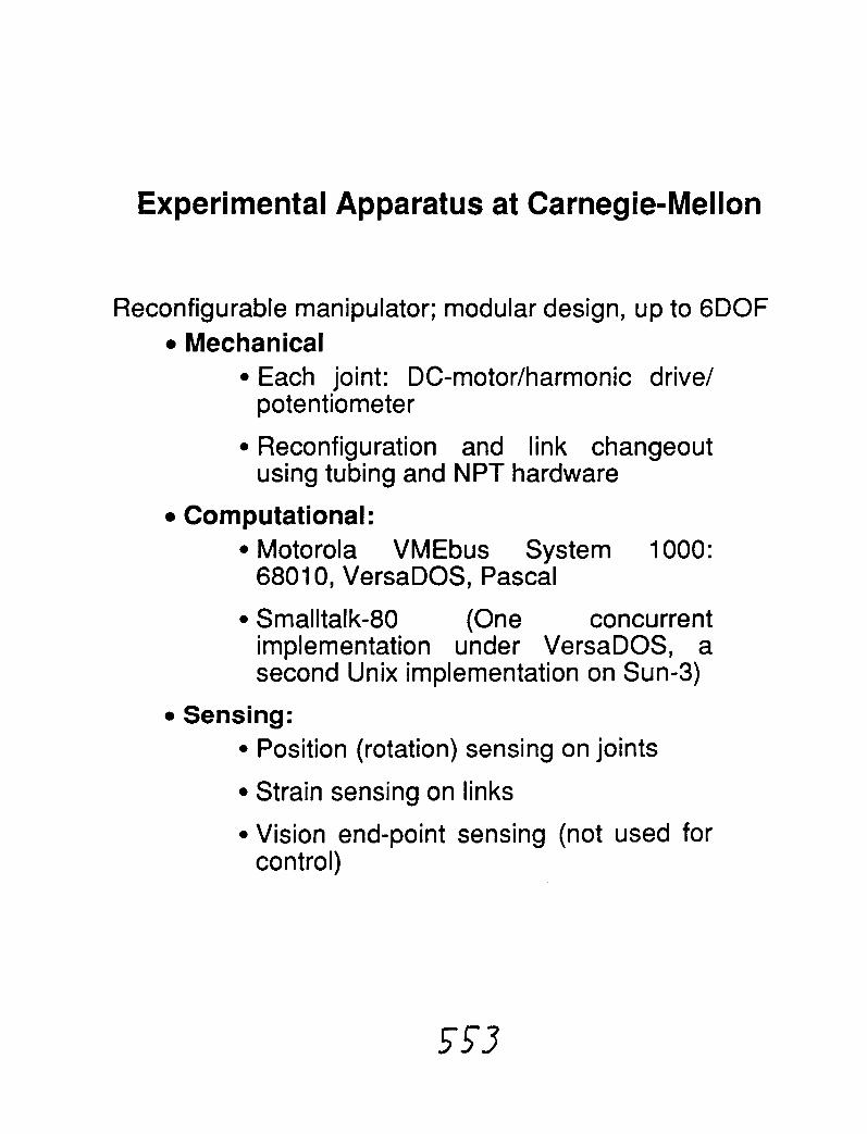
Experimental Apparatus at Carnegie-Mellon

Reconfigurable manipulator; modular design, up to 6DOF Mechanical

Each joint: DC-motorlharmonic drivel potentiometer

Reconfiguration and link changeout using tubing and NPT hardware

Computational: Motorola VMEbus System 1000: 6801 0, VersaDOS, Pascal

Smalltalk-80 (One concurrent implementation under VersaDOS, a second Unix implementation on Sun-3)

Sensing: Position (rotation) sensing on joints

Strain sensing on links

Vision end-point sensing (not used for control)

MANIPULATOR IN A 6-DOF TWO LINK CONFIGURATION (BOTH LINKS RIGID)

MANIPULATOR IN A 3-DOF TWO LINK CONFIGURATION (ONE RIGID, ONE FLEXIBLE)

554 ORIGINAL PAGE

BLACK AND WHITE PHOTOGRAPH

MANIPULATOR I N A S INGLE L I N K 3-D CONFIGURATION

ORIGINAL PAGE 555 BLACK AND WHITE PHOTOGRAPH

MANIPULATOR IN A 3-DOF TWO LINK CONFIGURATION

MANIPULATOR IN A 4-DOF TWO LINK CONFIGURATION FOR FORCE COGNITIVE EXCAVATION

A Simple Model for a General Flexible Link

Starting points to consider: Link motion results from concatenation to other links; the non-linear configuration problem, present in rigid manipulators as well.

The link itself deforms as a result of the end- forces and the inertial forces acting on it.

Which quantities can be observed or sensed?

Which quantities can be controlled?

How is the (approximate) solution to the PDE for link deformation to be contained within the dynamics equation? (What are the amplitude variables for the generalized co-ordinates chosen?)

First step in the approach: View first the motion of the chord connecting the end points, and then refer the (elastic) deformations to that chord.

A FLEXIBLE LINK (SHOW IN 2-D) IN MOTION

NOTE "CHORD" ACTS AS A "RIGID BODY"

ELASTIC DEFORMATIONS REFERENCED TO THE CHORD

Kinematics/Mechanics of the Simple Model

Chord motion: Denote rotation by 8, equivalent to a rigid-link formulation.

Include dynamic effects of concentrated masses and inertias at joints.

Assume that inertial effects of the link are modelled (from 8 and a) by the translation and rotation of the (c.m. of) the chord.

Deformations (displacements) of the flexible link: Displacements y(x) are referenced to the chord.

Assume that the displacements equal those resulting from static application of end- rotations $ and y~.

Displacement and potential energy: YCX) = ~ o - a [ c g + r ) x - + a j / p L

A SINGLE L I N K SYSTEM; EQUATIONS OF MOTION FROM APPLICATION OF THE SIMPLE MODEL

COMPARISON OF TRANSFER FUNCTIONS, SIMPLE MODEL VS. EXACT MODEL

Properties of the Simple Model

The model is equivalent to Rayleigh's method, using an assumed shape with two amplitude variables, $ and y ~ .

Inertial effects of the joints are properly modelled, and are consistent with the mathematical formulation. (Functions in 8)

The model is also a lumped mass assumption of m acting on the chord. (If this is the dominant link inertial effect, then the error is small.)

The assumed shape has only 2 "dof," and can only approximate the real shape.

Some higher order effects are plainly "missed," as they would be for a truncated mode solution.

The formulation would be useful for control, because the variables 0, $ and y~ can be measured and actuated.

For joint-dominant systems the model should be very accurate, and if joint inertias are small the equations reduce in order.

Applications to Manipulator Control

Equations of motion can be used as follows: To confirm the number and the identity of state variables for control.

To perform simulation studies.

To set gains from classical control theory. (In principle)

To compute variable gains for a non-linear system. (In principle)

To accomplish model-based (shaped) control.

To accomplish model-based feedforward control; requires real-time performance.

Single Link Systems

1. Planar (2-D) motion I Actuator was a direct drive DC motor.

The simple model produces 3x3 equations of motion.

Tip has mass but low inertia; system order reduces to 2; state variables are identified as 8 and $.

~ Sensing of rotation (8+$) and strain (-$). I

Perform experiments; set gains by trial and error.

Discussion of friction effects.

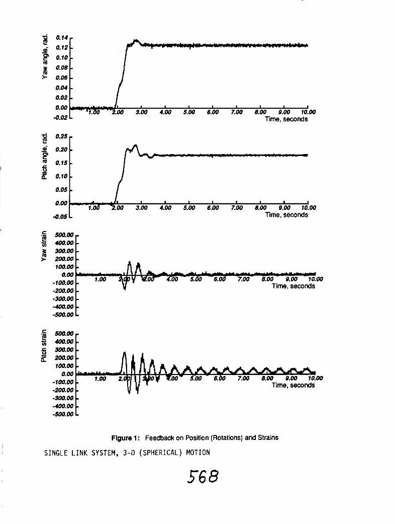
2. Spherical (3-D) motion Actuation using two joints of the modular manipulator.

See videotaped results.

Controllable despite friction and backlash.

#"&A

\ C

t, sec

10

t, 5ec

EXPERIMEIJTAL RESULTS, PLANAR SINGLE L I N K SYSTEM

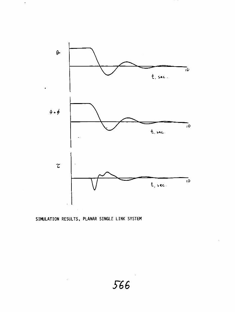
SIMULATION RESULTS, PLANAR SINGLE L I N K SYSTEM

0.00 I I I I I I I I I 2.00 3.00 4.00 5.00 6.00 7.00 8.00 9.00 10.00

0.02 Time, seconds

100.00 - Time, seconds

1 0.w.

Figure 1 : Feedback on Position (Rotation) Only

SINGLE LINK SYSTEM, 3-0 (SPHERICAL) MOTION

0.18 0.16

m 0.14 5 0.12 E 0.10

0.08 O.M 0.04

- - - - - - - - I I I I I a I I 1

0.00 1.00 2.00 3.00 4.00 5-00 6.00 7.00 8.00 9.00 10.00 Time, seconds = 500.00- '@

tj 100.00- h g 300.00- > 200.00-

100.00 - I

&do 9.00 1 .OO

?CYd Time, seconds -300.00 -400.00 -500.00

0.00 I I I I I I I I I 00 3.00 4.00 5.00 6.00 7.00 8.00 9.00 10.00

-4.02 Time, seconds

0.20 - 0.15-

0.05 - -4.05 D Time, seconds

.- = 500.00-

g 400.00- 3 300.00 - 2 moo-


-204.00 -

.- = 500.00-

g m.00- = 300.04- 0 CI a m.OO-


-200.00 -

Figure 1 : Feedback on Position (Rotations) and Strains

SINGLE L I N K SYSTEM, 3-D (SPHERICAL) MOTION

Planar Two Link System

Experiments performed at Toshiba.

Air table, 2-D manipulator.

Four state variables: 8's and $'s.

Compare experimental and simulation results.

Friction in actuators causes vibration.

Feedforward control is attempted, inclusive of friction effects.

Model based feedforward control limits vibration.

2-DOF TWO L I N K PLANAR SYSTEM ( A I R TABLE, HORIZONTAL PLANE)

( EXPERIMENTS CONDUCTED A T TOSHI BA)

I SHOULDER 0

I

3 0 I

6 0 9 0 1 2 0 TIME (SEC)

I

1 ELBOW , 0 3 0 60 9 0 , 1 2 0

I

1 5 0 0 t TIME (SEC 1

0 30 60 90 120 TIME (SEC)

PLANAR TWO-L I N K MANIPULATOR: EXPERIMENTAL RESULTS

60 90 TIME (SEC 1

Y -10.- U

f 0 : Y

SHOULDER

60 90 TIME (SEC)

- -20.- 8 Q - u -10.- 4 U z

a-.

I I I

0 30 6 0 90 120

1500-- TINE (SEC)

L. 5 1000-- CI r SOO*.

8 0

40,- n U

LOWER ARM 8 -loo@-

ELBOW

60 90 TIME (SEC)

PLANAR TWO-LINK MANIPULATOR: SIMULATION RESULTS

EXPERIMENTAL RESULTS, FEEDBACK CONTROL: NOTE V I B R A T I O N EFFECT, FROM F R I C T I O N

EXPERIMENTAL RESULTS, FEEDFORWARD CONTROL: NOTE E L I M I N A T I O N OF V I B R A T I O N

Combined Flexural-Torsional (3-D) Motion

Experiments performed April 1988: Three actuated DOF (yaw, pitch, roll).

Two links; one flexible, one rigid.

Linear feedback control; gains by trial and error.

Coupled flexural and torsional vibrations.

See videotape; see experimental results.

Actuator properties by system identification (in process).

Analtyical model used in simulation studies (in process).

Next phase: distal link made flexible, 4 (or 5) actuated DOF.

Time, seconds

Time, seconds

Time, seconds

150.00 100.00 50.00

0.00 -50.00 00

s! -100.00 V) " V Y = -150.00~

1 COUPLED FLEXURAL-TORSIONAL MOTIONd ROTATIONS AND STRAINS I

FEEDBACK CONTROL ON POSITION; NO FEEDBACK ON STRAIN

COUPLED FLEXURAL-TORSIONAL MOTION: STRAINS

FEEDBACK CONTROL ON POSITION; NO FEEDBACK ON STRAIN

.- 400.00 - 2 300.00 - a 200.00 - 5 100.00 - CI

-200.00 - Time, seconds -300.00 - -400.00

50.00 - ,o 0.00

Time, seconds

COUPLED FLEXURAL-TORSIONAL MOTION: STRAINS

FEEDBACK CONTROL ON POSIT ION AND ON STRAIN

Discussion and Conclusions

The model may be well suited for serial link manipulators, including joint-dominated systems.

Accuracy for MDOF systems, non-linear in configuration, remains to be examined.

Control experiments must be extended beyond linearized regions.

The major application is model-based control, still to be studied in depth.

Effects of friction, backlash, deadband should be included.

Friction or torque ripple can excite higher modes.

Frequencies of unmodelled (higher) modes can be adjusted by inserting "redundant" actuators.

MINIMUM-VARXANCE REDUCED-ORDER ESTIMATION ALGORITHMS FROM PONTRYGIN'S MINIMUM PRINCIPLE

Yaghoob S. Ebrahiml Boeing Commercial Airplanes

Seattle, Washington

ABSTRACT

It has become apparent with the introduction of modem control and estimation theory that the entire knowledge of a system cannot be included in the system design for most ~)ractical applications. Such mechanlsration of a total system usually results in a model exceeding the capacity of a real-time processor. thus requiring a reduction in the state sbx. In addition. linear filtering and smoothing problems have been extensively lrlvestlgated for a case wherein the fllter or smoother is of the same state dimension as the dimension of the "best state" model available.

Thls paper presents a uniform derivation of m u m - v a r i a n c e reduced-order (MVRO) filter-smoother algorithms from Pontrygin's Minimum Principle. An appropriate performance Index for a general class of reduced order estimation problem is formulated herein to yield optimal results over the entire time interval of estimation. These results provide quantitative criteria for measuring the performance d certain classes of heurlsllcally designed. suboptimal reduced-order estimators as well as expllclt guidance to the subopttmal fllter design process with both continuous and dlscrete filter-smoother algorithms being considered.

Uy the duality principle. the algorithms of reduced-order estimation can be easIly extended to the deterministic problenls of optimal control (1.e.. the regulator and linear tracking problem).

58 1 PRECEDING PAGE BUNK NOT FILMED WWWLLW~ t k i I & A ~ A NUI i r i * ( tU

MODIFYING HIGHORDER AEROELASTIC MATH MODEL OF A JET TRANSPORT USING MAXIMUM LIKELIHOOD ESTXMATION

Amlr A Anissipour and Russell A. Benson The Boeing Company Seattle. Washington

ABSTRACT

The design of control laws to damp flexible structural modes requires accurate math models. Unllke the design of control laws for rigid body motion (e.g.. where robust control is used to compensate for modeling inaccuracies). structural mode damping usually employs narrow band notch filters. In order to obtain the required accuracy in the math model. maximum likelihood estimation technique is employed to improve the accuracy of the math model using flight data. This paper presents all phases of this methodology: ( 1) pre-flight analysis (1.e.. optimal input signal design for flight test, sensor location determination. model reduction technique. etc.). (2) data collection and preprocessing. and (3) post-flight analysis (1.e.. estimation technique and model vcrlflcatlon). In addition. a discussion is presented herein of the software tools used for tlils study and the need for future study in this field.

Modifying High-Order Aeroelastic Math Model of a Jet Transport Using Maximum Likelihood Estimation

Amir A. Anissipouf Russell A. Benson

The Boeing Compaliy Boeing Commercial Airplanes P.O. Box 3707 M/S 9W-38

Seattle ,Wa. 98124

The design of control laws to damp flexible structure modes requires accurate math models of the dynamic system. To obtain the required accuracy of a math model, the parameter estimation technique using maximum likelihood estimation is employed to improve the accuracy of the model based on flight data. This paper presents all phases of this methodology: preflight analysis (i.e., optimal input signal design for flight test, sensor location determination, model reduction technique, etc.), data collection and preprocessing, and post-flight analysis (i.e., estimation technique and model verification). The results of this study indicate that the parameter estimation technique (i.e., maximum likelihood estimation) is an effective and powerful technique in modifing high-order aeroelastic aircraft models. However, the accuracy of the results depends upon the fidelity of the theoretical model with regards to the correct number of dominant modes for the desired frequency bandwith in the model (i.e., model order). If the number of modes in the model are not representative, then an identification problem can occure in the parameter estimation technique. Nevertheless, this problem can be overcome using the system identification technique.

Having an accurate mathematical representation is fundamental to any airaaft control system design. In general, aircraft models are developed from a theoretical basis and modified by analyzing the experimental data (i.e., wind-tunnel data for aerodynamic models or ground shake test data for structural models). Although present techniques provide very good dynamic models for the design stages of an aircraft, often these models do not match the actual dynamic flight response. This problem has generated a need for advanced system identifiaction and parameter estimation techniques in upgrading dynamic models of an aircraft based on flight test data. This modeling problem is more apparent with high-order aeroelastic models with which our experince with modeling techniques is limited.

Low-frequency structural modes are easily excited for a jet transport with a long fuselage. This excitation causes a lateral ride discomfort in certain flight conditions. In order to design a yaw damper to dampen Dutch roll response and suppress the undesirable low-frequency structure modes by means of active control, an accurate aeroelastic model of the aircraft must be available. In this study, parameter estimation technique is applied to upgrade the high-order aeroelstic math model of a jet transport. The following is a summary of the parameter estimation technique using maximum likelihood estimation.

. . Likelihhood Est

Suppose the actual system is described by (Reference 1):

where

x (t) state vector u (t) control vector z( t , ) measurement vector s (t) bias vector n (t) process noise m (t I measurement noise

t i time sample A,B,C,D,S,H,F,G system matrices withunknownparameters n (t) and m (t) are zero mean ,Gaussian and independent noise

Assume k is the vector of unknowns that contains elements of the system matrices A, B, C, D, S, H, F and G. The objective is to maximize the probability distribution of unknowns (i.e., k) when the measurements z are available. Therefore, maximizing P(k/z), where P is the probability distribution function of k given z.

By Bayes' rule:

Since in these equations z is given, so P(z) becomes a constant. Assume there is no a priori preference for k, so P(k) becomes a constant. Therefore, P(z/k) differs from P(k/z) only by a constant. In other words equation (3) becomes:

I Equation (4) indicates that P(z/k) may be maximized instead of P(k/z). Therefore, using Gaussian assumption, the likelihood ratio may be written as:

where

z k (ti) predicted estimate at time ti GG* measurement noise covariance matrix L number of measurements

If the logarithm of equation (5) is taken, the consatnt terms are eliminated by the maximization, and the equation is multiplied by -1 to do minimization rather than maximization, then equation (6) will be obtained as:

where J(k) is the cost function to be minimized. Two steps are taken to obtain zk(ti). Prediction step:

where t

and Y =lo e ~ ~ d s

and the correction step:

~ ~ ( t ~ + ~ ) = x k ( f i + i ) + K [z(ti+1) -zk( t i+ l ) ]

K in equation (8) is the Kalman filter gain matrix given by:

where P is the solution to the discrete time Riccati equation:

After obtaining the cost function J(k), the Newton-Raphson algorithm is used iteratively to minimize the cost function by revising the unknowns parameters.

This algorithm requires an intial estimate for the vector of unknowns (ko). A priori

~ estimate is available for each unknown parameter through the analytical model.

I

The MMLE software tool developed by NASA Dryden is a parameter estimation program supporting this estimation technique. This software has been modified by Boeing to accept and handle higher order models. A comprehensive description of this software tool is described in Reference 1.

GHT

A sixtieth order linear aeroelastic math model for a flight condition of Mach .6 speed, 15000 foot altitude, and no turbulance, and cruise configuration of a jet transport was provided in the form of:

where M mass matrix C damping matrix K stiffness matrix q generalized coordinate u control inputs

The model is defined in the inertial axis system, and the dynamics (q), consist of rigid body and flexible modes. The model is tuned using data from ground shake testing. The system of equations (12) was transformed into state-space form using the following transformation:

therefore the system equation (12) becomes:

where

and

This transformation always exists because the mass matrix is positive definite. Although this is a well-posed theoretical problem, it is not trivial. The flexible model is usually on the order of one hundred states, thus causing numerical inaccuracies in the inversion of the mass matrix. In our analysis the software package MPAC was used to perform the transformation. (MPAC is a numerically robust modern control and analysis software tool developed by the Boeing Company.)

For the identification process, the system equation (13) was transformed into the conjugate modal form using the following transformation:

Equation (13) becomes:

where

A = dia (1,) X, = ih eigenvalue - B =T- 'B controllability matrix

= C T observability matrix

The advantage of using the modalized form given by equation (14) is that all the modes through A matrix, along with the controllability and observability matrices are readily available for an analyst to quickly locate uncontrollable and unobservable modes. In addition, the modes in the A matrix are decoupled and may be partitioned into rigid model and elaastic model.

The order of the model was reduced to nineteen by deleting the modes above 6 Hz. Since this model will eventually be used for ride quality study and modal supperasion design, only those modes less than 6 Hz were retained.

The reduced order, modal model (19th order) is represented by:

This model contains one state for heading, one for the spiral mode, two for the Dutch roll mode, one for roll mode, eight for low-damped elastic modes, and six for high-damped elastic modes.

To support this study, a special set of sensors were installed on the aircraft to measure the dynamic response of the jet transport. The locations of these sensors were based on the mode shapes of the aircraft determined by the math model and physical constraints (Table I). (A complete discussion on sensor selection and location placement on the aircraft is omitted herein for proprietary reasons.)

TABLE I: Sensor Type and Locations for High-order

Aeroelastic Modeling

The sensors selected for the analysis were: body roll angle (@), heading angle W), roll

rate (p) and yaw rate (r) at the IRU; body yaw rate at the pilot seat; 9 lateral accelerometers along the fuselage; 2 lateral accelerometers on the nacelle number 2; and 3 lateral accelerometers on the vertical tail.

SENSOR TYPE

Position Transducer

Yaw Rate Gyro

Lateral Accelerometer

Vertical Accelerometer

Roll rate, Yaw rate, Bank angle, Heading,

The flight test input-signal design analysis for high-order aeroelastic modeling was performed using the reduced order analytical model (equation 15). Although a number of "optimum" input signals have been proposed for flight testing in conjunction with parameter estimation, none have been found to be appropriate for

SENSOR LOCATION

On all control surfaces

Pilot seat, IRU (a station between CG and cockpit below the cabin floor), CG station

1 Pilot seat, 1 Cockpit ceiling, 8 on the passanger cabin floor from the cockpit to the aft galley, 1 on the aft galley ceiling, 3 on

vertical tail (tip and mid section, front

and rear spar), three on each nacelle, 1 IRU station

1 on the pilot seat, 1 IRU, 1 aft galley, 8 on each wing, 3 on each horizontal tail,

2 on each nacelle

IRU and CG stations

high-order aeroelastic modeling. Essentially, all the analytical techniques proposed in designing the optimum input signals are based on the analytical model. This model is the subject of improvement by the identification and estimation techniques. Hence, no "optimum" input signal exists.

A number of different input signals were evaluated for this study. After a comprehensive simulation study, it was determined that a frequency sweep of a linear sine-wave with adequate energy to excite all the modes (rigid and elastic) yeilds the best results. In addition, the linear sine-wave frequency sweep optimizes the most commonly used criterion for input signal design:

9? = - log (det M)

where M is the Fisher information matrix (or sensitivity matrix) defined by:

J is the cost funtion defied in equation (6). The criterion % defined in equation (16) is related to the volume of highest probability density region for the parameters k. An interesting property of the determinant criterion is that it is independent of scaling parameters (Refernce 2).

Fifteen tests were designed for the same flight condition. Five frequency sweeps were designed for each control surface. Each test was repeated for rudder, aileron, and both surfaces in phase. The first frequency sweep covered 0 to 6 Hz to excite all the modes in one test. The other four tests were then designed to excite specifically high-damped modes by sweeping from .25 Hz below to .25 Hz above the frequency of the mode.

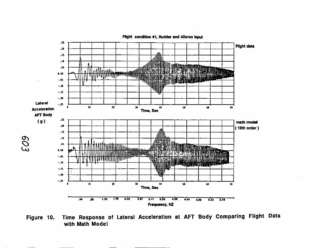
The amplitude of the input signals were designed to be constant for practical purposes (i.e., rate limits). The designed input signals were tested in the lab to confirm that the signals did not saturate the servos and actuators of the control surfaces. However, the output of the actuators during flight test generated signals with decaying amplitutes. These decaying amplitudes reduced the energy level initially designed for the test. Figures 1 and 2 show the actual control surface

Rudder deflection ( deg

Aileron deflection

( deg

18 20 - 38 ' 48 ' 58 60 71 ' The, Sec

10 20 - 30 40. 60 ' 70 '

Time, Sec

Flight data

Flight data

Figure 1. Actual Control Surface Deflections for Flight Condition 21

deflections for rudder sweep alone, and for rudder and aileron surfaces simultaneously in phase.

To record the data in flight test, a simulation study was conducted to determine the required sampling frequency. The analytical model (i.e., system equations 15) was assumed to be the true model, and simulated using the designed input signal. A considerable amount of noise was added to the simulation data, and then that data was treated as pseudo-flight data. The acutal model was used for parameter estimation to determine the required sampling frequency. Sampling frequencies of 20,25,50,100,200 Hz were considered for this study. One mode or group of modes at a time were selected for the estimation process of each sampling frequency. The results indicated that 100 Hz is the best sampling frequency for this study. Figure 3 shows the typical results for identified parameters when different sampling frequencies were used.

A

#

True

Value

I I I I I

Sampling Frequency

Figure 3. Typical Results from Estimation with Different Sampling Frequency

The flight test was performed using designed linear sine-wave frequency sweeps for rudder and aileron. The test conditions were conducted at a speed of Mach .6, an altitude of 15,000 feet, and minimal turbulence. A preprogrammed frequency function generator was used to apply the linear sinusoidal frequency sweeps (0-6 Hz) to the aileron and rudder (through the autopilot servo).

The flight test data were recorded with 100 sample per second, and then filtered using a Graham low-pass filter with the cutoff frequency of 10 Hz and rolloff frequency of 15 Hz. Prior to estimation analysis, the data were cleaned up by removing all the sensor biases and data dropouts.

POST FLIGHT ANAJ.YSIS

The analytical model (system equations 15) was simulated using actual control surface defelection during flight as input signals. The comparison of flight data with the response of the analytical model for flight condition 41, where both rudder and

I aileron frequency sweeps are used, is presented in the Figures 4-11.

The maximum likelihood estimation software tool (MMLE) developed by NASA Dryden was used to minimize the residuals between flight data and response of the analytical model in Figures 4-11. At the time of analysis, MMLE was hosted on the Cyber mainfram. Due to Cyber having a memory limit, the capability of using process noise was not available for analysis. Hence the results obtained herein, are preliminary results which do not include the effect of process noise. The final results of this study will be reported at the 1989 AIAA Guidance, Navigation and Control conference.

The high-order model was partitioned into two sections: rigid model and elastic model. For rigid model identification, 15 seconds of data were used. First the rigid portion of the control and measurement matrices were upgraded. Then, the A matrix was upgraded. Finally, all the parameters in the rigid section of the A tB and - C matrices were simultaneously estimated.

b

-44 .no 1.33 1-78 2.22 2 . b ~ 3.11 3.1 4.00 4.44 4.89 8.33 8 . n Q

Frequency, HZ

Figure 5. Time Response of Body Yaw at IRU Comparing Flight Data with Math Model

Flight condition 41, Rudder and Aileron input

Lateral -.es

Acceleration IRU

.2s

. ? I

3@ . Time, Sec

mght data

I math model

8 I I 20 38 40 51 b t 71 Time, Sec

t .44 .80 1.33 1-78 2-22 237 3.11 3.50 4.00 4.4 4.80 8:33 6.78

Frequency, HZ

Figure 9. Time Response of Lateral Acceleration at IRU Comparing Flight Data with Math Model


flight data

Lateral Acceleratlon

Engine 2 .s

lnlet .4

( 9 ) , 3

3 1 ' 4 1 , Time, Sec

math

( 19th

0 20 30 51 6 1 7 1 Time, ~ e c "

t .44 .a@ 1.33 1.78 2.22 237 3.11 3.60 4.00 4-24 4 . 0 b:33 6.78

Frequency, HZ

model

order )

Figure 11. Time Response of Lateral Acceleration at Engine 2 lnlet Comparing Flight Data with Math Model

Two different approches were taken for the elastic model identification. In the first approach, the 19a order model was used for the analysis with all the elements of B and being estimated. All 70 seconds of data were used for this estimation approach, . In this process, those parameters in the B andc that did not contribute to the residuals were identified and kept constant for the remainder of the analysis. Then, the elements of A were added to the estimation process while keeping some of the elements of B and e constant. The results of this estimation approach are show in Figures 12-19.

The second approach was to add one elastic mode at a time to the rigid model. For this approach, the first elastic mode was added with 28 seconds of data used for the analysis. The corresponding parameters in the B and c matrices were estimated every time a mode was added to the model. The result of this approach was not satisfactory because several times the algorithem diverged and the residuals were big.

Figures 20-26 show the PSD plots obtained from the analytical model. Figures 27-34 show the PSD plots obtained from the estimated model. The PSD plots obtained from the estimated model, clearly show that the estimation analysis improved the accuracy of the model in terms of its modal representation. However, the estimated parameters in the B and c matrices are biased. Since an accurate representation of the transfer functions was desired for this study rather than true values of the B and matrices, the biased estimates in theB and c matrices did not create any problem.

Figures 16, 17 and 19 indicate that another mode is present in the flight data which is not modeled in the analytical or estimated model. This problem can not be solved via parameter estimation technique which assumes the structure of the model (i.e., the order of the model) is correct. Hence, it is suggested that the system identification technique developed by V. klein and J. Batterson of NASA LaRC be used to overcome this problem.

Fllght condltlon 41, Rudder a;ld A l l e m Input

Body Yaw mu

(d-1

Figure 13. Time Response of Body Yaw at IRU Comparing Flight Data with MLE Model

Fllght condition 41, Rudder and Aileron Input

P

.U .a9 1.33 1.78 2.22 2.b7 3.11 3.58 4.00 4.44 4.89 8.33 8.78 I

Frequency, HZ

Figure 14. Time Response of Roll Rate at IRU Comparing Flight Data with MLE Model


Lateral Acceleration

I I I I 10 20 38 48 58 6 1 70

Tlme, Sec

Flight data

18 2) ' 31 ' 4:

Tlme, Sec

1 .U .as 1.33 1-70 a-21 2167 3.11 3.80 4.00 , 4:44 4 . 8 833 0.78 I

Frequency, HZ

model

Figure 18. Time Response of Lateral Acceleration at AFT Body Comparing Flight Data with MLE Model

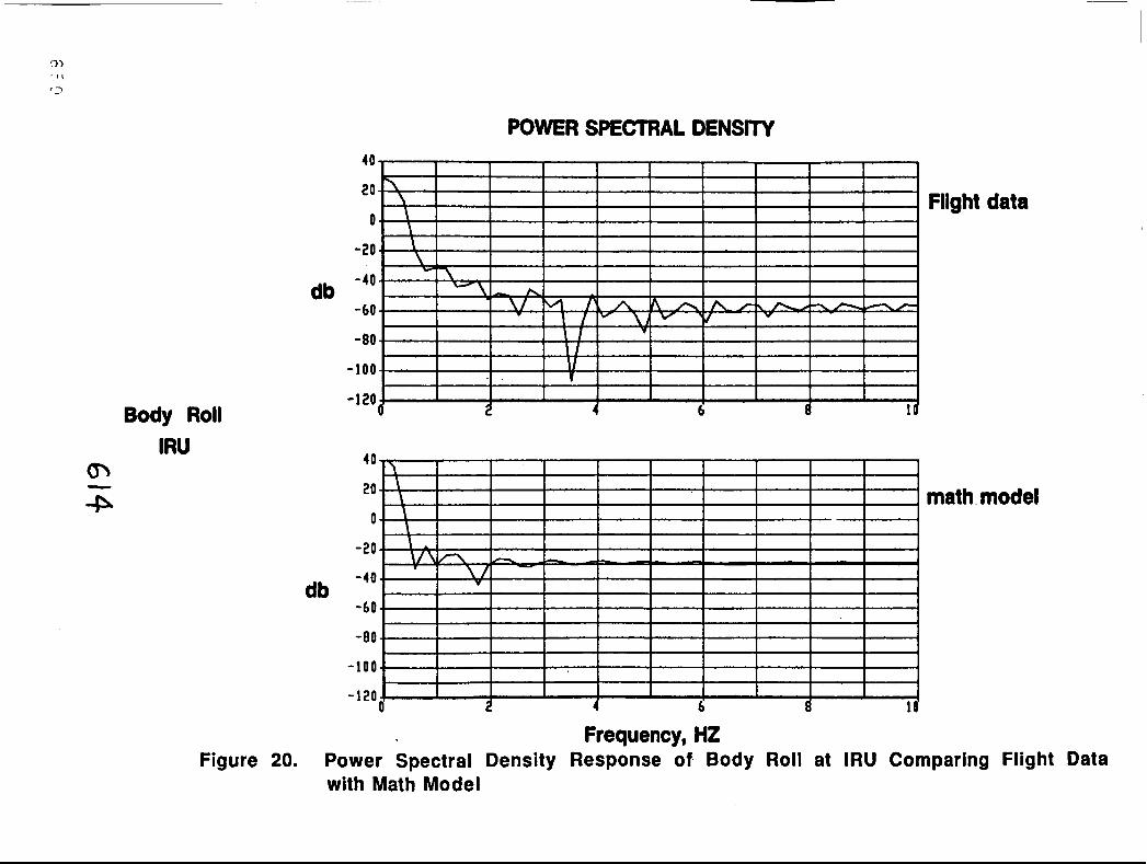
IaPoW 41eW 41!M eaea 146!1j 6u!~edwoa nu1 le Apog jo asuodsau Aaisuaa le~wads raMod '02 a~n6!j

ZH 'ltauenbard

I I I I I I I I I

I I I I I I I I A I OC- qP

POWER SPECTRAL DENSITY

Body Yaw IRU

Flight data

db

math model

db

Frequency, HZ Figure 21. Power Spectral Density Response of Body Yaw at IRU Comparing Flight Data

with Math Model

09-

Ot- - gP

03-

09-

Ot- qP 02-

0


Yaw Rate IRU

20 -.

0 - /

math model

db

Frequency, HZ Figure 23. Power Spectral Density Response of Yaw Rate at IRU Comparing Flight Data

\,

with Math Model

Flight data


I I -

20 I 1 I I I I 1

Flight data I I 1 I I


Not seat 2 0 1 I 1 1 I I I I I I math model

Frequency, HZ Figure 24. Power Spectral Density Response of Lateral Acceleration at Pilot Seat Comparing

Flight Data with Math Model

021-

001-

08-

09-

Ot- qP

02-

0

0 2

0 t

09-

or- qP

02-

08-

09-

Ot- 9P

08-

09-

Ot- qP I I I I I I I I I I \ I


Body Yaw IRU

I \ / I -w Flight data 0

I I I /4 -- --

\ I - - MLE model 0 - I I

Frequency, HZ Figure 28. Power Spectral Density Response of Body Yaw at IRU Comparing Flight Data

with MLE Model


I I 1 I I I I I

0 \ I I I ! I I I I 1 Flight data

Roll Rate IRU

MLE model

db

Frequency, HZ Figure 29. Power Spectral Density Response of Roll Rate at IRU Comparing Flight Data

with MLE Model

I I I I I I I I I

I I I I I I I I -I. oa- I I I . .

Y A, A A V

/\ I -09- I \. I \ - Ot- qp

I I \ I I I I I I I

I I I I I I 1 oe-

I I I I I I 1 I I I Lot



IRU

1 I I I I I I 1 I . O

Flight data I I I I I I I I I

I I I I I I I I I ( MLE model

Figure 32.

Frequency, HZ

Power Spectral Density Response of Lateral Acceleration at IRU Comparing Flight Data with MLE Model

09-

Ot-

02-



Ch Englne 2 M Qa

Inlet

I I I 1 I I I I I

o I I I I I I I I I I Flight data

Frequency, HZ

4 0 -

Figure 34. Power Spectral Density of Lateral Acceleration at Engine 2 Inlet Comparing Flight Data with MLE Model

MLE model 20.- ;

REFERENCES

1. R.E. Maine and K.W. Iliff, "User's Manual for MMLE, a General FORTRAN Program for Maximum Likelihhood Parameter Estimation", NASA Technical Paper 1563, November 1980.

2. G.C. Goodwin and R.L. Payne, "Dynamic System Identification - Experiment Design and Data Analysis", Academic Press, 1977.

AUTOMATED MODEL FORMULATION FOR TME-VARYING FLEXIBLE STRUCTURES

B. J. Glass* and S. Hanagud Georgia Institute of Technology

Atlanta. Georgia

ABSTRACT

'me control of many types of flexible structures. such as robotic manipulators or large space structures. usually requires an accurate analytical model. Once obtained, these models are currently compared with observations of the behavior of the structure and Incremental changes can be made by using Kalrnan filtering techniques or other parameter ldentlZication techniques. For the-varylng flexible structures. however. such changes may occur in sudden changes to boundary conditions or to the form of the model dllrerentlal equations. Some of the primary causes for such changes are growth, reconfigurntion or damage. This class of changes often requires a reformulation of the analytical model. This paper presents an identification technique that uses the sensor Information to choose a new model out of a flnlte set of discrete model space. in order to follow the observed changes to the given time varying flexible structure. Boundary condlllon sets or other Information on model variations are used to organize the set of possible models laterally into a search tree with levels of abstraction used lo order the models vertically within branches. An object-oriented programming approach is used to represent the model set in the search tree. A modified A* best flrst search algorithm nnds the model where the model response best matches the current observations. Sweral extensions to this methodology will be discussed. Methods of possible Integration of rules wlth the current search algorithm will be considered to give weight lo interpreted trends that may be found in a series of observations. This capabillty nilght lead. for instance. to 1dentifLing a model that incorporates a progressive damage rather than with Incorrect parameters such as added mass. Another new direction is to consider the use of noisy time domain sensor feedback rather than frequency domain lnformation in the search algorithm to improve the real-time capability of the (leveloped procedure. The next logical step will be to automatically expand the model space by adding subsets of recognized possible models. This can be accomplished by using developed methods of machine learning. Finally, testing of the currently developed approach wlth model spaces that are derived from more complex structures will bc discussed.

Dr. Class Is currently wlth the System Autonomy Demonstration Project Omce of the NASA Arnes Research Center. Moffett Field. Callfornla 94035

PRECE@lNG PAGE BUNK NOT FILMED

NUMERICALLY EFFICIENT ACOOIUTHM FOR MODEL DEVELOPMENT OF HIGH-ORDER SYSTEMS

L. 0. Parada Calspan Advanced Technology Center

Buffalo. New York

ABSTRACT

Frequency domain parameter identincation techniques provide a straightforward approach to transfer function estimation. However, for high-order systems, numerical dlff~cultles may be encountered during the estimation process. Inaccuracies may result because of the large variation of the transfer function polynomial coemcients for high- order systems. The lack of numerical precision to represent this variation may cause the estimation process to break down.

This paper presents a technique for estimating transfer functions in partial fraction expansion form from frequency response data for a high-order system. The problem formulation avoids many of the numerical difficulties associated with high-order polynomials and has the advantage of having the option to fix the damping and frequency of a mode. If known. during the estimation process. The resulting transfer funclion(s) may be converted to Jordan-Form time domain equations directly.

Ilurlng the implementation of this technique, a frequency and amplitude normalizing window was developed that maximhd the emciency of the optimization algorithm. The comblnatlon of estimating the transfer function In factored form. the ability to fix previously determined parameters and the efi'ectiveness of the normallzing window led to a progresslve approach to synthesizing transfer functions from frequency response dala for hlgh-order systems.

PAGE BLANK NOT FILMED

A b s t r a c t

N u m e r i c a l l y E f f i c i e n t A l g o r i t h m f o r Model Development o f H igh Order Systems

L . 0. Parada Calspan Advanced Technology Center

P.O. Box 400 B u f f a l o , NY 14225

(716) 632-7500

f o r p r e s e n t a t i o n a t t h e I I

NASA Lang ley Research Center Workshop on Computat ional Aspects i n t h e Cont ro l o f F l e x i b l e S t r u c t u r e s

Frequency domain parameter i d e n t i f i c a t i o n techniques p r o v i d e a s t r a i g h t f o r w a r d approach t o t r a n s f e r f u n c t i o n e s t i m a t i o n . However, f o r h i g h o r d e r systems, numer ica l d i f f i c u l t i e s may be encountered d u r i n g t h e e s t i m a t i o n process. I naccu rac ies may r e s u l t because o f t h e l a r g e v a r i a t i o n o f t h e t r a n s f e r f u n c t i o n po lynomia l c o e f f i c i e n t s f o r h i g h o r d e r systems. The 1 ack o f numer ica l p r e c i s i o n t o rep resen t t h i s v a r i a t i o n may cause t h e e s t i m a t i o n process t o break down.

T h i s paper p r e s e n t s a techn ique f o r e s t i m a t i n g t r a n s f e r f u n c t i o n s i n p a r t i a l f r a c t i o n expansion form f rom f requency response data f o r a h i g h o r d e r system. The problem f o r m u l a t i o n avo ids many o f t h e numer ica l d i f f i c u l t i e s assoc ia ted w i t h h i g h o r d e r po lynomia ls and has t h e advantage o f hav ing t h e o p t i o n t o f i x t h e damping and f requency o f a mode, i f known, d u r i n g t h e e s t i m a t i o n process. The r e s u l t i n g t r a n s f e r f u n c t i o n ( s ) may be conver ted t o Jordan-Form t i m e domain equa t i ons d i r e c t l y .

D u r i n g t h e imp lemen ta t i on o f t h i s techn ique, a f requencyand amp l i t ude n o r m a l i z i n g window was developed t h a t maximized t h e e f f i c i e n c y o f t h e o p t i m i z a t i o n a l g o r i t h m . The combinat ion o f e s t i m a t i n g t h e t r a n s f e r f u n c t i o n i n f a c t o r e d form, t h e a b i 1 i t y t o f i x p r e v i o u s l y determined parameters and t h e e f f e c t i v e n e s s o f t he normal i z i n g window l e d t o a p r o g r e s s i v e approach t o s y n t h e s i z i n g t r a n s f e r I

I f u n c t i o n s f r o m f requency response da ta f o r h i g h o r d e r systems.

NUMERICALLY EFFICIENT ALGORITHM FOR MODEL DEVELOPMENT OF HIGH ORDER SYSTEMS

Statement of Problem Development of Mat hematical Models:

Time Domain - Difficult to implement - Instrumentation Complement - Input Design - Noise - Computational Load

Freq Domain - Simplified Implementation - Fewer parameters per computation

cycle - Statistical methods applicable

PREVIOUS WORK

Frequency domain parameter identification requires Determination of characteristic equation

(nonlinear or iterative techniques) Estimation of numerator polynomials

m LJ Factor characteristic equation d

Estimate zeros or residues

Inaccuracies (for high order systems) due to: Variation of transfer function polynomial coefficients Transformation errors Sensitivity of polynomial roots to variations in polynomial coefficients

U

gs a, E

_I

*-

sin =-a

z5

0.. 3 0

F%

+

a, ..C 0 a, >

E

- .- t-a

a g

a

Ez

e Q

a,

Q

--O

V)V

)

9a

,w

N a,

0.- 3

o

Er

n I

=-s

v)3

60

.. C

~5

g3

ou

k%

0.

car: 0

8r

.- 3W

e-i G

22

FACTORED FORM ESTIMATION

Classical Nonlinear Regression Problem

Estimate parameters from measured amplitude and phase data

Error Function:

Square of distance between measured and estimated frequency responses summed over all discrete frequency points

where: M = # frequency points cn w F(j a) = measured frequency response -0 Goo) = estimated frequency response

1 Estimated Transfer Function - G (jo)

where: N = order of system Q = # of second order terms

D - a CU

-3

+

CU- D

Fifth Order Single Precision Example

Simulate parameter identification of high order system Modes distributed over wide frequency range

Single precision: Scale down problem Reduce number of variables

5th Order Transfer Function:

Cascade form

Parallel form

Frequency Range: 1 x to 1 x 1 o + ~ Hz.

Term

DENOMINATOR COEFFICIENTS

Exact Coefficient Additive Components

1-1 = Single Precision Variable Representation

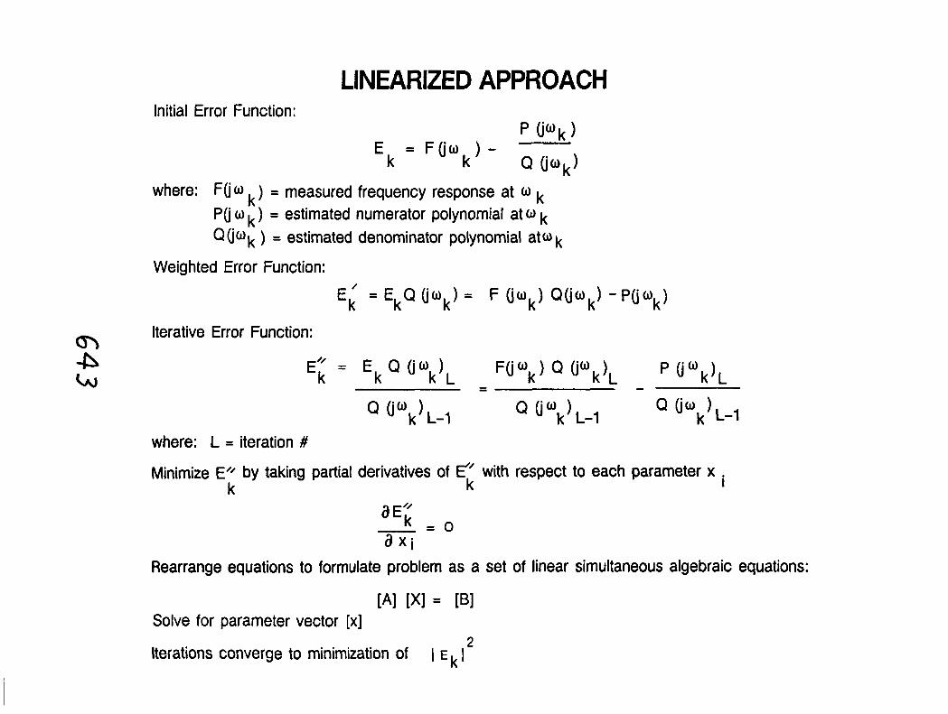
LINEARIZED APPROACH Initial Error Function:

p 0'w

where: F(i@ k ) = measured frequency response at o P(j w k ) = estimated numerator polynomial at @ k Q (iw ) = estimated denominator polynomial at o k

Weighted Error Function:

E; = E ~ Q owk) = F (jwk) ~ ( i o ~ ) - P(iOk)

6\ Iterative Error Function:

where: L = iteration #

Minimize Eo by taking partial derivatives of with respect to each parameter x k k

Rearrange equations to formulate problem as a set of linear simultaneous algebraic equations:

[A1 [XI = [Bl Solve for parameter vector [x]

2 Iterations converge to minimization of I E 1

5th Order example: Polynomial Results

Exact (s + 5 x (S + 5 x 10-I) (s + 5 x (s + 5 x Transfer Function ( ~ 2 + 2 x i 0 - 3 ~ + 10-4)(s + 1) (s2 + 1 x lot4 s + 10'~)

Linear (s + 5 x (s + 5 x 10-I) (s + 4.24 XI@') (S - 7.17 x 10'~) Results

( ~ 2 + 2 10-3 s + 10 -4) (S + 9.98 10-1) (S - 7.17 (S + 1.725

Cost 2.37 x Function

+ + + = measured

FREQ-RADISEC

FREQ-RADISEC

6M

STEPWISE FACTORED FORM TECHNIQUE

I Plot Amplitude t Phase Data I Section Amplitude Plot into J

4th Order Sections

Initialize Parameter Vector Elements to 1 I

5th Order Example: Factored Form Approach

FREQ = 1.0

AMP = 1 x 18

FREQ=I x i o t 4 l X 1 O l k

AMP = 1 X 10 -5

5th Order Example: Factored Form Results

Exact 1.25 x I O - ~ S + 6.12 x 1.22 x 9.98 x 10-'s + 5.02 x Transfer + t

Function s2 + 2 + s + l s2 + 1 x 10+4s + 10+8

Factored 1.25 x I O - ~ S + 6.12 x 1.23 x 9.79 x 10-'s + 5.21 x Form + + Results s2 + 2.00 s + + 1.01 s2 + 9.95 x I O + ~ S + 1.03 x

Cost 1.90 x 10-12 Function

+ + + = measured

1 ~ l o - ~ t I X I O - ~ I X I O - ~ l x l o O 1 x 1 0 ~ 1 x 1 0 ~ 1 x 1 0 6

FREQ-RADISEC

FREQ-RADISEC

648

16th Order Transfer Function Estimation

PcgNg: Roll Rate Measured at C.G. of Aircraft

-360.0 t-mT-jIq71nm s 1 . I . p n n . l . I -

1 X I O - ~ 1 X IO- * 1 XIO-I 1 x l o O 1 x l o l 1 x 1 0 2

FREQ-RADISEC

Cost Function: 4.5 x 10-12

Unit Gust Along Y-Body Axis 1 x 1 0 2

1 1 x 1 0 -

0 1 x 1 0 -

1 X 10 -l

1 x 10-2

1 X 10 -3

1 x

+ + + = measured

--%. -+

-\

t

t +

f \ t.

I .l'll'rTTq ' I 'l'I'TTlI'q ' 1 ' I '

1 x 1 0 - ~ I X I O - ~ 1 x 1 0 - I 1 x l o 0 1 x l o 1 1 x

_ , , , ,

FREQ-RADISEC

ON MODELLING NONLINEAR DAMPING IN DISTRIBUTED

PARAMETER SYSTEMS

A. V. Balakrishnan UCLA

Los Angeles, California

12 July 1988

In One Dimension

Without hysteresis

Z(t) + 02x(t) + 2 0 6 i ( t )

2 m + yx(t) lX(t) l a ~ ( t ) ~ " + IA(t) 1 " + Bu(t) + FN(t)

- - 0

NONLINEAR DAMPING

~ ~ ~ I ~ ~ ~ ~ . t l I ~ ~ ~ ~ ~ ~ ~ ~ I I I I I 1 l I 1 1 1 1 1 1 1 1 tmmmmm

200.00 400.00 600.00 m.00 1OOO.00 I NUMBER OF W S

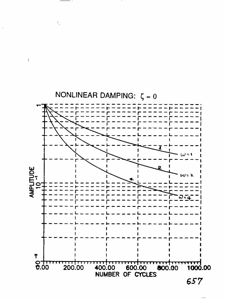
NONLINEAR DAMPING: 6 = O

NUMBER OF CYCLES

Beam Model

t "(s, t )

n : zero or positive integer

5 : Linear Damping Ratio

Prime represents space derivative

Dot represents time derivative

d4 clamped beam A "

L

J uys, t ) i*'(s, t) ds

L - j' u(s, t) u s , t ) ds

F(x, Dk) = Y ( [ x , d z k ] ) 2 ( n + p ) + 1 4. x

Energy

1 = - 2 {[-ic(t), W)l + h [Ax(t), x(t)] )

[F(x, DA) , k(t)] = ( [x, dx 21) 2 ( n + p ) + 2

dE (t) * d t I 0

Alternate Form

n : zero or positive integer

6 : Linear Damping Ratio

Prime represents space derivative

Dot represents time derivative

USE OF THE Q U A S I L ~ T I O N AWORX'MiM FOR THE SIMULATION OF L88 SXSWDJG

Feiyue Li and P. M. Bainum Howard University

Washington. DC 20059

ABSTRACT

The use of the Maximum Principle for the large angle slewing of LSS usually results in the so-called two-point boundary-value problem. in which many requirements (e.g.. mlnlmum time. small amplitude, and limited control power. etc.) must be satisfled sln~ultaneously. The successful solutlon of this problem depends largely on the use of an emcien t numerical algorithm. There are many candidate algorithms available for thls problem (e.g.. quasilinearizatlon. gradient. etc.). Here we discuss only the quaslllne'arization method which has been used for several cases of large angle slewing of US. The baslc idea of this algorithm is to make a series of successive approximations of the solution from a particular solvable case (Iinear or nonlinear) to a more general practical case.

For the rIgld spacecraft slewing problem with no constraints on the controls. the solutlon procedure can be found in the literature. This procedure needs to be modifled if a mlnlrnum time for the slewing problem is desired with control llmits given. Recently. an lndlrect method for finding the minimum time was developed to meet all these rcqu lrements.

For the general mixed (including both rigid and flexible parts) problem. an additional constraint of small vibrational amplitude on the flexible parts is imposed. To solve thls problem several steps In which the complexity increases gradually are needed. i.e., from a Iinearlzed version to a final nonlinear problem, from a less constrained case for the control to a more constrained one. from a nonmlnimum-time level to a near- rnlnin~um-time slewing in which a trade-off needs to be made between minimum time and small flexural amplitude requirements. Some examples of these algorithms are presented for planar slewlrlg maneuvers of the SCOLE configuration.

USE OF THE OUASlLlNEARl ZATlON ALGORITHM

FOR THE SIMULATION OF LSS SLEWING

P. M. BAl NUM

PROFESSOR OF AEROSPACE ENGINEERING

FEIYUE L I

GRADUATE RESEARCH ASS1 STANT

DEPARTMENT OF MECHANl CAL ENGl NEER l NG

HOWARD UNI VERSI TY, WASHINGTON, D.C. 20059

WORKSHOP ON COflPUTATlONM ASPECTS

IN THE CONTROL OF FLEXIBLE SYSTEHS

JULY 12- 14, 1988

WILLIAMSBURG, VIRGINIA

PRECEDlNG PAGE BLANK NOT TlLkKD

Use of the Quasilinearization Algorithm

for the Simulation of LSS Slewing

Feiyue Li Graduate Research Assistant, (202)636-7124

and P. M. Bainum

Professor of Aerospace Engineering, (202)636-6612 Department of Mechanical Engineering

Howard University, Washington, D.C. 20059

Abstract

The use of the Maximum Principle for the large angle slewing of LSS usually results in the so-called two-point boundary-value problem, in which many requirements (e.g., minimum time, small amplitude, and limited control power, etc) must be satisfied simultaneously. The successful solution of this problem depends largely on the use of an efficient numerical algorithm. There are many candidate algorithms available for this problem (e.g., quasilinearization, gradient, etc.). Here we discuss only the quasilinearization method which has been used for several cases of large angle slewing of LSS. The basic idea of this algorithm is to make a series of successive approximations of the solution from a particular solvable case (linear or nonlinear) to a more general practical case.

For the rigid spacecraft slewing problem with no constraints on the controls, the solution procedure can be found in the literature. This procedure needs to be modified if a minimum time for the slewing problem is desired with control limits given. Recently, an indirect method for finding the minimum time is developed to meet all these requirements.

For the general mixed (including both rigid and flexible parts) problem, an additional constraint of small vibrational amplitude on the flexible parts is imposed. To solve this problem several steps in which the complexity increases gradually are needed, i.e., from a linearized version to a final nonlinear problem, from a less constrained case for the control to a more constrained one, from a non-minimum-time level to a near-minimum-time slewing in which a trade-off needs to be made between minimum time and small flexural amplitude requirements. Some example,$ of these algorithms are presented for planar slewing maneuvers of the SCOLE configuration.

l NTRODUCT ION

M I f l l J M PRINCIPLE IS APPLIED TO

THE ATTITUDE HANEUVER AND VIBRATION CONTROL

OFLARGESPACESTRUCTURES

(A) PERFORflANCE INDICES

(B) BOUNDARY CONDl TlONS

(C) CONTROL REQUIREMENTS

THIS LEADS TO THE TWO-POINT BOUNDARY-VNUE PROBLEM

(TPBVP)

ONE OF THE METHODS OF SOLVING TPBVP I S THE

OUASILINEARIZATION MGORITW

MAXIMUM PRINCIPLE

STATE EQUATIONS

- f(x) + B(x)u, x(0)=xo, x(tf)=xf

PERPORMANCE l NDl CES

1 NECESSARY CONDITIONS

H~ =( I IP)(XTQX + U*RU) + k ( r ( x ) + BU) (4)

= - O H /ax), X (0) unknown (5 )

(dH /du)=O. RU= -13% (6)

H2= I + hT(f(x) + Bu) ( 7 )

= - H 2 h (0) unknown (8)

u$= - uib ~ i ~ n ( 6 ~ ~ , 1.1 ... n (9)

i = t J ( z ) , r = [ x . A I T = [ z 1 . z 2 1 T ( 1 0)

~ ~ ( 0 ) . zl(tf) known:

z2(0), zp(tf) unknown.

z2(0) to be determined.

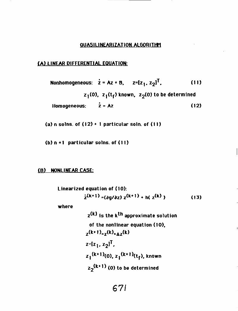
(A) LINEAR DIFFERENTIAL EQUATION:

T Nonhomogeneous: = Az + B. z=[z z2] . (1 1)

z (0). z, (tf) known. z2(0) t o be determined

Homogeneous: ; = A 2 (1 2)

(a) n solns. of ( 12) + 1 particular soln. o f ( 1 1 )

(b) n +1 part icular solns. of (1 1)

lB) NONLINEAR CASE:

Linearized equation of ( 1 0):

i(*+ 1 ) =(ag/az) Z(k+ 1) + h( Z(k) ) (13)

where

z ( ~ ) i s the kth approximate solution

of the nonlinear equation ( 10).

z (k+ ' )(o). z )(tf), known

22 (0 ) t o be determined

TOWARDS THE CENTER OF THE EARTH - '1 P

SHUTT

X

- - REFLECTOR

TOWARDS THE CENTER OF THE EARTH

SHUTTLE

- REFLECTOR Fig. I b. Att i tude o f the SCOLE Showlng Antenna Lfne o f Slght

SCOLE ( rigid) - ExmpC Slew;o , = 8.69434 6)

ToRQUEs X 1 0,000 FT-LB

1.0

0.0

-I .o

. - 'JY

Ux -7----------- 'I 'I ur

-

0 3 6 96)

FQEESX 8o_QLB

I I

1 .o

0.0

-1.0

I I

I ------ I 1 &

0 3 6 9 ($1

I I

fr - I I I \----- -

b I I

------ - I

fx I I I I I I I -

PLANAR SLEWING OF FLEXIBLE SCOLE

j-INEARIZED EQUATION OF MOTION:

where

8 i s the angle of rotation,

7 nxl i s the amplitude vector of the flexible modes, 4

n Is the number of mode used,

I i s the moment of inertia about the axis of rotation

r. M are the Inert la parameter vector, matrix.

I: )S the stiffness matrix,

@ ( z ) i s the mode shape functlon vector.

9 ,=#(q) . 4 is the coordinate along z axis,

L is the length of the beam,

us is the control torque on the Shuttle.

ui are the control actuators on the beam and the

re f lector.

STATE EQUATIONS

BOUNDARY CONDITIONS FOR s

where n is the number of mode shapes used.

PERFORMANCE l NMX

TPBVP

i = c z . z - I S . A lT= [z1.z21T

A i s the costate vector,

z l(O), z 1 (tf known; z2(0) to be determined.

t

\ ~ c t u a t o r r

I

\

\

$1 \

a r t a c t u g t o r r

I 0 &

4.1 I

1

I 6

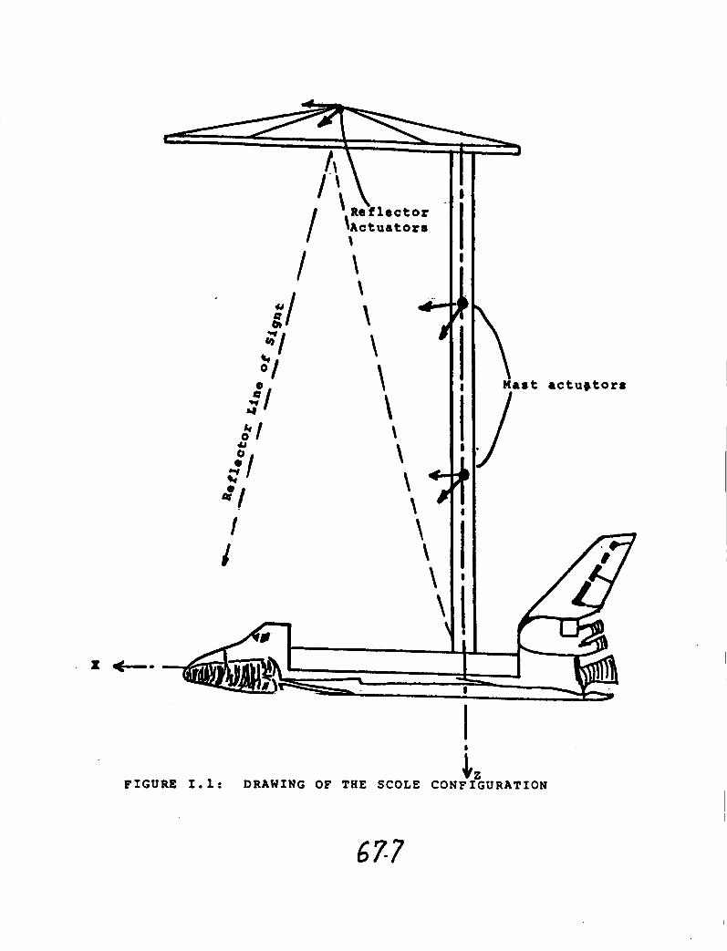
F I G U R E I . 1: DRAWING O F THE S C O L E C O N F I G U R A T I O N

NUMERICAL RESULTS

JA) SLEWING ABOUT X-AXIS (ROLL)

CASE: Urn( 1 0 0 ). 0-( 0.000 0.010 0.010 0.010 ) 1

CONCLUDING REMARKS

I) Solution has been obtained for nonlinear r ig id spacecraft

att i tude manewer (including the r igidized SCME).

2) Use of the Maximum Principle can make the states

sat isfy the boundary conditions very well.

3) Due the fact that the costates must be used in the method,

the dimension of equations of the system i s doubled, and

higher computational abi l i ty i s needed in th is method.

4) Further work on more complicated models (nonlinear

d i f ferent ia l equation) i s needed.

5) Need t o consider di f ferent cost functions and perf o m

parametric studies.

SESSION V - CONTROL SYNTHESIS AND SMUIATION

CONTROL LAW SYNTHESIS AND OITRKEZATION SOFTWARE FOR LARGE ORDER AEROSERVOELASTIC 8 Y S m

V. Mukhopadhyay. A. Pototzky, and T. Noll NASA Langley Research Center

Hampton, Virginia

ABSTRACT

Motivation: A flexible aircraft or space structure with active control is typically modeled by a large-order state space system of equations in order to accurately represent the rigid and flexible body modes. unsteady aerodynamic forces. actuator dynamics and gust spectra. The control law of this multi-lnput/multi-output (MIMO) system is expected to satisfy multiple design requirements on the dynamic loads. responses, actuator deflection and rate limitations. as well as maintain certah stability margins. yet should be simple enough to be implemented on an onboard digital microprocessor. This paper describes a software package for performing an analog or digital control law synthesis for such a system. using optimal control theory and constrained optimization techniques.

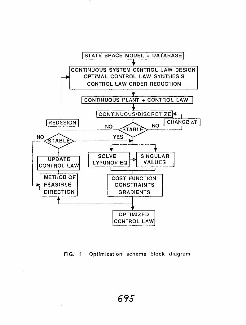
Software Capabilities: The primary software capability Is the optimization of the system by changlng the control law design varlables to improve stability and performance. A block diagram of the optlmlzation scheme is shown in Flg. 1.

I ) The optimbation module minimizes a linear quadratic Gaussian (LQC) type cost funcllon. while trylng to satlsfy a set of constraints on the conflicting design requlrcments such as design loads. responses and stability margins. Analytical expressions for the gradients of the cost function and the constraints. with respect to the control law design varlables. are used for computation. This facilitates rapid convergence of the numerical optimfiatlon process. The designer c,m choose the structure of the control law and the design variables. This enables optimization of a classical control law as well as an estimator-based full or reduced order control law. Selected design responses are incorporated as inequality constraints instead of lumping them into the cost function. This feature is used to modify a control law to meet indMdual root-mean-square (RMS) response llmitatlons and design requirements.

2) In order to lrnprove the multiloop system stability robustness properties in the frequency domain. the minimum singular value of the return dmerence matrlx at the plant input and output are as additional inequality constraints.

3) Other supporting capabilities include: (a) singular value analysis evaluation and plotting at the plant input and output; (b) llnear quadratic optimal control law synthesis: (c) Kalman Filter design, LQC Loop transfer recovery; (d) pole-zero computation: (e) frequency response, Nyquist and Bode Plot: (I) root locus plot; (g) block diagonalfiation; (h) modal residuallzation and truncalion; (1) transient response to deterministic and white noise input: (1) transfer of quadruple data to and from MATRIX-X and DICIKON: (k) parameter search to stabilbx an unstable control law, and (1) both interactive and batch mode execution using the Cyber NOS system.

Applications: The mftwarc has been used In the past for the following applications: (1) flutter mppmaslon control law for the ARW-I wind tunnel wing model: (2) gust load alleviation control law for the ARW-I1 drone: (3) flutter suppression control law synthesis for ARW-11 drone and the DC- 10 Dcrlvattve wind tunnel wlng model; (4) robust Digital gust load alleviation control law synthesis for ARW-11 drone: and the (5) Active Fladble Wing 0 flutter suppression control law synthesis which 1s presently being canied out.

1 STATE SPACE MODEL + DATABASE]

CONTINUOUS SYSTEM CONTROL LAW DESIGN OPTIMAL CONTROL LAW SYNTHESIS 1

I I CONTROL LAW ORDER REDUCTION I

1 CONTINUOUS PLANT + CONTROL LAW I b

I 1 REDESIGN 1 I

SOLVE SINGULAR

CONTROL LAW LYPUNOV EQ.+ VALUES

q FEASIBLE COST FUNCTION / CONSTRAINTS I

FIG. 1 Optimization scheme block diagram

CONTRO LAW SYNTHESIS AND OPTIMIZATION SOFTWARE

FOR LARGE ORDER AEROSERVOELASTIC SYSTEMS

V. Mukhopadhyay, A. Pototzky and T. No11 Aeroservoelasticity Branch

NASA Langley Research Center Hampton, VA

Workshop on Computational Aspects in the Control of Flexible Systems

Williamsburg, Virginia July 12-14, 1988

Abstract

A flexible aircraft or space structure with active control is typically modeled by a large order state space system of equations in order to accurately represent the rigid body and flexible modes, unsteady aerodynamic forces, actuator dynamics and gust spectra. The control law of this multi-input multi-output (MIMO) system is expected to satisfy multiple design requirements on the dynamic loads, root mean square (RMS) responses, actuator deflection and rate limitations as well as maintain certain guaranteed stability margins, yet should be simple enough to be implementable on an onboard digital microprocessor. This paper describes an interactive software named DESIGN for analysis and synthesis of analog and digital control laws for such a system, using optimal control theory and constrained optimization techniques.

large flex. sys

Overview

A multi-input mblti-output aeroservoelastic system is typically represented by a large order state-space system of equations in order to accurately represent the rigid body and flexible modes, unsteady aerodynamic forces, actuator dynamics, gust spectra, antialiasing filters, computational delays etc. The active control law is expected to satisfy a set of conflicting design requirements on the performance and stability margins, yet should be simple enough to be implementable on an onboard digital microprocessors. This objective can be achieved using the synthesis software described in this paper. The methodology used are optimal control theory, order reduction techniques, unconstrained and constrained optimization with constraints on the design RMS responses and the minimum singular value of the return difference matrix at the plant input and output. Optimization can be performed for both continuous system and discrete systems. The methodology has been used to synthesize a) Analog and digital gust load alleviation control laws for a remotely controlled drone b) Analog and digital flutter suppression control laws for Active Flexible Wing (AFW) wind tunnel model . Other potential future applications include a) Rapid maneuver load control for AFW d) Vibration suppression for large space structur~ and control structure interaction study.

OVERVIEW

CONTROL LAW SYNTHESIS AND OPTIMIZATION SOFTWARE FOR FLEXIBLE STRUCTURE

DESIGN OBJECTIVES LOW ORDER ROBUST CONTROL LAW FOR A HIGH ORDER AEROSERVOELASTIC SYSTEM

METHODOLOGY OPTIMAL CONTROL THEORY CONTROL LAW ORDER REDUCTION NUMERICAL OPTIMIZATION

COST FUNCTION LQG TYPE CONSTRAINTS RMS RESPONSES

SINGULAR VALUES

SYSTEMS CONTINUOUS DISCRETE

APPLICATIONS GUST LOAD ALLEVIATION OF A DRONE FLUlTER SUPPRESSION OF AFW MODEL RAPID MANEUVER LOAD CONTROL

Optimization Block Diagram

The optimization procedure minimizes a linear quadratic Gaussian (LQG) type cost function, while trying to satisfy a set of constraints on the conflicting design requirements such as dynamic loads, design RMS responses and singular value based stability margins at the plant input and output. The analytical expressions for the gradients of the cost function and the constraints, with respect to the control law design variables are used for computation. This facilitates rapid convergence of the optimization process. The designer can choose the structm of the control law and the design variables. This enables optimization of classical control law as well as an estimator based full or reduced order control law. Selected design responses are incorporated as inequality constraints instead of lumping them into the cost function. This feature is used to modify a control law to meet individual RMS response limitations and design requirements.

DISCRETE SYSTEM

T

CONTINUOUS SYSTEM CONTROL LAW DESIGN OPTIMAL CONTROL LAW SYNTHESIS

CONTROL LAW ORDER REDUCTION

+ [CONTINUOUS PLANT + CONTROL LAW I

C I CONTINUOUS/DISCRETIZE~

I REDESIGN ( I

CHANGE AT I I

UPDATE SOLVE SINGULAR

CONTROL LA LYPUNOVEQ.+ VALUES

I I I - I METHOD OF COST FUNCTION

-b FEASIBLE CONSTRAINTS DIRECTION GRADIENTS

4 I + OPTIMIZED

Software Organization

The interactive software DESIGN is organized to interact with several well used softwares such as 1) ISAC (Interaction of Structure, Aerodynamics and Control) for receiving state-space quadruple data, 2) DIGIKON for discretization, interconnection, model generation, digital design, verification and graphics and 3) MATRIX-X for matrix manipulation, interconnection, quadruple data transfer, graphics and design verification. DESIGN can also be run in batch mode on the CYBER/NOS system for large order problems involving systems with more than 120 states with large number of design variables and constraints. This batch version was previously known as PADLOCS (Program for Analysis and Design of Linear Optimal Control Systems).

DESIGN

I NTE RACTlVE

PADLOCS

. 1 *

, MATRIX X

I

*

BATCH I

Basic Command Summary

The quadruple data is generated and stored in a sequencial binary file called QDATA. The design starts with the file command

GET, QDATA. GET, DESIGN. DESIGN.

The random access files DBASE, and sequencial file PLDATA are used to transport quadruple data to and from DIGIKON and MATRIX-X, while random access file TAPE7 is ued to transfer data from 1SAC.using the UTILITY commands. The system parameter and quadruple data are read by the SYSTEM INPUT commands as shown in the figure above. The primary capability of this software is the optimization of the system by changing the control law design variables to improve the stability robustness and performance requirements. The supporting capabilities include a) Linear quadratic optimal control law synthesis; b) Kalman filter design, linear quadratic Gaussian design (LQG) and loop transfer recovery (LTR); c) Singular value analysis , evaluation and plotting at the plant input and output; d) Pole-zero computation; e) Open and closed loop frequency response, Nyquist and Bode plot, and loop breaking test; fj Root locus plot g) Block diagonal transformation; h) Modal residualization and truncation; i) Transient response to deterministic and white noise input; etc.

READ TITLE READ INPUT

PRINT INPUT

EXC ITWC OPEN EXC ITR@ CLOSED

Basic Design Commands

The basic design commands are shown in the figure above. For systems with known stable control laws the optimization procedure can be executed directly using the command EXC OPTM for continuous systems and EXC OFTD for discrete systems. For MIMO systems with no known initial stabilizing control laws, first an Linear Quadratic Gaussian (LQG/L,TR) design is performed to obtain a full order robust control law using a set of LQG design commands. The order of the control law is then reduced by truncation, residualization or balanced realization method using DESIGN, DIGIKON or MATRIX-X. The singular value analysis and block diagonal transformation procedure is very helpful in the reduction process. Since this reduced order control law is not optimal and may not satisfy the design requirements, constrained optimization procedure is used to update the reduced order control law. Constraints can be imposed on the design RMS responses and minimum singular values at the plant input and output.

BASIC DESIGN COMMANDS

LQG DESIGN

EXC OFSF EXC KFGM EXC WRES

I COVA ORDER REDUCTION

EXC WMSV - EXC OLFR EXC DIAG EXCEERO EXCEIGN - EXC PERM OPTIMIZATION

VRUNCAV E RESlDUALlZE ExC OPT'

I BALANCE(MX) U(C ITRC CLOSED EXC SING

OPTIMIZE EXC ITRC CLO EXC OPTD EXC EIGN EX6 TIME EXC lTWC OPEN

EXC FREQ EXC EIGN

ANALYSEIREOPTIMIZE

Gust Load Alleviation of A Flexible Drone

The synthesis procedure was applied to the gust load alleviation problem of a flexible drone. The basic control scheme is shown in the figure. In longitudinal motion, the symmetric elevator and outboard aileron deflections are used as the two control inputs. The accelerometer sensors at the outboard aileron and on the fuselage near the center of gravity are used as two measurement outputs. The output signals are filtered through first order antialiasing filters 50/(s+50) before digitization at 100 Hz. The two input two output system was modeled by a 32nd order system flying symmetrically through a Dryden gust.

GUST LOAD ALLEVIATION OF FLEXIBLE DRONE

aileron accelerometer

dla 'e 32nd order plant a.a.fil s+50

/+on flex. aircraft I L -

- I actuator sensor I - / q z o h 2 rbm 3 flex. mode

6a

I ald

I Gust Load Alleviation Design Requirements

The objective is to obtain a low order robust digital GLA control law which would reduce the open loop root-mean- square values of the wing root bending moment and shear by 50% without increasing the wing outboard bending moment and torsion The control law should maintain certain guaranteed stability margins based on minimum singular value of 0.6 at both the plant input and output. The control surface deflections and rates should be within the allowable limits. First a full order LQG control law is synthesized to satisfy the design requirements. This 32nd order control law is then reduced to a second order control law and then discretized. This control law does not satisfy the design requirements. After unconstrained optimization most of the requirements are satisfied except the wing outboard bending moment and the singular values. Using constraints on the RMS wing loads and on the minimum singular values of the return difference matrix at the plant input and output, the control law parameters are reoptimized (Ref. l,2).

GUST LOAD ALLEVIATION

DESIGN REQUIREMENTS Aileron 32nd order

Accl. airplane eqns. sensors

control law

How we do i t

1. LQG design

2. Control law order reduction

3. Discretize

4. Optimization

5. Apply constraints a) on rms loads b) on singular val.

Physical quantities

Root bending moment

Root shear

Outboard bending mom.

Outboard torsion

Elevator deflection

Elevator rate

Aileron deflection

Aileron rate

Design objectives

50% reduction

50% reduction

No increase

No increase

Within max limit

Within max limit

Within max limit

Within max limit

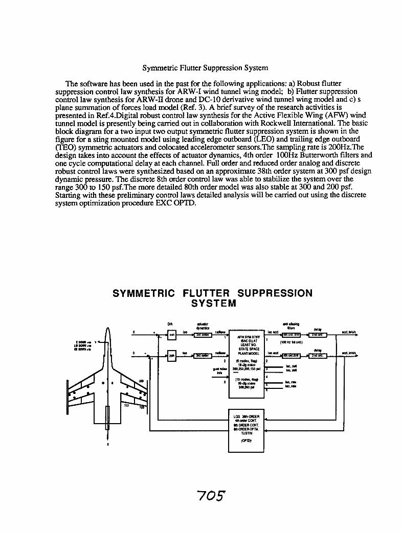
Symmetric Flutter Suppression System

The software has been used in the past for the following applications: a) Robust flutter suppression control law synthesis for ARW-I wind tunnel wing model; b) Flutter suppression control law synthesis for ARW-I1 drone and DC-10 derivative wind tunnel wing model and c) s plane summation of forces load model (Ref. 3). A brief survey of the research activities is presented in Ref.4.Digital robust control law synthesis for the Active Flexible Wing (AFW) wind tunnel model is presently being carried out in collaboration with Rockwell International. The basic block diagram for a two input two output symmetric flutter suppression system is shown in the figure for a sting mounted model using leading edge outboard (LEO) and trailing edge outboard (TEO) symmetric actuators and colocated accelerometer sensors.The sampling rate is 200Hz.The design takes into account the effects of actuator dynamics, 4th order l00Hz Butterworth filters and one cycle computational delay at each channel. Full order and reduced order analog and discrete robust control laws were synthesized based on an approximate 38th order system at 300 psf design dynamic pressure. The discrete 8th order control law was able to stabilize the system over the range 300 to 150 psf.The more detailed 80th order model was also stable at 300 and 200 psf. Starting with these preliminary control laws detailed analysis will be carried out using the discrete system optimization procedure EXC OPTD.

SYMMETRIC FLUTTER SUPPRESSION SYSTEM

CONCLUDING REMARKS

Software Improvement

1. Direct time response constraints 2. New reduction techniques 3. H-infinity design 4. Additional derivativelsensitivity capabilities 5. User help and online documentation

Portability improvement

1. Microvax 2. NOS VE

Future Applications

1. AFW rapid roll maneuver 2. Large space structure-control interaction

AFW RAPID ROLL CONTROL M l v e Flexible Wi Ra Ron Mechanization

Wind Tunnd%oc$%Digital Control (L

I I LARGE SPACE STRUCTURE

ACTIVE CONTROL

References

1. Mukhopadhyay, V., "Digital Robust Active Control Law Synthesis for Large Order Systems using Constrained Optimization," AIAA Paper 87-2588 CP, Guidance, Navigation and Control Conference, Monterey, CA, 1987.

2. Mukhopadhyay. V., "Digital Robust Control Law Synthesis Using Constrained Optimization," Journal of Guidance Control and Dynamics,l988 (TBP)

3. Pototzsky, A. S. and Perry, 111, B.,"New and Existing Techniques for Dynamic Loads Analyses of Flexible Airplanes," Journal of Aircraft, April 1986, pp. 340-347.

4. Abel, I. and Noll, T.E., Research and Applications in Aerosewoelasticity at the NASA Langley Research Center," 16th ICAS Congress, Jerusalem, Israel, August, 1988.

FLEXIBLE AIRCRAFT DYNAMIC MODELING FOR DYNAMIC ANALYSIS AND CONTROL SYNTHESIS

David K. Schmidt Purdue University

West Lafayette. Indiana

ABSTRACT

171e linearbation and slmpllfication of a nonllnear. literal model for flexible aircraft is hlghllghted. Areas of model fidelity that are critical if the model is to be used for control system synthesis are developed and several s lmp~cat ion techniques that can deliver the necessary model fidelity are discussed. These techniques include both r~r~rncrlcal and analytical approaches. An analytical approach, based on first-order scnsltlvlty theory b shown to lead not only to excellent numerical results. but also to closed-form analytical expressions for key system dynamic properties such as the pole/zero factors of the vehicle transfer-function matrix. The analytical results are cxpressed in terms of vehicle mass properties, vibrational characteristics. and rigid- body and aeroelastic stability derivatives. thus leading to the underlying causes for crltical dynamic characteristics.

PRECWINO PAGE DUNK NOT FKMED

MODELING FLEXIBLE AIRCRAFT

FOR DYNAMIC ANALYSIS

AND CONTROL SYNTHESIS

David K. Schmidt School of Aeronautics and Astronautics

Purdue University

July 1988

TOPICAL OUTLINE

What Constitutes a Valid Model? How Validity Will Be Measured What's Important in a Feedback System

Some Approaches to Obtain (Simple) Valid Models Numerical Literal

Physical Causes of Critical Dynamic Characteristics

WHAT VEHICLE DYNAMIC CHARACTERISTICS ARE CRITICAL IN A FEEDBACK SYSTEM?

They Are Important If They Can:

- Induce Critical PolefZero Interactions

- Significantly Affect Frequency Response Near Crossover

- Significantly Affect Time Response

CRITICAL DI-POLE EFFECT

STABILITY I N THE FACE OF UNCERTAINTY

NOMI NAL LOOP

-160

I

CHARACTERIZING UNCERTAINTY

\I - 0,

Stability of the Loop Guaranteed If

Stability of the Loop Guaranteed If

f - ~

Let's Look At Potentid Slmc'es For Mi or ~(jo) <

A MEANINGFUL METRIC FOR MODEL VALIDITY

6G = E(jw) = Gum) - G,(jo) In Crossover (or ~( jo) = I - G-IG,) Region

Can Use Singular Values If Desired

-?h G(E) = A (EE*),

A Possible Metric A Conservative Metric

sup o(~(jm)) IIE(~oI)II~ = IIE(~u)II~ =

SUP ~@o'W 0 1 c w < 0 2 o c o < -

Or Just look at Bode Plots

&(s) - %(s) det [Ai I Bj] L I P =

Uj(s) Uj(s) C det [A]

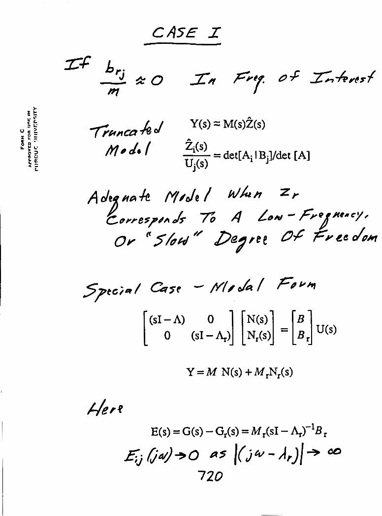
k J Y (s) = M(s)?(s) ' T i h A C i i

M @ J @ / &(s) = det[Ai I Bj]/det [A] Uj (s)

2 I F

n

'I'

w

CA-

- Y

zb &

II 62

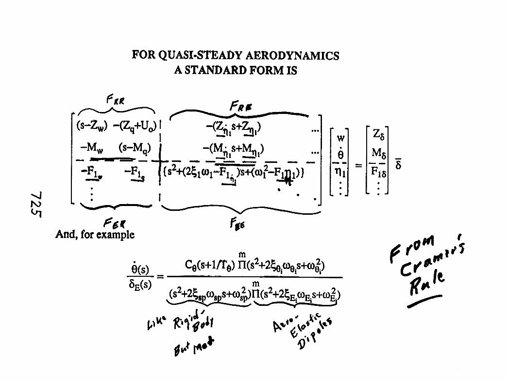
a*

.

Table 10. Transfer Functions For the True Model

gains

zeros

poles

G,"

(fvs2/deg)

52.01

6.473E-5

-.008887

-.01958 kj1.661

-.3610f jll.OO

-1.0035 j11.13

1.549 f j11.71

-3.144f j14.34

-03324

-.a268

-.4513f j1.171

-.4408 f j6.010

-.2240 f j 10.78

-.3611 fjll.00

12.558 + j13.05

G:

(rad/s/deg)

8.001

0

-.05 103

-.2020

3.642

-4.020

-.3610 f jll.OO

-2.838 f j12.71

.5735 f j13.41

0,"

(fr/s2/deg)

-244.5

1.087E-4

-.008093

.1703f j1.795

-.8996 f j4.132

-.2252 f j 10.77

-.3607 f jll.OO

-2.601 f j13.06

~t (rad/s/deg)

15.65

0

-.0554 1

-. 1 172 -.5973 f j2.9 12

-.2556 f j 10.68

-.3562f j10.99

-2.564f j13.12

"true" --------- t run. / resid. . . . . . . . . .ful b reduction

F l gure 4 . < G ~ E Frequency Response

,-" 1:-

2': (i. I/:-- _ _ m e - . . . . . . . . . . . . . .

- "true"

......... ---------trun./resfd. f w i b reduction

~i . J 1 i o 100

.. .- -.

- .,--.-. - .

- "true" ---------trun./resid. ......... f w i b reduction

. . .

i . J 1 i o 100 w ( r a d l s )

6 Ftgure 6. < G E Frequency Response q~

731

I 25. o i I . . J J i o 100 I* ( r r d l s )

Figure 8. < G ~ C Frequency Response Oz

Figure 10. < 6% Frequency Response q~

Table 12. Transfer Functions For FWIB Reduction Model

gains

zeros

G:

(fr/s2/deg)

52.0 1

-.02102 f j 1.670

1.244f j13.51

G:

(rad/s/deg)

14.96

-. 1789

2.78 1

-3.732

poles -.4679 f j 1.234

-.4413 f j6.015

G,"

(fr/s2/deg)

-244.5

.I725 f j1.806

-.9 177 f j4.143

G:

(rad/s/deg)

15.29

-. 1437

-.6806 f j2.900

Table 14. Lower-Order Transfer Function Forms

where D(s)=s[s~ + (2c0)~~s + ( o ~ ) ~ ~ ] [ s ~ + ( 2 c ~ ) ~ l ~ + ( ~ 2 ) f i l

Table 8. Polynomial Coefficient and Factor Relationships

CLOSED-FORM EXPRESSIONS FOR THESE TERMS

Specifically, it has been shown that for a slender (low aspect ratio) vehicle

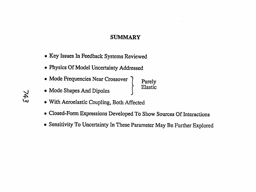
EXPERIMENTAL VALIDATION OF FLEXIBLE ROBOT ARM MODELING AND CONTROL

OUTLINE

a INTRODUCTION Motivation Background

a MODEL EVALUATION Formulation Result8

a CONTROLLER EVALUATION Formulation Results

SUMMARY AND CONCLUSIONS

M A. Galip U h y

Mechanical Engineering and Applied Mechanics College of Engineering University of Michigan

- - - PRECEDING PAGE BLANK NOT FILMED

INTRODUCTION

Flexibili ty is important for high speed, high precision operation of lightweight manipulators.

Accurate dynamic modeling of flexible robot arms is needed. Previous work has mostly been based on linear elasticity with prescribed rigid body motions (i-e.. no effect of flexible motion on rigid body motion).

Litt le or no experimental validation of dynamic models for flexible arms is available. Experimental results are also limited for flexible arm control.

~ We include the effects of prismatic as I well as revolute joints.

We investigate the effect of ful l coupling between the rigid and flexible motions, and of axial shortening.

i We also consider the control of flexible arms using only additional sensors.

BACKGROUND

Research since 1970's (e.g., [Book, Maizzo-Neto, Whitney 751)

Modelina of flexible mechanisms and structures (e.6, Ehsto-Kineto Dynamics, Floating Frames, 70's)

roaches to control . - Trajectory planning [Meckl, Seering 03,051 open kop (none) Closed bop with micromanipuhtor

[Cannon et al, Book et all Closed loop with additional sensors only (none)

Experimental work [Zalucky and Hardt $41 [Cannon et al83,04]

Theoretical control studies [Book et al, Cannon et al, etc, early 1 980'tl Various control strategies proposed typically assuming all states available, no spillover, simple models, m, implementation considerations.

MODELING AND SIMULATION OF FLEXIBLE ROBOTS WITH PRISMATIC JOINTS

Robots with both rigid and flexible l inks attached with revolute and/or prismatic joints can be modeled and analyzed.

The equations of motion are derived using Lagrange's equations. The prescribed motion, and prescribed torque/force cases can both be hand led.

Flexible elements are represented as Euler-Bernoulli beams, and the axial shortening effect is also included.

Finite element analysis is used for the discretization of the resulting hybrid equations of motion. m Constraints are handled using Lagrange multipliers. m The resulting algebraic-differential equations are solved numerically using constraint stabilization methods.

a Nominal configuration

Actual configuration

Schematic of a two-link robot.

Axial shortening of a beam under plane transverse deflection.

Schematic of revolute joint i.

link i- 1 link i ...................................

link i'

Schematic of prismatic joint i.

Schematic of prismatic joint i.

Beam moving over bilateral supports.

-0.02 0.0 0.5 1 .O 1.5 2.0 2.5 3.0 3.5

T i e (sa.)

- Buffinton and Kane [291. - - - presentmethod

I I I I I I

Tip @lacement in "slow push" case with C1 = 0.725 m, C2 = 0.7 m and T = 3.5 sec.

0.02

0.01 E w -. C

ii 0 :: 0.00 5 . - u C . - b

-0.0 1

-0.02 0.0 0.1 0.2 0.3 0.4 0.5 0.6 0.7

Time (sec.)

Tip displacement in "fast push" case with C1 = 0.725 m, C2 = 0.7 m and T = 0.7 sec.

-

- Buffinton and Kane [29]. - - - - present method.

1 I I I 1 I

0.02

r, 0.01 E w - C

2 iJ 0.00 - 5 . - 0 a . - I-

-0.0 1

-0.02 0.0 0.1 0.2 0.3 0.4 0.5 0.6 0.7

r i (stc.) Tip displacement in "fast pull" case with C1 = 0.025 m, C2 = -0.7 m and T = 0.7 sec.

- Buffinton and Kane [29]. - - - present method

-

I I 1 1 I I

LAB0 RATORY ROBOT

Small table top spherical coordinate robot with 3 DOF I

Designed and built at UM

Interfaced to an ISM PCIXT

Convienent test bed e~perimental research work

r and 0 axes are dc motor driven through leadscrews

$ axis is dc motor driven driven through a gear train

all axes have tachometers and optical incremental encoders with counter circuits

last link is intentionally designed to be flexible

I accelerometen (in two orthogonal directions) measure end of arm accelerations which are integrated to get velocities and positions

Lead Screw

Lead

Third Link Accelerometers

! i i 1

Screw .:CTa\

Schematic of the experimental setup.

f \

UO Pan . - v - D

- * IBM P C N A

A Microcomputer D 4 C C

Second Link

Coupler

Rotating Base

J I

Filter

4

U Analog Double

I c 1

1

t

4

Optical Encoder

DC Motor

-.0154 . . . , - v . - . 3 . +

0 1 2 3 4 5 6 7 8 9 10 Time (sec.)

Elastic tip displacement obtained by numerical simulation after filtering.

-. o l s ~ . , . , . . . I . I . I . ~ ~ + 0 1 2 3 4 5 6 7 8 9 10

Time (sec.)

Vemcal elastic tip displacement of the last link in the two-dimensional maneuver.

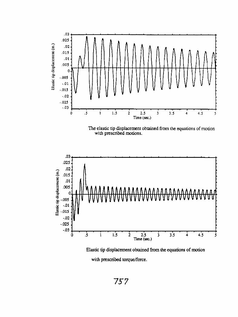
-.025 -.03

0 . 5 1 1.5 2 2.5 3 3.5 4 4.5 5 T i e (sec.)

The elastic tip displacement obtained from the equations of motion with prescribed motions.

Elastic tip displacement obtained from the equations of motion

with prescribed torque/force.

Angular velocity of the first joint of the rigid manipulator with controller.

Translational velocity of the third joint of the rigid manipulator with controller.

1 :s 2 2 :5 Time (sec.)

Angular velocity of the first joint of the flexible manipulator with conmller.

Translational velocity of the third joint of the flexible manipulator with controller.

. o h

- 0.. ui - E -.05. Y

a .- 8 ' . I . - f - -.IS. m C 0 .- -.2. - In C E -.25. C

-. 3.

-. 35. 0 .5 1 1 .S 2 2.5 3 3.5 4

r

Time (sec.)

I I 1 I I I 1

L

.015+ b

- .01. E - e

f .005- z 0 - S 0- 5 CL .- - 0 -.005. .- - .--- without axial shortening effect V) 0 5 - with axial shortening effect

-.01.

-.015+ I 1 I I 1 Y

0 . 5 1 1.5 2 2.5 3 Time (sec.)

Elastic tip displacements in the case with T = 2 sex.

. l a - - - . - . - - - * - - - - - . - a - b

.08.

E .06- .

-.-- without a x d shortening effect ,

- with axial shortening effect . 0 .2 .4 .6 .8 1 1.2 1.4 1.6 1.8 2

Time (sec.) Elastic tip displacemnt in the case with T = 1 sec.


A general modeling procedure for robot arms consis 'ting of rigid and flexible links connected by revolute and/or prismatic joints has been developed and experimentally validated.

The significance of full coupling (effect of flexible motion on rigid body motion) has been demonstrated.

The axial shortening effect is shown to be significant for high speed operation of lightweight manipulators.

CONTROL OF A LEADSCREW DRIVEN FLEXIBLE ROBOT ARM

The laboratory robot is used to compare the performance of a rigid body motion controller with that of a rigid and flexible motion controller.

The rigid body motion controller uses only the joint motion measurements and joint actuators. The rigid and flexible motion controller also uses the end of arm motion measurements, but no additional actuators.

The leadscrew transmission characteristics as well as observation and control spillover are considered.

The numerical and experimental results show good agreement, and indicate that significant reductions in arm vibration are possible through use of the rigid and flexible motion controller.

Arm geometry and coordinates.

PHYSICAL CONSTRAINTS

The physical constraints that are considered in this work are the ones imposed by the leadscrews only.

. Condition for self locking assumption to be valid is :

P > tan(ur,)

where

p is the thread coefficient of friction.

v, is the thread helix angle.

. Effect of the self locking condition.

. Effect of coulomb friction.

CONTROLLER DESIGN

Equations o f motion:

Linearized equations:

Integral plus state feedback controller: t t +

y,, = / ( y , - U , ) d t 0 ; yf2 = j c Y 2 - R t ) d t 0 . ; y , , = J q 3 - R s ) d t 0

Block diagram of the integral plus state feedback controller.

Flgun 3. ~lexlbie motlon coordlnatr, q1 ,.(t), In response to the rlgld and flexlble motlon controller In the reduced order model case.

flgum 4. Flexlble motlon coordlnate, 42, (1). In response to the. rigld and flexlble motlon c~.ntroller In the reduced order mode! cam.

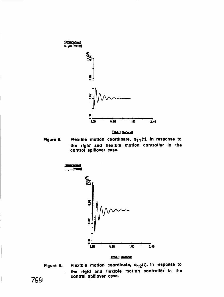
Flgun 5. Flexlblo motlon coordlnate, ql1 (t), In response to the rIgId and flexlble motlon controller In the control spillover case.

Flgure 6. Flexlble motlon coordlnate, qI2(t), In response to the rlgld and flexlble motlon control#id In the control spillover case.

C#?laNAL PAGE 1% 6~ IBm QUALITY

amd- Flgun 7. Flexlble motlon coordlnate, q12(t), In response to

the rlgld and flexible motlon controller In the control and obsewatlon spillover case.

Flgute 8. Flexible motlon coordlnate, q12(t), In response to the rlgld and flexlble motlon contrvller In the control and observatlon spillover xlth structural damping Included. 76 9

TABLE 1

Standud Set of Phyrlul Syrkrn Parameters

> f u r of the first beam (m ,) hfsa of the second beam ( m 2 ) M m i of the Payload (m, ) Cross scctioarl ares ot the second

berm (A ?)

Length of the first beam (L ,) Length of the second beam ( L 2 ) Gravitational acceleration (g ) Aluminum density (p) Flexural rigidity (EI ) Reference position for r Reference position for 6 Reference position for 4 Desired reference position for r Desired rdereect position for 6 Desired rettreucc pitioa for # Servo n a t r d fitqoency for r (w, ) Servo mWd Irtqotacy for I (w, ,) Scwo satrnl. frqueocy far # ( w , ,) Fkxibk ntorior gain, K 5 Fkxibk m n o t b m gin, K& FkxiMc mdom gain, K

1 .

VALUE

0.454 Kg 0.816 Kg 0.07 K#

0.000151 m2 0.233 rn 2 rn 9.81 rn/rce2 ?707 Kg/ m ' 770.87 Pa 1.85 m O d O d 2m 0.5 r d 0.5 r d

. 4 ndlm : 4 nd/bec

8 d / w c -0.000178 4.084 1.568

d

Table a.

770

rigid body controller

r

rigid and flexible motion controller

settling time (seconds)

11 .O

3.0

maximum deflectiom (peak to perk)

7.5mm

2.7mm

OR!GIMAL PAGE IS OF POOR QUALITY

Flgw 10. e respoqsa obtalned from tho rlgld body controller In the experlmental work.

Flgun 11. Total vartlcal deflbctlon In response to the rlgld body controller In the experlmental work.

--

'La 4

4.m 0.a PI

Flgum 12. 8 response obtalnd from the rlgld and flexlble motlon controller In the experimental work.

-- I-)

- *- ' ~ a 4.a LOO n.m

Flgure 13. Control slgnal for the second Jolnt obtalned from the rlgld and flexible motlon controllar In the experlmmtal work.

ORIGINAL PAGE IS OF POOR QUALITY

Flgura 14. Totat vertical deflection In response to the rlgld and flexible motion controller In the experimental work.

RIGID BODY CONTROLLER VERSUS RIGID AND FLEXIBLE MOTION CONTROLLER

I

Simulation results:

* Control spillover effect can be observed, but does not cause significant deterioration.

* Control and observation spillover can destabilize the residual mode. However, a small amount o f damping (0.0 145) eliminates the problem.

* Settling time i s reduced from 3.5 to 1.07 seconds, and maximum vibration amplitude is

I

reduced by 50%.

~ Experimental results:

* With low pass filtering and light structural damping, no detrimental spillover effects were observed.

* Settling time is reduced from 1 1 t o 3 seconds, and maximum vibration amplitude is reduced by 75%.

1. A dynamic model of a spherical coordinate robot arm, whose last link is flexible, is developed. The constraints imposed by the leadscrew transmission mechanisms are also considered.

2. The interrelationships between the robot arm structural flexibility and the controller design are investigated using a rigid body controller.

3. The rigid and flexible motion controller, which employs additional sensors only, has led to an approximate 50% reduction in the magnitude of the flexible motion even in the presence of the observation and control spillover.

4. The experimental results of the rigid and flexible motion controller show good agreement with those of the digital simulation.


A general modeling method for robot arms with flexible and rigid links connected by prosmatic and revolute joints has been presented and experimentally validated.

• A flexible arm controller which uses end of arm motion meaurements, but only joint actuators has been numerically and experimentally studied and found to give good rigid body control with significant reduction in end of arm vibrations.

ACKNOWLEDGEMENTS

The work described was based on the Ph.D. dissertation research of Ye-Chen Pan (co- advisors: A.G. Ulsoy and R.A. Scott) and Nabil Chalhoub (advisor: A.G. Ulsoy). The

I

I experimental studies were done with the assistance of Steve Culp and Rob Giles.

M A. Galip U h y

Mechanical Engim?ering and Applied Mechanics College of -ring University of Michigan

REFERENCES (available upon request from A .G. Ulsoy)

D m - u of Flexible ~ ~ ~ 8 m ; ~ larlardb Pnkmrfie hid., Ye-Chen Pan, Ph.D. Dissertation, Mechanical Engineering and Applied Mechanics, University of Michigan, AM Arbor, Michigan, April 1988.

'Dynamic Modeling and Simulation of Flexible Robots with Prismatic Joints, Part I: Modeling and Solution Method,' Y .C. Pan, R.A. Scott, and A.G. Ulsoy , (in preparation).

'Dynamic Modeling and Simulation of Flexible Robots with Prismatic Joints, Part 11: Experimental Validation and Numerical results," Y.C. Pan, A.G. Ulsoy , and R .A. Scott, (in preparation).

C o n ~ l of z Le;r&mw Dn-wn f3exib.e Robor Arm, Nabil 6. Chalhoub, Ph.D. Dissertation, Mechanical Engineering and Applied Mechanics, University of Michigan, AM Arbor, Michigan, June 1986.

'Dynamic Simulation of a Leadserer Driven Flexible Robot Arm and Controller,' N.G. Chalhoub and A.G. Ulsoy, ASME j b d of D y I c syltenau, M~;1~urreme.tiadCon.l, Vol. 108, No. 2, June 1986, pp 119-126. rn 'Control of a Flexible Robot Arm: Experimental and Theoretical Results', N.G. Chalhoub, and A.G. Ulsoy, ASME k d of Dyn?aIc -gem, M-mment, ipd Cua&nI, Vol. 109, No. 4, December 1987, pp 299-309.

"Dynamic Modeling of a Self-Locking Leadscrew and Its Implications in Robotics,' N.G. Chdhoub and A.G. Ulroy, ASME h d of D-Ic mte-, M'im-nt and Con.1 (submitted).

CONTROLLING FLEWXlWe STRUCTURES - A SURVEY OF METHODS

A. A. Anlsslpour, R A Benson. and E. E. Coleman The Boelng Company Seattle. Washlngton

ABSTRACT

In response to the demand for higher fuel emclency. new jet transport designs are using composites to reduce wefght. Since these composites have less inherent damping than the materfals they are replacing. flexible body dynamics are becoming more significant. Low frequency structural modes that in the past had sumclent open loop damping to avoid stablllty and ride performance problems now require compensation. Control law design can no longer be concerned solely wlth rigid-body dynamics.

Control systems design techniques which have proven effective for rigid dynamics may no longer be applicable when including flexible modes. This paper studies the dillerent control strategies and thelr application to systems including flexible dynamics. The control law deslgn goal with respect to flexible modes is twofold. First. the modal damping must be Increased to some minimum acceptable level. Second. the rigid body modes must be controlled whlle minimlsr.ing excltatlon of the flexible modes. A necessary. and often nontrivial first step is identification of the flexible modes (both mode frequency and shape). The following addresses these issues with respect to a particular control law design tcchnlque.

1) Off-llne Modeling/OlT-line Controller Design

171e on-line modcllng controller deslgn technique has been used historically as the standard for alrplane control system deslgn. Thls technique consists of building up a n~tdel on mathematlcal prediction, wind tunnel analysis. and fllght test data. Controllers are then deslgned off-line based on the model. Controller implementation may include scheduling based on flight condition, but wlth no on-line modlllcations made to the controller.

2) On-line Modellng/On-line Controller Design

Thc same type of model used for the previous technique is developed using the off-line modellng/on-line controller deslgn wlth the primary dillerence being that the controller structure is defined off-line. while the controller gains are adapted on-line to minimize certaln performance criteria. With lhls technique no attempt is made to model the open loop system on-Une. and all controller gain changes are made solely in response to performance criteria.

PRECWiNG PAGE BLANK NOT FILMED

On-line modellng/off-llne deslgn technique d e h e s the controller ln terms of a general open loop system model for a speclned structure. With this technique each controller Rain 1s defined as a functlon of model parameler values. lmplemcntatlon Is executed by bulldlng an on-llne adaptive open loop esllnialor. The controller gains are then set based on Ihe model estlmale values per Ihe definlllons developed off-llnc.

4) Off- llne Modellng/OK-llne Controller/On-llne AdJustment

The control law is deslgned uslng the ofr-llne modeling/og-me controller to stabilize the nomlnal plant. With thls technlque an adaptive loop is placed around the system. creating an adaptive system that tunes the control input to improve the a-nomlnal performance. This adaptlve loop Is designed lo never destablllze the nominal plant and when the plant Is at nomlnal. the adaptive control signal Is zero.

CONTROLLING FLEXIBLE STRUCTURES - A SURVEY OF METHODS

RUSSELL A. BENSON EDWARD E. COLEMAN

The Boeing Company Boeing Commercial Airplanes

P. 0. Box 3707 Seattle, Washington 98124-2207

Most of the presently available control system design techniques applicable to flexible structure problems were developed to design controllers for rigid body systems. Although many of these design methods can be applied to flexible dynamics problems, recently developed techniques may be more suitable for flexible structure controller design. The purpose of this presentation is to examine briefly the peculiarities of the dynamics of flexible structures and to stimulate discussion about top level controller design approaches when designing controllers for flexible structures.

This presentation contains a suggestion of a set of categories of design methods for designing controllers for flexible structures as well as a discussion of the advantages and disadvantages of each category. No attempt has been made herein to select one category of design techniques as the best for flexible structure controller design. Instead, it is hoped that the structure suggested by these categories will facilitate further discussion on the merrits of particular methods that will eventually point to those design techniques suitable for further development.

CHARACTERISTICS OF FLEXIBLE STRUCI'URE DYNAMICS

Flexible structure dynamics tend to differ from rigid body dynamics in several important ways. First, flexible dynamics are higher order than rigid body dynamics. By definition, rigid body dynamics involve six degrees of freedom. Since each degree of freedom results in two states, the full set of dynamics for a rigid body system will involve only twelve states. (Additionally, servo, actuator, sensor, and controller compensation states must be added.) By comparison, a flexible structure model may have 100 or more states. This increase in the number of states derives an increase in the complexity of the control problem. Hence, those design techniques which work well for tenth order systems may have difficulties handling systems with ten times that many states.

A second important difference between rigid body and flexible dynamics is flexible dynamics tend to be more difficult to predict than rigid body dynamics. It is the

structure of a system which derives its flexible dynamics. Parameters such as mass distribution, material stiffness and damping, and unsteady aerodynamics become influential. Often mathematical models developed to predict the flexible dynamics differ with the physical system representation. As a result, the controller design based on these prediction models must be made robust to withstand the discrepancies between the model and physical system.

A third difference between these dynamics is that rigid body dynamics can often be treated as decoupled, whereas flexible body dynamics are most often highly coupled. As a result, control problems that can often be treated as a single input / single output (SISO) or as a series of SISO problems when dealing with rigid body systems, become multiple input / multiple output (MIMO) problems when dealing with flexible systems. SISO methods appropriate for decoupled rigid body system controller design may be unsuitable for flexible system controller design.

A fourth difference between these dynamics is the goal of the systems designed to control them. Rigid body control usually involves commanding the rigid degrees of freedom to follow desired trajectories. For an airplane these might be altitude, heading, and airspeed. By contrast, the goal of most flexible structure controllers is either to perform the desired rigid body control without exciting flexible modes, or to provide active damping for structural modes that are excited. In almost all applications the objective is to keep flexible structure dynamic responses at the lowest possible levels. The difference between the goals for rigid body control and flexible structure control may require different controller design approachs.

Four categories of controllers are detailed in the following paragraphs with a discussion on the advantages and disadvantages of each category with respect to the design of controllers for flexible structure systems. It is not the author's intent to favor any category of controller design techniques over another. The divisions herein are made simply to facilitate comparison of different top level strategies for the design of controllers for flexible structures. The categories are deliniated by the types of models each use for controller synthesis, and whether the controller is designed off-line, on-line, or both.

1) Off-line Modeling / Off-line Controller Design

Off-line modeling / off-line controller design techniques have been historically used as the standard for control system design. This technique consists of building up a model using mathematical prediction, wind tunnel analysis, and flight test data. Controllers are then designed off-line based on the model. Although separate controllers may be designed for different flight conditions (i.e., requiring gain scheduling based on flight condition), only these on-line modifications defined previous to flight are made to the controller.

This category of controller design techniques has the advantage of all controller synthesis work being completed ahead of time off-line. As a result, the on-line computational load is kept to a minimum. In addition, since the controller is well defined for each flight condition, rigorous analysis is possible for predicting performance and robustness characteristics.

A disadvantage of this controller design approach is that disaepanaes between the model and the physical system itself must be handled solely by controller robustness. The controller is unable to tune itself to account for modeling errors or changes in the dynamics as a result of different flight conditions or weight distributions. Hence, this design approach requires development of an accurate system model. Whenever possible, the off-line model is updated to concur with the obtained test data using the physical system to be controlled. In those cases where test data is not available, analysis must be done to show that the controller will function in an acceptable manner for the set of anticipated dicrepanaes between the model and the physical system.

2) Off-line Modeling / On-line Controller Design

The same type of model used for the previous category of controller is used for off- line modeling / on-line controller design techniques. However, the primary difference with this category is that while the controller structure is defined off-line, the controller gains are adapted on-line to minimize certain performance criteria. With this technique no attempt is made to model the open-loop system on-line, and all controller gain changes are made solely in response to performance criteria.

This approach has the advantage of the controller being able to tune itself to account for parameter variations between the model and the physical system. The off-line system model does not have to be as precise for this type of controller as for those desaibed in category 1. The off-line model is used to note the structure of the system and the general trend of the dynamics. Furthermore, a related advantage is that since the controller is able to tune itself, gain scheduling does not have to be as detailed as for a controller that is designed completely off-line.

A disadvantage of this approach is that the controller must be tuned on-line, thus requiring more computation power. Another disadvantage is that while the controller is able to tune itself to account for parameter variations, its structure is fixed. If the structure of the flexible system changes or there are wide swings in its general dynamics, the controller may not be able to tune itself sufficiently to provide the necessary control. A third disadvantage is that while the controller is continuously tuning itself, it is impossible to predict the gains for any given flight condition. As a result, it is impossible to obtain the level of performance and robustness analysis possible with each flight condition assigned a fixed set of controller gains.

3) On-line Modeling I Off-line Design

On-line modeling / off-line design techniques define the controller in terms of a general open-loop system model of a specified structure. With these techniques each controller gain is defined as a function of model parameter values. Implementation wnsis ts of building an on-line adaptive estimator to estimate the model parameters. The controller gains are then set based on the model estimate values per the definitions developed off-line.

An advantage of this approach is that the controller gain definitions can be chosen to give the desired performance and robustness properties regardless of the model parameters. (It is assumed that sufficient controllability and observability exist for all variations of the model parameters.) Gain scheduling is not an issue since the controller gain definitions automatically give appropriate gains for any given operating condition.

A disadvantage of this approach is that the controller gains must be defined symbolically rather than numerically. Controller synthesis requires solution of symbolic rather than numeric equations. Fortunately this task is done off-line and will not require real-time computing resources, but it is still a formidable task nonetheless. Another disadvantage is that on line estimation of the model parameters is required along with computation of the controller gains. Evaluation of the equations defining the controller gains may be quite expensive to compute. An additional disadvantage is that the controller gain definitions may include singular points within the region of possible model parameter sets. A method to avoid singularity is needed.

4) Off-line Modeling I Off-line Controller / On-line Adjustment

The final controller design approach category involves off-line modeling, off-line nominal controller design, and on-line controller adjustment. The nominal controller is designed to stabilize the nominal system. With this technique an adaptive loop is placed around the system to tune the control input for improving the off-nominal performance. This adaptive loop is designed to consistantly stabilize the nominal system. Furthermore, when the system is at nominal, the adaptive control signal is zero.

An advantage of this system is that while the controller is able to tune itself to account for modeling errors, the tuning is restricted so that the closed-loop system remains stable. This method can be thought of as a compromise between a fixed gain controller and fully adaptive controller. The nominal controller gains are fixed while the adaptive algorithm is free to vary the gains within a range about nominal.

A disadvantage of this system is that if the physical system varies greatly from the I nominal given by the off-line model, there is no longer a guarantee of stability. I

Hence on the one hand, the adaptive tuning is restricted to keep from destabilizing the nominal system. On the other hand, this restriction may lead to a situation where the actual system is driven unstable and the limitations on the adaptive tuning are such that the controller is unable to tune itself sufficiently to provide closed-loop stability.

SUMMARY

Rather than point to a single design approach as the best for designing controllers for flexible structures, the goal of this presentation is to simulate thought and discussion. Most likely a single approach is not well suited for all problems. The key is to realize that there are fundemental differences between rigid body and flexible structure dynamics and that these differences may require different approaches to controller design.

CONTROLLING FLEXIBLE STRUCTURES:

A SURVEY OF METHODS

Russell A. Benson Edward E. Coleman

The Boeing Company Boeing Commercial Airplanes

P.O. Box 3707 Seattle, Washington 98124-2207

BOEING COMMERCIAL AIRPLANES GUIDANCE AND CONTROL RESEARCH

Outline of Presentation:

o Characteristics of Flexible Structure Dynamics

o Four Categories of Controller Design Approaches

o Open Discussion on Merits and Maturity of Design Approaches


Characteristics of Flexible Structure Dynamics

o High order (100 or more states)

o Difficult to predict

o Coupled dynamics


Advantaaes:

o Low on-line computation requirement

o Well defined controller allows for rigorous analysis

Disadvantaaes:

o Controller cannot react to modeling errors

o Model must match physical system closely

o Controller must have significant robustness


Advantaaes:

o Controller gain equations give explicitly the desired performance and robustness characteristics

o Controller gain equations developed off-line and must be computed only once

Disadvantaaes:

o Controller gain equations must be solved symbolically rather than numerically

o On-line model estimation is computationally expensive


Discussion of Merits and Maturity

of Top Level Approaches to Controller

Design for Flexible Structures

AIRCRAFT MODAL 8UPRESSION SYSTEM: EXISTING DESIGN APPROACH AND ITS SHORTCOMINGS

J. K Ho. T. J. Goslln.and C. B. Tran The Boeing Company Seattle, Washington

ABSTRACT

The bending of flexible body aircraft may degrade the ride comfort of passengers. This is especially noticeable towards the aft end of the aircraft (due to the relatively large tail surfaces) which may easily be excited when flying through turbulence. In addition. some aircraft may experience a front body bending mode which can be annoying to the cabin crew and first class passengers. Normally. this dominant body bending mode falls between 1-5 Hz. This range is easily perceived by the human body. Also. in some situations, Ule a i d body control law may be out of phase with the mode and aggravate the vibration. Hence. an active modal suppression system is desirable for improving the ride quality of the airplane.

The she of the mathematical model. which has both the airplane rigid body and flexible chancterlstics. could easily exceed 100 states. This paper addresses the computational burden and fidelity of this large structural model. Later. the deslgn methodology of the control law. which could be categorized into three steps:-41) sensor selection. (2) modal phase determination and (3) modal suppression filter design--41 be discussed. Each of these steps will be discussed in detail. Then we will present the theoretical results and compare them with flight test results. Here we will highlight the shortcomings of this design approach and briefly dlscuss what can be done in light of these deficiencies. Finally, we will include a brief description of the software tools.

PRECEDING PAGE BUNK NOT FILMED

AIRCRAFT MODAL SUPPRESSION SYSTEM:

EXISTING DESIGN APPROACH AND I T S SHORTCOMINGS

BY

J e HO, Tm GOSLIN, AND C. TRAN

BOEING COUMERCIAL AIRPLANES

SEAlTLE, WASHINGTON

OBJECTIVES OF NODAL SUPPRESSION YAW DAMPER

o CONTROL DUTCH ROLL RESPONSE

o PROVIDE GOOD TURN COORDINATION

o IMPROVE LATERAL RIDE COMFORT BY SUPPRESSING FLEXIBLE BODY MODES

- -

DESIGN PROCESS

o MODEL GENERATION o BAS IC YAW DAMPER DESIGN o MODAL SUPPRESSION SYSTEM DESIGN

o SELECTION OF SENSOR LOCATION, CONTROL SURFACE o ESTABLISHMENT OF MODAL PHASE RELATIONSHIP o MODAL SUPPRESSION F I L T E R DESIGN

o FL IGHT TEST o ITERATE I F NEEDED

0 P

STRUCTURAL MODEL

o ORDER OF STRUCTURAL MODEL EXCEEDS 60 STATES

o WITH A N T I - A L I A S I N G F I L T E R , TRANSPORT DELAY, SAMPLE AND HOLD, CONTROL LAW, RUDDER PCU, ORDER OF MODEL EXCEEDS 100 STATES

o M A I N FRAME COMPUTER REQUIRED FOR REASONABLE TURNAROUND T I M E

Design Requirements

The damping ratio for the closed loop airplane should be 0.4 or greater for \

the Dutch roll mode. Phase and gain margin requirements are:

Mode frequency (fM) Gain Margin Phase Margin

.06 <= fM <= 1st aeroelastic mode

fM > 1st aeroelastic mode

PSD

2.5 5.0 FREQUENCY IN HZ

YAW DAMPER CLOSED LOOP AIRPLANE

PSD OF THE LATERAL ACCELERATION AT THE AFT STATION

2.5 5.0 FREQUENCY IN HZ

YAW DAMPER CLOSED LOOP AIRPLANE PSD OF THE LATERAL ACCELERATION AT THE PILOT STATION

o WITH BASIC YAW DAMPER LOOP CLOSED, USE MPAC TO COMPUTE OBSERVABILITY AND CONTROLLABILITY

-

LATERAL ACCEL AT P ILOT STATION o P ICK ) AS SENSORS

L LATERAL ACCEL AT AFT GALLEY 1

PICK RUDDER AS CONTROL SURFACE Q3 - - o DESIGN AFT F ILTER F IRST BY DETERMINING I T S MODAL PHASE RELATIONSHIP

Plant Model for Aft Filter Design

-----.----------.-----.---.---- I 3 I Plant I I I 1

1 I I Rudder

Yaw Damper I

- I f I t t I

I I I I 1 I

I

Command '

Model -

I

Disturbance

I I

I

b

D den 2 " S t

Power e;o - i l Control

Actuator Structural Airplane

I f

Model I - I >

I -------------------II)--J

I

I

Rudder I Command

Aft Sensor

z~ ul Aauonbo~j

O'L 0'9 0'9 0' P 0' C 0 ' 0'0

I ozc-

Plant Model for Pilot Station Filter Deslgn

I v-----v--o-w--v--v------------

I 7

Plant 1

I

I . I

I I

I Yaw Damper I Rudder I

I Command ,

I I

I I

I Disturbance + D den 2"St - I

I I

Model I

I I I I 1

Airplane I Structural I

Model I

Aft Sensor

I I I I I

~ ~ - ~ ~ v - - - m ~ -

Front Sensor

I J I I

z~ ul Aauenbe~~

0'4 0'9 0'9 O'P 10'~ Oat 0'1 0'0 04-

09-

09-

OP-

OC-

02-

O'L 0.9 0'9 O'P O'C 0'2 0'1 0'0 09C-

I u I 1 Modal Suppression I I System I @ ~ O ~ ~ . I . ~ w ~ - - - .

I Plant I I I I I

Closed-Loop System

I % Yaw Damper I

1 + 1 Rudder

I 1 1 1 I I

Command I r I

Disturbance Dryden Gust Model

.

I - I I

I I

b

I

--C Airplane , I

Structural I

Model - I 1 Servo + Power

Actuator Control

a I w-o----------D---------J

Rudder - - - - - - -w-w-

1 t I ommand 1

I ~ f t Sensor a @ ; I Aft FiIter i I

Rudder I 7 I Command I

I

I

f ~ r o n t Sensor Fore Filter

I

OSd OOEZ S8

1333U 1U

1

MODELLING DIFFICULTIES

o LACK OF ACCURACY I N STRUCTURAL MODEL

o RUDDER ACTUATION SYSTEM INCLUDES NON-LINEAR ELEMENTS:

RATE SATURATION, POSIT ION L I M I T E R , HYSTERESIS,'DEADZONE, VARIABLE 00 ru

GAIN

o USE OF TRANSFER FUNCTIONS RESULT I N LOSS OF ACCURACY I N FREQUENCY DOMAIN

STRUCTURAL STABILM AUGMENTATION SYSTEM DESIGN USING BODED- A QUICK AND ACCURATE APPROACR

T. J. Coslin and J. K Ho Boeing Commercial Airplane Company

Seattle. Washington

ABSTRACT

Both aft and forward sections of long slender aircrall suffer from lateral accelerations In turbulence. Some of these accelerations can be attributed to flexible body bending of the airplane in the 1-6 Hz region. Given an accurate flexible body model of the aircraft, a control law can be employed using lateral acceleration feedback loop augmented with the basic dutch roll yaw damper system to actfveiy damp out these modes.

In thls paper a methodology will be presented for a modal suppression control law deslgn using flight test data instead of mathematical models to obtain the required gain and phase lnformatlon about the flexlble airplane. This approach wlll be referred to as I30DEDIREm. The purpose of the BODEDIRECT program b to p d d e a method of analy~lng the modal phase relationships measured directly from the airplane. These measurements can be achieved with a frequency sweep at the control surface input whlle measuring the outputs of interest. The measured "Bode-models" can be used dlrectly for analysis in the frequency domain, and for control law deslgn. Besides providing a more accurate representation for the system inputs and outputs of interest, I his method Is quick and relatively inexpensive.

To date. the BODEDIRECT program has been tested and verlfled for computational 1nteRrily. Its capabilities include calculation of serles. parallel and loop closure conneclions between Bode-model representations. System PSD, together with gain and phase margins of stability may be calculated for s u c c c s s ~ loop closures of multi- Input /multi-ou tput systems. Current plans include extensive flight testing to obtain a Bode model representation of a commercial aimraft for design of a structural stability allfinlentation system.

In addition to the BODEDIRECT approach. an indirect approach using flight test data to derlve a mathematical mode for analysis using a 'hansfer Function Matching Routine wlll be presented along with the strengths and weaknesses of each approach.

PRECEDING PAGE BUNK NOT FILMED

STRUCTURAL STABILITY AUGMENTATION SYSTEM

DESIGN using BODEDIRECT; A QUICK and ACCURATE APPROACH

BY

T. J. GOSLIN and J. K. HO

BOEING COMMERCIAL AIRPLANES

THE MODES WHICH MUST BE ACTIVELY CONTROLLED INCLUDE

BASIC YAW DAMPER ;

The Dutch Roll Mode

Spiral Mode for turn coordination

MODAL SUPPRESSION SYSTEM ; I

1st and 2nd Body Bending Modes

All other modes must be passively controlled or have sufficient gain and phase margins.

Note : This discussion is limited to the sysnthesis of a modal suppression system using the BODEDIRECT program. It is assumed that a good basic yaw damper already exists.

TRADITIONAL METHOD

BODEDIRECT

THEORETICAL ANALYSIS

CONTROL LAW

FIGURE 1 B

LARGE STATE - SPACE STRUCTURAL MODELS

BODE PLOTS CONTROL LAW AND PSD DESIGN

-

FIGURE 1A

WIND TUNNEL AERODYNAMIC

DATA

FLIGHT TEST DATA

Mathematical Models

Advantaaes ;

1) No prototype is necessary

2) Analysis in both time and frequency domain

3) Observabilitylcontrollability

CD directly available LC, O 4) Eigenvalues & damping ratios

directly available

isadvantaaes b

1) Require large computing budgets (main frame computer)

2) Lack requlred precision

isadvantaaes ;

1) A prototype must exist

2) Analysis in frequency domain only

3) ObservabiIitylcontroIIabiIity not directly available

4) Eigenvaluesldamping ratios not directly available

Advantaaes ;

1) Quick and inexpensive (work station environment)

2) Accurate nasa workshop/v3-tjgoslin

MODAL SUPPRESSION SYSTEM CONTROL LAW DESIGN

For control law design, we determine the modal phase relationship in the feedback loop such that a compensator can be synthesized

I to bring the feedback signal into phase with the desired mode(s).

LATERAL ACCEL (PILOT ST)

LATERAL ACCEL (AFT)

2

&

,--------------------------, * *

HIGH FREQUENCY ! AlTENUATI ON

B A S I C

FILTER . YAW 4 i ( I F NECESSARY) DAMPER b b I

&--------------------------a

*-------------------------- b 7 b MODAL b

* PHASE I

RELATIONSHIP f b AFT b

I

* !-,----------------,,,,,--------*

.--------------------------. b

b

* b MODAL I

PHASE b ? RELATIONSHIP i i PILOT STATION

AIRPLANE

MODEL 4 ) . ACTUATION

MODEL

DATA PRE-PROCESSING

Each bode-model requires magnitude and phase at each frequency point.

With the current program version,

Up to 500 frequency points may be stored for the frequency range. The

frequency vector may be loaded from a file or generated.

Example:

*LOAD FREQUENCY POINTS 201

,umber of frequency points (from file)

'GENERATE FREQUENCY POINTS LOG 0.1,10.0,201

f \ \ Number of frequency points

starting point Ending point

Frequency points may be loaded or generated in log or linear scale.

Similarly bode-models may either be loaded from a file

I in terms of magnitude and phase or generated from a

transfer function.

I Example:

*LOAD 'modelname'

transfer f I function {

coeff icients I

I In addition, a bode-model may be extrapolated from a previous

I bode-model or a set of lab test data using the command:

! *CREATE BODE-MODEL 'modelname'

data points to { ext rapola te

I \

i This allows quick bode-model generation from a few test data points.

*CONNECT IN SERIES ;

MAG = GAlN ' MAG1 ' MAG2

PHASE = PHASE1 + PHASE2

IF( GAlN .LT. 0 ) PHASE = PHASE + 180'

MAG=MCOMZ+ YCOM2

PHASE ='TAN- (YCOMIXCOM)

where

XCOM = GAIN1 ' MAG1 ' COS (PHASEI)

+ GAIN2 ' MAG2 ' COS (PHASE2)

YCOM - GAIN1 ' MAG1 ' SIN (PHASEI)

+ GAIN2 MAG2 ' SIN (PHASE2)

OUT SOLVE FEEDBACK JUNCTION 4

MAG = ~ / V X C O M * + YCOM FBAC

PHASE - -TAN.- {YCOMIXCOM) FBAC

GAIN H -) *

where

XCOM = 1.0 - MAG (G'H) COS (PHAS (G'H)) ' GAIN

YCOM = -MAG (G*H) SIN (PHAS (G'H))* GAlN

'RESOLVE CLOSED-LOOP SYSTEM

CLOSED-LOOP = FBAC ' G (SERIES CONNECTION)

*COMPUTE BODE-LOCUS

(This routine computes a locus of bode-plots for a range of specified closed-loop gains. The user provides G,H, and the range of gain values.)

*COMPUTE GAlN AND PHASE MARGINS

(The gain and phase margins are determined from the broken loop system bode plot. For good stability the gain should be -6 db or

0 less at the 2 180 crossings. Additionally, the phase should be 2 45' away from 2180~ at the 0 db crossing. For clarity, all phase values are scaled between 0 and -360 in all bode-model plots. Uncertainty values for gain(db) and phase(deg) may be declared by the user. The program will warn of near 0 db or 180 deg crossings based on these uncertainties.)

EXAMPLE USING SIMPLE (YAW RATE ONLY ) BASIC YAW DAMPER

LATERAL ACCEL (AFT) RESPONSE TO RUDDER - BODE MODEL (NYAFTR) -

- G MPRAFT - * NYAFTR

1 + GH

ACT

--

MP%s - - NYPSR

1 + GH

where G = act model

and H = ROR * K

D b

3~ *

LATERAL ACCEL (PS) RESPONSE TO RUDDER - BODE MODEL (NYPSR) - .

I

b

b YAW RATE RESPONSE TO RUDDER

BODE MODEL (ROR)

BASIC YAW DAMPER GAiN (Kl

SOLVF OPEN-LOOP SYSTEM

THlS ROUTINE WILL RESOLVE THE OPEN LOOP BODE-MODELS (GI, G2, G3 ...) FOR A MULTILOOP SYSTEM IF THE CLOSED-LOOP AND FEEDBACK BODE-MODELS ARE KNOWN. A GAUSS-JORDON SOLUTION IS REPEATED FOR EACH FREQUENCY POINT TO SOLVE THE SET OF SIMULTANEOUS EQUATIONS.

THlS ROUTINE MAY BE USEFUL WHEN THE FLIGHT TEST DATA IS OBTAINED WITH THE BASIC YAW DAMPER ON AND THE EFFECTS OF THE YAW DAMPER ON STRUCTURAL MODES ARE THE DESIRED INFORMATION.

BODEDIRECT INCLUDES NONLINEAR CAPABILITIES

which incorporates a describing function (DF) analysis

for the following :

a) hysteresis \ b) rate or position limits \ common nonlinearities

i in control actuation

c) deadzones (rudder) systems

d) variable gain

Using this analysis, different bode-models may be

generated as a function of input amplitude. Using

polar plots for the describing function a prediction

can be made if limit cycling will occur and at what

frequency and amplitude. Notice that BODEDIRECT

may use actual lab test data for the rudder system

if desired over the theoretical model.

POGIER SPECTRUM

( G2

0 MSS ON

+ MSS OFF

POWER SPECTRUM

(G2,

0 MSS ON

+ MSS OFF

POWER SPECTRUM

CRUISE CONDITION S I N E WAVE SWEEP DATA

LATERAL ACCELERATION AT AFT STATION BODEDIRECT PERFORMANCE PREDICTION

MSS ON

MSS OFF

POWER SPECTRUM

0 MSS ON

+ MSS OFF

POWER SPECTRUM 0.04

P O E R SPECTRUM

(Ci2,

FLIGHT TEST RESULTS - CRUISE CONDITION

Mathematical Models

Advantaaes ;

1) No prototype is necessary

2) Analysis in both time and frequency domain

3) Observabiiitylcontroilabiilty directly available

cb -p 4) Eigenvalues & damping ratios 3 directly available

1) Require large computing budgets (main frame computer)

2) Lack required precision

isadvantaaes :

1) A prototype must exist

2) Analysis in frequency domain only

3) ObservabiiitylcontroiIabiIIty not directly available

4) Eigenvaluesldamping ratios not directly available

Advantaaes ;

1) Quick and inexpensive (work station environment)

2) Accurate nasa worksh0p/v3-tjgoslin

DESCENT C O N D I T I O N SQUARE WAVE SWEEP DATA

LATERAL ACCELERATION AT P I L O T S T A T I O N BODEDIRECT PERFORMANCE P R E D I C T I O N

DESCENT C O N D I T I O N S I N E WAVE SWEEP DATA

LATERAL ACCELERATION AT P I L O T S T A T I O N BODEDIRECT PERFORMANCE P R E D I C T I O N

Damll Williamson Australlan National University Ca~nberra

ACT 2601. Australla

and

Robert E. Skelton Purdue University

West Lafayette. Indlana

ABSTRACT

The exlsting q-Markov COVER realization theory does not take into account the problems of arithrnetlc emrs due to both the quantlzatlorl of states and coemcients of the reduced order model. All q-Marlrov COVERS allow m e freedom in the choice of parameters. In this talk, we explolt thls freedom ln the adsting theory to opt- the models wlth respect to these b i t e wordlength dects.

PREUZDING PAGE BUNK NOT FILMECI

Optimal q-Markov Cover for Finite Precision Implementation

Darrell Williamson* and Robert E. Skelton**

Abstract

The existing q-Markov COVER realization theory does not take into account the problems of arithmetic errors due to both the quantiziition of states and coefficients of the reduced order model. All q-Markov CCBVERs allow some freedom in the choice of parameters. In this paper we exploit this freedom in the existing theory to optimize the models with respect to the&: finite wordlength effects.

*Dept. of Systems Engineering, Research School of Physical Sciencets, Australian National University Canberra, ACT 2601. Australia

**School of Aeronautics and Astronautics, Purdue University, West Lafayette, IN 47907, U.S.A.

PRECmiIVG PAGE B U N K NOT FlLMED

An asymptotically stable system can be characterized in terms of its impulse response sequence (Markov parameters) and its output covariance sequence (covariance parameters) due to a zero mean white noise input process. A general approach has been developed [3] for realizing a system which matches q Markov parameters and q covariance parameters. Such a system is referred to as a q- Markov COVER, and q-Markov COVERs may be generated from output data [3,4] or from higher order models [5,6]. The Markov and covariance parameters are not independent and consequently the q-Markov COVER is not unique. In particular, all q-Markov COVERs are not related by state space similarity transformations [4]. In this paper we shall exploit the remaining degrees of freedom to optimize the q-Markov COVER realization with respect to an a s p : of its finite wordlength realization.

Specifically, when digital controllers are to be implemented, both the controller coefficients and the controller states must be represented in finite wordlength precision. This finite wordlength (FWL) representation (or quantization) causes inaccuracies in the response when compared to the ideal (i.e. infinite precision) behaviour. Effects of quantization on the controller are increased noise at the output due to internal state quantization, and errors in time and frequency response characteristics due to coefficient errors.

In digital filter design, the FWL effects are known to be most significant when the poles of the filter are very close to the unit circle [12]. In particular, narrow band filters have all these poles near z = lkjo. For digital control, the zero-order-hold equivalent of a continuous time model (or controller) with a pole at X will have a discrete pole at exp (hT). Hence for fast sampling and/or low damping of the continuous models, the discrete model will behave like a narrow band filter. The synthesis of optimal digital controllers with respect to arithemetic quantization noise is an important consideration in design especially for continuous time systems operating under a fast sampling rate [9,10]. The effects of quantization depend highly on the structure of the controller. This paper seeks to reduce these errors in the synthesis of q-Markov COVERs.

1. Discrete q-Markov COVER

Consider the asymptotically stable nominal discrete system

where (u(k)) is a zero mean process with unit intensity E (u(k)J(j)) = 16u and E (x(k)u*~j)) = 0 for k r j. The Markov parameters Mi and covariance parameters Rj of (1.1) are defined by

Y =d CA~B ; R~ 4 CA~XC*, j 2 0, R~ 4 CXA*~?, j s o (1.2)

where the state covariance matrix X satisfies the Lyapunov Equation

x = AXA' + BB* . (1.3)

These parameters Mi and Rj appear as coefficients in the expimsion of the transfer function H(z) and power spectral density H(z)H*(z-I); that is

We suppose that as data we are given the first q-Markov aind first q-covariance parameters (Mi, Ri; i = 0, 1, ..., q-1) of an asymptotically stable system from which we construct the two data matrices

where R q, Mq and 6 are the Toeplitz matrices of the data a!l; defined by

The first data matrix D q in (1.4a) is Hermitian and it is shown in [3-41 m be

positive semidefinite. Hence we can obtain a (nonunique) full rank factorization

D = P$;; P , E R ~ = ~ , (1.5a)

where A rq = rank (D q) = rank(Pq) 5 nyq (1.5b)

If we partition Pq according to

P,' = [E; F,']; E ~ E R ~ ~ ~ , F,ER(V' ( 1.6)

then it follows that the second data matrix 4 can be factored as - - -* D , = P,P, ; P,ER~A=~ ( 1.7)

where

F: = @ G;]; G ~ E R $ ~ ~ (1.8)

for some Gq (to be determined). The following result has been established.

Theorem 1.1 [3]

Given the q Markov parameters {Mi; i = 0,1, ..., q-1) and the q covariance parameters {Ri; i = O,l, ..., q-1 ) and a matrix Gq in (1.8) such that (1.7) is satisfied, then the realization {Aq, B,, C,) of order rq defined by

Aq = P;% ; B~ = p;[MO. . . M;~]*; Cq = Eq (1.9)

where P l denotes the Moore-Penrose inverse of P is a q-Markov COVER The corresponding controllability grammian $ is given by

xq=l (1.10)

Furthermore

P, = [c; A;C; (%P-~)*C;]* (1.11)

This theorem describes a large but not complete class Cq of q-Markov COVERS parameterized by (0,) such that for some Eq,Fq the data matrices Dq, 4 satisfy (1.5)-(1.8). Each matrix Gq will (generally) result in a q-Markov COVER having a different transfer function. In order to compute the set of all such Gq, observe in (1.5)-(1.8) that

Then

iq€ R"Y-

implies - ~ d 3 p ' = , F~F; = i5q-l, F~G; = i& G~(;; = (1.13)

Now expand Dq in terms of its singular value decompositicm

Then from (1.12a) lt.2~. (E9.~;)=xl 1 (1.15)

so that Eq = Cq is defined by the first ny rows and Fq by the last (q-l)ny rows of ulxP. Define

A Pq = rank pq) (1.16a)

Then from (1.15)

4 I& (rq. (q-l)ny) (1.16b)

Next, expand Fq in (1.13) in terms of its singular value decomposition. If shict inequality occurs in (1.16b) we have

The Moore-Penrose inverse F; of Fq is then given by

F; = va ui

Corollary 1.1

Define

(i) Gql 4 (F: %)* E RVq

A- (ii) Gq2 E R$% such that Gq2Gq2 = dsq4*6&& where

A -+-+ - s , = ~ ~ [ $ p - d p ~ ~ l d p l (1.20)

and

(iii) Gq3 4 V; E R (rq*S='q (1.21)

Then if strict inequality occurs in (1.16b) the set of all Gq which satisfy (1.13) are given by

Gq = Gq1 + Gq2UqGq3 (1.22a)

where

u E R'+('~-"S ; S, s ~g - pq s n,, Q (1.22b)

is an arbitrary row unitary matrix (i.e. U,U; = I). Furthemore, if the Moon- .

Penrose P: of

Pq = a':]* (1.23)

is expressed as r x( 1 p l = K l l LIJ; i l 1 ~ R q v h , L ~ ~ E R ~ * (1.24)

then the corresponding state space representation {Aq, B,, Cq) of the q-Markov COVER is given by

A,=Lll +Ll&; Rreq

B~ = P,'[%*M; . q l l * ; cq = E ~ .

If rq = p,, then Gq = Gql is unique.

Pmofi The expression for F ~ G ~ in (1.13) implies G: is of the form

G: = F& + GGM*; M E R'(~~*S

for some M. Then expanding GqG; using (1.13) we have

&q = q(Fl)*Fl& + $(F~*G~~M' + M G ~ ~ F ~ < -- MG~~GGM* Also from (1.13) and (1.21)

(F,~)*F,* = 6Gl , G q 3 ~ $ = I ; (F~)*G;) = 0

so that

MM* = 8 - a;(Fl)*F;q

Since MM* has rank sq,

2. Optimal Finite Wordlength q-Markov COVER

A fixed point finite wordlength realization of the ideal (i.e. infinite precision) q-Markov COVER (1.1) shall be referred to as a q-FWL lvlarkov COVER and is described by

where e(k) is the error in computing %(k). The componenlts of the matrices j\, fi, e are assumed to have a Wo bit fractional representation abtained by quantization of the components of A, B, C in (1.1). The components of %(k) have a W+Wo bit fractional part while components of Q[%(k)] and O(k) all have a W bit fractional part. The components of the state residue vector e(k) has a W+Wo bit fractional representation in which the most significant W bits are zero. The LHS and RHS of (2.1) are therefore consistent with respect to their fractional wordlength representation. The number of bits qu i red to represent dhe integer parts of j\, fi and e depend on the dynamic range of the coefficients. fltate space structures in which all coefficients are less than unity are therefore advalntageous in this regard. The required integer representation of Q[%(k)] will depend on the dynamic range of the input signal O(k). Inadequate dynamic range will result in arithmetic overflow. The accuracy in the computation of %(k) is detannined by its fractional wordlength W.

Define the state error vector ~ ( k ) and output error vector &,,(k) by

%(k) 4 f (k) - xO; Ey(k) =d f(k) - y(k) (2.2)

Then from (1. I), (2.1) and (2.2)

where

There are five terms which contribute to the output error (i) internal arithmetic errors e(k) due to state quantization (ii) coefficient errors due to errors AA in A (iii) AB in B (iv) AC in C, and (v) input quantization errors Au(k). Under weak 'sufficiently exciting' conditions on the input (u(k)) it can be shown [q that if Q[*] in (2.1) denotes 'roundoff quantization, then (e(k)) is a zero mean uniform white process with covariance

Similarly (Au(k)) is assumed to be a zero mean white uniform process with

E ( AU(~)A*U(~) ) = ?I (2.5)

We assume that the quantized coefficients A, 6, e are obtained by rounding A, B, C to Wo bit fractions. Consequently, all components Ap of the error matrices AA, AB, AC satisfy

For simplicity we normalize the error matrices and define 6A, 6B, 6C by

so that all components 6p of 6A, 6B and 6C satisfy

16p1 < 1 .

The steady state output error covariance Y of (%(k)) is then given by (we assume independence -- of EQ, e(k) and ?(k)).

Y = CPC* + ~ C C * + y , 3 6 ~ ) ( % 4 1 ) ( ~ ) * + yOq[c(8~)* + (~c)c*] , (2.9)

where

P = E ( eX(kk*(k))

= APA* + ?AA* + yz(6~) (%41) (6~)* + ~?(SB)(~B)* + ~ B B *

and

jc = E { P@)R*Q) = Ak(A)* + ?&A)* + (1-$)BB*

For the remainder of this section we assume no coefficient errors (i.e. yo = 0 in (2.9)) and consider only the effects due tofinite state wordlength (FSWL). The issue of coefficient error shall be resumed in Section 4.

Theorem 2.1

Define the output noise measure A J = t r M .

Then for yo = 0

J = +? ( tr[~] + trp*~~] )

where

K = A*KA + C*C .

Proof: From (2.9)

Y=cW; P = A ' + ~ z = P + ? I where

Z=I+BB*;

Now

and

so that

A fixed point q-FSWL Markov COVER corresponding to the (ideal) q- Markov COVER (1.1) is therefore described by

%(k+l) = AQ[%(k)] + Bii(k)

The output noise gain (qx) due to state quantization and the output noise gain (q,) due to input quantization are defined by

A q x = tr[K]; qu =d ~~[B*KB] (2.13)

The noise gain q, generally varies with state space representation whereas q, is independent of the coordinate basis. Specifically, consider the q-FSWL Markov COVER

where

A = TIAT, B = T~B, c = cr and Q[i?Q] has a W bit fractional representation. Assuming 'sufficient excitation' by Q@), the state residue sequence (f(k)) in (2.14a) due to roundoff quantization will again be a zero mean white uniform process with covariance ?I as in (2.5). The corresponding output quantization noise gains q, and 4, due respectively to state and input quantization are given by

where B is given by (2.14b) and

&=AK#*+c*c.

But from (2.11). K, = T*KT, so that

Notice from (2.13) that the noise gain q, due to input quantization errors is u d - fected by a similarity transformation. Conversely the noise gain q, due to state quantization generally changes with co-ordinate bases. There is no change if T is unitary. The q-FSWL Markov COVER (2.14) is superior to the q-FSWL Markov COVER (2.12) if

However the comparison in (2.18) must be made under the assumption of identi- cal scaling of the states ?(k) and L(k). Specifically, equal 12-(scaling of gain a from a zero mean unit intensity white noise input O(k) to the state components ?,(k) of ?(k) requires

Xi = a for all j (2.19)

where Xj denotes the jth diagonal component of the state covariance matrix X given by (1.3). Equal 12-scaling of gain a of components of 2(k) in (2.14) requires

Equality in 12-scaling of representations (2.12) and (2.14) is equivalent to equality in the state dynamic range (i.e. number of bits in the integer representation of states) for a given probability of overflow. We now state a resu It which is important for establishing 12-scaling.

Lemma 2.1 [8,9] Suppose M = M* > 0 is an nxn matrix. Then a necessary and sufficient condition for the existence of a unitary matrix V such that

V M V ~ = a for a l l j

We have shown in Lemma 1.1 that different similarity trari~sformations of an ideal q-Markov COVER corresponds to different factorizatiot~ of the first data matrix D in (1.5a). Our aim is to optimize this factorization.

Definition 2.1

The Optimal q-FSWL Markov COVER minimizes the output quantization noise gain q due to state quantization errors; that is

= min tr[~*$q; T*T = A-' T.Gq

(2.21)

subject to the 12-scaling constraint:

Ai = a for all j

where the observability grammian Kq satisfies

$ = A&A~ + c;cq with (%, Bq, Cq) defined by (1.22)-(1.25).

rm

In corollary 1.1 we have shown that all the degrees of freedom available to select Gq are confined to an arbitrary row unitary matrix Ug. We now show how to optimize Ug.

Theorem 2.1

a. The optimal q-FSWL Markov COVER (1.25) is defined by

where U q ~ R ~ ~ ~ ( ~ ~ ~ ~ is an arbitrary row unitary mahix and Kg satisfies (2.23).

b. The transfer function of the optimal q-FSWL Markov COVER has Hankel singular values given by the eigenvalues of defined by the minimizing

us. c. Suppose Uq = Uqo is the minimizing solution corresponding to the optimal

Gq = G, in (1.22a). Let (Ag,, BqW Cqo) be the corresponding state space realization in (1.24). Then the optimal q-FSWL Markov COVER has a (nonunique) state space representation ( T ~ ' A ~ ~ T ~ , T ~ ' B ~ ~ , CqoT) when

such that

(i) the unitary matrix Uo is defined by

where 2 2 2 % = A , G ~ + cf cqo ; z2 = diag(qo, a]% ..., a*) (2.26b)

in which (og ) are the optimal Hankel singular values (eigelnvalues of b). (ii)

and (iii) Vo is unitary such that

3% h1

( v ~ ~ v ~ ) ~ = - for all j (2.28) G

ProoE By corollary 1.1 we have for Gq &fined by (1.23!) for any row unitary matrix Uq (of appropriately specified dimensions) that Oiq defines a q-Markov COVER. The corresponding realization (Aq,Bq,Cq) for eakh such Uq has identity controllability grammian and observability grammian % defined by (2.23). Now given a particular Uq, apply a similarity transfornation

to the given q-Markov COVER. Then

and -2 fi-' = volto v')

By lemma 2.1, the 12-scaling constant can be satisfied for some V, provided tr(n2) = not. Following Williamson [l. Theorem 4.11 (willh a minor modification of the 12-scaling constraint), the optimal performance is given by

where (a?) an the eigenvalues of Kg. That is,

The optimal q-FSWL Markov COVER therefore achieves the minimum in (2.24). The structure of Uo, q,. Vo in (2.25)-(2.29) follow directly from Williamson (11 (see proof of Theorem 4.1 with U = I).

3. Computation of the Optimal FSWL Markov COVER Necessary conditions for the optimal solution in Theorem 2.1 can be

obtained using the method of Lagrange multipliers. Specifically, let H 2 J = (tr[K, I) + tr[A(-\+A&A, + c~c,)] + ~~[R(I-U,U:)] (3.la)

where

H x' h=hLERrdVq; Q = Q * ~ R ' ~ % $=$ K1 (3.1 b)

are symmetric Lagrange multipliers. After taking derivatives of J using (1.22) and (1.25)

a J -=-Kg+ A;K~%+c;c, ah

By setting these derivatives to zero we obtain the following result.

Lemma 3.1 Necessary conditions for the derivation of the optimal q-FSWL Mar- kov COVER are given by

where

% = ~;2~;2$@,1+~12~~1).~;3 E R 'G('q* PI

and Aq, GPi, Lij are defined by (1.20)-(1.24)

rm These necessary conditions cannot be solved explicitly tor the optimal row

unitary matrix Uq and so an iterative procedure is required. One possible algorithm is now described.

Recursive Algorithm for Optimal q-FSWL Markov COVER:

(0) Set j = 0 and choose any row unitary Uq(0) in (1.21a)

(1) Form &(j) from

40') = a 1 1 + L12Gq1) + L1zGq2UqU)Gq3 (3.5a)

(2) Compu* KP(j): Kl(j) = ~g*(j)%(j)&(j) + c;Cq (3.5b)

(3) Compu* A(j): A(j) =Aq(i)~(i)A;(j) + v(j); A(j) = (3 .5~)

(4) compute pqw, q a ) %u):

pqu) = G:~L:~K~(~)LIzG~~; Qq(j) = G ~ ~ A ( ~ ) G ~ ; ;

%(i) = ~;2~:2$( i )~1 I+LI~G~~)Ao')G;~ (3.5d)

(5) Update Uq(j) by solving the nonlinear algebra problem:

The most difficult step at each stage of the algorithm is to solve (3.5e) for a row unitary Uq(j+l) and symmetric nu). There is generally no explicit solution except for the following special cases.

Lemma 3.2 Consider the equation

where

P,,=P,'E R-; Q ~ = < E R (rq~Sx(rq*S; % E s # ( r r ~ S (3.7)

are given. Then there exists an analytical solution (n,Uq) with R symmetric and Up row unitary when sq = 1 or Q = PI. (P scalar)

a When sq = 1, R and Pq scalars and % is a row vector. Then Uq is arbitrary for % = 0 while for % + 0

uq = %(RI-P~Q,)-'; IIuJl = 1 (3.8)

b. When $ = PI, let %R; have the singular value decomposition

when is invertible. Then

uq = (v;)+&?v;q . = $Pq + vl&yv; In particular, when %$ has full rank,

uq = R,Q-%,

Prook For case (a)

U,,(RI-PqQ,$ = % ; R scalar

so that (3.8) follows by the mw unitary property uqu; = I. In case (b)

and using the row unitary property of Uq

( Q - ~ P ~ ) ~ = R,R;

Hence using the SVD of %< v,g$v;uq = %

But V;V~ = I and V; has full row rank which gives (3.9).

Strictly speaking, (3.8) is not an analytical solution sinlce the scalar R must still be chosen so that llU& = 1. Note that by Corollary 1.1, G ~ ~ G ; ~ = I so that %(j) = I in (3.5b) if A(j) =I . The necessary conditian (3.5e) is equivalent to assuming &(j), A(j), Pq(j), q(j) and %(j) are known and optimizing over row unitary Uq(j+l). That is, after dropping the index j and j+l in (3.5e) we have the following result.

Lemma 3.3 Suppose Pq, Q9 and % in (3.7) are known. Then a necessary condition for a row unitary matrix Uq to achieve optimally for the problem:

min tr[Q9u;Pquq + 2RqUq]; Uq E R sdrq-Pa (3.1 1) uq

is that there exists a symmetric matrix Q such that (3.6) is satisfied.

Furthermore, the optimization in (3.1 1) is equivalent to

x(r -Pq) rnin J(U); U E R('~* (3.12a) U

where

J(U) = ~~[QU*PU + 2RU]

over unitary matrices U' = [u; v:] where Q = Qq and

rm The advantage of the point of view (3.12) is that U can be treated as a square

matrix. The solution to (3.12) when U is a 2x2 unitary matrix is provided in the following lemma. The result can be derived by directly substituting into (3.12).

Lemma 3.4 Suppose P = P* = [pi,], Q = Q* = [qd and R = [rill are 2x2 matrices. Then the minimum in (3.12) over 2x2 unitary matrices U is achieved by either

(i) U = diag(ul,uz) where u: = 1, u i = 1 minimize

or (ii)

where I x l S 1 minimizes

Note that we must optimize over the disjoint sets of 2x2 unitary matrices consisting of signature matrices (as in (3.13)) and rotations (as in (3.14)). The optimal solution of (3.13) can be obtained by inspection of the magnitudes of the coefficients in uj. For example, suppose

IrllI 2 lq1g121 2 IrzI

Then

u1= -sgn(rll); UlU2 = -sgn(q12P12)

However the optimization in (3.14) requires numerical solution.

A general nxn unitary matrix U is either a signature matrix (i.e. a diagonal matrix C such that x2 = I) or a product of 1/2 n(n-1) rotations Uii where the components of Ug(k,l) Uij are defined by

Ug(i,i) = Uij(jJ) = cosBij (3.15a)

Uij(k,k) = 1 for k # i, k # j

Uij(k,l) = 0 otherwise

A particular signature matrix is also defined by (3.15b) where

Uij(k,k) = f 1 for k = i j

Uij(k,l) = 0 for k # 1 (3.16)

By letting

The optimization in (3.12) can be reduced to a sequence of one dimensional optimizations over the angles Bij. To be complete, J(U) should also be evaluated separately for all 2n (n = rq-pq) signature matrices. A :ompromise during the iterative procedure is to include the possibility of components Uij being defined by (3.16) as well as (3.15a). Rather than present the general result we only illus- trate by means of an example.

Specifically, suppose we express a 3x3 unitary matrix U as

Then by invoking the trace property, J in (3.12b) can equivalently be expressed as

where

Qo = Q ; PZ = u:~u:~Pu~~u~~; RU = ltUl2Ul3

With i = i,, and j = j, fixed in (3.18a), J can be optimizatlion over Uq; The pro-

cedure is recursive. That is, first assume i = 1, j = 2 with 1U13 and UD both initial- ized to (say) the identity. After optimizing over U12, fix U12 and U13 and optimize over Us, etc. Many cycles may be necessary for convergence.

In order to explicitly demonstrate the formulation fur each of the 2x2 optimizations consider the case i = 1, j = 2, and express

1 1 1

where Q12, P12, R12 E R ~ ~ . Wen from (3.15). (3.16) the optimal eI2 which minimizes J12(U12) also minimizes

where components of the 2x2 unitary matrix U; is defined by (3.15a) or (3.16) for i, j, E { 1,2) The 2x2 optimization of Jl2(e1i) over e12 is partially solved in lemma 3.4.

Before concluding this section it is important to reiterate that the dimension of the problem for optimizing over the row unitary matrices Uq is generally low. In particular from (1.21b) both the number of rows and columns of Uq is not greater than the number of outputs. For a single output systems, Uq is a scalar and so there are at most two possibilities, and no optimization is necessary. That is, for pq < rq we merely evaluate the cost in (2.24) for two values of Gq in (1.21a) corresponding to Uq = +I, while if pq = rq, then Gq = Gql is unique.

4. Coefficient Errors

Recall that Y in (2.9) is the error in the covariance of the output {y(k)) due to finite precision implementation of both states and coefficients of the q-Markov COVER. The optimal q-FSWL Markov COVER minimizes the trace of Y when there are no coeficient errors (corresponding to yo = 0). Furthermore, when there are no coefficient errors, there are no errors in either the Markov parameters M, or covariance parameters R, in (1.2). Once coefficient errors are introduced and alI finite wordlength (FWL) errors are considered, there is no longer a clear interpre- tation of what should constitute the optimal q-FSWL Markov COVER. One possibility is to again attempt to minimize the trace of Y. Alternative performance criteria could be based on the errors AMi and ARj in the Markov and covariance parameters as given by

where X satisfies X = & + BB'. For example, one could attempt to minimize

However there are no results which directly connect CM cs CR with errors in time or frequency response of the q-Markov COVERS. Furifiermore, the analytical and computational aspects involved in the resulting opti~mization would be very difficult if not practically impossible.

A convenient approach to parameter optimization ii to assume a statistical model for parameter errors. A statistical design can be justified along the following lines. Suppose (as is the case in practice) that both the Markov parameters M, and covariance parameters Rj are known only to be accurate up to a specified wordlength, and any higher precisional representation is I-egarded as uncomlated random noise. Then the calculation of all q-Markov COVERS (for a particular row unitary matrix Up) will also only be accurate to a finite precision beyond which the parameter representation contains uncomlated random noise.

Lemma 4.1 Suppose M = M* > 0 and K = K* > 0 are given nxn matrices. Let vj s Rn be a zero mean random variable uniformly disbibuted between f 1 with uncomlated components which are also uncorrelated with components of vi. Then we have

Furthermore

where

rm Unfortunately these results cannot be applied directly to (2.9) since X itself is a random variable. However if we approximate k by X we can deduce the following result.

Theorem 4.1

Suppose the components of 6A, 6B and 6C are zerc~ mean uncorrelated random variables uniformly distributed between +1. Then E (J) where J = tr[V is

approximated by ~ ( j ) where 2 2

E ( j ) = ?tr[B*KB] + (?+ $)tr[K] + x ( ~ X K l + t r ~ ) 3 (4.5)

where K, X are defined by (2.11) and (1.3).

rm

Proof: From (2.9) ignoring the linear term in 6C

J = ?(tr[K] + ~~[B*KB]) +

The result then follows using Theorem 2.1.

TTJ1

Under a similarity transformation T, the performance measure (4.5) becomes

E (jT) =d?MB*KB] + (+ + $)tdT*T.KT] + $(tr[XK] + trFIXCrl)*] (4.6)

Note that both tr[B*KB] and tr[XK] are invariant. In fact the invariant eigenvalues (a:) of XK are the squares of the Hankel singular values of the system defined by (A,B,C). Consequently we need only consider the minimization of

over similarity transformations T. We make use of an earlier result [8] to provide the minimum in (4.7).

Theorem 4.2 [8]

Consider a minimal asymptotically stable order system (A,B,C) with controllability grammian X and observability grammian K. Let 2 and a be the transformed grarnmians as a result of applying a similarity transformation T; that is

2 = T~x(T-~)*; i(: = T*KT (4.8)

Then

where (0;) are the Hankel singular values. Momver equdity is achieved in (4.9) if and only if

8 = $2 (4.10)

In particular, in (4.7)

'Y: rq G min T E {jT) = ?~~[B*KB] + ?(C 0:+2a~ i ~ 3 (4.1 la)

k=l bl

where

a= 4- The minimum value is achieved in (4.1 la) when ff, 2 satisfy (4.10) with a given by (4.1 1 b)

m One optimal realization (4.10) is a scaled internally balanced structure; that is

From the point of view of 12-scaling, equal diagonal components of % guarantee equal dynamic range of the state components. It is evident from (4.10) that any unitary transfoxmation 0 applied to the coordinate basis having % and as the respective controllability and observability grammians will nlot alter the optimal performance. Consequently an optimal realization in which all diagonal components of the conuollability gramrnian are equal exists with controllability - * - - - * - - gramrnian U XIU and observability grammian U KIU such th~at

- * - - 1 'q u x,Uj= - I: ok for all j lcsl

where 21, Rl are defined by (4.12) and 0 unitary. The existence of 0 is guaranteed by lemma 2.1 and an explicit algorithm for constructing a (nonunique) 0 is available in [9, Appendix A].

Corollary 4.1

The optimal q-FSWL COVER which minimizes (2.21) subject to the 12- scaling constraint

also minimizes E (jr] in (4.6)

This result provides a connection between the optimal q-FSWL COVER structure which minimizes only the effects due to state quantization noise, and the suboptimal q-FWL Marlcov COVER structure which minimizes E (jT) subject to the assumed random parameter error model stated in Theorem 4.1. Once again we note that the result is suboptimul in the sense that ]Z and X in (2.9) and (4.5) arc only approximately equal. The result of Corollary 4.1 is also only of academic value since the 12-constraint (4.14) is not known until the design is complete since the Hankel singular values (aj] depend on the optimal row unitary matrix Up as provided in Theorem 2.1. However a more explicit result can be stated,

Corollary 4.2

The optimal q-FSWL cover subject to the 12-scaling constraint (2.22) also minimizes E (jT] in (4.12) subject to (2.22).

m

5. An Example

Consider a 5 mode simply supported beam of length K having 2 inputs ul, u2 and 2 outputs yl, y2

ul= F(0.2x.t) , ~2 = T(lt,t)

yl= 0 , t ) , y2 = CL(O.~X,~)

where F(0.2~,t) denotes a force applied at . 2 ~ units from the left end of the beam, T(x,t) denotes a torque at the right end of the beam, B(0,t) denotes angular deflection at the left end, and p(O.6x,t) denotes rectilinear deflection at 0 . 6 ~ from the left end of the beam. The equations of motion are assumed to be described by

where 4 = k2 radslsec. and 5 = 0.005. A continuous time 10th order state space model is defined by

where

A zero order hold equivalent 10th order discrete model (1.1) is defined by

For the numerical work, a sampling period T = 0.025 slec. was selected which corresponded to approximately 10 samples in the shortest period. The eigenvalues of A are at

Using the algorithm described in Corollary 1.1 the :Following results were obtained.

Hence for q = 2,3,4, Uq in (1.22b) can be an arbitrary 2x2 unitary matrix, while for q 2 5 there is no remaining freedom in the q-COVER.

Optimal q-FSWL COVER designs:

-1 0 (other cases [i 4 and L o I] were also checked and neither was optimal).

The cost ranges from (2.29) for a = 1 we=

q* = 0.3143~106 5 q2 5 0.8478~106

The actual FWL output roundoff noise is given by

where W bits are assigned to the fractional wordlength of the state. Hence a factor of 4 improvement in qq corresponds to a wordlength saving of 1 bit. There is little savings in this example when q = 2,3. However for q = 4 we have a saving of 4 bits. In practice, for fast sampling and low structural damping, the savings would increase as the dimension of the model increases (e.g. a simply supported beam of 50 modes with q = 8).

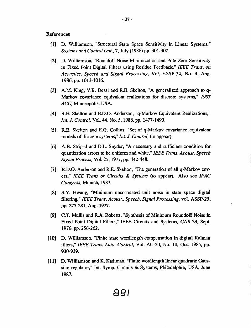
References

1 D. Williamson, "Structural State Space Sensitivity in Linear Systems," System and Control Lett., 7, July (1986) pp. 301-307.

[2] D. Williamson, "Roundoff Noise Minimization ant1 Pole-Zero Sensitivity in Fixed Point Digital Filters using Residue Feedl)ack," IEEE Trans. on Acoustics, Speech and Signal Processing, Vol. ASSP-34, No. 4, Aug. 1986, pp. 1013-1016.

[3] A.M. King, V.B. Desai and R.E. Skelton, "A generalized approach to q- Markov covariance equivalent realizations for discrete systems," I987 ACC, Minneapolis, USA.

[4] R.E. Skelton and B.D.O. Anderson, "q-Markov Equivalent Realizations," Int. J. Control, Vol. 44, No. 5, 1986, pp. 1477-1490,

[5] R.E. Skelton and E.G. Collins, "Set of q-Markov covariance equivalent models of discrete systems," Int. J. Control, (to appear).

[6] A.B. Stripad and D.L. Snyder, "A necessary and sufficient condition for quantization errors to be uniform and white," IEEE Trans. Acoust. Speech Signal Process, Vol. 25, 1977, pp. 442-448.

[7] B.D.O. Anderson and R.E. Skelton, "The generation of all q-Markov covers," IEEE Trans or Circuits & Systems (to appear). Also see IFAC Congress, Munich, 1987.

[8] S.Y. Hwang, "Minimum uncorrelated unit noise in state space digital filtering," IEEE Trans. Acoust., Speech, Signal Proressing, vol. ASSP-25, pp. 273-281, Aug. 1977.

[9] C.T. Mullis and R.A. Roberts, "Synthesis of Minimum Roundoff Noise in Fixed Point Digital Filters," IEEE Circuits and Systems, CAS-23, Sept. 1976, pp. 256-262.

[lo] D. Williamson, "Finite state wordlength compensation in digital Kalman filters," IEEE Trans. Auto. Control, Vol. AC-30, No. 10, Oct. 1985, pp. 930-939.

[l 11 D. Williamson and K. Kadiman, "Finite wordlength linear quadratic Gaus- sian regulator," Int. Symp. Circuits & Systems, Philadelphia, USA, June 1987.

INPUT-OUTPUT ORIENTED COMPUTATION AU;;Ow:THWS FOR THE CONTROL OF LARGE STRUClliJRES

K. D. Mint0 GE Corporate Research and Development Cente r

Schenectady. New York

ABSTRACT

This presentation will overview work in progress aimed at developilng computational algorithms addressing two important aspects in the control of large: flexible space sln~clures; namely. the selection and placement of sensors and actuators. and the resulting multivariable control law design problem.

' n ~ e issue of sensor/acluator set selection Is particularly crucial to obtalnlng a satisfactory control design. a s clearly a poor choice will inherently llrnit the degree to which "good" control can be achieved. Moreover. it is becoming inareasingly clear that systematlc methods are required for determining prior to the contrhl law design phase whether a parllcular candidate sensor/actuator set will yleld accepltable closed-loop perfomlance, irrespective of the particular control system design methodology used.

With regard to control law design we are driven by concerns stemmlng from the practical issues associated with eventual implementation of multtl,rariable control laws. such as reliabillty. limlt protection, multimode operation. saimpling rate selection. processor throughput. elc. Naturally. the burden imposecl by dealing with these aspects of the problem can be reduced by ensuring that the cotnplexity of the con~pensator is mlnimljrxd.

Our approach to lhese problems is based on extensions to input/outtput oriented techniques that have proven useful in the deslgn of multivariable c13ntrol systems for alrcraft engines. In parlicular. we are exploring the use of relative #ain analysis and the condition number as a means of quantifying the process of senslor/actuator selection and placement for shape control of a large space platform. Complementing ttrls activity is the development of a new multivariable design appra~ach that allows the designer to precisely control the complexity of the resulting compensator. The technique incorporates input-output performance criteria such as the popular singular- value loop-shaping approach. yet without resorting to hlgh-order compensators Inherent to observer-based design approaches.

@ Corporate R & D Center, Schenectady, NY, 12301

IN PUT/OUTPUT ORIENTED COMPIJTATIONAL ALGORITHMS FOR THE CONTROL OF

LARGE FLEXIBLE STRUCTURES

K. Dean Minto Control Systems Laboatory, GE - CRD KWD - 207, Schenectady, NY, 1:2301

(51 8) 387 - 6760

Ted F. Knaak GE - Astro-Space Division

Building 100, U4248 King of Prussia, PA, 19406

(21 5) 354 - 3672

NASA Workshop on Computational Aspects in the Control of Flexible Systems

WilliamsburgJ VA July, 1988

885

PRECEDING PAGE BLANK NOT FlLMED

OUTLINE

Motivation for research

Approach

design philosophy

focus: shape control

Results

preliminary experiences with key aspect of design problem: SIA set selection

1 kdm - 7B8 I

Motivation

control of flexible structures recognized as a key emerging technology for GE

e leverage considerable design experience with MlMO design process for medium complexity problems (aircraft engines) to high complexity systems (LFSS, IFPSC)

a particularly important unresolvo?d issue: decoupling the process of senjsorlactuator selection from control law design phase

GOALS:

- Quantitative, systematic approach to problem of decoupling S/A selectlion from control law design process

- Complexity reductionlmanagement

- Design process

- Final product

kdm - 7/88

Complexity clearly a major issue ...

(1) countably infinite number of S/A sets

~ - number

- placement

- types, etc.

(2) large dynamic-order models (many flex. modes) I

1

- order reduction a critical step, due primarily to limitations in traditional control law design approaches ( observer-based compensators imply

high-order)

- model accuracylfidelity often sacrificied to accomodate these inherent computational limitations (spillover effects, etc.)

- conflict with S/A selection process, where numerical behaviour improves with model dynamic order

(3) Shape Control - very large I10 dimensionality

I ~ kdm - 7/88

Apptvach

- traditional F.E.M. IMIMO design aptproach, based on the following cycle

Modeling I Focus:

I Implementation I - MIMO design w/ fixed order comDensators

(1) Control Structure Design

(3) Uncertainty Modeling

Control Structure Design

(4) Computations

- SIA placement

- Frequency-domain control-law dlesign

- Stable Factorization (balancing, order reduction)

- selectilon, pairing

- demonstrate via shape control problem for LFSS

kdm - 7/88 889

Control Law Design (2) Control 1 . a ~ Design

Control Structure Design:

" That portion of the control system design process which deals with the selection and pairing of measurement and manipulation variables f #

- S.O.A.: typically Ad - hoc, often arbitrarily chosen

much iteration, involving control law design phase

- probably the most critical step in entire design process (certainly true for shape control via MlMO techniques ... )

/ I ) SensorlActuator Selection

- how many? - locations? - types* (* ignor for the present ... )

colocated VS. non-colocated

x = sensor 0 = actuator

- systematic search for candidates that guarantee "good" closed-loop control

1 kdrn - 7/88

(2) Pairinas and Decentralization

- given a SIA set, how do we interconnect for minimal closed-loop interaction?

- assume standard unity-feedback configuration

Decentralization: Choose C as followsi ...

I10 Pairing:

VS.

X X X X X X X X X X X X



Example:

Colocated, fully dlecentralized:

ui <--> ei, for all i.

kdm - 7/88

11) SIA Selection

High level algorithm ...

- determine a large number of candidate sensorlactuator sets

- reduce to a manageable number of acceptable control structures (design - by - analysis)

Specifics ... - develop a necessary condition for assessing

a candidate control structure based on stability robustness

- uncertainty characterization: modified additive perturbations ...

- connect control structure design process with stability robustness via following accepted fact: " plants with low condition number are 'easy'

to control ... 11

- base selection process on condition number

1 kdm - 7/88

- we have the following result ...

Theorem: If C stabilizes P, tthen necessarily

K(P) < 8' - = 5 , for o<o,

0 ( PC(I + PC j1 ) - - assumes "perfect" control at DC ...

Selection Process:

- compute condition number of candidate structures at DC

- discard those with large condition number ...

Computational Aspects:

- RGA (relative gain array) yields lower bounds on condition number, hence! a necessary condition for viable control structures

- computational burden of RGA calculation small, but problem with elxponential growth in complexity required to examine all possible combinations

- Example: > 3 x 10D10 ways to choose a 12 x 12 control structure from a set of 20 possible I10 pairs

kdm - 7/88

Heuristic Solution:

- direct selection of inputs/outputs to minimize condition number

- based on SVD of plant DC-gain.

- reduce condition number <-> (i) reduce max. sv

(ii) increase min. sv

- DC gain: G(0) = D + C (-A)-'%

- introduce notion of inputloutput coupling operators ...

kdm - 7/88

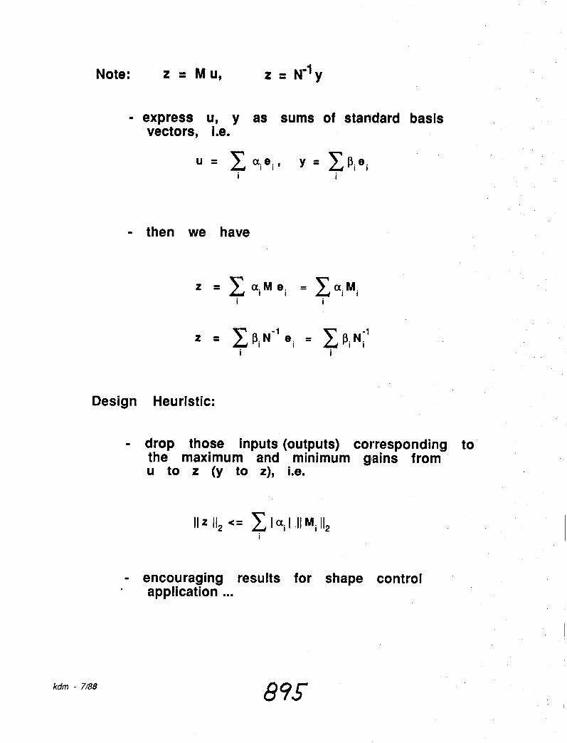
Note: z = MU, z = N" y

- express u, y as sums of standard basis vectors, i.e.

- then we have

Design Heuristic:

- drop those inputs (outputs) corresponding to the maximum and minimum gains from u to z (y to z), i.e.

- encouraging results for shape control application ...

kdm - 7/88

Coupling Operators: 20 x 20 110, 25 flexible modes

INPUT COUPLING OPERATOR OUTPUT COUPLING OPERATOR

SIA selection: Condition number vs. 110 dimension

1 *lo6 R1: 1/0 - CONDITION NUMBER ANALYSIS

I 1/0 DIMENSIONALITY I

kdm - 7/88

I l l 1

C I

0 3 1 ,-

N 4

D I T

0 5 10 15 2 0 25

I 0 N

" 1 N U M

'1 B E R 1 4 -

- 0 I l l 1 I I I I I I I I

- 1 1 1 1

n n

Some Observations :

- systems characterized by large condition numbers (in general), and relatively large uncertainty

- extremely difficult to control

- severe performance limitations

- tendency towards partially calocated feedback structures (as a result of S'A selection process)

- lower condition numbers with non-colocated, and in particular, non-square control structures ( non-square systems a challenge for MlMO

control law design )

- numerical conditioning improvr?~ (generically) with increasing information content

RGA: G(O) = c ( -A) -1~

Generically fulir-rank ... kdm - 7/88

1 (21 PairinaslCross-feed Dearadation

Tools:

- RGA, BRG (Bristol, Arkun, Maniousiouthakis)

Usage:

- Assess interactions between various feedback blocks

- Account for cross-feed degradation due to use of decentralized control structure

Preliminary result: 12 x 12 system of previous example ...

actuators sensors 1 kdm - 7/88

Control Law Design

- loop-shaping design philosophy

- account for practical implemelltation constraints

- fault-tolerance and reliability

- limit-protection and multimode operation

- digital control aspects

All severely impacted by culmplexity of compensator!

- 2 - stage design procedure allulwing explicit constraints on compensator complexity

1 st Staae: "Ideal" Compensator co~nputation

- model-match ing performance specification (sv loop-shaping basis)

- controller parameterization (IMIC, SF)

- identify constraints on achieva~ble performance ( inner-outer factorization)

- compute "ideal" compensator, i.e. K* such that

11 - HD 112 =

kdm - 7/88

2nd S t a a "Low-order" Compensator Computation

- analysis of "ideal" compensator (frequency response) to determine (i) approx. required complexity (dynamic order)

(ii) values of compensator denominator terms, initial values of numerator terms

- parametric optimization to adjust compensator numerator terms (least-square approach) to minimize

Features:

- NOT an open-loop order-reduction procedure

- Closed-loop low (fixed) order design procedure, with a flavour of order reduction (Ideal comp. => lower-order parametric design)

- Frequency-domain oriented design, hence complexity proportional to 110 dimension, NOT state dimension

- Reduced emphasis/reliance on explicit order- reduction

kdm - 7/88

Balancina & Order Reduction ISFPACUJ

- balancing a popular method for model/controller order reduction

- also useful for avoiding large coefficients in state-space manipulations

Problems: Unstable or marginally staible systems

- decomposition solution: G = 01, + 0.

- balance, reduce components, tgecombine

- Stable Factorization approach:

G = N D", N, D stable, right-coprime

Form a composite system F, with state-space realization ...

( as star ble as we wish ... )

& = fi b" - a reduced-order model of G

kdm - 7/88

THE ACTLVE FLEXIBtE WING A E R O S E N f l V O ~ C -TUNNEL TEST PROGRAJU

Thomas No11 and Boyd Pen). NASA Langley Research Center

Hampton. Virginia

ABSTRACT

The evolution of advanced. high performance aircrafl Is reqluirlng that the engineering dlsclplines of aerodynamlcs. controls, and structures be indegrated into a unined aeroservoelastic technology. To provide for technology malturation. sophisticated analysis and design methodologles must be developed and Qerified through data correlation with experimental results. The most economicdl means of obtaining test data that includes the eflects of these three disciplines without actually conducting full-scale flight tests is through the use of flexible wind-tunnel modell, scaled for aeroelastic phenomena. For a speciflc application of aeroservoelastic technology. Rockwell International Corporation developed a concept known a s th e Active Flexlble Wing (AFW). The concept Incorporates multiple active leading- and trailllng-edge control surfaces with a very flexible wing such that wing shape is varied in an oplimum manner resulting in improved performance and reduced weight. A s a result of a cooperative program between the AFWAL's Flight Dynamlcs Laboratory. Rockwell. and NASA LaRC a scaled aeroelastic wind-tunnel model of an advanced flghter was designed. fabricated. and tested in the NASA LaRC Transonic Dynamics Tunnel ("IDTI to validate the AFW concept. Besides contiucting the wind-tunnel tests NASA provided a design crf an Active Roll Control (ARC) System that was implemented and evaluated during the tests. The ARC system used a cor~cept referred to as Control Law Parameterization which involves maintaining constant performance. robustness. and stability while uswg difftrent combinations of nlultiple control surface displacements. Since the ARC systc:m used measured control surface stablllly derivatives during the design. the predicted performance and stability results correlated very well with test measurements.

The wind-tunnel model described above serves as the basis of a follow-on program to validate LaRC's and Rockwell's aeroservoelastic analysis nlethodology and multifunction digital control law design capability. This program provldels an excellent opportunlty for NASA and Rockwell to obtain an experimental database for the subsonic. transonic. and low supersonic speed regimes on an advanced aircrall configuration and to obtain cxperlence with digital control systems and simulation me d hods. Signillcant activities to be conducted by NASA LaRC during the next 2 to 3 yeam to sl~pport the program include: (1) the design of multifunction digital control laws for flutter si~ppression and rolling maneuver load alleviation acting singularly and simultaneolusly: (2) the design and fabrication of a digital controller and the implementation alnd coding of advanced control laws: (3) a "hot bench simulation of a flexible model with ullsteady aerodynamics to verlfy the functlonallty of the digital controller; and (4) groulnd vibration, control system functional. and wlnd-tunnel tests on a model with violent fltltter characteristics. Besides providing a multimillion dollar aeroelastic model for the program, Rockwell will design

903 PREOCDING PAOE BLANK NOT FILMED

and fabrkate a wing "tlp misslle" capable of elther inducing flutter within the TDT performance envelope or prevenllng flutter through a decoupler mechanism. assist in the development of the advanced dlgltal control laws. and participate during the testlng and cvaluallon phases.

Some results from the two previous wlnd-tunnel entrles whlch describe the ARC system and the Conlrol Law ParameterlzaUon concepl will be presented durfnR the workshop to cslabllsh the background for the more advanced studies now being pursued. In addition. a slatus reporl on the follow-on cooperallve program will be discussed covtrlng all facets of the elrort.

THE ACIWE FLEXIBLE WING AEROSERVOELASTIC WDID TUNNEL TEST PROGRAM A STATUS REPORT

1

Thomas No11 and Boyd Peny 111 Aeroservoelasticity Branch

NASA Langley Research Center Hampton, Virginia

Workshop on Computational Aspects .n the Control of Flexible Systems

Williamsburg, Virginia July 12-14, 1988

THE ACTIVE FLEXIBLE WING AEROSERVOELASTIC WIND TUNNEL TEST PROGRAM

A STATUS REPORT

Thomas E. Noll and Boyd Perry Ill

Aeroservoelasticity Branch NASA Langley Research Center

Workshop on Computational Aspects in the Control of Flexible Systems July 12-1 4, 1988

Williamsburg, Virginia

THE ACTIVE FLEXIBLE WING AEROSERVOELASTIC WIND TUNNEL TEST PROGRAM

The Active Flexible Wing (AFW) AeroServoElastic (ASE) Wind Tunnel Test Program is a recently-initiated cooperative effort between the NASA LaRC and the Rockwell International Corporation. The objective of this effort is to develop the analysis, design and test methodologies required to apply Active Controls Technology (ACT) for contrailling and exploiting the aeroelastic characteristics of a flexible aircraft to improve performance. Th~e approach selected to accomplish the program objectives includes the demonstration of various ACT concepts on a flexible full-span wind tunnel model, and the testing of the model to obtain an experimental data base for validating the analysis and design methodologies associated with ACT. ?'his effort is being directed by the Aeroservoelasticity Branch of the Structural Dynamics Divisior~ at LaRC.

OUTLINE

I. Program Objectives

II. Background

Ill. Current ProgramIDescription of Tasks

Controller Development

Design of Tip Missile Concept

Development of EOM

Synthesis of RMLA and FSS Control Laws

"Hot Bench" Simulation

Wind Tunnel Model Testing

V. Concluding Remarks

OUTLINE

This chart shows an outline of the topics to be discussed. Since thi: effort has only recently begun, today's presentation is a status report on where we arc today. I will begin by reviewing the objectives of the program to scope the tasks involved. I will then describe some of the NASA analysis and test results obtained during a previous AFW wind tunale1 test program between the Air Force Flight Dynamics Laboratory, the Rockwell International Coaporation and the LaRC. This portion of the presentation will demonstrate the requirement to go beyond what had been accomplished, pushing the state-of-the-art into more challenging an~d rewarding areas for ACT application. Next, a few charts describing each of the major tasks associated with this program will be discussed along with the progress and milestones recently accomplished. Finally, some concluding remarks and projections will end the presentation.

mu

-

%<

c.

2

ccc

0 'Z

'5 E

--

W

an

n

o0

%

-0

z )r 0

+-

-

V)

O

0

z I-

r

om

a

a ) .r

+as

L-1

,o -

0

- 2

V)-a

,

C -

Sog

so ..

- 'u

.- W

ac

-003

2 3 3 z

4 a ca

- c. = r -2

-0

+

u

cd -;=

E ,

o g

3

L-

V)

W

$j

C

u

C

0

$00

r a>

0 .- u

- .- >

.cn >

2 % 2

n

an

,

OR

IGIN

AL PA

GE

BLA

CK

AN

D W

Hl TE

Pt-fO

TOG

RA

PH

DEMONSTRATION AND VALIDAT [ON OF ACTIVE AEROELASTIC CONTROL TECHNOLOGY

The objective of this effort is to demonstrate the potential of using multifunction active control laws for controlling or exploiting aeroelastic response to improve aircraft performance. In addition, it gives NASA an opportunity to obtain an experimental data base on a flexible high performance advanced fighter configuration for validating analysis and design cd:s, to develop simulation techniques that include structural flexibility and unsteady aerodynamics, and to gain experience with digital control law implementation procedures. The NASA LaRC team consists of about twelve researchers from three different directorates (Structures, Flighl: Systems and Electronics). The team as a whole has the multidisciplinary experience required to perform the tasks identified for the AFW Aeroservoelasticity Program. The team will be required to design and fabricate the digital controller, design multifunctional control laws and code the controller, perform simulation studies to verify controller operation and conduct all model ground and wind tunnel tests. Rockwell through a Memorandum of Agreement and a separate suppa,rt contract will provide the wind tunnel model for use during the program, assist in the developm~znt of the active control laws and participate during the wind tunnel tests. This cooperative effort provides an excellent opportunity to directly transfer technology to the aerospace industry.

ORlGlNAL PAGE BLACK AND WHITE PiiGTC31GTiAPH

ACTIVE FLEXIBLE WING WIND TUNNEL MODEL MOUNTED IN THE 16-FOOT TRANSONIC DYNAMICS TlJNNEL

In mid 1985 the Air Force Flight Dynamics Laboratory in cooperatiou with the NASA LaRC awarded a research contract to Rockwell International to test advancedi control concepts on an aeroelastically scaled full-span wind tunnel model representative of ar advanced fighter configuration. The model, shown in the photo mounted in the LaRC 16-Foot Transonic Dynamics Tunnel, was designed and fabricated by Rockwell using company fumids. To give some perspective to the photo, the wing span from tip-to-tip is about 9 feet. The model consists of a rigid fuselage with scaled inertia characteristics and flexible wings. The wing box contains an aluminum honeycomb core and aeroelastically tailored plies of graphite epoxy. Each wing has two leading edge and two trailing edge control surfaces powered by rotary vane electrohydraulic actuators. The control surfaces have a chord and span of 25 percent of the local chord and 28 percent of the wing semispan, respectively. They can receive constant signals remotely or time varying signals from a computer for active control investigations. Deiflection limits are imposed on the various control surfaces to avoid exceeding hinge moment and wing load limitations. The model has the capability to roll about the sting axis or can be held fixeid at any roll angle using a roll brake assembly mounted in the sting. In addition, the model can be tc:sted at various pitch angles remotely controlled by an actuator located in the sting. All actuators ;re powered by an onboard hydraulic system.

ORIGINAL PAGE BLACK AND WHITE PHOTOGRAPH

INTERNAL DETAIL OF THE AFW MlODEL

This chart shows the wind tunnel model with some of the fuselage and wing panels removed to expose the complex internal detail required for ASE investigations. ?'he outboard trailing edge control surface is driven by one actuator while the other three are driven by two each. Therefore, the control surfaces are powered by 14 actuators all supplied by onboard hydraulics. Eleven accelerometers ( five on each wing and one on the fuselage) can be used as sensors for active control systems or for monitoring model response during testing. In addition, the model has sixteen strain gages, nine rotary variable differential transformers (RVDT) to indicate control surface and pitch actuator position, a roll rate gyroscope and 141 stalic pressure taps on the upper and lower surfaces of the left hand wing along five spanwise stations. A six-degree of freedom force and moment balance is also present.

ACTIVE FLEXIBLE WING WIND TUNNEL TEST PROGRAM

The AFW concept integrates active controls techno lo^ with a ilcxlblc ~tructure b wing leading n i and trailing edge control surfaces to deform the wing in an optimum manner to e ance

aerodynamic performance and contra1 . Two wind tunnel testrr were viously conducted to validate the AFW concept The purpose of the fmt test (March and X" pril, 1986) was to measure static aeroelastic and flexibliztd stabrlity derivative data as model ant&-of-attack and control surface deflections were varied, Some typical c o m p ~ n s between an cxpcrimentally determined stability derivative and the predicted (uncomctcd analysis) value a, a function of dynamic pressure is shown in the upper right hand comer of the figure. The comctcd analysis results were determined by using two ee arate "correction factors" in the analysii~, The fust factor was used to match the expected rigid v a! ue of the stability derivative (extragolatbn of the experimental data to the zero dynamic pressum value), The second factor, which vaticd with dynamic pressure (flexibility effect), was used to match the experimental values of the ntability derivative with +

dynamic pressure and to match the reversal conditions for each appro tc control surface. Theae factors were then employed dwing the &sign of the active roll contdo P" law which was evaluated during the 2nd test period. The predicted performance for the roll ctmtrol law &aim i s shown in the lower right portlon of the figure. For both flight cditiona analj,zcd, the predicted performance exceeded the goals established. In addition to these tests, the model was flutter tested for safety considerations across the planned flight envelop even though the model was desi8nc.d to be flutter free.

AEROSERVOELASTIC ANALYSES VALIDATED BY WIND TUNNEL TESTS

The 2nd wind tunnel test period was conducted during February and March, 1987 to evaluate Active Roll Control (ARC), Maneuver Load Control and Structural Made Control Systems developed by Rockwell under Air Force sponsorship. In addition, an riRC system designed by NASA using the aerodynamic corrections factors discussed previously md a "parameterization" procedure was evaluated in the tunnel. This "parameterization" procediire allowed the designer the flexibility of maintaining a fixed closed loop stability and a fmed closed loop roll performance while using different commanded control surface deflections for the active surfaces involved. The consequence of this concept is that the deflections of one pair of contro I surfaces can be traded-off against the deflections another pair with no loss or gain in aircraft stabi ity or system performance. This idea becomes very important when control surfaces are required to undertake multiple active control functions simultaneously. The chart shows some of the NASA ARC system test results obtained. The lower right hand figure presents a sampling of data to demonstrate the principle of the concept and illustrates the excellent correlation obtained between ths: test and the calculated data. The figure shows that by changing one control law parameter, stability and performance are maintained while different amounts of leading edge and trailing edge cclntrol surface deflections are used.

AFW SCHEDULE FOR FIRST WIND-TUNNEL TEST

Two wind tunnel test entries are planned for the current program; the 1:;t entry is scheduled for April, 1989 and the 2nd test, one year later. During the 1st entry active flutter suppression and rolling maneuver load alleviation systems will be demonstrated separata:ly. A schedule showing the major activities prior to the 1st wind tunnel entry is presented on thc: chart These multidiscipline activities include: 1) the model digital controller design, acquisition/fabrication, checkout and software coding; 2) the design and fabrication of a wing t ~ p missile device to cause flutter within the flight envelope of the model and to act as a flutter-stopper for safety purposes; 3) the development of the aeroelastic equations of motion for six different model structural conditions; 4) the synthesis of the RMLA and the FSS active control laws; 5) the "hot bench" simulation of the digital controller and associated software; and 6) the appropriate ground testing of the model to define its structural and dynamic zero-airspeed characteristics. Each of these activities will be discussed separately in the following figures. Although the details invc~lving the 2nd wind tunnel entry will not be discussed here, the goal is to demonstrate active flutte- suppression while the model is undergoing rolling maneuvers and alleviating wing loads.

AFW CONTROL LAW DEVELOPhIENT SYSTEM

The control law development system for the AFW wind tunnel model includes a Sun 31160M and a Sun 3/50M workstation, a 141 megabyte hard disk with a 60 megabyte tape backup and a Apple Laserwriter for printer output The workstations, driven by the Unir. operating system, are connected h u g h a Ethernet line. This network provides an excellerlt environment for several people to develop software and implement control laws independently. The Sun 3/50M is only used cisring the con 01. law development, implementation and coding, phases of the program. To f cx'ecute the control awsae Sun 31160M workstation requires a SKY Challenger processor board and a SKY Warrior processor board to be attached to the VME bus. 'The SKY Challenger is a VME digital signal processor board that is required to perform the sclteduling and interfacing of the control law to the AFW model during simulation and testing phases. The SKY Warrior is a VME array processor board which can be used by either the Sun or the Chzllenger for performing high speed floating point arithmetic. In addition, two DT 1401 (VME Dati Translation Cards) each of which has 32 analog-to-digital converters (ADC) and 2 digital-to-analog converters (DAC), and two DT 1406 each of which has 8 DAC are required to interface the illcoming and outgoing model signals. These four boards provide 64 ADC and 20 DAC for use by the control program. A 282 megabyte SCSI is also attached to the bus for the storage of data.

AFW MODEL DIGITAL CONTROLLER

AFW Wind Tunnel Model AFW Hot Bench Sim (Cyber 175)

Discrete Raalea

Warr ior m

AFW MODEL DIGITAL CONTROLLER

This chart contains a schematic drawing of the "interface box" and the A F N Control and Development System the comprise the model digital controller. The interface box processes the signals coming from or going to either the wind tunnel model or the "hot bench" simulation through low-pass filters, anti-aliasing filters and electrical isolation networks. The purpose of the low-pass filters is to reduce the high frequency noise and to limit voltage sipikes that might appear on any of the 64 analog input lines. Currently, a 4th order Butterworth filter with a cutoff frequency of 100 Hz is planned to be used during the wind tunnel tests fot the anti-aliasing filters. To be compatible with the "hot bench" simulation computers, the cutoff fri:quency of the antialiasing filters will require time scaling. The 16 analog signals returning to the model or to the simulation computer will also be filtered to prevent sharp edge transitions from being sent to the actuators. The Development System consists of several components linkad to the Sun Workstation. The SKY Challenger is required to command the SKY Wanrior, control the management of the data acquisition system (reads the ADC and writes to the DAC), monitor and update the User Control Panel, check limits and act as the system timekeeper. As described on the previous chart the SKY Warrior performs the required high speed floating point arithmetic.

AFW FLUTTER BOUNDARY MODIFIED BY THE ADDITION OF A WING TIP MISSILE

Goal: Demonstrate Significant Increase in Flutter Dynamic Pressure Using Digital Active Flutter Suppression System

Problem: Basic AFW Flutter Boundary is Beyond the TDT Tunnel Limits

Solution: Add Wing Tip Missile to Lower Flutter Boundary

Benefit:

Dynamic Pressure (psf)

Tip Missile Designed to be a Flutter Stopper for Safety

FLUTTER BOUNDARIES

,0° 1 Antisymmetric, With Tip Missile

i ------ Symmetric, With 200 Tip Missile

0 I I I 1 0.7 0.8 0.9 1 .O

Mach Number

AFW Wing

/ / Decoupler - /- Mechanism - -

n u

AFW FLUTTER BOUNDARY MODIFIl3D BY THE ADDITION OF A WING TIP MI?;SILE

Since active flutter suppression is one of the concepts being investigated during the present program, it is necessary to modlfy the model so that it will have a flutter instability within the operational capabilities of the TDT. In addition, this flutter instability wust occur at sufficiently low dynamic pressures such that flutter suppression may be demonstrattd experimentally. Several options were considered for lowering the flutter speed of the wind tuma:l model; the option most attractive was to add a wing tip missile. The tip missile significantly increases the wing pitch inertia while only slightly changing the wing total mass. This in effect decreases the zero-airspeed 1st wing torsion and 1st bending mode frequencies, and brings the two frequencies closer together. Because of the aerodynamic/structuraYinertia interaction, the two modes wilt coalesce and cause flutter at a significantly lower dynamic pressure than without the tip missile present. The lower left figure on the chart shows typical flutter boundary calculations for the model with and without the tip missile present. Because of the close proximity of a symmetric and an antisymmetric flutter boundary, the active flutter suppression system must be capable of preventing both flutter modes simultaneously if the concept is to be effective. An added benefit of using a tip missile for causing flutter is its ability, with a little ingenuity, of returning the model to a flutter-free and, thus safe condition. This is accomplished by &coupling the rnissi1.e dynamics from the wing by the use of a soft pitch spring at the wingtmissile interface. The decoripling mechanism could be two pins, one stiff and one soft, as shown in the figure to the right. With the two pins installed the model would be flutter critical; with the stiff pin retracted, the wing is d~:coupled from the missile and becomes flutter free.

EQUATIONS OF MOTION

One approach to formulating the equations of motion of an elastic aircraft is based on a chosen set of vehicle vibration modes and the Lagrange energy equation. Considering only small perturbations from a level equilibrium flight condition, the aircraft can be represented by a set of linear equations expressed in terms of the generalized coordinates, q6t). An example of such an equation is provided at the top of the slide. This equation represents a summation of forces and includes the inertial, the dissipation and the internal restoring forces, and the aerodynamic forces caused by the aircraft's rigid body, control surface and flexible motions and caused by gusts. To determine the aeroelastic characteristics of the vehicle, these equations are classically transformed into the frequency domain so that state-of-the-art unsteady aerodynamic theories based on simple harmonic motion can be used. These unsteady aerodynamic generali~zed force coefficients are transcendental tabular functions of several parameters, including frealuency. Analyses in the frequency domain are straight forward using common methods. To lxrform aeroelastic analyses and design studies that include the effects of active feedback control systems, the equations of motion are transformed into the Laplace domain. The transformation1 of these equations into the Laplace domain is complicated by the transcendental functions of the generalized forces. The use of rational functions to approximate the generalized forces provides one solution to this problem. Several procedures are available for determining the rational function approximations. The equation shown on the slide is one of the more common forms. Her~e, a least square fit of the aerodynamic data is performed to determine the coefficients of the pc~lynomial for each element of the frequency dependent generalized force matrices. Once the transfbrmed generalized forces are obtained, the equations of motion are then placed into state-space form for design investigations.

ANALYSIS FLOW

Aeroservoelastic Analysis Tools

ISAC, STABCAR, MATRIXx, etc.

I

Batch Simulation Workstation

Control Law SynthesisTools

CFSll5

ANALYSIS FLOW

This chart illustrates the major analyses performed and the flow of data slnd information between analyses. Circles represent both input to and output from the various analyses; rect'angular boxes represent analyses. The starting point, at the upper left, is a circle contaiining lumped-mass matrices and either stiffness or structural-influence-coefficient matrices. These matrices have come from a structural analysis code (not shown) and go into an eigenvalueleigenvector analysis yielding in-vacuum frequencies, mode shapes and generalized masses. These quantities then go to three other boxes, the first of which is labelled Aeroservoelastic Analysis. Within this box the open- loop (and, when control laws are available, the closed-loop) aeroelastic equations of motion are generated, various analyses are performed, and intermediate results are passed "downstream" to a Control Law Synthesis box and two Simulation boxes. When generateld, control laws are passed back up to the Aeroservoelastic Analysis box for computation of closed-loop frequency responses, closed-loop time responses, closed-loop flutter, etc. Control laws and p~rher data are also passed to the two Simulation boxes which ultimately provide a functionality check of the digital control computers and a "best" pre-test estimate of the stability and perforrnanc: of the closed-loop wind tunnel model.

SYMMETRIC FLUTTER ROOT LOClJS

Various analysis procedures can be used to obtain the aeroelastic charac:teristics of the model. This chart shows typical stability results using a root locus approach. To adequately define the flutter stability for the AFW wind tunnel model it was necessary to develop ecuations of motion for six different model representations. These included the model undergoing :symmetric motion with the tip missile attached to the wing with either the stiff spring or the soft spring as discussed previously, and the model undergoing antisymmetric motion with the tip missile attached to the wing with either the stiff spring or the soft spring with the roll brake on and off. The data shown on the plot represents the AFW model undergoing symmetric motion with the tip missile attached to the wing with a stiff spring. Mach 0.9 doublet lattice unsteady aeralynamics were used for these calculations. Velocity was held constant and the air density was varied so that a matched point solution was obtained For this analysis, the first ten vehicle elastic modes were used to define the generalized coordinates. The predicted flutter mode involves the coalescence of the 2nd and 3rd elastic modes at a dynamic pressure of 213 psf at a frequency c f 1 1.1 Hz as can be seen when the 2nd elastic mode root moves into the right half plane. The objective of the FSS is to move the unstable root back into the left hand plane of the plot

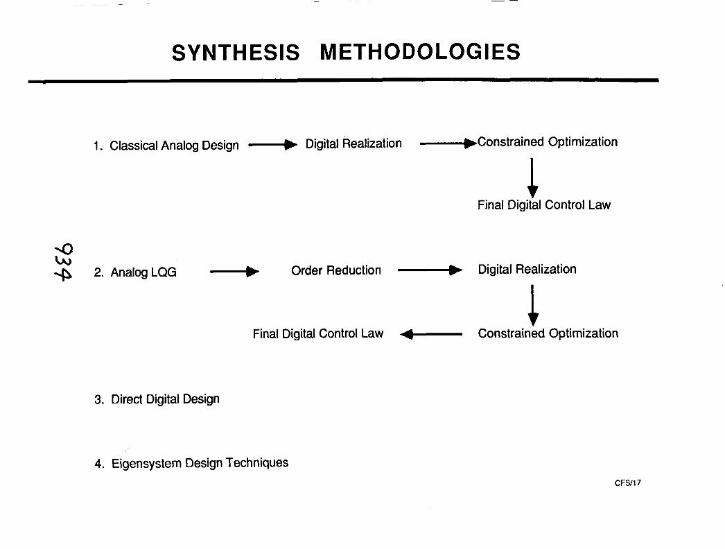
SYNTHESIS METHODOLOGIES

1. Classical Analog Design ---.) Digital Realization -----)Constrained Optimization

Final ~igit-al Control Law

\O bu + 2. Analog LQG - Order Reduction - Digital Realization

Final Digital Control Law Constrained Optimization

3. Direct Digital Design

4. Eigensystem Design Techniques

SYNTHESIS METHODOLOGIES

Several approaches that include classical analog and modem/optirnal ccntrol techniques an being evaluated for use in designing the digital active flutter suppression system. The classical techniques being considered are based on root locus, Bode (transfer fuqctions) or Nyquist plots and are useful for single-input, single-output systems. Once an analog control law which provides at least minimum stability for the a i rcdt at a certain design point is found, it is transformed into the z-domain and then optimized based on constraints such as design loads, actuator deflection and rate limits, and stability margins. The optimization task results in improved stability margins and robustness characteristics. The Linear-Quadratic-Gaussian (LQG) met ~ o d is a systematic approach for designing multi-input, multi-output control laws. The LQG methoc. is based on minimizing a cost performance index consisting of quantities such as control deflection, design loads, accelerations, etc. The control law developed using this technique, however, is the same order as the aircraft being modeled. For flexible aircraft with unsteady aerodyr~amic forces, the number of states required to represent the vehicle is usually quite large. This order problem is solved through the truncation or residulation of the Kalman Filter. As described above, the LQG reduced-order control law is transformed into the digital domain and further optirnizec to improve performance and robustness. A third approach being considered involves the direct digital design of the control law. The methodology for the direct synthesis (determination of the coefficients for the z terms) of the digital FSS uses constrained optimization, and will meet multiple design requirements if necessary while maintaining reasonable stability requirements. The las : method being evaluated is an eigensystem design technique. The method involves the placement 3f the closed loop roots to obtain a control law with satisfactory stability, performance and robust~ess characteristics.

SYSTEM OVERVIEW OF HOT BENCH SIMULATION

S U N (" .......................................

D / A Law

Interface

Wind tunnel model - 8648 ," ............................................... !

......................................................... L time scale

Hot Bench Simulation

Site Rack - 81268

\ CYBER 175

A I D . Simulation of AFW wind tunnel model

CAMAC crate

ADAGE Gen. Av. Cockpit R1.T vector graphics generation

Video link R/T Console 50 Mega-bit r

Optical Ring Network

Operator interface Displays Strip charts Data entry

CFSIl8 I ~,rrrr,rrrrrrr.rrr....~.~,,,.,..rr~,~~,,~,~,.~~.,,,...~~,,,..,~,,.,.~....~..... ~..,-.--..-...-.--......--..-...........-*..~.---....,..-.,~,..........~

SYSTEM OVERVIEW OF HOT BENCH SITdULATION

The purpose of the "hot bench" simulation is to provide a comprehen:;ive evaluation of the functionality of the Sun digital controller and the user control softwax, and to provide a low order, linear check of the flexible/dynarnic system coupled with the active control laws. It is planned that this activity will be accomplished by attaching the Sun digital controller to a Cyber 175. The Cyber represents the AFW aeroelastic equations of motion modeled to include a sufficient number of elastic modes and the unsteady aerodynamic forces needed to accuratr:ly predict the static and dynamic characteristics of the test article across its expected test envelop. The Cyber will send sensor and other model or test condition information to the Sun for p messing by the digital controller and will receive control actuator displacements from the Slm. Issues which can be investigated during the "hot bench simulation besides the user control software, and control law stability and performance evaluations include:

1) the operation of the flutter stopper, 2) actuator transfer function differences between left and riglit wings which could cause

coupling between symmetric and antisymmetric model chiuacteristics, 3) failed actuators and sensors, 4) control surface displacement and rate limits.

A schematic that demonstrates the procedure to provide the interface between the Sun digital controller with the Cyber 175 during the "hot bench" simulation or tcl the AFW model during the wind tunnel tests is shown on this chart. On a previous chart, the NASA/Rockwell Interface box was discussed. Recall that this box takes discrete and analog signals from the wind tunnel model or from the Cyber during the "hot bench" simulation studies. Became of the clock step and time step differences between the Sun and the Cyber, it will be necessary to conduct the simulation in synchronized slow time.

PRELIMINARY AFW MODEL TEST PLANS

o Ground Vibration Tests

o Control System Functional Tests

Open Loop Transfer Function Measurements

o Servoelastic Coupling tests

Closed Loop limit Cycle and Ground Resonance

Q o Wind Tunnel Tests

Measure Control Surface Stability Derivatives

Obtain Static Pressure Distributions at Selected Wing Locations

Perform Roll Maneuvers with and without Active Load Alleviation

Define Flutter Free Test Envelop for Decoupled Tip Missile

Define Passive Flutter Boundary

Demonstrate Active Flutter Suppression

PRELIMINARY AFW MODEL TEST.PLANS

The wind tunnel model will arrive at LaRC during the summer of 1988 for extensive ground testing prior to installing the model into the Transonic Dynamics Tunlie1 . Initially, the model will be ground vibration tested with the tip missile attached to the wing using both the stiff and soft spmg representations separately. Symmetric and antisymmetric elas~ic mode frequencies, mode shapes and structural damping coefficients will be obtained with the rnodel roll brake on and off. In addition, all sensor signals expected to be used by the active control laws will be measured. During these tests all actuators will be hydraulically powered. Open loop end-to-end tests will be accomplished to obtain transfer functions over a broad frequency range for all control surface/sensor combinations using several different amplitude signal!; to evaluate the nonlinear effects. The m s f e r function of selected components, such as the actuators and sensors will also be measured separately. Closed loop tests will also be accomplished for each active control law to be evaluated in the wind tunnel. These tests will include limit cycle tc:sts to measure gain and phase margins at zero airspeed, model stability evaluations following an im?ulse excitation, and ground vibration tests. The intent of these tests is to obtain measured data for. validating math models at zero airspeed (without aerodynamics). The various math models will be corrected and the control system designs updated as appropriate prior to the wind tunnel tests. Finally, the chart shows the expected wind tunnel tests and the order of conducting these tests. Routine force, moment and static pressure data will be measured first. Next the performance of t le Rolling Maneuver Load Alleviation System will be evaluated. The higher risk tests which include the passive flutter and the active flutter suppression tests for preventing a high frequency violent flutter mode will be accomplished last.

VALIDATION OF TOOLS FOR MULTIDISCIPLINARY TECHNOLOGY

MULTIDISCIPLINARY AREAS

Elasticity

1 . Aerodynamics 5. Closed-Loop Stability and Control

2. Controls 6. Servoelasticity

3. Structures 7. Aeroservoelasticity

PLANNED TESTSIVALIDATION

Static Pressure Distributions

Analog and Digital Transfer Functions

Frequencies and Mode Shapes

Control Effectiveness and Flutter

None Planned

Closed-Loop Ground Tests

"Hot Bench" SimulationIRMLA and FSS

4. Aeroelasticity

VALIDATION OF TOOLS FOR MULTIDISCIPLIE ARY TECHNOLOGY

In summary, aeroservoelasticity is a multidisciplinary technology tt at involves unsteady aerodynamics, active control systems and flexible structures. This chart illustrates the potential interactions of these three technologies with the aid of three intersecting circles to represent individual technical disciplines. ASE represents that area common :o all three circles. To adequately develop analysis and design tools for application to ASE,, it is important and critical to validate software within each area of interacting technologies. Recall, that one of the objectives of this program is to obtain test data for evaluating the usefulness and accuracy of our codes involved in the design of flexible vehicles. The approach being followed during this program is to obtain experimental data to validate each of the primary technical disciplinl:~ prior to proceeding to levels involving two interacting technologies or three (ASE for this case). In conclusion, the NASAIRockwell AFW program began in October, 1987 and will cxtinue for about three years. This presentation has been a status report that addressed:

1) why the program is being pursued, 2) where we are today, and 3) what to look forward to in the coming months.

For those interested in pursuing the progress of the program, additional status reports will be presented at various conferences and workshops during the progra n.

MODELING AM) STABILIZATION OF LARGE FLEXI19LE SPACE STATIONS

S. S. Llm and N. U. Ahmed University of Ottawa

Ottawa. CANADA

ABSTRACT

In thls paper we present a preliminary formulation of a large space structure. m e system conslsts of a (rigid) massive body. which may play l.he role of experimental modules located at the center of the space station and a fleutble connguration, consisting of several beams. which is rigidly attached to t h ~ main body. The equations that govern the motlon of the complete system consist of several partial differential equations with boundary conditions descrlblng the vibration of flexible components coupled with slx ordinary differentla1 equations that describe the rotational and translational motion of the central body.

In our investlgatlon we consider the problem of (feedback) dabflization of the system mentioned above.

'1111s study is expected to prwlde an insight into the compltxlty of design and stabllljr.ation of actual space stations. Some numerical resiilts will be presented.

Mode4'n9 of Space SJWibns V

I w l r w .Iu I

S p x c Station Bastlint i - - i ORIGINAL PAGE IS OF POOR QUALITY

I I C, Y1, 21 / 4 , 4 I I 5, '. 1 ---- - - - - - - - -- 54 - - - --rz

Z # c. R Jd bus 4 A , a s3 , %

I,, = J a t dm, - (t. dm, f t r -

S,- JR, S8, $4 (or W ) we aQ;-Cmv, 4 e &e

1 - 5 1

m-o, / v = o ;

~ ~ l . ( ~ ' , $ j l l ' - 4 1 . ( ~ r , y ' ) l 4 ~ 0

fi F 0

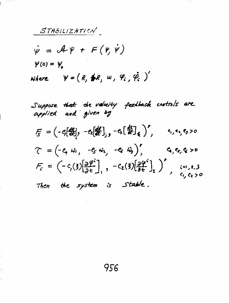
ACTIVE VIBRATION MITIGATION OF DISTRIBUTED PARAM;ETER, SMART-TYPE STRUCTURE8 USING PSEUDO-FEEDBACK OPTIAdAL CCINTROL (PFOC)

W. N. Patten. H. H. Robertshaw. D. Pierpont, R H. Wynn Virginia Polytechnic Institute and State Univc:rsity

Blacksburg, Virginla

ABSTRACT

A ncw. near-optimal feedback control technique is introduced that is shown to provide excellent vlbration attenuation for those distributed parameter systems that are often encountered in the areas of aeroservoelasticity and large space systems. The technique relies on a novel solution methodologr for the classical optimal control problem. Specifically. the quadratic regulator control problem for a flexible vibrating structure is flrst cast in a weak funcuonal form that adrnlts an appr0xhna:e solution. The necessary conditions (first-order) are then solved via a time finite-element method. The procedure produces a low dimensional. algebraic parameterlzati~n of the optimal control problem that provides a rigorous bask for a discrete controller with a first- order "like" hold output.

Slmrllation has shown that the algorithm can successfully control a wide variety of plant forms including mulli-input/multi-output systems and sy:stems exhibiting slgnlflcanl nonllnearities. In order to firmly establish the emcav of the algorithm. a laboratory control experiment was implemented to provide planar (bending) vibration attenuation of a highly flexlble beam (with a first clamped-free rnode of approximately 0.5 EIL). Base actuation for the cantilever was accomplished usiqi a three degree-of- freedom active bay (variable geometry truss) actuator. On-line pi~wessing was accomplished wilh a 14 mhz "AT' type microcomputer with data acquisition capability. The results of the tests corroborate the utility of the method.

WEAK (VARIATIONAL) FORMULATION

WHY?

TECHNIQUE FAMILIAR TO COMMUNITY

EASE OF IMPLEMENTATION

USING FINITE ELEMENT PARADIGMS AND CODES

FOR LINEAR AND NONLINEAR SYSTEMS

WHAT IS

PSEUDO

FEEDBACK CONTROL

DRIVER -IN-THE-LOOP CONTROL

(OHIO STATE --LATE 60's)

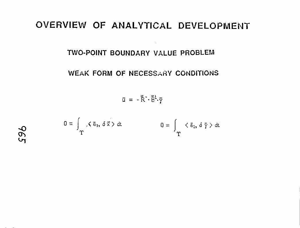
CONSTRUCT INTERPOLENTS TO APPROXIMATE

STATE, COSTATE AND CONTROL VECTORS

ON EACH OF THE SUBDOMAINS

EXAMPLE

I LINEAR SECOND ORDER OSCILLATOR (UEIDAMPED)

-------- Anal!.tical .Solution - Applied Control

--Anal3ticaI Solution -Actual Raponsc

where

LLI

OR

IGIN

AL PA

GE IS

----- . - C

~F

POO

R QU

ALrrY

1

- _ ---- -.

- .) * ./---

*,. /--

-r - - - - - . - - -

. . ..

.. .--

I:;;;! ::;.!I.+ .. --i.:: .

I=;------- I

. :-.!:.-:!x::!. !. ::

1..-

. . . - --

. . - - - - -

. .

1.

3

, ! x :.

:--. '. .!

. - - - - . -

-.

1.- .

- . ,

.

. .

- . , . .

. - -- - -. .

.

. .

BR

IGiaW

L PAG

E IS

OF PO

OR

QU

ALITY

OF PO

OR

QU

ALITY

h

a

ci P

z

' 4

-.

m 0

*"jt

m

2

0

K&

a

0-

zf

o

-0

2

Pz

a

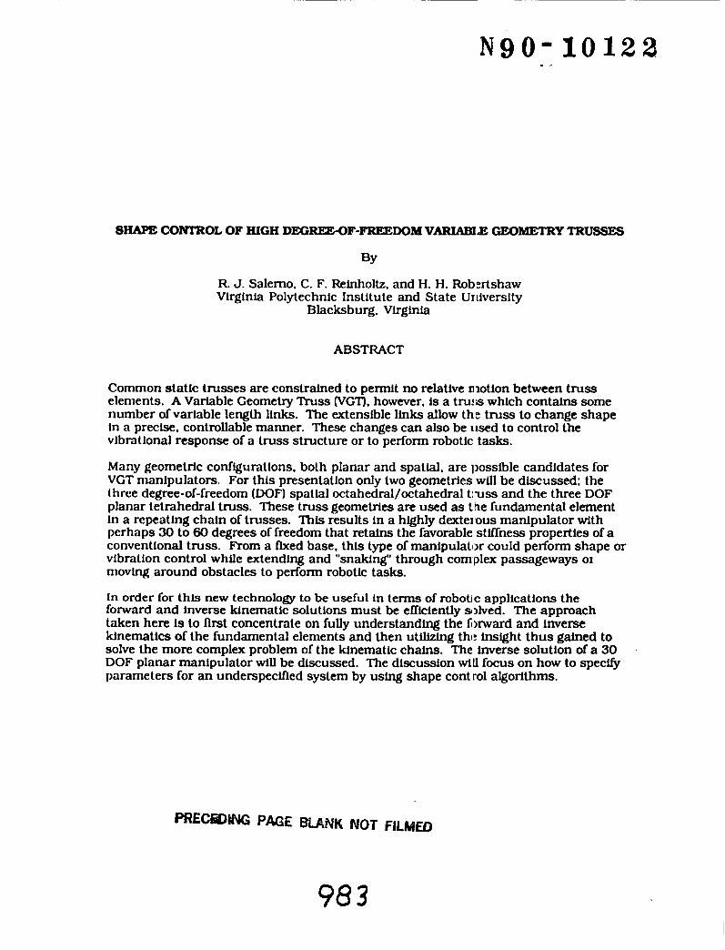
SHAPE CONTROL OF HIGH DEGREE-OF-FREEDOM VARLABlE GEOMETRY TRUSSES

R. J. Salerno. C. F. Relnholtz. and H. H. Rob~rtshaw Virginia Polytechnic Institute and State Ur~iverslty

Blacksburg. Virginia

ABSTRACT

Common static trusses are constrained to permit no relative nlotion between truss elements. A Variable Geometry Truss (VCT), however, is a truss which contains some number of variable length links. The extensible links allow the truss to change shape in a precise. controllable manner. These changes can also be used to control the vlbratlonal response of a truss structure or to perform robotic tasks.

Many Re~metr i~ conflgurations. both planar and spatlal, are ~~ossible candidates for VCT manipulators. For this presentation only two geometries will be discussed: the three degree-of-freedom (DOF) spatial octahedral/octahedral tiuss and the three DOF planar tetrahedral truss. These truss geometries are used as the fundamental element in a repeating chain of trusses. This results in a highly dextel,ous manipulator with perhaps 30 to 60 degrees of freedom that retains the favorable stiffness properties of a conventional truss. From a h e d base. this type of manipulator could perform shape or vibration control while extending and "snaking" through com plex passageways 01 nlovlng around obstacles to perform robotic tasks.

In order for thls new technology to be useful in terms of robotic applications the forward and inverse kinematic solutions must be eniciently solved. The approach taken here Is to first concentrate on fully understanding the fixward and inverse kinematics of the fundamental elements and then utilizing thl: insight thus gained to solve the more complex problem of the kinematic chains. The inverse solution of a 30 DOF planar manipulator will be discussed. The discussion wlll focus on how to spec@ parameters for an underspecifled system by using shape control algorithms.

PREcHWG PAGE BLANK NOT FlLMED

Shape Control of High

Variable Geometry Trusses

R o b e r t J - Sa l e rno

Babu Padmanabhan

C h a r l e s F - R e i n h o l t z

H a r r y H. R o b e r t s h a w

Variable Geometry

Charac te r i s t ics

Trusses

- C o m p o s e d e n t i r e l y o f

t w o f o r c ~ m e m b ~ rs

C pure tens i o n / c o m p ress i on 1

w e i g h t r a t i o

- N u m b e r o f D O F i s equal

to t h ~ nurnbe r o f

e x t e n s i b l e l inks

Two Candidate Geometries

P l anarC 2 - 0 3

T e t rahed ra I T russ

S p a t i a l ( 3 - D l

O c tahed ra l t russ

Q)+' L --

9- L

I 0

9- 4

oo

x

Curve Fitting Approach

G o a I - T o spec i f y s o m e m i n i mum

n u m b e r o f p a r a m e t e r s w h i c h

de te r m i nes the t russ shape

I n p u t o n l y the three end

p a r a m e t a r s , X , y . and T h e t a . and

have an a l go r i t h m w h i ch ass i gns

the o t h e r 27 var i ab I es i n s o m e

sys t e m a t i c m a n n e r .

- .- cam

OE

-

M --

u

Spatial Octahedral Truss

LJO Actuators

v Cross - L ongerm Members

Spatial Truss Forward Kinematics

Emp l oy the concep t o f

k i n s m a t i ca I I y aqu i va I en t dev i ces

REVOLUTE / 7 JOINT

Constraint Equations

OPTIMAL INTEGRAL CONTROLIER WITH SENSOR FAILURIL ACCOMMODATION

Dr. T. Alberts Old Dominion University

Norfolk. Virginia

and

Dr. T. Houllhan The Jonathan Corporation

Norfolk. Virginia

ABSTRACT

An Optimal Integral Controller that readily accommodates Ser.sor Failure - without rcsorllng to (Kalman) filler or obselver generation - has been designed. The system is based on Navy-sponsored research for the control of high performance aircraft.

In conjunction with a NASA developed Numerical Optirnizatior~ Code. the Integral Feedback Controller will provide optimal system response wen in the case of Incomplete state feedback. Hence. the need for costly replicaticln of plant sensors is avoided since failure accommodation is elfected by system sof .ware reconfiguration.

The control deslgn has been applied to a particularly ill-behaved, third-order system. Dominant-root design in the classical sense produced an almorit 100 percent overshoot for the thlrd-order system response. An application of the newly-developed Optimal Integral Controller--assuming all stale information available-.produces a response with NO overshoot. A further appllcation of the controller design--assuming a one- third sensor failure scenario--produced a slight overshoot response that still preserved the steady slate tlme-point of the full-state feedback response.

The control design should have wide application in space systems. The design can be expanded to Include @In scheduling that enhances system res])onse to large-scale transicnls. For thls latter instance, using the NASA optimizat Lon scheme. the guesswork normally requlred lo determine feedback gains for large transients is ellmlnated.

Optimal Integral Contrc~l

With

Sensor Failure Accommoda~tions

Dr. Thomas Alberts

Old Dominion University

Norfolk, Virginia

Dr. Thomas Houlihan

The Jonathan corpora ti or^

Norfolk, Virginia

N A S A Workshop

Flexible System Control

12 July 1988

PRECWtNG PAGE BUNK NOT FILMED

N A S A Workshop

Optimal Integral

Control Design

Introduction

Optimal Regulator

Augmented System

(Rates of Change of Input Signals)

Optimal Tracker

Optimal Integral

Control Design

Sensor Failure

Accommodation

Preliminary Results:

Third Order System

1006

July 1988

N A S A WORKSHOP

Introduction

Optimal Control Designs Compromised By:

Inaccessible States (Sensors)

Noisy Feed back Signals

OC Designs Resort To Use Of

Filter 1 Estimating Technique!,

To Overcome These Obstacle!;

NAVY Research in 1970s

Leads to Alternative Approach

JULY 1988

N A S A Workshop

Optimal Regulator - Classic Design

Tradeoffs Between Accuracy of Control

And Energy Expenditure Reflected

In Weighting Matrices (Q and R)

Of Performance lndex (J)

Performance lndex Formulation

Assumes Unconstrained Inputs.

In Reality, Inputs are Limited.

Futhermore, Rates of.Change of

Input Signals Are Limited.

July 1988

F i g u r e 1 . T y p i c a l System Response.

1009

F i g u r e 2. Comparat ive Op t ima l Responses.

l O l 0

F I SURE 3 . GPT I MAL REGULATOR SYSTEF'

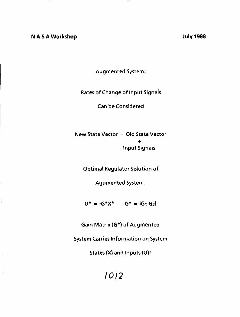
N A S A Workshop

Augmented System:

Rates of Change of lnput Signals

Can be Considered

New State Vector = Old State Vector +

lnput Signals

Optimal Regulator Solution of

Agumented System:

Gain Matrix (G*) of Augmented

System Carries Information on System

States (X) and Inputs (U)!

July 1988

FIGURE 4 . SPTIMAL REGULATOR-AUGMENTED SYS-EM

1013

N A S A Workshop July 1988

Optimal Tracker:

Add Gain Matrix (M) to

Select Command Inputs

NOTE: Tracker is NOT Integral Controller

Since Control Commands are NOT

Generated by Integral of Error

Between Desired Signals (r)

And Output Signals (z).

NOTE: Solution to Tracker Control

Configuration is KNOWN. It is

Solution of Augmented System.


Optimal Integral Control Design

Equality of Optimal Integral Control

Design and Optimal Tracker Design

Effected by Block Diagram Reduction

Techniques (Laplace Domain).

Results:

Knowns:

A, B, C, D, E - Configuration Matrices

GI, G2 - Augmented System Solution

Thus:

L and H Matrices are Determinable

- 1 I L H I = IGiG2I A B EC ED

N A S A Workshop

Sensor Failure Accommodation

Matrices:

H = Error Gain Matrix L = State Gain Matrix

If State Information Unavailable,

Corresponding Column Elements of L

Matrix Are Zeroed - Suboptimal Control! From Before

Hence, New Gain Matrix I GS I = I Gis GzS I

Can be Determined to Effect Control

Preliminary Results are Encouraging

July 1988

(1)) - Oplinml Control


Summary

Optimal Integral Control Design

Effected by a Combination of

Multivariable Control Analyses

Sensor Failure Accommodatio~~

Accomplished Without Resort to

Supplemental Filter 1 Estimator Designs

Suboptimal Control Response

Effective for Ill-Behaved,

Third-Order Test Case

Postscript to Computatior~al Aspects ... Lawrence W. Taylor, Jr. NASA Langley Research Center

What started as an effort to transcend various project and reasearch activities has become an official progi~am..Computational Controls. The following charts describes that program at this early stage in its development. The next meeting on the subjects of the Computational Aspects Workshop will be the 3rd Annual Conference on Aerospace Computational Control. The conference will be held August 128-30, 1989 at Oxnard.

PilECEDiNG PAGE BLANK NOT FYktED

Computational Controls

I OBJECTIVE 1

"To Develop the NEra GENERATION

HIGH PERFORMANCE Aerospace

It/odehhg, - Conzrul and S~~muhtlin Tooh"

/ A THREE-PART PROGRAM I

SPACECRAFT

DD 0

COMPUTATIONAL

\

AIRCRAFT CONTROLS

TRANSPORT AT ION

Contacts:

Lee Holcomb - NASA HQ Code R C

John Dibatt i s ta - NASA HQ Code R C

Guy Man - JPL

Larry Taylor - LaRC

Harry Frisch - GSC

Henry Waites - MSFC

Ken Cox - JSC

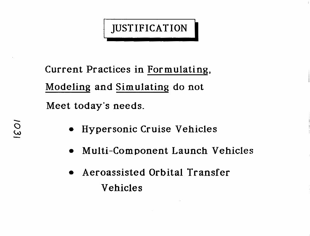
JUSTIFICATION 1

Current Practices in For mulatina.

Modeling and Simulating do not

Meet today's needs.

a Hypersonic Cruise Vehicles

Multi-Component Launch Vehicles

Aeroassisted Orbital Transfer

Vehicles

I APPROACH 1 --

c -_ Reference Problems ----- - ---> ____------a

_---- - - - _ (:Advanced --_ _ ~ormulations-7 ----* ---- -----

__---- .__--- -----__ (.Parallel --__ ~rocessin~-::::~ -- -- --- -- __-----

___--- ------- _ ____ (:user --__ Expedient Software..> --_ -- - --- - -

I \

Advanced Modeling, Analysis & Control Capability

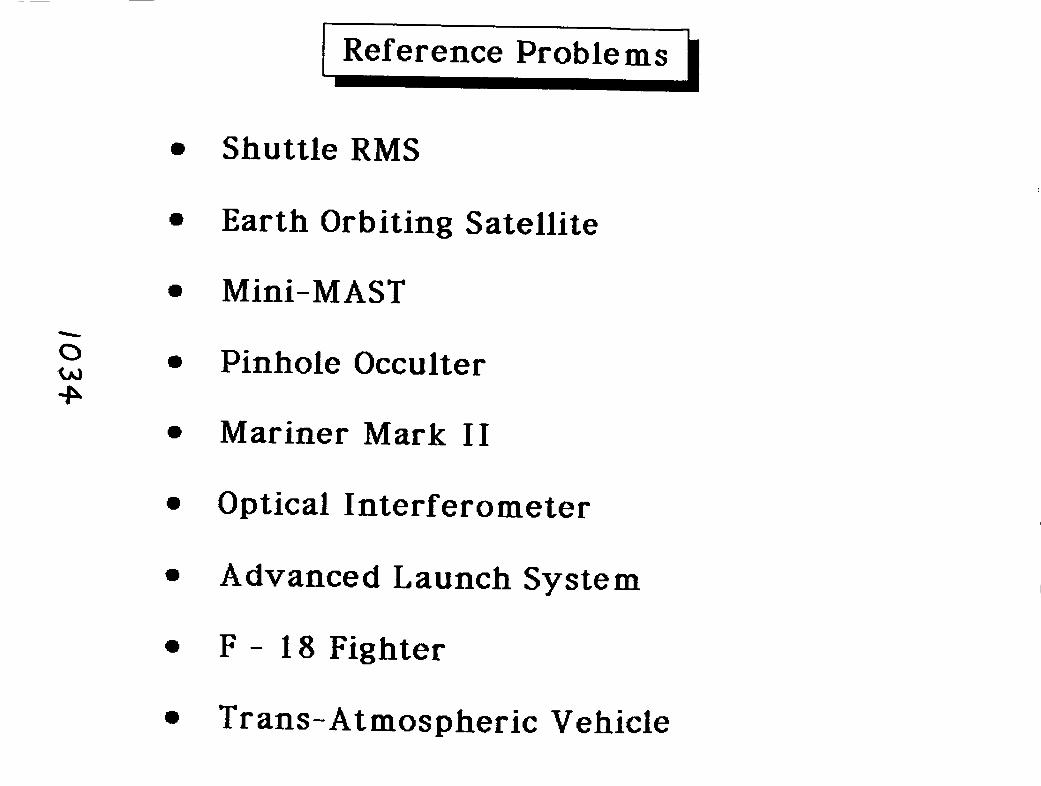
/ SOFTWARE 1 Macintosh-Like User Environment

Simultaneous Tasking

a Real-Time and Off-Line

u w Modular (Particular Methods) w

Data Base Management

r interactive Graphics

I Related Activities 1

( Integrated Design I

( Activit ies Specific

Applications

( Control Techniques 1

Computational Controls Real-Time, Flex. Simulation Efficient Computations I

PROPOSED LA RC A ERO TASKS 1 .I

DYNAMICS INTEGRATION AND ADVANCED CONTROL THEORY AND MODELING

TRANS-ATMOSPHERIC

OUT

HIGH-ORDER, HlGH FIDELITY, NONLINEAR MATHEMATICAL MODELS OF HlGH PERFORMANCE AIRCRAFT ADVANCED MODEL ORDER REDUCTION METHODS ROBUST INTEGRATED CONTROL DESIGN METHODOLOGIES

1.5 RAPID CONTROLLER IMPLEMENTATION METHODOLOGIES

AERODYNAMIC /

REACTION CONTROL SYSTEM HEATING

PROPULSION

AEROTHERMO- 4 ACTUATORS SERVOELASTIC

HIGH FIDELITY MODELING

MULTIDISCIPLINARY NL MODEL PLANT

ORDER REDUCTION

CONTROLLER MODEL REDUCTION

CONTROL DESIGN

CONTROL LAW DESIGN

, PERFORMANCE EVALUATION

IMPLEMENTATION REAL-TI ME NL MODEL

SIMULATION

ANNOUNCEMENT & CALL FOR PAPERS -

3rd Annual Conference on Aerospace Computational Control

Radisson Suite Hotel August 28-30. 1989 Oxnard, California

NASA

N S F

DoD

~ ANNOUNCEMENT of a CLASS on

a A Control System Simulation for Flexible and Articulating Structures

August 31 ,1989(After Conference)

I : 3rd Annual Conference on Aerospace Computational Control Radisson Suite Hotel, Oxnard, CA

C@)NTJEiNT: a Overview Example Problems Hands-On Experience User's Manual

C@)Sr: No Charge for Class or Materials for Registered Conferees

A S S T Larry Taylor NASA Langley

Report Documentation Page

I NASA TM-101578, Part 2 1 I ( 2. Government Accession No. ( 3. Recipient's Catalog No.

I I

4. Title and Subtitle 1 5. Report Date I

I

Proceedings of the Workshop on Computational Aspects May 1989 in the Control of Flexible Systems 6. Performing Organization Code I Lawrence W. Taylor, Jr . (Compiler)

I

9. Performing Organization Name and Address

7. Authorts)

NASA Langley Research Center Hampton, VA 23665-5225

8. Performing Organization Report No.

12. Sponsoring Agency Name and Address

National Aeronautics and Space Administration Washington, DC 20546-0001

m o r k Unit 6. !

11. Contract or Grant No.

13. Type of Repon and Period Covered

Technical Memorandum 14. Sponsoring Egency Code

This report is part 2 of two parts published as NASA TM-101578.

I

I 15. Supplementary Notes

I

17. Key Words (Suggested by Authorls)) 18. Ditribution Stat#- /,ant -- 16. Abstract

This publication is a collection of papers presented at the Workshop on Computational Aspects in the Control of Flexible Systems held at the Royce Hotel, Williamsburg, Virginia, July 12-14, 1988. The papers address the formulation, modeling, computation, software and control for flexible spacecraft, aircraft and robotic manipulators.

Large Flexible Spacecraft Control, Strucutal Dynamics

t

Unclassified-Unlimited Subject Category - 18

I 22. Price

A2 2

NASA FORM 1626 OCT 86 + U . S . C O ~ ~ ~ C O m C E : 1 9 8 9 S 2 9 - 2 9 5 1 0 0 0 2 9

21. No. of pages

505 19. Security Classif. (of this report)

Unclassifed

20. Security Classif. (of this page)

Unclassified

Documents

NASA Technical Memorandum 10 1578, Part Two