Embed Size (px)
Citation preview

N A S A C O N T R A C T O R N A S A CR-1855 R E P O R T
ICI I h
C
A MATHEMATICAL MODEL OF PHYSIOLOGICAL TEMPERATURE REGULATION IN MAN
by J, A, J, Stolwgk
Prepared by YALE UNIVERSITY SCHOOL OF MEDICINE New Haven, Conn. 06510
for
UTlCS A N D SPACE ADMINISTRATIO, YASHINGTON, D. C. AUGUST 1971
https://ntrs.nasa.gov/search.jsp?R=19710023925 2018-05-20T23:45:38+00:00Z

1. Report No. 2. Government Accession No.
NASA C R - 1 8 5 5 4. Title and Subtitle
A MATKElrlATICALp MODEL OF PHYSIOLQGICAL "F'ERATUHE IGGULATION I N [email protected]
3. Recipient's Catalog No.
5. Report Date
7. Author(sJ
J. A. J . Stolwijk
9. Performing Organization Name and Address
John B. Pierce Foundation Laboratory and Department of Epidemiology and Public Health, Yale University School of Medicine New Haven, Connecticut 06510
12. Sponsoring Agency Name and Address
National Aeronautics and Space Administration Washington, D. C . a546
16. Abstract
8. Performing Organization Report No.
IO. Work Unit No.
914 50 93 73
1 1 . Contract or Grant No.
NAS 9-9531 13. Type of Report and Period Covered
Contractor Report 14. Sponsoring Agency Code
A dynamic mathematical model is presented of physiological rcgulation of body tcmpcroture in man. A total of 25 nodes is used to represent the thermal characterist ics of the body, with four nodes each representing the head, trunk, arms, hands, legs and feet. The twenty-fifth node rep- resents the central blood. Each node has the appropriate metabolic heat production, convective heat exchange with the central blood compartments, and conductive heat exchange with adjacent compartments. The outer nodes represent the skin and exchange heat with the environment via radiation, convection and evaporation. In the model the thermoregulatory system receives t e m - perature signals from a l l compartments and after integration and processing the system causes appropriate commands to be sent t o a l l appropriate compartments changing metabolic heat produc- tion, blood flow or the rate of sweat secretion. The model is presented in the form of a documented FORTRAN program. Simulations of experimental exposures t o s tep changes in environmental tempera- ture at res t and of 30 minute exercise bouts a t 2 5 , 50 and 75 percent of maximum aerobic capacity at different ambient temperatures are compared with actual results.
17. Key Words (Suggested by Author(s)) body temperature regulation mathematical model of thermoregulation simulation of temperature regulation a t rest
and in exercise
18. Distribution Statement
Unclassi f ied - U n l i m i t e d
Unclassi f ied
For sale by the National Technical Information Service, Springfield, Virginia 22151
Unclassi f ied a3 I $3.00

CONTENTS
Section
INTRODUCTION
DEVELOPMENT OF THE MODEL
THE CONTROLLED SYSTEM
THE CONTROLLING SYSTEM
ANNOTATED LISTING O F FORTRAN STATEMENTS IMPLEMENTING THE MODEL
CONTROL COE FFIC IENTS
CONTROL O F SWEATING
CONTROL O F VASODILATATION
CONTROL O F SHIVERING
CONTROL OF VASOCONSTRICTION
PERFORMANCE O F MODEL OF THERMOREGULATION IN MAN AT REST
PERFORMANCE O F MODEL OF THERMOREGULATION IN MAN DURING EXERCISE
DISCUSSION OF MODEL PERFORMANCE, SHORTCOMINGS AND THE PATH FOR IMPROVEMENT
REFERENCES
Page
1
2
3
i a
33
50
50
53
54
58
60
65
65
72

TABLES
Table Page
1 LIST OF SYMBOLS USED IN THE CONTROLLED SYSTEM WITH DEFINITION AND DIMENSIONS 4
2 VALUES FOR SURFACE AREAS OF MEN AND WOMEN 6
3 PERCENT OF TOTAL BODY VOLUME IN SIX SEGMENTS 7
4 DISTRIBUTION BY WEIGHT OF TISSUE TYPES 8
5 WEIGHT AND SPECIFIC HEAT OF THE FOUR LAYERS IN EACH SEGMENT 10
6 CALCULATION OF ESTIMATED THERMAL CONDUCTANCE BETWEEN COMPARTMENTS 11
7 ESTIMATED AND CALCULATED COMBINED ENVIRONMENTAL HEAT TRANSFER COEFFICIENT 13
8 ESTIMATE O F CORE COMPARTMENT RESTING STATE HEAT PRODUCTION AND BASAL EVAPORATIVE HEAT LOSSES 17
9 DEFINITION OF SYMBOLS USED IN THE DESCRIPTION OF THE CONTROLLING SYSTEM 20
10 DEFINITION OF SYMBOLS USED AS CONTROL COEFFICIENTS 21
11 TENTATIVE ESTIMATES OF DISTRJBUTION OF SENSORY INPUT AND EFFECTOR OUTPUT OVER THE VARIOUS SKIN AREAS 24
1 2 ESTIMATES OF DISTRIBUTION OF HEAT PRODUCTION IN MUSCLE COMPARTMENTS 27
13 SET POINT VALUES AND INITIAL CONDITION TEMPERATURES 37
14 COMPUTER PRINTOUT 59
15 COMPUTER PRINTOUT 64
16 COMPUTER PRINTOUT 69
17 COMPUTER PRINTOUT 71
V

FIGURES
Figure Page
1 Schematic diagram of the four compartments of Segment I 5
2 Dependence of local sweat rate on the skin of the thigh, on average skin temperature, and local skin temperature 32
3 Flow diagram f o r simulation of thermoregulation in man 34
4 Linearity of local sweating response with average skin temperature , at constant internal temperature 40
5 Deviation f rom sweating response l inear with average skin temperature , as a function of ra te of fall of mean skin temperature 40
6 Composite plot of more o r less steady s ta te rates of sweating as dependent on internal tempera tures 52
7 Output f rom the central controller 55
8 Plot of a number of experimental conditions 56
9 Experimental profile 57
10 Experiment in which subject spends 30 minutes at thermally neutral temperature; 120 minutes at ambient temperature of 48" C; and 60minutes recovery in 30" C environment 62
11 Experiment resu l t s 63
12 Experimental resul ts 68
13 Experimental model prediction 70
vii

Introduction
The deep space environment is a very hostile one for life as it exists on
earth. The protection of space travelers from this hostile environment is a
challenge t o biology and technology in which both disciplines are dealing in
largely uncharted territory. Solutions require communication between these
disciplines of unprecedented effectiveness. In technology, the analysis of
the behaviour of complex systems is a well-developed technique which yields
many benefits. An important benefit is the ability to simulate the behaviour
of a complex system under almost any imaginable set of circumstances using
mathematical models with great savings in t i m e and expense. The accuracy
of such models of technological systems can be very high since the character-
istics of their components are well known, and the controlling systems have
known structure and characteristics.
It is highly desirable t o develop similar mathematical models of biological
systems for obvious reasons: simulations of the biological responses to
dynamically varying sets of environmental circumstances would allow savings
in t i m e and expense required for evaluating the effects of such environments.
Another very attractive feature of mathematical models of biological systems is
that they can be made to communicate with models of technical systems, and
it thus becomes possible to simulate the combined system of man with his
life support system.
There are serious difficulties in constructing mathematical models of biological
systems. These difficulties rest in the complexity of biological systems with

respect t o the number of identifiable components, but they are especially
due to a great deal of redundancy in the control systems. This redundancy
results in control systems with many multiple control loops. In a multiple
control loop system, it is hard t o study the system by opening one or more
control loops since one cannot be sure that there are no remaining loops and
that a particular component under study is really isolated.
It is thus not surprising that a mathematical model of thermoregulation of
man, such as is described in this report, is far from accounting completely
for all thermoregulatory responses ever reported. It can, however, give
reasonable estimates of dynamic thermophysiological responses t o a variety
of environmental conditions and rates of internal heat production. This
report is intended t o present the current status together with the experimental
findings which form the basis of much of the structure of the current model.
Development of the Model
An early forerunner of the current model was described in 1966 (1). This
forerunner was implemented on an analog computer, but a s the definition of
the model increased, it soon became preferable t o express the model equations
in Fortran so that the simulations could be carried out on a digital computer.
A s proposed for models of the respiratory system by Yamamoto and Raub (2),
symbol tables and equations will be given in a Fortran notation.
Although in practice the two are very closely interwoven, we can conceptually
distinguish two separate systems in thermor,egulation: the control system and
the controlled system. The controlled system is a representation of the body
2

in the thermal characterist ics of its different parts. Thermal s t resses ac t on
the controlled system and cause strains. These thermal changes are recognized
by sensor mechanisms belonging to the control system and after integration
the control system causes corrective actions which act t o reduce the thermal
strain.
The controlled system in the current model consis ts of s ix segments, each
with four concentric layers. A central blood compartment exchanges heat with
a l l other compartments via the convective heat transfer occurring with the blood
flow t o each compartment. Each of the twenty-five compartments is represented
by a heat balance equation which accounts for conductive heat exchange with
adjacent compartments, metabolic heat production, convective heat exchange
with the central blood compartment and evaporative heat loss and heat exchange
with the environment if the compartment is in direct contact with the environment.
The Controlled System
The controlled system is based on a man with a body weight of 74.1 kg and
2 a surface area of 1.89 m . It consis ts of the head which is considered as a
sphere, and cylinders representing the trunk, the arms, the hands, the legs and
the feet. Both arms, hands, legs and feet are represented by one cylinder each.
Table 1 gives a list of symbols used in the controlled system with their definition
and dimension.
3

TABLE 1
LIST OF SYMBOLS USED IN THE CONTROLLED SYSTEM WITH DEFINITION AND
Vector Definition Dimensions &- Length
k c a l . "C- l
V
TAI R
RH
TI ME
PA1 R
IT1 ME
INT
DT
p (1)
EMAX (1)
25
25 25
25
24
24
24
24
24
24
24
24
2 4
6
6
6
6
10
6
6
Heat capacitance of compartment N
Temperature of N Rate of change of temperature in N
Rate of heat flow into or from N
Thermalconductance between N and N + 1
Conductive heat transfer between N and N+l
Basal metabolic heat production in N
Total metabolic heat production in N
Basal evaporative heat loss from N
Total evaporative heat loss from N
Basal effective blood flow to N Total effective blood flow to N
Convective heat transfer between central blood and N
Convective and conductive heat transfer coefficient for Segment I
Surface area of Segment I
Radiant heat transfer coeff. for Segment I
Total environmental heat transfer coeff. for Segment I
Air velocity
Effective environmental temperature
Relative humidity in environment
Elapsed t i m e
Vapor pressure in environment
Elapsed t i m e
Interval between outputs
Integration s tep
Vapor pressure table from 5 - 50°C
Calc. max. rate of evaporative heat loss
Total metabolic rate required by exercise
Saturated water vapor pressure at skin temp.
from Segment I
"C "C . h-l
-1 kcal . h -1 kcal . h . "C-'
kcal . h-l
kcal . h-l
kcal . h-l
kcal . h-l -1 kcal . h
1 , h-l -1
1 . h
-1 kca l . h
-2 -1 kca l . m . h . "C-'
m
kca l . m . 2
- 2 h-l* oc-l
kcal . h- l . "C-' -1 m . sec
"C
h
mm Hg
min
min
h
mm Hg
kcal . h-l kcal . h-l
mm Hg

A schematic representation of one segment is given in Figure 1, showing the
interrelations between the four concentric layers. The subscript I in Table 1
and' hereafter refers t o the segment, I = 1 being the head, I = 2 the trunk, I = 3
the arms, I = 4 the hands, I = 5 the legs and I = 6 the feet. The subscript N is
used to indicate the individual compartments, such that N = 4 I - 3 always
identifies the core layer of segment I, with N = 4 I - 2 representing the muscle
layer, N = 4 I - 1 the subcutaneous fat layer and N = 4 I is the skin com-
*
*
* *
partment of segment I. The central blood compartment is represented by N = 25.
h h cr) rl I
w Q (4*1-3) * W Q (4*1-2)
C (4*1-3) 2 C (4*1-2) C (4*I) + Y
skin core muscle - central blood
Figure 1. Schematic diagram of the four compartments of Segment I.
5
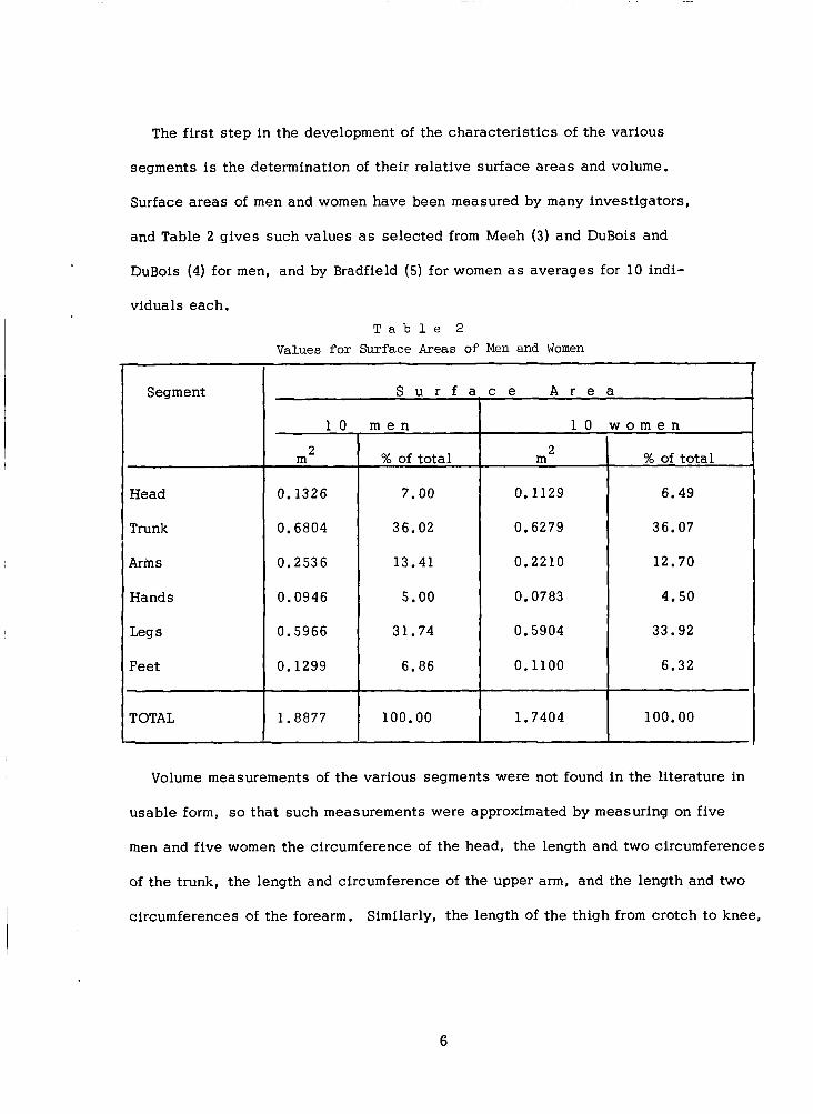
The first s t ep in the development of the characteristics of the various
segments is the determination of their relative surface areas and volume.
Surface areas of men and women have been measured by many investigators,
and Table 2 gives such values a s selected from Meeh (3) and DuBois and
DuBois (4) for men, and by Bradfield (5) for women as averages for 10 indi-
100.00 1.7404 I
viduals each.
100.00
Segment
Head
Trunk
Arins
Hands
Legs
Feet
TOTAL
T a b l e 2 Values for Surface Areas of Men and Women
S u r f a
1 0
2 m
0.1326
0.6804
0.2536
0.0946
0.5966
0.1299
1.8877
m e n
% of total
7.00
36.02
13.41
5.00
31.74
6.86
I
c e A r e a
1 0
2 m
0.1129
0.6279
0.2210
0.0783
0.5904
0.1100
I
i o m e n
% of total
6.49
36.07
12.70
4.50
33.92
6.32
Volume measurements of the various segments were not found in the literature in
usable form, so that such measurements were approximated by measuring on five
men and five women the circumference of the head, the length and two circumferences
of the trunk, the length and circumference of the upper arm, and the length and two
circumferences of the forearm. Similarly, the length of the thigh from crotch to knee,
6

and two circumferences were measured for the thigh, and a similar set of
measurements were taken for the lower legs: the volume of hands and feet were
measured by displacement upon submersion in water. The volumes of the other
segments were estimated from lengths and diameter assuming cylindrical shapes,
The total estimated volumes were checked against the individual weights and
were found to agree t o within 8% with the total weight assuming a density of 1.00.
Table 3 gives the percentages of the total volume in the various segments, a s
averaged for 5 men and 5 women.
100.00
Segment
Head
Trunk
A r m s
Hands
Legs
Feet
100.00 100.00 TOTAL
T a b l e 3
Percent of Total Body Volume in Six Seqments
Men
5.34
56.70
7.78
0.88
27.90
1.43
Women
5.58
57.00
6.52
0.90
28.70
1.34
~- ~ ~~
Average
5.46
56.85
7.15
0.89
28.30
1.38
According to Wilmer (6), the t issue distribution in the human body is 25%
skin and fat, 11% viscera, nervous t issue 3%, muscle 43% and skeleton 18%.
Scammon (7) tabulates average weights of different body divisions and organs
and his numbers can be used t o make assignments of the t issue types t o the layers
in each segment a s given in Table 4.
7

w 0
C 4
rn Ll a, h m 9 a,
4
5 Ll a,
Kr 3 0 rn
a, a, R CI
4
SI a,
4
ry r 3 +
0
3.. SI
2
5 tn a, -4
4
c,
CI W
m 0
0 a, tn m CI C a,
a, a 0 rn m rn c, C a,
E
?5 a, 0
X 4 rn
0 0 0 0 0 0 q d m l n m m v ) D v ) l n O h d
v) cu
4
CI m 0 H
4
CI m 0 H
C 0 a, a, .Y cn
CI
d
CI C a,
a, cn ?5
d
0 0 0 w w a J m o o o v ) o O V d O N O
o l n m o c o o v ) O v ) d ( D d
o q w o m o cu d
0 0 0 0 0 0 v ) m m c u w m O l n d O r n O
8

With the aid of the preceding tables, the necessary computations to obtain
C (N) and TC (N) can be carried out for any s ize man: but, for our purposes,
we will l i m i t ourselves to a "Standard" man with a height of 172 c m and a weight
of 74.4 kg who, according to DuBois and DuBois (8) has a surface area of 1.89 m . 2
The process for obtaining C (N) is indicated in Table 5. The values are based on
a specific heat for the skeleton of 0 .5 gcal/g . "Cy 0.6 gcal/g . OC for fat and
0 ,9 gcal/g . OC for a l l other t i s sues . The central blood compartment representing
the blood in the heart and the great vessels is assumed to contain 2.5 liters of
blood a t a specific heat of 0.9 gcal/g . OC. This heat capacitance of 2.25
Kcal/OC should be subtracted from the heat capacitance of the trunk core which
thus becomes 9.82 Kcalp C.
Thermal conductance between layers in each segment can be calculated from
the dimensions derived before, using the method outlined by Stolwijk and Hardy (1).
The lengths of the segments were obtained from measurements taken for the volume
estimates described above. Results are given in Table 6. Although the volume
estimates and surface area estimates have different origins, there is a con-
siderable consistency in the data a s can be demonstrated by recalculating the
total surface area from the estimates in length and radius given in Table 6.
Ignoring end surfaces, such a calculation yields a value very close to the DuBois
area assumed at the outset.
9

- C
.PI
A
cn
- CI
m
L
5s
0 h
u)
I s + C
2 B cn s u m w c m L, a,
..-I
s s
s 0 L a,
rcI
c, 0
m $ u
0 a, a VI)
a c
.PI
2
m 3 tn .PI s
4 co co e3
a,
u m 3
4
2 -
a,
L,
0
u
h m d m
2s d m 0 cu d
-m
2s c, 0 l+
m w c u o w o d
C D w m m U J ( D U 3 O h O
O O O d O d
d O O d 0 d
1 ‘ 1 2
2s c u 0 u ) h c o h 0 o o u ) w m r r d h 0 0 0
rr cu
4
m m m o h . - r m N
10

T a b l e 6
Calculation of Estimated Thermal Conductance Between Compartments
Volume Length
c m 3 c m
Head core 3010 --- --- muscle 33 80
fat 3750 skin 4020
--- ---
Trunk core 14680 60 muscle 32580 60 fat 39650 60 skin 41000 60
Arms core 2240 112 muscle 5610 112 fat 6580 112 skin 7060 112
Hands core 2 60 96 muscle 330 96 fat 480 96 skin 670 96
Legs core 6910 160 muscle 17100 160 fat 19480 160 skin 20680 160
Feet core 43 0 125 muscle 510 125 fat 73 0 125 skin 970 125
Radius
c m
8.98 9.32 9.65 9.88
8.75 13.15 14.40 14.70
2.83 4.48 4.85 5.02
0.93 1.04 1.27 1.49
3.71 5.85 6.23 6.42
1.06 1.14 1.36 1.57
Avg . cond. gcal/cm . TC (N) ylbtec 1 Kc;l/OC
10 10 8 8
10 10 8 8
‘ 1.38 ‘ 11.4 13.8
I ---
1.37 4.75
19.80 ---
l o 10
8 8
1.20 8.90
26.20 ---
l o 10
8 8
5.50 9.65 9.90 ---
l o 10 8 8
9 .0 12.4 64.0 ---
l o 10 8 8
14.0 17.7 14.1 ---
11

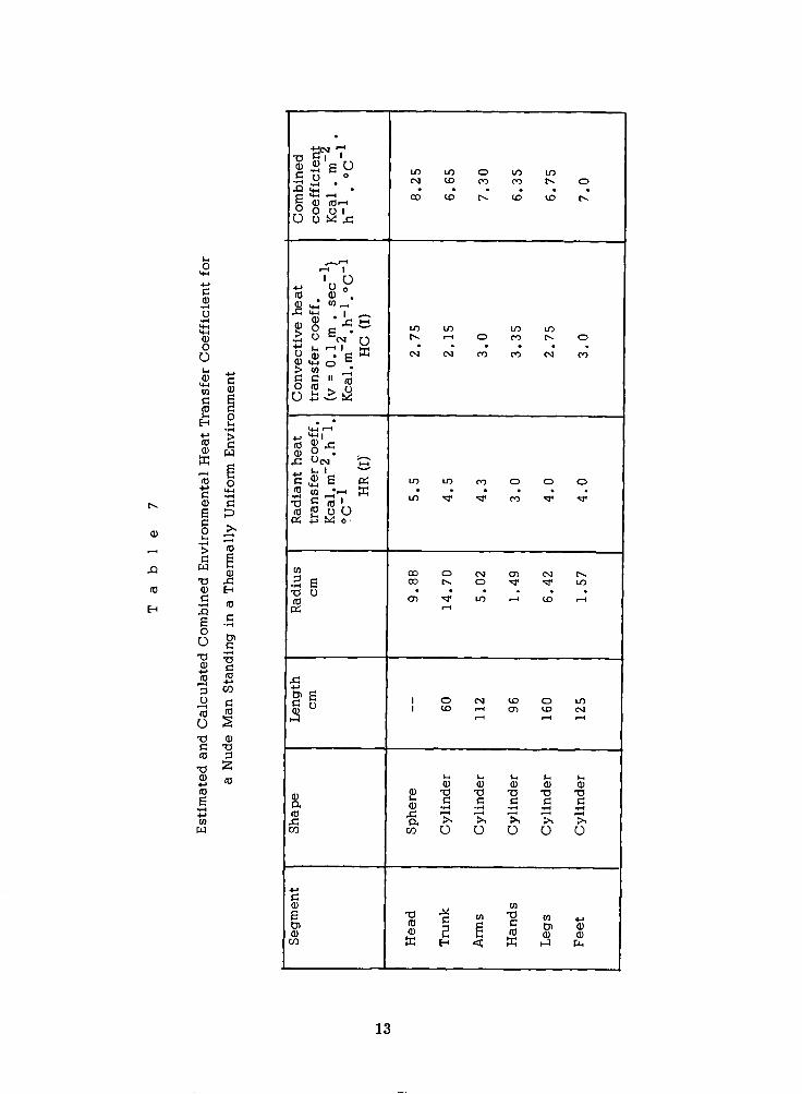
The various segments have different dimensional characteristics and, as
a result, the overall environmental heat transfer coefficient H (I) has different
values.
are high for head and trunk, somewhat lower for arms and legs and even lower
for hands and feet. Estimates for the effective radiant heat transfer coefficients
of the six segments are given in Table 7. It should be pointed out that these are
estimates, and that behavioral adjustments can increase and decrease these co-
efficients substantially. The values for the convective heat transfer coefficient
given in Table 7 are based on measurements by Nishi and Gagge (9) in our
laboratory using the naphthalene m a s s transfer method. They represent values
in still a i r and we can assume that the effective air speed was 0.1 m . sec
due to gravitational convection. The combined heat transfer coefficient H (I)
can be calculated for any air speed V by the expression
Radiant heat transfer depends on effective radiant surface areas which
-1
H (I) = (HR (I) + HC (I)* (V/O. 1)** 0. 5)* S (I)
This expression is valid within about 2 5% for an ambient temperature range
-1 of 10" t o 40°C and for a i r velocities up to 10 m . sec . The value for the combined heat transfer coefficient is slightly higher
than found experimentally for sitting, resting subjects in shorts (10, l l ) , but
this could be due to the minimal clothing and to behavioral adjustments of
their effective surface area by the subjects.
12
8 ry
CI C a, U
a, 0
-4
4
ry ry
u L a, W a
4 (0
c h a,
.r
a, 2 4
4 s C a w
13
I O N W O V ) I W d C n W N
d d d

The model will be called upon t o compute heat loss caused by evaporation
of secreted sweat. The amount of sweat secreted is determined by the con-
trolling system. For any given set of conditions there is a maximum rate of
evaporation which is possible, indicated by EMAX (I) for segment (I). This
maximum rate depends on the vapor pressure in a i r PAIR, the vapor pressure
a t the skin PSKIN (I) and the convective heat transfer coefficient H (I) - HR (I)
The following expression will compute EMAX (I) for segment I:
* S(1).
* EMAX (11 = (PSKIN (11 - PAIR)* 2 . 2 (H (I) - HR (I) * s (I)
in which 2 . 2 is the Lewis relationship a s described and validated by Brebner, et
al. (12) . If E (4 I) for any segment I exceeds EMAX (I), then it must be reduced
t o EMAX (I). The ratio E (4
wetted area, a factor first described by Gagge (13) and later implicated a s an
important determinant in thermal comfort by Gagge, et al. (14). A weighted
average of this ratio will correspond t o the wetted area described in these
reports.
*
* I)/EMAX (I) for each segment gives the fractional
Aschoff and Wever (15) have estimated that the metabolic rate of the
brain is 16% of the total basal metabolic rate, and that the trunk core accounts
for 56% of the resting metabolic rate. They estimate the total skin and mus-
culature to produce 18% of the basal metabolic heat which leaves 10% for the
skeleton and connective t issue. If the resting metabolic rate is presumed t o
be 74.4 Kcal . h . h-' ), the
head core has a metabolic rate of 11.9 Kcal . h ', and the trunk core of
41.6 Kcal . h
-1 -2 for the whole standard man (39.4 Kcal . m
-1 . A total resting metabolic rate of 13.4 Kcal . h-l is t o be
14

divided between skin and musculature. If the resting metabolic rate is 0.3
Kcal . h-l . kg- l for skin t issue and subcutaneous fat is included in this,
we find a total of 4 .47 Kcal . h-l t o be divided between the various skin and
fat layers, This leaves 8.93 Kcal , h-l t o be divided proportionally between
the different muscle compartments, All core compartments can then share the
remainder of the resting heat production in proportion t o their weight. The
values of Q B (N) resulting from these estimates and considerations are given
in Table 8.
-1 In the resting state, the total evaporative heat loss is about 18 Kcal . h
-1 (Stolwijk and Hardy (10) ). Of this, about half, or 9 Kcal . h represents
respiratory heat loss which is considered t o come from the trunk core. The
remaining 9 Kcal . h comes from the skin and represents diffusion losses -1
through the skin. Strictly speaking both of these values are affected to some
extent by the water vapor pressure in the ambient air, but this effect is
relatively small and is ignored for our present purposes.
The values of basal evaporative heat loss EB (N) resulting from these
estimates are given in Table 8.
The controlled system is further characterized by convective heat exchange
between its parts as a result of blood flow. Certain regions are characterized
by a very constant blood flow. The brain receives a very constant flow of
about 750 m l . mm or 45 1 . h
require 1 . 2 1 . h
-1 -1 (16). Resting muscle can be assumed t o
of metabolic heat pro- -1 -1 of blood flow for each Kcal . h
duction, purely on the basis of supplying the needed oxygen. Stolwijk and
Hardy (1) added up the blood flows t o visceral organs in the trunk core and
estimated a total flow of 210 1 . h-’. The skin, in the resting state, receives
15

far more blood flow than is required to sustain its metabolic rate. Behnke
and Willmon (17) found a total skin blood flow in resting man of
240 m l . mm
considerable vasodilatation. In the neutral environmental temperature of
3OoC, this is assumed to be reduced to 105 m l . min
to the reduction in core to skin conductance which occurs at an environ-
mental temperature of 30°C in comparison with 35°C. Hertzman, et al. (18)
investigated the distribution of blood flow to different skin areas, and skin
blood flow was distributed in Table 8 according to his findings.
-1 -2 . m at an ambient temperature of 35°C which would cause
-1 -2 . m in proportion
16

Head (1)
Trunk (2)
Estimate
core muscle fat skin
core muscle fat skin
I
--- ~ 0.33 0. l o
0.22 0.11 --- ' 0.24 0.08 0.63
Segment Layer (I 1 I
I
9.82 45.38 9.00 16.15 5.00 ---
1 4.25 2.13 --- 1 . 2 1 0.40 3.25
Arms (3 1
core muscle fat skin
9 10 11 12
13 14 15 +
2.25 3.37 0.97 0.48
0.26 0.07 0.15
1.41 3.04 0.58 0.43
0.14 0.06 0.09
0.70 --- 0.95 0.17 --- 0.13 1.20
---
0.08 --- 0.20 0.03 ---
---
T a b 1 3f Core Compartmen
and Basal Evapo
Hands (4)
1 2
4 i 3
5 6 7 8
core muscle fat skin
3.01 0.37 0.37 0.27
Legs (5)
12.18 17.90 7.07 1.35
core muscle fat skin
Feet (6)
Total
21 22 23 24
core muscle fat skin
Central Blood
0.43 0.07 0.22 0.24
74.45 I I
e 8 ; Resting State Heat Production a t ive Heat Losses
I
I I
I I
4.24 2.23 --- 9.17 2.86 1.43 0.43 1.08 0.32 2.85
--- ---
2.25 1 --- 1 ---
59.17 74.45 18.00
BFB (N)
45.00 0.12 0.13 1.44
210.00 6.00 2.56 2.10
~
0.84 1.14 0.20 0.50
0.10 0.24 0.04 2.00
2.69 3.43 0.52 2.85
0.16 0.02 0.05 3.00
285.13
17

The Controlling System
The controlling system in body temperature regulation can be divided
into three distinctly separate parts. The first part contains the sensing mechanisms
which recognize the thermal state of the controlled system. The second part
receives information regarding the thermal state, integrates it and sends out
appropriate effector commands to the various effector systems. The third part
of the controlling system receives the effector commands and if appropriate
modifies them according t o the conditions at the periphery before translating
such commands into effector action.
Thermoreceptors have been described in a wide variety of locations in
the body. Sometimes these descriptions are based on functional thermosensitivity
in short, local temperature changes and produce thermoregulatory effector output
much in excess of the s i ze of the stimulus. On other occasions, and using
electrophysiological methods, investigators find fibers in which the electrical
activity is determined by the temperature of t issues innervated by such a fiber,
Areas in which thermosensitivity has been demonstrated by both methods
are the preoptic area and anterior hypothalamus in the brain (19, 20), the spinal
cord (21 , 22) and the skin (23, 24), and the abdominal viscera (25, 26). Other
areas have been suspected, such as muscle tissue or the veins draining muscle
(27). Final and irrefutable proof of the functional role of thermosensitive areas,
and the precise mode of detection is extremely difficult t o obtain, even for the
anterior hypothalamic area where there is general acceptance of the importance
in thermoregulation.
18

Such uncertainties s t e m from the fact that it is usually difficult t o dis-
sociate temperatures in various parts of the body because of the strong thermal
coupling which takes place. Uncoupling for experimental purposes is difficult
because it can only be achieved for a very short t i m e during rapid transients
in load. During such transients, thermal fluxes are high, thermal gradients
are steep, and the available t i m e is short, a l l adding up to potential errors
in such measurements and to general difficulties in devising appropriate
methods.
A listing of a l l symbols used in the description of the controlling system
is given in Tables 9 and 10.
In order t o allow for maximum flexibility in the evaluation of different thermo-
regulatory controller concepts, it is easiest t o assume that thermoreceptor
structures are present in all t issues . Error signals are derived from all compart-
ments with the following expression:
ERROR (N) = T (N) - TSET (N) + RATE (N)* F (N)
In first approximation, the error signal is thus equal t o the difference between
the instantaneous temperature T (N) and the reference temperature TSET (N).
For appropriate compartments where dynamic sensitivity of the thermoreceptors
is quantitatively known, the dynamic term RATE (N)
values. T (N) and F (N) are continuously computed from the passive system,
and TSET (N) and RATE (N) are controlling system characteristics supplied as
initial constants.
* F (N) can assume non-zero
19

T a b l e 9
Definition of Symbols Used in the Description of the Controlling System
I Symbol
TSET (N)
ERROR (N)
RATE (N)
COLD (N)
WARM (N)
COLDS
WARMS
SWEAT
CHILL
DI IAT
STRIC
SKINR (I)
SKINS (I)
SKINV (I)
SKINC (I)
MWORK (I)
MCH'IL (I)
Vector Length
25
25
2 5
25
25
6
6
6
6
6
6
-~ ~ ~
D e f i n i t i o n
"Set point" or reference point for receptors in compartment N
Output from thermoreceptors in compartment N
Dynamic sensitivity of thermoreceptors in N
Output from cold receptors in N
Output from warm receptors in N
Integrated output from skin cold receptors
Integrated output from. skin warm receptors
Total efferent sweat command
Total efferent shivering command
Total efferent skin vasodilation command
Total efferent skin vasoconstriction command
Fraction of all skin receptors in Segment I
Fraction of sweating command applicable t o skin of Segment I
Fraction of vasodilatation command applicable to skin of Segment I
Fraction of vasoconstriction command applicable to skin of Segment I
Fraction of total work done by muscles in Segment I
Fraction of total shivering occurring in muscles of Segment I
~ ~-
Dimension
OC
OC
h
OC
"C
" C
OC
Kcal . h
Kcal . h
1 . h-l
N. D.
N. D.
N. D.
-1
-1
N. D.
N. D.
N. D.
N. D.
20

T a b l e 1 0
Definition of Symbols Used as Control Coefficients
Symbol
csw
ssw
CDIL
SDIL
CCON
SC ON
CCHIL
SCHIL
PSW
PDIL
PCON
PCHIL
BULL
D e f i n i t i o n
Sweating from head core
Sweating from skin
Vasodilatation from head core
Vasodilatation from skin
Vasoconstriction from head core
Vasoconstriction from skin
Shivering from head core
Shivering from skin
Sweating from skin and head core
Vasodilatation from skin and head core
Vasoconstriction from skin and head core
Shivering from skin and head core
Factor determining temperature sensitivity of sweat gland response
Dimension
Kcal . h-l . OC-l
Kcal . h-' . OCel
1 . h-l . "C
1 . h- l . OC
OC
OC
Kcal . h-' . OC-'
Kcal . h-l . OC-'
-1 -2 Kcal . h . OC
-2 1 . h- l . OC
"C
"C
-1
-1
-1
-1
-2
-2
21

There can be conceptual controllers ( I , 21) which are based on outputs which
have a positive value on one s ide of the reference point, and have no output on
the other side of the se t point. This conceptual construction is supported by the
obvious fact that there can be no negative firing rate, or negative sweating,
negative blood flow or negative shivering. Non-linearity is thus introduced some-
where in the chain from receptors t o effectors, and it is convenient t o have this
non-linearity available at the receptor level. This is conveniently accomplished
by testing ERROR (N) for its sign. If it is positive, we can assume warm receptors
are active, and WARM (N) can be set t o the value of ERROR (N). If ERROR (N) is
negative, we are dealing with a cold receptor output, and COLD (N) can be set to
-ERROR (N). The resulting lists of WARM (N), COLD (N) and ERROR (N) then con-
tain a l l thermal information which could be available t o the thermoregulatory
controller. There is very little information concerning the distribution of receptors
in different compartments. This is of special importance in tissues which are wide-
spread so that different compartments can be at widely different temperatures. The
skin is a prime example. In the absence of any further information, the simplest
approach would be the weight of the different compartments in different segments
according to their mass. For the skin, Aschoff and Wever (15) have proposed rela-
tive sensit ivit ies which can be adopted although their factual basis is not clear.
Bader and Macht (28) show a relatively higher sensitivity in the skin of head and
chest than in the extremities, but there is reason t o suspect that in their case the
heat applied t o the skin was sufficient t o warm the central blood appreciably so
that deeper or central thermoreceptors could have been involved in producing the
results they observed.
. .
22

There is little doubt that the trunk :!:in plays a more than pro2ortionate role in
skin thermoreception as evidenced by the difference in response t o a uniform s1.h
temperature and t o an identical average skin temperature with divergent local t em-
peratures. The tentative values for SKINR (I) shown ir. Table 11 have been obtained
by multiplying the number of cold points for various segments given by Aschoff and
Wever (15) with the corresponding surface areas and assigning to each area the
appropriate fraction of the total sum of these products,
Hertzman and Randall (18) surveyed the skin with respect t o local blood flow.
Although their measurements were photoelectric and consequently hard to quantitate,
the relative proportions can probably be accepted. After rearrangement, the follow-
ing fractions of the total blood flow are obtained for the basal and maximally dilated
state respectively: head 0.288 and 0.132, trunk 0.265 and 0.322, arms 0.078 and
0.095, hands 0.10 and 0.122, legs 0.186 and 0.23, and feet 0.083 and 0.10.
The fractions for the maximally dilated state are taken as the distribution of
vasodilatation over the skin, SKINV (I), in Table 11. Vasoconstriction is a l so not
uniform over the skin area. In addition, the effects of countercurient heat exchange
will tend t o exaggerate the effects of vasoconstriction in the distal extremities.
On the other hand, countercurrent heat exchange is not so pronounced in the skin
of the head and the trunk. Msed on this, the assignments of SKINC (I) are made
as shown in Table 11.
The relative distribution of sweat secretion in the absence of information based
on local secretion measurements is perhaps best approximated by the distribution
of sweat glands. Randall (29) made such observations and the different skin areas
were weighted as to the number of sweat glands, and the fractional distribution is
given as SKINS (I) in Table 11. In addition, some weight was given t o provisional
results from thermograms presented by Stolwijk, et al. (30).

8
E
+ u a,
LH
a C D + 2
5 C H
0 m C a, 03
0 C 0
5
LH
.r( +
2
6 L .v m
LH 0 m a, +
.,-I + m w a, > 0 C a, H
.,-I +
m m m l n h m o d o m o m 0 0 0 0 0 0
m a 2
3 4 C
rn m 5 0 4 L
a, s L a,
8
8 + 5 a .v
0 0
d
Y
0 0 0 0 0 0 d
r 0 0 0 0 ~
I d
‘ d I - ‘ 0 0 0 0 0
24

The total warm receptor output from the skin WARMS can be obtained by * *
summing SIUNR (I) WARM (4 I) for the skin compartments of all six segments (I).
The total cold receptor output from the skin can be integrated from a similar
summation.
I t depends on the concept whether the signals from skin warm receptors are
integrated without being offset by simultaneous cold receptor output from other
skin areas. Available data is not adequate to clearly determine where integration
of cold receptor signals and warm receptor signals takes place, so that the regu-
lator in the controlling system must have either form available. Conceptual
regulators which rely on linear addition of thermal signals from different sets of
receptors (10,20) use the ERROR (N) value in the controller equations, whereas
conceptual models which use non-linear thermal signals either in a linear (1 0)
or a non-linear expression ( 1 ) should use the WARM (N) or COLD (N) values
in their controller equations. I t will be clear that the weighted skin signal can
be recovered in its linear form by subtraction of COLDS from WARMS.
In the suggested controller equations which follow, we have assumed that
the central receptors are located in the brain, so that WARM ( l ) , COLD (1) or
ERROR (1) constitutes the thermal signal from the interior. There are reasons to
believe that central receptors occur elsewhere (25, 28) but not enough is known
t o take them separately into account, and central temperatures will not normally
be found t o move far apart, so that lumping central receptors into the brain com-
partment will only result in a second order error for most circumstances.
In general, the controller equations produce signals which drive the effector
part of the regulator. These drives are not necessarily identical t o effector action
25

since they may be modified a t the effector site by mechanisms responding to local
conditions. The controller equations a l l have a term consisting of the product of
a control coefficient and a central temperature signal, a term consisting of the
product of a control coefficient and an integrated skin temperature signal and a
third term consisting of the product of a control coefficient, a central temperature
signal, and a skin temperature signal. Controller equations are then a s follows:
SWEAT = CSW* ERROR (1) + SSW* (WARMS-COLDS) + PSW* WARM (1)* WARMS
DILAT = CDIL* ERROR (1) + SDIL* (WARMS - COLDS) + PDIL* WARM (I)* WARMS
* * CHILL = -CCHIL* ERROR (1) + SCHIL* (COLDS-WARMS) + PCHIL COLD (1) COLDS
* * STRIC = -CCON ERROR (1) + SCON (COLDS - WARMS)+ PCON COLD (1)* COLDS
Since these expressions can become negative under certain circumstances , it
is necessary to make sure that any negative values of SWEAT, DILAT, CHILL or STRIC
are set to zero.
The third part of the controller distributes the effector commands to the appropriate
compartment and, if required and appropriate, modifies them according to local
conditions.
In order t o facil i tate the description of this distribution, the fallowing con-
vention will be used: for segment I, the core layer will be indexed a s N (equal
t o 4 I -3) , which makes the concentric muscle layer be indexed a s (N + 1); the
subcutaneous fat layer and the skin layer for segment I then are indicated by the
subscripts (N + 2) and (N + 3) respectively. The metabolic rates for a l l compartments
then become a s follows:
*
Q (N) = QB (N)
26

This expression states that the basal metabolic rate assigned to the cores of
the various segments is not thought to vary under the relatively short term con-
ditions for which the model will be used.
Q (N + 1) = ?B (N + 1) + WORKM (I)* (WORKI) + CHILM (I)* CHILL
The metabolic heat production in the muscle compartment is the sum of the
basal rate of heat production QB (N + 1) , and the sum of the heat production
rates assigned due to muscular work done and any shivering thermogenesis.
WORKI is the total heat production as one would determine from the oxygen up-
take minus the basal metabolic rate and the caloric equivalent of the external
work performed. WORKM (I) and CHILM (I) are estimates of the distribution of
extra heat production over the various muscle compartments. Th estimates used
are given in Table 12.
T a b l e 1 2
Estimates of Distribution of Heat Production in Muscle Compartments
Head
Trunk
Arms
Hands
Legs
Feet
WORKM (I)
2.323
54.790
10.525
0.233
31.897
0.233
---
0.30
0.08
0.01
0.60
0.01
CHILM (I)
0.02
0.85
0.05
0.00
0.07
0.00
27

In the absence of data, the he?' from shivering wac distributed according to the
mass in the various muscle compartments, whereas the values for WORKM (I) are
based on estimates for bicycle exercise. Values for WORKM (I) should be reviewed
for other types of exercise.
For the subcutaneous fat and the skin compartments, it is assumed that the
basal heat production does not change in the conditions t o be evaluated by the
model, so that:
Q (N + 2) = QB (N + 2)
Q (N + 3) = QB (N + 3)
The convective heat transfer by blood flow plays a very important role in the
thermal responses t o internal and external s t resses . Certain simplificaticns are
implicit in the expressions which follow. Some of these simplifications are due
t o a scarcity of applicable data, some of them are justified by the fact tliat although
inaccuracies in mass flow are introduced by the simplifications, these inaccuracies
have only a very s m a l l effect on heat transfer. For example, it is assumed that
blood flow t o the core compartment remains a t the basal value:
BF (N) = BFB (N)
This ignores the fact that blood flow t o the trunk core in fact can be reduced
during exercise s t ress (16, 31, 32), but, in fact, the blood flow t o these compart-
ments is considerably in excess of that required to supply oxygen t o these compart-
ments, so that only small thermal gradients can ever exist between the head core,
trunk core and the central blood. Small reductions in core blood flow will then re-
sult in slight increases in these small gradients, and convective heat transfer is not
materially affected. The muscle compartments, on the other hand, can have widely
28

varying metabolic rates, and substantial variations in blood flow. Regional blood
flow measurements over working quadriceps muscle (34) and measurements of ar-
teriovenous oxygen differences across the working quadriceps muscle (3 5) can be
added t o measurements of local muscle temperature (36) during exercise to arrive
at an insight of muscle blood flow during exercise. Under conditions where
heat loss in exercise is mostly from evaporation of sweat, the temperature of the
working muscle is about 1 .0 " C above that of the arterial blood supplying oxygen
(35) . If venous blood leaves at muscle temperature, then every liter of blood
carries off 0 .95 Kcal. Each liter of blood contains about 200 m l O2 which, if
completely scavenged, could produce about 1.0 Kcal of heat. It is thus reason-
able t o assume that at least 1 1 of blood is required t o produce 1 Kcal of heat.
A s a result, the following equation describes the blood flow to the muscle compart-
ments.
BF (N + 1) = BFB (N + 1) + Q (N + 1) - Q B (N + 1)
Blood flow t o the subcutaneous fat is not very high in basal value, and it is
assumed that i t is not effectively changed a s a result of thermoregulatory adjustments:
BF (N + 2) = BFB (N + 2)
Skin blood flow is highly dependent on the thermoregulatory controller. The
basal blood flow a t thermal neutrality can be reduced t o very low values through
basoconstriction, and increased substantially through vasodilatation; in addition,
there is an effect of the local temperature which has a substantial modifying influ-
ence on resistance of cutaneous veins,. as demonstrated by Webb-Peploe and
Shepherd (36 ) . These investigators showed that the local temperature of the
saphenous vein had a very strong effect on the response of the vein to a given level
29

of constricting stimulation. The peripheral resistance caused by a given level of
sympathetic tone would be reduced by high local temperatures and increased by low
local temperatures. In many cases, the resistance would about double for a 10°C
drop in local temperature, and for a given central signal. The tentative expression
for skin blood flow then becomes: * **
BF (N) = ( (BFB (N) + SKINV (I)* DILAT) / (1. + SKINC (I)* STRIC) 2. (ERROR ( N ) / ~ o * )
In this expression, the weighted DILAT drive is added t o the basal blood flow.
The weighted constrictive tone operates through a resistance and thus is entered a s
a divisor. The local skin temperature effect then ac t s on the total flow drive multi-
plying i t by unity in neutral conditions, by l e s s than unity a t skin temperatures below
normal and by more than one at skin temperatures above the neutral value.
I t could be that the local effect on cutaneous veins described by Webb-Peploe
and Shepherd does not affect total skin blood flow very much, but reduces heat l o s s
by shifting venous return to deeper veins. This shift would activate a n effective
counter-current heat exchange between arteries and veins, which could not be dis-
tinguished from a reduction in skin blood flow as far a s convective heat exchange
is concerned.
Evaporative heat loss occurs from the trunk through respiratory water loss, and
through evaporation from the skin. Respiratory water loss is a function of the water
vapor pressure in the inspired air (PAIR) and the ventilation volume. The ventilation
volume is closely related t o the metabolic rate, and ventilatory evaporative heat l o s s
can be approximated over a wide range of metabolic rates by:
E (5) = (74 .4 + WORI(I)* 0.023* (44.0 - PAIR)
in which 44.0 is the vapor pressure in expired air.
30

For all other core compartments
E (N) = EB (N)
and since muscle and subcutaneous fat compartments have no evaporative heat
10s s:
E (N + 1) = EB (N + 1)
E (N + 2) = EB (N + 2)
The different skin compartments receive a sweating drive from the central
controller. The local response in a given compartment depends on the skin
area and on the number of sweat glands present, expressed by SKINS (I). In
addition, the local skin temperature modifies the response t o a given sweat
command a s described by Bullard and associates (24) .
On repeating these observations in our laboratory, we confirmed the local
temperature effect, but found it t o have a somewhat lower Q
Figure 2. A s a result, the Q l o
report as about 8 is used here at a value of 2 . The evaporative heat loss of the
as shown in 10
of the local temperature effect which Bullard, et al .
skin of each segment then becomes:
** ( (T (N + 3) - TSET (N + 3) )/BULL) E (N + 3) = (EB (N-+ 3) + SKINS XI)* SWEAT)* 2.
31

C .- E
0.60 W
e t
L
Ts= 34.60
T, = 34.50
fs5 34.40
30 32 34 36 38
TsL
Figure 2 . Dependence of local sweat rate on the skin of the thigh, on average skin t e m - perature, and local skin temperature. Internal temperatures were constant during these measurements.
32

Annotated Listing of FORTRAN Statements Implementinq the Mode l
A flow sheet of the program for simulation of body temperature regulation in man
is given in Figure 3 , and the listing will follow by sections as identified in the flow
diagram.
DIMENSION TC(24), S(6), SKINR(6), SKINS (6), SKINV(6), SKINC (6), WORKM (6)
DIMENSION CHILM (6), HR(6), HC (61, P ( lo) , F (25), H (6), WARM (25), COLD (25)
DIMENSION ERROR ( 25), Q (24), E (241, BF (241, EMAX (61, BC (241, TD (24) C C C
READ CONSTANTS FOR THE CONTROLLED SYSTEM
100 FORMAT (14F5.2)
101 CONTINUE
READ (2, 100)
READ (2, 100)
READ (2, 100)
READ (2, 100)
READ (2, 100)
READ (2, 100)
READ (2, 100)
READ (2, 100)
READ (2, 100)
SA = 0 .0
C
QB
EB
BF B
TC
S
HR
HC
P
D'O 110 K = 1, 6
110 SA = SA+ S (K)
33

READ CONSTANTS CONTROLLED
SYSTEM
PREPARE OUTPUT
I I
Y E S
EXPERIMENTAL CONDITIONS
*
ESTABLISH THERMORECEPTOR
-- 1
h
DETERMINE INTEGRATION 4- STEP
qgl TEMPERATURE S
CALCULATE HEAT FLOWS <-
ASSIGN EFFECTOR OUTPUT
Fig. 3 . Flow diagram, for s imula t ion of thermoregula t ion in man
34
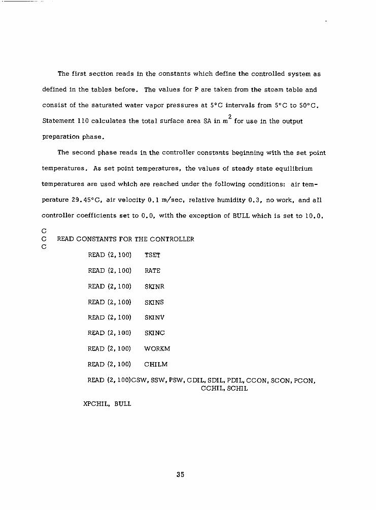
The first section reads in the constants which define the controlled system as
defined in the tables before. The values for P are taken from the steam table and
consist of the saturated water vapor pressures at 5OC intervals from 5OC to 5OOC. n z Statement 110 calculates the total surface area SA in m for use in the output
preparation phase.
The second phase reads in the controller constants beginning with the set point
temperatures. A s set point temperatures, the values of steady state equilibrium
temperatures are used which are reached under the following conditions: a i r tem-
perature 29.45OC, air velocity 0.1 m/sec, relative humidity 0.3, no work, and all
controller coefficients set to 0.0, with the exception of BULL which is set to 10.0.
C C READ CONSTANTS FOR THE CONTROLLER G
READ (2,100) TSET
READ (2,100) RATE
READ (2,100) SKINR
READ (2,100) SKINS
READ (2,100) SKINV
READ (2,100) SKINC
READ (2,100) WORKM
READ (2,100) CHILM
READ (2, lOO)CSW, SSW, PSW, CDIL, SDIL, PDIL, CCON, SCON, PCON, CCHIL, SCHIL
XPCHIL, BULL
35

The values for SKINR, SKINS, SKINV, SKINC, WORKM and CHILM have been de-
fined before in preceding Tables l l and 1 2 .
C C READ INITIAL CONDITIONS C
READ (2, 100) T
TIME = 0.0
ITIME = 0
JTIME = 0
DO 102 N = 1, 25
F (N) = 0.0
102 CONTINUE
The init ial conditions for the next phase consis t of the init ial values for the
temperatures in all compartments. These values are the same as those for TSET
and were obtained a s described there. The values are given in Table 13.
C C READ EXPENMENTAL CONDITIONS C READ (2,299) TAIR, V, RH, WORK, INT
299 FORMAT (4F5.0, 12)
IF (WORK - 74.4) 104, 104, 105
104 WORKI = 0.0
G O T 0 106
105 WORKI = (WORK - 74.4) * 0.78
106 CONTINUE
DO 202 I = 1, 6
H(I) = (HR(1) + HC (I) * (V/O. 1) ** 0.5) * S (I)
202 CONTINUE
I = TAIR/S
PAIR = RH*(P(I) + (P (I + 1) - P (I) )*(TAIR - 5 * I)/S.O)
36

k Cent ra l Blood
Compartment N
C o r e 1 M u s c l e 2 Fa t 3 Skin 4
C o r e 5 M u s c l e 6 Fa t 7 Skin 8
C o r e 9 M u s c l e 1 0 Fa t 11 Skin 12
C o r e 13 M u s c l e 14 Fa t 1 5 Skin 16
C o r e 17 M u s c l e 18 Fat 19 Skin 20
C o r e 21 M u s c l e 22 Fa t 23 Skin 24
25
T a b l e 1 3
Se t Point Values a n d In i t i a l Condi t ion Temperatures
Temperature O C
36.96 35 .07 34 .81 34.58
36 .89 36 .28 34.53 33.62
35.53 34.12 33.59 33 .25
35 .41 35 .38 35 .30 35.22
35 .81 35 .30 35.31 34.10
35 .14 35.03 35.11 35 .04
36 .71
37

The next phase reads in the experimental conditions, a i r temperature, air velocity -
in m. sec ’, the relative humidity a s a fraction rather than a percentage, the work
rate in total heat production in Kca1.h as normally computed from oxygen uptake, -1
and the interval in minutes between desired outputs. Next, WORKI is computed by
subtracting the basal metabolic rate, and by subtracting the external work, so that
WORKI represents the total extra heat production in the working muscle. Subse-
quently, H(1) is calculated in Kca1.h-’ , O C ’ l for each segment. The last two
statements look up the partial pressure of water vapor in the environment by inter-
polation from the steam table.
C C ESTABLISH THERMORECEPTOR OUTPUT C
3 0 1 CONTINUE
D O 302 N = 1, 2 5
WARM (N) = 0.0
COLD (N) = 0.0
IF (F(N) ) 310, 311, 311
311 F (N) = 0.0
3 1 0 CONTINUE
ERROR (N) = T (N) - TSET (N) + RATE (N) * F (N)
IF (ERROR (N) ) 303, 302, 304
303 COLD (N) = ERROR (N)
GO TO 302
304 WARM (N) = ERROR (N)
302 CONTINUE
38

In the next phase, the actual instantaneous temperatures in a l l compartments are
compared with the "set point" temperatures, taking into account the rate of change
in those c a s e s where this is appropriate. The direction of rate of change is first
determined, and positive rates of change are set to zero. This was done because
we have not been able to demonstrate specific effects of a positive rate of change,
although a direct effect of negative rate of change of skin temperature on sweating
has been demonstrated. Such effects had been implied earlier (37) and were studied
quantitatively in our laboratory by Nadel, Bullard and Stolwijk (38). In these exper-
iments i t was shown that local sweating rate as measured by a sweat capsule and
resistance hygrometry was linearly dependent on average skin temperature, a s long
as local skin temperature and internal temperatures were held constant, Radiant
energy was used t o bring about rapid changes in average skin temperature. Figure
4 shows such linear dependence on average skin temperature a t various local skin
temperature, in a steady state condition. When rapid changes were brought about,
it was found that during skin warminq the instantaneous mean skin temperature was
a good predictor of instantaneous local sweat rate, but during cooling the sweat rate
at any instant was lower than that predicted by instantaneous mean skin temperature.
It was found that this deviation was proportional t o the negative rate of change in
average skin temperature as shown in Figure 5.
39

0 80 1
Figure 4. Linearity of local sweating response with average skin
temperature, a t constant internal temperature.
OEVLATION FROM LINEAR SWEATING RESPONSE
mg / cmt mm
-0 2 0 T
Iran cooling rkm worming
! I1 .I0
Figure 5. Deviation from sweating response linear with average skin
temperature, as a function of rate of fall of mean skin temperature.
40

This phase results in lists of temperature deviations from normal, in linear
terms (ERROR (N) ) and in non-linear terms WARM (N) and COLD (N) which are
zero for values below and above the set point respectively,
C C INTEGRATE PERIPHERAL AFFERENTS C
WARMS = 0.0
COLDS = 0.0
DO 305 I = 1, 6
K = 4*1
WARMS = WARMS +WARM (K) * SKINR (I)
COLDS = COLDS + COLD (K) * SKINR (I)
305 CONTINUE
Since only the skin afferents are used in the present model, these signals are
the only ones t o be weighted for integration. Weighting is done according to the
receptor density estimates SKINR (I). The use of WARM (K) and COLD (K) does not
necessarily cause the loss of linear information. A linear form of the weighted
value of the skin error signal can be recovered by the use of WARMS - COLDS.
C C DETERMINE EFFERENT OUTFLOW C
SWEAT = CSW*ERROR(l) +SSW * (WARMS-COLDS) + PSW * WARM (1) *WARMS
DILAT = CDIL*ERROR(l)+SDIL* (WARMS-COLDS)+PDIL*WARM(l) *WARMS
STRIC = -CCON * ERROR (1) -SCON* (WARMS - COLDS) + PCON *COLD (1) * COLDS
CHILL = -CCHIL * ERROR (1) -SCHIL * (WARMS-COLDS) + PCHIL * COLD (1) * COLDS
IF (SWEAT) 309, 312, 312
309 SWEAT = 0.0
312 IF (DILAT) 313, 314, 314
41

313 DILAT = 0.0
314 IF (STRIC) 315, 316, 316
3 1 5 STRIC = 0.0
316 IF (CHILL) 317, 318, 318
3 1 7 CHILL = 0.0
318 CONTINUE
The next section calculates the control commands going to the periphery.
Since the ERROR (N) terms can become negative a s well as positive, each of the
commands is protected against becoming negative.
C C C
ASSIGN EFFECTOR OUTPUT TO THE COMPARTMENTS
400 CONTINUE
DO 401 I = 1, 6
N = 4 * I - 3
BF (N) = BFB (N)
E (N) = EB (N)
Q (N + 1) = QB (N + 1) + WORKM (I) * WORKI + CHILM (I) * CHILL
E (N + 1) = 0.0
BF (N + 1) = BFB (N + 1) + Q (N + 1) - QB (N + 1)
Q (N + 2) = QB (N + 2)
E ( N + 2) = 0.0
BF (N + 2) = BFB (N + 2)
Q (N + 3) = QB (N + 3)
E(N + 3) = (EB(N+3) + SKINLS(I)*SWEAT)*~.O**(ERROR(N+~)/BULL)
BF (N + 3) = ( (BFB (N + 3) + SKINV (I) * DIIAT)/(l. 0 + SKINC (I)* STRIC) )* 2.0**
X(ERR0R (N + 3) / 10.0)
42

K = T (N +3)/5
PSKIN (I)
EMAX (I) = (PSKIN (I) -PAIR) *2.2 * (H (I) -HR (I) * S (I) )
IF ( E ( N + 3) -EMAX (I)) 403, 403, 402
= P (K) + (P (K + 1) -P(K) ) * (T (N + 3) -5*K) / 5.0
402 E (N + 3) = EMAX (I)
403 CONTINUE
401 CONTINUE
E (5) = (74.4 + WORKI) * 0.0023 * (44.0 -PAIR)
This phase distributes the control commands to the various segments and within
the segments t o compartments in the form of the calculated effect of heat flow in
Kcal . h-l for Q (N) and E (N), and of conductance in Kcal . h
The core compartments (N) and the fat compartments (N + 3) remain a t basal values.
The muscle compartments receive their assigned portion of the total internal heat
production due to work, and of that due to shivering, For each Kcal of heat produced,
the muscle requires a t least one liter of blood, a s seen in BF (N + 1).
-1 . "C-l for BF (N) .
Skin metabolic rate remains a t basal values, but skin blood flow and evaporative
heat loss are determined by command signals, as modified by the local temperature.
The water vapor pressure a t the skin surface temperature is read and interpolated
from the steam table and the maximum evaporative heat loss from a completely wet
skin EMAX (I) is computed, based on existing conditions.
from the skin E (N + 3) exceeds the maximum possible EMAX (I), then the former is
set equal t o EMAX (I). The las t statement calculates the evaporative heat loss from
the respiratory tract with the aid of total metabolic rate and the water vapor pressure
in the environment.
If the computed evaporation
43

C C CALCULATE HEAT FLOWS C
DO 500 K = 1, 2 4
BC (K) = BF (a * (T (K) -T (25) )
TD (K) = TC (K) * (T (K) -T (K + 1) )
500 CONTINUE
DO 5 0 1 I = 1. 6
K = 4 * 1-3
HF (K) = Q (K) -E (K) -BC (K) -TD (K)
HF ( K + 1) = Q (K + 1) -BC (K + 1) + TD (K) -TD (K + 1)
HF (K + 2) = Q (K + 2) -BC ( K + 2) + TD (K + 1) -TD (K + 2 )
HF (1; + 3) = Q ( K + 3) -BC (K + 3) -E (K + 3) + TD (K + 2) -H(I) * (T(K+3)-TAIR)
5 0 1 CONTINUE
HF (25) = 0.
DO 502 K = 1, 2 4
HF (25) = HF (25) + BC (K)
502 CONTINUE
The next section computes the net h - a t f l w rates into or out of each of the com-
partments. Initially BC (K), the convective heat flow rate, and TD (K), the conductive
heat flow rate for each compartment t o the next compartment are calculated. After
this, all the heat flow rate components are added up for each compartment. The only
exception is the central blood compartment which receives the sum of a l l convective
heat flows.
44

C C DETERMINE OPTIMUM INTEGRATION STEP C
DT = 0.016666666667
DO 600 K = 1, 25
IF (U * DT -0.1) 600, 600, 601
601 DT = O . l / U
600 CONTINUE
The optimum integration t i m e s t ep is determined in the next phase. Initially
the t i m e increment for numerical integration is set to 0.01667 hours or 1 minute
this being considered the shortest plausible print-out interval. Based on th i s
increment, the temperature s teps in each compartment are calculated and if any
exceed 0. l 0 C then the t i m e increment DT is reduced so that the maximum tem-
perature change in any compartment in each iteration is kept to 0. l 0 C or less.
C C CALCULATE NEW TEMPERATURES C
DO 700 K = 1, 25
T (K) = T (K) + F (K) * DT
700 C ON TIN UE
TIME = TIME + DT
LTIME = 60. * TIME
IF (LTIME -1NT -1TIME) 301, 701, 701
701 CONTINUE
45

Based on the t i m e increment thus arrived a t , the next section calculates
the new temperatures and increments the clock with the value of the integration
increment DT. This followed by a test t o see whether output is desired. If such
output is not desired, the program returns to the phase where thermoreceptor output
is re-computed. If output is desired, the program proceeds t o the next phase.
C C PREPARE FOR OUTPUT C
EXVET = 0.0
DO 450 I = 1. 6
EXVET = EXVET + (E (4 * I)/EMAX (I) ) * (S (I)/SA)
450 CONTINUE
W E T = 100. * W E T
ITIME = ITIME + INT
co = 0.0
HP = 0.0
EV = 0.0
TS = 0.0
TB = 0.0
HFLOW = 0.0
SBF = 0.0
DO 800 N = 1, 24
CO = CO + BF (N)/60.O
HP = HP + Q (N)
EV = EV + E (N)
800 CONTINUE
DO 802 I = 1, 6
SBF = SBF + BF (4 * I ) / 60.0
46

802 CONTINUE
DO 801 N = 1, 25
TB = TB + T (N) * C (N) /59 .17
HFLOW = HFLOW + HF (N)
801 CONTINUE
EV = EV/SA
HP = HP/SA
HFLOW = HFLOW / SA
COND = (HP -E(5) /SA -HFLOW) / (T (25) -TS)
In this phase, the value of variables which refer to compartments or segments
are combined to yield values in the dimensions usually used for reporting thermo-
physiological experiments. The first few statements calculate the fractional wetted
area of the skin according to Gagge (13) from the area-weighted ratios of the actual
evaporation rate and the maxirlium possible evaporation rate. The output t i m e clock
is incremented with one print-out interval t i m e . The cardiac output, heat production
and evaporative heat loss are obtained by summing of blood flow, metabolic heat
production rate and evaporative heat loss over all compartments . Skin blood flow, SBF,
and mean skin temperature,TS, are calculated by summing of segmental skin blood flows
and skin temperatures. Similarly, mean body temperature is obtained by averaging
of a l l compartmental temperatures weighted with their thermal capacitance. N e t
rate of heat storage for the whole body is obtained by summinr, all net heat flow over
a l l compartments. EV, HP and heat flow are reduced to Kcal . m . h by dividing
them by the total body surface area SA, The core-to-skin thermal conductance, COND,
which is often derived in physiological experiments is derived in the conventional
manner.
-2 -1
47

The next phase contains the output statements which are not a material part of
the program and which would normally depend on the purpose for which the simula-
tion is intended.
C C BEGINNING OF OUTPUT SECTION C
CALL DATSW (0, K)
GO TO (951, 950), K
951 CONTINUE
IF (ITIME -1NT) 909, 909, 911
909 PAUSE
910 WRITE (1, 912)
912 FORMAT ('TIME S M EV TB TS TH TO TR TM 1 SBF CO COND PWET')
NN = 0
911 IF ("-42) 913, 913, 914
913 WRITEO, 915) ITIME, HFLOW, HP, EV, TB, TS, T(1), T(25), T(5), T(18), SBF,
CO, 1 COND, PWET
915 FORMAT (13, 3F7.1, 8F6.2, 2F6.1)
NN = NN + 1
G O T 0 1100
914 WRITE (1, 916)
916 FORMAT ( 2 2 0 )
GO TO 910
950 CONTINUE
1100 JTIME = JTIME+INT
CALL DATSW (1, K)
GO TO (917, 1102), K
48

917 CONTINUE
ITA = TAIR * 10.
ISKSW = 1.16 * (EV-9.5-0.08 * WORK/SA)
IHP = HP
ITS = TS * 100.
ITR = T (5) * 100.
I T 0 = T (25) * 100.
ITM = T (18) * 100.
IEV = EV
ICOND = COND * 1.16
IRM = HP * 1.16
ITB = TB* 100.
WRITE (2, 9901) ITIME, ITA, IHP, ITS, ITR, ITO, ITM, IEV, ISKSW, ICOND,
IRM, XITB, SBF, C O
9901 FORMAT (313, 414, 3X, 13, 3X, 313, 4X, 14, F4.2, F5.2)
1102 IF (JTIME-30) 301, 1101, 1101
1101 DIME = 0
PAUSE
IF (ITIME-210) 102, 101, 101
9990 CALL LEAVE
901 CALL EXIT
END
49

Control Coefficients
As will be evident from simulations shown later, it is not yet possible
to account for a l l experimental results with a single set of control coefficients.
This section is concerned with the description of current controller concepts and
values of control coefficients and the experimental justification and validation.
It will be seen that there is a tendency to obtain values from a variety of steady
state responses with backgrounds a s diverse as possible, and to attempt t o
validate them under dynamic conditions.
the validity of concept and quantitative character of the controller, but they a l so
challenge the validity of the controlled system a s described here. The relatively
s m a l l number of nodes in the finite difference method used here does impose a
limit on the t i m e resolution which can usefully be obtained, especially in con-
ditions where large gradients exist, or where vasoconstriction reduces convective
heat transfer.
The dynamic conditions do not only test
Control of Sweating
We have available in the results obtained in this laboratory in resting ex-
periments and exercise experiments the basic information t o describe the control
of sweating. Figure 6 shows a composite plot of more or l e s s steady state rates
of sweating a s dependent on internal temperature and skin temperature, taken
from (IO, 11, 30). The broken line demarcates the area outside which, for physical
or physiological reasons, it would be hard or impossible t o produce a steady state.
It is clear that the different lines of equal mean skin temperatures have
different slopes as well as intercepts. From Figure 6 and Figure 4, we can then
draw the following conclusions:
50

1. A t constant skin temperature, sweating is proportional
t o internal temperature (Figure 6).
2. A t constant internal temperature, sweating is proportional t o
mean skin temperature (Figure 4).
3. A t a given combination of internal temperature and mean skin
temperature, the local sweating is dependent on local skin
temperature with a Q of about 2 (Figure 4). 10
I t is clear then that Figure 6 has included in it this local effect. By making
the arbitrary assumption that the mean skin temperature at thermal neutrality
is the "normal" one for referencing the peripheral Q effect, we can eliminate
the local effect from Figure 6 and this produces Figure 7 which then represents
10
the output from the central controller. The expression of the controller output
in Figure 7 then becomes: * *
SWEAT = 320. ERROR (I) + 29. (WARMS - COLDS) so that
CSW = 320.0 SSW = 29.0 and PSW = 0.0 become the controller coefficients
for the central controllers. From Figure 6, it can be derived that the local skin
temperature effect has a Q,, of 2 so that the local coefficient BULL = 10.0, and **
the local multiplier becomes: 2.0 (ERROR (N + 3) / 10.0).
This concept of the control of sweating thus contains the additive as well
as multiplicative aspects of integration of central and peripheral signals, and,
moreover, does not require for steady state conditions a non-thermal factor
which has been postulated,
51

kcal LI TI-'* h-'
200 -
.I
100 -
D
0 J
36.0 370 38.0 39.0 O C Tbt
Figure 6. Composite plot of more or less steady state rates of sweating as dependent on internal temperatures.
52

Control of Vasodilatation
Measurements of peripheral vasodilatation is not directly possible as is
the c a s e with sweating. The most widely used measurement is a derived one
usuaily indicated by the symbol K which is the effective thermal conductance
from core t o skin surface, expressed in Kcal . m . h . OC : K is cal- -2 -1 -1
culated from:
COND = (HP - E (5) -HFLOW)/((T (5) - TS)/SA)
I t is implicit in the definition that the thermal conductance can only be calculated
during conditions where no gradients are changing: i.e., in quasi-steady states.
Such values have more inherent fluctuation than direct measurements so that the
plot assembling such values from a number of experimental conditions from (10,
11, 30) is not as orderly as that for sweating. The plot is given in Figure 8.
The similarity of this plot t o that of Figure 6 is probably not altogether coinci-
dental, in view of the similarity between the Bullard, et al. (24) findings for the
action of peripheral temperature on sweat gland response, and the findings of
Webb - Peploe and Shepherd (36) on the action of peripheral temperature directly
on the responsiveness of cutaneous veins t o sympathetic tone.
If we may make the not yet completely proven assumption that the similarity
is more than suggestive, it is useful t o derive control equations for the central
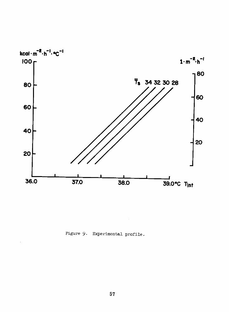
vasodilatory drive in a manner similar t o that in the c a s e of sweating. Figure 10
then shows the value of K for different values of central temperature and mean
skin temperature, with the local peripheral effect removed, again normalizing at
the skin temperature at thermal neutrality. It is then found that the slope of the
lines is 62 1 . m -2 . h -1 . OC-' if we equate a n increase of 1 Kcal . m -2 . h -1 . OC-l
in the conductance with at least 1 1 . h-l . m-2 increase in skin blood flow. It
then also follows that 1 OC change in mean skin temperature at constant internal -~
53

-2 -1 temperature results in about 4 1 . m . h change in skin blood flow. The
controller command then becomes: * *
DILAT = 1 17, ERROR (I) + 7.5 (WARMS - COLDS)
so that CDIL = 117.0, SDIL = 7.5 and PDIL = 0.0
It a l so becomes clear that the local effect causes a doubling or halving of
local blood flow for a 6OC change in local temperature, so that the local mul-
tiplier becomes: **
2 . 0 (ERROR ( N + 3 ) / 6.
The value for the central control coefficient CDIL of 117.0 is very close t o
one proposed in earlier reports and a l so compares with a value of about 90
proposed by Benzinger, et a l . (39 ) .
Control of Shivering
Shivering, although easi ly measured, is among the elusive physiological
responses since steady states are difficult t o obtain. However, a large number of
measurements all point t o the fact that b o t h s k i n temperature and internal tempwa-
ture must be below a certain threshold. Such measurements were made by Benzinger,
et al . (39) and by Nadel (40). Probably a s a result of differences in methods,
these authors find slightly different values for the threshold for the central and
mean skin temperatures. These authors, as do many others, report responses
which can consistently be predicted by a multiplicative expression.
in this laboratory have failed to give responses which were consistent enough to use
for quantitative extrapolation. One very consistent difference was found in that
for a given cold exposure women shivered earlier and to a much higher degree
Measurements
54

200
100
0 36.0 37.0 38.0
Figure 7. Output from the c e n t r a l c o n t r o l l e r .
55

-2 -1, kca1.m *h 100
80
60
40
20
7 80
- 60
- 40
- 20
36.0 37.0 38.0 39.OoC Tint
Figure 8. Plot of a number of experimental condi t ions.
56
loa
80
60
40
-
-
Ts 3432 30 28 - 80
-60
40
20
1
20
I I I I I I
37.0 38.0 39.OoC Tint 36.0
Figure 9 . Experimental prof i le .
57

than men, Women a l s o showed a more labile vasomotor response in heat and
cold and had a consistently lower CSW value than men, The latter difference
resulted in women reaching higher internal body temperatures during resting
heat exposure. A detailed report on these experiments is in preparation.
Benzinger, et al. (39 ) report results which would suggest that in the expression
for shivering control the following value should be used: * *
CHILL = 21.0 COLD (I) COLDS
which would result in the following control coefficients:
CCHIL = 0.0, SCHIL = 0.0 and PCHIL = 21.0.
Nadel's results would indicate a higher value for PCHIL in the range of 40.0, but
his measurements were short lasting and should, therefore, be approached with
more caution.
Control of Vasoconstriction
The type of vasoconstriction implied here is largely limited to the special
peripheral vascular beds in the hands and feet which normally have a high non-
nutritive blood flow which is highly sensit ive to both internal temperature and
mean skin temperature. In addition, there is a high sensitivity t o psychogenic dis-
turbances. A s the mean skin temperature decreases below normal, or as the central
temperature decreases below normal, constrictor tone in hands and feet increase.
Since this represents an increase in resistance, the calculated local blood flow is
reduced by dividing it by a value STRIC. In the absence of clear data, the following
expression is used t o define STRIC:
* STRIC = -5.0 (ERROR (I) + WARMS - COLDS).
58

& - I O . . . . . . . . . . . . . . . . . . . . . . . . . . . . . . . . . . . . . . . . . .
2 m m m ' m m m m,m m m m ' m m m m m m m m m m m m m m m m m m m m m m m m m m m m m m m l + a a w w w ' w w h h h h h h h h h h h h h h h h h h h h h h h w w w w w w w w a w w w
-
59

Performance of Model of Thermoregulation in Man at Rest
It is easily recognized that the model will reproduce the steady state thermo-
regulatory responses with acceptable accuracy since the control coefficients are
essentially based on steady state relationships. The best method of validation
then is t o reproduce a sudden change in conditions with the resultant dynamic
thermoregulatory response. In order t o do this, two specific experiments were
simulated which were a l s o evaluated with an earlier model (1). Young male sub-
jects were quickly transferred between two ambient temperatures: the ai r and
wall temperatures were equal, and the air velocities were minimal (i.e., 0.1 m/sec
or less). Average skin temperature, rectal temperature, tympanic membrane t em-
perature, rate of evaporative weight loss and metabolic rate were determined con-
tinuously. The experiments have been described in more detail before (10, 11).
Figure 10 shows an experiment in which the subject spent 30 minutes a t a thermally
neutral temperature, followed by 120 minutes a t an ambient temperature of 48"C,
and an additional 60 minutes of recovery in a 30°C environment. In each case,
the broken line represents the response predicted by the model, and the solid line
shows the experimental result, in measurements of rectal temperature, mean skin
temperature and sweat rate. The metabolic rate, during the whole experiment, stayed
in the range of 38 - 42 Kcal , m -2 -1 . h . The results predicted by the model are given in
more detail in Table 14 . The headings in Table 14 and other tables following after Table
14 are abbreviations for the following variables: TIME, in minutes; S: rate of heat
storage in Kcal. , m -2 . h - '; M: metabolic heat production in Kcal . m - 2 . h-l;
-2 EV: total evaporative heat l o s s in Kcal . m . h-l: TB: mean weighted body
temperature in "C; TS: mean weighted skin temperature in "C; TH: temperature of
the head core representing hypothalamic temperature in OC: T O temperature of
60

the central blood compartment, representing esophageal temperature in "C; TR:
trunk core temperature representing rectal temperature in OC; TM: temperature of
-1 the muscle compartment in the leg in OC; SBF: total skin blood flow in 1 . min ;
CO: estimated cardiac output in 1 . min '; COND: equivalent thermal conductance
from core t o skin, Kcal . m . h . OC : W E T : percentage of the skin surface
a s wetted area (13, 14) for the sweat rate and environmental conditions given.
- -2 -1 -1
In a different type of experiment, the subjects spent 60 minutes a t an en-
vironmental temperature of 43OC followed by 120 minutes at 17OC and a final 30
minutes at 43OC. Data and simulation of this experiment are given in Figure 11
and Table 15. In the experiment, the metabolic rate remained at near basal levels
and descended continuously from an initial 45 Kcal . m . h-l t o a final 36 Kcal
. m . h . It will be seen from Table 15 that in the simulation some shivering
started after about one hour in the cold, and it remained at one basal metabolic
rate through much of the remaining hour. In the experiment, there was a con-
tinuing negative heat storage of about 37 Kcal . m
hour. In the experiment, it was calculated that the total net heat loss during
the cold exposure amounted t o 92 Kcal , m
temperature, We have a l so observed that the model response to this regimen of
cold exposure is very close t o that shown consistently by women subjects.
- 2
- 2 -1
-2 -1 . h throughout that same
-2 or about a 2.6OC drop in mean body
61

O C
38
37
-30- I 48 I- 30 - Tambient
- - 0 - 4 c
I I I I I I I
U
I I I
0 30 60 90 120 I50 180 210min I I I I 1
90
70
50
30
IO
62
Figure 10. Experiment i n which subject spends 30 minutes a t thermally neut ra l temperature; I20 minutes a t ambient temperature of 48" C; and 60 minutes recovery i n 30" C environment.

0 0
c .- E 0 25
0 s
0 In -
0 fi
0 Q,
8
8
0
rl rl
63

64

Performance of Model of Thermorequlation in Man During Exercise
In order t o test the performance of the model in predicting the results of ther-
moregulatory s t ress resulting from internally produced heat during exercise, i t was
applied t o conditions for which experimental measurements were obtained. Mini-
mally dressed male subjects were seated on a bicycle ergometer, in an environ-
ment of 30°C at 30% relative humidity, with an air velocity of 10 c m . sec . Evaporative heat loss was determined by weight recording, and metabolic rate
through recording of oxygen consumption. Figure 12 shows the experimental re-
sults in solid lines, and the model predictions in broken lines. A more complete
tabulation of the model responses is given in Table 16. This experiment constitutes
a severe stress, and it requires well-trained individuals. Physically less f i t sub-
jects usually have t o terminate the experiment before the end of the heavy exercise,
During the final part of the heaviest exercise bout, the model estimates skin blood
flow at over 3 liters . min , and the percentage wetted area goes up t o 66%, both
these values are indices of thermal discomfort,
-1
-1
A comparison of an identical exercise experiment carried out a t an ambient
temperature of 20°C and the model prediction for the same condition is shown in
Figure 13, with more complete model predictions in Table 17.
Discussion of Model Performance, Short Comings and the Path for Improvement
Any model is by definition simpler than the system it attempts t o represent.
The structure and definition of a model is focused on certain characteristics or
conditions which are deemed of primary importance. In the manned space program,
the thermophysiological problems are mainly related t o prevention of hyperthermia
(Stolwijk (41) ). Both the experimental efforts and the emphasis of the model re-
ported on here were directed a t heat elimination. As can be seen in the previous
65

section, the model predicts with reasonable accuracy the dynamic thermoregulatory
responses to dynamic loads of ambient temperature and internal heat production
even during very heavy exercise. There are discrepancies of absolute value and
sometimes for short periods even of direction of change. Such discrepancies
are associated with two types of conditions: exposure t o thermal environments
in which cooling occurs, and during the onset of exercise. During prolonged
cooling, such as shown in Figure 11, between 60 and 180 minutes the core cools
more in the simulation than in the experiment, and consequently shivering is
initiated. The shivering causes perfusion of cold muscle with warm blood, and
a resultant further drop of core temperatures increases shivering even more.
Similarly in Figure 13 a t 3 5 minutes and again a t 9 5 minutes, there is a marked
drop of core temperature a t the onset of exercise, a l s o due t o perfusion of
relatively cold muscle with warmer blood.
Since each of the segments in the controlled system consists of only 4 layers,
there will be errors in the finite difference method of solution during the develop-
ment of new gradients in the relatively thick m u s c l e and core layers. During heat
s t ress , such errors are small because the gradients are relatively small, and con-
vective heat flow by the circulatory system is the major avenue of heat flow. During
cooling this convective heat transport largely disappears, gradients appear and
considerable errors can occur which tend to draw heat from the core in the model,
before this happens in the experiment. Such errors tend t o become smaller again as
a steady state is approached. It is obvious that a simple remedy is available which
consis ts of introducing additional layers in the controlled system. This method
was used by Wissler (42) and it provides improved performance during cold exposure.
66

The erroneous, rapid and transient drop in internal temperature a t the onset
of exercise in the model, especially after prolonged rest in a cool environment,
is probably the result of another simplification: immediately a t the onset of
exercise, the whole lumped mass of muscle in a given compartment is supplied
with a l l the blood required for oxygen transport. Two factors are probably
associated with the sudden drop in internal temperature. The present model
does not make allowance for the development or repayment of an oxygen debt, and
if such allowance were made it would tend to reduce the initial cooling of the blood
in the muscle. A second factor might be that in a given muscle compartment not
all muscles are likely to be active, so that those groups which are active warm
up faster and cause less initial blood cooling than now occurs in the model.
Since it is intended to combine the present model of thermoregulation with
simultaneous models of the cardio-vascular and the respiratory system, it is to
be expected that improvements in this particular idiosyncrasy of the present thermo-
regulation model will result.
67

kc
0 30 60 90 120 150 180 210 min
,m-'. h-'
400
300
200
100
0
Figure 12. Experimental r e s u l t s .
68

69

.c "'1 37
32
28
.*---
*- 'I ,' 'I," meat
min
Figure 13. Experimental model p r e d i c t i o n .
70

m . . . . . . . . . . . . . . . . . . . . . . . . . . . . . . . . . I . . . . . . , . . ~ ~ r l ~ r l o o m m m m ~ m o ~ ~ o ~ o m m ~ ~ ~ o r l r l ~ r l ~ o ~ r l ~ r l ~ ~ ~ ~ ~ r l ~ r l
m m m m m m c v ~ ~ w ~ ~ m m m m m m ~ ~ m m m m m m m m m m m m m m m m m m m m h m
w
71

REFERENCES
1. Stolwijk, J. A. J. and J. D. Hardy, Temperature regulation in man -
a theoretical study.
Yamamoto, W. S. and W. F. Raub, Models of the regulation of
PflGgers Arch. 291, 129-162 (1966).
2.
internal respiration in mammals. Problems and promises.
Computers and Biomet. Res. 1, 65-104 (1967).
3. Meeh, K., Oberflachenmessungen d e s menschlichen Korpers, J. Biol., I I II
- 15, 428-458 (1879).
4. DuBois , D. a n d E. F. DuBois. C l i n i c a l Calorimetry: Fifth pape r , The
measurement of surface area of'man. Arch. Intern. Med.,
15, 868-888 (1915).
5. Bradfield, H. S., The determination of surface area of women and its
use in expressing basal metabolic rate. Am. J. Physiol.,
82, 570-576 (1927).
6. Wilmer, H. A , , Changes in structural components of human body from
six lunar months to maturity. Proc. SOC. Exp. Biol. Med.,
- 43, 545-547 (1940).
7. Scammon, R. E., Developmental Anatomy& Schaeffer, J. P. (Editor)
Morris' Human Anatomy, 1 l th Ed., New York, McGraw Hill
(1953).
8. DuBois, D. and E. F. DuBois, Clinical Calorimetry: Tenth paper,
A formula t o estimate the approximate surface area i f height
and weight be known. Arch. Intern. Med., l7, 863-871 (1915).
72

REFERENCES
9.
10.
11.
1 2 .
13.
14.
15.
16.
Nishi, Y. and A. P. Gagge, Mean skin temperature for man weighted
by regional heat transfer coefficients. Fed. Proc. 2!3, 852
(1970).
Stolwijk, J. A. J. and J. D. Hardy. Partitional calorimetric s tudies of
responses of man to thermal transients. J. Appl. Physiol. ,
- 2 1 , 967-977 (1966).
Hardy, J. D. and J. A. J. Stolwijk, Partitional calorimetric s tudies of
man during exposures to thermal transients. J. Appl. Physiol. ,
- 21, 1799-1806 (1966).
Brebner, D. F., D. McK. Kerslake and J. L. Waddell, The relation
between the coefficients for heat exchange by convection
and evaporation by man. J. Physiol., 141, 164-168 (1958).
Gagge, A. P. , A new physiological variable associated with sensible
and insensible perspiration. Am. J, Physiol., 120, 277-287
(1937).
Gagge, A. P., J. A. J. Stolwijk and B. Saltin, Comfort and thermal
sensations and associated physiological responses during
exercise at various ambient temperatures. Environmental Research,
- 2 , 209-229 (1969).
Aschoff, Y. and R. Wever, Kern und Schale im W&-mehaushalt des Meuschen.
Naturwinenschaften, 45, 477-485 (1958).
Scheinburg, P., L. I. Blackburn, M. Rich and M. Saslaw, Effects of
vigorous physical exercise on cerebral circulation and
metabolism. Am. J. Medicine, l6, 549-554 (1954).
73

17.
18.
19.
20.
21.
22.
23.
24.
REFERENCES m
Behnke, A. R. and T. L. Willmon, Cutaneous diffusion of helium in
relation t o peripheral blood flow and absorption of
atmospheric nitrogen through the skin. Am. J. Physiol.,
- 131, 627-632 (1941).
Hertzman, A. B. and W. C. Randall, Regional differences in the basal
J. Appl. Physiol., and maximal rates of blood flow in the skin,
- 1, 234-241 (1948)
Cabanac, M., J. A. J , Stolwijk and J. D. Hardy, Effect of temperature
and pyrogens on single-unit activity i n the rabbit's brain
s t e m . J. Appl. Physiol., 24, 645-652 (1968).
Hellstrdm, B. and H. T. Hammel, Some characteristics of temperature
regulation in unanesthetized dog. Am. J. Physiol.,
- 213, 547-556 (1967)
Simon, E., W. Rautenberg, R. Thauer and M. Iriki, Die Ausl6sung von
Khez i t t e rn durch lokale KGhlung i m Wirbelkanal. PflGgers Archiv.,
- 281, 309-331 (1964).
W&nenberg, W. and K. BGck, Untersuchimgen cber die Funktionsweise
thermoreceptiver Strukturen i m Cervicalmark des Meerschweinchens . PflGgers Archiv., 294, 83 (1967).
Hensel, H., Electrophysiology of cutaneous thermoreceptors, In Skin senses , D. R. Kenshalo, Editor, Thomas, Springfield, Ill.,
(1968).
Bullard, R. W., M. R. Banerjee and B. A. MacIntyre, The role of the skin
in negative feedback regulation of eccrine sweating. Int. J.
Biometeor., ll, 93-104 (1967).
74

REFERENCES
25.
26.
27.
28.
29.
30.
31,.
32.
Rawson, R. 0. and K. P. Quick, Evidence of deep-body thermoreceptor
response to intra-abdominal heating of the ewe. J. Appl.
Physiol., 28, 813-820 (1970).
Wood, J. D. , Electrical activity from single neurons in Auerbach's
plexus. Am. J. Physiol., 219, 159-169 (1970).
Robinson, S., F. R. Meyer, J. L. Newton, C. H. TS'ao and L. 0.
Holgersen, Relations between sweating, cutaneous blood
flow and body temperature in work. J. Appl. Physiol., 20,
575-582 (1965).
Bader, M. E. and M. B. Macht, Indirect peripheral vasodilatation
produced by warming of various body areas. J. Appl. Physiol. ,
- 1, 215-226 (1948).
Randall, W. C., Quantitation and regional distribution of sweat glands
in man. J. Clin. Invest., 25, 761-767 (1946).
Stolwijk, J. A. J. , B. Saltin and A. P. Gagge, Physiological factors
associated with sweating during exercise. J. Aerospace Med.,
- 39, 1101-1105 (1968).
Bishop, J. M., K. W. Donald, S. H. Taylor and P. N. Wormald,
Changes in arterial hepatic venous oxygen content difference
during and after supine leg exercise. J. Physiol., 137, 309-317
(1957).
Bucht, H., J. Ek, H. Eliasch, A. Holmgren, B. Josephson and L. Werko,
The effect of exercise in the recumbent position on the renal
circulation and sodium excretion in normal individuals. Acta
Physiol. Scand., 28, 95-100 (1953).
75

REFERENCES
133 33. Grimby, G. E., E. Haggendahl and B. Saltin, Local Xenon
clearance from the quadriceps muscle during exercise
in man. J. Appl. Physiol., 22, 305-310 (1967).
34. Saltin, B., G. Blomquist, J. H. Mitchell, R. Johnson, Jr.,
K. Wildenthal and C. D. Chapman, Response to submaximal
and maximal exercise after bed rest and training.
Circulation, 38, Suppl. 7, 1-78 (1968).
35. Saltin, B., A. P. Gagge and J. A. J. Stolwijk, Muscle temperature
during submaximal exercise in man. J. Appl. Physiol., 25,
679-688 (1968).
36. Webb-Peploe, M. M. and J. T. Shepherd, Peripheral mechanism
involved in response of dogs' cutaneous veins to local tem-
perature change. Circulation Res., 23, 701-708 (1968).
37. Wurster, R. D. and R. D. McCook, Influence of rate of change of
skin temperature on sweating. J. Appl. Physiol. 27, 237-240 (1969).
38. Nadel, E. R., R. W. Bullard and J. A. J. Stolwijk, Sensitivity to rate
of change in skin temperature in the regulation of sweating.
m . s . to be submitted. (1970).
39. Benzinger, T. H. , C. Kitzinger and A. W. Pratt, The Human Thermostat
- in Temperature - its measurement and control in science and industry,
vol. 3, J. D. Hardy, Editor, p 637-665, Reinhold, New York (1963).
76

REFERENCES
40. Nadel, E. R., The role of peripheral thermoreceptors in the integrated
thermoregulatory response in resting and exercising man.
Dissertation, Univ. Cal i f . , Santa Barbara (1969).
41. Stolwijk, J. A. J . , Thermal loads in lunar ambulation. Aerospace
Medicine (in press) (1970).
42. Wissler, E. H. , A mathematical model of the human thermal system.
Bull. Math. Biophysics, 26, 147-166 (1964).
NASA-Langley, 1971 - 4 CR-1855 77