NBER WORKING PAPER SERIES

INCREASING TIME TO BACCALAUREATE DEGREE IN THE UNITED STATES

John BoundMichael F. Lovenheim

Sarah Turner

Working Paper 15892http://www.nber.org/papers/w15892

NATIONAL BUREAU OF ECONOMIC RESEARCH1050 Massachusetts Avenue

Cambridge, MA 02138April 2010

We would like to thank Paul Courant, Harry Holzer, Caroline Hoxby, Tom Kane, and Jeff Smith forcomments on an earlier draft of this paper, Charlie Brown, John DiNardo and Justin McCrary forhelpful discussions and N.E. Barr for editorial assistance. We also thank Jesse Gregory and CaseyCox for providing helpful research support. We have benefited from comments of seminar participantsat NBER, the Society of Labor Economics, the Harris School of Public Policy, the Brookings Institution,Stanford University and the University of Michigan. We would like to acknowledge funding duringvarious stages of this project from the National Science Foundation, National Institute of Child Healthand Human Development, the Andrew W. Mellon Foundation, and the Searle Freedom Trust. Muchof this work was completed while Bound was a fellow at the Center For Advanced Study in the BehavioralSciences and Lovenheim was a fellow at the Stanford Institute for Economic Policy Research. Theviews expressed herein are those of the authors and do not necessarily reflect the views of the NationalBureau of Economic Research.

NBER working papers are circulated for discussion and comment purposes. They have not been peer-reviewed or been subject to the review by the NBER Board of Directors that accompanies officialNBER publications.

© 2010 by John Bound, Michael F. Lovenheim, and Sarah Turner. All rights reserved. Short sectionsof text, not to exceed two paragraphs, may be quoted without explicit permission provided that fullcredit, including © notice, is given to the source.

Increasing Time to Baccalaureate Degree in the United StatesJohn Bound, Michael F. Lovenheim, and Sarah TurnerNBER Working Paper No. 15892April 2010JEL No. I2,I21,I23

ABSTRACT

Time to completion of the baccalaureate degree has increased markedly in the United States over thelast three decades, even as the wage premium for college graduates has continued to rise. Using datafrom the National Longitudinal Survey of the High School Class of 1972 and the National EducationalLongitudinal Study of 1988, we show that the increase in time to degree is localized among those whobegin their postsecondary education at public colleges outside the most selective universities. In addition,we find evidence that the increases in time to degree were more marked amongst low income students.We consider several potential explanations for these trends. First, we find no evidence that changesin the college preparedness or the demographic composition of degree recipients can account for theobserved increases. Instead, our results suggest that declines in collegiate resources in the less-selectivepublic sector increased time to degree. Furthermore, we present evidence of increased hours of employmentamong students, which is consistent with students working more to meet rising college costs and likelyincreases time to degree by crowding out time spent on academic pursuits.

John BoundDepartment of EconomicsUniversity of MichiganAnn Arbor, MI 48109-1220and NBERjbound@umich.edu

Michael F. LovenheimCornell University103 MVR HallIthaca, NY 14853mfl55@cornell.edu

Sarah TurnerDepartment of EconomicsUniversity of Virginia249 Ruffner HallCharlottesville, VA 22903-2495and NBERsturner@virginia.edu

Page 1

Over the past three decades, the share of BA degree recipients that graduate within four

years has decreased and, more generally, the length of time it takes college students to attain

degrees has increased. This shift, which may involve substantial costs for students in terms of

foregone earnings and additional tuition expenditures, has drawn increased public policy

attention. 1 Among researchers, however, the length of time to collegiate degree attainment has

received little attention.

In this paper, we examine how time to completion of the baccalaureate degree (BA) has

changed in the past three decades by comparing outcomes for two cohorts from the high school

classes of 1972 and 1992 using data from the National Longitudinal Study of 1972 (NLS72) and

the National Educational Longitudinal Study of 1988 (NELS:88). We find evidence of large

aggregate shifts in time to degree: in the 1972 cohort, 58% of eventual BA degree recipients

graduated within four years of finishing high school, but for the 1992 high school cohort only

44% did so. This extension of time to degree, and the associated reduction in “on-time” degree

completion, did not occur evenly over the different sectors of higher education. Time to degree

increased mostly among students beginning college at less selective public universities as well as

at community colleges. We further document that increased time to degree does not reflect more

human capital accumulation among students; rather, students are accumulating college credits

more slowly.

Our objective in this paper is to assess competing explanations for the observed increases

in time to degree in the context of available evidence. One hypothesis is that aggregate increases

in time to degree reflect increased college completion among students with relatively low levels of

pre-collegiate preparedness who were induced to attend by greater economic rewards and require

1 To underscore this point, twelve states recently conducted studies of elongating time to degree in the

public postsecondary system, and California and Colorado passed legislation to attempt to curb time to degree increases.

Page 2

a somewhat longer period of enrollment to finish degree requirements. Alternative explanations

consider how resources from public sources and those required from students and families change

to affect degree progression. To the extent that some colleges and universities experienced

reductions in resources per student, the rate of degree progression may decline as students find

increased barriers to attaining the credits required for graduation. In addition, rising net costs of

college may have increased challenges to individuals in financing full-time enrollment and, in

turn, slowed the rate of degree attainment to the extent that employment crowds out credit

attainment.

Strikingly, we find no evidence that changing student preparedness for college or student

demographic characteristics can explain any of the time to degree increases. Indeed, the

observable characteristics of college graduates, including high school test scores, have become

more favorable in terms of predicted time to degree across cohorts. In contrast, we find evidence

that decreases in institutional resources at public colleges and universities are important for

explaining changes in time to degree. With a significant link between institutional resources, such

as student faculty ratios, and time to degree, the declines in resources per student at public sector

colleges and universities predict some of the observed extension of time to degree. In addition,

the dramatic rise in student employment and the comparatively large increase in time to degree

among students from lower-income families are suggestive of a relationship between increased

difficulties students have in financing college and increasing time to degree. Our results also

highlight increased stratification in the higher education market: students attending less-selective

public-sector institutions and students from below-median family income are most likely to

experience increases in degree time.

Page 3

We employ a diverse set of micro data and institutional information to assess these

explanations. While we lack an unassailable natural experiment or regression evidence to provide

definitive evidence for the causal inferences we make, our findings describe compelling

proximate explanations for the observed increase in time to degree. Our results also show clear

increases in stratification of time to degree across sectors of higher education and by socio-

economic circumstances. In effect, reductions in public subsidies and increased costs of

collegiate attainment concentrated among poorer students attending public colleges and

universities have had material effects on the rate of collegiate attainment.

The rest of this paper is organized as follows: Section 1 describes the increase in time to

degree found in the data. Section 2 outlines the potential explanations for these trends that inform

our empirical analysis. Section 3 describes our data, and Section 4 presents our empirical

approach and the results from our empirical analyses. Section 5 concludes.

Section 1. Increased Time to Degree

Evidence of increased time to college degree conditional on graduating can be found in a

range of data sources. The Current Population Survey (CPS) provides a broad overview of trends

in the rate of collegiate attainment by age (or birth cohort). While the share of the population with

some collegiate participation increased substantially between the 1950 and the 1975 birth cohorts,

the share obtaining the equivalent of a college degree by age 23 increased only slightly over this

interval, as shown in Figure 1. Extending the period of observation through age 28, however,

shows a more substantial rise in the proportion of college graduates among recent birth cohorts.2

Taken together, the inference is that time to degree has increased.

2 Data from cross-sections of recent college graduates assembled by the Department of Education from the

Recent College Graduates and Baccalaureate & Beyond surveys corroborate this finding. For example, from 1970

Page 4

1.1. Time to Degree in NLS72 and NELS:88

To measure changes in time to degree in connection with micro data on individual and

collegiate characteristics, this analysis uses the National Longitudinal Study of the High School

Class of 1972 (NLS72) and the National Educational Longitudinal Study (NELS:88). These

surveys draw from nationally representative cohorts of high school and middle school students,

respectively, and track the progress of students through collegiate and employment experiences.

To align these surveys, we focus on outcomes within eight years of high school graduation among

those who entered college within two years of their cohort’s high school graduation.3 We measure

time to degree in each survey as the number of years between cohort high school graduation and

BA receipt.4 These micro-level surveys afford two principal advantages over the CPS. First, the

data include measures of pre-collegiate achievement, which allow us to analyze the

the relationship between time to degree attainment and pre-collegiate academic characteristics.

to 1993, the share of graduates taking more than six years rose from less than 25% to about 30%, while the share finishing in four years or less fell from about 45% of degree recipients in 1977 to only 31% in the 1990s (see McCormick and Horn, 1997 and Bradburn et al., 2003). In careful descriptive work, Adelman (2004) uses data from the NLS72 and NELS:88 cohorts to trace college completion and time to degree. Although he uses a slightly different sample and defines the timing of college entry differently than in our analysis, he also shows time to degree increased across these cohorts, from 4.34 years to 4.56 years.

3 Cohort high school graduation is June 1972 for NLS72 respondents and June 1992 for NELS:88 respondents. We define time to degree as the elapsed time from high school cohort graduation. An alternative would have been to measure time to degree from the point of college entry. The results are not sensitive to this choice and, with the NELS:88 cohort only followed for eight years after high school graduation, our approach affords eight years of post-high school observation for both cohorts. While we measure time to degree from cohort high school graduation, the sample includes those who do not graduate high school on time. Because the NLS72 survey follows a 12th grade cohort and the NELS:88 survey follows an 8th grade cohort, there are more late high school completers in the latter sample. However, when one conditions on college completion within eight years, over 99% of respondents finish high school on time in both samples.

4 Because the last NELS:88 follow-up was conducted in 2000, we are forced to truncate the time to degree distributions at eight years, reflecting the time between cohort high school graduation and the last follow-up. We are therefore truncating on a dependent variable, which may introduce a bias into our analysis if the truncation occurs at different points in the full time to degree distribution for each of the two cohorts. Empirically, the proportion of eventual college degree recipients receiving their degrees within eight years has not changed appreciably. The National Survey of College Graduates (2003) allows us to examine year of degree by high school cohort. For the cohorts from the high school classes of 1960 to 1979 for which there are more than 20 years to degree receipt, we find the share of eventual degree recipients finishing within eight years holds nearly constant at between 0.83 and 0.85. Focusing on more recent cohorts (and, hence, observations with more truncation) we find that in the 1972 high school graduating cohort, 92.3% of those finishing within twelve years had finished in eight years, with a figure of 92.4% for the 1988 cohort. This evidence supports the assumption made throughout this analysis that the eight-year truncation occurs at similar points in the time to degree distribution in both surveys.

Page 5

Second, these data identify the colleges attended by students, permitting us to analyze outcomes

for different sets of collegiate characteristics.

In Table 1, we show the cumulative share of BA recipients who attained their degree in

years four through eight beyond their cohort’s high school graduation. A significant shift in time

to degree among BA recipients is evident across the two cohorts. Mean time to degree increased

from 4.69 to 4.97 years. In addition, not only did the proportion finishing within four years

decline by a statistically significant 14.2 percentage points (or 24.6%), but the entire distribution

shifted outward.

Higher education in the United States is characterized by substantial heterogeneity across

institution types. To capture this heterogeneity and examine changes across the spectrum of higher

education institutions, we categorized the first colleges and universities attended by BA recipients

into five broad sectors:5 non-top 50 ranked public universities, top 50 ranked public universities,

less selective private schools, highly selective private schools, and community colleges.6 Table 1

presents cumulative time to degree distributions by these sectors and shows that the elongation of

time to degree is far from uniform across types of undergraduate institutions. Extensions are

pronounced in the non-top 50 public sector, in which the likelihood of a BA recipient graduating

within four years dropped from 55.5% to 34.7%, a statistically significant decline of 20.8

percentage point (or 37.5%), and – as with the full sample – the proportion graduating within each

5 We use the 2005 U.S. News and World Report undergraduate college rankings to classify institutions into

these 5 categories. The highly selective 4 year private schools are the top 65-ranked private universities and the top 50 private liberal arts schools. Less selective 4 year private schools are all other private universities. Highly selective private schools and top-50 public schools are listed in Appendix Table A-2. While admittedly crude, this breakdown correlates well with several measures of quality, such as average SAT scores and high school GPAs. Other metrics, such as resources per student or selectivity in undergraduate admissions, give similar results.

6 All references to two-year schools and community colleges refer to public institutions only. We exclude private two-year schools as they are often professional schools with little emphasis on eventual BA completion. In both cohorts, only a very small fraction of eight-year BA recipients first attended a private two-year school.

Page 6

subsequent time frame also declined significantly. Mean time to degree consequently increased in

the non-top 50 public sector, from 4.71 to 5.08 years.

The time-to-degree increases were even more dramatic for BA recipients whose first

institution was a community college. Degree recipients beginning in this sector experienced a 24

percentage point decline in the likelihood of completion within four years, a 23.5 percentage point

decline in completion within five years, and a 0.7 year increase in mean time to degree. In the

NELS:88 cohort, less than 17% of BA recipients who started at a community college earned their

degree within four years.

In the top-50 public sector, while the share of degree recipients finishing within four years

declined, the share finishing within five years does not. Mean time to degree increased negligibly

as well. We also find little evidence of time to degree increases in the private sector. While the

likelihood of graduating within four years dropped by 7.9 percentage points in the less selective

private sector, this is only an 11.3% decline. Mean time to degree also increased by 0.13 years, or

2.9%. In the elite private sector, time to degree declines, although the standard errors are

relatively large due to small sample sizes.

Table 1 illustrates one of the central descriptive findings of this analysis: time to degree

has increased most dramatically across surveys among students beginning their studies at less-

selective public schools and the community colleges. Unlike the case with completion rates,

where women exhibited no change and men’s likelihood of completion declined substantially

(Bound, Lovenheim and Turner, forthcoming), time to degree for women and men changed very

similarly in most sectors, particularly in percentage terms.7

1.2. Credit Attainment

7 Separate results by gender are available from the authors upon request.

Page 7

Given observed increases in time to degree, it is natural to ask whether these changes

reflect increased difficulty in passing through the course sequences or increased course taking. At

the extreme, if increased time to degree primarily captured increased attainment in the form of

course credits, then policy concern over the effects of time to degree might be misplaced. With

access to transcript data, we are able to chart the time path of credit accumulation. For students at

four-year public institutions outside the top 50 as well as those at community colleges, we find a

slower pace of credit accumulation in the 1992 cohort relative to the 1972 cohort; although

students in both cohorts accumulated a similar number of credits after eight years, students in the

1992 cohort took longer to do so. For example, students starting at non-top 50 public schools in

the later cohort accumulated, on average, about 9.7 fewer credits within four years of high school

graduation than did their counterparts in the 1972 cohort. After four years, the credit gaps track

the time to degree gaps from Table 1 closely within each school type.8

We also explored cross-cohort differences in the ratio of attempted credits to accumulated

credits. The modest increase we found in this ratio suggests attempted credits did not rise

appreciably over the period and are not large enough to explain much of the increase in time to

degree. We also considered double majoring, which could increase time to degree without altering

the total number of accumulated credits. However, double majoring is too low in the sectors that

experienced increased time to degree to explain a significant portion of the phenomenon.9 Finally,

we considered the possibility that students may be taking more difficult courses in areas such as

mathematics and science and reducing the number of courses they take per term to better their

chances of success in such classes. Using the course-level transcript files from the NELS:88 and

8 Appendix Figure B-1 shows the cumulative distribution of credits by type of institution. Similar patterns

emerge from other measures of the distribution of credits. 9 Using counts of double majors in the IPEDS survey, we find that double majoring is reasonably common

in the private and top 50 public universities, but quite uncommon for students graduating from non-top 50 public schools.

Page 8

NLS72 transcript studies, we find no large changes in course-taking behavior or majors across

fields that could explain the time to degree increases we document.

With no supporting evidence of greater credit accumulation to suggest a link between

time to degree and human capital accumulation, we interpret observed increases in time to degree

as a reduction in the rate of human capital accumulation rather than an increase in the amount of

human capital, with this change concentrated outside the top public schools and private

institutions. We now turn to explanations of why time to degree has shifted in the manner

observed in the data.

Section 2. Potential Explanations for Increased Time to Degree

There are multiple theoretically plausible explanations for the observed changes in time to

degree, and we consider these explanations as a framework for guiding our empirical approach

and interpreting our results. Note that ceteris paribus, an increase in the returns to education,

which raises the opportunity cost of time spent in school, will reduce time to degree. Explanations

that can account for a rise in time to degree during a period of increasing returns to education

include shifts in student demand, reflecting the rate at which students choose to complete courses,

and changes in the supply-side of the higher education market. We focus on three explanations:

first, increased enrollment among students less academically prepared for college who may

require a longer time to obtain a BA may shift outward average time to degree by changing the

composition of the student body; secondly, decreases in collegiate resources per student may

extend time to degree through, for example, reductions in course offerings needed for degree

progress; and, third, increases in the direct cost of education may lead students to increase

employment and reduce the rate of credit accumulation.

Page 9

Demand-side explanations for increased time to degree are driven by the changing

characteristics of the student body: increasing returns to education since the 1980s have,

presumably, resulted in higher enrollment among less-prepared students. Increasing returns to

college only will increase time to degree in the aggregate if the number of marginal students

induced to attend and complete college is large relative to the effect of rising returns on

inframarginal students.

A second type of explanation for increases in time to degree looks to changes on the

supply-side of the market that reduce per-student resources at the collegiate level. Because state

subsidies are a significant component of the resources available to public colleges and

universities, changes in student demand that are not accompanied by adjustments in public

funding lead to dilution of resources per student. Bound and Turner (2007) examine variation in

student demand generated by changes in cohort size and find evidence that public colleges and

universities do not fully offset changes in student demand with more resources. However, they

also find that public colleges and universities adjust to demand increases in somewhat different

ways across the strata of higher education. Top-tier public and private schools make few

adjustments in degree (or enrollment) outcomes in response to demand shocks. To the extent that

these institutions use selectivity in admissions to regulate enrollment, it is likely time to degree is

unchanged, or, perhaps, even decreases, with increased demand. In contrast, enrollment is

relatively elastic among public universities outside of the most selective few. Here, we expect

increased demand to lead to reductions in resources per student, because the increased enrollment

is not met with a commensurate increase in appropriations from public sources and other non-

tuition revenues.

Page 10

One of the potential mechanisms through which increased enrollment leads to increased

time to degree in the most elastic sectors is “crowding,” which is manifested by queuing and

course enrollment constraints in response to limited resources.10 Students in a large cohort that

cannot be accommodated fully by the university face an increased cost to obtaining the requisite

number and distribution of courses to earn a degree. It is straightforward to see how such

institutional barriers lead to delays in degree progress.

Increases in collegiate demand therefore can affect the supply-side of higher education and

the rate of collegiate attainment by reducing resources per student in the public sector, particularly

at open-access four-year institutions and community colleges. Because these institutions are

unable to adjust fully to demand shocks, the sectors absorbing the bulk of the students will

experience a reduction in resources. The result is increased stratification of resources across the

sectors of higher education in the United States, which we would expect to produce the patterns of

time to degree shifts we observe in the NLS72 and NELS:88 data.

The final potential explanation for expanding time to degree we will consider is increased

student labor supply, which may be a response to increased difficulty in paying for college in the

presence of rising direct college costs and falling real family incomes in the lower portion of the

income distribution. With increases in college costs, individuals will respond by decreasing

current consumption, working more hours and borrowing more. The presence of liquidity

constraints limiting individuals’ capacity to fully finance college investments exacerbates

increases in student employment. As result, if students are induced to work more hours while in

college to finance attendance, academic pursuits may be crowded out by work time, thereby

10 Queuing and shortages of courses may result from the absence of adjustments in tuition and enrollment at

public universities when appropriations per student decrease. Because public colleges and universities are insulated from some competitive pressures, it also is possible that some of the queuing on the supply-side is indicative of the failure of public institutions to reallocate resources in response to changes in demand (Smith, 2008).

Page 11

increasing time to degree. For example, students may enroll part-time, or have less time to

study.11 In the context of the Becker-Tomes (1979) model of intergenerational transfers (see also

Solon, 2004 and Brown, Mazzocco, Scholz, and Seshadri, 2006), rising tuition charges and falling

family income lead to the expectation that students will shoulder a higher fraction of college costs.

With relatively modest availability of federal aid and limited institutional financial aid funds

outside the most affluent colleges and universities, students from low and moderate income

families may face considerable borrowing constraints (e.g., Ellwood and Kane, 2000; Belley and

Lochner, 2007; Lovenheim, 2009).12 As such, rising college costs may increase the incidence of

employment while in school.13

One point of distinction across the sectors of higher education is the extent to which

institutions charge tuition per course or per term.14 Where institutions charge per credit hour, the

tuition costs associated with increased time to degree will be substantially smaller than where

institutions charge by the term. When we split our sample according to the pricing structure of

11 Stinebrickner and Stinebrickner (2003) present evidence from a natural experiment at Berea College that

students who work more do worse academically. 12 In addition, Brown, Scholz and Seshadri (2009) show that many students are credit constrained because

their parents do not provide the expected family contribution assumed in financial aid calculations. As tuition rises, such students are likely to be the most affected by financial constraints. Unfortunately, we lack information on parental transfers to children in order to test how this constraint impacts time to degree.

13 Keane and Wolpin (2001) show that, in a forward-looking dynamic model with limited access to credit, increases in employment while enrolled in school are the expected response to tuition increases. An alternative reason for students working while in school is that there is a potential post-graduation return to this employment experience (Light, 2001). For example, working for a professor may teach valuable skills or generate a strong and credible reference letter. However, the majority of jobs held by college students are in the trade and service sectors of the economy, such as working as a waiter or waitress (Scott-Clayton, 2007). While such jobs may enhance soft skills, there are likely decreasing returns to work experience in these sectors.

14 Examples of institutions with this type of “fixed term” pricing structure include many residential private institutions such as Princeton, Harvard, Amherst, and Williams and selective public universities like the University of Virginia. Institutions serving constituencies focused on full-time residential undergraduates are much more likely to post “flat fee” tuition schedules, while those with many working and adult students tend to offer pricing per credit hour. Looking at tuition structures offered by public four-year colleges and universities in 1992, more than 52% report a per credit pricing system. Yet, among the more selective top-15 public institutions, only 1 institution reported tuition on a per credit basis. While historical trends in tuition structure are difficult to find nationally, we collected information from Michigan, California, and Virginia for all public universities going back to the 1970s. The data suggest the structure of tuition is remarkably stable within institution with respect to charging per term or per credit hour.

Page 12

tuition rather than by the quality rank of the institution, we find only modest increases have

occurred at institutions that charge by the term, with the bulk of the increases occurring at schools

that charge by the unit.15 Thus, differences across institutions in terms of pricing structures might

partially explain the cross-sectoral patterns we observe in time to degree changes. Still, since

pricing structure has not changed notably over the last 40 years, these differences cannot explain

why time to degree has increased so dramatically at public colleges and universities outside the

top tier.

Section 3. Data

3.1. Student Attributes from the NLS72 and NELS:88 Surveys

The NLS72 and NELS:88 datasets we use contain a rich set of student background

characteristics. The student attributes we analyze are high school math test percentile,16 father’s

education level, mother’s education level, real parental income levels, gender, and race. The

NLS72 and NELS:88 datasets contain a significant amount of missing information brought about

by item non-response. While a small share of observations is missing multiple variables, a

substantial number of cases are missing either test scores, parental education or parental income.

15 At all public fixed-fee institutions, the proportion of graduates who obtain a BA within 4 years decreased

from 56.5% to 48.7%, but within the institutions that charge by the credit hour, the four-year completion rate dropped from 52.7% to 35.4%. It is important to note the pricing structures of universities are often complex and contain aspects of both fixed and hourly pricing. While this simple breakdown is suggestive that the predominant pricing system is correlated with the increases in time to degree observed in the data, pricing structure also is correlated with other institutional attributes, such as the availability of financial aid and the degree of commitment to open access admission policies.

16 The math test refers to the NCES-administered exams that were given to all students in the longitudinal surveys in their senior year of high school. Because the tests in NLS72 and NELS:88 covered different subject matter, were of different lengths, and were graded on different scales, the scores are not directly comparable across surveys. Instead, we construct the percentile of the score distribution for each test type and for each survey. The comparison of students in the same test percentile across surveys is based on the assumption overall achievement did not change over this time period. This assumption is supported by the observation that there is little change in the overall level of test scores on the nationally-representative NAEP over our period of observation. Similarly, examination of time trends in standard college entrance exams such as the SAT provides little support for the proposition that achievement declined appreciable over the interval within test quartiles.

Page 13

We use multiple imputation methods (Rubin, 1987) on the sample of all high school graduates to

impute missing values using other observable characteristics of each individual.17 The Data

Appendix (Appendix A) provides a detailed description of the construction of the analysis data

set.18

Table 2 presents means of selected observable characteristics for the sample of

respondents who obtain a BA within eight years of cohort high school graduation in the two

surveys overall and for each type of institution. Means of the full set of variables used in our

analysis are shown in Appendix Table B-1. Table 2 shows clearly that there has been no aggregate

reduction in academic preparedness among college graduates over time, as measured by math test

percentiles.19 Indeed, in all sectors except community colleges, math test percentiles actually

increased among college graduates across cohorts. The increased demand for higher education

that took place across surveys did not translate into reductions in math test scores among

graduates for two reasons. First, enrollment increases occurred across the distribution of academic

preparation, muting the impact that the increased demand for higher education had on the average

preparedness of college students.20 Second, the less prepared students induced to attend college

had very low completion rates, both because they disproportionately attended sectors in which

completion rates are low and because they were not well prepared for college (Bound, Lovenheim

17 Under the assumption that the data are missing conditionally at random, multiple imputation is a general

and statistically valid method for dealing with missing data (Rubin, 1987; Little, 1982). The relative merits of various approaches for dealing with missing data have been widely discussed (e.g. Little and Rubin, 2002; Schafer, 1997). See the Data Appendix for complete details of the imputation procedure. Because the surveys contain good supplementary predictor variables, such as high school GPA, standardized test scores from earlier survey waves, and parental income reports, we are able to use a great deal of information about each respondent to impute ranges of missing data points.

18 The data we use are almost identical to those used in Bound, Lovenheim and Turner (forthcoming), distinguished only by the restriction of the sample to eight-year college graduates in this analysis.

19 Reading test percentiles exhibit similar trends. We exclude these from our analysis because conditional on math test percentiles, reading test percentiles add no further predictive power in our empirical models. Results using reading test percentiles are available upon request.

20 In Bound, Lovenheim and Turner (forthcoming), we present evidence suggesting that, if anything, the preparedness of students entering four year schools actually increased between 1972 and 1992. The bulk of the marginal students attended two year schools.

Page 14

and Turner, forthcoming). As a result, changes in academic preparedness among graduates go in

the wrong direction to explain an overall lengthening of time to degree in all but the community

college sector. Furthermore, Table 2 shows that the both the educational attainment and real

income of parents increased for college graduates. These shifts are in the direction of shortening

time to degree, all else equal.

3.2. Supply-side Variables

Across the two cohorts, there was a sizeable change in where BA recipients first attend

college. As shown in Table 2, the proportion of graduates entering at community colleges

increased from 12.5 to 16.8%. In addition, graduates from non-top 50 public universities declined

10.6 percentage points, with consequent increases in the private and top-50 public sectors. Despite

the increase in graduates entering in community colleges, that the distribution of initial school

types shifted towards sectors with lower time to degree suggests changes in initial institution can

explain at most a small proportion of the aggregate time to degree increases evident in the data.

Our direct measure of institutional resources is student-faculty ratios, calculated from the

1972 Higher Education General Information System (HEGIS) survey and the 1992 Integrated

Postsecondary Education Data System (IPEDS) survey. Table 3 contains means and distributions

of student-faculty ratios for our sample of eight-year BA recipients. Overall, student-faculty ratios

increased (i.e., per-student resources decreased) across the two cohorts, from 25.5 to 29.8. While

these increases occurred throughout the student-faculty ratio distribution, they are largest at the

top of the distribution, suggesting an increased stratification of resources over time.

The remaining panels of Table 3 show student-faculty ratios by school type. The increases

have been most dramatic in the sectors that experienced the largest time to degree increases: non-

top 50 public schools and community colleges. In the elite public and private schools, student-

Page 15

faculty ratios actually decreased. These tabulations present further evidence that resources not

only have declined overall but have become more stratified over time across higher education

sectors. They also are suggestive of a role for institutional resources in explaining increasing time

to degree.

The final columns of Table 3 show median student-related expenditures per student and

subsidies per student, measured as the difference between student-related expenditures and net

tuition revenues. Median expenditures per student increased slightly overall across the institution

of first attendance among BA recipients, yet this modest gain combines declines in the public

sector with increases in the private sector, most notably among the most selective privates where

expenditures increased by about 37%. In the public sector, subsidies per student fell, reflecting

declining state support. That tuition also increased at these institutions points to a shift from

public sector funding to student funding in financing higher education. In the private sector, by

contrast, the subsidy component rose somewhat. These calculations echo other findings of a

divergence between the public and private sector and the more general increased stratification in

the higher education market. Kane, Orszag and Gunter (2003) document how declines in state

appropriations led to declines in spending per student at public schools relative to private schools,

with the ratio of per-student funding dropping from about 70% in the mid-1970s to about 58% in

the mid-1990s. In addition, Hoxby (2009, 1997) shows that tuition, subsidies, and student quality

have stratified dramatically across the 1962 quality spectrum of higher education since that time.

Section 4. Empirical Methodology and Results 4.1. Changing Student Attributes, Institution Type and Student-Faculty Ratios

We first examine whether changes in observed student background characteristics, student

preparedness for college (as measured by math test percentiles), and institutional characteristics

Page 16

such as institution type and student-faculty ratios can explain the observed shifts in the time to

degree distribution. An ordered logit analysis of time to degree on these variables is suggestive of

an important role for student preparedness and institutional resources. Both overall and within

collegiate sector, a student’s math test percentile has a negative and statistically significant effect

on time to degree. Furthermore, in the non-top 50 public sector, student-faculty ratios are strongly

positively related to time to degree.21

Given these cross-sectional relationships, we examine how changes in observable pre-

collegiate characteristics of students and the characteristics of the universities they attend relate to

changes in time to degree. Our approach is similar to the Blinder-Oaxaca decomposition in that

our objective is to determine the extent to which changes in the distribution of observable student

and collegiate attributes can explain the observed changes in the distribution of time to degree.

We re-weight the NELS:88 time-to-degree distribution using the characteristics of students and

the first post-secondary institution they attend from the NLS72 survey.22 This calculation leads to

a counterfactual time-to-degree distribution in which the proportion of students with a given

characteristic or a given set of characteristics has not changed between the two surveys. By

comparing the observed NELS:88 outcomes and the re-weighted NELS:88 outcomes, we can

determine the proportion of the observed change that is due to changes in the mix of students with

a given set of attributes attending college. The remainder reflects changes in other determinants of

time to degree as well as changes over time in how characteristics affect time to degree. What we

21 For example, a 10 point increase in math test percentiles is associated with a 0.064 year decline in mean

time to degree overall and a 0.057 decline in mean time to degree in the non-top 50 public sector. A 10% increase in student-faculty ratios implies a 0.014 year increase in overall time to degree and a 0.059 year increase in time to degree in the non-top 50 public sector.

22 Re-weighting and matching estimators have a long history in statistics dating back at least to the work of Horvitz and Thompson (1952) and have become increasingly popular in economics (see, for example, DiNardo, Fortin and Lemieux , 1996; Heckman, Ichimura and Todd , 1997 and 1998; and Barsky, Bound, Charles and Lupton, 2002). One advantage of these methods over standard regression methods is that they allow researchers to examine distributions, not just means.

Page 17

are estimating is the change in time to degree conditional on various observable characteristics,

integrated over the distribution of characteristics (see Barsky, Bound, Charles and Lupton (2002)

for a further discussion).

We generate weights by estimating logistic regressions of a dummy variable equal to 1 if

an observation is in the NLS72 cohort on the observable student characteristics. The weights used

in the re-weighting analysis are ,1 i

i

W

W

where the iW are the predicted value from the logistic

regressions.23 These weights are used to generate our counterfactual NELS:88 time-to-degree

distributions.

The validity of our counterfactual calculations (e.g., the time to degree for those

completing college in the 1990s had they been as academically prepared for college as those who

attended in the 1970s) depends crucially on the cross-sectional association between background

characteristics and college outcomes reflecting a causal relationship not seriously influenced by

confounding factors. For example, we simulate the time to degree distribution under a

counterfactual distribution of test scores. For this simulation to accurately represent the

counterfactual, it must be the case that the cross-sectional relationship between test scores and

time to degree reflects the impact of pre-collegiate academic preparedness on this outcome.

Regardless of whether the re-weighting calculation produces the true counterfactual, the results

present a clear accounting framework for assessing the descriptive impact of the change in the

composition of students and the institutions they attend on the timing of degree receipt.

23 As with all re-weighting analyses, the choice of indexing is arbitrary. We chose to re-weight the

NELS:88 distribution due to ease of interpretation. Given the fact that the strength of the association between test scores, family income, parental education and educational outcomes have all increased over time, if anything, re-weighting the NLS72 outcomes using the distribution of observable characteristics in NELS:88 accounts for less of the NLS72/NELS:88 shift in time to degree than if we had reversed the indexing. Results from reversing the indexing are available upon request.

Page 18

Table 4 presents the difference between observed time to degree in the NELS:88 cohort

and the distribution of time to degree that would have been expected to prevail if individual

attributes among students had remained at their 1972 level across all types of undergraduate

institutions. As shown in Panel A, changes in math test percentiles alone and all pre-collegiate

student attributes (including math tests) predict a downward shift in time to degree across cohorts,

despite the large upward shift observed in the data. For example, the shift in math test percentiles

among graduates (row 3) predict a 1.1 percentage point increase in the likelihood of graduating in

four years (conditional on graduating in eight years) and a 0.01 year decline in mean time to

degree. These findings are consistent with the means presented in Table 2, which show an

increase in mathematics preparation among BA completers over time. Other changes in this

population, such as parental education, also go in the wrong direction to explain the increase in

time to degree. We found that regardless of which variables we standardized on or how we

performed the standardization, changes in the characteristics of students graduating from college

could not explain the observed increased time to degree.

In the remaining panels of Table 4, we perform the re-weighting analysis separately by

type of first institution. Similar to the results for the full sample, we find that changes in math test

percentiles of college graduates explain none of the increase in time to degree across cohorts

within each type of institution except community colleges, and the addition of other covariates

serves to push the re-weighted estimates a greater distance from the actual values observed for

1972. In the community college sector, the decline in math test percentiles shown in Table 2

predict a 1.8 percentage point decline in the likelihood of completing in four years, which is 7.5%

of the observed 24 percentage point decrease and, more generally, 7.4% of the mean time to

degree increase. Thus, in this sector, declining student preparation for college can explain a small

Page 19

but non-trivial amount of the outward shift in time to degree. Overall and for the other collegiate

sectors, however, Table 4 provides a strong rejection of the hypothesis that changing individual

characteristics can explain the extension of time to degree.

We next turn to an examination of whether changes in the supply-side of higher education

provide any empirical traction in explaining time to degree increases. Table 4 (row 4) contains

reweighting estimates that include student-faculty ratios, as well as institution-type fixed effects

(for the full sample in Panel A only), in the logistic weighting function. For the full sample, this

simulation shows how much the time to degree distribution is predicted to change if student-

faculty ratios had remained at their 1972 levels and the distribution of students across institution

types had not changed across cohorts. Row 5 shows the estimated effect of the institutional

variables calculated as the difference between the full counterfactual estimates (row 4) and the

estimates that only account for individual-level attributes (row 2).

On the whole, these estimates are consistent with an important role for supply-side shifts

in explaining time to degree increases. Changes in student-faculty ratios and where students attend

college can explain more than 11% of the overall mean time to degree increase. As Panel B

shows, this effect is driven largely by the non-top 50 public sector. In that sector, increases in

student-faculty ratios alone account for 3.2 out of the 20.8 percentage-point drop in the share of

degree recipients completing within four years and account for 2.8 of the 11.2 percentage- point

drop in the share of degree recipients completing within five years. They also can explain 21.6%

of the mean time to degree increase in this sector.

Notably, we find no effect of changing student-faculty ratios on expanding time to degree

in the community college sector. This result is driven by the fact that we do not find a cross-

sectional relationship between community college student-faculty ratios and time to degree; the

Page 20

coefficient on student-faculty ratios in our ordered logit is small and not statistically different

from zero. This finding should be interpreted with caution, however, because resource measures at

community colleges may be appreciably noisier than those in other sectors of higher education.24

Students in this sector are more likely to attend less than full-time and more faculty are employed

on an adjunct basis. Moreover, students starting at a community college who receive a BA degree

receive at least one-half of their eventual credits from a four-year institution, and we do not

account for these potential institutional resource effects.

Although the magnitudes of the time-to-degree increases explained by rising student-

faculty ratios are small, even in the non-top 50 public sector, these estimates are arguably lower

bounds of the true effect of resource changes on time to degree, because student-faculty ratios are

an imperfect proxy for school resources. The estimates are further attenuated by the fact that

student-faculty resources are not precisely measured, and we only are able to associate individuals

with the first institution attended. To generate estimates of the effect of changing collegiate

resources on time to degree that are less susceptible to such attenuation biases, we turn to a state-

level estimation strategy that uses demand shocks for college as an instrument for institutional

resources.

4.2. Institutional “Crowding” Estimates

Given that over 85% of students attend college in their state of residence, we generate

exogenous variation in higher education resources using changes in the number of 18-year-olds in

each state between 1972 and 1992. This instrument is based on the fact that demand shifts

generate incomplete adjustments in educational subsidies, thus causing exogenous variation in

24 Similarly, Stange (2009) and Bound, Lovenheim and Turner (forthcoming) find little evidence that

measured collegiate resources affect the likelihood of completion in the community college sector. A further explanation for the weak observed relationship between resource measures and college attainment is that some of the most resource-intensive programs at community colleges are likely to be vocational programs that do not serve the students most likely to transfer and complete BA degrees.

Page 21

institutional resources per student (Bound and Turner, 2007). Our analysis thus is at the state

level, as this is the governmental level of control for public universities and, in turn, the division

used in determining access for in-state tuition and fees. We use as our key dependent variables the

probability of graduating in four years conditional on graduating in eight years, log time to

degree, and time to degree in years.

A potential confounding factor in analyzing the relationship between the change in the

time to degree measures and the 18-year old population is the role of changing demographic

characteristics within each state. For example, if states that witness an increase in their 18-year

old population also experience an increase in the number of students with low achievement or

from groups with traditionally lower collegiate attainment, and if more high school students are

pulled from this group, we would observe a time-to-degree increase regardless of the effect of

resources per student on this outcome. To address this problem, we use a two-stage estimator.

First, we regress the dependent variable of interest on the student characteristics described in

Table B-1, a state-specific indicator variable, a cohort-specific dummy (NELS:88 =1), and a state-

cohort interaction terms at the individual level:

ijtjjtjjijtijt DSDSXTTD 9292ln .

We then construct a counterfactual time to degree measure equal to the expected time to degree in

state j if the NELS:88 cohort had the same distribution of observables as the NLS72 cohort:

jjjjijj SSXTTD 729272 . In practice, 92

72 jTTD is calculated by taking the state- and

cohort-level fitted values from each regression, and then, for the NLS72 observations, adding in

the cohort and relevant state-by-cohort fixed effect for each observation. In cases where the

dependent variable is binary, we use a logit to estimate the parameters of this regression,

otherwise we use OLS. Our goal is to compare the observed NLS72 outcome and the

Page 22

counterfactual outcome for NELS:88 if observable characteristics of students had remained

unchanged over time. Second, we take state-level means of the observed outcomes and the

counterfactual outcomes and estimate the second stage:

jtjtjj PdTTDTTD ln)ln()ln( 927272 ,

where )ln( jtP is the change in log population of 18 year olds in each state.

Results are reported in Table 5. In the first column, the dependent variables are the

changes in actual state-level outcomes that are not regression-adjusted, NELS:88-NLS72. In the

second column, the dependent variables are the differences between the NELS:88 counterfactual

and the actual NLS72 value of the outcome variable. This difference represents the average

change within each state in the outcome variable that is not attributable to changes in observable

background characteristics.

Taken as a whole, the results are consistent with the hypothesis that time to degree has

expanded the most in states where cohort size has increased, in turn reducing resources per

student. In Panel A, which shows results for the full sample, a 1% increase in a state’s 18-year-old

population decreases the likelihood of graduating in four years by -0.28% and increases time to

degree by 0.14%, or 0.71 years. These results are attenuated somewhat but are qualitatively

similar when we control for covariates, as shown in the second column.

In Panel B, we present results for the sample of respondents whose first institution is a

public non-top 50 school. Because these institutions are more “open access” and because their

funding is much more tied to state appropriations than private or top public schools, the effect of

demand shocks should be larger in this sector. Results are consistent with that hypothesis: a 1%

increase in a state’s population of 18-year olds reduces the probability of four-year graduation by

0.41% and increases time to degree by 0.22%, or 1.11 years. All three estimates are statistically

Page 23

significant at the 5% level and are robust to adjusting for changes in observable characteristics of

respondents.

The results presented in Table 5 can be thought of as the reduced form of the structural

model in which cohort size is used as an instrument for resources. The implied first-stage

regression estimating the effect of cohort size on student faculty ratios (in logs) produces a

coefficient of 0.277 (0.189) for the full sample and 0.437 (0.174) for the non-top 50 public

institutions. These estimates imply that increasing the student-faculty ratio by 10% would lead to

an increase in time to degree on the order of 0.2 to 0.25 years. Such increases represent 74% of

the overall time to degree increase and 68% of the time-to-degree increase in the non-top 50

public sector.

Conversely, when we repeat this analysis for the elite public and private schools and for

both private sectors, we find no statistically significant evidence that time to degree is influenced

by the size of the 18-year old population, which is an expected result as these sectors should be

less responsive to demand shocks because enrollment is less responsive to demand. Similar to our

reweighting results, we find no evidence that reductions in resources brought about by crowding

extend time to degree among students beginning at community colleges.25

4.3. Qualitative Evidence on Cohort Crowding

We also have collected qualitative evidence that enrollment limitations occur in higher

education to support our empirical evidence that institutional crowding has played an important

role in expanding time to degree. For example, a recent survey by the University of California-

Davis Time to Degree Task Force asked students who took more than 12 quarters to graduate why

they had not graduated within four years. Fifty percent of students cited lack of required course

25 These additional results for selective institutions are available from the authors upon request.

Page 24

availability, while 13% reported they lost credits when they transferred from another school

(Lehman, 2002).26 In addition, press clippings and summary reports assembled by state higher

education authorities provide evidence of a link between crowding and time to degree. Illinois,

Texas, Oklahoma, Colorado, Florida, Maryland, Washington, California, Indiana, New York,

Missouri and Alabama all have reported on time to degree trends within their state public

universities. A consistent theme in these reports is that institutional factors contribute to the

extension of time to degree at state universities. To illustrate, a report from Texas cites

“inadequate availability and capacity in required courses [that do] not allow students to take full

course loads” among the causes of the observed average of six years to complete degree

requirements (Texas Higher Education Coordinating Board, 1996). Similarly, a report from the

Maryland Higher Education Commission (1996, p. 8) notes: “By far the most frequently

mentioned institutional factors related to the quality of advising are the availability of courses and

transfer policies.”

This qualitative evidence is consistent with our quantitative results on crowding and

institutional resources in suggesting that supply in higher education is not perfectly elastic.

Within less-selective public universities, where the local market is likely to define collegiate

options for the marginal college student, supply constraints slow the rate of collegiate attainment

for those who obtain a BA.

4.4. Credit Constraints and Student Labor Supply

Over the past several decades, the number of hours worked by students increased

dramatically. Between 1972 and 1992, average weekly hours worked (unconditional) among those

enrolled in college increased by about 2.9 hours, from 9.5 to 12.4, as measured for 18-21 year old

26 Full survey results and details of the UC Davis Time to Degree Task Force can be found at

http://timetodegree.ucdavis.edu.

Page 25

college students in the October CPS, with a further increase to 13.2 hours per week evident in

2005. Consistent with observations from the CPS, the comparison of the NLS72 and NELS:88

cohorts also shows hours worked rose sharply for students in their first year of college.27 For the

full sample, average unconditional weekly hours worked increased from 6.6 to 13.0 hours and

increased from 14.9 to 20.5 hours on the intensive margin. This increase in working behavior

occurred differently across initial school types. For the public non-top 50 sample, average hours

increased from 7.3 to 13.5 and from 10.2 to 18.2 hours for students in the sample entering two-

year colleges. In the public top 50 sector, average hours increased from 4.8 to 10.6, while average

hours rose from 5.6 to 11.8 and from 4.1 to 10.1 in the less-selective and highly selective private

sectors, respectively. While these sectors all experienced similar proportional increases in student

work, we expect the effect of work hours on post-secondary attainment to be increasing in hours

of work, as the potential for crowd-out within the time constraint increases.

Figure 2 shows the distribution of work hours for those enrolled in college by broad type

of institution from the CPS. Panel A of Figure 2 shows the steady rise in employment rates

among 18-19 year old college students, particularly in the two-year and four-year public sectors.

Panel B further explores these trends by presenting the share of enrolled students working more

than 20 hours per week. The figure reinforces the distinct separation in employment behavior

between students at two-year and four-year institutions, with the former group systematically

more likely to be employed and working more than 20 hours per week. Focusing on differences

among students at four-year institutions, students at public and private four-year institutions

demonstrate similar employment behavior in the early 1970s, but beginning in the 1980s, students

27 The NELS:88 survey does not allow one to track work histories fully between the 1994 and 2000 follow-

ups. Thus, we restrict the analysis of working hours in both surveys to those enrolled in college in the first year following high school cohort graduation. The distributions of hours worked by survey and school type among BA recipients are shown in Figure B-2.

Page 26

at the public institutions are more likely to be both employed and work more than 20 hours per

week relative to those at private institutions.

Estimating the effect of working while in school on the rate of collegiate attainment is

difficult because the decision to work and the choice of hours of employment are endogenous.

That said, it is hard to imagine that increases of the magnitude seen would not have an impact on

time spent on academic pursuits and therefore time to degree. To bound the potential effects of

hours worked on time to degree, consider a student with a time budget of 50 hours per week

available for course work and employment. With this fixed budget, increased hours worked

necessarily reduce the time available for study. One of the key parameters in estimating the effect

of labor supply on time to degree is the extent of crowd-out of school time for work time.

Obtaining credible estimates of this parameter is difficult. However, as Stinebrickner and

Stinebrickner (2003) show using experimental data from Berea College, reduced form

relationships understate (in absolute value) the negative effect of working time on school time. As

long as Stinebrickner and Stinebrickner’s results generalize to the national collegiate population,

using the raw correlation in the data will provide a lower bound on the extent of crowd-out.

Assuming full crowd-out of school time with work time will provide an upper bound on this

effect.

We use the American Time Use Survey (ATUS) from 2003-2006, which is linked to the

CPS. The ATUS asks respondents about minutes worked and minutes spent in school (both study

time and class time) on the day of the interview. We use interviews from Monday through Friday

only, as students may allocate their time differently on weekends, and we scale the time measures

to hours per 5-day week. Using the population of enrolled students, we regress total amount of

time spent on school on the total amount of work time. Results from these regressions are shown

Page 27

in Table B-2, and we find crowd-out on the order of -0.3 in the raw data. This estimate, which

implies that each hour of work per week leads to at least 0.3 fewer hours per week spent on

schooling, is fairly robust to restricting to the sample to those who were surveyed in school

months and to those who report spending positive time in school (though all report being enrolled

in school in the CPS). We also include in Table B-2 estimates from a regression of total school

hours on indicator variables for the total number of hours worked in the week. We find a clear

negative relationship between working time and school time, with the largest effects coming from

those who work more than 20 hours per week. This result is particularly suggestive that increased

working behavior among students is related to time to degree, as Figures 2 and B-2 show an

increasing proportion of students working more than 20 hours per week.

Using the crowd-out estimate of -0.3, we measure the extent to which “effective time to

degree” has changed, measured as the amount of non-working time, in years, it takes each

individual to obtain a baccalaureate degree out of high school. For each respondent, effective time

to degree is measured as

ttdie = )*)50/(1(* crowdouthttd ii ,

where crowdout is our ATUS estimate of 0.3 at a lower-bound and 1 at the upper bound. The

variable h is hours per week worked in the first year after cohort graduation for NLS72 and

NELS:88 respondents. In the above calculation, we assume the average student would spend 50

hours per week on schooling if she did not work.28 For example, out of a 50 hour week, if a

student works 20 hours, she then will have between (1-(2/5)*0.3)=88% and 1-2/5=60% of her

28 Stinebrickner and Stinebrickner (2008) report students at Berea College study on average 6.8 hours per

day, which amounts to 47.6 hours per week. They also work on average 11 hours per week, which at a crowd-out rate of 0.3, suggests an extra 3.3 hours (11*0.3) of study time if a student did not work. Thus, the total amount of study time for a student who does not work is approximately 50 hours (47.6+3.3). Note that the ATUS estimates suggest a somewhat lower amount of school time for those who do not work, so our assumption of 50 hours is conservative.

Page 28

time for study, depending on where true crowd-out falls in the range between 0.3 and 1. If we

observe it takes this student five years to graduate, then we calculate the effective time to degree

as (1-0.12) x 5 = 4.4 years, assuming a crowd-out of 0.3.

We estimate an increase in “effective” time to degree from 4.46 to 4.53 years for the full

sample assuming a 0.3 crowd-out, suggesting that increases in time working can explain 71.9% of

the observed mean increase in time to degree across samples of 0.28 years. For students beginning

at public non-top 50 schools, effective time to degree increases by 0.19 years, which is 51.4% of

the observed mean increase in time to degree in this sector. With the assumption of full crowd-

out, increased student labor supply can explain the entire time to degree change. Thus, higher

student labor supply can explain between 71.9 and 100% of the overall increase in time to degree.

In the public non-top 50 sector, it can explain between 51.4 and 100%, and for for students

starting at two-year schools, student work explains between 46.5 and 100% of the 0.67 year mean

increase in time to degree. These estimates are supported by anecdotal evidence of the

relationship between time to degree and working. For example, in the survey conducted by the

University of California-Davis Time to Degree Task Force, 25% of students who do not graduate

in four years report they could not take a full course load because they had to work (Lehman,

2002).

Although we lack a natural experiment generating exogenous variation in student labor

supply that would allow us to sharply identify the causal role of student working behavior in time

to degree, we believe the evidence is strongly suggestive of a causal link. Even assuming a crowd-

out of 0.3 hours of study for every hour worked can explain most of the observed time-to-degree

increases.

Page 29

Consistent with the interpretation that increased employment of students and the

associated extension in time to degree reflects constraints in the capacity to finance college, we

find some evidence of a widening difference in time to degree for students from above and below

the median of the income distribution. As has been widely noted by the press and policymakers,

direct college costs have increased dramatically in the last several decades, with real tuition costs

rising by about 240% between 1976 and 2003 at four-year institutions. While college costs

increased substantially, the financial aid available to students from low- and moderate-income

families eroded, as the real value of the maximum Pell grant declined from $5,380 in 1975-76 to

$3,196 in 1995-1996 and the proportion of total loans constituted by unsubsidized Stafford loans

and private-sector loans rose dramatically. Over time, as college costs have risen, families as well

as individual students have been expected to shoulder an increasingly larger portion of the cost of

college attendance.

Although our descriptive statistics and decomposition analysis lead to the rejection of the

hypothesis that family economic circumstances among college graduates eroded, students in the

1992 cohort from below the median family income level may have faced greater challenges in

paying for college as the direct costs of college attendance increased relative to those for the 1972

cohort while the availability of financial aid eroded. Figure 3 plots the distribution of time to

degree, holding the distribution of student achievement constant, for graduates above and below

the median family income in both cohorts. Overall and for students at the public institutions

outside the top 50, the gap in time to degree grows appreciably between 1972 and 1992 between

below-median family income students and their peers above the median. Notably, among

students at public colleges outside the top 50, the time path of BA completion across these family

income levels was similar for the 1972 cohort, with about 84% of eventual completers from both

Page 30

income groups finishing in five years. For the 1992 cohort, however, a substantial gap emerged in

outcomes by socioeconomic circumstances, with 75% of high-income degree recipients finishing

in five years relative to 69% of low-income degree recipients.

Section 5. Discussion

The data are clear with respect to the growth in time to degree for BA recipients over the

past three decades. While we focus our analysis on the inter-cohort comparison afforded by

NLS72 and NELS:88, this finding is re-enforced in other data sets, including the CPS and the

National Survey of College Graduates. Furthermore, it is clear the rise in time to degree is largely

concentrated among students beginning at non-top 50 ranked public universities and two-year

colleges. Although we are constrained by limited exogenous variation that would provide sharp

identification of causal mechanisms, we marshal substantial proximate evidence for and against

three main explanations for the time to degree increases we observe.

First, we find no evidence that changes in student background characteristics or incoming

academic preparation, as measured by high school math tests, can explain these shifts. In fact,

changes in these observables go in the “wrong direction” to explain time to degree increases.

Second, our analysis points to the importance of changes in resources on the supply side of

public higher education in explaining time to degree changes. We present evidence that increases

in student-faculty ratios can explain some of the expansion in time to degree we document,

particularly in the non-top 50 public sector. Furthermore, we find that increases in cohort size

within some states led to declines in resources per student at non-top tier public institutions –

schools that could not ration access through selective admissions. The resulting increased

stratification in per-student resources within the public sector led to substantial extension of time

Page 31

to degree for students beginning college at non-top 50 public four-year colleges compared to only

very modest increases for students at top-tier public universities.

Third, we argue that increased student labor supply in response to increases in direct

college costs, plausibly reflecting credit constraints that limit the capacity of students to finance

full-time attendance, is empirically relevant to explaining increased time to degree. For many

students, family economic circumstances have eroded relative to the cost of college, contributing

to the need to increase employment to cover a greater share of college costs. Consequently,

students in the more recent cohorts are working a significantly higher number of hours while they

are in school. Although the magnitude of the effect of increased employment on degree progress

is hard to ascertain with precision, the direction of the effect is unambiguous, and our lower-

bound estimates suggest increased working behavior alone can explain about 71.9% of the mean

increase in time to degree.

The sum total of our evidence points strongly toward the central role of declines in both

personal and institutional resources available to students in explaining the increases in time to

baccalaureate degree in the U.S. That these increases are concentrated among students attending

public colleges and universities outside the most selective few suggests a need for more attention

to how these institutions adjust to budget constraints and student demand and how students at

these colleges finance higher education. Moreover, that students from below-median income

families have experienced the largest increases in time to degree not only supports the hypothesis

that credit constraints limit the rate of collegiate attainment but also points to substantial

distributional consequences, as extended time to degree has unambiguously large private costs.

Page 32

While clear evidence in the U.S. and abroad indicates that the rate of degree attainment

responds to incentives in financial aid and tuition pricing,29 our analysis also indicates that

reducing students’ financial burdens while enrolled in college would help to reduce time to

degree. Our finding of increased stratification in resources among colleges and universities – both

between publics and privates and within the public sector – suggests that the attenuation of

resources at less-selective public universities in particular limits the rate of degree attainment. To

this end, further work to understand how students, public funders and colleges assume the costs of

increased time to degree is important to better understand the social welfare implications of

policies designed to reduce time to degree.

29 Scott-Clayton (2009) presents evidence of increases in four-year degree completion among students

receiving a West Virginia scholarship contingent on completion of a full course load, and Garibaldi et al (2009) show how expected changes in tuition price for extended enrollment affect the rate of degree attainment at an Italian university.

Page 33

References

Adelman, Clifford. 2004. Principal Indicators of Student Academic Histories in Postsecondary Education, 1972-2000. Washington, DC: U.S. Department of Education. Barsky, R.; J. Bound, K. Charles and J. Lupton. 2002. “Accounting for the Black-White Wealth Gap: A Nonparametric Approach.” Journal of the American Statistical Association 97:663-673. Becker, G. and N. Tomes. 1979. “An Equilibrium Theory of the Distribution of Income and Intergenerational Mobility.” The Journal of Political Economy 87: 1153-89. Belley, P. and L. Lochner. 2007. “The Changing Role of Family Income and Ability in Determining Educational Achievement.” Journal of Human Capital, 1(1): 37-89 (Winter). Bound, J., M. Lovenheim and S. Turner. Forthcoming. “Why Have College Completion Rates Declined? An Analysis of Changing Student Preparation and Collegiate Resources.” American Economic Journal: Applied Economics. Bound, J. and S. Turner. 2007. “Cohort Crowding: How Resources Affect Collegiate Attainment.” Journal of Public Economics 91 (5-6): 877-899. Bradburn, E.M., R. Berger, X. Li, K. Peter, and K. Rooney. 2003. A Descriptive Summary of 1999–2000 Bachelor’s Degree Recipients 1 Year Later, With an Analysis of Time to Degree, NCES 2003–165, Project Officer: James Griffith. Washington, DC: U.S. Department of Education, National Center for Education Statistics. Brown, M., K. Scholz and A. Seshadri. 2009. “A New Test of Borrowing Constraints for Education.” Mimeo. Brown, M., M. Mazzocco, J.K. Scholz, and A. Seshadri. 2007. “Tied Transfers.” Mimeo. DiNardo, J., N. M. Fortin, and T. Lemieux. 1996. “Labor Market Institutions and the Distribution of Wages: 1973-1993, A Semi-Parametric Approach.” Econometrica 64(5): 1001-1044. Ellwood, D. and T. Kane. 2000. “Who is Getting a College Education?: Family Background and the Growing Gaps in Enrollment.” In Sheldon Danziger and Jane Waldfogel (eds.) Securing the Future. New York: Russell Sage. Fitzpatrick, M. and S. Turner. 2006. “Blurring the Boundary: Changes in the Transition from College Participation to Adulthood.” In S. Danziger and C. Rouse (eds.) The Economics of the Transition to Adulthood. New York: Russell Sage Foundation. Garibali, P., F. Giavazzi, A. Ichino, and E. Rettore. 2009. “College Cost and Time to Complete a Degree: Evidence from Tuition Discontinuities.” Mimeo.

Page 34

Heckman, J.J., H. Ichimura, and P. E. Todd. 1997. “Matching as an Econometric Evaluation Estimator: Evidence from Evaluating a Job Training Program.” Review of Economic Studies 64: 605-654. __________. 1998. “Matching as an Econometric Evaluation Estimator.” Review of Economic Studies 65: 261-294. Horvitz, D.G. and D.J. Thompson. 1952. “A Generalization of Sampling Without Replacement from a Finite Universe.” Journal of the American Statistical Association 47: 663-685. Hoxby, Caroline. 1997. “How the Changing Market Structure of U.S. Higher Education Explains College Tuition” NBER Working Paper No. 6323. Hoxby, Caroline M. 2009. “The Changing Selectivity of American Colleges.” Journal of Economic Perspectives 23(4): 95-118. Kane, Thomas J., Peter R. Orszag, and David L. Gunter. 2003. “State Fiscal Constraints and Higher Education Spending: The Role of Medicaid and the Business Cycle.” Brookings Institution Discussion Paper. Keane, M. and K. Wolpin. 2001. “The Effect of Parental Transfers and Borrowing Constraints on Educational Attainment.” International Economic Review 42(4): 1051-1103. Lehman, M. 2002. “Spending More Than Four Years as an Undergraduate: Contributing Factors.” UC Davis Student Affairs Research and Information Report 241, May. Light, A. 2001. “In-School Work Experience and the Returns to Schooling.” Journal of Labor Economics 19: 65-93. Little, Roderick J.A. 1982. “Models for Nonresponse in Sample Surveys.” Journal of the American Statistical Association, 77(378): 237-250. Little, Roderick J.A., and Donald B. Rubin. 2002. Statistical Analysis with Missing Data, 2nd Edition. New York: Wiley. Lovenheim, M. 2009. “Housing Wealth, Liquidity Constraints and College Enrollment.” Mimeo. McCormick, A. and L. Horn. 1996. “A Descriptive Summary of 1992–93 Bachelor's Degree Recipients: 1 Year Later, With an Essay on Time to Degree.” U.S. Department of Education NCES 96–158, Office of Educational Research and Improvement. Rubin, Donald B. 1987. Multiple Imputation for Nonresponse in Surveys. New York: Wiley.

Schafer, Joseph L. 1997. Analysis of Incomplete Multivariate Data. London: Chapman and Hall.

Page 35

Scott-Clayton, J. 2007. “What Explains Rising Labor Supply Among U.S. Undergraduates, 1970-2003?” Mimeo. Scott-Clayton, J. 2008. “On Money and Motivation: A Quasi-Experimental Analysis of Financial Incentives for College Achievement,” Mimeo. Smith, J. 2008. “Heterogeneity and Higher Education.” In M. McPherson and M. Schapiro (eds.) College Success: What it Means and How to Make it Happen. New York: College Board. Solon, G. 2004. “A Model of Intergenerational Mobility Variation over Time and Place,” in Generational Income Mobility in North America and Europe, ed. Miles Corak, 38-47. Cambridge: Cambridge University Press. Stange, Kevin. 2009. “Ability Sorting and the Importance of College Quality to Student Achievement: Evidence from Community Colleges.” Mimeo. Stinebrickner, R. and T. Stinebrickner. 2008. “The Causal Effect of Studying on Academic Performance,” The B.E. Journal of Economic Analysis and Policy: Vol. 8: Issue1 (Frontiers), Article 14. Stinebrickner, R. and T. Stinebrickner. 2003. “Working During School and Academic Performance.” Journal of Labor Economics 23: 473-491. Texas Higher Education Coordinating Board. 1996. “Ten Strategies and Their Financial Implications for Reducing Time-to-Degree in Texas Universities.” http://www.thecb.state.tx.us/reports/PDF/0093.PDF Turner, S. E. 2005. “Going to College and Finishing College: Explaining Different Educational Outcomes.” In C. Hoxby (ed.) College Decisions: How Students Actually Make Them and How They Could. Chicago: University of Chicago Press for NBER. U.S. Department of Education, National Center for Education Statistics. Higher Education General Information Survey (HEGIS), “Degrees and Other Formal Awards Conferred” surveys, and Integrated Postsecondary Education Data System (IPEDS), “Completions” surveys.

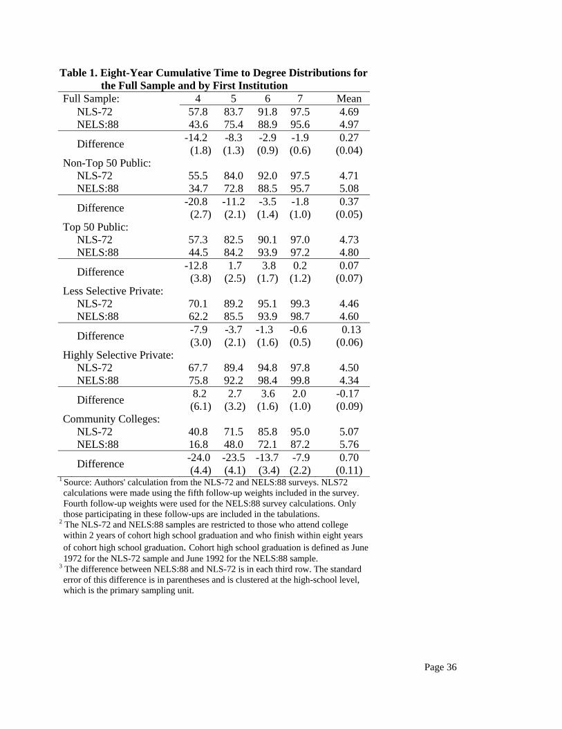
Page 36

Table 1. Eight-Year Cumulative Time to Degree Distributions for the Full Sample and by First Institution

Full Sample: 4 5 6 7 Mean NLS-72 57.8 83.7 91.8 97.5 4.69 NELS:88 43.6 75.4 88.9 95.6 4.97

Difference -14.2 (1.8)

-8.3 (1.3)

-2.9 (0.9)

-1.9 (0.6)

0.27 (0.04)

Non-Top 50 Public: NLS-72 55.5 84.0 92.0 97.5 4.71 NELS:88 34.7 72.8 88.5 95.7 5.08

Difference -20.8 (2.7)

-11.2 (2.1)

-3.5 (1.4)

-1.8 (1.0)

0.37 (0.05)

Top 50 Public: NLS-72 57.3 82.5 90.1 97.0 4.73 NELS:88 44.5 84.2 93.9 97.2 4.80

Difference -12.8 (3.8)

1.7 (2.5)

3.8 (1.7)

0.2 (1.2)

0.07 (0.07)

Less Selective Private: NLS-72 70.1 89.2 95.1 99.3 4.46 NELS:88 62.2 85.5 93.9 98.7 4.60

Difference -7.9 (3.0)

-3.7 (2.1)

-1.3 (1.6)

-0.6 (0.5)

0.13 (0.06)

Highly Selective Private: NLS-72 67.7 89.4 94.8 97.8 4.50 NELS:88 75.8 92.2 98.4 99.8 4.34

Difference 8.2 (6.1)

2.7 (3.2)

3.6 (1.6)

2.0 (1.0)

-0.17 (0.09)

Community Colleges: NLS-72 40.8 71.5 85.8 95.0 5.07 NELS:88 16.8 48.0 72.1 87.2 5.76

Difference -24.0 (4.4)

-23.5 (4.1)

-13.7 (3.4)

-7.9 (2.2)

0.70 (0.11)

1 Source: Authors' calculation from the NLS-72 and NELS:88 surveys. NLS72 calculations were made using the fifth follow-up weights included in the survey. Fourth follow-up weights were used for the NELS:88 survey calculations. Only those participating in these follow-ups are included in the tabulations.

2 The NLS-72 and NELS:88 samples are restricted to those who attend college within 2 years of cohort high school graduation and who finish within eight years of cohort high school graduation. Cohort high school graduation is defined as June 1972 for the NLS-72 sample and June 1992 for the NELS:88 sample.

3 The difference between NELS:88 and NLS-72 is in each third row. The standard error of this difference is in parentheses and is clustered at the high-school level, which is the primary sampling unit.

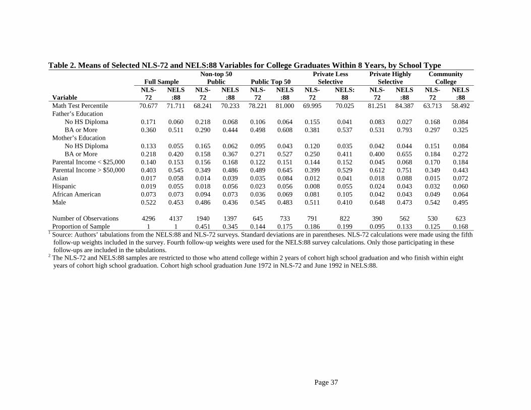
Page 37

Table 2. Means of Selected NLS-72 and NELS:88 Variables for College Graduates Within 8 Years, by School Type

Full Sample Non-top 50

Public

Public Top 50 Private Less

Selective Private Highly

Selective Community

College

Variable NLS-

72 NELS

:88 NLS-

72 NELS

:88 NLS-

72 NELS

:88 NLS-

72 NELS:

88 NLS-

72 NELS

:88 NLS-

72 NELS

:88 Math Test Percentile 70.677 71.711 68.241 70.233 78.221 81.000 69.995 70.025 81.251 84.387 63.713 58.492 Father’s Education

No HS Diploma 0.171 0.060 0.218 0.068 0.106 0.064 0.155 0.041 0.083 0.027 0.168 0.084 BA or More 0.360 0.511 0.290 0.444 0.498 0.608 0.381 0.537 0.531 0.793 0.297 0.325

Mother’s Education No HS Diploma 0.133 0.055 0.165 0.062 0.095 0.043 0.120 0.035 0.042 0.044 0.151 0.084 BA or More 0.218 0.420 0.158 0.367 0.271 0.527 0.250 0.411 0.400 0.655 0.184 0.272

Parental Income < $25,000 0.140 0.153 0.156 0.168 0.122 0.151 0.144 0.152 0.045 0.068 0.170 0.184 Parental Income > $50,000 0.403 0.545 0.349 0.486 0.489 0.645 0.399 0.529 0.612 0.751 0.349 0.443 Asian 0.017 0.058 0.014 0.039 0.035 0.084 0.012 0.041 0.018 0.088 0.015 0.072 Hispanic 0.019 0.055 0.018 0.056 0.023 0.056 0.008 0.055 0.024 0.043 0.032 0.060 African American 0.073 0.073 0.094 0.073 0.036 0.069 0.081 0.105 0.042 0.043 0.049 0.064 Male 0.522 0.453 0.486 0.436 0.545 0.483 0.511 0.410 0.648 0.473 0.542 0.495 Number of Observations 4296 4137 1940 1397 645 733 791 822 390 562 530 623 Proportion of Sample 1 1 0.451 0.345 0.144 0.175 0.186 0.199 0.095 0.133 0.125 0.168

1 Source: Authors’ tabulations from the NELS:88 and NLS-72 surveys. Standard deviations are in parentheses. NLS-72 calculations were made using the fifth follow-up weights included in the survey. Fourth follow-up weights were used for the NELS:88 survey calculations. Only those participating in these follow-ups are included in the tabulations.

2 The NLS-72 and NELS:88 samples are restricted to those who attend college within 2 years of cohort high school graduation and who finish within eight years of cohort high school graduation. Cohort high school graduation June 1972 in NLS-72 and June 1992 in NELS:88.

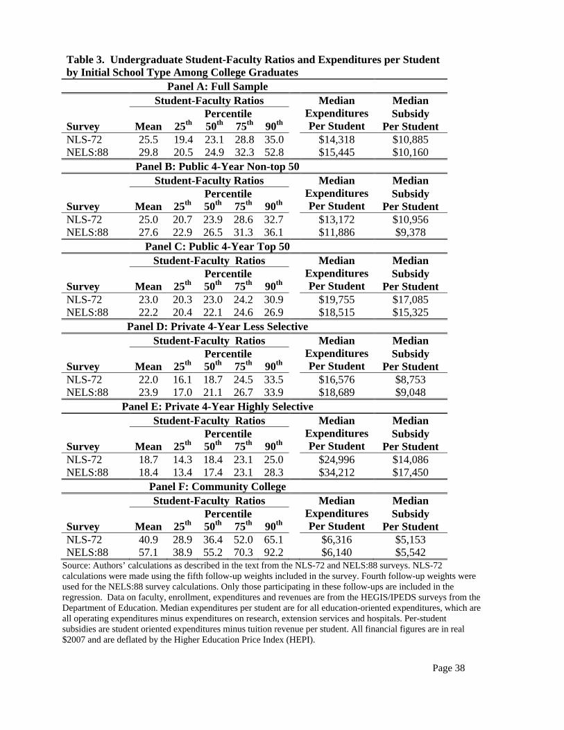
Page 38

Table 3. Undergraduate Student-Faculty Ratios and Expenditures per Student by Initial School Type Among College Graduates

Panel A: Full Sample Student-Faculty Ratios Median

Expenditures Per Student

Median Percentile Subsidy Survey Mean 25th 50th 75th 90th Per Student NLS-72 25.5 19.4 23.1 28.8 35.0 $14,318 $10,885 NELS:88 29.8 20.5 24.9 32.3 52.8 $15,445 $10,160

Panel B: Public 4-Year Non-top 50 Student-Faculty Ratios Median

Expenditures Per Student

Median Percentile Subsidy Survey Mean 25th 50th 75th 90th Per Student NLS-72 25.0 20.7 23.9 28.6 32.7 $13,172 $10,956 NELS:88 27.6 22.9 26.5 31.3 36.1 $11,886 $9,378

Panel C: Public 4-Year Top 50 Student-Faculty Ratios Median

Expenditures Per Student

Median Percentile Subsidy Survey Mean 25th 50th 75th 90th Per Student NLS-72 23.0 20.3 23.0 24.2 30.9 $19,755 $17,085 NELS:88 22.2 20.4 22.1 24.6 26.9 $18,515 $15,325

Panel D: Private 4-Year Less Selective Student-Faculty Ratios Median

Expenditures Per Student

Median Percentile Subsidy Survey Mean 25th 50th 75th 90th Per Student NLS-72 22.0 16.1 18.7 24.5 33.5 $16,576 $8,753 NELS:88 23.9 17.0 21.1 26.7 33.9 $18,689 $9,048

Panel E: Private 4-Year Highly Selective Student-Faculty Ratios Median

Expenditures Per Student

Median Percentile Subsidy Survey Mean 25th 50th 75th 90th Per Student NLS-72 18.7 14.3 18.4 23.1 25.0 $24,996 $14,086 NELS:88 18.4 13.4 17.4 23.1 28.3 $34,212 $17,450

Panel F: Community College Student-Faculty Ratios Median

Expenditures Per Student

Median Percentile Subsidy Survey Mean 25th 50th 75th 90th Per Student NLS-72 40.9 28.9 36.4 52.0 65.1 $6,316 $5,153 NELS:88 57.1 38.9 55.2 70.3 92.2 $6,140 $5,542

Source: Authors’ calculations as described in the text from the NLS-72 and NELS:88 surveys. NLS-72 calculations were made using the fifth follow-up weights included in the survey. Fourth follow-up weights were used for the NELS:88 survey calculations. Only those participating in these follow-ups are included in the regression. Data on faculty, enrollment, expenditures and revenues are from the HEGIS/IPEDS surveys from the Department of Education. Median expenditures per student are for all education-oriented expenditures, which are all operating expenditures minus expenditures on research, extension services and hospitals. Per-student subsidies are student oriented expenditures minus tuition revenue per student. All financial figures are in real $2007 and are deflated by the Higher Education Price Index (HEPI).

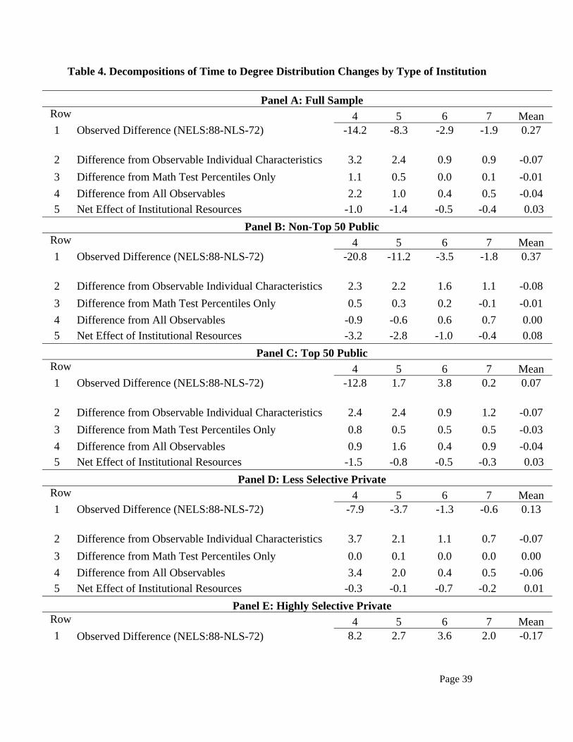
Page 39

Table 4. Decompositions of Time to Degree Distribution Changes by Type of Institution

Panel A: Full Sample Row 4 5 6 7 Mean

1 Observed Difference (NELS:88-NLS-72) -14.2 -8.3 -2.9 -1.9 0.27 2 Difference from Observable Individual Characteristics 3.2 2.4 0.9 0.9 -0.07

3 Difference from Math Test Percentiles Only 1.1 0.5 0.0 0.1 -0.01

4 Difference from All Observables 2.2 1.0 0.4 0.5 -0.04 5 Net Effect of Institutional Resources -1.0 -1.4 -0.5 -0.4 0.03 Panel B: Non-Top 50 Public

Row 4 5 6 7 Mean 1 Observed Difference (NELS:88-NLS-72) -20.8 -11.2 -3.5 -1.8 0.37 2 Difference from Observable Individual Characteristics 2.3 2.2 1.6 1.1 -0.08

3 Difference from Math Test Percentiles Only 0.5 0.3 0.2 -0.1 -0.01

4 Difference from All Observables -0.9 -0.6 0.6 0.7 0.00

5 Net Effect of Institutional Resources -3.2 -2.8 -1.0 -0.4 0.08 Panel C: Top 50 Public

Row 4 5 6 7 Mean 1 Observed Difference (NELS:88-NLS-72) -12.8 1.7 3.8 0.2 0.07 2 Difference from Observable Individual Characteristics 2.4 2.4 0.9 1.2 -0.07

3 Difference from Math Test Percentiles Only 0.8 0.5 0.5 0.5 -0.03

4 Difference from All Observables 0.9 1.6 0.4 0.9 -0.04 5 Net Effect of Institutional Resources -1.5 -0.8 -0.5 -0.3 0.03 Panel D: Less Selective Private

Row 4 5 6 7 Mean 1 Observed Difference (NELS:88-NLS-72) -7.9 -3.7 -1.3 -0.6 0.13 2 Difference from Observable Individual Characteristics 3.7 2.1 1.1 0.7 -0.07

3 Difference from Math Test Percentiles Only 0.0 0.1 0.0 0.0 0.00

4 Difference from All Observables 3.4 2.0 0.4 0.5 -0.06

5 Net Effect of Institutional Resources -0.3 -0.1 -0.7 -0.2 0.01 Panel E: Highly Selective Private

Row 4 5 6 7 Mean 1 Observed Difference (NELS:88-NLS-72) 8.2 2.7 3.6 2.0 -0.17

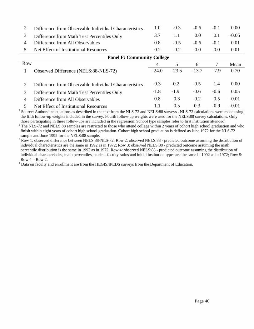
Page 40

2 Difference from Observable Individual Characteristics 1.0 -0.3 -0.6 -0.1 0.00

3 Difference from Math Test Percentiles Only 3.7 1.1 0.0 0.1 -0.05

4 Difference from All Observables 0.8 -0.5 -0.6 -0.1 0.01 5 Net Effect of Institutional Resources -0.2 -0.2 0.0 0.0 0.01 Panel F: Community College

Row 4 5 6 7 Mean 1 Observed Difference (NELS:88-NLS-72) -24.0 -23.5 -13.7 -7.9 0.70

2 Difference from Observable Individual Characteristics -0.3 -0.2 -0.5 1.4 0.00

3 Difference from Math Test Percentiles Only -1.8 -1.9 -0.6 -0.6 0.05

4 Difference from All Observables 0.8 0.3 -0.2 0.5 -0.01

5 Net Effect of Institutional Resources 1.1 0.5 0.3 -0.9 -0.01 1 Source: Authors’ calculations as described in the text from the NLS-72 and NELS:88 surveys . NLS-72 calculations were made using the fifth follow-up weights included in the survey. Fourth follow-up weights were used for the NELS:88 survey calculations. Only those participating in these follow-ups are included in the regression. School type samples refer to first institution attended.

2 The NLS-72 and NELS:88 samples are restricted to those who attend college within 2 years of cohort high school graduation and who finish within eight years of cohort high school graduation. Cohort high school graduation is defined as June 1972 for the NLS-72 sample and June 1992 for the NELS:88 sample.

3 Row 1: observed difference between NELS:88-NLS-72; Row 2: observed NELS:88 - predicted outcome assuming the distribution of individual characteristics are the same in 1992 as in 1972; Row 3: observed NELS:88 - predicted outcome assuming the math percentile distribution is the same in 1992 as in 1972; Row 4: observed NELS:88 - predicted outcome assuming the distribution of individual characteristics, math percentiles, student-faculty ratios and initial institution types are the same in 1992 as in 1972; Row 5: Row 4 – Row 2.

4 Data on faculty and enrollment are from the HEGIS/IPEDS surveys from the Department of Education.

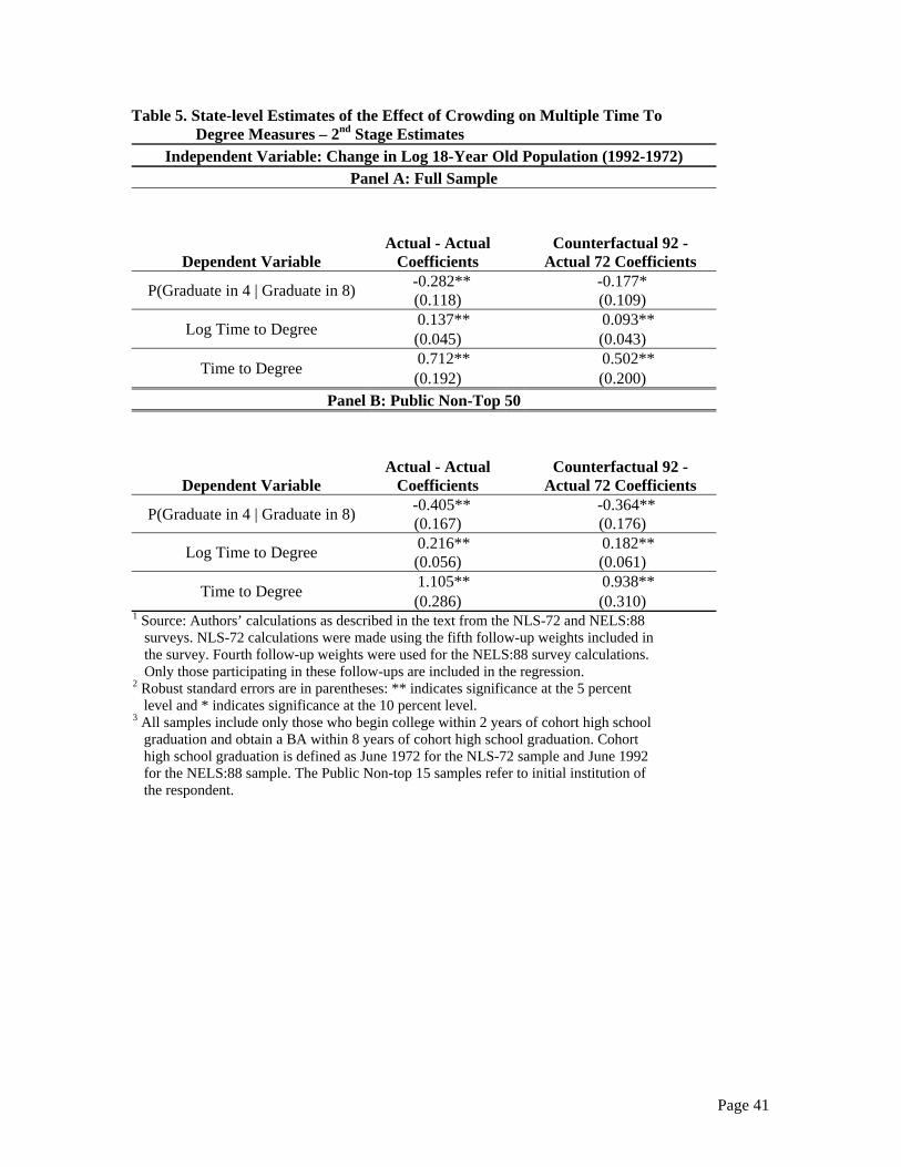
Page 41

Table 5. State-level Estimates of the Effect of Crowding on Multiple Time To Degree Measures – 2nd Stage Estimates

Independent Variable: Change in Log 18-Year Old Population (1992-1972) Panel A: Full Sample

Dependent Variable Actual - Actual

Coefficients

Counterfactual 92 - Actual 72 Coefficients

P(Graduate in 4 | Graduate in 8) -0.282** -0.177*

(0.118) (0.109)

Log Time to Degree 0.137** 0.093**

(0.045) (0.043)

Time to Degree 0.712** 0.502**

(0.192) (0.200) Panel B: Public Non-Top 50

Dependent Variable Actual - Actual

Coefficients

Counterfactual 92 - Actual 72 Coefficients

P(Graduate in 4 | Graduate in 8) -0.405** -0.364**

(0.167) (0.176)

Log Time to Degree 0.216** 0.182**

(0.056) (0.061)

Time to Degree 1.105** 0.938**

(0.286) (0.310) 1 Source: Authors’ calculations as described in the text from the NLS-72 and NELS:88

surveys. NLS-72 calculations were made using the fifth follow-up weights included in the survey. Fourth follow-up weights were used for the NELS:88 survey calculations. Only those participating in these follow-ups are included in the regression.

2 Robust standard errors are in parentheses: ** indicates significance at the 5 percent level and * indicates significance at the 10 percent level.

3 All samples include only those who begin college within 2 years of cohort high school graduation and obtain a BA within 8 years of cohort high school graduation. Cohort high school graduation is defined as June 1972 for the NLS-72 sample and June 1992 for the NELS:88 sample. The Public Non-top 15 samples refer to initial institution of the respondent.

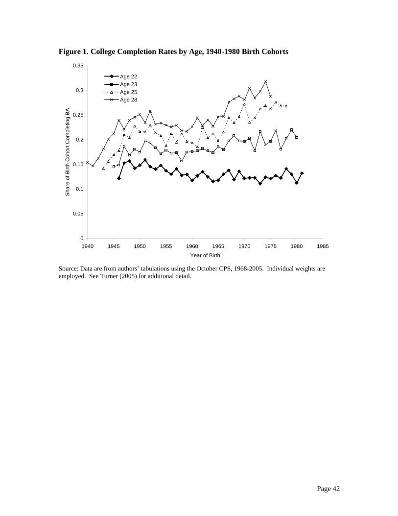
Page 42

Figure 1. College Completion Rates by Age, 1940-1980 Birth Cohorts

0

0.05

0.1

0.15

0.2

0.25

0.3

0.35

1940 1945 1950 1955 1960 1965 1970 1975 1980 1985

Year of Birth

Sh

are

of

Birt

h C

oh

ort

Co

mp

letin

g B

A

Age 22

Age 23

Age 25

Age 28

Source: Data are from authors’ tabulations using the October CPS, 1968-2005. Individual weights are employed. See Turner (2005) for additional detail.

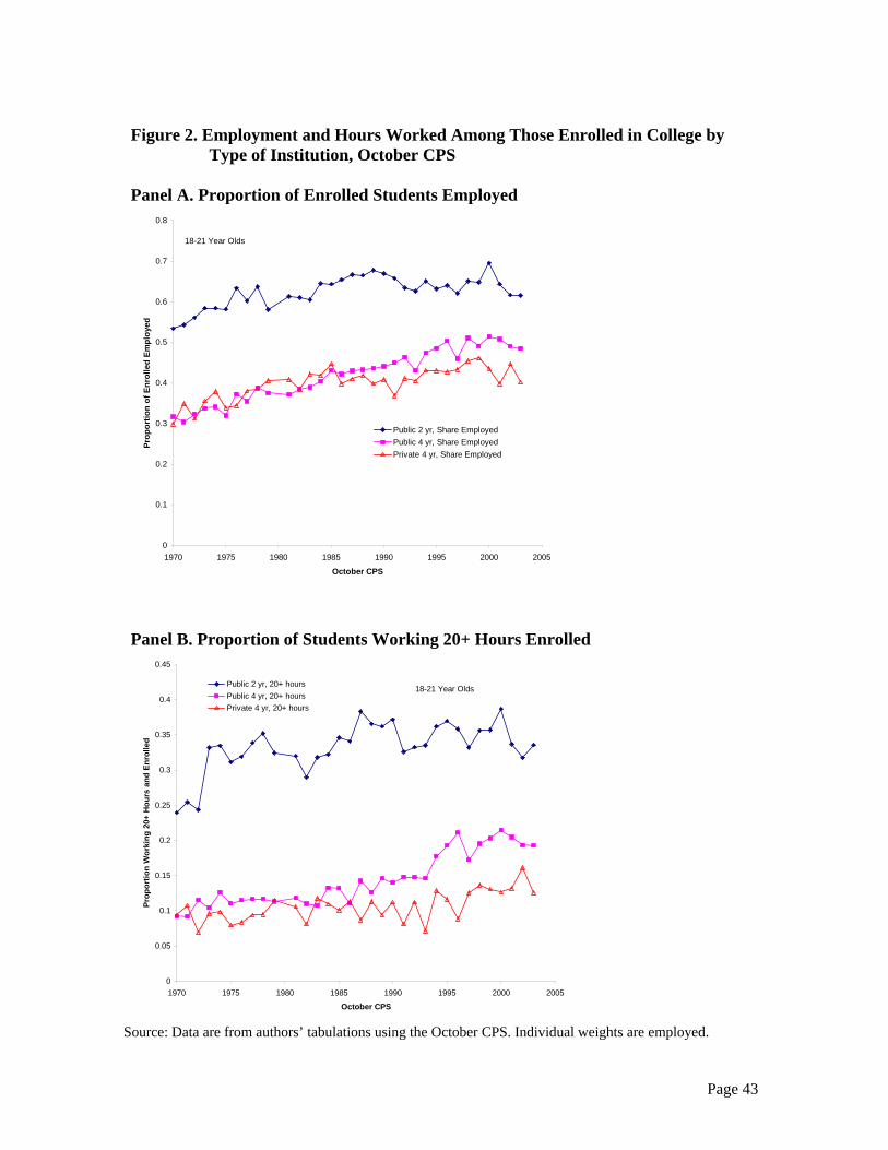
Page 43

Figure 2. Employment and Hours Worked Among Those Enrolled in College by

Type of Institution, October CPS Panel A. Proportion of Enrolled Students Employed

0

0.1

0.2

0.3

0.4

0.5

0.6

0.7

0.8

1970 1975 1980 1985 1990 1995 2000 2005

October CPS

Pro

po

rtio

n o

f E

nro

lled

Em

plo

yed

Public 2 yr, Share Employed

Public 4 yr, Share Employed

Private 4 yr, Share Employed

18-21 Year Olds

Panel B. Proportion of Students Working 20+ Hours Enrolled

0

0.05

0.1

0.15

0.2

0.25

0.3

0.35

0.4

0.45

1970 1975 1980 1985 1990 1995 2000 2005

October CPS

Pro

po

rtio

n W

ork

ing

20+

Ho

urs

an

d E

nro

lled

Public 2 yr, 20+ hours

Public 4 yr, 20+ hours

Private 4 yr, 20+ hours

18-21 Year Olds

Source: Data are from authors’ tabulations using the October CPS. Individual weights are employed.

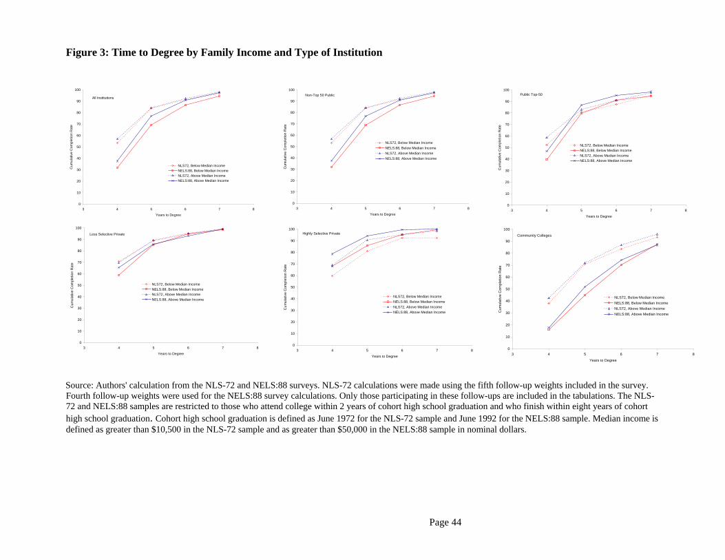
Page 44

Figure 3: Time to Degree by Family Income and Type of Institution

0

10

20

30

40

50

60

70

80

90

100

3 4 5 6 7 8

Years to Degree

Cu

mu

lativ

e C

ompl

etio

n R

ate

NLS72, Below Median Income

NELS:88, Below Median Income

NLS72, Above Median Income

NELS:88, Above Median Income

All Institutions

0

10

20

30

40

50

60

70

80

90

100

3 4 5 6 7 8

Years to Degree

Cu

mu

lativ

e C

om

ple

tion

Ra

te

NLS72, Below Median Income

NELS:88, Below Median Income

NLS72, Above Median Income

NELS:88, Above Median Income

Non-Top 50 Public

0

10

20

30

40

50

60

70

80

90

100

3 4 5 6 7 8

Years to Degree

Cum

ulat

ive

Com

plet

ion

Ra

te

NLS72, Below Median Income

NELS:88, Below Median Income

NLS72, Above Median Income

NELS:88, Above Median Income

Public Top-50

0

10

20

30

40

50

60

70

80

90

100

3 4 5 6 7 8

Years to Degree

Cum

ulat

ive

Com

plet

ion

Rat

e

NLS72, Below Median Income

NELS:88, Below Median Income

NLS72, Above Median Income

NELS:88, Above Median Income

Less Selective Private

0

10

20

30

40

50

60

70

80

90

100

3 4 5 6 7 8

Years to Degree

Cu

mu

lativ

e C

om

ple

tion

Ra

te

NLS72, Below Median Income

NELS:88, Below Median Income

NLS72, Above Median Income

NELS:88, Above Median Income

Highly Selective Private

0

10

20

30

40

50

60

70

80

90

100

3 4 5 6 7 8

Years to Degree

Cu

mu

lativ

e C

om

ple

tion

Rat

e

NLS72, Below Median Income

NELS:88, Below Median Income

NLS72, Above Median Income

NELS:88, Above Median Income

Community Colleges

Source: Authors' calculation from the NLS-72 and NELS:88 surveys. NLS-72 calculations were made using the fifth follow-up weights included in the survey. Fourth follow-up weights were used for the NELS:88 survey calculations. Only those participating in these follow-ups are included in the tabulations. The NLS-72 and NELS:88 samples are restricted to those who attend college within 2 years of cohort high school graduation and who finish within eight years of cohort high school graduation. Cohort high school graduation is defined as June 1972 for the NLS-72 sample and June 1992 for the NELS:88 sample. Median income is defined as greater than $10,500 in the NLS-72 sample and as greater than $50,000 in the NELS:88 sample in nominal dollars.

45

Increasing Time to Baccalaureate Degree in the United States: Appendices

Appendix A: Data Appendix

B-1. NLS72 and NELS:88 Data

a. Time to Degree and Degree Completion Time to degree and degree completion are calculated using NLS72 and NELS:88

survey responses from the first through fifth follow-ups in NLS72 and the fourth follow-up in NELS:88. The NLS72 study participants were seniors in high school in the spring of 1972. Following the base year interview, participant follow-up surveys were administered in 1973, 1974, 1976, 1979, and 1986 (for a subsample), with questions covering collegiate participation and degree attainment. In addition, detailed high school records and postsecondary transcripts were collected by the Department of Education.

The NELS:88 survey started with students who were in the eighth grade in 1988 (high school class of 1992) and conducted follow-up surveys with participants in 1990, 1992, 1994, and 2000. Similar to the NLS72 survey, NELS:88 contains high school records and collegiate transcripts as well as a host of background information that may be relevant to time to degree.

Although degrees can be awarded throughout a year, we record the timing of degree receipt in discrete units of years since cohort high school graduation. Cohort high school graduation is defined as June 1972 for the NLS72 sample and June 1992 for the NELS:88 sample. The cut-point in each survey that defines a new year is the end of August (and thus the start of the new academic year). For example, NLS72 respondents who received a degree in January and June of 1976 would both be classified as taking 4 years to obtain a BA. However, a student who received a degree in September 1976 would be classified as taking 5 years.

Because the NELS:88 survey is comprised of eighth graders from 1988 and the NLS72 survey follows 12th graders from the class of 1972, the NELS:88 survey contains more students who graduate high school after their cohort’s high school graduation. In our base sample, 1.3% of respondents in NLS72 and 4.4% of respondents in NELS:88 finish high school after June of their respective cohort graduation year. However, looking only at eight-year BA recipients, 0.3% and 0.6%, respectively in NLS72 and NELS:88 did not finish high school on time. It is therefore unlikely the larger preponderance of late high school graduates in the NELS:88 survey biases our time to degree calculations.

Table A-1 of this Appendix contains variable names and definitions used to define the sample and to calculate time to degree and degree completion in both the NLS72 and NELS:88 surveys.

b. School Type and Collegiate Start Dates We define enrollment as those who start at an academic institution within two

years of cohort high school graduation. Academic institutions are all four-year schools and public two-year schools. We exclude private two-year schools because they typically are not oriented towards allowing students to obtain a BA post-graduation.

46

College transcript data and self-reported enrollment records from the first through fourth follow-up surveys for the NLS72 survey and from NCES-aggregated responses in the NELS:88 survey are used to define the type of institution of initial collegiate enrollment. We use the transcript for the first institution post-high school attended by respondents in the transcript files to assign first institution attended for most respondents. In the cases in which there are multiple first transcripts from different institutions on the same date, we assign each student to the school at which she took the most credits during the first semester. There are some students who report attending college within two years of their cohort’s high school graduation but do not have any transcripts. In NLS72, 6.8% of the sample reporting attendance do not have transcripts, and in NELS:88, 8.2% of the sample falls into this category. For these respondents, we use the first institution reported by them in the survey files.

In the NLS72 survey, we begin by determining the year in which a student first enrolls in an academic post-secondary institution, where “academic” is defined as granting at least an associates degree or BA. In each follow-up, students were asked about colleges they attended (up to three) in each year since the previous survey. The first college attended is identified from the entry the first time a student reports attending an academic institution and we record the institutional identifier (FICE code) either directly from transcript files or from the student survey responses about which institution they attended. We then merge institutional-level information that contains public/private status, 2-year/4-year identifiers, and collegiate rankings and classify the respondent’s initial institution accordingly.

In the NELS:88 survey, we use a similar methodology to identify each respondent’s initial institution. NCES has constructed variables that identify first institution attended in the transcript files (the “ref” variables). We use the transcript-based NCES-constructed institutional identifier (“unitid”) code when it is available. For those who report college attendance and the sector of first attendance but are not assigned a transcript-based first institution identifier by NCES, we use the NCES-constructed variables that report individual enrollment histories from the survey data that identify first institution of enrollment (“unitid”) and first institution type (“f4efsect”).

For students with post-secondary experience preceding high school graduation, we use the first start date and institution after high school graduation taken from the post-secondary transcript files. For all other students in the NELS:88 survey, first start date is identified by f4efmy, which is the NCES-constructed date of first post-secondary attendance.

A list of the top-50 public schools from the 2005 U.S. News and World Report rankings as well as the top-65 private schools and the top-50 liberal arts colleges plus the United States Armed Services Academies, which constitute the highly selective private schools, is shown is shown in Table A-2.

c. Background Characteristics

i. Math Tests

In both surveys, tests of academic achievement were administered to students in the senior year. The NLS72 exam was administered as a 69-minute test book with sections on vocabulary, picture numbers (associative memory), reading, letter groups,

47

mathematics, and mosaic comparisons. Each section was 15 minutes (except for the mosaic comparison, which was 9 minutes). The math test included 25 items and contained only quantitative comparisons in order to measure basic quantitative competence. We use the reported scaled math score (scmatsc) test score measure in NLS72.

The NELS:88 cognitive test batteries were administered in each of the first three waves, with sections on reading, math, science and social studies. The tests were 85 minutes and consisted of 116 questions, 40 of which were on math and 21 of which were on reading comprehension. Unlike the NLS72 exams, the NELS:88 tests covered more material and tested more skills. The math exam consisted of word problems, graphs, equations, quantitative comparisons, and geometric figures. Further, because the NELS:88 tests were given in subsequent waves, students were given harder or easier tests in the first and second follow-ups depending on their scores in the previous wave to guard against floor and ceiling effects. We use the math IRT theta score (f22xmth) from the second follow-up as the base measure of test scores. These scores are psychometric evaluation scores of each student’s ability that account for the difficulty of the exam.

Because the tests in NLS72 and NELS:88 covered different subject matter, were of different lengths, and were graded on different scales, the scores are not directly comparable across surveys. Instead, we construct the percentile of the score distribution for each survey among all high school graduates. The comparison of students in the same test percentile across surveys is based on the assumption overall achievement did not change over this time period. This assumption is supported by the observation that there is little change in the overall level of test scores on the nationally-representative NAEP over our period of observation. Similarly, examination of time trends in standard college entrance exams such as the SAT provides little support for the proposition that achievement declined appreciable over the interval. For the SAT, the ratio of test takers to high school graduates increased from 33% to 42%, while mean math scores declined from 509 to 501 over the 1972 to 1992 interval (Digest of Education Statistics, 2005, Table 129).

In the NLS72 survey, we use high school GPA as an imputation variable in order to measure pre-collegiate academic ability for students with missing test scores. The GPA measure we use is “imptaver” from the NLS72 survey. In the multiple imputation of missing variables in the NELS:88 survey, we use IRT theta test scores from the first follow-up for math (f12xmth) and from the base year for math (by2xmth). The IRT theta scores are scaled to a common metric across years by NCES. The imputed math test scores from the senior year in each survey are used to construct the test percentiles used in the main analysis.

ii. Parental Education

We obtain student reported measures of father’s and mother’s education separately. In the NLS72 survey, we have three different measures of this variable. For mother’s education, we use the variables cmoed, bq90b, and fq78b. For father’s education, we use the variables cfaed, bq90a, and fq78a. If there are disagreements across measures, fq78b and fq78a take precedence.

In the NELS:88 survey, we also use student reports of father’s education (bys34a) and mother’s education (bys34b). For the multiple imputation model, we include parent

48

self-reports of their own education from the base year and second follow-up parental surveys. In the base year parent survey, we combine information on whether the respondent and his/her spouse is the father or mother (byp1a1 and byp1a2) with reported self (byp30) and spouse (byp31) educational attainment. A similar methodology is used for the second-follow up parent survey, using f2p1a and f2p1b to identify the gender of the respondent and the spouse, respectively, and f2p101a and f2p101b to identify educational attainment of the respondent and the spouse, respectively. The base year and second follow-up parental education information is aggregated into two variables, father’s education and mother’s education, used in the multiple imputation model.

iii. Parental Income Levels The parental income variables are bq93 for NLS72 and f2p74 for NELS:88. The

former is reported by the student while the latter is reported by the parents. Unfortunately, NLS72 does not contain a parent-reported measure and the NELS:88 survey does not contain a student-reported measure, so these variables are the most closely aligned parental income measures across the two surveys.

Rather than asking directly for parental income levels, the NELS:88 and NLS72 surveys ask for income ranges from respondents. Because we are interested in measuring parents’ ability to finance college, the variable of interest is the real income level, not one’s place in the income distribution. We thus align the income blocks across the two surveys using the CPI. In NLS72, the measured income groups we construct are less than $3000, $3000-$6000, $6000-$7500, $7500-$10500, $10500-$15000, and greater than $15000. In NELS:88, the corresponding real income blocks we create are less than $10000, $10000-$20000, $20000-$25000, $25000-$35000, $35000-$50000, and greater than $50000. Across surveys, the six income groups are comparable in real terms.

iv. Race Race is measured in the NLS72 survey using “crace” and “race86.” The latter is

used if the former is blank due to non-response. In the NELS:88 survey, race is measured using the “race” variable available in the data files.

B-2. Procedures to Handle Missing Data

a. Multiple Imputation

There is a considerable amount of missing data in the NLS72 and NELS:88

surveys. Table A-3 of this Appendix presents the number of unweighted missing observations by variable and survey. These observations are not missing completely at random; respondents who have no math test scores have lower time to degree conditional on starting finishing.

Casewise deletion of missing observations will therefore cause a bias in the calculation of the base trends we are seeking to explain in this analysis. To deal with this problem, we use the multiple imputation by chained equation (MICE) algorithm developed by Van Buuren, Boshuizen, and Knook (1999) that is implemented through the STATA module “ICE” (see Royston (2004) for a detailed discussion of ICE).

49

MICE is implemented by first defining the set of predictor variables (x1…xk) and the set of variables with missing values to be imputed: math test scores, father’s education, mother’s education, and parental income levels (y1…y5). The MICE algorithm implemented by ICE first randomly fills in all missing values from the posterior distribution of each variable. Then, for each variable with missing data, yi, STATA runs a regression (or ordered logit) of yi on y~i and x1…xk and calculates expected values from these regressions for all missing data points. The expected values then replace the randomly assigned values for the missing data points. A sequence of regressions for each yi is a cycle, and this process is repeated for 10 cycles, replacing the missing values with the new expected values from each regression in each cycle. The imputed values after 10 cycles constitute one imputed data set, and this process is repeated five different times to generate five imputed data sets.

There are two important specifications in implementing MICE: determination of the predictor variables and determination of the imputation models. Because of the different structure of the two surveys, different variables are used in the imputation procedure across surveys. In both surveys, we include dummy variables for cumulative time to degree from four to eight years, dummy variables for initial school type, interactions between these variables, an indicator for college attendance within two years of cohort high school graduation, as well as race and gender indicators.

For imputations with the NLS72 sample, we include a measure of high school GPA in order to proxy for unobserved ability among those without test score information. Due to the structure of the NELS:88 survey, there is more background information with which to impute missing data. We use 8th and 10th grade math test scores, parental reports of their education from the base year and second follow-up parent surveys, and parental reports of their income level from the base year parent survey. The definitions of the variables used in the imputation models are discussed in the preceding section.

Because the math test scores are continuous variables, we use OLS regressions to impute these variables. Mother’s and father’s education and income, however, are categorical variables. Because of the ordered nature of these variables, we use ordered logits to impute the missing values of these variables. While these model choices are reasonably arbitrary, they are only used to draw ranges of plausible estimates of missing data.

The multiple imputation procedure creates five different data sets, each with different imputed values for the missing observations. All reported statistics and results in our analysis are averages across data sets. In other words, we conduct each analysis separately for each data set and average the final result. The average of final results is what is reported in the tables and figures in the paper.

b. Dropped Observations and Missing Transcript Data

The base sample in this analysis consists of all respondents who graduate high

school, attend college within two years of their cohort’s high school graduation and obtain a BA within 8 years of their cohort’s high school graduation. We further restrict the sample to exclude those whose only enrollment over this time period is at a private two-year institution as these schools are predominantly professional without a BA track. Table A-4 presents information on the number of observations that are dropped by survey

50

and the reason for dropping the observation. For example, 168 respondents are dropped because they are not high school graduates in NLS72 whereas 720 are dropped in NELS:88 for this reason. The apparently higher dropout rate in NELS:88 is because the universe of students are all those enrolled in the 8th grade in 1988, whereas the universe in NLS72 are all those enrolled in 12th grade in 1972.

In the NLS72 survey, 63 observations are dropped because they report attending college but provide no information on either the type of institution or the date they first began attending this institution, and in NELS:88, 50 respondents do not provide this information. In addition, 200 observations were dropped because they were not in all four waves of the NELS:88 survey. In other words, they have a sample weight of zero. Furthermore, in NELS:88, 4150 observations are dropped because they do not earn a BA within 8 years, and 2923 observations are dropped in NLS72 for this reason.

Of potential concern in constructing our sample is the exclusion of those beginning college more than two years post-high school cohort graduation. We exclude these observations because we are interested in the truncated, eight-year time to degree distribution. These statistics have a different interpretation for a student who began college directly after high school than for a student who began college, for instance, five years after high school. In NLS72, 889 respondents attend college more than 2 years after their cohort’s high school graduation, and in NELS:88, 970 do so. Given the similarity of these numbers, shifts in when students began attending college cannot account for the trends in time to degree reported in the main text.

51

References Royston, Patrick. 2004. “Multiple Imputation of Missing Values.” Stata Journal, 4(3): 227-241. Van Buuren, Stef, Hendriek C. Boshuizen, and Dick L. Knook. 1999. “Multiple Imputation of Missing Blood Pressure Covariates in Survival Analysis.” Statistics in Medicine, 18(6): 681-694.

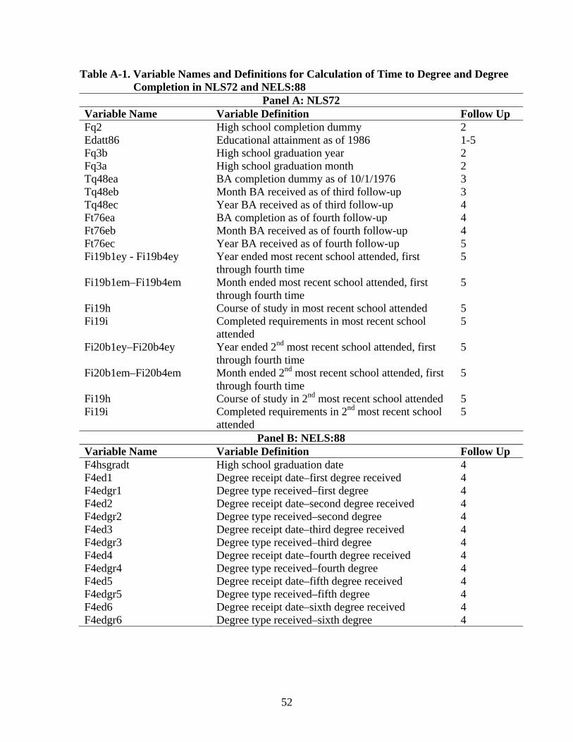
52

Table A-1. Variable Names and Definitions for Calculation of Time to Degree and Degree Completion in NLS72 and NELS:88

Panel A: NLS72 Variable Name Variable Definition Follow Up Fq2 High school completion dummy 2 Edatt86 Educational attainment as of 1986 1-5 Fq3b High school graduation year 2 Fq3a High school graduation month 2 Tq48ea BA completion dummy as of 10/1/1976 3 Tq48eb Month BA received as of third follow-up 3 Tq48ec Year BA received as of third follow-up 4 Ft76ea BA completion as of fourth follow-up 4 Ft76eb Month BA received as of fourth follow-up 4 Ft76ec Year BA received as of fourth follow-up 5 Fi19b1ey - Fi19b4ey Year ended most recent school attended, first

through fourth time 5

Fi19b1em–Fi19b4em Month ended most recent school attended, first through fourth time

5

Fi19h Course of study in most recent school attended 5 Fi19i Completed requirements in most recent school

attended 5

Fi20b1ey–Fi20b4ey Year ended 2nd most recent school attended, first through fourth time

5

Fi20b1em–Fi20b4em Month ended 2nd most recent school attended, first through fourth time

5

Fi19h Course of study in 2nd most recent school attended 5 Fi19i Completed requirements in 2nd most recent school

attended 5

Panel B: NELS:88 Variable Name Variable Definition Follow Up F4hsgradt High school graduation date 4 F4ed1 Degree receipt date–first degree received 4 F4edgr1 Degree type received–first degree 4 F4ed2 Degree receipt date–second degree received 4 F4edgr2 Degree type received–second degree 4 F4ed3 Degree receipt date–third degree received 4 F4edgr3 Degree type received–third degree 4 F4ed4 Degree receipt date–fourth degree received 4 F4edgr4 Degree type received–fourth degree 4 F4ed5 Degree receipt date–fifth degree received 4 F4edgr5 Degree type received–fifth degree 4 F4ed6 Degree receipt date–sixth degree received 4 F4edgr6 Degree type received–sixth degree 4

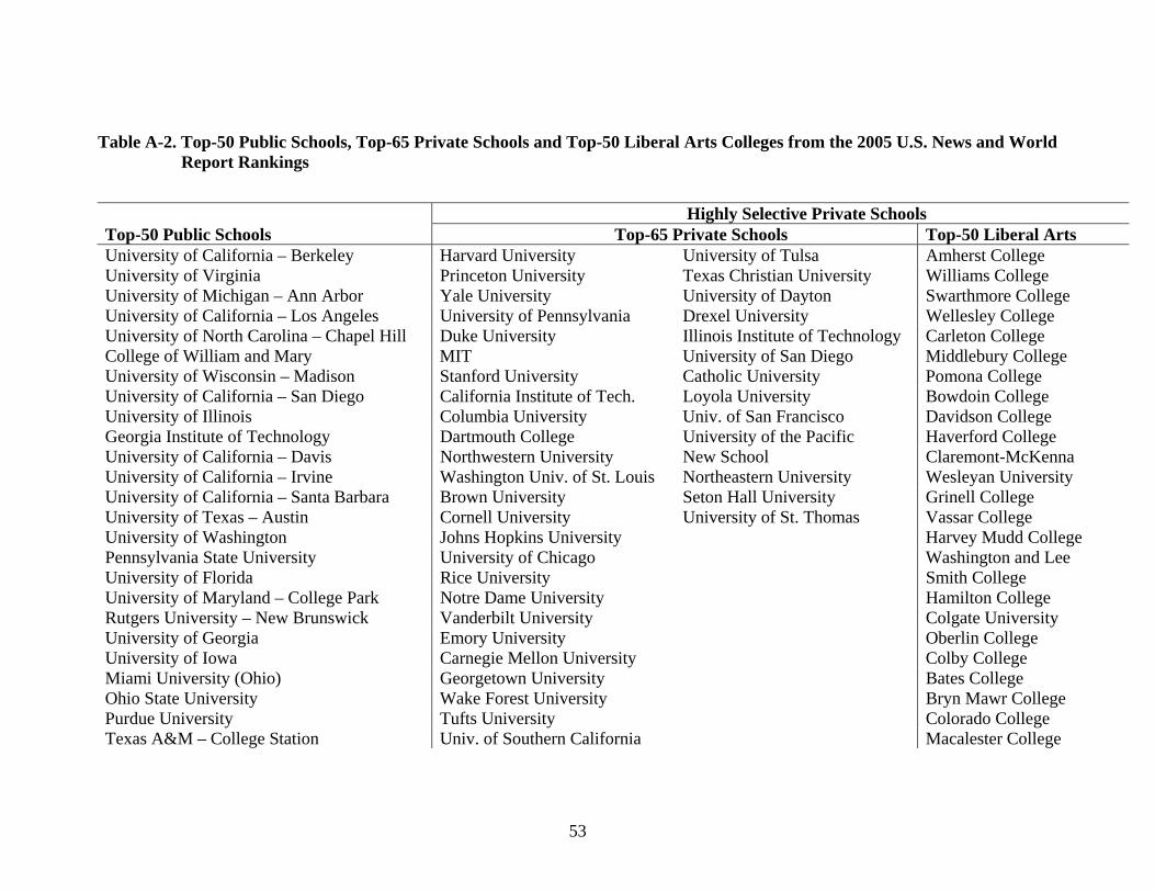
53

Table A-2. Top-50 Public Schools, Top-65 Private Schools and Top-50 Liberal Arts Colleges from the 2005 U.S. News and World Report Rankings

Highly Selective Private Schools Top-50 Public Schools Top-65 Private Schools Top-50 Liberal Arts University of California – Berkeley Harvard University University of Tulsa Amherst College University of Virginia Princeton University Texas Christian University Williams College University of Michigan – Ann Arbor Yale University University of Dayton Swarthmore College University of California – Los Angeles University of Pennsylvania Drexel University Wellesley College University of North Carolina – Chapel Hill Duke University Illinois Institute of Technology Carleton College College of William and Mary MIT University of San Diego Middlebury College University of Wisconsin – Madison Stanford University Catholic University Pomona College University of California – San Diego California Institute of Tech. Loyola University Bowdoin College University of Illinois Columbia University Univ. of San Francisco Davidson College Georgia Institute of Technology Dartmouth College University of the Pacific Haverford College University of California – Davis Northwestern University New School Claremont-McKenna University of California – Irvine Washington Univ. of St. Louis Northeastern University Wesleyan University University of California – Santa Barbara Brown University Seton Hall University Grinell College University of Texas – Austin Cornell University University of St. Thomas Vassar College University of Washington Johns Hopkins University Harvey Mudd College Pennsylvania State University University of Chicago Washington and Lee University of Florida Rice University Smith College University of Maryland – College Park Notre Dame University Hamilton College Rutgers University – New Brunswick Vanderbilt University Colgate University University of Georgia Emory University Oberlin College University of Iowa Carnegie Mellon University Colby College Miami University (Ohio) Georgetown University Bates College Ohio State University Wake Forest University Bryn Mawr College Purdue University Tufts University Colorado College Texas A&M – College Station Univ. of Southern California Macalester College

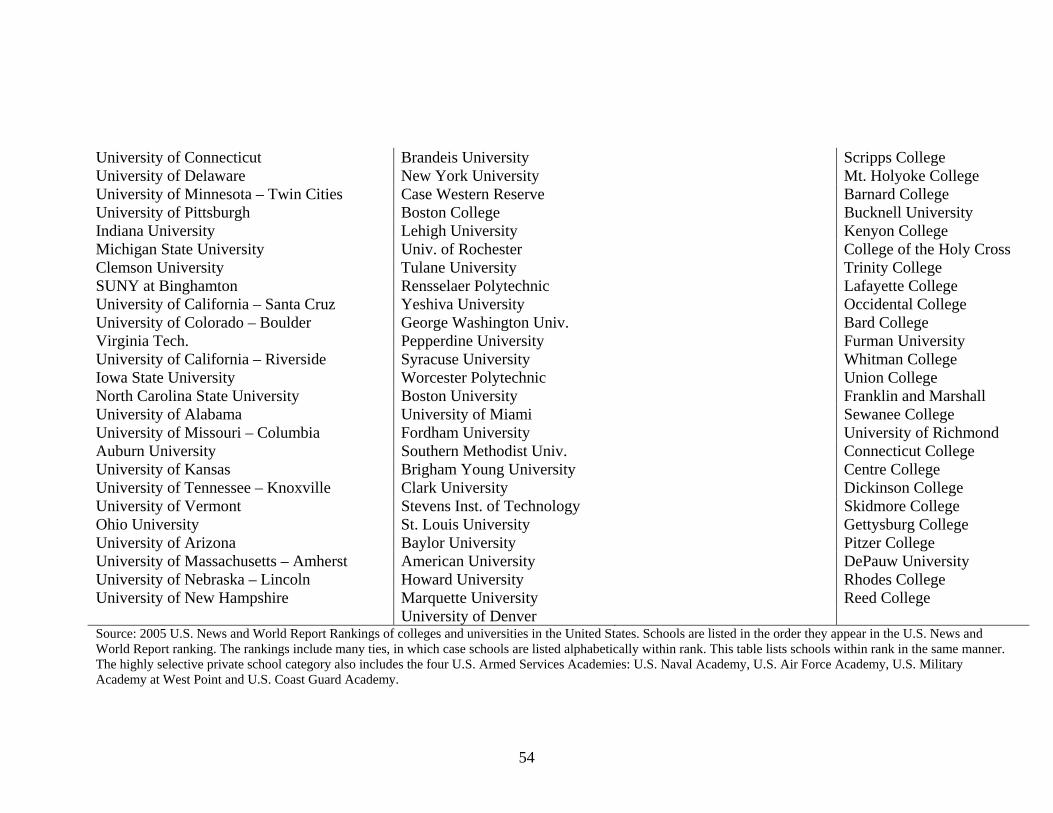
54

Source: 2005 U.S. News and World Report Rankings of colleges and universities in the United States. Schools are listed in the order they appear in the U.S. News and World Report ranking. The rankings include many ties, in which case schools are listed alphabetically within rank. This table lists schools within rank in the same manner. The highly selective private school category also includes the four U.S. Armed Services Academies: U.S. Naval Academy, U.S. Air Force Academy, U.S. Military Academy at West Point and U.S. Coast Guard Academy.

University of Connecticut Brandeis University Scripps College University of Delaware New York University Mt. Holyoke College University of Minnesota – Twin Cities Case Western Reserve Barnard College University of Pittsburgh Boston College Bucknell University Indiana University Lehigh University Kenyon College Michigan State University Univ. of Rochester College of the Holy Cross Clemson University Tulane University Trinity College SUNY at Binghamton Rensselaer Polytechnic Lafayette College University of California – Santa Cruz Yeshiva University Occidental College University of Colorado – Boulder George Washington Univ. Bard College Virginia Tech. Pepperdine University Furman University University of California – Riverside Syracuse University Whitman College Iowa State University Worcester Polytechnic Union College North Carolina State University Boston University Franklin and Marshall University of Alabama University of Miami Sewanee College University of Missouri – Columbia Fordham University University of Richmond Auburn University Southern Methodist Univ. Connecticut College University of Kansas Brigham Young University Centre College University of Tennessee – Knoxville Clark University Dickinson College University of Vermont Stevens Inst. of Technology Skidmore College Ohio University St. Louis University Gettysburg College University of Arizona Baylor University Pitzer College University of Massachusetts – Amherst American University DePauw University University of Nebraska – Lincoln Howard University Rhodes College University of New Hampshire Marquette University Reed College University of Denver

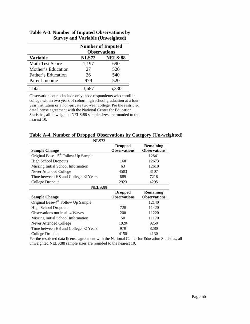
Page 55

Table A-3. Number of Imputed Observations by Survey and Variable (Unweighted)

Observation counts include only those respondents who enroll in college within two years of cohort high school graduation at a four-year institution or a non-private two-year college. Per the restricted data license agreement with the National Center for Education Statistics, all unweighted NELS:88 sample sizes are rounded to the nearest 10. Table A-4. Number of Dropped Observations by Category (Un-weighted)

NLS72

Sample Change Dropped

Observations Remaining

Observations Original Base - 5th Follow Up Sample 12841 High School Dropouts 168 12673 Missing Initial School Information 63 12610 Never Attended College 4503 8107 Time between HS and College >2 Years 889 7218 College Dropout 2923 4295

NELS:88

Sample Change Dropped

Observations Remaining

Observations Original Base-4th Follow Up Sample 12140 High School Dropouts 720 11420 Observations not in all 4 Waves 200 11220 Missing Initial School Information 50 11170 Never Attended College 1920 9250 Time between HS and College >2 Years 970 8280 College Dropout 4150 4130

Per the restricted data license agreement with the National Center for Education Statistics, all unweighted NELS:88 sample sizes are rounded to the nearest 10.

Number of Imputed Observations

Variable NLS72 NELS:88 Math Test Score 1,197 690 Mother’s Education 27 520 Father’s Education 26 540 Parent Income 979 520

Total 3,687 5,330

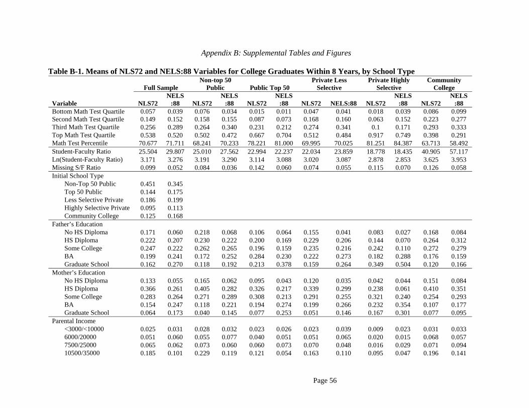
Page 56

Appendix B: Supplemental Tables and Figures Table B-1. Means of NLS72 and NELS:88 Variables for College Graduates Within 8 Years, by School Type

Full Sample Non-top 50

Public

Public Top 50 Private Less

Selective Private Highly

Selective Community

College

Variable NLS72 NELS

:88 NLS72 NELS

:88 NLS72 NELS

:88 NLS72 NELS:88 NLS72 NELS

:88 NLS72 NELS

:88 Bottom Math Test Quartile 0.057 0.039 0.076 0.034 0.015 0.011 0.047 0.041 0.018 0.039 0.086 0.099 Second Math Test Quartile 0.149 0.152 0.158 0.155 0.087 0.073 0.168 0.160 0.063 0.152 0.223 0.277 Third Math Test Quartile 0.256 0.289 0.264 0.340 0.231 0.212 0.274 0.341 0.1 0.171 0.293 0.333 Top Math Test Quartile 0.538 0.520 0.502 0.472 0.667 0.704 0.512 0.484 0.917 0.749 0.398 0.291 Math Test Percentile 70.677 71.711 68.241 70.233 78.221 81.000 69.995 70.025 81.251 84.387 63.713 58.492 Student-Faculty Ratio 25.504 29.807 25.010 27.562 22.994 22.237 22.034 23.859 18.778 18.435 40.905 57.117 Ln(Student-Faculty Ratio) 3.171 3.276 3.191 3.290 3.114 3.088 3.020 3.087 2.878 2.853 3.625 3.953 Missing S/F Ratio 0.099 0.052 0.084 0.036 0.142 0.060 0.074 0.055 0.115 0.070 0.126 0.058 Initial School Type Non-Top 50 Public 0.451 0.345 Top 50 Public 0.144 0.175 Less Selective Private 0.186 0.199 Highly Selective Private 0.095 0.113 Community College 0.125 0.168 Father’s Education

No HS Diploma 0.171 0.060 0.218 0.068 0.106 0.064 0.155 0.041 0.083 0.027 0.168 0.084 HS Diploma 0.222 0.207 0.230 0.222 0.200 0.169 0.229 0.206 0.144 0.070 0.264 0.312 Some College 0.247 0.222 0.262 0.265 0.196 0.159 0.235 0.216 0.242 0.110 0.272 0.279 BA 0.199 0.241 0.172 0.252 0.284 0.230 0.222 0.273 0.182 0.288 0.176 0.159 Graduate School 0.162 0.270 0.118 0.192 0.213 0.378 0.159 0.264 0.349 0.504 0.120 0.166

Mother’s Education No HS Diploma 0.133 0.055 0.165 0.062 0.095 0.043 0.120 0.035 0.042 0.044 0.151 0.084 HS Diploma 0.366 0.261 0.405 0.282 0.326 0.217 0.339 0.299 0.238 0.061 0.410 0.351 Some College 0.283 0.264 0.271 0.289 0.308 0.213 0.291 0.255 0.321 0.240 0.254 0.293 BA 0.154 0.247 0.118 0.221 0.194 0.274 0.199 0.266 0.232 0.354 0.107 0.177 Graduate School 0.064 0.173 0.040 0.145 0.077 0.253 0.051 0.146 0.167 0.301 0.077 0.095

Parental Income <3000/<10000 0.025 0.031 0.028 0.032 0.023 0.026 0.023 0.039 0.009 0.023 0.031 0.033 6000/20000 0.051 0.060 0.055 0.077 0.040 0.051 0.051 0.065 0.020 0.015 0.068 0.057 7500/25000 0.065 0.062 0.073 0.060 0.060 0.073 0.070 0.048 0.016 0.029 0.071 0.094 10500/35000 0.185 0.101 0.229 0.119 0.121 0.054 0.163 0.110 0.095 0.047 0.196 0.141

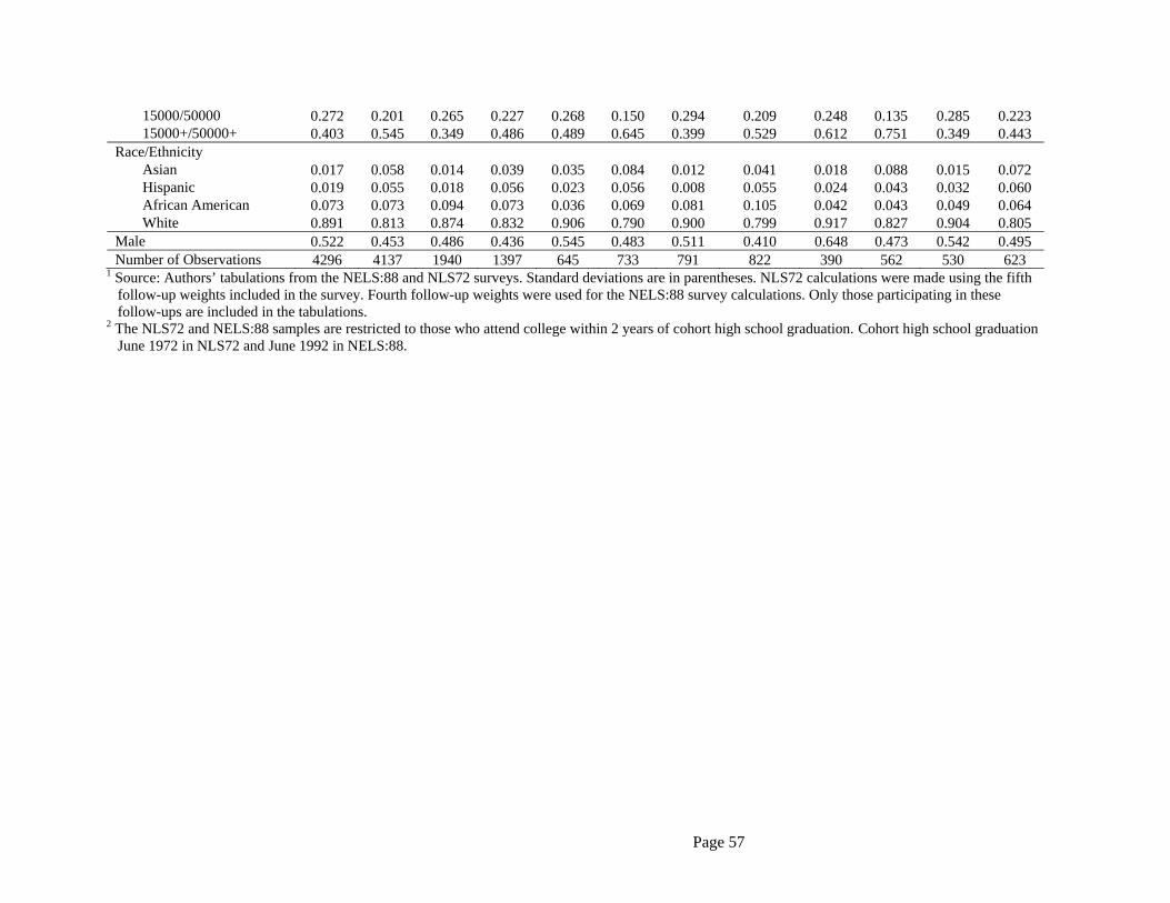
Page 57

15000/50000 0.272 0.201 0.265 0.227 0.268 0.150 0.294 0.209 0.248 0.135 0.285 0.223 15000+/50000+ 0.403 0.545 0.349 0.486 0.489 0.645 0.399 0.529 0.612 0.751 0.349 0.443

Race/Ethnicity Asian 0.017 0.058 0.014 0.039 0.035 0.084 0.012 0.041 0.018 0.088 0.015 0.072 Hispanic 0.019 0.055 0.018 0.056 0.023 0.056 0.008 0.055 0.024 0.043 0.032 0.060 African American 0.073 0.073 0.094 0.073 0.036 0.069 0.081 0.105 0.042 0.043 0.049 0.064 White 0.891 0.813 0.874 0.832 0.906 0.790 0.900 0.799 0.917 0.827 0.904 0.805

Male 0.522 0.453 0.486 0.436 0.545 0.483 0.511 0.410 0.648 0.473 0.542 0.495 Number of Observations 4296 4137 1940 1397 645 733 791 822 390 562 530 623

1 Source: Authors’ tabulations from the NELS:88 and NLS72 surveys. Standard deviations are in parentheses. NLS72 calculations were made using the fifth follow-up weights included in the survey. Fourth follow-up weights were used for the NELS:88 survey calculations. Only those participating in these follow-ups are included in the tabulations.

2 The NLS72 and NELS:88 samples are restricted to those who attend college within 2 years of cohort high school graduation. Cohort high school graduation June 1972 in NLS72 and June 1992 in NELS:88.

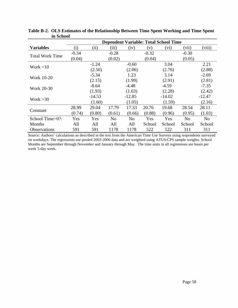
Page 58

Table B-2. OLS Estimates of the Relationship Between Time Spent Working and Time Spent in School

Dependent Variable: Total School Time Variables (i) (ii) (iii) (iv) (v) (vi) (vii) (viii)

Total Work Time -0.34 -0.28 -0.32 -0.30

(0.04) (0.02) (0.04) (0.05)

Work <10 -1.24 -0.60 3.04 2.21 (2.50) (2.06) (2.76) (2.88)

Work 10-20 -5.34 1.23 3.14 -2.69 (2.15) (1.99) (2.91) (2.81)

Work 20-30 -8.64 -4.48 -4.59 -7.35 (1.93) (1.63) (2.28) (2.42)

Work >30 -14.53 -12.85 -14.02 -12.47 (1.60) (1.05) (1.59) (2.16)

Constant 28.99 29.04 17.79 17.33 20.76 19.68 28.54 28.11

(0.74) (0.80) (0.61) (0.66) (0.88) (0.96) (0.95) (1.03) School Time>0?: Yes Yes No No Yes Yes No No Months All All All All School School School School Observations 591 591 1178 1178 522 522 311 311

Source: Authors’ calculations as described in the text from the American Time Use Surveys using respondents surveyed on weekdays. The regressions use pooled 2003-2006 data and are weighted using ATUS/CPS sample weights. School Months are September through November and January through May. The time units in all regressions are hours per week 5-day week.

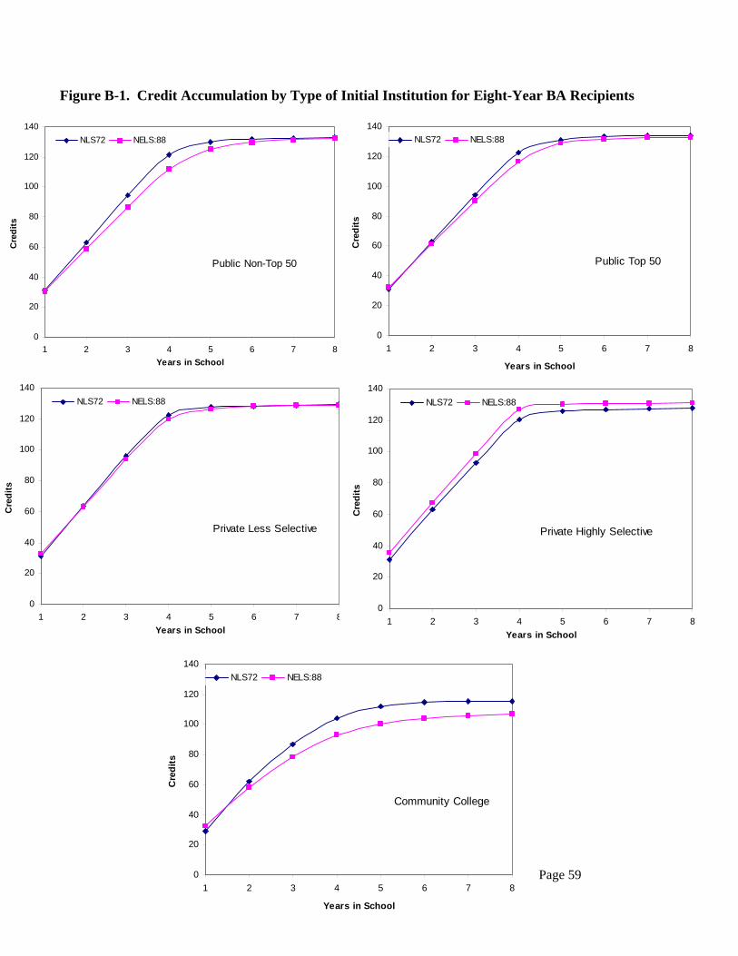
Page 59

Figure B-1. Credit Accumulation by Type of Initial Institution for Eight-Year BA Recipients 1 Source: Authors’ calculations from the NLS72 and NELS:88 transcript surveys. NLS72 calculations were made using the fifth

follow-up weights included in the survey. Fourth follow-up weights were used for the NELS:88 survey calculations. Only those participating in these follow-ups are included in the tabulations.

2 The credit accumulation schedules represent total average credits by years enrolled in college. For those who graduate in less than eight years, their number of credits are held constant for each subsequent year post graduation.

3 The NLS72 and NELS:88 samples are restricted to those who attend college within 2 years of cohort high school graduation and receive a BA within eight years. Cohort high school graduation is defined as June 1972 for the NLS72 sample and June 1992 for the NELS:88 sample. The figure does not include outliers who accumulate more than 45 credits per year.

Figure

0

20

40

60

80

100

120

140

1 2 3 4 5 6 7 8

Years in School

Cre

dit

s

NLS72 NELS:88

Public Non-Top 50

0

20

40

60

80

100

120

140

1 2 3 4 5 6 7 8

Years in SchoolC

red

its

NLS72 NELS:88

Public Top 50

0

20

40

60

80

100

120

140

1 2 3 4 5 6 7 8

Years in School

Cre

dit

s

NLS72 NELS:88

Private Less Selective

0

20

40

60

80

100

120

140

1 2 3 4 5 6 7 8

Years in School

Cre

dit

s

NLS72 NELS:88

Private Highly Selective

0

20

40

60

80

100

120

140

1 2 3 4 5 6 7 8

Years in School

Cre

dit

s

NLS72 NELS:88

Community College

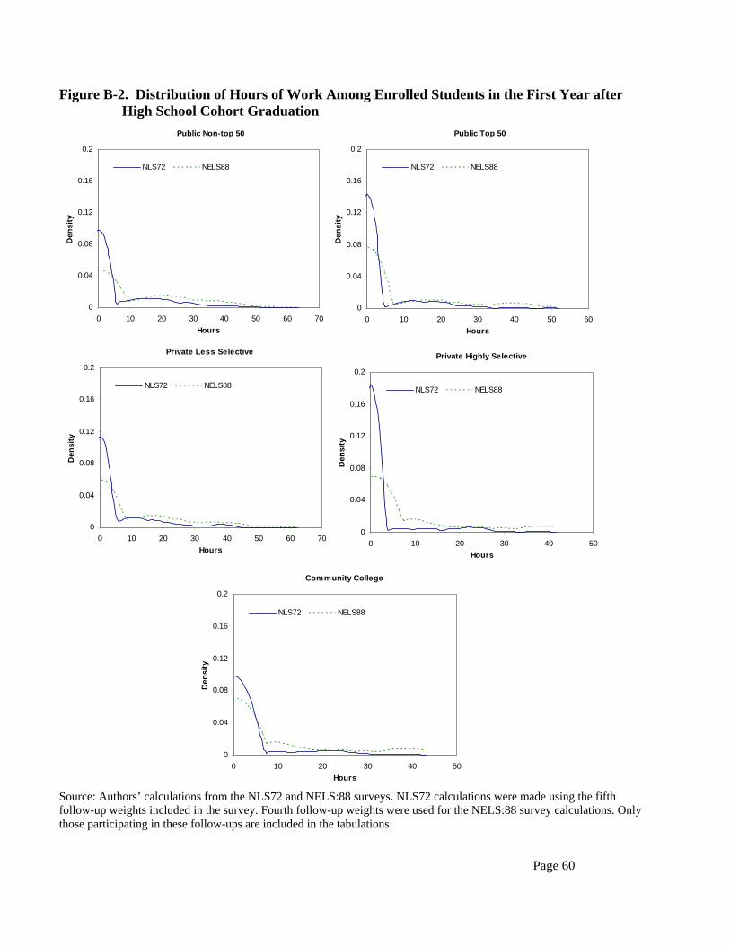
Page 60

Figure B-2. Distribution of Hours of Work Among Enrolled Students in the First Year after High School Cohort Graduation

Source: Authors’ calculations from the NLS72 and NELS:88 surveys. NLS72 calculations were made using the fifth follow-up weights included in the survey. Fourth follow-up weights were used for the NELS:88 survey calculations. Only those participating in these follow-ups are included in the tabulations.

Public Non-top 50

0

0.04

0.08

0.12

0.16

0.2

0 10 20 30 40 50 60 70

Hours

Den

sity

NLS72 NELS88

Public Top 50

0

0.04

0.08

0.12

0.16

0.2

0 10 20 30 40 50 60

HoursD

ensi

ty

NLS72 NELS88

Private Less Selective

0

0.04

0.08

0.12

0.16

0.2

0 10 20 30 40 50 60 70

Hours

Den

sity

NLS72 NELS88

Private Highly Selective

0

0.04

0.08

0.12

0.16

0.2

0 10 20 30 40 50

Hours

Den

sity

NLS72 NELS88

Community College

0

0.04

0.08

0.12

0.16

0.2

0 10 20 30 40 50

Hours

Den

sity

NLS72 NELS88