NCCA 2010 TECHNICAL REPORT

National Coastal Condition Assessment 2010

U. S. Environmental Protection Agency

January 2016

i

This page intentionally blank.

i

Table of Contents

Contents Section 1: Survey Design ..................................................................................................................................... 1

Section 2: Assessing Benthic Condition (NCCA 2010) ........................................................................................ 3

Section 3: Assessing Water Quality (NCCA 2010) ............................................................................................. 11

Section 4: Assessing Sediment Quality (NCCA 2010)........................................................................................ 19

Section 5: Assessing Ecological Fish Tissue Contaminants (NCCA 2010)......................................................... 28

Section 6: Quality Assurance and Quality Control (NCCA 2010) ..................................................................... 43

This document provides supplemental technical information on the background and development of the Benthic Index, Water Quality Index, Sediment Quality Index, and Ecological Fish Tissue Contaminants Index used in the National Coastal Condition (NCCA) 2010 Report. It was developed by EPA to provide technical information to readers of the NCCA 2010.

ii

This page intentionally blank.

1

Section 1: Survey Design The National Coastal Condition Assessment uses a probability-based survey design to select sites within the target population. This type of survey design allows for spatially-balanced sampling wherein each point has a known probability of being included in the draw. The design also ensures that no points in the target population are too far from a sampled point, while reducing the clumping of points that are close together. The target population is divided (or “stratified”) into unequal probability categories allowing for adequate representation of varying characteristics within the sample frame. Estuarine Design Target population: All coastal waters of the United States from the head-of-salt to confluence with ocean including inland waterways and major embayments such as Florida Bay and Cape Cod Bay. Survey Design: A Generalized Random Tessellation Stratified (GRTS) survey design for an area resource is used. The survey design is a stratified design with unequal probability of selection based on area within each stratum. The details are given below. Stratification: Stratification is based on major estuaries based on NOAA Coastal Assessment framework and National Estuaries Program estuaries. Multi-density categories: Unequal probability categories were created based on area of polygons within each major estuary. The number of categories ranged from 3 to 7. The categories were used to ensure that sites were selected in the smaller polygons. Expected sample size: The expected sample size is 682 sites for conterminous coastal states and 45 sites for Hawaii and Puerto Rico. The maximum number of sites for a major estuary was 46 (Chesapeake Bay). In total, the estuarine design contains 682 sites. Of these 68 were revisited, for a total of 750 total visits. Great Lakes Design Target population: Near shore waters of the Great Lakes of the United States and Canada. Near shore zone is defined as up to 30m depth and a maximum distance of 5 km from shoreline. Great Lakes include Lake Superior, Lake Michigan, Lake Huron, Lake Erie, and Lake Ontario. The NARS Great Lakes survey will be restricted to the United States portion. It does not include the connecting channels of the Great Lakes (between lakes and the St. Lawrence River outlet). Survey Design: A Generalized Random Tessellation Stratified (GRTS) survey design for an area resource is used. The survey design is stratified by Lake and country with unequal probability of selection based on state shoreline length within each stratum. Stratification: Stratification is based on Great Lake and country. Multi-density categories: Unequal probability categories are states within each Great Lake based on proportion of state shoreline length within each stratum.

2

Expected sample size: Expected sample size of 45 sites in Near Shore zone for each Great Lake and country combination for a total of 405 sites. Sample sizes were allocated proportional to shoreline length by state within each Great Lake. Additional Sites: Additional sites that followed the above design frames as well as sample collection methods for special studies were included in this assessment. An example of this is the embayment study which added 150 sites into the Great Lakes assessment. Site Weights Each site has an associated weighting factor equal to the surface area represented by the site. As in previous assessments, the status of the nation and each region for each of the indices used in this assessment, is reported as the percent area in good, fair, poor, or missing condition. The percent area in each condition is calculated as the sum of weighting factors (areas) of sites in a condition category, divided by the sum of weights (total area) of all sites in the region. For instance, for the Northeast region, the percent area in good condition is calculated as the sum of the weighting factors (areas) of sites rated as good, divided by the sum of all NE weighting factors. Results were reported in this manner for the component metrics and the overall indices. Data availability All data used in the 2010 survey are available from the NARS web site (http://www.epa.gov/national-aquatic-resource-surveys/ncca). In particular, “NCCA 2010 Assessed [indicator name] – Data (CSV)” data files contain only sites and data used to develop the assessments in this report. The data files also contain any auxiliary parameters necessary to calculate all report metrics and indices. Survey Design References Diaz-Ramos, S., Stevens, D. L., Jr, & Olsen, A. R. (1996). EMAP Statistical Methods Manual. EPA/620/R-96/002,

U.S. Environmental Protection Agency, Office of Research and Development, NHEERL-Western Ecology Division, Corvallis, Oregon.

Olsen, T. (2010, January). USEPA. National Coastal Assessment 2010 Great Lakes Embayment Survey Design.

Olsen, T. (2009, January). USEPA. National Coastal Assessment 2010 Great Lakes Survey Design.

3

Section 2: Assessing Benthic Condition (NCCA 2010) The worms, mollusks, crustaceans, and other invertebrates that inhabit the bottom substrates of coastal waters are collectively called benthic macroinvertebrates, or benthos. These organisms play a vital role in monitoring water quality and provide an important food source for bottom-feeding fish; shrimp; ducks; and marsh birds. Benthos are often used as indicators of disturbance in coastal environments because they are not very mobile and thus cannot avoid environmental problems. Benthic populations and communities serve as reliable indicators of coastal environmental quality because they are sensitive to chemical-contaminant and dissolved-oxygen stresses, salinity fluctuations, and sediment disturbance.

To assess the ecological condition of benthic communities, EMAP and the NCA developed regional benthic indices of environmental condition for the Southeast (Van Dolah et al., 1999), Northeast (Paul et al., 2001; Hale and Heltshe, 2008), and Gulf coasts (Engle et al., 1994; Engle and Summers, 1999). Each index was developed independently for a specific biogeographical region, used different statistical methods, and incorporated different metrics of benthic community condition (Table B-1). In general, however, all of the benthic indices reflect changes in benthic community diversity and the abundance of pollution-tolerant and pollution-sensitive species. A good benthic index rating for benthos means that the benthic habitats contain a wide variety of species, including low proportions of pollution-tolerant species and high proportions of pollution-sensitive species. A poor benthic index rating indicates that the benthic communities are less diverse than expected and are populated by more pollution-tolerant species and fewer pollution-sensitive species than expected.

Table B-1. NCA Benthic Indices

Region/ Province Data Source

Statistical Method Component Metrics

Index Condition Scale

Source Good Fair Poor

Northeast/ Acadian NCA

2000-2001

Logistic Regression Analysis

Diversity (Shannon H’) Pollution Tolerant Taxa Proportion Capitellids

> 5 4–5 < 4 Hale & Heltsche 2008

Northeast/ Virginian EMAP

1990-1993

Discriminant Analysis

Diversity (Gleason D) Abundance Tubificids Abundance Spionids

> 0 n/a ≤ 0 Paul et al. 2001

Southeast/ Carolinian EMAP

1993-1994

Cluster Analysis

Abundance Species Richness Dominance Pollution Sensitive Taxa

> 2.5 2–2.5 < 2 Van Dolah et al. 1999

Gulf/ Louisianian

EMAP 1991-1992

Discriminant Analysis

Diversity (Shannon H’) Abundance Tubificids Proportion Capitellids Proportion Bivalves Proportion Amphipods

> 5 3–5 < 3

Engle et al. 1994; Engle & Summers 1999

No regional benthic index has been developed for the West Coast, although several local benthic indices have been developed (e.g., Smith et al. 2001; Ranasinghe et al. 2007). In the West Coast region benthic species richness was used as a surrogate for a regional benthic index. Values for species richness were compared with salinity regionally to determine if a significant relationship existed. For West Coast estuaries, a highly significant (p < 0.0001) linear regression between log species richness and salinity was found for the region, although variability was high (R2 = 0.33). A surrogate benthic index was calculated by determining the expected species richness from the statistical relationship to salinity and then calculating the ratio of observed to expected

4

species richness. Poor benthic condition was defined as observed species richness less than 75% of the lower 95% confidence interval of the regression for expected benthic species richness at a particular salinity (Table 2). Good benthic condition was defined as observed species richness greater than 90% of the lower 95% confidence interval of the regression for expected benthic species richness at a particular salinity (Table 2).

In the Great Lakes, the State of the Lakes Ecosystem Conference (SOLEC) assesses benthic community condition using an oligochaete trophic index (OTI) based on Howmiller & Scott’s (1977) index with subsequent modifications by Milbrink (1983) and Lauritsen et al. (1985). The OTI is based on the classification of oligochaete species by their known tolerance to organic enrichment (Environment Canada & USEPA 2014). The OTI ranges from 0 to 3 where scores less than 0.6 indicate oligotrophic conditions, scores between 0.6 and 1.0 indicate mesotrophic conditions, and scores > 1.0 indicate eutrophic conditions (Table B-2). In this report, oligotrophic equates to good condition, mesotrophic equates to fair condition, and eutrophic equates to poor condition.

Table B-2. Thresholds for Assessing Benthic Condition

Region Good Fair Poor Northeast

Acadian Province

Benthic index score is greater than 5.0.

Benthic index score is between 4.0 and 5.0.

Benthic index score is less than 4.0.

Virginian Province

Benthic index score is greater than 0.0.

NAa Benthic index score is less than or equal to 0.0.

Southeast Benthic index score is greater than 2.5.

Benthic index score is between 2.0 and 2.5.

Benthic index score is less than 2.0.

Gulf Benthic index score is greater than 5.0.

Benthic index score is between 3.0 and 5.0.

Benthic index score is less than 3.0.

West

Observed species richness is more than 90% of the lower 95% confidence interval of expected species richness for a specific salinity.

Observed species richness is between 75% and 90% of the lower 95% confidence interval of expected species richness for a specific salinity.

Observed species richness is less than 75% of the lower 95% confidence interval of expected species richness for a specific salinity.

Great Lakes Oligochaete trophic index score is less than 0.6

Oligochaete trophic index score is between 0.6 and 1.0

Oligochaete trophic index score is greater than 1.0

aBy design, the Virginian Province index discriminates between good and poor conditions only.

5

Detailed Methods for Calculating Benthic Indices

Preparation of NCCA Benthic Data

Sediment samples were collected using sediment grab apparatus as shown in Table B-3. Crews sieved the sediment*, retained macroinvertebrates, preserved them and sent them to benthic taxonomy laboratories for taxonomic identification and organism counts. Because States used different grabs to collect sediment samples, it is necessary to standardize raw counts of benthic abundance by using the grab areas in Table B-3 (i.e., convert number/grab to number/m2):

Number m-2 = Number grab-1 / (grab size in m2 x number of grabs) (Formula B-1)

Table B-3. Benthic grab types, surface area, and states where each grab was used.

Grab Type Grab Area (m2)

States where used

Small van Veen 0.04 CT, DE, FL, GA, LA, MD, MS, NC, NH, NJ, NY, RI, VA

Large van Veen 0.1 CA, OR, WA Young-modified van Veen

0.04 SC, VA

Standard Ponar 0.052 AL, CA, IL, IN, MA, ME, MI, MN, NY, OH, PA, WI

Petite Ponar 0.023** FL, VA Ekman 0.046 TX Modified Post-hole Digger

0.1 OR, WA

6-inch Corer 0.182 FL * All sediment grabs but those collected on the West Coast were sieved using 0.5 mm mesh; the West Coast grabs were sieved using 1.0 mm mesh. ** Two benthic grabs composited for grabs smaller than 0.03 m2.

Different laboratories were used for benthic taxonomy, which required standardization of taxonomic names. The World Register of Marine Species (WoRMS) was used to standardize taxonomic nomenclature for marine species [http://www.marinespecies.org/] and the Integrated Taxonomic Information System (ITIS) was used to standardize freshwater species [http://www.itis.gov/]. Taxa that were not considered to be benthic macroinvertebrate infauna were removed from the data (i.e., Phylum Nematoda, Phylum Bryozoa, Class Ostracoda, Class Maxillopoda, and Class Arachnida). Standard benthic community metrics, including total abundance, species richness, and Shannon’s diversity (H’) were calculated for the benthic data at all stations. Bottom salinity measures were also added to the database for all stations. Gulf of Mexico Benthic Index The Gulf of Mexico benthic index is based on a benthic index originally developed by Engle et al. (1999) and revised by Engle & Summers (1999) for the Louisianian biogeographic province. This index was developed from EMAP-Estuaries data collected from 1991-1992 in the Louisianian Province (Texas/Mexico border to Anclote Key, FL). Reference and degraded sites were selected based on criteria for dissolved oxygen, sediment

6

contaminants, and sediment toxicity. Discriminant analysis was performed on a set of benthic community metrics to determine those metrics that best distinguished between reference and degraded sites. The benthic index included the following metrics: Proportion of Expected Shannon’s H’ Diversity (based on salinity), Mean Abundance of Family Tubificidae, Percent Abundance of Family Capitellidae, Percent Abundance of Class Bivalvia, and Percent Abundance of Order Amphipoda. Proportion of Expected Shannon’s H’ Diversity (based on salinity) is calculated as:

(Formula B-2)

(Formula B-3)

(Formula B-4)

Mean Abundance of Family Tubificidae is transformed using log10 and Percent Abundance of Family Capitellidae, Percent Abundance of Class Bivalvia, and Percent Abundance of Order Amphipoda are transformed using arcsine. All parameters are standardized to mean=1 and standard deviation=0. The Gulf of Mexico Benthic Index is then calculated as;

Gulf BI =(((Proportion of Expected Diversity x 1.51038682) +

(Mean Abundance of Family Tubificidae x -1.033492089) + (Percent Abundance of Family Capitellidae x -0.560706007) + (Percent Abundance of Class Bivalvia x -0.446995840) + (Percent Abundance of Order Amphipoda x 0.502344732)) + 3.2059424) x 1.3325

Southeast Benthic Index The Southeast benthic index is based on a benthic index originally developed by Van Dolah et al. (1999) for the Carolinian biogeographic province. This index was developed from EMAP-Estuaries data collected from 1993-1994 in the Carolinian Province (Cape Henry, VA to St. Lucie Inlet, FL). Reference and degraded sites were selected based on criteria for dissolved oxygen, sediment contaminants, and sediment toxicity. Sites were also grouped by habitat type (Oligohaline-mesohaline stations (≤ 18 psu) from all latitudes; Polyhaline-euhaline stations (> 18 psu) from northern latitudes (> 34.5° N); Polyhaline-euhaline stations from middle latitudes (30-34.5° N); and Polyhaline-euhaline stations from southern latitudes (< 30° N). Classification cluster analysis was performed on a set of benthic community metrics to determine those metrics that best distinguished between reference and degraded sites within each habitat type. The final benthic index included four metrics: Mean Abundance per grab, Mean number of taxa per grab, 100% minus percent abundance of two most dominant taxa, and % Pollution-sensitive taxa (Group C - Ampeliscidae, Haustoriidae, Tellinidae, Lucinidae, Hesionidae, Cirratulidae, Cyathura polita, Cyathura burbancki.). Scoring criteria for each metric were developed based on the distribution of values at the non-degraded (reference) sites in the 1994 development data set. A score of 1 was used if the value of the metric for the station being evaluated was in the lower 10th percentile of corresponding reference values. A score of 3 was used if the value of the metric for the station was in the lower 10-50th percentile of reference values. A score of 5 was used if the value of the metric for the station was in the upper 50th percentile of reference values. Individual metric scores were then averaged for each site. Scoring criteria were determined separately for each metric and habitat type using the threshold values provided in Table B-4.

(Formula B-5)

7

Table B-4. Scoring criteria percentile breakpoints for metrics used in the Southeast Benthic Index (Van Dolah et al. 1999)

Metric Oligohaline-mesohaline All latitudes

Polyhaline-euhaline Northern latitudes

Polyhaline-euhaline Middle latitudes

Polyhaline-euhaline Southern latitudes

10th 50th 10th 50th 10th 50th 10th 50th Mean abundance per 0.04 m2 53.50 93.00 26.00 109.75 18.50 255.50 112.50 301.00

Mean number of taxa per 0.04 m2 7.00 8.50 7.50 17.00 6.25 23.00 26.50 35.00

100% of two most dominant taxa 9.62 25.45 28.94 51.53 17.36 52.04 52.89 61.19

% Pollution-sensitive taxa 0.61 5.04 0.00 12.83 1.61 12.23 0.71 2.22

West Coast Benthic Index

Since no regional benthic index has been developed for the West Coast, benthic species richness was used as a surrogate for a regional benthic index. Species richness was first log10-transformed. A highly significant (p < 0.0001) linear regression between log species richness and salinity was found for the region, although variability was high (R2 = 0.26). A surrogate benthic index was calculated by determining the lower 95th confidence limit for expected species richness from the linear regression with salinity and then calculating a ratio by dividing observed species richness by the lower 95th confidence limit. Poor benthic condition was defined as observed species richness less than 75% of the lower 95% confidence interval of the regression for expected benthic species richness at a particular salinity. Good benthic condition was defined as observed species richness greater than 90% of the lower 95% confidence interval of the regression for expected benthic species richness at a particular salinity. Great Lakes Benthic Index In the Great Lakes, benthic community condition is assessed using an oligochaete trophic index (OTI) based on Howmiller & Scott’s (1977) index with subsequent modifications by Milbrink (1983) and Lauritsen et al. (1985) . The OTI is based on the classification of oligochaete species by their known tolerance to organic enrichment (Environment Canada & USEPA 2014). Table 4 shows the oligochaete species that were assigned to four trophic groups as well as those that could not be assigned to a group. The abundance of oligochaete species in each group is calculated for each site, and the OTI is calculated as:

OTI = (Formula B-6)

where , , , refer to the total abundance of species in Group 0, 1, 2, 3 and adjusts the ratio to the total abundance of tubificid and lumbriculid oligochaetes (n = number per m2) as follows:

when n ≥ 3600

when 1200 ≤ n < 3600 when 400 ≤ n < 1200

when 130 ≤ n < 400

8

when n < 130

The OTI ranges from 0 to 3, where scores less than 0.6 indicate oligotrophic conditions, scores between 0.6 and 1.0 indicate mesotrophic conditions, and scores > 1.0 indicate eutrophic conditions. In this report, oligotrophic equates to good condition, mesotrophic equates to fair condition, and eutrophic equates to poor condition.

9

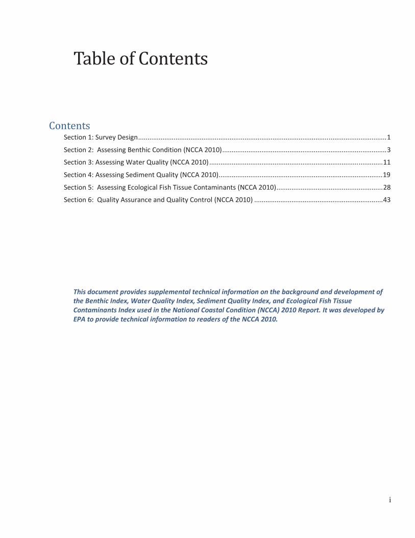
Table B-5. Trophic Classification of Oligochaete Species in NCCA 2010 Great Lakes data1†

Group 0 Group 1 Group 2 Group 3 Unassigned4 Limnodrilus profundicola Rhyacodrilus coccineus Rhyacodrilus montana Rhyacodrilus sp. Spirosperma nikolskyi Stylodrilus heringianus Lumbriculidae3 Trasserkidrilus superiorensis Trasserkidrilus americanus Tubifex tubifex*

Arcteonais lomondi2 Aulodrilus americanus Aulodrilus limnobius Aulodrilus pigueti Dero digitata2 Ilyodrilus templetoni Isochaetides freyi Slavina appendiculata2 Spirosperma ferox Uncinais uncinata2

Aulodrilus pluriseta Limnodrilus angustipenis Limnodrilus cervix Limnodrilus claparedianus Limnodrilus maumeensis Limnodrilus udekemianus Potamothrix bedoti Potamothrix moldaviensis Potamothrix vejdovskyi Quistadrilus multisetosus

Limnodrilus hoffmeisteri Tubifex tubifex*

Branchiura sowerbyi (2) Chaetogaster diaphanus (2) Dero sp. (2) Ilyodrilus frantzi Naidinae Nais sp. Nais bretscheri Ophidonais serpentina (2) Paranais grandis Paranais litoralis Piguetiella sp. Piguetiella blanci (2) Specaria Stylaria lacustris (2) Tubificinae Varichaetadrilus Vejdovskyella intermedia (1)

† Species in bold above were not reported from NCCA 2010 Great Lakes samples

*Tubifex tubifex is assigned to Group 0 or Group 3 according to the following rules: - if : < 0.75 then Group 0; - if : > 1.25 then Group 3; - if : = 0.75 – 1.25 then Group 0 if c < 0.5 or Group 3 if c ≥ 0.5; - if =0 then Group 0 if is relatively high and/or c is low; otherwise Group 3 1 from State of the Great Lakes 2012 – Draft – Benthic Diversity and Abundance Table 1. [Classifications are from Howmiller and Scott (1977), Milbrink (1983), Kreiger (1984), and Lauritsen et al (1985)]. Only species in the families, Naididae (formerly Tubificidae and Lumbriculidae were included. 2 These species were not included in SOLEC 2011 list presumably because they were thought to be in the family Naididae, not Tubificidae, although they were included in group 2 in earlier publications. However, recent taxonomy changes have reclassified Tubificidae to Naididae which has several subfamilies Naidinae within Tubificinae, so they were included in Group 1. 3 SOLEC classified all immature Lumbriculidae as Stylodrilus heringianus. Therefore taxa in NCCA 2010 GL samples that were identified as Lumbriculidae are assigned Group=0. 4 Taxa with numbers are group assignments recommended by Kurt Schmude, Univ. of Wisconsin - Superior

Benthic Condition References

Engle, V.D., and J.K. Summers. 1999. Refinement, validation, and application of a benthic condition index for

northern Gulf of Mexico estuaries. Estuaries 22(3A):624–635. Engle, VD., J.K. Summers, and G.R. Gaston. 1994. A benthic index of environmental condition of Gulf of Mexico

estuaries. Estuaries 17:372–384. Environment Canada and the U.S. Environmental Protection Agency. 2014. State of the Great Lakes 2011. Cat No. En161-3/1-2011E-PDF. EPA 950-R-13-002. Available at http://binational.net

Hale, S.S., and J.F. Heltshe. 2008. Signals from the benthos: Development and evaluation of a benthic index for

the nearshore Gulf of Maine. Ecological Indicators 8:338–350. Howmiller, R.P., and Scott, M.A. 1977. An environmental index based on relative abundance of oligochaete

species. J. Wat. Poll. Cont. Fed. 49:809-815. Lauritsen, D.D., S.C. Mozley, and D.S. White. 1985. Distribution of oligochaetes in Lake Michigan and comments

on their use as indices of pollution. J. Great Lakes Res. 11(1): 67-76.

10

Milbrink, G. 1983. An improved environmental index based on the relative abundance of oligochaete species. Hydrobiologia 102:89-97.

Paul, JF, KJ Scott, DE Campbell, et al. 2001. Developing and applying a benthic index of estuarine condition for the Virginian Biogeographic Province. Ecological Indicators 1:83-99.

Ranasinghe, JA, SB Weisberg, RW Smith, et al. 2009. Calibration and evaluation of five indicators of benthic

community condition in two California bay and estuary habitats. Marine Pollution Bulletin. 59:5-13. Smith, RW, M Bergen, SB Weisberg, et al. 2001. Benthic response index for assessing infaunal communities on

the southern California mainland shelf. Ecological Applications 11:1073-1087. Van Dolah, R.F., J.L. Hyland, A.F. Holland, J.S. Rosen, and T.T. Snoots. 1999. A benthic index of biological integrity

for assessing habitat quality in estuaries of the southeastern USA. Marine Environmental Research 48:(4–5):269–283.

11

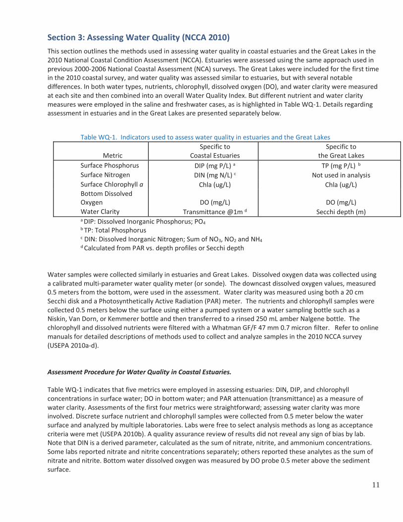
Section 3: Assessing Water Quality (NCCA 2010) This section outlines the methods used in assessing water quality in coastal estuaries and the Great Lakes in the 2010 National Coastal Condition Assessment (NCCA). Estuaries were assessed using the same approach used in previous 2000-2006 National Coastal Assessment (NCA) surveys. The Great Lakes were included for the first time in the 2010 coastal survey, and water quality was assessed similar to estuaries, but with several notable differences. In both water types, nutrients, chlorophyll, dissolved oxygen (DO), and water clarity were measured at each site and then combined into an overall Water Quality Index. But different nutrient and water clarity measures were employed in the saline and freshwater cases, as is highlighted in Table WQ-1. Details regarding assessment in estuaries and in the Great Lakes are presented separately below.

Water samples were collected similarly in estuaries and Great Lakes. Dissolved oxygen data was collected using a calibrated multi-parameter water quality meter (or sonde). The downcast dissolved oxygen values, measured 0.5 meters from the bottom, were used in the assessment. Water clarity was measured using both a 20 cm Secchi disk and a Photosynthetically Active Radiation (PAR) meter. The nutrients and chlorophyll samples were collected 0.5 meters below the surface using either a pumped system or a water sampling bottle such as a Niskin, Van Dorn, or Kemmerer bottle and then transferred to a rinsed 250 mL amber Nalgene bottle. The chlorophyll and dissolved nutrients were filtered with a Whatman GF/F 47 mm 0.7 micron filter. Refer to online manuals for detailed descriptions of methods used to collect and analyze samples in the 2010 NCCA survey (USEPA 2010a-d).

Assessment Procedure for Water Quality in Coastal Estuaries.

Table WQ-1 indicates that five metrics were employed in assessing estuaries: DIN, DIP, and chlorophyll concentrations in surface water; DO in bottom water; and PAR attenuation (transmittance) as a measure of water clarity. Assessments of the first four metrics were straightforward; assessing water clarity was more involved. Discrete surface nutrient and chlorophyll samples were collected from 0.5 meter below the water surface and analyzed by multiple laboratories. Labs were free to select analysis methods as long as acceptance criteria were met (USEPA 2010b). A quality assurance review of results did not reveal any sign of bias by lab. Note that DIN is a derived parameter, calculated as the sum of nitrate, nitrite, and ammonium concentrations. Some labs reported nitrate and nitrite concentrations separately; others reported these analytes as the sum of nitrate and nitrite. Bottom water dissolved oxygen was measured by DO probe 0.5 meter above the sediment surface.

Table WQ-1. Indicators used to assess water quality in estuaries and the Great Lakes

Metric Specific to

Coastal Estuaries Specific to

the Great Lakes Surface Phosphorus DIP (mg P/L) a TP (mg P/L) b Surface Nitrogen DIN (mg N/L) c Not used in analysis Surface Chlorophyll a Chla (ug/L) Chla (ug/L) Bottom Dissolved Oxygen DO (mg/L) DO (mg/L) Water Clarity Transmittance @1m d Secchi depth (m) a DIP: Dissolved Inorganic Phosphorus; PO4 b TP: Total Phosphorus c DIN: Dissolved Inorganic Nitrogen; Sum of NO3, NO2 and NH4 d Calculated from PAR vs. depth profiles or Secchi depth

12

Table WQ-2. Thresholds used to calculate water quality condition at estuarine sites

Surface DIP

(mg P/L)

Surface DIN

(mg N/L)

Surface CHLA

(ug/L)

Bottom DO

(mg/L)

TH1 TH2 TH1 TH2 TH1 TH2 TH1 TH2

Northeast 0.01 0.05 0.1 0.5 5 20 2 5

Southeast 0.01 0.05 0.1 0.5 5 20 2 5

Gulf 0.01 0.05 0.1 0.5 5 20 2 5

West 0.07 0.1 0.35 0.5 5 20 2 5

Tropics 0.005 0.01 0.05 0.1 0.5 1 2 5

Nutrient, chlorophyll a, and DO measurements in estuaries were evaluated as good, fair, or poor relative to thresholds listed in the Tables WQ-2. The thresholds for nutrients and chlorophyll vary by region. The Northeast encompasses the coasts of Maine through Virginia; the Southeast includes the remaining southern Atlantic seaboard; the Gulf refers to the Gulf of Mexico coastline Florida through Texas; and the West pertains to the coasts of California, Oregon, and Washington. While the tropics included various low latitude tropical locations in previous NCA surveys, the classification is limited to Florida Bay and Biscayne in this report. The nutrient and chlorophyll thresholds were set by consensus of regional experts at the beginning of the NCA program and maintained through all surveys (including this assessment) to maintain continuity. Dissolved oxygen thresholds reflect documented limits of disruption to estuarine communities (Diaz and Rosenberg, 1995; USEPA, 2000) and regulatory limits set by some states. Conditions for DIN, DIP, and CHLA were calculated as: good < TH1, fair < TH2, and poor > TH2; and for DO as: good > TH2, fair < TH2, and poor < TH1. Water clarity in estuaries was characterized primarily as Transmittance, defined as the percent of photosynthetically active radiation (PAR) transmitted through one meter of water, calculated as follows. PAR attenuation was measured using two PAR sensors. One sensor was lowered through the water column, measuring PAR intensity (Iz) at depths z. A second sensor in air reported varying incident PAR intensity (Io) arising, for instance, from changing cloud cover. The normalized PAR attenuation (Iz/Io) is assumed to follow Beer’s law, i.e., light intensity decreasing exponentially with distance:

Iz/Io = exp(-Kd*z) (Formula WQ-1)

Where Kd is the PAR attenuation coefficient; larger Kd magnitudes indicate greater attenuation, i.e., poorer water clarity. Equation WQ-1 is equivalently expressed as follows, highlighting the fact that the decreasing intensity ln(Iz/Io) is linearly proportional to depth:

ln(Iz/Io) = - Kd *z (Formula WQ-2)

Operationally, Kd is calculated as the negative slope of a regression of ln(Iz/Io) vs depth. PAR intensities and depth measurements are reported in a “hydrolab” data file available at the NARS website (http://water.epa.gov/type/watersheds/monitoring/aquaticsurvey_index.cfm). An Excel spreadsheet was devised to quickly review the regression plots for every site in order to identify, flag, and remove errant data values used in the regression calculation—a necessary step, as errant values were common.

Once reliable Kd values are obtained, % transmittance at one meter (i.e., Iz/Io at one meter) was calculated from Formula WQ-1 as:

13

% Trans @ 1m = exp(-Kd)*100 (Formula WQ-3)

The water clarity condition at a site (good, fair, or poor) was then determined by evaluating Transmittance relative to the thresholds in Table WQ-3. These transmittance thresholds vary depending on the turbidity level or SAV restoration status of the site. Less stringent thresholds hold for naturally turbid regions, and more stringent thresholds apply for waters supporting SAV restoration. To proceed with the analysis, sites must be categorized as to their turbidity status. For consistency with previous NCA reports, the same regional delineations of turbidity classes were used for this report (Smith et al., 2006). Naturally turbid regions consisted of waters in Alabama, Louisiana, Mississippi, South Carolina, Georgia, and Delaware Bay. Regions supporting SAV restoration included Laguna Madre, the Big Bend region of Florida, the coast from Tampa Bay to Florida Bay, the Indian River lagoon, and portions of Chesapeake Bay. All other sites were considered to exhibit normal turbidity. The turbidity class assignments for sites measured in 2010 are indicated in Figure WQ-1. Water clarity conditions were calculated as: good > TH2, fair < TH2, and poor < TH1.

Table WQ-3. Thresholds used to calculate water clarity (Transmittance) at estuarine sites

% Transmittance @ 1m* Kd = c/Secchi Depth**

TH1 TH2 Value of c

Naturally Turbid 5% 10% 1.0

Normal Turbidity 10% 20% 1.4

SAV Restoration 20% 40% 1.7

** Transmittance is calculated from PAR attenuation coefficient (Kd): Trans = exp(-Kd)*100 ** If not measured, Kd is estimated from Secchi Depth: Kd = c/Secchi Depth

14

Figure WQ-1. Turbidity class assignments for sites assessed in the 2010 NCCA.

If a Kd value was not available for a site, it was estimated from Secchi depth as:

Alternate Kd (estimated) = c/Secchi depth (Formula WQ-4)

where c is a constant specific to the water type, as indicated in Table WQ-3 (Smith et al, 2006). If neither Kd or Secchi depth was available, the condition at the site was set to “missing”. In summary, water clarity condition in estuaries was based on light transmittance derived from PAR attenuation or Secchi depth, evaluated relative to thresholds dependent on turbidity or SAV restoration status.

A Water Quality Index (WQI) for an estuarine site was then determined based on the condition of the five component metrics, evaluated according to the rules in Table WQ-4.

Table WQ-4. Rules for determining the Water Quality Index rating at estuarine sites

Rating Thresholds Good A maximum of one indicator is rated fair, and no indicators are rated poor. Fair One of the indicators is rated poor, or two or more indicators are rated fair. Poor Two or more of the five indicators are rated poor. Missing Two component indicators are missing, and the available indicators do not suggest a fair or

poor rating.

15

Historical perspective regarding water quality assessment in estuaries. Prior to writing this report, an advisory committee was assembled to review the NCA approach of assessing water quality. The committee largely found the original approach sound, but suggested using total nitrogen and total phosphorus rather than DIN and DIP as nutrient indicators, and recommended considering adjusting the regional thresholds for nutrients and chlorophyll to better bracket historical ranges of measured values (particularly in the case of DIP). NCCA program managers decided to retain the original NCA approach entirely, primarily to maintain continuity with earlier surveys and also because of an absence of any peer-reviewed alternate thresholds. TN and TP may be adopted for the 2015 survey if a review of relationships between total and dissolved measures of nutrients in 2010 suggest thresholds for TN and TP that would permit reliable comparison with earlier survey findings.

Assessment Procedure for Water Quality in the Great Lakes

Water Quality of the Great Lakes nearshore waters were assessed for the first time in 2010 as part of the National Assessment Resource Survey (NARS). Prior to writing this report, an advisory committee was convened to recommend methods for evaluating the Great Lakes that were compatible with methods used to assess water quality in estuaries. The committee found the general estuarine approach of basing the assessment on measures of nutrients, chlorophyll a, dissolved oxygen, and water clarity, applicable but recommended several changes appropriate for assessing a fresh water system.

Table WQ-1 outlines the recommended approach for assessing water quality along the Great Lakes coastline. Changes from the estuarine approach included: 1) assessing TP rather than DIP to characterize freshwater nutrient status; 2) excluding nitrogen from the assessment, following historical precedent and because of an absence of documented evaluation thresholds; and 3) using Secchi depth as the primary indicator of water clarity in the current assessment (rather than PAR attenuation) to ease comparison with prior Great Lakes assessments and to make use of established Secchi depth evaluation thresholds. Importantly, this recommended approach was based on existing International Joint Commission studies (IJC 1979 and IJC, 1980). Although the 1980 IJC guidelines were intended for open water, some of the 1979 IJC guidelines focused on nearshore waters and overlap with some of the 2010 design frame. The United States and Canada, under Annex 4 of the Great Lakes Water Quality Agreement (GLWQA of 2012) are currently reviewing and negotiating new guidelines, and the committee strongly advised against introducing new NCCA assessment methods or thresholds at this time. The advisory committee was open to including TN and PAR attenuation in future assessments following a careful review of 2010 data and release of new GLWQA guidelines.

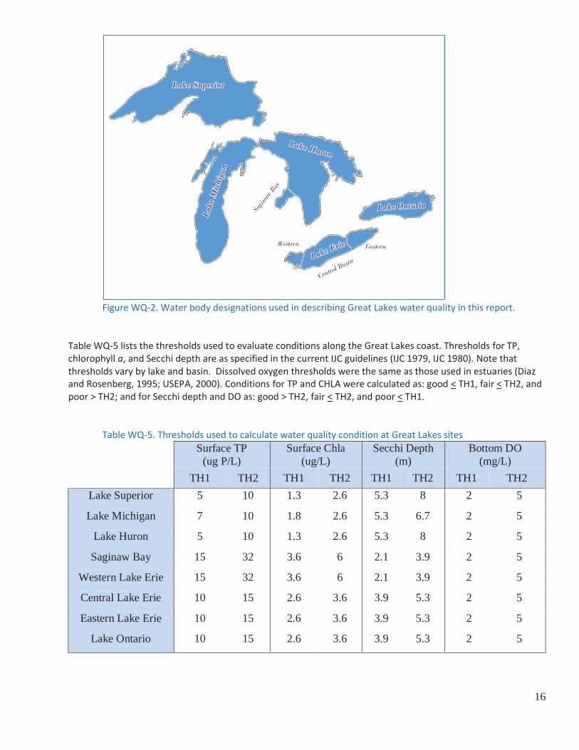
In the report the overall water quality condition of the Great Lakes is presented, based on assessment by basin and lake. Figure WQ-2 below shows the different basin categories used in the assessment. These categories are based on the expected trophic status of the basin. Lake Huron, Michigan and Superior are considered oligotrophic basins whereas most of Lake Erie and Ontario are oligomesotrophic. Saginaw Bay and western basin of Lake Erie are mesotrophic.

16

Figure WQ-2. Water body designations used in describing Great Lakes water quality in this report.

Table WQ-5 lists the thresholds used to evaluate conditions along the Great Lakes coast. Thresholds for TP, chlorophyll a, and Secchi depth are as specified in the current IJC guidelines (IJC 1979, IJC 1980). Note that thresholds vary by lake and basin. Dissolved oxygen thresholds were the same as those used in estuaries (Diaz and Rosenberg, 1995; USEPA, 2000). Conditions for TP and CHLA were calculated as: good < TH1, fair < TH2, and poor > TH2; and for Secchi depth and DO as: good > TH2, fair < TH2, and poor < TH1.

Table WQ-5. Thresholds used to calculate water quality condition at Great Lakes sites

Surface TP (ug P/L)

Surface Chla (ug/L)

Secchi Depth (m)

Bottom DO (mg/L)

TH1 TH2 TH1 TH2 TH1 TH2 TH1 TH2 Lake Superior 5 10 1.3 2.6 5.3 8 2 5

Lake Michigan 7 10 1.8 2.6 5.3 6.7 2 5

Lake Huron 5 10 1.3 2.6 5.3 8 2 5

Saginaw Bay 15 32 3.6 6 2.1 3.9 2 5

Western Lake Erie 15 32 3.6 6 2.1 3.9 2 5

Central Lake Erie 10 15 2.6 3.6 3.9 5.3 2 5

Eastern Lake Erie 10 15 2.6 3.6 3.9 5.3 2 5

Lake Ontario 10 15 2.6 3.6 3.9 5.3 2 5

17

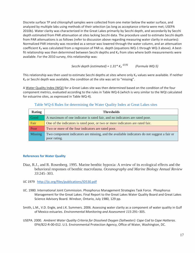
Discrete surface TP and chlorophyll samples were collected from one meter below the water surface, and analyzed by multiple labs using methods of their selection (as long as acceptance criteria were met; USEPA 2010b). Water clarity was characterized in the Great Lakes primarily by Secchi depth, and secondarily by Secchi depth estimated from PAR attenuation at sites lacking Secchi data. The procedure used to estimate Secchi depth from PAR attenuations is as follows (refer to discussion above regarding measuring water clarity in estuaries): Normalized PAR intensity was recorded as a sensor was lowered through the water column, and an attenuation coefficient Kd was calculated from a regression of PAR vs. depth (equations WQ-1 through WQ-3 above). A best-fit relationship was then determined between Secchi depths and Kd from sites where both measurements were available. For the 2010 survey, this relationship was:

Secchi depth (estimated) = 1.31* Kd

-0.91 (Formula WQ-5)

This relationship was then used to estimate Secchi depths at sites where only Kd values were available. If neither Kd or Secchi depth was available, the condition at the site was set to “missing”.

A Water Quality Index (WQI) for a Great Lakes site was then determined based on the condition of the four component metrics, evaluated according to the rules in Table WQ-6 (which is very similar to the WQI calculated for estuarine sites, as expressed in Table WQ-4).

Table WQ-6 Rules for determining the Water Quality Index at Great Lakes sites

Rating Thresholds Good A maximum of one indicator is rated fair, and no indicators are rated poor. Fair One of the indicators is rated poor, or two or more indicators are rated fair. Poor Two or more of the four indicators are rated poor. Missing Two component indicators are missing, and the available indicators do not suggest a fair or

poor rating.

References for Water Quality Diaz, R.J., and R. Rosenberg. 1995. Marine benthic hypoxia: A review of its ecological effects and the

behavioral responses of benthic macrofauna. Oceanography and Marine Biology Annual Review 33:245–303.

IJC 1979 http://ijc.org/files/publications/ID530.pdf IJC. 1980. International Joint Commission. Phosphorus Management Strategies Task Force. Phosphorus

Management for the Great Lakes. Final Report to the Great Lakes Water Quality Board and Great Lakes Science Advisory Board. Windsor, Ontario, July 1980, 129 pp.

Smith, L.M., V.D. Engle, and J.K. Summers. 2006. Assessing water clarity as a component of water quality in Gulf

of Mexico estuaries. Environmental Monitoring and Assessment 115:291–305. USEPA. 2000. Ambient Water Quality Criteria for Dissolved Oxygen (Saltwater): Cape Cod to Cape Hatteras.

EPA/822-R-00-012. U.S. Environmental Protection Agency, Office of Water, Washington, DC.

18

USEPA. 2010a. National Coastal Condition Assessment: Field Operations Manual. EPA-841-R-09-003. U.S. Environmental Protection Agency, Office of Water. Washington, DC.

USEPA. 2010b. National coastal condition assessment: Laboratory methods manual. EPA 841-R-09-002. U.S.

Environmental Protection Agency, Office of Water. Washington, DC. USEPA. 2010c. National Coastal Condition Assessment: Quality Assurance Project Plan 2008-2012. EPA/841-R-

09-004. U.S. Environmental Protection Agency, Office of Water. Washington, D.C. USEPA. 2010d. National Coastal Condition Assessment: Site Evaluation Guidelines. U.S. Environmental

Protection Agency, Office of Water. Washington, DC. USEPA. 2012. National Coastal Condition Report IV. EPA-842-R-10-003. U.S. Environmental Protection Agency,

Office of Water. Washington, DC. Costantini, Marco; Kolesar, Sarah; Ludsin, Stuart A; Mason, Doran M.; Rae, Christopher M.; Zhang, Hongyan.

2011. Does hypoxia reduce habitat quality for Lake Erie walleye (Sander vitreus)? A bioenergetics perspective. Canadian Journal of Fisheries and Aquatic Sciences, Volume 68, Number 5, pp. 857-879(23). http://www.ingentaconnect.com/content/nrc/cjfas/2011/00000068/00000005/art00011

Ohio Lake Erie Commission Report “Nearshore Hypoxia as a New Lake Erie Metric”

http://lakeerie.ohio.gov/Portals/0/Closed%20Grants/small%20grants/SG%20334-07%20Final%20Report.pdf

19

Section 4: Assessing Sediment Quality (NCCA 2010) The National Coastal Condition Assessment (NCCA) program uses sediment chemistry and sediment toxicity data to assess the sediment quality of the Nation’s nearshore coastal waters. Field crews collect comparable sediment samples that are analyzed to determine concentrations of a suite of contaminants and subjected to sediment toxicity tests (USEPA 2010a; 2010b). All of these studies are conducted with a high level of quality assurance/quality control procedures (USEPA 2010c). The NCCA program reports integrate sediment chemistry and sediment toxicity data into a Sediment Quality Index (SQI) to designate the percentage of the Nation’s coastal waters that are in good, fair, and poor condition. The NCCA has determined changes are needed for how this index is calculated. Better techniques are now available for calculating the index for estuarine sediments. In addition, the NCCA field surveys in 2010 were expanded to include freshwater nearshore areas along the Great Lakes, and this provided a new opportunity to develop a SQI specific to freshwater sites. This section describes how the Sediment Quality Index was calculatedfor nearshore estuarine and freshwater areas. Sediment Quality Index in the NCCA 2010 Survey

Sediment Collection The NCCA field crews collected surficial sediment samples during the summer of 2010 from nearshore coastal areas of the Great Lakes and contiguous United States. Sediment was collected using a variety of grab apparatus (see Table B-3). Samples were collected as close to a predetermined probabilistic site as possible. If sediment was not found at the site and within 37 meters (anchor swing), crews moved outward, attempting collection

What’s New for the Sediment Quality Index? Sediment Contaminant condition

o Estuarine mean Effects Range Median quotient (ERM-Q) Logistic regression models (LRM)

o Freshwater (Great Lakes) mean probable Effects Concentration quotient (PEC-Q)

Sediment Toxicity condition o Estuarine

Control-corrected survival of amphipods and statistical significance of test vs. control survival

Leptochirus plumulosus or Eohaustorius estuarus (California only).

o Freshwater (Great Lakes) Control-corrected survival of amphipods Hyalella azteca

Total Organic Carbon (TOC)- o No longer part of the indices for estuarine sediment assessment. o Data are collected and maintained for ancillary purposes.

20

within a 100 meter radius of the index site in estuarine waters or within a 500 meter radius in the Great Lakes. At each site, the top two centimeters of sediment were composited from multiple grab samples to obtain the volumes necessary to analyze for concentrations of chemical constituents, sediment toxicity, TOC, and grain size (USEPA 2010a; 2010b). Assessing Sediment Chemistry With the exception of South Carolina and California, who used in-state labs, all sediment chemistry samples were collected and sent to one contracted laboratory to determine the concentrations of metals, mercury, PAHs, PCBs, organochlorine pesticides and TOC (USEPA 2010a; 2010b). Laboratory results were transmitted to the NARS database and collated in a single database. Values for total PAHs (i.e., Sum of LMW PAH (Acenaphthene, Acenaphthylene, Anthracene, Fluorene, 2-methylnaphthalene, Naphthalene, Phenanthrene) and HMW PAH (Benz(a)anthracene, Benzo(a)pyrene, Chrysene, Dibenz(a,h)anthracene, Fluoranthene, Pyrene), total PCBs, and total DDTs (i.e., p,p’-DDT, o,p’-DDT, p,p’-DDE, o,p’-DDE, p,p’-DDD, o,p’-DDD) were calculated as the sum of concentrations of individual chemicals in each class. Detection limits all had to be below or at the Effects Range Low (ERL) or Threshold Effect Concentration (TEC) or T25 to be included in calculation of their respective methods. See Table S-4 for these values. Where concentrations were reported as non-detects, concentrations were converted to one-half the method detection limit (0.5*MDL). Sediment quality guidelines (SQGs) identify concentrations of individual contaminants that may be associated with adverse effects on benthic organisms (Long et al. 2006). Two such SQGs are the effects-range median (ERM; Long et al. 1995) developed for marine waters, and the probable effects concentrations (PEC; MacDonald et al. 2000; Ingersoll et al. 2001) developed for freshwater. While these SQGs are adequate for assessing individual contaminants in sediment, contaminants rarely occur alone; rather, they are almost always present as complex mixtures. Therefore, researchers use mean SQG quotients that consider the composition of the mixture to assess the relative degree of contamination and corresponding probability of toxicity to benthic organisms (Long et al. 2006). Details about the use of SQGs in estuarine and freshwater samples can be found below. In addition to SQGs, a logistic regression model (LRM) approach was also used in estuarine waters to evaluate relationships between contaminant concentrations and adverse effects of select contaminants (Field et al. 2002; USEPA 2005). The model provides information on chemical concentrations associated with particular levels of sediment toxicity to benthic invertebrates. An LRM type of model does not exist for assessing freshwater sediments in the Great Lakes. Estuarine Samples The mean ERM quotient (mERM-Q) SQG approach was used in combination with the LRM to provide multiple lines of evidence to interpret the sediment chemistry collected at estuarine coastal sites.

The mERM-Q approach calculates the degree to which concentrations of various chemical contaminants in a sample exceed corresponding ERM SQG values (Table S-4). To avoid redundancy, 4,4’-DDE, total PAHs, and summed low or high molecular weight PAHs were excluded from this calculation. Nickel was also excluded due to the unreliability of its ERM guideline (Long et al. 1998). To calculate mERM-Q, each chemical concentration is divided by its corresponding ERM value. The mERM-Q is the average of the resulting ratios for a sample:

Individual ERM-Q = chemical concentration (dry wt.)/corresponding ERM value (Formula S-1)

Mean ERM-Q = (ERM-Qarsenic + ERM-Qchromium + ... ERM-Qtotal PCBs)/n (Formula S-2)

21

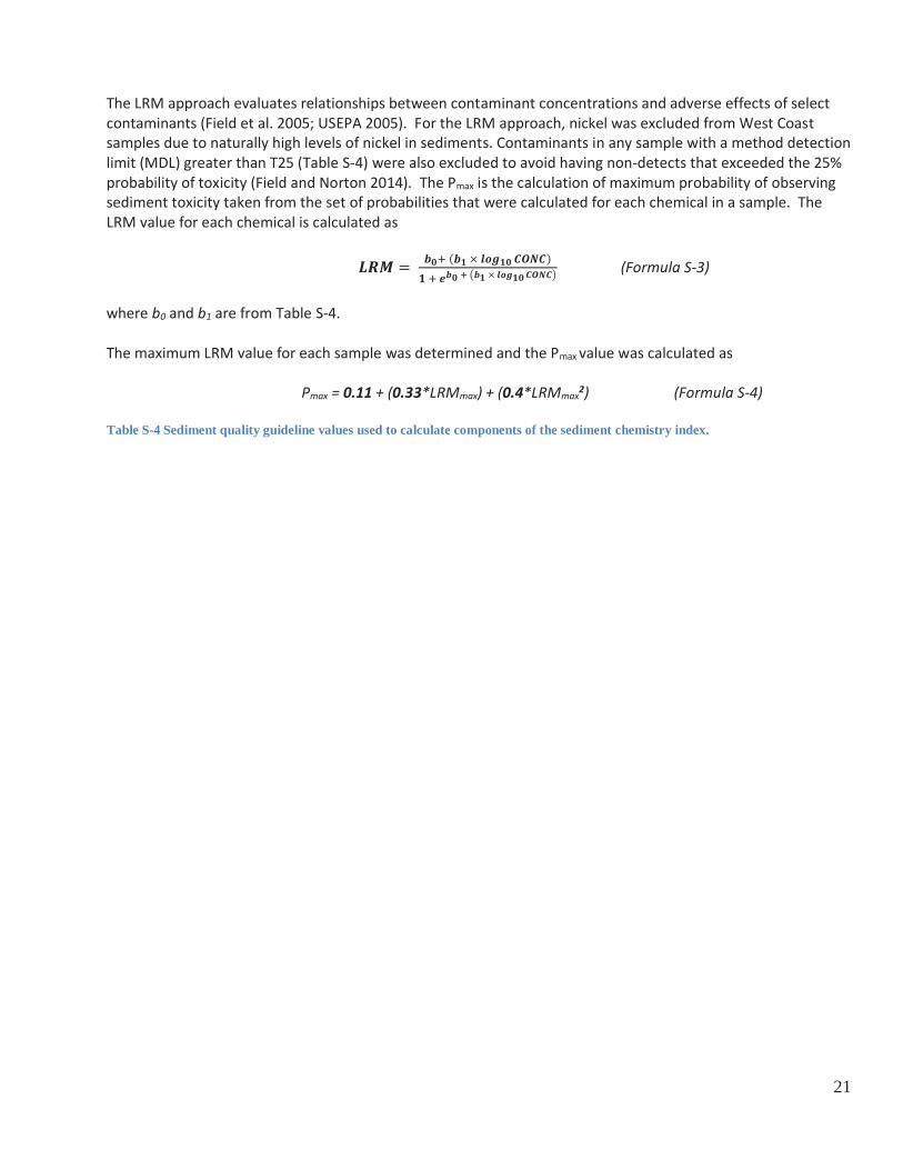
The LRM approach evaluates relationships between contaminant concentrations and adverse effects of select contaminants (Field et al. 2005; USEPA 2005). For the LRM approach, nickel was excluded from West Coast samples due to naturally high levels of nickel in sediments. Contaminants in any sample with a method detection limit (MDL) greater than T25 (Table S-4) were also excluded to avoid having non-detects that exceeded the 25% probability of toxicity (Field and Norton 2014). The Pmax is the calculation of maximum probability of observing sediment toxicity taken from the set of probabilities that were calculated for each chemical in a sample. The LRM value for each chemical is calculated as

(Formula S-3)

where b0 and b1 are from Table S-4. The maximum LRM value for each sample was determined and the Pmax value was calculated as

Pmax = 0.11 + (0.33*LRMmax) + (0.4*LRMmax2) (Formula S-4) Table S-4 Sediment quality guideline values used to calculate components of the sediment chemistry index.

22

Sediment Chemicals analyzed for NCCA 2010

(Metals in μg/g; PAHs, Pesticides and PCBs in ng/g)

ERL/ERM Values

Used to calculate mERM-Q

Used in LRM - Pmax calculation

B0 B1

LRM

T25

LRM

T75

Consensus based

TEC/PEC Values

Consensus Based mPECq

Aluminum Antimony -0.9005 2.4111 0.83 6.75 Arsenic 8.2/70 x -4.1407 3.1674 9.13 45.10 9.79/33 x Cadmium 1.2/9.6 x -0.3400 2.5073 0.50 3.75 .99/4.98 x Chromium 81/370 x -6.4395 2.9952 60.69 328.65 43.4/111 x Copper 34/270 x -5.7878 2.9325 39.72 223.00 31.6/149 x Iron Lead 46.7/218 x -5.4523 2.7662 37.49 233.45 35.8/128 x Manganese Mercury .15/.71 x 0.8041 2.5461 0.18 1.31 .18/1.06 Nickel 20.9/51.6 -4.6119 2.7658 18.63 116.06 22.7/48.6 x Selenium Silver 1/3.7 x -0.1117 1.9684 0.32 4.12 Tin Zinc 150/410 x -7.9834 3.3420 114.84 521.84 121/459 x

Acenaphthene 16/500 X -3.6165 1.7532 27.30 489.14 6.7/89 Acenaphthylene 44/640 X -2.9620 1.3797 22.42 877.23 5.9/130 Anthracene 85.3/1100 X -3.6574 1.4854 52.80 1591.62 57.2/845 Benz(a)anthracene 261/1600 X -4.2013 1.5747 93.40 2320.94 108/1050 Benzo(b)fluoranthene -4.5409 1.4916 203.13 6037.37 Benzo(e)pyrene Benzo(k)fluoranthene -4.2781 1.5669 106.94 2700.43 Benzo(ghi)perylene 101.00 2444.30 Benzo(a)pyrene 430/1600 X -4.3005 1.5832 105.30 2571.89 150/1450 Biphenyl -4.1144 2.2085 23.20 229.31 Chrysene 384/2800 X -4.3241 1.5372 125.40 3370.20 166/1290 Dibenz(a,h)anthracene 63.4/260 X -3.6308 1.7692 26.99 471.19 Dibenzothiophene 2,6-dimethylnapthalene -4.0456 1.9040 35.30 503.26 Fluoranthene 600/5100 X -4.4574 1.4787 186.83 5719.56 423/2230 Fluorene 19/540 X -3.7146 1.8071 28.03 460.79 77.4/536 Indeno(1,2,3-c,d)pyrene -4.3674 1.6245 102.84 2315.98 1-methylnapthalene -4.1405 2.0961 28.26 315.83 2-methylnapthalene 70/670 X -3.7579 1.7833 30.99 528.85 20.2/200 1-methylphenanthrene -3.5884 1.7501 26.46 476.58 Napthalene 160/2100 X -3.7753 1.6152 45.41 1041.19 176/561 Perylene -4.6827 1.7632 107.82 1900.53 Phenanthrene 240/1500 X -4.4576 1.6768 100.74 2058.64 204/1170 Pyrene 665/2600 X -4.7080 1.5854 189.08 4597.84 195/1520 2,3,5-trimethylnapthalene LMWPAH 552/3160 HMWPAH 1700/9600 Total PAHs* 4020/44800 1610/22800 x Total PCB congeners 22.7/180 X -3.4613 1.3488 56.45 2402.80 60/676 x Aldrin Alpha-Chlordane Lindane 2.37/4.99 2,4’DDD 4,4’DDD -1.8983 1.4913 3.44 102.23 2,4’DDE 4,4’DDE 2.2/27 -1.8392 0.9129 6.48 1652.38 2,4’DDT 4,4’DDT -1.7705 1.6786 2.51 51.20 Total DDT 1.6/46.1 X 5.28/572 Dieldrin -1.1728 2.5580 1.07 7.73 1.9/61.8 Endosulfan I Endosulfan II Endosulfan sulfate Endrin 2.2/207 Heptachlor Heptachlor epoxide 2.5/16

23

Sources: Field et al. 2002; Long 1995; McDonald et al. 2000; Crane et al. 2002, Crane and Hennes 2007) Freshwater Samples The freshwater consensus-based PEC values were derived from an aggregation of several different empirically derived sediment quality guidelines having similar narrative intent (MacDonald et al. 2000). Similar to the mERM-Q approach, the mPEC-Q distills data from a mixture of contaminants into one unitless index which can be compared to incidence of sediment toxicity. The mean PEC quotient is calculated using the average of three PEC-Qs using only those contaminants with reliable PECs: 1) mean PEC-Q for metals; 2) PEC-Q for total PAHs; and 3) PEC-Q for total PCBs. Total PAHs are used instead of summing the PEC-Qs of individual PAHs (Table S-4). Individual PEC-Qs are calculated as follows:

Individual PEC-Q = chemical concentration (dry w.t)/corresponding PEC value (Formula S-5)

Next, the mPEC-Q for the metals with reliable PECs (i.e., arsenic, cadmium, chromium, copper, lead, nickel, and zinc) is calculated as follows:

mPEC-Qmetals = ∑individual metal PEC-Qs/n (Formula S-6)

where n is the number of metals with reliable PECs for which sediment chemistry data are available. Finally, the mPEC-Q for the main classes of chemicals with reliable PECs is calculated as follows:

mPEC-Q = (mPEC-Qmetals + PEC-Qtotal PAHs + PEC-Qtotal PCBs)/n (Formula S-7)

Where n = number of classes of chemicals for which sediment chemistry data are available (i.e., 1 to 3).

Thresholds Thresholds were selected based on the probability of toxic effects and do not represent values for which adverse effects are always observed or not observed. They are based on literature review, best professional judgment and statistical analysis of historic data. The thresholds for mERMq are based on a study that used a national dataset (Long et al. 1998) and the mPECq thresholds are based on several studies (Ingersoll et al. 2001, Crane et al. 2002, Crane and Hennes 2007). The LRM thresholds were selected as 0.75 and 0.50, however, the LRM model is designed to determine continuous estimates of risk so the application can match the degree of risk as defined by the user and their objective (Field et al. 1999, Field et al. 2002, EPA 2005). The thresholds for rating sediment chemistry based on the mERM-Q and LRM approaches for estuarine sites and the mPEC-Q approach for Great Lakes sites are shown in Table S-5.

Heptachlorobenzene Mirex Trans-Nonachlor

24

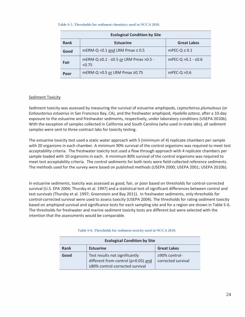
Table S-5. Thresholds for sediment chemistry used in NCCA 2010.

Ecological Condition by Site

Rank Estuarine Great Lakes

Good mERM-Q <0.1 and LRM Pmax ≤ 0.5 mPEC-Q ≤ 0.1

Fair mERM-Q ≥0.1 - ≤0.5 or LRM Pmax >0.5 -<0.75

mPEC-Q >0.1 - ≤0.6

Poor mERM-Q >0.5 or LRM Pmax ≥0.75 mPEC-Q >0.6

Sediment Toxicity Sediment toxicity was assessed by measuring the survival of estuarine amphipods, Leptocheirus plumulosus (or Eohaustorius estuarius in San Francisco Bay, CA), and the freshwater amphipod, Hyalella azteca, after a 10-day exposure to the estuarine and freshwater sediments, respectively, under laboratory conditions (USEPA 2010b). With the exception of samples collected in California and South Carolina (who used in-state labs), all sediment samples were sent to three contract labs for toxicity testing. The estuarine toxicity test used a static water approach with 5 (minimum of 4) replicate chambers per sample with 20 organisms in each chamber. A minimum 90% survival of the control organisms was required to meet test acceptability criteria. The freshwater toxicity test used a flow through approach with 4 replicate chambers per sample loaded with 10 organisms in each. A minimum 80% survival of the control organisms was required to meet test acceptability criteria. The control sediments for both tests were field-collected reference sediments. The methods used for the survey were based on published methods (USEPA 2000; USEPA 2001; USEPA 2010b). In estuarine sediments, toxicity was assessed as good, fair, or poor based on thresholds for control-corrected survival (U.S. EPA 2004; Thursby et al. 1997) and a statistical test of significant differences between control and test survivals (Thursby et al. 1997; Greenstein and Bay 2011). In freshwater sediments, only thresholds for control-corrected survival were used to assess toxicity (USEPA 2004). The thresholds for rating sediment toxicity based on amphipod survival and significance tests for each sampling site and for a region are shown in Table S-6. The thresholds for freshwater and marine sediment toxicity tests are different but were selected with the intention that the assessments would be comparable.

Table S-6. Thresholds for sediment toxicity used in NCCA 2010.

Ecological Condition by Site

Rank Estuarine Great Lakes Good Test results not significantly

different from control (p>0.05) and ≥80% control-corrected survival

≥90% control-corrected survival

25

Ecological Condition by Site

Rank Estuarine Great Lakes Fair Test results significantly different

from control (p≤0.05) and ≥80% control-corrected survival or Test not significantly different from control (p>0.05) and <80% control-corrected survival

75-<90% control-corrected survival

Poor Test results significantly different from control (p<0.05) and <80% control-corrected survival

<75% control-corrected survival

Sediment Quality Index The NCCA 2010 calculates a sediment quality index (SQI) from the component indicators. The SQI relies on sediment chemistry and toxicity to suggest whether a site is highly likely or not likely to cause adverse effects to benthic organisms. For instance, the SQI at a site is rated poor when either of the component metrics are poor. Table S-7 summarizes the rules used in assessing sediment quality conditions for both marine and Great Lakes coastal regions. The sediment chemistry and sediment toxicity thresholds do not address variations in bioavailability due to geochemical factors or differences in the nature of chemical mixtures between sites or regions. The thresholds and index are not intended for regulatory or site-specific interpretations.

TableS- 2. Thresholds for the sediment quality index used in NCCA 2010.

Rank Ecological Condition by Site

Good Both sediment chemistry index and sediment toxicity index are rated good. Fair Neither sediment chemistry index nor sediment toxicity index are rated

poor and at least one index is rated fair Poor Either sediment chemistry index or sediment toxicity index are rated poor

References for Sediment Quality Crane, J.L. and S. Hennes. 2007. Guidance for the use and application of sediment quality targets for the

protection of sediment-dwelling organisms in Minnesota. Minnesota Pollution Control Agency, St. Paul, MN. MPCA Doc. No. tdr-gl-04. (http://www.pca.state.mn.us/index.php/view-document.html?gid=9163)

Crane, J.L., D.D. MacDonald, C.G. Ingersoll, D.E. Smorong, R.A. Lindskoog, C.G. Severn, T.A. Berger, and L.J. Field.

2002. Evaluation of numerical sediment quality targets for the St. Louis River Area of Concern. Arch. Environ. Contam. Toxicol. 43:1-10

Fairey, E. R. Long, C. A. Roberts, B. S. Anderson, B. M. Phillips, J. W. Hunt, H. R. Puckett, C. J. Wilson. 2001. An evaluation of methods for calculating mean sediment quality guideline quotients as indicators of

26

contamination and acute toxicity to amphipods by chemical mixtures. Environmental Toxicology & Chemistry 20 (10): 2236-2286.

Field J.F., D.D. MacDonald, S.B. Norton, C.G. Severn, and C.G. Ingersoll. 1999. Evaluating sediment chemistry

and toxicity data using logistic regression modeling. Environ. Toxicol. Chem. 18 ( 6):1311–1322. Field, L.J., D.D. MacDonald, S.B. Norton, C.G. Ingersoll, C.G. Severn, D. Smorong, and R. Lindskoog. 2002.

Predicting amphipod toxicity from sediment chemistry using logistic regression models. Environ. Toxicol. Chem. 21: 1993-2005.

Field, L.J. and S.B. Norton. 2014. Regional models for sediment toxicity assessment. Environ. Toxicol. Chem.

33:708-717. Greenstein, D.J. and S.M. Bay. 2011. Selection of methods for assessing sediment toxicity in California bays and

estuaries. Integr. Environ. Assess. Manage. 8:625-637. Hyland,J, L. Balthis, I. Karakassis, P. Magni, A. Petrov, J. Shine,O. Vesterg aard, R. Warwick. 2005. “Organic

carbon content of sediments as an indicator of stress in the marine benthos” Marine Ecology Progress Series.

Vol. 295: 91–103, 2005 Published June 23 Ingersoll, C.G., D.D. MacDonald, N. Wang, J.L. Crane., L.J. Field, P.S. Haverland, N.E. Kemble, R.A Lindskoog, C.

Severn, and D.E. Smorong. 2001. Predictions of sediment toxicity using consensus-based freshwater sediment quality guidelines. Arch. Environ. Contam. Toxicol. 41:8-21.

Long, E.R., D.D. MacDonald, S.L. Smith, and F.D. Calder. 1995. Incidence of adverse biological effects within

ranges of chemical concentrations in marine and estuarine sediments. Environ. Manage. 19:81–97. Long, E.R., L.J. Field, and D.D. MacDonald. 1998. Predicting toxicity in marine sediments with numerical sediment

quality guidelines. Environ. Toxicol. Chem. 17:714–727. Long, E.R., D.D. MacDonald, C.G. Severn and C.B. Hong. 2000. Classifying the probabilities of acute toxicity in

marine sediments with empirically derived sediment quality guidelines. Environ. Toxicol. Chem. 19:2598-2601. Long, E. R., C. G. Ingersoll, D. D. MacDonald. 2005. Calculation and uses of mean sediment quality guideline

quotients: A critical review. Environmental Science and Technology 40 (6): 1726-1736. Long, E.R., C.G. Ingersoll and D.D. MacDonald. 2006. Calculation and uses of mean sediment quality guideline

quotients: A critical review. Environmental Science & Technology 40:1726-1736. MacDonald D.D., C.G. Ingersoll, and T.A. Berger. 2000. Development and evaluation of consensus-based

sediment quality guidelines for freshwater ecosystems. Arch. Environ. Contam. Toxicol. 39:20-31. McCready, S., G. F. Birch, E. R. Long, G. Spyrakis, C. R. Greely. 2006. Predictive abilities of numerical sediment

quality guidelines in Sydney Harbour, Australia, and vicinity. Environment International 32: 638-649 Thursby G.B., J. Heltshe and K.J. Scott. 1997. Revised approach to toxicity test acceptability criteria using a

statistical performance assessment. Environ. Toxicol. Chem. 16:1322-1329.

27

USEPA. 2000. Methods for measuring the toxicity and bioaccumulation of sediment-associated contaminants with freshwater invertebrates. Second Edition. EPA 600-R-99-064. U.S. Environmental Protection Agency. Washington, DC.

USEPA. 2001. Method for assessing the chronic toxicity of marine and estuarine sediment-associated

contaminants with the amphipod Leptocheirus plumulosus. EPA 600-R-01-020. U.S. Environmental Protection Agency. Washington, DC.

USEPA. 2002. A guidance manual to support the assessment of contaminated sediments in freshwater

ecosystems. Volume III – Interpretation of the results of sediment quality investigations. EPA-905-B02-001-C. U.S. Environmental Protection Agency, Great Lakes National Program Office, Chicago, IL.

USEPA. 2004. The incidence and severity of sediment contamination in surface waters of the United States,

National Sediment Quality Survey: Second Edition. EPA-823-R-04-007. U.S. Environmental Protection Agency, Office of Science and Technology. Washington, DC.

USEPA. 2005. Predicting toxicity to amphipods from sediment chemistry. EPA/600/R-04/030. U.S.

Environmental Protection Agency, Office of Research and Development. Washington, DC. USEPA. 2010a. National Coastal Condition Assessment: Field Operations Manual. EPA-841-R-09-003. U.S.

Environmental Protection Agency, Office of Water. Washington, DC. USEPA. 2010b. National coastal condition assessment: Laboratory methods manual. EPA 841-R-09-002. U.S.

Environmental Protection Agency, Office of Water. Washington, DC. USEPA. 2010c. National Coastal Condition Assessment: Quality Assurance Project Plan 2008-2012. EPA/841-R-

09-004. U.S. Environmental Protection Agency, Office of Water. Washington, D.C. USEPA. 2010d. National Coastal Condition Assessment: Site Evaluation Guidelines. U.S. Environmental

Protection Agency, Office of Water. Washington, DC. USEPA. 2012. National Coastal Condition Report IV. EPA-842-R-10-003. U.S. Environmental Protection Agency,

Office of Water. Washington, DC.

28

Section 5: Assessing Ecological Fish Tissue Contaminants (NCCA 2010) Contaminant concentrations in biotic tissues provide a time integrated assessment of bioavailability and information on chemical fate and distribution. The National Coastal Condition Assessment (NCCA) program uses whole-body fish tissue data to assess the biologically available contaminant conditions in the Nation’s nearshore coastal waters. Statistically-based field surveys are designed to collect fish samples of selected species that are analyzed for a suite of contaminants (USEPA 2010a; 2010b). All of these studies are conducted with a high level of quality assurance/quality control procedures (USEPA 2010c) that ensure data collected from a subset of sampled sites can be applied to broader coastal regions. Tissue chemistry results provide the basis for calculating an Ecological Fish Tissue Contaminant Index (EFTCI). For the current report, NCCA has determined that index calculation changes were needed in order to better represent ecological relevance. This appendix describes how the EFTCI was calculated in previous assessments, the rationale for updating it, and the new procedure for calculating the index for nearshore estuarine and Great Lakes coastal areas. Review and approach development for this effort was prepared for US EPA, Region 6 by Tetra Tech, Inc. (Tetra Tech, 2012).

Ecological Fish Tissue Contaminant Index for the NCCA 2010 Survey

The evaluation of risk using food webs for contaminant exposure through dietary uptake has been well documented (USEPA, 1997; US ARMY 2006; Sample et al., 1996). USEPA has established risk assessment guidelines primarily for its Superfund program under the Resource Conservation and Recovery Act (RCRA) (USEPA, 1997; 1998; 1999). These guidelines evaluate whether environmental concentrations of contaminants (i.e., soil, sediment, water, and tissue) potentially pose risk to nonhuman receptors of concern. The guidelines governing the evaluation of ecological risk derivation are well documented and have been used in many programs (Newell et al., 1987; USEPA, 1997; CCME, 1998; US Army, 2006; and ODEQ, 2007). Field crews collected selected fish specimens (USEPA 2010a) from over 800 sampling locations randomly located within continental US nearshore marine and estuarine areas as well as throughout the Great Lakes nearshore coastal areas. Whole fish tissue samples of predominantly forage-size fish were analyzed for measurable concentrations of multiple contaminants of concern (USEPA 2010b). Analytical results were compared with updated ecological fish tissue contaminant screening values that were developed to evaluate risk to upper-trophic level fish and wildlife, including birds and mammals. Using an ecological risk assessment approach (USEPA, 1997), risk was defined by developing a ratio of exposure concentration compared to a concentration that is known to have toxicological effects. The exposure concentration is developed based on known characteristics of each of the receptors of concern (i.e., fish, birds and mammals) including body weight, food ingestion rate, and home range (i.e., natural range of receptor with respect to foraging, breeding, and other activities). The concentration of contaminant that is known to elicit toxicological effects (i.e., toxicological reference value or TRV), is reported in the literature for certain species for each contaminant. Using an ecological risk assessment framework, a ratio greater than 1.0 indicates that exposure concentration is greater than the toxicological reference value. By using the minimum risk level of 1.0, the fish tissue concentration that would indicate this minimum risk can be calculated. Methods for Developing Ecological Fish Tissue Contaminant Threshold Values

29

Risk potential was derived by calculating a hazard quotient (HQ) or the ratio of exposure concentration divided by a concentration known to elicit toxicological effects (Low Observed Adverse Effects Level or LOAEL) or known not to elicit toxicological effects (No Observed Adverse Effect Level or NOAEL). Risk can be expressed as:

Risk (HQ) = Exposure Concentration/Toxicity (Formula EFTC-1)

Thus, when the exposure concentration is greater than the concentration known to elicit toxic effects, the HQ is greater than 1.0, and the receptor is at risk. The derivation of the exposure concentration was specific for each receptor and dependent on known characteristics for each receptor including body weight, food ingestion rate, exposure area relative to the amount of time the organism spends in the area (or Area Use Factor, AUF), and fish tissue concentration. The exposure concentration can be represented by the formula:

(Formula EFTC-2)

Where:

FI = food ingestion (kg/kg bw/d) [Fish] = concentration in fish tissue (mg/kg)

AUF = area use factor

BW = body weight of receptor (kg-bw)

For added conservativeness the AUF was set to 1.0 indicating all foraging, resting, breeding and other activities are expected to occur within the exposure area of concern. Toxicity was quantified as toxicity reference values (TRVs). Toxicity reference values are established from the available scientific literature. For the 2010 NCCA survey, the NOAEL and LOAEL served as the basis for establishing threshold contaminant values. Toxicity reference values are typically established for each receptor of concern or group of receptors (i.e., avian, freshwater and marine fish and mammals, etc.).

Receptors of Concern For NCCA, upper trophic level organisms including birds, fish and mammals are considered receptors of concern (ROCs). ROCs are typically those animals that are exposed to contaminants through ingestion, dermal contact, and/or inhalation. The exposure of ROCs to contaminants by ingestion is through either incidental media uptake (i.e., eating soil or sediment that is associated with prey items), drinking contaminated surface water, or through the ingestion of prey items which have accumulated contaminants in their tissues. For NCCA, data evaluated were whole-body forage fish tissue concentrations; therefore the only pathway of exposure evaluated for the assessment focused on the uptake of contaminants that have been accumulated in the tissues of prey items (i.e., fish). Classes of receptors were created to develop potential exposure-based screening values since data consisted of both freshwater and marine fish tissues. These classes include: freshwater predatory fish, marine predatory

30

fish, piscivorous birds, piscivorous freshwater mammals and piscivorous marine mammals. Receptors were chosen based on their diet (predominantly fish) and the availability of data in the literature. Potential receptors evaluated for NCCA represent those species that are typically included in ecological risk assessments (Table EFTC-1).

Table EFTC-1. Potential receptors of concern often evaluated in ecological risk assessments.

Avian Receptor Freshwater Mammalian

Receptor

Marine Mammalian

Receptor

Freshwater Fish Receptor

Marine Fish Receptor

Great Blue Heron River Otter Harbor Seal Largemouth Bass Bluefin Tuna Osprey Mink Bottlenose

Dolphin Florida Gar Yellowfin Tuna

Bald Eagle Walrus Muskellunge Shortfin Mako Herring Gull Snakehead Sandbar Shark Belted Kingfisher Lake Walleye Mackerel Tuna Brown Pelican Swordfish

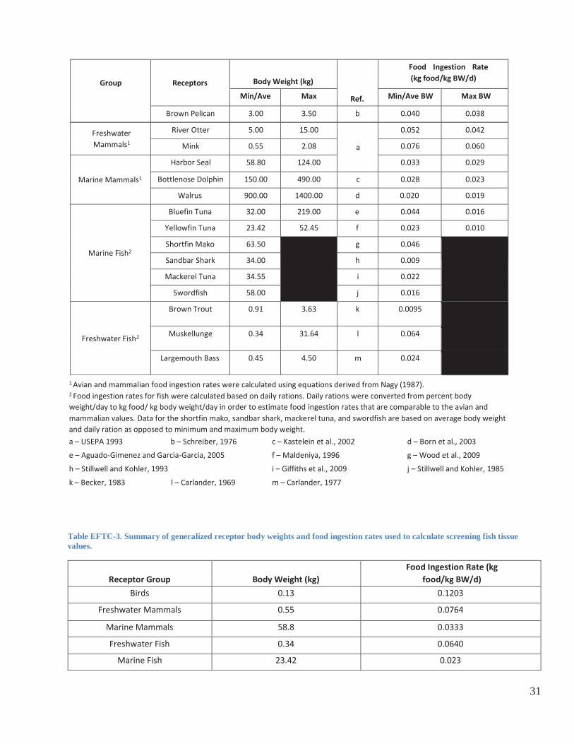
The list summarized in Table EFTC-1 may not be representative of potential receptor species at all sampling locations. To account for this limitation, generalized body weights and food ingestion rates for freshwater and marine fish, birds, and mammals were estimated from the receptor species listed. To be most protective, the lowest body weight and highest food ingestion rate where chosen for each receptor category for calculating dosage estimates. Table EFTC-2 summarizes the minimum and maximum receptor factors considered in determining weight and ingestion rate constants applied in the developing the threshold values. Table EFTC-3 describes the “generalized” receptor factors used to derive the new NCCA threshold values.

Table EFTC-2. Minimum and Maximum Body Weights and Derived Food Ingestion Rates for Selected Receptors of Concern.

Group Receptors Body Weight (kg)

Ref.

Food Ingestion Rate (kg food/kg BW/d)

Min/Ave Max Min/Ave BW Max BW

Avian1

Great Blue Heron 1.47 2.99

a

0.051 0.040

Osprey 1.22 1.95 0.054 0.046 Bald Eagle 3.00 4.50 0.040 0.034

Herring Gull 0.83 1.62 0.062 0.049 Belted Kingfisher 0.13 0.22 0.120 0.100

31

Group Receptors Body Weight (kg)

Ref.

Food Ingestion Rate (kg food/kg BW/d)

Min/Ave Max Min/Ave BW Max BW

Brown Pelican 3.00 3.50 b 0.040 0.038

Freshwater Mammals1

River Otter 5.00 15.00

a

0.052 0.042 Mink 0.55 2.08 0.076 0.060

Marine Mammals1

Harbor Seal 58.80 124.00 0.033 0.029 Bottlenose Dolphin 150.00 490.00 c 0.028 0.023

Walrus 900.00 1400.00 d 0.020 0.019

Marine Fish2

Bluefin Tuna 32.00 219.00 e 0.044 0.016 Yellowfin Tuna 23.42 52.45 f 0.023 0.010 Shortfin Mako 63.50 g 0.046 Sandbar Shark 34.00 h 0.009 Mackerel Tuna 34.55 i 0.022

Swordfish 58.00 j 0.016

Freshwater Fish2

Brown Trout 0.91 3.63 k 0.0095

Muskellunge 0.34 31.64 l 0.064

Largemouth Bass 0.45 4.50 m 0.024

1 Avian and mammalian food ingestion rates were calculated using equations derived from Nagy (1987). 2 Food ingestion rates for fish were calculated based on daily rations. Daily rations were converted from percent body weight/day to kg food/ kg body weight/day in order to estimate food ingestion rates that are comparable to the avian and mammalian values. Data for the shortfin mako, sandbar shark, mackerel tuna, and swordfish are based on average body weight and daily ration as opposed to minimum and maximum body weight. a – USEPA 1993 b – Schreiber, 1976 c – Kastelein et al., 2002 d – Born et al., 2003 e – Aguado-Gimenez and Garcia-Garcia, 2005 f – Maldeniya, 1996 g – Wood et al., 2009 h – Stillwell and Kohler, 1993 i – Giffiths et al., 2009 j – Stillwell and Kohler, 1985 k – Becker, 1983 l – Carlander, 1969 m – Carlander, 1977

Table EFTC-3. Summary of generalized receptor body weights and food ingestion rates used to calculate screening fish tissue values.

Receptor Group Body Weight (kg) Food Ingestion Rate (kg

food/kg BW/d) Birds 0.13 0.1203

Freshwater Mammals 0.55 0.0764

Marine Mammals 58.8 0.0333 Freshwater Fish 0.34 0.0640

Marine Fish 23.42 0.023

32

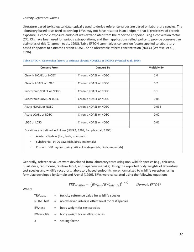
Toxicity Reference Values Literature based toxicological data typically used to derive reference values are based on laboratory species. The laboratory based tests used to develop TRVs may not have resulted in an endpoint that is protective of chronic exposure. A chronic exposure endpoint was extrapolated from the reported endpoint using a conversion factor (CF). CFs have been used for various extrapolations, and their applications reflect policy to provide conservative estimates of risk (Chapman et al., 1998). Table EFTC-4 summarizes conversion factors applied to laboratory-based endpoints to estimate chronic NOAEL or no observable effects concentration (NOEC) (Wentsel et al., 1996). Table EFTC-4. Conversion factors to estimate chronic NOAELs or NOECs (Wentsel et al., 1996).

Convert From Convert To Multiply By

Chronic NOAEL or NOEC Chronic NOAEL or NOEC 1.0

Chronic LOAEL or LOEC Chronic NOAEL or NOEC 0.2

Subchronic NOAEL or NOEC Chronic NOAEL or NOEC 0.1

Subchronic LOAEL or LOEC Chronic NOAEL or NOEC 0.05

Acute NOAEL or NOEC Chronic NOAEL or NOEC 0.033

Acute LOAEL or LOEC Chronic NOAEL or NOEC 0.02

LD50 or LC50 Chronic NOAEL or NOEC 0.01

Durations are defined as follows (USEPA, 1999; Sample et al., 1996):

• Acute: <14 days (fish, birds, mammals) • Subchronic: 14-90 days (fish, birds, mammals) • Chronic: >90 days or during critical life stage (fish, birds, mammals)

Generally, reference values were developed from laboratory tests using non-wildlife species (e.g., chickens, quail, duck, rat, mouse, rainbow trout, and Japanese medaka). Using the reported body weights of laboratory test species and wildlife receptors, laboratory based endpoints were normalized to wildlife receptors using formulae developed by Sample and Arenal (1999). TRVs were calculated using the following equation:

(Formula EFTC-3) Where:

TRVwildlife = toxicity reference value for wildlife species NOAELtest = no observed adverse effect level for test species

BWtest = body weight for test species

BWwildlife = body weight for wildlife species

X = scaling factor

33

Scaling factors presented by Sample and Arenal (1999) indicated that mammalian sensitivity increases with increased body weight, and avian sensitivity increases with decreased body weight. Scaling factors were unavailable for fish receptors but, like avian receptors, an increase in sensitivity with decreased body weight was reported (Buhler and Shanks, 1970). A scaling factor of 0.94 was used for mammalian receptors (Sample and Arenal, 1999) and a scaling factor of 1.2 was used for avian (Sample and Arenal, 1999) and fish receptors (Buhler and Shanks, 1970). Table EFTC-5 shows calculated TRVs for each NCCA analyte of interest that was used for estimating threshold values.

Table EFTC-5. Calculated toxicity reference values (TRVs) based cited literature and estimation methods.

Constituent TRV Type

Calculated Wildlife TRVs

Avian Mammal Fish

Freshwater Marine Freshwater Marine

TRV Ref. TRV Ref. TRV Ref. TRV Ref. TRV Ref.

Arsenic NOAEL 3.39

z 0.11

b 0.08

b 0.027

aa 0.06

aa LOAEL 8.51 0.53 0.4 0.14 0.3

Cadmium NOAEL 0.94

b 0.89

x 0.67

x 76.34

y 168

y LOAEL 12.93 4.46 3.37 763.49 1680

Mercury (methyl) NOAEL 0.02

v 0.31

b 0.024

b 0.14

w 0.31

w LOAEL 0.12 0.16 0.12 0.28 0.62

Selenium NOAEL 0.27

b 0.19

b 0.15

b 5.02

u 11.04

u LOAEL 0.53 0.32 0.24 6.7 14.75

Chlordane NOAEL 0.53

a 3.85

b 2.91

b NA

NA NA

NA LOAEL 2.66 7.69 5.81 NA NA

DDTs NOAEL 0.15

a 0.78

b 0.59

b 0.28

t 0.62

t LOAEL 1.47 3.89 2.94 1.42 3.12

Dieldrin NOAEL 0.08

b 0.033

q 0.025

q 0.065

r 0.14

r LOAEL 0.39 0.17 0.13 0.33 0.72

Endosulfan NOAEL 7.99

b 1.19

o 0.9

o 0.26

p 0.6

p LOAEL 39.93 5.95 4.5 0.6 1.31

Endrin NOAEL 0.019

b 0.15

b 0.11

b 0.16

n 0.34

n LOAEL 0.099 0.77 0.58 0.78 1.72

Heptachlor epoxide NOAEL 1.16

l 0.21

b 0.16

b 8.09

m 17.8

m LOAEL 5.79 1.037 0.78 16.2 35.6

Hexachlorobenzene NOAEL 0.11

h,j 0.97

j 0.74

j 0.0018

k 0.003

9 k LOAEL 0.56 1.95 1.47 0.0088 0.019

Lindane NOAEL 0.54

b 7.79

b 5.88

b 14.99

g 32.98

g LOAEL 2.19 38.93 29.41 74.95 164.9

1

Mirex NOAEL 0.0066

d 0.064

e 0.048

e 0.4

f 0.87

f LOAEL 0.66 0.64 0.048 1.98 4.35

Toxaphene NOAEL 0.66 a 7.79 b 5.88 b 0.0011 c 0.0024 c

34

Constituent TRV Type

Calculated Wildlife TRVs

Avian Mammal Fish

Freshwater Marine Freshwater Marine

TRV Ref. TRV Ref. TRV Ref. TRV Ref. TRV Ref.

LOAEL 3.32 38.93 29.41 0.0056 0.012

PCBs (Arochlor 1254)

NOAEL 0.12 b

0.055 b

0.041 b

0.078 bb

0.17 bb

LOAEL 1.2 0.55 0.41 0.39 0.86

High Molecular Weight PAHs

NOAEL 4.35 ii

0.58 jj

0.44 jj

0.55 kk

1.21 kk

LOAEL 21.77 2.92 2.21 2.76 6.07

Low Molecular Weight PAHs

NOAEL 15.16 ll

2.97 mm

2.24 mm

NA NA

NA NA

LOAEL 151.6 297 224.4 NA NA

a – Wiemeyer 1996 h – Coulston and Kolbye 1994 p – Lunebye et al. 2010 x – ATSDR 2008

b – Sample et al. 1996 i – Terretox 2002 q – ATSDR 2002b y – Szczerbik et al. 2006 c – Fabraeus-Van Ree and Payne (1997) j – ATSDR 2002a r – Argyle et al. 1975 z – USFWS 1964

d – Hyde et al. 1973 k – Woodburn et al. 2008 s – USEPA 1995 aa – Pedlar et al. 2002

e – NTP 1990 l – USEPA 1972 t – Macek et al. 1970 bb – Leatherland and Sonstegard 1980

f – Skea et al. 1981 m – Andrews et al. 1996

u – Ogle and Knight 1989 cc – Giesy et al. 2002

g – Cossarini-Dunier et al. 1987 n – Argyle et al. 1973 v – Heinz and Locke 1976 dd – USEPA 2008

o – ATSDR 2000 w – Berntssen et al. 2003 ee – Nakamaya 2004

Calculating Ecological Fish Tissue Contaminant Threshold Values

The tissue contaminant concentration threshold values for the suite of NCCA analytes was derived using the following equation:

[Fish] = (TRV*BW)/FI (Formula EFTC-4) Where:

[Fish] = threshold concentration in fish tissue (mg/kg) for a specific analyte TRV = related estimated toxicity reference value

BW = generalized body weight of receptor (kg-bw)

Thus, using the toxicity reference values plus estimated body weights and food ingestion rates, the concentration value of a selected analyte measured in fish tissues that presented a minimum exposure risk (HQ=1.0) was calculated for each group of receptors. The calculated fish tissue concentrations can be used to screen fish tissue data to determine if piscivorous fish and wildlife may be at risk due to the consumption of fish. A fish tissue concentration for each receptor group was calculated and can be used individually to screen for the potential risk to each receptor group. The lowest calculated fish tissue concentration can be used to screen

35

tissue concentration for risk to any receptor group regardless of the source of equation terms. In Table EFTC-6, the results for each group of receptors used for the NCCA Ecological Fish Tissue Contaminant Index are summarized.

36

Tab

le E

FTC

-6. S

umm

ary

of c

alcu

late

d ec

olog

ical

fish

tiss

ue c

onta

min

ant t

hres

hold

val

ues

in m

g/kg

.

Ecol

ogic

al

Cont

amin

ants

of

Con

cern

Fres

hwat

er

Mam

mal

M

arin

e M

amm

al

Bird

Fr

eshw

ater

Fish

M

arin

e Fi

sh

NCC

A 20

10

Scre

enin

g Va

lue

Fish

Tiss

ue

Fish

Tiss

ue

Fish

Tiss

ue

Fish

Tiss

ue

Fish

Tiss

ue

Fish

Tiss

ue

NOAE

L LO

AEL

NOAE

L LO

AEL

NOAE

L LO

AEL

NOAE

L LO

AEL

NOAE

L LO

AEL

NOAE

L LO

AEL

Toxa

phen

e 56

.05

280.

25

1038

7.34

51

936.

72

0.72

3.

59

0.00

56

0.03

2.

49

12.4

5 0.

0056

0.

03

Mire

x 0.

46

4.6

85.2

4 85

2.35

0.

0072

0.

72

2.0

9.91

88

5.39

44

26.9

7 0.

0072

0.

72

Linda

ne

56.0

5 28

0.25

10

387.

34

5193

6.72

0.

59

2.36

75

.16

375.

78

3358

5.06

16

7925

.32

0.59

2.

36

Hexa

chlo

robe

nze

ne

7.01

14

.01

1298

.42

2596

.84

0.12

0.

6 0.

0088

0.

044

3.95

19

.77

0.00

88

0.04

4

Hept

achl

or

epox

ide

1.49

7.

46

276.

57

1382

.84

1.25

6.

26

40.5

6 81

.12

1812

5.16

36

250.

33

1.25

6.

26

Endr

in

1.09

5.

56

201.

68

1030

.83

0.02

0.

11

0.78

3.

92

349.

98

1749

.90

0.02

0.

11

Endo

sulfa

n 8.

57

42.8

4 15

87.7

1 79

38.5

4 8.

63

43.1

5 0.

0014

0.

0030

0.

60

1.33

0.

0014

0.

0030

Diel

drin

0.

24

1.2

44.4

6 22

2.28

0.

067

0.33

0.

33

1.64

14

6.75

73

3.73

0.

067

0.33

DDT

5.61

28

.03

1038

.73

5193

.67

0.16

1.

59

1.42

7.

12

636.

28

3181

.41

0.16

1.

59

Chlo

rdan

e 27

.69

55.3

8 51

31.7

2 10

263.

45

0.57

2.

87

NA

NA

NA

NA

0.57

2.

87

Sele

nium

1.

4 2.

31

259.

68

428.

48

0.29

0.

57

25.1

6 33

.60

1124

4.05

15

016.

72

0.29

0.

57

Mer

cury

0.

22

1.12

41

.55

207.

75

0.02

0.

13

0.72

1.

41

320.

30

629.

23

0.02

2 0.

13

Cadm

ium

6.

43

32.1

3 11

90.7

8 59

53.9

1.

01

13.9

7 38

2.81

38

28.1

3 17

1068

.02

1710

680.

18

1.01

13

.97

Arse

nic

0.76

3.

81

141.

18

705.

89

3.66

9.

2 0.

14

0.69

61

.36

306.

80

0.14

0.

69

PCB

0.39

3.

93

72.7

9 72

7.86

0.

13

1.29

0.

39

1.95

17

4.16

87

0.81

0.

13

1.29

HMW

PAH

s 4.

2 21

.02

779.

05

3895

.25

4.7

23.5

2 2.

77

13.8

3 12

35.9

7 61

79.8

4 2.

77

13.8

3

LMW

PAH

s 21

.38

2137

.9

3961

.96

3961

95.9

1 16

.38

163.

83

NA

NA

NA

NA

16.3

83

163.

83

37

References for Ecological Fish Tissue Contaminants

Agency for Toxic Substances and Disease Registry (ATSDR). 1994. Toxicological profile for pentachlorophenol. May.

Agency for Toxic Substances and Disease Registry (ATSDR). 2000. Toxicological profile for endosulfan. September.

Agency for Toxic Substances and Disease Registry (ATSDR). 2002a. Toxicological profile for hexachlorobenzene. September.

Agency for Toxic Substances and Disease Registry (ATSDR). 2002b. Toxicological profile for dieldrin. September.

Agency for Toxic Substances and Disease Registry (ATSDR). 2008. Toxicological profile for cadmium. September.

Aguado-Giménez, F., and B. Garcia-Garcia. 2005. Growth, food intake and feed conversion rates in captive Atlantic bluefin tuna (Thunnus thynnus Linnaeus, 1758) under fattening conditions. Aquae. Res. 36: 610-614.

Andrews, A.K., C.C. Van Valin, and B.E. Stebbings. 1966. Some Effects of Heptachlor on Bluegills (Lepomis macrochirus). Transactions of the American Fisheries Society 95: 297-309.

Argyle, R.L., G.C. Williams, and H.K. Dupree. 1973. Endrin uptake and release by fingerling channel catfish (Ictalarus punctatus). J. Fish. Res. Board Can. 30: 1743-1744.

Argyle, R.L., G.C. Williams, and C.B. Daniel. 1975. Dieldrin in the diet of channel catfish (Ictalurus punctatus): uptake and effect on growth. J. Fish. Res. Board Can. 32: 21972204.

Becker, G. C. 1983. Fishes of Wisconsin. University of Wisconsin Press.

Berntssen, H.G., A. Aatland, and R.D. Handy. 2003. Chronic dietary mercury exposure causes oxidative stress, brain lesions, and altered behaviour in Atlantic salmon (Salmo salar) parr. Aquatic Toxicology 65: 55-72.

Born E.W., S. Rysgaard, G. Ehlme´, M. Sejr, M. Acquarone and N. Levermann. 2003. Underwater observations of foraging free-living Atlantic walruses (Odobenus rosmarus) and estimates of their food consumption. Polar Biol. 26: 348-357.

Bowersox, M., Siwinski, P., and J. Diamond. 2012. Development of § 303(d) Listing Mechanism, TMDL Targets and National Coastal Conditions Assessment (NCCA) Benchmarks for Selected Bioaccumulative Pollutants. Tetra Tech, Inc. Prepared for US EPA Region 6 (EP-C-07-068 Work Assignments 3-08 and 4-08).

Buhler DR, Shanks WE (1970) Influence of body weight on chronic oral DDT toxicity in coho salmon. J Fish Res Bd Can 27: 347-356.

Canadian Council of Ministers of the Environment (CCME). 1998. Protocol for the Derivation of Canadian Tissue Residue Guidelines for the Protection of Wildlife that Consume Aquatic Biota. CCME, Winnipeg.

38

Carlander, K.D. 1969. Handbook of freshwater fishery biology, volume 1. The Iowa State University Press, Ames. Iowa.

Carlander, K.D. 1977. Handbook of freshwater fishery biology, volume 1. The Iowa State University Press, Ames. Iowa.

Chapman, P.M., A. Fairbrother, and D. Brown. 1998. A Critical Evaluation of Safety (Uncertainty) Factors for Ecological Risk Assessment. Environmental Toxicol. Chem. 17: 99 – 108.

Cossarini-Dunier, M., G. Monod, A. Damael, and D. Lepot. 1987. Effect of γ-Hexachlorocyclohexane (Lindane) on Carp (Cyprinus carpio). I. Effect of Chronic intoxication on Humoral Immunity in Relation to Tissue Pollutant Levels. Exotoxicology and Environmental Safety 13: 339-345.

Coulston, F. and A.C. Kolbye, Jr. (eds). 1994. Interpretive review of the potential adverse effects of chlorinated organic chemicals on human health and the environment. Regulatory Toxicology and Pharmacology. 20: S1-S1056.

De Jong, W.H., E.D. Kroese, J.G. Vos, and H. Van Loveren. 1999. Detection of immunotoxicity of benzo(a)pyrene in a subacute toxicity study after oral exposure in rats. Toxicol. Sci. 50: 214-220

Eisler, R. 1989. Pentachlorophenol hazards to fish, wildlife, and invertebrates: a synoptic review.U.S. Fish and Wildlife Service Biological Report 85(1.17), Contaminant Hazard Reviews Report No. 17. 72 pp.Exponent. 2010. Risk Assessment and Risk Management of PCBs in Gas Transmission Lines. Prepared for INGAA. Washington, DC.

Fabraeus-Van Ree, G.E. and Payne J. F. 1997. Effect of Toxaphene on Reproduction of Fish. Chemosphere 34 (4): 855-867.

Giesy, J.P., P.D. Jones, K. Kannan, J.L. Newsted, D.E. Tillitt, and L.L. Williams. 2002. Effects of chronic dietary exposure to environmentally relevant concentrations of 2,3,7,8 tetrachlorodibenzo-p-dioxin on survival, growth, reproduction and biochemical responses of female rainbow trout (Oncorhynchus mykiss). Aquatic Toxicology 59: 35–53.

Griffiths, S.P., P.M. Kuhnert, G.F. Fry, and F.J. Manson. 2009. Temporal and size-related variation in the diet, consumption rate, and daily ration of mackerel tuna (Euthynnus affinis) in neritic waters of eastern Australia. Ices Journal of Marine Science 66 (4): 720733.

Heinz, G.H. and L.N. Locke. 1976. "Brain Lesions in Mallard Ducklings from Parents Fed Methylmercury." Avian Diseases. 20: 9-17.

Hyde, K.M., J.B. Graves, A.B. Watts, and F.L. Bonner. 1973. Reproductive Success of Mallard Ducks Fed Mirex. J. Wildl. Manage. 37 (4): 479-484.

Kastelein, R.A., N. Vaughan, S. Walton, and P.R. Wiepkema. 2002. Food intake and body measurements of Atlantic bottlenose dolphins (Tursiops truncates) in captivity. Marine Environmental Research 53: 199–218.

Kim, S.G., D.K. Park, S.W. Jang, J.S. Lee, S.S. Kim, and M.H. Chung. 2008. Effects of Dietary Benzo(a)pyrene on Growth and Hematological Parameters in Juvenile Rockfish, Sebates schlegeli (Hilgendorf). Bull. Environ. Contam. Toxicol. 81:470 - 474.

39

Leatherland, J.F. and R.A. Sonstegard. 1980. Effect of dietary Mirex and PCB's in combination with food deprivation and testosterone administration on thyroid activity and bioaccumulation of organochlorines in rainbow trout Salmo gairdeneri Richardson. Journal of Fish Diseases 3: 115-124.

Macek, K.J., C.R. Rodgers, D.L. Stalling, and S. Korn. 1970. The Uptake, Distribution and Elimination of Dietary 14C-DDT and 14C-Dieldrin in Rainbow Trout. Transactions of the American Fisheries Society 4: 689-695.

MacKenzie, K.M., and D.M. Angevine. 1981. “Infertility in Mice Exposed in Utero to Benzo(a)pyrene.” Biology of Reproduction. Volume 24. Pages 183-191.

Maldeniya, R. 1996. Food consumption of yellowfin tuna, Thunnus albacares, in Sri Lankan waters. Environmental Biology of Fishes. 47 (1): 101-107.

Nagy, K. A. 1987. Field metabolic rate and food requirement scaling in mammals and birds. Ecol. Monogr. 57: 111-128.

Nakayama, K., Y. Oshima, T. Yamaguchi, Y. Tsuruda, I.J. Kang, M. Kobayashi, N. Imada, and T. Honjo. 2004. Fertilization success and sexual behavior in male medaka, Oryzias latipes, exposed to tributyltin. Chemosphere 55: 1331–1337.

Newell, A.J., D.W. Johnson, and L.K. Allen. 1987. Niagra River biota contamination project: Fish flesh criteria for piscivorous wildlife. Tech. Rep. 87-3. New York State Department of Environmental Conservation, Albany, New York.

NTP (National Toxicology Program). 1990. Toxicology and Carcinogenesis Studies of MIREX (CAS No. 2385-85-5) in F344/N Rats (Feed Studies). NTP TR 313.

Ogle, S.E. and A.W. Knight. 1989. Effects of Elevated Foodborne Selenium on Growth and Reproduction of the Fathead Minnow (Pimephales promelas). Arch. Environ. Contam. Toxicol. 18: 795-803.

Oregon Department of Environmental Quality (ODEQ). 2007. Guidance for Assessing Bioaccumulative Chemicals of Concern in Sediment. Portland, OR.

Patton J.F. and M.P. Dieter. 1980. Effects of petroleum hydrocarbons on hepatic function in the duck. Comp. Biochem. Physiol. 65C:33-36.

Plasterer, M. R., W.S. Bradshaw, G.M. Booth, and M. W. Carter. 1985. Developmental toxicity of nine selected compounds following prenatal expsoures in the mouse: naphthalene, pnitrophenol, sodium selenate, dimethyl phthalate, ethylenethiourea, and four glycol ether derivatives. J. Toxicol. Environ. Health. 15: 25 - 38.

Rigdon, R.H. and J. Neal. 1963. Fluorescence of chickens and eggs following the feeding of benzpyrene crystals. Texas Reports on Biology and Medicine 21(4):558-566.

Sample, B.E., D.M. Opresko, and G.W. Suter II. 1996. Toxicological benchmarks for wildlife: 1996 revision. Environmental Restoration Division, ORNL Environmental Restoration Program. ES/ER/TM-86/R3.

40

Sample, B. E. and C. A. Arenal. 1999. Allometric models for interspecies extrapolation of wildlife toxicity data. Bull. Environ. Contam. Toxicol. 62:653-663.

Schreiber, R.W. 1976. Growth and development of nestling brown pelicans. Bird-Band. 47 (1): 19-39.

Schuytema, G.S., A.V. Nebecker, J.A. Peterson, and W.L. Griffis. 1993. Effects of Pentachlorophenol-Contaminated Food Organisms on Toxicity and Bioaccumulation in the Frog Xenopus laevis. Arch. Of Env. Tox. 24: 359 - 364.

Skea, J.C., Simonin, H.J., Jackling, S., and J. Symula. 1981, Accumulation and Retention of Mirex by Brook Trout Fed a Contaminated Diet. Bull. Environm. Contam. Toxicol. 27: 79-83.

Stillwell, C.E. and N.E. Kohler. 1985. Food and feeding ecology of the swordfish Xiphias gladius in the western North Atlantic Ocean with estimates of daily ration. Mar. Ecol. Prog. Ser. 22: 239-247.

Stillwell, C.E. and N.E. Kohler. 1993. Food habits of the sandbar shark Carcharhinus plumbeus off the U.S. northeast coast, with estimates of daily ration. Fish. Bull. 91: 138–150.

Szczerbik, P., T. Mikołajczyk, M. Sokołowska-Mikołajczyk, M. Socha, J. Chyb, and P. Epler. 2006. Influence of long-term exposure to dietary cadmium on growth, maturation and reproduction of goldfish (subspecies: Prussian carp Carassius auratus gibelio B.). Aquatic Toxicology 77: 126-135.

TERRETOX. 2002. On-line terrestrial toxicity database. U.S. Environmental Protection Agency.

Tetra Tech, Inc. 2012. Development of § 303(d) Listing Mechanism, TMDL Targets and National Coastal Condition Assessment (NCCA) Benchmarks for Selected Bioaccumulative Pollutants. Prepared for US EPA Region 6.

US Army. 2006. Development of Terrestrial Exposure and Bioaccumulation Information for Ecological Risk Assessments. Contract No. DAAD050-00-P-8365. Aberdeen Proving Ground.

U.S. Environmental Protection Agency (USEPA). 1972. Heptachlor- A review of its uses, chemistry, environmental hazards, and toxicology.

U.S. Environmental Protection Agency (USEPA). 1993. Wildlife Exposure Factors Handbook, Vol 1 of II. EPA/600/R-93/187a.

U.S. Environmental Protection Agency (USEPA). 1995. Great Lakes Water Quality Initiative criteria documents for the protection of wildlife: DDT, mercury, 2,3,7,8-TCDD, PCBs. EPA/820/B-95/008.

U.S. Environmental Protection Agency (USEPA). 1997. Ecological Risk Assessment Guidance for Superfund: Process for Designing and Conducting Ecological Risk Assessments. Interim Final. EPA/540/R-97/006.

U.S. Environmental Protection Agency (USEPA). 1998. Guidelines for Ecological Risk Assessment. EPA/630/R-95/002F.

U.S. Environmental Protection Agency (USEPA). 1999. Issuance of final Guidance: Ecological risk Assessment and Risk Management Principles for Superfund Sites.OSWER Directive 9285.7-28.

41

U.S. EPA (Environmental Protection Agency). 2000. Guidance for Assessing Chemical Contaminant Data for Use in Fish Advisories, Volume 2: Risk Assessment and Fish Consumption Limits. EPA-823-B-00-008. U.S. Environmental Protection Agency, Office of Water, Washington, DC.

U.S. Environmental Protection Agency (USEPA). 2010a. National Coastal Condition Assessment: Field Operations Manual. EPA-841-R-09-003. U.S. Environmental Protection Agency, Office of Water. Washington, DC.

U.S. Environmental Protection Agency (USEPA). 2010b. National coastal condition assessment: Laboratory methods manual. EPA 841-R-09-002. U.S. Environmental Protection Agency, Office of Water. Washington, DC.

U.S. Environmental Protection Agency (USEPA). 2010c. National Coastal Condition Assessment: Quality Assurance Project Plan 2008-2012. EPA/841-R-09-004. U.S. Environmental Protection Agency, Office of Water. Washington, D.C.

U.S. Fish and Wildlife Service. 1964. Pesticide-wildlife studies, 1963: a review of Fish and Wildlife Service investigations during the calendar year. FWS Circular 199.

Wentsel, R.S., T.W. LaPoint, M. Simini, R. Checkai, D. Ludwig and L. Brewer. 1996. May. Tri-Service Procedural Guidelines for Ecological Risk Assessments. Air Force Center for Environmental Excellence (AFCEE), U.S. Army Environmental Center (USAEC), Naval Facilities Engineering Service Center (NFESC).

Wiemeyer, S.N. 1996. Other organochlorine pesticides in birds. Pages 99-115 IN Beyer, W.N., G.H. Heinz, and A.W. Redmon-Norwood (eds). Environmental contaminants in wildlife: interpreting tissue concentrations. Lewis Publishers, Boca Raton, FL. 494 pp.

Woodburn, K.B., T.A. Marino, E.L. McClymont, and D.L. Rick. 2008. Determination of the dietary absorption efficiency of hexachlorobenzene with the channel catfish (Ictalurus punctatus). Ecotoxicology and Environmental Safety 71: 419-425.

Wood A.D., B.M. Wetherbee, F. Juanes, N.E. Kohler, and C. Wilga. 2009. Recalculated diet and daily ration of the shortfin mako (Isurus oxyrinchus), with a focus on quantifying predation on bluefish (Pomatomus saltatrix) in the northwest Atlantic Ocean. Fish. Bull. 107: 76 – 88.

Research Bibliographic References Not Cited

Forseth, T., and B. Jonsson. The Growth and Food Ration of Piscivorous Brown Trout (Salmo trutta). Functional Ecology 8: 171-177.

Lundebye, A.K., E.J. Lock, D. Boyle, K. Ruohonen, and M.H. Berntssen. 2010. Tolerance of Atlantic Salmon (Salmo salar) to dietborne endosulfan assessed by haematology, biochemistry, histology and growth. Aquaculture Nutrition 16: 549-558.

Navarro et al., 1991. Developmental toxicity evaluation of naphthalene (CAS NO. 91-20-3) administered by gavage to Sprague-Dawley (CD) rats on gestation days 6 through 15. Chemistry and Life Sciences, Research Triangle Institute (RTI). Research Triangle Park, NC. RTI Master Protocol Number: RTI-376. December 5.

42

Neal, J. and R. H. Rigdon. 1967. Gastic tumors in mice fed benzo(a)pyrene: a quantitative study. Texas Reports on Biology and Medicine, 13(4):553-557.

Shopp, G.M., K.L. White, M.P. Holsapple; D. W. Barnes, S.S. Duke, A. C. Anderson, L. W. Condie, J.R. Hayes, and J.F. Borzelleca. 1984. Naphthalene toxicity in CD-1 mice: general toxicology and immunotoxicology. Fundam. Appl. Toxicol. 4: 406 - 419.

U.S. Environmental Protection Agency (USEPA). 2008. Reregistration Eligibility Decision (RED): Naphthalene; EPA 738-R-07-010. U.S. Environmental Protection Agency, Office of Prevention, Pesticides, and Toxic Substances, Washington, DC.

U.S. Environmental Protection Agency (USEPA). 2008a. Ecological hazard and environmental risk assessment chapter pentachlorophenol. EPA-HQ-OPP-2004-0402-0072. Washington, D.C.

U.S. Environmental Protection Agency (USEPA). 2008b. Ecological Hazard and Environment Risk Assessment Tributlytin-containing Compounds (TBT). EPA-HQ-OPP-0171-0007. Washington, D.C.

43

Section 6: Quality Assurance and Quality Control (NCCA 2010) This section of the Technical Report documents the procedures for managing and assessing the quality of data used for the NCCA 2010 Report. The National Coastal Condition Assessment (NCCA) program follows the guidance of the EPA Office Water Quality Management Plan (USEPA 2009) to integrate quality assurance and quality control (QA/QC) into every aspect of the survey. This QA/QC effort involves a team of personnel who are responsible for ensuring data quality (e.g., the NCCA QA Team):

NCCA Program Quality Assurance Coordinator (QAC) – Responsible for ensuring that a QA program is in place and is being followed, the quality of data used in the assessment is evaluated and documented, and identifying data that do not meet the quality requirements of the NCCA, as specified by the Quality Assurance Project Plan (USEPA 2010a).

Quality Assurance Advisors – EPA staff from the Office of Research and Development who provide advice to the QAC about specific aspects of QA/QC for individual indicators or parameters.

National Aquatic Resource Surveys Information Management Center (NARS IM) staff – Contract staff who manage the NCCA survey data and information. NARS IM staff add record qualifiers that document potential quality issues, make corrective changes to the data and disseminate, after review by the QAC, data-related information as requested.

Approach for Implementing the NCCA Quality Assurance Strategy The NCCA Program employs several key elements to assure the quality of the data used in the assessments. Each element is briefly described in the following paragraphs. Quality Assurance Project Plan The NCCA Quality Assurance Project Plan (QAPP) outlines the program's quality objective requirements. The QAPP addresses multiple levels of the program ranging from sample collection in the field and laboratory processing of samples to review of results data sets. The QAPP establishes target Data Quality Objectives (DQO) for assessing the status of condition indicators for the NCCA population of coastal waters (USEPA 2010a), as follows:

For each indicator of condition, estimate the proportion of the nation’s estuaries and combined area of the Great Lakes in degraded condition with a ± 5% margin of error and with 95% confidence.

44

For each indicator of condition, estimate the proportion of regional estuarine resources (Northeast, Southeast, Gulf of Mexico, West Coast and Great Lakes) in degraded condition with a ± 15% margin of error and with 95% confidence.

Field Operations and Laboratory Methods Manuals The Field Operations Manual (FOM, USEPA 2010b) and Laboratory Methods Manual (LMM, USEPA 2010c) provide an interpretation of the QAPP that guide the activities of NCCA participants in a manner that meets quality requirements. The FOM and the LMM help ensure that quality objectives are attainable and survey activities are more tractable. Every NCCA participant (e.g., field crews and laboratories) is provided training and expected to comply with the procedures published in the FOM and the LMM. The LMM and FOM also list measurement quality objectives (MQOs). MQOs allow NCCA quality staff to evaluate the level of quality attainment for individual survey metrics. Field Method Pilot Testing A representative group of the NCCA steering and oversight staff pilot tested sampling methods and documentation requirements (e.g., field forms) described in the FOM. The purpose of this activity was three-fold. First, the pilot period ensures that instructions are clear. Second, NCCA staff have the opportunity to evaluate the capacity of the FOM for adequately supporting and documenting the quality objectives. Finally, the pilot period allows time to test the feasibility of sampling logistics, sample preparation and sample shipping instructions. Any deficiencies noted in the FOM during pilot testing are corrected prior to field crew training. Field Crew Training As a nationwide survey, the NCCA requires that all crews use the same methods. To ensure data comparability, all field crews must attend training prior to sampling. For the 2010 survey, NCCA trainers led seven regional field crew training sessions consisting of classroom and field based lessons. These ranged from how to conduct site reconnaissance and record field observations and in situ data, to sample collection, shipping, reporting and troubleshooting. The field crew leaders were taught to review every form and verify that all hand-entered data were complete and correct. Field Assistance Visits In addition to attending training sessions, an EPA employee or contractor visited every NCCA field crew during the 2010 field season. These visits, known as assistance visits or AVs, provided an opportunity to observe field crews in the normal course of a field day and document adherence to sampling procedures. If circumstances are noted where a field crew was not conducting a procedure properly, the observer recorded the deficiency, reviewed appropriate procedure with field team as a preemptory intervention and assisted the field crew until the procedure was completed correctly. Laboratory Quality Assurance and Quality Control All laboratories were required to submit documentation of their analytical capabilities prior to analyzing any 2010 NCCA sample. EPA NCCA Team members reviewed documentation to ensure that the labs could meet required MQOs (e.g., reporting limits, detection limits, etc.). National Environmental Laboratory Accreditation Conference certification, satisfactory participation in round-robin or other usual and customary types of evaluations were considered acceptable capabilities documentation. For

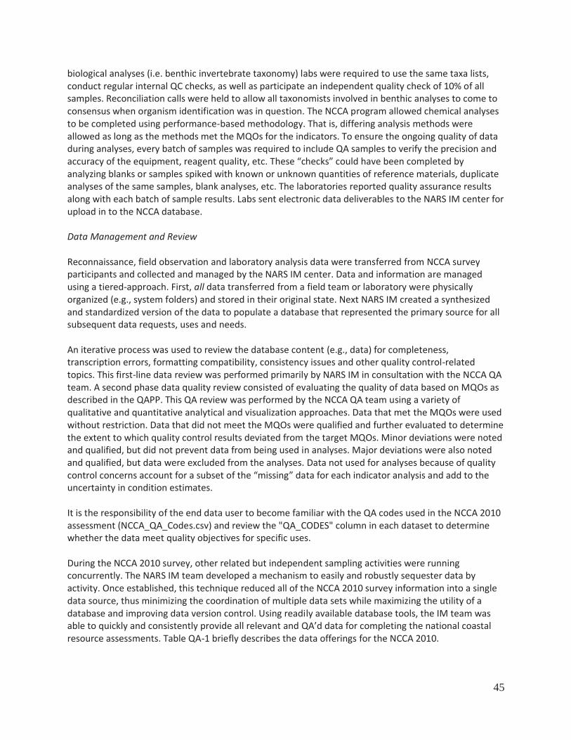
45

biological analyses (i.e. benthic invertebrate taxonomy) labs were required to use the same taxa lists, conduct regular internal QC checks, as well as participate an independent quality check of 10% of all samples. Reconciliation calls were held to allow all taxonomists involved in benthic analyses to come to consensus when organism identification was in question. The NCCA program allowed chemical analyses to be completed using performance-based methodology. That is, differing analysis methods were allowed as long as the methods met the MQOs for the indicators. To ensure the ongoing quality of data during analyses, every batch of samples was required to include QA samples to verify the precision and accuracy of the equipment, reagent quality, etc. These “checks” could have been completed by analyzing blanks or samples spiked with known or unknown quantities of reference materials, duplicate analyses of the same samples, blank analyses, etc. The laboratories reported quality assurance results along with each batch of sample results. Labs sent electronic data deliverables to the NARS IM center for upload in to the NCCA database. Data Management and Review Reconnaissance, field observation and laboratory analysis data were transferred from NCCA survey participants and collected and managed by the NARS IM center. Data and information are managed using a tiered-approach. First, all data transferred from a field team or laboratory were physically organized (e.g., system folders) and stored in their original state. Next NARS IM created a synthesized and standardized version of the data to populate a database that represented the primary source for all subsequent data requests, uses and needs. An iterative process was used to review the database content (e.g., data) for completeness, transcription errors, formatting compatibility, consistency issues and other quality control-related topics. This first-line data review was performed primarily by NARS IM in consultation with the NCCA QA team. A second phase data quality review consisted of evaluating the quality of data based on MQOs as described in the QAPP. This QA review was performed by the NCCA QA team using a variety of qualitative and quantitative analytical and visualization approaches. Data that met the MQOs were used without restriction. Data that did not meet the MQOs were qualified and further evaluated to determine the extent to which quality control results deviated from the target MQOs. Minor deviations were noted and qualified, but did not prevent data from being used in analyses. Major deviations were also noted and qualified, but data were excluded from the analyses. Data not used for analyses because of quality control concerns account for a subset of the “missing” data for each indicator analysis and add to the uncertainty in condition estimates. It is the responsibility of the end data user to become familiar with the QA codes used in the NCCA 2010 assessment (NCCA_QA_Codes.csv) and review the "QA_CODES" column in each dataset to determine whether the data meet quality objectives for specific uses. During the NCCA 2010 survey, other related but independent sampling activities were running concurrently. The NARS IM team developed a mechanism to easily and robustly sequester data by activity. Once established, this technique reduced all of the NCCA 2010 survey information into a single data source, thus minimizing the coordination of multiple data sets while maximizing the utility of a database and improving data version control. Using readily available database tools, the IM team was able to quickly and consistently provide all relevant and QA’d data for completing the national coastal resource assessments. Table QA-1 briefly describes the data offerings for the NCCA 2010.

46

Table QA-1. List of NCCA 2010 database tables and/or groupings. Name Description

Benthic Benthic invertebrate data Comments Compiled comments from field forms Fish info Fish collection information HHFish tissue Human health fish tissue data Hydroprofile Hydrographic profile data SedTox Sediment toxicity data SedChem Sediment chemistry data Tissue chemistry Ecological fish tissue contaminant data Water chemistry Nutrients and chlorophyll a data SiteInfo Site identification, location and weighting

information References for Quality Assurance and Control USEPA. 2009. Quality Management Plan. EPA 821-R-09-001. U.S. Environmental Protection Agency,

Office of Water. Washington, DC. USEPA. 2010a. National Coastal Condition Assessment: Quality Assurance Project Plan 2008-2012.

EPA/841-R-09-004. U.S. Environmental Protection Agency, Office of Water. Washington, D.C. USEPA. 2010b. National Coastal Condition Assessment: Field Operations Manual. EPA-841-R-09-003. U.S.

Environmental Protection Agency, Office of Water. Washington, DC. USEPA. 2010c. National Coastal Condition Assessment: Laboratory Methods Manual. EPA 841-R-09-002.

U.S. Environmental Protection Agency, Office of Water. Washington, DC.