Embed Size (px)
Citation preview

1
Applied Mathematics
National Seminar 2

Welcome
2

Expectations for Online CPD
3
The PDST does not give permission for this event to be recorded.

4
Resource
Prior Knowledge
Booklet activity
Group work
Reflection
Teaching Approach
Contact us
Planning
Keys

Schedule for Seminar 1
5
09:30 – 09:50 Introduction:Overview of the professional development programme & Key messages.Approaches to integrating mathematical modelling in all strands.
09:50 - 11:00 Session 1:Matrices for Networks and GraphsIntroduction to Matrix algebra.
11:00 - 11:15 Break
11:15 – 13:00 Session 2:Review of algorithms.Development of Dijkstra’s algorithm through modelling.
13:00 - 13:45 Lunch
13:45 – 15:15 Session 3:Connecting strands through modellingDevelopment of accelerated linear motion.
15:15 – 15:30 Evaluations and Q&A

Overview of Professional Development and Supports Available
6
Year 1 Nov 2020 - June 2021
Year 2 Year 3
3 X National
Seminars
4 X National
Seminars
2 X PLCs 2 X PLCs
1 X Webinar 1 X Webinar
1 X
Technology
Workshop
1 X
Technology
Workshop

Key Messages
Core to the specification is a non-linear
approach empowered by the use of rich
pedagogy which promotes the making of
connections between various Applied
Mathematics learning outcomes.
Strand 1 of the specification is a unifying
strand and emphasises the importance of
utilising modelling across all learning
outcomes.
Applied Mathematics is rooted in authentic
problems as a context for learning about the
application of Mathematics to design solutions
for real-world problems and to develop
problem solving skills applicable to a variety of
disciplines.7
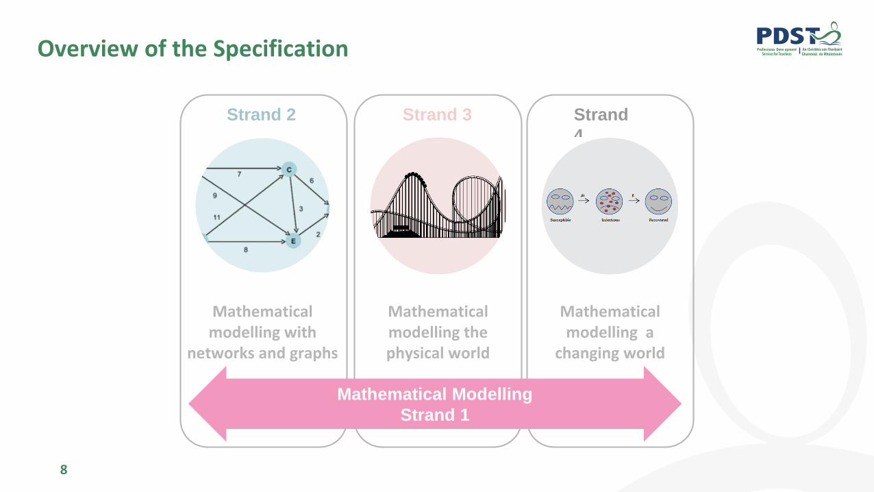
8
Strand 2
Mathematical modelling with
networks and graphs
Strand 3
Mathematical modelling the physical world
Strand
4
Mathematical modelling a
changing world
Mathematical Modelling
Strand 1
Overview of the Specification
Strand
4
Mathematical modelling a
changing world
Strand 3
Mathematical modelling the physical world
Strand 2
Mathematical modelling with
networks and graphs
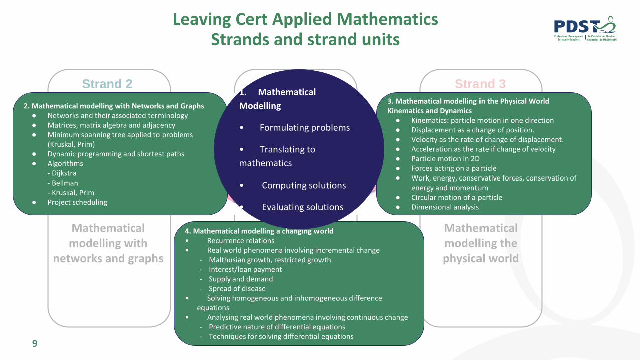
9
Leaving Cert Applied Mathematics Strands and strand units
2. Mathematical modelling with Networks and Graphs● Networks and their associated terminology● Matrices, matrix algebra and adjacency● Minimum spanning tree applied to problems
(Kruskal, Prim)● Dynamic programming and shortest paths● Algorithms
- Dijkstra- Bellman- Kruskal, Prim
● Project scheduling
3. Mathematical modelling in the Physical WorldKinematics and Dynamics
● Kinematics: particle motion in one direction● Displacement as a change of position.● Velocity as the rate of change of displacement. ● Acceleration as the rate if change of velocity● Particle motion in 2D● Forces acting on a particle● Work, energy, conservative forces, conservation of
energy and momentum● Circular motion of a particle● Dimensional analysis
4. Mathematical modelling a changing world• Recurrence relations• Real world phenomena involving incremental change
- Malthusian growth, restricted growth- Interest/loan payment- Supply and demand- Spread of disease
• Solving homogeneous and inhomogeneous difference equations
• Analysing real world phenomena involving continuous change- Predictive nature of differential equations- Techniques for solving differential equations
1. Mathematical
Modelling
• Formulating problems
• Translating to
mathematics
• Computing solutions
• Evaluating solutions
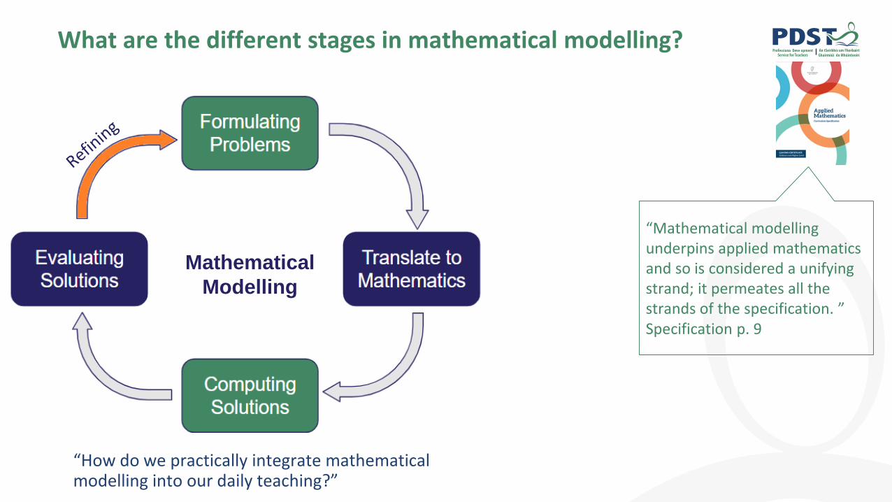
What are the different stages in mathematical modelling?
Mathematical
Modelling
“Mathematical modelling underpins applied mathematics and so is considered a unifying strand; it permeates all the strands of the specification. ” Specification p. 9
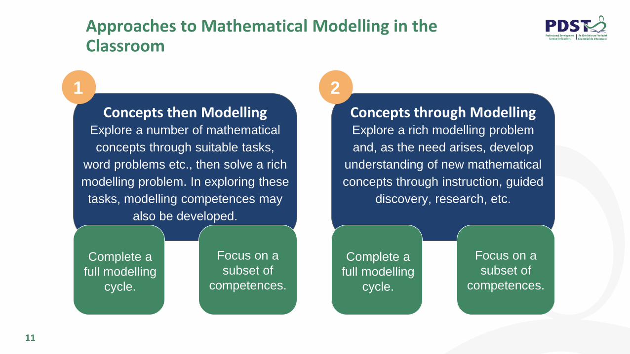
Concepts through ModellingExplore a rich modelling problem
and, as the need arises, develop
understanding of new mathematical
concepts through instruction, guided
discovery, research, etc.
Concepts then ModellingExplore a number of mathematical
concepts through suitable tasks,
word problems etc., then solve a rich
modelling problem. In exploring these
tasks, modelling competences may
also be developed.
11
Approaches to Mathematical Modelling in the Classroom
Complete a
full modelling
cycle.
Focus on a
subset of
competences.
1 2
Complete a
full modelling
cycle.
Focus on a
subset of
competences.

12
Session 1: Matrices for Networks and Graphs
09:50 - 11:15
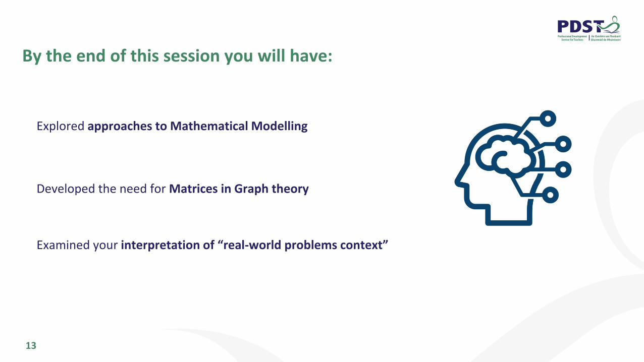
By the end of this session you will have:
13
Developed the need for Matrices in Graph theory
Explored approaches to Mathematical Modelling
Examined your interpretation of “real-world problems context”

14
Examining prior knowledge using Kahoot“..varied assessment strategies will
support learning and provide
feedback””
Specification p. 22
Kahoot link in Chat: kahoot.it
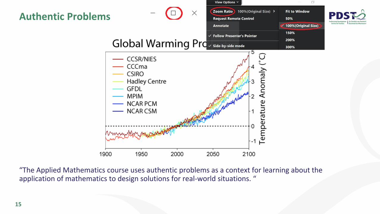
Authentic Problems
15
“The Applied Mathematics course uses authentic problems as a context for learning about the application of mathematics to design solutions for real-world situations. “

16
A company wishes to engage in an online marketing campaign. The company has limited resources to invest in such a campaign. How will they create this marketing campaign?
Formulating problems: - research the
background - determine information relevant
to problem - decompose problem into
manageable parts …”
Specification p. 16
Concepts through Modelling
2
Authentic Problem - Online Marketing
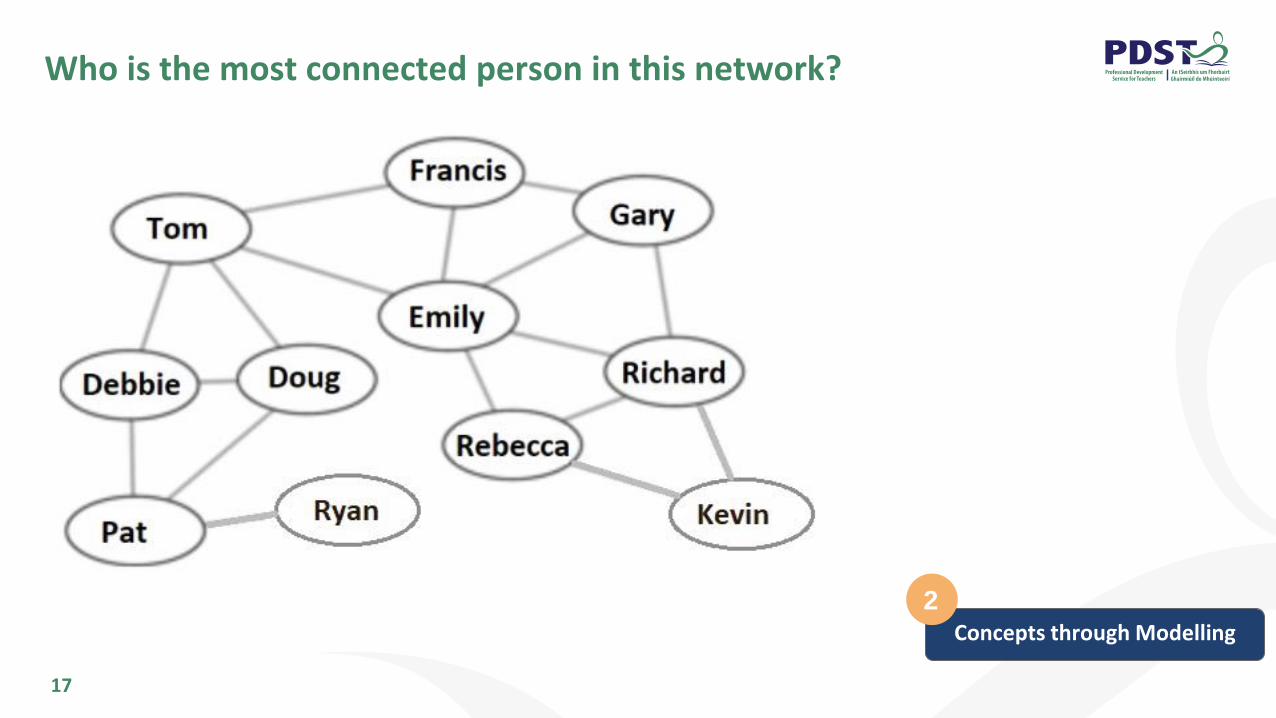
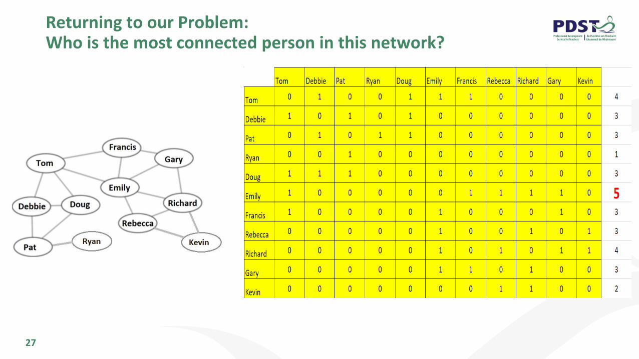
Who is the most connected person in this network?
17
Concepts through Modelling
2

Application of Ordered Lists
18
19
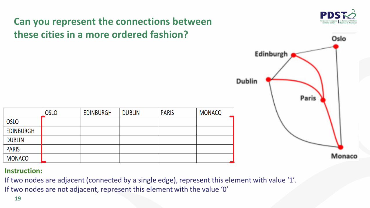
Can you represent the connections between these cities in a more ordered fashion?
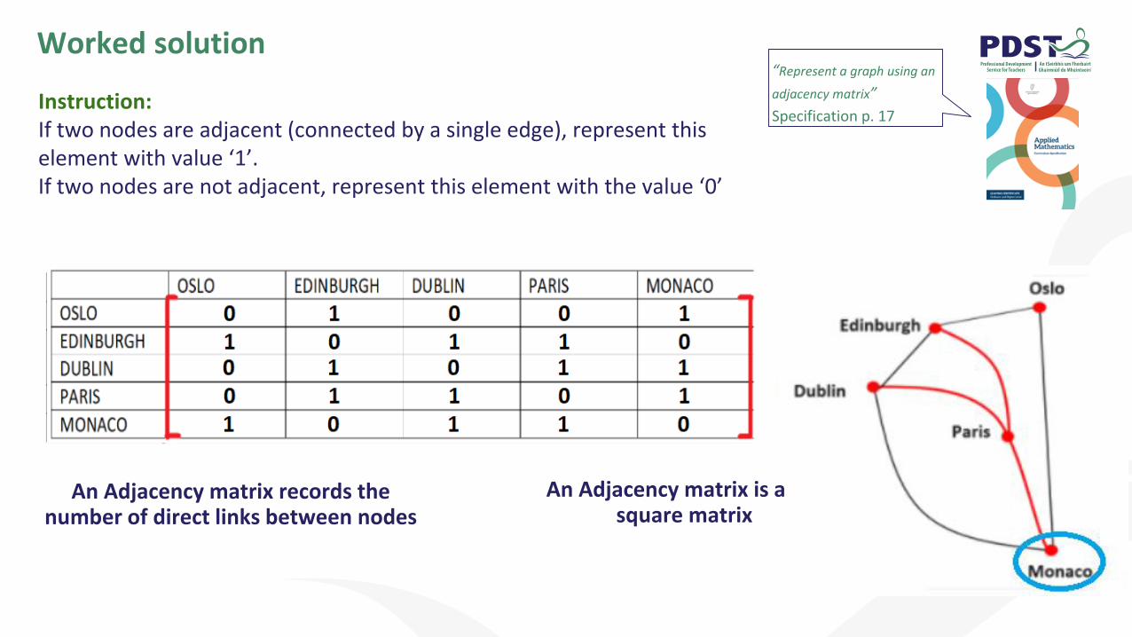
Instruction:If two nodes are adjacent (connected by a single edge), represent this element with value ‘1’.If two nodes are not adjacent, represent this element with the value ‘0’
“Represent a graph using an
adjacency matrix”
Specification p. 17
An Adjacency matrix records the number of direct links between nodes
An Adjacency matrix is a square matrix
Worked solution
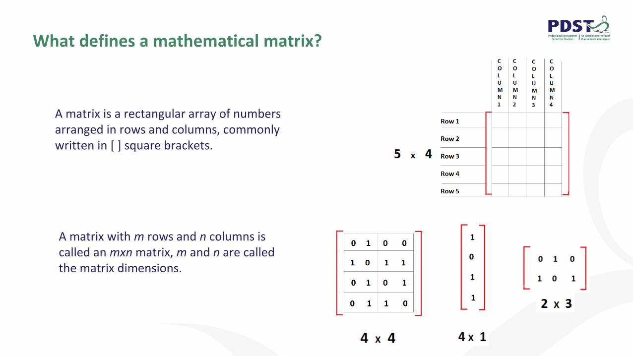
What defines a mathematical matrix?
A matrix is a rectangular array of numbers arranged in rows and columns, commonly written in [ ] square brackets.
A matrix with m rows and n columns is called an mxn matrix, m and n are called the matrix dimensions.
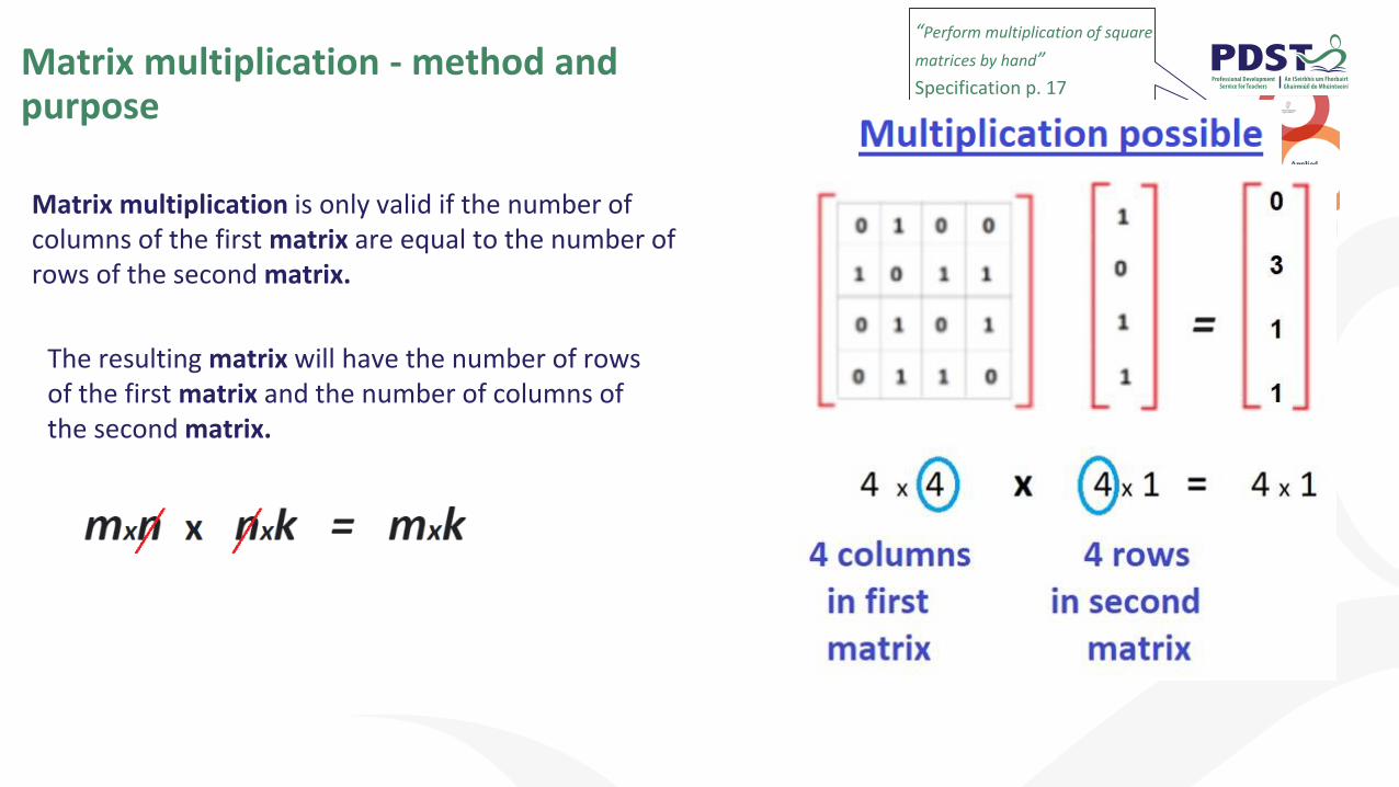
Matrix multiplication is only valid if the number of columns of the first matrix are equal to the number of rows of the second matrix.
“Perform multiplication of square
matrices by hand”
Specification p. 17
The resulting matrix will have the number of rows of the first matrix and the number of columns of the second matrix.
Matrix multiplication - method and purpose
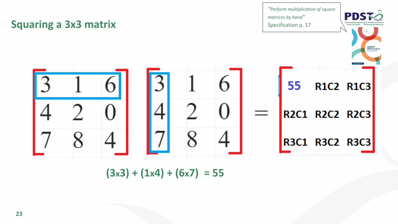
Squaring a 3x3 matrix
23
“Perform multiplication of square
matrices by hand”
Specification p. 17
(3x3) + (1x4) + (6x7) = 55
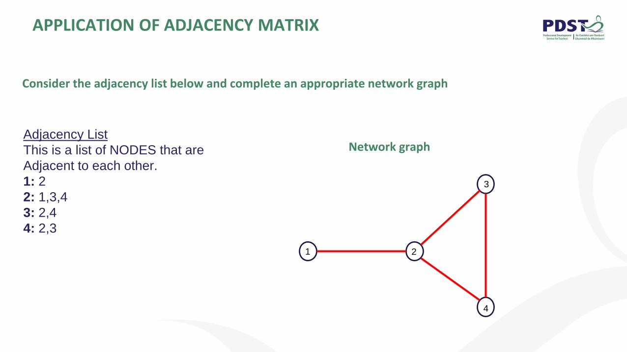
APPLICATION OF ADJACENCY MATRIX
Consider the adjacency list below and complete an appropriate network graph
Adjacency List
This is a list of NODES that are
Adjacent to each other.
1: 2
2: 1,3,4
3: 2,4
4: 2,3
Network graph
1 2
3
4
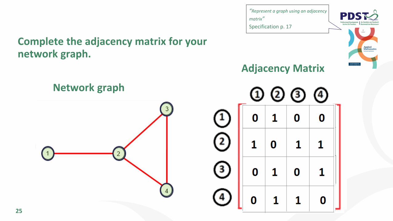
25
Network graph
Adjacency Matrix
“Represent a graph using an adjacency
matrix”
Specification p. 17
Complete the adjacency matrix for your network graph.
26
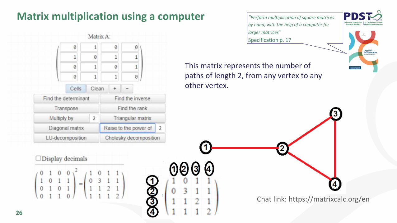
Matrix multiplication using a computer “Perform multiplication of square matrices
by hand, with the help of a computer for
larger matrices”
Specification p. 17
Chat link: https://matrixcalc.org/en
This matrix represents the number of paths of length 2, from any vertex to any other vertex.
27
Returning to our Problem: Who is the most connected person in this network?
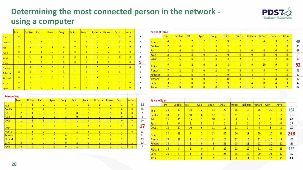
28
Determining the most connected person in the network -using a computer
29
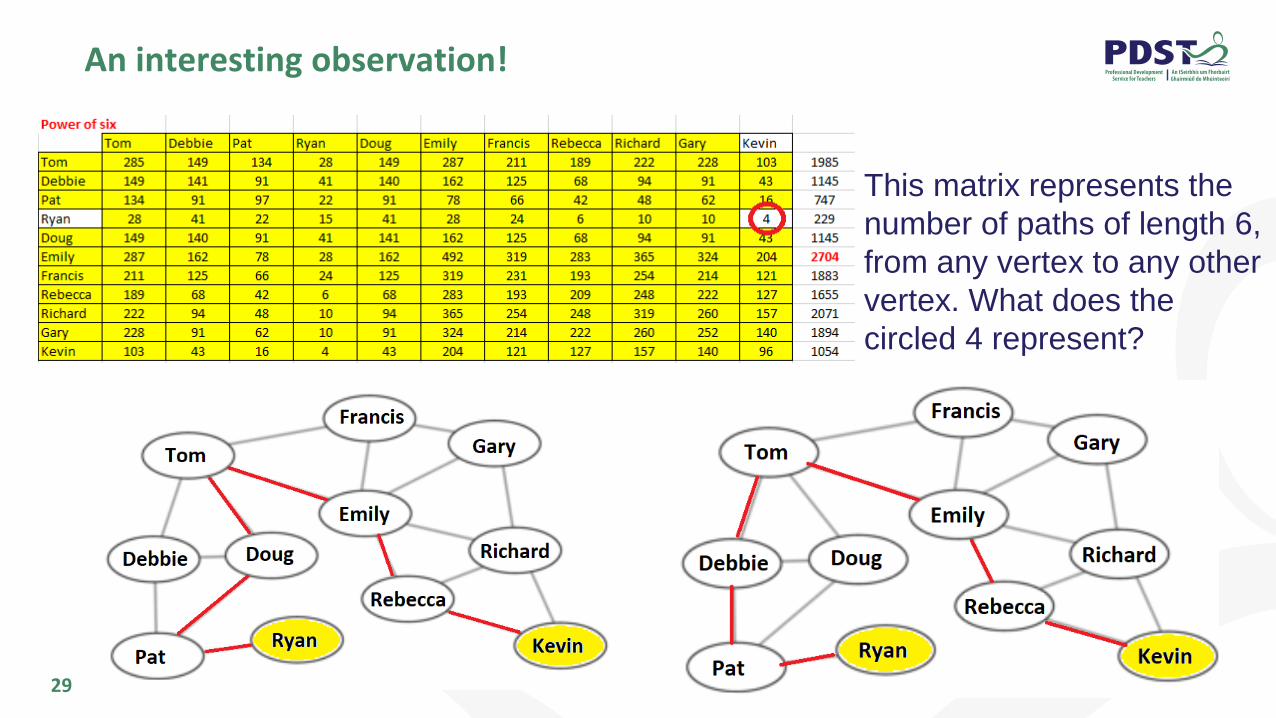
An interesting observation!
This matrix represents the
number of paths of length 6,
from any vertex to any other
vertex. What does the
circled 4 represent?

30
Reflection on Teaching and Learning: Session 1
How can I suitably apply the various teaching and learning strategies demonstrated this morning?
What teaching and learning strategy did I find the most useful this morning?
What critical skills can I help develop in my students?

Reflection: Session 1
31
32
Session 2: Development of Algorithms through Modelling
11:15 - 13:00
By the end of this session you will have:
33
Revisited Kruskal’s and Prim’s algorithms.
Further explored the use of algorithms to solve authentic problems.
Explored various stages of the modelling cycle in solving real world
problems.
Made distinctions between the algorithms experienced to date and
their applications.
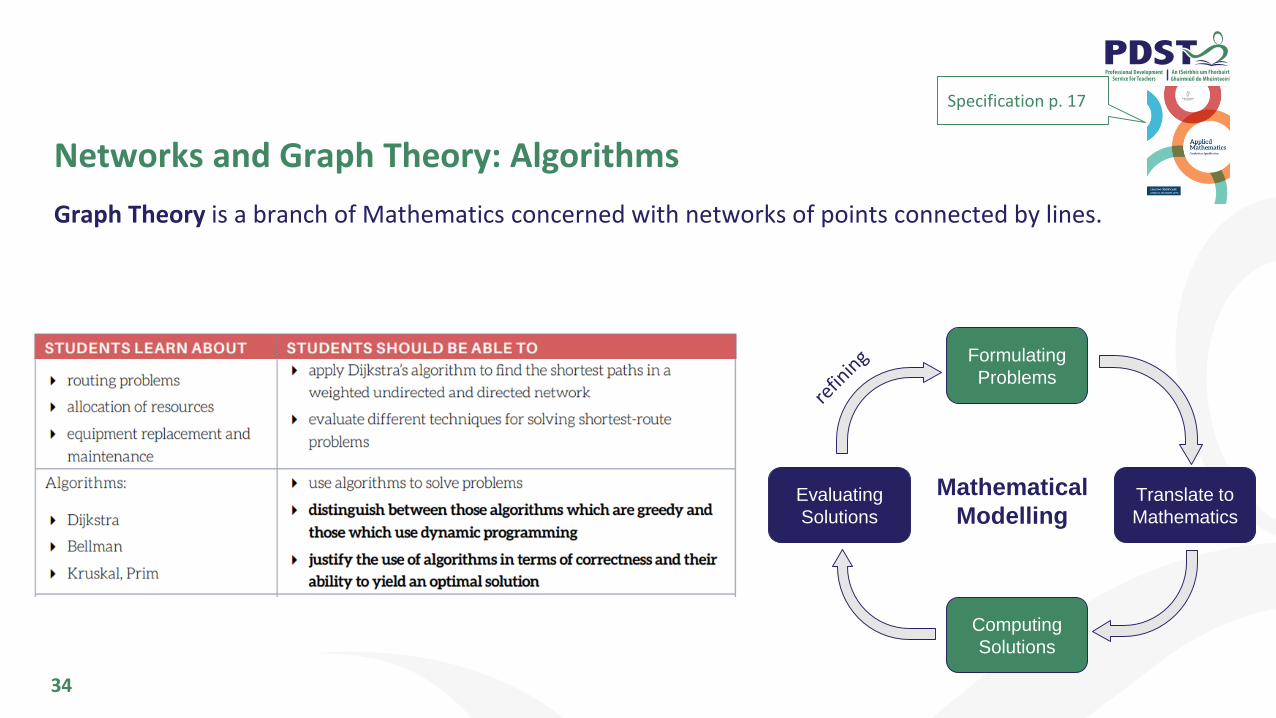
Networks and Graph Theory: Algorithms
34
Graph Theory is a branch of Mathematics concerned with networks of points connected by lines.
Formulating
Problems
Evaluating
Solutions
Translate to
Mathematics
Computing
Solutions
Mathematical
Modelling
Specification p. 17
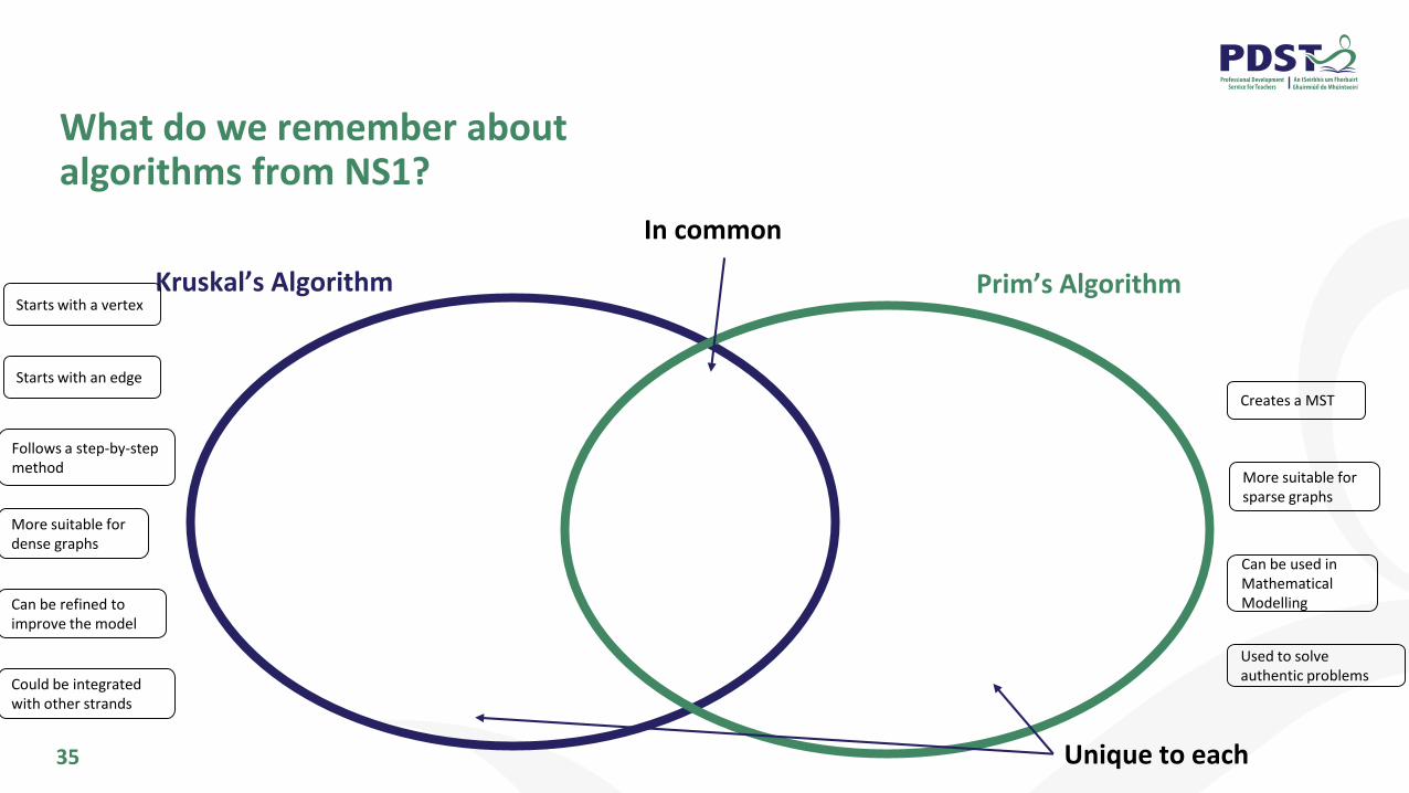
What do we remember about algorithms from NS1?
35
Kruskal’s Algorithm Prim’s Algorithm
In common
Unique to each
Starts with an edge
Starts with a vertex
Follows a step-by-step method
More suitable for dense graphs
Can be refined to improve the model
Could be integrated with other strands
Creates a MST
Can be used in Mathematical Modelling
Used to solve authentic problems
More suitable for sparse graphs

Reflection: Connecting with Prior Knowledge
36
What are the benefits for students in connecting with previously learnt material?
How could we support students to be more personally effective in making connections between their learning?
What other strategies could be used to scaffold and build knowledge between concepts?
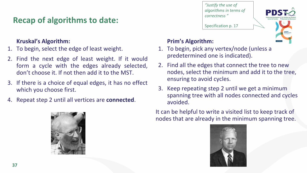
Recap of algorithms to date:
37
Kruskal’s Algorithm:1. To begin, select the edge of least weight.
2. Find the next edge of least weight. If it wouldform a cycle with the edges already selected,don’t choose it. If not then add it to the MST.
3. If there is a choice of equal edges, it has no effectwhich you choose first.
4. Repeat step 2 until all vertices are connected.
Prim’s Algorithm:1. To begin, pick any vertex/node (unless a
predetermined one is indicated).
2. Find all the edges that connect the tree to new nodes, select the minimum and add it to the tree, ensuring to avoid cycles.
3. Keep repeating step 2 until we get a minimum spanning tree with all nodes connected and cycles avoided.
It can be helpful to write a visited list to keep track of nodes that are already in the minimum spanning tree.
“Justify the use of algorithms in terms of correctness ”
Specification p. 17
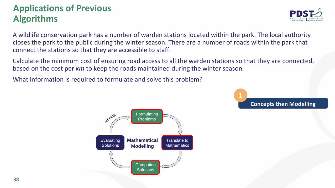
Applications of Previous Algorithms
38
A wildlife conservation park has a number of warden stations located within the park. The local authority closes the park to the public during the winter season. There are a number of roads within the park that connect the stations so that they are accessible to staff.
Calculate the minimum cost of ensuring road access to all the warden stations so that they are connected, based on the cost per km to keep the roads maintained during the winter season.
What information is required to formulate and solve this problem?
Formulating
Problems
Evaluating
Solutions
Translate to
Mathematics
Computing
Solutions
Mathematical
Modelling
Concepts then Modelling
1
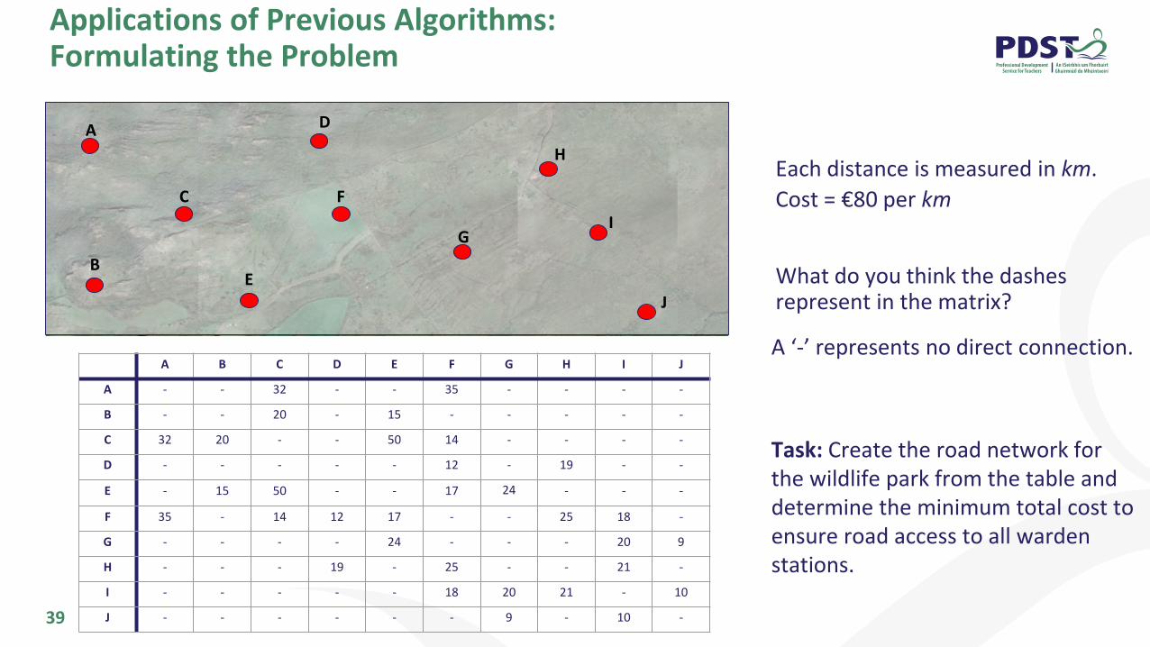
Applications of Previous Algorithms:Formulating the Problem
39
A B C D E F G H I J
A - - 32 - - 35 - - - -
B - - 20 - 15 - - - - -
C 32 20 - - 50 14 - - - -
D - - - - - 12 - 19 - -
E - 15 50 - - 17 24 - - -
F 35 - 14 12 17 - - 25 18 -
G - - - - 24 - - - 20 9
H - - - 19 - 25 - - 21 -
I - - - - - 18 20 21 - 10
J - - - - - - 9 - 10 -
A ‘-’ represents no direct connection.
Task: Create the road network for the wildlife park from the table and determine the minimum total cost to ensure road access to all warden stations.
Each distance is measured in km.
Cost = €80 per km
What do you think the dashes represent in the matrix?
A
B
C
E
F
D
H
GI
J
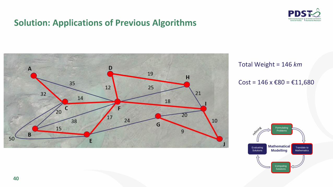
Solution: Applications of Previous Algorithms
40
Total Weight = 146 km
Cost = 146 x €80 = €11,680
Formulating
Problems
Evaluating
Solutions
Translate to
Mathematics
Computing
Solutions
Mathematical
Modelling
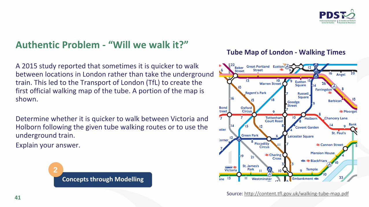
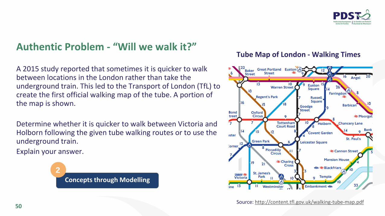
Authentic Problem - “Will we walk it?”
A 2015 study reported that sometimes it is quicker to walk between locations in London rather than take the underground train. This led to the Transport of London (TfL) to create the first official walking map of the tube. A portion of the map is shown.
Determine whether it is quicker to walk between Victoria and Holborn following the given tube walking routes or to use the underground train.
Explain your answer.
41Source: http://content.tfl.gov.uk/walking-tube-map.pdf
Tube Map of London - Walking Times
Concepts through Modelling
2
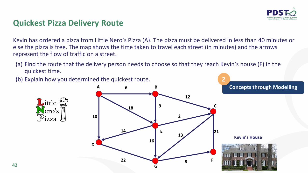
Quickest Pizza Delivery Route
42
Kevin has ordered a pizza from Little Nero’s Pizza (A). The pizza must be delivered in less than 40 minutes or else the pizza is free. The map shows the time taken to travel each street (in minutes) and the arrows represent the flow of traffic on a street.
(a) Find the route that the delivery person needs to choose so that they reach Kevin’s house (F) in the quickest time.
(b) Explain how you determined the quickest route.6
12
13
2
9
16
8
21
22
14
10
18
Kevin’s House
A
E
C
B
F
D
G
Concepts through Modelling
2
Quickest Pizza Delivery Route
43
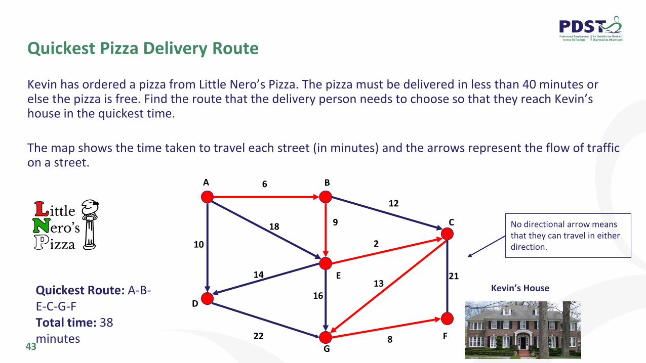
Kevin has ordered a pizza from Little Nero’s Pizza. The pizza must be delivered in less than 40 minutes or else the pizza is free. Find the route that the delivery person needs to choose so that they reach Kevin’s house in the quickest time.
The map shows the time taken to travel each street (in minutes) and the arrows represent the flow of traffic on a street.
6
12
13
2
9
16
8
21
22
14
10
18
A
E
C
B
F
D
G
Quickest Route: A-B-E-C-G-FTotal time: 38 minutes
Kevin’s House
No directional arrow means that they can travel in either direction.
Quickest Pizza Delivery Route
44
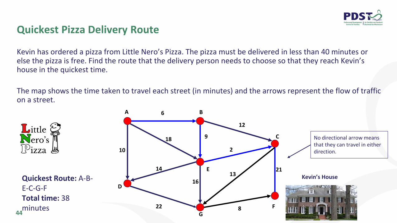
Kevin has ordered a pizza from Little Nero’s Pizza. The pizza must be delivered in less than 40 minutes or else the pizza is free. Find the route that the delivery person needs to choose so that they reach Kevin’s house in the quickest time.
The map shows the time taken to travel each street (in minutes) and the arrows represent the flow of traffic on a street.
6
12
13
2
9
16
8
21
22
14
10
18
A
E
C
B
F
D
G
Quickest Route: A-B-E-C-G-FTotal time: 38 minutes
Kevin’s House
No directional arrow means that they can travel in either direction.
Describe the Approach
45
Create a formal step-by-step approach to find the
shortest/quickest/cheapest path between two points in a network
using suitable terminology.
Dijkstra’s Algorithm
46
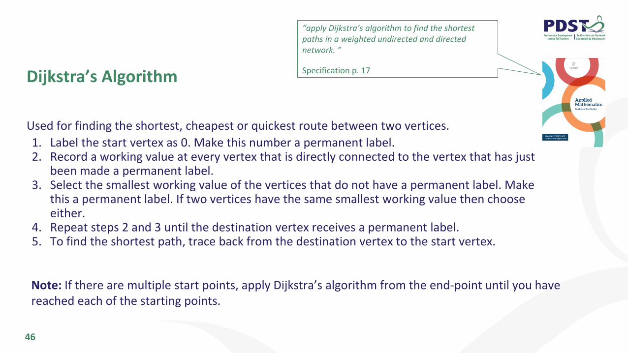
Used for finding the shortest, cheapest or quickest route between two vertices.
1. Label the start vertex as 0. Make this number a permanent label.2. Record a working value at every vertex that is directly connected to the vertex that has just
been made a permanent label.3. Select the smallest working value of the vertices that do not have a permanent label. Make
this a permanent label. If two vertices have the same smallest working value then choose either.
4. Repeat steps 2 and 3 until the destination vertex receives a permanent label.5. To find the shortest path, trace back from the destination vertex to the start vertex.
“apply Dijkstra’s algorithm to find the shortest paths in a weighted undirected and directed network. ”
Specification p. 17
Note: If there are multiple start points, apply Dijkstra’s algorithm from the end-point until you have reached each of the starting points.
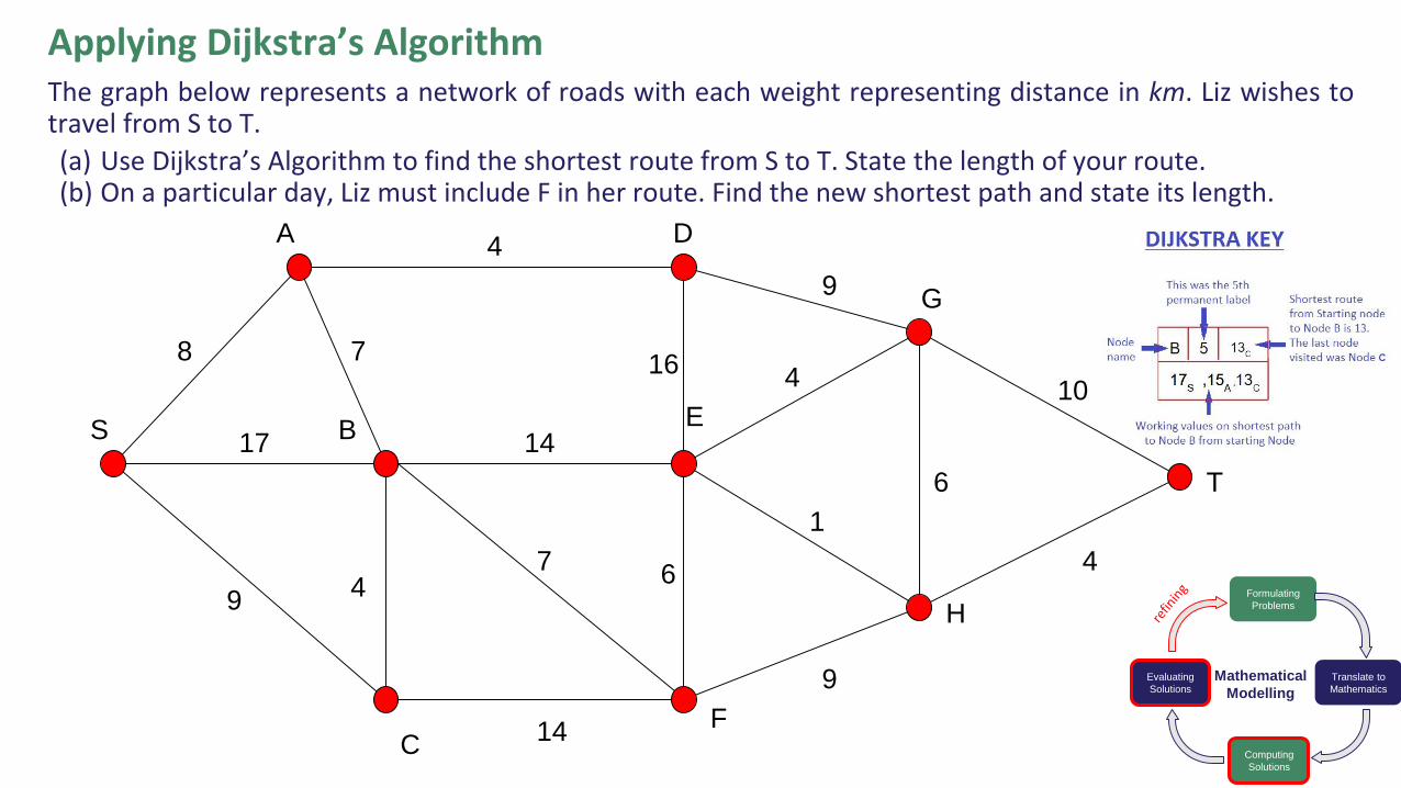
Applying Dijkstra’s AlgorithmThe graph below represents a network of roads with each weight representing distance in km. Liz wishes totravel from S to T.
(a) Use Dijkstra’s Algorithm to find the shortest route from S to T. State the length of your route.(b) On a particular day, Liz must include F in her route. Find the new shortest path and state its length.
DA
BE
G
S
T
C
H
F
4
816
7
9
17
14
14
76
1
4
9
6
10
44
9
Formulating
Problems
Evaluating
Solutions
Translate to
Mathematics
Computing
Solutions
Mathematical
Modelling
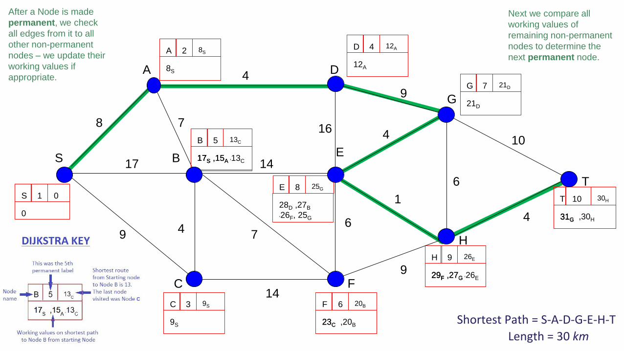
29F ,27G 29F ,27G ‘26E29F
23C ,20B
17S ,15A ‘13C
0
12A
Shortest Path = S-A-D-G-E-H-T
D 4 12A
S 1 0
B 5 13C
8S
A 2 8S
9S
C 3 9S F 6 20B
E 8 25G
21D
G 7 21D
H 9 26E
31G ,30H
T 10 30H
B
14
14
7
4
9
DA
E
G
S
T
C
H
F
4
816
7
9
17
6
1
6
10
44
9
17S ,15A 17S
23C
28D ,27B
‘26F, 25G 31G
Length = 30 km
After a Node is made
permanent, we check
all edges from it to all
other non-permanent
nodes – we update their
working values if
appropriate.
Next we compare all
working values of
remaining non-permanent
nodes to determine the
next permanent node.
Shortest Path = S-C-B-F-E-H-T
Solution
B
14
14
7
4
9
DA
E
G
S
T
C
H
F
4
816
7
9
17
6
1
6
10
44
9
Length via Node F = (20 +11) = 31 km
F 6 20B
23C, 20B
C 3 9S
9S
S 1 0
0
A 2 8S
8S
B 5 13C
17S, 15A, 13C
D 4 12A
12A
T
0
1 0
H
4T
2 4T
G
10T
E
4 9E
F
13H
3 5H
5H
5 11E
13H, 11E
10T, 9E
Authentic Problem - “Will we walk it?”
A 2015 study reported that sometimes it is quicker to walk between locations in the London rather than take the underground train. This led to the Transport of London (TfL) to create the first official walking map of the tube. A portion of the map is shown.
Determine whether it is quicker to walk between Victoria and Holborn following the given tube walking routes or to use the underground train.
Explain your answer.
50Source: http://content.tfl.gov.uk/walking-tube-map.pdf
Tube Map of London - Walking Times
Concepts through Modelling
2
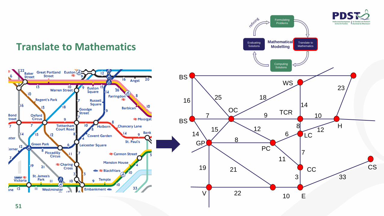
Translate to Mathematics
51
V
19
E
BS
GP
CC
PC
LC
TCROC
CS
H
WS
16
14
22
21
25
7
15
8
11
3
10
8
7
6
9
12
18
12
10
23
14
33
BS
Formulating
Problems
Evaluating
Solutions
Translate to
Mathematics
Computing
Solutions
Mathematical
Modelling
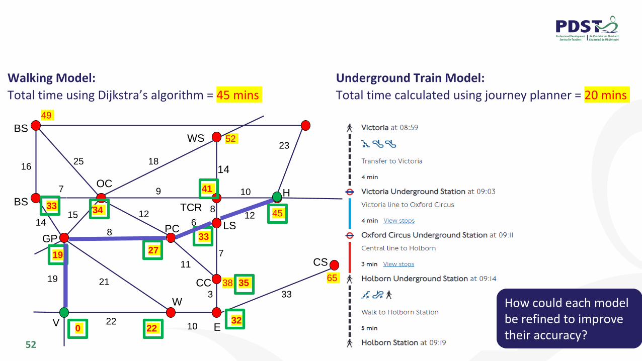
52
Walking Model:
Total time using Dijkstra’s algorithm = 45 mins
Underground Train Model:
Total time calculated using journey planner = 20 mins
V
19
E
BS
GP
CC
PC LS
TCR
OC
CS
H
WS
16
14
22
21
25
7
15
8
11
3
10
8
7
6
9
12
18
12
10
23
14
33
BS
19
0 22
33 34
27
32
38
49
33
41
45
35
52
65
How could each model be refined to improve their accuracy?
W
After a Node is made permanent, we check all
edges from it to all other non-permanent nodes –
we update their working values if appropriate.
Next we compare all working
values of remaining non-
permanent nodes to determine the
next permanent node.
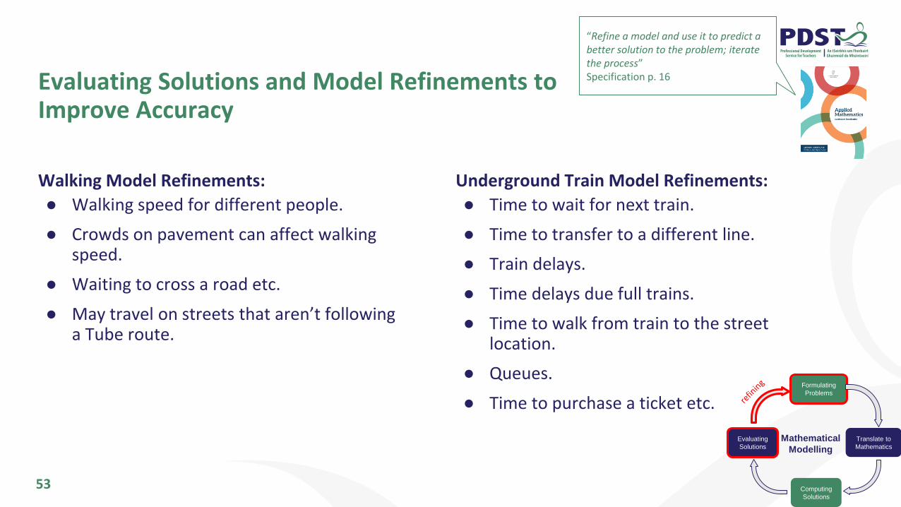
Evaluating Solutions and Model Refinements to Improve Accuracy
53
Walking Model Refinements:
● Walking speed for different people.
● Crowds on pavement can affect walking speed.
● Waiting to cross a road etc.
● May travel on streets that aren’t following a Tube route.
Underground Train Model Refinements:
● Time to wait for next train.
● Time to transfer to a different line.
● Train delays.
● Time delays due full trains.
● Time to walk from train to the street location.
● Queues.
● Time to purchase a ticket etc.Formulating
Problems
Evaluating
Solutions
Translate to
Mathematics
Computing
Solutions
Mathematical
Modelling
“Refine a model and use it to predict a better solution to the problem; iterate the process”Specification p. 16
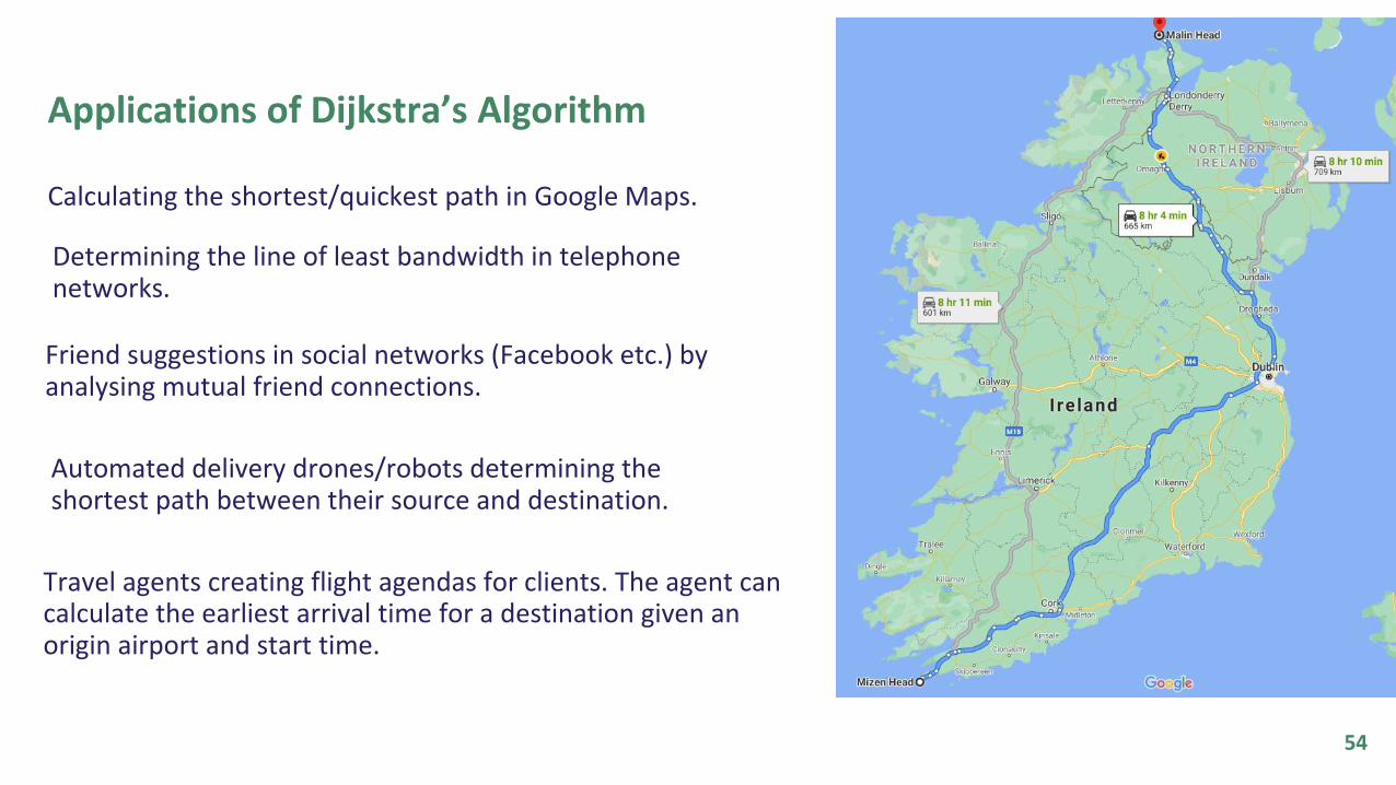
Applications of Dijkstra’s Algorithm
Calculating the shortest/quickest path in Google Maps.
54
Travel agents creating flight agendas for clients. The agent can calculate the earliest arrival time for a destination given an origin airport and start time.
Automated delivery drones/robots determining the shortest path between their source and destination.
Friend suggestions in social networks (Facebook etc.) by analysing mutual friend connections.
Determining the line of least bandwidth in telephone networks.

Reflection on Algorithms
55
In your groups, analyse the three algorithms visited to date and
discuss/comment on each using the following as guides:
Purpose
Teaching and learning
Suitability to real life applications
Other comments
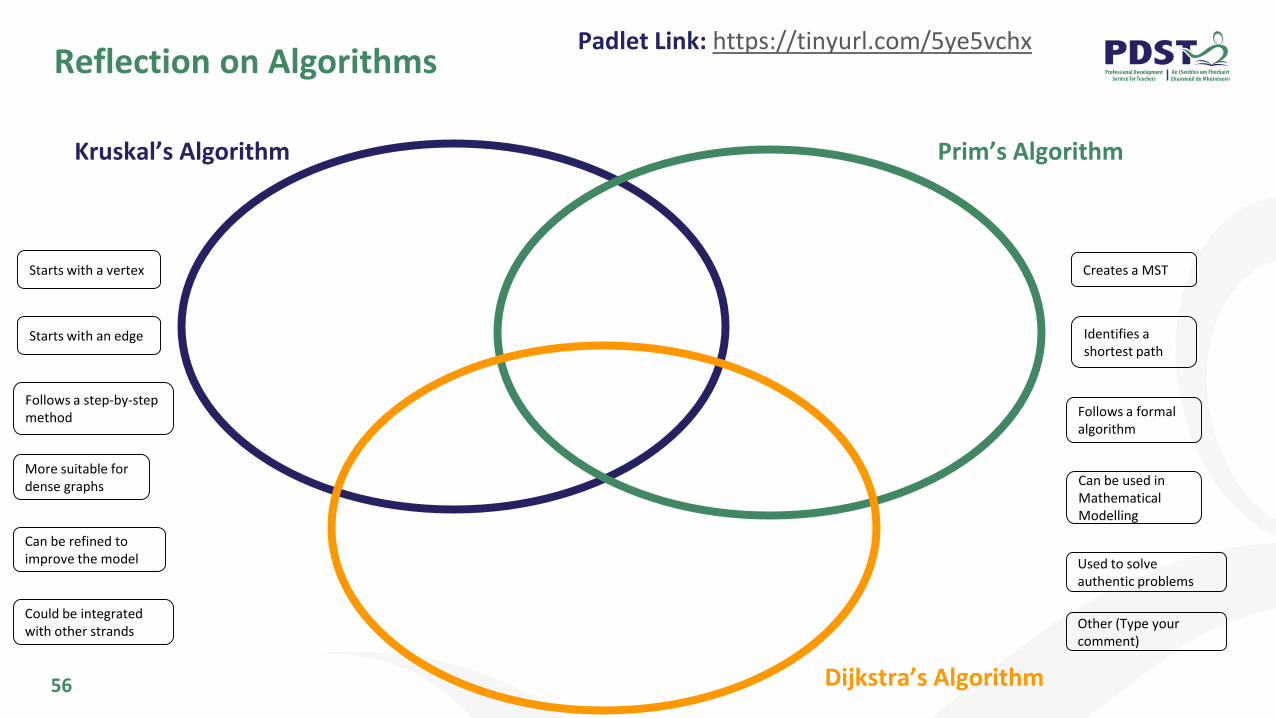
Reflection on Algorithms
56
Kruskal’s Algorithm Prim’s Algorithm
Dijkstra’s Algorithm
Starts with an edge
Starts with a vertex Creates a MST
Identifies a shortest path
Follows a formal algorithm
Follows a step-by-step method
Can be used in Mathematical Modelling
Used to solve authentic problems
More suitable for dense graphs
Can be refined to improve the model
Could be integrated with other strands
Other (Type your comment)
Padlet Link: https://tinyurl.com/5ye5vchx
Reflection on Teaching and Learning: Session 2
57
Consider how the teaching and learning strategies used in this session support the integration of mathematical modelling in students’ understanding of algorithms?
What student modelling key skills could be developed using the teaching and learning approaches demonstrated in this session?
Consider how the learning outcomes of Strand 1 were necessarily and purposefully integrated into our teaching and learning of algorithms from Strand 2.
58
Session 3: Connecting Strands
13:45 - 15:15

By the end of this session you will have:
59
Developed a deeper understanding of how to present problems which will
develop students modelling skills & competencies.
Experienced a constructivist teaching approach to actively involve
students in deriving the equations of motion for constant acceleration.
Reflected on approaches to planning teaching and learning
strategies for September 2021.
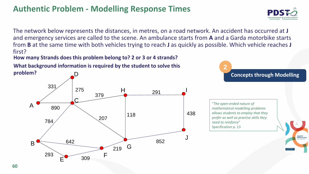
Authentic Problem - Modelling Response Times
60
The network below represents the distances, in metres, on a road network. An accident has occurred at Jand emergency services are called to the scene. An ambulance starts from A and a Garda motorbike starts from B at the same time with both vehicles trying to reach J as quickly as possible. Which vehicle reaches Jfirst?
E
D
CA
331
B
F
G
H I
J
275
890
784
293
642
309
219
207
379291
852
118 438
Concepts through Modelling
2
“The open-ended nature of mathematical modelling problems allows students to employ that they prefer as well as practise skills they need to reinforce”Specification p. 13
How many Strands does this problem belong to? 2 or 3 or 4 strands?
What background information is required by the student to solve this problem?
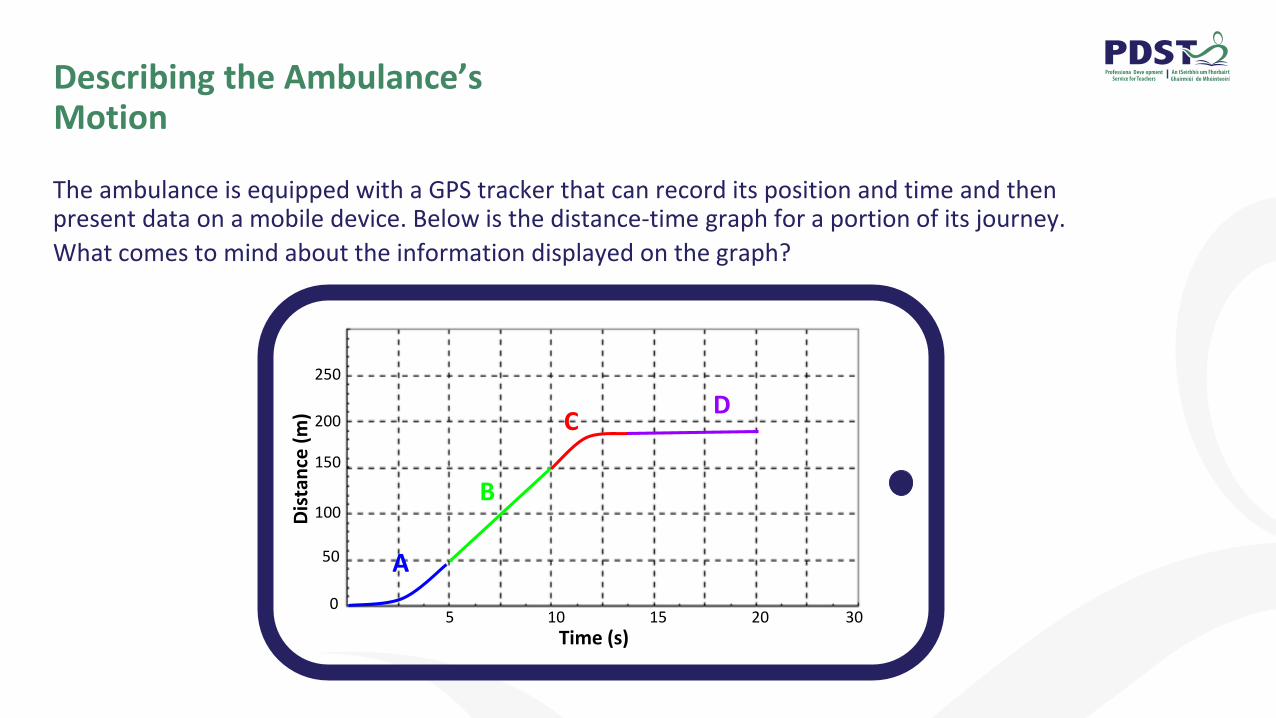
Describing the Ambulance’s Motion
The ambulance is equipped with a GPS tracker that can record its position and time and then present data on a mobile device. Below is the distance-time graph for a portion of its journey.
What comes to mind about the information displayed on the graph?
Dis
tan
ce (
m)
Time (s)
A
B
CD
5 10 150
200
50
150
100
20
250
30
Dis
tan
ce (
m)
Time (s)
A
B
C D
Ve
loci
ty (
m/s
)
Time (s)
A
B
C
D0
20
10
5 10 15
5 10 150
200
50
150
100
20
20
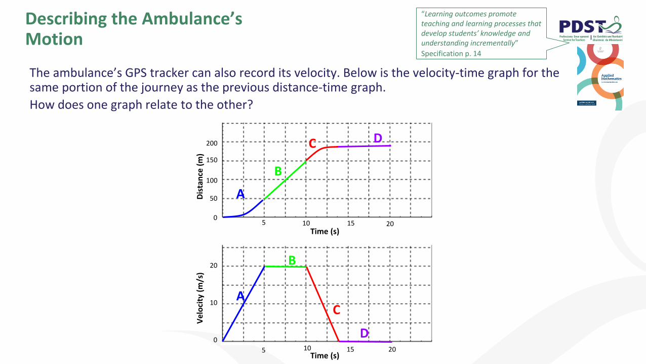
The ambulance’s GPS tracker can also record its velocity. Below is the velocity-time graph for the same portion of the journey as the previous distance-time graph.
How does one graph relate to the other?
Describing the Ambulance’s Motion
“Learning outcomes promote teaching and learning processes that develop students’ knowledge and understanding incrementally”
Specification p. 14
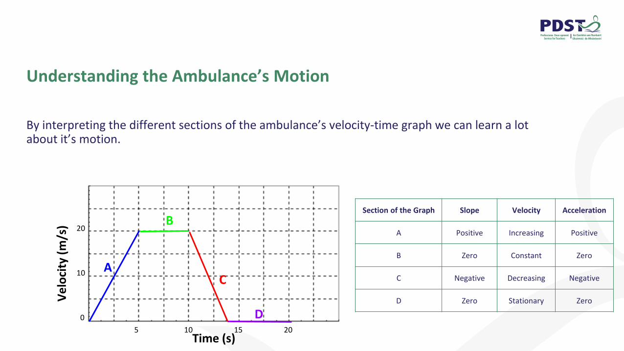
Understanding the Ambulance’s Motion
By interpreting the different sections of the ambulance’s velocity-time graph we can learn a lot about it’s motion.
Ve
loci
ty (
m/s
)
Time (s)
A
B
C
D0
20
10
5 10 15 20
Section of the Graph Slope Velocity Acceleration
A Positive Increasing Positive
B Zero Constant Zero
C Negative Decreasing Negative
D Zero Stationary Zero
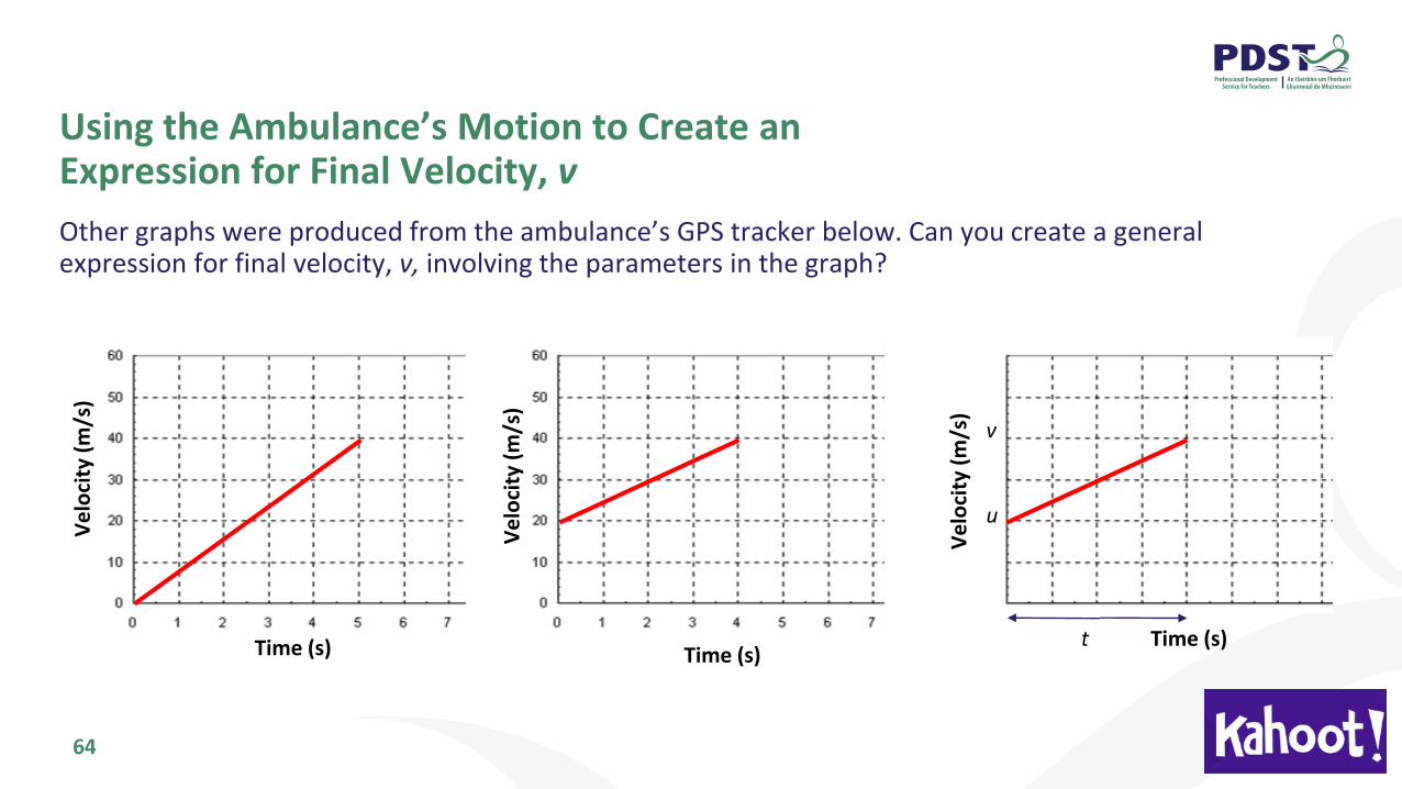
Using the Ambulance’s Motion to Create an Expression for Final Velocity, v
64
Other graphs were produced from the ambulance’s GPS tracker below. Can you create a general expression for final velocity, v, involving the parameters in the graph?
u
v
t
Ve
loci
ty (
m/s
)
Time (s)
Ve
loci
ty (
m/s
)
Time (s)
Ve
loci
ty (
m/s
)
Time (s)
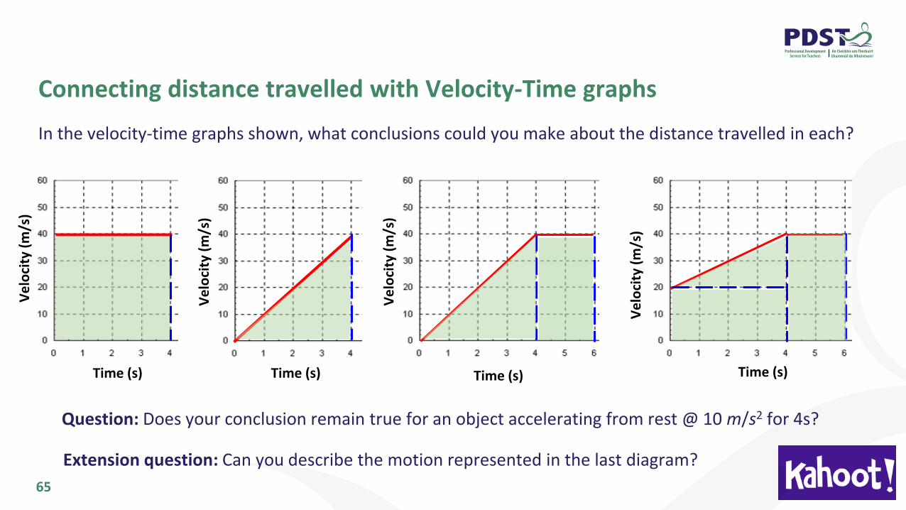
Connecting distance travelled with Velocity-Time graphs
65
In the velocity-time graphs shown, what conclusions could you make about the distance travelled in each?
Ve
loci
ty (
m/s
)
Time (s)
Ve
loci
ty (
m/s
)
Time (s)
Question: Does your conclusion remain true for an object accelerating from rest @ 10 m/s2 for 4s?
Ve
loci
ty (
m/s
)Time (s)
Ve
loci
ty (
m/s
)
Time (s)
Extension question: Can you describe the motion represented in the last diagram?
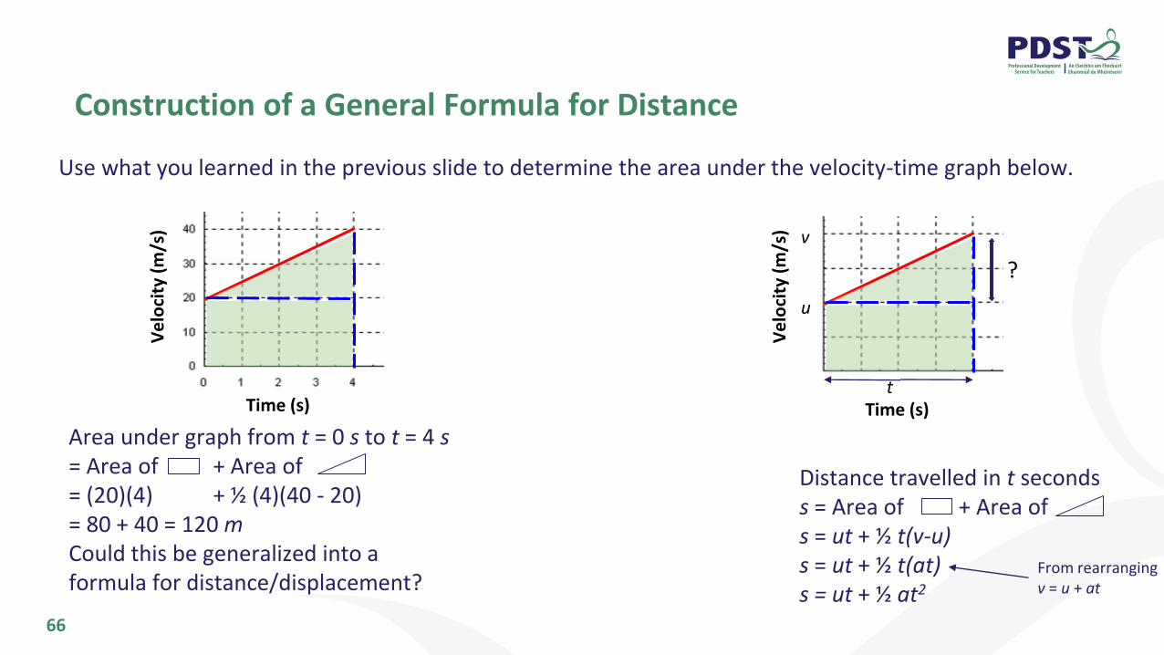
Construction of a General Formula for Distance
66
Use what you learned in the previous slide to determine the area under the velocity-time graph below.V
elo
city
(m
/s)
Time (s)
Area under graph from t = 0 s to t = 4 s= Area of + Area of = (20)(4) + ½ (4)(40 - 20)= 80 + 40 = 120 mCould this be generalized into a formula for distance/displacement?
Distance travelled in t secondss = Area of + Area of s = ut + ½ t(v-u)s = ut + ½ t(at)s = ut + ½ at2
From rearranging v = u + at
Ve
loci
ty (
m/s
)
Time (s)
u
v
t
?

Reflection on Teaching and Learning
67
What did you notice about the teaching and learning approach used here?
“The focus on the experiential approach to teaching and learning, which is central to applied mathematics, means that students can be engaged in learning activities that complement their own needs and ways of learning.”
Specification p. 14
What are some of the benefits for students of using an approach like this?
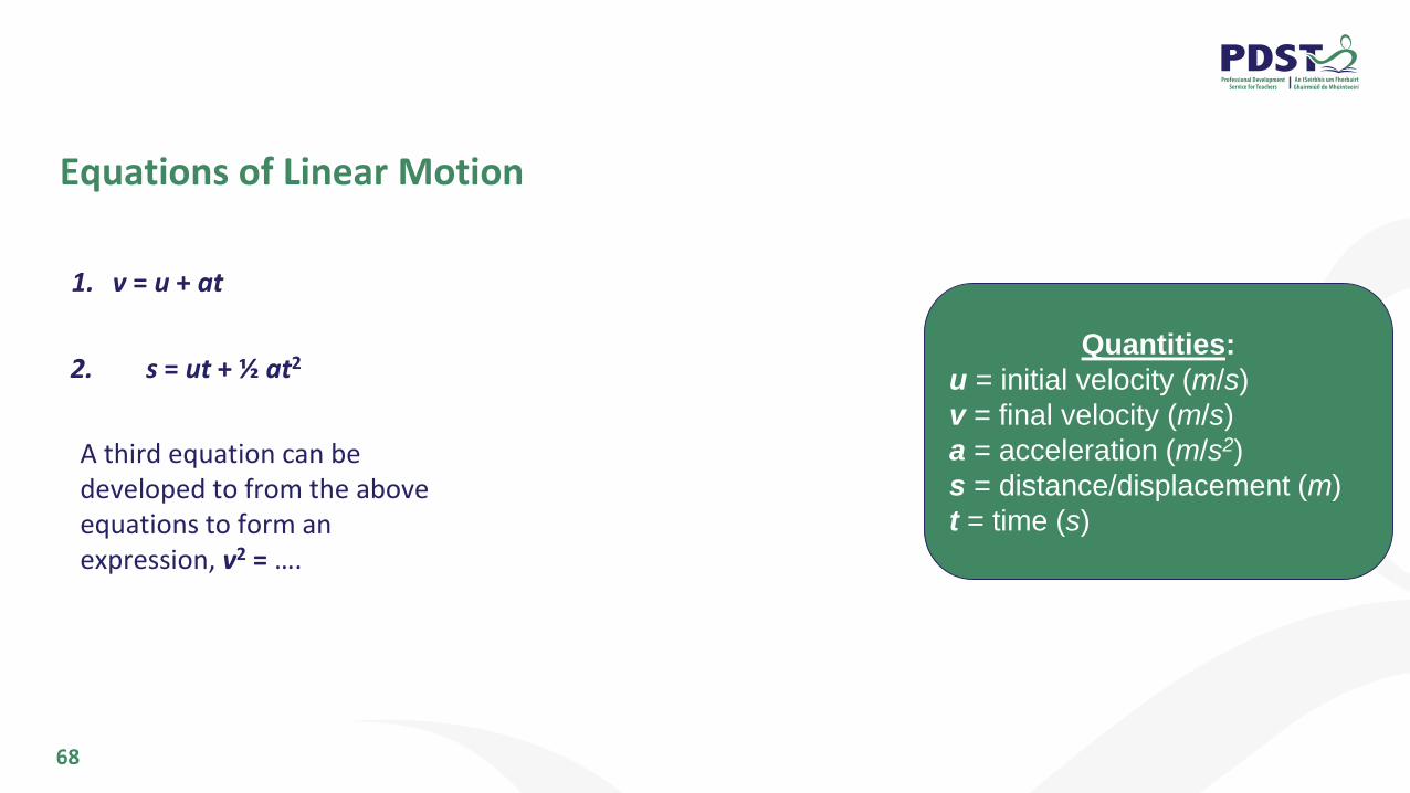
Equations of Linear Motion
68
1. v = u + at
Quantities:
u = initial velocity (m/s)
v = final velocity (m/s)
a = acceleration (m/s2)
s = distance/displacement (m)
t = time (s)
2. s = ut + ½ at2
A third equation can be developed to from the above equations to form an expression, v2 = ….
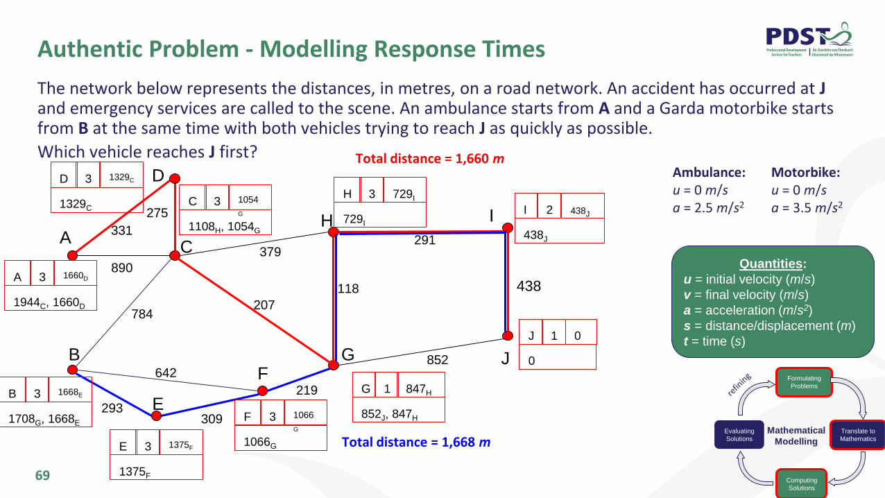
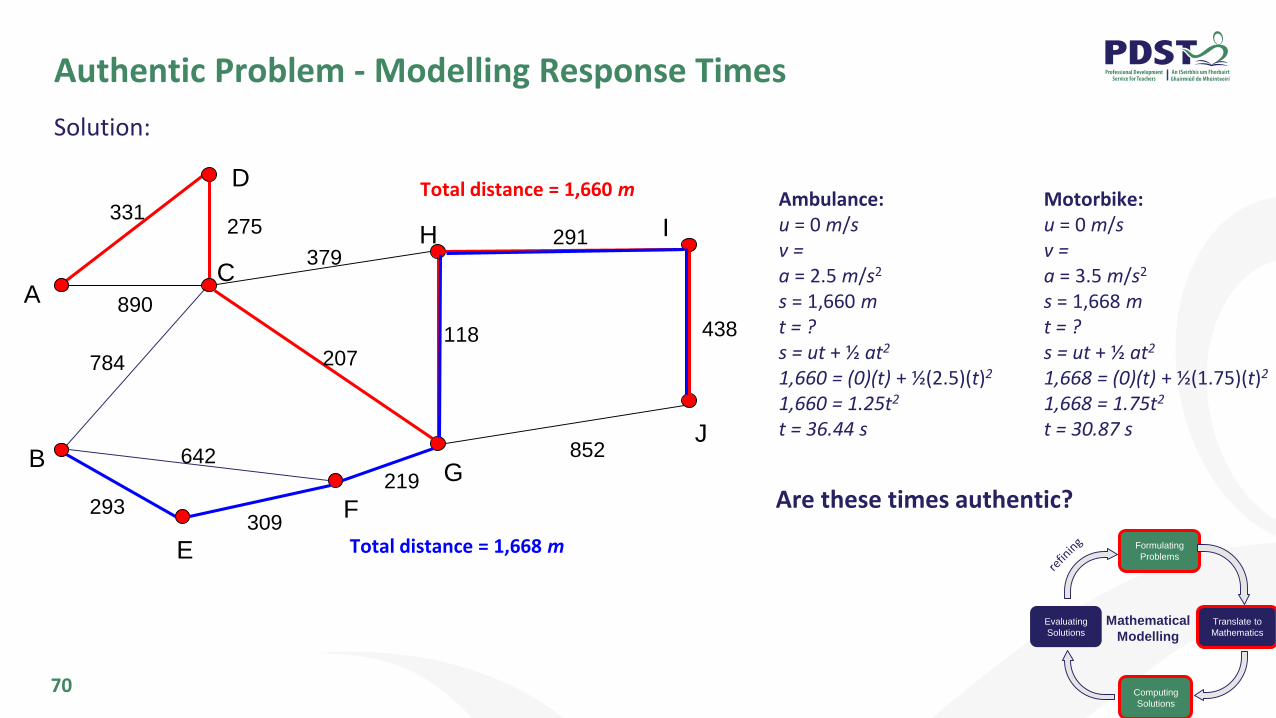
Authentic Problem - Modelling Response Times
69
The network below represents the distances, in metres, on a road network. An accident has occurred at Jand emergency services are called to the scene. An ambulance starts from A and a Garda motorbike starts from B at the same time with both vehicles trying to reach J as quickly as possible.
Which vehicle reaches J first?
Formulating
Problems
Evaluating
Solutions
Translate to
Mathematics
Computing
Solutions
Mathematical
Modelling
Ambulance:u = 0 m/sa = 2.5 m/s2
Motorbike:u = 0 m/sa = 3.5 m/s2
CA
331
B
E
FG
H I
J
D
275
890
784
293
642
309
219
207
379291
852
118 438
Total distance = 1,660 m
Total distance = 1,668 m
0
J 1 0
438J
I 2 438J
852J, 847H
G 1 847H
729I
H 3 729I
1108H, 1054G
C 3 1054
G
1708G, 1668E
B 3 1668E
1375F
E 3 1375F1066G
F 3 1066
G
1944C, 1660D
A 3 1660D
1329C
D 3 1329C
Quantities:
u = initial velocity (m/s)
v = final velocity (m/s)
a = acceleration (m/s2)
s = distance/displacement (m)
t = time (s)
Authentic Problem - Modelling Response Times
70
Solution:
CA
331
B
E
F
G
H I
J
D
275
890
784
293
642
309
219
207
379291
852
118 438
Formulating
Problems
Evaluating
Solutions
Translate to
Mathematics
Computing
Solutions
Ambulance:u = 0 m/sv = a = 2.5 m/s2
s = 1,660 mt = ?s = ut + ½ at2
1,660 = (0)(t) + ½(2.5)(t)2
1,660 = 1.25t2
t = 36.44 s
Mathematical
Modelling
Motorbike:u = 0 m/sv = a = 3.5 m/s2
s = 1,668 mt = ?s = ut + ½ at2
1,668 = (0)(t) + ½(1.75)(t)2
1,668 = 1.75t2
t = 30.87 s
Total distance = 1,660 m
Total distance = 1,668 m
Are these times authentic?
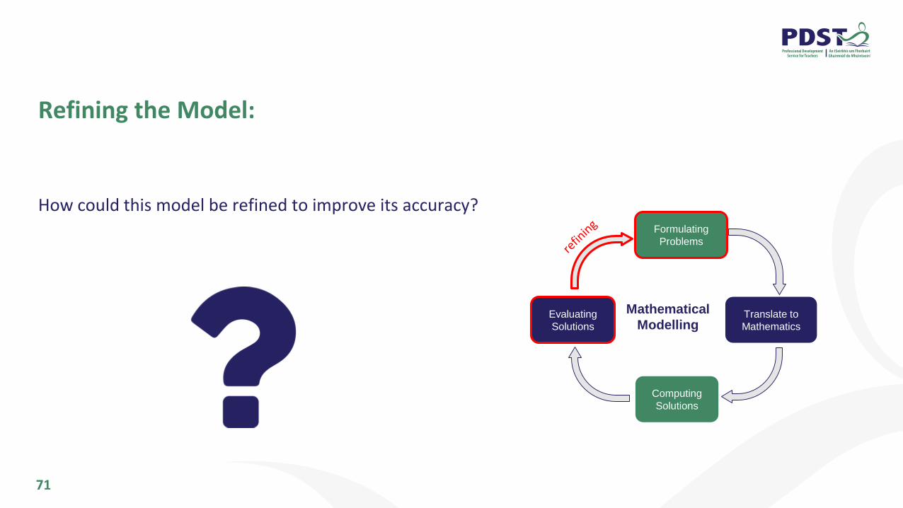
Refining the Model:
71
How could this model be refined to improve its accuracy?Formulating
Problems
Evaluating
Solutions
Translate to
Mathematics
Computing
Solutions
Mathematical
Modelling
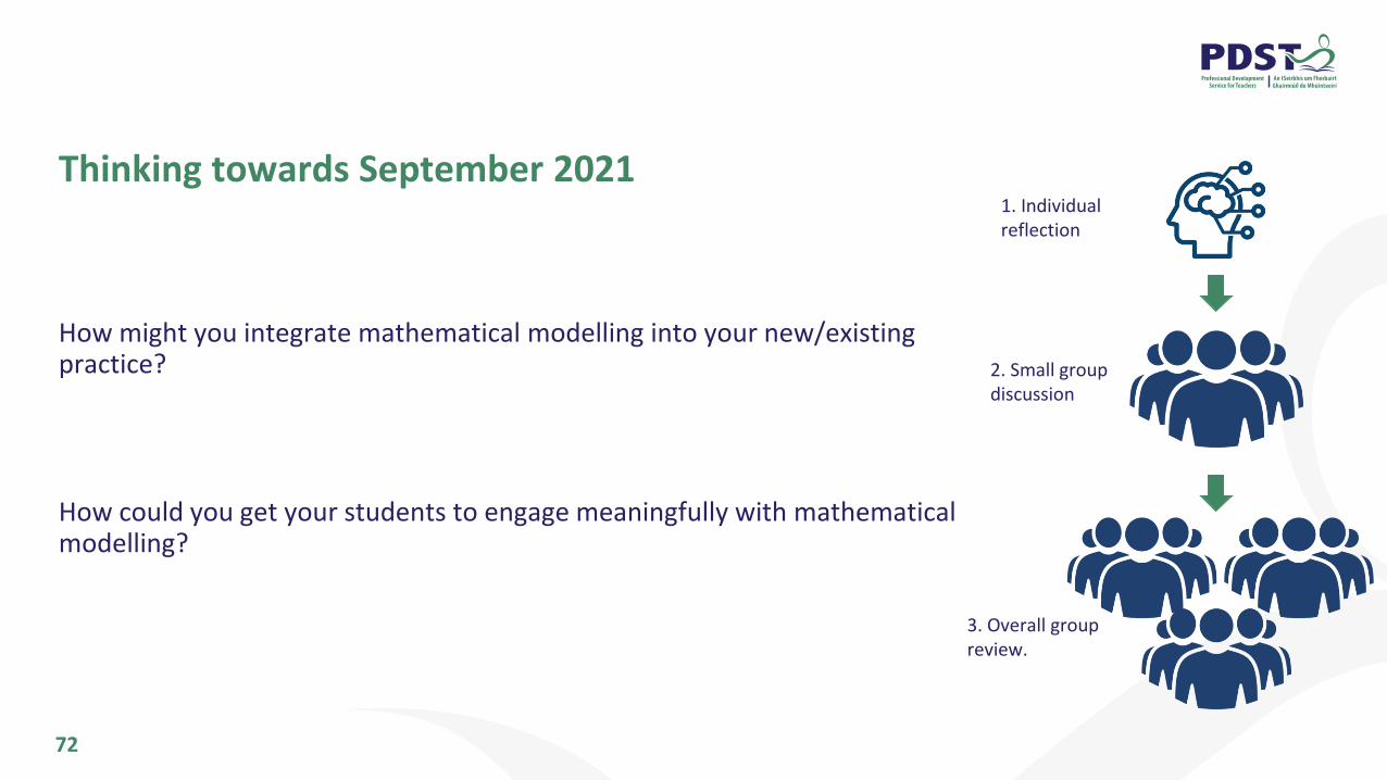
Thinking towards September 2021
How might you integrate mathematical modelling into your new/existing practice?
How could you get your students to engage meaningfully with mathematical modelling?
72
1. Individual reflection
2. Small group discussion
3. Overall group review.

Next Steps?
73
Next event - Webinar (May 2021).
Focus of webinar will be based on feedback from all events to date.

What’s next? Timeline 2020 - 2021

Single VisitSustained Support
pdst.ieScoilnet.ie
PDST Supports
School VisitsProfessional
Learning Communities
WebinarsSeminars PDST Websites
Supports Provided by PDST

Questions?
● Any further questions please contact: [email protected]
● Follow us on Twitter: @PDSTAppliedMath77