Embed Size (px)
Citation preview

Aapo HyvarinenJarmo HurriPatrik O. Hoyer
Natural Image Statistics
A probabilistic approach to earlycomputational vision
February 27, 2009
Springer


Contents overview
1 Introduction . . . . . . . . . . . . . . . . . . . . . . . . . . . . . . . . . . . . . . . . . . . . . . . . . . .1Part I Background2 Linear filters and frequency analysis . . . . . . . . . . . . . . . . . . . . . . . . . . . . . 253 Outline of the visual system . . . . . . . . . . . . . . . . . . . . . . . . . . . . . . . . . . . . . 514 Multivariate probability and statistics . . . . . . . . . . . . . . . . . . . . . . . . . . . . 69Part II Statistics of linear features5 Principal components and whitening. . . . . . . . . . . . . . . . . . . . . . . . . . . . . 976 Sparse coding and simple cells. . . . . . . . . . . . . . . . . . . . . . . . . . . . . . . . . . . 1377 Independent component analysis. . . . . . . . . . . . . . . . . . . . . . . . . . . . . . . . . 1598 Information-theoretic interpretations . . . . . . . . . . . . . . . . . . . . . . . . . . . . . 185Part III Nonlinear features & dependency of linear features9 Energy correlation of linear features & normalization . . . . . . . . . . . . . . 20910 Energy detectors and complex cells. . . . . . . . . . . . . . . . . . . . . . . . . . . . . . . 22311 Energy correlations and topographic organization. . . . . . . . . . . . . . . . . 24912 Dependencies of energy detectors: Beyond V1. . . . . . . . . . . . . . . . . . . . . 27313 Overcomplete and non-negative models. . . . . . . . . . . . . . . . . . . . . . . . . . . 28914 Lateral interactions and feedback. . . . . . . . . . . . . . . . . . . . . . . . . . . . . . . . 307Part IV Time, colour and stereo15 Colour and stereo images. . . . . . . . . . . . . . . . . . . . . . . . . . . . . . . . . . . . . . . 32116 Temporal sequences of natural images. . . . . . . . . . . . . . . . . . . . . . . . . . . . 337Part V Conclusion17 Conclusion and future prospects. . . . . . . . . . . . . . . . . . . . . . . . . . . . . . . . . 379Part VI Appendix: Supplementary mathematical tools18 Optimization theory and algorithms . . . . . . . . . . . . . . . . . . . . . . . . . . . . . . 39319 Crash course on linear algebra. . . . . . . . . . . . . . . . . . . . . . . . . . . . . . . . . . 41520 The discrete Fourier transform . . . . . . . . . . . . . . . . . . . . . . . . . . . . . . . . . . 42321 Estimation of non-normalized statistical models. . . . . . . . . . . . . . . . . . . 437Index . . . . . . . . . . . . . . . . . . . . . . . . . . . . . . . . . . . . . . . . . . . . . . . . . . .. . . . . . . . . . 445References. . . . . . . . . . . . . . . . . . . . . . . . . . . . . . . . . . . . . . . . . . . . . . . . . . .. . . . . . 453
v


Contents
1 Introduction . . . . . . . . . . . . . . . . . . . . . . . . . . . . . . . . . . . . . . . . . . . . . . . . . . .11.1 What this book is all about . . . . . . . . . . . . . . . . . . . . . . . . . .. . . . . . . . . 11.2 What is vision? . . . . . . . . . . . . . . . . . . . . . . . . . . . . . . . . . . .. . . . . . . . . 31.3 The magic of your visual system . . . . . . . . . . . . . . . . . . . . . .. . . . . . . . 31.4 Importance of prior information . . . . . . . . . . . . . . . . . . . .. . . . . . . . . . 6
1.4.1 Ecological adaptation provides prior information . .. . . . . . . . 61.4.2 Generative models and latent quantities . . . . . . . . . . .. . . . . . . 81.4.3 Projection onto the retina loses information . . . . . . .. . . . . . . 91.4.4 Bayesian inference and priors . . . . . . . . . . . . . . . . . . . .. . . . . . 10
1.5 Natural images . . . . . . . . . . . . . . . . . . . . . . . . . . . . . . . . . . .. . . . . . . . . . 111.5.1 The image space . . . . . . . . . . . . . . . . . . . . . . . . . . . . . . . . .. . . . 111.5.2 Definition of natural images . . . . . . . . . . . . . . . . . . . . . .. . . . . 12
1.6 Redundancy and information . . . . . . . . . . . . . . . . . . . . . . . .. . . . . . . . . 131.6.1 Information theory and image coding . . . . . . . . . . . . . . .. . . . 131.6.2 Redundancy reduction and neural coding . . . . . . . . . . . .. . . . 15
1.7 Statistical modelling of the visual system . . . . . . . . . . .. . . . . . . . . . . . 161.7.1 Connecting information theory and Bayesian inference . . . . . 161.7.2 Normative vs. descriptive modelling of visual system. . . . . . 161.7.3 Towards predictive theoretical neuroscience . . . . . .. . . . . . . . 17
1.8 Features and statistical models of natural images . . . . .. . . . . . . . . . . 181.8.1 Image representations and features . . . . . . . . . . . . . . .. . . . . . . 181.8.2 Statistics of features . . . . . . . . . . . . . . . . . . . . . . . . . .. . . . . . . . 191.8.3 From features to statistical models . . . . . . . . . . . . . . .. . . . . . . 19
1.9 The statistical-ecological approach recapitulated. .. . . . . . . . . . . . . . . 211.10 References . . . . . . . . . . . . . . . . . . . . . . . . . . . . . . . . . . . . .. . . . . . . . . . . 21
Part I Background
2 Linear filters and frequency analysis . . . . . . . . . . . . . . . . . . . . . . . . . . . . . 252.1 Linear filtering . . . . . . . . . . . . . . . . . . . . . . . . . . . . . . . . . .. . . . . . . . . . . 25
2.1.1 Definition . . . . . . . . . . . . . . . . . . . . . . . . . . . . . . . . . . . . .. . . . . 25
vii

viii Contents
2.1.2 Impulse response and convolution . . . . . . . . . . . . . . . . .. . . . . 282.2 Frequency-based representation . . . . . . . . . . . . . . . . . . .. . . . . . . . . . . . 29
2.2.1 Motivation . . . . . . . . . . . . . . . . . . . . . . . . . . . . . . . . . . . .. . . . . . 292.2.2 Representation in one and two dimensions . . . . . . . . . . .. . . . 302.2.3 Frequency-based representation and linear filtering. . . . . . . . 332.2.4 Computation and mathematical details . . . . . . . . . . . . .. . . . . 37
2.3 Representation using linear basis . . . . . . . . . . . . . . . . . .. . . . . . . . . . . . 382.3.1 Basic idea . . . . . . . . . . . . . . . . . . . . . . . . . . . . . . . . . . . . .. . . . . 382.3.2 Frequency-based representation as a basis . . . . . . . . .. . . . . . . 40
2.4 Space-frequency analysis . . . . . . . . . . . . . . . . . . . . . . . . .. . . . . . . . . . . 412.4.1 Introduction . . . . . . . . . . . . . . . . . . . . . . . . . . . . . . . . . .. . . . . . . 412.4.2 Space-frequency analysis and Gabor filters . . . . . . . . .. . . . . . 432.4.3 Spatial localization vs. spectral accuracy . . . . . . . .. . . . . . . . . 46
2.5 References . . . . . . . . . . . . . . . . . . . . . . . . . . . . . . . . . . . . . .. . . . . . . . . . 482.6 Exercices . . . . . . . . . . . . . . . . . . . . . . . . . . . . . . . . . . . . . . .. . . . . . . . . . 48
3 Outline of the visual system . . . . . . . . . . . . . . . . . . . . . . . . . . . . . . . . . . . . . 513.1 Neurons and firing rates . . . . . . . . . . . . . . . . . . . . . . . . . . . .. . . . . . . . . 513.2 From the eye to the cortex . . . . . . . . . . . . . . . . . . . . . . . . . . .. . . . . . . . 543.3 Linear models of visual neurons . . . . . . . . . . . . . . . . . . . . .. . . . . . . . . 55
3.3.1 Responses to visual stimulation . . . . . . . . . . . . . . . . . .. . . . . . 553.3.2 Simple cells and linear models . . . . . . . . . . . . . . . . . . . .. . . . . 563.3.3 Gabor models and selectivities of simple cells . . . . . .. . . . . . 583.3.4 Frequency channels . . . . . . . . . . . . . . . . . . . . . . . . . . . . .. . . . . 59
3.4 Nonlinear models of visual neurons . . . . . . . . . . . . . . . . . .. . . . . . . . . 593.4.1 Nonlinearities in simple-cell responses . . . . . . . . . .. . . . . . . . 593.4.2 Complex cells and energy models . . . . . . . . . . . . . . . . . . .. . . 62
3.5 Interactions between visual neurons . . . . . . . . . . . . . . . .. . . . . . . . . . . 633.6 Topographic organization . . . . . . . . . . . . . . . . . . . . . . . . .. . . . . . . . . . . 653.7 Processing after the primary visual cortex . . . . . . . . . . .. . . . . . . . . . . 663.8 References . . . . . . . . . . . . . . . . . . . . . . . . . . . . . . . . . . . . . .. . . . . . . . . . 663.9 Exercices . . . . . . . . . . . . . . . . . . . . . . . . . . . . . . . . . . . . . . .. . . . . . . . . . 67
4 Multivariate probability and statistics . . . . . . . . . . . . . . . . . . . . . . . . . . . . 694.1 Natural images patches as random vectors . . . . . . . . . . . . .. . . . . . . . . 694.2 Multivariate probability distributions . . . . . . . . . . . .. . . . . . . . . . . . . . 70
4.2.1 Notation and motivation . . . . . . . . . . . . . . . . . . . . . . . . .. . . . . 704.2.2 Probability density function . . . . . . . . . . . . . . . . . . . .. . . . . . . 71
4.3 Marginal and joint probabilities . . . . . . . . . . . . . . . . . . .. . . . . . . . . . . . 734.4 Conditional probabilities . . . . . . . . . . . . . . . . . . . . . . . .. . . . . . . . . . . . 754.5 Independence . . . . . . . . . . . . . . . . . . . . . . . . . . . . . . . . . . . .. . . . . . . . . . 774.6 Expectation and covariance . . . . . . . . . . . . . . . . . . . . . . . .. . . . . . . . . . 79
4.6.1 Expectation . . . . . . . . . . . . . . . . . . . . . . . . . . . . . . . . . . .. . . . . . 794.6.2 Variance and covariance in one dimension . . . . . . . . . . .. . . . 804.6.3 Covariance matrix . . . . . . . . . . . . . . . . . . . . . . . . . . . . . .. . . . . 80

Contents ix
4.6.4 Independence and covariances . . . . . . . . . . . . . . . . . . . .. . . . . 814.7 Bayesian inference . . . . . . . . . . . . . . . . . . . . . . . . . . . . . . .. . . . . . . . . . 83
4.7.1 Motivating example . . . . . . . . . . . . . . . . . . . . . . . . . . . . .. . . . . 834.7.2 Bayes’ Rule . . . . . . . . . . . . . . . . . . . . . . . . . . . . . . . . . . . .. . . . . 854.7.3 Non-informative priors . . . . . . . . . . . . . . . . . . . . . . . . .. . . . . . 864.7.4 Bayesian inference as an incremental learning process . . . . . 86
4.8 Parameter estimation and likelihood . . . . . . . . . . . . . . . .. . . . . . . . . . . 884.8.1 Models, estimation, and samples . . . . . . . . . . . . . . . . . .. . . . . 884.8.2 Maximum likelihood and maximum a posteriori . . . . . . . .. . 894.8.3 Prior and large samples . . . . . . . . . . . . . . . . . . . . . . . . . .. . . . . 91
4.9 References . . . . . . . . . . . . . . . . . . . . . . . . . . . . . . . . . . . . . .. . . . . . . . . . 924.10 Exercices . . . . . . . . . . . . . . . . . . . . . . . . . . . . . . . . . . . . . .. . . . . . . . . . . 92
Part II Statistics of linear features
5 Principal components and whitening. . . . . . . . . . . . . . . . . . . . . . . . . . . . . 975.1 DC component or mean grey-scale value . . . . . . . . . . . . . . . .. . . . . . . 975.2 Principal component analysis . . . . . . . . . . . . . . . . . . . . . .. . . . . . . . . . . 99
5.2.1 A basic dependency of pixels in natural images . . . . . . .. . . . 995.2.2 Learning one feature by maximization of variance . . . .. . . . . 1005.2.3 Learning many features by PCA . . . . . . . . . . . . . . . . . . . . .. . . 1035.2.4 Computational implementation of PCA . . . . . . . . . . . . . .. . . . 1045.2.5 The implications of translation-invariance . . . . . . .. . . . . . . . . 106
5.3 PCA as a preprocessing tool . . . . . . . . . . . . . . . . . . . . . . . . .. . . . . . . . . 1075.3.1 Dimension reduction by PCA . . . . . . . . . . . . . . . . . . . . . . .. . . 1085.3.2 Whitening by PCA . . . . . . . . . . . . . . . . . . . . . . . . . . . . . . . .. . . 1095.3.3 Anti-aliasing by PCA . . . . . . . . . . . . . . . . . . . . . . . . . . . .. . . . . 111
5.4 Canonical preprocessing used in this book . . . . . . . . . . . .. . . . . . . . . . 1135.5 Gaussianity as the basis for PCA . . . . . . . . . . . . . . . . . . . . .. . . . . . . . . 115
5.5.1 The probability model related to PCA . . . . . . . . . . . . . . .. . . . 1155.5.2 PCA as a generative model . . . . . . . . . . . . . . . . . . . . . . . . .. . . 1155.5.3 Image synthesis results . . . . . . . . . . . . . . . . . . . . . . . . .. . . . . . 116
5.6 Power spectrum of natural images . . . . . . . . . . . . . . . . . . . .. . . . . . . . . 1165.6.1 The 1/ f Fourier amplitude or 1/ f 2 power spectrum . . . . . . . 1165.6.2 Connection between power spectrum and covariances . .. . . . 1195.6.3 Relative importance of amplitude and phase . . . . . . . . .. . . . . 120
5.7 Anisotropy in natural images . . . . . . . . . . . . . . . . . . . . . . .. . . . . . . . . . 1215.8 Mathematics of principal component analysis* . . . . . . . .. . . . . . . . . . 122
5.8.1 Eigenvalue decomposition of the covariance matrix . .. . . . . . 1235.8.2 Eigenvectors and translation-invariance . . . . . . . . .. . . . . . . . . 125
5.9 Decorrelation models of retina and LGN *. . . . . . . . . . . . . .. . . . . . . . 1265.9.1 Whitening and redundancy reduction . . . . . . . . . . . . . . .. . . . . 1265.9.2 Patch-based decorrelation . . . . . . . . . . . . . . . . . . . . . .. . . . . . . 1275.9.3 Filter-based decorrelation . . . . . . . . . . . . . . . . . . . . .. . . . . . . . 130
5.10 Concluding remarks and References . . . . . . . . . . . . . . . . .. . . . . . . . . . 134

x Contents
5.11 Exercices . . . . . . . . . . . . . . . . . . . . . . . . . . . . . . . . . . . . . .. . . . . . . . . . . 135
6 Sparse coding and simple cells. . . . . . . . . . . . . . . . . . . . . . . . . . . . . . . . . . . 1376.1 Definition of sparseness . . . . . . . . . . . . . . . . . . . . . . . . . . .. . . . . . . . . . 1376.2 Learning one feature by maximization of sparseness . . . .. . . . . . . . . 138
6.2.1 Measuring sparseness: General framework . . . . . . . . . .. . . . . 1396.2.2 Measuring sparseness using kurtosis . . . . . . . . . . . . . .. . . . . . 1406.2.3 Measuring sparseness using convex functions of square . . . . 1416.2.4 The case of canonically preprocessed data . . . . . . . . . .. . . . . 1446.2.5 One feature learned from natural images . . . . . . . . . . . .. . . . . 145
6.3 Learning many features by maximization of sparseness . .. . . . . . . . . 1456.3.1 Deflationary decorrelation . . . . . . . . . . . . . . . . . . . . . .. . . . . . . 1466.3.2 Symmetric decorrelation . . . . . . . . . . . . . . . . . . . . . . . .. . . . . . 1476.3.3 Sparseness of feature vs. sparseness of representation . . . . . . 148
6.4 Sparse coding features for natural images . . . . . . . . . . . .. . . . . . . . . . 1506.4.1 Full set of features . . . . . . . . . . . . . . . . . . . . . . . . . . . . .. . . . . . 1506.4.2 Analysis of tuning properties . . . . . . . . . . . . . . . . . . . .. . . . . . 150
6.5 How is sparseness useful? . . . . . . . . . . . . . . . . . . . . . . . . . .. . . . . . . . . 1556.5.1 Bayesian modelling . . . . . . . . . . . . . . . . . . . . . . . . . . . . .. . . . . 1556.5.2 Neural modelling . . . . . . . . . . . . . . . . . . . . . . . . . . . . . . .. . . . . 1556.5.3 Metabolic economy . . . . . . . . . . . . . . . . . . . . . . . . . . . . . .. . . . 155
6.6 Concluding remarks and References . . . . . . . . . . . . . . . . . .. . . . . . . . . 1566.7 Exercices . . . . . . . . . . . . . . . . . . . . . . . . . . . . . . . . . . . . . . .. . . . . . . . . . 156
7 Independent component analysis. . . . . . . . . . . . . . . . . . . . . . . . . . . . . . . . . 1597.1 Limitations of the sparse coding approach . . . . . . . . . . . .. . . . . . . . . . 1597.2 Definition of ICA . . . . . . . . . . . . . . . . . . . . . . . . . . . . . . . . . .. . . . . . . . 160
7.2.1 Independence . . . . . . . . . . . . . . . . . . . . . . . . . . . . . . . . . .. . . . . 1607.2.2 Generative model . . . . . . . . . . . . . . . . . . . . . . . . . . . . . . .. . . . . 1617.2.3 Model for preprocessed data . . . . . . . . . . . . . . . . . . . . . .. . . . . 162
7.3 Insufficiency of second-order information . . . . . . . . . . .. . . . . . . . . . . 1627.3.1 Why whitening does not find independent components . . .. . 1637.3.2 Why components have to be non-gaussian . . . . . . . . . . . . .. . 164
7.4 The probability density defined by ICA . . . . . . . . . . . . . . . .. . . . . . . . 1667.5 Maximum likelihood estimation in ICA . . . . . . . . . . . . . . . .. . . . . . . . 1677.6 Results on natural images . . . . . . . . . . . . . . . . . . . . . . . . . .. . . . . . . . . . 168
7.6.1 Estimation of features . . . . . . . . . . . . . . . . . . . . . . . . . .. . . . . . 1687.6.2 Image synthesis using ICA . . . . . . . . . . . . . . . . . . . . . . . .. . . . 169
7.7 Connection to maximization of sparseness . . . . . . . . . . . .. . . . . . . . . . 1707.7.1 Likelihood as a measure of sparseness . . . . . . . . . . . . . .. . . . . 1717.7.2 Optimal sparseness measures . . . . . . . . . . . . . . . . . . . . .. . . . . 172
7.8 Why are independent components sparse? . . . . . . . . . . . . . .. . . . . . . . 1757.8.1 Different forms of non-gaussianity . . . . . . . . . . . . . . .. . . . . . . 1757.8.2 Non-gaussianity in natural images . . . . . . . . . . . . . . . .. . . . . . 1767.8.3 Why is sparseness dominant? . . . . . . . . . . . . . . . . . . . . . .. . . . 177

Contents xi
7.9 General ICA as maximization of non-gaussianity . . . . . . .. . . . . . . . . 1777.9.1 Central Limit Theorem . . . . . . . . . . . . . . . . . . . . . . . . . . .. . . . 1787.9.2 “Non-gaussian is independent” . . . . . . . . . . . . . . . . . . .. . . . . . 1787.9.3 Sparse coding as a special case of ICA . . . . . . . . . . . . . . .. . . 179
7.10 Receptive fields vs. feature vectors . . . . . . . . . . . . . . . .. . . . . . . . . . . . 1807.11 Problem of inversion of preprocessing . . . . . . . . . . . . . .. . . . . . . . . . . 1817.12 Frequency channels and ICA . . . . . . . . . . . . . . . . . . . . . . . .. . . . . . . . . 1827.13 Concluding remarks and References . . . . . . . . . . . . . . . . .. . . . . . . . . . 1827.14 Exercices . . . . . . . . . . . . . . . . . . . . . . . . . . . . . . . . . . . . . .. . . . . . . . . . . 183
8 Information-theoretic interpretations . . . . . . . . . . . . . . . . . . . . . . . . . . . . . 1858.1 Basic motivation for information theory . . . . . . . . . . . . .. . . . . . . . . . . 185
8.1.1 Compression . . . . . . . . . . . . . . . . . . . . . . . . . . . . . . . . . . .. . . . . 1858.1.2 Transmission . . . . . . . . . . . . . . . . . . . . . . . . . . . . . . . . . .. . . . . . 187
8.2 Entropy as a measure of uncertainty . . . . . . . . . . . . . . . . . .. . . . . . . . . 1878.2.1 Definition of entropy . . . . . . . . . . . . . . . . . . . . . . . . . . . .. . . . . 1888.2.2 Entropy as minimum coding length . . . . . . . . . . . . . . . . . .. . . 1898.2.3 Redundancy . . . . . . . . . . . . . . . . . . . . . . . . . . . . . . . . . . . .. . . . 1908.2.4 Differential entropy . . . . . . . . . . . . . . . . . . . . . . . . . . .. . . . . . . 1918.2.5 Maximum entropy . . . . . . . . . . . . . . . . . . . . . . . . . . . . . . . .. . . 192
8.3 Mutual information . . . . . . . . . . . . . . . . . . . . . . . . . . . . . . .. . . . . . . . . . 1928.4 Minimum entropy coding of natural images. . . . . . . . . . . . .. . . . . . . . 194
8.4.1 Image compression and sparse coding . . . . . . . . . . . . . . .. . . . 1948.4.2 Mutual information and sparse coding . . . . . . . . . . . . . .. . . . . 1958.4.3 Minimum entropy coding in the cortex . . . . . . . . . . . . . . .. . . 196
8.5 Information transmission in the nervous system . . . . . . .. . . . . . . . . . 1968.5.1 Definition of information flow and infomax . . . . . . . . . . .. . . 1968.5.2 Basic infomax with linear neurons . . . . . . . . . . . . . . . . .. . . . . 1978.5.3 Infomax with nonlinear neurons . . . . . . . . . . . . . . . . . . .. . . . . 1988.5.4 Infomax with non-constant noise variance . . . . . . . . . .. . . . . 199
8.6 Caveats in application of information theory . . . . . . . . .. . . . . . . . . . . 2028.7 Concluding remarks and References . . . . . . . . . . . . . . . . . .. . . . . . . . . 2038.8 Exercices . . . . . . . . . . . . . . . . . . . . . . . . . . . . . . . . . . . . . . .. . . . . . . . . . 204
Part III Nonlinear features & dependency of linear features
9 Energy correlation of linear features & normalization . . . . . . . . . . . . . . 2099.1 Why estimated independent components are not independent . . . . . . 209
9.1.1 Estimates vs. theoretical components . . . . . . . . . . . . .. . . . . . . 2099.1.2 Counting the number of free parameters . . . . . . . . . . . . .. . . . 211
9.2 Correlations of squares of components in natural images. . . . . . . . . . 2119.3 Modelling using a variance variable . . . . . . . . . . . . . . . . .. . . . . . . . . . 2139.4 Normalization of variance and contrast gain control . . .. . . . . . . . . . . 2149.5 Physical and neurophysiological interpretations . . . .. . . . . . . . . . . . . 216
9.5.1 Cancelling the effect of changing lighting conditions . . . . . . 216

xii Contents
9.5.2 Uniform surfaces . . . . . . . . . . . . . . . . . . . . . . . . . . . . . . .. . . . . 2169.5.3 Saturation of cell responses . . . . . . . . . . . . . . . . . . . . .. . . . . . . 217
9.6 Effect of normalization on ICA . . . . . . . . . . . . . . . . . . . . . .. . . . . . . . . 2179.7 Concluding remarks and References . . . . . . . . . . . . . . . . . .. . . . . . . . . 2199.8 Exercices . . . . . . . . . . . . . . . . . . . . . . . . . . . . . . . . . . . . . . .. . . . . . . . . . 221
10 Energy detectors and complex cells. . . . . . . . . . . . . . . . . . . . . . . . . . . . . . . 22310.1 Subspace model of invariant features . . . . . . . . . . . . . . .. . . . . . . . . . . 223
10.1.1 Why linear features are insufficient . . . . . . . . . . . . . .. . . . . . . 22310.1.2 Subspaces or groups of linear features . . . . . . . . . . . .. . . . . . . 22410.1.3 Energy model of feature detection . . . . . . . . . . . . . . . .. . . . . . 225
10.2 Maximizing sparseness in the energy model . . . . . . . . . . .. . . . . . . . . 22710.2.1 Definition of sparseness of output . . . . . . . . . . . . . . . .. . . . . . 22710.2.2 One feature learned from natural images . . . . . . . . . . .. . . . . . 228
10.3 Model of independent subspace analysis . . . . . . . . . . . . .. . . . . . . . . . 22910.4 Dependency as energy correlation . . . . . . . . . . . . . . . . . .. . . . . . . . . . . 230
10.4.1 Why energy correlations are related to sparseness . .. . . . . . . 23110.4.2 Spherical symmetry and changing variance . . . . . . . . .. . . . . . 23110.4.3 Correlation of squares and convexity of nonlinearity . . . . . . . 232
10.5 Connection to contrast gain control . . . . . . . . . . . . . . . .. . . . . . . . . . . . 23410.6 ISA as a nonlinear version of ICA . . . . . . . . . . . . . . . . . . . .. . . . . . . . . 23410.7 Results on natural images . . . . . . . . . . . . . . . . . . . . . . . . .. . . . . . . . . . . 235
10.7.1 Emergence of invariance to phase. . . . . . . . . . . . . . . . .. . . . . . 23510.7.2 The importance of being invariant . . . . . . . . . . . . . . . .. . . . . . 24210.7.3 Grouping of dependencies . . . . . . . . . . . . . . . . . . . . . . .. . . . . . 24310.7.4 Superiority of the model over ICA . . . . . . . . . . . . . . . . .. . . . . 243
10.8 Analysis of convexity and energy correlations* . . . . . .. . . . . . . . . . . . 24510.8.1 Variance variable model gives convexh. . . . . . . . . . . . . . . . . . 24610.8.2 Convexh typically implies positive energy correlations . . . . 246
10.9 Concluding remarks and References . . . . . . . . . . . . . . . . .. . . . . . . . . . 24710.10Exercices . . . . . . . . . . . . . . . . . . . . . . . . . . . . . . . . . . . . .. . . . . . . . . . . . 248
11 Energy correlations and topographic organization. . . . . . . . . . . . . . . . . 24911.1 Topography in the cortex . . . . . . . . . . . . . . . . . . . . . . . . . .. . . . . . . . . . 24911.2 Modelling topography by statistical dependence . . . . .. . . . . . . . . . . . 250
11.2.1 Topographic grid . . . . . . . . . . . . . . . . . . . . . . . . . . . . . .. . . . . . 25011.2.2 Defining topography by statistical dependencies . . .. . . . . . . 251
11.3 Definition of topographic ICA . . . . . . . . . . . . . . . . . . . . . .. . . . . . . . . . 25211.4 Connection to independent subspaces and invariant features . . . . . . . 25411.5 Utility of topography. . . . . . . . . . . . . . . . . . . . . . . . . . . .. . . . . . . . . . . . 25411.6 Estimation of topographic ICA . . . . . . . . . . . . . . . . . . . . .. . . . . . . . . . 25611.7 Topographic ICA of natural images . . . . . . . . . . . . . . . . . .. . . . . . . . . 257
11.7.1 Emergence of V1-like topography . . . . . . . . . . . . . . . . .. . . . . 25711.7.2 Comparison with other models . . . . . . . . . . . . . . . . . . . .. . . . . 262
11.8 Learning both layers in a two-layer model * . . . . . . . . . . .. . . . . . . . . 264

Contents xiii
11.8.1 Generative vs. energy-based approach . . . . . . . . . . . .. . . . . . . 26411.8.2 Definition of the generative model . . . . . . . . . . . . . . . .. . . . . . 26411.8.3 Basic properties of the generative model . . . . . . . . . .. . . . . . . 26511.8.4 Estimation of the generative model . . . . . . . . . . . . . . .. . . . . . 26611.8.5 Energy-based two-layer models . . . . . . . . . . . . . . . . . .. . . . . . 270
11.9 Concluding remarks and References . . . . . . . . . . . . . . . . .. . . . . . . . . . 270
12 Dependencies of energy detectors: Beyond V1. . . . . . . . . . . . . . . . . . . . . 27312.1 Predictive modelling of extrastriate cortex . . . . . . . .. . . . . . . . . . . . . . 27312.2 Simulation of V1 by a fixed two-layer model . . . . . . . . . . . .. . . . . . . 27412.3 Learning the third layer by another ICA model . . . . . . . . .. . . . . . . . . 27612.4 Methods for analysing higher-order components . . . . . .. . . . . . . . . . . 27712.5 Results on natural images . . . . . . . . . . . . . . . . . . . . . . . . .. . . . . . . . . . . 278
12.5.1 Emergence of collinear contour units . . . . . . . . . . . . .. . . . . . . 27812.5.2 Emergence of pooling over frequencies . . . . . . . . . . . .. . . . . . 279
12.6 Discussion of results . . . . . . . . . . . . . . . . . . . . . . . . . . . .. . . . . . . . . . . . 28412.6.1 Why coding of contours? . . . . . . . . . . . . . . . . . . . . . . . . .. . . . . 28412.6.2 Frequency channels and edges . . . . . . . . . . . . . . . . . . . .. . . . . 28512.6.3 Towards predictive modelling . . . . . . . . . . . . . . . . . . .. . . . . . . 28512.6.4 References and related work . . . . . . . . . . . . . . . . . . . . .. . . . . . 286
12.7 Conclusion . . . . . . . . . . . . . . . . . . . . . . . . . . . . . . . . . . . . .. . . . . . . . . . . 287
13 Overcomplete and non-negative models. . . . . . . . . . . . . . . . . . . . . . . . . . . 28913.1 Overcomplete bases . . . . . . . . . . . . . . . . . . . . . . . . . . . . . .. . . . . . . . . . 289
13.1.1 Motivation . . . . . . . . . . . . . . . . . . . . . . . . . . . . . . . . . . .. . . . . . . 28913.1.2 Definition of generative model . . . . . . . . . . . . . . . . . . .. . . . . . 29013.1.3 Nonlinear computation of the basis coefficients . . . .. . . . . . . 29113.1.4 Estimation of the basis . . . . . . . . . . . . . . . . . . . . . . . . .. . . . . . . 29413.1.5 Approach using energy-based models . . . . . . . . . . . . . .. . . . . 29413.1.6 Results on natural images . . . . . . . . . . . . . . . . . . . . . . .. . . . . . 29713.1.7 Markov Random Field models * . . . . . . . . . . . . . . . . . . . . .. . . 297
13.2 Non-negative models . . . . . . . . . . . . . . . . . . . . . . . . . . . . .. . . . . . . . . . 30013.2.1 Motivation . . . . . . . . . . . . . . . . . . . . . . . . . . . . . . . . . . .. . . . . . . 30013.2.2 Definition . . . . . . . . . . . . . . . . . . . . . . . . . . . . . . . . . . . .. . . . . . 30013.2.3 Adding sparseness constraints . . . . . . . . . . . . . . . . . .. . . . . . . . 302
13.3 Conclusion . . . . . . . . . . . . . . . . . . . . . . . . . . . . . . . . . . . . .. . . . . . . . . . . 305
14 Lateral interactions and feedback. . . . . . . . . . . . . . . . . . . . . . . . . . . . . . . . 30714.1 Feedback as Bayesian inference . . . . . . . . . . . . . . . . . . . .. . . . . . . . . . 307
14.1.1 Example: contour integrator units . . . . . . . . . . . . . . .. . . . . . . . 30814.1.2 Thresholding (shrinkage) of a sparse code . . . . . . . . .. . . . . . 31114.1.3 Categorization and top-down feedback . . . . . . . . . . . .. . . . . . 313
14.2 Overcomplete basis and end-stopping . . . . . . . . . . . . . . .. . . . . . . . . . . 31514.3 Predictive coding . . . . . . . . . . . . . . . . . . . . . . . . . . . . . . .. . . . . . . . . . . . 31614.4 Conclusion . . . . . . . . . . . . . . . . . . . . . . . . . . . . . . . . . . . . .. . . . . . . . . . . 317

xiv Contents
Part IV Time, colour and stereo
15 Colour and stereo images. . . . . . . . . . . . . . . . . . . . . . . . . . . . . . . . . . . . . . . 32115.1 Colour image experiments . . . . . . . . . . . . . . . . . . . . . . . . .. . . . . . . . . . 321
15.1.1 Choice of data . . . . . . . . . . . . . . . . . . . . . . . . . . . . . . . . .. . . . . . 32215.1.2 Preprocessing and PCA . . . . . . . . . . . . . . . . . . . . . . . . . .. . . . . 32315.1.3 ICA results and discussion . . . . . . . . . . . . . . . . . . . . . .. . . . . . 323
15.2 Stereo image experiments . . . . . . . . . . . . . . . . . . . . . . . . .. . . . . . . . . . . 32815.2.1 Choice of data . . . . . . . . . . . . . . . . . . . . . . . . . . . . . . . . .. . . . . . 32815.2.2 Preprocessing and PCA . . . . . . . . . . . . . . . . . . . . . . . . . .. . . . . 32915.2.3 ICA results and discussion . . . . . . . . . . . . . . . . . . . . . .. . . . . . 330
15.3 Further references . . . . . . . . . . . . . . . . . . . . . . . . . . . . . .. . . . . . . . . . . . 33515.3.1 Colour and stereo images . . . . . . . . . . . . . . . . . . . . . . . .. . . . . 33515.3.2 Other modalities, including audition . . . . . . . . . . . .. . . . . . . . 336
15.4 Conclusion . . . . . . . . . . . . . . . . . . . . . . . . . . . . . . . . . . . . .. . . . . . . . . . . 336
16 Temporal sequences of natural images. . . . . . . . . . . . . . . . . . . . . . . . . . . . 33716.1 Natural image sequences and spatiotemporal filtering .. . . . . . . . . . . 33716.2 Temporal and spatiotemporal receptive fields . . . . . . . .. . . . . . . . . . . 33816.3 Second-order statistics . . . . . . . . . . . . . . . . . . . . . . . . .. . . . . . . . . . . . . 341
16.3.1 Average spatiotemporal power spectrum . . . . . . . . . . .. . . . . . 34116.3.2 The temporally decorrelating filter . . . . . . . . . . . . . .. . . . . . . . 345
16.4 Sparse coding and ICA of natural image sequences . . . . . .. . . . . . . . 34716.5 Temporal coherence in spatial features . . . . . . . . . . . . .. . . . . . . . . . . . 349
16.5.1 Temporal coherence and invariant representation . .. . . . . . . . 34916.5.2 Quantifying temporal coherence . . . . . . . . . . . . . . . . .. . . . . . . 34916.5.3 Interpretation as generative model * . . . . . . . . . . . . .. . . . . . . . 35116.5.4 Experiments on natural image sequences . . . . . . . . . . .. . . . . 35216.5.5 Why Gabor-like features maximize temporal coherence . . . . 35516.5.6 Control experiments . . . . . . . . . . . . . . . . . . . . . . . . . . .. . . . . . . 358
16.6 Spatiotemporal energy correlations in linear features . . . . . . . . . . . . . 35916.6.1 Definition of the model . . . . . . . . . . . . . . . . . . . . . . . . . .. . . . . 35916.6.2 Estimation of the model . . . . . . . . . . . . . . . . . . . . . . . . .. . . . . . 36016.6.3 Experiments on natural images . . . . . . . . . . . . . . . . . . .. . . . . . 36116.6.4 Intuitive explanation of results . . . . . . . . . . . . . . . .. . . . . . . . . 364
16.7 Unifying model of spatiotemporal dependencies . . . . . .. . . . . . . . . . . 36516.8 Features with minimal average temporal change . . . . . . .. . . . . . . . . . 367
16.8.1 Slow feature analysis . . . . . . . . . . . . . . . . . . . . . . . . . .. . . . . . . 36716.8.2 Quadratic slow feature analysis . . . . . . . . . . . . . . . . .. . . . . . . 37116.8.3 Sparse slow feature analysis . . . . . . . . . . . . . . . . . . . .. . . . . . . 374
16.9 Conclusion . . . . . . . . . . . . . . . . . . . . . . . . . . . . . . . . . . . . .. . . . . . . . . . . 375
Part V Conclusion

Contents xv
17 Conclusion and future prospects. . . . . . . . . . . . . . . . . . . . . . . . . . . . . . . . . 37917.1 Short overview . . . . . . . . . . . . . . . . . . . . . . . . . . . . . . . . . .. . . . . . . . . . . 37917.2 Open, or frequently asked, questions . . . . . . . . . . . . . . .. . . . . . . . . . . 381
17.2.1 What is the real learning principle in the brain? . . . .. . . . . . . 38217.2.2 Nature vs. nurture . . . . . . . . . . . . . . . . . . . . . . . . . . . . .. . . . . . . 38217.2.3 How to model whole images . . . . . . . . . . . . . . . . . . . . . . . .. . . 38317.2.4 Are there clear-cut cell types? . . . . . . . . . . . . . . . . . .. . . . . . . . 38417.2.5 How far can we go? . . . . . . . . . . . . . . . . . . . . . . . . . . . . . . .. . . 385
17.3 Other mathematical models of images . . . . . . . . . . . . . . . .. . . . . . . . . 38617.3.1 Scaling laws . . . . . . . . . . . . . . . . . . . . . . . . . . . . . . . . . .. . . . . . 38617.3.2 Wavelet theory . . . . . . . . . . . . . . . . . . . . . . . . . . . . . . . .. . . . . . 38717.3.3 Physically inspired models . . . . . . . . . . . . . . . . . . . . .. . . . . . . 388
17.4 Future work . . . . . . . . . . . . . . . . . . . . . . . . . . . . . . . . . . . . .. . . . . . . . . . 388
Part VI Appendix: Supplementary mathematical tools
18 Optimization theory and algorithms . . . . . . . . . . . . . . . . . . . . . . . . . . . . . . 39318.1 Levels of modelling . . . . . . . . . . . . . . . . . . . . . . . . . . . . . .. . . . . . . . . . . 39318.2 Gradient method . . . . . . . . . . . . . . . . . . . . . . . . . . . . . . . . .. . . . . . . . . . 395
18.2.1 Definition and meaning of gradient . . . . . . . . . . . . . . . .. . . . . 39518.2.2 Gradient and optimization . . . . . . . . . . . . . . . . . . . . . .. . . . . . . 39618.2.3 Optimization of function of matrix . . . . . . . . . . . . . . .. . . . . . . 39718.2.4 Constrained optimization . . . . . . . . . . . . . . . . . . . . . .. . . . . . . . 398
18.3 Global and local maxima . . . . . . . . . . . . . . . . . . . . . . . . . . .. . . . . . . . . 39918.4 Hebb’s rule and gradient methods . . . . . . . . . . . . . . . . . . .. . . . . . . . . . 400
18.4.1 Hebb’s rule . . . . . . . . . . . . . . . . . . . . . . . . . . . . . . . . . . .. . . . . . 40018.4.2 Hebb’s rule and optimization . . . . . . . . . . . . . . . . . . . .. . . . . . 40118.4.3 Stochastic gradient methods . . . . . . . . . . . . . . . . . . . .. . . . . . . 40218.4.4 Role of the Hebbian nonlinearity . . . . . . . . . . . . . . . . .. . . . . . 40318.4.5 Receptive fields vs. synaptic strengths . . . . . . . . . . .. . . . . . . . 40418.4.6 The problem of feedback . . . . . . . . . . . . . . . . . . . . . . . . .. . . . . 405
18.5 Optimization in topographic ICA * . . . . . . . . . . . . . . . . . .. . . . . . . . . . 40518.6 Beyond basic gradient methods * . . . . . . . . . . . . . . . . . . . .. . . . . . . . . 407
18.6.1 Newton’s method . . . . . . . . . . . . . . . . . . . . . . . . . . . . . . .. . . . . 40718.6.2 Conjugate gradient methods . . . . . . . . . . . . . . . . . . . . .. . . . . . 410
18.7 FastICA, a fixed-point algorithm for ICA . . . . . . . . . . . . .. . . . . . . . . . 41118.7.1 The FastICA algorithm . . . . . . . . . . . . . . . . . . . . . . . . . .. . . . . 41118.7.2 Choice of the FastICA nonlinearity . . . . . . . . . . . . . . .. . . . . . 41118.7.3 Mathematics of FastICA * . . . . . . . . . . . . . . . . . . . . . . . .. . . . . 412
19 Crash course on linear algebra. . . . . . . . . . . . . . . . . . . . . . . . . . . . . . . . . . 41519.1 Vectors . . . . . . . . . . . . . . . . . . . . . . . . . . . . . . . . . . . . . . . .. . . . . . . . . . . 41519.2 Linear transformations . . . . . . . . . . . . . . . . . . . . . . . . . .. . . . . . . . . . . . 41619.3 Matrices . . . . . . . . . . . . . . . . . . . . . . . . . . . . . . . . . . . . . . .. . . . . . . . . . . 41719.4 Determinant . . . . . . . . . . . . . . . . . . . . . . . . . . . . . . . . . . . .. . . . . . . . . . . 418

xvi Contents
19.5 Inverse . . . . . . . . . . . . . . . . . . . . . . . . . . . . . . . . . . . . . . . .. . . . . . . . . . . 41919.6 Basis representations . . . . . . . . . . . . . . . . . . . . . . . . . . .. . . . . . . . . . . . . 41919.7 Orthogonality . . . . . . . . . . . . . . . . . . . . . . . . . . . . . . . . . .. . . . . . . . . . . . 42019.8 Pseudo-inverse * . . . . . . . . . . . . . . . . . . . . . . . . . . . . . . . .. . . . . . . . . . . 421
20 The discrete Fourier transform . . . . . . . . . . . . . . . . . . . . . . . . . . . . . . . . . . 42320.1 Linear shift-invariant systems . . . . . . . . . . . . . . . . . . .. . . . . . . . . . . . . 42320.2 One-dimensional discrete Fourier transform . . . . . . . .. . . . . . . . . . . . 424
20.2.1 Euler’s formula . . . . . . . . . . . . . . . . . . . . . . . . . . . . . . .. . . . . . . 42420.2.2 Representation in complex exponentials . . . . . . . . . .. . . . . . . 42520.2.3 The discrete Fourier transform and its inverse . . . . .. . . . . . . 428
20.3 Two- and three-dimensional discrete Fourier transforms . . . . . . . . . . 433
21 Estimation of non-normalized statistical models. . . . . . . . . . . . . . . . . . . 43721.1 Non-normalized statistical models . . . . . . . . . . . . . . . .. . . . . . . . . . . . 43721.2 Estimation by score matching . . . . . . . . . . . . . . . . . . . . . .. . . . . . . . . . 43821.3 Example 1: Multivariate gaussian density . . . . . . . . . . .. . . . . . . . . . . 44021.4 Example 2: Estimation of basic ICA model . . . . . . . . . . . . .. . . . . . . . 44221.5 Example 3: Estimation of an overcomplete ICA model . . . .. . . . . . . 44321.6 Conclusion . . . . . . . . . . . . . . . . . . . . . . . . . . . . . . . . . . . . .. . . . . . . . . . . 443
Index . . . . . . . . . . . . . . . . . . . . . . . . . . . . . . . . . . . . . . . . . . . . . . . . . . .. . . . . . . . . . 445
References. . . . . . . . . . . . . . . . . . . . . . . . . . . . . . . . . . . . . . . . . . . . . . . . . . .. . . . . . 453

Preface
Aims and scope
This book is both an introductory textbook and a research monograph on modellingthe statistical structure of natural images. In very simpleterms, “natural images” arephotographs of the typical environment where we live. In this book, their statisticalstructure is described using a number of statistical modelswhose parameters areestimated from image samples.
Our main motivation for exploring natural image statisticsis computational mod-elling of biological visual systems. A theoretical framework which is gaining moreand more support considers the properties of the visual system to be reflections ofthe statistical structure of natural images, because of evolutionary adaptation pro-cesses. Another motivation for natural image statistics research is in computer sci-ence and engineering, where it helps in development of better image processing andcomputer vision methods.
While research on natural image statistics has been growingrapidly since themid-1990’s, no attempt has been made to cover the field in a single book, providinga unified view of the different models and approaches. This book attempts to do justthat. Furthermore, our aim is to provide an accessible introduction to the field forstudents in related disciplines.
However, not all aspects of such a large field of study can be completely coveredin a single book, so we have had to make some choices. Basically, we concentrateon the neural modelling approaches at the expense of engineering applications. Fur-thermore, those topics on which the authors themselves havebeen doing researchare, inevitably, given more emphasis.
xvii

xviii Preface
Targeted audience and prerequisites
The book is targeted for advanced undergraduate students, graduate students and re-searchers in vision science, computational neuroscience,computer vision and imageprocessing. It can also be read as an introduction to the areaby people with a back-ground in mathematical disciplines (mathematics, statistics, theoretical physics).
Due to the multidisciplinary nature of the subject, the bookhas been written soas to be accessible to an audience coming from very differentbackgrounds such aspsychology, computer science, electrical engineering, neurobiology, mathematics,statistics and physics. Therefore, we have attempted to reduce the prerequisites to aminimum. The main thing needed are basic mathematical skills as taught in intro-ductory university-level mathematics courses. In particular, the reader is assumed toknow the basics of
• univariate calculus (e.g. one-dimensional derivatives and integrals)• linear algebra (e.g. inverse matrix, orthogonality)• probability and statistics (e.g. expectation, probability density function, variance,
covariance)
To help readers with a modest mathematical background, a crash course on linearalgebra is offered at Chapter 19, and Chapter 4 reviews probability theory and statis-tics on a rather elementary level.
No previous knowledge of neuroscience or vision science is necessary for readingthis book. All the necessary background on the visual systemis given in Chapter 3,and an introduction to some basic image processing methods is given in Chapter 2.
Structure of the book and its use as a textbook
This book is a hybrid of a monograph and an advanced graduate textbook. It startswith background material which is rather classic, whereas the latter parts of the bookconsider very recent work with many open problems. The material in the middle isquite recent but relatively established.
The book is divided into the following parts
Introduction , which explains the basic setting and motivation.Part I , which consists of background chapters. This is mainly classic materialfound in many textbooks in statistics, neuroscience, and signal processing. How-ever, here it has been carefully selected to ensure that the reader has the rightbackground for the main part of the book.Part II starts the main topic, considering the most basic models fornatural imagestatistics. These models are based on the statistics of linear features, i.e. linearcombinations of image pixel values.Part III considers more sophisticated models of natural image statistics, in whichdependencies (interactions) of linear features are considered, which is related tocomputing nonlinear features.

Preface xix
Part IV applies the models already introduced to new kinds of data: colour im-ages, stereo images, and image sequences (video). Some new models on the tem-poral structure of sequences are also introduced.Part V consists of a concluding chapter. It provides a short overview of the bookand discusses open questions as well as alternative approaches to image mod-elling.Part VI consists of mathematical chapters which are provided as a kind of an ap-pendix. Chapter 18 is a rather independent chapter on optimization theory. Chap-ter 19 is background material which the reader is actually supposed to know; itis provided here as a reminder. Chapters 20 and 21 provide sophisticated supple-mentary mathematical material for readers with such interests.
Dependencies of the parts are rather simple. When the book isused as a textbook,all readers should start by reading the first 7 chaptersin the order they are given(i.e. Introduction, Part I, and Part II except for the last chapter), unless the reader isalready familiar with some of the material. After that, it ispossible to jump to laterchapters in almost any order, except for the following:
• Chapter 10 requires Chapter 9, and Chapter 11 requires Chapters 9 and 10.• Chapter 14 requires Section 13.1.
Some of the sections are marked with an asterisk *, which means that they are moresophisticated material which can be skipped without interrupting the flow of ideas.
An introductory course on natural image statistics can be simply constructed bygoing through the firstn chapters of the book, wheren would typically be between7 and 17, depending on the amount of time available.
Referencing and Exercises
To keep the text readable and suitable for a textbook, the first 11 chapters do notinclude references in the main text. References are given ina separate section atthe end of the chapter. In the latter chapters, the nature of the material requiresthat references are given in the text, so the style changes toa more scholarly one.Likewise, mathematical exercises and computer assignments are given for the first10 chapters.
Code for reproducing experiments
For pedagogical purposes as well as to ensure the reproducibility of the experiments,the MatlabTM code for producing most of the experiments in the first 11 chapters,and some in Chapter 13, is distributed on the Internet at
www.naturalimagestatistics.net

xx Preface
This web site will also include other related material.
Acknowledgements
We would like to thank Michael Gutmann, Asun Vicente, and Jussi Lindgren fordetailed comments on the manuscript. We have also greatly benefited from discus-sions with Bruno Olshausen, Eero Simoncelli, Geoffrey Hinton, David Field, PeterDayan, David Donoho, Pentti Laurinen, Jussi Saarinen, SimoVanni, and many oth-ers. We are also very grateful to Dario Ringach for providingthe reverse correlationresults in Figure 3.7. During the writing process, the authors were funded by theUniversity of Helsinki (Department of Computer Science andDepartment of Math-ematics and Statistics), the Helsinki Institute for Information Technology, and theAcademy of Finland.
Helsinki, Aapo HyvarinenDecember 2008 Jarmo Hurri
Patrik Hoyer

Acronyms
DFT discrete Fourier transformFFT fast Fourier transformICA independent component analysisISA independent subspace analysisLGN lateral geniculate nucleusMAP maximum a posterioriMRF Markov random fieldNMF non-negative matrix factorizationPCA principal component analysisRF receptive fieldRGB red-green-blueV1 primary visual cortexV2, V3, ... other visual cortical areas
xxi


Chapter 1Introduction
1.1 What this book is all about
The purpose of this book is to present a general theory of early vision and image pro-cessing. The theory is normative, i.e. it says what is the optimal way of doing thesethings. It is based on construction of statistical models ofimages combined withBayesian inference. Bayesian inference shows how we can useprior informationon the structure of typical images to greatly improve image analysis, and statisticalmodels are used for learning and storing that prior information.
The theory predicts what kind of features should be computedfrom the incomingvisual stimuli in the visual cortex. The predictions on the primary visual cortexhave been largely confirmed by experiments in visual neuroscience. The theory alsopredicts something about what should happen in higher areassuch as V2, whichgives new hints for people doing neuroscientific experiments.
Also, the theory can be applied on engineering problems to develop more effi-cient methods for denoising, synthesis, reconstruction, compression, and other tasksof image analysis, although we do not go into the details of such applications in thisbook.
The statistical models presented in this book are quite different from classic sta-tistical models. In fact, they are so sophisticated that many of them have been devel-oped only during the last 10 years, so they are interesting intheir own right. The keypoint in these models is the non-gaussianity (non-normality) inherent in image data.The basic model presented is independent component analysis, but that is merely astarting point for more sophisticated models.
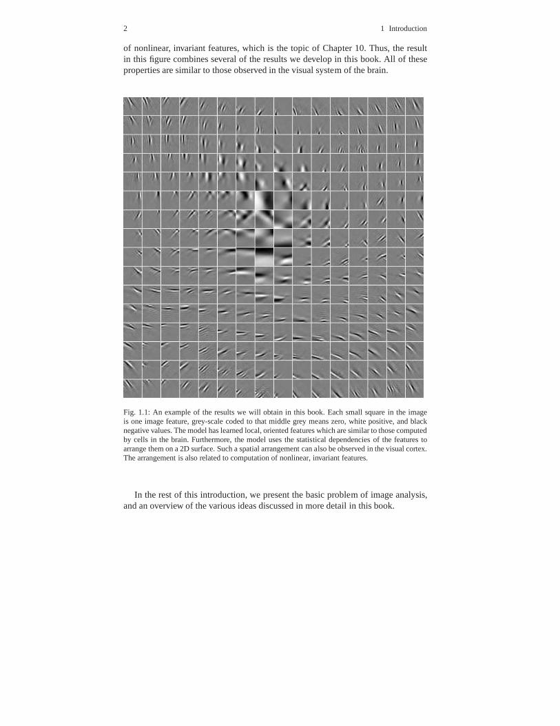
A preview of what kind of properties these models learn is in Figure 1.1. Thefigure shows a number of linear features learned from naturalimages by a statisticalmodel. Chapters 5–7 will already consider models which learn such linear features.In addition to the features themselves, the results in Figure 1.1 show another visu-ally striking phenomenon, which is their spatial arrangement, or topography. Theresults in the figure actually come from a model called Topographic ICA, whichis explained in Chapter 11. The spatial arrangement is also related to computation
1
2 1 Introduction
of nonlinear, invariant features, which is the topic of Chapter 10. Thus, the resultin this figure combines several of the results we develop in this book. All of theseproperties are similar to those observed in the visual system of the brain.
Fig. 1.1: An example of the results we will obtain in this book. Each small square in the imageis one image feature, grey-scale coded to that middle grey means zero, white positive, and blacknegative values. The model has learned local, oriented features which are similar to those computedby cells in the brain. Furthermore, the model uses the statistical dependencies of the features toarrange them on a 2D surface. Such a spatial arrangement can also be observed in the visual cortex.The arrangement is also related to computation of nonlinear, invariant features.
In the rest of this introduction, we present the basic problem of image analysis,and an overview of the various ideas discussed in more detailin this book.

1.3 The magic of your visual system 3
1.2 What is vision?
We can define vision as the process of acquiring knowledge about environmental ob-jects and events by extracting information from the light the objects emit or reflect.The first thing we will need to consider is in what form this information initially isavailable.
The light emitted and reflected by objects has to be collectedand then measuredbefore any information can be extracted from it. Both biological and artificial sys-tems typically perform the first step by projecting light to form a two-dimensionalimage. Although there are, of course, countless differences between the eye and anycamera, the image formation process is essentially the same. From the image, theintensity of the light is then measured in a large number of spatial locations, or sam-pled. In the human eye this is performed by the photoreceptors, whereas artificialsystems employ a variety of technologies. However, all systems share the funda-mental idea of converting the light first into a two-dimensional image and then intosome kind of signal that represents the intensity of the light at each point in theimage.
Although in general the projected images have both temporaland chromatic di-mensions, we will be mostly concerned with static, monochrome (grey-scale) im-ages. Such an image can be defined as a scalar function over twodimensions,I(x,y),giving the intensity (luminance) value at every location(x,y) in the image. Althoughin the general case both quantities (the position(x,y) and the intensityI(x,y)) takecontinuous values, we will focus on the typical case where the image has been sam-pled at discrete points in space. This means that in our discussionx andy take onlyinteger values, and the image can be fully described by an array containing the inten-sity values at each sample point.1 In digital systems, the sampling is typicallyrect-angular, i.e. the points where the intensities are sampled form a rectangular array.Although the spatial sampling performed by biological systems is not rectangularor even regular, the effects of the sampling process are not very different.
It is from this kind of image data that vision extracts information. Informationabout the physical environment is contained in such images,but only implicitly.The visual system must somehow transform this implicit information into an explicitform, for example by recognizing the identities of objects in the environment. This isnot a simple problem, as the demonstration of the next section attempts to illustrate.
1.3 The magic of your visual system
Vision is an exceptionally difficult computational task. Although this is clear tovision scientists, it might come as a surprise to others. Thereason for this is that we
1 When images are stored on computers, the entries in the arrays also have to be discretized; this is,however, of less importance in the discussion that follows,and we will assume that this has beendone at a high enough resolution so that this step can be ignored.

4 1 Introduction
are equipped with a truly amazing visual system that performs the task effortlesslyand quite reliably in our daily environment. We are simply not aware of the wholecomputational process going on in our brains, rather we experience only the resultof that computation.
To illustrate the difficulties in vision, Figure 1.2 displays an image in its numer-ical format (as described in the previous section), where light intensities have beenmeasured and are shown as a function of spatial location. In other words, if youwere to colour each square with the shade of grey corresponding to the containednumber you would see the image in the form we are used to, and itwould be eas-ily interpretable. Without looking at the solution just yet, take a minute and try todecipher what the image portrays. You will probably find thisextremely difficult.
Now, have a look at the solution in Figure 1.4. It is immediately clear what theimage represents! Our visual system performs the task of recognizing the imagecompletely effortlessly. Even though the image at the levelof our photoreceptorsis represented essentially in the format of Figure 1.2, our visual system somehowmanages to make sense of all this data and figure out the real-world object thatcaused the image.
In the discussion thus far, we have made a number of drastic simplifications.Among other things, the human retina contains photoreceptors with varying sensi-tivity to the different wavelengths of light, and we typically view the world throughtwo eyes, not one. Finally, perhaps the most important difference is that we normallyperceive dynamic images rather than static ones. Nonetheless, these differences donot change the fact that the optical information is, at the level of photoreceptors,represented in a format analogous to that we showed in Figure1.2, and that the taskof the visual system is to understand all this data.
Most people would agree that this task initially seems amazingly hard. But after amoment of thought it might seem reasonable to think that perhaps the problem is notso difficult after all? Image intensity edges can be detectedby finding oriented seg-ments where small numbers border with large numbers. The detection of such fea-tures can be computationally formalized and straightforwardly implemented. Per-haps such oriented segments can be grouped together and subsequently object formbe analyzed? Indeed, such computations can be done, and theyform the basis ofmany computer vision algorithms. However, although current computer vision sys-tems work fairly well on synthetic images or on images from highly restricted en-vironments, they still perform quite poorly on images from an unrestricted, naturalenvironment. In fact, perhaps one of the main findings of computer vision researchto date has been that the analysis of real-world images is extremely difficult! Evensuch a basic task as identifying the contours of an object is complicated becauseoften there is no clear image contour along some part of its physical contour, asillustrated in Figure 1.3.
In light of the difficulties computer vision research has runinto, the computa-tional accomplishment of our own visual system seems all themore amazing. Weperceive our environment quite accurately almost all the time, and only relativelyrarely make perceptual mistakes. Quite clearly, biology has solved the task of ev-

1.3 The magic of your visual system 5
0 1 2 3 4 5 6 7 8 9
1 3 3 3 3 3 3 2 2 2 2 2 2 2 2 2 2 1 1 3 3 3 3 2 2 1 1 1 1 1 0 2 4 5 3 3 3 3 3 4 4 2 2 3 4 22 4 5 5 5 5 4 3 3 3 4 3 3 2 3 3 3 2 3 4 6 5 5 3 4 5 5 5 6 5 3 4 3 3 4 4 4 4 4 5 6 5 4 4 5 32 3 4 4 4 4 3 3 4 4 4 4 2 2 3 3 2 3 4 4 5 4 5 6 5 4 4 5 4 3 2 2 2 3 5 5 5 4 4 5 6 6 4 4 4 33 4 4 3 3 3 4 4 4 3 2 3 4 3 3 2 2 3 4 5 3 3 4 3 4 4 3 4 3 2 2 2 3 3 4 3 4 5 4 3 4 5 5 4 5 33 5 5 3 2 3 3 2 2 2 2 2 2 3 3 3 3 4 5 5 4 3 3 3 3 2 2 3 4 6 5 4 4 5 5 4 4 4 4 5 5 5 6 5 5 33 5 4 2 2 2 2 1 1 3 1 2 3 3 4 4 4 3 5 4 3 3 4 3 2 2 3 3 2 3 4 3 3 3 4 5 5 4 3 3 4 5 5 5 5 33 5 4 2 1 1 1 1 2 2 2 3 3 3 4 3 3 4 4 3 3 4 4 3 3 3 4 5 5 4 4 4 3 2 3 3 3 5 3 3 3 5 6 5 4 34 5 4 3 2 1 0 1 2 1 2 3 2 3 3 2 4 4 3 3 5 4 3 3 2 1 2 4 5 4 3 4 3 2 3 4 4 5 5 3 3 3 4 4 3 14 5 3 3 2 1 1 2 3 3 3 2 3 2 2 3 4 4 3 4 5 4 3 2 2 2 3 3 4 5 5 4 4 4 4 4 4 5 5 4 3 4 4 4 3 13 5 4 3 2 2 2 3 4 5 4 3 3 2 3 3 3 4 3 4 5 4 3 4 4 4 3 3 3 4 5 5 4 3 3 3 3 4 5 4 4 4 4 5 4 13 6 4 4 3 4 5 6 6 6 5 5 4 3 3 4 4 3 4 5 5 4 5 5 5 4 3 3 3 3 4 4 4 3 2 2 3 4 5 4 4 4 3 4 4 13 6 6 5 4 5 6 6 7 7 6 5 5 5 4 4 4 5 5 5 5 5 5 5 5 5 4 3 4 4 3 3 3 2 2 2 3 3 3 4 4 4 4 3 4 23 5 6 5 4 6 6 7 7 7 7 6 6 6 5 6 6 6 6 6 6 6 6 5 5 5 5 4 3 3 3 3 4 2 3 2 3 3 3 5 5 5 4 4 3 22 5 6 5 4 6 7 7 7 7 7 7 7 8 8 7 7 7 7 7 7 7 7 6 6 6 5 4 4 3 3 3 4 3 3 3 3 3 3 3 3 3 4 5 4 23 5 6 4 5 7 7 7 7 7 7 8 8 8 8 8 8 8 8 8 7 7 7 6 6 6 5 5 4 4 4 4 3 3 3 3 3 3 2 2 3 3 4 4 5 32 5 5 5 6 7 7 7 7 7 8 8 8 9 8 8 8 8 8 8 8 8 7 7 6 6 6 5 4 4 4 3 2 3 2 3 3 3 3 4 4 4 4 5 5 33 5 5 5 7 7 7 7 8 8 8 9 8 9 9 9 8 8 8 8 8 8 7 7 6 6 6 5 5 5 4 3 3 2 1 2 2 2 3 4 5 4 4 4 5 33 4 4 6 8 7 7 7 8 8 9 8 8 8 9 8 8 8 8 8 8 8 7 7 7 6 6 5 5 5 5 4 4 4 3 2 2 3 3 3 5 5 5 4 5 43 5 5 6 8 7 7 7 8 8 9 9 9 9 8 8 8 8 8 8 8 7 7 6 6 6 6 5 5 5 5 4 4 4 4 3 3 3 4 4 5 6 4 4 5 33 6 5 6 7 7 7 7 8 8 8 9 9 8 8 8 8 8 8 7 7 7 6 6 6 6 6 6 6 6 5 5 5 4 3 3 4 4 4 4 4 3 4 3 3 22 5 5 7 7 7 8 7 8 8 8 8 8 7 7 8 7 7 7 7 7 7 7 6 6 6 6 6 6 6 5 5 5 4 3 3 3 4 5 4 5 5 5 4 4 32 3 5 7 7 7 7 7 7 7 8 7 7 7 7 8 7 7 7 7 7 7 6 6 6 6 6 6 5 5 5 5 5 4 4 3 3 3 4 3 4 5 5 6 6 43 4 6 7 7 7 7 7 7 8 8 8 8 8 7 8 7 7 8 7 7 7 6 6 6 6 6 6 5 5 5 4 5 4 4 3 3 3 5 5 4 4 5 6 6 44 4 6 7 7 7 7 7 7 8 8 8 8 8 8 8 8 8 8 8 8 8 7 7 6 6 6 6 5 5 5 5 4 4 4 4 3 3 3 5 4 4 4 6 6 33 4 6 7 7 6 7 7 8 8 8 8 9 9 8 8 8 8 8 8 8 7 6 5 5 5 5 5 5 4 5 5 5 4 4 4 4 3 3 4 4 3 4 4 2 22 4 6 6 6 6 6 7 7 6 6 7 7 8 8 8 8 8 8 8 7 6 5 5 5 5 5 5 5 5 4 4 4 4 5 5 4 4 3 4 4 4 3 3 1 12 4 6 6 5 6 6 6 6 6 7 7 7 7 8 7 7 7 8 7 6 6 6 6 6 6 6 6 5 5 5 5 5 5 5 5 5 4 4 5 5 5 4 3 2 11 4 6 6 5 6 7 7 8 8 8 8 7 7 7 8 7 7 7 6 5 6 8 7 7 6 6 5 5 5 4 4 5 5 5 5 5 5 4 5 5 4 2 2 2 12 5 6 6 6 7 7 7 8 7 6 7 7 7 7 8 8 7 6 4 3 7 6 4 5 4 2 2 3 4 4 4 4 5 5 5 4 4 4 4 5 2 1 2 2 13 5 6 6 7 6 6 5 4 3 2 2 4 6 7 7 8 7 5 1 2 5 5 5 8 6 2 2 2 1 2 4 4 5 5 4 4 4 4 3 4 3 0 1 2 23 5 6 7 7 6 4 2 5 5 3 3 4 4 6 7 7 7 4 1 3 5 5 5 7 6 5 4 4 3 2 3 4 5 5 4 4 4 3 4 4 4 1 0 2 21 4 6 7 7 6 5 5 5 7 6 5 4 6 7 6 7 6 4 2 2 5 6 6 6 7 7 6 5 5 4 4 5 5 6 5 4 4 3 4 4 4 2 0 3 20 2 6 7 7 6 6 7 7 8 6 5 5 6 6 6 6 6 4 2 2 2 6 7 7 7 7 6 5 4 4 5 6 6 6 5 4 4 3 3 4 3 2 3 4 30 2 6 7 7 7 7 7 7 7 7 7 7 7 6 6 6 6 4 3 3 2 4 7 7 7 6 5 5 5 5 6 6 6 6 5 4 3 3 3 4 3 2 5 5 31 3 6 6 7 7 7 7 7 7 8 7 6 6 6 6 7 6 5 3 3 3 3 5 6 6 6 6 6 6 6 6 6 6 5 4 4 4 3 4 4 3 4 5 5 21 4 5 6 7 7 7 7 7 7 7 6 7 6 6 7 6 6 5 3 3 3 3 4 5 5 5 6 6 6 6 6 6 6 5 4 4 4 3 3 4 2 3 4 4 10 2 5 6 7 7 7 7 7 6 6 6 7 7 7 6 6 6 5 4 3 3 3 4 5 6 6 6 6 6 6 6 6 5 5 4 4 4 3 3 4 3 3 4 2 20 1 3 6 6 7 7 7 7 7 7 7 7 7 6 6 6 6 5 4 3 2 3 5 6 7 7 6 6 5 5 6 6 5 5 4 3 4 4 4 4 3 3 1 1 20 1 2 6 6 6 6 7 7 8 8 8 8 7 6 6 7 6 5 5 4 3 2 4 6 7 7 7 6 6 5 5 5 5 4 4 3 3 4 4 3 2 2 0 1 20 0 1 6 6 6 7 7 8 8 8 7 7 7 6 8 8 7 5 4 4 3 3 2 5 7 7 7 6 6 5 5 5 4 4 4 3 3 3 4 3 0 2 1 1 20 1 1 5 6 6 6 7 8 8 8 7 7 6 6 8 8 7 5 4 3 3 3 2 5 7 7 7 6 6 6 5 4 4 4 4 3 3 3 3 4 2 3 1 2 20 1 1 5 6 6 6 7 7 8 7 7 8 6 5 6 6 6 5 3 2 1 2 2 4 6 7 7 6 6 5 5 4 4 4 4 3 3 3 3 4 4 3 0 2 20 1 0 4 6 6 7 7 7 7 7 8 7 6 5 5 5 5 4 1 1 2 3 3 4 5 7 7 6 6 5 5 5 4 4 3 3 3 3 3 4 4 3 1 2 30 1 1 3 6 6 7 7 7 7 8 7 7 6 6 6 6 6 5 4 3 3 4 4 4 5 6 7 6 6 6 6 5 5 4 3 3 3 3 3 4 4 3 1 2 30 2 4 5 6 7 7 7 7 7 7 7 6 6 6 6 8 7 7 7 6 4 5 4 4 5 7 6 6 6 6 6 5 5 4 3 3 3 3 3 4 3 3 1 2 31 5 8 7 6 7 7 7 7 7 7 7 7 6 6 6 7 7 8 7 5 5 4 4 4 4 7 6 5 6 6 6 5 5 4 3 3 3 3 3 4 1 1 1 2 32 6 9 8 6 6 7 7 7 7 7 7 5 4 4 5 5 5 5 5 5 3 4 3 2 1 6 7 5 6 6 6 5 4 4 3 3 3 3 3 4 1 0 0 2 21 5 8 7 4 6 7 7 7 7 7 6 4 2 2 7 9 9 9 9 9 6 4 2 1 4 6 7 6 7 6 6 5 4 3 3 3 2 3 3 4 2 0 0 2 30 2 4 4 2 5 6 7 7 7 7 6 6 6 3 4 5 6 6 5 6 2 1 2 4 5 6 6 7 7 6 5 5 4 3 3 2 2 2 3 4 5 0 0 0 20 1 2 1 1 3 6 7 7 7 7 7 7 7 6 5 4 3 3 3 3 4 4 4 4 5 6 6 7 6 5 5 5 4 3 2 2 2 2 3 4 8 1 0 0 00 1 1 0 1 2 4 6 7 7 7 7 7 7 6 6 6 7 6 6 6 5 5 4 5 6 6 6 6 5 5 5 4 3 2 2 2 2 2 2 5 9 2 0 0 00 1 0 0 1 2 2 5 6 7 6 7 7 7 7 6 7 7 7 7 6 5 5 5 5 6 6 6 6 5 5 5 4 3 2 1 1 1 2 2 6 9 2 0 0 00 1 1 0 1 2 2 3 5 6 6 7 7 7 7 7 7 7 7 7 6 6 5 5 6 6 5 6 5 4 4 4 3 2 1 1 1 1 2 2 7 9 2 0 0 00 1 0 0 1 2 2 1 3 6 6 7 7 7 7 7 8 8 7 7 7 6 6 6 6 6 5 5 4 3 4 4 2 1 1 1 1 1 2 3 8 7 1 0 0 00 1 0 0 1 2 2 2 2 4 6 7 7 7 8 8 8 7 7 7 6 6 6 6 6 6 5 5 4 3 3 2 1 1 1 1 1 1 1 6 9 6 0 0 0 00 0 0 0 1 2 2 1 2 3 4 6 7 7 7 7 7 7 7 7 6 5 6 6 6 5 5 4 3 2 2 1 1 1 1 1 1 1 2 8 8 3 0 0 0 00 1 0 1 2 3 2 1 1 1 1 4 7 7 6 6 6 7 7 6 6 5 5 5 6 5 4 3 2 2 2 1 1 2 2 1 1 1 6 8 7 1 0 0 0 00 1 1 2 5 4 2 1 0 0 0 0 4 6 6 6 7 7 7 7 6 5 5 5 5 4 3 3 2 1 1 1 2 2 2 2 1 4 8 8 5 0 0 0 0 00 1 3 5 6 3 1 0 0 0 0 0 1 5 6 7 7 7 7 7 7 6 5 5 4 3 2 2 1 2 2 2 2 2 2 1 3 7 8 7 2 0 0 0 0 01 3 4 2 1 0 0 0 0 0 0 0 0 3 6 6 7 7 7 7 6 6 5 5 4 2 2 2 2 3 3 3 2 2 1 3 8 8 8 5 0 0 0 0 0 01 1 0 0 0 0 0 0 0 0 0 0 0 2 4 3 4 4 4 4 4 3 3 2 2 1 2 2 2 2 2 2 2 1 1 5 5 5 5 1 0 0 0 0 0 0
Fig. 1.2: An image displayed in numerical format. The shade of grey of each square has beenreplaced by the corresponding numerical intensity value. What does this mystery image depict?

6 1 Introduction
Fig. 1.3: This image of a cup demonstrates that physical contours and image contours are often verydifferent. The physical edge of the cup near the lower-left corner of the image yields practically noimage contour (as shown by the magnification). On the other hand, the shadow casts a clear imagecontour where there in fact is no physical edge.
eryday vision in a way that is completely superior to any present-day machine visionsystem.
This being the case, it is natural that computer vision scientists have tried to drawinspiration from biology. Many systems contain image processing steps that mimicthe processing that is known to occur in the early parts of thebiological visualsystem. However, beyond the very early stages, little is actually known about therepresentations used in the brain. Thus, there is actually not much to guide computervision research at the present.
On the other hand, it is quite clear that good computational theories of visionwould be useful in guiding research on biological vision, byallowing hypothesis-driven experiments. So it seems that there is a dilemma: computational theory isneeded to guide experimental research, and the results of experiments are neededto guide theoretical investigations. The solution, as we see it, is to seek synergy bymultidisciplinary research into the computational basis of vision.
1.4 Importance of prior information
1.4.1 Ecological adaptation provides prior information
A very promising approach for solving the difficult problemsin vision is based onadaptation to the statistics of the input. An adaptive representation is one that doesnot attempt to represent all possible kinds of data; instead, the representation isadapted to a particular kind of data. The advantage is that then the representationcan concentrate on those aspects of the data that are useful for further analysis. Thisis in stark contrast to classic representations (e.g. Fourier analysis) that are fixedbased on some general theoretical criteria, and completelyignore what kind of datais being analyzed.

1.4 Importance of prior information 7
Fig. 1.4: The image of Figure 1.2. It is immediately clear that the image shows a male face. Manyobservers will probably even recognize the specific individual (note that it might help to view theimage from relatively far away).

8 1 Introduction
Thus, the visual system is not viewed as a general signal processing machine ora general problem-solving system. Instead, it is acknowledged that it has evolved tosolve some very particular problems that form a small subsetof all possible prob-lems. For example, the biological visual system needs to recognize faces under dif-ferent lighting environments, while the people are speaking, possibly with differ-ent emotional expressions superimposed; this is definitelyan extremely demandingproblem. But on the other hand, the visual system doesnotneed to recognize a facewhen it is given in an unconventional format, as in Figure 1.2.
What distinguished these two representations (numbers vs.a photographic im-age) from each other is that the latter isecologically valid, i.e. during the evolutionof the human species, our ancestors have encountered this problem many times,and it has been important for their survival. The case of an array of numbers doesdefinitely not have any of these two characteristics. Most people would label it as“artificial”.
In vision research, more and more emphasis is being laid on the importance ofthe enormous amount of prior information that the brain has about the structure ofthe world. A formalization of these concepts has recently been pursued under theheading “Bayesian perception”, although the principle goes back to the “maximumlikelihood principle” by Helmholtz in the 19th century. Bayesian inference is thenatural theory to use when inexact and incomplete information is combined withprior information. Such prior information should presumably be reflected in thewhole visual system.
Similar ideas are becoming dominant in computer vision as well. Computer vi-sion systems have been used on many different kinds of images: “ordinary” (i.e.optical) images, satellite images, magnetic resonance images, to name a few. Is itrealistic to assume that the same kind of processing would adequately represent allthese different kinds of data? Could better results be obtained if one uses methods(e.g. features) that are specific to a given application?
1.4.2 Generative models and latent quantities
The traditional computational approach to vision focuses on how, from the imagedataI , one can compute quantities of interest calledsi , which we group togetherin a vectors. These quantities might be, for instance, scalar variablessuch as thedistances to objects, or binary parameters such as signifying if an object belongs tosome given categories. In other words, the emphasis is on a function f that trans-forms images into world or object information, as ins= f(I). This operation mightbe called imageanalysis.
Several researchers have pointed out that the opposite operation, imagesynthesis,often is simpler. That is, the mappingg that generates the image given the state ofthe world
I = g(s), (1.1)

1.4 Importance of prior information 9
is considerably easier to work with, and more intuitive, than the mappingf. Thisoperation is often calledsynthesis. Moreover, the framework based on a fixed ana-lyzing functionf does not give much room for using prior information. Perhaps, byintelligently choosing the functionf, some prior information on the data could beincorporated.
Generative models use Eq. (1.1) as a starting point. They attempt to explain ob-served data by some underlying hidden (latent) causes or factorssi about which wehave only indirect information.
The key point is that the models incorporate a set ofprior probabilities for thelatent variables si . That is, it is specified how often different combinations oflatentvariables occur together. For example, this probability distribution could describe,in the case of a cup, thetypical shape of a cup. Thus, this probability distributionfor the latent variables is what formalizes the prior information on the structure ofthe world.
This framework is sufficiently flexible to be able to accommodate many differentkinds of prior information. It all depends on how we defined the latent variables,and the synthesis functiong.
But how does knowingg help us, one may ask. The answer is that one maythen search for the parameterss that produce an imageI = g(s) which, as well aspossible, matches the observed imageI . In other words, a combination of latentvariables that is the “most likely”. Under reasonable assumptions, this might lead toa good approximation of the correct parameterss.
To make all this concrete, consider again the image of the cupin Figure 1.3.The traditional approach of vision would propose that an early stage extracts localedge information in the image, after which some sort of grouping of these edgepieces would be done. Finally, the evoked edge pattern wouldbe compared withpatterns in memory, and recognized as a cup. Meanwhile, analysis of other scenevariables, such as lighting direction or scene depth, wouldproceed in parallel. Theanalysis-by-synthesis framework, on the other hand, wouldsuggest that our visualsystem has an unconscious internal model for image generation. Estimates of objectidentity, lighting direction, and scene depth are all adjusted until a satisfactory matchbetween the observed image and the internally generated image is achieved.
1.4.3 Projection onto the retina loses information
One very important reason why it is natural to formulate vision as inference oflatent quantities is that the world is three dimensional whereas the retina is onlytwo-dimensional. Thus, the whole 3D structure of the world is seemingly lost in theeye! Our visual system is so good in reconstructing a three-dimensional perceptionof the world that we hardly realize that a complicated reconstruction procedure isnecessary. Information about the depth of objects and the space between is onlyimplicit in the retinal image.

10 1 Introduction
We do benefit from having two eyes which give slightly different views of theoutside world. This helps a bit in solving the problem of depth perception, but itis only part of the story. Even if you close one eye, you can still understand whichobject is in front of another. Television is also based on theprinciple that we canquite well reconstruct the 3D structure of the world from a 2Dimage, especially ifthe camera (or the observer) is moving.
1.4.4 Bayesian inference and priors
The fundamental formalism for modelling how prior information can be used inthe visual system is based on what is called Bayesian inference. Bayesian inferencerefers to statistically estimating the hidden variabless given an observed imageI .In most models it is impossible (even in theory) to know the precise values ofs,so one must be content with a probability densityp(s|I). This is the probability ofthe latent variablesgiventhe observed image. By Bayes’ rule, which is explained inSection 4.7, this can be calculated as
p(s|I) =p(I |s)p(s)
p(I). (1.2)
To obtain an estimate of the hidden variables, many models simply find the particu-lar swhich maximize this density,
s= argmaxs
p(s|I). (1.3)
Ecological adaptation is now possible by learning the priorprobability distri-bution from a large number of natural images. Learning refers, in general, to theprocess of constructing a representation of the regularities of data. The dominanttheoretical approach to learning in neuroscience and computer science is the prob-abilistic approach, in which learning is accomplished by statistical estimation: thedata is described by a statistical model that contains a number of parameters, andlearning consists of finding “good” values for those parameters, based on the inputdata. In statistical terminology, the input data is a samplethat contains observations.
The advantage of formulating adaptation in terms of statistical estimation is verymuch due to the existence of an extensive theory of statistical theory and inference.Once the statistical model is formulated, the theory of statistical estimation imme-diately offers a number of tools to estimate the parameters.And after estimation ofthe parameters, the model can be used in inference accordingto the Bayesian theory,which again offers a number of well-studied tools that can bereadily used.

1.5 Natural images 11
1.5 Natural images
1.5.1 The image space
How can we apply the concept of prior information about the environment in earlyvision? “Early” vision refers to the initial parts of visualprocessing, which are usu-ally formalized as the computation of features, i.e. some relatively simple functionsof the image (features will be defined in Section 1.8 below). Early vision does notyet accomplish such tasks as object recognition. In this book, we consider earlyvision only.
The central concept we need here is the image space. Earlier we described animage representation in which each image is represented as anumerical array con-taining the intensity values of its picture elements, orpixels. To make the followingdiscussion concrete, say that we are dealing with images of afixed size of 256-by-256 pixels. This gives a total of 65536= 2562 pixels in an image. Each image canthen be considered as a point in a 65536-dimensionalspace, each axis of which spec-ifies the intensity value of one pixel. Conversely, each point in the space specifiesone particular image. This space is illustrated in Figure 1.5.
Image space
I(2,1)
I(1,1)
I(1,2)
1
I(x,y)
Image pixels
2
2
4
1 4
Fig. 1.5: The space representation of images. Images are mapped to points in the space in a one-to-one fashion. Each axis of the image space corresponds to the brightness value of one specific pixelin the image.
Next, consider taking an enormous set of images, and plotting each as the corre-sponding point in our image space. (Of course, plotting a 65536-dimensional spaceis not very easy to do on a two-dimensional page, so we will have to be content withmaking a thought experiment.) An important question is: howwould the points bedistributed in this space? In other words, what is the probability density function of

12 1 Introduction
our images like? The answer, of course, depends on the set of images chosen. Astro-nomical images have very different properties from holidaysnapshots, for example,and the two sets would yield very different clouds of points in our space.
It is this probability density function of the image set in question that we willmodel in this book.
1.5.2 Definition of natural images
In this book we will be specifically concerned with a particular set of images callednatural imagesor images ofnatural scenes. Some images from our data set areshown in Figure 1.6. This set is supposed to resemble the natural input of the visualsystem we are investigating. So what is meant by “natural input”? This is actuallynot a trivial question at all. The underlying assumption in this line of research isthat biological visual systems are, through a complex combination of the effectsof evolution and development, adapted to process the kind ofsensory input thatthey receive. Natural images is thus some set that we believehas similar statisticalstructure to that which the visual system is adapted to.
Fig. 1.6: Three representative examples from our set of natural images.
This poses an obvious problem, at least in the case of human vision. The humanvisual system has evolved in an environment that is in many ways different fromthe one most of us experience daily today. It is probably quite safe to say that im-ages of skyscrapers, cars, and other modern entities have not affected our geneticmakeup to any significant degree. On the other hand, few people today experiencenature as omnipresent as it was tens of thousands of years ago. Thus, the input onthe time-scale of evolution has been somewhat different from that on the time-scaleof the individual. Should we then choose images of nature or images from a modern,urban environment to model the “natural input” of our visualsystem? Most workto date has focused on the former, and this is also our choice in this book. Fortu-nately, this choice of image set does not have a drastic influence on the results ofthe analysis: Most image sets collected for the purpose of analysing natural imagesgive quite similar results in statistical modelling, and these results are usually com-

1.6 Redundancy and information 13
pletely different from what you would get using most artificial, randomly generateddata sets.
Returning to our original question, how wouldnatural imagesbe distributed inthe image space? The important thing to note is that they would not be anything likeuniformly distributed in this space. It is easy for us to drawimages from a uniformdistribution, and they do not look anything like our naturalimages! Figure 1.7 showsthree images randomly drawn from a uniform distribution over the image space. Asthere is no question that we can easily distinguish these images from natural images(Figure 1.6) it follows that these are drawn from separate, very different, distribu-tions. In fact, the distribution of natural images is highlynon-uniform. This is thesame as saying that natural images contain a lot ofredundancy, an information-theoretic term that we turn to now.
Fig. 1.7: Three images drawn randomly from a uniform distribution in the image space. Each pixelis drawn independently from a uniform distribution from black to white.
1.6 Redundancy and information
1.6.1 Information theory and image coding
At this point, we make a short excursion to a subject that may seem, at first sight, tobe outside of the scope of statistical modelling: information theory.
The development of the theory of information by Claude Shannon and others isone of the milestones of science. Shannon considered the transmission of a messageacross a communication channel and developed a mathematical theory that quan-tified the variables involved (these will be presented in Chapter 8). Because of itsgenerality the theory has found, and continues to find, a growing number of appli-cations in a variety of disciplines.
One of the key ideas in information theory is that the amount of memory neededto store an image is often less than what is needed in a trivialrepresentation (code),where each pixel is stored using a fixed number of bits, such as8 or 24. This isbecause some of the memory capacity is essentially consumedby redundant struc-ture in the image. The more rigid the structure, the less bits is really needed to code

14 1 Introduction
the image. Thus, the contents of any image, indeed any signal, can essentially bedivided into information and redundancy. This is depicted in Figure 1.8.
Memory bits in trivial code
Bits needed
Information
for an efficient code
Redundancy
Fig. 1.8: Redundancy in a signal. Some of the memory consumedby the storage of a typical imageis normally unnecessary because of redundancy (structure)in the image. If the signal is optimallycompressed, stripping it of all redundancy, it can be storedusing much less bits.
To make this more concrete, consider the binary image of Figure 1.9. The imagecontains a total of 32×22= 704 pixels. Thus, the trivial representation (where thecolour of each pixel is indicated by a ‘1’ or a ‘0’) for this image requires 704 bits.But it is not difficult to imagine that one could compress it into a much smallernumber of bits. For example, one could invent a representation that assumes a whitebackground on which black squares (with given positions andsizes) are printed.In such a representation, our image could be coded by simply specifying the top-left corners of the squares ((5,5) and (19,11)) and their sizes (8 and 6). This couldcertainly be coded in less than 704 bits.2
The important thing to understand is that this kind of representation is good forcertain kinds of images (those with a small number of black squares) but not oth-ers (that do not have this structure and thus require a huge amount of squares to becompletely represented). Hence, if we are dealing mostly with images of the formerkind, and we are using the standard binary coding format, then our representation ishighly redundant. By compressing it using our black-squares-on-white representa-tion we achieve an efficient representation. Although natural images are much morevariable than this hypothetical class of images, it is nonetheless true that they alsoshow structure and can be compressed.
Attneave was the first to explicitly point out the redundancyin images in 1954.The above argument is essentially the same as originally given by Attneave, al-though he considered a ‘guessing game’ in which subjects guessed the colour ofpixels in the image. The fact that subjects perform much better than chance provesthat the image is predictable, and information theory ensures that predictability isessentially the same thing as redundancy.
Making use of this redundancy of images is essential for vision. But the samestatistical structure is in fact also crucial for many othertasks involving images.
2 The specification of each square requires three numbers which each could be coded in 5 bits,giving a total of 30 bits for two squares. Additionally, a fewbits might be needed to indicate howmany squares are coded, assuming that we do not knowa priori that there are exactly two squares.

1.6 Redundancy and information 15
Fig. 1.9: A binary image containing a lot of structure. Images like this can be coded efficiently; seemain text for discussion.
Engineers who seek to find compact digital image formats for storing or transmittingimages also need to understand this structure. Image synthesis and noise reductionare other tasks that optimally would make use of this structure. Thus, the analysisof the statistical properties of images has widespread applications indeed, althoughperhaps understanding vision is the most profound.
1.6.2 Redundancy reduction and neural coding
Following its conception, it did not take long before psychologists and biologistsunderstood that information theory was directly relevant to the tasks of biologicalsystems. Indeed, the sensory input is a signal that carriesinformation about theoutside world. This information iscommunicatedby sensory neurons by means ofaction potentials.
In Attneave’s original article describing the redundancy inherent in images, At-tneave suggested that the visual system recodes the inputs to reduce redundancy,providing an ‘economical description’ of the sensory signals. He likened the taskof the visual system to that of an engineer who seeks to represent pictures with thesmallest possible number of bits. It is easy to see the intuitive appeal of this idea.Consider again the image of Figure 1.9. Recoding images of this kind using ourblack-squares-on-white representation, we reduce redundancy and obtain an effi-cient representation. However, at the same time we havediscovered the structureinthe signal: we now have the concept of ‘squares’ which did notexist in the origi-nal representation. More generally: to reduce redundancy one must first identify it.Thus, redundancy reductionrequiresdiscovering structure.

16 1 Introduction
Although he was arguably the first to spell it out explicitly,Attneave was certainlynot the only one to have this idea. Around the same time, Barlow, in 1961, providedsimilar arguments from a more biological/physiological viewpoint. Barlow has alsopointed out that the idea, in the form of ‘economy of thought’, is clearly expressedalready in the writings of Mach and Pearson in the 19th century. Nevertheless, withthe writings of Attneave and Barlow, the redundancy reduction (or efficient coding)hypothesis was born.
1.7 Statistical modelling of the visual system
1.7.1 Connecting information theory and Bayesian inference
Earlier we emphasized the importance of prior information and Bayesian modelling,but in the preceding section we talked about information theory and coding. Thismay seem a bit confusing at first sight, but the reason is that the two approaches arevery closely related.
Information theory wants to find an economical representation of the data forefficient compression, while Bayesian modelling uses priorinformation on the datafor such purposes as denoising and recovery of the 3D structure. To accomplish theirgoals, both of these methods fundamentally need the same thing: a good model ofthe statistical distribution of the data. That is the basic motivation for this book. Itleads to a new approach to normative visual modelling as willbe discussed next.
1.7.2 Normative vs. descriptive modelling of visual system
In visual neuroscience, the classic theories of receptive field structure3 can be calleddescriptivein the sense that they give us mathematical tools (such as Fourier andGabor analysis, see Chapter 2) that allow us to describe parts of the visual systemin terms of a small number of parameters.
However, the question we really want to answer is:Why is the visual systembuilt the way neuroscientific measurements show? The basic approach to answersuch a question in neuroscience is to assume that the system in question has beenoptimizedby evolution to perform a certain function. (This does not mean that thesystem would be completely determined genetically, because evolution can just havedesigned mechanisms for self-organization and learning that enable the system tofind the optimal form.)
Models based on the assumption of optimality are often called normativebecausethey tell how the systemshouldbehave. Of course, there is no justification to assume
3 i.e., the way visual neurons respond to stimulation, see Section 3.3

1.7 Statistical modelling of the visual system 17
that evolution has optimized all parts of the organism; mostof them may be far fromthe optimum, and such an optimum may not even be a well-definedconcept.
However, in certain cases it can be demonstrated that the system is not far fromoptimal in certain respects. This happens to be the case withthe early cortical visualprocessing system (in particular, the primary visual cortex, see Chapter 3 for a briefdescription of the visual system). That brain area seems to function largely basedon principles of statistical modelling, as will be seen in this book. Thus, there isconvincing proof that parts of the system are optimal for statistical inference, and itis this proof that justifies these normative models.
Previous models of the early visual system did not provide satisfactory norma-tive models, they only provided practical descriptive models. Although there weresome attempts to develop a normative theory, the predictions were too vague.4 Thestatistical approach is the first one to give exact quantitative models of visual pro-cessing, and these have been found to provide a good match with neuroscientificmeasurements.
1.7.3 Towards predictive theoretical neuroscience
Let us mention one more important application of this framework: a mode of mod-elling where we are able to predict the properties of visual processing beyond theprimary visual cortex. Then, we obtain quantitative predictions on what kinds ofvisual processing should take place in areas whose functionis not well understoodat this point.
Almost all the experimental results in early visual processing have concernedthe primary visual cortex, or even earlier areas such as the retina. Likewise, mostresearch in this new framework of modelling natural image statistics has been onvery low-level features. However, the methodology of statistical modelling can mostprobably be extended to many other areas.
Formulating statistical generative models holds great promise as a frameworkthat will give new testable theories for visual neuroscience, for the following rea-sons:
• This framework is highly constructive. From just a couple ofsimple theoreticalspecifications, natural images lead to the emergence of complex phenomena, e.g.the forms of the receptive fields of simple cells and their spatial organization inFig. 1.1.
• This framework is, therefore, less subjective than many other modelling ap-proaches. The rigorous theory of statistical estimation makes it rather difficultto insert the theorist’s subjective expectations in the model, and therefore the
4 The main theory attempting to do this is the joint space-frequency localization theory leading toGabor models, see Section 2.4.2. However, this does not provide predictions on how the parametersin Gabor models should be chosen, and what’s more serious, itis not really clear why the featuresshould be jointly localized in space and frequency in the first place.

18 1 Introduction
results are strongly determined by the data, i.e. the objective reality. Thus, theframework can be called data-driven.
• In fact, in statistical generative models we often see emergence of new kinds offeature detectors — sometimes very different from what was expected when themodel was formulated.
So far, experiments in vision research have been based on rather vague, qualita-tive predictions. (This is even more true for other domains of neuroscience.) How-ever, using the methodology described here, visual neuroscience has the potential ofstarting a new mode of operation where theoretical developments directly give newquantitativehypotheses to be falsified or confirmed in experimental research. Be-coming theory-driven would be a real revolution in the way neuroscience is done. Infact, this same development is what gave much of the driving force to exact naturalsciences in the 19th and 20th centuries.
1.8 Features and statistical models of natural images
1.8.1 Image representations and features
Most statistical models of natural images are based on computing features. The word“feature” is used rather loosely for any function of the image which is to be used infurther visual processing. The same word can be used for the output (value) of thefunction, or the computational operation of which computesthat value.
A classic approach to represent an image is a linear weightedsum of features.Let us denote each feature byAi(x,y), i = 1, . . . ,n. These features are assumed tobe fixed. For each incoming image, the coefficients of each feature in an image aredenoted bysi . Algebraically, we can write:
I(x,y) =n
∑i=1
Ai(x,y)si (1.4)
If we assume for simplicity that the number of featuresn equals the number ofpixels, the system in Eq. (1.4) can be inverted. This means that for a given imageI ,we can find the coefficientssi that fulfill this equation. In fact, they can be computedlinearly as
si = ∑x,y
Wi(x,y)I(x,y) (1.5)
for certain inverse weightsW. The terminology is not very fixed here, so eitherAi ,Wi , or si can be called a “feature”. TheWi can also be called afeature detector.
There are many different sets of features that can be used. Classic choices includeFourier functions (gratings), wavelets, Gabor functions,features of discrete cosinetransform, and many more. What all these sets have in common is that they attemptto represent all possible images, not just natural images, in a way which is “optimal”.

1.8 Features and statistical models of natural images 19
What we want to do is tolearn these features so that they are adapted to theproperties ofnatural images. We do not believe that there could be a single set offeatures which would be optimal for all kinds of images. Also, we want to use thefeatures to build a statistical model of natural images. Thebasis for both of these isto consider the statistics of the featuressi .
1.8.2 Statistics of features
The most fundamental statistical properties of images are captured by the his-tograms of the outputssi of linear feature detectors. Let us denote the output ofa single linear feature detector with weightsW(x,y) by s:
s= ∑x,y
W(x,y)I(x,y) (1.6)
Now, the point is to look at the statistics of the output when the input of the detectorconsists of a large number of natural image patches. Naturalimage patches meanssmall subimages (windows) taken in random locations in randomly selected naturalimages. Thus, the features is a random variable, and for each input patch we geta realization (observation) of that random variable. (Thisprocedure is explained inmore detail in Section 4.1).
Now we shall illustrate this with real natural image data. Let us consider a coupleof simple feature detectors and the histograms of their output when the input consistsof natural images. In Fig. 1.10 we show three simple feature detectors. The first is aDirac detector, which means that all the weightsW(x,y) are zero except for one. Thesecond is a simple one-dimensional grating. The third is a basic Gabor edge detector.All three feature detectors have been normalized to unit norm, i.e.∑x,yW(x,y)2 = 1.
The statistics of the output are contained in the histogram of the outputs. InFig. 1.11, we show the output histograms for the three different kinds of linear detec-tors. We can see that the histograms are rather different. Inaddition to the differentshapes, note that their variances are also quite different from each other.
Thus, we see that different feature detectors are characterized by different statis-tics of their outputs for natural image input. This basic observation is the basis forthe theory in this book. We canlearn featuresfrom image data by optimizing somestatistical properties of the featuressi .
1.8.3 From features to statistical models
The Bayesian goal of building a statistical (prior) model ofthe data, and learningfeatures based on their output statistics are intimately related. This is because themost practical way of building a statistical model proceedsby using features andbuilding a statistical model for them. The point is that the statistical model for fea-

20 1 Introduction
a) b) c)
Fig. 1.10: Three basic filters.a) a Dirac feature, i.e. only one pixel is non-zero.b) a sinusoidalgrating.c) Gabor edge detector.
a)
−5 0 50
1000
2000
3000
4000
5000 b)
−40 −20 0 20 400
2000
4000
6000
8000 c)
−10 −5 0 5 100
2000
4000
6000
8000
10000
Fig. 1.11: The histograms of the outputs of the filters in Fig.1.10 when the input is natural imageswith mean pixel value subtracted.a) output of Dirac filter, which is the same as the histogram ofthe original pixels themselves.b) output of grating feature detector.c) output of edge detector.Note that the scales of both axes are different in the three plots.
tures can be much simpler than the corresponding model for the pixels, so it makessense to first transform the data into a feature space.
In fact, a large class of model buildsindependentmodels for each of the featuressi in Equation (1.5). Independence is here to be taken both in anintuitive sense,and in the technical sense of statistical independence. Most models in Part II of thisbook are based on this idea. Even if the features are not modelled independently, theinteractions (dependencies) of the features are usually much simpler than those ofthe original pixels; such models are considered in Part III of this book.
Thus, we will describe most of the models in this book based onthe principleof learning features. Another reason for using this approach is that the most inter-esting neurophysiological results concern usually the form of the features obtained.In fact, it is very difficult to interpret or visualize a probability distribution givenby the model; comparing the distribution with neurophysiological measurements isnext to impossible. It is the features which give a simple andintuitive idea of whatkind of visual processing these normative models dictate, and they allow a directcomparison with measured properties (receptive fields) of the visual cortex.

1.10 References 21
1.9 The statistical-ecological approach recapitulated
This chapter started with describing the difficulty of vision, and ended up proposingone particular solution, which can be called the statistical-ecological approach. Thetwo basic ingredients in this approach are
• Ecology: The visual system is only interested in propertiesthat are importantin a real environment. This is related to the concept ofsituatednessin cognitivesciences.
• Statistics: Natural images have regularities. The regularities in the ecologicallyvalid environment could be modelled by different formal frameworks, but statis-tical modelling seems to be the one that is most relevant.
Thus, we take the following approach to visual modelling:
1. Different sets of features are good for different kinds ofdata.2. The images that our eyes receive have certain statisticalproperties (regularities).3. The visual system has learned a model of these statisticalproperties.4. The model of the statistical properties enables (close to) optimal statistical infer-
ence.5. The model of the statistical properties is reflected in themeasurable properties of
the visual system (e.g. receptive fields of the neurons)
Most of this book will be concerned on developing different kinds of statisticalmodels for natural images. These statistical models are based on very few theoreticalassumptions, while they give rise to detailed quantitativepredictions. We will showhow these normative models are useful in two respects:
1. They provide predictions that are largely validated by classic neuroscientificmeasurements. Thus, they provide concise and theoretically well-justified ex-planations of well-known measurements. This is the evidence that justifies ournormative modelling.
2. Moreover, the models lead to new predictions of phenomenawhich have not yetbeen observed, thus enabling theory-driven neuroscience.This is the big promiseof natural image statistics modelling.
Another application of these models is in computer science and engineering.Such applications will not be considered in detail in this book: We hope we willhave convinced the reader of the wide applicability of such methods. See below forreferences on this topic.
1.10 References
For textbook accounts of computer vision methods, such as edge detection algo-rithms, see, e.g. (Marr, 1982; Sonka et al, 1998; Gonzales and Woods, 2002); forinformation theory, see (Cover and Thomas, 2006). The approach of generative

22 1 Introduction
models is presented in, e.g. (Grenander, 1976–1981; Kersten and Schrater, 2002;Mumford, 1994; Hinton and Ghahramani, 1997).
For short reviews on using natural image statistics for visual modelling, see(Field, 1999; Simoncelli and Olshausen, 2001; Olshausen, 2003; Olshausen andField, 2004; Hyvarinen et al, 2005b). For reviews on engineering applications ofstatistical models, see (Simoncelli, 2005).
Historical references include (Mach, 1886; Pearson, 1892;Helmholtz, 1867;Shannon, 1948; Attneave, 1954; Barlow, 1961). See also (Barlow, 2001a,b) on adiscussion on the history of redundancy reduction.

Part IBackground


Chapter 2Linear filters and frequency analysis
This chapter reviews some classical image analysis tools: linear filtering, linearbases, frequency analysis, and space-frequency analysis.Some of the basic ideasare illustrated in Figure 2.1. These basic methods need to beunderstood before theresults of statistical image models can be fully appreciated. The idea of processingof different frequencies is central in the reviewed tools. Therefore, a great deal of thefollowing material is devoted to explaining what afrequency-based representationof images is, and why it is relevant in image analysis.
2.1 Linear filtering
2.1.1 Definition
Linear filtering is a fundamental image-processing method in which afilter is ap-plied to an input image to produce an output image.
Figure 2.2 illustrates the way in which the filter and the input image interact toform an output image: the filter is centered at each image location (x,y), and thepixel value of the output imageO(x,y) is given by the linear correlation of the filterand the filter-size subarea of the image at coordinate(x,y). (Note that the word“correlation” is used here in a slightly different way than in the statistical context.)LettingW(x,y) denote a filter with size(2K+1)×(2K +1), I(x,y) the input image,andO(x,y) the output image, linear filtering is given by
O(x,y) =K
∑x∗=−K
K
∑y∗=−K
W(x∗,y∗)I(x+x∗,y+y∗). (2.1)
An example of linear filtering is shown in Figure 2.3.What Equation (2.1) means is that we “slide” the filter over the whole image and
compute a weighted sum of the image pixel values, separatelyat each pixel location.
25

26 2 Linear filters and frequency analysis
a)
b) c)
d) e)
Fig. 2.1: The two classical image analysis tools reviewed inthis chapter are linear filtering b)-c) andspace-frequency analysis d)-e).a) An input image.b) An example output of linear filtering of a); inthis case, the filter has retained medium-scaled vertical structures in the image. A more completedescription of what a linear filtering operation does is provided by the frequency representation(Section 2.2).c) An example of how the outputs of several linear filters can be combined in imageanalysis. In this case, the outputs of four filters have been processed nonlinearly and added togetherto form an edge image: in the image, lighter areas correspondto image locations with a luminanceedge. This kind of a result could be used, for example, as a starting point to locate objects of acertain shape.d)–e) An example of space-frequency analysis, where the main ideais to analyzethe magnitude of a frequency d) at different locations. The end result e) reflects the magnitude ofthis frequency at different points in the input image a). From the point of view of image analysis,this result suggests that the upper part of the image is of different texture than the lower part.
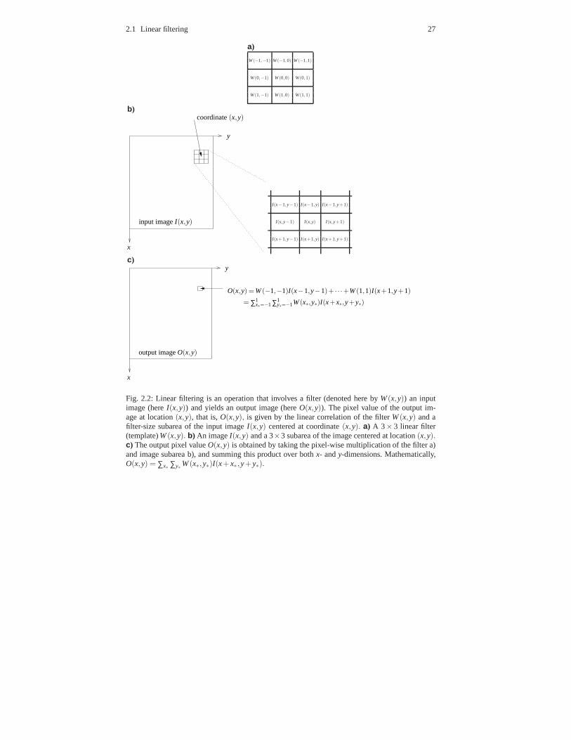
2.1 Linear filtering 27
a)
W(−1,−1) W(−1,0) W(−1,1)
W(0,−1) W(0,0) W(0,1)
W(1,−1) W(1,0) W(1,1)
b)
x
y
input imageI(x,y)
coordinate(x,y)
I(x−1,y−1) I(x−1,y) I(x−1,y+1)
I(x,y−1) I(x,y) I(x,y+1)
I(x+1,y−1) I(x+1,y) I(x+1,y+1)
c)
x
y
output imageO(x,y)
O(x,y) = W(−1,−1)I(x−1,y−1)+ · · ·+W(1,1)I(x+1,y+1)
= ∑1x∗=−1∑1
y∗=−1W(x∗,y∗)I(x+x∗,y+y∗)
Fig. 2.2: Linear filtering is an operation that involves a filter (denoted here byW(x,y)) an inputimage (hereI(x,y)) and yields an output image (hereO(x,y)). The pixel value of the output im-age at location(x,y), that is,O(x,y), is given by the linear correlation of the filterW(x,y) and afilter-size subarea of the input imageI(x,y) centered at coordinate(x,y). a) A 3× 3 linear filter(template)W(x,y). b) An imageI(x,y) and a 3×3 subarea of the image centered at location(x,y).c) The output pixel valueO(x,y) is obtained by taking the pixel-wise multiplication of the filter a)and image subarea b), and summing this product over bothx- andy-dimensions. Mathematically,O(x,y) = ∑x∗ ∑y∗W(x∗,y∗)I(x+x∗ ,y+y∗).

28 2 Linear filters and frequency analysis
a) b) c)
Fig. 2.3: An example of linear filtering.a) An input image.b) A filter. c) An output image.
Visual inspection of a filter alone is usually not sufficient to interpret a filteringoperation. This is also the case in the example in Figure 2.3:what does this filteringoperation actually accomplish? For a complete interpretation of a filtering opera-tion a different type of mathematical language is needed. This language utilizes afrequency-based representation of images, as explained inSection 2.2 below.
2.1.2 Impulse response and convolution
The impulse responseH(x,y) is the response of a filter to an impulse
δ (x,y) =
{
1, if x = 0 andy = 0
0, otherwise,(2.2)
that is, to an image in which a single pixel is “on” (equal to 1)and the others are“off” (equal to 0). The impulse response characterizes the system just as well asthe original filter coefficientsW(x,y). In fact, in frequency-based analysis of lin-ear filtering, rather than filtering with a filter, it is customary to work with im-pulse responses and an operation calledconvolution. This is because the frequency-modifying properties of the linear filter can be read out directly from the frequency-based representation of the impulse response, as will be seen below. (In general, thisholds for any linear shift-invariant system, which are defined in Section 20.1.)
Based on the definition of filtering in Equation (2.1), it is not difficult to see that
H(x,y) = W(−x,−y) (2.3)
Thus, the impulse responseH(x,y) is a “mirror image” of the filter weightsW(x,y):the relationship is simply that of a 180◦ rotation around the center of the filter. Thisis due to the change of signs ofx∗ andy∗; the impulse response is equal to one only ifx+x∗= 0, which implies that only at pointsx∗ =−x we have one and elsewhere the

2.2 Frequency-based representation 29
impulse response is zero. For a filter that is symmetric with respect to this rotation,the impulse response is identical to the filter.
The convolution of two imagesI1 andI2 is defined as
I1(x,y)∗ I2(x,y) =∞
∑x∗=−∞
∞
∑y∗=−∞
I1(x−x∗,y−y∗)I2(x∗,y∗) (2.4)
The only real difference to the definition of a filtering operation in Eq. (2.1) is thatwe have minus signs instead of plus signs. Note that convolution is symmetric inthe sense that we can change the order ofI1 andI2, since by making the change insummation indexx′∗ = x−x∗ andy′∗ = y−y∗ we get the same formula with the rolesof I1 andI2 interchanged (this is left as an exercise).
Therefore, we can express the filtering operation using the impulse response(which is considered just another image here) and the convolution simply as
O(x,y) = I(x,y)∗H(x,y) (2.5)
which is a slight modification of the original definition in Eq. (2.1). Introductionof this formula may seem like splitting hairs, but the point is that convolution isa well-known mathematical operation with interesting properties, and the impulseresponse is an important concept as well, so this formula shows how filtering can beinterpreted using these concepts.
2.2 Frequency-based representation
2.2.1 Motivation
Frequency-based representation is a very useful tool in theanalysis of image-processing systems. In particular, a frequency-based representation can be used tointerpret what happens during linear filtering: it describes linear filtering as modifi-cation of strengths (amplitudes) and spatial locations (phases) of frequencies (sinu-soidal components) that form the input image. As an example and sneak preview,Figures 2.8a)–d) on page 36 show how the filtering operation of Figure 2.3 can beinterpreted as attenuation of low and high frequencies, which can be seen in theoutput image as disappearance of large- and fine-scale structures or, alternatively,preservation of medium-scale structures. This interpretation can be read out fromFigure 2.8d), which shows the frequency amplification map for this filter: this map,which is called theamplitude responseof the filter, shows that both low frequen-cies (in the middle of the figure) and high frequencies (far from the middle) areattenuated; in the map, higher grey-scale value indicates larger amplitude response.
In what follows we will first describe the frequency-based representation, andthen demonstrate its special role in the analysis and designof linear filters.

30 2 Linear filters and frequency analysis
2.2.2 Representation in one and two dimensions
Figure 2.4 illustrates the main idea of the frequency-basedrepresentation in the caseof one-dimensional data. In the usual (spatial) representation (Figure 2.4a), a signalis represented by a set of numbers at each pointx = 0, ...,N−1; in this example,N = 7.Therefore, to reconstruct the signal in Figure 2.4a), we need 7 numbers. In thefrequency-based representation of this signal we also use 7numbers to describe thecontents of the signal, but in this case the numbers have a totally different meaning:they are theamplitudesandphasesof sinusoidal components, that is, parametersAandψ of signals of the formAcos(ωx+ ψ), whereω is the frequency parameter,see Figure 2.4c.
The theory of thediscrete Fourier transform(treated in detail in Chapter 20)states thatanysignal of length 7 can be represented by the four amplitudes and thethree phases of the four frequencies; the phase of the constant signal correspond-ing to ω = 0 is irrelevant because the constant signal does not change when it isshifted spatially. For a family of signals of given lengthN, the set of frequenciesωu, u = 0, ...,U −1, employed in the representation is fixed; in our example, thesefrequencies are listed in the second column of the table in Figure 2.4b). Overall, thefrequency-based representation is given by the sum
I(x) =U−1
∑u=0
Aucos(ωux+ ψu), (2.6)
whereωu are the frequencies andAu their amplitudes andψu their phases.In the case of images – that is, two-dimensional data – the sinusoidal components
are of the formAcos(ωxx+ ωyy+ ψ), (2.7)
whereωx is the frequency in thex-direction andωy in they-direction. In order tograsp the properties of such a component, let us define vectorω = (ωx,ωy), anddenote the dot-product by〈.〉. Then, the component (2.7) can be written as
Acos(ωxx+ ωyy+ ψ) = Acos(〈(x,y),ω〉+ ψ)
= Acos( ‖ω‖︸︷︷︸
“frequency”
〈(x,y), ω‖ω‖〉
︸ ︷︷ ︸
projection
+ψ), (2.8)
which shows that computation of the argument of the cosine function can be inter-preted as a projection of coordinate vector(x,y) onto the direction of the vectorω ,followed by a scaling with frequency‖ω‖ . Figure 2.5 illustrates this dependency ofthe frequency and the direction of the sinusoidal componenton ωx andωy.
Figure 2.5 also illustrates why it is necessary to consider both positive and nega-tive values of eitherωx or ωy: otherwise it is not possible to represent all directionsin the(x,y)-plane. However, there is a certain redundancy in this representation. Forexample, the frequency pairsω = (ωx,ωy) and−ω = (−ωx,−ωy) represent sinu-

2.2 Frequency-based representation 31
a)
0 2 4 6
−2−1
012
x
c)
0 1 2 30
0.51
1.52
u
Au
0 1 2 3
−3
0
3
u
ψu
b)
u ωx,u Au ψu Au cos(ωx,ux+ψu) ∑uℓ=1
Aℓ cos(ωx,ℓx+ψℓ)
0 0 0.42 0
0 2 4 6
−2−1
012
x0 2 4 6
−2−1
012
x
1 2π7 0.91 2.36
0 2 4 6
−2−1
012
x0 2 4 6
−2−1
012
x
2 4π7 0.45 3.04
0 2 4 6
−2−1
012
x0 2 4 6
−2−1
012
x
3 6π7 1.24 -3.01
0 2 4 6
−2−1
012
x0 2 4 6
−2−1
012
x
Fig. 2.4: In frequency-based representation, a signal is represented as amplitudes and phases ofsinusoidal components.a) A signal.b) A table showing how the signal in a) can be constructedfrom sinusoidal components. In the table, the number of sinusoidal components runs from 1 to4 (frequency indexu runs from 0 to 3), and the rightmost column shows the cumulative sumof the sinusoidal components with frequenciesωx,u having amplitudesAu and phasesφu. In thefifth column, the grey continuous lines show the continuous frequency components from whichthe discrete versions have been sampled. Here the frequencycomponents are added in increasingfrequency, that is,ωx,u1 >ωx,u2 if u1> u2. c) A frequency-based representation for the signal in a):the signal is represented by the set of frequency amplitudesAu, which is also called the amplitudespectrum (on the left), and the set of frequency phasesψu (on the right) of the correspondingfrequenciesωx,u, u = 0, ...,3. Note that the phase of the constant componentu = 0 correspondingto frequencyωx,0 = 0 is irrelevant; thus 7 numbers are needed in the frequency-based representationof the signal, just as in the usual representation a).

32 2 Linear filters and frequency analysis
soidal components that have the same direction and frequency, becauseω and−ωhave the same direction and length. So, it can be seen that anyhalf of the(ωx,ωy)-plane suffices to represent all directions. In practice it has become customary to usea redundant frequency representation which employs the whole (ωx,ωy)-plane, thatis, negative and positive parts ofboththeωx- andωy-axis.1
ω = (ωx,ωy) ‖ω‖ ω‖ω‖ I(x,y)
( 110,
110)
√2
10 ≈ 0.14ωx
ωy
ω
‖ω‖
( 110,− 1
10)√
210 ≈ 0.14 ωx
ωy
ω
‖ω‖
( 610,
310) 3
√5
10 ≈ 0.67ωx
ωy
ω
‖ω‖
Fig. 2.5: In an equationI(x,y) = cos(ωxx+ ωyy
)of a two-dimensional sinusoidal image, the fre-
quenciesωx andωy determine the direction and the frequency of the component.More specifically,if ω = (ωx,ωy), then the length ofω determines the frequency of the component, and the directionof ω determines the direction of the component. This is illustrated here for three different(ωx,ωy)pairs; the sinusoidal components are of size 128×128 pixels. Notice that in the plots in the thirdcolumn,ωy runs from top to bottom because of the convention that in images they-axis runs in thisdirection. See equation (2.8) on page 30 for details.
1 In fact, because cosine is an even function — that is, cos(−α) = cos(α) — the frequency com-ponents corresponding to these two frequency pairs are identical whenAcos[ 〈(x,y),ω〉+ψ] =Acos[−(〈(x,y),ω〉+ψ)] = Acos[〈(x,y), (−ω)〉+(−ψ)] , that is, when their amplitudes are thesame and their phases are negatives or each other. Therefore, when employing the whole(ωx,ωy)-plane, the amplitude of a frequency component are customarily split evenly among the frequencypairsω and−ω with phasesψ and−ψ.

2.2 Frequency-based representation 33
Figure 2.6 shows an example of the resulting frequency representation. Again,the theory of discrete Fourier transform (see Chapter 20) states thatany image ofsize 3×3 pixels can be represented by five amplitudes and four phases, a total of9 numbers as in the usual spatial representation; the phase of the constant signalcorresponding toω = (0,0) is irrelevant as before.
Note on terminology The square of the amplitudeA2 is also called theFourierenergyor power, and when it is computed for many different frequencies, we getwhat is called thepower spectrum. The power spectrum is a classic way of charac-terizing which frequencies are present and with which “strengths” in a given signalor image. If the original amplitudes are used, we talk about the amplitude spectrum(Fig. 2.4 c). It should be noted that the terminology of frequency-based analysis isnot very well standardized, so other sources may use different terminology.
2.2.3 Frequency-based representation and linear filtering
Sinusoidals also play a special role in the analysis and design of linear filters. Whatmakes sinusoidals special is the fact that when a sinusoidalis input into a linearfilter, the response is a sinusoidalwith the same frequency, but possibly differentamplitude and phase. Figure 2.7 illustrates this phenomenon. Furthermore, both theamplification factor of the amplitude and the shift in the phase depend only on thefrequency of the input, and not its amplitude or phase (see Chapter 20 for a detaileddiscussion).
For a linear filter with impulse responseH(x,y), let∣∣H(ωx,ωy)
∣∣ denote the am-
plitude magnification factor of the system for horizontal frequencyωx and verticalfrequencyωy, and∠H(ωx,ωy) denote the phase shift of the filter. Then if the inputsignal has frequency-based representation
I(x,y) = ∑ωx
∑ωy
Aωx,ωy cos(ωxx+ ωyy+ ψωx,ωy
), (2.9)
where the sum overωx andωy is here and below taken over both positive and nega-tive frequencies, the response of the linear filter has the following frequency-basedrepresentation
O(x,y) = H(x,y)∗ I(x,y)
= ∑ωx
∑ωy
∣∣H(ωx,ωy)
∣∣Aωx,ωy
︸ ︷︷ ︸
amplitude
cos(ωxx+ ωyy+ ψωx,ωy +∠H(ωx,ωy)
︸ ︷︷ ︸
phase
).
(2.10)
The amplitude magnification factor∣∣H(ωx,ωy)
∣∣ is called theamplitude response
of the linear system, while the phase shift∠H(ωx,ωy) is called thephase response.

34 2 Linear filters and frequency analysis
a)
x
y
0 1 2
012
−0.70 0.59 0.670.01 −0.25 −0.08−0.78 0.48 0.89
b)
ωx
ωy
−2.1 0 2.1
2.10
−2.1
1.81 0.89 1.342.68 0.82 2.681.34 0.89 1.81
c)
2.06 −1.07 1.95−2.93 0.00 2.93−1.95 1.07 −2.06
d)
location of the componentin the(ωx,ωy)-plane
ωx
ωy
−2.1 0 2.1
2.1
0
−2.1
ωx
ωy
−2.1 0 2.1
2.1
0
−2.1
ωx
ωy
−2.1 0 2.1
2.1
0
−2.1
ωx
ωy
−2.1 0 2.1
2.1
0
−2.1
the component
x
y
0 1 2
0
1
2
x
y
0 1 2
0
1
2
x
y0 1 2
0
1
2
x
y
0 1 2
0
1
2
Fig. 2.6: An example of a two-dimensional frequency representation.a) The grey-scale (left) andnumerical (right) representation of an image of size 3× 3 pixels.b) Amplitude information ofthe frequency representation of the image in a): the grey-scale (left) and numerical (right) repre-sentation of the amplitudes of the different frequencies. Notice the symmetries/redundancies: theamplitude of frequencyω is the same as the amplitude of frequency−ω. c) Phase information ofthe frequency representation of the image in a); the axis of this representation are the same as in b).Notice the symmetries/redundancies: the phase ofω is the negative of the phase of−ω. d) Fourexamples of the actual sinusoidal components that make up the image in a) in the frequency repre-sentation. In each column, the first row shows the location ofthe component in the(ωx,ωy)-plane,while the second row shows the actual component. The leftmost component is the constant com-ponent corresponding toω = (0,0). The second component is a horizontal frequency component.Because of the symmetry in the frequency representation, the third and the fourth components areidentical. Notice that the second component (the horizontal frequency component) is stronger thanthe other components, which can also be seen in the amplituderepresentation in b).

2.2 Frequency-based representation 35
a)
I(x) H(x) H(x)∗ I(x)
x x x
x x x
b)
I(x,y) H(x,y) H(x,y)∗ I(x,y)
Fig. 2.7: Sinusoidal components play a special role in the analysis and design of linear systems,because if a sinusoidal is input into a linear filter, the output is a sinusoidal with the same frequencybut possibly different amplitude and phase.a) Two examples of this phenomenon are shown herein the one-dimensional case, one on each row. The left columnshows the input signal, which ishere assumed to be a sinusoidal of infinite duration. The middle column shows a randomly selectedimpulse response, and the column on the right the response ofthis linear system to the sinusoidal.Notice the different scale in the output signals, which is related to the amplitude change takingplace in the filtering.b) An illustration of the two-dimensional case, with a 64×64 -pixel input onthe left, a random 11×11 -pixel impulse response in the middle, and the output on the right.
The way these quantities are determined for a linear filter isdescribed shortly below;for now, let us just assume that they are available.
Figure 2.8 shows an example of the insight offered by the frequency representa-tion of linear filtering (equation (2.10)). The example shows how a linear filter canbe analyzed or designed by its amplitude response (the phaseresponse is zero forall frequencies in this example). Notice that while relating the forms of the filtersthemselves (Figures 2.8b and f) to the end result of the filtering is very difficult,describing what the filter does is straightforward once the frequency-based repre-sentation (Figures 2.8d and e) is available.
How can the amplitude and phase responses of a linear system be determined?Consider a situation where we feed into the system a signal which contains a mixtureof all frequencies with unit amplitudes and zero phases:

36 2 Linear filters and frequency analysis
a) b) c) d)
ωx
ωy
−2.2 −1.1 0 1.1 2.2
2.2
1.1
0
−1.1
−2.2
e)
ωx
ωy
−2.2 −1.1 0 1.1 2.2
2.2
1.1
0
−1.1
−2.2
f) g)
Fig. 2.8: An example of the usefulness of frequency-based representation in the analysis and designof linear filters.a) An input image.b) A filter of size 17×17 pixels.c) The output of linear filteringof image a) with filter b).d) The amplitude response of the filter in b); in this representation darkpixels indicate amplitude response values close to zero andbright pixels values close to one. Theamplitude response shows that the filterattenuates low and high frequencies, that is, frequencieswhich are either close to the origin(ωu,ωv) = (0,0) or far away from it. This can be verified inc), where medium-scaled structures have been preserved in the image, while details and large-scale grey-scale variations are no longer visible. The phase response of the filter is zero for allfrequencies.e) Assume that we want to design a filter that has a reverse effectthan the filter shownin b): our new filter attenuates medium frequencies. The filter can be designed by specifying itsamplitude and phase response. The amplitude response is shown here, the phase response is zerofor all frequencies.f) The filter corresponding to the frequency-based representation e). g) Theresult obtained when the filter f) is applied to the image in a). The results is as expected: the filterpreserves details and large-scale grey-scale variations,while medium-scale variations are no longervisible. Notice that just by examining the filters themselves (b and f) it is difficult to say what thefilters do, while this becomes straightforward once the frequency-based representations (d and e)are available.
I(x,y) = ∑ωx
∑ωy
cos(ωxx+ ωyy
). (2.11)
Then, applying equation (2.10), the frequency-based representation of the output is
O(x,y) = H(x,y)∗ I(x,y) = ∑ωx
∑ωy
∣∣H(ωx,ωy)
∣∣
︸ ︷︷ ︸
amplitude
cos(ωxx+ ωyy+∠H(ωx,ωy)
︸ ︷︷ ︸
phase
).
(2.12)

2.2 Frequency-based representation 37
k 0 1 2 3 4 5 6 7 8
ωx,k− 2π3 −
2π3 −
2π3 0 0 0 2π
32π3
2π3
ωy,k− 2π3 0 2π
3 − 2π3 0 2π
3 − 2π3 0 2π
3
cos(ωx,kx+ωy,ky
)
∑kℓ=0cos
(ωx,ℓx+ωy,ℓy
)
Fig. 2.9: An image containing all frequencies with unit amplitudes and zero phases is an impulse.Here, the different frequency components are being added from left to right; the right-most imageis an impulse response.
In other words, the amplitude and phase responses of the linear system can be readfrom the frequency-based representation of the outputO(x,y). What remains to bedetermined is what kind of a signal the signalI(x,y) in Equation (2.11) is. The theoryof the Fourier transform states that the image obtained whenall frequencies withidentical amplitudes and zero phases are added together is an impulse. Figure 2.9illustrates this when image size is 3× 3 pixels. To summarize, when we feed animpulse into a linear filter,
• from the point of view of frequency-based description, we are giving the systeman input with equal amplitudes of all frequencies at phase zero
• the linear system modifies the amplitudes and phases of thesefrequencies ac-cording to the amplitude and phase response of the system
• the amplitude and phase response properties can be easily read out from the im-pulse response, since the amplitudes of the input were equaland phases were allzero.
In other words, theamplitude and phase responses of a linear filter are obtainedfrom the frequency-based representation of the impulse response: the amplituderesponses are the amplitudes of the frequencies, and the phase responses are thephases of the frequencies.An example of this principle is shown in Figure 2.8: theamplitude response images d) and e) are in fact the amplitudes of the frequency-based representations of the impulse responses b) and f).
2.2.4 Computation and mathematical details
Above we have outlined the nature of the frequency-based representation in the one-and two-dimensional case, and the usefulness of this representation in the designand analysis of linear systems. The material presented so far should therefore pro-vide the reader with the knowledge needed to understand whatthe frequency-basedrepresentation is, and why it is used.

38 2 Linear filters and frequency analysis
However, a number of questions have been left unanswered in the text above,including the following:
• What exactly are the values of the frequenciesω used in the frequency-basedrepresentation?
• How is the frequency-based representation computed?• What guarantees that a frequency-based representation exists?
The set of mathematical tools used to define and analyze frequency-based rep-resentations are part of mathematics calledFourier analysis. In particular,Fouriertransformsare used to convert data and impulse responses to and from frequency-based representation. There are different types of Fouriertransforms for differentpurposes: continuous/discrete and finite/infinite data. When working with digital im-ages, the most important Fourier transform is thediscrete Fourier transform (DFT),which is particularly suited for representation of discrete and finite data in comput-ers. The basics of DFT are described in Chapter 20. The computational implementa-tion of DFT is usually through a particular algorithm calledFast Fourier Transform,or FFT.
The DFT has fairly abstract mathematical properties, because complex numbersare employed in the transform. The results of the DFT are, however, quite easily un-derstood in terms of the frequency-based representation: for example, Figure 2.8d)was computed by taking the DFT of the filter in Figure 2.8b), and then showing themagnitudes of the complex numbers of the result of the DFT.
A working knowledge of the frequency-based representationis not needed inreading this book: it is sufficient to understand what the frequency-based represen-tation is and why it is used. If you are interested in working with frequency-basedrepresentations, then studying the DFT is critical, because the DFT has some coun-terintuitive properties that must be known when working with results of transforms;for example, the DFT assumes that the data (signal or image) is periodic, whichcauses periodicity effects when filtering is done in the frequency-based representa-tion.
2.3 Representation using linear basis
Now we consider a general and widely-used framework for image representation: alinear basis. We will also see how frequency-based representation can be seen as aspecial case in this framework.
2.3.1 Basic idea
A traditional way to represent grey-scale images is the pixel-based representation,where the value of each pixel denotes the grey-scale value atthat particular loca-
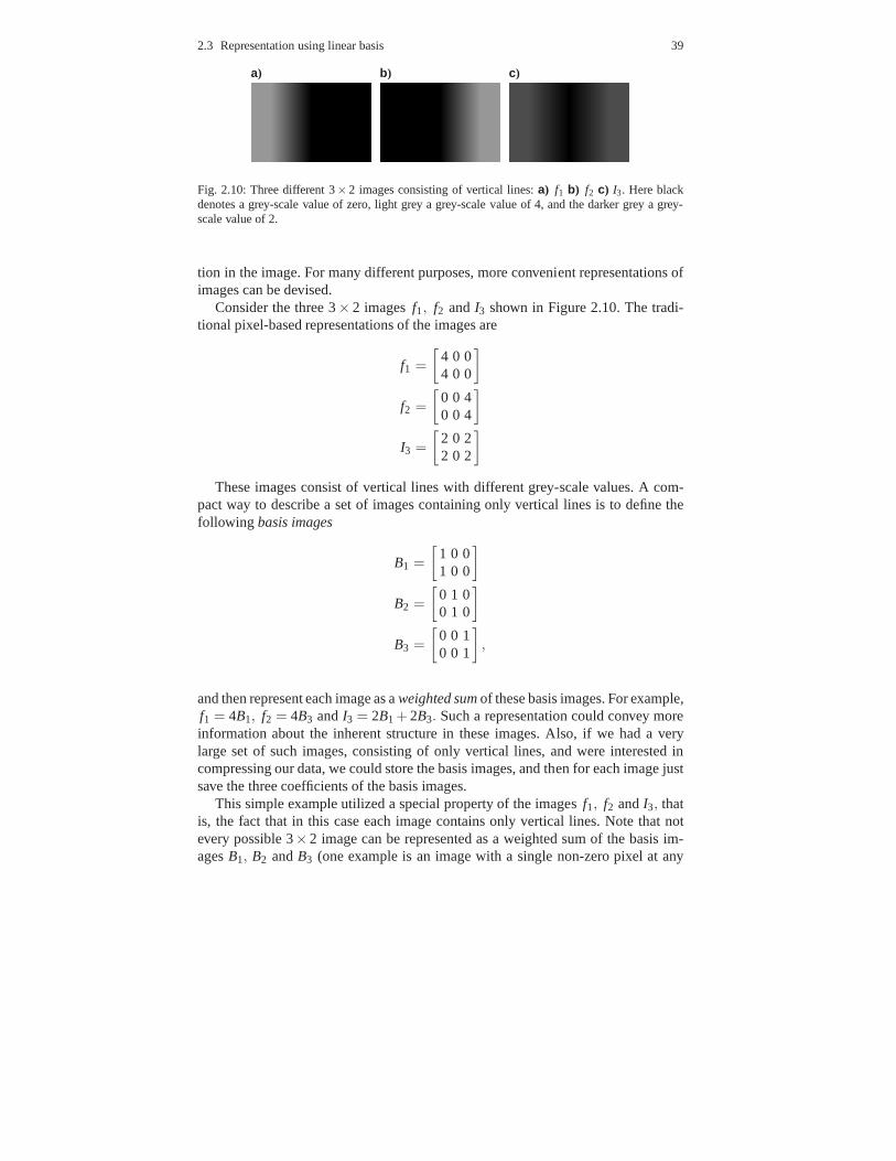
2.3 Representation using linear basis 39
a) b) c)
Fig. 2.10: Three different 3×2 images consisting of vertical lines:a) f1 b) f2 c) I3. Here blackdenotes a grey-scale value of zero, light grey a grey-scale value of 4, and the darker grey a grey-scale value of 2.
tion in the image. For many different purposes, more convenient representations ofimages can be devised.
Consider the three 3× 2 imagesf1, f2 andI3 shown in Figure 2.10. The tradi-tional pixel-based representations of the images are
f1 =
[4 0 04 0 0
]
f2 =
[0 0 40 0 4
]
I3 =
[2 0 22 0 2
]
These images consist of vertical lines with different grey-scale values. A com-pact way to describe a set of images containing only verticallines is to define thefollowing basis images
B1 =
[1 0 01 0 0
]
B2 =
[0 1 00 1 0
]
B3 =
[0 0 10 0 1
]
,
and then represent each image as aweighted sumof these basis images. For example,f1 = 4B1, f2 = 4B3 andI3 = 2B1 + 2B3. Such a representation could convey moreinformation about the inherent structure in these images. Also, if we had a verylarge set of such images, consisting of only vertical lines,and were interested incompressing our data, we could store the basis images, and then for each image justsave the three coefficients of the basis images.
This simple example utilized a special property of the images f1, f2 andI3, thatis, the fact that in this case each image contains only vertical lines. Note that notevery possible 3×2 image can be represented as a weighted sum of the basis im-agesB1, B2 andB3 (one example is an image with a single non-zero pixel at any

40 2 Linear filters and frequency analysis
image location). This kind of a basis is called anundercompletebasis. Usually theword basisis used to refer to acomplete basis, a basis which – when used in theform of a weighted sum – can be used to represent any image. Forthe set of 3×2images, one example of a complete basis is the set of 6 images with a single one atexactly one image location(x,y). This basis is typically associated with the tradi-tional pixel-based image representation: each pixel valuedenotes the coefficient ofthe corresponding basis image.
A particularly important case is anorthogonalbasis. Then, the coefficients in thebasis simply equal the dot-products with the basis vectors.For more on bases andorthogonality, see Section 19.6.
The use of different bases in the representation of images has several importantareas of application in image processing. Two of these were mentioned already: thedescription and analysis of the structure of images, and image compression. Otherimportant applications are in the domain of image processing systems: differentimage representations are central in the analysis of these systems (including theanalysis of the visual system), design of such systems, and in their efficient imple-mentation.
2.3.2 Frequency-based representation as a basis
Now we consider how frequency-based representation can be rephrased as findingthe coefficients in a basis. Consider the situation where we want to analyze, in agiven signal, the amplitudeA and phaseψ of a sinusoidal component
Acos(ωx+ ψ). (2.13)
The key point here is that instead of determiningA andψ directly, we can determinethe coefficientsC andSof a cosine and sine signal with (centered) phase zero:
Ccos(ωx)+Ssin(ωx). (2.14)
To show this we will demonstrate that there is a one-to-one correspondence betweensignals of the form (2.13) and of the form (2.14). First, a given sinusoidal of theform (2.13) can be represented in form (2.14) as follows:
Acos(ωx+ ψ) = A(cos(ωx)cosψ−sin(ωx)sinψ)
= Acosψ︸ ︷︷ ︸
=C
cos(ωx)+A(−sinψ)︸ ︷︷ ︸
=S
sin(ωx)
= Ccos(ωx)+Ssin(ωx).
(2.15)
Conversely, if we are given a signal in form (2.14), the derivation (2.15) can bereversed (this is left as an exercise), so that we get
2.4 Space-frequency analysis 41
A =√
C2 +S2, (2.16)
ψ =−atanSC. (2.17)
Thus, to analyze the amplitude and phase of frequencyω in a given signal, it sufficesto find coefficientsC andS in equationCcos(ωx)+Ssin(ωx); after the coefficientshave been computed, equations (2.16) and (2.17) can be used to compute the am-plitude and phase. In particular, the square of the amplitude (“Fourier power” or“Fourier energy”) is obtained as the sum of squares of the coefficients.
The formula in Equation (2.16) is also very interesting froma neural modellingviewpoint because it shows how to compute the amplitude using quite simple op-erations, since computation of the coefficients in a linear basis is a linear operation(at least if the basis is complete). Computation of Fourier energy in a given fre-quency thus requires two linear operations, followed by squaring, and summing ofthe squares. As we will see in Chapter 3, something similar tolinear Fourier op-erators seems to be computed in the early parts of visual processing, which makescomputation of Fourier energy rather straightforward.
How are the coefficientsC andS then computed? The key is orthogonality. Thesignals cos(ωx) and sin(ωx) are orthogonal, at least approximately. So, the coeffi-cientsC andS are simply obtained as the dot-products of the signal with the basisvectors given by the cos and sin functions.
In fact, Discrete Fourier Transform can be viewed as defininga basis with suchcos and sin functions with many different frequencies, and those frequencies arecarefully chosen so that the sinusoidals are exactly orthogonal. Then, the coefficientsfor all the sin and cos functions, in the different frequencies, canbe computed as thedot-products
∑x
I(x)cos(ωx) and∑x
I(x)sin(ωx) (2.18)
The idea generalizes to two dimensions (images) in the same way as frequency-based analysis was shown to generalize above. More details on the DFT can befound in Chapter 20.
2.4 Space-frequency analysis
2.4.1 Introduction
The frequency representation utilizes global sinusoidal gratings, that is, componentswhich span the whole image (see, e.g., Figure 2.5). This is particularly useful for theanalysis and design of linear filters. However, because of the global nature of sinu-soidals, the frequency representation tells us nothing about the spatial relationshipof different frequencies in an image. This is illustrated inFigures 2.11a) and b),which show an image and the amplitudes of its frequency representation. The upperpart of the image contains grass, which tends to have a more vertical orientation

42 2 Linear filters and frequency analysis
a) b)
ωx
ωy
−2.5 −1.3 0 1.3 2.5
2.5
1.3
0
−1.3
−2.5
c)
d) e) f)
Fig. 2.11: The main idea in space-frequency analysis is to consider the amplitudes/phases of differ-ent frequenciesat different locations in an image. a) An image. Notice how different areas of theimage differ in their frequency contents.b) The standard frequency representation: the amplitudesof the different frequencies that make up the frequency representation of the image in a). Note thatwhile this representation suggests that fairly high horizontal frequencies are present in the image,it does not convey information about the spatial location ofdifferent frequencies. For purposes ofvisibility, the amplitudes of different frequencies have been transformed with logarithmic mappingbefore display.c) A spatially localized non-negative windowing function.d) A localized area ofthe image can be obtained by multiplying the image a) with thewindowing function c).e) In thisexample the amplitude (strength) of this horizontal frequency is analyzed at each point in the im-age.f) Applying the weighting scheme c)-d) at each point in the image a), and then analyzing theamplitude of the frequency e) at each of these points resultsin this spatial map of the amplitude ofthe frequency. As can be seen, the frequency tends to have larger amplitudes in the upper part ofthe image, as can be expected.
and sharper structure than the lower part of the image. The amplitudes of the fre-quency representation (Figures 2.11b) show that many horizontal or near-horizontalfrequencies – that is, frequencies in the vicinity of axisωy = 0 – have a relativelylarge amplitude, even at fairly high frequencies. (Notice that structures with verticallines correspond tohorizontalfrequencies.) From the amplitude spectrum there is,however, no way to tell the spatial location of these frequencies.
The spatial locations of different frequencies can containimportant informationabout the image. In this example, if we are able to locate those areas which tend tohave more horizontal frequencies, we can use that information, for example, to facil-itate the identification of the grass area in the image. How can the spatial locationsof these frequencies be found? A straightforward way to do this is to analyze the fre-

2.4 Space-frequency analysis 43
quency contents oflimited spatial areas. Figures 2.11c)–f) illustrate this idea. Theoriginal image (Figure 2.11a) is multiplied with a non-negativewindowing function(Figure 2.11c) to examine the frequency contents of a spatially localized image area(Figure 2.11d). For example, for the horizontal frequency shown in Figure 2.11e), aspatial map of the amplitude of this frequency is shown in Figure 2.11f); the map hasbeen obtained by applying the weighting scheme (Figure 2.11c and d) atevery pointof the image, and analyzing the amplitude of the frequency inthe localized imagearea. Now, we see that in Figure 2.11f) that the different areas (grass vs. water) areclearly separated by this space-frequency analysis.
In the case of space-frequency analysis, the computationaloperations underlyingthe analysis are of great interest to us. This is because someimportant results ob-tained with statistical modelling of natural images can be interpreted as performingspace-frequency analysis, so the way the analysis is computed needs to be under-stood to appreciate these results. Because of this connection, we need to delve alittle deeper into the mathematics.
Before going into the details, we first state the main result:space-frequency anal-ysis can be done by the method illustrated in Figure 2.12: by filtering the imagewith two different localized sinusoidal filters, and computing the amplitudes andphases (in this example only the amplitudes) from the outputs of these two filters.The following section explains the mathematics behind thismethod.
2.4.2 Space-frequency analysis and Gabor filters
Consider a situation where we want to analyze the local frequency contents of animage: we want to compute the amplitude and phase for each location(x0,y0). Al-ternatively, we could compute a set of coefficientsC(x0,y0) andS(x0,y0) as in Sec-tion 2.3.2, which now are functions of the location. The analysis is made local byapplying a weighting function, sayW(x,y), centered at(x0,y0) before the analysis.
We can simply modify the analysis in Section 2.3.2 by centering the signalfaround the point(x0,y0) and weighting it byw before the analysis. Thus, we get aformula for the coefficientC at a given point:
C(x0,y0)≈∑x
∑y
I(x,y)W(x−x0,y−y0)cos(ωx(x−x0)+ ωy(y−y0)). (2.19)
and similarly forS(x0,y0). Note that the order in which we multiply the three images(imagef , weighting imagew, sinusoidal cos) inside the sum is irrelevant. Thereforeit does not make any difference whether we apply the weighting to the imageI(x,y)or to the sinusoidal cos(ωx(x− x0) + ωy(y− y0)). If we define a new weightingfunction
W2(x,y) = W(x,y)cos(ωxx+ ωyy), (2.20)
equation (2.19) becomes

44 2 Linear filters and frequency analysis
C(x0,y0)≈∑x
∑y
I(x,y)W2(x−x0,y−y0). (2.21)
Equations (2.20) and (2.21) show that computation of coefficientsC(x0,y0) can beapproximated by filtering the image with a filter that is the product of a sinusoidalcos(ωxx+ ωyy) and the weighting window. Similar analysis applies to coefficientsS(x0,y0), except that in that case the sinusoidal is sin(ωxx+ωyy). Because the mag-nitude of the weighting functionW(x,y) typically falls off quite fast from the origin(x,y) = (0,0), computational savings can be obtained by truncating the filter to zerofor (x,y) far away from the origin.
To summarize the result in an example, Figure 2.12 shows how the ampli-tude map of Figure 2.11f on page 42 was computed:C(x0,y0) andS(x0,y0) werecomputed by filtering the image with weighted versions of cos(ωxx+ ωyy) andsin(ωxx+ ωyy), respectively, and the amplitude mapA(x0,y0) was obtained byA(x0,y0) =
√
C(x0,y0)2 +S(x0,y0)2.The two filters used in the computation ofC(x0,y0) andS(x0,y0) are often called
a quadrature-phase pair. This is because sin(x+ π2 ) = cos(x), so the two filters are
W(x,y)cos(ωxx+ ωyy) andW(x,y)cos(ωxx+ ωyy+ π2 ), that is, they are otherwise
identical expect for a a phase difference of one quarter of a whole cycle:2π4 = π
2 .When the weighting function is a gaussian window, which in the one-dimensional
case is of the form
Wσ (x) =1d
e− x2
σ2 , (2.22)
the resulting filter is called aGabor filter; parameterσ determines the width ofthe window, and the scaling constantd is typically chosen so that∑xWσ (x) = 1.Overall, a one-dimensional Gabor function
Wσ ,ω,ψ (x) = Wσ (x)cos(ωx+ ψ) (2.23)
has three parameters, widthσ , frequencyω and phaseψ . One-dimensional Gaborfunctions are illustrated in Fig. 2.13.
In the two-dimensional case, a Gabor filter has a few additional parameters thatcontrol the two-dimensional shape and orientation of the filter. When the sinusoidalin the filter has vertical orientation the filter is given by the following equation
Wσx,σy,ω,ψ (x,y) =1d
e−(
x2
σ2x
+ y2
σ2y
)
cos(ωx+ ψ); (2.24)
hereσx andσy control the width of the weighting window in thex- andy-directions,respectively. A Gabor-filter with orientationα can be obtained by rotating the orig-inal (x,y) coordinate system by−α to yield a new coordinate system(x∗,y∗) (thisrotation is equivalent to the rotation of the filter itself byα). The equations thatrelate the two coordinate systems are
x = x∗ cosα +y∗sinα (2.25)
y = −x∗sinα +y∗cosα. (2.26)
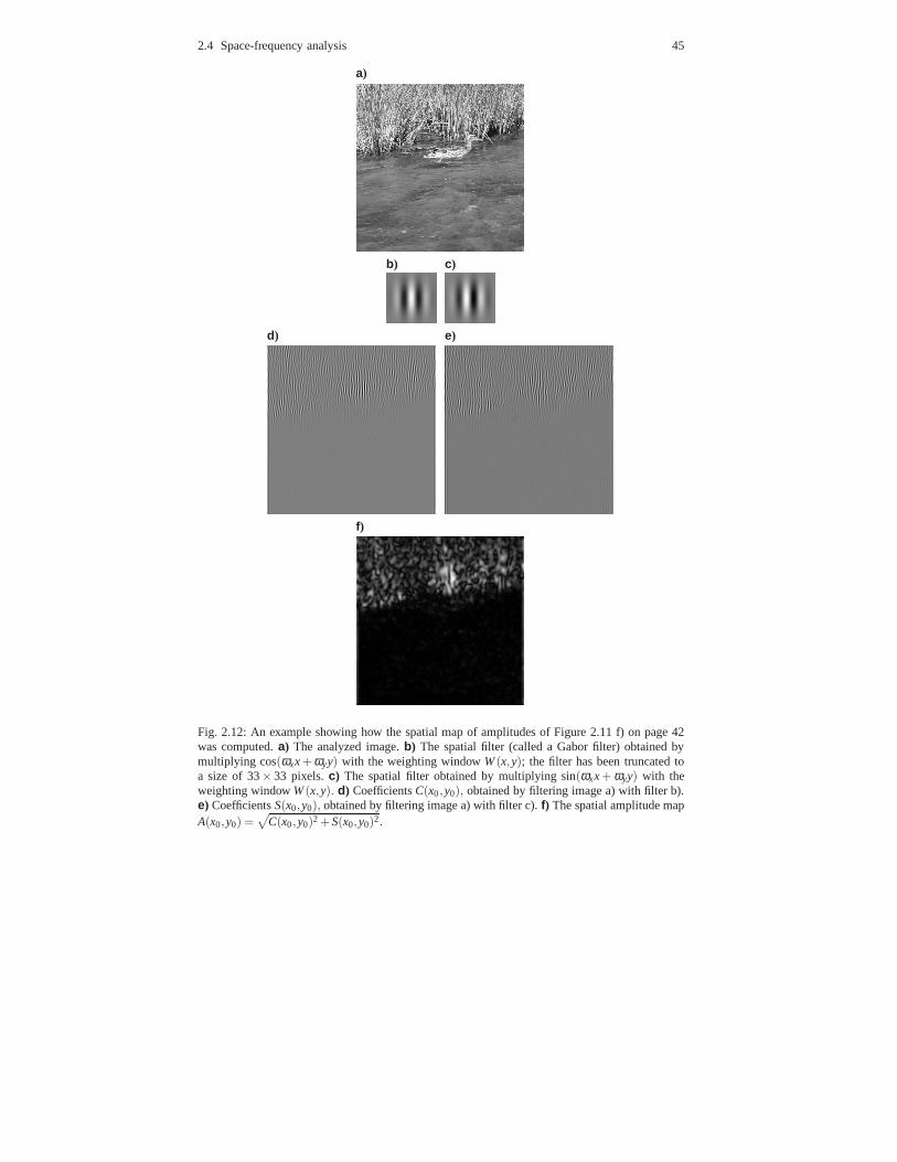
2.4 Space-frequency analysis 45
a)
b) c)
d) e)
f)
Fig. 2.12: An example showing how the spatial map of amplitudes of Figure 2.11 f) on page 42was computed.a) The analyzed image.b) The spatial filter (called a Gabor filter) obtained bymultiplying cos(ωxx+ ωyy) with the weighting windowW(x,y); the filter has been truncated toa size of 33× 33 pixels.c) The spatial filter obtained by multiplying sin(ωxx+ ωyy) with theweighting windowW(x,y). d) CoefficientsC(x0,y0), obtained by filtering image a) with filter b).e) CoefficientsS(x0,y0), obtained by filtering image a) with filter c).f) The spatial amplitude mapA(x0,y0) =
√
C(x0,y0)2 +S(x0,y0)2.
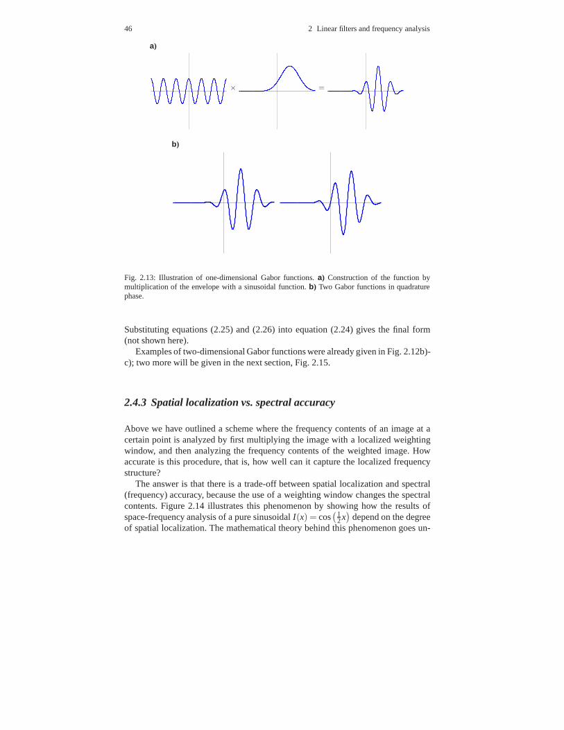
46 2 Linear filters and frequency analysis
a)
× =
b)
Fig. 2.13: Illustration of one-dimensional Gabor functions. a) Construction of the function bymultiplication of the envelope with a sinusoidal function.b) Two Gabor functions in quadraturephase.
Substituting equations (2.25) and (2.26) into equation (2.24) gives the final form(not shown here).
Examples of two-dimensional Gabor functions were already given in Fig. 2.12b)-c); two more will be given in the next section, Fig. 2.15.
2.4.3 Spatial localization vs. spectral accuracy
Above we have outlined a scheme where the frequency contentsof an image at acertain point is analyzed by first multiplying the image witha localized weightingwindow, and then analyzing the frequency contents of the weighted image. Howaccurate is this procedure, that is, how well can it capture the localized frequencystructure?
The answer is that there is a trade-off between spatial localization and spectral(frequency) accuracy, because the use of a weighting windowchanges the spectralcontents. Figure 2.14 illustrates this phenomenon by showing how the results ofspace-frequency analysis of a pure sinusoidalI(x) = cos
(12x)
depend on the degreeof spatial localization. The mathematical theory behind this phenomenon goes un-

2.4 Space-frequency analysis 47
σ W(x) W(x)cos( 1
2x)
A(ω)
∞ 01
0 150x
−11
0 150x
070
−5 0 5ω
1601
0 150x
−11
0 150x
015
−5 0 5ω
401
0 150x
−11
0 150x
04
−5 0 5ω
101
0 150x
−11
0 150x
01.5
−5 0 5ω
Fig. 2.14: In space-frequency analysis, there is a trade-off between spatial localization and spectralaccuracy. This example shows how the use of a weighting window W(x) (second column) changesthe spectral (frequency) contents of a pure sinusoidalI(x) = cos
( 12x), x= 0, ...,127. The rightmost
column shows the amplitude spectrum of the localized signalW(x)I(x), which in turn is plottedin the third column. With no spatial localization (window width σ = ∞; top row), the amplitudespectrumA(ω) shows a clear peak at the locationω = 1
2 . As window widthσ decreases, spatiallocalization increases, but accuracy in the spectral domain decreases: the two peaks inA(ω) spreadout and eventually fuse so thatA(ω) is a unimodal function whenσ = 1.
der the nametime-bandwidth product theoremin signal processing , oruncertaintyprinciple in physics. These theories state that there is a lower bound on the productof the spread of the energy in the spatial domain and the frequency domain. SeeReferences at the end of this chapter for more details.
With images, the extra dimensions introduce another factor: uncertainty aboutorientation. This parameter behaves just like frequency and location in the sensethat if we want to have a filter which is very localized in orientation, we have to giveup localization in the other parameters. This is illustrated in Fig. 2.15, in which wesee that a basic Gabor which is very localized in space a) responds to a wider rangeof different orientations than the Gabor in b). The Gabor in b) has has been designedto respond only to a small range of orientations, which was only possible by makingit more extended in space.

48 2 Linear filters and frequency analysis
a) b)
Fig. 2.15: Uncertainty in two dimensions. Compared with a “basic” Gabor function ina), theGabor inb) is very localized in orientation, that is, it responds to only a small range of differentorientations. The thin black lines show the orientations ofthin lines which still fall on the white(positive) area of the function: a line which is more obliquewill partly fall on the black (negative)areas and thus the response of the filter will the reduced. We can see that in b), the range oforientations producing very large responses (falling on the white area only) is much smaller than ina). This illustrates that in order to make the basic Gabor function in a) more localized in orientation,it is necessary to make it longer, and thus to reduce its spatial localization.
2.5 References
Most of the material covered in this chapter can be found in most image-processingtextbooks. A classic choice is (Gonzales and Woods, 2002), which does not, how-ever, consider space-frequency analysis. A large number oftextbooks explain time-frequency analysis, which is the one-dimensional counterpart of space-frequencyanalysis, for example (Cohen, 1995). Related material can also be found in text-books on wavelets, which are a closely related method (see Section 17.3.2 for a veryshort introduction), for example (Vetterli and Kovacevi´c, 1995; Strang and Nguyen,1996).
2.6 Exercices
Mathematical exercises
1. Show that convolution is a symmetric operation.2. Show Eq. (2.3).3. Prove Equation (2.17). Hint: Find two different values for x so that you get the
two equations
Acosψ = C (2.27)
−Asinψ = S (2.28)
Now, solve forA andψ as follows. First, take the squares of both sides of bothequations (2.27) and (2.28) and sum the two resulting equations. Recall the sum

2.6 Exercices 49
of squares of a sine and a cosine function. Second, divide both sides of the equa-tions (2.27) and (2.28) with each other.
Computer assignments
The computer assignments in this book are designed to be madewith MatlabTM.Most of them will work on Matlab clones such as Octave. We willassume that youknow the basics of Matlab.
1. The commandmeshgrid is very useful for image processing. It creates two-dimensional coordinates, just like a command such as[5:.01:5] creates a one-dimensional coordinate. Give the command[X,Y]=meshgrid([-5:0.1:5]); andplot the matricesX andY usingimagesc.
2. Create Fourier gratings bysin(X), sin(Y), sin(X+Y). Plot the gratings.3. Create a gabor function using theseX andY, simply by plugging in those matri-
ces in the formula in Eq. 2.24. Try out different values for the parameters untilyou get a function which looks like the one in Fig. 2.12b).
4. Change the roles ofX andY to get a Gabor filter in a different orientation.5. Try out a Gabor function of a different orientation by plugging inX+Y instead of
X andX-Y instead ofY.6. Linear filtering is easily done with the functionconv2 (the “2” means two-
dimensional convolution, i.e. images). Take any image, import it to Matlab, andconvolve it with the three Gabor functions obtained above.


Chapter 3Outline of the visual system
In this chapter, we review very briefly the structure of the human visual system. Thisexposition contains a large number of terms which are likelyto be new for readerswho are not familiar with neuroscience. Only a few of them areneeded later in thisbook; they are given in italics for emphasis.
3.1 Neurons and firing rates
Neurons The main information processing workload of the brain is carried bynerve cells, orneurons. Estimates of the number of neurons in the brain typicallyvary between 1010 and 1011. What distinguishes neurons from other cells are theirspecial information-processing capabilities. A neuron receives signals from otherneurons, processes them, and sends the result of that processing to other neurons. Aschematic diagram of a neuron is shown in Fig. 3.1, while a more realistic picture isgiven in Fig. 3.2.
Axons How can such tiny cells send signals to other cells which may be far away?Each neuron has one very long formation called anaxonwhich connects it to othercells. Axons can be many centimeters or even a couple of metres long, so they canreach from one place in the brain to almost any other. Axons have a sophisticatedbiochemical machinery to transmit signals over such relatively long distances. Themachinery is based on a phenomenon calledaction potential.
Action potentials An action potential is a very short (1 ms) electrical impulsetravelling via the axon of the neuron. Action potentials areillustrated in Fig. 3.3.Due to their typical shape, action potential are also calledspikes. Action potentialsare fundamental to the information processing in neurons; they constitute the signalsby which the brain receives, analyzes, and conveys information.
51

52 3 Outline of the visual system
Axon
Computation
receptionSignal
transmissionSignal
Other neurons
Synapses
bodyCell
Dendrites
Fig. 3.1: A schematic diagram of information-processing ina neuron. Flow of information is fromright to left.
Fig. 3.2: Neurons (thick bodies, some lettered), each with one axon (thicker line going up) for send-ing out the signal, and many dendrites (thinner lines) for receiving signals. Drawing by SantiagoRamon y Cajal in 1900.

3.1 Neurons and firing rates 53
Action potentials are all-or-none, in the sense that they always have the samestrength (a potential of about 100mV) and shape. Thus, a key principle in brainfunction is that the meaning of a spike is not determined by what the spike is like(because they are all the same), but rather,whereit is, i.e. which axon is it travellingalong, or equivalently, which neuron sent it. (Of course, the meaning also dependsonwhenthe spike was fired.)
Time
Ele
ctric
pot
entia
l
Fig. 3.3: An action potential is a wave of electrical potential which travels along the axon. It travelsquite fast, and is very short both in time and its spatial length (along the axon). The figure showsthe potentials in different parts of the axon soon after the neuron has emitted two action potentials.
Signal reception and processingAt the receiving end, action potentials are inputto neurons via shorter formations called dendrites. Typically, an axon has manybranches, and each of them connects to a dendrite of another neuron. Thus, the axoncould be thought of as output wires along which the output signal of the neuron issent to other neurons; dendrites are input wires which receive the signal from otherneurons. The site where an axon meets a dendrite is called a synapse. The main cellbody, or soma, is often thought of as the main “processor” which does the actualcomputation. However, an important part of the computationis already done in thedendrites.
Firing rate The output of the neuron consists of a sequence of spikes emitted(a “spike train”). To fully describe such a sequence, one should record the timeintervals between each successive spike. To simplify the situation, most research invisual neuroscience has concentrated on the neurons’firing rates, i.e. the number ofspikes “fired” (emitted) by a neuron per second. This gives a single scalar quantitywhich characterizes the activity of the cell. Since it is these action potentials whichare transmitted to other cells, the firing rate can also be viewed as the “result” of thecomputation performed by the neuron, in other words, its output.
Actually, most visual neurons are emitting spikes all the time, but with a rela-tively low frequency (of the order of 1 Hz). The “normal” firing rate of the neuronwhen there is no specific stimulation is called thespontaneous firing rate. When thefiring rate is increased from the spontaneous one, the neuronis said to be active oractivated.

54 3 Outline of the visual system
Computation by the neuron How is information processed, i.e. how are the in-coming signals integrated in the soma to form the outcoming signal? This questionis extremely complex and we can only give an extremely simplified exposition here.
A fundamental principle of neural computation is that the reception of a spike at adendrite can either excite (increase the firing rate) of the receiving neuron, or inhibitit (decrease the firing rate), depending on the neuron from which the signal came.Furthermore, depending on the dendrite and the synapse, some incoming signalshave a stronger tendency to excite or inhibit the neuron. Thus, a neuron can bethought of as an elementary pattern-matching device: its firing rates is large whenit receives input from those neurons which excite it (strongly), and no input fromthose neurons which inhibit it. A basic mathematical model for such an action is toconsider the firing rate as a linear combination of incoming signals; we will considerlinear models below.
Thinking in terms of the original visual stimuli, it is oftenthought that a neuronis active when the input contains a feature for which the neuron is specialized — butthis is a very gross simplification. Thus, for example, a hypothetical “grandmothercell” is one that only fires when the brain perceives, or perhaps thinks of, the grand-mother. Next we will consider what are the actual response properties of neurons inthe visual system.
3.2 From the eye to the cortex
Figure 3.4 illustrates the earliest stages of the main visual pathway. Light entersthe eye, reaching theretina. The retina is a curved, thin sheet of brain tissue thatgrows out into the eye to provide the starting point for neural processing of visualsignals. The retina is covered by a more than a hundred million photoreceptors,which convert the light into an electric signal, i.e. neuralactivity.
From the photoreceptors, the signal is transmitted througha couple of neurallayers. The last of the retinal processing layer consists ofganglion cells, whichsend the output of the retina (in form of action potentials) away from the eye usingtheir very long axons. The axons of the ganglion cells form the optic nerve. Theoptic nerve transmits the visual signals to the lateral geniculate nucleus (LGN) ofthe thalamus. The thalamus is a structure in the middle of thebrain through whichmost sensory signals pass on their way from the sensory organs to the main sensoryprocessing areas in the brain.
From the LGN the signal goes to various other destinations, the most importantbeing the visual cortex at the back of the head, where most of the visual processingis performed. Cortex, or cerebral cortex to be more precise,means here the surfaceof the two cerebral hemispheres, also called the “grey matter”. Most of the neuronsassociated with sensory or cognitive processing are located in the cortex. The rest ofthe cerebral cortex consists mainly of axons connecting cortical neurons with eachother, or the “white matter”.

3.3 Linear models of visual neurons 55
The visual cortex contains some 1/5 of the total cortical area in humans, whichreflects the importance of visual processing to us. It consists of a number of distinctareas. Theprimary visual cortex, or V1 for short, is the area to which most of theretinal output first arrives. It is the most widely-studied visual area, and also themain focus in this book.
Fig. 3.4: The main visual pathway in the human brain.
3.3 Linear models of visual neurons
3.3.1 Responses to visual stimulation
How to make sense of the bewildering network of neurons processing visual infor-mation in the brain? Much of visual neuroscience has been concerned with measur-ing the firing rates of cells as a function of some properties of a visual input. Forexample, an experiment might run as follows: An image is suddenly projected onto a(previously blank) screen that an animal is watching, and the number of spikes firedby some recorded cell in the next second are counted. By systematically changingsome properties of the stimulus and monitoring the elicitedresponse, one can makea quantitative model of the response of the neuron. An example is shown in Fig. 3.5.Such a model mathematically describes the response (firing rate)r j of a neuron as afunction of the stimulusI(x,y).
In the early visual system, the response of a typical neuron depends only onthe intensity pattern of a very small part of the visual field.This area, where lightincrements or decrements can elicit increased firing rates,is called the (classical)receptive field(RF) of the neuron. More generally, the concept also refers to theparticular light pattern that yields the maximum response.

56 3 Outline of the visual system
time
stimulus spiking activity of cell orientation of bar stimulus
resp
onse
(sp
ikes
/s)
Fig. 3.5: A caricature of a typical experiment. A dark bar on awhite background is flashed ontothe screen, and action potentials are recorded from a neuron. Varying the orientation of the baryields varying responses. Counting the number of spikes elicited within a fixed time window fol-lowing the stimulus, and plotting these counts as a functionof bar orientation, one can construct amathematical model of the response of the neuron.
So, what kind of light patterns actually elicit the strongest responses? This ofcourse varies from neuron to neuron. One thing that most cells have in common isthat they don’t respond to a static image which consists of a uniform surface. Theyrespond to stimuli in which there is some change, either temporally or spatially;such change is calledcontrastin vision science.
The retinal ganglion cells as well as cells in the lateral geniculate nucleus typi-cally have circular center-surround receptive field structure: Some neurons are ex-cited by light in a small circular area of the visual field, butinhibited by light in asurrounding annulus. Other cells show the opposite effect,responding maximally tolight that fills the surround but not the center. This is depicted in Figure 3.6a).
3.3.2 Simple cells and linear models
The cells that we are modelling are mainly in the primary visual cortex (V1). Cellsin V1 have more interesting receptive fields than those in theretina or LGN. The so-calledsimple cellstypically have adjacent elongated (instead of concentric circular)regions of excitation and inhibition. This means that thesecells respond maximallyto orientedimage structure. This is illustrated in Figure 3.6b).
Linear models are the ubiquitous workhorses of science and engineering. Theyare also the simplest successful neuron models of the visualsystem. A linear modelfor a visual neuron1 means that the response of a neuron is modelled by a weighted
1 Note that there are two different kinds of models one could develop for a visual neuron. First,one can model the output (firing rate) as a function of theinput stimulus, which is what we do here.

3.3 Linear models of visual neurons 57
−−
−−
−
−−−− −
+
simple cells
b
off
+
−−
+ +−
++ + +
+
− − −
+
−+++
−
+
+
+++
on
++
a
+ −
−++
−−−
++
−−
− −−+
−−−
−
+
+ ++
++
Fig. 3.6: Typical classical receptive fields of neurons early in the visual pathway. Plus signs de-note regions of the visual field where light causes excitation, minuses regions where light inhibitsresponses.a) Retinal ganglion and LGN neurons typically exhibit center-surround receptive fieldorganization, in one of two arrangements.b) The majority of simple cells in V1, on the other hand,have oriented receptive fields.
sum of the image intensities, as in
r j = ∑x,y
Wj(x,y)I(x,y)+ r0, (3.1)
whereWj(x,y) contains the pattern of excitation and inhibition for lightfor the neu-ron j in question. The constantr0 is the spontaneous firing rate. We can define thespontaneous firing rate to be the baseline (zero) by subtracting it from the firing rate:
r j = r j − r0, (3.2)
which will be done in all that follows.Linear receptive-field models can be estimated from visual neurons by employ-
ing a method called reverse correlation. In this method, a linear receptive field isestimated so that the mean square error between the estimated r j in equation (3.1),and the actual firing rate is minimized, where the mean is taken over a large set ofvisual stimuli. The name “reverse correlation” comes from the fact that the generalsolution to this problem involves the computation of the time-correlation of stimu-lus and firing rate. However, the solution is simplified when temporally and spatiallyuncorrelated (“white noise”, see Section 4.6.4) sequencesare used as visual stim-uli – in this case, the optimalWj is obtained by computing an average stimulusover those stimuli which elicited a spike. Examples of estimated receptive fields areshown in Fig. 3.7.
Alternatively, one could model the output as a function of thedirect inputsto the cell, i.e. the ratesof action potentials received in its dendrites. This latterapproach is more general, because it canbe applied to any neuron in the brain. However, it is not usually used in vision research because itdoes not tell us much about the function of the visual system unless we already know the responseproperties of those neurons whose firing rates are input to the neuron via dendrites, and just findingthose cells whose axons connect to a given neuron is technically very difficult.

58 3 Outline of the visual system
Fig. 3.7: Receptive fields of simple cells estimated by reverse correlation based on single-cellrecordings in a macaque monkey. Courtesy of Dario Ringach, UCLA.
3.3.3 Gabor models and selectivities of simple cells
How can we describe the receptive field of simple cells in mathematical terms? Typ-ically, this is based on modelling the receptive fields by Gabor functions, reviewed inSection 2.4.2. A Gabor function consists of an oscillatory sinusoidal function whichgenerates the alternation between the excitatory and inhibitory (“white/black”) ar-eas, and a gaussian “envelope” function which determines the spatial size of thereceptive field. In fact, when comparing the receptive field in Fig. 3.7 with the Ga-bor functions in Fig. 2.12b)-c), it seems obvious that Gaborfunctions provide areasonable model for the receptive fields.
Using a Gabor function, the receptive field is reduced to a small number of pa-rameters:
• Orientation of the oscillation• Frequency of oscillation• Phase of the oscillation• Width of the envelope (in the direction of the oscillation)• Length of the envelope (in the direction orthogonal to the oscillation). The ratio
of the length to the width is called the aspect ratio.• The location in the image (on the retina)

3.4 Nonlinear models of visual neurons 59
These parameters are enough to describe the basic selectivity properties of simplecells: a simple cell typically gives a strong response when the input consists of aGabor function with approximately the right (“preferred”)values for all, or at leastmost, of these parameters (the width and the length of the envelope are not criti-cal for all simple cells). Thus, we say that simple cells are selective for frequency,orientation, phase, and location.
In principle, one could simply try to find a Gabor function which gives the bestfit to the receptive field estimated by reverse correlation. In practice, however, moredirect methods are often used since reverse correlation is rather laborious. Typi-cally, what is computed aretuning curvesfor some of these parameters. This wasillustrated in Fig. 3.5. Typical stimuli include two-dimensional Fourier gratings (seeFig. 2.5) and simple, possibly short, lines or bars. Examples of such analyses willbe seen in Chapters 6 and 10.
3.3.4 Frequency channels
The selectivity of simple cells (as well as many other cells)to frequency is relatedto the concept of “frequency channels” which is widely used in vision science. Theidea is that in the early visual processing (something like V1), information of differ-ent frequencies is processed independently. Justificationfor talking about differentchannels is abundant in research on V1. In fact, the very point in using Gabor modelsis to model the selectivity of simple cells to a particular frequency range.
Furthermore, a number of psychological experiments point to such a divisionof early processing. For example, in Figure 3.8, the information in the high- andlow-frequency parts are quite different, yet observes haveno difficulty in process-ing (reading) them separately. This figure also illustratesthe practical meaning offrequency selectivity: some of the cells in V1 respond to the“yes” letters but donot respond to the “no” letters, while for other cells, the responses are the otherway round. (The responses depend, however, on viewing distance: stimuli whichare low-frequency when viewed from a close distance will be high-frequency whenviewed from far away.)
3.4 Nonlinear models of visual neurons
3.4.1 Nonlinearities in simple-cell responses
Linear models are widely used in modelling visual neurons, but they are definitely arough approximation of the reality. Real neurons exhibit different kinds of nonlinearbehaviour. The most basic nonlinearities can be handled by adding a simple scalar

60 3 Outline of the visual system
a)
b) c)
Fig. 3.8: A figure with independent (contradictory?) information in different frequency channels.a)the original figure,b) low-frequency part of figure in a), obtained by taking the Fourier transformand setting to zero all high-frequency components (whose distance from zero is larger than a certainthreshold) ,c) high-frequency part of figure in a). The sum of the figures in b)and c) equals a).

3.4 Nonlinear models of visual neurons 61
nonlinearity to the model, which leads to what is simply called alinear-nonlinearmodel.
In the linear-nonlinear model, a linear stage is followed bya static nonlinearityf :
r j = f
(
∑x,y
Wj(x,y)I(x,y)
)
. (3.3)
A special case of the linear-nonlinear model ishalf-wave rectification, defined by
f (α) = max{0,α} . (3.4)
One reason for using this model is that if a neuron has a relatively low spontaneousfiring rate, the firing rates predicted by the linear model maythen tend to be negative.The firing rate, by definition, cannot be negative.
We must distinguish here between two cases. Negative firing rates are, of course,impossible by definition. In contrast, it is possible to havepositive firing rates thatare smaller than the spontaneous firing rate; they give a negative r j in Equation (3.2).Such firing rates correspond to the sum term in Eq. (3.1) beingnegative, but not solarge that ther j becomes negative. However, in V1, the spontaneous firing rate tendsto be rather low, and the models easily predict negative firing rates for cortical cells.(This is less of a problem for ganglion and LGN cells, since their spontaneous firingrates are relatively high.)
Thus, half-wave rectification offers one way to interpret the purely linear modelin Eq. (3.1) in a more physiologically plausible way: the linear model combines theoutputs of two half-wave rectified (non-negative) cells with reversed polarities intoa single outputr j – one cell corresponds to linear RFWj and the other to RF−Wj .
The linear-nonlinear model is flexible and can accommodate anumber of otherproperties of simple cell responses as well. First, when thelinear model predictssmall outputs, i.e., the stimulus is weak, no output (increase in firing rate) is actuallyobserved in simple cells. In other words, it seems there is athresholdwhich thestimulus must attain to elicit any response. This phenomenon, combined with half-wave rectification, could be modelled by using a nonlinearity such as
f (α) = max(0,α−c) (3.5)
wherec is a constant that gives the threshold.Second, due to biological properties, neurons have a maximum firing rate. When
the stimulus intensity is increased above a certain limit, no change in the cell re-sponse is observed, a phenomenon calledsaturation. This is in contradiction withthe linear model, which has no maximum response: if you multiply the input stimu-lus by, say, 1,000,000, the output of the neuron increases bythe same factor. To takethis property into account, we need to use a nonlinearity that saturates as well, i.e.has a maximum value. Combining the three nonlinear properties listed here leads usto a linear-nonlinear model with the nonlinearity
f (α) = min(d,max(0,α−c)) (3.6)

62 3 Outline of the visual system
whered is the maximum response. Figure 3.9 shows the form of this function.Alternatively, we could use a smooth function with the same kind of behaviour,
such as
f (α) = dα2
c′+ α2 . (3.7)
wherec′ is another constant that is related to the thresholdc.
Fig. 3.9: The nonlinear function in (3.6).
3.4.2 Complex cells and energy models
Although linear-nonlinear models are useful in modelling many cells, there are alsoneurons in V1 calledcomplex cellsfor which these models are completely inade-quate. These cells do not show any clear spatial zones of excitation or inhibition.Complex cells respond, just like simple cells, selectivelyto bars and edges at a par-ticular location and of a particular orientation; they are,however, relatively invariantto the spatial phase of the stimulus. An example of this is that reversing the contrastpolarity (e.g. from white bar to black bar) of the stimulus does not markedly alterthe response of a typical complex cell.
The responses of complex cells have often been modelled by the classical ‘energymodel’. (The term ‘energy’ simply denotes the squaring operation.) In such a model(see Figure 3.10) we have
r j =
(
∑x,y
Wj1(x,y)I(x,y)
)2
+
(
∑x,y
Wj2(x,y)I(x,y)
)2
whereWj1(x,y) andWj2(x,y) are quadrature-phase Gabor functions, i.e., they havea phase-shift of 90 degrees, one being odd-symmetric and theother being even-symmetric. It is often assumed that V1 complex cells pool theresponses of simple
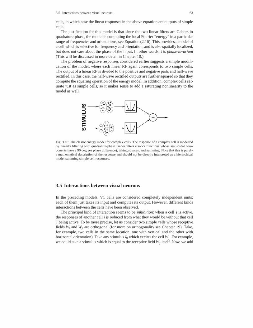
3.5 Interactions between visual neurons 63
cells, in which case the linear responses in the above equation are outputs of simplecells.
The justification for this model is that since the two linear filters are Gabors inquadrature-phase, the model is computing the local Fourier“energy” in a particularrange of frequencies and orientations, see Equation (2.16). This provides a model ofa cell which is selective for frequency and orientation, andis also spatially localized,but does not care about the phase of the input. In other words it is phase-invariant(This will be discussed in more detail in Chapter 10.)
The problem of negative responses considered earlier suggests a simple modifi-cation of the model, where each linear RF again corresponds to two simple cells.The output of a linear RF is divided to the positive and negative parts and half-waverectified. In this case, the half-wave rectified outputs are further squared so that theycompute the squaring operation of the energy model. In addition, complex cells sat-urate just as simple cells, so it makes sense to add a saturating nonlinearity to themodel as well.
++
++
−
+
+++
++++
+
−−−−
−−−
−
−−−−−−
++++
+++S
TIM
ULU
S
Fig. 3.10: The classic energy model for complex cells. The response of a complex cell is modelledby linearly filtering with quadrature-phase Gabor filters (Gabor functions whose sinusoidal com-ponents have a 90 degrees phase difference), taking squares, and summing. Note that this is purelya mathematical description of the response and should not bedirectly interpreted as a hierarchicalmodel summing simple cell responses.
3.5 Interactions between visual neurons
In the preceding models, V1 cells are considered completelyindependent units:each of them just takes its input and computes its output. However, different kindsinteractions between the cells have been observed.
The principal kind of interaction seems to beinhibition: when a cellj is active,the responses of another celli is reduced from what they would be without that cellj being active. To be more precise, let us consider two simple cells whose receptivefieldsWi andWj are orthogonal (for more on orthogonality see Chapter 19). Take,for example, two cells in the same location, one with vertical and the other withhorizontal orientation). Take any stimulusI0 which excites the cellWj . For example,we could take a stimulus which is equal to the receptive fieldWj itself. Now, we add

64 3 Outline of the visual system
another stimulus pattern, sayI1, to I0. This simply means that we add the intensitiespixel-by-pixel, showing the following stimulus to the retina:
I(x,y) = I0(x,y)+ I1(x,y) (3.8)
The added stimulusI1 is often called a mask or a pedestal.The point is that by choosingI1 suitably, we can demonstrate a phenomenon
which is probably due to interaction between the two cells. Specifically, let uschoose a stimulus which is equal to the receptive field of celli: I1 = Wi . This ismaximally excitatory for the celli, but it is orthogonal to the receptive field of cellj. With this kind of stimuli, the typical empirical observation is that the cellj has alower firing rate for the compound stimulusI = I0+ I1 than forI0 alone. This inhibi-tion cannot be explained by the linear models (or the linear-nonlinear models). ThemaskI1 should have no effect on the linear filter stage, because the mask is orthog-onal to the receptive fieldWj . So, to incorporate this phenomenon in our models,we must include some interaction between the linear filters:The outputs of somemodel cells must reduce the outputs of others. (It is not completely clear whetherthis empirical phenomenon is really due to interaction between the cells, but that isa widely-held view, so it makes sense to adopt it in our models.)
a) b) c)
Fig. 3.11: Interaction between different simple cells.a) Original stimulusI0 of a simple cell, cho-sen here as equal the receptive field ofWj . b) Masking patternI1 which is orthogonal toI0. c)Compound stimulusI . The response toI is smaller than the response toI0 although the linearmodels predicts that the responses should be equal.
This phenomenon is typically called “contrast gain control”. The idea is thatwhen there is more contrast in the image (due to the addition of the mask), thesystem adjusts its responses to be generally weaker. It is thought to be necessarybecause of the saturating nonlinearity in the cells and the drastic changes in illumi-nation conditions observed in the real world. For example, the cells would be re-sponding with the maximum value most of the time in bright daylight (or a brightlylit part of the visual scene), and they would be responding hardly at all in a dimenvironment (or a dimly lit part of the scene). Gain control mechanisms alleviate
3.6 Topographic organization 65
this problem by normalizing the variation of luminance overdifferent scenes, ordifferent parts of the same scene. For more on this point, seeSection 9.5.2
This leads us to one of the most accurate currently known simple-cell models, interms of predictive power, the divisive normalization model. Let W1, . . . ,WK denotethe receptive fields of those cells whose receptive fields areapproximately in thesame location, andσ a scalar parameter. In the divisive normalization model, theoutput of the cell corresponding to RFWj is given by
r j =f(
∑x,yWj(x,y)I(x,y))
∑Ki=1 f
(
∑x,yWi(x,y)I(x,y))+ σ2
, (3.9)
where f is again a static nonlinearity, such as the half-wave rectification followedby squaring. This divisive normalization model provides a simple account of con-trast gain control mechanisms. In addition, it also automatically accounts for suchsimple-cell nonlinearities as response saturation and threshold. In fact, if the inputstimulus is such that it only excites cellj, and the linear responses in the denomi-nator are all zero expect for the one corresponding to cellj, the model reduces tothe linear-nonlinear model in Section 3.4.1. If we further define f to be the squarefunction, we get the nonlinearity in Equation 3.7.
3.6 Topographic organization
A further interesting point is how the receptive fields of neighbouring cells are re-lated. In the retina, the receptive fields of retinal ganglion cells are necessarily linkedto the physical position of the cells. This is due to the fact that the visual fieldis mapped in an orderly fashion to the retina. Thus, neighbouring retinal ganglioncells respond to neighbouring areas of the visual field. However, there is nothing toguarantee the existence of a similar organization further up the visual pathway.
But the fact of the matter is that, just like in the retina, neighbouring neurons inthe LGN and in V1 tend to have receptive fields covering neighbouring areas of thevisual field. This phenomenon is calledretinotopy. Yet this is only one of severaltypes of organization. In V1, the orientation of receptive fields also tends to shiftgradually along the surface of the cortex. In fact, neurons are often approximatelyorganized according to several functional parameters (such as location, frequency,orientation) simultaneously. This kind oftopographic organizationalso exists inmany other visual areas.
Topographical representations are not restricted to cortical areas devoted to vi-sion, but are present in various forms throughout the brain.Examples include the
2 In fact, different kinds of gain control mechanisms seem to be operating in different parts ofthe visual system. In the retina, such mechanisms normalizethe general luminance level of theinputs, hence the name “luminance gain control”. Contrast gain control seems to be done after thatinitial gain control. The removal of the mean grey-scale value (DC component) that we do in laterchapters can be thought to represent a simple luminance gaincontrol mechanism.

66 3 Outline of the visual system
tonotopic map (frequency-based organization) in the primary auditory cortex andthe complete body map for the sense of touch. In fact, one might be pressed to finda brain area that would not exhibit any sort of topography.
3.7 Processing after the primary visual cortex
From V1, the visual signals are sent to other areas, such as V2, V4, and V5, calledextrastriateas another name for V1 is the “striate cortex”. The function of someof these areas (mainly V5, which analyzes motion) is relatively well understood,but the function of most of them is not really understood at all. For example, itis assumed that V2 is the next stage in the visual processing,but the differencesin the features computed in V1 and V2 are not really known. V4 has been vari-ously described as being selective to long contours, corners, crosses, circles, “non-Cartesian” gratings, colour, or temporal changes (see the references section below).Another problem is that the extrastriate cortex may be quitedifferent in humansand monkeys (not to mention other experimental animals), soresults from animalexperiments may not generalize to humans.
3.8 References
Among general introductions to the visual system, see, e.g., (Palmer, 1999). A mostinteresting review of the state of modelling of the visual cortex, with extensive ref-erences to experiments, is in (Carandini et al, 2005).
For a textbook account of reverse correlation, see e.g. (Dayan and Abbott, 2001);reviews are (Ringach and Shapley, 2004; Simoncelli et al, 2004). Classic applicationof reverse correlation for estimating simple cell receptive fields is (Jones and Palmer,1987b; Jones et al, 1987; Jones and Palmer, 1987a). For spatiotemporal extensionssee (DeAngelis et al, 1993a,b). LGN responses are estimated, e.g., in (Cai et al,1997), and retinal ones, e.g. in (Davis and Naka, 1980).
The nonlinearities in neuron responses are measured in (Anzai et al, 1999b;Ringach and Malone, 2007); theoretical studies include (Hansel and van Vreeswijk,2002; Miller and Troyer, 2002). These studies concentrate on the “thresholding”part of the nonlinearity, ignoring saturation. Reverse correlation in the presence ofnonlinearities is considered in (Nykamp and Ringach, 2002).
A review on contrast gain control can be found in (Carandini,2004). The divisivenormalization model is considered in (Heeger, 1992; Carandini et al, 1997, 1999).More on the interactions can be found in (Albright and Stoner, 2002). For reviewof the topographic organization in different parts of the cortex, see (Mountcastle,1997).
A discussion on our ignorance of V2 function can be found in (Boynton andHedge, 2004). Proposed selectivities in V4 include long contours (Pollen et al,

3.9 Exercices 67
2002), corners and related features (Pasupathy and Connor,1999, 2001), crosses,circles, and other non-Cartesian gratings (Gallant et al, 1993; Wilkinson et al, 2000),as well as temporal changes (Gardner et al, 2005). An alternative viewpoint is thatthe processing might be quite similar in most extrastriate areas, the main differencebeing the spatial scale (Hegde and Essen, 2007). A model of V5 is proposed in(Simoncelli and Heeger, 1998).
Basic historical references on the visual cortex include (Hubel and Wiesel, 1962,1963, 1968, 1977).
3.9 Exercices
Mathematical exercises
1. Show that the addition of a mask which is orthogonal to the receptive field, as inSection 3.5 should not change the output of the cell in the linear model
2. What is the justification for using the same letterd for the constants in Equa-tions (3.6) and (3.7)?
Computer assignments
1. Plot function in Equation (3.7) and compare with the function in (3.6).2. Receptive fields in the ganglion cells and the LGN are oftenmodelled as a
“difference-of-gaussians” model in whichW(x,y) is defined as
exp(− 1
2σ21
[(x−x0)2+(y−y0)
2])−aexp(− 1
2σ22
[(x−x0)2 +(y−y0)
2]) (3.10)
Plot the receptive fields for some choices of the parameters.Find some parametervalues that reproduce a center-surround receptive field.


Chapter 4Multivariate probability and statistics
This chapter provides the theoretical background in probability theory and statis-tical estimation needed in this book. This is not meant as a first introduction toprobability, however, and the reader is supposed to be familiar with the basics ofprobability theory. The main emphasis here is on the extension of the basic notionsto multidimensionaldata.
4.1 Natural images patches as random vectors
To put the theory on a concrete basis, we shall first discuss the fundamental idea onhow natural image patches can be considered as a random vector.
A random vector is a vector whose elements are random variables. Randomnesscan be defined in different ways. In probability theory, it isusually formalized byassuming that the value of the random variable or vector depends on some othervariable (“state of the world”) whose value we do not know. So, the randomness isdue to our ignorance.
In this book, an image patchI is typically modelled as a random vector, whoseobtained values (called “observations”) are the numericalgrey-scale values of pixelsin a patch (window) of a natural image. A patch simply means a small sub-image,such as the two depicted in Fig. 1.3. We use small patches because whole imageshave too large dimensions for existing computers (we must beable to perform com-plicated computations on a large number of such images or patches). A typical patchsize we use in this book is 32×32 pixels.
To get one observation of the random vector in question, we randomly select oneof the images in the image set we have, and then randomly select the location of theimage patch. The randomness of the values in the vector stemsfrom the fact thatthe patch is taken in some “random” position in a “randomly” selected image fromour database. The “random” position and image selection arebased on a randomnumber generator implemented in a computer.
69

70 4 Multivariate probability and statistics
It may be weird to call an image patch a “vector” as it is two-dimensional andcould also be called a matrix. However, for the purposes of most of this book, atwo-dimensional image patch has to be treated like a one-dimensional vector, or apoint in the image space, as was illustrated in Fig. 1.5. (A point and a vector arebasically the same thing in this context.) This is because observed data are typicallyconsidered to be such vectors in statistics, and matrices are used for something quitedifferent (that is, to represent linear transformations, see Section 19.3 for details).In practical calculations, one often has to transform the image patches into one-dimensional vectors, i.e. “vectorize” them. Such a transformation can be done inmany different ways, for example by scanning the numerical values in the matrixrow-by-row; the statistical analysis of the vector is not atall influenced by the choiceof that transformation. In most of the chapters in this book,it is assumed that sucha transformation has been made.
On a more theoretical level, the random vector can also represent the whole set ofnatural images, i.e. each observation is one natural image,in which case the databaseis infinitely large and does not exist in reality.
4.2 Multivariate probability distributions
4.2.1 Notation and motivation
In this chapter, we will denote random variables byz1,z2, . . . ,zn ands1,s2, . . . ,sn
for some numbern. Taken together, the random variablesz1,z2, . . . ,zn form ann-dimensional random vector which we denote byz:
z =
z1
z2...
zn
(4.1)
Likewise, the variabless1,s2, . . . ,sn can be collected to a random vector, denoted bys.
Although we will be considering general random vectors, in order to make thingsconcrete, you can think of eachzi as the grey-scale value of a pixel in the imagepatch. In the simple case of two variables,z1 andz2, this means that you take samplesof two adjacent pixels (say, one just to the right of the other). A scatter plot of sucha pixel pair is given in Fig. 4.1. However, this is by no means the only thing thevariables can represent; in most chapters of this book, we will also consider variouskinds of features which are random variables as well.
The fundamental goal of the models in this book is to describethe probabilitydistribution of the random vector of natural image patches.So, we need to nextconsider the concept of a probability density function.

4.2 Multivariate probability distributions 71
−4 −2 0 2 4 6−4
−2
0
2
4
6
Fig. 4.1: Scatter plot of the grey-scale values of two neighbouring pixels. The horizontal axis givesthe value of the pixel on the left, and the vertical axis givesthe value of the pixel on the right. Eachdot corresponds to one observed pair of pixels.
4.2.2 Probability density function
A probability distribution of a random vector such asz is usually represented usingaprobability density function(pdf). The pdf at a point in then-dimensional space isdenoted bypz.
The definition of the pdf of a multidimensional random vectoris a simple gen-eralization of the definition of the pdf of a random variable in one dimension. Letus first recall that definition. Denote byz a random variable. The idea is that wetake a small numberv, and look at the probability thatz takes a value in the interval[a,a+v] for any givena. Then we divide that probability byv, and that is the valueof the probability density function at the pointa. That is
pz(a) =P(z is in [a,a+v])
v(4.2)
This principle is illustrated in Fig. 4.2. Rigorously speaking, we should take thelimit of an infinitely smallv in this definition.
This principle is simple to generalize to the case of ann-dimensional randomvector. The value of the pdf function at a point, saya = (a1,a2, . . . ,an), gives theprobability that an observation ofz belongs to a small neighbourhood of the pointa, divided by the volume of the neighbourhood. Computing the probability that thevalues of eachzi are between the values ofai andai +v, we obtain
pz(a) =P(zi is in [ai ,ai +v] for all i)
vn (4.3)
wherevn is the volume of then-dimensional cube whose edges all have lengthv.Again, rigorously speaking, this equation is true only in the limit of infinitely smallv.
A most important property of a pdf is that it is normalized: its integral is equal toone ∫
pz(a)da = 1 (4.4)

72 4 Multivariate probability and statistics
a a+vFig. 4.2: The pdf of a random variable at a pointa gives the probability that the random variabletakes a value in a small interval[a,a+ v], divided by the length of that interval, i.e.v. In otherwords, the shaded area, equal top(a)v, gives the probability that that the variable takes a value inthat interval.
This constraint means that you cannot just take any non-negative function and saythat it is a pdf: you have to normalize the function by dividing it by its integral.(Calculating such an integral can actually be quite difficult and sometimes leads toserious problems, as discussed in Chapter 21).
For notational simplicity, we often omit the subscriptz. We often also writep(z)which means the value ofpz at the pointz. This simplified notation is rather ambigu-ous because nowz is used as an ordinary vector (likea above) instead of a randomvector. However, often it can be used without any confusion.
Example 1 The most classic probability density function for two variables is thegaussian, or normal, distribution. Let us first recall the one-dimensional gaussiandistribution, which in the basic case is given by
p(z) =1√2π
exp(−12
z2) (4.5)
It is plotted in Fig. 4.3 b). This is the “standardized” version (mean is zero andvariance is one), as explained below. The most basic case of atwo-dimensionalgaussian distribution is obtained by taking this one-dimensional pdf separately foreach variables, and multiplying them together. (The meaning of such multiplicationis that the variables are independent, as will be explained below.) Thus, the pdf isgiven by
p(z1,z2) =1
2πexp(−1
2(z2
1 +z22)) (4.6)
A scatter plot of the distribution is shown in Fig. 4.3 a). Thetwo-dimensional pdfitself is plotted in Fig. 4.3 c).
Example 2 Let us next consider the following two-dimensional pdf:

4.3 Marginal and joint probabilities 73
p(z1,z2) =
{
1, if |z1|+ |z2|< 1
0, otherwise(4.7)
This means that the data is uniformly distributed inside a square which has beenrotated 45 degrees. A scatter plot of data from this distribution is shown in Figure 4.4a).
a)
−4 −2 0 2 4−4
−2
0
2
4 b)
−4 −2 0 2 40
0.1
0.2
0.3
0.4
0.5
c)
−50
5
−5
0
50
0.1
0.2
Fig. 4.3: a) scatter plot of the two-dimensional gaussian distributionin Equation (4.6).b) Theone-dimensional standardized gaussian pdf. As explained in Section 4.3, it is also the marginaldistribution of one of the variables in a), and furthermore,turns out to be equal to the conditionaldistribution of one variable given the other variable.c) The probability density function of thetwo-dimensional gaussian distribution.
4.3 Marginal and joint probabilities
Consider the random vectorz whose pdf is denoted bypz. It is important to makea clear distinction between thejoint pdf and themarginal pdf’s. The joint pdf isjust what we called pdf above. The marginal pdf’s are what youmight call the

74 4 Multivariate probability and statistics
a)
−1.5 −1 −0.5 0 0.5 1 1.5−1.5
−1
−0.5
0
0.5
1
1.5 b)
−1.5 −1 −0.5 0 0.5 1 1.5−0.5
0
0.5
1
1.5
c)
−1.5 −1 −0.5 0 0.5 1 1.5−0.5
0
0.5
1
1.5
2
2.5 d)
−1.5 −1 −0.5 0 0.5 1 1.5−0.5
0
0.5
1
1.5
2
2.5
Fig. 4.4:a) scatter plot of data obtained from the pdf in Eq. (4.7).b) marginal pdf of one of thevariables in a).c) conditional pdf ofz2 givenz1 = 0. d) conditional pdf ofz2 givenz1 = .75
“individual” pdf’s of zi , i.e. the pdf’s of those variables,pz1(z1), pz2(z2), . . . whenwe just consider one of the variables and ignore the existence of the other variables.
There is actually a simple connection between marginal and joint pdf’s. We canobtain a marginal pdf by integrating the joint pdf over one ofthe variables. This issometimes called “integrating out”. Consider for simplicity the case where we onlyhave two variables,z1 andz2. Then, the marginal pdf ofz1 is obtained by
pz1(z1) =
∫
pz(z1,z2)dz2 (4.8)
This is a continuous-space version of the intuitive idea that for a given value ofz1,we “count” how many observations we have with that value, going through all thepossible values ofz2.1 (In this continuous-valued case, no observed values ofz1 are
1 Note again that the notation in Eq. (4.8) is sloppy, because now z1 in the parentheses, both onthe left and the right-hand side, stands for any valuez1 might obtain, although the same notation isused for the random quantity itself. A more rigorous notation would be something like:
pz1(v1) =∫
pz(v1,v2)dv2 (4.9)

4.4 Conditional probabilities 75
likely to be exactly equal to the specified value, but we can use the idea of a smallinterval centred around that value as in the definition of thepdf above.)
Example 3 In the case of the gaussian distribution in Equation (4.6), we have
p(z1) =
∫
p(z1,z2)dz2 =
∫1
2πexp(−1
2(z2
1 +z22))dz2
=1√2π
exp(−12
z21)∫
1√2π
exp(−12
z22)dz2 (4.10)
Here, we used the fact that the pdf is factorizable since exp(a+b) = exp(a)exp(b).In the last integral, we recognize the pdf of the one-dimensional gaussian distribu-tion of zero mean and unit variance given in Equation (4.5). Thus, that integral isone, because the integral of any pdf is equal to one. This means that the marginaldistributionp(z1) is just the the classic one-dimensional standardized gaussian pdf.
Example 4 Going back to our example in Eq. (4.7), we can calculate the marginalpdf of z1 to equal
pz1(z1) =
{
1−|z1|, if |z1|< 1
0, otherwise(4.11)
which is plotted in Fig. 4.4 b), and shows the fact that there is more “stuff” nearthe origin, and no observation can have an absolute value larger than one. Due tosymmetry, the marginal pdf ofz2 has exactly the same form.
4.4 Conditional probabilities
Another important concept is theconditionalpdf of z2 givenz1. This means the pdfof z2 when we have observed the value ofz1. Let us denote the observed value ofz1
by a. Then conditional pdf is basically obtained by just fixing the value ofz1 to a inthe pdf, which givespz(a,z2). However, this is not enough because a pdf must havean integral equal to one. Therefore, we must normalizepz(a,z2) by dividing it byits integral. Thus, we obtain the conditional pdf, denoted by p(z2 |z1 = a) as
p(z2 |z1 = a) =pz(a,z2)
∫pz(a,z2)dz2
(4.12)
Note that the integral in the denominator equals the marginal pdf of z1 at pointa, sowe can also write
where we have used two new variables,v1 to denote the point where we want to evaluate themarginal density, andv2 which is the integration variable. However, in practice we often do notwant to introduce new variable names in order to keep things simple, so we use the notation inEq. (4.8).

76 4 Multivariate probability and statistics
p(z2 |z1 = a) =pz(a,z2)
pz1(a)(4.13)
Again, for notational simplicity, we can omit the subscripts and just write
p(z2 |z1 = a) =p(a,z2)
p(a)(4.14)
or, we can even avoid introducing the new quantitya and write
p(z2 |z1) =p(z1,z2)
p(z1)(4.15)
Example 5 For the gaussian density in Equation (4.6), the computationof the con-ditional pdf is quite simple, if we use the same factorization as in Equation (4.10):
p(z2|z1) =p(z1,z2)
p(z1)=
1√2π exp(− 1
2z21)
1√2π exp(− 1
2z22)
1√2π exp(− 1
2z21)
=1√2π
exp(−12
z22) (4.16)
which turns out to be the same as the marginal distribution ofz2. (This kind of situ-ation wherep(z2|z1) = p(z2) is related to independence as discussed in Section 4.5below.)
Example 6 In our example pdf in Eq. (4.7), the conditional pdf changes quite a lotas a function of the valuea of z1. If z1 is zero (i.e.a = 0), the conditional pdf ofz2
is the uniform density in the interval[−1,1]. In contrast, ifz1 is close to 1 (or -1),the values that can be taken byz2 are quite small. Simply fixingz1 = a in the pdf,we have
p(a,z2) =
{
1, if |z2|< 1−|a|0 otherwise
(4.17)
which can be easily integrated:∫
p(a,z2)dz2 = 2(1−|a|) (4.18)
(This is just the length of the segment in whichz2 is allowed to take values.) So, weget
p(z2|z1) =
{1
2−2|z1| , if |z2|< 1−|z1|0 otherwise
(4.19)
where we have replaceda by z1. This pdf is plotted forz1 = 0 andz1 = 0.75 inFig. 4.4 a) and b), respectively.
Generalization to many dimensions The concepts of marginal and conditionalpdf’s extend naturally to the case where we haven random variables instead of justtwo. The point is that instead of two random variables,z1 andz2, we can have two

4.5 Independence 77
random vectors, sayz1 andz2, and use exactly the same formulas as for the tworandom variables. So, starting with a random vectorz, we take some of its variablesand put them in the vectorz1, and leave the rest in the vectorz2
z =
(z1
z2
)
(4.20)
Now, the marginal pdf ofz1 is obtained by the same integral formula as above:
pz1(z1) =
∫
pz(z1,z2)dz2 (4.21)
and, likewise, the conditional pdf ofz2 givenz1 is given by:
p(z2 |z1) =p(z1,z2)
p(z1)(4.22)
Both of these are, naturally, multidimensional pdf’s.
Discrete-valued variables For the sake of completeness, let us note that theseformulas are also valid for random variables with discrete values; then the integralsare simply replaced by sums. For example, for the conditional probabilities, wesimply have
P(z2 |z1) =Pz(z1,z2)
Pz1(z1)(4.23)
where marginal probability ofz1 can be computed as
Pz1(z1) = ∑z2
Pz(z1,z2) (4.24)
4.5 Independence
Let us consider two random variables,z1 andz2. Basically, the variablesz1 andz2
are said to be statistically independent if information on the value taken byz1 doesnot give any information on the value ofz2, and vice versa.
As an example, let us consider again the grey-scale values oftwo neighbouringpixels. As in Fig. 4.1, we go through many different locations in an image in randomorder, and take the grey-scale values of the pixels as the observed values of the tworandom variables. These random variables willnotbe independent. One of the basicstatistical properties of natural images is that two neighbouring pixels are depen-dent. Intuitively, it is clear that two neighbouring pixelstend to have very similargrey-scale values: If one of them is black, then the other oneis black with a highprobability, so they do give information on each other. Thisis seen in the obliqueshape (having an angle of 45 degrees) of the data “cloud” in Fig. 4.1. Actually, the

78 4 Multivariate probability and statistics
grey-scale values are correlated, which is a special form ofdependence as we willsee below.
The idea thatz1 gives no information onz2 can be intuitively expressed using con-ditional probabilities: the conditional probabilityp(z2 |z1) should be just the sameasp(z2):
p(z2 |z1) = p(z2) (4.25)
for any observed valuea of z1. This implies
p(z1,z2)
p(z1)= p(z2) (4.26)
orp(z1,z2) = p(z1)p(z2) (4.27)
for any values ofz1 andz2. Equation (4.27) is usually taken as the definition ofindependence because it is mathematically so simple. It simply says that the jointpdf must be a product of the marginal pdf’s. The joint pdf is then called factorizable.
The definition is easily generalized ton variablesz1,z2, . . . ,zn, in which case it is
p(z1,z2, . . . ,zn) = p(z1)p(z2) . . . p(zn) (4.28)
Example 7 For the gaussian distribution in Equation (4.6) and Fig. 4.3, we have
p(z1,z2) =1√2π
exp(−12
z21)×
1√2π
exp(−12
z22) (4.29)
So, we have factorized the joint pdf as the product of two pdf’s, each of whichdepends on only one of the variables. Thus,z1 andz2 are independent. This can alsobe seen in the form of the conditional pdf in Equation (4.16),which does not dependon the conditioning variable at all.
Example 8 For our second pdf in Eq. (4.7), we computed the conditional pdfp(z2|z1) in Eq. (4.19). This is clearly not the same as the marginal pdfin Eq. (4.11);it depends onz1. So the variables are not independent. (See the discussion just beforeEq. (4.17) for an intuitive explanation of the dependencies.)
Example 9 Consider the uniform distribution on a square:
p(z1,z2) =
{112, if |z1| ≤
√3 and|z2| ≤
√3
0, otherwise(4.30)
A scatter plot from this distribution is shown in Fig. 4.5. Now, z1 andz2 are indepen-dent because the pdf can be expressed as the product of the marginal distributions,which are

4.6 Expectation and covariance 79
p(z1) =
{1
2√
3, if |z1| ≤
√3
0, otherwise(4.31)
and the same forz2.
−4 −2 0 2 4−4
−2
0
2
4
Fig. 4.5: A scatter plot of the two-dimensional uniform distribution in Equation (4.30)
4.6 Expectation and covariance
4.6.1 Expectation
The expectation of a random vector, or its “mean” value, is, in theory, obtained bythe same kind of integral as for a single random variable
E{z}=
∫
pz(z)zdz (4.32)
In practice, the expectation can be computed by taking the expectation of each vari-able separately, completely ignoring the existence of the other variables
E{z}=
E{z1}E{z2}
...E{zn}
=
∫pz1(z1)z1dz1
∫pz2(z2)z2dz2
...∫
pzn(zn)zndzn
(4.33)
The expectation of any transformationg, whether one- or multidimensional, can becomputed as:
E{g(z)}=
∫
pz(z)g(z)dz (4.34)

80 4 Multivariate probability and statistics
The expectation is a linear operation, which means
E{az+bs}= aE{z}+bE{s} (4.35)
for any constantsa andb. In fact, this generalizes to any multiplication by a matrixM :
E{Mz}= ME{z} (4.36)
4.6.2 Variance and covariance in one dimension
The variance of a random variable is defined as
var(z1) = E{z21}− (E{z1})2 (4.37)
This can also be written var(z1) = E{(z1−E{z1})2}, which more clearly showshow variance measures average deviation from the mean value.
When we have more than one random variable, it is useful to analyze thecovari-ance:
cov(z1,z2) = E{z1z2}−E{z1}E{z2} (4.38)
which measures how well we can predict the value of one of the variables using asimple linear predictor, as will be seen below.
The covariance is often normalized to yield the correlationcoefficient
corr(z1,z2) =cov(z1,z2)
√
var(z1)var(z2)(4.39)
which is invariant to the scaling of the variables, i.e. it isnot changed if one or bothof the variables is multiplied by a constant.
If the covariance is zero, which is equivalent to saying thatthe correlation coef-ficient is zero, the variables are said to beuncorrelated.
4.6.3 Covariance matrix
The variances and covariances of the elements of a random vector z are often col-lected to acovariance matrixwhosei, j-th element is simply the covariance ofzi
andzj :
C(z) =
cov(z1,z1) cov(z1,z2) . . . cov(z1,zn)cov(z2,z1) cov(z2,z2) . . . cov(z2,zn)
.... . .
...cov(zn,z1) cov(zn,z2) . . . cov(zn,zn)
(4.40)

4.6 Expectation and covariance 81
Note that the covariance ofzi with itself is the same as the variance ofzi . So, thediagonal of the covariance matrix gives the variances. The covariance matrix is ba-sically a generalization of variance to random vectors: in many cases, when movingfrom a single random variable to random vectors, the covariance matrix takes theplace of variance.
In matrix notation, the covariance matrix is simply obtained as a generalizationof the one-dimensional definitions in Equations (4.38) and (4.37) as
C(z) = E{zzT}−E{z}E{z}T (4.41)
where taking the transposes in the correct places is essential. In most of this book,we will be dealing with random variables whose means are zero, in which case thesecond term in Equation (4.41) is zero.
If the variables are uncorrelated, the covariance matrix isdiagonal. If they areall further standardized to unit variance, the covariance matrix equals the identitymatrix.
The covariance matrix is the basis for the analysis of natural images in the nextchapter. However, in many further chapters, the covariancematrix is not enough,and we need further concepts, such as independence, so we need to understand theconnection between these concepts.
4.6.4 Independence and covariances
A most important property ofindependentrandom variablesz1 andz2 is that theexpectation of any product of a function ofz1 and a function ofz2 is equal to theproduct of the expectations:
E{g1(z1)g2(z2)}= E{g1(z1)}E{g2(z2)} (4.42)
for any functionsg1 andg2. This implies thatindependent variables are uncorre-lated, since we can takeg1(z) = g2(z) = z, in which case Eq. (4.42) simply says thatthe covariance is zero.
Example 10 In the standardized gaussian distribution in Equation (4.6), the meansof bothz1 andz2 are zero, and their variances are equal to one (we will not trytoprove this here). Actually, the word “standardized” means exactly that the meansand variances have been standardized in this way. The covariance cov(z1,z2) equalszero, because the variables are independent, and thus uncorrelated.
Example 11 What would be the covariance ofz1 andz2 in our example pdf inEq. (4.7)? First, we have to compute the means. Without computing any integrals,we can actually see thatE{z1}= E{z2}= 0 because of symmetry: both variables aresymmetric with respect to the origin, so their means are zero. This can be justified asfollows: take a new variabley = −z1. Because of symmetry of the pdf with respect

82 4 Multivariate probability and statistics
to zero, the change of sign has no effect and the pdf ofy is just the same as the pdfof z1. Thus, we have
E{y}= E{−z1}=−E{z1}= E{z1} (4.43)
which implies thatE{z1} = 0. Actually, the covariance is zero because of the samekind of symmetry with respect to zero. Namely, we have cov(y,z2) = cov(z1,z2)because again, the change of sign has no effect and the joint pdf of y,z2 is justthe same as the pdf ofz1,z2. This means cov(y,z2) = E{(−z1)z2} = −E{z1z2} =E{z1z2}. This obviously implies that the covariance is zero. The covariance matrixof the vectorz is thus diagonal (we don’t bother to compute the diagonal elements,which are the variances).
Example 12 Let’s have a look at a more classical example of covariances.Assumethatz1 has mean equal to zero and variance equal to one. Assume thatn (a “noise”variable) is independent fromz1. Let us consider a variablez2 which is a linearfunction ofx, with noise added:
z2 = az1 +n (4.44)
What is the covariance of the two variables? We can calculate
cov(z1,z2) = E{z1(az1 +n)}+0×E{z2}= aE{z21}+E{z1n}
= a+E{z1}E{n}= a+0×E{z1}= a (4.45)
Here, we have the equalityE{z1n} = E{z1}E{n} because of the uncorrelatednessof z1 andn, which is implied by their independence. A scatter plot of such data,created for parametera set at 0.5 and with noise variance var(n) = 1, is shown inFig. 4.6. The covariance matrix of the vectorz = (z1,z2) is equal to
C(z) =
(1 aa 1
)
(4.46)
Example 13 White noiserefers to a collection of random variables which are in-dependent and have the same distribution. (In some sources,only uncorrelatednessis required, not independence, but in this book the definition of white noise includesindependence.) Depending on the context, the variables could be the value of noiseat different time pointsn(t), or at different pixelsN(x,y). In the first case, whitenoise in the system is independent at different time points;in the latter, noise at dif-ferent pixels is independent. When modelling physical noise, which can be found inmost measurement devices, it is often realistic and mathematically simple to assumethat the noise is white.

4.7 Bayesian inference 83
−4 −2 0 2 4−4
−2
0
2
4
Fig. 4.6: A scatter plot of the distribution created by the dependence relation in Equation (4.44)
4.7 Bayesian inference
Bayesian inference is a framework that has recently been increasingly applied tomodel such phenomena as perception and intelligence. Thereare two viewpoints onwhat Bayesian inference is.
1. Bayesian inference attempts to infer underlying causes when we observe theireffects.
2. Bayesian inference uses prior information on parametersin order to estimatethem better.
Both of these goals can be accomplished by using the celebrated Bayes’ formula,which we will now explain.
4.7.1 Motivating example
Let us start with a classic example. Assume that we have a testfor a rare geneticdisorder. The test is relatively reliable but not perfect. For a patient with the disorder,the probability of a positive test result is 99%, whereas fora patient without thedisorder, the probability of a positive test is only 2%. Let us denote the test result byt and the disorder byd. A positive test result is expressed ast = 1 and a negative oneast = 0. Likewise,d = 1 means that the patient really has the disorder, whereasd = 0means the patients doesn’t. Then, the specifications we justgave can be expressedas the following conditional probabilities:
P(t = 1|d = 1) = .99 (4.47)
P(t = 1|d = 0) = .02 (4.48)

84 4 Multivariate probability and statistics
Because probabilities sum to one, we immediately find the following probabilitiesas well:
P(t = 0|d = 1) = .01 (4.49)
P(t = 0|d = 0) = .98 (4.50)
Now, the question we want to answer is:Given a positive test result, what is theprobability that the patient has the disorder?Knowing this probability is, of course,quite important when applying this medical test. Basically, we then want to computethe conditional probability of the formp(d = 1|t = 1). The order of the variables inthis conditional probability is reversed from the formulasabove. This is because theformulas above gave us the observable effects given the causes, but now we want toknow the causes, given observations of their effects.
To find that probability, let’s try to use the definition in Eq.(4.23)
P(d = 1|t = 1) =P(d = 1,t = 1)
P(t = 1)(4.51)
which presents us with two problems: We know neither the denominator nor the nu-merator. To get further, let’s assume we know the marginal distributionP(d). Then,we can easily find the numerator by using the definition of conditional probability
P(d = 1,t = 1) = P(t = 1|d = 1)P(d = 1) (4.52)
and after some heavy thinking, we see that we can also computethe denominator inEq. (4.51) by using the formula for marginal probability:
P(t = 1) = P(d = 1,t = 1)+P(d = 0,t = 1) (4.53)
which can be computed once we know the joint probabilities by(4.52) and its cor-responding version withd = 0. Thus, in the end we have
P(d = 1|t = 1) =P(t = 1|d = 1)P(d = 1)
P(t = 1|d = 1)P(d = 1)+P(t = 1|d = 0)P(d = 0)(4.54)
So, we see that the key to inferring the causes from observed effects is to knowthe marginal distribution of the causes, in this caseP(d). This distribution is alsocalled theprior distribution ofd, because it incorporates our knowledge of the caused prior to any observations. For example, let’s assume 0.1% of the patients giventhis test have the genetic disorder. Then, before the test our best guess is that agiven patient has the disorder with the probability of 0.001. However, after makingthe test, we have more information on the patient, and that information is givenby the conditional distributionP(d |t = 1) which we are trying to compute. Thisdistribution, which incorporates both our prior knowledgeond and the observationof t, is called theposteriorprobability.
To see a rather surprising phenomenon, let us plug in the valueP(d = 1) = 0.001 as the prior probability of disorder in Equation (4.54).Then,

4.7 Bayesian inference 85
we can calculate
P(d = 1|t = 1) =0.99×0.001
0.99×0.001+0.02× (1−0.001)≈ 0.05 (4.55)
Thus, even after a positive test result, the probability that the patient has the disorderis approximately 5%. Many people find this quite surprising,because they wouldhave guessed that the probability is something like 99%, as the test gives the rightresult in 99% of the cases.
This posterior probability depends very much on the prior probability. Assumethat half the tested patients actually have the disorder,P(d = 1) = 0.5. Then theposterior probability is 99%. This prior actually gives us no information because thechances are 50-50, and the 99% accuracy of the test is directly seen in the posteriorprobability.
Thus, in cases where the prior assigns very different probabilities to differentcauses, Bayesian inference shows that the posterior probabilities of the causes canbe very different from what one might expect by just looking at the effects.
4.7.2 Bayes’ Rule
The logic of the previous section was actually the proof of the celebrated Bayes’rule. In the general case, we consider a continuous-valued random vectors thatgives the causes andz that gives the observed effects. The Bayes’ rule then takes theform
p(s|z) =p(z|s) ps(s)
∫p(z|s) ps(s)ds
(4.56)
which is completely analogous to Eq. (4.54) and can be derived in the same way.This is the Bayes’ rule, in one of its formulations. It gives the posterior distributionof sbased on its prior distributionp(s) and the conditional probabilitiesp(z|s). Notethat instead of random variables, we can directly use vectors in the formula withoutchanging anything.
To explicitly show what is random and what is observed in Bayes rule, we shouldrewrite it as
p(s= b |z = a) =pz|s(a|b) ps(b)
∫pz|s(a|u) ps(u)du
(4.57)
wherepz|s(a|b) is the conditional probabilityp(z= a|s= b), a is the observed valueof z, andb is a possible value ofs. This form is, of course, much more difficult toread than Eq. (4.56).
In theoretical treatment, Bayes rule can sometimes be simplified because the de-nominator is actually equal top(z), which gives
p(s|z) =p(z|s) ps(s)
pz(z)(4.58)

86 4 Multivariate probability and statistics
However, in practice we usually have to use the form in Eq. (4.56) because we donot know how to directly computepz.
The prior ps contains the prior information on the random variables. The con-ditional probabilitiesp(z|s) show the connection between the observed quantityz(the “effect”) and the underlying variables (the “cause”).
Where do we get the prior distributionp(s)? In some cases,p(s) can be esti-mated, because we might be able to observe the originals. In the medical exampleabove, the prior distributionp(d) can be estimated if some of the patients are sub-jected to additional tests which are much more accurate (thus usually much moreexpensive) so that we really know for sure how many of the patients have the dis-order. In other cases, the prior might be formulated more subjectively, based on theopinion of an expert.
4.7.3 Non-informative priors
Sometimes, we have no information on the prior probabilities ps. Then, we shoulduse a non-informative prior that expresses this fact. In thecase of discrete variables,a non-informative prior is one that assigns the same probability to all the possiblevalues ofs (e.g. 50% probability of a patient to have the disorder or not).
In the case of continuous-valued priors defined in the whole real line[−∞,∞], thesituation is a bit more complicated. If we take a “flat” pdf that is constant,p(s) = c,it cannot be a real pdf because the integral of such a pdf is infinite (or zero ifc= 0).Such a prior is called improper. Still, they can often be usedin Bayesian inferenceeven though the non-integrability may pose some theoretical problems.
What happens in the Bayes rule if we take such a flat, non-informative prior? Weget
p(s|z) =p(z|s)c
∫p(z|s)cds
=p(z|s)
∫p(z|s)ds
(4.59)
The denominator does not depend ons (this is always true in Bayes’ rule), so wesee thatp(s|z) is basically the same ofp(z|s); it is just rescaled so that the integralis equal to one. What this shows is that if we have no information on the priorprobabilities, the probabilities of effects given the causes are simply proportional tothe probabilities of causes given the effects. However, if the prior p(s) is far fromflat, these two probabilities can be very different from eachother, as the exampleabove showed in the case where the disorder is rare.
4.7.4 Bayesian inference as an incremental learning process
The transformation from the prior probabilityp(s) to p(s|z) can be compared to anincremental (on-line) learning process where a biologicalorganism receives moreand more information in an uncertain environment.

4.7 Bayesian inference 87
In the beginning, the organism’s belief about the value of a quantity s is theprior probability p(s). Here we assume that the organism performs probabilisticinference: the organism does not “think” that it knows the value ofs with certainty;rather, it just assigns probabilities to different valuess might take. This does notmean that we assume the organism is highly intelligent and knows Bayes’ rule.Rather, we assume that the neural networks in the nervous system of the organismhave evolved to perform something similar.
Then, the organism receives information via sensory organsor similar means. Astatistical formulation of “incoming information” is thatthe organism observes thevalue of a random variablez1. Now, the belief of the organism is expressed by theposterior pdfp(s|z1). This pdf gives the probabilities that the organism assignstodifferent values ofs.
Next, assume that the organism observes another piece of information, sayz2.Then the organism’s belief is changed top(s|z1,z2)
p(s|z1,z2) =p(z1,z2 |s)p(s)
p(z1,z2)(4.60)
Assume further thatz2 is independent fromz1 givens, which meansp(z1,z2 |s) =p(z1 |s)p(z2 |s) (see Sec. 4.5 for more on independence). Then, the posteriorbe-comes
p(s|z1,z2) =p(z1 |s)p(z2 |s)p(s)
p(z1)p(z2)=
p(z2 |s)p(z2)
p(z1 |s)p(s)p(z1)
(4.61)
Now, the expressionp(z1 |s)p(s)/p(z1) is nothing but the posteriorp(s|z1) that theorganism computed previously. So, we have
p(s|z1,z2) =p(z2 |s)p(s|z1)
p(z2)(4.62)
The right-hand side is just like the Bayes’ Rule applied onsandz2 but instead of theprior p(s) it hasp(s|z1). Thus, the new posterior (after observingz2) is computedas if the previous posterior were a prior.
This points out an incremental learning interpretation of Bayes rule. When theorganism observes new information (new random variables),it updates its beliefabout the world by the Bayes rule, where the current belief istaken as the prior, andthe new belief is computed as the posterior. This is illustrated in Fig. 4.7
Such learning can happen on different time scales. It could be thats is a veryslowly changing parameter, say, the length of the arms (or tentacles) of the organism.In that case, the organism can collect a large number of observations over time, andthe belief would change very slowly. The first “prior” beliefthat the organism mayhave had before collection of any data, eventually loses itssignificance (see nextsection).
On the other hand,scould be a quantity that has to be computed instantaneously,say, the probability that the animal in front of you is tryingto eat you. Then, onlya few observed quantities (given by the current visual input) are available. Such

88 4 Multivariate probability and statistics
Prior p(s) Posterior p(s|z)
Replace prior by posterior
Observe new z
Fig. 4.7: Computation of posterior as an incremental learning process. Given the current prior, theorganism observes the inputz, and computes the posteriorp(s|z). The prior is then replaced by thisnew posterior, which is used as the prior in the future.
inference can then be heavily influenced by the prior information that the organismhas at the moment of encountering the animal. For example, ifthe animal is smalland cute, the prior probability is small, and even if the animal seems to behaves inan aggressive way, you will probably infer that it is not going to try to eat you.
4.8 Parameter estimation and likelihood
4.8.1 Models, estimation, and samples
A statistical modeldescribes the pdf of the observed random vector using a numberof parameters. The parameters typically have an intuitive interpretation; for exam-ple, in this book, they often define image features. A model isbasically a conditionaldensity of the observed data variable,p(z|α), whereα is the parameter. The param-eter could be a multidimensional vector as well. Different values of the parameterimply different distributions for the data, which is why this can be thought of as aconditional density.
For example, consider the one-dimensional gaussian pdf
p(z|α) =1√2π
exp(−12(z−α)2) (4.63)
Here, the parameterα has an intuitive interpretation as the mean of the distribution.Given α, the observed data variablez then takes values aroundα, with varianceequal to one.
Typically, we have a large number of observations of the random variablez,which might come from measuring some phenomenonn times, and these obser-vations are independent. The set of observations is called asamplein statistics.2 So,we want to use all the observations to better estimate the parameters. For example,
2 In signal processing, sampling refers the process of reducing a continuous signal to a discretesignal. For example, an imageI(x,y) with continuous-valued coordinatesx andy is reduced to a

4.8 Parameter estimation and likelihood 89
in the model in (4.63), it is obviously not a very good idea to estimate the mean ofthe distribution based on just a single observation.
Estimationhas a very boring mathematical definition, but basically it means thatwe want to find a reasonable approximation of the value of the parameter based onthe observations in the sample. A method (a formula or an algorithm) that estimatesα is called an estimator. The value given by the estimator for aparticular sample iscalled an estimate. Both are usually denoted by a hat:α.
Assume we now have a sample ofn observations. Let us denote the observedvalues byz(1),z(2), . . . ,z(n). Because the observations are independent, the jointprobability is simply obtained by multiplying the probabilities of the observations,so we have
p(z(1),z(2), . . . ,z(n) |α) = p(z(1) |α)× p(z(2) |α)× . . .× p(z(n) |α) (4.64)
This conditional density is called thelikelihood. It is often simpler to consider thelogarithm, which transforms products into sums. If we take the logarithm, we havethe log-likelihood as
logp(z(1),z(2), . . . ,z(n) |α) = logp(z(1) |α)+ logp(z(2) |α)+ . . .
+ logp(z(n) |α) (4.65)
4.8.2 Maximum likelihood and maximum a posteriori
The question is then, How can we estimateα? In a Bayesian interpretation, we canconsider the parameters as “causes” in Bayes’ rule, and the observed data are theeffects. Then, the estimation of the parameters means that we compute the posteriorpdf of the parameters using Bayes rule:
p(α |z(1) . . . ,z(n)) =p(z(1) . . . ,z(n) |α)p(α)
p(z(1) . . . ,z(n))(4.66)
In estimating parameters of the model, one usually takes a flat prior, i.e. p(α) = c.Moreover, the termp(z(1) . . . ,z(n)) does not depend onα, it is just for normaliza-tion, so we don’t need to care about its value. Thus, we see that
p(α |z(1) . . . ,z(n)) = p(z(1),z(2), . . . ,z(n) |α)×const. (4.67)
the posterior of the parameters is proportional to the likelihood in the case of a flatprior.
Usually, we want a single value as an estimate. Thus, we have to somehow sum-marize the posterior distributionp(α |z(1) . . . ,z(n)), which is a function ofα. The
finite-dimensional vector in which the coordinatesx andy take only a limited number of values(e.g. as on a rectangular grid). These two meanings of the word “sample” need to be distinguished.

90 4 Multivariate probability and statistics
most widespread solution is to use the value ofα that gives the highest value of theposterior pdf. Such estimation is calledmaximum a posteriori(MAP) estimation.
In the case of a flat prior, the maximum of the posterior distribution is obtained atthe same point as the maximum of the likelihood, because likelihood is then propor-tional to the posterior. Thus, the estimation is then calledthe maximum likelihoodestimator. If the prior is not flat, the maximum a posteriori estimator may be quitedifferent from the maximum likelihood estimator.
The maximum likelihood estimator has another intuitive interpretation: it givesthe parameter value that gives the highest probability for the observed data. This in-terpretation is slightly different from the Bayesian interpretation that we used above.
Sometimes the maximum likelihood estimator can be computedby a simple al-gebraic formula, but in most cases, the maximization has to be done numerically.For a brief introduction to optimization methods, see Chapter 18.
Example 13 In the case of the model in Eq. (4.63), we have
logp(z|α) =−12(z−α)2 +const. (4.68)
where the constant is not important because it does not depend onα. So, we havefor a sample
logp(z(1),z(2), . . . ,z(n) |α) =−12
n
∑i=1
(z(i)−α)2 +const. (4.69)
It can be shown (this is left as an exercise) that this is maximized by
α =1n
n
∑i=1
z(i) (4.70)
Thus, the maximum likelihood estimator is given by the average of the observedvalues. This is not a trivial result: in some other models, the maximum likelihoodestimator of such a location parameter is given by the median.
Example 14 Here’s an example of maximum likelihood estimation with a lessobvious result. Consider the exponential distribution
p(z|α) = α exp(−αz) (4.71)
wherez is constrained to be positive. The parameterα determines how likely largevalues are and what the mean is. Some examples of this pdf are shown in Fig. 4.8.The log-pdf is given by
logp(z|α) = logα−αz (4.72)
so the log-likelihood for a sample equals

4.8 Parameter estimation and likelihood 91
logp(z(1),z(2), . . . ,z(n) |α) = nlogα−αn
∑i=1
z(i) (4.73)
To solve for theα which maximizes the likelihood, we take the derivative of thiswith respect toα and find the point where it is zero. This gives
nα−
n
∑i=1
z(i) = 0 (4.74)
from which we obtain
α =1
1n ∑n
i=1z(i)(4.75)
So, the estimate is the reciprocal of the mean of thez in the sample.
0 1 2 30
0.5
1
1.5
2
2.5
3
Fig. 4.8: The exponential pdf in Equation (4.71) plotted forthree different values ofα , which isequal 1,2, or 3. The value ofα is equal to the value of the pdf at zero.
4.8.3 Prior and large samples
If the prior is not flat, we have the log-posterior
logp(α |z(1),z(2), . . . ,z(n))
= logp(α)+ logp(z(1) |α)+ logp(z(2) |α)+ . . .+ logp(z(n) |α)+const.(4.76)
which usually needs to be maximized numerically.Looking at Equation (4.76), we see an interesting phenomenon: whenn grows
large, the prior loses its significance. There are more and more terms in the like-lihood part, and, eventually, they will completely determine the posterior because

92 4 Multivariate probability and statistics
the single prior term will not have any influence anymore. In other words, whenwe have a very large sample, the data outweighs the prior information. This phe-nomenon is related to the learning interpretation we discussed above: the organismeventually learns so much from the incoming data that the prior belief it had in thevery beginning is simply forgotten.
4.9 References
Most of the material in this chapter is very classic. Most of it can be found in ba-sic textbooks to probability theory, while Section 4.8 can be found in introductorytextbooks to the theory of statistics. A textbook covering both areas is (Papoulis andPillai, 2001). Some textbooks on probabilistic machine learning also cover all thismaterial, in particular (Mackay, 2003; Bishop, 2006).
4.10 Exercices
Mathematical exercises
1. Show that a conditional pdf as defined in Eq. (4.15) is properly normalized, i.e.its integral is always equal to one.
2. Compute the mean and variance of a random variable distributed uniformly inthe interval[a,b] (b> a).
3. Considern scalar random variablesxi , i = 1,2, . . . ,n, having, respectively, thevariancesσ2
xi. Show that if the random variablesxi are all uncorrelated, the vari-
ance of their sum equals the sum of their variances
σ2y =
n
∑i=1
σ2xi
(4.77)
4. Assume the random vectorx has uncorrelated variables, all with unit variance.Show that the covariance matrix equals the identity matrix.
5. Take a linear transformation ofx in the preceding exercise:y = Mx for somematrixM . Show that the covariance matrix ofy equalsMM T .
6. Show that the maximum likelihood estimator of the mean of agaussian distribu-tion equals the sample average, i.e. Eq. (4.70).
7. Next we consider estimation of the variance parameter in agaussian distribution.We have the pdf
p(z|σ) =1√2πσ
exp(− z2
2σ2 ) (4.78)

4.10 Exercices 93
Formulate the likelihood and the log-likelihood, given a sample z(1), . . . ,z(n).Then, find the maximum likelihood estimator forσ .
Computer assignments
1. Generate 1,000 samples of 100 independent observations of a gaussian variableof zero mean and unit variance (e.g. with Matlab’srandn function). That is,you generate a matrix of size 1000×100 whose all elements are all independentgaussian observations.
a. Compute the average of each sample. This is the maximum likelihood estima-tor of the mean for that sample.
b. Plot a histogram of the 1,000 sample averages.c. Repeat all the above, increasing the sample size to 1,000 and to 10,000.d. Compare the three histograms. What is changing?
2. Generate a sample of 10,000 observations of a two-dimensional random vectorx with independent standardized gaussian variables. Put each observation in acolumn and each random variable in a row, i.e. you have a 2× 10000 matrix,denote it byX.
a. Compute the covariance matrix of this sample ofx, e.g. by using thecovfunction in Matlab. Note that the transpose convention in Matlab is differentfrom what we use here, so you have to apply thecov function of the transposeof X. Compare the result with the theoretical covariance matrix(what is itsvalue?)
b. Multiply x (or in practice,X) from the left with the matrix
A =
(2 30 1
)
(4.79)
Compute the covariance matrix ofAx. Compare withAAT .


Part IIStatistics of linear features

Chapter 5Principal components and whitening
The most classical method of analyzing the statistical structure of multidimen-sional random data is principal component analysis (PCA), which is also called theKarhunen-Loeve transformation, or the Hotelling transformation. In this chapter wewill consider the application of PCA to natural images. It will be found that it is not asuccessful model in terms of modelling the visual system. However, PCA providesthe basis for all subsequent models. In fact, before applying the more successfulmodels described in the following chapters, PCA is often applied as a preprocessingof the data. So, the investigation of the statistical structure of natural images muststart with PCA.
Before introducing PCA, however, we will consider a very simple and funda-mental concept: the DC component.
5.1 DC component or mean grey-scale value
To begin with, we consider a simple property of an image patch: its DC component.The DC component refers to the mean grey-scale value of the pixels in an image oran image patch.1 It is often assumed that the DC component does not contain inter-esting information. Therefore, it is often removed from theimage before any furtherprocessing to simplify the analysis. Removing the DC component thus means thatwe preprocess each image (in practice, image patch) as follows
I(x,y) = I(x,y)− 1m ∑
x′,y′I(x′,y′) (5.1)
wherem is the number of pixels. All subsequent computations would then useI .
1 The name ”DC” comes from a rather unrelated context in electrical engineering, in which itoriginally meant “direct current” as opposed to “alternating current”. The expression has becomerather synonymous with “constant” in electrical engineering.
97

98 5 Principal components and whitening
In section 1.8, we looked at the outputs of some simple feature detectors when theinput is natural images. Let us see what the effect of DC removal is on the statisticsof these features; the features are depicted in Fig. 1.10 on page 20. Let us denote theoutput of a linear feature detector with weightsWi(x,y) by s:
si = ∑x,y
Wi(x,y)I(x,y) (5.2)
The ensuing histograms of thesi , for the three detectors when input with naturalimages, and after DC removal, are shown in Fig. 5.1. Comparing with Fig. 1.11 onpage 20, we can see that the first histogram changes radically, where as the latter twodo not. This is because the latter two filters were not affected by the DC componentin the first place, which is because the sum of their weight wasapproximately zero:∑x,yW(x,y) = 0. Actually, the three histograms are now more similar to each other:the main difference is in the scale. However, they are by no means identical, as willbe seen in the analyses of this book.
The effect of DC component removal depends on the size of the image patch.Here, the patches were relatively small, so the removal had alarge effect on thestatistics. In contrast, removing the DC component from whole images has littleeffect on the statistics.
In the rest of this book, we will assume that the DC component has been removedunless otherwise mentioned. Removing the DC component alsomeans that the meanof anys is zero; this is intuitively rather obvious but needs some assumptions to beshown rigorously (see Exercises). Thus, in what follows we shall assume that themean of any features is zero.
a)
−4 −2 0 2 4 60
2000
4000
6000
8000 b)
−40 −20 0 20 400
2000
4000
6000
8000 c)
−10 −5 0 5 100
2000
4000
6000
8000
10000
Fig. 5.1: Effect of DC removal. These are histograms of the outputs of the filters in Fig. 1.10 whenthe output is natural images whose DC component has been removed. Left: output of Dirac filter,which is the same as the histogram of the original pixels themselves. Center: output of gratingfeature detector. Right: output of edge detector. The scales of the axes are different from those inFig. 1.10.
Some examples of natural image patches with DC component removed are shownin Figure 5.2. This is the kind of data analyzed in almost all of the rest of this book.

5.2 Principal component analysis 99
Fig. 5.2: Some natural image patches, with DC component removed.
5.2 Principal component analysis
5.2.1 A basic dependency of pixels in natural images
The point in PCA is to analyze the dependencies of the pixel grey-scale valuesI(x,y) andI(x′,y′) for two different pixel coordinate pairs(x,y) and(x′,y′). Morespecifically, PCA considers the second-order structure of natural images, i.e. thevariances and and covariances of pixel valuesI(x,y).
If the pixel values were all uncorrelated, PCA would have nothing to analyze.Even a rudimentary analysis of natural images shows, however, that the pixel val-ues are far from independent. It is intuitively rather clearthat natural images aretypically smoothin the sense that quite often, the pixel values are very similar intwo near-by pixels. This can be easily demonstrated by a scatter plot of the pixelvalues for two neighbouring pixels sampled from natural images. This is shown inFigure 5.3. The scatter plot shows that the pixels are correlated. In fact, we can com-pute the correlation coefficient (Equation 4.39), and it turns out to be approximatelyequal to 0.9.
Actually, we can easily compute the correlation coefficients of a single pixel withall near-by pixels. Such a plot is shown in grey-scale in Fig.5.4, both without re-moval of DC component (in a) and with DC removal (in b). We see that the correla-tion coefficients (and, thus, the covariances) fall off withincreasing distance. Thesetwo plots, with or without DC removal, look rather similar because the plots usedifferent scales; the actual values are quite different. Wecan take one-dimensionalcross-sections to see the actual values. They are shown in Fig. 5.4 c) and d). We see

100 5 Principal components and whitening
that without DC removal, all the correlation coefficients are strongly positive. Re-moving the DC components reduces the correlations to some extent, and introducesnegative correlations.
a)
−4 −2 0 2 4 6−4
−2
0
2
4
6 b)
−4 −2 0 2 4−4
−2
0
2
4
6
Fig. 5.3: Scatter plot of the grey-scale values of two neighbouring pixels.a) Original pixel values.The values have been scaled so that the mean is zero and the variance one.b) Pixel values afterremoval of DC component in a 32×32 patch.
5.2.2 Learning one feature by maximization of variance
5.2.2.1 Principal component as variance-maximizing feature
The covariances found in natural images pixel values can be analyzed by PCA. InPCA, the point is to find linear features that explain most of the variance of the data.
It is natural to start the definition of PCA by looking at the definition of the firstprincipal component. We consider the variance of the output:
var(s) = E{s2}− (E{s})2 = E{s2} (5.3)
where the latter equality is true becauseshas zero mean.Principal components are featuress that contain (or “explain”) as much of the
variance of the input data as possible. It turns out that the amount of variance ex-plained is directly related to the variance of the feature, as will be discussed inSection 5.3.1 below. Thus, the first principal component is defined as the feature, orlinear combination of the pixel values, which has the maximum variance. Finding afeature with maximum variance can also be considered interesting in its own right.The idea is to find the “main axis” of the data cloud, which is illustrated in Fig. 5.5.
Some constraint on the weightsW, which we call theprincipal componentweights, must be imposed as well. If no constraint were imposed, the maximumof the variance would be attained whenW becomes infinitely large (and the mini-

5.2 Principal component analysis 101
a) b)
c)
−15 −10 −5 0 5 10 150
0.2
0.4
0.6
0.8
1 d)
−15 −10 −5 0 5 10 15
0
0.2
0.4
0.6
0.8
1
Fig. 5.4: The correlation coefficients of a pixel (in the middle) with all other pixels.a) For originalpixels. Black is small positive and and white is one.b) After removing DC component. The scaleis different from a): black is now negative and white is plus one.c) A cross-section of a) in 1D toshow the actual values.d) A cross-section of b) in 1D.
Fig. 5.5: Illustration of PCA. The principal component of this (artificial) two-dimensional data isthe oblique axis plotted. Projection on the principal axis explains more of the variance of the datathan projection on any other axis.

102 5 Principal components and whitening
mum would be attained when all theW(x,y) are zero). In fact, just multiplying allthe weights inW by a factor of two, we would get a variance that is four timesas large, and by dividing all the coefficients by two the variance decreases to onequarter.
A natural thing to do is to constrain the norm ofW:
‖W‖=√
∑x,y
W(x,y)2 (5.4)
For simplicity, we constrain the norm to be equal to one, but any other value wouldgive the same results.
5.2.2.2 Learning one feature from natural images
What is then the feature detector that maximizes the variance of the output, givennatural image input, and under the constraint that the norm of the detector weightsequals one? We can find the solution by taking a random sample of image patches.Let us denote byT the total number of patches used, and byIt each patch, wheretis an index that goes from 1 toT. Then, the expectation ofs2 can be approximatedby the average over this sample. Thus, we maximize
1T
T
∑t=1
(
∑x,y
W(x,y)It(x,y)
)2
(5.5)
with respect to the weights inW(x,y), while constraining the values ofW(x,y) sothat the norm in Equation (5.4) is equal to one. The computation of the solution isdiscussed in Section 5.2.4.
Typical solutions for natural images are shown in Fig. 5.6. The feature detectoris an object of the same size and shape as an image patch, so it can be plotted as animage patch itself. To test whether the principal componentweights are stable, wecomputed it ten times for different image samples. It can be seen that the componentis quite stable.
Fig. 5.6: The feature detectors giving the first principal component of image windows of size32× 32, computed for ten different randomly sampled datasets taken from natural images. Thefeature detector is grey-scale-coded so that the grey-scale value of a pixel gives the value of thecoefficient at that pixel. Grey pixels mean zero coefficients, light-grey or white pixels are positive,and dark-grey or black are negative.

5.2 Principal component analysis 103
5.2.3 Learning many features by PCA
5.2.3.1 Defining many principal components
One of the central problems with PCA is that it basically gives only one well-definedfeature. It cannot be extended to the learning of many features in a very meaningfulway. However, if we want to model visual processing by PCA, itwould be absurdto compute just a single feature which would then be supposedto analyze the wholevisual scene.
Definition Typically, the way to obtain many principal components is bya “de-flation” approach: After estimating the first principal component, we want to findthe feature of maximum varianceunder the constraintthat the new feature must beorthogonalto the first one (i.e. the dot-product is zero, as in Equation 5.8). Thiswill then be called the second principal component. This procedure can be repeatedto obtain as many components as there are dimensions in the data space. To putthis formally, assume that we have estimatedk principal components, given by theweight vectorsW1,W2 . . . ,Wk. Then thek+1-th principal component weight vectoris defined by
maxW
var
(
∑x,y
I(x,y)W(x,y)
)
(5.6)
under the constraints
‖W‖=√
∑x,y
W(x,y)2 = 1 (5.7)
∑x,y
Wj(x,y)W(x,y) = 0 for all j = 1, . . . ,k (5.8)
An interesting property is that any two principal components are uncorrelated, andnot only orthogonal. In fact, we could change the constraintin the definition touncorrelatedness, and the principal components would be the same.
Critique of the definition This classic definition of many principal componentsis rather unsatisfactory, however. There is no really good justification for thinkingthat the second principal component corresponds to something interesting: it is nota feature that maximizes any property in itself. It only maximizes the variance notexplained by the first principal component.
Moreover, the solution is not quite well defined, since for natural images, thereare many principal components that give practically the same variance. After the firstfew principal components, the differences of the variancesof different directions getsmaller and smaller. This is a serious problem for the following reason. If two prin-cipal components, saysi andsj , have the same variance, then any linear combinationq1si + q2sj has the same variance as well,2 and the weightsq1Wi(x,y)+ q2Wj(x,y)
2 This is due to the fact that the principal components are uncorrelated, see Section 5.8.1.

104 5 Principal components and whitening
fulfill the constraints of unit norm and orthogonality, if wenormalize the coefficientsq1 andq2 so thatq2
1 + q22 = 1. So, not only we cannot say what is the order of the
components, but actually there is an infinite number of different components fromwhich we cannot choose the “right” one.
In practice, the variances of the principal components are not exactly equal dueto random fluctuations, but this theoretical result means that the principal compo-nents are highly dependent on those random fluctuations. In the particular sampleof natural images that we are using, the maximum variance (orthogonal to previouscomponents) can be obtained by any of these linear combinations. Thus, we cannotreally say what the 100th principal component is, for example, because the resultwe get from computing it depends so much on random sampling effects. This willbe demonstrated in the experiments that follow.
5.2.3.2 All principal components of natural images
The first 320 principal components of natural images patchesare shown in Fig-ure 5.7, while Figure 5.9 shows the variances of the principal components. For lackof space, we don’t show all the components, but it is obvious from the figure whatthey look like. As can be seen, the first couple of features seem quite meaningful:they are oriented, something like very low-frequency edge detectors. However, mostof the features given by PCA do not seem to be very interesting. In fact, after thefirst, say, 50 features, the rest seem to be just garbage. Theyare localized in fre-quency as they clearly are very high-frequency features. However, they do not seemto have any meaningful spatial structure. For example, theyare not oriented.
In fact, most of the features do not seem to be really well defined for the reasonexplained in the previous section: the variances are too similar for different features.For example, some of the possible 100th principal components, for different randomsets of natural image patches, are shown in Figure 5.8. The random changes in thecomponent are obvious.
5.2.4 Computational implementation of PCA
In practice, numerical solution of the optimization problem which defines the prin-cipal components is rather simple and based on what is calledthe eigenvalue de-composition. We will not go into the mathematical details here; they can be foundin Section 5.8.1. Briefly, the computation is based on the following principles
1. The variance of any linear feature as in Equation (5.2) canbe computed if wejust know the variances and covariances of the image pixels.
2. We can collect the variances and covariances of image pixels in a single matrix,called thecovariance matrix, as explained in Section 4.6.3. Each entry in the ma-trix then gives the covariance between two pixels—varianceis simply covarianceof a pixel with itself.

5.2 Principal component analysis 105
Fig. 5.7: The 320 first principal components weightsWi of image patches of size 32×32. The orderof decreasing variances is left to right on each row, and top to bottom.
Fig. 5.8: Ten different estimations of the 100th principal component of image windows of size32×32. The random image sample was different in each run.

106 5 Principal components and whitening
0 500 1000 1500−3
−2
−1
0
1
2
Fig. 5.9: The logarithms of the variances of the principal components for natural image patches,the first of which were shown in Fig. 5.7.
3. Any sufficiently sophisticated software for scientific computation is able to com-pute the eigenvalue decomposition of that matrix. (However, the amount of com-putation needed grows fast with the size of the image patch, so the patch sizecannot be too large.)
4. As a result of the eigenvalue decomposition we get two things. First, theeigen-vectors, which give theWi which are the principal component weights. Second,theeigenvalues, which give the variances of the principal componentssi . So, weonly need to order the eigenvectors in the order of descending eigenvalues, andwe have computed the whole PCA decomposition.
5.2.5 The implications of translation-invariance
Many of the properties of the PCA of natural images are due a particular property ofthe covariance matrix of natural images. Namely, the covariance for natural imagesis translation-invariant, i.e. it depends only on the distance
cov(I(x,y), I(x′,y′)) = f ((x−x′)2 +(y−y′)2) (5.9)
for some functionf . After all, the covariance of two neighbouring pixels is notlikely to be any different depending on whether they are on the left or the right sideof the image. (This form of translation-invariance should not be confused with theinvariances of complex cells, discussed in Section 3.4.2 and Chapter 10).

5.3 PCA as a preprocessing tool 107
The principal component weightsWi(x,y) for a covariance matrix of this formcan be shown to always have a very particular form: they are sinusoids:
Wi(x,y) = sin(ax+by+c) (5.10)
for some constantsa,b,c (the scaling is arbitrary so you could also multiplyWi witha constantd). See Section 5.8.2 below for a detailed mathematical analysis whichproves this.
The constantsa andb determine the frequency of the oscillation. For example,the first principal components have lower frequencies than the later ones. They alsodetermine the orientation of the oscillation. It can be seenin Fig. 5.7 that some ofthe oscillations are oblique while others are vertical and horizontal. Some have os-cillations in one orientation only, while others form a kindof checkerboard pattern.The constantc determines the phase.
The variances associated with the principal components thus tell how strongly thefrequency of the sinusoid is present in the data, which is closely related to computingthe power spectrum of the data.
Because of random effects in the sampling of image patches and computationof the covariance matrix, the estimated feature weights arenot exactly sinusoids.Of course, just the finite resolution of the images makes themdifferent from realsinusoidal functions.
Since the principal component weights are sinusoids, they actually perform somekind of Fourier analysis. If you apply the obtainedWi as feature detectors on animage patch, that will be related to a discrete Fourier transform of the image patch.In particular, this can be interpreted as computing the coefficients of the patch in thebasis given by sinusoidal functions, as discussed in Section 2.3.2.
An alternative viewpoint is that you could also consider thecomputation of theprincipal components as doing a Fourier analysis of the covariance matrix of theimage patch; this interesting connection will be considered in Section 5.6.
5.3 PCA as a preprocessing tool
So far, we have presented PCA as a method for learning features, which is the classicapproach to PCA. However, we saw that the results were ratherdisappointing in thesense that the features were not interesting as neurophysiological models, and theywere not even well-defined.
However, PCA is not a useless model. It accomplishes severalusefulpreprocess-ing tasks, which will be discussed in this section.

108 5 Principal components and whitening
5.3.1 Dimension reduction by PCA
One task where PCA is very useful is in reducing the dimensionof the data so thatthe maximum amount of the variance is preserved.
Consider the following general problem that also occurs in many other areasthan image processing. We have a very large number, saym, of random variablesx1, . . . ,xm. Computations that use all the variables would be too burdensome. Wewant to reduce the dimension of the data by linearly transforming the variables intoa smaller number, sayn, of variables that we denote byz1, . . . ,zn:
zi =m
∑j=1
wi j x j , for all i = 1, . . . ,n (5.11)
The number of new variablesn might be only 10% or 1% of the original numberm. We want to find the new variables so that they preserve as muchinformation onthe original data as possible. This “preservation of information” has to be exactlydefined. The most wide-spread definition is to look at the squared error that we getwhen we try to reconstruct the original data using thezi . That is, we reconstructx j
as a linear transformation∑i a jizi , minimizing the average error
E
∑
j
(
x j −∑i
a jizi
)2
= E
{
‖x−∑i
aizi‖2}
(5.12)
where thea ji are also determined so that they minimize this error. For simplicity, letus consider only transformations for which the transforming weights are orthogonaland have unit norm:
∑j
w2i j = 1, for all i (5.13)
∑j
wi j wk j = 0, for all i 6= k (5.14)
What is the best way of doing this dimension reduction? The solution is to takeas thezi then first principal components! (A basic version of this result is shown inthe exercises.) Furthermore, the optimal reconstruction weight vectorsai in Equa-tion (5.12) are given by the very same principal components weights which computethezi .
The solution is not uniquely defined, though, because any orthogonal transforma-tion of thezi is just as good. This is understandable because any such transformationof thezi contains just the same information: we can make the inverse transformationto get thezi from the transformed ones.
As discussed above, the features given by PCA suffer from theproblem of notbeing uniquely defined. This problem is much less serious in the case of dimensionreduction. What matters in the dimension reduction contextis not so much the actualcomponents themselves, but thesubspacewhich they span. Theprincipal subspace

5.3 PCA as a preprocessing tool 109
means the set of all possible linear combinations of then first principal components.It corresponds to taking all possible linear combinations of the principal componentweight vectorsWi associated with then principal components. As pointed out above,if two principal componentssi andsj have the same variance, any linear combina-tion q1si + q2sj has the same variance forq2
1 + q22 = 1. This is not a problem here,
however, since such a linear combination still belongs to the same subspace as thetwo principal componentssi andsj . Thus, it does not matter if we consider the com-ponentssi andsj , or two components of the formq1si +q2sj andr1si + r2sj wherethe coefficientsr1 andr2 give a different linear combination than theq1 andq2.
So, then-dimensional principal subspace is usually uniquely defined even if someprincipal components have equal variances. Of course, it may happen that then-thand the(n+ 1)-th principal components have equal variances, and that we cannotdecide which one to include in the subspace. But the effect onthe whole subspaceis usually quite small and can be ignored in practice.
Returning to the case of image data, we can rephrase this result by saying thatit is thesetof features defined by then first principal components and their linearcombinations that is (relatively) well defined, and not the features themselves.
5.3.2 Whitening by PCA
5.3.2.1 Whitening as normalized decorrelation
Another task for which PCA is quite useful is whitening. Whitening is an impor-tant preprocessing method where the image pixels are transformed to a set of newvariabless1, . . . ,sn so that thesi are uncorrelated and have unit variance:
E{sisj}=
{
0 if i 6= j
1 if i = j(5.15)
(It is assumed that all the variables have zero mean.) It is also said that the resultingvector(s1, . . . ,sn) is white.
In addition to the principal components weights being orthogonal, the principalcomponents themselves are uncorrelated, as will be shown inmore detail in Sec-tion 5.8.1. So, after PCA, the only thing we need to do to get whitened data is tonormalize the variances of the principal components by dividing them by their stan-dard deviations. Denoting the principal components byyi , this means we compute
si =yi
√
var(yi)(5.16)
to get whitened componentssi . Whitening is a useful preprocessing method thatwill be used later in this book. The intuitive idea is that it completely removes thesecond-order information of the data. “Second-order” means here correlations and

110 5 Principal components and whitening
variances. So, it allows us to concentrate on properties that are not dependent oncovariances, such as sparseness in the next chapter.
Whitening by PCA is illustrated in Figure 5.10.
a)
−1.5 0 1.5−1.5
−1
−0.5
0
0.5
1
1.5
u2
u1
b)
−1.5 0 1.5−1.5
−1
−0.5
0
0.5
1
1.5
c)
−1.5 0 1.5−1.5
−1
−0.5
0
0.5
1
1.5
Fig. 5.10: Illustration of PCA and whitening.a) The original data “cloud”. The arrows show theprincipal components. The first one points in the direction of the largest variance in the data, andthe second in the remaining orthogonal direction.b) When the data is transformed to the principalcomponents, i.e. the principal components are taken as the new coordinates, the variation in thedata is aligned with those new axes, which is because the principal components are uncorrelated.c) When the principal components are further normalized to unit variance, the data cloud hasequal variance in all directions, which means it has been whitened. The change in the lengths ofthe arrows reflects this normalization; the larger the variance, the shorter the arrow.
5.3.2.2 Whitening transformations and orthogonality
It must be noted that there are many whitening transformations. In fact, if the ran-dom variablessi , i = 1. . . ,n are white, then anyorthogonal transformationof thosevariables is also white (the proof is left as an exercise). Often, whitening is basedon PCA because PCA is a well-known method that can be computedvery fast, but

5.3 PCA as a preprocessing tool 111
it must be kept in mind that PCA is just one among the many whitening transforma-tions. Yet, PCA is a unique method because it allows us to combine three differentpreprocessing methods into one: dimension reduction, whitening, and anti-aliasing(which will be discussed in the next section).
In later chapters, we will often use the fact that the connection between orthog-onality and uncorrelatedness is even stronger for whiteneddata. In fact, if we com-pute two linear components∑i visi and∑i wisi from white data, they are uncorrelatedonly if the two vectorsv andw (which contain the entriesvi andwi , respectively)are orthogonal.
In general, we have the following theoretical result. For white data, multiplicationby a square matrix gives white components ifand only if the matrix is orthogonal.Thus, when we have computed one particular whitening transformation, we alsoknow thatonlyorthogonal transformations of the transformed data can be white.
Note here the tricky point in terminology: a matrix if calledorthogonal if itscolumns, or equivalently its rows, are orthogonal,and the norms of its columnsare all equal to one. To emphasize this, some authors call an orthogonal matrixorthonormal. We stick to the word “orthogonal” in this book.
5.3.3 Anti-aliasing by PCA
PCA also helps combat the problem ofaliasing, which refers to a class of problemsdue to the sampling of the data at a limited resolution — in ourcase the limitednumber of pixels used to represent an image. Sampling of the image loses infor-mation; this is obvious since we only know the image through its values at a finitenumber of pixels. However, sampling can also introduce lessobvious distortions inthe data. Here we consider two important ones, and show how PCA can help.
5.3.3.1 Oblique gratings can have higher frequencies
One problem is that in the case of the rectangular sampling grid, oblique higherfrequencies are overrepresented in the data, because the grid is able to representoblique oscillations which have a higher frequency than either the vertical or hori-zontal oscillations of the highest possible frequency.
This is because we can have an image which takes the form of a checkerboardas illustrated in Figure 5.11 a). If you draw long oblique lines along the white andblack squares, the distance between such lines is equal to
√
1/2 as can be calculatedby basic trigonometry. This is smaller than one, which is theshortest half-cycle (halfthe length of an oscillation) we can have in the vertical and horizontal orientation.(It corresponds to the Nyquist frequency as discussed in thenext subsection, andillustrated in Figure 5.11 b).
In the Fourier transform, this lack of symmetry is seen in thefact that the areaof possible 2-D frequencies is of the form of a square, instead of a circle as would

112 5 Principal components and whitening
be natural for data which is the same in all orientations (“rotation-invariant”, aswill be discussed in Section 5.7). Filtering out the highestoblique frequencies isthus a meaningful preprocessing step to avoid any artefactsdue to this aliasing phe-nomenon. (Note that we are here talking about the rectangular form of the samplinggrid, i.e. the relation of the pixels centerpoints to each other. This is not at all relatedto the shape of the sampling window, i.e. the shape of the patch.)
It turns out that we can simply filter out the oblique frequencies by PCA. Withnatural images, the last principal components are those that correspond to the high-est oblique frequencies. Thus, simple dimension reductionby PCA alleviates thisproblem.
a) b)
Fig. 5.11: Effects of sampling (limited number of pixels) onvery high-frequency gratings.a) Asinusoidal grating which has a very high frequency in the oblique orientation. The cycle of theoscillation has a length of 2
√
1/2 =√
2 which is shorter than the smallest possible cycle length(equal to two) in the vertical and horizontal orientations.b) A sinusoidal grating which has theNyquist frequency. Although it is supposed to be sinusoidal, due to the limited sampling (i.e.,limited number of pixels), it is really a block grating.
5.3.3.2 Highest frequencies cannot can have only two different phases
Another problem is that at the highest frequencies, we cannot have sinusoidal grat-ings with different phases. Let us consider the highest possible frequency, called inFourier theory the Nyquist frequency, which means that there is one cycle for everytwo pixels, see Figure 5.11 b). What happens when you change the phase of thegrating a little bit, i.e. shift the “sinusoidal” grating a bit? Actually, almost noth-ing happens: the grating does not shift at all because due to the limited resolutiongiven by the pixel size, it is impossible to represent a smallshift in the grating. (Thegrey-scale values will be changed; they depend on the match between the samplinglattice and the underlying sinusoidal they try to represent.) The sampled image re-ally changes only when the phase is changed so much that the best approximationis to flip all the pixels from white to black and vice versa.

5.4 Canonical preprocessing used in this book 113
Thus, a grating sampled at the Nyquist frequency can really have only two differ-ent phases which can be distinguished. This means that many concepts dependingon the phase of the grating, such as the phase tuning curve (Section 6.4) or phase-invariance (Chapter 10) are rather meaningless on the Nyquist frequency. So, wewould like to low-pass filter the image to be able to analyze such phenomena with-out the distorting effect of a limited resolution.
Again, we can alleviate this problem by PCA dimension reduction, because itamounts to discarding the highest frequencies.
5.3.3.3 Dimension selection to avoid aliasing
So, we would like to do PCA so that we get rid of the checkerboard patterns as wellas everything in the Nyquist frequency. On the other hand, wedon’t want to get ridof any lower frequencies.
To investigate the dimension reduction needed, we computedwhat amount ofcheckerboard and Nyquist gratings is present in the data as afunction of dimensionafter PCA. We also computed this for gratings that had half the Nyquist frequency(i.e. a cycle was four pixels), which is a reasonable candidate for the highest fre-quency patterns that we want to retain.
The results are shown in Figure 5.12. We can see in the figure that to get ridof checkerboard patterns, not much dimension reduction is necessary: 10% or soseems to be enough.3 To get rid of the Nyquist frequency, at least 30% seems to benecessary. And if we look at how much we can reduce the dimension without losingany information on the highest frequencies that we are really interested in, it seemswe can easily reduce even 60%-70% of the dimensions.
Thus, the exact number of dimensions is not easy to determinebecause we don’thave a very clear criterion. Nevertheless, a reduction of atleast 30% seems to benecessary to avoid the artifacts, and even 60%-70% can be recommended. In theexperiments in this book, we usually reduce dimension by 75%.
5.4 Canonical preprocessing used in this book
Now, we have arrived at a preprocessing method that we call “canonical preprocess-ing” because it is used almost everywhere in this book. Canonical preprocessingmeans:
1. Remove the DC component as in Eq. (5.1).2. Compute the principal components of the image patches.
3 Note that this may be an underestimate: van Hateren proposedthat 30% may be needed (vanHateren and van der Schaaf, 1998). This is not important in the following because we will anywayreduce at least 30% for other reasons that will be explained next.

114 5 Principal components and whitening
0 20 40 60 80 1000
20
40
60
80
100
Fig. 5.12: The percentage of different frequencies presentin the data as a function of PCA di-mension reduction. Horizontal axis: Percentage of dimensions retained by PCA. Vertical axis:Percentage of energy of a given grating retained. Solid lines: Gratings of half Nyquist frequency(vertical and oblique) (wanted). Dotted line (see lower right-hand corner): checkerboard pattern(unwanted). Dashed lines: Gratings of Nyquist frequency (vertical and oblique) (unwanted).
3. Retain only then first principal components and discard the rest. The numbernis typically chosen as 25% of the original dimension.
4. Divide the principal components by their standard deviations as in Equation (5.16)to get whitened data.
Here we see two important (and interrelated) reasons for doing whitening byPCA instead of some other whitening method. We can reduce dimension to com-bat aliasing and to reduce computational load with hardly any extra computationaleffort.
Notation The end-product of this preprocessing is ann-dimensional vector foreach image patch. The preprocessed vector will be denoted byz, and its elements byz1, . . . ,zn, when considered as a random vector and random variables. Observationsof the random vector will be denoted byz1,z2, . . ., or more often with the subscriptt as inzt . In the rest of this book, we will often use such canonically preprocesseddata. Likewise, observed image patches will be denoted byI , and their individualpixels byI(x,y), when these are considered a random vector and random variables,respectively, and their observations will be denoted byIt andIt(x,y).

5.5 Gaussianity as the basis for PCA 115
5.5 Gaussianity as the basis for PCA
5.5.1 The probability model related to PCA
In PCA and whitening, it is assumed that the only interestingaspect of the datavariablesx1, . . . ,xn is variances and covariances. This is the case with gaussiandata,where the probability density function equals
p(x1, . . . ,xn) =1
(2π)n/2|detC|−1/2exp(−1
2 ∑i, j
xix j [C−1]i j ) (5.17)
whereC is the covariance matrix of the data,C−1 is its inverse, and[C−1]i j isthe i, j-th element of the inverse. Thus, the probability distribution is completelycharacterized by the covariances (as always, the means are assumed zero here).
These covariance-based methods are thus perfectly sufficient if the distributionof the data is gaussian. However, the distribution of image data is typically very farfrom gaussian. Methods based on the gaussian distribution thus neglect some of themost important aspects of image data, as will be seen in the next chapter.
Using the gaussian distribution, we can also interpret PCA as a statistical model.After all, one of the motivations behind estimation of statistical models for naturalimages was that we would like to use them in Bayesian inference. For that, it isnot enough to just have a set of features. We also need to understand how we cancompute the prior probability density functionp(x1, . . . ,xn) for any given imagepatch.
The solution is actually quite trivial: we just plug in the covariance of the data inEq. (5.17). There is actually no need to go through the trouble of computing PCA inorder to get a probabilistic model! The assumption of gaussianity is what gives usthis simple solution.
In later chapters, we will see the importance of the assumption of gaussianity, aswe will consider models which do not make this assumption.
5.5.2 PCA as a generative model
A more challenging question is how to interpret PCA as a generative model, i.e. amodel which describes a process which “generated” the data.There is a large litera-ture on such modelling, which is typically calledfactor analysis. PCA is considereda special case, perhaps the simplest one, of factor analyticmodels. The point is thatwe can express data as a linear transformation of the principal components
I(x,y) = ∑i
Wi(x,y)si (5.18)

116 5 Principal components and whitening
What we have done here is simply to invert the transformationfrom the data to theprincipal components, so that the data is a function of the principal componentsand not vice versa. This is very simple because the vectorsWi are orthogonal: thenthe inverse of the system (matrix) they form is just the same matrix transposed, asdiscussed in Section 19.7. Therefore, the feature vectors in this generative modelare just the same as the feature detector weights that we computed with PCA.
Now, we define the distribution of thesi as follows:
1. the distribution of eachsi is gaussian with variance equal to the variance of thei-th principal component
2. thesi are statistically independent from each other.
This gives us, using Equation (5.18), a proper generative model of the data. That is,the data can be seen as a function of the “hidden” variables that are now given bythe principal componentssi .
5.5.3 Image synthesis results
Once we have a generative model, we can do an interesting experiment to test ourmodel: We can generate image patches from our model, and see what they looklike. Such results are shown in Figure 5.13. What we see is that the PCA modelcaptures the general smoothness of the images. The smoothness comes from thefact that the first principal components correspond to feature vectors which changevery smoothly. Other structure is not easy to see in these results. The results can becompared with real natural images patches shown in Figure 5.2 on page 99; theyclearly have a more sophisticated structure, visible even in these small patches.
5.6 Power spectrum of natural images
An alternative way of analyzing the covariance structure ofimages is throughFourier analysis. The covariances and the frequency-basedproperties are relatedvia the Wiener-Khinchin theorem. We begin by considering the power spectra ofnatural images and then show the connection.
5.6.1 The1/ f Fourier amplitude or1/ f 2 power spectrum
The fundamental result on frequency-based representationof natural images is thatthe power spectrum of natural images typically falls off inversely proportional tothe square of the frequency. Since the power spectrum is the square of the Fourieramplitude (spectrum), this means that the Fourier amplitude falls off as a function

5.6 Power spectrum of natural images 117
Fig. 5.13: Image synthesis using PCA. 20 patches were randomly generated using the PCA modelwhose parameters were estimated from natural images. Compare with real natural image patchesin Figure 5.2.
c/ f wherec is some constant andf is the frequency. It is usually more convenientto plot the logarithms. For the logarithm this means
Log Fourier amplitude=− log f +const. (5.19)
orLog power spectrum=−2log f +const. (5.20)
for some constant which is the logarithm of the constantc.Figure 5.15 a) shows the logarithm of the power spectrum of the natural im-
age in Fig. 5.14 a). What we can see in this 2D plot is just that the spectrum issmaller for higher frequencies. To actually see how it fallsoff, we have to look atone-dimensional cross-sections of the power spectrum, so that we average over allorientations. This is how we get Fig. 5.15 b), in which we havealso taken the log-arithm of the frequency as in Equation (5.20). This plot partly verifies our result: itis largely linear with a slope close to minus two, as expected. (Actually, more thor-ough investigations have found that the log-power spectrummay, in fact, change abit slower than 1/ f 2, with a exponent closer to 1.8 or 1.9. ) In addition, the powerspectra are very similar for the two images in Fig. 5.15.
A large literature in physics and other fields has consideredthe significance ofsuch a behaviour of the power spectrum. Many other kinds of data have the samekind of spectra. An important reason for this is that if the data is scale-invariant,or self-similar, i.e. it is similar whether you zoom in or out, the power spectrum is
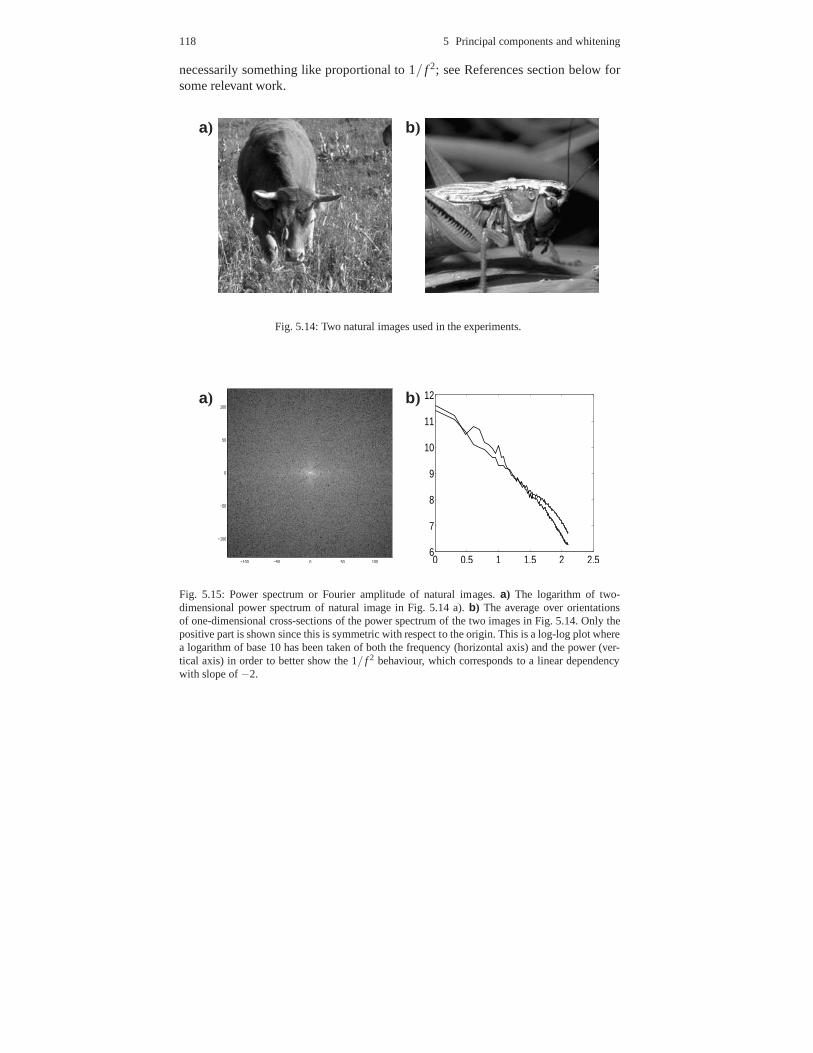
118 5 Principal components and whitening
necessarily something like proportional to 1/ f 2; see References section below forsome relevant work.
a) b)
Fig. 5.14: Two natural images used in the experiments.
a)
−100 −50 0 50 100
−100
−50
0
50
100b)
0 0.5 1 1.5 2 2.56
7
8
9
10
11
12
Fig. 5.15: Power spectrum or Fourier amplitude of natural images.a) The logarithm of two-dimensional power spectrum of natural image in Fig. 5.14 a).b) The average over orientationsof one-dimensional cross-sections of the power spectrum ofthe two images in Fig. 5.14. Only thepositive part is shown since this is symmetric with respect to the origin. This is a log-log plot wherea logarithm of base 10 has been taken of both the frequency (horizontal axis) and the power (ver-tical axis) in order to better show the 1/ f 2 behaviour, which corresponds to a linear dependencywith slope of−2.

5.6 Power spectrum of natural images 119
5.6.2 Connection between power spectrum and covariances
What is then the connection between the power spectrum of an image, and the co-variances between pixels we have been computing in this chapter? To this end, weneed a theorem from the theory of stochastic processes (we will not rigorously de-fine what stochastic processes are because that is not necessary for the purposes ofthis book). The celebrated Wiener-Khinchin theorem statesthat for a stochastic pro-cess,the average power spectrum is the Fourier Transform of the autocorrelationfunction.
The theorem talks about the “autocorrelation function”. This is the terminologyof stochastic processes, which we have not used in this chapter: we simply consid-ered different pixels as different random variables. The “autocorrelation function”means simply the correlations of variables (i.e. pixel values) as a function of the hor-izontal and vertical distances between them. Thus, the autocorrelation function is amatrix constructed as follows. First, take one row of the covariance matrix, say theone corresponding to the pixel at(x0,y0). To avoid border effects, let’s take(x0,y0)which is in the middle of the image patch. Then, convert this vector back to theshape of the image patch. Thus, we have a matrixC(x0,y0)
cov(I(x0,y0), I(1,1)) . . . cov(I(x0,y0), I(1,n))...
cov(I(x0,y0), I(n,1)) . . . cov(I(x0,y0), I(n,n))
(5.21)
which has the same sizem×mas the image patch. This matrix is nothing else thanwhat was already estimated from natural images and plotted in Fig. 5.4.
Actually, it is obvious that this matrix essentially contains all the information inthe covariance matrix. As discussed in Section 5.2.5, it is commonly assumed thatimage patches are translation-invariant in the sense that the covariances actuallyonly depend on the distance between two pixels, and not on where in the patch thepixels happen to be. (This may not hold for whole images, where the upper halfmay depict sky more often and lower parts, but it certainly holds for small imagepatches.) Thus, to analyze the covariance structure of images, all we really need isa matrix like in Equation (5.21).
What the Wiener-Khinchin theorem now says is that when we take the Fouriertransformation ofC(x0,y0), just as if this matrix were an image patch, the Fourieramplitudes equal theaveragepower spectrum of the original image patches. (Due tothe special symmetry properties of covariances, the phasesin the Fourier transformof C(x0,y0) are all zero, so the amplitudes are also equal to the coefficients of thecos functions.)
Thus, we can see the connection between the 1/ f Fourier amplitude of naturalimages and the covariances of the pixels structure. The average 1/ f Fourier ampli-tude or the 1/ f 2 power spectrum of single images implies that the Fourier transformof C(x0,y0) also falls of as 1/ f 2. Now, since the features obtained from PCA arenot very different from those used in a discrete Fourier transform (sine and cosine

120 5 Principal components and whitening
functions), and the squares of the coefficients in that basisare the variances of theprincipal components, we see that the variances of the principal components falloff as 1/ f 2 as a function of frequency. (This cannot be seen in the variance plot inFig. 5.9 because that plot does not give the variances as a function of frequency.)
Another implication of the Wiener-Khinchin theorem is thatit shows howconsid-ering the power spectrum of images alone is related to using gaussian model. Sincethe average power spectrum contains essentially the same information as the covari-ance matrix, and using covariances only is equivalent to using a gaussian model, wesee that considering the average power spectrum alone is essentially equivalent tomodelling the data with a gaussian pdf as in Section 5.5. Since the power spectrumdoes not contain information about phase, using the phase structure is thus relatedto using the non-gaussian aspects of the data, which will be considered in the nextchapters.
5.6.3 Relative importance of amplitude and phase
When considering frequency-based representations of natural images, the followingquestion naturally arises: Which is more important, phase or amplitude (power) —or are they equally important? Most researchers agree that the phase information ismore important for the perceptual system than the amplitudestructure. This view isjustified by experiments in which we take the phase structurefrom one image andthe power structure from another, and determine whether theimage is more similarto one of the natural images. What this means is that we take the Fourier transform(using the Discrete Fourier Transform) of the two images, and isolate the phase andamplitude from the two transforms. Then we compute the inverse of the Fouriertransform from the combination of the phase from the first image and the amplitudefrom the second; this gives us a new image. We also create another image with theinverse Fourier transform using the phase from the second image and the amplitudefrom the first.
Results of such an experiment are shown in Fig. 5.16. In both cases, the image“looks” more like the image from which the phase structure was taken, althoughin a) this is not very strongly so. This may be natural if one looks at the Fourieramplitudes of the images: since they are both rather similar(showing the typical1/ f fall-off), they cannot provide much information about whatthe image reallydepicts. If all natural images really have amplitude spectra which approximatelyshow the 1/ f shape, the power spectrum cannot provide much information on anynatural image, and thus the phase information has to be the key to identifying thecontents in the images.
Thus, one can conclude that since PCA concentrates only on information in thepower spectrum, and the power spectrum does not contain a lotof perceptually im-portant information, one cannot expect PCA and related methods to yield too muchuseful information about the visual system. Indeed, this provides an explanation forthe rather disappointing performance of PCA in learning features from natural im-

5.7 Anisotropy in natural images 121
ages as seen in Fig. 5.7 — the performace is disappointing, atleast, if we want tomodel receptive fields in V1. In the next chapter we will see that using informationnot contained in the covariances gives an interesting modelof simple cell receptivefields.
a) b)
Fig. 5.16: Relative importance of phase and power/amplitude information in natural images.a)Image which has the Fourier phases of the image in Fig. 5.14 a), and the Fourier amplitudes of theimage in Fig. 5.14 b).b) Image which has the phases of the image in Fig. 5.14 b), and theamplitudestructure of the image in Fig. 5.14 a). In both cases the images are perceptually more similar to theimage from which the phase structure was taken, which indicates that the visual system is moresensitive to the phase structure of natural images.
5.7 Anisotropy in natural images
The concept of anisotropy refers to the fact that natural images are not completelyrotationally invariant (which would be called isotropy). In other words, the statisticalstructure is not the same in all orientations: if you rotate an image, the statisticschange.
This may come as a surprise after looking at the correlation coefficients in Fig-ure 5.4 d), in which it seems that the correlation is simply a function of the distance:the closer to each other the two pixels are, the stronger their correlation; and theorientation does not seem to have any effect. In fact, isotropy is not a bad first ap-proximation, but a closer analysis reveals some dependencies on orientation.
Figure 5.17 show the results of such an analysis. We have taken the correlationcoefficients computed in Figure 5.4, and analyzed how they depend on the orienta-tion of the line segment connecting the two pixels. An orientation of 0 (orπ) meansthat the two pixels have the samey coordinate; orientation ofπ/2 means that theyhave the samex coordinate. Other values mean that the pixels have an oblique rela-tionship to each other. Figure 5.17 shows that the correlations are the very strongest

122 5 Principal components and whitening
if the pixels have the samey coordinate, that is, they are on the same horizontal line.The correlations are also elevated if the pixels have the samex coordinate.
In fact, we already saw in Figure 5.6 that the first principal component is, con-sistently, a low-frequency horizontal edge. This is in linewith the dominance ofhorizontal correlations. If the images exactly isotropic,horizontal edges and verti-cal edges would have exactly the same variance, and the first principal componentwould not be well-defined at all; this would be reflected in Figure 5.6 so that wewould get edges with different random orientations.
Thus, we have discovered a form of anisotropy in natural image statistics. It willbe seen in different forms in all the later models and analyses as well.
0 1.57 3.14−0.2
−0.1
0
0.1
0.2
0.3
0.4
Fig. 5.17: Anisotropy, i.e. lack of rotational invariance,in natural image statistics. We took thecorrelation coefficients in Figure 5.4 and plotted them on three circles with different radii (themaximum radius allowed by the patch size, and that multiplied by one half and one quarter). Foreach of the radii, the plot shows that the correlations are maximized for the orientations of 0 orπ , which mean horizontal orientation: the pixels are on the same horizontal line. The verticalorientationπ/2 shows another maximum which is less pronounced.
5.8 Mathematics of principal component analysis*
This section is dedicated to a more sophisticated mathematical analysis of PCA andwhitening. It can be skipped by a reader not interested in mathematical details.

5.8 Mathematics of principal component analysis* 123
5.8.1 Eigenvalue decomposition of the covariance matrix
The “second-order” structure of data is completely described by the covariance ma-trix, defined in Section 4.6.3. In our case with thex andy coordinates of the patches,we can write:
C(x,y;x′,y′) = E{I(x,y)I(x′,y′)} (5.22)
The point is that the covariance ofanytwo linear features can be computed by
E
{
[∑x,y
W1(x,y)I(x,y)][∑x,y
W2(x,y)I(x,y))]
}
= E
{
[ ∑xyx′y′
W1(x,y)I(x,y)W2(x′,y′)I(x′,y′))]
}
= ∑xyx′y′
W1(x,y)W2(x′,y′)E{I(x,y)I(x′,y′)}
= ∑xyx′y′
W1(x,y)W2(x′,y′)C(x,y;x′,y′) (5.23)
which reduces to a something which can be computed using the covariance ma-trix. The second-order structure is thus conveniently represented by a single matrix,which enables us to use classic methods of linear algebra to analyze the second-order structure.
To go into details, we change the notation so that the whole image is in onevector,x, so that each pixel is one element in the vector. This can be accomplished,for example, by scanning the image row by row, as was explained in Section 4.1.This simplifies the notation enormously.
Now, considering any linear combinationwTx = ∑i wixi we can compute its vari-ance simply by:
E{(wTx)2}= E{(wTx)(xTw)}= E{wT(xxT)w}= wTE{xxT}w= wTCw (5.24)
where we denote the covariance matrix byC = E{xxT}. So, the basic PCA problemcan be formulated as
maxw:‖w‖=1
wTCw (5.25)
A basic concept in linear algebra is the eigenvalue decomposition. The startingpoint is thatC is a symmetric matrix, because cov(xi ,x j) = cov(x j ,xi). In linearalgebra, it is shown that any symmetric matrix can be expressed as a product of theform:
C = UDUT (5.26)

124 5 Principal components and whitening
whereU is an orthogonal matrix, andD = diag(λ1, . . . ,λm) is diagonal. The columnsof U are called theeigenvectors, and theλi are called theeigenvalues. Many efficientalgorithms exist for computing the eigenvalue decomposition of a matrix.
Now, we can solve PCA easily. Lets us make the change of variablesv = UTw.Then we have
wTCw = wTUDUTw = vTDv = ∑i
v2i λi (5.27)
BecauseU is orthogonal,‖v‖ = ‖w‖, so the constraint is the same forv as it wasfor w. Let us make the further change of variables tomi = v2
i . The constraint of unitnorm of v is now equivalent to the constraints that the sum of themi must equalone (they must also be positive because they are squares). Then, the problem istransformed to
maxmi≥0,∑mi=1
∑i
miλi (5.28)
It is rather obvious that the maximum is found when themi corresponding to thelargestλi is one and the others are zero. Let us denote byi∗ the index of the max-imum eigenvalue. Going back to thew, this corresponds tow begin equal to thei∗-th eigenvector, that is, thei∗-th column ofU. Thus, we see how the first principalcomponent is easily computed by the eigenvalue decomposition.
Since the eigenvectors of a symmetric matrix are orthogonal, finding the secondprincipal component means maximizing the variance so thatvi∗ is kept zero. This isactually equivalent to making the neww orthogonal to the first eigenvector. Thus,in terms ofmi , we have exactly the same optimization problem, but with theextraconstraint thatmi∗ = 0. Obviously, the optimum is obtained whenw is equal to theeigenvector corresponding to thesecondlargest eigenvalue. This logic applies to thek-th principal component.
Thus, all the principal components can be found by ordering the eigenvectorsui , i = 1, . . . ,m in U so that the corresponding eigenvalues are in decreasing order.Let us assume thatU is ordered so. Then thei-th principal componentsi is equal to
si = uTi x (5.29)
Note that it can be proven that theλi are all non-negative for a covariance matrix.Using the eigenvalue decomposition, we can prove some interesting properties
of PCA. First, the principal components areuncorrelated, because for the vector ofthe principal components
s= UTx (5.30)
we have
E{ssT}= E{UTxxTU}= UTE{xxT}U = UT(UDUT)U
= (UTU)D(UTU) = D (5.31)
because of the orthogonality ofU. Thus, the covariance matrix is diagonal, whichshows that the principal components are uncorrelated.

5.8 Mathematics of principal component analysis* 125
Moreover, we see that the variances of the principal components are equal to theλi . Thus, to obtain variables that are white, that is, uncorrelated and have unit vari-ance, it is enough to divide each principal component by the square root of the cor-responding eigenvalue. This proves that diag(1/
√λ1, . . . ,1/
√λm)UT is awhitening
matrix forx.This relation also has an important implication for the uniqueness of PCA. If
two of the eigenvalues are equal, then the variance of those principal componentsare equal. Then, the principal components are not well-defined anymore, because wecan make arotationof those principal components without affecting their variances.This is because ifzi andzi+1 have the same variance, then linear combinations suchas√
1/2zi +√
1/2zi+1 and√
1/2zi −√
1/2zi+1 have the same variance as well;all the constraints (unit variance and orthogonality) are still fulfilled, so these areequally valid principal components. In fact, in linear algebra, it is well-known thatthe eigenvalue decomposition is uniquely defined only when the eigenvalues are alldistinct.
5.8.2 Eigenvectors and translation-invariance
Using the eigenvalue decomposition, we can show why the principal componentsof a typical image covariance matrix are sinusoids as statedin Section 5.2.5. This isbecause of their property of being translation-invariant,i.e. the covariance dependsonly on the distance as in (5.9). For simplicity, let us consider a one-dimensionalcovariance matrixc(x−x′). The functionc is even-symmetric with respect to zero,i.e.c(−u) = c(u). By a simple change of variablez= x−x′, we have
∑x
cov(x,x′)sin(x+ α) = ∑x
c(x−x′)sin(x+ α) = ∑z
c(z)sin(z+x′+ α) (5.32)
Using the property that sin(a+b) = sinacosb+cosasinb, we have
∑z
c(z)sin(z+x′+ α) = ∑z
c(z)(sin(z)cos(x′+ α)+cos(z)sin(x′+ α))
= [∑z
c(z)sin(z)]cos(x′+ α)+ [∑z
c(z)cos(z)]sin(x′+ α) (5.33)
Finally, becausec(z) is even-symmetric and sin is odd-symmetric, the first sum inbrackets is zero. So, we have
∑x
cov(x,x′)sin(x+ α) = [∑z
c(z)cos(z)]sin(x′+ α) (5.34)
which shows that the sinusoid is an eigenvector of the covariance matrix, with eigen-value∑zc(z)cos(z). The parameterα gives the phase of the sinusoid; this formulashows thatα can have any value, so sinusoids of any phase are eigenvectors.

126 5 Principal components and whitening
This proof can be extended to sinusoids of different frequenciesβ : they all areeigenvalues with eigenvalues that depend on how strongly the frequency is presentin the data:∑zc(z)cos(βz).
In the two-dimensional case, we have cov(I(x,y), I(x′,y′)) = c((x− x′)2 + (y−y′)2) and withξ = x−x′ andη = y−y′ we have
∑x,y
c((x−x′)2 +(y−y′)2)sin(ax+by+c)
= ∑ξ ,η
c(ξ ,η)sin(aξ +bη +ax′+by′+c)
= ∑ξ ,η
c(ξ ,η)[sin(aξ +bη)cos(ax′+by′+c)+cos(aξ +bη)sin(ax′+by′+c)]
= 0+[∑ξ ,η
c(ξ ,η)cos(aξ +bη)]sin(ax′+by′+c) (5.35)
which shows, likewise, that sinusoids of the form sin(ax′+by′+c) are eigenvectors.
5.9 Decorrelation models of retina and LGN *
In this section, we consider some further methods for whitening and decorrelationof natural images, and the application of such methods as models of processing inthe retina and the LGN. This material can be skipped without interrupting the flowof ideas.
5.9.1 Whitening and redundancy reduction
The starting point here is the redundancy reduction hypothesis, discussed in Chap-ter 1. In its original form, this theory states that the earlyvisual system tries toreduce the redundancy in its input. As we have seen in in this chapter, image pixeldata is highly correlated, so a first approach to reduce the redundancy would be todecorrelateimage data, i.e. to transform it into uncorrelated components.
One way to decorrelate image data is to whiten it with a spatial filter. In a visualsystem, this filtering would correspond to a set of neurons, with identical spatialreceptive fields, spaced suitably in a lattice. The outputs of the neurons would thenbe uncorrelated, and if we were to look at the outputs of the whole set of neurons asan image (or a set of images for multiple input images), theseoutput images wouldon the average have a flat power spectrum.
The whitening theory has led to well-known if rather controversial models of thecomputational underpinnings of the retina and the lateral geniculate nucleus (LGN).In this section we will discuss spatial whitening and spatial receptive fields accord-

5.9 Decorrelation models of retina and LGN * 127
ing to this line of thought; the case of temporal whitening and temporal receptivefields will be discussed in detail in Section 16.3.2 (page 345).
The basic idea is that whitening alone could explain the center-surround structureof the receptive fields of ganglion cells in the retina, as well as those in the LGN.Indeed, certain spatial whitening filters are very similar to ganglion RF’s, as wewill see below. However, such a proposal is problematic because there are manycompletely different ways of whitening the image input, andit is not clear why thisparticular method should be used. Nevertheless, this theory is interesting becauseof its simplicity and because it sheds light on certain fundamental properties of thecovariance structure of images.
There are at least two ways to derive the whitening operationin question. Thefirst is to compute it directly from the covariance matrix of image patches sampledfrom the data; this will lead to a set of receptive fields, but with a suitable constraintthe RF’s will be identical except for different center locations, as we will see below.We will call this patch-based whitening. The second way is to specify a whiteningfilter in the frequency domain, which will give us additionalinsight and control overthe process. This we will callfilter-based whitening.
5.9.2 Patch-based decorrelation
Our first approach to spatial whitening is based on the PCA whitening introducedabove in Section 5.3.2 (page 109). The data transformation is illustrated in the two-dimensional case in Figure 5.18.
Here, we will use the matrix notation because it directly shows some importantproperties of the representation we construct. Here, we denote byU the matrix withthe vectors defining the principal components as its columns
U = (u1,u2, · · · ,uk). (5.36)
Let x denote the data vector. Because the vectorsu are orthogonal, each of theprincipal componentsyk, k = 1, ...,K, of the data vectorx can be computed simplyby taking the dot product between the data vector and thekth PCA vector:
yk = uTk x, k = 1, ...,K. (5.37)
Defining the vectory = (y1,y2, · · · ,yK)T , the Equations (5.37) for allk = 1, ...,Kcan be expressed in a single matrix equation
y = UTx. (5.38)
In our two-dimensional illustration, the result of this transformation is shown inFigure 5.18b).
As in Section 5.3.2, we next whiten the data by dividing the principal componentswith their standard deviations. Thus we obtain whitened componentssk
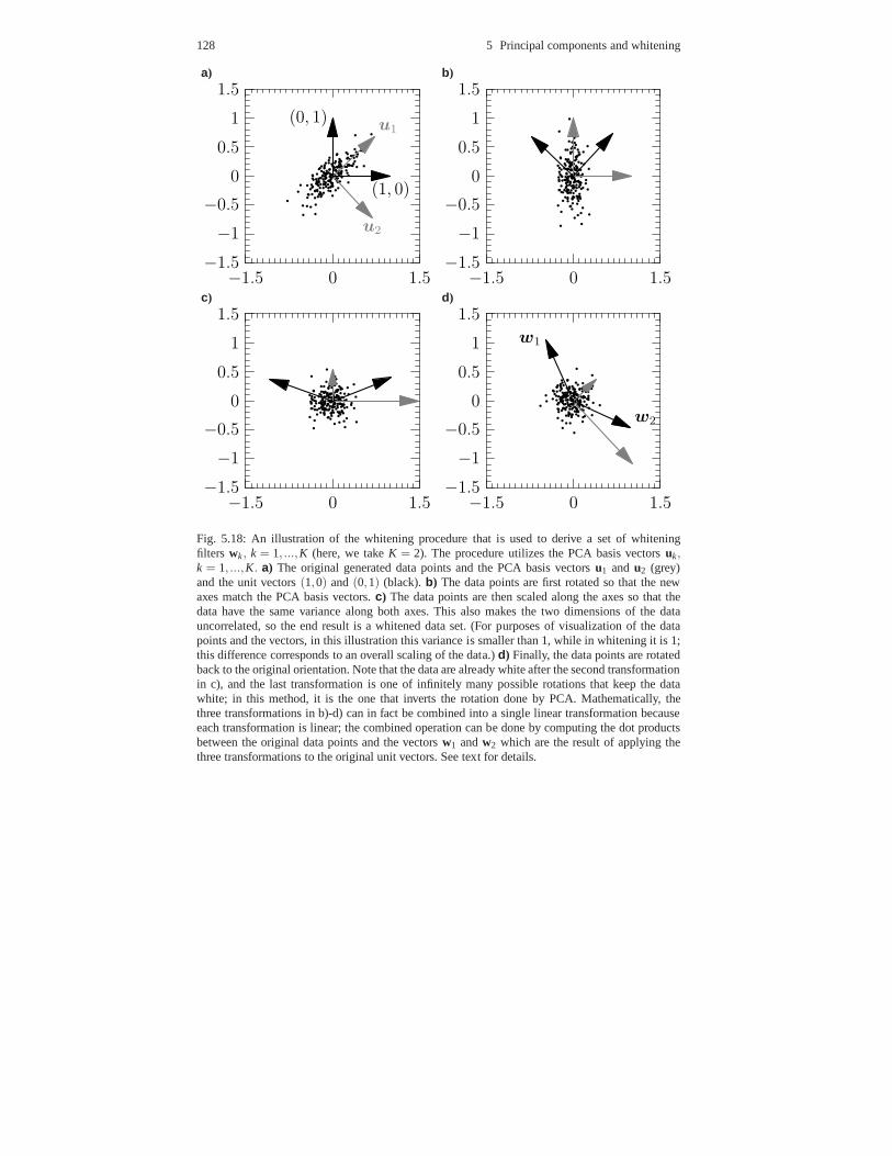
128 5 Principal components and whitening
a)
−1.5 0 1.5−1.5
−1
−0.5
0
0.5
1
1.5
u2
u1
(1, 0)
(0, 1)
b)
−1.5 0 1.5−1.5
−1
−0.5
0
0.5
1
1.5
c)
−1.5 0 1.5−1.5
−1
−0.5
0
0.5
1
1.5d)
−1.5 0 1.5−1.5
−1
−0.5
0
0.5
1
1.5
w2
w1
Fig. 5.18: An illustration of the whitening procedure that is used to derive a set of whiteningfilters wk, k = 1, ...,K (here, we takeK = 2). The procedure utilizes the PCA basis vectorsuk,k = 1, ...,K. a) The original generated data points and the PCA basis vectorsu1 and u2 (grey)and the unit vectors(1,0) and(0,1) (black). b) The data points are first rotated so that the newaxes match the PCA basis vectors.c) The data points are then scaled along the axes so that thedata have the same variance along both axes. This also makes the two dimensions of the datauncorrelated, so the end result is a whitened data set. (For purposes of visualization of the datapoints and the vectors, in this illustration this variance is smaller than 1, while in whitening it is 1;this difference corresponds to an overall scaling of the data.)d) Finally, the data points are rotatedback to the original orientation. Note that the data are already white after the second transformationin c), and the last transformation is one of infinitely many possible rotations that keep the datawhite; in this method, it is the one that inverts the rotationdone by PCA. Mathematically, thethree transformations in b)-d) can in fact be combined into asingle linear transformation becauseeach transformation is linear; the combined operation can be done by computing the dot productsbetween the original data points and the vectorsw1 andw2 which are the result of applying thethree transformations to the original unit vectors. See text for details.

5.9 Decorrelation models of retina and LGN * 129
sk =yk
√
var(yk), k = 1, ...,K, (5.39)
This is shown for our illustrative example in Figure 5.18c).Again, we can express theseK equations by a single matrix equation. Define a
vectors= (s1,s2, · · · ,sK)T , and letΛ denote a diagonal matrix with the inverses ofthe square roots of the variances on its diagonal:
Λ =
1√var(y1)
0 · · · 0
0 1√var(y2)
· · · 0
......
.. ....
0 0 · · · 1√var(yK)
; (5.40)
thens= Λy = ΛUTx. (5.41)
So far we have just expressed PCA whitening as a matrix formulation. Now,we will make a new operation. Among the infinitely many whitening matrices, wechoose the one which is given by inverting the PCA computation given byU. Ina sense, we go “back from the principal components to the original coordinates”(Figure 5.18d). Denoting byz the final component computed, this is defined by thefollowing matrix equation:
z = Us= UΛUTx. (5.42)
The computation presented in Equation (5.43) consist of three linear (matrix)transformations in a cascade. The theory of linear transformation states that a cas-cade of consecutive linear transformations is simply another linear transformation,and that this combined transformation – which we will here denote byW – can beobtained as the matrix product of the individual transformations:
z = UΛUT︸ ︷︷ ︸
=W
x = Wx. (5.43)
When written ask scalar equations, Equation (5.43) shows that the components ofvectorz = [z1 z2 · · · zK ]T can be obtained as a dot product between the data vectorx and thekth row of matrixW = [w1 w2 · · ·wK ]T :
zk = wTk x, k = 1, ...,K. (5.44)
The vectorswk, k = 1, ...,K, are of great interest to us, since they are filters whichmap the inputx to the whitened data. In other words, the vectorswk, k = 1, ...,K,can be interpreted as receptive fields. The receptive fieldswk, k = 1, ...,K, can beobtained simply by computing the matrix product in Equation(5.43).
Matrix square root As an aside, we mention an interesting mathematical inter-pretation of the matrixW. The matrixW is called theinverse matrix square rootof

130 5 Principal components and whitening
the covariance matrixC, and denoted byC−1/2. In other words, the inverseW−1
is called the square root ofC, and denoted byC1/2. The reason is that if we multi-ply W−1 with itself, we getC. This is because, first,(UΛUT)−1 = UΛ−1UT , andsecond, we can calculate
W−1W−1 = (UΛ−1UT)(UΛ−1UT) = UΛ−1(UTU)Λ−1UT = UΛ−2UT (5.45)
The matrixΛ−2 is simply a diagonal matrix with the variances in its diagonal, so theresult is nothing else than the eigenvalue decomposition ofthe covariance matrix asin Equation (5.26).
Symmetric whitening matrix Another interesting mathematical property of thewhitening matrixW in Equation (5.43) is that it is symmetric, which can be shownas
WT =(UΛUT)T
=(UT)T ΛTUT = UΛUT = W. (5.46)
In fact, it is the only symmetric whitening matrix.
Application to natural images When the previous procedure is applied to naturalimage data, interesting receptive fields emerge. Figure 5.19a) shows the resultingwhitening filters (rows / columns ofW); a closeup of one of the filters is shownin Figure 5.19b). As can be seen, the whitening principle results in the emergenceof filters which have center-surround structure. All of the filters are identical, soprocessing image patches with such filters is analogous to filtering them with thespatial filter shown in Figure 5.19b).
As pointed out several times above, whitening can be done in infinitely manydifferent ways: ifW is a whitening transformation, so is any orthogonal transfor-mation ofW. Here the whitening solution in Equation (5.43) has been selected sothat it results in center-surround-type filters. This is a general property that we willbump into time and again below: the whitening principle doesconstrain the formof the emerging filters, but additional assumptions are needed before the results canhave a meaningful interpretation.
Note that the theory results in a single receptive field structure, while in the retina,there are receptive fields with differing spatial properties – in particular scale (fre-quency) – in the retina and the LGN. This is another limitation of the whiteningprinciple, and additional assumptions are needed to produce a range of differingfilters.
5.9.3 Filter-based decorrelation
Now we reformulate this theory in a filter-based framework. Then the theory pos-tulates that the amplitude response properties (see Section 2.2.3, page 33) of retinaland LGN receptive fields follow from the following two assumptions:

5.9 Decorrelation models of retina and LGN * 131
a)
b)
Fig. 5.19: The application of the whitening principle results in the emergence of a set of center-surround filters from natural image data.a) The set of filters (rows / columns of whitening matrixW) obtained from image data.b) A closeup of one of the filters; the other filters are identicalexceptfor spatial location.
132 5 Principal components and whitening
1. the linear filters are whitening natural image data2. with the constraint that noise is not amplified unduly.
Additional assumptions are needed to derive the phase response in order to specifythe filter completely. This is equivalent to the observationmade above in the generalcase of whitening: there are infinitely many whitening transformations. Here, thephases are defined by specifying that the energy of the filter should be concentratedin either time or space, which in the spatial case can be loosely interpreted to meanthat the spatial RF’s should be as localized as possible.
The amplitude response of the filter will be derived in two parts: the first part isthe whitening filter, and the second part suppresses noise. The filter will be derivedin the frequency domain, and thereafter converted to the spatial domain by inverseFourier transform. It is often assumed that the statistics of image data do not dependon spatial orientation; we make the same assumption here andstudy the orientation-independent spatial frequencyωs. Conversion from the usual two-dimensional fre-
quenciesωx andωy to spatial frequencyωs is given byωs =√
ω2x + ω2
y . Let Ri(ωs)
denote the average power spectrum in natural images. We knowthat for uncorrelated/ whitened data, the average power spectrum should be a constant (flat). Because theaverage power spectrum of the filtered data is the product of the average power spec-trum of the original data and the squared amplitude responseof the whitening filter,which we denote by|V(ωs)|2 , this means that the amplitude response of a whiteningfilter can be specified by
|V(ωs)|=1
√
Ri(ωs), (5.47)
since then|V(ωs)|2Ri(ωs) = 1.Real measurement data contains noise. Assume that the noise, whose average
power spectrum isRn(ωs), is additive and uncorrelated with the original image data,whose average power spectrum isRo(ωs); thenRi(ωs) = Ro(ωs)+ Rn(ωs). To de-rive the amplitude response of the filter that suppresses noise, one can use aWienerfiltering approach. Wiener filtering yields a linear filter that can be used to com-pensate for the presence of additive noise: the resulting filter optimally restores theoriginal signal in the least mean square sense. The derivation of the Wiener filter inthe frequency space is somewhat involved, and we will skip ithere; see (Dong andAtick, 1995b). The resulting response properties of the filter are fairly intuitive: theamplitude response|F(ωs)| of the Wiener filter is given by
|F(ωs)|=Ri(ωs)−Rn(ωs)
Ri(ωs). (5.48)
Notice that if there are frequencies that contain no noise – that is,Rn(ωs) = 0 –the amplitude response is simply 1, and that higher noise power leads to decreasedamplitude response.
The overall amplitude response of the filter|W(ωs)| is obtained by cascading thewhitening and the noise-suppressive filters (equations (5.47) and (5.48)). Becausethis cascading corresponds to multiplication in the frequency domain, the amplitude

5.9 Decorrelation models of retina and LGN * 133
response of the resulting filter is
|W(ωs)|= |V(ωs)| |F(ωs)|=1
√
Ri(ωs)
Ri(ωs)−Rn(ωs)
Ri(ωs). (5.49)
In practice,Ri(ωs) can be estimated directly from image data for eachωs, or one canuse the parametric form derived in Section 5.6 (page 116). (Negative values givenby this formula (5.49) have to be truncated to zero.) Noise isassumed to be spatiallyuncorrelated, implying a constant (flat) power spectrum, and to have power equal todata power at a certain characteristic frequency, denoted by ωs,c, so that
Rn(ωs) =Ri(ωs,c)
2for all ωs. (5.50)
In order to fully specify the resulting filter, we have to define its phase response.Here we simply set the phase response to zero for all frequencies:
∠W(ωs) = 0 for all ωs. (5.51)
With the phases of all frequencies at zero, the energy of the filter is highly concen-trated around the spatial origin, yielding a highly spatially localized filter. After theamplitude and the phase responses have been defined, the spatial filter itself can beobtained by taking the inverse two-dimensional Fourier transform.
The filter properties that result from the application of equations (5.49), (5.50)and (5.51) are illustrated in Figure 5.20 for characteristic frequency valueωs,c =0.3cycles per pixel. For this experiment, 100,000 image windows of size 16× 16pixels were sampled from natural images.4 The average power spectrum of theseimages was then computed; the average of this spectrum over all spatial orientationsis shown in Figure 5.20a). The squared amplitude response ofthe whitening filter,obtained from equation (5.49), is shown in Figure 5.20b). The power spectrum of thefiltered data is shown in Figure 5.20c); it is approximately flat at lower frequenciesand drops off sharply at high frequencies because of the higher relative noise powerat high frequencies. The resulting filter is shown in Figure 5.20d); for comparison,a measured spatial receptive field of an LGN neuron is shown inFigure 5.20e).
Thus, the center-surround receptive-field structure, found in the retina and theLGN, emerges from this computational model and natural image data. However, wemade several assumptions above – such as the spacing of the receptive fields – andobtained as a result only a single filter instead of a range of filters in different scalesand locations. In Section 16.3.2 (page 345) we will see that in the temporal domain,similar principles lead to the emergence of temporal RF properties of these neurons.
4 Here, we did not use our ordinary data set but that of van Hateren and van der Schaaf (1998).

134 5 Principal components and whitening
a)
106
107
108
109
1010
Ri(ω
s)
10−2 10−1 100
ωs (c/p)
b)
10−2
10−1
100
101
|W(ω
s)|
2
10−2 10−1 100
ωs (c/p)
c)
106
107
108
109
1010
|W(ω
s)|
2R
i(ω
s)
10−2 10−1 100
ωs (c/p)
d) e)
Fig. 5.20: The application of the whitening principle, combined with noise reduction and zerophase response, leads to the emergence of center-surround filters from natural image data.a) Thepower spectrumRi(ωs) of natural image data.b) The squared amplitude response of a whiteningfilter which suppresses noise: this curve follows the inverse of the data power spectrum at lowfrequencies, but then drops off quickly at high frequencies, because the proportion of noise is largerat high frequencies.c) The power spectrum of the resulting (filtered) data, showingapproximatelyflat (white) power at low frequencies, and dropping off sharply at high frequencies.d) The resultingfilter which has been obtained from the amplitude response inb) and by specifying a zero phaseresponse for all frequencies; see text for details.e) For comparison, the spatial receptive field ofan LGN neuron.
5.10 Concluding remarks and References
This chapter considered models of natural images which werebased on analyzingthe covariances of the image pixels. The classic model is principal component anal-ysis, in which variance of a linear feature detector is maximized. PCA fails to yieldinteresting feature detectors if the goal is to model visualcells in brain. However,it is an important model historically and conceptually, andalso provides the basisfor the preprocessing we use later in this book: dimension reduction combined withwhitening. In the next chapter, we will consider a differentkind of learning criterionwhich does yield features which are interesting for visual modelling.
Most of the work on second-order statistics of images is based on the (approxi-mate) 1/ f 2 property of the power spectrum. This was investigated earlyin (Field,1987; Burton and Moorehead, 1987; Tolhurst et al, 1992; Ruderman and Bialek,

5.11 Exercices 135
1994a; van der Schaaf and van Hateren, 1996). It has been proposed to explaincertain scaling phenomena in the visual cortex, such as the orientation bandwidth(van der Schaaf and van Hateren, 1996) and the relative sensitivity of cells tuned todifferent frequencies (Field, 1987). Early work on PCA of images include (Sanger,1989; Hancock et al, 1992). The 1/ f property is closely related to the study of self-similar stochastic processes (Embrechts and Maejima, 2000) which has a very longhistory (Mandelbrot and van Ness, 1968). The study of self-critical systems (Baket al, 1987) may also have some connection. A model of how suchself-similaritiescome about as a result of composing an image of different “objects” is proposed in(Ruderman, 1997).
A recent paper with a very useful discussion and review of thepsychophysicalimportance of the Fourier powers vs. phases is (Wichmann et al, 2006); see also(Hansen and Hess, 2007).
Another line of research proposes that whitening explains retinal ganglion recep-tive fields (Atick and Redlich, 1992). (An extension of this theory explains LGNreceptive field by considering temporal correlations as well (Dan et al, 1996a), seealso Chapter 16.) For uniformity of presentation, we followthe mathematical the-ory of (Dong and Atick, 1995b) both here in the spatial case and in the temporalcase in Section 16.3.2. As argued above, the proposal is problematic because thereare many ways of whitening data. A possible solution to the problem is to considerenergy consumption or wiring length, see Chapter 11 for thisconcept, as was donein (Vincent and Baddeley, 2003; Vincent et al, 2005).
The anisotropy of pixel correlations has been used to explain some anisotropicproperties in visual psychophysics in (Baddeley and Hancock, 1991).
An attempt to characterize the proportion of information explained by the covari-ance structure in natural images can be found in (Chandler and Field, 2007).
5.11 Exercices
Mathematical exercises
1. Show that if the expectations of the grey-scale values of the pixels are the samefor all x,y:
E{I(x,y)}= E{I(x′,y′)} for anyx,y,x′,y′ (5.52)
then removing the DC component implies than the expectationof I(x,y) is zerofor anyx,y.
2. Show that if∑x,yWx,y = 0, the removal of the DC component has no effect on theoutput of the features detector.
3. Show that if the vector(y1, . . . ,yn)T is white, any orthogonal transformation of
that vector is white as well.4. To get used to matrix notation:

136 5 Principal components and whitening
a. The covariance matrix of the vectorx = (x1, . . . ,xn)T is defined as the matrix
C with elementsci j = cov(xi ,x j). Under what condition do we haveC =E{xxT}?
b. Show that the covariance matrix ofy = Mx equalsMCM T
5. Denote byw a vector which reduces the dimension ofx to one asz= ∑i wixi .Now, we will show that taking the first principal component isthe optimal way ofreducing dimension if the optimality criterion is least-squares error. This meansthat we reconstruct the original data as a linear transformation of zas:
J(W) = E{∑j(x j −wjz)
2} (5.53)
a. Show thatJ is equal to
∑j
w2j ∑
i,i′wiwi′cov(xi ,xi′)−2∑
j
wj ∑i
wicov(x j ,xi)+∑j
var(x j) (5.54)
b. Using this expression forJ, show that thew which minimizesJ under theconstraint‖w‖= 1 is the first principal component ofx.
Computer assignments
1. Take some images from the Web. Take a large sample of extremely small patchesof the images, so that the patch contains just two neighbouring pixels. Convertthe pixels to grey-scale if necessary. Make a scatter plot ofthe pixels. What canyou see? Compute the correlation coefficient of the pixel values.
2. Using the same patches, convert them into two new variables: the sum of thegrey-scale values and and their difference. Do the scatter plot and computer thecorrelation coefficient.
3. Using the same images, take a sample of 1,000 patches of theform of 1× 10pixels. Compute the covariance matrix. Plot the covariancematrix (because thepatches are one-dimensional, you can easily plot this two-dimensional matrix).
4. The same as above, but remove the DC component of the patch.How does thischange the covariance matrix?
5. The same as above, but with only 50 patches sampled from theimages. How arethe results changed, and why?
6. *Take the sample of 1,000 one-dimensional patches computed above. Computethe eigenvalue decomposition of the covariance matrix. Plot the principal com-ponent weightsWi(x).
Chapter 6Sparse coding and simple cells
In the preceding chapter, we saw how features can be learned by PCA of naturalimages. This is a classic method of utilizing the second-order information of sta-tistical data. However, the features it gave were not very interesting from a neuralmodelling viewpoint, which motivates us to find better models. In fact, it is clearthat the second-order structure of natural images is scratching the surface of the sta-tistical structure of natural images. Look at the outputs ofthe feature detectors ofFigure 1.10, for example. We can see that the outputs of different kinds of filtersdiffer from each other in other ways than just variance: the output of the Gabor filterhas a histogram that has a strong peak at zero, whereas this isnot the case for thehistogram of pixel values. This difference is captured in a property calledsparse-ness. It turns out that a more interesting model is indeed obtained if we look at thesparseness of the outputs instead of the variance as in PCA.
6.1 Definition of sparseness
Sparseness means that the random variable is most of the timevery close to zero,and only occasionally gets clearly nonzero values. One often says that the randomvariable is “active” only rarely.
It is very important to distinguish sparseness from small variance. When we say“very close to zero”, this is relative to the general deviation of the random variablefrom zero, i.e. relative to its variance and standard deviation. Thus, “very close tozero” would mean something like “an absolute value that is smaller than 0.1 timesthe standard deviation”.
To say that a random variable is sparse needs a baseline of comparison. Hereit is the gaussian (normal) distribution; a random variableis sparse if it is activemore rarely compared to a gaussian random variable of the same variance (andzero mean). Figure 6.1 shows a sample of a sparse random variable, comparedto the gaussian random variable of the same variance. Another way of looking atsparseness is to consider the probability density function(pdf). The property of
137

138 6 Sparse coding and simple cells
being most of the time very close to zero is closely related tothe property that the pdfhas a peak at zero. Since the variable must have some deviation from zero (variancewas normalized to unity), the peak at zero must be compensated by a relativelylarge probability mass at large values; a phenomenon often called “heavy tails”. Inbetween these two extremes, the pdf takes relatively small values, compared to thegaussian pdf. This is illustrated in Fig. 6.2.1
−5
0
5
gaus
sian
−5
0
5
spar
se
Fig. 6.1: Illustration of sparseness. Random samples of a gaussian variable (top) and a sparsevariable (bottom). The sparse variable is practically zeromost of the time, occasionally takingvery large values. Note that the variables have the same variance, and that these are not time seriesbut just observations of random variables.
6.2 Learning one feature by maximization of sparseness
To begin with, we consider the problem of learning a single feature based on max-imization of sparseness. As explained in Section 1.8, learning features is a simpleapproach to building statistical models. Similar to the case of PCA, we consider onelinear featurescomputed using weightsW(x,y) as
s= ∑x,y
W(x,y)I(x,y) (6.1)
1 Here we consider the case of symmetric distributions only. It is possible to talk about the sparse-ness of non-symmetric distributions as well. For example, if the random variable only obtainsnon-negative values, the same idea of being very close to zero most of the time is still valid andis reflected in a peak on the right side of the origin. See Section 13.2.3 for more information.However, most distributions found in this book are symmetric.

6.2 Learning one feature by maximization of sparseness 139
a)
−3 −2 −1 0 1 2 30
0.5
1
1.5
2 a)
−3 −2 −1 0 1 2 3−5
−4
−3
−2
−1
0
1
Fig. 6.2: Illustration of a typical sparse probability density. The sparse density function, calledLaplacian, is given by the solid curve (see Eq. (7.18) in the next chapter for an exact formula) Forcomparison, the density of the absolute value of a gaussian random variable of the same varianceis given by the dash-dotted curve.a) the probability density functions,b) their logarithms.
While a single feature is not very useful for vision, this approach shows the basicprinciples in a simplified setting. Another way in which we simplify the problemis by postponing the formulation of a proper statistical model. Thus, we do notreally estimatethe feature in this section, but rather learn it by some intuitivelyjustified statistical criteria. In Section 6.3 we show how tolearn many features, andin Chapter 7 we show how to formulate a proper statistical model and learn thefeatures by estimating it.
6.2.1 Measuring sparseness: General framework
To be able to find features that maximize sparseness, we have to develop statisticalcriteria for measuring sparseness. When measuring sparseness, we can first normal-ize s to unit variance, which is simple to do by dividings by its standard deviation.This simplifies the formulation of the measures.
A simple way to approach the problem is to look at the expectation of somefunction ofs, a linear feature of the data. If the function is the square function, weare just measuring variance (which we just normalized to be equal to one), so wehave to use something else. Since we know that the variance isequal to unity, wecan consider the square function as a baseline and look at theexpectations of theform
E{h(s2)} (6.2)
whereh is somenonlinearfunction.How should the functionh be chosen so that the formula in Equation (6.2) mea-
sures sparseness? The starting point is the observation that sparse variables have a

140 6 Sparse coding and simple cells
lot of data (probability mass) around zero because of the peak at zero, as well as alot of data very far from zero because of heavy tails. Thus, wehave two differentapproaches to measuring sparseness. We can chooseh so that it emphasizes valuesthat are close to zero, or values that are much larger than one. However, it may notbe necessary to explicitly measure both of them, because theconstraint of unit vari-ance means that if there is a peak at zero, there has to be something like heavy tailsto make the variance equal to unity, and vice versa.
6.2.2 Measuring sparseness using kurtosis
A simple function that measures sparseness with emphasis onlarge values (heavytails) is the quadratic function
h1(u) = (u−1)2 (6.3)
(We denote byu the argument ofh, to emphasize that it is not a function ofsdirectly.Typically, u = s2.) Algebraic simplifications show that then the sparseness measureis equal to
E{h1(s2)}= E{(s2−1)2}= E{s4−2s2+1}= E{s4}−1 (6.4)
where the last equality holds because of the unit variance constraint. Thus, this mea-sure of sparseness is basically the same as the fourth moment; subtraction of theconstant (one) is largely irrelevant since it just shifts the measurement scale.
Using the fourth moment is closely related to the classic statistic calledkurtosis
kurt(s) = E{s4}−3(E{s2})2. (6.5)
If the variance is normalized to 1, kurtosis is in fact the same as the fourth momentminus a constant (three). This constant is chosen so that kurtosis is zero for a gaus-sian random variable (this is left as an exercise). If kurtosis is positive, the variableis called leptokurtic (or super-gaussian); this is a simpleoperational definition ofsparseness.
However, kurtosis is not a very good measure of sparseness for our purposes.The basic problem with kurtosis is its sensitivity to outliers. An “outlier” is a datapoint that is very far from the mean, possibly due to an error in the data collectionprocess. Consider, for example, a data set that has 1,000 scalar values and has beennormalized to unit variance. Assume that one of the values isequal to 10. Then,kurtosis is necessarily equal to at least 104/1000−3= 7. A kurtosis of 7 is usuallyconsidered a sign of strong sparseness. But here it was due toa single value, and notrepresentative of the whole data set at all!
Thus, kurtosis is a very unreliable measure of sparseness. This is due to the factthath1 puts much more weight on heavy tails than on values close to zero (it grows

6.2 Learning one feature by maximization of sparseness 141
infinitely when going far from zero). It is, therefore, useful to consider other mea-sures of sparseness, i.e. other nonlinear functionsh.
6.2.3 Measuring sparseness using convex functions of square
Convexity and sparseness Many valid measures can be found by consideringfunctionsh that areconvex. 2 Convexity means that a line segment that connectstwo points on the graph is always above the graph of the function, as illustrated inFigure 6.3. Algebraically, this can be expressed as follows:
h(αx1 +(1−α)x2)< αh(x1)+ (1−α)h(x2) (6.6)
for any 0< α < 1. It can be shown that this is true if the second derivative ofh ispositive for allx (except perhaps in single points).
0 0.5 1 1.5 20
0.5
1
1.5
Fig. 6.3: Illustration of convexity. The plotted function isy =−√x+x+ 12 , which from the view-
point of measurement of sparseness is equivalent to just thenegative square root, as explained inthe text. The segment (dashed line) connecting two points onits graph is above the graph; actually,this is always the case.
Why is convexity enough to yield a valid measure of sparseness? The reason isthat the expectation of a convex function has a large value ifthe data is concentratedin the extremes, in this case near zero and very far from zero.Any points between theextremes decrease the expectation of the convexh due to the fundamental equation(6.6), wherex1 andx2 correspond to the extremes, andαx1+(1−α)x2 is a point inbetween.
The functionh1 in Equation (6.3) is one example of a convex function, but belowwe will propose better ones.
2 The convexity we consider here is usually called “strict” convexity in mathematical literature.

142 6 Sparse coding and simple cells
An example distribution To illustrate this phenomenon, consider a simple casewheres takes only three values:
P(s=−√
5) = 0.1,P(s=√
5) = 0.1,P(s= 0) = 0.8 (6.7)
This distribution has zero mean, unit variance, and is quitesparse. The squares2
takes the values 0 and 5, which can be considered very large inthe sense that it israre for a random variable to take values that are
√5 times the standard deviation,
and 0 is, of course an extremely small absolute value. Now, let us move some of theprobability mass from 0 to 1, and to preserve unit variance, make the largest valuesmaller. We define
P(s=−2) = 0.1, P(s= 2) = 0.1, P(s= 0) = 0.6, (6.8)
P(s=−1) = 0.1, P(s= 1) = 0.1 (6.9)
We can now compute the value of the measureE{h(s2)} for the new distributionand compare it with the value obtained for the original distribution, based on thedefinition of convexity:
0.2h(4)+0.2h(1)+0.6h(0)
= 0.2h(0.8×5+0.2×0)+0.2h(0.2×5+0.8×0)+0.6h(0)
< 0.2× (0.8h(5)+0.2h(0))+0.2× (0.2h(5)+0.8h(0))+0.6h(0)
= 0.2h(5)+0.8h(0) (6.10)
where the inequality is due to the definition of convexity in Eq. (6.6). Now, the lastexpression is the value of the sparseness measure in the original distribution. Thus,we see that the convexity ofh makes the sparseness measure smaller when proba-bility mass is taken away from the extremes. This is true for any convex function.
Suitable convex functions A simple convex function — which will be found to bevery suitable for our purposes — is given by the negative square root:
h2(u) =−√
u (6.11)
This function is actually equivalent to the one in Figure 6.3, because the addition ofu = s2 just adds a constant 1 to the measure: Adding a linear term to the sparsenessmeasureh has no effect because it only adds a constant due to the constraint of unitvariance. Adding a linear term has no effect on convexity either (which is left asan exercise). This linear term and the constant term were just added to the functionFigure 6.3 to illustrate the fact that it puts more weight on values near zero and farfrom zero, but the weight for values far from zero do not grow too fast.
The validity ofh2 as a sparseness measure is easy to see from Figure 6.3, whichshows how the measure gives large values if the data is eitheraround zero, or takesvery large values. In contrast toh1, or kurtosis, it does not suffer from sensitivity to

6.2 Learning one feature by maximization of sparseness 143
outliers because it is equivalent to using the square root which grows very slowlywhen going away from zero. Moreover,h2 also emphasizes the concentration aroundzero because it has a peak at zero itself.3
Another point to consider is that the functionh2(s2) is actually equal to the neg-ative of the absolute value function−|s|. It is not differentiable at zero, becauseits slope abruptly changes from−1 to +1. This may cause practical problems, forexample in the optimization algorithms that will be used to maximize sparseness.Thus, it is often useful to take a smoother function, such as
h3(u) =− logcosh√
u (6.12)
which is as a function ofsh3(s
2) =− logcoshs (6.13)
The relevant functions and their derivatives are plotted inFigure 6.4. Note that thepoint is to have a functionh that is a convex function as a function of the squareu = s2 as in Eq. (6.12). When expressed as a function ofs as in Eq. (6.13), thefunction need not be convex anymore.
Alternatively, one could modifyh2 as
h2b =−√
u+ ε (6.14)
whereε is a small constant. This is another smoother version of the square rootfunction. It has the benefit of being simpler thanh3 when we considerh as a functionof u; in contrast,h3 tends to be simpler when considered a function ofs.
There are many different convex function that one might choose, so the questionarises whether there is an optimal one that we should use. In fact, estimation theoryas described in detail in Chapter 7 shows that the optimal measure of sparseness isbasically given by choosing
hopt(s2) = logps(s) (6.15)
whereps is the probability density function ofs. The functionh2 is typically not abad approximation of this optimal function for natural images. Often, the logarithmof a pdf has an even stronger singularity (peak) at zero than whath2 has. Thus, toavoid the singularity, it may be better to use something moresimilar to h2 or h3.This will be considered in more detail in Section 7.7.2.
Summary To recapitulate, finding linear feature detectors of maximum sparsenesscan be done by finding a maximum of
E{h(∑x,y
W(x,y)I(x,y)]2)} (6.16)
3 One could also argue thath2 does not give a large value for large values ofsat all, but only forsvery close to zero, because the functionh2 has a peak at zero. This is a complicated point becausewe can add a linear function toh2 as pointed out above. In any case, it is certain thath2 puts muchmore weight on values ofu very close to zero.

144 6 Sparse coding and simple cells
a)
0 1 2 3 4 5−2.5
−2
−1.5
−1
−0.5
0 b)
−3 −2 −1 0 1 2 3−5
−4
−3
−2
−1
0
1
c)
−3 −2 −1 0 1 2 3−2
−1
0
1
2
Fig. 6.4: Illustration of the log cosh function and its comparison with the absolute value function.a) The functionh2 is Eq. (6.11) is given in solid curve. The functionh3 in (6.12) is given as adash-dotted curve.b) The same functionsh2 andh3 are given as function ofs (and not its square).c) the derivatives of the functions in b).
with respect toW, constrainingW so that
E{[∑x,y
W(x,y)I(x,y)]2}= 1, (6.17)
where the functionh is typically chosen as in Eq. (6.12).Usually, there are many local maxima of the objective function (see Section 18.3
for the concept of global and local maxima). Each of the localmaxima gives adifferent feature.
6.2.4 The case of canonically preprocessed data
In practice, we use data that has been preprocessed by the canonical way describedin Section 5.4. That is, the dimension of the data has been reduced by PCA to re-

6.3 Learning many features by maximization of sparseness 145
duce computational load and to get rid of the aliasing artifacts, and the data hasbeen whitened to simplify the correlation structure. Denoting the canonically pre-processed data byzi , i = 1, . . . ,n the maximization then takes the form
E
{
h([n
∑i=1
vizi ]2)
}
(6.18)
with respect to the weightsvi which are constrained so that
‖v‖2 = ∑i
v2i = 1 (6.19)
6.2.5 One feature learned from natural images
Consider again the three distributions in Figure 5.1. All ofthem look quite sparsein the sense that the histograms (which are just estimates ofthe pdf’s) have a peakat zero. It is not obvious what kind of features are maximallysparse. However,optimizing a sparseness measure we can find well-defined features.
Figure 6.5 shows the weightsWi obtained by finding a local maximum of sparse-ness, using the sparseness measureh3 and canonically preprocessed data. It turns outthat features similar to Gabor functions and simple-cell receptive fields are charac-terized by maximum sparseness. The features that are local maxima of sparseness,they turn out to have the three basic localization properties: they are localized inthe (x,y)-space, localized in frequency (i.e. they are band-pass), and localized inorientation space (i.e. they are oriented).
Note that in contrast to variance, sparseness has many localmaxima. Most localmaxima (almost all, in fact) are localized in space, frequency, and orientation. Thesparsenesses of different local maxima are often not very different from each other.In fact, if you consider a feature detectors whose weights are given by the Gaborfunctions which are but otherwise similar but are in two different locations, it isnatural to assume that the sparsenesses of the two features must be equal, sincethe properties of natural images should be the same in all locations. The fact thatsparseness has many local maxima forms the basis for learning many features.
6.3 Learning many features by maximization of sparseness
A single feature is certainly not enough: Any vision system needs many featuresto represent different aspects of an image. Since sparseness is locally maximizedby many different features, we could, in principle, just findmany different localmaxima — for example, by running an optimization algorithm starting from many

146 6 Sparse coding and simple cells
Fig. 6.5: Three weight vectors found by maximization of sparseness in natural images. The max-imization was started in three different points which each gave one vector corresponding to onelocal maximum of sparseness.
different random initial conditions. Such a method would not be very reliable, how-ever, because the algorithm could find the same maxima many times.
A better method of learning many features is to find many localmaxima thatfulfill some given constraint. Typically, one of two optionsis used. First, we couldconstrain the detector weightsWi to be orthogonal to each other, just as in PCA.Second, we could constraint the differentsi to be uncorrelated. We choose here thelatter because it is a natural consequence of the generative-model approach that willbe explained in Chapter 7.
Actually, these two methods are not that different after all, because if the data iswhitened as part of canonical preprocessing (see Section 5.4), orthogonality and un-correlatedness are, in fact, the same thing, as was discussed in Section 5.3.2.2. Thisis one of the utilities in canonical preprocessing. Thus, decorrelation is equivalentto orthogonalization, which is a classic operation in matrix computations.
Note that there is no order that would be intrinsically defined between the fea-tures. This is in contrast to PCA, where the definition automatically leads to theorder of the first, second, etc. principal component. One canorder the obtainedcomponents according to their sparseness, but such an ordering is not as importantas in the case of PCA.
6.3.1 Deflationary decorrelation
There are basically two approaches that one can use in constraining the different fea-ture detectors to have uncorrelated outputs. The first one iscalled deflation, and pro-ceeds by learning the features one-by-one. First, one learns the first feature. Then,one learns a second feature under the constraint that its output must be uncorrelatedfrom the output of the first one, then a third feature whose output must be uncorre-lated from the two first ones, and so on, always constraining the new feature to beuncorrelated from the previously found ones. In algorithmic form, this deflationaryapproach can be described as follows:
1. Setk = 1.

6.3 Learning many features by maximization of sparseness 147
2. Find a vectorW that maximizes the sparseness:
E
{
h
(
[∑x,y
W(x,y)I(x,y)]2)}
(6.20)
under the constraints of unit variance ofdeflationarydecorrelation:
E
(
∑x,y
W(x,y)I(x,y)
)2
= 1 (6.21)
E
{
∑x,y
W(x,y)I(x,y)∑x,y
Wi(x,y)I(x,y)
}
= 0 for all 1≤ i < k (6.22)
3. Store this vector inWk and incrementk by one.4. If k does not equal the dimension of the space, go back to step 2.
The deflationary approach is easy to understand. However, itis not recommendedbecause of some drawbacks. Basically, in the deflationary approach those featuresthat are found in the beginning are privileged over others. They can do the optimiza-tion in the whole space whereas the last vectors (k close to the dimension of thespace) have very little space where to optimize. This leads to the gradual deterio-ration of the features: the latter ones are often rather poorbecause their form is soseverely restricted. In other words, the random errors (dueto limited sample size),as well as numerical errors (due to inexact optimization) inthe first feature weightspropagate to latter weights, and produce new errors in them.A further problemis that the method is not very principled; in fact, the more principled approach tosparse coding discussed in the next chapter leads to the following method, symmet-ric decorrelation.
6.3.2 Symmetric decorrelation
It would be more natural and efficient to use a method in which all the featuresare learned on an equal footing. This is achieved in what is called the symmetricapproach. In the symmetric approach, we maximize thesumof the sparsenesses ofthe outputs. In this maximization, the outputs of all units are constrained to be un-correlated. Thus, no filters are privileged. Using the measures of sparseness definedabove, this leads to an opimization problem of the followingform:
Maximizen
∑i=1
E
{
h
(
[∑x,y
Wi(x,y)I(x,y)]2
)}
(6.23)
under the constraints of unit variance andsymmetricdecorrelation:

148 6 Sparse coding and simple cells
E
(
∑x,y
Wi(x,y)I(x,y)
)2
= 1 for all i (6.24)
E
{
∑x,y
Wi(x,y)I(x,y)∑x,y
Wj(x,y)I(x,y)
}
= 0 for all i 6= j (6.25)
This approach can also be motivated by considering that we are actually maximiz-ing the sparseness of a representation instead of sparsenesses of the features; theseconcepts will be discussed next.
Whichever method of decorrelation is used, this approach limits the number offeatures that we can learn to the dimensionality of the data.For canonically prepro-cessed data, this is the dimensionality chosen in the PCA stage. This is because thefeatures are constrained orthogonal in the whitened space,and there can be at mostnorthogonal vectors in ann-dimensional space. Some methods are able to learn morefeatures than this, they will be treated later in Section 13.1.
6.3.3 Sparseness of feature vs. sparseness of representation
When considering a group of features, sparseness has two distinct aspects. First, wecan look at the distribution of a single features when the input consists of manynatural imagesIt ,t = 1, . . .T, as we did above — this is what we call the sparsenessof features (or “lifetime sparseness”). The second aspect is to look at the distributionof the featuressi over the indexi = 1, . . . ,n, for a single input imageI — this is whatwe call the sparseness of the representation (or “population sparseness”).
Sparseness of a representation means that a given image is represented by onlya small number of active (clearly non-zero) features. This was, in fact, one of themain motivations of looking for sparse features in the first place, and it has beenconsidered the defining feature of sparse coding, i.e. a sparse representation.
A sparse representation can be compared to a vocabulary in a spoken language.A vocabulary typically consists of tens of thousands of words. Yet, to describe asingle event or a single object, we only need to choose a few words. Thus, most ofthe words are not active in the representation of a single event. In the same way, asparse representation consists of a large number of potential features; yet, to describea single input image, only a small subset of them are activated.
This kind of reduction of active elements must be clearly distinguished fromdimension reduction techniques such as principal component analysis (PCA). InPCA, we choose once and for all a small set of features that areused for representingall the input patches. The number of these principal features is smaller than thedimension of the original data, which is why this is called dimension reduction. Ina sparse representation, the active features are differentfrom patch to patch, and thetotal number of features in the representation need not be smaller than the numberof dimensions in the original data — in fact, it can even be larger.

6.3 Learning many features by maximization of sparseness 149
What is then the connection between these two concepts of sparseness? Basically,we could measure the sparseness of the representation of a given image using thesame measures as we used for the sparseness of the features. Thus,for a single imageIt , the sparseness of the representation given by the image filtersWi , i = 1. . . ,n canbe measured as:
n
∑i=1
h
(
[∑x,y
Wi(x,y)It(x,y)]2
)
(6.26)
For this measure to be justified in the same way as we justified it above, it must beassumed that for the single image, the following two normalization conditions hold:
1. the mean of the features is zero, and2. the mean of the square of the features equals one (or any other constant).
While these conditions do not often hold exactly for a singleimage, they typicallyare approximately true for large sets of features. In particular, if the features arestatistically independent and identically distributed (see Section 4.5), the conditionswill be approximately fulfilled by the law of large numbers — the basic statisticallaw that says that the average of independent observations tends to the expectation.
Now, let us assume that we have observedT image patchesIt(x,y),t = 1, . . . ,T,and let us simply take the sum of the sparsenesses of each image computed as inEquation (6.26) above. This gives
T
∑t=1
n
∑i=1
h
(
[∑x,y
Wi(x,y)It(x,y)]2
)
(6.27)
Rearranging the summations, we see that this is equal to
n
∑i=1
T
∑t=1
h
(
[∑x,y
Wi(x,y)It(x,y)]2
)
(6.28)
The expression in Equation (6.28) is the sum of the sparsenesses of the features.The expression in Equation (6.27) is the sum of the sparsenesses of representations.Thus we see that these two measures are equal. However, for this equality to bemeaningful, it must be assumed that the normalization conditions given above holdas well. Above, we argued that they are approximately fulfilled if the features areapproximately independent.
So, we can conclude that sparseness of features and sparseness of representationgive approximately the same function to maximize, hence thesame feature set. Thefunctions are closer to equal when the feature sets are largeand the features arestatistically independent and have identical distributions. However, the measuresmight be different if the normalization conditions above are far from true.4
4 Here’s a counterexample in which the sparseness of featuresis zero but the sparseness of repre-sentation is high. Consider ten independent gaussian features with zero mean. Assume nine havea very small variance, and one of them has a very large variance. Each of the features, consideredseparately, is gaussian, and thus not sparse. However, for each image, the feature distribution has

150 6 Sparse coding and simple cells
6.4 Sparse coding features for natural images
6.4.1 Full set of features
Now we are ready to learn a whole set of features from natural images. We sampledrandomly 50,000 image patches of 32× 32 pixels, and applied canonical prepro-cessing to them, reducing the dimension to 256, which meant retaining 25% of thedimensions. We used the logcosh function, i.e.h3 in Eq. (6.12), and symmetricdecorrelation. The actual optimization was done using a special algorithm calledFastICA, described in Section 18.7.
The obtained results are shown in Figure 6.6. Again, the feature detector weightsare coded so that the grey-scale value of a pixel means the value of the coefficientat that pixel. Grey pixels mean zero coefficients.
Visually, one can see that these feature detectors have interesting properties. First,they are localized in space: most of the coefficients are practically zero outside of asmall receptive field. The feature detectors are also oriented. Furthermore, they aremultiscale in the sense that most of them seem to be coding forsmall things whereasa few are coding for large things (in fact, so large that they do not fit in the window,so that the detectors are not completely localized).
6.4.2 Analysis of tuning properties
We can analyze the feature detectorsWi further by looking at the responses whengratings, i.e. sinusoidal functions, are input to them. In other words, we create arti-ficial images which are two-dimensional sinusoids, and compute the outputssi . Weconsider sinusoidal functions of the form
fo(x,y) = sin(2πα(sin(θ )x+cos(θ )y)) (6.29)
fe(x,y) = cos(2πα(sin(θ )x+cos(θ )y)) (6.30)
These are sinusoidal gratings whereθ gives the orientation (angle) of the oscilla-tion, thex axis corresponding toθ = 0. The parameterα gives the frequency. Thetwo functions give two oscillations in different phases; more precisely, they are inquadrature-phase, i.e. a 90 degrees phase difference.
Now, we compute these functions for a large number of orientations and fre-quencies. We normalize the obtained functions to unit norm.Then we compute thedot-products of theWi with each of the gratings. We can then compute the opti-mal orientation and frequency by finding theα andθ that maximize the sum of thesquares of the two dot-products corresponding to the sin andcos functions. (We take
nine values close to zero and one which is typically very large, and therefore the distribution issparse. The key here is that the features have different variances, which violates the normalizationconditions.

6.4 Sparse coding features for natural images 151
Fig. 6.6: The whole set of symmetrically orthogonalized feature vectorsWi maximizing sparsity,learned from natural images.
the sum of squares because we do not want the phase of theWi to have influence onthis computation.)
This is actually almost the same as computing the 2-D power spectrum for allorientations and frequencies. We could do similar computations using the Discrete(or Fast) Fourier Transform as well, but we prefer here this direct computation fortwo reasons. First, we see the concrete meaning of the power spectrum in thesecomputations. Second, we can compute the gratings for many more combinationsof orientations and frequencies than is possible by the DFT.
In neurophysiology, this kind of analysis is usually done using drifting gratings.In other words, the gratings move on the screen in the direction of their oscilla-tion. The maximum response of the cell for a drifting gratingof a given (spatial)frequency and orientation is measured. This is more or less the same thing as the
152 6 Sparse coding and simple cells
analysis that we are conducting here on our model simple cells. The fact that thegratings move in time may be necessary in neurophysiology because movementgreatly enhances the cell responses, and so this method allows faster and and moreaccurate measurement of the optimal orientation and frequency. However, it compli-cates the analysis because we have an additional parameter,the temporal frequencyof the grating, in the system. Fortunately, we do not need to use drifting gratings inour analysis.
When we have found the optimal frequency and orientation parameters, we cananalyze the selectivities by changing one of the parametersin the grating, and com-puting again the total response to two gratings that have thenew parameters andare in quadrature phase. Such analysis of selectivity (tuning curves) is routinelyperformed in visual neuroscience.
In the same way, we can analyze the selectivity to phase. Here, we must obvi-ously take a slightly different approach since we cannot take two filters in quadra-ture phase since then the total response would not depend on the phase at all. Inneurophysiology, this is analyzed by simply plotting the response as a function oftime when the input is a drifting grating with the optimal frequency and orientation.We can simulate the response by simply taking the dot-product of Wi with gratingswhose phase goes through all possible values, and still keeping the orientation andfrequency at optimal values. (The real utility of the analysis of phase selectivity willbe seen when the responses of linear features are compared with nonlinear ones inChapter 10.)
In Figure 6.7 we show the results of the analysis for the first ten features inFig. 6.6, i.e., the first ten receptive fields on the first row. What we see is that allthe cells are tuned to a specific values of frequency, orientation, and phase: anydeviation from the optimal value decreases the response.
It is also interesting to look at how the (optimal) orientations and frequencies arerelated to each other. This is shown in Fig. 6.8. One can see that the model triesto cover all possible combinations of these variables. However, there is a strongemphasis on the highest frequencies that are present in the image. Note that prepro-cessing by PCA removed the very highest frequencies, so the highest frequenciespresent are much lower (approx. 9 cycles per patch) than the Nyquist frequency(32/2=16 cycles per patch).
Another way of looking at the distributions is to plot the histograms of the twoparameters separately, as shown in Fig. 6.9. Here we see again that most of the fea-tures have very high frequencies. The orientations are covered rather uniformly, butthere are more features with horizontal orientation (0 or, equivalently,π). This is an-other expression of the anisotropy of natural images, already seen in the correlationsin Section 5.7.

6.4 Sparse coding features for natural images 153
0 5 10 15 200
0.05
0.1
0.15
0.2
0.25
0 1 2 3 40
0.05
0.1
0.15
0.2
0.25
0 1 2 3 4 5−1
−0.5
0
0.5
1
0 5 10 15 200
0.1
0.2
0.3
0.4
0 1 2 3 40
0.1
0.2
0.3
0.4
0 1 2 3 4 5−1
−0.5
0
0.5
1
0 5 10 15 200
0.2
0.4
0.6
0.8
0 1 2 3 40
0.2
0.4
0.6
0.8
0 1 2 3 4 5−1
−0.5
0
0.5
1
0 5 10 15 200
0.1
0.2
0.3
0.4
0 1 2 3 40
0.1
0.2
0.3
0.4
0 1 2 3 4 5−1
−0.5
0
0.5
1
0 5 10 15 200
0.1
0.2
0.3
0.4
0.5
0 1 2 3 40
0.1
0.2
0.3
0.4
0.5
0 1 2 3 4 5−1
−0.5
0
0.5
1
0 5 10 15 200
0.2
0.4
0.6
0.8
0 1 2 3 40
0.2
0.4
0.6
0.8
0 1 2 3 4 5−1
−0.5
0
0.5
1
0 5 10 15 200
0.1
0.2
0.3
0.4
0 1 2 3 40
0.1
0.2
0.3
0.4
0 1 2 3 4 5−1
−0.5
0
0.5
1
0 5 10 15 200
0.1
0.2
0.3
0.4
0 1 2 3 40
0.1
0.2
0.3
0.4
0 1 2 3 4 5−1
−0.5
0
0.5
1
0 5 10 15 200
0.1
0.2
0.3
0.4
0 1 2 3 40
0.1
0.2
0.3
0.4
0 1 2 3 4 5−1
−0.5
0
0.5
1
0 5 10 15 200
0.1
0.2
0.3
0.4
0.5
0 1 2 3 40
0.1
0.2
0.3
0.4
0.5
0 1 2 3 4 5−1
−0.5
0
0.5
1
Fig. 6.7: Tuning curves of the ten first sparse coding features Wi in Figure 6.6. Left: change infrequency (the unit is cycles in the window of 32×32 pixels, so that 16 means wavelength of 2pixels). Middle: change in orientation. Right: change in phase.

154 6 Sparse coding and simple cells
−1 0 1 2 3 40
2
4
6
8
10
Fig. 6.8: Scatter plot of the frequencies and orientations of the sparse coding features. Horizontalaxis: orientation, vertical axis: frequency
a)
0 5 10 150
50
100
150 b)
0 1 2 3 40
10
20
30
40
50
Fig. 6.9: Histograms of the optimala) frequencies andb) orientations of the linear features ob-tained by sparse coding.

6.5 How is sparseness useful? 155
6.5 How is sparseness useful?
6.5.1 Bayesian modelling
The central idea in this book is that it is useful to find good statistical models for nat-ural images because such models provide the prior probabilities needed in Bayesianinference, or, in general, the prior information that the visual system needs on theenvironment. These tasks include denoising and completionof missing data.
So, sparse coding models are useful for the visual system simply because theyprovide a better statistical model of the input data. The outputs of filter detectors aresparse, so this sparseness should be accounted for by the model. We did not reallyshow that we get a better statistical model this way, but thispoint will be consideredin the next chapter.
A related viewpoint is that of information theory: sparseness is assumed to leadto a more efficient code of the input. This viewpoint will be considered in Chapter 8.
6.5.2 Neural modelling
Another viewpoint is to just consider the power of the statistical models to accountfor the properties of the visual system. From the viewpoint of computational neuro-science,sparse coding leads to the emergence of receptive fields similar to simplecells, so sparse coding is clearly a better model of the visual cortex in this respectthan, say, PCA. Results in Chapters 15 and 16 give even more support to this claim.This viewpoint does not considerwhythe visual system should use sparseness.
6.5.3 Metabolic economy
However, there are other, additional, reasons as well why itwould be advantageousfor the visual system to use sparse coding, and these reasonshave nothing to do withthe statistics of the input stimuli. The point is that firing of cells consumes energy,and energy is one of the major constraints on the biological “design” of the brain. Asparse code means that most cells do not fire more than their spontaneous firing ratemost of the time. Thus, sparse coding isenergy-efficient.
So, we have a fortunate coincidence where those linear features that are opti-mal statistically are also optimal from the viewpoint of energy consumption. Possi-bly, future research will show some deep connections between these two optimalityproperties.

156 6 Sparse coding and simple cells
6.6 Concluding remarks and References
In this chapter, we learned feature detectors which maximize the sparseness of theiroutputs when the input is natural images. Sparseness is a statistical property whichis completely unrelated to variance, which was the criterion in PCA in the precedingchapter. Maximization of sparseness yield receptive fieldswhich are quite similar tothose of simple cells. This fundamental result is the basis of all the developments inthe rest of this book.
Early work on finding maximally sparse projection can be found in (Field, 1987,1994). Estimating a whole basis for image patches was first accomplished in theseminal paper (Olshausen and Field, 1996) using a method considered in Sec-tion 13.1. A detailed comparison with simple cell receptivefields is in (van Haterenand van der Schaaf, 1998); see also (van Hateren and Ruderman, 1998). A discus-sion on sparseness of features vs. sparseness of representation is in (Willmore andTolhurst, 2001).
The idea of increasing metabolic efficiency by sparse codingdates back to (Bar-low, 1972); for more recent analysis, see e.g. (Levy and Baxter, 1996; Balasubra-maniam et al, 2001; Attwell and Laughlin, 2001; Lennie, 2003).
Some researchers have actually measured the sparseness of real neuron outputs,typically concluding that they are sparse, see (Baddeley etal, 1997; Gallant et al,1998; Vinje and Gallant, 2000, 2002; Weliky et al, 2003).
An approach that is popular in engineering is to take a fixed linear basis and thenanalyze the statistics of the coefficients in that basis. Typically, one takes a waveletbasis (see Section 17.3.2) which is not very much unlike the sparse coding basis.See (Simoncelli, 2005) for reviews based on such an approach.
Approaches for sparse coding using concepts related to spike trains instead ofmean firing rates include (Olshausen, 2002; Smith and Lewicki, 2005, 2006).
6.7 Exercices
Mathematical exercises
1. Show that iff (x) is a (strictly) convex function, i.e. fulfils Eq. (6.6),f (x)+ax+bhas the same property, for any constantsa,b.
2. Show that the kurtosis of a gaussian random variable is zero. (For simplicity,assume the variable is standardized to zero mean and unit variance. Hint: trypartial integration to calculate the fourth moment.)
3. The Gram-Schmidt orthogonalization algorithm is definedas follows. Givennfeature detector vectorsWi(x,y) which have been normalized to unit norm, do
a. Seti→ 1.b. Compute the new value of the vectorwi as

6.7 Exercices 157
Wi(x,y)←Wi(x,y)−i−1
∑j=1
∑x′ ,y′
Wj(x′,y′)Wi(x
′,y′)Wj(x,y) (6.31)
c. RenormalizeWi : Wi(x,y)←Wi(x,y)/√
∑x′ ,y′Wi(x′,y′)2.
d. Incrementi by one and go back to step 1, ifi is not yet larger thann.
Show that the set of vectors is orthogonal after applicationof this algorithm.
Computer assignments
1. Take some images. Take samples of 10× 10 pixels. Construct a simple edgedetector. Compute its output. Plot the histogram of the output, and compute itskurtosis.


Chapter 7Independent component analysis
In this chapter, we discuss a statistical generative model called independent compo-nent analysis. It is basically a proper probabilistic formulation of the ideas under-pinning sparse coding. It shows how sparse coding can be interpreted as providinga Bayesian prior, and answers some questions which were not properly answered inthe sparse coding framework.
7.1 Limitations of the sparse coding approach
In the preceding chapter, we showed that by finding linear feature detectors thatmaximize the sparseness of the outputs, we find features thatare localized in space,frequency, and orientation, thus being similar to Gabor functions and simple cellreceptive fields. While that approach had intuitive appeal,it was not completelysatisfactory in the following respects:
1. The choice of the sparseness measure was rather ad hoc. It would be interestingto find a principled way of determining the optimal nonlinearfunctionh used inthe measures.
2. The learning of many features was done by simply constraining the outputs offeature detectors to be uncorrelated. This is also quite ad hoc, and some justifi-cation for the decorrelation is needed.
3. The main motivation for this kind of statistical modelling of natural images isthat the statistical model can be used as a prior distribution in Bayesian infer-ence. However, just finding maximally sparse features does not give us a priordistribution.
A principled approach that also solves these problems is using generative models. Agenerative model describes how the observed data (natural images) is generated astransformations of some simple original variables. The original variables are calledlatentsince they cannot usually be observed directly.
159
160 7 Independent component analysis
The generative model we propose here for modelling natural image patches iscalled independent component analysis. This model was originally developed tosolve rather different kinds of problems, in particular, the so-called blind sourceseparation problem, see the References section below for more information. How-ever, it turns out that the same model can be interpreted as a form of sparse coding,and is more or less equivalent to finding linear features thatare maximally sparse,as we will see in this chapter.
7.2 Definition of ICA
7.2.1 Independence
The latent variables in independent component analysis (ICA) are called indepen-dent components. While the term “component” is mainly used for historical reasons(inspired by the expression “principal components”), the word “independence” tellswhat the basic starting point of ICA is: the latent variablesare assumed to be statis-tically independent.
Let us consider two random variables, says1 ands2. Basically, the variabless1
ands2 are statistically independent if information on the value of s1 does not giveany information on the value ofs2, and vice versa. In this book, whenever the word“independent” is used, it always refers to statistical independence, unless otherwisementioned.
Section 4.5 gave a more extensive treatment of independence. Here we recall thebasic definition. Let us denote byp(s1,s2) the joint probability density function ofs1 ands2. Let us further denote byp1(s1) the marginal pdf ofs1, i.e. the pdf ofs1
when it is considered alone. Then we define thats1 ands2 are independent if andonly if the joint pdf isfactorizable, i.e. the pdf can be expressed as a product of theindividual marginal pdf’s
p(s1,s2) = p1(s1)p2(s2). (7.1)
This definition extends naturally for any numbern of random variables, in whichcase the joint density must be a product ofn terms. (Note that we use here a sim-plified notation in whichsi appears in two roles: it is the random variable, and thevalue taken by the random variable — often these are denoted by slightly differentsymbols.)
It is important to understand the difference between independence and uncor-relatedness. If the two random variables are independent, they are necessarily un-correlated as well. However, it is quite possible to have random variables that areuncorrelated, yet strongly dependent. Thus, correlatedness is a special kind of de-pendence. In fact, if the two variabless1 ands2 were independent, any nonlineartransformation of the outputs would be uncorrelated as well:

7.2 Definition of ICA 161
cov(g1(s1),g2(s2)) = E{g1(s1)g2(s2)}−E{g1(s1)}E{g2(s2)}= 0 (7.2)
for any two functionsg1 andg2. When probing the dependence ofsi andsj , a sim-ple approach would thus be to consider the correlations of some nonlinear functions.However, for statistical and computational reasons, we will develop a different ap-proach below.
7.2.2 Generative model
The generative model in ICA is defined by a linear transformation of the latentindependent components. Let us again denote byI(x,y) the pixel grey-scale values(point luminances) in an image, or in practice, a small imagepatch. In ICA, animage patch is generated as a linear superposition of some featuresAi , as discussedin Section 2.3:
I(x,y) =m
∑i=1
Ai(x,y)si (7.3)
for all x andy. Thesi are coefficients that are different from patch to patch. Theycan thus be considered as random variables, since their values change randomlyfrom patch to patch. In contrast, the featuresAi are the same for all patches.
The definition of ICA is now based on three assumptions made regarding thislinear generative model:
1. The fundamental assumption is that thesi arestatistically independentwhen con-sidered as random variables.
2. In the next sections we will also see that in order to be ableto estimate the model,we will also have to assume that the distributions of thesi arenon-gaussian. Thisassumption shows the connection to sparse coding since sparseness is a form ofnon-gaussianity.
3. We will also usually assume that the linear system defined by theAi is invertiblebut this is a technical assumption that is not always completely necessary. Infact, we will see below that we might prefer to assume that thelinear system isinvertible after canonical preprocessing, which is not quite the same thing.
These assumptions are enough to enableestimationof the model. Estimationmeans that given a large enough sample of image patches,It ,t = 1, . . . ,T, we canrecover some reasonable approximations of the values ofAi , without knowing thevalues of the latent componentssi in advance.
One thing that we cannot recover is the scaling and signs of the components. Infact, you could multiply a componentsi by any constant, say -2, and if you divide thecorrespondingAi by the same constant, this does not show up in the data in any way.So, we can only recover the components up to a multiplicativeconstant. Usually, wesimplify the situation by defining that the components have unit variance. This onlyleaves the signs of the components undetermined. So, for anycomponentsi , wecould just as well consider the component−si .

162 7 Independent component analysis
As typical in linear models, estimation of theAi is equivalent to determining thevalues of theWi which give thesi as outputs of linear feature detectors with someweightsWi :
si = ∑x,y
Wi(x,y)I(x,y) (7.4)
for each image patch. The coefficientsWi are obtained by inverting the matrix of theAi .
7.2.3 Model for preprocessed data
In practice, we will usually prefer to formulate statistical models for canonically pre-processed data (see Section 5.4). The data variables in thatreduced representationare denoted byzi . For a single patch, they can be collected to a vectorz=(z1, . . . ,zn).Since a linear transformation of a linear transformation isstill a linear transforma-tion, thezi are also linear transformations of the independent components si , al-though the coefficients are different from those in the original space. Thus, we have
zi =m
∑j=1
bi j sj (7.5)
for some coefficientsbi j which can be obtained by transforming the featuresAi usingthe same PCA transformation which is applied on the images.
We want to choose the numbern of independent components so that the lin-ear system can be inverted. Since we are working with preprocessed data, we willchoosen so that it equals the number of variables after canonical preprocessing (in-stead of the number of original pixels). Then, the system in Eq. (7.5) can be invertedin a unique way and we can compute thesi as a linear function of thezi :
si =n
∑j=1
vi j zj = vTi z (7.6)
Here, the vectorvi = (v1i , . . . ,vni) allows a simple expression using vector prod-ucts. The coefficientsvi j are obtained by inverting the matrix of the coefficientsbi j .The coefficientsWi in Equation (7.4) are then obtained by concatenating the lineartransformations given byvi j and canonical preprocessing (i.e. multiplying the twomatrices).
7.3 Insufficiency of second-order information
When comparing the feature learning results by PCA and sparse coding, it is nat-ural to conclude that the second-order information (i.e. covariances) used in PCA
7.3 Insufficiency of second-order information 163
and other whitening methods is insufficient. In this section, we justify the sameconclusion from another viewpoint: we show that second-order information is notsufficient for estimation of the ICA model, which also implies that the componentsshould not be gaussian.
7.3.1 Why whitening does not find independent components
It is tempting to think that if we just whiten the data, maybe the whitened com-ponents are equal to the independent components. The justification would be thatICA is a whitening transformation, because it gives components which are inde-pendent, and thus uncorrelated, and we defined their variances to be equal to one.The fundamental error with this logic is that there is an infinite number of whiten-ing transformations, because any orthogonal transformation of whitened data is stillwhite, as pointed out in Section 5.3.2. So, if you whiten the data by, say, PCA, youget just one of those many whitening transformations, and there is absolutely noreason to assume that you would get the ICA transformation.
There is a reason why it is, in fact, not possible to estimate the ICA model usinganymethod which is only based on covariances. This is due to thesymmetryof thecovariance matrix: cov(z1,z2) = cov(z2,z1). Thus, the number of different covari-
ances you can estimate from data is equal ton(n+1)2 , i.e. roughly one half ofn2. In
contrast, the number of parametersbi j we want to estimate (this refers to the modelwith preprocessed data in Equation (7.5)) is equal ton2. So, if we try to solve thebi j
by forcing the model to give just the right covariance structure, we have less equa-tions (by one half!) than we have variables, so the solution is not uniquely defined!The same logic applies equally well to the original data before preprocessing.
This is illustrated in Figure 7.1. We take two independent componentss1 ands2 with very sparse distributions. Their joint distribution,in a), has a “star-shape”because the data is rather much concentrated on the coordinate axes. Then, we mixthese variables linearly using randomly selected coefficientsb11 = 0.5, b12 = 1.5,b21 = 1 andb22 = 0.2. The resulting distribution is shown in Figure 7.1b). The starhas now been “twisted”. When we whiten the data with PCA, we get the distributionin c). Clearly, the distribution is not the same as the original distribution in a). So,whitening failed to recover the original components.
On the positive side, we see that the whitened distribution in Figure 7.1c) hasthe right “shape”, because what remains to be determined is the right orthogonaltransformation, since all whitening transformations are orthogonal transformationsof each other. In two dimension, an orthogonal transformation is basically a rotation.So, we have solved part of the problem. After whitening, we know that we onlyneed to look for the remaining orthogonal transformation, which reduces the spacein which we need to search for the right solution.
Thus, we see why it was justified to constrain the different feature detectors togive uncorrelated outputs in the sparse coding framework inSection 6.3. Constrain-ing the transformation to be orthogonal for whitened data isequivalent to constrain-

164 7 Independent component analysis
a) b) c)
Fig. 7.1:a) The joint distribution of the independent componentss1 ands2 with sparse distribu-tions. Horizontal axis:s1, vertical axis:s2. b) The joint distribution of the observed data which arelinear transformations of thes1 ands2. c) The joint distribution of observed data after whiteningby PCA.
ing the featuressi to be uncorrelated (and to have unit variance). Even in the case ofICA estimation, the features are often constrained to be uncorrelated, because thissimplifies the objective function, as discussed later in this chapter, and allows thedevelopment of very efficient algorithms (see Section 18.7). In contrast, in the ICAframework, it is not justified, for example, to constrain theoriginal featuresAi or thedetector weightsWi to be orthogonal, since the mixing matrix (or rather, its inverse)is not necessarily orthogonal in the ICA model.
7.3.2 Why components have to be non-gaussian
The insufficiency of second-order information also impliesthat the independentcomponents must not be gaussian, because gaussian data contains nothing else thansecond-order information. In this section, we explain a couple of different view-points which further elaborate this point.
7.3.2.1 Whitened gaussian pdf is spherically symmetric
We saw above that after whitening, we have to find the rightrotation (orthogonaltransformation) which gives ICA. If the data is gaussian, this is, in fact, not possibledue to a symmetry property of gaussian data.
To see why, let us consider the definition of the gaussian pdf in Equation (5.17)on page 115. Consider whitened variables, whose covariancematrix is the identitymatrix by definition. The inverse of the identity matrix is the identity matrix, soC−1 is the identity matrix. Thus, we have∑i j xix j [C−1]i j = ∑i x
2i . Furthermore, the
determinant of the identity matrix is equal to one. So, the pdf in Equation (5.17)becomes
p(x1, . . . ,xn) =1
(2π)n/2exp(−1
2 ∑i
x2i ) =
1
(2π)n/2exp(−1
2‖x‖2) (7.7)

7.3 Insufficiency of second-order information 165
Thispdf depends only on the norm‖x‖. Such a pdf is called spherically symmetric:It is the same in all directions. So, there is no information left in the data to determinethe rotation corresponding to the independent components.
An illustration of this special property of the gaussian distribution is in Fig-ure 7.2, which shows a scatter plot of two uncorrelated gaussian variables of unitvariance. The distribution is the same in all directions, except for random samplingeffects. The circles show contours on which the pdf is constant. It is clear that if yourotate the data in any way, the distribution does not change,so there is no way todistinguish the right rotation from the wrong ones.
Fig. 7.2: A scatter plot of two uncorrelated gaussian variables of unit variance. This is what anywhitening method would give when applied on gaussian data. The distribution is spherically sym-metric, i.e. the same in all directions. This is also seen by looking at contours on which the pdf isconstant: they are circles, as further plotted here.
7.3.2.2 Uncorrelated gaussian variables are independent
A further justification why ICA is not possible for gaussian variables is provided bya fundamental result in probability theory. It says that if random variabless1, . . . ,sn
have a gaussian distribution and they are uncorrelated, then they are also indepen-dent. Thus,for gaussian variables, uncorrelatedness and independence are the samething, although in general uncorrelatedness does not imply independence. This fur-ther shows why ICA brings nothing new for gaussian variables: The main interest-ing thing you can do to gaussian variables is to decorrelate them, which is alreadyaccomplished by PCA and other whitening methods in Chapter 5.

166 7 Independent component analysis
It is easy to see from Equation (7.7) why uncorrelated gaussian variables areindependent. Here, the variables are actually white, i.e. they have also been stan-dardized to unit variance, but this makes no difference since such standardizationobviously cannot change the dependencies between the variables. The point is thatthe pdf in Equation (7.7) is something which can be factorized:
p(x1, . . . ,xn) = ∏i
1√2π
exp(−12
x2i ) (7.8)
where we have used the classic identity exp(a+ b) = exp(a)exp(b). This form isfactorized, i.e. it is a product of the one-dimensional standardized gaussian pdf’s.Such factorization is the essence of the definition of independence, as in Equa-tion (7.1). So, we have shown that gaussian variablesxi are independent if theyare uncorrelated.
Thus, the components in ICA have to be non-gaussian in order for ICA to bemeaningful. This also explains why models based on non-gaussianity (such as ICA)are very new in the field of statistics: classic statistics islargely based on the assump-tion that continuous-valued variables have a gaussian distribution—that is why it iscalled the “normal” distribution!
7.4 The probability density defined by ICA
Now that we have a statistical generative model of the data, we can compute theprobability of each observed image patch using basic results in probability theory.Then we can estimate the optimal features using classic estimation theory. Thissolves some of the problems we mentioned in the introductionto this chapter: wewill find the optimal measure of sparseness, and we will see why the constraint ofuncorrelatedness of the features makes sense. And obviously we can then use themodel as a prior probability in Bayesian inference.
Let us assume for the moment that we know the probability density functions(pdf’s) of the latent independent componentssi . These are denoted bypi . Then, bydefinition of independence, the multidimensional pdf of allthe si is given by theproduct:
p(s1, . . . ,sn) =n
∏i=1
pi(si) (7.9)
What we really want to find is the pdf of the observed preprocessed variableszi ,which is almost the same thing as having a pdf of the image patchesI(x,y). It istempting to think that we could just plug the formula for thesi given by equation(7.6) into equation (7.9). However, this is not possible. The next digression (whichcan be skipped by readers not interested in mathematical details) will show why not.
Short digression to probability theory To see why we cannot just combine (7.9) and (7.6),let us consider what the pdf means in the one-dimensional case, where we have just one variables with probability densityps. By definition, the pdf at some points0 gives the probability thats

7.5 Maximum likelihood estimation in ICA 167
belongs to a very small interval of lengthd as follows:
P(s∈ [s0,s0 +d]) = ps(s0)d (7.10)
Now, let us consider a linearly transformed variablex = as for a> 0. Here,s can be solved ass= wxwherew= 1/a (note that we use a notation that is as close to the ICA case as possible). Letus just plug this in the equation (7.10) and consider the probability at points0 = wx0:
P(wx∈ [wx0,wx0 +d]) = ps(wx0)d (7.11)
Obviously,P(wx∈ [x1,x2]) = P(x∈ [x1/w,x2/w]). So, we can express (7.11) as
ps(wx0)d = P(x∈ [x0,x0 +dw
]) = px(x0)dw
(7.12)
Note that the length of the intervald changed tod/w, and so we changed the right-hand sideof the equation to get the same term. Multiplying both sides of this equation byw/d we getps(wx0)w= px(x0). Thus, the actual pdf ofx is ps(wx)w, instead of simplyps(wx) ! This shows thatin computing the pdf of a transformation, thechange in scalecaused by the transformation mustbe taken into account, by multiplying the probability density by a suitable constant that dependson the transformation.
In general, an important theorem in probability theory saysthat for any lineartransformation, the probability density function should be multiplied by the absolutevalue of thedeterminantdetV of the matrix that gives the linear transformation.Thedeterminant of a matrix is a measure of the associated changein scale (volume).The absolute value of the determinant is equal to the volume of the parallelepipedthat is determined by its column vectors. (For more information on the determinant,see Section 19.4.)
Thus, the pdf of the preprocessed dataz defined by ICA is actually given by
p(z) = |det(V)|n
∏i=1
pi(vTi z) = |det(V)|
n
∏i=1
pi(n
∑j=1
vi j zj) (7.13)
whereV is a matrix whose elements are given by the coefficientsvi j ; in other words,the rows ofV are given by the vectorsvi .
The pdf depends not only on the patch viaz, but also on the parameters of themodel, i.e. the weightsvi j . Equivalently, we could consider the probability as afunction of the featuresbi j , but this does not make any difference, since thevi j areuniquely determined by thebi j and vice versa. The formula for the probability inequation (7.13) is more easily formulated as a function of the vectorsvi .
7.5 Maximum likelihood estimation in ICA
Maximum likelihood estimation is a classic, indeed,theclassic method for estimat-ing parameters in a statistical model. It is based on a simpleprinciple: Find thoseparameter values that would give the highest probability for the observed data. Abrief description was provided in Section 4.8.

168 7 Independent component analysis
The likelihood is the probability of observing the data for given model parame-ters. For a given data set, it is thus a function of the parameters. Let us assume thatwe have observedT image patchesIt(x,y),t = 1, . . . ,T that are collected at randomlocations in some natural images. We consider here canonically preprocessed data,let us denote byzt the vector obtained by canonically preprocessing the imagepatchIt .
Because the patches are collected in random locations, we can assume that thepatches are independent from each other. Thus, the probability of observing all thesepatches is the product of the probabilities of each patch. This gives the likelihoodLof the observed data:
L(v1, . . . ,vn) =T
∏t=1
p(zt) =T
∏t=1
[
|det(V)|n
∏i=1
pi(vTi zt)
]
(7.14)
It is much simpler to look at the logarithm of the likelihood,which is, after somesimple rearrangements:
logL(v1, . . . ,vn) = T log|det(V)|+n
∑i=1
T
∑t=1
logpi(vTi zt) (7.15)
Since the logarithm is a increasing function, maximizationof the likelihood is thesame as maximization of this log-likelihood. Estimation bythe maximum likelihoodmethod now means that we maximize the log-likelihood in Equation (7.15) withrespect to the parameters, that is, the weightsvi . (Choosing the functions logpi willbe discussed in Section 7.7.)
Maximization of the log-likelihood can be accomplished by numerical optimiza-tion methods. In addition to general-purpose methods, special tailor-made methodshave been developed for this particular ICA maximization task. A thorough discus-sion of such optimization methods can be found in Chapter 18,and we will not gointo details here. Let us just note that the first term in Equation 7.15 can be consid-ered to be constant and omitted, as we will see in Section 7.7.1.
7.6 Results on natural images
7.6.1 Estimation of features
Using maximum likelihood estimation on 50,000 image patches of size 32×32 pix-els as in the preceding chapters, we obtain the results in Figure 7.3. These featureshave the same qualitative properties as the feature detectors estimated by maxi-mization of sparseness in Figure 6.6 on page 151. That is, thefeatures are spatiallylocalized, oriented, and code for different scales (frequencies).
This is actually not surprising because, as will be shown next, maximum like-lihood estimation of ICA is mathematically almost equivalent to the sparse coding

7.6 Results on natural images 169
analysis we did in Section 6.4. The only difference is that weare here showingthe (generating) featuresAi instead of the feature detectorsWi . This difference isexplained in detail in Section 7.10.
Fig. 7.3: The whole set of featuresAi obtained by ICA. In this estimation, the functions logpi werechosen as in Equation (7.19) in Section 7.7.
7.6.2 Image synthesis using ICA
Now that we have defined a generative model, we can generate image data from it.We generate the values of thesi independently from each other, and multiply theestimated featuresAi with them to get one generated image patch. One choice we

170 7 Independent component analysis
have to make is what our model of the marginal (i.e. individual) distributions of theindependent component is. We use here two distributions. Inthe first case, we simplytake the histogram of the actual component in the natural images, i.e. the histogramof each∑x,yWi(x,y)I(x,y) when computed over the whole set of images. In thesecond case, we use a well-known sparse distribution, the Laplacian distribution(discussed in the next section), as the distribution of the independent components.
Figures 7.4 and 7.5 show the results in the two cases. The synthesis results areclearly different than those obtained by PCA on page 117: Here we can see moreoriented, edge-like structures. However, we are obviouslyfar from reproducing allthe properties of natural images.
Fig. 7.4: Image synthesis using ICA. 20 patches were randomly generated using the ICA modelwhose parameters were estimated from natural images. In this figure, the marginal distributions ofthe components were those of the real independent components. Compare with real natural imagepatches in Figure 5.2 on page 99, and the PCA synthesis results in Figure 5.13 on page 117.
7.7 Connection to maximization of sparseness
In this section, we show how ICA estimation is related to sparseness, how we shouldmodel the logpi in the log-likelihood in Equation 7.15 and how this connection tellsus how we should design the sparseness measure.

7.7 Connection to maximization of sparseness 171
Fig. 7.5: Image synthesis using ICA, and a Laplacian approximation of the pdf of the independentcomponents. Compare with Figure 7.4, in which the real distributions were used for the indepen-dent components. The results are perhaps less realistic because the Laplacian distribution is lesssparse than the real distributions.
7.7.1 Likelihood as a measure of sparseness
Let us assume, as we typically do, that the linear features considered are constrainedto be uncorrelated and to have unit variance. This is equivalent to assuming that thetransformation given byV is orthogonal in the canonically preprocessed (whitened)space. Thus, the matrixV is constrained orthogonal. It can be proven that the deter-minant of an orthogonal matrix is always equal to±1. This is because an orthogonaltransformation does not change distances and thus not volumes either; so the abso-lute value of the determinant which measures the change in volume must be equalto 1. Thus, the first term on the right-hand-side of Eq. (7.15)is zero and can beomitted.
The second term on the right-hand-side of Eq. (7.15) is the expectation (mul-tiplied by T) of a nonlinear function logpi of the outputsi of the feature detector(more precisely, an estimate of that expectation, since this is computed over the sam-ple). Thus, what the likelihood really boils down to is measuring the expectations ofthe formE{ f (si)} for some functionf .
The connection to maximization of sparseness is now evident. If the feature out-puts are constrained to have unit variance, maximization ofthe likelihood is equiv-alent to maximization of the sparsenesses of the outputs,if the functions logpi areof the form required for sparseness measurements, i.e. if wewe can express them as
logpi(s) = hi(s2) (7.16)

172 7 Independent component analysis
where the functionshi areconvex. In other words, the functions
hi(u) = logpi(√
u) (7.17)
should be convex foru≥ 0. It turns out that this is usually the case in natural images,as will be seen in the next section.
Earlier, we considered using the negative of square root ashi . In the probabilisticinterpretation given by ICA, using the square root means that the pdf of a componentsi is of the form
p(si) =1√2
exp(−√
2|si |) (7.18)
where the constants have been computed so thatsi has unit variance, and the integralof the pdf is equal to one, as is always required. This distribution is called Laplacian.It is also sometimes called the double exponential distribution, since the absolutevalue ofsi has the classic exponential distribution (see Equation (4.71) on page 90).The Laplacian pdf was already illustrated in Figure 6.2 on page 139.
As already pointed out in Chapter 6, using the Laplacian pdf maybe numeri-cally problematic because of the discontinuity of its derivative. Thus, one might usea smoother version, where the absolute value function is replaced by the logcoshfunction. This also corresponds to assuming a particular pdf for the independentcomponents, usually called the “logistic” pdf. When properly normalized and stan-dardized to unit variance, the pdf has the form
logpi(s) =−2logcosh(π
2√
3s)− 4
√3
π(7.19)
In practice, the constants here are often ignored, and simply the plain logcosh func-tion often is used to keep things simple.
7.7.2 Optimal sparseness measures
The maximum likelihood framework tells us what the nonlinearities used in thesparseness measure really should be. They should be chosen according to Equation(7.17). These nonlinearities can be estimated from naturalimages. To really findthe best nonlinearities, we could first maximize the likelihood using some initialguesses of thehi , then estimate the pdf’s of the obtained independent componentsand recompute thehi according to Equation (7.17). In principle, we should thenre-estimate theWi using these newhi , re-estimate thehi using the latestWi and soon until the process converges. This is because we are basically maximizing thelikelihood with respect to two different groups of parameters (theWi and thehi) andthe real maximum can only be found if we go on maximizing one ofthe parametersgroups with the other fixed until no increase in likelihood can be obtained. However,

7.7 Connection to maximization of sparseness 173
in practice we do not need to bother to re-iterate this process because thehi do notchange that much after their initial estimation.
Figure 7.6 shows twohi ’s estimated from natural images with the correspondinglog-pdf’s; most of them tend to be very similar. These are obtained by computinga histogram of distribution of two independent components estimated by a fixedhi :the histogram gives an estimate ofpi from whichhi can be derived.
We see that the estimatedhi are convex, if we ignore the behaviour in the tails,which are impossible to estimate exactly because they contain so few data points.Thehi estimated here are not very different from the square root function, althoughsometimes they tend to be more peaked.
If we want to use such optimal nonlinearities in practice, weneed to use para-metric probability models for the (log-)pdf’s. Using histogram estimates that weshow here is not used in practice because such estimates can be very inexact andnon-smooth. One well-known option for parameterized densities is the generalizedgaussian density (sometimes also called the generalized Laplacian density):
p(s) =1c
exp(−|si |αbα ) (7.20)
The parametersb andc are determined so that this is a pdf (i.e. its integral equalsone) which has unit variance. The correct values are
b =
√
Γ ( 1α )
Γ ( 3α )
and c =2b√
πΓ ( 1α )
αΓ (1/2)(7.21)
whereΓ is the so-called “gamma” function which can be computed veryfast in mostsoftware for scientific computation. The parameterα > 0 controls the sparsenessof the density. Ifα = 2, we actually have the gaussian density, and forα = 1, theLaplacian density. What is most interesting when modellingimages is that forα < 1,we have densities that are sparser than the Laplacian density, and closer to the highlysparse densities sometimes found in image features.
Another choice is the following density:
p(s) =12
(α +2) [α (α +1)/2](α/2+1)
[√
α (α +1)/2+ |s|](α+3)(7.22)
with a sparseness parameterα. Whenα → ∞, the Laplacian density is obtained asthe limit. The strong sparsity of the densities given by thismodel can be seen e.g.,from the fact that the kurtosis of these densities is always larger than the kurtosis ofthe Laplacian density, and reaches infinity forα ≤ 2. Similarly,p(0) reaches infinityasα goes to zero.
A problem with these highly peaked distributions is that they are not smooth, inparticular their derivatives are discontinuous at zero. For the generalized gaussiandistribution, the derivative is actually infinite at zero for α < 1. Thus, to avoid prob-lems in the computational maximization of sparseness measures, it may not be a badidea to use something more similar to a square root function in practical maximiza-
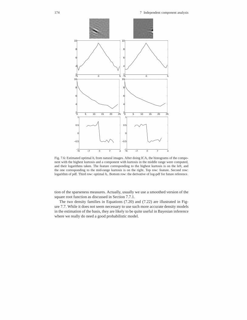
174 7 Independent component analysis
−5 0 52
4
6
8
10
−5 0 52
4
6
8
10
0 5 10 15 20 252
4
6
8
10
0 5 10 15 20 252
4
6
8
10
−4 −2 0 2 4−1
−0.5
0
0.5
1
−4 −2 0 2 4−1
−0.5
0
0.5
1
Fig. 7.6: Estimated optimalhi from natural images. After doing ICA, the histograms of the compo-nent with the highest kurtosis and a component with kurtosisin the middle range were computed,and their logarithms taken. The feature corresponding to the highest kurtosis is on the left, andthe one corresponding to the mid-range kurtosis is on the right. Top row: feature. Second row:logarithm of pdf. Third row: optimalhi . Bottom row: the derivative of log-pdf for future reference.
tion of the sparseness measures. Actually, usually we use a smoothed version of thesquare root function as discussed in Section 7.7.1.
The two density families in Equations (7.20) and (7.22) are illustrated in Fig-ure 7.7. While it does not seem necessary to use such more accurate density modelsin the estimation of the basis, they are likely to be quite useful in Bayesian inferencewhere we really do need a good probabilistic model.

7.8 Why are independent components sparse? 175
−4 −2 0 2 40
0.5
1
1.5
2
2.5
3
−4 −2 0 2 4−8
−6
−4
−2
0
2
−4 −2 0 2 40
0.5
1
1.5
2
2.5
3
−4 −2 0 2 4−8
−6
−4
−2
0
2
Fig. 7.7: Top row: Some plots of the density function (left) and its logarithm (right) given in Eqs(7.20),α is given values 0.75, 1 and 1.5. More peaked ones correspond to smallerα . Bottom row:Plots of the density function (7.22),α is given values 0.5,2,10. More peaked values correspond tosmallerα .
7.8 Why are independent components sparse?
There are many different ways in which random variables can be non-gaussian.What forms do there exist, and why is it that independent components in images arealways sparse — or are they? These are the questions that we address in this section.
7.8.1 Different forms of non-gaussianity
While the forms of non-gaussianity are infinite, most of the non-gaussian as-pects that are encountered in real data can be described as sub-gaussianity, super-gaussianity, or skewness.
Super-gaussianity is basically the same as sparseness. Often, super-gaussianity isdefined as positive kurtosis (see Equation (6.5) for a definition of kurtosis), but otherdefinitions exist as well. The intuitive idea is that the probability density functionhas heavy tails and a peak at zero.

176 7 Independent component analysis
The opposite of super-gaussianity is sub-gaussianity, which is typically charac-terized by negative kurtosis. The density function is “flat”around zero. A goodexample is the uniform distribution (here standardized to unit variance and zeromean)
p(s) =
{1
2√
3, if |s| ≤
√3
0, otherwise(7.23)
The kurtosis of this distribution equals−6/5, which is left as an exercise.An unrelated form of non-gaussianity is skewness which basically means the lack
of symmetry of the probability density function. A typical example is the exponen-tial distribution:
p(s) =
{
exp(−s), if s≥ 0
0, otherwise(7.24)
which is not symmetric with respect to any point on the horizontal (s) axis. Skewnessis often measured by the third moment (assuming the mean is zero)
skew(s) = E{s3} (7.25)
This is zero for a symmetrically-distributed random variable that has zero mean(this is left as an exercise). In fact, skewness is usually defined as exactly the thirdmoment. However, any other nonlinear odd function could be used instead of thethird power, for example the function that gives the sign (±1) of s.
7.8.2 Non-gaussianity in natural images
Is it true that all the independent components in natural images are sparse, and noother forms of non-gaussianity are encountered? This is almost true, but not quite.
The skewness of the components is usually very small. After all, natural imagestend to be rather symmetric in the sense that black and white are equally probable.This may not be exactly so, since such symmetry depends on themeasurement scaleof the grey-scale values: a non-linear change of measurement scale will make sym-metric data skewed. However, in practice, skewness seems tobe so small that it canbe ignored.
There are some sub-gaussian components, though. In particular, the DC compo-nent, i.e. the mean luminance of the image patch, is typically sub-gaussian. In fact,its distribution is often not far from a uniform distribution. If we do not remove theDC component from the images (in contrast to what we usually do), and we usean ICA algorithm that is able to estimate sub-gaussian components as well (not allof them are), the DC component actually tends to be estimatedas one independentcomponent. Depending on the window size and the preprocessing used, a couple offurther very low-frequency components can also be sub-gaussian.

7.9 General ICA as maximization of non-gaussianity 177
7.8.3 Why is sparseness dominant?
One reason why the independent components in images are mostly sparse is thevariation of the local variance in different parts of an image. Some parts of theimage have high variation whereas others have low variation. In fact, flat surfaceshave no variation, which is sometimes called the blue-sky effect.
To model this change in local variance, let us model an independent componentsi as a product of an “original” independent componentgi of unit variance, and anindependent, non-negative “variance” variabledi :
si = gi di (7.26)
We calldi a variance variable because it changes the scale of each observation ofgi .Such a variance variables will be the central topic in Chapter 9.
Let us assume that the original componentgi is gaussian with zero mean and unitvariance. Then the distributions of thesi is necessarily super-gaussian, i.e. it haspositive kurtosis. This can be shown using fact that for a gaussian variable, kurtosisis zero and thusE{g4
i }= 3, so we have
kurt si = E{s4i }−3(E{s2
i })2 = E{d4i g4
i }−3(E{d2i g2
i })2
= E{d4i }E{g4
i }−3(E{d2i })2(E{g2
i })2 = 3[E{d4i }− (E{d2
i })2] (7.27)
which is always non-negative because it is the variance ofd2i multiplied by 3. It can
be zero only ifdi is constant.Thus, the changes in local variance are enough to transform the gaussian distri-
bution of gi into a sparse distribution forsi . The resulting distribution is called agaussian scale mixture.
7.9 General ICA as maximization of non-gaussianity
Now we can consider the problem of ICA estimation in more generality, in thecase where the components are not necessarily sparse. In particular, we consider thefollowing two questions: Does estimation of ICA for non-sparse components havea simple intuitive interpretation, and: Is there a deeper reason why maximizationof sparseness is related to the estimation of the ICA model. These questions canbe answered based on the Central Limit Theorem, a most fundamental theorem inprobability theory. Here we explain this connection and show how it leads to a moregeneral connection between independence and non-gaussianity.

178 7 Independent component analysis
7.9.1 Central Limit Theorem
The Central Limit Theorem (CLT) basically says that when youtake an average orsum of many independent random variables, it will have a distribution that is closeto gaussian. In the limit of an infinite number of random variables, the distributionactually tends to the gaussian distribution, if properly normalized:
limN→∞
1√N
N
∑n=1
sn = gaussian (7.28)
where we assume thatsn have zero mean. We have to normalize the sum here be-cause otherwise the variance of the sum would go to infinity. Note that if we nor-malized by 1/N, the variance would go to zero.
Some technical restrictions are necessary for this resultsto hold exactly. Thesimplest choice is to assume that thesn all have the same distribution, and thatdistribution has finite moments. The CLT is illustrated in Figure 7.8.
7.9.2 “Non-gaussian is independent”
What does the CLT mean in the context of ICA? Let us consider a linear combi-nation of the observed variables,∑i wizi . This is also a linear combination of theoriginal independent components:
∑i
wizi = ∑i
wi ∑j
ai j sj = ∑j(∑
iwiai j )sj = ∑
jq jsj (7.29)
where we have denotedq j = ∑i wiai j . We do not know the coefficientsq j becausethey depend on theai j .
The CLT would suggest that this linear combination∑ j q jsj is closer to gaussianthan the original independent componentssj . This is not exactly true because theCLT is exactly true only in the limit of an infinite number of independent compo-nents, and there are restrictions on the distributions (forexample, the variablesq jsj
do not have identical distributions if theq j are not equal). However, the basic ideais correct. This is illustrated in Figure 7.9 which shows that the original indepen-dent components are more gaussian than the observed data after whitening, shownin Figure 7.1.
Thus, based on the central limit theorem, we can intuitivelymotivate a generalprinciple for ICA estimation: find linear combinations∑i wizi of the observed vari-ables that are maximally non-gaussian.
Why would this work? The linear combination∑i wizi equals a linear combina-tion of the independent components with some coefficientsq j . Now, if more thanone of theq j is non-zero, we have a sum of two independent random variables. Be-cause of the CLT, we can expect that such a sum is closer to gaussian that any of the
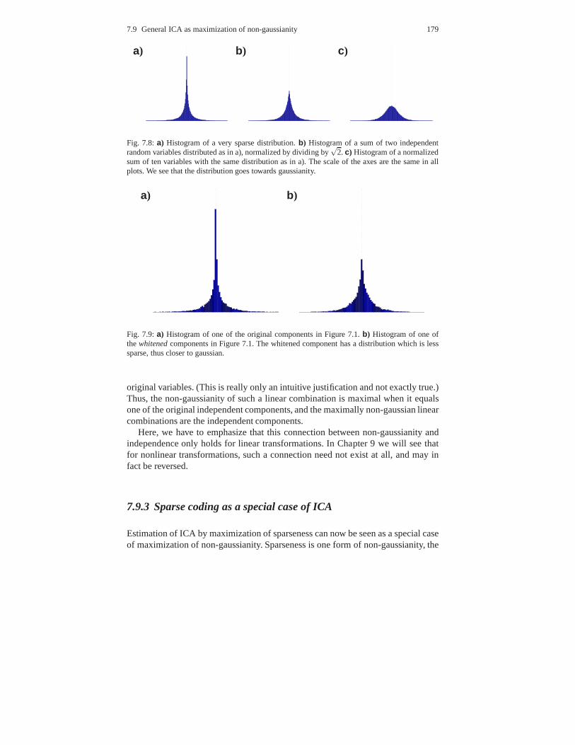
7.9 General ICA as maximization of non-gaussianity 179
a) b) c)
Fig. 7.8:a) Histogram of a very sparse distribution.b) Histogram of a sum of two independentrandom variables distributed as in a), normalized by dividing by
√2.c) Histogram of a normalized
sum of ten variables with the same distribution as in a). The scale of the axes are the same in allplots. We see that the distribution goes towards gaussianity.
a) b)
Fig. 7.9:a) Histogram of one of the original components in Figure 7.1.b) Histogram of one ofthewhitenedcomponents in Figure 7.1. The whitened component has a distribution which is lesssparse, thus closer to gaussian.
original variables. (This is really only an intuitive justification and not exactly true.)Thus, the non-gaussianity of such a linear combination is maximal when it equalsone of the original independent components, and the maximally non-gaussian linearcombinations are the independent components.
Here, we have to emphasize that this connection between non-gaussianity andindependence only holds for linear transformations. In Chapter 9 we will see thatfor nonlinear transformations, such a connection need not exist at all, and may infact be reversed.
7.9.3 Sparse coding as a special case of ICA
Estimation of ICA by maximization of sparseness can now be seen as a special caseof maximization of non-gaussianity. Sparseness is one formof non-gaussianity, the

180 7 Independent component analysis
one that is dominant in natural images. Thus, in natural images, maximization ofnon-gaussianity is basically the same as maximization of sparseness. For other typesof data, maximization of non-gaussianity may be quite different from maximizationof sparseness.
For example, in the theory of ICA, it has been proposed that the non-gaussianityof the components could be measured by the sum of the squares of the kurtoses:
n
∑i=1
[kurt(vTi z)]2 (7.30)
where, as usual, the data vectorz is whitened and the feature vectorsvi are con-strained to be orthogonal and to have unit norm. It can be shown that ICA estimationcan really be accomplished by maximizing this objective function. This works forboth sub-gaussian and super-gaussian independent components.
Now, if the components all have positive kurtoses, maximizing this sum is closelyrelated to finding vectorsvi such that thevT
i z are maximally non-gaussian. Thesquare of kurtosis is, however, a more general measure of non-gaussianity becausethere are cases where the kurtosis is negative as we saw abovein Section 7.8.1. Forsuch components, maximization of non-gaussianity meansminimizingkurtosis (andsparseness), because for negative values of kurtosis, maximization of the squaremeans to minimize kurtosis.
In fact, maximization of sparseness may not always be the correct method forestimation ICA even on images. If we do not remove the DC component from theimages, the DC component turns out to be one independent component, and it some-times has negative kurtosis. For such data, simply maximizing sparseness of all thecomponents will produce misleading results.
Thus, we see that there is a difference between basic linear sparse coding andICA in the sense that ICA works for different kinds of non-gaussianity and not justsparseness.
7.10 Receptive fields vs. feature vectors
An important point to note is the relation between the feature vectorsAi and thefeature detector weightsWi . The feature vectors are shown Fig. 7.3. However, it isoften theWi that are more interesting, since they are the weights that are applied tothe image to actually compute thesi , and in neurophysiological modelling, they aremore closely connected to the receptive fields of neurons.
There is, in fact, a simple connection between the two: theAi are basically low-pass filtered versions of theWi . In fact, simple calculations show that the covariancecov(I(x,y), I(x′,y′)) in images generated according to the ICA model equals
∑i
Ai(x,y)Ai(x′,y′) (7.31)

7.11 Problem of inversion of preprocessing 181
because thesi are uncorrelated and have unit variance. Thus we have
∑x′ ,y′
cov(I(x,y), I(x′,y′))Wi(x′,y′) = ∑
x′,y′∑i
Ai(x,y)Ai(x′,y′)Wi(x
′,y′)
= ∑i
Ai(x,y) ∑x′ ,y′
Ai(x′,y′)Wi(x
′,y′) = Ai(x,y) (7.32)
by definition of theWi as the inverse of theAi . This means that theAi can be obtainedby multiplying theWi by the covariance matrix of the data.
Such multiplication by the covariance matrix has a simple interpretation as alow-pass filteringoperation. This is because the covariances are basically a decreasingfunction of the distance between(x,y) and(x′,y′), as shown in Figure 5.4. Thus,Ai
andWi have essentially the same orientation, location and frequency tuning proper-ties. On the other hand, theAi are better to visualize because because they actuallycorrespond to parts of the image data; especially with data that is not purely spatial,as in Chapter 15, visualization of the detector weights would not be straightforward.
7.11 Problem of inversion of preprocessing
A technical point that we have to consider is computation of the Ai for originalimages based on ICA of canonically preprocessed data. Thereis actually a problemhere: in order to get theAi we have to invert the canonical preprocessing, becauseestimation of the model gives the vectorsvi in the reduced (preprocessed) spaceonly. But canonical preprocessing is not invertible in the strict sense of the word,because it reduces the dimension and therefore loses information!
Typically, a solution based on the idea of computing the bestpossible approxima-tion of the inverse of the PCA/whitening transformation. Such best approximationcan be obtained by the theory of multivariate regression, or, alternatively, by the the-ory of pseudo-inverses (see Section 19.8). Without going into details, the descriptionof the solution is simple.
Denote byU the orthogonal matrix which contains then vectors giving the direc-tions of the principal components as its rows, i.e. then dominant eigenvectors of thecovariance matrix. Denote byλi the corresponding eigenvalues. Then, steps 3 and4 of canonical preprocessing in Section 5.4 consist of multiplying the vectorizedimage patches by diag(1/
√λi)U.
We now define the inverse preprocessing as follows: After computing the fea-ture vectors in the preprocessed space (thevi), the basis vectors are multiplied byUTdiag(
√λi). These are the optimal approximations of the feature vectors in the
original space. They can also be computed by taking the pseudoinverse of the ma-trix of the featuresWi , which is what we did in our simulations.
Note that we have no such problem with computation of theWi for the originaldata because we just multiply the vectorsvi with the PCA/whitening matrix, and noinversion is needed.

182 7 Independent component analysis
7.12 Frequency channels and ICA
A long-standing tradition in vision science is to talk about“frequency channels”,and more rarely, about “orientation” channels. The idea is that in the early visualprocessing (something like V1), information of different frequencies is processedindependently. The word “independence” as used here has nothing to do with sta-tistical independence: it means that processing happens indifferent physiologicalsystems that are more or less anatomically separate, and do not exchange informa-tion with each other.
Justification for talking about different channels is abundant in research on V1. Inrecordings from single cells, simple and complex cell receptive fields are band-pass,i.e. respond only to stimuli in a certain frequency range, and various optimal fre-quencies are found in the cells (see Chapter 3 and its references). In psychophysics,a number of experiments also point to such a division of earlyprocessing. For exam-ple, in Figure 3.8 on page 60, the information on the high- andlow-frequency partsare quite different, yet observes have no difficulty in processing (reading) them sep-arately.
In the results of ICA on natural images, we see an interestingnew interpretationof why the frequency channels might be independent in terms of physiological andanatomical separation in the brain. The reason is that the information in differentfrequency channels seems to bestatisticallyindependent, as measured by ICA. Thefeature vectorsAi given by ICA are band-pass, thus showing that a decompositioninto statistically independent features automatically leads to frequency channels.
7.13 Concluding remarks and References
Independent component analysis is a statistical generative model whose estimationboils down to sparse coding. It gives a proper probabilisticformulation of sparsecoding and thereby solves a number of theoretical problems in sparse coding (inparticular: optimal ways of measuring sparseness, optimality of decorrelation), andgives a proper pdf to be used in Bayesian inference. The expression “independentcomponent analysis” also points out another important property of this model: thecomponents are considered statistically independent. This independence assumptionis challenged in many more recent models which are the topicsof Chapters 9–11.
The first application of ICA, as opposed to sparse coding, on image patches wasin (Bell and Sejnowski, 1997) based on the earlier sparse coding framework in (Ol-shausen and Field, 1996) considered in Section 13.1.
For more information on the ICA model, see (Hyvarinen and Oja, 2000) or(Hyvarinen et al, 2001b). Some of the earliest historical references on ICA include(Herault and Ans, 1984; Mooijaart, 1985; Cardoso, 1989; Jutten and Herault, 1991).Classic references include (Delfosse and Loubaton, 1995),which showed explicitlyhow maximization of non-gaussianity is related to ICA estimation; (Comon, 1994),which showed the uniqueness of the decomposition, and the validity of the sum-

7.14 Exercices 183
of-squares-of-kurtosis in Equation (7.30); the maximum likelihood framework wasintroduced in (Pham et al, 1992; Pham and Garrat, 1997).
For more information on the central limit theorem, see any standard textbook onprobability theory, for example (Papoulis and Pillai, 2001).
A related way of analyzing the statistics of natural images is to look at the cu-mulant tensors (Thomson, 1999, 2001). Cumulants (strictlyspeaking, higher-ordercumulants) are statistics which can be used as measures of non-gaussianity; for ex-ample, kurtosis and skewness are one of the simplest cumulants. Cumulant tensorsare generalizations of the covariance matrix to higher-order cumulants. Analysis ofcumulant tensors is closely related to ICA, as discussed in detail in Chapter 11 of(Hyvarinen et al, 2001b). Equivalently, one can analyze the polyspectra (usually thetrispectrum) which are obtained by Fourier transformations of the cumulant spec-tra, in a similar way as the ordinary Fourier spectrum function can be obtained asthe Fourier transform of the autocovariance function; see e.g. (Nikias and Mendel,1993; Nikias and Petropulu, 1993) for further information.
7.14 Exercices
Mathematical exercises
1. Prove (7.2).2. Based on (7.2), prove that two independent random variables are uncorrelated.3. Calculate the kurtosis of the uniform distribution in (7.23).4. Calculate the kurtosis of the Laplacian distribution in (7.18).5. Show that the skewness of a random variable with a pdf whichis even-symmetric
(i.e. p(−x) = p(x)) is zero.6. In this exercise we consider a very simple case of gaussianmixtures (see Sec-
tion 7.8.3). Assume that a component followss = vz wherez is gaussian withzero mean and unit variance. Let us assume that in 50% of the natural images thevariance coefficientv has valueα. In the remaining 50% of natural images,v hasvalueβ .
a. What is the distribution of the random variables in the set of all natural im-ages? (Give the density functionp(s))
b. Show thatE{s2}= 12(α2 + β 2)
c. Show thatE{s4}= 32(α4 + β 4)
d. What is the kurtosis of this distribution?e. Show that the kurtosis is positive for almost any parameter values.
7. Prove (7.31).

184 7 Independent component analysis
Computer assignments
1. Using numerical integration, compute the kurtoses of theLaplacian and uniformdistributions.
2. Load the FastICA program from the web. This will be used in the followingassignments. You will also need some images; try to find some that have notbeen compressed, since compression can induce very nasty effects.
3. Take patches of 16×16 of the image. 10,000 is a sufficient amount of patches.Input these to FastICA.
4. Plot histograms of the independent components. Compute their kurtoses. Plot(some of the) RF’s. Look at the RF’s and comment on whether they look like V1RF’s or not. If not, why not?

Chapter 8Information-theoretic interpretations
So far, we have been operating within the theoretical framework of Bayesian in-ference: the goal of our models is to provide priors for Bayesian inference. An al-ternative framework is provided by information theory. In information theory, thegoal is to find ways of coding the information as efficiently aspossible. This turnsout to be surprisingly closely connected to Bayesian inference. In many cases, bothapproaches start by estimation of parameters in a parameterized statistical model.
This chapter is different from the previous ones because we do not provide anynew models for natural image statistics. Rather, we describe a new framework forinterpreting some of the previous models.
8.1 Basic motivation for information theory
In this section, we introduce the basic ideas of informationtheory using intuitive ex-amples illustrating the two principal motivations: data compression and data trans-mission.
8.1.1 Compression
One of the principal motivations of information theory is data compression. Let usbegin with a simple example. Consider the following string of characters:
BABABABADABACAABAACABDAAAAABAAAAAAAADBCA
We need to code this using a binary string, consisting of zeros and ones, becausethat’s the form used in computer memory. Since we have four different characters,a basic approach would be to assign the four possible two-digit codewords for eachof them:
185

186 8 Information-theoretic interpretations
A→ 00 (8.1)
B→ 01 (8.2)
C→ 10 (8.3)
D→ 11 (8.4)
(8.5)
Replacing each of the characters by its two-digit codeword gives the code
01000100010001001100010010000001000010000111000000000001000000000000000011011000
However, a shorter code can be obtained by using the fundamental insight ofinformation theory:frequent characters should be given shorter codewords. Thismakes intuitive sense: if frequent characters have short codewords, even at the ex-pense of giving less frequent characters longer codewords,the average length couldbe shortened.
In this example, the character A is the most frequent one: approximately one halfof the letters are A’s. The letter B is the next, with a proportion of approximatelyone quarter. So, let us consider the following kind of codeword assignment:
A→ 0 (8.6)
B→ 10 (8.7)
C→ 110 (8.8)
D→ 111 (8.9)
(8.10)
Now, the code becomes
1001001001001110100110001000110010111000001000000000111101100
This is more than 10% shorter than the basic code given above.(In real-world appli-cations, the saving is often much larger, sometimes reaching more than 90% in im-age compression.) Note that the codeword assignment has been cleverly constructedso that the original string can be recovered from this code without any ambiguity.
Compression was possible because some of the characters were more commonthan others. In other words, it was due to the statistical regularities of the data (orredundancy, which will be defined later). Thus, it is not surprising that the methodsdeveloped in information theory have also been applied in the field of natural imagestatistics.

8.2 Entropy as a measure of uncertainty 187
8.1.2 Transmission
A rather different application of information theory is in data transmission. In trans-mission, the central problem isnoise. That is, the transmission will introduce ran-dom errors in the data. The goal here is to code the data so thatthe receiving end ofthe system can correct as many of the random errors as possible.
As a simple example, consider the following binary string which we want totransmit:
1111101100100011100110100101110110100101
To code this string we use a very simple method: we simply repeat all the digitsthree times. Thus we get the code
111111111111111000111111000000111000000000111111111000000111111000111000000111000111111111000111111000111000000111000111
This is transmitted through a channel which has relatively strong noise: 25% of thedigits are randomly changed to the opposite. So, the receiving end in the channelreceives the following string:
111110011111111000011111000000111010000110001101001001001110101010111000010101001111111111000110101000111010010111100111
Now, we can use the repetitions in the string in the followingway: we look at allconsecutive groups of three digits, and guess that the original string probably hadthe digit which has the most occurrences among each group. Thus, we obtain thefollowing string
1111101100100101000110100101110110100101
This string has less than 10% wrong digits. Thus, our encoding scheme reduced thenumber of errors introduced by the channel from 25% to less than 10%. (Actually,we were a bit lucky with this string: on the average the errorswould be of the orderof 16%.)
So, the central idea in transmission is very different from compression. In orderto combat noise, we want to code the data so that we introduce redundancy (to bedefined later), which often means making the code longer thanthe original data.
8.2 Entropy as a measure of uncertainty
Now, we introduce the concept of entropy, which is the foundation of informationtheory. First, we give its definition and a couple of examples, and then show how itis related to data compression.

188 8 Information-theoretic interpretations
8.2.1 Definition of entropy
Consider a random variablez which takes values in a discrete seta1, . . . ,aN withprobabilitiesP(z= ai), i = 1, . . . ,N. The most fundamental concept of informationtheory isentropy, denoted byH(z), which is defined as
H(z) =−N
∑i=1
P(z= ai) log2P(z= ai) (8.11)
If the logarithms to base 2 are used, the unit of entropy is called abit. Entropy is ameasure of theaverage uncertaintyin a random variable. It is always non-negative.We will next present a couple of examples to illustrate the basic idea.
Example 1 Consider a random variable which takes only two values,A andB.Denote the probabilityP(z= A) by p0. Then, entropy ofzequals
H(z) =−p0 log2 p0− (1− p0) log2(1− p0) (8.12)
We can plot this as a function ofp0, which is shown in Fig. 8.1 The plot shows thatthe maximum entropy is obtained whenp0 = 0.5, which means that both outcomesare equally probable. Then the entropy equals one bit. In contrast, if p0 equals 0 or1, there is no uncertainty at all in the random variable, and its entropy equals zero.
0 0.2 0.4 0.6 0.8 10
0.5
1
1.5
Fig. 8.1: Entropy of a random variable which can only take twovalues, plotted as a function of theprobability p0 of taking one of those values.
Example 2 Consider a random variablezwhich takes, for some givenn, any of 2n
values with equal probability, which is obviously 1/2n. The entropy equals

8.2 Entropy as a measure of uncertainty 189
H(z) =−2n
∑i=1
12n log2
12n =−2n 1
2n (−n) = n (8.13)
Thus, the entropy equalsn bits. This is also the number of binary digits (also calledbits) that you would need to represent the random variable ina basic binary repre-sentation.
Example 3 Consider a random variablez which always takes the same value, i.e.it is not really random at all. Its entropy equals
H(z) =−1× log2 1 = 0 (8.14)
Again, we see that the entropy is zero since there is no uncertainty at all.
8.2.2 Entropy as minimum coding length
An important result in information theory shows that the numerical value of entropydirectly gives theaverage code length for the shortest possible code(i.e. the onegiving maximum compression). It is no coincidence that the unit of entropy is calleda bit, since the length of the code is also given in bits, in thesense of the number ofzero-one digits used in the code.
The proof of this property is very deep, so we will only try to illustrate it with anexample.
Example 4 Now we will return back to the compression example in the precedingsection to show how entropy is connected to compression. Consider the charactersin the string as independent realizations of a random variable which takes values inthe set{A,B,C,D}. The probabilities used in generating this data are
P(A) = 1/2 (8.15)
P(B) = 1/4 (8.16)
P(C) = 1/8 (8.17)
P(D) = 1/8 (8.18)
We can compute the entropy, which equals 1.75 bits. Thus, theentropy is smallerthan 2 bits, which would be (according to Example 2), the maximum entropy fora variable with four possible values. Using the definition ofentropy as minimumcoding length, we see that the saving in code length can be at most (2-1.75)/2 =12.5 % for data with these characteristics. (This holds in the case of infinite stringsin which random effects are averaged out. Of course, for a finite-length string, thecode would be a bit shorter or longer due to random effects.)
Note also it is essential here that the characters in the string are generated inde-pendently at each location; otherwise, the code length might be shorter. For example,

190 8 Information-theoretic interpretations
if the characters would be generated in pairs, as in AACCBBAA..., this dependencycould obviously be used to reduce the code length, possibly beyond the bound thatentropy gives.
8.2.3 Redundancy
Redundancy is a word which is widely used in information theory, as well as in nat-ural image statistics. It is generally used to refer to the statistical regularities, whichmake part of the information “redundant”, or unnecessary. Unfortunately, when talk-ing about natural images, different authors use the word in slightly different ways.
An information-theoretic definition of redundancy is basedon entropy. Given arandom variable which has 2n different values, say 1, . . . ,2n, we compare the lengthof the basicn-bit code and the length of the shortest code, given by entropy:
redundancy= n−H(z) (8.19)
This is zero only if all the values 1, . . . ,2n are equally likely. Using this terminology,we can say that compression of the string in Section 8.1.1 waspossible because thestring had some redundancy (n was larger thanH(z)). Compression is possible byremoving, or at least reducing, redundancy in the data.
This definition is actually more general than it seems, because it can also considerdependenciesbetweendifferent variables (say, pixels). If we have two variablesz1
andz2, we can simply define a new variablez whose possible values correspond toall the possiblecombinations1 of the values ofz1 andz2. Then, we can define entropyand redundancy for this new variable. If the variables are highly dependent fromeach other, some combinations will have very small probabilities, so the entropywill be small and redundancy large.
It is important to understand that you may want to either reduce or increase re-dundancy, depending on your purpose. In compression you want to reduce it, butin information transmission, you actually want to increaseit. The situation is evenmore complicated than this because usually before transmission, you want to com-press the data in order to reduce the time needed for data transmission. So, you firsttry to remove the redundancy to decrease the length of the data to be transmitted,and then introduce new redundancy to combat noise. This neednot be contradictorybecause in introducing new redundancy, you do it is a controlled way using care-fully designed codes which increase code length as little aspossible for a requiredlevel of noise-resistance. A result called “source-channel coding theorem” lays outthe conditions under which such a two-stage procedure is, infact, optimal.
1 More precisely: if z1 can take values in the set{1,2} and z2 can take values in theset {1,2,3}, we definez so that it takes values in the Cartesian product of those sets, i.e.{(1,1), (1,2), (1,3), (2,1), (2,2), (2,3)}, so that the probabilityz= (a1,a2) simply equals the prob-ability thatz1 = a1 and z2 = a2

8.2 Entropy as a measure of uncertainty 191
8.2.4 Differential entropy
The extension of entropy to continuous-valued random variables or random vec-tors is algebraically straightforward. For a random variable with probability densityfunction pz we define thedifferential entropy, denoted byH just like entropy, asfollows:
H(z) =−∫
pz(z) logpz(z)dz (8.20)
So, basically we have just replaced the summation in the original definition in Equa-tion (8.11) by an integral. The same definition also applies in the case of a randomvector.
It is not difficult to see what kind of random variables have small differentialentropies. They are the ones whose probability densities take large values, sincethese give strong negative contributions to the integral inEq. (8.20). This meansthat certain small intervals are quite probable. Thus we again see that entropy issmall when the variable is not very random, that is, it is typically contained in somelimited intervals with high probabilities.
Differential entropy is related to the shortest code lengthof adiscretizedversionof the random variablez. Suppose we discretizez so that we divide the real lineto bins (intervals) of lengthd, and define a new discrete-valued random variable ˜zwhich tells which of these bins the value ofz belongs to. This is similar to usinga limited number of decimals in the representation, for example using only onedecimal place as in “1.4” to represent the values of the random variable. Then, theentropy ofz is approximately equal to the differential entropy ofz plus a constantwhich only depends on the size of the bins,d.
Example 5 Consider a random variablez which follows a uniform distribution inthe interval[0,a]: Its density is given by
pz(z) =
{
1/a, for 0≤ z≤ a
0, otherwise(8.21)
Differential entropy can be evaluated as
H(z) =−∫ a
0
1a
log1a
dz= loga (8.22)
We see that the entropy is large ifa is large, and small ifa is small. This is naturalbecause the smallera is, the less randomness there is inz. Actually, in the limitwhereagoes to 0, differential entropy goes to−∞, because in the limit,z is no longerrandom at all: it is always 0. This example also shows that differential entropy, incontrast to basic entropy, need not be non-negative.
192 8 Information-theoretic interpretations
8.2.5 Maximum entropy
An interesting question to ask is: What kind of distributions have maximum en-tropy?
In the binary case in Example 1, we already saw that it was the distributionwith 50%-50% probabilities which is clearly consistent with the intuitive idea ofmaximum uncertainty. In the general discrete-valued case,it can be shown that theuniform distribution (probabilities of all possible values are equal) has maximumentropy.
With continuous-valued variables, the situation is more complicated. Differentialentropy can become infinite; consider, for example whena→∞ in Example 5 above.So, some kind of constraints are needed. The simplest constraint would perhaps beto constrain the random variable to take values only inside afinite interval[a,b]. Inthis case, the distribution of maximum entropy is, again, the uniform distribution,i.e. a pdf which equals1
b−a in the whole interval and is zero outside of it. However,such a constraint may not be very relevant in most applications.
If we consider random variables whosevariance is constrainedto a given value(e.g. to 1), the distribution of maximum entropy is, interestingly, the gaussian distri-bution. This is why the gaussian distribution can be considered the least “informa-tive”, or the least “structured”, of continuous-valued distributions.
This also means that differential entropy can be considereda measure ofnon-gaussianity. The smaller the differential entropy, the further away thedistributionis from the gaussian distribution. However, it must be notedthat differential en-tropy depends on the scale as well. Thus, if entropy is used asa measure of non-gaussianity, the variables have to normalized to unit variance first, just like in thecase of kurtosis. We will see in Section 8.4 how differentialentropy is, in fact,closely related to the sparseness measures we used in Chapter 6.
8.3 Mutual information
In information transmission, we need a measure of how much information the outputof the channel contains about the input. This the purpose of the concept of mutualinformation.
Let’s start with the concept ofconditional entropy. It is simply the average en-tropy calculated for the conditional distribution of the variablez, where the condi-tioning is by the observation of another variabley:
H(z|y) =−∑y
P(y)∑z
P(z|y) logP(z|y) (8.23)
That is, it measures how much entropy there is left inzwhen we know (observe) thevalue ofy; this is averaged over all values ofy.

8.3 Mutual information 193
If z andy are independent, the conditional distribution ofz giveny is the sameas the distribution ofz alone, so conditional entropy is the same as the entropy ofz. If z andy are not independent, conditional entropy is smaller than the entropyof z, because then knowledge of the value ofy reduces the uncertainty onz. Inthe extreme case wherez= y, the conditional distributionz giveny is such that allthe probability is concentrated on the observed value ofy. The entropy of such adistribution is zero (see Example 3 above), so the conditional entropy is zero.
Let us assume thatz is the message input to a transmission channel andy is theoutput, i.e. the received signal. Basically, if transmission is very good, knowledgeof y will tell us very much about whatz was. In other words, the conditional distri-bution ofzgiveny is highly concentrated on some values. So, we could measure thetransmitted information by the change in entropy which is due to measurement ofy.It is called the mutual information, which we denote2 by J:
J(z,y) = H(z)−H(z|y) (8.24)
Just as entropy gives the code length of the optimal code, mutual information isrelated to the amount of information which can be obtained aboutz, based on obser-vation of the channel outputy.
Note that, in practice, mutual information depends not onlyon the noise in thechannel, but also on how we code the data as the variablez in the first place. There-fore, to characterize the properties of the channel itself,we need to consider themaximum of mutual information over all possible ways of coding z. This is calledchannel capacityand gives the maximum amount of information which can be trans-mitted through the channel.
A generalization of mutual information to many variables isoften used in thetheory of ICA. In that case, the interpretation as information transmitted over achannel is no longer directly applicable. The generalization is based on the fact thatmutual information can be expressed in different forms:
J(z,y) = H(z)−H(z|y) = H(y)−H(y|z) = H(z)+H(y)−H(z,y) (8.25)
whereH(z,y) is thejoint entropy, which is simply obtained by defining a new ran-dom variable so that it can take all the possible combinations of values ofz andy.Based on this formula, we define mutual information ofn random variables as
J(z1,z2, . . . ,zn) =n
∑i=1
H(zi)−H(z1,z2, . . . ,zn) (8.26)
The utility in this quantity is that it can be used a measure ofindependence: it isalways non-negative and zero only if the variableszi are independent.
2 We use a non-conventional notationJ for mutual information because the conventional one,I ,could be confused with the notation for an image.

194 8 Information-theoretic interpretations
Conditional entropy, joint entropy, and mutual information can all be defined forcontinuous-valued variables by using differential entropy in the definitions insteadof ordinary entropy.
8.4 Minimum entropy coding of natural images
Now, we discuss the application of the information-theoretic concepts in the contextof natural image statistics. This section deals with data compression models.
8.4.1 Image compression and sparse coding
Consider first the engineering application of image compression. Such compressionis routinely performed when images are transmitted over theInternet or stored on adisk. Most successful image compression methods begin witha linear transforma-tion of image patches. The purpose of such a transformation is to reduce (differen-tial) entropy. Grey-scale values of single pixels have a much larger entropy than, forexample, the coefficients in a Fourier or discrete cosine transform (DCT) basis (atleast when these are applied on small patches). Since the coefficients in those baseshave smaller differential entropy, discretized (quantized) versions of the coefficientsare easier to code: the quantization error, i.e. the error inquantizing the coefficientsfor a fixed code length, in reduced. This is why such a transformation is done as thefirst step.
This means that the optimal linear transformation of imagesas the first step ofa compression method would be a transformation which minimizes the differentialentropy of the obtained components. This turns out to be related to sparse coding,as we will now show.
Let us consider the differential entropy of a linear component s. How can wecompute the valueH(s) using the definition in Equation (8.20) in practice? The keyis to understand that entropy is actually the expectation ofa nonlinear function ofs.We have
H(s) = E{G(s)} (8.27)
where the functionG is the negative of the log-pdf:G(s) =− logps(s). In practice,we have a sample ofs, denote it bys(t),t = 1, . . . ,T. Assume we also have reason-able approximation ofG, that is, we know rather well what the log-pdf is like. Then,differential entropy can be estimated as the sample averagefor a fixedG as
H(s) =1T ∑
tG(s(t)) (8.28)
Comparing this with Equation (6.2) on page 139, we see that differential entropy issimilar the sparseness measures we used in sparse coding. Infact, in Section 7.7.2 it
8.4 Minimum entropy coding of natural images 195
was shown that the optimal sparseness measures are obtainedwhen we use exactlythe log-pdf ofs as the nonlinearity. Thus,differential entropy is the optimal sparse-ness measurein the sense of Section 7.7.2: it provides the maximum likelihoodestimator of the ICA model.
However, there is one important point which needs to be takeninto account. Thesparseness measures assumed that the variance ofs is constrained to be equal toone. This is consistent with the theory of ICA which tells that the transformationshould be orthogonal in the whitened space. In contrast, in image compression, thetransformation giving the components is usually constrained to be orthogonal (in theoriginal image space). One reason is that then the quantization error in the imagespace is the same as the quantization error in the component space. This makessense because then minimizing quantization error for the components is directlyrelated to the quantization error of the original image. In contrast, any method whichwhitens the data amplifies high-frequency components whichhave low variance,thus emphasizing errors in their coding. So, the quantization error in the componentsis not the same as the error in the original image—which is what we usually want tominimize in engineering applications.
If we consider transformations which are orthogonal in the original space, theconstraint of unit variance of a components is not at all fulfilled. For example, PCAis an orthogonal transformation which finds components withmaximally differentvariances. From the viewpoint of information theory, logp changes quite a lot asa function of variance, so using a fixedG may give a very bad approximation ofentropy. So, while sparse coding, as presented in Chapter 6,is related to findingan optimal basis for image compression, it uses a rather unconventional constraintwhich means it does not optimize the compression in the usualsense.
8.4.2 Mutual information and sparse coding
Information-theoretic concepts allow us to see the connection between sparse cod-ing and ICA from yet another viewpoint. Consider a linear invertible transformationy = Vz of a random vectorz which iswhite. The mutual information between thecomponentsyi is equal to
J(y1, . . . ,yn) =n
∑i=1
H(vTi z)−H(Vz) (8.29)
Recall that mutual information can be interpreted as a measure of dependence. Now,let us constrainV to be orthogonal. Then, we haveH(Vz) = H(z) because theshape(in an intuitive sense) of the distribution is not changed atall: an orthogonal trans-formation simply rotates the pdf in then-dimensional space, leaving its shape intact.This means that the values taken bypz and logpz in the definition in Equation (8.20)

196 8 Information-theoretic interpretations
are not changed; they are just taken at new values ofz. That is why differential en-tropy is not changed by an orthogonal transformation of the data.3
So, to minimize the mutual information, we simply need to findan orthogonaltransformation which minimizes the differential entropies of the components; thisis the same as maximizing the nongaussianities of the components. And for sparsedata, maximizing non-gaussianity is usually the same as maximizing sparseness.Thus, we see that under the constraint of orthogonality,sparse coding is equiva-lent to minimization of the dependence of the components, if the data is white. Thisprovides another deep link between information theory, sparse coding, and indepen-dence.
8.4.3 Minimum entropy coding in the cortex
A very straightforward application of the data compressionprinciple is then to as-sume that V1 “wants” to obtain a minimum entropy code. This isvery well in linewith the results on sparse coding and ICA in Chapters 6 and 7, because we have justshown that the objective functions optimized there can be interpreted as differentialentropies and code lengths. Basically, what information theory provides is a newinterpretation of the objective functions used in learningsimple cell receptive fields.
Yet, it is not quite clear whether such an entropy-based arguments are relevant tothe computational tasks facing the visual cortex. A critical discussion on the analogybetween compression and cortical coding is postponed to Section 8.6.
8.5 Information transmission in the nervous system
Following the fundamental division of information theory into compression andtransmission, the second influential application of information theory to visual cod-ing considers maximization of data transmission, usually called simply infomax.
8.5.1 Definition of information flow and infomax
Assume thatx is a continuous-valued random vector. It is the input to a neuralsystem, which is modelled using a linear-nonlinear model (see Section 3.4.1), with
3 A rigorous proof is as follows: denotingy = Vz, we simply havepy(y) = pz(VTy) for an or-thogonalV. The basic point is that the absolute value of the determinant of the transformationmatrix needed in transforming pdf’s, or variables in an integral formula, (see Section 7.4) is equalto one for an orthogonal transformation, so it can be omitted. Thus, we have
∫py(y) logpy(y)dy =
∫pz(VTy) logpz(VTy)dy. In this integral we make a change of variablesz = VTy and we get
∫pz(z) logpz(z)dz.
8.5 Information transmission in the nervous system 197
additive noise. Thus, outputs are of the form
yi = φi(bTi x)+n (8.30)
where theφi are some scalar functions, thebi are the connection weight vectors ofthe neurons, andn is a vector of white gaussian noise. That is, the neural networkfirst computes a linear transformation of the input data, with the coefficients given bynetwork connection weightsbi ; then it transforms the outputs using scalar functionsφi , and there is noise in the system.
Let us consider information flow in such a neural network. Efficient informationtransmission requires that we maximize the mutual information between the inputsx and the outputsy, hence the name “infomax”. This problem is meaningful onlyif there is some information loss in the transmission. Therefore, we assume thatthere is some noise in the network; in practice, we have to assume that the noise isinfinitely small to be able to derive clear results. We can then ask how the networkparameters should be adapted (learned) so as to maximize information transmission.
8.5.2 Basic infomax with linear neurons
To begin with, we shall consider the very basic case where there are actually no non-linearities: we defineφ(u) = u, and the noise has constant variance. (It may seemodd to say that white noise has constant variance, because that seems obvious. How-ever, in Section 8.5.4 we will consider a model where the variance is not constantbecause that is the case in neural systems.)
By definition of mutual information, we have
J(x,y) = H(y)−H(y|x) (8.31)
In the present case, the conditional distribution ofy givenx is simply the distributionof the gaussian white noise. So, the entropyH(y|x) does not depend on the weightsbi at all: it is just a function of the noise variance. This meansthat for the purposeof finding thebi which maximize information flow, we only need to consider theoutput entropyH(y). This is true as long as the noise variance is constant.
To simplify the situation, let us assume, just for the purposes of this section, thatthe transformation matrixB, with thebi as its rows, is orthogonal. Then,y is just anorthogonal transformation ofx, with some noise added.
Furthermore, in all infomax analysis, we consider the limitwhere the noise vari-ance goes to zero. This is because simple analytical resultscan only be obtained inthat limit.
So, combining these assumptions and results, infomax for linear neurons withconstant noise variance boils down to the following: we maximize the entropyH(y),wherey is an orthogonal transformation ofx. Noise does not need to be taken intoaccount because we consider the limit of zero noise. But, as shown in Section 8.4.2,

198 8 Information-theoretic interpretations
an orthogonal transformation does not change differentialentropy, so the informa-tion flow does not depend onB at all!
Thus, we reach the conclusion that for linear neurons with constant noise vari-ance, the infomax principle does not really give anything interesting. Fortunately,more sophisticated variants of infomax are more interesting. In the next subsections,we will consider the two principal cases: noise of constant variance with nonlinearneurons, and noise of non-constant variance with linear neurons.
8.5.3 Infomax with nonlinear neurons
8.5.3.1 Definition of model
First, we consider the case where
1. the functionsφi are nonlinear. One can build a more realistic neuron model bytaking a nonlinearity which is saturating, and has no negative outputs.
2. The vectorn is additive gaussian white noise.This is the simplest noisemodel tobegin with.
Maximization of this mutual informationJ(x,y) is still equivalent to maximiza-tion of the output entropy, as in the previous subsection. Again we take the limitwhere the noise has zero variance. We will not go into detailshere, but it can beshown that the output entropy in this nonlinear infomax model then equals
H(y) = ∑i
E{logφ ′i (bTi x)}+ log|detB| (8.32)
It turns out that this has a simple interpretation in terms ofthe ICA model. Nowwe see that the output entropy is of the same form as the expectation of the likelihoodas in Equation (7.15). The pdf’s of the independent components are here replacedby the functionsφ ′i . Thus, if the nonlinearitiesφi used in the neural network arechosen as the cumulative distribution functions corresponding to the densitiespi ofthe independent components, i.e.,φ ′i (·) = pi(·), the output entropy is actually equalto the likelihood. This means that infomax is equivalent to maximum likelihoodestimation of the ICA model.
Usually, the logistic function
φi(u) =1
1+exp(−u)(8.33)
is used in the nonlinear infomax model (see Fig. 8.2 a). This estimates the ICAmodel in the case of sparse independent components, becauseif we interpretφ ′i as apdf, it is sparse. In fact, the log-pdf given by logφ ′i is nothing else than the familiarlogcosh function (with negative sign and some unimportant constants), which wehave used as a measure of sparseness in Chapter 6, and as a model of a smoothsparse log-pdf in Equation (7.19).

8.5 Information transmission in the nervous system 199
8.5.4 Infomax with non-constant noise variance
Here, we present some critique of the nonlinear infomax model, and propose analternative formulation.
8.5.4.1 Problems with nonlinear neuron model
Using a logistic function as in Equation (8.33) is a correct way of estimating the ICAmodel for natural image data in which the components really are super-gaussian.However, if the transfer functionφi is changed to the gaussian cumulative distri-bution function, the method does not estimate the ICA model anymore, since thiswould amount to assuming gaussian independent components,which makes the es-timation impossible. An even worse situation arises if we change the functionφi sothatφ ′i is the pdf of a sub-gaussian (anti-sparse) distribution. This amounts to esti-mating the ICA model assuming sub-gaussian independent components. Then, theestimation fails completely because we have made a completely wrong assumptionon the distribution of the components.
Unfortunately, the three nonlinear functionsφi corresponding to Equation (8.33),the gaussian case, and one particular sub-gaussian case look all very similar, how-ever. This is illustrated in Fig. 8.2 a). All the three functions have the same kind ofqualitative behaviour. In fact, all cumulative distribution functions look very similarafter appropriate scaling along the x-axis.
It is not very likely that the neural transfer functions (which are only crude ap-proximations anyway) would consistently be of the type in Eq. (8.33), and not closerto the two other transfer functions. Thus,the model can be considered to be non-robust, that is, too sensitive to small fluctuations in its parameters.4
8.5.4.2 Using neurons with non-constant variance
A possible solution to the problems with nonlinear infomax is to consider a morerealistic noise model. Let us thus take the linear function as φi , and change thedefinition of the noise term instead.
What would be a sensible model for the noise? Many classic models of neuronsassume that the output is coded as the mean firing rate in a spike train, which followsa Poisson process. Without going into details, we just note that in that case, thevariance of mean firing rate has a variance that is equal to itsmean. Thus, we have
var(ni |x) ∝ r + |bTi x| (8.34)
4 It could be argued that the nonlinear transfer function can be estimated from the data and it neednot be carefully chosen beforehand, but this only modifies this robustness problem because thenthat estimation must be very precise.

200 8 Information-theoretic interpretations
a)
−6 −4 −2 0 2 4 60
0.1
0.2
0.3
0.4
0.5
0.6
0.7
0.8
0.9
1
b)
0 0.2 0.4 0.6 0.8 1 1.2 1.4 1.6 1.8 21
1.2
1.4
1.6
1.8
2
2.2
2.4
2.6
2.8
3
Fig. 8.2:a) Three sigmoidal nonlinearities corresponding to logistic, gaussian, and sub-gaussian(with log-pdf proportional to−x4) prior cumulative distributions for the independent components.The nonlinearities are practically indistinguishable. (Note that we can freely scale the functionsalong the x-axis since this has no influence on the behaviour in ICA estimation. Here we havechosen the scaling parameters so as to emphasize the similarity.) b) Three functionsh that givethe dependencies of noise variance (functionsh) which are equivalent to different distributions.Solid line: basic Poisson like variance as in Eq. (8.36), corresponding to a sparse distribution.Dashed line: the case of gaussian distribution as in Eq. (8.39). Dotted line: the sub-gaussian distri-bution used in a). Here, the function in the basic Poisson-like variance case is very different fromthe others, which indicates better robustness for the modelwith changing noise variance. From(Hyvarinen, 2002), Copyrightc©2002 Elsevier, used with permission
wherer is a constant that embodies the spontaneous firing rate whichis not zero(and hence does not have zero noise). We take the absolute value of bT
i x becausewe consider the output of a signed neuron to be actually codedby two differentneurons, one for the negative part and one for the positive part. The distribution ofnoise in mean firing rate is non-gaussian in the Poisson process case. However, inthe following we approximate it as gaussian noise: The fundamental property of thisnew type of noise is considered to be the variance behaviour given in Eq. (8.34), andnot its non-gaussianity. Therefore, we call noise with thiskind of variance behaviour“noise withPoisson-like variance” instead of Poisson noise.
A more general form of the model can be obtained by defining thevariance tobe a nonlinear function of the quantity in Eq. (8.34). To investigate the robustnessof this model, we do in the following all the computations in the more general casewhere
var(ni|x) = h(bTi x) (8.35)
whereh is some arbitrary function with non-negative values, for example
h(u) = r + |u| (8.36)
in the case of Eq. (8.34).It then can be shown that the mutual information in the limit of zero noise is
equal to

8.5 Information transmission in the nervous system 201
J(x,y) = log|detB|−∑i
E{log√
h(bTi x)}+const. (8.37)
where terms that do not depend onB are grouped in the constant. A comparisonof Eq. (8.37) with Eq. (8.32) reveals that in fact, mutual information is of the samealgebraic form in the two cases. By takingh(u) = 1/φ ′i (u)2, we obtain an expressionof the same form. Thus, we see thatconsidering noise with non-constant variance,we are able to reproduce the same results as with a nonlinear transfer function.
If we consider the basic case of Poisson-like variance, which means defining thefunction h so that we have Eq. (8.34), this is equivalent to the nonlinear infomaxwith
φ ′i (u) =1
√
r + |u|(8.38)
In the nonlinear infomax,φ ′i corresponds to the probability density function assumedfor the independent component. The function in (8.38) is an improper probabilitydensity function, since it is not integrable. However, its qualitative behaviour is typ-ically super-gaussian: very heavy tails and a peak at zero.
Thus, in the basic case of Poisson-like variance, the infomax principle is equiva-lent to estimation of the ICA model with this improper prior density for the compo-nents. Since the choice of nonlinearity is usually criticalonly along the sub-gaussianvs. super-gaussian axis, this improper prior distributioncan still be expected to prop-erly estimate the ICA model for most super-gaussian components.5
To investigate the robustness of this model, we can considerwhat the noise vari-ance structure should be like to make the estimation of super-gaussian componentsfail. As with the nonlinear infomax, we can find a noise structure that correspondsto the estimation of gaussian independent components. In the limit of r = 0, we havethe relationh(u) = 1/φ ′(u)2, and we see that the gaussian case corresponds to
h(u) ∝ exp(u2) (8.39)
This is a fast-growing (“exploding”) function which is clearly very different fromthe Poisson-like variance structure given by the essentially linear function in Equa-tion (8.36). In the space of possible functionsh that define the noise structure in thismodel, the function in Eq. (8.39) can be considered as a borderline between thosevariance structures that enable the estimation of super-gaussian independent com-ponents, and those that do not. These two different choices for h, together with onecorresponding to sub-gaussian independent components (see caption) are plotted inFig. 8.2 b). The Poisson-like variance is clearly very different from the other twocases.
Thus, we may conclude that the model with Poisson-like variance is quite robustagainst changes of parameters in the model, since the main parameter is the function
5 There is, however, the problem of scaling the components. Since the improper density has infinitevariance, the estimates of the components (and the weight vectors) grow infinitely large. Such be-haviour can be prevented by adding a penalty term of the formα ∑i ‖wi‖2 in the objective function.An alternative approach would be to use a saturating nonlinearity asφi , thus combining the twoinfomax models.

202 8 Information-theoretic interpretations
h, and this can change qualitatively quite a lot before the behaviour of the modelwith respect to ICA estimation changes. This is in contrast to the nonlinear infomaxprinciple where the nonlinearity has to be very carefully chosen according to thedistribution of the data.
8.6 Caveats in application of information theory
We conclude this chapter with a discussion on some open problems encountered inthe application of information theory to model cortical visual coding in the contextof natural image statistics.
Classic information theory is fundamentally a theory of compression and trans-mission of binary strings. It is important to askIs this theory really useful in the studyof cortical visual representations?Often, the concepts of information theory are di-rectly applied in neuroscience simply because it is assumedthat the brain processes“information”. However, the concept of information, or theway it is processed, maybe rather different in the two cases.
In the data compression scheme, we start with a binary string, i.e. a sequenceof zeros and ones. We want to transform the vectors into a another string, so thatthe string is as short as possible. This is basically accomplished by coding the mostfrequent realizations by short substrings or codewords, and using longer codewordsfor rarely occurring realizations. Such an approach has been found immensely usefulin storage of information in serial digital computers.
However, if the processing of information is massively parallel, as in the brain,it is not clear what would be the interpretation of such reduction in codelength.Consider an image that is coded in the millions of neurons in V1. A straightforwardapplication of information theory would suggest that for some images, we only usek1 neurons, where each neuron codes for one digit in the string,whereas othersneedk2 neurons wherek2 > k1. Furthermore, an optimal image code would be onewhere the average number of neurons is minimized. Yet, the number of neurons thatare located in, say, the primary visual cortex is just the same for different stimuli. Itwould be rather absurd to think that some region of V1 is not needed to represent themost probable images. Even if some cells are not activated above the spontaneousfiring rate, this lack of activation is an important part of the code, and does not meanthat the neuron is not “part of the code”.
In fact, in sparse coding the active neurons are assumed to bedifferent for differ-ent stimuli, and each neuron is more or less equally important for representing someof the stimuli. While sparseness, when interpreted in termsof entropy, has somesuperficial similarity to information theoretic arguments, reducing the length of astring is very different from sparse coding because sparse coding is fundamentallya parallel scheme where no sequential order is given to the neurons, and the outputsof all neurons are needed to reconstruct the stimulus. That is, there is no reduc-tion of code “length” because the number of coding units needed for reconstructingthe stimulus is always the same, i.e. the total number of neurons. The whole con-

8.7 Concluding remarks and References 203
cept of “length” is not well-defined in the case of massively parallel and distributedprocessing. Reducing the length of a string is fundamentally an objective inserialinformation processing.
Another motivation for application of information theory in learning optimal rep-resentations comes from transmission of data. Optimal transmission methods areimportant in systems where data have to be sent through a noisy channel of limitedcapacity. Again, the basic idea is to code different binary sequences using other bi-nary strings, based on their probabilities of occurrence. This allows faster and morereliable transmission of a serial binary signal.
Such “limited-capacity channel” considerations may be quite relevant in the caseof the retina and optic nerve as well as nerves coming from other peripheral sensoryorgans. Another important application for this theory is inunderstanding codingof signals using spike trains. However, in V1, a limited capacity channel may bedifficult to find. A well-known observation is that the visualinput coming from thelateral geniculate nucleus (LGN) is expanded in the V1 by using a representationconsisting of many more neurons than there are in the LGN. So,the transmission ofinformation from LGN to V1 may not be seriously affected by the limited capacityof the “channel”. Yet, the limited capacity of the channel coming to V1 is the basicassumption in infomax models.6
Thus, we think application of information-theoretical arguments in the study ofcortical visual coding has to be done with some caution. Borrowing of conceptsoriginally developed in electrical engineering should be carefully justified. This isan important topic for future research.
8.7 Concluding remarks and References
Information theory provides another viewpoint to the utility of statistical modellingof images. The success in tasks such as compression and transmission depends onfinding a useful representation of the data, and informationtheory points out thatthe optimal representation is the one which provides the best probabilistic model.Some studies therefore apply information-theoretic concepts to the study of naturalimage statistics and vision modelling. The idea of minimum-entropy coding givessome justification for sparse coding, and information transmission leads to objec-tive functions which are sometimes equivalent to those of ICA. Nevertheless, wetake here a more cautious approach because we think it is not clear if informationtheoretical concepts can be directly applied in the contextof neuroscience, whichmay be far removed from the original digital communicationssetting in which thetheory was originally developed.
A basic introduction to information theory is (Mackay, 2003). A classic referencewhich can be read as an introduction as well is (Cover and Thomas, 2006).
6 Possibly, the channelfrom V1 to V2 and other other extrastriate areas could have a very limitedcapacity, but that is not the usual assumption in current infomax models.

204 8 Information-theoretic interpretations
Basic and historical references on the infomax principle are (Laughlin, 1981;van Hateren, 1992; Linsker, 1988; Fairhall et al, 2001). Thenonlinear infomaxprinciple was introduced in (Nadal and Parga, 1994; Bell andSejnowski, 1995).Infomax based on noise models with non-constant variance were introduced by(van Vreeswijk, 2001; Hyvarinen, 2002), using rather different motivations. Pois-son models for spike trains are discussed in (Dayan and Abbott, 2001). Informationcontent in spike trains in considered in, e.g. (Rieke et al, 1997). Another critique ofthe application of infomax principles to cortical coding can be found in (Ringachand Malone, 2007).
8.8 Exercices
Mathematical exercises
1. Consider the set of all possible probability distributions for a random variablewhich takes values in the set{1,2, . . . ,100}. Which distribution has minimumentropy?
2. Prove Equation (8.25).3. Consider a general (not standardized) one-dimensional gaussian distribution,
with pdf given by
p(z) =1√2πσ
exp(− 12σ2 (z− µ)2) (8.40)
Compute its differential entropy. When it is maximized? When minimized?4. Consider a random variablezwith pdf
1σ
p0(zσ
) (8.41)
wherez takes values on the whole real line, and the functionp0 is fixed. Computethe differential entropy as a function ofσ andp0.
5. * Assume we have a random vectorz with pdf pz, and differential entropyH(z).Consider a linear transformationy = Mz. What is the differential entropy ofy?Hint: don’t forget to use the probability transformation formula involving thedeterminant ofM , as in Equation (7.13); and note that the preceding exerciseisa special case of this one.
Computer assignments
1. Let’s consider discrete probability distributions which take values in the set{1,2, . . . ,100}. Create random probabilities for each of those values taken(re-

8.8 Exercices 205
member to normalize). Compute the entropy of the distribution. Repeat this 1,000times. Find the distribution which had the largest and smallest entropies. Whatdo they look like? Compare with results in Examples 2 and 3.


Part IIINonlinear features & dependency of linear
features


Chapter 9Energy correlation of linear features &normalization
It turns out that when we estimate ICA from natural images, the obtained compo-nents are not really independent. This may be surprising since after all, in the ICAmodel, the components are assumed to be independent. But it is important to under-stand that while the components in the theoretical model areindependent, theesti-matesof the components ofreal image dataare often not independent. What ICAdoes is that it finds the most independent components that arepossible by a lineartransformation, but a linear transformation has so few parameters that the estimatedcomponents are often quite far from being independent. In this chapter and the fol-lowing ones, we shall consider some dependencies that can beobserved betweenthe estimated independent components. They turn out to be extremely interestingboth from the viewpoint of computational neuroscience and image processing. Likein the case of ICA, the models proposed here are still very farfrom providing acomplete description of natural image statistics, but eachmodel does exhibit somevery interesting new phenomena just like ICA.
9.1 Why estimated independent components are not independent
9.1.1 Estimates vs. theoretical components
A paradox with ICA is that in spite of the name of the method, the estimated com-ponents need not be independent. That is, when we have a sample of real imagepatches, and estimate the independent components by an ICA algorithm, we getcomponents which are usually not independent. The key to this paradox is the dis-tinction between the estimated components and theoreticalcomponents. The theo-retical components, which do not really exist because they are just a mathematicalabstraction, are assumed to be independent. However, what an ICA algorithm gives,for any real data, is estimates of those theoretical components, and the estimates do
209

210 9 Energy correlation of linear features & normalization
not have all the properties of the theoretical components. In particular, the estimatesneed not be independent.
Actually, it is not surprising that the components estimated by ICA are not inde-pendent. If they were, the statistical structure of naturalimages would be completelydescribed by the simple ICA model. If we knew the linear featuresAi and the dis-tributions of the independent components, we would know everything there is toknow about the statistical structure of natural images. This would be rather absurd,because natural images are obviously an extremely complex data set; one could sayit is as complex as our world.
There are two different reasons why the estimates need not have the propertiesassumed for the theoretical components. First, the real data may not fulfill the as-sumptions of the model. This is very often the case, since models are basically ab-stractions or approximations of reality. (We will see belowhow the ICA model doesnot hold for natural image data.) The second reason is randomfluctuation, calledsampling effect in statistics: When we estimate the model for a finite number ofimage patches, we have only a limited amount of information about the underlyingdistribution, and some errors in the estimates are bound to occur because of this.
Consider, for example, the two-dimensional data in Fig. 9.1. This data is white(uncorrelated and unit variance), so we can constrain the ICA matrix to be orthogo-nal. If we input this data into an ICA algorithm, the algorithm says that the horizon-tal and vertical axis (say,s1 ands2) are the “independent components”. However, itis easy to see that these components are not independent: If we know thats1 is zero,we know thats2 cannot be zero. Thus, information on one of the components givesinformation on the other component, so the components cannot be independent.This data does not follow the ICA model foranyparameter values.
−4 −2 0 2 4−4
−2
0
2
4
Fig. 9.1: Scatter plot of a distribution which cannot be linearly decomposed to independent compo-nents. Thus, the estimated components (given by the horizontal and vertical axes) are dependent.

9.2 Correlations of squares of components in natural images 211
9.1.2 Counting the number of free parameters
Another way of looking at this paradox is to think of the number of free parameters.A linear transformation ofn variables ton new variables hasn2 free parameters. Wecan think of the problem of finding really independent components as a large systemof equations which express the independence of the obtainedcomponents. Howmany equations are there? In Section 4.6 we saw that two independent componentshave the following nonlinear uncorrelatedness property:
cov( f1(si), f2(sj)) = 0 (9.1)
for any nonlinear functionsf1 and f2. Now, there are an infinite number of differentnonlinearities we could use. So, based on Equation (4.42) wecan form an infinitenumber of different equations (constraints) that need to befulfilled, but we onlyhave a finite number of free parameters, namelyn2. Thus, it is clear1 that usually,no solution can be found!
Note that the situation with respect to independence is in stark contrast to thesituation with whitening. As we saw in Chapter 5, we canalwaysfind a lineartransformation which gives uncorrelated, and further whitened, components. Thisis because whitening only needs to consider the covariance matrix, which has a rel-atively small number of free parameters. In fact, the numberof equations we get isn(n+1)/2 (because the covariance is a symmetric operation, this is the number offree parameters), which is smaller thann2, so we can find a transformation whichwhitens the data.
9.2 Correlations of squares of components in natural images
Now, let us consider the dependencies of the components estimated in the Chapter 7.The components are forced to be exactly uncorrelated by the ICA method we used.So, any dependencies left between the components must take the form of some kindof nonlinear correlations. Let us compute correlations of the type in Equation (9.1)for different nonlinear functionsf (we use the same function as bothf1 and f2).Because the variances of the nonlinear transformations arenot necessarily equal toone, it is a good idea to normalize the covariance to yield thecorrelation coefficient:
corr( f (si), f (sj )) =E{ f (si) f (sj )}−E{ f (si)}E{ f (sj)}
√var( f (si))var( f (sj ))
(9.2)
1 Strictly speaking, we should show that we can form an infinitenumber of equations which cannotbe reduced to each other. This is too difficult to show but it islikely to be true when we look atsome arbitrary data distribution, such as the distributionof natural images. Of course, the situationis different when the data actually follows the ICA model: inthat case we know that there is asolution. A solution is then possible because in this very special case, the equations can be reduced,just as if we needed to solve a system of linear equations where the matrix is not full rank.

212 9 Energy correlation of linear features & normalization
In Figure 9.2 we show the correlation coefficients for several different functionsf . The figure shows the histograms of all the correlation coefficients between dif-ferent pairs of independent components estimated in Chapter 7.
It turns out that we have a strong correlation for even-symmetric functions, i.e.functions for which
f (−s) = f (s) (9.3)
Typical examples are the square function or the absolute value (b and a in the figure).
a)
−0.2 0 0.2 0.4 0.60
1000
2000
3000
4000
5000 b)
−0.2 0 0.2 0.4 0.60
1000
2000
3000
4000
5000
6000
c)
−0.2 0 0.2 0.4 0.60
1000
2000
3000
4000
5000
6000 d)
−0.2 0 0.2 0.4 0.60
5000
10000
15000
e)
−0.4 −0.2 0 0.2 0.40
5000
10000
15000
Fig. 9.2: Histograms of correlation coefficients of nonlinear functions of independent componentsestimated from natural images.a) f (s) = |s|, b) f (s) = s2, c) f (s) is a thresholding function thatgives 0 between -1 and 1 and gives 1 elsewhere,d) f (s) = sign(s), e) f (s) = s3. Note that linearcorrelations, i.e. the casef (s) = sare zero up to machine precision by definition.

9.3 Modelling using a variance variable 213
9.3 Modelling using a variance variable
Intuitively, the dependency of two components that was described above is suchthat the components tend to be “active”, i.e. have non-zero outputs, at the sametime. However, the actual values of the components are not easily predictable fromeach other. To understand this kind of dependency consider acase where the compo-nentssi are defined as products of “original” independent variablessi and a common“variance” variabled, which is independent of the ˜si . For simplicity, let us definethat the means of the ˜si are zeros and the variances are equal to one. Thus, we definethe distribution of the components as follows:
s1 = s1d (9.4)
s2 = s2d
...
sn = snd
Now, si andsj are uncorrelated fori 6= j, but they are not independent. The idea isthatd controls the overall activity level of the two components: if d is very small,s1
ands2 are probably both very small, and ifd is very large, both components tend tohave large absolute values.
Such dependency can be measured by the correlation of their squaress2i , some-
times called the “energies”. This means that
cov(s2i ,s
2j ) = E{s2
i s2j}−E{s2
i }E{s2j}> 0. (9.5)
In fact, assuming that ˜si andsj have zero mean and unit variance, the covariance ofthe squares equals
E{s2i d2s2
j d2}−E{s2
i d2}E{s2
j d2}
= E{s2i }E{s2
j}E{d2d2}−E{s2i }E{d2}E{s2
j}E{d2}= E{d4}−E{d2}2 (9.6)
This covariance is positive because it equals the variance of d2, and the variance ofa random variable is always positive (unless the variable isconstant).
Moreover, if the ˜si are gaussian, the resulting componentss1 ands2 can be shownto be sparse (leptokurtic). This is because the situation for each of the componentsis just the same as in Section 7.8.3: changing the variance ofa gaussian variablecreates a sparse variable. However, we do not assume here that original componentssi are gaussian, so the effect of the variance variables is toincreasetheir sparseness.
What is not changed from basic ICA is that the componentssi are uncorrelatedin the ordinary sense. This is because we have
E{sisj}= E{si}E{sj}E{d2}= 0 (9.7)

214 9 Energy correlation of linear features & normalization
due to the independence of thed from sj . One can also define that thesi have vari-ance equal to one, which is just a scaling convention as in ICA. Thus the vector(s1,s2, . . . ,sn) can be considered to be white.
9.4 Normalization of variance and contrast gain control
To reduce the effect of the variance dependencies, it is useful to normalize the localvariance. Let us assume that the image patch is generated as alinear combinationof independent features, as in ICA. However, now the variances of the componentschange from patch to patch as above. This can be expressed as
I(x,y) =m
∑i=1
Ai(x,y)(dsi) = dm
∑i=1
Ai(x,y)si (9.8)
whered is the variance variables that gives the standard deviationat each patch. Itis a random variable because its value changes from patch to patch.
Here we made the strong assumption that the variances of all the components aredetermined by a single variance variabled. This may be not a bad approximationwhen considering small image patches. It simplifies the situation considerably, sincenow we can simply estimated and divide the image patch byd:
I(x,y)← I(x,y)
d(9.9)
Assuming that we have a perfect estimatord = d, the normalized imagesI thenfollow the basic ICA model
I(x,y) =dd
m
∑i=1
Ai(x,y)si =m
∑i=1
Ai(x,y)si (9.10)
with the original components ˜si . In practice we don’t have a perfect estimator, so thedata will follow the ICA model only approximatively. Also, it is preferable to do
I(x,y)← I(x,y)
d+ ε(9.11)
whereε is a relatively small constant that prevents division by zero or a very smallnumber.2
This kind of normalization of variances is calledcontrast gain control. It canbe compared with the subtraction of the DC component: an unrelated (irrelevant)variable that has a strong effect on the statistics of the features we are modelling isremoved so that we have a more direct access to the statistics.
2 A reasonable method for determiningε might be to take the 10% quantile of the values ofd,which we did in our simulations.

9.4 Normalization of variance and contrast gain control 215
For small image patches, one rather heuristic approach is tosimply estimatedusing the norm of the image patch
d = c√
∑x,y
I(x,y)2 (9.12)
wherec is a constant that is needed to make thesi have unit variance after normal-ization; it depends of the covariance matrix of the data. Usually, however, we do notneed to computec because it only changes the overall scaling of the data.
When we normalize the contrast as described here, and compute the output oflinear feature detector, the result is closely related to the neurophysiological modelof divisive normalization, see Equation (3.9) on page 65. The output of the linearfeature detector is then computed as
s=∑x,yW(x,y)I(x,y)√
∑x,y I(x,y)2 + ε(9.13)
In the divisive normalization model, the denominator was essentially the sum of thesquares of the outputs of linear feature detectors. Here, wehave the norm of theimage patch instead. However, these two can be closely related to each other if theset of linear feature detectors form an orthogonal basis fora small image patch; thenthe sum of squares of pixel values and feature detectors are exactly equal.
The approach to estimatingd in this section was rather ad hoc. A more principledmethod for contrast gain control could be obtained by properly defining a probabilitydistribution ford together with the ˜s, and estimating all those latent variables usingmaximum likelihood estimation or some other principled methods. Furthermore, ifthe model is to be used on whole images instead of small patches, a single variancevariable is certainly insufficient. This is still an area of ongoing research, see theReferences section for more information.
Let us just mention here a slight modification of the divisivenormalization inEquation (9.11) and (9.12) which has been found useful in some contexts. The ideais that one could compute a weighted sum of the pixel valuesI(x,y) to estimate thevariance variable. In particular, low frequencies dominate Equation (9.12) becausethey have the largest variances. This effect could be eliminated by computing awhitening matrix and using the norms of the patches in the whitened space asd.Note that the divisive normalization destroys the whiteness of the data, so after suchnormalization, the whitening matrix has to be recomputed, and the data has to bewhitened with this new whitening matrix.

216 9 Energy correlation of linear features & normalization
9.5 Physical and neurophysiological interpretations
Why are the variances, or general activity levels, so strongly correlated, and whatis the point in contrast gain control? A number of intuitive explanations can be putforward.
9.5.1 Cancelling the effect of changing lighting conditions
The illumination (lighting) conditions can drastically change from one image toanother. The same scene can be observed under very differentlighting conditions,think for example of daylight, dusk, and indoor lighting. The light coming onto theretina is a function of the reflectances of the surfaces in thescene (R), and the light(illuminance) level (L). In fact, the reflectances are multiplied by the illuminance togive the luminanceI arriving at the retina:
I(x,y) = L(x,y)R(x,y) (9.14)
In bright daylight, the luminance levels are uniformly larger than in an indoor room,and so are the contrasts. The average luminance level is not visible in our imagesbecause we have removed the DC component, which is nothing else than the meanluminance in an image patch. But the general illuminance level still has a clear effecton the magnitude of the contrasts in the image, and these are seen in the values of theindependent components. In a whole scene the illuminance may be quite different indifferent parts of the image due to shadows, but in a small image patch illuminance islikely to be approximately the same for all pixels. Thus, thesingle variance variabled, which does not depend onx or y, could be interpreted as the general illuminancelevel in an image patch.
In this interpretation, the utility of divisive normalization is that it tries to estimatethe reflectancesRof the surfaces (objects). These are what we are usually interestedin, because they are needed for object recognition. IlluminanceL is usually not ofmuch interest.
9.5.2 Uniform surfaces
A second reason for the correlated changes in the variances of features outputs iswhat is called the “blue sky effect”. Natural images containlarge areas of almostzero contrast, such as the sky. In such areas, the variances of all the independentcomponents should be set to almost zero. Thus, the variance variabled is related towhether the image patch is in a uniform surface or not. This would partly explainthe observed changes in the variances of the components, butthis does not seem toexplain utility of contrast gain control.
9.6 Effect of normalization on ICA 217
9.5.3 Saturation of cell responses
Mechanisms related to gain control have been observed in many parts of the visualsystem, from the retina to the visual cortex (see the References section below). Be-fore the advent of statistical modelling, their existence was usually justified by thelimited response range of neurons. As discussed in section 3.4.1, the neurons cannotfire above a certain firing rate. The range of contrasts that are present in the stim-uli coming to the retina is huge because of the changes in illuminance condition:the incoming signal can differ in several orders of magnitude. Contrast gain con-trol is assumed to solve this problem by dividing the contrasts (to be coded by cellresponses) by a measure of the general contrast level. This leads to a very similarcomputation to what our statistical modelling proposes, although our model does notconsider limited response ranges of neurons — linear RF’s have no such limitation.
9.6 Effect of normalization on ICA
Although we considered the dependencies after estimating ICA, it makes sense todo the variance normalization before ICA. This would be theoretically optimal be-cause then the ICA estimation would be performed on data whose distribution iscloser to the distribution given by the ICA model. In fact, the method given abovein Section 9.4 can actually normalize the patches without computing independentcomponents.
A valid question then is: does variance normalization affect the independent com-ponents? Let us now estimate ICA after variance normalization to see what effectthere may be. The obtainedWi andAi are shown in Figures 9.3 and 9.4. The simi-larity to the results obtained without variance normalization (Figs. 6.6 on page 151and 7.3 on page 169) is striking.3
There is one important difference, however. Variance normalization makes thecomponents less sparse. In Fig. 9.5 we have plotted the histogram of the kurtoses ofthe independent components, estimated either with and without variance normaliza-tion. Variance normalization clearly reduces the average kurtosis of the components.The components after variance normalization correspond toestimates ˜si .
This reduction in kurtosis is not very surprising if we recall the results in Sec-tion 7.8.3. There, it was shown that changing variance of gaussian variables is onemechanism for creating sparse variables. The variance variable in Equation (9.8)does exactly that. Here, the variance variable is the same for all components, butthat does not change the situation regarding the marginal distributions of the singlecomponents: multiplication by the variance variable makesthem more sparse. Thus,if we cancel the effect of the variance variable, it is natural that the components be-come less sparse.
3 However, there is some difference as well: the vectorsAi now have some spurious oscillations.The reason for this phenomenon remains to be investigated.

218 9 Energy correlation of linear features & normalization
Fig. 9.3: The whole set of detector weightsWi obtained by ICA after the variances have beennormalized as in Equations (9.11) and (9.12).
In practice, normalization of the image patches only reduces the variance depen-dencies but does not eliminate them. The process described above for modelling thevariances of the components was only a very rough approximation. Let us do thesame measurements on the variance dependencies that we did above before normal-ization. The results are shown in Figure 9.6. We see that energy correlations stillremain, although they are now smaller.

9.7 Concluding remarks and References 219
Fig. 9.4: The whole set of featuresAi obtained by ICA after the variances have been normalized.
9.7 Concluding remarks and References
This chapter focused on the simple empirical fact that the “independent compo-nents” estimated from natural images are not independent. This seemingly para-doxical statement is due to the slightly misleading way the expression “indepen-dent component” is used in the context of ICA. While ICA finds the most indepen-dent components possible by a linear transformation, thereis no guarantee that theywould be completely independent. The dependencies observed in the case of naturalimages can be partly explained by the concept of a global variance variable whichchanges from patch to patch. Attempts to cancel the dependencies generated by sucha changing variance lead to divisive normalization or gain control models. However,

220 9 Energy correlation of linear features & normalization
a)
0 5 10 15 200
10
20
30
40
50
60 b)
−5 0 5 10 15 200
50
100
150
Fig. 9.5: Histograms of kurtoses of independent components. a) estimatedwithout variance nor-malization,b) estimatedwith variance normalization.
a)
−0.2 0 0.2 0.4 0.60
1000
2000
3000
4000 b)
−0.2 0 0.2 0.4 0.60
1000
2000
3000
4000
5000
6000
c)
−0.2 0 0.2 0.4 0.60
1000
2000
3000
4000
5000
6000
Fig. 9.6: Histograms of correlation coefficients of nonlinear functions of independent componentsestimatedwith variance normalization.a) f (s)= |s|, b) f (s)= s2, c) f (s) is a thresholding functionthat gives 0 between -1 and 1 and gives 1 elsewhere. Compare with a)-c) in Fig. 9.2.

9.8 Exercices 221
this is merely the beginning of a new research direction — modelling dependenciesof “independent” components — which will be continued in thefollowing chapters.
The results in this chapter also point out an interesting, and very important,change in the relationship between sparseness and independence. With linear mod-els, maximization of sparseness is equivalent to maximization of independence,if the linear projections are sparse (super-gaussian). Butin Section 9.6, we sawthat divisive normalizationincreases independence, as measured by correlations ofsquares, whiledecreasing sparsenessas measured by kurtosis. Thus, sparseness andindependence have a simple relation in linear models only; with nonlinear process-ing, we cannot hope to maximize both simultaneously. This point is elaborated in(Lyu and Simoncelli, 2008); we will also return to this pointin Section 17.2.1.
A seminal work on normalizing images to get more gaussian distributions forthe components is (Ruderman and Bialek, 1994b). Simoncelliand coworkers haveproposed sophisticated methods for modelling variance dependencies in large im-ages. They start with a fixed wavelet transform (which is similar to the ICA de-composition, see Section 17.3.2). Since the linear basis isfixed, it is much easier tobuild further models of the wavelet coefficients, which can then be used in contrastgain control (Schwartz and Simoncelli, 2001a; Schwartz et al, 2005). More com-plex model include hidden Markov models (Wainwright et al, 2001; Romberg et al,2001) as well as Markov Random Fields (Gehler and Welling, 2005; Lyu and Si-moncelli, 2007). A recent experimental work which considers different alternativesfor the functional form of divisive normalization is (Boninet al, 2006); the authorsconclude that something like the division by the norm is a good model of contrastgain control in the cat’s LGN.
Finally, let us mention that some work considers the statistical properties of il-lumination itself, before its interaction with objects (Dror et al, 2004; Mury et al,2007).
Gain control phenomena can be found in many different parts of the visual sys-tem. Some of the earliest quantitative work on the effect of natural stimuli statisticsconsidered gain control in the retina (Laughlin, 1981; van Hateren, 1992). Recentwork on gain control in the LGN can be found in (Bonin et al, 2006).
9.8 Exercices
Mathematical exercises
1. Show that if two componentss1 and s2 are created using a variance variableas in Eq. (9.4), then also their absolute values have a positive correlation, i.e.cov(|s1|, |s2|)> 0 unlessd is constant.
2. Consider a variance variabled which only takes two values:α with probability1/2 andβ with probability 1/2. Assumes1 ands2 follow Eq. (9.4) with gaussians1 ands2.

222 9 Energy correlation of linear features & normalization
a. Show that forα,β > 0, the resulting joint pdf of(s1,s2) is a sum of twogaussian pdf’s.
b. Takeα = 0 andβ > 0. What is the distribution now like? Can you write thepdf?
Computer assignments
1. Take some images and sample patches from them. Then, buildtwo edge detectorsin orthogonal orientations. Compute the outputs of both edge detectors for all thepatches. Normalize the outputs to unit variance. What are the
a. the ordinary covariances and correlation coefficients ofedge detector outputsb. the covariances and correlation coefficients of the squares of the edge detector
outputs?

Chapter 10Energy detectors and complex cells
In preceding chapters we considered only linear features. In this chapter, we intro-duce nonlinear features. There is an infinite variety of different kinds of nonlinear-ities that one might use for computing such features. We willconsider a very basicform inspired by models previously used in computer vision and neuroscience. Thisapproach is based on the concepts of subspaces and energy detectors. The resultingmodel called “independent subspace analysis” gives nonlinear features which turnout to be very similar to complex cells when the parameters are learned from naturalimages.
10.1 Subspace model of invariant features
10.1.1 Why linear features are insufficient
In the previous chapters, we assumed that each feature is basically a linear entity.Linearity worked in two directions: The coefficient (strength) si of the feature inthe image was computed by a linear feature detector as in Equation (7.4) on page162, and the image was composed of a linear superposition of the featuresAi , as inEquation (7.3) on page 161.
A problem with linear features is that they cannot representinvariances. Forexample, an ideal complex cell gives the same response for a grating irrespective ofits phase. A linear feature detector cannot have such behaviour, because the responseof a linear system to a grating depends on the match between the phase of the inputand the phase of the detector, as discussed in Section 2.2.3.In higher levels of thevisual system, there are cells which respond to complex object parts irrespective oftheir spatial location. This cannot be very well described by a single linear template(feature detector), either.
223

224 10 Energy detectors and complex cells
10.1.2 Subspaces or groups of linear features
Linear combinations are a flexible tool that is capable of computing and representinginvariant features. Let us consider a feature that consist of several vectors and alltheir linear combinations. Thus, one such feature corresponds to a group of simplelinear features which are mixed together with some coefficients:
invariant feature= set ofq
∑i=1
Ai(x,y)si for all values ofsi (10.1)
whereq is the number of vectors in a single group. This grouping of components isclosely related to the concept ofsubspacein linear algebra. The subspace spannedby the vectorsAi for i = 1, . . . ,q is defined as the set of all the possible linear combi-nations of the vectors. Thus, the range of values that the invariant feature representsis a subspace.
The point is that each such subspace is representing an invariant feature by takingdifferent linear combinations of the vectors. Let us consider, for example, the prob-lem of constructing a detector for some shape, so that the output of the detector doesnot depend on location of that shape, i.e. it detects whetherthe shape occurs any-where in the image. You could approach the problem by linear vectors (templates)Ai that represent the shape in many different locations. Now, if these vectors aredense enough in the image space, so that all locations are covered, the occurrenceof the shape in any location can be represented as a trivial linear combination of thetemplates: take the coefficient at the right location to be equal to one, and all theother coefficientssi to be zero. Thus, the subspace can represent the shape in a waythat is invariant with respect to the location, i.e. it does not depend on the location.In fact, subspaces are even more powerful, because to represent a shape that is notexactly in the locations given by the basic vectors, a satisfactory representation canoften be obtained by taking the average of two or more templates in nearby locations(say, just to the left and just to the right of the actual location). It is this capacity ofinterpolationthat makes the linear subspace representation so useful.
The whole image (patch) can be expressed as a linear superposition of thesenonlinear features. Let us denote byS(k) the set of indicesi of thoseAi that belongto the k-th group or subspace; for example, if all the subspaces havedimensiontwo, we would haveS(1) = {1,2},S(2) = {3,4} etc. Thus, we obtain the followingmodel
I(x,y) = ∑k
∑i∈S(k)
Ai(x,y)si (10.2)
The image is still a linear superposition of the vectorsAi(x,y), but the point is thatthese vectors are grouped together. The grouping is useful in defining nonlinearfeature detectors, as shown next.

10.1 Subspace model of invariant features 225
10.1.3 Energy model of feature detection
In Equation (10.2), there was no quantity that would directly say what the strength(value, output) of a subspace feature is. It is, of course, important to define such ameasure, which is the counterpart of thesi in the case of simple linear features. Wenow define the value of the feature, i.e. the output of a feature detector as a particularnonlinearfunction of the input image patch. We shall denote it byek.
First of all, since the model in Equation (10.2) is still a linear superpositionmodel, we can invert the system given by the vectorsAi as in the linear case. Tobe able to do this easily, we assume, as in ICA, that the total number of vectorsAi
is equal to the number of pixels (alternatively, equal to thenumber of dimensionsafter canonical preprocessing, as discussed below). Then,each linear coefficientsi
can be computed by inverting the system, just as in equation (7.6):
si = ∑x,y
Wi(x,y)I(x,y). (10.3)
for some detector weightsWi which are obtained just as with any linear image model(e.g. the ICA model).
Now, how do we compute the strength of the subspace feature asa function of thecoefficientssi that belong to that subspace? There are several reasons for choosingthe square root of the sum of the squares:
ek =
√
∑i∈S(k)
s2i (10.4)
The first reason for using this definition is that the sum of squares is related to thenorm of the vector∑i∈S(k) Aisi . In fact, if theAi form an orthogonal matrix i.e. theyare orthogonal and have norms equal to one, the square root ofthe sum of squaresis equal to the norm of that vector. The norm of the vector is anobvious measureof its strength; here it can be interpreted as the “total” response of all thesi in thesubspace.
Second, a meaningful measure of the strengthek of a subspace feature in animageI could be formed by computing the distance ofI from the best approximation(projection) that the subspace feature is able to provide:
minsi ,i∈S(k)
∑x,y
[I(x,y)− ∑i∈S(k)
siAi(x,y)]2 (10.5)
Again, if theAi form an orthogonal matrix, this can be shown to be equal to
∑x,y
I(x,y)2− ∑i∈S(k)
s2i (10.6)
which is closely related to the sum of squares, because the first term does not dependon the coefficientssi at all.

226 10 Energy detectors and complex cells
Third, a sum of squares is often used in Fourier analysis: the“energy” in a givenfrequency band is usually computed as the sum of squares of the Fourier coefficientsin the band. This is why a feature detector using sum of squares is often called anenergy detector. Note, however, that the connection to energy in the sense of physicsis quite remote.
Fourth, the sum of squares seems to be a good model of the way complex cellsin the visual cortex compute their outputs from outputs of simple cells, see Sec-tion 3.4.2. In the physiological model, a square root is not necessarily taken, but thebasic idea of summing the squares is the same. In that context, the summation isoften called “pooling”.
Note that we could equally well talk about linear combinations of linear featuredetectorsWi instead of linear combinations of theAi . For an orthogonal basis, theseare essentially the same thing, as shown in Section 19.6. Then, linear combinationsof theWi in the same subspace give the forms of all possible linear feature detectorsassociated with that subspace.
Figure 10.1 illustrates such an energy pooling (summation)model.
IInput
8<w , I>
7<w , I>
(.)
2(.)
2
6
<w , I>
2<w , I>
1<w , I>
3
<w , I>
5<w , I>
4<w , I>
(.)
2(.)
2(.)Σ
2(.)
2(.)
2
2(.)
Σ
Fig. 10.1: Illustration of computation of complex cell outputs by pooling squares of linear featuredetectors. From (Hyvarinen and Hoyer, 2000), Copyrightc©2000 MIT Press, used with permis-sion.

10.2 Maximizing sparseness in the energy model 227
Canonically preprocessed data
Invariant features can be directly applied to data whose dimension has been re-duced. Just as in the case of a basic linear decomposition, wecan simply formu-late the linear model as in Equation (10.2) where the data on the left-hand side isthe preprocessed datazi , and the linear feature vectors are in the reduced space.Nothing is changed in the concept of subspaces. Likewise, the energy detector inEquation (10.4) takes the same form.
10.2 Maximizing sparseness in the energy model
10.2.1 Definition of sparseness of output
What we are now going to show is that we can learn invariant features from natu-ral images by maximization of sparseness of the energy detectors ek given by thesubspace model. Sparseness can be measured in the same way asin the linear case.That is, we consider the expectation of a convex function of the square of the detec-tor output.
First of all, we take a number of linear features that span a feature subspace. Tokeep things simple, let us take just two in the following. Letus denote the detectorweight vectors, which work in the reduced space after canonical preprocessing, byv1 andv2. Since we are considering a single subspace, we can drop the indexi ofthe subspace. So, what we want to maximize is a measure of sparseness of the form
E{h(e2)}= E{
h((vT1 z)2 +(vT
2 z)2)}
= E
{
h((n
∑j=1
v1 jzj )2 +(
n
∑j=1
v2 jzj)2)
}
(10.7)
whereh is a convex function just as in the linear feature case.An important point that must be considered is how the relation betweenv1 and
v2 should be constrained. If they are not constrained at all, itmay easily happen thatthese two linear detectors end up being the equal to each other. Then we lose thecapability of representing a subspace. Mathematically speaking, such a situation isviolating our assumption that the linear system given by thevectorsAi is invertible,because this assumption implies that theWi (or thevi) are not linear combinationsof each other.
We constrain herev1 andv2 in the same way as in the linear feature case: theoutputs of the linear feature detectors must be uncorrelated:
E{(vT1 z) (vT
2 z)}= 0 (10.8)
and, as before, we also constrain the output variances to be equal to one:
E{(vTi z)2}= 1, for i = 1,2 (10.9)

228 10 Energy detectors and complex cells
Now, we can maximize the function in Equation (10.7) under the constraints inEquations (10.8) and (10.9).
10.2.2 One feature learned from natural images
To give some preview of what this kind of analysis means in practice, we show theresults of estimation of a single four-dimensional subspace from natural images.The four vectorsvi , converted back to the original image space (inverting the pre-processing), are shown in Figure 10.2.
Fig. 10.2: A group of weight vectorsWi found by maximization of the nonlinear energy detector innatural images.
What is the invariance represented by the subspace like? A simple way to analyzethis is to plot a lot of linear combinations of the weight vectorsWi belonging to thesame subspace. Thus, we see many instances of the different features that togetherdefine the invariant feature. This is shown in Fig. 10.3 for the weight vectors inFig. 10.2, using random coefficients inside the subspace.
Fig. 10.3: Random combinations of the weight vectorsWi in the subspace shown in Fig. 10.2. Thesecombinations are all particular instances of the feature set represented by the invariant feature
The resulting invariance has a simple interpretation: The invariant feature ob-tained by the algorithm is maximally invariant with respectto thephaseof the in-put. This is because all the four linear featuresWi are similar to Gabor functionswhich have quite similar parameters otherwise, but with themajor difference thatthe phases of the underlying oscillations are quite different. In the theory of space-frequency analysis (Section 2.4), and in complex cell models (Section 3.4.2), invari-

10.3 Model of independent subspace analysis 229
ance to phase is achieved by using two different linear feature detectors which arein quadrature-phase (as sine and cosine functions). Here, we have four linear featuredetectors, but the basic principle seems to be the same.
Such phase-invariance does, in fact, practically always emerge for the featuresubspaces estimated from natural image data, see Section 10.7 for a more detailedanalysis. The invariant features are thus similar to complex cells in the visual cor-tex. This invariance appears because the linear features inthe same subspace havesimilar orientations, and frequencies, whereas they have quite different phases, andslightly different positions. Note that it is not easy to distinguish the effects of dif-ferent phases and slightly different positions, since theyresult in very much thesame transformations in the overall shape of the features (something that looks likea small displacement of the feature).
These results indicate that from a statistical viewpoint, the invariance to phaseis a more important feature of natural images that, say, invariance to orientation.Such invariance to phase has been considered very importantin visual neurosciencebecause it is the function usually attributed to complex cells: phase-invariance is thehallmark property that distinguished simple and complex cells.
To see that this “emergence” of phase-invariant features isnot self-evident, wecan consider some alternatives. A well-known alternative would be a feature sub-space invariant to orientation, called “steerable filters”in computer vision. Actually,by taking a subspace of Gabor-like vectors that are similar in all other parametersthan orientation, one can obtain exactly orientation-invariant features (see Refer-ences and Exercises sections below). What our results show is that in representingnatural images, invariance with respect to phase is more important in the sense thatit gives a better statistical model of natural images. This claim will be justified inthe next section, where we build a proper probabilistic model based on sparse, inde-pendent subspaces.
10.3 Model of independent subspace analysis
Maximization of sparseness can be interpreted as estimation of a statistical modeljust as in the case of linear features. Assume that the pdf of thesk is of the followingform:
logp(s1, . . . ,sn) = ∑k
h(e2k) = ∑
k
h( ∑i∈S(k)
s2i ) (10.10)
(A constant needs to be added to make this a proper pdf if the functionh is not prop-erly normalized, but it has little significance in practice.) Denote byzt ,t = 1, . . . ,T aset of observed image patches after preprocessing. Then, the likelihood of the modelcan be obtained in very much the same way as in the case of ICA inEquation (7.15)on page 168. The log-likelihood is given by

230 10 Energy detectors and complex cells
logL(v1, . . . ,vn) = T log|det(V)|+∑k
T
∑t=1
h( ∑i∈S(k)
(vTi zt)
2) (10.11)
Again, if we constrain thesi to be uncorrelated and of unit variance, which is equiv-alent to orthogonality of the matrixV, the term log|det(V)| is constant. The re-maining term is just the sum of the sparseness measures of allthe energy detectors.Thus, we see that maximization of the sparsenesses is equivalent to estimation ofthe statistical generative model by maximization of likelihood.
As a concrete example, let us consider the case of two-dimensional subspaces,and chooseh(y) =−√y. This defines a distribution inside each subspace for which
logp(si ,sj) =−√
s2i +s2
j . If we further normalize this pdf so that its integral is equal
to one, and so thatsi andsj have unit variance, we get the following pdf forsi andsj in the same subspace:
p(si ,sj) =2
3πexp(−
√3√
s2i +s2
j ) (10.12)
This could be considered as a two-dimensional generalization of the Laplacian dis-tribution. If you assumesj is given assj = 0, the conditional pdf ofsi is proportional
to exp(−√
3√
s2i ), which is as in the Laplacian pdf in Equation (7.18) up to some
scaling constants.What is the main difference between this statistical model and ICA? In ICA,
the pdf was derived using the assumption of independence of the componentssi .Since we have here a rather different model, it must mean thatsome statistical de-pendencies exist among the components. In fact, the pdf above corresponds to amodel where thenonlinear features ek are independent, but the components (i.e.linear features) in the same subspace are not. The independence of the nonlinearfeatures can be seen from the fact that the log-density in Equation (10.10) is a sumof functions of the nonlinear features. By definition, the nonlinear features are thenindependent. This also implies that two components in two different subspaces areindependent. Since the subspaces are independent in these two ways, this model iscalled independent subspace analysis (ISA).
The more difficult question is: What kind of dependencies exist between the com-ponents in a single subspace? This will be considered next.
10.4 Dependency as energy correlation
The basic result is that in the ISA model, the dependencies ofthe linear componentsin the same subspace take the form of energy correlations already introduced inChapter 9. This result will be approached from different angles in the following.

10.4 Dependency as energy correlation 231
10.4.1 Why energy correlations are related to sparseness
To start this investigation on the statistical dependencies of components in ISA, weconsider a simple intuitive explanation of why the sparseness of energy detectors isrelated to the correlations of energies of the underlying linear features.
Let us consider the following two cases. First, consider just two linear featuredetectors which have the same output distributions, and whose output energies aresummed (pooled) in a nonlinear energy detector. If the outputs are statistically inde-pendent, the pooling reduces sparseness. This is because ofthe fundamental resultgiven by the Central Limit Theorem (see Section 7.9.1). It says, roughly speaking,that the sum of independent random variables is closer to gaussian (and therefore,less sparse) than the original random variables themselves.
Second, consider the contrasting extreme case where the linear detector outputsare perfectly dependent, that is, equal. This means that thedistribution of the pooledenergies is equal to the distribution of the original energies (up to a scaling constant),and therefore there is no reduction in sparseness.
So, we see that maximization of the sparseness of the energy is related to maxi-mization of the energy correlations (dependencies) of the underlying linear features.
10.4.2 Spherical symmetry and changing variance
Next, we show how the ISA pdf can be interpreted in terms of a variance variable,already used in Chapter 9.
The distribution inside each subspace, as defined by Eq. (10.10), has the distin-guishing property of beingspherically symmetric. This simply means that the pdf
depends on the norm√
∑i∈S(k) s2i only. Then, any rotation (orthogonal transforma-
tion) of the variables in the subspace has exactly the same distribution.Spherically symmetric distributions constitute one of thesimplest models of non-
linear correlations. Ifh is nonlinear, the variables in the same subspace are depen-dent. In contrast, an important special case of sphericallysymmetric distributions isobtained whenh(u) = u, in which case the distribution is just the ordinary gaussiandistribution with no dependencies or correlations.
Spherical symmetry is closely related to the the model in which a separate vari-ance variable multiplies two (or more) independent variables as in Equation (9.4)on page 213. If the independent variables ˜s1 ands2 aregaussian, the distribution ofthe vector(s1,s2) is spherically symmetric. To show this, we use the basic principlethat the marginal pdf of the vector(s1,s2) can be computed by integrating the jointpdf of (s1,s2,d) overd. First note that we have ˜s2
i = s2i /d
2. Since the ˜si are gaussianand independent (let us say they have unit variance), and independent ofd, the pdfcan be computed as:
p(s1,s2) =
∫
p(s1,s2,d)dd =
∫1
2πd2 exp(−s21 +s2
2
2d2 )p(d)dd (10.13)

232 10 Energy detectors and complex cells
Even without actually computing the integral (“integrating d out”) in this formula,we see that the pdf only depends on the (square of the) norms2
1 + s22. Thus, the
distribution is spherically symmetric. This is because thedistribution of(s1, s2) wasspherically symmetric to begin with. The distribution ofd, given by p(d) in theequation above, determines what the distribution of the norm is like.
In the model estimation interpretation,h is obtained as the logarithm of the pdf,when it is expressed as a function of the square of the norm. Thus, based in Equa-tion (10.13) we have
h(e2) = log∫
12πd2 exp(− e2
2d2 )p(d)dd (10.14)
Note that we obtain a spherically symmetric distribution only if the si are gaus-sian, because only gaussian variables can be both spherically symmetrically dis-tributed and independent. In Chapter 9, we did not assume that the si are gaussian;in fact, when we normalized the data we saw the the estimated ˜si are still quitesuper-gaussian. This apparent contradiction arises because in the ISA model, wehave a different variance variabledk for each subspace, whereas in Chapter 9 therewas only oned for the whole image patch. If we estimated the ˜si in the ISA model,their distributions would presumably be much closer to gaussian than in Chapter 9.
10.4.3 Correlation of squares and convexity of nonlinearity
Next we consider the role of the nonlinearityh in Equation (10.11). In the modeldeveloped in this chapter, we don’t have just anyh, but h is assumed to be convexbecause we are considering measures of sparseness. Actually, it turns out that theh that can be derived from the model with a variance variable asin the precedingsection, are necessarily convex. A detailed mathematical analysis of this connectionis given in Section 10.8.
Conversely, if we define the pdf inside a subspace by taking a convex functionhof the square of the norm, we usually get a positive covariance between the squaresof the components. Again, a detailed mathematical analysisof this connection isgiven in Section 10.8, but we will discuss this connection here with an example.
As an illustrative example, consider two-dimensional subspaces with pdf definedas in Equation (10.12). The covariance of the squares ofsi andsj can be calculated,it is equal to 2/3. The kurtosis of eithersi or sj is equal to 2, and the variablesare uncorrelated. (This density has been standardized to that its mean is zero andvariance equal to one.) Using this pdf we can investigate theconditional distributionof sj for a givensi :
p(sj |si) =p(si ,sj )
p(si)=
p(si ,sj )∫
p(si ,sj)dsj(10.15)

10.4 Dependency as energy correlation 233
This can be easily computed for our pdf, and is plotted in Fig,10.4 a). We see a shapethat has been compared to abow-tie: when going away from zero on the horizontalaxis (si), the distribution on the vertical axis (sj ) becomes wider and wider, i.e. itsvariance grows. This can be quantified by the conditional variance
var(sj |si) =
∫
s2j p(sj |si)dsj (10.16)
The actual conditional variance ofsi , givensj is shown in Fig. 10.4 b). We see thatthe conditional variance grows with the absolute value ofsi .
What is the connection to energy correlations? Both increasing conditional vari-ance and energy correlations try to formalize the same intuitive idea: when one ofthe variables has a large absolute values, the other(s) is likely to have a large abso-lute values as well. Correlations of squares or energies is something we can easilycompute, whereas conditional variance is a more faithful formalization of the sameidea.
Thus, we see that taking a convexh, or assuming the data to come from thevariance variable model (with gaussian “original” variablessi) are closely related.
a)
−1.2 −0.4 0.4 1.2 2
1.2
0.4
−0.4
−1.2
−2
b)
−2 −1 0 1 20.4
0.5
0.6
0.7
0.8
0.9
Fig. 10.4: Illustration of the correlation of squares in theprobability density in Equation (10.12).a) The two-dimensionalconditional density ofsj (vertical axis) givensi (horizontal axis). Theconditional density is obtained by taking vertical slices of the density function, and then normal-izing each slice so that it integrates to one, and thus definesa proper probability density function.Black means low probability density and white means high probability density. We see that theconditional distribution get broader assi goes further from zero in either direction. This leads tocorrelation of energies since the expectation of the squareis nothing but the variance.b) The condi-tional variance ofsj (vertical axis) for a givensi (horizontal axis). Here we see that the conditionalvariance grows with the square (or absolute value) ofsi .

234 10 Energy detectors and complex cells
10.5 Connection to contrast gain control
Both the ISA model and the model we used to motivate divisive normalization inChapter 9 lead to a similar kind of dependency. This may give the impression thatthe two are actually modelling the same thing. This is not so because in ISA, thevariance variablesd are different for each subspace, whereas in the contrast gaincontrol there was a singled for the whole patch.
In the ISA model, the variance variablesdi are actually closely related to the out-puts of nonlinear feature detectors. The sum of squares of thesi inside one subspace(or rather, that sum divided by the dimension of the subspace) can be considereda very crude estimator of thed2
i of that subspace, because, in general, the averageof squares is an estimator of variance. No such interpretation of d can be made inthe contrast gain control context, where the singled is considered an uninteresting“nuisance parameter”, something whose influence we want to cancel.
Although the contrast gain control models could be generalized to the case wherethe patch is modelled using several variance variables, which possibly control thevariances in different parts of the patch due to different illumination conditions,the basic idea is still that in ISA, there are many more energydetectors than thereare variance variables due to illumination conditions in the contrast gain model inChapter 9.
Because the dependencies in the two models are so similar, one could envisiona single model that encompasses both models. Steps towards such a model are dis-cussed in Section 11.8. On the other hand, we can use ISA to model the energycorrelations that remain in the imagesafterdivisive normalization. In the image ex-periments below, we first reduce energy correlation by divisive normalization usingEquation (9.11), and then model the data by ISA. This has two different motivations:
1. We want to model energy correlations, or in general the statistical structure ofimages, as precisely as possible. So it makes sense to first reduce the overall valueof energy correlations to be able better to see fine details. This can be comparedwith removal of the DC component, which makes the details in second-ordercorrelations more prominent. Just like in ICA, one finds thatthe dependenciesbetween the subspaces are reduced by divisive normalization, so the ISA modelis then simply a better model of image data.
2. On a more intuitive level, one goal in image modelling is tofind some kind of“original” independent features. Reducing the dependencies of linear features bydivisive normalization seems a reasonable step toward sucha goal.
10.6 ISA as a nonlinear version of ICA
It is also possible to interpret the ISA model of independentsubspace analysis as anonlinear invertible transformation of the data. Obviously the transformation is non-linear, but how can we say that it is invertible? The point is to consider not just the

10.7 Results on natural images 235
norms of the coefficients in the subspaces, but also the angles inside the subspaces.That is, we look at what is called thepolar coordinates inside each subspace. Forsimplicity, let us consider just two-dimensional subspaces, although this discussionalso applies in higher-dimensional subspaces.
The point is that if we express the coordinatess1,s2 in a two-dimensional sub-
space as a function of the normr =√
s21 +s2
2 and the angleθ = arctans2/s1 withrespect to one of the axes. This is an invertible transformation; the inverse is givenby s1 = r cosθ ands2 = r sinθ .
The fundamental point is that the two variablesr andθ areindependentunder theISA model. This is precisely because of the assumption that the pdf is sphericallysymmetric, i.e. it depends on the norm only. Intuitively, this is easy to see: sincethe pdf only depends on the norm, it can be factorized, as required by the defini-tion of statistical independence, to two factors. The first depends on the norm only,and the second, completely trivial factor is equal to 1. The constant factor can beinterpreted to be a (constant) function ofθ , corresponding to a uniform distributionof the angles. So, we see that the pdf can be factorized into a product of a functionof r and a functionθ , which proves the independence. (Note that this proof is notquite correct because we have to take into account the determinant of the Jacobian,as always when we transform pdf’s. The rigorous proof is leftas an exercise formathematically very sophisticated readers.)
Thus we see that we can think of the generative model of ISA as anonlinear,invertible transformation, which is, in the case of two-dimensional subspaces, asfollows:
r1
θ1...
rn/2θn/2
→
z1
z2...
zn−1
zn
(10.17)
where the components on the left-hand-side are all independent from each other.The same idea holds for subspaces of any dimensions; we just need to parameterizearbitrary rotations in those subspaces (which is rather complicated).
10.7 Results on natural images
10.7.1 Emergence of invariance to phase
10.7.1.1 Data and preprocessing
We took the same 50,000 natural image patches of size 32×32 as in the ICA case.We performed contrast gain control by divisive normalization as in Equation (9.11),

236 10 Energy detectors and complex cells
as motivated in Section 10.5. Then, we preprocessed the normalized patches in thesame (“canonical”) way as with ICA, reducing the dimension to 256.
The nonlinearityh used in the likelihood or sparseness measure was chosen tobe a smoothed version of the square root as in Eq. (6.14) on page 143. We then esti-mated the whole set of feature subspaces using subspace size4 for natural images,which means 64= 256/4 subspaces.
10.7.1.2 Features obtained
The results are shown in Fig. 10.5 and Fig. 10.6 for theWi and theAi , respectively.Again, the feature detectors are plotted so that the grey-scale value of a pixel meansthe value of the coefficient at that pixel. Grey pixels mean zero coefficients. As withlinear independent components, the order of the subspaces is not defined by themodel. For further analysis, the subspaces are ordered according to the sparsenessesof the subspaces as measure by the term∑T
t=1 h(∑i∈S(k)(vTi zt)
2) in the likelihood.Visually, one can see that these feature detectors have interesting localization
properties. First, they are localized in space: most of the coefficients are practicallyzero outside of a small receptive field. This is true of the individual feature detectorsin the same way as in the case of linear feature detectors estimated by sparse codingor ICA. What is important here is that it is also true with respect to the whole sub-space, because the non-zero coefficients are more or less in the same spatial locationfor all feature detectors corresponding to the same subspace. The linear feature de-tectors and the invariant features are also oriented and multiscale in exactly the sameway: the optimal orientations and frequencies seem to be thesame for all the linearfeatures in the same subspace.
10.7.1.3 Analysis of tuning and invariance
We can analyze these features further by fitting Fourier gratings, just as in Sec-tion 6.4. In determining the optimal orientation and frequency for a subspace, wefind the grating that has maximum energy response, i.e. maximum sum of squares oflinear dot-products inside the subspace. The analysis is made a bit more complicatedby the fact that for these nonlinear features, we cannot find the maximum responseover all phases by using two filters in quadrature-phase and taking the square of theresponses as we did in Section 6.4. We have to compute the responses over differentvalues of orientation, frequencyandphase. Thus we take many different values ofα,β andθ in
f (x,y) = sin(2πα(sin(θ )x+cos(θ )y)+ β ) (10.18)
Then we compute the responses of the energy detectors and findtheα,θ that max-imize the sum of responses over the differentβ for each subspace.
We can then investigate the selectivities of the features bychanging one of theparameters, while the others are fixed to the optimal values.This gives the tuning

10.7 Results on natural images 237
Fig. 10.5: The whole set of vectorsWi obtained by independent subspace analysis. The four vectorsin the same subspace are shown consecutively on the same row.The subspaces have been orderedso that the sparsest ones are first (top rows).
curves for each of the parameters. Note that when computing the responses for vary-ing orientation or frequency, we again take the sum over all possible phases to sim-ulate the total response to a drifting grating. On the other hand, when we computethe tuning curve for phase, we do not take a sum over differentphases.
In Figure 10.7 we have show the results of the analysis for thefirst ten (i.e. the tensparsest) subspaces in Fig. 10.5. We can clearly see that estimated energy detectorsare still selective to orientation and frequency. However,they are less selective tophase. Some of the features are rather completely insensitive to phase, whereas inother, some selectivity is present. This shows that the model successfully producesthe hallmark property of complex cells: invariance to phase—at least in some of the

238 10 Energy detectors and complex cells
Fig. 10.6: The whole set of vectorsAi obtained by independent subspace analysis.
cells.1 Thus, the invariance and selectivities that emerge from natural images by ISAis just the same kind that characterize complex cells.
The selectivity to orientation and frequency is a simple consequence of the factthat the orientation and frequency selectivities of the underlying linear feature de-tectors are similar in a given subspace. This can be analyzedin more detail by vi-sualizing the correlations of the optimal parameters for two linear features in the
1 It should be noted that the invariance to phase of the sum of squares of linear filter responsesis not an interesting property in itself. Even taking receptive fields with random coefficients givessimilar phase-response curves as in Fig. 10.7 for the sum of squares. This is because the phase-responses are always sinusoids, and so are their squares, soif the phases of different filters aredifferent enough, their sum often ends up being relatively constant. What is remarkable, and needssophisticated learning, is thecombinationof selectivity to orientation and frequency with phase-invariance.

10.7 Results on natural images 239
0 5 10 15 200
50
100
150
200
250
0 1 2 3 40
50
100
150
200
250
0 1 2 3 4 50
0.2
0.4
0.6
0.8
1
0 5 10 15 200
50
100
150
200
250
300
0 1 2 3 40
50
100
150
200
250
300
0 1 2 3 4 50
0.2
0.4
0.6
0.8
1
0 5 10 15 200
50
100
150
200
250
0 1 2 3 40
50
100
150
200
250
0 1 2 3 4 50
0.2
0.4
0.6
0.8
1
0 5 10 15 200
50
100
150
200
250
300
0 1 2 3 40
50
100
150
200
250
300
0 1 2 3 4 50
0.2
0.4
0.6
0.8
1
0 5 10 15 200
50
100
150
200
250
0 1 2 3 40
50
100
150
200
250
0 1 2 3 4 50
0.2
0.4
0.6
0.8
1
0 5 10 15 200
50
100
150
200
250
0 1 2 3 40
50
100
150
200
250
0 1 2 3 4 50
0.2
0.4
0.6
0.8
1
0 5 10 15 200
100
200
300
400
0 1 2 3 40
100
200
300
400
0 1 2 3 4 50
0.2
0.4
0.6
0.8
1
0 5 10 15 200
50
100
150
200
250
0 1 2 3 40
50
100
150
200
250
0 1 2 3 4 50
0.2
0.4
0.6
0.8
1
0 5 10 15 200
50
100
150
200
0 1 2 3 40
50
100
150
200
0 1 2 3 4 50
0.2
0.4
0.6
0.8
1
0 5 10 15 200
50
100
150
200
250
0 1 2 3 40
50
100
150
200
250
0 1 2 3 4 50
0.2
0.4
0.6
0.8
1
Fig. 10.7: Tuning curves of the ISA featuresWi . Left: change in frequency (the unit is relative to thewindow size of 32 pixels, so that 16 means wavelength of 2 pixels). Middle: change in orientation.Right: change in phase.

240 10 Energy detectors and complex cells
same subspace. In Fig. 10.8 we see that the orientations (b) are strongly correlated.In the case of frequencies the correlation is more difficult to see because of the over-all concentration to high frequencies. As for phases, no correlation (or any kind ofstatistical dependency) can be seen.
In this analysis, it is important to reduce the dimension by PCA quite a lot. This isbecause as explained in Section 5.3.3.2, the phase is not a properly defined quantityat the very highest frequencies (the Nyquist frequency) that can be represented bythe sampling lattice, i.e. the pixel resolution.
a)
0 2 4 6 8 100
2
4
6
8
10 b)
0 1 2 30
0.5
1
1.5
2
2.5
3
c)
0 2 4 60
1
2
3
4
5
6 d)
0 0.2 0.4 0.6 0.8 10
0.2
0.4
0.6
0.8
1
Fig. 10.8: Correlation of parameters characterizing the linear features in the same independentsubspace. In each plot, we have divided the subspaces into two pairs, and plotted the optimalparameter values for the two linear features in a scatter plot. a) scatter plot of frequencies,b)scatter plot of orientations,c) scatter plot of phases,d) scatter plot of locations (x-coordinate ofcenterpoints).
Finally, we can analyze the distribution of the frequenciesand orientations of thesubspace features. The plot in Fig. 10.9 shows that while allorientations are ratherequally present (except for the anisotropy seen even in ICA results), the frequencydistribution is strongly skewed: most invariant features are tuned to high frequen-cies.

10.7 Results on natural images 241
a)
0 5 10 150
10
20
30
40 b)
0 1 2 3 40
5
10
15
Fig. 10.9: Histograms of the optimala) frequencies andb) orientations of the independent sub-spaces.
10.7.1.4 Image synthesis results
Results of synthesizing image with the ISA model are shown inFigure 10.10. Thisis based on the interpretation as a nonlinear ICA in Section 10.6, but the model withvariance dependencies in Section 10.4 would give the same results.
Here, the normsr i , i.e. the values of the invariance features, were chosen to beequal to those actually observed in the data. The angles inside the subspace werethen randomly generated.
The synthesized images are quite similar to those obtained by ICA. The invari-ance is not really reflected in the visual quality of these synthesized images.
Fig. 10.10: Image synthesis using ISA. Compare with the ICA results in Figure 7.4 on page 170.

242 10 Energy detectors and complex cells
10.7.2 The importance of being invariant
What is the point in features that are invariant to phase? In general, the variabilityof how objects are expressed in the retinal image is one of thegreatest challenges,perhaps the very greatest, to the visual system. Objects canbe seen in differentlocations in the visual space (= retinal space). They can appear at different distancesto the observer, which changes their size in the retinal image. Objects can rotate,turn around, and transform in a myriad of ways. And that’s notall: the environmentcan change, moving light sources and changing their strength, casting shadows andeven occluding parts of the object.
The visual system has learned to recognize objects despite these difficulties. Oneapproach used in the early parts of the system is to compute features that are in-variant to some of such changes. Actually, in Chapter 9 we already saw one suchoperation: contrast gain control attempts to cancel some effects of changes in light-ing, and removal of the DC component is doing something similar.
With energy detectors, we find phase-invariant features, similar to those in com-plex cells. It is usually assumed that the point in such an invariance is to makerecognition of objects less dependent on the exact positionwhere they appear. Thepoint is that a change in phase is very closely related to a change in position. In fact,it is rather difficult to distinguish between phase-invariance and position-invariance(which is often called translation- or shift-invariance.)If you look at the differentfeature vectorsAi inside the same subspace in Fig. 10.6, you might say that theyarethe same feature in slightly different positions.
Changing the phase of a grating, and in particular of a Gabor function is in-deed very similar to moving the stimulus a bit. However, it isnot movement inan arbitrary direction: It is always movement in the direction of oscillations. Thus,phase-invariance is rather a special case of position-invariance. And, of course, theposition-invariance exhibited by these energy detectors is very limited. If the stim-ulus is spatially localized (say, a Gabor function as always!), only a small changein the position is allowed, otherwise the stimulus goes out of the receptive field andthe response goes to zero. Even this very limited position-invariance can be usefulas a first step, especially if combined with further invariant computations in the nextprocessing layers.
Figure 10.11 shows a number of Gabor stimuli that have all other parametersfixed at the same values but the phase is changed systematically. An ideal phase-invariant feature detector would give the same response to all these stimuli.
Fig. 10.11: A Gabor stimulus whose phase is changed.

10.7 Results on natural images 243
10.7.3 Grouping of dependencies
Next we analyze how grouping of dependencies can be seen in the ISA results onnatural images. A simple approach is to compute the correlation coefficients of thesquares of components. This is done separately for components which belong tothe same subspace, and for components which belong to different subspaces. Whenthis is computed for all possible component pairs, we can plot the histogram of thecorrelation coefficients in the two cases. This is shown in Figure 10.12. We see thatsquare correlations are much stronger for components in thesame subspace. Ac-cording to the model definition, square correlations shouldbe zero for componentsin different subspaces, but again we see that the real data does not exactly respectthe independence assumptions.
a)
−0.2 0 0.2 0.4 0.60
50
100
150
200
250 b)
−0.2 0 0.2 0.4 0.60
0.5
1
1.5
2x 10⁴
Fig. 10.12: Correlation coefficients of the squares of all possible pairs of components estimated byISA. a) Components in the same subspace,b) Components in different subspaces.
Another way of analyzing the results is to visualize the square correlations. Thisis done in Figure 10.13 for the first 80 components, i.e. 20 first subspaces. Visually,we can see a clear grouping of dependencies.
10.7.4 Superiority of the model over ICA
How do we know if the ISA model really is better for natural images when comparedto the ICA model? The first issue to settle is what it means to have a better model.
Of course, ISA is better than ICA in the sense that it shows emergence of newkinds of phenomena. However, since we are building statistical models, it is impor-tant to ask if the new model we have introduced, in this case ISA, really is betterthan ICA in a purely statistical sense. One useful way of approaching this is tocompute the maximum likelihood. In a Bayesian interpretation, the likelihood is the

244 10 Energy detectors and complex cells
20 40 60 80
20
40
60
80
Fig. 10.13: Correlation coefficients of the squares of the 80first components in Figure 10.5. Thecorrelation coefficients are shown in grey-scale. To improve the visualization, values larger than0.3 have been set to 0.3.
probability of the parameters given the data, if the prior isflat. This helps us in com-paring ICA and ISA models because we can consider the subspace size as anotherparameter. The ICA model is obtained in the case where the subspace size equalsone. So, we can plot the maximum likelihood as a function of subspace size, alwaysrecomputing theWi so as to maximize the likelihood for each subspace size. If themaximum is obtained for a subspace size larger than one, we can say that ISA is abetter model than ICA.2
It is important to note that we need to use a measure which is inline with thetheory of statistics. One might think that comparison of, say, sparsenesses of theICA and ISA features could be used to compare the models, but such a compari-son would be more problematic. First, ISA has fewer features, so how to comparethe total sparseness of the representations? Second, we would also encounter themore fundamental question: Which sparseness measure to use? If we use likeli-hood, statistical theory automatically shows how to compute the quantities used inthe comparison.
2 Comparison of models in this way is actually a bit more complicated. One problem is that ifthe models may have a different number of parameters, a direct comparison of the likelihoods isnot possible because having more parameters can lead to overfitting. Here, this problem is notserious because the number of parameters in the two models isessentially the same (it may be a bitdifferent if the nonlinearitieshi are parameterized as well). Furthermore, Bayesian theory proposesa number of more sophisticated methods for comparing models; they consider the likelihood withmany different parameter values and not only at the maximal point. Such methods are, however,computationally quite complicated, so we don’t use them here.

10.8 Analysis of convexity and energy correlations* 245
In Figure 10.14, likelihood is given as a function of subspace size for the ISAmodel, for image patches is 24×24. What we see here is that the likelihood growswhen the subspace size is made larger than one—a subspace size of one is the sameas the ICA model. Thus, ISA gives a higher likelihood. In addition, the graph showsthat the likelihood is maximized when the subspace size is 32, which is quite large.However, this maximum depends quite a lot on how contrast gain control is per-formed. Here, it was performed by dividing the image patchesby their norms, butas noted in Chapter 9, this may not a very good normalization method. Thus, the re-sults in Figure 10.14 should not be taken too seriously. Combining a proper contrastgain control method with the ICA and ISA model is an importanttopic for futureresearch.
1 2 4 8 16 32 64 128 256
−1.3
−1.28
−1.26
−1.24
−1.22
Subspace size
log−
Like
lihoo
d
Fig. 10.14: Maximum likelihood of natural image data as a function of subspace dimensionalityin ISA. Subspace size equal to 1 corresponds to the ICA model.The error bars are computed bydoing the estimation many times for different samples of patches. Adapted from (Hyvarinen andKoster, 2007).
10.8 Analysis of convexity and energy correlations*
In this section, we show more detailed mathematical analysis on the connection ofthe correlation of squares and convexity ofh discussed in Section 10.4.3. It can beomitted by readers not interested in mathematical details.

246 10 Energy detectors and complex cells
10.8.1 Variance variable model gives convexh
First we show that the dependency implied by the model with a convexh typicallytakes the form of energy correlations. To prove thath in (10.14) is always convex, itis enough to show that the second derivative ofh is always positive. We can ignorethe factor 1/2π . Using simple derivation under the integral sign, we obtain
h′′(u) =
∫ 1d6 exp(− u
2d2 )p(d)dd∫ 1
d2 exp(− u2d2 )p(d)dd− [
∫ 1d4 exp(− u
2d2 )p(d)dd]2
[∫ 1
d2 exp(− u2d2 )p(d)dd]2
(10.19)Since the denominator is always positive, it is enough to show that the numerator isalways positive. Let is consider exp(− u
2d2 )p(d) as a new pdf ofd, for any fixedu,after it has been normalized to have unit integral. Then, thenumerator takes the form(E{1/d6}E{1/d2}−E{1/d4}2). Thus, it is enough that we prove the followinggeneral result: for any random variablez≥ 0, we have
(E{z2})2≤ E{z3}E{z} (10.20)
When we apply this onz= 1/d2, we have shown that the numerator is positive. Theproof of Equation (10.20) is possible by the classic Cauchy-Schwarz inequality,which says that for anyx,y≥ 0, we have
E{xy} ≤ E{x2}1/2E{y2}1/2 (10.21)
Now, choosex = z3/2 and y = z1/2. Then, taking squares on both sides, Equa-tion (10.21) gives Equation (10.20).
10.8.2 Convexh typically implies positive energy correlations
Next we show why convexity ofh implies energy correlations in the general case.We cannot show this exactly, we have to use a first-order approximation. Let usconsider two variables, and look at the conditional pdf ofs2 near the points2 = 0.This gives
h(s21 +s2
2) = h(s21)+h′(s2
1)s22 +smaller terms (10.22)
Let us interpret this as the logarithm of the pdf ofs2, given a fixeds1. Some nor-malization term should then be added, corresponding to the denominator in (10.15),but it is a function ofs1 alone. This first-order approximation of the conditional pdfis gaussian, because only the gaussian distribution has a log-pdf that is a quadraticfunction. The variance of the distribution is equal to 2/|h′(s2
1)|. Because of convex-ity, h′ is increasing. Usually,h′ is also negative, because the pdf must go to zero(and its log to−∞) whens2 goes infinite. Thus,|h′(s2
1)| is a decreasing function,and 2/|h′(s2
1)| is increasing. This shows that the conditional variance ofs2 increases

10.9 Concluding remarks and References 247
with s21, if h is convex. Of course, this was only an approximation, but it justifies the
intuitive idea that a convexh leads to positive energy correlations.Thus, we see that using a convexh in the ISA model is closely related to assuming
that thesi inside the same subspace have positive energy correlations.
10.9 Concluding remarks and References
Independent subspace analysis is for complex cells what ICAwas for simple cells.When estimated from natural image data, it learns an energy detector model whichis similar to what is computed by complex cells in V1. The resulting features have arelatively strong phase-invariance, while they retain thesimple-cell selectivities forfrequency, orientation, and to a lesser degree, location. Arestriction in the model isthat the pooling in the second layer is fixed; relaxing this restriction is an importanttopic of current research and will be briefly considered in Section 11.8. Anotherquestion is whether the squaring nonlinearity in computation of the features is betterthan, say, the absolute value; experiments in (Hyvarinen and Koster, 2007) indicatethat it is.
Steerable filters (orientation-invariant features) are discussed in the exercises andcomputer assignments below. The earliest references include (Koenderink and vanDoorn, 1987; Freeman and Adelson, 1991; Simoncelli et al, 1992). An alterna-tive viewpoint on using quadratic models on natural images is in (Lindgren andHyvarinen, 2007), which uses a different approach and findsvery different features.
Early and more recent work on energy detectors can be found in(Pollen andRonner, 1983; Mel et al, 1998; Emerson et al, 1992; Gray et al,1998). It is alsopossible to directly incorporate energy detectors in wavelets using complex-valuedwavelets (Romberg et al, 2000). The idea of transforming thedata into polar coor-dinates can be found in (Zetzsche et al, 1999). Using position-invariant features inpattern recognition goes back to at least (Fukushima, 1980), see e.g. (Fukushimaet al, 1994; Riesenhuber and Poggio, 1999) for more recent developments.
Only recently, reverse correlation methods have been extended to estimation en-ergy models (Touryan et al, 2005; Rust et al, 2005; Chen et al,2007). These provideRF’s for linear subunits in an energy model. The obtained results are quite similar tothose we learned in this chapter. However, such reverse-correlation are quite scarceat the moment, so a detailed comparison is hardly possible. Alternative approachesto characterizing complex cells is presented in (Felsen et al, 2005; Touryan et al,2002).

248 10 Energy detectors and complex cells
10.10 Exercices
Mathematical exercises
1. Show Equation (10.6).2. This exercise considers the simplest case of steerable filters. Consider the gaus-
sian function
ϕ(x,y) = exp(−12(x2 +y2)) (10.23)
a. Compute the partial derivatives ofϕ with respect tox andy. Denote them byϕx andϕy.
b. Show thatϕx andϕy are orthogonal:
∫
ϕx(x,y)ϕy(x,y)dxdy= 0 (10.24)
c. The two functionsϕx andϕy define a pair of steerable filters. The subspacethey span has an invariance property which will be shown next. Define anorientation angle parameterα. Consider a linear combination
ϕα = ϕx cosα + ϕysinα (10.25)
The point is to show thatϕα has just the same shape asϕx or ϕy, the onlydifference being that they are all rotated versions of each other. Thus,ϕx andϕy form an orthogonal basis for a subspace which consists of simple edgedetectors with all possible orientations. The proof can be obtained as follows.Define a rotated version of the variables as
(x′
y′
)
=
(sinβ cosβ−cosβ sinβ
)(xy
)
(10.26)
Expressϕ as a function ofx′ andy′. Show that this is equivalent toϕα for asuitably chosenβ .
Computer assignments
1. Create two two-dimensional Gabor filters in quadrature-phase and plot randomlinear combinations of them.
2. Next we consider steerable filters.
a. Plot the partial derivativesϕx andϕy defined in the mathematical exercise 2above.
b. For a couple of different values of alpha, plot their linear combinationsϕα .
Compare visually the shapes of the functions plotted.

Chapter 11Energy correlations and topographicorganization
The energy detection model in the preceding chapter can easily be modified to in-corporate topography, i.e. an arrangement of the features on a two-dimensional grid.This is very interesting because such organization is one ofthe most prominent phe-nomena found in the primary visual cortex. In this chapter, we shall investigate sucha topographic version of the ICA model. It is, mathematically, a rather simple mod-ification of the independent subspace analysis model.
11.1 Topography in the cortex
Topography means that the cells in the visual cortex are not in any random order;instead, they have a very specific spatial organization. When moving on the corti-cal surface, the response properties of the neurons change in systematic ways. Thephenomenon can also be called topological organization, and sometimes the term“columnar organization” is used in almost the same sense.
Fundamentally the cortex is, of course, three-dimensional. In addition to the sur-face coordinates, which we denote byxc andyc, there is the depth dimensionzc. Thedepth “axis” goes from the very surface of the cortex throughdifferent layers of thegrey matter to the white matter.
However, the depth dimension is usually assumed to be different from the othertwo dimensions. In the most simplistic interpretations, the cells that are on the samesurface location(xc,yc) are similar irrespective of how deep they are on the cortex.This is most clearly expressed in the classic “ice cube” model of V1. Such a simplis-tic view has been challenged, and it is now well-known that atleast some propertiesof the cells are clearly different in different (depth) layers. In particular, input to V1is received in some of the layers and others are specialized in outputting the results.Still, it seems that the response properties which we consider in this book, such aslocation, frequency, and orientation selectivities, depend mainly on the coordinates(xc,yc) of the cell with respect to the surface.
249

250 11 Energy correlations and topographic organization
Looking at the spatial organization of response propertiesas a function of thesurface coordinatesxc andyc, the most striking aspect of topographic organization isretinotopy, which means that the location of the receptive field in the retinal space isclosely correlated with thexc andyc coordinates. The global correspondence of theretinal coordinates and the cortical coordinates is somewhat complicated due to suchphenomena as the magnification factor (the area in the centerof the visual field hasa relatively larger representation on the cortex), the division into two hemispheres,some unexpected discontinuities, and so on. The correlation is, therefore, more of alocal nature.
The second important topographic property is the gradual change of orienta-tion tuning. The preferred orientation of simple and complex cells mostly changessmoothly. This phenomenon is often referred to asorientation columns. They can beseen most clearly in optical imaging experiments where one takes a “photograph” ofthe cortex that shows which regions are active when the inputconsists of a gratingof a given orientation. Such activity patterns take the formof stripes (columns).
The third important property of spatial organization is that frequency selectivityseems to be arranged topographically into low-frequency blobs so that the blobs (orat least their centers) contain predominantly cells that prefer low-frequency cellsand the interblob cells prefer higher frequencies. These low-frequency blobs seemto coincide with the well-known cytochrome oxidase blobs.
A final point to note is that phase is not arranged topographically. In fact, phaseseems to be completely random: there is no correlation between the phase parame-ters in two neighbouring cells.
11.2 Modelling topography by statistical dependence
Now we show how to extend the models of natural image statistics to include to-pography. The key is to consider the dependencies of the components. The model isthus closely related to the model of independent subspace analysis in Chapter 10. Infact, ISA can be seen as a special case of this model.
11.2.1 Topographic grid
To model topographic organization, we have to first define which features are “closeto each other” on the cortical surface. This is done by arranging the featuressi ona two-dimensional grid or lattice. The restriction to 2D is motivated by corticalanatomy, but higher dimensions are equally possible. The spatial organization onthe grid models the organization on the cortical surface. The arrangement on thelattice is illustrated in Figure 11.1.
The topography is formally expressed by a neighbourhood function π(i, j) thatgives the proximity of the features (components) with indicesi and j. Typically, one

11.2 Modelling topography by statistical dependence 251
independent
dependent
S1 S 32 S
Si
neighbour−hood ofsi
Fig. 11.1: Illustration of topography and its statistical interpretation. The neurons (feature detec-tors) are arranged on a two-dimensional grid that defines which neurons are near to each other andwhich are far from each other. It also defines the neighbourhood of a cell as the set of cells whichare closer than a certain radius. In the statistical model, neurons that are near to each other havestatistically dependent outputs, neurons that are far fromeach other have independent outputs.
defines thatπ(i, j) is 1 if the features are sufficiently close to each other (theyare“neighbours”), and 0 otherwise. Typically, the neighbourhood function is chosen bydefining the neighbourhood of a feature to be square. For example,π(i, j) is 1 if thefeaturej is in a 5×5 square centered on featurei; otherwiseπ(i, j) is zero.
11.2.2 Defining topography by statistical dependencies
Consider a number of featuressi , i = 1, . . . ,n. How can we order the features on thetopographic grid in a meaningful way? The starting point is to define a measure ofsimilarity between two features, and then to order the features so that features thatare similar are close to each other on the grid. This is a general principle that seemsfair enough. But then, what is a meaningful way of defining similarity between twofeatures? There are, actually, a couple of different possibilities.
In many models, the similarity of features is defined by similarity of the featuresweights or receptive fieldsWi . Typically, this means the dot-product (also called,somewhat confusingly, the correlation of the receptive fields). This is the case inKohonen’s self-organizing map and related models. However, this seems rather in-

252 11 Energy correlations and topographic organization
adequate in the case of the visual cortex. For example, two features of the samefrequency need not exhibit large dot-products of weight vectors; in fact, the dot-product can be zero if the features are of orthogonal orientations with otherwisesimilar parameters. Yet, since the V1 exhibits low-frequency blobs, low-frequencyfeatures should be considered similar to each other even if they are quite differ-ent with respect to other parameters. What’s even worse is that since the phaseschange randomly when moving a bit on the cortical surface, the dot-products be-tween neighbouring components also change rather randomlysince the phase has alarge influence on the shape of the receptive fields and on the dot-products.
Another candidate for a similarity measure would be correlation of the featuredetector outputssi when the input consists of natural images. However, this is nogood either, since the outputs (components) are typically constrained to be exactlyuncorrelated in ICA and related models. Thus, they would allbe maximally dissim-ilar if similarity is based on correlations.
Yet, using correlations seems to be a step in the right direction. The central hy-pothesis used in this book — visual processing in the cortex is strongly influencedby the statistical structure of the natural input — would suggest that we have to lookat the statistics of feature detector outputs in order to finda meaningful measure ofsimilarity to be used in a model of topography. We just need more information thanthe ordinary linear correlations.
Our statistical approach to topography thus concentrates on the pattern of statis-tical dependencies between thesi , assuming that the joint distribution of thesi isdictated by the natural image input. The basic idea is thatsimilarity is defined bythe statistical dependency of the outputs. Thus, features that have strong statisticaldependencies are defined to be similar, and features that areindependent or weaklydependent are defined to be dissimilar.
The application of this principle is illustrated in Fig. 11.1. The linear featuredetectors (simple cells) have been arranged on a grid (cortex) so that any two fea-ture detectors that are close to each other have dependent outputs, whereas featuredetectors that are far from each other have independent outputs.
Actually, from Chapters 9 and 10 we know what are the most prominent statis-tical dependencies that remains after ordinary ICA: the correlations of squares (orabsolute values, which seems to be closely related). Thus, we do not need to modelthe whole dependency structure of thesi , which would be most complicated. We canjust concentrate on the dependencies of the squaress2
i .
11.3 Definition of topographic ICA
As in the ICA and ISA models, we model the image as a linear superposition offeaturesAi with random coefficientssi :
I(x,y) =m
∑i=1
Ai(x,y)si (11.1)

11.3 Definition of topographic ICA 253
As in ICA and ISA, thesi are obtained as the outputs of linear feature detectors as
si = ∑x,y
Wi(x,y)I(x,y) =n
∑j=1
vi j zj = vTi z (11.2)
where thezj denotes thej-th variable obtained from the image patch by canonicalpreprocessing.
The point is now to define the joint pdf of thesi so that it expresses the topo-graphic ordering. First, we define the “local energies” as
ci =n
∑j=1
π(i, j)s2j . (11.3)
This is basically the general activity level in the neighbourhood of the linear featuresi . The weighting byπ(i, j) means that we only sum oversj which are close tosi inthe topography.
Next, we define the likelihood of the topographic ICA model bya simple mod-ification of the log-likelihood in the ISA model, given in Equation (10.11) on page230. We replace the subspace energiesek by these local energies. (The connectionbetween the two models is discussed in more detail later.) Thus, define the pdf ofthesi as
logp(s1, . . . ,sn) =n
∑i=1
h(n
∑j=1
π(i, j)s2j ) (11.4)
whereh is a convex function as in the preceding chapters, e.g. Section 6.2.1. As-suming we have observed a set of image patches, represented by zt ,t = 1, . . . ,Tafter canonical preprocessing, we obtain the likelihood
logL(v1, . . . ,vn) = T log|det(V)|+n
∑i=1
T
∑t=1
h(n
∑j=1
π(i, j)(vTj zt)
2) (11.5)
The topography given byπ(i, j) is considered fixed, and only the linear featureweightsv j are estimated, so this likelihood is a function of thev j only. As in earliermodels, the vectorsv j are constrained to form an orthogonal matrix, so the determi-nant is constant (one) and the termT log|det(V)| can be ignored.
The central feature of this model is that the responsessi of near-by simple cellsarenotstatistically independent in this model. The responses arestill linearly uncor-related, but they have nonlinear dependencies. In fact, theenergiess2
i are stronglypositively correlated for neighbouring cells. This property is directly inherited fromthe ISA model; that connection will be discussed next.

254 11 Energy correlations and topographic organization
11.4 Connection to independent subspaces and invariant features
Topographic ICA can be considered a generalization of the model of independentsubspace analysis. The likelihood of ISA, see Equation (10.11), can be expressed asa special case of the likelihood in Equation (11.5) with a neighbourhood functionwhich is one if the components are in the same subspace and zero otherwise, ormore formally:
π(i, j) =
{
1, if there is some subspace with indexq so thati, j ∈ S(q)
0 otherwise.
This shows that topographic ICA is closely connected to the principle of invari-ant feature subspaces in Chapter 10. In topographic ICA, every component has itsown neighbourhood, which corresponds to a subspace in ISA. Each of the local en-ergiesci could be considered as the counterpart of the energiesek in ISA. Thus thelocal energies, possibly after a nonlinear transform, can be interpreted as the valuesof invariant features. The pooling process is controlled bythe neighbourhood func-tion π(i, j). This function directly gives the pooling weights, i.e. theconnectionsbetween the linear features with indexi and the invariant feature cell with indexj.Note that the number of invariant features is here equal to the number of underlyinglinear features.
The dependencies of the components can also be deduced from this analogywith ISA. In ISA, components which are in the same subspace have correlationsof energies. In topographic ICA, components which are closeto each other in thetopographic grid have correlations of squares. Thus, all the features in the sameneighbourhood tend to be active (non-zero) at the same time.
In a biological interpretation, our definition of the pooling weights from simplecells to complex cells in topographic ICA is equivalent to the assumption that com-plex cells only pool outputs of simple cells that are near-byon the topographic grid.Neuroanatomic measurements indicate that the wiring of complex cells may indeedbe so constrained, see References below. Such a two-layer network is illustrated inFig. 11.2.
11.5 Utility of topography
What is the computational utility of a topographic arrangement? A widely used ar-gument is that such a spatial arrangement is useful tominimize wiring length. Wiringlength means here the length of the physical connections (axons) needed to send sig-nals from one neuron to another. Consider, for example, the problem of designingthe connections from simple cells to complex cells so that the “wires” are as shortas possible. It is rather obvious that topographic ICA is related to minimizing thatwiring length because in topographic ICA all such connections are very local in thesense that they are not longer that the radius of the neighbourhoods. A more general

11.5 Utility of topography 255
task may be to pool of responses to reduce noise: if a cell in a higher area wantsto “read”, say, the orientation of the stimulus, it could reduce noise in V1 cell re-sponses by looking at the average of the responses of many cells which have thesame orientation selectivity.
In general, if we assume that two cells need to communicate with each otherif (and only if) their outputs are statistically dependent,topographic ICA providesoptimal wiring. The same applies if the responses of two cells are combined by athird cell only if the outputs of the two cells are statistically dependent. Such as-sumptions are reasonable because if the cells represent pieces of information whichare related (in some intuitive sense), it is likely that their outputs are statistically de-pendent, and vice versa; so, statistical dependence tells which cells contain relatedinformation which has to be combined in higher levels.
Minimization of wiring length may be important for keeping the total brain vol-ume minimal: a considerable proportion of the brain volume is used up in intercon-necting axons. It would also speed up processing because thesignal travels alongthe axons with limited speed.
2( ) ( )
Σ
( ) 2 ( ) 2 ( ) 22 ( )2 ( ) 2 ( ) 2 ( ) 2
Fig. 11.2: Computation of invariant features in the topographic ICA model. Invariant features (com-plex cell outputs) are obtained by summing the squares of linear features (simple cell outputs) ina neighbourhood of the topographic grid. From (Hyvarinen et al, 2001a), Copyrightc©2001 MITPress, used with permission.

256 11 Energy correlations and topographic organization
11.6 Estimation of topographic ICA
A fundamental similarity to ISA is that we donot specify what parameters shouldbe considered as defining the topographic order. That is, themodel does not specify,for example, that near-by neurons should have receptive fields that have similarlocations, or similar orientations. Rather, we let the natural images decide what thetopography should be like, based on their statistical structure.
(locally pooled energies)
(linear filters)
square rectification
PIXEL INPUT
maximizesparseness
SIMPLE CELLS
COMPLEX CELLS
fixed
learnedweights
weights
Fig. 11.3: Illustration of learning in the topographic ICA model. From (Hyvarinen and Hoyer,2001), Copyrightc©2001 Elsevier, used with permission.
Since we have already defined the likelihood in Equation (11.5), estimation needshardly any further comment. We use whitened (canonically preprocessed) data, sowe constrainV to be orthogonal just like in ICA and ISA. We maximize the like-lihood under this constraint. The computational implementation of such maximiza-tion is discussed in detail in Chapter 18, in particular Section 18.5.
The intuitive interpretation of such estimation is that we are maximizing thesparsenesses of the local energies. This is completely analogue to ISA, where wemaximize sparsenesses of complex cell outputs. The learning process is illustratedin Fig. 11.3.

11.7 Topographic ICA of natural images 257
11.7 Topographic ICA of natural images
11.7.1 Emergence of V1-like topography
11.7.1.1 Data and preprocessing
We performed topographic ICA on the same data as in previous chapters. We tookthe same 50,000 natural image patches of size 32×32 as in the preceding chapters.We preprocessed the data in the same way as in the ISA case: This means divisivenormalization using Equation (9.11), and reducing the dimension to 256 by PCA.The nonlinearityh was chosen to be a smoothed version of the square root as inEq. (6.14), just like in the ISA experiments.
The topography was chosen so thatπ(i, j) is 1 if the cell j is in a 5×5 squarecentered on celli; otherwiseπ(i, j) is zero. Moreover, it was chosen to be cyclic(toroidal) so that the left edge of the grid is connected to the right edge, and theupper edge is connected to the lower edge. This was done to reduce border artifactsdue to the limited size to the topographic grid.
11.7.1.2 Results and analysis
The linear detector weightsWi obtained by topographic ICA from natural imagesare shown in Fig. 11.4, and the corresponding feature vectors Ai are in Fig. 11.5.The topographic ordering is visually obvious. The underlying linear features aretuned for the three principal parameters: orientation, frequency and location. Visualinspection of the map shows that orientation and location mostly change smoothlyas a function of position on the topographic grid. A strikingfeature of the map is a“blob” grouping low-frequency features. Thus the topography is determined by thesame set of parameters for which the features are selectively tuned; these are just thesame as in ICA and ISA. These are also the three parameters with respect to whicha clear spatial organization has been observed in V1.
The topography can be analyzed in more detail by either a global or a local anal-ysis. A local analysis is done by visualizing the correlations of the optimal Gaborparameters for two linear features that are immediate neighbours. In Fig. 11.6 wesee that the locations (a,b) and orientations (c) are strongly correlated. In the caseof frequencies (d) the correlation is more difficult to see because of the overall con-centration to high frequencies. As for phases (e), no correlation (or any kind of sta-tistical dependency) can be seen, which is again similar to what has been observedin V1. Furthermore, all these correlations are similar to the correlations inside inde-pendent subspaces in Figure 10.8 on page 240. This is not surprising because of theintimate connection between the two models, explained above in Section 11.4.
A global analysis is possible by colour-coding the Gabor parameters of linearfeatures. This gives “maps” whose smoothness shows the smoothness of the under-lying parameter. The maps are shown in Figure 11.7. The locations (a and b) can be

258 11 Energy correlations and topographic organization
Fig. 11.4: The whole set of vectorsWi obtained by topographic independent component analysis,in the topographic order.
seen to change smoothly, which is not obvious from just looking at the features inFigure 11.4. The orientation and frequency maps (c and d) mainly change smoothly,which was rather obvious from Figure 11.4 anyway. In some points, the orientationseems to change abruptly, which may correspond to so-called“pinwheels”, whichare points in which many different orientations can be foundnext to each other, andhave been observed on the cortex. As for phases, the map in (e)shows that theyreally change randomly.
We can also analyze the distribution of the frequencies and orientations of thefeatures. The plot in Fig. 11.8 shows the histograms preferred orientations andfrequencies for the linear features. We see that all orientations are almost equallypresent, but the horizontal orientation is slightly overrepresented. This is the sameanisotropy we have seen all preceding models. In contrast, the frequency distribu-

11.7 Topographic ICA of natural images 259
Fig. 11.5: The whole set of vectorsAi obtained by topographic independent component analysis.
tion is very strongly skewed: most linear features are tunedto high frequencies.However, the distribution of frequencies is a bit closer to uniform than in the casesof ICA (Fig. 6.9) or ISA (Fig. 10.9).
The connection of the model to ISA suggests that the local energies can be in-terpreted as invariant features. What kind of invariances do we see emerging fromnatural images? Not surprisingly, the invariances are similar to what we obtainedwith ISA, because the neighbourhoods have the same kinds of parameters correla-tions (Figure 11.6) as in ICA; we will not analyze them in moredetail here. Themain point is thatlocal energies are like complex cells. That is, the topographic ICAmodel automatically incorporates a complex cell model.
Basically, the conclusion to draw from these results is thatthe topographic ICAmodel produces a spatial topographic organization of linear features that is quitesimilar to the one observed in V1.

260 11 Energy correlations and topographic organization
a)
0 0.2 0.4 0.6 0.8 10
0.2
0.4
0.6
0.8
1 b)
0 0.2 0.4 0.6 0.8 10
0.2
0.4
0.6
0.8
1
c)
0 1 2 30
0.5
1
1.5
2
2.5
3 d)
0 2 4 6 8 100
2
4
6
8
10
e)
0 2 4 60
1
2
3
4
5
6
Fig. 11.6: Correlation of parameters characterizing the linear features of two neighbouring featuresin Figure 11.4. An immediate neighbour for each cell chosen as the one immediately to the right.Each point in the scatter plots is based on one such couple.a) scatter plot of locations along x-axis,b) locations along y-axis,c) orientations,d) frequencies, ande) phases. The plots are very similarto corresponding plots for ISA in Fig. 10.8 on page 240; the main visual difference is simply dueto the fact that here we have twice the number of dots in each plot.
11.7.1.3 Image synthesis results & sketch of generative model
Next, we will synthesize images from the topographic ICA model. This is a bit trickybecause in fact, we did not yet introduce a proper generativemodel for topographicICA. Such a model can be obtained as a special case of the framework introducedlater in Section 11.8.2. We will here briefly describe how such a generative modelcan be obtained.
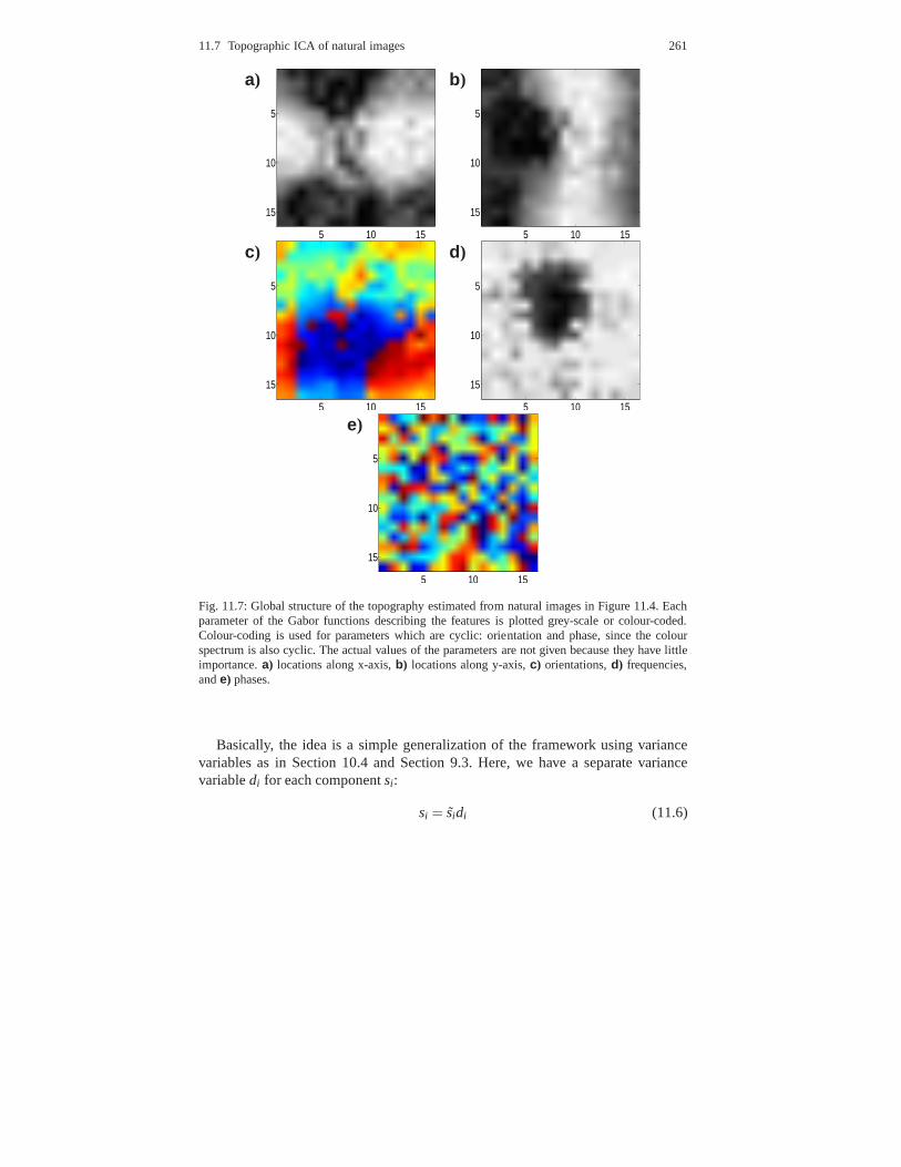
11.7 Topographic ICA of natural images 261
a)
5 10 15
5
10
15
b)
5 10 15
5
10
15
c)
5 10 15
5
10
15
d)
5 10 15
5
10
15
e)
5 10 15
5
10
15
Fig. 11.7: Global structure of the topography estimated from natural images in Figure 11.4. Eachparameter of the Gabor functions describing the features isplotted grey-scale or colour-coded.Colour-coding is used for parameters which are cyclic: orientation and phase, since the colourspectrum is also cyclic. The actual values of the parametersare not given because they have littleimportance.a) locations along x-axis,b) locations along y-axis,c) orientations,d) frequencies,ande) phases.
Basically, the idea is a simple generalization of the framework using variancevariables as in Section 10.4 and Section 9.3. Here, we have a separate variancevariabledi for each componentsi :
si = sidi (11.6)
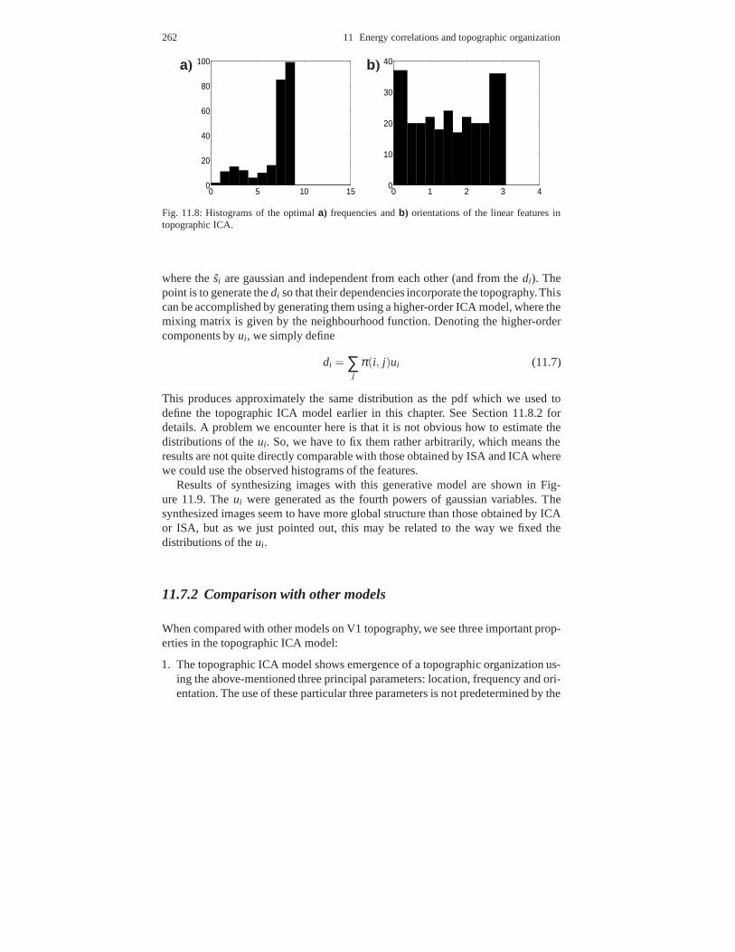
262 11 Energy correlations and topographic organization
a)
0 5 10 150
20
40
60
80
100 b)
0 1 2 3 40
10
20
30
40
Fig. 11.8: Histograms of the optimala) frequencies andb) orientations of the linear features intopographic ICA.
where the ˜si are gaussian and independent from each other (and from thedi). Thepoint is to generate thedi so that their dependencies incorporate the topography.Thiscan be accomplished by generating them using a higher-orderICA model, where themixing matrix is given by the neighbourhood function. Denoting the higher-ordercomponents byui , we simply define
di = ∑j
π(i, j)ui (11.7)
This produces approximately the same distribution as the pdf which we used todefine the topographic ICA model earlier in this chapter. SeeSection 11.8.2 fordetails. A problem we encounter here is that it is not obvioushow to estimate thedistributions of theui. So, we have to fix them rather arbitrarily, which means theresults are not quite directly comparable with those obtained by ISA and ICA wherewe could use the observed histograms of the features.
Results of synthesizing images with this generative model are shown in Fig-ure 11.9. Theui were generated as the fourth powers of gaussian variables. Thesynthesized images seem to have more global structure than those obtained by ICAor ISA, but as we just pointed out, this may be related to the way we fixed thedistributions of theui .
11.7.2 Comparison with other models
When compared with other models on V1 topography, we see three important prop-erties in the topographic ICA model:
1. The topographic ICA model shows emergence of a topographic organization us-ing the above-mentioned three principal parameters: location, frequency and ori-entation. The use of these particular three parameters is not predetermined by the

11.7 Topographic ICA of natural images 263
Fig. 11.9: Image synthesis using topographic ICA. Compare with the ICA results in Figure 7.4 onpage 170 and ISA results in Figure 10.10 on page 241.
model, but determined by the statistics of the input. This isin contrast to mostmodels that only model topography with respect to one or two parameters (usu-ally orientation possibly combined with binocularity) that are chosen in advance.
2. No other model has shown the emergence of a low-frequency blob.3. Topographic ICA may be the first one to explicitly show a connection between
topography and complex cells. The topographic, columnar organization of thesimple cells is such that complex cell properties are automatically created whenconsidering local activations. This is related to the randomness of phases, whichmeans that in each neighbourhood, there are linear featureswith very differentphases, like in the subspaces in ISA.
It is likely that the two latter properties (blobs and complex cells) can onlyemerge in a model that is based on simultaneous activation (energy correlation)instead of similarity of receptive fields as measured by Euclidean distances or recep-tive field correlations. This is because Euclidean distances or correlations betweenfeature vectors of different frequencies, or of different phases, are quite arbitrary:they can obtain either large or small values depending on theother parameters. Thus,they do not offer enough information to qualitatively distinguish the effects of phasevs. frequency, so that phase can be random and frequency can produce a blob.

264 11 Energy correlations and topographic organization
11.8 Learning both layers in a two-layer model *
In this section, we discuss estimation of a two-layer model which is a generaliza-tion of the topographic ICA. The section is quite sophisticated mathematically, andpresents ongoing work with a lot of open problems, so it can beskipped by readersnot interested in mathematical details.
11.8.1 Generative vs. energy-based approach
Many of the results in the preceding chapters are related to atwo-layer generativemodel. In the model, the observed variablesz are generated as a linear transforma-tion of componentss, just as in the basic ICA model:z = As. The point is to definethe joint density ofs so that it expresses the correlations of squares that seem tobedominant in image data.
There are two approaches we can use. These parallel very muchthe sparse cod-ing and ICA approaches in Chapters 6 and 7. In the first approach, typically called“energy-based” for historical reasons,1 we just define an objective function whichexpresses sparseness or some related statistical criterion, and maximize it. In thesecond approach, we formulate a generative model which describes how the datais generated starting from some elementary components. We shall consider herefirst the generative-model approach; the energy-based model is considered in Sec-tion 11.8.5.
11.8.2 Definition of the generative model
In the generative-model approach, we define the joint density of s as follows. Thevariancesd2
i of thesi are not constant, instead they are assumed to be random vari-ables. These random variablesdi are, in their turn, generated according to a modelto be specified. After generating the variancesd2
i , the variablessi are generated in-dependently from each other, using some conditional distributions to be specified.In other words, thesi areindependent given their variances. Dependence among thesi is implied by the dependence of their variances.
This is a generalization of the idea of a common variance variable presentedin Section 7.8.3. Here, there is no single common variance variable, since there isa separate variance variabled2
i corresponding to eachsi . However, these variancevariables are correlated, which implies that the squares ofthesi are correlated. Con-sider the extreme case where thedi are completely correlated. Then, thed2
i are actu-ally the same variable, possibly multiplied by some constants. Thus, in this extreme
1 Note that the word “energy” here has nothing to do with Fourier energy, it comes from a com-pletely different physical analogy.

11.8 Learning both layers in a two-layer model * 265
case, we actually have just a single variance variable as in the divisive normalizationmodel in Chapter 9.
Many different models for the variancesd2i could be used. We prefer here to use
an ICA model followed by a nonlinearity:
di = r(n
∑k=1
π(i,k)uk) (11.8)
Here, theuk are the “higher-order” independent components used to generate thevariances, andr is some scalar nonlinearity (possibly just the identityr(z) = z).The coefficientsπ(i,k) are the entries of a higher-order feature matrix. It is closelyrelated to the matrix defining the topography in topographicICA, which is why weuse the same notation.
This particular model can be motivated by two facts. First, taking sparseui , wecan model a two-layer generalization of sparse coding, where the activations (i.e. thevariances) of the componentssi are sparse, and constrained to some groups of “re-lated” components. Related components means here components whose variancesare strongly influenced by the same higher-order componentsui .
In the model, the distributions of theui and the actual form ofr are additionalparameters; some suggestions will be given below. It seems natural to constrain theuk to be non-negative. The functionr can then be constrained to be a monotonictransformation in the set of non-negative real numbers. This ensures that thedi ’s arenon-negative, so is a natural constraint since they give thestandard deviation of thecomponents.
The resulting two-layer model is summarized in Fig. 11.10. Note that the twostages of the generative model can be expressed as a single equation, analogously to(9.4), as follows:
si = r(∑k
π(i,k)uk)si (11.9)
wheresi is a random variable that has the same distribution assi given thatdi isfixed to unity. Theuk and the ˜si are all mutually independent.
11.8.3 Basic properties of the generative model
Here we discuss some basic properties of the generative model just defined.
11.8.3.1 The componentssi are uncorrelated
This is because according to (11.9) we have
E{sisj}= E{si}E{sj}E{r(∑k
π(i,k)uk)r(∑k
π( j,k)uk)} = 0 (11.10)
266 11 Energy correlations and topographic organization
due to the independence of theuk from si and sj . (Recall that ˜si and sj are zero-mean.) To simplify things, one can define that the marginal variances (i.e. integratedover the distribution ofdi) of thesi are equal to unity, as in ordinary ICA. In fact,we have
E{s2i }= E{s2
i }E{r(∑k
π(i,k)uk)2}, (11.11)
so we only need to rescaleπ(i, j) (the variance of ˜si is equal to unity by definition).
11.8.3.2 The componentssi are sparse
This is true in the case where componentsi is assumed to have a gaussian distribu-tion when the variance is given. This follows from the proof given in Section 7.8.3:the logic developed there still applies in this two-layer model, when the marginaldistribution of each componentsi is consider separately. Then, the marginal, uncon-ditional distributions of the componentssi are called gaussian scale mixtures.
11.8.3.3 Topographic organization can be modelled
This is possible simply by constraining the higher-order matrix π(i, j) to equal atopographic neighbourhood matrix as in Section 11. We can easily prove that com-ponents which are far from each other on the topography are then independent.Assume that thatsi andsj are such that their neighbourhoods have no overlap, i.e.there is no indexk such that bothπ(i,k) andπ( j,k) are non-zero. Then their vari-ancesdi andd j are independent because no higher-order component influences bothof these variances. Thus, the componentssi andsj are independent as well.
11.8.3.4 Independent subspaces are a special case
This is more or less implied by the discussion in Section 11.4where independentsubspace analysis was shown to be a special case of topographic ICA. A more directconnection is seen by noting that each variance variable could determine the vari-ance inside a single subspace, with no interactions betweenthe variance variables.Then we get the ISA model as explained in Section 10.4.
11.8.4 Estimation of the generative model
11.8.4.1 Integrating out
In this section, we discuss the estimation of the two-layer model introduced in theprevious section. In principle, this can be done by “integrating out” the latent vari-

11.8 Learning both layers in a two-layer model * 267
u
Σ
Σ
Σ
2
3
1
x
x
x
A
3
r
r
r
u
u
1
2
s
s
s
2
3
1
d
d 1
d
2
3
Fig. 11.10: An illustration of the two-layer generative model. First, the “variance-generating” vari-ablesui are generated randomly. They are then mixed linearly. The resulting variables are thentransformed using a nonlinearityr, thus giving the local variancesd2
i . Componentssi are thengenerated with variancesd2
i . Finally, the componentssi are mixed linearly to give the observedvariablesxi (which are subsequently whitened to give thezi ).
ables. Integrating out is an intuitive appealing method: since the likelihood dependson the values of the variance variablesui which we don’t know, why not just com-pute the likelihood averaged over all possible values ofui? Basically, if we have thejoint density of thesi and theui , we could just compute the integral over theui toget the density oversi alone:
p(s) =∫
p(s,u)du (11.12)
The problem is, as always with integration, that we may not beable to express thisintegral with a simple formula, and numerical integration may be computationallyimpossible.
In our case, the joint density ofs, i.e. the topographic components, andu, i.e. thehigher-order independent components generating the variances, can be expressed as
p(s,u) = p(s|u)p(u) = ∏i
psi (
si
r(∑k π(i,k)uk))
1r(∑k π(i,k)uk)
∏j
puj (u j) (11.13)
where thepui are the marginal densities of theui and theps
i are the densities ofpsi for
variance fixed to unity. The marginal density ofscould be obtained by integration:
p(s) =
∫
∏i
psi (
si
r(∑k π(i,k)uk))
∏ j puj (u j)
r(∑k π(i,k)uk)du (11.14)
Possibly, for some choices of the nonlinearityr and the distributionspui , this integral
could be computed easily, but no such choices are known to us.
11.8.4.2 Approximating the likelihood
One thing which we can do is toapproximatethe likelihood by an analytical expres-sion. This approximation actually turns out to be rather useless for the purpose of

268 11 Energy correlations and topographic organization
estimating the two-layer model, but it shows an interestingconnection to the likeli-hood of the topographic ICA model.
To simplify the notation, we assume in the following that thedensitiespui are
equal for all i, and likewise forpsi . To obtain the approximation, we first fix the
densitypsi = ps to be gaussian, as discussed in Section 11.8.3, and we define the
nonlinearityr asr(∑
k
π(i,k)uk) = (∑k
π(i,k)uk)−1/2 (11.15)
The main motivation for these choices is algebraic simplicity that makes a sim-ple approximation possible. Moreover, the assumption of conditionally gaussiansi ,which implies that the unconditional distribution ofsi super-gaussian, is compatiblewith the preponderance of super-gaussian variables in ICA applications.
With these definitions, the marginal density ofsequals:
p(s) =
∫1√2πn exp(−1
2 ∑i
s2i [∑
k
π(i,k)uk])∏i
pu(ui)√
∑k
π(i,k)uk du (11.16)
which can be manipulated to give
p(s) =
∫1√2πn exp(−1
2 ∑k
uk[∑i
π(i,k)s2i ])∏
ipu(ui)
√
∑k
π(i,k)uk du. (11.17)
The interesting point in this form of the density is that it isa function of the “localenergies”∑i π(i,k)s2
i only. The integral is still intractable, though. Therefore, weuse the simple approximation:
√
∑k
π(i,k)uk ≈√
π(i, i)ui. (11.18)
This is actually a lower bound, and thus our approximation will be a lower bound ofthe likelihood as well. This gives us the following approximation p(s):
p(s) = ∏k
exp(G(∑i
π(i,k)s2i )) (11.19)
where the scalar functionG is obtained from thepu by:
G(y) = log∫
1√2π
exp(−12
uy)pu(u)√
π(i, i)udu. (11.20)
Recall that we assumedπ(i, i) to be constant.Next, using the same derivation as in ICA, we obtain the likelihood of the data as
logL(V) =T
∑t=1
n
∑j=1
G(n
∑i=1
π(i, j)(vTi z(t))2)+T log|detV|. (11.21)

11.8 Learning both layers in a two-layer model * 269
whereV = (v1, . . . ,vn)T = A−1, and thez(t),t = 1, . . . ,T are the observations ofz.
It is here assumed that the neighbourhood function and the nonlinearity r as wellas the densitiespu
i and psi are known. This approximation is a function of local
energies. Every term∑ni=1 π(i, j)(vT
i z(t))2 could be considered as the energy of aneighbourhood, related to the output of a higher-order neuron as in complex cellmodels. The functionG has a similar role as the log-density of the independentcomponents in ICA; the corresponding functionh is basically obtained ash(u) =G(√
|u|).The formula forG in (11.20) can be analytically evaluated only in special cases.
One such case is obtained if theuk are obtained as squares of standardized gaussianvariables. Straight-forward calculation then gives the following function
G0(y) =− log(1+y)+const. (11.22)
However, in ICA, it is well-known that the exact form of the log-density does notaffect the consistency of the estimators, as long as the overall shape of the functionis correct. This is probably true in topographic ICA as well.
11.8.4.3 Difficulty of estimating the model
What we have really shown in deriving the approximation of likelihood in Equa-tion (11.21) is that the heuristically justified objective function in Equation (11.5)can be obtained from the two-layer generative model as an approximation. But wehave not really got any closer to the goal of estimating both layers of weights. Thisis because the approximation used here approximates the dependence of the likeli-hood fromπ quite badly. To see why, consider maximization of the approximativelikelihood in Equation (11.21) with respect to theπ(i, j). TakeG as in (11.22). Now,∑n
i=1 π(i, j)(vTi z(t))2 is always non-negative. On the other hand,G attains its max-
imum at zero. So, if we simply takeπ(i, j) = 0 for all i, j, G is actually alwaysevaluated at zero and the approximative likelihood is maximized. So, taking all ze-ros inπ is the maximum, which is absurd!
One approach would be to find the values of the latent variables ui which max-imize the likelihood, treating theui like the parameters. Thus, we would not try tointegrate out theui , but rather just formulate the joint likelihood ofV,π(i, j),ui(t)for all i, j and allt = 1, . . . ,T. This is computationally very difficult because the la-tent variablesdi are different for each image patch, so there is a very large number ofthem. The situation could be simplified by first estimating the first layer by ordinaryICA, and then fixingV once and for all (Karklin and Lewicki, 2005). However, thisdoes not reduce the number of dimensions.
So, we see that the estimation of both layers in a generative two-layer model isquite difficult. However, abandoning the generative-modelapproach simplifies thesituation, and provides a promising approach, which will betreated next.

270 11 Energy correlations and topographic organization
11.8.5 Energy-based two-layer models
A computationally simpler alternative to estimation of thetwo layers is provided byan “energy-based” approach. The idea is to take the likelihood in Equation (11.5) asthe starting point. As pointed out above, it does not make sense to try to maximizethis with respect to theπ , because the maximum is obtained by taking all zeros asthe second layer weights.
There is a deep mathematical reason why we cannot maximize the likelihoodin Equation (11.5) with respect to theπ . The reason is that the likelihood isnotnormalized. That is, when we interpret the likelihood as a pdf, its integral over thedata variables is not equal to one: the integral depends on the values of theπ . Thismeans it is not a properly defined pdf, because a pdf must always integrate to one,so the likelihood is not a properly defined likelihood either. To alleviate this, wehave to introduce what is called anormalization constantor apartition functioninthe likelihood. The normalization constant, which is actually not a constant but afunction of the model parameters, is chosen so that it makes the integral equal toone. Denoting the normalization constant byZ(π), we write
logL(v1, . . . ,vn) =T
∑t=1
∑i
h(n
∑j=1
π(i, j)(vTi zt)
2)− log|detV|− logZ(π) (11.23)
See Section 13.1.5 and Chapter 21 for more discussion on the normalization con-stant.
In principle, the normalization constant can be computed bycomputing the inte-gral of the underlying pdf over the space of thev, but this is extremely complicatednumerically. Fortunately, there is a way around this problem, which is to use spe-cial estimation methods which do not require the normalization constant. Thus, weabandon maximization of likelihood, because it requires that we compute the nor-malization constant. See Chapter 21 for information on suchmethods.
Attempts to estimate both layers in a two-layer model, usingan energy-basedapproach, and estimation methods which circumvent the needfor a normalizationconstant, can be found in (Osindero et al, 2006; Koster and Hyvarinen, 2007, 2008).This is a very active area of research (Karklin and Lewicki, 2008). Some more re-motely related work is in (Koster et al, 2009a).
11.9 Concluding remarks and References
A simple modification of the model of independent subspace analysis leads to emer-gence of topography, i.e. the spatial arrangement of the features. This is in contrastto ICA and ISA, in which the features are in random order. (In ISA, it is the sub-spaces which are in random order, but the linear features have some organizationbecause of their partition to subspaces.) The basic idea in modelling topography isto consider subspaces which are overlapping, so that the neighbourhood of each cell

11.9 Concluding remarks and References 271
is one subspace. It is also possible to formulate a proper generative model which in-corporates the same kind of statistical dependencies usingvariance variables whichare generated by a higher-order ICA model, but that approachis mathematicallydifficult and still under construction.
Basic though old papers on topography are (Hubel and Wiesel,1968; DeValoiset al, 1982). Optical imaging results are shown in (Blasdel,1992), and a recent high-resolution imaging study is in (Ohki et al, 2005). Topography with respect to spatialfrequency is investigated in (Tootell et al, 1988; Silverman et al, 1989; Edwards et al,1996). Seminal papers on pinwheels are (Bonhoeffer and Grinvald, 1991; Maldon-ado et al, 1997). A most interesting recent paper is (DeAngelis et al, 1999) that alsoshows that the phases are not correlated in neighbouring cells. The relationships ofthe topographic representation for different parameters are considered in (Hubeneret al, 1997). An important point is made in (Yen et al, 2007), who show that thetopography of responses is not so clear when the stimuli are complex, presumabledue to nonlinear interactions. The connection between topography and complex cellpooling is discussed in (Blasdel, 1992; DeAngelis et al, 1999).
The idea of minimum wiring length, or wiring economy, goes back to Ramony Cajal, cited in (Chen et al, 2006). The metabolic advantages of topography arefurther considered in (Durbin and Mitchison, 1990; Mitchison, 1992; Koulakov andChklovskii, 2001; Attwell and Laughlin, 2001). Comparisons between white andgrey matter volume also point out how brain (skull) size limits the connectivity(Zhang and Sejnowski, 2000).
Original papers describing the topographic ICA models are (Hyvarinen andHoyer, 2001; Hyvarinen et al, 2001a). Kohonen’s famous self-organizing map isalso closely related (Kohonen, 1982, 2001), but it has not been shown to producea realistic V1-like topography; reasons for this were discussed in Section 11.7.2.A model which produces more a realistic topography (but still no low-frequencyblobs) is Kohonen’s ASSOM model (Kohonen, 1996; Kohonen et al, 1997). How-ever, in that model the nature of the topography is strongly influenced by an artificialmanipulation of the input (a sampling window that moves smoothly in time), and itdoes not really emerge from the structure of images alone.
A related idea on minimization of wiring length has been proposed in (Vincentand Baddeley, 2003; Vincent et al, 2005), in which it is proposed that the retinalcoding minimizes wiring, whereas cortical coding maximizes sparseness of activi-ties.


Chapter 12Dependencies of energy detectors: Beyond V1
All the models in this book so far have dealt with the primary visual cortex (V1).In this chapter, we show how statistical models of natural images can be extendedto deal with properties in the extrastriate cortex, i.e. those areas which are close toV1 (also called the striate cortex) and to which the visual information is transmittedfrom V1.
12.1 Predictive modelling of extrastriate cortex
Most of the experimental results in early cortical visual processing have consideredV1. The function of most extrastriate areas is still rather much a mystery. Likewise,most research in modelling natural image statistics has been on low-level features,presumably corresponding to V1.
However, the methodology that we used in this book could possibly be extendedto such extrastriate areas as V2, V3(A), V4, and V5. Actually, since the function ofmost extrastriate areas is not well understood, it would be most useful if we coulduse this modelling endeavour in apredictivemanner, so that we would be able topredict properties of cells in the visual cortex, in cases where the properties havenot yet been demonstrated experimentally. This would give testable, quantitativehypotheses that might lead to great advances in visual neuroscience.
In the next sections, we attempt to accomplish such predictive modelling in orderto predict properties of a third processing step, followingthe simple and complexcell layers. The predictions should be based on the statistical properties of modelledcomplex-cell outputs. Our method is to apply ordinary independent component anal-ysis to modelled outputs of complex cells whose input consists of natural images.1
1 This chapter is based on the article (Hyvarinen et al, 2005a), originally published in BMC Neu-roscience. The experiments were done by Michael Gutmann. Copyright retained by the authors.
273

274 12 Dependencies of energy detectors: Beyond V1
12.2 Simulation of V1 by a fixed two-layer model
The basic idea in this chapter is to fix a model of complex cellsand then learna representation for complex cell outputs using a statistical model. The resultingthree-layer network is depicted in Fig. 12.1.
This approach is rather different from the one used in previous chapters, in whichwe learned first the simple cells and then the complex cells from the data. Here, tosimplify the model and the computations, we do not attempt tolearn everythingat the same time. Instead, we fix the first two layers (simple and complex cells)according to well-known models, and learn only the third layer.
image
complex cells
contour cells
simple cells
i
ija
s
c j
Fig. 12.1: The simplified hierarchical model investigated in this chapter. Modelled complex-cellresponses are calculated in a feedforward manner, and theseresponses are subsequently analyzedby a higher-order feature layer in the network (“contour” layer). To emphasise that the lower layersare fixed and not learned, these layers have been greyed out inthe figure. The direction of the arrowsis from higher features to lower ones which is in line with theinterpretation of our analysis as agenerative model.
The classic complex-cell model is based on Gabor functions.As explained inSection 3.4.2, complex cells can be modelled as the sum of squares of two Gaborfunctions which are in quadrature phase. Quadrature phase means, simply, that ifone of them is even-symmetric, the other one is odd-symmetric. This is related tocomputation of the Fourier energy locally, as explained in Section 2.4.
Complex-cell responsesck to natural images were thus modelled with a Gaborenergy model of the following form:
ck =
(
∑x,y
Wok (x,y)I(x,y)
)2
+
(
∑x,y
Wek (x,y)I(x,y)
)2
(12.1)

12.2 Simulation of V1 by a fixed two-layer model 275
whereWek andWo
k are even- and odd-symmetric Gabor receptive fields; the equa-tion shows that their squares (energies) are pooled together in the complex cell. Thecomplex cells were arranged on a 6× 6 spatial grid. They had 6× 6 = 36 differ-ent spatial locations, and at each location, four differentpreferred orientations andthree different frequency selectivities (“bands”). The aspect ratio (ratio of spatiallength to width) was fixed to 1.5. The frequency selectivities of the Gabor filtersare shown in Figure 12.2, in which all the filtersW were normalized to unit normfor visualization purposes. The actual normalization we used in the experimentsconsisted of standardizing the variances of the complex cell outputs so that theywere equal to unity for natural image input. The number of complex cells totalled36×4×3= 432.
0 0.1 0.2 0.3 0.4 0.50
0.1
0.2
0.3
0.4
0.5
0.6
0.7
0.8
0.9
1
Spatial Frequency [cycles/pixel]
Filt
er R
espo
nse
Fig. 12.2: We used fixed complex cells with three different frequency selectivities. The amplitudesof the Fourier Transforms of the odd-symmetric Gabor filtersare shown here. The selectivities aresuch that each cell is sensitive to a certain frequency “band”. The underlying Gabor filters hadlogarithmically spaced frequency peaks. Peak spatial frequencies were chosen as follows:f1 = 0.1cycles/pixel,f2 = 0.21 cycles/pixel andf3 = 0.42 cycles/pixel.
As the basic data, we used 1008 grey-scale natural images of size 1024×1536pixels from van Hateren’s database2. We manually chose natural images in the nar-rower sense, i.e. only wildlife scenes. From the source images, 50,000 image patchesof size 24×24 pixels were randomly extracted. The mean grey value of each im-age patch was subtracted and the pixel values were rescaled to unit variance. Theresulting image patch will be denoted byI(x,y).
2 Available athttp://hlab.phys.rug.nl/imlib/index.html , category “deblurred”(van Hateren and van der Schaaf, 1998).

276 12 Dependencies of energy detectors: Beyond V1
12.3 Learning the third layer by another ICA model
After fixing the first two layers, we learned the feature weights in the third layerby doing a simple ICA of the complex cell (second-layer) outputs denoted byck.No PCA dimension reduction was done here, so the number of independent com-ponents equals the number of complex cells,K. Thus, ICA was performed on thevectorc = (c1, . . . ,cK) using the FastICA algorithm (see Section 18.7). In ICA, theorthogonalization approach was symmetric. Different nonlinearitiesg were used,see Table 12.1. (The nonlinearities are related to the non-gaussianity measures used,see Section 18.7.)
Non-gaussianity measure FastICA nonlinearity MotivationG1(y) = logcoshy g1(y) = tanh(y) Basic sparseness measureG2(y) =−exp(−y2/2) g2(y) = yexp(−y2/2) More robust variant ofg1
G3(y) = 13y3 g3(y) = y2 Skewness (asymmetry)
G4(y) = Gaussian cum. distr. functiong4(y) = exp(−y2/2) Robust variant ofg3
Table 12.1: The measures of non-gaussianity used, i.e. the different functionsG = logps used inthe likelihood of the ICA model. These correspond to different nonlinearitiesg in the FastICAalgorithm, and to different sparseness measuresh. The measures probe the non-gaussianity of theestimated components in different ways.
Thus we learned (estimated) a linear decomposition of the form
ck =K
∑i=1
akisi for all k = 1, . . . ,K (12.2)
or in vector form
c =K
∑i=1
aisi = As (12.3)
where each vectorai = (a1i, . . . ,aKi) gives a higher-order feature vector. Thesi de-fine the values of the higher-order features in the third cortical processing stage.Recall that the input to the system was natural images, so thestatistics ofc reflectnatural image statistics.
Note that the signs of the feature vectors are not defined by the ICA model, i.e.the model does not distinguish betweenai and−ai because any change in sign of thefeature vector can be cancelled by changing the sign ofsi accordingly. Here, unlikein the original natural images, the features will not be symmetric with respect tosuch a change of sign, so it makes sense to define the signs of the ai based on thatasymmetry. We defined the sign for each vectorai so that the sign of the elementwith the maximal absolute value was positive.
This model can be interpreted as a generative model of image patches, followingthe interpretation of ISA as a nonlinear ICA in Section 10.6.The higher-order inde-pendent component (here denoted bysi) are generated according to Equation (12.2).

12.4 Methods for analysing higher-order components 277
Then, the activity of the complex cell is expressed as activities of simple cells withrandom division of the activity to the simple cells, using a random angle variableas in Equation (10.17) on page 235. Finally, the simple cell activities are linearlytransformed to image patches as in ICA or ISA models. This provides a completegenerative model from the higher-order features to image pixel values.
12.4 Methods for analysing higher-order components
We need to introduce some special methods to analyze the “higher-order” compo-nents obtained by this method, because the resulting higher-order feature vectorsai
cannot be simply plotted in the form of image patches.We visualize the vectorsai by plotting an ellipse at the centerpoint of each com-
plex cell. The orientation of the ellipse is the orientationof the complex cell withindexk, and the brightness of the ellipse with indexi is proportional to the coeffi-cientaki of the feature vectorai , using a grey-scale coding of coefficient values. Weplotted complex cells in each frequency band (i.e. with the same frequency selectiv-ity) separately.
We are also interested in the frequency pooling of complex cells in differenthigher-order features. We quantified the pooling over frequencies using a simplemeasure defined as follows. Let us denote byai(x,y,θ , fn) the coefficient in thehigher-order feature vectorai that corresponds to the complex cell with spatial loca-tion (x,y), orientationθ and preferred frequencyfn. We computed a quantity whichis similar to the sums of correlations of the coefficients over the three frequencybands, but normalized in a slightly different way. This measure Pi was defined asfollows:
Pi = ∑m<n
|∑x,y,θ ai(x,y,θ , fm)ai(x,y,θ , fn)|CmCn
(12.4)
where the normalization constantCm is defined as
Cm =
√
1K ∑
j ,x,y,θa j(x,y,θ , fm)2 (12.5)
and likewise forCn.For further analysis of the estimated feature vectors, we defined the preferred
orientation of a higher-order feature. First, let us define for a higher-order fea-ture of indexi the hot-spot(xi ,yi)
∗ as the centre location(x,y) of complex cellswhere the higher-order componentsi generates the maximum amount of activity.That is, we sum the elements ofai that correspond to a single spatial location, andchoose the largest sum. This allows us to define the tuning to agiven orientation ofa higher-order featurei by summing over the elements ofai that correspond to thespatial hotspot and a given orientation; the preferred orientation is the orientation forwhich this sum is maximized. We also computed the length of a higher-order feature

278 12 Dependencies of energy detectors: Beyond V1
by least-squares fitting a gaussian kernel to the patternsai (Hoyer and Hyvarinen,2002).
It is also possible to perform an image synthesis from a higher-order featurevector. However, the mapping from image to complex-cell outputs is not one-to-one. This means that the generation of the image is not uniquely defined given theactivities of higher-order features alone. A unique definition can be achieved byconstraining the phases of the complex cells. For the purposes of image synthesis,we assume that only odd-symmetric Gabor filters are active. Furthermore, we makethe simplifying assumptions that the receptive fieldsW in simple cells are equal tothe corresponding feature vectors, and that all the elements in the higher-order fea-ture vector are non-negative (or small enough to be ignored). Then, the synthesizedimageI i
synth for higher-order feature vectorai is given by
I isynth(x,y) = ∑
k∈H
Wok (x,y)
√aki (12.6)
where the square root cancels the squaring operation in the computation of complex-cell responses, andH denotes the set of indices that correspond to complex cells ofthe preferred orientation at the hotspot. Negative values of aki were set to zero inthis formula.
Since we are applying ICA on data which has been heavily processed (by thecomplex cell model), we have to make sure that the model is notonly analyzing theartefacts produced by that processing. To obtain a baselinewith which to compareour results, and to show which part of the results is due to thestatistical propertiesof natural images instead of some intrinsic properties of our filterbank and analysismethods, we did exactly the same kind of analysis for 24×24 image patches thatconsisted of white gaussian noise, i.e. the grey-scale value in each pixel was ran-domly and independently drawn from a gaussian distributionof zero mean and unitvariance. The white gaussian noise input provides a “chancelevel” for any quantitiescomputed from the ICA results. In a control experiment, suchwhite noise patcheswere thus fed to the complex cell model, and the same kind of ICA was applied onthe outputs.
12.5 Results on natural images
12.5.1 Emergence of collinear contour units
In the first experiment, we used only the output from complex cells in a singlefrequency band,f2 in Figure 12.2.
The higher-order features are represented by their featurevectorsai which showthe contribution of the third-stage feature of indexi on the activities of complexcells. A collection of the obtained feature vectors is shownin Figure 12.3 for thenonlinearityg1 (see Table 12.1), visualized as described above. We can see emer-

12.5 Results on natural images 279
gence of collinear features. That is, the higher-order features code for the simulta-neous activation of complex cells that together form something similar to a straightline segment.
Those coefficients that are clearly different from zero havealmost always thesame sign in a single feature vector. Defining the sign as explained above, this meansthat the coefficients are essentially non-negative.3
Other measures of non-gaussianity (FastICA nonlinearities) led to similar featurevectors. However, some led to a larger number of longer contours. Figure 12.4 showsthe distribution of lengths for different nonlinearities.The nonlinearityg4 (robustskewness) seems to lead to the largest number of long contours. The outputs ofcomplex cells are skewed (non-symmetric), so it makes senseto use a skewness-based measure of non-gaussianity, as discussed in Section 7.9. In this experiment,the results were very similar to those obtained by sparseness, however.
0
0.2
0.4
0.6
0.8
1
Fig. 12.3: Random selection of learned feature vectorsai when the complex cells are all in a singlefrequency band. ICA nonlinearityg was the tanh nonlinearityg1. Each patch gives the coefficientsof one higher-order feature. Each ellipse means that the complex cell in the corresponding locationand orientation is present in the higher-order feature, thebrightness of the ellipse is proportional tothe coefficientaki.
12.5.2 Emergence of pooling over frequencies
In the second experiment, the complex cell set was expanded to include cells ofthree different preferred frequencies. In total, there were now 432 complex cells.We performed ICA on the complex cell outputs when their inputconsisted of nat-ural images. Thus, we obtained 432 higher-order feature vectors (features)ai withcorresponding activitiessi .
3 In earlier work (Hoyer and Hyvarinen, 2002) we actually imposed a non-negativity constrainton the coefficients, see Section 13.2. The results reported here show that those results can bereplicated using ordinary ICA methods. The constraint of non-negativity of the feature vectors haslittle impact on the results: even without this constraint,the system learns feature vectors whichare mainly non-negative.

280 12 Dependencies of energy detectors: Beyond V1
0 0.1 0.2 0.3 0.4 0.5 0.6 0.7 0.8 0.9 10
10
20
30
40
50
60
Length
Per
cent
age
of c
ell p
opul
atio
n
g1
g2
g3
g4
Fig. 12.4: Comparison of different measures of non-gaussianity (FastICA nonlinearities) in thefirst experiment. The histogram gives the lengths of the contour patterns for the four differentnonlinearitiesg1, . . . ,g4 in Table 12.1.
We visualized a random selection of higher-order features learned from naturalimages in Figure 12.5. The visualization shows that the features tend to be spatiallylocalized and oriented, and show collinearity as in the single-channel experimentabove. What is remarkable in these results is that many cellspool responses overdifferent frequencies. The pooling is coherent in the sensethat the complex cellsthat are pooled together have similar locations and orientations. A smaller number ofcells is shown in more detail in Figure 12.6, where the coefficients in all orientationsare shown separately.
We computed the frequency pooling measurePi in Equation (12.4) for the learnedfeature vectors. The distribution of this measure for natural image input and whitegaussian noise input is shown in Figure 12.7. The figure showsthat frequency pool-ing according to this measure was essentially nonexistent for white gaussian noiseinput, but relatively strong for many feature vectors when the input consisted ofnatural images. To express this more quantitatively, we computed the 99% quantilefor the white gaussian noise input. Then, 59% of the basis vectors for natural imageinput had a pooling indexPi that was larger than this quantile. (For the 95% quantilethe proportion was 63%.) Thus, we can say that more than half of the higher-orderbasis vectors, when learned from natural images, have a pooling over frequenciesthat is significantly above chance level.
To show that the pooling measure is valid, and to further visualize the frequencypooling in the higher-order features, we chose randomly feature vectors learnedfrom natural images that have pooling significantly over chance level (Pi above its99% quantile for white gaussian noise). These are plotted inFigure 12.8. Visual in-spection shows that in this subset, all basis vectors exhibit pooling over frequenciesthat respects the orientation tuning and collinearity properties.
The corresponding results when the input is white gaussian noise are shown inFigure 12.9, for a smaller number of higher-order cells . (Tomake the comparisonfair, these were randomly chosen among the 59% that had higher pooling mea-

12.5 Results on natural images 281
sures, the same percentage as in Figure 12.8.) Pooling over frequencies as well ascollinearity are minimal. Some weak reflections of these properties can be seen, pre-sumably due to the small overlap of the filters in space and frequency, which leadsto weak statistical correlations between complex cells that are spatially close to eachother or in neighbouring frequency bands.
We also examined quantitatively whether the higher-order features are tuned toorientation. We investigated which complex cell has the maximum weight inai foreachi in each frequency band. When the data used in learning consisted of naturalimages, in 86% of the cells the maximally weighted complex cells were found to belocated at the hot-spot(xi ,yi)
∗ (i.e., point of maximum activity, see above) and tunedto the preferred orientation of the higher-order feature for everyfrequencyf . Thisshows how the higher-order features are largely selective to a single orientation.When the data used in learning consisted of gaussian white noise, only 34% of thecells were found to be orientation-selective according to this criterion.
Fre
quen
cy [c
ycle
s/pi
xel]
0.1
0.21
0.42
0.1
0.21
0.42
−0.050
0.1
0.2
0.3
0.4
0.5
0.6
0.7
0.8
0.9
1
Fig. 12.5: A random selection of higher-order feature vectors ai estimated from natural imagesusing complex cells of multiple frequencies in the second experiment. ICA nonlinearityg was thetanh nonlinearityg1. Each display of three patches gives the coefficients of one higher-order fea-ture. Each patch gives the coefficients of one higher-order feature in one frequency band. Eachellipse means that the complex cell in the corresponding location, and of the corresponding orien-tation and frequency is present in the higher-order feature, brightness of ellipse is proportional tocoefficientaki.
Finally, we synthesized images from higher-order feature activities. Figure 12.10shows a slice orthogonal to the preferred orientation of onehigher-order featurevector (H209 in Figure 12.6). The intensity of the synthesized image shows no side-lobes (unnecessary oscillations), while representing a sharp, localized edge. In con-trast, synthesis in the white gaussian noise case (also shown in Figure 12.10) givescurves that have either side-lobes like the underlying Gabor filters, or do not give a

282 12 Dependencies of energy detectors: Beyond V1
Orientation [degree]
Fre
quen
cy [c
ycle
s/pi
xel]
H150
90 45 0 45
0.1
0.21
0.42
0
0.2
0.4
0.6
0.8
1
Orientation [degree]
Fre
quen
cy [c
ycle
s/pi
xel]
H209
90 45 0 45
0.1
0.21
0.42
0
0.2
0.4
0.6
0.8
1
Orientation [degree]
Fre
quen
cy [c
ycle
s/pi
xel]
H218
90 45 0 45
0.1
0.21
0.42
0
0.2
0.4
0.6
0.8
1
Orientation [degree]
Fre
quen
cy [c
ycle
s/pi
xel]
H235
90 45 0 45
0.1
0.21
0.42
0
0.2
0.4
0.6
0.8
1
Fig. 12.6: Higher-order feature vectors of four selected higher-order features in the second ex-periment, shown in detail. The coefficients in each orientation and frequency band are plottedseparately.
0 0.5 1 1.5 2 2.5 3 3.5 4 4.5 50
10
20
30
40
50
60
Per
cent
age
of c
ell p
opul
atio
n
Pooling Measure
White Gaussian NoiseNatural images
Fig. 12.7: The distributions of the frequency pooling measure in Equation (12.4) for natural imagesand white gaussian noise.

12.5 Results on natural images 283
Fre
quen
cy [c
ycle
s/pi
xel]
0.1
0.21
0.42
0.1
0.21
0.42
0.1
0.21
0.42
−0.08
0
0.1
0.2
0.3
0.4
0.5
0.6
0.7
0.8
0.9
1
Fig. 12.8: A selection of higher-order feature vectorsai estimated from natural images in the secondexperiment. These basis vectors were chosen randomly amongthose that have frequency poolingsignificantly above chance level.
Fre
quen
cy [c
ycle
s/pi
xel]
0.1
0.21
0.42
0
0.25
0.5
0.75
1
Fig. 12.9: For comparison, higher-order feature vectors estimated from white gaussian noise, witheach frequency band shown separately.
sharp localized edge. Thus, the curve obtained from synthesis of the features learnedfrom natural images corresponds better to the notion of an edge.
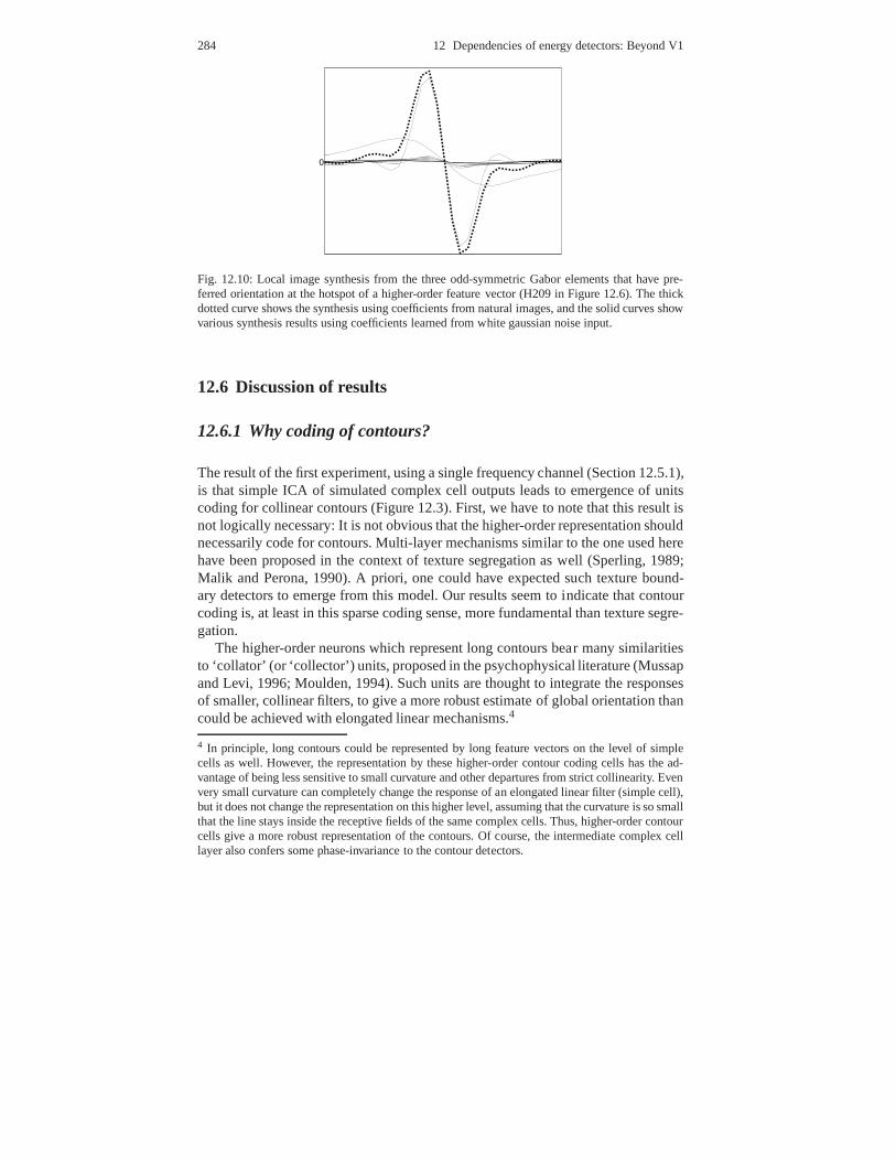
284 12 Dependencies of energy detectors: Beyond V1
0
Fig. 12.10: Local image synthesis from the three odd-symmetric Gabor elements that have pre-ferred orientation at the hotspot of a higher-order featurevector (H209 in Figure 12.6). The thickdotted curve shows the synthesis using coefficients from natural images, and the solid curves showvarious synthesis results using coefficients learned from white gaussian noise input.
12.6 Discussion of results
12.6.1 Why coding of contours?
The result of the first experiment, using a single frequency channel (Section 12.5.1),is that simple ICA of simulated complex cell outputs leads toemergence of unitscoding for collinear contours (Figure 12.3). First, we haveto note that this result isnot logically necessary: It is not obvious that the higher-order representation shouldnecessarily code for contours. Multi-layer mechanisms similar to the one used herehave been proposed in the context of texture segregation as well (Sperling, 1989;Malik and Perona, 1990). A priori, one could have expected such texture bound-ary detectors to emerge from this model. Our results seem to indicate that contourcoding is, at least in this sparse coding sense, more fundamental than texture segre-gation.
The higher-order neurons which represent long contours bear many similaritiesto ‘collator’ (or ‘collector’) units, proposed in the psychophysical literature (Mussapand Levi, 1996; Moulden, 1994). Such units are thought to integrate the responsesof smaller, collinear filters, to give a more robust estimateof global orientation thancould be achieved with elongated linear mechanisms.4
4 In principle, long contours could be represented by long feature vectors on the level of simplecells as well. However, the representation by these higher-order contour coding cells has the ad-vantage of being less sensitive to small curvature and otherdepartures from strict collinearity. Evenvery small curvature can completely change the response of an elongated linear filter (simple cell),but it does not change the representation on this higher level, assuming that the curvature is so smallthat the line stays inside the receptive fields of the same complex cells. Thus, higher-order contourcells give a more robust representation of the contours. Of course, the intermediate complex celllayer also confers some phase-invariance to the contour detectors.

12.6 Discussion of results 285
12.6.2 Frequency channels and edges
In the second experiment using multiple frequency channels(Section 12.5.2), wesaw emergence of pooling of contour information across multiple frequencies (Fig-ures 12.5,12.6,12.8).What is the functional meaning of this frequency pooling? Onepossibility is that this spatially coherent pooling of multiple frequencies leads to arepresentation of an edge that is more realistic than the edges given by typical Ga-bor functions. Presumably, this is largely due to the fact that natural images containmany sharp, step-like edges that are not contained in a single frequency band. Thus,representation of such “broad-band” edges is difficult unless information from dif-ferent frequency bands is combined.
In terms of frequency channels, the model predicts that frequency channelsshould be pooled together after complex cell processing. Models based on frequencychannels and related concepts have been most prominent in image coding litera-ture in recent years, both in biological and computer visioncircles. The utility offrequency channels in the initial processing stages is widely acknowledged, and itis not put into question by these results — in fact, the results in Chapters 6–10show that using frequency-selective simple and complex cells is statistically opti-mal. However, the question of when the frequency channels should be pooled orotherwise combined has received little attention. The results in this chapter (secondexperiment) indicate that a statistically optimal way is topool them together rightafter the complex cell “stage”, and this pooling should be done among cells of agiven orientation which form a local, collinear configuration.
12.6.3 Towards predictive modelling
As we explained in the beginning of the chapter, the present results are an instance ofpredictive modelling, where we attempt to predict properties of cells and cell assem-blies that have not yet been observed in experiments. To be precise, the prediction isthat in V2 (or some related area) there should be cells whose optimal stimulus is abroad-band edge that has no sidelobes while being relatively sharp, i.e. the optimalstimulus is closer to a step-edge than the Gabor functions that tend to be optimal forV1 simple and complex cells. The optimal stimulus should also be more elongated(Polat and Tyler, 1999; Gilbert and Wiesel, 1985) than what is usually observed inV1, while being highly selective for orientation.
Statistical models of natural images offer a framework thatlends itself to pre-dictive modelling of the visual cortex. First, they offer a framework where we of-ten see emergence of new kinds of feature detectors — sometimes very differentfrom what was expected when the model was formulated. Second, the frameworkis highly constrained and data-driven. The rigorous theoryof statistical estimationmakes it rather difficult to insert the theorist’s subjective expectations in the model,and therefore the results are strongly determined by the data. Third, the framework

286 12 Dependencies of energy detectors: Beyond V1
is very constructive. From just a couple of simple theoretical specifications, e.g.non-gaussianity, natural images lead to the emergence of complex phenomena.
We hope that the present work as well as future results in the same direction willserve as a basis for a new kind of synergy between theoreticaland experimentalneuroscience.
12.6.4 References and related work
Several investigators have looked at the connection between natural image statistics,Gestalt grouping rules, and local interactions in the visual cortex (Geisler et al, 2001;Sigman and Gilbert, 2000; Elder and Goldberg, 2002; Kruger, 1998). However, fewhave considered the statistical relations between features of different frequencies.It should be noted that some related work on interactions of different frequenciesdoes exist in the models of contrast gain control, see Chapter 9 or (Schwartz andSimoncelli, 2001a).
Recent measurements from cat area 18 (somewhat analogous toV2) emphasizeresponses to “second-order” or “non-Fourier” stimuli, typically sine-wave gratingswhose amplitudes are modulated (Mareschal and Baker, 1998a,b). These resultsand the proposed models are related to our results and predictions, yet fundamen-tally different. In the model in (Mareschal and Baker, 1998b), a higher-order cellpools outputs of complex cells in the same frequency band to find contours that aredefined by texture-like cues instead of luminance. The same cell also receives directinput from simple cells of a different frequency, which enables the cell to combineluminance and second-order cues. This is in stark contrast to higher-order cells inthe model we used in this chapter, which pool outputs of complex cells of differentfrequencies. They can hardly find contours defined by second-order cues; insteadthey seem to be good for coding broad-band contours. Furthermore, in (Mareschaland Baker, 1998a,b), any collinearity of pooling seems to beabsent. This naturallyleads to the question: Why are our predictions so different from these results fromarea 18? We suspect this is because it is customary to think ofvisual processingin terms of division into frequency channels — “second-order” stimuli are just anextension of this conceptualization. Therefore, not much attempt has been made tofind cells that break the division into frequency channels according to our prediction.On the other hand, one can presume that the cells found in area18 in (Mareschaland Baker, 1998a,b) are different from our predictions because they use a learningstrategy which is different from sparse coding used in our model, perhaps related tothe temporal aspects of natural image sequences, see Chapter 16.
Another closely related line of work is by Zetzsche and coworkers (Zetzsche andKrieger, 1999; Zetzsche and Rohrbein, 2001) who emphasizethe importance of de-composing the image information to local phase and amplitude information. Thelocal amplitude is basically given by complex cell outputs,whereas the physiologi-cal coding of the local phases is not known. An important question for future workis how to incorporate phase information in the higher-orderunits. Some models by

12.7 Conclusion 287
Zetzsche et al actually predict some kind of pooling over frequencies, but ratherdirectly after the simple cell stage, see Fig. 16 in (Zetzsche and Rohrbein, 2001).
Related models in which edge detection uses phase information pooled over dif-ferent frequencies are in (Morrone and Burr, 1988; Kovesi, 1999). An interestinginvestigation into the relation of edges and space-frequency analysis filter outputs innatural images is in (Griffin et al, 2004). A psychophysical study on the integrationof information over different frequencies is (Olzak and Wickens, 1997).
The model in this chapter opens the way to highly nonlinear multilayer modelsof natural image statistics. While this seems like a most interesting direction ofresearch, not much work has been done so far. Related attempts to construct verygeneral, nonlinear models of natural image statistics include (Pedersen and Lee,2002; Lee et al, 2003; Malo and Gutierrez, 2006; Chandler and Field, 2007; Griffin,2007).
12.7 Conclusion
Experiments in this chapter show that two different kinds ofpooling over complexcells emerge when we model the statistical properties of natural images. First, thehigher-order features group collinear complex cells whichform a longer contour.Second, they group complex cells of different frequency preferences. This is ac-complished by applying ordinary ICA on a set of modelled complex cells with mul-tiple frequencies, and inputting natural images to the complex cells. Thus, statisticalmodelling of natural stimuli leads to an interesting hypothesis on the existence of anew kind of cells in the visual cortex.


Chapter 13Overcomplete and non-negative models
In this chapter, we discuss two generalizations of the basicICA and sparse codingmodels. These do not reject the assumption of independence of the componentsbut change some of the other assumptions in the model. Although the generativemodels are linear, the computation of the features is nonlinear. In the overcompletebasis model, the number of independent components is largerthan the number ofpixels. In the non-negative model, the components, as well as the feature vectors,are constrained to be non-negative.
13.1 Overcomplete bases
13.1.1 Motivation
An important restriction of most of the models treated so faris that the number offeatures cannot be larger than the dimension of the data. Thedimension of the datais at most equal to the number of pixels, and it is actually smaller after canonicalpreprocessing including PCA. This was for two reasons:
1. In the sparse coding models the feature detector weights were constrained to beorthogonal. In a space withn dimensions, we can have at mostn orthogonalvectors, so this constrains the number of features.
2. In the generative models such as ICA, we had to assume that the matrixA, whichhas the features as its columns, is invertible. Again, a matrix can be invertibleonly if it is square: thus the number of features cannot be larger than the numberof pixels.
However, it can be argued that the number of features should be larger than thedimension of the image data. The computational justification for such a claim goesas follows:
289

290 13 Overcomplete and non-negative models
1. The processing of an image part, corresponding perhaps toan object, should notdepend on which location of the image it happens to occupy. That is, if a faceis in on the left side of the visual field, it should be processed in the same wayas if it were on the right side; and if the object is moved one pixel to the left, itsprocessing should not change either.1
2. Thus, any feature the system computes should be computed at each possible loca-tion — at the minimum at the location corresponding to each pixel. For example,if we have an edge detector, the output of that edge detector should be computedat each possible(x,y) location possible. Denote their number byN.
3. So, any feature should basically haveN replicates in the system, one for eachlocation. Possibly it could be a bit less because we may not want to replicate thefeature very close to borders where they could not be replicated completely, butthis does not change the basic argument.
4. What all this implies is that if we just take one feature, say a vertical odd-symmetric Gabor of a given frequency and envelope, copy it inall different loca-tions, we already haveN different features, supposedly the maximum number!
5. Of course, we would actually like to have many different Gabors with differentorientations, different phases, different frequencies and maybe something elseas well. Actually, the argument in point 1 can be applied equally well to differ-ent orientations and frequencies, which should be processed equally well. So, inthe end, the number of features must be many times greater than the number ofpixels.
A neuroanatomical justification for the same phenomenon is the following cal-culation: the number of simple cells in V1 seems to be much larger than the numberof retinal ganglion cells which send out the information on the retina, perhaps bya factor of 25 (Olshausen, 2003). So, if we consider the number of ganglion cellsas the “dimension” of input to V1, the number of features seems to be much largerthan the number of dimensions.2
13.1.2 Definition of generative model
Now we define a generative model which has more features than the data has di-mensions. In this context, to avoid any confusion, we call the feature vectorsAi
basis vectors. A set of basis vectors which contains more vectors than the space has
1 The resolution of the retinal image changes as a function of eccentricity (the distance from thecenterpoint), so talking about moving “one pixel to the left” is an oversimplification. However, thisdoes not change the underlying logic very much, if one simplythinks of photoreceptors or ganglioncells instead of pixels.2 This point is a bit complicated by the fact that the number of photoreceptors in the retina isapproximately 100 times larger than the number of ganglion cells. Thus, ganglion cells reducethe dimension of the data, and V1 seems to increase it again. Nevertheless, if we consider thecomputational problem faced by V1, it does seem justified to say that it uses an overcomplete basisbecause it can only receive the outputs of ganglion cells.

13.1 Overcomplete bases 291
dimensions is called anovercomplete basis(Simoncelli et al, 1992; Olshausen andField, 1997).
The definition of a generative model with an overcomplete basis is rather straight-forward. We just need to express the image as a linear superposition
I(x,y) =m
∑i=1
Ai(x,y)si (13.1)
where the only difference to previous models is that the number of featuresm isarbitrarily large. We also need to specify the statistical properties of the componentssi . In the basic case, we assume that they are sparse and statistically independent.
For technical reasons, another modification is also usuallyintroduced at thispoint: we assume that the image is not exactly a linear sum of the features, butthere is noise as well. That is, gaussian noiseN(x,y) is added to each pixel:
I(x,y) =m
∑i=1
Ai(x,y)si +N(x,y) (13.2)
This does not change the behaviour of the model very much, especially if the noiselevel is small, but it simplifies the computations in this case. (In the case of basicICA, introduction of noise in the model just complicates things, so it is usuallyneglected.)
Note that the meaning of overcompleteness changes when the dimension is re-duced by PCA. From the viewpoint of statistical modelling, the dimension of thedata is then the dimension given by PCA. So, even a basis whichhas the same num-ber of vectors as there are pixels can be called overcomplete, because the number ofpixels is larger than the PCA-reduced dimension.
Despite the simplicity of the definition of the model, the overcomplete basismodel is much more complicated to estimate. What is interesting is that it has aricher behaviour than the basic sparse coding and ICA modelsbecause it leads tosome nonlinearities in the computation of the features. We will treat this point first.
13.1.3 Nonlinear computation of the basis coefficients
Consider first the case where the basis vectorsAi are given, and we want to computethe coefficientssi for an input imageI . The fundamental problem is that the linearsystem given by the basis vectorsAi is not invertible: If one tries to solve for thesi
given anI , there are more unknownssi than there are equations. So, computation ofthesi seems impossible. Indeed, it is impossible in the sense thateven if the imagewere created as a linear sum of theAi for some coefficient valuessi , we cannotrecover those original coefficients from the input image alone, without some furtherinformation.

292 13 Overcomplete and non-negative models
As an illustration, consider an image with two pixels with values(1,1). Assumewe use a basis with three vectors:(0,1), (1,0), and(1,1). Thus, we have
(1,1) = (0,1)s1 +(1,0)s2+(1,1)s3 (13.3)
Obviously, we could represent the image by settings1 = 0, s2 = 0, ands3 = 1. But,equally well, we could sets1 = 1, s2 = 1, ands3 = 0. Even if the image was exactlygenerated using one of these choices forsi , we cannot tell which one it was by usinginformation in the image alone. Actually, there is an infinite number of differentsolutions: you could take any weighted average with of the two solution just given,and it would be a solution as well.
However, there is a partial solution to this problem. The keyis to use sparseness.Since we know that thesi are sparse, we can try decide to find thesparsest solution.In the illustration above, we would choose the solutions1 = 0, s2 = 0, ands3 = 1because it is the sparsest possible in the sense that only onecoefficient is differentfrom zero.3
There is a clear probabilistic justification for such a procedure. Basically, we canfind the most probable values for the coefficientssi , under the assumption that thesi have sparse distributions. This is possible by using conditional probabilities in amanner similar to Bayes’ rule (see Section 4.7). Now we will derive the procedurebased on probabilistic reasoning. By the definition of conditional pdf’s, we have
p(s|I) =p(s, I)p(I)
=p(I |s)p(s)
p(I)(13.4)
which is the basis for Bayes’ rule. The formula can be simplified becausep(I) doesnot depend ons. Since our goal is to find thes which maximizesp(s|I), we canjust ignore this constant. We can also maximize its logarithm instead because it isoften simpler, and equivalent because logarithm is a strictly increasing function.This gives us the following objective function to maximize:
logp(I |s)+ logp(s) (13.5)
Such estimation of thes is called maximum a posteriori (MAP) estimation, as dis-cussed in Section 4.8.2.
Now, we have to compute the probabilities logp(I |s) and logp(s) needed. Thefirst thing we consider is theprior distributionp(s) of thesi . In Bayesian inference,the prior distribution (or prior for short) incorporates the knowledge we have beforemaking any observations. What prior knowledge do we have here? First, we knowthat the components are sparse. Second, we assume that they are independent, whichis a simple approximation although it is not terribly precise. Thus, logp(s) is similarto what was used in ordinary ICA estimation and linear sparsecoding. It can beexpressed as
3 Another solution would be to use the Moore-Penrose pseudo-inverse, see Section 19.8. However,that method is less justified by statistical principles, andless useful in practice.

13.1 Overcomplete bases 293
logp(s) =m
∑i=1
G(si) (13.6)
where the functionG is the same kind of function we used in ICA estimation, seee.g. Equation (7.19) on page 172.
To computep(I |s), we will use the noisy version of the model in Equation (13.2).Assume that we know the variance of the gaussian noise, and denote it by byσ2.Then, the conditional probability ofI(x,y) given all thesi is the gaussian pdf ofN(x,y) = ∑m
i=1Ai(x,y)si − I(x,y). By definition of the gaussian pdf, the pdf of asingle noise variable is thus
p(N(x,y)) =1√2π
exp(− 12σ2N(x,y)2) (13.7)
So, the conditional log-pdf for one pixel is
logp(I(x,y)|s) =− 12σ2N(x,y)2− 1
2log2π
=− 12σ2 [I(x,y)−
m
∑i=1
Ai(x,y)si ]2− 1
2log2π (13.8)
We assume that the noise is independent in all pixels, so the conditional pdf of thewhole imageI is the sum of these log-pdf’s:
logp(I |s) =− 12σ2 ∑
x,y[I(x,y)−
m
∑i=1
Ai(x,y)si ]2− 1
2log2π (13.9)
The constant12 log2π can be omitted for simplicity.Putting all this together: To find the most probables1, . . . ,sm that generated the
image, we maximize
logp(s|I) = logp(I |s)+ logp(s)+const.
=− 12σ2 ∑
x,y[I(x,y)−
m
∑i=1
Ai(x,y)si ]2 +
m
∑i=1
G(si)+const. (13.10)
where the “const” means terms which do not depend ons. Maximization of thisobjective function is usually not possible in closed form, and numerical optimiza-tion methods have to be used. We have here assumed that theAi are known; theirestimation will be considered below.
Maximization of such an objective function leads to anonlinearcomputation ofthe cell activitiessi . This is in stark contrast to ordinary (non-overcomplete) mod-els, in which thesi are a linear function of theI(x,y). The implications of such anonlinearity will be considered in more detail in Chapter 14.

294 13 Overcomplete and non-negative models
13.1.4 Estimation of the basis
Estimation of the basis vectorsAi can be performed using the same principle as es-timation of thesi . Basically, the solution is hidden in Equation (13.10). First, notethat the pdf in Equation (13.9) depends on theAi as well. So, that equation actu-ally describesp(I |s,A1, . . . ,Am) instead of justp(I |s). Further, if we backtrack inthe logic that lead us to Equation (13.10), we see that the conditional probabilityin Equation (13.10), when considered as a function of boths and theAi , is equalto p(s,A1, . . . ,Am|I), if we assume a flat (constant) prior for theAi . This is the con-ditional probability ofboth s and theAi , given the imageI . Thus, the conditionallog-pdf can be interpreted as essentially the likelihood oftheAi .
Estimation of theAi can now be performed by maximizing the conditional pdfin Equation (13.10) for asampleof imagesI1, I2, . . . , IT . (Obviously, we cannot es-timate a basis from a single image.) As usual, we assume that the images in thesample have been collected independently from each other, in which case the log-pdf for the sample is simply the sum of the log-pdf. So, we obtain the final objectivefunction
T
∑t=1
logp(s(t),A1, . . . ,Am|It)
=− 12σ2
T
∑t=1
∑x,y
[It(x,y)−m
∑i=1
Ai(x,y)si(t)]2 +
T
∑t=1
m
∑i=1
G(si(t))+const. (13.11)
When we maximize this objective function with respect to allthe basis vectorsAi
and cell outputssi(t) (the latter are different for each image), we obtain, at the sametime, the estimates of the components and the basis vectors.4 In other words, wecompute both the nonlinear cell outputs and the featuresAi .
Note that it is not straightforward to define the receptive fields of the cell any-more. This is because computation of the cell outputs is nonlinear, and receptivefields are simple to define for linear cells only. Actually, ifwe collect the basisvectorsAi into a matrixA as we did earlier in the ordinary ICA case, that matrixis simply not invertible, so we cannot define the receptive fields as the rows of itsinverse, as we did earlier.
13.1.5 Approach using energy-based models
An alternative approach for estimating an overcomplete representation is the follow-ing: We give up a generative model and concentrate on generalizing the sparseness
4 One technical problem with this procedure is that the scalesof the independent components arenot fixed, which leads to serious problems. This problem can be solved simply by normalizing thevariances of the independent components to be equal to unityat every optimization step. Alterna-tively, one can normalize the basis vectorAi to unit norm at every step.

13.1 Overcomplete bases 295
criteria. Basically, we take the log-likelihood of the basic ICA model, and relax theconstraint that there cannot be too many linear feature detectors. This approach iscomputationally more efficient because we do not need to compute the nonlinearestimates of the componentssi which requires another optimization.
Consider the log-likelihood of the basic ICA model in Equation (7.15), which wereproduce here for convenience:
logL(v1, . . . ,vn;z1, . . . ,zT) = T log|det(V)|+m
∑i=1
T
∑t=1
Gi(vTi zt) (13.12)
wherezt is the canonically preprocessed data sample, and thevi are the feature de-tector vectors in the preprocessed space. We have changed the number of featuredetectors tom in line with the notation in this section. Moreover, we use here gen-eral functionsGi , which in the case of basic ICA is equal to logpi , the log-pdf ofthe independent component. (In this section, we revert to using canonically prepro-cessed data, but this does not really change anything in the mathematical develop-ments. Overcompleteness then means that the number of features is larger than thePCA-reduced dimension.)
Now, could we just use the formula in Equation (13.12) with more features thandimensions? Let us denote the dimension of the data byn. Then, this means that wejust takem> n to achieve an overcomplete representation.
Unfortunately, this is not possible. The problem is the termlog|det(V)|. Thesimple reason is that ifm> n, the matrixV, which collects thevi as its rows, wouldnot be square, and the determinant is only defined for a squarematrix.
On the other hand, the second term on the right-hand side in Equation (13.12)is just a sum of measures of sparseness of the features, so this term need not bechanged if we want to have an overcomplete representation.
So, we have to understand the real meaning of the term log|det(V)| to obtaina model with an overcomplete representation. This term is actually the logarithmof what is called thenormalization constantor apartition function. It is a functionof the model parameters which makes the pdf of the data fulfillthe fundamentalconstraint that the integral of the pdf is equal to one—a constraint that every pdfmust fulfill. A likelihood is nothing else than a pdf interpreted as a function of theparameters, and computed for the whole sample instead of oneobservation. So, thelikelihood must fulfill this constraint as well.
The normalization constant is, in theory, obtained in a straightforward manner.Let us define the pdf (for one observation) by replacing the first term in Equa-tion (13.12) by the proper normalization constant, which wedenote byZ:
logL(z;v1, . . . ,vn) =− logZ(V)+n
∑i=1
Gi(vTi z) (13.13)
Normalization of the pdf means that we should have∫
L(z;v1, . . . ,vn)dz = 1 (13.14)

296 13 Overcomplete and non-negative models
In the present case, this means
∫
L(z;v1, . . . ,vn)dz =1
Z(V)
∫ n
∏i=1
exp(Gi(vTi z))dz = 1 (13.15)
So, in principle, we just need to take
Z(V) =∫ n
∏i=1
exp(Gi(vTi z))dz (13.16)
because this makes the integral in Equation (13.15) equal toone.However, in practice, evaluation of the integral in Equation (13.16) is extremely
difficult even with the best numerical integration methods.So, the real problemwhen we take more feature detector vectors than there are dimensions in the data, isthe computation of the normalization constant.
Estimation of the model by maximization of likelihood requires that we knowZ. If we omit Z and maximize only the first term in Equation (13.13), the estima-tion goes completely wrong: If theGi have a single peak at zero (like the negativelog cosh function), as we have assumed in earlier chapters, the maximum of such atruncated likelihood is obtained when theWi(x,y) are all zero, which is quite absurd!
So, the model becomes much more complicated to estimate since we don’t knowhow to normalize the pdf as a function of the vectorsvi . This is in stark contrast tothe basic case where the number of feature detector vectors equals the number ofinput variables: the functionZ is simply obtained from the determinant of the matrixcollecting all the vectorsvi , as seen in Equation (7.15).
Fortunately, there are methods for estimating models in thecase whereZ can-not be easily computed. First of all, there is a number of methods for computingZapproximately, so that the maximum likelihood estimation is computationally pos-sible. However, in our case, it is probably more useful to look at methods whichestimate the model directly, avoiding the computation of the normalization con-stant. Score matching and contrastive divergence are two methods for estimatingsuch “non-normalized” models. The mathematical details ofscore matching are de-scribed in Chapter 21.
One point to note is that we are really estimating linear receptive fieldsWi us-ing this method. Thus, the result is not really an overcomplete basisbut rather anovercomplete representation using an overcomplete set of receptive fields.
This approach is sometimes called “energy-based” due to complicated historicalreasons. The model in Equation (13.13) has also been called a“Products of Experts”model (Hinton, 2002). Further related methods are considered in (Hyvarinen andInki, 2002). See (Utsugi, 2001) for an overcomplete versionof the ISA model.

13.1 Overcomplete bases 297
13.1.6 Results on natural images
We estimated an overcomplete representation from natural images using the methodin Section 13.1.5. Thus, we defined the model using the non-normalized log-likelihood in Equation 13.13. We basically used the classic(negative) log cosh func-tion asG, but we allowed a bit more flexibility by allowing rescaling of the Gi bydefiningGi(u) = −αi logcosh(u), whereαi are parameters that are estimated at thesame time as thevi. We also constrained the norms of thevi to be equal to one.We used the score matching approach (see above or Chapter 21)to estimate theparameters without computation of the normalization constant.
To reduce the computational load, we took patches of 16×16 pixels. We prepro-cessed the data just like with ICA in Chapter 7, but the dimension reduction wasless strong: we retained 128 principal components, i.e. onehalf of the dimensions.Then, we estimated a representation with 512 receptive fields. The representation isthus 4 times overcomplete when compared to the PCA dimension, and two timesovercomplete when compared with the number of pixels.
The resulting receptive fields are shown in Figure 13.1. To save space, only arandom sample of 192 receptive fields is shown. The receptivefields are quite sim-ilar to those estimated by basic ICA or sparse coding. Some are more oscillatory,though.
13.1.7 Markov Random Field models *
The approach of energy-based overcomplete representations can be readily extendedto models which cover the whole image using the principle of Markov RandomFields. Here, we provide a very brief description of this extension for readers withsome background in MRF’s.
A very important question for any image-processing application is how the mod-els for image patches can be used for whole images which have tens of thousands,or even millions, of pixels. One approach for this is to use Markov random fields(MRF). What this means is that we define what is called in that theory aneighbour-hoodfor each pixel, and define the probability density for the image as a functionof each pixel value and the values of the pixels in the neighbourhood. The centralidea is that we compute the same function in all possible locations of the image.
In our context, the neighbourhood of a pixel can be defined to be an image patchtaken so that the pixel in question is in the very middle. To extend our models to aMRF, we can also use the outputs of linear feature detectors to define the pdf.
This leads to a pdf of the following form:
logp(I ;W1, . . . ,Wn) = ∑x,y
n
∑i=1
G(∑ξ ,η
Wi(ξ ,η)I(x+ ξ ,y+ η))− logZ(W1, . . . ,Wn)
(13.17)

298 13 Overcomplete and non-negative models
Fig. 13.1: Receptive fieldsWi in a four times overcomplete basis for canonically preprocessed data,estimated using the model in Equation (13.13) and score matching estimation. Only a randomsample of theWi is shown to save space.

13.1 Overcomplete bases 299
Here, the first sum overx,y goes over all possible image locations and neighbour-hoods. For each location, we compute the outputs ofn linear feature detectors sothat they are always centered around the locationx,y. The functionG is the samekind of function, for example logcosh, as used in sparse coding.
An important point is that the indicesξ ,η only take values inside a small range,which is the neighbourhood size. For example, we could definethat they belong tothe range−5, . . . ,5, in which case the patch size would be 11×11 pixels.
One interpretation of this pdf is that we are sliding a windowover the wholeimage and computing the outputs of the feature detectors in those windows. In otherwords, we compute the convolution of each of theWi with the image, and then applythe nonlinear functionG on the results of the convolution. Summation overx,y andover i then simply means that the log-pdf is the sum over the whole convolved,nonlinearly processed image, and all the filters.
As in the case of the model in Section 13.1.5, the log-pdf includes a normaliza-tion constantZ, which is a function of the feature detector weightsWi . Again, thecomputation of the normalization constant is most difficult, and the model is prob-ably best estimated using methods which avoid computation of the normalizationconstant (see e.g. Chapter 21).
In fact, we can see a direct connection with the overcompletebasis frameworkas follows. Define the translated feature detectorW(a,b) as a feature detector whoseweights have been translated by the amount given bya andb, so thatW(a,b)(x,y) =W(x−a,y−b). Also, redefine indices asx+ ξ = x′, y+ η = y′. Then we can writethe log-pdf as
logp(I ;W1, . . . ,Wn) =n
∑i=1
∑x,y
G(∑x′ ,y′
W(x,y)i (x′,y′)I(x′,y′))− logZ (13.18)
This model is just like the overcomplete model in Section 13.1.5, but the featureweights areconstrainedso that they are copies of a small number of feature weightsWi in all the different locations, obtained by the translationoperationWi(x,y). Dueto the summation over the translation parametersx,y, each weight vector is copiedto all different locations. (We are here neglecting any border effects which appearbecause for those weight in theWi which go over the edges of the image.) Further-more, the normalization constant is computed in a slightly different way because theintegration is over the whole image.
Learning feature detector weights of MRF’s was proposed in (Roth and Black,2005). A related approach was proposed in (Zhu et al, 1997). At the time of thiswriting, the first successful attempt to estimate MRF’s in the sense that we obtainGabor-like features was obtained in (Koster et al, 2009b).A review of classic MRFmodels, i.e. models in which the features are not learned butmanually tuned, is in(Li, 2001); a more mathematical treatise is (Winkler, 2003).
Let us finally mention some completely different approachesto modelling wholeimages or scenes. One is to extract some global statistics, i.e. feature histograms,which can then be further analyzed by various statistical models, as in , e.g., (Liu andCheng, 2003; Lindgren and Hyvarinen, 2004). Yet another alternative is to compute

300 13 Overcomplete and non-negative models
a low-dimensional holistic representation by techniques related to PCA, as in e.g.,(Torralba and Oliva, 2003).
13.2 Non-negative models
13.2.1 Motivation
Neural firing rates are never negative. Even if we consider the spontaneous firingrate as the baseline and define it to be zero in our scale, the firing in cortical cellscannot go much below zero because the spontaneous firing rates are so low; so,it may be useful to consider them non-negative anyway. It hasbeen argued thatthis non-negativity of firing rates should be taken into account in statistical models.Non-negative matrix factorization (NMF) (Lee and Seung, 1999) is a recent methodfor finding such a representation. It was originally introduced in a different contextand calledpositivematrix factorization (Paatero and Tapper, 1994), but the acronymNMF is now more widely used.5
13.2.2 Definition
Let us assume that our data consists ofT of n-dimensional vectors, denoted byx(t) (t = 1, . . . ,T). These are collected to a non-negative data matrixX which hasx(t) as its columns. NMF finds an approximate factorization ofX into non-negativefactorsA andS. Thus, non-negative matrix factorization is a linear, non-negativeapproximate data representation, given by
x(t)≈m
∑i=1
aisi(t) = As(t) or X ≈ AS
whereA is an n×m matrix containing thebasis vectorsai as its columns. Thisrepresentation is, of course, similar in many respects to PCA and ICA. In particular,the dimension of the representationmcan be smaller than the dimension of the data,in which the the dimension is reduced as in PCA.
Whereas PCA and ICA do not in any way restrict the signs of the entries ofA andS, NMF requires all entries of both matrices to be non-negative. What this meansis that the data is described by using additive components only. This constraint hasbeen motivated in a couple of ways: First, in many applications one knows (for ex-ample by the rules of physics) that the quantities involved cannot be negative—firingrates are one example. In such cases, it can be difficult to interpret the results of PCA
5 This section is based on the article (Hoyer, 2004), originally published in Journal of MachineLearning Research. Copyright retained by the author.

13.2 Non-negative models 301
and ICA (Paatero and Tapper, 1994; Parra et al, 2000). Second, non-negativity hasbeen argued for based on the intuition that parts are generally combined additively(and not subtracted) toform a whole; hence, these constraints might be useful forlearning parts-based representations (Lee and Seung, 1999).
Given a data matrixX, the optimal choice of matricesA andS are defined tobe those non-negative matrices that minimize the reconstruction error betweenXandAS. Various error functions have been proposed (Paatero and Tapper, 1994; Leeand Seung, 2001), perhaps the most widely used is the squarederror (Euclideandistance) function
D(A,S) = ‖X−AS‖2 = ∑i, j
(xi j − [AS]i j )2.
A gradient algorithm for this optimization was proposed by (Paatero and Tapper,1994), whereas in (Lee and Seung, 2001) a multiplicative algorithm was devisedthat is somewhat simpler to implement and also showed good performance.
Although some theoretical work on the properties of the NMF representation ex-ists (Donoho and Stodden, 2004), much of the appeal of NMF comes from its em-pirical success in learning meaningful features from a diverse collection of real-lifedatasets. It was shown in (Lee and Seung, 1999) that, when thedataset consisted of acollection of face images, the representation consisted ofbasis vectors encoding forthe mouth, nose, eyes, etc; the intuitive features of face images. In Figure 13.2a) wehave reproduced that basic result using the same dataset. Additionally, they showedthat meaningful topics can be learned when text documents are used as data. Sub-sequently, NMF has been successfully applied to a variety ofdatasets (Buchsbaumand Bloch, 2002; Brunet et al, 2004; Jung and Kim, 2004; Kim and Tidor, 2003).
Despite this success, there also exist datasets for which NMF does not give anintuitive decomposition into parts that would correspond to our idea of the ‘buildingblocks’ of the data. It was shown by (Li et al, 2001) that when NMF was appliedto a different facial image database, the representation was global rather than local,qualitatively different from that reported by (Lee and Seung, 1999). Again, we havererun that experiment and confirm those results, see Figure 13.2b). The differencewas mainly attributed to how well the images were hand-aligned (Li et al, 2001).
Another case where the decomposition found by NMF does not match the under-lying elements of the data is shown in Figure 13.2c). In this experiment, natural im-age patches were whitened and subsequently split into positive (‘ON’) and negative(‘OFF’) contrast channels, simply by separating positive and negative values intoseparate channels (variables). This is somewhat similar tohow visual information isprocessed by the retina. Each image patch of 12×12 pixels was thus represented bya 2×12×12= 288 -dimensional vector, each element of which mimics the activ-ity of an ON- or OFF-center neuron to the input patch. These vectors made up thecolumns ofX. When NMF is applied to such a dataset, the resulting decompositiondoes not consist of the oriented filters which form the cornerstone of most of visualmodels and modern image processing. Rather, NMF representsthese images usingsimple, dull, circular ‘blobs’.

302 13 Overcomplete and non-negative models
a c
b
Fig. 13.2: NMF applied to various image dataset.a) Basis imagesgiven by NMF applied to face image data from the CBCL database(http://cbcl.mit.edu/cbcl/software-datasets/FaceData2.html),following (Lee and Seung, 1999). In this case NMF produces a parts-based repre-sentation of the data.b) Basis images derived from the ORL face image database(http://www.uk.research.att.com/facedatabase.html), following (Li et al,2001). Here, the NMF representation is global rather than parts-based.c) Basis vectors from NMFapplied to ON/OFF-contrast filtered natural image data. Top: Weights for the ON-channel. Eachpatch represents the part of one basis vectorai corresponding to the ON-channel. (White pixelsdenote zero weight, darker pixels are positive weights.) Middle: Corresponding weights for theOFF-channel. Bottom: Weights for ON minus weights for OFF. (Here, grey pixels denote zero.)NMF represents this natural image data using simple blobs.
13.2.3 Adding sparseness constraints
Now we show, following (Hoyer, 2004), how explicitly controlling the sparseness ofthe representation leads to representations that are parts-based and match the intu-itive features of the data. Here we use a sparseness measure based on the relationshipbetween the sum of absolute values and the sum of squares (Euclidean norm):
sparseness(s) =
√m− (∑ |si |)/
√
∑s2i√
m−1,
13.2 Non-negative models 303
wherem is the dimensionality ofs. This function evaluates to unity if and only ifs contains only a single non-zero component, and takes a valueof zero if and onlyif all components are equal (up to signs), interpolating smoothly between the twoextremes.
Our aim is to constrain NMF to find solutions with desired degrees of sparseness.The first question to answer is then: what exactly should be sparse? The basis vectorsA or the coefficientsS? This is a question that cannot be given a general answer; itall depends on the specific application in question. Further, just transposing the datamatrix switches the role of the two, so it is easy to see that the choice of which toconstrain (or both, or none) must be made by the experimenter.
When trying to learn useful features from images, it might make sense to requireboth A andS to be sparse, signifying that any given object ispresentin few im-ages andaffectsonly a small part of the image. Or, we could take the approach inChapter 6 and only require thesi to be sparse.
These considerations lead us to defining NMF with sparsenessconstraints asfollows: Given a non-negative data matrixX of sizen×T, find the non-negativematricesA andS of sizesn×mandm×T (respectively) such that
D(A,S) = ‖X−AS‖2 (13.19)
is minimized, underoptional constraints
sparseness(ai) = Sa, ∀isparseness(si) = Ss, ∀i,
whereai is the i-th columnof A andsi is the i-th row of S. Here,m denotes thenumber of components, andSa andSs are the desired sparsenesses ofA andS (re-spectively). These three parameters are set by the user.
Note that we did not constrain the scales ofai or si yet. However, sinceaisi =(aiλ )(si/λ ) for anyλ , we are free to arbitrarily fix any norm of either one. In ouralgorithm, we thus choose to fix the Euclidean norm (sum of squares) ofs to unity,as a matter of convenience.
An algorithm for learning NMF with sparseness constraints is described in(Hoyer, 2004). In Figure 13.2c we showed that standard NMF applied to natu-ral image data produces only circular features, not oriented features as have beenobserved in the cortex. Now, let us see the result of using additional sparsenessconstraints. Figure 13.3 shows the basis vectors obtained by putting a sparsenessconstraint on the coefficients (Ss = 0.85) but leaving the sparseness of the basisvectors unconstrained. In this case, NMF learns oriented Gabor-like features thatrepresent edges and lines. This example illustrates how it is often useful to combinesparseness and non-negativity constraints to obtain a method which combines thebiologically plausible results of low-level features withthe purely additive learn-ing of NMF. Such combinations may be useful in future models which attempt togo beyond the primary visual cortex, because non-negativity may be an important

304 13 Overcomplete and non-negative models
property of complex cell outputs and other higher-order features, as was alreadypointed out in Chapter 12.
Fig. 13.3: Basis vectors from ON/OFF-filtered natural images obtained using NMF with sparse-ness constraints. The sparseness of the coefficients was fixed at 0.85, and the sparseness of thebasis images was unconstrained. Top: weights in ON channel.Middle: weights in OFF channel.Bottom: weights in ON channel minus weights in OFF channel. As opposed to standard NMF (cfFigure 13.2c), the representation is based on oriented, Gabor-like, features.

13.3 Conclusion 305
13.3 Conclusion
In this chapter, we saw two quite different extensions of thebasic linear ICA model.The model with overcomplete basis is well motivated as a model of simple cells,and the next chapter will show some more implications of the principle.
In contrast, the utility of non-negative models for featureextraction is still tobe explored. Possibly, non-negative models can be useful inlearning higher-orderfeatures, which can be considered either to be “there” (positive values) or “not there”(zero value), negative values being less meaningful. On theother hand, negativevalues can often be interpreted as meaning that the feature is there “less strongly” or“less likely”, possibly related to some baseline. In fact, after our initial work (Hoyerand Hyvarinen, 2002) learning the third layer as in Chapter12 using non-negativityconstraints, we found out that the non-negativity constraints had little effect on theresults, and the results in Chapter 12 do not use any such contraint.
Moreover, it is not clear if both the basis vectors and their coefficients shouldbe constrains non-negative: A partly non-negative model inwhich either the basisvectors or the components are constrained non-negative mayalso be more meaning-ful. Non-negativity may, in the end, find its utility as one ofthe many properties of(some of the) parameters in a statistical model, instead of being very useful in itself.


Chapter 14Lateral interactions and feedback
So far, we have almost exclusively considered a “bottom-up”or feedforward frame-work, in which the incoming image is processed in a number of successive stages,the information flowing in one direction only. However, it iswidely appreciated invisual neuroscience that the brain is doing something much more complicated thanjust feedforward processing. There is a lot of evidence for
1. feedback from “higher” areas to lower areas, e.g., “top-down” connections fromV2 back to V1, as well as
2. lateral (horizontal) interactions, by which we mean hereconnections betweenfeatures in the same stage, e.g., connections between simple cells.
In this chapter, we will see how such phenomena are rather natural consequencesof Bayesian inference in the models we have introduced. First, we will introduce amodel of feedback based on thresholding, or shrinkage, of coefficients in the higherstage. Second, we will consider a lateral interaction phenomenon: end-stopping insimple cells. Finally, we will discuss the relationship of the principle of predictivecoding to these phenomena.
14.1 Feedback as Bayesian inference
A central question in visual neuroscience concerns the computational role of feed-back connections. It has been suggested that the purpose of feedback is that of usinginformation from higher-order units to modulate lower-level outputs, so as to se-lectively enhance responses which are consistent with the broader visual context(Lamme, 1995; Hupe et al, 1998). In hierarchical generative models, this is natu-rally understood as part of the inference process: finding the most likely configura-tion of the network requires integrating incoming (bottom-up) sensory informationwith priors stored in higher areas (top-down) at each layer of the network (Hintonand Ghahramani, 1997).
307

308 14 Lateral interactions and feedback
Why would this kind of feedback inference be useful? In many cases, there canbe multiple conflicting interpretations of the stimulus even on the lowest level, andtop-down feedback is needed to resolve such conflicts. In essence, feedback infer-ence computes the most likely interpretation of the scene (Knill and Richards, 1996;Lee and Mumford, 2003; Yuille and Kersten, 2006), combiningbottom-up sensoryinformation with top-down priors.
14.1.1 Example: contour integrator units
An example of Bayesian feedback inference can be constructed based on the modelof higher-order units that integrate outputs of complex cells, introduced in Chap-ter 12. Basically, the idea is as follows: if enough collinear complex cells are active,they will activate a higher-order contour-coding unit. Theactivation of such a unitis then evidence for a contour at that location, and this evidence will strengthen re-sponses of all complex cells lying on the contour, especially those whose bottom-upinput is relatively weak.
The structure of the network was depicted in Figure 12.1 in Chapter 12. In thatchapter, we interpreted this network as performing feedforward computations only:first the energy model for complex cells, and then a linear transformation. How canwe then simulate the full network inference process to modelfeedback?
One approach is reduction of noise (Hupe et al, 1998). “Noise” in this contextrefers to any activity that is not consistent with the learned statistical model andis thus not only neural or photoreceptor noise. Such noise reduction essentiallysuppresses responses which are not typical of the training data, while retaining re-sponses that do fit the learned statistical model. Denoting the complex cell responsesby ck, we model them by a linear generative model which includes a noise term:
ck =K
∑i=1
akisi +nk for all k (14.1)
wherenk is gaussian noise of zero mean and varianceσ2. The outputs of higher-order contour-coding units are still denoted bysi .
We postulate that the outputssi of higher-order cells are computed by Bayesianinference in this generative model. Given an image, the complex-cell outputs arefirst computed in a feedforward manner; these initial valuesare denoted byck. (Itis here assumed that the feature weightsaik have already been learned.) Next, theoutputs of higher-order cells are computed by finding thesi which have the high-est posterior probability — we use the Bayesian terminology“posterior probability(distribution)”, which simply means the conditional probability given the observa-tions. Let us denote the computed outputs ass:
s= argmaxs
logp(s|c) (14.2)

14.1 Feedback as Bayesian inference 309
As is typical in Bayesian inference (see Section 4.7), we canformulate the posteriorlog-probability as the sum of two terms:
logp(s|c) = logp(c|s)+ logp(s)−const. (14.3)
wherep(s) is theprior pdf of s. It incorporates our knowledge of the structure ofthe world, e.g. that the cell outputs are sparse. The term logp(c|s) incorporates ourknowledge of the image generation process; an example will be given below.
The important point here is that the outputs ˆsi of higher-order units arenonlinearfunctions of the complex cell outputs. We will discuss belowwhy this is so. Thisopens up the possibility ofreducing noisein the complex cell outputs by recon-structing them using the linear generative model in Equation (14.1), ignoring thenoise. The obtained reconstructions, i.e. the outputs of the complex cells after theyhave received feedback, are denoted by ˆck, and computed as
ck =K
∑i=1
akisi for all k (14.4)
Nonlinearity is essential in these models. If the outputs ˆsi were simply linear trans-formations of the complex cell outputs, little would be gained by such feedback.This is because the reconstructed values ˆck would still be linear transformations ofthe original feed-forwardck. Thus, one could wonder why any feedback would re-ally be needed to compute the ˆck because a linear transformation could certainly beeasily incorporated in the feedforward process which computes theck in the firstplace. However, the nonlinear computations that emerge from the Bayesian infer-ence process do need more complicated computing circuitry,so it is natural thatfeedback is needed.
The effect of this inference is that the top-down connections from the contour-coding units to the complex cells seek to adjust the complex cell responses towardsthat predicted by the contour units. To be more precise, suchan effect can be ob-tained, for example, by sending a dynamic feedback signal ofthe form
uki = [K
∑i=1
akisi ]−ck (14.5)
from the i-th higher-order cell to the k-th complex cell. When ck is equal to itsdenoised estimate, this signal is zero and equilibrium is achieved. Of course, thisfeedback signal is just one possibility and it is not known how this computationis actually achieved in the visual system. What is importanthere is that Bayesianinference gives an exact proposal on what thepurposeof such feedback signalsshould be, thus providing a normative model.
In Fig. 14.1, we show a very basic example of how feedback noise reduction inthis model results in the emphasis of smooth contours. We generated image patchesby placing Gabor functions at random locations and orientations (for simplicity,we consider only a single frequency band here). In one case, there was a collinear

310 14 Lateral interactions and feedback
alignment of three consecutive Gabors; in the other these same Gabors had randomorientations. These image patches are shown in Fig. 14.1 a).Next, we processedthese by our model complex cells, as we had processed the natural image patches inour experiments in Chapter 12. The resultingck are shown in Fig. 14.1 b). Finally,we calculated the contour-coding unit activitiessi (the actual method is discussedin the next subsection), and plotted the noise-reduced complex cell activity in Fig.14.1 c).
a b c
+
0
Fig. 14.1: Noise reduction and contour integration.a) Two image patches containing Gabors atrandom locations and orientations. In the top patch there isa collinear set of three Gabors, whereasin the bottom patch these same Gabors had random orientations. b) The response of the modelcomplex cells to the images in a).c) The response of the complex cells after feedback noise reduc-tion using the learned network model. Note that the reduction of noise has left the activations ofthe collinear stimuli but suppressed activity that did not fit the learned sparse coding model well.From (Hoyer and Hyvarinen, 2002), Copyrightc©2002 Elsevier, used with permission.
Note how the noise-reduction step suppresses responses to “spurious” edges,while emphasizing the responses that are part of the collinear arrangement. Suchresponse enhancement to contours is the defining characteristic of many proposedcomputational models of contour integration, see for example (Grossberg and Min-golla, 1985; Li, 1999; Neumann and Sepp, 1999). Comparing the denoised re-sponses (Fig. 12c) with each other one can also observe collinear contextual in-teractions in the model. The response to the central Gabor isstronger when it isflanked by collinear Gabors (upper row) than when the flankershave random orien-tations (bottom row), even though the flankers fall well outside the receptive fieldof the central neuron. This type of contextual interaction has been the subject ofmuch study recently (Polat and Sagi, 1993; Polat et al, 1998;Polat and Tyler, 1999;Kapadia et al, 1995, 2000; Kurki et al, 2006); see (Fitzpatrick, 2000) for a review. Itis hypothesized to be related to contour integration, although such a relation is notcertain (Williams and Hess, 1998).

14.1 Feedback as Bayesian inference 311
14.1.2 Thresholding (shrinkage) of a sparse code
What is the nonlinearity in the inference of thesi like in Equation (14.2)? Becausethe code is sparse, it turns out to be something like a thresholding of individual cellactivities, as we will show next.
14.1.2.1 Decoupling of estimates
Inference in an ICA model which contains gaussian noise, as in Equation (14.1), isa special case of the principle in Section 13.1.3, in which the coefficients in an over-complete basis were estimated. We will see that the noise alone leads to nonlinearcomputations even if the basis is not overcomplete as it was in Section 13.1.3. Wecan directly use the posterior pdf we calculated there, in Equation (13.10) on page293; instead of the original imageI the observed data is the vector of complex celloutputsc. Thus, we have
logp(s|c) =− 12σ2 ∑
k
[ck−m
∑i=1
akisi ]2 +
m
∑i=1
G(si)+const. (14.6)
whereaki is the matrix of higher-order features weights, and the constant does notdepend ons. Now, let us assume that the number of complex cells equals the numberof higher-order features. This is just the classic assumption that we usually makewith ICA (with the exception of the overcomplete basis modelin Section 13.1).Then, the matrixA, which has theaki as its entries, is invertible. Second, let usmake the assumption that the matrixA is orthogonal. This assumption is a bit moreintricate. It can be interpreted as saying that that the noise is added on the whiteneddata, becauseA is orthogonal after whitening. Since the noise is, in our case, anabstract kind of noise whose structure is not very well knownin any case, this maynot be an unreasonable assumption.
After these simplifying assumptions, the inference definedin Equation (14.6)becomes quite simple. First, note that the sum of squares is,in matrix notation, equalto ‖c−As‖2. Because an orthogonal transformation does not change the norm, wecan multiply the vectorc−As by AT without changing the norm. Thus, we canreplace the sum of squares in Equation (14.6) by‖ATc−s‖2, obtaining
logp(s|c) =− 12σ2
m
∑i=1
[K
∑k=1
akick−si]2 +
m
∑i=1
G(si)+const. (14.7)
Now we see the remarkable fact that this posterior log-pdf isa sum of functionsof the form
logp(si |c) =− 12σ2 [
K
∑k=1
akick−si ]2 +G(si)+const. (14.8)

312 14 Lateral interactions and feedback
which are functions of singlesi (higher-order features) only. Thus, we can maxi-mize this posterior pdf separately for eachsi : we only need to do one-dimensionaloptimization. Each such one-dimensional maximum depends only on ∑K
k=1akick.This means that the estimates of thesi which maximize this pdf are obtained byapplying some one-dimensional nonlinear functionf on linear transformations ofthe complex cell outputs:
si = f (K
∑k=1
akick) (14.9)
where the nonlinear functionf depends onG, the log-pdf of thesi .
14.1.2.2 Sparseness leads to shrinkage
What kind of nonlinearityf does noise reduction lead to? Intuitively, there are twoforces at play in the posterior log-density logp(si |c). The first term, squared error,says thatsi should be close to∑K
k=1 akick, which can be thought of as the feed-forward linear estimate forsi . The really interesting part is the prior given by thefunction G in Equation (14.8). Now, for a sparse density, the log-density G is apeaked function. For example, it equalsG(s) = −
√2|s| (plus some constant) for
the Laplacian density which we have used previously (see Equation (7.18)). Thispeakedness makes the inference nonlinear so that if the linear estimate∑K
k=1akick
is sufficiently close to zero, the maximum ofp(si |c) is obtained at zero. This isillustrated in Figure 14.2.
Actually, the form of the functionf can be obtained analytically for some choicesof G. In particular, assume thatG is the log-pdf of the Laplacian distribution. Then,the functionf becomes what is called a “shrinkage” function:
f (y) = sign(y)max(|y|−√
2σ2,0) (14.10)
What this function means is that the linear transformation of complex cell outputs∑K
k=1akick is “shrunk” towards zero by an amount which depends on noise levelσ2. Such a function can be considered a “soft” form of thresholding. In fact, forsome other choices ofG, such as the one in Equation (7.22), which correspondto much sparser pdf’s, the nonlinearity becomes very close to thresholding. SeeFig. 14.3 for plots of such functions. For more details in shrinkage functions, see(Hyvarinen, 1999b; Simoncelli and Adelson, 1996; Johnstone and Silverman, 2005)in a Bayesian context, and (Donoho, 1995) for a related method.
The nonlinear behaviour obtained by a sparse prior is in stark contrast to the casewhere the distribution ofsi is gaussian: thenG is quadratic, and so is logp(si |c).Minimization of a quadratic function leads to a linear function of the parameters. Infact, we can take the derivative of logp(si |c) = − 1
2σ2 [∑Kk=1akick− si ]
2− s2i /2 with
respect tosi and set it to zero, which gives as the solution ˆsi = 11+σ2 ∑K
k=1akick.This is a simple linear function of the feed-forward estimate. So, we see that it issparseness, or non-gaussianity, which leads to interesting nonlinear phenomena.

14.1 Feedback as Bayesian inference 313
Thus, we see that the function of Bayesian inference in this kind of a modelis to reduce small cell activities in the higher processing area to zero. If there isnot enough evidence that the feature encoded by a higher-order cell is there, thecell activity is considered pure noise, and set to zero. Feedback from higher ar-eas modulates activity in lower areas by suppressing cells which are not consistentwith the cell activity which is left after noise reduction onthe higher level. In otherwords, activities of some cells in the lower-level area are suppressed because theyare considered purely noise. At the same time, activities ofsome cells may even beenhanced so as to make them consistent with higher-level activities. Such a mech-anism can work on many different levels of hierarchy. However, the mathematicaldifficulties constrain most analysis to a network where the feedback is only betweentwo levels.
a)
−3 −2 −1 0 1 2 3−5
−4
−3
−2
−1
0 b)
−3 −2 −1 0 1 2 3−5
−4
−3
−2
−1
0
Fig. 14.2: Illustration of why noise reduction with a sparseprior for si leads to shrinkage. In bothplots, the dashed line gives the Laplacian prior pdfG(s) = −
√2|s|. The dash-dotted line gives
the squared error term in Equation (14.8). The solid line gives the sum of these two terms, i.e.the posterior log-probability log(si |c). The variance is fixed toσ 2 = 0.5. a) The case where thefeedforward signal is weak:∑K
k=1akick = 0.25. We can see that the peak at zero of the Laplacianpdf dominates, and the maximum of the posterior is obtained at zero. This leads to a kind ofthresholding.b) The case where the feedforward signal is strong:∑K
k=1 akick = 1.5. Now, the sparseprior does not dominate anymore. The maximum of the posterior is obtained at a value which isclearly different from zero, but a bit smaller than the valuegiven by the feedforward signal.
14.1.3 Categorization and top-down feedback
The shrinkage feedback treated above is only one example of Bayesian inferencein a noisy linear generative model. Different variants can be obtained dependingon the assumptions of the marginal distributions of the latent variables, and theirdependencies. Actually, even the generative model in Equation (14.1) is applicable

314 14 Lateral interactions and feedback
Fig. 14.3: Plots of the shrinkage functionsf which modify the outputs of the higher-order contourcells. The effect of the functions is to reduce the absolute value of its argument by a certain amountwhich depends on the noise level. Small arguments are set to zero. This reduces gaussian noisefor sparse random variables. Solid line: shrinkage corresponding to Laplace density. Dash-dottedline: a thresholding function corresponding to the highly sparse density in Equation (7.22). Theline x = y is given as the dotted line. The linear estimate to which thisnonlinearity is applied wasnormalized to unit variance, and noise variance was fixed to.3.
to any two groups of cells on two levels of hierarchy; theck need not be complexcells andsi need not be contour-coding cells.
For example, consider the latent variablessi as indicatingcategory membership.Each of them is zero or one depending on whether the object in the visual fieldbelongs to a certain category. For example, assume one of them, s1, signals thecategory “face”.
Thus, Bayesian inference based on Equation (14.2) can againbe used to inferthe most probable values for theck variables fors1. What is interesting here is thatthe binary nature ofs1 means that when the visual input is sufficiently close tothe prototype of a face, the most likely value ofs1 will be exactly 1; at a certainthreshold, it will jump from 0 to 1. This will affect the denoised estimates of thecomplex cell outputsck. The top-down feedback will now say that they should besimilar to the first basis vector(a11, . . . ,a1n). Thus, a combination of excitatory andinhibitory feedback will be sent down to complex cells to drive the complex celloutputs in this direction.
For example, if the input is a face in which some of the contours have very lowcontrast, due to lighting conditions, this feedback will try to enhance them (Lee andMumford, 2003). Such feedback will be triggered if the evidence fors1 being 1 isabove the threshold needed. Otherwise, possibly the feedback from another categoryunit is activated.

14.2 Overcomplete basis and end-stopping 315
14.2 Overcomplete basis and end-stopping
A second kind of phenomenon which emerges from Bayesian inference and goesbeyond a basic feedforward model iscompetitive interactions. This happens espe-cially in the model with overcomplete basis, see Section 13.1, and can explain thephenomenon of end-stopping.
End-stopping refers to a phenomenon, already described by Hubel and Wiesel inthe 1960’s, in which the cell output is reduced when the optimal stimulus is madelonger. That is, you first find a Gabor stimulus which gives maximum response in asimple cell. Then, you simply make that Gabor longer, that is, more elongated, with-out changing anything else. You would expect that the response of the cell does notchange because the new stuff that appears in the stimulus is outside of the receptivefield. However, some cells (both simple and complex) actually reduce their firingrate when the stimulus is made more elongated. This is what iscalled end-stopping.
As discussed in Section 13.1, in an overcomplete basis thereare often manydifferent combinations of coefficientssi which can give rise to the same image in alinear generative modelI(x,y) = ∑i Ai(x,y)si . Using Bayesian inference, the mostlikely coefficientssi can be found, and this may provide a more accurate model forhow simple cells in V1 compute their responses. This is related to end-stoppingbecause such Bayesian inference in an overcomplete basis leads to dynamics whichcan be conceptualized ascompetition.
Here is an example of such competition. Consider only three Gabor-shaped ba-sis vectors which are of the same shape but in slightly different locations, so thattogether they form an elongated Gabor. It is important that the Gabors areoverlap-ping; this is necessary for the competition to arise. The three Gabors are depicted inFigure 14.4.
First assume that the stimulus is a Gabor which is exactly thesame as the featurecoded by the cell in the middle. Then, obviously, the sparsest possible representationof the stimulus is to set the coefficients of the left- and right-most features to zero(s1 = s3 = 0), and use only the feature in the middle. Next, assume that the stimulusis a more elongated Gabor, which is actually exactly the sum of the two Gabors onthe left and the right sides. Now, the sparsest representation is such that the middlefeature has zero activity (s2 = 0), and the other two are used with equal coefficients.
Thus, the cell in the middle is first highly activated, but when the stimulus be-comes more elongated, its activity is reduced, and eventually becomes zero. We caninterpret this in terms of competition: The three cells are competing for the “right”to represent the stimulus, and with the first stimulus, the cell in the middle wins,whereas when the stimulus is elongated, the other two win. This competition pro-vides a perfect example of end-stopping.
This kind of experiments also show that the classical concept of receptive fieldmay need to be redefined, as already discussed in Section 13.1.4. After all, the con-cept of receptive field is based on the idea that the response of the cell only dependson the light pattern in a particular part of the retinal space. Now, end-stopping, andother phenomena such as contrast gain control, show that thecell response dependson stimulation outside of what is classically called the receptive field. Hence, the

316 14 Lateral interactions and feedback
Cell receptive fields
Stimuli
Fig. 14.4: The receptive fields and stimuli used in the end-stopping illustration. When the stimuluson the left is input to the system, the sparsest, i.e. the mostprobable pattern of coefficients is suchthat only the cell in the middle is activatedsi > 0. In contrast, when the stimulus is made longer,i.e. the stimulus on the right is input to the system, the inference leads to a representation in whichonly the cells on the left and the right are useds1,s3 > 0 whereas the cell in the middle has zeroactivity s2 = 0.
expressionclassicalreceptive field is used for the part which roughly correspondsto non-zero weights inW(x,y), and the area from which signals of contrast gaincontrol and end-stopping come is called the non-classical receptive field. See (An-gelucci et al, 2002) for an investigation of different kindsof receptive fields.
14.3 Predictive coding
A closely related idea on the relation between feedback and feedforward processingis predictive coding. There are actually rather different ideas grouped under thistitle.
Firstly, one can consider prediction in timeor in space, where “space” meansdifferent parts of a static image. Some of the earliest work in predictive codingconsidered prediction in both (Srivanivasan et al, 1982). Secondly, prediction can beperformed between different processing stages (Mumford, 1992; Rao and Ballard,1999) or inside a single stage (Srivanivasan et al, 1982; Hosoya et al, 2005). Thereis also a large body of engineering methods in which time signals, such as speech,are predicted in time in order to compress the signal (Spanias, 1994); we shall notconsider such methods here.
We constrain ourselves here to the case whereprediction happens between dif-ferent levels of neural processing and for static stimuli. The key idea here is thateach neural level tries to predict the activity in thelower processing level. This is

14.4 Conclusion 317
usually coupled with the idea that the lower level sends to the higher level the errorin that prediction.
Prediction of the activities in lower levels is, in fact, implicit in the noisy gen-erative model we have been using. As we saw in Section 13.1, estimation of themodel in Equation (14.1) can be accomplished by maximization of the objectivefunction (the posterior probability) in Equation (14.6) with respect to bothaki andsi . We can interpret∑i akisi as the prediction that the higher level makes of lower-level activities. (In Section 14.1 we interpreted it as a denoised estimate which isclosely related.) Then, the first term in Equation (14.6) canbe interpreted as the pre-diction that the higher level makes of the lower level activitiesck. Thus, estimationof the model is, indeed, based on minimization of a prediction error as in predictivecoding.
The idea that the lower level sends only the prediction errorto the higher levelneeds some reinterpretation of the model. In Section 14.1, we showed how inferenceof si can, under some assumptions, be interpreted as shrinkage. Let us approach themaximization of the posterior probability in Equation (14.8) by a basic gradientmethod. The partial derivative of the objective function with respect tosi equals:
∂ logp(s|c)∂si
=1
σ2 ∑k
aki[ck−m
∑i=1
akisi ]+G′(si) (14.11)
This derivative actually contains the prediction errorsck−∑mi=1akisi of the lower-
level activitiesck, and no other information on theck. Thus, if the higher level imple-ments a gradient descent method to infer the most likelysi , the information whichit needs from the lower level can be conveyed by sending theseprediction errors(multiplied by the weightsaki which can be considered as feedforward connectionweights).
The main difference between predictive coding and the generative modellingframework may thus be small from the viewpoint of statistical inference. The es-sential difference is in the interpretation of how the abstract quantities are computedand coded in the cortex. In the predictive modelling framework, it is assumed thatthe prediction errorsck−∑m
i=1akisi are actually the activities (firing rates) of theneurons on the lower level. This is a strong departure from the framework used inthis book, where theck are considered as the activities of the neurons. Which oneof these interpretations is closer to the neural reality is an open question which hasinspired some experimental work, see (Murray et al, 2002). Something like a syn-thesis of these views is to posit that there are two differentkinds of neurons, eachsending one of these signals (Roelfsema et al, 2002).
14.4 Conclusion
In this chapter, we have shown that, in contrast to the impression one might get frompreceding chapters, current models of natural images are not at all bound to a strict

318 14 Lateral interactions and feedback
feed-forward thinking which neglects top-down influence. Quite on the contrary,Bayesian inference in these models leads to different kind of lateral interactions andfeedback from higher cortical areas.
We have barely scratched the surface here. In many cases where connections be-tween latent variables and images are not completely deterministic and one-to-onein both directions, such phenomena emerge. For example, thetwo-layer generativemodel in Section 11.8 would also give rise to such phenomena:If the latent vari-ables are properly inferred from the input stimuli, some interesting dynamics mightemerge.
Another very important case is contour integration by lateral (horizontal) connec-tions between simple or complex cells. Basic dependencies between cells signallingcontours which are typically part of a longer contour were pointed out in (Kruger,1998; Geisler et al, 2001; Sigman et al, 2001; Elder and Goldberg, 2002). Proba-bilistic models incorporating horizontal connections canbe found in (Garrigues andOlshausen, 2008; Osindero and Hinton, 2008).
A very deep question related to feedback concerns the very definition of naturalimages. Any sufficiently sophisticated organism has an active mechanism, related toattention, which selects what kind of information it receives by its sensory organs.This introduces a complicated feedback loop between perception and action. It hasbeen pointed out that the statistics in those image parts to which people attend, ordirect their gaze, are different from the overall statistics (Reinagel and Zador, 1999;Krieger et al, 2000); see (Henderson, 2003) for a review. Theimplications of thisdifference can be quite deep. A related line of work considers contours labelled byhuman subjects in natural images (Martin et al, 2004).

Part IVTime, colour and stereo


Chapter 15Colour and stereo images
In this chapter, we show how we can model some other visual modalities, colour andstereopsis using ICA. We will see that ICA still finds features that are quite similarto those computed in the visual cortex.1
15.1 Colour image experiments
In this section, we extend the ICA image model from grey-scale (achromatic) tocolour (chromatic) images. Thus, for each pixel we have three values (red, greenand blue), instead of one (grey-scale). The corresponding ICA model is illustratedin Figure 15.1. First, we discuss the selection of data, thenwe analyse its second-order statistics and finally show the features found using ICA.
= s1· + s2· + · · ·+ sn·
Fig. 15.1: The colour image ICA model. As with grey-scale patches, we model the data as a linearcombination of feature vectorsAi . Here, each feature vector consists of the three colour planes(red, green and blue), shown separately to clearly illustrate the linear model.
1 This chapter was originally published as the article (Hoyerand Hyvarinen, 2000) in Network:Computation in Neural Systems. Copyrightc©2000 Institute of Physics, used with permission.
321

322 15 Colour and stereo images
15.1.1 Choice of data
Obviously we should select as input data as “natural” imagesas possible if we wishto make any connection between our results and properties ofneurons in the visualcortex. When analysing colours, the spectral composition of the images becomesimportant in addition to the spatial structure.
It is clear that the colour content of images varies widely with the environmentin which the images are taken. Thus we do not pretend to find some universallyoptimal features in which to code all natural colour images.Rather, we seek thegeneral qualitative properties of an ICA model of such images. In other words, wehope to find answers to questions such as: “How are colours coded in using suchfeatures; separate from, or mixed with achromatic channels?” and “What kind ofspatial configuration do colour-coding feature vectors have?”
We hope that, as with grey-scale images, the ICA features arenot too sensitiveto the particular choice of colour images, and that our data is realistic enough.
Neurons, of course, receive their information ultimately from the outputs of thephotoreceptors in the retina. Colour vision is made possible by the existence ofphotoreceptors called “cones” which come in three types, each sensitive to lightof different wavelengths. Thus our data should consist of the hypothetical outputsof the three types of cones in response to our images. However, any three linearcombinations of these outputs is just as good an input data, since we are applyingICA: Linearly transforming the data transforms the featurematrix A, but does notalter the independent components.
We choose to use standard red/green/blue (RGB) values as inputs, assuming thetransformation to cone outputs to be roughly linear. This has the advantage that thefeatures found are directly comparable to features currently in use in image pro-cessing operations such as compression or denoising, and could straightforwardlybe applied in such tasks. The drawback of using RGB values as inputs is of coursethat any nonlinearities inherent in the conversion from RGBto cone responses willaffect the ICA result and a comparison to properties of neurons may not be war-ranted. To test the effect of nonlinearities, we have experimented with transformingthe RGB values using the well-known gamma-nonlinearity2 of cathode ray tubesused in computer screens. This did not qualitatively changethe results, and there-fore we are confident that our results would be similar if we had used estimated coneoutputs as inputs.
Our main data consists of colour versions of natural scenes (depicting forest,wildlife, rocks, etc.) which we have used in previous work aswell. The data is inthe form of 20 RGB images (of size 384×256-pixels) in standard TIFF format.
2 The gamma-nonlinearity is the most significant nonlinearity of the CRT monitor. After gamma-correction the transform from RGB to cone responses is roughly linear; see the appendix in (Wan-dell, 1995).

15.1 Colour image experiments 323
15.1.2 Preprocessing and PCA
From the images, a total of 50,000 12-by-12 pixel image patches were sampled ran-domly. Since each channel yields 144 pixels, the dimensionality was now 3×144=432. Next, the mean value of each variable (pixel/colour pair) was subtracted fromthat component, centering the dataset on the origin. Note that the DC componentwas not subtracted.
Then, we calculated the covariance matrix and its eigenvectors, which gave usthe principal components. These are shown in Figure 15.2. The eigenvectors con-sist of global features, resembling 2D Fourier features. The variance decreases withincreasing spatial frequency, and when going from grey-scale to blue/yellow tored/green features.3 These results were established by (Ruderman et al, 1998) whoused hyperspectral images (i.e. data with many more than thethree spectral compo-nent in RGB data) as their original input data.
To analyze the colour content of the PCA filters in more detail, we will showthe pixels of a few filters plotted in a coloured hexagon. In particular, each pixel(RGB-triplet) is projected onto a plane given by
R+G+B= constant. (15.1)
In other words, the luminance is ignored, and only the colourcontent is used inthe display. Figure 15.3 shows the colours in this hexagon. Note that this is a verysimple 2D projection of the RGB colour cube and should not directly be comparedto any neural or psychophysical colour representations.
Figure 15.4 shows a bright/dark filter (no. 3), a blue/yellowfilter (no. 15), ared/green filter (no. 432, the last one), and a mixture (no. 67). Most filters are in-deed exclusively opponent colours, as was found in (Ruderman et al, 1998). How-ever, there are also some mixtures of these in the transitionzones of main opponentcolours.
As described earlier, we project the data onto then first principal componentsbefore whitening (we have experimented withn = 100, 160, 200, and 250). As canbe seen from Figure 15.2, dropping the dimension mostly discards blue/yellow fea-tures of high spatial frequency and red/green features of medium to high frequency.This already gives a hint as to why the blue/yellow and the red/green systems havea much lower resolution than the bright/dark system, as has been observed in psy-chophysical experiments (Mullen, 1985).
15.1.3 ICA results and discussion
The feature vectorsAi estimated by ICA are shown in Figure 15.5. Examining Fig-ure 15.5 closely reveals that the features found are very similar to earlier results on
3 It should be noted that chromatic aberration in the eye mighthave an effect of additionallyreducing signal energy at high spatial frequencies.

324 15 Colour and stereo images
Fig. 15.2: PCA features of colour images. These are the eigenvectors of the covariance matrix ofthe data, from left-to-right and top-to-bottom in order of decreasing corresponding eigenvalues. Asexplained in the main text, we projected the data on the first 160 principal components (top 8 rows)before performing ICA.
grey-scale image data, i.e. the features resemble Gabor-functions. Note that mostunits are (mainly) achromatic, so they only represent brightness (luminance) vari-ations. This is in agreement with the finding that a large partof the neurons in theprimary visual cortex seem to respond equally well to different coloured stimuli, i.e.are not selective to colour (Hubel and Wiesel, 1968; Livingstone and Hubel, 1984).In addition, there is a small number of red/green and blue/yellow features. These arealso oriented, but of much lower spatial frequency, similarto the grey-scale features

15.1 Colour image experiments 325
Fig. 15.3: The colour hexagon used for analyzing the colour content of the PCA and ICA features.The hexagon is the projection of the RGB cube onto a plane orthogonal to the luminance (R+G+B) vector. Thus achromatic RGB triplets map to the center of the hexagon while highly saturatedones are projected close to the edges.
Fig. 15.4: Colour content of four PCA filters. From left to right: Component no. 3, 15, 432, and67. All pixels of each filter have been projected onto the colour hexagon shown in Figure 15.3. Seemain text for a discussion of the results.
Fig. 15.5: ICA features of colour images. Each patch corresponds to one featureAi . Note thateach feature is equally well represented by its negation, i.e. switching each pixel to its opponentcolour in any one patch is equivalent to changing the sign ofai and does not change the ICA model(assuming components with symmetric distributions).

326 15 Colour and stereo images
of lowest frequency. One could think that the low frequency features together forma “colour” (including brightness) system, and the high-frequency grey-scale fea-tures a channel analysing form. Also note that the average colour (DC-value) of thepatches is represented by 3 separate feature vectors, just as the average brightnessin an ICA decomposition of grey-scale images is usually separate from the otherfeature vectors.
We now show typical ICA features plotted in the colour-hexagon (Figure 15.6),as we did with the PCA features. The figure shows a bright/darkfeature, a blue-yellow feature, and a red/green feature. There were no “mixtures” of the type seenfor PCA; in other words each feature clearly belonged to one of these groups. (Notethat the bright/dark features also contained blue/yellow to a quite small degree.)
Fig. 15.6: Colour content of three ICA filters, projected onto the colour hexagon of Figure 15.3.From left to right: no. 24, 82, and 12.
The dominance of bright/dark features is largely due to the dimension reductionperformed while whitening. To test the dependence of the group sizes on the valueof n used, we estimated the ICA features for different values ofn and counted thegroup sizes in each case. The results can be seen in Figure 15.7. Clearly, whenn isincreased, the proportion of colour-selective units increases. However, even in thecase of keeping over half of the dimensions of the original space (n = 250), thebright/dark features still make up over 60% of all units.
Another thing to note is that each ICA feature is “double-opponent”: For blue-yellow features stimulating with a blue spot always gives anopposite sign in theresponse compared to stimulating with a yellow spot. Red/green and bright/darkfeatures behave similarly. This is in fact a direct consequence of the linear ICAmodel. It would be impossible to have completely linear filters function in any otherway.
Although early results (Livingstone and Hubel, 1984) on thechromatic prop-erties of neurons suggested that most colour-sensitive cells were unoriented, andexhibited center-surround receptive fields, more recent studies have indicated thatthere are also oriented colour-selective neurons (Ts’o andGilbert, 1988). The factthat our colour features are mostly oriented is thus at leastin partial agreement withneurophysiological data.

15.1 Colour image experiments 327
0
20
40
60
80
100
Grays B/Y R/G
100 dim.160 dim.200 dim.250 dim.
Fig. 15.7: Percentages of achromatic, blue/yellow, and red/green feature vectors for different num-bers of retained PCA components (100, 160, 200 and 250). (In each case, the three features givingthe mean colour have been left out of this count.)
In any case, there is some agreement that most neurons are notselective tochromatic contrast, rather are more concerned about luminance (Hubel and Wiesel,1968; Livingstone and Hubel, 1984; Ts’o and Roe, 1995). Our basis is in agreementwith these findings. In addition, the cytochrome oxidase blobs which have beenlinked to colour processing (Livingstone and Hubel, 1984) have also been associ-ated with low spatial frequency tuning (Tootell et al, 1988;Shoham et al, 1997). Inother words, colour selective cells should be expected to betuned to lower spatialfrequencies. This is also seen in our features.
As stated earlier, we do not pretend that our main image set isrepresentative ofall natural environments. To check that the results obtained do not vary wildly withthe image set used, we have performed the same experiments onanother dataset:single-eye colour versions of the 11 stereo images described in Section 15.2.1. Thefound ICA features (not shown) are in most aspects quite similar to that shown inFigure 15.5: Features are divided into bright/dark, blue/yellow and red/green chan-nels, of which the bright/dark group is the largest, containing Gabor-like filters ofmostly higher frequency than the features coding colours. The main differences arethat (a) there is a slightly higher proportion of colour-coding units, and (b) the oppo-nent colours they code are slightly shifted in colour space from those found from ourmain data. In other words, the qualitative aspects, answering questions such as thoseproposed in Section 15.1.1, are quite similar. However, quantitative differences doexist.

328 15 Colour and stereo images
15.2 Stereo image experiments
Another interesting extension of the basic grey-scale image ICA model can be madeby modelling stereopsis, which means the extraction of depth information frombinocular disparity. (Binocular disparity refers to the difference in image locationof an object seen by the left and right eyes, resulting from the eyes’ horizontal sepa-ration.) Now, our artificial neurons are attempting to learnthe dependencies of cor-responding patches from natural stereo images. The model isshown in Figure 15.8.
15.2.1 Choice of data
Again, the choice of data is an important step for us to get realistic results. Differentapproaches are possible here. In some early work, a binocular correlation functionwas estimated from actual stereo image data, and subsequently analysed (Li andAtick, 1994). In addition, at least one investigation of receptive field developmentused artificially generated disparity from monocular images (Shouval et al, 1996).Here, we have chosen to use 11 images from a commercial collection of stereoimages of natural scenes; a typical image is given in Figure 15.9.
To simulate the workings of the eyes, we selected 5 focus points at random fromeach image and estimated the disparities at these points. Wethen randomly sampled16×16-pixel corresponding image patches in an area of 300×300 pixels centeredon each focus point, obtaining a total of 50,000 samples. Because of the local fluctu-ations in disparity (due to the 3D imaging geometry) corresponding image patchesoften contained similar, but horizontally shifted features; this is of course the basisof stereopsis.
Note that in reality the “sampling” is quite different. Eachneuron sees a certainarea of the visual field which is relatively constant with respect to the focus point.Thus a more realistic sampling would be to randomly select 50,000 focus pointsand from each take corresponding image patches at some givenconstant positionaloffset. However, the binocular matching is computationally slow and we thus optedfor the easier approach, which should give the same distribution of disparities.
= s1· + s2· + · · ·+ sn·
Fig. 15.8: The ICA model for corresponding stereo image patches. The top row contains the patchesfrom left-eye image and the bottom row corresponding patches from the right-eye image. Just asfor grey-scale and colour patches, we model the data as a linear combination of feature vectorsAi
with independent coefficientssi .

15.2 Stereo image experiments 329
Fig. 15.9: One of the stereo images used in the experiments. The left image should be seen withthe left eye, and the right image with the right eye (so-called uncrossed viewing).
15.2.2 Preprocessing and PCA
The same kind of preprocessing was used in these experimentsas for colour, inSection 15.1. Since each sample consisted of correspondingleft and right 16×16-patches our original data was 512-dimensional. First, the mean was removed fromeach variable, to center the data on the origin. Next, we calculated the covariancematrix of the data, and its eigenvalue decomposition. In order not to waste space,we show here (in Figure 15.10) the principal components for awindow size of 8×8pixels (the result for 16×16 is qualitatively very similar).
The most significant feature is that the principal components are roughly or-dered according to spatial frequency, just as in PCA on standard (monocular) imagepatches. However, in addition early components (low spatial frequency) are morebinocular than late ones (high frequency). Also note that binocular components gen-erally consist of features of identical or opposite phases.This is in agreement withthe binocular correlation function described in (Li and Atick, 1994).
As before, we select the first 160 principal components for further analysis byICA. Again, this is plausible as a coding strategy for neurons, but is mainly done tolower the computational expenses and thus running time and memory consumption.Due to the structure of the covariance matrix, dropping the dimension to 160 issimilar to low-pass filtering.

330 15 Colour and stereo images
Fig. 15.10: PCA features of stereo images, i.e. the eigenvectors of the covariance matrix of thedata, from left-to-right and top-to-bottom in order of decreasing corresponding eigenvalues. Seemain text for discussion.
15.2.3 ICA results and discussion
Figure 15.11 shows the estimated ICA feature vectorsAi . Each pair of patches rep-resents one feature. First, note that pairs have varying degrees of binocularity. Manyof our “model neurons” respond equally well to stimulation from both eyes, butthere are also many which respond much better to stimulationof one eye than tostimulation of the other. This is shown quantitatively in Figure 15.12, which givesan “ocular-dominance” histogram of the features. Ocular dominance thus meanswhether the neuron prefers input from one of the eyes (monocular) or combinesinformation from both eyes (binocular).
The histogram depends strongly on the area of the sampling around the focuspoints (which in these experiments was 300×300 pixels). Sampling a smaller areaimplies that the correlation between the patches is higher and a larger number offeatures fall into the middle bin of the histogram. In theory, if we chose to sampleonly exactly at the fixation point, we would obtain (ignoringfactors such as occlu-sion) identical left-right image patches; this would in turn make all feature vectorscompletely binocular with identical left-right patches, as there would be no signalvariance in the other directions of the data space. On the other hand, sampling alarger area leads to a spreading of the histogram towards theedge bins. As the area

15.2 Stereo image experiments 331
Fig. 15.11: ICA of stereo images. Each pair of patches represents one feature vectorAi . Note thesimilarity of these features to those obtained from standard image data (Figure 7.3 on page 169).In addition, these exhibit various degrees of binocularityand varying relative positions and phases.
gets larger, the dependencies between the left and right patches get weaker. In thelimit of unrelated left and right windows, all features fallinto bins 1 and 7 of thehistogram. This was confirmed in experiments (results not shown).
Taking a closer look at the binocular pairs reveals that for most pairs the leftpatch is similar to the right patch both in orientation and spatial frequency. The po-sitions of the features inside the patches are close, when not identical. In some pairsthe phases are very similar, while in others they are quite different, even completelyopposite. These properties make the features sensitive to different degrees of binoc-ular disparity. Identical left-right receptive fields makethe feature most responsiveto zero disparity, while receptive fields that are identicalexcept for a phase reversalshow strong inhibition (a response smaller than the “base-line” response given byan optimal monocular stimulus) to zero disparity.
To analyse the disparity tuning we first estimated several ICA bases using dif-ferent random number seeds. We then selected only relatively high frequency, welllocalized, binocular features which had a clear Gabor filterstructure. This was nec-essary because filters of low spatial frequency were not usually well confined within

332 15 Colour and stereo images
the patch and thus cannot be analysed as complete neural receptive fields. The setof selected feature vectors is shown in Figure 15.13.
1 2 3 4 5 6 70
20
40
60
80
Fig. 15.12: Ocular dominance histogram of the ICA features.For each pair, we cal-culated the value of(‖Aleft
i ‖ − ‖Arighti ‖)/(‖Aleft
i ‖ + ‖Alefti ‖), and used the bin boundaries
[−0.85,−0.5,−0.15,0.15,0.5,0.85] as suggested in (Shouval et al., 1996). Although many unitswhere quite monocular (as can be seen from Figure 15.11), no units fell into bins 1 or 7. Thishistogram is quite dependent on the sampling window around fixation points, as discussed in themain text.
Fig. 15.13: Units selected for disparity tuning analysis. These were selected from bases such asthe one in Figure 15.11 on the basis of binocularity, frequency content and localization (only well-localized Gabor filters were suitable for further analysis).

15.2 Stereo image experiments 333
For each stereo pair, we presented an identical stimulus at different disparitiesto both the left and right parts of the filter corresponding tothe pair. For each dis-parity, the maximum over translations was taken as the response of the pair at thatdisparity. This gave a disparity tuning curve. For stimuli we used the feature vectorsthemselves, first presenting the left patch of the pair to both “eyes”, then the right.The tuning curves were usually remarkably similar, and we took the mean of theseas the final curve.
We then classified each curve as belonging to one of the types “tuned excitatory”,“tuned inhibitory”, “near”, or “far”, which have been identified in physiological ex-periments (Poggio and Fischer, 1977; Fischer and Kruger, 1979; LeVay and Voigt,1988). Tuned excitatory units showed a strong peak at zero, usually with smallerinhibition at either side. Tuned inhibitory units on the other hand showed a markedinhibition (cancelling) at zero disparity, with excitation at small positive or nega-tive disparities. Features classified as “near” showed a clear positive peak at crossed(positive) disparity while those grouped as “far” a peak foruncrossed (negative) dis-parity. Some tuning curves that did not clearly fit any of these classes were groupedinto “others”.
In Figure 15.14 we give one example from each class. Shown arethe featurevectors and the corresponding tuning curves. It is fairly easy to see how the orga-nization of the patches gives the tuning curves. The tuned excitatory (top) unit hasalmost identical left-right profiles and thus shows a strongpreference for stimuliat zero disparities. The tuned inhibitory (second) unit hasnearly opposite polaritypatches which implies strong inhibition at zero disparity.The near (third) unit’s rightreceptive field is slightly shifted (positional offset) to the left compared with the leftfield, giving it a positive preferred disparity. On the otherhand, the far unit (bottom)has an opposite positional offset and thus responds best to negative disparities.
Figure 15.15 shows the relative number of units in the different classes. Note thatthe most common classes are “tuned excitatory” and “near”. One would perhapshave expected a greater dominance of the tuned excitatory over the other groups.The relative number of tuned vs. untuned units probably depends to a great deal onthe performance of the disparity estimation algorithm in the sampling procedure.We suspect that with a more sophisticated algorithm (we haveused a very simplewindow-matching technique) one would get a larger number oftuned cells. Theclear asymmetry between the “near” and “far” groups is probably due to the muchlarger range of possible disparities for near than for far stimuli: Disparities for ob-jects closer than fixation can in principle grow arbitrarilylarge whereas disparitiesfor far objects are limited (Barlow et al, 1967).
It is important to note that completely linear units (simplecells) cannot havevery selective disparity tuning. Also, since the disparitytuning curves vary with thestimulus, the concept “disparity tuning curve” is not very well-defined (Zhu andQian, 1996). However, disparity tuning is still measurableso long as one keeps inmind that the curve depends on the stimulus. Our tuning curves are “simulations” ofexperiments where a moving stimulus is swept across the receptive field at differ-ent binocular disparities, and the responses of the neuron in question is measured.As such, it is appropriate to use the estimated feature vectors as input. To obtain

334 15 Colour and stereo images
−10 −8 −6 −4 −2 0 2 4 6 8 100
0.2
0.4
0.6
0.8
1
−10 −8 −6 −4 −2 0 2 4 6 8 100
0.2
0.4
0.6
0.8
1
−10 −8 −6 −4 −2 0 2 4 6 8 100
0.2
0.4
0.6
0.8
1
−10 −8 −6 −4 −2 0 2 4 6 8 100
0.2
0.4
0.6
0.8
1
Fig. 15.14: Disparity tuning curves for units belonging to different classes. Top row: A “tunedexcitatory” unit (no. 4 in Figure 15.13). Second row: a “tuned inhibitory” unit (12). Third row:a “near” unit (38). Bottom row: a “far” unit (47). Crossed disparity (“near”) is labelled positiveand uncrossed (“far”) negative in the figures. The horizontal dotted line gives the “base-line” re-sponse (the optimal response to one-eye only) and the vertical dotted line the position of maximumdeviation from that response.
stimulus-invariant disparity tuning curves (as well as more complex binocular inter-actions than those seen here) one would need to model nonlinear (complex) cells.
Overall, the properties of the found features correspond quite well to those of re-ceptive fields measured for neurons in the visual cortex. Thefeatures show varyingdegrees of ocular dominance, just as neuronal receptive fields (Hubel and Wiesel,1962). Binocular units have interocularly matched orientations and spatial frequen-cies, as has been observed for real binocular neurons (Skottun and Freeman, 1984).It is easy by visual inspection to see that there exist both interocular position and

15.3 Further references 335
0
10
20
30
40
50
Far Tuned Near
Fig. 15.15: Disparity tuning histogram. The histogram shows the relative amounts of “tuned exci-tatory” (44), “near” (44), “far” (17) units (in black) and “tuned inhibitory” units (25) in white. Notshown are those which did not clearly fit into any of these categories (15).
phase differences, which seems to be the case for receptive fields of cortical neurons(Anzai et al, 1999a). Finally, simulated disparity tuning curves of the found featuresare also similar to tuning curves measured in physiologicalexperiments (Poggio andFischer, 1977).
15.3 Further references
15.3.1 Colour and stereo images
Work concerning the second-order statistics of colour include (Atick et al, 1992; vanHateren, 1993; Ruderman et al, 1998). In addition, colouredinput was used in (Bar-row et al, 1996) to emerge a topographic map of receptive fields. Again, that workbasically concerns only the second-order structure of the data, as the correlation-based learning used relies only on this information. Application of ICA on colourimages has been reported in (Hoyer and Hyvarinen, 2000; Wachtler et al, 2001;Doi et al, 2003; Caywood et al, 2004; Wachtler et al, 2007). Related work on LGNneurons can be found in (Mante et al, 2005).
In addition to learning chromatic receptive fields, it is also possible to investigatethe statistical properties of the chromatic spectra if single pixels (Wachtler et al,2001). That is, one measures the spectral content of single pixels with a high reso-lution which gives more than the conventional three dimensions. This can shed lighton the optimality of the three-cone dimensionality reduction used in the retina.
Emerging receptive fields from stereo input has been considered in (Li and Atick,1994; Shouval et al, 1996; Erwin and Miller, 1996, 1998). As with colour, most

336 15 Colour and stereo images
studies have explicitly or implicitly used only second-order statistics (Li and Atick,1994; Erwin and Miller, 1996, 1998). The exception is (Shouval et al, 1996) whichused the BCM learning rule (Bienenstock et al, 1982) which isa type of projectionpursuit learning closely linked to ICA. The main differencebetween their work andthe one reported in this chapter is that here we use data from actual stereo imageswhereas they used horizontally shifted (misaligned) data from regular images. Inaddition, we estimate a complete basis for the data, whereasthey studied only singlereceptive fields.
15.3.2 Other modalities, including audition
Further investigations into the statistical structure of other sensory modalities havebeen made especially in the context of audition, in which ICAyields interestingreceptive fields whether applied on raw audio data (Bell and Sejnowski, 1996;Lewicki, 2002; Cavaco and Lewicki, 2007) or spectrograms (Klein et al, 2003).See also (Schwartz et al, 2003) for work related to music perception, and (Schwartzand Simoncelli, 2001b) for work on divisive normalization for auditory signals.
Further topics which have been addressed using the statistical structure of theecologically valid environment include visual space (Yangand Purves, 2003), so-matosensory system (Hafner et al, 2003), and place cells (L¨orincz and Buzsaki,2000). Motion in image sequences is considered in Section 16.2.
For some work on multimodal integration and natural image statistics, see (Hurri,2006; Kruger and Worgotter, 2002) (the latter is on imagesequences). An image-processing application combining spatial, temporal, and chromatic information is in(Bergner and Drew, 2005).
15.4 Conclusion
In this chapter, we have investigated the use of independentcomponent analysis fordecomposing natural colour and stereo images. ICA applied to colour images yieldsfeatures which resemble Gabor functions, with most features achromatic, and therest red/green- or blue/yellow-opponent. When ICA is applied on stereo imageswe obtain feature pairs which exhibit various degrees of ocular dominance and aretuned to various disparities. Thus, ICA seems to be a plausible model also for thesemodalities and not just grey-scale images.

Chapter 16Temporal sequences of natural images
Up to this point this book has been concerned with static natural images. However,in natural environments the scene changes over time. In addition, the observer maymove, or the observer may move its eyes. Temporal sequences of natural images,temporal properties of the visual system, and temporal models of processing are thetopics of this chapter.
16.1 Natural image sequences and spatiotemporal filtering
Fig. 16.1: An example of an image sequence (van Hateren and Ruderman, 1998) with 5 frames.Here time proceeds from left to right.
In digital systems, dynamical (time-varying) images are often processed asimagesequences, which consist offrames, each frame being one static image. Figure 16.1shows an example of an image sequence with lateral camera movement.
Previous chapters have made clear the importance of linear operators as tools andmodels in image processing. In the case of image sequence data, the fundamentallinear operation isspatiotemporal linear filtering, which is a straightforward exten-sion of the spatial linear filtering discussed in Chapter 2. Remember that in spatiallinear filtering a two-dimensional filter is slid across the image, and the output isformed by computing a weighted sum of the pixels in the area ofthe filter, withthe weights given by the elements of the filter. In spatiotemporal linear filtering, a
337

338 16 Temporal sequences of natural images
three-dimensionalfilter is slid across the image sequence, and the output is formedby computing a weighted sum of the pixels in the spatiotemporal area of the filter,with the weights given by the elements of the filter.
Mathematically, letW(x,y,t) denote the filter weights,I(x,y,t) denote the inputimage sequence, andO(x,y,t) denote the output image sequence. The indext istime. Then linear spatiotemporal filtering is given by
O(x,y,t) =∞
∑x∗=−∞
∞
∑y∗=−∞
∞
∑t∗=−∞
W(x∗,y∗,t∗)I(x+x∗,y+y∗,t + t∗), (16.1)
where the upper and lower limits of the sums are in practical situations finite. Typ-ically only filters which do not use future time points are used; mathematically wewill denote thiscausalityrestriction byW(x,y,t) = 0 whent > 0.
The concepts of frequency-based representations, presented in Section 2.2 (p. 29)are applicable also in the three-dimensional, spatiotemporal case. An image se-quence can be represented as a sum of spatiotemporal sinusoidal components
I(x,y,t) = ∑ωx
∑ωy
∑ωt
Aωx,ωy,ωt cos(ωxx+ ωyy+ ωtt + ψωx,ωy,ωt
), (16.2)
whereωx andωy are spatial frequencies andωt is a temporal frequency,Aωx,ωy,ωt
is the amplitude associated with the frequency triple, andψωx,ωy,ωt is the phaseof the frequency triple. You may want to compare Equation (16.2) with its spatialcounterpart, Equation (2.9) on page 33. A spatiotemporal convolution operation isdefined by
H(x,y,t)∗ I(x,y,t) =∞
∑x∗=−∞
∞
∑y∗=−∞
∞
∑t∗=−∞
I(x−x∗,y−y∗,t− t∗)H(x∗,y∗,t∗), (16.3)
whereH(x,y,t) is the impulse response, which has a straightforward relationshipwith the linear filterW(x,y,t)
H(x,y,t) = W(−x,−y,−t). (16.4)
This impulse response has a complex-valued three-dimensional discrete FouriertransformH(u,v,w), the magnitude of which reveals the amplitude response of thefilter, and the angle reveals the phase response.
16.2 Temporal and spatiotemporal receptive fields
With the inclusion of time, we get two new kinds of receptive fields:spatiotemporalandtemporal; these are illustrated in Figure 16.2 in the case of a neuron from thelateral geniculate nucleus. A spatiotemporal receptive field W(x,y,t) (Figure 16.2a)corresponds to a causal spatiotemporal filter: it defines a linear model that relates the

16.2 Temporal and spatiotemporal receptive fields 339
a)t (ms)
0.0
x
y
−15.6 −31.2 −46.8 −62.4 −78.0 −93.6 −109.2 −124.8 −140.4 −156.0 −171.6
b)
x
t (m
s)
5 10 15
−160
−140
−120
−100
−80
−60
−40
−20
0
c)
−200−150−100−500−0.2
−0.1
0
0.1
0.2
0.3
0.4
0.5
t (ms)
W(t
)
Fig. 16.2: Spatiotemporal and temporal receptive fields of aneuron in the lateral geniculate nu-cleus (LGN), estimated from measurement data from the neuron. a) A spatiotemporal recep-tive field W(x,y, t), the equivalent of a causal linear spatiotemporal filter.b) A two-dimensionalvisualization of the RF in a), obtained by summing the spatiotemporal RF along they-axis:W(x, t) = ∑yW(x,y, t). c) A temporal receptive field, which is a single time-slice of the spatiotem-poral RF:W(t) = W(xconst,yconst, t). For the description of the original measurement data and itssource see (Dayan and Abbott, 2001; Kara et al, 2000).
history of all pixels in the image sequence to the output of a neuron. These inher-ently three-dimensional spatiotemporal receptive fields are often visualized in twodimensions with one spatial dimension and a temporal dimensionW(x,t) by takingeither a slice at wherey is constant (y = yconst) or summing over they-dimension(Figure 16.2b).1 A temporal receptive field (Figure 16.2c) is the time course of asingle spatial location in a spatiotemporal receptive field: W(t) = W(xconst,yconst,t).It defines a linear model that relates the history of a single pixel to the output of aneuron.
Spatiotemporal receptive fields are divided into two qualitatively different typesbased on whether or not they can be described as a cascade of a spatial and a tempo-ral filtering operation. In the case where this is possible, the spatiotemporal filter iscalled is calledspace-time separable. Let us denote again the output of the filteringby O(x,y,t), the spatial filter byWspat(x,y) and the temporal filter byWtemp(t). Then,the cascade can be combined into a single spatiotemporal filter as follows:
1 When the RF is selective to a certain spatial orientation of the stimulus, this visualization can beimproved by rotating the RF spatially so that the preferred orientation becomes they-axis.

340 16 Temporal sequences of natural images
O(x,y,t) =∞
∑x∗=−∞
∞
∑y∗=−∞
Wspat(x∗,y∗)∞
∑t∗=−∞
Wtemp(t∗)I(x+x∗,y+y∗,t + t∗)
=∞
∑x∗=−∞
∞
∑y∗=−∞
∞
∑t∗=−∞
Wspat(x∗,y∗)Wtemp(t∗)︸ ︷︷ ︸
=W(x∗,y∗,t∗)
I(x+x∗,y+y∗,t + t∗)
=∞
∑x∗=−∞
∞
∑y∗=−∞
∞
∑t∗=−∞
W(x∗,y∗,t∗)I(x+x∗,y+y∗,t + t∗).
(16.5)
Thus, the spatiotemporal filter is obtained as a product of the spatial and temporalparts as
W(x,y,t) = Wspat(x,y)Wtemp(t) (16.6)
By changing the ordering of the sums in Equation (16.5) it is easy to see that inthe space-time separable case, the order in which the spatial and the temporal fil-tering are done is irrelevant. A spatiotemporal receptive field that is not space-timeseparable is calledspace-time inseparable.
a)
Wspat
(x,y)
b)
−200−150−100−500−0.4
−0.2
0
0.2
0.4
0.6
0.8
1
t (ms)
Wtemp
(t)
c)
0.0
x
y
−15.6 −31.2 −46.8 −62.4 −78.0 −93.6 −109.2 −124.8 −140.4 −156.0 −171.6
Fig. 16.3: A space-time-separable representation of the spatiotemporal RF of Figure 16.2.a),b) The optimal spatial RFWspat(x,y) and temporal RFWtemp(t), estimated using the sep-arability conditionW(x,y, t) = Wspat(x,y)Wtemp(t). c) The resulting space-time-separable RFWspat(x,y)Wtemp(t); comparison of this with Figure 16.2a) demonstrates the good match providedby the separable model for this neuron.
The spatiotemporal receptive field shown in Figure 16.2 is approximately space-time separable: Figure 16.3 shows the decomposition of the receptive field into thespatial part and the temporal part, and the resulting space-time-separable approxi-

16.3 Second-order statistics 341
mation.2 This suggests that the linear model of the neuron can be divided into a spa-tial filter and a temporal filter. Intuitively speaking, space-time separability meansthat the RF does not contain anything that “moves” from one place to another, be-cause the spatial profile is all the time in the same place: only its magnitude (andpossibly sign) changes.
16.3 Second-order statistics
16.3.1 Average spatiotemporal power spectrum
Now, we begin the investigation of the statistical structure of natural image se-quences by characterizing the spatiotemporal correlations between two pixels inan image sequence. As was discussed in Section 5.6 on p. 116, acharacterization ofthe average power spectrum is equivalent to an examination of these second-orderstatistics. Therefore, following (Dong and Atick, 1995a),we proceed to analyze theaverage spatiotemporal power spectrum of natural image sequences.
The natural image sequences used as data were a subset of those used in (vanHateren and Ruderman, 1998). The original data set consisted of 216 monochrome,non-calibrated video clips of 192 seconds each, taken from television broadcasts.More than half of the videos feature wildlife, the rest show various topics such assports and movies. Sampling frequency in the data is 25 frames per second, andeach frame had been block-averaged to a resolution of 128× 128 pixels. For ourexperiments this data set was pruned to remove the effect of human-made objectsand artifacts. First, many of the videos feature human-madeobjects, such as houses,furniture etc. Such videos were removed from the data set, leaving us with 129videos. Some of these 129 videos had been grabbed from television broadcasts sothat there was a wide black bar with height 15 pixels at the topof each image, prob-ably because the original broadcast had been in wide screen format. Our samplingprocedure never took samples from this topmost part of the videos.
The results of this section are based on the following procedure. We first took10,000 samples of size 64× 64× 64 = ∆x×∆y×∆ t from the natural image se-quence. We then computed the spatiotemporal power spectrumof each of thesesamples by computing the squared amplitudes of three-dimensional discrete Fouriertransform of the sample. These power spectra were averaged over all of the sam-ples to obtain the average power spectrumR(ωx,ωy,ωt). Image data is often as-sumed to be approximately rotationally invariant (isotropic, see Section 5.7), soa two-dimensional average power spectrum was computed as a function of spa-
tial frequencyωs =√
ω2x + ω2
y by averaging over all spatial orientations, yielding
R(ωs,ωt).
2 The decomposition has been obtained by minimizing the squared Euclidean distance between theoriginal RF and its space-time-separable version. This canbe solved by employing the singular-value decomposition approximation of matrices.

342 16 Temporal sequences of natural images
a)
10−2
10−1
100
106
108
1010
1012
ωs (c/p)
R(ω
s,ωt)
ωt = 0 Hz
ωt = 3.1 Hz
ωt = 6.2 Hz
ωt = 9.4 Hz
ωt = 12 Hz
b)
100
101
106
108
1010
1012
1014
ωt (Hz)
R(ω
s,ωt)
ωs = 0 c/p
ωs = 0.12 c/p
ωs = 0.25 c/p
ωs = 0.38 c/p
ωs = 0.5 c/p
Fig. 16.4: One-dimensional slices of the two-dimensional average spatiotemporal power spectrumR(ωs,ωt) of natural image sequences.a) Plots in whichωt is held constant.b) Plots in whichωs
is held constant.
a)
10−2
10−1
100
100
105
1010
1015
ωs (c/p)
R(ω
s,ωt)
observed R(ωs,ω
t)
best separable Rs(ω
s)R
t(ω
t)
b)
100
101
100
105
1010
1015
ωt (Hz)
R(ω
s,ωt)
observed R(ωs,ω
t)
best separable Rs(ω
s)R
t(ω
t)
Fig. 16.5: The average spatiotemporal power spectrum of natural image sequencesR(ωs,ωt) isnot well approximated by a space-time separableRs(ωs)Rt (ωt ). These plots show the observedcurves plotted in Figure 16.4 along with plots from the best separable spatiotemporal spectrum(here “best” is defined by minimal least mean square distance). The uppermost curves contain boththe observed and best separated curves on almost exactly on top of each other, which shows that inthe case of the lowest frequencies, the approximation is very good.
One way to visualize the resulting two-dimensional function R(ωs,ωt) is to plotcurves of the function while keeping one of the variables fixed. This has been done inFigures 16.4a) and b), keepingωt constant in the former andωs in the latter. In orderto analyze the form of this power spectrum in more detail, onecan first fit a space-time separable power spectrumRs(ωs)Rt(ωt); the best fit (in terms of least meansquare) is visualized in Figure 16.5 in similar plots as those in Figures 16.4, but thistime plotting curves from both the observed and the best space-time separable powerspectrum. As can be seen, at higher frequencies the best separable power spectrumprovides a relatively poor match to the observed one.

16.3 Second-order statistics 343
a)
ωs
ωt
−2.9 −1.5 0 1.5 2.9−2.9
−1.5
0
1.5
2.9
s
t
20 40 60
10
20
30
40
50
60
b)
ωs
ωt
−2.9 −1.5 0 1.5 2.9−2.9
−1.5
0
1.5
2.9
s
t
20 40 60
10
20
30
40
50
60
Fig. 16.6: In the frequency-based representation of thes–t-space, the direction of the frequencyvectorω = [ωs ωt ]
T is equivalent to the speed of the pixels of a moving spatial grating in the imagesequence. This is illustrated here for two different(ωs,ωt)-pairs (a, b), for which the frequency-based representation is shown on the left, and thes–t-representation on the right. One can see thatthe pixels in the spatial gratings move with the same speed: for example, looking at the pixel whichstarts at the corner position(s, t) = (64,1), it can be seen that in both cases (a, b), the pixel movesacross the whole image when timet runs from 1 to 64, indicating similar speed of movement.
In order to proceed to a more accurate model of the spatiotemporal power spec-trum of natural image sequences, let us reconsider the frequency representationof the s–t-space. Referring to our presentation of the two-dimensional frequency-based representation in Section 2.2.2 – in particular, see Figure 2.5 on page 32 – letω = [ωs ωt ]
T . The vectorω has two important properties: direction and magnitude(length). Now consider the direction of the vector. In the case of a two-dimensionalspatial frequency-based representation, the direction ofthe vector[ωx ωy]
T deter-mines the spatial orientation of the sinusoidal in thex–y-space. Analogously, in thespatiotemporal case, the direction of the vectorω = [ωs ωt ]
T determines the ori-entation of the sinusoidal in thes–t-space. We are able to provide a more intuitiveinterpretation for orientation in thes–t-space: it is thespeedof the spatial patternthat is moving. Figure 16.6 illustrates this. Points in the(ωs,ωt)-space that have thesame speed (direction) lie on a lineωt = cωs, wherec is a constant. Therefore, theset of(ωs,ωt)-points have the same speed whenωt
ωs= constant.
It was observed by Dong and Atick (1995b) that the power spectrum has a par-ticularly simple form as a function of spatial frequencyωs when the speedωt
ωsis
held constant. Figure 16.7a) shows plots ofR(ωs,ωt) as a function of spatialωs fordifferent constant values of speedωt
ωs. As can be seen, in this log-log-plot all the
curves are similar to straight lines with the same slope but different intercepts fordifferent values ofωt
ωs. Denoting the common slope by−a, a> 0, and the intercepts
by b(
ωtωs
)
, this suggests that

344 16 Temporal sequences of natural images
a)
10−1
100
106
107
108
109
1010
1011
ωs (c/p)
R(ω
s,ωt)
ωt/ω
s = 1.9 p/s
ωt/ω
s = 3.3 p/s
ωt/ω
s = 7.1 p/s
ωt/ω
s = 17 p/s
ωt/ω
s = 33 p/s
b)
10−1
100
101
102
103
100
102
104
106
108
ωt/ω
s (p/s)
R(ω
s,ωt)ω
s3.7
Fig. 16.7: The average spatiotemporal power spectrumR(ωs,ωt) of natural image sequences canbe separated into functions depending on spatial frequencyωs and speedωt
ωs. a) Log-log plots of
R(ωs,ωt) as a function ofωs are straight lines, suggesting thatR(ωs,ωt) ≈ ω−as f
(ωtωs
)
, where
a> 0 and f(
ωtωs
)
is a function of speed.b) A plot of f(
ωtωs
)
≈ ω3.7s R(ωs,ωt). See text for details.
logR(ωs,ωt)≈−alogωs+b
(ωt
ωs
)
(16.7)
R(ωs,ωt)≈ ω−as exp
[
b
(ωt
ωs
)]
︸ ︷︷ ︸
= f( ωtωs)
(16.8)
R(ωs,ωt)≈ ω−as f
(ωt
ωs
)
, (16.9)
where f (·) is an unknown function of speed. When an estimate of the slopea hasbeen computed (e.g., from the data shown in Figure 16.7a), anapproximate plot offunction f (·) can be obtained from
f
(ωt
ωs
)
≈ ωas R(ωs,ωt); (16.10)
this plot is shown in Figure 16.7b) fora = 3.7.Dong and Atick (1995a) went two steps further in the characterization ofR(ωs,ωt).
First, they derived Equation (16.9) from the average power spectrum of static imagesand a model in which objects move with different velocities at different distances.Second, by assuming a distribution of object velocities they also derived a para-metric form for functionf (·) which agrees well with the observedR(ωs,ωt) withreasonable parameter values. See their paper for more details.
The spatiotemporal power spectrum seems to exhibit some anisotropies (see Sec-tion 5.7, i.e. it is not the same in all orientations). This can be used to explain somepsychophysical phenomena (Dakin et al, 2005).

16.3 Second-order statistics 345
16.3.2 The temporally decorrelating filter
In Section 5.9 (page 126) we saw that the removal of linear correlations – that is,whitening – forms the basis of a model that results in the emergence of spatialcenter-surround receptive fields from natural data. In thissection we apply similartheory to the case of temporal data and temporal receptive fields (see Figure 16.2c onpage 339). We are examining the statistical properties of purely temporal data here,that is, samples consisting of time courses of individual pixels (which are sampledfrom different spatial locations in the image sequences).
We proceed similarly as in the spatial case. LetRi(ωt) denote the temporal powerspectrum of natural image sequence data (time courses of individual pixels). As inthe spatial case, we assume that noise powerRn(ωt) is constant, and given by
Rn(ωt) =Ri(ωt,c)
2for all ωt , (16.11)
whereωt,c is the characteristic frequency at which the data and noise have the samepower. As in the spatial case (see Equation (5.49) on page 133), we define the am-plitude response of the filter
∣∣W(ωt)
∣∣ as the product of the amplitude responses of a
whitening filter and a noise-suppressive filter:
∣∣W(ωt)
∣∣=
1√
Ri(ωt)
Ri(ωt)−Rn(ωt)
Ri(ωt). (16.12)
As was mentioned in Section 5.9, a shortcoming of the decorrelation theory is thatit does not predict the phase response of the filter. Here we use the principle ofminimum energy delay: the phases are specified so that the energy in the impulseresponse of the resulting causal filter is delayed the least.The phase response of aminimum energy delay filter is given by theHilbert transformof the logarithm ofthe amplitude response; see (Oppenheim and Schafer, 1975) for details. After theamplitude and the phase responses have been defined, the temporal filter itself canbe obtained by taking the inverse Fourier transform.
The filter properties that result from the application of Equations (16.11) and(16.12) and the minimum energy delay principle are illustrated in Figure 16.8 fora characteristic frequency value ofωs,t = 7Hz (the same value was used in (Dongand Atick, 1995b)). For this experiment, 100,000 signals ofspatial size 1×1 pixelsand a duration of 64 time points (≈ 2.5s) were sampled from the image sequencedata of van Hateren and Ruderman (1998). The average temporal power spectrumof these signals was then computed and is shown in Figure 16.8a). The squared am-plitude response of the whitening filter, obtained from Equation (16.12), is shown inFigure 16.8b). The power spectrum of the filtered data is shown in Figure 16.8c); itis approximately flat at lower frequencies and drops off at high frequencies becauseof the higher relative noise power at high frequencies. The resulting filter is shownin Figure 16.8d); for comparison, a measured temporal receptive field of an LGNneuron is shown in Figure 16.8e). Please observe the difference in the time scalesin Figures 16.8d) and e). Here the match between the two linear filters is only qual-

346 16 Temporal sequences of natural images
a)
103
104
105
106
Ri(ω
t)
10−1 100 101 102
ωt (Hz)
b)
10−4
10−3
10−2
10−1
|W(ω
t)|
2
10−1 100 101 102
ωt (Hz)
c)
101
102
103
|W(ω
t)|
2R
i(ω
t)
10−1 100 101 102
ωt (Hz)
d)
−400−300−200−1000−0.1
−0.05
0
0.05
0.1
0.15
W(t
)
t (ms)
e)
−200−150−100−500−0.2
−0.1
0
0.1
0.2
0.3
0.4
0.5
t (ms)
W(t
)
Fig. 16.8: The application of the whitening principle, combined with noise reduction and minimumenergy delay phase response, leads to the emergence of filters resembling the temporal receptivefields of neurons in the retina and the LGN.a) The temporal power spectrumRi(ωt) of naturalimage sequence data.b) The squared amplitude response of a whitening filter which suppressesnoise: this curve follows the inverse of the data power spectrum at low frequencies, but drops offat high frequencies, because the proportion of noise is larger at high frequencies.c) The powerspectrum of the resulting (filtered) data, showing approximately flat (white) power at low frequen-cies, and dropping off at high frequencies.d) The resulting filter which has been obtained fromthe amplitude response in b) and by specifying a minimum energy delay phase response; see textfor details.e) For comparison, the temporal receptive field of an LGN neuron. Please note thedifferences in the time scales in d) and e).

16.4 Sparse coding and ICA of natural image sequences 347
itative; in experimental animals, the latencies of LGN cells seem to vary from tensto hundreds milliseconds (Saul and Humphrey, 1990). Similar temporal processingproperties are often attributed to retinal ganglion cells (Meister and Berry II, 1999),although Dong and Atick (1995a) argue that the temporal frequency response ofretinal cells is typically flat when compared with the response of neurons in theLGN.
Dong and Atick (1995a) proceed by showing that when combinedwith basicneural nonlinearities (rectification), the temporally decorrelating filter theory yieldsresponse properties that match the timing and phase response properties of LGNneurons. For additional experimental evaluation of the model, see (Dan et al, 1996b).
Here we have used a linear neuron model with a constant filter (static receptivefield). In reality the temporal receptive field of a visual neuron may change, and thisadaptation may be related to the short-term changes in stimulus statistics (Hosoyaet al, 2005).
16.4 Sparse coding and ICA of natural image sequences
To analyze the spatiotemporal statistics beyond covariances, the ICA model can beapplied directly to natural image sequences. Instead of vectorizing image patches(windows), and using them as data in the ICA model, spatiotemporal image se-quence blocks can be vectorized to form the datax. After a spatiotemporal featuredetector weight vectorw or, alternatively, a spatiotemporal feature vectora has beenlearned from the data, it can be visualized as an image sequence after “unvectoriz-ing” it, just like in the basic spatial case.
Results of estimating spatiotemporal features by ICA are shown in in Figure 16.9.The data consisted of image sequence blocks of size(11,11,9), where the two firstvalues are in pixels and the third value is in time steps. We used two different sam-pling rates, 25Hz and 3.125Hz because that parameter has a visible influence on theresults. The number of spatiotemporal patches was 200,000,and the dimension wasreduced by approximately 50% by PCA. The data set was the samevan Haterenand Ruderman (1998) dataset as used above. FastICA was run inthe symmetricmode with nonlinearityg(α) = tanh(α), which corresponds to the familiar log coshmeasure of sparseness (see Section 18.7).
The estimated features shown in Figure 16.9 are spatially Gabor-like, some ofthem are separable and other are not. The results clearly depend on the samplingrate: if the sampling rate is high (a), the features tend to bestatic, i.e., there is hardlyany temporal change. This is intuitively comprehensible: if the time resolution inthe data is too high, there is simply not enough time for any changes to occur. Whenthe sampling rate is lower (b), there is much more temporal change in the features.
The results are thus quite well in line with those measured insingle-cell record-ings, in e.g. (DeAngelis et al, 1993a,b, 1995).
Further results on estimating spatiotemporal features vectors obtained by apply-ing FastICA to natural image sequence data can be found at

348 16 Temporal sequences of natural images
http://hlab.phys.rug.nl/demos/ica/index.html, and the paper(van Hateren and Ruderman, 1998).
a) b)
Fig. 16.9: Spatiotemporal features estimated by ICA. Each row in each display (a or b) correspondsto one feature vector, i.e. one column of the matrixA in the ICA model. On a given row, eachframe corresponds to one spatial frame with time index fixed,so that time goes from left to right.Thus, each feature is basically obtained by “playing” the frames on one row one after the other.a)Sampling rate 25Hz, i.e., sampled every 40ms.b) Sampling rate 3.125Hz, i.e. sample every 320ms.

16.5 Temporal coherence in spatial features 349
16.5 Temporal coherence in spatial features
16.5.1 Temporal coherence and invariant representation
Our visual environment has inertia: during a short time interval, the scene we seetends to remain similar in the sense that the same objects persist in our field ofvision, the lighting conditions usually change slowly etc.Could our visual systemutilize this property of our environment?
In particular, it has been proposed that those properties which change morequickly are often less important for pattern recognition: The identities of the ob-jects in our visual field change slower than their appearance. For example, whenyou talk with somebody, you see the same face for a long time, but its appearanceundergoes various transformations due to the change in the facial expression and themuscle actions related to speech. So, if you consider those features which changethe slowest, they might be directly related to the identity of the interlocutor.
Thus, it has been proposed that a good internal representation for sensory inputwould be one that changes slowly. The termtemporal coherencerefers to a repre-sentation principle in which, when processing temporal input, the representation inthe computational system is optimized so that it changes as slowly as possible overtime (Hinton, 1989; Foldiak, 1991).
In this section, we will take a look at a model of temporal coherence whichresults in the emergence of simple-cell-like RF’s from natural image sequence data.In the next section, this will be extended to a model that exhibit complex-cell-likebehaviour and topographical organization of RF’s.
16.5.2 Quantifying temporal coherence
It has been argued that the neural output in the visual systemis characterized tem-porally as short, intense firing events, or bursts of spikes (Reinagel, 2001). Here wepresent a model which optimizes a measure of such temporal coherence of activitylevels – or energy – and which, when applied to a set of naturalimage sequences,leads to the emergence of RF’s which resemble simple-cell RF’s.3
We use a set of spatial feature detectors (weight vectors)w1, ...,wK to relate in-put to output. While it may first sound weird to use purely spatial features withspatiotemporal data, this simplification will make better sense below when we in-troduce the temporal filtering used in preprocessing; this combination of temporaland spatial features is equivalent to space-time separablespatiotemporal features(see Section 16.2, page 339). Let vectorx(t) denote the (preprocessed) input to thesystem at timet. The output of thekth feature detector at timet, denoted bysk(t),is given bysk(t) = wT
k x(t). Let matrix W = [w1 · · ·wK ]T denote a matrix with all
3 This section is based on the article (Hurri and Hyvarinen, 2003a) originally published in NeuralComputation. Copyrightc©2003 MIT Press, used with permission.

350 16 Temporal sequences of natural images
the feature detector weights as rows. Then the input-outputrelationship can be ex-pressed in vector form bys(t) = Wx(t), where vectors(t) = [s1(t) · · ·sK(t)]T .
To proceed to the objective function, we first define a nonlinearity g(·) that mea-sures the strength (amplitude) of the feature, and emphasizes large responses oversmall ones: we require thatg is strictly convex, even-symmetric (rectifying), anddifferentiable. Examples of choices for this nonlinearityareg1(x) = x2, which mea-sures the energy of the response, andg2(x) = logcoshx, which is a robustified ver-sion of g1 (less sensitive to outliers). Let the symbol∆ t denote a delay in time.Temporal response strength correlation, the objective function, is defined by
f (W) =K
∑k=1
T
∑t=1+∆ t
g(sk(t))g(sk(t−∆ t)). (16.13)
A set of feature detectors which has a large temporal response strength correlationis such that the same features often respond strongly at consecutive time points,outputting large (either positive or negative) values. This means that the same fea-tures will respond strongly over short periods of time, thereby expressing temporalcoherence of activity levels in the neuronal population.
To keep the outputs of the features bounded we enforce the unit varianceconstraint on each of the output signalssk(t), that is, we enforce the constraintEt{
s2k(t)}
= wTk Cxwk = 1 for all k,whereCx is the covariance matrixEt{x(t)xT(t)},
andEt means average overt. Additional constraints are needed to keep the featuredetectors from converging to the same solution. Standard methods are either to forcethe set of feature weights to be orthogonal, or to force theiroutputs to be uncorre-lated, from which we choose the latter, as in preceding chapters. This introducesadditional constraintswT
i Cxw j = 0, i = 1, ...,K, j = 1, ...,K, j 6= i. These uncorre-latedness constraints limit the number of featuresK we can find so that if the imagedata has spatial sizeN×N pixels, thenK ≤ N2. The unit variance constraints andthe uncorrelatedness constraints can be expressed by a single matrix equation
WCxWT = I . (16.14)
Note that if we use a nonlinearityg(x) = x2, and∆ t = 0, the objective functionbecomesf (W) = ∑K
k=1Et{
s4k(t)}. In this case the optimization of the objective
function under the unit variance constraint is equivalent to optimizing the sum ofkurtoses of the outputs. As was discussed in Section 6.2.1 onpage 139, kurtosis isa commonly used measure in sparse coding. Similarly, in the case of nonlinearityg(x) = logcoshx and∆ t = 0, the objective function can be interpreted as a non-quadratic measure of the non-gaussianity of features.
Thus, the receptive fields are learned in the model by maximizing the objectivefunction in Equation (16.13) under the constraint in Equation (16.14). The opti-mization algorithm used for this constrained optimizationproblem is a variant ofthe gradient projection method described in Section 18.2.4. The optimization ap-proach employs whitening, that is, a temporary change of coordinates, to transformthe constraint (16.14) into an orthogonality constraint. Then a gradient projection

16.5 Temporal coherence in spatial features 351
algorithm employing optimal symmetric orthogonalizationcan be used. See (Hurriand Hyvarinen, 2003a) for details.
16.5.3 Interpretation as generative model *
An interpretation of maximization of objective function (16.13) as estimation of agenerative model is possible, based on the concept of sources with non-stationary(non-constant) variances (Matsuoka et al, 1995; Pham and Cardoso, 2001; Hyvarinen,2001a). The linear generative model forx(t) is similar to the one in previous chap-ters:
x(t) = As(t). (16.15)
HereA = [a1 · · ·aK ] denotes a matrix which relates the image sequence patchx(t)to the activities of the simple cells, so that each columnak, k = 1, ...,K, gives thefeature that is coded by the corresponding simple cell. The dimension ofx(t) istypically larger than the dimension ofs(t), so that (16.15) is generally not invertible.A one-to-one correspondence betweenW andA can be established by using thepseudo-inverse solution (see Section 19.8):
A = WT(WWT)−1. (16.16)
a)
−3
0
3
0 200 400
time index
s(t)
b)
0
3
6
9
0 200 400
time index
s2(t
)
Fig. 16.10: Illustration of non-stationarity of variance.a) A temporally uncorrelated signals(t)with non-stationary variance.b) Plot ofs2(t).
The non-stationarity of the variances of sourcess(t) means that their varianceschange over time, and the variance of a signal is correlated at nearby time points.An example of a signal with non-stationary variance is shownin Figure 16.10. Itcan be shown (Hyvarinen, 2001a) that optimization of a cumulant-based criterion,similar to Equation (16.13), can separate independent sources with non-stationaryvariances. Thus, the maximization of the objective function can also be interpretedas estimation of generative models in which the activity levels of the sources varyover time, and are temporally correlated over time. This situation is analogous to

352 16 Temporal sequences of natural images
the application of measures of sparseness to estimate linear generative models withindependent non-gaussian sources, i.e. the ICA model treated in Chapter 7.
16.5.4 Experiments on natural image sequences
16.5.4.1 Data and preprocessing
The natural image data used in the experiments was describedin Section 16.3.1(page 341). The final, preprocessed (see below) data set consisted of 200,000 pairsof consecutive 11× 11 image patches at the same spatial position, but∆ t mil-liseconds apart from each other. In the main experiment,∆ t = 40ms; other valueswere used in the control experiments. However, because of the temporal filteringused in preprocessing, initially 200,000 longer image sequences with a duration of∆ t + 400ms, and the same spatial size 11×11, were sampled with the same sam-pling rate.
The preprocessing in the main experiment consisted of threesteps: temporaldecorrelation, subtraction of local mean, and normalization. The same preprocess-ing steps were applied in the control experiments; wheneverpreprocessing was var-ied in control experiments it is explained separately below. Temporal decorrelationcan be motivated in two different ways. First, as was discussed in Section 16.3.2(page 345) it can be motivated biologically as a model of temporal processing inthe early visual system. Second, as discussed above, for∆ t = 0 the objective func-tion can be interpreted as a measure of sparseness. Therefore it is important to ruleout the possibility that there is hardly any change in short intervals in video data,since this would imply that our results could be explained interms of sparse cod-ing or ICA. To make the distinction between temporal response strength correlationand measures of sparseness clear, temporal decorrelation was applied because it en-hances temporal changes. Note, however, that this still does not remove all of thestatic part in the video – this issue is addressed in the control experiments below.
Temporal decorrelation was performed with the temporal filter shown in Fig-ure 16.8d (page 346). As was already mentioned above, the useof such a temporalfilter in conjunction with the learned spatial features makes the overall model spa-tiotemporal (to be more exact, space-time separable).
16.5.4.2 Results and analysis
In the main experiment, nonlinearityg in objective function (16.13) was chosen tobeg(x) = logcoshx. A set of feature detector weights (rows ofW) learned by themodel is shown in Figure 16.11a). The features resemble Gabor functions. They arelocalized, oriented, and have different scales, and thus have the main properties ofsimple-cell receptive fields.

16.5 Temporal coherence in spatial features 353
a)
b)
Fig. 16.11: Simple-cell-like filters emerge when temporal response strength correlation is opti-mized in natural image sequences.a) Feature weightswk, k= 1, ...,120,which maximize temporalresponse strength correlation (Equation (16.13)); here the nonlinearityg(x) = logcoshx. The fea-tures have been ordered according to Et
{g(sk(t))g(sk(t−∆t))
}, that is, according to their “con-
tribution” into the final objective value (features with largest values top left).b) A correspondingset of feature vectorsak, k = 1, ...,120, from a generative-model-based interpretation of the results(see Equations (16.15) and (16.16)).
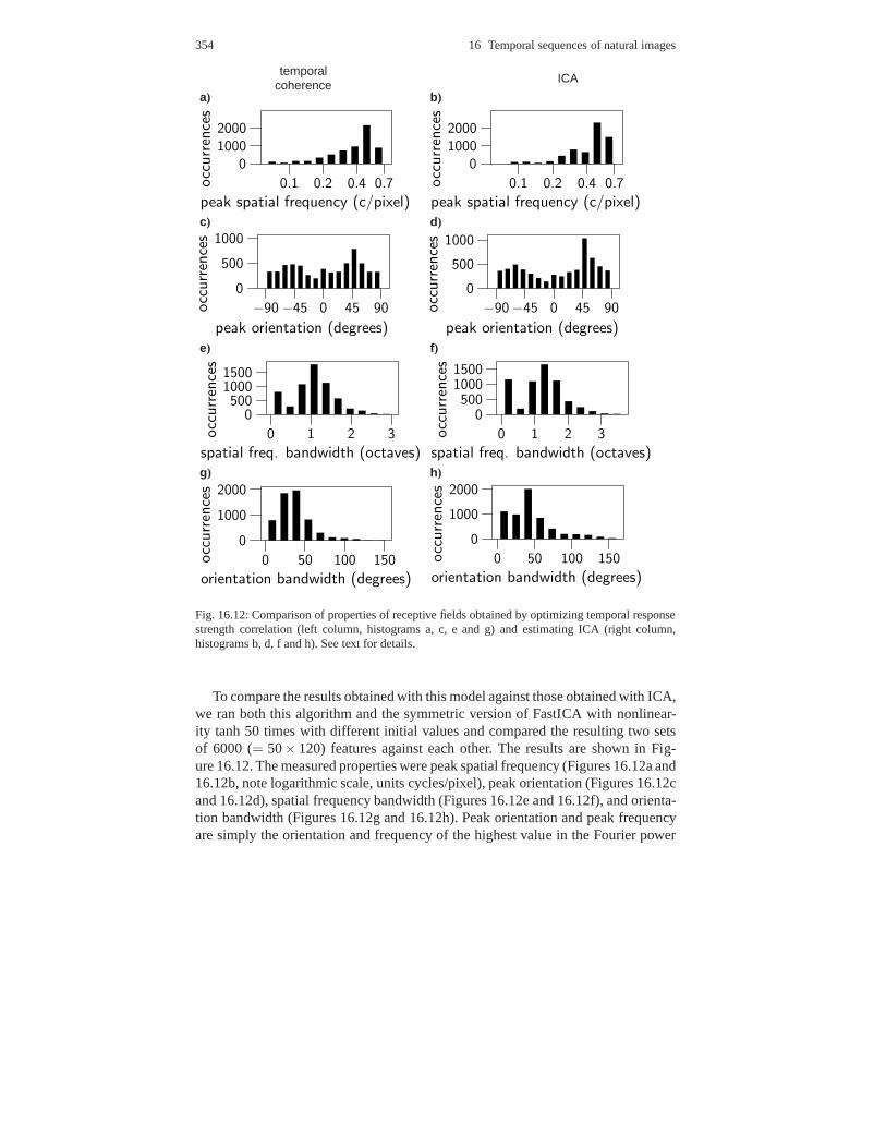
354 16 Temporal sequences of natural images
temporalcoherence
ICA
a)
010002000
0.1 0.2 0.4 0.7
peak spatial frequency (c/pixel)occ
urr
ence
s
b)
010002000
0.1 0.2 0.4 0.7
peak spatial frequency (c/pixel)
occ
urr
ence
s
c)
0
500
1000
−90−45 0 45 90
peak orientation (degrees)
occ
urr
ence
sd)
0
500
1000
−90−45 0 45 90
peak orientation (degrees)
occ
urr
ence
s
e)
0 1 2 3
0500
10001500
spatial freq. bandwidth (octaves)
occ
urr
ence
s
f)
0 1 2 3
0500
10001500
spatial freq. bandwidth (octaves)occ
urr
ence
s
g)
0 50 100 150
0
1000
2000
orientation bandwidth (degrees)
occ
urr
ence
s
h)
0 50 100 150
0
1000
2000
orientation bandwidth (degrees)
occ
urr
ence
s
Fig. 16.12: Comparison of properties of receptive fields obtained by optimizing temporal responsestrength correlation (left column, histograms a, c, e and g)and estimating ICA (right column,histograms b, d, f and h). See text for details.
To compare the results obtained with this model against those obtained with ICA,we ran both this algorithm and the symmetric version of FastICA with nonlinear-ity tanh 50 times with different initial values and comparedthe resulting two setsof 6000 (= 50× 120) features against each other. The results are shown in Fig-ure 16.12. The measured properties were peak spatial frequency (Figures 16.12a and16.12b, note logarithmic scale, units cycles/pixel), peakorientation (Figures 16.12cand 16.12d), spatial frequency bandwidth (Figures 16.12e and 16.12f), and orienta-tion bandwidth (Figures 16.12g and 16.12h). Peak orientation and peak frequencyare simply the orientation and frequency of the highest value in the Fourier power

16.5 Temporal coherence in spatial features 355
spectrum. Bandwidths measure the sharpness of the tuning and were computed fromthe tuning curve as the full width at at the point were half themaximum responsewas attained (full width at half maximum, FWHM); this measure is widely used invision science. See (van Hateren and van der Schaaf, 1998) for more details.
Although there are some differences between the two featuresets, the most im-portant observation here is the similarity of the histograms. This supports the ideathat ICA / sparse coding and temporal coherence are complementary theories, inthat they both result in the emergence of simple-cell-like receptive fields. As forthe differences, the results obtained using temporal response strength correlationhave a slightly smaller number of high-frequency receptivefields. Also, temporalresponse strength correlation seems to produce receptive fields that are somewhatmore localized with respect to both spatial frequency and orientation.4
16.5.5 Why Gabor-like features maximize temporal coherence
A simplified intuitive illustration of why the outputs of Gabor-like feature have suchstrong energy correlation over time is shown in Figure 16.13. Most transformationsof objects in the 3D world result in something similar to local translations of linesand edges in image sequences. This is obvious in the case of 3Dtranslations, andis illustrated in Figure 16.13a) for two other types of transformations: rotation andbending. In the case of a local translation, a suitably oriented simple-cell-like RF re-sponds strongly at consecutive time points, but the sign of the response may change.Note that when the output of a feature detector is consideredas a continuous sig-nal, the change of sign implies that the signal reaches zero at some intermediatetime point, which can lead to a weak measured correlation. Thus, a better model ofthe dependencies would be to consider dependencies of variances (Matsuoka et al,1995; Pham and Cardoso, 2001), as in the generative-model interpretation describedabove. However, for simplicity, we consider here the magnitude that is a crude ap-proximation of the underlying variance.
In order to further visualize the correlation of rectified responses at consecutivetime points, we will consider the interaction of features inone dimension (orthog-onal to the orientation of the feature). This allows us to consider the effect of localtranslations in a simplified setting. Figure 16.14 illustrates, in a simplified case, whythe temporal response strengths of lines and edges correlate positively as a result ofGabor-like feature structure. Prototypes of two differenttypes of image elements– the profiles of a line and an edge – which both have a zero DC component, areshown in the topmost row of the figure. The leftmost column shows the profiles of
4 When these results are compared against the results in (van Hateren and van der Schaaf, 1998),the most important difference is the peak at zero bandwidth in Figures 16.12e and 16.12f. Thisdifference is probably a consequence of the fact that no dimensionality reduction, anti-aliasing ornoise reduction was performed here, which results in the appearance of very small, checkerboard-like receptive fields. This effect is more pronounced in ICA,which also explains the stronger peakat the 45◦ angle in Figure 16.12d).

356 16 Temporal sequences of natural images
a)t−∆t t t−∆t
t
b)t−∆t t
Fig. 16.13: A simplified illustration of temporal activity level dependencies of simple-cell-likefeatures when the input consists of image sequences.a) Transformations of objects induce localtranslations of edges and lines in local regions in image sequences: rotation (left) and bending(right). The solid line shows the position/shape of a line inthe image sequence at timet−∆t, andthe dotted line shows its new position/shape at timet. The dashed square indicates the samplingwindow.b) Temporal activity level dependencies: in the case of a localtranslation of an edge or aline, the response of a simple-cell-like features with a suitable position and orientation is strong atconsecutive time points, but the sign may change. The figure shows a translating line superimposedon an oriented and localized receptive field at two differenttime instances (timet−∆t, solid line,left; time t, dotted line, right).
three different features with unit norm and zero DC component: a Gabor-like fea-ture, a sinusoidal (Fourier basis -like) feature, and an impulse feature. The rest of thefigure shows the square rectified responses of the features tothe inputs as functionsof spatial displacement of the input.
Consider the rectified response of the Gabor-like feature tothe line and the edge,that is, the first row of responses in Figure 16.14. The squared response at timet−∆ t(spatial displacement zero) is strongly positively correlated with response at timet,even if the line or edge is displaced slightly. This shows howsmall local transla-tions of basic image elements still yield large values of temporal response strengthcorrelation for Gabor-like features. If you compare the responses of the Gabor-likefeature to the responses of the sinusoidal feature – that is,the second row of re-sponses in Figure 16.14 – you can see that the responses to thesinusoidal featureare typically much smaller. This leads to a lower value of ourmeasure of temporalresponse strength correlation that emphasizes large values. Also, in the third row ofresponses in Figure 16.14 we can see that while the response of an impulse featureto an edge correlates quite strongly over small spatial displacements, when the inputconsists of a line even a very small displacement will take the correlation to almostzero.
Thus we can see that when considering three important classes of features –features which are maximally localized in space, maximallylocalized in frequency,or localized in both – the optimal feature is a Gabor-like feature, which is localizedboth in space and in frequency. If the feature is maximally localized in space, it failsto respond over small spatial displacements of very localized image elements. If the

16.5 Temporal coherence in spatial features 357
input
−2−1 0 1 2−2−1 0 1 2 3 0 1−2−1 0 1 2 3
filter square-rectified output
−1 0 1−2−1 0 1 2 3 −1 0 1−1 0 1 −1 0 1−1 0 1
−2−1 0 1 2 3−2−1 0 1 2 3 −1 0 1−1 0 1 −1 0 1−1 0 1
−2−1 0 1 2−2−1 0 1 2 3 −1 0 1−1 0 1 −1 0 1−1 0 1
Fig. 16.14: A simplified illustration of why a Gabor-like feature, localized in both space and fre-quency, yields larger values of temporal response strengthcorrelation than a feature localized onlyin space or only in frequency. Top row: cross sections of a line (left) and an edge (right) as func-tions of spatial position. Leftmost column: cross sectionsof three features with unit norm and zeroDC component – a Gabor-like feature (top), a sinusoidal feature (middle), and an impulse feature(bottom). The other plots in the figure show the responses of the feature detectors to the inputs asa function of spatial displacement of the input. The Gabor-like feature yields fairly large positivelycorrelated values for both types of input. The sinusoidal feature yields small response values. Theimpulse feature yields fairly large positively correlatedvalues when the input consists of an edge,but when the input consists of a line even a small displacement yields a correlation of almost zero.
the feature is maximally localized in frequency, its responses to the localized imagefeatures are not strong enough.
Figure 16.15 shows why we need nonlinear correlations instead of linear ones:raw output values might correlate either positively or negatively, depending on thedisplacement. Thus we see why ordinary linear correlation is not maximized forGabor-like features, whereas the rectified (nonlinear) correlation is.
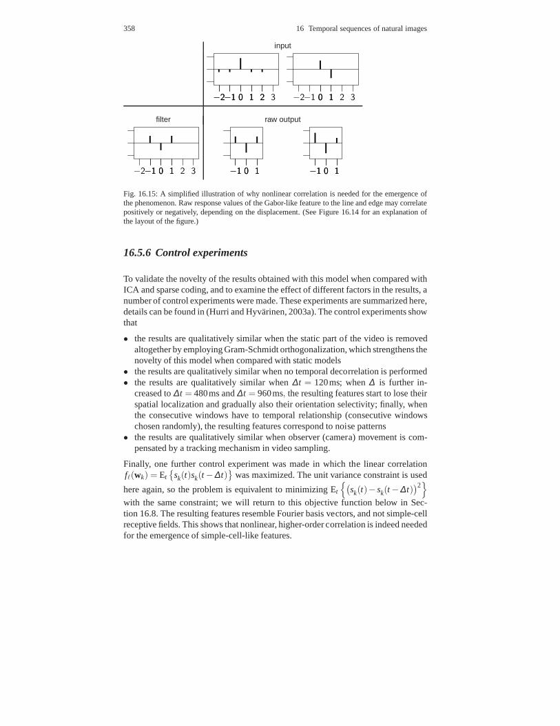
358 16 Temporal sequences of natural images
input
−2−1 0 1 2−2−1 0 1 2 3 0 1−2−1 0 1 2 3
filter raw output
−1 0 1−2−1 0 1 2 3 −1 0 1−1 0 1 −1 0 1−1 0 1
Fig. 16.15: A simplified illustration of why nonlinear correlation is needed for the emergence ofthe phenomenon. Raw response values of the Gabor-like feature to the line and edge may correlatepositively or negatively, depending on the displacement. (See Figure 16.14 for an explanation ofthe layout of the figure.)
16.5.6 Control experiments
To validate the novelty of the results obtained with this model when compared withICA and sparse coding, and to examine the effect of differentfactors in the results, anumber of control experiments were made. These experimentsare summarized here,details can be found in (Hurri and Hyvarinen, 2003a). The control experiments showthat
• the results are qualitatively similar when the static part of the video is removedaltogether by employing Gram-Schmidt orthogonalization,which strengthens thenovelty of this model when compared with static models
• the results are qualitatively similar when no temporal decorrelation is performed• the results are qualitatively similar when∆ t = 120ms; when∆ is further in-
creased to∆ t = 480ms and∆ t = 960ms, the resulting features start to lose theirspatial localization and gradually also their orientationselectivity; finally, whenthe consecutive windows have to temporal relationship (consecutive windowschosen randomly), the resulting features correspond to noise patterns
• the results are qualitatively similar when observer (camera) movement is com-pensated by a tracking mechanism in video sampling.
Finally, one further control experiment was made in which the linear correlationfℓ(wk) = Et
{sk(t)sk(t−∆ t)
}was maximized. The unit variance constraint is used
here again, so the problem is equivalent to minimizing Et
{(sk(t)−sk(t−∆ t)
)2}
with the same constraint; we will return to this objective function below in Sec-tion 16.8. The resulting features resemble Fourier basis vectors, and not simple-cellreceptive fields. This shows that nonlinear, higher-order correlation is indeed neededfor the emergence of simple-cell-like features.

16.6 Spatiotemporal energy correlations in linear features 359
16.6 Spatiotemporal energy correlations in linear features
16.6.1 Definition of the model
Temporal response strength correlation, defined in Equation (16.13) on page 350,maximizes the “temporal coherence” in the outputs of individual simple cells. Notethat in terms of the generative model described above, the objective functions saysnothing about the interdependencies in differentsk(t)’s – that is, different cells.Thus, there is an implicit assumption of independence in themodel, at least if itis interpreted as a probabilistic generative model. In thissection we add anotherlayer to the generative model to extend the theory to simple-cell interactions, and tothe level of complex cells.5
×abs(s(t)) s(t)
sign generationP(sk(t) > 0
∣∣∣∣s
k(t−∆t)> 0
)= Pret
x(t) = As(t)v(t) abs(s(t)) = Mabs(s(t−∆t))+v(t) x(t)
Fig. 16.16: The two layers of the generative model. Letabs(s(t)) = [|s1(t)| · · · |sK(t)|]T denotethe amplitudes of simple cell responses. In the first layer, the driving noise signalv(t) generatesthe amplitudes of simple cell responses via an autoregressive model. The signs of the responsesare generated randomly between the first and second layer to yield signed responsess(t). In thesecond layer, natural videox(t) is generated linearly from simple cell responses. In addition tothe relations shown here, the generation ofv(t) is affected byMabs(s(t−∆t)) to ensure non-negativity ofabs(s(t)) . See text for details.
Like in the many generative models discussed in this book, the output layer ofthe new model (see Figure 16.16) is linear, and maps cell responsess(t) to imagefeaturesx(t), but we do not assume that the components ofs(t) are independent.Instead, we model the temporal dependencies between these components in the firstlayer of our model. Letabs(s(t)) = [|s1(t)| · · · |sK(t)|]T denote the activities of thecells, and letv(t) denote a driving noise signal andM denote aK×K matrix; themodelled interdependencies will be “coded” inM .. Our model is amultidimensionalfirst-order autoregressive process, defined by
abs(s(t)) = Mabs(s(t−∆ t))+v(t). (16.17)
Again, we also need to fix the scale of the latent variables by defining Et
{
s2
k(t)}
= 1
for k = 1, ...,K.
5 This section is based on the article (Hurri and Hyvarinen, 2003b) originally published in Network:Computation in Neural Systems. Copyrightc©2003 Institute of Physics, used with permission.

360 16 Temporal sequences of natural images
There are dependencies between the driving noisev(t) and output strengthsabs(s(t)) , caused by the non-negativity ofabs(s(t)) . To take these dependenciesinto account, we use the following formalism. Letu(t) denote a random vector withcomponents which are statistically independent of each other. To ensure the non-negativity ofabs(s(t)) , we define
v(t) = max(−Mabs(s(t−∆ t)) ,u(t)) , (16.18)
where, for vectorsa andb,max(a,b)= [max(a1,b1) · · · max(an,bn)]T .We assume
thatu(t) andabs(s(t)) are uncorrelated. The point in this definition is to make surethat the noise does not drive the absolute values of thesK(t) negative, which wouldbe absurd.
To make the generative model complete, a mechanism for generating the signsof cell responsess(t) must be included. We specify that the signs are generated ran-domly with equal probability for plus or minus after the strengths of the responseshave been generated. Note that one consequence of this is that the differentsk(t)’sare uncorrelated. In the estimation of the model this uncorrelatedness property isused as a constraint. When this is combined with the unit variance (scale) constraintsdescribed above, the resulting set of constraints is the same as in the approach de-scribed above in Section 16.5 (page 349).
In Equation (16.17), a large positive matrix elementM(i, j), or M( j, i), indicatesthat there is strong temporal dependency between the outputstrengths of cellsi andj. Thinking in terms of grouping temporally coherent cells together, matrixM canbe thought of as containing similarities (reciprocals of distances) between differentcells. We will use this property below to derive a topographyof simple-cell receptivefields fromM .
16.6.2 Estimation of the model
To estimate the model defined above we need to estimate bothM andA. Instead ofestimatingA directly, we estimateW which maps image sequence data to responses
s(t) = Wx(t), (16.19)
and use the pseudo-inverse relationship – that is, Equation(16.16) on page 351 – tocomputeA. In what follows, we first show how to estimateM , givenW. We thendescribe an objective function which can be used to estimateW, given M . Eachiteration of the estimation algorithm consists of two steps. During the first stepM isupdated, andW is kept constant; during the second step these roles are reversed.
First, regarding the estimation ofM , consider a situation in whichW is keptconstant. It can be shown (Hurri and Hyvarinen, 2003b) thatM can be estimated byusing approximative method of moments, and that the estimate is given by

16.6 Spatiotemporal energy correlations in linear features 361
M ≈ βEt
{
(abs(s(t))−Et {abs(s(t))}) (abs(s(t−∆ t))−Et {abs(s(t))})T}
×Et
{
(abs(s(t))−Et {abs(s(t))}) (abs(s(t))−Et {abs(s(t))})T}−1
,
whereβ > 1. Since this multiplier does not change the relative strengths of theelements ofM , and since it has a constant linear effect in the objective function ofW given below, its value does not affect the optimalW, so we can simply setβ = 1in the optimization. The resulting estimator forM is the same as the optimal leastmean squares linear predictor in the case of unconstrainedv(t).
The estimation ofW is more complicated. A rigorous derivation of an objec-tive function based on well-known estimation principles isvery difficult, becausethe statistics involved are non-gaussian, and the processes have difficult interdepen-dencies. Therefore, instead of deriving an objective function from first principles,we derived an objective function heuristically (Hurri and Hyvarinen, 2003b), andverified through simulations that the objective function iscapable of estimating thetwo-layer model. The objective function is a weighted sum ofthe covariances offeature output strengths at timest−∆ t andt, defined by
f (W,M) =K
∑i=1
K
∑j=1
M(i, j)cov{|si(t)| ,
∣∣sj(t−∆ t)
∣∣}. (16.20)
In the actual estimation algorithm,W is updated by employing a gradient projectionapproach to the optimization off in Equation (16.20) under the constraints. Theinitial value ofW is selected randomly.
The fact that the algorithm described above is able to estimate the two-layermodel has been verified through extensive simulations. These simulations show thatmatrix W can be estimated fairly reliably, and that the relative error of the estimateof matrixM also decreases reliably in the estimation, but the remaining error forMis larger than in the case of matrixW. This difference is probably due to the approx-imation made in the estimation ofM ; see (Hurri and Hyvarinen, 2003b). However,the simulations suggest that the error in the estimate ofM is largely due to a sys-tematic, monotonic, nonlinear element-wise bias, which does not affect greatly ourinterpretation of the elements ofM , since we are mostly interested in their relativemagnitudes. See (Hurri and Hyvarinen, 2003b) for details.A very closely relatedmodel which can be analyzed in detail is in (Hyvarinen and Hurri, 2004), whichshows that a rigorous justification for our objective function above can be found inthe case where we use the quadratic function instead of the absolute value function.See also (Valpola et al, 2003) for related theoretical work.
16.6.3 Experiments on natural images
The estimation algorithm was run on the same data set as for the basic temporalcoherence model in Section 16.5 to obtain estimates forM andA. Figure 16.17

362 16 Temporal sequences of natural images
Fig. 16.17: The estimation of the two-layer generative model from natural visual stimuli resultsin the emergence of localized, oriented receptive fields with multiple scales. The feature vectors(columns ofA) shown here are in no particular order.
shows the resulting feature vectors – that is, columns ofA. As can be seen, theresulting features are localized, oriented, and have multiple scales, thereby fulfillingthe most important defining criteria of simple-cell receptive fields. This suggeststhat, as far as receptive-field structure is concerned, the method yields receptivefields with similar qualitative properties to those obtained with sparse coding, ICA,or temporal response strength correlation.
What is truly novel in this model is the estimation of matrixM , which capturesthe temporal and spatiotemporal activity-level dependencies between the featurevectors shown in Figure 16.17. The extracted matricesA and M can be visual-ized simultaneously by using the interpretation ofM as a similarity matrix (seepage 360). Figure 16.18 illustrates the feature vectors – that is, columns ofA – laidout at spatial coordinates derived fromM in a way explained below. The resultingfeature vectors are again oriented, localized and multiscale, as in the basic temporalcoherence model in Section 16.5.
In the resulting planar representation shown in Figure 16.18, the temporal coher-ence between the outputs of two cellsi and j is reflected in the distance betweenthe corresponding receptive fields: the larger the elementsM(i, j) andM( j, i) are,the closer the receptive fields are to each other. We can see that local topographyemerges in the results: those basis vectors which are close to each other seem to bemostly coding for similarly oriented features at nearby spatial positions. This kindof grouping is characteristic of pooling of simple cell outputs at complex cell level(Palmer, 1999). Some global topography also emerges: thosebasis vectors which

16.6 Spatiotemporal energy correlations in linear features 363
Fig. 16.18: Results of estimating the two-layer generativemodel from natural image sequences.Features (columns ofA) plotted at spatial coordinates given by applying multidimensional scal-ing to M . Matrix M was first converted to a non-negative similarity matrixM s by subtractingmini, j M(i, j) from each of its elements, and by setting each of the diagonalelements at value 1.Multidimensional scaling was then applied toM s by interpreting entriesM s(i, j) andM s( j , i) assimilarity measures between cellsi and j . Some of the resulting coordinates were very close toeach other, so tight cell clusters were magnified for purposes of visual display. Details are given in(Hurri and Hyvarinen, 2003b).
code for horizontal features are on the left in the figure, while those that code forvertical features are on the right.
Thus, the estimation of our two-layer model from natural image sequences yieldsboth simple-cell-like receptive fields, and grouping similar to the pooling of simplecell outputs. Linear receptive fields emerge in the second layer (matrixA), and celloutput grouping emerges in the first layer (matrixM ). Both of these layers are es-timated simultaneously. This is an important property whencompared with other
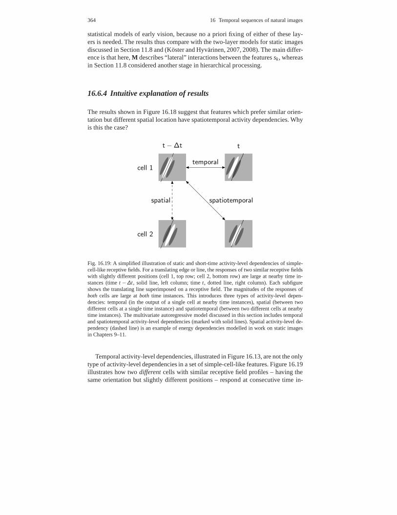
364 16 Temporal sequences of natural images
statistical models of early vision, because no a priori fixing of either of these lay-ers is needed. The results thus compare with the two-layer models for static imagesdiscussed in Section 11.8 and (Koster and Hyvarinen, 2007, 2008). The main differ-ence is that here,M describes “lateral” interactions between the featuressk, whereasin Section 11.8 considered another stage in hierarchical processing.
16.6.4 Intuitive explanation of results
The results shown in Figure 16.18 suggest that features which prefer similar orien-tation but different spatial location have spatiotemporalactivity dependencies. Whyis this the case?
temporal
spatial spatiotemporal
cell 1
cell 2
t−∆t t
Fig. 16.19: A simplified illustration of static and short-time activity-level dependencies of simple-cell-like receptive fields. For a translating edge or line, the responses of two similar receptive fieldswith slightly different positions (cell 1, top row; cell 2, bottom row) are large at nearby time in-stances (timet − ∆t, solid line, left column; timet, dotted line, right column). Each subfigureshows the translating line superimposed on a receptive field. The magnitudes of the responses ofboth cells are large atboth time instances. This introduces three types of activity-level depen-dencies: temporal (in the output of a single cell at nearby time instances), spatial (between twodifferent cells at a single time instance) and spatiotemporal (between two different cells at nearbytime instances). The multivariate autoregressive model discussed in this section includes temporaland spatiotemporal activity-level dependencies (marked with solid lines). Spatial activity-level de-pendency (dashed line) is an example of energy dependenciesmodelled in work on static imagesin Chapters 9–11.
Temporal activity-level dependencies, illustrated in Figure 16.13, are not the onlytype of activity-level dependencies in a set of simple-cell-like features. Figure 16.19illustrates how twodifferentcells with similar receptive field profiles – having thesame orientation but slightly different positions – respond at consecutive time in-

16.7 Unifying model of spatiotemporal dependencies 365
stances when the input is a translating line. The receptive fields are otherwise iden-tical, except that one is a slightly translated version of the other. It can be seen thatboth cellsare highly active atboth time instances,but again, the signs of the outputsvary. This means that in addition to temporal activity dependencies (the activity ofa cell is large at timet−∆ t and timet), there are two other kinds of activity-leveldependencies.
spatial (static) dependencies Both cells are highly activeat a single time instance.This kind of dependency is an example of the energy dependencies earlier mod-elled in static images in Chapters 9–11.
spatiotemporal dependencies The activity levels of different cells are also relatedover time. For example, the activity of cell 1 at timet−∆ t is related to the activityof cell 2 at timet.
What makes these dependencies important is that they seem tobe reflected inthe structure of the topography in the primary visual cortex. The results presentedin this section suggest that combining temporal activity level dependencies withspatiotemporal dependencies yields both simple-cell-like receptive fields and a setof connections between these receptive fields. These connections can be related toboth the way in which complex cells seem to pool simple-cell outputs, and to thetopographic organization observed in the primary visual cortex, in the same wayas described in Chapter 11. Therefore, the principle of activity level dependenciesseems to explain both receptive field structure and their organization.
16.7 Unifying model of spatiotemporal dependencies
In order to motivate the development of a model which unifies anumber of statisticalproperties in natural image sequences, let us summarize thekey results on proba-bilistic modelling of the properties of the neural representation at the simple-celllevel.
1. Results obtained using sparse coding / independent component analysis suggestthat, on the average, at a single time instant relatively fewsimple cells are activeon the cortex (see Chapter 6); furthermore, each cell is active only rarely.
2. In this chapter, we have described a complementary model,which suggests thatsimple cells tend to be highly active at consecutive time instants – that is, theiroutputs are burst-like (see Section 16.5).
3. Models on static dependencies between simple-cell-likefeatures, and the rela-tionship between these dependencies and cortical topography, suggest that theactive cells tend to be located close to each other on the cortex, as in Chapter 11.
4. As we saw in the preceding section, temporal correlationsalso lead to topo-graphic properties resembling cortical topography, basedon a model which uti-lizes temporal correlations between the outputs of different features.
These four different principles – sparseness, temporal coherence of activity levels,spatial activity level dependencies, and spatiotemporal activity level dependencies –

366 16 Temporal sequences of natural images
are not conflicting. That is, none of the principles excludesthe existence of another.Perhaps, then, each of these models offers just a limited view to a more completemodel of cortical coding at the simple-cell level. In fact, the following descriptionof simple-cell activation is in accordance with all of the principles: when an animalis viewing a natural scene, a relatively small number of patches of cortical area arehighly active in the primary visual cortex, and the activityin these areas tends to besustained for a while. That is, activity is sparse, and contiguous both in space andtime. This is thebubble codingmodel (Hyvarinen et al, 2003).
In the bubble coding model, the final generative mapping fromlatent componentsto natural image sequence data is linear, like in the previous sections:x(t) = As(t).The main idea in the bubble coding model is generation of thes(t) so that theyhave bubble-like activity. This is accomplished by introducing a bubble-like vari-ance signal fors(t), as illustrated by an example in Figure 16.20. The spatiotem-poral locations of the variance bubbles are determined by a sparse processu(t)(Figure 16.20a). A temporal filterφ and spatial pooling functionh, both of whichare fixed a priori in the model, spread the variance bubbles temporally and spa-tially (Figures 16.20b and c). The resulting variance bubbles can also overlap eachother, in which case the variance in the overlapping area is obtained as a sum ofthe variances in each bubble; in Figure 16.20, however, the variance bubbles arenon-overlapping for illustrative purposes. It is also possible that at this point a fixedstatic nonlinearityf is applied to rescale the magnitudes of the variance bubbles.These steps yield the variance signals
vk(t) = f
(
∑ℓ
h(k, ℓ) [φ(t)∗uℓ(t)]
)
. (16.21)
where∗ denotes temporal convolution. The burst-like oscillatingnature of the com-ponents inside the bubbles is introduced through a gaussiantemporally uncorrelated(white noise) processz(t) (Figure 16.20d). Thus, the componentssk(t) are gener-ated from the variance bubbles and the noise signals by multiplying the two together(Figure 16.20e):
sk(t) = vk(t)zk(t). (16.22)
Note that all three different types of activity level dependencies – temporal, spatial,and spatiotemporal (see Figure 16.19 on page 364) – are present in the bubble-coding model, as well as sparseness. To complete this generative model, thesk(t)are finally linearly transformed to the image using a linear transformation, as inalmost all models in this book.
An approximative maximum likelihood scheme can be used to estimate the bub-ble coding model; details can be found in (Hyvarinen et al, 2003). Note that becausethe pooling functionh is fixed, it enforces the spatial pooling, while in the two-layermodel described in the previous section, this pooling was learned from the data. Thetemporal smoothing (low-pass) filterφ is also fixed in the model.
Figure 16.21 shows the resulting spatial basis vectors, obtained when the bubblecoding model was estimated from natural image sequence data. The basis consistsof simple-cell-like linear receptive-field models, similar to those obtained by topo-

16.8 Features with minimal average temporal change 367
graphic ICA from static images (Figure 11.4 on page 258), or using the temporalmodels in Section 16.6. The orientation and the location of the feature coded bythe vectors change smoothly when moving on the topographic grid. Low-frequencybasis vectors are spatially segregated from the other vectors, so there also seems tobe some ordering based on preferred spatial frequency. Suchan organization withrespect to orientation, location, and spatial frequency issimilar to the topographicordering of simple cells in the primary visual cortex, as wasdiscussed in Chapter 11.
One can also estimate spatiotemporal features with this model. An animated ex-ample of the resulting spatiotemporal features can be foundatwww.cs.helsinki.fi/group/nis/animations/bubbleanimation.gif.
The features obtained by the bubble coding models are thus hardly any differentfrom what were obtained by the topographic ICA model, for example. The signifi-cance of the model is mainly theoretical in the sense that it gives a unified frameworkfor understanding the different models involved.
16.8 Features with minimal average temporal change
16.8.1 Slow feature analysis
16.8.1.1 Motivation and history
All of the models of temporal coherence discussed above – temporal responsestrength correlation, the two-layer autoregressive model, and the bubble-codingmodel – are based on temporal patterns in output energies (variances)s2(t). Whathappens if we just minimize a measure of the temporal change in the outputs of themodel neurons? That is, ifs(t) is the output of a model at timet, andw is our vectorof model parameters, we could for example minimize the squared difference of theoutput at close-by time points
fSFA(w) = Et
{
(s(t)−s(t−∆ t))2}
. (16.23)
An explicit formalization of this principle was given by Mitchison (1991) who sim-ply described it as “removal of time variation” (see also (Hinton, 1989; Foldiak,1991; Stone, 1996)). The principle was also used in blind source separation, inwhich a number of sophisticated methods for its algorithmicimplementation havebeen developed (Tong et al, 1991; Belouchrani et al, 1997; Hyvarinen et al, 2001b).Recently the principle has been given the nameslow feature analysis(Wiskott andSejnowski, 2002), thus the subscript SFA in the definition ofthe objective function.
In order to relate the SFA objective function to the models wehave discussedabove, let us analyze it in more detail. Expanding the squareand taking the expec-tations of the resulting terms we get

368 16 Temporal sequences of natural images
a)
sign
alin
dex
k→
uk(t)
time t→
b)
sign
alin
dex
k→
ξk(t) = φ(t)∗uk(t)
time t→c)
sign
alin
dex
k→
vk(t) = f (∑ℓ h(k, ℓ)ξℓ(t))
time t→
d)
sign
alin
dex
k→
zk(t)
time t→
e)
sign
alin
dex
k→
sk(t) = v
k(t)z
k(t)
time t→

16.8 Features with minimal average temporal change 369
fSFA(w) = Et{
s2(t)−2s(t)s(t−∆ t)+s2(t−∆ t)}
= Et{
s2(t)}−2Et {s(t)s(t−∆ t)}+Et
{s2(t−∆ t)
}
︸ ︷︷ ︸
=Et{s2(t)}= 2
(Et{
s2(t)}−Et {s(t)s(t−∆ t)}
)
(16.24)
The objective function is non-negative, and a trivial way tominimize it is to computea zero outputs(t) = 0 for all t. A standard way to avoid this anomaly is to constrainthe “energy” (second moment) of the output signal to unity, that is, define constraint
Et{
s2(t)}
= 1, (16.25)
in which case the objective function become simpler:
fSFA(w) = 2(1−Et {s(t)s(t−∆ t)}) , (16.26)
which shows that under the unit energy constraint, SFA is equivalent to maximiza-tion of the linear temporal correlation in the output. This is in contrast to the modelin Section 16.5 (page 349), which was based on maximization of nonlinear tem-poral correlation. Also note that if mean output is zero, that is, if Et {s(t)} = 0,then the unit energy constraint is equivalent to the unit variance constraint, sincevar(s(t)) = Et
{s2(t)
}− (Et {s(t)})2 .
16.8.1.2 SFA in a linear neuron model
In Section 16.5 (page 349) we mentioned that in a linear neuron model, maximiza-tion of linear temporal correlation results in receptive fields which resemble fre-quency components and not simple-cell-like receptive fields or Gabor functions. In
Fig. 16.20: (opposite page) Illustration of the generation of componentssk(t) in the bubble codingmodel. For simplicity of illustration, we use a one-dimensional topography instead of the moreconventional two-dimensional one.a) The starting point is the set of sparse signalsuk(t). b) Eachsparse signaluk(t) is filtered with a temporal low-pass filterφ(t), yielding signalsφ(t)∗uk(t). Inthis example, the filterφ(t) simply spreads the impulses uniformly over an interval.c) In the nextstep, a neighbourhood functionh(k, ℓ) is applied to spread the bubbles spatially; this is like a spatiallow-pass filter. A static nonlinearityf may also be applied at this point to rescale the magnitudesof the variance bubbles. This yields variance bubble signals vk(t) = f
(
∑ℓ h(k, ℓ) [φ(t)∗uℓ(t)]). In
this example, the neighbourhood functionh is simply 1 close-by and 0 elsewhere, and the staticnonlinearity f is just the identity mappingf (α)= α . d) Next, we generate gaussian temporally un-correlated (white noise) signalszk(t). e) Linear components (responses) are defined as products ofthe gaussian white noise signals and the spatiotemporally spread bubble signals:sk(t) = zk(t)vk(t).These are transformed linearly by the matrixA to give the observed image data (not shown). (Notethat in subfigures a)–c), white denotes value zero and black denotes value 1, while in subfiguresd) and e), medium grey denotes zero, and black and white denote negative and positive values,respectively.)

370 16 Temporal sequences of natural images
Fig. 16.21: A set of spatial features, estimated from natural image using the bubble coding estima-tion method, and laid out at spatial coordinates defined by the topographic grid in the bubble codingmodel. The topographic organization of the features exhibits ordering with respect to orientation,location, and spatial frequency of the vectors, being very similar to that obtained by topographicICA.
such a linear model, slow feature analysis can be analyzed mathematically in detail.Let s(t) denote the output of the unit at timet :
s(t) = wTx(t). (16.27)
Assume that the inputx(t) has zero mean (Et {x(t)} = 0), and that we impose theunit variance constraint to avoid the trivial solutionw = 0. Then the unit energyconstraint also holds, and instead of minimizing the SFA objective function (16.26)we can just maximize linear temporal correlation
fLTC(w) = Et {s(t)s(t−∆ t)}= Et{
wTx(t)x(t−∆ t)Tw}
= wTEt{
x(t)x(t−∆ t)T}w(16.28)

16.8 Features with minimal average temporal change 371
with the constraint
Et{
s2(t)}
= 1⇔ wTEt{
x(t)x(t)T}w = 1 (16.29)
A solution can be derived by adapting the mathematics of PCA described in Sec-tion 5.8.1. The connection becomes clear if we first whiten the datax(t) (spatially,i.e. in the same way as in Chapter 5, ignoring the temporal dependencies). For sim-plicity, we denote the whitened data byx(t) in the following. For the whitened data,the constraint of unit variance is equivalent to the constraint thatw has unit norm,because Et
{x(t)x(t)T
}is the identity matrix.
Thus, we have a maximization of a quadratic function under unit norm constraint,just as in PCA. There is a small difference, though: The matrix Et
{x(t)x(t−∆ t)T
}
defining the quadratic function is not necessarily symmetric. Fortunately, it is notdifficult to prove that actually, this maximization is equivalent to maximization usinga symmetric version of the matrix:
fLTC(w) = wT[
12
Et{
x(t)x(t−∆ t)T}+12
Et{
x(t−∆ t)x(t)T}]
w (16.30)
Thus, the same principle of computing the eigenvalue decomposition applies here(Tong et al, 1991). The optimal vectorw is obtained as the one corresponding to thelargest eigenvalue of this matrix. If we want to extract a setof RF’s, we can use thefollowing result: assuming that the output of the next selected RF has to be uncor-related with the outputs of the previously selected ones, then the next maximum isthe eigenvector with the next largest eigenvalue.
Figure 16.22 shows the filters that result from such optimization in a linear neu-ron model. The data set and preprocessing in this experimentwas identical to theone in Section 16.5. As can be seen, the resulting filters correspond to frequency(Fourier) features, and not the localized RF’s in the early visual system.
16.8.2 Quadratic slow feature analysis
As shown above, SFA in the case of a linear neuron model does not produce veryinteresting results. In contrast, application of the principle in the nonlinear case hasproven more promising, although results for real natural image sequences have notbeen reported.
A straightforward and computationally simple way to designnonlinear modelsis the basis expansionapproach. As a simple example, assume that out originalinput data is a single scalarx. This data can be expanded by computing the squareof the data pointx2. We can then design a model that is linear in the parametersa = (a1 a2)
T
y = a1x+a2x2 = aT
(xx2
)
(16.31)

372 16 Temporal sequences of natural images
Fig. 16.22: The set of filters which optimize the objective function in slow feature analysis fromnatural image data in the case of a linear neuron model. As canbe seen, the resulting filters do notresemble localized receptive fields of either retina/LGN orV1.
but obviously nonlinear in the datax (here, it is quadratic). A very nice propertyof this approach is that the analysis developed for the linear case is immediatelyapplicable: all we need to do is to replace the original data with the expanded data.In the SFA case, letf (x(t)) = [ f1(x(t)) f2(x(t)) · · · fM(x(t))]T denote a nonlinearexpansion of the data. Then the output is
s(t) = wT f (x(t)) , (16.32)
and all of the optimization results apply afterx(t) is replaced withf (x(t)) .The form of basis expansion we are particularly interested in is that of a quadratic
basis. Letx(t) = [x1(t) x2(t) · · · xK(t)]T denote our original data. Then a data vectorin our quadratic data setf (x(t)) includes, in addition to the original componentsx1(t),x2(t), ...,xK(t), the products of all pairs of componentsxk(t)xℓ(t), k = 1, ...,K,ℓ= 1, ...,K; note that this also includes the squaresx2
1(t),x22(t), ...,x
2K(t).

16.8 Features with minimal average temporal change 373
While the computation of the optimum in the case of basis-expanded SFA isstraightforward, the interpretation of the results is moredifficult: unlike in the caseof linear data, the obtained parameters can not simply be interpreted as a templateof weights at different positions in the image, because someof the parameters corre-spond to the quadratic termsxk(t)xℓ(t), k= 1, ...,K, ℓ= 1, ...,K.One way to analyzethe learned parameter vectorsw1, ...,wM is to compute the input images that elicitmaximal and minimal responses, while constraining the norm(energy) of the im-ages to make the problem well-posed; that is, ifc> 0 is a constant
xmax = argmax‖x‖=cwT f(x) (16.33)
xmin = argmin‖x‖=cwT f(x). (16.34)
A procedure for findingxmax andxmin is described in (Berkes and Wiskott, 2007).
a) b)
Fig. 16.23: Quadratic SFA of image sequence datagenerated from static image data. a) Inputimagesxmax that correspond to maximum output.b) Input imagesxmin that correspond to min-imum output. The maximum and minimum input images are at corresponding locations in thelattices. Most of the optimal input images are oriented and bandpass, and also spatially localizedto some degree. The maximum and minimum input images of the units have interesting relation-ships; for example, they may have different preferred orientations, different locations, or one canbe orientation-selective while the other is not.
Berkes and Wiskott (2005) applied quadratic SFA tosimulatedimage sequencedata: the image sequencesx(t) were obtained from static natural images by selectingan initial image location, obtaining asx(0) from the location with random orienta-tion and zoom factor, and then obtainingx(t), t > 0, by applying all of the followingtransformations at the location ofx(t−1) : translation, rotation, and zooming. Animportant property of the results obtained by Berkes and Wiskott (2005) using SFAwith simulated image sequence data is the phase invariance of the quadratic units.This has lead to an association between SFA and complex cells; in fact, Berkes andWiskott (2005) report a number of observed properties in quadratic SFA modelsthat match those of complex cells. See Figure 16.23 for a reproduction of those re-sults. However, the results by Berkes and Wiskott were obtained bysimulatedimage

374 16 Temporal sequences of natural images
sequences, whose temporal correlations were basically determined by the experi-menters themselves. Thus, they do not really provide a basisfor making conclusionsabout the connection between ecologically valid stimuli and visual processing.
Hashimoto (2003) applied quadratic SFA toreal natural image sequences. Shefound that the obtained features were only weakly related tocomplex cells, andproposed that better results could be found by asparsevariant of SFA. This will betreated next.
16.8.3 Sparse slow feature analysis
In sparse SFA, the measure of change is changed to one that emphasizes sparse-ness. In the original objective in Equation (16.23), it is not necessary to take thesquared error. The squared error is used here for algebraic and computational sim-plicity only: it allows us to maximize the objective function using the eigenvaluedecomposition. In general, we can consider objective function of the form
fSSFA(w) = Et {G(s(t)−s(t−∆ t))} . (16.35)
whereG is some even-symmetric function. A statistically optimal choice ofG ispresumably one that corresponds to a sparse pdf, because changes in images areusually abrupt, as in edges. We call resulting model Sparse SFA. The statisticaljustification is based on modelling the data with an autoregressive model in whichthe driving noise term (innovation process) is super-gaussian or sparse (Hyvarinen,2001b).
The same sparse model (using aG which is not the square function) can be usedin the context of quadratic SFA because quadratic SFA simplymeans defining theinput data in a new way. This leads to the concept of sparse quadratic SFA. It isimportant not to confuse the two ways in which an SFA model canbe quadratic: Itcan use squared error (i.e. takeG(u) = u2), or it can use a quadratic expansion ofthe input data (using products of the original input variables as new input variables).
Using sparse quadratic SFA, Hashimoto (2003) obtained energy detectors whichseem to be much closer to quadrature-phase filter pairs and complex cells than thoseobtained by ordinary quadratic SFA. Those results were obtained on real naturalimage sequences, from which ordinary quadratic SFA does notseem to learn verycomplex-cell like energy detectors.
Thus, we see how sparseness is ubiquitous in natural image statistics modelling,and seems to be necessary even in the context of SFA.

16.9 Conclusion 375
16.9 Conclusion
Different models of temporal coherence have been applied tosimulated and naturalvisual data. The results that emerge from these models agreewith neurophysiologi-cal observations to varying degrees. Thus far the principlehas mostly been appliedto model V1 cells – that is, simple and complex cells. In this chapter we focusedon models which have resulted in the emergence ofspatially localizedfilters withmultiple scales (responding to different frequencies) from natural image sequencedata. That is, we required that the spatial localization hasnot been forced in themodel, but emerges from learning, as happened in all the sparse coding and ICA-related models treated in this book so far; this is in contrast to some temporal coher-ence models, in which spatial localization isenforcedby sampling with a gaussianweighting window, so that the RF’s are then necessarily localized in the center ofthe patch. Also, we required that the image sequences come from a video cameraor a similar device, which is in contrast to some work in whichone takes static im-ages and then artificially creates sequence by sampling fromthem. Further work ontemporal coherence, in addition to the work already cited above, include (Kohonen,1996; Kohonen et al, 1997; Bray and Martinez, 2003; Kayser etal, 2003; Kordinget al, 2004; Wyss et al, 2006).
A more philosophical question concerns the priorities between models of staticimages and image sequences. We have seen models which produce quite similarresults in the two cases. For example, simple cell RF’s can belearned by sparsecoding and ICA from static natural images, or, alternatively, using temporal coher-ence from natural image sequences. Which model is, then, more “interesting”? Thisis certainly a deep question which depends very much of the justification of theassumptions in the models. Yet, one argument can be put forward in general: Weshould always prefer the simpler model, if both models have the same explanatorypower. This is a general principle in modelling, called parsimony, or Occam’s ra-zor. In our case, it could be argued that since static images are necessarily simplerthan image sequences, we should prefer models which use static images—at leastif the models have similar conceptual simplicity. Thus, onecould argue that modelson image sequences are mainly interesting if they enable learning of aspects whichcannot be learned with static images. This may not have been the case with manymodels we considered in this chapter; however, the principles introduced may verywell to lead to discoveries of new properties which cannot beeasily, if at all, foundin static images.
An important related question concerns learning image transformations (Memi-sevic and Hinton, 2007). One can view image sequences from a viewpoint whereeach image (frame) is a transformation of the preceding one.This is, in a sense,complementary to the viewpoint of temporal coherence, in which one tries to cap-ture features which are not transformed. It also seems to be closely related to theidea of predictive coding, see Section 14.3.


Part VConclusion


Chapter 17Conclusion and future prospects
In this chapter, we first provide a short overview of this book. Then, we discusssome open questions in the field, as well as alternative approaches to natural imagestatistics which we did not consider in detail in this book. We conclude with someremarks on possible future developments.
17.1 Short overview
We started this book in Chapter 1 by motivating the research on natural imagestatistics from an ecological-statistical viewpoint: Thevisual system is assumed tobe adapted to the statistical structure of natural images, because it needs to useBayesian inference. Next, we prepared the reader by introducing well-known math-ematical tools which are needed in natural image statisticsmodels (Part I, i.e. Chap-ters 2–4). The rest of the book, up to this chapter, was mainlya succession of differ-ent statistical models for natural images.
Part II was dedicated to models using purely linear receptive fields. The firstmodel we considered was principal component analysis in Chapter 5. It is an im-portant model for historical reasons, and also because it provides a preprocessingmethod (dimension reduction accompanied by whitening) which is used in mostsubsequent models. However, it does not provide a proper model for receptive fieldsin the primary visual cortex (V1).
In Chapter 6, the failure of principal component analysis was explained as thefailure to consider the sparse, non-gaussian structure of the data. In fact, naturalimages have a very sparse structure; the outputs of typical linear filters all havestrongly positive kurtosis. Based on this property, we developed a method in whichwe find the feature weights by maximizing the sparseness of the output when theinput to the feature detectors is natural images. Thus, we obtained a fundamentalresult: sparse coding finds receptive fields which are quite similar to those in V1simple cells in the sense that they are spatially localized,oriented, and band-pass(localized in Fourier space).
379

380 17 Conclusion and future prospects
Chapter 7 further elaborated on the linear sparse coding model and brought itfirmly into the realm of generative probabilistic models. Italso brought the view-point of independence: instead of maximizing the sparseness of single features, wecan maximize their statistical independence. A most fundamental theoretical resultssays that these two goals are equivalent for linear features. The resulting model hasbeen named independent component analysis (ICA) in the signal-processing litera-ture. An information-theoretic interpretation of the model was considered Chapter 8,as an alternative to the Bayesian one.
Part III took a clear step forward by introducing nonlinear feature detectors. Itturns out that independent component analysis is not able tocancel all the depen-dencies between the components, despite the name of the method. If we measurethe dependencies of components given by ICA by computing different kinds of cor-relations, we see that the squares of the components tend to be strongly correlated(Chapter 9). Such squares are called “energies” for historical reasons. We can modelsuch dependencies by introducing a random variable which controls the variancesof all the components at the same time. This enables the reduction of the depen-dencies based on processing which is quite similar to neurophysiological models ofinteractions between cells in V1, based on divisive normalization.
In Chapter 10, we used the same kind of energy dependencies tomodel stronglynonlinear features. Here, the nonlinearities took the formof computing the squaresof linear feature detectors and summing (“pooling”) such squares together. Just aswith linear features, we can maximize the sparseness of suchnonlinear featureswhen the input is natural images. The resulting features arequite similar to complexcells in V1. Again, we can build a probabilistic model, independent subspace anal-ysis, based on this maximization of sparseness. Interestingly, the model can also beconsidered a nonlinear version of independent component analysis.
The same idea of maximization of sparseness of energies was extended to modelthe spatial (“topographic”) arrangement of cells in the cortex in Chapter 11. Thismodel is really a simple modification of the complex cells model of the precedingchapter. We order the simple cells or linear feature detectors on a regular grid, whichthus defines which cells are close to each other. Then, we maximize the sparsenessesof energy detectors which pool the energies of close-by simple cells; we take thesum of such sparsenesses over all grid locations. This leadsto a spatial arrangementof linear features which is similar to the one in V1 in the sense that preferred ori-entations and frequencies of the cells change smoothly whenwe move on the grid(or cortex); the same applies to the locations of the centresof the features. Becauseof the close connection to the complex cell model, the pooledenergies of close-bycells (i.e. sums of squares of feature detectors which are close to each other on thegrid) have the properties of complex cells just like in the preceding chapter.
In Chapter 12 even more complicated nonlinear features werelearned, althoughwe didn’t introduce any new probabilistic models. The trickwas to fix the initialfeature extraction to computation of energies as in complexcell models. Then wecan just estimate a linear model, basic ICA, of the outputs ofsuch nonlinear featuredetectors. Effectively, we are then estimating a hierarchical three-layer model. Theresults show that there are strong dependencies between outputs of complex cells

17.2 Open, or frequently asked, questions 381
which are collinear, even if they are in different frequencybands. Thus, the learnedfeatures can be interpreted as short line segments which are, in contrast to the fea-tures computed by simple or complex cells, not restricted toa single frequency band(and they are also more elongated).
Chapter 13 we went back to the basic linear models such as ICA,and introducedtwo important extensions. First, we considered the case where the number of com-ponents is arbitrarily large, which results in what is called an overcomplete basis.Overcomplete bases seem to be important for building a good probabilistic model,although the receptive fields learned are not unlike those learned by basic ICA. Arelated extension is Markov random fields which may allow extension of the modelsto whole images instead of image patches.
To conclude Part III, we showed how the concept of feedback emerges naturallyfrom Bayesian inference in models of natural image statistics (Chapter 14). Feed-back can be interpreted as a communication between different feature sets to com-pute the best estimates of the feature values. Computing thevalues of the featureswas straightforward in models considered earlier, but if weassume that there is noisein the system or we have an overcomplete basis, things are much more complicated.The features are interpreted latent (hidden) random variables, and computing the op-timal Bayesian estimates of the features is a straightforward application of Bayesianinference. However, computationally it can be quite complicated, and requires up-dating estimates of some features based on estimates of others; hence the need forfeedback from one cortical area to another, or between groups of cells inside thesame cortical area. This topic is not yet well developed, butholds great promise toexplain the complicated phenomena of cortical feedback which are wide-spread inthe brain.
Part IV considered images which are not simple static grey-scale images. Forcolour images and stereo images (mimicking the capture of visual information bythe two eyes), ICA gives features which are similar to the corresponding processingin V1, as shown in Chapter 15. For motion (Chapter 16), the same is true, at least tosome extent; more interestingly, motion leads to a completely new kind of statisticalproperty, or learning principle. This is temporal coherence or stability, which isbased on finding features which change slowly.
17.2 Open, or frequently asked, questions
Next, we consider some questions on the general framework and fundamental as-sumptions adopted in this book.

382 17 Conclusion and future prospects
17.2.1 What is the real learning principle in the brain?
There has been some debate on what is the actual learning principle which the vi-sual cortex “follows”, or which it should follow. There are really two questionshere: What is the learning principle which the brainshouldfollow according to theecological-statistical approach, and what is the learningprinciple which best ex-plains the functioning of the brain. Answering the latter question seems impossibleconsidering our modest knowledge of the workings of the visual cortex, but the for-mer question needs some comment because it may seem the existing theory providesseveral contradictory answers.
In fact, in this book, we saw a few different proposals for thelearning principle:sparseness in Chapter 6, independence in Chapter 7, and temporal coherence inChapter 16. However, in our view, there is no need to argue which one of these isthe best since they are all subsumed under the greater principle of describing thestatistical structure of natural images as well as possible.
Having a good statistical model of the input is what the visual system needs inorder to perform Bayesian inference. Yet, it is true that Bayesian inference maynot be the only goal for which the system needs input statistics. Sparse coding,as well as topography, may be useful for reducing metabolic costs (Section 6.5 andSection 11.5). Information theoretic approaches (Chapter8) assume that the ultimategoal is to store and to transmit the data in noisy channels of limited capacity — thelimited capacity being presumably due to metabolic costs.
Our personal viewpoint is that the image analysis and pattern recognition are soimmensely difficult tasks that the visual system needs to be optimized to performthem. Metabolic costs may not be such a major factor in the design of the brain.However, we admit that this is, at best, an educated guess, and future research mayprove it to be wrong.
In principle, we can compare different models and learning principles as the the-ory of statistical estimation gives us clear guidelines on how to measure how well amodel describes a data set. There may not be a single answer, because one could use,for example, either the likelihood or the score matching distance. However, thesedifferent measures of model fit are likely to give very similar answers on whichmodels are good and which are not. In the future, such calculations may shed somelight on the optimality of various learning principles.
17.2.2 Nature vs. nurture
One question which we have barely touched is whether the formation of receptivefields is governed by genes or the input from the environment.One answer to thisquestion is simply that we don’t care: the statistical models are modelling the finalresult of genetic instructions and individual development, and we don’t even tryto figure out which part has what kind of contribution. The question of nature vs.

17.2 Open, or frequently asked, questions 383
nurture seems to be highly complex in the case of the visual system, and trying todisentangle the two effects has not produced very conclusive results.
What makes the situation even more complicated in vision research is that there isample evidence thatpre-natalexperience in the uterus has an important effect on thereceptive field properties, see (Wong, 1999) for a review. Infact, the retinal ganglioncells exhibit spontaneous activity which is characterizedby synchronised bursts,and they generate waves of activity that periodically sweepacross the retina. If such“travelling waves” are disrupted by experimental manipulations, the developmentof the visual cortex suffers considerably (Cang et al, 2005).
Spontaneous retinal waves may, in fact, be considered as a primitive form of vi-sual stimuli from which the visual cortex might learn in rather similar ways as itlearns from natural images. Application of ICA on such travelling waves can gen-erate something similar to ICA of natural images. Thus, travelling waves may bea method of enabling the rudimentary learning of some basic receptive field prop-erties even before the eyes receive any input. One might speculate that such wavesare a clever method, devised by evolution, of simulating some of the most funda-mental statistical properties of natural images. Such learning would bridge the gapbetween nature and nurture, since it is both innate (presentat birth) and learned from“stimuli” external to the visual cortex (Albert et al, 2008).
17.2.3 How to model whole images
Our approach was based on the idea of considering images as random vectors. Thismeans, in particular, that we neglect their two-dimensional structure, and the factthat different parts of the image tend to have rather similarstatistical regularities.Our approach was motivated by the desire to be sure that the properties we esti-mate are really about the statistics of images and not due to our assumptions. Thedownside is that this is computationally a very demanding approach: the number ofparameters can be very large even for small image patches, which means that weneed large amounts of data and the computational resources needed can be near thelimit of what is available — at the time of this writing.
The situation can be greatly simplified if we assume that the dependencies ofpixels are just the same regardless of whether the pixels considered are in, say, theupper-left corner of the image, or in the centre. We have already considered oneapproach based on this idea, Markov random fields in Section 13.1.7, and waveletapproaches to be considered below in Section 17.3.2 are another.
Wavelet theory has been successfully used in many practicalengineering tasksto model whole images. A major problem is that it does not really answer the ques-tion of what are the statistically optimal receptive fields;the receptive fields aredetermined largely by mathematical convenience, the desire to imitate V1 receptivefields, or, more recently, the desire to imitate ICA results.
On the other hand, the theory of Markov random fields offers a promising alter-native in which we presumably can estimate receptive fields from natural images, as

384 17 Conclusion and future prospects
well as obtain a computationally feasible probability model for Bayesian inference.However, at present, the theory is really not developed enough to see whether thatpromise will be fulfilled.
17.2.4 Are there clear-cut cell types?
There has been a lot of debate about the categorization of V1 cells into simple andcomplex cells. Some investigators argue that the cells cannot be meaningfully di-vided into two classes. They argue that there is a continuum of cell types, meaningthat there are many cells which are between the stereotypical simple cells and com-plex cells.
Consider some quantity (such as phase-variance) which can be measured fromcells in the primary visual cortex. The basic point in the debate is whether we canfind a quantity such that its distribution is bimodal. This isillustrated in Figure 17.1.In some authors’ view, only such bimodality can justify classification to simple andcomplex cells. Thus, there is not much debate on whether there are some cells whichfit the classical picture of simple cells, and others which fitthe complex cell cate-gory. The debate is mainly on whether there is a clear distinction or division betweenthese two classes.
Value of quantity
Num
ber
of c
ells
Fig. 17.1: Hypothetical histogram of some quantity for cells in the primary visual cortex. Some au-thors argue that the histogram should be bimodal (solid curve) to justify classification of cells intosimple and complex cells. On the other hand, even if the distribution is flat (dashed curve), charac-terizing the cells at the two ends of the distribution may be an interesting approach, especially incomputational models which always require some level of abstraction.
17.2 Open, or frequently asked, questions 385
This debate is rather complicated because there are very different dimensions inwhich one could assume simple and complex cells to be form twoclasses. One canconsider, for example, their response properties as measured by phase-invariance, orsome more basic physiological or anatomical quantities in the cells. It has, in fact,been argued that even marked differences in response properties need not imply anyfundamental physiological difference which would justifyconsidering two differentcell types (Mechler and Ringach, 2002).
A related debate is on the validity of the hierarchical model, in which complexcell responses are computed from simple cell responses. It has been argued thatcomplex cell responses might be due to lateral connections in a system with no hi-erarchical distinction between simple and complex cells (Chance et al, 1999). Thisdimension, hierarchy vs. lateral connections, might be considered another dimen-sion along which the bimodality or flatness of the distribution could be considered.
We would argue that this debate is not necessarily very relevant for natural imagestatistics. Even if the distribution of simple and complex cells is not bimodal withrespect to any interesting quantity, it still makes sense tomodel the two ends of thedistribution. This is a useful abstraction even if it neglects the cells in the middleof the distribution. Furthermore, if we have models of the cells at the ends of the“spectrum”, it may not be very difficult to combine them into one to provide a morecomplete model. In any case, mathematical and computational modelling always re-quire some level of abstraction; this includes classification of objects into categorieswhich are not strictly separated in reality.1
17.2.5 How far can we go?
So far, the research on natural image statistics has mainly been modelling V1, usingthe classic distinction of simple and complex cells. Chapter 12 presented an attemptto go beyond these two processing layers. How far is it possible to go with thismodelling approach?
A central assumption in natural image statistics research is that learning isunsu-pervised. In the terminology of machine learning, this means learning in which wedo not know what is good and what is bad; nor do we know what is the right outputof the system in contrast to classic regression methods. Thus, if the system knowsthat bananas are good (in the sense of increasing some objective function), we arein a domain which is perhaps outside of natural image statistics. So, the questionreally is: How much of the visual system is involved in processing which appliesequally to all stimuli, and does not require knowledge of what the organism needs?
Unsupervised learning may be enough for typical signal-processing tasks suchas noise reduction and compression. Noise reduction shouldbe taken here in a
1 In fact, when we talk about response properties of a cell, there is always a certain amount ofabstraction involves since the response properties change(adapt) depending on various parame-ters. For example, the contrast level may change the classification of a cell to simple or complex(Crowder et al, 2007).
386 17 Conclusion and future prospects
very general sense, including operations such as contour completion. More sophisti-cated tasks which may be possible in an unsupervised settinginclude segmentation,amodal completion (completion of occluded contours), and various kinds of filling-in of image areas which are not seen due to anatomical restrictions or pathologies.
Certainly, there need not be any clear-cut distinction between processing basedon unsupervised learning and the rest. For example, the system might be able toperform a rudimentary segmentation based on generic knowledge of natural imagestatistics; if that results in recognition of, say, a banana, the prior knowledge aboutthe banana can be used to refine the segmentation. That is, knowledge of the generalshapes of objects can be complemented by knowledge about specific objects, thelatter being perhaps outside of the domain of natural image statistics.
The greatest obstacle in answering the question in the titleof this section is ourlack of knowledge of the general functioning of the visual system. We simply don’tknow enough to make a reasonable estimate on which parts could be modelled bynatural image statistics. So, it may be better to leave this question entirely to futureresearch.
17.3 Other mathematical models of images
In this book, data-driven analysis was paramount: We took natural images and an-alyzed them with models which are as general as possible. A complementary ap-proach is to construct mathematical models of images based on some theoreticalassumptions, and then find the best representation. The obvious advantage is thatthe features can be found in a more elegant mathematical form, although usuallynot as a simple formula. The equally obvious disadvantage isthat the utility of sucha model crucially depends on how realistic the assumptions are. An ancestor of thisline of research is Fourier analysis, as well as the more elaborate Gabor analysis,which were discussed in Chapter 2.
In this section, we consider some of the most important models developed usingthis approach.
17.3.1 Scaling laws
Most of the mathematical models in this section are related to scaling laws, whichare one of the oldest observations of the statistical structure of natural images. Scal-ing laws basically describe the approximately 1/ f 2 behaviour of the power spectrumwhich we discussed in Section 5.6.1. As reviewed in (Srivastava et al, 2003), theywere first found by television engineers in the 1950’s (Deriugin, 1956; Kretzmer,1952).
The observed scaling is very closely related to scale-invariance. The idea is toconsider how natural image statistics change when you look at natural images at dif-

17.3 Other mathematical models of images 387
ferent scales (resolutions). The basic observation, or assumption, is that they don’t:natural images look just the same if you zoom in or zoom out. Such scale-invarianceis one of the basic motivations of a highly influential theoryof signal and imageanalysis: wavelet theory, which we consider next.
17.3.2 Wavelet theory
Beginning from the 1980’s the theory of wavelets became veryprominent in signaland image processing. Wavelets provide a basis for one-dimensional signals; thebasis is typically orthogonal. The key idea is that all the basis vectors (or functions,since the original formulation uses a continuous formalism) are based on asingleprototype function called the mother waveletφ(x). The functions in the waveletbasis are obtained by translationsφ(x+ l) and “dilations” (rescalings)φ(2−sx):
φs,l (x) = 2−s/2φ(2−sx− l) (17.1)
wheresandl are integers that represent scale and translation, respectively. The fun-damental property of a wavelet basis isself-similarity, which means that the samefunction is used in different scales without changing it shape. This is motivatedby the scale-invariance of natural images. Wavelet theory can be applied on sig-nals sampled with a finite resolution by considering discretized versions of thesefunctions, just like in Fourier analysis we can move from a continuous-time repre-sentation to a discretized one.
Much of the excitement around wavelets is based on mathematical analysis whichshows that the representation is optimal for several statistical signal-processing taskssuch as denoising (Donoho et al, 1995). However, such theoretical results always as-sume that the input data comes from a certain theoretical distribution (in this case,from certain function spaces defined using sophisticated functional analysis theory).Another great advantage is the existence of fast algorithmsfor computing the coef-ficients in such a basis (Mallat, 1989).
This classic formulation of wavelets is for one-dimensional signals, which isa major disadvantage for image analysis. Although it is straightforward to apply aone-dimensional analysis on images by first doing the analysis in, say, the horizontaldirection, and then, the vertical direction, this is not very satisfactory because thenthe analysis does not properly contain features of different orientations. In practicalimage processing, the fact that basic wavelets form an orthogonal basis may alsobe problematic: It implies that the number of features equals the number of pixels,whereas in engineering applications, an overcomplete basis is usually required. Var-ious bases which are similar to wavelets, but better for images, have therefore beendeveloped. In fact, the theory of multiresolution decompositions of images was oneof the original motivations for the general theory of wavelets (Burt and Adelson,1983).

388 17 Conclusion and future prospects
Wavelet-like bases specifically developed for images typically include featuresof different orientations, as well as some overcompleteness. “Steerable pyramids”are based on steerable filters, and therefore provide implicitly all possible orienta-tions, see, e.g. (Freeman and Adelson, 1991; Simoncelli et al, 1992). One of themost recent systems is “curvelets”. Curvelets can be shown to provide an optimallysparse representation of edges (Candes et al, 2005), thus providing a basis set whichis mathematically well-defined and statistically optimal.However, such strong theo-retical optimality results only come at the cost of considering edge representation inan artificial setting, and their relevance to natural imagesremains to be investigated.In any case, such ready-made bases may be very useful in engineering applications.
An interesting hybrid approach is to use a wavelet basis which is partly learned(Olshausen et al, 2001; Sallee and Olshausen, 2003), thus bridging the wavelet the-ory and the theory in this book; see also (Turiel and Parga, 2000).
17.3.3 Physically inspired models
Another line of research models the process which generatednatural images in thefirst place. As with wavelet analysis, scale-invariance plays a very important role inthese models. In the review by (Srivastava et al, 2003), these models were dividedinto two classes, superposition models and occlusion models.
In the superposition models (Mumford and Gidas, 2001; Grenander and Srivas-tava, 2001), it is assumed that the images are a linear sum of many independent“objects”. In spirit, the models are not very different fromthe linear superpositionwe have encountered ever since the ICA model in Chapter 7. What is different fromICA is that first, the objects come from a predefined model which is not learned, andsecond, the predefined model is typically richer than the oneused in ICA. In fact,the objects can be from a space which defines different sizes,shapes and textures(Grenander and Srivastava, 2001). One of the basic results in this line of research isto show that such superposition models can exhibit both scale-invariance and non-gaussianity for well-chosen distributions of the sizes of the objects (Mumford andGidas, 2001).
In occlusion models, the objects are not added linearly; they can occlude eachother if placed close to each other. An example is the “dead leaves” model, whichwas originally proposed in mathematical morphology, see (Srivastava et al, 2003).It can be shown that scale-invariance can be explained with this class of models aswell (Ruderman, 1997; Lee et al, 2001).
17.4 Future work
Modern research in natural statistics essentially startedin the mid-1990’s with thepublication of the seminal sparse coding paper by Olshausenand Field (1996). It co-

17.4 Future work 389
incided with a tremendous increase of interest in independent component analysis(Comon, 1994; Bell and Sejnowski, 1995; Delfosse and Loubaton, 1995; Cardosoand Laheld, 1996; Amari et al, 1996; Hyvarinen and Oja, 1997) and the highly in-fluential work by Donoho, Johnstone and others on application of wavelets to statis-tical signal processing (Donoho et al, 1995; Donoho, 1995; Donoho and Johnstone,1995). What we have tried to capture in this book is the developments of these ideasin the last 10-15 years.
What might be the next wave in natural image statistics? Multilayer models areseen by many as the Holy Grail, especially if we were able to estimate an arbitrarynumber of layers, as in classical multilayer perceptrons. Markov random fields mayopen the way to new successful engineering applications even if their impact ofneuroscientific modelling may be modest. Some would argue that image sequencesare the key because their structure is much richer than thoseof static images.
People outside of the mainstream natural image statistics research might put for-ward arguments in favour of embodiment, i.e., we cannot dissociate information pro-cessing from behaviour, and possibly not from metabolic needs either. This wouldmean we need research on robots, or simulated robot-like agents, which interactwith their environment. On the other hand, science has oftenadvanced faster whenit hasdissociated one problem from the rest; it may be that using robots makesmodelling technically too difficult.
Whatever future research may bring, natural image statistics seems to have con-solidated its place as the dominant functional explanationof why V1 receptive fieldsare as they are. Hopefully, it will lead to new insights on howthe rest of the visualsystem works. Combined with more high-level theories of pattern recognition byBayesian inference, it has the potential of providing a “grand unified theory” ofvisual processing in the brain.


Part VIAppendix: Supplementary mathematical
tools


Chapter 18Optimization theory and algorithms
In this book, we have considered features which are defined bysome optimalityproperties, such as maximum sparseness. In this chapter, webriefly explain howthose optimal features can be numerically computed. The solutions are based ei-ther on general-purpose optimization methods, such as gradient methods, or specifictailor-made methods such as fixed-point algorithms.
18.1 Levels of modelling
First, it is important to understand the different levels onwhich we can model vision.A well-known classification is due to Marr (1982), who distinguished between thecomputational, algorithmic, and implementation levels. In our context, we can actu-ally distinguish even more levels. We can consider, at least, the following differentlevels:
1. Abstract principle. The modelling begins by formulating an abstract optimalityprinciple for learning. For example, we assume that the visual system shouldhave a good model of the statistical properties of the typical input, or that therepresentation should be sparse to decrease metabolic costs.
2. Probabilistic model. Typically, the abstract principle leads to a number of con-crete quantitative models. For example, independent component analysis is onemodel which tries to give a good model of the statistics of typical input.
3. Objective function. Based on the probabilistic model, or sometimes directly us-ing the abstract principle, we formulate an objective function which we want tooptimize. For example, we formulate the likelihood of a probabilistic model.
4. Optimization algorithm. This is the focus of this Chapter. The algorithm allowsus to find the maximum or minimum of the objective function.
5. Physical implementation. This is the detailed physical implementation of the op-timization algorithm. The same algorithm can be implemented in different kindsof hardware: a digital computer or a brain, for example. Actually, this level is
393

394 18 Optimization theory and algorithms
quite complex and could be further divided into a number of levels: the phys-ical implementation can be described at the level of networks, single cells, ormolecules, whereas the detailed implementation of the numerical operations (e.g.matrix multiplication and nonlinear scalar functions) is an interesting issue in it-self. We will not go into details regarding this level.
Some of the levels may be missing in some cases. For example, in the basicsparse coding approach in Chapter 6, we don’t have a probabilistic model: We godirectly from the level of principles to the level of objective functions. However,the central idea of this book is that weshouldinclude the probabilistic modellinglevel—which was one motivation for going from sparse codingto ICA.
An important choice made in this book is that the level of objective function isalwayspresent. All our learning was based on optimization of objective functions—which are almost always based on probabilistic modelling principles. In some otherapproaches, one may go directly from the representational principle to an algorithm.The danger with such an approach is that it may be difficult to understand whatsuch algorithms actually do. Going systematically throughthe levels of probabilis-tic modelling, and objective function formulation, we gaina deeper understandingof what the algorithm does based on the theory of statistics.Also, this approachconstrains the modelling because we have to respect the rules of probabilistic mod-elling, and avoids completely ad hoc methods.
Since we always have an objective function, we always need anoptimizationalgorithm. In preceding chapters, we omitted any discussion on how such optimiza-tion algorithms can be constructed. One reason for this is that it is possible to usegeneral-purpose optimization methods readily implemented in many scientific com-puting environments. So, one could numerically optimize the objective functionswithout knowing anything, or at least not much, on the theoryof optimization.
However, it is of course very useful to understand optimization theory when do-ing natural image statistics modelling for several reasons:
• One can better choose a suitable optimization method, and fine-tune its parame-ters.
• Some optimization methods have interesting neurophysiological interpretations(in particular, Hebbian learning in Section 18.4).
• Some methods have tailor-made optimization methods (FastICA in Section 18.7).
That is why in this chapter, we review the optimization theory needed for under-standing how to optimize the objective functions obtained in this book.

18.2 Gradient method 395
18.2 Gradient method
18.2.1 Definition and meaning of gradient
The gradient method is the most fundamental method for maximizing a continuous-valued, smooth function in a multidimensional space.
We consider the general problem of finding the maximum of a function that takesreal values in ann-dimensional real space. Finding the minimum is just findingthemaximum of the negative of the function, so the same theory isdirectly applicableto both cases. We consider here maximization because that iswhat we needed inpreceding chapters. Let us denote the function to be maximized by f (w) wherew = (w1, . . . ,wn) is just ann-dimensional vector. The function to be optimized isusually called the objective function.
The gradient off , denoted by∇ f is defined as the vector of the partial deriva-tives:
∇ f (w) =
∂ f (w)∂w1...
∂ f (w)∂wn
(18.1)
The meaning of the gradient is that it points in the directionwhere the functiongrows the fastest. More precisely, suppose we want to find a vectorv which is suchthat f (w+v) is as large as possible when we constrain the norm ofv to be fixed andvery small. Then the optimalv is given by a suitably short vector in the directionof the gradient vector. Likewise, the vector that reduces the value of f as much aspossible is given by−∇ f (w), multiplied by a small constant. Thus, the gradient isthe direction of “steepest ascent”, and−∇ f (w) is the direction of steepest descent.
Geometrically, the gradient is always orthogonal to the curves in a contour plotof the function (i.e. to the curves that show wheref has the same value), pointing inthe direction of growingf .
For illustration, let us consider the following function:
f (w) = exp(−5(x−1)2−10(y−1)2) (18.2)
which is, incidentally, like a gaussian pdf. The function isplotted in Figure 18.1 a).Its maximum is at the point (1,1). The gradient is equal to
∇ f (w) =
(−10(x−1)exp(−5(x−1)2−10(y−1)2)−20(y−1)exp(−5(x−1)2−10(y−1)2)
)
(18.3)
Some contours where the function is constant are shown in Fig. 18.1 b). Also, thegradient at one point is shown. We can see that taking a small step in the directionof the gradient, one gets closer to the maximizing point. However, if one takes a bigenough step, one actually misses the maximizing point, so the step really has to besmall.

396 18 Optimization theory and algorithms
a)
01
2
0
1
20
0.5
1
b)
0 0.5 1 1.5 20
0.5
1
1.5
2
Fig. 18.1: The geometrical meaning of the gradient. Consider the function in Equation (18.3),plotted ina). In b), the closed curves are the sets where the functionf has a constant value. Thegradient at point (0.5,1.42) is shown and it is orthogonal tothe curve.
18.2.2 Gradient and optimization
The gradient method for finding the maximum of a function consists of repeatedlytaking small steps in the direction of the gradient,∇ f (w), recomputing the gradientat the current point after each step. We have to take small steps because we knowthat this direction leads to an increase in the value off only locally — actually,we can be sure of this only when the steps are infinitely small.The direction of thegradient is, of course, different at each point and needs to be computed again in thenew point. The method can then be expressed as
w←w+ µ∇ f (w) (18.4)
where the parameterµ is a small step size, typically much smaller than 1. Theiteration in (18.4) is repeated over and over again until thealgorithm converges toa point. This can be tested by looking at the change inw between two subsequentiterations: if it is small enough, we assume the algorithm has converged.
When does such an algorithm converge? Obviously, if it arrives at a point wherethe gradient it zero, it will not move away from it. This is notsurprising becausethe basic principles of optimization theory tell that at themaximizing points, thegradient is zero; this is a generalization of the elementarycalculus result which saysthat in one dimension, the minima or maxima of a function are obtained at thosepoints where the derivative is zero.
If the gradient method is used forminimizationof the function, as is more con-ventional in the literature, the sign of the increment in (18.4) is negative, i.e.
w←w− µ∇ f (w) (18.5)
Choosing a good step size parameterµ is crucial. If it is too large, the algorithmwill not work at all; if it is too small, the algorithm will be too slow. One method,

18.2 Gradient method 397
which we used in the ISA and topographic ICA experiments in this book, is to adaptthe step size during the iterations. At each step, we consider the step size used inthe previous iteration (sayµ0), and a larger one (say 2µ0) and a smaller one (µ0/2).Then, we compute the value of the objective function that results from using anyof these three step sizes in the current step, and choose the step size which givesthe largest value for the objective function, and use it as the µ0 in the next iteration.Such adaptation makes each step a bit slower, but it makes sure that the step sizesare reasonable.
18.2.3 Optimization of function of matrix
Many functions we want to maximize are actually functions ofa matrix. However,in this context, such matrices are treated just like vectors. That is, an×n matrix istreated as an ordinaryn2-dimensional vector. Just like we vectorize image patchesand consider them as very long vectors, we consider the parameter matrices as ifthey had been vectorized. In practice, we don’t need to concretely vectorize theparameter matrices we optimize, but that is the underlying idea.
For example, the gradient of the likelihood of the ICA model in Equation (7.15)is given by (see (Hyvarinen et al, 2001b) for derivation):
T
∑t=1
g(Vzt)zTt +(V−1)T (18.6)
where the latter term is the gradient of log|detV|. Here,g is a function of the pdfof the independent components:g = p′i/pi wherepi is the pdf of an independentcomponent. Thus, a gradient method for maximizing the likelihood of ICA is givenby:
V← V + µ [T
∑t=1
g(Vzt)zTt +(V−1)T ] (18.7)
whereµ is the learning rate, not necessarily constant in time. Actually, in this caseit is possible to use a very simple trick to speed up computation. If the gradient ismultiplied byVTV from the right, we obtain a simpler version
V← V + µT
∑t=1
[I +g(yt)yTt ]V. (18.8)
whereyt = Vzt . This turns out to be a valid method for maximizing likelihood.Simply, the algorithm can be assumed to converge to the same points as the one inEquation (18.7) becauseVTV is invertible, and thus the points where the changein V is zero are the same. A more rigorous justification of this natural or relativegradient method is given in (Cardoso and Laheld, 1996; Amari, 1998).
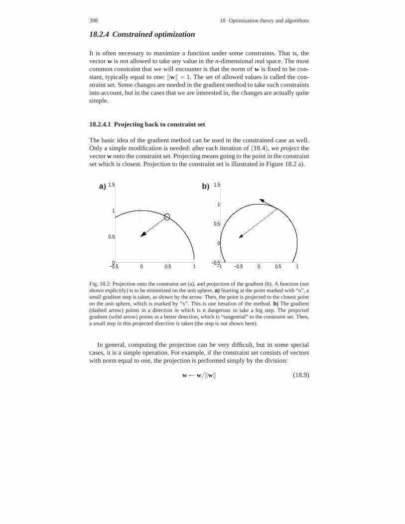
398 18 Optimization theory and algorithms
18.2.4 Constrained optimization
It is often necessary to maximize a function under some constraints. That is, thevectorw is not allowed to take any value in then-dimensional real space. The mostcommon constraint that we will encounter is that the norm ofw is fixed to be con-stant, typically equal to one:‖w‖ = 1. The set of allowed values is called the con-straint set. Some changes are needed in the gradient method to take such constraintsinto account, but in the cases that we are interested in, the changes are actually quitesimple.
18.2.4.1 Projecting back to constraint set
The basic idea of the gradient method can be used in the constrained case as well.Only a simple modification is needed: after each iteration of(18.4), weproject thevectorw onto the constraint set. Projecting means going to the pointin the constraintset which is closest. Projection to the constraint set is illustrated in Figure 18.2 a).
a)
−0.5 0 0.5 10
0.5
1
1.5 b)
−1 −0.5 0 0.5 1−0.5
0
0.5
1
1.5
Fig. 18.2: Projection onto the constraint set (a), and projection of the gradient (b). A function (notshown explicitly) is to be minimized on the unit sphere.a) Starting at the point marked with “o”, asmall gradient step is taken, as shown by the arrow. Then, thepoint is projected to the closest pointon the unit sphere, which is marked by “x”. This is one iteration of the method.b) The gradient(dashed arrow) points in a direction in which is it dangerousto take a big step. The projectedgradient (solid arrow) points in a better direction, which is “tangential” to the constraint set. Then,a small step in this projected direction is taken (the step isnot shown here).
In general, computing the projection can be very difficult, but in some specialcases, it is a simple operation. For example, if the constraint set consists of vectorswith norm equal to one, the projection is performed simply bythe division:
w← w/‖w‖ (18.9)

18.3 Global and local maxima 399
Another common constraint is orthogonality of a matrix. In that case, the projec-tion onto the constraint set is given by
W← (WWT)−1/2W (18.10)
Here, we see a rather involved operation: the inverse of the square root of the matrix.We shall not go into details on how it can be computed; suffice it to say that most nu-merical software can compute it quite efficiently.1 This operation often called sym-metric orthogonalization, and it is the way that symmetric decorrelation in sparsecoding and other algorithms is usually implemented.
18.2.4.2 Projection of the gradient
Actually, an even better method is obtained if we first project the gradient onto the“tangent space” of the constraint set, and then take a step inthat direction insteadof the ordinary gradient direction. What this means is that we compute a directionthat is “inside” the constraint set in the sense that infinitely small changes along thatdirection do not get us out of the constraint set, yet the movement in that directionmaximally increases the value of the objective function. This improves the methodbecause then we can usually take larger step sizes and obtainlarger increases in theobjective function without going in a completely wrong direction as is always thedanger when taking large steps. The projection onto the constraint set has to doneeven in this case. Projection of the gradient is illustratedin Figure 18.2 b).
This is quite useful in the case where we are maximizing with respect to a pa-rameter matrix that is constrained to be orthogonal. The projection can be shown toequal (Edelman et al, 1998):
∇ f (W) = ∇ f (W)−WT∇ f (W)WT (18.11)
where∇ f (W) is the ordinary gradient of the functionf .In Section 18.5 below we will see an example of how these ideasof constrained
optimization are used in practice.
18.3 Global and local maxima
An important distinction is between global and local maxima. Consider the one-dimensional function in Figure 18.3. The global maximum of the function is at thepoint x = 6; this is the “real” maximum point where the function attains its verylargest value. However, there are also two local maxima, atx= 2 andx = 9. A local
1 If you really want to know: the inverse square root(WWT)−1/2 of the symmetric matrixWWT
is obtained from the eigenvalue decomposition ofWWT = Ediag(λ1, . . . ,λn)ET as(WWT)−1/2 =Ediag(1/
√λ1, . . . ,1/
√λn)ET . It is easy to see that if you multiply this matrix with itself, you get
the inverse of the original matrix. See also Section 5.9.2

400 18 Optimization theory and algorithms
maximum is a point in which the function obtains a value whichis greater than thevalues in all neighbouring points close-by.
An important point to understand is that the result of a gradient algorithm de-pends on theinitial point, that is, the point where the algorithm starts in the firstiteration. The algorithm only sees the local behaviour of the function, so it will findthe closest local maximum. Thus, if in Figure 18.3, the algorithm is started in thepoint marked by circles, it will find the global maximum. In contrast, if it is startedin one of the points marked by crosses, it will converge to oneof the local maxima.
In many cases, we are only interested in the global maximum. Then, the be-haviour of the gradient method can be rather unsatisfactory, because it only findsa local optimum. This is, actually, the case with most optimization algorithms. So,when running optimization algorithms, we have to always keep in mind that thatalgorithm only gives a local optimum, not the global one.
0 2 4 6 8 1010
11
12
13
14
15
16
Fig. 18.3: Local vs. global maxima. The function has a globalmaximum atx = 6 and two localmaxima atx = 2 andx = 9. If a gradient algorithm starts near one of the local maxima(e.g. at thepoints marked by crosses), it will get stuck at one of the local maxima and it will not find the globalmaximum. Only if the algorithm starts sufficiently close to the global maximum (e.g. at the pointsmarked by circles), it will find the global maximum.
18.4 Hebb’s rule and gradient methods
18.4.1 Hebb’s rule
Hebb’s rule, or Hebbian learning, is a principle which is central in modern researchon learning and memory. It attempts to explain why certain synaptic connections getstrengthened as a result of experience, and others don’t; this is calledplasticity inneuroscience, andlearning is a more cognitive context. Donald Hebb proposed in1949 that

18.4 Hebb’s rule and gradient methods 401
When an axon of cell A (...) excites cell B and repeatedly or persistently takes part in firingit, some growth process of metabolic change takes place in one or both cells so that A’sefficiency as one of the cells firing B is increased. (Quoted in(Kandel et al, 2000))
This proposal can be readily considered in probabilistic terms: A statistical analysisis about things which happen “repeatedly or persistently”.
A basic interpretation of Hebb’s rule is in terms of thecovarianceof the firingrates of cells A and B: the change in the synaptic connection should be proportionalto that covariance. This is because if the firing rates of A andB are both high atthe same time, their covariance is typically large. The covariance interpretation isactually stronger because it would also imply that if both cells are silent (firing ratebelow average) at the same time, the synaptic connection is strengthened. Even morethan that: if one of the cells is typically silent when the other one fires strongly, thishas a negative contribution to the covariance, and the synaptic connection should bedecreased. Such an extension of Hebb’s rule seems to be quitein line with Hebb’soriginal idea (Dayan and Abbott, 2001).
Note a difference between this covariance interpretation,in which only the cor-relation of the firing rates matters, and the original formulation, in which cell A isassumed to “take part in firing [cell B]”, i.e. to have acausalinfluence on cell B’sfiring. This difference may be partly resolved by recent research which shows thatthe exact timing of the action potentials in cell A and cell B is important, a phe-nomenon calledspike-timing dependent plasticity(Dan and Poo, 2004), but we willnot consider this difference here.
18.4.2 Hebb’s rule and optimization
Hebb’s rule can be readily interpreted as an optimization process, closely relatedto gradient methods. Consider an objective function of the form which we haveextensively used in this book:
J(w) = ∑t
G(n
∑i=1
wixi(t)) (18.12)
To compute the gradient, we use two elementary rules. First,the derivative of a sumis the sum of the derivatives, so we just need to take the derivative ofG(∑n
i=1wixi(t))and take its sum overt. Second, we use the chain rule which gives the deriva-tive of a compound functionf1( f2(w)) as f ′2(w) f ′1( f2(w)). Now, the derivative of∑n
i=1wixi(t) with respect towi is simplyxi(t), and we denote byg = G′ the deriva-tive of G. Thus, the partial derivatives are obtained as
∂J∂wi
= ∑t
xi(t)g(n
∑i=1
wixi(t)) (18.13)
So, a gradient method to maximize this function would be of the form

402 18 Optimization theory and algorithms
wi ← wi + µ ∑t
xi(t)g(n
∑i=1
wixi(t)), for all i. (18.14)
Now, let us interpret the terms in Equation (18.14). Assume that
1. thexi(t) are the inputs to thei-th dendrite of a neuron at time pointt,2. thewi are the strengths of the synapses at those dendrites, and3. the firing rate of the neuron at time pointt is equal to∑n
i=1wixi(t)4. the inputsxi have zero mean, i.e. they describe changes around the mean firing
rate.
Further, let us assume that the functiong is increasing.Then, the gradient method in Equation (18.14) is quite similar to a Hebbian learn-
ing process. Consider the connection strength of one of the synapsesi. Then, theconnectionwi is increased ifxi(t) is repeatedly high at the same time as the firingrate of the neuron in question. In fact, the term multiplied by the learning rateµ isnothing else that the covariance between the input to thei-th dendrite and an increas-ing function of the firing rate of the neuron, as in the covariance-based extension ofHebb’s rule.
Such a “learning rule” would be incomplete, however. The reason is that wehave to constrainw somehow, otherwise it might simply go to zero or infinity. Inpreceding chapters, we usually constrained the norm ofw to be equal to unity. Thisis quite a valid constraint here as well. So, we assume that inaddition to Hebb’srule, some kind of normalization process is operating in cell B.
18.4.3 Stochastic gradient methods
The form of Hebb’s rule in Equation (18.14) uses the statistics of the data in thesense that it computes the correlation over many observations ofx. This is not veryrealistic in terms of neurobiological modelling. A simple solution for this problemis offered by the theory of stochastic gradient methods (Kushner and Clark, 1978).
The idea in a stochastic gradient is simple and very general.Assume we want tomaximize some expectation, sayE{g(w,x)} wherex is a random vector, andw is aparameter vector. The gradient method for maximizing this with respect tow gives
w←w+ µE{∇wg(w,x)} (18.15)
where the gradient is computed with respect tow, as emphasized by the subscript inthe∇ operator. Note that we have taken the gradient inside the expectation operator,which is valid because expectation is basically a sum, and the derivative of a sum isthe sum of the derivatives as noted above.
The stochastic gradient method now proposes that we don’t need to compute theexpectation before taking the gradient step. Foreach observationx, we can use thegradient iteration given that single observation:

18.4 Hebb’s rule and gradient methods 403
w←w+ µ∇wg(w,x) (18.16)
So, when given a sample of observations ofx, we compute the update in Equa-tion (18.16) for each observation separately. This is reasonable because the updatein the gradient will be,on the average, equal to the update in the original gradientwith the expectation given in Equation (18.15). The step size has to be much smaller,though, because of the large random fluctuations in this “instantaneous” gradient.
So, we can consider Hebbian learning in Equation (18.14) so that the sum overt is omitted, and each incoming observation, i.e. stimulus, is immediately used inlearning:
wi ← wi + µxi(t)g(n
∑i=1
wixi(t)) (18.17)
Such a learning method still performs maximization of the objective function, butis more realistic in terms of neurophysiological modelling: at each time point, theinput and output of the neuron make a small change in the synaptic weights.
18.4.4 Role of the Hebbian nonlinearity
By changing the nonlinearityg in the learning rule, and thus theG in the objectivefunction, we see that Hebb’s rule is quite flexible and allowsdifferent kinds of learn-ing to take place. If we assume thatg is linear the original functionG is quadratic.Then, Hebb’s rule is actually doing PCA (Oja, 1982), since itis simply maximizingthe variance ofwTx under the constraint thatw has unit norm.
On the other hand, ifg is nonlinear,G is non-quadratic. Then, we can go back tothe framework of basic sparse coding in Chapter 6. There, we used the expressionh(s2) instead ofG(s) in order to investigate the convexity ofh. So, if G is such thatit corresponds to a convexh, Hebb’s rule can be interpreted as doing sparse coding!The is no contradiction in that almost same rule is able to do both PCA and sparsecoding, because in Chapter 6 we also assumed that the data is whitened. So, we seethat the operation of Hebb’s rule depends very much on the preprocessing of thedata.
What kind of nonlinearities does sparse coding require? Consider the widely-used choiceG1(s) =− logcoshs. This would give
g1(s) =− tanhs (18.18)
This function (plotted in Fig. 18.4) would be rather odd to use as such in Hebb’srule, because it is decreasing, and the whole idea of Hebb’s rule would be inverted.(Actually, such “anti-Hebbian” learning has been observedin some contexts (Bellet al, 1993), and is considered important in some computational models (Foldiak,1990)).
However, because the data is whitened, we can find a way of interpreting thismaximization as Hebbian learning. The point is that for whitened data, we can add

404 18 Optimization theory and algorithms
a quadratic term toG, and consider
G2(s) =12
s2− logcoshs (18.19)
Since the data is whitened andw is constrained to unit norm, the expectation ofs2 = (wTx)2 is constant, and thus the maximization ofG2 produces just the sameresult as maximization ofG1. Now, the derivative ofG2 is
g2(s) = s− tanhs (18.20)
which is an increasing function, see Fig. 18.4.
−3 −2 −1 0 1 2 3−3
−2
−1
0
1
2
3
Fig. 18.4: Two nonlinearities:g1 in Equation (18.18), dash-dotted line, andg2 in Equation (18.20),solid line. For comparison, the linex = y is given as dotted line.
So, using a nonlinearity such asg2, sparse coding does have a meaningful inter-pretation as a special case of Hebb’s rule. The nonlinearityg2 even makes intuitivesense: it is a kind of a thresholding function (actually, a shrinkage function, seeSection 14.1.2.2), which ignores activations which are small.
18.4.5 Receptive fields vs. synaptic strengths
In the Hebbian learning context, the feature weightsWi are related to synapticstrengths in the visual cells. However, the visual input reaches the cortex only afterpassing through several neurons in the retina and the thalamus. Thus, theWi actuallymodel the compound effect of transformations in all those processing stages. Howcan we then interpret optimization of a function such asG(∑x,yW(x,y)I(x,y)) interms of Hebb’s rule?
In Section 5.9 we discussed the idea that the retina and LGN perform some-thing similar to a whitening of the data. Thus, as a rough approximation, we couldconsider thecanonically preprocesseddata as the input to the visual cortex. Thenmaximization of a function such asG(vTz), wherez is the preprocessed data, is in

18.5 Optimization in topographic ICA * 405
fact modelling the plasticity of synapses of the cells the primary visual cortex. So,Hebbian learning in that stage can be modelled just as we did above.
18.4.6 The problem of feedback
In the Hebbian implementation of ICA and related learning rules, there is one moreproblem which needs to be solved. This is the implementationof the constraint oforthogonality. The constraint is necessary to prevent the neurons from all learningthe same feature. A simple approach would be to consider the minimization of somemeasure of the covariance of the outputs (assuming the data is whitened as a pre-processing stage):
Q(v1, . . . ,vn) =−M ∑j 6=i
[E{sisj}]2 =−M ∑i 6= j
[E{(vTi z)(vT
j z)}]2 (18.21)
whereM is a large constant (say,M = 100). We can add this function as a so-calledpenaltyto the measures of sparseness. If we then consider the gradient with respectto vi , this leads to the addition of a term of the form
∇vi Q =−2M ∑j 6=i
E{zsj}E{sisj} (18.22)
to the learning rule forvi . BecauseM is large, after maximization the sum of the[E{sisj}]2 will be very close to zero—corresponding to the case where thesi are alluncorrelated. Thus, this penalty approximately reinforces the constraint of uncorre-latedness.
The addition ofQ to the sparseness measure thus results in the addition of afeedbackterm of the form in Equation (18.22).
18.5 Optimization in topographic ICA *
As an illustration of the gradient method and constrained optimization, we con-sider in this section maximization of likelihood of the topographic ICA in Equa-tion (11.5). This section can be skipped by readers not interested in mathematicaldetails.
Because independent subspace analysis is formally a special case of topographicICA, obtained by a special definition of the neighbourhood function, the obtainedlearning rule is also the gradient method for independent subspace analysis.
First note that we constrainV to be orthogonal, so detV is constant (equal to one),and can be ignored in this optimization. Another simple trick to simplify the problemis to note is that we can ignore the sum overt and just compute the “instantaneous”gradient as in stochastic gradient methods. We can always goback to the sum over

406 18 Optimization theory and algorithms
t by just summing the gradient overt, because the gradient of a sum is the sum ofthe gradients. In fact, we can simplify the problem even further by computing thegradient of the likelihood for each term of in the sum overi in the likelihood inEquation (11.5), and taking the sum afterwards.
So, the computation of the gradient is essentially reduced to computing the gra-dient of
Li(v1, . . . ,vn) = h(n
∑j=1
π(i, j)(vTj zt)
2) (18.23)
Denote byvlk the l -th component ofvk. By the chain rule, applied twice, we obtain
∂Li
∂vlk
= 2zltπ(i,k)(vT
k zt)h′(
n
∑j=1
π(i, j)(vTj zt)
2) (18.24)
This can be written in vector form by simply collecting thesepartial derivatives forall l in a single vector:
∇vkLi = 2ztπ(i,k)(vTk zt)h
′(n
∑j=1
π(i, j)(vTj zt)
2) (18.25)
(This is not really the whole gradient because it is just the partial derivatives withrespect to some of the entries inV, but the notation using∇ is still often used.)
Since the log-likelihood is simply the sum of theLi ’s we obtain
∇vk logL =T
∑t=1
n
∑i=1
∇vkLi = 2T
∑t=1
zt(vTk zt)
n
∑i=1
π(i,k)h′(n
∑j=1
π(i, j)(vTj zt)
2) (18.26)
We can omit the constant 2 which does not change the directionof the gradient.So, the algorithm for maximizing the likelihood in topographic ICA is finally as
follows:
1. Compute the gradients in Equation (18.26) for allk. Collect them in a matrix∇V logL which has the∇vk logL as its rows.
2. Compute the projection of this matrix on the tangent spaceof the constraintspace, using the formula in Equation (18.11). Denote the projected matrix asG. (This projection step is optional, but usually it speeds upthe algorithm.)
3. Do a gradient step asV← V + µG (18.27)
4. Orthogonalize the matrixV. For example, this can be done by the formula inEquation (18.10).
To see a connection of such an algorithm with Hebbian learning, consider a gra-dient update for eachvk separately. We obtain the gradient learning rule
vk← vk + µT
∑t=1
zt(vTk zt)r
kt (18.28)
18.6 Beyond basic gradient methods * 407
where
rkt =
n
∑i=1
π(i,k)h′(n
∑j=1
π(i, j)(vTj zt)
2). (18.29)
Equally well, we could use a stochastic gradient method, ignoring the sum overt.In a neural interpretation, the Hebbian learning rule in (18.28) can be considered a“modulated” Hebbian learning, since the ordinary Hebbian learning termzt(vT
k zt)is modulated by the termrk
t . This term could be considered as top-down feedback,since it is a function of the local energies which could be theoutputs of higher-orderneurons (complex cells).
18.6 Beyond basic gradient methods *
This section can be skipped by readers not interested in mathematical theory. Here,we briefly describe two further well-known classes of optimization methods. Actu-ally, in our context, these are not very often better than thebasic gradient method,so our description is very brief.
18.6.1 Newton’s method
As discussed above, the optima of an objective function are found in points wherethe gradient is zero. So, optimization can be approached as the problem of solvinga system of equations given by
∂ f∂w1
(w) = 0 (18.30)
... (18.31)
∂ f∂wn
(w) = 0 (18.32)
A classic method for solving such a system of equations is Newton’s method. Itcan be used to solve any system of equations, but we consider here the case of thegradient only.
Basically, the idea is to approximate the function linearlyusing its derivatives. Inone dimension, the idea is simply to approximate the graph ofthe function using itstangent, whose slope is given by the derivative. That is, fora general functiong:
g(w)≈ g(w0)+g′(w0)(w−w0) (18.33)
This very general idea of finding the point where the functionattains the value zerois illustrated in Figure 18.5.

408 18 Optimization theory and algorithms
w w0
Fig. 18.5: Illustration of Newton’s method for solving an equation (which we use in optimizationto solve the equation which says that the gradient is zero). The function is linearly approximated byits tangent. The point where the tangent intersects with thex-axis is taken as the next approximationof the point where the function is zero.
In our case,g corresponds to the gradient, so we use the derivatives of thegradi-ents, which are second partial derivatives of the original function f . Also, we needto use a multidimensional version of this approximation. This gives
∇ f (w) = ∇ f (w0)+H(w0)(w−w0) (18.34)
where the functionH, called the Hessian matrix, is the matrix of second partialderivatives:
H i j =∂ 2 f
∂wi∂wj(18.35)
Now, we can at every step of the method, find the new point as theone for whichthis linear approximation is zero. Thus, we solve
∇ f (w0)+H(w0)(w−w0) = 0 (18.36)
which givesw = w0−H(w0)
−1(∇ f (w0)) (18.37)
This is the idea in the Newton iteration. Starting from a random point, we iterativelyupdatew according to Equation (18.37), i.e. compute the right-handside for thecurrent value ofw, and take that as the new value ofw. Using the same notation aswith the gradient methods, we have the iteration
w← w−H(w)−1(∇ f (w)) (18.38)
Note that this iteration is related to the gradient method. If the matrixH(w0)−1
in Equation (18.37) is replaced by a scalar step sizeµ , we actually get the gradientmethod. So, the difference between the methods is threefold:
1. In Newton’s method the direction wherew “moves” is not given by the gradientdirectly, but the gradient multiplied by the inverse of the Hessian.

18.6 Beyond basic gradient methods * 409
2. This “step size” is not always very small: It is directly given by the inverse of theHessian matrix, and can be quite large.
3. In the gradient method, one can choose between minimization and maximiza-tion of the objective function, by choosing the sign in the algorithm (cf. Equa-tions (18.4) and (18.5)). In the Newton method, no such choice is possible. Thealgorithm just tries to find a local extremum in which the gradient is zero, andthis can be either a minimum or a maximum.
The Newton iteration has some advantages and disadvantagescompared to thebasic gradient method. It usually requires a smaller numberof steps to converge.However, the computations needed at each step are much more demanding, becauseone has to first compute the Hessian matrix, and then computeH(w)−1(∇ f (w))(which is best obtained by solving the linear systemH(w)v = ∇ f (w)).
In practice, however, the main problem with the Newton method is that its be-haviour can be quite erratic. There is no guarantee any one iteration gives aw whichincreasesf (w). In fact, a typical empirical observation is that for some functionsthis does not happen, and the algorithm may completely diverge, i.e. go to arbitraryvalues ofw, eventually reaching infinity. This is because the step sizecan be arbi-trarily large, unlike in the gradient methods. This lack of robustness is why Newton’smethod is not often used in practice.
As an example of this phenomenon, consider the function
f (w) = exp(−12
w2) (18.39)
which has a single maximum asw = 0. The first and second derivatives, whichare the one-dimensional equivalents of the gradient and theHessian, can be easilycalculated as
f ′(w) =−wexp(−12
w2) (18.40)
f ′′(w) = (w2−1)exp(−12
w2) (18.41)
which gives the Newton iteration as
w←w+w
w2−1(18.42)
Now, assume that we start the iteration at any point wherew> 1. Then, the changew
w2−1is positive, which means thatw is increased and it moves further and further
away from zero! In this case, the method fails completely andw goes to infinitywithout finding the maximum at zero. (In contrast, a gradientmethod, with a rea-sonably small step size, would find the maximum.)
However, different variants of the Newton method have proven useful. For ex-ample, methods which do something between the gradient method and Newton’smethod (e.g. the Levenberg-Marquardt algorithm) have proven useful in some ap-plications. In ICA, the FastICA algorithm (see below) uses the basic iteration of

410 18 Optimization theory and algorithms
Newton’s method but with a modification which takes the special structure of theobjective function into account.
18.6.2 Conjugate gradient methods
Conjugate gradient methods are often considered as the mostefficient general-purpose optimization methods. The theory is rather complicated and non-intuitive,so we do not try to explain it in detail.
Conjugate gradient methods try to find a direction which is better than the gra-dient direction. The idea is illustrated in Figure. 18.6. While the gradient directionis good for a very small step size (actually, it is still the best for an infinitely smallstep size), it is not very good for a moderately large step size. The conjugate gra-dient method tries to find a better direction based on information on the gradientdirections in previous iterations. In this respect, the method is similar to Newton’smethod, which also modifies the gradient direction.
0 0.2 0.4 0.6 0.8 1 1.2 1.4 1.6 1.8 20
0.2
0.4
0.6
0.8
1
1.2
1.4
1.6
1.8
2
Fig. 18.6: A problem with the gradient method. The gradient direction may be very bad for anythingbut the very smallest step sizes. Here, the gradient goes rather completely in the wrong directiondue to the strongly non-circular (non-symmetric) structure of the objective function. The conjugategradient method tries to find a better direction.
In fact, conjugate gradient methods do not just take a step ofa fixed size in the di-rection they have found. An essential ingredient, which is actually necessary for themethod to work, is a one-dimensionline search. This means that once the direction,sayd, in which w should move has been chosen (using the complicated theory ofconjugate gradient methods), many different step sizesµ are tried out, and the bestone is chosen. In other words, a one-dimensional optimization is performed on thefunctionh(µ) = f (w + µd), andµ maximizing this function is chosen. (Such linesearch could also be used in the basic gradient method. However, in the conjugategradient method it is completely necessary.)
Conjugate gradient methods are thus much more complicated than ordinary gra-dient methods. This is not a major problem if one uses a scientific computing en-

18.7 FastICA, a fixed-point algorithm for ICA 411
vironment in which the method is already programmed. Sometimes, the method ismuch more efficient than the ordinary gradient methods, but this is not always thecase.
18.7 FastICA, a fixed-point algorithm for ICA
Development of tailor-made algorithms for solving the optimization problems inICA is a subject of an extensive literature. Here we explain briefly one popularalgorithm for performing the maximization, more information and details can befound in the ICA book (Hyvarinen et al, 2001b).
18.7.1 The FastICA algorithm
Assume that the datat,t = 1, . . . ,T, is whitened and has zero mean. The basic formof the FastICA algorithm is as follows:
1. Choose an initial (e.g. random) weight vectorw.2. Letw← ∑t ztg(wTzt)−w∑t g′(wTzt)3. Letw← w/‖w‖4. If not converged, go back to 2.
Note that the sign ofw may change from one iteration to the next; this is in linewith the fact that the signs of the components in ICA are not well-defined. Thus,the convergence of the algorithm must use a criterion which is immune to this. Forexample, one might stop the iteration if|wTwold| is sufficiently close to one, wherewold is the value ofw at the previous iteration.
To use FastICA forseveralfeatures, the iteration step 2 is applied separatelyfor the weight vector of each unit. After updating all the weight vectors, they are or-thogonalized (assuming whitened data). This means projecting the matrixW, whichcontains the vectorswi as its rows, on the space of orthogonal matrices, which can beaccomplished, for example, by the classical method involving matrix square roots,given in Eq. (18.10). See Chapter 6 of (Hyvarinen et al, 2001b) for more informationon orthogonalization.
18.7.2 Choice of the FastICA nonlinearity
The FastICA algorithm uses a nonlinearity, usually denotedby g. This comes froma measure of non-gaussianity. Non-gaussianity is measuredasE{G(s)} for somenon-quadraticfunction. The functiong is then the derivative ofG.

412 18 Optimization theory and algorithms
Note that in Chapter 6 we measured non-gaussianity (or sparseness) asE{h(s2)}.Then, we haveG(s) = h(s2) which impliesg(s) = 2h′(s2)s. So, we must make aclear distinction between the nonlinearitiesh and the functionsG andg; they are alldifferent functions but they can be derived from one another.
The choice of the measure of non-gaussianity, or the nonlinearity, is actuallyquite free in FastICA. We are not restricted to functions such that maximization ofG corresponds to maximization of sparseness, or such thatG corresponds to the log-pdf of the components. We can use, for example, measures of skewness, i.e. the lackof symmetry of the pdf.
In practice, it has been found thatG(s) = logcoshsworks quite well in a varietyof domains; it corresponds to the tanh nonlinearity asg. (In FastICA, it makes nodifference if we take tanh or− tanh, the algorithm is immune to the change of sign.)
18.7.3 Mathematics of FastICA *
Here, we present the derivation of the FastICA algorithm, and show its connectionto gradient methods. This can be skipped by readers not interested in mathematicaldetails.
18.7.3.1 Derivation of the fixed-point iteration
To begin with, we shall derive the fixed-point algorithm foronefeature, using an ob-jective function motivated by projection pursuit, see (Hyvarinen, 1999a) for details.Denote the weight vector corresponding to one feature detector byw, and the canon-ically preprocessed input byz. The goal is to find the extrema ofE{G(wTz)} fora given non-quadratic functionG, under the constraintE{(wTz)2} = 1. Accordingto the Lagrange conditions (Luenberger, 1969), the extremaare obtained at pointswhere
E{zg(wTz)}−βCw = 0 (18.43)
whereC = E{zzT}, andβ is a constant that can be easily evaluated to giveβ =E{wT
0 zg(wT0 z)}, wherew0 is the value ofw at the optimum. Let us try to solve this
equation by the classical Newton’s method, see Section 18.6.1 above. Denoting thefunction on the left-hand side of (18.43) byF, we obtain its Jacobian matrix, i.e. thematrix of partial derivatives,JF(w) as
JF(w) = E{zzTg′(wTz)}−βC (18.44)
To simplify the inversion of this matrix, we decide to approximate the first term in(18.44). A reasonable approximation in this context seems to beE{zzTg′(wTz)} ≈E{zzT}E{g′(wTz)} = E{g′(wTz)}C. The obtained approximation of the Jacobianmatrix can be inverted easily:

18.7 FastICA, a fixed-point algorithm for ICA 413
JF(w)−1≈ C−1/(E{g′(wTz)}−β ). (18.45)
We also approximateβ using the current value ofw instead ofw0. Thus we obtainthe following approximative Newton iteration:
w←w− [C−1E{zg(wTz)}−βw]/[E{g′(wTz)}−β ] (18.46)
wherew+ denotes the new value ofw, andβ = E{wTzg(wTz)}. After every step,w+ is normalized by dividing it by
√
(w+)TCw+ to improve stability. This algo-rithm can be further algebraically simplified (see (Hyvarinen, 1999a)) to obtain theoriginal form the fixed-point algorithm:
w← C−1E{zg(wTz)}−E{g′(wTz)}w. (18.47)
These two forms are equivalent. Note that for whitened data,C−1 disappears, givingan extremely simple form of the Newton iteration. In (Hyvarinen and Oja, 1997),this learning rule was derived as a fixed-point iteration of agradient method max-imizing kurtosis, hence the name of the algorithm. However,image analysis mustuse the more general form in (Hyvarinen, 1999a) because of the non-robustness ofkurtosis.
18.7.3.2 Connection to gradient methods
There is a simple an interesting connection between the FastICA algorithm andgradient algorithms for ICA.
Let us assume that the number of independent components to beestimated equalsthe number of observed variables, i.e.n = m and A is square. Denote byW theestimate of the inverse ofA.
Now, consider the preliminary form of the algorithm in (18.46). To avoid theinversion of the covariance matrix, we can approximate it asC−1 ≈WTW, sinceC = AAT . Thus, collecting the updates for all the rows ofW into a single equation,we obtain the following form of the fixed-point algorithm:
W←W +D[diag(−βi)+E{g(y)y}]W (18.48)
wherey = Wz, βi = E{yig(yi)}, andD = diag(1/(βi −E{g′(yi)})). This can becompared to the natural gradient algorithm for maximization of the likelihood inEq. (18.8). We can see that the algorithms are very closely related. First, the expec-tation in (18.48) is in practice computed as a sample averageas in (18.8). So, themain difference is that in the natural gradient algorithm, the βi are all set to one,andD is replaced by identity times the step sizeµ . So,D is actually like a step size,although in the form of a matrix here, but it does not affect tothe point where thealgorithm converges (i.e. the update is zero). So, the only real difference is theβi .Now, it can be proven that if theg really is the derivative of the log-likelihood, thentheβi are also (for infinite sample) equal to one (Hyvarinen et al,2001b). In theory,

414 18 Optimization theory and algorithms
then, even this difference vanishes and the algorithms really converge to the samepoints.
It must be noted that the FastICA algorithm does not maximizesparseness butnon-gaussianity. Thus, in the case of sub-gaussian features, it may actually be min-imizing sparseness, see Section 7.9.3.

Chapter 19Crash course on linear algebra
This chapter explains basic linear algebra on a very elementary level. This is mainlymeant as a reminder: The readers hopefully already know thismaterial.
19.1 Vectors
A vector in ann-dimensional real space is an ordered collection ofn real numbers.In this book, a vector is typically either the grey-scale values of pixels in an imagepatch, or the weights in a linear filter or feature detector. The number of pixels isn in the former case, and the number of weights isn in the latter case. We denoteimages byI(x,y) and the weights of a feature detector typically byW(x,y). It isassumed that the indexx takes values from 1 tonx and the indexy takes values from1 to ny, where the dimensions fulfilln = nx×ny. In all the sums that follow, this isimplicitly assumed and not explicitly written to simplify notation.
One of the main points in linear algebra is to provide a notation in which manyoperations take a simple form. In linear algebra, the vectors such asI(x,y) andW(x,y) are expressed as one-dimensional columns or rows of numbers. Thus, weneed to index all the pixels by a single indexi that goes from 1 ton. This is obviouslypossible by scanning the image row by row, or column by column(see Section 4.1for details on such vectorization). It does not make any difference which method isused. A vector is usually expressed in column form as
v =
v1
v2...
vn
(19.1)
In this book, the vector containing image data (typically after some preprocessingsteps) will be usually denoted byz, and the vector giving the weights of a feature de-
415

416 19 Crash course on linear algebra
tector byv. In the following, we will use both the vector- and image-based notationsside-by-side.
The (Euclidean)normof a vector is defined as
‖W(x,y)‖ =√
∑x,y
W(x,y)2, or ‖v‖=√
∑i
v2i (19.2)
The norm gives the length (or “size”) of a vector. There are also other ways ofdefining the norm, but the Euclidean one is the most common.
Thedot-product(or inner productbetween two vectors is defined as
〈W, I〉= ∑x,y
W(x,y)I(x,y) (19.3)
If W is a feature detector, this could express the value of the feature when the inputimage isI . It basically computes amatchbetweenI andW. In vector notation, weuse the transpose operator, given byvT , to express the same operation:
vTz =n
∑i=1
vizi (19.4)
If the dot-product is zero, the vectorsW and I are calledorthogonal. The dot-product of a vector with itself equals the square of its norm.
19.2 Linear transformations
A linear transformation is the simplest kind of transformation in ann-dimensionalvector space. A vectorI is transformed to a vectorJ by taking weighted sums:
J(x,y) = ∑x′y′
m(x,y,x′,y′)I(x′,y′), for all x,y (19.5)
The weights in the sum are different for every point(x,y). The indicesx′ andy′ takeall the same values asx andy. Typical linear transformations include smoothing andedge detection.
We can compound linear transformations by taking a linear transformation ofJusing weights denoted byn(x,y,x′,y′). This gives the new vector as

19.3 Matrices 417
K(x,y) = ∑x′′y′′
n(x,y,x′′,y′′)J(x′′,y′′)
= ∑x′′y′′
n(x,y,x′′,y′′)∑x′y′
m(x′′,y′′,x′,y′)I(x′,y′)
= ∑x′y′
(
∑x′′y′′
n(x,y,x′′,y′′)m(x′′,y′′,x′,y′)
)
I(x′,y′) (19.6)
Definingp(x,y,x′,y′) = ∑
x′′y′′n(x,y,x′′,y′′)m(x′′,y′′,x′,y′) (19.7)
we see that the compounded transformation is a linear transformation with theweights given byp.
19.3 Matrices
In matrix algebra, linear transformations and linear systems of equations (see below)can be succinctly expressed by products (multiplications). In this book we avoidusing too much linear algebra to keep things as simple as possible. However, itis necessary to understand how matrices are used to express linear transformation,because in some cases, the notation becomes just too complicated, and also becausemost numerical software takes matrices as input.
A matrix M of sizen1×n2 is a collection of real numbers arranged inton1 rowsandn2 columns. The single entries are denoted bymi j wherei is the row andj is thecolumn. We can convert the weightsm(x,y,x′,y′) expressing a linear transformationby the same scanning process as was done with vectors. Thus,
M =
m11 m12 . . . m1m...
...mn1 mn2 . . . mnm
(19.8)
The linear transformation of a vectorz is then denoted by
y = Mz (19.9)
which is basically a short-cut notation for
yi =n2
∑j=1
mi j zj , for all i (19.10)
This operation is also the definition of the product of a matrix and a vector.If we concatenate two linear transformations, defining

418 19 Crash course on linear algebra
s= Ny (19.11)
we get another linear transformation. The matrixP that expresses this linear trans-formation is obtained by
pi j =n1
∑k=1
nikmk j (19.12)
This is the definition of the product of two matrices: the new matrix P is denoted by
P = MN (19.13)
This is the matrix version of Equation (19.7). The definitionis quite useful, becauseit means we can multiply matrices and vectors in any order when we computes. Infact, we have
s= Ny = N(Mz) = (NM)z (19.14)
Another important operation with matrices is the transpose. The transposeMT
of a matrixM is the matrix where the indices are exchanged: thei, j-th entry ofMT
is mji . A matrix M is called symmetric ifmi j = mji , i.e., if M equals its transpose.
19.4 Determinant
The determinant answers the question: how are volumes changed when the dataspace is transformed by the linear transformationm? That is, ifI takes values in acube whose edges are all of length one, what is the volume of the set of the valuesJin Equation (19.5)?. The answer is given by the absolute value of the determinant,denoted by|det(M)| whereM is the matrix form ofm.
Two basic properties of the determinant are very useful.
1. The determinant of a product is the product of the determinants: det(MN) =det(M)det(N). If you think that the first transformation changes the volume bya factor or 2 and the second by a factor of 3, it is obvious that when you do bothtransformation, the change in volume is by a factor of 2×3= 6.
2. The determinant of a diagonal matrix equals the product ofthe diagonal elements.If you think is two dimensions, a diagonal matrix simply stretches one coordinateby a factor of, say 2, and the other coordinate by a factor of, say 3, so the volumeof a square of area equal to 1 then becomes 2×3= 6.
(In Section 19.7 we will see a further important result on thedeterminant of anorthogonal matrix).

19.6 Basis representations 419
19.5 Inverse
If a linear transformation in Equation (19.5) does not change the dimension of thedata, i.e. the number of pixels, the transformation can usually be inverted. That is,Equation (19.5) can usually be solved forI : if we know J andm, we can computewhat was the originalI . This is the case if the linear transformation is invertible— atechnical condition that is almost always true. In this book, we will always assumethat a linear transformation is invertible if not otherwisementioned.
In fact, we can then find a matrix of coefficientsn(x,y), so that
I(x,y) = ∑x′y′
n(x,y,x′,y′)J(x′,y′), for all x,y. (19.15)
This is the inverse transformation ofm. In matrix algebra, the coefficient are ob-tained by computing the inverse of the matrixM , denoted byM−1. So, solving fory in (19.9) we have
y = M−1z (19.16)
A multitude of numerical methods for computing the inverse of the matrix exist.Note that the determinant of the inverse matrix is simply theinverse of the deter-
minant: det(M−1) = 1/det(M). Logically, if the transformation changes the volumeby a factor of 5 (say), then the inverse must change the volumeby a factor of 1/5.
The product of a matrix with its inverse equals theidentity matrixI :
MM −1 = M−1M = I (19.17)
The identity matrix is a matrix whose diagonal elements are all ones and the off-diagonal elements are all zero. It corresponds to the idenity transformation, i.e., atransformation which does not change the vector. This meanswe have
Iz = z (19.18)
for anyz.
19.6 Basis representations
An important interpretation of the mathematics in the preceding sections is the rep-resentation of an image in a basis. Assume we have a number of featuresAi(x,y)wherei goes from 1 ton. Given an imageI(x,y), we want to represent it as a linearsum of these feature vectors:
I(x,y) =n
∑i=1
Ai(x,y)si (19.19)

420 19 Crash course on linear algebra
Thesi are thecoefficientsof the feature vectorsAi . They can be considered as thevalues of the features in the imageI , since they tell “to what extent” the features arein the image. If, for example,s1 = 0, that means that the featureA1 is not present inthe image.
Using vector notation, the basis representation can be given as
z =n
∑i=1
aisi (19.20)
Interestingly, this equation can be further simplified by putting all thesi into a singlevectors, and forming a matrixA so that the columns of that matrix are the vectorsai , that is:
A = [a1,a2, . . . ,an] =
a11...
an1
a12...
an2
. . .
a1n...
an3
(19.21)
Then we have equivalentlyz = As (19.22)
From this equation, we see how we can apply all the linear algebra machinery toanswer the following questions:
• How do we compute the coefficientssi? This is done by computing the inversematrix of A (hoping that one exists), and then multiplyingz with the inverse,sinces= A−1z.
• When is it possible to represent anyz using the givenai? This question wasalready posed in the preceding section. The answer is: if thenumber of basisvectors equals the dimension ofz, the matrixA is invertible practically always.In such a case, we say that theai (or theAi) form a basis.
A further important question is: What happens then if the number of vectorsai issmallerthan the dimension of the vectorz? Then, we cannot represent all the possi-ble z’s using those features. However, we can find the best possible approximationfor anyz based on those features, which is treated in Section 19.8.
The opposite case is when we havemorevectorsai than the dimension of thedata. Then, we can represent any vectorz using those features; in fact, there areusually many ways of representing anyz, and the coefficientssi are not uniquelydefined. This case is calledovercomplete basisand treated in Section 13.1.
19.7 Orthogonality
A linear transformation is calledorthogonalif it does not change the norm of thevector. Likewise, a matrixA is called orthogonal if the corresponding transformationis orthogonal. An equivalent condition for orthogonality is

19.8 Pseudo-inverse * 421
ATA = I (19.23)
If you think about the meaning of this equation in detail, youwill realize that it saystwo things: the column vectors of the matrixA are orthogonal, and all normalized tounit norm. This is because the entries in the matrixATA are the dot-productsaT
i a j
between the column vectors of the matrixA.An orthogonal basis is nothing else than a basis in which the basis vectors are
orthogonal and have unit norm; in other words, if we collect the basis vectors into amatrix as in Equation (19.21), that matrix is orthogonal.
Equation (19.23) shows that the inverse of an orthogonal matrix (or an orthogonaltransformation) is trivial to compute: we just need to rearrange the entries by takingthe transpose. This means thatsi = aT
i z, or
si = ∑x,y
Ai(x,y)I(x,y) (19.24)
So, in an orthogonal basis we obtain the coefficients as simple dot-products with thebasis vectors. Note that this isnot true unless the basis is orthogonal.
The compound transformation of two orthogonal transformation is orthogonal.This is natural since if neither of the transformations changes the norm of the image,then doing one transformation after the other does not change the norm either.
The determinant of an orthogonal matrix is equal to plus or minus one. Thisis because because an orthogonal transformation does not change volumes, so theabsolute value has to be one. The change in sign is related to reflections. Think ofmultiplying one-dimenasional data by−1: This does not change the “volumes”, but“reflects” the data with respect to 0, and corresponds to a determinant of−1.
19.8 Pseudo-inverse *
Sometimes transformations change the dimension, and the inversion is more com-plicated. If there are more variables iny than in z in Equation (19.9), there arebasically more equations than free variables, so there is nosolution in general. Thatis, we cannot find a matrixM so that for any giveny, z = My is a solution forEquation (19.9). However, in many cases it is useful to consider an approximativesolution: Find a matrixM+ so that forz = M+y, the error‖y−Mz‖ is as smallas possible. In this case, the optimal “approximative inverse” matrix can be easilycomputed as:
M+ = (MTM)−1MT (19.25)
On the other hand, if the matrixM has fewer rows than columns (fewer variablesin y than inz), there are more free variables than there are constrainingequations.Thus, there are many solutionsz for (19.9) for a giveny, and we have to choose oneof them. One option is to choose the solution that has the smallest Euclidean norm.The matrix that gives this solution asM+y is given by

422 19 Crash course on linear algebra
M+ = MT(MM T)−1 (19.26)
The matrixM+ in both of these cases is called the (Moore-Penrose) pseudo-inverseof M . (A more sophisticated solution for the latter case, using sparseness, is consid-ered in Section 13.1.3.)

Chapter 20The discrete Fourier transform
This chapter is a mathematically sophisticated treatment of the theory of Fourieranalysis. It concentrates on the discrete Fourier transform which is the variant usedin image analysis practice.
It is not necessary to know this material to understand the developments in thisbook; this is meant as supplementary material.
20.1 Linear shift-invariant systems
Let us consider a systemH operating on one-dimensional input signalsI(x). Thesystem islinear if for inputs I1(x) andI2(x), and scalarα
H {I1(x)+ I2(x)} = H {I1(x)}+H {I2(x)} (20.1)
H {αI1(x)} = αH {I1(x)} ; (20.2)
similar definitions apply in the two-dimensional case. A systemH is shift-invariantif a shift in the input results in a shift of the same size in theoutput; that is, ifH {I(x)}= O(x), then for any integerm
H {I(x+m)}= O(x+m); (20.3)
or, in the two-dimensional case, for any integersmandn,
H {I(x+m,y+n)}= O(x+m,y+n). (20.4)
A linear shift-invariant systemH operating on signals (or, in the two-dimensionalcase, on images) can be implemented by either linear filtering with a filter, or anotheroperation, theconvolutionof the input and theimpulse responseof the system. Theimpulse responseH(x) is the response of the system to an impulse
423

424 20 The discrete Fourier transform
δ (x) =
{
1, if x = 0
0, otherwise,(20.5)
that isH(x) = H {δ (x)} . (20.6)
By noting that I(x) = ∑∞k=−∞ I(k)δ (x− k), and by applying linearity and shift-
invariance properties (Equations (20.1)–(20.3)) it is easy to show that
O(x) = H {I(x)}=∞
∑k=−∞
I(k)H(x−k) = I(x)∗H(x), (20.7)
where the last equality sign defines convolution∗. Note that convolution is a sym-metric operator since by making the change in summation index ℓ= x−k (implyingk = x− ℓ)
I(x)∗H(x) =∞
∑k=−∞
I(k)H(x−k) =∞
∑ℓ=−∞
H(ℓ)I(x− ℓ) = H(x)∗ I(x). (20.8)
20.2 One-dimensional discrete Fourier transform
20.2.1 Euler’s formula
For purposes of mathematical convenience, in Fourier analysis the frequency rep-resentation is complex-valued: both the basis images and the weights consist ofcomplex numbers; this is called the representation of an image in theFourier space.The fundamental reason for this is Euler’s formula, which states that
eai = cosa+ i sina (20.9)
wherei is the imaginary unit. Thus, a complex exponential containsboth the sin andcos function in a way that turns out to be algebraically very convenient. One of thebasic reasons for this is that the absolute value of a complexnumber contains thesum-of-squares operation:
|a+bi|=√
a2 +b2 (20.10)
which is related to the formula in Equation (2.16) on page 41 which gives the powerof a sinusoidal component. We will see below that we can indeed compute theFourier power as the absolute value (modulus) of some complex numbers.
In fact, we will see that the argument of a complex number on the complex planeis related to the phase in signal processing. The argument ofa complex numberc isa real numberφ ∈ (−π ,π ] such that
c = |c|eφ i (20.11)

20.2 One-dimensional discrete Fourier transform 425
We will use here the signal-processing notation∠c for the argument.We will also use the complex conjugate of a complex numberc= a+bi, denoted
by c, which can be obtained either asa− bi or, equivalently, as|c|e−φ i . Thus, thecomplex conjugate has the same absolute value, but oppositeargument (“phase”).
20.2.2 Representation in complex exponentials
In signal processing theory, sinusoidals are usually represented in the form of thefollowing complex exponential signal
eiωx = cos(ωx)+ i sin(ωx), x = 1, ...,M, (20.12)
A fundamental mathematical reason for this is that these signals areeigensignalsof linear shift-invariant systems. An eigensignal is a generalization of the conceptof an eigenvector in linear algebra (see Section 5.8.1). Denote byH(x) the impulseresponse of a linear shift-invariant systemH . Then
H{
eiωx}= H(x)∗eiωx =∞
∑k=−∞
H(k)eiω(x−k) = eiωx∞
∑k=−∞
H(k)e−iωk
︸ ︷︷ ︸
=H(ω)
= H(ω)eiωx,
(20.13)
where we have assumed that the sum∑∞k=−∞ H(k)e−iωk converges, and have de-
noted this complex number byH(ω). Equation (20.13) shows that when a complexexponential is input into a linear shift-invariant system,the output is the same com-plex exponential multiplied byH(ω); the complex exponential is therefore calledan eigensignal of the system.
To illustrate the usefulness of the representation in complex exponentials in an-alytic calculations, let us derive the response of a linear shift-invariant system to asinusoidal. This derivation uses the identity
cos(φ) =12
(eiφ +e−iφ) , (20.14)
which can be verified by applying Equation (20.12). LetH be a linear shift-invariant system, andAcos(ωx+ ψ) be an input signal; then
H {Acos(ωx+ ψ)}=A2
H
{
ei(ωx+ψ) +e−i(ωx+ψ)}
=A2
(eiψ
H{
eiωx}+e−iψH{
e−iωx})
=A2
(eiψH(ω)eiωx +e−iψH(−ω)e−iωx) .
(20.15)

426 20 The discrete Fourier transform
By the definition ofH(ω) (see Equation 20.13),H(−ω)= H(ω)=∣∣H(ω)
∣∣e−i∠H(ω).
Thus
H {Acos(ωx+ ψ)}=∣∣H(ω)
∣∣A
12
(
ei(ωx+ψ+∠H(ω)) +e−i(ωx+ψ+∠H(ω)))
=∣∣H(ω)
∣∣A
︸ ︷︷ ︸
amplitude
cos(ωx+ ψ +∠H(ω)︸ ︷︷ ︸
phase
). (20.16)
Equation (20.16) is a one-dimensional formal version of thetwo statements madein Section 2.2.3 (page 33):
• When a sinusoidal is input into a linear shift-invariant system, the output is asinusoidal with the same frequency.
• The change in amplitude and phase depend only on the frequency ω .
Furthermore, the equation contains another important result, namely that both theamplitude and the phase response can be read out fromH(ω) : the amplitude re-sponse is
∣∣H(ω)
∣∣ , and the phase response∠H(ω). This also explains the notation
introduced for amplitude and phase responses on page 33.In order to examine further the use of complex exponentialseiωx, let us derive
the representation of a real-valued signal in terms of thesecomplex-valued signals.Thus, the imaginary parts have to somehow disappear in the final representation. De-riving such a representation from the representation in sinusoidals (Equation (2.6),page 30) can be done by introducingnegative frequenciesω < 0, and using Equa-tion (20.14). Let us denote the coefficient of the complex exponentialeiωx by I∗(ω).The representation can be calculated as follows:
I(x) =ωM
∑ω=0
Aω cos(ωx+ ψω) =ωM
∑ω=0
Aω
2
(
ei(ωx+ψω ) +e−i(ωx+ψω ))
=ωM
∑ω=0
Aω2
(
eiψω eiωx +ei(−ψω)ei(−ω)x)
= A0︸︷︷︸
=I∗(0)
+ωM
∑ω=−ωM
ω 6=0
A|ω|2
ei sgn(ω)ψ|ω|
︸ ︷︷ ︸
=I∗(ω)whenω 6= 0
eiωx =ωM
∑ω=−ωM
I∗(ω)eiωx.
(20.17)
Note the following properties of the coefficientsI∗(ω) :
• In general, the coefficientsI∗(ω) are complex-valued, except forI∗(0) which isalways real.
• Forω ≥ 0, a coefficientI∗(ω) contains the information about both the amplitudeand the phase of the sinusoidal representation – amplitude information is givenby the magnitude
∣∣I∗(ω)
∣∣ and phase information by the angle∠I∗(ω) :

20.2 One-dimensional discrete Fourier transform 427
Aω =
{
I∗(0), if ω = 0
2∣∣I∗(ω)
∣∣ , otherwise
(20.18)
ψω =
{
undefined, if ω = 0
∠I∗(ω), otherwise.(20.19)
• A closer look at the derivation (20.17) shows that the magnitude and the angle ofthe positive and negative frequencies are related to each other as follows:
∣∣I∗(−ω)
∣∣=∣∣I∗(ω)
∣∣ (20.20)
∠I∗(−ω) =−∠I∗(ω) (20.21)
Thus I∗(w) and I∗(−w) form a complex-conjugate pair. This also means thatknowing only the coefficients of the positive frequencies – or only the coeffi-cients of the negative frequencies – is sufficient to reconstruct the whole rep-resentation. (This is true only for real-valued signals; ifone wants to representcomplex-valued signals, the whole set of coefficients is needed. However, suchrepresentations are not needed in this book.)
Above it was assumed that a frequency-based representationof a signalI(x) ex-ists:
I(x) =ωM
∑ω=0
Aω cos(ωx+ ψω). (20.22)
From that we derived a representation in complex exponentials
I(x) =ωM
∑ω=−ωM
I∗(ω)eiωx (20.23)
I∗(ω) =
{
A0 whenω = 0A|ω|
2 ei sgn(ω)ψ|ω| otherwise.(20.24)
This derivation can be reversed: assuming that a representation in complex expo-nentials exists – so that the coefficients of the negative andpositive frequencies arecomplex-conjugate pairs – a frequency-based representation also exists:
I(x) =ωM
∑ω=−ωM
I∗(ω)eiωx =ωM
∑ω=−ωM
∣∣I∗(ω)
∣∣ei(ωx+∠I∗(ω))
= I∗(0)+ωM
∑ω=ω1
2∣∣I∗(ω)
∣∣cos
(ωx+∠I∗(ω)
).
(20.25)

428 20 The discrete Fourier transform
20.2.3 The discrete Fourier transform and its inverse
Next, we introduce the discrete Fourier transform (DFT) andits inverse, which arethe tools that are used in practice to convert signals to their representation in com-plex exponentials and back. We will first give a definition of the transforms, andthen relate the properties of these transforms to the discussion we had above.
The word “discrete” refers here to the fact that the signal (or image) is sampledat a discrete set of points, i.e. the indexx is not continuous. This is in contrast tothe general mathematical definition of the Fourier transform which is defined forfunctions which take values in a real-valued space. Anotherpoint is that the DFTis in a sense closer to what is called the Fourier series in mathematics because theset of frequencies used is discrete as well. Thus, the theoryof DFT has a number ofdifferences to the general mathematical definitions used indifferential calculus.
The discrete Fourier transformation is used to compute the coefficients of thesignal’s representation in complex exponentials: this setof coefficients is called thediscrete Fourier transform. The inverse discrete Fourier transformation (IDFT) isused to compute the signal from its representation in complex exponentials. LetI(x) be a signal of lengthN. The discrete Fourier transform pair is defined by
DFT: I(u) =N−1
∑x=0
I(x)e−i 2πxN u, u = 0, ...,N−1. (20.26)
IDFT: I(x) =1N
N−1
∑u=0
I(u)ei 2πuN x, x = 0, ...,N−1, (20.27)
Notice that the frequencies utilized in the representationin complex exponentials ofthe IDFT (20.27) are
ωu =2πuN, u = 0, ...,N−1. (20.28)
The fact that Equations (20.27) and (20.26) form a valid transform pair – thatis, that the IDFT ofI(k) is I(x) – can be shown as follows. LetI(u) be defined asin Equation (20.26). Then – redefining the sum in Equation (20.26) to be overx∗instead ofx to avoid using the same index twice – the IDFT gives
1N
N−1
∑u=0
I(u)ei 2πuN x =
1N
N−1
∑u=0
(N−1
∑x∗=0
I(x∗)e−i 2πx∗N u
)
ei 2πuN x
=1N
N−1
∑x∗=0
I(x∗)
(N−1
∑u=0
ei 2πu(x−x∗)N
)
=1N
N−1
∑x∗=0
I(x∗)
[N−1
∑u=0
(
ei 2π(x−x∗)N
)u]
︸ ︷︷ ︸
term A
.
(20.29)
20.2 One-dimensional discrete Fourier transform 429
If x∗ = x, then term A in Equation (20.29) equalsN; whenx∗ 6= x, the value of thisgeometric sum is
N−1
∑u=0
(
ei 2π(x−x∗)N
)u=
=1︷ ︸︸ ︷(
ei 2π(x−x∗)N
)N−1
ei 2π(x−x∗)N −1
= 0. (20.30)
Therefore, the IDFT gives
1N
N−1
∑u=0
I(u)ei 2πuN x =
1N
I(x)N = I(x). (20.31)
We now discuss several of the properties of the discrete Fourier transform pair.
Negative frequencies and periodicity in the DFT The representation in complexexponentials in the DFT employs the following frequencies:
ωu =2πuN, u = 0, ...,N−1. (20.32)
In the previous section we discussed the use of negative frequencies in represen-tations based on complex exponentials. At first sight it looks like no negative fre-quencies are utilized in the DFT. However, the representation used by the DFT(Equation 20.27) isperiodic: as a function of the frequency indexu, both thecomplex exponentials and their coefficients have a period ofN. That is, for anyintegerℓ, for the complex exponentials we have
ei 2π(u+ℓN)N x = ei 2πu
N x ei2πℓx︸ ︷︷ ︸
=1
= ei 2πuN x, (20.33)
and for the coefficients
I(u+ ℓN) =N−1
∑x=0
I(x)e−i 2πxN (u+ℓN) =
N−1
∑x=0
I(x)e−i 2πxN ue−i2πuℓ︸ ︷︷ ︸
=1
=N−1
∑x=0
I(x)e−i 2πxN u = I(u).
(20.34)
Therefore, for example, the coefficientI(N− 1) corresponding to frequency2π(N−1)
N is the same as the coefficientI(−1) corresponding to frequency−2πN
would be. In general, the latter half of the DFT can be considered to correspondto the negative frequencies. To be more precise, for a real-valuedI(x), the DFTequivalent of the complex-conjugate relationships (20.20) and (20.21) is
430 20 The discrete Fourier transform
I(N−u) =N−1
∑x=0
I(x)e−i 2πxN (N−u) =
N−1
∑x=0
I(x)e−i2πx︸ ︷︷ ︸
=1
ei 2πxN u
=N−1
∑x=0
I(x)e−i 2πxN u = I(u).
(20.35)
This relation also explains why the DFT seems to have “too many numbers” forreal-valued signals. It consists ofN complex-valued numbers, which seems tocontain twice the amount of information as the original signal, which hasN real-valued numbers. The reason is that half the information in DFT is redundant, dueto the relation in Equation (20.35). For example, if you knowall the values ofI(u) for u from 0 to(N−1)/2 (assumingN is odd), you can compute all the restby just taking complex conjugates.
Periodicity of the IDFT and the convolution theorem The Fourier-transformpair implicitly assumes that the signalI(x) is periodic: applying a derivation sim-ilar to (20.34) to the IDFT (20.27) gives
I(x+ ℓN) = I(x). (20.36)
This assumption of periodicity is also important for perhaps the most importantmathematical statement about the discrete Fourier transform, namelythe convo-lution theorem. Loosely speaking, the convolution theorem states that theFouriertransform of the convolution of two signals is the product ofthe discrete Fouriertransforms of the signals. To be more precise, we have to takeborder effects intoaccount, i.e. what happens near the beginning and the end of signals, and this iswhere the periodicity comes into play.Now we shall derive the convolution theorem. LetI(x) andH(x) be two signals ofthe same lengthN (if they initially have different lengths, one of them can alwaysbe extended by “padding” zeros, i.e. adding a zero signal theend). Denote byI(u)andH(u) the Fourier transforms of the signals. Then the product of the Fouriertransforms is
H(u)I(u) =
(N−1
∑ℓ=0
H(ℓ)e−i2πℓu/N
)(N−1
∑k=0
I(k)e−i2πku/N
)
=N−1
∑ℓ=0
N−1
∑k=0
H(ℓ)I(k)e−i2π(ℓ+k)u/N.
(20.37)
Making a change of indexx = ℓ+k yields

20.2 One-dimensional discrete Fourier transform 431
H(u)I(u) =N−1
∑ℓ=0
ℓ+N−1
∑x=ℓ
H(ℓ)I(x− ℓ)e−i2πxu/N
=N−1
∑ℓ=0
[N−1
∑x=ℓ
H(ℓ)I(x− ℓ)e−i2πxu/N
+ℓ+N−1
∑x=N
H(ℓ)I(x− ℓ)e−i2πxu/N
︸ ︷︷ ︸
sum A
]
.
(20.38)
If we assume thatI(x) is periodic with a period ofN, then what has been denotedby sum A in equation (20.38) can be made simpler: since in thatsumH(ℓ) isconstant ande−i2πxu/N is periodic with a period ofN, the lower and upper limitsin the sum can simply be changed to 0 andℓ−1, respectively, yielding
H(u)I(u)=N−1
∑ℓ=0
[N−1
∑x=ℓ
H(ℓ)I(x− ℓ)e−i2πxu/N
+ℓ−1
∑x=0
H(ℓ)I(x− ℓ)e−i2πxu/N]
=N−1
∑ℓ=0
N−1
∑x=0
H(ℓ)I(x− ℓ)e−i2πxu/N
=N−1
∑x=0
N−1
∑ℓ=0
H(ℓ)I(x− ℓ)︸ ︷︷ ︸
=O(x)
e−i2πxu/N =N−1
∑x=0
O(x)e−i2πxu/N
= O(u),
(20.39)
whereO(u) is the discrete Fourier transform ofO(x).Notice thatO(x) is obtainedas a convolution ofH(x) andI(x) under the assumption of periodicity. That is,we define the values of the signal outside of its actual range by assuming that it isperiodic. (If we want to use the basic definition of convolution, we actually haveto define the values of the signal up to infinite values of the indices, because thedefinition assumes that the signals have infinite length.) Wecall such an operationcyclicconvolution.Equation (20.39) proves the cyclic version of the convolution theorem:the DFTof the cyclic convolution of two signals is the product of theDFTs of the signals.Note that the assumption of cyclicity is not needed in the general continuous-space version of the convolution theorem; it is a special property of the discretetransform.In practice, when computing the convolution of two finite-length signals, thedefinition of cyclic convolution is often not what one wants,because it means thatvalues of the signals nearx= 0 can have an effect on the values of the convolutionnearx = N−1. In most cases, one would like to define the convolution so thatthe effect of finite length is more limited. Usually, this is done by modifying the

432 20 The discrete Fourier transform
signals so that the difference between cyclic convolution and other finite-lengthversions disappear. For example, this can lead to adding (“padding”) zeros at theedges. Such zero-padding makes it simple to compute convolutions using DFT’s,which is usually much faster than using the definition.1
Real- and complex-valued DFT coefficients In general, the coefficientsI(u) arecomplex-valued, except forI(0) which is always real-valued. However, if thesignal has an even length so thatN
2 is an integer, then
I
(N2
)
= I
(
N− N2
)
= I
(N2
)
, (20.40)
where in the last step we have applied Equation (20.35). Therefore, whenN iseven,I
(N2
)is also real-valued.
The sinusoidal representation from the DFT If N is odd, then starting fromEquation (20.27), a derivation similar to (20.25) gives
I(x) =I(0)
N︸︷︷︸
=A0
+
N−12
∑u=1
2∣∣I(u)
∣∣
N︸ ︷︷ ︸
=Auwhenu 6= 0
cos
(2πuN︸︷︷︸=ωu
whenu 6= 0
x+ ∠I(u)︸ ︷︷ ︸=ψu
whenu 6= 0
)
. (20.41)
If N is even, then
I(x) =I(0)
N︸︷︷︸
=A0
+
N2−1
∑u=1
2∣∣I(u)
∣∣
N︸ ︷︷ ︸
=Auwhenu 6= 0andu 6= N
2
cos
(2πuN︸︷︷︸=ωu
whenu 6= 0andu 6= N
2
x+ ∠I(u)︸ ︷︷ ︸=ψu
whenu 6= 0andu 6= N
2
)
+I(N
2 )
N︸ ︷︷ ︸
=AN2
cos( π︸︷︷︸
=ω N2
x).
(20.42)
Comparing Equation (20.41) to Equation (20.25), we can see that the magni-tudes of the DFT coefficients are divided byN to get the amplitudes of the si-nusoidals. This corresponds to the1
N coefficient in front of the IDFT (20.27),which is needed so that the DFT and the IDFT form a valid transform pair. How-ever, the placement of this coefficient is ultimately a question of convention: thederivation in Equations (20.29)–(20.31) is still valid if the coefficient1
N wouldbe moved in front of the DFT in Equation (20.26), or even if both the IDFT andDFT equations would have a coefficient of1√
Nin front. The convention adopted
here in the DFT-IDFT equation pair (equations (20.27) and (20.26)) is the sameas in MATLAB .
1 See, for example, the MATLAB reference manual entry for the functionconv for details.

20.3 Two- and three-dimensional discrete Fourier transforms 433
The basis is orthogonal, perhaps up to scaling In terms of a basis representa-tion, the calculations in Equation (20.29) show that the complex basis vectorsused in DFT are orthogonal to each other. In fact, the dot-product of two basisvectors with frequenciesu andu∗ is
N−1
∑x=0
e−i 2πxN uei 2πx
N u∗ =N−1
∑x=0
(
ei 2πN (u∗−u)
)x(20.43)
where we have taken the conjugate of the latter term because that is how the dot-product of complex-valued vectors is defined. Now, this is almost like the “termA” in Equation (20.29) with the roles ofu andx exchanged (as well as the signsof u andu∗ flipped and the scaling ofu changed). So, the calculations given therecan be simply adapted to show that foru 6= u∗, this dot-product is zero. However,the norms of these basis vectors are not equal to one in this definition. This doesnot change much because it simply means that the inverse transform rescales thecoefficients accordingly. The coefficients in the basis are still obtained by justtaking dot-products with the basis vectors (and some rescaling if needed). Aspointed out above, different definitions of DFT exist, and insome of them, thebasis vectors are normalized to unit norm, so the basis is exactly orthogonal. (Insuch a definition, it is the convolution theorem which needs ascaling coefficient.)
DFT can be computed by the Fast Fourier Transformation A basic way ofcomputing the DFT would be to use the definition in Equation (20.26). Thatwould mean that we have to do something likeN2 operations, because com-puting each coefficient needs a sum withN terms, and there areN coefficients.A most important algorithm in signal processing is the Fast Fourier Transform(FFT), which computes the DFT using operations which are of the orderN logN,based on a recursive formula. This is much faster thanN2 because the logarithmgrows very slowly as a function ofN. Using FFT, one can compute the DFTfor very long signals. Practically all numerical software implementing DFT usesome variant of FFT, and usually the function is calledfft.
20.3 Two- and three-dimensional discrete Fourier transforms
The two- and three-dimensional discrete Fourier transforms are conceptually similarto the one-dimensional transform. The inverse transform can be thought of as arepresentation of the image in complex exponentials
I(x,y) =1
MN
M−1
∑u=0
N−1
∑v=0
I(u,v)ei2π( uxM + vy
N ),
x = 0, ...,M−1, y = 0, ...,N−1, (20.44)

434 20 The discrete Fourier transform
and the coefficientsI(u,v) in this representation are determined by the (forward)transform
I(u,v) =M−1
∑x=0
N−1
∑y=0
I(x,y)e−i2π( uxM + vy
N ),
u = 0, ...,M−1, v = 0, ...,N−1 (20.45)
The horizontal and vertical frequencies (see Section 2.2.2on page 30) in the repre-sentation in complex exponentials (Equation (20.44)) are
ωx,u =2πuM
, u = 0, ...,M−1 (20.46)
ωy,v =2πvN, v = 0, ...,N−1, (20.47)
and the amplitudeAu,v and phaseψu,v of the corresponding frequency components
Au,vcos(ωx,ux+ ωy,vy+ ψu,v), u = 0, ...,M−1, v = 0, ...,N−1, (20.48)
can be “read out” from the magnitude and angle of the complex-valued coefficientI(u,v). In a basis interpretation, the DFT thus uses a basis with different frequencies,phases,andorientations.
Computationally, the two-dimensional DFT can be obtained as follows. First,compute a one-dimensional DFT along for each row, i.e. for the one-dimensionalslice given by fixingy. For each row, replace the original valuesI(x,y) by the DFTcoefficients. Denote these byI(u,y). Then, just compute a one-dimensional DFT foreach column, i.e. for each fixedu. This gives the final two-dimensional DFTI(u,v).Thus, the two-dimensional DFT is obtained by applying the one-dimensional DFTtwice; typically, an FFT algorithm is used. The reason why this is possible is thefollowing relation, which can be obtained by simple rearrangement of the terms inthe definition in Equation (20.45):
I(u,v) =M−1
∑y=0
[N−1
∑x=0
I(x,y)e−i2π uxN
]
e−i2π vyM (20.49)
in which the term in brackets is just the one-dimensional DFTfor a fixedy.The three-dimensional discrete Fourier transform pair is defined similarly:
I(x,y,t) =1
MNT
M−1
∑u=0
N−1
∑v=0
T−1
∑w=0
I(u,v,w)ei2π( uxM + vy
N + wtN ),
x = 0, ...,M−1, y = 0, ...,N−1, t = 0, ...,T−1, (20.50)

20.3 Two- and three-dimensional discrete Fourier transforms 435
I(u,v,w) =M−1
∑x=0
N−1
∑y=0
T−1
∑t=0
I(x,y,y)e−i2π( uxM + vy
N + wtN ),
u = 0, ...,M−1, v = 0, ...,N−1, w = 0, ...,T−1, (20.51)
The two- and three-dimensional discrete Fourier transforms enjoy a number ofsimilar properties as the one-dimensional transform. For example, the properties oftwo-dimensional transform pair include:
Complex-conjugate symmetry I(−u,−v) = I(u,v)Convolution theorem holds when the convolution is defined asthe cyclic variantPeriodicity of the transform I(u,v) = I(u+M,v) = I(u,v+N) = I(u+N,v+M)Periodicity of the inverse I(x,y) = I(x+M,y) = I(x,y+N) = I(x+N,y+M)


Chapter 21Estimation of non-normalized statistical models
Statistical models are often based on non-normalized probability densities. Thatis, the model contains an unknown normalization constant whose computation istoo difficult for practical purposes. Such models were encountered, for example, inSections 13.1.5 and 13.1.7. Maximum likelihood estimationis not possible with-out computation of the normalization constant. In this chapter, we show how suchmodels can be estimated using a different estimation method. 1
It is not necessary to know this material to understand the developments in thisbook; this is meant as supplementary material.
21.1 Non-normalized statistical models
To fix the notation, assume we observe a random vectorx∈Rn which has a probabil-
ity density function (pdf) denoted bypx(.). We have a parametrized density modelp(.;θ ), whereθ is anm-dimensional vector of parameters. We want to estimate theparameterθ from observations ofx, i.e. we want to approximatepx(.) by p(.; θ ) forthe estimated parameter valueθ . (To avoid confusion between the random variableand an integrating variable, we useξ as the integrating variable instead ofx in whatfollows.)
The problem we consider here is that we only are able to compute the pdf givenby the model up to a multiplicative constant 1/Z(θ ):
p(ξ ;θ ) =1
Z(θ )q(ξ ;θ )
That is, we do know the functional form ofq as an analytical expression (or anyform that can be easily computed), but we donot know how to easily computeZwhich is given by an integral that is often analytically intractable:
1 This chapter is based on (Hyvarinen, 2005), first publishedin Journal of Machine LearningResearch. Copyright retained by the author.
437

438 21 Estimation of non-normalized statistical models
Z(θ ) =
∫
ξ∈Rnq(ξ ;θ )dξ
In higher dimensions (in fact, for almost anyn> 2), the numerical computation ofthis integral is practically impossible as well.
Thus, maximum likelihood estimation cannot be easily performed. One solutionis to approximate the normalization constantZ using Monte Carlo methods, see e.g.(Mackay, 2003). In this chapter, we discuss a simpler methodcalled score matching.
21.2 Estimation by score matching
In the following, we use extensively the gradient of the log-density with respect tothe data vector. For simplicity, we call this the score function, although accordingthe conventional definition, it is actually the score function with respect to a hypo-thetical location parameter (Schervish, 1995). For the model density, we denote thescore function byψ(ξ ;θ ):
ψ(ξ ;θ ) =
∂ log p(ξ ;θ)∂ξ1...
∂ log p(ξ ;θ)∂ξn
=
ψ1(ξ ;θ )...
ψn(ξ ;θ )
= ∇ξ logp(ξ ;θ )
The point in using the score function is that it does not depend onZ(θ ). In fact weobviously have
ψ(ξ ;θ ) = ∇ξ logq(ξ ;θ ) (21.1)
Likewise, we denote byψx(.) = ∇ξ logpx(.) the score function of the distributionof observed datax. This could in principle be estimated by computing the gradientof the logarithm of a non-parametric estimate of the pdf—butwe will see below thatno such computation is necessary. Note that score functionsare mappings fromRn
to Rn.
We now propose that the model is estimated by minimizing the expected squareddistance between the model score functionψ(.;θ ) and the data score functionψx(.).We define this squared distance as
J(θ ) =12
∫
ξ∈Rnpx(ξ )‖ψ(ξ ;θ )−ψx(ξ )‖2dξ (21.2)
Thus, ourscore matchingestimator ofθ is given by
θ = argminθ
J(θ )
The motivation for this estimator is that the score functioncan be directly com-puted fromq as in Equation (21.1), and we do not need to computeZ. However,this may still seem to be a very difficult way of estimatingθ , since we might have to

21.2 Estimation by score matching 439
compute an estimator of the data score functionψx from the observed sample, whichis basically a non-parametric estimation problem. However, no such non-parametricestimation is needed. This is because we can use a simple trick of partial integrationto compute the objective function very easily, as shown by the following theorem:
Theorem 1.Assume that the model score functionψ(ξ ;θ ) is differentiable, as wellas some weak regularity conditions.2
Then, the objective function J in Equation (21.2) can be expressed as
J(θ ) =
∫
ξ∈Rnpx(ξ )
n
∑i=1
[
∂iψi(ξ ;θ )+12
ψi(ξ ;θ )2]
dξ +const. (21.3)
where the constant does not depend onθ ,
ψi(ξ ;θ ) =∂ logq(ξ ;θ )
∂ξi
is the i-th element of the model score function, and
∂iψi(ξ ;θ ) =∂ψi(ξ ;θ )
∂ξi=
∂ 2 logq(ξ ;θ )
∂ξ 2i
is the partial derivative of the i-th element of the model score function with respectto the i-th variable.
The proof, given in (Hyvarinen, 2005), is based on a simple trick of partial integra-tion.
The theorem shows the remarkable fact that the squared distance of the modelscore function from the data score function can be computed as a simple expecta-tion of certain functions of the non-normalized model pdf. If we have an analyticalexpression for the non-normalized density functionq, these functions are readilyobtained by derivation using Equation (21.1) and taking further derivatives.
In practice, we haveT observations of the random vectorx, denoted byx(1), . . . ,x(T). The sample version ofJ is obviously obtained from Equation (21.3)as
J(θ ) =1T
T
∑t=1
n
∑i=1
[
∂iψi(x(t);θ )+12
ψi(x(t);θ )2]
+const. (21.4)
which is asymptotically equivalent toJ due to the law of large numbers. We proposeto estimate the model by minimization ofJ in the case of a real, finite sample.
One may wonder whether it is enough to minimizeJ to estimate the model, orwhether the distance of the score functions can be zero for different parameter val-ues. Obviously, if the model is degenerate in the sense that two different values ofθgive the same pdf, we cannot estimateθ . If we assume that the model is not degen-
2 Namely: the data pdfpx(ξ ) is differentiable, the expectationsEx{‖ψ(x;θ)‖2} andEx{‖ψx(x)‖2} are finite for anyθ , andpx(ξ )ψ(ξ ;θ) goes to zero for anyθ when‖ξ‖→ ∞.

440 21 Estimation of non-normalized statistical models
erate, and thatq> 0 always, we have local consistency as shown by the followingtheorem and the corollary:
Theorem 2.Assume the pdf ofx follows the model: px(.) = p(.;θ ∗) for someθ ∗.Assume further that no other parameter value gives a pdf thatis equal3 to p(.;θ ∗),and that q(ξ ;θ )> 0 for all ξ ,θ . Then
J(θ) = 0⇔ θ = θ∗
For a proof, see (Hyvarinen, 2005).
Corollary 1. Under the assumptions of the preceding Theorems, the score matchingestimator obtained by minimization ofJ is consistent, i.e. it converges in probabilitytowards the true value ofθ when sample size approaches infinity, assuming that theoptimization algorithm is able to find the global minimum.
The corollary is proven by applying the law of large numbers.4
This result of consistency assumes that the global minimum of J is found by theoptimization algorithm used in the estimation. In practice, this may not be true, inparticular because there may be several local minima. Then,the consistency is oflocal nature, i.e., the estimator is consistent if the optimization iteration is startedsufficiently close to the true value.
21.3 Example 1: Multivariate gaussian density
As a very simple illustrative example, consider estimationof the parameters of themultivariate gaussian density:
p(x;M ,µ) =1
Z(M ,µ)exp(−1
2(x− µ)TM(x− µ))
whereM is a symmetric positive-definite matrix (the inverse of the covariance ma-trix). Of course, the expression forZ is well-known in this case, but this serves asan illustration of the method. As long as there is no chance ofconfusion, we usexhere as the generaln-dimensional vector. Thus, here we have
q(x) = exp(−12(x− µ)TM(x− µ)) (21.5)
and we obtainψ(x;M ,µ) =−M(x− µ)
3 In this theorem, equalities of pdf’s are to be taken in the sense of equal almost everywhere withrespect to the Lebesgue measure.4 As sample size approaches infinity,J converges toJ (in probability). Thus, the estimator con-verges to a point whereJ is globally minimized. By Theorem 2, the global minimum is unique andfound at the true parameter value (obviously,J cannot be negative).

21.3 Example 1: Multivariate gaussian density 441
and∂iψi(x;M ,µ) =−mii
Thus, we obtain
J(M ,µ) =1T
T
∑t=1
[∑i
−mii +12(x(t)− µ)TMM (x(t)− µ)] (21.6)
To minimize this with respect toµ , it is enough to compute the gradient
∇µ J = MM µ−MM1T
T
∑t=1
x(t)
which is obviously zero if and only ifµ is the sample average1T ∑Tt=1 x(t). This is
truly a minimum because the matrixMM that defines the quadratic form is positive-definite.
Next, we compute the gradient with respect toM , which gives
∇M J =−I +M1
2T
T
∑t=1
(x(t)− µ)(x(t)− µ)T +1
2T[
T
∑t=1
(x(t)− µ)(x(t)− µ)T ]M
which is zero if and only ifM is the inverse of the sample covariance matrix1T ∑T
t=1(x(t)− µ)(x(t)− µ)T , which thus gives the score matching estimate.Interestingly, we see that score matching gives exactly thesame estimator as
maximum likelihood estimation. In fact, the estimators areidentical for any sample(and not just asymptotically). The maximum likelihood estimator is known to beconsistent, so the score matching estimator is consistent as well.
This example also gives some intuitive insight into the principle of score match-ing. Let us consider what happened if we just maximized the non-normalized log-likelihood, i.e., log ofq in Equation (21.5). It is maximized when the scale param-eters inM are zero, i.e., the model variances are infinite and the pdf iscompletelyflat. This is because then the model assigns the same probability to all possible val-ues ofx(t), which is equal to 1. In fact, the same applies to the second term inEquation (21.6), which thus seems to be closely connected tomaximization of thenon-normalized log-likelihood.
Therefore, the first term in Equation (21.3) and Equation (21.6), involving secondderivatives of the logarithm ofq, seems to act as a kind of a normalization term.Here it is equal to−∑i mii . To minimize this, themii should be made as large (andpositive) as possible. Thus, this term has the opposite effect to the second term.Since the first term is linear and the second term polynomial in M , the minimum ofthe sum is different from zero.
A similar interpretation applies to the general non-gaussian case. The secondterm in Equation (21.3), expectation of the norm of score function, is closely re-lated to maximization of non-normalized likelihood: if thenorm of this gradient iszero, then in fact the data point is in a local extremum of the non-normalized log-likelihood. The first term then measures what kind of an extremum this is. If it is

442 21 Estimation of non-normalized statistical models
a minimum, the first term is positive and the value ofJ is increased. To minimizeJ, the first term should be negative, in which case the extremumis a maximum.In fact, the extremum should be as steep a maximum (as opposedto a flat maxi-mum) as possible to minimizeJ. This counteracts, again, the tendency to assign thesame probability to all data points that is often inherent inthe maximization of thenon-normalized likelihood.
21.4 Example 2: Estimation of basic ICA model
Next, we show how score matching can be used in the estimationof the basic ICAmodel, defined as
logp(x) =n
∑k=1
G(wTk x)+Z(w1, . . . ,wn) (21.7)
Again, the normalization constant is well-known and equal to log|detW| where thematrixW has the vectorswi as rows, but this serves as an illustration of our method.
Here, we choose the distribution of the componentssi to be so-called logisticwith
G(s) =−2logcosh(π
2√
3s)− 4
√3
πThis distribution is normalized to unit variance as typicalin the theory of ICA. Thescore function of the model in (21.7) is given by
ψ(x;W) =n
∑k=1
wkg(wTk x) (21.8)
where the scalar nonlinear functiong is given by
g(s) =− π√3
tanh(π
2√
3s)
The relevant derivatives of the score function are given by:
∂iψi(x) =n
∑k=1
w2kig′(wT
k x)
and the sample version of the objective functionJ is given by

21.6 Conclusion 443
J =1T
T
∑t=1
n
∑i=1
[n
∑k=1
w2kig′(wT
k x(t))+12
n
∑j=1
wji g(wTj x(t))
n
∑k=1
wkig(wTk x(t))
]
=n
∑k=1
‖wk‖21T
T
∑t=1
g′(wTk x(t))+
12
n
∑j ,k=1
wTj wk
1T
T
∑t=1
g(wTk x(t))g(wT
j x(t)) (21.9)
21.5 Example 3: Estimation of an overcomplete ICA model
Finally, we how score matching can be applied in the case of the overcomplete basismodel in Section 13.1.5. The likelihood is defined almost as in Equation (21.7), butthe number of componentsm is larger than the dimension of the datan, and weintroduce some extra parameters. The likelihood is given by
logp(x) =m
∑k=1
αkG(wTk x)+Z(w1, . . . ,wn,α1, . . . ,αn) (21.10)
where the vectorswk = (wk1, . . . ,wkn) are constrained to unit norm (unlike in thepreceding example), and theαk are further parameters. We introduce here the extraparametersαk to account for different distributions for different projections. Con-strainingαk = 1 andm= n and allowing thewk to have any norm, this becomes thebasic ICA model.
We have the score function
ψ(x;W,α1, . . . ,αm) =m
∑k=1
αkwkg(wTk x)
whereg is the first derivative ofG. Going through similar developments as in thecase of the basic ICA model, the sample version of the objective functionJ can beshown to equal
J =m
∑k=1
αk1T
T
∑t=1
g′(wTk x(t))+
12
m
∑j ,k=1
α j αkwTj wk
1T
T
∑t=1
g(wTk x(t))g(wT
j x(t))
(21.11)Minimization of this function thus enables estimation of the overcomplete ICA
model using the energy-based formulation. This is how we obtained the results inFigure 13.1 on page 298.
21.6 Conclusion
Score matching is a simple method to estimate statistical models in the case wherethe normalization constant is unknown. Although the estimation of the score func-

444 21 Estimation of non-normalized statistical models
tion is computationally difficult, we showed that the distance of data and modelscore functions is very easy to compute. The main assumptions in the method are:1) all the variables are continuous-valued and defined overR
n, 2) the model pdf issmooth enough.
We have seen how the method gives an objective function whoseminimizationenables estimation of the model. The objective function is typically given as ananalytical formula, so any classic optimization method, such as gradient methods,can be used to minimize it.
Two related methods are contrastive divergence (Hinton, 2002) and pseudo-likelihood (Besag, 1975). The relationships between thesemethods are consideredin (Hyvarinen, 2007).

Index
action potential, 51aliasing, 355
and rectangular sampling grid, 111of phases of highest frequencies, 112reducing it by dimension reduction, 113
amodal completion, 386amplitude, 29amplitude response, 33, 426analysis by synthesis, 8anisotropy, 121, 152, 240, 258, 344argument (of Fourier coefficient), 424aspect ratio, 58, 275attention, 318audition, 336autocorrelation function, 119axon, 51
basisdefinition, 419illustration, 39orthogonal, 40overcomplete,seeovercomplete basisundercomplete, 40
basis vector, 290Bayes’ rule, 85Bayesian inference, 10
and cortical feedback, 307as higher-order learning principle, 382definition, 83in overcomplete basis, 292
blue sky effect, 216bottom-up, 307, 308bubble coding, 366
canonical preprocessing,seepreprocessing,canonical
category, 314
causal influence, 401central limit theorem, 178, 231channel
colour (chromatic), 322frequency,seefrequency channelsinformation, 192limited capacity, 193, 203ON and OFF, 301
chromatic aberration, 323coding, 13, 185
bubble, 366predictive, 316sparse,seesparse coding
collator units, 284collector units, 284colour, 321colour hexagon, 323competitive interactions, 315complex cells, 62, 223, 226, 228
energy model,seeenergy modelhierarchical model critisized, 385in ISA, 238in topographic ICA, 254, 259interactions between, 63
complex exponentials, 425compression, 13, 185cones, 322contours, 284, 308contrast, 56contrast gain control, 64, 236
and normalization of variance, 214relationship to ISA, 234
contrastive divergence, 296convexity, 172, 173, 227, 245
definition, 141convolution, 28, 423correlation
445

446 Index
and Hebb’s rule, 401between pixels, 99of squares (energies),seeenergy correlations
correlation coefficient, 80cortex, 54
extrastriate, 273striate,seeV1
covarianceand Hebb’s rule, 401definition, 80
covariance matrix, 80and PCA, 104connection to power spectrum, 119
curvelets, 388cytochrome oxidase blobs, 250, 327
DC component, 97is not always sparse, 176, 180removal, 65, 97, 214
as part of canonical preprocessing, 113dead leaves model, 388decorrelation
deflationary, 146symmetric, 147
dendrite, 53derivatives, 395, 408determinant
considered constant in likelihoods, 171definition, 418in density of linear transform, 167
dimension reductionas part of canonical preprocessing, 114by PCA, 108
Dirac filter, 19discrete cosine transform, 194disparity, 328divisive normalization, 65, 215, 236dot-product, 416double opponent, 326
ecological adaptation, 6eigensignal, 425eigenvalue decomposition
and Fourier analysis, 125and PCA, 106, 123and translation-invariant data, 125definition, 123finds maximum of quadratic form, 124of covariance matrix, 123
eigenvectors / eigenvalues,seeeigenvaluedecomposition
embodiment, 389end-stopping, 315energy correlations, 211, 230, 245, 355
spatiotemporal, 359, 365temporal, 350
energy model, 62, 253, 274as subspace feature in ISA, 225learning by sparseness, 227
entropyand coding length, 189definition, 188differential, 191
as measure of non-gaussianity, 192maximum, 192minimum, 194of neuron outputs, 197
estimation, 89maximum a posteriori (MAP), 90maximum likelihood,seelikelihood,
maximumEuler’s formula, 424excitation, 54expectation
definition, 79linearity, 80
exponential distribution, 176extrastriate cortex, 66, 307, 385
FastICA, 150, 347definition, 411
feature, 18output statistics, 19
feedback, 307, 405FFT, 433filling-in, 386filter
linear, 25spatiotemporal, 337temporally decorrelating, 345
firing rate, 53modelled as a function of stimulus, 55spontaneous, 53
Fourier amplitude (seepower spectrum)1/ f behaviour, 116, 386
Fourier analysis,seeFourier transformFourier energy, 33, 63Fourier power spectrum,seepower spectrumFourier space, 424Fourier transform, 29, 38, 423
connection to PCA, 107definition, 423discrete, 38, 428fast, 433spatiotemporal, 338two-dimensional, 433
frame (in image sequences), 337frequency

Index 447
negative, 426frequency channels, 59, 279, 285
produced by ICA, 182frequency-based representation, 29, 338
as a basis, 40function
log cosh, 143, 150, 172, 198, 276, 297, 299,347, 350, 403, 412
neighbourhood, 250nonlinear,seenonlinearitytanh,seenonlinearity, tanh
Gabor filter, 44, 274Gabor function, 44, 58, 285, 324, 355
in complex cell model, 63gain control, contrast,seecontrast gain controlgain control, luminance, 65ganglion cells, 54, 65, 127
learning receptive fields, 130number compared to V1, 290receptive fields, 56
gaussian distributionand PCA, 115and score matching estimation, 440generalized, 173multidimensional, 115one-dimensional, 72spherical symmetry when whitened, 164standardized, 72, 81uncorrelatedness implies independence, 165
gaze direction, 318gradient, 395gradient method, 396
conjugate, 410stochastic, 402with constraints, 398
Gram-Schmidt orthogonalization, 156grandmother cell, 54
Hebb’s rule, 400and correlation, 401and orthogonality, 405
Hessian, 408horizontal interactions
seelateral interactions 307
ice cube model, 249image, 3image space, 11image synthesis
by ICA, 169by ISA, 241by PCA, 116
impulse response, 28, 423
independenceas nonlinear uncorrelatedness, 160definition, 77implies uncorrelatedness, 81increased by divisive normalization, 218of components, 161
independent component analysis, 159after variance normalization, 217and Hebb’s rule, 402and mutual information, 195and non-gaussianity, 161and optimal sparseness measures, 172connection to sparse coding, 170definition, 161for preprocessed data, 162image synthesis, 169impossibility for gaussian data, 164indeterminacies, 161likelihood,seelikelihood, of ICAmaximum likelihood, 167need not give independent components, 209nonlinear, 234of complex cell outputs, 276of colour images, 323, 330of image sequences, 347of natural images, 168optimization in, 405pdf defined by, 166score matching estimation, 442topographic, 252vs. whitening, 163
independent subspace analysis, 223as nonlinear ICA, 234generative model definition, 229image synthesis, 241of natural images, 235special case of topographic ICA, 254special case of two-layer model, 266superiority over ICA, 243
infomax, 196basic, 197nonlinear neurons, 198with non-constant noise variance, 199
information flowmaximization,seeinfomax
information theory, 13, 185critique of application, 202
inhibition, 54integrating out, 266invariance
modelling by subspace features, 224not possible with linear features, 223of features, importance, 242of ISA features, 238

448 Index
rotational (of image),seeanisotropyshift (of a system), 423to orientation, 229, 247to phase, of a feature
and sampling grid, 113in complex cells, 63in ISA, 228, 235
to position, 224, 242to scale, 386, 388
and 1/ f 2 power spectrum, 118to translation, of an image, 125
and relation to PCA, 106inverse of matrix, 419
kurtosis, 173, 174, 350and classification of distributions, 175and estimation of ICA, 180definition, 140
Laplacian distribution, 172, 312generalized, 173two-dimensional generalization, 230
lateral geniculate nucleus,seeLGNlateral interactions, 307, 315, 318, 364, 385LGN, 54, 203
learning receptive fields, 130, 345receptive fields characterized, 56
likelihood, 89, 91, 167and divisive normalization, 215maximum, 90, 382, 438obtained by integrating out, 267of ICA, 168, 183
and infomax, 198and differential entropy, 195and optimal sparseness measures, 172as a sparseness measure, 170optimization, 397
of ISA, 229of topographic ICA, 253, 256of two-layer model, 267used for deciding between models, 244
linear featurescannot be invariant, 223
linear-nonlinear model, 61local maximum, 399local minimum, 399localization
simultaneous, 47log cosh,seefunction, log cosh
Markov random field, 297, 384, 389matrix
definition, 417identity, 419
inverse, 419of orthogonal matrix, 421
optimization of a function of, 397orthogonal, 111
matrix square root, 129and orthogonalization, 399and whitening, 130
maximum entropy, 192maximum likelihood,seelikelihood, maximummetabolic economy, 155, 382minimum entropy, 194
coding in cortex, 196model
descriptive, 16different levels, 393energy,seeenergy modelenergy-based, 264, 294generative, 8, 264normative, 16, 309, 382physically inspired, 388predictive, 273, 285statistical, 88, 393two-layer, 264
multilayer models, 389multimodal integration, 336music, 336mutual information, 192, 195, 197
natural imagesas random vectors, 69definition, 12sequences of, 337transforming to a vector, 69
nature vs. nurture, 382neighbourhood function, 250neuron, 51Newton’s method, 407noise
added to pixels, 291reduction and feedback, 308reduction by thresholding, 311white,seewhite noise
non-gaussianityand independence, 178different forms, 175maximization and ICA, 177
non-negative matrix factorization, 300with sparseness constraints, 302
nonlinearity, 139convex, 141, 172, 173, 227, 232gamma, 322Hebbian, 403in FastICA, 276, 411in overcomplete basis, 293

Index 449
in three-layer model, 309square root, 142, 172, 236tanh, 276, 347, 403, 412
norm, 416normal distribution,seegaussian distributionnormalization constant, 270, 295, 438
objective function, 394ocular dominance, 330optimization, 393
constrained, 398under orthogonality constraint, 398
orientation columns, 250orthogonality
and Hebb’s rule, 405equivalent to uncorrelatedness, 111of matrix or transformation, 420of vectors, 416of vectors vs. of matrix, 111prevents overcompleteness, 289
orthogonalizationas decorrelation, 146Gram-Schmidt, 156symmetric, 399
orthonormality, 111overcomplete basis
and end-stopping, 315and PCA, 291definition, 291energy-based model, 294
score matching estimation, 443generative model, 290
partition function,seenormalization constantPCA,seeprincipal component analysispdf, 71
non-normalized, 437phase, 29, 424
its importance in natural images, 120phase response, 33, 426photoreceptors, 54
and colour, 322pinwheels, 258, 271place cells, 336plasticity, 400
spike-time dependent, 401pooling, 226, 254
frequency, 277positive matrix factorization, 300posterior distribution, 84, 85, 308power spectrum, 33
1/ f 2 behaviour, 116, 386and covariances, 119and gaussian model, 120
and PCA, 120its importance in natural images, 120of natural images, 116spatiotemporal, 341Wiener-Khinchin theorem, 119
preprocessingby DC removal,seeDC component, removalcanonical, 113, 146, 150, 181, 227, 236, 253
how it changes the models, 162in sparse coding, 144input to visual cortex, 404inversion of, 181
primary visual cortex,seeV1principal component analysis
and Hebb’s rule, 403and whitening, 109as anti-aliasing, 111, 113as dimension reduction, 108as generative model, 115as part of canonical preprocessing, 113as preprocessing, 107components are uncorrelated, 124computation of, 104, 122connection to Fourier analysis, 107definition, 100definition is unsatisfactory, 103lack of uniqueness, 103, 125mathematics of, 122of colour images, 323of natural images, 102, 104of stereo images, 329
principal subspace, 108prior distribution, 6, 10, 85, 86, 166, 292
non-informative, 86prior information,seeprior distributionprobabilistic model,seemodel, statisticalprobability
conditional, 75joint, 73marginal, 73
probability density (function),seepdfproducts of experts, 296pseudoinverse, 421pyramids, 387
quadrature phase, 44, 150, 274in complex cell model, 63
random vector, 70receptive field, 55, 57
center-surround, 56, 127, 326, 345classical and non-classical, 316definition is problematic, 294, 315Gabor model, 58

450 Index
linear model, 56space-time inseparable, 340space-time separable, 339spatiotemporal, 338temporal, 338vs. feature (basis) vector, 180vs. synaptic strength, 404
rectification, 65, 347, 355half-wave, 61
redundancy, 13, 190as predictability, 14problems with, 190reduction, 15
representation, 18frequency-based,seefrequency-based
representationlinear, 18, 38
retina, 54learning receptive fields, 130receptive fields characterized, 56
retinotopy, 65, 250reverse correlation, 57RGB data, 322
sample, 88two different meanings, 88
sampling, 3, 111, 328, 347saturation, 61, 217scale mixture, 177, 266scaling laws, 386score matching, 296, 382, 438segmentation, 386selectivities
of ISA features, 238of simple cells, 58of sparse coding features, 152
sequencesof natural images, 337
shrinkage, 312, 404simple cells, 56, 254
distinct from complex cells?, 384Gabor models, 58interactions between, 63linear models, 56nonlinear responses, 59selectivities, 58
sinusoidal, 425skewness, 175, 176
in natural images, 176slow feature analysis, 367
linear, 369quadratic, 371sparse, 374
space-frequency analysis, 41
sparse coding, 137and compression, 194and Hebb’s rule, 402, 403connection to ICA, 170metabolic economy, 155, 382optimization in, 405results with natural images, 145, 150special case of ICA, 179utility, 155
sparsenessas non-gaussianity, 175definition, 137lifetime vs. population, 148measure, 139
absolute value, 143by convex function of square, 141kurtosis, 140log cosh, 143optimal, 159, 172relation to tanh function, 403
minimization of, 180of feature vs. of representation, 148why present in images, 175
spherical symmetry, 231spike, 51square root
of a matrix,seematrix square rootstatistical-ecological approach, 21steerable filters, 229, 247, 388step size, 396, 408stereo vision, 328stereopsis, 328striate cortex,seeV1sub-gaussianity, 175subgaussianity
in natural images, 176subspace features, 224, 225super-gaussianity, 175
temporal coherence, 349and spatial energy correlations, 359, 365
temporal response strength correlation,seetemporal coherence
thalamus, 54theorem
central limit, 178, 231of density of linear transform, 167Wiener-Khinchin, 119
three-layer model, 276, 308thresholding
and feedback, 312, 314in simple cell response, 61
top-down, 307, 308topographic grid, 250

Index 451
topographic ICA, 252connection to ISA, 254optimization in, 405
topographic lattice, 250topographic organization, 65, 249
utility, 254transmission
of data, 187transpose, 418tuning curve, 59
disparity, 333of ISA features, 236of sparse coding features, 152
two-layer modelenergy-based, 270fixed, 274generative, 264
uncertainty principle, 47uncorrelatedness
definition, 80equivalent to orthogonality, 111implied by independence, 81nonlinear, 160
uniform distribution, 78is sub-gaussian, 176maximum entropy, 192
unsupervised learning, 385
V1, see alsosimple cellsandcomplex cells, 55V2, 203, 286, 307V4, 66
V5, 66variance
as basis for PCA, 100changing (non-constant), 177, 199, 213,
231, 265, 351definition, 80
variance variable, 177, 213, 231, 265vector, 415vectorization, 70vision, 3visual space, 336
wavelets, 221, 387learning them partly, 388
wavesretinal travelling, 383
white noise, 57, 197, 198, 281, 366definition, 82
whitening, 109and center-surround receptive fields, 126and LGN, 126, 130and retina, 126, 130as part of canonical preprocessing, 114by matrix square root, 130by PCA, 109center-surround receptive fields, 130filter, 130patch-based and filter-based, 127symmetric, 130
Wiener-Khinchin theorem, 119wiring length minimization, 135, 254


References
Albert MV, Schnabel A, Field DJ (2008) Innate visual learning through spontaneous activity pat-terns. PLoS Computational Biology 4(8)
Albright TD, Stoner GR (2002) Contextual influences on visual processing. Annual Reviews inNeurosciences 25:339–379
Amari SI (1998) Natural gradient works efficiently in learning. Neural Computation 10(2):251–276
Amari SI, Cichocki A, Yang H (1996) A new learning algorithm for blind source separation. In:Advances in Neural Information Processing Systems 8, MIT Press, pp 757–763
Angelucci A, Levitt JB, Walton EJS, Hupe JM, Bullier J, LundJS (2002) Circuits for local andglobal signal integration in primary visual cortex. J of Neuroscience 22(19):8633–8646
Anzai A, Ohzawa I, Freeman RD (1999a) Neural mechanisms for encoding binocular disparity:Receptive field position vs. phase. Journal of Neurophysiology 82(2):874–890
Anzai A, Ohzawa I, Freeman RD (1999b) Neural mechanisms for processing binocular informa-tion: Simple cells. Journal of Neurophysiology 82(2):891–908
Atick JJ, Redlich AN (1992) What does the retina know about natural scenes? Neural Computation4(2):196–210
Atick JJ, Li Z, Redlich AN (1992) Understanding retinal color coding from first principles. NeuralComputation 4:559–572
Attneave F (1954) Some informational aspects of visual perception. Psychological Review 61:183–193
Attwell D, Laughlin SB (2001) An energy budget for signalingin the grey matter of the brain.Journal of Cerebral Blood Flow & Metabolism 21:1133–1145
Baddeley RJ, Hancock PJB (1991) A statistical analysis of natural images matches psychophysi-cally derived orientation tuning curves. Proceedings of the Royal Society B 246(1317):219–223
Baddeley RJ, Abbott LF, Booth MC, Sengpiel F, Freeman T, Wakeman EA, Rolls ET (1997)Responses of neurons in primary and inferior temporal visual cortices to natural scenes.Proc Royal Society ser B 264(1389):1775–1783
Bak P, Tang C, Wiesenfeld K (1987) Self-organized criticality: an explanation of 1/f noise. PhysicalReview Letters 59:381–384.
Balasubramaniam V, Kimber D, II MJB (2001) Metabolically efficient information processing.Neural Computation 13:799–815
Barlow HB (1961) Possible principles underlying the transformations of sensory messages. In:Rosenblith WA (ed) Sensory Communication, MIT Press, pp 217–234
Barlow HB (1972) Single units and sensation: A neuron doctrine for perceptual psychology? Per-ception 1:371–394
Barlow HB (2001a) The exploitation of regularities in the environment by the brain. Behavioraland Brain Sciences 24(3)
453

454 References
Barlow HB (2001b) Redundancy reduction revisited. Network: Computation in Neural Systems12:241–253
Barlow HB, Blakemore C, Pettigrew JD (1967) The neural mechanism of binocular depth discrim-ination. Journal of Physiology 193:327–342
Barrow HG, Bray AJ, Budd JML (1996) A self-organized model of‘color blob’ formation. NeuralComputation 8:1427–1448
Bell AJ, Sejnowski TJ (1995) An information-maximization approach to blind separation and blinddeconvolution. Neural Computation 7:1129–1159
Bell AJ, Sejnowski TJ (1996) Learning higher-order structure of a natural sound. Network 7:261–266
Bell AJ, Sejnowski TJ (1997) The ‘independent components’ of natural scenes are edge filters.Vision Research 37:3327–3338
Bell CC, Caputi A, Grant K, Serrier J (1993) Storage of a sensory pattern by anti-hebbian synapticplasticity in an electric fish. Proceedings of the National Academy of Science (USA) 90:4650–4654
Belouchrani A, Meraim KA, Cardoso JF, Moulines E (1997) A blind source separation techniquebased on second order statistics. IEEE Trans on Signal Processing 45(2):434–444
Bergner S, Drew MS (2005) Spatiotemporal-chromatic structure of natural scenes. In: Proc. IEEEInt. Conf. on Image Processing (ICIP2005), pp II–301–4
Berkes P, Wiskott L (2005) Slow feature analysis yields a rich repertoire of complex cell properties.Journal of Vision 5(6):579–602
Berkes P, Wiskott L (2007) Analysis and interpretation of quadratic models of receptive fields.Nature Protocols 2(2):400–407
Besag J (1975) Statistical analysis of non-lattice data. The Statistician 24:179–195Bienenstock EL, Cooper LN, Munro PW (1982) Theory for the development of neuron selectivity:
orientation specificity and binocular interation in visualcortex. Journal of Neuroscience 2:32–48
Bishop CM (2006) Pattern Recognition and Machine Learning.SpringerBlasdel GG (1992) Orientation selectivity, preference, and continuity in monkey striate cortex.
Journal of Neuroscience 12(8):3139–3161Bonhoeffer T, Grinvald A (1991) Iso-orientation domains incat visual cortex are arranged in
pinwheel-like patterns. Nature 353:429–431Bonin V, Mante V, Carandini M (2006) The statistical computation underlying contrast gain con-
trol. Journal of Neuroscience 26:6346–6353Boynton G, Hedge J (2004) Visual cortex: The continuing puzzle of area V2. Current Biology
14:R523–R524Bray A, Martinez D (2003) Kernel-based extraction of slow features: complex cells learn disparity
and translation-invariance from natural images. In: Becker S, Thrun S, Obermayer K (eds)Advances in Neural Information Processing Systems, The MITPress, vol 15, pp 253–260
Brunet JP, Tamayo P, Golub TR, Mesirov JP (2004) Metagenes and molecular pattern discoveryusing matrix factorization. Proceedings of the National Academy of Sciences 101:4164–4169
Buchsbaum G, Bloch O (2002) Color categories revealed by non-negative matrix factorization ofmunsell color spectra. Vision Research 42:559–563
Burt PJ, Adelson EH (1983) The laplacian pyramid as a compactimage code. IEEE Trans onCommunications 4:532–540
Burton GJ, Moorehead TR (1987) Color and spatial structure in natural scenes. Applied Optics26:157–170
Cai D, DeAngelis GC, Freeman RD (1997) Spatiotemporal receptive field organization in the lat-eral geniculate nucleus of cats and kittens. Journal of Neurophysiology 78(2):1045–1061
Candes EJ, Demanet L, Donoho DL, Ying L (2005) Fast discretecurvelet transforms. MultiscaleModel Simul 5:861–899
Cang J, Renterıa RC, M K, X L, Copenhagen ea D R (2005) Development of precise maps in visualcortex requires patterned spontaneous activity in the retina. Neuron 48:797–809

References 455
Carandini M (2004) Receptive fields and suppressive fields inthe early visual system. In: Gaz-zaniga MS (ed) The Cognitive Neurosciences III, MIT Press
Carandini M, Heeger DJ, Movshon JA (1997) Linearity and normalization in simple cells of themacaque primary visual cortex. Journal of Neuroscience 17:8621–8644
Carandini M, Heeger DJ, Movshon JA (1999) Linearity and gaincontrol in V1 simple cells. In:Jones EG, Ulinski PS (eds) Models of cortical function, Cerebral Cortex, vol 13, Plenum Press,pp 401–443
Carandini M, Demb JB, Mante V, Tolhurst DJ, Dan Y, Olshausen BA, Gallant JL, Rust NC (2005)Do we know what the early visual system does? J of Neuroscience 25(46):10,577–10,597
Cardoso JF (1989) Source separation using higher order moments. In: Proc. IEEE Int. Conf. onAcoustics, Speech and Signal Processing (ICASSP’89), Glasgow, UK, pp 2109–2112
Cardoso JF, Laheld BH (1996) Equivariant adaptive source separation. IEEE Trans on Signal Pro-cessing 44(12):3017–3030
Cavaco S, Lewicki MS (2007) Statistical modeling of intrinsic structures in impacts sounds. J ofthe Acoustical Society of America 121:3558–3568
Caywood MS, Willmore B, Tolhurst DJ (2004) Independent components of color natural scenesresemble V1 neurons in their spatial and color tuning. J of Neurophysiology 91:2859–2873
Chance FS, Nelson SB, Abbott LF (1999) Complex cells as cortically amplified simple cells. Na-ture Neuroscience 2(3):277–282
Chandler DM, Field DJ (2007) Estimates of the information content and dimensionality of naturalscenes from proximity distributions. Journal of the Optical Society of America A 24(4):922–941
Chen BL, Hall DH, Chklovskii DB (2006) Wiring optimization can relate neuronal structure andfunction. Proc National Academy of Sciences (USA) 103(1):4723–4728
Chen X, Han F, Poo MM, Dan Y (2007) Excitatory and suppressivereceptive field subunitsin awake monkey primary visual cortex (v1). Proc National Academy of Sciences (USA)104:19,120–19,125
Cohen L (1995) Time-Frequency Analysis. Prentice Hall Signal Processing Series, Prentice HallComon P (1994) Independent component analysis—a new concept? Signal Processing 36:287–314Cover TM, Thomas JA (2006) Elements of Information Theory, 2nd edn. WileyCrowder NA, van Kleef J, Dreher B, Ibbotson MR (2007) Complexcells increase their phase
sensitivity at low contrasts and following adaptation. Journal of Neurophysiology 98:1155–1166
Dakin SC, Mareschal I, Bex PJ (2005) An oblique effect for local motion: Psychophysics andnatural movie statistics. Journal of Vision 5:878–887
Dan Y, Poo MM (2004) Spike timing-dependent plasticity of neural circuits. Neuron 44:23–30Dan Y, Atick JJ, Reid RC (1996a) Efficient coding of natural scenes in the lateral geniculate nu-
cleus: Experimental test of a computational theory. Journal of Neuroscience 16:3351–3362Dan Y, Atick JJ, Reid RC (1996b) Efficient coding of natural scenes in the lateral geniculate nu-
cleus: experimental test of a computational theory. The Journal of Neuroscience 16(10):3351–3362
Davis GW, Naka K (1980) Spatial organization of catfish retinal neurons. I. single- and random-barstimulation. J of Neurophysiology 43:807–831
Dayan P, Abbott LF (2001) Theoretical Neuroscience. The MITPressDeAngelis GC, Ohzawa I, Freeman RD (1993a) Spatiotemporal organization of simple-cell re-
ceptive fields in the cat’s striate cortex. I. General characteristics and postnatal development.Journal of Neurophysiology 69(4):1091–1117
DeAngelis GC, Ohzawa I, Freeman RD (1993b) Spatiotemporal organization of simple-cell recep-tive fields in the cat’s striate cortex. II. Linearity of temporal and spatial summation. Journal ofNeurophysiology 69(4):1118–1135
DeAngelis GC, Ohzawa I, Freeman RD (1995) Receptive-field dynamics in the central visual path-ways. Trends in Neurosciences 18(10):451–458

456 References
DeAngelis GC, Ghose GM, Ohzawa I, Freeman RD (1999) Functional micro-organization ofprimary visual cortex: Receptive field analysis of nearby neurons. Journal of Neuroscience19(10):4046–4064
Delfosse N, Loubaton P (1995) Adaptive blind separation of independent sources: a deflation ap-proach. Signal Processing 45:59–83
Deriugin NG (1956) The power spectrum and the correlation function of the television signal.Telecommunications 1:1–12
DeValois RL, Albrecht DG, Thorell LG (1982) Spatial frequency selectivity of cells in macaquevisual cortex. Vision Research 22:545–559
Doi E, Inui T, Lee TW, Wachtler T, Sejnowski TJ (2003) Spatiochromatic receptive field propertiesderived from information-theoretic analyses of cone mosaic responses to natural scenes. NeuralComputation 15:397–417
Dong DW, Atick JJ (1995a) Statistics of natural time-varying images. Network: Computation inNeural Systems 6(3):345–358
Dong DW, Atick JJ (1995b) Temporal decorrelation: a theory of lagged and nonlagged responsesin the lateral geniculate nucleus. Network: Computation inNeural Systems 6(2):159–178
Donoho DL (1995) De-noising by soft-thresholding. IEEE Trans on Information Theory 41:613–627
Donoho DL, Johnstone IM (1995) Adapting to unknown smoothness via wavelet shrinkage. J ofthe American Statistical Association 90:1200–1224
Donoho DL, Stodden V (2004) When does non-negative matrix factorization give a correct de-composition into parts? In: Advances in Neural InformationProcessing 16 (Proc. NIPS*2003),MIT Press
Donoho DL, Johnstone IM, Kerkyacharian G, Picard D (1995) Wavelet shrinkage: asymptopia?Journal of the Royal Statistical Society, Ser B 57:301–337
Dror RO, Willsky AS, Adelson EH (2004) Statistical characterization of real-world illumination.Journal of Vision 4(9):821–837
Durbin R, Mitchison G (1990) A dimension reduction framework for understanding cortical maps.Nature 343:644–647
Edelman A, Arias TA, Smith ST (1998) The geometry of algorithms with orthogonality constraints.SIAM Journal on Matrix Analysis and Applications 20(2):303–353
Edwards DP, Purpura HP, Kaplan E (1996) Contrast sensitivity and spatial frequency responseof primate cortical neurons in and around the cytochromase oxidase blobs. Vision Research35(11):1501–23
Elder JH, Goldberg RM (2002) Ecological statistics of gestalt laws for the perceptual organizationof contours. Journal of Vision 2(4):324–353
Embrechts P, Maejima M (2000) An introduction to the theory of self-similar stochastic processes.International Journal of Modern Physics B 14:1399–1420
Emerson RC, Bergen JR, Adelson EH (1992) Directionally selective complex cells and the com-putation of motion energy in cat visual cortex. Vision Research 32:203–218
Erwin E, Miller KD (1996) Modeling joint development of ocular dominance and orientation mapsin primary visual cortex. In: Bower JM (ed) Computational neuroscience: Trends in research1995, New York: Academic Press, pp 179–184
Erwin E, Miller KD (1998) Correlation-based development ofocularly-matched orientation andocular dominance maps: determination of required input activities. Journal of Neuroscience18:5908–5927
Fairhall AL, Lewen GD, Bialek W, de Ruyter van Steveninck RR (2001) Efficiency and ambiguityin an adaptive neural code. Nature 412:787–792
Felsen G, Touryan J, Han F, Dan Y (2005) Cortical sensitivityto visual features in natural scenes.PLoS Biology 3(10):e342
Field DJ (1987) Relations between the statistics of naturalimages and the response properties ofcortical cells. Journal of the Optical Society of America A 4:2379–2394
Field DJ (1994) What is the goal of sensory coding? Neural Computation 6:559–601

References 457
Field DJ (1999) Wavelets, vision and the statistics of natural scenes. Philosophical Transactions ofthe Royal Society A 357(1760):2527 – 2542
Fischer B, Kruger J (1979) Disparity tuning and binocularity of single neurons in cat visual cortex.Experimental Brain Research 35:1–8
Fitzpatrick D (2000) Seeing beyond the receptive field in primary visual cortex. Current Opinionin Neurobiology 10(4):438–443
Foldiak P (1990) Forming sparse representations by localanti-Hebbian learning. Biological Cy-bernetics 64:165–170
Foldiak P (1991) Learning invariance from transformation sequences. Neural Computation 3:194–200
Freeman WT, Adelson EH (1991) The design and use of steerablefilters. IEEE Transactions onPattern Analysis and Machine Intelligence 13(9):891–906
Fukushima K (1980) Neocognitron: A self-organizing neuralnetwork model for a mechanism ofpattern recognition unaffected by shift in position. Biological Cybernetics 36(4):193–202
Fukushima K, Okada M, Hiroshige K (1994) Neocognitron with dual C-cell layers. Neural Net-works 7(1):41–47
Gallant J, Connor C, van Essen D (1998) Neural activity in areas V1, V2 and V4 during freeviewing of natural scenes compared to controlled viewing. NeuroReport 9:85–90
Gallant JL, Braun J, van Essen DC (1993) Selectivity for polar, hyperbolic, and cartesian gratingsin macaque visual cortex. Science 259:100–103
Gardner JL, Sun P, Waggoner RA, Ueno K, Tanaka K, Cheng K (2005) Contrast adaptation andrepresentation in human early visual cortex. Neuron 47:607–620
Garrigues PJ, Olshausen BA (2008) Learning horizontal connections in a sparse coding model ofnatural images. In: Advances in Neural Information Processing Systems, vol 20, MIT Press
Gehler P, Welling M (2005) Products of ”edge-perts”. In: Advances in Neural Information Pro-cessing Systems, vol 17, MIT Press
Geisler WS, Perry JS, Super BJ, Gallogly DP (2001) Edge co-occurrence in natural images predictscontour grouping performance. Vision Research 41:711–724
Gilbert CD, Wiesel TN (1985) Intrinsic connectivity and receptive field properties in visual cortex.Vision Research 25(3):365–374
Gonzales RC, Woods RE (2002) Digital Image Processing, 2nd edn. Prentice HallGray MS, Pouget A, Zemel RS, Nowlan SJ, Sejnowski TJ (1998) Reliable disparity estimation
through selective integration. Visual Neuroscience 15(3):511–528Grenander U (1976–1981) Lectures in Pattern Theory I, II, and III: Pattern analysis, pattern syn-
thesis and regular structures. Springer-VerlagGrenander U, Srivastava A (2001) Probability models for clutter in natural images. IEEE Transac-
tions on Pattern Analysis and Machine Intelligence 23:424–429Griffin LD (2007) The second order local-image-structure solid. IEEE Transaction on Pattern Anal-
ysis and Machine Intelligence 29(8):1355–1366Griffin LD, Lillholm M, Nielsen M (2004) Natural image profiles are most likely to be step edges.
Vision Research 44(4):407–421Grossberg S, Mingolla E (1985) Neural dynamics of perceptual grouping: textures, boundaries and
emergent segmentations. Perception and psychophysics 38(2):141–171Hafner VV, Fend M, Lungarella M, Pfeifer R, Konig P, Kording KP (2003) Optimal coding for
naturally occurring whisker deflections. In: Proc. Int. Conf. on Artificial Neural Networks(ICANN/ICONIP2002), pp 805–812
Hancock PJB, Baddeley RJ, Smith LS (1992) The principal components of natural images. Net-work: Computation in Neural Systems 3:61–72
Hansel D, van Vreeswijk C (2002) How noise contributes to contrast invariance of orientationtuning in cat visual cortex. J of Neuroscience 22:5118–5128
Hansen BC, Hess RF (2007) Structural sparseness and spatialphase alignment in natural scenes.Journal of the Optical Society of America A 24(7):1873–1885
Hashimoto W (2003) Quadratic forms in natural images. Network: Computation in Neural Systems14(4):765–788

458 References
van Hateren JH (1992) Real and optimal neural images in earlyvision. Nature 360:68–70van Hateren JH (1993) Spatial, temporal and spectral pre-processing for colour vision. Proc Royal
Society, Ser B 251:61–68van Hateren JH, Ruderman DL (1998) Independent component analysis of natural image sequences
yields spatiotemporal filters similar to simple cells in primary visual cortex. Proc Royal Society,Ser B 265:2315–2320
van Hateren JH, van der Schaaf A (1998) Independent component filters of natural images com-pared with simple cells in primary visual cortex. Proc RoyalSociety, Ser B 265:359–366
Heeger D (1992) Normalization of cell responses in cat striate cortex. Visual Neuroscience 9:181–198
Hegde J, Essen DCV (2007) A comparative study of shape representation in macaque visual areasV2 and V4. Cerebral Cortex 17(5):1100–16
Helmholtz H (1867) Handbuch der physiologischen Optik. Dritter Abschnitt. Die Lehre von denGesichtswahrnehmungen. (Physiological Optics. Volume III. The theory of the perceptions ofvision.). Leipzig: Leopold Voss
Henderson JM (2003) Human gaze control during real-world scene perception. Trends in CognitiveScience 7(11):498–504
Herault J, Ans B (1984) Circuits neuronaux a synapses modifiables: decodage de messages com-posites par apprentissage non supervise. Comptes-Rendusde l’Academie des Sciences 299(III-13):525–528
Hinton GE (1989) Connectionist learning procedures. Artificial Intelligence 40(1–3):185–234Hinton GE (2002) Training products of experts by minimizingcontrastive divergence. Neural Com-
putation 14(8):1771–1800Hinton GE, Ghahramani Z (1997) Generative models for discovering sparse distributed represen-
tations. Phil Trans R Soc Lond B 352:1177–1190Hosoya T, Baccus SA, Meister M (2005) Dynamic predictive coding in the retina. Nature
436(10):71–77Hoyer PO (2004) Non-negative matrix factorization with sparseness constraints. Journal of Ma-
chine Learning Research 5:1457–1469Hoyer PO, Hyvarinen A (2000) Independent component analysis applied to feature extraction from
colour and stereo images. Network: Computation in Neural Systems 11(3):191–210Hoyer PO, Hyvarinen A (2002) A multi-layer sparse coding network learns contour coding from
natural images. Vision Research 42(12):1593–1605Hubel DH, Wiesel TN (1962) Receptive fields, binocular interaction and functional architecture in
the cat’s visual cortex. Journal of Physiology 73:218–226Hubel DH, Wiesel TN (1963) Receptive fields of cells in striate cortex of very young, visually
inexperienced kittens. Journal of Neurophysiology 26:994–1002Hubel DH, Wiesel TN (1968) Receptive fields and functional architecture of monkey striate cortex.
J of Physiology (London) 195:215–243Hubel DH, Wiesel TN (1977) Functional architecture of macaque monkey visual cortex (Ferrier
Lecture). Proc Royal Soc London, Ser B 198:1–59Hubener M, Shoham D, Grinvald A, Bonhoeffer T (1997) Spatial relationships among three colum-
nar systems in cat area 17. J of Neuroscience 17(23):9270–9284Hupe JM, James AC, Payne BR, Lomber SG, Girard P, Bullier J (1998) Cortical feedback improves
discrimination between figure and background by V1, V2 and V3neurons. Nature 394:784–787Hurri J (2006) Learning cue-invariant visual responses. In: Advances in Neural Information Pro-
cessing Systems, vol 18, MIT PressHurri J, Hyvarinen A (2003a) Simple-cell-like receptive fields maximize temporal coherence in
natural video. Neural Computation 15(3):663–691Hurri J, Hyvarinen A (2003b) Temporal and spatiotemporal coherence in simple-cell responses:
A generative model of natural image sequences. Network: Computation in Neural Systems14(3):527–551
Hyvarinen A (1999a) Fast and robust fixed-point algorithmsfor independent component analysis.IEEE Transactions on Neural Networks 10(3):626–634

References 459
Hyvarinen A (1999b) Sparse code shrinkage: Denoising of nongaussian data by maximum likeli-hood estimation. Neural Computation 11(7):1739–1768
Hyvarinen A (2001a) Blind source separation by nonstationarity of variance: A cumulant-basedapproach. IEEE Transactions on Neural Networks 12(6):1471–1474
Hyvarinen A (2001b) Complexity pursuit: Separating interesting components from time-series.Neural Computation 13(4):883–898
Hyvarinen A (2002) An alternative approach to infomax and independent component analysis.Neurocomputing 44-46(C):1089–1097
Hyvarinen A (2005) Estimation of non-normalized statistical models using score matching. J ofMachine Learning Research 6:695–709
Hyvarinen A (2007) Connections between score matching, contrastive divergence, and pseudolike-lihood for continuous-valued variables. IEEE Transactions on Neural Networks 18:1529–1531
Hyvarinen A, Hoyer PO (2000) Emergence of phase and shift invariant features by decompositionof natural images into independent feature subspaces. Neural Computation 12(7):1705–1720
Hyvarinen A, Hoyer PO (2001) A two-layer sparse coding model learns simple and complex cellreceptive fields and topography from natural images. VisionResearch 41(18):2413–2423
Hyvarinen A, Hurri J (2004) Blind separation of sources that have spatiotemporal variance depen-dencies. Signal Processing 84(2):247–254
Hyvarinen A, Inki M (2002) Estimating overcomplete independent component bases from imagewindows. J of Mathematical Imaging and Vision 17:139–152
Hyvarinen A, Koster U (2007) Complex cell pooling and the statistics of natural images. Network:Computation in Neural Systems 18:81–100
Hyvarinen A, Oja E (1997) A fast fixed-point algorithm for independent component analysis. Neu-ral Computation 9(7):1483–1492
Hyvarinen A, Oja E (2000) Independent component analysis:Algorithms and applications. NeuralNetworks 13(4-5):411–430
Hyvarinen A, Hoyer PO, Inki M (2001a) Topographic independent component analysis. NeuralComputation 13(7):1527–1558
Hyvarinen A, Karhunen J, Oja E (2001b) Independent Component Analysis. Wiley InterscienceHyvarinen A, Hurri J, Vayrynen J (2003) Bubbles: A unifying framework for low-level statistical
properties of natural image sequences. J of the Optical Society of America A 20(7):1237–1252Hyvarinen A, Gutmann M, Hoyer PO (2005a) Statistical modelof natural stimuli predicts edge-
like pooling of spatial frequency channels in V2. BMC Neuroscience 6(12)Hyvarinen A, Hoyer PO, Hurri J, Gutmann M (2005b) Statistical models of images and early vi-
sion. In: Proc. Int. Conf. Adaptive Knowledge Representation and Reasoning, Espoo, Finland,pp 1–14
Johnstone IM, Silverman BW (2005) Empirical Bayes selection of wavelet thresholds. Annals ofStatistics 33(4):1700–1752
Jones JP, Palmer LA (1987a) An evaluation of the two-dimensional gabor filter model of simplereceptive fields in cat striate cortex. Journal of Neurophysiology 58:1233–1258
Jones JP, Palmer LA (1987b) The two-dimensional spatial structure of simple receptive fields incat striate cortex. Journal of Neurophysiology 58:1187–1211
Jones JP, Stepnoski A, Palmer LA (1987) The two-dimensionalspectral structure of simple recep-tive fields in cat striate cortex. Journal of Neurophysiology 58:1212–1232
Jung K, Kim EY (2004) Automatic text extraction for content-based image indexing. Advances inKnowledge Discovery and Data Mining: Proceedings Lecture Notes in Artificial Intelligence3056:497–507
Jutten C, Herault J (1991) Blind separation of sources, part I: An adaptive algorithm based onneuromimetic architecture. Signal Processing 24:1–10
Kandel ER, Schwartz JH, Jessell TM (2000) Principles of neural science, 4th edn. McGraw-HillKapadia MK, Ito M, Gilbert CD, Westheimer G (1995) Improvement in visual sensitivity by
changes in local context: parallel studies in human observers and in V1 of alert monkeys. Neu-ron 15(4):843–856

460 References
Kapadia MK, Westheimer G, Gilbert CD (2000) Spatial distribution of contextual interactions inprimary visual cortex and in visual perception. Journal of Neurophysiology 84:2048–2062
Kara P, Reinagel P, Reid C (2000) Low response variability insimultaneously recorded retinal,thalamic, and cortical neurons. Neuron 27(3):635–646
Karklin Y, Lewicki MS (2005) A hierarchical Bayesian model for learning nonlinear statisticalregularities in natural signals. Neural Computation 17:397–423
Karklin Y, Lewicki MS (2008) Emergence of complex cell properties by learning to generalize innatural scenes. Nature
Kayser C, Kording K, Konig P (2003) Learning the nonlinearity of neurons from natural visualstimuli. Neural Computation 15(8):1751–1759
Kersten D, Schrater P (2002) Pattern inference theory: A probabilistic approach to vision. In:Mausfeld R, Heyer D (eds) Perception and the Physical World,Wiley & Sons
Kim PM, Tidor B (2003) Subsystem identification through dimensionality reduction of large-scalegene expression data. Genome Research 13:1706–1718
Klein DJ, Konig P, Kording KP (2003) Sparse spectrotemporal coding of sounds. EURASIP Jour-nal of Applied Signal Processing 3:659–667
Knill DC, Richards W (eds) (1996) Perception as Bayesian Inference. Cambridge University PressKoenderink JJ, van Doorn AJ (1987) Representation of local geometry in the visual system. Bio-
logical Cybernetics 55:367–375Kohonen T (1982) Self-organized formation of topologically correct feature maps. Biological Cy-
bernetics 43(1):56–69Kohonen T (1996) Emergence of invariant-feature detectorsin the adaptive-subspace self-
organizing map. Biological Cybernetics 75:281–291Kohonen T (2001) Self-Organizing Maps, 3rd edn. SpringerKohonen T, Kaski S, Lappalainen H (1997) Self-organized formation of various invariant-feature
filters in the adaptive-subspace SOM. Neural Computation 9(6):1321–1344Kording K, Kayser C, Einhauser W, Konig P (2004) How are complex cell properties adapted to
the statistics of natural stimuli? Journal of Neurophysiology 91(1):206–212Koster U, Hyvarinen A (2007) A two-layer ICA-like model estimated by score matching. In: Proc.
Int. Conf. on Artificial Neural Networks (ICANN2007), Porto, Portugal, pp 798–807Koster U, Hyvarinen A (2008) A two-layer model of natural stimuli estimated with score matching
Submitted manuscriptKoster U, Lindgren JT, Gutmann M, Hyvarinen A (2009a) Learning natural image structure with a
horizontal product model. In: Proc. Int. Conference on Independent Component Analysis andBlind Signal Separation (ICA2009), Paraty, Brazil
Koster U, Lindgren JT, Hyvarinen A (2009b) Estimating markov random field potentials for nat-ural images. In: Proc. Int. Conference on Independent Component Analysis and Blind SignalSeparation (ICA2009), Paraty, Brazil
Koulakov AA, Chklovskii DB (2001) Orientation preference patterns in mammalian visual cortex:a wire length minimization approach. Neuron 29:519–27
Kovesi P (1999) Image features from phase congruency. Videre: Journal of Computer Vision Re-search 1(3)
Kretzmer ER (1952) Statistics of television signals. Bell Syst Tech Journal 31:751–763Krieger G, Rentschler I, Hauske G, Schill1 K, Zetzsche C (2000) Object and scene analysis by
saccadic eye-movements: an investigation with higher-order statistics. Spatial Vision 13:201–214
Kruger N (1998) Collinearity and parallelism are statistically significant second order relations ofcomplex cell responses. Neural Processing Letters 8:117–129
Kruger N, Worgotter F (2002) Multi-modal estimation of collinearity and parallelism in naturalimage sequences. Network: Computation in Neural Systems 13:553–576
Kurki I, Hyvarinen A, Laurinen P (2006) Collinear context (and learning) change the profile of theperceptual filter. Vision Research 46(13):2009–2014
Kushner H, Clark D (1978) Stochastic approximation methodsfor constrained and unconstrainedsystems. Springer-Verlag

References 461
Lamme VAF (1995) The neurophysiology of figure-ground segregation in primary visual cortex. Jof Neuroscience 15:1605–1615
Laughlin S (1981) A simple coding procedure enhances a neuron’s information capacity.Zeitschrift fur Naturforschung 36 C:910–912
Lee AB, Mumford D, Huang J (2001) Occlusion models for natural images: A statistical study ofscale-invariant dead leaves model. International Journalof Computer Vision 41:35–59
Lee AB, Pedersen KS, Mumford D (2003) The nonlinear statistics of high-contrast patches innatural images. International Journal of Computer Vision 54:83–103
Lee DD, Seung HS (1999) Learning the parts of objects by non-negative matrix factorization.Nature 401:788–791
Lee DD, Seung HS (2001) Algorithms for non-negative matrix factorization. In: Advances in Neu-ral Information Processing 13 (Proc. NIPS*2000), MIT Press
Lee TS, Mumford D (2003) Hierarchical Bayesian inference inthe visual cortex. J of the OpticalSociety of America A 20(7):1434–1448
Lennie P (2003) The cost of cortical computation. Current Biology 13:493–497LeVay S, Voigt T (1988) Ocular dominance and disparity coding in cat visual cortex. Visual Neu-
roscience 1:395–414Levy WB, Baxter RA (1996) Energy efficient neural codes. Neural Computation 8:531–43Lewicki MS (2002) Efficient coding of natural sounds. NatureNeuroscience 5(4):356–363Li SZ (2001) Markov Random Field Modeling in Image Analysis,2nd edn. SpringerLi SZ, Hou X, Zhang H, Cheng Q (2001) Learning spatially localized parts-based representations.
In: Proc. IEEE Conf. on Computer Vision and Pattern Recognition (CVPR 2001), Hawaii, USALi Z (1999) Pre-attentive segmentation in the primary visual cortex. Spatial Vision 13(1):25–50Li Z, Atick JJ (1994) Efficient stereo coding in the multiscale representation. Network: Computa-
tion in Neural Systems 5:157–174Lindgren JT, Hyvarinen A (2004) Learning high-level independent components of images through
a spectral representation. In: Proc. Int. Conf. on Pattern Recognition (ICPR2004), Cambridge,UK, pp 72–75
Lindgren JT, Hyvarinen A (2007) Emergence of conjunctive visual features by quadratic indepen-dent component analysis. In: Advances in Neural Information Processing Systems, vol 19, MITPress
Linsker R (1988) Self-organization in a perceptual network. Computer 21:105–117Liu X, Cheng L (2003) Independent spectral representationsof images for recognition. J of the
Optical Society of America A 20:1271–1282Livingstone MS, Hubel DH (1984) Anatomy and physiology of a color system in the primate visual
cortex. Journal of Neuroscience 4:309–356Lorincz A, Buzsaki G (2000) Two-phase computational model training long-term memories in the
entorhinal-hippocampal region. Annals of the New York Academy of Sciences 911(1):83–111Luenberger D (1969) Optimization by Vector Space Methods. WileyLyu S, Simoncelli EP (2007) Statistical modeling of images with fields of gaussian scale mixtures.
In: Advances in Neural Information Processing Systems, vol19, MIT PressLyu S, Simoncelli EP (2008) Nonlinear extraction of ’independent components’ of elliptically
symmetric densities using radial gaussianization. Tech. rep., Courant Inst. of MathematicalSciences, New York University
Mach E (1886) Die Analyse der Empfindungen und das Verhaltnis des Physischen zum Psychis-chen. (The analysis of sensations, and the relation of the physical to the psychical.). Jena:Gustav Fischer
Mackay DJC (2003) Information Theory, Inference and Learning Algorithms. Cambridge Univer-sity Press
Maldonado PE, Godecke I, Gray CM, Bonhoeffer T (1997) Orientation selectivity in pinwheelcenters in cat striate cortex. Science 276:1551–1555
Malik J, Perona P (1990) Preattentive texture discrimination with early vision mechanisms. Journalof the Optical Society of America A 7(5):923–932

462 References
Mallat SG (1989) A theory for multiresolution signal decomposition: The wavelet representation.IEEE Trans on Pattern Analysis and Machine Intelligence 11:674–693
Malo J, Gutierrez J (2006) V1 non-linear properties emergefrom local-to-global non-linear ICA.Network: Computation in Neural Systems 17:85–102
Mandelbrot BB, van Ness JW (1968) Fractional Brownian motions, fractional noises and applica-tions. SIAM Review 10:422–437
Mante V, Frazor RA, Bonin V, Geisler WS, Carandini M (2005) Independence of luminance andcontrast in natural scenes and in the early visual system. Nature Neuroscience 8:1690–1697
Mareschal I, Baker CL (1998a) A cortical locus for the processing of contrast-defined contours.Nature Neuroscience 1(2):150–154
Mareschal I, Baker CL (1998b) Temporal and spatial responseto second-order stimuli in cat area18. J of Neurophysiology 80:2811–2823
Marr D (1982) Vision. W. H. Freeman and Company, New YorkMartin DR, Fowlkes CC, Malik J (2004) Learning to detect natural image boundaries using lo-
cal brightness, color, and texture cues. IEEE Transactionson Pattern Analysis and MachineIntelligence 26:530–549
Matsuoka K, Ohya M, Kawamoto M (1995) A neural net for blind separation of nonstationarysignals. Neural Networks 8(3):411–419
Mechler F, Ringach DL (2002) On the classification of simple and complex cells. Vision Research42:1017–1033
Meister M, Berry II MJ (1999) The neural code of the retina. Neuron 22(3):435–450Mel BW, Ruderman DL, Archie KA (1998) Translation-invariant orientation tuning in visual ”com-
plex” cells could derive from intradendritic computations. Journal of Neuroscience 18:4325–4334
Memisevic RF, Hinton GE (2007) Unsupervised learning of image transformations. In: ComputerVision and Pattern Recognition
Miller KD, Troyer TW (2002) Neural noise can explain expansive, power-law nonlinearities inneural response functions. J of Neurophysiology 87:653–659
Mitchison G (1991) Removing time variation with the anti-Hebbian differential synapse. NeuralComputation 3(3):312–320
Mitchison G (1992) Axonal trees and cortical architecture.Trends in Neurosciences 15:122–126Mooijaart A (1985) Factor analysis for non-normal variables. Psychometrica 50:323–342Morrone MC, Burr DC (1988) Feature detection in human vision: a phase-dependent energy
model. Proceedings of the Royal Society of London B 235:221–224Moulden B (1994) Collator units: Second-stage orientational filters. In: Higher-order processing in
the visual system. Ciba Foundation Symposium 184, John Wiley, Chichester, U.K., pp 170–192Mountcastle VB (1997) The columnar organization of the neocortex. Brain 120:701–722Mullen KT (1985) The contrast sensitivity of human colour vision to red-green and blue-yellow
chromatic gratings. Journal of Physiology 359:381–400Mumford D (1992) On the computational architecture of the neocortex. II. The role of cortico-
cortical loops. Biological Cybernetics 66(3):241–251Mumford D (1994) Neuronal architectures for pattern-theoretic problems. In: Koch C, Davis JL
(eds) Large-Scale Neuronal Theories of the Brain, The MIT PressMumford D, Gidas B (2001) Stochastic models for generic images. Quarterly of Applied Mathe-
matics 59:85–111Murray SO, Kersten D, Olshausen BA, Schrater P, Woods D (2002) Shape perception reduces
activity in human primary visual cortex. Proc Natl Acad Sci (USA) 99:15,164–9Mury AA, Pont SC, Koenderink JJ (2007) Light field constancy within natural scenes. Applied
Optics 46:7308–7316Mussap AJ, Levi DM (1996) Spatial properties of filters underlying vernier acuity revealed by
masking: Evidence for collator mechanisms. Vision Research 36(16):2459–2473Nadal JP, Parga N (1994) Non-linear neurons in the low noise limit: a factorial code maximizes
information transfer. Network 5:565–581

References 463
Neumann H, Sepp W (1999) Recurrent V1-V2 interaction in early visual boundary processing.Biological Cybernetics 81:425–444
Nikias C, Mendel J (1993) Signal processing with higher-order spectra. IEEE Signal ProcessingMagazine pp 10–37
Nikias C, Petropulu A (1993) Higher-Order Spectral Analysis - A Nonlinear Signal ProcessingFramework. Prentice Hall
Nykamp DQ, Ringach DL (2002) Full identification of a linear-nonlinear system via cross-correlation analysis. Journal of Vision 2(1):1–11
Ohki K, Chung S, Ch’ng YH, Kara P, Reid RC (2005) Functional imaging with cellular resolutionreveals precise micro-architecture in visual cortex. Nature 433:597–603
Oja E (1982) A simplified neuron model as a principal component analyzer. J of MathematicalBiology 15:267–273
Olshausen BA (2002) Sparse codes and spikes. In: Rao R, Olshausen B, Lewicki M (eds) Proba-bilistic Models of the Brain, MIT Press, pp 257–272
Olshausen BA (2003) Principles of image representation in visual cortex. In: Chalupa LM, WernerJS (eds) The Visual Neurosciences, MIT Press
Olshausen BA, Field DJ (1996) Emergence of simple-cell receptive field properties by learning asparse code for natural images. Nature 381:607–609
Olshausen BA, Field DJ (1997) Sparse coding with an overcomplete basis set: A strategy employedby V1? Vision Research 37:3311–3325
Olshausen BA, Field DJ (2004) Sparse coding of sensory inputs. Current Opinion in Neurobiology14:481–487
Olshausen BA, Sallee P, Lewicki MS (2001) Learning sparse image codes using a wavelet pyramidarchitecture. In: Advances in Neural Information Processing Systems, vol 13, MIT Press, pp887–893
Olzak LA, Wickens TD (1997) Discrimination of complex patterns: orientation information isintegrated across spatial scale; spatial-frequency and contrast information are not. Perception26:1101–1120
Oppenheim A, Schafer R (1975) Digital Signal Processing. Prentice-HallOsindero S, Hinton GE (2008) Modeling image patches with a directed hierarchy of markov ran-
dom fields. In: Advances in Neural Information Processing Systems, vol 20, MIT PressOsindero S, Welling M, Hinton GE (2006) Topographic productmodels applied to natural scene
statistics. Neural Computation 18(2):381–414Paatero P, Tapper U (1994) Positive matrix factorization: Anon-negative factor model with optimal
utilization of error estimates of data values. Environmetrics 5:111–126Palmer SE (1999) Vision Science – Photons to Phenomenology.The MIT PressPapoulis A, Pillai SU (2001) Probability, Random Variables, and Stochastic Processes, 4th edn.
McGraw-HillParra L, Spence CD, Sajda P, Ziehe A, Muller KR (2000) Unmixing hyperspectral data. In: Ad-
vances in Neural Information Processing Systems 12, MIT Press, pp 942–948Pasupathy A, Connor CE (1999) Responses to contour featuresin macaque area V4. Journal of
Neurophysiology 82:2490–2502Pasupathy A, Connor CE (2001) Shape representation in area V4: Position-specific tuning for
boundary conformation. Journal of Neurophysiology 86:2505–2519Pearson K (1892) The grammar of science. Scott, LondonPedersen KS, Lee AB (2002) Toward a full probability model ofedges in natural images. In:
Proceedings of 7th European Conference on Computer Vision,pp 328–342Pham DT, Cardoso JF (2001) Blind separation of instantaneous mixtures of non stationary sources.
IEEE Trans Signal Processing 49(9):1837–1848Pham DT, Garrat P (1997) Blind separation of mixture of independent sources through a quasi-
maximum likelihood approach. IEEE Trans on Signal Processing 45(7):1712–1725Pham DT, Garrat P, Jutten C (1992) Separation of a mixture of independent sources through a
maximum likelihood approach. In: Proc. EUSIPCO, pp 771–774

464 References
Poggio GF, Fischer B (1977) Binocular interaction and depthsensitivity in striate and prestriatecortex of behaving rhesus monkey. Journal of Neurophysiology 40:1392–1405
Polat U, Sagi D (1993) Lateral interactions between spatialchannels: Suppression and facilitationrevealed by lateral masking experiments. Vision Research 33:993–999
Polat U, Tyler CW (1999) What pattern the eye sees best. Vision Research 39(5):887–895Polat U, Mizobe K, Pettet MW, Kasamatsu T, Norcia AM (1998) Collinear stimuli regulate visual
responses depending on cell’s contrast threshold. Nature 391:580–584Pollen D, Ronner S (1983) Visual cortical neurons as localized spatial frequency filters. IEEE Trans
on Systems, Man, and Cybernetics 13:907–916Pollen D, Przybyszewski A, Rubin M, Foote W (2002) Spatial receptive field organization of
macaque V4 neurons. Cerebral Cortex 12:601–616Rao RPN, Ballard DH (1999) Predictive coding in the visual cortex: a functional interpretation of
some extra-classical receptive field effects. Nature Neuroscience 2(1):79–87Reinagel P (2001) How do visual neurons respond in the real world? Current Opinion in Neurobi-
ology 11(4):437–442Reinagel P, Zador A (1999) Natural scenes at the center of gaze. Network: Computation in Neural
Systems 10:341–350Rieke F, Warland D, de R van Steveninck R, Bialek W (1997) Spikes: Exploring the neural code.
MIT PressRiesenhuber M, Poggio T (1999) Hierarchical models of object recognition in cortex. Nature Neu-
roscience 2:1019–1025Ringach DL, Malone BJ (2007) The operating point of the cortex: Neurons as large deviation
detectors. J of Neuroscience 27:7673–7683Ringach DL, Shapley R (2004) Reverse correlation in neurophysiology. Cognitive Science 28:147–
166Roelfsema PR, Lamme VAF, Spekreijse H, Bosch H (2002) Figure-ground segregation in a recur-
rent network architectureJ of Cognitive Neuroscience 14:525–537Romberg J, Choi H, Baraniuk R, Kingsbury N (2000) Hidden markov tree modelling of complex
wavelet transforms. In: Proc. IEEE Int. Conf. on Acoustics,Speech and Signal Processing(ICASSP2000), Istanbul, Turkey, pp 133–136
Romberg J, Choi H, Baraniuk R (2001) Bayesian tree-structured image modeling using wavelet-domain hidden markov models. IEEE Trans on Image Processing10:1056–1068
Roth S, Black MJ (2005) Fields of experts: a framework for learning image priors. In: Proc. IEEEInt. Conf. on Computer Vision and Pattern Recognition (CVRP2005), pp 860–867
Ruderman DL (1997) Origins of scaling in natural images. Vision Research 37:3358–3398Ruderman DL, Bialek W (1994a) Statistics of natural images:scaling in the woods. Phys Rev Lett
73:814–817Ruderman DL, Bialek W (1994b) Statistics of natural images:Scaling in the woods. Physics Re-
view Letters 73(6):814–817Ruderman DL, Cronin TW, Chiao C (1998) Statistics of cone responses to natural images: Impli-
cations for visual coding. Journal of the Optical Society ofAmerica A 15(8):2036–2045Rust NC, Schwartz O, Movshon JA, Simoncelli EP (2005) Spatiotemporal elements of macaque
V1 receptive fields. Neuron 46:945–956Sallee P, Olshausen BA (2003) Learning sparse multiscale image representations. In: Advances in
Neural Information Processing Systems, vol 15, MIT Press, pp 1327–1334Sanger T (1989) Optimal unsupervised learning in a single-layered linear feedforward network.
Neural Networks 2:459–473Saul AB, Humphrey AL (1990) Spatial and temporal response properties of lagged and nonlagged
cells in cat lateral geniculate nucleus. Journal of Neurophysiology 64(1):206–224van der Schaaf A, van Hateren JH (1996) Modelling the power spectra of natural images: statistics
and information. Vision Research 36:2759–2770Schervish M (1995) Theory of Statistics. SpringerSchwartz DA, Howe CQ, Purves D (2003) The statistical structure of human speech sounds pre-
dicts musical universals. J of Neuroscience 23:7160–7168

References 465
Schwartz O, Simoncelli EP (2001a) Natural signal statistics and sensory gain control. Nature Neu-roscience 4(8):819–825
Schwartz O, Simoncelli EP (2001b) Natural sound statisticsand divisive normalization in the au-ditory system. In: Advances in Neural Information Processing Systems, vol 13, MIT Press
Schwartz O, Sejnowski TJ, Dayan P (2005) Assignment of multiplicative mixtures in natural im-ages. In: Advances in Neural Information Processing Systems, vol 17, MIT Press, Cambridge,MA
Shannon CE (1948) A mathematical theory of communication. Bell System Technical Journal27:379–423
Shoham D, Hubener M, Schulze S, Grinvald A, Bonhoeffer T (1997) Spatio-temporal frequencydomains and their relation to cytochrome oxidase staining in cat visual cortex. Nature 385:529–533
Shouval H, Intrator N, Law CC, Cooper LN (1996) Effect of binocular cortical misalignment onocular dominance and orientation selectivity. Neural Computation 8:1021–1040
Sigman M, Gilbert CD (2000) Learning to find a shape. Nature Neuroscience 3(3):264–269Sigman M, Cecchi GA, Gilbert CD, Magnasco MO (2001) On a common circle: Natural scenes
and gestalt rules. Proceedings of the National Academy of Science, USA 98:1935–1940Silverman MS, Grosof DH, DeValois RL, Elfar SD (1989) Spatial-frequency organization in pri-
mate striate cortex. Proc National Academy of Sciences (USA) 86(2):711–715Simoncelli EP (2005) Statistical modeling of photographicimages. In: Bovik A (ed) Handbook of
Image and Video Processing (2nd Edition), Academic PressSimoncelli EP, Adelson EH (1996) Noise removal via Bayesianwavelet coring. In: Proc. Third
IEEE Int. Conf. on Image Processing, Lausanne, Switzerland, pp 379–382Simoncelli EP, Heeger D (1998) A model of neuronal responsesin visual area MT. Vision Research
38(5):743–761Simoncelli EP, Olshausen BA (2001) Natural image statistics and neural representation. Annual
Review of Neuroscience 24:1193–216Simoncelli EP, Freeman WT, Adelson EH, Heeger DJ (1992) Shiftable multiscale transforms. IEEE
Transactions on Information Theory 38:587–607Simoncelli EP, Paninski L, Pillow J, Schwartz O (2004) Characterization of neural responses with
stochastic stimuli. In: Gazzaniga M (ed) The New Cognitive Neurosciences, 3rd edn, MIT PressSkottun BC, Freeman RD (1984) Stimulus specificity of binocular cells in the cat’s visual cor-
tex: Ocular dominance and the matching of left and right eyes. Experimental Brain Research56(2):206–216
Smith E, Lewicki MS (2005) Efficient coding of time-relativestructure using spikes. Neural Com-putation 17:19–45
Smith E, Lewicki MS (2006) Efficient auditory coding. Nature439:978–982Sonka M, Hlavac V, Boyle R (1998) Image processing, analysis, and machine vision. Brooks/Cole
publishing company, Pacific Grove, CASpanias AS (1994) Speech coding: a tutorial review. Proceedings of the IEEE 82(10):1541–1582Sperling G (1989) Three stages and two systems of visual processing. Spatial Vision 4(2/3):183–
207Srivanivasan MV, Laughlin SB, Dubs A (1982) Predictive coding: a fresh view of inhibition in the
retina. Proceedings of the Royal Society of London B 216:427–459Srivastava A, Lee AB, Simoncelli EP, Chu SC (2003) On advances in statistical modelling of
natural images. Journal of Mathematical Imaging and Vision18:17–33Stone J (1996) Learning visual parameters using spatiotemporal smoothness constraints. Neural
Computation 8(7):1463–1492Strang G, Nguyen T (1996) Wavelets and Filter Banks. Wellesley-Cambridge Press, Wellesley,
MAThomson MGA (1999) Higher-order structure in natural scenes. J of the Optical Society of Amer-
ica A 16:1549–1553Thomson MGA (2001) Beats, kurtosis and visual coding. Network: Computation in Neural Sys-
tems 12:271–87

466 References
Tolhurst DJ, Tadmor Y, Chao T (1992) Amplitude spectra of natural images. Ophthalmic & Phys-iological Optics 12(2):229–232
Tong L, Liu RW, Soon VC, Huang YF (1991) Indeterminacy and identifiability of blind identifica-tion. IEEE Trans on Circuits and Systems 38:499–509
Tootell RBH, Silverman MS, Hamilton SL, Switkes E, Valois RLD (1988) Functional anatomy ofmacaque striate cortex. V. Spatial frequency. Journal of Neuroscience 8:1610–1624
Torralba A, Oliva A (2003) Statistics of natural image categories. Network: Computation in NeuralSystems 14:391–412
Touryan J, Lau B, Dan Y (2002) Isolation of relevant visual features from random stimuli forcortical complex cells. Journal of Neuroscience 22:10,811–10,818
Touryan J, Felsen G, Han F, Dan Y (2005) Spatial structure of complex cell receptive fields mea-sured with natural images. Neuron 45(5):781–791
Ts’o DY, Gilbert CD (1988) The organization of chromatic andspatial interactions in the primatestriate cortex. Journal of Neuroscience 8(5):1712–1727
Ts’o DY, Roe AW (1995) Functional compartments in visual cortex: Segregation and interaction.In: Gazzaniga MS (ed) The Cognitive Neurosciences, MIT Press, pp 325–337
Turiel A, Parga N (2000) The multi-fractal structure of contrast changes in natural images: Fromsharp edges to textures. Neural Computation 12:763–793
Utsugi A (2001) Ensemble of independent factor analyzers with application to natural image anal-ysis. Neural Processing Letters 14:49–60
Valpola H, Harva M, Karhunen J (2003) Hierarchical models ofvariance sources. In: Proceedingsof the Fourth International Symposium on Independent Component Analysis and Blind SignalSeparation, pp 83–88
Vetterli M, Kovacevic J (1995) Wavelets and Subband Coding. Prentice Hall Signal ProcessingSeries, Prentice Hall, Englewood Cliffs, New Jersey
Vincent B, Baddeley RJ (2003) Synaptic energy efficiency in retinal processing. Network: Com-putation in Neural Systems 43:1283–1290
Vincent B, Baddeley RJ, Troscianko T, Gilchrist ID (2005) Isthe early visual system optimised tobe energy efficient? Network: Computation in Neural Systems16:175–190
Vinje WE, Gallant JL (2000) Sparse coding and decorrelationin primary visual cortex duringnatural vision. Science 287(5456):1273–1276
Vinje WE, Gallant JL (2002) Natural stimulation of the nonclassical receptive field increases in-formation transmission efficiency in v1. J of Neuroscience 22:2904–2915
van Vreeswijk C (2001) Whence sparseness? In: Advances in Neural Information Processing Sys-tems, vol 13, MIT Press, pp 180–186
Wachtler T, Lee TW, Sejnowski TJ (2001) Chromatic structureof natural scenes. Journal of theOptical Society of America A 18(1):65–77
Wachtler T, Doi E, Lee TW, Sejnowski TJ (2007) Cone selectivity derived from the responses ofthe retinal cone mosaic to natural scenes. Journal of Vision7(8):1–14
Wainwright MJ, Simoncelli EP, Willsky AS (2001) Random cascades on wavelet trees and theiruse in analyzing and modeling natural images. Applied Computational and Harmonic Analysis11:89–123
Wandell BA (1995) Foundations of Vision. Sinauer Associates, Inc., Sunderland (Mass.)Weliky M, Fiser J, Hunt RH, Wagner DN (2003) Coding of naturalscenes in primary visual cortex.
Neuron 37(4):703–718Wichmann FA, Braun DI, Gegenfurtner KR (2006) Phase noise and the classification of natural
images. Vision Research 46:1520–1529Wilkinson F, James T, Wilson H, Gati J, Menon R, Goodale M (2000) An fMRI study of the
selective activation of human extrastriate form vision areas by radial and concentric gratings.Current Biology 10:1455–8
Williams CB, Hess RF (1998) Relationship between facilitation at threshold and suprathresholdcontour integration. J Opt Soc Am A 15(8):2046–2051
Willmore B, Tolhurst DJ (2001) Characterizing the sparseness of neural codes. Network: Compu-tation in Neural Systems 12:255–270

References 467
Winkler G (2003) Image Analysis, Random Field and Markov Chain Monte Carlo Methods, 2ndedn. Springer
Wiskott L, Sejnowski TJ (2002) Slow feature analysis: Unsupervised learning of invariances. Neu-ral Computation 14(4):715–770
Wong ROL (1999) Retinal waves and visual system development. Annual Review of Neuroscience22:29–47
Wyss R, Konig P, Verschure PFMJ (2006) A model of the ventralvisual system based on temporalstability and local memory. PLoS Biology 4(5):0836–0843
Yang Z, Purves D (2003) A statistical explanation of visual space. Nature Neuroscience 6:632 –640
Yen SC, Baker J, Gray CM (2007) Heterogeneity in the responses of adjacent neurons to naturalstimuli in cat striate cortex. J of Neurophysiology 97:1326–1341
Yuille A, Kersten D (2006) Vision as Bayesian inference: analysis by synthesis? Trends in Cogni-tive Science 10(7):301–308
Zetzsche C, Krieger G (1999) Nonlinear neurons and high-order statistics: New approaches tohuman vision and electronic image processing. In: RogowitzB, Pappas T (eds) Human Visionand Electronic Imaging IV (Proc. SPIE vol. 3644), SPIE, pp 2–33
Zetzsche C, Rohrbein F (2001) Nonlinear and extra-classical receptive field properties and thestatistics of natural scenes. Network: Computation in Neural Systems 12:331–350
Zetzsche C, Krieger G, Wegmann B (1999) The atoms of vision: Cartesian or polar? J of the OpticalSociety of America A 16:1554–1565
Zhang K, Sejnowski TJ (2000) A universal scaling law betweengray matter and white matter ofcerebral cortex. Proc National Academy of Sciences (USA) 97:5621–5626
Zhu SC, Wu ZN, Mumford D (1997) Minimax entropy principle andits application to texturemodeling. Neural Computation 9:1627–1660
Zhu Y, Qian N (1996) Binocular receptive field models, disparity tuning, and characteristic dispar-ity. Neural Computation 8:1611–1641


![Natural Image Statistics - University of Torontoasamir/cifar/lyu_08_11_10_slides.… · · 2010-08-11character. [Ruderman, 1996] 3 “natural image” dependency in ... • gray-scale](https://img.pdfslide.net/doc/110x75/5aa1be6d7f8b9ac67a8c3109/natural-image-statistics-university-of-asamircifarlyu081110slides2010-08-11character.jpg)