NAVAL POSTGRADUATE

SCHOOL

MONTEREY, CALIFORNIA

NEW RESULTS ON A STOCHASTIC DUEL GAME WITH EACH FORCE CONSISTING OF HETEROGENEOUS UNITS

by

Kyle Y. Lin

February 2013

Approved for public release; distribution is unlimited

Prepared for: U.S. Army Training and Doctrine Command (TRADOC) TRADOC Analysis Center TRAC-Monterey

700 Dyer Road, Monterey, CA 93943-0692

NPS-OR-13-002

THIS PAGE INTENTIONALLY LEFT BLANK

i

REPORT DOCUMENTATION PAGE Form Approved OMB No. 0704-0188

Public reporting burden for this collection of information is estimated to average 1 hour per response, including the time for reviewing instructions, searching existing data sources, gathering and maintaining the data needed, and completing and reviewing this collection of information. Send comments regarding this burden estimate or any other aspect of this collection of information, including suggestions for reducing this burden to Department of Defense, Washington Headquarters Services, Directorate for Information Operations and Reports (0704-0188), 1215 Jefferson Davis Highway, Suite 1204, Arlington, VA 22202-4302. Respondents should be aware that notwithstanding any other provision of law, no person shall be subject to any penalty for failing to comply with a collection of information if it does not display a currently valid OMB control number. PLEASE DO NOT RETURN YOUR FORM TO THE ABOVE ADDRESS. 1. REPORT DATE (DD-MM-YYYY) 26-02-2013

2. REPORT TYPE Technical Report

3. DATES COVERED (From-To) From 19-11-2012 To 30-4-2013

4. TITLE AND SUBTITLE New Results on a Stochastic Duel Game With Each Force Consisting of Heterogeneous Units

5a. CONTRACT NUMBER 5b. GRANT NUMBER 5c. PROGRAM ELEMENT NUMBER

6. AUTHOR(S) Kyle Y. Lin

5d. PROJECT NUMBER 5e. TASK NUMBER 5f. WORK UNIT NUMBER

7. PERFORMING ORGANIZATION NAME(S) AND ADDRESS(ES) AND ADDRESS(ES) Naval Postgraduate School Monterey, CA 93943

8. PERFORMING ORGANIZATION REPORT NUMBER

9. SPONSORING / MONITORING AGENCY NAME(S) AND ADDRESS(ES) U.S. Army Training and Doctrine Command (TRADOC) TRADOC Analysis Center TRAC-Monterey 700 Dyer Road, Monterey, CA 93943-0692

10. SPONSOR/MONITOR’S ACRONYM(S)

11. SPONSOR/MONITOR’S REPORT NUMBER(S)

12. DISTRIBUTION / AVAILABILITY STATEMENT Approved for public release; distribution is unlimited 13. SUPPLEMENTARY NOTES 14. ABSTRACT Two forces engage in a duel, with each force initially consisting of several heterogeneous units. Each unit can be assigned to fire at any opposing unit, but the kill rate depends on the assignment. As the duel proceeds, each force—knowing which units are still alive in real time—decides dynamically how to assign its fire, in order to maximize the probability of wiping out the opposing force before getting wiped out. It has been shown in the literature that an optimal pure strategy exists for this two-person, zero-sum game, but computing the optimal strategy remained cumbersome because of the game’s huge payoff matrix. This paper gives an efficient algorithm to compute the optimal strategy without enumerating the entire payoff matrix, and offers some insights into the special case, when one force has only one unit. 15. SUBJECT TERMS Stochastic duel, two-person zero-sum game, fire allocation 16. SECURITY CLASSIFICATION OF: 17. LIMITATION

OF ABSTRACT

UU

18. NUMBER OF PAGES

25

19a. NAME OF RESPONSIBLE PERSON Kyle Lin

a. REPORT

Unclassified

b. ABSTRACT

Unclassified

c. THIS PAGE

Unclassified 19b. TELEPHONE NUMBER (include area code) (831) 656-2648

Standard Form 298 (Rev. 8-98) Prescribed by ANSI Std. Z39.18

NPS-OR-13-002

ii

THIS PAGE INTENTIONALLY LEFT BLANK

iii

NAVAL POSTGRADUATE SCHOOL Monterey, California 93943-5000

RDML Jan E. Tighe O. Douglas Moses Interim President Acting Provost The report entitled “New Results on a Stochastic Duel Game With Each Force Consisting of Heterogeneous Units” was prepared for and funded by U.S. Army Training and Doctrine Command (TRADOC), TRADOC Analysis Center TRAC-Monterey, 700 Dyer Road, Monterey, CA 93943-0692. Further distribution of all or part of this report is authorized. This report was prepared by: Kyle Y. Lin Associate Professor Department of Operations Research Reviewed by: Ronald D. Fricker Robert F. Dell Associate Chairman for Research Chairman Department of Operations Research Department of Operations Research Released by: Jeffrey D. Paduan Vice President and Dean of Research

iv

THIS PAGE INTENTIONALLY LEFT BLANK

v

ABSTRACT

Two forces engage in a duel, with each force initially consisting of several heterogeneous units. Each unit can be assigned to fire at any opposing unit, but the kill rate depends on the assignment. As the duel proceeds, each force—knowing which units are still alive in real time—decides dynamically how to assign its fire, in order to maximize the probability of wiping out the opposing force before getting wiped out. It has been shown in the literature that an optimal pure strategy exists for this two-person zero-sum game, but computing the optimal strategy remained cumbersome because of the game’s huge payoff matrix. This paper gives an efficient algorithm to compute the optimal strategy without enumerating the entire payoff matrix, and offers some insights into the special case, when one force has only one unit.

vi

THIS PAGE INTENTIONALLY LEFT BLANK

1 Introduction

We consider a stochastic duel model with each force consisting of heterogeneous units. Sup-pose, at the beginning, force A has m units and force B has n units. If A’s unit i fires atB’s unit j, then the time to kill follows an exponential distribution with rate λij. If B’sunit j fires at A’s unit i, then the time to kill follows an exponential distribution with rateθji. If multiple units fire at the same target, then the time to kill follows an exponentialdistribution, with the rate equal to the sum of individual kill rates. Each force keeps perfectknowledge when a unit gets killed and decides dynamically how to assign its remaining unitsto fire at the opposing force’s remaining units. The goal of each force is to maximize theprobability of wiping out the opposing force before getting wiped out.

This stochastic duel model was first studied by Kikuta (1986), and it was shown that apure optimal strategy exists. It is, however, rather cumbersome to determine the optimalstrategy, because one needs to enumerate a huge payoff matrix. Our main contributionin this paper is to establish a necessary and sufficient condition for a pure strategy to beoptimal, and use the condition to facilitate an efficient algorithm to compute an optimalstrategy. We also provide some insights into the special case, when one force has only oneunit.

Two special cases of the model have been reported in the literature. If each force hashomogeneous units, such that λij = λ and θji = θ for all i, j, then any policy that keeps allunits busy firing at any opposing unit is optimal. Let V (m,n) denote A’s win probability ifA has m units and B has n units, for m,n = 1, 2, . . .. A recursive equation can be derivedby conditioning on whose unit is killed next, and is given by

V (m,n) =mλ

mλ+ nθV (m,n− 1) +

nθ

mλ+ nθV (m− 1, n),

with the boundary conditions V (m, 0) = 1 for m ≥ 1, and V (0, n) = 0 for n ≥ 1. Lettingr = λ/θ, Brown (1963) showed that

V (m,n) = rnm∑k=1

(−1)m−k km+n Γ(rk + 1)

(m− k)! k! Γ(n+ rk + 1).

When the units are heterogeneous, it makes a difference how each force allocates his fire. Inaddition, the fire allocation may change as both forces lose their units during the duel.

Another special case, when m = 1, was previously studied by Friedman (1977) and Kikuta(1983), where A needs to determine which fire order, among the n! possible fire orders, isoptimal. In many sequencing problems, when one decides in which order to process a numberof jobs, it is possible to compute an index for each job based on its own attributes, andto obtain the optimal sequence by sorting those indices (Ross, 1983; Gittins et al., 2011).Unfortunately, in this problem the preference between two targets depends on the othertargets still alive, which makes the problem difficult. Friedman (1977) gave a necessarycondition for the optimal order, while Kikuta (1983) strengthened the necessary conditionand gave a sufficient condition for optimality. In general, however, to find the optimal fireorder one needs to compare all n! fire orders by brute force.

1

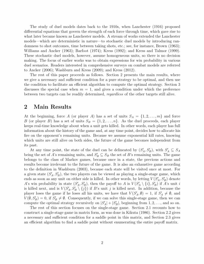
The study of duel models dates back to the 1910s, when Lanchester (1916) proposeddifferential equations that govern the strength of each force through time, which gave rise towhat later became known as Lanchester models. A stream of works extended the Lanchestermodels—which are deterministic in nature—to stochastic duel models by introducing ran-domness to shot outcomes, time between taking shots, etc.; see, for instance, Brown (1963);Williams and Ancker (1963); Barfoot (1974); Kress (1992); and Kress and Talmor (1999).These stochastic duel models, however, assume homogeneous units, so there is no decisionmaking. The focus of earlier works was to obtain expressions for win probability in variousduel scenarios. Readers interested in comprehensive surveys on combat models are referredto Ancker (2006); Washburn and Kress (2009); and Kress (2012).

The rest of this paper proceeds as follows. Section 2 presents the main results, wherewe give a necessary and sufficient condition for a pure strategy to be optimal, and then usethe condition to facilitate an efficient algorithm to compute the optimal strategy. Section 3discusses the special case when m = 1, and gives a condition under which the preferencebetween two targets can be readily determined, regardless of the other targets still alive.

2 Main Results

At the beginning, force A (or player A) has a set of units SA = {1, 2, . . . ,m} and forceB (or player B) has a set of units SB = {1, 2, . . . , n}. As the duel proceeds, each playerkeeps real-time knowledge about when a unit gets killed. In other words, each player has fullinformation about the history of the game and, at any time point, decides how to allocate hisfire on the opponent’s remaining units. Because we assume exponential kill rates, knowingwhich units are still alive on both sides, the future of the game becomes independent fromits past.

At any time point, the state of the duel can be delineated by (S ′A, S′B), with S ′A ⊆ SA

being the set of A’s remaining units, and S ′B ⊆ SB the set of B’s remaining units. The gamebelongs to the class of Markov games, because once in a state, the previous actions andresults become irrelevant to the future of the game. It is also an exhaustive game accordingto the definition in Washburn (2003), because each state will be visited once at most. Fora given state (S ′A, S

′B), the two players can be viewed as playing a single-stage game, which

ends as soon as any unit on either side is killed. In other words, by letting V (S ′A, S′B) denote

A’s win probability in state (S ′A, S′B), then the payoff to A is V (S ′A \ {i}, S ′B) if A’s unit i

is killed next, and is V (S ′A, S′B \ {j}) if B’s unit j is killed next. In addition, because the

player loses the game if he loses all his units, we have that V (S ′A, ∅) = 1, if S ′A 6= ∅, andV (∅, S ′B) = 0, if S ′B 6= ∅. Consequently, if we can solve this single-stage game, then we cancompute the optimal strategy recursively on |S ′A|+ |S ′B|, beginning from 1, 2, . . ., and so on.

The rest of this section focuses on the single-stage game. Section 2.1 recounts how toconstruct a single-stage game in matrix form, as was done in Kikuta (1986). Section 2.2 givesa necessary and sufficient condition for a saddle point in this matrix, and Section 2.3 givesan efficient algorithm to find a saddle point without enumerating the entire payoff matrix.

2

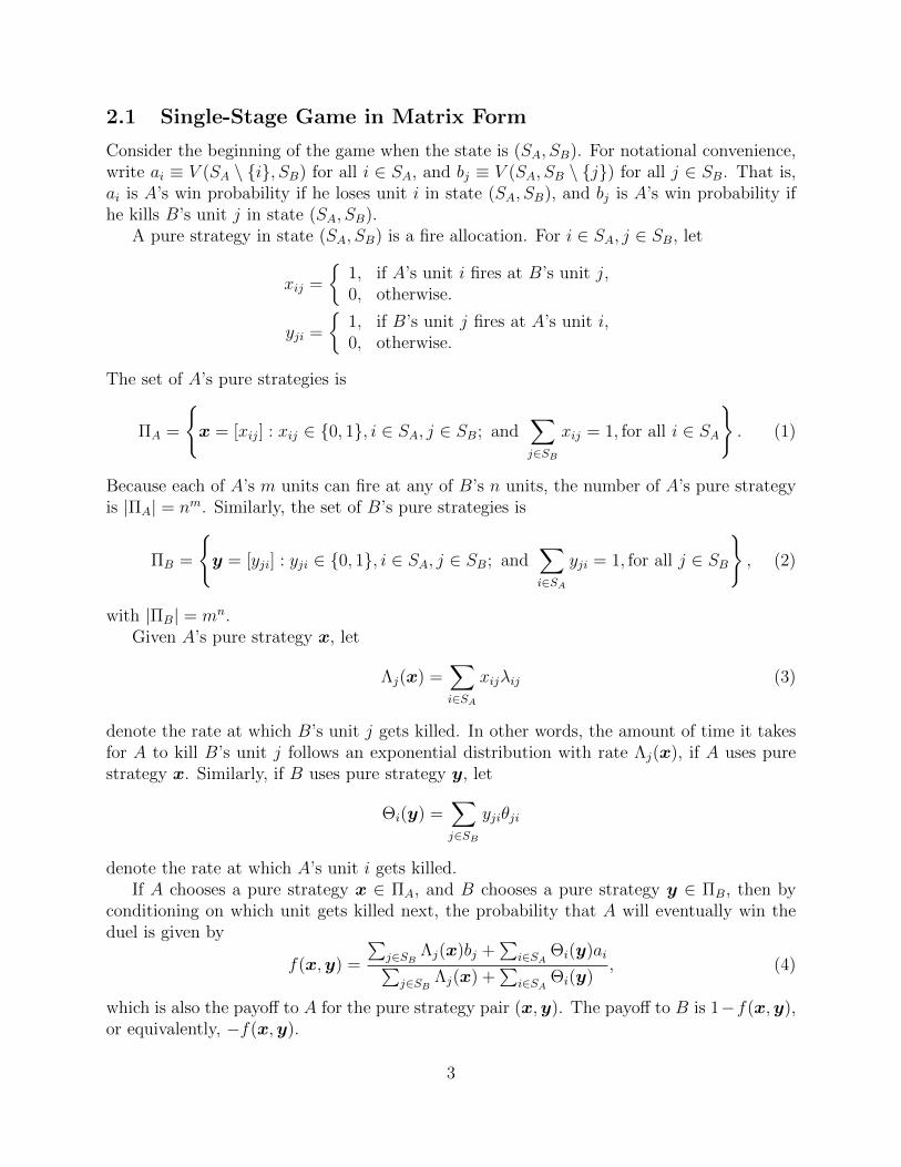
2.1 Single-Stage Game in Matrix Form

Consider the beginning of the game when the state is (SA, SB). For notational convenience,write ai ≡ V (SA \ {i}, SB) for all i ∈ SA, and bj ≡ V (SA, SB \ {j}) for all j ∈ SB. That is,ai is A’s win probability if he loses unit i in state (SA, SB), and bj is A’s win probability ifhe kills B’s unit j in state (SA, SB).

A pure strategy in state (SA, SB) is a fire allocation. For i ∈ SA, j ∈ SB, let

xij =

{1, if A’s unit i fires at B’s unit j,0, otherwise.

yji =

{1, if B’s unit j fires at A’s unit i,0, otherwise.

The set of A’s pure strategies is

ΠA =

{x = [xij] : xij ∈ {0, 1}, i ∈ SA, j ∈ SB; and

∑j∈SB

xij = 1, for all i ∈ SA

}. (1)

Because each of A’s m units can fire at any of B’s n units, the number of A’s pure strategyis |ΠA| = nm. Similarly, the set of B’s pure strategies is

ΠB =

{y = [yji] : yji ∈ {0, 1}, i ∈ SA, j ∈ SB; and

∑i∈SA

yji = 1, for all j ∈ SB

}, (2)

with |ΠB| = mn.Given A’s pure strategy x, let

Λj(x) =∑i∈SA

xijλij (3)

denote the rate at which B’s unit j gets killed. In other words, the amount of time it takesfor A to kill B’s unit j follows an exponential distribution with rate Λj(x), if A uses purestrategy x. Similarly, if B uses pure strategy y, let

Θi(y) =∑j∈SB

yjiθji

denote the rate at which A’s unit i gets killed.If A chooses a pure strategy x ∈ ΠA, and B chooses a pure strategy y ∈ ΠB, then by

conditioning on which unit gets killed next, the probability that A will eventually win theduel is given by

f(x,y) =

∑j∈SB

Λj(x)bj +∑

i∈SAΘi(y)ai∑

j∈SBΛj(x) +

∑i∈SA

Θi(y), (4)

which is also the payoff to A for the pure strategy pair (x,y). The payoff to B is 1−f(x,y),or equivalently, −f(x,y).

3

In this two-person zero-sum game in standard matrix form, A has nm pure strategies andB has mn pure strategies. Kikuta (1986) showed that this matrix game has a saddle point.To determine the saddle point, however, one needed to enumerate the entire payoff matrixof size nm by mn.

Remark 1 The two-person zero-sum game discussed in this section can be regarded as aspecial case of a race-to-reward game as follows. Two players, A and B, each have resourcesto allocate among tasks. A has a set of resources, SA, to allocate among a set of tasks, TA,with allocation of resource i to task k leading to a task completion rate λik, for i ∈ SA andk ∈ TA. Similarly, B has a set of resources, SB, to allocate among a set of tasks, TB, withallocation of resource j to task l leading to a task completion rate θjl, for j ∈ SB and l ∈ TB.Each task has an associated reward to A, namely ak for k ∈ TA, and bl for l ∈ TB, withak > bl for all k ∈ TA and l ∈ TB to avoid triviality. The payoff to A is the reward of thetask that is completed first. The game is zero-sum, with A trying to maximize his expectedpayoff and B trying to minimize it. If TA = SB and TB = SA, then this race-to-reward gamereduces to the single-stage duel game described in this section. Although we present ouranalysis in the context of a single-stage duel game, all the results can be straightforwardlyextended to the race-to-reward game.

2.2 Necessary and Sufficient Condition for Saddle Points

Theorem 1 gives an alternative proof that the matrix game in Section 2.1 has a saddle point.The proof also shows how to determine the optimal strategy if one knows the value of thegame, and facilitates a necessary and sufficient condition for a saddle point, which we presentin Theorem 2.

Theorem 1 Consider the two-person zero-sum game defined by pure strategy sets ΠA in(1), ΠB in (2), and player A’s payoff function f(x,y) in (4). This game has at least onesaddle point. In particular, letting v∗ denote the value of the game, x′ ∈ ΠA a pure strategythat maximizes ∑

j∈SB

Λj(x) · (bj − v∗), (5)

and y′ ∈ ΠB a pure strategy that minimizes∑i∈SA

Θi(y) · (ai − v∗), (6)

then f(x′,y′) = v∗, and (x′,y′) is a saddle point.

Proof. We prove the theorem by contradiction. First, suppose that x′ maximizes (5) and y′

minimizes (6), but f(x′,y′) > v∗, or equivalently,

0 <∑j∈SB

Λj(x′)(bj − v∗) +

∑i∈SA

Θi(y′)(ai − v∗). (7)

4

Because y′ minimizes (6), it follows that∑i∈SA

Θi(y′)(ai − v∗) ≤

∑i∈SA

Θi(y)(ai − v∗), ∀y ∈ ΠB. (8)

Adding∑

j∈SBΛj(x

′)(bj − v∗) to both sides of the preceding, together with (7), we canconclude that

0 <∑j∈SB

Λj(x′)(bj − v∗) +

∑i∈SA

Θi(y)(ai − v∗), ∀y ∈ ΠB,

or equivalently,f(x′,y) > v∗, ∀y ∈ ΠB.

In other words, using the pure strategy x′, player A can guarantee a payoff strictly greaterthan v∗, showing that the value of the game is strictly greater than v∗, which is a contradictionthat v∗ is the value of the game.

Second, by supposing that f(x′,y′) < v∗, we can draw a similar contradiction. Therefore,we have shown that f(x′,y′) = v∗.

To prove that (x′,y′) is a saddle point, we need to show that f(x′,y) ≥ v∗ for all y ∈ ΠB,and f(x,y′) ≤ v∗ for all x ∈ ΠA. To do so, note that

0 =∑j∈SB

Λj(x′)(bj − v∗) +

∑i∈SA

Θi(y′)(ai − v∗),

≤∑j∈SB

Λj(x′)(bj − v∗) +

∑i∈SA

Θi(y)(ai − v∗), ∀y ∈ ΠB,

where the equality follows from f(x′,y′) = v∗, and the inequality from adding∑

j∈SBΛj(x

′)(bj−v∗) to (8). Hence, f(x′,y) ≥ v∗ for all y ∈ ΠB. A similar argument shows that f(x,y′) ≤ v∗

for all x ∈ ΠA. Consequently, (x′,y′) is a saddle point. 2

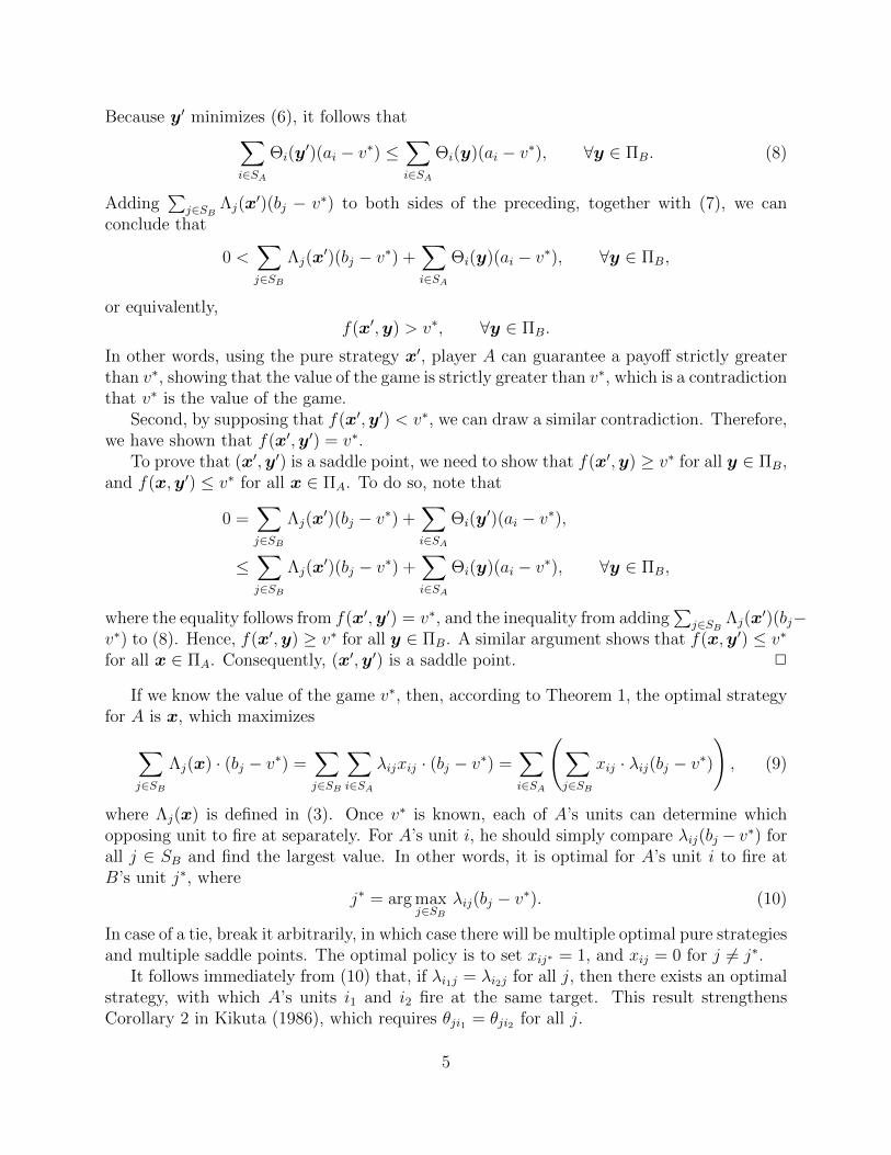
If we know the value of the game v∗, then, according to Theorem 1, the optimal strategyfor A is x, which maximizes∑

j∈SB

Λj(x) · (bj − v∗) =∑j∈SB

∑i∈SA

λijxij · (bj − v∗) =∑i∈SA

(∑j∈SB

xij · λij(bj − v∗)

), (9)

where Λj(x) is defined in (3). Once v∗ is known, each of A’s units can determine whichopposing unit to fire at separately. For A’s unit i, he should simply compare λij(bj − v∗) forall j ∈ SB and find the largest value. In other words, it is optimal for A’s unit i to fire atB’s unit j∗, where

j∗ = arg maxj∈SB

λij(bj − v∗). (10)

In case of a tie, break it arbitrarily, in which case there will be multiple optimal pure strategiesand multiple saddle points. The optimal policy is to set xij∗ = 1, and xij = 0 for j 6= j∗.

It follows immediately from (10) that, if λi1j = λi2j for all j, then there exists an optimalstrategy, with which A’s units i1 and i2 fire at the same target. This result strengthensCorollary 2 in Kikuta (1986), which requires θji1 = θji2 for all j.

5

Theorem 2 A pair of pure strategies (x′,y′) is a saddle point, and a real number v′ is thevalue of the game, if and only if all three conditions hold:

C1. x′ maximizes∑

j∈SBΛj(x) · (bj − v′),

C2. y′ minimizes∑

i∈SAΘi(y) · (ai − v′),

C3. f(x′,y′) = v′.

Proof. From Theorem 1, the game has at least one saddle point. Denote by (x∗,y∗) a saddlepoint, and v∗ the value of the game. It follows immediately that f(x∗, y∗) = v∗.

To prove that C1–C3 are sufficient conditions, we need to show v′ = v∗. To prove v′ = v∗

by contradiction, first suppose that v′ < v∗ to get a string of inequalities involving x′ andx∗ as ∑

j∈SB

Λj(x′)(bj − v′) ≥

∑j∈SB

Λj(x∗)(bj − v′) >

∑j∈SB

Λj(x∗)(bj − v∗),

where the first inequality follows from C1, while the second inequality follows because of theassumption v′ < v∗. Similarly, we get another string of inequality involving y′ and y∗ as∑

i∈SA

Θi(y′)(ai − v′) >

∑i∈SA

Θi(y′)(ai − v∗) ≥

∑i∈SA

Θi(y∗)(ai − v∗),

where the first inequality follows because of the assumption v′ < v∗, while the second in-equality follows from Theorem 1. Adding these two equations together, we arrive at∑j∈SB

Λj(x′)(bj − v′) +

∑i∈SA

Θi(y′)(ai− v′) >

∑j∈SB

Λj(x∗)(bj − v∗) +

∑i∈SA

Θi(y∗)(ai− v∗). (11)

The left-hand side of the preceding is 0 according to C3, while the right-hand side is also 0since f(x∗, y∗) = v∗. Hence, we arrive at a contradiction.

If we suppose v′ > v∗ instead, then we can use a similar argument to draw a contradiction.Consequently, we have shown that v′ = v∗. Finally, using Theorem 1, together with v′ = v∗,C1, and C2, it follows that (x′,y′) is a saddle point. Therefore, we have proved that C1–C3are sufficient conditions.

We next prove that C1–C3 are necessary conditions. To prove C3, we write

f(x′,y′) = v∗ = v′,

where the first equality follows because (x′,y′) is a saddle point, and the second followsbecause v′ is the value of the game.

To prove C1 and C2, note that because (x′,y′) is a saddle point, f(x′,y′) must be thesmallest in its row and largest in its column. The former implies that

f(x′,y′) ≤ f(x′,y), ∀y ∈ ΠB,

6

with equality when y = y′. Use C3 to replace the left-hand side with v′, and use (4) to spellout the right-hand side. After some algebra, the preceding equation becomes∑

j∈SB

Λj(x′) · (bj − v′) +

∑i∈SA

Θi(y) · (ai − v′) ≥ 0, ∀y ∈ ΠB,

with equality when y = y′. In other words, y′ minimizes∑

i∈SAΘi(y) ·(ai−v′), which proves

C2. Beginning withf(x′,y′) ≥ f(x,y′), ∀x ∈ ΠA,

with equality when x = x′, we can use a similar argument to prove C1. Consequently, wehave proved that C1–C3 are necessary conditions. 2

2.3 Computing Saddle Points

This section presents an iterative algorithm to compute saddle points without enumeratingthe entire payoff matrix of size nm ×mn. The algorithm goes as follows.

1. Pick v arbitrarily in [0, 1].

2. For v ∈ [0, 1], define

x(v) ≡ arg maxx

∑j∈SB

Λj(x) · (bj − v), (12)

y(v) ≡ arg miny

∑i∈SA

Θi(y) · (ai − v). (13)

In case of a tie, break it arbitrarily. Next, compute

T (v) ≡ f(x(v), y(v)) =

∑j∈SB

Λj(x(v))bj +∑

i∈SAΘi(y(v))ai∑

j∈SBΛj(x(v)) +

∑i∈SA

Θi(y(v)). (14)

3. If T (v) = v, then v is the value of the game and (x(v), y(v)) is a saddle point. IfT (v) 6= v, then update v ← T (v), and go to step 2.

It is worth noting that computing x(v) and y(v) in (12) and (13) does not require linearprogramming, and can be done quickly, as is the case in (10). When the algorithm stops, wehave a triplet (x(v), y(v), v) that satisfies the three conditions in Theorem 2; therefore, theoptimal solution. It follows immediately from Theorem 2 that the value of the game v∗ isa fixed point of the function T (·), namely T (v∗) = v∗. We next present two lemmas, beforeproving that the algorithm will stop after a finite number of iterations. Although Lemma 1can be viewed as a special case of Lemma 2, we put them separately for ease of explanation.

Lemma 1 If v < v∗, then T (v) > v; if v > v∗, then T (v) < v.

7

Proof. From Theorem 1 there exists a saddle point; let (x∗,y∗) denote one. If v < v∗, thenusing the same argument that gives rise to (11), we have that∑j∈SB

Λj(x(v))(bj − v) +∑i∈SA

Θi(y(v))(ai − v) >∑j∈SB

Λj(x∗)(bj − v∗) +

∑i∈SA

Θi(y∗)(ai − v∗).

The right-hand side of the preceding is equal to 0, because f(x∗,y∗) = v∗. Therefore,∑j∈SB

Λj(x(v))bj +∑

i∈SAΘi(y(v))ai∑

j∈SBΛj(x(v)) +

∑i∈SA

Θi(y(v))> v,

or equivalently, T (v) > v. If v > v∗, then, using a similar argument, we can show thatT (v) < v, which completes the proof. 2

Let T (0)(v) ≡ v, and for k = 1, 2, . . ., let T (k)(v) ≡ T ◦ T (k−1)(v). The next lemmageneralizes Lemma 1.

Lemma 2 If v < v∗, then T (k)(v) > v, for k = 1, 2, . . .; if v > v∗, then T (k)(v) < v, fork = 1, 2, . . ..

Proof. Consider the case v < v∗, and for notational simplicity write v0 ≡ v < v∗, andvk ≡ T (k)(v), for k = 1, 2, . . .. We need to show that vk > v0 for k = 1, 2, . . ..

Because v0 < v∗, it follows from Lemma 1 that v1 > v0. If v1 < v∗, then it follows fromLemma 1 again that v2 > v1 > v0. In other words, the sequence v0, v1, . . . increases strictlyuntil, at some point, it either reaches v∗ or exceeds v∗. In the former case, all followingnumbers in the sequence are v∗ because T (v∗) = v∗, so it is true that vk > v0 for k = 1, 2, . . ..

Suppose now that the sequence v0, v1, . . . exceeds v∗ at some point. Let

s = min{k : vk > v∗}.

In other words, v0 < v1 < · · · < vs−1 < v∗ < vs, as depicted in Figure 1. Because vs > v∗,it follows again from Lemma 1 that vs+1 < vs. If vk ≥ v∗ for k = s, s + 1, . . ., then thestatement that vk > v0 for all k = 1, 2, . . . is also true.

-

v0 v1 · · · vs−1 vt

v∗

vt−1 · · · vs+1 vs

Figure 1: This diagram depicts the sequence v0, v1, . . . , vs, . . . , vt, . . ., where vk ≡ T (k)(v0), fork = 0, 1, . . .. Each new number in the sequence either gives a better lower bound or a betterupper bound for v∗, and the sequence converges to v∗ after a finite number of iterations.

To complete the proof, suppose now that the sequence vs, vs+1, . . . drops below v∗ at somepoint, and let

t = min{k : k > s, vk < v∗}.

8

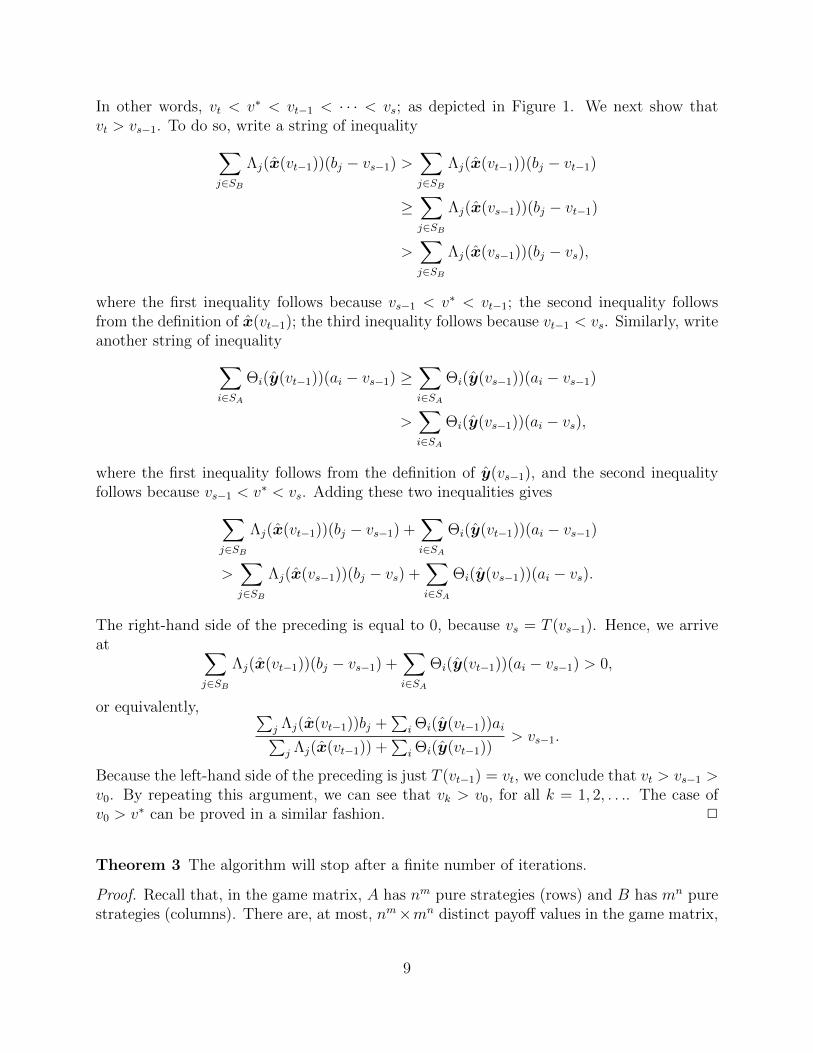
In other words, vt < v∗ < vt−1 < · · · < vs; as depicted in Figure 1. We next show thatvt > vs−1. To do so, write a string of inequality∑

j∈SB

Λj(x(vt−1))(bj − vs−1) >∑j∈SB

Λj(x(vt−1))(bj − vt−1)

≥∑j∈SB

Λj(x(vs−1))(bj − vt−1)

>∑j∈SB

Λj(x(vs−1))(bj − vs),

where the first inequality follows because vs−1 < v∗ < vt−1; the second inequality followsfrom the definition of x(vt−1); the third inequality follows because vt−1 < vs. Similarly, writeanother string of inequality∑

i∈SA

Θi(y(vt−1))(ai − vs−1) ≥∑i∈SA

Θi(y(vs−1))(ai − vs−1)

>∑i∈SA

Θi(y(vs−1))(ai − vs),

where the first inequality follows from the definition of y(vs−1), and the second inequalityfollows because vs−1 < v∗ < vs. Adding these two inequalities gives∑

j∈SB

Λj(x(vt−1))(bj − vs−1) +∑i∈SA

Θi(y(vt−1))(ai − vs−1)

>∑j∈SB

Λj(x(vs−1))(bj − vs) +∑i∈SA

Θi(y(vs−1))(ai − vs).

The right-hand side of the preceding is equal to 0, because vs = T (vs−1). Hence, we arriveat ∑

j∈SB

Λj(x(vt−1))(bj − vs−1) +∑i∈SA

Θi(y(vt−1))(ai − vs−1) > 0,

or equivalently, ∑j Λj(x(vt−1))bj +

∑i Θi(y(vt−1))ai∑

j Λj(x(vt−1)) +∑

i Θi(y(vt−1))> vs−1.

Because the left-hand side of the preceding is just T (vt−1) = vt, we conclude that vt > vs−1 >v0. By repeating this argument, we can see that vk > v0, for all k = 1, 2, . . .. The case ofv0 > v∗ can be proved in a similar fashion. 2

Theorem 3 The algorithm will stop after a finite number of iterations.

Proof. Recall that, in the game matrix, A has nm pure strategies (rows) and B has mn purestrategies (columns). There are, at most, nm×mn distinct payoff values in the game matrix,

9

each of which corresponds to f(x,y) for some pure strategy pair (x,y). In addition, at leastone of the payoff values is v∗, since the game has a saddle point.

Again for notational simplicity, write v0 ≡ v, and vk ≡ T (k)(v), for k = 1, 2, . . .. To provethe theorem, suppose instead that the algorithm does not stop, or equivalently, vk 6= v∗ for allk = 0, 1, 2, . . .. Because vk 6= v∗, it follows from Lemma 2 that its value will not be repeatedin the subsequence vk+1, vk+2, . . .. In other words, all numbers in the sequence v0, v1, v2, . . .are distinct. Other than v0, however, each number in the sequence v1, v2, . . . corresponds toa payoff value in the game matrix. We then arrive at a contradiction because there are onlya finite number of distinct payoff values in the game matrix, which completes the proof. 2

The proof in Theorem 3 shows that the algorithm will stop after at most nm × mn

iterations. This worst case would happen if all the payoff values in the game matrix aredistinct, and if the sequence T (k)(v), k = 1, 2, . . . visits all these distinct values. In practice,the actual number of iterations required to compute v∗ is often far smaller than nm ×mn,because the sequence gets closer to v∗ after each iteration. In particular, as seen from theproof in Lemma 2, each new value generated in the sequence is either v∗, or the best lowerbound to date if it is less than v∗, or the best upper bound to date if it is larger than v∗.

One way to speed up the computation is to pick the initial value close to v∗ to reducethe number of iterations. To this end, note that maxi∈SA

ai ≤ v∗ ≤ minj∈SBbj, because A

will increase his win probability if he kills any of B’s units, and decrease his win probabilityif any of his units are killed. Hence, an initial pick between maxi∈SA

ai and minj∈SBbj, such

as

v =1

2

(maxi∈SA

ai + minj∈SB

bj

),

should work well.This algorithm can be used to recursively compute V (SA, SB), the value of the game in

state (SA, SB). Specifically, we need to compute V (S ′A, S′B) for all S ′A ⊆ SA and S ′B ⊆ SB, by

iterating on |S ′A|+ |S ′B|, the total number of units still alive. The case when |S ′A|+ |S ′B| = 1is trivial. If we have computed V (S ′A, S

′B) for all states when |S ′A| + |S ′B| = k, then those

values become the ai and bj used to compute v∗ for states (S ′A, S′B) with |S ′A|+ |S ′B| = k+ 1,

which, in turn, becomes the ai and bj for next iteration when |S ′A|+ |S ′B| = k + 2.

Example 1 Consider an example with three unit types: rock (R), paper (P), and scissors(S). Assume that

λR,P = λP,S = λS,R = 0.5,

λR,R = λP,P = λS,S = 1,

λR,S = λS,P = λP,R = 2,

and θij = λij for i, j = R,P, S. Table 1 gives the probability that A wins the duel in variousstates. For instance, if A has 2 rocks and B has 1 rock and 1 paper, then A will win theduel with probability V (RR,RP) = 0.262.

There is one interesting observation. Whereas, in 1-on-1 and 2-on-2 duels, the winprobability depends highly on the unit types on each side, in a 3-on-3 duel having RPS

10

Table 1: Probability that Player A wins the duel in different states as discussed in Example 1,when there are three unit types: Rock, Paper, and Scissors.

Player BPlayer A PP RP RS PS RPS RPP RSS PPS PSS

R 0.022 0.071 0.320 0.133 0.040 0.007 0.178 0.013 0.076RR 0.111 0.262 0.696 0.375 0.186 0.049 0.533 0.079 0.279RP 0.304 0.500 0.623 0.377 0.228 0.186 0.358 0.121 0.189

RRR 0.270 0.494 0.906 0.609 0.402 0.152 0.813 0.211 0.514RRP 0.467 0.673 0.879 0.642 0.463 0.325 0.714 0.286 0.453RRS 0.721 0.618 0.814 0.812 0.474 0.353 0.675 0.547 0.647RPS 0.814 0.772 0.772 0.772 0.500 0.526 0.537 0.537 0.526

would guarantee a win probability at least 0.5, regardless of the opponent’s three units. Itis better to have a balanced force, which makes it difficult for the opponent to exploit theweakness. 2

3 One Against Many

Consider the special case when m = 1. The optimal strategy for B is clearly for all hisremaining units to fire at A’s only unit, while A needs to decide in which of the n! possibleorders his only unit should fire at B’s units. Because A has only one unit, in this section wewrite λj = λ1j, and θj = θj1 for notational convenience. We also use target j and B’s unit jinterchangeably.

The problem has been previously studied by Friedman (1977) and Kikuta (1983), wherethey identified necessary conditions and sufficient conditions for an optimal fire order. Inparticular, Friedman (1977) showed that if the fire order 1, 2, . . . , n is optimal, then

θk

(λk + θk +

n∑i=k+2

θi

)≥ θk+1

(λk+1 + θk+1 +

n∑i=k+2

θi

), for k = 1, 2, . . . , n− 1, (15)

because otherwise, swapping k and k + 1 results in a better fire order. Equation (15),however, is not a sufficient condition for optimality, as seen by a counterexample given inKikuta (1983). There is no simple way to rank the targets in a complete list, because whethertarget k or target k+ 1 should be fired at first depends on the other targets present, as seenby the term

∑ni=k+2 θi in (15).

Intuitively, A prefers to fire at a target that is easier to kill so as to eliminate a targetsooner. He should also prefer to kill a target that poses a bigger threat. That is, if λ1 > λ2 andθ1 > θ2, then it is intuitive that A should kill target 1 before trying to kill target 2, regardlessof the other targets still alive. It turns out this conjecture is true. The next theorem presents

11

a slightly weaker condition than the preceding one, under which it is possible to rank thepreference between two targets, regardless of the other targets still alive.

Theorem 4 If either

1. θ1 > θ2 and λ1 + θ1 ≥ λ2 + θ2, or

2. θ1 = θ2 and λ1 > λ2,

then target 1 stands higher than target 2 in the optimal fire order, regardless of the othertargets.

Proof. Consider fire order 1:

. . . , 1, i1, . . . , ik, 2, j1, . . . , jl.

Let α =∑k

s=1 θis and β =∑l

s=1 θjs for notational convenience. The probability that A winswith fire order 1 is

P{wipe out all targets in front of target 1 before getting killed}

× λ1λ1 + θ1 + α + θ2 + β

(k∏

s=1

λis

λis +∑k

r=s θir + θ2 + β

)λ2

λ2 + θ2 + β

× P{wipe out targets j1, . . . , jl before getting killed}. (16)

Swap targets 1 and 2 in fire order 1 to get fire order 2:

. . . , 2, i1, . . . , ik, 1, j1, . . . , jl.

The probability that A wins with fire order 2 is

P{wipe out all targets in front of target 2 before getting killed}

× λ2λ2 + θ1 + α + θ2 + β

(k∏

s=1

λis

λis +∑k

r=s θir + θ1 + β

)λ1

λ1 + θ1 + β

× P{wipe out targets j1, . . . , jl before getting killed}. (17)

The first term and the last term in equations (16) and (17) are identical. In addition, theproduct term in the middle in (16) is at least as large as the product term in the middle in(17), because of the assumption θ1 ≥ θ2 in the theorem. Hence, fire order 1 is strictly betterthan fire order 2 if

λ1λ1 + θ1 + α + θ2 + β

λ2λ2 + θ2 + β

>λ2

λ2 + θ1 + α + θ2 + β

λ1λ1 + θ1 + β

.

If either condition stated in the theorem is met, then one can verify that

(λ1 + θ1 + α + θ2 + β)(λ2 + θ2 + β)− (λ2 + θ1 + α + θ2 + β)(λ1 + θ1 + β)

= θ2(λ2 + θ2) + (λ2 + θ2)α + θ2β − θ1(λ1 + θ1)− (λ1 + θ1)α− θ1β < 0,

12

which completes the proof. 2

A natural question to ask is whether Theorem 4 can be extended to the case when A hasm ≥ 2 units. In other words, if each of the m units can individually rank all of B’s unitsaccording to the condition in Theorem 4, then does each unit’s optimal fire order collectivelygive rise to the group optimal policy? It turns out that is not the case, as seen in thecounterexample below.

Example 2 Consider an example with m = 2 and n = 2, with their kill-rate matrices givenas follows:

[λij] =

(0.9 11 0.9

), [θji] =

(1.1 11 1.1

).

In state ({1}, {1, 2}), from the standpoint of A’s unit 1, the rates

λ11 = 0.9, λ12 = 1, θ11 = 1.1, θ21 = 1

meet the condition in Theorem 4. Therefore, in state ({1}, {1, 2}) it is optimal for A’s unit1 to fire at B’s unit 1. For the same reason, in state ({2}, {1, 2}) it is optimal for A’s unit 2to fire at B’s unit 2.

If A still has both units and B also has both units, however, then A’s pure strategy

x =

(1 00 1

)is not optimal, as another pure strategy

x′ =

(0 11 0

)can do strictly better, because

Λ1(x′) = 1 > 0.9 = Λ1(x),

Λ2(x′) = 1 > 0.9 = Λ2(x).

As a matter of fact, x′ is optimal for A in state ({1, 2}, {1, 2}). Hence, even if each unit canindividually rank all opposing units according to the condition in Theorem 4, collectively,these individual rankings do not necessarily give rise to the group optimal policy. 2

To conclude this section, we give a condition weaker than the one in Theorem 4, underwhich the fire order 1, 2, . . . , n is optimal. Theorem 2 in Kikuta (1983) also gives a sufficientcondition for the fire order 1, 2, . . . , n to be optimal. It is straightforward to show thatKikuta’s condition implies the one in Corollary 1; however, the condition in Corollary 1 ismuch easier to verify.

13

Corollary 1 Ifθ1 ≥ θ2 ≥ · · · ≥ θn,

andθ1(λ1 + θ1) ≥ θ2(λ2 + θ2) ≥ · · · ≥ θn(λn + θn),

then the fire order 1, 2, . . . , n is optimal.

Proof. Consider an arbitrary fire order . . . , i, j, . . . other than 1, 2, . . . , n, where i > j. Forany constant D ≥ 0, we can verify that

θi(λi + θi +D) ≤ θj(λj + θj +D).

Hence, according to (15), swapping i and j results in another fire order that is at least asgood.

Starting with an arbitrary fire order, we can repeatedly look for adjacent targets that areout of order and swap them—analogous to bubble sort—so that in each step we get a newfire order that is at least as good. When no such swapping is possible, we arrive at the fireorder 1, 2, . . . , n, which is at least as good as the initial fire order. Because this argumentworks for any initial fire order, the fire order 1, 2, . . . , n is optimal. 2

Acknowledgment

The authors would like to thank Alan Washburn, Moshe Kress, and Michael Atkinson fortheir suggestions that improve the presentation of this paper.

14

References

Ancker, C. J. (2006). A proposed foundation for a theory of combat. Naval Research LogisticsQuarterly, 42(3):311–343.

Barfoot, C. B. (1974). Markov duels. Operations Research, 22(2):318–330.

Brown, R. H. (1963). Theory of combat: The probability of winning. Operations Research,11(3):418–425.

Friedman, Y. (1977). Optimal strategy for the one-against-many battle. Operations Research,25(5):884–888.

Gittins, J., Glazebrook, K. D., and Weber, R. (2011). Multi-Armed Bandit Allocation Indices.Wiley, United Kingdom, 2nd edition.

Kikuta, K. (1983). A note on the one against many battle. Operations Research, 31(5):952–956.

Kikuta, K. (1986). The matrix game derived from the many-against-many battle. NavalResearch Logistics Quarterly, 33(4):603–612.

Kress, M. (1992). A many-on-many stochastic duel model for a mountain battle. NavalResearch Logistics, 39:437–446.

Kress, M. (2012). Modeling armed conflicts. Science, 336(6083):865–869.

Kress, M. and Talmor, I. (1999). A new look at the 3:1 rule of combat through markovstochastic lanchester models. The Journal of the Operational Research Society, 50(7):733–744.

Lanchester, F. W. (1916). Aircraft in Warfare: The Dawn of the Fourth Arm. Constable,London.

Ross, S. M. (1983). Introduction to Stochastic Dynamic Programming. Academic Press, NewYork.

Washburn, A. R. (2003). Two-Person Zero-Sum Games. INFORMS, Rockville, MD, 3rdedition.

Washburn, A. R. and Kress, M. (2009). Combat Modeling. Springer.

Williams, T. and Ancker, C. J. (1963). Stochastic duels. Operations Research, 11(5):803–817.

15

16

THIS PAGE INTENTIONALLY LEFT BLANK

17

INITIAL DISTRIBUTION LIST

1. Defense Technical Information Center Ft. Belvoir, Virginia

2. Dudley Knox Library Naval Postgraduate School Monterey, California

3. Research Sponsored Programs Office, Code 41 Naval Postgraduate School Monterey, California

4. Richard Mastowski (Technical Editor) ..........................................................................1 Graduate School of Operational and Information Sciences (GSOIS) Naval Postgraduate School Monterey, California

5. Jonathan K. Alt ..............................................................................................................1 TRAC-Monterey Monterey, California

6. Christopher E. Marks .....................................................................................................1 TRAC-Monterey Monterey, California

7. Christian J. Darken .........................................................................................................1 Computer Science Department Naval Postgraduate School Monterey, California

8. Arnold H. Buss ..............................................................................................................1 Modeling, Virtual Environments, and Simulation Institute Naval Postgraduate School Monterey, California

9. Kyle Y. Lin ....................................................................................................................1 Operations Research Department Naval Postgraduate School Monterey, California