Embed Size (px)
Citation preview
NAVAL
POSTGRADUATE SCHOOL
MONTEREY, CALIFORNIA
THESIS
Approved for public release; distribution is unlimited.
COST-CONSTRAINED PROJECT SCHEDULING WITH TASK DURATIONS AND COSTS THAT MAY INCREASE OVER TIME: DEMONSTRATED WITH
THE U.S. ARMY FUTURE COMBAT SYSTEMS
by
Roger Grose
June 2004 Thesis Advisor: Robert A. Koyak Second Reader: Gerald G. Brown

THIS PAGE INTENTIONALLY LEFT BLANK
i
REPORT DOCUMENTATION PAGE Form Approved OMB No. 0704-0188 Public reporting burden for this collection of information is estimated to average 1 hour per response, including the time for reviewing instruction, searching existing data sources, gathering and maintaining the data needed, and completing and reviewing the collection of information. Send comments regarding this burden estimate or any other aspect of this collection of information, including suggestions for reducing this burden, to Washington headquarters Services, Directorate for Information Operations and Reports, 1215 Jefferson Davis Highway, Suite 1204, Arlington, VA 22202-4302, and to the Office of Management and Budget, Paperwork Reduction Project (0704-0188) Washington DC 20503. 1. AGENCY USE ONLY (Leave blank)
2. REPORT DATE June 2004
3. REPORT TYPE AND DATES COVERED Master’s Thesis
4. TITLE AND SUBTITLE: Cost-Constrained Project Scheduling with Task Durations and Costs That May Increase Over Time: Demonstrated with the U.S. Army Future Combat Systems 6. AUTHOR(S) Major Roger Grose
5. FUNDING NUMBERS
7. PERFORMING ORGANIZATION NAME(S) AND ADDRESS(ES) Naval Postgraduate School Monterey, CA 93943-5000
8. PERFORMING ORGANIZATION REPORT NUMBER
9. SPONSORING /MONITORING AGENCY NAME(S) AND ADDRESS(ES) Cost Analysis Improvement Group. Program Analysis and Evaluation (PA&E). Office of the Secretary of Defense.
10. SPONSORING/MONITORING AGENCY REPORT NUMBER
11. SUPPLEMENTARY NOTES The views expressed in this thesis are those of the author and do not reflect the official policy or position of the Department of Defense or the U.S. Government. 12a. DISTRIBUTION / AVAILABILITY STATEMENT Approved for public release; distribution is unlimited.
12b. DISTRIBUTION CODE
13. ABSTRACT (maximum 200 words) We optimize long-term project schedules subject to annual budget constraints, where the duration and cost of each task may increase as the project progresses. Initially, tasks are scheduled without regard to budgets and the project completion time is minimized. Treating the task durations as random variables, we then use simulation to describe the distribution of the project completion time. Next, we minimize the completion time under budget constraints with fixed task durations, where budget violations are tolerated albeit with penalties. Annual reviews are then introduced, which allow underway tasks to be delayed or monthly budgets to be increased. We obtain estimates of the completion time of the project and its final cost under each of these scenarios. The U.S. Army Future Combat Systems (FCS) is used for illustration. FCS is a suite of information technologies, sensors, and command systems with an estimated acquisition cost of over $90 billion. The U.S. General Accounting Office found that FCS is at risk of substantial cost overrun and delay. We analyze three schedule plans for FCS to identify which can be expected to deliver the earliest completion time and the least cost.
15. NUMBER OF PAGES
133
14. SUBJECT TERMS Integer Linear Programming, Optimization, Project Management, Future Combat Systems, Cost Constrained Project Scheduling.
16. PRICE CODE
17. SECURITY CLASSIFICATION OF REPORT
Unclassified
18. SECURITY CLASSIFICATION OF THIS PAGE
Unclassified
19. SECURITY CLASSIFICATION OF ABSTRACT
Unclassified
20. LIMITATION OF ABSTRACT
UL
NSN 7540-01-280-5500 Standard Form 298 (Rev. 2-89) Prescribed by ANSI Std. 239-18

ii
THIS PAGE INTENTIONALLY LEFT BLANK
iii
Approved for public release; distribution is unlimited.
COST-CONSTRAINED PROJECT SCHEDULING WITH TASK DURATIONS AND COSTS THAT MAY INCREASE OVER TIME: DEMONSTRATED WITH
THE U.S. ARMY FUTURE COMBAT SYSTEMS
Roger T. Grose Major, Australian Army
Submitted in partial fulfillment of the requirements for the degree of
MASTER OF SCIENCE IN OPERATIONS RESEARCH
from the
NAVAL POSTGRADUATE SCHOOL June 2004
Author: Major Roger T. Grose Australian Army
Approved by: Assistant Professor R. Koyak
Thesis Advisor
Distinguished Professor G. Brown Second Reader/Co-Advisor
James N. Eagle Chairman, Department of Operations Research

iv
THIS PAGE INTENTIONALLY LEFT BLANK
v
ABSTRACT We optimize long-term project schedules subject to annual budget constraints,
where the duration and cost of each task may increase as the project progresses. Initially,
tasks are scheduled without regard to budgets and the project completion time is
minimized. Treating the task durations as random variables, we then use simulation to
describe the distribution of the project completion time. Next, we minimize the
completion time under budget constraints with fixed task durations, where budget
violations are tolerated albeit with penalties. Annual reviews are then introduced, which
allow underway tasks to be delayed or monthly budgets to be increased. We obtain
estimates of the completion time of the project and its final cost under each of these
scenarios. The U.S. Army Future Combat Systems (FCS) is used for illustration. FCS is
a suite of information technologies, sensors, and command systems with an estimated
acquisition cost of over $90 billion. The U.S. General Accounting Office found that FCS
is at risk of substantial cost overrun and delay. We analyze three schedule plans for FCS
to identify which can be expected to deliver the earliest completion time and the least
cost.

vi
THIS PAGE INTENTIONALLY LEFT BLANK
vii
TABLE OF CONTENTS
I. INTRODUCTION........................................................................................................1 A. ACQUISITION OF THE U.S. ARMY FUTURE COMBAT
SYSTEMS.........................................................................................................2 B. SCHEDULE OPTIONS AND SCHEDULE RISK .......................................5
1. Baseline Plan.........................................................................................6 2. Alternate Plan 1....................................................................................6 3. Alternate Plan 2....................................................................................7
C. PURPOSE OF THESIS...................................................................................7
II. RELATED RESEARCH.............................................................................................9 A. THE RESOURCE-CONSTRAINED PROJECT SCHEDULING
PROBLEM .......................................................................................................9 B. PROJECT SCHEDULING UNDER UNCERTAINTY.............................10
III. UNCONSTRAINED STOCHASTIC SCHEDULE ANALYSIS...........................13 A. STOCHASTIC MODELING OF TASK DURATIONS ............................13 B. THE UNCONSTRAINED REACHING ALGORITHM...........................16
IV. BUDGET-CONSTRAINED DETERMINISTIC OPTIMIZATION MODEL....19 A. MODEL STATEMENT ................................................................................19
1. Index Use.............................................................................................19 2. Data [units] .........................................................................................20 3. Variables [units] .................................................................................20 4. Formulation ........................................................................................21 5. Description of the Model ...................................................................22 6. Computer Implementation................................................................22
B. TASK DURATIONS AND COSTS..............................................................23 C. PROJECT BUDGET.....................................................................................24 D. SIMULATION OF ANNUAL REVIEWS...................................................24
V. EXPERIMENTAL RESULTS..................................................................................29 A. FCS INPUT DATA ........................................................................................29 B. RESULTS OF THE UNCONSTRAINED STOCHASTIC
SCHEDULE ANALYSIS ..............................................................................30 C. RESULTS OF THE BUDGET-CONSTRAINED DETERMINISTIC
OPTIMIZATION ANALYSIS .....................................................................33 1. Scenario 3: Deterministic Model without Annual Review
Simulation...........................................................................................33 a. Results for the Baseline Plan without Annual Review
Simulation ...............................................................................34 b. Results for Alternate Plan 1 without Annual Review
Simulation ...............................................................................35 c. Results for Alternate Plan 2 without Annual Review
Simulation ...............................................................................36
viii
2. Scenario 4: Deterministic Model with Annual Review Simulation...........................................................................................39
3. Budget Decomposition.......................................................................40 a. Results for the Baseline Plan with Annual Review
Simulation ...............................................................................43 b. Results for Alternate Plan 1 with Annual Review
Simulation ...............................................................................45 c. Results for Alternate Plan 2 with Annual Review
Simulation ...............................................................................48 4. Plan Comparisons ..............................................................................50 5. Solution Times and Convergence .....................................................52 6. Number of Simulation Realizations .................................................52
VI. CONCLUSIONS..........................................................................................................55 A. CONCLUSIONS ............................................................................................55 B. FUTURE AREAS OF STUDY .....................................................................56
LIST OF REFERENCES......................................................................................................59
APPENDIX A.........................................................................................................................63 A. MANNED GROUND VEHICLES ...............................................................63 B. UNMANNED AERIAL VEHICLES (UAV) ...............................................66 C. UNMANNED GROUND VEHICLES (UGV).............................................66 D. INTELLIGENT MUNITIONS.....................................................................68
APPENDIX B .........................................................................................................................69 A. FUTURE COMBAT SYSTEMS DEVELOPMENT AND
DEMONSTRATION SCHEDULE PLANS ................................................69 1. Baseline Plan: Proceed with Current Plan ......................................70 2. Alternate Plan 1: Mitigate High Risk Technologies First ..............73 3. Alternate Plan 2: Develop C4ISR Infrastructure First .................76
B. ANNUAL FCS BUDGET BANDS BY COMPLETION YEAR................79
APPENDIX C.........................................................................................................................81 A. JAVA CODE FOR UNCONSTRAINED REACHING ALGORITHM...81
APPENDIX D.........................................................................................................................85 A. COMPLETE ILP FORMULATION ...........................................................85
1. Index Use.............................................................................................85 2. Data .....................................................................................................85 3. Variables .............................................................................................86 4. Formulation ........................................................................................87 5. Verbal Description.............................................................................88 6. Model Discussion................................................................................89 7. Appendix D References .....................................................................89
APPENDIX E .........................................................................................................................91 A. GAMS IMPLEMENTATION ......................................................................91
INITIAL DISTRIBUTION LIST .......................................................................................111

ix
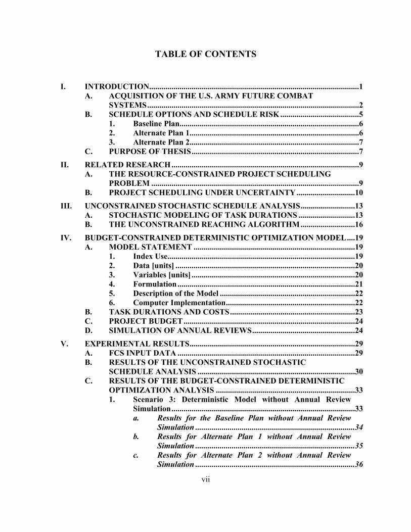
LIST OF FIGURES
Figure 1. Future Combat Systems Composition (after Brady, 2003)................................2 Figure 2. Defense Acquisition Framework (after Wynne, 2003)......................................3 Figure 3. Unconstrained Reaching Algorithm Pseudo-Code ..........................................17 Figure 4. Annual Review Resampling Mechanism.........................................................25 Figure 5. Abstraction of the Moving Window for the Simulated RCPSP with
Annual Review.................................................................................................27 Figure 6. Scenario 2: Distribution of Finish Times from Unconstrained Reaching
Algorithm with Simulation ..............................................................................31 Figure 7. Project Expenditure without Annual Review Simulation for Baseline Plan ...34 Figure 8. Cumulative Project Expenditure without Annual Review Simulation for
Baseline Plan....................................................................................................35 Figure 9. Project Expenditure without Annual Review Simulation for Alternate
Plan 1 ...............................................................................................................36 Figure 10. Cumulative Project Expenditure without Annual Review Simulation for
Alternate Plan 1................................................................................................36 Figure 11. Project Expenditure without Annual Review Simulation for Alternate
Plan 2 ...............................................................................................................37 Figure 12. Cumulative Project Expenditure without Annual Review Simulation for
Alternate Plan 2................................................................................................37 Figure 13. Project Expenditure without Annual Review Simulation for All Schedule
Plans.................................................................................................................38 Figure 14. Cumulative Project Expenditure without Annual Review Simulation for
All Schedule Plans ...........................................................................................38 Figure 15. Project Completion Times with Annual Reviews............................................39 Figure 16. Baseline Plan Budget Broken down by Project Completion Year ..................41 Figure 17. Baseline Plan Cumulative Budget Broken down by Project Completion
Year..................................................................................................................42 Figure 18. Annual Project Expenditure with Annual Review Simulation for Baseline
Plan ..................................................................................................................43 Figure 19. Cumulative Project Expenditure with Annual Review Simulation for
Baseline Plan....................................................................................................44 Figure 20. Project Expenditure with and without Annual Review Simulation for
Baseline Plan....................................................................................................44 Figure 21. Project Budgets with and without Annual Review Simulation for
Baseline Plan....................................................................................................45 Figure 22. Project Expenditure with Annual Review Simulation for Alternate Plan 1 ....46 Figure 23. Cumulative Project Expenditure with Annual Review Simulation for
Alternate Plan 1................................................................................................46 Figure 24. Project Expenditure with and without Annual Review Simulation for
Alternate Plan 1...............................................................................................47
x
Figure 25. Project Budgets with and without Annual Review Simulation for Alternate Plan 1................................................................................................47
Figure 26. Project Expenditure with Annual Review Simulation for Alternate Plan 2 ....48 Figure 27. Cumulative Project Expenditure with Annual Review Simulation for
Alternate Plan 2................................................................................................49 Figure 28. Project Expenditure with and without Annual Review Simulation for
Alternate Plan 2................................................................................................49 Figure 29. Project Budgets with and without Annual Review Simulation for
Alternate Plan 2................................................................................................50 Figure 30. Annual Project Expenditure by Schedule Plan ................................................51 Figure 31. Cumulative Project Expenditure by Schedule Plan .........................................51
xi
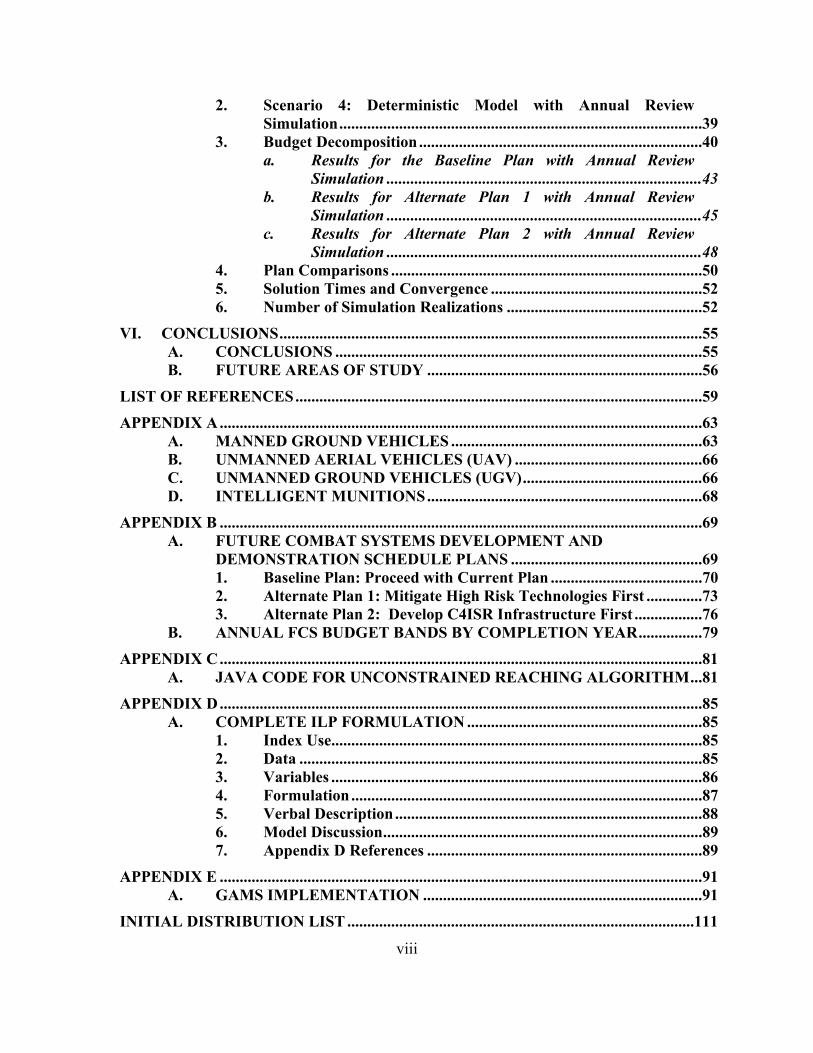
LIST OF TABLES
Table 1. Association of Risk Levels to Attributes of the Three-Parameter Weibull Distribution (after Miller, 2003). .....................................................................15
Table 2. Association Between Attributes and Parameters of the Three-Parameter Weibull Distribution ........................................................................................15
Table 3. Scenario 1: Unconstrained Project Completion Times without Simulation. ...30 Table 4. Scenario 2: Unconstrained Project Completion Times with Simulation. ........32 Table 5. Scenario 3: Constrained Project Completion Times without Annual
Review Simulation...........................................................................................34 Table 6. Scenario 4: Constrained Project Completion Times with Annual Review
Simulation ........................................................................................................40 Table 7. Overview of Percentage Schedule Delay by Plan and by Scenario.................55

xii
THIS PAGE INTENTIONALLY LEFT BLANK
xiii
ACKNOWLEDGMENTS
This thesis would not have possible without the indefatigable assistance of
Distinguished Professor of Operations Research Gerald G. Brown, and the help of
Assistant Professor of Operations Research Robert A. Koyak. I also wish to
acknowledge valuable assistance from my research sponsor, Mr. Walt Cooper of the Cost
Analysis Improvement Group (CAIG), Program Analysis and Evaluation branch, Office
of the Secretary of Defense without whom this thesis would not have been possible.

xiv
THIS PAGE INTENTIONALLY LEFT BLANK
xv
EXECUTIVE SUMMARY
Scheduling an acquisition project subject to time and budget constraints is a
challenging management problem. A task not completed on time threatens cost overrun
and cascading delay of succeeding tasks, perhaps ultimately delaying the entire project
and its fielded capability, and maybe even threatening outright failure of the project.
A project scheduling problem is characterized and viewed as a directed network
with an arc depicting each pairwise partial order between completion of a predecessor
task and start of a successor task. Planned project completion is governed by the longest
directed path in terms of total task durations in this network.
In reality, a task may fail to finish within its planned duration for reasons that
cannot be known in advance. One strategy for scheduling the tasks may be more robust
to effects of delays than others, even though all schedules are subject to the same
constraints. Our objective is to identify the scheduling strategy or strategies that offer the
least schedule risk.
This thesis shows how to assess the risks of defense acquisition scheduling under
budget constraints. The approach considered is applicable to a wide range of programs
that encompass multiple developmental tasks with durations that are subject to
uncertainty.
We use the U.S. Army’s planned acquisition of the Future Combat Systems (FCS)
to demonstrate schedule re-optimization responding to random delays. FCS is a “system
of systems” that requires successful completion of many developmental tasks over
approximately ten years, where many tasks are dependent on prior completion of other
tasks, and many tasks depend on nascent technologies. FCS is ideal to illustrate new
concepts of project scheduling under uncertainty.
The U.S. General Accounting Office (GAO) reports that FCS suffers significant
risks of cost and schedule growth. These risks might lead to major consequences for the
entire U.S. Defense budget. Costs for FCS acquisition include $92 billion (2004 U.S.
dollars) to acquire only 14 of the 18 systems that are needed for FCS to achieve initial
xvi
operational capability by the year 2010 and $16 billion for the system development and
demonstration (SDD) phase alone. In fiscal year 2005, FCS is expected to consume more
than 50 percent of the U.S. Army budget for all programs in SDD phases, and over 30
percent of the total budget for research and development and test and evaluation tasks
This thesis examines three plans for scheduling FCS tasks in the SDD phase. The
baseline plan is the current schedule. Alternate plan 1 and alternate plan 2 are schedules
that were developed based on 2003 GAO recommendations to mitigate schedule risks.
Nominal data on FCS tasks provided by the Cost Analysis Improvement Group (CAIG)
of the Office of the Secretary of Defense (OSD) are used to optimize the three schedules
both with and without annual budget constraints.
Each plan is analyzed under four different scheduling scenarios. Under the first
scenario tasks are scheduled without regard to costs and treating the task durations as
fixed. Under the second scenario annual budget constraints are not imposed but the task
durations in months are generated as random variables using probability distributions in a
computer simulation of the entire project. By simulating a schedule many times, we
induce project completion time and final project cost as random variables. Summary
statistics, such as the mean completion time or mean cost, can be used to evaluate a
proposed schedule or to compare multiple schedules.
The third scenario introduces budget constraints by fiscal year, and
deterministically optimizes the project schedule by determining for each task the best
start month, and selecting from a feasible range of task durations the best planned
duration in months, given that monthly task costs may differ depending on start month
and duration. In addition, there is a complete project budget by fiscal year for any
feasible fiscal year when the project might be completed, and the optimization selects
which of these overall project budgets to use while scheduling all the task starts and
durations. Although the optimization can insert slack in the project between tasks to
satisfy budget constraints, it cannot interrupt a task once that task is started for some
given duration. Each fiscal year budget alternative is given as an interval, or “budget
band,” within which we stipulate that the project is in planned cost control. Because
there may be no feasible pattern of task starts and durations that result in spending within
xvii
these budget bands, the budgets are expressed cumulatively over the planning horizon,
and under- and over-expenditures are tolerated, albeit at a high penalty cost per dollar of
violation. The idea is to permit some flexibility by carrying forward any cumulative
under- or over-expenditure until it is repaid in some later fiscal year, and encouraging
prompt repayment by continuing to penalize any outstanding cumulative violation.
In scenario 4, the budget-constrained, deterministic project schedule optimization
is subjected to annual reviews. In each of these successive fiscal year reviews, any task
already underway and not yet finished may suffer cost growth and/or duration delay.
Such events are influenced by the degree of risk assigned to each task, and we decide
whether and by how much to inflate cost and duration of tasks under review by a random
simulation.
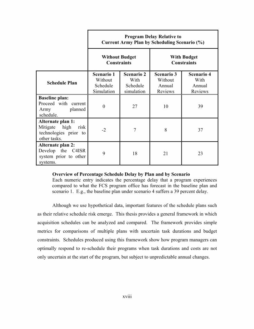
The results for all four scenarios are summarized in the table below. For example,
using the baseline plan under scenario 1 as our reference schedule, alternate plan 1 under
scenario 2 leads to an estimated project delay of seven percent. When budget constraints
with annual reviews are imposed, this delay grows to approximately 37 percent. For
FCS, a 37 percent delay corresponds to approximately four years, where a one-year delay
has been estimated by the GAO to add between $4 billion and $5 billion to the total
acquisition cost.
In the absence of budget constraints, developing critical technologies to a
production-suitable readiness level prior to other tasks (alternate plan 1) leads to project
completion faster than the baseline plan. When budget constraints are added, this plan
maintains its advantage although it is subject to delays similar to the baseline plan.
Development of the C4ISR system up front (alternate plan 2) presents a very
different schedule risk. Although this plan stands out as the least desirable option in the
absence of budget constraints, it emerges as the most favorable option when these
constraints are imposed. Because budget constraints are a reality in defense acquisition,
alternate plan 2 evidently presents the least schedule risk.
xviii
Program Delay Relative to Current Army Plan by Scheduling Scenario (%)
Without Budget Constraints
With Budget Constraints
Schedule Plan
Scenario 1 Without Schedule
Simulation
Scenario 2 With
Schedule simulation
Scenario 3 Without Annual Reviews
Scenario 4 With
Annual Reviews
Baseline plan: Proceed with current Army planned schedule.
0 27 10 39
Alternate plan 1: Mitigate high risk technologies prior to other tasks.
-2 7 8 37
Alternate plan 2: Develop the C4ISR system prior to other systems.
9 18 21 23
Overview of Percentage Schedule Delay by Plan and by Scenario Each numeric entry indicates the percentage delay that a program experiences compared to what the FCS program office has forecast in the baseline plan and scenario 1. E.g., the baseline plan under scenario 4 suffers a 39 percent delay. Although we use hypothetical data, important features of the schedule plans such
as their relative schedule risk emerge. This thesis provides a general framework in which
acquisition schedules can be analyzed and compared. The framework provides simple
metrics for comparisons of multiple plans with uncertain task durations and budget
constraints. Schedules produced using this framework show how program managers can
optimally respond to re-schedule their programs when task durations and costs are not
only uncertain at the start of the program, but subject to unpredictable annual changes.

xix
LIST OF ACRONYMS
AFSS Advanced Fire Support System ARV Armed Reconnaissance Vehicle BLOS Beyond Line of Sight C2 Command and Control C4ISR Command, Control, Communications, Computers, Intelligence,
Surveillance, and Reconnaissance CAIG Cost Analysis Improvement Group CDF Cumulative Distribution Function CLU Container Launch Unit CPLEX Optimization Solver developed by ILOG CPM Critical Path Method CV Command Vehicle DoD Department of Defense DRR Design Readiness Review FCS Future Combat Systems FY Fiscal Year GAMS General Algebraic Modeling System GAO General Accounting Office GUB Generalized Upper Bounds ILP Integer Linear Programming INFORMS Institute for Operations Research and the Management Sciences IOC Initial Operational Capability IOT&E initial operational test and evaluation LOS Line of Sight LAM Loitering Attack Missile LWIR Long-Wave Infrared MDAP Major Defense Acquisition Program MULE Multi-functional Utility Logistics and Equipment vehicle MWIR Medium Wave Infrared NLOS Non-Line of Sight NP Non-Polynomial OSD Office of the Secretary of Defense OSL Optimization Subroutine Library PAM Precision Attack Missile PDF Probability Distribution Function PEO Program Executive Office PERT Program Evaluation and Review Technique RCPSP Resource Constrained Project Scheduling Problem RSTA Reconnaissance, Surveillance and Target Acquisition S&T Science and Technology SDD System Design and Development

xx
SUAV Small unmanned air vehicle T&E Test and Evaluation TRL Technology Readiness Level TV Television UAV Unmanned Aerial Vehicle UGV Unmanned Ground Vehicle
1
I. INTRODUCTION
This thesis presents an approach for analyzing defense acquisition scheduling
plans with uncertain task durations, and subject to annual budget constraints on monthly
task costs. The paradigm that we consider is applicable to a wide range of programs
which require multiple developmental tasks with timelines that are subject to uncertainty.
Tasks not completed within their designated timelines pose risks to an acquisition
program. These risks consist of cost overruns, cascading delays as some tasks cannot
begin before others finish, the lack of fielded capability on a timely basis, and even the
outright failure of the program itself.
In acquisition planning, the tasks that comprise a project are scheduled as a
network, recognizing their interdependencies. A task may fail to finish within its allotted
time for reasons that cannot be known in advance. This uncertainty arises from resource
unavailability, the need to modify start times due to previous tasks not having finished on
schedule, changes in project scope, and other factors (Herroelen and Leus, 2004).
This thesis considers two types of scheduling problems. The first is where
budgets and activity costs are not considered, but task durations are described using
probability distribution functions in a computer simulation of the entire project. From
this analysis, it is possible to characterize the completion time and final cost of the project
as random variables. Summary statistics, such as the mean completion time or mean
cost, can be used to evaluate a proposed schedule or to compare multiple schedules.
The second scheduling problem considered is the resource-constrained project
scheduling problem (RCPSP) that has been considered since the earliest days of
operations research (Kelly, 1963). In this thesis, the optimal start times and durations of
future tasks are determined and scheduled subject to both annual and overall budget
constraints.
The U.S. Army’s planned acquisition of the Future Combat Systems (FCS) is
used to demonstrate the schedule-analysis approach developed in the thesis. FCS is a
networked “system of systems” that requires the successful completion of many
developmental tasks in order to bring it to fruition. An extended acquisition period

2
(approximately ten years), reliance on nascent technologies, and interdependence among
developmental tasks make FCS well suited for illustration of the concepts of project
scheduling under uncertainty.
A. ACQUISITION OF THE U.S. ARMY FUTURE COMBAT SYSTEMS FCS is a networked system of systems that is under development to enable the
U.S. Army and the Department of Defense (DoD) project overwhelming military power
anywhere in the world. An overview of the systems that comprise FCS is shown in
Figure 1. FCS includes a family of air-deployable manned ground vehicles, two
unmanned aerial vehicles and three unmanned ground vehicles. An unattended ground
sensor and a non-line of sight rocket launch system complement these systems. All of
these systems are integrated within a sophisticated command, control, communications,
computers, intelligence, surveillance, and reconnaissance (C4ISR) architecture. Detailed
descriptions of the systems that comprise FCS are provided in Appendix A.
• Armed Robotic Vehicle (ARV) Assault
• ARV RSTA
• ARV Assault (Light)
• Multifunctional/Utility Logistics & Equipment (MULE)
• Small (Manpackable) UGV
Unmanned Ground Vehicles
Unmanned Payloads
Unattended Ground Sensors
Unattended Munitions
• Intelligent Munitions
• NLOS LS
NLOS Cannon
Mounted Combat System
NLOS MortarReconnaissance & Surveillance
Medical Treatment& Evacuation
Maintenance & Recovery
Manned Systems
The Soldier
Unmanned Air Platforms (Systems)Network
UAV IVaUAV IIIUAV I
Command & Control Vehicle
Infantry Carrier Vehicle
UAV IVbUAV II
Figure 1. Future Combat Systems Composition (after Brady, 2003). The scope and magnitude of the FCS program is unprecedented in U.S. Army acquisition.
3
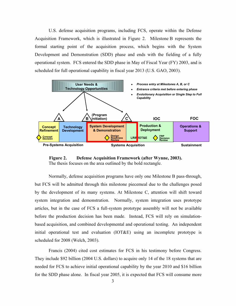
U.S. defense acquisition programs, including FCS, operate within the Defense
Acquisition Framework, which is illustrated in Figure 2. Milestone B represents the
formal starting point of the acquisition process, which begins with the System
Development and Demonstration (SDD) phase and ends with the fielding of a fully
operational system. FCS entered the SDD phase in May of Fiscal Year (FY) 2003, and is
scheduled for full operational capability in fiscal year 2013 (U.S. GAO, 2003).
IOCBA
Technology Development
System Development& Demonstration
Production & Deployment
Systems Acquisition
Operations & Support
C
User Needs &Technology Opportunities
Sustainment
Process entry at Milestones A, B, or CEntrance criteria met before entering phaseEvolutionary Acquisition or Single Step to Full Capability
FRP DecisionReview
FOC
LRIP/IOT&EDesignReadiness Review
Pre-Systems Acquisition
(ProgramInitiation)
Concept Refinement
ConceptDecision
Figure 2. Defense Acquisition Framework (after Wynne, 2003). The thesis focuses on the area outlined by the bold rectangle.
Normally, defense acquisition programs have only one Milestone B pass-through,
but FCS will be admitted through this milestone piecemeal due to the challenges posed
by the development of its many systems. At Milestone C, attention will shift toward
system integration and demonstration. Normally, system integration uses prototype
articles, but in the case of FCS a full-system prototype assembly will not be available
before the production decision has been made. Instead, FCS will rely on simulation-
based acquisition, and combined developmental and operational testing. An independent
initial operational test and evaluation (IOT&E) using an incomplete prototype is
scheduled for 2008 (Welch, 2003).
Francis (2004) cited cost estimates for FCS in his testimony before Congress.
They include $92 billion (2004 U.S. dollars) to acquire only 14 of the 18 systems that are
needed for FCS to achieve initial operational capability by the year 2010 and $16 billion
for the SDD phase alone. In fiscal year 2005, it is expected that FCS will consume more
4
than 50 percent of the U.S. Army budget for all programs in SDD phases, and over 30
percent of the total budget for research and development (R&D) and test and evaluation
(T&E) tasks.
The complexity of FCS and an aggressive developmental schedule introduce risks
into its acquisition program. At the start of the SDD phase in 2003 about three-quarters
of its critical technologies were classified as immature (Francis, 2004). FCS acquisition
planning is based extensively on developmental concurrency across the different phases
of the project. Francis (2004) outlines the myriad of tasks that must be coordinated in
order for this strategy to be successful:
• A specialized C4ISR network must be developed for FCS.
• Fourteen major weapon systems and platforms must be designed and integrated simultaneously with other systems, subject to physical limitations.
• At least 53 technologies that are considered critical to achieving required performance capabilities must be matured and integrated.
• At least 157 Army and joint-forces systems must also be adapted to interoperate with FCS, which will require the development of nearly a hundred new network interfaces.
• An estimated 34 million lines of software code will be required to operate FCS. This is nearly five times the software required for the Joint Strike Fighter, which had the largest software requirement of any Department of Defense acquisition prior to FCS.
It is difficult to ensure that the development of a new technology will be
completed within a specified time period. As a system of systems, FCS is especially
vulnerable to the cascading effects of schedule overruns from projects to follow-on tasks.
Francis (2004) observes that the completion of FCS as planned is unlikely given the
many opportunities for delay in development of its constituent systems. He estimates that
a one-year delay late in FCS development could add $4 billion to $5 billion to the total
cost. Non-budgetary costs, such as the effect on warfighting capability of not having a
fielded system on schedule, are more difficult to quantify but are no less important.
5
B. SCHEDULE OPTIONS AND SCHEDULE RISK The term schedule risk refers to the costs of schedule overruns balanced by their
likelihood of occurrence. Planners may be presented with a set of options for scheduling
the range of tasks that comprise a large acquisition project. These options must abide by
a common set of temporal and fiscal constraints. They should also reflect the inherent
uncertainty of the completion time of a developmental task. A rational planner seeks to
assess the schedule risks of each option, and to select the option that poses the least risk.
Significant knowledge demonstration often occurs late in development and early
in production of major defense acquisition programs (MDAPs), of which FCS is an
example. Integration of developed components into a system of systems has the highest
schedule risk. Welch (2003) observes that the unusual complexity of FCS exposes it to
higher integration schedule risk than normally expected of a MDAP. In particular, FCS
is susceptible to “late cycle churn” due to the anticipated need to fix problems discovered
late in development. Francis (2004) identifies the following factors that dispose FCS to
late cycle churn:
• Technology development that is expected to continue through to the production decision (Milestone C);
• Technology development that will still be ongoing at the design readiness review (DRR) in July 2006, putting at risk the stability of ongoing system integration;
• The planned move into production in December 2007 while technology development and system integration are continuing and the first prototypes are being delivered;
• The planned final production decision in November 2008 that will be made before some technologies will have reached their required maturation and an integrated system demonstration will remain to be done;
• The planned start of production delivery in early 2010 before the Army has completed the first full demonstration of FCS as an integrated system;
• The planned full rate production decision in mid-2013 while testing and demonstration are continuing.
The FCS Program Executive Office (PEO) has prepared a “baseline” project plan
for the SDD phase that governs current acquisition policy. Several alternate project plans
were developed by the General Accounting Office (U.S. GAO, 2003) to mitigate FCS
6
schedule risks. The baseline plan and two of the alternate plans proposed by GAO are
examined in this thesis. The first alternative is based on addressing risky technologies
prior to undertaking further development. The second alternative is focused on the
development of the C4ISR infrastructure prior to all other systems. Each of the three
plans is discussed separately below.
1. Baseline Plan The baseline plan develops all major sub-systems concurrently, rather than
developing one first to set the development context for follow-on systems. Details of the
baseline plan can be found in Appendix B. The FCS PEO has acknowledged that this
plan is ambitious, and that the program was not ready for system development and
demonstration when it was approved (Francis, 2004).
2. Alternate Plan 1 Alternate plan 1 modifies the baseline plan by first developing critical
technologies that are not at a production-suitable readiness level at the start of the SDD
phase. Most of the lower-risk FCS technologies have already been developed from early
proof of concept experiments to a prototype demonstration in test environments prior to
the SDD phase (Francis, 2004). For the purposes of this plan, prototypes must be
demonstrated in mission environment before it can be considered ready for integration
(Wynne, 2003). Risk-mitigation strategies have already been developed by the FCS PEO
for the high-risk technologies that are yet to demonstrate a prototype in a mission
environment (Welch, 2003). The duration of these mitigation tasks are listed in the
schedule for alternate plan 1, provided in Appendix B. Once risk mitigation activities are
complete, alternate plan 1 proceeds as scheduled for the baseline plan. The advantage of
this approach is that test and integration tasks occur later in the schedule, with reduced
schedule risk compared to the baseline plan.
7
3. Alternate Plan 2 Alternate plan 2 modifies the baseline plan by prioritizing the development of
C4ISR tasks before all others. The C4ISR components are believed to pose the greatest
schedule risks in FCS development due to the scope and complexity of their
requirements. Software engineering estimates for C4ISR components anticipate the need
for approximately 16 million lines of code, of which more than half will be new code
(Welch, 2003). This huge undertaking is vulnerable to cost and schedule overruns. By
placing early priority on these components, subsequent C4ISR test and integration tasks
should entail less risk than in the baseline plan. Full details of alternate plan 2 are in
Appendix B.
C. PURPOSE OF THESIS The purpose of this thesis is to schedule FCS tasks in the SDD phase to minimize
the total project duration, which is the elapsed time from the start of the first task to the
end of the last task. The last task is assumed to be achievement of the FCS initial
operational capability (IOC). Minimization is subject to periodic (annual) and overall
budget constraints, and to temporal ordering relationships among the tasks. Because all
schedules operate under a common set of constraints, minimization of the total project
duration is taken to be synonymous with minimization of schedule risk. Together, the
cost constraints, task network, and task duration attributes constitute data that are input to
the minimization procedure. Although the thesis is focused on applying this procedure to
FCS, by varying the inputs it can be applied to any scheduling problem of similar
structure.
Minimization of the project completion time falls within the scope of the
Resource Constrained Project Scheduling Problem (RCPSP), which has a long history in
operations research. Chapter II provides a brief review of the RCPSP literature for both
deterministic and random task durations. Task durations are modeled as random
variables, and an algorithm for solving the unconstrained scheduling problem is described
in Chapter III. In Chapter IV an integer linear program (ILP) is formulated for the
scheduling problem subject to budgetary constraints. Chapter IV also presents the annual
review simulation. The results of applying the ILP to nominal data for FCS tasks in the
8
SDD phase are presented in Chapter V. Conclusions and recommendations for further
research are discussed in Chapter VI.
Nominal FCS task information was provided by the Cost Analysis Improvement
Group (CAIG) of the Program Analysis and Evaluation (PA&E) branch of the Office of
the Secretary of Defense (OSD), who sponsored this thesis.
9
II. RELATED RESEARCH
A. THE RESOURCE-CONSTRAINED PROJECT SCHEDULING PROBLEM The Resource Constrained Project Scheduling Problem (RCPSP) is to find task
starting times that minimize the total project duration subject to resource and temporal
constraints. Tasks are configured in a network that defines precedence relationships.
Project duration is the length of the longest path through the network, which is also
known as the critical path. Minimization of this length is subject to time constraints on
tasks, and to resource constraints that can be formulated in a number of ways: on the
total cost of the project, on the annual costs of the project, etc. A review of methods for
solving formulations of the RCPSP can be found in Demeulemeester and Herroelen
(2002).
The use of linear programming to solve scheduling problems has a long history in
operations research (Bowman, 1958). ILP approaches followed with the pioneering work
of researchers including Senju (1968), and Pritsker, Watters and Wolfe (1969). The
RCPSP is known to be non-polynomial (NP)-hard in general, which suggests that
polynomial-time algorithms for solving this problem are unlikely to exist (Ullman, 1975).
Most algorithms use heuristics to reduce problem size and complexity prior to initiating
enumeration of feasible solutions. Integer linear programming (ILP) based on branch-
and-bound or other polyhedral-based techniques can then be used to identify the optimal
feasible solution.
Probabilistic modeling of task durations began to appear in the scheduling
literature in the late 1950s and 1960’s. During that time, the Program Evaluation and
Review Technique (PERT) and the Critical Path Method (CPM) were developed.
Seminal papers include Malcolm, Roseboom, Clark, and Fazar (1959) in which PERT
was first developed for the Polaris Fleet Ballistic Missile program, and Kelly (1961)
which provides much of the mathematical basis for its later use. CPM and PERT have
since combined to form a single method that is among the most widely used operations
research techniques in project management.
10
Drawbacks to PERT are that it does not allow for the inclusion of resource
constraints, and that it only considers the critical path formed when all tasks are fixed to
their mean duration (Weist, 1964). Significantly, a task not on the PERT critical path
using its mean duration may be on the critical path with positive probability when its
duration is treated as a random variable. PERT estimates of project duration are
generally optimistic. Fulkerson (1962) demonstrates this optimism using tasks that are
modeled as discrete random variables. He shows that PERT networks using only mean
durations always under-estimate the project finish time relative to treating the durations
as random variables.
Dodin (1984) reports upper and lower bounds on the project duration where task
durations are modeled as independent random variables. The independence assumption
is used to invoke the Central Limit Theorem to justify treating the project duration as
approximately normally distributed. While this assumption lends tractability, it is rarely
true in practice and it can give misleading results.
B. PROJECT SCHEDULING UNDER UNCERTAINTY A number of approaches have been developed for solving the RCPSP with
stochastic inputs. Seminal papers include Babbar, Tintner, and Heady (1955), Tintner
(1955), Tintner (1960), and Sengupta, Tintner, and Morrison (1963). Factors that
influence task duration are treated as random variables with distributions that may not be
completely known (Herroelen, Reyck, and Demeulemeester, 1998). These factors
include resources availability, scheduling of deliveries, modification of due dates, and
changes in project scope that may imply the cancellation or addition of future tasks
(Herroelen and Leus, 2004).
Although stochastic modeling lends greater realism to the RCPSP, it also
increases its analytical complexity. Instead of minimizing the project critical path length,
objectives such as minimizing the expected project critical path length are often
considered, or minimizing expected costs that include penalties for violating constraints
(Gutjahr, Stauss, and Wagner 2000).
11
With many interdependent tasks represented in a project network, and task
durations that are interdependent, the probability distribution of the total project duration
is difficult to characterize (Yang, Geunes, and O’Brien, 2001). An independence
assumption is often made to allow for tractable analysis, but as noted above this
assumption is not realistic. Nonetheless, some insight can be gained by adopting an
independence assumption. For example, in a deterministic setting an optimal schedule
may be found, but it may fail to be robust to small changes in its underlying data. An
optimal deterministic schedule typically has insufficient slack to remain optimal (or even
feasible) in an uncertain setting, and thus lacks robustness (Herroelen, 2004).
Introducing randomness in even a simplified manner can reveal this property.
In planning a large, multifaceted project, managers would want to have the
flexibility to change their scheduling decisions as the project evolves. Under full
dynamic scheduling this can be done during project execution, at decision points
consisting of the completion times of tasks (Igelmund and Radermacher, 1983). These
decision points are stochastic, because they depend on the task durations. This thesis
adopts a simpler form of dynamic scheduling whereby the decision points are the ends of
fiscal years, which are deterministic. All tasks that have not completed by the end of a
given fiscal year are eligible for rescheduling. This brings the realism of dynamic
scheduling into the RCPSP formulation that is described in Chapter IV.

12
THIS PAGE INTENTIONALLY LEFT BLANK
13
III. UNCONSTRAINED STOCHASTIC SCHEDULE ANALYSIS
This chapter presents an approach to studying the completion time of a project
with random task durations, but without resource constraints. Task durations are
modeled as independent random variables having three-parameter Weibull distributions.
Properties of the three-parameter Weibull distribution and a model selection procedure
that can be used to guide its application are presented in Section A. In a simulation
exercise a full set of task durations is generated, and an unconstrained reaching algorithm
is used to identify the completion time of the project, which is the longest path in a
network from the first to last task. This algorithm is described in Section B. The
simulation was coded in Java, which is presented in Appendix C.
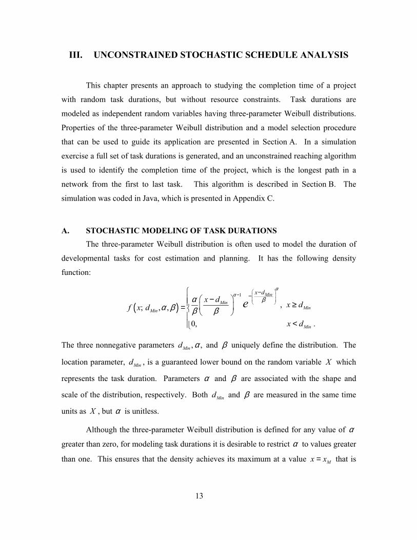
A. STOCHASTIC MODELING OF TASK DURATIONS The three-parameter Weibull distribution is often used to model the duration of
developmental tasks for cost estimation and planning. It has the following density
function:
( )1
,; , ,
0, .
MinMinMin
Min
Minx dx d x df x d
x d
eα
α
βαα β β β
−
−− − ≥ =
<
The three nonnegative parameters , ,Mind α and β uniquely define the distribution. The
location parameter, Mind , is a guaranteed lower bound on the random variable X which
represents the task duration. Parameters α and β are associated with the shape and
scale of the distribution, respectively. Both Mind and β are measured in the same time
units as X , but α is unitless.
Although the three-parameter Weibull distribution is defined for any value of α
greater than zero, for modeling task durations it is desirable to restrict α to values greater
than one. This ensures that the density achieves its maximum at a value Mx x= that is
14
strictly greater than Mind . The maximum likelhood value Mx is also known as the mode,
or most likely value, of the distribution.
Through proper selection of its parameters, the three-parameter Weibull
distribution can emulate intuitive features of task duration. For example, large deviations
from the norm are more common in the positive than in the negative direction, which is
reflected in the positive skewness of the three-parameter Weibull distribution. And, many
developmental tasks cannot finish in less than a minimum time, which is represented
by Mind .
Selection of a three-parameter Weibull distribution to model task duration is
equivalent to specifying its parameters. This specification is largely subjective,
depending on the judgment of the planner for the task in question. Miller (2003)
describes a convenient procedure for specifying the parameters of a three-parameter
Weibull distribution from intuitive features of the task duration. The analyst needs to
provide the following information:
• A value for the duration mode, Mx ;
• Categorization of the risk level as High, Medium, or Low.
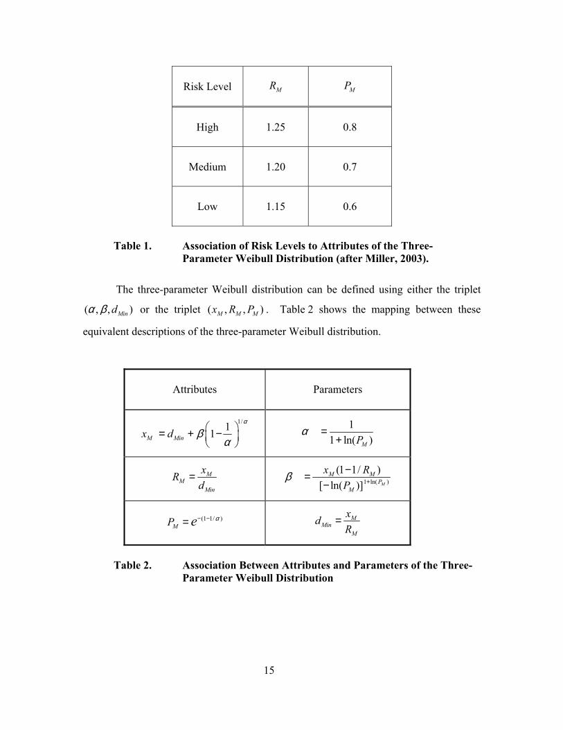
Each risk level is assigned to fixed values of two attributes of the task duration,
which together with Mx are sufficient to determine all three parameters of the model.
Attribute /M M MinR x d= is the ratio of the mode to the guaranteed duration, and
( )M MP P X x= > is the probability that the duration exceeds the mode. Table 1 shows
the association of risk levels to values of these two attributes. The values shown in
Table 1 were chosen by Miller (2003) to reflect historical evidence of task durations in
cost estimation. He suggest using the following guidelines for selection of the schedule
risk level:
• High risk for unprecedented tasks;
• Medium risk for development and some integration tasks;
• Low risk for routine tasks that are well understood.
15
Risk Level MR MP
High 1.25 0.8
Medium 1.20 0.7
Low 1.15 0.6
Table 1. Association of Risk Levels to Attributes of the Three-
Parameter Weibull Distribution (after Miller, 2003).
The three-parameter Weibull distribution can be defined using either the triplet
( , , )Mindα β or the triplet ( , , )M M Mx R P . Table 2 shows the mapping between these
equivalent descriptions of the three-parameter Weibull distribution.
Attributes Parameters
1/11M Minx dα
βα
= + −
1
1 ln( )MPα =
+
MM
Min
xRd
= 1 ln( )
(1 1/ )[ ln( )] M
M MP
M
x RP
β +
−=−
(1 1/ )MP e α− −= M
MinM
xdR
=
Table 2. Association Between Attributes and Parameters of the Three-
Parameter Weibull Distribution

16
Example. A task is identified as having medium risk, and its most likely duration is
36Mx = months. From Table 1, 1.20MR = and 0.7MP = . The model parameters are
found using the mapping in Table 2:
1 ln(0.7)
1 36(1 1/1.20) 361.554, 11.65, 30.0 .1 ln(0.7) [ ln(0.7)] 1.20Mindα β +
−= = = = = =+ −
Simulation of three-parameter Weibull variates is easily done by applying the
inverse cumulative distribution function (CDF) to uniform variates. If U has a uniform
distribution on the interval [0,1] , then X has a three-parameter Weibull distribution with
parameters ( , , )Mindα β , where
1/[ ln( )] .MinX d U αβ= + −
A drawback to the use of the three-parameter Weibull distribution to model task
durations is that its upper bound is infinite. Not only does this fail to reflect practical
realities of project development, it also creates problems for simulation of task durations
under budget constraints, which is expored in Chapter IV. To ensure that a task finishes
within a fixed allotment of time, the thesis research uses three-parameter Weibull
distributions that are truncated at the 90th percentile. The truncation point, Maxd , is the
maximum allowable duration. It is calculated as follows:
1/[ ln(0.1)] .Max Mind d αβ= + −
Variates from the truncated distribution are generated as
1/[ ln(1 .9 )] .MinX d U αβ= + − −
B. THE UNCONSTRAINED REACHING ALGORITHM The unconstrained reaching algorithm searches over the schedule to identify the
completion time of the project, given a task network with fixed durations. The
completion time is characterized by the length of the longest path from the start to finish
nodes in the network. The unconstrained reaching algorithm, shown in Figure 3, is one
17
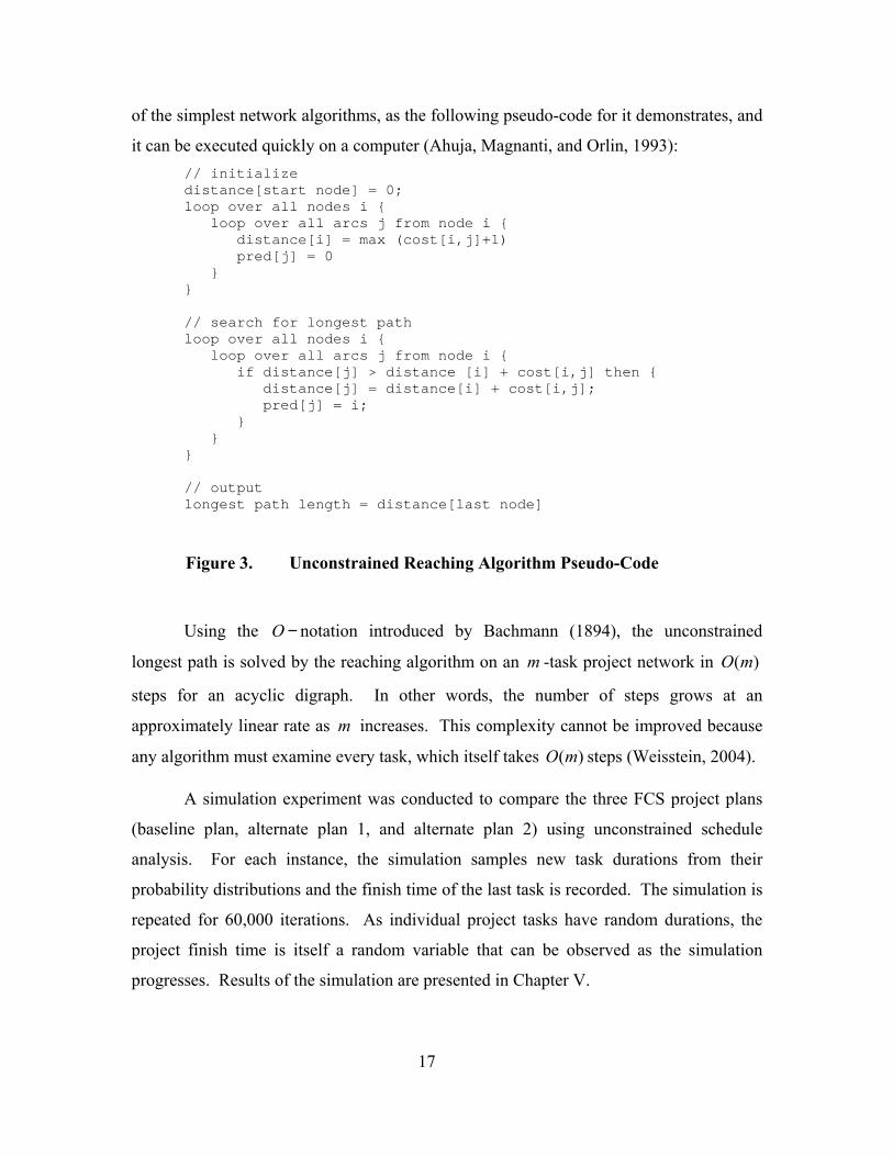
of the simplest network algorithms, as the following pseudo-code for it demonstrates, and
it can be executed quickly on a computer (Ahuja, Magnanti, and Orlin, 1993): // initialize distance[start node] = 0; loop over all nodes i { loop over all arcs j from node i { distance[i] = max (cost[i,j]+1) pred[j] = 0 } } // search for longest path loop over all nodes i { loop over all arcs j from node i { if distance[j] > distance [i] + cost[i,j] then { distance[j] = distance[i] + cost[i,j]; pred[j] = i; } } } // output longest path length = distance[last node] Figure 3. Unconstrained Reaching Algorithm Pseudo-Code
Using the O − notation introduced by Bachmann (1894), the unconstrained
longest path is solved by the reaching algorithm on an m -task project network in ( )O m
steps for an acyclic digraph. In other words, the number of steps grows at an
approximately linear rate as m increases. This complexity cannot be improved because
any algorithm must examine every task, which itself takes ( )O m steps (Weisstein, 2004).
A simulation experiment was conducted to compare the three FCS project plans
(baseline plan, alternate plan 1, and alternate plan 2) using unconstrained schedule
analysis. For each instance, the simulation samples new task durations from their
probability distributions and the finish time of the last task is recorded. The simulation is
repeated for 60,000 iterations. As individual project tasks have random durations, the
project finish time is itself a random variable that can be observed as the simulation
progresses. Results of the simulation are presented in Chapter V.

18
THIS PAGE INTENTIONALLY LEFT BLANK
19
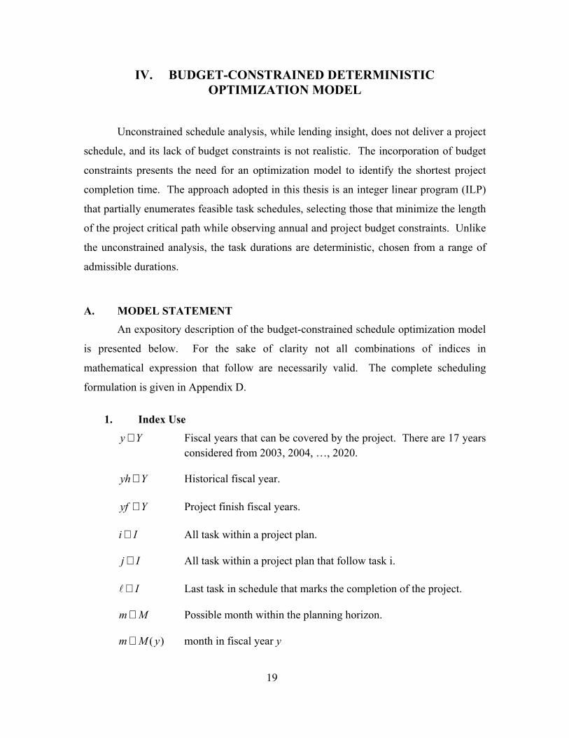
IV. BUDGET-CONSTRAINED DETERMINISTIC OPTIMIZATION MODEL
Unconstrained schedule analysis, while lending insight, does not deliver a project
schedule, and its lack of budget constraints is not realistic. The incorporation of budget
constraints presents the need for an optimization model to identify the shortest project
completion time. The approach adopted in this thesis is an integer linear program (ILP)
that partially enumerates feasible task schedules, selecting those that minimize the length
of the project critical path while observing annual and project budget constraints. Unlike
the unconstrained analysis, the task durations are deterministic, chosen from a range of
admissible durations.
A. MODEL STATEMENT An expository description of the budget-constrained schedule optimization model
is presented below. For the sake of clarity not all combinations of indices in
mathematical expression that follow are necessarily valid. The complete scheduling
formulation is given in Appendix D.
1. Index Use
y Y∈ Fiscal years that can be covered by the project. There are 17 years considered from 2003, 2004, …, 2020.
yh Y∈ Historical fiscal year. yf Y∈ Project finish fiscal years. i I∈ All task within a project plan. j I∈ All task within a project plan that follow task i.
I∈ Last task in schedule that marks the completion of the project.
m M∈ Possible month within the planning horizon.
( )m M y∈ month in fiscal year y
20
i is S M∈ ⊆ Start month for task i
i id D∈ Task i duration in months. 1 i ip d≤ ≤ Period of ongoing task i.
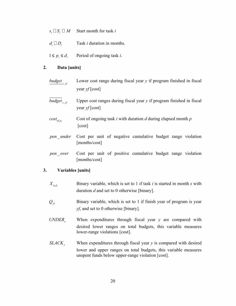
2. Data [units]
,y yfbudget Lower cost range during fiscal year y if program finished in fiscal
year yf [cost]
,y yfbudget Upper cost ranges during fiscal year y if program finished in fiscal year yf [cost]
i iid pcost Cost of ongoing task i with duration d during elapsed month p
[cost]
_pen under Cost per unit of negative cumulative budget range violation [months/cost]
_pen over Cost per unit of positive cumulative budget range violation
[months/cost]
3. Variables [units]
i iis dX Binary variable, which is set to 1 if task i is started in month s with duration d and set to 0 otherwise [binary].
yfQ Binary variable, which is set to 1 if finish year of program is year yf, and set to 0 otherwise [binary].
yUNDER When expenditures through fiscal year y are compared with
desired lower ranges on total budgets, this variable measures lower-range violations [cost].
ySLACK When expenditures through fiscal year y is compared with desired
lower and upper ranges on total budgets, this variable measures unspent funds below upper-range violation [cost].
21
yOVER When expenditures through fiscal year y are compared with desired upper ranges on total budgets, this variable measures upper-range violations [cost].
4. Formulation
( )
( )
, ,
,
( 1), , , ,
,
( 1) _ _ ( 1)
1
, , ( 3)
1 4
. . ( 2)i i
i i
i i i i
i i
X QUNDERSLACKOVER
s d y ys d y
is ds d
yf
yfyf
id m s is dyf m i s d
yh
s d
y y y
s d X pen underUNDER pen over OVER F
X
Q yf s d F
Q F
cost X
budget
MIN
s t i I F
X
UNDER SLACK OVER− +
+ − + +
=
≤ ∀
=
∀ ∈
+ + −
=
∑ ∑
∑
∑
∑
( )
( )
{ }
,
, ,,
,
,
0,1
0; 0; 0
( 5)
( 6)
( , ), ( 7)
{0,1} , , ( 8)
( 9)
( 10)
i i
i ij j
i i
yfyh yf
yfyh yf yh yfyh yf
is d js d
yf
yf
y
jjs d
i iis d
y y y
budget budget Q
X
yf
Q y F
SLACK y Y F
X i j s d F
X i s d F
Q F
UNDER SLACK OVER y F
−
∈ ∀
≥ ≥ ≥
∀
≤ ∀ ∈
≥ ∀ ∀
∈ ∀
∀
∑
∑
∑
22
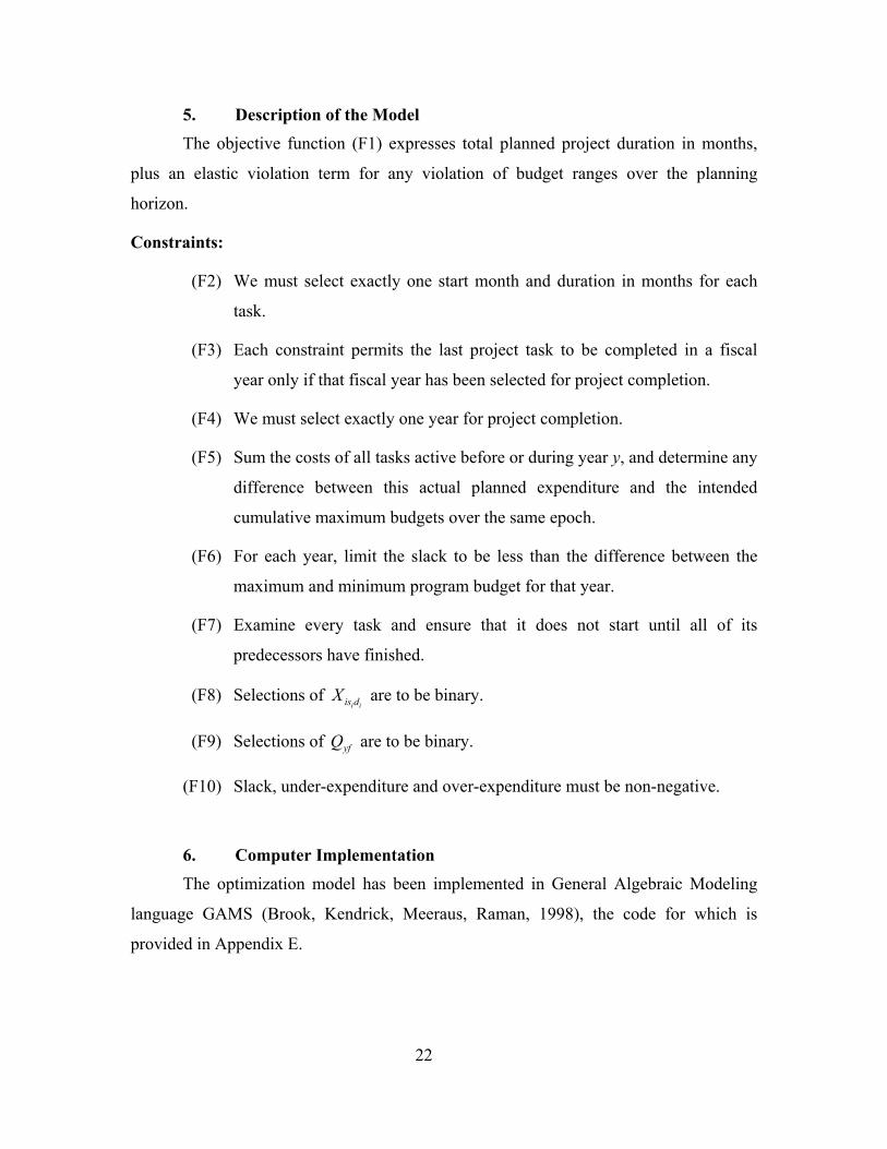
5. Description of the Model
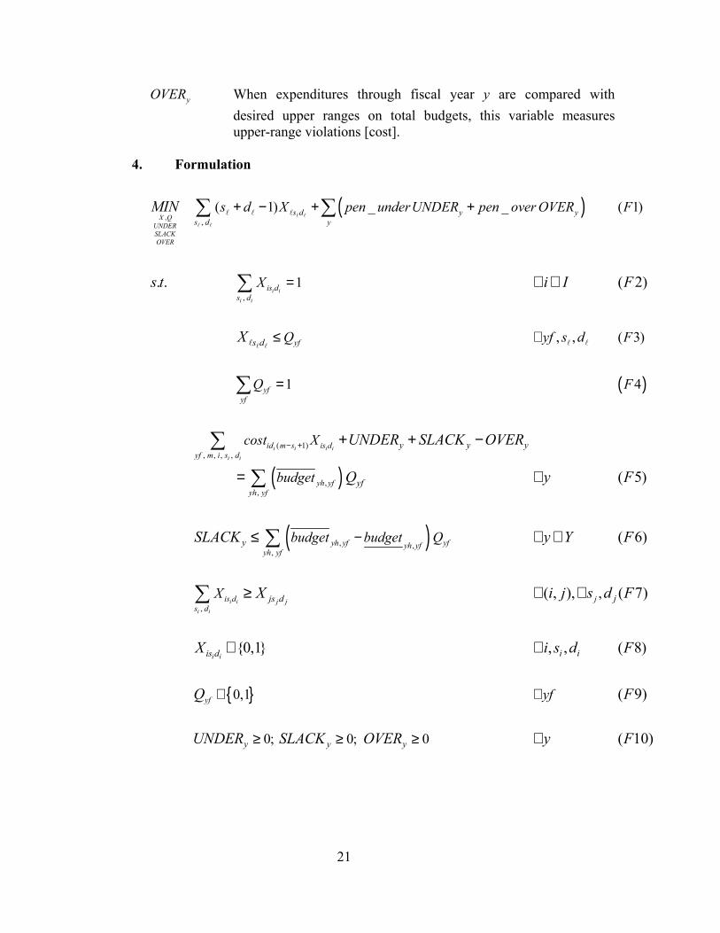
The objective function (F1) expresses total planned project duration in months,
plus an elastic violation term for any violation of budget ranges over the planning
horizon.
Constraints:
(F2) We must select exactly one start month and duration in months for each
task.
(F3) Each constraint permits the last project task to be completed in a fiscal
year only if that fiscal year has been selected for project completion.
(F4) We must select exactly one year for project completion.
(F5) Sum the costs of all tasks active before or during year y, and determine any
difference between this actual planned expenditure and the intended
cumulative maximum budgets over the same epoch.
(F6) For each year, limit the slack to be less than the difference between the
maximum and minimum program budget for that year.
(F7) Examine every task and ensure that it does not start until all of its
predecessors have finished.
(F8) Selections of i iis dX are to be binary.
(F9) Selections of yfQ are to be binary.
(F10) Slack, under-expenditure and over-expenditure must be non-negative.
6. Computer Implementation The optimization model has been implemented in General Algebraic Modeling
language GAMS (Brook, Kendrick, Meeraus, Raman, 1998), the code for which is
provided in Appendix E.
23
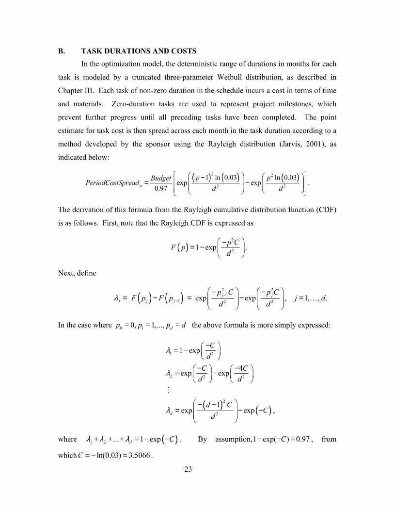
B. TASK DURATIONS AND COSTS
In the optimization model, the deterministic range of durations in months for each
task is modeled by a truncated three-parameter Weibull distribution, as described in
Chapter III. Each task of non-zero duration in the schedule incurs a cost in terms of time
and materials. Zero-duration tasks are used to represent project milestones, which
prevent further progress until all preceding tasks have been completed. The point
estimate for task cost is then spread across each month in the task duration according to a
method developed by the sponsor using the Rayleigh distribution (Jarvis, 2001), as
indicated below:
( ) ( ) ( )2 2
2 2
1 ln 0.03 ln 0.03exp exp .
0.97p
p pBudgetPeriodCostSpreadd d
− = −
The derivation of this formula from the Rayleigh cumulative distribution function (CDF)
is as follows. First, note that the Rayleigh CDF is expressed as
( )2
21 exp .p CF pd
−= −
Next, define
( ) ( )2 2
11 2 2exp exp , 1, , .j j
j j j
p C p CF p F p j d
d dλ −
−
− −= − = − =
…
In the case where 0 10, 1,..., dp p p d= = = the above formula is more simply expressed:
( ) ( )
1 2
2 2 2
2
2
1 exp
4exp exp
1exp exp ,d
Cd
C Cd d
d CC
d
λ
λ
λ
− = −
− − = −
− −= − −
where ( )1 2 ... 1 expd Cλ λ λ+ + + = − − . By assumption,1 exp( ) 0.97C− − = , from
which ln(0.03) 3.5066C = − = .
24
This method of spreading task costs over the months of its duration using a
Rayleigh distribution is widely used in budget phasing by the research sponsor, and is an
attempt to model historical experience with program expenditure (Jarvis, 2001). This is
in contrast to most scheduling approaches that assume task budgets are expended at a
uniform rate throughout the task duration.
C. PROJECT BUDGET
Upper and lower limits of the overall planned project budget must be estimated
for each fiscal year of the project duration. Separate estimates must be prepared for every
feasible project finish year. The same method, based on the Rayleigh distribution, is used
for spreading task costs over the desired project duration.
Over-expenditure or under-expenditure is permitted in the model, but is penalized.
To minimize penalties, it is desirable that in following periods corrections are made to
slow progress and recover from over-spending, or allow more tasks to occur in the case
of under-spending.
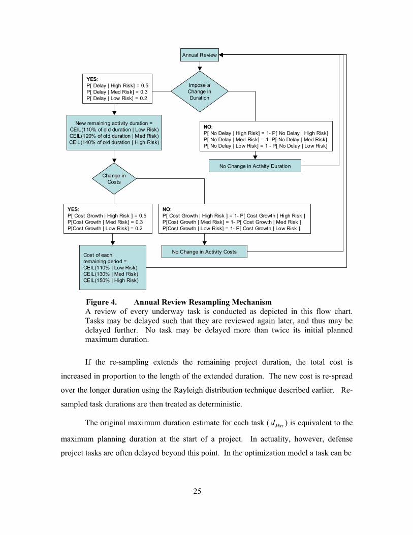
D. SIMULATION OF ANNUAL REVIEWS
The budget-constrained, deterministic project schedule optimization is subjected
to annual reviews. A simulation is used at the start of each fiscal year of the project to
resample parameters for tasks underway and not yet completed. The idea is to capture
the unpredictable nature of tasks’ completion times. Tasks planned further into the future
are more likely to require changes to their schedules. Moreover, if future tasks plan to
use advanced technologies (some of which are still in development) then such changes
are almost certain (Francis, 2004).
The initial solution, at time zero, is equivalent to the optimal schedule with no re-
sampling. At each subsequent time step the program optimally schedules underway tasks
given that decisions for completed tasks have already been made. As each fiscal year
boundary is reached a “program review” is conducted. Tasks already started and still in
progress are re-sampled to determine if the remaining task durations and costs will be
greater than that planned, or remain unchanged. The flowchart in Figure 4 shows the
annual review re-sampling mechanism.
25
Annual Review
New remaining activity duration =CEIL(110% of old duration | Low Risk)CEIL(120% of old duration | Med Risk)CEIL(140% of old duration | High Risk)
Impose aChange inDuration
No Change in Activity Duration
YES: P[ Delay | High Risk] = 0.5P[ Delay | Med Risk] = 0.3P[ Delay | Low Risk] = 0.2
NO: P[ No Delay | High Risk] = 1- P[ No Delay | High Risk]P[ No Delay | Med Risk] = 1- P[ No Delay | Med Risk]P[ No Delay | Low Risk] = 1 - P[ No Delay | Low Risk]
Change inCosts
Cost of each remaining period = CEIL(110% | Low Risk)CEIL(130% | Med Risk)CEIL(150% | High Risk)
YES: P[ Cost Growth | High Risk ] = 0.5P[Cost Growth | Med Risk] = 0.3P[Cost Growth | Low Risk] = 0.2
No Change in Activity Costs
NO: P[ Cost Growth | High Risk ] = 1- P[ Cost Growth | High Risk ]P[Cost Growth | Med Risk] = 1- P[ Cost Growth | Med Risk ]P[Cost Growth | Low Risk] = 1- P[ Cost Growth | Low Risk ]
Figure 4. Annual Review Resampling Mechanism A review of every underway task is conducted as depicted in this flow chart. Tasks may be delayed such that they are reviewed again later, and thus may be delayed further. No task may be delayed more than twice its initial planned maximum duration.
If the re-sampling extends the remaining project duration, the total cost is
increased in proportion to the length of the extended duration. The new cost is re-spread
over the longer duration using the Rayleigh distribution technique described earlier. Re-
sampled task durations are then treated as deterministic.
The original maximum duration estimate for each task ( Maxd ) is equivalent to the
maximum planning duration at the start of a project. In actuality, however, defense
project tasks are often delayed beyond this point. In the optimization model a task can be
26
delayed up to twice its original planned maximum duration. This represents an absolute
upper bound beyond which a task would not be delayed further as it would probably be
cancelled.
If the ensuing project plan takes longer than originally planned due to budget
shortfalls, a decision will need to be made whether to seek a supplemental appropriation,
or to continue spending under the current budget. As one of the inputs, a vector of
project budgets has been prepared for each possible year of project completion, which is
presented in Chapter VI.
Annual reviews are repeated through the end of the planning horizon or project
completion. The model does not make provision for the conditioning of cost or duration
on any successor task as a result of a predecessor taking longer than planned. Such
condition can be accommodated, but data on dependencies between tasks are not
available.
The cumulative effect of annual reviews on project duration is shown in Figure 5
for a simple four-task project. Under scenario 3, which has no annual reviews, the
project finishes in about three and a half years. Under scenario 4, which has annual
reviews until the project is completed, the project finishes in about five years. At the first
annual review one underway task is considered for cost and/or schedule growth, and is
delayed by about one-quarter year. Tasks that have not started must be rescheduled to
account for the later finish of the first task, which increases the projected duration of the
project to almost four years. At the second annual review, the first task has finished and
the second and third tasks are underway. Rescheduling decisions concerning these two
underway tasks delay the project even further. These delays accumulate over the
succession of annual reviews, which explains the longer project duration under scenario 4
vis-à-vis scenario 3. The effect of multiple annual reviews in this example is
representative of schedule growth resulting from such factors as annual budget
reallocations, contract disputes and defects with product performance.

27
Figure 5. Abstraction of the Moving Window for the Simulated RCPSP
with Annual Review Start of the project is signified by and project end by . Scenario 3 is the optimal deterministic schedule prior to any annual reviews. Scenario 4 uses the ILP to optimally reschedule projects after each annual review. Project end times are delayed as the reviews progress. Tasks marked with diagonal stripes are un-started so are not subject to any annual reviews. Gray tasks are underway at the time of the review, and may be subject to cost and/or schedule growth. Black tasks have finished and past scheduling decisions are fixed for all future annual reviews. The large shaded boxes show progress of annual reviews through time.
Schedule slippage of underway tasks expresses some of the uncertainty of real-
world projects. As the project schedule is re-optimized in each succeeding annual review
using different task costs, it is possible to obtain estimates of the probability distributions
of outcomes such as project duration and cost. Competing schedule plans can then be
compared to infer which has the best risk profile at any given time.
Fiscal Year 1 2 3 4 5
TS
Without Annual Review
Simulation
TS
TS
T S
TS
First Annual Review
Second Annual Review
Third Annual Review
Fourth & Final Annual Review
S T
Scen
ario
4: I
LP w
ith A
nnua
l Rev
iew
s Sc
enar
io 3
: ILP

28
THIS PAGE INTENTIONALLY LEFT BLANK
29
V. EXPERIMENTAL RESULTS
Information obtained from our sponsor on tasks related to FCS acquisition is
reported in Appendix B. Using this data, results are presented for the unconstrained
schedule analysis described in Chapter III (scenarios 1 and 2), and for the resource-
constrained schedule optimization described in Chapter IV (scenarios 3 and 4). The three
schedule plans that are considered (baseline plan, alternate plan 1, and alternate plan 2)
are described in Chapter I.
The aim is to identify differences between the three plans to produce a ranking
based on completion time: a faster schedule is preferable to a slower one. Because much
of the data on FCS are either classified or proprietary, the sponsor supplied hypothetical
information, which is sufficient to demonstrate concepts described in the thesis. Where
omissions existed, reasonable assumptions were made.
A. FCS INPUT DATA In optimization scenarios 3 and 4, annual expenditures are constrained to fall
within budget ranges. The ranges used in the experiment are based on a FCS project cost
estimate of approximately $20 billion developed from public source material obtained
from the research sponsor. This cost estimate covers the SDD phase and early production
of FCS, and is based on starting in 2003 and ending in 2012. Using the Rayleigh cost-
spread formula presented in Chapter IV, this cost estimate is allocated on an annual basis
from 2003 to the projected year of completion. A collection of annual budgets is called a
“project budget”. A separate project budget is required for each feasible completion year
ranging from 2010 to 2016.
For each year of completion after 2012 the cost estimate is increased by 0.5
percent compounded annually. This inflation factor reflects, on a percentage basis, the
estimated cost increase of $4 billion to $5 billion reported by Francis (2004) for a one-
year delay in completion of FCS. Conversely, planning to accelerate the pace of work to
complete the project one year early is assumed to require an increased budget of 0.2
percent (Lee, 1997).
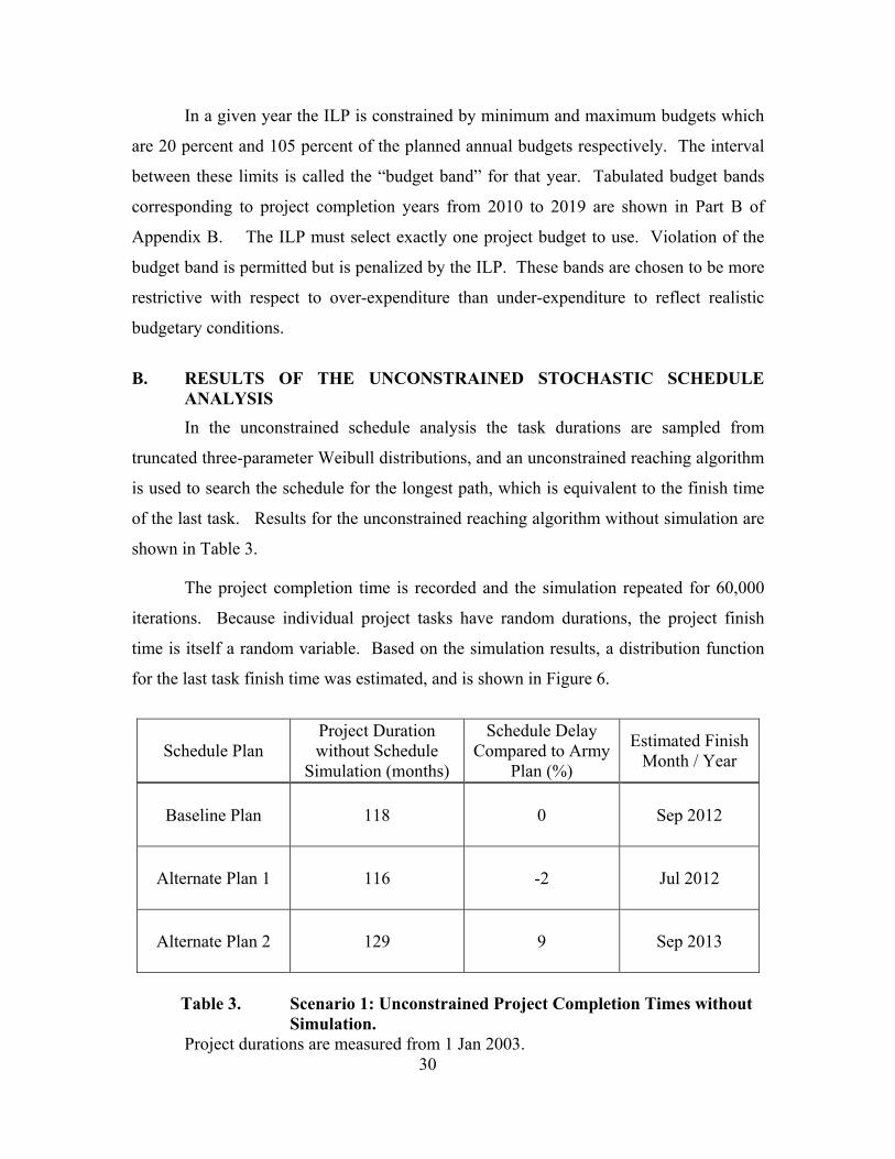
30
In a given year the ILP is constrained by minimum and maximum budgets which
are 20 percent and 105 percent of the planned annual budgets respectively. The interval
between these limits is called the “budget band” for that year. Tabulated budget bands
corresponding to project completion years from 2010 to 2019 are shown in Part B of
Appendix B. The ILP must select exactly one project budget to use. Violation of the
budget band is permitted but is penalized by the ILP. These bands are chosen to be more
restrictive with respect to over-expenditure than under-expenditure to reflect realistic
budgetary conditions.
B. RESULTS OF THE UNCONSTRAINED STOCHASTIC SCHEDULE
ANALYSIS
In the unconstrained schedule analysis the task durations are sampled from
truncated three-parameter Weibull distributions, and an unconstrained reaching algorithm
is used to search the schedule for the longest path, which is equivalent to the finish time
of the last task. Results for the unconstrained reaching algorithm without simulation are
shown in Table 3.
The project completion time is recorded and the simulation repeated for 60,000
iterations. Because individual project tasks have random durations, the project finish
time is itself a random variable. Based on the simulation results, a distribution function
for the last task finish time was estimated, and is shown in Figure 6.
Schedule Plan Project Duration without Schedule
Simulation (months)
Schedule Delay Compared to Army
Plan (%)
Estimated Finish Month / Year
Baseline Plan 118 0 Sep 2012
Alternate Plan 1 116 -2 Jul 2012
Alternate Plan 2 129 9 Sep 2013
Table 3. Scenario 1: Unconstrained Project Completion Times without
Simulation. Project durations are measured from 1 Jan 2003.
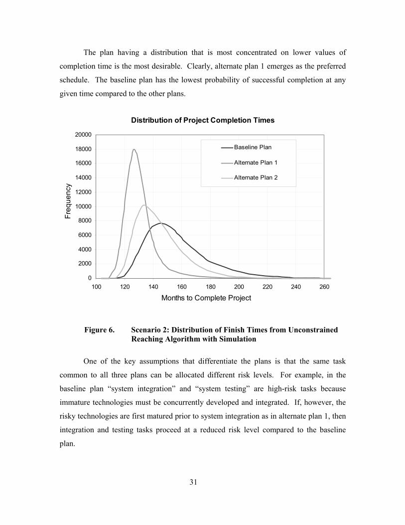
31
The plan having a distribution that is most concentrated on lower values of
completion time is the most desirable. Clearly, alternate plan 1 emerges as the preferred
schedule. The baseline plan has the lowest probability of successful completion at any
given time compared to the other plans.
Distribution of Project Completion Times
0
2000
4000
6000
8000
10000
12000
14000
16000
18000
20000
100 120 140 160 180 200 220 240 260
Months to Complete Project
Freq
uenc
y
Baseline Plan
Alternate Plan 1
Alternate Plan 2
Figure 6. Scenario 2: Distribution of Finish Times from Unconstrained
Reaching Algorithm with Simulation
One of the key assumptions that differentiate the plans is that the same task
common to all three plans can be allocated different risk levels. For example, in the
baseline plan “system integration” and “system testing” are high-risk tasks because
immature technologies must be concurrently developed and integrated. If, however, the
risky technologies are first matured prior to system integration as in alternate plan 1, then
integration and testing tasks proceed at a reduced risk level compared to the baseline
plan.
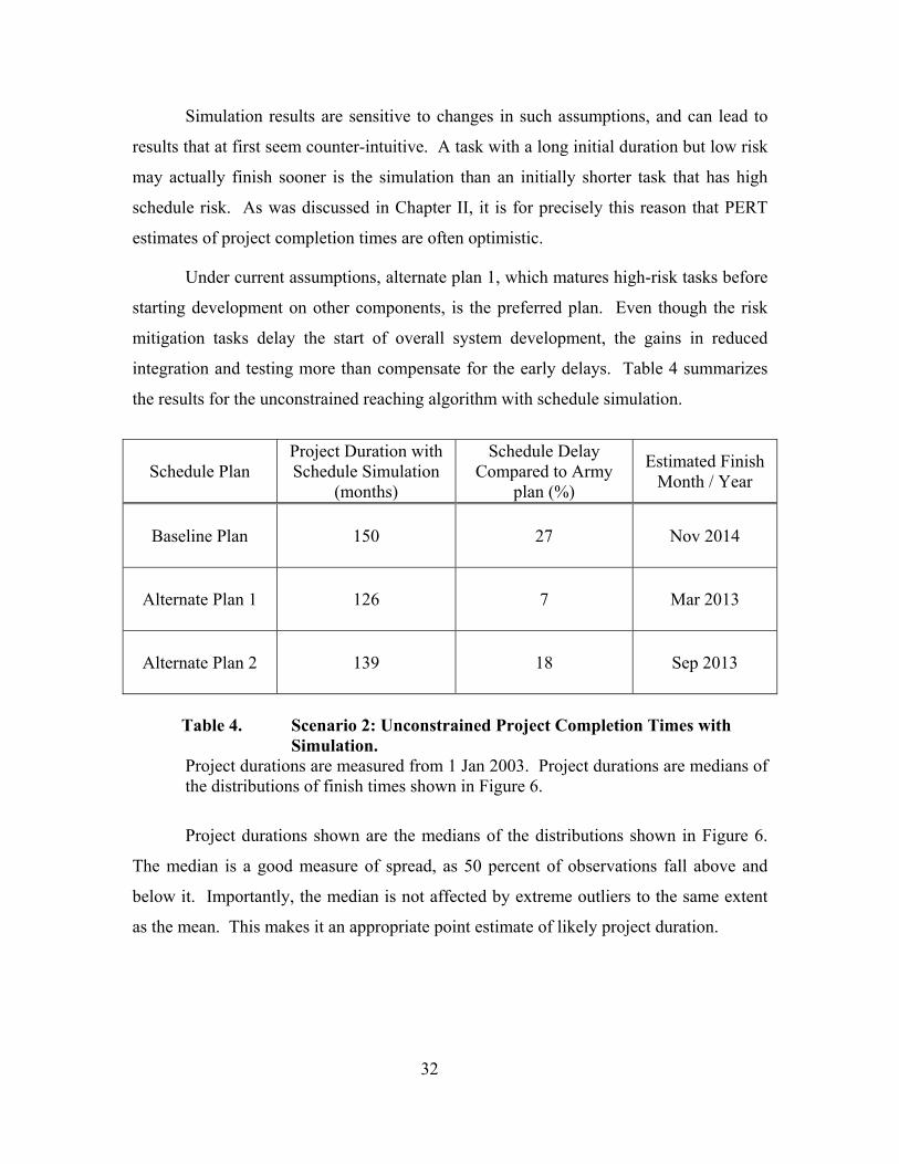
32
Simulation results are sensitive to changes in such assumptions, and can lead to
results that at first seem counter-intuitive. A task with a long initial duration but low risk
may actually finish sooner is the simulation than an initially shorter task that has high
schedule risk. As was discussed in Chapter II, it is for precisely this reason that PERT
estimates of project completion times are often optimistic.
Under current assumptions, alternate plan 1, which matures high-risk tasks before
starting development on other components, is the preferred plan. Even though the risk
mitigation tasks delay the start of overall system development, the gains in reduced
integration and testing more than compensate for the early delays. Table 4 summarizes
the results for the unconstrained reaching algorithm with schedule simulation.
Schedule Plan Project Duration with Schedule Simulation
(months)
Schedule Delay Compared to Army
plan (%)
Estimated Finish Month / Year
Baseline Plan 150 27 Nov 2014
Alternate Plan 1 126 7 Mar 2013
Alternate Plan 2 139 18 Sep 2013
Table 4. Scenario 2: Unconstrained Project Completion Times with
Simulation. Project durations are measured from 1 Jan 2003. Project durations are medians of the distributions of finish times shown in Figure 6.
Project durations shown are the medians of the distributions shown in Figure 6.
The median is a good measure of spread, as 50 percent of observations fall above and
below it. Importantly, the median is not affected by extreme outliers to the same extent
as the mean. This makes it an appropriate point estimate of likely project duration.
33
C. RESULTS OF THE BUDGET-CONSTRAINED DETERMINISTIC OPTIMIZATION ANALYSIS
The optimization model finds the most-compressed schedule that satisfies the
overall project budget selected by the optimal project completion year. Penalized
cumulative elastic budget constraints on the objective function allow for over-expenditure
in any particular annual project budget provided there is a compensating under-
expenditure in a later period.
The ILP balances the cost of taking longer to finish the project while strictly
observing budget constraints, with penalties incurred by adopting a shorter schedule but
exceeding annual budgets. Typically the latter option is favored by the ILP. As a result,
the project expenditure profile does not follow that projected by the Rayleigh distribution
of the budget.
In the annual review simulation, the costs and durations of tasks underway at each
annual review are subject to growth. This exogenously changes the data, and the ILP
must be re-solved in order to optimally re-schedule future tasks. As start time and
duration decisions for completed tasks are already fixed, and start times for underway
tasks are already fixed, re-scheduling future tasks is the only significant source of
flexibility. As the program nears completion, and the number of future tasks nears zero,
flexibility is nearly lost and the program must carry on as best as possible given past
scheduling decisions.
1. Scenario 3: Deterministic Model without Annual Review Simulation
The Army had planned to reach a key FCS completion milestone (fielding a unit
of action) by the end of September 2012. Results of applying the optimization model
without the annual review simulation are shown in Table 5. These completion times are
the fastest possible budget-constrained finish times as no random task delays are
imposed. These effectively form a lower bound on project completion time. Each of the
three plans induces a different expenditure profile, as discussed separately below.
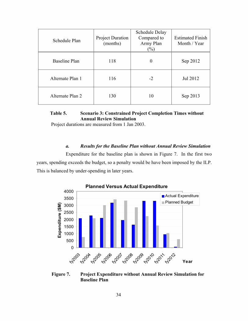
34
Schedule Plan Project Duration (months)
Schedule Delay Compared to Army Plan
(%)
Estimated Finish Month / Year
Baseline Plan 118 0 Sep 2012
Alternate Plan 1 116 -2 Jul 2012
Alternate Plan 2 130 10 Sep 2013
Table 5. Scenario 3: Constrained Project Completion Times without
Annual Review Simulation Project durations are measured from 1 Jan 2003.
a. Results for the Baseline Plan without Annual Review Simulation
Expenditure for the baseline plan is shown in Figure 7. In the first two
years, spending exceeds the budget, so a penalty would be have been imposed by the ILP.
This is balanced by under-spending in later years.
Planned Versus Actual Expenditure
0500
100015002000
2500300035004000
fy200
3
fy200
4
fy200
5
fy200
6
fy200
7
fy200
8
fy200
9
fy201
0
fy201
1
fy201
2Year
Expe
nditu
re ($
M)
Actual ExpenditurePlanned Budget
Figure 7. Project Expenditure without Annual Review Simulation for
Baseline Plan
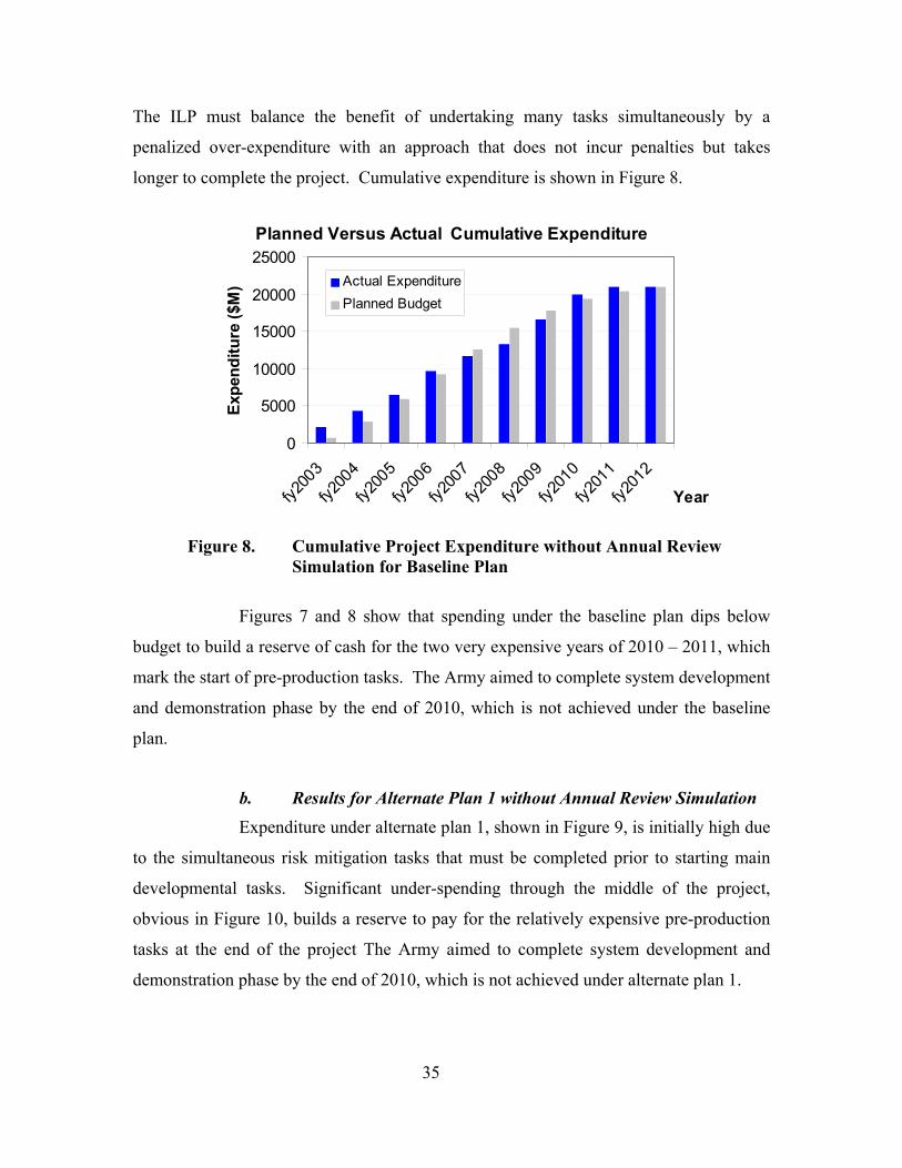
35
The ILP must balance the benefit of undertaking many tasks simultaneously by a
penalized over-expenditure with an approach that does not incur penalties but takes
longer to complete the project. Cumulative expenditure is shown in Figure 8.
Planned Versus Actual Cumulative Expenditure
0
5000
10000
15000
20000
25000
fy200
3
fy200
4
fy200
5
fy200
6
fy200
7
fy200
8
fy200
9
fy201
0
fy201
1
fy201
2
Year
Expe
nditu
re ($
M) Actual Expenditure
Planned Budget
Figure 8. Cumulative Project Expenditure without Annual Review
Simulation for Baseline Plan
Figures 7 and 8 show that spending under the baseline plan dips below
budget to build a reserve of cash for the two very expensive years of 2010 – 2011, which
mark the start of pre-production tasks. The Army aimed to complete system development
and demonstration phase by the end of 2010, which is not achieved under the baseline
plan.
b. Results for Alternate Plan 1 without Annual Review Simulation
Expenditure under alternate plan 1, shown in Figure 9, is initially high due
to the simultaneous risk mitigation tasks that must be completed prior to starting main
developmental tasks. Significant under-spending through the middle of the project,
obvious in Figure 10, builds a reserve to pay for the relatively expensive pre-production
tasks at the end of the project The Army aimed to complete system development and
demonstration phase by the end of 2010, which is not achieved under alternate plan 1.
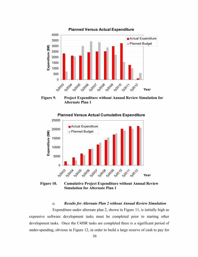
36
Planned Versus Actual Expenditure
0
500
1000
1500
2000
2500
3000
3500
4000
fy2003
fy2004
fy2005
fy2006
fy2007
fy2008
fy2009
fy2010
fy2011
fy2012
Year
Expe
nditu
re ($
M)
Actual ExpenditurePlanned Budget
Figure 9. Project Expenditure without Annual Review Simulation for
Alternate Plan 1
Planned Versus Actual Cumulative Expenditure
0
5000
10000
15000
20000
25000
fy2003
fy2004
fy2005
fy2006
fy2007
fy2008
fy2009
fy2010
fy2011
fy2012
Year
Expe
nditu
re ($
M)
Actual ExpenditurePlanned Budget
Figure 10. Cumulative Project Expenditure without Annual Review
Simulation for Alternate Plan 1
c. Results for Alternate Plan 2 without Annual Review Simulation
Expenditure under alternate plan 2, shown in Figure 11, is initially high as
expensive software development tasks must be completed prior to starting other
development tasks. Once the C4ISR tasks are completed there is a significant period of
under-spending, obvious in Figure 12, in order to build a large reserve of cash to pay for
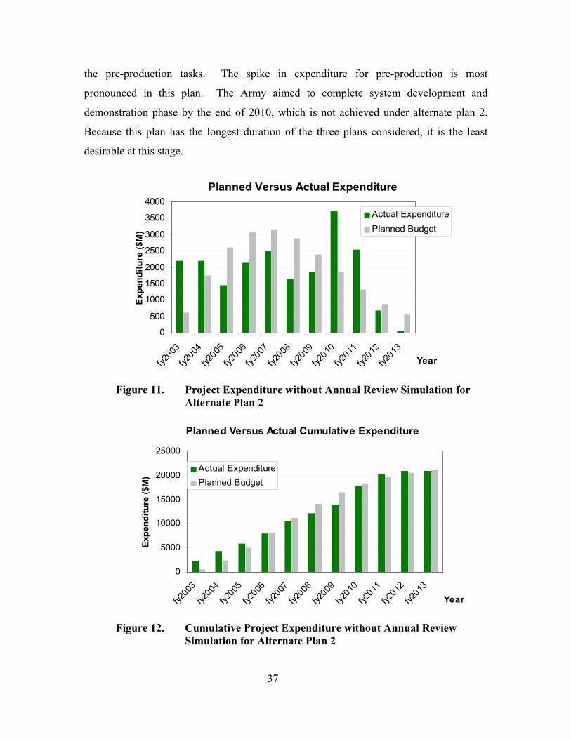
37
the pre-production tasks. The spike in expenditure for pre-production is most
pronounced in this plan. The Army aimed to complete system development and
demonstration phase by the end of 2010, which is not achieved under alternate plan 2.
Because this plan has the longest duration of the three plans considered, it is the least
desirable at this stage.
Planned Versus Actual Expenditure
0
500
1000
1500
2000
2500
3000
3500
4000
fy2003
fy2004
fy2005
fy2006
fy2007
fy2008
fy2009
fy2010
fy2011
fy2012
fy2013
Year
Expe
nditu
re ($
M)
Actual ExpenditurePlanned Budget
Figure 11. Project Expenditure without Annual Review Simulation for
Alternate Plan 2
Planned Versus Actual Cumulative Expenditure
0
5000
10000
15000
20000
25000
fy2003
fy2004
fy2005
fy2006
fy2007
fy2008
fy2009
fy2010
fy2011
fy2012
fy2013
Year
Expe
nditu
re ($
M)
Actual ExpenditurePlanned Budget
Figure 12. Cumulative Project Expenditure without Annual Review
Simulation for Alternate Plan 2
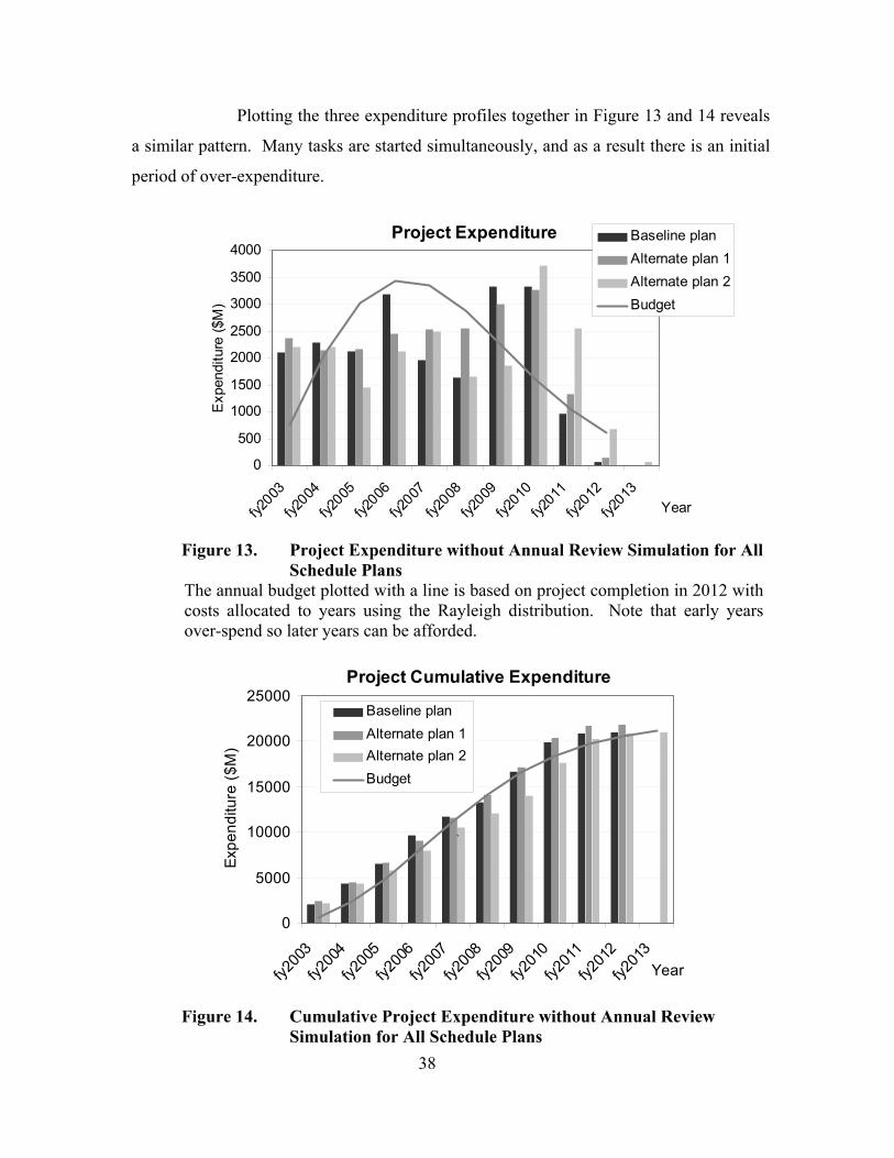
38
Plotting the three expenditure profiles together in Figure 13 and 14 reveals
a similar pattern. Many tasks are started simultaneously, and as a result there is an initial
period of over-expenditure.
Project Expenditure
0
500
1000
1500
2000
2500
3000
3500
4000
fy2003
fy2004
fy2005
fy2006
fy2007
fy2008
fy2009
fy2010
fy2011
fy2012
fy2013
Year
Exp
endi
ture
($M
)Baseline planAlternate plan 1Alternate plan 2Budget
Figure 13. Project Expenditure without Annual Review Simulation for All
Schedule Plans The annual budget plotted with a line is based on project completion in 2012 with costs allocated to years using the Rayleigh distribution. Note that early years over-spend so later years can be afforded.
Project Cumulative Expenditure
0
5000
10000
15000
20000
25000
fy200
3
fy200
4
fy200
5
fy200
6
fy200
7
fy200
8
fy200
9
fy201
0
fy201
1
fy201
2
fy201
3Year
Expe
nditu
re ($
M)
Baseline planAlternate plan 1Alternate plan 2Budget
`
Figure 14. Cumulative Project Expenditure without Annual Review
Simulation for All Schedule Plans
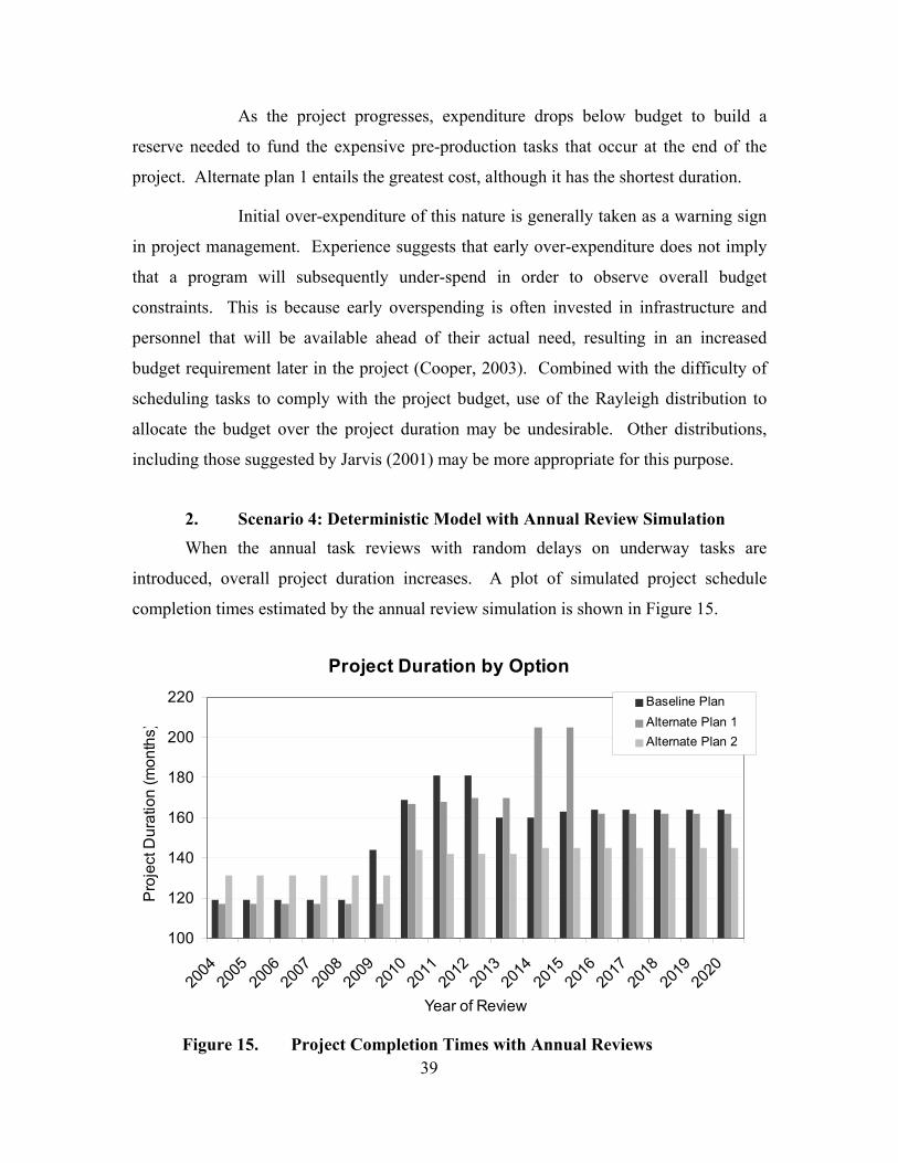
39
As the project progresses, expenditure drops below budget to build a
reserve needed to fund the expensive pre-production tasks that occur at the end of the
project. Alternate plan 1 entails the greatest cost, although it has the shortest duration.
Initial over-expenditure of this nature is generally taken as a warning sign
in project management. Experience suggests that early over-expenditure does not imply
that a program will subsequently under-spend in order to observe overall budget
constraints. This is because early overspending is often invested in infrastructure and
personnel that will be available ahead of their actual need, resulting in an increased
budget requirement later in the project (Cooper, 2003). Combined with the difficulty of
scheduling tasks to comply with the project budget, use of the Rayleigh distribution to
allocate the budget over the project duration may be undesirable. Other distributions,
including those suggested by Jarvis (2001) may be more appropriate for this purpose.
2. Scenario 4: Deterministic Model with Annual Review Simulation
When the annual task reviews with random delays on underway tasks are
introduced, overall project duration increases. A plot of simulated project schedule
completion times estimated by the annual review simulation is shown in Figure 15.
Project Duration by Option
100
120
140
160
180
200
220
2004
2005
2006
2007
2008
2009
2010
2011
2012
2013
2014
2015
2016
2017
2018
2019
2020
Year of Review
Pro
ject
Dur
atio
n (m
onth
s)
Baseline PlanAlternate Plan 1Alternate Plan 2
Figure 15. Project Completion Times with Annual Reviews
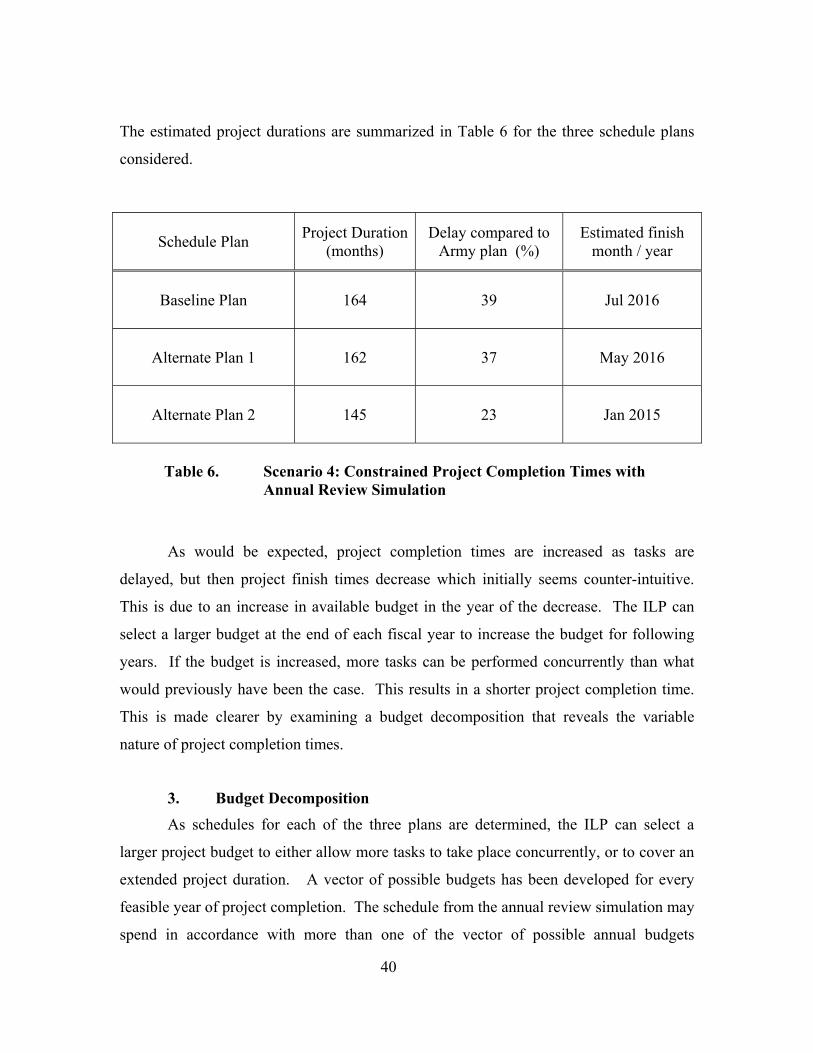
40
The estimated project durations are summarized in Table 6 for the three schedule plans
considered.
Schedule Plan Project Duration (months)
Delay compared to Army plan (%)
Estimated finish month / year
Baseline Plan 164 39 Jul 2016
Alternate Plan 1 162 37 May 2016
Alternate Plan 2 145 23 Jan 2015
Table 6. Scenario 4: Constrained Project Completion Times with
Annual Review Simulation
As would be expected, project completion times are increased as tasks are
delayed, but then project finish times decrease which initially seems counter-intuitive.
This is due to an increase in available budget in the year of the decrease. The ILP can
select a larger budget at the end of each fiscal year to increase the budget for following
years. If the budget is increased, more tasks can be performed concurrently than what
would previously have been the case. This results in a shorter project completion time.
This is made clearer by examining a budget decomposition that reveals the variable
nature of project completion times.
3. Budget Decomposition
As schedules for each of the three plans are determined, the ILP can select a
larger project budget to either allow more tasks to take place concurrently, or to cover an
extended project duration. A vector of possible budgets has been developed for every
feasible year of project completion. The schedule from the annual review simulation may
spend in accordance with more than one of the vector of possible annual budgets
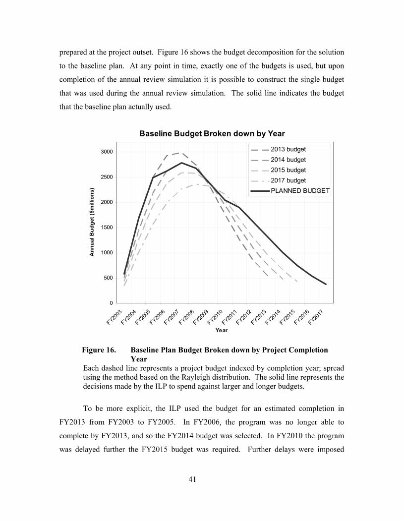
41
prepared at the project outset. Figure 16 shows the budget decomposition for the solution
to the baseline plan. At any point in time, exactly one of the budgets is used, but upon
completion of the annual review simulation it is possible to construct the single budget
that was used during the annual review simulation. The solid line indicates the budget
that the baseline plan actually used.
Baseline Budget Broken down by Year
0
500
1000
1500
2000
2500
3000
FY2003
FY2004
FY2005
FY2006
FY2007
FY2008
FY2009
FY2010
FY2011
FY2012
FY2013
FY2014
FY2015
FY2016
FY2017
Year
Ann
ual B
udge
t ($m
illio
ns)
2013 budget2014 budget2015 budget2017 budgetPLANNED BUDGET
Figure 16. Baseline Plan Budget Broken down by Project Completion
Year Each dashed line represents a project budget indexed by completion year; spread using the method based on the Rayleigh distribution. The solid line represents the decisions made by the ILP to spend against larger and longer budgets.
To be more explicit, the ILP used the budget for an estimated completion in
FY2013 from FY2003 to FY2005. In FY2006, the program was no longer able to
complete by FY2013, and so the FY2014 budget was selected. In FY2010 the program
was delayed further the FY2015 budget was required. Further delays were imposed
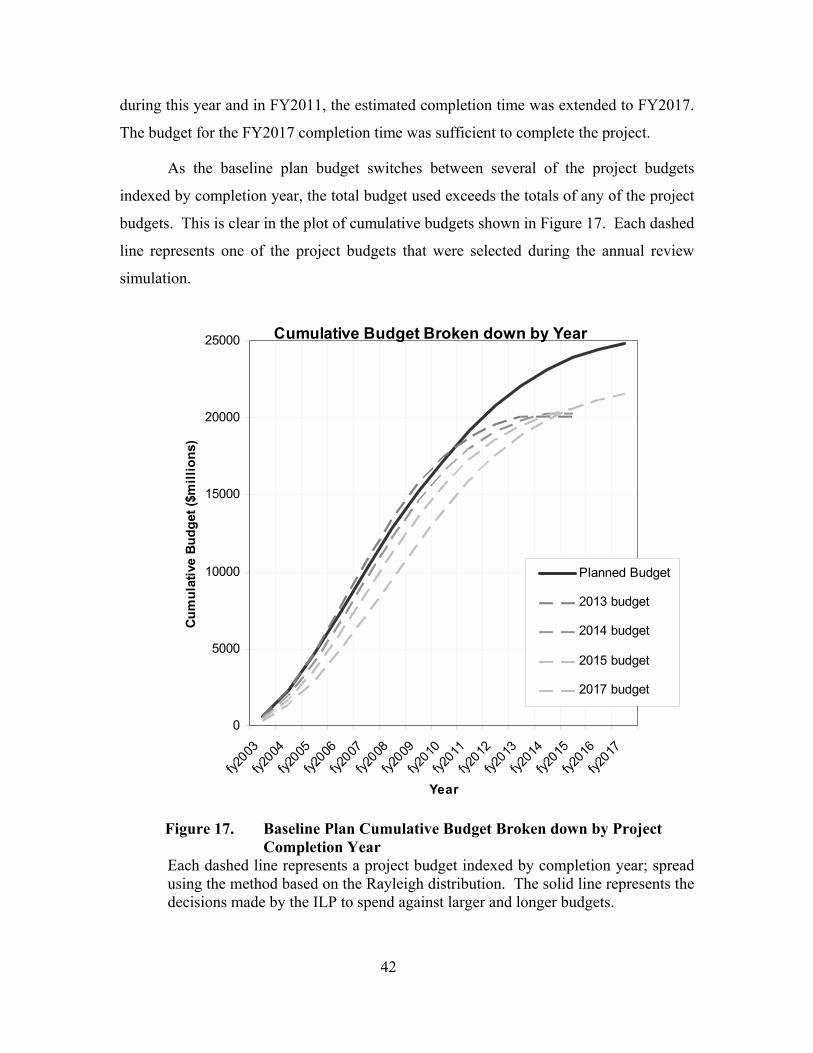
42
during this year and in FY2011, the estimated completion time was extended to FY2017.
The budget for the FY2017 completion time was sufficient to complete the project.
As the baseline plan budget switches between several of the project budgets
indexed by completion year, the total budget used exceeds the totals of any of the project
budgets. This is clear in the plot of cumulative budgets shown in Figure 17. Each dashed
line represents one of the project budgets that were selected during the annual review
simulation.
Cumulative Budget Broken down by Year
0
5000
10000
15000
20000
25000
fy2003
fy2004
fy2005
fy2006
fy2007
fy2008
fy2009
fy2010
fy2011
fy2012
fy2013
fy2014
fy2015
fy2016
fy2017
Year
Cum
ulat
ive
Budg
et ($
mill
ions
)
Planned Budget
2013 budget
2014 budget
2015 budget
2017 budget
Figure 17. Baseline Plan Cumulative Budget Broken down by Project
Completion Year Each dashed line represents a project budget indexed by completion year; spread using the method based on the Rayleigh distribution. The solid line represents the decisions made by the ILP to spend against larger and longer budgets.
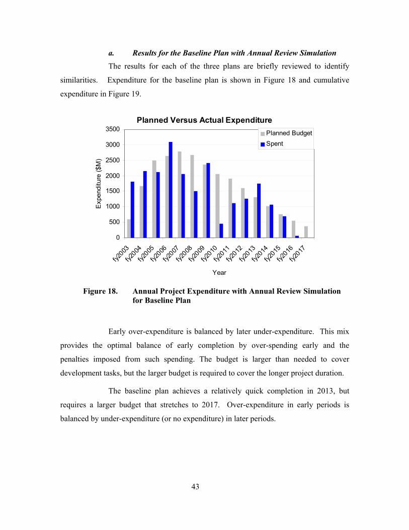
43
a. Results for the Baseline Plan with Annual Review Simulation The results for each of the three plans are briefly reviewed to identify
similarities. Expenditure for the baseline plan is shown in Figure 18 and cumulative
expenditure in Figure 19.
Planned Versus Actual Expenditure
0
500
1000
1500
2000
2500
3000
3500
fy2003
fy2004
fy2005
fy2006
fy2007
fy2008
fy2009
fy2010
fy2011
fy2012
fy2013
fy2014
fy2015
fy2016
fy2017
Year
Exp
endi
ture
($M
)
Planned BudgetSpent
Figure 18. Annual Project Expenditure with Annual Review Simulation
for Baseline Plan
Early over-expenditure is balanced by later under-expenditure. This mix
provides the optimal balance of early completion by over-spending early and the
penalties imposed from such spending. The budget is larger than needed to cover
development tasks, but the larger budget is required to cover the longer project duration.
The baseline plan achieves a relatively quick completion in 2013, but
requires a larger budget that stretches to 2017. Over-expenditure in early periods is
balanced by under-expenditure (or no expenditure) in later periods.
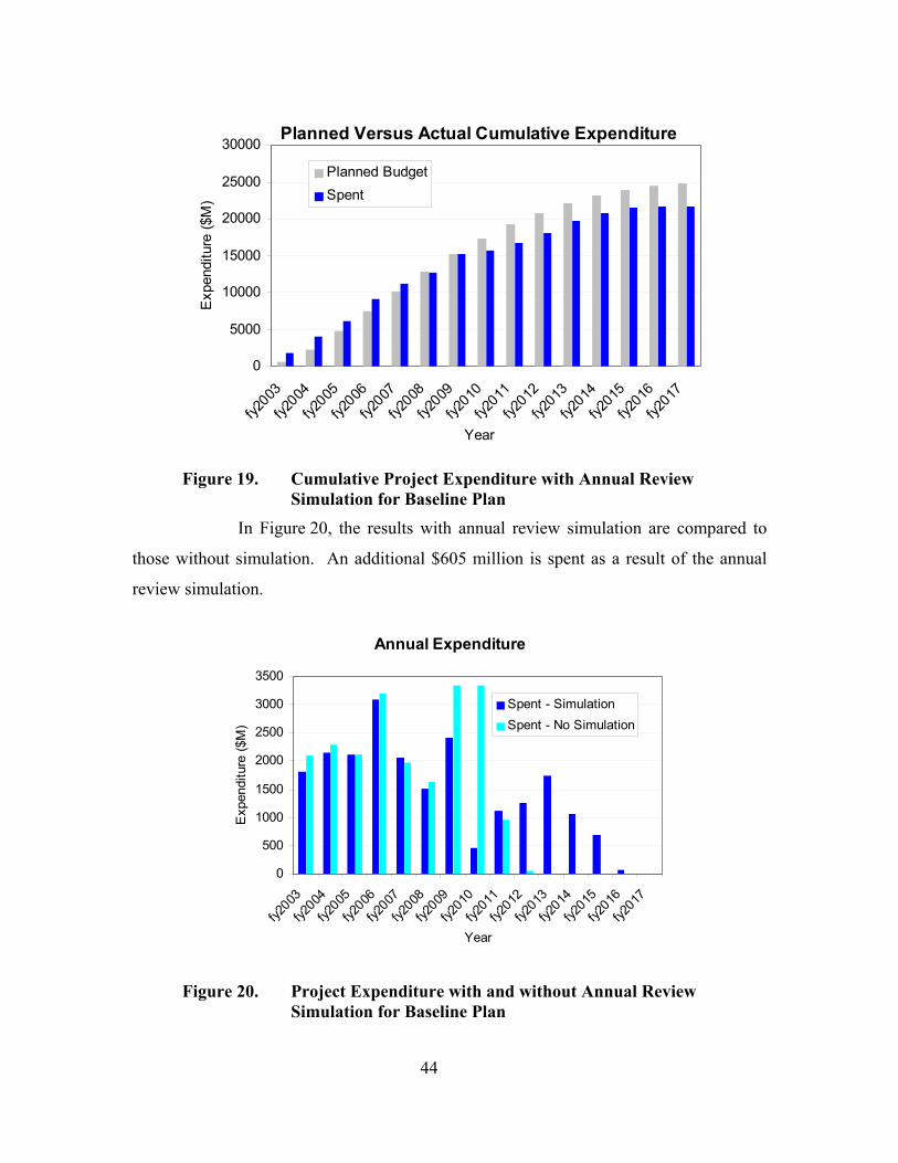
44
Planned Versus Actual Cumulative Expenditure
0
5000
10000
15000
20000
25000
30000
fy2003
fy2004
fy2005
fy2006
fy2007
fy2008
fy2009
fy2010
fy2011
fy2012
fy2013
fy2014
fy2015
fy2016
fy2017
Year
Exp
endi
ture
($M
)
Planned BudgetSpent
Figure 19. Cumulative Project Expenditure with Annual Review
Simulation for Baseline Plan
In Figure 20, the results with annual review simulation are compared to
those without simulation. An additional $605 million is spent as a result of the annual
review simulation.
Annual Expenditure
0
500
1000
1500
2000
2500
3000
3500
fy2003
fy2004
fy2005
fy2006
fy2007
fy2008
fy2009
fy2010
fy2011
fy2012
fy2013
fy2014
fy2015
fy2016
fy2017
Year
Exp
endi
ture
($M
)
Spent - SimulationSpent - No Simulation
Figure 20. Project Expenditure with and without Annual Review
Simulation for Baseline Plan
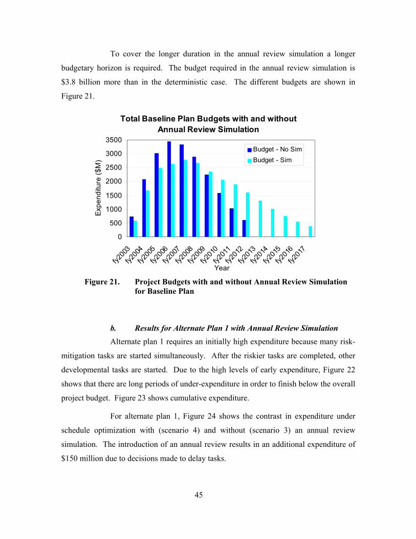
45
To cover the longer duration in the annual review simulation a longer
budgetary horizon is required. The budget required in the annual review simulation is
$3.8 billion more than in the deterministic case. The different budgets are shown in
Figure 21.
Total Baseline Plan Budgets with and without Annual Review Simulation
0
500
1000
1500
2000
2500
3000
3500
fy200
3
fy200
4
fy200
5
fy200
6
fy200
7
fy200
8
fy200
9
fy201
0
fy201
1
fy201
2
fy201
3
fy201
4
fy201
5
fy201
6
fy201
7
Year
Expe
nditu
re ($
M)
Budget - No SimBudget - Sim
Figure 21. Project Budgets with and without Annual Review Simulation
for Baseline Plan
b. Results for Alternate Plan 1 with Annual Review Simulation Alternate plan 1 requires an initially high expenditure because many risk-
mitigation tasks are started simultaneously. After the riskier tasks are completed, other
developmental tasks are started. Due to the high levels of early expenditure, Figure 22
shows that there are long periods of under-expenditure in order to finish below the overall
project budget. Figure 23 shows cumulative expenditure.
For alternate plan 1, Figure 24 shows the contrast in expenditure under
schedule optimization with (scenario 4) and without (scenario 3) an annual review
simulation. The introduction of an annual review results in an additional expenditure of
$150 million due to decisions made to delay tasks.
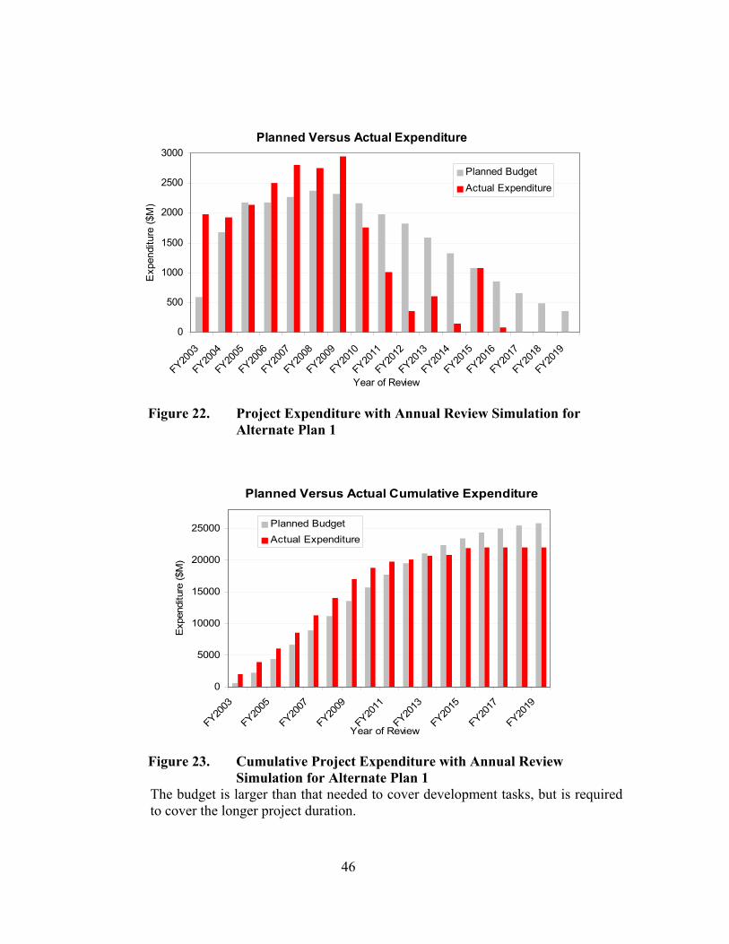
46
Planned Versus Actual Expenditure
0
500
1000
1500
2000
2500
3000
FY2003
FY2004
FY2005
FY2006
FY2007
FY2008
FY2009
FY2010
FY2011
FY2012
FY2013
FY2014
FY2015
FY2016
FY2017
FY2018
FY2019
Year of Review
Exp
endi
ture
($M
)
Planned BudgetActual Expenditure
Figure 22. Project Expenditure with Annual Review Simulation for
Alternate Plan 1
Planned Versus Actual Cumulative Expenditure
0
5000
10000
15000
20000
25000
FY2003
FY2005
FY2007
FY2009
FY2011
FY2013
FY20
15
FY2017
FY2019
Year of Review
Exp
endi
ture
($M
)
Planned BudgetActual Expenditure
Figure 23. Cumulative Project Expenditure with Annual Review
Simulation for Alternate Plan 1 The budget is larger than that needed to cover development tasks, but is required to cover the longer project duration.
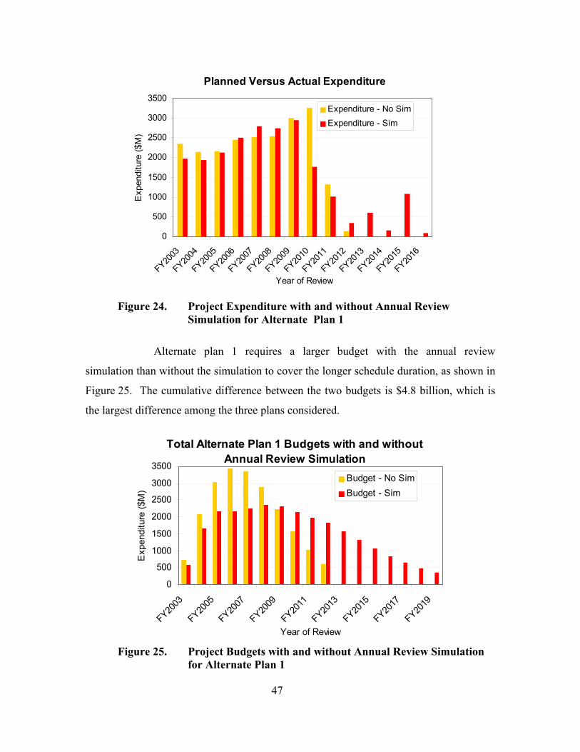
47
Planned Versus Actual Expenditure
0
500
1000
1500
2000
2500
3000
3500
FY2003
FY2004
FY2005
FY2006
FY2007
FY2008
FY2009
FY2010
FY2011
FY2012
FY2013
FY2014
FY2015
FY2016
Year of Review
Exp
endi
ture
($M
)
Expenditure - No SimExpenditure - Sim
Figure 24. Project Expenditure with and without Annual Review
Simulation for Alternate Plan 1
Alternate plan 1 requires a larger budget with the annual review
simulation than without the simulation to cover the longer schedule duration, as shown in
Figure 25. The cumulative difference between the two budgets is $4.8 billion, which is
the largest difference among the three plans considered.
Total Alternate Plan 1 Budgets with and without Annual Review Simulation
0
500
1000
1500
2000
2500
3000
3500
FY2003
FY2005
FY2007
FY2009
FY2011
FY2013
FY2015
FY2017
FY2019
Year of Review
Exp
endi
ture
($M
)
Budget - No SimBudget - Sim
Figure 25. Project Budgets with and without Annual Review Simulation
for Alternate Plan 1
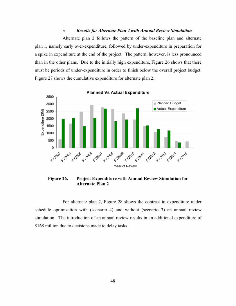
48
c. Results for Alternate Plan 2 with Annual Review Simulation Alternate plan 2 follows the pattern of the baseline plan and alternate
plan 1, namely early over-expenditure, followed by under-expenditure in preparation for
a spike in expenditure at the end of the project. The pattern, however, is less pronounced
than in the other plans. Due to the initially high expenditure, Figure 26 shows that there
must be periods of under-expenditure in order to finish below the overall project budget.
Figure 27 shows the cumulative expenditure for alternate plan 2.
Planned Vs Actual Expenditure
0
500
1000
1500
2000
2500
3000
3500
FY2003
FY2004
FY2005
FY2006
FY2007
FY2008
FY2009
FY2010
FY2011
FY2012
FY2013
FY2014
FY2015
Year of Review
Exp
endi
ture
($M
)
Planned BudgetActual Expenditure
Figure 26. Project Expenditure with Annual Review Simulation for
Alternate Plan 2
For alternate plan 2, Figure 28 shows the contrast in expenditure under
schedule optimization with (scenario 4) and without (scenario 3) an annual review
simulation. The introduction of an annual review results in an additional expenditure of
$168 million due to decisions made to delay tasks.
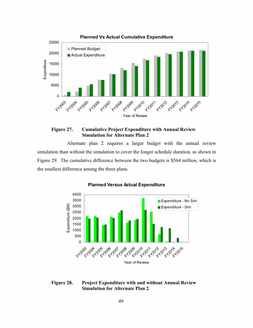
49
Planned Vs Actual Cumulative Expenditure
0
5000
10000
15000
20000
25000
FY2003
FY2004
FY2005
FY2006
FY2007
FY2008
FY2009
FY2010
FY2011
FY2012
FY2013
FY2014
FY2015
Year of Review
Exp
endi
ture
Planned BudgetActual Expenditure
Figure 27. Cumulative Project Expenditure with Annual Review
Simulation for Alternate Plan 2 Alternate plan 2 requires a larger budget with the annual review
simulation than without the simulation to cover the longer schedule duration, as shown in
Figure 29. The cumulative difference between the two budgets is $564 million, which is
the smallest difference among the three plans.
Planned Versus Actual Expenditure
0500
100015002000
2500300035004000
FY20
03
FY20
04
FY20
05
FY20
06
FY20
07
FY20
08
FY20
09
FY20
10
FY20
11
FY20
12
FY20
13
FY20
14
FY20
15
Year of Review
Exp
endi
ture
($M
)
Expenditure - No Sim
Expenditure - Sim
Figure 28. Project Expenditure with and without Annual Review
Simulation for Alternate Plan 2
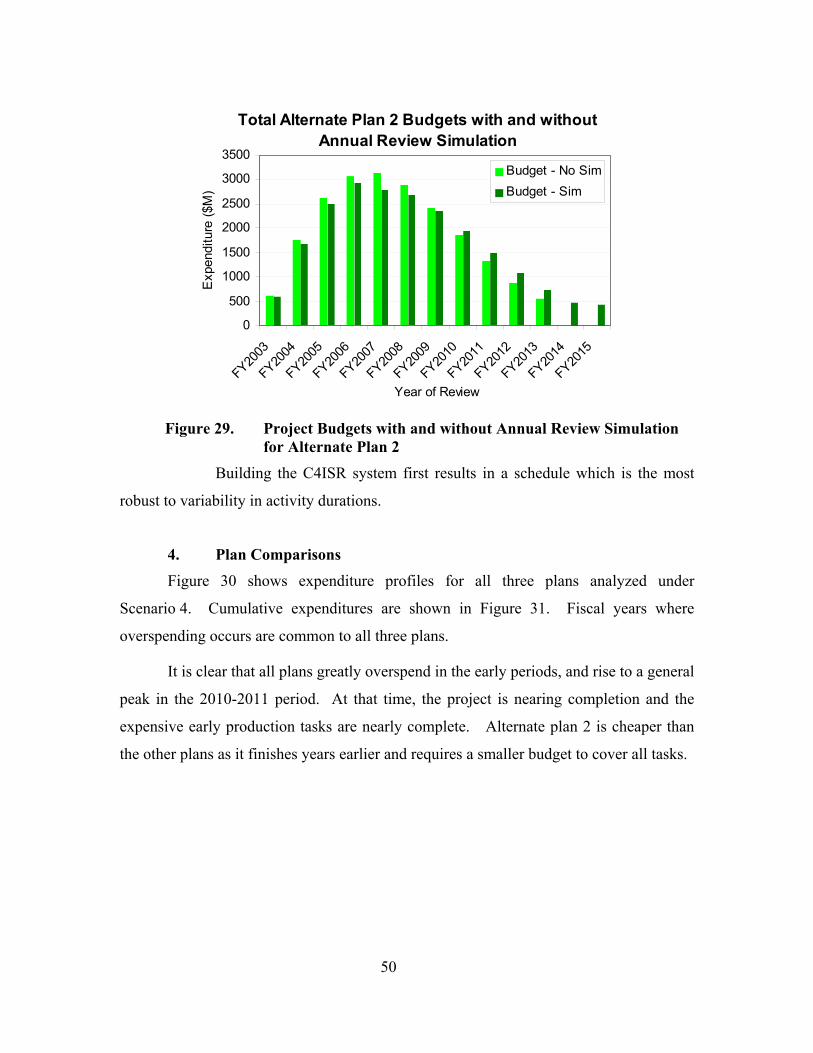
50
Total Alternate Plan 2 Budgets with and without Annual Review Simulation
0
500
1000
1500
2000
2500
3000
3500
FY2003
FY2004
FY2005
FY2006
FY2007
FY2008
FY2009
FY2010
FY2011
FY2012
FY2013
FY2014
FY2015
Year of Review
Exp
endi
ture
($M
)
Budget - No SimBudget - Sim
Figure 29. Project Budgets with and without Annual Review Simulation
for Alternate Plan 2
Building the C4ISR system first results in a schedule which is the most
robust to variability in activity durations.
4. Plan Comparisons
Figure 30 shows expenditure profiles for all three plans analyzed under
Scenario 4. Cumulative expenditures are shown in Figure 31. Fiscal years where
overspending occurs are common to all three plans.
It is clear that all plans greatly overspend in the early periods, and rise to a general
peak in the 2010-2011 period. At that time, the project is nearing completion and the
expensive early production tasks are nearly complete. Alternate plan 2 is cheaper than
the other plans as it finishes years earlier and requires a smaller budget to cover all tasks.
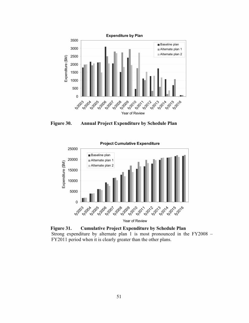
51
Expenditure by Plan
0
500
1000
1500
2000
2500
3000
3500
fy200
3
fy200
4
fy200
5
fy200
6
fy200
7
fy200
8
fy200
9
fy201
0
fy201
1
fy201
2
fy201
3
fy201
4
fy201
5
fy201
6
Year of Review
Exp
endi
ture
($M
)
Baseline planAlternate plan 1Alternate plan 2
Figure 30. Annual Project Expenditure by Schedule Plan
Project Cumulative Expenditure
0
5000
10000
15000
20000
25000
fy200
3
fy200
4
fy200
5
fy200
6
fy200
7
fy200
8
fy200
9
fy201
0
fy201
1
fy201
2
fy201
3
fy201
4
fy201
5
fy201
6
Year of Review
Exp
endi
ture
($M
)
Baseline planAlternate plan 1Alternate plan 2
Figure 31. Cumulative Project Expenditure by Schedule Plan Strong expenditure by alternate plan 1 is most pronounced in the FY2008 – FY2011 period when it is clearly greater than the other plans.
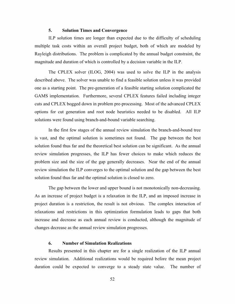
52
5. Solution Times and Convergence
ILP solution times are longer than expected due to the difficulty of scheduling
multiple task costs within an overall project budget, both of which are modeled by
Rayleigh distributions. The problem is complicated by the annual budget constraint, the
magnitude and duration of which is controlled by a decision variable in the ILP.
The CPLEX solver (ILOG, 2004) was used to solve the ILP in the analysis
described above. The solver was unable to find a feasible solution unless it was provided
one as a starting point. The pre-generation of a feasible starting solution complicated the
GAMS implementation. Furthermore, several CPLEX features failed including integer
cuts and CPLEX bogged down in problem pre-processing. Most of the advanced CPLEX
options for cut generation and root node heuristics needed to be disabled. All ILP
solutions were found using branch-and-bound variable searching.
In the first few stages of the annual review simulation the branch-and-bound tree
is vast, and the optimal solution is sometimes not found. The gap between the best
solution found thus far and the theoretical best solution can be significant. As the annual
review simulation progresses, the ILP has fewer choices to make which reduces the
problem size and the size of the gap generally decreases. Near the end of the annual
review simulation the ILP converges to the optimal solution and the gap between the best
solution found thus far and the optimal solution is closed to zero.
The gap between the lower and upper bound is not monotonically non-decreasing.
As an increase of project budget is a relaxation in the ILP, and an imposed increase in
project duration is a restriction, the result is not obvious. The complex interaction of
relaxations and restrictions in this optimization formulation leads to gaps that both
increase and decrease as each annual review is conducted, although the magnitude of
changes decrease as the annual review simulation progresses.
6. Number of Simulation Realizations Results presented in this chapter are for a single realization of the ILP annual
review simulation. Additional realizations would be required before the mean project
duration could be expected to converge to a steady state value. The number of
53
realizations may need to exceed 40 in order to invoke the Central Limit Theorem. This
requires an investment of computational resources beyond the scope of the thesis, but the
results presented in this thesis are representative of what can be expected. Moreover, as
the data used in this thesis are nominal (actual FCS project information is classified
beyond the clearance of the author), a significant computational investment to determine
steady state conditions may not be warranted without real data in hand.

54
THIS PAGE INTENTIONALLY LEFT BLANK
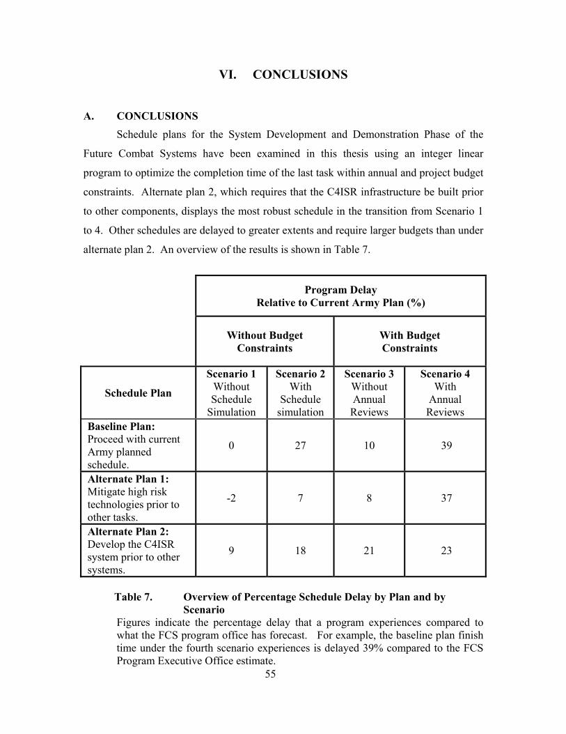
55
VI. CONCLUSIONS
A. CONCLUSIONS Schedule plans for the System Development and Demonstration Phase of the
Future Combat Systems have been examined in this thesis using an integer linear
program to optimize the completion time of the last task within annual and project budget
constraints. Alternate plan 2, which requires that the C4ISR infrastructure be built prior
to other components, displays the most robust schedule in the transition from Scenario 1
to 4. Other schedules are delayed to greater extents and require larger budgets than under
alternate plan 2. An overview of the results is shown in Table 7.
Program Delay Relative to Current Army Plan (%)
Without Budget Constraints
With Budget Constraints
Schedule Plan
Scenario 1 Without Schedule
Simulation
Scenario 2 With
Schedule simulation
Scenario 3 Without Annual Reviews
Scenario 4 With
Annual Reviews
Baseline Plan: Proceed with current Army planned schedule.
0 27 10 39
Alternate Plan 1: Mitigate high risk technologies prior to other tasks.
-2 7 8 37
Alternate Plan 2: Develop the C4ISR system prior to other systems.
9 18 21 23
Table 7. Overview of Percentage Schedule Delay by Plan and by
Scenario Figures indicate the percentage delay that a program experiences compared to what the FCS program office has forecast. For example, the baseline plan finish time under the fourth scenario experiences is delayed 39% compared to the FCS Program Executive Office estimate.
56
If there are no budget constraints, mitigating high risk technology first is preferred
both with and without schedule simulation. When budget constraints are added, this
option and the current Army project plan are both attractive. Annual review simulation
of the constrained optimization reveals that the third plan is the least vulnerable to delay.
Given the high levels of schedule risk that exist in the FCS program, alternate plan 2 is
the recommended plan because it is least affected by the effects of uncertainty.
Solution times for the ILP are longer than expected. The CPLEX solver used
required a pre-processed feasible solution to be provided as a starting point, and this
complicated the implementation. CPLEX had difficulty finding cuts to reduce problem
size, and bogged down in pre-processing. All solutions to the ILP are found using branch
and bound variable search techniques. As the annual review simulation progresses, the
solution found by the solver converges towards the optimal solution.
B. FUTURE AREAS OF STUDY The analytical approach presented in this thesis is generally applicable to the
scheduling of major defense acquisition projects. The budget-constrained optimization
model requires that the decision maker supply two parameters that characterize the
durations of tasks within a project, namely an estimated most likely duration and a
categorical schedule risk assessment. Although this simplifies the task for the decision
maker, care must be exercised in selection of these parameters to ensure that useful
results are obtained from the analysis. It would be useful to examine the efficacy of
current guidelines for parameter selection, and to propose refinements that better match
what has been observed in practice. Assumptions of cost growth of the overall project
schedule as a function of longer completion times may need to be reviewed.
There are many extensions that can be made to the optimization model itself.
Recovering the critical path at the end of each annual review would reveal which tasks
are more commonly on the critical path. Statistics on the frequency with which tasks fall
on the critical path could also reveal potential flaws with the project design. This could
be an aid to efficiently directing management effort, capacity planning and priorities for
future procurement.

57
More sophisticated elastic penalties could be developed to better reflect the
decisions made by real project managers. A questionable aspect of this model is its
tendency to produce scheduling solutions that over-spend early in the project,
compensated by under-spending during the mid-project phase. In practice an early over-
expenditure typically results in over-expenditure throughout the project.
Nonetheless, the tendency to schedule activities very early in the project and in
doing so incurring large penalties implies that this is better than waiting for the money to
become available according to the Rayleigh spread of the project budget. Evidently, the
Rayleigh budget spread does not schedule enough money early in the project. Schedule
optimization prefers to exceed the budget early and repay the shortfall later in the project.
It allows these violations of the Rayleigh budget spread albeit by imposing penalties. As
a result, expenditure profiles do not resemble the Rayleigh budget spread.
In the optimization individual task expenditures are spread over their durations
using Rayleigh distributions, and the overall project budget is also spread using a
Rayleigh distribution. It is difficult to impose these constraints simultaneously without
allowing for violations. This suggests the use of alternate models for spreading project
budgets, which may achieve developmental goals with fewer penalties, less cost, and
earlier completion times than the options presented here.

58
THIS PAGE INTENTIONALLY LEFT BLANK
59
LIST OF REFERENCES
Ahuja, R.K., Magnanti, T.L., and Orlin, J.B. (1993). Network Flows: Theory, Algorithms and Applications, Prentice Hall, Englewood Cliffs. Babbar, M.M., Tintner, G., and Heady, E.O. (1955). “Programming with Consideration of Variations in Input Coefficients”, Journal of Farm Economics, May, 37, No. 2, pp. 333-341. Bachmann, P.G.H. (1894). Die Analytische Zahlentheorie, Teubner, Leipzig. (unsighted). Bowman, E.H. (1958). “The Schedule Sequencing Problem”, Operations Research, 7, pp. 621-624. Brady, E. (2003). Future Combat Systems, Modeling and Simulation Conference, Project Executive Office Ground Combat Systems, U.S. Army, 30 Jan 2003. Accessed 14 Jan 2004 via the World Wide Web at http://www.boeing.com/defense-space/ic/fcs/bia/modsim_030130.html . Brook, A., Kendrick, D., Meeraus, A., and Raman, R. (1998). GAMS: A User’s Guide, The Scientific Press, Washington DC. Cooper, W. (2003). Cost Analysis Improvement Group, Program Analysis and Evaluation, Office of the Secretary of Defense, Various interviews, Dec 2003. Demeulemeester, E. and Herroelen, W. (2002). Project Scheduling: A Research Handbook, Volume 49 of the International Series in Operations Research and Management Science, Kluwer Academic Publishing, Boston. Dodin, B. (1984). “Bounding the Project Completion Time Distribution in PERT Networks”, Operations Research, 33, pp. 862-881. Francis, P.L. (2004). Defense Acquisitions: The Army’s Future Combat Systems’ Features, Risks and Alternatives, GAO-04-635T, testimony before the Subcommittee on Tactical Air and Land Forces, Committee on Armed Services, U.S. House of Representatives, April 2004. Fulkerson, D.R. (1962). “Expected Critical Path Lengths in PERT Networks”, Operations Research, 10, pp. 808-817. Gutjahr, W.J., Stauss, C., and Wagner, E. (2000). “A Stochastic Branch and Bound Approach to Activity Crashing in Project Management”, INFORMS Journal on Computing, 12, No. 2, pp. 125-135.
60
Herroelen, W. and Leus, R. (2004). “Robust and Reactive Scheduling: A Review and Classification of Procedures”, International Journal of Production Research, 42, No. 8 (15 April), pp. 1599-1620. Herroelen, W., Reyck, B.D., and Demeulemeester, E. (1998). “Resource-Constrained Project Scheduling: A Survey of Recent Developments”, Computers & Operations Research, 25, No. 4, pp. 279-302. Igelmund, G. and Radermacher, F.J. (1983). “Pre-selective Strategies for the Optimization of Stochastic Project Networks under Resource Constraints”, Networks, 13, pp. 1-28. ILOG (2004). ILOG Optimization Suite White Paper, Accessed 13 Jun 2004 via the World Wide Web at http://www.ilog.com/products/optimization/papers.cfm. Jarvis, W. (2001). “New Approaches to Phasing of Resources”, In Proceedings of the 34th Department of Defense Cost Analysis Symposium, Washington DC. Accessed 17 Jun 2004 via the World Wide Web at http://www.ra.pae.osd.mil/adodcas . Kelly, J.E. (1961). “Critical Path Planning and Scheduling: Mathematical Basis”, Operations Research, 9, pp. 296-320. Kelly, J.E. (1963). “The Critical Path Method: Resource Planning and Scheduling”, in Muth J.F. and Thompson G.L. (Eds.), Industrial Scheduling, Prentice Hall, Englewood Cliffs. Lee, D. (1997). The Cost Analyst’s Companion, Logistics Management Institute, McLean, VA. Malcolm, D.G., Roseboom, J.H., Clark, C.E., and Fazar, W. (1959). “Application of a Technique for Research and Development Program Evaluation”, Operations Research, 7, pp. 646-669. Miller, S. (2003). “Simulation Based Schedule Analysis”, In Proceedings of the 36th Department of Defense Cost Analysis Symposium, Washington DC. Accessed 12 Dec 2003 via the World Wide Web at http://www.ra.pae.osd.mil/adodcas/index2.htm. Pritsker, A.B., Watters, L.J., and Wolfe, P.M. (1969). “Multi-Project Scheduling with Limited Resources, A Zero-One Programming Approach”, Management Science, 16, pp. 93-108. Sengupta, J.K., Tintner, G., and Morrison, B. (1963). “Stochastic Linear Programming with Applications to Economic Models”, Economica, 30, pp. 262-275. Senju, S. and Toyoda, Y. (1968). “An Approach to Linear Programming with 0-1 Variables”, Management Science, 15, No. 4, pp. 196-207.
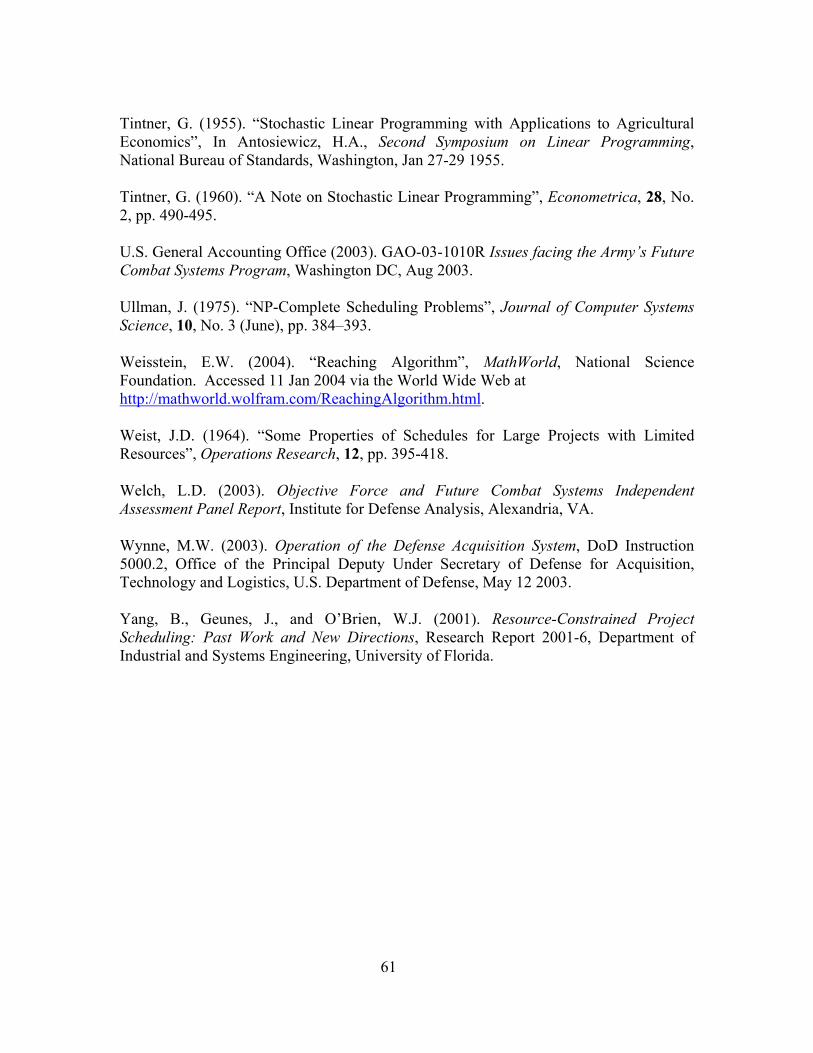
61
Tintner, G. (1955). “Stochastic Linear Programming with Applications to Agricultural Economics”, In Antosiewicz, H.A., Second Symposium on Linear Programming, National Bureau of Standards, Washington, Jan 27-29 1955. Tintner, G. (1960). “A Note on Stochastic Linear Programming”, Econometrica, 28, No. 2, pp. 490-495. U.S. General Accounting Office (2003). GAO-03-1010R Issues facing the Army’s Future Combat Systems Program, Washington DC, Aug 2003. Ullman, J. (1975). “NP-Complete Scheduling Problems”, Journal of Computer Systems Science, 10, No. 3 (June), pp. 384–393. Weisstein, E.W. (2004). “Reaching Algorithm”, MathWorld, National Science Foundation. Accessed 11 Jan 2004 via the World Wide Web at http://mathworld.wolfram.com/ReachingAlgorithm.html. Weist, J.D. (1964). “Some Properties of Schedules for Large Projects with Limited Resources”, Operations Research, 12, pp. 395-418. Welch, L.D. (2003). Objective Force and Future Combat Systems Independent Assessment Panel Report, Institute for Defense Analysis, Alexandria, VA. Wynne, M.W. (2003). Operation of the Defense Acquisition System, DoD Instruction 5000.2, Office of the Principal Deputy Under Secretary of Defense for Acquisition, Technology and Logistics, U.S. Department of Defense, May 12 2003. Yang, B., Geunes, J., and O’Brien, W.J. (2001). Resource-Constrained Project Scheduling: Past Work and New Directions, Research Report 2001-6, Department of Industrial and Systems Engineering, University of Florida.

62
THIS PAGE INTENTIONALLY LEFT BLANK
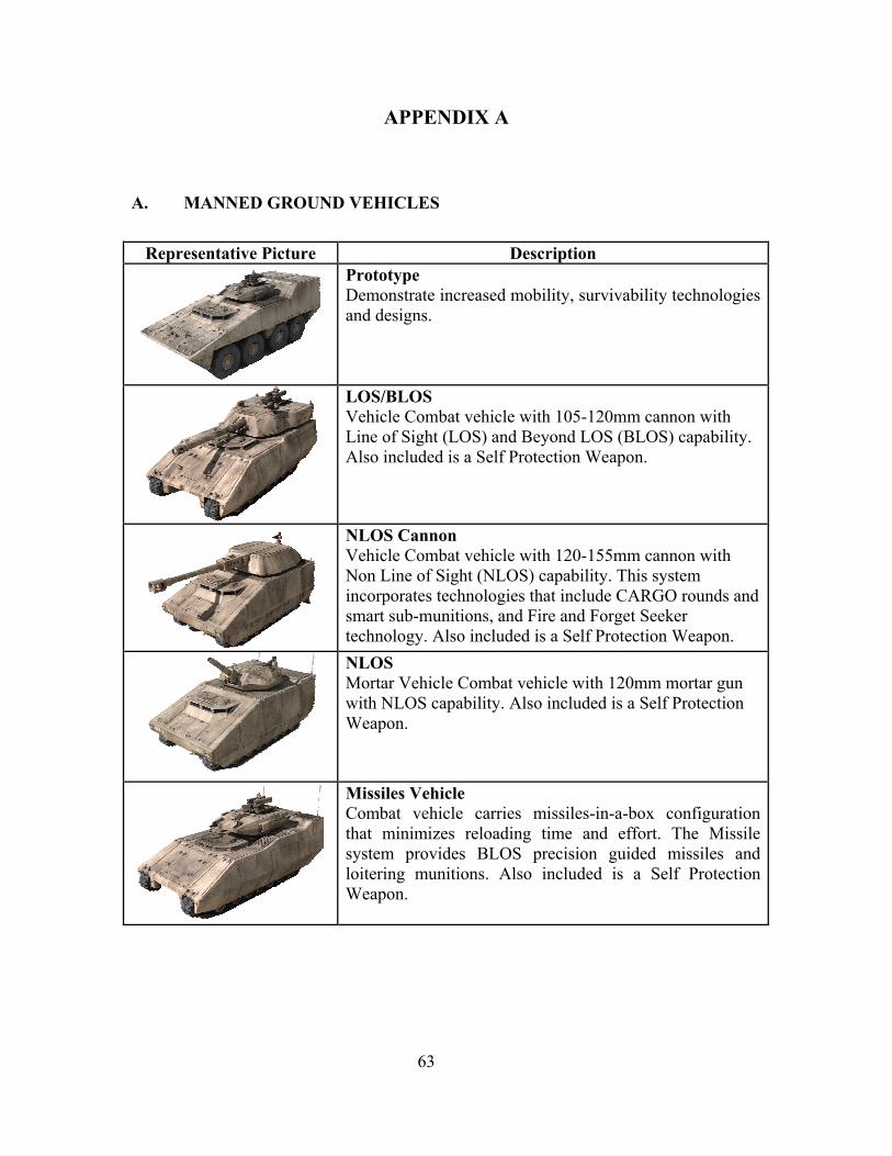
63
APPENDIX A
A. MANNED GROUND VEHICLES
Representative Picture Description
Prototype Demonstrate increased mobility, survivability technologies and designs.
LOS/BLOS Vehicle Combat vehicle with 105-120mm cannon with Line of Sight (LOS) and Beyond LOS (BLOS) capability. Also included is a Self Protection Weapon.
NLOS Cannon Vehicle Combat vehicle with 120-155mm cannon with Non Line of Sight (NLOS) capability. This system incorporates technologies that include CARGO rounds and smart sub-munitions, and Fire and Forget Seeker technology. Also included is a Self Protection Weapon.
NLOS Mortar Vehicle Combat vehicle with 120mm mortar gun with NLOS capability. Also included is a Self Protection Weapon.
Missiles Vehicle Combat vehicle carries missiles-in-a-box configuration that minimizes reloading time and effort. The Missile system provides BLOS precision guided missiles and loitering munitions. Also included is a Self Protection Weapon.

64
Armored Personnel Carrier Transports a full 9-man infantry squad including their associated gear and 2-soldier crew. Also included is a Self Protection Weapon.
Control Vehicle (CV) Provides 4-soldier workstation, 1 driver and 1 commander. Used for control of UGV's and UAV's. Also included is a Self Protection Weapon.
Command and Control (C2) Vehicle Provides 4 soldier workstation, 1 driver and 1 commander. Provides the connection among the Force and communication on the move. Also included is a Self Protection Weapon.
Re-supply Vehicle General-purpose vehicle with embedded semi-autonomy provides operation as a follower. Crew size consists of 1 driver and 1 commander. Also included is a Self Protection Weapon.
Reconnaissance, Surveillance, and Target Acquisition (RSTA) Vehicle Integrates RSTA suite of 5-meter mast, thermal imagers (Long-Wave Infrared (LWIR) and Medium-Wave Infrared (MWIR)), day/night television (TV) camera, 10 km+ laser range finder, Ka band radar, and 360 deg. all elevation azimuth. Provides 2 soldier workstation, 1 driver and 1 commander. Also included is a Self Protection Weapon.
155 mm Re-supply Vehicle Provides automated re-supply to the 155-mm NLOS vehicle; re-supplied with palletized ammunition: Crew size consists of 1 driver and 1 commander. Also included is a Self Protection Weapon.
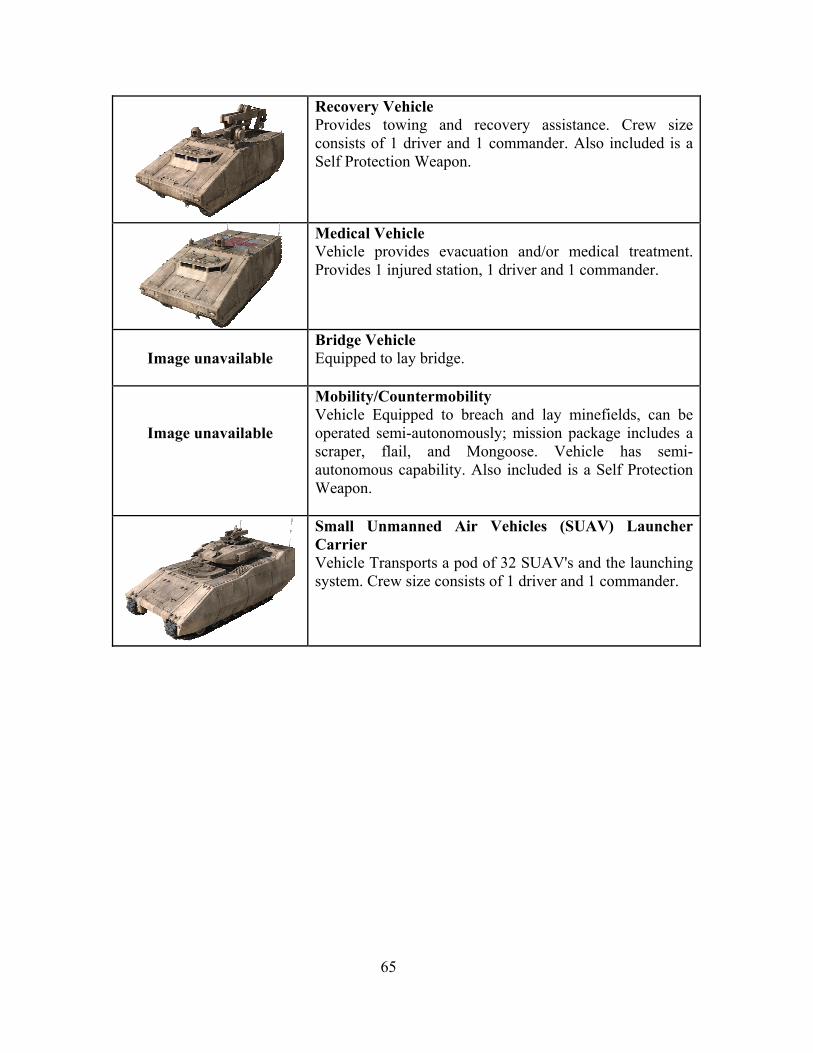
65
Recovery Vehicle Provides towing and recovery assistance. Crew size consists of 1 driver and 1 commander. Also included is a Self Protection Weapon.
Medical Vehicle Vehicle provides evacuation and/or medical treatment. Provides 1 injured station, 1 driver and 1 commander.
Image unavailable
Bridge Vehicle Equipped to lay bridge.
Image unavailable
Mobility/Countermobility Vehicle Equipped to breach and lay minefields, can be operated semi-autonomously; mission package includes a scraper, flail, and Mongoose. Vehicle has semi-autonomous capability. Also included is a Self Protection Weapon.
Small Unmanned Air Vehicles (SUAV) Launcher Carrier Vehicle Transports a pod of 32 SUAV's and the launching system. Crew size consists of 1 driver and 1 commander.
66
B. UNMANNED AERIAL VEHICLES (UAV)
Representative Picture Description
The Future Combat Systems will develop four classes of UAVs.
Class 1 will be a platoon-class small aircraft.
Class 2 will operate at the company level,
class 3 will be attached to the battalion and
Class 4 to the brigade commander.
Each FCS brigade would have 36 class-1, 36 class-2, 12 class-3 and 16 class-4 aircraft.
The FCS program generally has been described as a network of ground and air vehicles—both manned and un-piloted. The most “undefined” of the four classes of UAVs is the brigade-level aircraft. The funding and design of the FCS class-4 UAVs closely are tied to the Army’s next-generation helicopter, the Comanche. The service cut more than 600 helicopters out of the program (about half of the total), on the assumption that they would be replaced with UAVs.
C. UNMANNED GROUND VEHICLES (UGV)
Representative Picture Description
Armed Robotic Vehicle (ARV) - Assault - RSTA The ARV is a 5 to 6 ton unmanned ground vehicle (UGV) that performs an armed Reconnaissance, Surveillance, and Target Acquisition (RSTA) mission. The ARV will be part of an organization of vehicles, sensors, C2 hardware and software systems, and communications systems. The ARV assault incorporates a turret system capable of launching missiles such as the Common Missile or
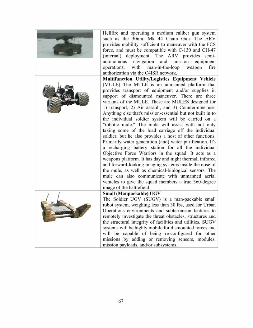
67
Hellfire and operating a medium caliber gun system such as the 30mm Mk 44 Chain Gun. The ARV provides mobility sufficient to maneuver with the FCS force, and must be compatible with C-130 and CH-47 (internal) deployment. The ARV provides semi-autonomous navigation and mission equipment operations, with man-in-the-loop weapon fire authorization via the C4ISR network.
Multifunction Utility/Logistics Equipment Vehicle (MULE) The MULE is an unmanned platform that provides transport of equipment and/or supplies in support of dismounted maneuver. There are three variants of the MULE. These are MULES designed for 1) transport, 2) Air assault, and 3) Countermine use. Anything else that's mission-essential but not built in to the individual soldier system will be carried on a "robotic mule." The mule will assist with not only taking some of the load carriage off the individual soldier, but he also provides a host of other functions. Primarily water generation (and) water purification. It's a recharging battery station for all the individual Objective Force Warriors in the squad. It acts as a weapons platform. It has day and night thermal, infrared and forward-looking imaging systems inside the nose of the mule, as well as chemical-biological sensors. The mule can also communicate with unmanned aerial vehicles to give the squad members a true 360-degree image of the battlefield
Small (Manpackable) UGV The Soldier UGV (SUGV) is a man-packable small robot system, weighing less than 30 lbs, used for Urban Operations environments and subterranean features to remotely investigate the threat obstacles, structures and the structural integrity of facilities and utilities. SUGV systems will be highly mobile for dismounted forces and will be capable of being re-configured for other missions by adding or removing sensors, modules, mission payloads, and/or subsystems.
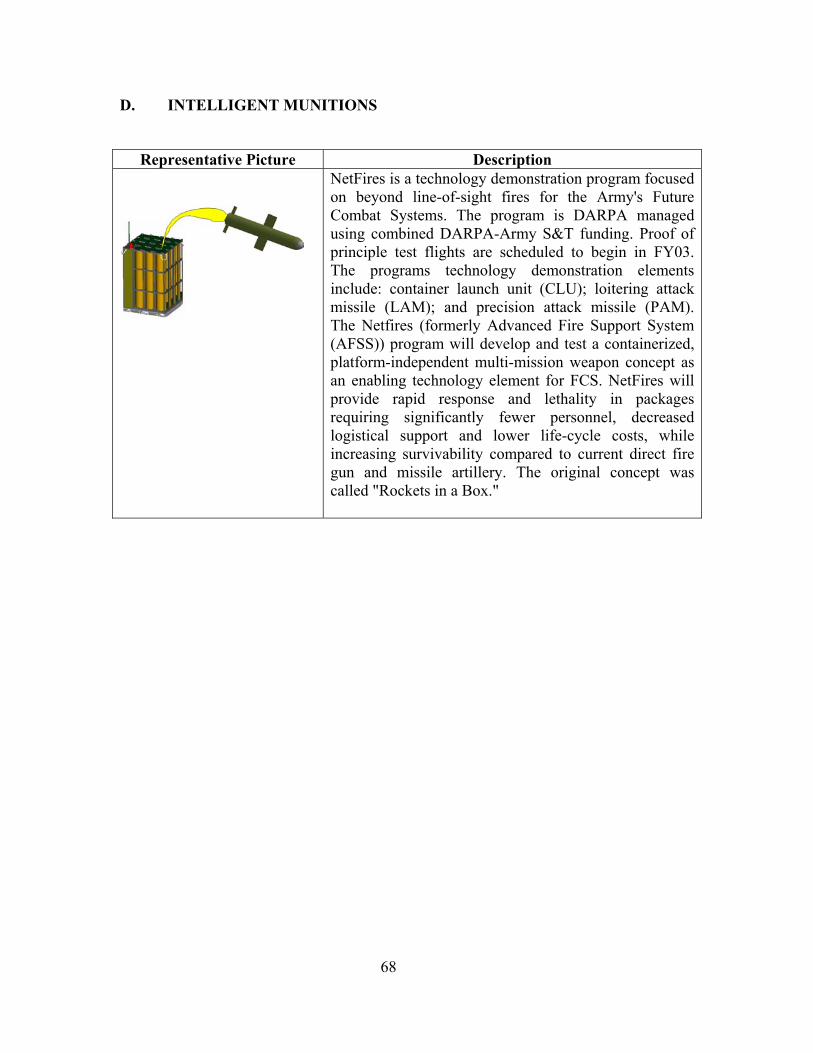
68
D. INTELLIGENT MUNITIONS
Representative Picture Description
NetFires is a technology demonstration program focused on beyond line-of-sight fires for the Army's Future Combat Systems. The program is DARPA managed using combined DARPA-Army S&T funding. Proof of principle test flights are scheduled to begin in FY03. The programs technology demonstration elements include: container launch unit (CLU); loitering attack missile (LAM); and precision attack missile (PAM). The Netfires (formerly Advanced Fire Support System (AFSS)) program will develop and test a containerized, platform-independent multi-mission weapon concept as an enabling technology element for FCS. NetFires will provide rapid response and lethality in packages requiring significantly fewer personnel, decreased logistical support and lower life-cycle costs, while increasing survivability compared to current direct fire gun and missile artillery. The original concept was called "Rockets in a Box."
69
APPENDIX B
A. FUTURE COMBAT SYSTEMS DEVELOPMENT AND DEMONSTRATION SCHEDULE PLANS
This thesis examines three plans for the FCS System Development and
Demonstration schedule to contrast the relative schedule risks. The three plans,
developed by the General Accounting Office (GAO) in its review of the FCS program
(GAO, 2003) are:
• Baseline Plan. Proceed with the concurrent development plan developed by the FCS Project Executive Office – Ground Combat Systems (PEO-GCS).
• Alternate Plan 1: Mature critical technologies first to mitigate risk, and then proceed with the concurrent development plan developed by the FCS PEO. System integration and test tasks are assumed to proceed with lower schedule risk under Option 1 than under the baseline plan.
• Alternate Plan 2: Develop the C4ISR infrastructure before initiating the development of other FCS systems. System integration and test tasks are assumed to proceed with lower schedule risk under alternate plan 2 than under the baseline plan.
Schedules for each of these tasks were developed in Microsoft Project 2000.
Summary reports of the key tasks are shown below.
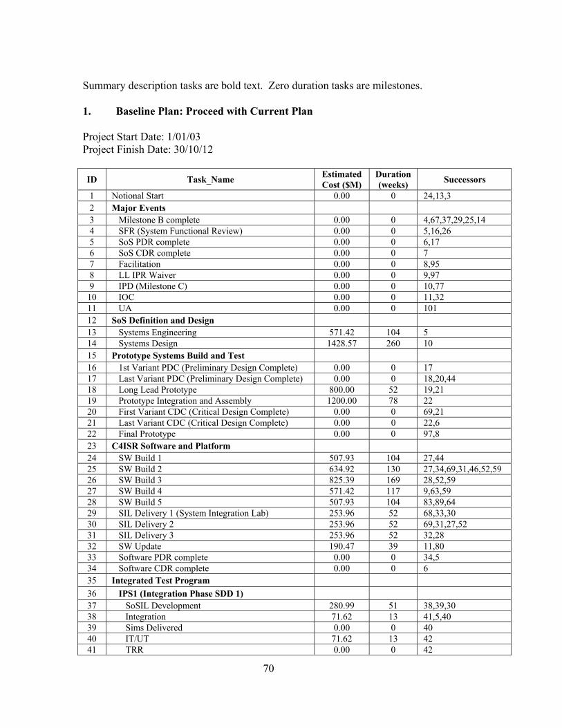
70
Summary description tasks are bold text. Zero duration tasks are milestones.
1. Baseline Plan: Proceed with Current Plan
Project Start Date: 1/01/03 Project Finish Date: 30/10/12
ID Task_Name Estimated Cost ($M)
Duration (weeks) Successors
1 Notional Start 0.00 0 24,13,3 2 Major Events 3 Milestone B complete 0.00 0 4,67,37,29,25,14 4 SFR (System Functional Review) 0.00 0 5,16,26 5 SoS PDR complete 0.00 0 6,17 6 SoS CDR complete 0.00 0 7 7 Facilitation 0.00 0 8,95 8 LL IPR Waiver 0.00 0 9,97 9 IPD (Milestone C) 0.00 0 10,77
10 IOC 0.00 0 11,32 11 UA 0.00 0 101 12 SoS Definition and Design 13 Systems Engineering 571.42 104 5 14 Systems Design 1428.57 260 10 15 Prototype Systems Build and Test 16 1st Variant PDC (Preliminary Design Complete) 0.00 0 17 17 Last Variant PDC (Preliminary Design Complete) 0.00 0 18,20,44 18 Long Lead Prototype 800.00 52 19,21 19 Prototype Integration and Assembly 1200.00 78 22 20 First Variant CDC (Critical Design Complete) 0.00 0 69,21 21 Last Variant CDC (Critical Design Complete) 0.00 0 22,6 22 Final Prototype 0.00 0 97,8 23 C4ISR Software and Platform 24 SW Build 1 507.93 104 27,44 25 SW Build 2 634.92 130 27,34,69,31,46,52,59 26 SW Build 3 825.39 169 28,52,59 27 SW Build 4 571.42 117 9,63,59 28 SW Build 5 507.93 104 83,89,64 29 SIL Delivery 1 (System Integration Lab) 253.96 52 68,33,30 30 SIL Delivery 2 253.96 52 69,31,27,52 31 SIL Delivery 3 253.96 52 32,28 32 SW Update 190.47 39 11,80 33 Software PDR complete 0.00 0 34,5 34 Software CDR complete 0.00 0 6 35 Integrated Test Program 36 IPS1 (Integration Phase SDD 1) 37 SoSIL Development 280.99 51 38,39,30 38 Integration 71.62 13 41,5,40 39 Sims Delivered 0.00 0 40 40 IT/UT 71.62 13 42 41 TRR 0.00 0 42
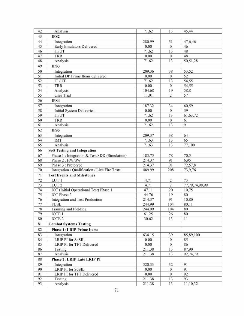
71
42 Analysis 71.62 13 45,44 43 IPS2 44 Integration 280.99 51 47,6,46 45 Early Emulators Delivered 0.00 0 46 46 IT/UT 71.62 13 48 47 TRR 0.00 0 48 48 Analysis 71.62 13 50,51,28 49 IPS3 50 Integration 209.36 38 53,52 51 Initial DP Prime Items delivered 0.00 0 52 52 IT /UT 71.62 13 54,55 53 TRR 0.00 0 54,55 54 Analysis 104.68 19 58,8 55 User Trial 11.01 2 57 56 IPS4 57 Integration 187.32 34 60,59 58 Initial System Deliveries 0.00 0 59 59 IT/UT 71.62 13 61,63,72 60 TRR 0.00 0 61 61 Analysis 71.62 13 9 62 IPS5 63 Integration 209.37 38 64 64 IMT 71.63 13 65 65 Analysis 71.63 13 77,100 66 SoS Testing and Integration 67 Phase 1 : Integration & Test SDD (Simulation) 183.75 78 70,5 68 Phase 2 : HW/SW 214.37 91 6,95 69 Phase 3 : Prototype 214.37 91 72,57,8 70 Integration / Qualification / Live Fire Tests 489.99 208 73,9,76 71 Test Events and Milestones 72 LUT 1 4.71 2 73 73 LUT 2 4.71 2 77,79,74,98,99 74 IOT (Initial Operational Test) Phase 1 47.11 20 10,75 75 IOT Phase 2 44.76 19 80 76 Integration and Test Production 214.37 91 10,80 77 FUSL 244.99 104 80,11 78 Training and Fielding 244.99 104 80 79 IOTE 1 61.25 26 80 80 IOTE 2 30.62 13 11 81 Combat Systems Testing 82 Phase 1: LRIP Prime Items 83 Integration 634.15 39 85,89,100 84 LRIP PI for SoSIL 0.00 0 85 85 LRIP PI for TFT Delivered 0.00 0 86 86 Testing 211.38 13 87,90 87 Analysis 211.38 13 92,74,79 88 Phase 2: LRIP Late LRIP PI 89 Integration 520.33 32 91 90 LRIP PI for SoSIL 0.00 0 91 91 LRIP PI for TFT Delivered 0.00 0 92 92 Testing 211.38 13 93 93 Analysis 211.38 13 11,10,32
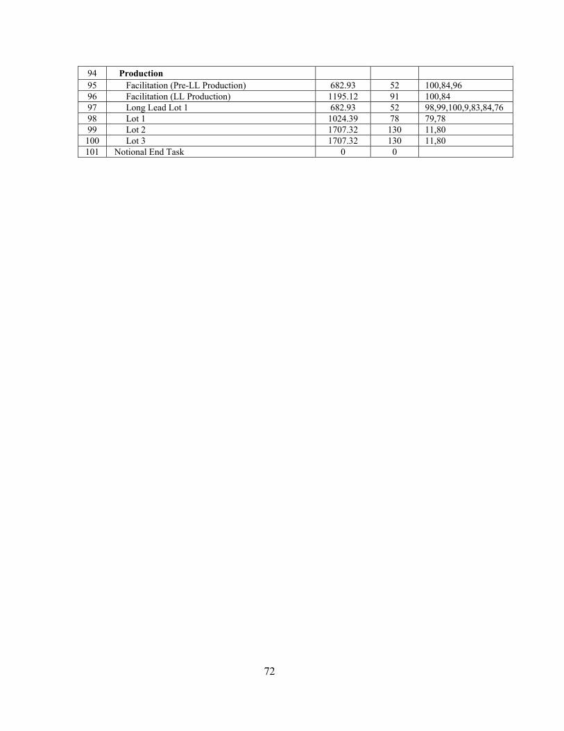
72
94 Production 95 Facilitation (Pre-LL Production) 682.93 52 100,84,96 96 Facilitation (LL Production) 1195.12 91 100,84 97 Long Lead Lot 1 682.93 52 98,99,100,9,83,84,76 98 Lot 1 1024.39 78 79,78 99 Lot 2 1707.32 130 11,80 100 Lot 3 1707.32 130 11,80 101 Notional End Task 0 0

73
2. Alternate Plan 1: Mitigate High Risk Technologies First
Project Start Date: 1/01/03 Project Finish Date: 22/01/13
ID Task_Name Estimated
Cost ($M) Duration (Weeks)
Successors
1 Notional Start 0.00 0 57,13,3 2 Major Events 3 Milestone B complete 0.00 0 4,100,70,62,58,14 4 SFR (System Functional Review) 0.00 0 5,49,59 5 SoS PDR complete 0.00 0 6,50 6 SoS CDR complete 0.00 0 7 7 Facilitation 0.00 0 8,128 8 LL IPR Waiver 0.00 0 9,130 9 IPD (Milestone C) 0.00 0 10,110
10 IOC 0.00 0 11,65 11 UA 0.00 0 134 12 SoS Definition and Design 13 Systems Engineering 571.43 104 5 14 Systems Design 1428.57 260 10 15 Prototype Systems Build and Test
16 TRL Mitigation (Technology Readiness Level)
17 KPP 1: Joint Interoperability 18 Interface & Information Exchange 113.24 65 4
19 KPP 2: Networked Battle Command
20 Security Systems & Algorithms 249.13 143 6 21 Quality of Service Algorithms 67.94 39 3 22 Wideband Waveforms 181.18 104 5 23 Multispectral Sensors & Seekers 90.59 52 3 24 Combat Identification 22.65 13 3
25 Sensor/Data Fusion & Data Compression
67.94 39 3
26 KPP 3: Networked Lethality
27 Dynamic Sensor-Shooter Pairing / Fire Control
90.59 52 3
28 LOS/BLOS/NLOS Precision Munitions Guidance
271.78 156 6
29 Aided Target Recognition 67.94 39 3 30 Auto Target Recognition 181.18 104 5
31 Recoil Management & Lightweight Components
90.59 52 3
32 Distributed Collaboration of Manned / Unmanned Vehicles
226.48 130 5
33 Rapid Battle Damage Assessment 67.94 39 3 34 KPP 4: Transportability
35 High Power Density / Fuel Efficient Propulsion
90.59 52 3
36 KPP 5: Sustainability / Reliability
37 Embedded Predictive Logistic Sensors / Algorithms
90.59 52 3
38 Water Generation and Purification 90.59 52 3
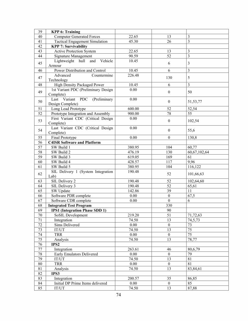
74
39 KPP 6: Training 40 Computer Generated Forces 22.65 13 3 41 Tactical Engagement Simulation 45.30 26 3 42 KPP 7: Survivability 43 Active Protection System 22.65 13 3 44 Signature Management 90.59 52 3
45 Lightweight hull and Vehicle Armour
10.45 6 3
46 Power Distribution and Control 10.45 6 3
47 Advanced Countermine Technology
226.48 130 5
48 High Density Packaged Power 10.45 6 3
49 1st Variant PDC (Preliminary Design Complete)
0.00 0 50
50 Last Variant PDC (Preliminary Design Complete)
0.00 0 51,53,77
51 Long Lead Prototype 600.00 52 52,54 52 Prototype Integration and Assembly 900.00 78 55
53 First Variant CDC (Critical Design Complete)
0.00 0 102,54
54 Last Variant CDC (Critical Design Complete)
0.00 0 55,6
55 Final Prototype 0.00 0 130,8 56 C4ISR Software and Platform 57 SW Build 1 380.95 104 60,77 58 SW Build 2 476.19 130 60,67,102,64 59 SW Build 3 619.05 169 61 60 SW Build 4 428.57 117 9,96 61 SW Build 5 380.95 104 116,122
62 SIL Delivery 1 (System Integration Lab)
190.48 52 101,66,63
63 SIL Delivery 2 190.48 52 102,64,60 64 SIL Delivery 3 190.48 52 65,61 65 SW Update 142.86 39 11 66 Software PDR complete 0.00 0 67,5 67 Software CDR complete 0.00 0 6 68 Integrated Test Program 330 69 IPS1 (Integration Phase SDD 1) 90 70 SoSIL Development 219.20 51 71,72,63 71 Integration 74.50 13 74,5,73 72 Sims Delivered 0.00 0 73 73 IT/UT 74.50 13 75 74 TRR 0.00 0 75 75 Analysis 74.50 13 78,77 76 IPS2 77 Integration 263.61 46 80,6,79 78 Early Emulators Delivered 0.00 0 79 79 IT/UT 74.50 13 81 80 TRR 0.00 0 81 81 Analysis 74.50 13 83,84,61 82 IPS3 83 Integration 200.57 35 86,85 84 Initial DP Prime Items delivered 0.00 0 85 85 IT/UT 74.50 13 87,88
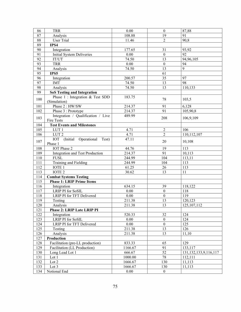
75
86 TRR 0.00 0 87,88 87 Analysis 108.88 19 91 88 User Trial 11.46 2 90,8 89 IPS4 90 Integration 177.65 31 93,92 91 Initial System Deliveries 0.00 0 92 92 IT/UT 74.50 13 94,96,105 93 TRR 0.00 0 94 94 Analysis 74.50 13 9 95 IPS5 61 96 Integration 200.57 35 97 97 IMT 74.50 13 98 98 Analysis 74.50 13 110,133 99 SoS Testing and Integration
100 Phase 1 : Integration & Test SDD (Simulation)
183.75 78 103,5
101 Phase 2 : HW/SW 214.37 91 6,128 102 Phase 3 : Prototype 214.37 91 105,90,8
103 Integration / Qualification / Live Fire Tests
489.99 208 106,9,109
104 Test Events and Milestones 105 LUT 1 4.71 2 106 106 LUT 2 4.71 2 110,112,107
107 IOT (Initial Operational Test) Phase 1
47.11 20 10,108
108 IOT Phase 2 44.76 19 113 109 Integration and Test Production 214.37 91 10,113 110 FUSL 244.99 104 113,11 111 Training and Fielding 244.99 104 113 112 IOTE 1 61.25 26 113 113 IOTE 2 30.62 13 11 114 Combat Systems Testing 115 Phase 1: LRIP Prime Items 116 Integration 634.15 39 118,122 117 LRIP PI for SoSIL 0.00 0 118 118 LRIP PI for TFT Delivered 0.00 0 119 119 Testing 211.38 13 120,123 120 Analysis 211.38 13 125,107,112 121 Phase 2: LRIP Late LRIP PI 122 Integration 520.33 32 124 123 LRIP PI for SoSIL 0.00 0 124 124 LRIP PI for TFT Delivered 0.00 0 125 125 Testing 211.38 13 126 126 Analysis 211.38 13 11,10 127 Production 128 Facilitation (pre-LL production) 833.33 65 129 129 Facilitation (LL Production) 1166.67 91 133,117 130 Long Lead Lot 1 666.67 52 131,132,133,9,116,117 131 Lot 1 1000.00 78 112,111 132 Lot 2 1666.67 130 11,113 133 Lot 3 1666.67 130 11,113 134 Notional End 0.00 0
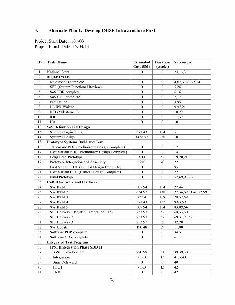
76
3. Alternate Plan 2: Develop C4ISR Infrastructure First
Project Start Date: 1/01/03 Project Finish Date: 15/04/14
ID Task_Name Estimated
Cost ($M) Duration (weeks)
Successors
1 Notional Start 0 0 24,13,3 2 Major Events 3 Milestone B complete 0 0 4,67,37,29,25,14 4 SFR (System Functional Review) 0 0 5,26 5 SoS PDR complete 0 0 6,16 6 SoS CDR complete 0 0 7,17 7 Facilitation 0 0 8,95 8 LL IPR Waiver 0 0 9,97,21 9 IPD (Milestone C) 0 0 10,77
10 IOC 0 0 11,32 11 UA 0 0 101 12 SoS Definition and Design 13 Systems Engineering 571.43 104 5 14 Systems Design 1428.57 260 10 15 Prototype Systems Build and Test 16 1st Variant PDC (Preliminary Design Complete) 0 0 17 17 Last Variant PDC (Preliminary Design Complete) 0 0 18 18 Long Lead Prototype 800 52 19,20,21 19 Prototype Integration and Assembly 1200 78 22 20 First Variant CDC (Critical Design Complete) 0 0 95 21 Last Variant CDC (Critical Design Complete) 0 0 22 22 Final Prototype 0 0 57,69,97,96 23 C4ISR Software and Platform 24 SW Build 1 507.94 104 27,44 25 SW Build 2 634.92 130 27,34,69,31,46,52,59 26 SW Build 3 825.4 169 28,52,59 27 SW Build 4 571.43 117 9,63,59 28 SW Build 5 507.94 104 83,89,64 29 SIL Delivery 1 (System Integration Lab) 253.97 52 68,33,30 30 SIL Delivery 2 253.97 52 69,31,27,52 31 SIL Delivery 3 253.97 52 32,28 32 SW Update 190.48 39 11,80 33 Software PDR complete 0 0 34,5 34 Software CDR complete 0 0 6 35 Integrated Test Program 36 IPS1 (Integration Phase SDD 1) 37 SoSIL Development 280.99 51 38,39,30 38 Integration 71.63 13 41,5,40 39 Sims Delivered 0 0 40 40 IT/UT 71.63 13 42 41 TRR 0 0 42
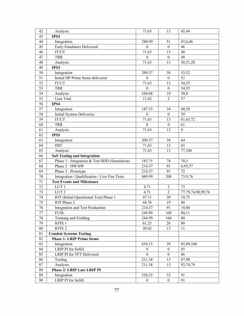
77
42 Analysis 71.63 13 45,44 43 IPS2 44 Integration 280.99 51 47,6,46 45 Early Emulators Delivered 0 0 46 46 IT/UT 71.63 13 48 47 TRR 0 0 48 48 Analysis 71.63 13 50,51,28 49 IPS3 50 Integration 209.37 38 53,52 51 Initial DP Prime Items delivered 0 0 52 52 IT/UT 71.63 13 54,55 53 TRR 0 0 54,55 54 Analysis 104.68 19 58,8 55 User Trial 11.02 2 57 56 IPS4 57 Integration 187.33 34 60,59 58 Initial System Deliveries 0 0 59 59 IT/UT 71.63 13 61,63,72 60 TRR 0 0 61 61 Analysis 71.63 13 9 62 IPS5 63 Integration 209.37 38 64 64 IMT 71.63 13 65 65 Analysis 71.63 13 77,100 66 SoS Testing and Integration 67 Phase 1 : Integration & Test SDD (Simulation) 183.75 78 70,5 68 Phase 2 : HW/SW 214.37 91 6,95,57 69 Phase 3 : Prototype 214.37 91 72 70 Integration / Qualification / Live Fire Tests 489.99 208 73,9,76 71 Test Events and Milestones 72 LUT 1 4.71 2 73 73 LUT 2 4.71 2 77,79,74,98,99,76 74 IOT (Initial Operational Test) Phase 1 47.11 20 10,75 75 IOT Phase 2 44.76 19 80 76 Integration and Test Production 214.37 91 10,80 77 FUSL 244.99 104 80,11 78 Training and Fielding 244.99 104 80 79 IOTE 1 61.25 26 80 80 IOTE 2 30.62 13 11 81 Combat Systems Testing 82 Phase 1: LRIP Prime Items 83 Integration 634.15 39 85,89,100 84 LRIP PI for SoSIL 0 0 85 85 LRIP PI for TFT Delivered 0 0 86 86 Testing 211.38 13 87,90 87 Analysis 211.38 13 92,74,79 88 Phase 2: LRIP Late LRIP PI 89 Integration 520.33 32 91 90 LRIP PI for SoSIL 0 0 91
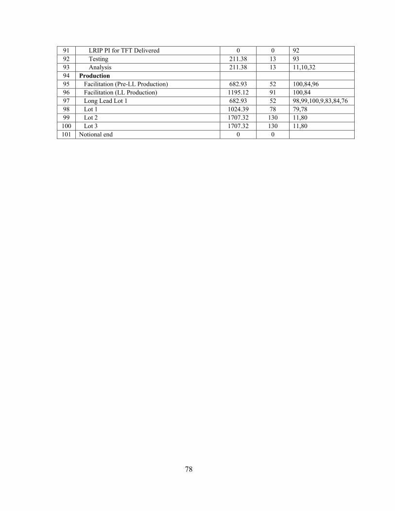
78
91 LRIP PI for TFT Delivered 0 0 92 92 Testing 211.38 13 93 93 Analysis 211.38 13 11,10,32 94 Production 95 Facilitation (Pre-LL Production) 682.93 52 100,84,96 96 Facilitation (LL Production) 1195.12 91 100,84 97 Long Lead Lot 1 682.93 52 98,99,100,9,83,84,76 98 Lot 1 1024.39 78 79,78 99 Lot 2 1707.32 130 11,80 100 Lot 3 1707.32 130 11,80 101 Notional end 0 0
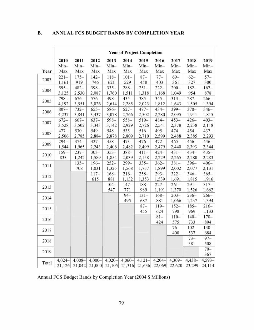
79
B. ANNUAL FCS BUDGET BANDS BY COMPLETION YEAR
Year of Project Completion
Year
2010 Min–Max
2011 Min–Max
2012 Min–Max
2013 Min–Max
2014 Min–Max
2015 Min–Max
2016 Min–Max
2017 Min–Max
2018 Min–Max
2019Min–Max
2003 221–1,161
175– 919
142– 746
118– 621
101– 529
87– 458
77– 403
69– 361
62– 327
57– 300
2004 595–3,125
482–2,530
398–2,087
335–1,760
288–1,511
251–1,318
222–1,168
200–1,049
182– 954
167– 878
2005 798–4,192
676–3,551
576–3,026
498–2,614
435–2,285
385–2,023
345–1,812
313–1,643
287–1,505
266–1,394
2006 807–4,237
732–3,841
655–3,437
586–3,078
527–2,766
477–2,502
434–2,280
399–2,095
370–1,941
346–1,815
2007 672–3,528
667–3,502
637–3,343
598–3,142
558–2,929
519–2,726
484–2,541
453–2,378
426–2,238
403–2,118
2008 477–2,506
530–2,785
549–2,884
548–2,878
535–2,809
516–2,710
495–2,599
474–2,488
454–2,385
437–2,293
2009 294–1,544
374–1,965
427–2,243
458–2,406
473–2,482
476–2,499
472–2,479
465–2,440
456– 2,393
446–2,344
2010 159– 833
237–1,242
303–1,589
353–1,854
388–2,039
411–2,158
424–2,229
431–2,265
434–2,280
435–2,283
2011 135– 708
196–1,031
252–1,325
299–1,568
335–1,757
362–1,899
381–2,002
396–2,077
406–2,131
2012 117– 615
168– 881
216–1,132
258–1,353
293–1,539
322–1,691
346–1,815
365–1,916
2013 104– 547
147– 771
188– 989
227–1,191
261–1,370
291–1,526
317–1,662
2014 94– 495
131– 687
168– 881
203–1,066
236–1,237
266–1,394
2015 87– 455
119– 624
152– 798
185– 969
216–1,133
2016 81– 424
110– 575
140– 733
170– 894
2017 76– 400
102– 537
130– 684
2018 73– 381
97– 508
2019
70– 367
Total 4,024–21,126
4,008–21,042
4,000–21,000
4,020–21,105
4,060–21,316
4,121–21,636
4,204–22,069
4,309–22,620
4,438–23,299
4,593–24,114
Annual FCS Budget Bands by Completion Year (2004 $ Millions)

80
THIS PAGE INTENTIONALLY LEFT BLANK
81
APPENDIX C
A. JAVA CODE FOR UNCONSTRAINED REACHING ALGORITHM /** * Unconstrained Reaching Algorithm **/ import java.util.*; import java.io.*; public class reach2 { // Class Constants public static final double mode_a_low = 1.15; public static final double mode_a_med = 1.20; public static final double mode_a_high = 1.25; public static final double pr_tML_low = 0.60; public static final double pr_tML_med = 0.70; public static final double pr_tML_high = 0.80; public static final int monteCarloIterations = 60000; private static PrintWriter outputStream = null; public static void main(String args[]) { // Text Input Tools String inputString; BufferedReader inputUnit; StringTokenizer tk; long startTime, finishTime, elapsedTime; try{ outputStream = new PrintWriter(new FileOutputStream ("num.txt")); } catch (FileNotFoundException e){ System.out.println("Error opening output file"); System.exit(0); } //Network data structure elements: forward-star int i, j, t, k, n, m, T, r; int [] point; int [] tail; int [] head; int [] duration; int [] origDuration; // random duration variables int [] risk; double [] min; double [] shape; double [] scale; double [] mode; double [] prob; //Check usage (at least one command line argument) if(args.length==0) { System.out.println("\nUsage: java reach2 <filename>"); return; } k=0; try { inputUnit = new BufferedReader(new FileReader(args[0])); if((inputString = inputUnit.readLine())==null){ System.out.println("Premature end of file encountered. k="+k); return;

82
} tk = new StringTokenizer(inputString); n = Integer.parseInt(tk.nextToken()); m = Integer.parseInt(tk.nextToken()); point = new int [n+2]; tail = new int [m+1]; head = new int [m+1]; origDuration = new int [m+1]; duration = new int [m+1]; risk = new int [m+1]; min = new double [m+1] ; shape = new double [m+1] ; scale = new double [m+1] ; prob = new double [m+1] ; mode = new double [m+1] ; point[0] =1; T =0; for(k=1; k<=m; k++){ if((inputString = inputUnit.readLine())==null){ System.out.println("Premature end of file encountered. k="+k); return; } tk = new StringTokenizer(inputString); i = Integer.parseInt(tk.nextToken()); j = Integer.parseInt(tk.nextToken()); t = Integer.parseInt(tk.nextToken()); r = Integer.parseInt(tk.nextToken()); // 1 = Low Risk,
// 2 = Med Risk, // 3 = High Risk
if(t > T){ T=t; } point[i]++; tail[k] =i; head[k] =j; origDuration[k] =t; risk[k] =r; // Assign standard risk based values from CAIG to each activity. if(r == 1){ // Low Risk mode[k] = mode_a_low; prob[k] = pr_tML_low; }else if (r == 2){ // med risk mode[k] = mode_a_med; prob[k] = pr_tML_med; }else if (r == 3){ // high risk mode[k] = mode_a_high; prob[k] = pr_tML_high; }else{ System.out.println("Invalid risk code at k = "+k); return; } } // close data input loop loop inputUnit.close(); } catch(FileNotFoundException e) { System.out.println(e); return; } catch(IOException e){ System.out.println(e); return; } catch(NoSuchElementException e) {
83
System.out.println("No data found: k="+k); return; } //Clean up point array for(i=1; i <= n+1; i++) { point[i]=point[i-1]+point[i]; } for(k=1; k <= m; k++) { i=tail[k]; point[i]--; } System.out.println(" Finished reading data file..."); //*************** END DATA ENTRY - START REACH ALGORITHM startTime = System.currentTimeMillis(); System.out.println(" Opening Simulation Loop - writing to file"); int monteCarloCounter; monteCarloCounter = 1; // Open the Monte Carlo Loop while ( monteCarloCounter < monteCarloIterations){ /* Change the Project Duration to reflect the project activity risk. * This will give one realization of the activity duration, which is * based on the Weibull timeribution. Assumptions are those used by * the Cost Analysis Improvement Group (CAIG), PA&E. */ for(k = 1; k <= m; k++){ min[k] = origDuration[k] / mode[k]; if (origDuration[k] > 0) { shape[k] = 1 / (Math.log(prob[k])+1); scale[k] = (origDuration[k]-min[k]) /
Math.pow((1-1/shape[k]),(1/shape[k])); duration[k] = (int)Math.ceil( (min[k] + scale[k]*
(Math.pow((-Math.log(1-Math.random())), (1/shape[k]))))); } else { shape[k] = 0; scale[k] = 0; } } // Data structure elements int s; int cardTEMP, cardPERM, minTime; boolean [] TEMP; boolean [] PERM; int [] pred; int [] activityTime; // Algorithm code starts here pred = new int[n + 1]; activityTime = new int[n + 1]; TEMP = new boolean[n + 1]; PERM = new boolean[n + 1]; s = 1; cardTEMP = 0; cardPERM = 0; // initialize the temp and perm cardinality flags. while (cardTEMP < n) { cardTEMP ++; activityTime[cardTEMP] = 0; TEMP[cardTEMP] = true; PERM[cardTEMP] = false; } activityTime[s] = 0;
84
pred[s] = 0; // Calculate the longest path. for (i=0; i < n; i++) { minTime = 0; PERM[i] = true; cardPERM ++; TEMP[i] = false; cardTEMP --; k = point[i]; while (k < point[i + 1]) { j = head[k]; if (activityTime[j] < (activityTime[i] + duration[k])) { activityTime[j] = (activityTime[i] + duration[k]); pred[j] = i; } k++; } } // End reaching code int maxsp; int maxnode; /*Now determine the results*/ maxsp=0; maxnode=0; for(i=1; i<=n; i++){ if(activityTime[i] > maxsp && activityTime[i] > 0){ maxsp = activityTime[i]; maxnode = i; } } i = maxnode; j = 0; outputStream.println(maxsp); //System.out.println(" Hops in longest SP: "+j); //System.out.println(" activity duration: "+monteCarloCounter+" is: "+
maxsp); if (monteCarloCounter == monteCarloIterations/2){ System.out.println(" ...Half way through the simulation..."); } monteCarloCounter++; } // close of Monte Carlo Loop System.out.println(" finished the Simulation "); outputStream.close(); finishTime = System.currentTimeMillis(); elapsedTime = finishTime-startTime; System.out.println(" Elapsed time = "+ elapsedTime); } }
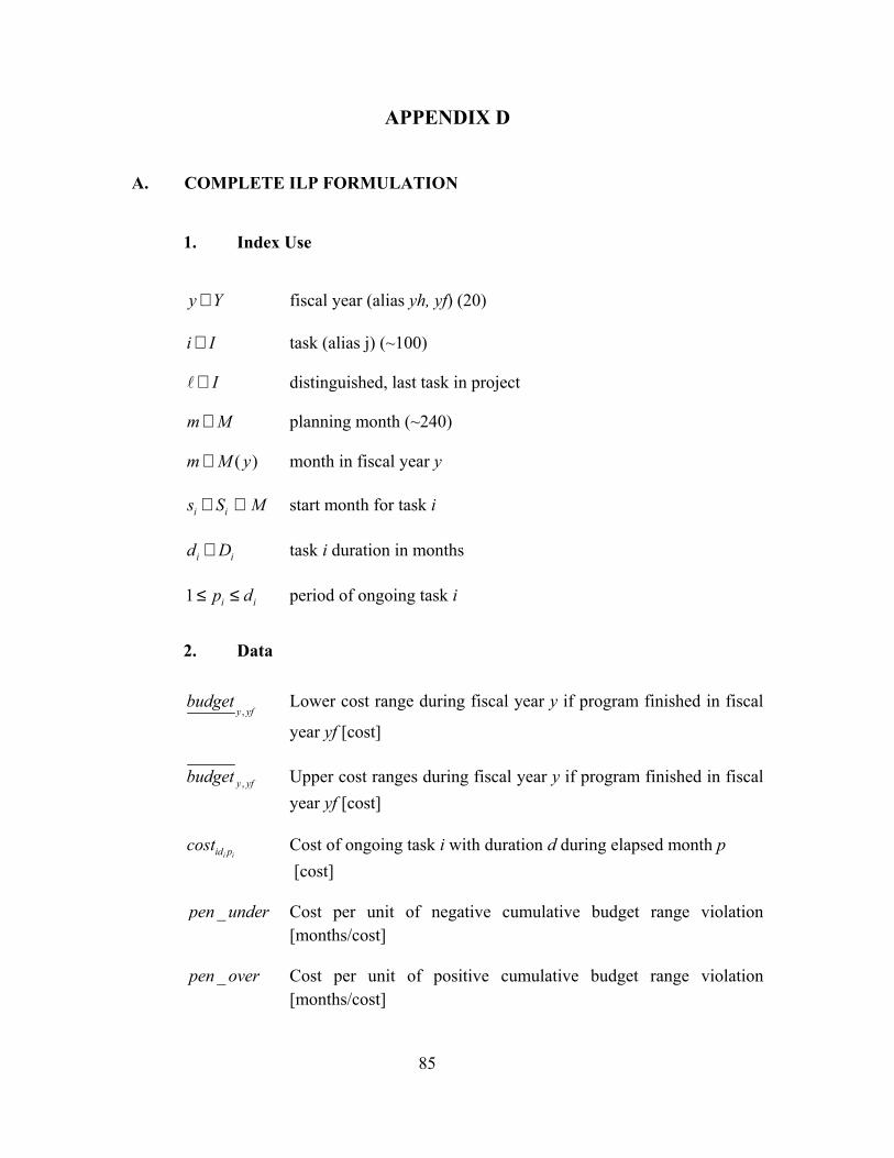
85
APPENDIX D
A. COMPLETE ILP FORMULATION
1. Index Use
y Y∈ fiscal year (alias yh, yf) (20)
i I∈ task (alias j) (~100)
I∈ distinguished, last task in project
m M∈ planning month (~240)
( )m M y∈ month in fiscal year y
i is S M∈ ⊆ start month for task i
i id D∈ task i duration in months
1 i ip d≤ ≤ period of ongoing task i
2. Data
,y yfbudget Lower cost range during fiscal year y if program finished in fiscal
year yf [cost]
,y yfbudget Upper cost ranges during fiscal year y if program finished in fiscal year yf [cost]
i iid pcost Cost of ongoing task i with duration d during elapsed month p
[cost]
_pen under Cost per unit of negative cumulative budget range violation [months/cost]
_pen over Cost per unit of positive cumulative budget range violation
[months/cost]
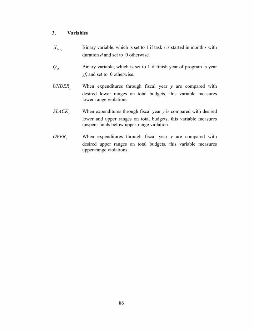
86
3. Variables
i iis dX Binary variable, which is set to 1 if task i is started in month s with
duration d and set to 0 otherwise
yfQ Binary variable, which is set to 1 if finish year of program is year yf, and set to 0 otherwise.
yUNDER When expenditures through fiscal year y are compared with
desired lower ranges on total budgets, this variable measures lower-range violations.
ySLACK When expenditures through fiscal year y is compared with desired
lower and upper ranges on total budgets, this variable measures unspent funds below upper-range violation.
yOVER When expenditures through fiscal year y are compared with
desired upper ranges on total budgets, this variable measures upper-range violations.
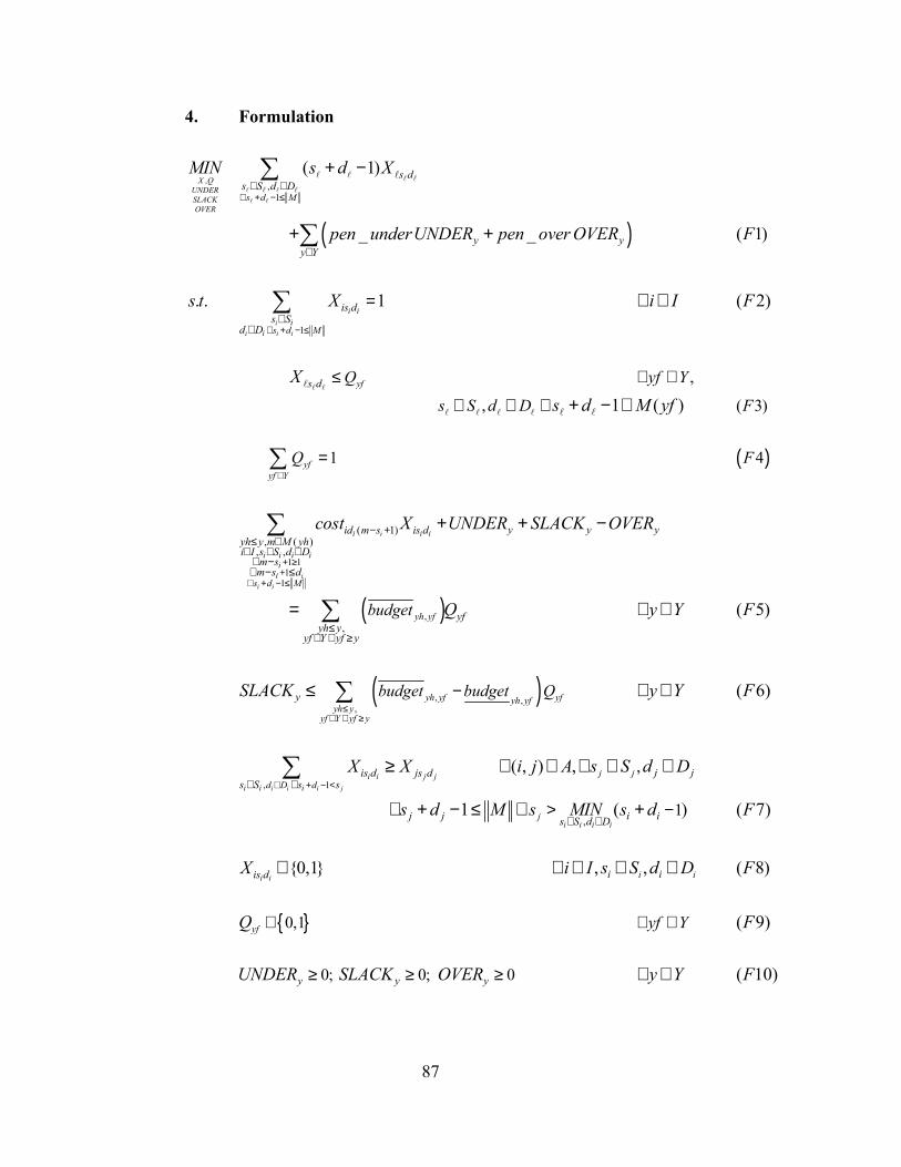
87
4. Formulation
( )
( )
,,
1
1
,
, ( 3)
1 4
( 1)
_ _ ( 1)
. . 1 ( 2)
1 ( )
ii i i
X QUNDERSLACKOVER
i ii
i
s d M
s d M
yf
yfyf Y
s ds S d D
y yy Y
is ds S
d D
s d Q yf Y
s S d D F
Q F
MIN s d X
pen underUNDER pen over OVER F
s t X i I F
Xs d M yf
c
∧ + − ≤
∧ + − ≤
∈
∈ ∈
∈
∈∈
=
≤ ∀ ∈
∈ ∈ ∧
=
+ −
+ +
∀ ∈
+ − ∈
∑
∑
∑
∑
( )
( )
1 11
1
,
, ,,
( 1), ( )
, ,
,( 5)
( 6)
i
ii i
i i i
i i i ii
i
i ii
s d M
yh yf
yfyh yf yh yfyh y
yf Y yf y
y y yid m s is dyh y m M yhi I s S d D
m sm s d
yfyh y
yf Y yf y
y
is ds
budget
budget budget Q
ost X UNDER SLACK OVER
Q y Y F
SLACK y Y F
X
+ ≥+
∧ + − ≤
≤∈ ∧ ≥
− +≤ ∈
∈ ∈ ∈∧ −∧ − ≤
≤∈ ∧ ≥
∈
−
+ + −
= ∀ ∈
≤ ∀ ∈∑
∑
∑
{ }
, 1
,
,
1
0,1
0; 0; 0
( , ) ,
1 ( ) ( 7)
{0,1} , , ( 8)
( 9)
( 10)
i i i j
j ji i
i i i i
i i
j jd D d
j
i i
yf
j jjs dS s s
j j i is S d D
i iis d
y y y
yf Y
X i j A s S d D
s d M s MIN s d F
X i I s S d D F
Q F
UNDER SLACK OVER y Y F
∈ + − <∧
∈ ∈> −
∈ ∀ ∈
≥ ≥ ≥
≥ ∀ ∈ ∀ ∈ ∈
∧ + − ≤ ∧ +
∈ ∀ ∈ ∈ ∈
∀ ∈
∑
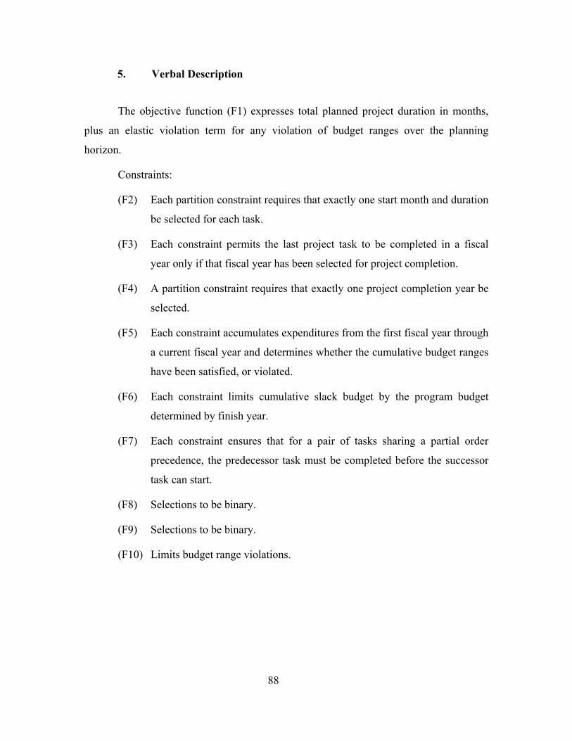
88
5. Verbal Description
The objective function (F1) expresses total planned project duration in months,
plus an elastic violation term for any violation of budget ranges over the planning
horizon.
Constraints:
(F2) Each partition constraint requires that exactly one start month and duration
be selected for each task.
(F3) Each constraint permits the last project task to be completed in a fiscal
year only if that fiscal year has been selected for project completion.
(F4) A partition constraint requires that exactly one project completion year be
selected.
(F5) Each constraint accumulates expenditures from the first fiscal year through
a current fiscal year and determines whether the cumulative budget ranges
have been satisfied, or violated.
(F6) Each constraint limits cumulative slack budget by the program budget
determined by finish year.
(F7) Each constraint ensures that for a pair of tasks sharing a partial order
precedence, the predecessor task must be completed before the successor
task can start.
(F8) Selections to be binary.
(F9) Selections to be binary.
(F10) Limits budget range violations.
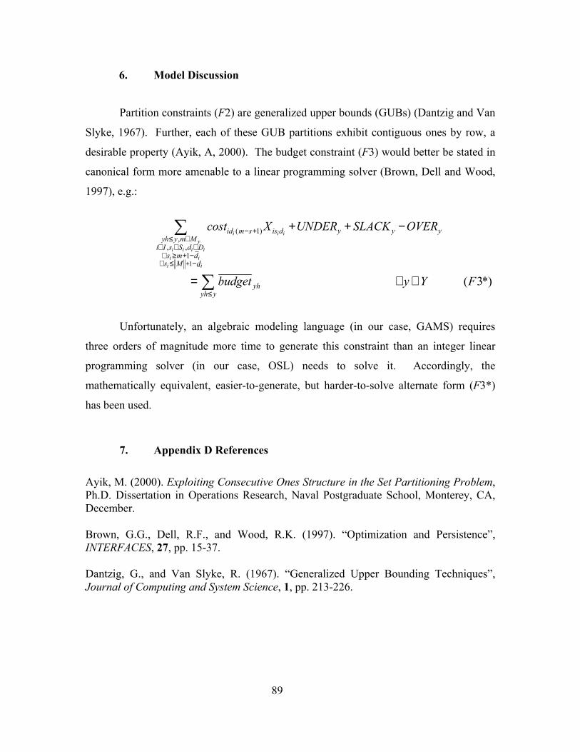
89
6. Model Discussion
Partition constraints (F2) are generalized upper bounds (GUBs) (Dantzig and Van
Slyke, 1967). Further, each of these GUB partitions exhibit contiguous ones by row, a
desirable property (Ayik, A, 2000). The budget constraint (F3) would better be stated in
canonical form more amenable to a linear programming solver (Brown, Dell and Wood,
1997), e.g.:
1
( 1),
, ,1
( 3*)
i i iy
i i i ii i
i i
y y yid m s is dyh y m M
i I s S d Ds m d
s M d
yhyh y
cost X UNDER SLACK OVER
budget y Y F+
− +≤ ∈
∈ ∈ ∈∧ ≥ + −
∧ ≤ −
≤
+ + −
= ∀ ∈
∑
∑
Unfortunately, an algebraic modeling language (in our case, GAMS) requires
three orders of magnitude more time to generate this constraint than an integer linear
programming solver (in our case, OSL) needs to solve it. Accordingly, the
mathematically equivalent, easier-to-generate, but harder-to-solve alternate form (F3*)
has been used.
7. Appendix D References
Ayik, M. (2000). Exploiting Consecutive Ones Structure in the Set Partitioning Problem, Ph.D. Dissertation in Operations Research, Naval Postgraduate School, Monterey, CA, December. Brown, G.G., Dell, R.F., and Wood, R.K. (1997). “Optimization and Persistence”, INTERFACES, 27, pp. 15-37. Dantzig, G., and Van Slyke, R. (1967). “Generalized Upper Bounding Techniques”, Journal of Computing and System Science, 1, pp. 213-226.

90
THIS PAGE INTENTIONALLY LEFT BLANK
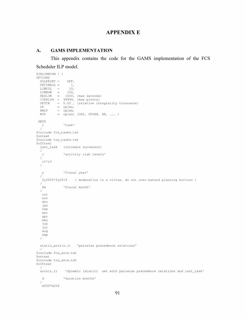
91
APPENDIX E
A. GAMS IMPLEMENTATION This appendix contains the code for the GAMS implementation of the FCS
Scheduler ILP model. $INLINECOM { } OPTIONS SOLPRINT = OFF, DECIMALS = 1, LIMCOL = 10, LIMROW = 100, RESLIM = 1000, {max seconds} ITERLIM = 99999, {max pivots} OPTCR = 0.05 , {relative integrality tolerance} LP = cplex, RMIP = cplex, MIP = cplex; {OSL, CPLEX, XA, ... } SETS i "task" / $include fcs_tasks.txt $ontext $include toy_tasks.txt $offtext last_task {ultimate successor} / r "activity risk levels" / r1*r3 / y "fiscal year" / fy2003*fy2019 { moderation is a virtue, do not over-extend planning horizon } / fm "fiscal month" / oct nov dec jan feb mar apr may jun jul aug sep / static_arcs(i,i) "pairwise precedence relations" / $include fcs_arcs.txt $ontext $include toy_arcs.txt $offtext / arcs(i,i) "dynamic (static) set with pairwise precedence relations and last_task" d "duration months" / m000*m204
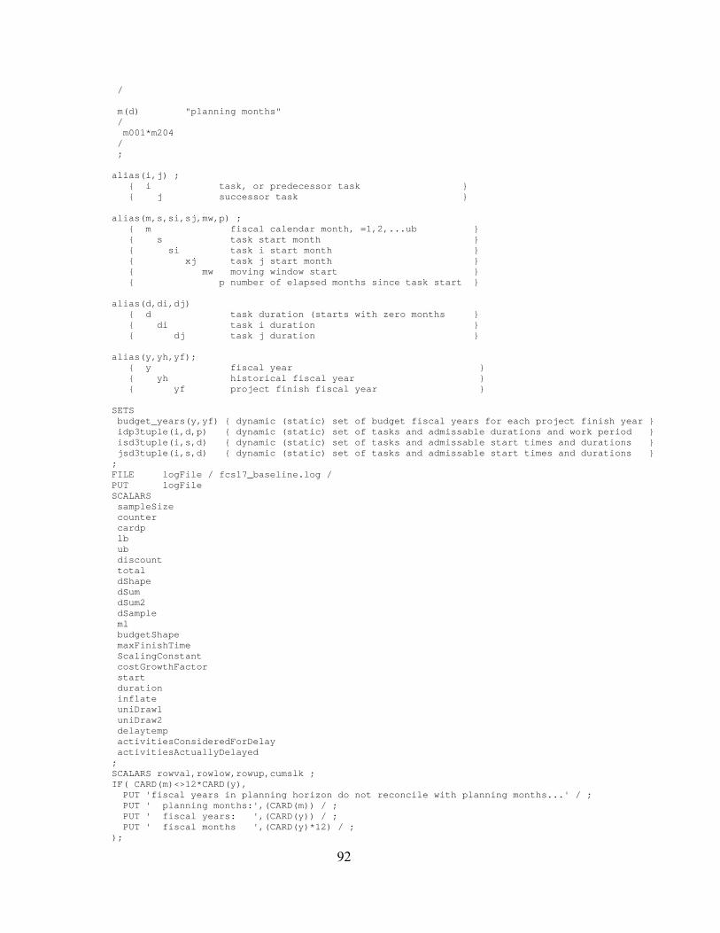
92
/ m(d) "planning months" / m001*m204 / ; alias(i,j) ; { i task, or predecessor task } { j successor task } alias(m,s,si,sj,mw,p) ; { m fiscal calendar month, =1,2,...ub } { s task start month } { si task i start month } { xj task j start month } { mw moving window start } { p number of elapsed months since task start } alias(d,di,dj) { d task duration (starts with zero months } { di task i duration } { dj task j duration } alias(y,yh,yf); { y fiscal year } { yh historical fiscal year } { yf project finish fiscal year } SETS budget_years(y,yf) { dynamic (static) set of budget fiscal years for each project finish year } idp3tuple(i,d,p) { dynamic (static) set of tasks and admissable durations and work period } isd3tuple(i,s,d) { dynamic (static) set of tasks and admissable start times and durations } jsd3tuple(i,s,d) { dynamic (static) set of tasks and admissable start times and durations } ; FILE logFile / fcs17_baseline.log / PUT logFile SCALARS sampleSize counter cardp lb ub discount total dShape dSum dSum2 dSample ml budgetShape maxFinishTime ScalingConstant costGrowthFactor start duration inflate uniDraw1 uniDraw2 delaytemp activitiesConsideredForDelay activitiesActuallyDelayed ; SCALARS rowval,rowlow,rowup,cumslk ; IF( CARD(m)<>12*CARD(y), PUT 'fiscal years in planning horizon do not reconcile with planning months...' / ; PUT ' planning months:',(CARD(m)) / ; PUT ' fiscal years: ',(CARD(y)) / ; PUT ' fiscal months ',(CARD(y)*12) / ; );
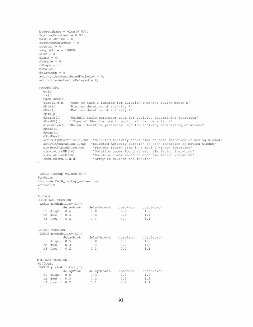
93
budgetShape = -log(0.03); ScalingConstant = 0.97 ; maxFinishTime = 0; costGrowthFactor = 0; counter = 0; sampleSize = 10000; dSum = 0; dSum2 = 0; dSample = 0; dShape = 1; total=0; delaytemp = 0; activitiesConsideredForDelay = 0; activitiesActuallyDelayed = 0; PARAMETERS es(i) ls(i) task_done(i) cost(i,d,p) "cost of task i running for duration d months during month p" dMin(i) "Minimum duration of activity i" dMax(i) "Maximum duration of activity i" fp(d,p) dScale(i) "Weibull Scale parameter used for activity determining durations" dMaxUB(i) " Copy of dMax for use in moving window comparisons" dLocation(i) "Weibull Location parameter used for activity determining durations" dMode(i) dMean(i) dStdDev(i) activityStartTime(i,mw) "Selected Activity start time at each iteration of moving window" activityDuration(i,mw) "Selected Activity duration at each iteration of moving window" projectFinishTime(mw) "Project finish time in a moving window iteration" simulationUB(mw) "Solution upper Bound at each simulation iteration" simulationLB(mw) "Solution lower Bound at each simulation iteration" results(mw,i,s,d) "Array to collect the results" ; TABLE lookup_values(r,*) $ondelim $include CAIG_lookup_values.csv $offdelim ; $ontext ORIGINAL VERSION TABLE probability(r,*) delayProb delayGrowth costProb costGrowth r1 {high} 0.6 1.8 0.8 1.8 r2 {med } 0.4 1.4 0.6 1.4 r3 {low } 0.2 1.1 0.4 1.1 ; LATEST VERSION TABLE probability(r,*) delayProb delayGrowth costProb costGrowth r1 {high} 0.5 1.8 0.5 1.8 r2 {med } 0.3 1.4 0.3 1.4 r3 {low } 0.2 1.1 0.2 1.1 ; MID-WAY VERSION $offtext TABLE probability(r,*) delayProb delayGrowth costProb costGrowth r1 {high} 0.5 1.4 0.5 1.5 r2 {med } 0.3 1.2 0.3 1.3 r3 {low } 0.2 1.1 0.2 1.1 ;
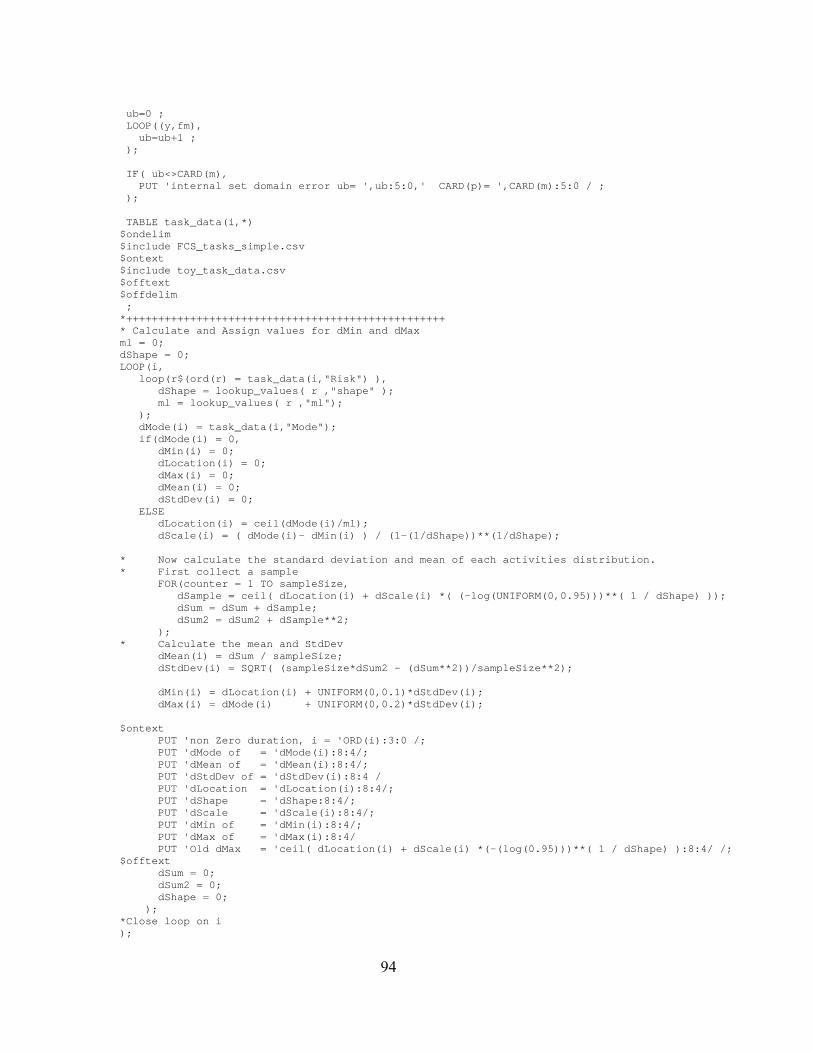
94
ub=0 ; LOOP((y,fm), ub=ub+1 ; ); IF( ub<>CARD(m), PUT 'internal set domain error ub= ',ub:5:0,' CARD(p)= ',CARD(m):5:0 / ; ); TABLE task_data(i,*) $ondelim $include FCS_tasks_simple.csv $ontext $include toy_task_data.csv $offtext $offdelim ; *++++++++++++++++++++++++++++++++++++++++++++++++++ * Calculate and Assign values for dMin and dMax ml = 0; dShape = 0; LOOP(i, loop(r$(ord(r) = task_data(i,"Risk") ), dShape = lookup_values( r ,"shape" ); ml = lookup_values( r ,"ml"); ); dMode(i) = task_data(i,"Mode"); if(dMode(i) = 0, dMin(i) = 0; dLocation(i) = 0; dMax(i) = 0; dMean(i) = 0; dStdDev(i) = 0; ELSE dLocation(i) = ceil(dMode(i)/ml); dScale(i) = ( dMode(i)- dMin(i) ) / (1-(1/dShape))**(1/dShape); * Now calculate the standard deviation and mean of each activities distribution. * First collect a sample FOR(counter = 1 TO sampleSize, dSample = ceil( dLocation(i) + dScale(i) *( (-log(UNIFORM(0,0.95)))**( 1 / dShape) )); dSum = dSum + dSample; dSum2 = dSum2 + dSample**2; ); * Calculate the mean and StdDev dMean(i) = dSum / sampleSize; dStdDev(i) = SQRT( (sampleSize*dSum2 - (dSum**2))/sampleSize**2); dMin(i) = dLocation(i) + UNIFORM(0,0.1)*dStdDev(i); dMax(i) = dMode(i) + UNIFORM(0,0.2)*dStdDev(i); $ontext PUT 'non Zero duration, i = 'ORD(i):3:0 /; PUT 'dMode of = 'dMode(i):8:4/; PUT 'dMean of = 'dMean(i):8:4/; PUT 'dStdDev of = 'dStdDev(i):8:4 / PUT 'dLocation = 'dLocation(i):8:4/; PUT 'dShape = 'dShape:8:4/; PUT 'dScale = 'dScale(i):8:4/; PUT 'dMin of = 'dMin(i):8:4/; PUT 'dMax of = 'dMax(i):8:4/ PUT 'Old dMax = 'ceil( dLocation(i) + dScale(i) *(-(log(0.95)))**( 1 / dShape) ):8:4/ /; $offtext dSum = 0; dSum2 = 0; dShape = 0; ); *Close loop on i );
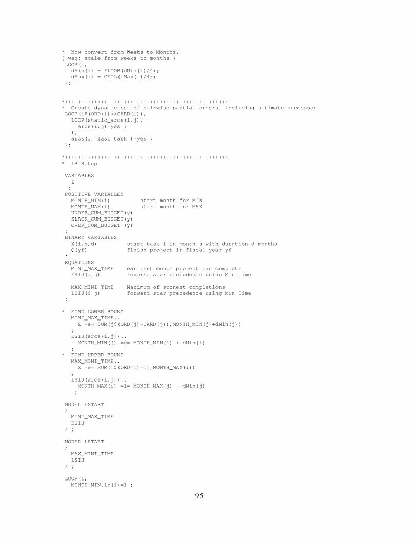
95
* Now convert from Weeks to Months. { wag: scale from weeks to months } LOOP(i, dMin(i) = FLOOR(dMin(i)/4); dMax(i) = CEIL(dMax(i)/4); ); *++++++++++++++++++++++++++++++++++++++++++++++++++ * Create dynamic set of pairwise partial orders, including ultimate successor LOOP(i$(ORD(i)<>CARD(i)), LOOP(static_arcs(i,j), arcs(i,j)=yes ; ); arcs(i,"last_task")=yes ; ); *++++++++++++++++++++++++++++++++++++++++++++++++++ * LP Setup VARIABLES Z ; POSITIVE VARIABLES MONTH_MIN(i) start month for MIN MONTH_MAX(i) start month for MAX UNDER_CUM_BUDGET(y) SLACK_CUM_BUDGET(y) OVER_CUM_BUDGET (y) ; BINARY VARIABLES X(i,s,d) start task i in month s with duration d months Q(yf) finish project in fiscal year yf ; EQUATIONS MINI_MAX_TIME earliest month project can complete ESIJ(i,j) reverse star precedence using Min Time MAX_MINI_TIME Maximum of soonest completions LSIJ(i,j) forward star precedence using Min Time ; * FIND LOWER BOUND MINI_MAX_TIME.. Z =e= SUM(j$(ORD(j)=CARD(j)),MONTH_MIN(j)+dMin(j)) ; ESIJ(arcs(i,j)).. MONTH_MIN(j) =g= MONTH_MIN(i) + dMin(i) ; * FIND UPPER BOUND MAX_MINI_TIME.. Z =e= SUM(i$(ORD(i)=1),MONTH_MAX(i)) ; LSIJ(arcs(i,j)).. MONTH_MAX(i) =l= MONTH_MAX(j) - dMin(j) ; MODEL ESTART / MINI_MAX_TIME ESIJ / ; MODEL LSTART / MAX_MINI_TIME LSIJ / ; LOOP(i, MONTH_MIN.lo(i)=1 ;
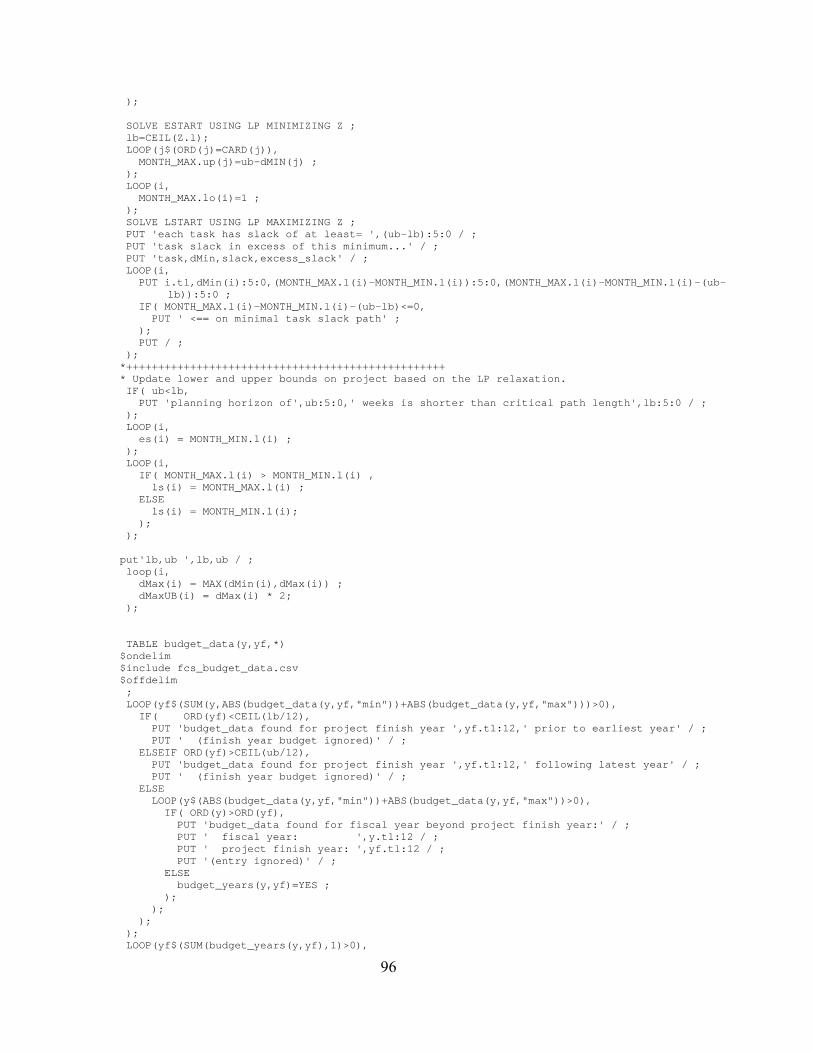
96
); SOLVE ESTART USING LP MINIMIZING Z ; lb=CEIL(Z.l); LOOP(j$(ORD(j)=CARD(j)), MONTH_MAX.up(j)=ub-dMIN(j) ; ); LOOP(i, MONTH_MAX.lo(i)=1 ; ); SOLVE LSTART USING LP MAXIMIZING Z ; PUT 'each task has slack of at least= ',(ub-lb):5:0 / ; PUT 'task slack in excess of this minimum...' / ; PUT 'task,dMin,slack,excess_slack' / ; LOOP(i, PUT i.tl,dMin(i):5:0,(MONTH_MAX.l(i)-MONTH_MIN.l(i)):5:0,(MONTH_MAX.l(i)-MONTH_MIN.l(i)-(ub-
lb)):5:0 ; IF( MONTH_MAX.l(i)-MONTH_MIN.l(i)-(ub-lb)<=0, PUT ' <== on minimal task slack path' ; ); PUT / ; ); *++++++++++++++++++++++++++++++++++++++++++++++++++ * Update lower and upper bounds on project based on the LP relaxation. IF( ub<lb, PUT 'planning horizon of',ub:5:0,' weeks is shorter than critical path length',lb:5:0 / ; ); LOOP(i, es(i) = MONTH_MIN.l(i) ; ); LOOP(i, IF( MONTH_MAX.l(i) > MONTH_MIN.l(i) , ls(i) = MONTH_MAX.l(i) ; ELSE ls(i) = MONTH_MIN.l(i); ); ); put'lb,ub ',lb,ub / ; loop(i, dMax(i) = MAX(dMin(i),dMax(i)) ; dMaxUB(i) = dMax(i) * 2; ); TABLE budget_data(y,yf,*) $ondelim $include fcs_budget_data.csv $offdelim ; LOOP(yf$(SUM(y,ABS(budget_data(y,yf,"min"))+ABS(budget_data(y,yf,"max")))>0), IF( ORD(yf)<CEIL(lb/12), PUT 'budget_data found for project finish year ',yf.tl:12,' prior to earliest year' / ; PUT ' (finish year budget ignored)' / ; ELSEIF ORD(yf)>CEIL(ub/12), PUT 'budget_data found for project finish year ',yf.tl:12,' following latest year' / ; PUT ' (finish year budget ignored)' / ; ELSE LOOP(y$(ABS(budget_data(y,yf,"min"))+ABS(budget_data(y,yf,"max"))>0), IF( ORD(y)>ORD(yf), PUT 'budget_data found for fiscal year beyond project finish year:' / ; PUT ' fiscal year: ',y.tl:12 / ; PUT ' project finish year: ',yf.tl:12 / ; PUT '(entry ignored)' / ; ELSE budget_years(y,yf)=YES ; ); ); ); ); LOOP(yf$(SUM(budget_years(y,yf),1)>0),
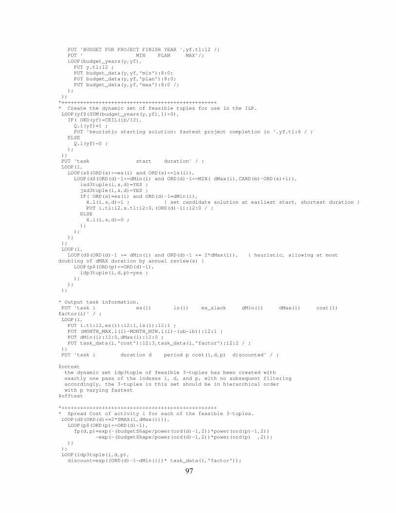
97
PUT 'BUDGET FOR PROJECT FINISH YEAR ',yf.tl:12 /; PUT ' MIN PLAN MAX'/; LOOP(budget_years(y,yf), PUT y.tl:12 ; PUT budget_data(y,yf,"min"):8:0; PUT budget_data(y,yf,"plan"):8:0; PUT budget_data(y,yf,"max"):8:0 /; ); ); *++++++++++++++++++++++++++++++++++++++++++++++++++ * Create the dynamic set of feasible tuples for use in the ILP. LOOP(yf$(SUM(budget_years(y,yf),1)>0), IF( ORD(yf)=CEIL(lb/12), Q.l(yf)=1 ; PUT 'heuristic starting solution: fastest project completion in ',yf.tl:6 / ; ELSE Q.l(yf)=0 ; ); ); PUT 'task start duration' / ; LOOP(i, LOOP(s$(ORD(s)>=es(i) and ORD(s)<=ls(i)), LOOP(d$(ORD(d)-1>=dMin(i) and ORD(d)-1<=MIN( dMax(i),CARD(m)-ORD(s)+1)), isd3tuple(i,s,d)=YES ; jsd3tuple(i,s,d)=YES ; IF( ORD(s)=es(i) and ORD(d)-1=dMin(i), X.l(i,s,d)=1 ; { set candidate solution at earliest start, shortest duration } PUT i.tl:12,s.tl:12:0,(ORD(d)-1):12:0 / ; ELSE X.l(i,s,d)=0 ; ); ); ); ); LOOP(i, LOOP(d$(ORD(d)-1 >= dMin(i) and ORD(d)-1 <= 2*dMax(i)), { heuristic, allowing at most doubling of dMAX duration by annual review(s) } LOOP(p$(ORD(p)<=ORD(d)-1), idp3tuple(i,d,p)=yes ; ); ); ); * Output task information. PUT 'task i es(i) ls(i) ex_slack dMin(i) dMax(i) cost(i) factor(i)' / ; LOOP(i, PUT i.tl:12,es(i):12:1,ls(i):12:1 ; PUT (MONTH_MAX.l(i)-MONTH_MIN.l(i)-(ub-lb)):12:1 ; PUT dMin(i):12:0,dMax(i):12:0 ; PUT task_data(i,"cost"):12:3,task_data(i,"factor"):12:2 / ; ); PUT 'task i duration d period p cost(i,d,p) discounted' / ; $ontext the dynamic set idp3tuple of feasible 3-tuples has been created with exactly one pass of the indexes i, d, and p, with no subsequent filtering accordingly, the 3-tuples in this set should be in hierarchical order with p varying fastest $offtext *++++++++++++++++++++++++++++++++++++++++++++++++++ * Spread Cost of activity i for each of the feasible 3-tuples. LOOP(d$(ORD(d)<=2*SMAX(i,dMax(i))), LOOP(p$(ORD(p)<=ORD(d)-1), fp(d,p)=exp(-(budgetShape/power(ord(d)-1,2))*power(ord(p)-1,2)) -exp(-(budgetShape/power(ord(d)-1,2))*power(ord(p) ,2)); ); ); LOOP(idp3tuple(i,d,p), discount=exp((ORD(d)-1-dMin(i))* task_data(i,"factor"));
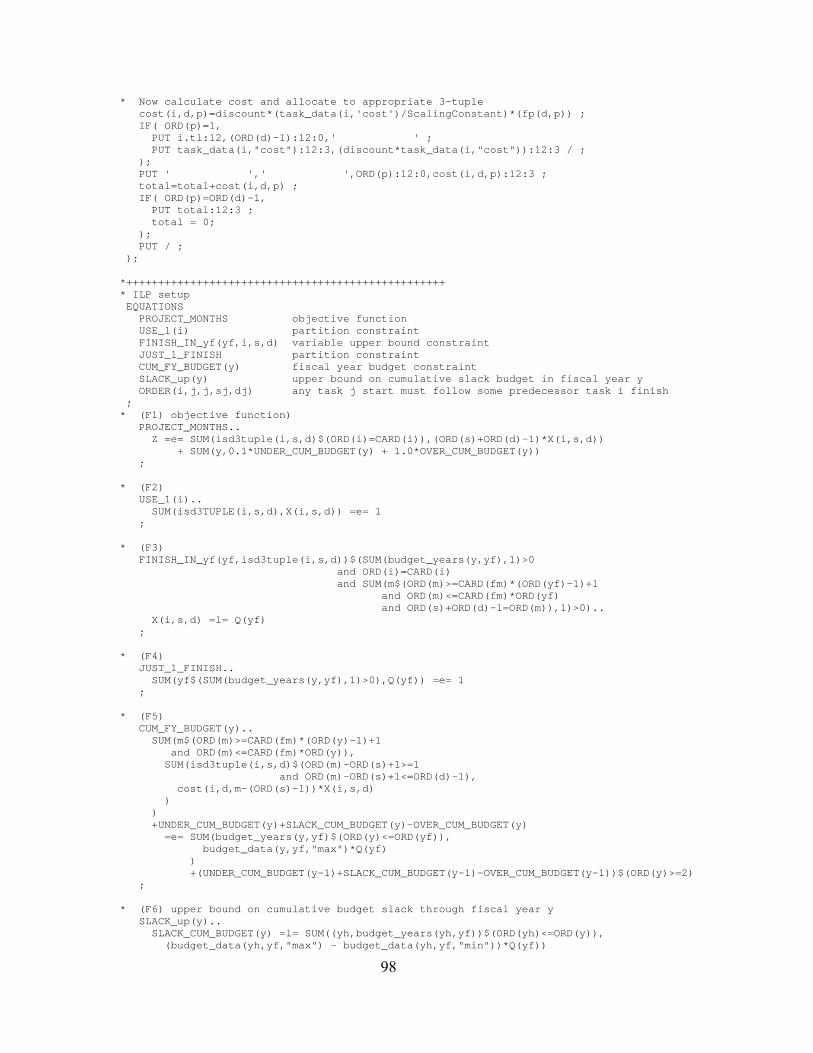
98
* Now calculate cost and allocate to appropriate 3-tuple cost(i,d,p)=discount*(task_data(i,'cost')/ScalingConstant)*(fp(d,p)) ; IF( ORD(p)=1, PUT i.tl:12,(ORD(d)-1):12:0,' ' ; PUT task_data(i,"cost"):12:3,(discount*task_data(i,"cost")):12:3 / ; ); PUT ' ',' ',ORD(p):12:0,cost(i,d,p):12:3 ; total=total+cost(i,d,p) ; IF( ORD(p)=ORD(d)-1, PUT total:12:3 ; total = 0; ); PUT / ; ); *++++++++++++++++++++++++++++++++++++++++++++++++++ * ILP setup EQUATIONS PROJECT_MONTHS objective function USE_1(i) partition constraint FINISH_IN_yf(yf,i,s,d) variable upper bound constraint JUST_1_FINISH partition constraint CUM_FY_BUDGET(y) fiscal year budget constraint SLACK_up(y) upper bound on cumulative slack budget in fiscal year y ORDER(i,j,j,sj,dj) any task j start must follow some predecessor task i finish ; * (F1) objective function) PROJECT_MONTHS.. Z =e= SUM(isd3tuple(i,s,d)$(ORD(i)=CARD(i)),(ORD(s)+ORD(d)-1)*X(i,s,d)) + SUM(y,0.1*UNDER_CUM_BUDGET(y) + 1.0*OVER_CUM_BUDGET(y)) ; * (F2) USE_1(i).. SUM(isd3TUPLE(i,s,d),X(i,s,d)) =e= 1 ; * (F3) FINISH_IN_yf(yf,isd3tuple(i,s,d))$(SUM(budget_years(y,yf),1)>0 and ORD(i)=CARD(i) and SUM(m$(ORD(m)>=CARD(fm)*(ORD(yf)-1)+1 and ORD(m)<=CARD(fm)*ORD(yf) and ORD(s)+ORD(d)-1=ORD(m)),1)>0).. X(i,s,d) =l= Q(yf) ; * (F4) JUST_1_FINISH.. SUM(yf$(SUM(budget_years(y,yf),1)>0),Q(yf)) =e= 1 ; * (F5) CUM_FY_BUDGET(y).. SUM(m$(ORD(m)>=CARD(fm)*(ORD(y)-1)+1 and ORD(m)<=CARD(fm)*ORD(y)), SUM(isd3tuple(i,s,d)$(ORD(m)-ORD(s)+1>=1 and ORD(m)-ORD(s)+1<=ORD(d)-1), cost(i,d,m-(ORD(s)-1))*X(i,s,d) ) ) +UNDER_CUM_BUDGET(y)+SLACK_CUM_BUDGET(y)-OVER_CUM_BUDGET(y) =e= SUM(budget_years(y,yf)$(ORD(y)<=ORD(yf)), budget_data(y,yf,"max")*Q(yf) ) +(UNDER_CUM_BUDGET(y-1)+SLACK_CUM_BUDGET(y-1)-OVER_CUM_BUDGET(y-1))$(ORD(y)>=2) ; * (F6) upper bound on cumulative budget slack through fiscal year y SLACK_up(y).. SLACK_CUM_BUDGET(y) =l= SUM((yh,budget_years(yh,yf))$(ORD(yh)<=ORD(y)), (budget_data(yh,yf,"max") - budget_data(yh,yf,"min"))*Q(yf))
99
; * (F7) any task j start must follow some predecessor task i finish ORDER(arcs(i,j),jsd3tuple(j,sj,dj))$(ORD(sj)>=MAX(es(j),es(i)+dMin(i))).. SUM(isd3tuple(i,si,di)$(ORD(si)+ORD(di)-1<=ORD(sj)),X(i,si,di)) =g= X(j,sj,dj) ; * begin do-it-yourself preprocessor *test initial incumbent $ontext * (F2) USE_1(i).. SUM(isd3TUPLE(i,s,d),X(i,s,d)) =e= 1 ; $offtext LOOP(i, IF( SUM(isd3TUPLE(i,s,d),X.l(i,s,d)) <> 1, PUT 'USE_1 ',i.tl / ; LOOP(isd3TUPLE(i,s,d)$(X.l(i,s,d)>0), put ' i,s,d,x.l(i.s.d) ',i.tl,s.tl,d.tl,X.l(i,s,d) / ; ); ); ); $ontext * (F3) FINISH_IN_yf(yf,isd3tuple(i,s,d))$(SUM(budget_years(y,yf),1)>0 and ORD(i)=CARD(i) and SUM(m$(ORD(m)>=CARD(fm)*(ORD(yf)-1)+1 and ORD(m)<=CARD(fm)*ORD(yf) and ORD(s)+ORD(d)-1=ORD(m)),1)>0).. X(i,s,d) =l= Q(yf) ; $offtext LOOP( (yf,isd3tuple(i,s,d))$(SUM(budget_years(y,yf),1)>0 and ORD(i)=CARD(i) and SUM(m$(ORD(m)>=CARD(fm)*(ORD(yf)-1)+1 and ORD(m)<=CARD(fm)*ORD(yf) and ORD(s)+ORD(d)-1=ORD(m)),1)>0), IF( X.l(i,s,d)>Q.l(yf), PUT 'FINISH_IN_yf ',yf.tl,i.tl,s.tl,d.tl / ; PUT 'X.l(i,s,d),Q.l(yf) ',X.l(i,s,d),Q.l(yf) / ; ); ); $ontext * (F4) JUST_1_FINISH.. SUM(yf$(SUM(budget_years(y,yf),1)>0),Q(yf)) =e= 1 ; $offtext IF( SUM(yf$(SUM(budget_years(y,yf),1)>0),Q.l(yf)) <> 1, PUT 'JUST_1_FINISH' / ; LOOP(yf$(SUM(budget_years(y,yf),1)>0), PUT 'yf.l,Q.l(yf) ',yf.tl,Q.l(yf) / ; ); ); $ontext * (F5) CUM_FY_BUDGET(y).. SUM(m$(ORD(m)>=CARD(fm)*(ORD(y)-1)+1 and ORD(m)<=CARD(fm)*ORD(y)), SUM(isd3tuple(i,s,d)$(ORD(m)-ORD(s)+1>=1 and ORD(m)-ORD(s)+1<=ORD(d)-1), cost(i,d,m-(ORD(s)-1))*X(i,s,d) )

100
) +UNDER_CUM_BUDGET(y)+SLACK_CUM_BUDGET(y)-OVER_CUM_BUDGET(y) =e= SUM(budget_years(y,yf)$(ORD(y)<=ORD(yf)),budget_data(y,yf,"max")*Q(yf)) +(UNDER_CUM_BUDGET(y-1)+SLACK_CUM_BUDGET(y-1)-OVER_CUM_BUDGET(y-1))$(ORD(y)>=2) ; * (F6) upper bound on cumulative budget slack through fiscal year y SLACK_up(y).. SLACK_CUM_BUDGET(y) =l= SUM((yh,budget_years(yh,yf))$(ORD(yh)<=ORD(y)), (budget_data(yh,yf,"max") - budget_data(yh,yf,"min"))*Q(yf)) ; $offtext LOOP( y, PUT 'CUM_FY_BUDGET ',y.tl / ; UNDER_CUM_BUDGET.l(y)=0 ; SLACK_CUM_BUDGET.l(y)=0 ; OVER_CUM_BUDGET.l(y)=0 ; cumslk= SUM((yh,budget_years(yh,yf))$(ORD(yh)<=ORD(y)), (budget_data(yh,yf,"max") - budget_data(yh,yf,"min"))*Q.l(yf)) ; rowval= SUM(m$(ORD(m)>=CARD(fm)*(ORD(y)-1)+1 and ORD(m)<=CARD(fm)*ORD(y)), SUM(isd3tuple(i,s,d)$(ORD(m)-ORD(s)+1>=1 and ORD(m)-ORD(s)+1<=ORD(d)-1), cost(i,d,m-(ORD(s)-1))*X.l(i,s,d) ) ) -SUM(budget_years(y,yf)$(ORD(y)<=ORD(yf)), budget_data(y,yf,"max")*Q.l(yf) ) -(+UNDER_CUM_BUDGET.l(y-1)+SLACK_CUM_BUDGET.l(y-1)-OVER_CUM_BUDGET.l(y-1))$(ORD(y)>=2) ; PUT y.tl,rowval / ; IF( rowval>=0, OVER_CUM_BUDGET.l(y)=rowval ; PUT 'over ',OVER_CUM_BUDGET.l(y) / ; ELSEIF -rowval<=cumslk, SLACK_CUM_BUDGET.l(y)=-rowval ; PUT 'slack ',SLACK_CUM_BUDGET.l(y) / ; ELSE UNDER_CUM_BUDGET.l(y)=-rowval-cumslk ; SLACK_CUM_BUDGET.l(y)=cumslk ; PUT 'under ',UNDER_CUM_BUDGET.l(y) / ; PUT 'slack ',SLACK_CUM_BUDGET.l(y) / ; ); IF( ORD(y)>=2, PUT 'bal forward ', (-(UNDER_CUM_BUDGET.l(y-1)-SLACK_CUM_BUDGET.l(y-1)+OVER_CUM_BUDGET.l(y-1))) /; ); PUT 'spent ', SUM(m$(ORD(m)>=CARD(fm)*(ORD(y)-1)+1 and ORD(m)<=CARD(fm)*ORD(y)), SUM(isd3tuple(i,s,d)$(ORD(m)-ORD(s)+1>=1 and ORD(m)-ORD(s)+1<=ORD(d)-1), cost(i,d,m-(ORD(s)-1))*X.l(i,s,d) ) ) /; PUT 'bal forward ', (-(UNDER_CUM_BUDGET.l(y)-SLACK_CUM_BUDGET.l(y)+OVER_CUM_BUDGET.l(y))) /;
101
); LOOP( y, IF( SLACK_CUM_BUDGET.l(y) > SUM((yh,budget_years(yh,yf))$(ORD(yh)<=ORD(y)), (budget_data(yh,yf,"max") - budget_data(yh,yf,"min"))*Q.l(yf)), PUT 'SLACK_up ',y.tl / ; PUT 'SLACK ',SLACK_CUM_BUDGET.l(y) / ; PUT 'CUM ',(SUM((yh,budget_years(yh,yf))$(ORD(yh)<=ORD(y)), (budget_data(yh,yf,"max") - budget_data(yh,yf,"min"))*Q.l(yf))) / ; ); ); LOOP(y, PUT y.tl,'under,slack,over' / ; IF( ORD(y)>=2, PUT UNDER_CUM_BUDGET.l(y-1); PUT SLACK_CUM_BUDGET.l(y-1); PUT OVER_CUM_BUDGET.l(y-1); ELSE PUT 0 ; PUT 0 ; PUT 0 ; ); PUT / ; PUT 'spent ', (SUM(m$(ORD(m)>=CARD(fm)*(ORD(y)-1)+1 and ORD(m)<=CARD(fm)*ORD(y)), SUM(isd3tuple(i,s,d)$(ORD(m)-ORD(s)+1>=1 and ORD(m)-ORD(s)+1<=ORD(d)-1), cost(i,d,m-(ORD(s)-1))*X.l(i,s,d) ) ))/; PUT 'max slack'; PUT(SUM((yh,budget_years(yh,yf))$(ORD(yh)<=ORD(y)), (budget_data(yh,yf,"max") - budget_data(yh,yf,"min"))*Q.l(yf)) )/; PUT UNDER_CUM_BUDGET.l(y); PUT SLACK_CUM_BUDGET.l(y); PUT OVER_CUM_BUDGET.l(y)/; ); $ontext * (F7) any task j start must follow some predecessor task i finish ORDER(arcs(i,j),jsd3tuple(j,sj,dj))$(ORD(sj)>=MAX(es(j),es(i)+dMin(i))).. SUM(isd3tuple(i,si,di)$(ORD(si)+ORD(di)-1<=ORD(sj)),X(i,si,di)) =g= X(j,sj,dj) ; $offtext LOOP((arcs(i,j),jsd3tuple(j,sj,dj))$(ORD(sj)>=MAX(es(j),es(i)+dMin(i))), IF( SUM(isd3tuple(i,si,di)$(ORD(si)+ORD(di)-1<=ORD(sj)),X.l(i,si,di)) < X.l(j,sj,dj), PUT 'ORDER i,j,sj,dj',i.tl,j.tl,sj.tl,dj.tl / ; LOOP(isd3tuple(i,si,di)$(ORD(si)+ORD(di)-1<=ORD(sj)), PUT 'i,si,di,X ',i.tl,si.tl,di.tl,X.l(i,si,di) / ; ); PUT 'j,sj,dj,x ',j.tl,sj.tl,dj.tl,X.l(j,sj,dj) / ; ); ); * end do-it-yourself preprocessor MODEL FCS_SCHEDULER / PROJECT_MONTHS USE_1 FINISH_IN_yf
102
JUST_1_FINISH CUM_FY_BUDGET SLACK_up ORDER / ; FCS_SCHEDULER.optfile = 1; * Solve once. This gives the case with no sliding window. $ontext FCS_SCHEDULER.prioropt = 1; Q.prior(yf)=1; X.prior(i,s,d)=2; $offtext * I have increased the reslim as will be running the model overnight. FCS_SCHEDULER.reslim=800 ; SOLVE FCS_SCHEDULER USING MIP MINIMIZING Z ; IF (FCS_SCHEDULER.modelstat <> 1 AND FCS_SCHEDULER.modelstat <> 8, PUT '++++ Error solving model. model status = 'FCS_SCHEDULER.modelstat:3:0/; ELSE PUT /' Best Upper Bound = 'Z.l:10:4 / ; PUT /' Best Lower Bound = 'FCS_SCHEDULER.objest:10:4 / ; ); LOOP(i, LOOP(isd3tuple(i,s,d)$(ORD(i)=CARD(i)), PUT 'i.tl,s.tl,d.tl,x(i,s,d) ',i.tl,s.tl,d.tl,' ',x.l(i,s,d) / ; PUT '((ORD(s)+ORD(d)-1-1)*X.l(i,s,d)) ',((ORD(s)+ORD(d)-1-1)*X.l(i,s,d)) / ; ); ); LOOP(y, IF( UNDER_CUM_BUDGET.l(y)>0, PUT '0.1*UNDER_CUM_BUDGET(y) ',y.tl:12,(0.1*UNDER_CUM_BUDGET.l(y)) / ; ); IF( OVER_CUM_BUDGET.l(y)>0, PUT '1.0*OVER_CUM_BUDGET(y) ',y.tl:12,(1.0*OVER_CUM_BUDGET.l(y)) / ; ); ); PUT 'finish last task in month ',(SUM(isd3tuple(i,s,d)$(ORD(i)=CARD(i)),(ORD(s)+ORD(d)-
1)*X.l(i,s,d))) / ; LOOP(yf$(Q.l(yf)=1), PUT 'finish project in fiscal year ',yf.tl:12 / ; ); *++++++++++++++++++++++++++++++++++++++++++++++++++++++++++++++++++++++ * Start the moving month window which move through the periods * and randomizes activities not yet started. It then resolves and * this solution is used as the next baseline. PUT 'Starting Moving Window Loop' / ; LOOP(i, task_done(i)=0 ; ); * Loop over all time periods. Alias of Month called mw (month window) LOOP(mw$(MOD(ORD(mw),12)=0 and ORD(mw)<0), PUT 'annual review, month ',mw.tl:12 / ; LOOP(i, LOOP(s$(ORD(s)>=es(i) and ORD(s)<=ls(i)), LOOP(d$(ORD(d)-1>=dMin(i) and ORD(d)-1<=MIN(dMax(i),ub-ORD(s)+1)), isd3tuple(i,s,d)=NO ; jsd3tuple(i,s,d)=NO ; ); ); );
103
put 'check for empty dynamic sets' / ; LOOP(isd3tuple(i,s,d), put 'isd leaker: ',i.tl,s.tl,d.tl / ; ); PUT 'Cleared out Dynamic sets. Looking for the new feasible sets...'/; * Loop over all tasks not already marked completed LOOP(i$( task_done(i)=0 ), * Loop over all feasible start times inflate=1 ; LOOP(s$(ORD(s)>=es(i) and ORD(s)<=ls(i) ), * not yet started * Loop over all feasible durations LOOP(d$( ORD(d)-1 >= dMin(i) and ORD(d)-1 <= MIN(dMax(i),ub-ORD(s)+1) and X.l(i,s,d) = 1 ), IF( ORD(s)+ORD(d)-1 <= ORD(mw), * task completed since last annual review task_done(i)=ORD(s)+ORD(d)-1 ; start=ORD(s) ; duration=ORD(d)-1 ; put 'task completed since last annual review ',i.tl,s.tl,d.tl,task_done(i):5:0 / ; ELSEIF ORD(s) <= ORD(mw), * task still in progress at this annual review put 'task annual review ',i.tl,s.tl,d.tl,task_data(i,"risk"):5:0 / ; start=ORD(s) ; duration=(ORD(d)-1) ; LOOP(r$(ord(r)=task_data(i,"Risk")), uniDraw1=UNIFORM(0,1) ; activitiesConsideredForDelay = activitiesConsideredForDelay + 1; PUT 'uniDraw1 = 'uniDraw1:5:4 ' at i,s,d = ',ORD(i):5:1,ORD(s):5:1,ORD(d):5:0 /; IF( uniDraw1<=probability(r,'delayProb'), activitiesActuallyDelayed = activitiesActuallyDelayed + 1; * Check to see if the delay is less than twice the original dMax(i) delayTemp = CEIL(duration*probability(r,'delayGrowth')) IF(delayTemp <= dMaxUB(i), duration=delayTemp; put ' *** delaying task ',i.tl,' by delayTemp = ',delayTemp /; put ' dMaxUB(i) = ',dMaxUB(i)/; put ' task ',i.tl,' duration delayed from ',d.tl,' to ',duration:5:0 / ; ELSE duration = dMaxUB(i); put ' task ',i.tl,' maximally delayed at ',d.tl/ ; ); IF( ORD(s)+duration <= ORD(mw), * despite delay, task completed since last annual review task_done(i)=ORD(s)+duration ; put ' delayed task completed since last annual review
',i.tl,s.tl,d.tl,duration:5:0,task_done(i):5:0 / ; ); uniDraw2=UNIFORM(0,1) ; IF( uniDraw2<=probability(r,'costProb'), inflate=probability(r,'costGrowth') ; ); ); ); ELSE * task not yet started by this annual review duration=-1 ; ); ); ); IF( task_done(i)>0, * task marked completed during this annual review es(i)=start ; ls(i)=start ; put 'completed ',es(i),ls(i) / ; ); IF( duration>=0,
104
dMin(i)=duration ; dMax(i)=duration ; LOOP(s$( ORD(s)=start ), LOOP(d$(ORD(d)-1=duration), X.lo(i,s,d)=1 ; ); ); ); IF( inflate>1, * apply inflation to remaining (future) costs LOOP(idp3TUPLE(i,d,p)$(ORD(d)-1=duration and ORD(p)>ORD(mw)+1-start), cost(i,d,p)=inflate*cost(i,d,p) ; put 'i.tl,start,d,tl,p.tl,inflate,cost ',i.tl,start:5:0,' ',d.tl,p.tl,inflate:5:1,cost(i,d,p) / ; ); ); ); LOOP((y,yf), budget_years(y,yf)=NO ; ); LOOP(yf$(SUM(y,ABS(budget_data(y,yf,"min"))+ABS(budget_data(y,yf,"max")))>0), IF( ORD(yf)<CEIL(lb/12), PUT 'budget_data found for project finish year ',yf.tl:12,' prior to earliest year' / ; PUT ' (finish year budget ignored)' / ; ELSEIF ORD(yf)>CEIL(ub/12), PUT 'budget_data found for project finish year ',yf.tl:12,' following latest year' / ; PUT ' (finish year budget ignored)' / ; ELSE LOOP(y$(ABS(budget_data(y,yf,"min"))+ABS(budget_data(y,yf,"max"))>0), IF( ORD(y)>ORD(yf), PUT 'budget_data found for fiscal year beyond project finish year:' / ; PUT ' fiscal year: ',y.tl:12 / ; PUT ' project finish year: ',yf.tl:12 / ; PUT '(entry ignored)' / ; ELSE budget_years(y,yf)=YES ; ); ); ); ); LOOP(yf$(SUM(budget_years(y,yf),1)>0), PUT 'BUDGET FOR PROJECT FINISH YEAR ',yf.tl:12 /; PUT ' MIN PLAN MAX'/; LOOP(budget_years(y,yf), PUT y.tl:12 ; PUT budget_data(y,yf,"min"):8:0; PUT budget_data(y,yf,"plan"):8:0; PUT budget_data(y,yf,"max"):8:0 /; ); ); FCS_SCHEDULER.optfile = 1; FCS_SCHEDULER.reslim=500 ; SOLVE ESTART USING LP MINIMIZING Z ; lb=CEIL(Z.l); * Create the dynamic set of feasible tuples for use in the ILP. LOOP(yf$(SUM(budget_years(y,yf),1)>0), IF( ORD(yf)=CEIL(lb/12), Q.l(yf)=1 ; PUT 'heuristic starting solution: fastest project completion in ',yf.tl:6 / ; ELSE Q.l(yf)=0 ; ); ); PUT 'task start duration' / ; LOOP(i, LOOP(s$(ORD(s)>=es(i) and ORD(s)<=ls(i)), LOOP(d$(ORD(d)-1>=dMin(i) and ORD(d)-1<=MIN(dMax(i),CARD(m)-ORD(s)+1)), isd3tuple(i,s,d)=YES ; jsd3tuple(i,s,d)=YES ; IF( ORD(s)=es(i) and ORD(d)-1=dMin(i),
105
X.l(i,s,d)=1 ; {set candidate solution at earliest start, shortest duration} PUT i.tl:12,s.tl:12:0,(ORD(d)-1):12:0 / ; ELSE X.l(i,s,d)=0 ; ); ); ); ); PUT ' Finished finding Feasible sets'/; PUT ' Ready to Solve the ILP'/; PUT 'check isd3TUPLE(i,s,d) task-by-task ' / ; LOOP(i, PUT i.tl,' alternatives available= ',(SUM(isd3TUPLE(i,s,d),1)):4:0 / ; ); * begin preprocessor * test initial incumbent $ontext * (F2) USE_1(i).. SUM(isd3TUPLE(i,s,d),X(i,s,d)) =e= 1 ; $offtext LOOP(i, IF( SUM(isd3TUPLE(i,s,d),X.l(i,s,d)) <> 1, PUT 'USE_1 ',i.tl / ; LOOP(isd3TUPLE(i,s,d)$(X.l(i,s,d)>0), put ' i,s,d,x.l(i.s.d) ',i.tl,s.tl,d.tl,X.l(i,s,d) / ; ); ); ); $ontext * (F3) FINISH_IN_yf(yf,isd3tuple(i,s,d))$(SUM(budget_years(y,yf),1)>0 and ORD(i)=CARD(i) and SUM(m$(ORD(m)>=CARD(fm)*(ORD(yf)-1)+1 and ORD(m)<=CARD(fm)*ORD(yf) and ORD(s)+ORD(d)-1=ORD(m)),1)>0).. X(i,s,d) =l= Q(yf) ; $offtext LOOP( (yf,isd3tuple(i,s,d))$(SUM(budget_years(y,yf),1)>0 and ORD(i)=CARD(i) and SUM(m$(ORD(m)>=CARD(fm)*(ORD(yf)-1)+1 and ORD(m)<=CARD(fm)*ORD(yf) and ORD(s)+ORD(d)-1=ORD(m)),1)>0), IF( X.l(i,s,d)>Q.l(yf), PUT 'FINISH_IN_yf ',yf.tl,i.tl,s.tl,d.tl / ; PUT 'X.l(i,s,d),Q.l(yf) ',X.l(i,s,d),Q.l(yf) / ; ); ); $ontext * (F4) JUST_1_FINISH.. SUM(yf$(SUM(budget_years(y,yf),1)>0),Q(yf)) =e= 1 ; $offtext IF( SUM(yf$(SUM(budget_years(y,yf),1)>0),Q.l(yf)) <> 1, PUT 'JUST_1_FINISH' / ; LOOP(yf$(SUM(budget_years(y,yf),1)>0), PUT 'yf.l,Q.l(yf) ',yf.tl,Q.l(yf) / ; ); );
106
$ontext * (F5) CUM_FY_BUDGET(y).. SUM(m$(ORD(m)>=CARD(fm)*(ORD(y)-1)+1 and ORD(m)<=CARD(fm)*ORD(y)), SUM(isd3tuple(i,s,d)$(ORD(m)-ORD(s)+1>=1 and ORD(m)-ORD(s)+1<=ORD(d)-1), cost(i,d,m-(ORD(s)-1))*X(i,s,d) ) ) +UNDER_CUM_BUDGET(y)+SLACK_CUM_BUDGET(y)-OVER_CUM_BUDGET(y) =e= SUM(budget_years(y,yf)$(ORD(y)<=ORD(yf)),budget_data(y,yf,"max")*Q(yf)) +(UNDER_CUM_BUDGET(y-1)+SLACK_CUM_BUDGET(y-1)-OVER_CUM_BUDGET(y-1))$(ORD(y)>=2) ; * (F6) upper bound on cumulative budget slack through fiscal year y SLACK_up(y).. SLACK_CUM_BUDGET(y) =l= SUM((yh,budget_years(yh,yf))$(ORD(yh)<=ORD(y)), (budget_data(yh,yf,"max") - budget_data(yh,yf,"min"))*Q(yf)) ; $offtext LOOP( y, PUT 'CUM_FY_BUDGET ',y.tl / ; UNDER_CUM_BUDGET.l(y)=0 ; SLACK_CUM_BUDGET.l(y)=0 ; OVER_CUM_BUDGET.l(y)=0 ; cumslk= SUM((yh,budget_years(yh,yf))$(ORD(yh)<=ORD(y)), (budget_data(yh,yf,"max") - budget_data(yh,yf,"min"))*Q.l(yf)) ; rowval= SUM(m$(ORD(m)>=CARD(fm)*(ORD(y)-1)+1 and ORD(m)<=CARD(fm)*ORD(y)), SUM(isd3tuple(i,s,d)$(ORD(m)-ORD(s)+1>=1 and ORD(m)-ORD(s)+1<=ORD(d)-1), cost(i,d,m-(ORD(s)-1))*X.l(i,s,d) ) ) -SUM(budget_years(y,yf)$(ORD(y)<=ORD(yf)), budget_data(y,yf,"max")*Q.l(yf) ) -(+UNDER_CUM_BUDGET.l(y-1)+SLACK_CUM_BUDGET.l(y-1)-OVER_CUM_BUDGET.l(y-1))$(ORD(y)>=2) ; PUT y.tl,rowval / ; IF( rowval>=0, OVER_CUM_BUDGET.l(y)=rowval ; PUT 'over ',OVER_CUM_BUDGET.l(y) / ; ELSEIF -rowval<=cumslk, SLACK_CUM_BUDGET.l(y)=-rowval ; PUT 'slack ',SLACK_CUM_BUDGET.l(y) / ; ELSE UNDER_CUM_BUDGET.l(y)=-rowval-cumslk ; SLACK_CUM_BUDGET.l(y)=cumslk ; PUT 'under ',UNDER_CUM_BUDGET.l(y) / ; PUT 'slack ',SLACK_CUM_BUDGET.l(y) / ; ); IF( ORD(y)>=2, PUT 'bal forward ', (-(UNDER_CUM_BUDGET.l(y-1)-SLACK_CUM_BUDGET.l(y-1)+OVER_CUM_BUDGET.l(y-1))) /; ); PUT 'spent ', SUM(m$(ORD(m)>=CARD(fm)*(ORD(y)-1)+1 and ORD(m)<=CARD(fm)*ORD(y)), SUM(isd3tuple(i,s,d)$(ORD(m)-ORD(s)+1>=1 and ORD(m)-ORD(s)+1<=ORD(d)-1),
107
cost(i,d,m-(ORD(s)-1))*X.l(i,s,d) ) ) /; PUT 'bal forward ', (-(UNDER_CUM_BUDGET.l(y)-SLACK_CUM_BUDGET.l(y)+OVER_CUM_BUDGET.l(y))) /; ); LOOP( y, IF( SLACK_CUM_BUDGET.l(y) > SUM((yh,budget_years(yh,yf))$(ORD(yh)<=ORD(y)), (budget_data(yh,yf,"max") - budget_data(yh,yf,"min"))*Q.l(yf)), PUT 'SLACK_up ',y.tl / ; PUT 'SLACK ',SLACK_CUM_BUDGET.l(y) / ; PUT 'CUM ',(SUM((yh,budget_years(yh,yf))$(ORD(yh)<=ORD(y)), (budget_data(yh,yf,"max") - budget_data(yh,yf,"min"))*Q.l(yf))) / ; ); ); LOOP(y, PUT y.tl,'under,slack,over' / ; IF( ORD(y)>=2, PUT UNDER_CUM_BUDGET.l(y-1); PUT SLACK_CUM_BUDGET.l(y-1); PUT OVER_CUM_BUDGET.l(y-1); ELSE PUT 0 ; PUT 0 ; PUT 0 ; ); PUT / ; PUT 'spent ', (SUM(m$(ORD(m)>=CARD(fm)*(ORD(y)-1)+1 and ORD(m)<=CARD(fm)*ORD(y)), SUM(isd3tuple(i,s,d)$(ORD(m)-ORD(s)+1>=1 and ORD(m)-ORD(s)+1<=ORD(d)-1), cost(i,d,m-(ORD(s)-1))*X.l(i,s,d) ) ))/; PUT 'max slack'; PUT(SUM((yh,budget_years(yh,yf))$(ORD(yh)<=ORD(y)), (budget_data(yh,yf,"max") - budget_data(yh,yf,"min"))*Q.l(yf)) )/; PUT UNDER_CUM_BUDGET.l(y); PUT SLACK_CUM_BUDGET.l(y); PUT OVER_CUM_BUDGET.l(y)/; ); put 'ping a' $ontext * (F7) any task j start must follow some predecessor task i finish ORDER(arcs(i,j),jsd3tuple(j,sj,dj))$(ORD(sj)>=MAX(es(j),es(i)+dMin(i))).. SUM(isd3tuple(i,si,di)$(ORD(si)+ORD(di)-1<=ORD(sj)),X(i,si,di)) =g= X(j,sj,dj) ; $offtext LOOP((arcs(i,j),jsd3tuple(j,sj,dj))$(ORD(sj)>=MAX(es(j),es(i)+dMin(i))), IF( SUM(isd3tuple(i,si,di)$(ORD(si)+ORD(di)-1<=ORD(sj)),X.l(i,si,di)) < X.l(j,sj,dj), PUT 'ORDER i,j,sj,dj',i.tl,j.tl,sj.tl,dj.tl / ; LOOP(isd3tuple(i,si,di)$(ORD(si)+ORD(di)-1<=ORD(sj)), PUT 'i,si,di,X ',i.tl,si.tl,di.tl,X.l(i,si,di) / ; ); PUT 'j,sj,dj,X ',j.tl,sj.tl,dj.tl,X.l(j,sj,dj) / ; ); ); put 'ping a' * end do-it-yourself preprocessor
108
SOLVE FCS_SCHEDULER USING MIP MINIMIZING Z ; IF (FCS_SCHEDULER.modelstat <> 1 AND FCS_SCHEDULER.modelstat <> 8, PUT '++++ Error solving model. model status = 'FCS_SCHEDULER.modelstat:3:0/; ELSE simulationUB(mw) = Z.l; simulationLB(mw) = FCS_SCHEDULER.objest; PUT /' Best Upper Bound = 'simulationLB(mw):10:4 / ; PUT /' Best Lower Bound = 'simulationUB(mw):10:4 / ; ); PUT 'finish last task in month ',(SUM(isd3tuple(i,s,d)$(ORD(i)=CARD(i)),(ORD(s)+ORD(d)-
1)*X.l(i,s,d))) / ; LOOP(yf$(Q.l(yf)=1), PUT 'finish project in fiscal year ',yf.tl:12 / ; ); PUT ' Finished solve. Solution set is:' / ; * Display the task list with start and duration options. PUT ' task i start duration' / ; LOOP(isd3tuple(i,s,d)$(X.l(i,s,d)>0) , activityStartTime(i,mw)=ORD(s) ; activityDuration(i,mw) =ORD(d) ; PUT i.tl:12,ORD(s):12:0,(ORD(d)-1):12:0 / ; IF((ORD(s)+ORD(d))>maxFinishTime , maxFinishTime=ORD(s)+ORD(d) ; ); ); projectFinishTime(mw)=maxFinishTime ; maxFinishTime=0 ; PUT / /'At end of Moving Window Iteration ' ORD(mw) / / ; * end loop on mw ); PUT / /'Finished the Time Step Simulation' / ; PUT '+++++++++++++++++++++++++++++++++++++++++++++++'/; LOOP(mw$(projectFinishTime(mw)>0), PUT 'projectFinishTime at iteration 'ORD(MW)' is 'projectFinishTime(mw) / ; PUT ' Best Lower Bound : ' simulationLB(mw)/; PUT ' Best Upper Bound : ' simulationUB(mw)/; ); PUT '*** Activities Considered For Delay = 'activitiesConsideredForDelay:3:0/; PUT '*** Activities Actually Delayed = 'activitiesActuallyDelayed:3:0/ /; PUT 'Output results for the final solve'/ /; LOOP(yf$(Q.l(yf)=1), PUT // 'cumulative budget for project finish in fiscal year ',yf.tl:12 / ; PUT ' year_min year_spent year_max cum_min cum_spent cum_max
cum_slack' / ; LOOP(budget_years(y,yf), PUT y.tl:12, PUT budget_data(y,yf,"min"):12:3 ; PUT (SUM(m$(ORD(m)>=CARD(fm)*(ORD(y)-1)+1 and ORD(m)<=CARD(fm)*ORD(y)), SUM(isd3tuple(i,s,d)$(ORD(m)-ORD(s)+1>=1 and ORD(m)-ORD(s)+1<=ORD(d)-1), cost(i,d,m-(ORD(s)-1))*X.l(i,s,d) ) )):12:3; PUT budget_data(y,yf,"max"):12:3 ;
109
PUT SUM(yh$(ORD(yh)<=ORD(y)),budget_data(yh,yf,"min")):12:3 ; PUT (SUM(yh$(ORD(yh)<=ORD(y)),budget_data(yh,yf,"max")) -UNDER_CUM_BUDGET.l(y)-SLACK_CUM_BUDGET.l(y)+OVER_CUM_BUDGET.l(y)):12:3 ; PUT (SUM(yh$(ORD(yh)<=ORD(y)),budget_data(yh,yf,"max"))):12:3 ; PUT SLACK_CUM_BUDGET.l(y) / ; IF( UNDER_CUM_BUDGET.l(y)>0, PUT ' under_cum_min:
',UNDER_CUM_BUDGET.l(y):12:3 / ; ); IF( SLACK_CUM_BUDGET.l(y)>0, PUT ' cum_slack:
',SLACK_CUM_BUDGET.l(y):12:3 / ; ); IF( OVER_CUM_BUDGET.l(y)>0, PUT ' over_cum_max:
',OVER_CUM_BUDGET.l(y):12:3 / ; ); ); PUT 'task i start duration' / ; LOOP(isd3tuple(i,s,d)$(X.l(i,s,d)>0), PUT i.tl:12,' s ',s.tl:8,' d ',(ORD(d)-1):8:0 / ; ); PUT 'fiscal schedule for project finish in fiscal year ',yf.tl:12 / ; LOOP(y, PUT y.tl:12 / ; LOOP(m$(ORD(m)>=CARD(fm)*(ORD(y)-1)+1 and ORD(m)<=CARD(fm)*ORD(y)), PUT ' ',m.tl:12 / ; LOOP(isd3tuple(i,s,d)$(X.l(i,s,d)>0), IF( ORD(m)-ORD(s)+1>=1 and ORD(m)-ORD(s)+1<=ORD(d)-1, PUT ' ' ; PUT i.tl:12,' s ',s.tl:8,' d ',(ORD(d)-1):8:0,' p ',(ORD(m)-ORD(s)+1):8:0 ; PUT cost(i,d,m-(ORD(s)-1)):12:3 / ; ); ); ); ); ); PUTCLOSE logFile
110
THIS PAGE INTENTIONALLY LEFT BLANK
111
INITIAL DISTRIBUTION LIST
1. Defense Technical Information Center Ft. Belvoir, Virginia
2. Dudley Knox Library Naval Postgraduate School Monterey, California
3. Walt Cooper Office of the Secretary of Defense PA&E/RA/OAPPD
Washington, DC
4. Dr. Richard Burke Office of the Secretary of Defense PA&E/RA/OAPPD
Washington, DC
5. John Thurman Office of the Secretary of Defense PA&E/RA/OAPPD
Washington, DC
6. Distinguished Professor G. Brown (Code OR/Bw) Naval Postgraduate School Monterey, California
7. Assistant Professor R. Koyak (Code OR/Kr) Naval Postgraduate School Monterey, California