NBER WORKING PAPER SERIES

BETTING ON THE HOUSE:SUBJECTIVE EXPECTATIONS AND MARKET CHOICES

Nicolas L. BottanRicardo Perez-Truglia

Working Paper 27412http://www.nber.org/papers/w27412

NATIONAL BUREAU OF ECONOMIC RESEARCH1050 Massachusetts Avenue

Cambridge, MA 02138June 2020, Revised September 2021

We are thankful for excellent comments from several colleagues and seminar discussants at UC Berkeley, Cornell University, Chicago-Booth, Brown University, Berkeley-Haas, CEBI Workshop, Jinan University, NTA Annual Meeting, Universidad de San Andres and the NBER Summer Institute. This project was reviewed and approved in advance by the Institutional Review Boards at University of California Los Angeles (#18-001496 and #19-000945) and Cornell University (#1811008440). The experiments were pre-registered in the AEA RCT Registry (#0003663). If and when the study is accepted for publication, we will make publicly available all the code and data used in this study. We thank funding from the UCLA’s Ziman Center for Real Estate’s Rosalinde and Arthur Gilbert Program in Real Estate, Finance and Urban Economics and UCLA Anderson’s Behavioral Lab. Sofia Shchukina and Zhihao Han provided outstanding research assistance. The views expressed herein are those of the authors and do not necessarily reflect the views of the National Bureau of Economic Research.

NBER working papers are circulated for discussion and comment purposes. They have not been peer-reviewed or been subject to the review by the NBER Board of Directors that accompanies official NBER publications.

© 2020 by Nicolas L. Bottan and Ricardo Perez-Truglia. All rights reserved. Short sections of text, not to exceed two paragraphs, may be quoted without explicit permission provided that full credit, including © notice, is given to the source.

Betting on the House: Subjective Expectations and Market Choices Nicolas L. Bottan and Ricardo Perez-TrugliaNBER Working Paper No. 27412June 2020, Revised September 2021JEL No. C81,C93,D83,D84,R31

ABSTRACT

Home price expectations play a central role in macroeconomics and finance. However, there is little direct evidence on how these expectations affect market choices. We provide the first causal evidence based on a large-scale, high-stakes, naturally occurring field experiment in the United States. We mailed letters with information on trends in home prices to 57,910 homeowners who recently listed their homes on the market. Collectively, these homes were worth $34 billion. We randomized the information contained in the mailing to create non-deceptive, exogenous variation in the subjects’ home price expectations. We then used rich administrative data to measure the effects of these information shocks on the subject’s market choices. We find that, consistent with economic theory, higher home price expectations caused a reduction in the probability of selling the home. These effects are highly statistically significant, economically large in magnitude, and robust to a number of sharp checks. Our results indicate that market choices are highly elastic to expectations: a 1 percentage point increase in home price expectations causes a 2.63 percentage point reduction in the probability of selling the property within 12 weeks. Also, our evidence indicates that information frictions play a significant role in the housing market.

Nicolas L. BottanPolicy Analysis and ManagementCornell UniversityMVR Hall 3220Ithaca, NY 14853nicolas.bottan@cornell.edu

Ricardo Perez-TrugliaHaas School of BusinessUniversity of California, Berkeley545 Student Services Building #1900Berkeley, CA 94720-1900and NBERricardotruglia@berkeley.edu

A randomized controlled trials registry entry is available at https://www.socialscienceregistry.org/trials/3663

A data appendix is available at https://data.nber.org/data-appendix/w27412/

1 Introduction

Consumer expectations play a central role in modern macroeconomics and finance, and theyare of special interest to policymakers (Bernanke, 2007). In the context of the housingmarket, there is growing interest in home price expectations, particularly the homeowners’expectations about future growth in home prices (Bailey, Cao, Kuchler, and Stroebel, 2018;Bailey, Davila, Kuchler, and Stroebel, 2018). Because homes account for a large fraction ofhouseholds’ assets, home price expectations can have major welfare and policy implications.Indeed, home price expectations are believed to have played a key role in the 2008 U.S.housing crisis (Shiller, 2005). Despite their central role, there is little direct evidence onwhether home price expectations have a causal effect on the decision to sell a property. Inthis paper, we fill this gap in the literature using a large-scale, high-stakes, pre-registerednatural field experiment.

Estimating the relationship between home price expectations and market choices is plaguedwith challenges to causal identification. Consider the following correlation as an example: inmarkets with more optimistic homes price expectations, homeowners are less willing to selltheir homes. This correlation does not imply that home price expectations have a causal ef-fect on sellers’ market behavior. Causality could run in the opposite direction: homeowners’reluctance to sell may drive up home price expectations, rather than the other way around.The correlation also may be spuriously driven by an omitted variable. For example, an im-provement in fundamentals may simultaneously generate a rise in home price expectationsand homeowners’ unwillingness to sell. Without exogenous variation in expectations, it ischallenging to identify the causal effect of home price expectations on market outcomes.

To better illustrate the link between subjective expectations and market choices, considera sample of homeowners who have listed a home for sale. Those sellers receive a sequenceof offers. For each offer, they must decide whether to accept it or wait for a better offer tocome along. According to economic theory, subjective home price expectations could be akey input in sellers’ decision-making (Glaeser and Nathanson, 2017; Anenberg, 2016). Moreprecisely, when homeowners become more optimistic about future home prices, they shouldbe less excited about selling their properties (i.e., they should increase their “reservationprice”). As a result, the property should take longer to sell. Conversely, homeowners whobecome more pessimistic about future home values are expected to sell the properties faster.

In the ideal experiment, we would take this group of sellers and flip a coin to randomizetheir expectations. For example, if the coin lands on heads, a homeowner would be persuadedthat median home prices will appreciate by 1% over the next year. If the coin lands on tails,the homeowner would be persuaded that median home prices will appreciate by 10% over

2

the next year. Then, we would check which owners sold their homes and which ones did notsell their homes in the months following the randomization. Our main hypothesis is that,relative to the homeowners who are randomly assigned to the 1% home price expectation,the homeowners assigned to the 10% home price expectation would take longer to sell theirproperties. Moreover, the magnitude of those effects can shed light on how elastic homeownersare to changes in their home price expectations.

We designed a field experiment that closely resembles the ideal experiment. We mailedletters to a sample of U.S. homeowners who had recently listed a home on the market. Theseletters included information on the current median home price for comparable homes (i.e.,homes in the same ZIP Code and with the same number of bedrooms). We randomizedadditional factual information in the letters to create non-deceptive, exogenous shocks to thesubjects’ home price expectations. By chance, some owners received optimistic shocks totheir expectations, while other owners received pessimistic shocks. We then used publiclyavailable administrative records to check if and when homeowners sold the listed property.We measure whether the exogenous shocks to home price expectations induced by our lettersaffected the subjects’ subsequent market choices.

Information-provision experiments typically require data on prior beliefs. For example,imagine that an individual is given information that home prices will grow by 5% per year.Whether that individual should update expectations up, down, or not at all depends on theindividual’s prior belief. Individuals who believe that home prices will grow by less than5% should adjust their expectations downward, whereas individuals who believe that homeswill appreciate by more than 5% should update their expectations upward. We devise anexperimental design to leverage exogenous shocks to beliefs even in the absence of data onprior beliefs. This design creates two distinct sources of exogenous shocks to the subjects’expectations, source-randomization and disclosure-randomization.

Source-randomization consists of randomizing the source used for the additional informa-tion on the evolution of home prices. We use three sources that prior survey experiments(Armona et al., 2019; Fuster et al., 2020) have shown to significantly affect the formationof home price expectations: the average price change over the past year, the average pricechange over the past two years, and one of three forecasts about the price change in the nextyear based on different statistical models.

To illustrate the intuition of the source-randomization design, consider a group of subjectsselling a 2-bedroom home in ZIP Code 33308. Each homeowner could be randomly allocatedto one of the following five signals of home price growth: an annual growth rate of 1.2%over the past one year; an annual growth rate of 3.6% over the past two years; an annualgrowth forecast of 2.6% (according to statistical model 1); an annual growth forecast of 4.1%

3

(model 2); or an annual growth forecast of 3.5% (model 3). For each subject, we randomizedwhich one of the five signals is shown to him or her. This source of variation constitutesthe exogenous information shock. By chance, some subjects in this group are shown a moreoptimistic signal and others a more pessimistic signal. Relative to receiving a signal from thefirst source (1.2%), receiving a signal from the second source (3.6%) constitutes a positiveinformation shock, which should result in more optimistic home price expectations. Moreprecisely, relative to being assigned to the first signal, being assigned to the second signalamounts to an information shock of +2.4 pp (= 3.6 − 1.2). Likewise, receiving the third,fourth, or fifth signal should amount to an information shock of +1.4 pp, +2.9 pp, or +2.3 pp,respectively.

The disclosure-randomization variation creates additional exogenous variation in beliefs.We cross-randomize whether the additional information on the evolution of home values isincluded in the letter or not. The disclosure-randomization follows a similar logic as thesource-randomization variation, but instead of leveraging variation in signals across sources,it exploits variation in signals across different markets. These two sources of variation,disclosure-randomization and source-randomization, can be analyzed separately or combinedin a single estimator to maximize power. Indeed, comparing the results across the twoidentification strategies provides a unique and valuable robustness check.

We implement the field experiment using a sample of individuals who had recently listedtheir homes for sale. We identify this subject pool using publicly available information froma major online listing website. Using unique identifiers for the property, we merge thoserecords with rich administrative data from the assessor’s office of their respective counties.These public records include detailed information about the property and its owners, such astheir full names and mailing addresses. We use that contact information to mail a letter tothe owners of the listed properties. We then use public records to track whether and wheneach property was sold during the six months following the mailing intervention. In June2019, we mailed the letters to 57,910 unique homeowners in 36 counties across seven U.S.states. The homes were collectively valued at $34 billion dollars.

The results from the field experiment confirm that the information shocks affect actual,high-stakes market choices and in the direction predicted by economic theory. A largerinformation shock (i.e., making expectations more optimistic) reduces the speed at whichproperties are sold. This effect is highly statistically significant and large in magnitude: a1 pp higher information shock causes a 0.350 pp drop in the probability that the propertysells within 12 weeks (p-value=0.001), implying a behavioral elasticity of -0.35.

The results from the field experiment are robust to a number of checks. We use an event-study analysis to exploit variation in the timing of when subjects receive and read our letters.

4

First, we estimate the effects on the outcomes right before the letters are delivered, at whichpoint they should have no effect on the sales outcome. As expected, the effects of the infor-mation shocks are precisely estimated around zero in the pre-treatment period. Moreover, weleverage the fact that not all letters are delivered and read at the same time but instead aregradually opened over a period of seven weeks. We show that, as expected, the effects of theletters intensify during that period and stabilize thereafter. Moreover, the event-study anal-ysis shows that the effects of our information shocks are highly persistent. For instance, thebehavioral elasticity estimated at 28 weeks post-treatment (-0.295, p-value=0.006) is close tothe corresponding elasticity estimated at 12 weeks post-treatment (-0.350, p-value=0.001).

For an additional falsification test, we estimate placebo regressions that are identical tothe baseline specification, except that they use pre-treatment characteristics as dependentvariables. For example, some of those placebo outcomes are the number of days the propertyhad been listed prior to our experiment or the original listing price. Because those outcomesare determined prior to our mailing intervention, the randomized information shocks con-tained in the letters should not affect them. As expected, we find that the placebo effectsare close to zero, statistically insignificant, and precisely estimated.

We provide several additional robustness checks. In our baseline specification, we com-bine the disclosure-randomization and source-randomization variation to maximize statisticalpower. However, the results are almost identical if we use those two sources of variation sep-arately. The results are almost identical in alternative specifications, such as including a richset of control variables. For a less parametric look at the data, we use a binned scatterplotversion of the baseline specification. The results confirm that the findings are not driven bynon-linearities or outliers.

To provide complementary evidence on the effects of information shocks, we designed asupplemental survey experiment. This supplemental experiment was included in the samerandomized control trial pre-registration as the field experiment, and it was conducted aroundthe same dates as the main field experiment too. The survey experiment exposes a sepa-rate sample of 1,404 subjects to the exact same information treatments used in the fieldexperiment. However, instead of measuring the effects of the information shocks on theirmarket choices, the survey experiment measures the effects on their subsequent home priceexpectations. The results from the supplementary experiment confirm that our informationshocks have significant effects on home price expectations and in the expected direction. A1 pp information shock increases the one-year-ahead home price expectations by 0.205 pp(p-value=0.001). Indeed, this degree of pass-through from information shocks to posteriorbeliefs is consistent in magnitude with the results from other survey experiments about homeprice expectations (Armona et al., 2019; Fuster et al., 2020) and other macroeconomic ex-

5

pectations (Cavallo et al., 2017; Roth and Wohlfart, 2019).Next, we discuss the magnitude of the effects of home price expectations on sellers’ behav-

ior. Due to the presence of two forms of non-compliance, the behavioral elasticity of -0.350reported above constitutes an intention-to-treat effect. First, some subjects may not havereceived or read the letter in time. Second, conditional on reading the information providedin the letter, some recipients may ignore the information or may update their expectationsonly partially. We provide estimates of the treatment-on-the-treated effect by correcting forboth forms of non-compliance. We use statistics from the U.S. Postal Office to correct forthe first form of non-compliance and estimates from the supplemental survey experiment tocorrect for the second. These calculations suggest that subjects are highly elastic to theirhome price expectations: increasing home price expectations by 1 pp would cause a reductionof 2.63 pp in the probability of selling the home within the next 12 weeks.

Given the large variation in home price expectations observed across households andover time, our findings imply that subjective expectations can be a major factor drivingdecisions in the housing market. For example, in a given cross-section of households, somehouseholds tend to be more optimistic than other households. Our treatment-on-the-treatedestimates imply that a one-standard-deviation increase in home price expectations wouldcause a reduction of 14.18 pp in the probability of selling the property within the next 12months.

Last, we measure heterogeneity in the effects of information shocks on home price ex-pectations using characteristics of the owner, property, and local housing market. We findsimilar effects across the board. For example, the point estimates are similar and statisticallyindistinguishable between male and female homeowners and between more and less expensivehomes. Two notable exceptions include stronger effects when the owner is a non-occupantand when the owner is aged 59 and above. These two differences must be taken with a grainof salt, however, as they are large in magnitude but statistically insignificant. Our preferredinterpretation for these sources of heterogeneity is based on optimization frictions: someowners may want to react to the information on home price expectations but face constraintson when to sell due to changes in job, school, or family composition.

This study relates and contributes to various strands of literature. Most important, itrelates to literature on the role of subjective expectations in the housing market. Some non-experimental studies measure the relationship between home price expectations and marketchoices, such as whether to buy or rent or the mortgage leverage choice (Bailey, Cao, Kuchler,and Stroebel, 2018; Bailey, Davila, Kuchler, and Stroebel, 2018). For example, Bailey et al.(2018) presents evidence that individuals are more likely to transition from renting to owningafter geographically distant friends experience large recent home price increases. To the best

6

of our knowledge, nobody conducted a field experiment to study the effects of home priceexpectations, likely because of the challenges associated with field experiments in such high-stakes contexts. There are a few experimental exercises in the contexts of surveys (Fuster,Perez-Truglia, Wiederholt, and Zafar, 2020) and laboratory games (Armona, Fuster, andZafar, 2019), but it is difficult to extrapolate from those stylized contexts to high-stakeschoices in the real world.

We thus contribute to this literature by being the first to measure the effects of homeprice expectations on market behavior using what is arguably a near ideal context. In termsof causal identification, our study uses the gold standard in economic research: a randomizedcontrolled trial. Our study exploits a naturally occurring context in that our subjects (likemillions of homeowners in the country each year) had already decided to put their homeson the market. We employ a high-stakes context wherein the decision accounts for a largefraction of the net worth of the decision maker. Indeed, buying or selling a home is arguablyone of the biggest decisions that Americans make, financially and otherwise (Brooks, 2017).Our study involves a large-scale experiment with 57,910 subjects, which allows us to provideprecise estimates and sharp falsification tests (e.g., event-study analysis). Finally, ratherthan using survey data to measure behavior, which is subject to many criticisms such asmeasurement error and experimenter demand effects, we measure the actual market outcomesusing administrative records.1

This study also contributes to the broader literature on deviations from rational expecta-tions in the housing market. These irrational expectations are frequently discussed as majorfactors in the housing market (Case and Shiller, 1989; Shiller, 2005; Glaeser and Nathanson,2015; Anenberg, 2016; Glaeser and Nathanson, 2017; Gennaioli and Shleifer, 2018; Baileyet al., 2018; Kaplan et al., 2019; Bailey et al., 2018). However, some observers have voicedskepticism about widespread non-rationality in the housing market (Guren, 2018). Accord-ing to their view, the stakes of housing transactions are so large that households couldnot possibly have irrational expectations. We provide experimental evidence that providinghouseholds with publicly available information on the evolution of home prices has substan-tial effects on their market choices. This direct evidence shows that despite the high-stakes,information frictions do play a significant role in the housing market.

Last, we intend to make a methodological contribution by using a field experiment to pro-1 Moreover, our contribution extends to a broader literature on subjective macroeconomic expectations,including other topics such as inflation (Armantier et al., 2016; Cavallo et al., 2017; Coibion et al., 2018)and GDP growth (Roth andWohlfart, 2019). These studies typically provide a random subset of respondentswith a piece of information and measure the corresponding effects on their subsequent survey responses,including their posterior beliefs, attitudes, or even small-stakes laboratory choices (Armantier et al., 2015;Armona et al., 2019). We contribute to this literature by assessing the effects of macroeconomic expectationson actual behavior in a high-stakes and naturally occurring context.

7

vide causal evidence on why individuals choose to sell their homes. Home price expectationsare one factor that individuals take into account in this decision. Our experimental frame-work can be adapted to study preferences over a host of other factors such as perceptionsabout the value of local amenities, property taxes, or the quality of government services.Other researchers can use this framework to test their own hypotheses from diverse fieldssuch as urban economics, real estate, finance, and behavioral economics. As discussed above,this approach is nearly ideal for revealed-preference evidence because it uses administrativedata in a large-scale, naturally occurring context and high-stakes choices. Additionally, ourframework has practical advantages. It relies on data sources that are publicly availableand easily accessible and thus can be conducted by any researcher. The experiments can beimplemented in a matter of a few weeks and scaled up to hundreds of thousands of subjects.Moreover, the cost per subject (around $0.25) is quite low, even relative to online surveys.

The rest of the paper proceeds as follows. Section 2 presents the conceptual design andeconometric model. Sections 3 and 4 discuss the details of the design and implementationof the field experiment. Section 5 presents the main results from the field experiment. Sec-tion 6 presents the results from the supplemental survey experiment. Section 7 discusses themagnitude of the estimates, while while Section 8 presents the heterogeneity analysis. Thelast section concludes.

2 Research Design and Econometric Model

Information-provision experiments typically rely on data about prior beliefs. Consider ran-domizing subjects to receive, or not receive, a signal that the annual growth rate of homeprices in the next 12 months will be 5%. The effect of the signal on the subsequent homeprice expectations (and market choices) depends on the prior beliefs of the individual. Forsubjects whose prior home price expectations were below 5%, we expect the signal to causethem to update their home price expectations upward (and subsequently take longer to selltheir homes). On the contrary, subjects whose prior home price expectations exceeded 5%should update their home price expectations downward (and subsequently sell their homesfaster). If the prior expectations were exactly 5%, then recipients should not update theirhome price expectations (and their behavior should not change either).

The challenge in our high-stakes, large-scale context is that it is not feasible to measure theprior beliefs of tens of thousands of homeowners. Thus, we designed an information-provisionexperiment that does not rely on information about prior beliefs (see e.g. Bergolo et al., 2017;Perez-Truglia and Troiano, 2018; Bottan and Perez-Truglia, 2020). In fact, our experimentaldesign creates not only one, but two sources of exogenous shocks to the subjects’ expectations,

8

that we call source-randomization and disclosure-randomization and are described in detailbelow. These two sources of variation can be combined in a single estimator to maximizepower, but they can be analyzed separately too – indeed, this comparison provides a uniquerobustness check of the identification strategy.

2.1 Source-Randomization

Let subscript i index subjects. Each subject belongs to a specific market m, denoted bythe combination of property location (in the field experiment: the 5-digit ZIP Code) andproperty type (the number of bedrooms).

Let Ejm be a signal about the future growth of home prices, where the subscript m notes

that this signal pertains to market m (e.g., 3-bedroom homes in ZIP Code 33308) and thesuperscript j = 1, ..., J corresponds to the information source. For example, j = 1 could bethe annual price change over the past one year, and j = 2 could be the annual price changeover the past two years. For this design, it is important that the signals produced by differentinformation sources cannot be exactly equal: e.g., even if two sources are equally optimisticon average, for some markets one source must provide a more optimistic signal while for othermarkets another source must provide a more pessimistic signal. In this design, all subjectsare provided with a signal, only that from a randomly-chosen source. We use j∗i to denotethe source that was chosen for individual i.

Let Y posti,m be the outcome of interest. In the field experiment, Y post

i,m is an indicator variablefor whether the homeowner i who has a property in market m sold the property within agiven number of months after the experiment. We use superscript post to make it salient thatthe outcome was measured in the post-treatment period (for falsification tests we will usepre-treatment outcomes, which will be denoted by superscript pre instead). The regressionof interest is as follows:

Y posti,m = ν0 + ν1 · Ej∗

im + φm + εi,m (1)

Where φm are market-specific fixed effects, to make sure that we are always comparingbetween pairs of individuals from the same market (i.e., comparing between individuals whocould have been assigned to the exact same set of signals). One intuitive way of thinkingabout this experiment is that for individuals in a given market m, they could be shownone of several signals (Ej

m for j = 1, ..., J), some of them more optimistic and other morepessimistic. So we flip a coin to decide which individuals in market m get the more optimisticsignal and which individuals get the more pessimistic signals, and then we measure if thethose who were randomly assigned to more optimistic signals behave differently than those

9

assigned to more pessimistic signals.The coefficient of interest, ν1, measures the effects of the information shock. To gain

more intuition about this coefficient, and without loss of generality, we can normalize Ej∗i

m

by taking the difference with respect to the first information source (j = 1) and re-expressequation (1) as follows:

Y posti,m = ν0 + ν1 · [Ej∗

im − E1

m] + φ′m + εi,m (2)

Note that since E1m is the same for every individual within market m, this transformation

amounts to a simple translation of the market fixed effects (from φm to φ′m). Consider asubject selling a 2-bedroom home in ZIP Code 33308. That homeowner could be randomlypresented with one of the following five signals: an annual growth rate of 1.2% over the pastone year (j = 1); an annual growth rate of 3.6% over the past two years (j = 2); an annualgrowth forecast of 2.6% according to statistical model 1 (j = 3); an annual growth forecast of4.1% according to model 2 (j = 4); or an annual growth forecast of 3.5% according to model3 (j = 5). The variable [Ej∗

im −E1

m] equals zero if j∗i = 1 and 2.4 if j∗i = 2. That is, relative toreceiving the first signal, receiving the second signal means an information shock of 2.4 pp(= 3.6 − 1.2). The information shock equals 1.4 pp, 2.9 pp, and 2.3 pp when j∗i = 3, j∗i = 4,and j∗i = 5, respectively. Thus, the coefficient ν1 measures the effect of a 1 pp increase in theinformation shock.

2.2 Disclosure-Randomization

The disclosure-randomization creates additional exogenous shocks to expectations. We ran-domly assigned one information source to every subject, but then cross-randomized whetherthe chosen signal would be actually disclosed to the subject (i.e., included in the letter sentto the subject or not included).

To explain this research design, it is useful to start with a stylized example. To keepthings simple, assume that we have a single information source. According to this source,some markets are expected to grow strongly in the future, but other markets should expectweak price growth. Again, for the sake of simplicity, let’s consider the extreme case wheresubjects do not have access to the information source. As a result, there will be no relationshipbetween the value of the signal and the home price expectations: subjects who could have beenshown the more optimistic signal will be equally optimistic as those subjects who could havebeen shown the more pessimistic signal, because they never got to actually see the signal. Forsubjects who are shown the signal, however, there should be a significant correlation betweenthe value of the signal and their home price expectations: individuals who find out that the

10

signal is optimistic in their market should react by forming more optimistic expectations;while individuals who find out that the signal is pessimistic in their market should form lessoptimistic expectations. Our research design seeks to exploit that prediction: i.e., that thecorrelation between expectations and the signal should become stronger when the signal isdisclosed vs. when it is not disclosed.

Let Di be an indicator variable that equals 1 if the chosen signal is disclosed to subjecti, and 0 otherwise. The regression of interest is as follows:

Y posti,m = µ0 + µ1 · Ej∗

im ·Di + µ2 · Ej∗

im + µ3 ·Di + εi,m (3)

The parameter µ2 measures the relationship between the signal (Ej∗i

m ) and the outcome(Y post

i,m ) for individuals who are not shown the signal (i.e., when Di = 0). The key parameteris µ1: i.e., how much stronger that relationship is for individuals who were shown the signal(Di = 1), relative to individuals who were not shown the signal (Di = 0). The coefficient ofinterest, µ1, measures the effect of a 1 pp increase in the information shock.

The exogenous shocks induced by disclosure-randomization operate similarly to the source-randomization, except that they exploit heterogeneity in signals across markets rather thanacross information sources. Note that the disclosure-randomization requires that there isheterogeneity in signals across subjects. If, for example, all subjects had properties in thesame market (i.e., same ZIP Code and property type), there would be no variation to identifyµ1.

2.3 Pooled Specification

As stated in the pre-registration, our baseline specification pools the two sources of randomvariation to maximize statistical power. This pooled specification is given by the followingequation:

Y posti,m = π0 + π1 · Ej∗

im ·Di + π2 ·Di + φm + εi,m (4)

The coefficient interest is π1, that measures the effect of a 1 pp increase in the informationshock. To show that equation (4) pools the two sources of variation, we can show thatequation (1), for source-randomization, and equation (3), for disclosure-randomization, arejust special cases of equation (4). First, consider what happens if we disclosed informationto every subject: i.e., Di = 1 for every i. In that case, by construction, the only exogenousvariation left would be the source-randomization. To represent this case, we can replaceDi = 1 in equation (4). As a result, equation (4) turns into equation (1). Second, considerwhat happens if we used a single information source: i.e., J = 1. By construction, the only

11

exogenous variation left would be the disclosure-randomization. To represent this case, wecan replace Ej∗

im by E1

m in equation (4). As a result, equation (4) turns into equation (3), withthe only difference that we do not need to control for E1

m (as in equation (3)) because thatcontrol would be absorbed by the market fixed effects (note that E1

m cannot take differentvalues within a given market m).

Last, it is important to note that, in practice, different individuals may react differentlyto changes in their home price expectations, amounting to heterogeneity in the key parameterof interest (e.g., π1). In that case, our estimates would identify the Local Average TreatmentEffect (LATE) of information shocks (Imbens and Angrist, 1994) – that is, a weighted averageof π1’s with a higher weight given to homeowners whose expectations are more responsive tothe information shocks. This is not a specific caveat to this study, but a common occurrencein information-provision experiments (e.g. see the discussion in Cullen and Perez-Truglia,2018). For these reasons, in the empirical analysis we present the effects of information shockson expectations and we also conduct heterogeneity analysis.

3 Design of the Field Experiment

3.1 Design of the Mailings

The field experiment consists of sending letters to a sample of homeowners who had listed aproperty for sale. Figure 1 shows a sample of the envelope. We took a number of measuresto communicate that the letter, though unsolicited, came from a legitimate source. The top-left corner of the envelope included the logo for the University of California at Los Angeles(UCLA) and a note about the research study. The top-right corner of the envelope includednon-profit organization postage. Figure 2 shows a sample letter, for a fictitious subject:panel (a) corresponds to the front page of the letter, while panel (b) corresponds to theback page (Figure 2.b). All letters included an introduction, the official UCLA logo in theheader, contact information in the footer, a physical correspondence address, and a URL ofthe study’s website with additional information.2

One letter was mailed to every individual in the subject pool. All letters were identical,except for some of the information that was personalized (e.g., the recipient’s name) andthe some of the information that was randomized. Figure 2 shows the placeholders (markedas «Information» and «Information Details») for the two pieces of information that differedacross treatment groups. The «Information» portion included a table with information about2 This website contained general information such as contact information for the researchers and institutionalreview board, but did not specify the hypotheses being tested. A copy of this website was hosted on theUCLA’s website. For a screenshot of the website, see Appendix C.

12

home prices. Figure 3 shows a sample table for each of the six treatment groups, which arediscussed in detail below. The «Information Details» portion included methodological notesfor the table, such as data sources and statistical models used.3

All letters contained information on the current median home value of similar properties.For example, subjects who listed a 3-bedroom home in ZIP Code 90210 received a letterindicating Zillow’s estimated median home value for 3-bedroom homes in ZIP Code 90210.We used the same property types as those used by online real estate market platforms: 1-bedroom, 2-bedroom, 3-bedroom, 4-bedroom, and 5+ bedroom.4 In addition to informationabout the current median home values, the table could include information on the evolution ofmedian home values, which individuals could use in forming their home price expectations.Homeowners were randomized into one of six treatment groups. These treatment groupsdiffer in whether the table includes additional information on the price evolution and thesource of said information:

Baseline: no additional information on price evolution

Past-1: price change over the past year

Past-2: price change over the past two years

Forecast-1: price change forecast over the next year using statistical model 1

Forecast-2: price change forecast over the next year using statistical model 2

Forecast-3: price change forecast over the next year using statistical model 3

We choose these information sources because they were shown to have significant effectson home price expectations in previous studies. For example, Fuster et al. (2020) showthat, upon being shown one of these types of information, subjects update their expectationsin the expected direction. Fuster et al. (2020) also show that most households are willingto pay to have access to these information sources, which suggests that they find themuseful. Beyond survey experiments, there are theoretical arguments for why subjects may beinterested in learning about these information sources. According to the backward-lookingexpectations model, individuals form beliefs by looking at recent price changes (Case and3 Appendix Figure A.1 shows the six corresponding methodological notes. For a sample letter with the finalproduct, see Appendix B.

4 For a small minority of properties, the number of bedrooms was not available in the tax rolls and thuswe assigned them to a broader category called “all homes”. Zillow does not produce estimates of medianhome values for some combinations of ZIP codes and number of bedrooms. For those subjects, we used thecategory “all homes” as well.

13

Shiller, 1989; Shiller, 2005). And according to models of rational expectation, householdsmay form expectations based on professional forecasts (Carroll, 2003).

The price changes over the past one year (Past-1) and past two years (Past-2) corre-sponded to the raw Zillow data. The three statistical forecasts (Forecast-1, Forecast-2, andForecast-3) were based on the same Zillow data. All three forecasts were estimated usingyear/ZIP Code-level data on the Zillow Home Value Index for 1997–2019. All three modelsare autoregressive, but they differed in the set of explanatory variables chosen. These differ-ences in specification yielded slightly different forecasts. Forecast Model 1 used five lags ofthe dependent variable. Forecast Model 2 used five lags of the dependent variable plus fivelags of the state-level average of the dependent variable. Forecast Model 3 used three lagsof the dependent variable, three lags of the city-level average of the dependent variable, andthree lags of the city-level employment rate.5 All five information sources were informativeto a reasonably similar degree: all had similar predictive power and were comparable to thepredictive power of Zillow’s official forecasts.6 It is important to note that this design isnon-deceptive: all letters, regardless of the source, were based on real data that homeownerscould access from publicly available sources.

Each panel of Figure 3 corresponds to the hypothetical table that a subject would receive,depending on the assigned treatment group. It shows real examples based on an individualselling a 2-bedroom home in ZIP Code 33308. Panel (a) shows the baseline letter, whichincludes the current median price level only. The following five panels add information onthe price evolution: panel (b) shows an average annual growth rate of 1.2% over the past year(Past-1 treatment); panel (c) shows an annual growth rate of 3.6% over the past two years(Past-2 treatment); panel (d) shows the annual growth of rate 2.6% projected by ForecastModel 1 (Forecast-1 treatment); panel (e) shows the annual growth rate of 4.1% projectedby Forecast Model 2 (Forecast-2 treatment); and panel (f) shows the annual growth rateof 3.5% projected by Forecast Model 3 (Forecast-3 treatment). As discussed in Section 2,our identification strategy requires heterogeneity in signals across individuals and acrossinformation sources, which we show in Section 4 below.

As shown inside the blue box at the bottom of Figure 2.a, the letter includes a URL toan online survey and a unique survey code to verify that the response came from a legitimatesubject.7 The main goal for including the survey link was to provide a proxy for the dateswhen recipients opened the letters, as in Perez-Truglia and Cruces (2017) and Nathan et al.5 For more details about the three forecasting models, see Appendix A.3.6 Details presented in Appendix A.5.7 To verify that the respondents were legitimate subjects and to link survey responses at the individual level,subjects had to enter a unique survey code in the first screen of the survey before they could answer anyquestions. Each code consisted of a unique combination of six characters and was displayed prominently inthe letter next to the URL of the survey.

14

(2020).

4 Data Sources and Implementation of the Field Ex-periment

4.1 Data Sources

To implement the mailing experiment, we combined two publicly available sources of data:data on active real estate listings and data for the property tax rolls from the county assessor.We scraped data on real estate listings from a major listing website. These data included richinformation about the listed properties, such as address, listing price, property characteristics(number of bedrooms, bathrooms, size, days on market), and the assessor’s unique parcelnumber (APN) for the property. We used the APN to match each listing to its correspondingrecord in the county assessor’s tax rolls. Tax rolls contain rich information on the propertiesand owners. Most important for our experiment, the tax rolls include the names of the ownersand their mailing addresses (for more details on the data sources, see Appendix A.1).

U.S. counties typically make their property tax rolls publicly available. However, howaccessible those tax rolls are can vary widely, even within a state. Some counties post thedata online. For example, raw data from all counties in Florida can be easily downloadedat any time using a file transfer protocol (FTP) address. Other counties, such as AlamedaCounty in California, provide this information only in person and on a case-by-case basis.Many others, such as Los Angeles County, require filling out a short form and paying a fee toobtain a Compact Disc with the raw data. For the field experiment, we selected a set of 36counties to obtain a large enough subject pool and for which all the required information fromthe tax rolls (e.g., owner’s name and mailing address) was easily accessible. These countiesare distributed across seven states and include 30 counties in Florida, Los Angeles Countyin California, Maricopa County in Arizona, Clark County in Nevada, Cuyahoga County inOhio, King County in Washington, and Harris County in Texas. In practice, many otherU.S. counties likely would be feasible to include in this type of experiment.

4.2 Mailing Campaign

On May 28, 2019, we obtained the information on the active real estate listings and thelatest available version of the secured tax rolls. Of the 173,708 active listings scraped, around164,298 included the APN. For these listings, we merged nearly all listings (164,176 out of164,298) with the county assessor’s data. As the number of individuals in this initial sample

15

was substantially higher than the number of subjects needed for our experiment, we adopteda conservative approach and excluded properties or individuals who were not ideal for theexperiment. For example, we excluded non-residential properties and residential propertiesowned by businesses, because it was unclear whether our letter would be delivered to theperson choosing whether to sell or not (e.g., the mailing address may correspond to the firm’slawyer). Similarly, we excluded individuals who recently moved, according to the latest mail-forwarding data from the U.S. Postal Services, and individuals who owned multiple propertiesin the same county (for more implementation details, see Appendix A.2).

After applying these filters, our pool of potential subjects consisted of 61,176 individuals.From those, we selected a random sample of 60,000 individuals to receive a letter. Afterprocessing the data through the U.S. Postal Service, we excluded a minority of subjects (2%)whose mailing addresses were flagged as undeliverable or vacant (1,198). An additional 892subjects were excluded, mainly because their tax rolls were outdated and thus we mailedthe letters to the previous owners.8 The final subject pool comprised 57,910 individuals toreceive letters. These individuals were randomly assigned to the following treatments: 20%to Baseline, 15% each to Past-1 and Past-2, and 16.6% each to Forecast-1, Forecast-2, andForecast-3. All letters were mailed on June 10, 2019.

4.3 Descriptive Statistics and Randomization Balance

We present descriptive statistics for the subject pool in column (1) of Table 1. The averageproperty was listed for $575,000, had 3.3 bedrooms, 2.6 bathrooms, 2,300 sq. ft. of livingspace, and a lot size of 13,000 sq. ft. Table 1 provides a balance test as well. Columns (2)through (7) of Table 1 break down the average property characteristics by treatment groups.The last column reports p-values for the null hypothesis that the average characteristics wereequal across all six treatment groups. The results are consistent with successful random as-signment: the observable characteristics are similar across all treatment groups in magnitudeand not statistically distinguishable from each other.

In Appendix A.4 we present additional details about the sample. For example, eventhough the tax rolls do not include owner characteristics such as gender, we were able to ob-tain complementary data from a private vendor. The average owner in our sample was 58.7years old, 31.9% were female, 62.9% were white, 3% were African-American, 13% were His-panic, 40% were College graduates and their average annual household income was $128,000.8 The tax rolls are updated with a lag. As a result, when we received the most up-to-date rolls we identified845 letters that were sent to a previous owner rather than the most current owner (i.e., the one wholisted the home on the market). Another 37 subjects were dropped because could not be matched to theadministrative data. Last, 10 subjects were dropped because they were “fake” subjects included on purposefor quality control of the mailing campaign.

16

Additionally, Appendix A.4 compares our subject pool to a representative sample of home-owners from the American Community Survey. We find that our experimental sample is fairlyrepresentative of homeowners in the same counties where the experiment was conducted.Moreover, the subject pool is representative of homeowners in the country as a whole inmany dimensions such as the numbers of bedrooms, bathrooms and living space. However,there is one notable difference: homes in our subject pool (average listing price of $575,000)are more expensive than in the country as a whole (average price of $222,000, according toZillow’s Consumer Housing Trends Report). However, this difference arises mechanically,because the subject pool includes counties that are more urban and more expensive than theU.S. average.

Besides the characteristics of the properties and the owners, the subject pool is fairlyrepresentative in terms of the characteristics of the housing markets. The time to sell forproperties in our subject pool (on average, 158 days) is somewhat higher, but still in thesame order of magnitude, than the corresponding average for homes in the same metropolitanareas (105 days).9 This difference is also mechanical, due to the way in which we selectedthe subject pool.10 The owner occupancy rate is quite close to the country average: around67% of the listings are owner-occupied in our subject pool, which is similar to the 64% of thehousing units that were owner-occupied in the country as a whole.11

4.4 Variation in Signals

As explained in Section 2, the identification strategy relies on variation in signals acrossinformation sources and across markets. In this section, we show that there is significantvariation in both of these dimensions.

Figure 4.a presents the variation in signals across information sources, which is the rele-vant variation for the source-randomization design. This scatterplot shows the relationshipbetween the signals that the subjects would have received had they been assigned to the Past-1 treatment (i.e., annual growth rate over the past one year) versus the Past-2 treatment (i.e.,annual growth rate over the past two years). For example, for 2-bedroom homes in ZIP Code33308, the recipient would have been shown a price change of 1.2% if randomly assigned to9 To calculate this benchmark, we start with Zillow’s Housing Data for June 2019 for the same metropolitanareas where the experiment was conducted. On average, it takes 60 days for a property to go from the initiallisting to sale pending status. And we then add 45 days to account for the average closing time (accordingto Ellie Mae’s Origination Insight Report).

10 When we selected the subject pool, we did not focus on the properties that had been listed on that sameday but we also chose to include properties that had been listed weeks or even months before, to increasethe sample size.

11 The U.S. average statistics are from the 5-year estimates from the American Community Survey corre-sponding to the period 2015–2019.

17

the Past-1 treatment and a price change of 3.5% if randomly assigned to the Past-2 treat-ment. The two signals are highly correlated: on average, an extra 1% increase in the annualprice change over the past one year is associated with an extra 0.659% increase in the annualprice change over the past two years. This relationship is partly mechanical (Past-2 is theaverage between Past-1 and another number) and partly due to the well-known momentumin home prices. In any case, the most important fact is that the relationship between thesetwo potential signals is far from perfect: the R2 = 0.659 is high but substantially below one.Moreover, we document significant variation occurs across other pairs of information sourcestoo (see Appendix A.5 for more details).

Figure 4.b shows the variation in signals across markets, which is relevant for the disclosure-randomization design. This figure shows a histogram of the signal that subjects would havereceived if they had they been assigned to the Past-1 treatment. The figure shows plenty ofvariation. Subjects in the 10th percentile lived in areas where median home values declinedby -0.7% in the previous 12 months, and subjects in the 90th percentile lived in areas whereproperty values increased 8.6%. There is quite a bit of variation in the other four informationsources too (see Appendix A.5 for more details).

4.5 Letter Delivery

The letters were mailed on June 10, 2019. To make the experiment more affordable, weused non-profit postage. According to the U.S. Monitor Non-Profit Standard Mail DeliveryStudy, it takes non-profit mailings about 10 days to be delivered, with some letters arrivingas much as a month after mailing (U.S. Monitor, 2014).12 As such, some subjects receivedthe letter a few days after June 10, whereas other subjects received it weeks later. Evenafter the envelope is delivered, it may take days or even weeks for the subjects to open theenvelope and read the letter. Some subjects may have been out of town when the letter wasdelivered to their homes. Other subjects may have received the letter right away but put itaway and did not open it until weeks later.

Following Perez-Truglia and Cruces (2017) and Nathan et al. (2020), we used the dis-tribution of dates when the individuals entered the survey codes included in the letter, asa proxy for when the letters were actually read. Hereafter, we refer to these dates as the“read-receipt.”13 Figure 5.a presents the results. The first survey response was recorded onJune 15, thus marking the start of letter delivery. Indeed, this date coincided with the best12 This delivery time is more than twice that of first-class mail, which is handled first, followed by presort

standard and finally non-profit mail.13 Our proxy probably had some upward bias, because some people may have read the letter and waited a

few days to respond to the survey. Another potential source of bias, which may be upwards or downwards,is that survey respondents could open the letters more or less slowly than survey non-respondents.

18

guess provided by the mailing company.14 This figure suggests that the letters were openedgradually from the start of the letter delivery until eight weeks later. The median time fromthe start of the letter delivery until the read-receipt was approximately three weeks.

4.6 Main Outcome: Home Sale

To measure the behavioral outcomes, we scraped the administrative data from the real estatelisting website on a weekly basis, from two weeks before the start of letter delivery until 28weeks after the start of letter delivery.15

Whether the property was sold by a given date is the main outcome of interest, as listed inthe American Economic Association randomized controlled trial pre-registry. Administrativerecords indicate whether the property was sold and on what date. Confirmation of propertysale came from either the Multiple Listing Service or the county assessor records. If we hadconfirmation from both sources, we used the earliest date for which we had confirmation. Ourrecords usually included both sources, and the two dates were typically close. The MultipleListing Service date is often earlier, allowing us to detect a sale as soon as possible (which ishelpful for the interpretation of the event-study analysis).

Figure 5.b shows the evolution of the sales outcome, corresponding to the cumulativefraction of properties in the subject pool. Note that the fraction of homes sold increasessmoothly over time. By 12 weeks after the start of letter delivery, 36.99% of homes had beensold. By 20 weeks after the start of letter delivery, 50.6% of homes had been sold. By 28weeks, the end of our panel data, 57.5% of the properties had been sold.

5 Main Results

5.1 Effects on Market Choices

We first present the main results from the field experiment: the reduced form effects of infor-mation shocks on market choices of homeowners. Our main outcome of interest is whetherthe property was sold a given number of weeks after the start of the mail delivery. Wheninterpreting these estimates, it is crucial to keep in mind that the effects of the informationshocks on the sales outcome are not expected to materialize instantaneously. First, whilesome letters were read shortly after the start of the letter delivery, most letters were not readuntil a few weeks after that date. Second, even after the subject has read the letter, some14 We asked the mailing company to provide a guess for when the first letters would be delivered based on

the location of the shipping facility (Lombard, Illinois) and the location of the letter recipients.15 While we have not processed or looked at the data yet, our algorithm continued to automatically scrape

the data on a weekly basis. As a result, if needed, we could look at longer time horizons too.

19

time needs to pass so that the owner has the opportunity to act on their updated expecta-tions: it may take one or more weeks for the seller to receive an offer; and after the offer isaccepted, it may take one or more weeks for the property to appear as sold in the records ofthe Multiple Listing Service or the county assessor’s office.

The main regression results are presented in Table 2. Each column corresponds to adifferent regression. All regressions in this table are based on data from the field experimentand using the same dependent variable: an indicator variable (S+12w) that takes the value100 if the property was sold at 12 weeks after the start of the letter delivery and 0 otherwise.36.99% of the properties were sold within this time horizon. We use this time horizon for thebaseline results just because it is provides enough time so that all subjects could have beenaffected by the information shocks.16 In any case, later we reproduce the estimates for everypossible time horizon and show that the results are robust.

We first examine the effects of information shocks by separately exploiting our two dis-tinct sources of experimental variation (source-randomization and disclosure randomization).Column (1) of Table 2 corresponds to the specification that uses the source-randomizationonly: i.e., equation (1) from Section 2, which is restricted to the sub-sample of subjects whoreceived signals (i.e., Di = 1). Information Shock in Table 2 always corresponds to the coef-ficient on the key independent variable (in this specification, Ej∗

im ). The results from column

(1) indicate that the information shocks significantly affected homeowners’ market choices:the information shock has a large negative effect on the probability that the property is sold(-0.318) and highly statistically significant (p-value=0.009). This negative sign is consistentwith the prediction from economic theory: i.e., a positive shock to expectations should de-crease the probability that the property is sold. This coefficient is also economically large:an increase in the information shock of just 1 pp causes a 0.318 pp drop in the probabilitythat the property is sold within the following 12 weeks. Since the right-hand-side and left-hand-side variables are measured in percentage points, this coefficient can be interpreted asa behavioral elasticity of -0.318. While this effect is already economically significant, notethat it reflects an intention-to-treat effect, because the information shocks should not beexpected to fully materialize in changes to expectations. We defer a more careful discussionon economic magnitude to Section 7 below, where we estimate a treatment-on-the-treatedeffect by correcting for various sources of non-compliance.

Using the variation induced solely by disclosure-randomization yields similar estimates.Results are presented in column (2) of Table 2 (corresponding to equation (3), that uses the16 According to the read-receipt proxy from Section 4.5, virtually all subjects read our letter within eight

weeks after the start of the letter delivery. As a result, when looking at the sales outcome at 12 weeksafter the start of the letter delivery, most subjects had been “exposed” to the information for 4–11 weeks,thus allowing sufficient of time for the information to affect the sales outcomes.

20

entire subject pool). As in column (1), the results from column (2) indicate that the infor-mation shock has an effect on market choices that is negative, large (-0.419) and statisticallysignificant (p-value=0.014). Most notably, the coefficients are similar in the specification thatuses solely the source-randomization (-0.318, from column (1)) as in the specification thatuses solely the disclosure-randomization (-0.419, from column (2)) – in fact, we cannot rejectthe null hypothesis that these two estimates (-0.318 and -0.419) are equal (p-value=0.577).The fact that the results are highly consistent across two very different experimental designsis quite re-assuring about the validity of the identification strategies.

To maximize statistical power, in column (3) of Table 2 we use the specification fromequation (4) that combines the shocks induced by both the source-randomization and thedisclosure-randomization. Again, we find that the information shock has an effect on marketchoices that is negative, large (-0.350) and highly statistically significant (p-value=0.001).Given that it combines both sources of variation, it should not be surprising that the pooledspecification yields an estimated value (-0.350, from column (3)) in between the correspondingestimates from the specification that uses the source-randomization (-0.318, from column(1)) and the disclosure-randomization (-0.419, from column (2)). As anticipated in the pre-registration, we use this pooled specification in the remainder of the paper due to its superiorstatistical power.

The baseline specification from equation (4) assumes that the effects of information shockson market choices are linear. This functional form assumption is natural for two reasons.First, in theory, this simple linear specification is consistent with a simple model of Bayesianlearning (Cavallo et al., 2017). Most importantly, in practice, several information-provisionexperiments found this linear specification to fit the data quite neatly in a variety of contextssuch as home price expectations and inflation expectations (Armantier et al., 2016; Cavalloet al., 2017; Bottan and Perez-Truglia, 2020; Fuster et al., 2020; Cullen and Perez-Truglia,2018). In theory, however, this functional form specification may miss some important fea-tures. For example, this specification may miss asymmetries: e.g., individuals may findit easier to react to good news than to bad news. This specification may also miss non-linearities: e.g., some individuals may only consider signals that are not too extreme. Totake a less parametric look at the data, Figure 6.a presents the binned scatterplot versionof the baseline results from column (3) of Table 2. The results indicate that the baselinespecification fits the data well. Moreover, this binned scatterplot confirms that the resultsare not driven by non-linearities or by outliers.

The next robustness test exploits the timing of when subjects read the letters. The letterswere being received and read progressively over a specific period of time. Thus, we can verifyif the timing of the estimated effects is consistent with the timing of when subjects read

21

the letters. Figure 7.a presents an event-study analysis of the effects of our informationintervention. Each coefficient in Figure 7.a corresponds to a different regression using thesame baseline specification from column (3) of Table 2 but with different dependent variables.For example, the leftmost coefficient uses a binary dependent variable that takes the value 100if the property was sold 2 weeks before the first letter was delivered.17 The next coefficientscorrespond to a horizon of 1 week prior to the start of the letter delivery, then 1 week afterthe letter delivery, and so on and so forth until the farthest horizon for which we have data(28 weeks after the start of letter delivery). To facilitate the comparison of timing of read-receipts and the effects of the information, the bottom half of Figure 7.a shows the evolutionof the read-receipt proxy.

The evidence indicates that the timing of the experimental effects is largely consistentwith the timing of letter delivery. First, the information contained in the letter should nothave any effects prior to the start of the letter delivery, because the subjects had not receivedthe letters yet. As expected, Figure 7.a shows estimated coefficients for the two pre-treatmenthorizons (i.e., the two leftmost coefficients) that are close to zero, precisely estimated andstatistically insignificant.

Next, we test two predictions about the timing of the effects in the post-treatment period.First, we expect the effects of the information shocks not to materialize immediately, but tobuild up gradually over the course of weeks as more and more letters are being read. Second,due to the nature of the sales process in the real estate market, some of the effects of theinformation shocks may lag a few weeks behind the read-receipt of the letters. More precisely,after reading our letter, some sellers may have been sitting on an offer already, but for othersellers it may take one or two weeks to receive their first offer and thus have the opportunityto sell. And even after a seller chooses to accept an offer, the due to the standard real estateclosing process, it may take one or more weeks for that property to appear as sold in therecords of the Multiple Listing Service or the county assessor’s office.

Figure 7.a shows that these two predictions about the post-treatment coefficients areborne out by the data. The effects of the information shocks build up over time at a similarrate as the read-receipt of the letters, and with a lag of a couple of weeks. Figure 7.bprovides a complementary view of the same results from Figure 7.a. For each possible weeklyhorizon, Figure 7.b plots our proxy for the share of letters read (in the x-axis) against theestimated effect of the information shocks (in the y-axis). Again, we see that the effects ofthe information shocks are close to zero prior to the start of the letter delivery, and then theybecome negative and grow stronger as more and more subjects read the letters.17 This is the earliest horizon we can use, since this is the date when the administrative data was first

downloaded to create the letters.

22

Figure 7.a also provides some useful information about the persistence of the effects. Ifthe information made some sellers delay their decision by a matter of just a few weeks, wewould expect the post-treatment coefficients in Figure 7.a to quickly revert back to zero.On the contrary, we find that the effects of the information shocks were highly persistent,remaining as strong at six months after the start of letter delivery as they were at threemonths after the start of the letter delivery. More precisely, Figure 7.a shows a coefficient for28 weeks later that is negative (-0.295), precisely estimated and statistically highly significant(p-value=0.006). Moreover, this coefficient at the 28-week horizon (-0.295) is similar inmagnitude, and statistically indistinguishable from, the corresponding coefficient for the 12-week horizon (-0.350).

In Section 4.3, we show that the pre-treatment characteristics were balanced across thesix treatment groups. However, given that our econometric model goes beyond a simple com-parison of means, this balance test is useful but not sufficient. In the spirit of Chetty et al.(2014), for a more direct falsification test we reproduce the same regression from the baselinespecification (column (3) of Table 2) but using pre-treatment characteristics as dependentvariables. One challenge with this type of falsification analysis is that the dependent vari-ables have different distributions and thus the coefficients are not directly comparable acrossdifferent regressions. As in Chetty et al. (2014), we standardize the coefficients by dividingthem by the standard deviation of the corresponding dependent variable. Then, we multiplythe standardized coefficients by 100, for readability.

The results from these falsification tests are presented in Figure 8. The two standard-ized coefficients on the left hand side of the figure correspond to two of the post-treatmentoutcomes shown in the Figure 7.a: whether the property was sold at 12 or 28 weeks af-ter the start of letter delivery. The six standardized coefficients on the right hand side ofthe figure are based on the exact same regression specification, but using “placebo” depen-dent variables based on pre-treatment characteristics: the number of days the property waslisted, the initial listing price, the number of bedrooms, the number of bathrooms, the squarefootage of the building and the lot size. Because each of these six placebo outcomes weredetermined before the letters were mailed, the information shocks should have no effect onthem. As expected, the coefficients on Information Shock for these falsification outcomes areclose to zero, statistically insignificant and precisely estimated. Moreover, these six placebocoefficients are statistically different from the corresponding effects on the post-treatmentoutcomes. For example, the standardized coefficients (times 100) are -0.725 (p-value=0.001)for the sales probability at 12 weeks post-treatment and -0.037 (p-value=0.868) for the pre-treatment number of days listed. Furthermore, the difference between these two coefficients

23

(-0.725 and -0.037) is statistically significant (p-value=0.021).18

5.2 Additional Robustness Checks

Columns (4)–(11) of Table 2 present some additional robustness checks. Columns (4)–(6)show the results under some alternative regression specifications. The specification fromcolumn (4) is identical to that of column (3), only that it includes a host of additional controlvariables: the number of the days the property was on the market prior to the experiment,the initial listing price, a set of four indicator variables for the number of bedrooms, fourindicator variables for the number of bathrooms, and the square footage of the building andthe lot. Because the treatment is randomized, controlling for additional variables should notsignificantly affect the coefficient on Information Shock. As expected, the point estimatewith the additional controls (-0.341, from column (4)) is almost identical to, and statisticallyindistinguishable from, the baseline coefficient (-0.350, from column (3)).

In the baseline specification (column (3) of Table 2) we control for one dummy variablethat indicates if the information was disclosed to the subject. Because letters disclosedinformation from different sources, one might worry that the source being presented may havean effect on its own, above and beyond the effect of its signal. For example, when sharinginformation sources like Past-1 and Past-2, the reader may be prompted to think about thepast and that may have an effect of its own. To address that concern, the specificationfrom column (5) of Table 2 is identical to the baseline specification of column (3), exceptthat instead of controlling for one disclosure indicator, it controls for a set of five disclosureindicators (i.e., one for each information source). The results are virtually identical in thisalternative specification as in the baseline specification. For instance, the coefficient fromthe alternative specification (-0.349, from column (5)) is almost identical to the coefficientfrom the baseline specification (-0.350, from column (3)), and their difference is statisticallyinsignificant (p-value=0.999).

The baseline specification (column (4) of Table 2) controls for market fixed effects. Thosefixed effects are meant to isolate the exogenous variation of the source-randomization, bycontrolling flexibly for the set of signals that a given subject could have been assigned to.While this baseline specification is feasible in the context of our large-scale field experiment,where there are multiple subjects per market, it has the limitation that it would not befeasible in smaller datasets. For example, this specification cannot be estimated with our18 This equality test between two coefficients is based on the same data but different regressions. To allow

for a non-zero covariance between these two coefficients, we estimate a system of seemingly unrelatedregressions. In the remainder of the paper, when comparing coefficients from the same data but differentregressions, we always use this method.

24

auxiliary survey experiment, for which there is typically one subject per market. Columns(6) of Table 2 is identical to that of column (3), except that instead of the market fixedeffects, it controls for the potential feedback in a less data-intensive way: it includes fivelinear terms, one for each of the five potential signals that the subject could have beenassigned to (i.e., one per information source), as well as five sets of dummies breaking thosevariables in deciles to deal with any potential non-linearities. The results from this less-demanding specification are almost identical to the results from the baseline specification: thecoefficient from the less-demanding specification (-0.330, from column (6)) is almost identicalin magnitude to, and statistically indistinguishable from, the corresponding coefficient fromthe baseline specification (-0.350, from column (3)).

In columns (7)–(11) of Table 2, we explore whether the results are sensitive to drop-ping observations for each of the five information sources, on a one-by-one basis. Relativeto the baseline specification, the resulting coefficients are a bit less precisely estimated, be-cause dropping each treatment group entails throwing away between 15% and 20% of theobservations. However, the results are always similar in magnitude, precisely estimated andstatistically significant. The six coefficients from columns (7)–(11) (-0.353, -0.307, -0.364, -0.411, and -0.331) are similar in magnitude to the corresponding coefficient from the baselinecoefficient (-0.350, from column (3)), thus confirming that the results are not driven by anysingle information source.19

Due to space constraints, some additional robustness checks and results are presented inthe Appendix. In the previous analysis, the outcome variable is the probability that propertyis sold at a given point in time. An alternative outcome variable would be the number of dayselapsed from the start of letter delivery to the sale of the property. As we anticipated in thepre-registration, a problem with this outcome is that it is truncated: for 42% of properties inthe sample that were not sold by the end of the sample window, we do not know when theywill ultimately be sold. By looking at the probability of selling at a given point in time, weavoid having to deal with any sort of truncation bias. In any case, there is a host of durationmodels that can deal with this type of truncation. We report those results in Appendix A.7,which are qualitatively and quantitatively similar to the results from the baseline specificationpresented above.

The data that we scraped to construct the main outcome of interest contained other19 A related question is whether the information about the past (Past-1 and Past-2 treatments) was more

or less compelling than the information about the forecasts (Forecast-1, Forecast-2, and Forecast-3 treat-ments). For example, if most subjects have backward-looking expectations, they may be more elastic toinformation about the past than to the forecasts (Case and Shiller, 1989; Shiller, 2005). In Appendix A.8,we provide some suggestive evidence that the backward-looking information may have been more effec-tive than the forecasts – however, that result must be taken with a grain of salt due to lack of sufficientstatistical power.

25

information that can be used to construct secondary outcomes. Appendix A.9 presents theeffects on these secondary outcomes, which shed light on the causal mechanisms at play. Weshow that there were some significant effects on listing prices: more optimistic home priceexpectations resulted in a lower probability of dropping the listing price. We also show thatthe sellers with more optimistic expectations kept their properties on the listing website,suggesting that they were still waiting for better offers to come along.

6 The Supplemental Survey Experiment

We designed a supplemental survey experiment that randomized the same information in-cluded in the field experiment but was designed to be conducted on an auxiliary sample ofrespondents recruited from an online platform. The goal of this supplemental survey experi-ment was twofold. The first goal was to provide direct evidence that the information shockshad the intended effects on expectations. The second goal is to quantify the strength of theeffects of information shocks on expectations, which we use to scale-up the intention-to-treatestimates.

6.1 Survey Design

The survey instrument was part of the same RCT pre-registration used for the field experi-ment. Moreover, the supplemental survey was also conducted around the same dates whenthe main field experiment was conducted.20 Appendix E includes the full survey instrument,which is summarized below:

Step 1 (Elicit Property Details): To provide randomized information relevant tothe respondent, we asked respondents about their current residency, such as the numberof bedrooms and 5-digit ZIP code.

Step 2 (Elicit Prior Belief): Respondents were shown the current median homevalue (in May 2019) for a similar home (same number of bedrooms and ZIP code) andwere asked to report their expectations for that median value one year later (in May2020).

20 The online survey that was included in the letter, which we use to construct the read-receipt proxy, includedsome survey questions about home price expectations (see Appendix D for the full survey instrument).However, based on previous studies, and as stated in the RCT pre-registration, we anticipated that thisadditional survey data would be inadequate for the analysis. For example, Perez-Truglia and Troiano(2018) conducted a mailing intervention in the context of tax compliance that included a link to an onlinesurvey similar to ours, but they received a response rate of just 0.2%. In line with that study, the responserate was to the survey link included in the letter was extremely low: 0.79% (i.e., 455 out of the 57,910subjects completed the survey).

26

Step 3 (Information-Provision Experiment): All respondents were told that somesurvey participants will be randomly chosen to receive information about home prices.On the following screen, respondents find out the information selected for them. Re-spondents were assigned to one of the same six treatment groups from the field exper-iment described in Section 3.1.

Step 4 (Elicit Posterior Belief): On the following screen, subjects were told thatall participants can reassess their guess about future home prices, regardless of whatthey guessed initially or the information that they received from us. We re-elicited thesame question about their expectations of the median price one year later, as well asan additional question on their expectations five years later. As a placebo outcome,respondents were asked about their stock market expectations: i.e., they were told theclosing price of the Dow Jones on May 31st and asked what they expected the price tobe 12 months later.21

We recruited subjects from Amazon’s Mechanical Turk (AMT) online marketplace. Wefollowed several best practices for recruiting participants and ensuring high-quality responsesvia AMT (Crump et al., 2013). We restricted participants to those who resided in the UnitedStates. We offered a $0.75 participation reward for a 5-minute survey and collected responsesfrom June 21 to June 24. The final AMT sample included 1,404 respondents. Appendix A.6presents more details about the AMT sample. For example, we show that relative to thefield experiment sample and the universe of U.S. homeowners, the online sample is younger,less wealthy, and lives in smaller and cheaper homes. And consistent with successful randomassignment, the observable characteristics were balanced across treatment groups.

6.2 Effects on Survey Expectations

Unlike the field experiment, in the auxiliary survey we do observe subjects’ the prior beliefs.As a result, we can use that information to estimate the updating of expectations as in moretraditional information-provision experiments.

Learning models, such as the Bayesian model, predict that respondents who overestimatedrelative to the signal would revise their beliefs downward when shown the signal, while thosewho underestimated with respect to the signal would revise their beliefs upward. Figure 9provides a simple test of this prediction. This figure provides a binned scatterplot between theprior gaps (i.e., the difference between the signal chosen for the subject and the subject’s prior21 The survey included some additional questions that could be used for disentangling mechanisms and for

heterogeneity analysis (see Appendix A.6 for more details). The survey also included a short follow-upmodule (see Appendix A.6 for more details).

27

belief, in the x-axis) and the belief revisions (i.e., the difference between posterior and priorbeliefs, in the y-axis). Intuitively, the x-axis shows the maximum revision we would expectif the respondent were to fully react to the information, and the y-axis shows the observedrevision. The red diamonds from Figure 9 correspond to individuals in the treatment group(i.e., those who were shown the signal). As expected, there is a strong relationship betweenthe belief revisions and prior gaps for individuals in the treatment group: an additional 1 ppin perception gap is associated with a 0.545 pp higher revision (p-value<0.001). In contrast,the blue circles show a much weaker relationship among individuals in the control group: anadditional 1 pp in the prior gap is associated with a revision of 0.10 pp (p-value<0.001). Thisfinding suggests a statistically significant but economically small degree of spurious revision,consistent with the results from other information-provision experiments (Armantier et al.,2016; Cavallo et al., 2017; Bottan and Perez-Truglia, 2020; Fuster et al., 2020; Cullen andPerez-Truglia, 2018).

The results from Figure 9 indicate that when receiving a signal, the average subject isupdating posterior belief, but not fully. There are many reasons why subjects, even if fullyrational, may update partially, or may even not update at all. For example, the subject mayhave already seen the information, or may feel more confident in their prior beliefs than inthe signal. Indeed, the degree to which individuals incorporated the information provided inthe experiment is comparable in magnitude with the findings from other survey experiments.The most direct comparison is with respect to Fuster et al. (2020), who conducted a surveyexperiment in the 2017 Federal Reserve Bank of New York’s Survey of Consumer Expec-tations. They randomly provided subjects with signals from similar information sources asthose used in this paper (e.g., price changes over recent years and professional forecasts forthe next year) and then measured the effects of the information provision on the subsequenthome price expectations. The results from our paper are not expected to be identical tothose in Fuster et al. (2020), because of differences in implementation and survey design.For example, Fuster et al. (2020) concerns expectations about national home prices whileour supplemental survey revolves around local home prices. There are even more significantdifferences in how the respondents were recruited: while our supplemental survey relies on aconvenience sample from AMT, Fuster et al. (2020) is based on a nationally representativesurvey conducted by the Federal Reserve Bank of New York.

Despite these significant differences in methods and the sample, the results from oursupplementary survey experiment are quantitatively similar to the results from Fuster et al.(2020). According to a simple Bayesian learning model, Fuster et al. (2020) estimates thattheir average subject forms posterior beliefs by assigning a weight of 0.380 to the signal and

28

the remaining weight of 0.620 to the prior belief.22 In comparison, when applied to ourown supplementary survey, the same model indicates that subject forms posterior beliefs byassigning a weight of 0.445 to the signal.23 These two learning rates (0.380 and 0.445) are inthe same ballpark. Moreover, the rate of learning we estimated in our survey experiment isalso in the same order of magnitude as the corresponding estimates in studies that involvedifferent types of macroeconomic expectations. For instance, Cavallo et al. (2017) reportsthat, when forming inflation expectations, the average Argentine respondent assigns a weightof 0.432 to the signal about inflation.24

Figure 9 presents a detailed analysis of belief updating, which relies heavily on the dataon prior beliefs. For a more direct comparison to the results of the main field experiment,Table 3 presents the results of the supplemental survey experiment using the exact sameregression specification used in the main field experiment, which does not require any dataon prior beliefs. More precisely, all regressions in Table 3 use the exact same econometricspecification as in column (6) of Table 2, but with different dependent variables.25 In column(1), the dependent variable is the posterior belief about the home price expectation one yearahead (Hpost

1y ). The coefficient on Information Shock from column (1) is positive (0.205) andstatistically significant (p-value=0.001). A 1 pp increase in the information shock causes anincrease in home price expectations of 0.205 pp. In other words, there is a 20.5% “pass-through” from the information shocks to the expectations. The fact that the coefficienton Information Shock is significantly greater than zero implies that the subjects found theinformation provided in the experiment relevant to form their home price expectations. Thefact that the coefficient on Information Shock is significantly less than one is due to a varietyof factors, such as the fact that some subjects felt confident about their prior beliefs, alreadyknew the information, or were just not paying enough attention to the survey.

Columns (2) through (4) of Table 3 present the effects on other survey outcomes. Thedependent variable in column (2) is identical to the dependent variable in column (1), exceptthat it corresponds to the expectation for five-years-ahead instead of one-year-ahead. The co-efficient on Information Shock is positive (0.167) and statistically significant (p-value=0.017).This result implies that the information shocks affected not only the more immediate expecta-tions (one-year-ahead) but also the more distant expectations (five-years-ahead). The point22 This estimate corresponds to the slope reported in Figure 3.a of Fuster et al. (2020).23 This estimate is based on the difference in slopes between the treatment and control groups from Figure 9

– for more details about this methodology, see Fuster et al. (2020).24 This estimate corresponds to coefficient α-statistics reported in Panel B, column (1) of Table 1 from Cavallo

et al. (2017).25 As explained in the above section, we cannot use the specification from column (3) of Table 2 because the

supplemental survey does not have multiple subjects with properties of the same type and in the same ZIPCode.

29

estimate from column (2) is smaller in magnitude than the point estimate from column(1), suggesting that the information shocks affected the one-year-ahead expectations morestrongly than the five-years-ahead expectations; however, that comparison must be takenwith a grain of salt because the difference between the coefficients from column (1) and (2)is statistically insignificant (p-value=0.560).

Columns (3) and (4) of Table 3 present some falsification tests. The dependent variablefrom columns (3) is identical to that in column (1), except that while column (1) correspondsto the posterior belief, column (3) refers to the corresponding prior belief (i.e., the home priceexpectations elicited before the information-provision experiment). Since information shockhad not been administered to the subject yet, it should have no effect on prior beliefs. Asexpected, the coefficient on Information Shock from column (3) is close to zero (-0.014),statistically insignificant (p-value=0.837), and precisely estimated. Moreover, we can rejectthe null hypothesis that the effect on posterior beliefs (0.205, from column (1)) is equal tothe falsification coefficient (-0.014, from column (3)), with a p-value<0.001.

Column (4) of Table 2 presents another falsification test. The dependent variables incolumns (1) and (4) are both posterior beliefs (i.e., elicited after the information-provisionexperiment). However, whereas the dependent variable from column (1) corresponds to thehome price expectations, the dependent variable from column (4) corresponds to stock marketexpectations. Because the information shock is specific to local home prices, we do not expectindividuals to extrapolate this information to the stock market expectations.26 As expected,the coefficient on Information Shock from column (4) is close to zero (0.017), statisticallyinsignificant (p-value=0.899), and precisely estimated.

As a final robustness check, Figure 6.b presents a binned scatterplot version of the resultsfrom column (1) of Table 3. As discussed in Section 2 above, the baseline specificationassumes that the effects of the information shocks are linear and symmetric around zero.The results from Figure 6.b indicate that the linear specification fits the data quite well, andalso confirms that the results are not driven by non-linearities or by outliers.

7 Magnitude of the Effects

The results from the main field experiment presented in Section 5 indicate an elasticitybetween the information shocks and the probability of selling the property within 12 weeksof -0.350 (column (3) of Table 2). However, the magnitude of this elasticity must be taken26 If, on the contrary, subjects did extrapolate to stock market expectations, that would suggest spurious

motives behind the belief updating such as numerical anchoring or experimenter-demand (Cavallo et al.,2017).

30

with a grain of salt, because it corresponds to an intention-to-treat effect. In this section, tobetter assess the true magnitude of the effects, we use complementary data to scale up fromintention-to-treat effects to treatment-on-the-treated effects.

7.1 First Form of Non-Compliance

The most basic form of non-compliance is that some subjects may not read the letter, andthus whatever information was included in the letter will have no chance of changing theirexpectations. To correct for this form of non-compliance, following Perez-Truglia and Cruces(2017) and others, we need to estimate the reading rate: i.e., the share of recipients whoactually read the letter and on time. For that, we need to figure out the share of letters thatwere not delivered, were delivered but not read, or were read but after it was too late (i.e.,after the owner had already accepted an offer). We estimate each of these shares using varioussources of data. The main estimates are summarized below, while the details are discussedin Appendix A.10. According to the U.S. Monitor Non-Profit Standard Mail Delivery Study,around 5% of standard non-profit mailers fail to be delivered (U.S. Monitor, 2014). Basedon data from the U.S. Postal Service Household Diary Survey (Mazzone and Rehman, 2019),conditional on delivery, around 26% of the letters were ignored. And based on the timingof survey responses and home sales in the baseline group, we estimate that roughly 7.7% ofthe letters were not read until after the property was sold. Combining these three estimatesleads to a reading rate of 64.9% (= 0.95 · 0.74 · 0.923). Following Perez-Truglia and Cruces(2017), to account for the first source of non-compliance we can divide the intention-to-treatelasticity (-0.350, from column (3) of Table 2) by the the reading rate. This adjustmentresults in an scaled-up elasticity of -0.539 (−0.350

0.649 ).

7.2 Second Form of Non-Compliance

The second source of non-compliance is that, even if they read the letter, the informationshocks introduced in the letter may not change the home price expectations of the recipients.To address this second form of non-compliance, we can combine the estimates from the mainfield experiment and the supplemental survey experiment.

An important caveat, however, is that this exercise relies on the assumption that thereaction to the information in the supplemental survey experiment is a reasonable approx-imation to the reaction to the information in the main field experiment. Indeed, there aremultiple reasons for why, in theory, the reaction to the information may have been somewhatstronger or weaker in one context than in the other.27 As discussed in Section 6 above, how-27 On the one hand, maybe the subjects in the supplemental survey paid less attention to the information

31

ever, the degree to which subjects updated their expectations in our supplemental survey isremarkably similar to the corresponding degrees in related studies concerning not only homeprice expectations but also other types such as expectations about the inflation rate or theGDP growth. Indeed, even within a given sample, it has been documented that subjectsupdate their expectations to a similar degree regardless of their characteristics such as gen-der, income or education (Fuster et al., 2020). For these reasons, it is not unreasonable toextrapolate the findings from the supplementary survey to the main field experiment.

With these caveats in mind, we proceed with combining the two sets of results. Theresults from the field experiment indicate that a 1 pp higher information shock decreasedthe probability of selling the property within 12 weeks by 0.350 pp (column (3) of Table 2).The survey experiment indicates that a 1 pp higher information shock increased home priceexpectations by 0.205 pp (column (1) of Table 3). Jointly, these two results imply that a 1 ppincrease in home price expectations causes a decline of 1.70 pp (= 0.350

0.205) in the probabilityof selling the property within 12 weeks: i.e., a behavioral elasticity between expectationsand sales probability of -1.70.28 Moreover, if we adjust for the two forms of non-compliancesimultaneously, we arrive to a scaled-up behavioral elasticity of -2.63 ( −0.350

0.205·0.649).This elasticity of -2.63 between market choices and home price expectations suggests

that sellers are highly elastic. Moreover, this estimate implies that changes in home priceexpectations across individuals and over time may be a powerful driver of choices in thehousing market. For example, according to the prior belief measures in our supplementalsurvey, the standard deviation in home price expectations across individuals is 5.39 pp.29

According to the elasticity of -2.63, an increase in home price expectations of this magnitude(5.39 pp) would reduce the probability that one of our subjects sells the property within 12weeks by 14.18 pp (= 2.63 · 5.39). In other words, a one standard deviation increase in homeprice expectations causes a decrease in the sales probability of 0.29 standard deviations.30

than the subjects in the field experiment, because they do not have strong financial incentives to stayinformed on local home prices. On the other hand, perhaps the subjects in the supplemental survey paidmore attention to the information because it is shown on the computer screen seconds before the elicitationof the posterior expectations.

28 In practice, the decision to sell probably depends jointly on expectations at many horizons (e.g., 1 month, 12months, 5 years). This back-of-the-envelope calculation focuses exclusively on the 1-year horizon, becausewe do not have sufficient data or exogenous variation to disentangle the contribution of the differenthorizons.

29 This measure corresponds to the raw standard deviation. The results are similar (5.51 instead of 5.39) ifwe instead use the standard deviation within a given property type (i.e., same ZIP code and number ofbedrooms).

30 To arrive at this estimate, we use the standard deviation in the probability of selling the property within12 weeks: 48.28 pp, as reported in column (3) of Table 2.

32

7.3 Other Forms of Non-Compliance

There are a couple of additional sources of attenuation bias that are worth mentioning butthat we do not adjust for. To the extent that it does not account for these additional sourcesof attenuation bias, the elasticity of -2.63 reported above constitutes a conservative estimate.

One form of attenuation bias is that the home price expectations may be irrelevant forthe decisions of some sellers. More precisely, if after selling the current property the sellerplans to buy another property in the same location, then the seller will be exposed to thesame home price appreciation regardless of when the current property is sold or whether itis sold at all. Thus, for these sellers, their home price expectations should not be relevantfor their selling decision. However, we present some data indicating that the scope for thisform of attenuation is probably minor because only a small minority of subjects would besubject to it. For instance, using the administrative data from the county assessor’s records,we find that after selling the properties, only 8% of subjects bought another property in thesame county.31 We reach estimates of the same order of magnitude using an alternative datasource: mail forwarding data from the United States Postal Service. Moreover, our estimatesare also in the same ballpark as the estimates reported by other analysts using independentsources of data (Zillow, 2019). Under the assumption that the above 8% of subjects do notcare about home price expectations, we would need to further scale-up our estimates by afactor of just 1.087 (= 1

0.92).Another potential source of attenuation bias relates to spillovers in the information treat-

ments. For example, one subject who received a signal from the source Past-1 could sharethat signal with a subject who received information from the source Forecast-1. In our base-line regression model, this type of information spillovers would lead to an attenuation bias.There are some contexts in which the room for information spillovers can be significant, suchas distributing information among classmates or coworkers (Cullen and Perez-Truglia, 2018).In the context of our housing experiment, however, the scope for spillovers is negligible. Wedistributed information to a tiny share of all the households who live in the counties wherethe experiment was conducted. As a result, the subjects who did receive information were ge-ographically distant from each other. These subjects are highly unlikely to know each other,much less to have opportunities to share the information included in our letters.32 Moreover,the type of information that we included in the letter was tailored to each subject (i.e., totheir specific ZIP Code and property type), which limits the scope of spillovers even further.There are standard methods for measuring and accounting for spillovers in an experiment likeours (Cullen and Perez-Truglia, 2018; Nathan et al., 2020). However, given how negligible31 For details, see Appendix A.11.32 For more details, see Appendix A.13.

33

the spillovers are in our context, we did not bother making these adjustments.

8 Heterogeneity Analysis

The evidence presented above indicates that, when deciding whether to sell a property, theaverage subject cares quite a lot about home price expectations. Next, we explore whetherthat average effect masks some meaningful heterogeneity across subjects. The heterogeneityanalysis is presented in Figure 10. The coefficient at the very top of the figure correspondsto the effect for the average subject (-0.350, from column (3) of Table 2). The rest ofthe coefficients are divided in pairs, corresponding to the same regression specification butestimated in split samples.

We split the sample by a series of observable characteristics of the property, the selleror the market, which are summarized below. The first form of heterogeneity presentedin Figure 10 corresponds to the owner occupancy status. We pre-registered this form ofheterogeneity based on the widespread conjecture that non-owner-occupied properties have adisproportionate influence on speculation in the housing market (Gao et al., 2020). We splitthe sample by whether the owner was living in the property at the time of letter delivery(66.99% of subjects) or not (33.01% of subjects).33 It is possible that home price expectationsare more relevant for homes that are more expensive. To shed light on this question, we splitthe properties by whether the listing price is above or below the median listing price inthe sample ($359,900). Our letters provided information about the median home values.Recipients may trust the information more when their listing price is close to that medianhome value, because they may infer that the information is more applicable to their ownproperty. Thus, we split the subjects by whether the initial listing price of the listed propertyis closer or farther away from the median home value in their market. It is possible that ownersreact differently depending on whether they started with a more aggressive or conservativelisting price. We split the sample by whether the initial listing price is above or below theestimated market value for that same property according to the website Redfin.com. Forsubjects for which the demographic data was available via a data vendor, we split them bygender, age and ethnicity.34 Last, we consider a number of characteristics of the local market.We split the sample by counties from Florida (68% of the subjects) versus the rest of the33 We can split subjects in this way by comparing the mailing address to the property address in the county

assessor’s office records. Since some mailing address may take some time to be updated in the officialrecords, we complemented those records with the mail forwarding data from the United States PostalService.

34 The vendor was able to provide data for most, but not all, the homeowners in the subject pool. For moredetails about this complementary data see Appendix A.4.

34

counties. To differentiate between more and less expensive areas, we split the ZIP Codes bywhether their median home values are above or below the median ZIP Code. And we alsosplit ZIP Codes by a measure of seller market power (Zillow’s Seller Power Index) as well asthe market size (Zillow’s Size Rank).

Figure 10 shows that the effects of home price expectations are similar across the board.None of the pairwise differences in Figure 10 are statistically significant at conventional levels.And almost all of the pairwise differences are close to zero.35 The most notable differenceare by owner occupancy status and age. We find that the effects of the information shocksare almost twice as strong for the non-occupant owners (-0.439, p-value=0.025) as for theoccupant owners (-0.247, p-value=0.060). The difference between those two estimates (-0.439and -0.247) must be taken with a grain of salt, however, as it is statistically insignificant (p-value=0.409).36 We also find that the point estimates were larger (in absolute value) forindividuals aged 59 or older (-0.404, p-value=0.032) than for individuals below the age of59 (-0.058, p-value=0.781). This result must be taken with a grain of salt, however, asthe difference in coefficients (-0.404 and -0.058) is statistically insignificant (p-value=0.220).Indeed, the data on the seller’s age is missing for a third of the sample, and as a result theheterogeneity by age is less precisely estimated.

The differences by occupancy status and age are statistically insignificant, so we shouldnot draw any strong conclusions. Moreover, even if those differences were statistically sig-nificant, we should still be cautious with our interpretation because we did not randomizethe owner occupancy status or the age of the subjects. With those caveats in mind, webelieve that the above evidence may be suggestive of optimization frictions. Owners who arenon-occupants and owners who are age 59 or older probably face less frictions when decidingwhether to sell their home or when to sell it, and thus are better able to react when theirexpectations change. Occupant owners need to move out of the property after selling it, whilenon-occupant owners do not need to move out.37 And relative to those aged 59 or above,owners aged below 59 years are more likely to experience changes in jobs, school or maritalstatus that may put constraints on when the property can be sold.38

35 These results must be taken with a grain of salt, however: given the statistical precision, in some cases wecannot rule out moderate or even large differences.

36 In Appendix A.12 we reproduce this heterogeneity analysis for other time horizons, and the results arebroadly consistent.

37 In principle, the large heterogeneity by occupancy status could be due to other factors. In Appendix A.12we discuss alternative explanations and present some evidence suggesting they are less plausible.

38 Our interpretation of optimization frictions in the housing market is related to evidence of optimizationfrictions on another important asset market: the market for stocks and bonds (Giglio et al., 2019).

35

9 Conclusions

We provide the first experimental evidence on the causal effects of home price expectations onmarket choices by conducting a large-scale, high-stakes, natural field experiment involving57,910 U.S. individuals who recently listed homes on the market. To generate exogenousshocks to their home price expectations, we send each of these homeowners a letter containingrandomized information about their home prices. We then use administrative records tomeasure the effects of those information shocks on the recipients’ subsequent sales outcomes.Consistent with economic theory, we find that higher home price expectations cause thehomes to take longer to sell. Moreover, the magnitude of this reaction indicates that marketchoices are highly elastic to expectations: a 1 pp increase in home price expectations reducesby 2.63 pp the probability that the property will sell in the following 12 weeks.

Our estimates address an open question that is central to the literature on macroeconomicsand finance: what is the causal effect of expectations on market choices? We believe ourexperimental framework can be adapted to study other questions in a range of fields (e.g.,macroeconomics, urban economics, finance, real estate economics, and behavioral economics)because the mailing can include any type of information hypothesized to be relevant in thedecision to sell a property. Our experimental framework also has several advantages thatcould warrant its widespread adoption. For example, it provides causal inferences based onexperimental variation. Also, the effects on behavior are measured using objective data fromadministrative records in a naturally occurring context and based on high-stakes choices. Ourframework has practical advantages, too. Following our detailed instructions, the experimentcan be implemented relatively quickly after a few weeks of preparation, and the data canbe ready for analysis within just a few months. The experiment is relatively cheap, costingless than $0.25 per subject. Last, it can be implemented at massive scales of up to 1 millionsubjects at a time.39

ReferencesAnenberg, E. (2016). Information Frictions and Housing Market Dynamics. International Economic

Review 57 (4), 1449–1479.

Armantier, O., W. Bruine de Bruin, G. Topa, W. van der Klaauw, and B. Zafar (2015). Infla-tion Expectations and Behavior: Do Survey Respondents Act on their Beliefs?’. InternationalEconomic Review 56 (10), 505–536.

39 For example, Zillow Research (https://www.zillow.com/research/data/) shows 1,705,251 unique activelistings in May 2019 (and county assessor records likely include data for most of these listings). Also,according to data from the National Association of Realtors, 5.34 million homes were sold in 2019.

36

Armantier, O., S. Nelson, G. Topa, W. van der Klaauw, and B. Zafar (2016). The Price Is Right:Updating Inflation Expectations in a Randomized Price Information Experiment. Review ofEconomics and Statistics 98 (3), 503–523.

Armona, L., A. Fuster, and B. Zafar (2019). Home Price Expectations and Behaviour: Evidencefrom a Randomized Information Experiment. Review of Economic Studies 86 (4), 1371–1410.

Bailey, M., R. Cao, T. Kuchler, and J. Stroebel (2018). The Economic Effects of Social Networks:Evidence from the Housing Market. Journal of Political Economy 126 (6), 2224–2276.

Bailey, M., E. Davila, T. Kuchler, and J. Stroebel (2018). House Price Beliefs And MortgageLeverage Choice. The Review of Economic Studies 86 (6), 2403–2452.

Bergolo, M. L., R. Ceni, G. Cruces, M. Giaccobasso, and R. Perez-Truglia (2017). Tax Audits asScarecrows: Evidence from a Large-Scale Field Experiment. NBER Working Paper No. 23631 .

Bernanke, B. S. (2007). Inflation Expectations and Inflation Forecasting. Cambridge, MA: Speechat the Monetary Economics Workshop of the NBER Summer Institute.

Bottan, N. L. and R. Perez-Truglia (2020). Choosing Your Pond: Location Choices and RelativeIncome. The Review of Economics and Statistics, forthcoming.

Brooks, D. (2017). The Home Buying Decision. New York Times, January 6, 2017 .

Carroll, C. (2003). Macroeconomic Expectations of Households and Professional Forecasters. Quar-terly Journal of Economics 118 (1), 269–298.

Case, K. and R. Shiller (1989). The Efficiency of the Market for Single-Family Homes. AmericanEconomic Review 79 (1), 125–137.

Cavallo, A., G. Cruces, and R. Perez-Truglia (2017). Inflation expectations, learning, and su-permarket prices: Evidence from survey experiments. American Economic Journal: Macroeco-nomics 9 (3), 1–35.

Chetty, R., J. N. Friedman, and J. E. Rockoff (2014). Measuring the Impacts of Teachers I: Evalu-ating Bias in Teacher Value-Added Estimates. American Economic Review 104 (9), 2593–2632.

Coibion, O., Y. Gorodnichenko, and S. Kumar (2018). How Do Firms Form Their Expectations?New Survey Evidence. American Economic Review 108 (9), 2671–2713.

Crump, M. J. C., J. V. McDonnell, and T. M. Gureckis (2013). Evaluating Amazon’s MechanicalTurk as a Tool for Experimental Behavioral Research. PLOS ONE 8 (3), 1–18.

Cullen, Z. and R. Perez-Truglia (2018). How Much Does Your Boss Make? The Effects of SalaryComparisons. NBER Working Paper No. 24841 .

Fuster, A., R. Perez-Truglia, M. Wiederholt, and B. Zafar (2020). Expectations with EndogenousInformation Acquisition: An Experimental Investigation. Review of Economics and Statistics,Forthcoming.

Gao, Z., M. Sockin, and W. Xiong (2020). Economic Consequences of Housing Speculation. TheReview of Financial Studies, forthcoming.

37

Gennaioli, N. and A. Shleifer (2018). A Crisis of Beliefs: Investor Psychology and FinancialFragility. New Jersey: Princeton University Press.

Gerber, A., M. Hoffman, J. Morgan, and C. Raymond (2020). One in a Million: Field Experimentson Perceived Closeness of the Election and Voter Turnout. American Economic Journal: AppliedEconomics 12 (3), 287–325.

Giglio, S., M. Maggiori, J. Stroebel, and S. Utkus (2019). Five Facts about Beliefs and Portfolios.NBER Working Paper No. 25744 .

Glaeser, E. L. and C. G. Nathanson (2015). Housing Bubbles. In G. Duranton, J. V. Henderson,and W. C. Strange (Eds.), Handbook of Regional and Urban Economics, Volume 5, Chapter 11,pp. 701–751. Elsevier.

Glaeser, E. L. and C. G. Nathanson (2017). An Extrapolative Model of House Price Dynamics.Journal of Financial Economics 126 (1), 147–170.

Guren, A. (2018). House Price Momentum and Strategic Complementarity. Journal of PoliticalEconomy 126 (3), 1172–1218.

Imbens, G. W. and J. D. Angrist (1994). Identification and Estimation of Local Average TreatmentEffects. Econometrica 62 (2), 467–475.

Kaplan, G., K. Mitman, and G. L. Violante (2019). The Housing Boom and Bust: Model MeetsEvidence. Journal of Political Economy, forthcoming.

Mazzone, J. and S. Rehman (2019). The Household Diary Study Mail Use and Attitudes in FY2018. Retrieved March 28, 2020, from https://www.prc.gov/dockets/document/109368 .

Nathan, B., R. Perez-Truglia, and A. Zentner (2020). My Taxes are Too Darn High: Tax Protestsas Revealed Preferences for Redistribution. NBER Working Paper No. 27816 .

Perez-Truglia, R. and G. Cruces (2017). Partisan interactions: Evidence from a field experiment inthe United States. Journal of Political Economy 125 (4).

Perez-Truglia, R. and U. Troiano (2018). Shaming Tax Delinquents. Journal of Public Eco-nomics 167, 120–137.

Roth, C. and J. Wohlfart (2019). How Do Expectations About the Macroeconomy Affect PersonalExpectations and Behavior? Review of Economics and Statistics 102 (4), 731–748.

Shiller, R. (2005). Irrational Exuberance. New Jersey: Princeton University Press.

U.S. Monitor (2014). 7 Myths of Direct Mailing. Retrieved March 28, 2020, fromhttps://www.targetmarketingmag.com/promo/7MythsofDM.pdf .

Zillow (2019). Consumer Housing Trends Report: 2019. Technical report.

38

Figure 1: Sample Envelope

Jane Doe1408 NE 17th AveFort Lauderdale, FL 33304

Notes: Screenshot of the outside of the envelope used in the field experiment.

39

Figure 2: Sample Lettera. First Page

110 Westwood Plaza, Suite C515

Los Angeles, CA 90095-1481 Website: http://www.anderson.ucla.edu/housingstudy Please

recycle

Los Angeles, May 10th 2019

Dear Jane Doe,

We are researchers at UCLA and we are reaching out to you as part of a research study about decision making of homeowners.

According to our records, you may be considering selling a property. We know these decisions can be difficult, so we want to share some information that we hope can be helpful:

If you would like to help us with our study, we kindly ask you fill out the following 2-minute survey:

Participation is voluntary and responses are 100% confidential. The results of this study can provide valuable insights to homeowners across the country. Your participation in the survey is greatly appreciated.

<<INFORMATION>>

Visit www.surveyhousing.com and enter validation code

b. Second Page

Your household was randomly chosen to receive this letter. We will not send you any more letters in the future. If you have any questions about the study, you can find contact information on our website: www.anderson.ucla.edu/housingstudy. Thank you for your attention! Ricardo Perez-Truglia Assistant Professor of Economics University of California, Los Angeles

Nicolas Bottan Post-Doctoral Associate Cornell University

If you have questions about your rights as a research subject, or you have concerns or suggestions and you want to talk to someone other than the researchers, you may contact the UCLA Office of the Human Research Protection Program by phone: (310) 206-2040; by email: participants@research.ucla.edu or by mail: Box 951406, Los Angeles, CA 90095-1406.

Methodological notes:

<<INFORMATION DETAILS>>

JANEDOE123FAKESTREETSANTAMONICA,CA90403

JaneDoe1408NE17thAveFortLauderdale,FL33104

Notes: Screenshot of the letter used in the field experiment. The two placeholders (marked as «Information» and«Information Details») indicate the placement of the two components that were randomly allocated. Their samples,by treatment group, are presented in Figures 3 and A.1 respectively. Appendix B shows a sample of the final product.

40

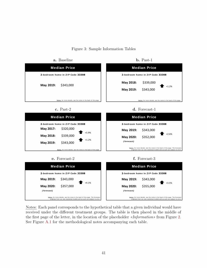
Figure 3: Sample Information Tables

a. Baseline

Median Price

2-bedroom home in ZIP Code 33308

May 2019: $343,000

Notes: for more details, see the notes in the back of this page.

b. Past-1

Median Price

2-bedroom home in ZIP Code 33308

Notes: for more details, see the notes in the back of this page.

May 2018: $339,000

May 2019: $343,000 +1.2%

c. Past-2

Median Price

2-bedroom home in ZIP Code 33308

Notes: for more details, see the notes in the back of this page.

May 2017: $320,000

May 2018: $339,000

May 2019: $343,000+1.2%

+5.9%

d. Forecast-1

Median Price

2-bedroom home in ZIP Code 33308

May 2019: $343,000

May 2020: $352,000 +2.6%

(forecast)

Notes: for more details, see the notes in the back of this page. The forecastsoriginate from our own statistical models and as such are subject to error.

e. Forecast-2

Median Price

2-bedroom home in ZIP Code 33308

May 2019: $343,000

May 2020: $357,000 +4.1%

(forecast)

Notes: for more details, see the notes in the back of this page. The forecastsoriginate from our own statistical models and as such are subject to error.

f. Forecast-3

Median Price

2-bedroom home in ZIP Code 33308

May 2019: $343,000

May 2020: $355,000 +3.5%

(forecast)

Notes: for more details, see the notes in the back of this page. The forecastsoriginate from our own statistical models and as such are subject to error.

Notes: Each panel corresponds to the hypothetical table that a given individual would havereceived under the different treatment groups. The table is then placed in the middle ofthe first page of the letter, in the location of the placeholder «Information» from Figure 2.See Figure A.1 for the methodological notes accompanying each table.

41

Figure 4: Variation in Signals Across Information Sources and Across Markets

a. Across Information Sources

≤−10%

−5%

0%

5%

10%

15%

≥20%

Pa

st−

2 S

ign

al

≤−10% −5% 0% 5% 10% 15% ≥20%Past−1 Signal

Weighted data

OLS

45 deg. line

β = 0.852 (0.017) R

2 = 0.659

b. Across Markets

0%

5%

10%

15%

Pe

rce

nt

≤−10% −5% 0% 5% 10% 15% ≥20%Past−1 Signal

Notes: Panel (a) is a scatterplot showing the relationship between the signals that the 57,910 subjects would have received ifthey had been assigned to the Past-1 treatment versus the Past-2 treatment. The size of the circles are proportional to thenumber of observations, and the signals are truncated at -10% and +20%. Panel (a) shows the distribution of the signals thatthe 57,910 subjects would have received if they had been assigned to the Past-1 treatment (i.e., the annual growth rate overthe past year). The bins have a width of 1 pp and are truncated at -10% and +20%.

42

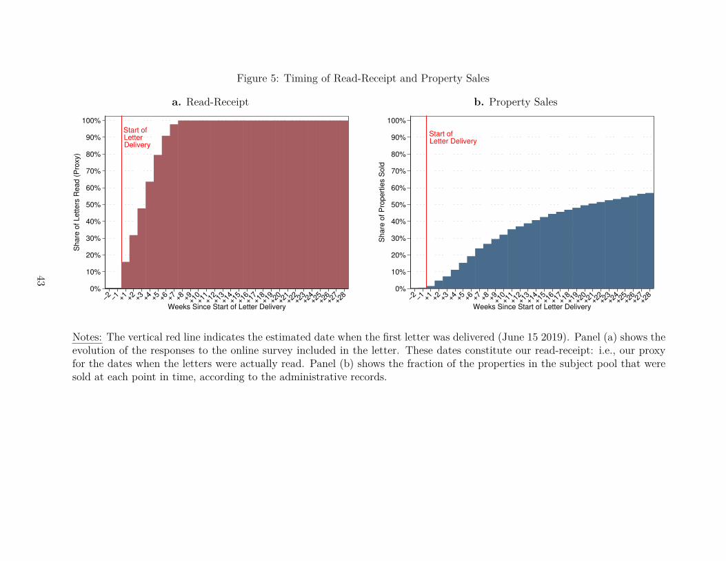
Figure 5: Timing of Read-Receipt and Property Sales

a. Read-Receipt

Start of Letter Delivery

0%

10%

20%

30%

40%

50%

60%

70%

80%

90%

100%

Share

of Letters

Read (

Pro

xy)

−2 −1 +1 +2 +3 +4 +5 +6 +7 +8 +9+10

+11

+12

+13

+14

+15

+16

+17

+18

+19

+20

+21

+22

+23

+24

+25

+26

+27

+28

Weeks Since Start of Letter Delivery

b. Property Sales

Start of Letter Delivery

0%

10%

20%

30%

40%

50%

60%

70%

80%

90%

100%

Share

of P

ropert

ies S

old

−2 −1 +1 +2 +3 +4 +5 +6 +7 +8 +9+10

+11

+12

+13

+14

+15

+16

+17

+18

+19

+20

+21

+22

+23

+24

+25

+26

+27

+28

Weeks Since Start of Letter Delivery

Notes: The vertical red line indicates the estimated date when the first letter was delivered (June 15 2019). Panel (a) shows theevolution of the responses to the online survey included in the letter. These dates constitute our read-receipt: i.e., our proxyfor the dates when the letters were actually read. Panel (b) shows the fraction of the properties in the subject pool that weresold at each point in time, according to the administrative records.

43

Figure 6: Effects of Information Shocks on Expectations and Behavior: Binned Scatterplots

a. Effects on Behavior

Slope = −0.350 (0.105)

N=57,91034%

35%

36%

37%

38%

39%

40%

P(S

old

at 12 w

eeks p

ost−

treatm

ent)

−1% 0% 1% 2% 3% 4% 5% 6% 7% 8%

Information Shock

b. Effects on Expectations

Slope = 0.205 (0.055)

N=1,4042%

3%

4%

5%

Housin

g E

xpecta

tions, P

oste

rior

Belie

f

0% 1% 2% 3% 4% 5% 6% 7% 8%

Information Shock

Notes: Panel (a) corresponds to a binned scatterplot representation of the results presented in column (3) of Table 2. Thisbinned scatterplot focuses on the key independent variable, Information Shock (Ej∗

im ·Di). Results are based on 57,910 subjects

from the field experiment. The dependent variable is an indicator variable taking the value 100 if the property was soldat 12 weeks after the start of the letter delivery and 0 otherwise. Panel (b) is the binned scatterplot representation of theresults presented in column (1) of Table 3. This binned scatterplot focuses on the key independent variable, Information Shock(Ej∗

im · Di). Results are based on 1,404 subjects from the AMT supplemental survey. The dependent variable is the posterior

belief (i.e., elicited after the information-provision experiment) about the expected growth rate of the median home value overthe following year. Each panel reports the slope with heteroskedasticity-robust standard errors in parentheses.

44

Figure 7: Effects of Information Shocks on Behavior: Event-Study Analysis

a. Effects vs. Time

Start of Letter Delivery

Share of Letters Read

0%

50%

100%−0.6

−0.5

−0.4

−0.3

−0.2

−0.1

0.0

0.1

Effect of In

form

ation S

hock o

n P

(Sold

)

−2 −1 +1 +2 +3 +4 +5 +6 +7 +8 +9+10

+11

+12

+13

+14

+15

+16

+17

+18

+19

+20

+21

+22

+23

+24

+25

+26

+27

+28

Weeks Since Start of Letter Delivery

b. Effects vs. Readership

−2w

−1w

+1w

+2w

+3w

+4w

+5w

+6w

+7w

+12w

+28w

−0.4

−0.3

−0.2

−0.1

0.0

0.1

Effect of In

form

ation S

hock o

n P

(Sold

)

0% 20% 40% 60% 80% 100%Share of Letters Read

Notes: Panel (a): each coefficient in the top half of the panel corresponds to a separate regression based on 57,910 subjectsfrom the field experiment. Every regression corresponds to equation (4) from Section 2, and the coefficient being graphedcorresponds to the coefficient on the key independent variable, Information Shock (Ej∗

im ·Di). All regressions are identical except

for the dependent variable. The x-axis indicates the dependent variable used, which is always an indicator variable that takesthe value 100 if the property has been sold at a number of weeks after the start of the letter delivery and 0 otherwise. Forexample, the coefficient on +12 weeks is based on a dependent variable that takes the value 100 if the property was sold at 12weeks after the start of the letter delivery. The vertical red line indicates the estimated date when the first letter was delivered(June 15 2019). The bottom half of the panel shows the proportion of the letters from the field experiment that had been readat every point in time according to our proxy (the responses to the online survey included in the letter). The 90% confidenceintervals are based on heteroskedasticity-robust standard errors. Panel (b): this figure combines the two series shown in panel(a), by by plotting the treatment effects against the proportion of the letters from the field experiment that had been read atevery point in time. The labels at each marker mark the number of weeks after the start of the letter delivery that the effectof the information shock and the share of letters read were recorded at.

45

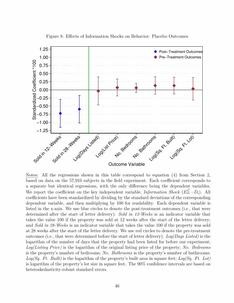
Figure 8: Effects of Information Shocks on Behavior: Placebo Outcomes

−1.25

−1.00

−0.75

−0.50

−0.25

0.00

0.25

0.50

0.75

1.00

1.25

Sta

nd

ard

ize

d C

oe

ffic

ien

t *1

00

Sold

in 1

2−W

eeks

Sold

in 2

8−W

eeks

Log(

Day

s Listed

)

Log(

List P

rice)

No.

Bed

room

s

No.

Bat

hroo

ms

Log(

Sq. F

t. Bui

lt)

Log(

Sq. F

t. Lo

t)

Outcome Variable

Post−Treatment Outcomes

Pre−Treatment Outcomes

Notes: All the regressions shown in this table correspond to equation (4) from Section 2,based on data on the 57,910 subjects in the field experiment. Each coefficient corresponds toa separate but identical regressions, with the only difference being the dependent variables.We report the coefficient on the key independent variable, Information Shock (Ej∗

im · Di). All

coefficients have been standardized by dividing by the standard deviations of the correspondingdependent variable, and then multiplying by 100 for readability. Each dependent variable islisted in the x-axis. We use blue circles to denote the post-treatment outcomes (i.e., that weredetermined after the start of letter delivery): Sold in 12-Weeks is an indicator variable thattakes the value 100 if the property was sold at 12 weeks after the start of the letter delivery;and Sold in 28-Weeks is an indicator variable that takes the value 100 if the property was soldat 28 weeks after the start of the letter delivery. We use red circles to denote the pre-treatmentoutcomes (i.e., that were determined before the start of letter delivery): Log(Days Listed) is thelogarithm of the number of days that the property had been listed for before our experiment;Log(Listing Price) is the logarithm of the original listing price of the property; No. Bedroomsis the property’s number of bedrooms; No. Bathrooms is the property’s number of bathrooms;Log(Sq. Ft. Built) is the logarithm of the property’s built area in square feet; Log(Sq. Ft. Lot)is logarithm of the property’s lot size in square feet. The 90% confidence intervals are based onheteroskedasticity-robust standard errors.

46

Figure 9: AMT Supplemental Survey Results: Belief Updating

β = 0.100 (0.026) R

2 = 0.058

β = 0.545 (0.016) R

2 = 0.501

−8%

−6%

−4%

−2%

0%

2%

4%

6%

8%

Po

ste

rio

r−P

rio

r H

ou

sin

g E

xp

ecta

tio

ns

−14%

−12%

−10% −8

%−6

%−4

%−2

% 0% 2% 4% 6% 8% 10%

12%

14%

Information − Prior Expectations

Information Disclosed

Information Not Disclosed

Notes: The binned scatterplot provides a finer description of the belief updat-ing for the 1,404 subjects from the AMT supplemental survey. The dependentvariable is the belief update about the expected growth rate of the median homevalue over the following year (i.e., the gap between the posterior belief that waselicited after the information-provision experiment, and the prior belief that waselicited before the information-provision experiment). The independent variableis the gap between the signal (the information about home prices provided tothe participant) and the prior belief about the expected home price growth rate.The blue circles represent the subjects that received no additional informationabout home price growth. The red diamonds represent the subjects that receivedadditional information about home price growth. β is the slope of each line, es-timated with a simple linear regression with heteroskedasticity-robust standarderrors reported in parentheses.

47

Figure 10: Heterogeneity Analysis

LIS

TIN

G C

HA

RA

CT

ER

IST

ICS

OW

NE

R D

EM

OG

RA

PH

ICS

MA

RK

ET

CH

AR

AC

TE

RIS

TIC

S

Overall

Owner−occupied (67% of sample)

Non−owner−occupied (33% of sample)

< $359.9K (50%)

≥ $359.9K (50%)

Within 25% (52%)

Over 25% (48%)

< 0 (23%)

≥ 0 (77%)

Female (25%)

Male (53%)

< 59 (33%)

≥ 59 (34%)

White (58%)

Non−white (34%)

Florida (68%)

Other state (32%)

< $311K (50%)

≥ $311K (50%)

< 4.06 (50%)

≥ 4.06 (50%)

< 2416 (51%)

≥ 2416 (49%)

By owner occupancy

By listing price

By listing price to 2019 ZHVI ratio

By price difference from Redfin estimate

By gender

By age

By race

By listing state

By 2019 ZHVI

By Zillow’s seller power index

By Zillow’s ZIP5 size rank

−1 −0.5 0 0.5

Notes: Each coefficient corresponds to a separate regression based on 57,910 subjects correspondingto equation (4) from Section 2. The coefficients correspond to the one on the key independentvariable, Information Shock (Ej∗

im · Di). The dependent variable used is an indicator variable that

takes the value 100 if the property has been sold at 12 weeks after the start of the letter delivery.All regressions are identical except for the sample restrictions, which are presented in the y-axislabels. For example, the coefficient for Owner-occupied represents the coefficient on Informationshock when the regression is run for occupant owners only. The percentage totals in parenthesesrepresent the proportion of the 57,910 subjects that each sample represents. The percentages do notsum to 100% for the demographic breakdowns due to missing values. The 90% confidence intervalsare based on heteroskedasticity-robust standard errors.

48

Table 1: Randomization Balance Test

By Treatment Group(1) (2) (3) (4) (5) (6) (7) (8)All Baseline Past-1 Past-2 Forecast-1 Forecast-2 Forecast-3 P-value

Days Listed 86.654 85.997 87.212 87.029 85.936 86.208 87.778 0.829(0.477) (1.017) (1.298) (1.253) (1.093) (1.203) (1.191)

List Price ($1,000s) 574.756 575.774 586.787 559.192 574.306 586.835 565.092 0.303(3.914) (8.517) (11.445) (9.516) (8.147) (10.937) (9.081)

No. Bedrooms 3.256 3.249 3.259 3.243 3.254 3.269 3.264 0.582(0.005) (0.010) (0.012) (0.012) (0.011) (0.011) (0.011)

No. Bathrooms 2.608 2.607 2.619 2.599 2.608 2.617 2.600 0.678(0.004) (0.010) (0.011) (0.011) (0.010) (0.011) (0.010)

Sq. Ft. Built (1,000s) 2.295 2.292 2.304 2.292 2.287 2.308 2.288 0.820(0.005) (0.012) (0.014) (0.013) (0.012) (0.013) (0.013)

Sq. Ft. Lot (1,000s) 12.958 12.992 12.666 12.934 13.223 13.163 12.730 0.389(0.089) (0.199) (0.222) (0.230) (0.219) (0.221) (0.213)

Observations 57,910 11,487 8,672 8,669 9,818 9,635 9,629

Notes: Average characteristics of the 57,910 properties in the field experiment, with standard errorsreported in parentheses. Column (1) corresponds to the entire sample. Columns (2) through (7)correspond to each of the six treatment groups. Column (8) reports the p-value of the test of equalmeans across all six treatment groups. All the variables correspond to pre-treatment characteristics(i.e., that were determined before the start of letter delivery). Days Listed is the number of daysthat the property had been listed for before our experiment. List Price is the original listing price ofthe property. No. Bedrooms is the property’s number of bedrooms. No. Bathrooms is the property’snumber of bathrooms. Sq. Ft. Built is the property’s built area in square feet. Sq. Ft. Lot is theproperty’s lot size in square feet.

49

Table 2: Main Regression Results

Dep. Var.: S+12w

(1) (2) (3) (4) (5) (6) (7) (8) (9) (10) (11)Information Shock -0.318∗∗∗ -0.419∗∗ -0.350∗∗∗ -0.341∗∗∗ -0.349∗∗∗ -0.330∗∗∗ -0.353∗∗∗ -0.307∗∗ -0.364∗∗∗ -0.411∗∗∗ -0.331∗∗∗

(0.122) (0.170) (0.105) (0.103) (0.113) (0.103) (0.121) (0.139) (0.113) (0.114) (0.109)Experimental Variation Source Disclosure PooledAdditional Controls YExtended Dummies YAlternative Specification YGroup Left Out Past-1 Past-2 Forecast-1 Forecast-2 Forecast-3Mean Outcome 36.93 36.99 36.99 36.99 36.99 36.99 37.10 37.10 36.95 36.91 36.92SD Outcome 48.26 48.28 48.28 48.28 48.28 48.28 48.31 48.31 48.27 48.26 48.26R2 0.167 0.008 0.155 0.193 0.155 0.034 0.164 0.164 0.165 0.165 0.165Observations 46,423 57,910 57,910 57,910 57,910 57,910 49,238 49,241 48,092 48,275 48,281

Notes: Significant at *10%, **5%, ***1%. Heteroskedasticity-robust standard errors in parentheses. Each column corresponds to adifferent regression. All regressions are based on data from the field experiment and using the same dependent variable: an indicatorvariable (S+12w) that takes the value 100 if the property was sold at 12 weeks after the start of the letter delivery and 0 otherwise.Column (1) corresponds to the source-randomization specification given by equation (1) from Section 2, which is restricted to thesample with Di = 1 and with Information Shock corresponding to the key independent variable: Ej∗

im . Column (2) corresponds to the

disclosure-randomization specification given by equation (3), with Information Shock referring to the key independent variable: Ej∗i

m · Di.Column (3)–(11) corresponds to the pooled specification given by equation (4), with Information Shock referring to the key independentvariable: E

j∗i

m · Di. Column (4) is identical to column (3) except that it includes some additional control variables: the logarithm ofthe days the property was on the market prior to the experiment, the logarithm of the initial listing price, four dummies for number ofbedrooms, four dummies for number of bedrooms, the logarithm of square footage built, the logarithm of lot size, and six state dummies.Column (5) is identical to column (3) except that instead of controlling for one treatment indicator, it controls for a set of five treatmentindicators (i.e., one for each of the five treatments that are not Baseline). Column (6) is identical to column (3) except that, rather thancontrolling non-parametrically for market fixed effects, it controls for the potential signals in a parametric way. Column (7)–(11) areidentical to column (3) except that they exclude subjects for one treatment group at a time.

50

Table 3: AMT Supplemental Survey Results

(1) (2) (3) (4)Hpost

1y Hpost5y Hprior

1y Mpost1y

Information Shock 0.205∗∗∗ 0.167∗∗ -0.014 0.017(0.064) (0.070) (0.066) (0.134)

Mean Outcome 3.86 2.31 3.88 3.58SD Outcome 4.42 4.36 5.39 9.05R2 0.140 0.044 0.028 0.043Observations 1,404 1,404 1,404 1,404

Notes: Significant at *10%, **5%, ***1%. Heteroskedasticity-robust standard errors in parentheses. Each column correspondsto a different regression based on data from the AMT supplemental survey using a different dependent variable: Hpost

1y is theposterior belief (i.e., elicited after the information-provision experiment) about the expected growth rate of the median homevalue over the following year. Hpost

5y is is the posterior belief about the annualized expected growth growth rate of the medianhome value over the following five years. Hprior

1y the prior belief (i.e., elicited before the information-provision experiment)about the expected growth rate of the median home value over the following year. And Mpost

1y is the posterior belief about theannualized expected growth growth rate of the stock market index over the following year.

51