NBER WORKING PAPER SERIES

RULE-OF-THUMB CONSUMERS AND THEDESIGN OF INTEREST RATE RULES

Jordi GalíJ. David López-Salido

Javier Vallés

Working Paper 10392http://www.nber.org/papers/w10392

NATIONAL BUREAU OF ECONOMIC RESEARCH1050 Massachusetts Avenue

Cambridge, MA 02138March 2004

We have benefited from comments by Bill Dupor, Ken West (the editor), an anonymous referee, andparticipants at the JMCB-Chicago Fed Tobin’s Conference and the NBER Summer Institute, as well asseminars at the Federal Reserve Board, BIS, CREI-UPF, George Washington University and Bank of Spain.All remaining errors are our own. Galí acknowledges financial support from DURSI (Generalitat deCatalunya), MCYT (Grant SEC2002-03816) and the Bank of Spain. The views expressed in this paper donot necessarily represent those of the Bank of Spain. The views expressed herein are those of the author andnot necessarily those of the National Bureau of Economic Research.

©2004 by Jordi Galí, J. David López-Salido, and Javier Vallés. All rights reserved. Short sections of text, notto exceed two paragraphs, may be quoted without explicit permission provided that full credit, including ©notice, is given to the source.

Rule-of-Thumb Consumers and the Design of Interest Rate RulesJordi Galí, J. David López-Salido, and Javier VallésNBER Working Paper No. 10392March 2004JEL No. E32, E52

ABSTRACT

We introduce rule-of-thumb consumers in an otherwise standard dynamic sticky price model, and

show how their presence can change dramatically the properties of widely used interest rate rules.

In particular, the existence of a unique equilibrium is no longer guaranteed by an interest rate rule

that satisfies the so called Taylor principle. Our findings call for caution when using estimates of

interest rate rules in order to assess the merits of monetary policy in specific historical periods.

Jordi GalíCentre de Recerca en Economia Internacional (CREI)Ramon Trias Fargas 2508005 Barcelona SPAINand NBERjordi.gali@upf.edu

J. David López-SalidoBank of Spaindavidl@bde.es

Javier VallésBank of Spainvalles@bde.es

1 Introduction

The study of the properties of alternative monetary policy rules, and the assessment

of their relative merits, has been one of the central themes of the recent literature

on monetary policy. Many useful insights have emerged from that research, with

implications for the practical conduct of monetary policy, and for our understanding

of its role in different macroeconomic episodes.

Among some of the recurrent themes, much attention has been drawn to the po-

tential benefits and dangers associated with simple interest rate rules. Thus, while it

has been argued that simple interest rate rules can approximate well the performance

of complex optimal rules in a variety of environments,1 those rules have also been

shown to contain the seeds of unnecessary instability when improperly designed.2

A sufficiently strong feedback from endogenous target variables to the short-term

nominal interest rate is often argued to be one of the requirements for the existence

a locally unique rational expectations equilibrium and, hence, for the avoidance of

indeterminacy and fluctuations driven by self-fulfilling expectations. For a large num-

ber of models used in applications that determinacy condition can be stated in a way

that is both precise and general: the policy rule must imply an eventual increase in

the real interest rate in response to a sustained increase in the rate of inflation. In

other words, the monetary authority must adjust (possibly gradually) the short-term

nominal rate more than one-for-one with changes in inflation. That condition, which

following Woodford (2001) is often referred to as the Taylor principle, has also been

taken as a benchmark for the purposes of evaluating the stabilizing role of central

banks’ policies in specific historical periods. Thus, some authors have hypothesized

that the large and persistent fluctuations in inflation and output in the late 60s and1This is possibly the main conclusion from the contributions to the Taylor (1999a) volume.2See, e.g., Kerr and King (1996), Bernanke and Woodford (1997), Taylor (1999b), Clarida, Galí

and Gertler (2000), and Benhabib, Schmitt-Grohé, and Uribe (2001a,b), among others.

1

70s in the U.S. may have been a consequence of the Federal Reserve’s failure to meet

the Taylor principle in that period; by contrast, the era of low and steady inflation

that has characterized most of Volcker and Greenspan’s tenure seems to have been

associated with interest rate policies that satisfied the Taylor principle.3

In the present paper we show how the presence of non-Ricardian consumers may

alter dramatically the properties of simple interest rate rules, and overturn some of

the conventional results found in the literature. In particular, we analyze a standard

new Keynesian model modified to allow for a fraction of consumers who do not borrow

or save in order to smooth consumption, but instead follow a simple rule-of-thumb:

each period they consume their current labor income.

To anticipate our main result: when the central bank follows a rule that implies an

adjustment of the nominal interest rate in response to variations in current inflation

and output, the size of the inflation coefficient that is required in order to rule out

multiple equilibria is an increasing function of the weight of rule-of thumb consumers

in the economy (for any given output coefficient). In particular, we show that if the

weight of such rule-of-thumb consumers is large enough, a Taylor-type rule must imply

a (permanent) change in the nominal interest rate in response to a (permanent) change

in inflation that is significantly above unity, in order to guarantee the uniqueness of

equilibrium. Hence, the Taylor principle becomes too weak a criterion for stability

when the share of rule-of-thumb consumers is large.

We also find that, independently of their weight in the economy, the presence

of rule-of-thumb consumers cannot in itself overturn the conventional result on the

sufficiency of the Taylor principle. Instead, we argue that it is the interaction of those

consumers with countercyclical markups (resulting from sticky prices in our model)3See, e.g., Taylor (1999b), and Clarida, Galí, and Gertler (2000). Orphanides (2001) argues that

the Fed’s failure to satisfy the Taylor principle was not intentional; instead it was a consequence of

a persistent bias in their real-time measures of potential output.

2

that lies behind our main result.

In addition to our analysis of a standard contemporaneous rule, we also investigate

the properties of a forward-looking interest rate rule. We show that the conditions

for a unique equilibrium under such a rule are somewhat different from those in a

contemporaneous one. In particular, we show that when the share of rule-of-thumb

consumers is sufficiently large it may not be possible to guarantee a (locally) unique

equilibrium or, if it is possible, it may require that interest rates respond less than

one-for-one to changes in expected inflation.

Our framework shares most of the features of recent dynamic optimizing sticky

price models.4 The only difference lies in the presence of rule-of-thumb consumers,

who are assumed to coexist with conventional Ricardian consumers. While the behav-

ior that we assume for rule-of-thumb consumers is admittedly simplistic (and justified

only on tractability grounds), we believe that their presence captures an important

aspect of actual economies which is missing in conventional models. Empirical sup-

port of non-Ricardian behavior among a substantial fraction of households in the U.S.

and other industrialized countries can be found in Campbell and Mankiw (1989). It

is also consistent, at least prima facie, with the findings of a myriad of papers reject-

ing the permanent income hypothesis on the basis of aggregate data. While many

authors have stressed the consequences of the presence of rule-of-thumb consumers

for fiscal policy,5 the study of its implications for the design of monetary policy is

largely non-existent.6

A number of papers in the literature have also pointed to some of the limitations4See, e.g., Rotemberg and Woodford (1999), Clarida, Gali and Gertler (1999), or Woodford

(2001).5See, e.g., Mankiw (2000) and Galí, López-Salido and Vallés (2003c).6A recent paper by Amato and Laubach (2003) constitutes an exception. In that paper the

authors derive the appropriate loss function that a benevolent central banker should seek to minimize

in the presence of habit formation and rule-of-thumb consumers.

3

of the Taylor principle as a criterion for the stability properties of interest rate rules,

in the presence of some departures from standard assumptions. Thus, Edge and Rudd

(2002) and Roisland (2003) show how the Taylor criterion needs to be strengthened

in the presence of taxes on nominal capital income. Fair (2003) argues that the

Taylor principle is not a requirement for stability if aggregate demand responds to

nominal interest rates (as opposed to real rates) and inflation has a negative effect on

consumption expenditures (through its effects on real wages and wealth), as it is the

case in estimated versions of his multicountry model. Christiano and Gust (1999) find

that the stability properties of simple interest rate rules are significantly altered when

the assumption of limited participation is introduced. Benhabib, Schmitt-Grohé and

Uribe (2001a) demonstrate that an interest rate rule satisfying the Taylor principle

will generally not prevent the existence of multiple equilibrium paths converging to

the liquidity trap steady state that arises in the presence of a zero lower bound on

nominal rates. The present paper can be viewed as complementing that work, by

pointing to an additional independent source of deviations from the Taylor principle

as a criterion for stability of monetary policy rules.

The rest of the paper is organized as follows. Section 2 lays out the basic model,

and derives the optimality conditions for consumers and firms, as well as their log-

linear counterparts. Section 3 contains an analysis of the equilibrium dynamics and

its properties under our baseline interest rate rule, with a special emphasis on the

conditions that the latter must satisfy in order to guarantee uniqueness. Section

4 examines the robustness of those results and the required modifications when a

forward looking interest rate rules is assumed. Section 5 concludes.

4

2 A New Keynesian Model with Rule-of-Thumb

Consumers

The economy consists of two types households, a continuum of firms producing differ-

entiated intermediate goods, a perfectly competitive final goods firm, and a central

bank in charge of monetary policy. Next we describe the objectives and constraints

of the different agents. Except for the presence of rule-of-thumb consumers, our

framework corresponds to a conventional New Keynesian model with staggered price

setting à la Calvo used in numerous recent applications. A feature of our model that

is worth emphasizing is the presence of capital accumulation. That feature has often

been ignored in the recent literature, on the grounds that its introduction does not

alter significantly most of the conclusions.7 In our framework, however, the existence

of a mechanism to smooth consumption over time is critical for the distinction be-

tween Ricardian and non-Ricardian consumers to be meaningful, thus justifying the

need for introducing capital accumulation explicitly.8

2.1 Households

We assume a continuum of infinitely-lived households, indexed by i ∈ [0, 1]. A fraction1 − λ of households have access to capital markets where they can trade a full set

of contingent securities, and buy and sell physical capital (which they accumulate

and rent out to firms). We use the term optimizing or Ricardian to refer to that

subset of households. The remaining fraction λ of households do not own any assets7Among the papers that introduce capital accumulation explicitly in a new Keynesian framework

we can mention King and Watson (1996), Yun (1996), Dotsey (1999), Kim (2000) and Dupor (2002).8Notice that in the absence of capital accumulation both types of households would behave

identically in equilibrium, thus implying that constraint on the behavior of rule-of-thumb consumers

would not be binding.

5

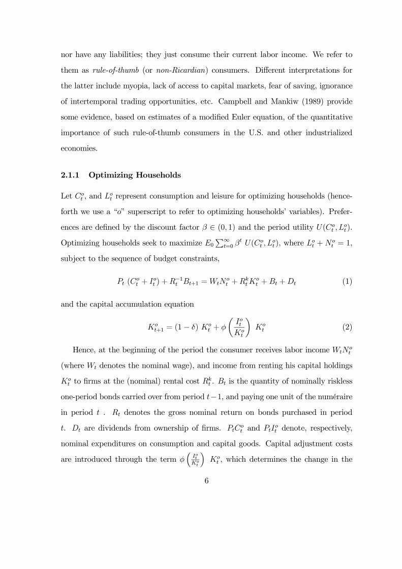
nor have any liabilities; they just consume their current labor income. We refer to

them as rule-of-thumb (or non-Ricardian) consumers. Different interpretations for

the latter include myopia, lack of access to capital markets, fear of saving, ignorance

of intertemporal trading opportunities, etc. Campbell and Mankiw (1989) provide

some evidence, based on estimates of a modified Euler equation, of the quantitative

importance of such rule-of-thumb consumers in the U.S. and other industrialized

economies.

2.1.1 Optimizing Households

Let Cot , and Lot represent consumption and leisure for optimizing households (hence-

forth we use a “o” superscript to refer to optimizing households’ variables). Prefer-

ences are defined by the discount factor β ∈ (0, 1) and the period utility U(Cot , Lot ).Optimizing households seek to maximize E0

P∞t=0 β

t U(Cot , Lot ), where L

ot +N

ot = 1,

subject to the sequence of budget constraints,

Pt (Cot + I

ot ) +R

−1t Bt+1 =WtN

ot +R

ktK

ot +Bt +Dt (1)

and the capital accumulation equation

Kot+1 = (1− δ) Ko

t + φ

µIotKot

¶Kot (2)

Hence, at the beginning of the period the consumer receives labor income WtNot

(where Wt denotes the nominal wage), and income from renting his capital holdings

Kot to firms at the (nominal) rental cost R

kt . Bt is the quantity of nominally riskless

one-period bonds carried over from period t−1, and paying one unit of the numérairein period t . Rt denotes the gross nominal return on bonds purchased in period

t. Dt are dividends from ownership of firms. PtCot and PtIot denote, respectively,

nominal expenditures on consumption and capital goods. Capital adjustment costs

are introduced through the term φ³IotKot

´Kot , which determines the change in the

6

capital stock (gross of depreciation) induced by investment spending Iot . We assume

φ0 > 0, and φ00 ≤ 0, with φ0(δ) = 1, and φ(δ) = δ. In what follows we specialize the

period utility to take the form U(C,L) ≡ 11−σ (C L

ν)1−σ where σ ≥ 0 and ν > 0.

The first order conditions for the optimizing consumer’s problem can be written

as:CotLot=1

ν

Wt

Pt(3)

1 = Rt Et {Λt,t+1} (4)

PtQt = Et

½Λt,t+1

·Rkt+1 + Pt+1Qt+1

µ(1− δ) + φt+1 −

µIot+1Kot+1

¶φ0t+1

¶¸¾(5)

Qt =1

φ0³IotKot

´ (6)

where φt+1 = φ³Iot+1Kot+1

´and φ0t+1 = φ0

³Iot+1Kot+1

´, respectively; Λt,t+k is the stochastic

discount factor for nominal payoffs given by:

Λt,t+k ≡ βkµCot+kCot

¶−σ µLot+kLot

¶ν(1−σ)µPtPt+k

¶(7)

and where Qt is the (real) shadow value of capital in place, i.e., Tobin’s Q. Notice

that, under our assumption on φ, the elasticity of the investment-capital ratio with

respect to Q is given by − 1φ00(δ)δ ≡ η.

2.1.2 Rule-of-Thumb Households

Rule-of-thumb households do not attempt (or are just unable) to smooth their con-

sumption path in the face of fluctuations in labor income. Each period they solve

the static problem, i.e. they maximize their period utility U(Crt , Lrt ) subject to the

constraint that all their labor income is consumed, that is:

PtCrt =WtN

rt (8)

and where an “r” superscript is used to denote variables specific to rule-of-thumb

households.

7

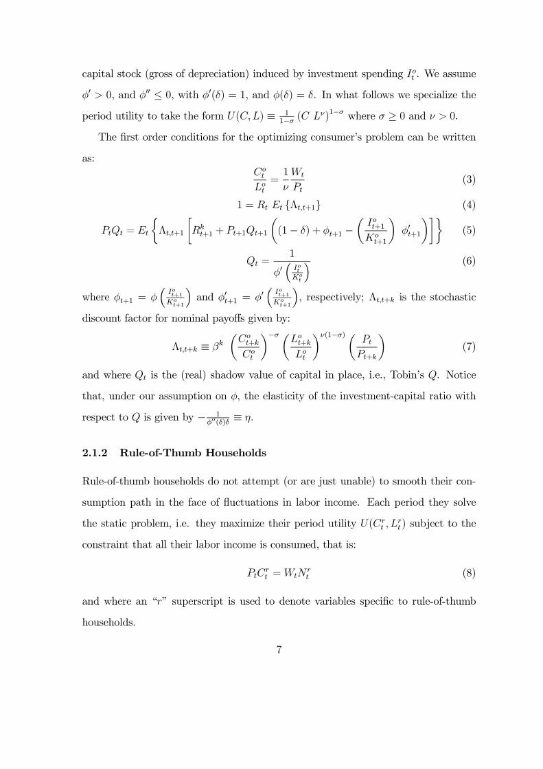
The associated first order condition is given by:

CrtLrt=1

ν

Wt

Pt(9)

which combined with (8) yields

N rt =

1

1 + ν≡ N r (10)

hence implying a constant employment for rule-of-thumb households9, as well as a

consumption level proportional to the real wage:10

Crt =1

1 + ν

Wt

Pt(11)

2.1.3 Aggregation

Aggregate consumption and leisure are a weighted average of the corresponding vari-

ables for each consumer type. Formally:

Ct ≡ λ Crt + (1− λ) Cot (12)

Nt ≡ λ N rt + (1− λ) No

t (13)

Similarly, aggregate investment and capital stock are given It ≡ (1 − λ) Iot , and

Kt ≡ (1− λ) Kot . We can combine (12) and (13) with the optimality conditions (9),

(10), and (11) to obtain,

Nt =λ

1 + ν+ (1− λ) No

t

9Alternatively we could have assumed directly a constant labor supply for rule of thumb house-

holds.10Notice that under our assumptions, real wages are the only source of fluctuations in rule of

thumb households’ disposable income. More realistically, as shown in Gali, Lopez-Salido and Valles

(2003c), the introduction of labor market frictions can generate fluctuations in hours of rule of thumb

consumers, thus implying a second margin of variation in disposable income. In that context, it may

be possible to preserve our findings even in the presence of wage stickiness (nominal or real). This

constitutes a natural extension of this paper and is part of our ongoing research.

8

Ct =1

ν

µWt

Pt

¶(1−Nt) (14)

which will be used below.

2.2 Firms

We assume the existence of a continuum of monopolistically competitive firms pro-

ducing differentiated intermediate goods. The latter are used as inputs by a (perfectly

competitive) firm producing a single final good.

2.2.1 Final Goods Firm

The final good is produced by a representative, perfectly competitive firm with a

constant returns technology: Yt =³R 1

0Xt(j)

ε−1ε dj

´ εε−1, where Xt(j) is the quantity

of intermediate good j used as an input. Profit maximization, taking as given the

final goods price Pt and the prices for the intermediate goods Pt(j), for all j ∈ [0, 1],yields the set of demand schedules, Xt(j) =

³Pt(j)Pt

´−εYt. Finally, the zero profit

condition yields, Pt =³R 1

0Pt(j)

1−ε dj´ 11−ε.

2.2.2 Intermediate Goods Firm

The production function for a typical intermediate goods firm (say, the one producing

good j) is given by:

Yt(j) = Kt(j)α Nt(j)

1−α (15)

where Kt(j) and Nt(j) represents the capital and labor services hired by firm j.11

Cost minimization, taking the wage and the rental cost of capital as given, implies

the optimality condition Kt(j)Nt(j)

=¡

α1−α¢ ³

Wt

Rkt

´. Hence, real marginal cost is common

to all firms and given by: MCt = 1Φ

³RktPt

´α ³Wt

Pt

´1−α, where Φ ≡ αα(1− α)1−α.

11Without loss of generality we have normalized the level of total factor productivity to unity.

9

Price Setting Intermediate firms are assumed to set nominal prices in a staggered

fashion, according to the stochastic time dependent rule proposed by Calvo (1983).

Each firm resets its price with probability 1−θ each period, independently of the timeelapsed since the last adjustment. Thus, each period a measure 1 − θ of producers

reset their prices, while a fraction θ keep their prices unchanged

A firm resetting its price in period t will seek to maximize

max{P∗t }

Et

∞Xk=0

θk Et {Λt,t+k Yt+k(j) (P ∗t − Pt+k MCt+k)}

subject to the sequence of demand constraints, Yt+k(j) = Xt+k(j) =³

P∗tPt+k

´−εYt+k,

where P ∗t represents the price chosen by firms resetting prices at time t. The first

order conditions for this problem is:

∞Xk=0

θk Et

½Λt,t+k Yt+k(j)

µP ∗t −

ε

ε− 1 Pt+k MCt+k¶¾

= 0 (16)

Finally, the equation describing the dynamics for the aggregate price level is given

by Pt =£θ P 1−εt−1 + (1− θ) (P ∗t )

1−ε¤ 11−ε .

2.3 Monetary Policy

The central bank is assumed to set the nominal interest rate rt ≡ Rt−1 every periodaccording to a simple linear interest rate rule:

rt = r + φπ πt + φy yt (17)

where φπ ≥ 0,φy ≥ 0 and r is the steady state nominal interest rate. Notice thatthe rule above implicitly assumes a zero inflation target, which is consistent with the

steady state around which we will log linearize the price setting equation (16). A

rule analogous to (17) was originally proposed by John Taylor (Taylor (1993)) as a

description for the evolution of short-term interest rates in the U.S. under Greenspan.

10

It has since become known as the Taylor rule and has been used in numerous theoret-

ical and empirical applications.12 In addition to (17), we also analyze the properties

of a forward-looking interest rate rule, in which interest rates respond to expected

inflation and output. We refer the reader to the discussion below for details.

2.4 Market Clearing

The clearing of factor and good markets requires that the following conditions are

satisfied for all t: Nt =R 10Nt(j) dj, Kt =

R 10Kt(j) dj, Yt(j) = Xt(j), for all j ∈ [0, 1]

and

Yt = Ct + It (18)

2.5 Linearized Equilibrium Conditions

Next we derive the log-linear versions of the key optimality and market clearing con-

ditions that will be used in our analysis of the model’s equilibrium dynamics. For

aggregate variables we generally use lower case letters to denote the logs of the cor-

responding original variables (or their log deviations from steady state), and ignore

constant terms throughout. Some of these conditions hold exactly, while others rep-

resent first-order approximations around a zero inflation steady state.

2.5.1 Households

The log-linearized versions of the households’ optimality conditions, expressed in

terms of aggregate variables, are presented next. The reader can find details of the

derivations in a companion working paper.13 Some of these optimality conditions turn12This is illustrated in many of the papers contained in the Taylor (1999) volume, which analyze

the properties of rules like (17) or variations thereof in the context a a variety of models.13See Galí, López-Salido and Vallés (2003a).

11

out to be independent of λ, the weight of rule-of-thumb consumers in the economy.

Among the latter we have the aggregate labor supply schedule that can be derived

taking logs on both sides of (3):

ct + ϕ nt = wt − pt (19)

where ϕ ≡ N1−N . The latter coefficient, which can be interpreted as the inverse of

the Frisch aggregate labor supply elasticity, can be shown to be independent of λ.14

The log-linearized equations describing the dynamics of Tobin’s Q (6)and its re-

lationship with investment (5)are also independent of λ, and given respectively by

qt = β Et{qt+1}+ [1− β(1− δ)] Et{(rkt+1 − pt+1)}− (rt −Et{πt+1}) (20)

and

it − kt = η qt (21)

The same invariance to λ holds for the log-linearized capital accumulation equa-

tion:

kt+1 = δ it + (1− δ) kt (22)

The only aggregate equilibrium condition that is affected by the weight of rule-of-

thumb consumers turns out to be the log-linearized aggregate Euler equation, which

takes the form

ct = Et{ct+1}− 1σ(rt −Et{πt+1}− ρ)−Θ Et{∆nt+1} (23)

where Θ ≡ ϕλ1−λ +

(1− 1σ)νϕ

(1−λ) .

Notice that the possibility of a non-separable utility (σ 6= 1) justifies in itself thepresence of the term involving expected employment growth in the aggregate Euler

equation. Notice, however, that in the absence of rule-of-thumb consumers we have14More specifically, ϕ is given by: ϕ ≡ N

1−N = 1ν

(ρ+δ)(1−α)ρ+δ(1−α)+µ(ρ+δ) .

12

Θ = (1− 1σ)νϕ < 1, since νϕ ∈ (0, 1). In general, however, the size of Θ is a highly

nonlinear function of λ, the weight of rule-of-thumb consumers. As discussed below,

that effect can potentially alter the local stability properties of the dynamical system

describing the equilibrium.

2.5.2 Firms

Log-linearization of (16) and the definition of aggregate price level, around the zero

inflation steady state, yields the familiar equation describing the dynamics of inflation

as a function of the deviations of the average (log) markup from its steady state level

πt = β Et{πt+1}− τ µt (24)

where τ = (1−βθ)(1−θ)θ

and (ignoring constant terms)

µt = (yt − nt)− (wt − pt) = (yt − kt)− (rkt − pt) (25)

Furthermore, it can be shown that the following aggregate production function

holds, up to a first order approximation:

yt = α kt + (1− α) nt (26)

2.5.3 Market clearing

Log-linearization of the market clearing condition of the final good around the steady

state yields:

yt = γc ct + (1− γc) it (27)

where γc ≡ CY= 1− δα(1− 1

ε)(ρ+δ)

is the aggregate consumption share in the steady state,

which is independent of the weight of rule-of-thumb consumers.

13

3 Analysis of Equilibrium Dynamics

We can now combine equilibrium conditions (19)-(27) to obtain a system of difference

equations describing the log-linearized equilibrium dynamics of our model economy.

After several straightforward though tedious substitutions, we can reduce that system

to one involving four variables:

A Et{xt+1} = B xt (28)

where xt ≡ (nt, ct, πt, kt)0. Notice that nt, ct, πt, kt are expressed in terms of

log deviations from their values in the zero inflation steady state. The elements of

matrices A and B are all functions of the underlying structural parameters.15

Notice that xt = 0 for all t , which corresponds to the perfect foresight zero

inflation steady state, always constitutes a solution to the above system. This should

not be surprising, given that for simplicity we have not introduced any fundamental

shocks in our model. In the remainder of the paper we study the conditions under

which the solution to (28) is unique and converges to the steady state, for any given

initial capital stock. In doing so we restrict our analysis to solutions of (28) (i.e.,

equilibrium paths) which remain within a small neighborhood of the steady state.16

Before we turn to that task, we discuss briefly the calibration that we use as a baseline

for that analysis.

3.1 Baseline Calibration

The model is calibrated to a quarterly frequency. Table 1 summarizes compactly the

values assumed for the different parameters in the baseline calibration. The rate of

depreciation δ is set to 0.025 (implying a 10 percent annual rate). The elasticity of15See the appendix in Galí, López-Salido and Vallés (2003a).16See, e.g., Benhabib, Schmitt-Grohé and Uribe (2001a) for a discussion of the caveats associated

with that approach.

14

output with respect to capital, α, is assumed to be 13, a value roughly consistent with

the observed labor income share given any reasonable steady state markup. With

regard to preference parameters, we set the discount factor β equal to 0.99 (implying

a steady state real annual return of 4 percent). The elasticity of substitution across

intermediate goods, ε, is set to 6, a value consistent with a steady state markup µ of

0.2. The previous parameters are kept at their baseline values throughout the present

section.

Next we turn to the parameters for which some sensitivity analysis is conducted,

by examining a range of values in addition to their baseline settings. We set the

baseline value for parameter ν in a way consistent with a unit Frisch elasticity of

labor supply (i.e., ϕ = 1) in our baseline calibration. That choice is associated

with a fraction of time allocated to work in the steady state given by N = 12. We

choose a baseline value of one for σ, which corresponds to a separable (log-log) utility

specification. The fraction of firms that keep their prices unchanged, θ, is given a

baseline value of 0.75, which corresponds to an average price duration of one year.

This is consistent with the findings reported in Taylor (1999c). Following King and

Watson (1996), we set η, the elasticity of investment with respect to Tobin’s Q, equal

to 1.0 under our baseline calibration.17 Finally, we set φπ = 1.5 and φy = 0.5 as the

baseline values for the interest rate rule coefficients, in a way consistent with Taylor’s

(1993) characterization of U.S. monetary policy under Greenspan.

Much of the sensitivity analysis below focuses on the weight of rule-of-thumb

households (λ) and its interaction with θ, σ, ϕ, η, and φπ and φy.

17Other authors who have worked with an identical specification of capital adjustment costs have

considered alternative calibrations of that elasticity. Thus, e.g., Dotsey (1999) assumes an elasticity

of 0.25; Dupor (2002) assumes a baseline elasticity of 5; Baxter and Crucini (1993) set a baseline

value of 15; Abel (1980) estimates that elasticity to be between 0.3 and 0.5 .

15

3.2 Determinacy Analysis

Vector xt contains three non-predetermined variables (hours, consumption and infla-

tion) and a predetermined one (capital stock). Hence, the solution to (28) is unique

if and only if three eigenvalues of matrix A−1B lie outside the unit circle, and one

lies inside.18 Alternatively, if there is more than one eigenvalue of A−1B inside the

unit circle the equilibrium is locally indeterminate: for any initial capital stock there

exists a continuum of deterministic equilibrium paths converging to the steady state,

and the possibility of stationary sunspot fluctuations arises. On the other hand, if

all the eigenvalues A−1B lie outside the unit circle, there is no solution to (28) that

converges to the steady state, unless the initial capital stock happens to be at its

steady state level (in which case xt = 0 for all t is the only non-explosive solution).

Below our focus is on how the the presence of rule-of-thumb consumers may influence

the configuration of eigenvalues of the dynamical system, and hence the properties of

the equilibrium.

3.3 The Taylor Principle and Indeterminacy

We start by exploring the conditions for the existence of a unique equilibrium as a

function of the degree of price stickiness (indexed by parameter θ) and the weight of

rule-of-thumb households (indexed by parameter λ) under an interest rate rule like

(17). As shown by Bullard and Mitra (2002) and Woodford (2001), in a version of

the model above with neither capital nor rule-of-thumb consumers, a necessary and

sufficient condition for the existence of a (locally) unique equilibrium is given by19

φπ > 1−(1− β) φyτ(1 + ϕ)

(29)

A rule like (17) which meets the condition above is said to satisfy the Taylor18See, e.g., Blanchard and Kahn (1980).19As in Bullard and Mitra (2002) we restrict ourselves to non-negative values of φπ and φy.

16

principle. As discussed in Woodford (2001), such a rule guarantees that in response

to permanent change in inflation (and, hence, in output), the nominal interest rate is

adjusted more than one-for-one. In the particular case of a zero coefficient on output

the Taylor principle is satisfied whenever φπ > 1. More generally, as (29) makes clear,

it is possible for the equilibrium to be unique for values of φπ less than one, as long

as as the central bank raises the interest rate sufficiently in response to an increase in

output. In other words, in the canonical model there is some substitutability between

the size of the response to output and that of the response to inflation. As shown in

Dupor (2002) and further illustrated below, the previous finding carries over, at least

qualitatively, to a version of the model with capital accumulation and fully Ricardian

consumers. In particular, when φy = 0 the condition for uniqueness is given by

φπ > 1.

Next we analyze the extent to which those conditions need to be modified in

order to guarantee the existence of a unique equilibrium in the model with rule-of-

thumb consumers laid out above. A key finding of our paper is illustrated by Figure

1. That figure represents the equilibrium properties of our model economy for all

configurations of λ and θ, under the assumption of φπ = 1.5 and φy = 0.5, parameter

values that clearly satisfy the Taylor criterion in standard models. In particular,

the figure displays the regions in the parameter space (λ, θ) that are associated with

the presence of uniqueness and multiplicity of a rational expectations equilibrium

in a neighborhood of the steady state. Notice that each graph corresponds to an

alternative pair of settings for the risk aversion coefficient σ and the inverse labor

supply elasticity ϕ.

A key finding emerges clearly: the combination of a high degree of price stickiness

with a large share of rule-of-thumb consumers rules out the existence of a unique

equilibrium converging to the steady state. Instead, the economy is characterized

17

in that case by indeterminacy of equilibrium (dark region). Conversely, if (a) prices

are sufficiently flexible (low θ) and/or (b) the share of rule-of-thumb consumers is

sufficiently small (low λ), the existence of a unique equilibrium is guaranteed. That

finding holds irrespective of the assumed values for σ and ϕ, even though the relative

size of the different regions can be seen to depend on those parameters. In particular,

the size of the uniqueness region appears to shrink as σ and ϕ increase. In sum, as

made clear by Figure 1, the Taylor principle may no longer be a useful criterion for

the design of interest rate rules in economies with strong nominal rigidities and a

substantial weight of rule-of-thumb consumers.

Importantly, while the previous result has been illustrated under the assumption

of φπ = 1.5 and φy = 0.5 (the values proposed by Taylor (1993)), similar patterns

arise for a large set of configurations of those coefficients that would be associated

with the existence of a unique equilibrium in the absence of rule-of-thumb consumers.

The size of the indeterminacy region can be shown to shrink gradually as the size

of the interest rate response to inflation and output increases (while keeping other

parameters constant). In particular, for any given value of the output coefficient, φy

(and given a configuration of settings for the remaining parameters), the minimum

threshold value for the inflation coefficient φπ consistent with an unique equilibrium

lies above the one corresponding to the model without rule-of-thumb consumers. In

other words, a strengthened condition on the size of the response of interest rates to

changes in inflation is required in that case. Next, we provide an explicit analysis of

the variation in the threshold value for φπ, as a function of different parameter values

and, most importantly, as a function of the share of rule-of-thumb households.

18

3.4 Interest Rate Rules and Rule-of-Thumb Consumers: Re-

quirements for Stability

Figure 2 plots the threshold value of φπ that is required for a unique equilibrium

as a function of the share of rule-of-thumb consumers, for three alternative values

of φy: 0.5 (our baseline case), 0.0 (the pure inflation targeting case) and 1.0 (as in

the modified Taylor rule considered in Taylor (1999c)). For convenience, we plot the

inverse of the threshold value of φπ.20 We notice that as φy increases, the threshold

value for φπ falls, for any given share of rule-of-thumb consumers. Yet, as the Figure

makes clear, the fact that the central bank is responding to output does not relieve

it from the need to respond to inflation on a more than one-for-one basis, once a

certain share of rule-of-thumb consumers is attained. Furthermore, as in our baseline

case, the size of the minimum required response is increasing in that share. Thus, for

instance, when φy = 0.0 the central bank needs to vary the nominal rate in response

to changes in inflation on a more than one-for-one basis whenever the share of rule-of-

thumb consumers is above 0.57. In particular, when λ = 23, the inflation coefficient φπ

must lie above 6 (approximately) in order to guarantee a unique equilibrium. Even

though our simple-minded rule-of-thumb consumers do not have a literal counterpart

that would allow us to determine λ with precision, we view these values as falling

within the range of empirical plausibility given some of the existing micro and macro

evidence. In particular, estimated Euler equations for aggregate consumption whose

specification allows for the presence of rule-of-thumb consumers point to values for λ

in the neighborhood of one-half (Campbell and Mankiw (1989)). In addition, and as

recently surveyed in Mankiw (2000), recent empirical microeconomic evidence tends

to support that finding. 21

20The inverse of the threshold value is bounded, which facilitates graphical display.21Empirical estimates of the marginal propensity to consume out of current income range from

0.35 up to 0.6 (see Souleles (1999)) or even 0.8 (see Shea (1995)), values that are well above those

19

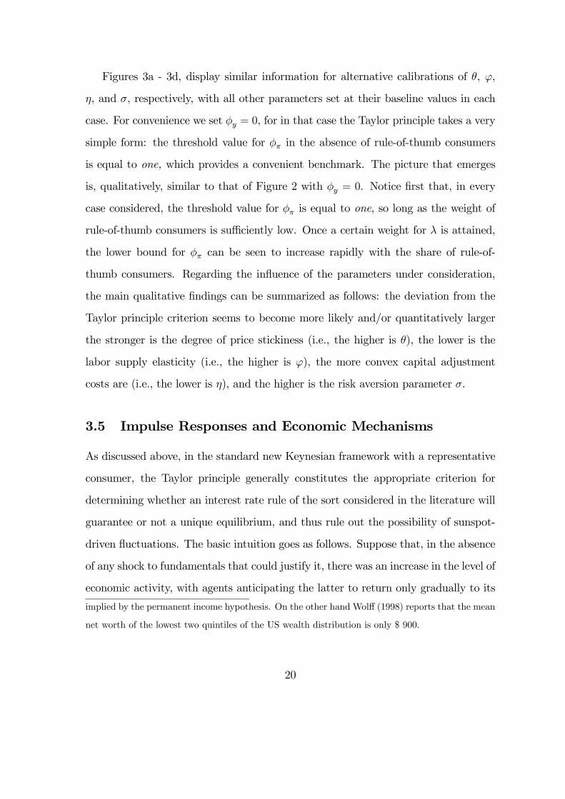
Figures 3a - 3d, display similar information for alternative calibrations of θ, ϕ,

η, and σ, respectively, with all other parameters set at their baseline values in each

case. For convenience we set φy = 0, for in that case the Taylor principle takes a very

simple form: the threshold value for φπ in the absence of rule-of-thumb consumers

is equal to one, which provides a convenient benchmark. The picture that emerges

is, qualitatively, similar to that of Figure 2 with φy = 0. Notice first that, in every

case considered, the threshold value for φπ is equal to one, so long as the weight of

rule-of-thumb consumers is sufficiently low. Once a certain weight for λ is attained,

the lower bound for φπ can be seen to increase rapidly with the share of rule-of-

thumb consumers. Regarding the influence of the parameters under consideration,

the main qualitative findings can be summarized as follows: the deviation from the

Taylor principle criterion seems to become more likely and/or quantitatively larger

the stronger is the degree of price stickiness (i.e., the higher is θ), the lower is the

labor supply elasticity (i.e., the higher is ϕ), the more convex capital adjustment

costs are (i.e., the lower is η), and the higher is the risk aversion parameter σ.

3.5 Impulse Responses and Economic Mechanisms

As discussed above, in the standard new Keynesian framework with a representative

consumer, the Taylor principle generally constitutes the appropriate criterion for

determining whether an interest rate rule of the sort considered in the literature will

guarantee or not a unique equilibrium, and thus rule out the possibility of sunspot-

driven fluctuations. The basic intuition goes as follows. Suppose that, in the absence

of any shock to fundamentals that could justify it, there was an increase in the level of

economic activity, with agents anticipating the latter to return only gradually to its

implied by the permanent income hypothesis. On the other hand Wolff (1998) reports that the mean

net worth of the lowest two quintiles of the US wealth distribution is only $ 900.

20

original (steady state) level. That increase in economic activity would be associated

with increases in hours, lower markups (because of sticky prices), and persistently

high inflation (resulting from the attempts by firms adjusting prices to re-establish

their desired markups). But an interest rate rule that satisfied the Taylor principle

would generate high real interest rates along the adjustment path, and hence, would

call for a low level of consumption and investment relative to the steady state. The

implied impact on aggregate demand would make it impossible to sustain the initial

boom, thus rendering it inconsistent with a rational expectations equilibrium.

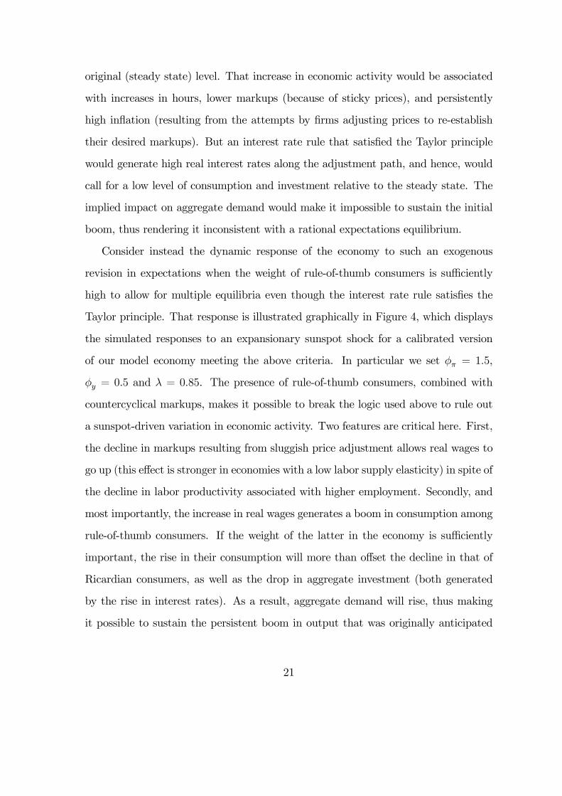
Consider instead the dynamic response of the economy to such an exogenous

revision in expectations when the weight of rule-of-thumb consumers is sufficiently

high to allow for multiple equilibria even though the interest rate rule satisfies the

Taylor principle. That response is illustrated graphically in Figure 4, which displays

the simulated responses to an expansionary sunspot shock for a calibrated version

of our model economy meeting the above criteria. In particular we set φπ = 1.5,

φy = 0.5 and λ = 0.85. The presence of rule-of-thumb consumers, combined with

countercyclical markups, makes it possible to break the logic used above to rule out

a sunspot-driven variation in economic activity. Two features are critical here. First,

the decline in markups resulting from sluggish price adjustment allows real wages to

go up (this effect is stronger in economies with a low labor supply elasticity) in spite of

the decline in labor productivity associated with higher employment. Secondly, and

most importantly, the increase in real wages generates a boom in consumption among

rule-of-thumb consumers. If the weight of the latter in the economy is sufficiently

important, the rise in their consumption will more than offset the decline in that of

Ricardian consumers, as well as the drop in aggregate investment (both generated

by the rise in interest rates). As a result, aggregate demand will rise, thus making

it possible to sustain the persistent boom in output that was originally anticipated

21

by agents. That possibility is facilitated by the presence of highly convex adjustment

costs (low η), which will mute the investment response, together with a low elasticity

of intertemporal substitution (a high σ), which will dampen the response of the

consumption of Ricardian households.

4 A Forward-Looking Rule

In the present section we analyze the properties of our model when the central bank

follows a forward-looking interest rate rule of the form

rt = r + φπ Et{πt+1}+ φy Et{yt+1} (30)

The rule above corresponds to a particular case of the specification originally

proposed by Bernanke and Woodford (1997), and estimated by Clarida, Galí and

Gertler (1998, 2000).22 Dupor (2002) analyzes the equilibrium properties of a rule

identical to (30) in the context of a new Keynesian model with capital accumulation

similar to the one used in the present paper, though without rule-of-thumb consumers.

His analysis suggests that the Taylor principle remains a useful criterion for this kind

of economies, but with an important additional constraint: φπ should not lie above

some upper limit φuπ > 1 (which in turn depends on φy) in order for the rational

expectations equilibrium to be (locally) unique. In other words, in addition to the

usual lower bound associated to the Taylor principle, there is an upper bound to the

size of the response to expected inflation that must be satisfied; if that upper bound

is overshot the equilibrium becomes indeterminate. A similar result has been shown

analytically in the context of a similar model without capital. See, e.g., Bernanke22In Galí, López-Salido and Vallés (2003a) we also provide an analysis of the properties of a

backward looking rule. For the most part those properties are qualitatively similar to those of a

forward looking rule.

22

and Woodford (1997) and Bullard and Mitra (2002).23

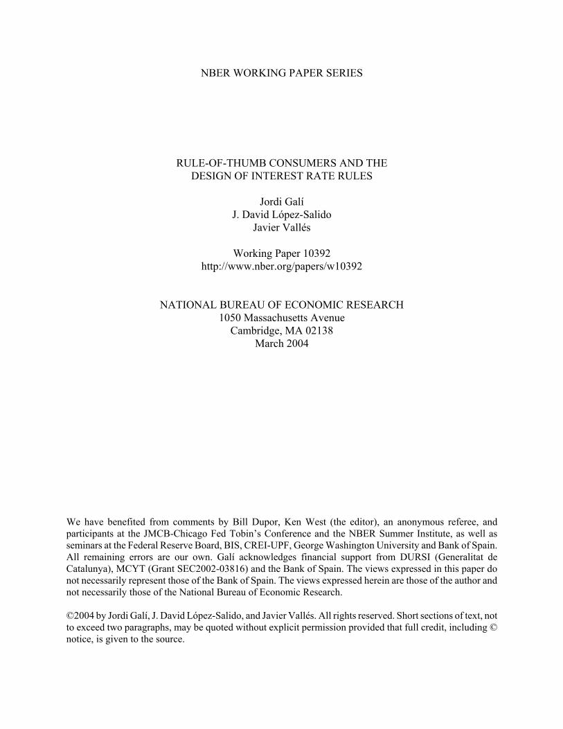
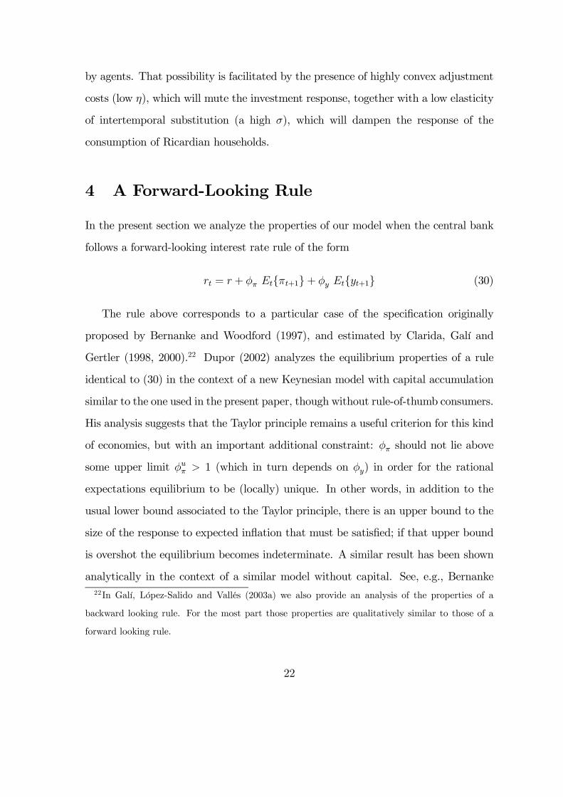
How does the presence of rule-of-thumb consumers affect the previous result?

Figure 5 represents graphically the interval of φπ values for which a unique equilibrium

exists, as a function of the weight of rule-of-thumb consumers λ, and for alternative

values of φy.

First, when φy = 0 and for low values of λ (roughly below 0.6) the qualitative

result found in the literature carries over to our economy: the uniqueness requires

that φπ lies within some interval bounded below by 1. Interestingly, for this region,

the size of that interval shrinks gradually as λ increases. That result is consistent

with the findings of Dupor (2002) for the particular case of λ = 0 (no rule-of-thumb

consumers).

Most interestingly (and surprisingly), when the weight of rule-of-thumb consumers

λ lies above a certain threshold, the properties of the forward-looking rule change

dramatically. In particular, a value for φπ below unity is needed in order to guarantee

the existence of a unique rational expectations equilibrium. In other words, the

central bank would be ill advised if it were to follow a forward-looking rule satisfying

the Taylor principle, since that policy would necessarily generate an indeterminate

equilibrium.24

A systematic response of the interest rate to changes in output (φy > 0), even

if small in size, has a significant impact on the stability properties of our model

economy. Thus, for low values of λ, a positive setting for φy tends to raise the upper

threshold for φπ consistent with a unique equilibrium. As seen in the four consecutive23More recently, Levin, Wieland and Williams (2003) have shown that the existence of such an

upper threshold is inherent to a variety of forward-looking rules, with the uniqueness region generally

shrinking as the forecast horizon is raised.24See Galí, López-Salido and Vallés (2003a) for a discussion of the reasons why a large presence of

rule-of-thumb consumers make it possible for a rule that responds less than one-for-one to (expected)

inflation to be consistent with a unique equilibrium.

23

graphs of Figure 5, the effect of φy on the size of the uniqueness region appears to

be non-monotonic, increasing very quickly for low values of φy and shrinking back

gradually for higher values. On the other hand, for higher values of λ, the opposite

effect takes place: the interval of φπ values for which there is a unique equilibrium

becomes smaller as we increase the size of the output coefficient relative to the φy = 0

case. In fact, under our baseline calibration, when φy = 0.5 and for λ sufficiently high,

an indeterminate equilibrium arises regardless of the value of the inflation coefficient.

The high sensitivity of the model’s stability properties to the size of the output

coefficient in a forward-looking interest rate rule in a model with capital accumulation

(but no rule-of-thumb consumers) had already been noticed by Dupor (2002). The

above analysis raises an important qualification (and warning) on such earlier results:

in the presence of rule-of-thumb consumers an aggressive response to output does not

seem warranted, for it can only reduce the region of inflation coefficients consistent

with a unique equilibrium. On the other hand, a small response to output has the

opposite effect: it tends to enlarge the size of the uniqueness region.

In summary, when the central bank follows a forward-looking rule like (30) the

presence of rule-of-thumb consumers either shrinks the interval of φπ values for which

the equilibrium is unique (in the case of low λ), or makes a passive policy necessary

to guarantee that uniqueness (for high values of λ).

5 Concluding Remarks

The Taylor principle, i.e., the notion that central banks should raise (lower) nominal

interest rates more than one-for-one in response to a rise (decline) in inflation, is

generally viewed as a prima facie criterion in the assessment of a monetary policy.

Thus, an interest rate rule that satisfies the Taylor principle is viewed as a policy

with stabilizing properties, whereas the failure to meet the Taylor criterion is often

24

pointed to as a possible explanation for periods characterized by large fluctuations in

inflation and widespread macroeconomic instability.

In the present paper we have provided a simple but potentially important qualifica-

tion to that view. We have shown how the presence of rule-of-thumb (non-Ricardian)

consumers in an otherwise standard dynamic sticky price model, can alter the prop-

erties of simple interest rate rules dramatically. The intuition behind the important

role played by rule-of-thumb consumers is easy to grasp: the behavior of those house-

holds is, by definition, insulated from the otherwise stabilizing force associated with

changes in real interest rates. We summarize our main results as follows.

1. Under a contemporaneous interest rate rule, the existence of a unique equilib-

rium is no longer guaranteed by the Taylor principle when the weight of rule-

of-thumb consumers attains a certain threshold. Instead the central bank may

be required to pursue a more anti-inflationary policy than it would otherwise

be needed.

2. Under a forward-looking interest rate rule, the presence of rule-of-thumb con-

sumers also complicates substantially the central bank’s task, by shrinking the

range of responses to inflation consistent with a unique equilibrium (when the

share of rule-of-thumb consumers is relatively low), or by requiring that a pas-

sive interest rate rule is followed (when the share of rule-of-thumb consumers is

large).

We interpret the previous results as raising a call for caution on the part of central

banks when designing their monetary policy strategies: the latter should not ignore

the potential importance of rule-of-thumb consumers (or, more broadly speaking, pro-

cyclical components of aggregate demand that are insensitive to interest rates). From

that viewpoint, our findings suggest that if the share of rule-of-thumb consumers is

25

non-negligible the strength of the interest rate response to contemporaneous inflation

may have to be increased in order to avoid multiple equilibria. But if that share takes

a high value, the size of the response required to guarantee a unique equilibrium may

be too large to be credible, or even to be consistent with a non-negative nominal rate.

In that case, our findings suggest that the central bank should consider adopting a

passive rule that responds to expected inflation only (as an alternative to a rule that

responds to current inflation with a very high coefficient). It is clear, however, that

such an alternative would have practical difficulties, especially from the viewpoint of

communication with the public.

The above discussion notwithstanding, it is not the objective of the present paper

to come up with specific policy recommendations: our model is clearly too simplistic

to be taken at face value, and any sharp conclusion coming out of it might not be

robust to alternative specifications. On the other hand we believe our analysis is

useful in at least one regard: it points to some important limitations of the Taylor

principle as a simple criterion for the assessment of monetary policy when rule-of-

thumb consumers (or the like) are present in the economy. In that respect, our

findings call for caution when interpreting estimates of interest rate rules similar to

the ones analyzed in the present paper in order to assess the merits of monetary policy

in specific historical periods.25 In particular, our results suggest that evidence on the

size of the response of interest rates to changes in inflation should not automatically

be viewed as allowing for indeterminacy and sunspot fluctuations (if the estimates

suggest that the Taylor principle is not met) nor, alternatively, as guaranteeing a

unique equilibrium (if the Taylor principle is shown to be satisfied in the data).

Knowledge of the exact specification of the interest rate rule (e.g. whether it is

forward looking or not) as well as other aspects of the model would be required for25See, e.g., Taylor (1999b) and Clarida, Galí, and Gertler (2000).

26

a proper assessment of the stabilizing properties of historical monetary policy rules.

In addition to its implications for the stability of interest rate rules, the presence of

rule-of-thumb consumers is also likely to have an influence in the nature of the central

bank objective function. Early results along these lines, though in the context of a

model somewhat different from the one in the present paper, can be found in Amato

and Laubach (2003). We think that the derivation of optimal monetary policy rules

as well as the assessment of simple policy rules using a welfare based criteria can be

a fruitful line of research.

More generally, we believe that the introduction of rule-of-thumb consumers in

dynamic general equilibrium models used for policy analysis not only enhances sig-

nificantly the realism of those models, but it can also allow us to uncover interesting

insights that may be relevant for the design of policies and helpful in our efforts to

understand many macroeconomic phenomena. An illustration of that potential use-

fulness can be found in a companion paper (Galí, López-Salido and Valles (2003c)),

where we have argued that the presence of rule-of-thumb consumers may help account

for the observed effects of fiscal policy shocks, some of which are otherwise hard to

explain with conventional new Keynesian or neoclassical models.

27

ReferencesAbel, A. (1980): “Empirical Investment Equations. An integrated Framework,”

Carnegie Rochester Conference Series on Public Policy , 12, 39-91.

Amato, Jeffery, and Thomas Laubach (2003): “Rule-of-Thumb Behavior andMon-

etary Policy,” European Economic Review, Vol 47 (5), 791-831.

Baxter, M. and M. Crucini, (1993): “Explaining Saving Investment Correlations,”

American Economic Review, vol. 83, no. 1, 416-436.

Benhabib, Jess, Stephanie Schmitt-Grohe, and Martin Uribe (2001a): “The Perils

of Taylor Rules,” Journal of Economic Theory 96, 40-69.

Benhabib, Jess, Stephanie Schmitt-Grohe, and Martin Uribe (2001b): “Monetary

Policy and Multiple Equilibria,” American Economic Review vol. 91, no. 1, 167-186.

Bernanke, Ben S., and Michael Woodford (1997): “Inflation Forecasts and Mon-

etary Policy,” Journal of Money, Credit and Banking, vol. 24, 653-684:

Blanchard, Olivier and Charles Kahn (1980), “The Solution of Linear Difference

Models under Rational Expectations”, Econometrica, 48, 1305-1311.

Bullard, James, and Kaushik Mitra (2002): “Learning About Monetary Policy

Rules,” Journal of Monetary Economics, vol. 49, no. 6, 1105-1130.

Campbell, John Y. and N. Gregory Mankiw (1989): “Consumption, Income, and

Interest Rates: Reinterpreting the Time Series Evidence,” in O.J. Blanchard and S.

Fischer (eds.), NBER Macroeconomics Annual 1989, 185-216, MIT Press

Calvo, Guillermo, 1983, “Staggered Prices in a Utility Maximizing Framework,”

Journal of Monetary Economics, 12, 383-398.

Christiano, Lawrence J., and Christopher J. Gust (1999): “A Comment on Ro-

bustness of Simple Monetary Policy Rules under Model Uncertainty,” in J.B. Taylor

ed., Monetary Policy Rules, University of Chicago Press.

Clarida, Richard, Jordi Galí, and Mark Gertler (1998): “Monetary Policy Rules

28

in Practice: Some International Evidence”, European Economic Review, 42 (6), June

1998, pp. 1033-1067.

Clarida, Richard, Jordi Galí, and Mark Gertler (1999): “The Science of Monetary

Policy: A New Keynesian Perspective,” Journal of Economic Literature, vol. 37,

1661-1707.

Clarida, Richard, Jordi Galí, and Mark Gertler (2000): “Monetary Policy Rules

and Macroeconomic Stability: Evidence and Some Theory,” Quarterly Journal of

Economics, vol. 105, issue 1, 147-180.

Dotsey, Michael (1999): “Structure from Shocks,” Federal Reserve Bank of Rich-

mond Working Paper 99-6.

Dupor, Bill (2002): “Interest Rate Policy and Investment with Adjustment Costs,”

manuscript.

Edge, Rochelle M., and Jeremy B. Rudd (2002): “Taxation and the Taylor Prin-

ciple” Federal Reserve Board, finance and Economics Discussion Series no. 2002-51

Fair, Ray C. (2003): “Estimates of the Effectiveness of Monetary Policy,” Journal

of Money, Credit and Banking, forthcoming.

Galí, Jordi, J. David López-Salido, and Javier Vallés (2003a): “rule-of-thumb

Consumers and the Design of Interest Rate Rules,” Working Paper # 0320, Banco

de España.

Galí, Jordi, J. David López-Salido, and Javier Vallés (2003b): “Technology Shocks

and Monetary Policy: Assessing the Fed’s Performance,” Journal of Monetary Eco-

nomics, vol. 50, no. 4.

Galí, Jordi, J. David López-Salido, and Javier Vallés (2003c): “Understanding the

Effects of Government Spending on Consumption,” mimeo Banco de España .

Kerr, William, and Robert G. King: “Limits on interest rate rules in the IS model,”

Economic Quarterly, Spring issue, 47-75.

29

Kim, J. (2000), “Constructing and estimating a realistic optimizing model of

monetary policy,” Journal of Monetary Economics, vol. 45, Issue 2 , April 2000,

329-359

King, Robert, and Mark Watson (1996), “Money, Prices, Interest Rates and the

Business Cycle” Review of Economics and Statistics, 78, 35-53

Levin, Andrew, Volker Wieland, John C. Williams (2002): “The Performance of

Forecast-Based Monetary Policy Rules under Model Uncertainty,” American Eco-

nomic Review, vol. 93, no. 3, 622-645.

Mankiw, N. Gregory (2000): “The Savers-Spenders Theory of Fiscal Policy,”

American Economic Review, vol. 90, no. 2, 120-125.

McCallum, B. (1999): “Issues in the Design of Monetary Policy Rules”, in J.B.

Taylor and M. Woodford eds., Handbook of Macroeconomics, vol. 1c, 1341-1397,

Elsevier, New York.

Orphanides, A. (2001), “Monetary Policy Rules based on Real Time Data,” Amer-

ican Economic Review, vol. 91, no. 4, 964-985

Roisland, Oistein (2003): “Capital Income Taxation, Equilibrium Determinacy,

and the Taylor Principle” Economics Letters 81, 147-153.

Rotemberg, J. and M. Woodford (1999): “Interest Rate Rules in an Estimated

Sticky Price Model,” in J.B. Taylor ed.,Monetary Policy Rules, University of Chicago

Press, 57-119.

Shea, John, (1995): “Union Contracts and the Life-Cycle/Permanent-Income Hy-

pothesis, ” American Economic Review vol. 85, 186—200.

Souleles, Nicholas S. (1999): “The Response of Household Consumption to Income

Tax Refund, ” American Economic Review vol. 89, 947—958.

Taylor, John B. (1993): “Discretion versus Policy Rules in Practice,” Carnegie

Rochester Conference Series on Public Policy , December 1993, 39, 195-214.

30

Taylor, John B. (1999a): Monetary Policy Rules, University of Chicago Press and

NBER.

Taylor, John B. (1999b): “An Historical Analysis of Monetary Policy Rules,” in

J.B. Taylor ed., Monetary Policy Rules, University of Chicago Press.

Taylor, John B. (1999c): “Staggered Price and Wage Setting in Macroeconomics,”

in J.B. Taylor and M. Woodford eds., Handbook of Macroeconomics, chapter 15, 1341-

1397, Elsevier, New York.

Woodford, Michael (2001): “The Taylor Rule and Optimal Monetary Policy,”

American Economic Review vol. 91, no. 2, 232-237.

Yun, Tack (1996): “Nominal Price Rigidity, Money Supply Endogeneity, and

Business Cycles,” Journal of Monetary Economics 37, 345-370.

Wolff, Edward (1998): ”Recent trends in the size distribution of Household wealth”,

Journal of Economic Perspectives, 12(3), 131-150

31

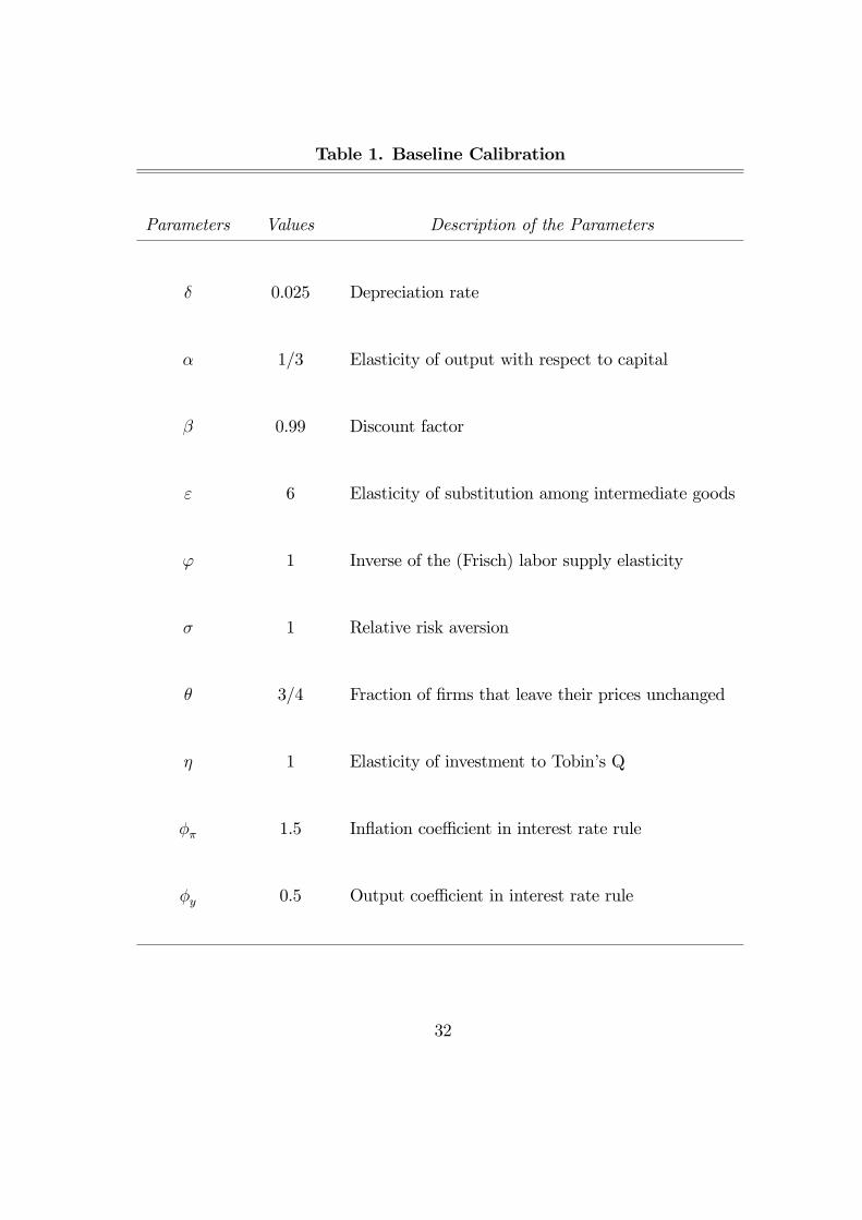
Table 1. Baseline Calibration

Parameters Values Description of the Parameters

δ 0.025 Depreciation rate

α 1/3 Elasticity of output with respect to capital

β 0.99 Discount factor

ε 6 Elasticity of substitution among intermediate goods

ϕ 1 Inverse of the (Frisch) labor supply elasticity

σ 1 Relative risk aversion

θ 3/4 Fraction of firms that leave their prices unchanged

η 1 Elasticity of investment to Tobin’s Q

φπ 1.5 Inflation coefficient in interest rate rule

φy 0.5 Output coefficient in interest rate rule

32

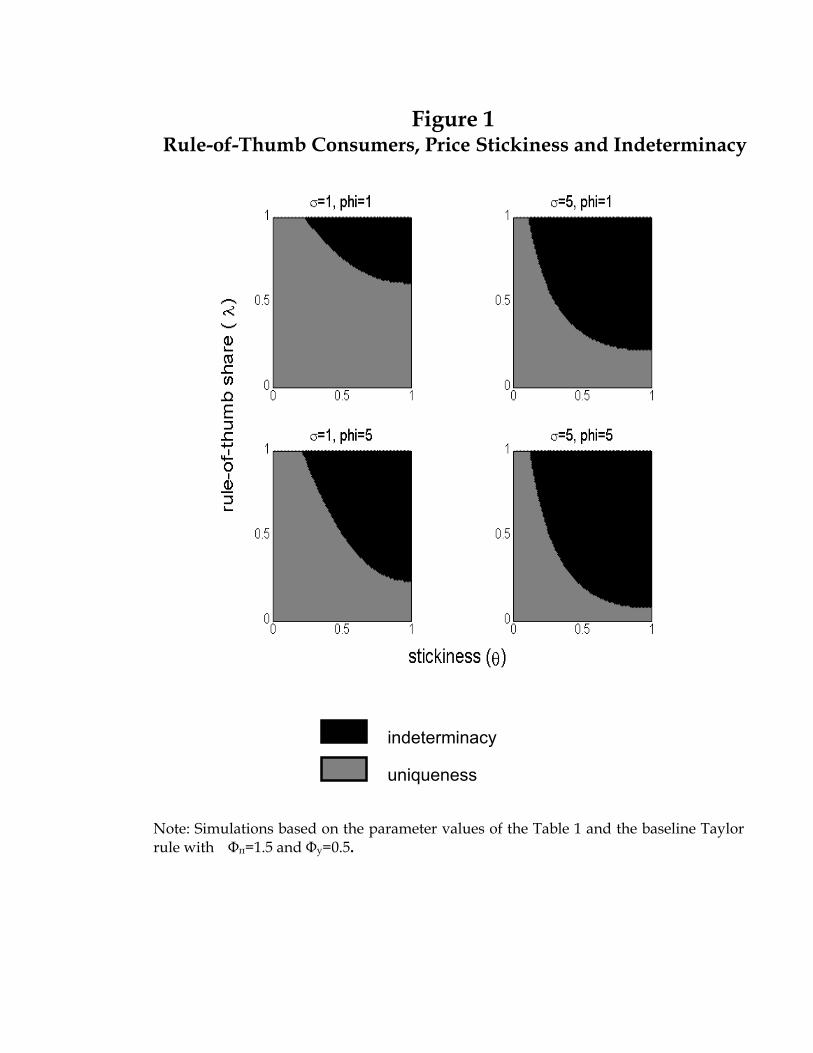
Figure 1 Rule-of-Thumb Consumers, Price Stickiness and Indeterminacy

indeterminacy uniqueness

Note: Simulations based on the parameter values of the Table 1 and the baseline Taylor rule with Φπ=1.5 and Φy=0.5.

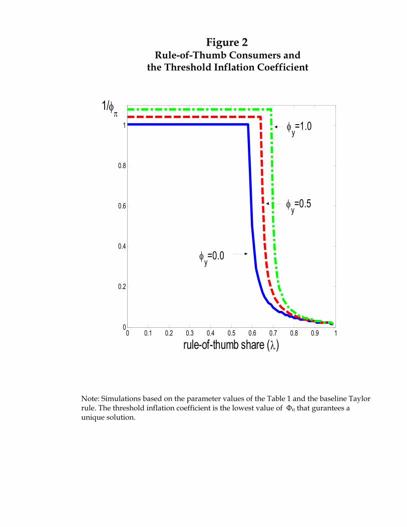
Figure 2 Rule-of-Thumb Consumers and

the Threshold Inflation Coefficient

0 0.1 0.2 0.3 0.4 0.5 0.6 0.7 0.8 0.9 10

0.2

0.4

0.6

0.8

1

φy=0.0

φy=0.5

1/φπ

φy=1.0

rule-of-thumb share (λ)

Note: Simulations based on the parameter values of the Table 1 and the baseline Taylor rule. The threshold inflation coefficient is the lowest value of Φπ that gurantees a unique solution.

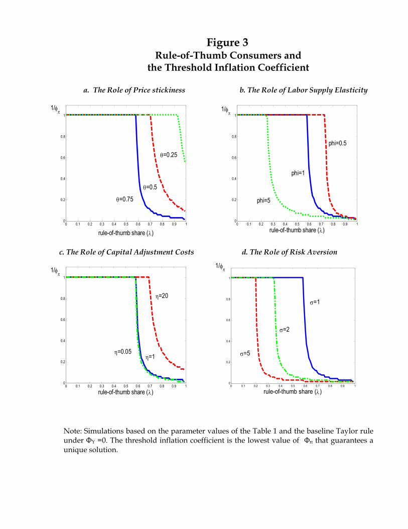
Figure 3 Rule-of-Thumb Consumers and

the Threshold Inflation Coefficient

a. The Role of Price stickiness b. The Role of Labor Supply Elasticity

0 0.1 0.2 0.3 0.4 0.5 0.6 0.7 0.8 0.9 10

0.2

0.4

0.6

0.8

1

θ=0.75

θ=0.5

1/φπ

θ=0.25

rule-of-thumb share (λ)

0 0.1 0.2 0.3 0.4 0.5 0.6 0.7 0.8 0.9 10

0.2

0.4

0.6

0.8

1

phi=1

phi=0.5

1/φπ

phi=5

rule-of-thumb share (λ)

c. The Role of Capital Adjustment Costs d. The Role of Risk Aversion

0 0.1 0.2 0.3 0.4 0.5 0.6 0.7 0.8 0.9 10

0.2

0.4

0.6

0.8

1

η=1

η=20

1/φπ

η=0.05

rule-of-thumb share (λ) 0 0.1 0.2 0.3 0.4 0.5 0.6 0.7 0.8 0.9 1

0

0.2

0.4

0.6

0.8

1

σ=1

σ=5

1/φπ

σ=2

rule-of-thumb share (λ)

Note: Simulations based on the parameter values of the Table 1 and the baseline Taylor rule under ΦY =0. The threshold inflation coefficient is the lowest value of Φπ that guarantees a unique solution.

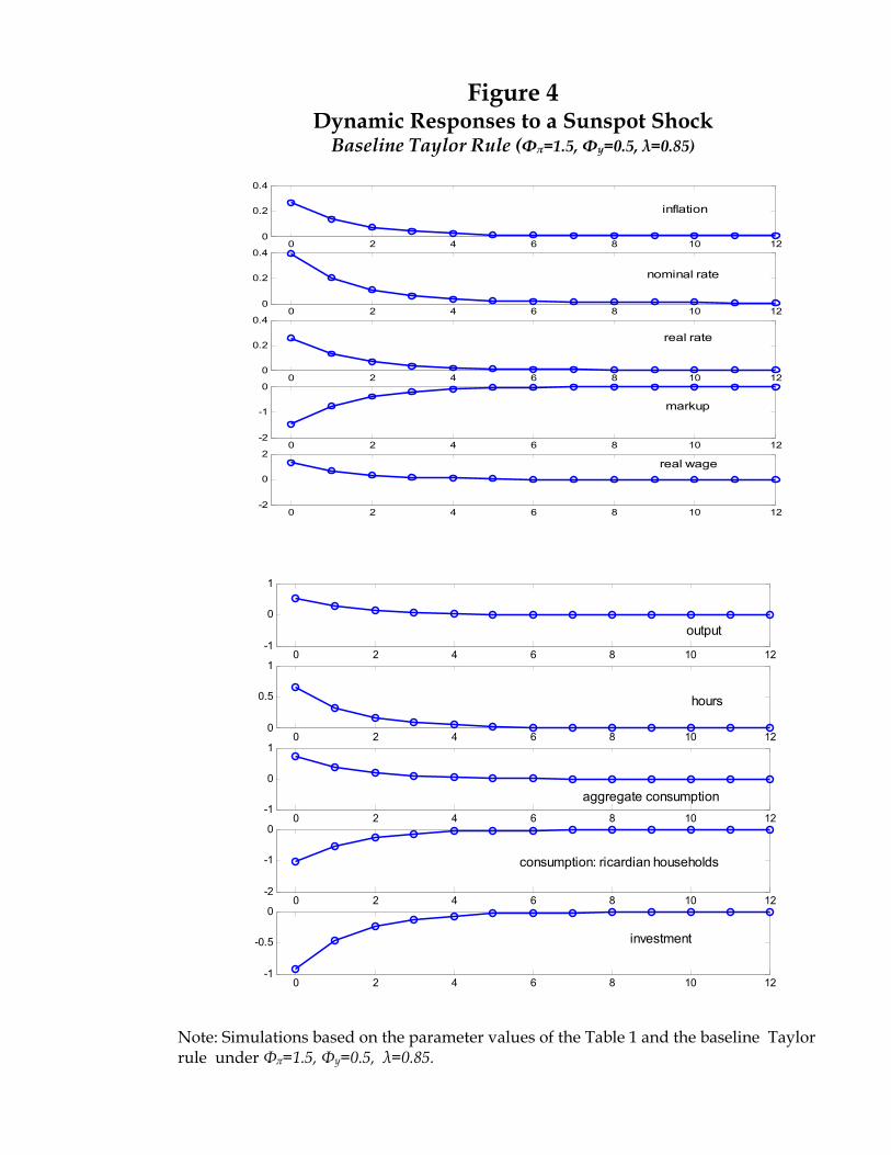
Figure 4 Dynamic Responses to a Sunspot Shock

Baseline Taylor Rule (Φπ=1.5, Φy=0.5, λ=0.85)

0 2 4 6 8 10 120

0.2

0.4

inflation

0 2 4 6 8 10 120

0.2

0.4

nominal rate

0 2 4 6 8 10 120

0.2

0.4

real rate

0 2 4 6 8 10 12-2

-1

0

markup

0 2 4 6 8 10 12-2

0

2real wage

0 2 4 6 8 10 12-1

0

1

output

0 2 4 6 8 10 120

0.5

1

hours

0 2 4 6 8 10 12-1

0

1

aggregate consumption

0 2 4 6 8 10 12-2

-1

0

consumption: ricardian households

0 2 4 6 8 10 12-1

-0.5

0

investment

Note: Simulations based on the parameter values of the Table 1 and the baseline Taylor rule under Φπ=1.5, Φy=0.5, λ=0.85.

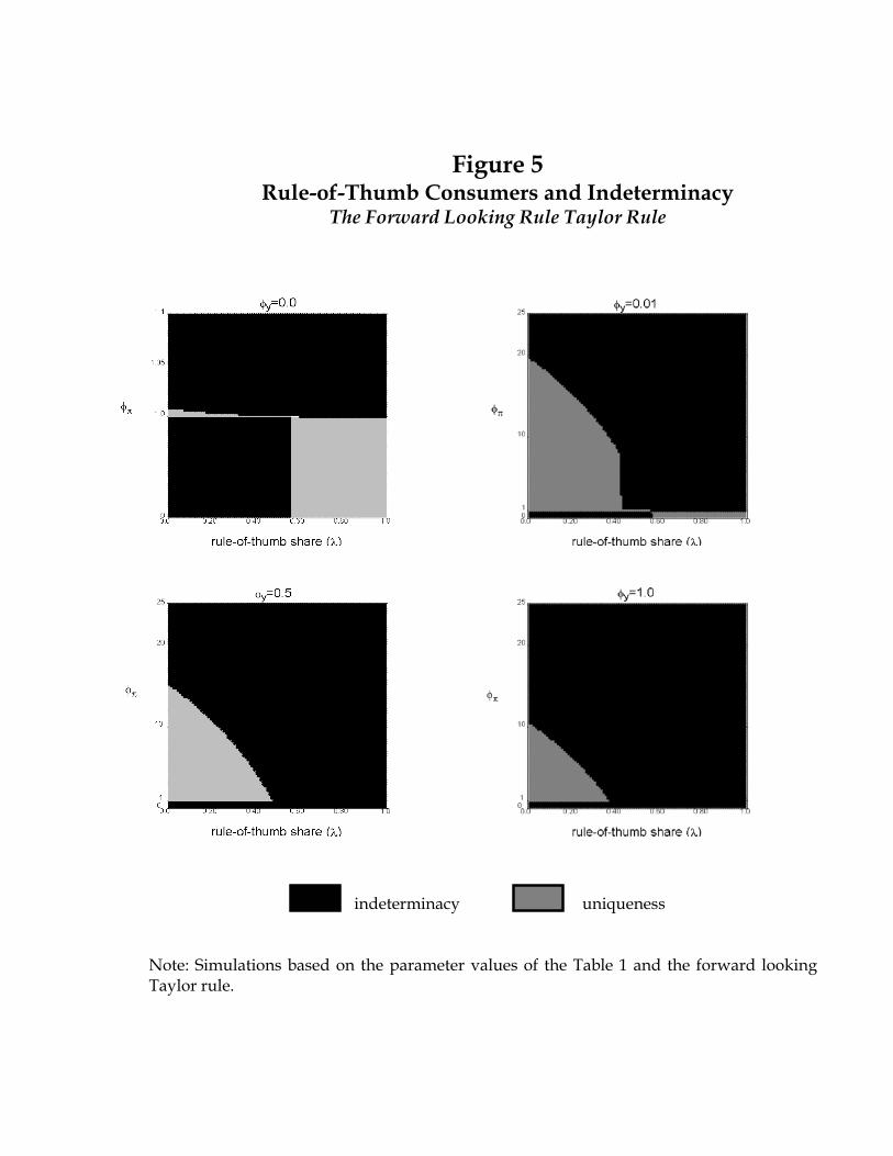
Figure 5 Rule-of-Thumb Consumers and Indeterminacy

The Forward Looking Rule Taylor Rule

indeterminacy uniqueness

Note: Simulations based on the parameter values of the Table 1 and the forward looking Taylor rule.

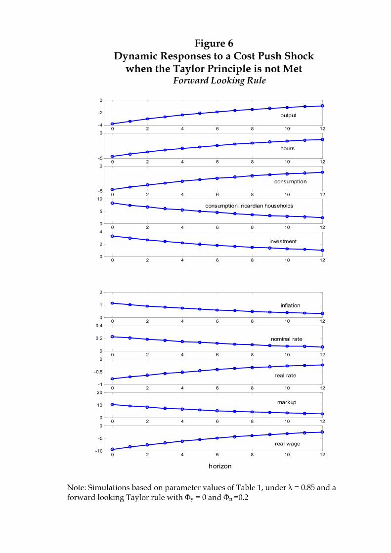
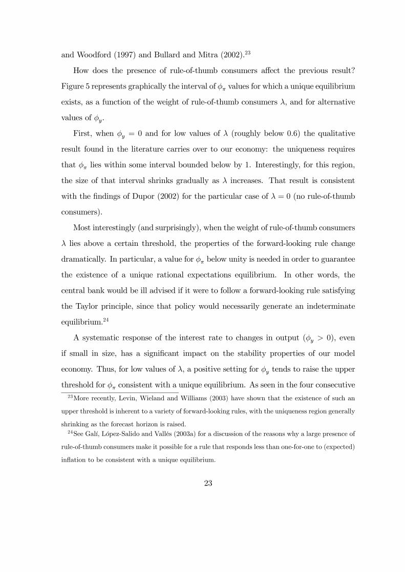
Figure 6 Dynamic Responses to a Cost Push Shock

when the Taylor Principle is not Met Forward Looking Rule

0 2 4 6 8 10 12-4

-2

0

output

0 2 4 6 8 10 12-5

0

hours

0 2 4 6 8 10 12-5

0

consumption

0 2 4 6 8 10 120

5

10consumption: ricardian households

0 2 4 6 8 10 120

2

4

investment

0 2 4 6 8 10 120

1

2

inflation

0 2 4 6 8 10 120

0.2

0.4

nominal rate

0 2 4 6 8 10 12-1

-0.5

0

real rate

0 2 4 6 8 10 120

10

20

markup

0 2 4 6 8 10 12-10

-5

0

real wage

horizon Note: Simulations based on parameter values of Table 1, under λ = 0.85 and a forward looking Taylor rule with Φy = 0 and Φπ =0.2