Embed Size (px)
Citation preview

NCAR/TN-503+STR NCAR Technical Note
________________________________________________________________________
July 2013
Technical Description of version 4.5 of the
Community Land Model (CLM)
Coordinating Lead Authors Keith W. Oleson, David M. Lawrence Lead Authors Gordon B. Bonan, Beth Drewniak, Maoyi Huang, Charles D. Koven, Samuel Levis, Fang Li, William J. Riley, Zachary M. Subin, Sean C. Swenson, Peter E. Thornton Contributing Authors Anil Bozbiyik, Rosie Fisher, Colette L. Heald, Erik Kluzek, Jean-Francois Lamarque, Peter J. Lawrence, L. Ruby Leung, William Lipscomb, Stefan Muszala, Daniel M. Ricciuto, William Sacks, Ying Sun, Jinyun Tang, Zong-Liang Yang
NCAR Earth System Laboratory Climate and Global Dynamics Division
________________________________________________________________________ NATIONAL CENTER FOR ATMOSPHERIC RESEARCH
P. O. Box 3000 BOULDER, COLORADO 80307-3000
ISSN Print Edition 2153-2397 ISSN Electronic Edition 2153-2400

NCAR TECHNICAL NOTES http://library.ucar.edu/research/publish-technote
The Technical Notes series provides an outlet for a variety of NCAR Manuscripts that contribute in specialized ways to the body of scientific knowledge but that are not yet at a point of a formal journal, monograph or book publication. Reports in this series are issued by the NCAR scientific divisions, serviced by OpenSky and operated through the NCAR Library. Designation symbols for the series include: EDD – Engineering, Design, or Development Reports Equipment descriptions, test results, instrumentation, and operating and maintenance manuals. IA – Instructional Aids Instruction manuals, bibliographies, film supplements, and other research or instructional aids. PPR – Program Progress Reports Field program reports, interim and working reports, survey reports, and plans for experiments. PROC – Proceedings Documentation or symposia, colloquia, conferences, workshops, and lectures. (Distribution maybe limited to attendees). STR – Scientific and Technical Reports Data compilations, theoretical and numerical investigations, and experimental results. The National Center for Atmospheric Research (NCAR) is operated by the nonprofit University Corporation for Atmospheric Research (UCAR) under the sponsorship of the National Science Foundation. Any opinions, findings, conclusions, or recommendations expressed in this publication are those of the author(s) and do not necessarily reflect the views of the National Science Foundation.
National Center for Atmospheric Research P. O. Box 3000
Boulder, Colorado 80307-300
NCAR/TN-503+STR NCAR Technical Note
________________________________________________________________________
July 2013
Technical Description of version 4.5 of the
Community Land Model (CLM)
Coordinating Lead Authors Keith W. Oleson, David M. Lawrence Lead Authors Gordon B. Bonan, Beth Drewniak, Maoyi Huang, Charles D. Koven, Samuel Levis, Fang Li, William J. Riley, Zachary M. Subin, Sean C. Swenson, Peter E. Thornton Contributing Authors Anil Bozbiyik, Rosie Fisher, Colette L. Heald, Erik Kluzek, Jean-Francois Lamarque, Peter J. Lawrence, L. Ruby Leung, William Lipscomb, Stefan Muszala, Daniel M. Ricciuto, William Sacks, Ying Sun, Jinyun Tang, Zong-Liang Yang
NCAR Earth System Laboratory Climate and Global Dynamics Division
________________________________________________________________________ NATIONAL CENTER FOR ATMOSPHERIC RESEARCH
P. O. Box 3000 BOULDER, COLORADO 80307-3000
ISSN Print Edition 2153-2397 ISSN Electronic Edition 2153-2400
i
TABLE OF CONTENTS
1. INTRODUCTION..................................................................................................... 1
1.1 MODEL HISTORY ................................................................................................. 1 1.1.1 Inception of CLM ............................................................................................ 1 1.1.2 CLM2 .............................................................................................................. 3 1.1.3 CLM3 .............................................................................................................. 5 1.1.4 CLM3.5 ........................................................................................................... 6 1.1.5 CLM4 .............................................................................................................. 7 1.1.6 CLM4.5 ........................................................................................................... 8
1.2 BIOGEOPHYSICAL AND BIOGEOCHEMICAL PROCESSES ...................................... 11
2. SURFACE CHARACTERIZATION AND MODEL INPUT REQUIREMENTS .......................................................................................................... 14
2.1 SURFACE CHARACTERIZATION .......................................................................... 14 2.1.1 Surface Heterogeneity and Data Structure ................................................... 14 2.1.2 Vegetation Composition ................................................................................ 17 2.1.3 Vegetation Structure ..................................................................................... 19 2.1.4 Phenology and vegetation burial by snow .................................................... 21
2.2 MODEL INPUT REQUIREMENTS .......................................................................... 21 2.2.1 Atmospheric Coupling .................................................................................. 21 2.2.2 Initialization .................................................................................................. 27 2.2.3 Surface Data ................................................................................................. 28 2.2.4 Adjustable Parameters and Physical Constants ........................................... 35
3. SURFACE ALBEDOS............................................................................................ 37
3.1 CANOPY RADIATIVE TRANSFER ......................................................................... 37 3.2 GROUND ALBEDOS ............................................................................................ 46
3.2.1 Snow Albedo.................................................................................................. 48 3.2.2 Snowpack Optical Properties ....................................................................... 52 3.2.3 Snow Aging ................................................................................................... 56
3.3 SOLAR ZENITH ANGLE ....................................................................................... 59
4. RADIATIVE FLUXES ........................................................................................... 63
4.1 SOLAR FLUXES .................................................................................................. 63 4.2 LONGWAVE FLUXES .......................................................................................... 67
5. MOMENTUM, SENSIBLE HEAT, AND LATENT HEAT FLUXES .............. 71
5.1 MONIN-OBUKHOV SIMILARITY THEORY ............................................................ 73 5.2 SENSIBLE AND LATENT HEAT FLUXES FOR NON-VEGETATED SURFACES .......... 82 5.3 SENSIBLE AND LATENT HEAT FLUXES AND TEMPERATURE FOR VEGETATED SURFACES ...................................................................................................................... 88
5.3.1 Theory ........................................................................................................... 88
ii
5.3.2 Numerical Implementation.......................................................................... 100 5.4 UPDATE OF GROUND SENSIBLE AND LATENT HEAT FLUXES ........................... 105 5.5 SATURATION VAPOR PRESSURE ....................................................................... 108
6. SOIL AND SNOW TEMPERATURES .............................................................. 112
6.1 NUMERICAL SOLUTION .................................................................................... 113 6.2 PHASE CHANGE ............................................................................................... 124
6.2.1 Soil and Snow Layers .................................................................................. 124 6.2.2 Surface Water.............................................................................................. 128
6.3 SOIL AND SNOW THERMAL PROPERTIES .......................................................... 129
7. HYDROLOGY ...................................................................................................... 133
7.1 CANOPY WATER .............................................................................................. 134 7.2 SNOW ............................................................................................................... 136
7.2.1 Snow Covered Area Fraction...................................................................... 138 7.2.2 Ice Content .................................................................................................. 139 7.2.3 Water Content ............................................................................................. 141 7.2.4 Black and organic carbon and mineral dust within snow .......................... 142 7.2.5 Initialization of snow layer ......................................................................... 145 7.2.6 Snow Compaction ....................................................................................... 145 7.2.7 Snow Layer Combination and Subdivision ................................................. 148
7.2.7.1 Combination ........................................................................................ 148 7.2.7.2 Subdivision ......................................................................................... 151
7.3 SURFACE RUNOFF, SURFACE WATER STORAGE, AND INFILTRATION ............... 152 7.3.1 Surface Runoff ............................................................................................. 152 7.3.2 Surface Water Storage ................................................................................ 154 7.3.3 Infiltration ................................................................................................... 155
7.4 SOIL WATER .................................................................................................... 157 7.4.1 Hydraulic Properties .................................................................................. 159 7.4.2 Numerical Solution ..................................................................................... 162
7.4.2.1 Equilibrium soil matric potential and volumetric moisture ................ 168 7.4.2.2 Equation set for layer 1i = ................................................................. 170 7.4.2.3 Equation set for layers 2, , 1levsoii N= − .......................................... 170
7.4.2.4 Equation set for layers , 1levsoi levsoii N N= + .................................... 171 7.5 FROZEN SOILS AND PERCHED WATER TABLE .................................................. 173 7.6 GROUNDWATER-SOIL WATER INTERACTIONS ................................................. 174 7.7 RUNOFF FROM GLACIERS AND SNOW-CAPPED SURFACES ................................. 177 7.8 THE VARIABLE INFILTRATION CAPACITY PARAMETERIZATIONS AS A HYDROLOGIC OPTION ................................................................................................... 178
8. STOMATAL RESISTANCE AND PHOTOSYNTHESIS ............................... 183
8.1 STOMATAL RESISTANCE ................................................................................... 183 8.2 PHOTOSYNTHESIS ............................................................................................ 186 8.3 VCMAX25 AND CANOPY SCALING ........................................................................ 191 8.4 SOIL WATER STRESS ......................................................................................... 193 8.5 NUMERICAL IMPLEMENTATION ........................................................................ 197
iii
9. LAKE MODEL ..................................................................................................... 200
9.1 VERTICAL DISCRETIZATION ............................................................................. 201 9.2 EXTERNAL DATA ............................................................................................. 202 9.3 SURFACE ALBEDO ............................................................................................ 202 9.4 SURFACE FLUXES AND SURFACE TEMPERATURE ............................................. 203
9.4.1 Overview of Changes from CLM4 .............................................................. 203 9.4.2 Surface Properties ...................................................................................... 203 9.4.3 Surface Flux Solution .................................................................................. 205
9.5 LAKE TEMPERATURE ....................................................................................... 211 9.5.1 Introduction................................................................................................. 211 9.5.2 Overview of Changes from CLM4 .............................................................. 212 9.5.3 Boundary Conditions .................................................................................. 213 9.5.4 Eddy Diffusivity and Thermal Conductivities ............................................. 213 9.5.5 Radiation Penetration ................................................................................. 216 9.5.6 Heat Capacities ........................................................................................... 217 9.5.7 Crank-Nicholson Solution ........................................................................... 217 9.5.8 Phase Change ............................................................................................. 219 9.5.9 Convection .................................................................................................. 220 9.5.10 Energy Conservation .............................................................................. 223
9.6 LAKE HYDROLOGY .......................................................................................... 223 9.6.1 Overview ..................................................................................................... 223 9.6.2 Water Balance ............................................................................................. 224 9.6.3 Precipitation, Evaporation, and Runoff ...................................................... 225 9.6.4 Soil Hydrology ............................................................................................ 226 9.6.5 Modifications to Snow Layer Logic ............................................................ 227
10. GLACIERS ........................................................................................................ 229
10.1 OVERVIEW ....................................................................................................... 229 10.2 MULTIPLE ELEVATION CLASS SCHEME ............................................................. 231 10.3 COMPUTATION OF THE SURFACE MASS BALANCE ............................................. 232
11. RIVER TRANSPORT MODEL (RTM) ......................................................... 235
12. URBAN MODEL (CLMU) .............................................................................. 239
13. CARBON AND NITROGEN POOLS, ALLOCATION, AND RESPIRATION ............................................................................................................. 244
13.1 INTRODUCTION ................................................................................................ 244 13.2 CARBON ALLOCATION FOR MAINTENANCE RESPIRATION COSTS .................... 246 13.3 CARBON AND NITROGEN STOICHIOMETRY OF NEW GROWTH .......................... 248 13.4 DEPLOYMENT OF RETRANSLOCATED NITROGEN ............................................... 252 13.5 PLANT NITROGEN UPTAKE FROM SOIL MINERAL NITROGEN POOL ..................... 253 13.6 FINAL CARBON AND NITROGEN ALLOCATION ................................................... 253 13.7 AUTOTROPHIC RESPIRATION ............................................................................ 256
13.7.1 Maintenance Respiration ........................................................................ 256 13.7.2 Growth Respiration ................................................................................. 257
14. VEGETATION PHENOLOGY ...................................................................... 259
iv
14.1 GENERAL PHENOLOGY FLUX PARAMETERIZATION .......................................... 259 14.1.1 Onset Periods .......................................................................................... 260 14.1.2 Offset Periods.......................................................................................... 261 14.1.3 Background Onset Growth ..................................................................... 262 14.1.4 Background Litterfall .............................................................................. 263 14.1.5 Livewood Turnover ................................................................................. 264
14.2 EVERGREEN PHENOLOGY ................................................................................. 265 14.3 SEASONAL-DECIDUOUS PHENOLOGY ............................................................... 265
14.3.1 Seasonal-Deciduous Onset Trigger ........................................................ 266 14.3.2 Seasonal-Deciduous Offset Trigger ........................................................ 269
14.4 STRESS-DECIDUOUS PHENOLOGY .................................................................... 269 14.4.1 Stress-Deciduous Onset Triggers ........................................................... 269 14.4.2 Stress-Deciduous Offset Triggers ........................................................... 271 14.4.3 Stress-Deciduous: Long Growing Season .............................................. 272
14.5 LITTERFALL FLUXES MERGED TO THE COLUMN LEVEL ................................... 274
15. DECOMPOSITION .......................................................................................... 276
15.1 CLM-CN POOL STRUCTURE, RATE CONSTANTS AND PARAMETERS ............... 279 15.2 CENTURY-BASED POOL STRUCTURE, RATE CONSTANTS AND PARAMETERS .... 283 15.3 ENVIRONMENTAL MODIFIERS ON DECOMPOSITION RATE .................................. 284 15.4 N-LIMITATION OF DECOMPOSITION FLUXES .................................................... 287 15.5 N COMPETITION BETWEEN PLANT UPTAKE AND SOIL IMMOBILIZATION FLUXES290 15.6 FINAL DECOMPOSITION FLUXES ...................................................................... 291 15.7 VERTICAL DISTRIBUTION AND TRANSPORT OF DECOMPOSING C AND N POOLS293 15.8 MODEL EQUILIBRATION ................................................................................... 294
16. EXTERNAL NITROGEN CYCLE................................................................. 296
16.1 ATMOSPHERIC NITROGEN DEPOSITION ............................................................ 296 16.2 BIOLOGICAL NITROGEN FIXATION ................................................................... 297 16.3 NITRIFICATION AND DENITRIFICATION LOSSES OF NITROGEN ......................... 299
16.3.1 CLM-CN formulation .............................................................................. 299 16.3.2 Century-based formulation ..................................................................... 302
16.4 LEACHING LOSSES OF NITROGEN ..................................................................... 303 16.5 LOSSES OF NITROGEN DUE TO FIRE ................................................................. 305
17. PLANT MORTALITY ..................................................................................... 306
17.1 MORTALITY FLUXES LEAVING VEGETATION POOLS ........................................ 306 17.2 MORTALITY FLUXES MERGED TO THE COLUMN LEVEL ................................... 309
18. FIRE ................................................................................................................... 314
18.1 NON-PEAT FIRES OUTSIDE CROPLAND AND TROPICAL CLOSED FOREST ............. 314 18.1.1 Fire counts .............................................................................................. 314 18.1.2 Average spread area of a fire ................................................................. 318 18.1.3 Fire impact .............................................................................................. 321
18.2 AGRICULTURAL FIRES ...................................................................................... 323 18.3 DEFORESTATION FIRES ..................................................................................... 324 18.4 PEAT FIRES ....................................................................................................... 327
v
19. METHANE MODEL ........................................................................................ 330
19.1 METHANE MODEL STRUCTURE AND FLOW ...................................................... 330 19.2 GOVERNING MASS-BALANCE RELATIONSHIP .................................................. 331 19.3 CH4 PRODUCTION ............................................................................................ 332 19.4 EBULLITION ..................................................................................................... 336 19.5 AERENCHYMA TRANSPORT .............................................................................. 336 19.6 CH4 OXIDATION .............................................................................................. 338 19.7 REACTIVE TRANSPORT SOLUTION ................................................................... 338
19.7.1 Competition for CH4 and O2 ................................................................... 339 19.7.2 CH4 and O2 Source Terms ...................................................................... 339 19.7.3 Aqueous and Gaseous Diffusion ............................................................. 340 19.7.4 Boundary Conditions .............................................................................. 341 19.7.5 Crank-Nicholson Solution ....................................................................... 342 19.7.6 Interface between water table and unsaturated zone ............................. 343
19.8 INUNDATED FRACTION PREDICTION ................................................................ 344 19.9 SEASONAL INUNDATION .................................................................................. 345
20. CROPS AND IRRIGATION ................................................................................. 346
20.1 SUMMARY OF CLM4.5 UPDATES RELATIVE TO THE CLM4.0 ........................... 346 20.2 THE CROP MODEL ............................................................................................. 346
20.2.1 Introduction............................................................................................. 346 20.2.2 Crop plant functional types ..................................................................... 347 20.2.3 Phenology ............................................................................................... 348
20.2.3.1 Planting ........................................................................................... 349 20.2.3.2 Leaf emergence ............................................................................... 350 20.2.3.3 Grain fill .......................................................................................... 351 20.2.3.4 Harvest ............................................................................................ 351
20.2.4 Allocation ................................................................................................ 351 20.2.4.1 Leaf emergence to grain fill ............................................................ 352 20.2.4.2 Grain fill to harvest ......................................................................... 352
20.2.5 General comments .................................................................................. 353 20.3 THE IRRIGATION MODEL ................................................................................... 358 20.4 THE DETAILS ABOUT WHAT IS NEW IN CLM4.5 ................................................ 359
20.4.1 Interactive irrigation for corn, temperate cereals, and soybean ............ 359 20.4.2 Interactive fertilization............................................................................ 361 20.4.3 Biological nitrogen fixation for soybeans ............................................... 362 20.4.4 Modified C:N ratios for crops................................................................. 363 20.4.5 Nitrogen retranslocation for crops ......................................................... 363 20.4.6 Separate reproductive pool ..................................................................... 365
21. TRANSIENT LANDCOVER CHANGE ........................................................ 367
21.1 ANNUAL TRANSIENT LAND COVER DATA AND TIME INTERPOLATION ............ 367 21.2 MASS AND ENERGY CONSERVATION ............................................................... 369 21.3 ANNUAL TRANSIENT LAND COVER DATASET DEVELOPMENT ......................... 370
21.3.1 UNH Transient Land Use and Land Cover Change Dataset ................. 370 21.3.2 Representing Land Use and Land Cover Change in CLM ..................... 372
vi
21.3.3 Present Day PFT Dataset ....................................................................... 373 21.3.4 Potential PFT Distribution ..................................................................... 374 21.3.5 Transient Land Cover Change Dataset .................................................. 375 21.3.6 Forest Harvest Dataset Changes ............................................................ 376
22. DYNAMIC GLOBAL VEGETATION MODEL .......................................... 379
22.1 ESTABLISHMENT AND SURVIVAL...................................................................... 380 22.2 LIGHT COMPETITION ........................................................................................ 381 22.3 CN PROCESSES MODIFIED FOR THE CNDV COUPLING ...................................... 381
23. BIOGENIC VOLATILE ORGANIC COMPOUNDS (BVOCS) ................. 384
24. DUST MODEL .................................................................................................. 386
25. CARBON ISOTOPES ...................................................................................... 391
25.1 GENERAL FORM FOR CALCULATING 13C AND 14C FLUX ................................... 391 25.2 ISOTOPE SYMBOLS, UNITS, AND REFERENCE STANDARDS ............................... 392 25.3 CARBON ISOTOPE DISCRIMINATION DURING PHOTOSYNTHESIS ...................... 394 25.4 14C RADIOACTIVE DECAY AND HISTORICAL ATMOSPHERIC 14C CONCENTRATIONS 396
26. OFFLINE MODE ............................................................................................. 398
27. REFERENCES .................................................................................................. 403
vii
LIST OF FIGURES Figure 1.1. Land biogeophysical, biogeochemical, and landscape processes simulated by
CLM (adapted from Lawrence et al. (2011) for CLM4.5). ...................................... 13 Figure 2.1. Configuration of the CLM subgrid hierarchy. ............................................... 15 Figure 4.1. Schematic diagram of (a) direct beam radiation, (b) diffuse solar radiation,
and (c) longwave radiation absorbed, transmitted, and reflected by vegetation and ground. ...................................................................................................................... 64
Figure 5.1. Schematic diagram of sensible heat fluxes for (a) non-vegetated surfaces and (b) vegetated surfaces. .............................................................................................. 90
Figure 5.2. Schematic diagram of water vapor fluxes for (a) non-vegetated surfaces and (b) vegetated surfaces. .............................................................................................. 91
Figure 6.1. Schematic diagram of numerical scheme used to solve for soil temperature.................................................................................................................................. 118
Figure 7.1. Hydrologic processes represented in CLM. ................................................ 134 Figure 7.2. Example of three layer snow pack ( 3s n l = − ). .......................................... 137 Figure 7.3. Schematic diagram of numerical scheme used to solve for soil water fluxes.
................................................................................................................................. 164 Figure 12.1. Schematic representation of the urban land unit. ...................................... 242 Figure 12.2. Schematic of urban and atmospheric model coupling. .............................. 243 Figure 13.1. Vegetation fluxes and pools. ..................................................................... 245 Figure 13.2: Carbon and nitrogen pools. ....................................................................... 246 Figure 14.1. Example of annual phenology cycle for seasonal deciduous. .................... 260 Figure 15.1. Schematic of decomposition model in CLM. ............................................. 277 Figure 15.2. Pool structure, transitions, respired fractions (numbers at end of arrows), and
turnover times (numbers in boxes) for the 2 alternate soil decomposition models included in CLM. .................................................................................................... 279
Figure 16.1. Biological nitrogen fixation as a function of annual net primary production.................................................................................................................................. 298
Figure 19.1. Schematic representation of biological and physical processes integrated in CLM that affect the net CH4 surface flux (Riley et al. 2011a). (left) Fully inundated portion of a CLM gridcell and (right) variably saturated portion of a gridcell. ...... 332
Figure 21.1. Schematic of land cover change impacts on CLM carbon pools and fluxes.................................................................................................................................. 377
Figure 21.2. Schematic of translation of annual UNH land units to CLM4 plant functional types. ...................................................................................................... 378
Figure 25.1. Atmospheric ∆14C used to drive 14C model over the historical period. ..... 397
viii
LIST OF TABLES Table 2.1. Plant functional types...................................................................................... 18 Table 2.2. Prescribed plant functional type heights ......................................................... 20 Table 2.3. Atmospheric input to land model.................................................................... 23 Table 2.4. Land model output to atmospheric model ...................................................... 26 Table 2.5. Surface data required for CLM and their base spatial resolution ................... 29 Table 2.6. Physical constants ........................................................................................... 36 Table 3.1. Plant functional type optical properties .......................................................... 45 Table 3.2. Intercepted snow optical properties ................................................................ 46 Table 3.3. Dry and saturated soil albedos ........................................................................ 48 Table 3.4. Spectral bands and weights used for snow radiative transfer ......................... 51 Table 3.5. Single-scatter albedo values used for snowpack impurities and ice ............... 54 Table 3.6. Mass extinction values (m2 kg-1) used for snowpack impurities and ice. ....... 55 Table 3.7. Asymmetry scattering parameters used for snowpack impurities and ice. ..... 56 Table 3.8. Orbital parameters........................................................................................... 62 Table 5.1. Plant functional type aerodynamic parameters ............................................. 100
Table 5.2. Coefficients for Tsate ...................................................................................... 110
Table 5.3. Coefficients for
Tsatde
dT .................................................................................. 111 Table 6.1. Soil layer structure. ....................................................................................... 114 Table 7.1. Meltwater scavenging efficiency for particles within snow ......................... 145 Table 7.2. Minimum and maximum thickness of snow layers (m) ............................... 151 Table 8.1. Plant functional type (PFT) photosynthetic parameters. .............................. 185 Table 8.2. Temperature dependence parameters for C3 photosynthesis. ....................... 190 Table 8.3. Plant functional type root distribution parameters. ....................................... 196 Table 13.1. Allocation and carbon:nitrogen ratio parameters ........................................ 250 Table 15.1. Decomposition rate constants for litter and SOM pools, C:N ratios, and
acceleration parameters (see section 15.8 for explanation) for the CLM-CN decomposition pool structure. ................................................................................. 281
Table 15.2. Respiration fractions for litter and SOM pools ........................................... 282 Table 15.3. Turnover times, C:N ratios, and acceleration parameters (see section 15.8 for
explanation) for the Century-based decomposition cascade. .................................. 283 Table 15.4. Respiration fractions for litter and SOM pools for Century-based structure
................................................................................................................................. 284 Table 18.1. PFT-specific combustion completeness and fire mortality factors. ............. 329 Table 19.1. Parameter descriptions and sensitivity analysis ranges applied in the methane
model....................................................................................................................... 335 Table 19.2. Temperature dependence of aqueous and gaseous diffusion coefficients for
CH4 and O2. ............................................................................................................. 340 Table 20.1. Crop plant functional types (pfts) in CLM4.5CNcrop and their parameters
relating to phenology and morphology. Numbers in the first column correspond to the list of pfts in Table 2.1. ..................................................................................... 355
Table 20.2. Crop pfts in CLM4.5CNcrop and their parameters relating to allocation. Numbers in the first column correspond to the list of pfts in Table 2.1. ................ 357

ix
Table 20.3. Pre- and post-grain fill C:N ratios for crop leaf, stem, fine root, and reproductive pools. .................................................................................................. 365
Table 22.1. Plant functional type (PFT) biogeography rules with respect to climate. ... 383 Table 24.1. Mass fraction im , mass median diameter ,v iD , and geometric standard
deviation ,g iσ , per dust source mode i .................................................................. 390
Table 24.2. Minimum and maximum particle diameters in each dust transport bin j . 390
x
ACKNOWLEDGEMENTS
The authors would like to acknowledge the substantial contributions of the
following members of the Land Model and Biogeochemistry Working Groups to the
development of the Community Land Model since its inception in 1996: Benjamin
Andre, Ian Baker, Michael Barlage, Mike Bosilovich, Marcia Branstetter, Tony Craig,
Aiguo Dai, Yongjiu Dai, Mark Decker, Scott Denning, Robert Dickinson, Paul Dirmeyer,
Jared Entin, Jay Famiglietti, Johannes Feddema, Mark Flanner, Jon Foley, Andrew Fox,
Inez Fung, David Gochis, Alex Guenther, Tim Hoar, Forrest Hoffman, Paul Houser,
Trish Jackson, Brian Kauffman, Silvia Kloster, Natalie Mahowald, Jiafu Mao, Lei Meng,
Sheri Michelson, Guo-Yue Niu, Adam Phillips, Taotao Qian, Jon Radakovich, James
Randerson, Nan Rosenbloom, Steve Running, Koichi Sakaguchi, Adam Schlosser,
Andrew Slater, Reto Stöckli, Quinn Thomas, Mariana Vertenstein, Nicholas Viovy,
Aihui Wang, Guiling Wang, Charlie Zender, Xiaodong Zeng, and Xubin Zeng.
The authors also thank the following people for their review of this document:
Jonathan Buzan, Kyla Dahlin, Sanjiv Kumar, Hanna Lee, Danica Lombardozzi, Quinn
Thomas, and Will Wieder.
Current affiliations for the authors are as follows:
K.W. Oleson, D.M. Lawrence, G.B. Bonan, S. Levis, S.C. Swenson, R. Fisher, E.
Kluzek, J.-F. Lamarque, P.J. Lawrence, S. Muszala, and W. Sacks (National Center for
Atmospheric Research); B. Drewniak (Argonne National Laboratory); M. Huang, L.R.
Leung (Pacific Northwest National Laboratory); C.D. Koven, W.J. Riley, and J. Tang
(Lawrence Berkeley National Laboratory); F. Li (Chinese Academy of Sciences); Z.M.
Subin (Princeton University); P.E. Thornton and D.M. Ricciuto (Oak Ridge National
xi
Laboratory); A. Bozbiyik (Bern University); C. Heald (Massachusetts Institute of
Technology), W. Lipscomb (Los Alamos National Laboratory); Ying Sun and Z.-L. Yang
(University of Texas at Austin)
1
1. Introduction
The purpose of this technical note is to describe the biogeophysical and
biogeochemical parameterizations and numerical implementation of version 4.5 of the
Community Land Model (CLM4.5). Scientific justification and evaluation of these
parameterizations can be found in the referenced scientific papers (Chapter 27). This
technical note and the CLM4.5 User’s Guide together provide the user with the scientific
description and operating instructions for CLM.
1.1 Model History
1.1.1 Inception of CLM The early development of the Community Land Model can be described as the
merging of a community-developed land model focusing on biogeophysics and a
concurrent effort at NCAR to expand the NCAR Land Surface Model (NCAR LSM,
Bonan 1996) to include the carbon cycle, vegetation dynamics, and river routing. The
concept of a community-developed land component of the Community Climate System
Model (CCSM) was initially proposed at the CCSM Land Model Working Group
(LMWG) meeting in February 1996. Initial software specifications and development
focused on evaluating the best features of three existing land models: the NCAR LSM
(Bonan 1996, 1998) used in the Community Climate Model (CCM3) and the initial
version of CCSM; the Institute of Atmospheric Physics, Chinese Academy of Sciences
land model (IAP94) (Dai and Zeng 1997); and the Biosphere-Atmosphere Transfer
Scheme (BATS) (Dickinson et al. 1993) used with CCM2. A scientific steering
committee was formed to review the initial specifications of the design provided by
2
Robert Dickinson, Gordon Bonan, Xubin Zeng, and Yongjiu Dai and to facilitate further
development. Steering committee members were selected so as to provide guidance and
expertise in disciplines not generally well-represented in land surface models (e.g.,
carbon cycling, ecological modeling, hydrology, and river routing) and included
scientists from NCAR, the university community, and government laboratories (R.
Dickinson, G. Bonan, X. Zeng, Paul Dirmeyer, Jay Famiglietti, Jon Foley, and Paul
Houser).
The specifications for the new model, designated the Common Land Model, were
discussed and agreed upon at the June 1998 CCSM Workshop LMWG meeting. An
initial code was developed by Y. Dai and was examined in March 1999 by Mike
Bosilovich, P. Dirmeyer, and P. Houser. At this point an extensive period of code testing
was initiated. Keith Oleson, Y. Dai, Adam Schlosser, and P. Houser presented
preliminary results of offline 1-dimensional testing at the June 1999 CCSM Workshop
LMWG meeting. Results from more extensive offline testing at plot, catchment, and
large scale (up to global) were presented by Y. Dai, A. Schlosser, K. Oleson, M.
Bosilovich, Zong-Liang Yang, Ian Baker, P. Houser, and P. Dirmeyer at the LMWG
meeting hosted by COLA (Center for Ocean-Land-Atmosphere Studies) in November
1999. Field data used for validation included sites adopted by the Project for
Intercomparison of Land-surface Parameterization Schemes (Henderson-Sellers et al.
1993) (Cabauw, Valdai, Red-Arkansas river basin) and others [FIFE (Sellers et al. 1988),
BOREAS (Sellers et al. 1995), HAPEX-MOBILHY (André et al. 1986), ABRACOS
(Gash et al. 1996), Sonoran Desert (Unland et al. 1996), GSWP (Dirmeyer et al. 1999)].
3
Y. Dai also presented results from a preliminary coupling of the Common Land Model to
CCM3, indicating that the land model could be successfully coupled to a climate model.
Results of coupled simulations using CCM3 and the Common Land Model were
presented by X. Zeng at the June 2000 CCSM Workshop LMWG meeting. Comparisons
with the NCAR LSM and observations indicated major improvements to the seasonality
of runoff, substantial reduction of a summer cold bias, and snow depth. Some
deficiencies related to runoff and albedo were noted, however, that were subsequently
addressed. Z.-L. Yang and I. Baker demonstrated improvements in the simulation of
snow and soil temperatures. Sam Levis reported on efforts to incorporate a river routing
model to deliver runoff to the ocean model in CCSM. Soon after the workshop, the code
was delivered to NCAR for implementation into the CCSM framework. Documentation
for the Common Land Model is provided by Dai et al. (2001) while the coupling with
CCM3 is described in Zeng et al. (2002). The model was introduced to the modeling
community in Dai et al. (2003).
1.1.2 CLM2 Concurrent with the development of the Common Land Model, the NCAR LSM
was undergoing further development at NCAR in the areas of carbon cycling, vegetation
dynamics, and river routing. The preservation of these advancements necessitated
several modifications to the Common Land Model. The biome-type land cover
classification scheme was replaced with a plant functional type (PFT) representation with
the specification of PFTs and leaf area index from satellite data (Oleson and Bonan 2000;
Bonan et al. 2002a, b). This also required modifications to parameterizations for
vegetation albedo and vertical burying of vegetation by snow. Changes were made to
4
canopy scaling, leaf physiology, and soil water limitations on photosynthesis to resolve
deficiencies indicated by the coupling to a dynamic vegetation model. Vertical
heterogeneity in soil texture was implemented to improve coupling with a dust emission
model. A river routing model was incorporated to improve the fresh water balance over
oceans. Numerous modest changes were made to the parameterizations to conform to the
strict energy and water balance requirements of CCSM. Further substantial software
development was also required to meet coding standards. The resulting model was
adopted in May 2002 as the Community Land Model (CLM2) for use with the
Community Atmosphere Model (CAM2, the successor to CCM3) and version 2 of the
Community Climate System Model (CCSM2).
K. Oleson reported on initial results from a coupling of CCM3 with CLM2 at the
June 2001 CCSM Workshop LMWG meeting. Generally, the CLM2 preserved most of
the improvements seen in the Common Land Model, particularly with respect to surface
air temperature, runoff, and snow. These simulations are documented in Bonan et al.
(2002a). Further small improvements to the biogeophysical parameterizations, ongoing
software development, and extensive analysis and validation within CAM2 and CCSM2
culminated in the release of CLM2 to the community in May 2002.
Following this release, Peter Thornton implemented changes to the model structure
required to represent carbon and nitrogen cycling in the model. This involved changing
data structures from a single vector of spatially independent sub-grid patches to one that
recognizes three hierarchical scales within a model grid cell: land unit, snow/soil column,
and PFT. Furthermore, as an option, the model can be configured so that PFTs can share
a single soil column and thus “compete” for water. This version of the model (CLM2.1)
5
was released to the community in February 2003. CLM2.1, without the compete option
turned on, produced only round off level changes when compared to CLM2.
1.1.3 CLM3 CLM3 implemented further software improvements related to performance and
model output, a re-writing of the code to support vector-based computational platforms,
and improvements in biogeophysical parameterizations to correct deficiencies in the
coupled model climate. Of these parameterization improvements, two were shown to
have a noticeable impact on simulated climate. A variable aerodynamic resistance for
heat/moisture transfer from ground to canopy air that depends on canopy density was
implemented. This reduced unrealistically high surface temperatures in semi-arid
regions. The second improvement added stability corrections to the diagnostic 2-m air
temperature calculation which reduced biases in this temperature. Competition between
PFTs for water, in which PFTs share a single soil column, is the default mode of
operation in this model version. CLM3 was released to the community in June 2004.
Dickinson et al. (2006) describe the climate statistics of CLM3 when coupled to
CCSM3.0. Hack et al. (2006) provide an analysis of selected features of the land
hydrological cycle. Lawrence et al. (2007) examine the impact of changes in CLM3
hydrological parameterizations on partitioning of evapotranspiration (ET) and its effect
on the timescales of ET response to precipitation events, interseasonal soil moisture
storage, soil moisture memory, and land-atmosphere coupling. Qian et al. (2006)
evaluate CLM3’s performance in simulating soil moisture content, runoff, and river
discharge when forced by observed precipitation, temperature and other atmospheric
data.
6
1.1.4 CLM3.5 Although the simulation of land surface climate by CLM3 was in many ways
adequate, most of the unsatisfactory aspects of the simulated climate noted by the above
studies could be traced directly to deficiencies in simulation of the hydrological cycle. In
2004, a project was initiated to improve the hydrology in CLM3 as part of the
development of CLM version 3.5. A selected set of promising approaches to alleviating
the hydrologic biases in CLM3 were tested and implemented. These included new
surface datasets based on Moderate Resolution Imaging Spectroradiometer (MODIS)
products, new parameterizations for canopy integration, canopy interception, frozen soil,
soil water availability, and soil evaporation, a TOPMODEL-based model for surface and
subsurface runoff, a groundwater model for determining water table depth, and the
introduction of a factor to simulate nitrogen limitation on plant productivity. Oleson et
al. (2008a) show that CLM3.5 exhibits significant improvements over CLM3 in its
partitioning of global ET which result in wetter soils, less plant water stress, increased
transpiration and photosynthesis, and an improved annual cycle of total water storage.
Phase and amplitude of the runoff annual cycle is generally improved. Dramatic
improvements in vegetation biogeography result when CLM3.5 is coupled to a dynamic
global vegetation model. Stöckli et al. (2008) examine the performance of CLM3.5 at
local scales by making use of a network of long-term ground-based ecosystem
observations [FLUXNET (Baldocchi et al. 2001)]. Data from 15 FLUXNET sites were
used to demonstrate significantly improved soil hydrology and energy partitioning in
CLM3.5. CLM3.5 was released to the community in May, 2007.
7
1.1.5 CLM4 The motivation for the next version of the model, CLM4, was to (1) incorporate
several recent scientific advances in the understanding and representation of land surface
processes, (2) expand model capabilities, and (3) improve surface and atmospheric
forcing datasets (Lawrence et al. 2011). Included in the first category are more
sophisticated representations of soil hydrology and snow processes. In particular, new
treatments of soil column-groundwater interactions, soil evaporation, aerodynamic
parameters for sparse/dense canopies, vertical burial of vegetation by snow, snow cover
fraction and aging, black carbon and dust deposition, and vertical distribution of solar
energy for snow were implemented. Major new capabilities in the model include a
representation of the carbon-nitrogen cycle (CLM4CN, see next paragraph for additional
information), the ability to model land cover change in a transient mode, inclusion of
organic soil and deep soil into the existing mineral soil treatment to enable more realistic
modeling of permafrost, an urban canyon model to contrast rural and urban energy
balance and climate (CLMU), and an updated biogenic volatile organic compounds
(BVOC) model. Other modifications of note include refinement of the global PFT,
wetland, and lake distributions, more realistic optical properties for grasslands and
croplands, and an improved diurnal cycle and spectral distribution of incoming solar
radiation to force the model in offline mode.
Many of the ideas incorporated into the carbon and nitrogen cycle component of
CLM4 derive from the earlier development of the offline ecosystem process model
Biome-BGC (Biome BioGeochemical Cycles), originating at the Numerical
Terradynamic Simulation Group (NTSG) at the University of Montana, under the
guidance of Prof. Steven Running. Biome-BGC itself is an extension of an earlier model,
8
Forest-BGC (Running and Coughlan, 1988; Running and Gower, 1991), which simulates
water, carbon, and, to a limited extent, nitrogen fluxes for forest ecosystems. Forest-
BGC was designed to be driven by remote sensing inputs of vegetation structure, and so
used a diagnostic (prescribed) leaf area index, or, in the case of the dynamic allocation
version of the model (Running and Gower, 1991), prescribed maximum leaf area index.
Biome-BGC expanded on the Forest-BGC logic by introducing a more mechanistic
calculation of leaf and canopy scale photosynthesis (Hunt and Running, 1992), and
extending the physiological parameterizations to include multiple woody and non-woody
vegetation types (Hunt et al. 1996; Running and Hunt, 1993). Later versions of Biome-
BGC introduced more mechanistic descriptions of belowground carbon and nitrogen
cycles, nitrogen controls on photosynthesis and decomposition, sunlit and shaded
canopies, vertical gradient in leaf morphology, and explicit treatment of fire and harvest
disturbance and regrowth dynamics (Kimball et al. 1997; Thornton, 1998; Thornton et al.
2002; White et al. 2000). Biome-BGC version 4.1.2 (Thornton et al. 2002) provided a
point of departure for integrating new biogeochemistry components into CLM4.
CLM4 was released to the community in June, 2010 along with the Community
Climate System Model version 4 (CCSM4). CLM4 is used in CCSM4, CESM1,
CESM1.1, and remains available as the default land component model option for coupled
simulations in CESM1.2.
1.1.6 CLM4.5 The motivations for the development of CLM4.5 (the model version described in
this Technical Description) were similar to those for CLM4: (1) incorporate several
recent scientific advances in the understanding and representation of land surface
9
processes, (2) expand model capabilities, and (3) improve surface and atmospheric
forcing datasets.
Specifically, several parameterizations were revised to reflect new scientific
understanding and in an attempt to reduce biases identified in CLM4 simulations
including low soil carbon stocks especially in the Arctic, excessive tropical GPP and
unrealistically low Arctic GPP, a dry soil bias in Arctic soils, unrealistically high LAI in
the tropics, a transient 20th century carbon response that was inconsistent with
observational estimates, and several other more minor problems or biases.
The main modifications include updates to canopy processes including a revised
canopy radiation scheme and canopy scaling of leaf processes, co-limitations on
photosynthesis, revisions to photosynthetic parameters (Bonan et al. 2011), temperature
acclimation of photosynthesis, and improved stability of the iterative solution in the
photosynthesis and stomatal conductance model (Sun et al. 2012). Hydrology updates
include modifications such that hydraulic properties of frozen soils are determined by
liquid water content only rather than total water content and the introduction of an ice
impedance function, and other corrections that increase the consistency between soil
water state and water table position and allow for a perched water table above icy
permafrost ground (Swenson et al. 2012). A new snow cover fraction parameterization is
incorporated that reflects the hysteresis in fractional snow cover for a given snow depth
between accumulation and melt phases (Swenson and Lawrence, 2012). The lake model
in CLM4 is replaced with a completely revised and more realistic lake model (Subin et al.
2012a). A surface water store is introduced, replacing the wetland land unit and
permitting prognostic wetland distribution modeling, and the surface energy fluxes are
10
calculated separately (Swenson and Lawrence, 2012) for snow-covered, water-covered,
and snow/water-free portions of vegetated and crop land units, and snow-covered and
snow-free portions of glacier land units. Globally constant river flow velocity is replaced
with variable flow velocity based on mean grid cell slope. A vertically resolved soil
biogeochemistry scheme is introduced with base decomposition rates modified by soil
temperature, water, and oxygen limitations and also including vertical mixing of soil
carbon and nitrogen due to bioturbation, cryoturbation, and diffusion (Koven et al. 2013).
The litter and soil carbon and nitrogen pool structure as well as nitrification and
denitrification are modified based on the Century model and biological fixation is revised
to distribute fixation more realistically over the year (Koven et al. 2013). The fire model
is replaced with a model that includes representations of natural and anthropogenic
triggers and suppression as well as agricultural, deforestation, and peat fires (Li et al.
2012a,b; Li et al. 2013a). The biogenic volatile organic compounds model is updated to
MEGAN2.1 (Guenther et al. 2012).
Additions to the model include a methane production, oxidation, and emissions
model (Riley et al. 2011a) and an extension of the crop model to include interactive
fertilization, organ pools (Drewniak et al. 2013), and irrigation (Sacks et al. 2009).
Elements of the Variable Infiltration Capacity (VIC) model are included as an alternative
optional runoff generation scheme (Li et al. 2011). There is also an option to run with a
multilayer canopy (Bonan et al. 2012). Multiple urban density classes, rather than the
single dominant urban density class used in CLM4, are modeled in the urban land unit.
Carbon (13C and 14C) isotopes are enabled (Koven et al. 2013). Minor changes include a
switch of the C3 Arctic grass and shrub phenology from stress deciduous to seasonal
11
deciduous and a change in the glacier bare ice albedo to better reflect recent estimates.
Finally, the carbon and nitrogen cycle spinup is accelerated and streamlined with a
revised spinup method, though the spinup timescale remains long.
Finally, the predominantly low resolution input data for provided with CLM4 to
create CLM4 surface datasets is replaced with newer and higher resolution input datasets
where possible (see section 2.2.3 for details). The default meteorological forcing dataset
provided with CLM4 (Qian et al. 2006) is replaced with the 1901-2010 CRUNCEP
forcing dataset (see Chapter 26) for CLM4.5, though users can also still use the Qian et
al. (2006) dataset or other alternative forcing datasets.
CLM4.5 was released to the community in June 2013 along with the Community
Earth System Model version 1.2 (CESM1.2).
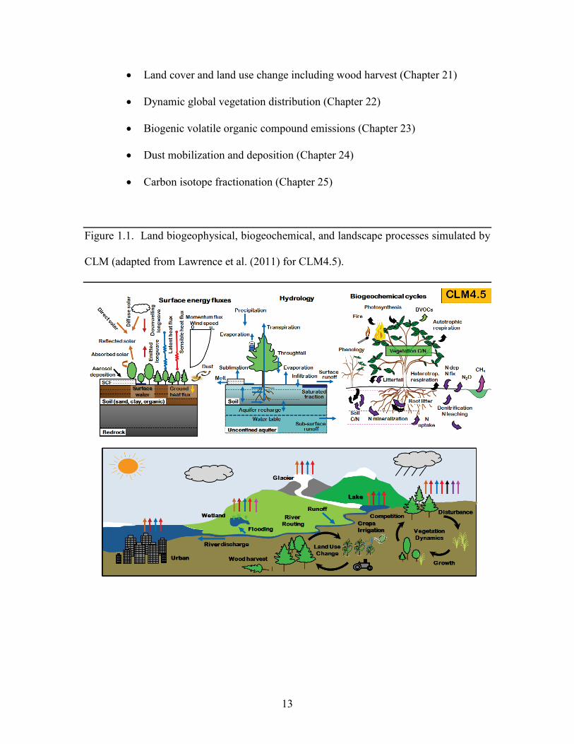
1.2 Biogeophysical and Biogeochemical Processes Biogeophysical and biogeochemical processes are simulated for each subgrid land
unit, column, and plant functional type (PFT) independently and each subgrid unit
maintains its own prognostic variables (see section 2.1.1 for definitions of subgrid units).
The same atmospheric forcing is used to force all subgrid units within a grid cell. The
surface variables and fluxes required by the atmosphere are obtained by averaging the
subgrid quantities weighted by their fractional areas. The processes simulated include
(Figure 1.1):
• Surface characterization including land type heterogeneity and ecosystem
structure (Chapter 2)
• Absorption, reflection, and transmittance of solar radiation (Chapter 3, 4)
• Absorption and emission of longwave radiation (Chapter 4)
12
• Momentum, sensible heat (ground and canopy), and latent heat (ground
evaporation, canopy evaporation, transpiration) fluxes (Chapter 5)
• Heat transfer in soil and snow including phase change (Chapter 6)
• Canopy hydrology (interception, throughfall, and drip) (Chapter 7)
• Snow hydrology (snow accumulation and melt, compaction, water transfer
between snow layers) (Chapter 7)
• Soil hydrology (surface runoff, infiltration, redistribution of water within the
column, sub-surface drainage, groundwater) (Chapter 7)
• Stomatal physiology and photosynthesis (Chapter 8)
• Lake temperatures and fluxes (Chapter 9)
• Glacier processes (Chapter 10)
• Routing of runoff from rivers to ocean (Chapter 11)
• Urban energy balance and climate (Chapter 12)
• Vegetation carbon and nitrogen allocation and respiration (Chapter 13)
• Vegetation phenology (Chapter 14)
• Soil and litter carbon decomposition (Chapter 15)
• Nitrogen cycling including deposition, biological fixation, denitrification,
leaching, and losses due to fire (Chapter 16)
• Plant mortality (Chapter 17)
• Fire ignition and suppression, including natural, deforestation, and
agricultural fire (Chapter 18)
• Methane production, oxidation, and emissions (Chapter 19)
• Crop dynamics and irrigation (Chapter 20)
13
• Land cover and land use change including wood harvest (Chapter 21)
• Dynamic global vegetation distribution (Chapter 22)
• Biogenic volatile organic compound emissions (Chapter 23)
• Dust mobilization and deposition (Chapter 24)
• Carbon isotope fractionation (Chapter 25)
Figure 1.1. Land biogeophysical, biogeochemical, and landscape processes simulated by
CLM (adapted from Lawrence et al. (2011) for CLM4.5).
14
2. Surface Characterization and Model Input Requirements 2.1 Surface Characterization
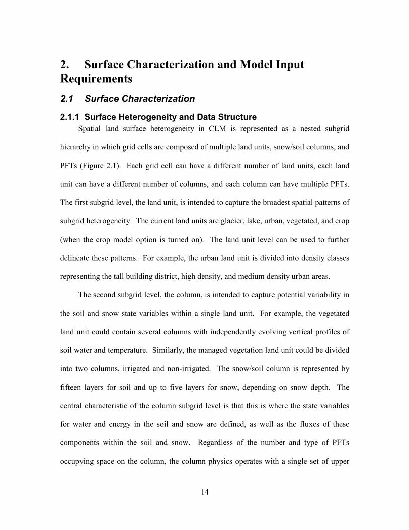
2.1.1 Surface Heterogeneity and Data Structure Spatial land surface heterogeneity in CLM is represented as a nested subgrid
hierarchy in which grid cells are composed of multiple land units, snow/soil columns, and
PFTs (Figure 2.1). Each grid cell can have a different number of land units, each land
unit can have a different number of columns, and each column can have multiple PFTs.
The first subgrid level, the land unit, is intended to capture the broadest spatial patterns of
subgrid heterogeneity. The current land units are glacier, lake, urban, vegetated, and crop
(when the crop model option is turned on). The land unit level can be used to further
delineate these patterns. For example, the urban land unit is divided into density classes
representing the tall building district, high density, and medium density urban areas.
The second subgrid level, the column, is intended to capture potential variability in
the soil and snow state variables within a single land unit. For example, the vegetated
land unit could contain several columns with independently evolving vertical profiles of
soil water and temperature. Similarly, the managed vegetation land unit could be divided
into two columns, irrigated and non-irrigated. The snow/soil column is represented by
fifteen layers for soil and up to five layers for snow, depending on snow depth. The
central characteristic of the column subgrid level is that this is where the state variables
for water and energy in the soil and snow are defined, as well as the fluxes of these
components within the soil and snow. Regardless of the number and type of PFTs
occupying space on the column, the column physics operates with a single set of upper
15
boundary fluxes, as well as a single set of transpiration fluxes from multiple soil levels.
These boundary fluxes are weighted averages over all PFTs. Currently, for glacier, lake,
and vegetated land units, a single column is assigned to each land unit. The crop land
unit is split into irrigated and unirrigated columns with a single crop occupying each
column. The urban land units have five columns (roof, sunlit walls and shaded walls, and
pervious and impervious canyon floor) (Oleson et al. 2010b).
Figure 2.1. Configuration of the CLM subgrid hierarchy.
Note that the Crop land unit is only used when the model is run with the crop model
active. Abbreviations: TBD – Tall Building District; HD – High Density; MD – Medium
Density, G – Glacier, L – Lake, U – Urban, C – Crop, V – Vegetated, PFT – Plant
Functional Type, I – Irrigated, U – Unirrigated .

16
The third subgrid level is referred to as the PFT level, but it also includes the
treatment for bare ground. It is intended to capture the biogeophysical and
biogeochemical differences between broad categories of plants in terms of their
functional characteristics. On the vegetated land unit, up to 16 possible PFTs that differ
in physiology and structure may coexist on a single column. All fluxes to and from the
surface are defined at the PFT level, as are the vegetation state variables (e.g. vegetation
temperature and canopy water storage). On the crop land unit, several different crop
types can be represented on each crop land unit column (see Chapter 20 for details).
In addition to state and flux variable data structures for conserved components at
each subgrid level (e.g., energy, water, carbon), each subgrid level also has a physical
state data structure for handling quantities that are not involved in conservation checks
(diagnostic variables). For example, the urban canopy air temperature and humidity are
defined through physical state variables at the land unit level, the number of snow layers
and the soil roughness lengths are defined as physical state variables at the column level,
and the leaf area index and the fraction of canopy that is wet are defined as physical state
variables at the PFT level.
The standard configuration of the model subgrid hierarchy is illustrated in Figure
2.1. Here, only four PFTs are shown associated with the single column beneath the
vegetated land unit but up to sixteen are possible. The crop land unit is present only
when the crop model is active.
Note that the biogeophysical processes related to soil and snow require PFT level
properties to be aggregated to the column level. For example, the net heat flux into the
17
ground is required as a boundary condition for the solution of snow/soil temperatures
(Chapter 6). This column level property must be determined by aggregating the net heat
flux from all PFTs sharing the column. This is generally accomplished in the model by
computing a weighted sum of the desired quantity over all PFTs whose weighting
depends on the PFT area relative to all PFTs, unless otherwise noted in the text.
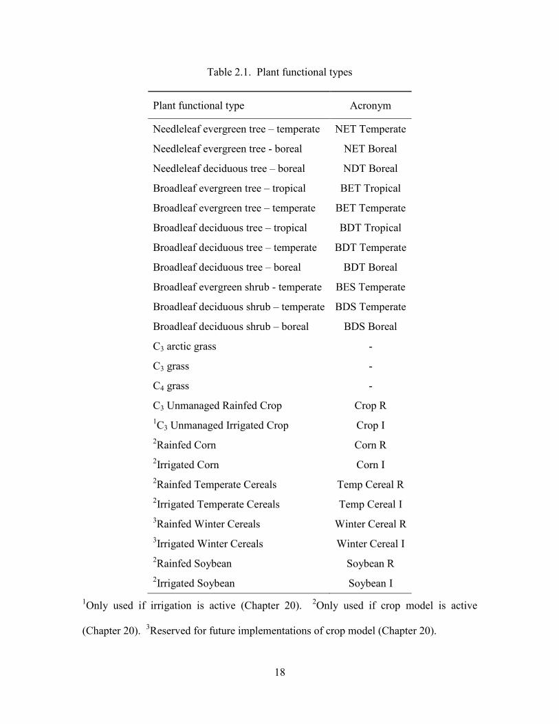
2.1.2 Vegetation Composition Vegetated surfaces are comprised of up to 15 possible plant functional types (PFTs)
plus bare ground (Table 2.1). An additional PFT is added if the irrigation model is active
and six additional PFTs are added if the crop model is active (Chapter 20). These plant
types differ in leaf and stem optical properties that determine reflection, transmittance,
and absorption of solar radiation (Table 3.1), root distribution parameters that control the
uptake of water from the soil (Table 8.3), aerodynamic parameters that determine
resistance to heat, moisture, and momentum transfer (Table 5.1), and photosynthetic
parameters that determine stomatal resistance, photosynthesis, and transpiration (Tables
8.1, 8.2). The composition and abundance of PFTs within a grid cell can either be
prescribed as time-invariant fields (e.g., using the present day dataset described in section
21.3.3) or can evolve with time if the model is run in transient landcover mode (Chapter
21).
18
Table 2.1. Plant functional types
Plant functional type Acronym
Needleleaf evergreen tree – temperate NET Temperate
Needleleaf evergreen tree - boreal NET Boreal
Needleleaf deciduous tree – boreal NDT Boreal
Broadleaf evergreen tree – tropical BET Tropical
Broadleaf evergreen tree – temperate BET Temperate
Broadleaf deciduous tree – tropical BDT Tropical
Broadleaf deciduous tree – temperate BDT Temperate
Broadleaf deciduous tree – boreal BDT Boreal
Broadleaf evergreen shrub - temperate BES Temperate
Broadleaf deciduous shrub – temperate BDS Temperate
Broadleaf deciduous shrub – boreal BDS Boreal
C3 arctic grass -
C3 grass -
C4 grass -
C3 Unmanaged Rainfed Crop Crop R 1C3 Unmanaged Irrigated Crop Crop I 2Rainfed Corn Corn R 2Irrigated Corn Corn I 2Rainfed Temperate Cereals Temp Cereal R 2Irrigated Temperate Cereals Temp Cereal I 3Rainfed Winter Cereals Winter Cereal R 3Irrigated Winter Cereals Winter Cereal I 2Rainfed Soybean Soybean R 2Irrigated Soybean Soybean I
1Only used if irrigation is active (Chapter 20). 2Only used if crop model is active
(Chapter 20). 3Reserved for future implementations of crop model (Chapter 20).
19
2.1.3 Vegetation Structure Vegetation structure is defined by leaf and stem area indices ( ,L S ) and canopy top
and bottom heights ( topz , botz ) (Table 2.2). Separate leaf and stem area indices and
canopy heights are prescribed or calculated for each PFT. Daily leaf and stem area
indices are obtained from gridded datasets of monthly values (section 2.2.3). Canopy top
and bottom heights are also obtained from gridded datasets. However, these are currently
invariant in space and time and were obtained from PFT-specific values (Bonan et al.
2002a). When the biogeochemistry model is active, vegetation state (LAI, SAI, canopy
top and bottom heights) are calculated prognostically (see Chapter 14).

20
Table 2.2. Prescribed plant functional type heights
Plant functional type topz (m) botz (m)
NET Temperate 17 8.5
NET Boreal 17 8.5
NDT Boreal 14 7
BET Tropical 35 1
BET temperate 35 1
BDT tropical 18 10
BDT temperate 20 11.5
BDT boreal 20 11.5
BES temperate 0.5 0.1
BDS temperate 0.5 0.1
BDS boreal 0.5 0.1
C3 arctic grass 0.5 0.01
C3 grass 0.5 0.01
C4 grass 0.5 0.01
Crop R 0.5 0.01
Crop I 0.5 0.01 1Corn R - - 1Corn I - - 1Temp Cereal R - - 1Temp Cereal I - - 1Winter Cereal R - - 1Winter Cereal I - - 1Soybean R - - 1Soybean I - -
1Determined by the crop model (Chapter 20)
21
2.1.4 Phenology and vegetation burial by snow When the biogeochemistry model is inactive, leaf and stem area indices (m2 leaf
area m-2 ground area) are updated daily by linearly interpolating between monthly values.
Monthly PFT leaf area index values are developed from the 1-km MODIS-derived
monthly grid cell average leaf area index of Myneni et al. (2002), as described in
Lawrence and Chase (2007). Stem area index is calculated from the monthly PFT leaf
area index using the methods of Zeng et al. (2002). The leaf and stem area indices are
adjusted for vertical burying by snow (Wang and Zeng 2009) as
( )* 1 snovegA A f= − (2.1)
where *A is the leaf or stem area before adjustment for snow, A is the remaining
exposed leaf or stem area, snovegf is the vertical fraction of vegetation covered by snow
( )
for tree and shrub
min ,for grass and crop
sno sno botveg
top bot
sno csnoveg
c
z zfz z
z zf
z
−=
−
=
, (2.2)
where 0, 0 1snosno bot vegz z f− ≥ ≤ ≤ , snoz is the depth of snow (m) (section 7.2), and
0.2cz = is the snow depth when short vegetation is assumed to be completely buried by
snow (m). For numerical reasons, exposed leaf and stem area are set to zero if less than
0.05. If the sum of exposed leaf and stem area is zero, then the surface is treated as
snow-covered ground.
2.2 Model Input Requirements
2.2.1 Atmospheric Coupling The current state of the atmosphere (Table 2.3) at a given time step is used to force
the land model. This atmospheric state is provided by an atmospheric model in coupled
22
mode or from an observed dataset in offline mode (Chapter 26). The land model then
initiates a full set of calculations for surface energy, constituent, momentum, and
radiative fluxes. The land model calculations are implemented in two steps. The land
model proceeds with the calculation of surface energy, constituent, momentum, and
radiative fluxes using the snow and soil hydrologic states from the previous time step.
The land model then updates the soil and snow hydrology calculations based on these
fluxes. These fields are passed to the atmosphere (Table 2.4). The albedos sent to the
atmosphere are for the solar zenith angle at the next time step but with surface conditions
from the current time step.
23
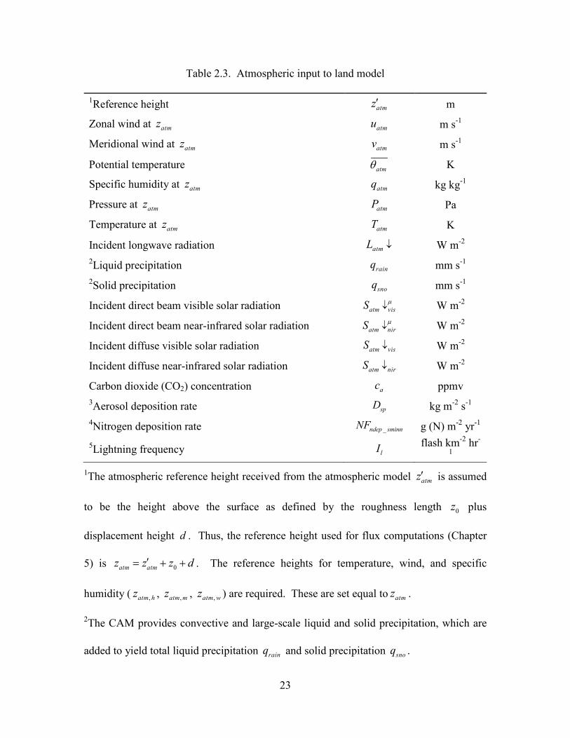
Table 2.3. Atmospheric input to land model
1Reference height atmz′ m
Zonal wind at atmz atmu m s-1
Meridional wind at atmz atmv m s-1
Potential temperature atmθ K
Specific humidity at atmz atmq kg kg-1
Pressure at atmz atmP Pa
Temperature at atmz atmT K
Incident longwave radiation atmL ↓ W m-2 2Liquid precipitation rainq mm s-1 2Solid precipitation snoq mm s-1
Incident direct beam visible solar radiation atm visS µ↓ W m-2
Incident direct beam near-infrared solar radiation atm nirS µ↓ W m-2
Incident diffuse visible solar radiation atm visS ↓ W m-2
Incident diffuse near-infrared solar radiation atm nirS ↓ W m-2
Carbon dioxide (CO2) concentration ac ppmv 3Aerosol deposition rate spD kg m-2 s-1 4Nitrogen deposition rate _ndep sminnNF g (N) m-2 yr-1 5Lightning frequency lI
flash km-2 hr-
1
1The atmospheric reference height received from the atmospheric model atmz′ is assumed
to be the height above the surface as defined by the roughness length 0z plus
displacement height d . Thus, the reference height used for flux computations (Chapter
5) is 0atm atmz z z d′= + + . The reference heights for temperature, wind, and specific
humidity ( ,atm hz , ,atm mz , ,atm wz ) are required. These are set equal to atmz .
2The CAM provides convective and large-scale liquid and solid precipitation, which are
added to yield total liquid precipitation rainq and solid precipitation snoq .
24
3There are 14 aerosol deposition rates required depending on species and affinity for
bonding with water; 8 of these are dust deposition rates (dry and wet rates for 4 dust size
bins, , 1 , 2 , 3 , 4, , ,dst dry dst dry dst dry dst dryD D D D , , 1 , 2 , 3 , 4, , ,dst wet dst wet dst wet dst wetD D D D ), 3 are black
carbon deposition rates (dry and wet hydrophilic and dry hydrophobic rates,
, , ,, ,bc dryhphil bc wethphil bc dryhphobD D D ), and 3 are organic carbon deposition rates (dry and wet
hydrophilic and dry hydrophobic rates, , , ,, ,oc dryhphil oc wethphil oc dryhphobD D D ). These fluxes are
computed interactively by the atmospheric model (when prognostic aerosol
representation is active) or are prescribed from a time-varying (annual cycle or transient),
globally-gridded deposition file defined in the namelist (see the CLM4.5 User’s Guide).
Aerosol deposition rates were calculated in a transient 1850-2009 CAM simulation (at a
resolution of 1.9x2.5x26L) with interactive chemistry (troposphere and stratosphere)
driven by CCSM3 20th century sea-surface temperatures and emissions (Lamarque et al.
2010) for short-lived gases and aerosols; observed concentrations were specified for
methane, N2O, the ozone-depleting substances (CFCs) ,and CO2. The fluxes are used by
the snow-related parameterizations (Chapters 3 and 7).
4The nitrogen deposition rate is required by the biogeochemistry model when active and
represents the total deposition of mineral nitrogen onto the land surface, combining
deposition of NOy and NHx. The rate is supplied either as a time-invariant spatially-
varying annual mean rate or time-varying for a transient simulation. Nitrogen deposition
rates were calculated from the same CAM chemistry simulation that generated the
aerosol deposition rates.
5Climatological 3-hourly lightning frequency at ~1.8o resolution is provided, which was
calculated via bilinear interpolation from 1995-2011 NASA LIS/OTD grid product v2.2
25
(http://ghrc.msfc.nasa.gov) 2-hourly, 2.5o lightning frequency data. In future versions of
the model, lightning data may be obtained directly from the atmosphere model.
Density of air ( atmρ ) (kg m-3) is also required but is calculated directly from
0.378atm atmatm
da atm
P eR T
ρ −= where a t mP is atmospheric pressure (Pa), a t me is atmospheric
vapor pressure (Pa), d aR is the gas constant for dry air (J kg-1 K-1) (Table 2.6), and a t mT
is the atmospheric temperature (K). The atmospheric vapor pressure a t me is derived from
atmospheric specific humidity a t mq (kg kg-1) as 0.622 0.378
atm atmatm
atm
q Peq
=+
.
The O2 partial pressure (Pa) is required but is calculated from molar ratio and the
atmospheric pressure a t mP as 0.209i atmo P= .
26
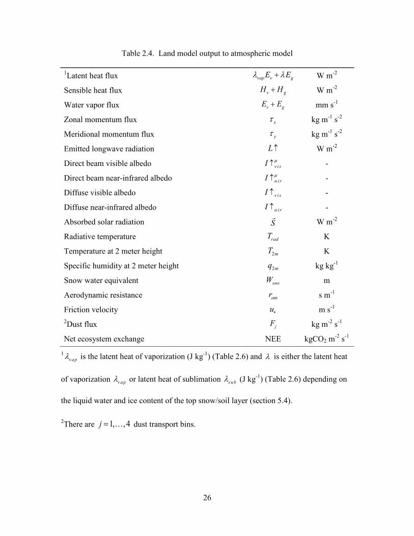
Table 2.4. Land model output to atmospheric model
1Latent heat flux vap v gE Eλ λ+ W m-2
Sensible heat flux v gH H+ W m-2
Water vapor flux v gE E+ mm s-1
Zonal momentum flux xτ kg m-1 s-2
Meridional momentum flux yτ kg m-1 s-2
Emitted longwave radiation L ↑ W m-2
Direct beam visible albedo v i sI µ↑ -
Direct beam near-infrared albedo n i rI µ↑ -
Diffuse visible albedo v i sI ↑ -
Diffuse near-infrared albedo n i rI ↑ -
Absorbed solar radiation S
W m-2
Radiative temperature radT K
Temperature at 2 meter height 2mT K
Specific humidity at 2 meter height 2mq kg kg-1
Snow water equivalent snoW m
Aerodynamic resistance amr s m-1
Friction velocity u∗ m s-1 2Dust flux jF kg m-2 s-1
Net ecosystem exchange NEE kgCO2 m-2 s-1
1v a pλ is the latent heat of vaporization (J kg-1) (Table 2.6) and λ is either the latent heat
of vaporization v a pλ or latent heat of sublimation s u bλ (J kg-1) (Table 2.6) depending on
the liquid water and ice content of the top snow/soil layer (section 5.4).
2There are 1, , 4j = dust transport bins.
27
2.2.2 Initialization Initialization of the land model (i.e., providing the model with initial temperature
and moisture states) depends on the type of run (startup or restart) (see the CLM4.5
User’s Guide). A startup run starts the model from either initial conditions that are set
internally in the Fortran code (referred to as arbitrary initial conditions) or from an initial
conditions dataset that enables the model to start from a spun up state (i.e., where the land
is in equilibrium with the simulated climate). In restart runs, the model is continued from
a previous simulation and initialized from a restart file that ensures that the output is bit-
for-bit the same as if the previous simulation had not stopped. The fields that are
required from the restart or initial conditions files can be obtained by examining the code.
Arbitrary initial conditions are specified as follows.
Vegetated and glacier land units have fifteen vertical layers, while lakes have ten.
For soil points, temperature calculations are done over all layers, 15levgrndN = , while
hydrology calculations are done over the top ten layers, 10levsoiN = , the bottom five
layers being specified as bedrock. Soil points are initialized with surface ground
temperature gT and soil layer temperature iT , for 1, , levgrndi N= , of 274 K, vegetation
temperature vT of 283 K, no snow or canopy water ( 0snoW = , 0canW = ), and volumetric
soil water content 0.15iθ = mm3 mm-3 for layers 1, , levsoii N= and 0.0iθ = mm3 mm-3
for layers 1, ,levsoi levgrndi N N= + . Lake temperatures ( gT and iT ) are initialized at 277
K and 0snoW = .
Glacier temperatures ( 1g snlT T += and iT for 1, , levgrndi snl N= + where snl is the
negative of the number of snow layers, i.e., snl ranges from –5 to 0) are initialized to
28
250 K with a snow water equivalent 1000snoW = mm, snow depth snosno
sno
Wzρ
= (m) where
250snoρ = kg m-3 is an initial estimate for the bulk density of snow, and iθ =1.0 for
1, , levgrndi N= . The snow layer structure (e.g., number of snow layers snl and layer
thickness) is initialized based on the snow depth (section 6.1). The snow liquid water and
ice contents (kg m-2) are initialized as , 0liq iw = and ,ice i i snow z ρ= ∆ , respectively, where
1, ,0i snl= + are the snow layers, and iz∆ is the thickness of snow layer i (m). The
soil liquid water and ice contents are initialized as , 0liq iw = and ,ice i i ice iw z ρ θ= ∆ for
i fT T≤ , and ,liq i i liq iw z ρ θ= ∆ and , 0ice iw = for i fT T> , where iceρ and liqρ are the
densities of ice and liquid water (kg m-3) (Table 2.6), and fT is the freezing temperature
of water (K) (Table 2.6). All vegetated and glacier land units are initialized with water
stored in the unconfined aquifer and unsaturated soil 4000aW = mm and water table
depth z∇ at five meters below the soil column.
2.2.3 Surface Data Required surface data for each land grid cell are listed in Table 2.5 and include the
glacier, lake, and urban fractions of the grid cell (vegetated and crop occupy the
remainder), the fractional cover of each plant functional type (PFT), monthly leaf and
stem area index and canopy top and bottom heights for each PFT, soil color, soil texture,
soil organic matter density, maximum fractional saturated area, slope, elevation, biogenic
volatile organic compounds (BVOCs) emissions factors, population density, gross
domestic production, peat area fraction, and peak month of agricultural burning.
Optional surface data include crop irrigation and managed crops. All fields are
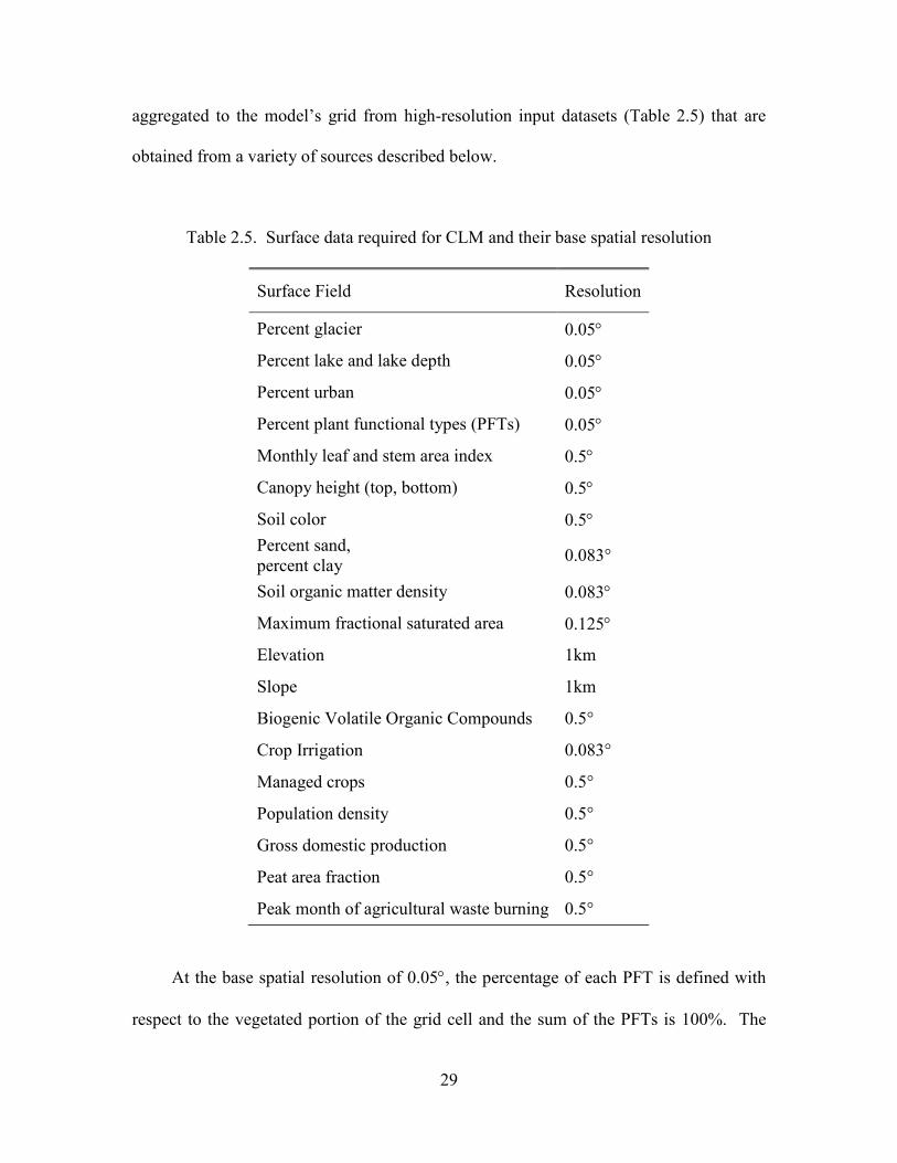
29
aggregated to the model’s grid from high-resolution input datasets (Table 2.5) that are
obtained from a variety of sources described below.
Table 2.5. Surface data required for CLM and their base spatial resolution
Surface Field Resolution
Percent glacier 0.05°
Percent lake and lake depth 0.05°
Percent urban 0.05°
Percent plant functional types (PFTs) 0.05°
Monthly leaf and stem area index 0.5°
Canopy height (top, bottom) 0.5°
Soil color 0.5° Percent sand, percent clay 0.083°
Soil organic matter density 0.083°
Maximum fractional saturated area 0.125°
Elevation 1km
Slope 1km
Biogenic Volatile Organic Compounds 0.5°
Crop Irrigation 0.083°
Managed crops 0.5°
Population density 0.5°
Gross domestic production 0.5°
Peat area fraction 0.5°
Peak month of agricultural waste burning 0.5°
At the base spatial resolution of 0.05°, the percentage of each PFT is defined with
respect to the vegetated portion of the grid cell and the sum of the PFTs is 100%. The

30
percent lake, wetland, glacier, and urban at their base resolution are specified with respect
to the entire grid cell. The surface dataset creation routines re-adjust the PFT percentages
to ensure that the sum of all land cover types in the grid cell sum to 100%. A minimum
threshold of 0.1% of the grid cell by area is required for urban areas.
The percentage glacier mask was derived from vector data of global glacier and ice
sheet spatial coverage. Vector data for glaciers (ice caps, icefields and mountain glaciers)
were taken from the first globally complete glacier inventory, the Randolph Glacier
Inventory version 1.0 (RGIv1.0: Arendt et al. 2012). Vector data for the Greenland Ice
Sheet were provided by Frank Paul and Tobias Bolch (University of Zurich: Rastner et al.
2012). Antarctic Ice Sheet data were provided by Andrew Bliss (University of Alaska)
and were extracted from the Scientific Committee on Antarctic Research (SCAR)
Antarctic Digital Database version 5.0. Floating ice is only provided for the Antarctic and
does not include the small area of Arctic ice shelves. High spatial resolution vector data
were then processed to determine the area of glacier, ice sheet and floating ice within 30-
second grid cells globally. The 30-second glacier, ice sheet and Antarctic ice shelf masks
were subsequently draped over equivalent-resolution GLOBE topography (Global Land
One-km Base Elevation Project, Hastings et al. 1999) to extract approximate ice-covered
elevations of ice-covered regions. Grid cells flagged as land-ice in the mask but ocean in
GLOBE (typically, around ice sheets at high latitudes) were designated land-ice with an
elevation of 0 meters. Finally, the high-resolution mask/topography datasets were
aggregated and processed into three 3-minute datasets: 3-minute fractional areal land ice
coverage (including both glaciers and ice sheets); 3-minute distributions of areal glacier
fractional coverage by elevation and areal ice sheet fractional coverage by elevation. Ice
31
fractions were binned at 100 meter intervals, with bin edges defined from 0 to 6000
meters (plus one top bin encompassing all remaining high-elevation ice, primarily in the
Himalaya). These distributions by elevation are needed when running CLM4 with
multiple glacier elevation classes.
Percent lake and lake depth are area-averaged from the 90-second resolution data of
Kourzeneva (2009, 2010) to the 0.05° resolution using the MODIS land-mask. Percent
urban is derived from LandScan 2004, a population density dataset derived from census
data, nighttime lights satellite observations, road proximity and slope (Dobson et al.
2000) as described by Jackson et al. (2010) at 1km resolution and aggregated to 0.05°. A
number of urban radiative, thermal, and morphological fields are also required and are
obtained from Jackson et al. (2010). Their description can be found in Table 3 of the
Community Land Model Urban (CLMU) technical note (Oleson et al. 2010b).
Percent PFTs are derived from MODIS satellite data as described in Lawrence and
Chase (2007) (section 21.3.3). Prescribed PFT leaf area index is derived from the
MODIS satellite data of Myneni et al. (2002) using the de-aggregation methods described
in Lawrence and Chase (2007) (section 2.2.3). Prescribed PFT stem area index is derived
from PFT leaf area index phenology combined with the methods of Zeng et al. (2002).
Prescribed canopy top and bottom heights are from Bonan (1996) as described in Bonan
et al. (2002b). If the biogeochemistry model is active, it supplies the leaf and stem area
index and canopy top and bottom heights dynamically, and the prescribed values are
ignored.
Soil color determines dry and saturated soil albedo (section 3.2). Soil colors are
from Lawrence and Chase (2007) (section 3.2).
32
The soil texture and organic matter content determine soil thermal and hydrologic
properties (sections 6.3 and 7.4.1). The International Geosphere-Biosphere Programme
(IGBP) soil dataset (Global Soil Data Task 2000) of 4931 soil mapping units and their
sand and clay content for each soil layer were used to create a mineral soil texture dataset
(Bonan et al. 2002b). Soil organic matter data is merged from two sources. The majority
of the globe is from ISRIC-WISE (Batjes, 2006). The high latitudes come from the 0.25°
version of the Northern Circumpolar Soil Carbon Database (Hugelius et al. 2012). Both
datasets report carbon down to 1m depth. Carbon is partitioned across the top seven
CLM4 layers (~1m depth) as in Lawrence and Slater (2008).
The maximum fractional saturated area ( maxf ) is used in determining surface runoff
and infiltration (section 7.3). Maximum fractional saturated area at 0.125o resolution is
calculated from 1-km compound topographic indices (CTIs) based on the USGS
HYDRO1K dataset (Verdin and Greenlee 1996) following the algorithm in Niu et al.
(2005). maxf is the ratio between the number of 1-km pixels with CTIs equal to or larger
than the mean CTI and the total number of pixels in a 0.125° grid cell. See section 7.3.1
and Li et al. (2013b) for further details. Slope and elevation are also obtained from the
USGS HYDRO1K 1-km dataset (Verdin and Greenlee 1996). Slope is used in the River
Transport Model (Chapter 11) and in the surface water parameterization (section 7.3.2),
and elevation is used to calculate the grid cell standard deviation of topography for the
snow cover fraction parameterization (section 7.2.1).
Biogenic Volatile Organic Compounds emissions factors are from the Model of
Emissions of Gases and Aerosols from Nature version 2.1 (MEGAN2.1; Guenther et al.
2012).
33
The default list of PFTs includes an unmanaged crop treated as a second C3 grass
(Table 2.1). The unmanaged crop has grid cell fractional cover assigned from MODIS
satellite data (Lawrence and Chase 2007). A managed crop option uses grid cell
fractional cover from the present-day crop dataset of Ramankutty and Foley (1998)
(CLM4CNcrop). Managed crops are assigned in the proportions given by Ramankutty
and Foley (1998) without exceeding the area previously assigned to the unmanaged crop.
The unmanaged crop continues to occupy any of its original area that remains and
continues to be handled just by the CN part of CLM4CNcrop. The managed crop types
(corn, soybean, and temperate cereals) were chosen based on the availability of
corresponding algorithms in AgroIBIS (Kucharik et al. 2000; Kucharik and Brye 2003).
Temperate cereals include wheat, barley, and rye here. All temperate cereals are treated
as summer crops (like spring wheat, for example) at this time. Winter cereals (such as
winter wheat) may be introduced in a future version of the model.
To allow crops to coexist with natural vegetation in a grid cell and be treated by
separate models (i.e., CLM4.5BGCcrop versus the Dynamic Vegetation version
(CLM4.5BGCDV)), we separate the vegetated land unit into a naturally vegetated land
unit and a human managed land unit. PFTs in the naturally vegetated land unit share one
soil column and compete for water (default CLM setting). PFTs in the human managed
land unit do not share soil columns and thus permit for differences in land management
between crops.
CLM includes the option to irrigate cropland areas that are equipped for irrigation.
The application of irrigation responds dynamically to climate (see Chapter 20). In CLM,
irrigation is implemented for the C3 generic crop only. When irrigation is enabled, the
34
cropland area of each grid cell is divided into an irrigated and unirrigated fraction
according to a dataset of areas equipped for irrigation (Siebert et al. 2005). The area of
irrigated cropland in each grid cell is given by the smaller of (1) the grid cell's total
cropland area, according to the default CLM4 dataset, and (2) the grid cell's area
equipped for irrigation. The remainder of the grid cell's cropland area (if any) is then
assigned to unirrigated cropland. Irrigated and unirrigated crops are placed on separate
soil columns, so that irrigation is only applied to the soil beneath irrigated crops.
Several input datasets are required for the fire model (Li et al. 2013a) including
population density, gross domestic production, peat area fraction, and peak month of
agricultural waste burning. Population density at 0.5o resolution for 1850-2100 combines
5-min resolution decadal population density data for 1850–1980 from the Database of the
Global Environment version 3.1 (HYDEv3.1) with 0.5o resolution population density
data for 1990, 1995, 2000, and 2005 from the Gridded Population of the World version 3
dataset (GPWv3) (CIESIN, 2005). Gross Domestic Production (GDP) per capita in 2000
at 0.5o is from Van Vuuren et al. (2006), which is the base-year GDP data for IPCC-
SRES and derived from country-level World Bank’s World Development Indicators
(WDI) measured in constant 1995 US$ (World Bank, 2004) and the UN Statistics
Database (UNSTAT, 2005). The peatland area fraction at 0.5o resolution is derived from
three vector datasets: peatland data in Indonesia and Malaysian Borneo (Olson et al.
2001); peatland data in Canada (Tarnocai et al. 2011); and bog, fen and mire data in
boreal regions (north of 45oN) outside Canada provided by the Global Lakes and
Wetlands Database (GLWD) (Lehner and Döll, 2004). The climatological peak month for
agricultural waste burning is from van der Werf et al. (2010).

35
2.2.4 Adjustable Parameters and Physical Constants Values of certain adjustable parameters inherent in the biogeophysical or
biogeochemical parameterizations have either been obtained from the literature or
calibrated based on comparisons with observations. These are described in the text.
Physical constants, generally shared by all of the components in the coupled modeling
system, are presented in Table 2.6.
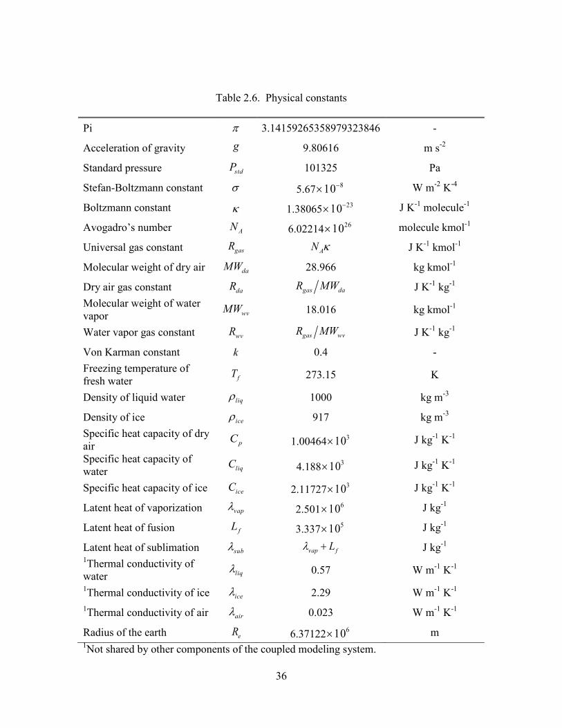
36
Table 2.6. Physical constants
Pi π 3.14159265358979323846 -
Acceleration of gravity g 9.80616 m s-2
Standard pressure stdP 101325 Pa
Stefan-Boltzmann constant σ 5.67 810−× W m-2 K-4
Boltzmann constant κ 1.38065 2310−× J K-1 molecule-1
Avogadro’s number AN 6.02214 2610× molecule kmol-1
Universal gas constant gasR AN κ J K-1 kmol-1
Molecular weight of dry air daMW 28.966 kg kmol-1
Dry air gas constant daR gas daR MW J K-1 kg-1 Molecular weight of water vapor wvMW 18.016 kg kmol-1
Water vapor gas constant wvR gas wvR MW J K-1 kg-1
Von Karman constant k 0.4 - Freezing temperature of fresh water fT 273.15 K
Density of liquid water liqρ 1000 kg m-3
Density of ice iceρ 917 kg m-3 Specific heat capacity of dry air pC 1.00464 310× J kg-1 K-1
Specific heat capacity of water liqC 4.188 310× J kg-1 K-1
Specific heat capacity of ice iceC 2.11727 310× J kg-1 K-1
Latent heat of vaporization vapλ 2.501 610× J kg-1
Latent heat of fusion fL 3.337 510× J kg-1
Latent heat of sublimation subλ vap fLλ + J kg-1 1Thermal conductivity of water liqλ 0.57 W m-1 K-1 1Thermal conductivity of ice iceλ 2.29 W m-1 K-1 1Thermal conductivity of air airλ 0.023 W m-1 K-1
Radius of the earth eR 6.37122 610× m 1Not shared by other components of the coupled modeling system.
37
3. Surface Albedos
3.1 Canopy Radiative Transfer Radiative transfer within vegetative canopies is calculated from the two-stream
approximation of Dickinson (1983) and Sellers (1985) as described by Bonan (1996)
( ) ( ) ( )01 1 K L SdI I I K e
d L Sµ β ω ωβ ωµ β − +↑
↑ ↓− + − − − = + (3.1)
( ) ( ) ( ) ( )01 1 1 K L SdI I I K e
d L Sµ β ω ωβ ωµ β − +↓
↓ ↑+ − − − = − + (3.2)
where I ↑ and I ↓ are the upward and downward diffuse radiative fluxes per unit
incident flux, ( )K G µ µ= is the optical depth of direct beam per unit leaf and stem
area, µ is the cosine of the zenith angle of the incident beam, ( )G µ is the relative
projected area of leaf and stem elements in the direction 1cos µ− , µ is the average
inverse diffuse optical depth per unit leaf and stem area, ω is a scattering coefficient, β
and 0β are upscatter parameters for diffuse and direct beam radiation, respectively, L is
the exposed leaf area index (section 2.1.4), and S is the exposed stem area index (section
2.1.4). Given the direct beam albedo ,gµα Λ and diffuse albedo ,gα Λ of the ground
(section 3.2), these equations are solved to calculate the fluxes, per unit incident flux,
absorbed by the vegetation, reflected by the vegetation, and transmitted through the
vegetation for direct and diffuse radiation and for visible (< 0.7 mµ ) and near-infrared (≥
0.7 mµ ) wavebands. The absorbed radiation is partitioned to sunlit and shaded fractions
38
of the canopy. The optical parameters ( )G µ , µ , ω , β , and 0β are calculated based on
work in Sellers (1985) as follows.
The relative projected area of leaves and stems in the direction 1cos µ− is
( ) 1 2G µ φ φ µ= + (3.3)
where 21 0.5 0.633 0.33L Lφ χ χ= − − and ( )2 10.877 1 2φ φ= − for 0.4 0.6Lχ− ≤ ≤ . Lχ
is the departure of leaf angles from a random distribution and equals +1 for horizontal
leaves, 0 for random leaves, and –1 for vertical leaves.
The average inverse diffuse optical depth per unit leaf and stem area is
( )
11 1 2
2 2 10
1 1 lndG
φ φ φµµ µµ φ φ φ
′ +′= = − ′ ∫ (3.4)
where µ′ is the direction of the scattered flux.
The optical parameters ω , β , and 0β , which vary with wavelength ( Λ ), are
weighted combinations of values for vegetation and snow. The model determines that
snow is on the canopy if v fT T≤ , where vT is the vegetation temperature (K) (Chapter 5)
and fT is the freezing temperature of water (K) (Table 2.6). In this case, the optical
parameters are
( )1veg snowet wetf fω ω ωΛ Λ Λ= − + (3.5)
( )1veg veg sno snowet wetf fω β ω β ω βΛ Λ Λ Λ Λ Λ= − + (3.6)
( )0, 0, 0,1veg veg sno snowet wetf fω β ω β ω βΛ Λ Λ Λ Λ Λ= − + (3.7)
39
where wetf is the wetted fraction of the canopy (section 7.1). The snow and vegetation
weights are applied to the products ω βΛ Λ and 0,ω βΛ Λ because these products are used in
the two-stream equations. If there is no snow on the canopy,
vegω ωΛ Λ= (3.8)
veg vegω β ω βΛ Λ Λ Λ= (3.9)
0, 0,veg vegω β ω βΛ Λ Λ Λ= . (3.10)
For vegetation, vegω α τΛ Λ Λ= + . αΛ is a weighted combination of the leaf and stem
reflectances ( ,leaf stemα αΛ Λ )
leaf stemleaf stemw wα α αΛ Λ Λ= + (3.11)
where ( )leafw L L S= + and ( )stemw S L S= + . τ Λ is a weighted combination of the
leaf and stem transmittances ( ,leaf stemτ τΛ Λ )
leaf stemleaf stemw wτ τ τΛ Λ Λ= + . (3.12)
The upscatter for diffuse radiation is
( ) 21 cos
2veg vegω β α τ α τ θΛ Λ Λ Λ Λ Λ = + + − (3.13)
where θ is the mean leaf inclination angle relative to the horizontal plane (i.e., the angle
between leaf normal and local vertical) (Sellers 1985). Here, cosθ is approximated by
1cos2
Lχθ += (3.14)
Using this approximation, for vertical leaves ( 1Lχ = − , o90θ = ),
( )0.5veg vegω β α τΛ Λ Λ Λ= + , and for horizontal leaves ( 1Lχ = , o0θ = ) , veg vegω β αΛ Λ Λ= ,
40
which agree with both Dickinson (1983) and Sellers (1985). For random (spherically
distributed) leaves ( 0Lχ = , o60θ = ), the approximation yields
5 8 3 8veg vegω β α τΛ Λ Λ Λ= + whereas the approximate solution of Dickinson (1983) is
2 3 1 3veg vegω β α τΛ Λ Λ Λ= + . This discrepancy arises from the fact that a spherical leaf
angle distribution has a true mean leaf inclination 57θ ≈ (Campbell and Norman 1998)
in equation (3.13), while 60θ = in equation (3.14). The upscatter for direct beam
radiation is
( )0,1veg veg
sK a
Kµω β µ
µΛ Λ Λ
+= (3.15)
where the single scattering albedo is
( ) ( )( ) ( )( )
( ) ( )( )
1
0
1 21
2 2 1
2
1 ln .2
veg
s
veg
Ga d
G G
G GG G
µ µωµ µµ µ µ µ
µ µφ µφ µω µφµφ µ µφ µ µφ
ΛΛ
Λ
′′=
′ ′+
+ + = − + +
∫ (3.16)
The upward diffuse fluxes per unit incident direct beam and diffuse flux (i.e., the
surface albedos) are
12 3
hI h hµ
σΛ↑ = + + (3.17)
7 8I h hΛ↑ = + . (3.18)
The downward diffuse fluxes per unit incident direct beam and diffuse radiation,
respectively, are
( ) 645 1
1
K L S hhI e h ss
µ
σ− +
Λ↓ = + + (3.19)
41
109 1
1
hI h ssΛ↓ = + . (3.20)
With reference to Figure 4.1, the direct beam flux transmitted through the canopy,
per unit incident flux, is ( )K L Se− + , and the direct beam and diffuse fluxes absorbed by the
vegetation, per unit incident flux, are
( ) ( ) ( ), ,1 1 1 K L S
g gI I I eµ µ µ µα α − +Λ Λ Λ Λ Λ↑ ↓= − − − − −
(3.21)
( ),1 1 gI I IαΛ Λ Λ Λ↑ ↓= − − −
. (3.22)
These fluxes are partitioned to the sunlit and shaded canopy using an analytical solution
to the two-stream approximation for sunlit and shaded leaves (Dai et al. 2004), as
described by Bonan et al. (2011). The absorption of direct beam radiation by sunlit leaves
is
( ) ( ), 2 1 211 1sunI s a aµ ωµΛ Λ
= − − + +
(3.23)
and for shaded leaves is
, ,sha sunI I Iµ µ µΛ Λ Λ= −
(3.24)
with
2
1 2 2 1 2 11 2 3
1 1 12
h s s s s sa h hK K h K hσ
− − − = + + + − (3.25)
2
4 2 2 1 2 12 5 6
1 1 12
h s s s s sa h hK K h K hσ
− − − = + + + − . (3.26)
For diffuse radiation, the absorbed radiation for sunlit leaves is
( ), 1 21
sunI a aωµ
ΛΛ
−= +
(3.27)
42
and for shaded leaves is
, ,sha sunI I IΛ Λ Λ= −
(3.28)
with
2 1 2 11 7 8
1 1s s s sa h hK h K h− − = + + −
(3.29)
2 1 2 12 9 10
1 1s s s sa h hK h K h− − = + + −
. (3.30)
The parameters 1h – 1 0h , σ , h , 1s , and 2s are from Sellers (1985) [note the error
in 4h in Sellers (1985)]:
1b ω ω βΛ Λ Λ= − + (3.31)
c ω βΛ Λ= (3.32)
0,d Kω µ βΛ Λ= (3.33)
( )0,1f Kω µ βΛ Λ= − (3.34)
2 2b chµ−
= (3.35)
( )2 2 2K c bσ µ= + − (3.36)
1 , 1 , or g gu b c u b cµα αΛ Λ= − = − (3.37)
2 , 2 , or g gu b c u b cµα αΛ Λ= − = − (3.38)
3 , 3 , or g gu f c u f cµα αΛ Λ= + = + (3.39)
( ) 1 exp min , 40s h L S= − + (3.40)
43
( ) 2 exp min , 40s K L S= − + (3.41)
1p b hµ= + (3.42)
2p b hµ= − (3.43)
3p b Kµ= + (3.44)
4p b Kµ= − (3.45)
( ) ( )1 11 2 1 1
1
p u hd p u h s
sµ
µ−
= − + (3.46)
( )22 2 1
1
u hd u h ss
µ µ+= − − (3.47)
1 4h dp cf= − − (3.48)
( ) ( )11 12 3 2 1 2
1 1
1 u hh hh d p p d c u K sd s
µµ
σ σ− = − − − − +
(3.49)
( ) ( )1 13 3 1 1 1 1 2
1
1 h hh d p u h s p d c u K sd
µ µσ σ
− = − + − − − + (3.50)
4 3h fp cd= − − (3.51)
( ) ( )4 2 45 3 2 2
2 1
1 h u h hh u u K sd s
µµ
σ σ + − = + − −
(3.52)
( ) ( )4 46 2 1 3 2 2
2
1 h hh u h s u u K sd
µ µσ σ
= − + − − (3.53)
( )17
1 1
c u hh
d sµ−
= (3.54)
( )1 18
1
c u h sh
dµ− +
= (3.55)
44
29
2 1
u hhd s
µ+= (3.56)
( )1 210
2
s u hh
dµ− −
= . (3.57)
Plant functional type optical properties (Table 3.1) for trees and shrubs are from Dorman
and Sellers (1989). Leaf and stem optical properties (VIS and NIR reflectance and
transmittance) were derived for grasslands and crops from full optical range spectra of
measured optical properties (Asner et al. 1998). Optical properties for intercepted snow
(Table 3.2) are from Sellers et al. (1986).
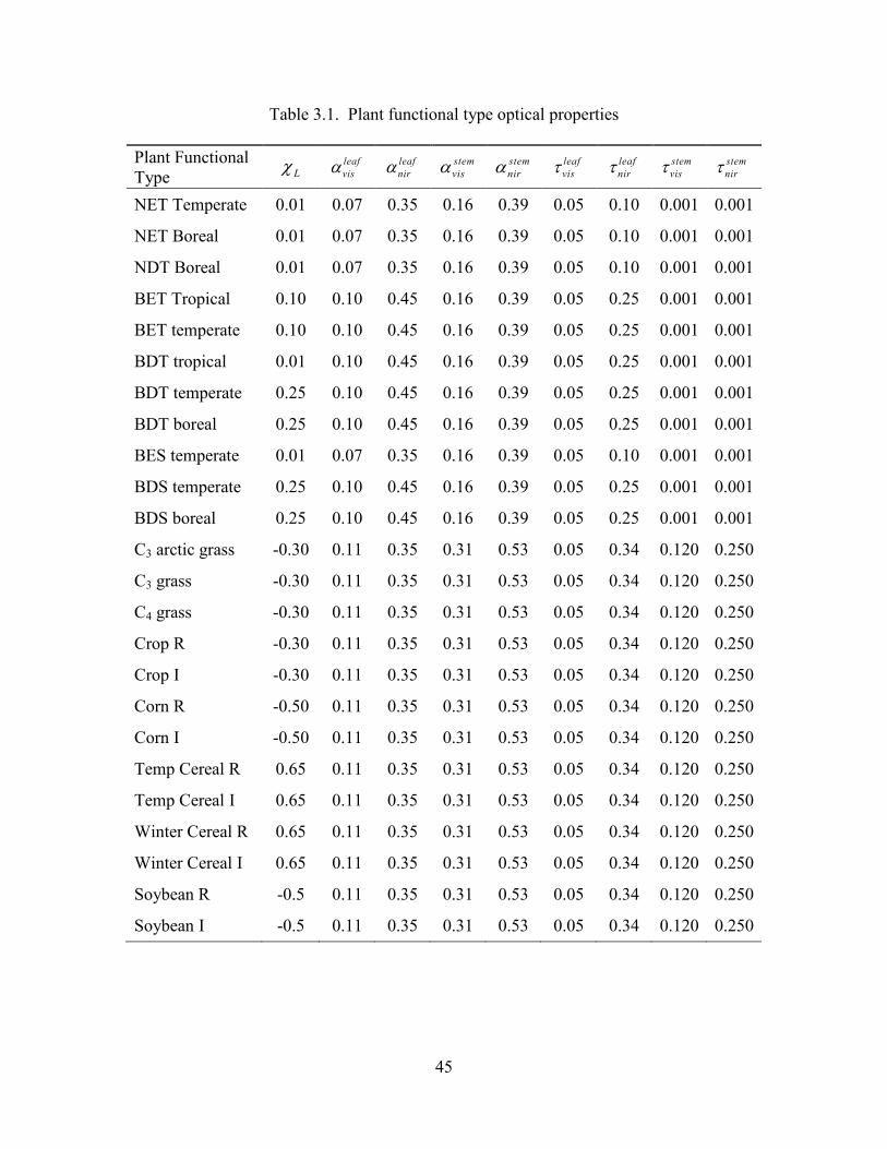
45
Table 3.1. Plant functional type optical properties
Plant Functional Type Lχ leaf
visα leafnirα stem
visα stemnirα leaf
visτ leafnirτ stem
visτ stemnirτ
NET Temperate 0.01 0.07 0.35 0.16 0.39 0.05 0.10 0.001 0.001
NET Boreal 0.01 0.07 0.35 0.16 0.39 0.05 0.10 0.001 0.001
NDT Boreal 0.01 0.07 0.35 0.16 0.39 0.05 0.10 0.001 0.001
BET Tropical 0.10 0.10 0.45 0.16 0.39 0.05 0.25 0.001 0.001
BET temperate 0.10 0.10 0.45 0.16 0.39 0.05 0.25 0.001 0.001
BDT tropical 0.01 0.10 0.45 0.16 0.39 0.05 0.25 0.001 0.001
BDT temperate 0.25 0.10 0.45 0.16 0.39 0.05 0.25 0.001 0.001
BDT boreal 0.25 0.10 0.45 0.16 0.39 0.05 0.25 0.001 0.001
BES temperate 0.01 0.07 0.35 0.16 0.39 0.05 0.10 0.001 0.001
BDS temperate 0.25 0.10 0.45 0.16 0.39 0.05 0.25 0.001 0.001
BDS boreal 0.25 0.10 0.45 0.16 0.39 0.05 0.25 0.001 0.001
C3 arctic grass -0.30 0.11 0.35 0.31 0.53 0.05 0.34 0.120 0.250
C3 grass -0.30 0.11 0.35 0.31 0.53 0.05 0.34 0.120 0.250
C4 grass -0.30 0.11 0.35 0.31 0.53 0.05 0.34 0.120 0.250
Crop R -0.30 0.11 0.35 0.31 0.53 0.05 0.34 0.120 0.250
Crop I -0.30 0.11 0.35 0.31 0.53 0.05 0.34 0.120 0.250
Corn R -0.50 0.11 0.35 0.31 0.53 0.05 0.34 0.120 0.250
Corn I -0.50 0.11 0.35 0.31 0.53 0.05 0.34 0.120 0.250
Temp Cereal R 0.65 0.11 0.35 0.31 0.53 0.05 0.34 0.120 0.250
Temp Cereal I 0.65 0.11 0.35 0.31 0.53 0.05 0.34 0.120 0.250
Winter Cereal R 0.65 0.11 0.35 0.31 0.53 0.05 0.34 0.120 0.250
Winter Cereal I 0.65 0.11 0.35 0.31 0.53 0.05 0.34 0.120 0.250
Soybean R -0.5 0.11 0.35 0.31 0.53 0.05 0.34 0.120 0.250
Soybean I -0.5 0.11 0.35 0.31 0.53 0.05 0.34 0.120 0.250
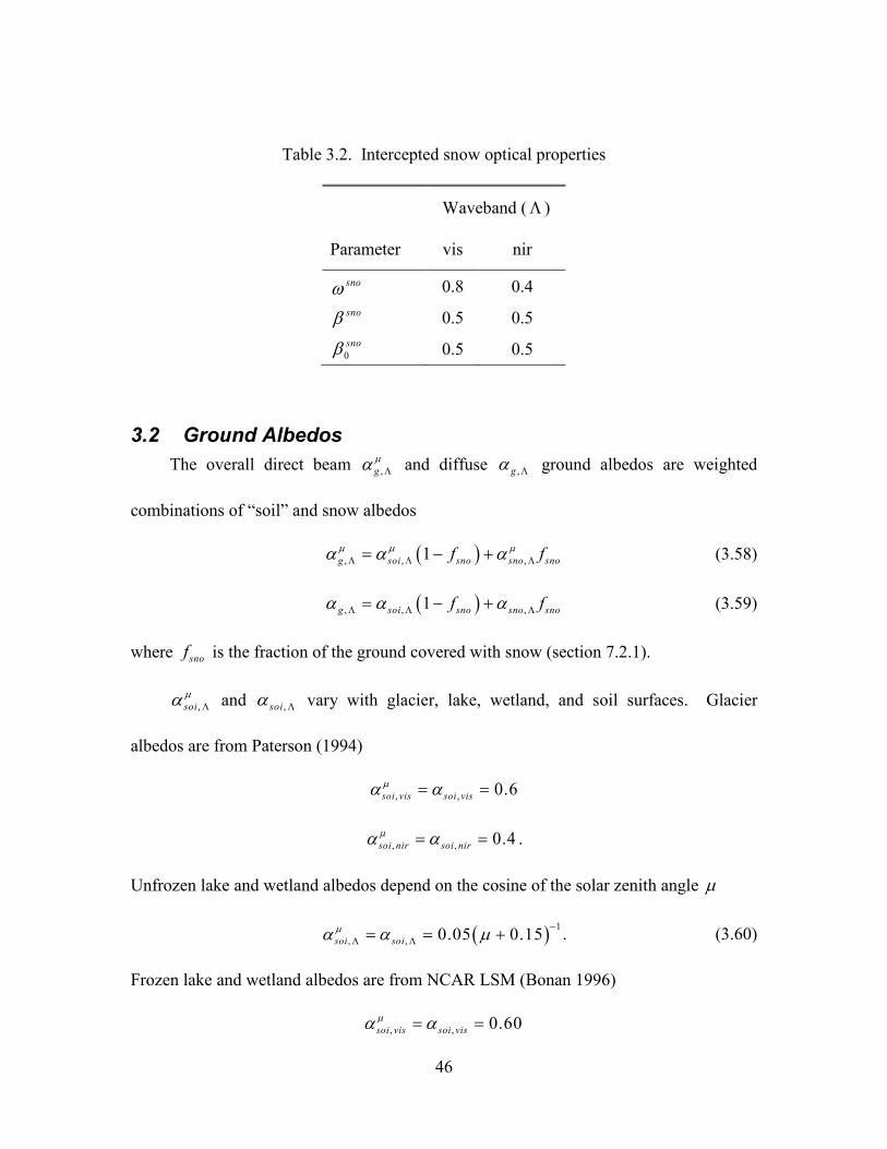
46
Table 3.2. Intercepted snow optical properties
Waveband ( Λ )
Parameter vis nir
snoω 0.8 0.4 snoβ 0.5 0.5
0snoβ 0.5 0.5
3.2 Ground Albedos The overall direct beam ,g
µα Λ and diffuse ,gα Λ ground albedos are weighted
combinations of “soil” and snow albedos
( ), , ,1g soi sno sno snof fµ µ µα α αΛ Λ Λ= − + (3.58)
( ), , ,1g soi sno sno snof fα α αΛ Λ Λ= − + (3.59)
where snof is the fraction of the ground covered with snow (section 7.2.1).
,soiµα Λ and ,soiα Λ vary with glacier, lake, wetland, and soil surfaces. Glacier
albedos are from Paterson (1994)
, , 0.6soi vis soi visµα α= =
, , 0.4soi nir soi nirµα α= = .
Unfrozen lake and wetland albedos depend on the cosine of the solar zenith angle µ
( ) 1, , 0.05 0.15soi soi
µα α µ −Λ Λ= = + . (3.60)
Frozen lake and wetland albedos are from NCAR LSM (Bonan 1996)
, , 0.60soi vis soi visµα α= =
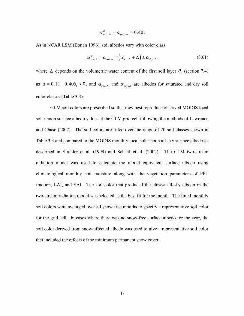
47
, , 0.40soi nir soi nirµα α= = .
As in NCAR LSM (Bonan 1996), soil albedos vary with color class
( ), , , ,soi soi sat dryµα α α αΛ Λ Λ Λ= = + ∆ ≤ (3.61)
where ∆ depends on the volumetric water content of the first soil layer 1θ (section 7.4)
as 10.11 0.40 0θ∆ = − > , and ,satα Λ and ,dryα Λ are albedos for saturated and dry soil
color classes (Table 3.3).
CLM soil colors are prescribed so that they best reproduce observed MODIS local
solar noon surface albedo values at the CLM grid cell following the methods of Lawrence
and Chase (2007). The soil colors are fitted over the range of 20 soil classes shown in
Table 3.3 and compared to the MODIS monthly local solar noon all-sky surface albedo as
described in Strahler et al. (1999) and Schaaf et al. (2002). The CLM two-stream
radiation model was used to calculate the model equivalent surface albedo using
climatological monthly soil moisture along with the vegetation parameters of PFT
fraction, LAI, and SAI. The soil color that produced the closest all-sky albedo in the
two-stream radiation model was selected as the best fit for the month. The fitted monthly
soil colors were averaged over all snow-free months to specify a representative soil color
for the grid cell. In cases where there was no snow-free surface albedo for the year, the
soil color derived from snow-affected albedo was used to give a representative soil color
that included the effects of the minimum permanent snow cover.
48
Table 3.3. Dry and saturated soil albedos
Dry Saturated Dry Saturated
Color Class vis nir vis nir Color
Class vis nir vis nir
1 0.36 0.61 0.25 0.50 11 0.24 0.37 0.13 0.26
2 0.34 0.57 0.23 0.46 12 0.23 0.35 0.12 0.24
3 0.32 0.53 0.21 0.42 13 0.22 0.33 0.11 0.22
4 0.31 0.51 0.20 0.40 14 0.20 0.31 0.10 0.20
5 0.30 0.49 0.19 0.38 15 0.18 0.29 0.09 0.18
6 0.29 0.48 0.18 0.36 16 0.16 0.27 0.08 0.16
7 0.28 0.45 0.17 0.34 17 0.14 0.25 0.07 0.14
8 0.27 0.43 0.16 0.32 18 0.12 0.23 0.06 0.12
9 0.26 0.41 0.15 0.30 19 0.10 0.21 0.05 0.10
10 0.25 0.39 0.14 0.28 20 0.08 0.16 0.04 0.08
3.2.1 Snow Albedo
Snow albedo and solar absorption within each snow layer are simulated with the
Snow, Ice, and Aerosol Radiative Model (SNICAR), which incorporates a two-stream
radiative transfer solution from Toon et al. (1989). Albedo and the vertical absorption
profile depend on solar zenith angle, albedo of the substrate underlying snow, mass
concentrations of atmospheric-deposited aerosols (black carbon, mineral dust, and
organic carbon), and ice effective grain size (re), which is simulated with a snow aging
routine described in section 3.2.3. Representation of impurity mass concentrations within
the snowpack is described in section 7.2.4. Implementation of SNICAR in CLM is also
described somewhat by Flanner and Zender (2005) and Flanner et al. (2007).
The two-stream solution requires the following bulk optical properties for each
snow layer and spectral band: extinction optical depth (τ), single-scatter albedo (ω), and
49
scattering asymmetry parameter (g). The snow layers used for radiative calculations are
identical to snow layers applied elsewhere in CLM, except for the case when snow mass
is greater than zero but no snow layers exist. When this occurs, a single radiative layer is
specified to have the column snow mass and an effective grain size of freshly-fallen snow
(section 3.2.3). The bulk optical properties are weighted functions of each constituent k,
computed for each snow layer and spectral band as
1
k
kτ τ= ∑ (3.62)
1
1
k
k k
k
k
ω τω
τ=
∑
∑ (3.63)
1
1
k
k k k
k
k k
gg
ω τ
ω τ=
∑
∑ (3.64)
For each constituent (ice, two black carbon species, two organic carbon species, and
four dust species), ω, g, and the mass extinction cross-section ψ (m2 kg-1) are computed
offline with Mie Theory, e.g., applying the computational technique from Bohren and
Huffman (1983). The extinction optical depth for each constituent depends on its mass
extinction cross-section and layer mass, wk (kg m-2) as
k k kwτ ψ= (3.65)
The two-stream solution (Toon et al. 1989) applies a tri-diagonal matrix solution to
produce upward and downward radiative fluxes at each layer interface, from which net
radiation, layer absorption, and surface albedo are easily derived. Solar fluxes are
computed in five spectral bands, listed in Table 3.4. Because snow albedo varies strongly
50
across the solar spectrum, it was determined that four bands were needed to accurately
represent the near-infrared (NIR) characteristics of snow, whereas only one band was
needed for the visible spectrum. Boundaries of the NIR bands were selected to capture
broad radiative features and maximize accuracy and computational efficiency. We
partition NIR (0.7-5.0μm) surface downwelling flux from CLM according to the weights
listed in Table 3.4, which are unique for diffuse and direct incident flux. These fixed
weights were determined with offline hyperspectral radiative transfer calculations for an
atmosphere typical of mid-latitude winter (Flanner et al. 2007). The tri-diagonal solution
includes intermediate terms that allow for easy interchange of two-stream techniques.
We apply the Eddington solution for the visible band (following Wiscombe and Warren
1980) and the hemispheric mean solution (Toon et al. 1989) for NIR bands. These
choices were made because the Eddington scheme works well for highly scattering
media, but can produce negative albedo for absorptive NIR bands with diffuse incident
flux. Delta scalings are applied to τ, ω, and g (Wiscombe and Warren 1980) in all
spectral bands, producing effective values (denoted with *) that are applied in the two-
stream solution
(3.66)
(3.67)
*
1gg
g=
+ (3.68)
* 2(1 )gτ ω τ= −
2*
2
(1 )1
gg
ωωω
−=
−
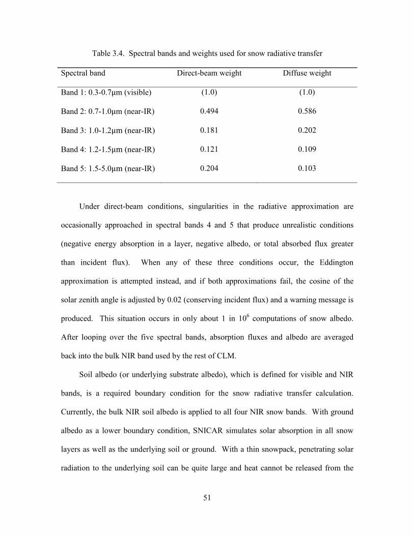
51
Table 3.4. Spectral bands and weights used for snow radiative transfer
Spectral band Direct-beam weight Diffuse weight
Band 1: 0.3-0.7μm (visible) (1.0) (1.0)
Band 2: 0.7-1.0μm (near-IR) 0.494 0.586
Band 3: 1.0-1.2μm (near-IR) 0.181 0.202
Band 4: 1.2-1.5μm (near-IR) 0.121 0.109
Band 5: 1.5-5.0μm (near-IR) 0.204 0.103
Under direct-beam conditions, singularities in the radiative approximation are
occasionally approached in spectral bands 4 and 5 that produce unrealistic conditions
(negative energy absorption in a layer, negative albedo, or total absorbed flux greater
than incident flux). When any of these three conditions occur, the Eddington
approximation is attempted instead, and if both approximations fail, the cosine of the
solar zenith angle is adjusted by 0.02 (conserving incident flux) and a warning message is
produced. This situation occurs in only about 1 in 106 computations of snow albedo.
After looping over the five spectral bands, absorption fluxes and albedo are averaged
back into the bulk NIR band used by the rest of CLM.
Soil albedo (or underlying substrate albedo), which is defined for visible and NIR
bands, is a required boundary condition for the snow radiative transfer calculation.
Currently, the bulk NIR soil albedo is applied to all four NIR snow bands. With ground
albedo as a lower boundary condition, SNICAR simulates solar absorption in all snow
layers as well as the underlying soil or ground. With a thin snowpack, penetrating solar
radiation to the underlying soil can be quite large and heat cannot be released from the
52
soil to the atmosphere in this situation. Thus, solar radiation penetration is limited to
snowpacks with total snow depth greater than or equal to 0.1 m ( 0.1snoz ≥ ) to prevent
unrealistic soil warming within a single timestep.
The radiative transfer calculation is performed twice for each column containing a
mass of snow greater than 1×10-30 kg m-2 (excluding lake and urban columns); once each
for direct-beam and diffuse incident flux. Absorption in each layer i of pure snow is
initially recorded as absorbed flux per unit incident flux on the ground ( ,sno iS ), as albedos
must be calculated for the next timestep with unknown incident flux. The snow
absorption fluxes that are used for column temperature calculations are
( ), , 1g i sno i snoS S α= − (3.69)
This weighting is performed for direct-beam and diffuse, visible and NIR fluxes. After
the ground-incident fluxes (transmitted through the vegetation canopy) have been
calculated for the current time step (sections 3.1 and 4.1), the layer absorption factors
( ,g iS ) are multiplied by the ground-incident fluxes to produce solar absorption (W m-2) in
each snow layer and the underlying ground.
3.2.2 Snowpack Optical Properties
Ice optical properties for the five spectral bands are derived offline and stored in a
namelist-defined lookup table for online retrieval (see CLM4.5 User’s Guide). Mie
properties are first computed at fine spectral resolution (470 bands), and are then
weighted into the five bands applied by CLM according to incident solar flux, ( )I λ↓ .
For example, the broadband mass-extinction cross section (ψ ) over wavelength interval
λ1 to λ2 is
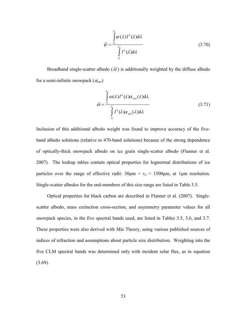
53
(3.70)
Broadband single-scatter albedo (ω ) is additionally weighted by the diffuse albedo
for a semi-infinite snowpack (αsno)
2
1
2
1
( ) ( ) ( )d
( ) ( )d
sno
sno
I
I
λ
λλ
λ
ω λ λ α λ λω
λ α λ λ
↓
↓
=∫
∫ (3.71)
Inclusion of this additional albedo weight was found to improve accuracy of the five-
band albedo solutions (relative to 470-band solutions) because of the strong dependence
of optically-thick snowpack albedo on ice grain single-scatter albedo (Flanner et al.
2007). The lookup tables contain optical properties for lognormal distributions of ice
particles over the range of effective radii: 30μm < re < 1500μm, at 1μm resolution.
Single-scatter albedos for the end-members of this size range are listed in Table 3.5.
Optical properties for black carbon are described in Flanner et al. (2007). Single-
scatter albedo, mass extinction cross-section, and asymmetry parameter values for all
snowpack species, in the five spectral bands used, are listed in Tables 3.5, 3.6, and 3.7.
These properties were also derived with Mie Theory, using various published sources of
indices of refraction and assumptions about particle size distribution. Weighting into the
five CLM spectral bands was determined only with incident solar flux, as in equation
(3.69).
2
1
2
1
( ) ( )d
( )d
I
I
λ
λλ
λ
ψ λ λ λψ
λ λ
↓
↓
=∫
∫
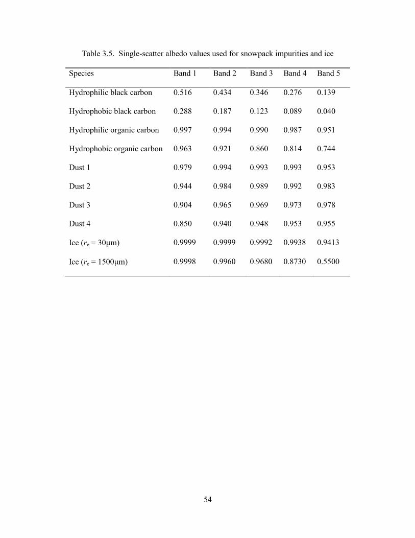
54
Table 3.5. Single-scatter albedo values used for snowpack impurities and ice
Species Band 1 Band 2 Band 3 Band 4 Band 5
Hydrophilic black carbon 0.516 0.434 0.346 0.276 0.139
Hydrophobic black carbon 0.288 0.187 0.123 0.089 0.040
Hydrophilic organic carbon 0.997 0.994 0.990 0.987 0.951
Hydrophobic organic carbon 0.963 0.921 0.860 0.814 0.744
Dust 1 0.979 0.994 0.993 0.993 0.953
Dust 2 0.944 0.984 0.989 0.992 0.983
Dust 3 0.904 0.965 0.969 0.973 0.978
Dust 4 0.850 0.940 0.948 0.953 0.955
Ice (re = 30μm) 0.9999 0.9999 0.9992 0.9938 0.9413
Ice (re = 1500μm) 0.9998 0.9960 0.9680 0.8730 0.5500
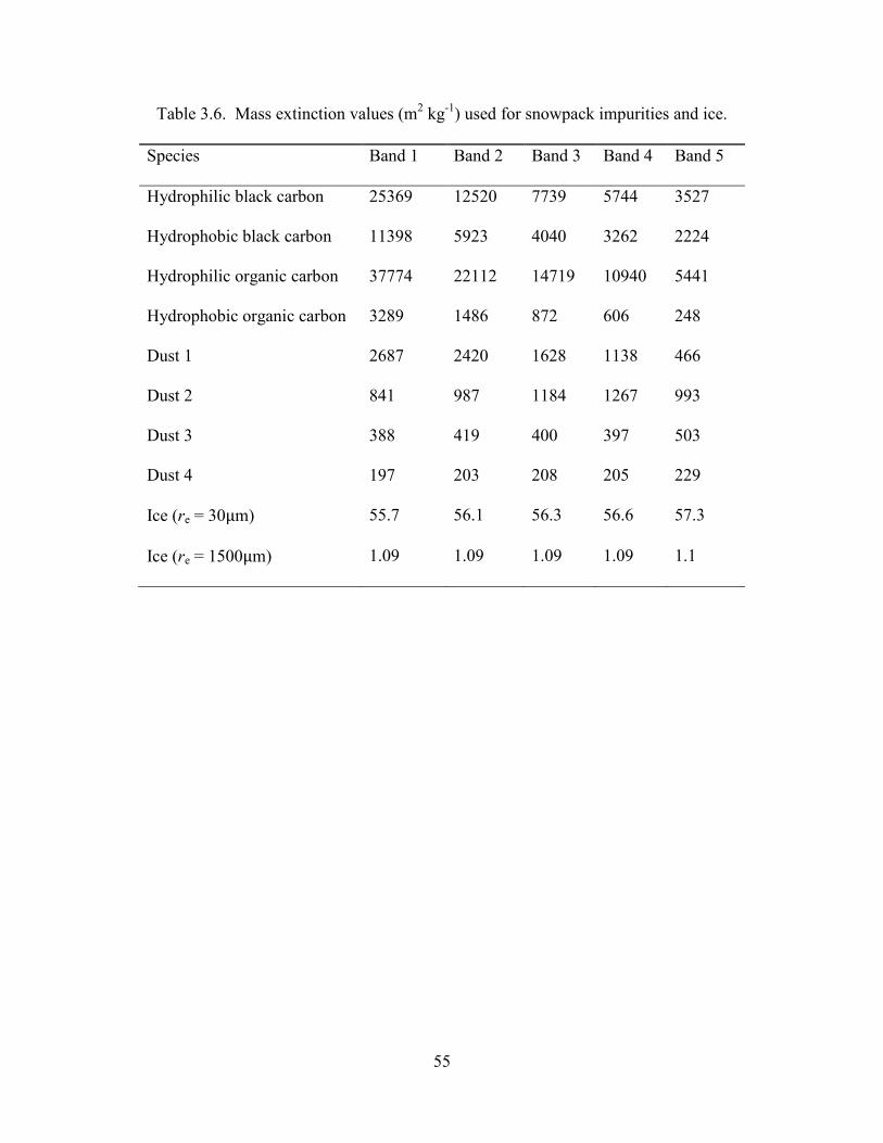
55
Table 3.6. Mass extinction values (m2 kg-1) used for snowpack impurities and ice.
Species Band 1 Band 2 Band 3 Band 4 Band 5
Hydrophilic black carbon 25369 12520 7739 5744 3527
Hydrophobic black carbon 11398 5923 4040 3262 2224
Hydrophilic organic carbon 37774 22112 14719 10940 5441
Hydrophobic organic carbon 3289 1486 872 606 248
Dust 1 2687 2420 1628 1138 466
Dust 2 841 987 1184 1267 993
Dust 3 388 419 400 397 503
Dust 4 197 203 208 205 229
Ice (re = 30μm) 55.7 56.1 56.3 56.6 57.3
Ice (re = 1500μm) 1.09 1.09 1.09 1.09 1.1
56
Table 3.7. Asymmetry scattering parameters used for snowpack impurities and ice.
Species Band 1 Band 2 Band 3 Band 4 Band 5
Hydrophilic black carbon 0.52 0.34 0.24 0.19 0.10
Hydrophobic black carbon 0.35 0.21 0.15 0.11 0.06
Hydrophilic organic carbon 0.77 0.75 0.72 0.70 0.64
Hydrophobic organic carbon 0.62 0.57 0.54 0.51 0.44
Dust 1 0.69 0.72 0.67 0.61 0.44
Dust 2 0.70 0.65 0.70 0.72 0.70
Dust 3 0.79 0.75 0.68 0.63 0.67
Dust 4 0.83 0.79 0.77 0.76 0.73
Ice (re = 30μm) 0.88 0.88 0.88 0.88 0.90
Ice (re = 1500μm) 0.89 0.90 0.90 0.92 0.97
3.2.3 Snow Aging
Snow aging is represented as evolution of the ice effective grain size (re). Previous
studies have shown that use of spheres which conserve the surface area-to-volume ratio
(or specific surface area) of ice media composed of more complex shapes produces
relatively small errors in simulated hemispheric fluxes (e.g., Grenfell and Warren 1999).
Effective radius is the surface area-weighted mean radius of an ensemble of spherical
particles and is directly related to specific surface area (SSA) as , where
ρice is the density of ice. Hence, re is a simple and practical metric for relating the
snowpack microphysical state to dry snow radiative characteristics.
3 / ( )e icer SSAρ=
57
Wet snow processes can also drive rapid changes in albedo. The presence of liquid
water induces rapid coarsening of the surrounding ice grains (e.g., Brun 1989), and liquid
water tends to refreeze into large ice clumps that darken the bulk snowpack. The
presence of small liquid drops, by itself, does not significantly darken snowpack, as ice
and water have very similar indices of refraction throughout the solar spectrum. Pooled
or ponded water, however, can significantly darken snowpack by greatly reducing the
number of refraction events per unit mass. This influence is not currently accounted for.
The net change in effective grain size occurring each time step is represented in
each snow layer as a summation of changes caused by dry snow metamorphism (dre,dry),
liquid water-induced metamorphism (dre,wet), refreezing of liquid water, and addition of
freshly-fallen snow. The mass of each snow layer is partitioned into fractions of snow
carrying over from the previous time step (fold), freshly-fallen snow (fnew), and refrozen
liquid water (frfz), such that snow re is updated each time step t as
(3.72)
Here, the effective radius of freshly-fallen snow (re,0) is fixed globally at 54.5μm
(corresponding to a specific surface area of 60 m2 kg-1), and the effective radius of
refrozen liquid water (re,rfz) is set to 1000μm.
Dry snow aging is based on a microphysical model described by Flanner and
Zender (2006). This model simulates diffusive vapor flux amongst collections of ice
crystals with various size and inter-particle spacing. Specific surface area and effective
radius are prognosed for any combination of snow temperature, temperature gradient,
density, and initial size distribution. The combination of warm snow, large temperature
gradient, and low density produces the most rapid snow aging, whereas aging proceeds
, , old ,0 new , rfrz( ) ( 1)e e e dry e wet e e rfzr t r t dr dr f r f r f = − + + + +
58
slowly in cold snow, regardless of temperature gradient and density. Because this model
is currently too computationally expensive for inclusion in climate models, we fit
parametric curves to model output over a wide range of snow conditions and apply these
parameters in CLM. The functional form of the parametric equation is
(3.73)
The parameters (dre/dt)0, η, and κ are retrieved interactively from a lookup table with
dimensions corresponding to snow temperature, temperature gradient, and density. The
domain covered by this lookup table includes temperature ranging from 223 to 273 K,
temperature gradient ranging from 0 to 300 K m-1, and density ranging from 50 to 400 kg
m-3. Temperature gradient is calculated at the midpoint of each snow layer n, using mid-
layer temperatures (Tn) and snow layer thicknesses (dzn), as
(3.74)
For the bottom snow layer ( 0n = ), Tn+1 is taken as the temperature of the top soil layer,
and for the top snow layer it is assumed that Tn-1 = Tn.
The contribution of liquid water to enhanced metamorphism is based on parametric
equations published by Brun (1989), who measured grain growth rates under different
liquid water contents. This relationship, expressed in terms of re (μm) and subtracting an
offset due to dry aging, depends on the mass liquid water fraction liqf as
(3.75)
The constant C1 is 4.22×10⁻¹³, and: / ( )liq liq liq icef w w w= + (section 7.2).
1/
,
0 ,0( )e dry e
e e
dr drdt dt r r
κη
η = − +
1 1 1 1
1 1
1 abs n n n n n n n n
n n n n n n
T dz T dz T dz T dzdTdz dz dz dz dz dz
− − + +
− +
+ + = + + +
18 31
2
104
liqe
e
C fdrdt rπ
=
59
In cases where snow mass is greater than zero, but a snow layer has not yet been
defined, re is set to re,0. When snow layers are combined or divided, re is calculated as a
mass-weighted mean of the two layers, following computations of other state variables
(section 7.2.7). Finally, the allowable range of re, corresponding to the range over which
Mie optical properties have been defined, is 30-1500μm.
3.3 Solar Zenith Angle The CLM uses the same formulation for solar zenith angle as the Community
Atmosphere Model. The cosine of the solar zenith angle µ is
(3.76)
where h is the solar hour angle (radians) (24 hour periodicity), δ is the solar declination
angle (radians), and φ is latitude (radians) (positive in Northern Hemisphere). The solar
hour angle h (radians) is
(3.77)
where d is calendar day ( 0.0d = at 0Z on January 1), and θ is longitude (radians)
(positive east of the Greenwich meridian).
The solar declination angle δ is calculated as in Berger (1978a,b) and is valid for
one million years past or hence, relative to 1950 A.D. The orbital parameters may be
specified directly or the orbital parameters are calculated for the desired year. The
required orbital parameters to be input by the user are the obliquity of the Earth ε
(degrees, 9 0 9 0ε− < < ), Earth’s eccentricity e ( 0 . 0 0 . 1e< < ), and the longitude of
the perihelion relative to the moving vernal equinox ω ( 0 360ω< <
) (unadjusted for
the apparent orbit of the Sun around the Earth (Berger et al. 1993)). The solar declination
δ (radians) is
sin sin cos cos cos hµ φ δ φ δ= −
2h dπ θ= +
60
( ) ( )1sin sin sinδ ε λ−= (3.78)
where ε is Earth’s obliquity and λ is the true longitude of the Earth.
The obliquity of the Earth ε (degrees) is
( )47
1* cos
i
i i ii
A f tε ε δ=
=
= + +∑ (3.79)
where *ε is a constant of integration (Table 3.8), iA , if , and iδ are amplitude, mean
rate, and phase terms in the cosine series expansion (Berger 1978a,b), and 0 1 9 5 0t t= −
where 0t is the year. The series expansion terms are not shown here but can be found in
the source code file shr_orb_mod.F90.
The true longitude of the Earth λ (radians) is counted counterclockwise from the
vernal equinox ( 0λ = at the vernal equinox)
( ) ( ) ( )3 2 31 5 132 sin sin 2 sin 34 4 12m m m me e e eλ λ λ ω λ ω λ ω = + − − + − + −
(3.80)
where mλ is the mean longitude of the Earth at the vernal equinox, e is Earth’s
eccentricity, and ω is the longitude of the perihelion relative to the moving vernal
equinox. The mean longitude mλ is
( )0
2365
vem m
d dπλ λ
−= + (3.81)
where 80.5ved = is the calendar day at vernal equinox (March 21 at noon), and
( )3 2 30
1 1 1 1 1 12 1 sin sin 2 sin 32 8 4 2 8 3m e e e eλ β ω β ω β ω = + + − + + +
(3.82)
where 21 eβ = − . Earth’s eccentricity e is
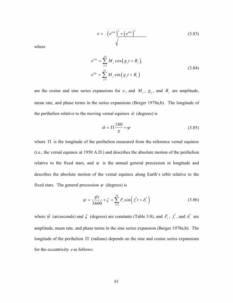
61
( ) ( )2 2cos sine e e= + (3.83)
where
( )
( )
19cos
1
19sin
1
cos ,
sin
j j jj
j j jj
e M g t B
e M g t B
=
=
= +
= +
∑
∑ (3.84)
are the cosine and sine series expansions for e , and jM , jg , and jB are amplitude,
mean rate, and phase terms in the series expansions (Berger 1978a,b). The longitude of
the perihelion relative to the moving vernal equinox ω (degrees) is
180ω ψπ
= Π + (3.85)
where Π is the longitude of the perihelion measured from the reference vernal equinox
(i.e., the vernal equinox at 1950 A.D.) and describes the absolute motion of the perihelion
relative to the fixed stars, and ψ is the annual general precession in longitude and
describes the absolute motion of the vernal equinox along Earth’s orbit relative to the
fixed stars. The general precession ψ (degrees) is
( )78
1sin
3600 i i ii
t F f tψψ ζ δ=
′ ′= + + +∑
(3.86)
where ψ (arcseconds) and ζ (degrees) are constants (Table 3.8), and iF , if ′ , and iδ ′ are
amplitude, mean rate, and phase terms in the sine series expansion (Berger 1978a,b). The
longitude of the perihelion Π (radians) depends on the sine and cosine series expansions
for the eccentricity e as follows:
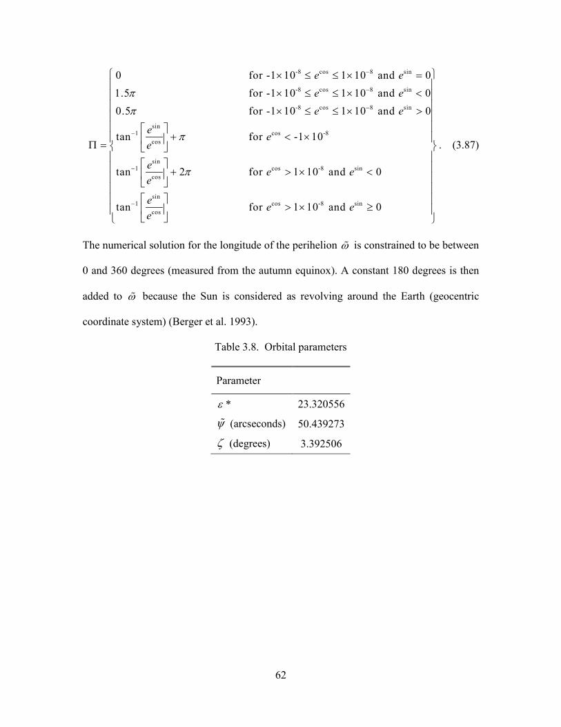
62
-8 cos 8 sin
-8 cos 8 sin
-8 cos 8 sin
sin1 cos -8
cos
sin1 cos -8 sin
cos
0 for -1 10 1 10 and 01.5 for -1 10 1 10 and 00.5 for -1 10 1 10 and 0
tan for -1 10
tan 2 for 1 10 and 0
ta
e ee ee e
e ee
e e ee
π
π
π
π
−
−
−
−
−
× ≤ ≤ × =
× ≤ ≤ × <
× ≤ ≤ × >
+ < × Π =
+ > × <
sin
1 cos -8 sincosn for 1 10 and 0e e e
e−
> × ≥
. (3.87)
The numerical solution for the longitude of the perihelion ω is constrained to be between
0 and 360 degrees (measured from the autumn equinox). A constant 180 degrees is then
added to ω because the Sun is considered as revolving around the Earth (geocentric
coordinate system) (Berger et al. 1993).
Table 3.8. Orbital parameters
Parameter
*ε 23.320556
ψ (arcseconds) 50.439273
ζ (degrees) 3.392506

63
4. Radiative Fluxes
The net radiation at the surface is ( ) ( )v g v gS S L L+ − +
, where S
is the net solar
flux absorbed by the vegetation (“v”) and the ground (“g”) and L
is the net longwave
flux (positive toward the atmosphere) (W m-2).
4.1 Solar Fluxes Figure 4.1 illustrates the direct beam and diffuse fluxes in the canopy. I µ
Λ↑ and
I Λ↑ are the upward diffuse fluxes, per unit incident direct beam and diffuse flux (section
3.1). I µΛ↓ and I Λ↓ are the downward diffuse fluxes below the vegetation per unit
incident direct beam and diffuse radiation (section 3.1). The direct beam flux transmitted
through the canopy, per unit incident flux, is ( )K L Se− + . I µΛ
and IΛ
are the fluxes absorbed
by the vegetation, per unit incident direct beam and diffuse radiation (section 3.1). ,gµα Λ
and ,gα Λ are the direct beam and diffuse ground albedos (section 3.2). L and S are the
exposed leaf area index and stem area index (section 2.1.4). K is the optical depth of
direct beam per unit leaf and stem area (section 3.1).
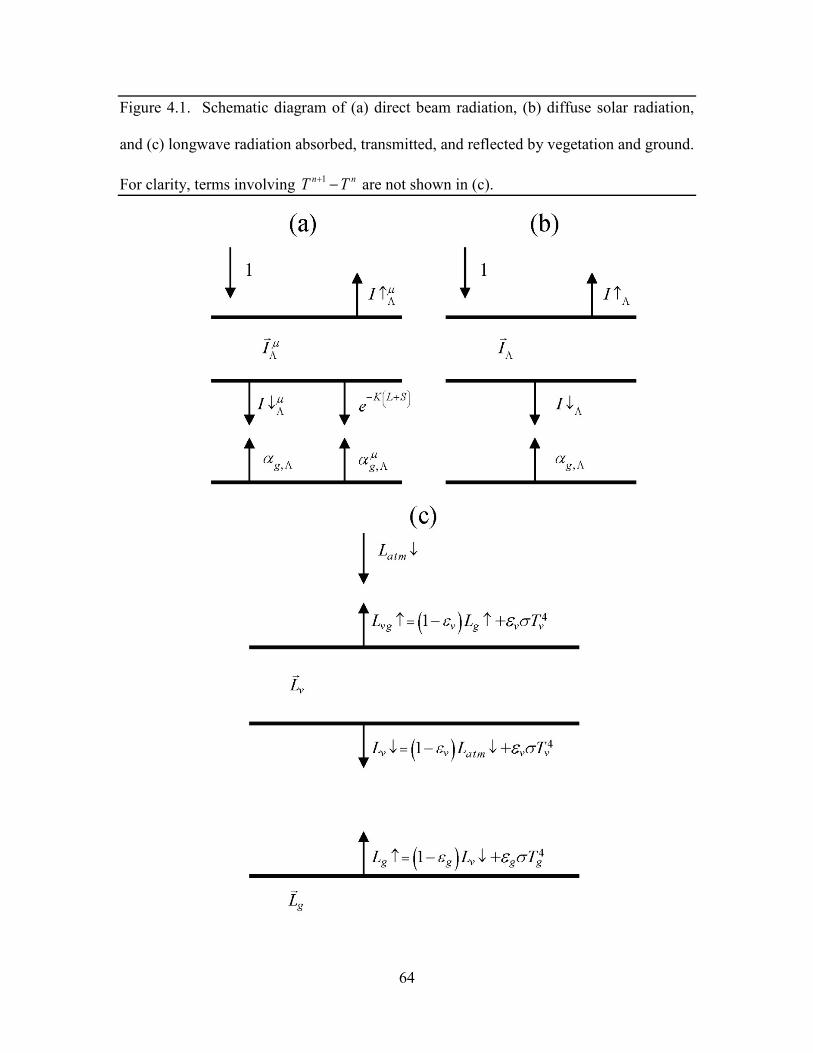
64
Figure 4.1. Schematic diagram of (a) direct beam radiation, (b) diffuse solar radiation,
and (c) longwave radiation absorbed, transmitted, and reflected by vegetation and ground.
For clarity, terms involving 1n nT T+ − are not shown in (c).
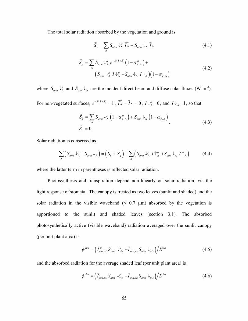
65
The total solar radiation absorbed by the vegetation and ground is
v atm atmS S I S IµµΛ ΛΛ Λ
Λ
↓ ↓= +∑
(4.1)
(4.2)
where atmS µΛ↓ and atmS Λ↓ are the incident direct beam and diffuse solar fluxes (W m-2).
For non-vegetated surfaces, ( ) 1K L Se− + = , 0I IµΛ Λ= =
, 0I µΛ↓ = , and 1I Λ↓ = , so that
( ) ( ), ,1 1
0
g atm g atm g
v
S S S
S
µ µα αΛ Λ Λ ΛΛ
↓ ↓= − + −
=
∑
. (4.3)
Solar radiation is conserved as
(4.4)
where the latter term in parentheses is reflected solar radiation.
Photosynthesis and transpiration depend non-linearly on solar radiation, via the
light response of stomata. The canopy is treated as two leaves (sunlit and shaded) and the
solar radiation in the visible waveband (< 0.7 µm) absorbed by the vegetation is
apportioned to the sunlit and shaded leaves (section 3.1). The absorbed
photosynthetically active (visible waveband) radiation averaged over the sunlit canopy
(per unit plant area) is
( ), ,sun sun
sun vis atm vis sun vis atm visI S I S Lµ µφ ↓ ↓= +
(4.5)
and the absorbed radiation for the average shaded leaf (per unit plant area) is
( ), ,sha sha
sha vis atm vis sha vis atm visI S I S Lµ µφ ↓ ↓= +
(4.6)
( ) ( )( ) ( )
,
,
1
1
K L Sg atm g
atm atm g
S S e
S I S I
µ µ
µ µ
α
α
− +Λ Λ
Λ
Λ Λ Λ Λ Λ
↓
↓ ↓ ↓ ↓
= − +
+ −
∑
( ) ( ) ( )atm atm v g atm atmS S S S S I S Iµ µ µΛ Λ Λ Λ Λ Λ
Λ Λ
↓ ↓ ↓ ↑ ↓ ↑+ = + + +∑ ∑
66
with sunL and shaL the sunlit and shaded plant area index, respectively. The sunlit plant
area index is
( )1 K L S
sun eLK
− +−= (4.7)
and the shaded leaf area index is ( )sha sunL L S L= + − . In calculating sunL ,
(4.8)
where ( )G µ and µ are parameters in the two-stream approximation (section 3.1).
The model uses the two-stream approximation to calculate radiative transfer of
direct and diffuse radiation through a canopy that is differentiated into leaves that are
sunlit and those that are shaded (section 3.1). The two-stream equations are integrated
over all plant area (leaf and stem area) in the canopy. The model has an optional (though
not supported) multi-layer canopy, as described by Bonan et al. (2012). The multi-layer
model is only intended to address the non-linearity of light profiles, photosynthesis, and
stomatal conductance in the plant canopy.
In the multi-layer canopy, canopy-integrated radiative fluxes are calculated from
the two-stream approximation. The model additionally derives the light profile with depth
in the canopy by taking the derivatives of the absorbed radiative fluxes with respect to
plant area index ( L L S′ = + ) and evaluating them incrementally through the canopy with
cumulative plant area index ( x ). The terms , ( )sundI x dLµΛ ′
and , ( )sundI x dLΛ ′
are the
direct beam and diffuse solar radiation, respectively, absorbed by the sunlit fraction of the
canopy (per unit plant area) at a depth defined by the cumulative plant area index x ;
, ( )shadI x dLµΛ ′
and , ( )shadI x dLΛ ′
are the corresponding fluxes for the shaded fraction of
( )GK
µµ
=
67
the canopy at depth x . These fluxes are normalized by the sunlit or shaded fraction at
depth x , defined by ( )expsunf Kx= − , to give fluxes per unit sunlit or shaded plant area
at depth x .
4.2 Longwave Fluxes The net longwave radiation (W m-2) (positive toward the atmosphere) at the surface
is
atmL L L↑ ↓= −
(4.9)
where L ↑ is the upward longwave radiation from the surface and atmL ↓ is the
downward atmospheric longwave radiation (W m-2). The radiative temperature r a dT (K)
is defined from the upward longwave radiation as
1 4
radLTσ
↑ =
(4.10)
where σ is the Stefan-Boltzmann constant (W m-2 K-4) (Table 2.6). With reference to
Figure 4.1, the upward longwave radiation from the surface to the atmosphere is
( ) ( )
( ) ( ) ( ) ( )4 3 1
1 1
1 4
veg vg veg g atm
n n n nveg g g g g g g
L L L
T T T T
δ δ ε
δ ε σ ε σ +
↑= ↑ + ↓ +− −
− + − (4.11)
where vgL ↑ is the upward longwave radiation from the vegetation/soil system for
exposed leaf and stem area 0.05L S+ ≥ , vegδ is a step function and is zero for
0.05L S+ < and one otherwise, gε is the ground emissivity, and 1ngT + and n
gT are the
snow/soil surface temperatures at the current and previous time steps, respectively
(Chapter 6).
For non-vegetated surfaces, the above equation reduces to
68
( ) ( ) ( ) ( )4 3 11 4n n n ng atm g g g g g gL L T T T Tε ε σ ε σ +↑= ↓ +− + − (4.12)
where the first term is the atmospheric longwave radiation reflected by the ground, the
second term is the longwave radiation emitted by the ground, and the last term is the
increase (decrease) in longwave radiation emitted by the ground due to an increase
(decrease) in ground temperature.
For vegetated surfaces, the upward longwave radiation from the surface reduces to
( ) ( )3 14 n n nvg g g g gL L T T Tε σ +↑= ↑ + − (4.13)
where
( ) ( ) ( )
( ) ( ) ( ) ( )( ) ( )
( ) ( ) ( )
( )( ) ( ) ( )
( ) ( )( ) ( ) ( ) ( )
( ) ( )
3 1
4
4
4
3 1
3 1
4
1 1 1
1 1 1 4
1
1 1 1
1 1
4
4 1 1
1
vg g v v atm
n n n nv g v v v v v
ng v g
g v v atm
nv v
nv g v v
n n nv v v v
n n nv g v v v v
ng v g
L L
T T T T
T
L
T
T
T T T
T T T
T
ε ε ε
ε ε ε σ
ε ε σ
ε ε ε
ε σ
ε ε ε σ
ε σ
ε ε ε σ
ε ε σ
+
+
+
↑ ↓
↓
= − − −
+ + − − + −
+ −
= − − −
+
+ − −
+ −
+ − − −
+ −
(4.14)
where vε is the vegetation emissivity and 1nvT + and n
vT are the vegetation temperatures at
the current and previous time steps, respectively (Chapter 5). The first term in the
equation above is the atmospheric longwave radiation that is transmitted through the
canopy, reflected by the ground, and transmitted through the canopy to the atmosphere.
The second term is the longwave radiation emitted by the canopy directly to the
atmosphere. The third term is the longwave radiation emitted downward from the
69
canopy, reflected by the ground, and transmitted through the canopy to the atmosphere.
The fourth term is the increase (decrease) in longwave radiation due to an increase
(decrease) in canopy temperature that is emitted by the canopy directly to the atmosphere.
The fifth term is the increase (decrease) in longwave radiation due to an increase
(decrease) in canopy temperature that is emitted downward from the canopy, reflected
from the ground, and transmitted through the canopy to the atmosphere. The last term is
the longwave radiation emitted by the ground and transmitted through the canopy to the
atmosphere.
The upward longwave radiation from the ground is
( ) ( )41 n
g g v g gL L Tε ε σ↑= ↓ +− (4.15)
where vL ↓ is the downward longwave radiation below the vegetation
( ) ( ) ( ) ( )4 3 11 4n n n nv v atm v v v v v vL L T T T Tε ε σ ε σ +↓= ↓ +− + − . (4.16)
The net longwave radiation flux for the ground is (positive toward the atmosphere)
( ) ( )41n
g g g veg g v veg g atmL T L Lε σ δ ε δ ε= ↓ − ↓− −
. (4.17)
The above expression for gL
is the net longwave radiation forcing that is used in the soil
temperature calculation (Chapter 6). Once updated soil temperatures have been obtained,
the term ( ) ( )3 14 n n ng g g gT T Tε σ + − is added to gL
to calculate the ground heat flux (section
5.4)
The net longwave radiation flux for vegetation is (positive toward the atmosphere)
( ) ( ) ( ) ( ) ( )442 1 1 1 1nv v g v v v g g v g v atmL T T Lε ε ε σ ε ε σ ε ε ε ↓ = − − − − + − −
. (4.18)
70
These equations assume that absorptivity equals emissivity. The emissivity of the
ground is
( )1g soi sno sno snof fε ε ε= − + (4.19)
where 0.96soiε = for soil, 0.97 for glacier, and 0.96 for wetland, 0.97snoε = , and snof is
the fraction of ground covered by snow (section 7.2.1). The vegetation emissivity is
( )1 L Sv e µε − += − (4.20)
where L and S are the leaf and stem area indices (section 2.1.4) and 1µ = is the
average inverse optical depth for longwave radiation.
71
5. Momentum, Sensible Heat, and Latent Heat Fluxes
The zonal xτ and meridional yτ momentum fluxes (kg m-1 s-2), sensible heat flux H
(W m-2), and water vapor flux E (kg m-2 s-1) between the atmosphere at reference height
,atm xz (m) [where x is height for wind (momentum) ( m ), temperature (sensible heat) ( h
), and humidity (water vapor) ( w ); with zonal and meridional winds atmu and atmv (m s-
1), potential temperature atmθ (K), and specific humidity atmq (kg kg-1)] and the surface
[with su , sv , sθ , and sq ] are
( )atm s
x atmam
u ur
τ ρ−
= − (5.1)
( )atm s
y atmam
v vr
τ ρ−
= − (5.2)
( )atm s
atm pah
H Cr
θ θρ
−= − (5.3)
( )atm s
atmaw
q qE
rρ
−= − . (5.4)
These fluxes are derived in the next section from Monin-Obukhov similarity theory
developed for the surface layer (i.e., the nearly constant flux layer above the surface
sublayer). In this derivation, su and sv are defined to equal zero at height 0mz d+ (the
apparent sink for momentum) so that amr is the aerodynamic resistance (s m-1) for
momentum between the atmosphere at height ,atm mz and the surface at height 0mz d+ .
Thus, the momentum fluxes become
72
atmx atm
am
ur
τ ρ= − (5.5)
atmy atm
am
vr
τ ρ= − . (5.6)
Likewise, sθ and sq are defined at heights 0hz d+ and 0wz d+ (the apparent sinks for
heat and water vapor, respectively). Consequently, ahr and awr are the aerodynamic
resistances (s m-1) to sensible heat and water vapor transfer between the atmosphere at
heights ,atm hz and ,atm wz and the surface at heights 0hz d+ and 0wz d+ , respectively.
The specific heat capacity of air pC (J kg-1 K-1) is a constant (Table 2.6). The
atmospheric potential temperature used here is
,atm atm d atm hT zθ = + Γ (5.7)
where atmT is the air temperature (K) at height ,atm hz and 0.0098dΓ = K m-1 is the
negative of the dry adiabatic lapse rate [this expression is first-order equivalent to
( ) da pR C
atm atm srf atmT P Pθ = (Stull 1988), where srfP is the surface pressure (Pa), atmP is
the atmospheric pressure (Pa), and daR is the gas constant for dry air (J kg-1 K-1) (Table
2.6)]. By definition, s sTθ = . The density of moist air (kg m-3) is
0.378atm atmatm
da atm
P eR T
ρ −= (5.8)
where the atmospheric vapor pressure atme (Pa) is derived from the atmospheric specific
humidity atmq
0.622 0.378
atm atmatm
atm
q Peq
=+
. (5.9)

73
5.1 Monin-Obukhov Similarity Theory The surface vertical kinematic fluxes of momentum u w′ ′ and v w′ ′ (m2 s-2),
sensible heat wθ ′ ′ (K m s-1), and latent heat q w′ ′ (kg kg-1 m s-1), where u′ , v′ , w′ , θ ′ ,
and q′ are zonal horizontal wind, meridional horizontal wind, vertical velocity, potential
temperature, and specific humidity turbulent fluctuations about the mean, are defined
from Monin-Obukhov similarity applied to the surface layer. This theory states that when
scaled appropriately, the dimensionless mean horizontal wind speed, mean potential
temperature, and mean specific humidity profile gradients depend on unique functions of
z dL
ζ −= (Zeng et al. 1998) as
( ) ( )m
k z du z
φ ζ∗
∂−=
∂u
(5.10)
( ) ( )h
k z dzθ φ ζ
θ∗
− ∂=
∂ (5.11)
( ) ( )w
k z d qq z
φ ζ∗
− ∂=
∂ (5.12)
where z is height in the surface layer (m), d is the displacement height (m), L is the
Monin-Obukhov length scale (m) that accounts for buoyancy effects resulting from
vertical density gradients (i.e., the atmospheric stability), k is the von Karman constant
(Table 2.6), and u is the atmospheric wind speed (m s-1). mφ , hφ , and wφ are universal
(over any surface) similarity functions of ζ that relate the constant fluxes of momentum,
sensible heat, and latent heat to the mean profile gradients of u , θ , and q in the surface
74
layer. In neutral conditions, 1m h wφ φ φ= = = . The velocity (i.e., friction velocity) u∗ (m
s-1), temperature θ∗ (K), and moisture q∗ (kg kg-1) scales are
( ) ( )2 22
atm
u u w v wρ∗ ′ ′ ′ ′= + =τ
(5.13)
atm p
Hu wC
θ θρ∗ ∗ ′ ′= − = − (5.14)
atm
Eq u q wρ∗ ∗ ′ ′= − = − (5.15)
where τ is the shearing stress (kg m-1 s-2), with zonal and meridional components
x
atm
u w τρ
′ ′ = − and y
atm
v wτρ
′ ′ = − , respectively, H is the sensible heat flux (W m-2) and E
is the water vapor flux (kg m-2 s-1).
The dimensionless length scale L is the Monin-Obukhov length defined as
23
,
,
v atm
vv
v atm
uuLkggk w
θθ
θθ
∗∗
∗
= − =
′ ′
(5.16)
where g is the acceleration of gravity (m s-2) (Table 2.6), and ( ), 1 0.61v atm atm atmqθ θ= +
is the reference virtual potential temperature. 0L > indicates stable conditions. 0L <
indicates unstable conditions. L = ∞ for neutral conditions. The temperature scale vθ ∗ is
defined as
( )1 0.61 0.61v atm atmu q q uθ θ θ∗ ∗ ∗ ∗ ∗ = + + (5.17)
where atmθ is the atmospheric potential temperature.
75
Following Panofsky and Dutton (1984), the differential equations for ( )mφ ζ ,
( )hφ ζ , and ( )wφ ζ can be integrated formally without commitment to their exact forms.
Integration between two arbitrary heights in the surface layer 2z and 1z ( 2 1z z> ) with
horizontal winds 1
u and 2
u , potential temperatures 1θ and 2θ , and specific humidities
1q and 2q results in
2 2 12 1
1
ln m mu z d z d z dk z d L L
ψ ψ∗ − − − − = − + −
u u (5.18)
2 2 12 1
1
ln h hz d z d z d
k z d L Lθθ θ ψ ψ∗
− − − − = − + − (5.19)
2 2 12 1
1
ln w wq z d z d z dq qk z d L L
ψ ψ∗ − − − − = − + −
. (5.20)
The functions ( )mψ ζ , ( )hψ ζ , and ( )wψ ζ are defined as
( ) ( )0
1m
mm z L
xdx
xζ φ
ψ ζ− = ∫ (5.21)
( ) ( )0
1h
hh z L
xdx
xζ φ
ψ ζ− = ∫ (5.22)
( ) ( )0
1w
ww z L
xdx
xζ φ
ψ ζ− = ∫ (5.23)
where 0mz , 0hz , and 0wz are the roughness lengths (m) for momentum, sensible heat, and
water vapor, respectively.
Defining the surface values
1 010 at ,mz z d= = +u
76
1 1 0 at , ands hz z dθ θ= = +
1 1 0 at ,s wq q z z d= = +
and the atmospheric values at 2 ,atm xz z=
2 2 22
= 1,a atm atm cV u v U= + + ≥u (5.24)
2 , andatmθ θ=
2 , atmq q=
the integral forms of the flux-gradient relations are
, , 0
0
ln atm m atm m ma m m
m
z d z d zuVk z L L
ψ ψ∗ − − = − +
(5.25)
, , 0
0
ln atm h atm h hatm s h h
h
z d z d zk z L L
θθ θ ψ ψ∗ − − − = − +
(5.26)
, , 0
0
ln atm w atm w watm s w w
w
z d z d zqq qk z L L
ψ ψ∗ − − − = − +
. (5.27)
The constraint 1aV ≥ is required simply for numerical reasons to prevent H and E from
becoming small with small wind speeds. The convective velocity cU accounts for the
contribution of large eddies in the convective boundary layer to surface fluxes as follows
0 0 (stable)
0 (unstable)c
c
UU w
ζβ ζ∗
= ≥= <
(5.28)
where w∗ is the convective velocity scale
1 3
,
v i
v atm
gu zw θθ
∗ ∗∗
−=
, (5.29)
1000iz = is the convective boundary layer height (m), and 1β = .
77
The momentum flux gradient relations are (Zeng et al. 1998)
( ) ( )( ) ( )( )( )
1 32 3
1 4
0.7 for 1.574 (very unstable)
1 16 for -1.574 0 (unstable)
1 5 for 0 1 (stable)
5 for >1 (very stable).
m
m
m
m
kφ ζ ζ ζ
φ ζ ζ ζ
φ ζ ζ ζ
φ ζ ζ ζ
−
= − < −
= − ≤ <
= + ≤ ≤
= +
(5.30)
The sensible and latent heat flux gradient relations are (Zeng et al. 1998)
( ) ( ) ( )( ) ( ) ( )( ) ( )( ) ( )
1 34 3
1 2
0.9 for 0.465 (very unstable)
1 16 for -0.465 0 (unstable)
1 5 for 0 1 (stable)
5 for >1 (very stable).
h w
h w
h w
h w
kφ ζ φ ζ ζ ζ
φ ζ φ ζ ζ ζ
φ ζ φ ζ ζ ζ
φ ζ φ ζ ζ ζ
−
−
= = − < −
= = − ≤ <
= = + ≤ ≤
= = +
(5.31)
To ensure continuous functions of ( )mφ ζ , ( )hφ ζ , and ( )wφ ζ , the simplest approach
(i.e., without considering any transition regimes) is to match the relations for very
unstable and unstable conditions at 1.574mζ = − for ( )mφ ζ and 0.465h wζ ζ= = − for
( ) ( )h wφ ζ φ ζ= (Zeng et al. 1998). The flux gradient relations can be integrated to yield
wind profiles for the following conditions:
Very unstable ( )1 . 5 7 4ζ < −
( ) ( ) ( )1 3 1 3 0*
0
ln 1.14m ma m m m m
m
L zuVk z L
ζ ψ ζ ζ ζ ψ = − + − − − +
(5.32)
Unstable ( )1 . 5 7 4 0ζ− ≤ <
( ), 0*
0
ln atm m ma m m
m
z d zuVk z L
ψ ζ ψ − = − +
(5.33)
Stable ( )0 1ζ≤ ≤
78
, 0*
0
ln 5 5atm m ma
m
z d zuVk z L
ζ − = + −
(5.34)
Very stable ( )1ζ >
[ ] 0*
0
ln 5 5 ln 1 5 ma
m
zu LVk z L
ζ ζ = + + + − −
(5.35)
where
( )2
11 12 ln ln 2 tan2 2 2m
x x x πψ ζ − + + = + − +
(5.36)
and ( )1 41 16x ζ= − .
The potential temperature profiles are:
Very unstable ( )0 . 4 6 5ζ < −
( ) ( ) ( )1 3 1 3 0*
0
ln 0.8h hatm s h h h h
h
L zk z L
ζθθ θ ψ ζ ζ ζ ψ− − − = − + − − − + (5.37)
Unstable ( )0 . 4 6 5 0ζ− ≤ <
( ), 0*
0
ln atm h hatm s h h
h
z d zk z Lθθ θ ψ ζ ψ
− − = − +
(5.38)
Stable ( )0 1ζ≤ ≤
, 0*
0
ln 5 5atm h hatm s
h
z d zk z Lθθ θ ζ
− − = + −
(5.39)
Very stable ( )1ζ >
79
[ ] 0*
0
ln 5 5 ln 1 5 hatm s
h
zLk z Lθθ θ ζ ζ
− = + + + − −
. (5.40)
The specific humidity profiles are:
Very unstable ( )0 . 4 6 5ζ < −
( ) ( ) ( )1 3 1 3 0*
0
ln 0.8w watm s w w w w
w
L zqq qk z L
ζ ψ ζ ζ ζ ψ− − − = − + − − − + (5.41)
Unstable ( )0 . 4 6 5 0ζ− ≤ <
( ), 0*
0
ln atm w watm s w w
w
z d zqq qk z L
ψ ζ ψ − − = − +
(5.42)
Stable ( )0 1ζ≤ ≤
, 0*
0
ln 5 5atm w watm s
w
z d zqq qk z L
ζ − − = + −
(5.43)
Very stable ( )1ζ >
[ ] 0*
0
ln 5 5 ln 1 5 watm s
w
zq Lq qk z L
ζ ζ − = + + + − −
(5.44)
where
( ) ( )212 ln
2h wxψ ζ ψ ζ
+= =
. (5.45)
Using the definitions of u∗ , θ∗ , and q∗ , an iterative solution of these equations can
be used to calculate the surface momentum, sensible heat, and water vapor flux using
atmospheric and surface values for u , θ , and q except that L depends on u∗ , θ∗ , and
q∗ . However, the bulk Richardson number
80
( ),, ,2
,
atm mv atm v siB
av atm
g z dR
Vθ θ
θ
−−= (5.46)
is related to ζ (Arya 2001) as
( ) ( )2
, ,
0 0
l n l na t m h a t m mi B h m
h m
z d z dR
z zζ ψ ζ ψ ζ
− − −
= − −
. (5.47)
Using ( ) 1 22 1 1 6h mφ φ ζ −= = − for unstable conditions and 1 5h mφ φ ζ= = + for stable
conditions to determine ( )mψ ζ and ( )hψ ζ , the inverse relationship ( )i Bf Rζ = can be
solved to obtain a first guess for ζ and thus L from
( )
,
0
,
0
ln0.01 2 for 0 (neutral or stable)
1 5 min , 0.19
ln 100 0.01 for 0 (unstable)
atm miB
miB
iB
atm miB iB
m
z dR
zR
R
z dR R
z
ζ ζ
ζ ζ
− = ≤ ≤ ≥
−
− = − ≤ ≤ − <
. (5.48)
Upon iteration (section 5.3.2), the following is used to determine ζ and thus L
( ),
2,
atm m v
v atm
z d kg
u
θζ
θ∗
∗
−= (5.49)
where
0.01 2 for 0 (neutral or stable)-100 -0.01 for 0 (unstable)
ζ ζζ ζ
≤ ≤ ≥≤ ≤ <
.
The difference in virtual potential air temperature between the reference height and the
surface is
( ) ( ) ( ), , 1 0.61 0.61v atm v s atm s atm atm atm sq q qθ θ θ θ θ− = − + + − . (5.50)
The momentum, sensible heat, and water vapor fluxes between the surface and the
atmosphere can also be written in the form
81
( )atm s
x atmam
u ur
τ ρ−
= − (5.51)
( )atm s
y atmam
v vr
τ ρ−
= − (5.52)
( )atm s
atm pah
H Cr
θ θρ
−= − (5.53)
( )atm s
atmaw
q qE
rρ
−= − (5.54)
where the aerodynamic resistances (s m-1) are
2
, , 02 2
0
1 ln atm m atm ma mam m m
a m
z d z dV zru k V z L L
ψ ψ∗
− − = = − +
(5.55)
, , 02
0
, , 0
0
1 ln
ln
atm m atm matm s mah m m
a m
atm h atm h hh h
h
z d z d zru k V z L L
z d z d zz L L
θ θ ψ ψθ
ψ ψ
∗ ∗
− − − = = − +
− − − +
(5.56)
, , 02
0
, , 0
0
1 ln
ln
atm m atm matm s maw m m
a m
atm w atm w ww w
w
z d z dq q zrq u k V z L L
z d z d zz L L
ψ ψ
ψ ψ
∗ ∗
− − − = = − +
− − − +
. (5.57)
A 2-m height “screen” temperature is useful for comparison with observations
0 0 02
0
2 2ln h h hm s h h
h
z z zTk z L L
θθ ψ ψ∗ + + = + − +
(5.58)
where for convenience, “2-m” is defined as 2 m above the apparent sink for sensible heat
( 0hz d+ ). Similarly, a 2-m height specific humidity is defined as
82
0 0 02
0
2 2ln w w wm s w w
w
z z zqq qk z L L
ψ ψ∗ + + = + − +
. (5.59)
Relative humidity is
2
22 min 100, 100
m
mm T
sat
qRHq
= ×
(5.60)
where 2mTsatq is the saturated specific humidity at the 2-m temperature 2mT (section 5.5).
A 10-m wind speed is calculated as (note that this is not consistent with the 10-m
wind speed calculated for the dust model as described in Chapter 24)
,
10 , , 0,
0
10
10ln 1010
a atm m
m atm m atm m ma m m atm m
m
V z
u z d z d zuV zk z L L
ψ ψ∗
≤
= − − + − − + > +
(5.61)
5.2 Sensible and Latent Heat Fluxes for Non-Vegetated Surfaces
Surfaces are considered non-vegetated for the surface flux calculations if leaf plus
stem area index 0.05L S+ < (section 2.1.4). By definition, this includes bare soil,
wetlands, and glaciers. The solution for lakes is described in Chapter 9. For these
surfaces, the surface may be exposed to the atmosphere, snow covered, and/or surface
water covered, so that the sensible heat flux gH (W m-2) is, with reference to Figure 5.1,
( )2 2 21g sno h osfc soil sno snow h osfc h osfcH f f H f H f H= − − + + (5.62)
where ( )21 sno h osfcf f− − , snof , and 2h osfcf are the exposed, snow covered, and surface
water covered fractions of the grid cell. The individual fluxes based on the temperatures
of the soil 1T , snow 1snlT + , and surface water 2h osfcT are
83
( )1atmsoil atm p
ah
TH C
rθ
ρ−
= − (5.63)
( )1atm snlsno atm p
ah
TH C
rθ
ρ +−= − (5.64)
( )2
2atm h osfc
h osfc atm pah
TH C
rθ
ρ−
= − (5.65)
where a t mρ is the density of atmospheric air (kg m-3), pC is the specific heat capacity of
air (J kg-1 K-1) (Table 2.6), a t mθ is the atmospheric potential temperature (K), and a hr is
the aerodynamic resistance to sensible heat transfer (s m-1).
The water vapor flux gE (kg m-2 s-1) is, with reference to Figure 5.2,
( )2 2 21g sno h osfc soil sno snow h osfc h osfcE f f E f E f E= − − + + (5.66)
( )soi atm atm soilsoil
aw
q qE
rβ ρ −
= − (5.67)
( )atm atm snosno
aw
q qE
rρ −
= − (5.68)
( )22
atm atm h osfch osfc
aw
q qE
rρ −
= − (5.69)
where soiβ is an empirical function of soil water (Sakaguchi and Zeng 2009), a t mq is the
atmospheric specific humidity (kg kg-1), s o i lq , s n oq , and 2h o s f cq are the specific
humidities (kg kg-1) of the soil, snow, and surface water, respectively, and a wr is the
aerodynamic resistance to water vapor transfer (s m-1). The specific humidities of the
snow s n oq and surface water 2h o s f cq are assumed to be at the saturation specific humidity
of their respective temperatures
84
1snlT
sno satq q += (5.70)
2
2h osfcT
h osfc satq q= (5.71)
The specific humidity of the soil surface s o i lq is assumed to be proportional to the
saturation specific humidity
1Tsoil soil satq qα= (5.72)
where 1Tsatq is the saturated specific humidity at the soil surface temperature 1T (section
5.5). The factor s o i lα is a function of the surface soil water matric potential ψ as in
Philip (1957)
13
1
exp1 10soil
wv
gR T
ψα
= × (5.73)
where w vR is the gas constant for water vapor (J kg-1 K-1) (Table 2.6), g is the
gravitational acceleration (m s-2) (Table 2.6), and 1ψ is the soil water matric potential of
the top soil layer (mm). The soil water matric potential 1ψ is
1 81 ,1 1 1 10B
sat sψ ψ −= ≥ − × (5.74)
where ,1satψ is the saturated matric potential (mm) (section 7.4.1), 1B is the Clapp and
Hornberger (1978) parameter (section 7.4.1), and 1s is the wetness of the top soil layer
with respect to saturation. The surface wetness 1s is a function of the liquid water and
ice content
,1 ,11 1
1 ,1
1 0.01 1.0liq ice
sat liq ice
w ws s
z θ ρ ρ
= + ≤ ≤ ∆
(5.75)
85
where 1z∆ is the thickness of the top soil layer (m), liqρ and iceρ are the density of liquid
water and ice (kg m-3) (Table 2.6), ,1liqw and ,1icew are the mass of liquid water and ice of
the top soil layer (kg m-2) (Chapter 7), and ,1satθ is the saturated volumetric water content
(i.e., porosity) of the top soil layer (mm3 mm-3) (section 7.4.1). If 1Ts a t a t mq q> and
a t m s o i lq q> , then s o i l a t mq q= and 0s o i ld qd T
= . This prevents large increases (decreases) in
s o i lq for small increases (decreases) in soil moisture in very dry soils.
The function soiβ ranges from 0 to 1 and is intended to represent the molecular
diffusion process from the soil pore to the surface within the dry part of the soil
(Sakaguchi and Zeng 2009) as
( )
1 ,1
2
12 2 1 ,1
,1
1 or 0
0.25 1 1 cos
fc atm soil
soisno h osfc sno h osfc fc
fc
q q
f f f f
θ θ
β θπ θ θθ
≥ − > =
− − − + + <
.(5.76)
where ,1fcθ is the field capacity of the top soil layer and 1 ,10.01 1fcθ θ≤ ≤ . The
volumetric water content of the top soil layer (mm3 mm-3) is
,1 ,11
1
1 liq ice
liq ice
w wz
θρ ρ
= +
∆ . (5.77)
The volumetric water content at field capacity is derived by assuming a hydraulic
conductivity of 0.1 mm day-1 and inverting the hydraulic conductivity function (section
7.4.1) as
12 3
,1 ,1,1
0.186400
iB
fc satsatk
θ θ+
=
(5.78)
86
where ,1satk is the saturated hydraulic conductivity of the top soil layer (mm s-1) (section
7.4.1) and the exponent 1B is a function of soil texture (section 7.4.1).
The roughness lengths used to calculate amr , ahr , and awr are 0 0 ,m m gz z= ,
0 0 ,h h gz z= , and 0 0 ,w w gz z= . The displacement height 0d = . The momentum roughness
length is 0 , 0.01m gz = for soil, glaciers, and wetland, and 0 , 0.0024m gz = for snow-
covered surfaces ( 0snof > ). In general, 0mz is different from 0hz because the transfer of
momentum is affected by pressure fluctuations in the turbulent waves behind the
roughness elements, while for heat and water vapor transfer no such dynamical
mechanism exists. Rather, heat and water vapor must be transferred by molecular
diffusion across the interfacial sublayer. The following relation from Zilitinkevich
(1970) is adopted by Zeng and Dickinson (1998)
( )0.450 ,
0 , 0 , 0 ,m ga u z
h g w g m gz z z e υ∗−= = (5.79)
where the quantity 0 ,m gu z υ∗ is the roughness Reynolds number (and may be interpreted
as the Reynolds number of the smallest turbulent eddy in the flow) with the kinematic
viscosity of air 51.5 10υ −= × m2 s-1 and 0.13a = .
The numerical solution for the fluxes of momentum, sensible heat, and water vapor
flux from non-vegetated surfaces proceeds as follows:
1. An initial guess for the wind speed aV is obtained from eq. (5.24) assuming an
initial convective velocity 0cU = m s-1 for stable conditions ( , , 0v a t m v sθ θ− ≥ as
evaluated from eq. (5.50)) and 0 . 5cU = for unstable conditions ( , , 0v a t m v sθ θ− < ).
87
2. An initial guess for the Monin-Obukhov length L is obtained from the bulk
Richardson number using eqs. (5.46) and (5.48).
3. The following system of equations is iterated three times:
• Friction velocity u∗ (eqs. (5.32), (5.33), (5.34), (5.35))
• Potential temperature scale θ∗ (eqs. (5.37), (5.38), (5.39), (5.40))
• Humidity scale q∗ (eqs. (5.41), (5.42), (5.43), (5.44))
• Roughness lengths for sensible 0 ,h gz and latent heat 0 ,w gz (eq. (5.79))
• Virtual potential temperature scale vθ ∗ (eq. (5.17))
• Wind speed including the convective velocity, aV (eq. (5.24))
• Monin-Obukhov length L (eq. (5.49))
4. Aerodynamic resistances amr , ahr , and awr (eqs. (5.55), (5.56), (5.57))
5. Momentum fluxes xτ , yτ (eqs. (5.5), (5.6))
6. Sensible heat flux gH (eq. (5.62))
7. Water vapor flux gE (eq. (5.66))
8. 2-m height air temperature 2mT and specific humidity 2mq (eqs. (5.58), (5.59))
The partial derivatives of the soil surface fluxes with respect to ground temperature,
which are needed for the soil temperature calculations (section 6.1) and to update the soil
surface fluxes (section 5.4), are
g atm p
g ah
H CT r
ρ∂=
∂ (5.80)
g gsoi atm
g aw g
E dqT r dT
β ρ∂=
∂ (5.81)
88
where
( )2
2 22
1h osfcsoil sno TT T
g sat sat satsno h osfc soil sno h osfc
g soil sno h osfc
dq dq dq dqf f f fdT dT dT dT
α= − − + + . (5.82)
The partial derivatives ah
g
rT
∂∂
and aw
g
rT
∂∂
, which cannot be determined analytically, are
ignored for g
g
HT
∂
∂ and g
g
ET
∂
∂.
5.3 Sensible and Latent Heat Fluxes and Temperature for
Vegetated Surfaces
In the case of a vegetated surface, the sensible heat H and water vapor flux E are
partitioned into vegetation and ground fluxes that depend on vegetation vT and ground gT
temperatures in addition to surface temperature sT and specific humidity sq . Because of
the coupling between vegetation temperature and fluxes, Newton-Raphson iteration is
used to solve for the vegetation temperature and the sensible heat and water vapor fluxes
from vegetation simultaneously using the ground temperature from the previous time
step. In section 5.3.1, the equations used in the iteration scheme are derived. Details on
the numerical scheme are provided in section 5.3.2.
5.3.1 Theory
The air within the canopy is assumed to have negligible capacity to store heat so
that the sensible heat flux H between the surface at height 0hz d+ and the atmosphere at
89
height ,atm hz must be balanced by the sum of the sensible heat from the vegetation vH
and the ground gH
v gH H H= + (5.83)
where, with reference to Figure 5.1,
( )atm s
atm pah
TH C
rθ
ρ−
= − (5.84)
( ) ( )v atm p s v
b
L SH C T T
rρ
+= − − (5.85)
( )2 2 21g sno h osfc soil sno snow h osfc h osfcH f f H f H f H= − − + + (5.86)
( )1ssoil atm p
ah
T TH C
rρ
−= −
′ (5.87)
( )1s snlsno atm p
ah
T TH C
rρ +−
= −′
(5.88)
( )2
2s h osfc
h osfc atm p
ah
T TH C
rρ
−= −
′ (5.89)
where a t mρ is the density of atmospheric air (kg m-3), pC is the specific heat capacity of
air (J kg-1 K-1) (Table 2.6), a t mθ is the atmospheric potential temperature (K), and a hr is
the aerodynamic resistance to sensible heat transfer (s m-1).
Here, sT is the surface temperature at height 0hz d+ , also referred to as the canopy
air temperature. L and S are the exposed leaf and stem area indices (section 2.1.4), br
is the leaf boundary layer resistance (s m-1), and ahr ′ is the aerodynamic resistance (s m-1)
to heat transfer between the ground at height 0hz ′ and the canopy air at height 0hz d+ .
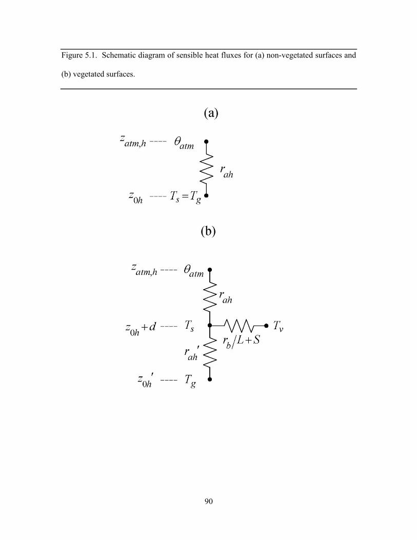
90
Figure 5.1. Schematic diagram of sensible heat fluxes for (a) non-vegetated surfaces and
(b) vegetated surfaces.
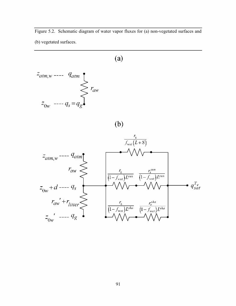
91
Figure 5.2. Schematic diagram of water vapor fluxes for (a) non-vegetated surfaces and
(b) vegetated surfaces.
92
Equations (5.83)-(5.86) can be solved for the canopy air temperature sT
h h ha atm g g v v
s h h ha g v
c c T c TT
c c cθ + +
=+ +
(5.90)
where
1ha
ah
cr
= (5.91)
1h
g
ah
cr
=′
(5.92)
( )h
vb
L Sc
r+
= (5.93)
are the sensible heat conductances from the canopy air to the atmosphere, the ground to
canopy air, and leaf surface to canopy air, respectively (m s-1).
When the expression for sT is substituted into equation (5.85), the sensible heat flux
from vegetation vH is a function of atmθ , gT , and vT
( )h
h h h h vv atm p a atm g g a g v h h h
a v g
cH C c c T c c Tc c c
ρ θ = − + − + + +. (5.94)
Similarly, the expression for sT can be substituted into equation (5.86) to obtain the
sensible heat flux from ground gH
( )hgh h h h
g atm p a atm v v a v g h h ha v g
cH C c c T c c T
c c cρ θ = − + − + + +
. (5.95)
The air within the canopy is assumed to have negligible capacity to store water
vapor so that the water vapor flux E between the surface at height 0wz d+ and the
93
atmosphere at height ,atm wz must be balanced by the sum of the water vapor flux from the
vegetation vE and the ground gE
v gE E E= + (5.96)
where, with reference to Figure 5.2,
( )atm s
atmaw
q qE
rρ
−= − (5.97)
( )vT
s satv atm
total
q qE
rρ
−= − (5.98)
( )2 2 21g sno h osfc soil sno snow h osfc h osfcE f f E f E f E= − − + + (5.99)
( )soi s soilsoil atm
aw litter
q qE
r r
βρ
−= −
′ + (5.100)
( )s snosno atm
aw litter
q qE
r rρ
−= −
′ + (5.101)
( )22
s h osfch osfc atm
aw litter
q qE
r rρ
−= −
′ + (5.102)
where a t mq is the atmospheric specific humidity (kg kg-1), a wr is the aerodynamic
resistance to water vapor transfer (s m-1), vTsatq (kg kg-1) is the saturation water vapor
specific humidity at the vegetation temperature (section 5.5), gq , snoq , and 2h osfcq are the
specific humidities of the soil, snow, and surface water (section 5.2), awr ′ is the
aerodynamic resistance (s m-1) to water vapor transfer between the ground at height 0wz ′
and the canopy air at height 0wz d+ , soiβ is an empirical function of soil water (section
94
5.2), and litterr is a resistance for the plant litter layer (s m-1). totalr is the total resistance to
water vapor transfer from the canopy to the canopy air and includes contributions from
leaf boundary layer and sunlit and shaded stomatal resistances br , s u nsr , and s h a
sr (Figure
5.2). The water vapor flux from vegetation is the sum of water vapor flux from wetted
leaf and stem area wvE (evaporation of water intercepted by the canopy) and transpiration
from dry leaf surfaces tvE
w tv v vE E E= + . (5.103)
Equations (5.96)-(5.99) can be solved for the canopy specific humidity sq
vTw w w
a atm g g v sats w w w
a v g
c q c q c qq
c c c+ +
=+ +
(5.104)
where
1wa
aw
cr
= (5.105)
( )w
vb
L Sc r
r+
′′= (5.106)
w soig
aw litter
cr r
β=
′ + (5.107)
are the water vapor conductances from the canopy air to the atmosphere, the leaf to
canopy air, and ground to canopy air, respectively. The term r′′ is determined from
contributions by wet leaves and transpiration and limited by available water and potential
evaporation as
95
,
,,
,
,,
,
min , 0, 0
min , 0, 0
1 0
w pot canv dry
w potwet dry v tw pot
v
w pot canv dry
w potwet v tw pot
v
w potv
WE rtf r E
E
WE rtr f E
E
E
β
β
′′ + ∆′′+ > >
′′ + ∆′′ = > ≤
≤
(5.108)
where wetf is the fraction of leaves and stems that are wet (section 7.1), c a nW is canopy
water (kg m-2) (section 7.1), t∆ is the time step (s), and tβ is a soil moisture function
limiting transpiration (Chapter 8). The potential evaporation from wet foliage per unit
wetted area is
( ),
vTatm s satw pot
vb
q qE
rρ −
= − . (5.109)
The term dryr ′′ is
sun sha
dry bdry sun sha
b s b s
f r L LrL r r r r
′′ = + + + (5.110)
where dryf is the fraction of leaves that are dry (section 7.1), sunL and shaL are the sunlit
and shaded leaf area indices (section 4.1), and sunsr and sha
sr are the sunlit and shaded
stomatal resistances (s m-1) (Chapter 8).
When the expression for sq is substituted into equation (5.98), the water vapor flux
from vegetation vE is a function of atmq , gq , and vTsatq
96
( ) v
wTw w w w v
v atm a atm g g a g sat w w wa v g
cE c q c q c c qc c c
ρ = − + − + + +. (5.111)
Similarly, the expression for sq can be substituted into equation (5.99) to obtain the
water vapor flux from the ground beneath the canopy gE
( )v
wgTw w w w
g atm a atm v sat a v g w w wa v g
cE c q c q c c q
c c cρ = − + − + + +
. (5.112)
The aerodynamic resistances to heat (moisture) transfer between the ground at
height 0hz ′ ( 0wz ′ ) and the canopy air at height 0hz d+ ( 0wz d+ ) are
1ah aw
s av
r rC U
′ ′= = (5.113)
where
1av a
am a
U V ur V ∗= = (5.114)
is the magnitude of the wind velocity incident on the leaves (equivalent here to friction
velocity) (m s-1) and sC is the turbulent transfer coefficient between the underlying soil
and the canopy air. sC is obtained by interpolation between values for dense canopy and
bare soil (Zeng et al. 2005)
, , (1 )s s bare s denseC C W C W= + − (5.115)
where the weight W is
( )L SW e− += . (5.116)
The dense canopy turbulent transfer coefficient in Zeng et al. (2005) is modified from its
original value of 0.004 (Dickinson et al. 1993) by Sakaguchi and Zeng (2009) to account
for stability as
97
( )
,
0.004 0
0.004 01 min ,10
s g
s denses g
T TC
T TSγ
− ≤ = − > +
(5.117)
where 0.5γ = and S is a stability parameter determined from
( )
2top s g
s
gz T TS
T u∗
−= (5.118)
where g is the gravitational acceleration (m s-2) (Table 2.6), and topz is canopy top
height (m) (Table 2.2). The bare soil turbulent transfer coefficient is
0.45
0 ,,
m g avs bare
z UkCa υ
−
=
(5.119)
where the kinematic viscosity of air 51.5 10υ −= × m2 s-1 and 0.13a = .
The litter resistance litterr (Sakaguchi and Zeng 2009) (s m-1) is
( )1 10.004
efflitterL
litterr eu
−
∗
= − (5.120)
where the effective litter area index efflitterL (m2 m-2) is the fraction of plant litter area index
litterL (currently set to 0.5 m2 m-2) that is not covered by snow
( )1 min ,1eff snowlitter litter litterL L f = − . (5.121)
The effective snow cover of the litter layer is
snow snolitter
litter
zfz
=∆
(5.122)
where 0.05litterz∆ = m is assumed as a typical depth for the litter layer, and snoz is the
depth of snow (section 7.2) (m).
The leaf boundary layer resistance br is
98
( ) 1 21b av leaf
v
r U dC
−= (5.123)
where 0.01vC = m s-1/2 is the turbulent transfer coefficient between the canopy surface
and canopy air, and leafd is the characteristic dimension of the leaves in the direction of
wind flow (Table 5.1).
The partial derivatives of the fluxes from the soil beneath the canopy with respect to
ground temperature, which are needed for the soil temperature calculations (section 6.1)
and to update the soil surface fluxes (section 5.4), are
h h
g atm p a vh h h
g ah a v g
H C c cT r c c c
ρ∂ +=
′∂ + + (5.124)
w w
g gsoi atm a vw w w
g aw litter a v g g
E dqc cT r r c c c dT
β ρ∂ +=
′∂ + + +. (5.125)
The partial derivatives ah
g
rT′∂
∂ and aw
g
rT′∂
∂, which cannot be determined analytically, are
ignored for g
g
HT
∂
∂ and g
g
ET
∂
∂.
The roughness lengths used to calculate amr , ahr , and awr from equations (5.55),
(5.56), and (5.57) are 0 0 ,m m vz z= , 0 0 ,h h vz z= , and 0 0 ,w w vz z= . The vegetation
displacement height d and the roughness lengths are a function of plant height and
adjusted for canopy density following Zeng and Wang (2007)
( ) ( ) ( )0 , 0 , 0 , 0 0 ,exp ln 1 lnm v h v w v top z m m gz z z V z R V z = = = + − (5.126)
top dd z R V= (5.127)
99
where topz is canopy top height (m) (Table 2.2), 0z mR and dR are the ratio of momentum
roughness length and displacement height to canopy top height, respectively (Table 5.1),
and 0 ,m gz is the ground momentum roughness length (m) (section 5.2). The fractional
weight V is determined from
( )
( )1 exp min ,
1 expcr
cr
L S L SV
L S
β
β
− − + + = − − +
(5.128)
where 1β = and ( ) 2cr
L S+ = (m2 m-2) is a critical value of exposed leaf plus stem area
for which 0mz reaches its maximum.

100
Table 5.1. Plant functional type aerodynamic parameters
Plant functional type 0z mR dR leafd (m)
NET Temperate 0.055 0.67 0.04
NET Boreal 0.055 0.67 0.04
NDT Boreal 0.055 0.67 0.04
BET Tropical 0.075 0.67 0.04
BET temperate 0.075 0.67 0.04
BDT tropical 0.055 0.67 0.04
BDT temperate 0.055 0.67 0.04
BDT boreal 0.055 0.67 0.04
BES temperate 0.120 0.68 0.04
BDS temperate 0.120 0.68 0.04
BDS boreal 0.120 0.68 0.04
C3 arctic grass 0.120 0.68 0.04
C3 grass 0.120 0.68 0.04
C4 grass 0.120 0.68 0.04
Crop R 0.120 0.68 0.04
Crop I 0.120 0.68 0.04
Corn R 0.120 0.68 0.04
Corn I 0.120 0.68 0.04
Temp Cereal R 0.120 0.68 0.04
Temp Cereal I 0.120 0.68 0.04
Winter Cereal R 0.120 0.68 0.04
Winter Cereal I 0.120 0.68 0.04
Soybean R 0.120 0.68 0.04
Soybean I 0.120 0.68 0.04
5.3.2 Numerical Implementation Canopy energy conservation gives
101
( ) ( ) ( ) 0vv v v v v vS L T H T E Tλ− + + + =
(5.129)
where vS
is the solar radiation absorbed by the vegetation (section 4.1), vL
is the net
longwave radiation absorbed by vegetation (section 4.2), and vH and vEλ are the
sensible and latent heat fluxes from vegetation, respectively. The term λ is taken to be
the latent heat of vaporization vapλ (Table 2.6).
vL
, vH , and vEλ depend on the vegetation temperature vT . The Newton-Raphson
method for finding roots of non-linear systems of equations can be applied to iteratively
solve for vT as
vv v vv
v v v
v v v
S L H ETH EL
T T T
λλ
− − −∆ =
∂ ∂∂+ +
∂ ∂ ∂
(5.130)
where 1n nv v vT T T+∆ = − and the subscript “n” indicates the iteration.
The partial derivatives are
( ) 34 2 1vv v g v
v
L TT
ε σ ε ε∂ = − − ∂
(5.131)
( )h
h hv vatm p a g h h h
v a v g
H cC c cT c c c
ρ∂= +
∂ + + (5.132)
( )vTw
w wv v satatm a g w w w
v a v g v
E c dqc cT c c c dT
λ λρ∂= +
∂ + +. (5.133)
The partial derivatives ah
v
rT
∂∂
and aw
v
rT
∂∂
, which cannot be determined analytically, are
ignored for v
v
HT
∂∂
and v
v
ET
λ∂∂
. However, if ζ changes sign more than four times during
102
the temperature iteration, 0.01ζ = − . This helps prevent “flip-flopping” between stable
and unstable conditions. The total water vapor flux vE , transpiration flux tvE , and
sensible heat flux vH are updated for changes in leaf temperature as
( )v
v
T wTw w w w sat v
v atm a atm g g a g sat v w w wv a v g
dq cE c q c q c c q TdT c c c
ρ
= − + − + + ∆ + + (5.134)
( )v
v
T hTt w w w w sat v
v dry atm a atm g g a g sat v w w wv a v g
dq cE r c q c q c c q TdT c c c
ρ ′′= − + − + + ∆ + +
(5.135)
( ) ( )h
h h h h vv atm p a atm g g a g v v h h h
a v g
cH C c c T c c T Tc c c
ρ θ = − + − + + ∆ + +. (5.136)
The numerical solution for vegetation temperature and the fluxes of momentum,
sensible heat, and water vapor flux from vegetated surfaces proceeds as follows:
1. Initial values for canopy air temperature and specific humidity are obtained from
2
g atms
TT
θ+= (5.137)
2
g atms
q qq
+= . (5.138)
2. An initial guess for the wind speed aV is obtained from eq. (5.24) assuming an
initial convective velocity 0cU = m s-1 for stable conditions ( , , 0v a t m v sθ θ− ≥ as
evaluated from eq. (5.50)) and 0 . 5cU = for unstable conditions ( , , 0v a t m v sθ θ− < ).
3. An initial guess for the Monin-Obukhov length L is obtained from the bulk
Richardson number using equation (5.46) and (5.48).
4. Iteration proceeds on the following system of equations:
• Friction velocity u∗ (eqs. (5.32), (5.33), (5.34), (5.35))
103
• Ratio a t m s
θθ θ
∗
− (eqs. (5.37), (5.38), (5.39), (5.40))
• Ratio a t m s
qq q
∗
− (eqs. (5.41), (5.42), (5.43), (5.44))
• Aerodynamic resistances amr , ahr , and awr (eqs. (5.55), (5.56), (5.57))
• Magnitude of the wind velocity incident on the leaves avU (eq. (5.114))
• Leaf boundary layer resistance br (eq. (5.123))
• Aerodynamic resistances ahr ′ and awr ′ (eq. (5.113))
• Sunlit and shaded stomatal resistances sunsr and sha
sr (Chapter 8)
• Sensible heat conductances hac , h
gc , and hvc (eqs. (5.91), (5.92), (5.93))
• Latent heat conductances wac , w
vc , and wgc (eqs. (5.105), (5.106), (5.107))
• Sensible heat flux from vegetation vH (eq. (5.94))
• Latent heat flux from vegetation vEλ (eq. (5.111))
• If the latent heat flux has changed sign from the latent heat flux computed at the
previous iteration ( 1 0n nv vE Eλ λ+ × < ), the latent heat flux is constrained to be
10% of the computed value. The difference between the constrained and
computed value ( 1 11 0.1 n n
v vE Eλ λ+ +∆ = − ) is added to the sensible heat flux
later.
• Change in vegetation temperature vT∆ (eq. (5.130)) and update the vegetation
temperature as 1n nv v vT T T+ = + ∆ . vT is constrained to change by no more than
1ºK in one iteration. If this limit is exceeded, the energy error is
104
2v v v
vv v v v v vv v v
H ELS L T H T E TT T T
λλ∂ ∂∂∆ = − − ∆ − − ∆ − − ∆
∂ ∂ ∂
(5.139)
where 1 or 1vT∆ = − . The error 2∆ is added to the sensible heat flux later.
• Water vapor flux vE (eq. (5.134))
• Transpiration tvE (eq. (5.135) if 0tβ > , otherwise 0t
vE = )
• The water vapor flux vE is constrained to be less than or equal to the sum of
transpiration tvE and the water available from wetted leaves and stems canW t∆ .
The energy error due to this constraint is
3 max 0, t canv v
WE Et
∆ = − − ∆ . (5.140)
The error 3λ∆ is added to the sensible heat flux later.
• Sensible heat flux vH (eq. (5.136)). The three energy error terms, 1∆ , 2∆ , and
3λ∆ are also added to the sensible heat flux.
• The saturated vapor pressure ie (Chapter 8), saturated specific humidity vTsatq
and its derivative vT
sat
v
dqdT
at the leaf surface (section 5.5), are re-evaluated based
on the new vT .
• Canopy air temperature sT (eq. (5.90))
• Canopy air specific humidity sq (eq. (5.104))
• Temperature difference a t m sθ θ−
• Specific humidity difference a t m sq q−
105
• Potential temperature scale ( )atm satm s
θθ θ θθ θ
∗∗ = −
− where
a t m s
θθ θ
∗
− was
calculated earlier in the iteration
• Humidity scale ( )atm satm s
qq q qq q
∗∗ = −
− where
a t m s
qq q
∗
− was calculated earlier
in the iteration
• Virtual potential temperature scale vθ ∗ (eq. (5.17))
• Wind speed including the convective velocity, aV (eq. (5.24))
• Monin-Obukhov length L (eq. (5.49))
• The iteration is stopped after two or more steps if 0.01vT∆ < and
1 0.1n nv vE Eλ λ+ − < where ( )1 1max ,n n n n
v v v v vT T T T T+ −∆ = − − , or after forty
iterations have been carried out.
5. Momentum fluxes xτ , yτ (eqs. (5.5), (5.6))
6. Sensible heat flux from ground gH (eq. (5.95))
7. Water vapor flux from ground gE (eq. (5.112))
8. 2-m height air temperature 2mT , specific humidity 2mq , relative humidity 2mRH
(eqs. (5.58), (5.59), (5.60))
5.4 Update of Ground Sensible and Latent Heat Fluxes The sensible and water vapor heat fluxes derived above for bare soil and soil
beneath canopy are based on the ground surface temperature from the previous time step
ngT and are used as the surface forcing for the solution of the soil temperature equations
106
(section 6.1). This solution yields a new ground surface temperature 1ngT + . The ground
sensible and water vapor fluxes are then updated for 1ngT + as
( )1 gn ng g g g
g
HH H T T
T+ ∂
′ = + −∂
(5.141)
( )1 gn ng g g g
g
EE E T T
T+ ∂
′ = + −∂
(5.142)
where gH and gE are the sensible heat and water vapor fluxes derived from equations
(5.80) and (5.81) for non-vegetated surfaces and equations (5.124) and (5.125) for
vegetated surfaces using ngT . One further adjustment is made to gH ′ and gE′ . If the soil
moisture in the top snow/soil layer is not sufficient to support the updated ground
evaporation, i.e., if 0gE′ > and 1e v a pf < where
( )( ) ( )
, 1 , 1
1
1ice snl liq snlevap npft
g jjj
w w tf
E wt
+ +
=
+ ∆= ≤
′∑, (5.143)
an adjustment is made to reduce the ground evaporation accordingly as
g evap gE f E′′ ′= . (5.144)
The term ( ) ( )1
n p f t
g jjj
E w t=
′∑ is the sum of gE′ over all evaporating PFTs where ( )g jE′ is the
ground evaporation from the t hj PFT on the column, ( ) jw t is the relative area of the
t hj PFT with respect to the column, and n p f t is the number of PFTs on the column.
, 1i c e s n lw + and , 1l i q s n lw + are the ice and liquid water contents (kg m-2) of the top snow/soil
layer (Chapter 7). Any resulting energy deficit is assigned to sensible heat as
107
( )g g g gH H E Eλ′′ ′ ′′= + − . (5.145)
The ground water vapor flux gE′′ is partitioned into evaporation of liquid water
from snow/soil sevaq (kg m-2 s-1), sublimation from snow/soil ice sublq (kg m-2 s-1), liquid
dew on snow/soil sdewq (kg m-2 s-1), or frost on snow/soil frostq (kg m-2 s-1) as
, 1, 1 , 1
, 1 , 1
max ,0 0, 0liq snlseva sno sno ice snl liq snl
ice snl liq snl
wq E E w w
w w+
+ ++ +
′′ ′′= ≥ + > +
(5.146)
0subl sno seva snoq E q E′′ ′′= − ≥ (5.147)
0 and sdew sno sno g fq E E T T′′ ′′= < ≥ (5.148)
0 and frost sno sno g fq E E T T′′ ′′= < < . (5.149)
The loss or gain in snow mass due to sevaq , sublq , sdewq , and frostq on a snow surface are
accounted for during the snow hydrology calculations (section 7.2). The loss of soil and
surface water due to sevaq is accounted for in the calculation of infiltration (section 7.3),
while losses or gains due to sublq , sdewq , and frostq on a soil surface are accounted for
following the sub-surface drainage calculations (section 7.6).
The ground heat flux G is calculated as
gg g gG S L H Eλ= − − −
(5.150)
where gS
is the solar radiation absorbed by the ground (section 4.1), gL
is the net
longwave radiation absorbed by the ground (section 4.2)
( ) ( ) ( )3 11 4 n n ng g veg g v veg g atm g g g gLL L L T T Tδ ε δ ε ε σ += ↑ ↓ − ↓ +− − −
, (5.151)
where
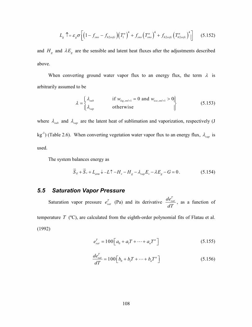
108
( ) ( ) ( ) ( )4 4 4
2 1 2 21 n n ng g sno h osfc sno sno h osfc h osfcL f f T f T f Tε σ= ↑ − − + +
(5.152)
and gH and gEλ are the sensible and latent heat fluxes after the adjustments described
above.
When converting ground water vapor flux to an energy flux, the term λ is
arbitrarily assumed to be
, 1 , 1if 0 and 0
otherwisesub liq snl ice snl
vap
w wλλ
λ+ += > =
(5.153)
where subλ and vapλ are the latent heat of sublimation and vaporization, respectively (J
kg-1) (Table 2.6). When converting vegetation water vapor flux to an energy flux, vapλ is
used.
The system balances energy as
0g v atm v g vap v gS S L L H H E E Gλ λ↓ − ↑+ + − − − − − =
. (5.154)
5.5 Saturation Vapor Pressure
Saturation vapor pressure Tsate (Pa) and its derivative
Tsatde
dT, as a function of
temperature T (ºC), are calculated from the eighth-order polynomial fits of Flatau et al.
(1992)
0 1100T nsat ne a a T a T = + + + (5.155)
0 1100T
nsatn
de b bT b TdT
= + + + (5.156)
109
where the coefficients for ice are valid for 75 C 0 CT− ≤ < and the coefficients for
water are valid for 0 C 100 CT≤ ≤ (Table 5.2 and 5.3). The saturated water vapor
specific humidity Tsatq and its derivative
Tsatdq
dT are
0.622
0.378
TT satsat T
atm sat
eqP e
=−
(5.157)
( )2
0.622
0.378
T Tsat atm sat
Tatm sat
dq P dedT dTP e
=−
. (5.158)
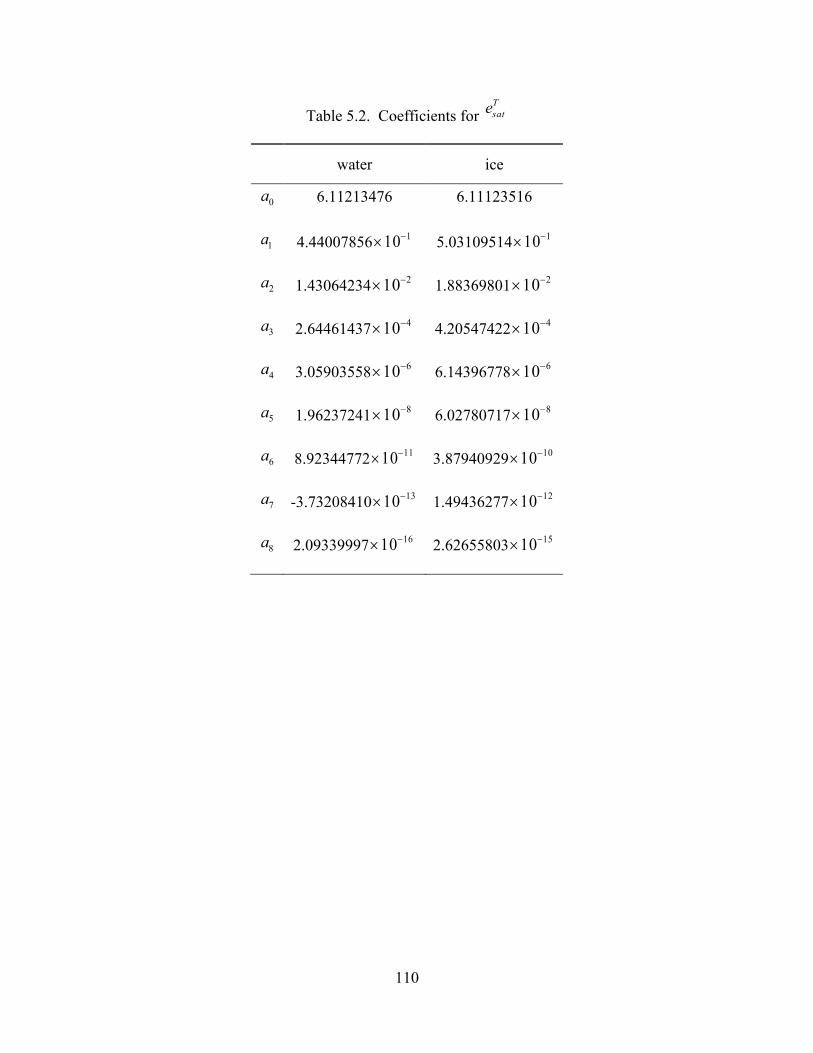
110
Table 5.2. Coefficients for Tsate
water ice
0a 6.11213476 6.11123516
1a 4.44007856 110−× 5.03109514 110−×
2a 1.43064234 210−× 1.88369801 210−×
3a 2.64461437 410−× 4.20547422 410−×
4a 3.05903558 610−× 6.14396778 610−×
5a 1.96237241 810−× 6.02780717 810−×
6a 8.92344772 1110−× 3.87940929 1010−×
7a -3.73208410 1310−× 1.49436277 1210−×
8a 2.09339997 1610−× 2.62655803 1510−×
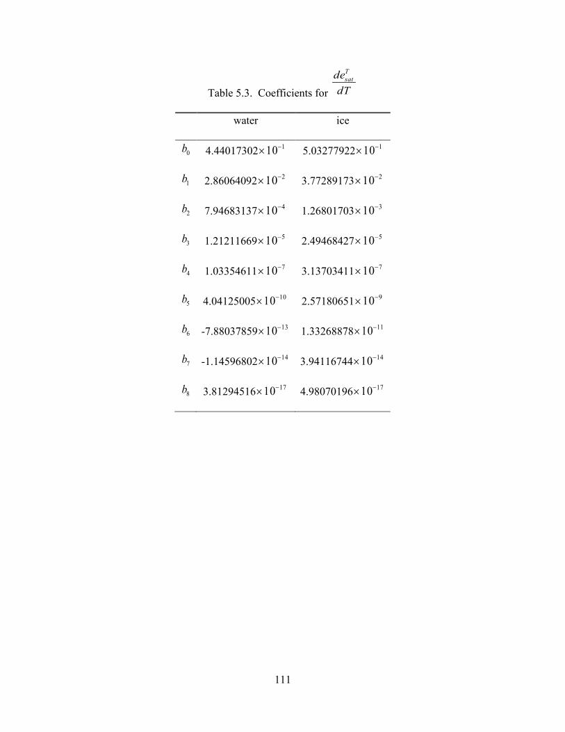
111
Table 5.3. Coefficients for
Tsatde
dT
water ice
0b 4.44017302 110−× 5.03277922 110−×
1b 2.86064092 210−× 3.77289173 210−×
2b 7.94683137 410−× 1.26801703 310−×
3b 1.21211669 510−× 2.49468427 510−×
4b 1.03354611 710−× 3.13703411 710−×
5b 4.04125005 1010−× 2.57180651 910−×
6b -7.88037859 1310−× 1.33268878 1110−×
7b -1.14596802 1410−× 3.94116744 1410−×
8b 3.81294516 1710−× 4.98070196 1710−×
112
6. Soil and Snow Temperatures
The first law of heat conduction is
F Tλ= − ∇ (6.1)
where F is the amount of heat conducted across a unit cross-sectional area in unit time
(W m-2), λ is thermal conductivity (W m-1 K-1), and T∇ is the spatial gradient of
temperature (K m-1). In one-dimensional form
zTFz
λ ∂= −
∂ (6.2)
where z is in the vertical direction (m) and is positive downward and zF is positive
upward. To account for non-steady or transient conditions, the principle of energy
conservation in the form of the continuity equation is invoked as
zFTct z
∂∂= −
∂ ∂ (6.3)
where c is the volumetric snow/soil heat capacity (J m-3 K-1) and t is time (s).
Combining equations (6.2) and (6.3) yields the second law of heat conduction in one-
dimensional form
T Tct z z
λ∂ ∂ ∂ = ∂ ∂ ∂ . (6.4)
This equation is solved numerically to calculate the soil, snow, and surface water
temperatures for a fifteen-layer soil column with up to five overlying layers of snow and
a single surface water layer with the boundary conditions of h as the heat flux into the
top soil, snow, and surface water layers from the overlying atmosphere (section 6.1) and
113
zero heat flux at the bottom of the soil column. The temperature profile is calculated first
without phase change and then readjusted for phase change (section 6.2).
6.1 Numerical Solution The soil column is discretized into fifteen layers (Table 6.1) where the depth of soil
layer i , or node depth, iz (m), is
( ) exp 0.5 0.5 1i sz f i= − − (6.5)
where 0.025sf = is a scaling factor. The thickness of each layer iz∆ (m) is
( )( )
1 2
1 1
1
0.5 1
0.5 2,3, , 1i i i levgrnd
N N levgrnd
z z i
z z z i Nz z i N
+ −
−
+ =
∆ = − = − − =
(6.6)
where 15levgrndN = is the number of soil layers. The depths at the layer interfaces ,h iz
(m) are
( )1
,
0.5 1, 2, , 1
0.5levgrnd levgrnd
i i levgrndh i
N N levgrnd
z z i Nz
z z i N++ = − = + ∆ =
. (6.7)
The exponential form of equation (6.5) is to obtain more soil layers near the soil surface
where the soil water gradient is generally strong (section 7.4).
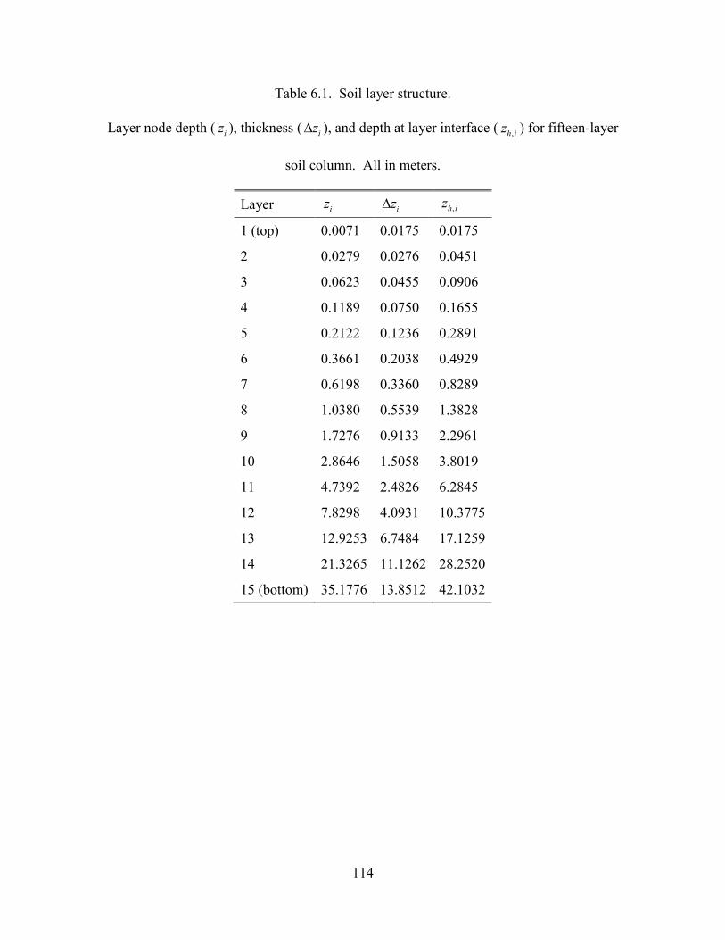
114
Table 6.1. Soil layer structure.
Layer node depth ( iz ), thickness ( iz∆ ), and depth at layer interface ( ,h iz ) for fifteen-layer
soil column. All in meters.
Layer iz iz∆ ,h iz
1 (top) 0.0071 0.0175 0.0175
2 0.0279 0.0276 0.0451
3 0.0623 0.0455 0.0906
4 0.1189 0.0750 0.1655
5 0.2122 0.1236 0.2891
6 0.3661 0.2038 0.4929
7 0.6198 0.3360 0.8289
8 1.0380 0.5539 1.3828
9 1.7276 0.9133 2.2961
10 2.8646 1.5058 3.8019
11 4.7392 2.4826 6.2845
12 7.8298 4.0931 10.3775
13 12.9253 6.7484 17.1259
14 21.3265 11.1262 28.2520
15 (bottom) 35.1776 13.8512 42.1032
115
The overlying snow pack is modeled with up to five layers depending on the total
snow depth. The layers from top to bottom are indexed in the Fortran code as
4, 3, 2, 1, 0i = − − − − , which permits the accumulation or ablation of snow at the top of the
snow pack without renumbering the layers. Layer 0i = is the snow layer next to the soil
surface and layer 1i s n l= + is the top layer, where the variable s n l is the negative of
the number of snow layers. The number of snow layers and the thickness of each layer is
a function of snow depth snoz (m) as follows.
0 sno
1for 0.01 z 0.03sno
snlz z
= − ∆ = ≤ ≤
,
1 sno
0 1
22 for 0.03< z 0.04sno
snlz zz z
−
−
= − ∆ = ≤ ∆ = ∆
,
1 sno
0 1
20.02 for 0.04 < z 0.07
sno
snlzz z z
−
−
= − ∆ = ≤ ∆ = − ∆
,
( )2
1 sno
0 1
30.02
0.02 2 for 0.07 < z 0.12sno
snlzz zz z
−
−
−
= − ∆ = ∆ = − ≤ ∆ = ∆
,
2
1 sno
0 2 1
30.020.05 for 0.12 < z 0.18
sno
snlzzz z z z
−
−
− −
= − ∆ = ∆ = ≤ ∆ = − ∆ − ∆ ,
116
( )
3
2 sno
1 3 2
0 1
40.020.05 for 0.18 < z 0.29
2sno
snlzzz z z zz z
−
−
− − −
−
= −
∆ = ∆ = ≤ ∆ = − ∆ − ∆ ∆ = ∆
,
3
2 sno
1
0 3 2 1
40.020.05 for 0.29 < z 0.410.11
sno
snlzzzz z z z z
−
−
−
− − −
= − ∆ = ∆ = ≤ ∆ = ∆ = − ∆ − ∆ − ∆
,
( )
4
3 sno
2
1 4 3 2
0 1
50.020.05 for 0.41< z 0.640.11
2sno
snlzzzz z z z zz z
−
−
−
− − − −
−
= − ∆ = ∆ = ≤ ∆ = ∆ = − ∆ − ∆ − ∆
∆ = ∆
,
4
3 sno
2
1
0 4 3 2 1
50.020.05 for 0.64 < z0.110.23
sno
snlzzzzz z z z z z
−
−
−
−
− − − −
= − ∆ = ∆ = ∆ = ∆ =
∆ = − ∆ − ∆ − ∆ − ∆
.
The node depths, which are located at the midpoint of the snow layers, and the layer
interfaces are both referenced from the soil surface and are defined as negative values
, 0.5 1, , 0i h i iz z z i snl= − ∆ = + (6.8)
, , 1 1 , , 1h i h i iz z z i snl+ += − ∆ = − . (6.9)
Note that ,0hz , the interface between the bottom snow layer and the top soil layer, is zero.
Thermal properties (i.e., temperature iT [K]; thermal conductivity iλ [W m-1 K-1];
117
volumetric heat capacity ic [J m-3 K-1]) are defined for soil layers at the node depths
(Figure 6.1) and for snow layers at the layer midpoints. When present, snow occupies a
fraction of a grid cell’s area, therefore snow depth represents the thickness of the
snowpack averaged over only the snow covered area. The grid cell average snow depth
is related to the depth of the snow covered area as sno sno snoz f z= . By default, the grid
cell average snow depth is written to the history file.
The heat flux iF (W m-2) from layer i to layer 1i + is
1,
1
i ii h i
i i
T TF zz z
λ +
+
− = − − (6.10)
where the thermal conductivity at the interface ,h izλ is
( )
( ) ( )1 1
1 , 1 ,,
1, , 1
0
i i i ilevgrnd
i i h i i h i ih i
levgrnd
z zi snl N
z z z zzi N
λ λλ λλ
+ +
+ +
− = + − − + − =
=
. (6.11)
These equations are derived, with reference to Figure 6.1, assuming that the heat flux
from i (depth iz ) to the interface between i and 1i + (depth ,h iz ) equals the heat flux
from the interface to 1i + (depth 1iz + ), i.e.,
11
, 1 ,
i m m ii i
h i i i h i
T T T Tz z z z
λ λ ++
+
− −− = −
− − (6.12)
where mT is the temperature at the interface of layers i and 1i + .
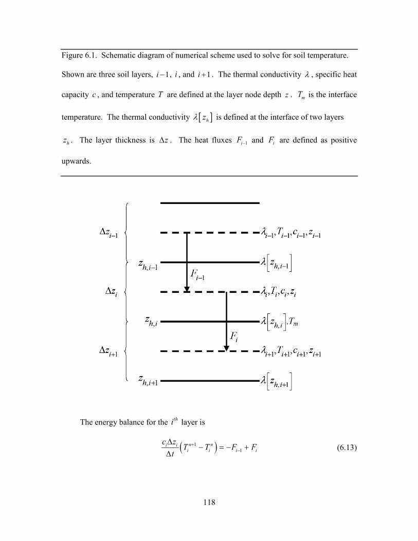
118
Figure 6.1. Schematic diagram of numerical scheme used to solve for soil temperature.
Shown are three soil layers, 1i − , i , and 1i + . The thermal conductivity λ , specific heat
capacity c , and temperature T are defined at the layer node depth z . mT is the interface
temperature. The thermal conductivity [ ]hzλ is defined at the interface of two layers
hz . The layer thickness is z∆ . The heat fluxes 1iF − and iF are defined as positive
upwards.
The energy balance for the thi layer is
( )11
n ni ii i i i
c z T T F Ft
+−
∆− = − +
∆ (6.13)
119
where the superscripts n and 1n + indicate values at the beginning and end of the time
step, respectively, and t∆ is the time step (s). This equation is solved using the Crank-
Nicholson method, which combines the explicit method with fluxes evaluated at n (
1,n n
i iF F− ) and the implicit method with fluxes evaluated at 1n + ( 1 11 ,n n
i iF F+ +− )
( ) ( ) ( ) ( )1 1 11 11n n n n n ni i
i i i i i ic z T T F F F F
tα α+ + +
− −
∆− = − + + − − +
∆ (6.14)
where 0.5α = , resulting in a tridiagonal system of equations
1 1 11 1
n n ni i i i i i ir a T bT c T+ + +
− += + + (6.15)
where ia , ib , and ic are the subdiagonal, diagonal, and superdiagonal elements in the
tridiagonal matrix and ir is a column vector of constants. When surface water is present,
the equation for the top soil layer has an additional term representing the surface water
temperature; this results in a four element band-diagonal system of equations.
For the top soil layer 1i = , top snow layer 1i snl= + , or surface water layer, the
heat flux from the overlying atmosphere h (W m-2, defined as positive into the surface)
is
( )1 11 11n n n
i ih F Fα α+ +− −= − − − . (6.16)
The energy balance for these layers is then
( ) ( )1 1 11n n n n ni ii i i i
c z T T h F Ft
α α+ + +∆− = + + −
∆. (6.17)
The heat flux h at 1n + may be approximated as follows
( )1 1n n n ni i
i
hh h T TT
+ +∂= + −
∂. (6.18)
The resulting equations are then
120
( ) ( )
( ) ( ) ( )
1 1
1 1, 1 , 1
1 1
1
n n n ni ii i i i
i
n n n nh i i i h i i i
i i i i
c z hT T h T Tt T
z T T z T Tz z z z
λ λα α
+ +
+ ++ +
+ +
∆ ∂− = + −
∆ ∂
− − − − −− −
(6.19)
For the top snow layer, 1i snl= + , the coefficients are
0ia = (6.20)
( ) ,
1
1 1 h ii
i i i i i
zt hbc z z z T
λα
+
∆ ∂ = + − −∆ − ∂
(6.21)
( ) ,
1
1 h ii
i i i i
ztcc z z z
λα
+
∆ = − −∆ −
(6.22)
n n ni i sno i i
i i i
t hr T h T Fc z T
α ∆ ∂
= + − + ∆ ∂ (6.23)
where
1,
1
n ni i
i h ii i
T TF zz z
λ +
+
− = − − . (6.24)
The heat flux into the snow surface from the overlying atmosphere h is
snosno sno snoh S L H Eλ= − − −
(6.25)
where snoS
is the solar radiation absorbed by the top snow layer (section 3.2.1), snoL
is
the longwave radiation absorbed by the snow (positive toward the atmosphere) (section
4.2), snoH is the sensible heat flux from the snow (Chapter 5), and snoEλ is the latent
heat flux from the snow (Chapter 5). The partial derivative of the heat flux h with
respect to temperature is
H Eh LT T T T
λ∂ ∂∂ ∂= − − −
∂ ∂ ∂ ∂
(6.26)
121
where the partial derivative of the net longwave radiation is
( )34 n
gL TT
ε σ∂=
∂
(6.27)
and the partial derivatives of the sensible and latent heat fluxes are given by equations
(5.80) and (5.81) for non-vegetated surfaces, and by equations (5.124) and (5.125) for
vegetated surfaces. σ is the Stefan-Boltzmann constant (W m-2 K-4) (Table 2.6) and gε
is the ground emissivity (section 4.2). For purposes of computing h and g
hT
∂∂
, the term
λ is arbitrarily assumed to be
, 1 , 1if 0 and 0
otherwisesub liq snl ice snl
vap
w wλλ
λ+ += > =
(6.28)
where subλ and vapλ are the latent heat of sublimation and vaporization, respectively (J
kg-1) (Table 2.6), and , 1l i q s n lw + and , 1i c e s n lw + are the liquid water and ice contents of the
top snow/soil layer, respectively (kg m-2) (Chapter 7).
For the top soil layer, 1i = , the coefficients are
( ) , 1
1
1 h ii sno
i i i i
zta fc z z z
λα −
−
∆ = − −∆ −
(6.29)
( ) ( ), 1 ,
1 1
1 1 1h i h ii sno sno
i i i i i i i i
z zt t hb f fc z z z z z c z T
λ λα −
− +
∆ ∆ ∂ = + − + − −∆ − − ∆ ∂
(6.30)
( ) ,
1
1 h ii
i i i i
ztcc z z z
λα
+
∆ = − −∆ −
(6.31)
( ) ( )11n n ni i sno soil i i sno i
i i
t hr T f h T F f Fc z T
α −
∆ ∂= + − − + − ∆ ∂
(6.32)
122
The heat flux into the soil surface from the overlying atmosphere h is
soilsoil soil soilh S L H Eλ= − − −
(6.33)
It can be seen that when no snow is present ( 0snof = ), the expressions for the
coefficients of the top soil layer have the same form as those for the top snow layer.
The surface snow/soil layer temperature computed in this way is the layer-averaged
temperature and hence has somewhat reduced diurnal amplitude compared with surface
temperature. An accurate surface temperature is provided that compensates for this effect
and numerical error by tuning the heat capacity of the top layer (through adjustment of
the layer thickness) to give an exact match to the analytic solution for diurnal heating.
The top layer thickness for 1i snl= + is given by
( ), 1 1 , 10.5i i h i a i h iz z z c z z∗ − + − ∆ = − + − (6.34)
where ac is a tunable parameter, varying from 0 to 1, and is taken as 0.34 by comparing
the numerical solution with the analytic solution (Z.-L. Yang 1998, unpublished
manuscript). iz ∗∆ is used in place of iz∆ for 1i snl= + in equations (6.19)-(6.24). The
top snow/soil layer temperature computed in this way is the ground surface temperature
1ngT + .
The boundary condition at the bottom of the snow/soil column is zero heat flux,
0iF = , resulting in, for levgrndi N= ,
( ) ( ) ( ) ( )1 1, 1 1 , 1 11
1 1
1n n n n
h i i i h i i in ni ii i
i i i i
z T T z T Tc z T Tt z z z z
λ λα α
+ +− − − −+
− −
− −∆ − = + −∆ − −
(6.35)
( ) , 1
1
1 h ii
i i i i
ztac z z z
λα −
−
∆ = − −∆ −
(6.36)
123
( ) , 1
1
1 1 h ii
i i i i
ztbc z z z
λα −
−
∆ = + −∆ −
(6.37)
0ic = (6.38)
1n
i i ii i
tr T Fc z
α −
∆= −
∆ (6.39)
where
( ), 11 1
1
h i n ni i i
i i
zF T T
z zλ −
− −−
= − −−
. (6.40)
For the interior snow/soil layers, 1 levgrndsnl i N+ < < , excluding the top soil layer,
( ) ( ) ( )
( ) ( ) ( ) ( )
, 1 , 1 11
1 1
1 1 1 1, 1 , 1 1
1 1
1 1
n n n nh i i i h i i in ni i
i ii i i i
n n n nh i i i h i i i
i i i i
z T T z T Tc z T Tt z z z z
z T T z T Tz z z z
λ λα α
λ λα α
+ − −+
+ −
+ + + ++ − −
+ −
− −∆ − = − +∆ − −
− − − − + −− −
(6.41)
( ) , 1
1
1 h ii
i i i i
ztac z z z
λα −
−
∆ = − −∆ −
(6.42)
( ) , 1 ,
1 1
1 1 h i h ii
i i i i i i
z ztbc z z z z z
λ λα −
− +
∆ = + − +∆ − −
(6.43)
( ) ,
1
1 h ii
i i i i
ztcc z z z
λα
+
∆ = − −∆ −
(6.44)
( )1 ,n
i i i i g ii i i i
t tr T F F Sc z c z
α −
∆ ∆= + − +
∆ ∆
. (6.45)
where ,g iS
is the absorbed solar flux in layer i (section 3.2.1).
When surface water exists, the following top soil layer coefficients are modified
124
( )
( )
, 1 ,22
2 1 1
2
1 1
1
h i h ih osfci h osfc sno
i i i h osfc i i i i
sno h osfci i
z ztb f fc z z z z z z z
t hf fc z T
λ λλα −
− +
∆ = + − + +∆ − − −
∆ ∂− − −
∆ ∂
(6.46)
( )
( )
2
21 2 1 2
1 2
1 n nsno h osfc soil i
ni i
i i h osfci sno i h osfc h osfc
h osfc
hf f h TTtr T
c zF f F f T T
z zλ
α −
∂− − − ∂ ∆ = + ∆ + − + − −
(6.47)
( ) 2
22
1 h osfci h osfc
i i i h osfc
td fc z z z
λα
∆= − −
∆ − (6.48)
where id is an additional coefficient representing the heat flux from the surface water
layer. The surface water layer coefficients are
2 0h osfca = (6.49)
( ) 22
2 2 1 2
1 1 h osfch osfc
h osfc h osfc h osfc
t hbc z z z T
λα
∆ ∂= + − −
∆ − ∂ (6.50)
( ) 22
2 2 1 2
1 h osfch osfc
h osfc h osfc h osfc
tcc z z z
λα ∆
= − −∆ −
(6.51)
( )22 2 2 2 1 2
1 2
h osfcn n nh osfc h osfc h osfc h osfc h osfc
i i h osfc
t hr T h T T Tc z T z z
λα
∆ ∂= + − + −
∆ ∂ − (6.52)
6.2 Phase Change
6.2.1 Soil and Snow Layers Upon update, the snow/soil temperatures are evaluated to determine if phase change
will take place as
125
1,
1,
1, , max,
and 0 1, , melting
and 0 1, , 0 freezing
and 1, , freezing
ni f ice i levgrnd
ni f liq i
ni f liq i liq i levgrnd
T T w i snl N
T T w i snl
T T w w i N
+
+
+
> > = +
< > = +
< > =
(6.53)
where 1niT + is the soil layer temperature after solution of the tridiagonal equation set,
,ice iw and ,liq iw are the mass of ice and liquid water (kg m-2) in each snow/soil layer,
respectively, and fT is the freezing temperature of water (K) (Table 2.6). For the
freezing process in soil layers, the concept of supercooled soil water from Niu and Yang
(2006) is adopted. The supercooled soil water is the liquid water that coexists with ice
over a wide range of temperatures below freezing and is implemented through a freezing
point depression equation
( ) 13
, max, ,,
10 iB
f f iliq i i sat i i f
i sat i
L T Tw z T T
gTθ
ψ
− −
= ∆ <
(6.54)
where , max,liq iw is the maximum liquid water in layer i (kg m-2) when the soil temperature
iT is below the freezing temperature fT , fL is the latent heat of fusion (J kg-1) (Table
2.6), g is the gravitational acceleration (m s-2) (Table 2.6), and ,sat iψ and iB are the soil
texture-dependent saturated matric potential (mm) and Clapp and Hornberger (1978)
exponent (section 7.4.1).
For the special case when snow is present (snow mass 0s n oW > ) but there are no
explicit snow layers ( 0snl = ) (i.e., there is not enough snow present to meet the
minimum snow depth requirement of 0.01 m), snow melt will take place for soil layer
1i = if the soil layer temperature is greater than the freezing temperature ( 11n
fT T+ > ).
126
The rate of phase change is assessed from the energy excess (or deficit) needed to
change iT to freezing temperature, fT . The excess or deficit of energy iH (W m-2) is
determined as follows
( ) ( )
( ) ( ) ( )
( )
2
1
1 1
1, 1
n ni if i f i
n ni ii sno h osfc f i f i
ni if i
c zh T T T T i snlT t
c zhH f f T T T T iT t
c z T T i snlt
∆∂ − − − = + ∂ ∆ ∆∂ = − − − − − = ∂ ∆
∆ − − ≠ + ∆
. (6.55)
If the melting criteria is met (equation (6.53)) and 0im
f
H tHL∆
= > , then the ice mass is
readjusted as
1, , 0 1, ,n n
ice i ice i m levgrndw w H i snl N+ = − ≥ = + . (6.56)
If the freezing criteria is met (equation (6.53)) and 0mH < , then the ice mass is
readjusted for 1, , 0i snl= + as
( )1, , , ,min ,n n n n
ice i liq i ice i ice i mw w w w H+ = + − (6.57)
and for 1, , levgrndi N= as
( ), , , max, , , , , max,1,
, , , max,
min ,
0
n n n n n n nliq i ice i liq i ice i m liq i ice i liq in
ice i n n nliq i ice i liq i
w w w w H w w ww
w w w+
+ − − + ≥ = + < . (6.58)
Liquid water mass is readjusted as
1 1, , , , 0n n n n
liq i liq i ice i ice iw w w w+ += + − ≥ . (6.59)
Because part of the energy iH may not be consumed in melting or released in freezing,
the energy is recalculated as
127
( )1
, ,n n
f ice i ice ii i
L w wH H
t
+
∗
−= −
∆ (6.60)
and this energy is used to cool or warm the snow/soil layer (if 0iH ∗ > ) as
( )
12
1 1
1 1 1
1, 1
f ii i i i
ni f i sno h osfc
i i i i
f ii i
t t hT H i snlc z c z T
t t hT T H f f ic z c z T
tT H i snlc z
∗
+∗
∗
∆ ∆ ∂+ − = + ∆ ∆ ∂
∆ ∆ ∂ = + − − − = ∆ ∆ ∂ ∆
+ ≠ + ∆
. (6.61)
For the special case when snow is present ( 0snoW > ), there are no explicit snow layers (
0snl = ), and 1 0f
H tL
∆> (melting), the snow mass s n oW (kg m-2) is reduced according to
1 1 0n nsno sno
f
H tW WL
+ ∆= − ≥ . (6.62)
The snow depth is reduced proportionally
1
1n
n nsnosno snon
sno
Wz zW
++ = . (6.63)
Again, because part of the energy may not be consumed in melting, the energy for the
surface soil layer 1i = is recalculated as
( )1
1 1
n nf sno snoL W W
H Ht
+
∗
−= −
∆. (6.64)
If there is excess energy ( 1 0H ∗ > ), this energy becomes available to the top soil layer as
1 1H H ∗= . (6.65)
The ice mass, liquid water content, and temperature of the top soil layer are then
determined from equations (6.56), (6.59), and (6.61) using the recalculated energy from
128
equation (6.65). Snow melt 1SM (kg m-2 s-1) and phase change energy ,1p SE (W m-2) for
this special case are
1
1 0n n
sno snoS
W WMt
+−= ≥
∆ (6.66)
,1 1p S f SE L M= . (6.67)
The total energy of phase change pE (W m-2) for the snow/soil column is
,1 ,1
levgrndN
p p S p ii snl
E E E= +
= + ∑ (6.68)
where
( )1
, ,,
n nice i ice i
p i f
w wE L
t
+−=
∆. (6.69)
The total snow melt M (kg m-2 s-1) is
0
11
i
S ii snl
M M M=
= +
= + ∑ (6.70)
where
( )1
, , 0n nice i ice i
i
w wM
t
+−= ≥
∆. (6.71)
The solution for snow/soil temperatures conserves energy as
( )1
10
levgrndi Nn ni i
p i ii snl
c zG E T Tt
=+
= +
∆− − − =
∆∑ (6.72)
where G is the ground heat flux (section 5.4).
6.2.2 Surface Water Phase change of surface water takes place when the surface water temperature,
2h osfcT , becomes less than fT . The energy available for freezing is
129
( ) ( )2 22 2 2
h osfc h osfcn nh osfc f h osfc f h osfc
c zhH T T T TT t
∆∂= − − −
∂ ∆ (6.73)
where 2h osfcc is the volumetric heat capacity of water, and 2h osfcz∆ is the depth of the
surface water layer. If 2 0h o s f cm
f
H tH
L∆
= > then mH is removed from surface water and
added to the snow column as ice
12 2
n nh o s f c h o s f c mH H H+ = − (6.74)
1,0 ,0
n ni c e i c e mw w H+ = + (6.75)
The snow depth is adjusted to account for the additional ice mass
ms n o
i c e
Hzρ
∆ = (6.76)
If mH is greater than s f cW , the excess heat ( )f m s f cL H W
t−
∆ is used to cool the snow layer.
6.3 Soil and Snow Thermal Properties The thermal and hydraulic (section 6.3 and 7.4.1) properties of the soil are assumed
to be a weighted combination of the mineral and organic properties of the soil (Lawrence
and Slater 2008). The soil layer organic matter fraction ,om if is
, , ,max/om i om i omf ρ ρ= . (6.77)
Soil thermal conductivity iλ (W m-1 K-1) is from Farouki (1981)
( ) 7
, , , , ,
7, ,
1 1 101, ,
1 10
1,
e i sat i e i dry i r ii levsoi
dry i r i
i bedrock levsoi levgrnd
K K Si N
S
i N N
λ λλ
λ
λ λ
−
−
+ − > × = = ≤ ×
= = +
(6.78)
130
where ,sat iλ is the saturated thermal conductivity, ,dry iλ is the dry thermal conductivity,
,e iK is the Kersten number, ,r iS is the wetness of the soil with respect to saturation, and
3bedrockλ = W m-1 K-1 is the thermal conductivity assumed for the deep ground layers
(typical of saturated granitic rock; Clauser and Huenges, 1995). For glaciers and
wetlands,
,
,
liq i i fi
ice i i f
T T
T T
λλ
λ
≥ = < (6.79)
where liqλ and iceλ are the thermal conductivities of liquid water and ice, respectively
(Table 2.6). The saturated thermal conductivity ,sat iλ (W m-1 K-1) depends on the thermal
conductivities of the soil solid, liquid water, and ice constituents
1
1liqliq
satsatliq iceliq icesat
sat s liq ice
θθθθ
θ θθ θθλ λ λ λ − ++− = (6.80)
where the thermal conductivity of soil solids ,s iλ varies with the sand, clay, and organic
matter content
, , ,min, , ,(1 )s i om i s i om i s omf fλ λ λ= − + (6.81)
where the mineral soil solid thermal conductivity ,min,s iλ is
( ) ( )( ) ( ),min,
8.80 % 2.92 %% %
i is i
i i
sand claysand clay
λ+
=+
, (6.82)
and , 0.25s omλ = W m-1 K-1 (Farouki, 1981). ,sat iθ is the volumetric water content at
saturation (porosity) (section 7.4.1).
The thermal conductivity of dry soil is
, , ,min, , ,(1 )dry i om i dry i om i dry omf fλ λ λ= − + (6.83)
131
where the thermal conductivity of dry mineral soil ,min,dry iλ (W m-1 K-1) depends on the
bulk density (kg m-3) as
,,min,
,
0.135 64.72700 0.947
d idry i
d i
ρλ
ρ+
=−
(6.84)
and , 0.05dry omλ = W m-1 K-1 (Farouki, 1981) is the dry thermal conductivity of organic
matter. The Kersten number ,e iK is a function of the degree of saturation rS and phase
of water
( ),,
,
log 1 0r i i fe i
r i i f
S T TK
S T T
+ ≥ ≥ = <
(6.85)
where
, , , ,,
, ,
1 1liq i ice i liq i ice ir i
liq i ice i sat i sat i
w wS
z zθ θ
ρ ρ θ θ +
= + = ≤ ∆ ∆ . (6.86)
Thermal conductivity iλ (W m-1 K-1) for snow is from Jordan (1991)
( )( )5 6 2, ,7.75 10 1.105 10i air sno i sno i ice airλ λ ρ ρ λ λ− −= + × + × − (6.87)
where airλ is the thermal conductivity of air (Table 2.6) and ,sno iρ is the bulk density of
snow (kg m-3)
, ,,
ice i liq isno i
i
w wz
ρ+
=∆
. (6.88)
The volumetric heat capacity ic (J m-3 K-1) for soil is from de Vries (1963) and
depends on the heat capacities of the soil solid, liquid water, and ice constituents
( ) , ,, ,1 ice i liq i
i s i sat i ice liqi i
w wc c C C
z zθ= − + +
∆ ∆ (6.89)
( ), ,2700 1d i sat iρ θ= −
132
where liqC and iceC are the specific heat capacities (J kg-1 K-1) of liquid water and ice,
respectively (Table 2.6). The heat capacity of soil solids ,s ic (J m-3 K-1) is
, , ,min, , ,(1 )s i om i s i om i s omc f c f c= − + (6.90)
where the heat capacity of mineral soil solids ,min,s ic (J m-3 K-1) is
( ) ( )( ) ( )
6,min,
,min, ,
2.128 % 2.385 %10 1, ,
% %
1, ,
i is i levsoi
i i
s i s bedrock levsoi levgrnd
sand clayc i N
sand clay
c c i N N
+= × = + = = +
(6.91)
where 6, 2 10s bedrockc = × J m-3 K-1 is the heat capacity of bedrock and 6
, 2.5 10s omc = × J m-3
K-1 (Farouki, 1981) is the heat capacity of organic matter. For glaciers, wetlands, and
snow
, ,ice i liq ii ice liq
i i
w wc C C
z z= +
∆ ∆. (6.92)
For the special case when snow is present ( 0snoW > ) but there are no explicit snow layers
( 0snl = ), the heat capacity of the top layer is a blend of ice and soil heat capacity
1 11
ice snoC Wc cz
∗= +∆
(6.93)
where 1c∗ is calculated from equation (6.89) or (6.92).
133
7. Hydrology
The model parameterizes interception, throughfall, canopy drip, snow accumulation
and melt, water transfer between snow layers, infiltration, evaporation, surface runoff,
sub-surface drainage, redistribution within the soil column, and groundwater discharge
and recharge to simulate changes in canopy water canW∆ , surface water sfcW∆ , snow
water snoW∆ , soil water ,liq iw∆ , and soil ice ,ice iw∆ , and water in the unconfined aquifer
aW∆ (all in kg m-2 or mm of H2O) (Figure 7.1).
The total water balance of the system is
( ), ,
1 2 ,
levsoi
can sfc sno
Nrain sno v g over
liq i ice i ai h osfc drai rgwl snwcp ice
W W W
q q E E qw w W t
q q q q=
∆ + ∆ + ∆ +
+ − − − ∆ + ∆ + ∆ = ∆ − − − −
∑ (7.1)
where rainq is the liquid part of precipitation, snoq is the solid part of precipitation, vE is
ET from vegetation (Chapter 5), gE is ground evaporation (Chapter 5), overq is surface
runoff (section 7.3), 2h osfcq is runoff from surface water storage (section 7.3), draiq is sub-
surface drainage (section 7.6), rgwlq and ,snwcp iceq are liquid and solid runoff from glaciers,
wetlands, and lakes, and runoff from other surface types due to snow capping (section
7.7) (all in kg m-2 s-1), l e v s o iN is the number of soil layers (note that hydrology
calculations are only done over soil layers 1 to l e v s o iN ; ground levels 1levsoiN + to levgrndN
are currently hydrologically inactive; Lawrence et al. 2008) and t∆ is the time step (s).
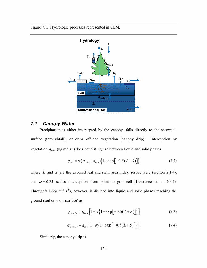
134
Figure 7.1. Hydrologic processes represented in CLM.
7.1 Canopy Water Precipitation is either intercepted by the canopy, falls directly to the snow/soil
surface (throughfall), or drips off the vegetation (canopy drip). Interception by
vegetation intrq (kg m-2 s-1) does not distinguish between liquid and solid phases
( ) ( ) 1 exp 0.5intr rain snoq q q L Sα= + − − + (7.2)
where L and S are the exposed leaf and stem area index, respectively (section 2.1.4),
and 0.25α = scales interception from point to grid cell (Lawrence et al. 2007).
Throughfall (kg m-2 s-1), however, is divided into liquid and solid phases reaching the
ground (soil or snow surface) as
( ) , 1 1 exp 0.5thru liq rainq q L Sα = − − − + (7.3)
( ) , 1 1 exp 0.5thru ice snoq q L Sα = − − − + . (7.4)
Similarly, the canopy drip is
135
,max, 0
intrcan can rain
drip liqrain sno
W W qqt q q
−= ≥
∆ + (7.5)
,max, 0
intrcan can sno
drip icerain sno
W W qqt q q
−= ≥
∆ + (7.6)
where
0intr ncan can intrW W q t= + ∆ ≥ (7.7)
is the canopy water after accounting for interception, ncanW is the canopy water from the
previous time step, and ,maxcanW (kg m-2) is the maximum amount of water the canopy can
hold
( ),maxcanW p L S= + . (7.8)
The maximum storage of solid water is assumed to be the same as that of liquid water,
0.1p = kg m-2 (Dickinson et al. 1993). The canopy water is updated as
( )1, , 0n n w
can can intr drip liq drip ice vW W q t q q t E t+ = + ∆ − + ∆ − ∆ ≥ . (7.9)
where wvE is the flux of water vapor from stem and leaf surfaces (Chapter 5). The total
rate of liquid and solid precipitation reaching the ground is then
, , ,grnd liq thru liq drip liqq q q= + (7.10)
, , ,grnd ice thru ice drip iceq q q= + . (7.11)
Solid precipitation reaching the soil or snow surface, ,grnd iceq t∆ , is added immediately to
the snow pack (section 7.2). The liquid part, ,grnd liqq t∆ is added after surface fluxes
(Chapter 5) and snow/soil temperatures (Chapter 6) have been determined.
136
The wetted fraction of the canopy (stems plus leaves), which is required for the
surface albedo (section 3.1) and surface flux (Chapter 5) calculations is (Dickinson et al.
1993)
( )
2 3
1 0
0 0
can
wet
W L Sf p L S
L S
≤ + > = +
+ =
(7.12)
while the fraction of the canopy that is dry and transpiring is
( )1
0
0 0
wet
dry
f LL Sf L SL S
− + > = +
+ =
. (7.13)
7.2 Snow The parameterizations for snow are based primarily on Anderson (1976), Jordan
(1991), and Dai and Zeng (1997). The snowpack can have up to five layers. These
layers are indexed in the Fortran code as 4, 3, 2, 1,0i = − − − − where layer 0i = is the
snow layer next to the top soil layer and layer 4i = − is the top layer of a five-layer snow
pack. Since the number of snow layers varies according to the snow depth, we use the
notation 1s n l + to describe the top layer of snow for the variable layer snow pack,
where snl is the negative of the number of snow layers. Refer to Figure 7.2 for an
example of the snow layer structure for a three layer snow pack.
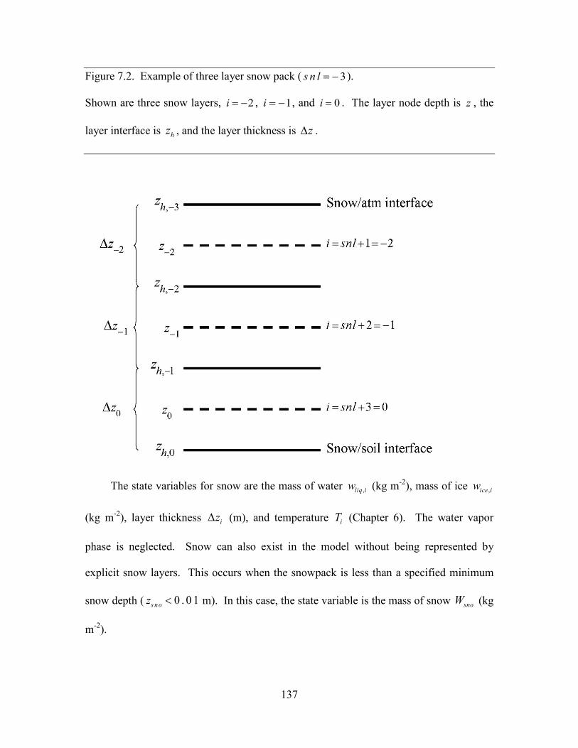
137
Figure 7.2. Example of three layer snow pack ( 3s n l = − ).
Shown are three snow layers, 2i = − , 1i = − , and 0i = . The layer node depth is z , the
layer interface is hz , and the layer thickness is z∆ .
The state variables for snow are the mass of water ,liq iw (kg m-2), mass of ice ,ice iw
(kg m-2), layer thickness iz∆ (m), and temperature iT (Chapter 6). The water vapor
phase is neglected. Snow can also exist in the model without being represented by
explicit snow layers. This occurs when the snowpack is less than a specified minimum
snow depth ( 0 . 0 1s n oz < m). In this case, the state variable is the mass of snow snoW (kg
m-2).
138
Section 7.2.1 describes the calculation of fractional snow covered area, which is
used in the surface albedo calculation (Chapter 3) and the surface flux calculations
(Chapter 5). The following two sections (7.2.2 and 7.2.3) describe the ice and water
content of the snow pack assuming that at least one snow layer exists. Section 7.2.4
describes how black and organic carbon and mineral dust particles are represented within
snow, including meltwater flushing. See section 7.2.5 for a description of how a snow
layer is initialized.
7.2.1 Snow Covered Area Fraction The fraction of the ground covered by snow, snof , is based on the method of
Swenson and Lawrence (2012). Because the processes governing snowfall and snowmelt
differ, changes in snof are calculated separately for accumulation and depletion. When
snowfall occurs, snof is updated as
( )( )( )1 1 1 tanh( ) 1n nsno accum sno snof k q t f+ = − − ∆ − (7.14)
where accumk is a constant whose default value is 0.1, snoq t∆ is the amount of new snow,
1nsnof + is the updated snow covered fraction (SCF), and n
snof is the SCF from the
previous time step.
When snow melt occurs, snof is calculated from the depletion curve
( )1cos 2 11
meltN
snosno
Rf
π
− −= −
(7.15)
where snoR is the ratio of snoW to the maximum accumulated snow maxW , and meltN is a
parameter that depends on the topographic variability within the grid cell. Whenever
139
snoW reaches zero, maxW is reset to zero. The depletion curve shape parameter is defined
as
( )200
min 10,melttopo
Nσ
= (7.16)
The standard deviation of the elevation within a grid cell, topoσ , is calculated from a high
resolution DEM (a 1km DEM is used for CLM).
7.2.2 Ice Content The conservation equation for mass of ice in snow layers is
( )
( )
,
, 1,
,
1
2, ,0
ice i psno ice i
ice i
ice i p
wf q i snlw t
t wi snl
t
−
∆ − = +∂ ∆= ∂ ∆
− = + ∆
(7.17)
where , 1ice iq − is the rate of ice accumulation from precipitation or frost or the rate of ice
loss from sublimation (kg m-2 s-1) in the top layer and ( ),ice i pw t∆ ∆ is the change in ice
due to phase change (melting rate) (section 6.2). The term , 1ice iq − is computed in two
steps as
( ), 1 ,ice i grnd ice frost sublq q q q− = + − (7.18)
where ,grnd iceq is the rate of solid precipitation reaching the ground (section 7.1) and
frostq and sublq are gains due to frost and losses due to sublimation, respectively (section
5.4). In the first step, immediately after ,grnd iceq has been determined after accounting for
interception (section 7.1), a new snow depth snoz (m) is calculated from
1n nsno sno snoz z z+ = + ∆ (7.19)
140
where
,grnd icesno
sno sno
q tz
f ρ∆
∆ = (7.20)
and snoρ is the bulk density of newly fallen snow (kg m-3) (Anderson 1976)
( )
( )
1.5
1.5
50 1.7 17 2
50 1.7 15 15 2
50 15
atm f
sno atm f f atm f
atm f
T T
T T T T T
T T
ρ
+ > + = + − + − < ≤ + ≤ −
(7.21)
where a t mT is the atmospheric temperature (K), and fT is the freezing temperature of
water (K) (Table 2.6). The mass of snow snoW is
1,
n nsno sno grnd iceW W q t+ = + ∆ . (7.22)
The ice content of the top layer and the layer thickness are updated as
1, 1 , 1 ,
n nice snl ice snl grnd icew w q t+
+ += + ∆ (7.23)
11 1
n nsnl snl snoz z z+
+ +∆ = ∆ + ∆ . (7.24) Since wetlands are modeled as columns of water (no soil), snow is not allowed to
accumulate if the surface temperature is above freezing ( g fT T> ). In this case, the
incoming solid precipitation is assigned to the runoff term rgwlq (section 7.7).
In the second step, after surface fluxes and snow/soil temperatures have been
determined (Chapters 5 and 6), , 1ice snlw + is updated for frost or sublimation as
( )1, 1 , 1
n nice snl ice snl sno frost sublw w f q q t+
+ += + − ∆ . (7.25)
If 1, 1 0n
ice snlw ++ < upon solution of equation (7.25), the ice content is reset to zero and
the liquid water content , 1l i q s n lw + is reduced by the amount required to bring 1, 1
ni c e s n lw +
+ up
to zero.
141
The snow water equivalent s n oW is capped to not exceed 1000 kg m-2. If the
addition of frostq were to result in 1 0 0 0s n oW > kg m-2, the frost term frostq is instead
added to the ice runoff term ,snwcp iceq (section 7.7).
7.2.3 Water Content The conservation equation for mass of water in snow layers is
( )( ),,
, 1 ,
liq iliq i pliq i liq i
wwq q
t t−
∆∂= − +
∂ ∆ (7.26)
where , 1liq iq − is the flow of liquid water into layer i from the layer above, ,liq iq is the
flow of water out of layer i to the layer below, ( ),liq i pw t∆ ∆ is the change in liquid
water due to phase change (melting rate) (section 6.2). For the top snow layer only,
( )( ), 1 ,liq i sno grnd liq sdew sevaq f q q q− = + − (7.27)
where ,g r n d l i qq is the rate of liquid precipitation reaching the snow (section 7.1), sevaq is
the evaporation of liquid water and sdewq is the liquid dew (section 5.4). After surface
fluxes and snow/soil temperatures have been determined (Chapters 5 and 6), , 1liq snlw + is
updated for the liquid precipitation reaching the ground and dew or evaporation as
( )1, 1 , 1 ,
n nliq snl liq snl sno grnd liq sdew sevaw w f q q q t+
+ += + + − ∆ . (7.28)
When the liquid water within a snow layer exceeds the layer’s holding capacity, the
excess water is added to the underlying layer, limited by the effective porosity (1 iceθ− ) of
the layer. The flow of water is assumed to be zero ( , 0liq iq = ) if the effective porosity of
either of the two layers ( , , 11 and 1ice i ice iθ θ +− − ) is less than 0.05impθ = , the water
142
impermeable volumetric water content. Thus, water flow between layers, ,liq iq , for layers
1, ,0i snl= + , is initially calculated as
( ), ,
,
10
liq liq i r ice i sno iliq i
S f zq
t
ρ θ θ − − ∆ = ≥∆
(7.29)
where the volumetric liquid water ,liq iθ and ice ,ice iθ contents are
,, 1ice i
ice isno i ice
wf z
θρ
= ≤∆
(7.30)
,, ,1liq i
liq i ice isno i liq
wf z
θ θρ
= ≤ −∆
, (7.31)
and 0.033rS = is the irreducible water saturation (snow holds a certain amount of liquid
water due to capillary retention after drainage has ceased (Anderson 1976)). The water
holding capacity of the underlying layer limits the flow of water ,liq iq calculated in
equation (7.29), unless the underlying layer is the surface soil layer, as
, 1 , 1 1,
11, , 1liq ice i liq i i
liq i
zq i snl
tρ θ θ+ + + − − ∆ ≤ = + −
∆ . (7.32)
The liquid water content ,liq iw is updated as
( )1, , 1
n nliq i liq i i iw w q q t+
−= + − ∆ . (7.33)
Equations (7.29)-(7.33) are solved sequentially from top ( 1i snl= + ) to bottom ( 0i = )
snow layer in each time step. The total flow of liquid water reaching the soil surface is
then ,0liqq which is used in the calculation of surface runoff and infiltration (section 7.3).
7.2.4 Black and organic carbon and mineral dust within snow Particles within snow originate from atmospheric aerosol deposition ( spD in Table
2.3 (kg m-2 s-1) and influence snow radiative transfer (sections 3.2.1, 3.2.2, and 3.3.3).
Particle masses and mixing ratios are represented with a simple mass-conserving scheme.
143
The model maintains masses of the following eight particle species within each snow
layer: hydrophilic black carbon, hydrophobic black carbon, hydrophilic organic carbon,
hydrophobic organic carbon, and four species of mineral dust with the following particle
sizes: 0.1-1.0, 1.0-2.5, 2.5-5.0, and 5.0-10.0 mµ . Each of these species has unique
optical properties (Table 3.5) and meltwater removal efficiencies (Table 7.1).
The black carbon and organic carbon deposition rates described in Table 2.3 are
combined into four categories as follows
, , ,bc hphil bc dryhphil bc wethphilD D D= + (7.34)
, ,bc hphob bc dryhphobD D= (7.35) , , ,oc hphil oc dryhphil oc wethphilD D D= + (7.36)
, ,oc hphob oc dryhphobD D= (7.37)
Deposited particles are assumed to be instantly mixed (homogeneously) within the
surface snow layer and are added after the inter-layer water fluxes are computed (section
7.2.3) so that some aerosol is in the top layer after deposition and is not immediately
washed out before radiative calculations are done. Particle masses are then redistributed
each time step based on meltwater drainage through the snow column (section 7.2.3) and
snow layer combination and subdivision (section 7.2.7). The change in mass of each of
the particle species ,sp im∆ (kg m-2) is
( ), , 1 , 1 ,sp i sp liq i sp i liq i i spm k q c q c D t− − ∆ = − + ∆ (7.38)
where spk is the meltwater scavenging efficiency that is unique for each species (Table
7.1), , 1liq iq − is the flow of liquid water into layer i from the layer above, ,liq iq is the flow
of water out of layer i into the layer below (kg m-2 s-1) (section 7.2.3), , 1sp ic − and ,sp ic are
144
the particle mass mixing ratios in layers 1i − and i (kg kg-1), spD is the atmospheric
deposition rate (zero for all layers except layer 1snl + ), and t∆ is the model time step
(s). The particle mass mixing ratio is
,
, ,
sp ii
liq i ice i
mc
w w=
+. (7.39)
Values of spk are partially derived from experiments published by Conway et al. (1996).
Particles masses are re-distributed proportionately with snow mass when layers are
combined or divided, thus conserving particle mass within the snow column. The mass
of particles carried out with meltwater through the bottom snow layer is assumed to be
permanently lost from the snowpack, and is not maintained within the model.
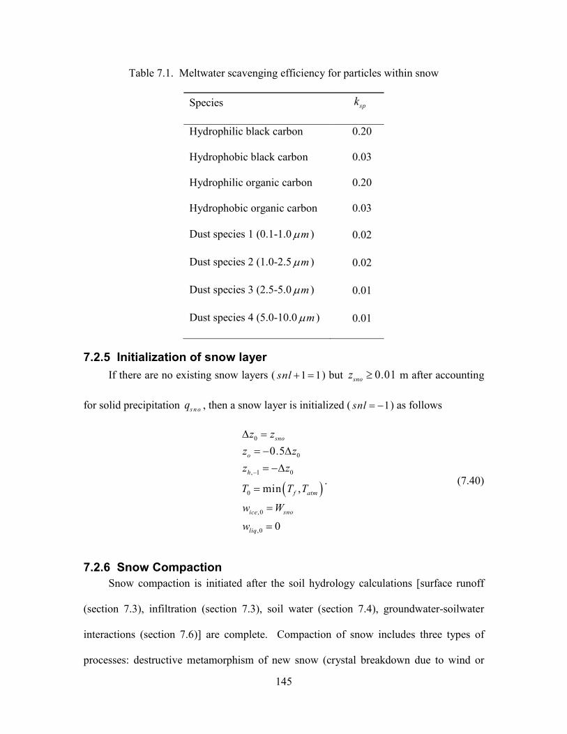
145
Table 7.1. Meltwater scavenging efficiency for particles within snow
Species spk
Hydrophilic black carbon 0.20
Hydrophobic black carbon 0.03
Hydrophilic organic carbon 0.20
Hydrophobic organic carbon 0.03
Dust species 1 (0.1-1.0 mµ ) 0.02
Dust species 2 (1.0-2.5 mµ ) 0.02
Dust species 3 (2.5-5.0 mµ ) 0.01
Dust species 4 (5.0-10.0 mµ ) 0.01
7.2.5 Initialization of snow layer If there are no existing snow layers ( 1 1snl + = ) but 0.01snoz ≥ m after accounting
for solid precipitation s n oq , then a snow layer is initialized ( 1snl = − ) as follows
( )
0
0
, 1 0
0
,0
,0
0.5
min ,
0
sno
o
h
f atm
ice sno
liq
z zz zz z
T T T
w W
w
−
∆ == − ∆
= −∆
=
=
=
. (7.40)
7.2.6 Snow Compaction Snow compaction is initiated after the soil hydrology calculations [surface runoff
(section 7.3), infiltration (section 7.3), soil water (section 7.4), groundwater-soilwater
interactions (section 7.6)] are complete. Compaction of snow includes three types of
processes: destructive metamorphism of new snow (crystal breakdown due to wind or
146
thermodynamic stress); snow load or overburden (pressure); and melting (changes in
snow structure due to melt-freeze cycles plus changes in crystals due to liquid water).
The total fractional compaction rate for each snow layer ,R iC (s-1) is the sum of the three
compaction processes
, 1, 2, 3,1 i
R i R i R i R ii
zC C C Cz t
∂∆= = + +
∆ ∂. (7.41)
Compaction is not allowed if the layer is saturated
, ,1 0.001ice i liq i
sno i ice sno i liq
w wf z f zρ ρ
− + ≤ ∆ ∆
(7.42)
or if the ice content is below a minimum value ( , 0.1ice iw ≤ ).
Compaction as a result of destructive metamorphism 1,R iC (s-1) is temperature
dependent (Anderson 1976)
( )1, 3 1 2 41 expi
R i f ii metamorphism
zC c c c c T Tz t
∂∆ = = − − − ∆ ∂ (7.43)
where 63 2.777 10c −= × (s-1) is the fractional compaction rate for i fT T= , 4 0.04c = K-1,
and
, -31
, , -31
,2
,2
1 100 kg m
exp 0.046 100 100 kg m
2 0.01
1 0.01
ice i
sno i
ice i ice i
sno i sno i
liq i
sno i
liq i
sno i
wc
f z
w wc
f z f z
wc
f zw
cf z
= ≤∆
= − − > ∆ ∆
= >∆
= ≤∆
(7.44)
147
where ( ),ice i sno iw f z∆ and ( ),liq i sno iw f z∆ are the bulk densities of liquid water and ice
(kg m-3).
The compaction rate as a result of overburden 2,R iC (s-1) is a linear function of the
snow load pressure ,s iP (kg m-2) (Anderson 1976)
(7.45)
where η is a viscosity coefficient (kg s m-2) that varies with density and temperature as
( ) ,0 5 6exp ice i
f isno i
wc T T c
f zη η
= − + ∆
(7.46)
where 50 9 10η = × kg s m-2, and 5 0.08c = K-1, 6 0.023c = m3 kg-1 are constants. The
snow load pressure ,s iP is calculated for each layer as the sum of the ice ,ice iw and liquid
water contents ,liq iw of the layers above plus half the ice and liquid water contents of the
layer being compacted
. (7.47)
The compaction rate due to melting 3,R iC (s-1) is taken to be the ratio of the change
in snow ice mass after the melting to the mass before melting
1
, ,3,
,
1 1 max 0,n n
sno i sno iiR i n
i sno imelt
W WzCz t t W
+ − ∂∆= = − ∆ ∂ ∆
(7.48)
and melting is identified during the phase change calculations (section 6.2). Because
snow depth is defined as the average depth of the snow covered area, the snow depth
must also be updated for changes in snof .
,2,
1 s iiR i
i overburden
PzCz t η
∂∆= = − ∆ ∂
( ) ( )1
, ,, , ,
12
j ii c e i l i q i
s i i c e j l i q jj s n l
w wP w w
= −
= +
+= + +∑
148
1
, ,4,
,
1 1 max 0,n n
sno i sno iiR i n
i sno ifsno
f fzCz t t f
+ − ∂∆= = − ∆ ∂ ∆
(7.49)
The snow layer thickness after compaction is then
( )1,1n n
i i R iz z C t+∆ = ∆ + ∆ . (7.50)
7.2.7 Snow Layer Combination and Subdivision After the determination of snow temperature including phase change (Chapter 6),
snow hydrology (sections 7.2.2, 7.2.3, and 7.2.4), and the compaction calculations
(7.2.6), the number of snow layers is adjusted by either combining or subdividing layers.
The combination and subdivision of snow layers is based on Jordan (1991).
7.2.7.1 Combination If a snow layer has nearly melted or if its thickness iz∆ is less than the prescribed
minimum thickness minz∆ (Table 7.2), the layer is combined with a neighboring layer.
The overlying or underlying layer is selected as the neighboring layer according to the
following rules
• If the top layer is being removed, it is combined with the underlying layer
• If the underlying layer is not snow (i.e., it is the top soil layer), the layer is
combined with the overlying layer
• If the layer is nearly completely melted, the layer is combined with the
underlying layer
• If none of the above rules apply, the layer is combined with the thinnest
neighboring layer.
149
A first pass is made through all snow layers to determine if any layer is nearly melted (
, 0.1ice iw ≤ ). If so, the remaining liquid water and ice content of layer i is combined with
the underlying neighbor 1i + as
, 1 , 1 ,liq i liq i liq iw w w+ += + (7.51)
, 1 , 1 ,ice i ice i ice iw w w+ += + . (7.52)
This includes the snow layer directly above the top soil layer. In this case, the liquid
water and ice content of the melted snow layer is added to the contents of the top soil
layer. The layer properties, iT , ,ice iw , ,liq iw , iz∆ , are then re-indexed so that the layers
above the eliminated layer are shifted down by one and the number of snow layers is
decremented accordingly.
At this point, if there are no explicit snow layers remaining ( 0snl = ), the snow water
equivalent snoW and snow depth snoz are set to zero, otherwise, snoW and snoz are re-
calculated as
( )0
, ,1
i
sno ice i liq ii snl
W w w=
= +
= +∑ (7.53)
0
1
i
sno ii snl
z z=
= +
= ∆∑ . (7.54)
If the snow depth 0 0.01snoz< < m or the snow density 50sno
sno sno
Wf z
< kg/m3, the
number of snow layers is set to zero, the total ice content of the snowpack 0
,1
i
ice ii snl
w=
= +∑ is
assigned to snoW , and the total liquid water 0
,1
i
liq ii snl
w=
= +∑ is assigned to the top soil layer.
Otherwise, the layers are combined according to the rules above.
150
When two snow layers are combined (denoted here as 1 and 2), their thickness
combination ( c ) is
1 2cz z z∆ = ∆ + ∆ , (7.55)
their mass combination is
, ,1 ,2liq c liq liqw w w= + (7.56)
, ,1 ,2ice c ice icew w w= + , (7.57)
and their temperatures are combined as
,
, ,
c f liq cc f
ice ice c liq liq c
h L wT T
C w C w−
= ++
(7.58)
where 1 2ch h h= + is the combined enthalpy ih of the two layers where
( )( ), , ,i ice ice i liq liq i i f f liq ih C w C w T T L w= + − + . (7.59)
In these equations, fL is the latent heat of fusion (J kg-1) and liqC and iceC are the
specific heat capacities (J kg-1 K-1) of liquid water and ice, respectively (Table 2.6). After
layer combination, the node depths and layer interfaces (Figure 7.2) are recalculated from
, 0.5 0, , 1i h i iz z z i snl= − ∆ = + (7.60)
, 1 , 0, , 1h i h i iz z z i snl− = − ∆ = + (7.61)
where iz∆ is the layer thickness.
151
Table 7.2. Minimum and maximum thickness of snow layers (m)
Layer minz∆ lN uN ( )max lz∆ ( )max u
z∆
1 (top) 0.010 1 >1 0.03 0.02
2 0.015 2 >2 0.07 0.05
3 0.025 3 >3 0.18 0.11
4 0.055 4 >4 0.41 0.23
5 (bottom) 0.115 5 - - -
The maximum snow layer thickness, maxz∆ , depends on the number of layers, lN and
uN (section 7.2.7.2).
7.2.7.2 Subdivision The snow layers are subdivided when the layer thickness exceeds the prescribed
maximum thickness maxz∆ with lower and upper bounds that depend on the number of
snow layers (Table 7.2). For example, if there is only one layer, then the maximum
thickness of that layer is 0.03 m, however, if there is more than one layer, then the
maximum thickness of the top layer is 0.02 m. Layers are checked sequentially from top
to bottom for this limit. If there is only one snow layer and its thickness is greater than
0.03 m (Table 7.2), the layer is subdivided into two layers of equal thickness, liquid water
and ice contents, and temperature. If there is an existing layer below the layer to be
subdivided, the thickness iz∆ , liquid water and ice contents, ,liq iw and ,ice iw , and
temperature iT of the excess snow are combined with the underlying layer according to
equations (7.55)-(7.58). If there is no underlying layer after adjusting the layer for the
excess snow, the layer is subdivided into two layers of equal thickness, liquid water and
152
ice contents. The vertical snow temperature profile is maintained by calculating the slope
between the layer above the splitting layer ( 1T ) and the splitting layer ( 2T ) and
constraining the new temperatures ( 12nT + , 1
3nT + ) to lie along this slope. The temperature
of the lower layer is first evaluated from
( )
11 2 2
3 21 2 22
n n nn
n n
T T zT Tz z
+ − ∆′ = − ∆ + ∆ , (7.62)
then adjusted as,
( )
13 2 3
11 1 2 2
2 2 31 2 22
n nf
n n nn n
fn
T T T T
T T zT T T Tz z
+
++
′= ≥
− ∆ ′ = + < ∆ + ∆
(7.63)
where here the subscripts 1, 2, and 3 denote three layers numbered from top to bottom.
After layer subdivision, the node depths and layer interfaces are recalculated from
equations (7.60) and (7.61).
7.3 Surface Runoff, Surface Water Storage, and Infiltration The moisture input at the grid cell surface , , 0liqq , is the sum of liquid precipitation
reaching the ground and melt water from snow (kg m-2 s-1). The moisture flux is then
partitioned between surface runoff, surface water storage, and infiltration into the soil.
7.3.1 Surface Runoff The simple TOPMODEL-based (Beven and Kirkby 1979) runoff model (SIMTOP)
described by Niu et al. (2005) is implemented to parameterize runoff. A key concept
underlying this approach is that of fractional saturated area satf , which is determined by
the topographic characteristics and soil moisture state of a grid cell. The saturated
153
portion of a grid cell contributes to surface runoff, overq , by the saturation excess
mechanism (Dunne runoff)
, 0over sat liqq f q= (7.64)
The fractional saturated area is a function of soil moisture
( )max exp 0.5sat overf f f z∇= − (7.65)
where maxf is the potential or maximum value of satf , overf is a decay factor (m-1), and
z∇ is the water table depth (m) (section 7.6). The maximum saturated fraction, maxf , is
defined as the value of the discrete cumulative distribution function (CDF) of the
topographic index when the grid cell mean water table depth is zero. Thus, maxf is the
percent of pixels in a grid cell whose topographic index is larger than or equal to the grid
cell mean topographic index. It should be calculated explicitly from the CDF at each grid
cell at the resolution that the model is run. However, because this is a computationally
intensive task for global applications, maxf is calculated once at 0.125° resolution using
the 1-km compound topographic indices (CTIs) based on the HYDRO1K dataset (Verdin
and Greenlee 1996) from USGS following the algorithm in Niu et al. (2005) and then
area-averaged to the desired model resolution (section 2.2.3). Pixels with CTIs
exceeding the 95 percentile threshold in each 0.125° grid cell are excluded from the
calculation to eliminate biased estimation of statistics due to large CTI values at pixels on
stream networks. For grid cells over regions without CTIs such as Australia, the global
mean maxf is used to fill the gaps. See Li et al. (2013b) for additional details. The decay
factor overf for global simulations was determined through sensitivity analysis and
comparison with observed runoff to be 0.5 m-1.
154
7.3.2 Surface Water Storage A surface water store has been added to the model to represent wetlands and small,
sub-grid scale water bodies. As a result, the wetland land unit has been removed. The
state variables for surface water are the mass of water sfcW (kg m-2) and temperature
2h osfcT (Chapter 6). Surface water storage and outflow are functions of fine spatial scale
elevation variations called microtopography. The microtopography is assumed to be
distributed normally around the grid cell mean elevation. Given the standard deviation of
the microtopographic distribution, microσ (m), the fractional area of the grid cell that is
inundated can be calculated. Surface water storage, sfcW , is related to the height (relative
to the grid cell mean elevation) of the surface water, d , by
2
2212 2 2
micro
dmicro
sfcmicro
d dW erf e σσσ π
− = + +
(7.66)
where erf is the error function. For a given value of sfcW , equation (7.66) can be solved
for d using the Newton-Raphson method. Once d is known, one can determine the
fraction of the area that is inundated as
21 12 2h osfc
micro
df erfσ
= +
(7.67)
No global datasets exist for microtopography, so the default parameterization is a simple
function of slope
( )0microησ β β= + (7.68)
155
where β is the topographic slope, ( )1
0 maxηβ σ= determines the maximum value of σ ,
and η is an adjustable parameter. Default values in the model are max 0.4σ = and 3η = −
.
If the spatial scale of the microtopography is small relative to that of the grid cell,
one can assume that the inundated areas are distributed randomly within the grid cell.
With this assumption, a result from percolation theory can be used to quantify the
fraction of the inundated portion of the grid cell that is interconnected
( )2 2
20connected h osfc c h osfc c
connected h osfc c
f f f for f f
f for f f
µ= − >
= ≤ (7.69)
where cf is a threshold below which no single connected inundated area spans the grid
cell and µ is a scaling exponent. Default values of cf and µ are 0.4 and 0.14,
respectively. When the inundated fraction of the grid cell surpasses cf , the surface water
store acts as a linear reservoir
, 2 21( )out h osfc h osfc sfc cconnectedq k f W Wt
= −∆
(7.70)
where , 2out h osfcq is the surface water runoff, 2h osfck is a constant, cW is the amount of
surface water present when 2h osfc cf f= , and t∆ is the model time step. The linear storage
coefficent ( )2 sinh osfck β= is a function of grid cell mean topographic slope where β is
the slope in radians.
7.3.3 Infiltration The surface moisture flux remaining after surface runoff has been removed,
in, , 0(1 )surface sat liqq f q= − (7.71)
156
is divided into inputs to surface water ( , 2in h osfcq ) and the soil ,in soilq . If ,in soilq exceeds the
maximum soil infiltration capacity (kg m-2 s-1),
, max (1 )sat ice satinflq f k= − Θ (7.72)
where iceΘ is an ice impedance factor (section 7.4), infiltration excess (Hortonian) runoff
is generated
( )( ), , 2 inf ,maxmax 1 , 0infl excess in soil h osfc lq q f q= − − (7.73)
and transferred from ,in soilq to , 2in h osfcq . After evaporative losses have been removed,
these moisture fluxes are
, 2, 2 2 , , evap h osfcin h osfc h osfc in surface infl excessq f q q q= + − (7.74)
and
in, ,2 , inf , 2(1 ) (1 )soil evap soilh osfc in surface l excess sno h osfcq f q q f f q= − − − − − . (7.75)
The balance of surface water is then calculated as
( ), 2 , 2 , 2in h osfc out h osfc drain h osfcsfcW q q q t∆ = − − ∆ . (7.76)
Bottom drainage from the surface water store
, 2 2 inf ,maxmin , sfcdrain h osfc h osfc l
Wq f q
t
= ∆ (7.77)
is then added to ,in soilq giving the total infiltration into the surface soil layer
, , 2infl in soil drain h osfcq q q= + (7.78)
Infiltration inflq and explicit surface runoff overq are not allowed for glaciers.
157
7.4 Soil Water Soil water is predicted from a multi-layer model, in which the vertical soil moisture
transport is governed by infiltration, surface and sub-surface runoff, gradient diffusion,
gravity, canopy transpiration through root extraction, and interactions with groundwater
(Figure 7.1). The following derivation generally follows that of Z.-L. Yang (1998,
unpublished manuscript) with modifications by Zeng and Decker (2009).
For one-dimensional vertical water flow in soils, the conservation of mass is stated
as
q Q
t zθ∂ ∂
= − −∂ ∂
(7.79)
where θ is the volumetric soil water content (mm3 of water mm-3 of soil), t is time (s), z
is height above some datum in the soil column (mm) (positive upwards), q is soil water
flux (kg m-2 s-1 or mm s-1) (positive upwards), and Q is a soil moisture sink term (mm of
water mm-1 of soil s-1) (ET loss). This equation is solved numerically by dividing the soil
column into multiple layers in the vertical and integrating downward over each layer with
an upper boundary condition of the infiltration flux into the top soil layer inflq and a
lower boundary condition that depends on the depth of the water table.
The soil water flux q in equation (7.79) can be described by Darcy’s law
hq kz
ψ∂= −
∂ (7.80)
where k is the hydraulic conductivity (mm s-1), and hψ is the hydraulic potential (mm).
The hydraulic potential is
h m zψ ψ ψ= + (7.81)
158
where mψ is the soil matric potential (mm) (which is related to the adsorptive and
capillary forces within the soil matrix), and zψ is the gravitational potential (mm) (the
vertical distance from an arbitrary reference elevation to a point in the soil). If the
reference elevation is the soil surface, then z zψ = . Letting mψ ψ= , Darcy’s law
becomes
( )zq k
zψ∂ +
= − ∂ . (7.82)
Darcy’s equation can be further manipulated to yield
( ) 1 1z
q k k kz z z
ψ ψ θ ψθ
∂ + ∂ ∂ ∂ = − = − + = − + ∂ ∂ ∂ ∂ . (7.83)
Substitution of this equation into equation (7.79), with 0Q = , yields the Richards
equation
1kt z zθ θ ψ
θ∂ ∂ ∂ ∂ = + ∂ ∂ ∂ ∂
. (7.84)
Zeng and Decker (2009) note that this θ -based form of the Richards equation
cannot maintain the hydrostatic equilibrium soil moisture distribution because of the
truncation errors of the finite-difference numerical scheme. They show that this
deficiency can be overcome by subtracting the equilibrium state from equation (7.82) as
( )z Cq k
zψ∂ + −
= − ∂ (7.85)
where C is a constant hydraulic potential above the water table z∇
( ) BE
E sat satsat
zC z z z
θψ ψ ψ
θ
−
∇
= + = + = +
(7.86)
159
so that
( )Eq kz
ψ ψ∂ − = − ∂
(7.87)
where Eψ is the equilibrium soil matric potential (mm). Substitution of equations (7.86)
and (7.85) into equation (7.84) yields Zeng and Decker’s (2009) modified Richards
equation
( )Ek Qt z z
ψ ψθ ∂ − ∂ ∂= − ∂ ∂ ∂
(7.88)
where the soil moisture sink term Q is now included.
7.4.1 Hydraulic Properties The hydraulic conductivity ik (mm s-1) and the soil matric potential iψ (mm) for
layer i vary with volumetric soil water iθ and soil texture. As with the soil thermal
properties (section 6.3) the hydraulic properties of the soil are assumed to be a weighted
combination of the mineral properties, which are determined according to sand and clay
contents based on work by Clapp and Hornberger (1978) and Cosby et al. (1984), and
organic properties of the soil (Lawrence and Slater 2008).
The hydraulic conductivity is defined at the depth of the interface of two adjacent
layers ,h iz (Figure 7.3) and is a function of the saturated hydraulic conductivity ,sat h ik z
, the liquid volumetric soil moisture of the two layers iθ and 1iθ + and an ice impedance
factor iceΘ
160
( )( )
2 3
1,
, , 1, 2 3
,,
0.51 1
0.5
i
i
B
i iice sat h i levsoi
sat i sat ih i B
iice sat h i levsoi
sat i
k z i N
k z
k z i N
θ θ
θ θ
θθ
+
+
+
+
+ Θ ≤ ≤ − + =
Θ = .
(7.89)
The ice impedance factor is a function of ice content, and is meant to quantify the
increased tortuosity of the water flow when part of the pore space is filled with ice.
Swenson et al. (2012) used a power law form 10 iceFice
−ΩΘ = where 6Ω = and
iceice
sat
F θθ
= is the ice-filled fraction of the pore space.
Because the hydraulic properties of mineral and organic soil may differ
significantly, the bulk hydraulic properties of each soil layer are computed as weighted
averages of the properties of the mineral and organic components. The water content at
saturation (i.e. porosity) is
, , ,min, , ,(1 )sat i om i sat i om i sat omf fθ θ θ= − + (7.90)
where ,om if is the soil organic matter fraction, , 0.9sat omθ = (Farouki 1981; Letts et al.
2000) is the porosity of organic matter and the porosity of the mineral soil ,min,sat iθ is
,min, 0.489 0.00126(% )sai i isandθ = − . (7.91)
The exponent “ B ” is
, min, ,(1 )i om i i om i omB f B f B= − + (7.92)
where 2.7omB = (Letts et al. 2000) and
min, 2.91 0.159(% )i iB clay= + . (7.93)
161
The soil matric potential (mm) is defined at the node depth iz of each layer i
(Figure 7.3)
8,
, ,
1 10 0.01 1iB
i ii sat i
sat i sat i
θ θψ ψθ θ
−
= ≥ − × ≤ ≤
(7.94)
where the saturated soil matric potential (mm) is
, , ,min, , ,(1 )sat i om i sat i om i sat omf fψ ψ ψ= − + (7.95)
where , 10.3sat omψ = − mm (Letts et al. 2000) is the saturated organic matter matric
potential and the saturated mineral soil matric potential ,min,sat iψ is
1.88 0.0131(% ),min, 10.0 10 isand
sat iψ −= − × . (7.96)
The saturated hydraulic conductivity, ,sat h ik z (mm s-1), for organic soils ( ,sat omk )
may be two to three orders of magnitude larger than that of mineral soils ( ,minsatk ). Bulk
soil layer values of satk calculated as weighted averages based on omf may therefore be
determined primarily by the organic soil properties even for values of omf as low as 1 %.
To better represent the influence of organic soil material on the grid cell average
saturated hydraulic conductivity, the soil organic matter fraction is further subdivided
into “connected” and “unconnected” fractions using a result from percolation theory
(Stauffer and Aharony 1994, Berkowitz and Balberg 1992). Assuming that the organic
and mineral fractions are randomly distributed throughout a soil layer, percolation theory
predicts that above a threshold value om thresholdf f= , connected flow pathways consisting
of organic material only exist and span the soil space. Flow through these pathways
162
interacts only with organic material, and thus can be described by ,sat omk . This fraction of
the grid cell is given by
( )
0
perc
perc perc om threshold om om threshold
perc om threshold
f N f f f f ff f f
β= − ≥
= < (7.97)
where 0.139percβ = , 0.5thresholdf = , and ( )1 perc
perc thresholdN f β−= − . In the unconnected
portion of the grid cell, ( ) 1 uncon percf f= − , the saturated hydraulic conductivity is
assumed to correspond to flow pathways that pass through the mineral and organic
components in series
( ) ( ) 1
,,min ,
1 om percomsat uncon uncon
sat sat om
f ffk f
k k
− −− = +
. (7.98)
where saturated hydraulic conductivity for mineral soil depends on soil texture (Cosby et
al. 1984) as
( )0.884 0.0153 %,min , 0.0070556 10 isand
sat h ik z − + = × . (7.99)
The bulk soil layer saturated hydraulic conductivity is then computed as
, , , , , , ,(1 )sat h i uncon i sat uncon h i uncon i sat om h ik z f k z f k z = + − . (7.100)
7.4.2 Numerical Solution With reference to Figure 7.3, the equation for conservation of mass (equation (7.79)
) can be integrated over each layer as
, 1 , 1 , 1
, , ,
h i h i h i
h i h i h i
z z z
z z z
qdz dz Q dzt zθ− − −− − −
− − −
∂ ∂= − −
∂ ∂∫ ∫ ∫ . (7.101)
Note that the integration limits are negative since z is defined as positive upward from
the soil surface. This equation can be written as
163
,1
liq ii i i iz q q e
tθ
−
∂∆ = − + −
∂ (7.102)
where iq is the flux of water across interface ,h iz , 1iq − is the flux of water across
interface , 1h iz − , and ie is a layer-averaged soil moisture sink term (ET loss) defined as
positive for flow out of the layer (mm s-1). Taking the finite difference with time and
evaluating the fluxes implicitly at time 1n + yields
, 1 11
i liq i n ni i i
zq q e
tθ + +
−
∆ ∆= − + −
∆ (7.103)
where 1, , ,
n nliq i liq i liq iθ θ θ+∆ = − is the change in volumetric soil liquid water of layer i in time
t∆ and iz∆ is the thickness of layer i (mm).
The water removed by transpiration in each layer ie is a function of the total
transpiration tvE (Chapter 5) and the effective root fraction ,e ir
,t
i e i ve r E= . (7.104)
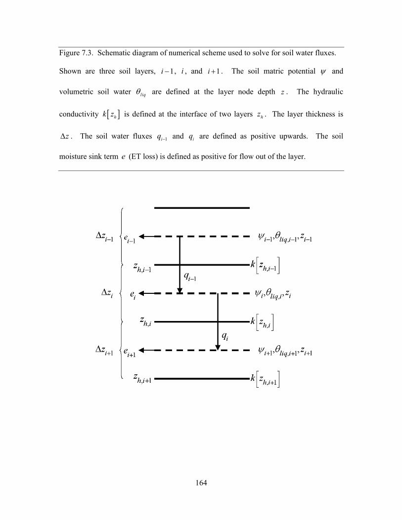
164
Figure 7.3. Schematic diagram of numerical scheme used to solve for soil water fluxes.
Shown are three soil layers, 1i − , i , and 1i + . The soil matric potential ψ and
volumetric soil water liqθ are defined at the layer node depth z . The hydraulic
conductivity [ ]hk z is defined at the interface of two layers hz . The layer thickness is
z∆ . The soil water fluxes 1iq − and iq are defined as positive upwards. The soil
moisture sink term e (ET loss) is defined as positive for flow out of the layer.
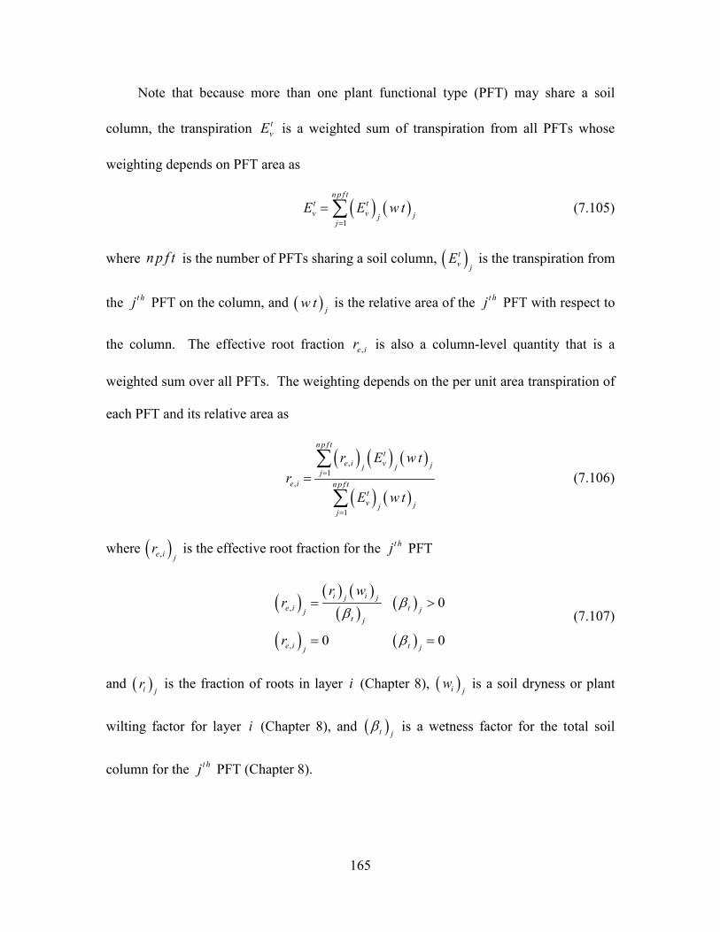
165
Note that because more than one plant functional type (PFT) may share a soil
column, the transpiration tvE is a weighted sum of transpiration from all PFTs whose
weighting depends on PFT area as
( ) ( )1
n p f tt tv v jj
jE E w t
=
= ∑ (7.105)
where n p f t is the number of PFTs sharing a soil column, ( )tv j
E is the transpiration from
the t hj PFT on the column, and ( ) jw t is the relative area of the t hj PFT with respect to
the column. The effective root fraction ,e ir is also a column-level quantity that is a
weighted sum over all PFTs. The weighting depends on the per unit area transpiration of
each PFT and its relative area as
( ) ( ) ( )
( ) ( )
,1
,
1
n p f tt
e i v jjjj
e i n p f ttv jj
j
r E w tr
E w t
=
=
=∑
∑ (7.106)
where ( ),e i jr is the effective root fraction for the t hj PFT
( ) ( ) ( )
( ) ( )
( ) ( )
,
,
0
0 0
i ij je i t jj
t j
e i t jj
r wr
r
ββ
β
= >
= =
(7.107)
and ( )i jr is the fraction of roots in layer i (Chapter 8), ( )i j
w is a soil dryness or plant
wilting factor for layer i (Chapter 8), and ( )t jβ is a wetness factor for the total soil
column for the t hj PFT (Chapter 8).
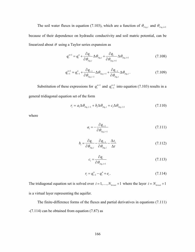
166
The soil water fluxes in equation (7.103), which are a function of ,l i q iθ and , 1l i q iθ +
because of their dependence on hydraulic conductivity and soil matric potential, can be
linearized about θ using a Taylor series expansion as
1, , 1
, , 1
n n i ii i liq i liq i
liq i liq i
q qq q θ θθ θ
++
+
∂ ∂= + ∆ + ∆
∂ ∂ (7.108)
1 1 11 1 , 1 ,
, 1 ,
n n i ii i liq i liq i
liq i liq i
q qq q θ θθ θ
+ − −− − −
−
∂ ∂= + ∆ + ∆
∂ ∂. (7.109)
Substitution of these expressions for 1niq + and 1
1niq +− into equation (7.103) results in a
general tridiagonal equation set of the form
, 1 , , 1i i liq i i liq i i liq ir a b cθ θ θ− += ∆ + ∆ + ∆ (7.110)
where
1
, 1
ii
liq i
qaθ
−
−
∂= −
∂ (7.111)
1
, ,
i i ii
liq i liq i
q q zbtθ θ
−∂ ∂ ∆= − −
∂ ∂ ∆ (7.112)
, 1
ii
liq i
qcθ +
∂=
∂ (7.113)
1n n
i i i ir q q e−= − + . (7.114)
The tridiagonal equation set is solved over 1, , 1levsoii N= + where the layer 1levsoii N= +
is a virtual layer representing the aquifer.
The finite-difference forms of the fluxes and partial derivatives in equations (7.111)
-(7.114) can be obtained from equation (7.87) as
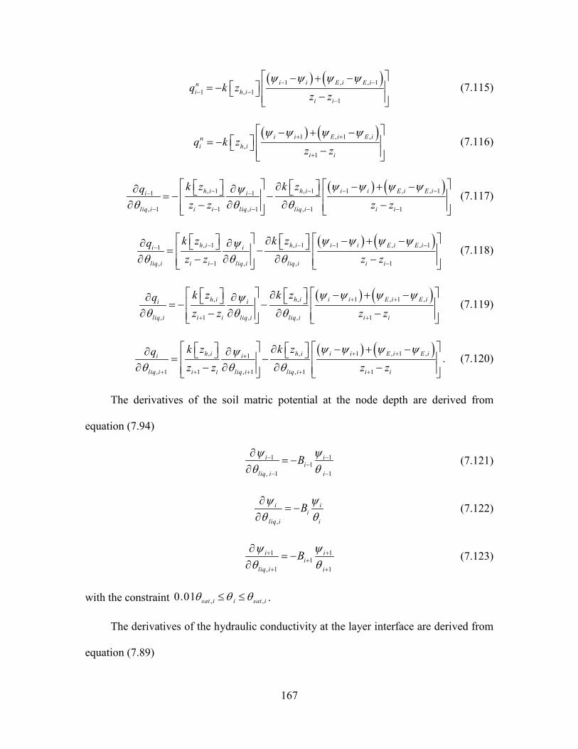
167
( ) ( )1 , , 1
1 , 11
i i E i E ini h i
i i
q k zz z
ψ ψ ψ ψ− −− −
−
− + − = − −
(7.115)
( ) ( )1 , 1 ,
,1
i i E i E ini h i
i i
q k zz z
ψ ψ ψ ψ+ +
+
− + − = − −
(7.116)
( ) ( )1 , , 1, 1 , 11 1
, 1 1 , 1 , 1 1
i i E i E ih i h ii i
liq i i i liq i liq i i i
k z k zqz z z z
ψ ψ ψ ψψθ θ θ
− −− −− −
− − − − −
− + −∂∂ ∂ = − −∂ − ∂ ∂ −
(7.117)
( ) ( )1 , , 1, 1 , 11
, 1 , , 1
i i E i E ih i h ii i
liq i i i liq i liq i i i
k z k zqz z z z
ψ ψ ψ ψψθ θ θ
− −− −−
− −
− + −∂∂ ∂ = −∂ − ∂ ∂ −
(7.118)
( ) ( )1 , 1 ,, ,
, 1 , , 1
i i E i E ih i h ii i
liq i i i liq i liq i i i
k z k zqz z z z
ψ ψ ψ ψψθ θ θ
+ +
+ +
− + −∂∂ ∂ = − −∂ − ∂ ∂ −
(7.119)
( ) ( )1 , 1 ,, ,1
, 1 1 , 1 , 1 1
i i E i E ih i h ii i
liq i i i liq i liq i i i
k z k zqz z z z
ψ ψ ψ ψψθ θ θ
+ ++
+ + + + +
− + −∂∂ ∂ = −∂ − ∂ ∂ −
. (7.120)
The derivatives of the soil matric potential at the node depth are derived from
equation (7.94)
1 11
, 1 1
i ii
liq i i
Bψ ψθ θ
− −−
− −
∂= −
∂ (7.121)
,
i ii
liq i i
Bψ ψθ θ∂
= −∂
(7.122)
1 11
, 1 1
i ii
liq i i
Bψ ψθ θ
+ ++
+ +
∂= −
∂ (7.123)
with the constraint , ,0.01 sat i i sat iθ θ θ≤ ≤ .
The derivatives of the hydraulic conductivity at the layer interface are derived from
equation (7.89)
168
( )
( )( ) ( )
1
, 1 , 1 , 1 ,1 , 1
, 1 ,
2 2
1
, 1 , , 1 ,
1 2 32
0.5 0.50.5 0.5
i
h i h i frz i frz ii sat h i
liq i liq i
B
i i
sat i sat i sat i sat i
k z k z f fB k z
θ θ
θ θ
θ θ θ θ
−
− − −− −
−
+
−
− −
∂ ∂ + = = − + × ∂ ∂
+ + +
(7.124)
( )
( )( ) ( )
, , , , 1,
, , 1
2 2
1
, , 1 , , 1
1 2 32
0.5 0.50.5 0.5
i
h i h i frz i frz ii sat h i
liq i liq i
B
i i
sat i sat i sat i sat i
k z k z f fB k z
θ θ
θ θ
θ θ θ θ
+
+
+
+
+ +
∂ ∂ + = = − + × ∂ ∂
+ + +
. (7.125)
7.4.2.1 Equilibrium soil matric potential and volumetric moisture The equilibrium soil matric potential Eψ can be derived from equation (7.86) as
( ) BE
E satsat
zθψ ψ
θ
−
=
(7.126)
and the equilibrium volumetric water content ( )E zθ at depth z can also be derived as
( )1B
satE sat
sat
z zz ψθ θψ
−
∇ + −=
. (7.127)
Here, the soil matric potentials, the water table depth z∇ and the soil depths have units of
mm. For the finite-difference scheme, a layer-average equilibrium volumetric water
content is used in equation (7.126) and can be obtained from
( ),
, 1
,, , 1
h i
h i
zE
E ih i h iz
zdz
z zθ
θ− −
=−∫ (7.128)
which when integrated yields
( )
1 11 1
, , , , , , 1,
, ,, , 1
11
i iB Bsat i sat i sat i h i sat i h i
E isat i sat i
h i h ii
z z z z
z zB
θ ψ ψ ψθ
ψ ψ
− −
∇ ∇ −
−
− + − + = − − −
.(7.129)
169
Equation (7.129) is valid when the water table z∇ is deeper than both interface depths
, 1h iz − and ,h iz . Since the water table can be within the soil column, the equation is
modified if the water table is within soil layer i ( , 1 ,h i h iz z z− ∇< < ) as a weighted average
of the saturated part and the unsaturated part
, ,, , 1
, , ,, , 1 , , 1
i ih i h i
E i E sat E unsath i h i h i h i
z z z zz z z z
θ θ θ∇ ∇ −
− −
− −= + − −
(7.130)
where ,, ,iE sat sat iθ θ= and the unsaturated part ,, iE unsatθ is
( )
11
, , , , 1, ,
,, 1
111
iBsat i sat i sat i h i
E unsat isat i
h ii
z z
z zB
θ ψ ψθ
ψ
−
∇ −
∇ −
− + = − − −
. (7.131)
If , 1h iz z∇ −< , then ,, , ,iE i E sat sat iθ θ θ= = . If the water table is below the soil column
( , levsoih Nz z∇ > ), an equilibrium volumetric soil moisture is calculated for a virtual layer
1levsoii N= + as
( )
1
1
11
, 1 , 1 , 1 , 1,
, 1, 1
1
111
i
levsoi
Bsat i sat i sat i h i
E i Nsat i
h ii
z z
z zB
θ ψ ψθ
ψ
−
+
−
− − − ∇ −=
−∇ −
−
− + = − − −
(7.132)
The equilibrium volumetric soil moisture is constrained by
, ,0 E i sat iθ θ≤ ≤ (7.133)
The equilibrium soil matric potential is then
, ,8, ,
, ,
1 10 0.01iB
E i E iE i sat i
sat i sat i
θ θψ ψ
θ θ
−
= ≥ − × ≥
(7.134)
170
7.4.2.2 Equation set for layer 1i = For the top soil layer ( 1i = ), the boundary condition is the infiltration rate (section
7.3), 1 11
n ni inflq q+ +− = − , and the water balance equation is
, 1 1i liq i n ninfl i i
zq q e
tθ + +∆ ∆
= + −∆
. (7.135)
After grouping like terms, the coefficients of the tridiagonal set of equations for 1i = are
0ia = (7.136)
,
i ii
liq i
q zbtθ
∂ ∆= −
∂ ∆ (7.137)
, 1
ii
liq i
qcθ +
∂=
∂ (7.138)
1n ni infl i ir q q e+= − + . (7.139)
7.4.2.3 Equation set for layers 2, , 1levsoii N= −
The coefficients of the tridiagonal set of equations for 2, , 1levsoii N= − are
1
, 1
ii
liq i
qaθ
−
−
∂= −
∂ (7.140)
1
, ,
i i ii
liq i liq i
q q zbtθ θ
−∂ ∂ ∆= − −
∂ ∂ ∆ (7.141)
, 1
ii
liq i
qcθ +
∂=
∂ (7.142)
1n n
i i i ir q q e−= − + . (7.143)
171
7.4.2.4 Equation set for layers , 1levsoi levsoii N N= +
For the lowest soil layer ( levsoii N= ), the bottom boundary condition depends on the
depth of the water table. If the water table is within the soil column ( , levsoih Nz z∇ ≤ ), a
zero-flux bottom boundary condition is applied ( 0niq = ) and the coefficients of the
tridiagonal set of equations for levsoii N= are
1
, 1
ii
liq i
qaθ
−
−
∂= −
∂ (7.144)
1
,
i ii
liq i
q zbtθ
−∂ ∆= − −
∂ ∆ (7.145)
0ic = (7.146)
1n
i i ir q e−= + . (7.147)
The coefficients for the aquifer layer 1levsoii N= + are then
0ia = (7.148)
ii
zbt
∆= −
∆ (7.149)
0ic = (7.150)
0ir = . (7.151)
If the water table is below the soil column ( , levsoih Nz z∇ > ), the coefficients for
levsoii N= are
1
, 1
ii
liq i
qaθ
−
−
∂= −
∂ (7.152)
1
, ,
i i ii
liq i liq i
q q zbtθ θ
−∂ ∂ ∆= − −
∂ ∂ ∆ (7.153)
172
, 1
ii
liq i
qcθ +
∂=
∂ (7.154)
1n n
i i i ir q q e−= − + . (7.155)
The 1levsoii N= + terms are evaluated using
81 , 1 1 10Nlevsoi
levsoi levsoi levsoi
B
N sat N Nsψ ψ−
+ + = ≥ − × (7.156)
( )1 0.5levsoi levsoiN Nz z z+ ∇= + (7.157)
where
,1 1
,
0.5 0.01 1levsoi levsoi
levsoi levsoi
levsoi
sat N NN N
sat N
s sθ θ
θ+ +
+= ≤ ≤
, (7.158)
, 1levsoiE Nψ + is evaluated from equations (7.132) and (7.134), and
1 1
, 1 ,
levsoi levsoi
levsoi
levsoi levsoi levsoi
N NN
liq N N sat N
Bs
ψ ψθ θ
+ +
+
∂= −
∂. (7.159)
The coefficients for the aquifer layer 1levsoii N= + are then
1
, 1
ii
liq i
qaθ
−
−
∂= −
∂ (7.160)
1
,
i ii
liq i
q zbtθ
−∂ ∆= − −
∂ ∆ (7.161)
0ic = (7.162)
1n
i ir q −= . (7.163)
Upon solution of the tridiagonal equation set (Press et al. 1992), the liquid water
contents are updated as follows
1, , , 1, ,n n
liq i liq i liq i i levsoiw w z i Nθ+ = + ∆ ∆ = . (7.164)
The volumetric water content is
173
, ,liq i ice ii
i liq i ice
w wz z
θρ ρ
= +∆ ∆
. (7.165)
7.5 Frozen Soils and Perched Water Table When soils freeze, the power-law form of the ice impedance factor (section 7.4.1)
can greatly decrease the hydraulic conductivity of the soil, leading to nearly impermeable
soil layers. When unfrozen soil layers are present above relatively ice-rich frozen layers,
the possibility exists for perched saturated zones. Lateral drainage from perched
saturated regions is parameterized as a function of the thickness of the saturated zone
( ), , ,drai perch drai perch frost perchq k z z∇= − (7.166)
where ,drai perchk depends on topographic slope and soil hydraulic conductivity,
[ ],
5, 10 sin( )
frost
perch
frost
perch
i N
ice i sat i ii N
drai perch i N
ii N
k z zk
zβ
=
=−=
=
Θ ∆
= ∆
∑
∑ (7.167)
where iceΘ is an ice impedance factor determined from the ice content of the soil layers
interacting with the water table (section 7.6), β is the mean grid cell topographic slope in
radians, frostz is the depth to the frost table, and , perchz∇ is the depth to the perched
saturated zone. The frost table frostz is defined as the shallowest frozen layer having an
unfrozen layer above it, while the perched water table , perchz∇ is defined as the depth at
which the volumetric water content drops below a specified threshold. The default
threshold is set to 0.9. Drainage from the perched saturated zone ,drai perchq is removed
from layers perchN through frostN , which are the layers containing , perchz∇ and, frostz
respectively.
174
7.6 Groundwater-Soil Water Interactions Drainage or sub-surface runoff is based on the SIMTOP scheme (Niu et al. 2005)
with a modification to account for reduced drainage in frozen soils. In the work of Niu et
al. (2005), the drainage draiq (kg m-2 s-1) was formulated as
( ),max expdrai drai draiq q f z∇= − . (7.168)
Here, the water table depth z∇ has units of meters. To restrict drainage in frozen soils,
Niu et al. (2005) added the following condition
, ,0 for levsoi levsoidrai ice N liq Nq w w= > . (7.169)
In preliminary testing it was found that a more gradual restriction of drainage was
required so that the water table depth remained dynamic under partially frozen
conditions. The following modification is made to equation (7.168)
( ),max expdrai ice drai draiq q f z∇= Θ − (7.170)
where iceΘ is an ice impedance factor determined from the ice content of the soil layers
interacting with the water table
,
10
i Nlevsoi
ice i ii jwti Nlevsoi
ii jwt
F z
z
ice
=
==
=
∆
−Ω
∆
∑
∑Θ =
(7.171)
where 6Ω = is an adjustable parameter, jwt is the index of the layer directly above the
water table, iceice
sat
F θθ
= is the ice-filled fraction of the pore space of soil layer i (kg m-2),
and iz∆ is the layer thickness (mm). This expression is functionally the same as that
used to determine the ice impedance factor in section 7.4. In equation (7.170), the decay
factor 2.5draif = m-1 and the maximum drainage when the water table depth is at the
175
surface ,max 10sin( )draiq β= kg m-2 s-1 , where β is the mean grid cell topographic slope
in radians, were determined for global simulations through sensitivity analysis and
comparison with observed runoff.
Determination of water table depth z∇ is based on work by Niu et al. (2007). In
this approach, a groundwater component is added in the form of an unconfined aquifer
lying below the soil column (Figure 7.1). The groundwater solution is dependent on
whether the water table is within or below the soil column. The water stored in the
unconfined aquifer aW has a prescribed maximum value (5000 mm). When the water
table is within the soil column, aW is constant because there is no water exchange
between the soil column and the underlying aquifer. In this case, recharge to the water
table is diagnosed by applying Darcy’s law across the water table
( )( )arg
jwtrech e aq
jwt
q kz z
∇
∇
Ψ − Ψ= −
− (7.172)
where 0∇Ψ = is the matric potential at the water table and , 1 1aq ice jwt jwtk k z+ + = Θ is the
hydraulic conductivity of the layer containing the water table. Change in the water table
is then calculated as the difference between recharge and drainage, scaled by the specific
yield of the layer containing the water table
( )argrech e drai
y
q qz t
S∇
−∆ = ∆ . (7.173)
The specific yield, yS , which depends on the soil properties and the water table location,
is derived by taking the difference between two equilibrium soil moisture profiles whose
water tables differ by an infinitesimal amount
176
1
1 1B
y satsat
zS θ
−
∇
= − + Ψ
(7.174)
where B is the Clapp-Hornberger exponent. Because yS is a function of the soil
properties, it results in water table dynamics that are consistent with the soil water fluxes
described in section 7.4.
For the case when the water table is below the soil column, the change in water
stored in the unconfined aquifer aW (mm) is updated as
( )a recharge draiW q q t∆ = − ∆ (7.174)
and the water table is updated using equation (7.173) with the specific yield of layer
levsoiN .
The recharge rate is defined as positive when water enters the aquifer
, 1 1levsoi levsoiliq N Nrecharge
zq
tθ + +∆ ∆
=∆
(7.174)
where 1, 1 , 1 , 1levsoi levsoi levsoi
n nliq N liq N liq Nθ θ θ+
+ + +∆ = − is the change in liquid water content for layer
1levsoii N= + calculated from the solution of the soil water equations (section 7.4), and
1levsoiNz +∆ (mm) is
1 ,levsoi levsoi
nN h Nz z z+ ∇∆ = − . (7.174)
After the above calculations, two numerical adjustments are implemented to keep
the liquid water content of each soil layer ( ,liq iw ) within physical constraints of
( )min, , ,liq liq i sat i ice i iw w zθ θ≤ ≤ − ∆ where min 0.01liqw = (mm). First, beginning with the
bottom soil layer levsoii N= , any excess liquid water in each soil layer
177
( ( ), , , , 0excessliq i liq i sat i ice i iw w zθ θ= − − ∆ ≥ ) is successively added to the layer above. Any
excess liquid water that remains after saturating the entire soil column (plus a maximum
surface ponding depth 10pondliqw = kg m-2), is added to drainage draiq . Second, to prevent
negative ,liq iw , each layer is successively brought up to min,liq i liqw w= by taking the
required amount of water from the layer below. If this results in min, levsoiliq N liqw w< , then the
layers above are searched in succession for the required amount of water ( min, levsoiliq liq Nw w− )
and removed from those layers subject to the constraint min,liq i liqw w≥ . If sufficient water
is not found, then the water is removed from tW and draiq .
The soil surface layer liquid water and ice contents are then updated for dew sdewq ,
frost frostq , or sublimation sublq (section 5.4) as
1,1 ,1
n nliq liq sdeww w q t+ = + ∆ (7.175)
1,1 ,1
n nice ice frostw w q t+ = + ∆ (7.176)
1,1 ,1
n nice ice sublw w q t+ = − ∆ . (7.177)
Sublimation of ice is limited to the amount of ice available.
7.7 Runoff from glaciers and snow-capped surfaces All surfaces are constrained to have a snow water equivalent 1000snoW ≤ kg m-2.
For snow-capped surfaces, the solid and liquid precipitation reaching the snow surface
and dew in solid or liquid form, is separated into solid ,snwcp iceq and liquid ,snwcp liqq runoff
terms
, ,snwcp ice grnd ice frostq q q= + (7.178)
178
, ,snwcp liq grnd liq dewq q q= + (7.179)
and snow pack properties are unchanged. The ,snwcp iceq runoff is sent to the River
Transport Model (RTM) (Chapter 11) where it is routed to the ocean as an ice stream
and, if applicable, the ice is melted there.
For snow-capped surfaces other than glaciers and lakes the ,snwcp liqq runoff is
assigned to the glaciers and lakes runoff term rgwlq (e.g. ,rgwl snwcp liqq q= ). For glacier
surfaces the runoff term rgwlq is calculated from the residual of the water balance
( )1
, , ,
n nb b
rgwl grnd ice grnd liq g v snwcp ice
W Wq q q E E q
t
+ −= + − − − −
∆ (7.180)
where nbW and 1n
bW + are the water balances at the beginning and ending of the time step
defined as
( ), ,1
N
b can sno ice i liq ii
W W W w w=
= + + +∑ . (7.181)
Currently, glaciers are non-vegetated and 0v canE W= = . The contribution of lake runoff
to rgwlq is described in section 9.6.3. The runoff term rgwlq may be negative for glaciers
and lakes, which reduces the total amount of runoff available to the RTM.
7.8 The Variable Infiltration Capacity parameterizations as a hydrologic option
The hydrologic parameterizations from the Variable Infiltration Capacity (VIC)
land surface model (Liang et al. 1994) have been implemented as a hydrologic option.
VIC includes two different time scales of runoff generation. To capture such dynamics,
the soil column in the original VIC model
(http://www.hydro.washington.edu/Lettenmaier/Models/VIC/Overview/ModelOverview.
179
shtml) is typically divided into three layers with variable soil depths. The upper two
layers are designed to represent the dynamic responses of the soil to rainfall events for
surface runoff generation, and the lower layer is used to characterize the seasonal soil
moisture behavior and subsurface runoff generation. The implementation of the VIC
parameterizations are as described in Li et al. (2011) except where updated for
consistency with modifications to CLM hydrology in CLM4.5. Note that unless
explicitly mentioned in this section, any descriptions from sections 7.1-7.7 are intact and
remain valid when the VIC hydrology option is turned on.
Three VIC soil layers are defined by aggregating multiple layers in the CLM soil
column with thicknesses of ∑ ∆𝑧𝑖3𝑖=1 , ∑ ∆𝑧𝑖
6𝑖=4 , ∑ ∆𝑧𝑖
𝑁𝑙𝑒𝑣𝑠𝑜𝑖𝑖=7 , respectively. At each time
step, the soil moisture profile is determined following the algorithms detailed in section
7.4, and aggregated to the three VIC layers for runoff generation calculations. The
surface runoff generated by the saturation excess runoff mechanism, qover, is calculated
using equation (7.64), but with the fractional saturated area defined as
( ) ( )1 1
,1 1 infb
sat top m topf w w+
= − − (7.182)
where 𝑤𝑡𝑜𝑝 and 𝑤𝑚,𝑡𝑜𝑝 are calculated as ∑ 𝜃𝑖∆𝑧𝑖6𝑖=1 and ∑ 𝜃𝑠,𝑖∆𝑧𝑖
6𝑖=1 , respectively, and
represent the soil moisture (kg m-2) and maximum soil moisture (kg m-2) in the top two
VIC layers combined.
In equation (7.182), it is hypothesized that the spatial heterogeneity of soil moisture
holding capacity in the top VIC layers can be represented by a soil moisture holding
capacity curve as defined in equation (7.183), in which 𝑏𝑖𝑛𝑓 is a parameter that controls
the shape of the curve. That is, if one assumes that a grid cell (or soil column in this case)
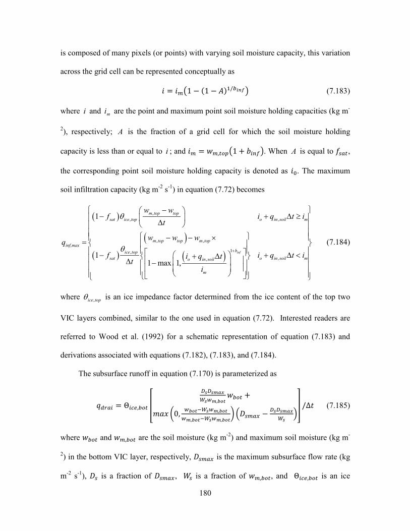
180
is composed of many pixels (or points) with varying soil moisture capacity, this variation
across the grid cell can be represented conceptually as
𝑖 = 𝑖𝑚1 − (1 − 𝐴)1/𝑏𝑖𝑛𝑓 (7.183)
where i and mi are the point and maximum point soil moisture holding capacities (kg m-
2), respectively; A is the fraction of a grid cell for which the soil moisture holding
capacity is less than or equal to i ; and 𝑖𝑚 = 𝑤𝑚,𝑡𝑜𝑝1 + 𝑏𝑖𝑛𝑓. When A is equal to 𝑓𝑠𝑎𝑡,
the corresponding point soil moisture holding capacity is denoted as 𝑖0. The maximum
soil infiltration capacity (kg m-2 s-1) in equation (7.72) becomes
( )
( )
( )( )
,, ,
, ,
1,,,
1
11 max 1,
inf
m top topsat ice top o in soil m
m top top m topinf,max
bice topsat o in soil mo in soil
m
w wf i q t i
t
w w wqf i q t ii q tt
i
θ
θ +
− − + ∆ ≥ ∆
− − ×= − + ∆ <+ ∆ ∆ −
(7.184)
where ,ice topθ is an ice impedance factor determined from the ice content of the top two
VIC layers combined, similar to the one used in equation (7.72). Interested readers are
referred to Wood et al. (1992) for a schematic representation of equation (7.183) and
derivations associated with equations (7.182), (7.183), and (7.184).
The subsurface runoff in equation (7.170) is parameterized as
𝑞𝑑𝑟𝑎𝑖 = Θ𝑖𝑐𝑒,𝑏𝑜𝑡
𝐷𝑠𝐷𝑠𝑚𝑎𝑥𝑊𝑠𝑤𝑚,𝑏𝑜𝑡
𝑤𝑏𝑜𝑡 +
𝑚𝑎𝑥 0, 𝑤𝑏𝑜𝑡−𝑊𝑠𝑤𝑚,𝑏𝑜𝑡𝑤𝑚,𝑏𝑜𝑡−𝑊𝑠𝑤𝑚,𝑏𝑜𝑡
𝐷𝑠𝑚𝑎𝑥 − 𝐷𝑠𝐷𝑠𝑚𝑎𝑥𝑊𝑠
/Δ𝑡 (7.185)
where 𝑤𝑏𝑜𝑡 and 𝑤𝑚,𝑏𝑜𝑡 are the soil moisture (kg m-2) and maximum soil moisture (kg m-
2) in the bottom VIC layer, respectively, 𝐷𝑠𝑚𝑎𝑥 is the maximum subsurface flow rate (kg
m-2 s-1), 𝐷𝑠 is a fraction of 𝐷𝑠𝑚𝑎𝑥, 𝑊𝑠 is a fraction of 𝑤𝑚,𝑏𝑜𝑡, and Θ𝑖𝑐𝑒,𝑏𝑜𝑡 is an ice
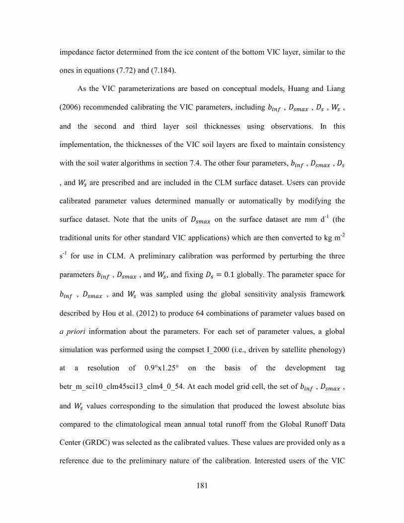
181
impedance factor determined from the ice content of the bottom VIC layer, similar to the
ones in equations (7.72) and (7.184).
As the VIC parameterizations are based on conceptual models, Huang and Liang
(2006) recommended calibrating the VIC parameters, including 𝑏𝑖𝑛𝑓 , 𝐷𝑠𝑚𝑎𝑥 , 𝐷𝑠 , 𝑊𝑠 ,
and the second and third layer soil thicknesses using observations. In this
implementation, the thicknesses of the VIC soil layers are fixed to maintain consistency
with the soil water algorithms in section 7.4. The other four parameters, 𝑏𝑖𝑛𝑓 , 𝐷𝑠𝑚𝑎𝑥 , 𝐷𝑠
, and 𝑊𝑠 are prescribed and are included in the CLM surface dataset. Users can provide
calibrated parameter values determined manually or automatically by modifying the
surface dataset. Note that the units of 𝐷𝑠𝑚𝑎𝑥 on the surface dataset are mm d-1 (the
traditional units for other standard VIC applications) which are then converted to kg m-2
s-1 for use in CLM. A preliminary calibration was performed by perturbing the three
parameters 𝑏𝑖𝑛𝑓 , 𝐷𝑠𝑚𝑎𝑥 , and 𝑊𝑠, and fixing 𝐷𝑠 = 0.1 globally. The parameter space for
𝑏𝑖𝑛𝑓 , 𝐷𝑠𝑚𝑎𝑥 , and 𝑊𝑠 was sampled using the global sensitivity analysis framework
described by Hou et al. (2012) to produce 64 combinations of parameter values based on
a priori information about the parameters. For each set of parameter values, a global
simulation was performed using the compset I_2000 (i.e., driven by satellite phenology)
at a resolution of 0.9°x1.25° on the basis of the development tag
betr_m_sci10_clm45sci13_clm4_0_54. At each model grid cell, the set of 𝑏𝑖𝑛𝑓 , 𝐷𝑠𝑚𝑎𝑥 ,
and 𝑊𝑠 values corresponding to the simulation that produced the lowest absolute bias
compared to the climatological mean annual total runoff from the Global Runoff Data
Center (GRDC) was selected as the calibrated values. These values are provided only as a
reference due to the preliminary nature of the calibration. Interested users of the VIC

182
hydrology option are encouraged to calibrate the parameters for their applications for
improved performance.
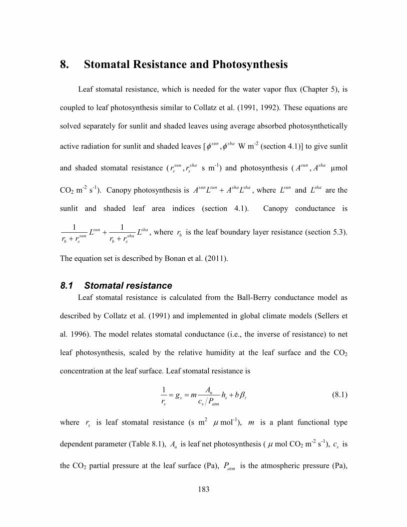
183
8. Stomatal Resistance and Photosynthesis
Leaf stomatal resistance, which is needed for the water vapor flux (Chapter 5), is
coupled to leaf photosynthesis similar to Collatz et al. (1991, 1992). These equations are
solved separately for sunlit and shaded leaves using average absorbed photosynthetically
active radiation for sunlit and shaded leaves [ sunφ , shaφ W m-2 (section 4.1)] to give sunlit
and shaded stomatal resistance ( sunsr , sha
sr s m-1) and photosynthesis ( sunA , shaA µmol
CO2 m-2 s-1). Canopy photosynthesis is sun sun sha shaA L A L+ , where sunL and shaL are the
sunlit and shaded leaf area indices (section 4.1). Canopy conductance is
1 1sun shasun sha
b s b s
L Lr r r r
++ +
, where br is the leaf boundary layer resistance (section 5.3).
The equation set is described by Bonan et al. (2011).
8.1 Stomatal resistance Leaf stomatal resistance is calculated from the Ball-Berry conductance model as
described by Collatz et al. (1991) and implemented in global climate models (Sellers et
al. 1996). The model relates stomatal conductance (i.e., the inverse of resistance) to net
leaf photosynthesis, scaled by the relative humidity at the leaf surface and the CO2
concentration at the leaf surface. Leaf stomatal resistance is
1 ns s t
s s atm
Ag m h br c P
β= = + (8.1)
where is leaf stomatal resistance (s m2 mol-1), is a plant functional type
dependent parameter (Table 8.1), nA is leaf net photosynthesis ( mol CO2 m-2 s-1), is
the CO2 partial pressure at the leaf surface (Pa), is the atmospheric pressure (Pa),
sr µ m
µ sc
atmP
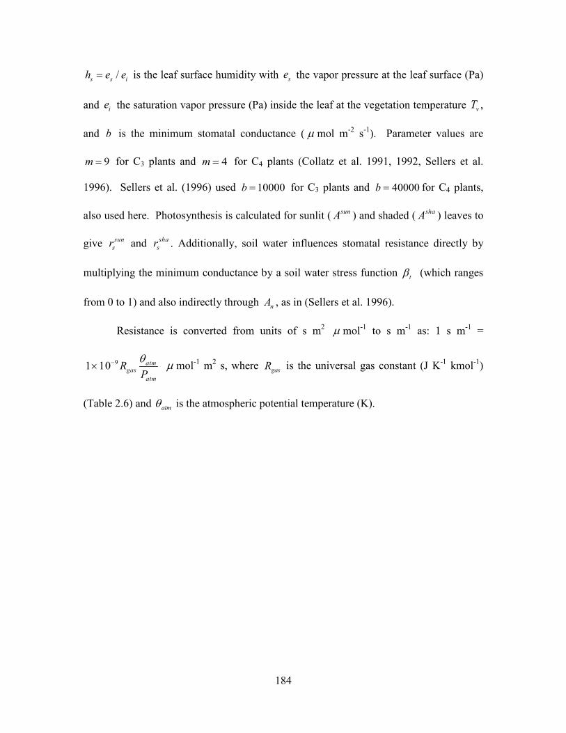
184
/s s ih e e= is the leaf surface humidity with the vapor pressure at the leaf surface (Pa)
and the saturation vapor pressure (Pa) inside the leaf at the vegetation temperature ,
and b is the minimum stomatal conductance ( mol m-2 s-1). Parameter values are
9m = for C3 plants and 4m = for C4 plants (Collatz et al. 1991, 1992, Sellers et al.
1996). Sellers et al. (1996) used 10000b = for C3 plants and 40000b = for C4 plants,
also used here. Photosynthesis is calculated for sunlit ( sunA ) and shaded ( shaA ) leaves to
give sunsr and sha
sr . Additionally, soil water influences stomatal resistance directly by
multiplying the minimum conductance by a soil water stress function tβ (which ranges
from 0 to 1) and also indirectly through nA , as in (Sellers et al. 1996).
Resistance is converted from units of s m2 mol-1 to s m-1 as: 1 s m-1 =
mol-1 m2 s, where gasR is the universal gas constant (J K-1 kmol-1)
(Table 2.6) and atmθ is the atmospheric potential temperature (K).
se
ie vT
µ
µ
91 10 atmgas
atm
RPθ−× µ
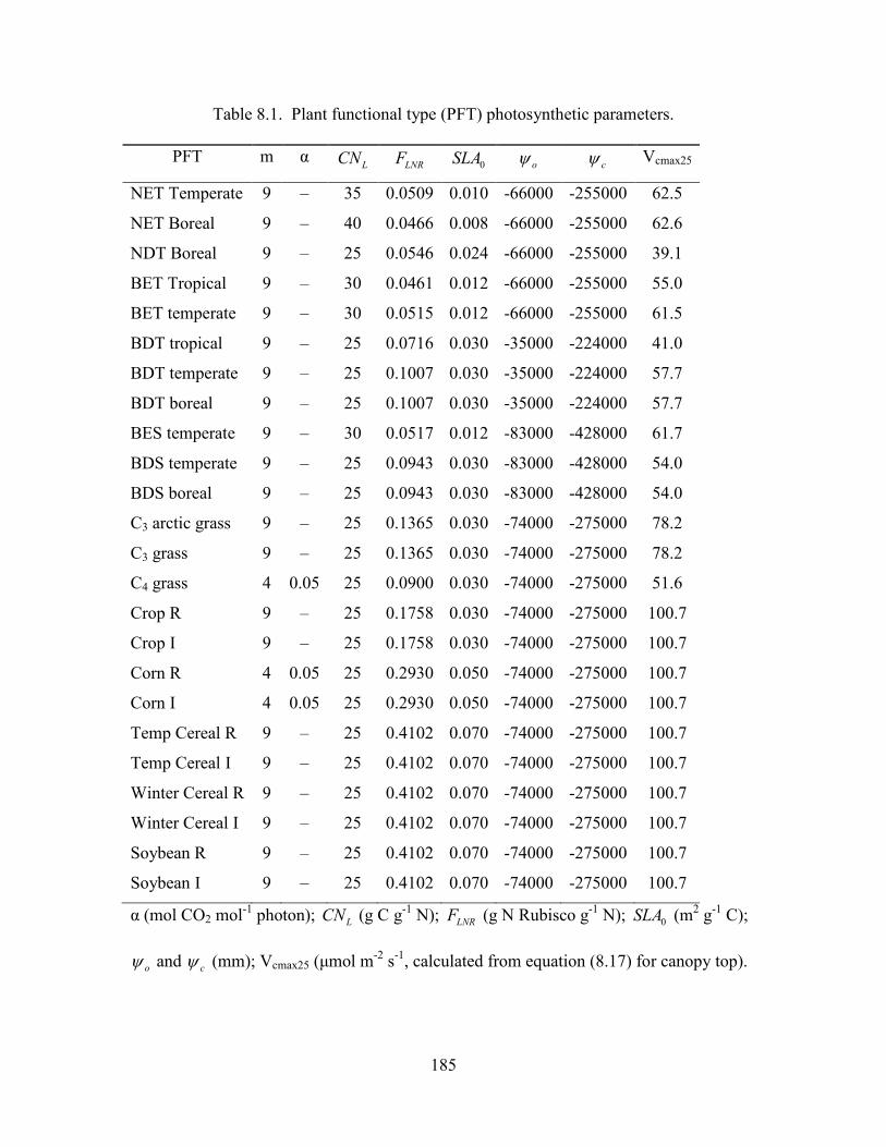
185
Table 8.1. Plant functional type (PFT) photosynthetic parameters.
PFT m α LCN LNRF 0SLA oψ cψ Vcmax25
NET Temperate 9 – 35 0.0509 0.010 -66000 -255000 62.5
NET Boreal 9 – 40 0.0466 0.008 -66000 -255000 62.6
NDT Boreal 9 – 25 0.0546 0.024 -66000 -255000 39.1
BET Tropical 9 – 30 0.0461 0.012 -66000 -255000 55.0
BET temperate 9 – 30 0.0515 0.012 -66000 -255000 61.5
BDT tropical 9 – 25 0.0716 0.030 -35000 -224000 41.0
BDT temperate 9 – 25 0.1007 0.030 -35000 -224000 57.7
BDT boreal 9 – 25 0.1007 0.030 -35000 -224000 57.7
BES temperate 9 – 30 0.0517 0.012 -83000 -428000 61.7
BDS temperate 9 – 25 0.0943 0.030 -83000 -428000 54.0
BDS boreal 9 – 25 0.0943 0.030 -83000 -428000 54.0
C3 arctic grass 9 – 25 0.1365 0.030 -74000 -275000 78.2
C3 grass 9 – 25 0.1365 0.030 -74000 -275000 78.2
C4 grass 4 0.05 25 0.0900 0.030 -74000 -275000 51.6
Crop R 9 – 25 0.1758 0.030 -74000 -275000 100.7
Crop I 9 – 25 0.1758 0.030 -74000 -275000 100.7
Corn R 4 0.05 25 0.2930 0.050 -74000 -275000 100.7
Corn I 4 0.05 25 0.2930 0.050 -74000 -275000 100.7
Temp Cereal R 9 – 25 0.4102 0.070 -74000 -275000 100.7
Temp Cereal I 9 – 25 0.4102 0.070 -74000 -275000 100.7
Winter Cereal R 9 – 25 0.4102 0.070 -74000 -275000 100.7
Winter Cereal I 9 – 25 0.4102 0.070 -74000 -275000 100.7
Soybean R 9 – 25 0.4102 0.070 -74000 -275000 100.7
Soybean I 9 – 25 0.4102 0.070 -74000 -275000 100.7
α (mol CO2 mol-1 photon); LCN (g C g-1 N); LNRF (g N Rubisco g-1 N); 0SLA (m2 g-1 C);
oψ and cψ (mm); Vcmax25 (μmol m-2 s-1, calculated from equation (8.17) for canopy top).
186
8.2 Photosynthesis Photosynthesis in C3 plants is based on the model of Farquhar et al. (1980).
Photosynthesis in C4 plants is based on the model of Collatz et al. (1992). Bonan et al.
(2011) describe the implementation, modified here. In its simplest form, leaf net
photosynthesis after accounting for respiration ( dR ) is
( )min , ,n c j p dA A A A R= − . (8.2)
The RuBP carboxylase (Rubisco) limited rate of carboxylation cA ( mol CO2 m-2 s-1) is
( )( )
max *3
*
max 4
for C plants1 0
for C plants
c i
i c i oc i
c
V cc K o KA cV
− Γ + += − Γ ≥
. (8.3)
The maximum rate of carboxylation allowed by the capacity to regenerate RuBP (i.e., the
light-limited rate) jA ( mol CO2 m-2 s-1) is
( )*
3**
4
for C plants04 8
(4.6 ) for C plants
i
j ii
J cA cc
α φ
− Γ = − Γ ≥+ Γ
. (8.4)
The product-limited rate of carboxylation for C3 plants and the PEP carboxylase-limited
rate of carboxylation for C4 plants pA ( mol CO2 m-2 s-1) is
3
4
3 for C plants
for C plants
p
p ip
atm
TA ck
P
=
. (8.5)
In these equations, is the internal leaf CO2 partial pressure (Pa) and is
the O2 partial pressure (Pa). and are the Michaelis-Menten constants (Pa) for
CO2 and O2. (Pa) is the CO2 compensation point. maxcV is the maximum rate of
µ
µ
µ
ic 0.209i atmo P=
cK oK
∗Γ
187
carboxylation (µmol m-2 s-1) and J is the electron transport rate (µmol m-2 s-1). pT is the
triose phosphate utilization rate (µmol m-2 s-1), taken as max0.167p cT V= so that
max0.5p cA V= for C3 plants (as in Collatz et al. 1991). For C4 plants, the light-limited rate
jA varies with φ in relation to the quantum efficiency ( 0.05α = mol CO2 mol-1 photon).
φ is the absorbed photosynthetically active radiation (W m-2) (section 4.1), which is
converted to photosynthetic photon flux assuming 4.6 mol photons per joule. pk is the
initial slope of C4 CO2 response curve.
For C3 plants, the electron transport rate depends on the photosynthetically active
radiation absorbed by the leaf. A common expression is the smaller of the two roots of
the equation
( )2max max 0PSII PSII PSIIJ I J J I JΘ − + + = (8.6)
where maxJ is the maximum potential rate of electron transport (μmol m–2 s–1), PSIII is the
light utilized in electron transport by photosystem II (µmol m–2 s–1), and PSIIΘ is a
curvature parameter. For a given amount of photosynthetically active radiation absorbed
by a leaf φ (W m-2), converted to photosynthetic photon flux density with 4.6 μmol J-1,
the light utilized in electron transport is
0.5 (4.6 )PSII PSIII φ= Φ (8.7)
where PSIIΦ is the quantum yield of photosystem II, and the term 0.5 arises because one
photon is absorbed by each of the two photosystems to move one electron. Parameter
values are PSIIΘ = 0.7 and PSIIΦ = 0.85. In calculating jA (for both C3 and C4 plants),
sunφ φ= for sunlit leaves and shaφ φ= for shaded leaves.
µ
188
The model uses co-limitation as described by Collatz et al. (1991, 1992). The
actual gross photosynthesis rate, A , is given by the smaller root of the equations
( )( )
2
2
0
0
cj i c j i c j
ip i p i p
A A A A A A
A A A A A A
Θ − + + =
Θ − + + = . (8.8)
Values are 0.98cjΘ = and 0.95ipΘ = for C3 plants; and 0.80cjΘ = and 0.95ipΘ = for C4
plants. n dA A R= − .
The parameters , , and *Γ depend on temperature. Values at 25 °C are
625 404.9 10c atmK P−= × , 3
25 278.4 10o atmK P−= × , and 6*25 =42.75 10 atmP−Γ × . maxcV , maxJ ,
pT , pk , and dR also vary with temperature. Parameter values at 25 °C are calculated
from maxcV at 25 °C: max 25 max 251.97 cJ V= , 25 max 250.167p cT V= , and 25 max 250.015d cR V= (C3)
and 25 max 250.025d cR V= (C4). For C4 plants, 25 max 2520000p ck V= . However, when the
biogeochemistry is active, 25dR is calculated from leaf nitrogen as 25 0.2577d aR N= ,
where aN is the area-based leaf nitrogen concentration (g N m-2 leaf area, equation (8.18)
) and 0.2577 μmol CO2 g-1 N s-1 the base respiration rate. The parameters max 25cV , max 25J ,
25pT , 25pk , and 25dR are scaled over the canopy for sunlit and shaded leaves (section 8.3).
In C3 plants, these are adjusted for leaf temperature vT (K) as:
( ) ( )( ) ( )
( ) ( )( ) ( )( )( )( )
max max 25
max max 25
25
25
25
25
* *25
c c v H v
v H v
p p v H v
d d v H v
c c v
o o v
v
V V f T f T
J J f T f T
T T f T f T
R R f T f T
K K f T
K K f T
f T
=
=
=
=
=
=
Γ = Γ
(8.9)
cK oK
189
with
( ) 298.15exp 1298.15 0.001
av
gas v
Hf TR T
∆= − ×
(8.10)
and
( )
298.151 exp298.15 0.001
1 exp0.001
d
gasH v
v d
gas v
S HR
f TST H
R T
∆ − ∆+ × =
∆ − ∆+
. (8.11)
Table 8.2 list parameter values for aH∆ , dH∆ , and S∆ , from Bonan et al. (2011).
Because pT as implemented here varies with maxcV , the same temperature parameters are
used for pT . For C4 plants,
( ) ( )( ) ( )( ) ( )
( 298.15)/1010
max max 25
1 2
3 4
1 exp
1 exp
vT
c cH v L v
H v v
L v v
QV Vf T f T
f T s T s
f T s s T
− =
= + − = + −
(8.12)
with 10 2Q = , 1 0.3s = K-1, 2 313.15s = K, 3 0.2s = K-1, and 4 288.15s = K. Additionally,
( )
( 298.15)/1010
255 61 exp
vT
d dv
QR Rs T s
− = + −
(8.13)
with 10 2Q = , 5 1.3s = K-1, and 6 328.15s = K, and
( 298.15)/1025 10
vTp pk k Q −= (8.14)
with 10 2Q = .
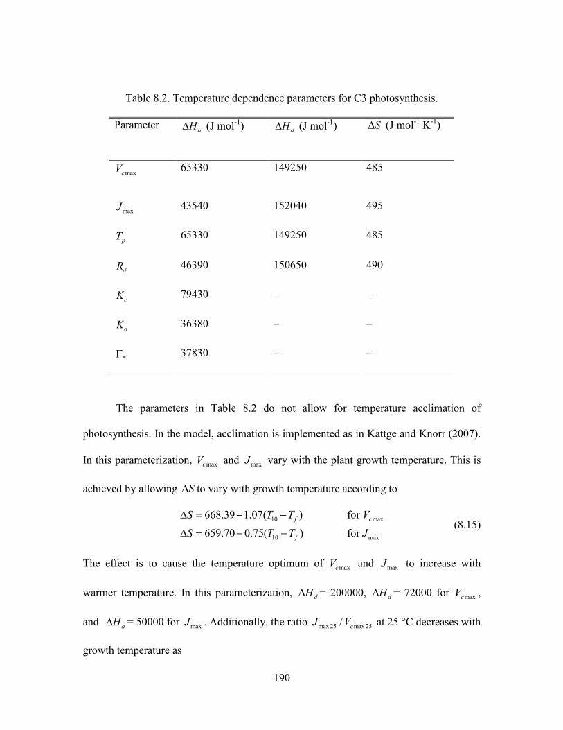
190
Table 8.2. Temperature dependence parameters for C3 photosynthesis.
Parameter aH∆ (J mol-1) dH∆ (J mol-1)
S∆ (J mol-1 K-1)
maxcV 65330
149250
485
maxJ 43540 152040 495
pT 65330 149250 485
dR 46390 150650 490
cK 79430 – –
oK 36380 – –
*Γ 37830 – –
The parameters in Table 8.2 do not allow for temperature acclimation of
photosynthesis. In the model, acclimation is implemented as in Kattge and Knorr (2007).
In this parameterization, maxcV and maxJ vary with the plant growth temperature. This is
achieved by allowing S∆ to vary with growth temperature according to
10 max
10 max
668.39 1.07( ) for
659.70 0.75( ) for f c
f
S T T VS T T J
∆ = − −
∆ = − − (8.15)
The effect is to cause the temperature optimum of maxcV and maxJ to increase with
warmer temperature. In this parameterization, dH∆ = 200000, aH∆ = 72000 for maxcV ,
and aH∆ = 50000 for maxJ . Additionally, the ratio max 25 max 25/ cJ V at 25 °C decreases with
growth temperature as
191
max 25 max 25 10/ 2.59 0.035( )c fJ V T T= − − . (8.16)
In these acclimation functions, 10T is the 10-day mean air temperature (K) and fT is the
freezing point of water (K). For lack of data, pT acclimates similar to maxcV . Acclimation
is restricted over the temperature range 10 11fT T− ≥ °C and 10 35fT T− ≤ °C.
8.3 Vcmax25 and canopy scaling The maximum rate of carboxylation at 25 °C varies with foliage nitrogen
concentration and specific leaf area and is calculated as in Thornton and Zimmermann
(2007). At 25ºC,
max 25 25c a LNR NR RV N F F a= (8.17)
where aN is the area-based leaf nitrogen concentration (g N m-2 leaf area), LNRF is the
fraction of leaf nitrogen in Rubisco (g N in Rubisco g-1 N), 7.16NRF = is the mass ratio
of total Rubisco molecular mass to nitrogen in Rubisco (g Rubisco g-1 N in Rubisco), and
25 60Ra = is the specific activity of Rubisco (µmol CO2 g-1 Rubisco s-1). aN is calculated
from mass-based leaf N concentration and specific leaf area
0
1a
L
NCN SLA
= (8.18)
where LCN is the leaf carbon-to-nitrogen ratio (g C g-1 N) and 0SLA is specific leaf area
at the canopy top (m2 leaf area g-1 C). Table 8.1 lists values of LNRF , LCN , and 0SLA for
each plant functional type. LNRF was chosen to give max 25cV consistent with Kattge et al.
(2009), as discussed by Bonan et al. (2011, 2012). Table 8.1 lists derived values for
max 25cV at the top of the canopy using 0SLA . Tropical broadleaf evergreen trees are an
exception, and a higher max 25cV is used to alleviate model biases (Bonan et al. 2012).
192
max 25cV is calculated separately for sunlit and shaded leaves using an exponential
profile to area-based leaf nitrogen ( aN ), as in Bonan et al. (2011). max 25cV at cumulative
leaf area index x from the canopy top scales directly with aN , which decreases
exponentially with greater cumulative leaf area, so that
( ) ( )max 25 max 25 0 nK xc cV x V e−= (8.19)
where ( )max 25 0cV is defined at the top of the canopy using 0SLA , and nK is the decay
coefficient for nitrogen. The canopy integrated value for sunlit and shaded leaves is
( ) ( )
( ) ( )
max 25 max 250
max 2510 1 n
Lsun
c c sun
K K Lc
n
V V x f x dx
V eK K
− +
=
= − +
∫ (8.20)
( ) ( )
( ) ( )
max 25 max 250
max 25
1
1 10 1 1 nn
Lsha
c c sun
K K LK Lc
n n
V V x f x dx
V e eK K K
− +−
= −
= − − − +
∫ (8.21)
and the average value for the sunlit and shaded leaves is
max 25 max 25sun sun sun
c cV V L= (8.22)
max 25 max 25sha sha sha
c cV V L= . (8.23)
This integration is over all leaf area ( L ) with ( )( ) expsunf x Kx= − and K the direct beam
extinction coefficient (equation 4.9). Photosynthetic parameters max 25J , 25pT , 25pk , and
25dR scale similarly.
The value 0.11nK = chosen by Bonan et al. (2011) is consistent with
observationally-derived estimates for forests, mostly tropical, and provides a gradient in
193
Vcmax similar to the original CLM4 specific leaf area scaling. However, Bonan et al.
(2012) showed that the sunlit/shaded canopy parameterization does not match an explicit
multi-layer canopy parameterization. The discrepancy arises from absorption of scattered
radiation by shaded leaves and can be tuned out with higher nK . The model uses
0.30nK = to match an explicit multi-layer canopy.
max 25cV additionally varies with daylength ( DYL ) using the function ( )f DYL ,
which introduces seasonal variation to maxcV
( ) ( )( )
2
2max
DYLf DYL
DYL= (8.24)
with ( )0.01 1f DYL≤ ≤ . Daylength (seconds) is given by
( ) ( )( ) ( )
1 sin sin2 13750.9871cos
cos coslat decl
DYLlat decl
− −= ×
(8.25)
where lat (latitude) and decl (declination angle) are from section 3.3. Maximum
daylength ( maxDYL ) is calculated similarly but using the maximum declination angle for
present-day orbital geometry (±23.4667º [±0.409571 radians], positive for Northern
Hemisphere latitudes and negative for Southern Hemisphere).
8.4 Soil water stress Soil water influences stomatal conductance directly by multiplying the minimum
conductance by a soil water stress function tβ and also indirectly through nA in the C3
and C4 photosynthesis models, as in Sellers et al. (1996). The latter effect is achieved by
multiplying maxcV and dR by tβ .
194
The function ranges from one when the soil is wet to near zero when the soil
is dry and depends on the soil water potential of each soil layer, the root distribution of
the plant functional type, and a plant-dependent response to soil water stress
t i ii
w rβ = ∑ (8.26)
where is a plant wilting factor for layer and is the fraction of roots in layer .
The plant wilting factor is
, ,
,,
,
1 for 2 and 0
0 for 2 or 0
sat i ice ic ii f liq i
c o sat ii
i f liq i
T Tw
T T
θ θψ ψ θψ ψ θ
θ
−−≤ > − >
−= ≤ − ≤
(8.27)
where iψ is the soil water matric potential (mm) and cψ and oψ are the soil water
potential (mm) when stomata are fully closed or fully open (respectively) (Table 8.1).
The term in brackets scales iw by the ratio of the effective porosity (accounting for the
ice fraction; sat iceθ θ− ) relative to the total porosity.
Here, the soil water matric potential iψ is defined as
,iB
i sat i i csψ ψ ψ−= ≥ (8.28)
where is the soil wetness for layer with respect to the effective porosity and ,sat iψ
and iB are the saturated soil matric potential (mm) and the Clapp and Hornberger (1978)
parameter (section 7.4.1). The soil wetness is
(8.29)
tβ
iw i ir i
iw
is i
is
,
, ,
0.01liq ii
sat i ice i
sθ
θ θ= ≥
−
195
where and .
and are the ice and liquid water contents (kg m-2) (Chapter 7), is the
saturated volumetric water content (section 7.4.1), and are the densities of ice
and liquid water (kg m-3) (Table 2.6), and is the soil layer thickness (m) (section
6.1).
The root fraction in each soil layer depends on the plant functional type
( ) ( )( ) ( )( ) ( )
, 1 , 1
, ,
, 1 , 1
exp exp0.5 for 1
exp exp
0.5 exp exp for
a h i b h i
levsoi
a h i b h ii
a h i b h i levsoi
r z r zi N
r z r zr
r z r z i N
− −
− −
− + − − ≤ < − − −=
− + − =
(8.30)
where (m) is the depth from the soil surface to the interface between layers and
( , the soil surface) (section 6.1), and and are plant-dependent root
distribution parameters adopted from Zeng (2001) (Table 8.3).
( ), , ,ice i ice i ice i sat iw zθ ρ θ= ∆ ≤ ( ), , , ,liq i liq i liq i sat i ice iw zθ ρ θ θ= ∆ ≤ − ,i c e iw
,l i q iw ,sat iθ
i c eρ l i qρ
iz∆
ir
,h iz i
1i + , 0 0hz = ar br
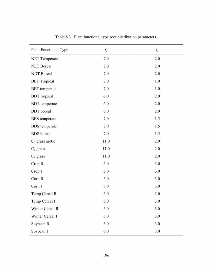
196
Table 8.3. Plant functional type root distribution parameters.
Plant Functional Type
NET Temperate 7.0 2.0
NET Boreal 7.0 2.0
NDT Boreal 7.0 2.0
BET Tropical 7.0 1.0
BET temperate 7.0 1.0
BDT tropical 6.0 2.0
BDT temperate 6.0 2.0
BDT boreal 6.0 2.0
BES temperate 7.0 1.5
BDS temperate 7.0 1.5
BDS boreal 7.0 1.5
C3 grass arctic 11.0 2.0
C3 grass 11.0 2.0
C4 grass 11.0 2.0
Crop R 6.0 3.0
Crop I 6.0 3.0
Corn R 6.0 3.0
Corn I 6.0 3.0
Temp Cereal R 6.0 3.0
Temp Cereal I 6.0 3.0
Winter Cereal R 6.0 3.0
Winter Cereal I 6.0 3.0
Soybean R 6.0 3.0
Soybean I 6.0 3.0
ar br
197
8.5 Numerical implementation The CO2 partial pressure at the leaf surface (Pa) and the vapor pressure at the
leaf surface (Pa), needed for the stomatal resistance model in equation (8.1), and the
internal leaf CO2 partial pressure (Pa), needed for the photosynthesis model in
equations (8.3)-(8.5), are calculated assuming there is negligible capacity to store CO2
and water vapor at the leaf surface so that
( )1.4 1.6 1.4 1.6
a i a s s in
b s atm b atm s atm
c c c c c cAr r P r P r P
− − −= = =
+ (8.31)
and the transpiration fluxes are related as
a i a s s i
b s b s
e e e e e er r r r
− − −= =
+ (8.32)
where is leaf boundary layer resistance (s m2 mol-1) (section 5.3), the terms 1.4 and
1.6 are the ratios of diffusivity of CO2 to H2O for the leaf boundary layer resistance and
stomatal resistance, ( )-12CO mol mola atmc P= is the atmospheric CO2 partial pressure
(Pa) calculated from CO2 concentration (ppmv), ie is the saturation vapor pressure (Pa)
evaluated at the leaf temperature vT , and ae is the vapor pressure of air (Pa). The vapor
pressure of air in the plant canopy (Pa) is determined from
(8.33)
where is the specific humidity of canopy air (kg kg-1) (section 5.3). Equations (8.31)
and (8.32) are solved for and
1.4s a b atm nc c r P A= − (8.34)
sc
se
ic
br µ
ae
0.622atm s
aP qe =
sq
sc se
198
a s i bs
b s
e r e rer r
+=
+ (8.35)
Substitution of equation (8.35) into equation (8.1) gives an expression for stomatal
resistance ( sr ) as a function of photosynthesis ( nA ), given here in terms of conductance
with 1/s sg r= and 1/b bg r=
( ) ( )2* 0s s s b n atm s b s n atm a vc g c g b mA P g g c b mA P e e T+ − − − + = . (8.36)
Stomatal conductance is the larger of the two roots that satisfy the quadratic equation.
Values for are given by
( )1.4 1.6i a b s atm nc c r r P A= − + (8.37)
The equations for ic , sc , sr , and nA are solved iteratively until ic converges. Sun
et al. (2012) pointed out that the CLM4 numerical approach does not always converge.
Therefore, the model uses a hybrid algorithm that combines the secant method and
Brent’s method to solve for ic . The equation set is solved separately for sunlit ( sunnA , sun
sr
) and shaded ( shanA , sha
sr ) leaves.
The model has an optional (though not supported) multi-layer canopy, as
described by Bonan et al. (2012). The multi-layer model is only intended to address the
non-linearity of light profiles, photosynthesis, and stomatal conductance in the plant
canopy. In the multi-layer canopy, sunlit ( sunnA , sun
sr ) and shaded ( shanA , sha
sr ) leaves are
explicitly resolved at depths in the canopy using a light profile (Chapter 4). In this case,
max 25cV is not integrated over the canopy, but is instead given explicitly for each canopy
layer using equation (8.19). This also uses the Lloyd et al. (2010) relationship whereby
Kn scales with Vcmax as
ic

199
( )maxexp 0.00963 2.43n cK V= − (8.38)
such that higher values of Vcmax imply steeper declines in photosynthetic capacity through
the canopy with respect to cumulative leaf area.
200
9. Lake Model
The lake model, denoted the Lake, Ice, Snow, and Sediment Simulator (LISSS), is
from Subin et al. (2012a). It includes extensive modifications to the lake code of Zeng et
al. (2002) used in CLM versions 2 through 4, which utilized concepts from the lake
models of Bonan (1996), Henderson-Sellers (1985, 1986), Hostetler and Bartlein (1990)
and the coupled lake-atmosphere model of Hostetler et al. (1993, 1994). Lakes have
spatially variable depth prescribed in the surface data (section 9.2); the surface data
optionally includes lake optical extinction coeffient and horizontal fetch, currently only
used for site simulations. Lake physics includes freezing and thawing in the lake body,
resolved snow layers, and “soil” and bedrock layers below the lake body. Temperatures
and ice fractions are simulated for 10levlakN = layers (for global simulations) or
25levlakN = (for site simulations) with discretization described in section 9.1. Lake
albedo is described in section 9.3. Lake surface fluxes (section 9.4) generally follow the
formulations for non-vegetated surfaces, including the calculations of aerodynamic
resistances (section 5.2); however, the lake surface temperature gT (representing an
infinitesimal interface layer between the top resolved lake layer and the atmosphere) is
solved for simultaneously with the surface fluxes. After surface fluxes are evaluated,
temperatures are solved simultaneously in the resolved snow layers (if present), the lake
body, and the soil and bedrock, using the ground heat flux G as a top boundary condition.
Snow, soil, and bedrock models generally follow the formulations for non-vegetated
surfaces (Chapter 6), with modifications described below.
201
9.1 Vertical Discretization Currently, there is one lake modeled in each grid cell (with prescribed or assumed
depth d, extinction coefficient η, and fetch f), although this could be modified with
changes to the CLM subgrid decomposition algorithm in future model versions. As
currently implemented, the lake consists of 0-5 snow layers; water and ice layers (10 for
global simulations and 25 for site simulations) comprising the “lake body;” 10 “soil”
layers; and 5 bedrock layers. Each lake body layer has a fixed water mass (set by the
nominal layer thickness and the liquid density), with frozen mass-fraction I a state
variable. Resolved snow layers are present if the snow thickness minsnoz s≥ , where smin =
4 cm by default, and is adjusted for model timesteps other than 1800 s in order to
maintain numerical stability (section 9.6.5). For global simulations with 10 body layers,
the default (50 m lake) body layer thicknesses are given by: iz∆ of 0.1, 1, 2, 3, 4, 5, 7, 7,
10.45, and 10.45 m, with node depths iz located at the center of each layer (i.e., 0.05, 0.6,
2.1, 4.6, 8.1, 12.6, 18.6, 25.6, 34.325, 44.775 m). For site simulations with 25 layers, the
default thicknesses are (m): 0.1 for layer 1; 0.25 for layers 2-5; 0.5 for layers 6-9; 0.75 for
layers 10-13; 2 for layers 14-15; 2.5 for layers 16-17; 3.5 for layers 18-21; and 5.225 for
layers 22-25. For lakes with depth d ≠ 50 m and d ≥ 1 m, the top layer is kept at 10 cm
and the other 9 layer thicknesses are adjusted to maintain fixed proportions. For lakes
with d < 1 m, all layers have equal thickness. Thicknesses of snow, soil, and bedrock
layers follow the scheme used over non-vegetated surfaces (Chapter 6), with
modifications to the snow layer thickness rules to keep snow layers at least as thick as
smin (section 9.6.5).
202
9.2 External Data As discussed in Subin et al (2012a, b), the Global Lake and Wetland Database
(Lehner and Doll 2004) is currently used to prescribe lake fraction in each land model
grid cell, for a total of 2.3 million km-2. As in Subin et al. (2012a, b), the Kourzeneva
(2012) global gridded dataset is currently used to estimate a mean lake depth in each grid
cell, based on interpolated compilations of geographic information.
9.3 Surface Albedo For direct radiation, the albedo a for lakes with ground temperature Tg (K) above
freezing is given by (Pivovarov, 1972)
0.5cos 0.15
az
=+
(9.1)
where z is the zenith angle. For diffuse radiation, the expression in eq. (9.1) is integrated
over the full sky to yield a = 0.10.
For frozen lakes without resolved snow layers, the albedo at cold temperatures a0 is
0.60 for visible and 0.40 for near infrared radiation. As the temperature at the ice surface,
Tg, approaches freezing [Tf (K) (Table 2.6)], the albedo is relaxed towards 0.10 based on
Mironov et al. (2010):
( )0 1 0.10 , exp 95 f g
f
T Ta a x x x
T −
= − + = −
(9.2)
where a is restricted to be no less than that given in eq. (9.1).
For frozen lakes with resolved snow layers, the reflectance of the ice surface is
fixed at a0, and the snow reflectance is calculated as over non-vegetated surfaces
(Chapter 3). These two reflectances are combined to obtain the snow-fraction-weighted
albedo as in over non-vegetated surfaces (Chapter 3).
203
9.4 Surface Fluxes and Surface Temperature
9.4.1 Overview of Changes from CLM4 i. The surface roughnesses, and surface absorption fraction β, are diagnostic rather
than constants. As the surface roughnesses depend (weakly) on the friction
velocity u∗ (which itself depends weakly on the surface roughnesses), their
calculation has been incorporated into the iteration solution for Tg, and the
maximum number of iterations has been increased to 4. Convergence of the
modified solution was tested during development.
ii. A coefficient of β has been added to Sg in eq. (9.17), correcting a previous error.
iii. The top layer thickness Tz∆ used in eq. (9.13) has been appended with a
coefficient of ½, correcting a previous error.
iv. The thermal conductivity Tλ used in eq. (9.13) depends on the properties of the
top model layer (e.g., snow, ice, or water). When this layer is unfrozen, Tλ
includes the eddy conductivity calculated in the previous timestep.
v. Several conditions are imposed on the ground temperature Tg to maintain a stable
density profile at the lake surface eq. (9.24).
9.4.2 Surface Properties The fraction of shortwave radiation absorbed at the surface, β, depends on the lake
state. If resolved snow layers are present, then β is set equal to the absorption fraction
predicted by the snow-optics submodel (Chapter 3) for the top snow layer. Otherwise, β
is set equal to the near infrared fraction of the shortwave radiation reaching the surface
simulated by the atmospheric model or atmospheric data model used for offline
simulations (Chapter 26). The remainder of the shortwave radiation fraction (1 − β) is
204
absorbed in the lake body or soil as described in section 9.5.5.
The surface roughnesses are functions of the lake state and atmospheric forcing.
For frozen lakes ( g fT T≤ ) with resolved snow layers, the momentum roughness length
30 2.4 10 mmz −= × (as over non-vegetated surfaces; Chapter 5), and the scalar roughness
lengths (z0q, for latent heat; and z0h, for sensible heat) are given by (Zilitinkevich 1970)
00
0.450 0 0 0
,
exp 0.13
m
h q m
z uR
z z z Rν
∗=
= = − (9.3)
where R0 is the near-surface atmospheric roughness Reynolds number, z0h is the
roughness length for sensible heat, z0q is the roughness length for latent heat, ν (m2 s-1) is
the kinematic viscosity of air, and u∗ (m s-1) is the friction velocity in the atmospheric
surface layer. For frozen lakes without resolved snow layers, 30 1 10 mmz −= × (Subin et al.
2012a), and the scalar roughness lengths are given by (9.3).
For unfrozen lakes, z0m is given by (Subin et al. 2012a)
2
0 max ,muz C
u gαν ∗
∗
=
(9.4)
where α = 0.1, ν is the kinematic viscosity of air given below, C is the effective Charnock
coefficient given below, and g is the acceleration of gravity (Table 2.6). The kinematic
viscosity is given by
1.5
00
0
g
ref
T PT P
ν ν
=
(9.5)
205
where 25 m0 s1.51 10ν −= × , 0 293.15 KT = , 5
0 1.013 10 PaP = × , and Pref is the pressure at
the atmospheric reference height. The Charnock coefficient C is a function of the lake
fetch F (m), given in the surface data or set to 25 times the lake depth d by default:
( ) min max min
1 3
2
( ) exp min ,
c
C C C C A B
FgA fu
dgB
uε
∗
= + − −
=
=
(9.6)
where A and B define the fetch- and depth-limitation, respectively; min 0.01C = ,
max 0.01C = , 1ε = , 100cf = , and u (m s-1) is the atmospheric forcing wind.
9.4.3 Surface Flux Solution Conservation of energy at the lake surface requires
0g g g gS L H E Gβ λ− − − − =
(9.7)
where gS
is the absorbed solar radiation in the lake, β is the fraction absorbed at the
surface, gL
is the net emitted longwave radiation (+ upwards), gH is the sensible heat
flux (+ upwards), gE is the water vapor flux (+ upwards), and G is the ground heat flux (+
downwards). All of these fluxes depend implicitly on the temperature at the lake surface
Tg. λ converts gE to an energy flux based on
sub g f
vap g f
T TT T
λλ
λ
≤ = > . (9.8)
The sensible heat flux (W m-2) is
( )atm g
g atm pah
TH C
rθ
ρ−
= − (9.9)
206
where atmρ is the density of moist air (kg m-3) (Chapter 5), pC is the specific heat
capacity of air (J kg-1 K-1) (Table 2.6), atmθ is the atmospheric potential temperature (K)
(Chapter 5), gT is the lake surface temperature (K) (at an infinitesimal interface just
above the top resolved model layer: snow, ice, or water), and ahr is the aerodynamic
resistance to sensible heat transfer (s m-1) (section 5.1).
The water vapor flux (kg m-2 s-1) is
( )gT
atm atm satg
aw
q qE
r
ρ −= − (9.10)
where atmq is the atmospheric specific humidity (kg kg-1) (section 2.2.1), gTsatq is the
saturated specific humidity (kg kg-1) (section 5.5) at the lake surface temperature gT , and
awr is the aerodynamic resistance to water vapor transfer (s m-1) (section 5.1).
The zonal and meridional momentum fluxes are
atmx atm
atm
ur
τ ρ= − (9.11)
atmy atm
atm
vr
τ ρ= − (9.12)
where atmu and atmv are the zonal and meridional atmospheric winds (m s-1) (section
2.2.1), and amr is the aerodynamic resistance for momentum (s m-1) (section 5.1).
The heat flux into the lake surface G (W m-2) is
( )2 Tg T
T
G T Tzλ
= −∆
(9.13)
where Tλ is the thermal conductivity (W m-1 K-1), Tz∆ is the thickness (m), and TT is the
temperature (K) of the top resolved lake layer (snow, ice, or water). The top thermal
207
conductivity Tλ of unfrozen lakes ( g fT T> ) includes conductivities due to molecular (
liqλ ) and eddy ( Kλ ) diffusivities (section 9.5.4), as evaluated in the top lake layer at the
previous timestep, where liqλ is the thermal conductivity of water (Table 2.6). For frozen
lakes without resolved snow layers, T iceλ λ= . When resolved snow layers are present,
Tλ is calculated based on the water content, ice content, and thickness of the top snow
layer, as for non-vegetated surfaces.
The absorbed solar radiation gS
is
( ) ( ), ,1 1g atm g atm gS S Sµ µα αΛ Λ Λ ΛΛ
↓ ↓= − + −∑
(9.14)
where atmS µΛ↓ and atmS Λ↓ are the incident direct beam and diffuse solar fluxes (W m-2)
and Λ denotes the visible (< 0.7 mµ ) and near-infrared ( ≥ 0.7 mµ ) wavebands (section
2.2.1), and ,gµα Λ and ,g µα are the direct beam and diffuse lake albedos (section 9.3).
The net emitted longwave radiation is
g g atmL L L↑ ↓= −
(9.15)
where gL ↑ is the upward longwave radiation from the surface, atmL ↓ is the downward
atmospheric longwave radiation (section 2.2.1). The upward longwave radiation from the
surface is
( ) ( ) ( ) ( )4 3 11 4n n n ng atm g g g g g gL L T T T Tε ε σ ε σ +↑= ↓ +− + − (9.16)
where 0.97gε = is the lake surface emissivity, σ is the Stefan-Boltzmann constant (W
m-2 K-4) (Table 2.6), and 1n ng gT T+ − is the difference in lake surface temperature between
Newton-Raphson iterations (see below).
208
The sensible heat gH , the water vapor flux gE through its dependence on the
saturated specific humidity, the net longwave radiation gL
, and the ground heat flux G ,
all depend on the lake surface temperature gT . Newton-Raphson iteration is applied to
solve for gT and the surface fluxes as
gg g g
gg g g
g g g g
S L H E GT
H EL GT T T T
β λλ
− − − −∆ =
∂ ∂∂ ∂+ + +∂ ∂ ∂ ∂
(9.17)
where 1n ng g gT T T+∆ = − and the subscript “n” indicates the iteration. Therefore, the
surface temperature 1ngT + can be written as
1
g g gngg g g g
g g g gng
g g g
g g g g
H EL GS L H E G TT T T T
TH EL G
T T T T
λβ λ
λ+
∂ ∂∂ ∂− − − − + + + + ∂ ∂ ∂ ∂ =∂ ∂∂ ∂+ + +
∂ ∂ ∂ ∂
(9.18)
where the partial derivatives are
( )34g n
g gg
L TT
ε σ∂=
∂
, (9.19)
g atm p
g ah
H CT r
ρ∂=
∂, (9.20)
gT
g atm sat
g aw g
E dqT r dT
λ λρ∂=
∂, (9.21)
2 T
g T
GT z
λ∂=
∂ ∆. (9.22)
The fluxes of momentum, sensible heat, and water vapor are solved for
simultaneously with lake surface temperature as follows. The stability-related equations
209
are the same as for non-vegetated surfaces (section 5.2), except that the surface
roughnesses are here (weakly varying) functions of the friction velocity u∗ . To begin, z0m
is set based on the value calculated for the last timestep (for g fT T> ) or based on the
values in section 9.4.2 (otherwise), and the scalar roughness lengths are set based on the
relationships in section 9.4.2.
1. An initial guess for the wind speed aV including the convective velocity cU is
obtained from eq. (5.24) assuming an initial convective velocity 0cU = m s-1 for
stable conditions ( , , 0v a t m v sθ θ− ≥ as evaluated from eq. (5.50)) and 0 . 5cU = for
unstable conditions ( , , 0v a t m v sθ θ− < ).
2. An initial guess for the Monin-Obukhov length L is obtained from the bulk
Richardson number using equations (5.46) and (5.48).
3. The following system of equations is iterated four times:
• Heat of vaporization / sublimation λ (eq. (9.8))
• Thermal conductivity Tλ (above)
• Friction velocity u∗ (eqs. (5.32), (5.33), (5.34), (5.35))
• Potential temperature scale θ∗ (eqs. (5.37), (5.38), (5.39), (5.40))
• Humidity scale q∗ (eqs. (5.41), (5.42), (5.43), (5.44))
• Aerodynamic resistances amr , ahr , and awr (eqs. (5.55), (5.56), (5.57))
• Lake surface temperature 1ngT + (eq.(9.18))
• Heat of vaporization / sublimation λ (eq. (9.8))
• Sensible heat flux gH is updated for 1ngT + (eq.(9.9))
210
• Water vapor flux gE is updated for 1ngT + as
( )1g
g
TT n natm sat
g atm sat g gaw g
qE q q T Tr Tρ +
∂= − − − −
∂ (9.23)
where the last term on the right side of equation (9.23) is the change in saturated
specific humidity due to the change in gT between iterations.
• Saturated specific humidity gTsatq and its derivative
gTsat
g
dqdT
are updated for 1ngT +
(section 5.1).
• Virtual potential temperature scale vθ ∗ (eq. (5.17))
• Wind speed including the convective velocity, aV (eq. (5.24))
• Monin-Obukhov length L (eq. (5.49)).
• Roughness lengths (eq. (9.3), (9.4)).
Once the four iterations for lake surface temperature have been yielded a tentative
solution gT ′ , several restrictions are imposed in order to maintain consistency with the
top lake model layer temperature TT (Subin et al. 2012a).
1) ,
2) ,
3)
T f g g f
T g m g T
m g T f g T
T T T T T
T T T T T
T T T T T T
′≤ < ⇒ =
′> > ⇒ =
′> > > ⇒ =
(9.24)
where mT is the temperature of maximum liquid water density, 3.85°C (Hostetler and
Bartlein 1990). The first condition requires that, if there is any snow or ice present, the
surface temperature is restricted to be less than or equal to freezing. The second and third
conditions maintain convective stability in the top lake layer.
211
If eq. (9.24) is applied, the turbulent fluxes gH and gE are re-evaluated. The
emitted longwave radiation and the momentum fluxes are re-evaluated in any case. The
final ground heat flux G is calculated from the residual of the energy balance eq. (9.7) in
order to precisely conserve energy. This ground heat flux is taken as a prescribed flux
boundary condition for the lake temperature solution (section 9.5.3). An energy balance
check is included at each timestep to insure that eq. (9.7) is obeyed to within 0.1 W m-2.
9.5 Lake Temperature
9.5.1 Introduction The (optional-) snow, lake body (water and/or ice), soil, and bedrock system is
unified for the lake temperature solution. The governing equation, similar to that for the
snow-soil-bedrock system for vegetated land units (Chapter 6), is
vT T dct z z dz
φτ∂ ∂ ∂ = − ∂ ∂ ∂ (9.25)
where vc is the volumetric heat capacity (J m-3 K-1), t is time (s), T is the temperature
(K), τ is the thermal conductivity (W m-1 K-1), and ϕ is the solar radiation (W m-2)
penetrating to depth z (m). The system is discretized into N layers, where
sno levlak levgrndN n N N= + + , (9.26)
snon is the number of actively modeled snow layers at the current timestep (section 7.2),
and levgrndN is as for vegetated land units (Chapter 6). Energy is conserved as
( ) ( ),1
( ) ( ) 1N
v j j f j j gj
d c t T T L t z G Sdt
β=
− + ∆ = + − ∑
(9.27)
where , ( )v jc t is the volumetric heat capacity of the jth layer (section 9.5.5), ( )jL t is the
latent heat of fusion per unit volume of the jth layer (proportional to the mass of liquid
212
water present), and the right-hand side represents the net influx of energy to the lake
system. Note that , ( )v jc t can only change due to phase change (except for changing
snow layer mass, which, apart from energy required to melt snow, represents an
untracked energy flux in the land model, along with advected energy associated with
water flows in general), and this is restricted to occur at j fT T= in the snow-lake-soil
system, allowing eq. (9.27) to be precisely enforced and justifying the exclusion of ,v jc
from the time derivative in eq. (9.25).
9.5.2 Overview of Changes from CLM4 Thermal conductivities include additional eddy diffusivity, beyond the Hostetler
and Bartlein (1990) formulation, due to unresolved processes (Fang and Stefan 1996;
Subin et al. 2012a). Lake water is now allowed to freeze by an arbitrary fraction for each
layer, which releases latent heat and changes thermal properties. Convective mixing
occurs for all lakes, even if frozen. Soil and bedrock are included beneath the lake. The
full snow model is used if the snow thickness exceeds a threshold; if there are resolved
snow layers, radiation transfer is predicted by the snow-optics submodel (Chapter 3), and
the remaining radiation penetrating the bottom snow layer is absorbed in the top layer of
lake ice; conversely, if there are no snow layers, the solar radiation penetrating the
bottom lake layer is absorbed in the top soil layer. The lakes have variable depth, and all
physics is assumed valid for arbitrary depth, except for a depth-dependent enhanced
mixing (section 9.5.4). Finally, a previous sign error in the calculation of eddy diffusivity
(specifically, the Brunt-Väisälä frequency term; eq. (9.33)) was corrected.
213
9.5.3 Boundary Conditions The top boundary condition, imposed at the top modeled layer topi j= , where
1top snoj n= − + , is the downwards surface flux G defined by the energy flux residual
during the surface temperature solution (section 9.4.3). The bottom boundary condition,
imposed at levlak levgrndi N N= + , is zero flux. The 2-m windspeed 2u (m s-1) is used in the
calculation of eddy diffusivity:
20
2ln 0.1m
uuk z
∗ = ≥
. (9.28)
where u∗ is the friction velocity calculated in section 9.4.3 and k is the von Karman
constant (Table 2.6).
9.5.4 Eddy Diffusivity and Thermal Conductivities The total eddy diffusivity WK (m2 s-1) for liquid water in the lake body is given by
(Subin et al. 2012a)
( )W d e ed mK m Kκ κ= + + (9.29)
where eκ is due to wind-driven eddies (Hostetler and Bartlein 1990), edK is a modest
enhanced diffusivity intended to represent unresolved mixing processes (Fang and Stefan
1996), liqm
liq liqcλ
κρ
= is the molecular diffusivity of water (given by the ratio of its thermal
conductivity (W m-1 K-1) to the product of its heat capacity (J kg-1 K-1) and density (kg m-
3), values given in Table 2.6), and dm (unitless) is a factor which increases the overall
diffusivity for large lakes, intended to represent 3-dimensional mixing processes such as
caused by horizontal temperature gradients. As currently implemented,
214
1, 25m10, 25md
dm
d<
= ≥ (9.30)
where d is the lake depth.
The wind-driven eddy diffusion coefficient ,e iκ (m2 s-1) for layers 1 levlaki N≤ ≤ is
( ) ( )20,
exp1 37
0
ii g f
e i
g f
kw z k z T TP Ri
T Tκ
∗∗
− > += ≤
(9.31)
where 0 1P = is the neutral value of the turbulent Prandtl number, iz is the node depth
(m), the surface friction velocity (m s-1) is 20.0012w u∗ = , and k∗ varies with latitude φ
as 1.8426.6 sink u φ∗ −= . For the bottom layer, , , 1levlak levlake N e Nκ κ −= . As in Hostetler and
Bartlein (1990), the 2-m wind speed 2u (m s-1) (eq. (9.28)) is used to evaluate w∗ and k∗
rather than the 10-m wind used by Henderson-Sellers (1985).
The Richardson number is
( )2
2 2 2401 1exp 2
20
i
ii
N k zw k z
R∗ ∗
− + +−
= (9.32)
where
2
i
gNzρ
ρ∂
=∂
(9.33)
and g is the acceleration due to gravity (m s-2) (Table 2.6), iρ is the density of water (kg
m-3), and zρ∂
∂ is approximated as 1
1
i i
i iz zρ ρ+
+
−−
. Note that because here, z is increasing
downwards (unlike in Hostetler and Bartlein (1990)), eq. (9.33) contains no negative
215
sign; this is a correction from CLM4. The density of water is (Hostetler and Bartlein
1990)
( )1.6851000 1 1.9549 10 277i iTρ −= − × − . (9.34)
The enhanced diffusivity edK is given by (Fang and Stefan 1996)
( ) 0.438 2 2 5 21.04 10 , 7.5 10 sedK N N−− −= × ≥ × (9.35)
where 2N is calculated as in eq. (9.33) except for the minimum value imposed in (9.35).
The thermal conductivity for the liquid water portion of lake body layer i, ,liq iτ (W
m-1 K-1) is given by
,liq i W liq liqK cτ ρ= . (9.36)
The thermal conductivity of the ice portion of lake body layer i, ,ice effτ (W m-1 K-1), is
constant among layers, and is given by
,ice
ice eff iceliq
ρτ τρ
= (9.37)
where iceτ (Table 2.6) is the nominal thermal conductivity of ice: ,ice effτ is adjusted for the
fact that the nominal model layer thicknesses remain constant even while the physical ice
thickness exceeds the water thickness.
The overall thermal conductivity iτ for layer i with ice mass-fraction Ii is the
harmonic mean of the liquid and water fractions, assuming that they will be physically
vertically stacked, and is given by
( )
, ,
, 1ice eff liq i
iliq i i ice iI I
τ ττ
τ τ=
+ − . (9.38)
216
The thermal conductivity of snow, soil, and bedrock layers above and below the
lake, respectively, are computed identically to those for vegetated land units (Chapter 6),
except for the adjustment of thermal conductivity for frost heave or excess ice (Subin et
al., 2012a, Supporting Information).
9.5.5 Radiation Penetration If there are no resolved snow layers, the surface absorption fraction β is set
according to the near-infrared fraction simulated by the atmospheric model. This is
apportioned to the surface energy budget (section 9.4.2), and thus no additional radiation
is absorbed in the top az (currently 0.6 m) of unfrozen lakes, for which the light
extinction coefficient η (m-1) varies between lake columns (eq. (9.41)). For frozen lakes (
g fT T≤ ), the remaining ( )1 gSβ−
fraction of surface absorbed radiation that is not
apportioned to the surface energy budget is absorbed in the top lake body layer. This is a
simplification, as lake ice is partially transparent. If there are resolved snow layers, then
the snow optics submodel (Chapter 3) is used to calculate the snow layer absorption
(except for the absorption predicted for the top layer by the snow optics submodel, which
is assigned to the surface energy budget), with the remainder penetrating snow layers
absorbed in the top lake body ice layer.
For unfrozen lakes, the solar radiation remaining at depth az z> in the lake body is
given by
( ) ( ) 1 expg aS z zφ β η= − − −
. (9.39)
For all lake body layers, the flux absorbed by the layer i, iφ , is
217
( )1 exp exp2 2
i ii g i a i a
z zS z z z zφ β η η ∆ ∆ = − − − − − − + −
. (9.40)
The argument of each exponent is constrained to be non-negative (so iφ = 0 for layers
contained within za). The remaining flux exiting the bottom of layer levlaki N= is
absorbed in the top soil layer.
The light extinction coefficient η (m-1), if not provided as external data, is a
function of depth d (m) (Subin et al. 2012a):
0.4241.1925dη −= . (9.41)
9.5.6 Heat Capacities The vertically-integrated heat capacity for each lake layer, cv,i (J m-2) is determined
by the mass-weighted average over the heat capacities for the water and ice fractions:
( ), 1v i i liq liq i ice ic z c I c Iρ = ∆ − + . (9.42)
Note that the density of water is used for both ice and water fractions, as the thickness of
the layer is fixed.
The total heat capacity ,v ic for each soil, snow, and bedrock layer (J m-2) is
determined as for vegetated land units (Chapter 6), as the sum of the heat capacities for
the water, ice, and mineral constituents.
9.5.7 Crank-Nicholson Solution The solution method for thermal diffusion is similar to that used for soil (Chapter
6), except that the lake body layers are sandwiched between the snow and soil layers
(section 9.5.1), and radiation flux is absorbed throughout the lake layers. Before solution,
layer temperatures iT (K), thermal conductivities iτ (W m-1 K-1), heat capacities ,v ic (J
218
m-2), and layer and interface depths from all components are transformed into a uniform
set of vectors with length sno levlak levgrndN n N N= + + and consistent units to simplify the
solution. Thermal conductivities at layer interfaces are calculated as the harmonic mean
of the conductivities of the neighboring layers:
( )( ) ( )
1 1
1 1ˆ ˆi i i i
ii i i i i i
z zz z z z
τ τλ
τ τ+ +
+ +
−=
− + − , (9.43)
where iλ is the conductivity at the interface between layer i and layer i + 1, iz is the
depth of the node of layer i, and ˆiz is the depth of the interface below layer i. Care is
taken at the boundaries between snow and lake and between lake and soil. The governing
equation (9.25) is discretized for each layer as
( ), 11
v i n ni i i i i
cT T F F
tφ+
−− = − +∆
(9.44)
where superscripts n + 1 and n denote values at the end and beginning of the timestep t∆ ,
respectively, iF (W m-2) is the downward heat flux at the bottom of layer i, and iφ is the
solar radiation absorbed in layer i.
Eq. (9.44) is solved using the semi-implicit Crank-Nicholson Method, resulting in
a tridiagonal system of equations:
( )
1 1 11 1
1
, 1
1
, 1
,
1, ,
,
0.5 ,
1 0.5 ,
0.5 ,
0.5 .
n n ni i i i i i
ii n
v i i
i ii n n
v i i i
ii n
v i i
ni i i i i
v i v i
r a T bT cTt Fa
c T
t F Fbc T Tt Fc
c Tt tr T F F
c cφ
+ + +− +
−
−
−
−
−
= + +∆ ∂
= −∂
∆ ∂ ∂= + + ∂ ∂
∆ ∂= −
∂
∆ ∆= + − +
(9.45)
219
The fluxes iF are defined as follows: for the top layer, 1 2 ; 0top topj jF G a− = = , where G is
defined as in section 9.4.3 (the factor of 2 merely cancels out the Crank-Nicholson 0.5 in
the equation for topjr ). For the bottom layer, 0
levlak levgrndN NF + = . For all other layers:
1
1
n ni i
i in n
T TFz z
λ +
+
−=
− . (9.46)
9.5.8 Phase Change Phase change in the lake, snow, and soil is done similarly to that done for the soil
and snow for vegetated land units (Chapter 6), except without the allowance for freezing
point depression in soil underlying lakes. After the heat diffusion is calculated, phase
change occurs in a given layer if the temperature is below freezing and liquid water
remains, or if the temperature is above freezing and ice remains.
If melting occurs, the available energy for melting, availQ (J m-2), is computed as
( ) ,avail i f v iQ T T c= − (9.47)
where iT is the temperature of the layer after thermal diffusion (section 9.5.7), and ,v ic is
as calculated in section 9.5.6. The mass of melt in the layer M (kg m-2) is given by
min , availice
fus
QM MH
=
(9.48)
where fusH (J kg-1) is the latent heat of fusion of water (Table 2.6), and iceM is the mass
of ice in the layer: i liq iI zρ ∆ for a lake body layer, or simply the soil / snow ice content
state variable ( icew ) for a soil / snow layer. The heat remainder, remQ is given by
rem avail fusQ Q MH= − . (9.49)
220
Finally, the mass of ice in the layer iceM is adjusted downwards by M , and the
temperature iT of the layer is adjusted to
,
remi f
v i
QT Tc
= +′
(9.50)
where ( ), ,v i v i liq icec c M c c′ = + − .
If freezing occurs, availQ is again given by (9.47) but will be negative. The melt
M , also negative, is given by
max , availliq
fus
QM MH
= −
(9.51)
where liqM is the mass of water in the layer: ( )1 i liq iI zρ− ∆ for a lake body layer, or the
soil / snow water content state variable ( liqw ). The heat remainder remQ is given by eq.
(9.49) and will be negative or zero. Finally, liqM is adjusted downwards by M− and the
temperature is reset according to eq. (9.50).
In the presence of nonzero snow water snoW without resolved snow layers over
an unfrozen top lake layer, the available energy in the top lake layer ( )1 ,1f vT T c− is used
to melt the snow. Similar to above, snoW is either completely melted and the remainder of
heat returned to the top lake layer, or the available heat is exhausted and the top lake
layer is set to freezing. The snow thickness is adjusted downwards in proportion to the
amount of melt, maintaining constant density.
9.5.9 Convection Convective mixing is based on Hostetler et al.’s (1993, 1994) coupled lake-
atmosphere model, adjusting the lake temperature after diffusion and phase change to
221
maintain a stable density profile. Unfrozen lakes overturn when 1i iρ ρ +> , in which case
the layer thickness weighted average temperature for layers 1 to 1i + is applied to layers
1 to 1i + and the densities are updated. This scheme is applied iteratively to layers
1 1levlaki N≤ < − . Unstable profiles occurring at the bottom of the lake (i.e., between
layers 1levlaki N= − and levlaki N= ) are treated separately (Subin et al. 2012a), as
occasionally these can be induced by heat expelled from the sediments (not present in the
original Hostetler et al. (1994) model). Mixing proceeds from the bottom upward in this
case (i.e., first mixing layers 1levlaki N= − and levlaki N= , then checking 2levlaki N= − and
1levlaki N= − and mixing down to levlaki N= if needed, and on to the top), so as not to mix
in with warmer over-lying layers.
For frozen lakes, this algorithm is generalized to conserve total enthalpy and ice
content, and to maintain ice contiguous at the top of the lake. Thus, an additional mixing
criterion is added: the presence of ice in a layer that is below a layer which is not
completely frozen. When this occurs, these two lake layers and all those above mix.
Total enthalpy Q is conserved as
( ) ( )1
1
1i
j liq j f j liq j icej
Q z T T I c I cρ+
=
= ∆ − − + ∑ . (9.52)
Once the average ice fraction avI is calculated from
1
1
11
11
,
,
i
j jj
avi
i
i jj
I zI
Z
Z z
+
=
+
+
+=
∆=
= ∆
∑
∑
(9.53)
222
the temperatures are calculated. A separate temperature is calculated for the frozen ( frozT
) and unfrozen ( unfrT ) fractions of the mixed layers. If the total heat content Q is positive
(e.g. some layers will be above freezing), then the extra heat is all assigned to the
unfrozen layers, while the fully frozen layers are kept at freezing. Conversely, if Q < 0,
the heat deficit will all be assigned to the ice, and the liquid layers will be kept at
freezing. For the layer that contains both ice and liquid (if present), a weighted average
temperature will have to be calculated.
If Q > 0, then froz fT T= , and unfrT is given by
( )1 1unfr f
liq i av liq
QT TZ I cρ +
= + −
. (9.54)
If Q < 0, then unfr fT T= , and frozT is given by
[ ]1
froz fliq i av ice
QT TZ I cρ +
= + . (9.55)
The ice is lumped together at the top. For each lake layer j from 1 to i + 1, the ice
fraction and temperature are set as follows, where 1
j
j mm
Z z=
= ∆∑ :
1. If 1j i avZ Z I+≤ , then 1jI = and j frozT T= .
2. Otherwise, if 1 1j i avZ Z I− +< , then the layer will contain both ice and water. The
ice fraction is given by 1 1i av jj
j
Z I ZI
z+ −−
=∆
. The temperature is set to conserve the
desired heat content that would be present if the layer could have two
temperatures, and then dividing by the heat capacity of the layer to yield
223
( )
( )1
1froz j ice unfr j liq
jj ice j liq
T I c T I cT
I c I c+ −
=+ −
. (9.56)
3. Otherwise, 0jI = and j unfrT T= .
9.5.10 Energy Conservation To check energy conservation, the left-hand side of eq. (9.27) is re-written to yield
the total enthalpy of the lake system (J m-2) totH :
( ), , ,
levlak levgrnd
top
N N
tot v i i f liq i fus sno bulk fusi j
H c T T M H W H+
=
= − + − ∑ (9.57)
where ,liq iM is the water mass of the ith layer (similar to section 9.5.8), and ,sno bulkW is the
mass of snow-ice not present in resolved snow layers. This expression is evaluated once
at the beginning and once at the end of the timestep (re-evaluating each ,v ic ), and the
change is compared with the net surface energy flux to yield the error flux soiE (W m-2):
levlak levgrnd
top
N Ntot
soi ii j
HE Gt
φ+
=
∆= − −
∆ ∑ (9.58)
If 0.1soiE < W m-2, it is subtracted from the sensible heat flux and added to G.
Otherwise, the model is aborted.
9.6 Lake Hydrology
9.6.1 Overview Hydrology is done similarly to other impervious non-vegetated columns (e.g.,
glaciers) where snow layers may be resolved but infiltration into the permanent ground is
not allowed. The water mass of lake columns is currently maintained constant, aside
224
from overlying snow. The water budget is balanced with rgwlq (eq. (9.59); kg m-2 s-1), a
generalized runoff term for impervious land units that may be negative.
There are some modifications to the soil and snow parameterizations as compared
with the soil in vegetated land units, or the snow overlying other impervious columns.
The soil can freeze or thaw, with the allowance for frost heave (or the initialization of
excess ice) (sections 9.5.4 and 9.5.8), but no air-filled pore space is allowed in the soil.
To preserve numerical stability in the lake model (which uses a slightly different surface
flux algorithm than over other non-vegetated land units), two changes are made to the
snow model. First, dew or frost is not allowed to be absorbed by a top snow layer which
has become completely melted during the timestep. Second, because occasional
instabilities occurred during model testing when the Courant–Friedrichs–Lewy (CFL)
condition was violated, due to the explicit time-stepping integration of the surface flux
solution, resolved snow layers must be a minimum of mins = 4 cm thick rather than 1 cm
when the default timestep of 1800 s is used.
9.6.2 Water Balance The total water balance of the system is given by
( ) ( ), , ,1
levsoin
sno liq i ice i rain sno g rgwl snwcp icei
W w w q q E q q t=
∆ + ∆ + ∆ = + − − − ∆∑ (9.59)
where snoW (kg m-2) is the total mass of snow (both liquid and ice, in resolved snow
layers or bulk snow), ,liq iw and ,ice iw are the masses of water phases (kg m-2) in soil layer
i, rainq and snoq are the precipitation forcing from the atmosphere (kg m-2 s-1), ,snwcp iceq is
the ice runoff associated with snow-capping (below), gE is the ground evaporation
225
(section 9.4.3), and levsoin is the number of hydrologically active soil layers (as opposed to
dry bedrock layers).
9.6.3 Precipitation, Evaporation, and Runoff All precipitation reaches the ground, as there is no vegetated fraction. As for other
land types, incident snowfall accumulates (with ice mass snoW and thickness snoz ) until its
thickness exceeds a minimum thickness mins , at which point a resolved snow layer is
initiated, with water, ice, dissolved aerosol, snow-grain radius, etc., state variables
tracked by the Snow Hydrology submodel (section 7.2). The density of fresh snow is
assigned as for other land types (section 7.2). Solid precipitation is added immediately to
the snow, while liquid precipitation is added to snow layers, if they exist, after accounting
for dew, frost, and sublimation (below). If snoz exceeds mins after solid precipitation is
added but no snow layers are present, a new snow layer is initiated immediately, and then
dew, frost, and sublimation are accounted for. Snow-capping is invoked if the snow
depth 1000msnoz > , in which case additional precipitation and frost deposition is added
to ,snwcp iceq .
If there are resolved snow layers, the generalized “evaporation” gE (i.e.,
evaporation, dew, frost, and sublimation) is treated as over other land units, except that
the allowed evaporation from the ground is unlimited (though the top snow layer cannot
lose more water mass than it contains). If there are no resolved snow layers but 0snoW >
and 0gE > , sublimation ,sub snoq (kg m-2 s-1) will be given by
, min , snosub sno g
Wq Et
= ∆ . (9.60)
226
If 0,g g fE T T< ≤ , and there are no resolved snow layers or the top snow layer is not
unfrozen, then the rate of frost production frost gq E= . If 0gE < but the top snow layer
has completely thawed during the Phase Change step of the Lake Temperature solution
(section 9.5.8), then frost (or dew) is not allowed to accumulate ( 0frostq = ), to insure that
the layer is eliminated by the Snow Hydrology (section 7.2) code. (If g fT T> , then no
snow is present (section 9.4.3), and evaporation or dew deposition is balanced by rgwlq .)
The snowpack is updated for frost and sublimation:
( ),sno sno frost sub snoW W t q q= + ∆ − . (9.61)
If there are resolved snow layers, then this update occurs using the Snow Hydrology
submodel (section 7.2). Otherwise, the snow ice mass is updated directly, and snoz is
adjusted by the same proportion as the snow ice (i.e., maintaining the same density),
unless there was no snow before adding the frost, in which case the density is assumed to
be 250 kg m-3.
9.6.4 Soil Hydrology The combined water and ice soil volume fraction in a soil layer iθ is given by
,,1 liq iice ii
i ice liq
wwz
θρ ρ
= + ∆
. (9.62)
If ,i sat iθ θ< , the pore volume fraction at saturation (as may occur when ice melts), then
the liquid water mass is adjusted to
,, ,
ice iliq i sat i i liq
ice
ww zθ ρ
ρ
= ∆ −
. (9.63)
227
Otherwise, if excess ice is melting and , ,liq i sat i liq iw zθ ρ> ∆ , then the water in the layer is
reset to
, ,liq i sat i liq iw zθ ρ= ∆ (9.64)
This allows excess ice to be initialized (and begin to be lost only after the pore ice is
melted, which is realistic if the excess ice is found in heterogeneous chunks) but
irreversibly lost when melt occurs.
9.6.5 Modifications to Snow Layer Logic A thickness difference min minlsaz s s= − adjusts the minimum resolved snow layer
thickness for lake columns as compared to non-lake columns. The value of lsaz is chosen
to satisfy the CFL condition for the model timestep. By default, mins = 1 cm and mins = 4
cm. See Subin et al. (2012a; including Supporting Information) for further discussion.
The rules for combining and sub-dividing snow layers (section 7.2.7) are adjusted
for lakes to maintain minimum thicknesses of mins and to increase all target layer
thicknesses by lsaz . The rules for combining layers are modified by simply increasing
layer thickness thresholds by lsaz . The rules for dividing snow layers are contained in a
separate subroutine that is modified for lakes, and is a function of the number of layers
and the layer thicknesses. There are two types of operations: (a) subdividing layers in
half, and (b) shifting some volume from higher layers to lower layers (without increasing
the layer number). For subdivisions of type (a), the thickness thresholds triggering
subdivision are increased by 2 lsaz for lakes. For shifts of type (b), the thickness
thresholds triggering the shifts are increased by lsaz . At the end of the modified
subroutine, a snow ice and liquid balance check are performed.

228
In rare instances, resolved snow layers may be present over an unfrozen top lake
body layer. In this case, the snow layers may be eliminated if enough heat is present in
the top layer to melt the snow: see Subin et al. (2012a, Supporting Information).
229
10. Glaciers
This chapter describes features of CLM that are specific to coupling to an ice sheet
model (in the CESM context, this is the Glimmer-CISM model; Lipscomb and Sacks
(2012) provide documentation and user’s guide for Glimmer-CISM). General
information about glacier land units can be found elsewhere in this document (see
Chapter 2 for an overview).
10.1 Overview CLM is responsible for computing three quantities that are passed to the ice sheet
model:
1. Surface mass balance (SMB) – the net annual accumulation/ablation of mass at
the upper surface (section 10.3)
2. Ground surface temperature, which serves as an upper boundary condition for
Glimmer-CISM’s temperature calculation
3. Surface topography, which currently is fixed in time, and is provided on CLM’s
surface dataset
The ice sheet model is typically run at much higher resolution than CLM (e.g., ~5 km
rather than ~100 km). To improve the downscaling from CLM’s grid to the ice sheet
grid, the glaciated portion of each grid cell is divided into multiple elevation classes
(section 10.2). The above quantities are computed separately in each elevation class.
Glimmer-CISM then computes high-resolution quantities via horizontal and vertical
interpolation.
230
There are several reasons for computing the SMB in CLM rather than in Glimmer-
CISM:
1. It is much cheaper to compute the SMB in CLM for ~10 elevation classes than
in Glimmer-CISM. For example, suppose we are running CLM at a resolution
of ~50 km and Glimmer at ~5 km. Greenland has dimensions of about 1000 x
2000 km. For CLM we would have 20 x 40 x 10 = 8,000 columns, whereas for
Glimmer we would have 200 x 400 = 80,000 columns.
2. We can use the sophisticated snow physics parameterization already in CLM
instead of implementing a separate scheme for Glimmer-CISM. Any
improvements to the CLM are applied to ice sheets automatically.
3. The atmosphere model can respond during runtime to ice-sheet surface changes.
As shown by Pritchard et al. (2008), runtime albedo feedback from the ice sheet
is critical for simulating ice-sheet retreat on paleoclimate time scales. Without
this feedback the atmosphere warms much less, and the retreat is delayed.
4. Mass is more nearly conserved, given that the rate of surface ice growth or
melting computed in CLM is equal to the rate seen by the dynamic ice sheet
model. (Mass conservation is not exact, however, because of approximations
made in interpolating from the CLM grid to the ice-sheet grid.)
5. The improved SMB is available in CLM for all glaciated grid cells (e.g., in the
Alps, Rockies, Andes, and Himalayas), not just those which are part of ice
sheets.
231
The current coupling between CLM and Glimmer-CISM is one-way only. That is,
CLM sends the SMB and surface temperature to Glimmer-CISM but does not do
anything with the fields that are returned. The CLM glacier fraction and surface
topography are therefore fixed in time. One-way coupling is reasonable for runs of ~100
years or less, in which ice-sheet elevation changes are modest. For longer runs with
larger elevation changes, two-way coupling is highly desirable. A two-way coupling
scheme is under development.
10.2 Multiple elevation class scheme In the typical operation of CLM, the glacier land unit contains a single column
(section 2.1.1). However, when running CESM with an active ice sheet model, the
glacier land unit is replaced by a glacier_mec land unit, where “mec” denotes “multiple
elevation classes”. In most ways, glacier_mec land units behave the same as standard
glacier land units. However, each glacier_mec land unit is divided into a user-defined set
of columns based on surface elevation. The default is 10 elevation classes whose lower
limits are 0, 200, 400, 700, 1000, 1300, 1600, 2000, 2500, and 3000 m. Each column is
characterized by a fractional area and surface elevation that are read in during model
initialization. Each glacier_mec column within a grid cell has distinct ice and snow
temperatures, snow water content, surface fluxes, and SMB.
Glacier_mec columns, like glacier columns, are initialized with a temperature of
250 K. While glacier columns are initialized with a snow liquid water equivalent (LWE)
equal to the maximum allowed value of 1 m, glacier_mec columns begin with a snow
LWE of 0.5 m so that they will reach their equilibrium mean snow depth sooner.
232
Glacier_mec columns typically require several decades of spin-up to equilibrate with a
given climate.
The atmospheric surface temperature, potential temperature, specific humidity,
density, and pressure are downscaled from the mean grid cell elevation to the
glacier_mec column elevation using a specified lapse rate (typically 6.0 deg/km) and an
assumption of uniform relative humidity. At a given time, lower-elevation columns can
undergo surface melting while columns at higher elevations remain frozen. This gives a
more accurate simulation of summer melting, which is a highly nonlinear function of air
temperature. The precipitation rate and radiative fluxes are not currently downscaled, but
could be in the future if care were taken to preserve the cell-integrated values.
In contrast to most CLM subgrid units, glacier_mec columns can be active (i.e.,
have model calculations run there) even if their area is zero. This is done because the ice
sheet model may require a SMB even for some grid cells where CLM does not have
glacier land units. To allow for this, grid overlap files have been pre-computed. For
given resolutions of CLM and Glimmer-CISM, these files identify all land-covered grid
cells that overlap any part of the ice sheet grid. In these overlapping cells, glacier_mec
columns are defined in all elevation classes. Some columns may have zero area and are
called “virtual” columns. These columns do not affect energy exchange between the land
and the atmosphere, but are included for potential forcing of Glimmer-CISM.
10.3 Computation of the surface mass balance The SMB of a glacier or ice sheet is the net annual accumulation/ablation of mass at
the upper surface. Ablation is defined as the mass of water that runs off to the ocean.
Not all the surface meltwater runs off; some of the melt percolates into the snow and
233
refreezes. Accumulation is primarily by snowfall and deposition, and ablation is
primarily by melting and evaporation/sublimation. CLM uses a surface-energy-balance
(SEB) scheme to compute the SMB. In this scheme, the melting depends on the sum of
the radiative, turbulent, and conductive fluxes reaching the surface, as described
elsewhere in this document.
CLM has a somewhat unrealistic treatment of accumulation and melting for
standard glacier land units. The snow depth is limited to a prescribed depth of 1 m liquid
water equivalent, with any additional snow assumed to run off to the ocean. (This
amounts to a crude parameterization of iceberg calving.) Snow melting is treated in a
realistic fashion, with meltwater percolating downward through snow layers as long as
the snow is unsaturated. Once the underlying snow is saturated, any additional meltwater
runs off. When glacier ice melts, however, the meltwater is assumed to remain in place
until it refreezes. In warm parts of the ice sheet, the meltwater does not refreeze, but
stays in place indefinitely.
In the modified glacier_mec columns, the treatment of melting and freezing
depends on the logical variable glc_dyntopo. This variable controls whether CLM
surface topography changes dynamically as the ice sheet evolves (i.e., whether the
coupling is one-way or two-way). If glc_dyntopo is true, then CLM receives updated
topographic information from the ice sheet model. In this case, snow in excess of the
prescribed maximum depth is assumed to turn into ice, contributing a positive SMB to
the ice sheet model. Melting ice is assumed to run off to the ocean, giving a negative
SMB. The net SMB associated with ice formation (by conversion from snow) and
melting/runoff is computed for each column, averaged over the coupling interval, and
234
sent to the coupler (qice, mm/s). If glc_dyntopo is false, then surface runoff for
glacier_mec land units is computed as for glacier land units: (1) Any snow in excess of 1
m LWE runs off to the ocean, and (2) Melted ice remains in place until it refreezes.
Excess snow and melted ice still contribute to positive and negative values, respectively,
of qice, but only for the purpose of forcing Glimmer-CISM. Currently, glc_dyntopo =
false is the default, and the only supported option.
Note that the SMB typically is defined as the total accumulation of ice and snow,
minus the total ablation. The qice flux passed to Glimmer-CISM is the mass balance for
ice alone, not snow. We can think of CLM as owning the snow, whereas Glimmer-CISM
owns the underlying ice. Fluctuations in snow depth between 0 and 1 m LWE are not
reflected in the SMB passed to Glimmer-CISM.
235
11. River Transport Model (RTM)
The RTM was developed to route total runoff from the land surface model to either
the active ocean or marginal seas which enables the hydrologic cycle to be closed
(Branstetter 2001, Branstetter and Famiglietti 1999). This is needed to model ocean
convection and circulation, which is affected by freshwater input. It also provides
another method of diagnosing the performance of the land model because the river flow
can be directly compared to gauging station data (e.g., Dai and Trenberth 2002).
To improve global energy conservation when CLM is being run as part of the
Community Climate System Model, runoff is split into two streams, a liquid water stream
and an ice water stream (derived from excess snowfall in snow-capped grid cells, section
7.7). The liquid and ice streams are routed through the RTM, passed to, and dealt with
by the ocean separately.
The RTM uses a linear transport scheme to route water from each grid cell to its
downstream neighboring grid cell. The change in storage S of river water, whether it be
liquid or ice, within a RTM grid cell (m3 s-1) is
in outdS F F Rdt
= − +∑ (11.1)
where inF∑ is the sum of inflows of water from neighboring upstream grid cells (m3 s-
1), outF is the flux of water leaving the grid cell in the downstream direction (m3 s-1), and
R is the total runoff generated by the land model grid cell (m3 s-1). Downstream water
flow direction in each grid cell is determined as one of eight compass points (north,
northeast, east, southeast, south, southwest, west, and northwest) based on the steepest
236
downhill slope as determined from a digital elevation model (Graham et al. 1999). The
flux of water leaving the grid cell outF is
outvF Sd
= (11.2)
where v is the effective water flow velocity (m s-1), d is the distance between centers of
neighboring grid cells (m), and S is the volume of river water stored within the grid cell
(m3). The effective water flow velocity can be estimated from Manning’s equation,
which is a function of surface water slope, the hydraulic radius of the river channel, and a
channel roughness coefficient (Dingman, 2002). However, hydraulic radius and channel
roughness data are not available globally, so a simplified effective flow velocity
expression is used in RTM
( )1/2max 0.05,v kβ= (11.2)
where β is the grid cell mean topographic slope, and 1k = .
The distance d between two grid cell centers depends on river direction, latitude,
and longitude as
2 2d x y= ∆ + ∆ . (11.3)
The distance in the zonal direction x∆ (m) is
( ) ( )3, , , *, *1 10 0.5 cos cosi j i j e i j i jx Rθ θ φ φ∗ ∗
∆ = × − + (11.4)
where ,i jθ and ,i jθ ∗ ∗ are the latitudes (radians) of the upstream and downstream grid
cells, ,i jφ and ,i jφ ∗ ∗ are the longitudes (radians) of the upstream and downstream grid
cells, eR is the radius of the earth (km) (Table 2.6), and i and j are grid cell indices.
The distance in the meridional direction y∆ (m) is
237
( )3, ,1 10 i j i j ey Rθ θ ∗ ∗∆ = × − . (11.5)
The RTM is generally run at a time step greater than that of the CLM because of
computational constraints. The total runoff from the land model at each time step is
accumulated until the RTM is invoked. The total liquid water runoff at the land model
resolution (kg m-2 s-1) is
liq over drai rgwlR q q q= + + (11.6)
where overq is surface runoff (section 7.3), draiq is sub-surface drainage (section 7.6), and
rgwlq is liquid runoff from glaciers, wetlands, and lakes (all in kg m-2 s-1) (sections 7.7
and 9.6.3). The total ice water runoff, also at the land model resolution is
,ice snwcp iceR q= (11.7)
where ,snwcp iceq is the ice runoff from snow-capped surfaces (section 7.7). The runoff at
the land model resolution is interpolated to the resolution of RTM and converted to units
of m3 s-1 for use in equation (11.1) by multiplying by 31 10 A−× where A is the area (m2)
of the RTM grid cell.
The RTM grid cells that are at river mouths, hence providing freshwater flux to the
ocean, are identified by examining each RTM ocean grid cell and determining if a RTM
land grid cell flows to that ocean grid cell. River mouth grid cells are also assigned if any
overlapping grid cells at the land model resolution contain land. When used as part of the
Community Climate System Model, the ocean freshwater liquid and ice fluxes at the
RTM resolution are passed to the flux coupler which distributes the fluxes to the
appropriate ocean grid cells. When used with the Community Atmosphere Model or

238
when run offline, RTM serves only as a diagnostic tool. The river-routing scheme
conserves water globally as
,, ,,
i ji j i ji j
dS Rdt
=
∑ ∑ . (11.8)
239
12. Urban Model (CLMU)
At the global scale, and at the coarse spatial resolution of current climate models,
urbanization has negligible impact on climate. However, the urban parameterization
(CLMU; Oleson et al. 2008b,c) allows simulation of the urban environment within a
climate model, and particularly the temperature where people live. As such, the urban
model allows scientific study of how climate change affects the urban heat island and
possible urban planning and design strategies to mitigate warming (e.g., white roofs).
The urban model that was released as a component of CLM4.0 is separately
described in the urban technical note (Oleson et al. 2010b). Here, we provide a brief
overview of the urban model released as a component of CLM4.5. The main changes in
the urban model from CLM4.0 to CLM4.5 are 1) an expansion of the single urban
landunit to up to three landunits per grid cell stratified by urban density types, 2) the
number of urban layers for roofs and walls is no longer constrained to be equal to the
number of ground layers, 3) space heating and air conditioning wasteheat factors are now
set to zero by default so that the user can customize these factors for their own
application, 4) the elevation threshold used to eliminate urban areas in the surface dataset
creation routines has been changed from 2200 meters to 2600 meters, 5) hydrologic and
thermal calculations for the pervious road now follows CLM4.5 parameterizations.
Urban areas in CLM are represented by up to three urban landunits per gridcell
according to density class. The urban landunit is based on the “urban canyon” concept of
Oke (1987) in which the canyon geometry is described by building height ( H ) and street
width (W ) (Figure 12.1). The canyon system consists of roofs, walls, and canyon floor.
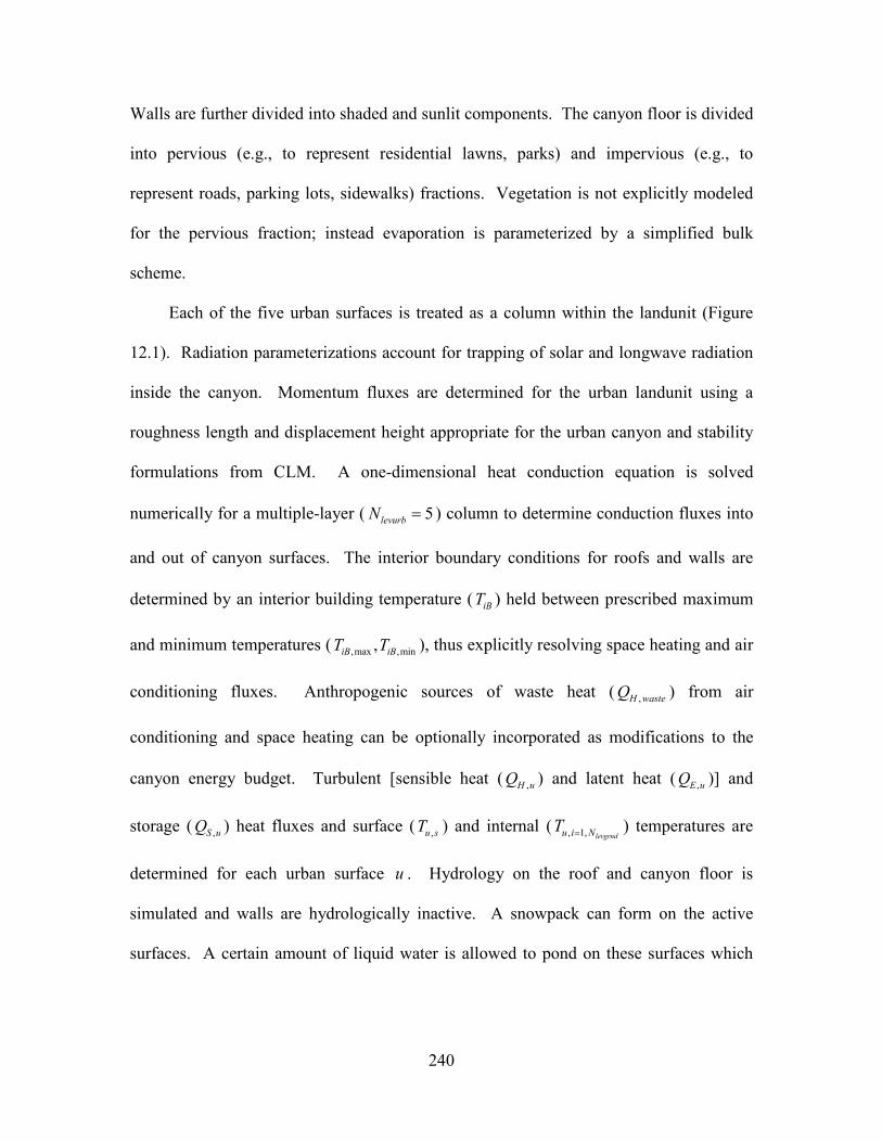
240
Walls are further divided into shaded and sunlit components. The canyon floor is divided
into pervious (e.g., to represent residential lawns, parks) and impervious (e.g., to
represent roads, parking lots, sidewalks) fractions. Vegetation is not explicitly modeled
for the pervious fraction; instead evaporation is parameterized by a simplified bulk
scheme.
Each of the five urban surfaces is treated as a column within the landunit (Figure
12.1). Radiation parameterizations account for trapping of solar and longwave radiation
inside the canyon. Momentum fluxes are determined for the urban landunit using a
roughness length and displacement height appropriate for the urban canyon and stability
formulations from CLM. A one-dimensional heat conduction equation is solved
numerically for a multiple-layer ( 5levurbN = ) column to determine conduction fluxes into
and out of canyon surfaces. The interior boundary conditions for roofs and walls are
determined by an interior building temperature ( iBT ) held between prescribed maximum
and minimum temperatures ( ,max ,min,iB iBT T ), thus explicitly resolving space heating and air
conditioning fluxes. Anthropogenic sources of waste heat ( ,H wasteQ ) from air
conditioning and space heating can be optionally incorporated as modifications to the
canyon energy budget. Turbulent [sensible heat ( ,H uQ ) and latent heat ( ,E uQ )] and
storage ( ,S uQ ) heat fluxes and surface ( ,u sT ) and internal ( , 1, levgrndu i NT = ) temperatures are
determined for each urban surface u . Hydrology on the roof and canyon floor is
simulated and walls are hydrologically inactive. A snowpack can form on the active
surfaces. A certain amount of liquid water is allowed to pond on these surfaces which
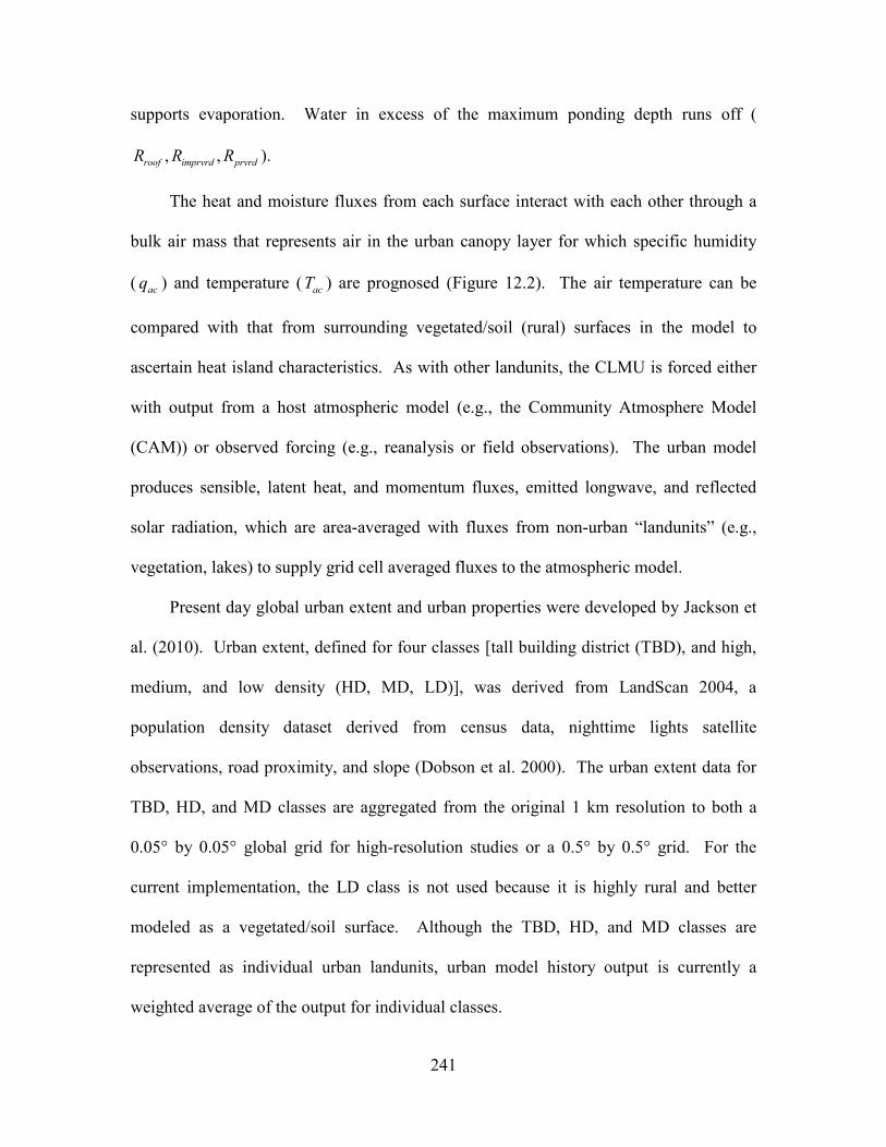
241
supports evaporation. Water in excess of the maximum ponding depth runs off (
, ,roof imprvrd prvrdR R R ).
The heat and moisture fluxes from each surface interact with each other through a
bulk air mass that represents air in the urban canopy layer for which specific humidity
( acq ) and temperature ( acT ) are prognosed (Figure 12.2). The air temperature can be
compared with that from surrounding vegetated/soil (rural) surfaces in the model to
ascertain heat island characteristics. As with other landunits, the CLMU is forced either
with output from a host atmospheric model (e.g., the Community Atmosphere Model
(CAM)) or observed forcing (e.g., reanalysis or field observations). The urban model
produces sensible, latent heat, and momentum fluxes, emitted longwave, and reflected
solar radiation, which are area-averaged with fluxes from non-urban “landunits” (e.g.,
vegetation, lakes) to supply grid cell averaged fluxes to the atmospheric model.
Present day global urban extent and urban properties were developed by Jackson et
al. (2010). Urban extent, defined for four classes [tall building district (TBD), and high,
medium, and low density (HD, MD, LD)], was derived from LandScan 2004, a
population density dataset derived from census data, nighttime lights satellite
observations, road proximity, and slope (Dobson et al. 2000). The urban extent data for
TBD, HD, and MD classes are aggregated from the original 1 km resolution to both a
0.05° by 0.05° global grid for high-resolution studies or a 0.5° by 0.5° grid. For the
current implementation, the LD class is not used because it is highly rural and better
modeled as a vegetated/soil surface. Although the TBD, HD, and MD classes are
represented as individual urban landunits, urban model history output is currently a
weighted average of the output for individual classes.
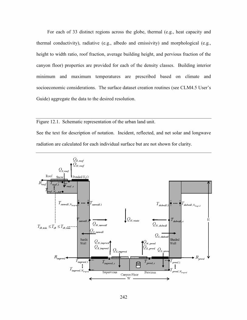
242
For each of 33 distinct regions across the globe, thermal (e.g., heat capacity and
thermal conductivity), radiative (e.g., albedo and emissivity) and morphological (e.g.,
height to width ratio, roof fraction, average building height, and pervious fraction of the
canyon floor) properties are provided for each of the density classes. Building interior
minimum and maximum temperatures are prescribed based on climate and
socioeconomic considerations. The surface dataset creation routines (see CLM4.5 User’s
Guide) aggregate the data to the desired resolution.
Figure 12.1. Schematic representation of the urban land unit.
See the text for description of notation. Incident, reflected, and net solar and longwave
radiation are calculated for each individual surface but are not shown for clarity.
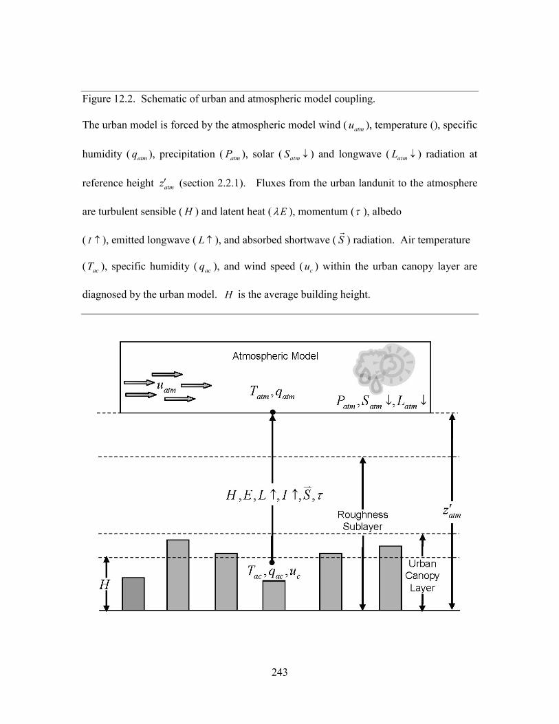
243
Figure 12.2. Schematic of urban and atmospheric model coupling.
The urban model is forced by the atmospheric model wind ( atmu ), temperature (), specific
humidity ( atmq ), precipitation ( atmP ), solar ( atmS ↓ ) and longwave ( atmL ↓ ) radiation at
reference height atmz′ (section 2.2.1). Fluxes from the urban landunit to the atmosphere
are turbulent sensible ( H ) and latent heat ( Eλ ), momentum (τ ), albedo
( I ↑ ), emitted longwave ( L ↑ ), and absorbed shortwave ( S
) radiation. Air temperature
( acT ), specific humidity ( acq ), and wind speed ( cu ) within the urban canopy layer are
diagnosed by the urban model. H is the average building height.
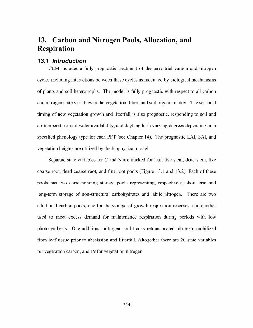
244
13. Carbon and Nitrogen Pools, Allocation, and Respiration 13.1 Introduction
CLM includes a fully-prognostic treatment of the terrestrial carbon and nitrogen
cycles including interactions between these cycles as mediated by biological mechanisms
of plants and soil heterotrophs. The model is fully prognostic with respect to all carbon
and nitrogen state variables in the vegetation, litter, and soil organic matter. The seasonal
timing of new vegetation growth and litterfall is also prognostic, responding to soil and
air temperature, soil water availability, and daylength, in varying degrees depending on a
specified phenology type for each PFT (see Chapter 14). The prognostic LAI, SAI, and
vegetation heights are utilized by the biophysical model.
Separate state variables for C and N are tracked for leaf, live stem, dead stem, live
coarse root, dead coarse root, and fine root pools (Figure 13.1 and 13.2). Each of these
pools has two corresponding storage pools representing, respectively, short-term and
long-term storage of non-structural carbohydrates and labile nitrogen. There are two
additional carbon pools, one for the storage of growth respiration reserves, and another
used to meet excess demand for maintenance respiration during periods with low
photosynthesis. One additional nitrogen pool tracks retranslocated nitrogen, mobilized
from leaf tissue prior to abscission and litterfall. Altogether there are 20 state variables
for vegetation carbon, and 19 for vegetation nitrogen.
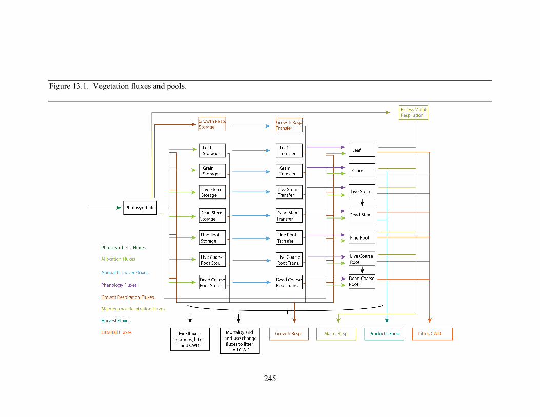
245
Figure 13.1. Vegetation fluxes and pools.
246
Figure 13.2: Carbon and nitrogen pools.
13.2 Carbon Allocation for Maintenance Respiration Costs The carbon and nitrogen allocation routines in CLM determine the fate of newly
assimilated carbon, coming from the calculation of photosynthesis, and available mineral
nitrogen, coming from plant uptake of mineral nitrogen in the soil or being drawn out of
plant reserves. Allocation fluxes are determined in three steps: first CFGPPpot is used to
evaluate the potential allocation of carbon and nitrogen assuming an unlimited nitrogen
supply, then the actual nitrogen supply is compared against the demand, and finally
allocation of carbon and nitrogen are reduced, if necessary, to match nitrogen supply and
demand.
247
Allocation of available carbon on each time step is prioritized, with first priority
given to the demand for carbon to support maintenance respiration of live tissues (section
13.7). Second priority is to replenish the internal plant carbon pool that supports
maintenance respiration during times when maintenance respiration exceeds
photosynthesis (e.g. at night, during winter for perennial vegetation, or during periods of
drought stress) (Sprugel et al., 1995). Third priority is to support growth of new tissues,
including allocation to storage pools from which new growth will be displayed in
subsequent time steps.
The total maintenance respiration demand (CFmr, gC m-2 s-1) is calculated as a
function of tissue mass and nitrogen concentration, and temperature (section 13.7). The
carbon supply to support this demand is composed of fluxes allocated from carbon
assimilated in the current timestep (CFGPP,mr, gC m-2 s-1) and from a storage pool that is
drawn down when total demand exceeds photosynthesis (CFxs,mr, gC m-2 s-1):
, ,mr GPP mr xs mrCF CF CF= + (13.1)
,
for
for mr mr GPPpot
GPP mrGPPpot mr GPPpot
CF CF CFCF
CF CF CF≤= >
(13.2)
,
0 for
for mr GPPpot
xs mrmr GPPpot mr GPPpot
CF CFCF
CF CF CF CF≤= − >
(13.3)
The storage pool that supplies carbon for maintenance respiration in excess of
current CFGPPpot (CSxs, gC m-2) is permitted to run a deficit (negative state), and the
magnitude of this deficit determines an allocation demand which gradually replenishes
CSxs. The logic for allowing a negative state for this pool is to eliminate the need to
know in advance what the total maintenance respiration demand will be for a particular
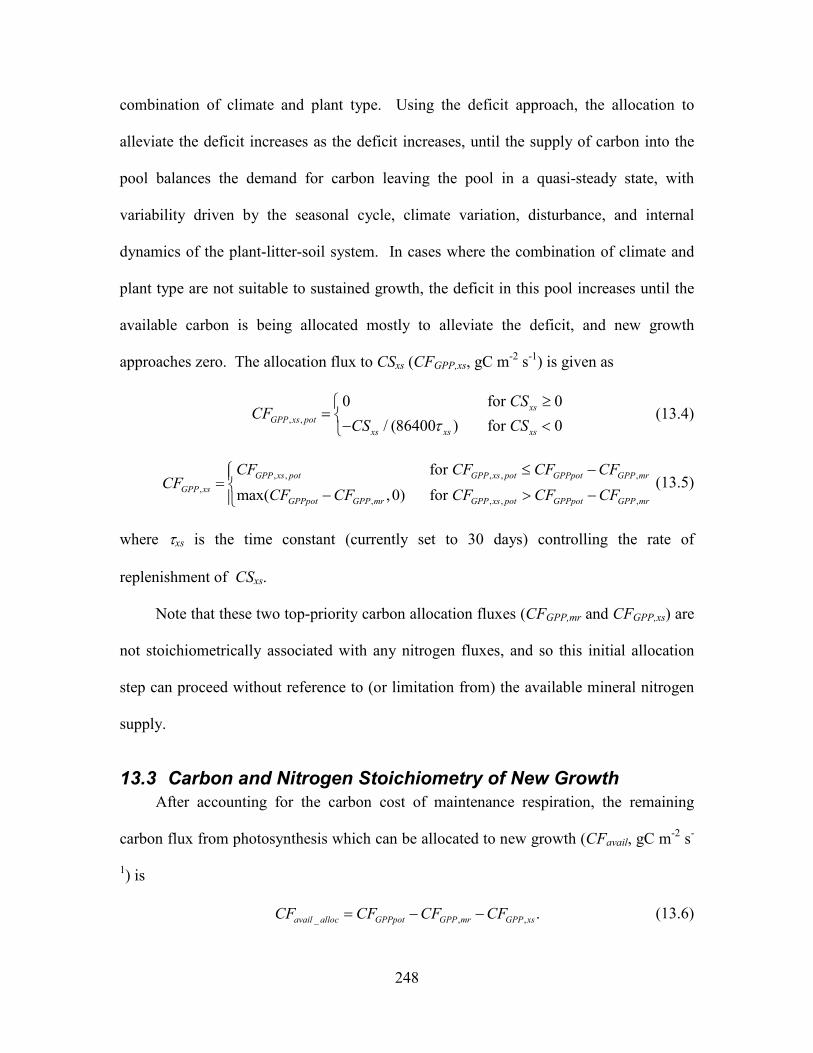
248
combination of climate and plant type. Using the deficit approach, the allocation to
alleviate the deficit increases as the deficit increases, until the supply of carbon into the
pool balances the demand for carbon leaving the pool in a quasi-steady state, with
variability driven by the seasonal cycle, climate variation, disturbance, and internal
dynamics of the plant-litter-soil system. In cases where the combination of climate and
plant type are not suitable to sustained growth, the deficit in this pool increases until the
available carbon is being allocated mostly to alleviate the deficit, and new growth
approaches zero. The allocation flux to CSxs (CFGPP,xs, gC m-2 s-1) is given as
, ,
0 for 0/ (86400 ) for 0
xsGPP xs pot
xs xs xs
CSCF
CS CSτ≥
= − < (13.4)
, , , , ,,
, , , ,
for
max( ,0) for GPP xs pot GPP xs pot GPPpot GPP mr
GPP xsGPPpot GPP mr GPP xs pot GPPpot GPP mr
CF CF CF CFCF
CF CF CF CF CF≤ −= − > −
(13.5)
where τxs is the time constant (currently set to 30 days) controlling the rate of
replenishment of CSxs.
Note that these two top-priority carbon allocation fluxes (CFGPP,mr and CFGPP,xs) are
not stoichiometrically associated with any nitrogen fluxes, and so this initial allocation
step can proceed without reference to (or limitation from) the available mineral nitrogen
supply.
13.3 Carbon and Nitrogen Stoichiometry of New Growth After accounting for the carbon cost of maintenance respiration, the remaining
carbon flux from photosynthesis which can be allocated to new growth (CFavail, gC m-2 s-
1) is
_ , , .avail alloc GPPpot GPP mr GPP xsCF CF CF CF= − − (13.6)
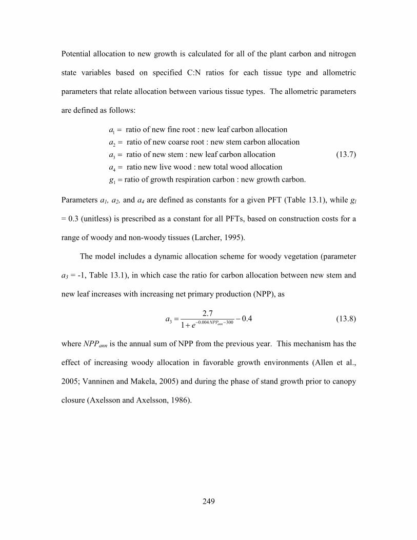
249
Potential allocation to new growth is calculated for all of the plant carbon and nitrogen
state variables based on specified C:N ratios for each tissue type and allometric
parameters that relate allocation between various tissue types. The allometric parameters
are defined as follows:
1
2
3
4
ratio of new fine root : new leaf carbon allocation ratio of new coarse root : new stem carbon allocation ratio of new stem : new leaf carbon allocation ratio new live wood : new total wo
aaaa
====
1
od allocationratio of growth respiration carbon : new growth carbon. g =
(13.7)
Parameters a1, a2, and a4 are defined as constants for a given PFT (Table 13.1), while gl
= 0.3 (unitless) is prescribed as a constant for all PFTs, based on construction costs for a
range of woody and non-woody tissues (Larcher, 1995).
The model includes a dynamic allocation scheme for woody vegetation (parameter
a3 = -1, Table 13.1), in which case the ratio for carbon allocation between new stem and
new leaf increases with increasing net primary production (NPP), as
3 0.004 3002.7 0.4
1 annNPPae− −= −
+ (13.8)
where NPPann is the annual sum of NPP from the previous year. This mechanism has the
effect of increasing woody allocation in favorable growth environments (Allen et al.,
2005; Vanninen and Makela, 2005) and during the phase of stand growth prior to canopy
closure (Axelsson and Axelsson, 1986).
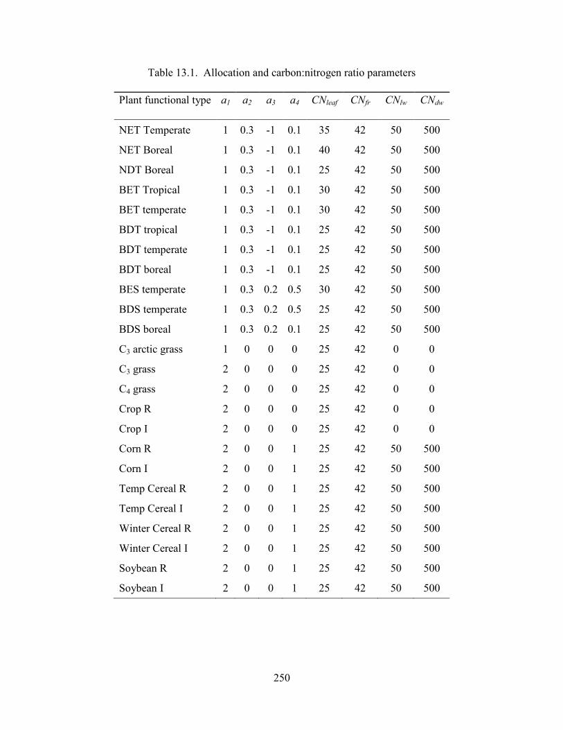
250
Table 13.1. Allocation and carbon:nitrogen ratio parameters
Plant functional type a1 a2 a3 a4 CNleaf CNfr CNlw CNdw
NET Temperate 1 0.3 -1 0.1 35 42 50 500
NET Boreal 1 0.3 -1 0.1 40 42 50 500
NDT Boreal 1 0.3 -1 0.1 25 42 50 500
BET Tropical 1 0.3 -1 0.1 30 42 50 500
BET temperate 1 0.3 -1 0.1 30 42 50 500
BDT tropical 1 0.3 -1 0.1 25 42 50 500
BDT temperate 1 0.3 -1 0.1 25 42 50 500
BDT boreal 1 0.3 -1 0.1 25 42 50 500
BES temperate 1 0.3 0.2 0.5 30 42 50 500
BDS temperate 1 0.3 0.2 0.5 25 42 50 500
BDS boreal 1 0.3 0.2 0.1 25 42 50 500
C3 arctic grass 1 0 0 0 25 42 0 0
C3 grass 2 0 0 0 25 42 0 0
C4 grass 2 0 0 0 25 42 0 0
Crop R 2 0 0 0 25 42 0 0
Crop I 2 0 0 0 25 42 0 0
Corn R 2 0 0 1 25 42 50 500
Corn I 2 0 0 1 25 42 50 500
Temp Cereal R 2 0 0 1 25 42 50 500
Temp Cereal I 2 0 0 1 25 42 50 500
Winter Cereal R 2 0 0 1 25 42 50 500
Winter Cereal I 2 0 0 1 25 42 50 500
Soybean R 2 0 0 1 25 42 50 500
Soybean I 2 0 0 1 25 42 50 500
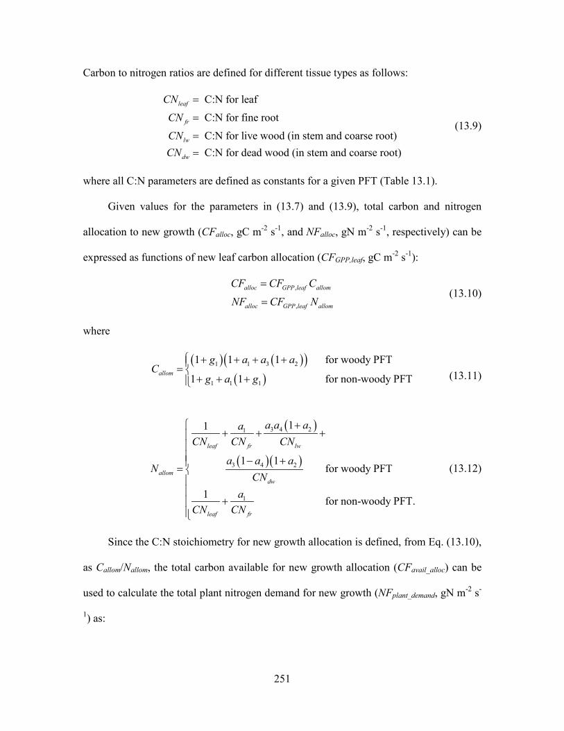
251
Carbon to nitrogen ratios are defined for different tissue types as follows:
C:N for leaf
C:N for fine root
C:N for live wood (in stem and coarse root) C:N for dead wood (in stem and coarse root)
leaf
fr
lw
dw
CNCNCNCN
=
=
==
(13.9)
where all C:N parameters are defined as constants for a given PFT (Table 13.1).
Given values for the parameters in (13.7) and (13.9), total carbon and nitrogen
allocation to new growth (CFalloc, gC m-2 s-1, and NFalloc, gN m-2 s-1, respectively) can be
expressed as functions of new leaf carbon allocation (CFGPP,leaf, gC m-2 s-1):
,
,
alloc GPP leaf allom
alloc GPP leaf allom
CF CF CNF CF N
=
= (13.10)
where
( ) ( )( )
( )1 1 3 2
1 1 1
1 1 1 for woody PFT
1 1 for non-woody PFTallom
g a a aC
g a g
+ + + += + + +
(13.11)
( )
( )( )
3 4 21
3 4 2
1
11
1 1for woody PFT
1 for non-woody PFT.
leaf fr lw
allomdw
leaf fr
a a aaCN CN CN
a a aN
CNa
CN CN
++ + +
− +=
+
(13.12)
Since the C:N stoichiometry for new growth allocation is defined, from Eq. (13.10),
as Callom/Nallom, the total carbon available for new growth allocation (CFavail_alloc) can be
used to calculate the total plant nitrogen demand for new growth (NFplant_demand, gN m-2 s-
1) as:
252
_ _ .allomplant demand avail alloc
allom
NNF CFC
= (13.13)
13.4 Deployment of retranslocated nitrogen In many plants, some portion of the nitrogen used to construct new tissues is
mobilized from senescing tissues, especially leaves, and retained within the plant when
the tissues are lost as litter. This store of retranslocated nitrogen is used to supply part of
the nitrogen demand for subsequent growth (Magill et al., 1997; Oikawa et al., 2005; Son
and Gower, 1991). CLM includes one pool of retranslocated nitrogen (NSretrans, gN m-2),
and the availability of nitrogen from this pool to support new growth (NFavail_retrans, gN m-
2 s-1) is proportional to the plant nitrogen demand, as:
__
_ __ min ,
plant demandretrans ann
plant demand ann retransavail retrans
NFNF
NF NSNFt t
= ∆ ∆
(13.14)
where NFretrans_ann (gN m-2 y-1) is the previous year’s annual sum of retranslocated
nitrogen extracted from senescing tissues, NFplant_demand_ann (gN m-2 y-1) is the previous
year’s annual sum of NFplant_demand, and ∆t (s) is the model’s biogeochemistry time step.
This formulation produces an annual cycle in the extraction of nitrogen from NSretrans
which corresponds to the annual cycle of plant nitrogen demand, and which is scaled to
give NSretrans approximately a one-year turnover time. The minimum function prevents
extraction of more than the remaining pool of retranslocated nitrogen, which can be an
important constraint under conditions where high rates of mortality are modifying the
size of the pool. During the first year of an initial simulation, before NFplant_demand_ann and
NFretrans_ann have valid values, NFavail_retrans is set to 0.0.
253
The actual flux of nitrogen from the retranslocated N pool into allocation of new
growth (NFretrans,alloc, gN m-2 s-1) is never greater than the plant demand for new nitrogen:
( ), _ _min ,retrans alloc plant demand avail retransNF NF NF= (13.15)
13.5 Plant nitrogen uptake from soil mineral nitrogen pool The total plant nitrogen demand is reduced by the nitrogen flux from NSretrans to
give the plant demand for mineral nitrogen from the soil (NFplant_demand_soil, gN m-2 s-1):
_ _ _ ,plant demand soil plant demand retrans allocNF NF NF= − . (13.16)
The combined demand from all PFTs sharing space on a soil column and the demand
from the heterotrophic community in the soil (nitrogen immobilization demand) compete
for the available soil mineral nitrogen pool. The result of this competition is passed back
to the allocation algorithm as fplant_demand, the fraction (from 0 to 1) of the plant nitrogen
demand which can be met given the current soil mineral nitrogen supply and competition
with heterotrophs. Plant uptake from the soil mineral nitrogen pool is then given as:
_ _ _sminn,alloc plant demand soil plant demandNF NF f= (13.17)
13.6 Final carbon and nitrogen allocation The total flux of allocated nitrogen is given as:
, ,alloc retrans alloc sminn allocNF NF NF= + (13.18)
From the stoichiometric relationship in Eq. (13.10), the associated carbon allocation flux
is:
allomalloc alloc
allom
CCF NFN
= . (13.19)
The downregulation of photosynthesis can then be calculated as:
254
_alloc avail allocdreg
GPPpot
CF CFf
CF−
= . (13.20)
Total allocation to new leaf carbon (CFalloc,leaf_tot, gC m-2 s-1) is calculated as:
allocalloc,leaf_tot
allom
CFCFC
= . (13.21)
There are two carbon pools associated with each plant tissue – one which represents
the currently displayed tissue, and another which represents carbon stored for display in a
subsequent growth period. The nitrogen pools follow this same organization. The model
keeps track of stored carbon according to which tissue type it will eventually be displayed
as, and the separation between display in the current timestep and storage for later display
depends on the parameter fcur (values 0 to 1). Given CFalloc,leaf and fcur, the allocation
fluxes of carbon to display and storage pools (where storage is indicated with _stor) for
the various tissue types are given as:
alloc,leaf alloc,leaf_tot curCF CF f= (13.22)
( )1alloc,leaf_stor alloc,leaf_tot curCF CF f= − (13.23)
, 1alloc froot alloc,leaf_tot curCF CF a f= (13.24)
( )1 1alloc, froot_stor alloc,leaf_tot curCF CF a f= − (13.25)
, 3 4alloc livestem alloc,leaf_tot curCF CF a a f= (13.26)
( )3 4 1alloc,livestem_stor alloc,leaf_tot curCF CF a a f= − (13.27)
( ), 3 41alloc deadstem alloc,leaf_tot curCF CF a a f= − (13.28)
( )( )3 41 1alloc,deadstem_stor alloc,leaf_tot curCF CF a a f= − − (13.29)
, 2 3 4alloc livecroot alloc,leaf_tot curCF CF a a a f= (13.30)
255
( )2 3 4 1alloc,livecroot_stor alloc,leaf_tot curCF CF a a a f= − (13.31)
( ), 2 3 41alloc deadcroot alloc,leaf_tot curCF CF a a a f= − (13.32)
( )( )2 3 41 1alloc,deadcroot_stor alloc,leaf_tot curCF CF a a a f= − − . (13.33)
The corresponding nitrogen allocation fluxes are given as:
,alloc,leaf_tot
alloc leaf curleaf
CFNF f
CN= (13.34)
( )1alloc,leaf_totalloc,leaf_stor cur
leaf
CFNF f
CN= − (13.35)
1,
alloc,leaf_totalloc froot cur
fr
CF aNF f
CN= (13.36)
( )1 1alloc,leaf_totalloc, froot_stor cur
fr
CF aNF f
CN= − (13.37)
3 4,
alloc,leaf_totalloc livestem cur
lw
CF a aNF f
CN= (13.38)
( )3 4 1alloc,leaf_totalloc,livestem_stor cur
lw
CF a aNF f
CN= − (13.39)
( )3 4
,
1alloc,leaf_totalloc deadstem cur
dw
CF a aNF f
CN−
= (13.40)
( ) ( )3 41
1alloc,leaf_totalloc,deadstem_stor cur
dw
CF a aNF f
CN−
= − (13.41)
2 3 4,
alloc,leaf_totalloc livecroot cur
lw
CF a a aNF f
CN= (13.42)
( )2 3 4 1alloc,leaf_totalloc,livecroot_stor cur
lw
CF a a aNF f
CN= − (13.43)
256
( )2 3 4
,
1alloc,leaf_totalloc deadcroot cur
dw
CF a a aNF f
CN−
= (13.44)
( ) ( ), 2 3 4
, _
11 .alloc leaf
alloc deadcroot stor curdw
CF a a aNF f
CN−
= − (13.45)
13.7 Autotrophic Respiration The model treats maintenance and growth respiration fluxes separately, even though
it is difficult to measure them as separate fluxes (Lavigne and Ryan, 1997; Sprugel et al.,
1995). Maintenance respiration is defined as the carbon cost to support the metabolic
activity of existing live tissue, while growth respiration is defined as the additional
carbon cost for the synthesis of new growth.
13.7.1 Maintenance Respiration Under the assumption that tissue nitrogen content is a suitable index of cellular
metabolic rate, maintenance respiration costs for live tissues (leaf, live stem, live coarse
root, and fine root) are calculated as functions tissue nitrogen content and the relevant
temperature, following the empirical relationship reported by Ryan (1991):
2( 20)/10_ 10
mTmr leaf leaf base QCF NS MR MR −= (13.46)
2( 20)/10_ 10
mTmr livestem livestem base QCF NS MR MR −= (13.47)
2( 20)/10_ 10
mTmr livecroot livecroot base QCF NS MR MR −= (13.48)
( 20)/10_ 10
1
jnlevsoi
Tsmr froot froot j base Q
jCF NS rootfr MR MR −
=
= ∑ (13.49)
where MRbase (= 2.525e-6 gC gN-1 s-1) is the base rate of maintenance respiration per unit
nitrogen content, MRq10 (= 2.0) is the temperature sensitivity for maintenance respiration,
257
T2m (°C) is the air temperature at 2m height, Tsj (°C) is the soil temperature at level j, and
rootfrj is the fraction of fine roots distributed in soil level j.
Note that, for woody vegetation, maintenance respiration costs are not calculated
for the dead stem and dead coarse root components. These components are assumed to
consist of dead xylem cells, with no metabolic function. By separating the small live
component of the woody tissue (ray parenchyma, phloem, and sheathing lateral meristem
cells) from the larger fraction of dead woody tissue, it is reasonable to assume a common
base maintenance respiration rate for all live tissue types.
The total maintenance respiration cost is then given as:
_ _ _ _ .mr mr leaf mr froot mr livestem mr livecrootCF CF CF CF CF= + + + (13.50)
13.7.2 Growth Respiration Growth respiration is calculated as a factor of 0.3 times the total carbon in new
growth on a given timestep, based on construction costs for a range of woody and non-
woody tissues (Larcher, 1995). For new carbon and nitrogen allocation that enters
storage pools for subsequent display, it is not clear what fraction of the associated growth
respiration should occur at the time of initial allocation, and what fraction should occur
later, at the time of display of new growth from storage. Eddy covariance estimates of
carbon fluxes in forest ecosystems suggest that the growth respiration associated with
transfer of allocated carbon and nitrogen from storage into displayed tissue is not
significant (Churkina et al., 2003), and so it is assumed in CLM that all of the growth
respiration cost is incurred at the time of initial allocation, regardless of the fraction of
allocation that is displayed immediately (i.e. regardless of the value of fcur, section 13.5).
This behavior is parameterized in such a way that if future research suggests that some

258
fraction of the growth respiration cost should be incurred at the time of display from
storage, a simple parameter modification will effect the change.1
1 Parameter grpnow in routines CNGResp and CNAllocation, currently set to 1.0, could be
changed to a smaller value to transfer some portion (1-grpnow) of the growth respiration forward in time to
occur at the time of growth display from storage.
259
14. Vegetation Phenology
The CLM phenology model consists of several algorithms controlling the transfer
of stored carbon and nitrogen out of storage pools for the display of new growth and into
litter pools for losses of displayed growth. PFTs are classified into three distinct
phenological types that are represented by separate algorithms: an evergreen type, for
which some fraction of annual leaf growth persists in the displayed pool for longer than
one year; a seasonal-deciduous type with a single growing season per year, controlled
mainly by temperature and daylength; and a stress-deciduous type with the potential for
multiple growing seasons per year, controlled by temperature and soil moisture
conditions.
The three phenology types share a common set of control variables. The
calculation of the phenology fluxes is generalized, operating identically for all three
phenology types, given a specification of the common control variables. The following
sections describe first the general flux parameterization, followed by the algorithms for
setting the control parameters for the three phenology types.
14.1 General Phenology Flux Parameterization Fluxes of carbon and nitrogen from storage pools and into displayed tissue pools
pass through a special transfer pool (denoted _xfer), maintained as a separate state
variable for each tissue type. Storage (_stor) and transfer (_xfer) pools are maintained
separately to reduce the complexity of accounting for transfers into and out of storage
over the course of a single growing season.
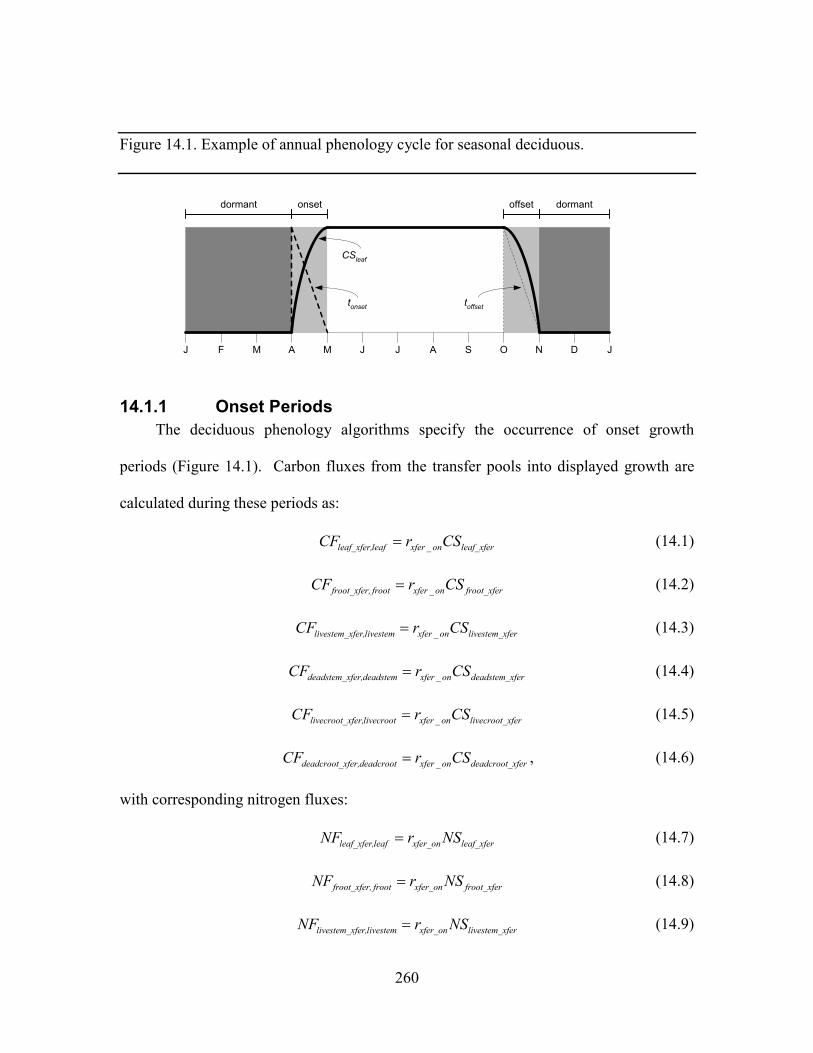
260
Figure 14.1. Example of annual phenology cycle for seasonal deciduous.
J JDNOSAJJMAMF
onset offsetdormant dormant
tonset toffset
CSleaf
14.1.1 Onset Periods The deciduous phenology algorithms specify the occurrence of onset growth
periods (Figure 14.1). Carbon fluxes from the transfer pools into displayed growth are
calculated during these periods as:
_leaf_xfer,leaf xfer on leaf_xferCF r CS= (14.1)
_froot_xfer, froot xfer on froot_xferCF r CS= (14.2)
_livestem_xfer,livestem xfer on livestem_xferCF r CS= (14.3)
_deadstem_xfer,deadstem xfer on deadstem_xferCF r CS= (14.4)
_livecroot_xfer,livecroot xfer on livecroot_xferCF r CS= (14.5)
_deadcroot_xfer,deadcroot xfer on deadcroot_xferCF r CS= , (14.6)
with corresponding nitrogen fluxes:
leaf_xfer,leaf xfer_on leaf_xferNF r NS= (14.7)
froot_xfer, froot xfer_on froot_xferNF r NS= (14.8)
livestem_xfer,livestem xfer_on livestem_xferNF r NS= (14.9)
261
deadstem_xfer,deadstem xfer_on deadstem_xferNF r NS= (14.10)
livecroot_xfer,livecroot xfer_on livecroot_xferNF r NS= (14.11)
deadcroot_xfer,deadcroot xfer_on deadcroot_xferNF r NS= , (14.12)
where CF is the carbon flux, CS is stored carbon, NF is the nitrogen flux, NS is stored
nitrogen, rxfer_on (s-1) is a time-varying rate coefficient controlling flux out of the transfer
pool:
2 for 1 for
onset onsetxfer_on
onset
t t tr
t t t≠ ∆
= ∆ = ∆ (14.13)
and tonset (s) is the number of seconds remaining in the current phenology onset growth
period (Figure 14.1). The form of Eq. (14.13) produces a flux from the transfer pool
which declines linearly over the onset growth period, approaching zero flux in the final
timestep.
14.1.2 Offset Periods The deciduous phenology algorithms also specify the occurrence of litterfall during
offset periods. In contrast to the onset periods, only leaf and fine root state variables are
subject to litterfall fluxes. Carbon fluxes from display pools into litter are calculated
during these periods as:
( )
( )
1 1 for
for
n nleaf,litter xfer_off leaf leaf,litter offset offsetn
leaf,litter
leaf alloc,leaf offset
CF r CS CF t t tCF
CS t CF t t
− − + − ≠ ∆= ∆ + = ∆
(14.14)
( )
( )
1 1
,
for
for
n nfroot,litter xfer_off froot froot,litter offset offsetn
froot,litter
froot alloc froot offset
CF r CS CF t t tCF
CS t CF t t
− − + − ≠ ∆= ∆ + = ∆
(14.15)
2
2xfer_off
offset
trt
∆= (14.16)
262
where superscripts n and n-1 refer to fluxes on the current and previous timesteps,
respectively. The rate coefficient rxfer_off varies with time to produce a linearly increasing
litterfall rate throughout the offset period, and the special case for fluxes in the final
litterfall timestep (toffset = ∆t) ensures that all of the displayed growth is sent to the litter
pools for deciduous plant types.
Corresponding nitrogen fluxes during litterfall take into account retranslocation of
nitrogen out of the displayed leaf pool prior to litterfall (NFleaf,retrans, gN m-2 s-1).
Retranslocation of nitrogen out of fine roots is assumed to be negligible. The fluxes are:
leaf,litter leaf,litter leaf_litterNF CF CN= (14.17)
froot,litter leaf,litter frootNF CF CN= (14.18)
( )leaf,retrans leaf,litter leaf leaf,litterNF CF CN NF= − . (14.19)
where CN is C:N.
14.1.3 Background Onset Growth The stress-deciduous phenology algorithm includes a provision for the case when
stress signals are absent, and the vegetation shifts from a deciduous habit to an evergreen
habit, until the next occurrence of an offset stress trigger . In that case, the regular onset
flux mechanism is switched off and a background onset growth algorithm is invoked (rbgtr
> 0). During this period, small fluxes of carbon and nitrogen from the storage pools into
the associated transfer pools are calculated on each time step, and the entire contents of
the transfer pool are added to the associated displayed growth pool on each time step.
The carbon fluxes from transfer to display pools under these conditions are:
leaf_xfer,leaf leaf_xferCF CS t= ∆ (14.20)
263
froot_xfer, froot froot_xferCF CS t= ∆ (14.21)
livestem_xfer,livestem livestem_xferCF CS t= ∆ (14.22)
deadstem_xfer,deadstem deadstem_xferCF CS t= ∆ (14.23)
livecroot_xfer,livecroot livecroot_xferCF CS t= ∆ (14.24)
deadcroot_xfer,deadcroot deadcroot_xferCF CS t= ∆ , (14.25)
and the corresponding nitrogen fluxes are:
leaf_xfer,leaf leaf_xferNF NS t= ∆ (14.26)
froot_xfer, froot froot_xferNF NS t= ∆ (14.27)
livestem_xfer,livestem livestem_xferNF NS t= ∆ (14.28)
deadstem_xfer,deadstem deadstem_xferNF NS t= ∆ (14.29)
livecroot_xfer,livecroot livecroot_xferNF NS t= ∆ (14.30)
deadcroot_xfer,deadcroot deadcroot_xferNF NS t= ∆ . (14.31)
14.1.4 Background Litterfall Both evergreen and stress-deciduous phenology algorithms can specify a litterfall
flux that is not associated with a specific offset period, but which occurs instead at a slow
rate over an extended period of time, referred to as background litterfall. For evergreen
types the background litterfall is the only litterfall flux. For stress-deciduous types either
the offset period litterfall or the background litterfall mechanism may be active, but not
both at once. Given a specification of the background litterfall rate (rbglf, s-1), litterfall
carbon fluxes are calculated as
leaf,litter bglf leafCF r CS= (14.32)
264
froot,litter bglf frootCS r CS= , (14.33)
with corresponding nitrogen litterfall and retranslocation fluxes:
leaf,litter leaf,litter leaf_litterNF CF CN= (14.34)
froot,litter froot,litter frootNF CF CN= (14.35)
( )leaf,retrans leaf,litter leaf leaf,litterNF CF CN NF= − . (14.36)
14.1.5 Livewood Turnover The conceptualization of live wood vs. dead wood fractions for stem and coarse
root pools is intended to capture the difference in maintenance respiration rates between
these two physiologically distinct tissue types. Unlike displayed pools for leaf and fine
root, which are lost to litterfall, live wood cells reaching the end of their lifespan are
retained as a part of the dead woody structure of stems and coarse roots. A mechanism is
therefore included in the phenology routine to effect the transfer of live wood to dead
wood pools, which also takes into account the different nitrogen concentrations typical of
these tissue types.
A live wood turnover rate (rlwt, s-1) is defined as
( )365 86400lwt lwtr p= ⋅ (14.37)
where plwt = 0.7 is the assumed annual live wood turnover fraction. Carbon fluxes from
live to dead wood pools are:
livestem,deadstem livestem lwtCF CS r= (14.38)
livecroot,deadcroot livecroot lwtCF CS r= , (14.39)
and the associated nitrogen fluxes, including retranslocation of nitrogen out of live wood
during turnover, are:
265
livestem,deadstem livestem,deadstem dwNF CF CN= (14.40)
( ), ,livestem,retrans livestem deadstem lw livestem deadstemNF CF CN NF= − (14.41)
livecroot,deadcroot livecroot,deadcroot dwNF CF CN= (14.42)
( ), ,livecroot,retrans livecroot deadcroot lw livecroot deadcrootNF CF CN NF= − . (14.43)
14.2 Evergreen Phenology The evergreen phenology algorithm is by far the simplest of the three possible
types. It is assumed for all evergreen types that all carbon and nitrogen allocated for new
growth in the current timestep goes immediately to the displayed growth pools (i.e. fcur =
1.0 (Chapter 13)). As such, there is never an accumulation of carbon or nitrogen in the
storage or transfer pools, and so the onset growth and background onset growth
mechanisms are never invoked for this type. Litterfall is specified to occur only through
the background litterfall mechanism – there are no distinct periods of litterfall for
evergreen types, but rather a continuous (slow) shedding of foliage and fine roots. This is
an obvious area for potential improvements in the model, since it is known, at least for
evergreen needleleaf trees in the temperate and boreal zones, that there are distinct
periods of higher and lower leaf litterfall (Ferrari, 1999; Gholz et al., 1985). The rate of
background litterfall (rbglf, section 14.1.4) depends on the specified leaf longevity (τleaf,
y), as
1365 86400bglf
leaf
rτ
=⋅ ⋅
. (14.44)
14.3 Seasonal-Deciduous Phenology The seasonal-deciduous phenology algorithm derives directly from the treatment
used in the offline model Biome-BGC v. 4.1.2, (Thornton et al., 2002), which in turn is
266
based on the parameterizations for leaf onset and offset for temperate deciduous
broadleaf forest from White et al. (1997). Initiation of leaf onset is triggered when a
common degree-day summation exceeds a critical value, and leaf litterfall is initiated
when daylength is shorter than a critical value. Because of the dependence on daylength,
the seasonal deciduous phenology algorithm is only valid for latitudes outside of the
tropical zone, defined here as latitude 19.5> ° . Neither the background onset nor
background litterfall mechanism is invoked for the seasonal-deciduous phenology
algorithm. The algorithm allows a maximum of one onset period and one offset period
each year.
The algorithms for initiation of onset and offset periods use the winter and summer
solstices as coordination signals. The period between winter and summer solstice is
identified as dayln > dayln-1, and the period between summer and winter solstice is
identified as dayln < dayln-1, where dayln and dayln-1 are the daylength (s) calculated for
the current and previous timesteps, respectively, using
sin( )sin( )2 13750.9871 acos
cos( )cos( )lat decldayl
lat decl −
= ⋅ ⋅
, (14.45)
where lat and decl are the latitude and solar declination (radians), respectively, and the
factor 13750.9871 is the number of seconds per radian of hour-angle.
14.3.1 Seasonal-Deciduous Onset Trigger The onset trigger for the seasonal-deciduous phenology algorithm is based on an
accumulated growing-degree-day approach (White et al., 1997). The growing-degree-
day summation (GDDsum) is initiated (GDDsum = 0) when the phenological state is
267
dormant and the model timestep crosses the winter solstice. Once these conditions are
met, GDDsum is updated on each timestep as
( )1
,3 ,3
1,3
for
for
nsum s day sn
sum nsum s
GDD T TKFRZ f T TKFRZGDD
GDD T TKFRZ
−
−
+ − >= ≤
(14.46)
where Ts,3 (K) is the temperature of the third soil layer, and 86400dayf t= ∆ . The onset
period is initiated if sum sum_critGDD GDD> , where
( )( )exp 4.8 0.13sum_crit 2m,ann_avgGDD T TKFRZ= + − (14.47)
and where T2m,ann_avg (K) is the annual average of the 2m air temperature, and TKFRZ is
the freezing point of water (273.15 K). The following control variables are set when a
new onset growth period is initiated:
0sumGDD = (14.48)
86400onset days_ont n= ⋅ , (14.49)
where ndays_on is set to a constant value of 30 days. Fluxes from storage into transfer
pools occur in the timestep when a new onset growth period is initiated. Carbon fluxes
are:
leaf_stor,leaf_xfer stor,xfer leaf_storCF f CS t= ∆ (14.50)
froot_stor, froot_xfer stor,xfer froot_storCF f CS t= ∆ (14.51)
livestem_stor,livestem_xfer stor,xfer livestem_storCF f CS t= ∆ (14.52)
deadstem_stor,deadstem_xfer stor,xfer deadstem_storCF f CS t= ∆ (14.53)
livecroot_stor,livecroot_xfer stor,xfer livecroot_storCF f CS t= ∆ (14.54)
deadcroot_stor,deadcroot_xfer stor,xfer deadcroot_storCF f CS t= ∆ (14.55)
268
gresp_stor,gresp_xfer stor,xfer gresp_storCF f CS t= ∆ (14.56)
and the associated nitrogen fluxes are:
leaf_stor,leaf_xfer stor,xfer leaf_storNF f NS t= ∆ (14.57)
froot_stor, froot_xfer stor,xfer froot_storNF f NS t= ∆ (14.58)
livestem_stor,livestem_xfer stor,xfer livestem_storNF f NS t= ∆ (14.59)
deadstem_stor,deadstem_xfer stor,xfer deadstem_storNF f NS t= ∆ (14.60)
livecroot_stor,livecroot_xfer stor,xfer livecroot_storNF f NS t= ∆ (14.61)
deadcroot_stor,deadcroot_xfer stor,xfer deadcroot_storNF f NS t= ∆ (14.62)
where fstor,xfer is the fraction of current storage pool moved into the transfer pool for
display over the incipient onset period. This fraction is set to 0.5, based on the
observation that seasonal deciduous trees are capable of replacing their canopies from
storage reserves in the event of a severe early-season disturbance such as frost damage or
defoliation due to insect herbivory.
If the onset criterion (GDDsum > GDDsum_crit) is not met before the summer solstice,
then GDDsum is set to 0.0 and the growing-degree-day accumulation will not start again
until the following winter solstice. This mechanism prevents the initiation of very short
growing seasons late in the summer in cold climates. The onset counter is decremented
on each time step after initiation of the onset period, until it reaches zero, signaling the
end of the onset period:
1n nonfset onfsett t t−= − ∆ (14.63)
269
14.3.2 Seasonal-Deciduous Offset Trigger After the completion of an onset period, and once past the summer solstice, the
offset (litterfall) period is triggered when daylength is shorter than 39300 s. The offset
counter is set at the initiation of the offset period: 86400offset days_offt n= ⋅ , where ndays_off is
set to a constant value of 15 days. The offset counter is decremented on each time step
after initiation of the offset period, until it reaches zero, signaling the end of the offset
period:
1n noffset offsett t t−= − ∆ (14.64)
14.4 Stress-Deciduous Phenology The stress-deciduous phenology algorithm was developed specifically for the CLM
based in part on the grass phenology model proposed by White et al. (1997). The
algorithm handles phenology for vegetation types such as grasses and tropical drought-
deciduous trees that respond to both cold and drought-stress signals, and that can have
multiple growing seasons per year. The algorithm also allows for the possibility that
leaves might persist year-round in the absence of a suitable stress trigger. In that case the
phenology switches to an evergreen habit, maintaining a marginally-deciduous leaf
longevity (one year) until the occurrence of the next stress trigger.
14.4.1 Stress-Deciduous Onset Triggers In climates that are warm year-round, onset triggering depends on soil water
availability. At the beginning of a dormant period (end of previous offset period), an
accumulated soil water index (SWIsum, d) is initialized (SWIsum = 0), with subsequent
accumulation calculated as:
270
1
,3
1,3
for
for
nsum day s onsetn
sum nsum s onset
SWI fSWI
SWI
−
−
+ Ψ ≥ Ψ= Ψ < Ψ
(14.65)
where Ψs,3 is the soil water potential (MPa) in the third soil layer and Ψonset = -2 MPa is
the onset soil water potential threshold. Onset triggering is possible once SWIsum > 15. If
the cold climate growing degree-day accumulator is not active at the time when this
threshold is reached (see below), and if the daylength is greater than 6 hours, then onset is
triggered. Except as noted below, SWIsum continues to accumulate according to Eq.
(14.65) during the dormant period if the daylength criterion prevents onset triggering, and
onset is then triggered at the timestep when daylength exceeds 6 hours.
In climates with a cold season, onset triggering depends on both accumulated soil
temperature summation and adequate soil moisture. At the beginning of a dormant
period a freezing day accumulator (FDsum, d) is initialized (FDsum = 0), with subsequent
accumulation calculated as:
1
,3
1,3
for
for
nsum day sn
sum nsum s
FD f T TKFRZFD
FD T TKFRZ
−
−
+ >= ≤
. (14.66)
If FDsum > 15 during the dormant period, then a cold-climate onset triggering
criterion is introduced, following exactly the growing degree-day summation (GDDsum)
logic of Eqs. (14.46) and (14.47). At that time SWIsum is reset (SWIsum = 0). Onset
triggering under these conditions depends on meeting all three of the following criteria:
SWIsum > 15, GDDsum > GDDsum_crit, and daylength greater than 6 hrs.
The following control variables are set when a new onset growth period is initiated:
SWIsum = 0, FDsum = 0, GDDsum = 0, ndays_active = 0, and 86400onset days_ont n= ⋅ , where
ndays_on is set to a constant value of 30 days. Fluxes from storage into transfer pools occur
271
in the timestep when a new onset growth period is initiated, and are handled identically to
Eqs. (14.50) - (14.56) for carbon fluxes, and to Eqs. (14.57) - (14.62) for nitrogen fluxes.
The onset counter is decremented on each time step after initiation of the onset period,
until it reaches zero, signaling the end of the onset period:
1n nonfset onfsett t t−= − ∆ (14.67)
14.4.2 Stress-Deciduous Offset Triggers Any one of the following three conditions is sufficient to initiate an offset period for
the stress-deciduous phenology algorithm: sustained period of dry soil, sustained period
of cold temperature, or daylength shorter than 6 hours. Offset triggering due to dry soil
or cold temperature conditions is only allowed once the most recent onset period is
complete. Dry soil condition is evaluated with an offset soil water index accumulator
(OSWIsum, d). To test for a sustained period of dry soils, this control variable can increase
or decrease, as follows:
( )
1,3
1,3
for
max ,0 for
nsum day s offsetn
sum nsum day s onset
OSWI fOSWI
OSWI f
−
−
+ Ψ ≤ Ψ= − Ψ > Ψ
(14.68)
where Ψoffset = -2 MPa is the offset soil water potential threshold. An offset period is
triggered if the previous onset period is complete and OSWIsum ≥ OSWIsum_crit, where
OSWIsum_crit = 15.
The cold temperature trigger is calculated with an offset freezing day accumulator
(OFDsum, d). To test for a sustained period of cold temperature, this variable can increase
or decrease, as follows:
( )
1,3
1,3
for
max ,0 for
nsum day sn
sum nsum day s
OFD f T TKFRZOFD
OFD f T TKFRZ
−
−
+ ≤= − >
(14.69)
272
An offset period is triggered if the previous onset period is complete and OFDsum >
OFDsum_crit, where OFDsum_crit = 15.
The offset counter is set at the initiation of the offset period: 86400offset days_offt n= ⋅ ,
where ndays_off is set to a constant value of 15 days. The offset counter is decremented on
each time step after initiation of the offset period, until it reaches zero, signaling the end
of the offset period:
1n noffset offsett t t−= − ∆ (14.70)
14.4.3 Stress-Deciduous: Long Growing Season Under conditions when the stress-deciduous conditions triggering offset are not met
for one year or longer, the stress-deciduous algorithm shifts toward the evergreen
behavior. This can happen in cases where a stress-deciduous vegetation type is assigned
in a climate where suitably strong stresses occur less frequently than once per year. This
condition is evaluated by tracking the number of days since the beginning of the most
recent onset period (ndays_active, d). At the end of an offset period ndays_active is reset to 0.
A long growing season control variable (LGS, range 0 to 1) is calculated as:
( )0 for 365
365 1 for 365 730
1 for 730
days_active
days_active days_active
days_active
n
LGS n n
n
<= − ≤ < ≥
. (14.71)
The rate coefficient for background litterfall (rbglf, s-1) is calculated as a function of LGS:
365 86400bglf
leaf
LGSrτ
=⋅ ⋅
(14.72)
where τleaf is the leaf longevity. The result is a shift to continuous litterfall as ndays_active
increases from 365 to 730. When a new offset period is triggered rbglf is set to 0.
273
The rate coefficient for background onset growth from the transfer pools (rbgtr, s-1)
also depends on LGS, as:
365 86400bgtr
LGSr =⋅
. (14.73)
On each timestep with rbgtr ≠ 0, carbon fluxes from storage to transfer pools are
calculated as:
leaf_stor,leaf_xfer leaf_stor bgtrCF CS r= (14.74)
froot_stor, froot_xfer froot_stor bgtrCF CS r= (14.75)
livestem_stor,livestem_xfer livestem_stor bgtrCF CS r= (14.76)
deadstem_stor,deadstem_xfer deadstem_stor bgtrCF CS r= (14.77)
livecroot_stor,livecroot_xfer livecroot_stor bgtrCF CS r= (14.78)
deadcroot_stor,deadcroot_xfer deadcroot_stor bgtrCF CS r= , (14.79)
with corresponding nitrogen fluxes:
leaf_stor,leaf_xfer leaf_stor bgtrNF NS r= (14.80)
froot_stor, froot_xfer froot_stor bgtrNF NS r= (14.81)
livestem_stor,livestem_xfer livestem_stor bgtrNF NS r= (14.82)
deadstem_stor,deadstem_xfer deadstem_stor bgtrNF NS r= (14.83)
livecroot_stor,livecroot_xfer livecroot_stor bgtrNF NS r= (14.84)
deadcroot_stor,deadcroot_xfer deadcroot_stor bgtrNF NS r= . (14.85)
The result, in conjunction with the treatment of background onset growth, is a shift to
continuous transfer from storage to display pools at a rate that would result in complete
turnover of the storage pools in one year at steady state, once LGS reaches 1 (i.e. after
274
two years without stress-deciduous offset conditions). If and when conditions cause
stress-deciduous triggering again, rbgtr is rest to 0.
14.5 Litterfall Fluxes Merged to the Column Level CLM uses three litter pools, defined on the basis of commonly measured chemical
fractionation of fresh litter into labile (LIT1 = hot water and alcohol soluble fraction),
cellulose/hemicellulose (LIT2 = acid soluble fraction) and remaining material, referred to
here for convenience as lignin (LIT3 = acid insoluble fraction) (Aber et al., 1990; Taylor
et al., 1989). While multiple plant functional types can coexist on a single CLM soil
column, each soil column includes a single instance of the litter pools. Fluxes entering
the litter pools due to litterfall are calculated using a weighted average of the fluxes
originating at the PFT level. Carbon fluxes are calculated as:
0
npfts
leaf,lit1 leaf,litter lab_leaf,p pp
CF CF f wcol=
= ∑ (14.86)
20
npfts
leaf,lit leaf,litter cel_leaf,p pp
CF CF f wcol=
= ∑ (14.87)
30
npfts
leaf,lit leaf,litter lig_leaf,p pp
CF CF f wcol=
= ∑ (14.88)
,0
npfts
froot,lit1 froot,litter lab_froot p pp
CF CF f wcol=
= ∑ (14.89)
2 ,0
npfts
froot,lit froot,litter cel_froot p pp
CF CF f wcol=
= ∑ (14.90)
3 ,0
npfts
froot,lit froot,litter lig_froot p pp
CF CF f wcol=
= ∑ , (14.91)
where flab_leaf,p, fcel_leaf,p, and flig_leaf,p are the labile, cellulose/hemicellulose, and lignin
fractions of leaf litter for PFT p, flab_froot,p, fcel_froot,p, and flig_froot,p are the labile,
275
cellulose/hemicellulose, and lignin fractions of fine root litter for PFT p, wtcolp is the
weight relative to the column for PFT p, and p is an index through the plant functional
types occurring on a column. Nitrogen fluxes to the litter pools are assumed to follow the
C:N of the senescent tissue, and so are distributed using the same fractions used for
carbon fluxes:
0
npfts
leaf,lit1 leaf,litter lab_leaf,p pp
NF NF f wcol=
= ∑ (14.92)
20
npfts
leaf,lit leaf,litter cel_leaf,p pp
NF NF f wcol=
= ∑ (14.93)
30
npfts
leaf,lit leaf,litter lig_leaf,p pp
NF NF f wcol=
= ∑ (14.94)
,0
npfts
froot,lit1 froot,litter lab_froot p pp
NF NF f wcol=
= ∑ (14.95)
2 ,0
npfts
froot,lit froot,litter cel_froot p pp
NF NF f wcol=
= ∑ (14.96)
3 ,0
npfts
froot,lit froot,litter lig_froot p pp
NF NF f wcol=
= ∑ . (14.97)
276
15. Decomposition
Decomposition of fresh litter material into progressively more recalcitrant forms of
soil organic matter is represented in CLM is defined as a cascade of ktras transformations
between mpool decomposing coarse woody debris (CWD), litter, and soil organic matter
(SOM) pools, each defined at nlev vertical levels. CLM allows the user to define, at
compile time, between 2 contrasting hypotheses of decomposition as embodied by two
separate decomposition submodels: the CLM-CN pool structure used in CLM4.0, or a
second pool structure, characterized by slower decomposition rates, based on the Century
model (Parton et al. 1988). In addition, the user can choose, at compile time, whether to
allow nlev to equal 1, as in CLM4.0, or to equal the number of soil levels used for the soil
hydrology (default 10).
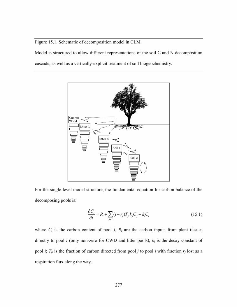
277
Figure 15.1. Schematic of decomposition model in CLM.
Model is structured to allow different representations of the soil C and N decomposition
cascade, as well as a vertically-explicit treatment of soil biogeochemistry.
For the single-level model structure, the fundamental equation for carbon balance of the
decomposing pools is:
(15.1)
where Ci is the carbon content of pool i, Ri are the carbon inputs from plant tissues
directly to pool i (only non-zero for CWD and litter pools), ki is the decay constant of
pool i; Tji is the fraction of carbon directed from pool j to pool i with fraction rj lost as a
respiration flux along the way.
∂Ci
∂t= Ri + (i − rj )Tjik jC j − kiCi
j≠i∑
278
Adding the vertical dimension to the decomposing pools changes the balance equation to
the following:
∂Ci (z)∂t
= Ri (z) + 1− rj( )Tjik j (z)Cj (z)i≠ j∑ − ki (z)Ci (z)
+∂∂z
D(z) ∂Ci
∂z
+∂∂z
A(z)Ci( )
(15.2)
where Ci(z) is now defined at each model level, and in volumetric (gC m-3) rather than
areal (gC m-2) units, along with Ri(z) and kj(z). In addition, vertical transport is handled
by the last two terms, for diffusive and advective transport. In the base model, advective
transport is set to zero, leaving only a diffusive flux with diffusivity D(z) defined for all
decomposing carbon and nitrogen pools. Further discussion of the vertical distribution of
carbon inputs Ri(z), vertical turnover times kj(z), and vertical transport D(z) is below.
Discussion of the vertical model and analysis of both decomposition structures is in
Koven et al (2013).
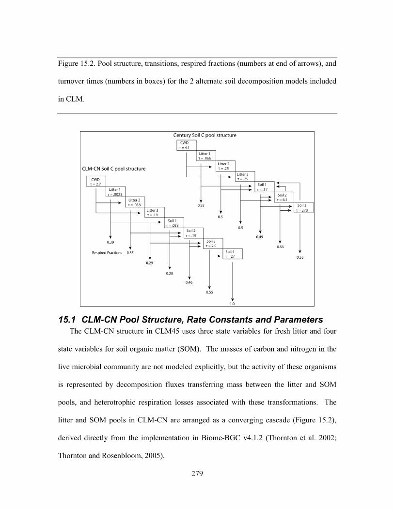
279
Figure 15.2. Pool structure, transitions, respired fractions (numbers at end of arrows), and
turnover times (numbers in boxes) for the 2 alternate soil decomposition models included
in CLM.
15.1 CLM-CN Pool Structure, Rate Constants and Parameters The CLM-CN structure in CLM45 uses three state variables for fresh litter and four
state variables for soil organic matter (SOM). The masses of carbon and nitrogen in the
live microbial community are not modeled explicitly, but the activity of these organisms
is represented by decomposition fluxes transferring mass between the litter and SOM
pools, and heterotrophic respiration losses associated with these transformations. The
litter and SOM pools in CLM-CN are arranged as a converging cascade (Figure 15.2),
derived directly from the implementation in Biome-BGC v4.1.2 (Thornton et al. 2002;
Thornton and Rosenbloom, 2005).
280
Model parameters are estimated based on a synthesis of microcosm decomposition
studies using radio-labeled substrates (Degens and Sparling, 1996; Ladd et al. 1992;
Martin et al. 1980; Mary et al. 1993; Saggar et al. 1994; Sørensen, 1981; van Veen et al.
1984). Multiple exponential models are fitted to data from the microcosm studies to
estimate exponential decay rates and respiration fractions (Thornton, 1998). The
microcosm experiments used for parameterization were all conducted at constant
temperature and under moist conditions with relatively high mineral nitrogen
concentrations, and so the resulting rate constants are assumed not limited by the
availability of water or mineral nitrogen. Table 15.1 lists the base decomposition rates
for each litter and SOM pool, as well as a base rate for physical fragmentation for the
coarse woody debris pool (CWD).
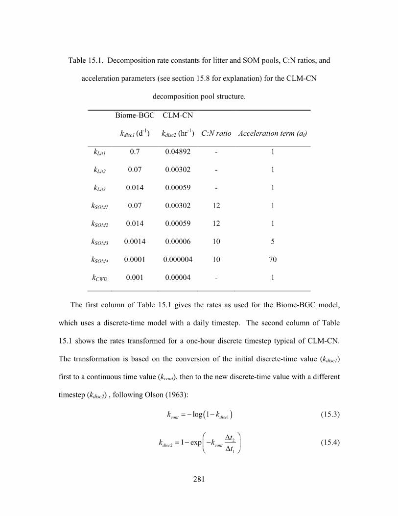
281
Table 15.1. Decomposition rate constants for litter and SOM pools, C:N ratios, and
acceleration parameters (see section 15.8 for explanation) for the CLM-CN
decomposition pool structure.
Biome-BGC CLM-CN
kdisc1 (d-1) kdisc2 (hr-1) C:N ratio Acceleration term (ai)
kLit1 0.7 0.04892 - 1
kLit2 0.07 0.00302 - 1
kLit3 0.014 0.00059 - 1
kSOM1 0.07 0.00302 12 1
kSOM2 0.014 0.00059 12 1
kSOM3 0.0014 0.00006 10 5
kSOM4 0.0001 0.000004 10 70
kCWD 0.001 0.00004 - 1
The first column of Table 15.1 gives the rates as used for the Biome-BGC model,
which uses a discrete-time model with a daily timestep. The second column of Table
15.1 shows the rates transformed for a one-hour discrete timestep typical of CLM-CN.
The transformation is based on the conversion of the initial discrete-time value (kdisc1)
first to a continuous time value (kcont), then to the new discrete-time value with a different
timestep (kdisc2) , following Olson (1963):
(15.3)
(15.4)
( )1log 1cont disck k= − −
22
1
1 expdisc conttk kt
∆= − − ∆
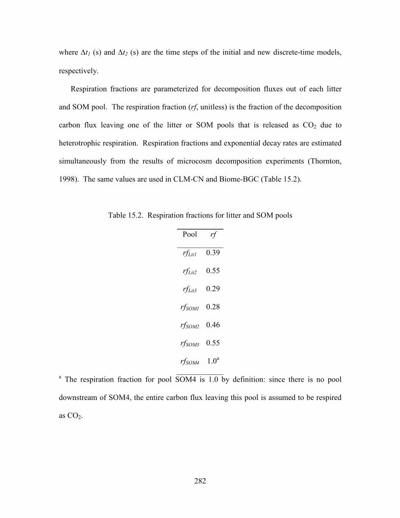
282
where ∆t1 (s) and ∆t2 (s) are the time steps of the initial and new discrete-time models,
respectively.
Respiration fractions are parameterized for decomposition fluxes out of each litter
and SOM pool. The respiration fraction (rf, unitless) is the fraction of the decomposition
carbon flux leaving one of the litter or SOM pools that is released as CO2 due to
heterotrophic respiration. Respiration fractions and exponential decay rates are estimated
simultaneously from the results of microcosm decomposition experiments (Thornton,
1998). The same values are used in CLM-CN and Biome-BGC (Table 15.2).
Table 15.2. Respiration fractions for litter and SOM pools
Pool rf
rfLit1 0.39
rfLit2 0.55
rfLit3 0.29
rfSOM1 0.28
rfSOM2 0.46
rfSOM3 0.55
rfSOM4 1.0a
a The respiration fraction for pool SOM4 is 1.0 by definition: since there is no pool
downstream of SOM4, the entire carbon flux leaving this pool is assumed to be respired
as CO2.
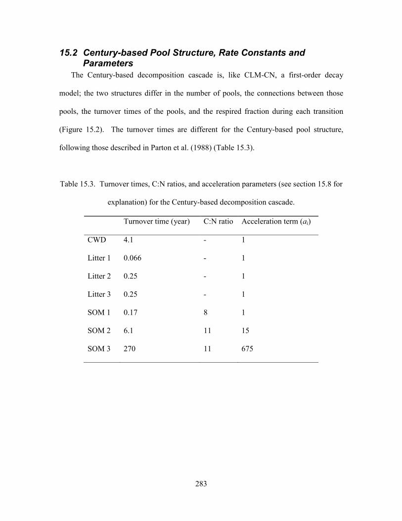
283
15.2 Century-based Pool Structure, Rate Constants and Parameters
The Century-based decomposition cascade is, like CLM-CN, a first-order decay
model; the two structures differ in the number of pools, the connections between those
pools, the turnover times of the pools, and the respired fraction during each transition
(Figure 15.2). The turnover times are different for the Century-based pool structure,
following those described in Parton et al. (1988) (Table 15.3).
Table 15.3. Turnover times, C:N ratios, and acceleration parameters (see section 15.8 for
explanation) for the Century-based decomposition cascade.
Turnover time (year) C:N ratio Acceleration term (ai)
CWD 4.1 - 1
Litter 1 0.066 - 1
Litter 2 0.25 - 1
Litter 3 0.25 - 1
SOM 1 0.17 8 1
SOM 2 6.1 11 15
SOM 3 270 11 675
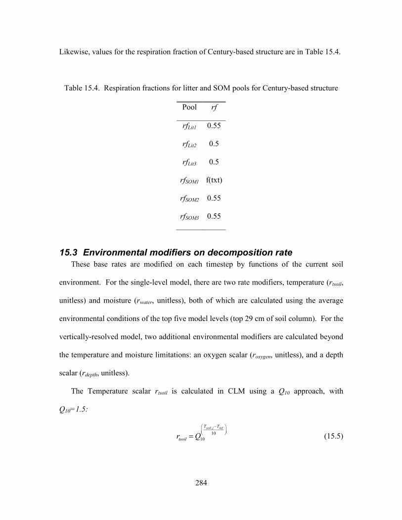
284
Likewise, values for the respiration fraction of Century-based structure are in Table 15.4.
Table 15.4. Respiration fractions for litter and SOM pools for Century-based structure
Pool rf
rfLit1 0.55
rfLit2 0.5
rfLit3 0.5
rfSOM1 f(txt)
rfSOM2 0.55
rfSOM3 0.55
15.3 Environmental modifiers on decomposition rate These base rates are modified on each timestep by functions of the current soil
environment. For the single-level model, there are two rate modifiers, temperature (rtsoil,
unitless) and moisture (rwater, unitless), both of which are calculated using the average
environmental conditions of the top five model levels (top 29 cm of soil column). For the
vertically-resolved model, two additional environmental modifiers are calculated beyond
the temperature and moisture limitations: an oxygen scalar (roxygen, unitless), and a depth
scalar (rdepth, unitless).
The Temperature scalar rtsoil is calculated in CLM using a Q10 approach, with
Q10=1.5:
(15.5) rtsoil = Q10
Tsoil , j −Tref
10
285
where j is the soil layer index, Tsoil,j (K) is the temperature of soil level j. The reference
temperature Tref = 25C.
The rate scalar for soil water potential (rwater, unitless) is calculated using a
relationship from Andrén and Paustian (1987) and supported by additional data in
Orchard and Cook (1983):
(15.6)
where Ψj is the soil water potential in layer j, Ψmin is a lower limit for soil water potential
control on decomposition rate (set to -10 MPa). Ψsat,j (MPa) is the saturated soil water
potential, calculated using the multivariate regression model from Cosby et al. (1984):
(15.7)
where Psand,j and Pclay,j are the volume percentages of sand and clay in soil layer j.
For frozen soils, the bulk of the rapid dropoff in decomposition with decreasing
temperature is due to the moisture limitation, since matric potential is limited by
temperature in the supercooled water formulation of Niu and Yang (2006),
(15.8)
An additional frozen decomposition limitation can be specified using a ‘frozen Q10’
following Koven et al. (2011), however the default value of this is the same as the
unfrozen Q10 value, and therefore the basic hypothesis is that frozen respiration is limited
by liquid water availability, and can be modeled following the same approach as thawed
but dry soils.
( )( )
5
,1
0 for
logfor
log1 for
j min
min jwater soil j min j max
j min max
j max
r w=
Ψ < Ψ
Ψ Ψ= Ψ ≤ Ψ ≤ Ψ Ψ Ψ
Ψ > Ψ
∑
( )( ) ( )( ), , , ,(9.8e -5)exp 1.54 0.0095 0.0063 100 log 10sat j sand j sand j clay jP P PΨ = − − + − −
ψ (T ) = −Lf (T − Tf )
103T
286
An additional rate scalar, roxygen is enabled when the CH4 submodel is used (set equal
to 1 for the single layer model or when the CH4 submodel is disabled). This limits
decomposition when there is insufficient molecular oxygen to satisfy stoichiometric
demand (1 mol O2 consumed per mol CO2 produced) from heterotrophic decomposers,
and supply from diffusion through soil layers (unsaturated and saturated) or aerenchyma
(Chapter 19). A minimum value of roxygen is set at 0.2, with the assumption that oxygen
within organic tissues can supply the necessary stoichiometric demand at this rate. This
value lies between estimates of 0.025–0.1 (Frolking et al. 2001), and 0.35 (Wania et al.
2009); the large range of these estimates poses a large unresolved uncertainty.
Lastly, a possible explicit depth dependence, rdepth, (set equal to 1 for the single layer
model) can be applied to soil C decomposition rates to account for processes other than
temperature, moisture, and anoxia that can limit decomposition. This depth dependence
of decomposition was shown by Jenkinson and Coleman (2008) to be an important term
in fitting total C and 14C profiles, and implies that unresolved processes, such as priming
effects, microscale anoxia, soil mineral surface and/or aggregate stabilization may be
important in controlling the fate of carbon at depth (Koven et al. 2013). CLM includes
these unresolved depth controls via an exponential decrease in the soil turnover time with
depth:
rdepth = exp −zzτ
(15.9)
where zτ is the e-folding depth for decomposition, set by default to 0.5m.
The combined decomposition rate scalar (rtotal, unitless) is:
. (15.10) rtotal = rtsoilrwaterroxygenrdepth
287
15.4 N-limitation of Decomposition Fluxes Decomposition rates can also be limited by the availability of mineral nitrogen, but
calculation of this limitation depends on first estimating the potential rates of
decomposition, assuming an unlimited mineral nitrogen supply. The general case is
described here first, referring to a generic decomposition flux from an “upstream” pool
(u) to a “downstream” pool (d), with an intervening loss due to respiration. The potential
carbon flux out of the upstream pool (CFpot,u, gC m-2 s-1) is:
(15.11)
where CSu (gC m-2) is the initial mass in the upstream pool and ku is the decay rate
constant (s-1) for the upstream pool, adjusted for temperature and moisture conditions.
Depending on the C:N ratios of the upstream and downstream pools and the amount of
carbon lost in the transformation due to respiration (the respiration fraction), the
execution of this potential carbon flux can generate either a source or a sink of new
mineral nitrogen (NFpot_min,u→d, gN m-2 s-1). The governing equation (Thornton and
Rosenbloom, 2005) is:
(15.12)
where rfu is the respiration fraction for fluxes leaving the upstream pool, CNu and CNd are
the C:N ratios for upstream and downstream pools, respectively. Negative values of
NFpot_min,u→d indicate that the decomposition flux results in a source of new mineral
nitrogen, while positive values indicate that the potential decomposition flux results in a
sink (demand) for mineral nitrogen.
,pot u u uCF CS k=
, 1 dpot u u
upot_min,u d
d
CNCF rfCN
NFCN→
− −
=
288
Following from the general case, potential carbon fluxes leaving individual pools in
the decomposition cascade, for the example of the CLM-CN pool structure, are given as:
(15.13)
(15.14)
(15.15)
(15.16)
(15.17)
(15.18)
(15.19)
where the factor (1/∆t) is included because the rate constant is calculated for the entire
timestep (Eqs. (15.3) and (15.4)), but the convention is to express all fluxes on a per-
second basis. Potential mineral nitrogen fluxes associated with these decomposition steps
are, again for the example of the CLM-CN pool structure (the CENTURY structure will
be similar but without the different terminal step):
(15.20)
(15.21)
(15.22)
(15.23)
pot,Lit1 Lit1 Lit1 totalCF CS k r t= ∆
pot,Lit2 Lit2 Lit2 totalCF CS k r t= ∆
pot,Lit3 Lit3 Lit3 totalCF CS k r t= ∆
pot,SOM1 SOM1 SOM1 totalCF CS k r t= ∆
pot,SOM2 SOM2 SOM2 totalCF CS k r t= ∆
pot,SOM3 SOM3 SOM3 totalCF CS k r t= ∆
pot,SOM4 SOM4 SOM4 totalCF CS k r t= ∆
1 SOM1pot_min,Lit1 SOM1 pot,Lit1 Lit1 SOM1
Lit1
CNNF CF rf CNCN→
= − −
1 SOM2pot_min,Lit2 SOM2 pot,Lit2 Lit2 SOM2
Lit2
CNNF CF rf CNCN→
= − −
1 SOM3pot_min,Lit3 SOM3 pot,Lit3 Lit3 SOM3
Lit3
CNNF CF rf CNCN→
= − −
1 SOM2pot_min,SOM1 SOM2 pot,SOM1 SOM1 SOM2
SOM1
CNNF CF rf CNCN→
= − −
289
(15.24)
(15.25)
(15.26)
where the special form of Eq. (15.26) arises because there is no SOM pool downstream
of SOM4 in the converging cascade: all carbon fluxes leaving that pool are assumed to be
in the form of respired CO2, and all nitrogen fluxes leaving that pool are assumed to be
sources of new mineral nitrogen.
Steps in the decomposition cascade that result in release of new mineral nitrogen
(mineralization fluxes) are allowed to proceed at their potential rates, without
modification for nitrogen availability. Steps that result in an uptake of mineral nitrogen
(immobilization fluxes) are subject to rate limitation, depending on the availability of
mineral nitrogen, the total immobilization demand, and the total demand for soil mineral
nitrogen to support new plant growth. The potential mineral nitrogen fluxes from Eqs.
(15.20) - (15.26) are evaluated, summing all the positive fluxes to generate the total
potential nitrogen immobilization flux (NFimmob_demand, gN m-2 s-1), and summing absolute
values of all the negative fluxes to generate the total nitrogen mineralization flux
(NFgross_nmin, gN m-2 s-1). Since NFgriss_nmin is a source of new mineral nitrogen to the soil
mineral nitrogen pool it is not limited by the availability of soil mineral nitrogen, and is
therefore an actual as opposed to a potential flux.
1 SOM3pot_min,SOM2 SOM3 pot,SOM2 SOM2 SOM3
SOM2
CNNF CF rf CNCN→
= − −
1 SOM4pot_min,SOM3 SOM4 pot,SOM3 SOM3 SOM4
SOM3
CNNF CF rf CNCN→
= − −
pot_min,SOM4 pot,SOM4 SOM4NF CF CN= −
290
15.5 N Competition between plant uptake and soil immobilization fluxes
Once NFimmob_demand is known, the competition between plant and microbial nitrogen
demand can be resolved. Mineral nitrogen in the soil pool (NSsminn, gN m-2) at the
beginning of the timestep is considered the available supply. Total demand for mineral
nitrogen from this pool (NFtotal_demand, gN m-2 s-1) is:
(15.27)
If NFtotal_demand∆t < NSsminn, then the available pool is large enough to meet both plant
and microbial demand, and neither plant growth nor immobilization steps in the
decomposition cascade are limited by nitrogen availability in the timestep. In that case,
the signaling variables fplant_demand and fimmob_demand are both set to 1.0, where fplant_demand is
defined and used in section 15.4, and fimmob_demand is the fraction of potential
immobilization demand that can be met given current supply of mineral nitrogen.
If NFtotal_demand∆t ≥ NSsminn, then there is not enough mineral nitrogen to meet the
combined demands for plant growth and heterotrophic immobilization, and both of these
processes proceed at lower-than-potential rates, defined by the fractions fplant_demand and
fimmob_demand, where:
(15.28)
This treatment of competition for nitrogen as a limiting resource is referred to a
demand-based competition, where the fraction of the available resource that eventually
flows to a particular process depends on the demand from that process in comparison to
the total demand from all processes. Processes expressing a greater demand acquire a
larger fraction of the available resource.
total_demand immob_demand plant_demand_soilNF NF NF= +
sminnplant_demand immob_demand
total_demand
NSf ft NF
= =∆
291
15.6 Final Decomposition Fluxes With fimmob_demand known, final decomposition fluxes can be calculated. Actual carbon
fluxes leaving the individual litter and SOM pools, again for the example of the CLM-CN
pool structure (the CENTURY structure will be similar but, again without the different
terminal step), are calculated as:
(15.29)
(15.30)
(15.31)
(15.32)
(15.33)
(15.34)
(15.35)
Heterotrophic respiration fluxes (losses of carbon as CO2 to the atmosphere) are:
(15.36)
(15.37)
(15.38)
(15.39)
,
, 1 ,
for 0
for 0pot,Lit1 immob_demand pot_min Lit1 SOM1
Lit1pot Lit pot_min Lit1 SOM1
CF f NFCF
CF NF→
→
>= ≤
for 0
for 0pot,Lit2 immob_demand pot_min,Lit2 SOM2
Lit2pot,Lit2 pot_min,Lit2 SOM2
CF f NFCF
CF NF→
→
>= ≤
for 0
for 0pot,Lit3 immob_demand pot_min,Lit3 SOM3
Lit3pot,Lit3 pot_min,Lit3 SOM3
CF f NFCF
CF NF→
→
>= ≤
for 0
for 0pot,SOM1 immob_demand pot_min,SOM1 SOM2
SOM1pot,SOM1 pot_min,SOM1 SOM2
CF f NFCF
CF NF→
→
>= ≤
for 0
for 0pot,SOM2 immob_demand pot_min,SOM2 SOM3
SOM2pot,SOM2 pot_min,SOM2 SOM3
CF f NFCF
CF NF→
→
>= ≤
for 0
for 0pot,SOM3 immob_demand pot_min,SOM3 SOM4
SOM3pot,SOM3 pot_min,SOM3 SOM4
CF f NFCF
CF NF→
→
>= ≤
SOM4 pot,SOM4CF CF=
Lit1,HR Lit1 Lit1CF CF rf=
Lit2,HR Lit2 Lit2CF CF rf=
Lit3,HR Lit3 Lit3CF CF rf=
SOM1,HR SOM1 SOM1CF CF rf=
292
(15.40)
(15.41)
(15.42)
Transfers of carbon from upstream to downstream pools in the decomposition
cascade are given as:
(15.43)
(15.44)
(15.45)
(15.46)
(15.47)
(15.48)
In accounting for the fluxes of nitrogen between pools in the decomposition cascade
and associated fluxes to or from the soil mineral nitrogen pool, the model first calculates
a flux of nitrogen from an upstream pool to a downstream pool, then calculates a flux
either from the soil mineral nitrogen pool to the downstream pool (immobilization) or
from the downstream pool to the soil mineral nitrogen pool (mineralization). Transfers of
nitrogen from upstream to downstream pools in the decomposition cascade are given as:
(15.49)
(15.50)
(15.51)
(15.52)
SOM2,HR SOM2 SOM2CF CF rf=
SOM3,HR SOM3 SOM3CF CF rf=
SOM4,HR SOM4 SOM4CF CF rf=
( )1Lit1,SOM1 Lit1 Lit1CF CF rf= −
( )1Lit2,SOM2 Lit2 Lit2CF CF rf= −
( )1Lit3,SOM3 Lit3 Lit3CF CF rf= −
( )1SOM1,SOM2 SOM1 SOM1CF CF rf= −
( )1SOM2,SOM3 SOM2 SOM2CF CF rf= −
( )1SOM3,SOM4 SOM3 SOM3CF CF rf= −
Lit1,SOM1 Lit1 Lit1NF CF CN=
Lit2,SOM2 Lit2 Lit2NF CF CN=
3, 3 3 3Lit SOM Lit LitNF CF CN=
SOM1,SOM2 SOM1 SOM1NF CF CN=
293
(15.53)
(15.54)
Corresponding fluxes to or from the soil mineral nitrogen pool depend on whether the
decomposition step is an immobilization flux or a mineralization flux:
(15.55)
(15.56)
(15.57)
(15.58)
(15.59)
(15.60)
(15.61)
15.7 Vertical Distribution and Transport of Decomposing C and N pools
Additional terms are needed to calculate the vertically-resolved soil C and N budget:
the initial vertical distribution of C and N from PFTs delivered to the litter and CWD
pools, and the vertical transport of C and N pools.
For initial vertical inputs, CLM uses separate profiles for aboveground (leaf, stem)
and belowground (root) inputs. Aboveground inputs are given a single exponential with
SOM2,SOM3 SOM2 SOM2NF CF CN=
SOM3,SOM4 SOM3 SOM3NF CF CN=
for 0
for 0pot_min,Lit1 SOM1 immob_demand pot_min,Lit1 SOM1
sminn,Lit1 SOM1pot_min,Lit1 SOM1 pot_min,Lit1 SOM1
NF f NFNF
NF NF→ →
→→ →
>= ≤
for 0
for 0pot_min,Lit2 SOM2 immob_demand pot_min,Lit2 SOM2
sminn,Lit2 SOM2pot_min,Lit2 SOM2 pot_min,Lit2 SOM2
NF f NFNF
NF NF→ →
→→ →
>= ≤
for 0
for 0pot_min,Lit3 SOM3 immob_demand pot_min,Lit3 SOM3
sminn,Lit3 SOM3pot_min,Lit3 SOM3 pot_min,Lit3 SOM3
NF f NFNF
NF NF→ →
→→ →
>= ≤
for 0
for 0pot_min,SOM1 SOM2 immob_demand pot_min,SOM1 SOM2
sminn,SOM1 SOM2pot_min,SOM1 SOM2 pot_min,SOM1 SOM2
NF f NFNF
NF NF→ →
→→ →
>= ≤
for 0
for 0pot_min,SOM2 SOM3 immob_demand pot_min,SOM2 SOM3
sminn,SOM2 SOM3pot_min,SOM2 SOM3 pot_min,SOM2 SOM3
NF f NFNF
NF NF→ →
→→ →
>= ≤
for 0
for 0pot_min,SOM3 SOM4 immob_demand pot_min,SOM3 SOM4
sminn,SOM3 SOM4pot_min,SOM3 SOM4 pot_min,SOM3 SOM4
NF f NFNF
NF NF→ →
→→ →
>= ≤
sminn,SOM4 pot_min,SOM4NF NF=
294
default e-folding depth = 0.1m. Belowground inputs are distributed according to rooting
profiles with default values based on the Jackson et al. (1996) exponential
parameterization.
Vertical mixing is accomplished by an advection-diffusion equation. The goal of this
is to consider slow, soild- and adsorbed-phase transport due to bioturbation,
cryoturbation, and erosion. Faster aqueous-phase transport is not included in CLM, but
has been developed as part of the CLM-BeTR suite of parameterizations (Tang and Riley
2013). The default value of the advection term is 0 cm/yr, such that transport is purely
diffusive. Diffusive transport differs in rate between permafrost soils (where
cryoturbation is the dominant transport term) and non-permafrost soils (where
bioturbation dominates). For permafrost soils, a parameterization based on that of Koven
et al. (2009) is used: the diffusivity parameter is constant through the active layer, and
decreases linearly from the base of the active layer to zero at a set depth (default 3m); the
default permafrost diffusivity is 5 cm2/yr. For non-permafrost soils, the default diffusivity
is 1 cm2/yr.
15.8 Model Equilibration Because of the coupling between the slowest SOM pools and productivity through N
downregulation of photosynthesis, equilibration of the model for initialization purposes
will take an extremely long time in the standard mode. This is particularly true for the
CENTURY-based decomposition cascade, which includes a passive pool. In order to
rapidly equilibrate the model, a modified version of the “accelerated decomposition”
(Thornton and Rosenbloom, 2005) is used. The fundamental idea of this approach is to
allow fluxes between the various pools (both turnover-defined and vertically-defined
295
fluxes) adjust rapidly, while keeping the pool sizes themselves small so that they can fill
quickly. To do this, the base decomposition rate ki for each pool i is accelerated by a
term ai such that the slow pools are collapsed onto an approximately annual timescale
(Koven et al. 2013). Accelerating the pools beyond this timescale distorts the seasonal
and/or diurnal cycles of decomposition and N mineralization, thus leading to a
substantially different ecosystem productivity than the full model. For the vertical model,
the vertical transport terms are also accelerated by the same term ai, as is the radioactive
decay when 14C is enabled, following the same principle of keeping fluxes between pools
(or fluxes lost to decay) close to the full model while keeping the pools sizes small. When
leaving the accelerated decomposition mode, the concentration of C and N in pools that
had been accelerated are multiplied by the same term ai, to bring the model into
approximate equilibrium. Note that in CLM, the model can also transition into
accelerated decomposition mode from the standard mode (by dividing the pools by ai),
and that the transitions into and out of accelerated decomposition mode are handled
automatically by CLM upon loading from restart files (which preserve information about
the mode of the model when restart files were written).
The acceleration terms for the two decomposition cascades are shown in Tables 15.1
and 15.3.
296
16. External Nitrogen Cycle
In addition to the relatively rapid cycling of nitrogen within the plant – litter – soil
organic matter system, CLM also represents several slow processes which couple the
internal nitrogen cycle to external sources and sinks. Inputs of new mineral nitrogen are
from atmospheric deposition and biological nitrogen fixation. Losses of mineral nitrogen
are due to nitrification, denitrification, leaching, and losses in fire. While the short-term
dynamics of nitrogen limitation depend on the behavior of the internal nitrogen cycle,
establishment of total ecosystem nitrogen stocks depends on the balance between sources
and sinks in the external nitrogen cycle.
CLM includes two separate treatments of the slow nitrogen cycle. The first is the
original CLM-CN formulations, which includes a single soil mineral nitrogen pool to
represent both NO3- and NH4
+, and with nitrogen losses via denitrification calculated as a
constant fraction of mineralization plus a fixed first-order loss of unutilized mineral
nitrogen at the end of every timestep. The second is based on the Century N-gas model;
this includes separate NH4+ and NO3
- pools, as well as environmentally controlled
nitrification and denitrification rates. Both are described below.
16.1 Atmospheric Nitrogen Deposition CLM uses a single variable to represent the total deposition of mineral nitrogen onto
the land surface, combining wet and dry deposition of NOy and NHx as a single flux
(NFndep_sminn, gN m-2 s-1). This flux is intended to represent total reactive nitrogen
deposited to the land surface which originates from the following natural and
anthropogenic sources (Galloway et al. 2004): formation of NOx during lightning, NOx
297
and NH3 emission from wildfire, NOx emission from natural soils, NH3 emission from
natural soils, vegetation, and wild animals, NOx and NH3 emission during fossil fuel
combustion (both thermal and fuel NOx production), NOx and NH3 emission from other
industrial processes, NOx and NH3 emission from fire associated with deforestation, NOx
and NH3 emission from agricultural burning, NOx emission from agricultural soils, NH3
emission from agricultural crops, NH3 emission from agricultural animal waste, and NH3
emission from human waste and waste water. The deposition flux is provided as a
spatially and (potentially) temporally varying dataset (see section 2.2.3 for a description
of the default input dataset).
In the CLM-CN mineral N pool model, the nitrogen deposition flux is assumed to
enter the soil mineral nitrogen pool (NSsminn) directly; while in the Century-based model,
all of the nitrogen is assumed to enter the NH4+ pool. Real pathways for wet and dry
nitrogen deposition can be more complex than currently represented in the CLM-CN,
including release from melting snowpack and direct foliar uptake of deposited NOy (e.g.
Tye et al. 2005; Vallano and Sparks, 2007).
16.2 Biological Nitrogen Fixation The fixation of new reactive nitrogen from atmospheric N2 by soil microorganisms is
an important component of both preindustrial and modern-day nitrogen budgets, but a
mechanistic understanding of global-scale controls on biological nitrogen fixation (BNF)
is still only poorly developed (Cleveland et al. 1999; Galloway et al. 2004). Cleveland et
al. (1999) suggested empirical relationships that predict BNF as a function of either
evapotranspiration rate or net primary productivity for natural vegetation. CLM assumes
that BNF is a function of net primary production (CFann_NPP, gC m-2 y-1). The rationale
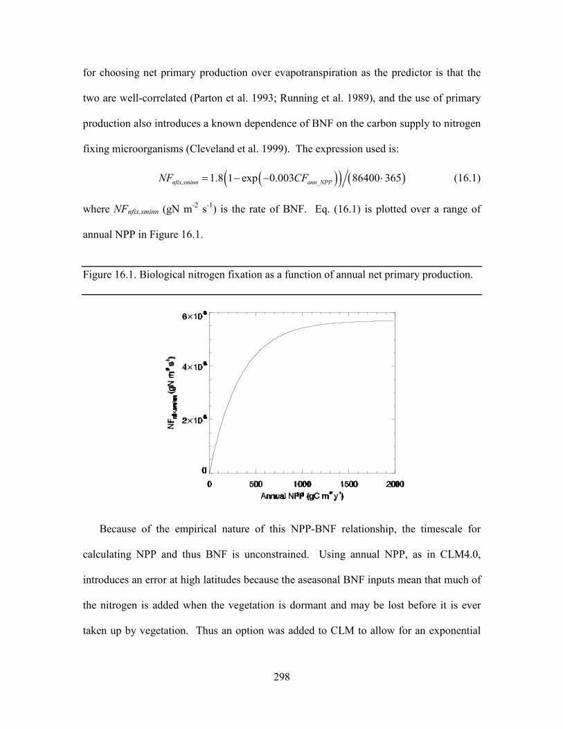
298
for choosing net primary production over evapotranspiration as the predictor is that the
two are well-correlated (Parton et al. 1993; Running et al. 1989), and the use of primary
production also introduces a known dependence of BNF on the carbon supply to nitrogen
fixing microorganisms (Cleveland et al. 1999). The expression used is:
( )( ) ( )1.8 1 exp 0.003 86400 365nfix,sminn ann_NPPNF CF= − − ⋅ (16.1)
where NFnfix,sminn (gN m-2 s-1) is the rate of BNF. Eq. (16.1) is plotted over a range of
annual NPP in Figure 16.1.
Figure 16.1. Biological nitrogen fixation as a function of annual net primary production.
Because of the empirical nature of this NPP-BNF relationship, the timescale for
calculating NPP and thus BNF is unconstrained. Using annual NPP, as in CLM4.0,
introduces an error at high latitudes because the aseasonal BNF inputs mean that much of
the nitrogen is added when the vegetation is dormant and may be lost before it is ever
taken up by vegetation. Thus an option was added to CLM to allow for an exponential
299
relaxation (with default e-folding time of 10 days) calculation of NPP, and BNF
calculated from that using equation 16.1.
As with Atmospheric N deposition, BNF N inputs are added directly to the mineral N
pools. In the CLM-CN N model, this is the single mineral N pool; in the Century-based
model, this is the NH4+ pool.
16.3 Nitrification and Denitrification Losses of Nitrogen In order to better understand the structural uncertainty in biogeochemical responses to
climate change, CLM includes two alternate representations of the mineral N
transformations and losses that define the slow N cycle. Each of these is described
below.
16.3.1 CLM-CN formulation Under aerobic conditions in the soil oxygen is the preferred electron acceptor
supporting the metabolism of heterotrophs, but anaerobic conditions favor the activity of
soil heterotrophs which use nitrate as an electron acceptor (e.g. Pseudomonas and
Clostridium) supporting respiration. This process, known as denitrification, results in the
transformation of nitrate to gaseous N2, with smaller associated production of NOx and
N2O. It is typically assumed that nitrogen fixation and denitrification were
approximately balanced in the preindustrial biosphere (Galloway et al. 2004). It is likely
that denitrification can occur within anaerobic microsites within an otherwise aerobic soil
environment, leading to large global denitrification fluxes even when fluxes per unit area
are rather low (Galloway et al. 2004).
Because the vertical distribution of soil organic matter is not resolved explicitly in
CLM-CN, a simple denitrification parameterization is used that treats denitrification as a
300
constant fraction of gross nitrogen mineralization. At each step in the decomposition
cascade, if the transformation from an upstream to a downstream pool is predicted to
mineralize (as opposed to immobilize) nitrogen, then a constant fraction of the nitrogen
mineralization flux is assumed to be lost via denitrification. Due to large uncertainties in
the mechanistic understanding of the environmental controls on denitrification, no
modifications to the denitrification fraction are made for different soil moisture
conditions. This is identified as a high-priority area for future model development.
Denitrification fluxes associated with gross mineralization in the decomposition
cascade are calculated as follows:
0 for 0
for 0pot_min,Lit1 SOM1
denit,Lit1 SOM1pot_min,Lit1 SOM1 denit pot_min,Lit1 SOM1
NFNF
NF f NF→
→→ →
>= − ≤ (16.2)
0 for 0
for 0pot_min,Lit2 SOM2
denit,Lit2 SOM2pot_min,Lit2 SOM2 denit pot_min,Lit2 SOM2
NFNF
NF f NF→
→→ →
>= − ≤ (16.3)
0 for 0
for 0pot_min,Lit3 SOM3
denit,Lit3 SOM3pot_min,Lit3 SOM3 denit pot_min,Lit3 SOM3
NFNF
NF f NF→
→→ →
>= − ≤ (16.4)
0 for 0
for 0pot_min,SOM1 SOM2
denit,SOM1 SOM2pot_min,SOM1 SOM2 denit pot_min,SOM1 SOM2
NFNF
NF f NF→
→→ →
>= − ≤ (16.5)
0 for 0
for 0pot_min,SOM2 SOM3
denit,SOM2 SOM3pot_min,SOM2 SOM3 denit pot_min,SOM2 SOM3
NFNF
NF f NF→
→→ →
>= − ≤ (16.6)
0 for 0
for 0pot_min,SOM3 SOM4
denit,SOM3 SOM4pot_min,SOM3 SOM4 denit pot_min,SOM3 SOM4
NFNF
NF f NF→
→→ →
>= − ≤ (16.7)
denit,SOM4 pot_min,SOM4NF NF= − (16.8)
where fdenit = 0.01 is the constant denitrification fraction of gross mineralization, and the
denitrification fluxes are assumed to be leaving the soil mineral nitrogen pool (NSsminn)
301
and entering the atmosphere. The speciation of gaseous nitrogen fluxes entering the
atmosphere (e.g. N2 vs. NOx or N2O) is not specified. Providing an explicit speciation of
these nitrogen losses is another high-priority area for future model development.
The model includes one other denitrification pathway, intended to represent the
observed losses of mineral nitrogen in systems experiencing nitrogen saturation. One
reason this mechanism has been included is in anticipation of an agricultural fertilization
flux, provided either through a prescribed dataset or through a prognostic agricultural
management routine. The model does not currently include an explicit representation of
the fertilization flux, but when it is introduced, it will be necessary to account for the
substantial denitrification losses associated with high nitrate concentrations in some
heavily fertilized agricultural soils. Nitrogen saturation can also occur in natural
vegetation systems, especially under conditions of high atmospheric nitrogen deposition,
and so this mechanism plays a useful role even prior to the introduction within the model
of agricultural fertilization.
For the purpose of this calculation, nitrogen saturation is evaluated on each timestep,
by comparing the total demand for new mineral nitrogen from plants and immobilization
with the available soil mineral nitrogen pool. The denitrification of excess soil mineral
nitrogen is non-zero whenever the supply of mineral nitrogen exceeds the demand:
for
0 for
sminntotal_demand dnx total_demand sminn
sminn,denit
total_demand sminn
NS NF f NF t NStNF
NF t NS
− ∆ < ∆= ∆ ≥
(16.9)
where fdnx (unitless) is the fraction of excess soil mineral nitrogen subject to
denitrification on each timestep. This fraction is parameterized such that 50% of any
excess soil mineral nitrogen would be lost to denitrification per day:
302
0.586400dnx
tf ∆= (16.10)
16.3.2 Century-based formulation CLM includes a detailed representation of nitrification and denitrification based on
the Century N model (Parton et al. 1996, 2001; del Grosso et al. 2000). In this approach,
nitrification of NH4+ to NO3
- is a function of temperature, moisture, and pH:
fnitr,p = NH4[ ]knitr f T( ) f H2O( )f pH( ) (16.11)
where fnitr,p is the potential nitrification rate (prior to competition for NH4+ by plant
uptake and N immobilization), knitr is the maximum nitrification rate (10 % day−1 ,
(Parton et al. 2001)), and f(T) and f(H2O) are rate modifiers for temperature and moisture
content. CLM uses the same rate modifiers as are used in the decomposition routine.
f(pH) is a rate modifier for pH; however, because CLM does not calculate pH, instead a
fixed pH value of 6.5 is used in the pH function of Parton et al. (1996).
The potential denitrification rate is co-limited by NO−3 concentration and C
consumption rates, and occurs only in the anoxic fraction of soils:
fdenitr,p = min f (decomp), f NO3−[ ]( )( )fracanox
(16.12)
where fdenitr,p is the potential denitrification rate and f(decomp) and f([NO3−]) are the
carbon- and nitrate- limited denitrification rate functions, respectively, (del Grosso et al.
2000). Because the modified CLM includes explicit treatment of soil biogeochemical
vertical profiles, including diffusion of the trace gases O2 and CH4 (Riley et al. 2011a),
the calculation of anoxic fraction fracanox uses this information following the anoxic
microsite formulation of Arah and Vinten (1995):
fracanox = exp −aRψ−αV −βC γ θ + χε[ ]δ( ) (16.13)
303
where a, α, β, γ, and δ are constants (equal to 1.5×10⁻¹⁰, 1.26, 0.6, 0.6, and 0.85,
respectively), Rψ is the radius of a typical pore space at moisture content ψ, V is the O2
consumption rate, C is the O2 concentration, θ is the water-filled pore space, χ is the ratio
of diffusivity of oxygen in water to that in air, and ε is the air-filled pore space (Arah and
Vinten, 1995). These parameters are all calculated separately at each layer to define a
profile of anoxic porespace fraction in the soil.
The nitrification/denitrification models used here also predict fluxes of N2O via a
“hole-in-the-pipe” approach (Firestone and Davidson, 1989). A constant fraction (6 * 10-
4, Li et al. 2000) of the nitrification flux is assumed to be N2O, while the fraction of
denitrification going to N2O, PN2:N2O, is variable, following the Century (del Grosso et al.
2000) approach:
PN2:N2O = max 0.16k1,k1 exp −0.8PNO3:CO2( )( )fWFPS
(16.14)
where PNO3:CO2 is the ratio of CO2 production in a given soil layer to the NO3-
concentration, k1 is a function of dg, the gas diffusivity through the soil matrix:
k1 = max 1.7,38.4 − 350 *dg( ) (16.15)
and fWFPS is a function of the water filled pore space WFPS:
fWFPS = max 0.1,0.015 × WFPS − 0.32( ) (16.16)
16.4 Leaching Losses of Nitrogen Soil mineral nitrogen remaining after plant uptake, immobilization, and
denitrification is subject to loss as a dissolved component of hydrologic outflow from the
soil column (leaching). This leaching loss (NFleached, gN m-2 s-1) depends on the
concentration of dissolved mineral (inorganic) nitrogen in soil water solution (DIN, gN
304
kgH2O), and the rate of hydrologic discharge from the soil column to streamflow (Qdis,
kgH2O m-2 s-1, section 7.6), as
.leached disNF DIN Q= ⋅ (16.17)
DIN is calculated assuming that a constant fraction (sf, proportion) of the remaining
soil mineral N pool is in soluble form, and that this entire fraction is dissolved in the total
soil water. For the CLM-CN soil model, it is further assumed that sf = 0.1, representing
an estimated 10% of the total NSsminn pool as soluble nitrate, with the remaining 90% as
less soluble ammonia; for the Century-based formulation, the leaching acts only on the
NO3- pool (which is assumed to be 100% soluble), while the NH4
+ pool is assumed to be
100% adsorbed onto mineral surfaces and unaffected by leaching. DIN is then given as
sminn
tot_soil
NS sfDINWS
= (16.18)
where WStot_soil (kgH2O m-2) is the total mass of soil water content integrated over the
column. The total mineral nitrogen leaching flux is limited on each time step to not
exceed the soluble fraction of NSsminn
min , sminnleached leached
NS sfNF NFt
= ∆ . (16.19)
The CLM-CN parameterization of the soluble fraction is poorly constrained by
observations. Fraction of total soil mineral N pool present as nitrate will vary spatially
and temporally, depending on oxygen status of soils and rates of nitrification. A
calibration of this parameterization against observations of dissolved nitrate in headwater
streams might be an effective method for imposing better observational constraints at
broad spatial scales.
305
16.5 Losses of Nitrogen Due to Fire The final pathway for nitrogen loss is through combustion, also known as
pyrodenitrification. Detailed equations are provided, together with the effects of fire on
the carbon budget, in Chapter 18. It is assumed in CLM-CN that losses of N due to fire
are restricted to vegetation and litter pools (including coarse woody debris). Loss rates of
N are determined by the fraction of biomass lost to combustion, assuming that most of
the nitrogen in the burned biomass is lost to the atmosphere (Schlesinger, 1997; Smith et
al. 2005). It is assumed that soil organic matter pools of carbon and nitrogen are not
directly affected by fire (Neff et al. 2005).
306
17. Plant Mortality
Plant mortality as described here applies to perennial vegetation types, and is
intended to represent the death of individuals from a stand of plants due to the aggregate
of processes such as wind throw, insect attack, disease, extreme temperatures or drought,
and age-related decline in vigor. These processes are referred to in aggregate as “gap-
phase” mortality. Mortality due to fire and anthropogenic land cover change are treated
separately (see Chapters 18 and 21, respectively).
17.1 Mortality Fluxes Leaving Vegetation Pools Whole-plant mortality is parameterized very simply, assuming a mortality rate of 2%
yr-1 for all vegetation types. This is clearly a gross oversimplification of an important
process, and additional work is required to better constrain this process in different
climate zones (Keller et al. 2004; Sollins 1982), for different species mixtures (Gomes et
al. 2003), and for different size and age classes (Busing 2005; Law et al. 2003).
Literature values for forest mortality rates range from at least 0.7% to 3.0% yr-1. Taking
the annual rate of mortality (am, proportion yr-1) as 0.02, a mortality rate per second (m)
is calculated as ( )365 86400m am= ⋅ . All vegetation carbon and nitrogen pools for
display, storage, and transfer are affected at rate m, with mortality fluxes out of
vegetation pools eventually merged to the column level and deposited in litter pools.
Mortality (mort) fluxes out of displayed vegetation carbon and nitrogen pools are
leaf_mort leafCF CS m= (17.1)
froot_mort frootCF CS m= (17.2)
livestem_mort livestemCF CS m= (17.3)
307
deadstem_mort deadstemCF CS m= (17.4)
livecroot_mort livecrootCF CS m= (17.5)
deadcroot_mort deadcrootCF CS m= (17.6)
leaf_mort leafNF NS m= (17.7)
froot_mort frootNF NS m= (17.8)
livestem_mort livestemNF NS m= (17.9)
deadstem_mort deadstemNF NS m= (17.10)
livecroot_mort livecrootNF NS m= (17.11)
deadcroot_mort deadcrootNF NS m= (17.12)
retrans_mort retransNF NS m= . (17.13)
where CF are carbon fluxes, CS is carbon storage, NF are nitrogen fluxes, NS is nitrogen
storage, croot refers to coarse roots, froot refers to fine roots, and retrans refers to
retranslocated.
Mortality fluxes out of carbon and nitrogen storage (stor) pools are
leaf_stor_mort leaf_storCF CS m= (17.14)
froot_stor_mort froot_storCF CS m= (17.15)
livestem_stor_mort livestem_storCF CS m= (17.16)
deadstem_stor_mort deadstem_storCF CS m= (17.17)
livecroot_stor_mort livecroot_storCF CS m= (17.18)
deadcroot_stor_mort deadcroot_storCF CS m= (17.19)
308
gresp_stor_mort gresp_storCF CS m= (17.20)
leaf_stor_mort leaf_storNF NS m= (17.21)
froot_stor_mort froot_storNF NS m= (17.22)
livestem_stor_mort livestem_storNF NS m= (17.23)
deadstem_stor_mort deadstem_storNF NS m= (17.24)
livecroot_stor_mort livecroot_storNF NS m= (17.25)
deadcroot_stor_mort deadcroot_storNF NS m= (17.26)
where gresp refers to growth respiration.
Mortality fluxes out of carbon and nitrogen transfer (xfer) growth pools are
leaf_xfer_mort leaf_xferCF CS m= (17.27)
froot_xfer_mort froot_xferCF CS m= (17.28)
livestem_xfer_mort livestem_xferCF CS m= (17.29)
deadstem_xfer_mort deadstem_xferCF CS m= (17.30)
livecroot_xfer_mort livecroot_xferCF CS m= (17.31)
deadcroot_xfer_mort deadcroot_xferCF CS m= (17.32)
gresp_xfer_mort gresp_xferCF CS m= (17.33)
leaf_xfer_mort leaf_xferNF NS m= (17.34)
froot_xfer_mort froot_xferNF NS m= (17.35)
livestem_xfer_mort livestem_xferNF NS m= (17.36)
deadstem_xfer_mort deadstem_xferNF NS m= (17.37)
309
livecroot_xfer_mort livecroot_xferNF NS m= (17.38)
deadcroot_xfer_mort deadcroot_xferNF NS m= (17.39)
17.2 Mortality Fluxes Merged to the Column Level Analogous to the treatment of litterfall fluxes, mortality fluxes leaving the vegetation
pools are merged to the column level according to the weighted distribution of PFTs on
the column ( pwcol ), and deposited in litter and coarse woody debris pools, which are
defined at the column level. Carbon and nitrogen fluxes from mortality of displayed leaf
and fine root into litter pools are calculated as
0
npfts
leaf_mort,lit1 leaf_mort lab_leaf,p pp
CF CF f wcol=
= ∑ (17.40)
0
npfts
leaf_mort,lit2 leaf_mort cel_leaf,p pp
CF CF f wcol=
= ∑ (17.41)
0
npfts
leaf_mort,lit3 leaf_mort lig_leaf,p pp
CF CF f wcol=
= ∑ (17.42)
,0
npfts
froot_mort,lit1 froot_mort lab_froot p pp
CF CF f wcol=
= ∑ (17.43)
,0
npfts
froot_mort,lit2 froot_mort cel_froot p pp
CF CF f wcol=
= ∑ (17.44)
,0
npfts
froot_mort,lit3 froot_mort lig_froot p pp
CF CF f wcol=
= ∑ (17.45)
0
npfts
leaf_mort,lit1 leaf_mort lab_leaf,p pp
NF NF f wcol=
= ∑ (17.46)
0
npfts
leaf_mort,lit2 leaf_mort cel_leaf,p pp
NF NF f wcol=
= ∑ (17.47)
310
0
npfts
leaf_mort,lit3 leaf_mort lig_leaf,p pp
NF NF f wcol=
= ∑ (17.48)
,0
npfts
froot_mort,lit1 froot_mort lab_froot p pp
NF NF f wcol=
= ∑ (17.49)
,0
npfts
froot_mort,lit2 froot_mort cel_froot p pp
NF NF f wcol=
= ∑ (17.50)
,0
npfts
froot_mort,lit3 froot_mort lig_froot p pp
NF NF f wcol=
= ∑ . (17.51)
where lab refers to labile, cel refers to cellulose, and lig refers to lignin. Carbon and
nitrogen mortality fluxes from displayed live and dead stem and coarse root pools are
merged to the column level and deposited in the coarse woody debris (cwd) pools:
0
npfts
livestem_mort,cwd livestem_mort pp
CF CF wcol=
= ∑ (17.52)
0
npfts
deadstem_mort,cwd deadstem_mort pp
CF CF wcol=
= ∑ (17.53)
0
npfts
livecroot_mort,cwd livecroot_mort pp
CF CF wcol=
= ∑ (17.54)
0
npfts
deadcroot_mort,cwd deadcroot_mort pp
CF CF wcol=
= ∑ (17.55)
0
npfts
livestem_mort,cwd livestem_mort pp
NF NF wcol=
= ∑ (17.56)
0
npfts
deadstem_mort,cwd deadstem_mort pp
NF NF wcol=
= ∑ (17.57)
0
npfts
livecroot_mort,cwd livecroot_mort pp
NF NF wcol=
= ∑ (17.58)
311
0
npfts
deadcroot_mort,cwd deadcroot_mort pp
NF NF wcol=
= ∑ (17.59)
All vegetation storage and transfer pools for carbon and nitrogen are assumed to exist
as labile pools within the plant (e.g. as carbohydrate stores, in the case of carbon pools).
This assumption applies to storage and transfer pools for both non-woody and woody
tissues. The mortality fluxes from these pools are therefore assumed to be deposited in
the labile litter pools (CSlit1, NSlit1), after being merged to the column level. Carbon
mortality fluxes out of storage and transfer pools are:
,0
npfts
leaf_stor_mort lit1 leaf_stor_mort pp
CF CF wcol=
= ∑ (17.60)
0
npfts
froot_stor_mort,lit1 froot_stor_mort pp
CF CF wcol=
= ∑ (17.61)
0
npfts
livestem_stor_mort,lit1 livestem_stor_mort pp
CF CF wcol=
= ∑ (17.62)
0
npfts
deadstem_stor_mort,lit1 deadstem_stor_mort pp
CF CF wcol=
= ∑ (17.63)
0
npfts
livecroot_stor_mort,lit1 livecroot_stor_mort pp
CF CF wcol=
= ∑ (17.64)
0
npfts
deadcroot_stor_mort,lit1 deadcroot_stor_mort pp
CF CF wcol=
= ∑ (17.65)
0
npfts
gresp_stor_mort,lit1 gresp_stor_mort pp
CF CF wcol=
= ∑ (17.66)
0
npfts
leaf_xfer_mort,lit1 leaf_xfer_mort pp
CF CF wcol=
= ∑ (17.67)
0
npfts
froot_xfer_mort,lit1 froot_xfer_mort pp
CF CF wcol=
= ∑ (17.68)
312
0
npfts
livestem_xfer_mort,lit1 livestem_xfer_mort pp
CF CF wcol=
= ∑ (17.69)
0
npfts
deadstem_xfer_mort,lit1 deadstem_xfer_mort pp
CF CF wcol=
= ∑ (17.70)
0
npfts
livecroot_xfer_mort,lit1 livecroot_xfer_mort pp
CF CF wcol=
= ∑ (17.71)
0
npfts
deadcroot_xfer_mort,lit1 deadcroot_xfer_mort pp
CF CF wcol=
= ∑ (17.72)
0
npfts
gresp_xfer_mort,lit1 gresp_xfer_mort pp
CF CF wcol=
= ∑ . (17.73)
Nitrogen mortality fluxes out of storage and transfer pools, including the storage pool
for retranslocated nitrogen, are calculated as:
,0
npfts
leaf_stor_mort lit1 leaf_stor_mort pp
NF NF wcol=
= ∑ (17.74)
0
npfts
froot_stor_mort,lit1 froot_stor_mort pp
NF NF wcol=
= ∑ (17.75)
0
npfts
livestem_stor_mort,lit1 livestem_stor_mort pp
NF NF wcol=
= ∑ (17.76)
0
npfts
deadstem_stor_mort,lit1 deadstem_stor_mort pp
NF NF wcol=
= ∑ (17.77)
0
npfts
livecroot_stor_mort,lit1 livecroot_stor_mort pp
NF NF wcol=
= ∑ (17.78)
0
npfts
deadcroot_stor_mort,lit1 deadcroot_stor_mort pp
NF NF wcol=
= ∑ (17.79)
0
npfts
retrans_mort,lit1 retrans_mort pp
NF NF wcol=
= ∑ (17.80)
313
0
npfts
leaf_xfer_mort,lit1 leaf_xfer_mort pp
NF NF wcol=
= ∑ (17.81)
0
npfts
froot_xfer_mort,lit1 froot_xfer_mort pp
NF NF wcol=
= ∑ (17.82)
0
npfts
livestem_xfer_mort,lit1 livestem_xfer_mort pp
NF NF wcol=
= ∑ (17.83)
0
npfts
deadstem_xfer_mort,lit1 deadstem_xfer_mort pp
NF NF wcol=
= ∑ (17.84)
0
npfts
livecroot_xfer_mort,lit1 livecroot_xfer_mort pp
NF NF wcol=
= ∑ (17.85)
0
npfts
deadcroot_xfer_mort,lit1 deadcroot_xfer_mort pp
NF NF wcol=
= ∑ . (17.86)
314
18. Fire The fire parameterization in CLM contains four components: non-peat fires outside
cropland and tropical closed forests, agricultural fires, deforestation fires in the tropical
closed forests, and peat fires (Li et al. 2012a, b, 2013a). In this fire parameterization,
burned area is affected by climate and weather conditions, vegetation composition and
structure, and human activities. After burned area is calculated, we estimate the fire
impact, including biomass and peat burning, fire-induced vegetation mortality, and the
adjustment of the carbon and nitrogen (C/N) pools. Justification for all equations and
parameter values is given by Li et al. (2012a, b; 2013a) in detail.
18.1 Non-peat fires outside cropland and tropical closed forest
Burned area in a grid cell per time step, bA (km2 (time step)–1), is determined by
b fA N a= (18.1)
where fN (count (time step)–1) is fire counts in the grid cell; a (km2) is average fire
spread area of a fire.
18.1.1 Fire counts
Fire counts fN is taken as
,f i b m se oN N f f f= (18.2)
where iN ( count (time step)–1) is the number of ignition sources due to natural causes and
human activities; bf and mf (fractions) represent the availability and combustibility of
315
fuel, respectively; ,se of is the fraction of anthropogenic and natural fires unsuppressed by
humans and related to the socioeconomic conditions.
iN (count (time step)–1) is given as
( )i n a gN I I A= + (18.3)
where nI (count km–2 (time step)–1) and aI (count km–2 (time step)–1) are the number of
natural and anthropogenic ignitions per km2 , respectively; Ag is the area of the grid cell
(km2). nI is estimated by
n lI Iγψ= (18.4)
where γ =0.25 is ignition efficiency of cloud-to-ground lightning;
15.16 2.16cos(3 )
ψλ
=+
is the cloud-to-ground lightning fraction and depends on the
latitude λ ; lI (flash km-2 (time step)–1) is the total lightning flashes. aI , is modeled as a
monotonic increasing function of population density:
( )P Pa
D k DIn
α= (18.5)
where 0.0035α = (count person–1 mon–1) is the number of potential ignition sources by a
person per month; PD (person km–2) is the population density; 0.6( ) 6.8P Pk D D −=
represents anthropogenic ignition potential as a function of human population density PD ;
n is the number of time steps in a month.
Fuel availability bf is given as
316
0
,
1
ag lowag low
b low ag upup low
ag up
B BB B
f B B BB B
B B
< −= ≤ ≤ − >
(18.6)
where agB (g C m–2) is the aboveground biomass of combined leaf, stem and
aboveground litter (leaf litter and woody debris) pools; lowB =155 g C m–2 is the lower
fuel threshold below which fire does not occur; upB = 1050 g C m–2 is the upper fuel
threshold above which fire occurrence is not limited by fuel availability.
Fuel combustibility mf is estimated by
m RH Tf f f fθ= (18.7)
where RHf , fθ , Tf represent the dependence of fuel combustibility on relative humidity
RH (%), surface soil wetness θ , and surface air temperature T (ºC), respectively. RHf is
calculated by
1
,
0
low
upRH low up
up low
up
RH RHRH RH
f RH RH RHRH RH
RH RH
≤
−= < < − ≥
(18.8)
RHlow =30% and upRH =70% are used as the lower and upper thresholds of relative
humidity. fθ is given by
2exp[ ( ) ]e
fθθπθ
= − (18.9)
where θ is the soil wetness defined as volumetric soil moisture relative to that at
saturation; eθ =0.69 is the extinction coefficient of soil wetness. Tf is given by
317
10max[0,min(1, )]10T
Tf += (18.9)
consistent with the fact that temperature is the main constraint for fire occurrence when
temperature is below freezing, and fire generally does not occur when the temperature is
less than -10 ºC.
For scarcely populated regions ( 0.1pD ≤ person km-2), we assume that
anthropogenic suppression on fire occurrence is negligible, i.e., , 1.0se of = . In regions of
0.1pD > person km-2, we parameterize the fraction of anthropogenic and natural fires
unsuppressed by human activities as
,se o d ef f f= (18.10)
where fd and fe are the effects of the demographic and economic conditions on fire
occurrence. The demographic influence on fire occurrence is
0.01 0.98exp( 0.025 )d Pf D= + − . (18.11)
For shrub and grass PFTs, the economic influence on fire occurrence is parameterized as
a function of Gross Domestic Product GDP (k 1995US$ capita-1):
0.50.1 0.9 exp[ ( ) ]8e
GDPf π= + × − (18.12)
which captures 73% of the observed MODIS fire counts with variable GDP in regions
where shrub and grass PFTs are dominant (fractional coverage of shrub and grass PFTs >
50%). In regions outside tropical closed forests and dominated by trees (fractional
coverage of tree PFTs > 50%), we divide the MODIS fire counts into only two bins (
318
20GDP ≥ k 1995US$ capita-1, and 20GDP < k 1995US$ capita-1) and parameterize the
economic influence on fire occurrence for tree PFTs as
0.39, 20
1 20e
GDPf
GDP≥
= < (18.13)
to reproduce that the MODIS fire counts in tree-dominated regions of GDP 20≥ k
1995US$ capita-1 is 39% of that in other tree-dominated regions.
18.1.2 Average spread area of a fire
Fire fighting capacity depends on socioeconomic conditions and affects fire spread
area. Due to a lack of observations, we consider the socioeconomic impact on the average
burned area rather than separately on fire spread rate and fire duration:
sea a F∗= (18.14)
where a∗ is the average burned area of a fire without anthropogenic suppression and seF
is the socioeconomic effect on fire spread area.
Average burned area of a fire without anthropogenic suppression is assumed
elliptical in shape with the wind direction along the major axis and the point of ignition at
one of the foci. According to the area formula for an ellipse, average burned area of a fire
can be represented as:
2 2
6 2 6110 (1 ) 102 2 4
p
B B
ul waL H
π τπ∗ − −= × = + × (18.15)
319
where pu (m s–1) is the fire spread rate in the downwind direction; τ (s) is average fire
duration; BL and BH are length-to-breadth ratio and head-to-back ratio of the ellipse; 10-6
converts m2 to km2.
According to Arora and Boer (2005),
1.0 10.0[1 exp( 0.06 )]BL W= + − − (18.16)
where W (m s–1) is the wind speed. According to the mathematical properties of the
ellipse, the head-to-back ratio BH is
2 0.5
2 0.5
( 1)( 1)
p B BB
b B B
u L LHu L L
+ −= =
− −. (18.17)
The fire spread rate in the downwind direction is represented as
max ( )p mu u C g W= (18.18)
(Arora and Boer, 2005), where maxu (m s–1) is the PFT-dependent average maximum fire
spread rate in natural vegetation regions; mC and ( )g W represent the dependence of pu
on fuel wetness and wind speed W , respectively. maxu is set to 0.55 m s–1 for grass PFTs,
0.46 m s–1 for shrub PFTs, 0.43 m s–1 for needleleaf tree PFTs, and 0.40 m s–1 for other
tree PFTs. m RHC C Cβ= is estimated by the dependence of pu on root zone soil wetness (
Cβ ) and relative humidity ( RHC ). Here, β is a root zone soil moisture limitation
function. Due to a lack of observations to calibrate Cβ , we adopt a simple linear
function, where lowβ =0.3 and upβ =0.7 are the lower and upper thresholds of root zone
soil wetness, respectively. RHC is set equal to RHf . ( )g W is derived from the
mathematical properties of the ellipse and Eqs (18.16) and (18.17)
320
2( ) (0)11B
B
Lg W g
H
=+
. (18.19)
Since g(W)=1.0, and BL and BH are at their maxima max 11.0BL = and max 482.0BH =
when W → ∞ , g(0) can be derived as
max
max
11(0) 0.05
2B
B
HgL
+= = . (18.20)
In the absence of globally gridded data on barriers to fire (e.g. rivers, lakes, roads,
firebreaks) and human fire-fighting efforts, average fire duration is simply assumed equal
to 1 which is the observed 2001–2004 mean persistence of most fires in the world (Giglio
et al. 2006).
As with the socioeconomic influence on fire occurrence, we assume that the
socioeconomic influence on fire spreading is negligible in regions of 0.1pD ≤ person km-
2, i.e., 1.0seF = . In regions of 0.1pD > person km-2, we parameterize such
socioeconomic influence as:
se d eF F F= (18.21)
where Fd and Fe are effects of the demographic and economic conditions on the average
spread area of a fire, and are identified by maximizing the explained variability of the
GFED3 burned area fraction with both socioeconomic indices in grid cells with various
dominant vegetation types. For shrub and grass PFTs, the demographic impact factor is
0.50.2 0.8 exp[ ( ) ]450
pd
DF π= + × − (18.22)
321
and the economic impact factor is
0.2 0.8 exp( )7e
GDPF π= + × − . (18.23)
For tree PFTs outside tropical closed forests, the demographic and economic impact
factors are given as
0.4 0.6 exp( )125
pd
DF π= + × − (18.24)
and
0.62, 200.83, 8 20
1, 8e
GDPF GDP
GDP
>= < ≤ ≤
. (18.25)
Eqs. (18.22)-(18.25) reflect that more developed and more densely populated regions
have a higher fire fighting capability.
18.1.3 Fire impact
In post-fire regions, we calculate PFT-level fire carbon emissions from the jth PFT,
jϕ (g C (time step)–1), as
,j b jAϕ = •j jC CC (18.26)
where ,b jA (km2 (time step)–1) is burned area for the jth PFT; Cj=(Cleaf, Cstem, Croot, Cts)j is
a vector with carbon density (g C km–2) for leaf, stem (live and dead stem), root (fine,
live coarse and dead coarse root), and transfer and storage carbon pools as elements;
CCj=(CCleaf, CCstem, CCroot, CCts)j is the corresponding combustion completeness factor
vector (Table 18.1). Moreover, we assume that 30% and 20% of column-level litter and
322
coarse woody debris are burned and the corresponding carbon is transferred to
atmosphere.
Tissue mortality due to fire leads to carbon transfers in two ways. First, carbon from
uncombusted leaf, live stem, dead stem, root, and transfer and storage pools
'1 leaf leaf livestem stem deadstem stem root root ts ts( (1 ), (1 ), (1 ), (1 ), (1 ))j jC CC C CC C CC C CC C CC= − − − − −C
(g C km–2) is transferred to litter as
, '1 1 1
b jj
j g
Af A
Ψ = •j jC M (18.27)
where 1 leaf livestem,1 deadstem root ts( , , , , ) jM M M M M M=j is the corresponding mortality factor
vector (Table 18.1). Second, carbon from uncombusted live stems is transferred to dead
stems as:
,livestem stem livestem,2(1 )b j
j2j g
AC CC M
f AΨ = − (18.28)
where livestem,2M is the corresponding mortality factor (Table 18.1).
Fire nitrogen emissions and nitrogen transfers due to fire-induced mortality are
calculated the same way as for carbon, using the same values for combustion
completeness and mortality factors. With CLM’s dynamic vegetation option enabled, the
number of tree PFT individuals killed by fire per km2 (individual km–2 (time step)–1) is
given by
,,
b jdisturb j j j
j g
AP P
f Aξ= (18.29)
323
where jP (individual km–2) is the population density for the jth tree PFT and jξ is the
whole-plant mortality factor (Table 18.1).
18.2 Agricultural fires
The burned area of cropland (km2 (time step)-1) is taken as Ab:
1b b se t crop gA a f f f f A= (18.30)
where 1a ((time step)-1) is a constant; bf is the fuel availability factor; sef represents the
socioeconomic effect on fires; tf determines the seasonality of agricultural fires; cropf is
the fractional coverage of cropland. 1a = 0.31 hr-1 is estimated using an inverse method,
by matching 1997-2004 simulations from an unreleased CLM4.5 version driven by Qian
et al. (2006) atmospheric forcing and climatological lightning data to the analysis of van
der Werf et al. (2010) that shows the 2001-2009 average contribution of cropland fires is
4.7% of the total global burned area.
We assume the same fuel-load requirement for all fires, so bf is set by Eq. (18.6).
The socioeconomic factor sef is given as follows:
se d ef f f= . (18.31)
Here
0.50.04 0.96 exp[ ( ) ]350
pd
Df π= + × − (18.32)
and
0.01 0.99 exp( )10e
GDPf π= + × − (18.33)
324
are the effects of population density and GDP on burned area, derived in a similar way to
Eqs. (18.22) and (18.23). tf is set to 1 during the climatological peak month for
agricultural fires (van der Werf et al. 2010) in time steps with no precipitation and T>Tf
if no agricultural fires occurred earlier in the year; ft is set to 0 otherwise. Peak month in
this dataset correlates with the month after harvesting or the month before planting. In
CLM we use this dataset the same way whether the CROP option is active or not, without
regard to the CROP option’s simulated planting and harvesting dates.
In the post-fire region, fire impact is parameterized similar to section 18.1.3 but
with combustion completeness factors and tissue mortality factors for crop PFTs (Table
18.1).
18.3 Deforestation fires
CLM focuses on deforestation fires in tropical closed forests. Tropical closed forests
are defined as grid cells with tropical tree coverage >60% according to the FAO
classification. Deforestation fires are defined as fires caused by deforestation, including
escaped deforestation fires, termed degradation fires. Deforestation and degradation fires
are assumed to occur outside of cropland areas in these grid cells. Burned area is
controlled by the deforestation rate and climate:
,b lu cli d gA bf f A= (18.34)
325
where b (time step)-1 is a global constant; luf (fraction) represents the effect of decreasing
fractional coverage of tree PFTs derived from land use data; and ,cli df (fraction)
represents the effect of climate conditions on the burned area.
Constants b and luf are calibrated based on observations and reanalysis datasets in
the Amazon rainforest (tropical closed forests within 15.5ºS−10.5ºN, 30.5ºW−91ºW).
b=0.035 d-1 and luf is defined as
max(0.0005,0.19 0.0011)luf D= − (18.35)
where D (yr-1) is the annual loss of tree cover based on CLM4’s land use and land cover
change data.
The effect of climate on deforestation fires is parameterized as:
0.5 0.52 60 3 10,
2 3
max[0,min(1, )] max[0,min(1, )]
0.25max[0,min(1, )]0.25
d dcli d
b P b Pfb b
P
− −=
− (18.36)
where P (mm d-1) is instantaneous precipitation, while 60dP (mm d-1) and 10dP (mm d-1)
are 60-day and 10-day running means of precipitation, respectively; 2b (mm d-1) and 3b
(mm d-1) are the grid-cell dependent thresholds of 60dP and 10dP ; 0.25 mm d-1 is the
maximum precipitation rate for drizzle. Le Page et al. (2010) analyzed the relationship
between large-scale deforestation fire counts and precipitation during 2003−2006 in
southern Amazonia where tropical evergreen trees (BET Tropical) are dominant. Figure 2
in Le Page et al. (2010) showed that fires generally occurred if both 60dP and 10dP were
less than about 4.0 mm d-1, and fires occurred more frequently in a drier environment.
326
Based on the 30-yr (1985−2004) precipitation data in Qian et al. (2006), the
climatological precipitation of dry months (P<4.0 mm d-1) in a year over tropical
deciduous tree (BDT Tropical) dominated regions is 46% of that over BET Tropical
dominated regions, so we set the PFT-dependent thresholds of 60dP and 10dP as 4.0 mm d-
1 for BET Tropical and 1.8 mm d-1 (= 4.0 mm d-1 × 46%) for BDT Tropical, and b2 and b3
are the average of thresholds of BET Tropical and BDT Tropical weighted by their
coverage.
The post-fire area due to deforestation is not limited to land-type conversion regions.
In the tree-reduced region, the maximum fire carbon emissions are assumed to be 80% of
the total conversion flux. According to the fraction of conversion flux for tropical trees in
the tree-reduced region (60%) assigned by CLM, to reach the maximum fire carbon
emissions in a conversion region requires burning this region about twice when we set
PFT-dependent combustion completeness factors to about 0.3 for stem [the mean of
0.2−0.4 used in van der Werf (2010)]. Therefore, when the burned area calculated from
Eq. (18.36) is no more than twice the tree-reduced area, we assume no escaped fires
outside the land-type conversion region, and the fire-related fraction of the total
conversion flux is estimated as /
2b gA A
D. Otherwise, 80% of the total conversion flux is
assumed to be fire carbon emissions, and the biomass combustion and vegetation
327
mortality outside the tree-reduced regions with an area fraction of 2b
g
A DA
− are set as in
section 18.1.3.
18.4 Peat fires
The burned area due to peat fires is given as Ab:
, (1 )b cli p peat sat gA cf f f A= − (18.37)
where c (time step)-1 is a constant; ,cli pf represents the effect of climate on the burned
area; peatf is the fractional coverage of peatland in the grid cell; and satf is the fraction of
the grid cell with a water table at the surface or higher. c=1.0×10⁻³ hr-1 for tropical peat
fires and c=4.2×10⁻⁵ hr-1 for boreal peat fires are derived using an inverse method, by
matching simulations from an unreleased CLM4.5 version driven by Qian et al. (2006)
atmospheric forcing and climatological lightning data to earlier studies: about 2.4 Mha
peatland was burned over Indonesia in 1997 (Page et al. 2002) and the average burned
area of peat fires in Western Canada was 0.2 Mha yr-1 for 1980−1999 (Tures tky et al.
2004).
For tropical peat fires, ,cli pf is set as a function of long-term precipitation 60dP :
260,
4max[0,min(1, )]4
dcli p
Pf −= . (18.38)
For boreal peat fires, ,cli pf is set to
1717, exp( ) max[0,min(1, )]
0.3 10cm fcm
cli p
T Tf θπ
−= − ⋅ (18.39)
328
where 17cmθ and 17cmT are the wetness and temperature of the top 17 cm of soil; fT
=273.15 K is the freezing temperature.
Peat fires lead to peat combustion and the combustion and mortality of vegetation in
peatlands. For tropical peat fires, based on Page et al. (2002), about 6% of the peat carbon
loss from stored carbon is caused by 33.9% of the peatland burned. Carbon emissions
due to peat combustion (g C m-2 (time step)-1) are therefore set as the product of
6%/33.9%, by burned area fraction of peat fire ((time step)-1), by soil organic carbon (g C
m-2). For boreal peat fires, the carbon emissions due to peat combustion are set as 2.2 kg
C m-2 peat fire area (Turetsky et al. 2002). Biomass combustion and vegetation mortality
in post-fire peatlands are set the same as section 18.1.3 for non-crop PFTs and as section
18.2 for crops PFTs.
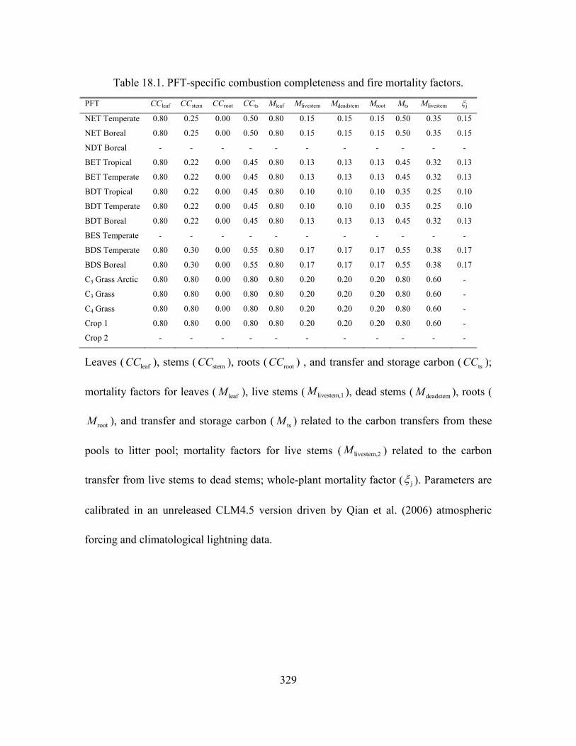
329
Table 18.1. PFT-specific combustion completeness and fire mortality factors.
PFT CCleaf CCstem CCroot CCts Mleaf Mlivestem Mdeadstem Mroot Mts Mlivestem ξj
NET Temperate 0.80 0.25 0.00 0.50 0.80 0.15 0.15 0.15 0.50 0.35 0.15
NET Boreal 0.80 0.25 0.00 0.50 0.80 0.15 0.15 0.15 0.50 0.35 0.15
NDT Boreal - - - - - - - - - - -
BET Tropical 0.80 0.22 0.00 0.45 0.80 0.13 0.13 0.13 0.45 0.32 0.13
BET Temperate 0.80 0.22 0.00 0.45 0.80 0.13 0.13 0.13 0.45 0.32 0.13
BDT Tropical 0.80 0.22 0.00 0.45 0.80 0.10 0.10 0.10 0.35 0.25 0.10
BDT Temperate 0.80 0.22 0.00 0.45 0.80 0.10 0.10 0.10 0.35 0.25 0.10
BDT Boreal 0.80 0.22 0.00 0.45 0.80 0.13 0.13 0.13 0.45 0.32 0.13
BES Temperate - - - - - - - - - - -
BDS Temperate 0.80 0.30 0.00 0.55 0.80 0.17 0.17 0.17 0.55 0.38 0.17
BDS Boreal 0.80 0.30 0.00 0.55 0.80 0.17 0.17 0.17 0.55 0.38 0.17
C3 Grass Arctic 0.80 0.80 0.00 0.80 0.80 0.20 0.20 0.20 0.80 0.60 -
C3 Grass 0.80 0.80 0.00 0.80 0.80 0.20 0.20 0.20 0.80 0.60 -
C4 Grass 0.80 0.80 0.00 0.80 0.80 0.20 0.20 0.20 0.80 0.60 -
Crop 1 0.80 0.80 0.00 0.80 0.80 0.20 0.20 0.20 0.80 0.60 -
Crop 2 - - - - - - - - - - -
Leaves ( leafCC ), stems ( stemCC ), roots ( rootCC ) , and transfer and storage carbon ( tsCC );
mortality factors for leaves ( leafM ), live stems ( livestem,1M ), dead stems ( deadstemM ), roots (
rootM ), and transfer and storage carbon ( tsM ) related to the carbon transfers from these
pools to litter pool; mortality factors for live stems ( livestem,2M ) related to the carbon
transfer from live stems to dead stems; whole-plant mortality factor ( jξ ). Parameters are
calibrated in an unreleased CLM4.5 version driven by Qian et al. (2006) atmospheric
forcing and climatological lightning data.
330
19. Methane Model
The representation of processes in the methane biogeochemical model integrated in
CLM [CLM4Me; (Riley et al. 2011a)] is based on several previously published models
(Cao et al. 1996; Petrescu et al. 2010; Tian et al. 2010; Walter et al. 2001; Wania et al.
2010; Zhang et al. 2002; Zhuang et al. 2004). Although the model has similarities with
these precursor models, a number of new process representations and parameterization
have been integrated into CLM.
Mechanistically modeling net surface CH4 emissions requires representing a complex
and interacting series of processes. We first (section 19.1) describe the overall model
structure and flow of information in the CH4 model, then describe the methods used to
represent: (19.2) CH4 mass balance; (19.3) CH4 production; (19.4) ebullition; (19.5)
aerenchyma transport; (19.6) CH4 oxidation; (19.7) reactive transport solution, including
boundary conditions, numerical solution, water table interface, etc.; (19.8) seasonal
inundation effects; and (19.9) impact of seasonal inundation on CH4 production.
19.1 Methane Model Structure and Flow The driver routine for the methane biogeochemistry calculations (ch4, in ch4Mod.F)
controls the (1) initialization of boundary conditions, inundation, and impact of redox
conditions; (2) calls to routines to calculate CH4 production, oxidation, transport through
aerenchyma, ebullition, and the overall mass balance (for unsaturated and saturated soils
and, if desired, lakes); (3) resolves changes to CH4 calculations associated with a
changing inundated fraction; (4) performs a mass balance check; and (5) calculates the
average gridcell CH4 production, oxidation, and exchanges with the atmosphere.
331
19.2 Governing Mass-Balance Relationship The model (Figure 19.1) accounts for CH4 production in the anaerobic fraction of soil
(P, mol m-3 s-1), ebullition (E, mol m-3 s-1), aerenchyma transport (A, mol m-3 s-1),
aqueous and gaseous diffusion (FD, mol m-2 s-1), and oxidation (O, mol m-3 s-1) via a
transient reaction diffusion equation:
( ) ( ) ( ) ( ) ( ), , , ,DRC F P z t E z t A z t O z tt z
∂ ∂∂ ∂
= + − − − (19.1)
Here z (m) represents the vertical dimension, t (s) is time, and R accounts for gas in both
the aqueous and gaseous phases: a H wR Kε ε= + , with εa, εw, and HK (-) the air-filled
porosity, water-filled porosity, and partitioning coefficient for the species of interest,
respectively, and C represents CH4 or O2 concentration with respect to water volume
(mol m-3).
An analogous version of equation (19.1) is concurrently solved for O2, but with the
following differences relative to CH4: P = E = 0 (i.e., no production or ebullition), and
the oxidation sink includes the O2 demanded by methanotrophs, heterotroph
decomposers, nitrifiers, and autotrophic root respiration.
As currently implemented, each gridcell contains an inundated and a non-inundated
fraction. Therefore, equation (19.1) is solved four times for each gridcell and time step: in
the inundated and non-inundated fractions, and for CH4 and O2. If desired, the CH4 and
O2 mass balance equation is solved again for lakes (Chapter 9). For non-inundated areas,
the water table interface is defined at the deepest transition from greater than 95%
saturated to less than 95% saturated that occurs above frozen soil layers. The inundated
fraction is allowed to change at each time step, and the total soil CH4 quantity is
conserved by evolving CH4 to the atmosphere when the inundated fraction decreases, and
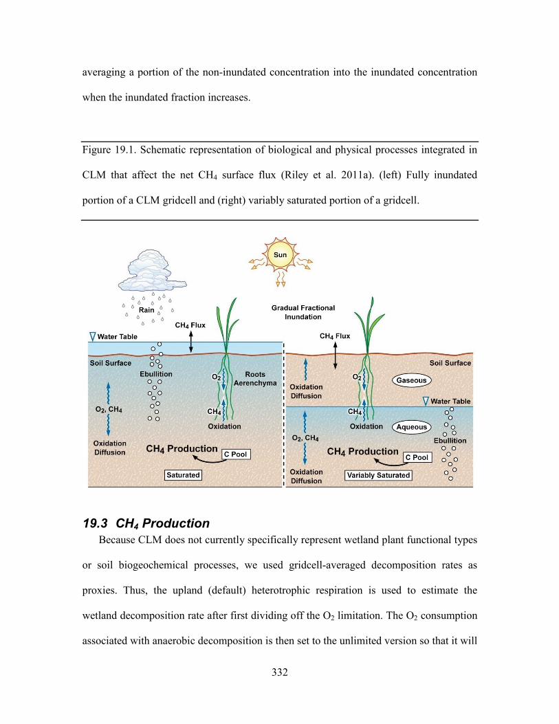
332
averaging a portion of the non-inundated concentration into the inundated concentration
when the inundated fraction increases.
Figure 19.1. Schematic representation of biological and physical processes integrated in
CLM that affect the net CH4 surface flux (Riley et al. 2011a). (left) Fully inundated
portion of a CLM gridcell and (right) variably saturated portion of a gridcell.
19.3 CH4 Production Because CLM does not currently specifically represent wetland plant functional types
or soil biogeochemical processes, we used gridcell-averaged decomposition rates as
proxies. Thus, the upland (default) heterotrophic respiration is used to estimate the
wetland decomposition rate after first dividing off the O2 limitation. The O2 consumption
associated with anaerobic decomposition is then set to the unlimited version so that it will
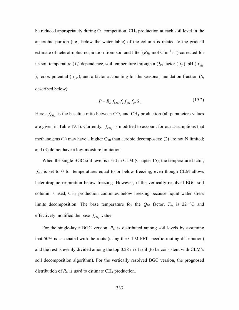
333
be reduced appropriately during O2 competition. CH4 production at each soil level in the
anaerobic portion (i.e., below the water table) of the column is related to the gridcell
estimate of heterotrophic respiration from soil and litter (RH; mol C m-2 s-1) corrected for
its soil temperature (Ts) dependence, soil temperature through a Q10 factor ( Tf ), pH ( pHf
), redox potential ( pEf ), and a factor accounting for the seasonal inundation fraction (S,
described below):
4H CH T pH pEP R f f f f S= . (19.2)
Here, 4CHf is the baseline ratio between CO2 and CH4 production (all parameters values
are given in Table 19.1). Currently, 4CHf is modified to account for our assumptions that
methanogens (1) may have a higher Q10 than aerobic decomposers; (2) are not N limited;
and (3) do not have a low-moisture limitation.
When the single BGC soil level is used in CLM (Chapter 15), the temperature factor,
, is set to 0 for temperatures equal to or below freezing, even though CLM allows
heterotrophic respiration below freezing. However, if the vertically resolved BGC soil
column is used, CH4 production continues below freezing because liquid water stress
limits decomposition. The base temperature for the Q10 factor, TB, is 22 °C and
effectively modified the base 4CHf value.
For the single-layer BGC version, RH is distributed among soil levels by assuming
that 50% is associated with the roots (using the CLM PFT-specific rooting distribution)
and the rest is evenly divided among the top 0.28 m of soil (to be consistent with CLM’s
soil decomposition algorithm). For the vertically resolved BGC version, the prognosed
distribution of RH is used to estimate CH4 production.
fT
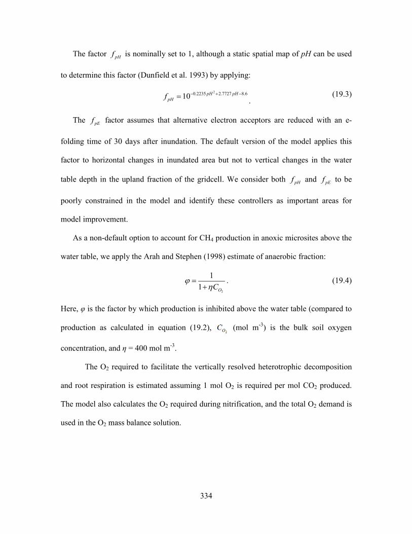
334
The factor pHf is nominally set to 1, although a static spatial map of pH can be used
to determine this factor (Dunfield et al. 1993) by applying:
20.2235 2.7727 8.610 pH pHpHf − + −= .
(19.3)
The pEf factor assumes that alternative electron acceptors are reduced with an e-
folding time of 30 days after inundation. The default version of the model applies this
factor to horizontal changes in inundated area but not to vertical changes in the water
table depth in the upland fraction of the gridcell. We consider both pHf and pEf to be
poorly constrained in the model and identify these controllers as important areas for
model improvement.
As a non-default option to account for CH4 production in anoxic microsites above the
water table, we apply the Arah and Stephen (1998) estimate of anaerobic fraction:
2
11 OC
ϕη
=+
. (19.4)
Here, φ is the factor by which production is inhibited above the water table (compared to
production as calculated in equation (19.2), (mol m-3) is the bulk soil oxygen
concentration, and η = 400 mol m-3.
The O2 required to facilitate the vertically resolved heterotrophic decomposition
and root respiration is estimated assuming 1 mol O2 is required per mol CO2 produced.
The model also calculates the O2 required during nitrification, and the total O2 demand is
used in the O2 mass balance solution.
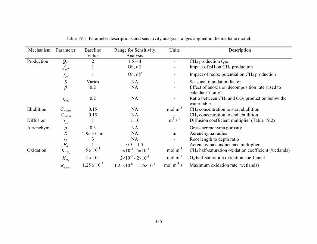
335
Table 19.1. Parameter descriptions and sensitivity analysis ranges applied in the methane model.
Mechanism Parameter Baseline Value
Range for Sensitivity Analysis
Units Description
Production Q10 2 1.5 – 4 - CH4 production Q10
pHf 1 On, off - Impact of pH on CH4 production pEf 1 On, off - Impact of redox potential on CH4 production S Varies NA - Seasonal inundation factor β 0.2 NA - Effect of anoxia on decomposition rate (used to
calculate S only)
4CHf 0.2 NA - Ratio between CH4 and CO2 production below the water table
Ebullition Ce,max 0.15 NA mol m-3 CH4 concentration to start ebullition Ce,min 0.15 NA - CH4 concentration to end ebullition Diffusion
0Df 1 1, 10 m2 s-1 Diffusion coefficient multiplier (Table 19.2) Aerenchyma p 0.3 NA - Grass aerenchyma porosity R 2.9×10⁻³ m NA m Aerenchyma radius rL 3 NA - Root length to depth ratio Fa 1 0.5 – 1.5 - Aerenchyma conductance multiplier Oxidation
4CHK 5 x 10⁻³ 5×10⁻⁴ - 5×10⁻²
mol m-3 CH4 half-saturation oxidation coefficient (wetlands)
2OK 2 x 10⁻² 2×10⁻³ - 2×10⁻¹ mol m-3 O2 half-saturation oxidation coefficient
,maxoR 1.25 x 10⁻⁵ 1.25×10⁻⁶ - 1.25×10⁻⁴ mol m-3 s-1 Maximum oxidation rate (wetlands)
336
19.4 Ebullition Briefly, the simulated aqueous CH4 concentration in each soil level is used to estimate
the expected equilibrium gaseous partial pressure ( ), as a function of temperature and
depth below the water table, by first estimating the Henry’s law partitioning coefficient (
) by the method described in Wania et al. (2010):
1 1 1 1log log sH s
H H
kk C T T
= − −
(19.5)
Ch H gk Tk R= (19.6)
w g
e Cs H
C R TC
k pθ= (19.7)
where HC is a constant, is the universal gas constant, sHk is Henry’s law partitioning
coefficient at standard temperature ( sT ), wC is local aqueous CH4 concentration, and p is
pressure.
The local pressure is calculated as the sum of the ambient pressure, water pressure
down to the local depth, and pressure from surface ponding (if applicable). When the CH4
partial pressure exceeds 15% of the local pressure (Baird et al. 2004; Strack et al. 2006;
Wania et al. 2010), bubbling occurs to remove CH4 to below this value, modified by the
fraction of CH4 in the bubbles [taken as 57%; (Kellner et al. 2006; Wania et al. 2010)].
Bubbles are immediately added to the surface flux for saturated columns and are placed
immediately above the water table interface in unsaturated columns.
19.5 Aerenchyma Transport Aerenchyma transport is modeled in CLM as gaseous diffusion driven by a
concentration gradient between the specific soil layer and the atmosphere and, if
337
specified, by vertical advection with the transpiration stream. There is evidence that
pressure driven flow can also occur, but we did not include that mechanism in the current
model.
The diffusive transport through aerenchyma (A, mol m-2 s-1) from each soil layer is
represented in the model as:
( ) ar
La
C z CA pTr z rD
ρ−
=+
, (19.8)
where D is the free-air gas diffusion coefficient (m2 s-1); C(z) (mol m-3) is the gaseous
concentration at depth z (m); is the ratio of root length to depth; p is the porosity (-); T
is specific aerenchyma area (m2 m-2); ra is the aerodynamic resistance between the
surface and the atmospheric reference height (s m-1); and is the rooting density as a
function of depth (-). The gaseous concentration is calculated with Henry’s law as
described in equation (19.6).
Based on the ranges reported in Colmer (2003), we have chosen baseline aerenchyma
porosity values of 0.3 for grass and crop PFTs and 0.1 for tree and shrub PFTs. The
aerenchyma area varies over the course of the growing season; we parameterize this
dependency using the simulated leaf area index L (m2 m-2), as in Wania et al. (2010):
2
0.22N af N LT Rπ= . (19.9)
Here is annual net primary production (NPP, mol m-2 s-1); R is the aerenchyma radius
(2.9×10⁻³ m); fN is the belowground fraction of annual NPP; and the 0.22 factor represents
the amount of C per tiller. O2 can also diffuse in from the atmosphere to the soil layer via
the reverse of the same pathway, with the same representation as Equation (19.8) but with
the gas diffusivity of oxygen.
338
CLM also simulates the direct emission of CH4 from leaves to the atmosphere via
transpiration of dissolved methane. We calculate this flux (4CH TF − ; mol m-2 s-1) using the
simulated soil water methane concentration (4 ,CH jC (mol m-3)) in each soil layer j and the
CLM predicted transpiration ( TF ) for each PFT, assuming that no methane was oxidized
inside the plant tissue:
4 4, ,CH T r j T CH j
jF F Cρ− = ∑ . (19.10)
19.6 CH4 Oxidation CLM represents CH4 oxidation with double Michaelis-Menten kinetics (Arah and
Stephen 1998; Segers 1998), dependent on both the gaseous CH4 and O2 concentrations:
4 2
4 4 2 2
,max 10CH O
oxic oCH CH O O
C CR R Q F
K C K C ϑ
=
+ + (19.11)
where 4CHK and
2OK are the half saturation coefficients (mol m-3) with respect to CH4
and O2 concentrations, respectively; ,maxoR is the maximum oxidation rate (mol m-3 s-1);
and Q10 specifies the temperature dependence of the reaction with a base temperature set
to 12 °C. The soil moisture limitation factor is applied above the water table to
represent water stress for methanotrophs. Based on the data in Schnell and King (1996),
we take cP
PF eϑ
−
= , where P is the soil moisture potential and Pc = -2.4×105 mm.
19.7 Reactive Transport Solution The solution to equation (19.1) is solved in several sequential steps: (1) resolve
competition for CH4 and O2 (section 19.7.1); (2) add the ebullition flux into the layer
directly above the water table or into the atmosphere; (3) calculate the overall CH4 or O2
Fϑ
339
source term based on production, aerenchyma transport, ebullition, and oxidation; (4)
establish boundary conditions, including surface conductance to account for snow,
ponding, and turbulent conductances and bottom flux condition (section 19.7.2); (5)
calculate diffusivity (section 19.7.3); and (6) solve the resulting mass balance using a
tridiagonal solver (section 19.7.5).
19.7.1 Competition for CH4 and O2 For each time step, the unlimited CH4 and O2 demands in each model depth interval
are computed. If the total demand over a time step for one of the species exceeds the
amount available in a particular control volume, the demand from each process
associated with the sink is scaled by the fraction required to ensure non-negative
concentrations. Since the methanotrophs are limited by both CH4 and O2, the stricter
limitation is applied to methanotroph oxidation, and then the limitations are scaled back
for the other processes. The competition is designed so that the sinks must not exceed the
available concentration over the time step, and if any limitation exists, the sinks must sum
to this value. Because the sinks are calculated explicitly while the transport is semi-
implicit, negative concentrations can occur after the tridiagonal solution. When this
condition occurs for O2, the concentrations are reset to zero; if it occurs for CH4, the
surface flux is adjusted and the concentration is set to zero if the adjustment is not too
large.
19.7.2 CH4 and O2 Source Terms The overall CH4 net source term consists of production, oxidation at the base of
aerenchyma, transport through aerenchyma, methanotrophic oxidation, and ebullition
(either to the control volume above the water table if unsaturated or directly to the
340
atmosphere if saturated). For O2 below the top control volume, the net source term
consists of O2 losses from methanotrophy, SOM decomposition, and autotrophic
respiration, and an O2 source through aerenchyma.
19.7.3 Aqueous and Gaseous Diffusion For gaseous diffusion, we adopted the temperature dependence of molecular free-air
diffusion coefficients (D0 (m2 s-1)) as described by Lerman et al. (1979) and applied by
Wania et al. (2010) (Table 19.2).
Table 19.2. Temperature dependence of aqueous and gaseous diffusion coefficients for
CH4 and O2.
D0 (m2 s-1) CH4 O2
Aqueous 0.9798 + 0.02986T + 0.0004381T2 1.172+ 0.03443T + 0.0005048T2
Gaseous 0.1875 + 0.0013T 0.1759 + 0.0011T
Gaseous diffusivity in soils also depends on the molecular diffusivity, soil structure,
porosity, and organic matter content. Moldrup et al. (2003), using observations across a
range of unsaturated mineral soils, showed that the relationship between effective
diffusivity ( (m2 s-1)) and soil properties can be represented as:
3
20
ba
e as
D D θθθ
=
, (19.12)
where and are the air-filled and total (saturated water-filled) porosities (-),
respectively, and b is the slope of the water retention curve (-). However, Iiyama and
θa
θ s
341
Hasegawa (2005) have shown that the original Millington-Quirk (Millington and Quirk
1961) relationship matched measurements more closely in unsaturated peat soils:
10
3
0 2a
es
D D θθ
= (19.13)
In CLM, we applied equation (19.12) for soils with zero organic matter content and
equation (19.13) for soils with more than 130 kg m-3 organic matter content. A linear
interpolation between these two limits is applied for soils with SOM content below 130
kg m-3. For aqueous diffusion in the saturated part of the soil column, we applied
(Moldrup et al. 2003):
20e sD D θ= . (19.14)
To simplify the solution, we assumed that gaseous diffusion dominates above the
water table interface and aqueous diffusion below the water table interface. Descriptions,
baseline values, and dimensions for parameters specific to the CH4 model are given in
Table 19.1. For freezing or frozen soils below the water table, diffusion is limited to the
remaining liquid (CLM allows for some freezing point depression), and the diffusion
coefficients are scaled by the volume-fraction of liquid. For unsaturated soils, Henry’s
law equilibrium is assumed at the interface with the water table.
19.7.4 Boundary Conditions We assume the CH4 and O2 surface fluxes can be calculated from an effective
conductance and a gaseous concentration gradient between the atmospheric concentration
and either the gaseous concentration in the first soil layer (unsaturated soils) or in
equilibrium with the water (saturated soil ( )1n
aw C C− and ( )11n
aw C C+ − for the fully
explicit and fully implicit cases, respectively (however, see Tang and Riley (2013) for a
342
more complete representation of this process). Here, w is the surface boundary layer
conductance as calculated in the existing CLM surface latent heat calculations. If the top
layer is not fully saturated, the 1
1
m
m
Dx∆
term is replaced with a series combination:
1
1
1
1 xw D
− ∆
+
, and if the top layer is saturated, this term is replaced with
1
1
1
12H
xKw D
− ∆
+
,
where KH is the Henry’s law equilibrium constant.
When snow is present, a resistance is added to account for diffusion through the snow
based on the Millington-Quirk expression (equation (19.13)) and CLM’s prediction of the
liquid water, ice, and air fractions of each snow layer. When the soil is ponded, the
diffusivity is assumed to be that of methane in pure water, and the resistance as the ratio
of the ponding depth to diffusivity. The overall conductance is taken as the series
combination of surface, snow, and ponding resistances. We assume a zero flux gradient at
the bottom of the soil column.
19.7.5 Crank-Nicholson Solution Equation (19.1) is solved using a Crank-Nicholson solution (Press et al. 1992), which
combines fully explicit and implicit representations of the mass balance. The fully
explicit decomposition of equation (19.1) can be written as
( ) ( )1 1
1 11 1
1 1
1n n n n n nj j j j p n n n n nm
j j j j jj p m
R C R C D DC C C C St x x x
+ +
+ −
−= − − − +
∆ ∆ ∆ ∆ , (19.15)
where j refers to the cell in the vertically discretized soil column (increasing downward),
n refers to the current time step, ∆t is the time step (s), p1 is j+½, m1 is j-½, and is the
S jn
343
net source at time step n and position j, i.e., ( ) ( ) ( ) ( ), , , ,njS P j n E j n A j n O j n= − − − .
The diffusivity coefficients are calculated as harmonic means of values from the adjacent
cells. Equation (19.15) is solved for gaseous and aqueous concentrations above and
below the water table, respectively. The R term ensure the total mass balance in both
phases is properly accounted for. An analogous relationship can be generated for the fully
implicit case by replacing n by n+1 on the C and S terms of equation (19.15). Using an
average of the fully implicit and fully explicit relationships gives:
( ) ( )
11 11 1 11 1
1 11 1 1 1
1 111 1
1 1
1 1 12 2 2
1 12 2
nj p pn n nm m
j j jj m j p m j p
nj p n n n n n nm
j j j j j jj p m
R D DD DC C Cx x t x x x x x
R D DC C C C S St x x x
++ + +− +
++ −
− + + + − = ∆ ∆ ∆ ∆ ∆ ∆ ∆ ∆
+ − − − + + ∆ ∆ ∆ ∆
, (19.16)
Equation (19.16) is solved with a standard tridiagonal solver, i.e.:
1 1 11 1
n n nj j jaC bC cC r+ + +− ++ + = , (19.17)
with coefficients specified in equation (19.16).
Two methane balance checks are performed at each timestep to insure that the
diffusion solution and the time-varying aggregation over inundated and non-inundated
areas strictly conserves methane molecules (except for production minus consumption)
and carbon atoms.
19.7.6 Interface between water table and unsaturated zone We assume Henry’s Law equilibrium at the interface between the saturated and
unsaturated zone and constant flux from the soil element below the interface to the center
of the soil element above the interface. In this case, the coefficients are the same as
described above, except for the soil element above the interface:
344
1
1 1
1 12 2p j j
Hp j j
D x xK
x D D
−
+
+
∆ ∆= +
∆
11 1
1 1
12
nj p m
Hj p m
R D Db Kt x x x
+ = + + ∆ ∆ ∆ ∆
( ) ( )1 111 1
1 1
1 12 2
nj pn n n n n n nm
j j H j j j j jj p m
R D Dr C C K C C C S St x x x
++ −
= + − − − + + ∆ ∆ ∆ ∆
(19.18)
and the soil element below the interface:
1
11
1 12 2j jm
Hm j j
x xD Kx D D
−
−
−
∆ ∆= +
∆
1
1
12
mH
j m
Da Kx x
= −∆ ∆
( ) ( )1 111 1
1 1
1 12 2
nj pn n n n n n nm
j j j j H j j jj p m
R D Dr C C C C K C S St x x x
++ −
= + + − − − + + ∆ ∆ ∆ ∆
(19.19)
19.8 Inundated Fraction Prediction We developed a simplified dynamic representation of spatial inundation based on
recent work by Prigent et al. (2007), who described a multi-satellite approach to estimate
the global monthly inundated fraction (Fi) over an equal area grid (0.25°×0.25° at the
equator) from 1993 - 2000. They suggested that the IGBP estimate for inundation could
be used as a measure of sensitivity of their detection approach at low inundation. We
therefore used the sum of their satellite-derived Fi and the constant IGBP estimate when
it was less than 10% to perform a simple inversion for the inundated fraction for methane
production (fs). The method optimized three parameters (p1, p2, p3) for each grid cell in a
simple model based on simulated water table depth (zw) and surface runoff (Qr (mm s-1)):
345
21 3
wzp
s rf Pe p Q−
= + . (19.20)
These parameters were evaluated at the 0.5° resolution, and aggregated for coarser
simulations. We expect that ongoing work in the hydrology submodel of CLM will
alleviate the need for this crude simplification of inundated fraction in future model
versions.
19.9 Seasonal Inundation We have developed a simplified scaling factor to mimic the impact of seasonal
inundation on CH4 production (see appendix B in Riley et al. (2011a) for a discussion of
this simplified expression):
( )
, 1f f f
S Sf
β − += ≤ . (19.21)
Here, f is the instantaneous inundated fraction, f is the annual average inundated
fraction (evaluated for the previous calendar year) weighted by heterotrophic respiration,
and β is the anoxia factor that relates the fully anoxic decomposition rate to the fully
oxygen-unlimited decomposition rate, all other conditions being equal.
346
20. Crops and Irrigation
20.1 Summary of CLM4.5 updates relative to the CLM4.0 We describe here the complete crop and irrigation parameterizations that appear
in CLM4.5. Corresponding information for CLM4.0 appeared on the CLM4.0 web site in
a pdf document independent of the CLM4.0 Technical Note (Oleson et al. 2010a). The
CLM4.0 crop model description also appeared in Levis et al. (2012).
CLM4.5 includes the following updates to the CROP option, where CROP refers to the
interactive crop management model:
- Interactive irrigation
- Interactive fertilization
- Biological nitrogen fixation for soybeans
- Modified C:N ratios for crops
- Nitrogen retranslocation for crops
- Separate reproductive pool
These updates appear in detail in section 20.4. Most also appear in Drewniak et al.
(2013).
20.2 The crop model
20.2.1 Introduction Groups developing Earth System Models generally account for the human footprint
on the landscape in simulations of historical and future climates. Traditionally we have
represented this footprint with natural vegetation types and particularly grasses because
they resemble many common crops. Most modeling efforts have not incorporated more
347
explicit representations of land management such as crop type, planting, harvesting,
tillage, fertilization, and irrigation, because global scale datasets of these factors have
lagged behind vegetation mapping. As this begins to change, we increasingly find models
that will simulate the biogeophysical and biogeochemical effects not only of natural but
also human-managed land cover.
AgroIBIS is a state-of-the-art land surface model with options to simulate dynamic
vegetation (Kucharik et al. 2000) and interactive crop management (Kucharik and Brye
2003). The interactive crop management parameterizations from AgroIBIS (March 2003
version) were coupled as a proof-of-concept to the Community Land Model version 3
[CLM3.0, Oleson et al. (2004)] (not published), then coupled to the CLM3.5 (Levis et al.
2009) and later released to the community with CLM4CN (Levis et al. 2012).
With interactive crop management and, therefore, a more accurate representation of
agricultural landscapes, we hope to improve the CLM’s simulated biogeophysics and
biogeochemistry. These advances may improve fully coupled simulations with the
Community Earth System Model (CESM), while helping human societies answer
questions about changing food, energy, and water resources in response to climate,
environmental, land use, and land management change (e.g., Kucharik and Brye 2003;
Lobell et al. 2006).
20.2.2 Crop plant functional types CLM’s default list of plant functional types (pfts) includes an unmanaged crop (Table
2.1) treated as a second C3 grass. The unmanaged crop has grid cell coverage assigned
from satellite data, as do all natural pfts when CLM’s dynamic vegetation model (CNDV;
Castillo et al. 2012) is not active.
348
The new crop pfts used in the CLM get grid cell coverage from the present-day crop
dataset of Portmann et al. (2010). We assign these managed crops in the proportions
given by Portmann et al. (2010) without exceeding the area previously assigned to the
unmanaged crop. The unmanaged crop continues to occupy any of its original area that
remains and continues to be handled just by the carbon/nitrogen cycling part of the CLM
(i.e., CN). The managed crop types (corn, soybean, and temperate cereals) were chosen
based on the availability of corresponding algorithms in AgroIBIS. Temperate cereals
include wheat, barley, and rye here. We treat all temperate cereals as summer crops (like
spring wheat, for example) at this time. We may introduce winter cereals (such as winter
wheat) in a future version of the model.
To allow crops to coexist with natural vegetation in a grid cell and be treated by
separate models (i.e., CLM4.5CNcrop versus CLM4.5CNDV), we separate the vegetated
land unit into a naturally vegetated land unit and a human managed land unit. Plant
functional types in the naturally vegetated land unit share one soil column and compete
for water (default CLM setting). Managed crop PFTs in the human managed land unit do
not share soil columns and thus permit for differences in land management between
crops.
20.2.3 Phenology CLM4.5CN includes evergreen, seasonally deciduous (responding to changes in
day length), and stress deciduous (responding to changes in temperature and/or soil
moisture) phenology algorithms (Chapter 14). In CLM4.5CNcrop we have added the
AgroIBIS crop phenology algorithm, consisting of three distinct phases.
349
Phase 1 starts at planting and ends with leaf emergence, phase 2 continues from leaf
emergence to the beginning of grain fill, and phase 3 starts from the beginning of grain
fill and ends with physiological maturity and harvest.
20.2.3.1 Planting Corn and temperate cereals must meet the following requirements between April 1st
and June 14th for planting in the northern hemisphere (NH):
10
min min10
8 min
d p
d p
T T
T TGDD GDD
>
>
≥
(20.1)
where T10d is the 10-day running mean of T2m, (the simulated 2-m air temperature at every
model time step) and min10dT is the 10-day running mean of min
2mT (the daily minimum of
T2m). Tp and minpT are crop-specific coldest planting temperatures (Table 20.1), GDD8 is
the 20-year running mean growing degree-days (units are degree-days or °days) tracked
from April through September (NH) base 8°C with maximum daily increments of
30°days (see Eq. (20.3)), and GDDmin is the minimum growing degree day requirement
(Table 20.1). Soy must meet the same requirements but between May 1st and June 14th for
planting. If the requirements in Eq. (20.1) are not met by June 14th, then corn, soybean,
and temperate cereals are still planted on June 15th as long as GDD8>0. In the southern
hemisphere (SH) the NH requirements apply 6 months later.
GDD8 does not change as quickly as T10d and min10dT , so it determines whether the
crop can be planted in a grid cell, while the two faster-changing variables determine
when the crop may be planted.
350
At planting, each crop is assigned 1 g leaf C m-2 pft column area to be transferred to
the leaves upon leaf emergence. An equivalent amount of seed leaf N is assigned given
the pft’s C to N ratio for leaves (CNleaf). (This differs from AgroIBIS, which uses a seed
leaf area index instead of seed C.)
At planting, the model updates the average growing degree-days necessary for the
crop to reach vegetative and physiological maturity, GDDmat, according to the following
AgroIBIS rules:
corn cornmat 8 mattemp. cereals temp. cerealsmat 0 matsoy soymat 10 mat
0.85 and 950 1850 days
and 1700 days
and 1700 days
GDD GDD GDDGDD GDD GDDGDD GDD GDD
= < < °
= < °
= < °
(20.2)
where GDD10 is the 20-year running mean growing degree-days tracked from April
through September (NH) base 10°C with maximum daily increments of 30°days. Eq.
(20.3) shows how we calculate GDD0, GDD8, and GDD10:
0 0 2m 2m
8 8 2m 2m
10 10 2m 2m
where 0 26 days
8 where 0 8 30 days
10 where 0 10 30 days
f f
f f
f f
GDD GDD T T T TGDD GDD T T T TGDD GDD T T T T
= + − ≤ − ≤ °
= + − − ≤ − − ≤ °
= + − − ≤ − − ≤ °
(20.3)
where, if T2m - Tf takes on values outside the above ranges, then it equals the minimum or
maximum value in the range. Also Tf equals 273.15 K, T2m has units of K, and GDD has
units of °days.
20.2.3.2 Leaf emergence According to AgroIBIS, leaves may emerge when the growing degree-days of soil
temperature to 0.05 m depth tracked since planting (soiTGDD ) reaches 3 to 5% of GDDmat
(Table 20.1). soiTGDD is base 8, 0, and 10°C for corn, soybean, and temperate cereals.
Leaf onset, as defined in the CN part of the model, occurs in the first time step of phase 2,
351
at which moment all seed C is transferred to leaf C. Subsequently, the leaf area index
generally increases and reaches a maximum value during phase 2.
20.2.3.3 Grain fill Phase 3 begins in a similar way to phase 2. A variable tracked since planting like
soiTGDD but for 2-m air temperature, 2mTGDD , must reach a heat unit threshold, h, of 40 to
70% of GDDmat (Table 20.1). For corn the percentage itself is an empirical function of
GDDmat (not shown). In phase 3, the leaf area index begins to decline in response to a
background litterfall rate calculated as the inverse of leaf longevity for the pft as done in
the CN part of the model.
20.2.3.4 Harvest Harvest is assumed to occur as soon as the crop reaches maturity. When
2mTGDD
reaches 100% of GDDmat or the number of days past planting reaches a crop-specific
maximum (Table 20.1), then the crop is harvested. Harvest occurs in one time step using
CN’s leaf offset algorithm. New variables track the flow of grain C and N to food and of
live stem C and N to litter. Currently, food C and N are routed directly to litter using the
labile, cellulose, and lignin fractions for leaves. The same fractions for leaves are used for
the flow of live stem C and N to litter for corn, soybean, and temperate cereals. This is in
contrast to the approach for unmanaged PFTs which puts live stem C and N to dead stems
first, rather than to litter.
20.2.4 Allocation Allocation responds to the same phases as phenology (section 20.2.3). Simulated C
assimilation begins every year upon leaf emergence in phase 2 and ends with harvest at
352
the end of phase 3; therefore, so does the allocation of such C to the crop’s leaf, live
stem, fine root, and reproductive pools.
20.2.4.1 Leaf emergence to grain fill During phase 2, the allocation coefficients (fraction of available C) to each C pool
are defined as:
2m 2m
2m
mat mat
0
( ) where 1
( )(1 ) where 0.1
11
T
repr
T Ti i ffroot froot froot froot
GDDbi b h
leafleaf froot b
livestem repr froot leaf
aGDD GDD
a a a aGDD GDD
a e ea a b
ea a a a
−−
−
=
= − − ≤
−= − ⋅ =
−= − − −
(20.4)
where ileafa , i
froota , and ffroota are initial and final values of these coefficients (Table 20.2),
and h is a heat unit threshold defined in section 20.2.3. At a crop-specific maximum leaf
area index, Lmax (Table 20.2), carbon allocation is directed exclusively to the fine roots.
20.2.4.2 Grain fill to harvest The calculation of froota remains the same from phase 2 to phase 3. Other allocation
coefficients change to:
2m 2m
,3 ,3
mat mat
,3 ,3
when else...
1 where 1
when else...
leafalloc
i i fleaf leaf leaf leaf
dT Tf
leaf leaf leafL L
i i flivestem livestem livestem livestem
a a a a
GDD h GDD ha a a
GDD d h GDD d h
a a a a
a
= ≤
− − = − ≥ ≤ − −
= ≤
2m 2m
mat mat
1 where 1
1
stemallocd
T Tflivestem livestem livestem
L L
repr froot livestem leaf
GDD h GDD ha a
GDD d h GDD d h
a a a a
− − = − ≥ ≤ − −
= − − −
(20.5)
353
where ,3ileafa and ,3i
livestema (initial values) equal the last leafa and livestema calculated in phase
2, Ld , leafallocd and stem
allocd are leaf area index and leaf and stem allocation decline factors, and
fleafa and f
livestema are final values of these allocation coefficients (Table 20.2).
20.2.5 General comments C and N accounting now includes new pools and fluxes pertaining to live stems and
reproductive tissues. For example, the calculations of growth respiration, above ground
net primary production, litter fall, and displayed vegetation all now account for
reproductive C.
We track allocation to reproductive C separately from CN’s allocation to other C
pools but within the CN framework. CN uses root
leaf
aa and livestem
leaf
aa to calculate C and N
allometry and plant N demand.
Stem area index (S) is equal to 0.1L for corn and 0.2L for other crops, as in
AgroIBIS, where L is the leaf area index. All live C and N pools go to 0 after crop
harvest, but the S is kept at 0.25 to simulate a post-harvest “stubble” on the ground.
Crop heights at the top and bottom of the canopy, ztop and zbot (m), come from the
AgroIBIS formulation:
2max
max max
0.05 where 11 1
0.02m
top top
bot
L Lz zL L
z
= ≥ ≤ − − =
(20.6)
The CN part of the model keeps track of a term representing excess maintenance
respiration that for perennial pfts or pfts with C storage may be extracted from later gross
primary production. Later extraction cannot continue to happen after harvest for annual
crops, so at harvest we turn the excess respiration pool into a flux that extracts CO2
354
directly from the atmosphere. This way we eliminate any excess maintenance respiration
remaining at harvest as if such respiration had not taken place.
In the list of plant physiological and other parameters used by the CLM, we started
the managed crops with the existing values assigned to the unmanaged C3 crop. Then we
changed the following parameters to distinguish corn, soybean, and temperate cereals
from the unmanaged C3 crop and from each other:
- Growth respiration coefficient from 0.30 to the AgroIBIS value of 0.25.
- Fraction of leaf N in the Rubisco enzyme from 0.1 to 0.2 g N Rubisco g-1 N leaf
for temperate cereals to increase productivity (not chosen based on AgroIBIS).
- Fraction of current photosynthesis displayed as growth changed from 0.5 to 1 (not
chosen based on AgroIBIS).
- CLM4.5CN curve for the effect of temperature on photosynthesis instead of crop-
specific curves from AgroIBIS.
- Quantum efficiency at 25°C, α , from 0.06 to 0.04 µmol CO2 µmol-1 photon for
C4 crops (corn and unmanaged C4 crop), using CLM4.5CN’s C4 grass value.
- Slope, m, of conductance-to-photosynthesis relationship from 9 to 4 for C4 crops
as in AgroIBIS.
- Specific leaf areas, SLA, to the AgroIBIS values (Table 20.1).
- Leaf orientation, Lχ , to the AgroIBIS values (Table 20.1).
- Soil moisture photosynthesis limitation factor, tβ , for soybeans multiplied as in
AgroIBIS by 1.25 for increased drought tolerance.
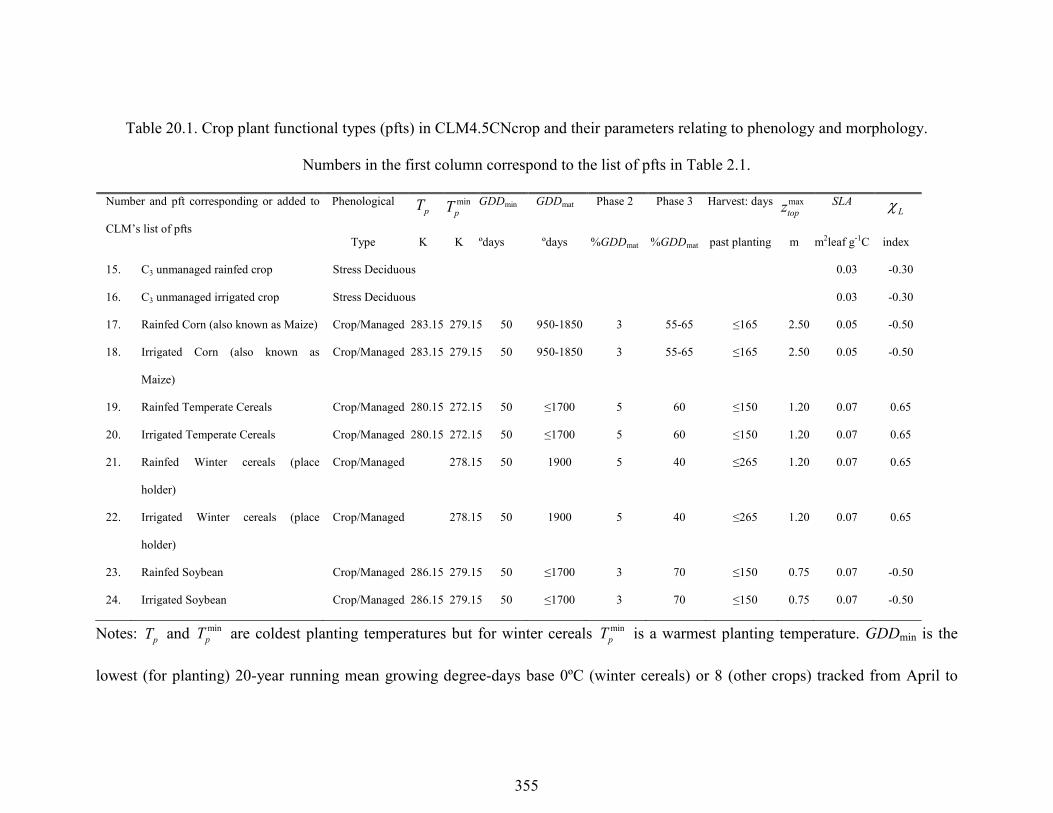
355
Table 20.1. Crop plant functional types (pfts) in CLM4.5CNcrop and their parameters relating to phenology and morphology.
Numbers in the first column correspond to the list of pfts in Table 2.1.
Number and pft corresponding or added to
CLM’s list of pfts
Phenological pT min
pT GDDmin GDDmat Phase 2 Phase 3 Harvest: days maxtopz
SLA Lχ
Type K K ºdays ºdays %GDDmat %GDDmat past planting m m2leaf g-1C index
15. C3 unmanaged rainfed crop Stress Deciduous 0.03 -0.30
16. C3 unmanaged irrigated crop Stress Deciduous 0.03 -0.30
17. Rainfed Corn (also known as Maize) Crop/Managed 283.15 279.15 50 950-1850 3 55-65 ≤165 2.50 0.05 -0.50
18. Irrigated Corn (also known as
Maize)
Crop/Managed 283.15 279.15 50 950-1850 3 55-65 ≤165 2.50 0.05 -0.50
19. Rainfed Temperate Cereals Crop/Managed 280.15 272.15 50 ≤1700 5 60 ≤150 1.20 0.07 0.65
20. Irrigated Temperate Cereals Crop/Managed 280.15 272.15 50 ≤1700 5 60 ≤150 1.20 0.07 0.65
21. Rainfed Winter cereals (place
holder)
Crop/Managed 278.15 50 1900 5 40 ≤265 1.20 0.07 0.65
22. Irrigated Winter cereals (place
holder)
Crop/Managed 278.15 50 1900 5 40 ≤265 1.20 0.07 0.65
23. Rainfed Soybean Crop/Managed 286.15 279.15 50 ≤1700 3 70 ≤150 0.75 0.07 -0.50
24. Irrigated Soybean Crop/Managed 286.15 279.15 50 ≤1700 3 70 ≤150 0.75 0.07 -0.50
Notes: pT and minpT are coldest planting temperatures but for winter cereals min
pT is a warmest planting temperature. GDDmin is the
lowest (for planting) 20-year running mean growing degree-days base 0ºC (winter cereals) or 8 (other crops) tracked from April to
356
September (NH). GDDmat is a crop’s 20-year running mean growing degree-days needed for vegetative and physiological maturity.
Harvest occurs at 100%GDDmat or when the days past planting reach the number in the 10th column. Crop growth phases are described
in the text. maxtopz is the maximum top-of-canopy height of a crop, SLA is specific leaf area, and leaf orientation index, Lχ , equals -1 for
vertical, 0 for random, and 1 for horizontal leaf orientation.
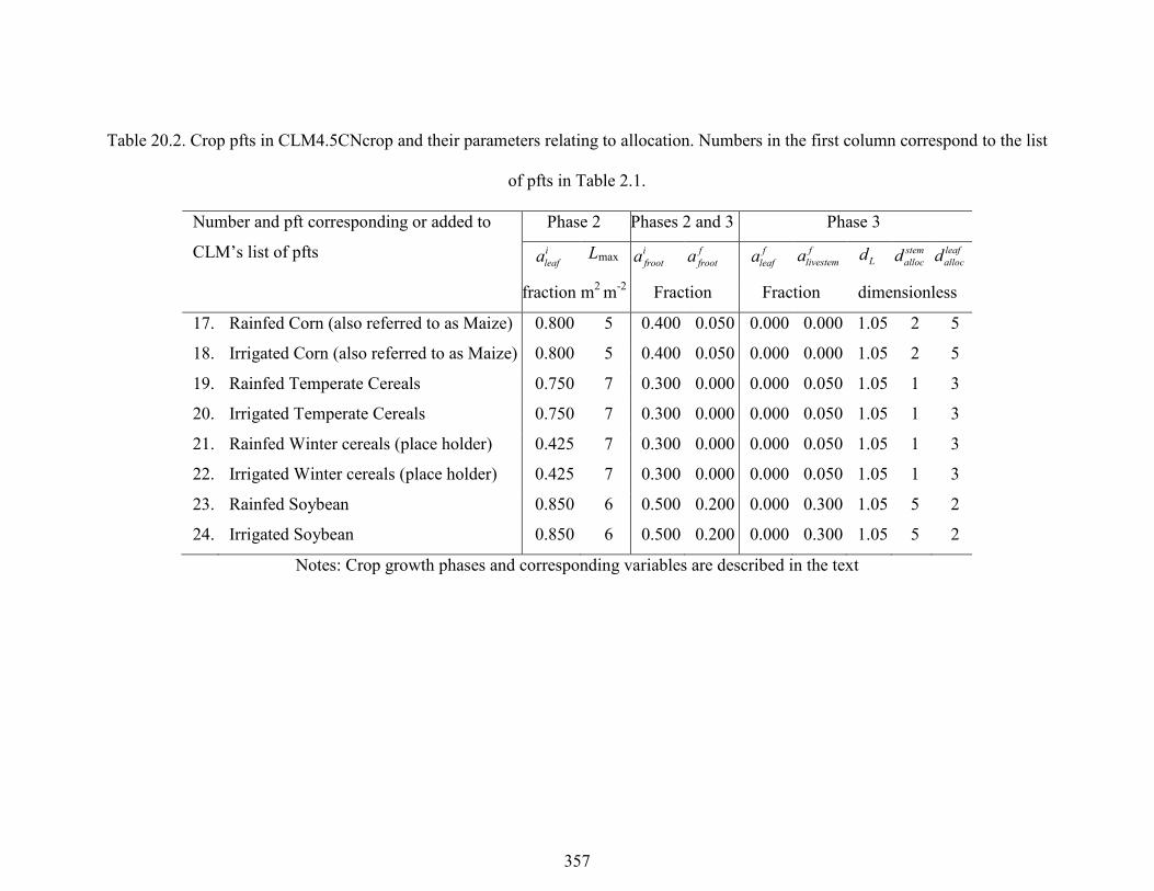
357
Table 20.2. Crop pfts in CLM4.5CNcrop and their parameters relating to allocation. Numbers in the first column correspond to the list
of pfts in Table 2.1.
Number and pft corresponding or added to
CLM’s list of pfts
Phase 2 Phases 2 and 3 Phase 3 ileafa Lmax i
froota ffroota f
leafa flivestema Ld stem
allocd leafallocd
fraction m2 m-2 Fraction Fraction dimensionless
17. Rainfed Corn (also referred to as Maize) 0.800 5 0.400 0.050 0.000 0.000 1.05 2 5
18. Irrigated Corn (also referred to as Maize) 0.800 5 0.400 0.050 0.000 0.000 1.05 2 5
19. Rainfed Temperate Cereals 0.750 7 0.300 0.000 0.000 0.050 1.05 1 3
20. Irrigated Temperate Cereals 0.750 7 0.300 0.000 0.000 0.050 1.05 1 3
21. Rainfed Winter cereals (place holder) 0.425 7 0.300 0.000 0.000 0.050 1.05 1 3
22. Irrigated Winter cereals (place holder) 0.425 7 0.300 0.000 0.000 0.050 1.05 1 3
23. Rainfed Soybean 0.850 6 0.500 0.200 0.000 0.300 1.05 5 2
24. Irrigated Soybean 0.850 6 0.500 0.200 0.000 0.300 1.05 5 2
Notes: Crop growth phases and corresponding variables are described in the text
358
20.3 The irrigation model The CLM includes the option to irrigate cropland areas that are equipped for
irrigation. The application of irrigation responds dynamically to the soil moisture
conditions simulated by the CLM. This irrigation algorithm is based loosely on the
implementation of Ozdogan et al. (2010).
When irrigation is enabled, the crop areas of each grid cell are divided into irrigated
and rainfed fractions according to a dataset of areas equipped for irrigation (Portmann et
al. 2010). Irrigated and rainfed crops are placed on separate soil columns, so that
irrigation is only applied to the soil beneath irrigated crops.
In irrigated croplands, a check is made once per day to determine whether irrigation
is required on that day. This check is made in the first time step after 6 AM local time.
Irrigation is required if (1) crop leaf area > 0, and (2) βt < 1, i.e., water is limiting for
photosynthesis (see section 8.4).
If irrigation is required, the model computes the deficit between the current soil
moisture content and a target soil moisture content; this deficit is the amount of water that
will be added through irrigation. The target soil moisture content in each soil layer i
(wtarget,i, kg m-2) is a weighted average of (1) the minimum soil moisture content that
results in no water stress in that layer (wo,i, kg m-2) and (2) the soil moisture content at
saturation in that layer (wsat,i, kg m-2):
, , ,(1 0.7) 0.7target i o i sat iw w w= − ⋅ + ⋅ (20.7)
wo,i is determined by inverting equation 8.19 in Oleson et al. (2010a) to solve for the
value of si (soil wetness) that makes Ψi = Ψo (where Ψi is the soil water matric potential
and Ψo is the soil water potential when stomata are fully open), and then converting this
359
value to units of kg m-2. wsat,i is calculated simply by converting effective porosity
(section 7.4) to units of kg m-2. The value 0.7 was determined empirically, in order to
give global, annual irrigation amounts that approximately match observed gross irrigation
water use around the year 2000 (i.e., total water withdrawals for irrigation: ~ 2500 – 3000
km3 year-1 (Shiklomanov 2000)). The total water deficit (wdeficit, kg m-2) of the column is
then determined by:
( ), ,max ,0deficit target i liq ii
w w w= −∑ (20.8)
where wliq,i (kg m-2) is the current soil water content of layer i (Chapter 7). The max
function means that a surplus in one layer cannot make up for a deficit in another layer.
The sum is taken only over soil layers that contain roots. In addition, if the temperature of
any soil layer is below freezing, then the sum only includes layers above the top-most
frozen soil layer.
The amount of water added to this column through irrigation is then equal to wdeficit.
This irrigation is applied at a constant rate over the following four hours. Irrigation water
is applied directly to the ground surface, bypassing canopy interception (i.e., added to
qgrnd,liq: section 7.1). Added irrigation is removed from total liquid runoff (Rliq: Chapter
11), simulating removal from nearby rivers.
20.4 The details about what is new in CLM4.5
20.4.1 Interactive irrigation for corn, temperate cereals, and soybean CLM4.0 included interactive irrigation only for the generic C3 crops, i.e. plant
functional types (pfts) 15 (rainfed) and 16 (irrigated) in the CLM list of pfts and not for
the additional crops of the interactive crop management model (CROP). Irrigation and
CROP were mutually exclusive in CLM4.0.
360
In CLM4.5 we have reversed this situation. Now the irrigation model can be used
only while running with CROP. To accomplish this we downloaded data of percent
irrigated and percent rainfed corn, soybean, and temperate cereals (wheat, barley, and
rye) (Portmann et al. 2010), available online from
ftp://ftp.rz.uni-frankfurt.de/pub/uni-
frankfurt/physische_geographie/hydrologie/public/data/MIRCA2000/harvested_area_gri
ds.
We embedded this data in CLM’s high-resolution pft data for use with the tool
mksurfdat to generate surface datasets at any desired resolution. Now this data includes
percent cover for 24 pfts:
1-16 as in the standard list of pfts, plus six more:
17 corn
18 irrigated_corn
19 spring_temperate_cereal
20 irrigated_spring_temperate_cereal
21 winter_temperate_cereal
22 irrigated_winter_temperate_cereal
23 soybean
24 irrigated_soybean
We intend surface datasets with 24 pfts only for CROP simulations with or without
irrigation. In simulations without irrigation, the rainfed and irrigated crops merge into just
rainfed crops at run time. Surface datasets with 16 pfts can be used for all other CLM
simulations.
361
20.4.2 Interactive fertilization CLM adds nitrogen directly to the soil mineral nitrogen pool to meet crop nitrogen
demands. CLM’s separate crop land unit ensures that natural vegetation will not access
the fertilizer applied to crops. Fertilizer amounts are obtained from the Agro-IBIS model
(Kucharik and Brye 2003), but can be modified in CLM’s pft-physiology input dataset.
Fertilizer is reported in g N/m2 by plant functional type. Total nitrogen fertilizer amounts
are 150 g N/m2 for maize, 80 g N/m2 for temperate cereals, and 25 g N/m2 for soybean,
representative of central U.S. annual fertilizer application amounts. Since CLM’s
denitrification rate is high and results in a 50% loss of the unused available nitrogen each
day, fertilizer is applied slowly to minimize the loss and maximize plant uptake. Fertilizer
application begins during the emergence phase of crop development and continues for 20
days, which helps reduce large losses of nitrogen from leaching and denitrification during
the early stage of crop development. The 20-day period is chosen as an optimization to
limit fertilizer application to the emergence stage. A fertilizer counter in seconds, f, is set
as soon as the onset growth for crops initiates:
f = n * 86400 (20.9)
where n is set to 20 fertilizer application days. When the crop enters phase 2 (leaf
emergence to the beginning of grain fill) of its growth cycle, fertilizer application begins
by initializing fertilizer amount to the total fertilizer divided by the initialized f. Fertilizer
is applied and f is decremented each time step until a zero balance on the counter is
reached.
The crop fertilization scheme was developed in versions of the CLM prior to
CLM4.5. In CLM4.5, crops with fertilization may be simulated over productive.
362
20.4.3 Biological nitrogen fixation for soybeans Nitrogen fixation by soybeans is similar to that in the SWAT model (Neitsch et al.
2005) and depends on soil moisture, nitrogen availability, and growth stage. Soybean
fixation is calculated only for unmet nitrogen demand; if soil nitrogen meets soybean
demand, there will be no fixation during the time step. Soybean fixation is determined by
( )_ * 1 , , * fix plant ndemandN N min fxw fxn fxg= (20.10)
where Nplant_demand is the balance of nitrogen needed to reach potential growth that cannot
be supplied from the soil mineral nitrogen pool, fxw is the soil water factor, fxn is the soil
nitrogen factor, and fxg is the growth stage factor calculated by
0.85wffxw = (20.11)
( )0 for 10
1.5 0.005 10 for 10 < 301 for 30
sminnfxn sminn sminn
sminn
≤ = − × ≥ >
(20.12)
2
2 2
2
2 2
2
0 for 0.15
6.67 1 for 0.15 0.30
1 for 0.30 0.55
3.75 5 for 0.55 0.75
0 for 0.75
m
m m
m
m m
m
T
T T
T
T T
T
GDD
GDD GDD
fxg GDD
GDD GDD
GDD
≤
× − < ≥ = < ≥ − × < ≥ >
(20.13)
where wf is the soil water content as a fraction of the water holding capacity for the top
0.05 m, sminn is the total nitrogen in the soil pool (g/m2), and 𝐺𝐷𝐷𝑇2𝑚 is the fraction of
growing degree-days accumulated during the growing season. 𝑁fix is added directly to the
soil mineral nitrogen pool for use that time step. Nitrogen fixation occurs after the plant
has accumulated 15%GDDmat and before 75%GDDmat, so before grain fill begins.
363
20.4.4 Modified C:N ratios for crops Typically, C:N ratios in plant tissue vary throughout the growing season and tend to
be lower during early growth stages and higher in later growth stages. In order to account
for this change, two sets of C:N ratios are established in CLM for the leaf, stem, and fine
root of crops. This modified C:N ratio approach accounts for the nitrogen retranslocation
that occurs during phase 3 of crop growth. Leaf and stem (and root for temperate cereals)
C:N ratios for phases 1 and 2 are lower than measurements (Table 20.3) to allow excess
nitrogen storage in plant tissue. During grain fill (phase 3) of the crop growth cycle, the
nitrogen in the plant tissues is moved to a storage pool to fulfill nitrogen demands of
organ (reproductive pool) development, such that the resulting C:N ratio of the plant
tissue is reflective of measurements at harvest. All C:N ratios were determined by
calibration process, through comparisons of model output versus observations of plant
carbon throughout the growth season.
20.4.5 Nitrogen retranslocation for crops Nitrogen retranslocation in crops occurs when nitrogen that was used for tissue
growth of leaves, stems, and fine roots during the early growth season is remobilized and
used for grain development (Pollmer et al. 1979; Crawford et al. 1982; Simpson et al.
1983; Ta and Weiland 1992; Barbottin et al. 2005; Gallais et al. 2006, 2007). Nitrogen
allocation for crops follows that of natural vegetation, is supplied in CLM by the soil
mineral nitrogen pool, and depends on C:N ratios for leaves, stems, roots, and organs.
Nitrogen demand during organ development is fulfilled through retranslocation from
leaves, stems, and roots. Nitrogen retranslocation is initiated at the beginning of the grain
fill stage for corn and temperate cereals, but not until after LAI decline in soybean.
Nitrogen stored in the leaf and stem is moved into a storage retranslocation pool. For
364
temperate cereals, nitrogen in roots is also released into the retranslocation storage pool.
The quantity of nitrogen mobilized depends on the C:N ratio of the plant tissue, and is
calculated as
_ _ leaf leaff
leaf leaf
c cleaf to retransn
CN CN= − (20.14)
_ _ stem stemf
stem stem
c cstemn to retransnCN CN
= − (20.15)
_ _ froot frootf
froot froot
c cfrootn to retransn
CN CN= − (20.16)
where Cleaf, Cstem, and Cfroot is the carbon in the plant leaf, stem, and fine root,
respectively, CNleaf, CNstem, and CNfroot is the pre-grain fill C:N ratio of the leaf, stem, and
fine root respectively, and 𝐶𝑁𝑙𝑒𝑎𝑓𝑓 , 𝐶𝑁𝑠𝑡𝑒𝑚
𝑓 , and 𝐶𝑁𝑓𝑟𝑜𝑜𝑡𝑓 is the post-grain fill C:N ratio of
the leaf, stem, and fine root respectively (Table 20.3). Since C:N measurements are taken
from mature crops, pre-grain development C:N ratios for leaves, stems, and roots are
optimized to allow maximum nitrogen accumulation for later use during organ
development. Post-grain fill C:N ratios are assigned the same as crop residue. Once
excess nitrogen is moved into the retranslocated pool, during the remainder of the
growing season the retranslocated pool is used first to meet plant nitrogen demand by
assigning the available nitrogen from the retranslocated pool equal to the plant nitrogen
demand. Once the retranslocation pool is depleted, soil mineral nitrogen pool is used to
fulfill plant nitrogen demands.
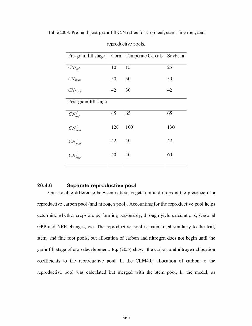
365
Table 20.3. Pre- and post-grain fill C:N ratios for crop leaf, stem, fine root, and
reproductive pools.
Pre-grain fill stage Corn Temperate Cereals Soybean
CNleaf 10 15 25
CNstem 50 50 50
CNfroot 42 30 42
Post-grain fill stage
fleafCN 65 65 65
fstemCN 120 100 130
ffrootCN 42 40 42
freprCN 50 40 60
20.4.6 Separate reproductive pool One notable difference between natural vegetation and crops is the presence of a
reproductive carbon pool (and nitrogen pool). Accounting for the reproductive pool helps
determine whether crops are performing reasonably, through yield calculations, seasonal
GPP and NEE changes, etc. The reproductive pool is maintained similarly to the leaf,
stem, and fine root pools, but allocation of carbon and nitrogen does not begin until the
grain fill stage of crop development. Eq. (20.5) shows the carbon and nitrogen allocation
coefficients to the reproductive pool. In the CLM4.0, allocation of carbon to the
reproductive pool was calculated but merged with the stem pool. In the model, as

366
allocation declines during the grain fill stage of growth, increasing amounts of carbon and
nitrogen are available for grain development.
367
21. Transient Landcover Change
CLM includes a treatment of mass and energy fluxes associated with prescribed
temporal change in land cover. Using an annual time series of the spatial distribution of
PFTs and wood harvest, CLM diagnoses the change in area for PFTs at each model time
step and then performs mass and energy balance accounting necessary to represent the
expansion and contraction of PFT area. This implementation currently only pertains to
the case where all PFTs for a particular grid cell coexist on a single soil/snow column. In
this case, the only biogeophysical state variable affected is canopy water ( canW ). The
biogeochemical impacts of land use and land cover change are simulated through changes
in CLM carbon pools and fluxes as shown in Figure 21.1 and described further in Chapter
13. Other implementations are possible, such as changing the area of soil/snow columns
or land unit area, however these require additional consideration of conservation of mass
and energy among the soil/snow columns and land units which will be implemented in
future versions of CLM.
21.1 Annual Transient Land Cover Data and Time Interpolation The changes in area over time associated with individual PFTs are prescribed
through a forcing dataset, referred to here as the dynpft dataset. The dynpft dataset
consists of an annual time series of global grids, where each annual time slice describes
the fractional area occupied by all PFTs and the annual wood harvest within each grid
cell. Changes in area and wood harvest for each PFT within a grid cell at each model
time step are inferred from a time-interpolation of the area information for the PFT from
the two bracketing annual time slices in the dynpft dataset.
368
As a special case, when the time dimension of the dynpft dataset starts at a later
year than the current model time step, the first time slice from the dynpft dataset is used
to represent the current time step PFT fractional area distributions. Similarly, when the
time dimension of the dynpft dataset stops at an earlier year than the current model time
step, the last time slice of the dynpft dataset is used. Thus, the simulation will have
invariant representations of PFT distributions through time for the periods prior to and
following the time duration of the dynpft dataset, with transient PFT distributions during
the period covered by the dynpft dataset.
The following equations capture this logic, where curyear is the calendar year for
the current timestep, _ (1)dynpft year and _ ( )dynpft year nyears are the first and last
calendar years in the dynpft dataset, respectively, nyears is the number of years in the
dynpft dataset, 1nt and 2nt are the two bracketing years used in the interpolation
algorithm, and n is the index value for the _dynpft year array corresponding to
_ ( ) curdynpft year n year= :
1
1 for _ (1)for _ (1) _ ( )for _ ( )
cur
cur
cur
year dynpft yearnt n dynpft year year dynpft year nyears
nyears year dynpft year nyears
< = ≤ < ≥
(21.1)
2
1 for _ (1)1 for _ (1) _ ( )
for _ ( )
cur
cur
cur
year dynpft yearnt n dynpft year year dynpft year nyears
nyears year dynpft year nyears
< = + ≤ < ≥
(21.2)
Interpolation of PFT weights between annual time slices in the dynpft dataset uses a
simple linear algorithm, based on the conversion of the current time step information into
a floating-point value for the number of calendar days since January 1 of the current
model year ( cday ). The interpolation weight for the current time step cdaytw is
369
366365cday
cdaytw −= (21.3)
where the numerator is 366 instead of 365 because the time manager function for CLM
returns a value of 1.0cday = for midnight Greenwich mean time on January 1. With
weights 1( )pw nt and 2( )pw nt obtained from the dynpft dataset for PFT p at the bracketing
annual time slices 1nt and 2nt , the interpolated PFT weight for the current time step ( ,p tw
) is
( ) ( ) ( ), 1 2 2p t cday p p pw tw w nt w nt w nt = − + (21.4)
The form of this equation is designed to improve roundoff accuracy performance, and
guarantees ,p tw stays in the range [0,1]. Note that values for 1( )pw nt , 2( )pw nt , and ,p tw
are fractional weights at the column level of the subgrid hierarchy.
The change in weight for a PFT between the current and previous time steps ( pw∆ )
is
1n np p pw w w −∆ = − (21.5)
where n denotes the current time step. The area of a given PFT increases for 0pw∆ >
and decreases for 0pw∆ < .
21.2 Mass and Energy Conservation Mass conservation is maintained across a PFT weight transition by summing up
all the water state variables to get the total vegetated land unit water content before ( ,1totW
) and after ( ,2totW ) new PFT weights are calculated. For example, ,1totW is
( ) ( ),1 , , , ,11 1
levgrndN npft
tot a sno liq i ice i can j ji j
W W W w w W wt= =
= + + + +∑ ∑ (21.6)
370
where aW is the aquifer water, snoW is the snow water, ,liq iw and ,ice iw are the liquid and
ice soil water contents, ,can jW is the canopy water content for PFT j , and ,1jwt is the PFT
weight for PFT j . For the situation where only PFT weights are changing and all other
land unit fractions are constant, any difference between ,1totW and ,2totW can only be due to
differences in the total canopy water before and after the PFT weight change. To ensure
water conservation, the typically very small difference between ,2totW and ,1totW is
subtracted from the grid cell runoff
,2 ,1liq liq tot totR R W W= + − . (21.7)
Total energy is unperturbed in this case and therefore an energy conservation
treatment is not required. As noted above, other implementations are possible and will be
desirable in the future, such as changing the area of soil/snow columns or land unit area,
for example in a situation in which crops are implemented on a separate soil column.
These would require additional consideration of conservation of mass and energy among
the soil/snow columns and land units.
21.3 Annual Transient Land Cover Dataset Development This section describes the development of the dynpft dataset. Development of this
dataset requires adapting for use with the CLM a harmonized dataset of land cover
change for the historical period and for different representations of the scenario period.
21.3.1 UNH Transient Land Use and Land Cover Change Dataset To coordinate the processing and consistency of land use and land cover change
data between the historical period (1850-2005) and the four IPCC representative
concentration pathways (RCPs) derived from integrated assessment models (IAM), the
371
University of New Hampshire (UNH) research group (Louise Chini, George Hurtt, Steve
Frolking; luh.unh.edu) produced a harmonized transient dataset for use in climate change
simulations. The historical component of the transient land use and land cover change
dataset is Version 1 of the Land-Use History A product (LUHa.v1) covering the period
1850-2005. The RCP transient land use and land cover change components (2005-2100)
are referred to as the Future Land-Use Harmonization A products. Version 1
(LUHa.v1_future.v1) is used for the AIM, MESSAGE, and MiniCAM IAMs; Version 1.1
(LUHa.v1_future.v1.1) is used for the IMAGE IAM. The land cover information is
provided at 0.5 degree grid resolution and includes fractional grid cell coverage by crops,
pasture, and primary and secondary natural vegetation.
The crop fraction of the grid cell represents the area of the grid cell used to grow
any type of crop. Similarly, pasture represents the fraction of a grid cell used for grazing
livestock. The remaining area in a half degree grid cell is partitioned into primary and
secondary vegetation. Primary vegetation represents the fractional area of a grid cell with
vegetation undisturbed by human activities. Secondary vegetation represents vegetated
areas that have recovered from some human disturbance; this could include re-vegetation
of pasture and crop areas as well as primary vegetation areas that have been logged.
The UNH dataset provides a transition matrix that describes the annual fraction of
land that is transformed from one category to another (e.g. primary land to crop, pasture
to crop, etc.; Hurtt et al. 2006). Included in these transitions is the conversion of
secondary land to secondary land, representing the logging on land recovering from an
earlier disturbance. These transitions provide information on all changes in land cover
through the sum of all transitions in a given year. Harmonized prescriptions of CMIP5
372
wood harvest statistics also are provided by (Hurtt et al. 2011) for the historical and RCP
time series. The wood harvest is prescribed spatially on the same 0.5 degree grid as the
land use class transitions for each year.
To ensure consistency with the various land use classes wood harvest is
prescribed as both the area of land harvested and the amount of carbon extracted in the
grid cell for a particular year. To account for the differences in standing amount of wood
carbon as well as the differences in harvest intensity associated with the different land
units, the harvest area and carbon amounts are prescribed for the five classes of: Primary
Forest, Primary Non-Forest, Secondary Mature Forest, Secondary Young Forest, and
Secondary Non-Forest.
21.3.2 Representing Land Use and Land Cover Change in CLM CLM represents the land surface as a hierarchy of sub-grid types: glacier; lake;
wetland; urban; and vegetated land. The vegetated land is further divided into a mosaic
of PFTs. To represent the UNH transient land use and land cover change dataset in
CLM, the annual fractional composition of crop, pasture, primary vegetation, and
secondary vegetation land units specified in the UNH dataset needs to be faithfully
represented with a corresponding PFT mosaic in CLM using the methods described in
Lawrence et al (2012). This method translated each of the UNH land units into fractional
PFT values based on current day and potential vegetation CLM land surface parameters
for that grid cell and for that year, as shown in Figure 21.2.
The methodology for creating the transient PFT dataset is based on four steps
which are applied across the time series. First, crop PFT composition is directly specified
from the crop land unit fractional area. Second, pasture PFTs are assigned based on grass
373
PFTs found in the potential vegetation and current day CLM land surface parameters
scaled by the area of pasture. Third, potential vegetation PFTs are assigned to the grid
cell scaled by the fractional area of the primary land unit. Last, current day non-crop and
non-pasture PFTs are assigned to the grid cell scaled by the fractional area of the
secondary land unit. The annual tree harvest values also are calculated from the harvest
information of the UNH dataset used in conjunction with transient tree PFT values.
Separate datasets representing the extent of water, wetland, ice and urban land cover are
used to compile the final land cover present in each CLM grid cell. These additional
non-vegetated land cover fractions are held constant throughout the time series. All
datasets are resolved at the half degree grid resolution.
21.3.3 Present Day PFT Dataset The present day dataset is based on the methodology of Lawrence and Chase
(2007) and uses a variety of satellite products to develop present day PFT distributions
with matching leaf area index values. The dataset initially derives fractions of bare
ground and tree cover from the Moderate Resolution Imaging Spectroradiometer
(MODIS) vegetation continuous fields product (Hansen et al. 2003). To further
distinguish tree types, the tree fraction is divided into broadleaf/needleleaf and
evergreen/deciduous types based on the Advanced Very High Resolution Radiometer
(AVHRR) continuous fields tree cover (DeFries et al. 2000). The remaining grid cell
area is assumed to be herbaceous grasses and shrubs, including crops. The area of crop is
initially determined from Ramankutty et al. (2008) circa 2000 global crop land areas, and
the remaining grass and shrub fractions are derived from the MODIS land cover (Friedl et
al. 2002). Further subdivisions of grass, shrub and tree PFTs into tropical, temperate and
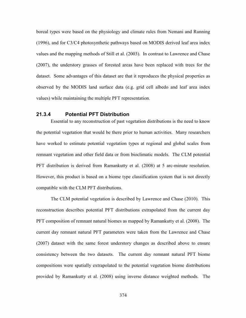
374
boreal types were based on the physiology and climate rules from Nemani and Running
(1996), and for C3/C4 photosynthetic pathways based on MODIS derived leaf area index
values and the mapping methods of Still et al. (2003). In contrast to Lawrence and Chase
(2007), the understory grasses of forested areas have been replaced with trees for the
dataset. Some advantages of this dataset are that it reproduces the physical properties as
observed by the MODIS land surface data (e.g. grid cell albedo and leaf area index
values) while maintaining the multiple PFT representation.
21.3.4 Potential PFT Distribution Essential to any reconstruction of past vegetation distributions is the need to know
the potential vegetation that would be there prior to human activities. Many researchers
have worked to estimate potential vegetation types at regional and global scales from
remnant vegetation and other field data or from bioclimatic models. The CLM potential
PFT distribution is derived from Ramankutty et al. (2008) at 5 arc-minute resolution.
However, this product is based on a biome type classification system that is not directly
compatible with the CLM PFT distributions.
The CLM potential vegetation is described by Lawrence and Chase (2010). This
reconstruction describes potential PFT distributions extrapolated from the current day
PFT composition of remnant natural biomes as mapped by Ramankutty et al. (2008). The
current day remnant natural PFT parameters were taken from the Lawrence and Chase
(2007) dataset with the same forest understory changes as described above to ensure
consistency between the two datasets. The current day remnant natural PFT biome
compositions were spatially extrapolated to the potential vegetation biome distributions
provided by Ramankutty et al. (2008) using inverse distance weighted methods. The
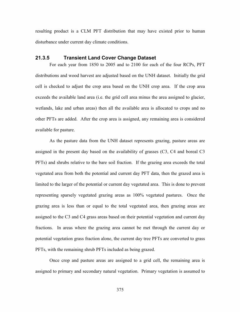
375
resulting product is a CLM PFT distribution that may have existed prior to human
disturbance under current day climate conditions.
21.3.5 Transient Land Cover Change Dataset For each year from 1850 to 2005 and to 2100 for each of the four RCPs, PFT
distributions and wood harvest are adjusted based on the UNH dataset. Initially the grid
cell is checked to adjust the crop area based on the UNH crop area. If the crop area
exceeds the available land area (i.e. the grid cell area minus the area assigned to glacier,
wetlands, lake and urban areas) then all the available area is allocated to crops and no
other PFTs are added. After the crop area is assigned, any remaining area is considered
available for pasture.
As the pasture data from the UNH dataset represents grazing, pasture areas are
assigned in the present day based on the availability of grasses (C3, C4 and boreal C3
PFTs) and shrubs relative to the bare soil fraction. If the grazing area exceeds the total
vegetated area from both the potential and current day PFT data, then the grazed area is
limited to the larger of the potential or current day vegetated area. This is done to prevent
representing sparsely vegetated grazing areas as 100% vegetated pastures. Once the
grazing area is less than or equal to the total vegetated area, then grazing areas are
assigned to the C3 and C4 grass areas based on their potential vegetation and current day
fractions. In areas where the grazing area cannot be met through the current day or
potential vegetation grass fraction alone, the current day tree PFTs are converted to grass
PFTs, with the remaining shrub PFTs included as being grazed.
Once crop and pasture areas are assigned to a grid cell, the remaining area is
assigned to primary and secondary natural vegetation. Primary vegetation is assumed to
376
be undisturbed and reflects the potential vegetation PFT distributions. In the secondary
region, the PFT distributions are based on the current day non-crop and non-pasture PFTs
in the grid cell. This process ensures that the PFT distributions are kept consistent with
the original current day and potential vegetation CLM parameters, while remaining
faithful to the UNH assigned areas.
21.3.6 Forest Harvest Dataset Changes Discussions following the initial analysis of CCSM4 land cover change
experiments found there were very high wood harvest areas compared to wood harvest
carbon in the RCP 6.0 and RCP 8.5 time series. The high wood harvest areas were traced
to using gridded spatially explicit wood harvest targets from the MESSAGE and AIM
groups for these two time series, rather than using regional targets with spatial
downscaling in GLM as done with the other three time periods. As a result of these
discussions new amended wood harvest targets were generated with regional targets
through GLM for the RCP 6.0 and RCP 8.5 time series as described in Lawrence et al.
(2012).
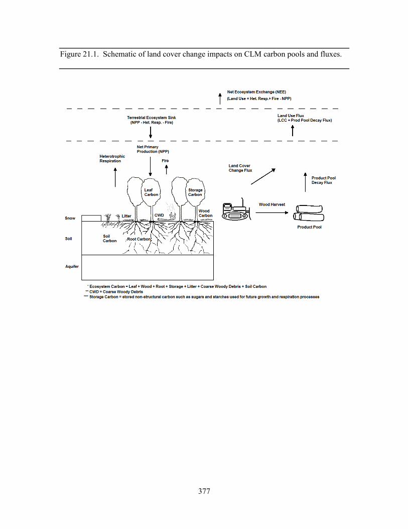
377
Figure 21.1. Schematic of land cover change impacts on CLM carbon pools and fluxes.
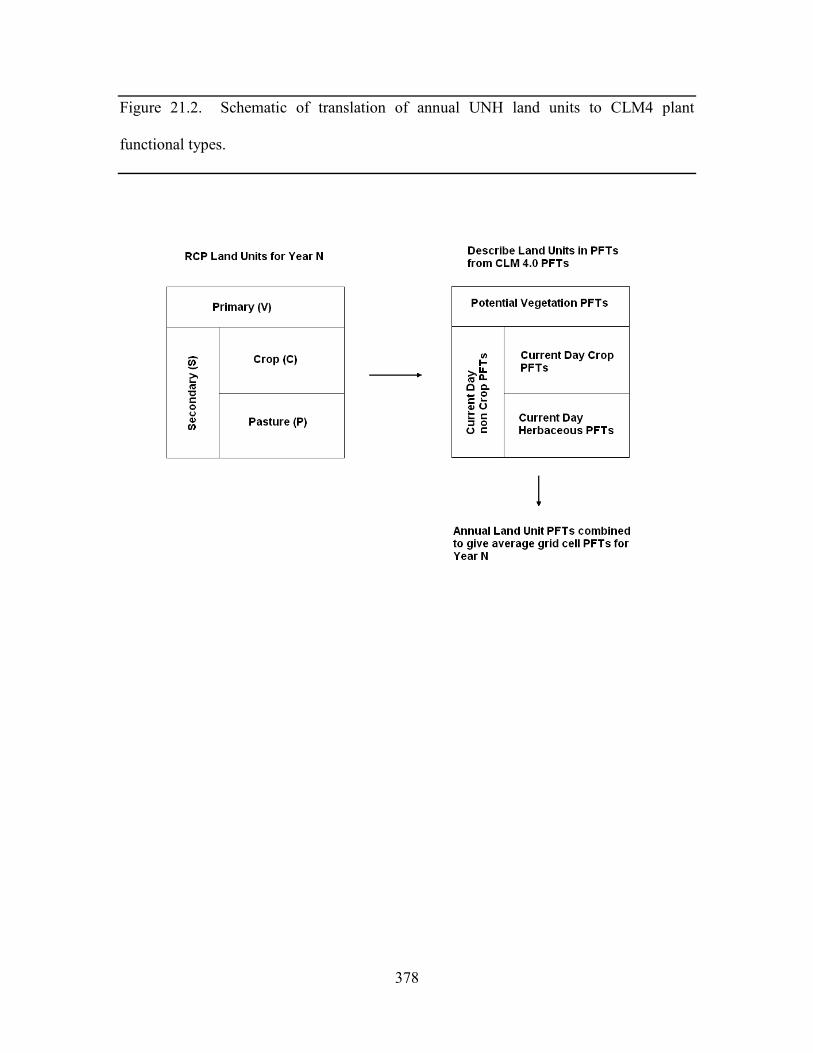
378
Figure 21.2. Schematic of translation of annual UNH land units to CLM4 plant
functional types.
379
22. Dynamic Global Vegetation Model
In CLM the user may choose to run the CN model as a dgvm (dynamic global
vegetation model) (CNDV). Note that CN must be active to run the dgvm in CLM. In
this section, a general description of the dgvm processes and how they integrate with CN
are provided. Further details are available in the CLM3DGVM Technical Note (Levis et
al. 2004). The focus here is on the differences relative to the corresponding processes in
the CLM3DGVM.
As with the CLM3DGVM, CNDV can simulate biogeographical changes only for
natural vegetation. Although the vegetated land unit may be separated into naturally
vegetated and human managed land units to permit a coexistence of natural and human
managed vegetation, CNDV only works if the human managed land units are fixed.
CLM’s transient land cover and land use change capability (see Chapter 21), which
permits transitions between natural and human managed plant functional types (PFTs), is
incompatible with the CNDV option at this time.
CNDV was implemented by introducing CLM3DGVM code to the hourly CN
framework only to the extent necessary to simulate annual biogeography updates. This
includes the annual processes of light competition, establishment, and survival [see
sections 2.7 and 2.10, Levis et al. (2004)] as they pertain to the calculations of PFT cover
(FPC) and population (P) but not processes related to carbon pools, leaf area index (LAI),
or canopy height. In CNDV we added complexity to the gap mortality calculation with
annual heat stress and growth efficiency considerations from the corresponding
CLM3DGVM algorithm [section 2.8, Levis et al. (2004)]. All other ecosystem processes
380
(allocation, phenology, fire, etc.) are handled by CN modules. Unlike in the
CLM3DGVM, in CNDV, annual biogeography updates are interpolated to hourly
intervals.
22.1 Establishment and survival The PFT distribution in the vegetated land unit is typically prescribed in CLM (see
section 2.1.2) except for the case when CNDV is active. In CNDV the model begins with
no PFT information per grid cell and evaluates whether or not a PFT may establish or
survive according to the PFT’s bioclimatic limits (Table 22.1). Shrub PFTs are treated as
trees at establishment.
CNDV omits the CLM3DGVM’s annual introduction of saplings when a PFT can
establish. The CLM3DGVM merged sapling carbon pools with a PFT’s existing carbon.
The resultant leaf carbon (annual maximum value) would update the FPC, i.e. the foliar
projective cover or fraction of the vegetated land unit occupied by the PFT [section 2.10,
Levis et al. (2004)]. Instead, CNDV updates the FPC using the PFT’s annual maximum
leaf carbon without an addition from saplings. For newly established PFTs, CNDV
assigns seed leaf carbon equal to 1 g C m-2 of land unit area and seed FPC equal to 0.05
for grasses and 0.000844 for trees (values determined from CLM3DGVM simulations).
The addition of establishing individuals to P, a PFT’s population, is handled as in the
CLM3DGVM.
FPC changes annually as in the CLM3DGVM but now is interpolated to an hourly
increment using the algorithms designed to conserve energy and mass in the CLM’s
dynamic land use option.
381
22.2 Light competition In CNDV’s order of annual processes, light competition is invoked before
establishment and survival. However, light competition does not affect a simulation
starting from bare ground until the vegetation fills the land unit (a few years at least).
Light competition starts with a calculation updating FPC. For reference, this update
was included at the end of allocation in the CLM3DGVM [section 2.6, Levis et al.
(2004)].
Due to their height advantage, trees will cover up to 95% of the land unit when their
productivity permits, as in the CLM3DGVM, regardless of grass and shrub productivity.
Grasses get second priority, as in the CLM3DGVM, even with shrubs included now.
Shrubs, then, have access to the remaining space and follow the tree algorithm for self
thinning [section 2.7, Levis et al. (2004)]. As a result, trees typically dominate in the most
productive regions, grasses in less productive regions, and shrubs in the least productive
non-desert regions (Zeng et al. 2008).
22.3 CN processes modified for the CNDV coupling Gap mortality and mortality from fire: Constant annual mortality rate of 0.02 is
changed for trees and shrubs to an annual rate calculated as in the CLM3DGVM
accounting for background and stress mortality [section 2.8, Levis et al. (2004)]. The CN
module converts the annual rate to hourly.
The CLM3DGVM used the concepts of average plant individual and PFT
population, P. CNDV retains these concepts in the light competition, establishment, and
survival calculations. In CNDV we account for the individuals removed hourly from P in
response to CN’s fire and gap mortality, while the carbon pools per individual and FPC
remain constant. Ultimately, P updates should only affect the annual processes of light
382
competition, establishment, and survival, so the P update may be moved to the end of the
year in a future version of CNDV.
Vegetation Structure Update: CN stocking is a constant, while in CNDV stocking
changes as P and FPC change. This affects the top-of-canopy height calculation. CN
specific leaf area and stem diameter calculations are kept, while the height calculation is
replaced with the CLM3DGVM’s [section 2.6, Levis et al. (2004)]. CN stem area index
(SAI) is kept.
Allocation: CN calculates a PFT’s fraction of currently allocated carbon relative to
the total allocation instead of obtaining a constant value from CLM’s PFT-physiology
file. In CNDV, we returned to the constant values in the old PFT-physiology file to get a
reasonable simulation of PFTs. For CNDV to use the calculated fraction, we will need to
change the algorithm for PFTs in early stages of growth.
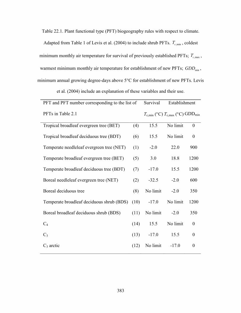
383
Table 22.1. Plant functional type (PFT) biogeography rules with respect to climate.
Adapted from Table 1 of Levis et al. (2004) to include shrub PFTs. ,mincT , coldest
minimum monthly air temperature for survival of previously established PFTs; ,maxcT ,
warmest minimum monthly air temperature for establishment of new PFTs; minGDD ,
minimum annual growing degree-days above 5°C for establishment of new PFTs. Levis
et al. (2004) include an explanation of these variables and their use.
PFT and PFT number corresponding to the list of Survival Establishment
PFTs in Table 2.1 Tc,min (°C) Tc,max (°C) GDDmin
Tropical broadleaf evergreen tree (BET) (4) 15.5 No limit 0
Tropical broadleaf deciduous tree (BDT) (6) 15.5 No limit 0
Temperate needleleaf evergreen tree (NET) (1) -2.0 22.0 900
Temperate broadleaf evergreen tree (BET) (5) 3.0 18.8 1200
Temperate broadleaf deciduous tree (BDT) (7) -17.0 15.5 1200
Boreal needleleaf evergreen tree (NET) (2) -32.5 -2.0 600
Boreal deciduous tree (8) No limit -2.0 350
Temperate broadleaf deciduous shrub (BDS) (10) -17.0 No limit 1200
Boreal broadleaf deciduous shrub (BDS) (11) No limit -2.0 350
C4 (14) 15.5 No limit 0
C3 (13) -17.0 15.5 0
C3 arctic (12) No limit -17.0 0
384
23. Biogenic Volatile Organic Compounds (BVOCs)
This chapter briefly describes the biogenic volatile organic compound (BVOC)
emissions model implemented in CLM. The CLM3 version (Levis et al. 2003; Oleson et
al. 2004) was based on Guenther et al. (1995). Heald et al. (2008) updated this scheme in
CLM4 based on Guenther et al. (2006). The current version in CLM4.5 is based on
MEGAN2.1 discussed in detail in Guenther et al. (2012). This update of MEGAN
incorporates four main features: (1) expansion to 147 chemical compounds (2) the
treatment of the light-dependent fraction (LDF) for each compound (3) inclusion of the
inhibition of isoprene emission by atmospheric CO2 and (4) emission factors mapped to
the specific PFTs of the CLM.
MEGAN2.1 now describes the emissions of speciated monoterpenes,
sesquiterpenes, oxygenated VOC as well as isoprene. A flexible scheme has been
implemented in the CLM to specify a subset of emissions. This allows for additional
flexibility in grouping chemical compounds to form the lumped species frequently used
in atmospheric chemistry. The mapping or grouping are therefore defined through a
namelist parameter in drv_flds_in, e.g. megan_specifier = 'ISOP = isoprene', 'BIGALK =
pentane + hexane + heptane + tricyclene'.
Terrestrial BVOC emissions from plants to the atmosphere are expressed as a flux,
iF ( µ g C m-2 ground area h-1), for emission of chemical compound i
( ),i i i j jj
F wtγ ρ ε= ∑ (23.1)
where iγ is the emission activity factor accounting for responses to meteorological and
phenological conditions, ρ is the canopy loss and production factor also known as
385
escape efficiency (set to 1), and ,i jε ( µ g C m-2 ground area h-1) is the emission factor at
standard conditions of light, temperature, and leaf area for plant functional type j with
fractional coverage ( ) jwt (Guenther et al. 2012). The emission activity factor iγ depends
on plant functional type, temperature, LAI, leaf age, and soil moisture (Guenther et al.
2012). For isoprene only, the effect of CO2 inhibition is now included as described by
Heald et al. (2009). Previously, only isoprene was treated as a light-dependent emission.
In MEGAN2.1, each chemical compound is assigned a LDF (ranging from 1.0 for
isoprene to 0.2 for some monoterpenes, VOCs and acetone). The activity factor for the
light response of emissions is therefore estimated as:
( ), _1P i i P LDF iLDF LDFγ γ= − + (23.2)
where the LDF activity factor ( _P LDFγ ) is specified as a function of PAR as in previous
versions of MEGAN.
The values for each emission factor ,i jε are now available for each of the 15 plant
functional types in the CLM and each chemical compound. This information is
distributed through an external file, allowing for more frequent and easier updates.
386
24. Dust Model
Atmospheric dust is mobilized from the land by wind in the CLM. The most
important factors determining soil erodibility and dust emission include the wind friction
speed, the vegetation cover, and the soil moisture. The CLM dust mobilization scheme
(Mahowald et al. 2006) accounts for these factors based on the DEAD (Dust Entrainment
and Deposition) model of Zender et al. (2003). Please refer to the Zender et al. (2003)
article for additional information regarding the equations presented in this section.
The total vertical mass flux of dust, jF (kg m-2 s-1), from the ground into transport
bin j is given by
,1
I
j m s i ji
F TSf Q Mα=
= ∑ (24.1)
where T is a global factor that compensates for the DEAD model’s sensitivity to
horizontal and temporal resolution and equals 5 x 10⁻⁴ in the CLM instead of 7 x 10⁻⁴ in
Zender et al. (2003). S is the source erodibility factor set to 1 in the CLM and serves as
a place holder at this time.
The grid cell fraction of exposed bare soil suitable for dust mobilization mf is given
by
( )( )( ) ,1
,1 ,1
1 1 1 liqm lake wetl sno v
liq ice
wf f f f f
w w= − − − −
+ (24.2)
where lakef and wetlf and snof are the CLM grid cell fractions of lake and wetland
(section 2.2.3) and snow cover (section 7.2.1), all ranging from zero to one. Not
mentioned by Zender et al. (2003), ,1liqw and ,1icew are the CLM top soil layer liquid water
387
and ice contents (mm) entered as a ratio expressing the decreasing ability of dust to
mobilize from increasingly frozen soil. The grid cell fraction of vegetation cover,vf , is
defined as
( ) ( ) 2 20 1 where 0.3 m mv t
t
L Sf L SL S
−+≤ = ≤ + =
+ (24.3)
where equation (24.3) applies only for dust mobilization and is not related to the plant
functional type fractions prescribed from the CLM input data or simulated by the CLM
dynamic vegetation model (Chapter 22). L and S are the CLM leaf and stem area index
values (m2 m-2) averaged at the land unit level so as to include all the pfts and the bare
ground present in a vegetated land unit. L and S may be prescribed from the CLM
input data (section 2.1.4) or simulated by the CLM biogeochemistry model (Chapter 13).
The sandblasting mass efficiency α (m-1) is calculated as
( )13.4 6.0 ln10 % 0.01 0 % 20100
20 0.01 20<% 100clay clayM
clay
M clay claye
M clayα − = × ≤ ≤= = × ≤
(24.4)
where clayM is the mass fraction of clay particles in the soil and %clay is determined from
the surface dataset (section 2.2.3). 0clayM = corresponds to sand and 0.2clayM = to
sandy loam.
sQ is the total horizontally saltating mass flux (kg m-1 s-1) of “large” particles
(Table 24.1), also referred to as the vertically integrated streamwise mass flux
23* * *
* ** *
* *
1 1 for
0 for
s atm s t tt s
s s s
t s
c u u u u uQ g u u
u u
ρ − + < = ≥
(24.5)
388
where the saltation constant sc equals 2.61 and atmρ is the atmospheric density (kg m-3)
(Table 2.3), g the acceleration of gravity (m s-2) (Table 2.6). The threshold wind friction
speed for saltation tu∗ (m s-1) is
12 17
2* * 2.5
6 10Re 1ft z t osp osp atm w
osp osp
u f gD fgD
ρ ρρ
− − ×= +
(24.6)
where zf is a factor dependent on surface roughness but set to 1 as a place holder for
now, ospρ and ospD are the density (2650 kg m-3) and diameter (75 x 10-6 m) of optimal
saltation particles, and wf is a factor dependent on soil moisture:
( ) 0.68
1 for
1 1.21 100 for
t
wt t
w wf
w w w w
≤= + − >
(24.7)
where
( )20.17 0.14 0 % 0.01 1t clay clay clayw a M M M clay= + ≤ = × ≤ (24.8)
and
1
,1
liq
d
wθ ρρ
= (24.9)
where 1claya M −= for tuning purposes, 1θ is the volumetric soil moisture in the top soil
layer (m3 m-3) (section 7.4), liqρ is the density of liquid water (kg m-3) (Table 2.6), and
,1dρ is the bulk density of soil in the top soil layer (kg m-3) defined as in section 6.3
rather than as in Zender et al. (2003). *Re ft from equation (24.6) is the threshold friction
Reynolds factor
389
( )*
2
***
20.0617(Re 10)2*
0.1291 for 0.03 Re 101 1.928ReRe
0.12 1 0.0858 for Re 10t
tf
tt
te− −
≤ ≤− +=
− >
(24.10)
and *Re t is the threshold friction Reynolds number approximation for optimally sized
particles
( )1.56
*Re 0.38 1331 100t ospD= + (24.11)
In equation (24.5), su∗ is defined as the wind friction speed (m s-1) accounting for the
Owen effect (Owen 1964)
( )
* 10 10,
2** 10 10, 10 10,
for
0.003 for
t
st t
u U Uu
u U U U U
<= + − ≥
(24.12)
where *u is the CLM wind friction speed (m s-1), also known as friction velocity (section
5.1), 10U is the 10-m wind speed (m s-1) calculated as the wind speed at the top of the
canopy in section 4.3 of Bonan (1996) but here for 10 m above the ground, and 10,tU is
the threshold wind speed at 10 m (m s-1)
1010, *
*t t
UU uu
= (24.13)
In equation (24.1) we sum ,i jM over 3I = source modes i where ,i jM is the mass
fraction of each source mode i carried in each of 4J = transport bins j
,max ,min
, ,
,, ,
ln lnerf erf
2 2 ln 2 ln
j j
v i v i
D DD Di
i jg i g i
mMσ σ
= −
(24.14)
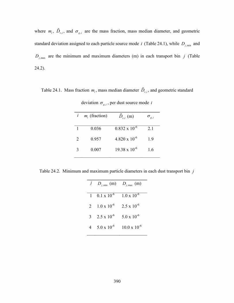
390
where im , ,v iD , and ,g iσ are the mass fraction, mass median diameter, and geometric
standard deviation assigned to each particle source mode i (Table 24.1), while ,minjD and
,maxjD are the minimum and maximum diameters (m) in each transport bin j (Table
24.2).
Table 24.1. Mass fraction im , mass median diameter ,v iD , and geometric standard
deviation ,g iσ , per dust source mode i
i im (fraction) ,v iD (m) ,g iσ
1 0.036 0.832 x 10⁻⁶ 2.1
2 0.957 4.820 x 10⁻⁶ 1.9
3 0.007 19.38 x 10⁻⁶ 1.6
Table 24.2. Minimum and maximum particle diameters in each dust transport bin j
j ,minjD (m) ,maxjD (m)
1 0.1 x 10⁻⁶ 1.0 x 10⁻⁶
2 1.0 x 10⁻⁶ 2.5 x 10⁻⁶
3 2.5 x 10⁻⁶ 5.0 x 10⁻⁶
4 5.0 x 10⁻⁶ 10.0 x 10⁻⁶
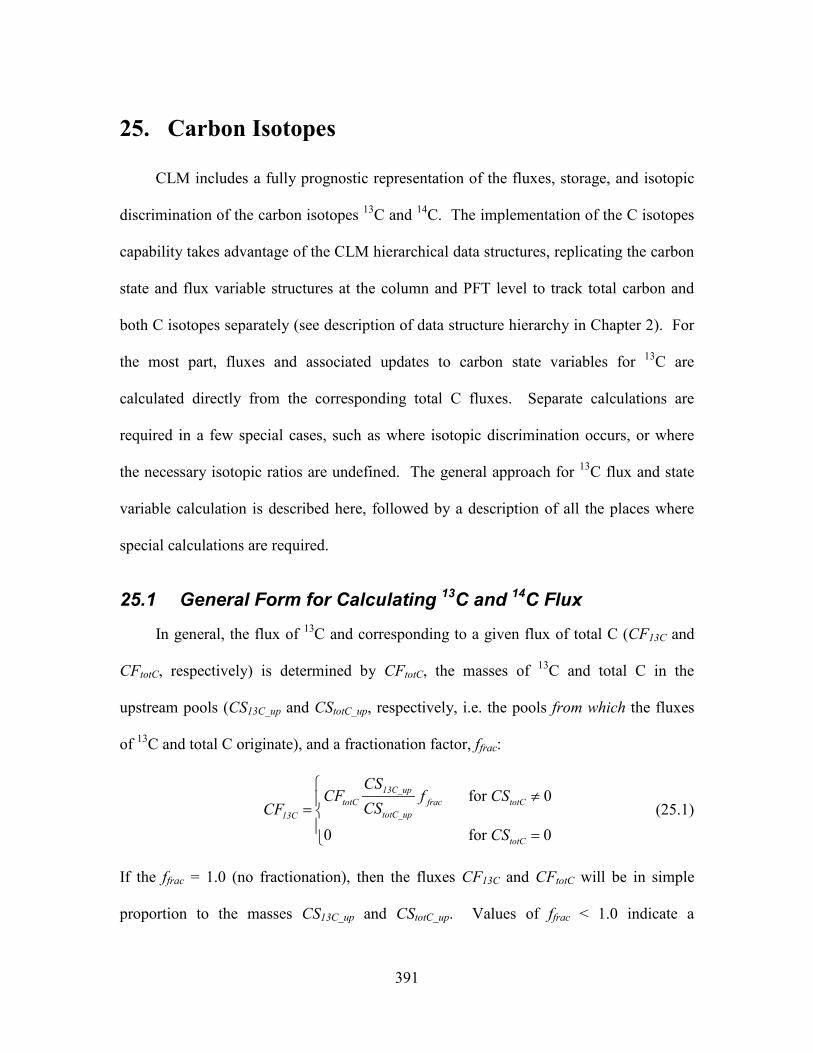
391
25. Carbon Isotopes
CLM includes a fully prognostic representation of the fluxes, storage, and isotopic
discrimination of the carbon isotopes 13C and 14C. The implementation of the C isotopes
capability takes advantage of the CLM hierarchical data structures, replicating the carbon
state and flux variable structures at the column and PFT level to track total carbon and
both C isotopes separately (see description of data structure hierarchy in Chapter 2). For
the most part, fluxes and associated updates to carbon state variables for 13C are
calculated directly from the corresponding total C fluxes. Separate calculations are
required in a few special cases, such as where isotopic discrimination occurs, or where
the necessary isotopic ratios are undefined. The general approach for 13C flux and state
variable calculation is described here, followed by a description of all the places where
special calculations are required.
25.1 General Form for Calculating 13C and 14C Flux
In general, the flux of 13C and corresponding to a given flux of total C (CF13C and
CFtotC, respectively) is determined by CFtotC, the masses of 13C and total C in the
upstream pools (CS13C_up and CStotC_up, respectively, i.e. the pools from which the fluxes
of 13C and total C originate), and a fractionation factor, ffrac:
(25.1)
If the ffrac = 1.0 (no fractionation), then the fluxes CF13C and CFtotC will be in simple
proportion to the masses CS13C_up and CStotC_up. Values of ffrac < 1.0 indicate a
for 0
0 for 0
13C_uptotC frac totC
totC_up13C
totC
CSCF f CS
CSCFCS
≠=
=
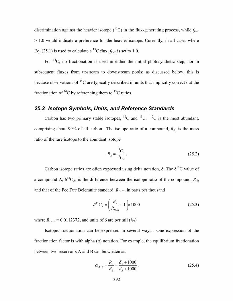
392
discrimination against the heavier isotope (13C) in the flux-generating process, while ffrac
> 1.0 would indicate a preference for the heavier isotope. Currently, in all cases where
Eq. (25.1) is used to calculate a 13C flux, ffrac is set to 1.0.
For 14C, no fractionation is used in either the initial photosynthetic step, nor in
subsequent fluxes from upstream to downstream pools; as discussed below, this is
because observations of 14C are typically described in units that implicitly correct out the
fractionation of 14C by referencing them to 13C ratios.
25.2 Isotope Symbols, Units, and Reference Standards
Carbon has two primary stable isotopes, 12C and 13C. 12C is the most abundant,
comprising about 99% of all carbon. The isotope ratio of a compound, RA, is the mass
ratio of the rare isotope to the abundant isotope
. (25.2)
Carbon isotope ratios are often expressed using delta notation, δ. The δ13C value of
a compound A, δ13CA, is the difference between the isotope ratio of the compound, RA,
and that of the Pee Dee Belemnite standard, RPDB, in parts per thousand
(25.3)
where RPDB = 0.0112372, and units of δ are per mil (‰).
Isotopic fractionation can be expressed in several ways. One expression of the
fractionation factor is with alpha (α) notation. For example, the equilibrium fractionation
between two reservoirs A and B can be written as:
10001000
A AA B
B B
RR
δαδ−
+= =
+. (25.4)
13
12A
AA
CRC
=
13 1 1000AA
PDB
RCR
δ
= − ×
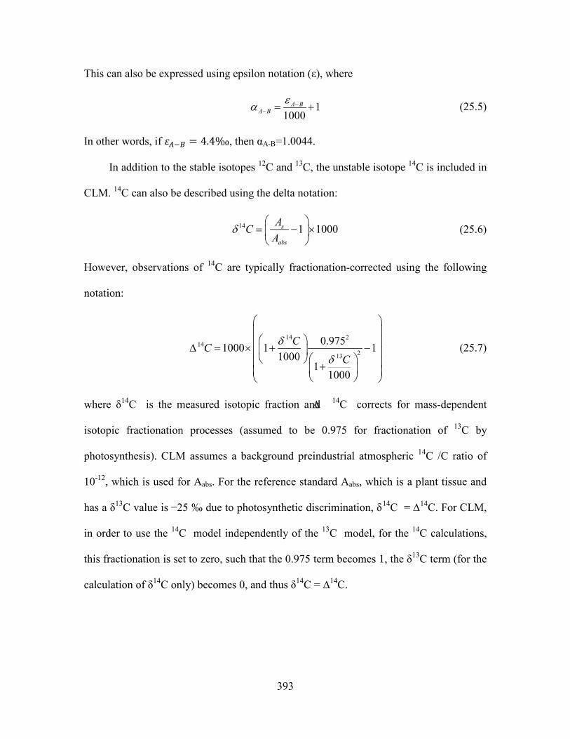
393
This can also be expressed using epsilon notation (ε), where
11000
A BA B
εα −− = + (25.5)
In other words, if 𝜀𝐴−𝐵 = 4.4‰, then αA-B=1.0044.
In addition to the stable isotopes 12C and 13C, the unstable isotope 14C is included in
CLM. 14C can also be described using the delta notation:
14 1 1000s
abs
ACA
δ
= − ×
(25.6)
However, observations of 14C are typically fractionation-corrected using the following
notation:
14 2
14213
0.9751000 1 11000
11000
CCC
δ
δ
∆ = × + − +
(25.7)
where δ14C is the measured isotopic fraction and ∆ 14C corrects for mass-dependent
isotopic fractionation processes (assumed to be 0.975 for fractionation of 13C by
photosynthesis). CLM assumes a background preindustrial atmospheric 14C /C ratio of
10-12, which is used for Aabs. For the reference standard Aabs, which is a plant tissue and
has a δ13C value is −25 ‰ due to photosynthetic discrimination, δ14C = ∆14C. For CLM,
in order to use the 14C model independently of the 13C model, for the 14C calculations,
this fractionation is set to zero, such that the 0.975 term becomes 1, the δ13C term (for the
calculation of δ14C only) becomes 0, and thus δ14C = ∆14C.
394
25.3 Carbon Isotope Discrimination During Photosynthesis
Photosynthesis is modeled in CLM as a two-step process: diffusion of CO2 into the
stomatal cavity, followed by enzymatic fixation (Chapter 8). Each step is associated with
a kinetic isotope effect. The kinetic isotope effect during diffusion of CO2 through the
stomatal opening is 4.4‰. The kinetic isotope effect during fixation of CO2 with
Rubisco is ~30‰; however, since about 5-10% of carbon in C3 plants reacts with
phosphoenolpyruvate carboxylase (PEPC) (Melzer and O'Leary, 1987), the net kinetic
isotope effect during fixation is ~27‰ for C3 plants. In C4 plant photosynthesis, only
the diffusion effect is important. The fractionation factor equations for C3 and C4 plants
are given below:
For C4 plants,
4.411000psnα = + (25.8)
For C3 plants,
2
4.4 22.61
1000
i
psn
cpCOα
∗
+= + (25.9)
where 𝛼𝑝𝑠𝑛 is the fractionation factor, and 𝑐𝑖∗ and pCO2 are the revised intracellular and
atmospheric CO2 partial pressure, respectively.
As can be seen from the above equation, kinetic isotope effect during fixation of
CO2 is dependent on the intracellular CO2 concentration, which in turn depends on the
net carbon assimilation. That is calculated during the photosynthesis calculation as
follows:
( ) ( )2
1.4 1.6s bi n
b s
g gc pCO a p
g g+
= − (25.10)
395
and
( ) ( ) ( )2
1.4 1.61 s b
i nb s
g gc pCO a d p
g g∗ +
= − − (25.11)
where 𝑎𝑛 is net carbon assimilation during photosynthesis, 𝑑 is downscaling factor due to
nitrogen limitation, 𝑝 is atmospheric pressure, 𝑔𝑏 is leaf boundary layer conductance, and
𝑔𝑠 is leaf stomatal conductance.
The fractionation factor 𝛼𝑝𝑠𝑛 and net assimilation 𝑎𝑛 are calculated during the
radiation time-step in CanopyFluxesMod.F90, whereas the downscaling factor 𝑑 is not
calculated until after the nitrogen limitation is computed in CNAllocationMod.F90. That
results in a difference between the actual photosynthesis, which is downscaled by 𝑑, and
the potential photosynthesis. In order to overcome this mismatch, downscaling due to
nitrogen limitation is factored in the calculation of the kinetic isotope effect during
fixation by defining a downscaled version of intracellular CO2 (𝑐𝑖∗), as a first order
approximation. However, since nitrogen down-regulation is calculated after the
photosynthesis calculation, down-regulation coefficient calculated in the previous time
step needs to be used.
Isotopic fractionation code is compatible with multi-layered canopy
parameterization; i.e., it is possible to calculate varying discrimination rates for each
layer of a multi-layered canopy. However, as with the rest of the photosynthesis model,
the number of canopy layers is currently set to one by default.
396
25.4 14C radioactive decay and historical atmospheric 14C concentrations
In the preindustrial biosphere, radioactive decay of 14C in carbon pools allows
dating of long-term age since photosynthetic uptake; while over the 20th century,
radiocarbon in the atmosphere was first diluted by radiocarbon-free fossil fuels and then
enriched by aboveground thermonuclear testing to approximately double its long-term
mean concentration. CLM includes both of these processes to allow comparison of
carbon that may vary on multiple timescales with observed values.
For radioactive decay, at each timestep all 14C pools are reduced at a rate of –
log(0.5)/τ, where τ is the half-life (Libby half-life value of 5568 years). In order to
rapidly equilibrate the long-lived pools during accelerated decomposition spinup, the
radioactive decay of the accelerated pools is also accelerated by the same degree as the
decomposition, such that the 14C value of these pools is in equilibrium when taken out of
the spinup mode.
For variation of atmospheric 14C over the historical period, ∆14C values can be set to
either fixed concentration (∆14C = 0‰) or time-varying concentrations read in from a file.
A default file is provided that is based on a spline fit through several observational
datasets spanning the 20th century: (Levin and Kromer, 2004; Manning and Melhuish,
1994; Nydal and Lövseth, 1996; Turnbull et al. 2007). This is shown in Figure 25.1.
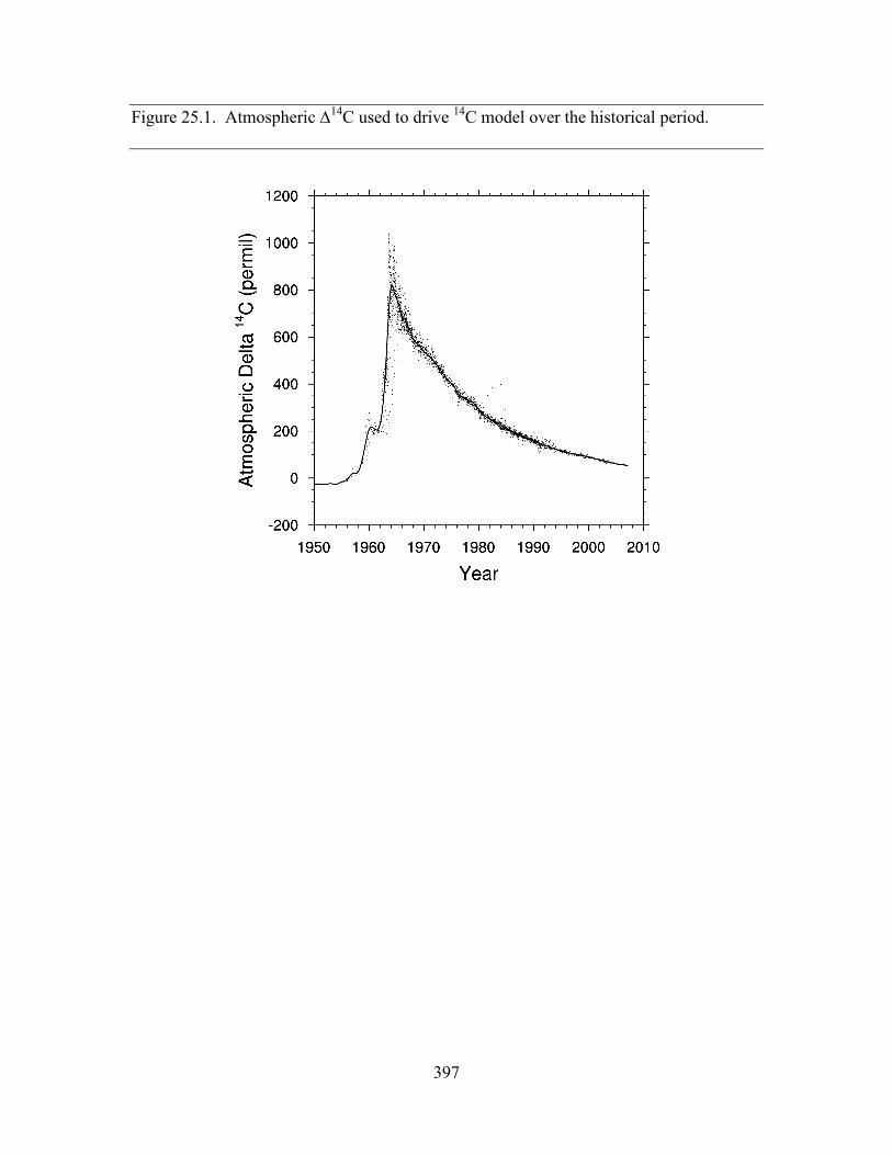
397
Figure 25.1. Atmospheric ∆14C used to drive 14C model over the historical period.
398
26. Offline Mode
In offline mode (uncoupled to an atmospheric model), the atmospheric forcing
required by CLM (Table 2.3) is supplied by observed datasets. The standard forcing
provided with the model is a 110-year (1901-2010) dataset (CRUNCEP; Viovy 2011)
that is a combination of two existing datasets; the CRU TS3.2 0.5° X 0.5° monthly data
covering the period 1901 to 2002 (Mitchell and Jones 2005) and the NCEP reanalysis
2.5° X 2.5° 6-hourly data covering the period 1948 to 2010. The CRUNCEP dataset has
been used to force CLM for studies of vegetation growth, evapotranspiration, and gross
primary production (Mao et al. 2012, Mao et al. 2013, Shi et al. 2013) and for the
TRENDY (trends in net land-atmosphere carbon exchange over the period 1980-2010)
project (Piao et al. 2012). Version 4 is used here (Viovy 2011). Alternative forcing
datasets can also be used (e.g., the Qian et al. (2006) dataset used for previous versions of
CLM is still available).
Here, the CRUNCEP dataset, which does not include data over oceans, lakes, and
Antarctica is modified. This missing data is filled with Qian et al. (2006) data from 1948
that is interpolated by the data atmosphere model to the 0.5° CRUNCEP grid. This
allows the model to be run over Antarctica and ensures data is available along coastlines
regardless of model resolution.
The forcing data is ingested into a data atmosphere model in three “streams”;
precipitation ( P ) (mm s-1), solar radiation ( atmS ) (W m-2), and four other fields
[atmospheric pressure atmP (Pa), atmospheric specific humidity atmq (kg kg-1),
atmospheric temperature atmT (K), and atmospheric wind atmW (m s-1)]. These are
399
separate streams because they are handled differently according to the type of field. In
the CRUNCEP dataset, the precipitation stream is provided at six hour intervals and the
data atmosphere model prescribes the same precipitation rate for each model time step
within the six hour period. The four fields that are grouped together in another stream
(pressure, humidity, temperature, and wind) are provided at six hour intervals and the
data atmosphere model linearly interpolates these fields to the time step of the model.
The total solar radiation is also provided at six hour intervals. The data is fit to the
model time step using a diurnal function that depends on the cosine of the solar zenith
angle µ to provide a smoother diurnal cycle of solar radiation and to ensure that all of
the solar radiation supplied by the six-hourly forcing data is actually used. The solar
radiation at model time step Mt is
( )
( ) ( )
( )( )
( ) ( )1
for 0.001
0 for 0.001
FD
M
i
FDatm FD M
Matm M Mt
t
Mi
atm M M
t S t ttS t t
t
S t t
µµ
µ
µ
∆∆
=
∆∆
= >
= ≤
∑ (26.1)
where FDt∆ is the time step of the forcing data (6 hours × 3600 seconds hour-1 = 21600
seconds), Mt∆ is the model time step (seconds), ( )atm FDS t is the six-hourly solar
radiation from the forcing data (W m-2), and ( )Mtµ is the cosine of the solar zenith angle
at model time step Mt (section 3.3). The term in the denominator of equation (26.1) is
the sum of the cosine of the solar zenith angle for each model time step falling within the
six hour period. For numerical purposes, ( ) 0.001iMtµ ≥ .
400
The total incident solar radiation atmS at the model time step Mt is then split into near-
infrared and visible radiation and partitioned into direct and diffuse according to factors
derived from one year’s worth of hourly CAM output from CAM version cam3_5_55 as
( )atm vis vis atmS R Sµ α↓ = (26.2)
( )1atm nir nir atmS R Sµ α↓ = − (26.3)
( )( )1atm vis vis atmS R Sα↓ = − (26.4)
( ) ( )1 1atm nir nir atmS R Sα↓ = − − . (26.5)
where α , the ratio of visible to total incident solar radiation, is assumed to be
0.5atm vis atm vis
atm
S SS
µ
α ↓ ↓+= = . (26.6)
The ratio of direct to total incident radiation in the visible visR is
( ) ( )2 30 1 2 3 0.01 0.99vis atm atm atm visR a a S a S a S Rα α α= + × + × + × ≤ ≤ (26.7)
and in the near-infrared nirR is
( ) ( ) ( )2 30 1 2 31 1 1 0.01 0.99nir atm atm atm nirR b b S b S b S Rα α α= + × − + × − + × − ≤ ≤ (26.8)
where 6 90 1 2 30.17639, 0.00380, 9.0039 10 , 8.1351 10a a a a− −= = = − × = × and
5 80 1 2 30.29548, 0.00504, 1.4957 10 , 1.4881 10b b b b− −= = = − × = × are coefficients from
polynomial fits to the CAM data.
The additional atmospheric forcing variables required by Table 2.3 are derived as
follows. The atmospheric reference height atmz′ (m) is set to 30 m. The directional wind
components are derived as 2atm atm atmu v W= = . The potential temperature atmθ (K) is
set to the atmospheric temperature atmT . The atmospheric longwave radiation atmL ↓ (W
401
m-2) is derived from the atmospheric vapor pressure atme and temperature atmT (Idso
1981) as
4150050.70 5.95 10 0.01 expatm atm atmatm
L e TT
σ↓ −= + × ×
(26.9)
where
0.622 0.378
atm atmatm
atm
P qeq
=+
(26.10)
and σ is the Stefan-Boltzmann constant (W m-2 K-4) (Table 2.6). The fraction of
precipitation P (mm s-1) falling as rain and/or snow is
( )rain Pq P f= , (26.11)
( )1snow Pq P f= − (26.12)
where
( )0 0.5 1P atm ff T T= < − < . (26.13)
The aerosol deposition rates spD (14 rates as described in Table 2.3) are provided by a
time-varying, globally-gridded aerosol deposition file developed by Lamarque et al.
(2010).
If the user wishes to provide atmospheric forcing data from another source, the data
format outlined above will need to be followed with the following exceptions. The data
atmosphere model will accept a user-supplied relative humidity RH (%) and derive
specific humidity atmq (kg kg-1) from
0.6220.378
atmatm
atm atm
eqP e
=−
(26.14)
402
where the atmospheric vapor pressure atme (Pa) is derived from the water ( atm fT T> ) or
ice ( atm fT T≤ ) saturation vapor pressure atmTsate as
100atmT
atm satRHe e= where fT is the freezing
temperature of water (K) (Table 2.6), and atmP is the pressure at height atmz (Pa). The
data atmosphere model will also accept a user-supplied dew point temperature dewT (K)
and derive specific humidity atmq from
0.6220.378
dew
dew
Tsat
atm Tatm sat
eqP e
=−
. (26.15)
Here, Tsate , the saturation vapor pressure as a function of temperature, is derived from
Lowe’s (1977) polynomials. If not provided by the user, the atmospheric pressure atmP
(Pa) is set equal to the standard atmospheric pressure 101325stdP = Pa, and surface
pressure srfP (Pa) is set equal to atmP .
The user may provide the total direct and diffuse solar radiation, atmS µ↓ and atmS ↓ .
These will be time-interpolated using the procedure described above and then each term
equally apportioned into the visible and near-infrared wavebands (e.g.,
0.5atm vis atmS Sµ µ↓ ↓= , 0.5atm nir atmS Sµ µ↓ ↓= ).
403
27. References Aber, J.D., Melillo, J.M. and McClaugherty, C.A., 1990. Predicting long-term patterns of mass loss,
nitrogen dynamics, and soil organic matter formation from initial fime litter chemistry in temperate forest ecosystems. Canadian Journal of Botany, 68: 2201-2208.
Aber, J.D., Goodale, C.L., Ollinger, S.V., Smith, M.-L., Magill, A.H., Martin, M.E., Hallett, R.A., and Stoddard, J.L. 2003. Is nitrogen deposition altering the nitrogen status of northeastern forests? BioScience 53:375-389.
Allen, C.B., Will, R.E., and Jacobson, M.A. 2005. Production efficiency and radiation use efficiency of four tree species receiving irrigation and fertilization. Forest Science 51:556-569.
Anderson, E.A. 1976. A point energy and mass balance model of a snow cover. NOAA Technical Report NWS 19, Office of Hydrology, National Weather Service, Silver Spring, MD.
André, J.-C., Goutorbe, J.-P., and Perrier, A. 1986. HAPEX-MOBILHY: A hydrologic atmosphere experiment for the study of water budget and evaporation flux at the climatic scale. Bull. Amer. Meteor. Soc. 67:138-144.
Andrén, O. and Paustian, K., 1987. Barley straw decomposition in the field: a comparison of models. Ecology 68(5):1190-1200.
Arah, J.R.M. and Stephen, K.D., 1998. A model of the processes leading to methane emission from peatland. Atmos. Environ. 32(19):3257-3264.
Arah, J. and Vinten, A., 1995. Simplified models of anoxia and denitrification in aggregated and simple-structured soils. European Journal of Soil Science 46(4):507-517.
Arendt, A., et al. 2012. Randolph Glacier Inventory: A Dataset of Global Glacier Outlines Version: 1.0, Global Land Ice Measurements from Space, Boulder Colorado, USA. Digital Media.
Arora, V.K. and Boer, G.J. 2005. Fire as an interactive component of dynamic vegetation models. J. Geophys. Res. 110:G02008. DOI:10.1029/2005JG000042.
Arya, S.P. 2001. Introduction to Meteorology. Academic Press, San Diego, CA.
Asner, G.P., Wessman, C.A., Schimel, D.S., and Archer, S. 1998. Variability in leaf and litter optical properties: implications for BRDF model inversions using AVHRR, MODIS, and MISR. Remote Sens. Environ. 63:243-257.
Axelsson, E., and Axelsson, B. 1986. Changes in carbon allocation patterns in spruce and pine trees following irrigation and fertilization. Tree Phys. 2:189-204.
Baird, A.J., Beckwith, C.W., Waldron, S. and Waddington, J.M., 2004. Ebullition of methane-containing gas bubbles from near-surface Sphagnum peat. Geophys. Res. Lett. 31(21). DOI:10.1029/2004GL021157.
Baldocchi, D., et al. 2001. FLUXNET: A new tool to study the temporal and spatial variability of ecosystem-scale carbon dioxide, water vapor, and energy flux densities. Bull. Amer. Meteor. Soc. 82:2415-2433.
Barbottin, A., Lecomte, C., Bouchard, C., and Jeuffroy, M.-H. 2005. Nitrogen remobilization during grain filling in wheat: Genotypic and environmental effects. Crop Sci. 45:1141-1150.
Batjes, N.H., 2006. ISRIC-WISE derived soil properties on a 5 by 5 arc-minutes global grid. Report 2006/02 (available through : http://www.isric.org)
Berger, A.L. 1978a. Long-term variations of daily insolation and quaternary climatic changes. J. Atmos. Sci. 35:2362-2367.
404
Berger, A.L. 1978b. A simple algorithm to compute long-term variations of daily or monthly insolation. Contribution de l’Institut d’Astronomie et de Géophysique, Université Catholique de Louvain, Louvain-la-Neuve, No. 18.
Berger, A., Loutre, M.-F., and Tricot, C. 1993. Insolation and Earth’s orbital periods. J. Geophys. Res. 98:10341-10362.
Berkowitz, B., and Balberg, I. 1992. Percolation approach to the problem of hydraulic conductivity in porous media. Transport in Porous Media 9:275–286.
Beven, K.J., and Kirkby, M.J. 1979. A physically based variable contributing area model of basin hydrology. Hydrol. Sci. Bull. 24:43-69.
Bohren, C. F., and Huffman, D. R. 1983. Absorption and scattering of light by small particles. John Wiley & Sons, New York, NY.
Bonan, G.B. 1996. A land surface model (LSM version 1.0) for ecological, hydrological, and atmospheric studies: Technical description and user's guide. NCAR Technical Note NCAR/TN-417+STR, National Center for Atmospheric Research, Boulder, CO, 150 pp.
Bonan, G.B. 1998. The land surface climatology of the NCAR Land Surface Model coupled to the NCAR Community Climate Model. J. Climate 11:1307-1326.
Bonan, G.B. 2002. Ecological Climatology: Concepts and Applications. Cambridge University Press.
Bonan, G.B., Oleson, K.W., Vertenstein, M., Levis, S., Zeng, X., Dai, Y., Dickinson, R.E., and Yang, Z.-L. 2002a. The land surface climatology of the Community Land Model coupled to the NCAR Community Climate Model. J. Climate 15: 3123-3149.
Bonan, G.B., Levis, S., Kergoat, L., and Oleson, K.W. 2002b. Landscapes as patches of plant functional types: An integrating concept for climate and ecosystem models. Global Biogeochem. Cycles 16: 5.1-5.23.
Bonan, G.B., and Levis, S. 2006. Evaluating aspects of the Community Land and Atmosphere Models (CLM3 and CAM3) using a dynamic global vegetation model. J. Climate 19:2290-2301.
Bonan, G.B., Lawrence P.J., Oleson K.W., Levis S., Jung M., Reichstein M., Lawrence, D.M., and Swenson, S.C. 2011. Improving canopy processes in the Community Land Model (CLM4) using global flux fields empirically inferred from FLUXNET data. J. Geophys. Res. 116, G02014. DOI:10.1029/2010JG001593.
Bonan, G. B., Oleson, K.W., Fisher, R.A., Lasslop, G., and Reichstein, M. 2012. Reconciling leaf physiological traits and canopy flux data: Use of the TRY and FLUXNET databases in the Community Land Model version 4, J. Geophys. Res., 117, G02026. DOI:10.1029/2011JG001913.
Branstetter, M.L., and Famiglietti, J.S. 1999. Testing the sensitivity of GCM-simulated runoff to climate model resolution using a parallel river transport algorithm. Preprints, 14th Conference on Hydrology, Dallas, TX, Amer. Meteor. Soc., 391-392.
Branstetter, M.L. 2001. Development of a parallel river transport algorithm and applications to climate studies. Ph.D. dissertation, University of Texas at Austin.
Brun, E. 1989. Investigation of wet-snow metamorphism in respect of liquid water content. Ann. Glaciol. 13:22-26.
Bugmann, H., and Solomon, A.M. 2000. Explaining forest composition and biomass across multiple biogeographical regions. Ecol. Appl. 10:95-114.
Busing, R.T. 2005. Tree mortality, canopy turnover, and woody detritus in old cove forests of the southern Appalachians. Ecology 86:73-84.
Campbell, G.S., and Norman, J.M. 1998. An Introduction to Environmental Biophysics (2nd edition). Springer-Verlag, New York.
405
Castillo, G., Kendra, C., Levis, S., and Thornton, P. 2012. Evaluation of the new CNDV option of the Community Land Model: effects of dynamic vegetation and interactive nitrogen on CLM4 means and variability. J. Climate 25:3702–3714.
Cao, M., Marshall, S. and Gregson, K., 1996. Global carbon exchange and methane emissions from natural wetlands: Application of a process-based model. J. Geophys. Res. 101(D9):14,399-14,414.
Churkina, G. et al., 2003. Analyzing the ecosystem carbon dynamics of four European coniferous forests using a biogeochemistry model. Ecosystems, 6: 168-184.
CIESIN: Gridded population of the world version 3 (GPWv3), 2005. Population density grids, Technical report, Socioeconomic Data and Applications Center (SEDAC), Columbia University, Palisades, New York, USA.
Clapp, R.B., and Hornberger, G.M. 1978. Empirical equations for some soil hydraulic properties. Water Resour. Res. 14:601-604.
Clauser, C., and Huenges, E. 1995. Thermal conductivity of rocks and minerals. pp. 105-126. In: T. J. Ahrens (editor) Rock Physics and Phase Relations: A Handbook of Physical Constants. Washington, D.C.
Cleveland, C.C., Townsend, A.R., Schimel, D.S., Fisher, H., Howarth, R.W., Hedin, L.O., Perakis, S.S., Latty, E.F., Von Fischer, J.C., Elseroad, A., and Wasson, M.F. 1999. Global patterns of terrestrial biological nitrogen (N2) fixation in natural ecosystems. Global Biogeochem. Cycles 13:623-645.
Collatz, G.J., Ball, J.T., Grivet, C., and Berry, J.A. 1991. Physiological and environmental regulation of stomatal conductance, photosynthesis, and transpiration: A model that includes a laminar boundary layer. Agric. For. Meteor. 54:107-136.
Collatz, G.J., Ribas-Carbo, M., and Berry, J.A. 1992. Coupled photosynthesis-stomatal conductance model for leaves of C4 plants. Aust. J. Plant Physiol. 19:519-538.
Colmer, T.D., 2003. Long-distance transport of gases in plants: a perspective on internal aeration and radial oxygen loss from roots. Plant Cell and Environment 26(1):17-36.
Conway, H., Gades, A., and Raymond, C.F. 1996. Albedo of dirty snow during conditions of melt. Water Resour. Res. 32:1713-1718.
Cosby, B.J., Hornberger, G.M., Clapp, R.B., and Ginn, T.R. 1984. A statistical exploration of the relationships of soil moisture characteristics to the physical properties of soils. Water Resour. Res. 20:682-690.
Crawford, T. W., Rendig, V. V., and Broadent, F. E. 1982. Sources, fluxes, and sinks of nitrogen during early reproductive growth of maize (Zea mays L.). Plant Physiol. 70:1645-1660.
Dai, Y., and Zeng, Q. 1997. A land surface model (IAP94) for climate studies. Part I: formulation and validation in off-line experiments. Adv. Atmos. Sci. 14:433-460.
Dai, Y., et al. 2001. Common Land Model: Technical documentation and user’s guide [Available online at http://climate.eas.gatech.edu/dai/clmdoc.pdf].
Dai, Y., Zeng, X., Dickinson, R.E., Baker, I., Bonan, G.B., Bosilovich, M.G., Denning, A.S., Dirmeyer, P.A., Houser, P.R., Niu, G., Oleson, K.W., Schlosser, C.A., and Yang, Z.-L. 2003. The Common Land Model. Bull. Amer. Meteor. Soc. 84:1013-1023.
Dai, Y., Dickinson, R.E., and Wang, Y.-P. 2004. A two-big-leaf model for canopy temperature, photosynthesis, and stomatal conductance. J. Climate 17:2281-2299.
Dai, A., and Trenberth, K.E. 2002. Estimates of freshwater discharge from continents: Latitudinal and seasonal variations. J. Hydrometeor. 3:660-687.
DeFries, R.S., Hansen, M.C., Townshend, J.R.G., Janetos, A.C., and Loveland, T.R. 2000. A new global 1-km dataset of percentage tree cover derived from remote sensing. Global Change Biol. 6:247-254.
406
Degens, B. and Sparling, G., 1996. Changes in aggregation do not correspond with changes in labile organic C fractions in soil amended with 14C-glucose. Soil Biology and Biochemistry, 28(4/5): 453-462.
de Vries, D.A. 1963. Thermal Properties of Soils. In: W.R. van Wijk (editor) Physics of the Plant Environment. North-Holland, Amsterdam.
Dickinson, R.E. 1983. Land surface processes and climate-surface albedos and energy balance. Adv. Geophys. 25:305-353.
Dickinson, R.E., Henderson-Sellers, A., and Kennedy, P.J. 1993. Biosphere-Atmosphere Transfer Scheme (BATS) version 1e as coupled to the NCAR Community Climate Model. NCAR Technical Note NCAR/TN-387+STR. National Center for Atmospheric Research, Boulder, CO.
Dickinson, R.E., Oleson, K.W., Bonan, G., Hoffman, F., Thornton, P., Vertenstein, M., Yang, Z.-L., and Zeng, X. 2006. The Community Land Model and its climate statistics as a component of the Community Climate System Model. J. Climate 19:2302-2324.
Dingman, S.L. 2002. Physical Hydrology. Second Edition. Prentice Hall, NJ.
Dirmeyer, P.A., Dolman, A.J., and Sato, N. 1999. The pilot phase of the Global Soil Wetness Project. Bull. Amer. Meteor. Soc. 80:851-878.
Dobson, J.E., Bright, E.A., Coleman, P.R., Durfee, R.C., and Worley, B.A. 2000. LandScan: A global population database for estimating populations at risk. Photogramm. Eng. Rem. Sens. 66:849-857.
Dorman, J.L., and Sellers, P.J. 1989. A global climatology of albedo, roughness length and stomatal resistance for atmospheric general circulation models as represented by the simple biosphere model (SiB). J. Appl. Meteor. 28:833-855.
Dougherty, R.L., Bradford, J.A., Coyne, P.I., and Sims, P.L. 1994. Applying an empirical model of stomatal conductance to three C4 grasses. Agric. For. Meteor. 67:269-290.
Drewniak, B., Song, J., Prell, J., Kotamarthi, V.R., and Jacob, R. 2013. Modeling agriculture in the Community Land Model. Geosci. Model Dev. 6:495-515. DOI:10.5194/gmd-6-495-2013.
Dunfield, P., Knowles, R., Dumont, R. and Moore, T.R., 1993. Methane Production and Consumption in Temperate and Sub-Arctic Peat Soils - Response to Temperature and Ph. Soil Biology & Biochemistry 25(3):321-326.
Entekhabi, D., and Eagleson, P.S. 1989. Land surface hydrology parameterization for atmospheric general circulation models including subgrid scale spatial variability. J. Climate 2:816-831.
Fang, X. and Stefan, H.G., 1996. Long-term lake water temperature and ice cover simulations/measurements. Cold Regions Science and Technology 24(3):289-304.
Farouki, O.T. 1981. The thermal properties of soils in cold regions. Cold Regions Sci. and Tech. 5:67-75.
Farquhar, G.D., von Caemmerer, S., and Berry, J.A. 1980. A biochemical model of photosynthetic CO2 assimilation in leaves of C3 species. Planta 149:78-90.
Farquhar, G.D., and von Caemmerer, S. 1982. Modeling of photosynthetic response to environmental conditions. pp. 549-587. In: O.L. Lange, P.S. Nobel, C.B. Osmond, and H. Zeigler (editors) Encyclopedia of Plant Physiology. Vol. 12B. Physiological Plant Ecology. II. Water Relations and Carbon Assimilation. Springer-Verlag, New York.
Ferrari, J.B., 1999. Fine-scale patterns of leaf litterfall and nitrogen cycling in an old-growth forest. Canadian Journal of Forest Research, 29: 291-302.
Firestone, M.K. and Davidson, E.A. 1989. Exchange of Trace Gases between Terrestrial Ecosystems and the Atmosphere. In: M.O. Andreae and D.S. Schimel (Editors). John Wiley and Sons, pp. 7-21.
Flanner, M.G., and Zender. C.S. 2005. Snowpack radiative heating: Influence on Tibetan Plateau climate. Geophys. Res. Lett. 32:L06501. DOI:10.1029/2004GL022076.
407
Flanner, M.G., and Zender, C.S. 2006. Linking snowpack microphysics and albedo evolution. J. Geophys. Res. 111:D12208. DOI:10.1029/2005JD006834.
Flanner, M.G., Zender, C.S., Randerson, J.T., and Rasch, P.J. 2007. Present day climate forcing and response from black carbon in snow. J. Geophys. Res. 112:D11202. DOI:10.1029/2006JD008003.
Flatau, P.J., Walko, R.L., and Cotton, W.R. 1992. Polynomial fits to saturation vapor pressure. J. Appl. Meteor. 31:1507-1513.
Friedl, M.A., McIver, D.K., Hodges, J.C.F., Zhang, X.Y., Muchoney, D., Strahler, A.H., Woodcock, C.E., Gopal, S., Schneider, A., Cooper, A., Baccini, A., Gao, F., and Schaaf, C. 2002. Global land cover mapping from MODIS: algorithms and early results. Remote Sens. Environ. 83:287-302.
Frolking, S., et al. 2001. Modeling Northern Peatland Decomposition and Peat Accumulation. Ecosystems. 4(5):479-498.
Gallais, A., Coque, M. Quillere, I., Prioul, J., and Hirel, B. 2006. Modeling postsilking nitrogen fluxes in maize (Zea mays) using 15N-labeling field experiments. New Phytologist 172:696-707.
Gallais, A., Coque, M., Gouis, J. L., Prioul, J. L., Hirel, B., and Quillere, I. 2007. Estimating the proportion of nitrogen remobilization and of postsilking nitrogen uptake allocated to maize kernels by Nitrogen-15 labeling. Crop Sci. 47:685-693.
Galloway, J.N., et al. 2004. Nitrogen cycles: past, present, and future. Biogeochem. 70:153-226.
Garcia, R.L., Kanemasu, E.T., Blad, B.L., Bauer, A., Hatfield, J.L., Major, D.A., Reginato, R.J., and Hubbard, K.G. 1988. Interception and use efficiency of light in winter wheat under different nitrogen regimes. Agric. For. Meteor. 44:175-186.
Gash, J.H.C., Nobre, C.A., Roberts, J.M., and Victoria, R.L. 1996. An overview of ABRACOS. pp. 1-14. In: J.H.C. Gash, C.A. Nobre, J.M. Roberts, and R.L. Victoria (editors) Amazonian Deforestation and Climate. John Wiley and Sons, Chichester, England.
Gholz, H.L., Perry, C.S., Cropper, W.P., Jr. and Hendry, L.C., 1985. Litterfall, decomposition, and nitrogen and phosphorous dynamics in a chronosequence of slash pine (Pinus elliottii) plantations. Forest Science, 31(2): 463-478.
Giglio, L., Csiszar, I., and Justice, C.O. 2006. Global distribution and seasonality of active fires as observed with the Terra and Aqua Moderate Resolution Imaging Spectroradiometer (MODIS) sensors. J. Geophys. Res. 111:G02016. DOI:10.1029/2005JG000142.
Global Soil Data Task 2000. Global soil data products CD-ROM (IGBP-DIS). International Geosphere-Biosphere Programme-Data and Information Available Services [Available online at http://www.daac.ornl.gov].
Gomes, E.P.C., Mantovani, W., and Kageyama, P.Y. 2003. Mortality and recruitment of trees in a secondary montane rain forest in southeastern Brazil. Brazilian Journal of Biology 63:47-60.
Gosz, J.R., Likens, G.E., and Bormann, F.H. 1973. Nutrient release from decomposing leaf and branch litter in the Hubbard Brook Forest, New Hampshire. Ecological Monographs 43:173-191.
Gotangco Castillo C., Levis S., and Thornton P. 2012. Evaluation of the new CNDV option of the Community Land Model: Effects of dynamic vegetation and interactive nitrogen on CLM4 means and variability. J. Climate 25:3702-3714. DOI:10.1175/JCLID-11-00372.1.
Graham, S.T., Famiglietti, J.S., and Maidment, D.R. 1999. Five-minute, 1/2º, and 1º data sets of continental watersheds and river networks for use in regional and global hydrologic and climate system modeling studies. Water Resour. Res. 35:583-587.
Grenfell, T.C., and Warren, S.G. 1999. Representation of a nonspherical ice particle by a collection of independent spheres for scattering and absorption of radiation. J. Geophys. Res. 104(D24):37697-37709.
408
del Grosso, S.J., et al. 2000. General model for N2O and N2 gas emissions from soils due to dentrification. Global Biogeochem. Cycles 14(4):1045-1060.
Guenther, A., Hewitt, C.N., Erickson, D., Fall, R., Geron, C., Graedel, T., Harley, P., Klinger, L., Lerdau, M., McKay, W.A., Pierce, T., Scholes, B., Steinbrecher, R., Tallamraju, R., Taylor, J., and Zimmerman, P. 1995. A global model of natural volatile organic compound emissions. J. Geophys. Res. 100:8873-8892.
Guenther, A., Karl, T., Harley, P., Wiedinmyer, C., Palmer. P.I., and Geron, C. 2006. Estimates of global terrestrial isoprene emissions using MEGAN (Model of Emissions of Gases and Aerosols from Nature). Atmos. Chem. Phys. 6:3181–3210.
Guenther, A. B., Jiang, X., Heald, C. L., Sakulyanontvittaya, T., Duhl, T., Emmons, L. K., & Wang, X., 2012. The Model of Emissions of Gases and Aerosols from Nature version 2.1 (MEGAN2.1): an extended and updated framework for modeling biogenic emissions, Geosci. Model Dev., 5, 1471–1492. DOI:10.5194.
Hack, J.J., Caron, J.M., Yeager, S.G., Oleson, K.W., Holland, M.M., Truesdale, J.E., and Rasch, P.J. 2006. Simulation of the global hydrological cycle in the CCSM Community Atmosphere Model version 3 (CAM3): mean features. J. Climate 19:2199-2221.
Hansen, M., DeFries, R.S., Townshend, J.R.G., Carroll, M., Dimiceli, C., and Sohlberg, R.A. 2003. Global percent tree cover at a spatial resolution of 500 meters: first results of the MODIS vegetation continuous fields algorithm. Earth Interactions 7(10):1-15.
Hastings, D.A., Dunbar, P.K., Elphingstone, G.M., Bootz, M., Murakami, H., Maruyama, H., Masaharu, H., Holland, P., Payne, J., Bryant, N.A., Logan, T.L., Muller, J.-P., Schreier, G., and MacDonald, J.S., eds., 1999. The Global Land One-kilometer Base Elevation (GLOBE) Digital Elevation Model, Version 1.0. National Oceanic and Atmospheric Administration, National Geophysical Data Center, 325 Broadway, Boulder, Colorado 80305-3328, U.S.A.
Heald, C.L., Henze, D.K., Horowitz, L.W., Feddema, J., Lamarque, J.-F., Guenther, A., Hess, P.G., Vitt, F., Seinfeld, J.H., Goldstein, A.H., and Fung, I. 2008. Predicted change in global secondary organic aerosol concentrations in response to future climate, emissions, and land use change. J. Geophys. Res. 113:D05211. DOI:10.1029/2007JD009092.
Heald, C.L., Wilkinson, M.J., Monson, R.K., Alo, C.A., Wang, G.L., and Guenther, A. 2009. Response of isoprene emission to ambient CO2 changes and implications for global budgets. Global Change Biol. 15:1127-1140. DOI:10.1111/j.1365-2486.2008.01802.x
Henderson-Sellers, B. 1985. New formulation of eddy diffusion thermocline models. Appl. Math. Modelling 9:441-446.
Henderson-Sellers, B. 1986. Calculating the surface energy balance for lake and reservoir modeling: A review. Rev. Geophys. 24:625-649.
Henderson-Sellers, A., Yang, Z.-L., and Dickinson, R.E. 1993. The project for intercomparison of land-surface parameterization schemes. Bull. Amer. Meteor. Soc. 74: 1335-1349.
Hostetler, S.W., and Bartlein, P.J. 1990. Simulation of lake evaporation with application to modeling lake level variations of Harney-Malheur Lake, Oregon. Water Resour. Res. 26:2603-2612.
Hostetler, S.W., Bates, G.T., and Giorgi, F. 1993. Interactive coupling of a lake thermal model with a regional climate model. J. Geophys. Res. 98:5045-5057.
Hostetler, S.W., Giorgi, F., Bates, G.T., and Bartlein, P.J. 1994. Lake-atmosphere feedbacks associated with paleolakes Bonneville and Lahontan. Science 263:665-668.
Hou, Z., Huang, M., Leung, L.R., Lin, G., and Ricciuto, D.M. 2012. Sensitivity of surface flux simulations to hydrologic parameters based on an uncertainty quantification framework applied to the Community Land Model. J. Geophys. Res. 117:D15108.
409
Huang, M., and Liang, X. 2006. On the assessment of the impact of reducing parameters and identification of parameter uncertainties for a hydrologic model with applications to ungauged basins. J. Hydrol. 320:37-61.
Hugelius, G., C. Tarnocai, G. Broll, J.G. Canadell, P. Kuhry, adn D.K. Swanson, 2012. The Northern Circumpolar Soil Carbon Database: spatially distributed datasets of soil coverage and soil carbon storage in the northern permafrost regions. Earth Syst. Sci. Data Discuss., 5, 707-733 (available online at (http://dev1.geo.su.se/bbcc/dev/ncscd/).
Hunt, H.W., Ingham, E.R., Coleman, D.C., Elliott, E.T., and Reid, C.P.P. 1988. Nitrogen limitation of production and decomposition in prairie, mountain meadow, and pine forest. Ecology 69:1009-1016.
Hunt, E.R., Jr. and Running, S.W., 1992. Simulated dry matter yields for aspen and spruce stands in the north american boreal forest. Canadian Journal of Remote Sensing, 18(3): 126-133.
Hunt, E.R., Jr. et al., 1996. Global net carbon exchange and intra-annual atmospheric CO2 concentrations predicted by an ecosystem process model and three-dimensional atmospheric transport model. Global Biogeochemical Cycles, 10(3): 431-456.
Hurtt, G.C., Frolking, S., Fearon, M.G., Moore, B., Shevliakova, E., Malyshev, S., Pacala, S.W., and Houghton, R.A. 2006. The underpinnings of land-use history: three centuries of global gridded land-use transitions, wood-harvest activity, and resulting secondary lands. Global Change Biol. 12:1208-1229.
Hurtt, G.C., et al. 2011. Harmonization of land-use scenarios for the period 1500-2100: 600 years of global gridded annual land-use transitions, wood harvest, and resulting secondary lands. Climatic Change 109:117-161. DOI:10.1007/s10584-011-0153-2.
Idso, S.B. 1981. A set of equations for full spectrum and 8- to 14- µ m and 10.5- to 12.5- µ m thermal radiation from cloudless skies. Water Resour. Res. 17:295-304.
Iiyama, I. and Hasegawa, S., 2005. Gas diffusion coefficient of undisturbed peat soils. Soil Science and Plant Nutrition 51(3):431-435.
Jackson, R. B., Canadell, J., Ehleringer, J. R., Mooney, H. A., Sala, O. E., and Schulze, E. D. 1996. A global analysis of root distributions for terrestrial biomes Oecologia 108:389–411. DOI:10.1007/BF00333714.
Jackson, T.L., Feddema, J.J., Oleson, K.W., Bonan, G.B., and Bauer, J.T. 2010. Parameterization of urban characteristics for global climate modeling. Annals of the Association of American Geographers. 100(4):848-865.
Jenkinson, D. and Coleman, K. 2008. The turnover of organic carbon in subsoils. Part 2. Modelling carbon turnover. European Journal of Soil Science 59(2):400-413.
Jordan, R. 1991. A One-dimensional Temperature Model for a Snow Cover: Technical Documentation for SNTHERM.89. U.S. Army Cold Regions Research and Engineering Laboratory, Special Report 91-16.
Kattge, J., and Knorr, W. 2007. Temperature acclimation in a biochemical model of photosynthesis: a reanalysis of data from 36 species. Plant Cell Environ. 30:1176-1190. DOI:10.1111/j.1365-3040.2007.01690.x.
Kattge, J., Knorr, W., Raddatz, T., and Wirth C. 2009: Quantifying photosynthetic capacity and its relationship to leaf nitrogen content for global–scale terrestrial biosphere models. Global Change Biol. 15:976–991.
Keller, M., Palace, M., Asner, G.P., Pereira, R., Jr. and Silva, J.N.M., 2004. Coarse woody debris in undisturbed and logged forests in the eastern Brazilian Amazon. Global Change Biology, 10: 784-795.
Kellner, E., Baird, A.J., Oosterwoud, M., Harrison, K. and Waddington, J.M., 2006. Effect of temperature and atmospheric pressure on methane (CH4) ebullition from near-surface peats. Geophys. Res. Lett. 33(18). DOI:10.1029/2006GL027509.
410
Kimball, J.S., Thornton, P.E., White, M.A. and Running, S.W. 1997. Simulating forest productivity and surface-atmosphere exchange in the BOREAS study region. Tree Physiology 17:589-599.
Kohyama, T., Suzuki, E., Partomihardjo, T., and Yamada, T. 2001. Dynamic steady state of patch-mosaic tree size structure of a mixed diptocarp forest regulated by local crowding. Ecological Research 16:85-98.
Kourzeneva, E., 2009. Global dataset for the parameterization of lakes in Numerical Weather Prediction and Climate modeling. ALADIN Newsletter, No 37, July-December, 2009, F. Bouttier and C. Fischer, Eds., Meteo-France, Toulouse, France, 46-53.
Kourzeneva, E., 2010: External data for lake parameterization in Numerical Weather Prediction and climate modeling. Boreal Environment Research, 15, 165-177.
Kourzeneva, E., Asensio, H., Martin, E. and Faroux, S., 2012. Global gridded dataset of lake coverage and lake depth for use in numerical weather prediction and climate modelling. Tellus A 64.
Koven, C., et al. 2009. On the formation of high-latitude soil carbon stocks: The effects of cryoturbation and insulation by organic matter in a land surface model. Geophys. Res. Lett. 36: L21501.
Koven, C.D., et al. 2011. Permafrost carbon-climate feedbacks accelerate global warming. Proceedings of the National Academy of Sciences 108(36):14769-14774.
Koven, C.D. et al. 2013. The effect of vertically-resolved soil biogeochemistry and alternate soil C and N models on C dynamics of CLM4. Biogeosciences Discussions 10(4):7201-7256.
Kucharik, C.J., Foley, J.A., Delire, C., Fisher, V.A., Coe, M.T., Lenters, J.D., Young-Molling, C., and Ramankutty, N. 2000. Testing the performance of a dynamic global ecosystem model: water balance, carbon balance, and vegetation structure. Global Biogeochem. Cycles 14: 795–825.
Kucharik, C.J., and Brye, K.R. 2003. Integrated BIosphere Simulator (IBIS) yield and nitrate loss predictions for Wisconsin maize receiving varied amounts of nitrogen fertilizer. Journal of Environmental Quality 32: 247–268.
Ladd, J.N., Jocteur-Monrozier, L. and Amato, M., 1992. Carbon turnover and nitrogen transformations in an alfisol and vertisol amended with [U-14C] glucose and [15N] ammonium sulfate. Soil Biology and Biochemistry, 24(4): 359-371.
Lamarque, J.-F., et al. 2010. Historical (1850-2000) gridded anthropogenic and biomass burning emissions of reactive gases and aerosols: methodology and application. Atmos. Chem. Phys. Discuss. 10:4963-5019. DOI:10.5194/acpd-10-4963-2010.
Larcher, W. 1995. Physiological Plant Ecology, Springer-Verlag, Berlin Heidelberg.
Lavigne, M.B., and Ryan, M.G. 1997. Growth and maintenance respiration rates of aspen, black spruce, and jack pine stems at northern and southern BOREAS sites. Tree Phys. 17:543-551.
Law, B.E., Sun, O.J., Campbell, J., Van Tuyl, S. and Thornton, P.E. 2003. Changes in carbon storage and fluxes in a chronosequence of ponderosa pine. Global Change Biology, 9(4): 510-514.
Lawrence, D.M., Thornton, P.E., Oleson, K.W., and Bonan, G.B. 2007. The partitioning of evapotranspiration into transpiration, soil evaporation, and canopy evaporation in a GCM: Impacts on land-atmosphere interaction. J. Hydrometeor. 8:862-880.
Lawrence, D.M., and Slater, A.G. 2008. Incorporating organic soil into a global climate model. Clim. Dyn. 30. DOI:10.1007/s00382-007-0278-1.
Lawrence, D.M., Slater, A.G., Romanovsky, V.E., and Nicolsky, D.J. 2008. The sensitivity of a model projection of near-surface permafrost degradation to soil column depth and inclusion of soil organic matter. J. Geophys. Res. 113:F02011. DOI:10.1029/2007JF000883.
Lawrence, D.M., K.W. Oleson, M.G. Flanner, P.E. Thornton, S.C. Swenson, P.J. Lawrence, X. Zeng, Z.-L. Yang, S. Levis, K. Sakaguchi, G.B. Bonan, and A.G. Slater, 2011. Parameterization improvements and
411
functional and structural advances in version 4 of the Community Land Model. J. Adv. Model. Earth Sys. 3. DOI:10.1029/2011MS000045.
Lawrence, P.J., and Chase, T.N. 2007. Representing a MODIS consistent land surface in the Community Land Model (CLM 3.0). J. Geophys. Res. 112:G01023. DOI:10.1029/2006JG000168.
Lawrence, P.J., and Chase, T.N. 2010. Investigating the climate impacts of global land cover change in the Community Climate System Model. Int. J. Climatol. 30:2066-2087. DOI:10.1002/joc.2061.
Lawrence, P.J., et al. 2012. Simulating the biogeochemical and biogeophysical impacts of transient land cover change and wood harvest in the Community Climate System Model (CCSM4) from 1850 to 2100. J. Climate 25:3071-3095. DOI:10.1175/JCLI-D-11-00256.1.
Lehner, B. and Döll, P., 2004. Development and validation of a global database of lakes, reservoirs and wetlands, J. Hydrol., 296, 1–22.
Le Page, Y., van der Werf, G.R., Morton, D.C., and Pereira, J.M.C. 2010. Modeling fire-driven deforestation potential in Amazonia under current and projected climate conditions. J. Geophys. Res. 115:G03012. DOI:10.1029/2009JG001190.
Lerman, A., 1979. Geochemical processes: Water and sediment environments. John Wiley and Sons, New York, N.Y.
Letts, M.G., Roulet, N.T., Comer, N.T., Skarupa, M.R., and Verseghy, D.L. 2000. Parametrization of peatland hydraulic properties for the Canadian Land Surface Scheme. Atmos.-Ocean 38:141-160.
Levin, I. and Kromer, B. 2004. The tropospheric 14CO2 level in mid-latitudes of the Northern Hemisphere (1959-2003) Radiocarbon 46(3):1.
Levis, S., Wiedinmyer, C., Bonan, G.B., and Guenther, A. 2003. Simulating biogenic volatile organic compound emissions in the Community Climate System Model. J. Geophys. Res. 108:4659. DOI:10.1029/2002JD003203.
Levis, S., Bonan, G.B., Vertenstein, M., and Oleson, K.W. 2004. The community land model's dynamic global vegetation model (CLM-DGVM): technical description and user's guide. NCAR Technical Note NCAR/TN-459+STR. National Center for Atmospheric Research, Boulder, Colorado. 50 pp.
Levis, S., Thornton, P., Bonan, G., and Kucharik, C. 2009. Modeling land use and land management with the Community Land Model. iLeaps newsletter, No. 7.
Levis, S., Bonan, G., Kluzek, E., Thornton, P., Jones, A., Sacks, W., and Kucharik, C 2012. Interactive crop management in the Community Earth System Model (CESM1): Seasonal influences on land-atmosphere fluxes. J. Climate 25: 4839-4859. DOI:10.1175/JCLI-D-11-00446.1.
Li, C., Aber, J., Stange, F., Butterbach-Bahl, K. and Papen, H. 2000. A process-oriented model of N2O and NO emissions from forest soils: 1. Model development. J. Geophys. Res. 105(D4):4369-4384.
Li, F., Zeng, X.-D., and Levis, S. 2012a. A process-based fire parameterization of intermediate complexity in a Dynamic Global Vegetation Model. Biogeosciences 9:2761-2780.
Li, F., Zeng, X. D., and Levis, S. 2012b. Corrigendum to "A process-based fire parameterization of intermediate complexity in a Dynamic Global Vegetation Model" published in Biogeosciences, 9, 2761–2780, 2012”. Biogeosciences 9: 4771-4772.
Li, F., Levis, S., and Ward, D. S. 2013a. Quantifying the role of fire in the Earth system – Part 1: Improved global fire modeling in the Community Earth System Model (CESM1). Biogeosciences 10:2293-2314.
Li, H.-Y., Huang, M., Tesfa, T., Ke, Y., Sun, Y., Liu, Y., and Leung, L. R. 2013b. A subbasin-based framework to represent land surface processes in an Earth System Model, Geosci. Model Dev. Discuss. 6:2699-2730. DOI:10.5194/gmdd-6-2699-2013.
Li, H., Huang, M., Wigmosta, M.S., Ke, Y., Coleman, A.M., Leung, L.R., Wang, A., and Ricciuto, D.M. 2011. Evaluating runoff simulations from the Community Land Model 4.0 using observations from
412
flux towers and a mountainous watershed. J. Geophys. Res. 116:D24120. DOI:10.1029/2011JD016276.
Liang, X., Lettenmaier, D.P., Wood, E.F., and Burges, S.J. 1994. A simple hydrologically based model of land surface water and energy fluxes for GSMs. J. Geophys. Res. 99(D7):14,415–14,428.
Lipscomb, W., and Sacks, W. 2012. The CESM land ice model documentation and user’s guide. 46 pp. [Available online at http://www.cesm.ucar.edu/models/cesm1.1/cism/].
Lloyd, J. and Taylor, J.A., 1994. On the temperature dependence of soil respiration. Functional Ecology, 8: 315-323.
Lloyd, J., et al. 2010. Optimisation of photosynthetic carbon gain and within-canopy gradients of associated foliar traits for Amazon forest trees. Biogeosci. 7:1833-1859. DOI:10.5194/bg-7-1833-2010.
Lobell, D.B., Bala, G., and Duffy, P.B. 2006. Biogeophysical impacts of cropland management changes on climate. Geophys. Res. Lett. 33:L06708. DOI:10.1029/2005GL025492.
Loveland, T.R., Reed, B.C., Brown, J.F., Ohlen, D.O., Zhu, Z., Yang, L., and Merchant, J.W. 2000. Development of a global land cover characteristics database and IGBP DISCover from 1 km AVHRR data. Int. J. Remote Sens. 21:1303-1330.
Lowe, P.R. 1977. An approximating polynomial for the computation of saturation vapor pressure. J. Appl. Meteor. 16:100-103.
Luo, Y., Hui, D., and Zhang, D. 2006. Elevated CO2 stimulates net accumulations of carbon and nitrogen in land ecosystems: a meta-analysis. Ecology 87:53-63.
Magill, A.H. et al., 1997. Biogeochemical response of forest ecosystems to simulated chronic nitrogen deposition. Ecological Applications, 7(2): 402-415.
Mahowald, N.M., Muhs, D.R., Levis, S., Rasch, P.J., Yoshioka, M., Zender, C.S., and Luo, C. 2006. Change in atmospheric mineral aerosols in response to climate: last glacial period, pre-industrial, modern and doubled CO2 climates. J. Geophys. Res. 111:D10202. DOI:10.1029/2005JD006653.
Makela, A. 2002. Derivation of stem taper from the pipe model theory in a carbon balance framework. Tree Phys. 22:891-905.
Manning, M.R. and Melhuish, W.H. 1994. Trends: A Compendium of Data on Global Change. Carbon Dioxide Information Analysis Center,. Oak Ridge National Laboratory, U.S. Department of Energy, Oak Ridge, Tenn., U.S.A.
Mao, J., Thornton, P.E., Shi, X., Zhao, M., and Post, W.M. 2012. Remote sensing evaluation of CLM4 GPP for the period 2000 to 2009. J. Climate 25:5327-5342.
Mao, J., Shi, X., Thornton, P.E., Hoffman, F.M., Zhu, Z., and Ranga B. Myneni, R.B. 2013. Global latitudinal-asymmetric vegetation growth trends and their driving mechanisms: 1982-2009. Remote Sensing 5(3):1484-1497.
Martin, J.P., Haider, K. and Kassim, G., 1980. Biodegradation and stabilization after 2 years of specific crop, lignin, and polysaccharide carbons in soils. Soil Science Society of America Journal 44:1250-1255.
Mary, B., Fresneau, C., Morel, J.L. and Mariotti, A., 1993. C and N cycling during decomposition of root mucilage, roots and glucose in soil. Soil Biology and Biochemistry 25(8):1005-1014.
McGuire, A.D., Melillo, J.M., Joyce, L.A., Kicklighter, D.W., Grace, A.L., Moore III, B., and Vorosmarty, C.J. 1992. Interactions between carbon and nitrogen dynamics in estimating net primary productivity for potential vegetation in North America. Global Biogeochem. Cycles 6:101-124.
Melzer, E., and O'Leary, M.H. 1987. Anapleurotic CO2 Fixation by Phosphoenolpyruvate Carboxylase in C3 Plants. Plant. Physiol. 84:58.
Miller, J.R., Russell, G.L., and Caliri, G. 1994. Continental-scale river flow in climate models. J. Climate 7:914-928.
413
Millington, R. and Quirk, J.P., 1961. Permeability of Porous Solids. Transactions of the Faraday Society 57(8):1200-1207.
Mironov, D. et al., 2010. Implementation of the lake parameterisation scheme FLake into the numerical weather prediction model COSMO. Boreal Environment Research 15(2):218-230.
Mitchell, T.D., and Jones, P.D. 2005. An improved method of constructing a database of monthly climate observations and associated high-resolution grids. Int. J. Climatol. 25:693-712.
Moldrup, P. et al. 2003. Modeling diffusion and reaction in soils: X. A unifying model for solute and gas diffusivity in unsaturated soil. Soil Science 168(5):321-337.
Myneni, R.B., et al. 2002. Global products of vegetation leaf area and fraction absorbed PAR from year one of MODIS data. Remote Sens. Environ. 83:214-231.
Neff, J.C., Harden, J.W. and Gleixner, G. 2005. Fire effects on soil organic matter content, composition, and nutrients in boreal interior Alaska. Canadian Journal of Forest Research-Revue Canadienne De Recherche Forestiere 35(9):2178-2187.
Neitsch, S.L., Arnold, J.G., Kiniry, J.R., and Williams J.R. 2005. Soil and Water Assessment Tool, Theoretical Documentation: Version 2005. Temple, TX. USDA Agricultural Research Service and Texas A&M Blackland Research Center.
Nemani, R.R., and Running, S.W. 1996. Implementation of a hierarchical global vegetation classification in ecosystem function models. J. Veg. Sci. 7:337-346.
Niinemets, U., Kull, O., and Tenhunen, J.D. 1998. An analysis of light effects on foliar morphology, physiology, and light interception in temperate deciduous woody species of contrasting shade tolerance. Tree Phys. 18:681-696.
Niu, G.-Y., Yang, Z.-L., Dickinson, R.E., and Gulden, L.E. 2005. A simple TOPMODEL-based runoff parameterization (SIMTOP) for use in global climate models. J. Geophys. Res. 110:D21106. DOI:10.1029/2005JD006111.
Niu, G.-Y., and Yang, Z.-L. 2006. Effects of frozen soil on snowmelt runoff and soil water storage at a continental scale. J. Hydrometeor. 7:937-952.
Niu, G.-Y., Yang, Z.-L., Dickinson, R.E., Gulden, L.E., and Su, H. 2007. Development of a simple groundwater model for use in climate models and evaluation with Gravity Recovery and Climate Experiment data. J. Geophys. Res. 112:D07103. DOI:10.1029/2006JD007522.
Niu, G.-Y., and Yang, Z.-L. 2007. An observation-based formulation of snow cover fraction and its evaluation over large North American river basins. J. Geophys. Res. 112:D21101. DOI:10.1029/2007JD008674.
Nydal, R. and Lövseth, K. 1996. Carbon-14 Measurements In Atmospheric CO2 From Northern And Southern Hemisphere Sites, 1962-1993, Carbon Dioxide Information Analysis Center.
Oikawa, S., Hikosaka, K. and Hirose, T., 2005. Dynamics of leaf area and nitrogen in the canopy of an annual herb, Xanthium canadense. Oecologia, 143(4): 517-526.
Oke, T. 1987. Boundary Layer Climates (2nd edition). Routledge, London and New York.
Oleson, K.W., and Bonan, G.B. 2000. The effects of remotely-sensed plant functional type and leaf area index on simulations of boreal forest surface fluxes by the NCAR land surface model. J. Hydrometeor. 1:431-446.
Oleson, K.W., Dai, Y., Bonan, G., Bosilovich, M., Dickinson, R., Dirmeyer, P., Hoffman, F., Houser, P., Levis, S., Niu, G.-Y., Thornton, P., Vertenstein, M., Yang, Z.-L., and Zeng. X. 2004. Technical description of the Community Land Model (CLM). NCAR Technical Note NCAR/TN-461+STR. National Center for Atmospheric Research, Boulder, Colorado. 173 pp.
Oleson, K.W., Niu, G.-Y., Yang, Z.-L., Lawrence, D.M., Thornton, P.E., Lawrence, P.J., Stöckli, R., Dickinson, R.E., Bonan, G.B., Levis, S., Dai, A., and Qian, T. 2008a. Improvements to the Community
414
Land Model and their impact on the hydrological cycle. J. Geophys. Res. 113:G01021. DOI:10.1029/2007JG000563.
Oleson, K.W., Bonan, G.B., Feddema, J., Vertenstein, M., and Grimmond, C.S.B. 2008b. An urban parameterization for a global climate model. 1. Formulation and evaluation for two cities. J. Appl. Meteor. Clim. 47:1038-1060.
Oleson, K.W., Bonan, G.B., Feddema, J., and Vertenstein, M. 2008c. An urban parameterization for a global climate model. 2. Sensitivity to input parameters and the simulated urban heat island in offline simulations. J. Appl. Meteor. Clim. 47:1061-1076.
Oleson, K.W., et al. 2010a. Technical description of version 4.0 of the Community Land model (CLM). NCAR Technical Note NCAR/TN-478+STR, National Center for Atmospheric Research, Boulder, CO, 257 pp.
Oleson, K.W., Bonan, G.B., Feddema, J., Vertenstein, M., and Kluzek, E. 2010b. Technical description of an urban parameterization for the Community Land Model (CLMU). NCAR Technical Note NCAR/TN-480+STR, National Center for Atmospheric Research, Boulder, CO, 169 pp.
Olson, J.S., 1963. Energy storage and the balance of producers and decomposers in ecological systems. Ecology 44(2):322-331.
Olson, D.M., Dinerstein, E., Wikramanayake, E.D., Burgess, N.D., Powell, G.V.N., Underwood, E.C., D’Amico, J.A., Itoua, I., Strand, H. E., Morrison, J. C., Loucks, C. J., Allnutt, T. F., Ricketts, T. H., Kura, Y., Lamoreux, J. F., Wettengel, W. W., Heda, P., and Kassem, K. R., 2001. Terrestrial ecoregions of the world a new map of life on earth, Bioscience, 51, 933–938.
Orchard, V.A. and Cook, F.J., 1983. Relationship between soil respiration and soil moisture. Soil Biology and Biochemistry, 15(4): 447-453.
Owen, P.R. 1964. Saltation of uniform grains in air. J. Fluid Mech. 20:225-242.
Ozdogan, M., Rodell, M., Beaudoing, H.K., and Toll, D.L. 2010. Simulating the effects of irrigation over the United States in a land surface model based on satellite-derived agricultural data. Journal of Hydrometeorology 11:171-184.
Page, S.E., Siegert, F., Rieley, J.O., Boehm, H-D.V., Jaya, A., and Limin, S. 2002. The amount of carbon released from peat and forest fires in Indonesia in 1997. Nature 420:61-65.
Panofsky, H.A., and Dutton, J.A. 1984. Atmospheric Turbulence: Models and Methods for Engineering Applications. John Wiley and Sons, New York.
Parton, W., Stewart, J. and Cole, C., 1988. Dynamics of C, N, P And S in Grassland Soils - A Model. Biogeochemistry 5:109-131.
Parton, W.J., et al. 1993. Observations and modeling of biomass and soil organic matter dynamics for the grassland biome worlwide. Global Biogeochemical Cycles 7(4):785-809.
Parton, W. et al. 1996. Generalized model for N2 and N2O production from nitrification and denitrification. Global Biogeochemical Cycles 10(3):401-412.
Parton, W.J. et al. 2001. Generalized model for NOx and N2O emissions from soils. J. Geophys. Res. 106(D15):17403-17419.
Paterson, W.S.B., 1994. The Physics of Glaciers. Elsevier Science Inc., New York, 480 pp.
Petrescu, A.M.R. et al. 2010. Modeling regional to global CH4 emissions of boreal and arctic wetlands. Global Biogeochemical Cycles, 24(GB4009).
Philip, J.R. 1957. Evaporation, and moisture and heat fields in the soil. J. Meteor. 14:354-366.
Piao, S.L., et al. 2012. The carbon budget of terrestrial ecosystems in East Asia over the last two decades. Biogeosciences 9:3571-3586.
Pivovarov, A.A., 1972. Thermal Conditions in Freezing Lakes and Reservoirs. John Wiley, New York.
415
Pollmer, W.G., Eberhard, D., Klein, D., and Dhillon, B.S. 1979. Genetic control of nitrogen uptake and translocation in maize. Crop Sci. 19:82-86.
Portmann, F.T., Siebert, S., and Döll, P. 2010. MIRCA2000 - Global monthly irrigated and rainfed crop areas around the year 2000: A new high-resolution data set for agricultural and hydrological modeling. Global Biogeochem. Cycles. 24, GB1011. DOI:10.1029/2008GB003435.
Press, W.H., Teukolsky, S.A., Vetterling, W.T., and Flannery, B.P. 1992. Numerical Recipes in FORTRAN: The Art of Scientific Computing. Cambridge University Press, New York.
Prigent, C., Papa, F., Aires, F., Rossow, W.B. and Matthews, E. 2007. Global inundation dynamics inferred from multiple satellite observations, 1993-2000. J. Geophys. Res. 112(D12).
Pritchard, M.S., Bush, A.B.G., and Marshall, S.J. 2008. Neglecting ice-atmosphere interactions underestimates ice sheet melt in millennial-scale deglaciation simulations. Geophys. Res. Lett. 35:L01503. DOI:10.1029/2007GL031738.
Qian, T., Dai, A., Trenberth, K.E., and Oleson, K.W. 2006. Simulation of global land surface conditions from 1948 to 2004: Part I: Forcing data and evaluations. J. Hydrometeor. 7:953-975.
Ramankutty, N., and Foley, J. A., 1998. Characterizing patterns of global land use: An analysis of global croplands data. Global Biogeochemical Cycles, 12(4), 667-685.
Ramankutty, N., Evan, A., Monfreda, C., and Foley, J.A. 2008. Farming the Planet. Part 1: The Geographic Distribution of Global Agricultural Lands in the Year 2000. Global Biogeochem. Cycles. 22:GB1003. DOI:10.1029/2007GB002952.
Randlett, D.L., Zak, D.R., Pregitzer, K.S., and Curtis, P.S. 1996. Elevated atmospheric carbon dioxide and leaf litter chemistry: Influences on microbial respiration and net nitrogen mineralization. Soil Sci. Soc. Am. J. 60:1571-1577.
Rastetter, E.B., Ryan, M.G., Shaver, G.R., Melillo, J.M., Nadelhoffer, K.J., Hobbie, J.E., and Aber, J.D. 1991. A general biogeochemical model describing the responses of the C and N cycles in terrestrial ecosystems to changes in CO2, climate and N deposition. Tree Phys. 9:101-126.
Rastner, P., Bolch, T., Mölg, N., Machguth, H., and Paul, F., 2012. The first complete glacier inventory for the whole of Greenland, The Cryosphere Discuss., 6, 2399-2436, 10.5194/tcd-6-2399-2012.
Riley, W. J., Z. M. Subin, D. M. Lawrence, S. C. Swenson, M. S. Torn, L. Meng, N. Mahowald, and P. Hess, 2011a. Barriers to predicting global terrestrial methane fluxes: Analyses using a methane biogeochemistry model integrated in CESM. Biogeosciences, 8, 1925–1953. DOI:10.5194/bg-8-1925-2011.
Riley, W.J. et al. 2011b. CLM4Me, a Methane Biogeochemistry Model Integrated in CESM, Land and Biogeochemistry Model Working Group Meeting, Boulder, CO.
Ryan, M. G. 1991. A simple method for estimating gross carbon budgets for vegetation in forest ecosystems. Tree Phys. 9:255-266.
Running, S.W. and Coughlan, J.C., 1988. A general model of forest ecosystem processes for regional applications. I. Hydrological balance, canopy gas exchange and primary production processes. Ecological Modelling, 42: 125-154.
Running, S.W. et al., 1989. Mapping regional forest evapotranspiration and photosynthesis by coupling satellite data with ecosystem simlation. Ecology, 70(4): 1090-1101.
Running, S.W. and Gower, S.T., 1991. FOREST BGC, A general model of forest ecosystem processes for regional applications. II. Dynamic carbon allocation and nitrogen budgets. Tree Physiology, 9: 147-160.
Running, S.W. and Hunt, E.R., Jr., 1993. Generalization of a forest ecosystem process model for other biomes, BIOME-BGC, and an applicationfor global-scale models. In: J.R. Ehleringer and C. Field (Editors), Scaling Physiological Processes: Leaf to Globe. Academic Press, San Diego, CA, pp. 141-158.
416
Sacks, W. J., Cook, B. I., Buenning, N., Levis, S., and Helkowski, J. H. 2009. Effects of global irrigation on the near-surface climate. Climate Dyn., 33, 159–175. DOI:10.1007/s00382-008-0445-z.
Saggar, S., Tate, K.R., Feltham, C.W., Childs, C.W. and Parshotam, A., 1994. Carbon turnover in a range of allophanic soils amended with 14C-labelled glucose. Soil Biology and Biochemistry, 26(9): 1263-1271.
Sakaguchi, K., and Zeng, X. 2009. Effects of soil wetness, plant litter, and under-canopy atmospheric stability on ground evaporation in the Community Land Model (CLM3.5). J. Geophys. Res. 114:D01107. DOI:10.1029/2008JD010834.
Schaaf, C.B., Gao, F., Strahler, A.H., Lucht, W., Li, X., Tsang, T., Strugnell, N.C., Zhang, X., Jin, Y., and Muller, J.-P. 2002. First operational BRDF, albedo nadir reflectance products from MODIS. Remote Sens. Environ. 83:135-148.
Schlesinger, W.H., 1997. Biogeochemistry: an analysis of global change. Academic Press, London, 588 pp.
Schnell, S. and King, G.M., 1996. Responses of methanotrophic activity in soils and cultures to water stress. Applied and Environmental Microbiology 62(9):3203-3209.
Segers, R., 1998. Methane production and methane consumption: a review of processes underlying wetland methane fluxes. Biogeochemistry 41(1):23-51.
Sellers, P.J. 1985. Canopy reflectance, photosynthesis and transpiration. Int. J. Remote Sens. 6:1335-1372.
Sellers, P.J., Mintz, Y., Sud, Y.C., and Dalcher, A. 1986. A simple biosphere model (SiB) for use within general circulation models. J. Atmos. Sci. 43:505-531.
Sellers, P.J., Hall, F.G., Asrar, G., Strebel, D.E., and Murphy, R.E. 1988. The First ISLSCP Field Experiment (FIFE). Bull. Amer. Meteor. Soc. 69:22-27.
Sellers, P.J., Berry, J.A., Collatz, G.J., Field, C.B., and Hall, F.G. 1992. Canopy reflectance, photosynthesis, and transpiration. III. A reanalysis using improved leaf models and a new canopy integration scheme. Remote Sens. Environ. 42:187-216.
Sellers, P.J., et al. 1995. The Boreal Ecosystem-Atmosphere Study (BOREAS): An overview and early results from the 1994 field year. Bull. Amer. Meteor. Soc. 76:1549-1577.
Sellers, P.J., Randall, D.A., Collatz, G.J., Berry, J.A., Field, C.B., Dazlich, D.A., Zhang, C., Collelo, G.D., and Bounoua, L. 1996. A revised land surface parameterization (SiB2) for atmospheric GCMs. Part I: Model formulation. J. Climate 9:676-705.
Shi, X., Mao, J., Thornton, P.E., and Huang, M. 2013. Spatiotemporal patterns of evapotranspiration in response to multiple environmental factors simulated by the Community Land Model. Environ. Res. Lett. 8(2):024012.
Shiklomanov, I.A. 2000. Appraisal and assessment of world water resources. Water International 25:11-32.
Siebert, S., Döll, P., Hoogeveen, J., Faures, J.M., Frenken, K., Feick, S., 2005. Development and validation of the global map of irrigation areas. Hydrol Earth Syst Sc 9:535–547
Simpson, R.J., Lambers, H., and Dalling, M.J. 1983. Nitrogen redistribution during grain growth in wheat (Triticum avestivum L.). Plant Physiol. 71:7-14.
Smith, A.M.S., Wooster, M.J., Drake, N.A., Dipotso, F.M. and Perry, G.L.W., 2005. Fire in African savanna: Testing the impact of incomplete combustion on pyrogenic emissions estimates. Ecological Applications, 15(3): 1074-1082.
Sollins, P., 1982. Input and decay of coarse woody debris in coniferous stands in western Oregon and Washington. Canadian Journal of Forest Research, 12: 18-28.
Son, Y. and Gower, S.T., 1991. Aboveground nitrogen and phosphorus use by five plantation-grown trees with different leaf longevities. Biogeochemistry, 14: 167-191.
417
Sørensen, L.H., 1981. Carbon-nitrogen relationships during the humification of cellulose in soils containing different amounts of clay. Soil Biology and Biochemistry, 13: 313-321.
Sprugel, D.G., Ryan, M.G., Brooks, J.R., Vogt, K.A., and Martin, T.A. 1995. Respiration from the organ level to stand level. pp. 255-299. In: W. K. Smith and T. M. Hinkley (editors) Resource Physiology of Conifers. Academic Press, San Diego,CA.
Stauffer, D., and Aharony, A. 1994. Introduction to Percolation Theory. Taylor and Francis, London.
Still, C.J., Berry, J.A., Collatz, G.J., and DeFries, R.S. 2003. Global distribution of C3 and C4 vegetation: carbon cycle implications. Global Biogeochem. Cycles 17:1006. DOI:10.1029/2001GB001807.
Stöckli, R., Lawrence, D.M., Niu, G.-Y., Oleson, K.W., Thornton, P.E., Yang, Z.-L., Bonan, G.B., Denning, A.S., and Running, S.W. 2008. Use of FLUXNET in the Community Land Model development. J. Geophys. Res. 113:G01025. DOI:10.1029/2007JG000562.
Strack, M., Kellner, E. and Waddington, J.M., 2006. Effect of entrapped gas on peatland surface level fluctuations. Hydrological Processes 20(17):3611-3622.
Strahler, A.H., Muchoney, D., Borak, J., Friedl, M., Gopal, S., Lambin, E., and Moody. A. 1999. MODIS Land Cover Product: Algorithm Theoretical Basis Document (Version 5.0). Boston University, Boston.
Stull, R.B. 1988. An Introduction to Boundary Layer Meteorology. Kluwer Academic Publishers, Dordrecht.
Subin, Z.M., Riley, W.J. and Mironov, D. 2012a. Improved lake model for climate simulations, J. Adv. Model. Earth Syst., 4, M02001. DOI:10.1029/2011MS000072.
Subin, Z.M., Murphy, L.N., Li, F., Bonfils, C. and Riley, W.J., 2012b. Boreal lakes moderate seasonal and diurnal temperature variation and perturb atmospheric circulation: analyses in the Community Earth System Model 1 (CESM1). Tellus A, North America, 64.
Sun, Y., Gu, L., and Dickinson, R. E. 2012. A numerical issue in calculating the coupled carbon and water fluxes in a climate model, J. Geophys. Res., 117, D22103. DOI:10.1029/2012JD018059.
Swenson, S.C., Lawrence, D.M., and Lee, H. 2012. Improved Simulation of the Terrestrial Hydrological Cycle in Permafrost Regions by the Community Land Model. JAMES, 4, M08002. DOI:10.1029/2012MS000165.
Swenson, S.C. and Lawrence, D.M. 2012. A New Fractional Snow Covered Area Parameterization for the Community Land Model and its Effect on the Surface Energy Balance. JGR, 117, D21107. DOI:10.1029/2012JD018178.
Ta, C.T. and Weiland, R.T. 1992. Nitrogen partitioning in maize during ear development. Crop Sci. 32:443-451.
Tang, J.Y. and Riley, W.J. 2013. A new top boundary condition for modeling surface diffusive exchange of a generic volatile tracer: Theoretical analysis and application to soil evaporation. Hydrol. Earth Syst. Sci. 17:873-893.
Tarnocai, C., Kettles, I. M., and Lacelle, B., 2011. Peatlands of Canada, Geological Survey of Canada, Open File 6561, CD-ROM. DOI:10.495/288786.
Taylor, B.R., Parkinson, D. and Parsons, W.F.J., 1989. Nitrogen and lignin content as predictors of litter decay rates: A microcosm test. Ecology, 70(1): 97-104.
Thonicke, K., Venevsky, S., Sitch, S., and Cramer, W. 2001. The role of fire disturbance for global vegetation dynamics: coupling fire into a Dynamic Global Vegetation Model. Global Ecology and Biogeography 10:661-667.
Thornton, P.E., 1998. Regional ecosystem simulation: combining surface- and satellite-based observations to study linkages between terrestrial energy and mass budgets. Ph.D. Thesis, The University of Montana, Missoula, 280 pp.
418
Thornton, P.E., Law, B.E., Gholz, H.L., Clark, K.L., Falge, E., Ellsworth, D.S., Goldstein, A.H., Monson, R.K., Hollinger, D., Falk, M., Chen, J., and Sparks, J.P. 2002. Modeling and measuring the effects of disturbance history and climate on carbon and water budgets in evergreen needleleaf forests. Agric. For. Meteor. 113:185-222.
Thornton, P.E., and Rosenbloom, N.A. 2005. Ecosystem model spin-up: estimating steady state conditions in a coupled terrestrial carbon and nitrogen cycle model. Ecological Modelling 189:25-48.
Thornton, P.E., and Zimmermann, N.E. 2007. An improved canopy integration scheme for a land surface model with prognostic canopy structure. J. Climate 20:3902-3923.
Thornton, P.E., Lamarque, J.-F., Rosenbloom, N.A., and Mahowald, N.M. 2007. Influence of carbon-nitrogen cycle coupling on land model response to CO2 fertilization and climate variability. Global Biogeochem. Cycles 21:GB4018.
Thornton, P.E., Doney, S.C., Lindsay, K., Moore, J.K., Mahowald, N., Randerson, J.T., Fung, I., Lamarque, J.F., Feddema, J.J., and Lee, Y.H. 2009. Carbon-nitrogen interactions regulate climate-carbon cycle feedbacks: results from an atmosphere-ocean general circulation model. Biogeosci. 6:2099-2120.
Tian, H. et al. 2010. Spatial and temporal patterns of CH4 and N2O fluxes in terrestrial ecosystems of North America during 1979-2008: application of a global biogeochemistry model. Biogeosciences 7:2673-2694.
Toon, O.B., McKay, C.P., Ackerman, T.P., and Santhanam, K. 1989. Rapid calculation of radiative heating rates and photodissociation rates in inhomogeneous multiple scattering atmospheres. J. Geophys. Res. 94(D13):16,287-16,301.
Turetsky, M.R., Wieder, R.K., Halsey, L.A., and Vitt, D.H. 2002. Current disturbance and the diminishing peatland carbon sink. Geophys. Res. Lett. 29:1526. DOI:10.1029/2001GL014000.
Turetsky, M.R., Amiro, B.D., Bosch, E., andBhatti, J.S. 2004. Historical burn area in western Canadian peatlands and its relationship to fire weather indices. Global Biogeochem. Cycles 18:GB4014. DOI:10.1029/2004GB002222.
Turnbull, J.C. et al. 2007. A new high precision (CO2)-C-14 time series for North American continental air. Journal of Geophysical Research-Atmospheres 112(D11).
Tye, A.M., et al. 2005. The fate of N-15 added to high Arctic tundra to mimic increased inputs of atmospheric nitrogen released from a melting snowpack. Global Change Biology 11(10):1640-1654.
Unland, H.E., Houser, P.R., Shuttleworth, W.J., and Yang, Z.-L. 1996. Surface flux measurement and modeling at a semi-arid Sonoran Desert site. Agric. For. Meteor. 82:119-153.
UNSTAT, 2005. National Accounts Main Aggregates Database, United Nations Statistics Division.
Vallano, D.M. and Sparks, J.P. 2007. Quantifying foliar uptake of gaseous itrogen dioxide using enriched foliar δ15 N values. New Phytologist 177:946-955.
van der Werf, G.R., Randerson, J.T., Giglio, L., Collatz, G.J., Mu, M., Kasibhatla, S.P., Morton, D.C., DeFries, R.S., Jin, Y., van Leeuwen, T.T. 2010. Global fire emissions and the contribution of deforestation, savanna, forest, agricultural, and peat fires (1997-2009) Atmos. Chem. Phys. 10:11707-11735.
van Veen, J.A., Ladd, J.N. and Frissel, M.J., 1984. Modelling C and N turnover through the microbial biomass in soil. Plant and Soil, 76: 257-274.
Van Vuuren, D.P., Lucas, P.S., and Hilderink, H.B.M., 2006. Downscaling drivers of global environmental change: enabling use of global SRES scenarios at the national and grid levels, Report 550025001, Netherlands Environmental Assessment Agency, 45 pp.
Vanninen, P., and Makela, A. 2005. Carbon budget for Scots pine trees: effects of size, competition and site fertility on growth allocation and production. Tree Phys. 25:17-30.
419
Verdin, K. L., and S. K. Greenlee, 1996. Development of continental scale digital elevation models and extraction of hydrographic features, paper presented at the Third International Conference/Workshop on Integrating GIS and Environmental Modeling, Santa Fe, New Mexico, 21–26 January, Natl. Cent. for Geogr. Inf. and Anal., Santa Barbara, Calif.
Viovy, N. 2011. CRUNCEP dataset. [Description available at http://dods.extra.cea.fr/data/p529viov/cruncep/readme.htm. Data available at http://dods.extra.cea.fr/store/p529viov/cruncep/V4_1901_2011/].
Vitousek, P.M., and Howarth, R.W. 1991. Nitrogen limitation on land and in the sea: How can it occur? Biogeochem. 13:87-115.
Walter, B.P., Heimann, M. and Matthews, E., 2001. Modeling modern methane emissions from natural wetlands 1. Model description and results. J. Geophys. Res. 106(D24):34189-34206.
Wania, R., Ross, I. and Prentice, I.C. 2009. Integrating peatlands and permafrost into a dynamic global vegetation model: 2. Evaluation and sensitivity of vegetation and carbon cycle processes. Global Biogeochem. Cycles 23(3).
Wania, R., Ross, I. and Prentice, I.C. 2010. Implementation and evaluation of a new methane model within a dynamic global vegetation model LPJ-WHyMe v1.3. Geoscientific Model Development Discussions 3:1-59.
Wang, A., and Zeng, X. 2009. Improving the treatment of vertical snow burial fraction over short vegetation in the NCAR CLM3. Adv. Atmos. Sci. 26:877-886. DOI:10.1007/s00376-009-8098-3.
White, M.A., Thornton, P.E., and Running, S.W. 1997. A continental phenology model for monitoring vegetation responses to interannual climatic variability. Global Biogeochem. Cycles 11:217-234.
White, M.A., Thornton, P.E., Running, S.W., and Nemani, R.R. 2000. Parameterization and sensitivity analysis of the Biome-BGC terrestrial ecosystem model: net primary production controls. Earth Interactions 4:1-85.
Wiscombe, W.J., and Warren, S.G. 1980. A model for the spectral albedo of snow. I. Pure snow. J. Atmos. Sci. 37:2712-2733.
Wood, E.F., Lettenmaier, D.P., and Zartarian, V.G. 1992. A land-surface hydrology parameterization with subgrid variability for general circulation models. J. Geophys. Res. 97(D3):2717–2728. DOI:10.1029/91JD01786.
World Bank, 2004. World development indicators 2004, Oxford University Press, New York, 416 pp.
Yang, Z.-L. 1998. Technical note of a 10-layer soil moisture and temperature model. Unpublished manuscript.
Zender, C.S., Bian, H., and Newman, D. 2003. Mineral dust entrainment and deposition (DEAD) model: Description and 1990s dust climatology. J. Geophys. Res. 108(D14):4416. DOI:10.1029/2002JD002775.
Zeng, X., and Dickinson, R.E. 1998. Effect of surface sublayer on surface skin temperature and fluxes. J.Climate 11:537-550.
Zeng, X., Zhao, M., and Dickinson, R.E. 1998. Intercomparison of bulk aerodynamic algorithms for the computation of sea surface fluxes using the TOGA COARE and TAO data. J. Climate 11:2628-2644.
Zeng, X. 2001. Global vegetation root distribution for land modeling. J. Hydrometeor. 2:525-530.
Zeng, X., Shaikh, M., Dai, Y., Dickinson, R.E., and Myneni, R. 2002. Coupling of the Common Land Model to the NCAR Community Climate Model. J. Climate 15:1832-1854.
Zeng, X., Dickinson, R.E., Barlage, M., Dai, Y., Wang, G., and Oleson, K. 2005. Treatment of under-canopy turbulence in land models. J. Climate 18:5086-5094.
Zeng, X., and Wang, A. 2007. Consistent parameterization of roughness length and displacement height for sparse and dense canopies in land models. J. Hydrometeor. 8:730-737.
420
Zeng, X., and Decker, M. 2009. Improving the numerical solution of soil moisture-based Richards equation for land models with a deep or shallow water table. J. Hydrometeor. 10:308-319.
Zeng, X., Zeng, X., and Barlage, M. 2008. Growing temperate shrubs over arid and semiarid regions in the Community Land Model - Dynamic Global Vegetation Model. Global Biogeochem. Cycles 22:GB3003. DOI:10.1029/2007GB003014.
Zhang, Y., Li, C.S., Trettin, C.C., Li, H. and Sun, G., 2002. An integrated model of soil, hydrology, and vegetation for carbon dynamics in wetland ecosystems. Global Biogeochemical Cycles 16(4). DOI:10.1029/2001GB001838.
Zhuang, Q., et al. 2004. Methane fluxes between terrestrial ecosystems and the atmosphere at northern high latitudes during the past century: A retrospective analysis with a process-based biogeochemistry model. Global Biogeochemical Cycles 18(3). DOI:10.1029/2004GB002239.
Zilitinkevich, S.S. 1970. Dynamics of the Atmospheric Boundary Layer. Leningrad Gidrometeor.