Near-Optimal Decision-Making in Dynamic Environments

Manu Chhabra1

Robert Jacobs2

1Department of Computer Science2Department of Brain & Cognitive Sciences

University of Rochester

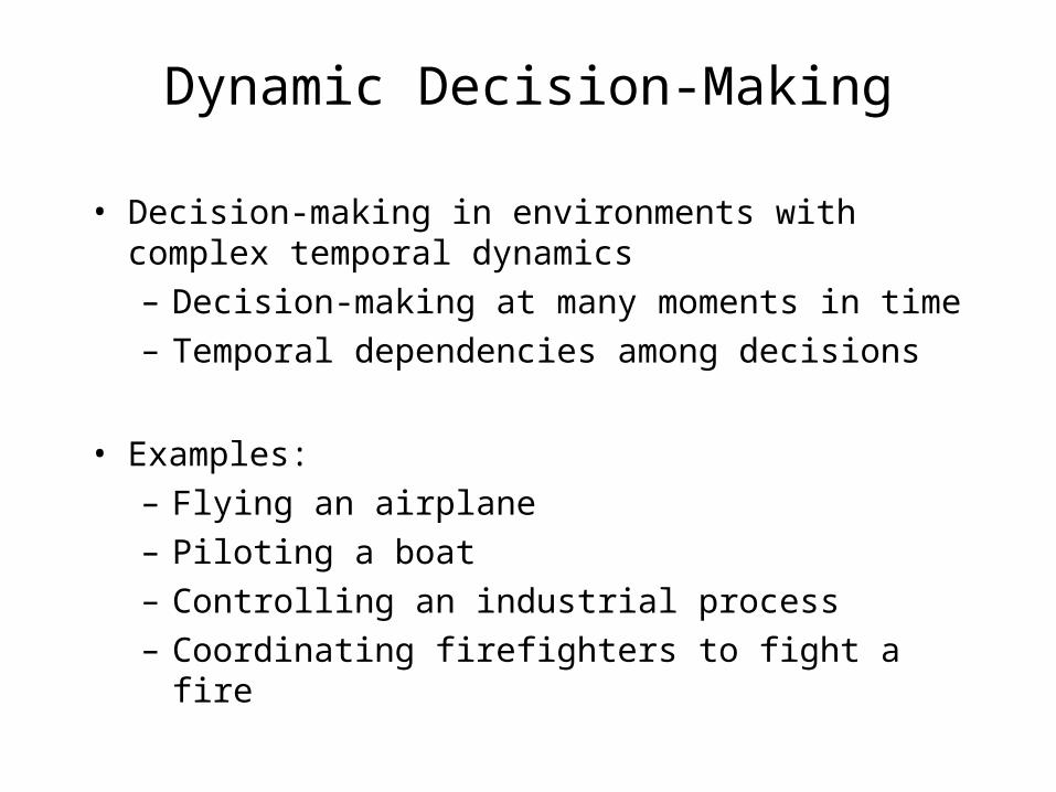
Dynamic Decision-Making

• Decision-making in environments with complex temporal dynamics

– Decision-making at many moments in time

– Temporal dependencies among decisions

• Examples:

– Flying an airplane

– Piloting a boat

– Controlling an industrial process

– Coordinating firefighters to fight a fire

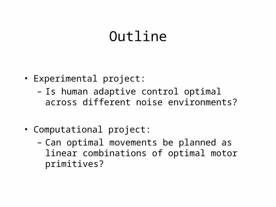
Outline

• Experimental project:

– Is human adaptive control optimal across different noise environments?

• Computational project:

– Can optimal movements be planned as linear combinations of optimal motor primitives?

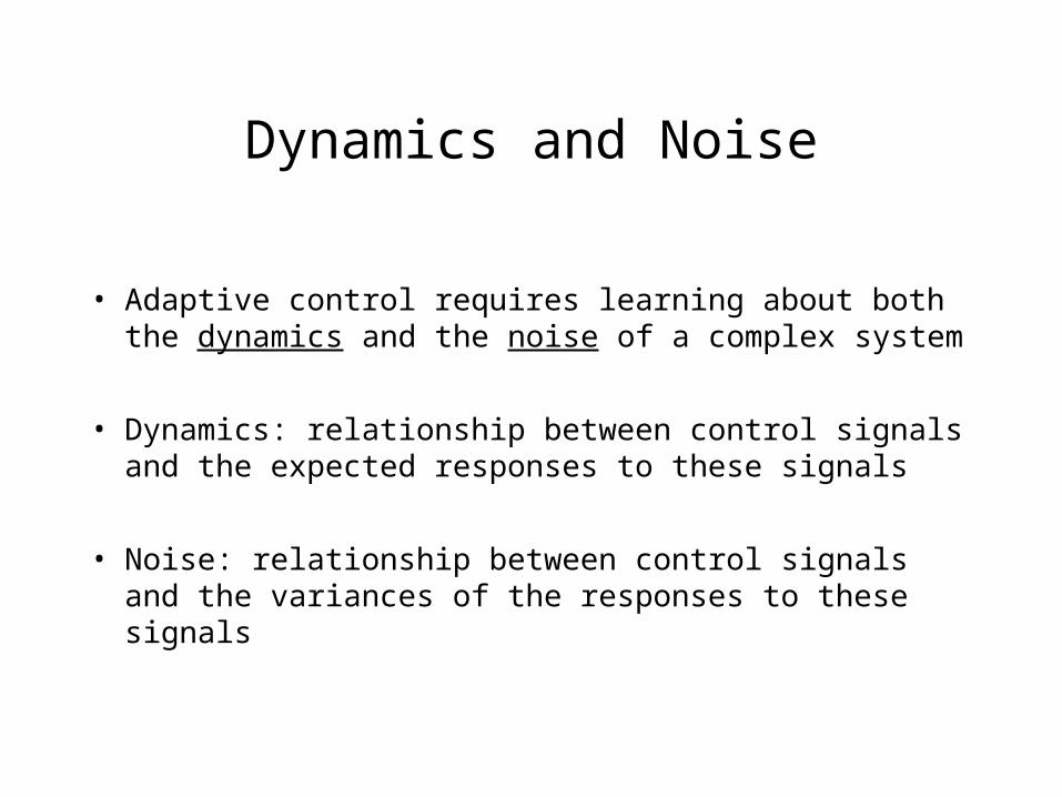
Dynamics and Noise

• Adaptive control requires learning about both the dynamics and the noise of a complex system

• Dynamics: relationship between control signals and the expected responses to these signals

• Noise: relationship between control signals and the variances of the responses to these signals

Dynamics and Noise

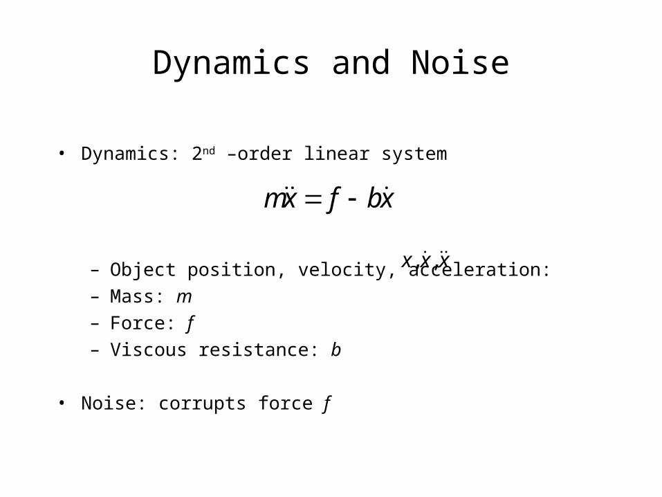
• Dynamics: 2nd –order linear system

– Object position, velocity, acceleration:

– Mass: m

– Force: f

– Viscous resistance: b

• Noise: corrupts force f

xbfxm

xxx ,,

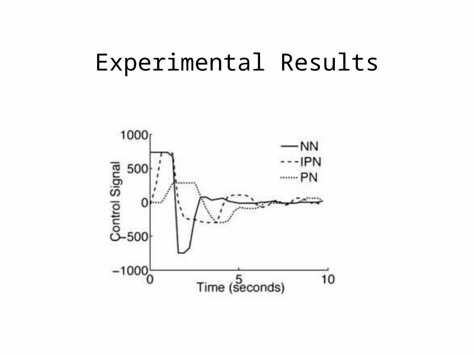
Three Noise Conditions

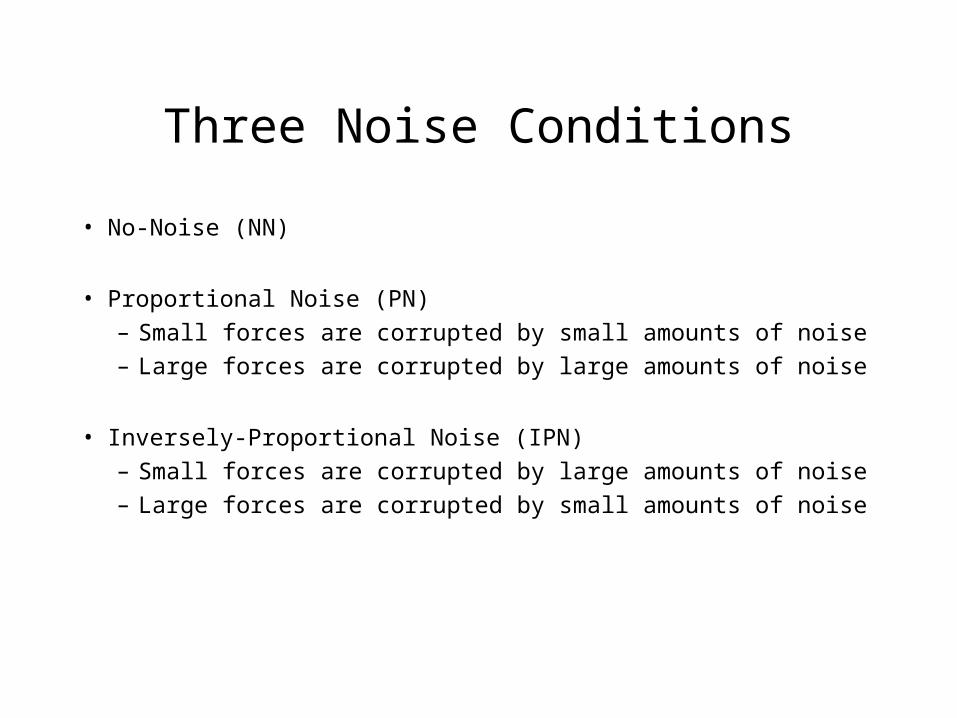
• No-Noise (NN)

• Proportional Noise (PN)

– Small forces are corrupted by small amounts of noise

– Large forces are corrupted by large amounts of noise

• Inversely-Proportional Noise (IPN)

– Small forces are corrupted by large amounts of noise

– Large forces are corrupted by small amounts of noise

Ideal Actors

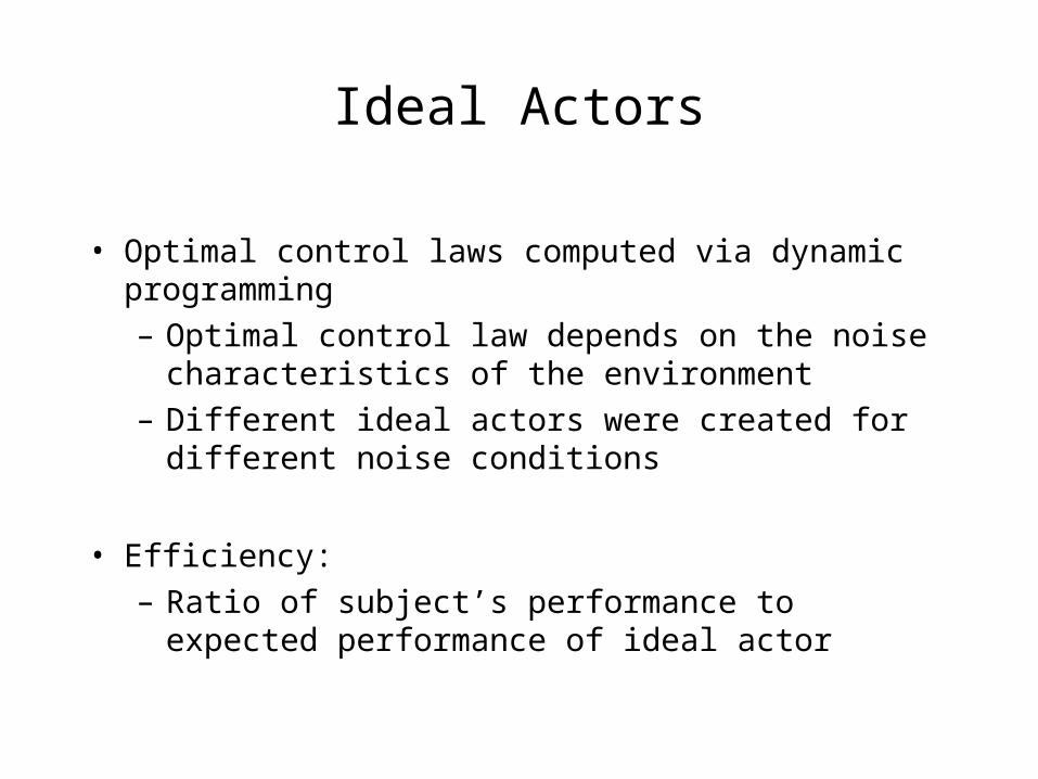
• Optimal control laws computed via dynamic programming

– Optimal control law depends on the noise characteristics of the environment

– Different ideal actors were created for different noise conditions

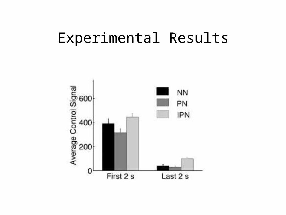
• Efficiency:

– Ratio of subject’s performance to expected performance of ideal actor

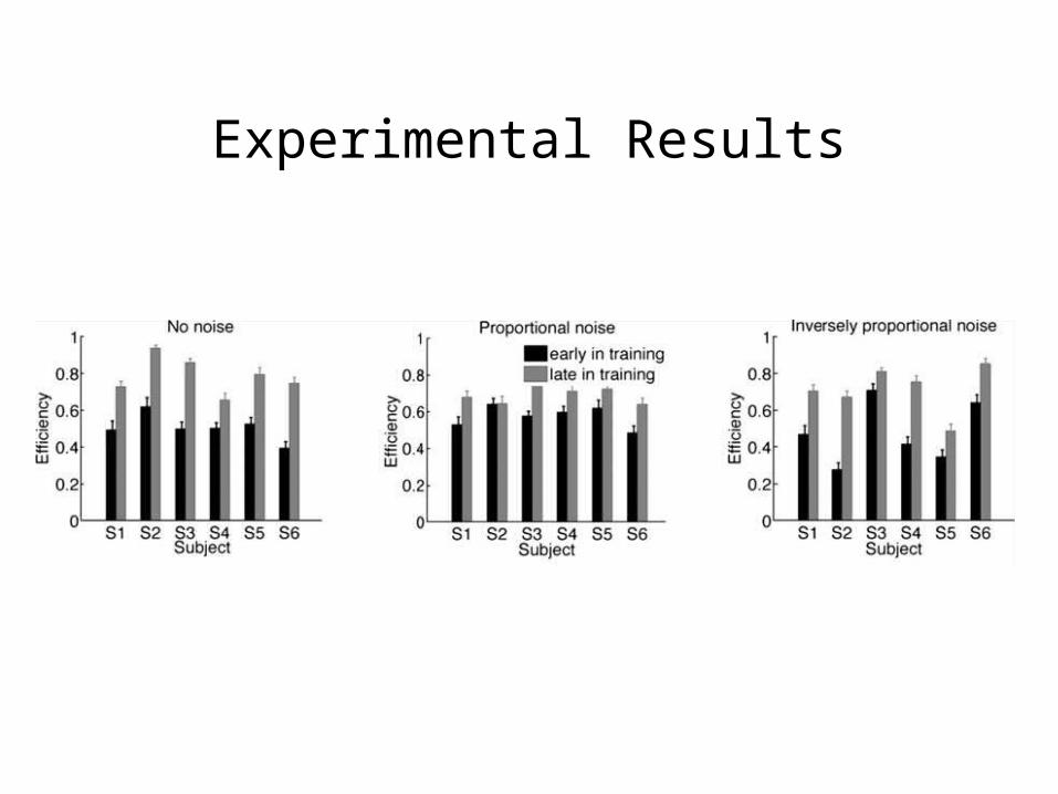
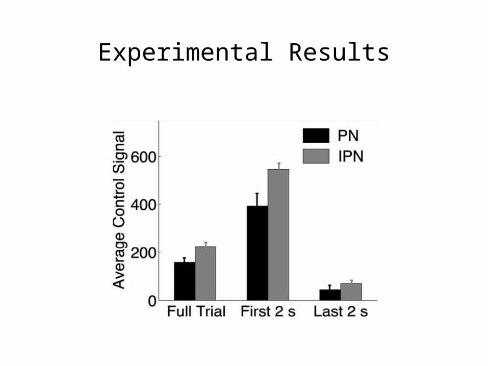
Experimental Results

Experimental Results

Experimental Results

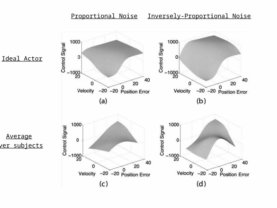
Proportional Noise Inversely-Proportional Noise

Ideal Actor

Average

over subjects

Conclusions

• Subjects learned control strategies tailored to the specific noise characteristics of their conditions

– Allowed them to achieve levels of performance near the information-theoretic upper bounds

• Conclude: Subjects learned to efficiently use all available information to plan and execute control policies that maximized performances on their tasks

Conclusions

• Q: Is human adaptive control optimal across different noise environments?

• A: Yes (under the conditions studied here)

Computational Complexity of Motor Control

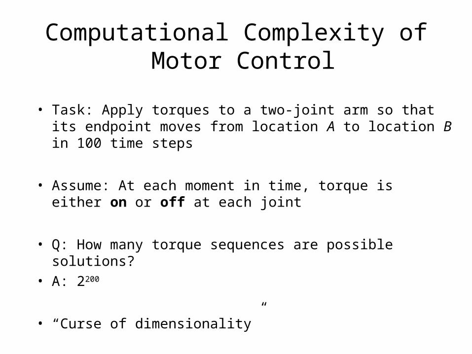
• Task: Apply torques to a two-joint arm so that its endpoint moves from location A to location B in 100 time steps

• Assume: At each moment in time, torque is either on or off at each joint

• Q: How many torque sequences are possible solutions?

• A: 2200

• “Curse of dimensionality”

Motor Synergies

• Motor synergies: dependencies among degrees of freedom

• Motor synergies = motor primitives– Basic units of behavior that can be linearly combined to

form complex units of behavior– To form complex behavior: only need to specify linear coefficients

• Behavioral and physiological evidence

Approach

• Hypothesis: Optimal motor control can be achieved by combining a small number of scaled and time-shifted optimal synergies

• If so, motor control is easy

– Only need to specify scaling coefficients and time-shifts

• Q: How do we find optimal synergies?

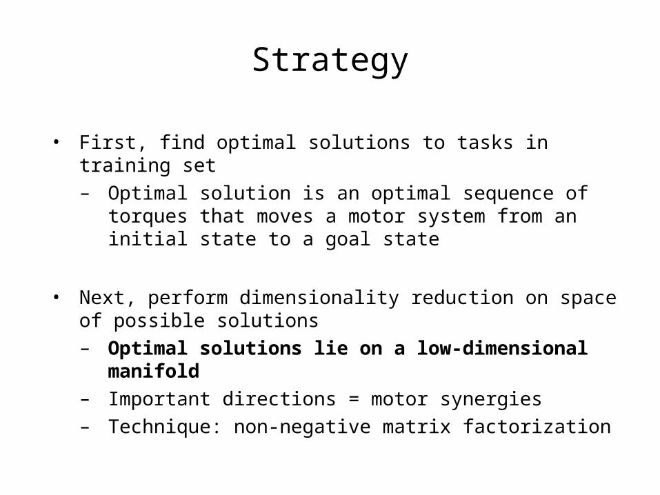
Strategy

• First, find optimal solutions to tasks in training set

– Optimal solution is an optimal sequence of torques that moves a motor system from an initial state to a goal state

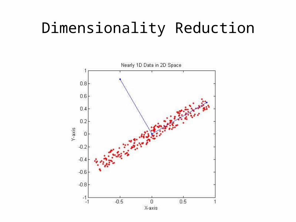
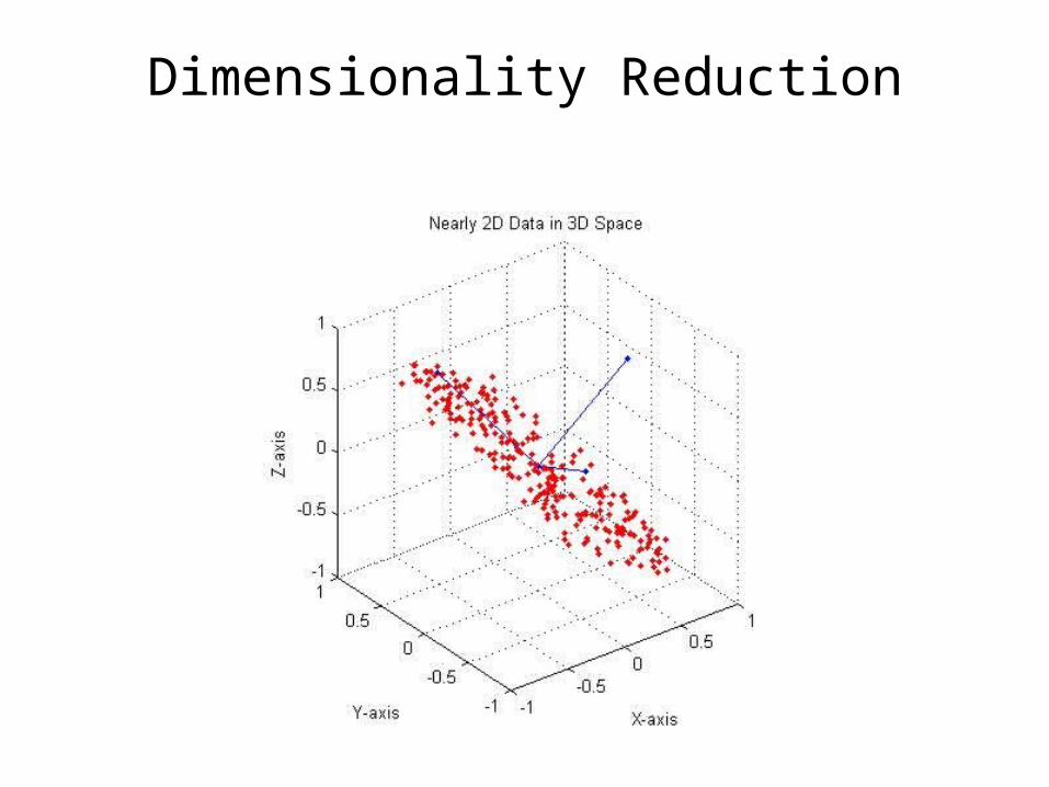
• Next, perform dimensionality reduction on space of possible solutions

– Optimal solutions lie on a low-dimensional manifold

– Important directions = motor synergies

– Technique: non-negative matrix factorization

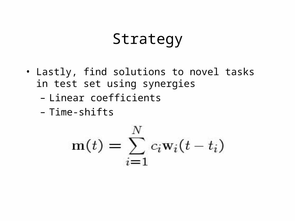
Strategy

• Lastly, find solutions to novel tasks in test set using synergies

– Linear coefficients

– Time-shifts

Motor Tasks

• Reaching task: move the endpoint of a simulated two-joint robot arm from one location to another in a specified time period

• Via-point task: move from one location to another while passing through an intermediate location

Simulations

Example: Reaching task

• 256 tasks in training set

– Find (approximate) optimal solutions to each task

– Find optimal motor synergies via dimensionality reduction

• 64 tasks in test set

– Find solution to each task by combining motor synergies• Linear coefficients

• Time-shifts

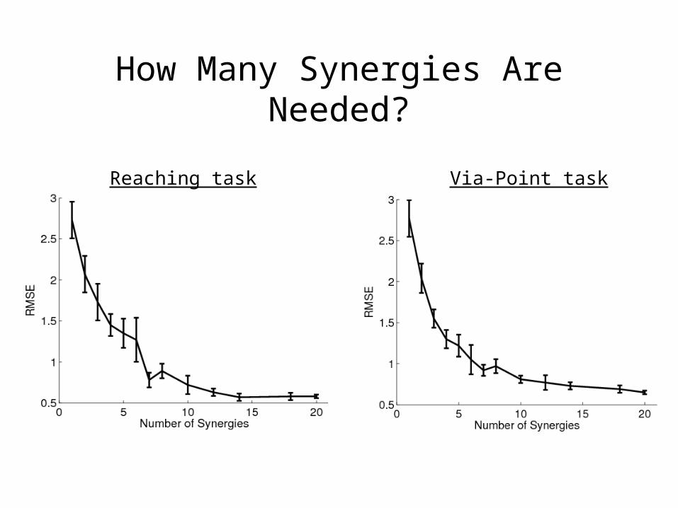
How Many Synergies Are Needed?

Reaching task Via-Point task

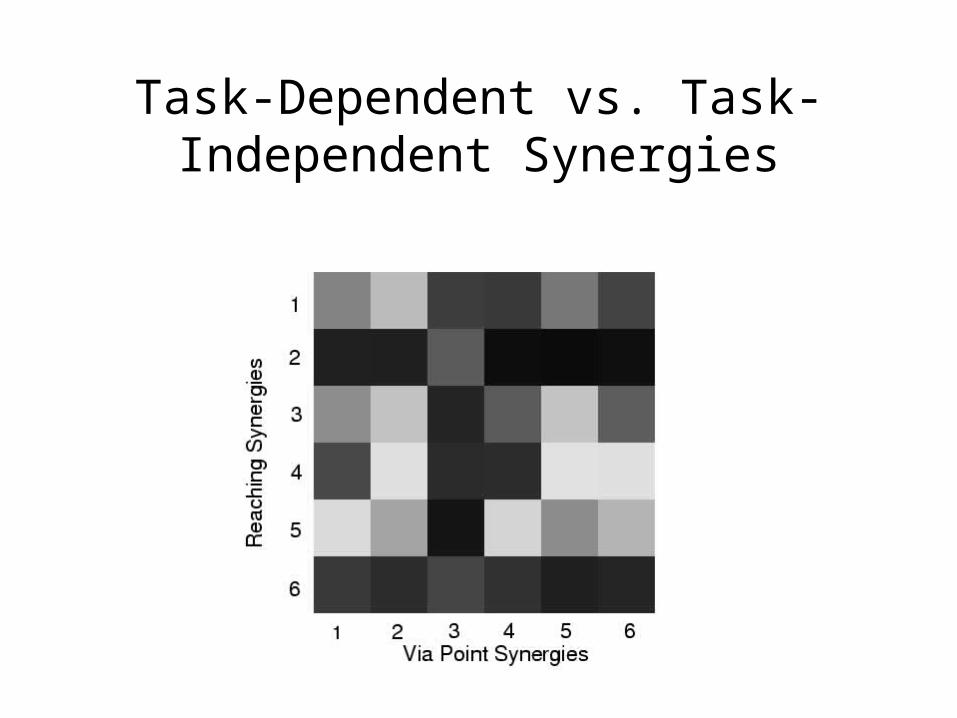
Task-Dependent vs. Task-Independent Synergies

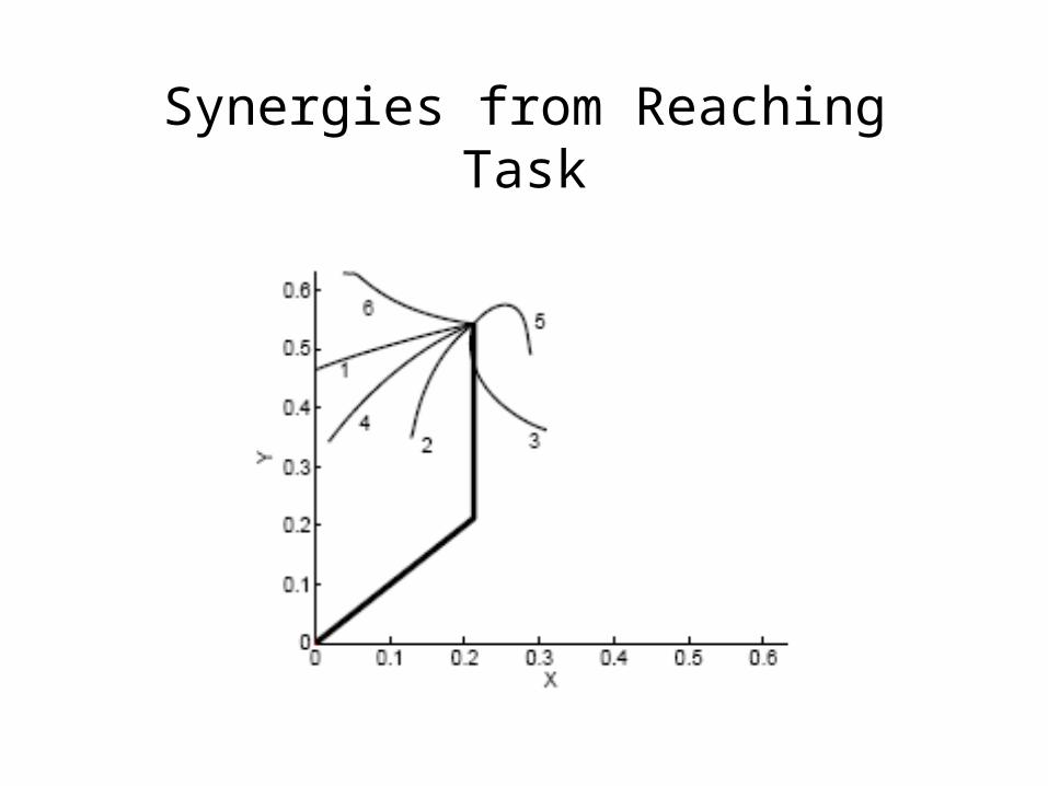
Synergies from Reaching Task

Synergies from Via-Point Task

Fast Learning with Synergies

Summary

• Optimal solutions lie on a low-dimensional manifold– Dimensionality reduction for discovering optimal

synergies

• Near-optimal motor control by combining scaled and time-shifted synergies

• A small number of synergies are sufficient

• Task-dependent and task-independent synergies

• Learning with synergies is fast

• Additional research: two-joint arm with muscle model

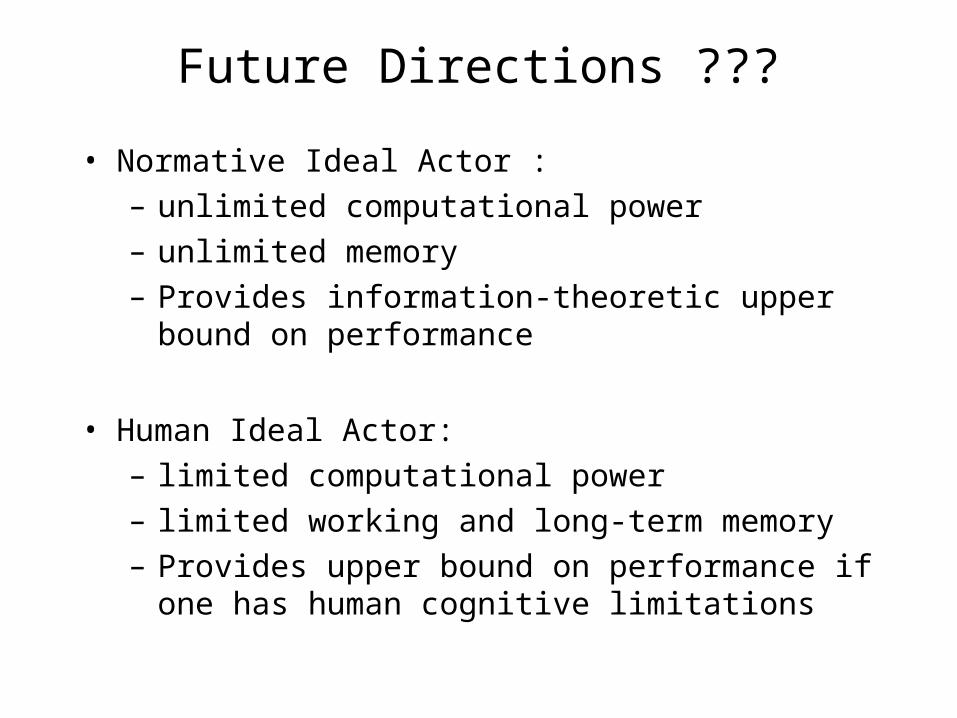
Future Directions ???

• Normative Ideal Actor :

– unlimited computational power

– unlimited memory

– Provides information-theoretic upper bound on performance

• Human Ideal Actor:

– limited computational power

– limited working and long-term memory

– Provides upper bound on performance if one has human cognitive limitations

Experimental Results

Dimensionality Reduction

Dimensionality Reduction