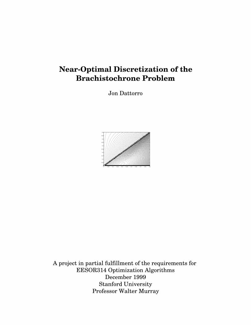
Near-Optimal Discretization of the

Brachistochrone Problem

Jon Dattorro

0 0.05 0.1 0.15 0.2 0.25 0.3 0.35 0.4 0.45 0.50

0.05

0.1

0.15

0.2

0.25

0.3

0.35

0.4

0.45

0.5

A project in partial fulfillment of the requirements for

EESOR314 Optimization Algorithms

December 1999

Stanford University

Professor Walter Murray

Abstract

The analytical solution to the Brachistochrone problem is well known. [Thomas] [Strang] In

this digital age, what is less-well studied is the proper discretization1 of the problem so as

to arrive at an optimal numerical solution. The problem thus posed asks, given a fixed

number of samples with which to discretize a numerical solution, what is the optimal spacing

of those samples along the abscissa? It is intuitively clear that the answer is not equi-

spacing, because the proper spacing must somehow be related to curvature. Indeed, the

study of non-uniform discretization is prompted by observations like this. [Marks] But an

analytical solution to the optimal discretization problem is not what we seek here. What we

develop is a simple numerical algorithm using a piecewise-linear fit to find the best

discretization of the Brachistochrone problem for a fixed given number of samples. We

conclude by speculating as to the best discretization using a fit of any order.

1A discrete one-dimensional signal conventionally refers to a continuous signal sampled with infinite

precision along both axes. A digital signal is a discrete signal, but quantized along the ordinate. Both discrete

and digital signals are said to be sampled signals.

2 Tue Nov 20 2001

1 What exactly is a cycloid?

We defer the reader to an excellent statement of the physical problem given in [Thomas].2

"Among all smooth curves joining two given points, find that one along which a bead might

slide, subject only to the force of gravity, in the shortest time3." Thomas’ problem

statement applies to any two arbitrary points (t,x) �, one implicitly higher than the other.

The analytical solution of this arbitrary problem is most accurately described by him as an

arc of a cycloid. A cycloid is a specific trajectory that is maintained by a strict relationship of

the abscissa t with the ordinate x �, each in the variable φ and the parameter a�;

( )( ) ( )( )axat φ+=φ−φ= cos1,sin (1)

This means, for example, that scaling the ordinate without similarly scaling the abscissa,

produces a trajectory which is not, strictly speaking, a cycloid. The utility of this rigid

definition of the cycloid comes when we describe the solution to this Brachistochrone problem

as "an arc" of a cycloid. That is to say, the solution for arbitrary points is not necessarily a

half-cycle of a cycloid; the solution will always be some portion of a half-cycle of the cycloid

described by Eq.(1). But the solution can never be a half-cycle of a cycloid expanded or

contracted (scaled) in either coordinate alone.

In this paper we restrict our attention to a corresponding normalized mathematical problem,

illustrated in Figure�1. The normalization is such that we restrict the range x and domain tof the function describing the path travelled by the bead, such that

[ ] [ ]txπ∈∈2

,0,1,0

(2)

and we specify the two "given points" as the boundaries of these two intervals. The purpose

of this normalization is to make our exposition less abstract, the tradeoff being some loss of

generality. The given start and end points are chosen such that the expected solution is

precisely one half-cycle of the cycloid Eq.(1) having parameter a�=�1/2�, the half-cycle

occurring when φ�=�π�.

2a = 1

tπ a = π/2

x

Figure 1. A bead travels along the "normalized" path shown, motivated only by gravity.

2Neither [Thomas] nor [Strang] present the method of solution, known as the calculus of variations. The

method and the solution are presented in [Bliss].3Brachistochrone is Greek for "shortest time".

3 Tue Nov 20 2001

1.1 A Good GuessThis Brachistochrone problem is unusual in so far as we have a good obvious guess for the

solution, which is not too far from the optimal solution; a straight line between the two

normalized points,

txo π−= 2

1

(3)

Eq.(3) will serve as the initialization of the curve x in all our subsequent experiments.

1.2 The Analytical SolutionThe continuous optimal solution to the Brachistochrone problem is the curve x that

minimizes the following integral:

( ) � ( )�

( )�

ktdxk

xTπ+=

−+

=2

1;1

1

21 π

22

2

0

tdxd

∆

(4)

A lower bound Tmin on the value of the integral is provided by the cycloid trajectory

described by the parametric Eq.(1) over one half-cycle;

( )?

| ( ) � ( ) ( )��

||

|||

( )

3653480212

1T

=

φφπ

=,1.qE

22

0,1.qEmin =π=φ

−+

== .k

dxk

xT

a

dxd

dtd

a

21

21

(5)

The constant k is chosen for convenience such that T(xo)=1 for xo from Eq.(3).

2 A Strategy for Discrete SolutionWe will numerically approximate x by finding a sampled, linearly interpolated version of it

that minimizes Eq.(4). We change the meaning of our nomenclature by now designating xto represent a vector of sample values of the continuous function in Eq.(2). Likewise, we

hereinafter designate the vector t to represent the corresponding instants in time.

?( ) [ ] ( ) [ ]

?( ) ( ) ( ) ( )ttxx

itix

tx

π====

π∈∈

ℜ∈ℜ∈ NN

∆∆∆∆2

N,01,0N,11

2,0,1,0

,

(6)

4 Tue Nov 20 2001

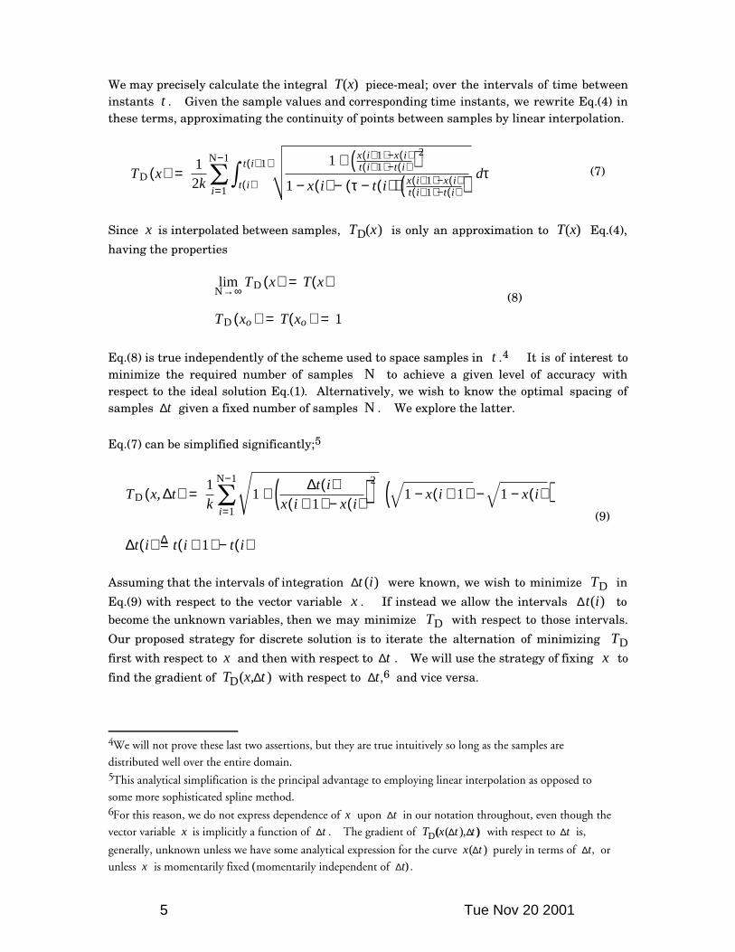
We may precisely calculate the integral T(x) piece-meal; over the intervals of time between

instants t�. Given the sample values and corresponding time instants, we rewrite Eq.(4) in

these terms, approximating the continuity of points between samples by linear interpolation.

( ) ( )

( )� ( ) ( )( ) ( )( )

( ) ( )( ) ( ) ( )( ) ( )( )

��d

itixkxT

−+−+

−+−+

+

=

−

11

211

1

1

1N

D τ−τ−−

+=

1

1

21

ititixix

ititixix

it

it

i

(7)

Since x is interpolated between samples, TD(x) is only an approximation to T(x) Eq.(4),

having the properties

( ) ( )?

( ) ( ) 1

lim∞→

D

DN

xTxT

xTxT

==

=

oo

(8)

Eq.(8) is true independently of the scheme used to space samples in t�.4 It is of interest to

minimize the required number of samples N to achieve a given level of accuracy with

respect to the ideal solution Eq.(1). Alternatively, we wish to know the optimal spacing of

samples ∆t given a fixed number of samples N�. We explore the latter.

Eq.(7) can be simplified significantly;5

( ) ( )( ) ( )( )

�( )

�( )

�( )

?( ) ( ) ( )ititit

ixixixix

itk

t,xT

∆

=

− 2

1

1N

D

−+=∆

−−+−−+

∆+=∆

1

1111

11

i

(9)

Assuming that the intervals of integration ∆t �(i�) were known, we wish to minimize TD in

Eq.(9) with respect to the vector variable x�. If instead we allow the intervals ∆t�(i�) to

become the unknown variables, then we may minimize TD with respect to those intervals.

Our proposed strategy for discrete solution is to iterate the alternation of minimizing TDfirst with respect to x and then with respect to ∆t�. We will use the strategy of fixing x to

find the gradient of TD(x,∆t�) with respect to ∆t�,6 and vice versa.

4We will not prove these last two assertions, but they are true intuitively so long as the samples are

distributed well over the entire domain.5This analytical simplification is the principal advantage to employing linear interpolation as opposed to

some more sophisticated spline method.6For this reason, we do not express dependence of x upon ∆t in our notation throughout, even though the

vector variable x is implicitly a function of ∆t�. The gradient of TD(x(∆t�),∆t�) with respect to ∆t is,

generally, unknown unless we have some analytical expression for the curve x(∆t�) purely in terms of ∆t�, or

unless x is momentarily fixed (momentarily independent of ∆t�).

5 Tue Nov 20 2001

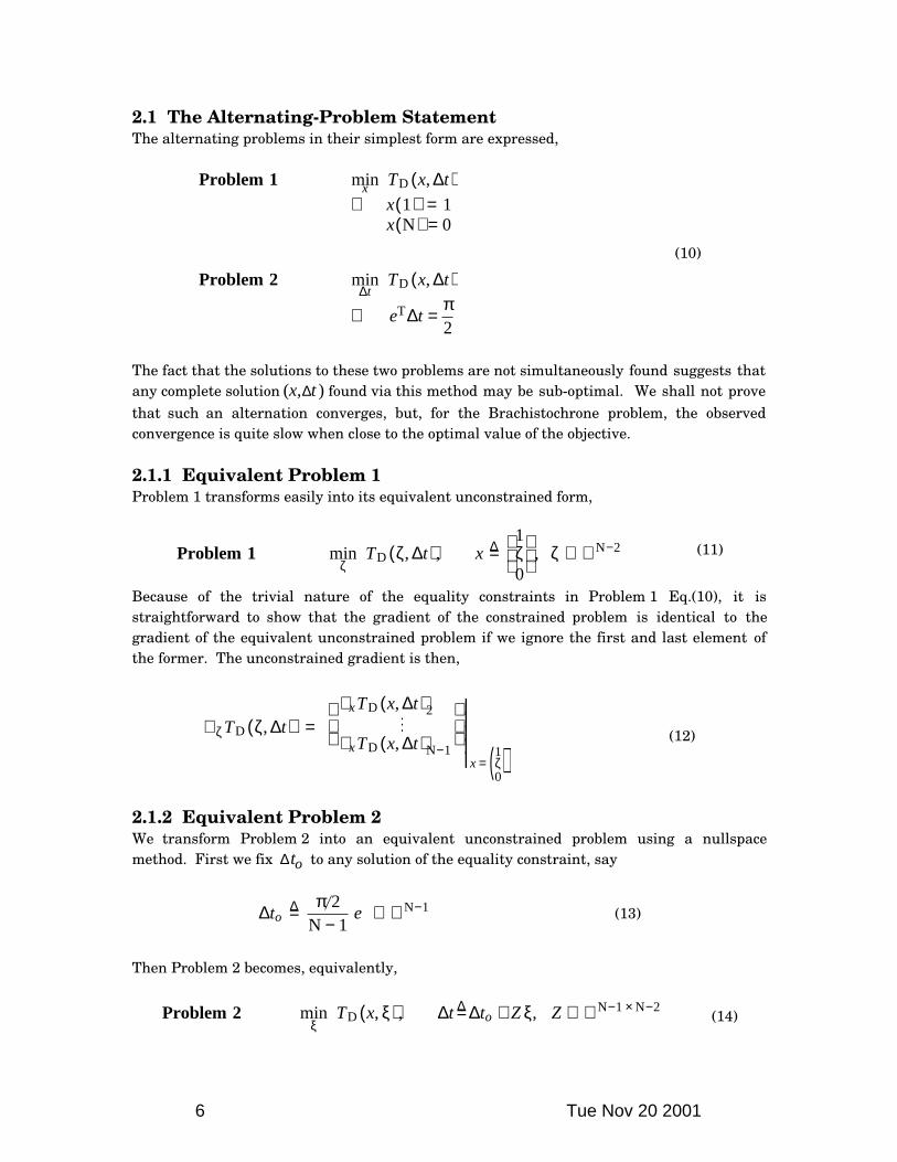
2.1 The Alternating-Problem StatementThe alternating problems in their simplest form are expressed,

( )( )( )

??

( )2melborP

1melborP

2

,min

0N11

,min

∆t

x

te

txT

xx

txT

T

D

D

π=∆∋

∆

==∋∆

(10)

The fact that the solutions to these two problems are not simultaneously found suggests that

any complete solution (x,∆t�) found via this method may be sub-optimal. We shall not prove

that such an alternation converges, but, for the Brachistochrone problem, the observed

convergence is quite slow when close to the optimal value of the objective.

2.1.1 Equivalent Problem 1Problem�1 transforms easily into its equivalent unconstrained form,

( )

1melborP ,0

1,,min −∆

ζxtT 2N

D ℜ∈ζζ=∆ζ

(11)

Because of the trivial nature of the equality constraints in Problem�1 Eq.(10), it is

straightforward to show that the gradient of the constrained problem is identical to the

gradient of the equivalent unconstrained problem if we ignore the first and last element of

the former. The unconstrained gradient is then,

( )( )�( )

?||

|||

( )∆∇

∆∇=∆ζ∇

ζ=−

ζtxT

txTtT

0

11ND

2D

D,

,,

xx

x

(12)

2.1.2 Equivalent Problem 2We transform Problem�2 into an equivalent unconstrained problem using a nullspace

method. First we fix ∆to to any solution of the equality constraint, say

ℜ∈−

π=∆ et −∆o 1N

2 1N

(13)

Then Problem�2 becomes, equivalently,

( )2melborP ,,,min −×−∆ξ

ZZttxT 2N1ND ℜ∈ξ+∆=∆ξ o

(14)

6 Tue Nov 20 2001

where ċ? ?

? ? ?? ? ?

? ?

ZeZ =

−−−

= 0

10

101111

dna T

(15)

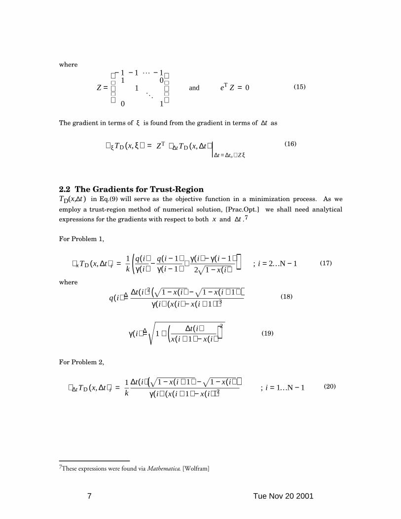
The gradient in terms of ξ is found from the gradient in terms of ∆t as

( ) ( )? |

?

∆∇=ξ∇ξ+∆=∆

∆ξ txTZxT DT

D ,,Ztt

t

o

(16)

2.2 The Gradients for Trust-RegionTD(x,∆t �) in Eq.(9) will serve as the objective function in a minimization process. As we

employ a trust-region method of numerical solution, [Prac.Opt.] we shall need analytical

expressions for the gradients with respect to both x and ∆t�.7

For Problem�1,

( ) ( )( )

( )( )

( ) ( )( )

�( ) −=−

−γ−γ+−γ−−

γ=∆∇ ix …i

ix

iiiiq

iiq

ktxTD 1N2;

12

1111

,

(17)

where

( )( ) ( )�

( )�

( )( ) ( ) ( )( )ixixi

ixixitiq

+−γ+−−−∆

=∆ 3

2

1

111

(18)

( ) ( )( ) ( )( )

�−+

∆+=γixix

iti ∆

11

2

(19)

For Problem�2,

( )( ) ( )�

( )�

( )( ) ( ) ( )( )

−=−+γ

−−+−∆=∆∇ ∆ it …i

ixixi

ixixit

ktxT 2D 1N1;

1

1111,

(20)

7These expressions were found via Mathematica. [Wolfram]

7 Tue Nov 20 2001

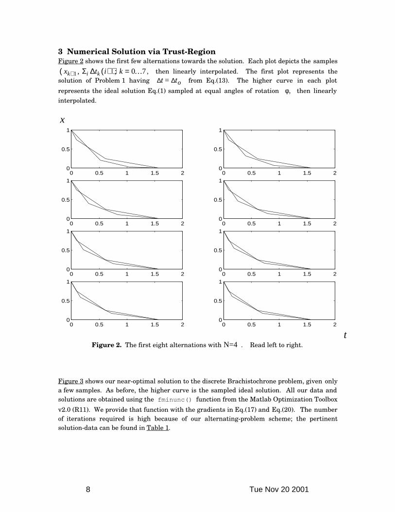
3 Numerical Solution via Trust-RegionFigure�2 shows the first few alternations towards the solution. Each plot depicts the samples

( )( ) =∆Σ …kitx + kik 1 70;, , then linearly interpolated. The first plot represents the

solution of Problem�1 having ∆t�=�∆to from Eq.(13). The higher curve in each plot

represents the ideal solution Eq.(1) sampled at equal angles of rotation φ�, then linearly

interpolated.

x

0 0.5 1 1.5 20

0.5

1

0 0.5 1 1.5 20

0.5

1

0 0.5 1 1.5 20

0.5

1

0 0.5 1 1.5 20

0.5

1

0 0.5 1 1.5 20

0.5

1

0 0.5 1 1.5 20

0.5

1

0 0.5 1 1.5 20

0.5

1

0 0.5 1 1.5 20

0.5

1

tFigure 2. The first eight alternations with N�=�4. Read left to right.

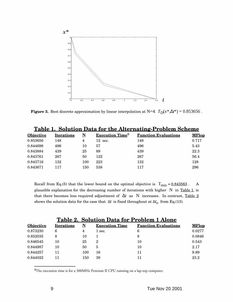
Figure�3 shows our near-optimal solution to the discrete Brachistochrone problem, given only

a few samples. As before, the higher curve is the sampled ideal solution. All our data and

solutions are obtained using the fminunc() function from the Matlab Optimization Toolbox

v2.0 (R11). We provide that function with the gradients in Eq.(17) and Eq.(20). The number

of iterations required is high because of our alternating-problem scheme; the pertinent

solution-data can be found in Table�1.

8 Tue Nov 20 2001

x*

0 0.2 0.4 0.6 0.8 1 1.2 1.4 1.60

0.1

0.2

0.3

0.4

0.5

0.6

0.7

0.8

0.9

1

t

Figure 3. Best discrete approximation by linear interpolation at N=4. TD(x*,∆t*) = 0.853656�.

Table 1. Solution Data for the Alternating-Problem SchemeObjective Iterations N Execution Time8 Function Evaluations MFlop

0.853656 148 4 12 sec. 148 0.717

0.844698 496 10 57 496 5.43

0.843884 439 25 89 439 22.3

0.843761 267 50 122 267 56.4

0.843716 132 100 223 132 128

0.843671 117 150 538 117 296

Recall from Eq.(5) that the lower bound on the optimal objective is Tmin�=�0.843563�. A

plausible explanation for the decreasing number of iterations with higher N in Table�1, is

that there becomes less required adjustment of ∆t as N increases. In contrast, Table 2

shows the solution data for the case that ∆t� is fixed throughout at�∆to from Eq.(13).

Table 2. Solution Data for Problem 1 AloneObjective Iterations N Execution Time Function Evaluations MFlop

0.873230 6 4 1 sec. 6 0.0277

0.852035 8 10 1 8 0.0846

0.846545 10 25 2 10 0.543

0.844987 10 50 5 10 2.17

0.844257 11 100 16 11 9.89

0.844022 11 150 39 11 23.2

8The execution time is for a 300MHz Pentium�II CPU running on a lap-top computer.

9 Tue Nov 20 2001

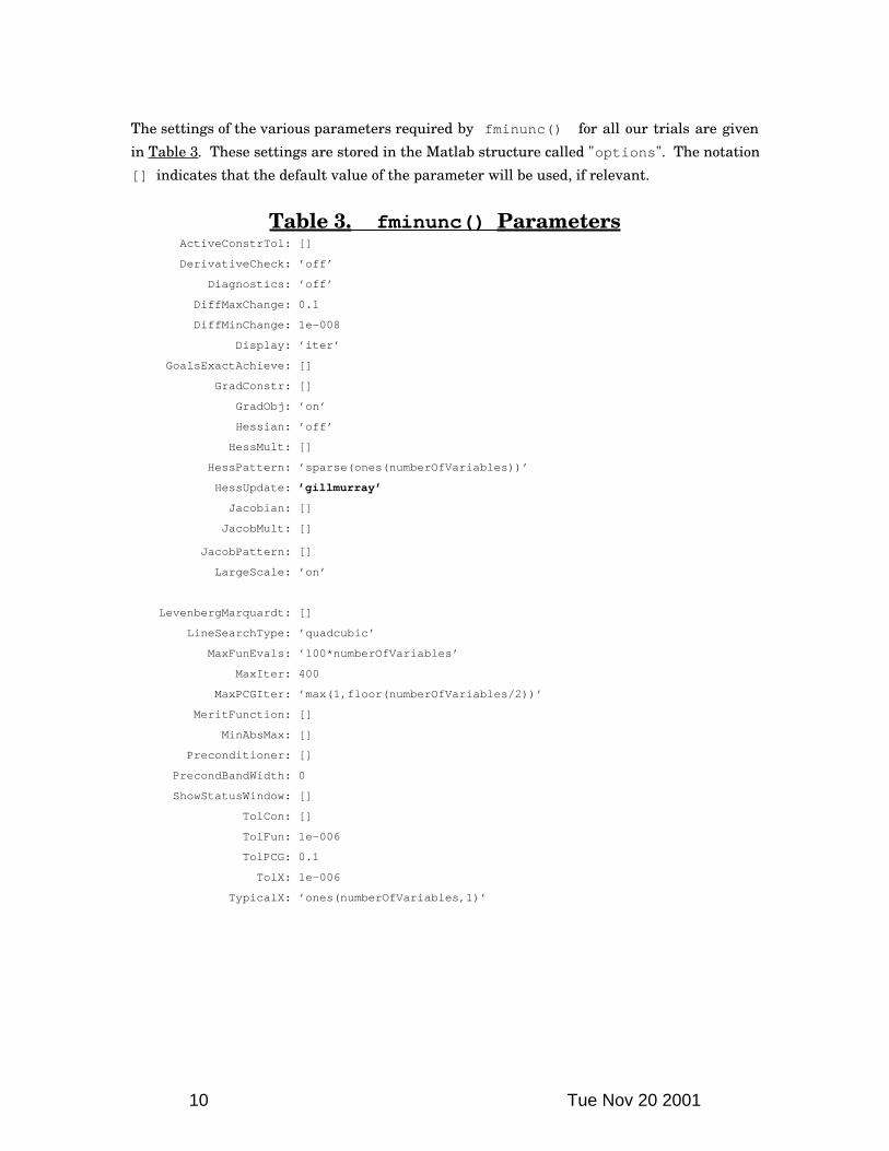
The settings of the various parameters required by fminunc() for all our trials are given

in Table�3. These settings are stored in the Matlab structure called "options". The notation

[] indicates that the default value of the parameter will be used, if relevant.

Table 3. fminunc() Parameters ActiveConstrTol: []

DerivativeCheck: ’off’

Diagnostics: ’off’

DiffMaxChange: 0.1

DiffMinChange: 1e-008

Display: ’iter’

GoalsExactAchieve: []

GradConstr: []

GradObj: ’on’

Hessian: ’off’

HessMult: []

HessPattern: ’sparse(ones(numberOfVariables))’

HessUpdate: ’gillmurray’

Jacobian: []

JacobMult: []

JacobPattern: []

LargeScale: ’on’

LevenbergMarquardt: []

LineSearchType: ’quadcubic’

MaxFunEvals: ’100*numberOfVariables’

MaxIter: 400

MaxPCGIter: ’max(1,floor(numberOfVariables/2))’

MeritFunction: []

MinAbsMax: []

Preconditioner: []

PrecondBandWidth: 0

ShowStatusWindow: []

TolCon: []

TolFun: 1e-006

TolPCG: 0.1

TolX: 1e-006

TypicalX: ’ones(numberOfVariables,1)’

10 Tue Nov 20 2001

4 Contour Plots of Objective

x(3)

0 0.05 0.1 0.15 0.2 0.25 0.3 0.35 0.4 0.45 0.50

0.05

0.1

0.15

0.2

0.25

0.3

0.35

0.4

0.45

0.5

x(2)

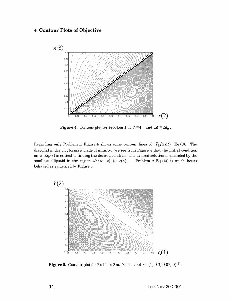
Figure 4. Contour plot for Problem�1 at N�=�4 and ∆t�=�∆to�.

Regarding only Problem�1, Figure�4 shows some contour lines of TD(x,∆t�) Eq.(9). The

diagonal in the plot forms a blade of infinity. We see from Figure�4 that the initial condition

on x Eq.(3) is critical to finding the desired solution. The desired solution is encircled by the

smallest ellipsoid in the region where x(2)�>�x(3)�. Problem 2 Eq.(14) is much better

behaved as evidenced by Figure 5.

ξ(2)

-0.5 -0.4 -0.3 -0.2 -0.1 0 0.1 0.2 0.3 0.4 0.5-0.5

-0.4

-0.3

-0.2

-0.1

0

0.1

0.2

0.3

0.4

0.5

ξ(1)

Figure 5. Contour plot for Problem�2 at N�=�4 and x�=�(1, 0.3, 0.03, 0)T�.

11 Tue Nov 20 2001

5 ConclusionsThe continuous Brachistochrone problem can be fit well by a piecewise-linear discrete

approximation. But Eq.(8) tells us that there is error built into our fit which only disappears

as N�→�∞�. It is obvious that the most error will occur for low N �, which is why we

concentrated there. What is not obvious is the best spacing of samples ∆t given any finite

N �. We observed that with no optimization of the sample spacing, our linear fit makes its

worst errors at locations of high curvature. That observation motivated a look into

optimization of the sample-spacing vector ∆t�. Because of the proximity of our near-optimal

solution for N�=�4 to the sampled ideal solution, illustrated in Figure�3, we speculate that

the best sample spacing corresponds to equal angles of rotation φ in Eq.(1). We recommend

that spacing independent of the particular order fit used to solve the discrete

Brachistochrone problem. The data observed in Table�1 tells us that as N is increased, the

sample spacing becomes less important. In any case, we developed a numerical algorithm

which calculates, in the second phase of two alternating minimization problems, the best

sample spacing for our chosen piecewise-linear fit.

12 Tue Nov 20 2001

References

[Bliss] G. A. Bliss, Calculus of Variations, Mathematical Association of America, 1925

[Marks] Robert J. Marks II, editor, Advanced Topics in Shannon Sampling and

Interpolation Theory, Springer-Verlag, 1993

[Prac.Opt.] Philip E. Gill, Walter Murray, Margaret H. Wright, Practical Optimization,

Academic Press, 1981

[Strang] Gilbert Strang, Calculus, Wellesley-Cambridge Press, 1991

[Thomas] George B. Thomas, Calculus and Analytic Geometry, 4th edition, Addison-Wesley,

1972

[Wolfram] Stephen Wolfram, Mathematica, Third Edition, Cambridge University Press,

1996

13 Tue Nov 20 2001