NEARSHORE HYDRODYNAMICS AT KAANAPALI, MAUl &

HAW AlI EXTREME WA VB STATISTICS

A THESIS SUBMITTED TO THE GRADUATE DMSION OF THE

UNIVERSITY OF HAW AI'I IN PARTIAL FULFILLMENT

OF THE REQUIREMENTS FOR THE DEGREE OF

MASTER OF SCIENCE

IN

GEOLOGY & GEOPHYSICS

DECEMBER 2007

By Sean Vitousek

Thesis Committee:

Chip Fletcher, Chairperson Mark Merrifield

GenoPawlak Robert Dunn

We certify that we have read this thesis and that, in our opinion, it is satisfactory in scope and quality as a thesis for the degree of Master of Science in Geology & Geophysics.

THESIS COMMITTEE

Chairperson

ii

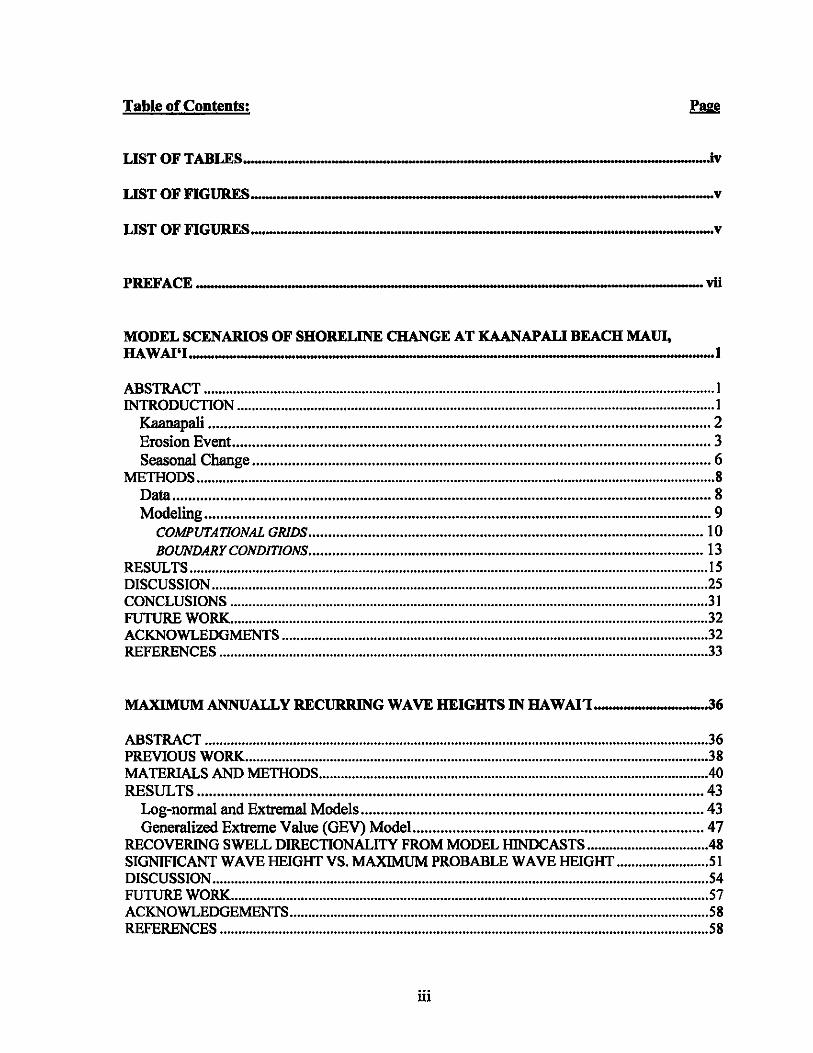
Table of Contents:

LIST OF TABLES_ .................... __________ ._._,,_,,_,,_,,_,,,_,,_,,_,, __ _ , ____ • .iv

LIST OF FIGURES ____ ... _ .. __ . _,,_,,_,,_,,_,,_,,_,,_,,_,,_,,_,, ____ • _ll_ .. _ .. _"._,,_,,_,,_. _"_"' __ . _______ v

LIST OF FIGURES ........................................................... __ .............. __ .......... __ ._ ••• _.v

PREFACE _""". I

_,, ___ 0 ___ ,_,_,_,_,_,,_, _____ ._u_,,_"_"_"_11._._. ___ ,_._. ____ vii

MODEL SCENARIOS OF SHORELINE CHANGE AT KAANAPALI BEACH MAUl. HA W AI"I .................... _ ............... ___ .. _ .. __ ... __ ..................... ___ ••• _ ............... _.1

ABSTRACT ........................................................................................................................................... 1 INTRODUCTION .................................................................................................................................. 1

Kaanapali .............................................................................................................................. 2 Erosion Event ........................................................................................................................ 3 Seasonal Change ................................................................................................................... 6

METHODS ............................................................................................................................................. 8 Data ....................................................................................................................................... 8 Modeling ............................................................................................................................... 9

COMPUTATIONAL GRIDS ................................................................................................... 10

BOUNDARYCONDmONS ................................................................................................... 13 RESULTS ............................................................................................................................................. 15 DISCUSSION ....................................................................................................................................... 25 CONCLUSIONS .................................................................................................................................. 31 FUTURE WORK .................................................................................................................................. 32 ACKNOWLEDGMENTS .................................................................................................................... 32 REFERENCES ..................................................................................................................................... 33

MAXIMUM ANNUALLY RECURRING WAVE HEIGHTS IN HA WAI'1 __ ... _ ... _ ... _ ... _ .. _. _-,.3,6

ABSTRACT ......................................................................................................................................... 36 PREVIOUS WORK .............................................................................................................................. 38 MATERIALS AND METHODS .......................................................................................................... 40 RESULTS ............................................................................................................................... 43

Log-nonnal and Extremal Models ...................................................................................... 43 Generalized Extreme Value (GEV) Model.. ....................................................................... 47

RECOVERING SWELL DIRECTIONALITY FROM MODEL HINDCASTS ................................. 48 SIGNIFICANT WAVE HEIGHT VS. MAXIMUM PROBABLE WAVE HEIGHT ......................... 51 DISCUSSION ....................................................................................................................................... 54 FUTURE WORK .................................................................................................................................. 57 ACKNOWLEDGEMENTS .................................................................................................................. 58 REFERENCES ..................................................................................................................................... 58

iii

LIST OF TABLES

Table 1 - Model Parameters .................................................................................................... 12 Table 2 - Observed vs. modeled tidal constituents at instrument locations ............................ 16 Table 3 - The observed and modeled directional annually recurring maximum significant

wave heights using extremal and GEV exceedance probability models. Wave hindcasts of Buoy 3 do not return more than one swell event per year in the southerly and westerly directional windows; hence Buoy 1 is used instead ........................................................ 49

iv

LIST OF FIGURES

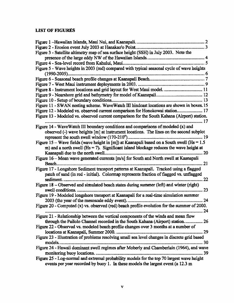
Figure 1 -Hawaiian Islands, Maui Nui, and Kaanapali ............................................................ 2 Figure 2 - Erosion event July 2003 at Hanakao'o Point... ......................................................... 3 Figure 3 - Satellite altimetry map of sea surface height (SSH) in July 2003. Note the

presence of the large eddy NW of the Hawaiian Islands .................................................. 4 Figure 4 - Sea-level record from Kahului, Maui ....................................................................... 5 Figure 5 - Wave heights in 2003 (red) compared with typical seasonal cycle of wave heights

(1990-2005) ....................................................................................................................... 6 Figure 6 - Seasonal beach profile changes at Kaanapali Beach. ............................................... 7 Figure 7 - West Maui instrument deployments in 2003 ........................................................... 9 Figure 8 -Instrument locations and grid layout for West Maui model. ................................. 11 Figure 9 - Nearshore grid and bathymetry for model ofKaanapali... ..................................... 12 Figure 10 - Setup of boundary conditions ............................................................................... 13 Figure 11 - SWAN nesting scheme. WaveWatch ill hindcast locations are shown in boxes. 15 Figure 12 - Modeled vs. observed current comparison for Honokowai station ...................... 17 Figure 13 - Modeled vs. observed current comparison for the South Kahana (Airport) station.

......................................................................................................................................... 17 Figure 14 - WaveWatch ill boundary conditions and comparisons of modeled (x) and

observed (-) wave heights [m] at instrument locations. The lines on the second subplot represent the south swell window (170-21 0") ................................................................. 19

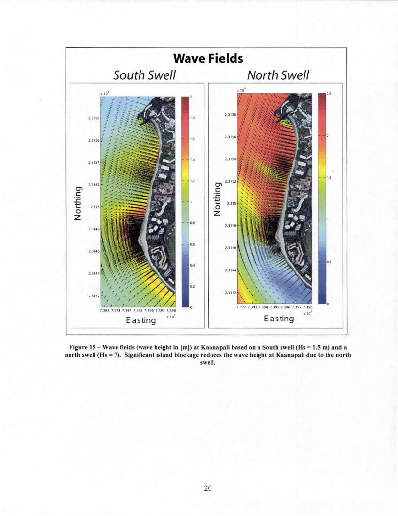
Figure 15 - Wave fields (wave height in [m]) at Kaanapali based on a South swell (Hs = 1.5 m) and a north swell (Hs = 7). Significant island blockage reduces the wave height at Kaanapali due to the north swell ..................................................................................... 20

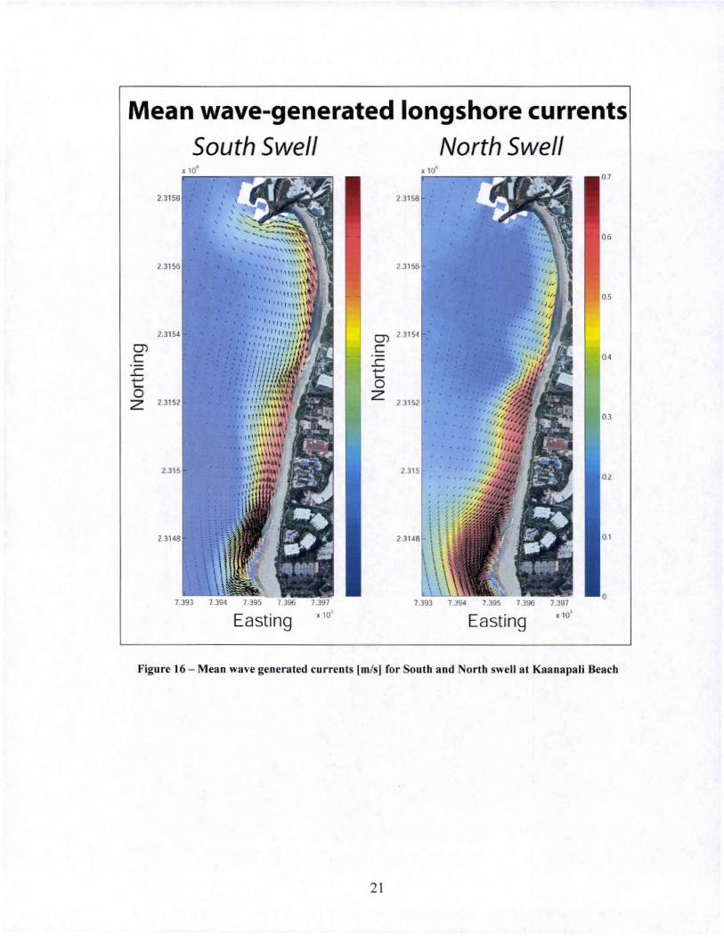
Figure 16 - Mean wave generated currents [mls] for South and North swell at Kaanapali Beach ............................................................................................................................... 21

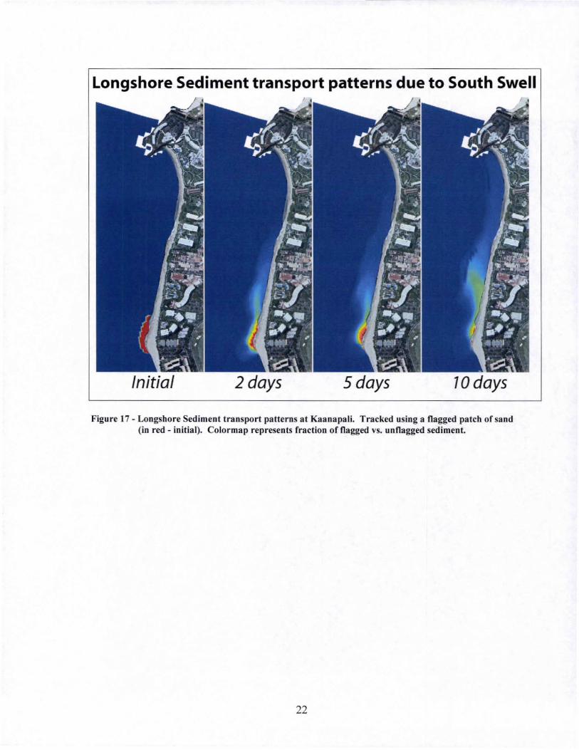
Figure 17 - Longshore Sediment transport patterns at Kaanapali. Tracked using a flagged patch of sand (in red - initial). Colormap represents fraction of flagged vs. unflagged sediment ......................................................................................................................... 22

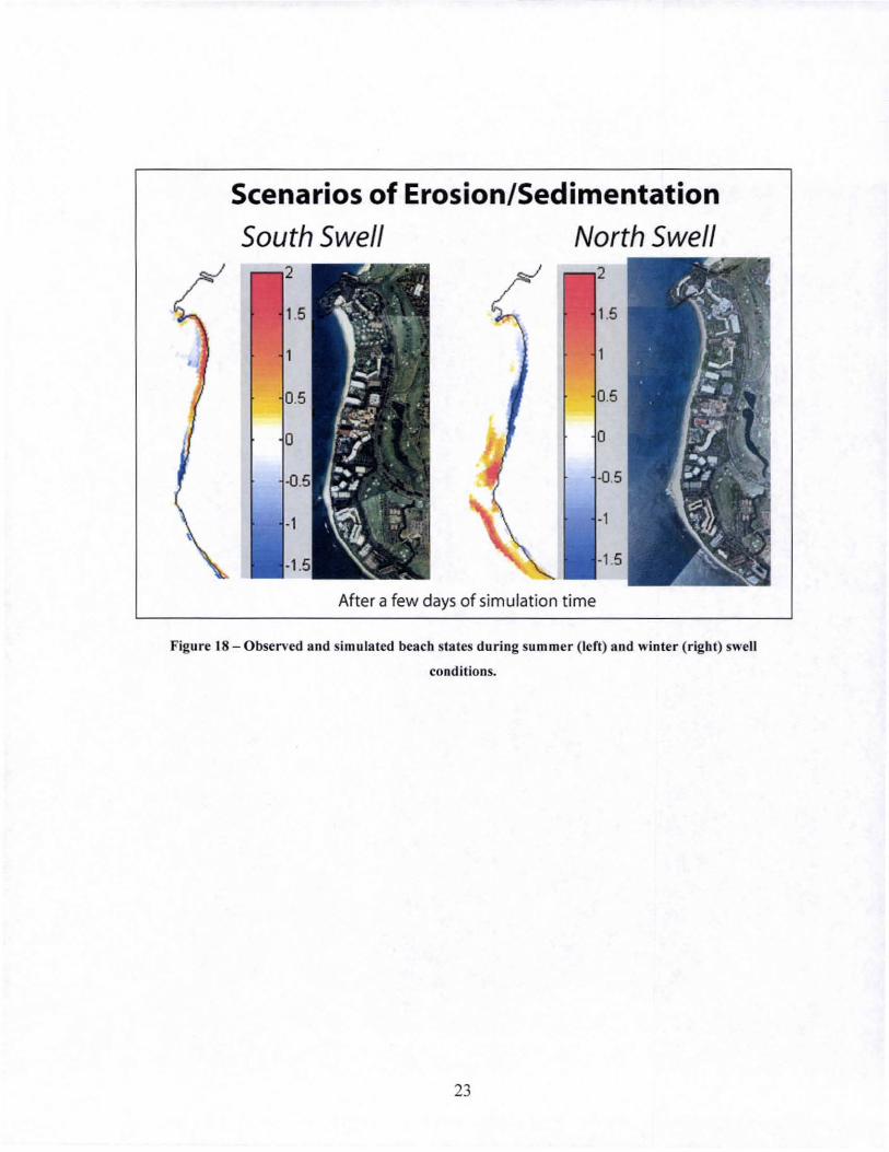
Figure 18 - Observed and simulated beach states during summer (left) and winter (right) swell conditions .............................................................................................................. 23

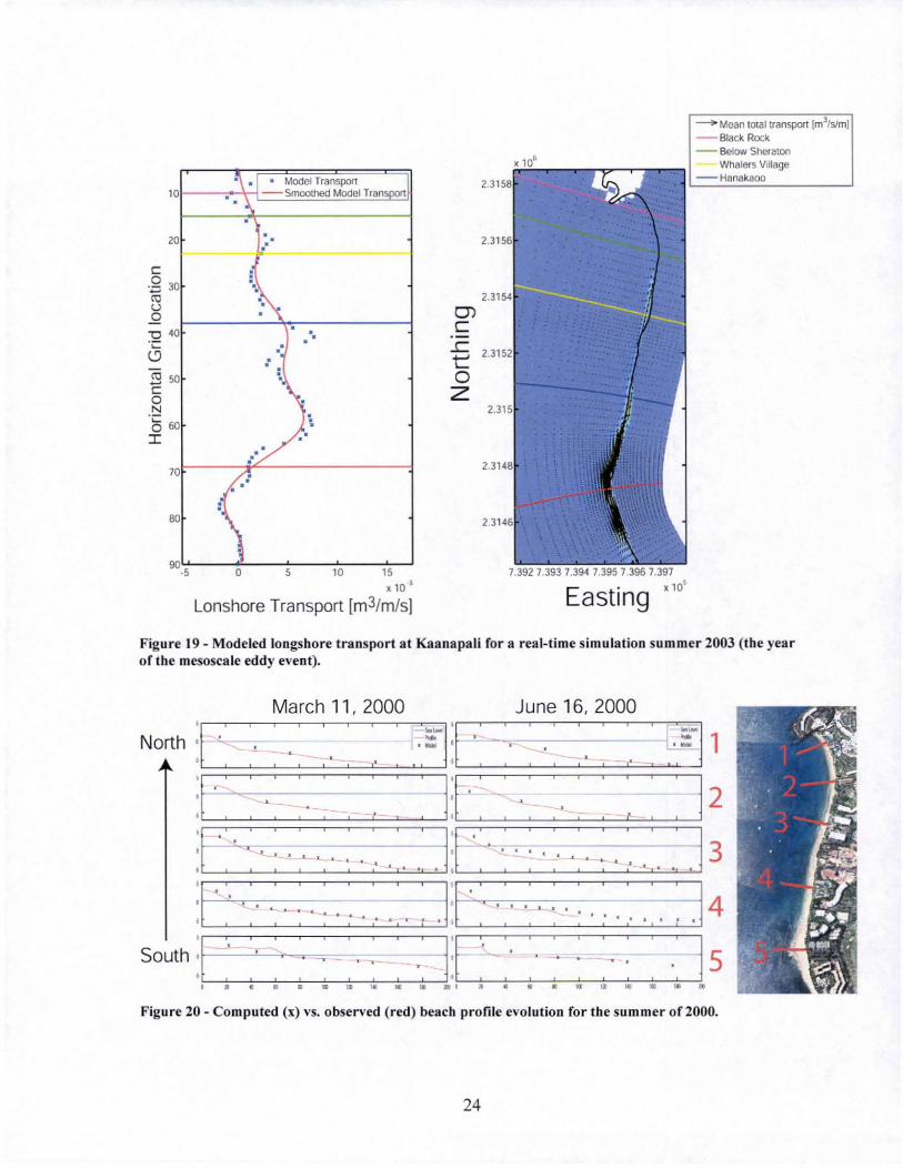
Figure 19 - Modeled longshore transport at Kaanapali for a real-time simu1ation summer 2003 (the year of the mesoscale eddy event) .................................................................. 24

Figure 20 - Computed (x) vs. observed (red) beach profile evolution for the summer of2000 . ......................................................................................................................................... 24

Figure 21 - Relationship between the vertical components of the winds and mean flow through the Pailolo Channel recorded in the South Kahana (Airport) station ................ 26

Figure 22 - Observed vs. modeled beach profile changes over 3 months at a number of locations at Kaanapali, Summer 2000 ............................................................................ 29

Figure 23 - lliustration of problems resolving small sea level changes in discrete grid based models ............................................................................................................................. 30

Figure 24 - Hawaii dominant swell regimes after Moberly and Chamberlain (1964), and wave monitoring buoy locations .............................................................................................. 39

Figure 25 - Log-normal and extremal probability models for the top 70 largest wave height events per year recorded by buoy 1. In these models the largest event (a 12.3 m

v

significant wave height) outlier has been removed and the peak over threshold method is used with a threshold of 5 m ........................................................................................... 44

Figure 26 - The Generalized Extreme Value probability model used to determine the annually recurring significant wave height. .................................................................... 48

Figure 27 - The observed directional annually recurring maximum significant wave heights (Hs) given from extremal (A) and GEV (B) models ....................................................... 49

Figure 28 - Top percent of waves vs. relation to significant wave height (H.) ...................... 52 Figure 29 - Sensitivity of models to number of largest events selected per year ...•..•.••.••••••••••••••••••••••••••••• 54 Figure 30 - When a large number of events is used in analysis, the log-normal model is fit

strongly the high frequency events (which represent the bulk of the data) at the expense of the extreme events ...................................................................................................... 55

vi

PREFACE

My Masters of Science project at the University of Hawai'i involves modeling

multiple coastal hazards with the end-goal to improve the scientific basis for coastal

management. My advisor, Chip Fletcher, and I have focused on coastal erosion and

inundation hazards as influenced by wave climates and sea-level rise. Our primary efforts

involve a numerical modeling case study of beach erosion at Kaanapali, Maui, Hawai'i and

with secondary efforts on determining probabilistic estimates of recurring wave heights and

water levels in Hawai'i, and producing a practical means of mapping coastal inundation

hazard zones.

Our case study of Kaanapali Beach focuses on the dramatic beach change in 2003 as

a result of the combined effect of extreme sea levels caused by the presence of an oceanic

mesoscale eddy and seasonal wave cycles. Using Delft3D, a process-based numerical model,

we were able to simulate hydrodynamics, waves and sediment transport at Kaanapali. We

have achieved very successful hydrodynamic and wave modeling which compares well with

an extensive data set of observations along West M!mi and Kaanapali collected as part of the

USGS coral reef project. Sediment transport and beach morphology modeling remains the

major chaJlenge of modeling efforts. One staggering deficiency of most coastal modeling

packages is the inability to resolve wave runup, and swash transport, which may significantly

influence subaerial beach morphology on steep, reflective beaches such as Kaanapali.

The second aspect of this project has concerned the determination of recurring wave

heights and water levels in Hawai'i. One particular focus has been on the annually recurring

vii

wave height around the Hawaiian Island to inform the Hawai'i administrative process as to

the "upper reach of the wash of the waves" which delineates the shoreline (Hawai'i Revised

Statuses (H.R.S.) § 205-A). Using log-normal and extremal exceedance probability models

and Generalized Extreme Value (GEV) analysis using 25 years of buoy data and long-term

wave hindcasts, the annual recurring significant wave height is found to be 7.7 ± 0.2 m (25 ft

± 0.7 ft). Directional annual wave heights are also determined by applying hindcasted swell

direction to observed buoy data lacking directional information.

The efforts discussed above have resulted in the following publications and conference

presentations:

Vitousek, S., Fletcher, C.H., Merrifield, M.A., Pawlak, G., "Shoreline change in response to

extreme tides and along-shore forcing modeled by Delft3D". Shoreline Change Conference

II Oral Presentation. Charleston, South Carolina, May 2006.

Vitousek, S., Fletcher, C.H., Strolazzi, C.D., "Modeling alongshore propagating tides and

currents at West Maui, Hawai'i: Implications for transport using De1ft3D". Poster. AGU fall

meeting. San Francisco, California, December 2006.

Vitousek, S., Fletcher, C.H., Merrifield, M.A., Pawlak, G., Storiazzi, C.D., "Model scenarios

of shoreline change at Kaanapali Beach, Maui, Hawai'i: Seasonal and extreme events".

ASCE Coastal Sediments 2007 Meeting Proceedings, v. 2, p. 1227-1240.

viii

Vitousek, S., Fletcher, C.H., "Hawai'i Swell Record Statistics and the Maximwn Annually

Recurring Wave Height". Pacific Science (in revision)

Recently we have developed a practicaI/ engineering approach to mapping coastal

inundation hazard zones, by applying statistical models of recurring wave heights and water

levels to produce expected runup levels and return periods. These levels are mapped on

high-resolution coastal elevation models produced from topographic and bathymetric

LIDAR. The evolution of these inundation levels as a function of future sea-level rise is a

very interesting aspect that this practical model is capable of evaluating. The major issues

that question the validity of this approach are the applicability of the empirical runup

equation (Stockdon et. al. 2006) and nearshore wave model (SWAN), which are used to

translate the recurrence model of deep-water wave height to a recurrence model of runup.

Runup remains a process that is highly variable, often unpredictable with traditional methods

especially in diverse coastal environments (particularly fringing reefs) such as those found in

Hawai'i. The best/most illuminating approach to study and predict runup, be it practical

through empirical equations, theoretical through equations and observations of nearshore

energy transfer, nwnerical through the use of process-based models, or a combination of

these approaches remains to be seen. This is a potential topic of study for my Ph. D.

ix

Sean Vitousek 7-31-07

MODEL SCENARIOS OF SHORELINE CHANGE AT KAANAPALI BEACH MAUl,

HAWAI'I

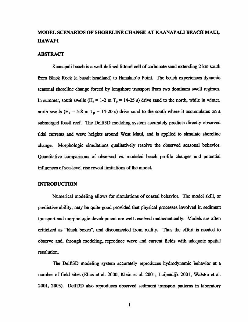
ABSTRACT

Kaanapali beach is a well-defined littoral cell of carbonate sand extending 2 kIn south

from Black Rock (a basalt headland) to Hanskao'o Point. The beach experiences dynamic

seasonal shoreline change forced by longshore transport from two dominant swell regimes.

In summer, south swells (Hs = 1-2 m Tp = 14-25 s) drive sand to the north, while in winter,

north swells (Hs = 5-8 m Tp = 14-20 s) drive sand to the south where it accumulates on a

submerged fossil reef. The Delft3D modeling system accurately predicts directly observed

tidal currents and wave heights around West Maui, and is applied to simulate shoreline

change. Morphologic simulations qualitatively resolve the observed seasonal behavior.

Quantitative comparisons of observed vs. modeled beach profile changes and potential

influences of sea-level rise reveal limitations of the model.

INTRODUCTION

Numerical modeling allows for simulations of coastal behavior. The model skill, or

predictive ability, may be quite good provided that physical processes involved in sediment

transport and morphologic development are well resolved mathematically. Models are often

criticized as "black boxes", and disconnected from reality. Thus the effort is needed to

observe and, through modeling,. reproduce wave and current fields with adequate spatial

resolution.

The Delft3D modeling system accurately reproduces hydrodynamic behavior at a

number of field sites (Elias et al. 2000; Klein et al. 2001; Luijendijk 2001; Walstra et al.

2001, 2003). Delft3D also reproduces observed sediment transport patterns in laboratory

1

tests and morphologic simulations (Lesser 2000; Lesser et. al. 2004; Elias 2006) using the

Van Rijn 1993 transport formulations. As an extension of these successes, it is hoped that

adequate resolution of water levels, waves, and currents allow the model to reproduce

sediment transport patterns in carbonate reef environments.

Kaanapali

Kaanapali Beach, located on the west coast of Maui, Hawaii, lies within a well ­

defined littoral cell extending 2 km south from Black Rock (a basalt headland) to Hanakao 'o

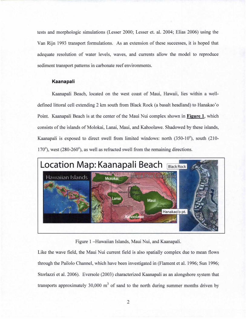
Point. Kaanapali Beach is at the center of the Maui Nui complex shown in Figure 1, which

consists of the islands of Molokai, Lanai , Maui, and Kaboolawe. Shadowed by these islands,

Kaanapali is exposed to direct swell from limited windows: north (350-10°), south (210-

170"), west (280-260"), as well as refracted swell from the remaining directions.

Location Map: Kaanapali Beach

Figure 1 -Hawaiian Islands, Maui Nui , and Kaanapali.

Like the wave field, the Maui Nui current field is also spatially complex due to mean flows

through the Pailolo Channel, which have been investigated in (Flament et al. 1996; Sun 1996;

Storlazzi et al. 2006). Eversole (2003) characterized Kaanapali as an alongshore system that

transports approximately 30,000 m3 of sand to the north during summer months driven by

2

south swell, which later returns to the south in winter months forced by north swell. This

volume of sand can result in dramatic beach width changes of more than 50 m at Hanakao' o

Point over the course of the year.

Erosion Event

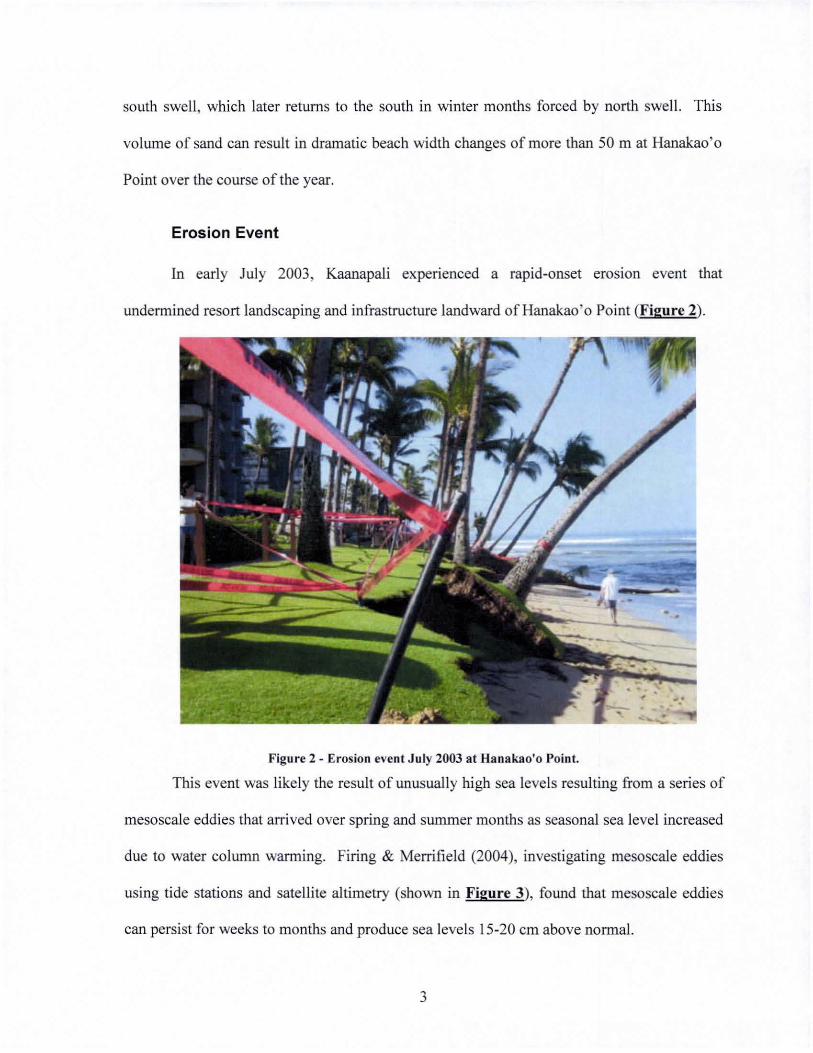
In early July 2003, Kaanapali experienced a rapid-onset eroSIOn event that

undermined resort landscaping and infrastructure landward of Hanakao' o Point (Figure 2).

Figure 2 - Erosion event J uly 2003 at Hana kao'o Point.

This event was likely the result of unusually high sea levels resulting from a series of

mesoscale eddies that arrived over spring and summer month as seasonal sea level increased

due to water column warming. Firing & Merrifield (2004), investigating mesoscale eddies

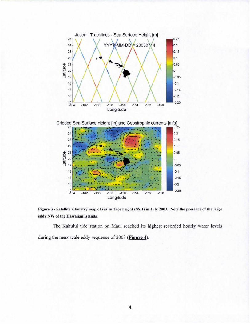
using tide stations and satellite altimetry (shown in Figure 3), found that mesoscale eddies

can persist for weeks to months and produce sea levels 15-20 cm above normal.

3

25

24

<1> 21 "0 B 20 ~ --' 19

18

17

Jason1 Tracklines - Sea Surface Height [m]

~M-D7D / 20030 ,. ·7·

16

15~--~~L-~~~~--~~--~L--~~~~ ~~ ~~ ~M ~~ -1~ ~M ~~ ~~

Longitude

Gridded Sea Surface Height [m] and Geostrophic currents [m/s] 25 0.25

• • \ . I •

""'-, .-••• ~." - ___ ... I

.J~,......,,_ ..... ..... .. \ \ "\\\ ........ , '- - .. ~ ""----

-1~ ~M ~~ -1~ -1M -1~ -1~

Longitude

0.2

0.15

0.1

0.05

o

-0.05

-0.1

-0.15

-0.2

-0.25

Figure 3 - Satellite altimetry map of sea surface height (SSH) in July 2003. Note the presence of the large

eddy NW of the Hawaiian Islands.

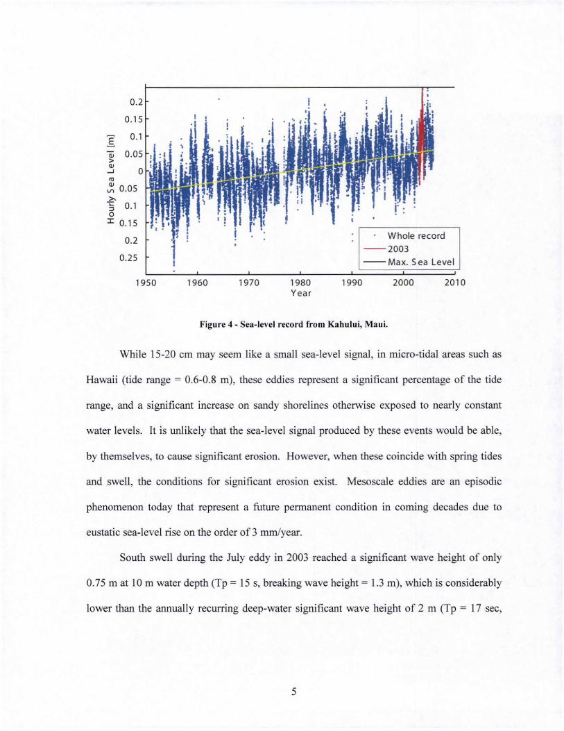
The Kahului tide station on Maui reached its highest recorded hourly water levels

during the mesoscale eddy sequence 0[2003 (Figure 4).

4

'" > '" ..J

'" ~ 0.05 >-"§ 0.1 o I 0.15

0.2

0.25

1950 1960 1970 1980 Yea r

1990

Whole record

--2003

--Max. Sea Level

2000 2010

Figure 4 - Sea-level record from Kahului, Maui.

While 15-20 cm may seem like a small sea-level signal, in micro-tidal areas such as

Hawaii (tide range = 0.6-0.8 m), these eddies represent a significant percentage of the tide

range, and a significant increase on sandy shorelines otherwise exposed to nearly constant

water levels. It is unlikely that the sea-level signal produced by these events would be able,

by themselves, to cause significant erosion. However, when these coincide with spring tides

and swell, the conditions for significant erosion exist. Mesoscale eddies are an episodic

phenomenon today that represent a future permanent condition in coming decades due to

eustatic sea-level rise on the order of 3 nun/year.

South swell during the July eddy in 2003 reached a significant wave height of only

0.75 mat 10 m water depth (Tp = 15 s, breaking wave height = 1.3 m), which is considerably

lower than the annually recurring deep-water significant wave height of 2 m (Tp = 17 sec,

5

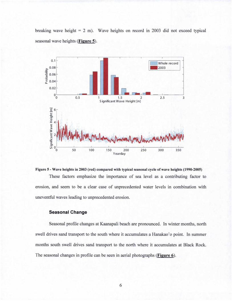
breaking wave height = 2 m). Wave heights on record m 2003 did not exceed typical

seasonal wave heights (Figure 5).

0. 1

~ 0.08

~ 0.06 ~ 0 ~ 0.04

0.02

a a 0.5 1.5 2 2.5 3 Significant Wave Height [m1

]:6 E C\

'0; :1: 4 ~ > ~

~ E 2 ~ u

'" 'c C\ ;;; 0

a 50 100 150 200 250 300 350 Yearday

Figure 5 - Wave heights in 2003 (red) compared with typical seasonal cycle of wave heights (1990-2005)

These factors emphasize the importance of sea level as a contributing factor to

erosion, and seem to be a clear case of unprecedented water levels in combination with

uneventful waves leading to unprecedented erosion.

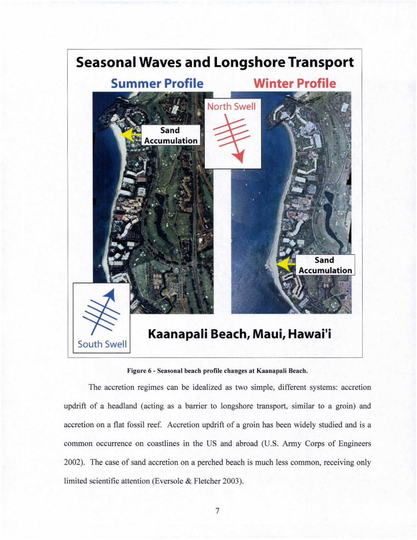
Seasonal Change

Seasonal profile changes at Kaanapali beach are pronounced. In winter months, north

swell drives sand transport to the south where it accumulates a Hanakao'o point. In summer

months south swell drives sand transport to the north where it accumulates at Black Rock.

The seasonal changes in profile can be seen in aerial photographs (Figure 6).

6

Seasonal Waves and Longshore Transport

Summer Profile Winter Profile

South Swell Kaanapali Beach, Maui, Hawai'i

Figure 6 - Seasonal beach profile changes at Kaanapali Beach.

The accretion regimes can be idealized as two simple, dilTerent systems: accretion

updrift of a headland (acting as a barrier to longshore transport, similar to a groin) and

accretion on a flat fossil reef. Accretion updri ft of a groin has been widely studied and is a

common occurrence on coastlines in the US and abroad (U.S. Army Corps of Engineers

2002). The case of sand accretion on a perched beach is much less common, receiving only

limited scientific attention (Eversole & Fletcher 2003).

7

Beach widening at Hanakao'o Point during winter months is an acute example of

accretion on a perched beach, and poses one of the most interesting questions presented by

the dynamic cycle of accretion and erosion at Kaanapali. Accretion at Hanakao' 0 is much

more concentrated and dramatic than at Black Rock, even though the north end has an

obvious accretion mechanism in place: the physical barrier of Black Rock. It is likely that

the shallow, rough reef at Hanakao'o slows southward propagating alongshore currents

generated by north swell leading to bed deposition. Hanakao'o also marks the point where

swell regimes change from surging breakers in the northern portion of the beach at Black

Rock where swash transport may play an important role in beach morphology to offshore

dissipative breakers on the reef (characterizing the southern portion of the beach). Because

of the difference in offshore depth and wave breaking characteristics, Hanakao' 0 likely

marks the termination of swash zone transport. Improving an understanding of the various

processes governing beach dynamics is critical to defining the role of eddy-generated water­

level changes in episodic erosion.

MEmODS

Data

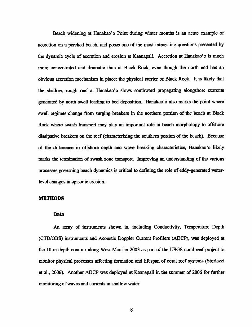
An array of instruments shown in, including Conductivity, Temperature Depth

(CTD/OBS) instruments and Acoustic Doppler Current Profilers (ADCP), was deployed at

the 10 m depth contour along West Maui in 2003 as part of the USGS coral reef project to

monitor physical processes affecting formation and lifespan of coral reef systems (Storlazzi

et al., 2006). Another ADCP was deployed at Kaanapali in the summer of 2006 for further

monitoring of waves and currents in shallow water.

8

West Maui Instrument locations: r

South Kahana (Airport) - ADCP •

Honokowai - ADCP • West Maui

Kaanapali- CTD/OBS

Kaanapali- ADCP (2006) · Kaanapali

Lahaina

Puamana - CTD/OBS •

Figure 7 - West Maui instrument deployments in 2003.

For morphologic calibration we use beach profiles at Kaanapali from Eversole and

Fletcher 2003. Monthly beach profiles were conducted from March 2000 to April 2001.

The profiles were measured with a Geodimiter® total station and a 7 m telescoping rod.

Shore normal transects were spaced every 2 m or at specific shoreline features including

changes in slope on the subaerial beach and extended to a water depth of 5 to 7 m.

Modeling

The Oelft30-FLOW module (v. 3.24.03 used here) solves the unsteady shallow-water

equations with the hydrostatic and Boussinesq assumptions. In 20 mode the model solves

two horizontal momentum equations (see Eq. 1-2), a continuity equation (Eq. 3) and a

transport (advection-diffusion) equation (Eq. 4) shown below:

9

au au au a." Iv Th• E'. a2U a2u (1) -+u-+v-+ g-- + V (-+-)=0

at ax ay ax p .. (h+.,,) Pw(h+.,,) e ax2 ay2

Ov Ov Ov a." T I>y F, 82v a2v (2) -+u-+v-+g-- fu+ V (-+-)=0

at ax ay ay p .. (h+.,,) Pw(h+.,,) e ax2 ay2

a." +u a[(h+.,,)u] +v a[(h+.,,)v] 0 at ax ay

(3)

a[;] + 8[:C] + a[:c] h[ !( Dn :)+ ~( Dn :)] (4)

where u and v = the horizontal velocities in the x and y directions respectively; t = time; g =

gravity; ." = free surface height; h = water depth;! = coriolis force; Pw = density of water; Th

= bed friction; F = external forces due to wind and waves, Ve = horizontal eddy viscosity;

Dn = horizontal eddy diffusivity; and c = concentration of suspended sediment. The

equations are solved on a staggered finite difference grid using the Alternating Direction

Implicit (ADI) method after Stelling (1984).

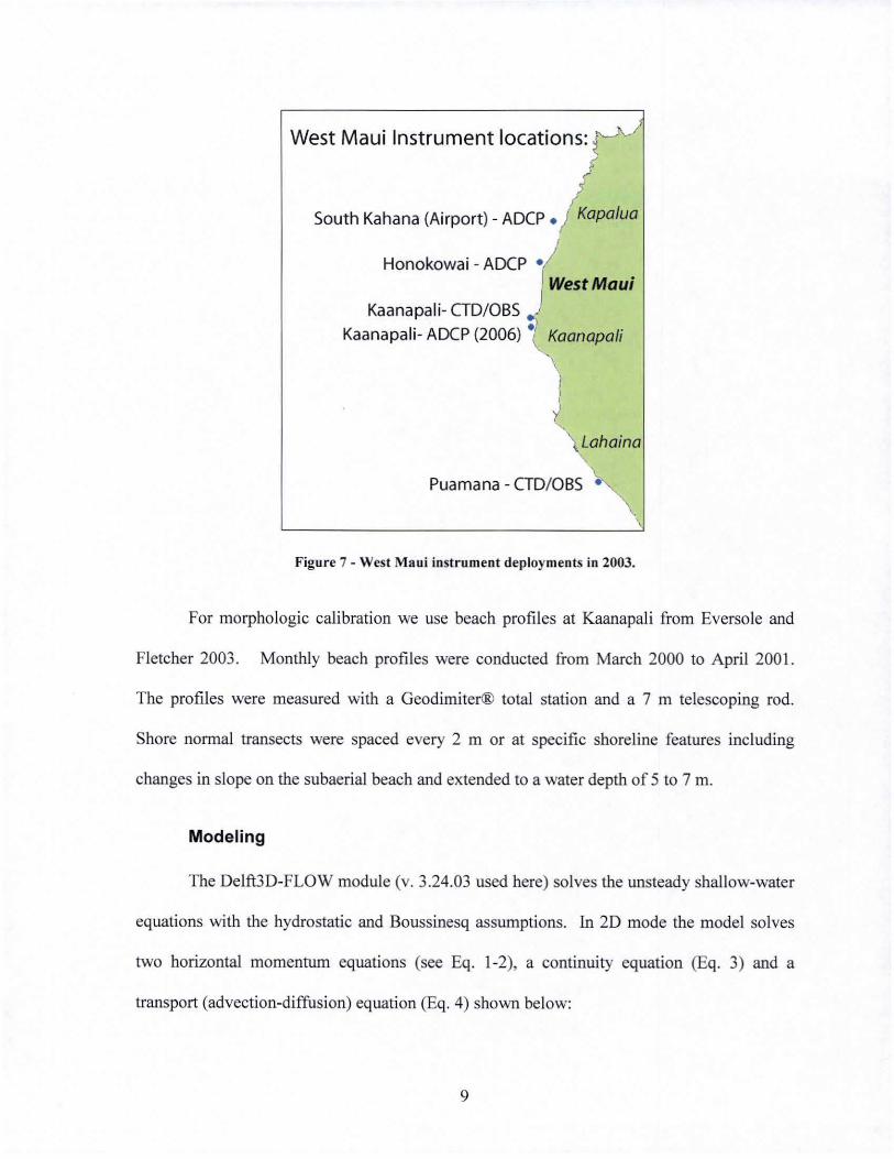
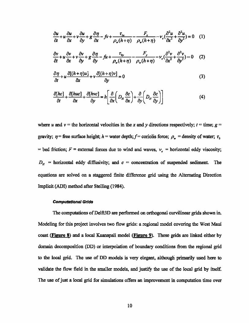
Computational Grids

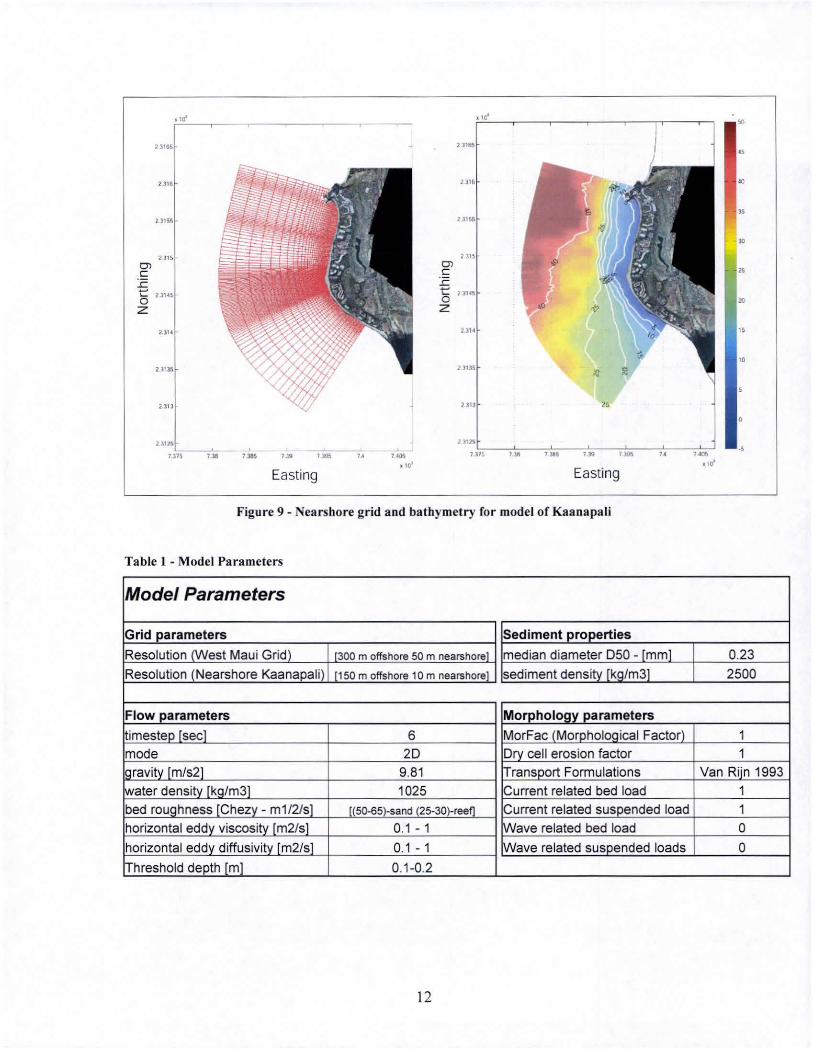
The computations ofDelft3D are performed on orthogonal curvilinear grids shown in.

Modeling for this project involves two flow grids: a regional model covering the West Maui

coast (Figure 8) and a local Kaanapali model (Figure 9). These grids are linked either by

domain decomposition (DD) or interpolation of boundary conditions from the regional grid

to the local grid. The use of DD models is very elegant, although primarily used here to

validate the flow field in the smaIIer models, and justify the use of the local grid by itself.

The use of just a local grid for simulations offers an improvement in computation time over

10

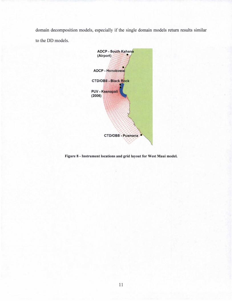
domain decomposition models, especially if the single domain models return results similar

to the DO models.

CTOIOBS - Pu.unana,-<'

Figure 8 - Instrument locations and grid layout for West Maui model.

11

Ol .~ -5

.,'

1116

21155

\... 2l14~

o z:

u u

~ )1)5

~ 1 13 -

'~~~'~=---~7~--- '~ . 10'

Easting

Ol C ~ t:: o z:

, '"

"

,. Easting

Figure 9 - Nearshore grid and bathymetry for model of Kaanapali

Table 1 - Model Parameters

Model Parameters

Grid parameters Sediment properties

Resolution (West Maui Grid) [300 m offshore 50 m nearshore] median diameter 050 - [mm]

Resolution (Nearshore Kaanapali) [150 m offshore 10m nearshore) sediment density [kg/m3]

Flow parameters Morphology parameters

imestep [sec] 6 MorFac (Morpholoqical Factor)

mode 20 Dry cell erosion factor Igravity Im/s2] 9.81 Transport Formulations fNater density [kg/m3] 1025 Current related bed load bed rouQhness [Chezy - m1/2/s] [(50-65)-sand (25-30)-reefi Current related suspended load horizontal eddy viscosity [m2/s] 0.1 - 1 Wave related bed load

horizontal eddy diffusivity [m2/s] 0.1 - 1 Wave related suspended loads

IThreshold depth [m] 0.1-0.2

12

"'" ,,'

"

.,

0.23

2500

1 1

Van Rijn 1993 1

1 0

0

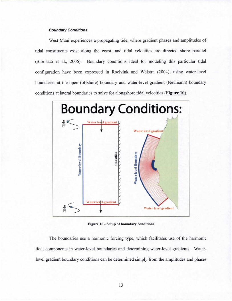
Boundary Conditions

West Maui experiences a propagating tide, where gradient phases and amplitudes of

tidal constituents exist along the coast, and tidal velocities are directed shore parallel

(Storlazzi et al., 2006). Boundary conditions ideal for modeling this particular tidal

configuration have been expressed in Roelvink and Walstra (2004), using water-level

boundaries at the open (offshore) boundary and water-level gradient (Neumann) boundary

conditions at lateral boundaries to solve for alongshore tidal velocities (Figure 10).

Boundary Conditions: ~S

~ /

• 'i / • d

/

/

/

/

/

/ /

\\ 1t1i.:r 1 ... '\ ·1 :.tf"'oulitnt

\Valer k. ... cI ~r.Hlicn

\\-ster ICH'. :;,!radi, .. nt

Figure 10 - Setup of boundary condit ions

The boundaries use a hannonic forcing type, which faci litates use of the harmonic

tidal components in water-level boundaries and determining water-level gradients. Water-

level gradient boundary conditions can be determined simply from the amplitudes and phases

13

of the tidal constitutes at each lateral boundary using the equations given in Roelvink and

Wa1stra (2004):

Given tidal constituent Gradient amplitude:

Amplitude: ( ¢,norlh _ ¢,~ )

(5) TJ, TJ I i I d

Is

Phase: tPl tPl +7r/2 (6)

where TJ, = amplitude of the tidal constituent (m); tPl = phase of the tidal constituent

(tP,fWrlh ,tPI~ for north and south boundaries respectively (radians» and dis = distance

between the lateral boundaries (m). With these boundary conditions prescribed, the bed

roughness is tuned to match the observed current magnitude. These boundary conditions

have been shown to provide accurate simulations of tidal velocities in Roelvink and

Wa1stra's modeling studies (2004) at Egmond (Netherlands). This study provides another

example of the excellent performance of boundary conditions developed from this scheme

(see Results).

The wave boundary conditions are determined from model hindcasts (WaveWatch

III) because there are no recorded buoy observations that include wave direction. These

hindcasts adequately resolve observed wave heights and periods at a number of buoy

locations in Hawaii. In this study, hindcast values of significant wave height, peak period

and direction are applied uniformly at the open boundaries of the largest SWAN model, and a

series of nested grids resolve the wave field down to the nearshore scale (10m grid) at West

Maui and Kaanapali Beach. The SWAN nesting scheme is shown on Figure 11.

14

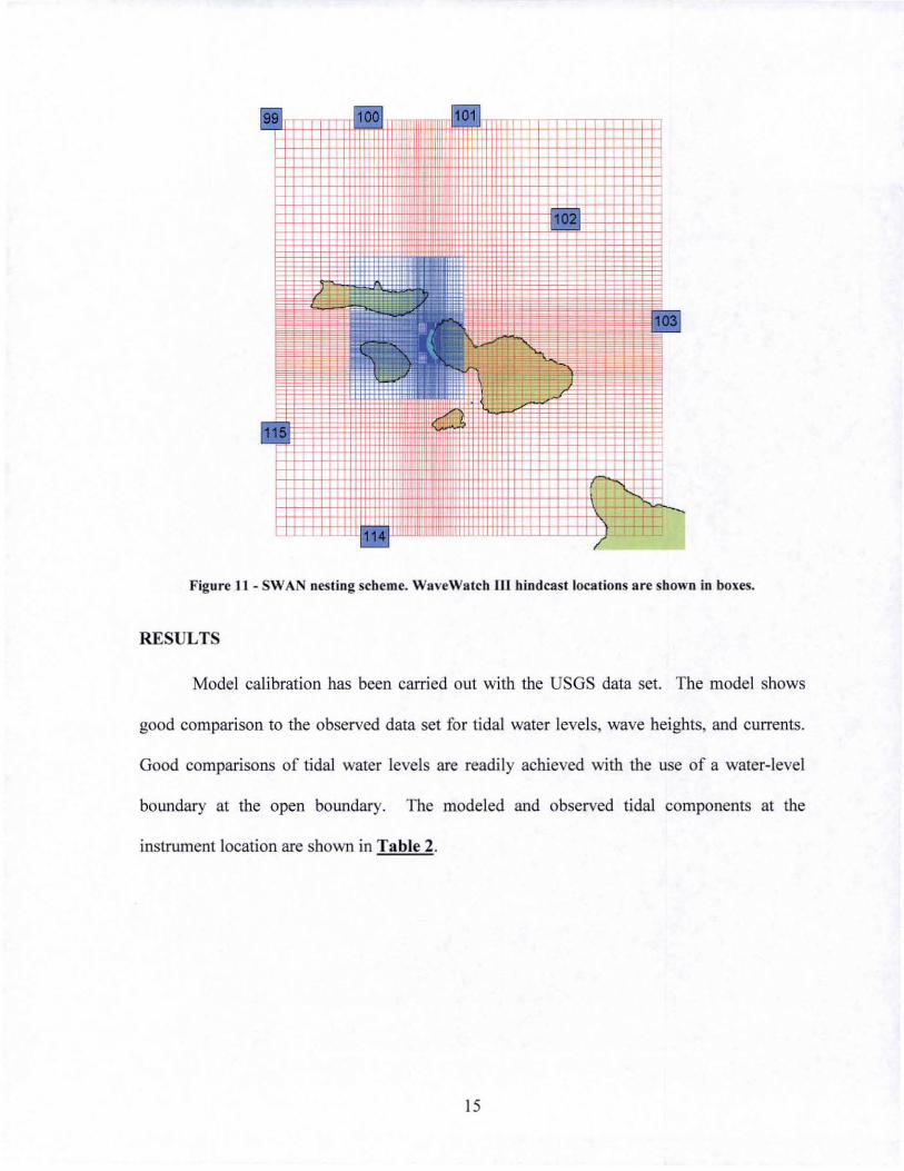
Figure II - SWA nesting scheme. WaveWatch nt hindcast locations are shown in boxes.

RESULTS

Model calibration has been carried out with the USGS data set. The model shows

good comparison to the observed data set for tidal water levels, wave heights, and currents.

Good comparisons of tidal water levels are readily achieved with the use of a water-level

boundary at the open boundary. The modeled and observed tidal components at the

instrument location are shown in Table 2.

15

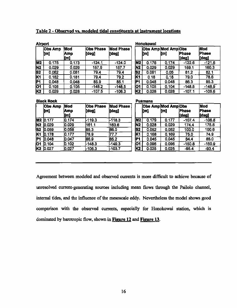
Table 2 - Observed vs. modeled tidal constituents at instrument locations

Airport ObsAmp Mod ObsPhase Mod Phase [m] ~p [deg] [deg]

M2 0.175 0.173 -124.1 -124.0 N2 0.029 0.029 157.9 157.7 52 0.062 0.061 79.4 79.4 K1 0.182 0.181 79.4 79.2 P1 0.048 0.048 85.9 85.1 01 0.105 0.105 -148.2 ·148.5 K2 0.029 0.028 -107.5 -108.3

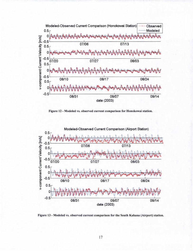
Agreement between modeled and observed currents is more difficult to achieve because of

unresolved current-generating sources including mean flows through the Pailolo channel,

internal tides, and the influence of the mesoscale eddy. Nevertheless the model shows good

comparison with the observed currents, especially for Honokowai station, which is

dominated by barotropic flow, shown in Figure 12 and Figure 13.

16

Modeled-Observed Current Comparison (Honokowai Station) Observed

0 .5 ~ --Modeled ~ 0 '" @, .. Lf.i.. ~ ~""' '' ' ~ .~. ~ foe .J\., .!(! _ iilVVV~VVVvV =l1'V""''WV~ ""'I.Ii'Y~"''f'i1V~\!IV'¥V~ £-05L------~~------~~--------~ 0 :5~ 07/06 07/13

~ O M'L1 .~A. 2t '" ~A. A • 1\ A iii. , I\. An,. W " Cl~ ~ > _ VV"'"iII~ v~'4i~ .. ~ '''''v~vvtvvv¥ ~ ,,';IV 'V Y ... C -0 .5~~------~~~------~~------~ 07120 07127 08/03

:; 0 .5 ~ ~ 0 '" 10. y. ~ . k A • ~v· to. • t. .. L a .. ~'" '-J~A ~ ~ ""V~ Vl!! V'lJWV"V'V ijY"!V'T<ilyV-V~~ ~ ~v"""V o-0.5 L--~--~~------~~------~~~--~ 0.5 08/10 08/17 08124

~ o[!\.Qi~~~UU1'\~~ . A.".~~A.Al\"A~Ai > ~VVVVYV V!VVV~-V '" V -.:, It\i~vvv~v~'tnPJ'V~'II'

-0.5 08/31 09/07 09/14 date (2003)

Figure 12 - Modeled VS. observed current comparison for Honokowai station.

Modeled-Observed Current Comparison (Airport Station)

0.5 rJ

l_o.~flvVv~~~~~~ ~ 0.5 ~m6 Orn3

~ O~~ M ~ -0.5 07120 07127 08/03

8 0 . 5 ~

j OO [ ~ ~ - .5 08/10 08/17 08124

3 0.5

> o[.IW~hGUW~~V~rr.~~f1!~~ ~ "n n ~n'w V V'l "I'J ':f V ~ .., V ?IV WW't! 'J/il W/~ 'IJI? ~

-0.5 '------:-='::--c---------::-==---- ------::-::-'-:-:-08/31 09/07 09/14

date (2003)

Figure 13 - Modeled VS. observed current comparison for the South Kahana (A irport) station.

17

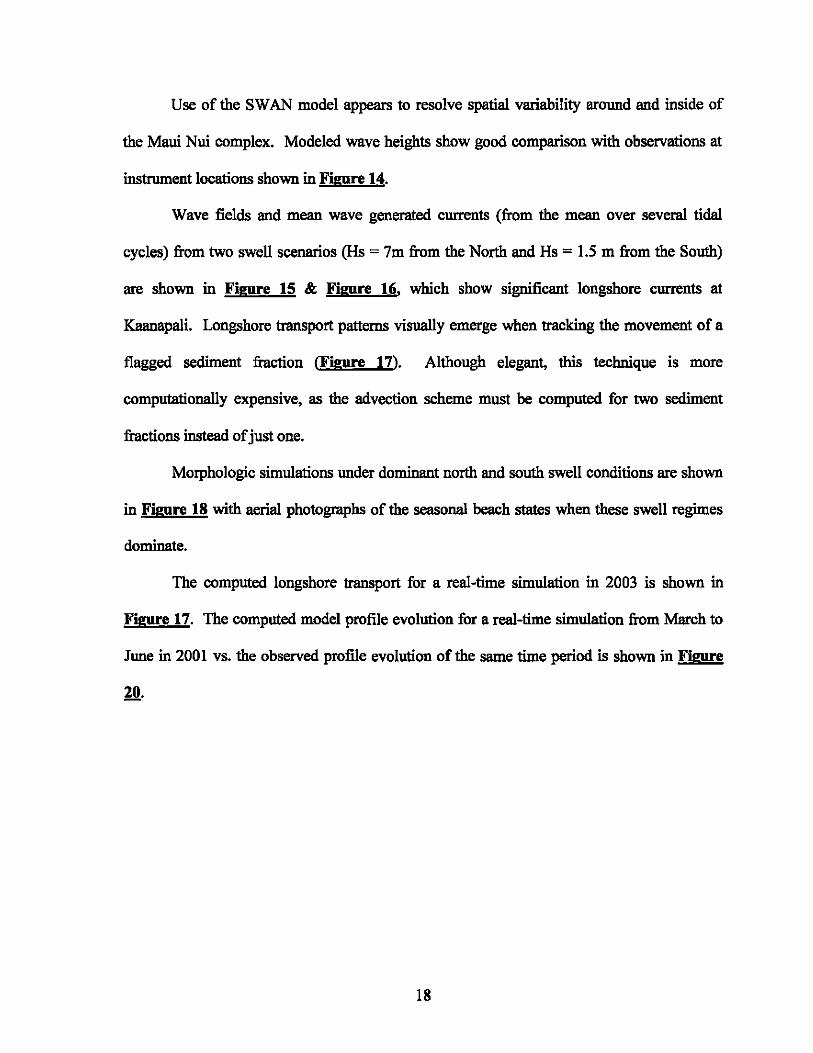
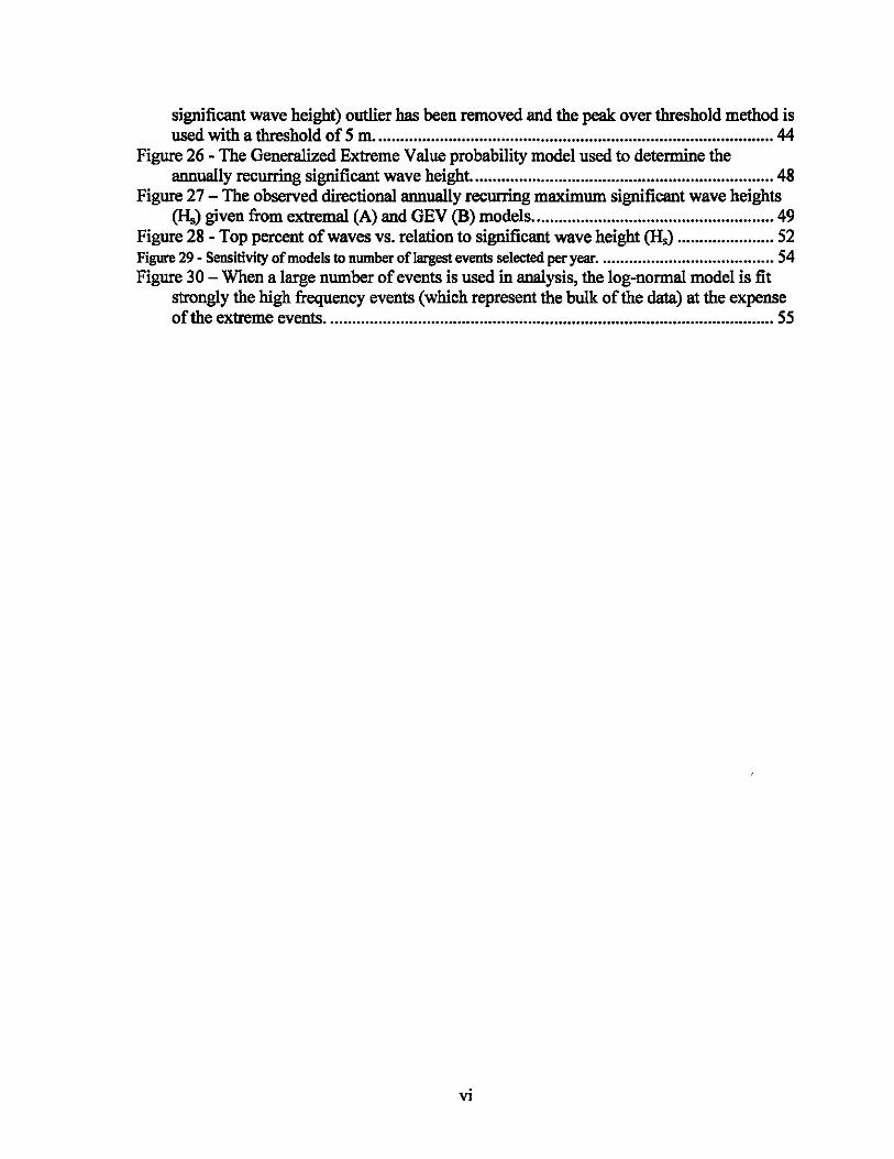
Use of the SWAN model appears to resolve spatial variability around and inside of

the Maui Nui complex. Modeled wave heights show good comparison with observations at

instrument locations shown in Figure 14.

Wave fields and mean wave generated currents (from the mean over several tidal

cycles) from two swell scenarios (Hs = 7m from the North and Hs = 1.5 m from the South)

are shown in Figure 15 & Figure 16. which show significant longshore currents at

Kaanapali. Longshore transport patterns visually emerge when tracking the movement of a

flagged sediment fraction (Figure 17). Although elegant, this technique is more

computationally expensive, as the advection scheme must be computed for two sediment

fractions instead of just one.

Morphologic simulations under dominant north and south swell conditions are shown

in Figure 18 with aerial photographs of the seasonal beach states when these swell regimes

dominate.

The computed longshore transport for a real-time simulation in 2003 is shown in

Figure 17. The computed model profile evolution for a real-time simulation from March to

June in 2001 vs. the observed profile evolution of the same time period is shown in Figure

20.

18

.,.= ?s k b ... ..... ...

L te\ 'r · ... ... .. I

1°,sL.....,'b l: 0 Jul

M a .p Sop

~ 'r •. i O.5~ ., it .. t" 14 - .. ." t ~ o~ ~

Figure 14 - WaveWatch III boundary conditions and comparisons of modeled (x) and observed (-) wave

heights Iml at instrument locations, The lines on the second subplot represent the south swell window

(170-210'),

19

01 C

-€ o z

Wave Fields South Swell North Swell

7.39' 1.J'n 7. 394 7.195 1.396 7397 7.398

E asting

01 C

-€ o z

7.3927.393 7.194 7.395 1.396 7.397 7. 398

Easting

Figu re IS - Wave fields (wave height in 1m!) at Kaanapali based on a South swell (Hs = I.S m) and a north swell (Hs = 7). Significant island blockage reduces the wave height at Kaanapali due to the north

swell.

20

Mean wave-generated longshore currents

O'l C ~ t o Z

South Swell North Swell

Easting It 'O~

O'l C ~ t o Z

7_393 7394 7.395 7.396 7.397

Easting

Figure 16 - Mean wave generated currents Imlsl for South and North swell at Kaanapa li Beach

2 1

Longshore Sediment transport patterns due to South Swell

Initial 2 days 5 days 70 days

Figure 17 - Longshore Sediment transport patterns at Kaanapa li. Tracked using a flagged patch of sand (in red - initial). Colormap represents fraction of flagged vs. u"f1agged sediment.

22

Scenarios of Erosion/Sedimentation

South Swell North Swell

•

After a few days of simulat ion time

Figure 18 - Observed and simu lated beach states d uring summ er (left) and wi nter (right) swell

conditions.

23

• MOIlel Transport

l 0r--..-;-'s~-=~sm~OO1hed~!!!Mod~"~T~ra~ns~

20

c .g 30 CO u o "0 40 . ~ 19

8 sa c o N

'§ 60 I

' . .'

: . .

7o1:-- ----2""---------:l

80

OO.~5-~0~-5~-1~0-~,5~

x 10 I

Lonshore Transport [m3/m/s]

O"l C ..c +-' I-

0 Z

7.3927.3937.39' 7.395 7.396 7.397

Easting x 10'

~ Mean lOlal uansporl (mJ'slmj - Black Rock - Below Sheraton

Whalers Village - Hanakaoo

Figure 19 - Modeled longshore transport at Kaanapali for a real-time simulation summer 2003 (the yea r of the mesoscale eddy event).

Figure 20 - Computed (x) vs. observed (red) beach profile evolution for the summer of2000.

24

DISCUSSION

Using Delft3D with water-level gradient boundary conditions prescribed in Roelvink

and Walstra (2004) provide excellent resolution of current velocities in regions dominated by

barotropic tidal flow. For regions influenced by mean flows and internal tides. more physical

processes need to be accounted for to better resolve observed velocities. It appears the

Honokowai station (Figure 12) is well resolved, while the South Kahana (Airport) station

(Figure 13) is influenced by the presence of mean flows and internal tides. Despite the

influence of unresolved processes, the models show good comparison with the observed flow

velocities.

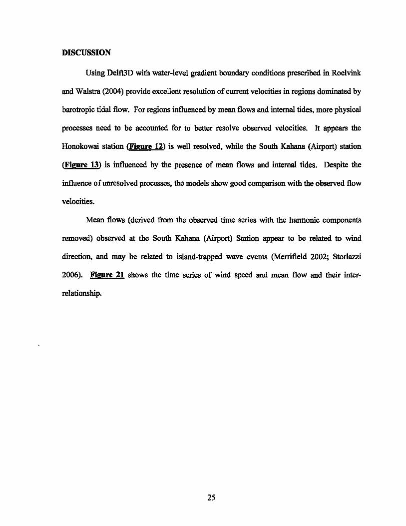
Mean flows (derived from the observed time series with the harmonic components

removed) observed at the South Kahana (Airport) Station appear to be related to wind

direction, and may be related to island-trapped wave events (Merrifield 2002; Storlazzi

2006). Figure 21 shows the time series of wind speed and mean flow and their inter­

relationship.

2S

~

t _:~b ... nn,,""".JI'\liIi .. ~1ta III iF ~IbUI ~ . Jul Aug Sep Oct

~ 0.2 ~ 0

orne

~ -02 t:::~ ~ -OA ~ _8L-----~----~-L--~---L------~~~

-4 -2 Wi nd speed [m/sJ

Figure 21 - Relationship between the ve rtical components of the winds and mean now through the Pailolo

Channel recorded in the South Kahana (Airport) station.

Wind speed and mean flow seem to mirror each other. A notable event in the time

series is the decrease in wind speed in late July, which leads to a corresponding decrease in

the mean flow through the channel. Although the model accounts for wind forcing, the mean

flow is not resolved. If the mean flow is due to wind forcing, the inability to resolve the

mean flow is probably due to the limited coverage of the model domain: inability to develop

significant wind-generated currents, and/or the topographic influence of West Maui which

may cause local acceleration of the wind fie ld.

The mean flow observed at South Kahana seems unlikely, from the two observed

time series, to extend past the Honokowai station and potentially affect currents and sand

transport at Kaanapali Beach. The major influence in sand transport at Kaanapali seems to

be the wave-generated currents that arise from obl iquely incident waves from north and south

swell breaking on the westward-facing shoreline.

26

The misfit between the observed and modeled wave heights along West Maui, shown

in Figure 14, may result from using simulations from a larger model (WaveWatch III -

referred to as WWIII) to force the smaller model. WWIII has been well-validated using buoy

and altimetry data (Tolman 2002, Baird and Associates 2005, Tracy et. al. 2006). However,

we do not have observation stations at the boundary locations of the small West Maui model

to validate WWIII around this particular location. The two main discrepancies between

modeled and observed wave height are that the model does not capture a few particular swell

events, and a background wave height exists in the data that is not resolved in the model.

The first issue may be cause by WWIII's inability to resolve swell direction adequately. Any

slight deviation in swell direction and significant island blockage (shadowing) can

significantly reduce the modeled wave heights around West MauL The second issue may be

due to the use of parametric wave conditions (a single significant wave height, period and

direction) applied to the boundary. Currently Delft3D cannot use time-varying wave spectra

as boundary conditions. Using parametric wave boundary conditions only resolves the

dominant wave conditions, not the smaller background swell.

While simulations of shoreline accretion and erosion forced by the dominant swell

regimes show a qualitative morphologic behavior, the ultimate goal of modeling is to

reproduce or predict transport volumes and resulting changes in the beach profile. The

default transport parameters of Delft3D predict a northward longshore transport of around

7,000 m3 for the summer of 2000, which is around a factor of 4 lower than the observed

transport of 30,000 m3 for the summer of 2000 based on beach profiles of Eversole (2003).

For calibration purposes, tuning model parameters to match the data, is often done, however

unsatisfying the practice may be.

27

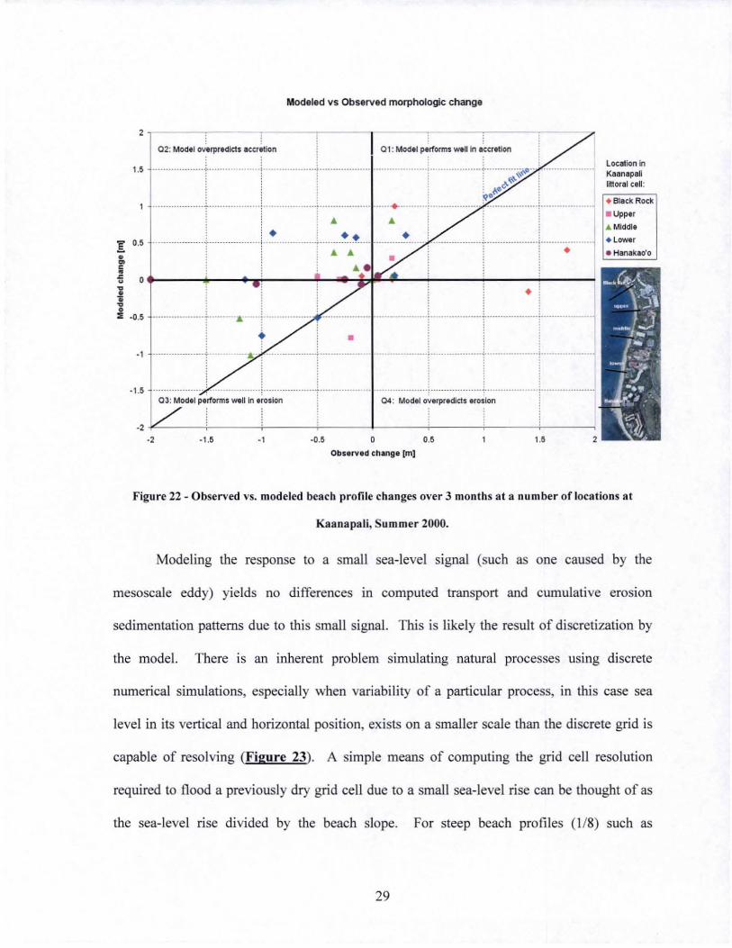
Modeling beach profile changes often captures observed changes in mean state, but is

less successful at predicting significant erosion and accretion events (Figure 20). While the

model seems to perform adequately for scenarios on timescales of a few days, variability of

wave and current conditions on longer timesca1es make simulations on timesca1es of months

to years more difficult to resolve. Long-term morphological modeling often use of

techniques such as input reduction (reducing the tide & wave climate into a few dominant

scenarios) to eliminate unimportant swell regimes and reduce computational time (Roelvink

2006). Comparisons of observed and modeled profile changes (in the vertical direction), in

Figure 22, show that the model tends to over predict accretion (indicated by the frequency of

records in quadrant 2 and above the perfect fit line) and to miss large erosion and accretion

events in the end members of the littoral cell (Black Rock and Hanakao'o). Bias towards

accretion is likely due to the persistence of sma11 wave states during the 3-month simu1ation,

and inability to resolve swell events that lead to significant change. The effects of 2D vs. 3D

modeling on accretion predictions should also be investigated.

28

Modeled vs Observed morphologic change

2 -,----,.--- ,

, I 01: Model p~"om" we' in ":"."on 02: Model ovtrprtdlc1s lIcer.lion

·············t· ................ ' ~ ........ ........... ;. ................... ····················i····· .. ············ ~·.. . ~ .. . .. .... .. ! : 1 ~~ •

! , •• ,} ; ~ qe\'

1.'

1 ... ....... .... .... - .•. . .•. . .... •. •.•. ••• . .••... ·········f··················· ······ ... ··········i······ , A A

, + , ++ + . ! . i 0.' ············· +·· .. ·!..............r .... · .... · .... · ,..... ... ,.. .... !. ....,

~ o+-------~----.,ri-------~--.. ~~~L---~------~------~-------~ • • 1; ~ o S -0.5 ................... - ..... ...... : ...... j.................. .. ...................................... ·· .. ·· .. ·········~······ · ···· .. · .. ···i· .. · .. ·· .. ·········

t · i ......... ~ .................... -·· .. ·· .. ·· .... · ··~··· .. ·· .. · .. ·······+···················l·· ................ . ; . i

... ; .................... ~ ..................................... : . ...... . ..... ...... ~ ........ ........... .............. ...... . -1.5 Q3: Model p.r1'onns wallin erosion 04: Model overpredic1s erosion

-2~----+-----~----4------+------+-----~---~r-----, -2 -1 .5 -1 ·0.5 o 0.' 1.'

Observed change [m]

location in Koanopol1 littorol cell :

. maek Roek

• Upper .. Middle

• lower • Honakao'o

Figure 22 - Observed vs. modeled beach profile changes over 3 months at a number of locations at

Kaa napali, Summer 2000.

Modeling the response to a small sea-level signal (such as one caused by the

mesoscale eddy) yields no differences in computed transport and cumulative erosion

sedimentation patterns due to this small signal. This is likely the result of discretization by

the model. There is an inherent problem simulating natural processes using discrete

numerical simulations, especially when variabi lity of a particular process, in this case sea

level in its vertical and horizontal position, exists on a smaller scale than the discrete grid is

capable of resolving (Figure 23). A simple means of computing the grid cell resolution

required to flood a previously dry grid cell due to a small sea-level rise can be thought of as

the sea-level rise divided by the beach slope. For steep beach profiles (118) such as

29

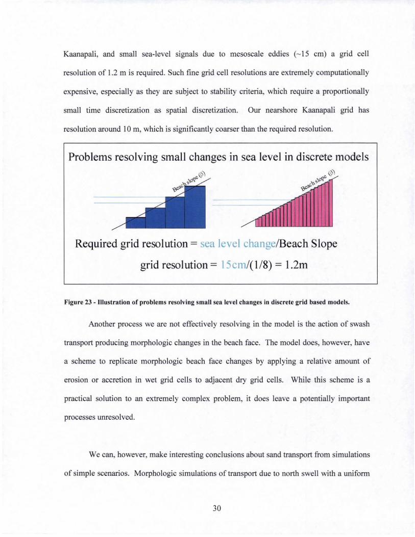
Kaanapali, and small sea-level signals due to mesoscale eddies (- 15 cm) a grid cell

resolution of 1.2 m is required. Such fine grid cell resolutions are extremely computationally

expensive, especially as they are subject to stabi lity criteria, which require a proportionally

small time discretization as spatial discretization. Our nearshore Kaanapali grid has

resolution around 10m, which is significantly coarser than the required resolution.

Problems resolving small changes in sea level in discrete models \Sl1

r,\O<I' ~'<>

Required grid resolution = sea level change/Beach Slope

grid resol ution = 15 cm/( 1 /8) = 1.2m

Figure 23 - Illustration of problems resolving small sea level changes in discrete grid based models.

Another process we are not effectively resolving in the model is the action of swash

transport producing morphologic changes in the beach face. The model does, however, have

a scheme to replicate morphologic beach face changes by applying a relative amount of

erosion or accretion in wet grid cells to adjacent dry grid cells. While th is scheme is a

practical solution to an extremely complex problem, it does leave a potentially important

processes unresolved.

We can, however, make interesting conclusions about sand transport from simulations

of simple scenarios. Morphologic simulations of transport due to north swell with a uniform

30

bed roughness demonstrate transport of a considerable amount of sand around Hanakao'o

Point. Increasing the simulated roughness for the submerged fossil reef offshore (making it

spatially variable) from Banakao'o Point causes the sand to accumulate in this location. This

is consistent with field observations.

Inability of the model to resolve the signal of the mesoscale eddy should not cause us

to dismiss its influence. Simple Bruunian models assign sea-level position paramount

influence, although the presence of reef surfaces may change this simple dynamic. It appears

that increased sea level on a normal shoreline profile (not perched) may exist in unstable

equilibrium until wave energy initiates transfer to a new position. The duration of mesoscale

eddies is sufficient to begin this transition as evidenced by the considerable erosion observed

in summer 2003 at Kaanapali. The event also suggests that increased sea-level signals may

cause accelerated seasonal response in alongshore systems.

CONCLUSIONS

Robust numerical models allow for realistic shoreline change simulations. Adequate

observations are indispensable to ensure realistic performance. Poor modeling performance

arises from inadequate tuning, unresolved processes, and spatial discretization of continuous

natural processes. Use of water-level gradient boundary conditions given by observations of

tidal components and the equations used in Roelvink and Wa1stra (2004) successfully model

tidal velocities. Scenario-based modeling of seasonal shoreline change is qualitatively

successful, whereas real-time, long-term simu1ations often to not capture significant changes

in beach profile and shoreline position.

31

Mesoscale eddies and accretion perched beaches atop rough reef substrates play a

potentially significant role in beach morphology of Hawaiian shorelines, and merit continued

investigation.

FUTURE WORK

The work presented here may be helpful in preparing future experiments to study

approaching mesoscale eddies. Satellite altimetry takes a snapshot of the sea surface height

of the entire globe every 10 days. Using this data, eddies approaching the islands can be

identified and assessed for risk. If the eddies estimated arrival coincides with the start of the

seasonal wave cycle and before significant beach profile changes have occurred, several

nearshore wave and current instruments should be placed in an array at the particular beach.

To accompany the instrumentation T-LIDAR beach surveys should be conducted at

intermediate temporal resolution when swell is not expected, and at high temporal resolution

(before, during and after) when swell is expected. The temporal resolution ofT-LIDAR

beach surveys should also attempt to resolve the beach profile changes as a function of the

tide. It is expected that at high tide the wave runup may reach further on the beach, and

potentially impact dunes and cause scarps to form. If these small sea-level signatures can

lead to increased erosion, much larger erosion events may occur with the coincidence of

these eddies, spring tides and large swell, rather than with large swell alone.

ACKNOWLEDGMENTS

The author would like to thank Edwin Elias, Dolan Eversole, Chris Conger, Jeff List,

Capt. Joe Reich, Lamber Hulsen, Dano Roelvink, Dirk-Jan Walstra, Everyone at Delft3D

support: Johan Dijkzeul, Atjen Luijendijk, and Meo de Rover.

32

REFERENCES

Baird and Associates. 2005. Pacific Ocean Wave Information Study Validation of Wave

Model: Results Against Satellite Altimeter Data. Prepared for u.S. Army Corps of

Engineers Engineering Research and Development Center

Elias, W.P.L. (2000). "Hydrodynamic validation of Delft2/3D with field measurements at

Edmond," Proc. 27th ICCE. Sydney. Australia.

Elias, W.P.L. (2006). "Morphodynamics of Texel Inlet," Ph. D. thesis. Delft University of

Technology, The Netherlands.

Eversole, D., Fletcher, C.H., (2003). "Longshore Sediment Transport Rates on a Reef­

Fronted Beach: Field Data and Empirical Models Kaanapali Beach, Hawaii," Journal of

Coastal Research: Vol. 19, No.3, pp. 649-663.

Firing, Y. L., and Merrifield, M. A., (2004). "Extreme sea level events at Hawaii: Influence

ofmesosca1e eddies," Geophys. Res. Lett. 31, L24306

Flament, P., Lumpkin, C., (1996). "Observations of currents through the Pailolo Channel:

Implications for nutrient transport," In: Wiltse, W. (Ed.), Algal Blooms: Progress Report

on Scientific Research, West Maui Watershed Management Project, pp. 57 -64.

Klein, M.D., Elias, E.P.L., Stive, MJ.F., Walstra, DJ.R., (2001). "Modelling inner surf zone

hydrodynamics at Egmond, The Netherlands," In: Hanson, H., Larson, M (Eds.), Proc.

4th Int. Conf. on Coastal Dynamics '01. ASCE, Reston, pp. 500-509.

Lesser, G.R., (2000). "Computation of Three-dimensional Suspended Sediment Transport

within the DELFTID-FLOW Module," Master's thesis. Delft University of Technology,

The Netherlands.

33

Lesser, G.R., Roelvink, J.A., van Kester, J.A.T.M., Stelling G.S., (2004). "Development and

validation ofa three-dimensional morphological model," Coastal Engineering. v. 51. pp.

883-915.

Luijendijk, A.P., (2001). "Validation, calibration and evaluation of Delft3D-FLOW model

with ferry measurements," Master's thesis. Delft University of Technology, The

Netherlands.

Merrifield, M.A., Yang, L., Luther, D.S., (2002). "Numerical simulations of a storm

generated island-trapped wave event at the Hawaiian Islands" Journal of Geophysical

Research 107 (CI0), 3169.

Roelvink, J.A., Wasltra, D.J., (2004). "Keeping in simple by using complex models," 6th

International Conference on Hydroscience and Engineering, Advances in Hydro­

Science and Engineering, Brisbane, Australia.

Roelvink, J.A., (2006). "Coastal Morphodynamic Evolution Techniques Coastal Engineering.

53, February (2006) 277-287

Stelling, G.S., (1984). "On the construction of computational methods of shallow water flow

problems," Rijkswaterstaat communications, No. 35

Storlazzi, C.D., McManus, M.A., Logan, J.B. Mclaughlin, B.E., (2006). "Cross-shore

velocity shear, eddies and heterogeneity in water column properties over fringing coral

reefs: West Maui, Hawaii," Continental Shelf Research 26 (2006) 401 -421

Sun, L.C., (1996). "The Maui algal bloom: the role of physics," In: Wiltse, W. (Ed.), Algal

Blooms: Progress Report on Scientific Research. West Maui Watershed Management

Project, pp. 54 -57.

34

Tolman, H.L. 2002. Validation of W A VEW ATCH III version 1.15 for a global domain.

NOAA I NWS I NCEP I OMB Technical Note Nr. 213: 33.

Tracy, B., Hanson, J., Cialone, A., Tolman, H.L., Scott, D. and Jensen, R 2006. Hawaiian

Islands Severe Wave Climate 1995-2004; 9th Waves Workshop Program. September

24-29. Victoria B.C.

U.S. Army Corps of Engineers. 2002. Shore Protection Projects. Coastal Engineering

Manual: V-3-59.

Walstra, D.J.R, Roelvink, J.A., Groeneweg, J., (2000). "Calculation of wave -driven currents

in a 3D mean flow model," Proc. 27th Int Conf. on Coastal Engineering. ASCE, New

York, pp. 1050-- 1063.

Walstra, D.J.R., Van Rijn, L.C., Boers, M., Roelvink, J.A., (2003). "Offshore sand pits:

verification and application of hydrodynamic and morphodynamic models," Proc. 5th

Int. Conf. on Coastal Sediments '03. ASCE, Reston, Virginia

35

MAXIMUM ANNUALLY RECURRING WAVE HEIGHTS IN HAWAI'1

ABSTRACT

The goal of this study is to determine the maximum annually recurring wave height

approaching Hawai'i. The motivation is scientific as well as administrative; to enhance

understanding of the recurring nature of dominant swell events, as well as to inform the

Hawai'i administrative process of determining the "upper reaches of the wash of the waves"

(Hawai'i Revised Statutes (H.R.S.) § 205-A), which delineates the shoreline. We test three

approaches to determine the maximum annually recurring wave including log-normal and

extremal exceedance probability models and Generalized Extreme Value (GEV) analysis

using 25 years of buoy data and long-term wave hindcasts. The annual recurring significant

wave height is found to be 7.7 ± 0.28m (25 ft ± 0.9 ft), and the top 10% and 1% wave

heights during this annual swell is 9.8 ± 0.35 m (32.1 ft ± 1.15 ft) and 12.9:!: 0.47 m (42.3 ft

:!: 1.5 ft) respectively, for open north and northwest swell. Directional annual wave heights

are also determined by applying hindcasted swell direction to observed buoy data lacking

directional information.

The islands of Hawai'i lie in the midst of a large swell-generating basin, the north

Pacific. Tropical storms tracking to the northwest and north of the islands produce winter

swell with breaking face heights exceeding 5 m several times each year. These swell events

lead to concerns over coastal erosion, coastal flooding, and water safety for the large

population of ocean communities in Hawai'i. Runup generated by the largest of these waves

poses a hazard to coastal development by flooding roadways, undermining structures and

36

causing erosion. According to Hawai'i State law (Hawai'i Revised Statutes (H.R.S.) § 205-

A) the highest runup of these annual swells sets the legal position of the shoreline.

In Hawai'i, the shoreline serves as a reference line used to delineate public beach

access, construction setbacks, state conservation land, submerged lands, and the border of

management jurisdiction. Several states define the shoreline differently, for instance

California uses the mean high water mark and Massachusetts uses the mean low water mark

based on tidal water levels (not including wave setup or runup).1n 1968, the State ofHawai'i

changed the definition of the shoreline from the mean high water mark to the highest reach of

the waves (IN RE ASHFORD). The State of Hawai'i definition of the shoreline is "the upper

reaches of the wash of the waves, other than storm and seismic waves, at high tide during the

season of the year in which the highest wash of the waves occurs, usually evidenced by the

edge of vegetation growth, or the upper limit of debris left by the wash of the waves"

(Hawai'i Revised Statutes (H.R.S.) § 205-A). In Oct. 2006, the Hawai'i Supreme Court

issued a ruling (Diamond v. State ofHawai'i) that the shoreline should be established "at the

highest reach of the highest wash of the waves."

The State of Hawai'i has established a coastal management system that relies on this

definition of the shoreline, not only as a demarcation of public shoreline access, but also to

establish a baseline for construction control and development setbacks. The discord of

private landowners seeking to preserve or develop the economic value of their property and

public ocean users wishing to access and preserve pristine coastal environments is

responsible for continuing debate over shoreline laws. Resolving the annually recurring

maximum wave height around the islands would improve the scientific basis to

understanding the shoreline definition, since this line is set by the upper limit of wave runup

37

resulting from the largest or set of largest annually recurring waves (under optimal run-up

conditions).

Local consulting engineers as part of their respective design projects on the coast are

required to describe the regional and local wave climate. This analysis typically consists of

specifying the largest characteristic ranges and scatter tables or rose diagrams of wave height,

period and direction of the dominant swell regime for the area of interest. Such engineering

reports (e.g. Noda and Associates 1991, Bodge & Sullivan 1999. Bodge 2000) do not give

detailed statistical analyses of the recurring nature of swells in Hawai'i.

To provide a comprehensive analysis, we wish to resolve the annually recurring

maximum wave based on the best records and state-of-the-art methods. The determination of

the annually recurring wave height is also the first step to ensuring a sound scientific basis

for policy-based decision-making involved in the determination of the shoreline as defined

by H.R.S. § 205-A.

PREVIOUS WORK

The seasonal wave cycle in Hawai'i has been explored in several different

publications. Moberly and Chamberlain (1964) outlined the wave cycle in terms of four

swell regimes: north Pacific swell, northeast trade wind waves, Kona storm waves and

southern swell. We have added a wave rose to their original graphic depicting annual swell

heights and directions (Figure 24).

38

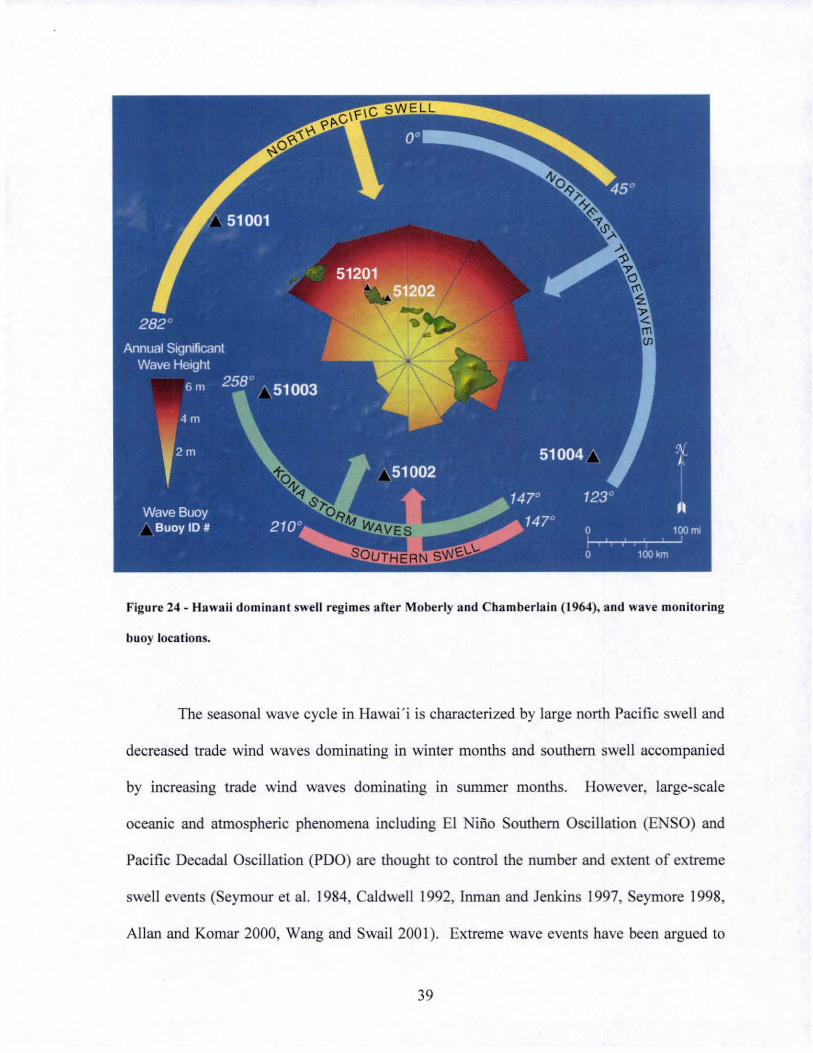
Figure 24 - Hawaii dominant swell regimes after Moberly and Chamberlain (1964). and wave monitoring

buoy locations.

The seasonal wave cycle in Hawai ' i is characterized by large north Pacific swell and

decreased trade wind waves dominating in winter months and southern swell accompanied

by increasing trade wind waves dominating in summer months. However, large-scale

oceanic and atmospheric phenomena including EI ilio Southern Oscillation (ENSO) and

Pacific Decadal Oscillation (PDO) are thought to control the number and extent of extreme

swell events (Seymour et at. 1984, Caldwell 1992, Inman and Jenkins 1997, Seymore 1998,

Allan and Komar 2000, Wang and Swail 2001). Extreme wave events have been argued to

39

control processes such as coral development (Dollar and Tribble 1993, Rooney et al. 2004)

and beach morphology (Moberly and Chamberlain 1964, Ruggiero et al. 1997, Storlazzi and

Griggs 2000).

While there are several factors that contribute to annual variability in maximum wave

height in Hawai ' i including the ENSO and PDO cycles, the legal importance of the annually

recurring wave height requires its clarification. Ruggiero et al. (1997) evaluated extreme

run up using empirical equations as a means of calculating frequency of dune impact. This

empirical approach or a more robust process-based numerical modeling approach could

similarly be used to evaluate the extent of extreme runup in Hawaii based on the annual

maximum wave height. This study could provide boundary conditions for a more

sophisticated wave transfomlation alld runup model for identification of the shoreline in

Hawai ' i for a particular location.

MATERIALS AND METHODS

To determine the annually recurring maximum wave height we use the record of

wave buoys from the National Oceanic and Atmospheric Administration (NOAA) National

Data Buoy Center (NDBC) and WaveWatch III (WWUI) model hind casts from the Coastal

and Hydraulics Laboratory' s (CHL) Wave Information Studies (WIS) program (Vicksburg,

Miss.).

Hourly reports of significant wave height (average of the largest 1/3 of wave heights,

Hs ) and other meteorological information from monitoring buoys are available from

OAA's NDBC website (hnp://\\ww.ndbc.noaa.gov/MapsfIlawaii.shtml) . Based on the

observation that wave heights follow a Rayleigh distribution we can use the significant wave

height to estimate other statistics of a swell, such as the mean wave height or the top 10%

40

wave height, based on the significant wave height. These buoys have an instrument

precision of 0.2 In, which result in small errors (less than 5% for all waves above 4 m).

Our focus concerns buoy 51001 (buoy 1), which is located 170 nautical miles

northwest of the island ofKauai and is moored at a depth of 3.25 Ian. The buoy has recorded

25 years of wave height and period data, since 1981.

Buoy 1 is ideally located to record north and northwest Pacific swell without

interference from neighboring islands. Only recently has buoy 1 been able to record swell

direction. Thus the time-series recorded in the majority of buoy 1 and all of the remaining

buoys lack swell direction. The lack of observations of wave direction means that any

analysis of open north and northwest swell is limited to buoy 1 as all the remaining buoys are

significantly affected by island blockage, however hindcasts using Wave Watch ill can be

used to recover directional information.

Long-term statistical analysis is applied to the simple case of the I-year recurring

significant swell height Statistics of extremes can usually be extrapolated to approximately

3 times the length of the time-series. As we are primarily interested in the annually recurring

maximum wave height, our 25 year time-series is more than adequate to resolve this value.

Long-term statistical models are typically applied to long return period events such as the 50-

100 year events; such methods were origina1ly developed to define stream flood heights or

return periods from discharge records (Gumbel 1941). Although typically applied to long

return periods, they can also be applied for short and intermediate return periods. The

following procedure was used to construct our long-term statistical model:

41

1. Large swen events (n per year) from the buoy record are assigned an exceedance

probability (given below).

2. Log-normal and extremal models use linear regressions to determine the

relationship between large swen events and exceedance probability (the

probability that a larger swen event will occur during the return period). To

corroborate this analysis Generalized Extreme Value (GEV) probability models

also determine the relationship between large swen events and exceedance

probability using Maximum Likelihood Estimates (MLE).

3. Methods including removing outliers and the Peak Over Threshold (van Vledder

et aI. 1993) method are evaluated to improve model performance.

4. These statistical models assign probabilities to a full range of swen heights and

are modified to give the relationship between swen heights and return period

(particularly the I-year return period).

5. The maximum annually recurring wave height is determined from the tail of a

Rayleigh distribution.

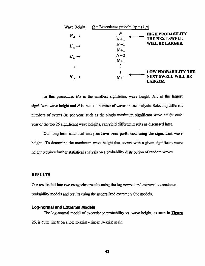
The log-normal statistical models is constructed on the assumption that maximum

swen events will plot as a linear function on a horizontal logarithmic-scale of exceedance

probability. Exceedance probability (Q = 1 - p) is given by the probability that the next

swen will be greater than the sorted wave events on record as if drawing from a hat

containing all the maximum swen heights and the next swen event.

42

Wave Height Q = Exceedance probability = (l-p)

N IDGH PROBABILITY N + I" THE NEXT SWELL N -I WILL BE LARGER.

N+I N-2 N+I

I

N+I

.-__ LOW PROBABILITY THE .. NEXT SWELL WILL BE

LARGER.

In this procedure, Hsl is the smallest significant wave height, HaN is the largest

significant wave height and N is the total number of waves in the analysis. Selecting different

numbers of events (n) per year, such as the single maximum significant wave height each

year or the top 25 significant wave heights, can yield different results as discussed later.

Our long-term statistical analyses have been performed using the significant wave

height. To determine the maximum wave height that occurs with a given significant wave

height requires further statistical analysis on a probability distribution of random waves.

RESULTS

Our results fall into two categories: results using the log-normal and extremal exceedance

probability models and results using the generalized extreme value models.

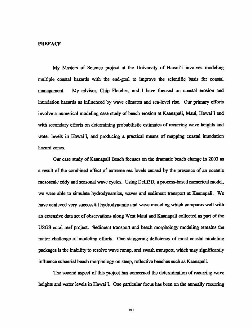
Log-normal and Extremal Models The log-normal model of exceedance probability vs. wave height, as seen in Figure

~ is quite linear on a log (x-axis) -linear (y-axis) scale.

43

E ~

:r:

A

11 Error RMS (log-normal)= 0.0749 m

10 , , <J ..

9 ,

8

7 Error RMS (extremal)= 0.0615

6 0 Wave Data

5 --Log-normal fit - - - Extremal fit (k fit)

4 0 2 4 6 8

-log(Q)

11

10

9

E 8

:r: 7 m

6

5

4 0

B

----- ---

1-Year Return Swell Event = 7.67 ± 0.014 m

~ Wave Data

Log-norma l fit - - - Extremal fit (k fit)

10 20 30 Return Period Tr (years )

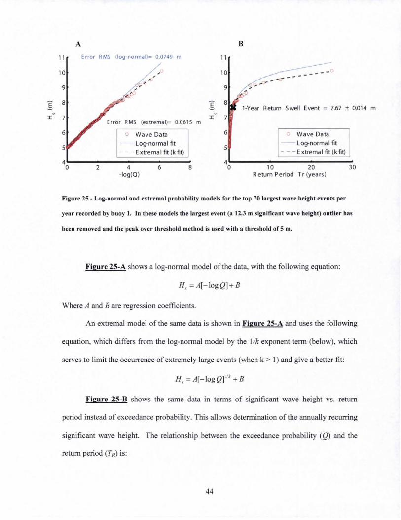
Figure 25 - Log-normal and extremal probability models for the top 70 largest wave height events per

yea r recorded by buoy I. In these models the largest event (a 12.3 m significant wave height) outlier has

been removed and the peak over threshold method is used with a threshold of 5 m.

Figure 2S-A shows a log-normal model of the data, with the following equation:

H, = A[- logQJ + B

Where A and B are regression coefficients.

An extremal model of the same data is shown in Figure 2S-A and uses the following

equation, which differs from the log-normal model by the Ilk exponent term (below), which

serves to limit the occurrence of extremely large events (when k > 1) and give a better fit:

H, = A[- logQJ'1k + B

Figure 2S-B shows the same data in terms of significant wave height vs. return

period instead of exceedance probability. This allows determination of the annually recurring

significant wave height. The relationship between the exceedance probability (Q) and the

rerum period (TR) is:

44

T. = ri. R Q

where r.i. is the recurrence interval.

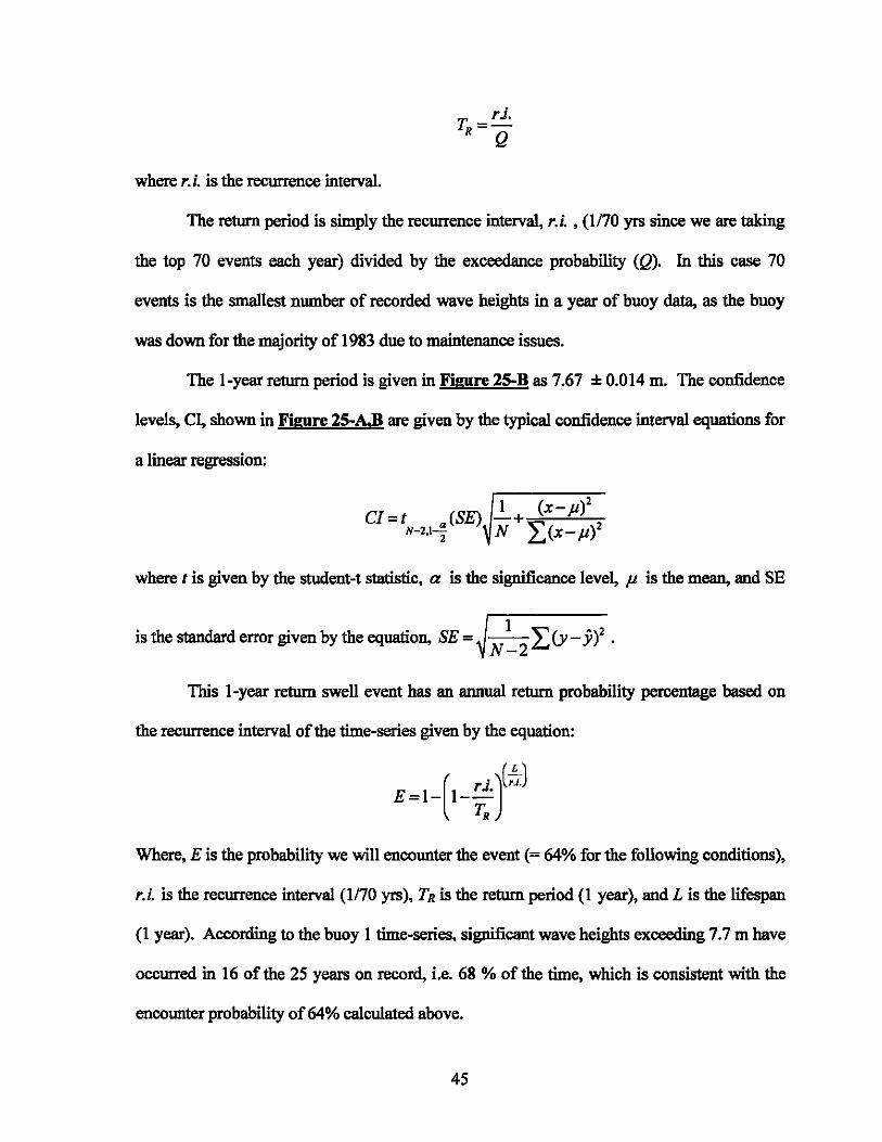
The return period is simply the recurrence interval, r.i. , (1170 yrs since we are taking

the top 70 events each year) divided by the exceedance probability (Q). In this case 70

events is the smallest number of recorded wave heights in a year of buoy data, as the buoy

was down for the majority of 1983 due to maintenance issues.

The I-year return period is given in Figure 25-B as 7.67 ± 0.014 m. The confidence

levels, CI, shown in Figure 25-A.B are given by the typical confidence interval equations for

a linear regression:

CI=t (8E) .!.+ (X-fJ)2 N-2.1~ N L(X-fJ)2

where t is given by the student-t statistic, a is the significance level, fJ is the mean, and SE

is the standard error given by the equation, 8E = ~_I-L (y _ y)2 . N-2

This I-year return swell event has an annual return probability percentage based on

the recurrence interval of the time-series given by the equation:

( ri.)('~J E=I- 1--

TR

Where, E is the probability we will encounter the event (= 64% for the following conditions),

r.i. is the recurrence interval (1170 yrs), TR is the return period (1 year), and L is the lifespan

(1 year). According to the buoy 1 time-series. significant wave heights exceeding 7.7 m have

occurred in 16 of the 2S years on record, i.e. 68 % of the time, which is consistent with the

encounter probability of 64% calculated above.

4S

Log-normal models tend to over-predict large events because physical processes exert

natural limitations on event magnitude that are not accounted for in the model. For instance,

flood height is limited by the rainfall amount, wave height is limited by energy dissipation,

and hurricane intensity is limited by heat transfer to fuel propagation. Thus, extreme events

(long return period events) are often not best fit with a log-normal relationship, and other

models such as the extremal model should be considered. A particular example of this

concerns the largest significant wave height in the 25-year record of buoy 1: a 12.3 m event

that occurred at 4:00 am on November 5th, 1988. The second largest on record is 10.1 m

(1985). These are the only two events with significant wave heights exceeding 10 m and

notably, the largest swell on record is more than 2 m greater than the next largest swell. In

the analysis above this 12.3 event is removed. We must consider the possibility that the 12.3

m significant wave height event was an extraordinary swell, and perhaps unlikely to occur

during a period of 25 years. In exceedance probability models the largest event (12.3 m)

provides information about the longest return period of recorded data (25 years in this case).

In reality, this 12.3 m event could very well be the 50 or 100-year swell event, and including

this event over-estimates the frequency of large events in the model as well as affects the

value for the annually recurring wave height. A simple procedure is to test potential over­

estimation to determine the best fit without the outlier event and determine the expected

return period of the removed outlier. Using the model above, the return period ofa 12.3 m

event is approximately 150 and 700 years using log-normal and extremal models

respectively. Typically, forecasts longer than 3-4 times the data collection period (25 years

in this case) are not realistic, and further more they are not the focus of this paper. However,

46

we perform such analysis to confirm our suspicion that a very large event occurred in 1988

with a recurrence interval exceeding 100 years, and justify its removal from the analysis.

Returning to the annual return period, a log-normal model would perhaps be

appropriate, but for completeness we investigate the behavior of swell events using both log-

normal and extremal models as well as the GEV model (below). The GEV statistical model

returns very similar results to the log-normal and extremal models, which focus on our

estimates of the annually recurring significant wave height.

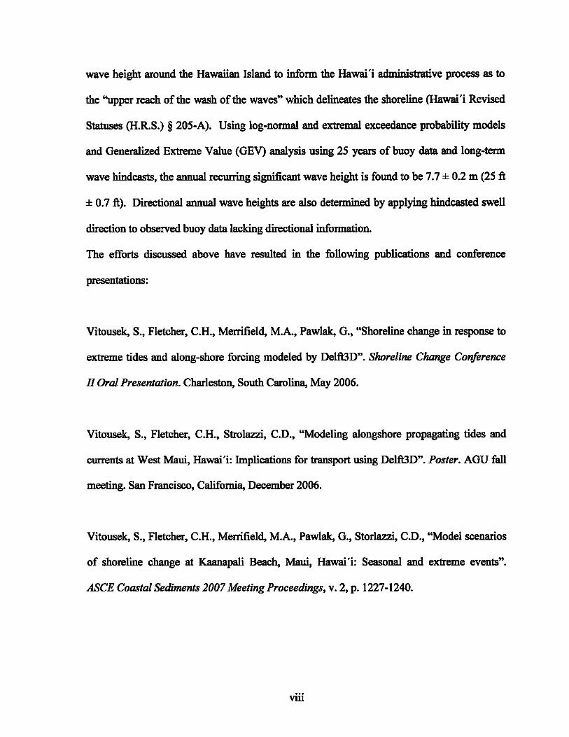
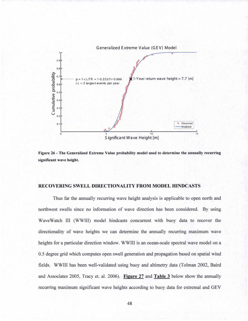
Generalized Extreme Value (GEV) Model The Generalized Extreme Value (GEV) distribution is applied to determine

relationships between wave height and return period with particular focus on the annually

recurring wave height. Introduced by Jenkinson (1955), the GEV distribution uses Gumbel

(type I), Frechet (type 11). and Weibull (type III) distributions for different values of the

shape parameter. K: = O. K: < 0, K > 0 respectively. Iterative maximum-likelihood estimates

(MLE) fit the observed data to find the best estimates of the shape (K). scale (0') and

location (p ) parameters of the GEV cumulative distribution function, F(x). given by:

F(x)- OXP(-[I+« 7 t 1 forK¢O

exp{ _exp[ (x:p )]} forK=O

Based on given probability distributions and the return period probability equation Pr. = 1- r J. , wave beight R To

R

for an arbitrary return period is found. The GEV model is more robust than the previous approach

because it combines the Gumbel, Frechet, and Weibull extreme value distributions, although it yields very

similar results to our log-normal and extremal analysis (FIgure 26). The GEV analysis, being a more

robust model, remains largely unaffected by the presence of the 12.3 m event

47

Generalized Extreme Value (GEV) Model

0.9

0.'

l!-:.= 0.7 :0 1<--- p= 1-r.i./TR = 1-0.33311 = 0.666 l-Year re turn wave height = 7.7 [m] ] 0.6 rJ. = 3 largest events per year

e c.. O.S

'" > .'" ~ 0 ,1,

:::> E 0.3 :::>

U 0.2

0.1

o

'I

S 10

5 ignifica nt Wave Height [m] 15

Figure 26 - The Generalized Extreme Value probability model used to determine the annually recurring

significant wave height.

RECOVERING SWELL DIRECTIONALITY FROM MODEL HJNDCASTS

Thus far the annually recurring wave height analysis is appl icable to open north and

northwest swells since no information of wave direction has been considered. By using

WaveWatch III (WWlII ) model hindcasts concurrent with buoy data to recover the

directionality of wave heights we can determine the annually recurring maximum wave

heights for a particular direction window. WWIlI is an ocean-scale spectral wave model on a

0.5 degree grid which computes open swell generation and propagation based on spatial wind

fields. WWlll has been well-validated using buoy and altimetry data (Tolman 2002, Baird

and Associates 2005, Tracy el. al. 2006). Figure 27 and Table 3 below show the annually

recurring maximum significant wave heights according to buoy data for extremal and GEV

48

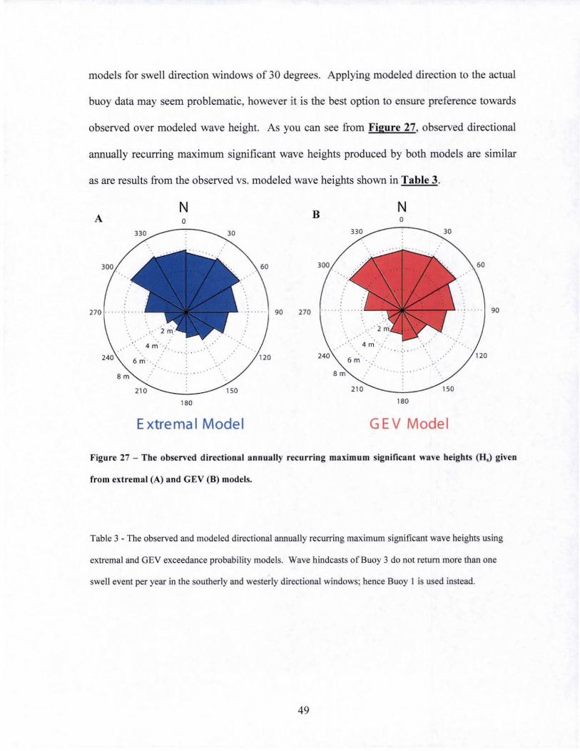
models for swell direction windows of 30 degrees. Applying modeled direction to the actual

buoy data may seem problematic, however it is the best option to ensure preference towards

observed over modeled wave height. As you can see from Figure 27, observed directional

annually recurring maximum significant wave heights produced by both models are similar

as are results from the observed vs. modeled wave heights shown in Table 3.

N A o

330 30

300

270 . 90 270

240

8m .. .. :. ....

210 150

180

Extrema I Model

B

240

8m

330

4 m" ·": ..

6 m ".:'

210

N o

. ....

180

30

,," .

150

GEV Model

60

. 90

120

Figure 27 - The observed directional annually recurring maximum significant wave heights (H,) given

from extremal (A) and GEV (8) models.

Table 3 - The observed and modeled directional annually recurring maximum significant wave heights us ing

extremal and GEV exceedance probability models. Wave hindcaslS of Buoy 3 do not return more than one

swell event per year in the southerly and westerly directional windows; hence Buoy I is used instead.

49

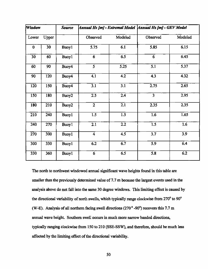
~indow Source f4nnual Hs {m{- Extremal Model f4nnual Hs {m] - GEV Model

Lower Upper Observed Modeled Observed Modeled

0 30 Buoyl 5.75 6.1 5.85 6.15

30 60 Buoy1 6 6.5 6 6.45

60 90 Buoy4 5 5.25 5.1 5.37

90 120 Buoy4 4.1 4.2 4.3 4.32

120 150 Buoy4 3.1 3.1 2.75 2.65

150 180 Buoy2 2.5 2.4 3 2.95

180 210 Buoy2 2 2.1 2.35 2.35

210 240 Buoy1 1.5 1.5 1.6 1.65

240 270 Buoy 1 2.1 2.2 1.5 1.6

270 300 Buoy1 4 4.5 3.7 3.9

300 330 Buoy1 6.2 6.7 5.9 6.4

330 360 Buoy1 6 6.5 5.8 6.2

The north to northwest windowed annual significant wave heights found in this table are

smaller than the previously determined value of7. 7 m because the largest events used in the

analysis above do not fall into the same 30 degree windows. This limiting effect is caused by

the directional variability of north swells, which typically range clockwise from 2700 to 900

(W -E). Analysis of all northern facing swell directions (270 0 -90~ recovers this 7.7 m

annual wave height. Southern swell occurs in much more narrow banded directions,

typically ranging clockwise from 150 to 210 (SSE-SSW), and therefore, should be much less

affected by the limiting effect of the directional variability.

50

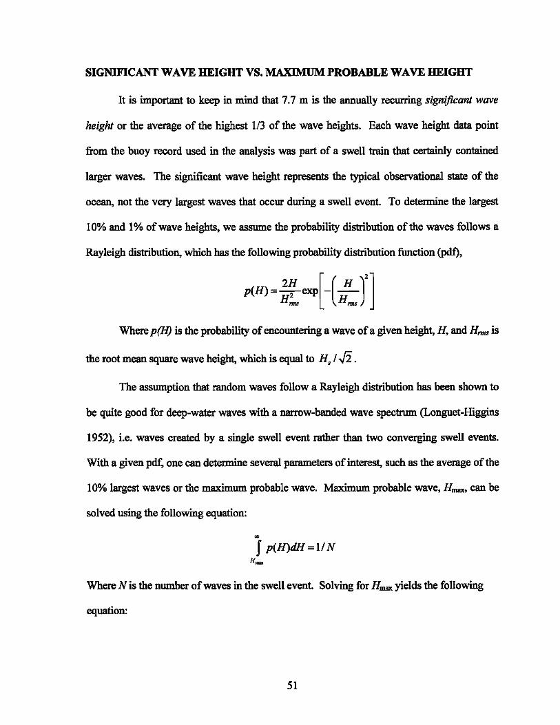
SIGNIFICANT WAVE HEIGHT VS. MAXIMUM PROBABLE WAVE HEIGHT

It is important to keep in mind that 7.7 m is the annually recurring significant wave

height or the average of the highest 113 of the wave heights. Each wave height data point

from the buoy record used in the analysis was part of a swell train that certainly contained

larger waves. The significant wave height represents the typical observational state of the

ocean, not the very largest waves that occur during a swell event. To determine the largest

10% and 1 % of wave heights. we assume the probability distribution of the waves follows a

Rayleigh distribution, which has the following probability distribution function (pdf).

Where p(H) is the probability of encountering a wave of a given height, H, and H171IJI is

the root mean square wave height, which is equal to Hs / .J2 .

The assumption that random waves follow a Rayleigh distribution has been shown to

be quite good for deep-water waves with a narrow-banded wave spectrum (Longuet-Higgins

1952). i.e. waves created by a single swell event rather than two converging swell events.

With a given pdf, one can determine several parameters of interest, such as the average of the

10% largest waves or the maximum probable wave. Maximum probable wave, Hrrmx. can be

solved using the following equation:

Where N is the number of waves in the swell event. Solving for HUJBX yields the following

equation:

51

!-1m", = H".,Jln N = !-I, ~~lnN

The average of the 10% largest waves is given by the following equation:

'" '" f p(H)HdH f p(H)Hd!-l

Avg. of H,Wo = -"H"',,:"-___ _ all f !-I II ",%

or more gener y, Avg.o J'C' % = --"''''' ''-----f p(H)d!-l f p(H)dH

H, .. 11",%

Where !-I/O'/, or (Hpcff,) is given by the equation: H , t-ln 1 , where pet is the percent of 2 pel

interest. By integrating the equation above, the average of the top percentages of wave

heights in relation to the significant wave height are shown on Figure 28.

2

1.9

1.8

Avg. of Top 1% = 1.67Hs 1.7

1.6 VI

1.5 :r -:r 1.4

1.3

1.2

1.1

1 35% 30% 25% 20% 15% 10% 5% 0%

Top Percent of Waves

Figure 28 - Top percent of waves vs. relation to significant wave height (H.)

52

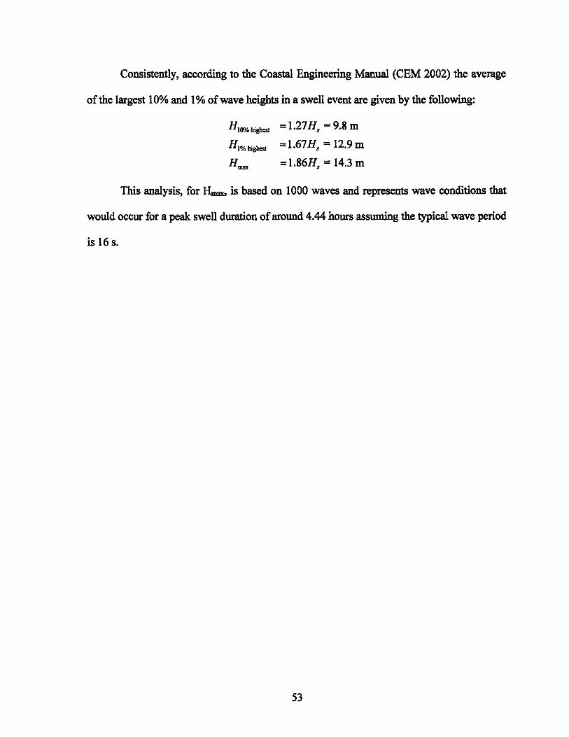
Consistently, according to the Coastal Engineering Manual (CEM 2002) the average

of the largest 10% and 1 % of wave heights in a swell event are given by the following:

HIO%hiP. =1.27Hs =9.8m

HI% hiP. = 1.67 H, = 12.9 m

Hnw =1.86H, = 14.3 m

This analysis, for Hmax. is based on 1000 waves and represents wave conditions that

would occur for a peak swell duration of around 4.44 hours assuming the typical wave period

is 16 s.

53

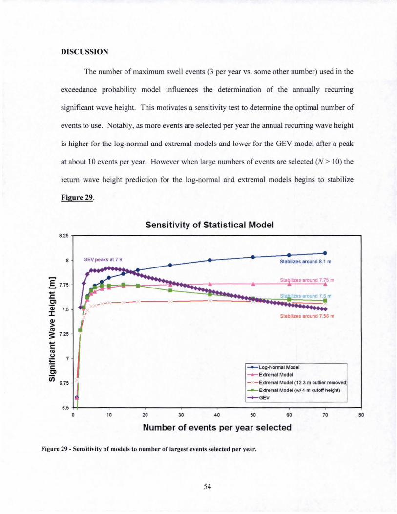
DISCUSSION

The number of maximum swell events (3 per year vs. some other number) used in the

exceedance probabi lity model influences the determination of the annually recurring

significant wave height. This motivates a sensitivity test to determine the optimal number of

events to use. Notably, as more events are selected per year the annual recurring wave height

is higher for the log-normal and extremal models and lower for the GEV model after a peak

at about 10 events per year. However when large numbers of events are selected (N ) 10) the

return wave height prediction for the log-normal and extremal models begins to stabilize

Figure 29.

Sensitivity of Statistical Model 8.25

~

8 GEV peeks at 7.9 Stablltzes around 8.1 m ..... ~

oS 7.75 r~ Staliil1Z8S around 7.15 m

Jr -.= OJ C1I 7.5 J:

~ ~ 7.25 -c: C'(I \J ~ 7 c: OJ

iii 6.75

6 .5

-,

o 10

Ste,bJIIZSS around 7.6 m

....... StabilIZes around 7.56 m

-"-Log-Nonnal Model -&- Extremal Model

- - Extremal Model (12.3 m outlIer removed

__ EX1remal Model flNI4 m colotl height) __ GEV

20 30 40 50 60 70

Number of events per year selected

Figure 29 - Sensitivity of models to num ber of largest events selected per year.

54

80

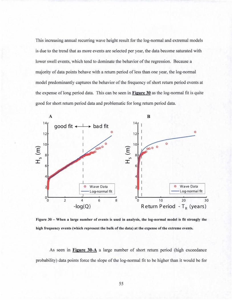
This increasing annual recurring wave height result for the log-normal and extremal models

is due to the trend that as more events are selected per year, the data become saturated with

lower swell events, which tend to dominate the behavior of the regression. Because a

majority of data points behave with a return period of less than one year, the log-nonnal

model predominantly captures the behavior of the frequency of short return period events at

the expense of long period data. This can be seen in Figure 30 as the log-normal fit is quite

good for short return period data and problematic for long return period data.

A B

14 good fit • ) bad fit

14

12 0 12 0

10 10 0 - -E E ~ 8 ~ 8

In In

I I 6 6

0 Wave Data 2 0 Wave Data -- Log-norma I fit

a 0 0 2 4 6 8 0 10 20 30

-log(Q) Return Period -TR (years)

Figure 30 - When a large number of events is used in analysis, the log-normal model is lit strongly the

high frequency events (which represent the bulk of the data) at the expense of the extreme events.

As seen in Figure 30-A a large number of short return period (high exceedance

probability) data points force the slope of the log-normal fit to be higher than it would be for

55

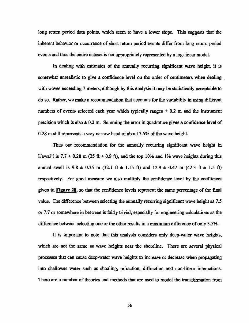
long return period data points, which seem to have a lower slope. This suggests that the

inherent behavior or occurrence of short return period events differ from long return period

events and thus the entire dataset is not appropriately represented by a log-linear model.

In dealing with estimates of the annually recurring significant wave height, it is

somewhat unrealistic to give a confidence level on the order of centimeters when dealing

with waves exceeding 7 meters, although by this analysis it may be statistically acceptable to

do so. Rather. we make a recommendation that accounts for the variability in using different

numbers of events selected each year which typically ranges :!: 0.2 m and the instrument

precision which is also :!: 0.2 m. Summing the error in quadrature gives a confidence level of

0.28 m still represents a very narrow band of about 3.5% of the wave height.

Thus our recommendation for the annually recurring significant wave height in

Hawai'i is 7.7 ± 0.28 m (25 ft ± 0.9 ft), and the top 10% and 1% wave heights during this

annual swell is 9.8 :!: 0.35 m (32.1 ft :!: 1.15 ft) and 12.9 :!: 0.47 m (42.3 ft :!: 1.5 ft)

respectively. For good measure we also multiply the confidence level by the coefficient

given in Figure 28. so that the confidence levels represent the same percentage of the fina1

value. The difference between selecting the annually recurring significant wave height as 7.5

or 7.7 or somewhere in between is fairly trivial, especially for engineering calculations as the

difference between selecting one or the other results in a maximum difference of only 3.5%.

It is important to note that this analysis considers only deep-water wave heights,

which are not the same as wave heights near the shoreline. There are several physical

processes that can cause deep-water wave heights to increase or decrease when propagating

into shallower water such as shoaling, refraction, diffraction and non-linear interactions.

There are a number of theories and methods that are used to model the transformation from

56

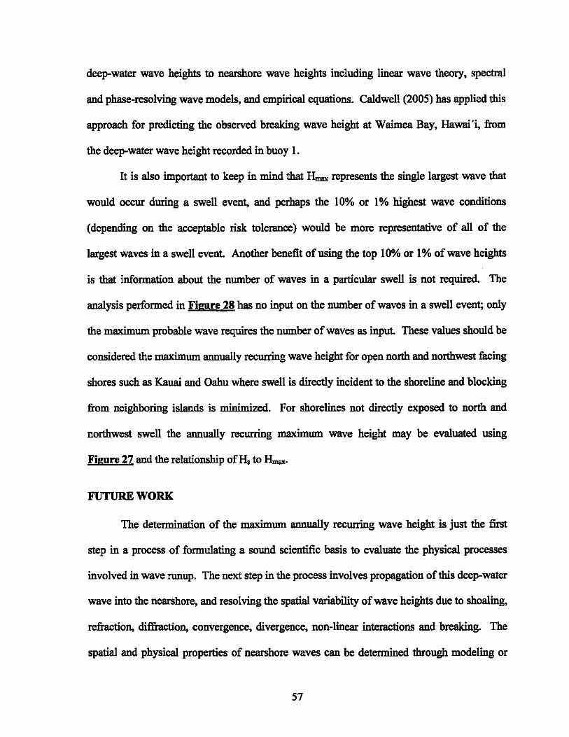
deep-water wave heights to nearshore wave heights including linear wave theory, spectral

and phase-resolving wave models, and empirical equations. Caldwell (2005) has applied this

approach for predicting the observed breaking wave height at Waimea Bay, Hawai'i, from

the deep-water wave height recorded in buoy 1.

It is also important to keep in mind that Hmax represents the single largest wave that

would occur during a swell event, and perhaps the 10% or I % highest wave conditions

(depending on the acceptable risk tolerance) would be more representative of all of the

largest waves in a swell event. Another benefit of using the top 10% or I % of wave heights

is that information about the number of waves in a particular swell is not required. The

analysis performed in Figure 28 has no input on the number of waves in a swell event; only

the maximum probable wave requires the number of waves as input. These values should be

considered the maximum annually recurring wave height for open north and northwest facing

shores such as Kauai and Oahu where swell is directly incident to the shoreline and blocking

from neighboring islands is minimized. For shorelines not directly exposed to north and

northwest swell the annually recurring maximum wave height may be evaluated using

Figure 27 and the relationship ofH, to Hmax.

FUTURE WORK

The determination of the maximum annually recurring wave height is just the first

step in a process of formulating a sound scientific basis to evaluate the physical processes

involved in wave runup. The next step in the process involves propagation of this deep-water

wave into the nearshore, and resolving the spatial variability of wave heights due to shoaling,

refraction, diffiaction, convergence, divergence, non-linear interactions and breaking. The

spatial and physical properties of nearshore waves can be determined through modeling or

57

empirical approaches. Finally, to evaluate nmup, these near-shore wave properties can be

used as boundary conditions in a nmup model, and observations of nmup should be recorded

during wave events with deep-water wave heights around the annually recurring maximum

level.

ACKNOWLEDGEMENTS

This paper is funded by a grant/cooperative agreement from the National Oceanic and

Atmospheric Administration, Project # RlEP-26, which is sponsored by the University of

Hawaii Sea Grant College Program, SOEST, under Institutional Grant No.

NA050AR4171048 from NOAA Office of Sea Grant, Department of Commerce. The views

expressed herein are those of the author(s) and do not necessarily reflect the views of NOAA

or any ofits subagencies. UNllll-SEAGRANT- JC-06-17.

REFERENCES

Allan. J., and Komar, P. 2000. Are ocean wave heights increasing in the eastern North Pacific? Eos 81: 561-

567.

Baird and Associates. 2005. Pacific Ocean Wave Information Study Validation of Wave Model: Results

Against Satellite Altimeter Data. Prepared for U.S. Army Corps of Engineers Engineering Research

and Development Center

Bodge, K. R. 2000.lndependent evaluation study of proposed Kuhio beach improvements, Prepared for State of

Hawaii, Department ofLand and Natural Resources.

Bodge, K. R., and Sullivan, S. 1999. Hawaii Pilot Beach Restoration Project: Coastal engineering investigation,

Prepared for State of Hawaii, Department ofLand and Natural Resources.

58

CaldweD, P. 1992. Surfing the EI Nifto. Mariners Weather Log 36: 60--64.

Dollar, S. J. and Tnoble, G.W. 1993. Recwrent storm disturbance and recovery: a long-term study of coral

communities in Hawaii. Coral Reefs, 12,223-233.

Gumbel, E. J. 1941. The Return Period of Flood Flows. Annals ofMatk Stat. 12: 163-190.

Jenkinson, A. F. 1955. The frequency distn"bution of the annual maximum (or minimum) values of

meteOrological elements, Q. J. R. MeteoroL Soc., 81: 158-171.

Longuet-Higgins, M. S. 1952. On the Statistical Distribution of the Wave Heights of Sea Waves. Jour. Marine

Res. 11: 245-266.

Moberly, R. and Cbamber1ain, T. 1964. Hawaiian Beach Systems. Hawaii Institute of Geophysics Report 64-2,

University of Hawaii.

Noda, E.K. and associates. 1991. Wave Measurement Program: Offshore Waikiki Beach, Prepared for State of

Hawaii, Department of Land and Natural Resources.

Inman, D. L., and Jenkins, S. A. 1997. Changing wave climate and littoral drift along the California coast.

Pages 314-327 in O. T. Magoon, ed. Proceedings of the California and the World Ocean Conference

'97 Conference. American Society of Civil Engineers, San Diego.

Rooney, J. Fletcher, C.H., Grossman, E, Engels, M. and Field, M. 2004. EI Nifto Influence on Holocene Reef

Accretion in Hawai'i, Pacific Science vol. 58 :305-324.

59

Ruggiero, P., Kaminsky, G.M., Komar, P.O., and McDougal, W.G. 1997. "Extreme waves and coasta1 erosion

in the Paeific Northwest, " Ocean Wave Measuremeots and Analysis, Proceedings of the 3'"

loternationai Symposium, Waves '97,947·961.

Seymour, R. J. 1998. Effect ofEI Niilos on west coast wave climate. Shore & Beach 66: 3-11.

Seymour, R. J., R. R. Strange ill, D. R. Cayan, and Nathan. R. A. 1984. 10fIuence ofE! Niilos on California's

wave climate. in B. L. Edge, ed Proceedings of the 19th lotemationai Conference on Coasta1

Engineering. American Society of Civil Engineers, New York. 35:215-230.

Storlazzi, C.D., and Griggs, G.B. 2000. 10fIuence of EI Niilo-Southern Oscillation (ENSO) events on the

evolution of central California's shoreline. GSA Bulletin. 112: 236-249.

Tolman, H.L. 2002. Validation ofW A YEW ATCH ill version 1.15 for a global domain. NOAA / NWS / NCEP

/OMB Technical Note Nr. 213: 33.

Tracy, B., Hanson, J., Cialone, A., Tolman, H.L., Scott, D. and Jensen, R. 2006. Hawaiian Islands Severe Wave

Climate 1995·2004; 9th Waves Workshop Program. September 24-29. Victoria B.C.

u.s. Army Corps of Engineers. 2002. Water Wave Mechanics. Coastal Engineering Manual: 1I·1·74.

Van Vledder, G., Y. Gods, P. Hawkes, E. Mansard, MJ. Martin, M. Mathiesen, E. Peltier and E. Thompson,

Case studies of extreme wave analysis: a comparative analysis, Proceedings Waves 93, Ocean wave

Measurement and Analysis, American society of Civil Engineers, pp. 978·992. 1993.

Wang, S. L., and Swail, V. R. 2001. Changes of extreme wave heights in Northern Hemisphere oceans and

related atmospheric circu1ation regimes. J. Clim. 14: 2204--2221.

60