ORIGINAL ARTICLE

NeAT: a Nonlinear Analysis Toolbox for Neuroimaging

Adrià Casamitjana1 & Verónica Vilaplana1 & Santi Puch2& Asier Aduriz3 & Carlos López1 & Grégory Operto4

&

Raffaele Cacciaglia4 & Carles Falcón4,5& José Luis Molinuevo4,6,7,8

& Juan Domingo Gispert4,7,8,9 & for the Alzheimer’sDisease Neuroimaging Initiative

# The Author(s) 2020

AbstractNeAT is a modular, flexible and user-friendly neuroimaging analysis toolbox for modeling linear and nonlinear effects over-coming the limitations of the standard neuroimaging methods which are solely based on linear models. NeAT provides a widerange of statistical and machine learning non-linear methods for model estimation, several metrics based on curve fitting andcomplexity for model inference and a graphical user interface (GUI) for visualization of results.We illustrate its usefulness on twostudy cases where non-linear effects have been previously established. Firstly, we study the nonlinear effects of Alzheimer’sdisease on brain morphology (volume and cortical thickness). Secondly, we analyze the effect of the apolipoprotein APOE-ε4genotype on brain aging and its interaction with age. NeAT is fully documented and publicly distributed at https://imatge-upc.github.io/neat-tool/.

Keywords nonlinear . neuroimaging . GLM . GAM . SVR . Alzheimer's disease . inference . APOE

Introduction

The increase of computational power and advances in neuro-imaging acquisition that enable faster scans and provide mul-tiple image contrasts and modalities has motivated the

development of complex modeling techniques for imagingdata. An armoury of neuroimaging analysis tools is availableto the neuroscientific community, whose ultimate goal is toconduct statistical tests to identify significant effects in theimages without any a priori hypothesis on the location or

Alzheimer’s Disease Neuroimaging Initiative (ADNI) is a Group/Institutional Author.Data used in preparation of this article were obtained from theAlzheimer’s Disease Neuroimaging Initiative (ADNI) database(adni.loni.ucla.edu). As such, the investigators within the ADNI contrib-uted to the design and implementation of ADNI and/or provided data butdid not participate in analysis or writing of this report. A complete listingof ADNI investigators can be found at: http://adni.loni.ucla.edu/wpcontent/uploads/how_to_apply/ADN I_Acknowledgement_List.pdf

* Verónica Vilaplanaveronica.vilaplana@upc.edu

* Juan Domingo Gispertjdgispert@barcelonabeta.org

1 Department of Signal Theory and Communications, UniversitatPolitècnica de Catalunya (UPC), Barcelona, Spain

2 QMENTA, Barcelona, Spain3 Vilynx, Barcelona, Spain4 BarcelonaBeta Brain Research Center (BBRC), Pasqual Maragall

Foundation, Barcelona, Spain

5 Alzheimer’s Disease and Other Cognitive Disorders Unit, HospitalClínic, Institut d’Investigacions Biomèdiques August Pi i Sunyer(IDIBAPS), Barcelona, Spain

6 CIBER Fragilidad y Envejecimiento Saludable (CIBERFES),Madrid, Spain

7 Universitat Pompeu Fabra, Barcelona, Spain

8 IMIM (Hospital del Mar Medical Research Institute),Barcelona, Spain

9 Centro de Investigación Biomédica en Red de Bioingeniería,Biomateriales y Nanomedicina (CIBER-BBN), Madrid, Spain

Neuroinformaticshttps://doi.org/10.1007/s12021-020-09456-w

extent of these effects. In the literature, analysis at differentlevels of brain morphometry are found, involving voxel-based(Penny et al. 2011), surface-based (Fischl 2012) or boundary-based analysis (Freeborough and Fox 1997).

Irrespective of their particular characteristics, the vast ma-jority of them perform statistical inference upon differentimplementations of the General Linear Model (GLM). GLMhas been shown to be flexible enough for conducting most ofthe typical statistical analysis (Friston et al. 1994). However, ithas a rather limited capability to model nonlinear effects. Inthis regard, it is worth noting that linear models have beenreported not to be sufficient to fully describe cerebral structur-al variation with cognitive decline (Samtani et al. 2012;Mendiondo et al. 2000) or associated to pathological progres-sion in neurodegenerative disease (Villemagne et al. 2013;Insel et al. 2017; Insel et al. 2015; Sabuncu et al. 2011;Schuff et al. 2012; Bateman et al. 2012; Gispert et al. 2015).Moreover, many relevant confounders in neuroimaging areshown to be better described by nonlinear processes, such asthe impact of aging on cognitive decline (Kornak et al. 2018)or gray-matter volume (Fjell et al. 2013). Under the GLM, themodeling of non-linear effects is limited to using polynomialexpansion or transforming the variables of interest to linearizetheir effects. However, such approximations are suboptimal(Fjell et al. 2010; Vinke et al. 2018; Ziegler et al. 2012). Onthe other hand, a wide range of non-linear modeling methodshave been developed but specific implementations that enablethe unbiased analysis of neuroimaging data are lacking(Breeze et al. 2012).

In this work, we describe a new analytic toolbox which isable to model nonlinear effects on brain scansat the voxel-wise level as well as for surface data. We pool together severalnonlinear parametric models, provide different model compar-ison strategies and implement a graphical user interface (GUI)for visualization purposes. In the following sections we brieflydescribe the main functionalities of the toolbox and illustrateits features with two studies: (i) nonlinear atrophy patternsacross the Alzheimer’s disease continuum defined as a func-tion of cerebrospinal fluid (CSF) biomarkers (Gispert et al.2015) and (ii) the effects of apolipoprotein E4 genotype onbrain aging, a risk factor to develop sporadic Alzheimer’sdisease (AD) (Cacciaglia et al. 2018).

Material and Methods

A general overview of the tool operatibility and its options andfunctionalities are introduced in this section. A detailed math-ematical description of the curve fitting methods and statisticalinference metrics is provided, even though the reader is en-couraged to read the original sources for a more deep under-standing of such methods. More instructions on how to

download and use the tool can be found in https://imatge-upc.github.io/neat-tool/.

NeAT Overview

The NeAT toolbox is a modular and easy-to-use toolbox forthe analysis of non-linear effects on medical brain images.Several curve fitting methods are used to model the relation-ship between certain factors (e.g: age, disease phenotype, ge-notype) and pre-processed scans. Any imagemodality that hasbeen spatially normalized and is ready for voxelwise analysiscan be submitted to NeAT (e.g: Normalized VBM modulatedimages (Ashburner and Friston 2000) or FDG PET scans(Frackowiak et al. 1980)), as well as cortical thickness dataresulting from Freesurfer processing (Fischl 2012). Thosemethods may include multiple covariates (factors) that canbe split into confounder factors and variables of interest byusing contrasts. A simple preprocessing step allows to orthog-onalize, orthonormalize or simply normalize all covariates. Awide range of metrics can be used to assess the goodness of fitof each model. Statistical inference also allows the use ofcontrasts on modeling factors. The embedded 3D visualiza-tion GUI provides a unified and interactive environment tovisualize both 3D statistical inference maps and the estimatedcurve at each voxel.

A high-level overview of the toolbox pipeline is providedin Fig. 1. It consists of several interdependent modules con-nected through a Processing library that performs serializationbetween functionalities. Each other module (Curve Fitting, FitEvaluation and Visualization) is designed separately usingabstract classes that facilitate both continuous adaptation andpossible extensions of the toolbox. A description of eachmodule/ functionality is detailed in the following sections.

Model Estimation

The model estimation step (Curve Fitting module) is in chargeof finding a parametric function of several explanatory vari-ables that best fits the observations in terms of maximizing aquality metric or minimizing a loss function. Different speci-fication of the latter two give rise to different models or fitters.To analyze the basics of each fitter, we consider the regressionmodel

Y ¼ f Xð Þ þ E

where Y ¼ y1; y2;…; yN½ �∈RLxN are the N dependent observa-

tions (e.g. number of voxels), X ¼ x1; x2;…; xM½ �∈RLxM are

the M independent factors constant for all observations, f Xð Þ∈RLxN is the fitted curve and E ¼ e1; e2;…; eN½ �∈RLxN is theestimation noise. Each input variable (yi, x1,…, xM) is an L-dimensional vector corresponding to different measures (e.g.different subjects) of the same magnitude. Each covariate can

Neuroinform

be independently entered and the overall estimated model isfound by adding up the contribution of each one:

by ¼ ∑Mm¼1 f m xmð Þ

being fm(xm) the associated curve fitting method for each co-variate. The available methods.

are detailed below. All observations are processed inchunks and fitted independently.

(yi = fi(X) + ei, where i represents each observation). Dataprocessing (normalization and orthogonalization) techniquesare optionally prepended to the overall analysis.

In this toolbox we consider the general framework thatsplits explanatory variables into.

variables of interest (predictor variables) and confounderfactors (corrector variables) as explained in Henson and Penny(2003). The goal of this scheme is to deduct confounder ef-fects on the dependent variables to isolate the main effects ofthe variables of interest we want to analyze. This paradigm iswidely used in neuroimaging: for example, using age(corrector).

as confounder variable when analyzing the effect ofAlzheimer’s disease (predictor).

on hippocampus volume (observation or dependent vari-able). Concretely, we split the initial space S, defined by allexplanatory variables X, into two subspaces: predictor (SP)and corrector (SC) subspaces of dimensionsMC andMP, respec-tively (M =MC +MP). The predictor subspace is defined usinga contrast matrix C, described by XP =X ·C, and its model is

defined as bYP ¼ f P X Pð Þ. On the other hand, the corrector

subspace is built using a null-contrast matrix (orthogonal tothe contrast matrix), C0 = I − C · C#, where C# is thepseudoinverse of C. Hence, the corrector subspace is described

by XC =XC0, and its model is defined as bYC ¼ f C X Cð Þ. Eventhough C and C0 are orthogonal, both subspaces are orthogonalonly if the columns of X are orthogonal.

We model the contribution of each subspace on the overall

effect using an additive model Y ¼ bYP þ bYC þ E , fitting firstthe corrector model (Y = fC(XC) +EC ) on the observations andthen the predictor model (EC = fP(XP) + E) on the residuals.Since the fitting is done separately, both corrector and predictorfunctions, fC and fP can be any nonlinear model implemented inthe toolbox. Note that each corrector and predictor variables canbe modeled using different curve fitting methods:

bY ¼ bYC þ bYP ¼ f C X Cð Þ þ f P X Pð Þ¼ ∑MC

c¼1 f c xcð Þ þ ∑MPp¼1 f p xp

� �

Baseline curve fitting methods implemented in the toolboxare: (i) GLM, (ii) GAM and (iii) SVR. Each subspace (predictorand corrector) can be modeled by any of these techniques.Whilethe first two methods model each dimension independently, thethird allows for interactions between different dimensions.

General Linear Model: GLM

The General LinearModel (Christensen 2011) is the extensionof multiple regression models to the case of multiple

Fig. 1 Toolbox pipeline. TheProcessing module govern theinteraction between all otherlibraries that will be explainedthrough the manuscript

Neuroinform

observations. The effect of each factor is independently ana-lyzed without accounting for interactions between them. Themodel reads as follows:

y ¼ f Xð Þ þ e ¼ Xβ þ e;

where β are the model parameters and e is the error of themodel. GLM optimization involves minimizing the mean

squared error ek k22 between data points and the fitted curve.Nonlinear relationships can be modeled in the GLM frame-work by using a polynomial basis expansion of each regressor.The total number of degrees of freedom is the number ofcovariates in the analysis (df =M), including each basis ex-pansion if used.

Generalized Additive Model: GAM

A Generalized Additive Model (Hastie 2017) is an extensionof additive models (AM) to the case of multiple observations.In GAM, each observation depends on unknown smoothfunctions of each covariate:

y ¼ f Xð Þ þ e ¼ f 1 x1ð Þ þ f 2 x2ð Þ þ…þ f M xMð Þ þ e:

In the context of this toolbox, fi refer to parametric smoothfunctions, called smoothers, that are iteratively estimatedusing the backfitting algorithm (Breiman and Friedman

1985) to minimize the mean squared error ek k22. If linear orpolynomial smoothers are used, GAM is equivalent to GLM.Other smoothers available are B-splines or natural splines,implemented using the Patsy library (https://patsy.readthedocs.io/en/latest/). The total number of degrees offreedom is the sum of degrees of freedom of each smootherdf = df1 + df2 +… + dfM. For a linear smoother, the number ofdegrees of freedom is one (dfi = 1), for polynomial smoother,the number of degrees of freedom is the polynomialorder (dfi = d) and for splines-based smoothers, the numberof degrees of freedom is an input parameter set by the user.

Support Vector Regression: SVR

Support Vector Regression (Drucker et al. 1997) is a multivar-iate method that inherently accounts for interactions betweencovariates unlike GLM or GAM, that only account for theadditive effect between covariates. In SVR the goal is to finda function f(X) that has at most ε-deviation from the observa-tions and is as smooth as possible. However, since the ε-de-viation constraint might not be feasible, a hyperparameter Ccontrols the balance between smoothness and errors greaterthan ε. SVR is a linear method in the parameters with a closedform solution. To introduce nonlinearities, SVR uses the ker-nel trick which implicitly transforms the inputs to a higherdimensional feature space by only specifying their inner prod-uct, i.e. the kernel function k(xi, xj) = <φ(xi), φ(xj)>, where xi

and xj are two feature vectors from different observations.Once estimated, the overall model is parameterized using pa-rameters β as follows

y ¼ f Xð Þ þ e ¼ ∑L−1l¼0k xl; x

� �βl þ e;

where xl are all data points used to fit the model and x is anyfeature vector. Two kernel functions are implemented in thistoolbox using the scikit-learn library (Pedregosa, 2011): poly-nomial and the radial basis function (RBF) defined as k(xl,x) = exp ( − γ‖ xl − x‖2, where γ is a hyperparameter definingthe width of the kernel. The total number of degrees of free-dom depends on the kernel used and it is based on the solutionproposed in Dinuzzo et al. (2007).

Hyperparameter Search SVR relies on the election of severalhyperparameters: εand C for the general solution and kernelrelated hyperparameters, such as γin RBF kernels. Thehyperparameter values can be automatically determined by agrid search on the hyperparameter space (Hsu et al. 2003).This method consists of several steps: (i) sample H differentvalue combinations from the hyperparameter space using oneof the sampling strategies provided in this toolbox: random ordeterministic sampling with linear or logarithmic scale, (ii) fita subset Gof the observations on all H hyperparameter com-binations and (iii) select the hyperparameter combination thatminimizes the metric of interest, ti, on the subset G (T =∑i ∈

Gti). The available metrics are: (i) minimum squared error, (ii)F-test goodness of fit and (iii) Mallows’s Cp statistic (Jameset al. 2013). To avoid selection bias, this procedure is iteratedvarying the selected subset G of observations. Larger subsetsizes provide better hyperparameter estimations but increasingtime and memory requirements, due to the intensive searchperformed. However, we allow parallelization of the secondstep and further iterations of the algorithm. To account for thegreat between subject variability of medical images thevoxelwise metric values are weighted by the inverse of thevariance (1/σi) of each observation

bti ¼ ti=σi; bT ¼ ∑i∈Gbti� �

. Moreover, due to the vast amount

of background voxels, only those with minimum variance(σmin) can be included in the subset of observations.

Statistical Inference

Statistical maps evaluating the goodness of fit and penalizingby the complexity of the model can be computed for each ofthe fitting methods presented in section 2.2. To this purpose,several metrics are available in the tool:

& Minimum squared error (MSE) and Coefficient of de-termination (R2): these two metrics evaluate the predic-tive power of the model without penalizing for its

Neuroinform

complexity.

MSE ¼ y− f Xð Þk k22 ð1Þ

R2 ¼ 1−SSresSSy

; SSres ¼ y− f Xð Þk k22; SSy

¼ y−yk k22 ð2Þ

where y ¼ 1N ∑

N−1i¼0 y

i is the mean of the observations.

& Akaike Information Criterion (AIC): the AIC criteria(Sakamoto et al. 1986) is founded on information theory.It is useful for model comparison as it provides a trade-offbetween the quality or goodness of fit and the complexityof the model, which is proportional to the number of pa-rameters.

AIC ¼ 2k−2LLR; LLR

¼ −N2

log 2π �MSEð Þ þ 1ð Þ ð3Þ

where k is the total number of parameters and LLR is the loglikelihood ratio.

& F-test: the F-test is a statistical test following an F-distribution under its null-hypothesis. In the context of thistoolbox, it evaluates whether the variance of the full model(correctors and predictors) is significantly lower than thevariance of the restricted model (only correctors). Underthe null-hypothesis, the full-model does not provide anysignificantly better fit than the restricted model, resultingan F-statistic with (dffull, dfrestricted) degrees of freedomand the corresponding p value. Rejection of the null hy-pothesis is based upon the p value.

f score ¼SSres−SSfull

SSfull

N−df fulldf full−df restricted

pvalue ¼ 1−F f score; df res; df full� �

where SSres ¼ y− f c X cð Þk k22,SSfull ¼ y− f C X Cð Þ− f P X Pð Þk k22, and F(x, d1, d2)is the F-distribution.

& Penalized Residual Sum of Squares (PRSS), Variance-Normalized PRSS (VNPRSS): PRSS is introduced in thistoolbox as another evaluation metric that accounts for the

goodness of fit and penalizes the model complexity.However, differently from other metrics, complexity is notcomputed with the degrees of freedom but using the curveshape itself. Hence, a complex model such as SVR withGaussian kernel that provides a linear curve will penalize asmuch as the GLM. VNPRSS is an adaptation of PRSS fordata with high-variability, like medical images, and penalizeseach error term by the inverse of the observations variance.

PRSS ¼ MSE þ γ � cabruptness; cabruptness

¼ ∫ f 00 Xð Þ dx ð4Þ

VNPRSS ¼ PRSScvariance

; cvariance ¼ f Xð Þ−yk k22 ð5Þ

Post-hoc Analysis

The NeAT toolbox provides several functionalities for post-hoc analysis of the generated curves and statistical maps.Different model comparison strategies and a curve clusteringalgorithm are presented in what follows.

Model Comparison

In order to compare L statistical maps generated using differ-ent fitting models we combine them into a single statisticalmap providing different information:

& Diff-map (L = 2): it provides the difference betweenmaps, being useful for quantitative detection of differ-ences between L = 2 fitting models.

& ABSdiff-map (L = 2): it provides the absolute differencebetween maps, being useful for quantitative detection ofdifferences between L = 2 fitting models.

& SE-map (L = 2): it provides the squared difference be-tween maps, being useful for quantitative detection of dif-ferences between L = 2 fitting models.

& RGB-map (L = 3): it places each map in a different colorchannel. It might be useful to compare the intersection ofseveral fitting models showing agreement and disagree-ment among them.

& Best-map (L > 1): it computes the best fitting model at eachvoxel. It might be useful for model localization in the brain.

Clustering

We incorporate a curve clustering functionality (Jacques andPreda 2014) for extracting distinct pattens of brain data

Neuroinform

variation with respect covariates of interest. In that sense, weprovide a scalable and non-parametric algorithm that is able toexplore similarities and dissimilarities of the fitted curvesacross the brain and group them in a total of NC clusters.

We adopted the hierarchical clustering framework(Murtagh and Legendre 2014) implemented in scikit-learn(Pedregosa et al. 2011). It is a bottom-up approach whereinitially each curve defines its own cluster. Next, pairs of clus-ters are successively merged according to a certain similaritymetric and a linkage criterion. As a similarity metric, we use aweighted sum of distances:

SD x; yð Þ ¼ ∑ND−1i¼0 wndn x; yð Þ ð6Þ

where (x, y)are two different curves, dn is the Euclidean dis-tance between the nth discrete derivative of each curve, wn isthe weight of each derivative to the total similarity metric andND is the total number of derivatives used. In our implemen-tation, we fix ND = 3 and wT = [0.2, 0.8, 0.2]. As a linkagecriterion, we use the average distance between all possiblepairs of elements of both clusters

L A;Bð Þ ¼ 1

jAj � jBj ∑a∈A∑b∈BSD a; bð Þ ð7Þ

where (A, B) are two different clusters, (| A| , | B| ) are the car-dinalities of the clusters and (a, b) represent a curve from eachcluster. Hence, at each step of the hierarchy, the two clustersthat minimize the linkage criterion are combined. The algo-rithm stops when it reaches NCclusters (a parameterpredefined by the user).

Please note that there is not a single optimal value for thenumber of clusters (Nc). Hence, we include a functionality toplot the variance between and within clusters as well as thesilhouette coefficient (SC) metric (Rousseeuw 1987) that canbe used to assess the optimal number of clusters for the anal-ysis as a trade-off between within and between clusterdistance.

Visualization

This toolbox provides show-curves and show-data-distribution functionalities and a graphical user interface(GUI) for visualization purposes. The show-curves is a com-mand line functionality that reads either the voxel coordinatesin mm (x,y,z) for voxel-based morphometry (VBM) analysis,or the vertex number (x) for surface-based morphometry(SBM) analysis, both referenced to the template specified inthe configuration file. The show-data-distribution functional-ity allows the user to visualize the input data distribution (ob-servations, residuals, covariates) using different types of plots:univariate and bivariate densities, boxplots and a categoricalboxplots.

Graphical User Interface (GUI)

An interactive visualization GUI for 3D volumes (VBM) isprovided for further analysis of the results. It allows to load 3Doverlays over a template and visualize the generated curvesfor one or several fitting models of interest. Overlays musthave the same extension as specified in the configuration fileand can be either generated by the tool (e.g: statistical maps,model comparison maps or clustering maps) or external (e.g:brain structure atlases). Simultaneously, it shows the threeorthogonal planes (axial, coronal and sagittal) and the curveof the corresponding voxel. Inspection of the overall brain andassociated curves can be done online using the cursor in aninteractive way.

Due to long rendering times, for visualization of 2D sur-faces (2D) we recommend using other visualization software(e.g: FreeSurfer) in parallel with the show-curvesfunctionality.

NeAT Specifications

NeAT toolbox uses a configuration file to specify experi-ment related options such as input/output files or experi-ment parameters. The overall analysis pipeline (model es-timation, statistical inference, visualization) is split intosmaller steps using different scripts. A command line in-terface (CLI) is used for communication between the tool-box and the user, allowing to run the scripts and set spe-cific parameters for the analysis (e.g. which fitting moduleto use as model estimator).

The toolbox input files consist of covariates and images.Input covariates need to be stored in a spreadsheet either .csvor .xls extension. Input images can be either preprocessedusing voxel-based morphometry (VBM) or surface-basedmorphometry (SBM): nifti formats (.nii/.nii.gz), theMassachusetts General Hospital formats (.mgh/.mgz) andmeasurements of cortical thickness (.thickness) and surfacearea (.area) can be used in the tool.

Each analysis step of the global pipeline generates dif-ferent output files saved under the directory specified inthe configuration file. Statistical maps are saved using thesame extension as input files allowing compatibility withother neuroimaging packages (e.g: visualization soft-ware). As a programming language, Python (version3.6) is used due to its object-oriented programming par-adigm that provides flexibility in toolboxes with increas-ing size and complexity. Moreover, Python is becomingprogressively popular in the neuroimaging field withgrowing scientific libraries (e.g: scipy (Jones et al.2014)), neuroimaging (e.g: nibabel (Brett et al. 2016))or machine learning toolkits (e.g: scikit-learn (Pedregosaet al. 2011)).

Neuroinform

Fig. 3 Curve clustering algorithmrun on relevant atrophy patternsalong the AD-CSF index usingGAM fitting. The number ofclusters is set to NC = 6. On theleft, we show the relevant voxelscolor-coded to describe theassociation of each voxel witheach cluster. On the right, weshow all curves associated to eachcluster (red) and their respectivecentroid (black)

Fig. 2 Comparison between different curve fitting models: third orderpolynomial expansion of GLM (blue), B-splines GAM (green), SVRwith polynomial kernel (yellow) and SVR with Gaussian kernel (red).The best-map is used for statistical comparison, showing the best (interms of F-test) model among all four models with statisticalsignificance using uncorrected p < 0.001 separately for each model.

Estimated curves show the variation of gray matter volume (y-axis) andAD-CSF index (x-axis). Based on CSF amyloid-beta and tau levels, theAD-CSF index measures biomarker progression using a single indexnormalized between 0 (no altered biomarkers) and 2 (full AD-likealteration) (Molinuevo, 2013). The figure on (A) corresponds to the lefthippocampus and the figure on (B) corresponds to the right precuneus>

Neuroinform

Validation Results and Discussion

To exemplify NeAT’s main functionality, it has been appliedto three case studies where non-linear behaviour of neuroim-aging data has been described previously.

Case Study 1: Atrophy Patterns across the Alzheimer’sDisease Continuum

Voxelwise Volumetric Analysis

Nonlinear volumetric changes in gray matter across theAlzheimer’s disease (AD) continuum have been described(Gispert et al. 2015). In this report, nonlinearity is modeledusing GLM with a 3rd-order polynomial basis expansion, andthe relevance of linear against higher-order predictors wascompared. Here, we use NeAT to fit several nonlinear modelsto the same dataset in order to statistically compare them.

In brief, study participants were enrolled in a single-cohortstudy from the Alzheimer’s Disease and Other CognitiveDisorders Unit in Hospital Clinic of Barcelona (HCB). Thecohort comprises 129 subjects (62 controls, 18 preclinical AD,28 mild cognitive impairment (MCI) due to AD and 21 diag-nosed AD) that underwent an MRI scan, registered to a com-mon space, and a CSF lumbar puncture. The AD continuum isdefined biologically by the AD-CSF index (Molinuevo et al.2013) which combines CSF biomarkers into a single indicatorthat determines the position of each subject along the ADcontinuum. For further details on both MRI processing andCSF acquisition, refer to Gispert et al. (2015).

Following the standard procedure of splitting covariates intoconfounding factors and predictors, we fit a corrector GLMmodel using sex and a second order polynomial expansion ofage. We use AD-CSF index as the predictor variable fittingseveral models to the GMv corrected observations: (i) GLMwith third order polynomial expansion, (ii) GAM using b-splines as smoothing function (iii) SVR using third order

Fig. 4 Subject distribution (left) and age distribution (right) along the AD-CSF index of the subset of ADNI used in the analysis. For the subjectdistribution we compute the histogram while for the age distribution we show a boxplot splitting the AD-CSF index into deciles

Fig. 5 Statistical comparison maps between three different curve fittingmethods (GLM, GAM and SVR with polynomial kernel). We use anRGB map (A) to show regions relevant for each method with thefollowing legend: yellow (only GAM) green (only SVR), light blue

(GAM and SVR) and dark blue (GLM, GAM, SVR). We use the bestmap (B) to show the method with best statistical inference metrics withthe following legend: red (GLM), green (GAM), blue (SVR)

Neuroinform

polynomial kernel and (iv) SVR using Gaussian kernel. We usean F-test to statistically compare all predictor models. Statisticalsignificance was set to p < 0.001 uncorrected for multiple com-parisons with a cluster-extent threshold of 100 voxels.

Figure 2 shows a few examples of the visualization GUIusing the best-map option to compare the aforementionedfitting methods. Results using GLM with polynomial basisexpansion are coherent with the ones found in Gispert et al.(2015). However, better goodness-of-fit can be achieved usingnonlinear models in NeAT and, in particular, GAM seems tobetter fit extreme values. There is a high overlap betweensecond order polynomial expansion of GLM, GAM with b-splines and SVR with polynomial and Gaussian kernels. Dueto the low numbers of degrees of freedom used, GLM andGAM appear to be the most relevant models across the brain.On the other hand, using a Gaussian kernel on SVR employ

higher number of degrees of freedom and its relevance isrestricted at the center of typical AD subcortical regions (e.g:hippocampus and amygdala).

Further analysis of the results can be done using theclustering functionality of the tool. Using the GAM mod-el, we look for regions with similar atrophy patternsalong the AD continuum. We compute the silhouettefor a large number of clusters and end up with an opti-mal number of NC = 2 clusters, with a silhouette averagevalue of S = 0.32. In fig. 3 we show the results with thecurves for each cluster and their associated brain regions.We can clearly distinguish two different patterns: a linearpattern involving region such as the precuneus or thecingulate cortex while another non-linear pattern groupother regions such as the middle temporal orhippocampus.

Fig. 7 Statistical inference usingvolumetric data and differentcurve fitting modules: using GLM(A), using GAM (B) and usingSVR with a polynomial kernel(C). For visualization purposes,statistical significance threshold isset to p < 0.05 uncorrected

Fig. 6 Generated curves for the evolution of cortical thickness of the leftentorhinal (left) and the right parahippocampal (right) regions. For eachROI we use a linear (GLM) and two nonlinear (GAM and SVR with

polynomial kernel) models. All three are statistically relevant for the leftentorhinal while only the two nonlinear models appear to be relevant forthe right hippocampal

Neuroinform

ROI Cortical Thickness Analysis

To further validate the toolbox we perform a cortical thicknessanalysis along the Alzheimer’s continuum. Global corticalthinning is known for Alzheimer’s disease patients eventhough the evolution may vary temporally along the continu-um and spatially across the brain. Hence, nonlinear models areflexible to model such variability.

In this analysis we use publicly available data from theAlzheimer’s Disease Neuroimaging Initiative (ADNI, http://adni.loni.usc.edu/). We use baseline average cortical thicknessfor each of the KROI = 68 ROIs using the Desikan-Killianyatlas (Desikan et al. 2006) and CSF biomarkers measurementsfrom a total of 610 subjects. We use a sex and a second orderpolynomial expansion of age as correctors. From CSF bio-markers we use Aβ and tau values to construct the AD-CSFindex (Molinuevo et al. 2013) as the predictor. In fig. 4 weshow the distribution of subjects and its related age along theAD-CSF index. Following ADNI guidelines, 191 subjectslabeled as cognitively unimpaired, 284 subjects were labeledas having mild cognitive impairment and 135 subjects werediagnosed with dementia.

We compare linear and non-linear models, being the lattermore statistically significant across the brain (figs. 5, 6). Infig. 5 we show statistical inference maps comparing threedifferent fitting methods: (a) GLM, (b) GAM and (c) SVRwith polynomial kernel. For each method we compute andF-test with statistical significance p < 0.001 uncorrected.Using a best map we see that GAM method has generallybetter inference metrics while using the RGB map we see thatthe linear method missed many regions outside the temporallobe. Finally, Fig. 6 shows the fitted curves for the left ento-rhinal and the right hippocampus. Similar effects on the ex-treme values as the ones described in the previous dataset canbe observed in Fig. 6 with parametric fitting, which are muchalleviated with other non-linear fitting methods.

Case Study 2: Effects of APOE-ε4 in Brain Aging

The ε4 allele of the apolipoprotein E (APOE) gene is thestrongest genetic risk factor for AD. APOE is polymorphicand contains three different alleles referred as APOE-ε2, −ε3and -ε4 coding three different isoforms and six different ge-notypes. Here, we apply NeAT to analyze the interaction be-tween APOE-ε4 allele load and age on the brain morphologyof middle-aged cognitively unimpaired individuals, thusexpanding previously published results in Cacciaglia et al.(2018). The ALFA (ALzheimer’s and FAmilies) cohort pre-sented in Molinuevo et al. (2016) was used for this purpose,involving 533 subjects that underwent APOE genotyping andan MRI scan. For statistical analysis, participants were pooledaccording to the APOE-ε4 allele load: 65 homozygotes (HO)that have APOE-genotype with 2 copies of the APOE-ε4 al-lele, 207 heterozygotes (HE) with a single copy of theAPOE-ε4 allele and 261 non-carriers (NC).

APOE Genotype Effects on Brain Morphology in NormalAging

In this case study, we replicate the results of Cacciaglia et al.(2018) with respect to the APOE genotype effects on brainmorphology with NeAT and use it to expand previously de-scribed non-linear effects. The baseline model consists ofthree dummy variables characterizing each genotype (NC,HE, HO) defining the number of ε4 alleles. Sex, years ofeducation, total intracranial volume and linear and quadraticexpansions of age were included as covariates. Due to thereported interactions (ten Kate et al. 2016) of APOE statusand age, we fit the model with the interaction terms APOExage and APOEx age2. We apply the contrast [−1,0,1] on dum-my variables indicating APOE-ε4 allele load, defining an ad-ditive model that predicts incremental/decremental effects ofAPOE-ε4 homozygotes. Results using the linear model are

Fig. 8 Statistical inference usingcortical thickness data and GLM.For visualization purposes,statistical significance threshold isset to p < 0.05 uncorrected

Neuroinform

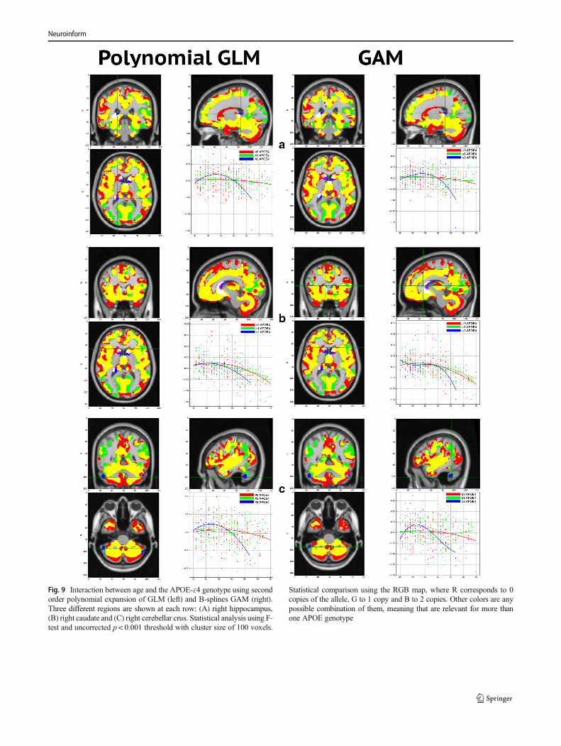
Fig. 9 Interaction between age and the APOE-ε4 genotype using secondorder polynomial expansion of GLM (left) and B-splines GAM (right).Three different regions are shown at each row: (A) right hippocampus,(B) right caudate and (C) right cerebellar crus. Statistical analysis using F-test and uncorrected p < 0.001 threshold with cluster size of 100 voxels.

Statistical comparison using the RGB map, where R corresponds to 0copies of the allele, G to 1 copy and B to 2 copies. Other colors are anypossible combination of them, meaning that are relevant for more thanone APOE genotype

Neuroinform

shown in fig. 7(A), replicating the findings in Cacciaglia et al.(2018). The use of the tool allowed us to study non-lineareffects of the genotype. Concretely, in fig. 7b and c we showresults using GAM and SVR with polynomial kernel models,respectively. Smaller effects are observed and only relevanteffects are found in regions such as bilateral thalamus, righthippocampus, right superior frontal and small cluster aroundthe right caudate and the left middle occipital. Nonlinearmodeling fail behind linear modeling of APOE-ε4 count,probably because it is a categorical (C = 3) predictor. Hence,due to higher degrees of freedom used in GAM and SVR, onlylarger significant values survive the used threshold.

Using the tool, we could also study the APOE genotypeeffects in cortical thickness data. In fig. 8, we show the resultson different surface views using the GLMmodel. In this case,even smaller effects are found being statistically relevant(p < 0.05) in small clusters across the brain, specially in re-gions such as the insular cortex and fusiform.

Interaction between APOE Genotype and Age in NormalAging Population

In this second part, we investigate the interaction betweenAPOE genotype and age on brain morphology. For this pur-pose, we model each APOE genotype separately to find theirassociated curves and generate a goodness-of-fit metric usingthe F-test. Statistical inference threshold is set to p < 0.001.We perform post-hoc analysis combining statistical maps intoan RGB-map that sums up the results of all three APOE-ge-notype models: we place eachmodel (NC, HE, HO) in each R,G, B channel, respectively. Volumetric and cortical thicknessanalyses were performed but no significant results were foundwith the later.

In fig. 9, we show the RGB-map and the associated curvesof regions corresponding to significant effect of age on brainmorphology of homozygotes APOE-e4 carriers (see section3.2.1): right hippocampus, right caudate and right cerebellarcrus. We present two different curve fitting models: usingpolynomial expansion of second order of the GLM on the leftand B-splines GAM on the right.

Clearly, relevant regions for the HO group show nonlinearrelationship between age and voxel intensities. Statistical andRGB-maps present analogous results on polynomial expan-sion of GLM and GAM analysis. The right hippocampus

and the right cerebellar crus follow a quadratic curve withage similar to GLM fitting. HO subjects show an earlier de-creasing of GMv in both regions compared to NC and HEaround their fifties with an initial volumetric increase inmiddle-aged individuals, more pronounced in the cerebellum,again replicating the results in Cacciaglia et al. (2018). On theother hand, GMv volume on the right caudate appears to de-crease at the sixth decade for all APOE genotypes butdecaying faster for HO subjects. Due to the non-quadraticbehaviour of the right caudate, it appears to be better modeledwith GAM, as shown in fig. 10.

Conclusions

In this paper, we present NeAT; a tool for non-linear analysisof neuroimaging data at the voxel or surface levels and illus-trate its functionality in three case studies where a nonlinearbehavior of brain morphology was previously described.NeAT is a modular, flexible and user-friendly toolbox thatprovides advanced curve fitting methods for voxelwise andsurface-based modeling and different metrics for statisticalinference of the results. Visualization features are available,such as an interactive GUI that shows statistical maps togetherwith the resulting fitted curves. Finally, post-hoc analysisfunctionalities such as model comparison (e.g: linear vs.non-linear) or a curve clustering algorithm that show similarfittings across the brain are available. Altogether, NeAT con-stitutes a complementary tool for the standard processing ofnon-linear associations between neuroimaging data and a setof factors (e.g: age, environmental factors, disease, genetics ordemographics) at the voxel and surface levels.

Future Work the potential of NeAT is expected to expand as itwill grow. At the short term, the expansion of the tool to ROI-based analysis is granted. Moreover, a longitudinal analysismodule might be interesting due to the increasing number ofcohorts with longitudinal follow-up visits. Seemingly, the in-tegration of fMRI modality should be considered in futurerevisions of the toolbox. Other statistical methods, such asPartial Least Squares (PLS) or Canonical CorrelationAnalysis (CCA) can be incorporated for multivariate effectsmodeling. Finally, other curve fitting models (e.g: based onneural networks) can be designed and implemented.

Fig. 10 Differences between statistical maps of the HE model using GLM and GAM at different brain ROIs: right hippocampus (A), right caudate (B)and right cerebellar crus (C). A positive (negative) value indicates that GAM (GLM) is statistically better using the f-test metric

Neuroinform

Information Sharing Statement

The source code of the presentedmethod is freely available fornon-commercial use from https://imatge-upc.github.io/neat-tool/.

Acknowledgements This work has been partially supported by the pro-ject MALEGRATEC2016-75976-R financed by the Spanish Ministeriode Economía y Competitividad and the European Regional DevelopmentFund (ERDF). Adrià Casamitjana is supported by the Spanish “Ministeriode Educación, Cultura y Deporte” FPU Research Fellowship. Juan D.Gispert holds a “‘Ramón y Cajal’” fellowship (RYC-2013-13054).

Data used in preparation of this article were obtained from theAlzheimer’s Disease Neuroimaging Initiative (ADNI) database (adni.loni.usc.edu). As such, the investigators within the ADNI contributed tothe design and implementation of ADNI and/or provided data but did notparticipate in analysis or writing of this report. A complete listing ofADNI investigators can be found at: http://adni.loni.usc.edu/wpcontent/uploads/how to apply/ADNI Acknowledgement List.pdf.

Compliance with Ethical Standards

Conflict of Interest Author Santi Puch is employed by companyQMENTA and author Asier Aduriz is employed by company VILYNX.All other authors declare no competing interests.

Open Access This article is licensed under a Creative CommonsAttribution 4.0 International License, which permits use, sharing, adap-tation, distribution and reproduction in any medium or format, as long asyou give appropriate credit to the original author(s) and the source, pro-vide a link to the Creative Commons licence, and indicate if changes weremade. The images or other third party material in this article are includedin the article's Creative Commons licence, unless indicated otherwise in acredit line to the material. If material is not included in the article'sCreative Commons licence and your intended use is not permitted bystatutory regulation or exceeds the permitted use, you will need to obtainpermission directly from the copyright holder. To view a copy of thislicence, visit http://creativecommons.org/licenses/by/4.0/.

References

Ashburner, J., & Friston, K. J. (2000). Voxel-based morphometry—Themethods. Neuroimage, 11(6), 805–821.

Bateman, R. J., Xiong, C., Benzinger, T. L., Fagan, A.M., Goate, A., Fox,N. C., et al. (2012). Clinical and biomarker changes in dominantlyinherited Alzheimer's disease. N Engl J Med, 367(9), 795–804.

Breeze, J. L., Poline, J. B., & Kennedy, D. N. (2012). Data sharing andpublishing in the field of neuroimaging. GigaScience, 1(1), 9.

Breiman, L., & Friedman, J. H. (1985). Estimating optimal transforma-tions for multiple regression and correlation. J Am Stat Assoc,80(391), 580–598.

Brett, M., Hanke, M., Cipollini, B., Côté, M. A., Markiewicz, C.,Gerhard, S., Larson, E., Lee, G. R., Halchenko, Y., Kastman, E.,Morency, F. C., Millman, J., Rokem, A., Gramfort, A., van denBosch, J. J. F., Subramaniam, K., Nichols, N., Oosterhof, N. N.,St-Jean, S., Amirbekian, B., Nimmo-Smith, I., Ghosh, S.,Varoquaux, G., Garyfallidis, E. (2016). nibabel: 2.1. 0.

Cacciaglia, R., Molinuevo, J. L., Falcón, C., Brugulat-Serrat, A.,Sánchez-Benavides, G., Gramunt, N., et al. (2018). Effects ofAPOE-ε4 allele load on brain morphology in a cohort of middle-

aged healthy individuals with enriched genetic risk for Alzheimer'sdisease. Alzheimers Dement, 14(7), 902–912.

Christensen, R. (2011). Plane answers to complex questions: The theoryof linear models. Springer Science & Business Media.

Desikan, R. S., Ségonne, F., Fischl, B., Quinn, B. T., Dickerson, B. C.,Blacker, D., et al. (2006). An automated labeling system forsubdividing the human cerebral cortex on MRI scans into gyralbased regions of interest. Neuroimage, 31(3), 968–980.

Dinuzzo, F., Neve, M., Nicolao, G. D., & Gianazza, U. P. (2007). On therepresenter theorem and equivalent degrees of freedom of SVR. JMach Learn Res, 8(Oct), 2467–2495.

Drucker, H., Burges, C. J., Kaufman, L., Smola, A. J., & Vapnik, V.(1997). Support vector regression machines. Advances in neuralinformation processing systems, 9, 155–161.

Fischl, B. (2012). FreeSurfer. Neuroimage, 62(2), 774–781.Fjell, A. M., Walhovd, K. B., Westlye, L. T., Østby, Y., Tamnes, C. K.,

Jernigan, T. L., et al. (2010). When does brain aging accelerate?Dangers of quadratic fits in cross-sectional studies. Neuroimage,50(4), 1376–1383.

Fjell, A. M., Westlye, L. T., Grydeland, H., Amlien, I., Espeseth, T.,Reinvang, I., et al. (2013). Critical ages in the life course of the adultbrain: Nonlinear subcortical aging. Neurobiol Aging, 34(10), 2239–2247.

Frackowiak, R., Lenzi, G. L., Jones, T., & Heather, J. D. (1980).Quantitative measurement of regional cerebral blood flow and oxy-gen metabolism in man using 15O and positron emission tomogra-phy: Theory, procedure, and normal values. J Comput AssistTomogr, 4(6), 727–736.

Freeborough, P. A., & Fox, N. C. (1997). The boundary shift integral: Anaccurate and robust measure of cerebral volume changes from reg-istered repeat MRI. IEEE Trans Med Imaging, 16(5), 623–629.

Friston, K. J., Holmes, A. P., Worsley, K. J., Poline, J. P., Frith, C. D., &Frackowiak, R. S. (1994). Statistical parametric maps in functionalimaging: A general linear approach. Hum Brain Mapp, 2(4), 189–210.

Gispert, J. D., Rami, L., Sánchez-Benavides, G., Falcon, C., Tucholka,A., Rojas, S., &Molinuevo, J. L. (2015). Nonlinear cerebral atrophypatterns across the Alzheimer's disease continuum: Impact ofAPOE4 genotype. Neurobiol Aging, 36(10), 2687–2701.

Hastie, T., & Tibshirani, R. (1987). Generalized additive models: someapplications. Journal of the American Statistical Association,82(398), 371–386.

Henson, R. N. A., & Penny, W. D. (2003). ANOVAs and SPM. TechnicalReport Wellcome Department of Imaging Neuroscience, London.

Hsu, C. W., Chang, C. C., & Lin, C. J. (2003). A practical guide tosupport vector classification. Technical Report, Department ofComputer Science, National Taiwan University

Insel, P. S., Mattsson, N., Donohue, M. C., Mackin, R. S., Aisen, P. S.,Jack Jr, C. R., Shaw, L. M., Trojanowski, J. Q., Weiner, M. W.,Alzheimer's Disease Neuroimaging Initiative et al. (2015). The tran-sitional association between β-amyloid pathology and regionalbrain atrophy. Alzheimer’s & Dementia 11(10), 1171–1179.

Insel, P. S., Ossenkoppele, R., Gessert, D., Jagust, W., Landau, S.,Hansson, O., et al. (2017). Time to amyloid positivity and preclinicalchanges in brain metabolism, atrophy, and cognition: Evidence foremerging amyloid pathology in Alzheimer's disease. FrontNeurosci, 11, 281.

Jacques, J., & Preda, C. (2014). Functional data clustering: A survey.ADAC, 8(3), 231–255.

James, G.,Witten, D., Hastie, T., & Tibshirani, R. (2013). An introductionto statistical learning (Vol. 112, p. 18). New York: Springer.

Jones, E., Oliphant, T., & Peterson, P. (2014). others.(2001). SciPy: Opensource scientific tools for Python. Online at: http://www scipy org.

Kornak, J., Fields, J. A., Farmer, S., Boeve, B. F., Rosen, H. J., Boxer, A.L., et al. (2018). Nonlinear N-score estimation for establishing cog-nitive norms from the National Alzheimer’s coordinating center

Neuroinform

(NACC) dataset. Alzheimer's & Dementia: The Journal of theAlzheimer's Association, 14(7), P390–P391.

Mendiondo, M. S., Ashford, J. W., Kryscio, R. J., & Schmitt, F. A.(2000). Modelling mini mental state examination changes inAlzheimer's disease. Stat Med, 19(11–12), 1607–1616.

Molinuevo, J. L., Gispert, J. D., Dubois, B., Heneka, M. T., Lleo, A.,Engelborghs, S., et al. (2013). The AD-CSF-index discriminatesAlzheimer's disease patients from healthy controls: A validationstudy. J Alzheimers Dis, 36(1), 67–77.

Molinuevo, J. L., Gramunt, N., Gispert, J. D., Fauria, K., Esteller, M.,Minguillon, C., Sánchez-Benavides, G., Huesa, G., Morán, S., Dal-Ré, R., &Camí, J. (2016). The ALFA project: A research platform toidentify early pathophysiological features of Alzheimer's disease.Alzheimer's & Dementia: Translational Research & ClinicalInterventions, 2(2), 82–92.

Murtagh, F., & Legendre, P. (2014). Ward’s hierarchical agglomerativeclustering method: Which algorithms implement Ward’s criterion? JClassif, 31(3), 274–295.

Pedregosa, F., Varoquaux, G., Gramfort, A., Michel, V., Thirion, B.,Grisel, O., et al. (2011). Scikit-learn: Machine learning in Python.J Mach Learn Res, 12(Oct), 2825–2830.

Penny, W. D., Friston, K. J., Ashburner, J. T., Kiebel, S. J., & Nichols, T.E. (2011). Statistical parametric mapping: The analysis of functionalbrain images. Elsevier.

Rousseeuw, P. J. (1987). Silhouettes: A graphical aid to the interpretationand validation of cluster analysis. J Comput Appl Math, 20, 53–65.

Sabuncu, M. R., Desikan, R. S., Sepulcre, J., Yeo, B. T. T., Liu, H.,Schmansky, N. J., et al. (2011). The dynamics of cortical and hip-pocampal atrophy in Alzheimer’s disease. Arch Neurol, 68(8),1040–1048.

Sakamoto, Y., Ishiguro, M., & Kitagawa, G. (1986). Akaike informationcriterion statistics (p. 81). Dordrecht: D. Reidel.

Samtani, M. N., Farnum, M., Lobanov, V., Yang, E., Raghavan, N.,DiBernardo, A., et al. (2012). An improved model for disease pro-gression in patients from the Alzheimer's disease neuroimaging ini-tiative. J Clin Pharmacol, 52(5), 629–644.

Schuff, N., Tosun, D., Insel, P. S., Chiang, G. C., Truran, D., Aisen, P. S.,et al. (2012). Nonlinear time course of brain volume loss in cogni-tively normal and impaired elders. Neurobiol Aging, 33(5), 845–855.

ten Kate, M., Sanz-Arigita, E. J., Tijms, B. M., Wink, A. M., Clerigue,M., Garcia-Sebastian, M., et al. (2016). Impact of APOE-ɛ4 andfamily history of dementia on gray matter atrophy in cognitivelyhealthy middle-aged adults. Neurobiol Aging, 38, 14–20.

Villemagne, V. L., Burnham, S., Bourgeat, P., Brown, B., Ellis, K. A.,Salvado, O., et al. (2013). Amyloid β deposition, neurodegenera-tion, and cognitive decline in sporadic Alzheimer's disease: A pro-spective cohort study. The Lancet Neurology, 12(4), 357–367.

Vinke, E. J., De Groot, M., Venkatraghavan, V., Klein, S., Niessen, W. J.,Ikram, M. A., & Vernooij, M. W. (2018). Trajectories of imagingmarkers in brain aging: The Rotterdam study. Neurobiol Aging, 71,32–40.

Ziegler, G., Dahnke, R., & Gaser, C. (2012). Models of the aging brainstructure and individual decline. Frontiers in neuroinformatics, 6, 3.

Publisher’s Note Springer Nature remains neutral with regard to jurisdic-tional claims in published maps and institutional affiliations.

Neuroinform