Embed Size (px)
Citation preview
NETE4631:Capacity Planning (2)- Lecture 10
Suronapee Phoomvuthisarn, Ph.D.Email: [email protected] / Q305

Lecture Outline Basic terminology Queueing Analysis M/M/1 M/M/m M/M/m/m Exercise

Capacity planning strategies Capacity planning problems:
A web server needs to complete an HTTP request within 0.5s when there are 500 HTTP requests per second, what CPU speed do you need?
Let us turn the capacity planning question into a performance analysis question
Performance analysis question: If the web server has a CPU with x MIPS, what is the
response time when there are 500 HTTP requests per second?
If you can solve the performance analysis question for any value of x, you can also solve the capacity planning question
Solutions: Build the system and perform measurement Simulation Mathematical modeling.

Modelling computer systems Single server queue considers only a
component within a computer system A request may require multiple resources E.g.
CPU, disk, network transmission We model a computer systems with multiple
resources by a Queueing Networks (QNs)

Representation of queue

A simple database server

Queueing analysis - Scale up or Scale out better?

Queues with Poisson arrivals
Open, single server queues and How to find:
Waiting time Response time Mean queue length etc.
The technique to find waiting time etc. is called Queueing Theory

Single Server Queue: Terminology
Response Time T = Waiting time W + Service time S

Single Server Queue: Terminology

Motivating example Given
Observation period = 1 minute CPU
Busy for 36s. 1790 transactions arrived 1800 transactions completed
Find Mean service time per completion Utilisation Arrival rate System throughput

Little’s Law Applicable to any “box” that contains some
queues or servers Mean number of jobs in the “box” = Mean response time x Throughput We will use Little’s Law in this lecture to
derive the mean response time We first compute the mean number of jobs in the
“box” and throughput

Single server system In order to determine the response time, you
need to know The inter-arrival time probability distribution The service time probability distribution
Possible distributions Deterministic
Constant inter-arrival time Constant service time
Exponential distribution We will focus on exponential distribution
Exponential inter-arrivals (λ) Exponential service time (μ)

Exponential inter-arrival with rate λ
We assume that successive arrivals are independent
Probability that inter-arrival time is between x and x + δx
= λ exp(- λx) δx

Probabilistic distribution function
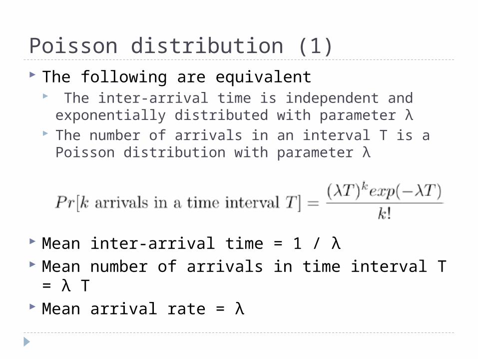
Poisson distribution (1) The following are equivalent
The inter-arrival time is independent and exponentially distributed with parameter λ
The number of arrivals in an interval T is a Poisson distribution with parameter λ
Mean inter-arrival time = 1 / λ Mean number of arrivals in time interval T = λ T Mean arrival rate = λ
Poisson distribution (2) Assumption of Poisson arrival process
The number of customers in the system is very large.
Impact of a single customer on the performance of the system is very small, i.e. a single customer consumes a very small percentage of the system resources.
All customers are independent, i.e. their decision to use the system are independent of other users.

Explore …

Service time distribution Service time = the amount of processing time a job
requires from the server We assume that the service time distribution is
exponential with parameter μ The probability that the service time is between t and t +
δt is:
Here: μ = service rate = 1 / mean service time Another interpretation of exponential service time:
Consider a small time interval δ Probability [ a job will finish its service in next δ seconds ]
= μ δ
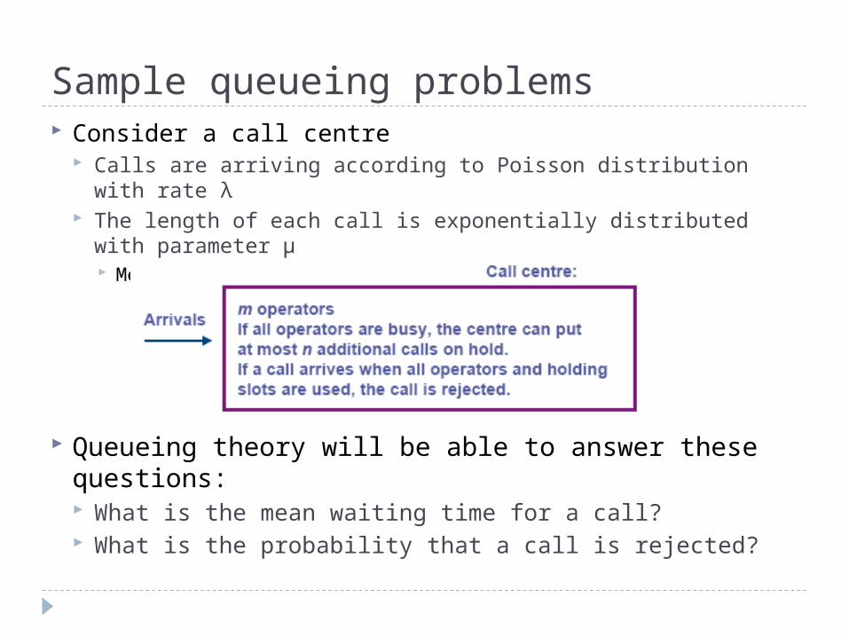
Sample queueing problems Consider a call centre
Calls are arriving according to Poisson distribution with rate λ The length of each call is exponentially distributed with
parameter μ Mean length of a call is 1/ μ
Queueing theory will be able to answer these questions: What is the mean waiting time for a call? What is the probability that a call is rejected?

Markov chain The state-transition model that we have used is
called a continuous-time Markov chain The transition from a state of the Markov chain
to another state is characterised by an exponential distribution E.g. The transition from State p to State q is
exponential with rate rpq, then consider a small time interval δ
Probability [ Transition from State p to State q in time δ ] = rpq δ
Method for solving Markov chain A Markov chain can be solved by
Identifying the states (may not be easy) Find the transition rate between the states Solve the steady state probabilities
You can then use the steady state probabilities as a stepping stone to find the quantity of interest (e.g. response time etc.)

Call centre with 1 operator and no holding slots Let us see how we can solve the queuing problem for a
very simple call centre with 1 operator and no holding slots
What happens to a call that arrives when the operator is busy?
The call is rejected What happens to a call that arrives when the operator is idle?
The call is admitted without delay. We are interesting to find the probability that an arriving
call is rejected.
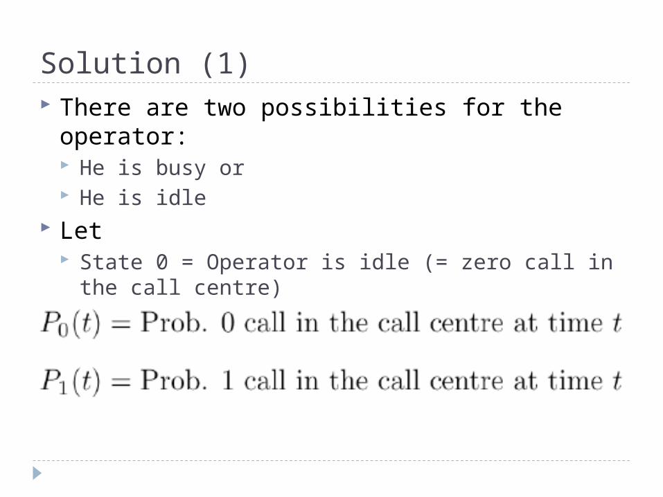
Solution (1) There are two possibilities for the operator:
He is busy or He is idle
Let State 0 = Operator is idle (= zero call in the call
centre) State 1 = Operator is busy (= 1 call in the call
centre)

Solution (2) Transition from State 0 to State 1
Caused by an arrival, the rate is λ Transition from State 1 to State 0
Caused by a completed service, the rate is μ State diagram representation
Each circle is a state Label the arc between the states with transition
rate

Solution (3) Steady state means
We have for state 0:

Solution (4) We can do the same for State 1: Steady state means
We have for state 1:

Solution (5) We have one equation
We have 2 unknowns and we need one more equation.
Since we must be either one of the two states:
Solving these two equations, we get the same steady state solution as before

Solving a queueing problem Procedure:
Draw a diagram with the states Add arcs between states with transition rates Derive flow balance equation for each state, i.e. Rate of entering a state = Rate of leaving a state Solve the equation for steady state probability
It is harder to find how a queue evolves with time It is simpler to find how a queue behaves at steady
state

Kendall’s notation To represent different types of queues, queueing
theorists use the Kendall’s notation The call centre example on the previous page can
be represented as:
The call centre example on the last page is a M/M/m/(m+n) queue If n = ∞, we simply write M/M/m

M/M/1 queue
Consider a call centre analogy Calls are arriving according to Poisson distribution with rate λ The length of each call is exponentially distributed with parameter μ
Mean length of a call is 1/ μ
Queueing theory will be able to answer these questions: What is the mean waiting time for a call?

Solving M/M/1 queue (1) We will solve for the steady state response Define the states of the queue
State 0 = There is zero job in the system (= The server is idle)
State 1 = There is 1 job in the system (= 1 job at the server, no job queueing)
State 2 = There are 2 jobs in the system (= 1 job at the server, 1 job queueing)
State k = There are k jobs in the system (= 1 job at the server, k-1 job queueing)
The state transition diagram

Solving M/M/1 queue (2)
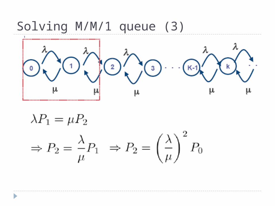
Solving M/M/1 queue (3)

Solving M/M/1 queue (4)

Solving M/M/1 queue (5)

Solving M/M/1 queue (6)

Solving M/M/1 queue (7)

Solving M/M/1 queue (8)

Solving M/M/1 queue (9)

Observing response time

Multi-server queues M/M/m

A call centre analogy of M/M/m queue Consider a call centre analogy
Calls are arriving according to Poisson distribution with rate λ
The length of each call is exponentially distributed with parameter μ Mean length of a call is 1/ μ

State transition for M/M/m

M/M/m This is a Markov chain, we have mean
response time T is

Multi-server queues M/M/m/m with no waiting room

A call centre analogy of M/M/m/m queue Consider a call centre analogy
Calls are arriving according to Poisson distribution with rate λ
The length of each call is exponentially distributed with parameter μ Mean length of a call is 1/ μ

State transition for M/M/m/m

What configuration has the best response time?

References Most of the slides have been modified from
COMP9334 Capacity Planning of Computer Systems and Networks Week 1-4: Introduction to Capacity Planning, Chou, C. T., 2008
Recommended reading from Chou Queues with Poisson arrival are discussed in
Bertsekas and Gallager, Data Networks, Sections 3.3 to 3.4.3
Note: Chou has derived the formulas here using continuous Markov chain but Bertsekas and Gallager used discrete Markov chain.

Example You have a computer system with a single
CPU. Both inter-arrival and service times are exponentially distributed. The job only requires services at the CPU. Each job only visits the CPU once. A finished job will leave the system. Mean arrival rate is 9 request/s. Mean service time at the CPU is 0.1s. What is the utilisation of the CPU? What is the mean response time? The utilisation is pretty high and you want to
change the system. -> You can think of 3 alternatives.

Alternative 1 Replace the existing CPU by one that is 2
times faster You may assume that the service time is
inversely proportional to CPU speed.

Alternative 2 Buy a system which is identical to the current
one Put the two system in parallel Add a switch in front of the system
Route 1st,3rd,5th,… requests to System 1 Route 2nd,4th,6th … requests to System 2
Assume the switch requires negligible time

Alternative 3 Similar to Alternative 2, we buy a system
which is identical to the current one and we also buy a switch
However, we only maintain a queue at the switch.
If both system are busy, the request waits at the switch; otherwise, the switch dispatches the request to any of the available systems
Assuming that it takes negligible time for the switch to find out whether a system is idle.

Question 1 Part (a): Calculate the resulting mean response
time for each for the three alternatives Part (b): Repeat part (a) for a number of
different mean arrival rates. Plot a graph of arrival rates against the mean response time.
Part (c): What observations can you make from these calculations?
Part (d): What is the best way to upgrade the system in terms of performance? However, the best way to upgrade in terms of performance may not be the best way to upgrade in terms of cost, why?